Rongpei Shi-Variant Selection during Alpha Precipitation in Titanium Alloys-Thesis
398
Variant Selection during Alpha Precipitation in Titanium Alloys A Simulation Study DISSERTATION Presented in Partial Fulfillment of the Requirements for the Degree Doctor of Philosophy in the Graduate School of The Ohio State University By Rongpei Shi Graduate Program in Materials Science and Engineering The Ohio State University 2014 Dissertation Committee: Yunzhi Wang, Adviosr Suliman Dregia Hamish Fraser
-
Upload
independent -
Category
Documents
-
view
1 -
download
0
Transcript of Rongpei Shi-Variant Selection during Alpha Precipitation in Titanium Alloys-Thesis

Variant Selection during Alpha Precipitation in Titanium Alloys
A Simulation Study
DISSERTATION
Presented in Partial Fulfillment of the Requirements for the Degree Doctor of Philosophy
in the Graduate School of The Ohio State University
By
Rongpei Shi
Graduate Program in Materials Science and Engineering
The Ohio State University
2014
Dissertation Committee:
Yunzhi Wang, Adviosr
Suliman Dregia
Hamish Fraser

Copyright by
Rongpei Shi
2014
ii
Abstract
Variant selection of alpha phase during its precipitation from beta matrix plays a key role
in determining transformation texture and final mechanical properties of ⁄ and
titanium alloys. In this study we develop a three-dimensional quantitative phase field
model (PFM) to predict variant selection and microstructure evolution during beta to
alpha transformation in polycrystalline Ti-6Al-4V under the influence of different
processing variables. The model links its inputs directly to thermodynamic and mobility
databases, and incorporates crystallography of BCC to HCP transformation, elastic
anisotropy, defects within semi-coherent alpha/beta interfaces and elastic
inhomogeneities among different beta grains. In particular, microstructure and
transformation texture evolution are treated simultaneously via orientation distribution
function (ODF) modeling of alpha/beta two-phase microstructure in beta polycrystalline
obtained by PFM. It is found that, for a given undercooling, the development of
transformation texture of the alpha phase due to variant selection during precipitation
depends on both externally applied stress or strain, initial texture state of parent beta
sample and internal stress generated by the precipitation reaction itself. Moreover, the
growth of pre-existing widmanstatten alpha precipitates is accompanied by selective
nucleation and growth of secondary alpha plates of preferred variants.
We further develop a crystallographic model based on the ideal Burgers orientation
relationship (BOR) between GB and one of the two adjacent beta grains to investigate
Sony
高亮
Sony
高亮
Sony
高亮
Sony
高亮
iii
how a prior beta grain boundary contributes to variant selection of grain boundary
allotriomorph (GB ). The model is able to predict all possible special beta grain
boundaries where GB is able to maintain BOR with two neighboring grain. In
particular, the model has been used to evaluate the validity of all current empirical variant
selection rules to obtain more insight of how all grain boundary parameters
(misorientation and grain boundary plane inclination) contribute to variant selection
behavior titanium alloys. This work could shed light on how to control processing
conditions to reduce microtexture at both the individual grain level and the overall
polycrystalline sample level.
Sony
高亮
iv
Dedication
This document is dedicated to my family.

v
Acknowledgments
I can't believe this day has finally come. Firstly, I would like to express my deepest and
sincere gratitude to my advisor, Prof. Yunzhi Wang for offering the opportunity to do my
Ph.D. study in the US that I had never imagined when I was in China. I joined the group
with little background of phase transformation in solid state. Thanks for his incredible
patience and constant support that allows me to survive after a long incubation time in
my learning curve in this field.
Thanks also go to the committee members, Prof. Suliman Dregia. Many fruitful
discussions with him contribute a lot to the work done in the thesis. In particular, his
enthusiasm and humor when discussing about scientific research also lead me to enjoy
doing research.
I must thank Prof. Hamish Fraser for giving me a really big picture about the physical
metallurgy of titanium alloys. Through working with Dr. Yufeng Zheng and Dr. Vikas
Dixit in his group, I find scientific problems remaining unsolved in the field of Ti-alloys
that I, as a modeler, can take over and have some contributions. This is the way I have
been doing most of work described in the thesis.
Thanks to Prof. Xingjun Liu and Prof. Cuiping Wang, my advisor at Xiamen University
in China. The couple gave me the best training in computation thermodynamics, and the
incredible flexibility for doing my Ph.D. study in the US.
vi
Thanks to Prof. Wenzheng Zhang at Tsinghua University for teaching me O-lattice
theory during Gordon Research Conference in 2009, and her continuing help to improve
my understanding of the theory that offers me a complete new insight to think about
phase transformations in solid.
Thanks to Dr. Chen Shen, Dr. Ning Ma and Dr. Ning Zhou. They showed me the beauty
of microstructure modeling that is the one of the most important reasons that I still have
enthusiasm to build new models, do coding, debugging and post-processing data for
publications, though most of them are only between 0 and 1, during midnight.
Special thanks to Dr. Chen Shen. He introduced me to do summer intern in General
Electric, Global Research Center. During that time, he taught me how to work with
industry people within a team and, more importantly, let me realize that how the
knowledge I learn in the college can be direct applied to the R&D of turbine engine.
Thanks to Dr. Ning Ma for the solid basis that he had built for the Ti-research in the
group.
Thanks to Dr. Ning Zhou for his support and help during the hard initial time when I
joined the group. I will always miss our coffee time during his stay in the group.
Thanks go to my group members, Dr. Yipeng Gao, Dr. Dong Wang, Pengyang Zhao,
Xiaoqin Ke. I benefit a lot from many useful discussions with them in phase field
modeling, martensitic transformation, physics, and inter-diffusion.
Thanks to my friends, Lin Li, HongQing Sun, Fan Yang, Yufeng Zheng, Liu Cao, Weiqi
Luo, Xiaoji Li, Huang Lin, Di Qiu, who have encouraged, entertained, and supported me

vii
through the dark times, celebrated with me through the good, I take this opportunity to
thank you.
A special gratitude and love goes to my family for their unfailing support. Deeply
appreciate my parent’s incredible patience and constant support throughout my Ph.D.
study that allow me to stay in the college until 30 years old without making big money. I
will never truly be able to express my sincere appreciation to the both of you. Without the
great help from my parents-in-law during his stay with us, I would not be able to start
work on the thesis.
Thanks to my adorable daughter, Ellen. A smile from her is able to refresh my mind
much better than cups of coffee. Spending time with her is not a consolation prize, it is
the prize. But, an apology to her, to whom, I should have spent more time with her as a
father.
Finally, I want to express my deepest love and thanks to my wife, Pingting Bai, for her
incredible understanding and support, making amazing food everyday throughout my
Ph.D. study, and taking care of our daughter during the most difficult time of thesis
writing.
viii
Vita
July 2004 ........................................................B.S. Fuzhou University, Fuzhou, China
Sep 2004- July 2008.......................................Xiamen University, Xiamen, China
Sep 2008 to present .......................................Graduate Research Associate, Department
of Materials Science and Engineering, The
Ohio State University
Publications
[1] Shi R, Vikas D, Fraser H. L. and Wang Y. Crystallographic Studies for Variant
Selection of Grain Boundary Alpha in Titanium Alloys. Acta Materialia ; Under Review
[2] Shi R, Wang Y. Variant Selection during Alpha Precipitation in Ti-6Al-4V under the
Influence of Local Stress - A Simulation Study. Acta Materialia 2013; 61:6006..
[3] Shi R, Wang C, Wheeler D, Liu X, Wang Y. Formation mechanisms of self-organized
core/shell and core/shell/corona microstructures in liquid droplets of immiscible alloys.
Acta Materialia 2012;60:4172.
[4] Shi R, Ma N, Wang Y. Predicting equilibrium shape of precipitates as function of
coherency state. Acta Materialia 2012;60:4172.
[5] Boyne A, Wang D, Shi R, Zheng Y, Behera A, Nag S, Tiley J, Fraser H, Banerjee R,
Wang Y. Pseudospinodal mechanism for fine α/β microstructures in β-Ti alloys. Acta
ix
Materialia 2014;64:188.
[6] Lu Y, Wang C, Gao Y, Shi R, Liu X, Wang Y. Microstructure Map for Self-Organized
Phase Separation during Film Deposition. Physical Review Letters 2012;109:086101.
[7] Li Y, Shi R, Wang C, Liu X, Wang Y. Phase-field simulation of thermally induced
spinodal decomposition in polymer blends. Modelling and Simulation in Materials
Science and Engineering 2012;20:075002.
[8] Gao Y, Liu H, Shi R, Zhou N, Xu Z, Zhu Y, Nie J, Wang Y. Simulation study of
precipitation in an Mg–Y–Nd alloy. Acta Materialia 2012;60:4819.
[9] Shi R, Wang Y, Wang C, Liu X. Self-organization of core-shell and core-shell-corona
structures in small liquid droplets. Applied Physics Letters 2011;98:204106.
[10] Li Y, Shi R, Wang C, Liu X, Wang Y. Predicting microstructures in polymer blends
under two-step quench in two-dimensional space. Physical Review E 2011;83:041502.
Fields of Study
Major Field: Materials Science and Engineering

x
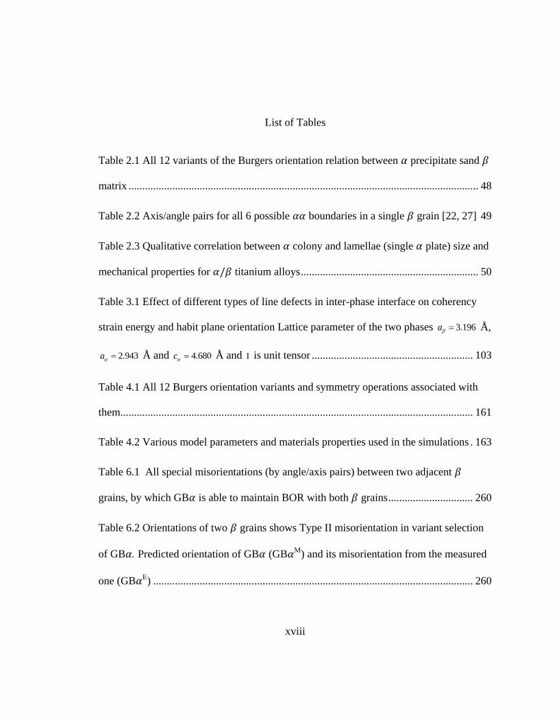
Table of Contents
Abstract ............................................................................................................................... ii
Dedication .......................................................................................................................... iv
Acknowledgments............................................................................................................... v
Vita ................................................................................................................................... viii
List of Tables ................................................................................................................. xviii
List of Figures ................................................................................................................. xxii
CHAPTER 1 Introduction................................................................................................... 1
1.1 Motivations................................................................................................................ 1
1.2 Organization of the thesis .......................................................................................... 6
1.3. Reference: ............................................................................................................... 10
CHAPTER 2 Literature Review ....................................................................................... 15
Abstract ......................................................................................................................... 15
2.1 Introduction ............................................................................................................. 16
2.2. precipitation in titanium alloys ........................................................................... 17
2.2.1 Two-phase titanium alloys ......................................................................... 17
2.2.2 Microstructure development during precipitation ......................................... 19

xi
2.2.3 Orientation relationship between and phases ............................................ 21
2.2.4 Determination of the number of variants ..................................................... 22
2.2.5 The nature of interface between precipitate and matrix ............................ 23
2.2.6 Relationship between microstructure and mechanical properties .................... 24
2.3. Variant selection during precipitation ................................................................ 26
2.3.1 Variant selection of GB .................................................................................. 27
2.3.2 Variant selection of secondary side plates by GB ..................................... 29
2.3.3 Variant selection in basketweave microstructures ............................................ 30
2.3.4 Variant selection due to dislocations ................................................................ 33
2.4. Unresolved issues ................................................................................................... 35
2.4.1 Grain boundary nucleation ............................................................................ 35
2.4.2 Correlations between precipitates with different variants in the basketweave
microstructure ............................................................................................................ 36
2.4.3 The effect of dislocation on variant selection ................................................... 37
2.4.4 Microstructure evolution with variant selection ............................................... 37
2.5. References: ............................................................................................................. 51
CHAPTER 3 Predicting Equilibrium Shape of Precipitates as Function of Coherency
State................................................................................................................................... 59
Abstract: ........................................................................................................................ 59

xii
3.1. Introduction ............................................................................................................ 60
3.2. Elastic Strain Energy of Coherent and Semi-Coherent Precipitates ...................... 62
3.2.1. Stress-free transformation strain for coherent precipitates .............................. 65
3.2.2. Deformation gradient matrix due to defects at hetero-phase interfaces .......... 66
3.3. Estimation of Interfacial Energy for Semi-Coherent Interfaces ............................. 69
3.4. Worked Examples .................................................................................................. 71
3.4.1. Derivation of effective SFTS for the semi-coherent precipitates ................ 72
3.4.2. Strain energy density and habit plane orientation of semi-coherent
precipitates ................................................................................................................. 77
3.4.3. Interfacial energy anisotropy of semi-coherent precipitates ........................ 78
3.4.4. Equilibrium shape of -precipitates in different cases .................................... 79
3.4.5. Coherency lost ................................................................................................. 81
3.5. Discussions ............................................................................................................. 82
3.6. Summary ................................................................................................................ 88
3.7. Reference ................................................................................................................ 90
CHAPTER 4 Variant Selection during Precipitation in Ti-6Al-4V under the Influence
of Local Stress ................................................................................................................. 106
Abstract: ...................................................................................................................... 106
4.1. Introduction .......................................................................................................... 107
xiii
4.2. Method ................................................................................................................. 111
4.2.1. Determination of number of variants of a low symmetry precipitate phase . 111
4.2.2. Free energy formulation ................................................................................ 113
4.2.2.1. Chemical free energy .................................................................................. 114
4.2.2.2. Elastic strain energy.................................................................................... 116
4.2.3. Stress-free transformation strain for coherent and semi-coherent precipitates
................................................................................................................................. 117
4.2.4. Effect of misfit dislocation on interfacial energy .......................................... 121
4.2.5. Kinetic equations ........................................................................................... 123
4.2.6. Model inputs and parameters ......................................................................... 124
4.3. Results .................................................................................................................. 124
4.3.1. Growth behavior of a single plate .............................................................. 124
4.3.2. Effect of pre-strain on variant selection ........................................................ 126
4.3.2.1. Pre-strain due to compressive stress along [010] ..................................... 127
4.3.2.2. Pre-strain due to tensile stress along [010] .............................................. 128
4.3.3. Variant selection due to pre-existing plates ............................................... 129
4.4. Discussion ............................................................................................................ 131
4.4.1. Lengthening and thickening kinetics of plate ............................................ 131
xiv
4.4.2. Elastic interaction between pre-strain and transformation strain of variants
................................................................................................................................. 132
4.4.3. Competition between pre-strain and evolving microstructure ...................... 135
4.4.4. Variant selection due to pre-existing microstructure ..................................... 138
4.5. Summary .............................................................................................................. 145
4.6. References ............................................................................................................ 164
CHAPTER 5 Evolution of Microstructure and Transformation Texture during Alpha
Precipitation in Polycrystalline Titanium alloys .................................................... 174
Abstract: ...................................................................................................................... 174
5.1. Introduction .......................................................................................................... 175
5.2. Model Formulation ............................................................................................... 180
5.2.1. Polycrystalline sample ................................................................................ 180
5.2.2 Phase Field Model for precipitation in an elastically and structurally
inhomogeneous polycrystalline sample................................................................ 180
5.2.2.1 Chemical free energy for polycrystalline system ........................................ 181
5.2.2.2. Strain energy of an elastically and structurally inhomogeneous system .... 183
5.2.2.3 Kinetic equations ......................................................................................... 187
5.2.3 Orientation Distribution Function modeling of microstructure in
polycrystalline sample ............................................................................................. 189

xv
5.3. Results .................................................................................................................. 192
5.3.1. Starting polycrystalline and texture ........................................................ 192
5.3.2. Evolution of microstructure and texture during precipitation ......... 193
5.3.3. Effect of pre-strain on variant selection ........................................................ 194
5.3.4. Effect of starting texture on variant selection ............................................ 195
5.3.5. Quantifying the degree of variant selection ................................................... 197
5.3.6. Effect of boundary constraint on variant selection ........................................ 198
5.4. Discussions ........................................................................................................... 198
5.5. Summary .............................................................................................................. 205
5.6. References: ........................................................................................................... 226
CHAPTER 6 Variant Selection of Grain Boundary by Special Prior Grain
Boundaries in Titanium Alloys ....................................................................................... 233
Abstract ....................................................................................................................... 233
6.1. Introduction .......................................................................................................... 234
6.2. Model formulation and Experimental procedures ................................................ 237
6.2.1. Crystallographic model .................................................................................. 237
6.2.2. Experimental procedures ............................................................................... 240
6.3. Results .................................................................................................................. 241

xvi
6.3.1. Special grain boundaries where GB maintainsBOR with both adjacent
grains ....................................................................................................................... 242
6.3.2. Violation of variant selection rule derived from closeness between poles
................................................................................................................................. 244
6.4. Discussion ............................................................................................................ 245
6.5. Conclusions .......................................................................................................... 251
6.6 References: ............................................................................................................ 262
CHAPTER 7 Effects of Grain Boundary Parameters on Variant Selection of Grain
Boundary in Titanium Alloys ...................................................................................... 266
Abstract ....................................................................................................................... 266
7.1. Introduction .......................................................................................................... 267
7.2. Experimental procedure ....................................................................................... 274
7.3. Results .................................................................................................................. 276
7.3.1. Overall Characteristics of variant selection of GB ..................................... 276
7.3.2. Variant selection of GB when different rules are dominant ....................... 278
7.3.2.1. Rule I is dominant....................................................................................... 279
7.3.2.2. Rule II is dominant ..................................................................................... 280
7.3.2.3. Rule III is dominant .................................................................................... 281
7.3.3. Abnormal cases.............................................................................................. 282

xvii
7.3.3.1 Abnormal variant selection when the minimum ....................... 282
7.3.3.2 Abnormal variant selection when .............................................. 284
7.4. Discussions ........................................................................................................... 284
7.5. Summary .............................................................................................................. 293
7.6. Reference .............................................................................................................. 321
CHAPTER 8 Conclusions and Future Works ................................................................. 324
8.1 Conclusions ........................................................................................................... 324
8.2 Direction for future research Conclusions ............................................................ 329
Reference ........................................................................................................................ 332
Appendix A: Determination of the number of variants of precipitate phase .............. 361
Appendix B: Stress free transformation strain for all 12 variants ............................... 363
B.1. Coherent nuclei .................................................................................................... 363
B.2. Fully-grown plates ............................................................................................... 364
xviii
List of Tables
Table 2.1 All 12 variants of the Burgers orientation relation between precipitate sand
matrix ................................................................................................................................ 48
Table 2.2 Axis/angle pairs for all 6 possible boundaries in a single grain [22, 27] 49
Table 2.3 Qualitative correlation between colony and lamellae (single plate) size and
mechanical properties for titanium alloys ................................................................. 50
Table 3.1 Effect of different types of line defects in inter-phase interface on coherency
strain energy and habit plane orientation Lattice parameter of the two phases 3.196a Å,
2.943a Å and 4.680c Å and I is unit tensor ........................................................... 103
Table 4.1 All 12 Burgers orientation variants and symmetry operations associated with
them................................................................................................................................. 161
Table 4.2 Various model parameters and materials properties used in the simulations . 163
Table 6.1 All special misorientations (by angle/axis pairs) between two adjacent
grains, by which GB is able to maintain BOR with both grains ............................... 260
Table 6.2 Orientations of two grains shows Type II misorientation in variant selection
of GB Predicted orientation of GB (GB ) and its misorientation from the measured
one (GB ) ..................................................................................................................... 260
xix
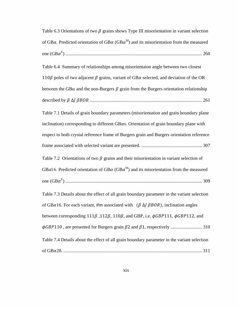
Table 6.3 Orientations of two grains shows Type III misorientation in variant selection
of GB Predicted orientation of GB (GB ) and its misorientation from the measured
one (GB ) ..................................................................................................................... 260
Table 6.4 Summary of relationships among misorientaion angle between two closest
poles of two adjacent grains, variant of GB selected, and deviation of the OR
between the GBand the non-Burgers grain from the Burgers orientation relationship
described by ................................................................................................ 261
Table 7.1 Details of grain boundary parameters (misorientation and grain boundary plane
inclination) corresponding to different GB s. Orientation of grain boundary plane with
respect to both crystal reference frame of Burgers grain and Burgers orientation reference
frame associated with selected variant are presented. .................................................... 307
Table 7.2 Orientations of two grains and their misorientation in variant selection of
GB Predicted orientation of GB (GB ) and its misorientation from the measured
one (GB ) ..................................................................................................................... 309
Table 7.3 Details about the effect of all grain boundary parameter in the variant selection
of GB 16. For each variant, associated with , inclination angles
between corresponding , , , and GBP, i.e. , , and
, are presented for Burgers grain and , respectively ........................... 310
Table 7.4 Details about the effect of all grain boundary parameter in the variant selection
of GB 28. ....................................................................................................................... 311
xx
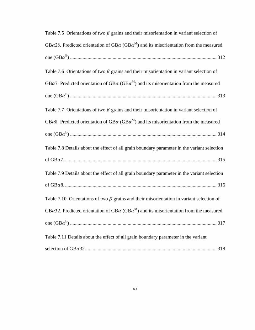
Table 7.5 Orientations of two grains and their misorientation in variant selection of
GB Predicted orientation of GB (GB ) and its misorientation from the measured
one (GB ) ..................................................................................................................... 312
Table 7.6 Orientations of two grains and their misorientation in variant selection of
GB Predicted orientation of GB (GB ) and its misorientation from the measured
one (GB ) ..................................................................................................................... 313
Table 7.7 Orientations of two grains and their misorientation in variant selection of
GB Predicted orientation of GB (GB ) and its misorientation from the measured
one (GB ) ..................................................................................................................... 314
Table 7.8 Details about the effect of all grain boundary parameter in the variant selection
of GB 7. ......................................................................................................................... 315
Table 7.9 Details about the effect of all grain boundary parameter in the variant selection
of GB 8. ......................................................................................................................... 316
Table 7.10 Orientations of two grains and their misorientation in variant selection of
GB Predicted orientation of GB (GB ) and its misorientation from the measured
one (GB ) ..................................................................................................................... 317
Table 7.11 Details about the effect of all grain boundary parameter in the variant
selection of GB 32. ........................................................................................................ 318
xxi
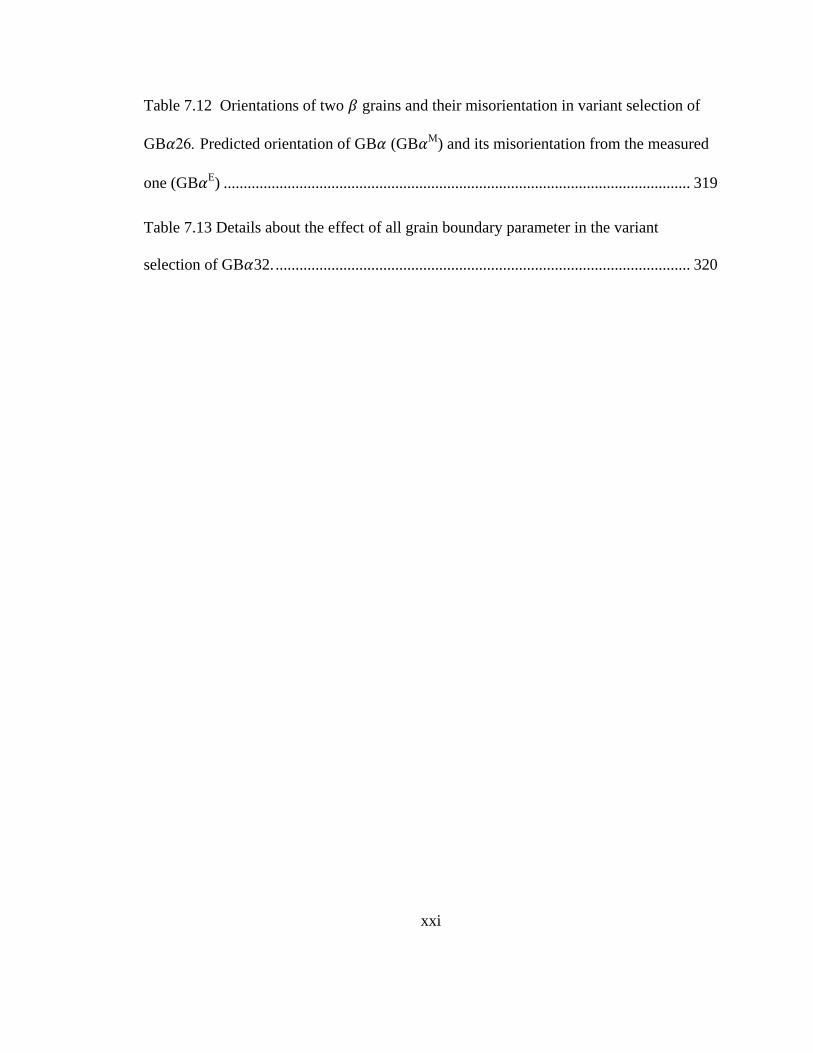
Table 7.12 Orientations of two grains and their misorientation in variant selection of
GB Predicted orientation of GB (GB ) and its misorientation from the measured
one (GB ) ..................................................................................................................... 319
Table 7.13 Details about the effect of all grain boundary parameter in the variant
selection of GB 32. ........................................................................................................ 320
xxii
List of Figures
Figure 2.1 Schematic representation of three types of titanium alloys: alloy, alloy,
and alloy in a pseudo-binary section through a isomorphous phase diagram [2] ...... 39
Figure 2.2 Typical microstructures in Titanium alloys: (a) Grain boundary GB (b)
Colony ; (c) Basketweave and (d) Secondary microstructure ......................... 40
Figure 2.3 Schematic illustration of the Burgers orientation relationship, by looking down
[101] // [0001] (pointing into the plane of paper) ........................................................ 41
Figure 2.4 Schematic illustration of the interface and misfit dislocation configuration
........................................................................................................................................... 42
Figure 2.5 stereographic projection shows that GB maintains Burger OR with
grain and exhibits a small deviation from Burger OR with respect to adjacent grain
(G. B. P. indicates grain boundary plane) ......................................................................... 42
Figure 2.6 Schematic illustration of the variant selection rule by the grain boundary plane
(G.B.P.)-conjugate direction tends to parallel to G.B.P. .......................... 43
Figure 2.7 Schematic illustration of GB of different variants formed at a grain boundary
with a slight variation in its boundary plane ..................................................................... 43
Figure 2.8 (a) a prior grain boundary with the colony microstructure in one of the
grain ( grain 1) and the basketweave microstructure in the adjoining grain 2 (b)
xxiii
Orientation Image Microscopy (OIM) map of the same region as shown in (a). Regions
with the same color represent the same orientation variant .............................................. 44
Figure 2.9 (a) OIM map of three different laths sharing a common direction in a
basketweave microstructure selected from grain 2; (b) Superimposed pole figures of
{110} poles in matrix with the {0001} poles of the clustering laths; (c)
Superimposed pole figures o matrix with the poles of the
clustering laths [26] ....................................................................................................... 45
Figure 2.10 (a) OIM map of a cluster of three different laths in the basketweave
microstructure; (b) and (c) superimposed pole figures indicate that lath 1 and 2 share a
common basal plane; (d) and (e) superimposed pole figures indicate that lath 2
and 3 share a common .............................................................................. 46
Figure 2.11 (a) precipitates of single variant showed same morphology within slip band
in the matrix [15]; (b) Schematic illustration of the variant selection of on the slip
band [20] ........................................................................................................................... 47
Figure.4.1 Growth behavior of an plate. (a) Thickening kinetic of an infinite plate.
Results by phase field (symbol) and DICTRA (solid line) simulations are compared. (b)
Lengthening and (c) Thickening kinetics of a single finite plate embedded in a
supersaturated matrix. Error bars represent uncertainty in the determination of interface
position ............................................................................................................................ 148
Figure. 4.2 (a) Morphology of an isolated plate visualized by a constant contour of Al
concentration. The transparent light yellow plane denotes the experimentally observed
xxiv
habit plane . (b) A cross-section of the matrix phase surrounding the
plate showing variations in Al concentration in the matrix up to the precipitate/matrix
interface. The color bar indicates the relative value of Al concentration. ...................... 149
Figure. 4.3 Variant selection and microstructure development under a pre-stain obtained
via a compressive stress (50Mpa) along [010] . (a) 2D cross-sections showing
microstructure evolution (color online with phase shown in red and phase shown in
blue). Arrows indicate regions with transformation texture. (b) 3D microstructure
obtained at t = 10s. (c) Volume fraction of each variant as function of time. ................ 150
Figure. 4.4 Variant selection and microstructure development under a pre-stain obtained
via a tensile stress (50Mpa) along [010] . (a) 2D cross-sections showing microstructure
evolution (color online with phase shown in red and phase shown in blue). Arrows
indicate regions with transformation texture. (b) 3D microstructure at t=10s. (c) Volume
fraction of each variant as a function of time ................................................................. 151
Figure. 4.5 Variant selection of secondary by a pre-existing plate. (a) Pre-existing
plate of variant 1 (V1). (b)-(d) Formation of secondary laths on the broad face of the
pre-existing plate. Different types of secondary are visualized through different
colors (see online version). (e) Volume fraction analysis of each secondary (f) - (h)
Formation of secondary on the other side of broad face of pre-existing plate from a
different view direction. (g) shows the relative locations between secondary (at t = 2s)
and pre-existing plate (at t = 0s). ................................................................................. 152
xxv
Figure.4.6 Interaction energy density between pre-strain and each variant under both
coherent and semi-coherent conditions. The pre-strain is obtained by applying a 50MPa
tensile stress along (a) and (b) , and a 50Mpa compressive stress along (c)
and (d) ...................................................................................................... 153
Figure.4.7 Variant selection caused by a pre-stain obtained via uni-axial tension or
compression (50Mpa) along . Volume fraction of each variant as function of time
under tension (a) and compression (b). 3D microstructure (at t = 10s) under tension (c)
and compression (d). ....................................................................................................... 154
Figure.4.8 Chemical driving force for nucleation around a growing pre-existing plate
(Variant 1). The contour line indicates the chemical driving force in the supersaturated
matrix far away from pre-existing plate .......................................................................... 155
Figure . 4.9 Elastic interaction energy associated with all 12 variants of coherent nuclei
around a pre-existing semi-coherent plate (Variant 1). The contour lines indicate that
the elastic interaction energy is equal to the chemical driving force for nucleation in the
supersaturated matrix far away from the growing pre-existing plate shown in Fig. 4.8.
......................................................................................................................................... 156
Figure. 4.10 Elastic interaction energy associated with all 12 variants of semi-coherent
laths around a pre-existing semi-coherent plate (Variant 1). The contour lines indicate
vanishing elastic interaction energy. ............................................................................... 158
Figure 4.10 (continued) ................................................................................................... 159
xxvi
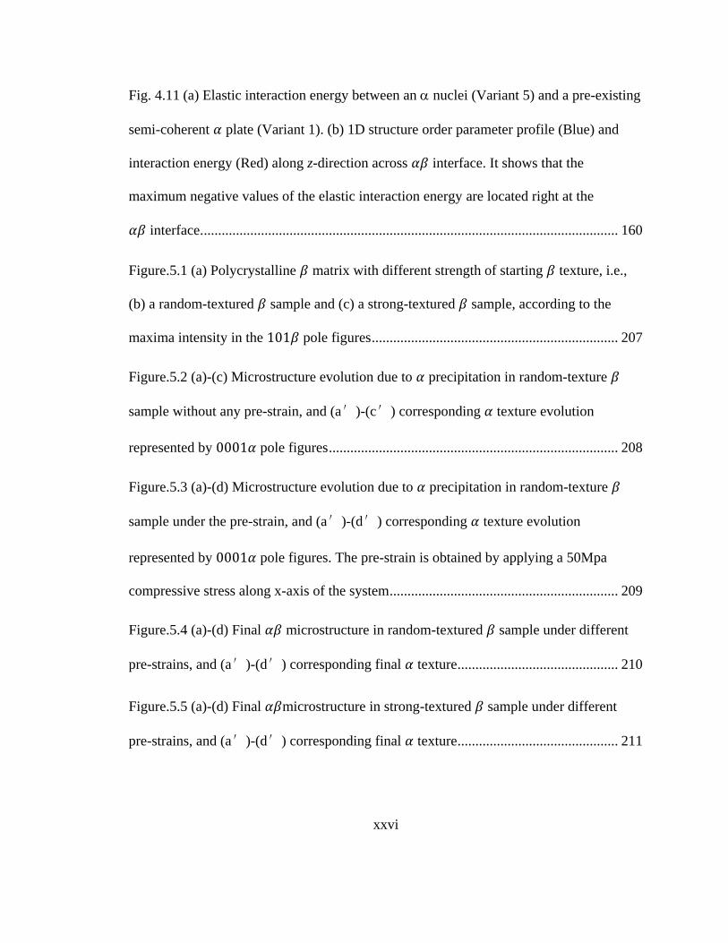
Fig. 4.11 (a) Elastic interaction energy between an nuclei (Variant 5) and a pre-existing
semi-coherent plate (Variant 1). (b) 1D structure order parameter profile (Blue) and
interaction energy (Red) along z-direction across interface. It shows that the
maximum negative values of the elastic interaction energy are located right at the
interface. .................................................................................................................... 160
Figure.5.1 (a) Polycrystalline matrix with different strength of starting texture, i.e.,
(b) a random-textured sample and (c) a strong-textured sample, according to the
maxima intensity in the pole figures ..................................................................... 207
Figure.5.2 (a)-(c) Microstructure evolution due to precipitation in random-texture
sample without any pre-strain, and (a′)-(c′) corresponding texture evolution
represented by pole figures ................................................................................. 208
Figure.5.3 (a)-(d) Microstructure evolution due to precipitation in random-texture
sample under the pre-strain, and (a′)-(d′) corresponding texture evolution
represented by pole figures. The pre-strain is obtained by applying a 50Mpa
compressive stress along x-axis of the system ................................................................ 209
Figure.5.4 (a)-(d) Final microstructure in random-textured sample under different
pre-strains, and (a′)-(d′) corresponding final texture ............................................. 210
Figure.5.5 (a)-(d) Final microstructure in strong-textured sample under different
pre-strains, and (a′)-(d′) corresponding final texture ............................................. 211
xxvii
Figure.5.6 (a) Maximum intensity in pole figures as a function of time in random-
textured sample under different pre-strain, (b) Maximum intensity in pole
figures as a function of time in strong-textured sample under different pre-strain, (c)
Maximum intensities in pole figures of final texture in both random-texture and
strong textured samples under different pre-strain ...................................................... 212
Figure.5.7 (a) and (b) pole figures for random-textured and strong-textured
sample; (c) and (d) corresponding pole figures of final texture in random-
textured and strong-textured sample without variant selection ...................................... 213
Figure.5.8 Degree of variant selection in both random-texture and strong textured
samples under different pre-strain .................................................................................. 214
Figure.5.9 (a) Degree of variant selection in random-textured sample under
different boundary constraint, (b) Degree of variant selection in random-textured
sample under different boundary constraint ................................................................... 215
Figure.5.10 (a)-(b) microstructure in the 2nd
and 5th
grain in random-textured
sample under x-tensil pre-strain, respectively; (c)-(d) volume fraction of each variant as a
function of time in the two grains; (e)-(f) local stress state in the two grains; (g)-
(h) interaction energy density between the external loading and each α variant under both
coherent and semi-coherent conditions within these two grains .................................... 216
Figure.5.11 (a)-(b) microstructure in the 2nd
and 5th
grain in strong-textured
sample under x-tensil pre-strain, respectively; (c)-(d) volume fraction of each variant as a
function of time in the two grains; (e)-(f) local stress state in the two grains; (g)-
xxviii
(h) interaction energy density between the external loading and each α variant under both
coherent and semi-coherent conditions within these two grains .................................... 218
Figure.5.12 (a)-(b) microstructure in the 2nd
and 5th
grain in random-textured
sample under x-tensil external loading (Free-end), respectively; (c)-(d) volume fraction of
each variant as a function of time in the two grains; ................................................... 220
Figure.5.13 (a) all possible misorientation between pairs of variants. Misorientation
axes are expressed in a strand triangle for HCP structure; (b) uncorrelated misorientation
analysis for both phase field simulated microstructure and the one without variant
selection; (c) the maximum degree of variant selection within individual grain where a
single variant percolates the whole grain .................................................................... 221
Figure.5.14 (a) degree of variant selection within the largest and the smallest grain in
random-texture sample under different pre-strains and boundary constraint, (b)
corresponding overall degree of variant selection .......................................................... 222
Figure. 5.15 (a) and (b) degree of variant selection within the largest in random-texture
sample under Z-Comp pre-strain and X-Comp external loading (X-Comp-Free),
respectively, (c) and (d) pole figures for final textue under Z-Comp pre-strain
and X-Comp external loading (X-Comp-Free), respectively ......................................... 223
Figure. 5.16 (a) Macro-texture of random-textured sample represented by three different
pole figures, , and poles, respectively; (b) Macro-texture of final
phase without occurrence of variant selection represented by corresponding three
different pole figures, , , and , respectively;(c) Macro-texture of
xxix
final phase with occurrence of variant selection represented by corresponding three
different pole figures, , , and , respectively .................................. 224
Figure. 5.17 Examples showing the pseudo variant selection due to 2D sampling effect.
EBSD scan is performed along at different layers of the sample ................................... 225
Figure 6.1. Illustrations of all special crystallographic orientation relationships between
GB (Red) and two adjacent grains (Blue and Green) that are able to hold the Burgers
Orientation Relationship with the GB (a) Type I - 10.52 º/<110>, (b) Type II- 49.48
º/<110>, (c) Type III- 60º/<110> and Type IV- 60º/<111>. ....................................... 253
Figure 6.2. Experimental observations of a Type II special grain boundary where
GB maintains BOR with two adjacent grainsaOIM image of the Type II
boundary; (b) superimposed pole figures of the poles of the two grains and the
pole of the GB (c) Superimposed pole figures among the poles of the
two grains and the pole of the GB ........................................................... 254
Figure 6.3. Experimental observations of a Type III special grain boundary where
GB maintains BOR with two adjacent grainsaOIM image of the Type III
boundary; (b) superimposed pole figures of the poles of the two grains and the
pole of the GB (c) Superimposed pole figures among the poles of the
two grains and the pole of the GB ........................................................... 255
Figure 6.4. OIM images ((a) and (b)) and superimposed pole figures of GB and
pole figures of the two grains with different angular deviation between two

xxx
closest poles ((a) and (c): ; (b) and (d):
). ........................................................................................... 256
Figure 6.6. (a) OIM image for two grains with GB 9 and GB on different locations
of the grain boundary with different inclinations; (b) Disorientation angles associate
with for all 12 variants; (c) Superimposed pole figures among the
poles of the two grains and the pole of GB ; (d) Superimposed pole figures
among the poles of the two grains and the pole of GB (e)
Superimposed pole figures among the poles of the two grains and the
pole of GB ; (d) Superimposed pole figures among the poles of the two grains
and the pole of GB ...................................................................................... 258
Figure 7.1 Overall characteristic of grain boundary alpha (GB ) precipitation shown by
OIM. Presence of GB only occurs at certain grain boundaries .................................... 295
Figure 7.2 Standard stereographic triangle projection shows the orientation of grain
boundary (GB) planes (red solid circles) relative to the crystal reference frame in Burgers
grain ................................................................................................................................ 295
Figure 7.3 (a) Stereographic projection shows the orientation of GB planes relative to the
Burgers reference frame of selected variant, i.e. - - ; (b) and (c) the
frequency of occurrence of variant selection as a function of the inclination angle
between GBP and direction and between GBP and planes
, respectively .................................................................................................. 296
xxxi
Figure 7.4 (a) Stereographic projection shows the orientation of GB planes relative to the
Burgers reference frame of selected variant in the case of ; (b) and (c) the
frequency of occurrence of variant selection as a function of and ,
respectively ..................................................................................................................... 297
Figure.7.5 (a) Stereographic projection shows the orientation of GB planes relative to the
Burgers reference frame of selected variant in the case of ; (b) and (c) the
frequency of occurrence of variant selection as a function of and ,
respectively ..................................................................................................................... 298
Figure 7.6 Experimental observations of variant selection of GB 16aOIM image; (b)
superimposed pole figures among the poles of the two grains and the
pole of the GB (c) Superimposed pole figures among the poles of the two
grains and the pole of the GB (d) superimposed pole figures of the
poles of the two grains and the pole of the GB (e) Disorientation angles
associate with and (f) for all 12 variants with respect to
different Burgers grain; grain boundary plane orientation is also superimposed in (b)-(d).
......................................................................................................................................... 299
Figure 7.7 Experimental observations of variant selection of GB 28aOIM image; (b)
superimposed pole figures among the poles of the two grains and the
pole of the GB(c) Superimposed pole figures among the poles of the two
grains and the pole of the GB (d) superimposed pole figures of the
poles of the two grains and the pole of the GB (e) Disorientation angles

xxxii
associate with and (f) for all 12 variants with respect to
different Burgers grain .................................................................................................... 300
Figure 7.7 (Continued) .................................................................................................... 301
Figure 7.8 Experimental observations of variant selection of GB 7 and GB 8aOIM
image; (b) Disorientation angles associate with for all 12 variants with
respect to different Burgers grain; (c) and (f) superimposed pole figures among the
poles of the two grains and the pole of the GB and GB 8(d) and (g)
Superimposed pole figures among the poles of the two grains and the
pole of the GB and GB 8(e) and (h) superimposed pole figures of the poles of
the two grains and the pole of the GB and GB 8; (i) and (j) for
all 12 variants with respect to different Burgers grain .................................................... 302
Figure 7.8 (Continued) .................................................................................................... 303
Figure 7.9 Experimental observations of variant selection of GB 31aOIM image; (b)
superimposed pole figures among the poles of the two grains and the
pole of the GB(c) Superimposed pole figures among the poles of the two
grains and the pole of the GB (d) superimposed pole figures of the
poles of the two grains and the pole of the GB (e) Disorientation angles
associate with and (f) for all 12 variants with respect to
different Burgers grain .................................................................................................... 304
Figure 7.10 Experimental observations of variant selection of GB 26aOIM image;
(b) superimposed pole figures among the poles of the two grains and the

xxxiii
pole of the GB(c) Superimposed pole figures among the poles of the two
grains and the pole of the GB (d) superimposed pole figures of the
poles of the two grains and the pole of the GB (e) Disorientation angles
associate with and (f) for all 12 variants with respect to
different Burgers grain .................................................................................................... 305
Figure 7.11 A scenario for nucleation of a grain boundary on a prior grain boundary
between and . The nuclei maintain Burgers orientation with , and the low energy
facets and develop into Burgers grain . The zone axis between two facets
is assumed to included in the grain boundary ....................................................... 306
1
CHAPTER 1 Introduction
1.1 Motivations
Titan, the Giant divine being in Greek mythology, a son of Uranos (Father Heaven) and
Gaia (Mother Earth), had lost several wars against the Olympic Gods that resulted in his
being confined in the underground dark world. The element, titanium, confined within
rutile ores, was first discovered by a German chemist Martin Heinrich Klaproth. It was
then confirmed as a new element and, in 1795, was named for the Latin word for Earth
(also the name for the Titan of Greek myth).
Because of their lightweight, high strength-to-weight ratio, low modulus of elasticity, and
excellent corrosion resistance, titanium-based materials (both unalloyed and alloyed)
have been finding increasingly widespread application in many industries for the
production of a wide variety of components and work pieces since the early 1950s. It was
very hard to predict, at that time, that titanium materials would currently receive their
attention, interest and importance not only for industrial applications but also equally for
dental and medical applications. It is believed that the expansion of titanium alloys usage
will continue for the forthcoming years.
The mechanical properties of titanium alloys, such as ductility, strength, creep resistance,
crack propagation resistance and fracture toughness, depend, to a large degree, on the
microstructure, which is formed during the thermomechanical processing (TMP) and
2
thermal treatment procedures. According to the application, a specific properties (or
combination of properties) can be obtained through microstructure fabrication or
modification. Microstructure evolution and control in titanium alloys rely heavily on the
allotropic transformation from a body-centered cubic crystal structure (denoted as beta
phase) at high temperatures to a hexagonal close-packed (HCP) crystal structure (referred
to as alpha phase) found at low temperatures.
The defining characteristic of the transformation is the Burgers orientation relationship
(BOR) [1] between the two phases, i.e. { } and ⟨ ⟩ [ ] . Owing
to the symmetry of the parent and product phases and the BOR between them [2], there
are twelve possible crystallographically equivalent orientation variants of the phase
within a single parentgrain. It is typically the case that only a small subset of the 12
possible variants is formed preferentially within each beta grain under different TMPs,
i.e., variant selection occurs frequently during TMP.
During thermo-mechanical processing, many factors could lead to the occurrence of
variant selection during the transformation and hence formation of microtexture.
For both and processing routes, the transformation starts from prior
grain boundaries that have strong preference to select certain variants for allotriomorphic
GB Colony , i.e., cluster of parallel plates belonging to a single variant
(the same variant as the GB ) could then develop into the grain that holds a BOR [1]
with the GB . The development of colony structures on the other adjacent
3
grain is also subjected to the influence of GB . Defects such as dislocations
and stacking faults generated during TMP in either or phase region act
frequently as preferred nucleation sites for specific subset of variants. Upon further
cooling or aging at a lower temperature within the two-phase region, a specific set
of variants for secondary plates will be further selected to nucleate and fill the retained
matrix between the primary plates or around the primary globular particles.
Besides dislocations, there exists a rich variety of other sources that are able to result in
local stresses and lead to variant selection within sample during TMP. For instance,
owing to the anisotropy of thermal expansion coefficient of the phase (which is 20%
larger than in the ⟨ ⟩ than in the ⟨ ⟩ directions), substantial residual stresses are
common in Ti alloys even after a stress relief annealing treatment [10-12]. Moreover,
local stress fields will also be generated by precipitation and autocatalysis has been
shown frequently to cause variant selection [13, 14]. Furthermore, for polycrystalline
materials under an external stress or strain field, local stress state within the sample will
vary significantly from grain to grain because of the elastic anisotropy in each grain that
leads to elastic inhomogeneity in the sample [15]. Apparently, local stress state, due to a
rich variety of sources, is a key factor in controlling variant selection and hence the final
transformation texture during precipitation in Ti alloys. To sum up, frequent
occurrence of variant selection due to a rich variety of factors during TMP results in a
relative hierarchical and relatively coarse microstructure at the scale of individual

4
grain, across prior grain boundaries, within the overall polycrystalline sample, and
also significant transformation texture (i.e., appearance of large regions of plates
consisting of the same crystallographic orientation variant or different variants but with a
common crystallographic feature such as common basal pole; these regions
within individual grains or across grain boundaries are often referred to as “macro-
zones” or micro-textured regions).
Therefore, in order to control the microstructure, to understand processing-
microstructure-properties relationships, and thus to tailor manufacturing conditions to
obtain specific mechanical properties through TMP, it is of significant importance to
develop a quantitative understanding/prediction of variant selection mechanisms for its
occurrence at different scales and further investigate both microstructure and micro-
texture development of phase due to variant selection. However, variant selections
depend on a wide variety of interacting parameters and thus are very complex. Owing to
this complexity, the mechanisms of variant selection are very difficult to determine
experimentally. For example, the main challenges to study the effect of external
loading/pre-strain variant selection during transformations in polycrystalline
sample under the influence of stress are three-folds: first, one needs to determine stress
distribution in an elastically anisotropic and inhomogeneous polycrystalline matrix
under a given applied stress/strain condition; and second, one needs to describe
interactions of local stress with precipitation of coherent and semi-coherent precipitates,
i.e., to describe interactions of local stress with an evolving microstructures. During
5
early stages of a phase transformation, precipitates or structural non-uniformities tend to
be fully coherent to minimize the interfacial energy. However, they may lose coherency
during continued growth when the elastic strain energy becomes dominant. Defect
structure, including misfit dislocations and structural ledges, at the interfaces will
alter not only the coherency elastic strain energy associated with the precipitation, but
also the interfacial energy and its anisotropy. It could introduce growth anisotropy as
well. These anisotropies, together with the high volume fraction and multi-variants of the
precipitate phase and long-range elastic interactions between the precipitates and local
stress, and among different variants of precipitates themselves, lead to highly non-
random spatial distribution of precipitates with different variants. Third, in order to
provide new insight into materials processing- microstructure- properties relationship,
microstructure and texture needs to be considered together. In other words, variant
selection behavior at the scale of individual parent grains and scale of the whole
polycrystalline sample, and their influence on the microstructure evolution and final
transformation texture need to be considered simultaneously. In sum, variant selections
depend on a wide variety of interaction parameters and thus are very complex.
Based on gradient thermodynamics [16-18] and microelasticity theory [19-23], the phase
field approach [24-30] (also called the diffuse-interface approach) offers an ideal
framework to deal rigorously and realistically with these difficult challenges. As will be
demonstrated in the current study of the transformation in Ti-6Al-4V (in wt%)
[31, 32], in the framework of phase field model , , the formulation of the total free energy
6
functional, which consists of the bulk chemical free energy, elastic strain energy and
interfacial energy, has accounted for the following: (a) a reliable thermodynamic data for
the bulk chemical free energy for Ti-6Al-4V system [32, 33]; (b) crystallography of the
crystal lattice rearrangement, including orientation relationship, i.e. BOR, and
lattice correspondence (LC, i.e. atomic site correspondence for diffusional
transformation) as functions of the lattice parameters of the precipitate and parent phases
(i.e., the effect of alloy chemistry); (c) accommodation of the transformation strain; (d)
development of defect structures (misfit dislocations and structural ledges) at ⁄
interfaces as precipitates grow in size; (e) elastic interaction of nucleating particles with
existing chemical and structural non-uniformities and other stress-carrying defects such
as dislocations [34]. In particular, in combination with orientation distribution function
(ODF) modeling [35] of the simulated ⁄ microstructures, the phase field model allows
for a treatment of both micro- and macro-texture evolution accompanying the ⁄
microstructure evolution during different thermo-mechanical treatments.
1.2 Organization of the thesis
The objective of the current work is to investigate variant selection behavior at the scale
of individual parent grains, on the prior grain boundaries, and scale of the whole
polycrystalline sample, and the influence of occurrence of variant selection at different
scales on the microstructure evolution and final transformation texture. For the
purpose of illustrating this point, a brief literature review about physical metallurgy of
7
titanium alloys based on phase transformation and a variety of factors that would
result in the occurrence of variant selection and transformation texture at different length
scales will be made in Chapter2.
In Chapter 3, a general approach is proposed to predict equilibrium shapes of precipitates
in crystalline solids as function of size and coherency state. The model incorporates
effects of interfacial defects such as misfit dislocations and structural ledges on strain
energy anisotropy and on interfacial energy anisotropy. Using precipitation in
titanium alloys as an example, how the interfacial defects relax the coherency elastic
strain energy and affect the habit plane orientation are analyzed in detail by incorporating
the effect of the defects into the stress-free transformation strain. How the interfacial
defects affect the interfacial energy anisotropy and the final equilibrium shape of
precipitates is also investigated. Various possible equilibrium shapes of precipitates
having different defect contents at interfaces are obtained by phase field simulations.
Determination of habit plane orientation of precipitate due to interplay between the
strain energy minimization and interfacial energy anisotropy will be investigated. In
combination with crystallographic theories of interfaces such as O-lattice theory and
experimental characterization of habit plane of finite precipitates, this approach has the
ability to predict the coherency state (i.e., defect structures at interfaces) and equilibrium
shape of finite precipitates.
In Chapter 4, we develop a three-dimensional (3D) quantitative phase field model to
8
predict variant selection and microstructure evolution during transformation in Ti-
6Al-4V (wt.%) at the scale of a single grain under the influence of both external and
internal stress fields such as those associated with, but not limited to, pre-straining and
pre-existing precipitates. The model links its inputs directly to thermodynamic and
mobility databases, and incorporates the crystallography (Burgers lattice correspondence
and orientation relationship) of BCC to HCP transformation, elastic anisotropy, and
defects within semi-coherent / interfaces in its total free energy formulation.
In Chapter 5, the three-dimensional quantitative phase field model (PFM) formulated in
Chapter 4 is further extended to predict variant selection and microstructure evolution
during transformation in polycrystalline Ti-6Al-4V sample under the influence of
different processing conditions such as pre-strain and boundary constraint. The model
updates local stress state according to the interactions among external loading, elastic
inhomogeneity and structural inhomgeneity due to evolving precipitation using an
iterative solver. In particular, texture evolution is coupled simultaneously with
microstructure evolution through orientation distribution function (ODF) modeling of
two-phase microstructure in polycrystalline obtained by the PFM. Under different
processing routes, degrees of variant selection at the scale of individual parent grains and
scale of the whole polycrystalline sample, and their effects on the final macro-texture of
phase under the influences of different processing variables and starting texture have
been investigated. The effect of non-uniform stress state, due to elastic inhomogeneity
under pre-strain, on the variant selection behavior within individual grain has been
9
investigated. The connection between variant selection within individual grain and the
overall polycrystalline sample will be made.
It has been observed frequently that GB prefers its ⟨ ⟩ pole to be parallel to a
common ⟨ ⟩ pole of the two adjacent grains and results in a micro-textured region
across the grain boundary (GB) and, as a consequence, slip transmission may take place
more easily across that GB. In order to investigate how such a special prior GB
contributes to variant selection of GB, in Chapter 6, we develop a crystallographic
model based on the Burgers orientation relationship (BOR) between GB and one of the
two grains. The model predicts all possible special grain boundaries at which GB is
able to maintain BOR with both grains. A new measure for variant selection of GB,
, i.e. a measure of the deviation of the actual OR between the GB and the
non-Burgers grain from the BOR, is proposed. The validity of the specific variant
selection rule based on the closeness between two closet { } poles between two
grains widely used in literature will be analyzed using the new parameter, .
For variant selection of GBon prior grain boundary, several empirical rules have
been proposed to explain how grain boundary parameters, misorientation and grain
boundary plane inclination, contribute to the selection of GB. However, there is no a
general rule that is able to explain all variant selection behavior of GB. In Chapter 7,
based on the new parameter formulated in Chapter 6, the applicability of all current

10
empirical variant selection rules with respect to grain boundary parameters such as
misorientation and inclination on VS of GBα has been assessed systematically in Ti-
5553. Violations of different variant selection rules will be investigated.
The final conclusions and discussions on some future directions that would extend the
current work are presented in Chapter 8.
1.3. Reference:
[1] Burgers WG. On the process of transition of the cubic-body-centered
modification into the hexagonal-close-packed modification of zirconium. Physica
1934;1:561.
[2] Cahn JW, Kalonji GM. Symmetry in Solid-Solid Transformation Morphologies.
PROCEEDINGS OF an Interantional Conference On Solid-Solid Phase Transformations
1981:3.
[3] Banerjee D, Williams JC. Perspectives on Titanium Science and Technology.
Acta Materialia 2013;61:844.
[4] Lutjering G, Williams JC. Titanium (Engineering Materials and Processes).
Berlin: Springer, 2007.
[5] Bhattacharyya D, Viswanathan GB, Denkenberger R, Furrer D, Fraser HL. The
role of crystallographic and geometrical relationships between alpha and beta phases in
an alpha/beta titanium alloy. Acta Materialia 2003;51:4679.
11
[6] Bhattacharyya D, Viswanathan GB, Fraser HL. Crystallographic and
morphological relationships between beta phase and the Widmanstatten and
allotriomorphic alpha phase at special beta grain boundaries in an alpha/beta titanium
alloy. Acta Materialia 2007;55:6765.
[7] Stanford N, Bate PS. Crystallographic variant selection in Ti-6Al-4V. Acta
Materialia 2004;52:5215.
[8] van Bohemen SMC, Kamp A, Petrov RH, Kestens LAI, Sietsma J. Nucleation
and variant selection of secondary alpha plates in a beta Ti alloy. Acta Materialia
2008;56:5907.
[9] Shi R, Dixit V, Fraser HL, Wang Y. Variant Selection of Grain Boundary Alpha
by Special Prior Beta Grain Boundaries in Titanium Alloys. Submitted to Acta Materialia
2014.
[10] Sargent GA, Kinsel KT, Pilchak AL, Salem AA, Semiatin SL. Variant Selection
During Cooling after Beta Annealing of Ti-6Al-4V Ingot Material. Metallurgical and
Materials Transactions a-Physical Metallurgy and Materials Science 2012;43A:3570.
[11] Winholtz RA. Residual Stresses: Macro and Micro Stresses. In: Buschow KHJ,
Robert WC, Merton CF, Bernard I, Edward JK, Subhash M, Patrick V, editors.
Encyclopedia of Materials: Science and Technology. Oxford: Elsevier, 2001. p.8148.
[12] Zeng L, Bieler TR. Effects of working, heat treatment, and aging on
microstructural evolution and crystallographic texture of [alpha], [alpha]', [alpha]'' and
[beta] phases in Ti-6Al-4V wire. Materials Science and Engineering: A 2005;392:403.
12
[13] Kar S, Banerjee R, Lee E, Fraser HL. Influence of crystallography varaiant
selection on microstructure evolution in titanium alloys. In: Howe JM, Laughlin DE, Lee
JK, Dahmen U, Soffa WA, editors. Solid-Solid Phase Transformation in Inorganic
Materials 2005, vol. 1: TMS, 2005.
[14] Lee E, Banerjee R, Kar S, Bhattacharyya D, Fraser HL. Selection of alpha
variants during microstructural evolution in alpha/beta titanium alloy. Philosophical
Magazine 2007;87:3615.
[15] Wang YU, Jin YM, Khachaturyan AG. Three-dimensional phase field
microelasticity theory of a complex elastically inhomogeneous solid. Applied Physics
Letters 2002;80:4513.
[16] Cahn JW, Hilliard JE. Free energy of a nonuniform system. I. Interfacial free
energy. The Journal of Chemical Physics 1958;28:258.
[17] Landau LD, Lifshitz E. On the theory of the dispersion of magnetic permeability
in ferromagnetic bodies. Phys. Z. Sowjetunion 1935;8:101.
[18] Rowlinson JS. Translation of J. D. van der Waals' “The thermodynamik theory of
capillarity under the hypothesis of a continuous variation of density”. Journal of
Statistical Physics 1979;20:197.
[19] Eshelby JD. The determination of the elastic field of an ellipsoidal inclusion, and
related problems. Proceedings of the Royal Society of London. Series A 1957;241.
[20] Eshelby JD. The Elastic Field Outside an Ellipsoidal Inclusion. Proceedings of the
Royal Society A 1959;252:561.
13
[21] Khachaturyan A. Some questions concerning the theory of phase transformations
in solids. Soviet Phys. Solid State 1967;8:2163.
[22] Khachaturyan AG. Theory of Structural Transformations in Solids. New York:
John Wiley & Sons, 1983.
[23] Khachaturyan AG, Shatalov GA. Elastic interaction potential of defects in a
crystal. Sov. Phys. Solid State 1969;11:118.
[24] Boettinger WJ, Warren JA, Beckermann C, Karma A. Phase-field simulation of
solidification. Annual Review of Materials Research 2002;32:163.
[25] Chen L-Q. PHASE-FIELD MODELS FOR MICROSTRUCTURE
EVOLUTION. Annual Review of Materials Research 2002;32:113.
[26] Emmerich H. The diffuse interface approach in materials science: thermodynamic
concepts and applications of phase-field models: Springer, 2003.
[27] Karma A. Phase Field Methods. In: Buschow KHJ, Cahn RW, Flemings MC,
Ilschner B, Kramer EJ, Mahajan S, Veyssière P, editors. Encyclopedia of Materials:
Science and Technology (Second Edition). Oxford: Elsevier, 2001. p.6873.
[28] Shen C, Wang Y. Coherent precipitation - phase field method. In: Yip S, editor.
Handbook of Materials Modeling, vol. B: Models. Springer, 2005. p.2117.
[29] Wang Y, Chen LQ, Zhou N. Simulating Microstructural Evolution using the
Phase Field Method. Characterization of Materials. John Wiley & Sons, Inc., 2012.
[30] Wang YU, Jin YM, Khachaturyan AG. Dislocation Dynamics—Phase Field.
Handbook of Materials Modeling. Springer, 2005. p.2287.
14
[31] Shi R, Ma N, Wang Y. Predicting equilibrium shape of precipitates as function of
coherency state. Acta Materialia 2012;60:4172.
[32] Wang Y, Ma N, Chen Q, Zhang F, Chen SL, Chang YA. Predicting phase
equilibrium, phase transformation, and microstructure evolution in titanium alloys. JOM
Journal of the Minerals Metals and Materials Society 2005;57:32.
[33] Chen Q, Ma N, Wu KS, Wang YZ. Quantitative phase field modeling of
diffusion-controlled precipitate growth and dissolution in Ti-Al-V. Scripta Materialia
2004;50:471.
[34] Shi R, Wang Y. Variant selection during α precipitation in Ti–6Al–4V under the
influence of local stress – A simulation study. Acta Materialia 2013;61:6006.
[35] Bunge HJ. Texture Analysis in Materials Science- Mathematical Methods.
London, 1982.
15
CHAPTER 2 Literature Review
Abstract
The ⁄ titanium alloys have been widely used as advanced structural materials in the
aerospace industry. Their mechanical properties mainly depend on the volume fraction,
size, morphology and spatial distribution of precipitates, which form through the
diffusional transformation. According to the symmetry of the
parent (BCC)and product (HCP)phases and their Burgers orientation relationship,
there are twelve possible orientation variants of precipitates within a single prior
grain. However, quite often, some variants appear more frequently than others, a
phenomenon referred to as variant selection. Variant selection during precipitation
generally governs the microstructure evolution and the final mechanical properties of
⁄ titanium alloys. It was found that variant selection is closely related to the
heterogeneous nucleation of phase on pre-existing defects such as grain boundaries
and dislocations. Coupling between plates with different variants also contributes to
variant selection. A full understanding of the mechanism of variant selection can provide
16
important insight into the engineering of microstructure in ⁄ titanium alloys in order
to achieve the desirable mechanical properties.
2.1 Introduction
Titanium alloys have been widely used in industrial and medical applications, ranging
from aircraft jet engine components, to bicycle frames [1-4] and medical implants [5-7]
because the alloys have fascinating combinations of high strength-to-density ratio, high
fracture toughness and high corrosion resistance [6, 8]. Among these alloys, /titanium
alloys are the most widely used because their microstructure and properties can be
manipulated widely by appropriate heat treatments and/or mechanical processing [9].
The basis for the manipulation of microstructure in / alloys relies heavily on the →
+ transformation during cooling, in which, the phase precipitates from the matrix
in the form of laths or plates. It is well known that precipitates usually exhibit a
specific orientation relationship (OR) with the matrix, referred to as Burgers OR [10].
According to the symmetry of the parent and product phases and their Burgers
relationship, there are twelve possible orientation variants of the precipitates in a single
prior grain. Variant selection of phase (some variants grow preferentially over others)
always accompanies with the processing of titanium alloys. Since the HCP phase is
17
highly anisotropic in nature [11], the morphology, distribution and arrangement of it in
the final microstructure influenced by variant selection significantly govern the properties
of the alloys [12-14].
There are many factors that could contribute to the variant selection of phase [15-29].
An understanding of the mechanism of variant selection and its effect on microstructure
development in / titanium alloys will benefit us in terms of better manipulation of
microstructure to obtain desirable mechanical properties.
2.2. precipitation in titanium alloys
2.2.1 Two-phase ⁄ titanium alloys
Titanium and its alloys exist in two allotropic forms: the hexagonal close-packed (HCP)
phase and the body-centered cubic (BCC) phase. Pure titanium exists as phase
below 882 °C (1620 °F). The HCP structure can be defined by placing two atoms at (0, 0,
0) and (2/3, 1/3, 1/2) positions in its unit cell. The space group for the phase is
P63mmc. The predominant slip mode in phase is the 1010 1120 , which is
consistent with the fact that the c/a ratio in pure titanium and its alloys (about 1.587) is
less than the ideal one of 1.633 [1, 2, 30]. The secondary slip systems are 0001
1120 and 1011 1120 . Above 882 °C, pure titanium transforms allotropically
from to phase. The BCC structure can be defined by placing two atoms at (0, 0, 0)
18
and (1/2, 1/2, 1/2) positions in its unit cell. The space group for the phase is Im3m .
The slip systems generally observed in the phase are: 011 111 , 112 111 and
123 111 [1, 2, 30].
In titanium alloys, the to transformation temperature ( transus) strongly depends on
the type and amount of alloying elements [1, 2, 31]. According to their effect on the
transus temperature, alloying elements in titanium alloys can be classified into and
stabilizers. stabilizers, such as Al, C, O and N elements, raise the transus temperature
and thus stabilize the phase. On the other hand, stabilizers, such as V, Cr, Mo, Nb,
etc., stabilize the phase by lowering the transus temperature. The addition of alloying
elements serves one or more of the following functions [2, 6, 31]: to control the
constitution of the alloy, to control the transformation kinetics and to solid-solution
strengthen one or more of the constituent phases [6].
Depending on the phases present and the relative proportions of the constituent phases,
titanium alloys can be classified broadly into three categories: (a) alloys, (b) /alloys
and (c) alloys, as schematically shown in an isomorphous pseudo-binary phase diagram
in Fig. 1 [2].
The/ alloys are in a phase region from the and + phase boundary up to the
intersection of the Ms-line (Martensite starting temperature) with the room temperature.
19
The / alloys have a mixture of and phases at low temperature and contain both
and stabilizing elements. In the most commercially used Ti-6Al-4V (wt. %) alloys, for
example, the Al element partitions selectively to the -phase offering solid-solution
strengthening of phase. The V element, however, is rejected from the -phase due to its
low solubility in this phase and is thus concentrated in the -phase, therefore solid-
solution strengthening the -phase [6]. The phase offers precipitation strengthening for
/ alloys.
2.2.2 Microstructure development during precipitation
For titanium alloys, upon cooling from the single phase region into the +two-
phase phase region, the phase decomposes by nucleation of phase at prior grain
boundaries and subsequently by diffusion controlled growth into the retained matrix.
There are three types of precipitates formed during the to diffusional
transformation in terms of where their nucleation sites: grain boundary allotriomorphic-
(GB), inter-granular and intra-granular [32].
During the cooling from above the transus, a layer of GB heterogeneously nucleates
at and grows preferentially along the grain boundaries (Fig. 2(a)). On further cooling, a

20
set of parallel inter-granular side plates develop either by nucleating directly from the
prior grain boundaries or by branching out from GB(Fig. 2(a)), and shooting into the
interior of prior grains. The plates which nucleate directly from grain boundaries are
referred to as primary side plates while those created by branching of GB are designated
as secondary side plates [33, 34]. Intra-granular plates nucleate and grow within the
interior of the prior -grains. Inter-granular and intra-granular plates comprise the so-
called the widmanstätten microstructure [32]. Depending on the cooling rate, the
widmanstätten plates may group together either in the form of colony attaching to the
prior grain boundaries or in the form of basketweave microstructure within the prior
grains [1, 2]. The Colony microstructure, i.e., clusters of parallel plates belonging to a
single crystallographic variant, forms during slow cooling from the phase field, as
clearly shown in Fig. 2(b). While the basketweave microstructure, i.e., multiple
crystallographic variants of plates clustering in the same region, develops upon higher
cooling rate, as shown in Fig. 2(c). A mixture of the colony and basketweave
microstructures forms at intermediate cooling rates [26].
Depending on their size-scale and sequence of nucleation and growth, widmanstätten
structures can also be subdivided into primary and secondary plates. Secondary
plates nucleate and fill the retained matrix between primary plates upon further
cooling or aging at a lower temperature within two-phase region, as shown in Fig.
2(d).
21
2.2.3 Orientation relationship between and phases
The orientation relationship between the precipitate and matrix during the BCC to
HCP phase transformation has been a subject of intensive research [10, 16, 35-40].
The major orientation relationship between the and phases is the Burgers orientation
relationship [10], described by:
Equation Chapter 2 Section 1
101 // 0001
; 111 // 1120
; 121 // 1100
(2.1)
Recently, more accurate measurements in titanium alloys have showed that the actual
orientation relationship between and phases is deviated slightly from the ideal
Burgers relationship [38], i.e., near Burgers OR. For example, the misorientation angles
between 101 // 0001
and 111 // 1120
are 0.78º and 0.56º [38], respectively.
There is another OR, though less frequently observed than the Burgers OR, in titanium
alloys, i.e., the Pitsch-Schrader OR [41] given by
101 // 0001
; 010 // 1120
; 101 // 1100
(2.2)
Note that a 5.26º crystallographic rotation along 101 // 0001
converts the Pitsch-
Schrader OR to ideal Burgers OR.
22
The precipitate is different from the matrix in both composition and crystal structure.
With the lattice parameters [38] abcc= 0.3196 nm, ahcp=0.2943 nm, and chcp = 0.4680 nm,
the transformation strain ij for an precipitate in matrix with the OR given in Eq.
(2.1) can be described by:
0.0759
0.13620.0356
ij
(2.3)
when referred to 010 // 1120
; 101 // 1100
; 101 // 0001
.
2.2.4 Determination of the number of variants
According to the Burgers OR, the single close-packed basal plane {0001} in the HCP
phase is parallel to one of the six close-packed planes 110
in the BCC phase. In
addition, one of the three close-packed 1120 directions in the basal plane 0001
is
parallel to one of the two close-packed directions 111 lying within the specific
close-packed plane 110
in the phase. However, there are only two distinguishable
combinations of parallel directions 1120 // 111 on 0001
plane due to the
presence of 6 fold rotation symmetry along 0001
. Since there are six possible 101
planes in the phase, there are twelve (6×2) possible equivalent orientation variants of
precipitate allowed by the Burgers OR. Accordingly, the decomposition of a prior grain
23
will give rise to one or more of twelve possible variant of phase, each with its own
distinct orientation with respect to the matrix. All twelve variants are listed in the Table
1. The number of variants can also be derived by group theory [42, 43].
Note that combinations of any two of the 12 variants result in the formation of 6 distinct
types of /grain boundaries in a single grain. These /boundariesare referred to as
Types 1 to 6 boundaries and the reduced axis/angle pairs for each type are listed in Table
2 [22]. Based on a random distribution of each variant, the probability of occurrence of
each type of / boundary, randomP , can be calculated.
2.2.5 The nature of interface between precipitate and matrix
The nature of interface between the precipitate and matrix is crucial to
understand the microstructure evolution during the processing [21, 25] and the properties
of the plastic deformation [44]. Therefore, it has been studied in great details [36-38, 44-
46] including its crystallographic orientation, habit planes and dislocation structures. The
precipitate usually appears in the form of plate and can be characterized as having a
broad face, a side face and an edge face as shown in the Fig 4.
Obviously, the interfaces are semi-coherent with misfit dislocations. Based on the
detailed experimental characterization by Mills et al. [38], the board face is wrapped by a
single set of parallel c-type misfit dislocations with a Burgers vector of 1 2 0001
and
24
the side face is looped by a-type misfit dislocations with a Burgers vector of 1 3 2110
. The dislocations on the broad face and the side face loop around the plate and form a
dislocation network on the edge face. Moreover, the broad face is comprised of structural
ledges [47] or steps that enable the interface to be stepped down along the lattice
invariant line direction 353
1[48], which is also the growth direction (major axis) for
the plate. The terrace plane of step is parallel to 121 // 1100
. The macroscopic
surface of the broad face is generally an irrational plane close to 11 13 11
[36-38, 45].
2.2.6 Relationship between microstructure and mechanical properties
The microstructure of titanium alloys are primarily described by the size, volume
fraction, morphology and spatial distribution of the phase, which in turn has a
substantial influence on the final tensile strength, ductility and fatigue properties of the
alloys.
The size of colonies is the most influential microstructural parameter on the mechanical
properties because it determines the effective slip length [9]. Slip length and colony size
are equal to the width of individual plate. The colony boundaries are major barriers
1 Specific indices are assigned according to the particular variant with OR in Eq.(1)
25
to slip, while the plates do not serve as major deformation barriers because slip transfer
is relatively easy due to the Burgers relationship between the and phases [49].
In general, small colony size and small plate seems to promote better mechanical
properties such as yield stress 0.2, ductility F, high cycle fatigue strength (HCF), except
macrocrack propagation resistance [1, 2, 9], as shown in Table 3.
For example, the yield stress and tensile ductility increase with decreasing colony size
due to the reduction in effective slip length. The dependence of HCF strength on
colony size is qualitatively similar to that of yield stress because the HCF strength
(resistance to crack nucleation) depends primarily on the resistance to dislocation motion.
For the propagation rate of the small, self-initiated cracks (microcracks) , it has been
shown that the microcracks propagate much faster in the coarse colony microstructure as
compared to the fine colony microstructure [9]. In addition, the fatigue cracks usually
nucleate at and propagate through the longest and widest plates due to the preferred slip
band activity within these coarse plates. It will be detrimental to mechanical properties if
a single variant of plate percolates the whole matrix.
It is thus thought that the introduction of more variants for phase leads to an
improvement of fatigue properties because a fine-scale microstructure of phase within
matrix can be obtained through the growth of randomly distributed nuclei of phase
with different variants. In addition, since all variants are distinct in their spatial
26
orientation, the introduction of more variants of phase would increase the tortuosity of
crack paths and thus impede the crack propagation. If there are coarse plates
percolating the whole matrix due to the variant selection of a specific variant, it will
favor the nucleation and propagation of microcracks. Thus, it is important to study the
mechanism of variant selection.
2.3. Variant selection during precipitation
The term “variant selection” will be discussed in detail since it has a significant effect on
the formation of transformation texture and the final mechanical properties [21, 24, 25,
27]. According to the Burgers OR, there are twelve possible orientation variants of
phase that can form within a single prior grain. The chemical driving force, as a
function of only temperature and composition, is the same for all variants, during the to
transformation. It is thus generally thought that all variants should appear with equal
statistical probability. However, some variants can appear more frequently than others
due to certain physical reasons. This phenomenon is referred to as variant selection [21,
22, 24, 25, 27].
There are many factors that could result in the variant selection during precipitation
such as heterogeneous nucleation of phase on the pre-existing defects in parent

27
phases such as grain boundary [27] and dislocations [15, 20]. The coupling between
plates with different variants also induces variant selection [26, 50].
2.3.1 Variant selection of GB
When GB nucleates and develops within the prior grain boundary, selection of one or
multiple specific variants (from the possible 12) are made according to certain rules
[21, 23, 25-27].
It has been commonly observed that Burgers OR exists between GB and one of the two
adjacent prior grains [16, 20, 21, 25, 27] (referred to as , whereas the GB
generally manipulates itself an orientation that has a small deviation from the Burgers
relathiship with respect to the other grain (referred to as , as shown in Fig. 5 [16].
It has been shown by Furuhara et al. [16] that morphologically indistinguishable -
precipitates formed along a relatively straight prior -grain boundary belong to a single
crystallographic variant. Furthermore, the selection of variant from the grain
boundary is made in such a manner that the variant has the minimum possible angle
between the matching direction 1120 // 111 and the grain boundary plane [20,
21], i.e., the matching direction 1120 // 111 of the selected variant tends to
parallel to the grain boundary plane. The variant selection rule seems to be consistent
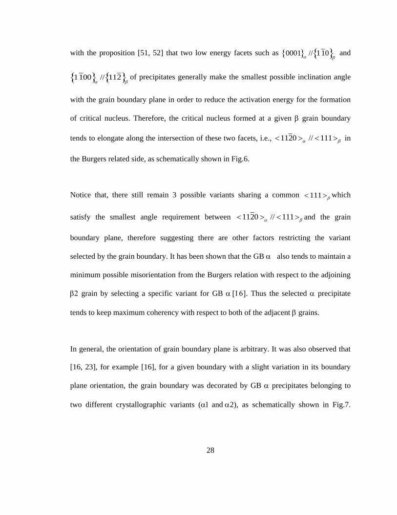
28
with the proposition [51, 52] that two low energy facets such as 0001 // 110
and
1100 // 112
of precipitates generally make the smallest possible inclination angle
with the grain boundary plane in order to reduce the activation energy for the formation
of critical nucleus. Therefore, the critical nucleus formed at a given grain boundary
tends to elongate along the intersection of these two facets, i.e., 1120 // 111 in
the Burgers related side, as schematically shown in Fig.6.
Notice that, there still remain 3 possible variants sharing a common 111 which
satisfy the smallest angle requirement between 1120 // 111 and the grain
boundary plane, therefore suggesting there are other factors restricting the variant
selected by the grain boundary. It has been shown that the GB also tends to maintain a
minimum possible misorientation from the Burgers relation with respect to the adjoining
grain by selecting a specific variant for GB . Thus the selected precipitate
tends to keep maximum coherency with respect to both of the adjacent grains.
In general, the orientation of grain boundary plane is arbitrary. It was also observed that
[16, 23], for example [16], for a given boundary with a slight variation in its boundary
plane orientation, the grain boundary was decorated by GB precipitates belonging to
two different crystallographic variants (and2), as schematically shown in Fig.7.
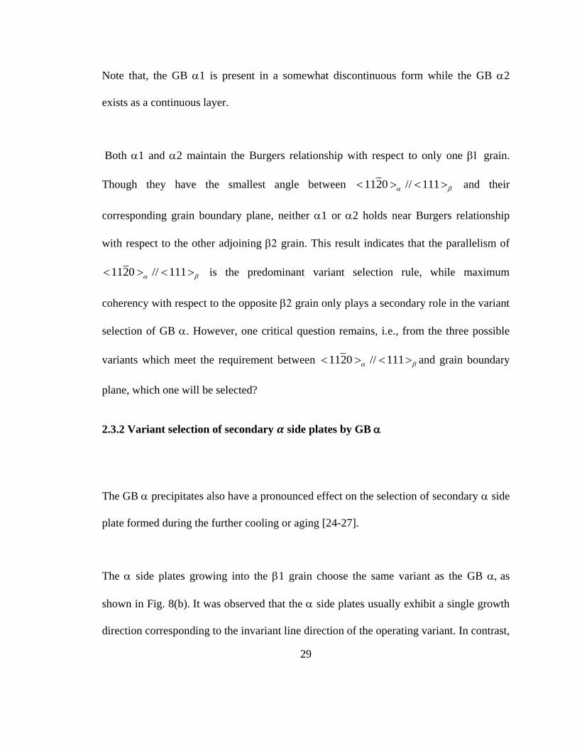
29
Note that, the GB 1 is present in a somewhat discontinuous form while the GB 2
exists as a continuous layer.
Both 1 and 2 maintain the Burgers relationship with respect to only one grain.
Though they have the smallest angle between 1120 // 111 and their
corresponding grain boundary plane, neither 1 or 2 holds near Burgers relationship
with respect to the other adjoining grain. This result indicates that the parallelism of
1120 // 111 is the predominant variant selection rule, while maximum
coherency with respect to the opposite grain only plays a secondary role in the variant
selection of GB . However, one critical question remains, i.e., from the three possible
variants which meet the requirement between 1120 // 111 and grain boundary
plane, which one will be selected?
2.3.2 Variant selection of secondary side plates by GB
The GB precipitates also have a pronounced effect on the selection of secondary side
plate formed during the further cooling or aging [24-27].
The side plates growing into the 1 grain choose the same variant as the GB as
shown in Fig. 8(b).It was observed that the side plates usually exhibit a single growth
direction corresponding to the invariant line direction of the operating variant. In contrast,
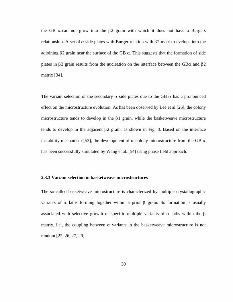
30
the GB can not grow into the 2 grain with which it does not have a Burgers
relationship. A set ofside plates with Burger relation with 2 matrix develops into the
adjoining 2 grain near the surface of the GB This suggests that the formation of side
plates in 2 grain results from the nucleation on the interface between the GB and 2
matrix [34].
The variant selection of the secondary side plates due to the GB has a pronounced
effect on the microstructure evolution. As has been observed by Lee et al.[26], the colony
microstructure tends to develop in the 1 grain, while the basketweave microstructure
tends to develop in the adjacent 2 grain, as shown in Fig. 8. Based on the interface
instability mechanism [53], the development of colony microstructure from the GB
has been successfully simulated by Wang et al. [54] using phase field approach.
2.3.3 Variant selection in basketweave microstructures
The so-called basketweave microstructure is characterized by multiple crystallographic
variants of laths forming together within a prior grain. Its formation is usually
associated with selective growth of specific multiple variants of laths within the
matrix, i.e., the coupling between variants in the basketweave microstructure is not
random [22, 26, 27, 29].

31
Two types of coupling between variants in basketweave microstructure have been
commonly observed. In one case, laths belonging to three distinct variants tend to
cluster in a same region, as shown in Fig. 9(a). The three distinct variants share a
common 1120
direction that is parallel to the 111
direction of the matrix with
their basal poles 0001
rotated by 60º, as shown in Fig. 9 (b) and Fig. 9 (c). In other
words, three laths with Type 2 / grain boundary tend to cluster in the same region.
In the other case as shown in Fig.10, laths 1 and 2 in the cluster share a common
0001
basal plane with their 1120 directions being rotated by about 10.53º along
the common [0001] direction (Fig. 10 (b) and (c)), i.e., laths 1 and 2 have Type 6
boundary, whereas laths 2 and 3 have Type 2 boundary between them (Fig. 10 (d) and
(e)).
According to the experimental results from Lee [26] and Bohemen [27] , both Type 2 and
Type 6 / grain boundaries occur more frequently than expected on the basis a random
distribution of variants (Table 2), which indicates that variant selection occurs during the
formation of basketweave microstructure too.
It was suggested by Bohemen et al. that the preferential occurrence of Type 2 /
boundaries can not be explained by a favored orientation of the plates during individual
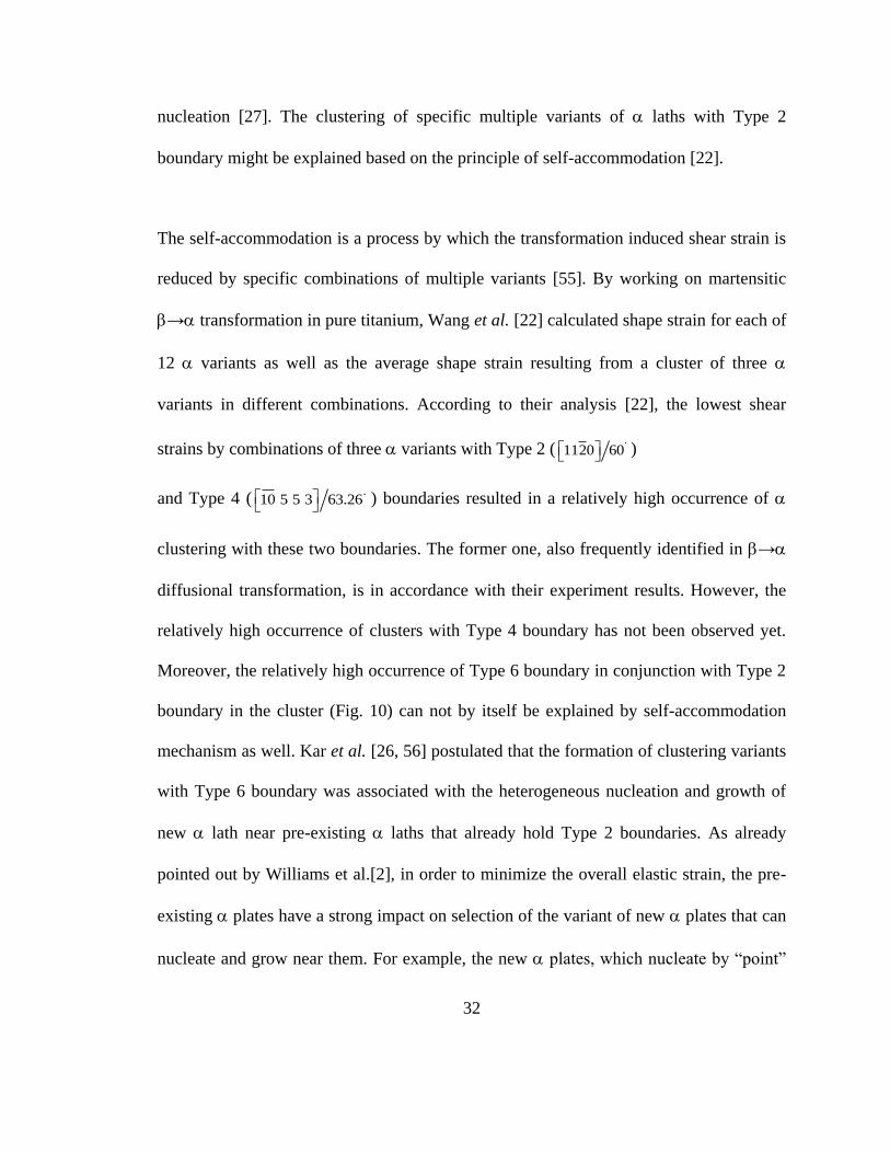
32
nucleation [27]. The clustering of specific multiple variants of laths with Type 2
boundary might be explained based on the principle of self-accommodation [22].
The self-accommodation is a process by which the transformation induced shear strain is
reduced by specific combinations of multiple variants [55]. By working on martensitic
→ transformation in pure titanium, Wang et al. [22] calculated shape strain for each of
12 variants as well as the average shape strain resulting from a cluster of three
variants in different combinations. According to their analysis [22], the lowest shear
strains by combinations of three variants with Type 2 ( 1120 60 )
and Type 4 ( 10 5 5 3 63.26
) boundaries resulted in a relatively high occurrence of
clustering with these two boundaries. The former one, also frequently identified in →
diffusional transformation, is in accordance with their experiment results. However, the
relatively high occurrence of clusters with Type 4 boundary has not been observed yet.
Moreover, the relatively high occurrence of Type 6 boundary in conjunction with Type 2
boundary in the cluster (Fig. 10) can not by itself be explained by self-accommodation
mechanism as well. Kar et al. [26, 56] postulated that the formation of clustering variants
with Type 6 boundary was associated with the heterogeneous nucleation and growth of
new lath near pre-existing laths that already hold Type 2 boundaries. As already
pointed out by Williams et al.[2], in order to minimize the overall elastic strain, the pre-
existing plates have a strong impact on selection of the variant of new plates that can
nucleate and grow near them. For example, the new plates, which nucleate by “point”
33
contact on the broad face (habit plane) of an existing plate, tend to grow nearly
perpendicular to it. As has been observed by Bhattacharyya et al. [21], the growth
directions of two plates with Type 6 boundary are nearly perpendicular, ~80.5 º or 99.5
º, to each other.
In summary, there is a strong coupling between the precipitates, which result in the
formation of the basketweave microstructure. The coupling may be induced by the
accommodation of the strain energy.
2.3.4 Variant selection due to dislocations
It is well known that pre-existing dislocations in the parent phase frequently act as
preferential nucleation sites for precipitates [57, 58]. Furuhara et al. investigated the
influence of dislocations on the selection of variants [15, 20]. In their experiments,
coarse planar slip bands, corresponding to 112 111
slip systems, were introduced by
cold rolling in the matrix at room temperature and precipitates nucleated
preferentially on the dislocations in these slip bands during the subsequent aging [15].
The precipitates in the slip band were of the same morphology and selected a single
variant (V4 in Table 2), as shown in Fig. 11 (a).
The authors tried to explain why only a single variant was selected in terms of the
effective accommodation of transformation stain by the stress field around dislocations.
They derived the maximum misfit strain direction bmax associated with 12 variants of
precipitate by Frank-Bilby equation (FBE) [59, 60]. According to the FBE, the misfit

34
across the interface between the precipitate and matrix can be described in terms of
the net Burgers vector tb crossing a vector p in the interface, as given by:
1
t
Ib A p (2.4)
where A is the homogeneous transformation matrix from lattice to and I is identity
matrix. The calculation results showed that three variants V4, V8 and V12 (in Table 1),
which share a common 111 // 1120
direction, equally gave the closet bmax to the
Burgers vector 2 111a
of the dislocation.
Therefore, according to the effective accommodation of the maximum misfit strain, the
variants of precipitate that are most preferred to nucleate on the 2 111a
dislocation
are limited to three variants V4, V8 and V12. However, only variant V4 was observed in
the slip band. Therefore the criterion of the maximum misfit accommodation is not
sufficient to explain the variant selection rule in this case. Indeed, the other components
of the transformation strain may have further restriction on the selection of the specific
variant of the phase. In fact, the author argued that the exclusive selection of variant 4
can be reasonably explained by the slip plane of dislocation because the slip plane
112
is parallel to the 1100
of variant 4, as shown in Fig. 11(b). As suggested by
Burgers [10], the to transformation begins with shear movements of atoms on 112

35
planes in 111 directions. Thus, prior activity of 112
111 specific systems may
favor the formation of related alpha variants.
2.4. Unresolved issues
The objective of this review on variant selection of phaseduring its precipitation is to
pave the way to better understand the effect of different factors and their interplay on the
variant selection and thus microstructure development in / titanium alloys. According
to the review, there are several unresolved problems:
2.4.1 Grain boundary nucleation
As mentioned above, there are quite stringent restrictions on the possible -variants that
can be precipitated at a given -grain boundaries. The GB is selected from three
possible variants which meet the minimum angle requirement between
1120 // 111 and grain boundary plane. Such a restriction probably serves to
reduce the nucleation barrier for GB . In addition, the selected GB maintains Burgers
OR with respect to one of the two adjacent grains. However, the exact mechanism for
such a variant selection rule is not well understood yet. The relationship between the
morphology of GB and the interface orientation of prior grain boundary is still not
clear. In order to develop a fundament understanding of the variant selection of GB, the
following two problems will be addressed:
36
a) Activation energy and critical nucleus configuration (size, shape, spatial orientation
and OR with the grains) for each of the 12 variants to nucleate at a given grain
boundary between two grains
b) Under what conditions (misorientation and inclination of grain boundary,
undercooling) discontinuous is preferred over a continuous layer of
2.4.2 Correlations between precipitates with different variants in the basketweave
microstructure
As mentioned above, specific variants of plates prefer to cluster together in the
basketweave microstructure. Variants with Type 2 and Type 6 boundary are non-
randomly selected to comprise the basketweave microstructure. However, it is not clear
which of the following two situations occurs: (1) specific variants of appear in group
during their nucleation [61, 62] and then form the cluster; (2) specific variants of new
plates selected by pre-existing plate nucleate and grow near it and thus form the cluster.
It is well known that during nucleation and in early stages of growth, precipitates tend to
be coherent. The observed semi-coherent / interface indicates that precipitates will
lose coherency during its continued growth. Thus the nucleation of coherent plates will
induce large lattice distortion and hence the coherency strain energy will play an
important role during the nucleation process. How the coherency strain energy affects the
nucleation process (the size and configuration of critical nuclei) need to be critically

37
evaluated. In addition, in order to understand the selectivity of new precipitates due to
arbitrary pre-existing plates, anisotropic elastic interaction of a nucleating precipitate
for each variant with the pre-existing plates is also required to analyze.
2.4.3 The effect of dislocation on variant selection
The variant selection due to dislocation is achieved by the heterogeneous nucleation of
phase with specific variant on the dislocation.
However, the maximum misfit accommodation alone fails to explain the variant induced
by dislocation. In order to better understand the variant selection due to dislocation, it still
requires analyzing in details the elastic interaction between the strain field of the coherent
nucleus for each variant and the stress field generated by dislocation in the matrix.
2.4.4 Microstructure evolution with variant selection
As has been demonstrated in this review, variant selection affects the microstructure
evolution in / alloys to a large degree, including the formation of GB, colony and
basketweave microstructure during precipitation. In order to describe and predict the
microstructure evolution and hence to establish a robust microstructure-property

38
relationship, integration of variant selection mechanisms inherent in the precipitation
process is also required in any modeling attempt.

39
Figures
Figure 2.1 Schematic representation of three types of titanium alloys: alloy, ⁄ alloy,
and alloy in a pseudo-binary section through a isomorphous phase diagram [2]

40
Figure 2.2 Typical microstructures in ⁄ Titanium alloys: (a) Grain boundary
GB (b) Colony ; (c) Basketweave and (d) Secondary microstructure
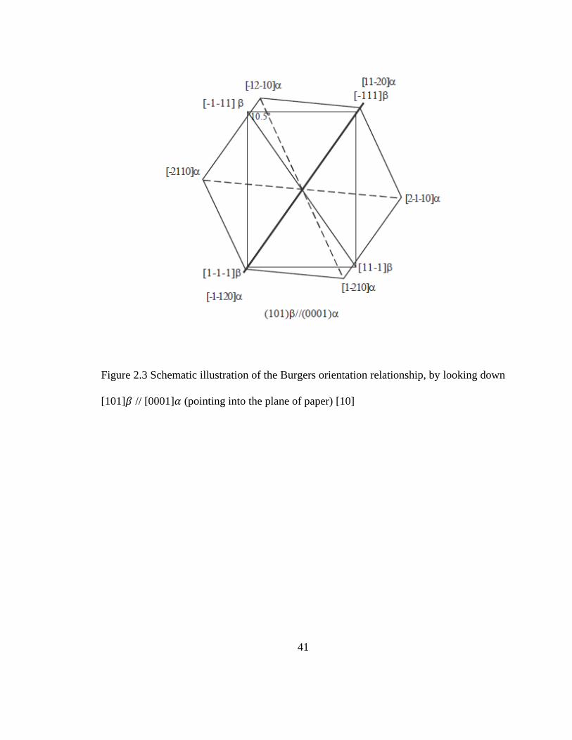
41
Figure 2.3 Schematic illustration of the Burgers orientation relationship, by looking down
[101] // [0001] (pointing into the plane of paper) [10]
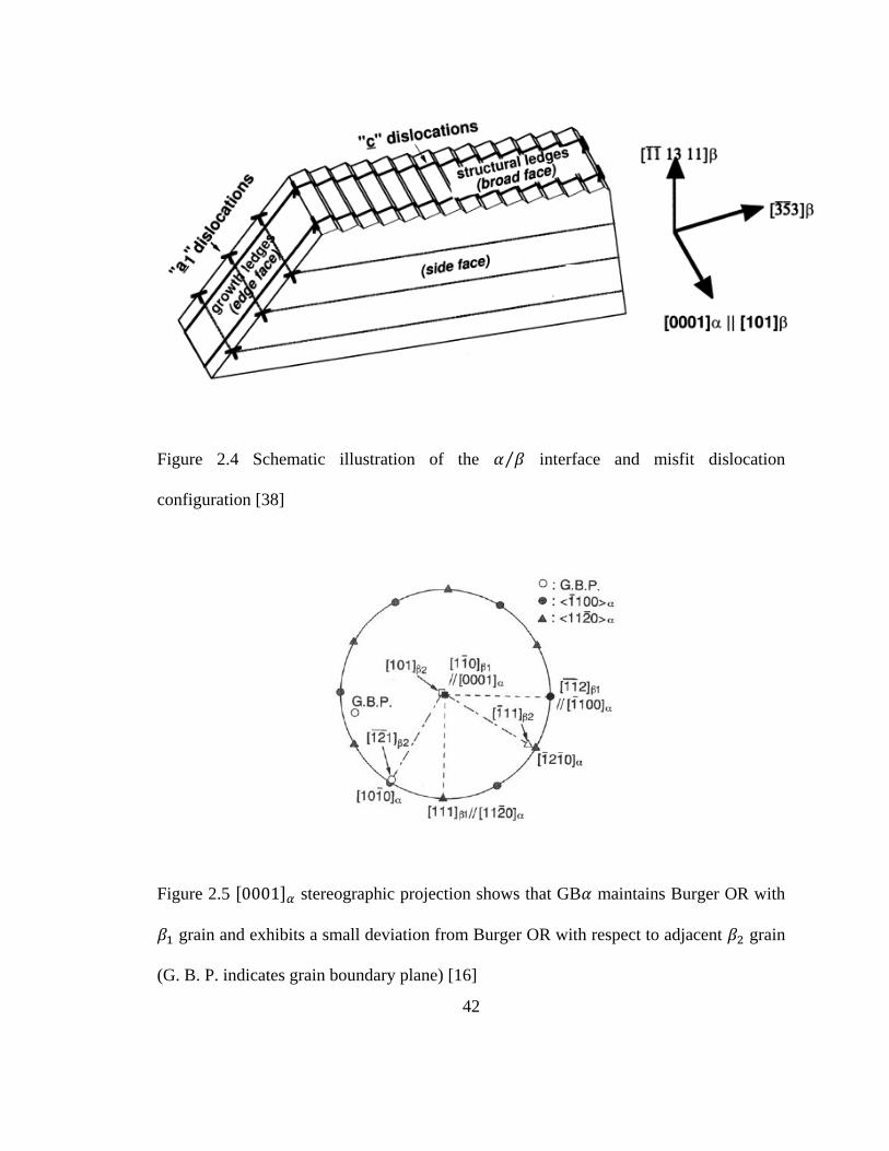
42
Figure 2.4 Schematic illustration of the ⁄ interface and misfit dislocation
configuration [38]
Figure 2.5 [ ] stereographic projection shows that GB maintains Burger OR with
grain and exhibits a small deviation from Burger OR with respect to adjacent grain
(G. B. P. indicates grain boundary plane) [16]

43
Figure 2.6 Schematic illustration of the variant selection rule by the grain boundary plane
(G.B.P.)-conjugate ⟨ ⟩ ⟨ ⟩ direction tends to parallel to G.B.P. [16]
Figure 2.7 Schematic illustration of GB of different variants formed at a grain boundary
with a slight variation in its boundary plane [16]
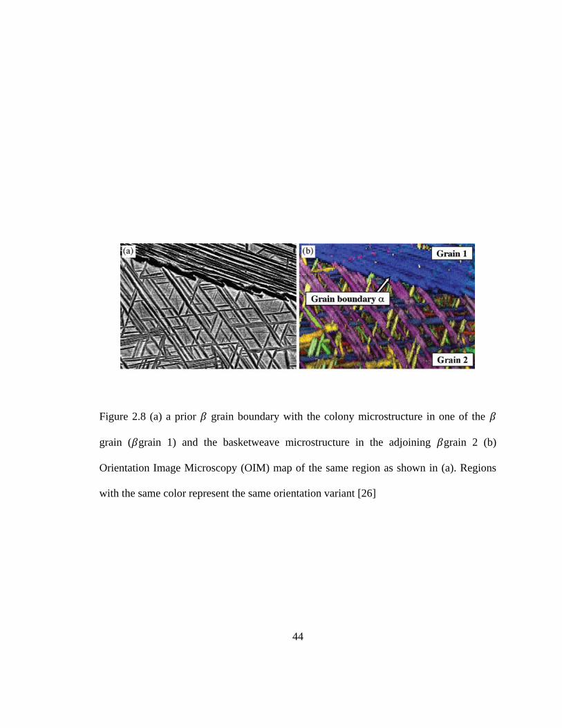
44
Figure 2.8 (a) a prior grain boundary with the colony microstructure in one of the
grain ( grain 1) and the basketweave microstructure in the adjoining grain 2 (b)
Orientation Image Microscopy (OIM) map of the same region as shown in (a). Regions
with the same color represent the same orientation variant [26]
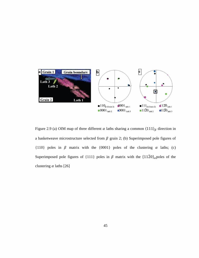
45
Figure 2.9 (a) OIM map of three different laths sharing a common ⟨ ⟩ direction in
a basketweave microstructure selected from grain 2; (b) Superimposed pole figures of
{110} poles in matrix with the {0001} poles of the clustering laths; (c)
Superimposed pole figures of {111} poles in matrix with the { } poles of the
clustering laths [26]

46
Figure 2.10 (a) OIM map of a cluster of three different laths in the basketweave
microstructure; (b) and (c) superimposed pole figures indicate that lath 1 and 2 share a
common basal plane; (d) and (e) superimposed pole figures indicate that lath 2
and 3 share a common ⟨ ⟩ ⟨ ⟩ [64]

47
Figure 2.11 (a) precipitates of single variant showed same morphology within slip band
in the matrix [15]; (b) Schematic illustration of the variant selection of on the slip
band [20]
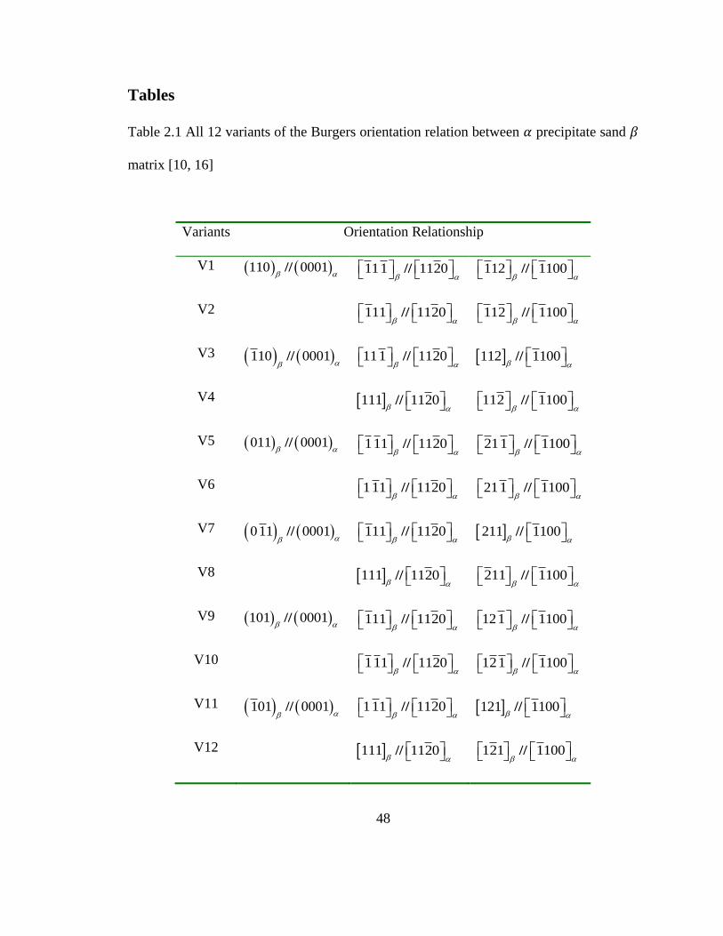
48
Tables
Table 2.1 All 12 variants of the Burgers orientation relation between precipitate sand
matrix [10, 16]
Variants Orientation Relationship
V1 110 0001//
111 1120//
112 1100//
V2 111 1120//
112 1100//
V3 110 0001//
111 1120//
112 1100//
V4 111 1120//
112 1100//
V5 011 0001//
111 1120//
211 1100//
V6 111 1120//
211 1100//
V7 011 0001//
111 1120//
211 1100//
V8 111 1120//
211 1100//
V9 101 0001//
111 1120//
121 1100//
V10 111 1120//
121 1100//
V11 101 0001//
111 1120//
121 1100
//
V12 111 1120//
121 1100
//
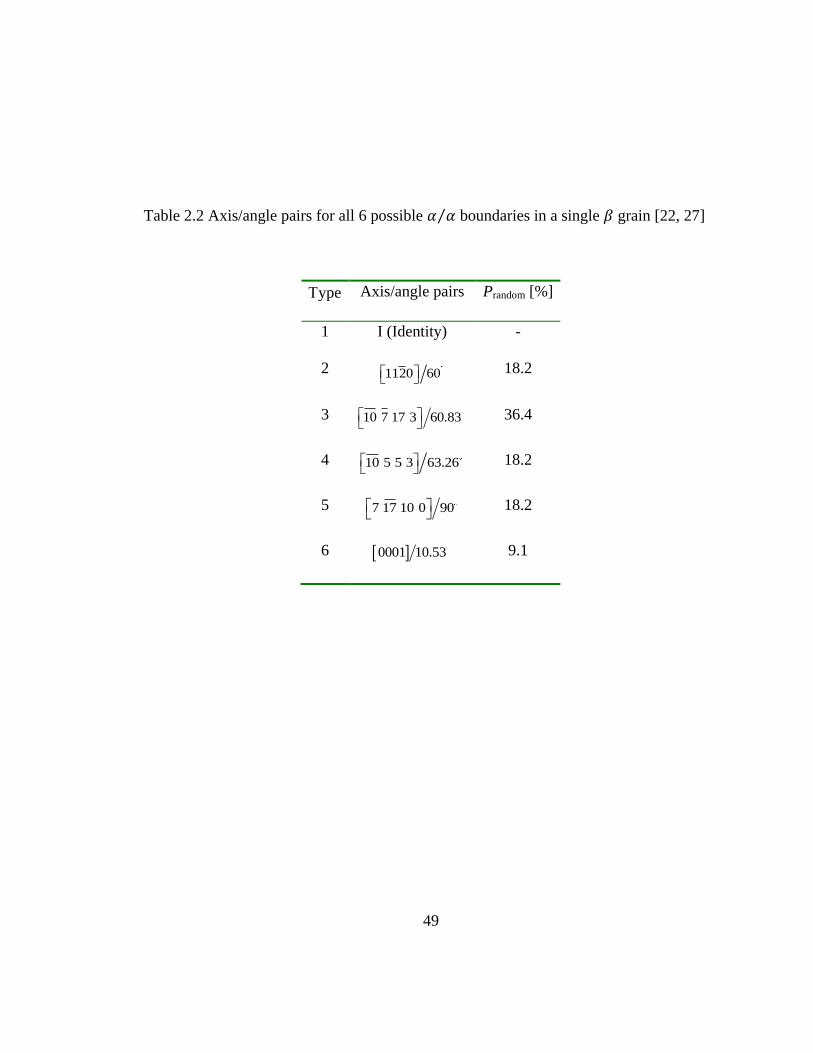
49
Table 2.2 Axis/angle pairs for all 6 possible ⁄ boundaries in a single grain [22, 27]
ype Axis/angle pairs Prandom [%]
1 I (Identity) -
2 1120 60 18.2
3 10 7 17 3 60.83
36.4
4 10 5 5 3 63.26
18.2
5 7 17 10 0 90
18.2
6 0001 10.53 9.1
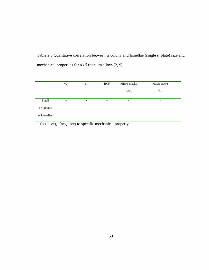
50
Table 2.3 Qualitative correlation between colony and lamellae (single plate) size and
mechanical properties for titanium alloys [2, 9]
0.2 F HCF Micro-cracks
ΔKth
Macrocracks
KIC
Small
Colonies
Lamellae
+ + + + -
+ (positive), -(negative) to specific mechanical property

51
2.5. References:
[1] Leyens C, Peters M, editors. Titanium and Titanium Alloys-Fundamentals and
Applications. Weinheim: WILEY-VCH, 2003.
[2] Lutjering G, Williams JC. Titanium (Engineering Materials and Processes).
Berlin: Springer, 2007.
[3] Boyer RR. Attributes, Characteristics, and Applications of Titanium and Its
Alloys. JOM 2010;62:21.
[4] Boyer RR. An overview on the use of titanium in the aerospace industry.
Materials Science and Engineering a-Structural Materials Properties Microstructure and
Processing 1996;213:103.
[5] Freese HL, Volas MG, Wood JR, Textor M. Titanium and its Alloys in
Biomedical Engineering. In: Buschow KHJ, Robert WC, Merton CF, Bernard I, Edward
JK, Subhash M, Patrick V, editors. Encyclopedia of Materials: Science and Technology.
Oxford: Elsevier, 2001. p.9374.
[6] Froes FH. Titanium Alloys: Properties and Applications. In: Buschow KHJ,
Robert WC, Merton CF, Bernard I, Edward JK, Subhash M, Patrick V, editors.
Encyclopedia of Materials: Science and Technology. Oxford: Elsevier, 2001. p.9367.
[7] Geetha M, Singh AK, Asokamani R, Gogia AK. Ti based biomaterials, the
ultimate choice for orthopaedic implants - A review. Prog Mater Sci 2009;54:397.
[8] Froes FH. Titanium Alloys: Corrosion. In: Buschow KHJ, Robert WC, Merton
CF, Bernard I, Edward JK, Subhash M, Patrick V, editors. Encyclopedia of Materials:
Science and Technology. Oxford: Elsevier, 2001. p.9366.
52
[9] Lütjering G. Influence of processing on microstructure and mechanical properties
of ([alpha]+[beta]) titanium alloys. "Mater Sci Eng, A " 1998;243:32.
[10] Burgers WG. On the process of transition of the cubic-body-centered
modification into the hexagonal-close-packed modification of zirconium. Physica
1934;1:561.
[11] Wenk HR, Houtte PV. Texture and anisotropy. Rep Prog Phys 2004;67:1367.
[12] Peters M, Gysler A, LÜtjering G. Influence of texture on fatigue properties of Ti-
6Al-4V. Metallurgical and Materials Transactions A 1984;15:1597.
[13] Bache MR, Evans WJ. Impact of texture on mechanical properties in an advanced
titanium alloy. "Mater Sci Eng, A " 2001;319-321:409.
[14] Bache MR, Evans WJ, Suddell B, Herrouin FRM. The effects of texture in
titanium alloys for engineering components under fatigue. Int J Fatigue 2001;23:153.
[15] Furuhara T, Nakamori H, Maki T. Crystallography of alpha phase precipitated on
dislocations and deformation twin boundaries in a beta titanium alloy. Materials
Transactions JIM 1992;33:585.
[16] Furuhara T, Takagi S, Watanabe H, Maki T. Crystallography of grain boundary α
precipitates in a β titanium alloy. Metallurgical and Materials Transactions A
1996;27:1635.
[17] Gey N, Humbert M, Philippe MJ, Combres Y. Modeling the transformation
texture of Ti-64 sheets after rolling in the [beta]-field. "Mater Sci Eng, A " 1997;230:68.
[18] Moustahfid H, Humbert M, Philippe MJ. Modeling of the texture transformation
in a Ti-64 sheet after hot compression. Acta Mater 1997;45:3785.
53
[19] Divinski SV, Dnieprenko VN, Ivasishin OM. Effect of phase transformation on
texture formation in Ti-base alloys. "Mater Sci Eng, A " 1998;243:201.
[20] Furuhara T, Maki T. Variant selection in heterogeneous nucleation on defects in
diffusional phase transformation and precipitation. Materials Science and Engineering a-
Structural Materials Properties Microstructure and Processing 2001;312:145.
[21] Bhattacharyya D, Viswanathan GB, Denkenberger R, Furrer D, Fraser HL. The
role of crystallographic and geometrical relationships between alpha and beta phases in
an alpha/beta titanium alloy. Acta Mater 2003;51:4679.
[22] Wang SC, Aindow M, Starink MJ. Effect of self-accommodation on alpha/alpha
boundary populations in pure titanium. Acta Mater 2003;51:2485.
[23] Banerjee R, Bhattacharyya D, Collins PC, Viswanathan GB, Fraser HL.
Precipitation of grain boundary alpha in a laser deposited compositionally graded Ti-8Al-
xV alloy - an orientation microscopy study. Acta Mater 2004;52:377.
[24] Stanford N, Bate PS. Crystallographic variant selection in Ti-6Al-4V. Acta Mater
2004;52:5215.
[25] Bhattacharyya D, Viswanathan GB, Fraser HL. Crystallographic and
morphological relationships between beta phase and the Widmanstatten and
allotriomorphic alpha phase at special beta grain boundaries in an alpha/beta titanium
alloy. Acta Mater 2007;55:6765.
[26] Lee E, Banerjee R, Kar S, Bhattacharyya D, Fraser HL. Selection of alpha
variants during microstructural evolution in alpha/beta titanium alloy. Philos Mag
2007;87:3615.

54
[27] van Bohemen SMC, Kamp A, Petrov RH, Kestens LAI, Sietsma J. Nucleation
and variant selection of secondary alpha plates in a beta Ti alloy. Acta Mater
2008;56:5907.
[28] Kar S, Banerjee R, Lee E, Fraser HL. Influence of crystallography varaiant
selection on microstructure evolution in titanium alloys. In: Howe JM, Laughlin DE, Lee
JK, Dahmen U, Soffa WA, editors. Solid-Solid Phase Transformation in Inorganic
Materials 2005, vol. 1: TMS, 2005.
[29] Whittaker R, Fox K, Walker A. Texture variations in titanium alloys for
aeroengine applications. Mater Sci Technol 2010;26:676.
[30] Mills MJ, Neeraj T. Dislocations in Metals and Metallic Alloys. In: Buschow
KHJ, Robert WC, Merton CF, Bernard I, Edward JK, Subhash M, Patrick V, editors.
Encyclopedia of Materials: Science and Technology. Oxford: Elsevier, 2001. p.2278.
[31] Froes FH. Titanium: Alloying. In: Buschow KHJ, Robert WC, Merton CF,
Bernard I, Edward JK, Subhash M, Patrick V, editors. Encyclopedia of Materials:
Science and Technology. Oxford: Elsevier, 2001. p.9361.
[32] Purdy GR. Widmanstätten Structures. In: Buschow KHJ, Robert WC, Merton CF,
Bernard I, Edward JK, Subhash M, Patrick V, editors. Encyclopedia of Materials:
Science and Technology. Oxford: Elsevier, 2001. p.9575.
[33] Aaronson HI, Medalist RFM. Atomic mechanisms of diffusional nucleation and
growth and comparisons with their counterparts in shear transformations. Metall Trans A
1993;24A:241.
55
[34] Aaronson HI, Spanos G, Masamura RA, Vardiman RG, Moon DW, Menon ESK,
Hall MG. Sympathetic Nucleation - an Overview. Materials Science and Engineering B-
Solid State Materials for Advanced Technology 1995;32:107.
[35] Potter DI. The structure, morphology and orientation relationship of V3N in
[alpha]-vanadium. Journal of the Less Common Metals 1973;31:299.
[36] Furuhara T, Howe JM, Aaronson HI. Interphase boundary structures of
intragranular proeutectoid [alpha] plates in a hypoeutectoid Ti---Cr alloy. Acta Metall
Mater 1991;39:2873.
[37] Furuhara T, Ogawa T, Maki T. Atomic-Structure of Interphase Boundary of an
Alpha-Precipitate Plate in a Beta-Ti-Cr Alloy. Philos Mag Lett 1995;72:175.
[38] M. J. Mills, D. H. Hou, S. Suri, Viswanathan GB. Orientation relationship and
structure of alpha/beta interface in conventional titanium alloys. In: R. C. Pond, W. A. T.
Clark, King AH, editors. Boundaries and Interfaces in Materials: The David A. Smith
Symposium: The Minerals, Metals & Materials Society, 1998, 1998. p.295.
[39] Miyano N, Ameyama K. Three dimensional near-coincidence site lattice analysis
of orientation relationship and interface structure in two phase alloys. J Jpn Inst Met
2000;64:42.
[40] Miyano N, Fujiwara H, Ameyama K, Weatherly GC. Preferred orientation
relationship of intra- and inter-granular precipitates in titanium alloys. Materials Science
and Engineering a-Structural Materials Properties Microstructure and Processing
2002;333:85.
[41] Pitsch W, Schrader A. Arch. Eisenhutt Wes 1958:715.
56
[42] Cahn JW, Kalonji GM. Symmetry in Solid-Solid Transformation Morphologies.
PROCEEDINGS OF an Interantional Conference On Solid-Solid Phase Transformations
1981:3.
[43] Dahmen U. Phase Transformations, Crystallographic Aspects. In: Robert AM,
editor. Encyclopedia of Physical Science and Technology. New York: Academic Press,
2001. p.821.
[44] Suri S, Viswanathan GB, Neeraj T, Hou DH, Mills MJ. Room temperature
deformation and mechanisms of slip transmission in oriented single-colony crystals of an
alpha/beta titanium alloy. Acta Mater 1999;47:1019.
[45] Ye F, Zhang WZ, Qiu D. A TEM study of the habit plane structure of
intragrainular proeutectoid [alpha] precipitates in a Ti-7.26 wt%Cr alloy. Acta Mater
2004;52:2449.
[46] Ye F, Zhang WZ. Dislocation structure of non-habit plane of [alpha] precipitates
in a Ti-7.26 wt.% Cr alloy. Acta Mater 2006;54:871.
[47] Aaronson H, Plichta M, Franti G, Russell K. Precipitation at interphase
boundaries. Metallurgical and Materials Transactions A 1978;9:363.
[48] Dahmen U. Orientation relationships in precipitation systems. Acta Metall
1982;30:63.
[49] Lin F, Starke E, Chakrabortty S, Gysler A. The effect of microstructure on the
deformation modes and mechanical properties of Ti-6Al-2Nb-1Ta-0.8Mo: Part I.
Widmanstätten structures. Metallurgical and Materials Transactions A 1984;15:1229.
57
[50] Zeng L, Bieler TR. Effects of working, heat treatment, and aging on
microstructural evolution and crystallographic texture of [alpha], [alpha]', [alpha]'' and
[beta] phases in Ti-6Al-4V wire. Materials Science and Engineering: A 2005;392:403.
[51] Lee JK, Aaronson HI. Influence of faceting upon the equilibrium shape of nuclei
at grain boundaries--I. Two-dimensions. Acta Metall 1975;23:799.
[52] Lee JK, Aaronson HI. Influence of faceting upon the equilibrium shape of nuclei
at grain boundaries--II. Three-dimensions. Acta Metall 1975;23:809.
[53] Mullins WW, Sekerka RF. Morphological Stability of a Particle Growing by
Diffusion or Heat Flow. J Appl Phys 1963;34:323.
[54] Wang Y, Ma N, Chen Q, Zhang F, Chen S, Chang Y. Predicting phase
equilibrium, phase transformation, and microstructure evolution in titanium alloys. JOM
Journal of the Minerals, Metals and Materials Society 2005;57:32.
[55] Otsuka K, Ren X. Physical metallurgy of Ti-Ni-based shape memory alloys. Prog
Mater Sci 2005;50:511.
[56] Kar S, Banerjee R, Lee E, Fraser HL. Influence of crystallographic variant
selection on microstructure evolution in titanium alloys. Warrendale: Minerals, Metals &
Materials Soc, 2005.
[57] Porter D, Easterling K. Phase transformations in metals and alloys: CRC, 1992.
[58] Robert WB, Allen SM, Carter WC. Kinetics of materials. Hoboken: John Wiley &
Sons, 2005.
[59] Christian JW. The Theory of Transformations in Metals and Alloys. Oxford:
Pergamon, 2002.
58
[60] Sutton AP, Balluffi RW. Interfaces in Crystalline Materials. Oxford: Oxford
University Press, 1995.
[61] Shen C, Li J, Wang YZ. Finding critical nucleus in solid-state transformations.
Metallurgical and Materials Transactions a-Physical Metallurgy and Materials Science
2008;39A:976.
[62] Wang Y, Khachaturyan AG. Three-dimensional field model and computer
modeling of martensitic transformations. Acta Mater 1997;45:759.
[63] Courtesy of H.L. Fraser. Courtesy of H.L. Fraser in The Ohio state university.
[64] Lee E. Microstructure evolution and microstructure/mechanical properties
relationships in alpha+beta titanium alloys. vol. Ph.D. dissertation: The Ohio State
University, 2004.
59
CHAPTER 3 Predicting Equilibrium Shape of Precipitates as
Function of Coherency State
Abstract:
A general approach is proposed to predict equilibrium shapes of precipitates in crystalline
solids as function of size and coherency state. The model incorporates effects of
interfacial defects such as misfit dislocations and structural ledges on transformation
strain and on interfacial energy. Using precipitation in titanium alloys as an
example, various possible equilibrium shapes of precipitates having different defect
contents at interfaces are obtained by phase field simulations. The simulation results
agree with experimental observations in terms of both precipitate habit plane orientation
and defect content at the interface. In combination with crystallographic theories of
interfaces and experimental characterization of habit plane of finite precipitates, this
approach has the ability to predict the coherency state (i.e., defect structures at interfaces)
and equilibrium shape of finite precipitates.
60
3.1. Introduction
Most engineering alloys are strengthened by second-phase particles and their quantity,
size, shape, orientation, coherency state and spatial distribution determine the
deformation mechanism and mechanical behavior of the alloys [1, 2]. Classical examples
include Al- , Ti- and Mg-based light alloys [3-6] and high-temperature Ni-base
superalloys [7], to name a few. To assist in alloy design, it is essential to develop
modeling capabilities to predict these key microstructural features. However these
features are determined by the interplay between interfacial and elastic strain energy
minimization during precipitation, which is difficult to quantify theoretically or by
experiment.
New phases formed during precipitation reactions in solids usually have different
compositions and structures from those of the parent phase. During nucleation and in the
early stages of growth, precipitates tend to be coherent with the matrix, which minimizes
the interfacial energy [8, 9]. They may lose coherency during continued growth when the
elastic strain energy contribution to the total free energy of the system becomes
dominant. Formation of line defects such as misfit dislocations within the interface
relieves misfit stress at the expanse of increasing interfacial energy. In addition to misfit
dislocations, another type of line defects, structure ledges [10], which exhibit step
character as well as dislocation properties [11, 12], are also frequently observed at inter-
phase interfaces. They are also referred to as transformation dislocations or
disconnections to distinguish themselves from defects without the step character in the

61
topological model for structural phase transformations [11]. In contrast to misfit
dislocations, it is well recognized that the existence of structure ledges increases the
degree of coherency of a hetero-phase interface and hence lowers the interfacial energy
[13]. Examples of these line defects at a BCC-HCP interface are shown schematically in
Fig. 3.1(a).
Since misfit dislocations and structure ledges not only alter the coherency stress and
change the interfacial energy and its anisotropy, but also introduce growth anisotropy,
they impact all the key microstructural features mentioned above. In addition, the
structural defects at interfaces may alter the nature of precipitate-dislocation interactions
and change the deformation mechanisms (e.g., cutting vs. looping), as well as the nature
of precipitate-martensite interactions and change the transformation paths [14, 15].
Therefore, in order to predict the key microstructural features of precipitates and how
they interact with dislocations and other types of precipitates, the interfacial defect
structure as a function of precipitate size has to be determined first. With the advances in
high resolution electron microscopy, defect structures at many hetero-phase interfaces
have been characterized. However, it is difficult to determine how the defect structure
changes when particle size changes. Models accounting for misfit dislocations and
structural ledges in an integrated manner, in terms of their effect on coherency elastic
strain energy, interfacial energy and final equilibrium shape of finite precipitates, are still
lacking. Existing crystallographic theories, such as the invariant line model [16, 17],
structure ledge model [18], edge-to-edge matching model [19], O-lattice model [20, 21],
62
and topological model [11, 12], have been successful in predicting some of the major
crystallographic features of hetero-phase interfaces in infinite systems, including
orientation relationship (OR), habit plane orientation and defect structure within
interfaces. Nevertheless, it is difficult to predict the shape and interfacial defect structure
of a finite precipitate, which is a typical variational problem where the sum of the
interfacial and elastic strain energies as a functional of interfacial defect structure is
minimized.
Most of the existing models for microstructural evolution during precipitation consider
either coherent [22-24] or incoherent precipitates and ignore interfacial defects. In this
chapter, we propose a general approach that incorporates interfacial defects in a phase
field model. Using precipitation reaction in a near titanium alloy as an example, we
show how different types of interfacial defects relieve the coherency elastic strain,
change the interfacial energy and its anisotropy, and affect the habit plane orientation and
equilibrium shape of precipitates. We also discuss how to predict interfacial defect
structures and the critical information required.
3.2. Elastic Strain Energy of Coherent and Semi-Coherent Precipitates
As aforementioned, a precipitate phase is usually different from the matrix in terms of
composition, crystal structure and orientation, which results in lattice misfit across the
precipitate-matrix interface. The elastic deformation that accommodates the misfit in the
Sony
高亮
Sony
高亮

63
crystal lattices of adjoining phases to form coherent or semi-coherent inter-phase
boundaries, known as coherency strain, usually plays a significant role in solid-state
phase transformations [22-26]. Being both volume- and morphology-dependent, the
coherency elastic strain energy affects precipitate shape, spatial arrangement, as well as
the overall driving force for the transformation. In addition, as a nucleating phase may
possibly adopt a metastable structure with low-energy coherent interfaces with the parent
matrix, the final transition to the stable phase structure is controlled by the coherency
strain energy and its interplay with the interfacial energy.
Coherency strain energy of an arbitrary coherent or semi-coherent multi-phase mixture
can be treated in the framework of Eshelby [27, 28] using the general theory of phase
field microelasticity by Khachaturyan and Shaltov (KS theory) [22, 29, 30], formulated
upon spatial distribution of the stress-free transformation strain (SFTS). The SFTS
associated with arbitrary compositional and structural non-uniformities in an arbitrary
multi-phase mixture can be expressed in terms of a set of conserved (e.g., concentration)
and non-conserved (e.g., long-range order parameter, inelastic displacement, etc.) order
parameter fields (also called phase fields) [22, 25, 31-33]:
Equation Chapter 3 Section 1
0 00
1
( ) ( ) ( )N
ij ij p
p
p
x x (3.1)
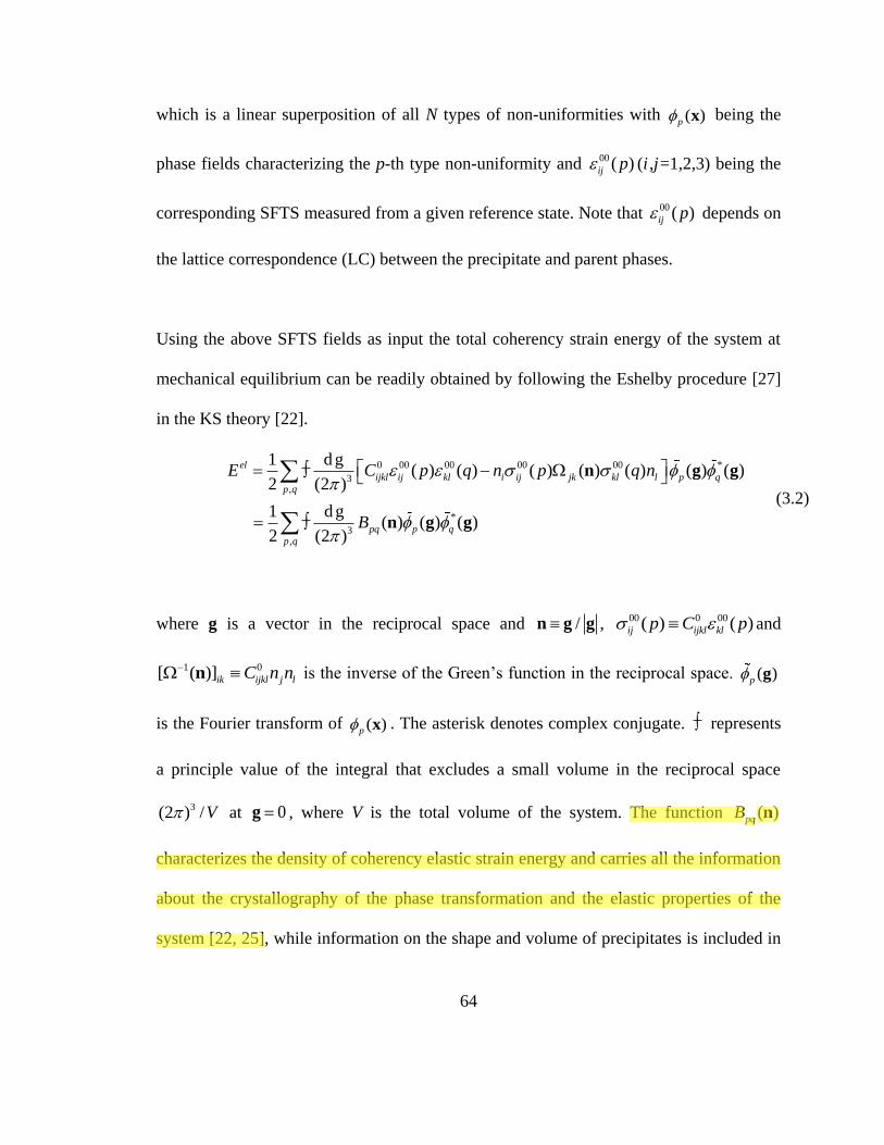
64
which is a linear superposition of all N types of non-uniformities with ( )p x being the
phase fields characterizing the p-th type non-uniformity and 00 ( )ij p (i ,j=1,2,3) being the
corresponding SFTS measured from a given reference state. Note that 00 ( )ij p depends on
the lattice correspondence (LC) between the precipitate and parent phases.
Using the above SFTS fields as input the total coherency strain energy of the system at
mechanical equilibrium can be readily obtained by following the Eshelby procedure [27]
in the KS theory [22].
0 00 00 00 00 *
3,
*
3,
1 d g( ) ( ) ( ) ( ) ( ) ( ) ( )
2 (2 )
1 d g ( ) ( ) ( )
2 (2 )
el
ijkl ij kl i ij jk kl l p q
p q
pq p q
p q
E C p q n p q n
B
n g g
n g g
(3.2)
where g is a vector in the reciprocal space and /n g g , 00 0 00( ) ( )ij ijkl klp C p and
1 0[ ( )]ik ijkl j lC n n n is the inverse of the Green’s function in the reciprocal space. ( )p g
is the Fourier transform of ( )p x . The asterisk denotes complex conjugate. represents
a principle value of the integral that excludes a small volume in the reciprocal space
3(2 ) /V at 0g , where V is the total volume of the system. The function ( )pqB n
characterizes the density of coherency elastic strain energy and carries all the information
about the crystallography of the phase transformation and the elastic properties of the
system [22, 25], while information on the shape and volume of precipitates is included in
Sony
高亮
65
( )p x that is equivalent to shape functions of the precipitates. We shall introduce a unit
vector n0 such that the function ( )pqB n reaches its minimum at n=n0 [22]. The physical
meaning of n0 is that it represents the normal to the habit of a precipitate in the real space.
In other words, the minimum strain energy for a given precipitate volume is obtained if
the precipitate develops into an infinite platelet with infinitesimal thickness whose habit
is normal to n0.
In the current study, precipitates are assumed to have the same elastic modulus as that of
the matrix (i.e. the homogeneous modulus case), which simplifies significantly the strain
energy analysis. However, the analysis is valid in cases of inhomogeneous modulus as
well. As a matter of fact, the KS microelasticity theory has been extended to
inhomogeneous modulus systems [34, 35].
3.2.1. Stress-free transformation strain for coherent precipitates
The calculation of the SFTS, 00 ( )ij p , is an important step towards calculating the
coherency elastic strain energy. For fully coherent precipitates, the SFTS can be
calculated directly from the LC between the precipitate and matrix phases, which could
be obtained according to Bollman’s nearest neighbor principle [21]. There are a number
of choices for relating the lattices of the parent and product phases by uniform lattice
deformation. The one with the minimum energy barrier is, in general, the one that
involves the minimum lattice distortion and rotation. Both the Bain correspondence [36]
Sony
高亮
Sony
高亮
Sony
高亮
66
for the BCC FCC transformation and the Burgers correspondence [37] for the BCC
HCP are such LCs. The calculation of SFTS for a given LC is then straightforward
[22, 38]. For example, if F0 is the transformation matrix or deformation gradient matrix
describing the uniform lattice distortion from the parent phase to the pth
variant of the
product phase following a given LC, then [22, 39]
T
00 0 0 I2
F Fp
(3.3)
where I is the unit tensor and the symbol ''T'' denotes a transpose operation on the
associated matrix. The transformation matrix, 0F , relates the parent crystal lattice site
vector , r , to the product crystal lattice site vector, 'r , by 0' Fr r . Generally, three
pairs of non-coplanar vectors, r and 'r , related by the LC are selected to construct 0F .
The crystal lattice site displacements, u r , associate with the transformation are given
by 0 IF u r r . The strain tensor obtained in Eq. (3.3) is identical to
T1
2 u r u r , where u r characterizes the displacement gradient.
3.2.2. Deformation gradient matrix due to defects at hetero-phase interfaces
For semi-coherent precipitates, the effect of misfit dislocations and structural ledges on
misfit strain can be considered by superposition of their eigenstrains with the SFTS
Sony
高亮
Sony
高亮
Sony
高亮
Sony
高亮

67
calculated for fully coherent precipitates, which can be achieved by treating the
interfacial defects as successive deformations, following the uniform lattice deformation,
applied to the precipitate phase. For structural ledges, their eigenstrains are determined by
the requirements [11, 12] that the misfits in and normal to the terrace plane are cancelled
by dislocation characters associated with the ledges, as shown in Fig. 3.1(b). The
dislocation content by relaxes the misfit normal to the terrace plane while the dislocation
content bx compensates the misfit in the terrace plane. The step character of the structural
ledges causes the habit plane to become inclined by an angel from the terrace plane, as
depicted schematically in Fig. 3.1(b). Knowing the dislocation characters of the structural
ledges, one could treat them as regular dislocations when deriving their eigenstrains.
The deformation gradient matrix, Fdis, due to the presence of a set of periodical misfit
dislocations with spacing D and its Burgers vector being parallel to the z-direction (Fig.
3.1(a)) can be expressed as the following:
dis
D
0
0 IF
b
(3.4)
where b is the length of the Burgers vector of the misfit dislocations. Following the same
approach, the deformation gradient matrix, stepF , due to the presence of steps with
spacing S and height h (as shown in Fig. 3.1(b) ) can be formulated as:
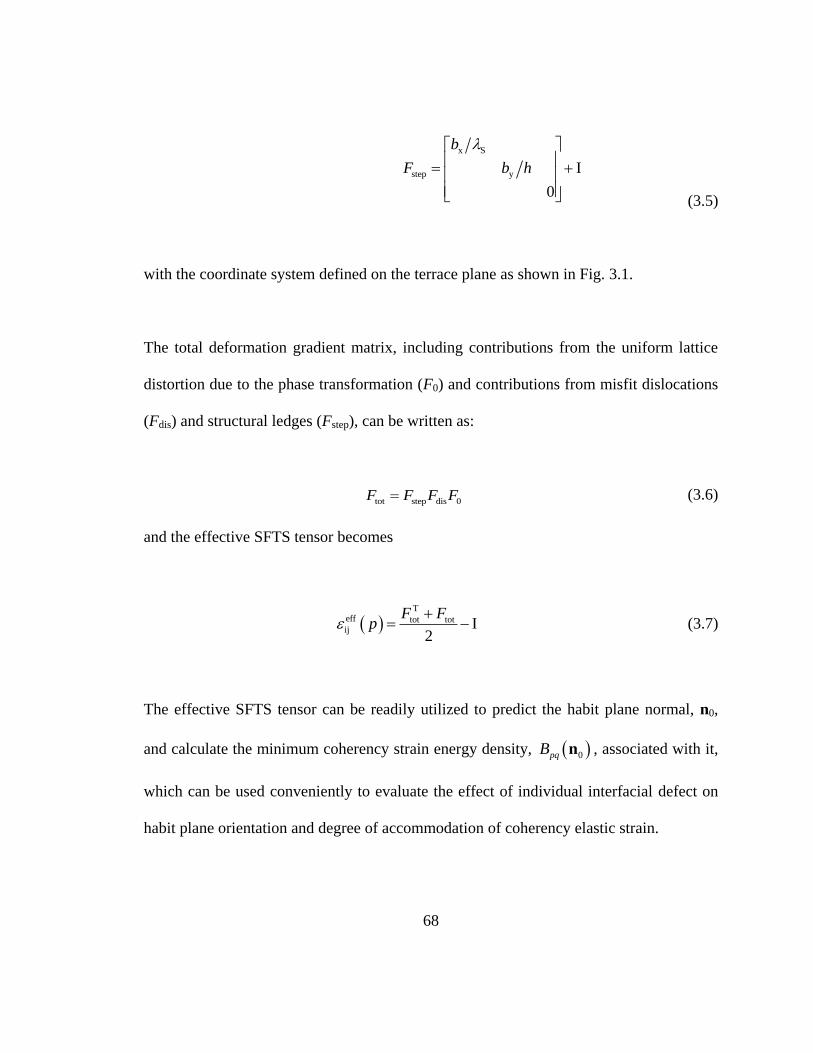
68
x S
step y I
0
b
F b h
(3.5)
with the coordinate system defined on the terrace plane as shown in Fig. 3.1.
The total deformation gradient matrix, including contributions from the uniform lattice
distortion due to the phase transformation (F0) and contributions from misfit dislocations
(Fdis) and structural ledges (Fstep), can be written as:
tot step dis 0F F F F (3.6)
and the effective SFTS tensor becomes
T
eff tot totij I
2
F Fp
(3.7)
The effective SFTS tensor can be readily utilized to predict the habit plane normal, n0,
and calculate the minimum coherency strain energy density, 0pqB n , associated with it,
which can be used conveniently to evaluate the effect of individual interfacial defect on
habit plane orientation and degree of accommodation of coherency elastic strain.
69
3.3. Estimation of Interfacial Energy for Semi-Coherent Interfaces
The energy of a semi-coherent hetero-phase interface sc consists of both chemical c
and structural contributions s [9, 40]. The contributions from the misfit dislocations to
the interfacial energy could be determined by using the microscopic phase field model
(MPF) of dislocations [33] or approximated simply by the Read–Shockley formula [41,
42]. With the information of Burgers vector and spacing between misfit dislocations at
the interface, one could estimate the contribution from misfit dislocations to the structural
part of the interfacial energy in different facets of the precipitates according to the Reed-
Shockley formula [42] as following:
s m m m1 lnE (3.8)
where mE represents the energy of a general high misorientation boundaries, is the
misorientaton angle and m (~ 10 - 20º) is a constant determined by the structures of the
two joining crystals. If the magnitude of the Burgers vector and the spacing between
misfit dislocations are b and D, respectively, the misorientation angle can be determined
by ~ b D .
By knowing the effect of interfacial defects on interfacial energy and SFTS, the
equilibrium shape of a finite precipitate can be predicted using phase field simulations
[31-33] that minimize the total free energy of the system, i.e., the sum of bulk chemical
70
free energy, interfacial energy and elastic strain energy. The interfacial defects of an
infinite planar interface could be predicted by specific crystallography theories. For
example, the dislocation content (Burgers vector and spacing) has been well predicted for
precipitate in Ti-7.26 wt. % Cr system [43]. Besides the habit plane or broad face, a
finite precipitate is also surrounded by other non-habit facets. When the O-lattice model
[20] in 3D is not solvable for the OR that permits only one set of periodical dislocation
on the habit plane, the possible orientations and dislocation structures of non-habit facets
(out of habit plane) could be predicted by an extended near-coincidence-sites (NCS)
methods [44, 45], which combines the analysis of fit/misfit distribution in three
dimensions (3D) at a given OR by NCS model [44], with analysis of properties of Moiré
planes [46] developed based on the O-lattice theory [21]. The approach has been applied
successfully to predict orientation of non-habit facets, the Burgers vector and the spacing
of the misfit dislocations in non-habit facets of precipitates in FCC/BCC [45] and
BCC/HCP [47] systems. When structure ledges are also present on irrational habit planes,
the dislocation content, ledge height and inter-ledge spacing associated with the structural
ledges can be derived by the O-lattice theory [48], computer-aid graphical techniques [10,
49], and the topological model [12].
Note that the outputs from these geometrical methods in terms of Burgers vector and
spacing of misfit dislocation are not always unique [43, 47]. Thus, additional constraints
such as the condition of maximum dislocation spacing are required to refine the results,
which rely on advanced experimental characterization (such as TEM or HRTEM).
71
Therefore, both theory and experimental characterization are required to obtain all the
information about the interfacial defects for a finite precipitate.
3.4. Worked Examples
In Ti-alloys, the interfaces between the (HCP) precipitates and the (BCC) matrix
are typical examples of semi-coherent interfaces that contain both misfit dislocations [43,
50] and structural ledges [49]. The precipitates usually exhibit a specific orientation
relationship with the matrix, referred to as the Burgers OR [37], i.e.,
101 // 0001
, 111 // 2110
(3.9)
The interface structures in a near titanium alloy (Ti-5Al-2.5Sn-0.05Fe)
characterized by TEM [50] are shown schematically in Figure 3.2. The broad and edge
faces are wrapped with a single set of c-type misfit dislocations with a Burgers vector of
0001 2
(specific indices are assigned in accordance with the particular variant of OR
described in Eq. (3.9)). The spacing between these dislocations is about 7 nm, which
corresponds to ~30 atomic planes of 0002
or 101
, and their line direction is close
to the invariant line direction 353
. The side and end faces are wrapped with a set of
a-type misfit dislocations with a Burgers vector of 2110 3
, which are associated
with the 0110
and 110
planes with extra half planes in the phase and spaced by
about 9 to 13 0110
atomic plane spacing. On the broad face, in addition to the c-
72
dislocations, the atomic structure of the / interface consists of structural ledges that
enable the interface to step down along the invariant line direction.
3.4.1. Derivation of effective SFTS for the semi-coherent precipitates
To formulate the SFTS, it is required to know the lattice correspondence between the
parent and product phases. Figure 3.3 shows the Burgers orientation relationships
between the two phases in both three-dimension Fig.3.3 (a)-(c) and two-dimension
Fig.3.3 (d)-(f). Three non-coplanar vectors in lattice are selected, i.e., 010
,
111 2
and 101
. According to the nearest neighbor principle [21], the
corresponding three non-coplanar vectors in the phase lattice after the to
transformation are 1210 3
, 2110 3
and 0001
[37], respectively. Thus, the
lattice correspondence between the BCC and HCP lattices can be described as,
010 1210 3
; 111 2 2110 3
; 101 0001 (3.10)
as shown in the Fig. 3.3 (a)-(b). Three non-coplanar vectors are chosen as the axes of a
new orthogonal reference coordinate N1, i.e., 1 // 010 // 1210x
,
2 // 101 // 1010x
, 3 // 101 // 0001x
, as shown in Fig. 3.3.
In the reference frame N1, the transformation matrix to deform the lattice
homogeneously to the lattice can be described as:

73
0
0 0
0 3 2 0
0 0 2
a a
F a a
c a
(3.11)
where the lattice parameters of the two phases are 3.196a Å, 2.943a Å and
4.680c Å [50]. Note that, as shown in Fig. 3.3(b), during the actual BCC to HCP
lattice transformation, atomic shuffling on every other 0002
plane is required in
addition to the homogeneous deformation 0F [37]. However, since shuffling does not
change the shape and size of the unit cells of the two crystal lattices, 0F does represent
the actual transformation matrix.
In addition to 0F , a rigid body rotation, RF , by 5.26º along axis 101 // 0001
is
required to realize the exact Burgers OR shown in Eq. (3.9) and Fig. 3.3(c)
cos 5.26 sin 5.26
sin 5.26 cos 5.26
1
RF
(3.12)
Thus, the overall transformation matrix for a coherent precipitate can be expressed as
0RF F F , which expresses the coherent transformation matrix of a specific Burgers
variant with OR defined by Eq. (3.9).
74
The c-dislocations accommodate the misfit between the 0002
and 101
planes.
According to Eq. (3.4), the deformation gradient matrix due to the c-dislocations on the
broad face can be described as
01
0 I30
1
cF
(3.13)
Similarly, the deformation gradient matrix due to the a-dislocations on the side face can
be described as
01
1 I11
0
aF
(3.14)
In addition to the misfit dislocations, structure ledges also exhibit dislocation characters.
As shown in Fig 1(a), the Burgers vector associated with the structure ledges can be
expressed as x y; ;0 b b b , in a new reference coordinate N2 associated with the terrace
plane:
75
'
1 // 111 // 2110x
; '
2 // 121 // 0110x
; '
3 // 101 // 0001x
(3.15)
Dislocation xb lies in the terrace plane and has a Burgers vector of 1 12 111
associated with the riser of the structural ledges [48, 49]. The component xb
compensates the misfit along 111
direction on the terrace plane. Thus, the existence
of the structural ledges can eliminate one set of the a-type (i.e. b= 111
) misfit
dislocations on the terrace plane. The structural ledges have also been shown to have
Burgers vectors and inter-ledge spacing Sλ (i.e. about 17 xb ) both one sixth of their misfit
dislocation counterparts [48]. Moreover, the height of risers or steps, h, is found to be 2
atomic layer of the terrace plane, i.e., 121
or 0110
[34, 35]. On the other hand,
structural ledges step down along the invariant line direction in order to accommodate
simultaneously the misfit normal to the terrace plane [48], which can be well represented
by the dislocation yb . Thus, the Burgers vector of
yb is given by 6 3 3 2a a
according to the O-lattice calculation [48].
Thus, the deformation gradient matrix due to the structural ledges on the terrace face can
be determined as
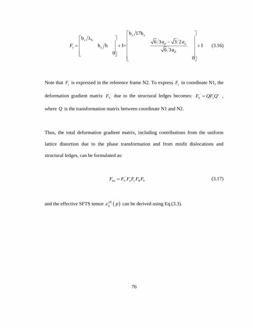
76
x x
x S
y
b 17bb λ
6 3 3 2b h I= I
6 30
0
s
a aF
a
(3.16)
Note that sF is expressed in the reference frame N2. To express sF in coordinate N1, the
deformation gradient matrix '
SF due to the structural ledges becomes: ' 'S sF QF Q ,
where Q is the transformation matrix between coordinate N1 and N2.
Thus, the total deformation gradient matrix, including contributions from the uniform
lattice distortion due to the phase transformation and from misfit dislocations and
structural ledges, can be formulated as:
'
tot 0S a c RF F F F F F (3.17)
and the effective SFTS tensor eff
ij p can be derived using Eq.(3.3).
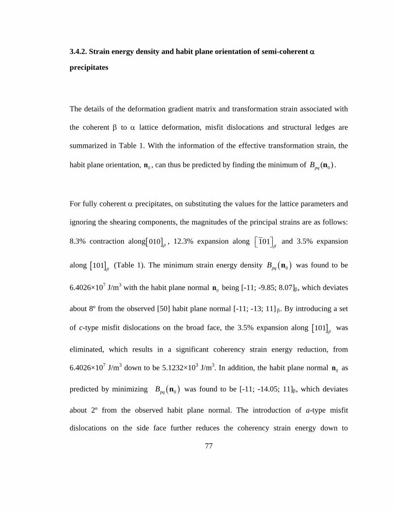
77
3.4.2. Strain energy density and habit plane orientation of semi-coherent
precipitates
The details of the deformation gradient matrix and transformation strain associated with
the coherent to lattice deformation, misfit dislocations and structural ledges are
summarized in Table 1. With the information of the effective transformation strain, the
habit plane orientation, 0n , can thus be predicted by finding the minimum of 0( )pqB n .
For fully coherent precipitates, on substituting the values for the lattice parameters and
ignoring the shearing components, the magnitudes of the principal strains are as follows:
8.3% contraction along 010
, 12.3% expansion along 101
and 3.5% expansion
along 101
(Table 1). The minimum strain energy density 0pqB n was found to be
6.4026×10⁷ J/m
3 with the habit plane normal 0n being [-11; -9.85; 8.07], which deviates
about 8º from the observed [50] habit plane normal [-11; -13; 11]. By introducing a set
of c-type misfit dislocations on the broad face, the 3.5% expansion along 101
was
eliminated, which results in a significant coherency strain energy reduction, from
6.4026×10⁷ J/m
3 down to be 5.1232×10
3 J/m
3. In addition, the habit plane normal 0n as
predicted by minimizing 0pqB n was found to be [-11; -14.05; 11], which deviates
about 2º from the observed habit plane normal. The introduction of a-type misfit
dislocations on the side face further reduces the coherency strain energy down to
78
4.7269×10³ J/m
3. However, the habit plane normal 0n deviates further from the
experimental observation (see Table I). Finally, the structural ledges on the broad face
further relax the coherency strain energy, though not by much. However, due to the
presence of the structural ledges, the habit plane rotated towards the experimentally
observed orientation with only about 0.8º deviation.
The calculated coherency strain energy density, pqB n , as a function of habit plane
normal is projected onto the basal plane, as shown in Fig. 4. The solid circles represent
the case without considering defects at the interfaces. The minimum of pqB n is
obtained where 0n is indicated by the solid arrow. For comparison, the result obtained for
the case where interfacial defects are considered is shown in Fig. 4 by the open circles. It
can be readily seen that the defects on the interface relax considerably the coherency
elastic strain energy. In addition, pqB n reaches its minimum at 0n corresponding to [-
11; -12.63; 11]as indicated by the dotted arrow, which deviates only by 0.8º from the
experimentally observed habit plane [-11; -13; 11]
3.4.3. Interfacial energy anisotropy of semi-coherent precipitates
On substituting the dislocation spacing and the corresponding Burgers vector, the
equivalent misorientation angles for the broad and side faces are 1 1 30 1.9 and
3 1 11 5.2 , respectively. The equivalent misorientation angle of the edge face is

79
assumed to be 3 m . According to Eq.(3.8), the structural components, s , of the
broad, side and edge faces are m0.39E , m0.72E and mE , respectively. mE is assumed to
be 250 mJ/m2 [51]. In addition, the chemical components of the interfacial energy for the
three faces are assumed all equal for simplicity and have a value of 50 mJ/m2, which is
reasonable for fully coherent interfaces. Therefore, the interfacial energies of the broad,
side and end faces are 150, 230 and 300 mJ/m2, respectively. The results are incorporated
in the gradient energy coefficient characterizing structural non-uniformities in the phase
field free energy formulated based on the gradient thermodynamics [52].
3.4.4. Equilibrium shape of -precipitates in different cases
The equilibrium shapes of an isolated precipitate determined by the interplay between
the interfacial energy and strain energy under different cases are obtained by phase field
simulations [14] and are presented in Fig. 3.5 with the coordinates being indicated in Fig.
3.5(a)-1. In all cases, a specific initial composition is selected along the tie-line of Ti-
6Al-4V (wt. %) [53] to obtain an equilibrium volume fraction of 5% for the precipitate.
The three-dimensional equilibrium shape of a fully coherent precipitate obtained under
the assumption of isotropic interfacial energy of 50 mJ/m2
is shown in Fig. 3.5(a)-1. Also,
the projections of the three-dimensional equilibrium shape along 010
, 101
and
101
are shown in Figs. 5(a)-2 - 5(a)-4, respectively. The total system size is 16 nm. It

80
is readily seen that the particle has a disk-like shape with a well-defined habit plane.
However, the orientation of the habit plane obviously deviated from the experimentally
observed one, which is indicated by a transparent light yellow plane across the center of
the simulation cell. The deviation manifests itself via the shaded top end of plate since it
lies below the light yellow plane, as shown in Fig. 3.5(a)-1 and 5(a)-3. Note that the
minor axis of the disk in the habit plane is about 7 nm, which is commensurate with the
spacing of the c-dislocations on the broad face. Therefore, particles of such a size are
most likely to be coherent.
The equilibrium shape for a semi-coherent precipitate with the consideration of c- type
misfit dislocations on the broad face is presented in Fig. 3.5(b). It can be easily found in
this case that the habit plane is almost parallel to the light yellow plane which indicates
the experimental observed habit plane. Superposition of Figs. 5(a)-4 and 5(b)-4 indicates
that the c-dislocations change the habit normal to nearly parallel to the experimentally
observed one, as shown in Fig. 3.5(c). When considering all the defects, including misfit
dislocations and structural ledges, the equilibrium shape of the precipitate, in the case
of isotropic interfacial energy (200 mJ/m2), is shown in Fig. 3.5(d). The habit plane
normal almost coincides with the experimentally observed one. In the case of interfacial
energy anisotropy alone, the equilibrium shape of the precipitate is shown in Fig.
3.5(e), which becomes an ellipsoid with no obvious habit plane. Finally Fig. 3.5(f)
presents the equilibrium shape of the semi-coherent particle obtained when the
anisotropy in interfacial energy is considered. Obviously, it has a well developed plate

81
shape with a habit plane normal almost parallel to the experimentally determined habit
plane normal. However, compared to Fig. 3.5(d)-4, it is more elongated along the
invariant line direction and contracted along z or [101] direction as shown in Fig. 3.5(f)-
4.
3.4.5. Coherency lost
A coherent precipitate may lose its coherency during its continued growth. Although the
dislocation spacing on the semi-coherent interface can be well characterized by high
resolution TEM or predicted by O-line theory, it is still desirable to estimate a critical size
beyond which the coherent precipitate changes to a semi-coherent one. As mentioned
earlier, the coherency state of precipitates may change the nature of precipitate-
dislocation interactions and hence the deformation mechanisms. There is no doubt that
the critical size must be larger than the inter-dislocation spacing. However, this critical
size depends on the difference between the total energy (interfacial energy and strain
energy) of the coherent precipitate and its semi-coherent counterpart of a given size [9].
In other words, beyond a critical size, rcrit, it becomes energetically favorable for a
coherent particle to lose coherency. Since the optimum shapes of the precipitate in
different cases have been obtained for both coherent and semi-coherent precipitate (with
c-dislocations only since their contribution to the strain energy reduction is dominant as
shown in Table 3.1) (Fig. 3.5(a)-(b)), it is possible to evaluate its interfacial energy [52]
and strain energy [22] and hence the total energy of a given size by the phase field
method. The results are shown in Fig. 3.6. The coherent precipitate has a lower interfacial
82
energy than the semi-coherent one (Fig. 3.6(a)) due to extra structural contribution to the
interfacial energy s. On the other hand, as shown in Fig. 3.6 (b), the semi-coherent
precipitate has lower strain energy than the coherent one since misfit dislocation release
part of the coherency strain energy. Therefore, there exists a crossover point between the
total energy of the coherent (open circle) and semi-coherent (solid) precipitates as
function of their volumes, as show in Fig. 3.6(c), which yields a critical size, rcrit, of ~27
nm when s is 50 mJ/m2 and 22 nm when s = 25 mJ/m
2. Thus, the critical size rcrit scales
with the structural part of the interfacial energy due to misfit dislocations, which agrees
with the analysis by Porter and Easterling [9]. Note that the predicted critical sizes are
about 3-4 times of the c-dislocation spacing on the broad face.
3.5. Discussions
A plane remains undistorted under the action of a homogeneous lattice strain if and only
if one of the principal strains is zero and the other two are of opposite signs [38]. Due to
the introduction of c-type misfit dislocations on the broad face, an interesting feature of
the BCC to HCP transformation is that the principal strain ( 3 ) along the 101
direction becomes very small (-0.03%) and the other two are of opposite signs, i.e., 8.3%
contraction along 010
, and 12.3% expansion along 101
. It is thus not
unreasonable to treat the transformation with the approximation that 3 is zero.
Therefore, the lattice deformation would have left a plane undistorted when considering

83
the effect of the c-type dislocations. As shown in Table 3.1, the introduction of the c-type
misfit dislocations relax most of the coherency strain energy if the precipitate develops
into a thin plate whose habit is normal to 0n , [-11; -14.05; 11]
Based on the assumption that the long-range misfit strain in the interface is completely
accommodated by a single set of periodical array of misfit dislocations on a singular
interface [54], Zhang et al. [43] predicted the habit plane structure of precipitates in Ti-
7.26wt%Cr alloy using the O-line model developed in the frame work of the O-lattice
theory. The Burgers vector, line direction and spacing of dislocations on the habit plane
from their predictions agree well with their experimental observations [43]. However, the
assumption that there is no long-range strain may not be truly satisfied. Otherwise, the
set of a-type misfit dislocations would not develop on the side face of the precipice. The
O-lattice theory, in essence, is a geometrical method that considers two infinite crystals.
In practice, precipitates are finite and the strain energy of a plate-shaped precipitate
having a finite thickness is finite. Accumulation of the residual strain will induce misfit
dislocations on the other facets of interfaces, such as the a-type dislocations on the side
face of the precipitate. This additional set of misfit dislocations further relaxes the
coherency strain energy (see the calculation results in Table 3.1). However, due to the
introduction of the a-type misfit dislocations on the side face, the predicted habit plane
obviously deviates from the experimentally observed one. When further considering the
structural ledges on the habit plane, the orientation of the precipitated is rotated back to
84
the experimentally observed one. Therefore, the a-type misfit dislocations and the
structural ledges seem to be coupled and they have to be considered simultaneously.
It is worth mentioning that in predicting dislocation structures on non-habit facets, the
OR was fixed to the one determined by the O-line model when applied to predict
dislocation structures on the habit plane. This suggests that the dislocation structures on
the non-habit planes would not change the OR any more. This may not be the case for
finite precipitate. As suggested by Aaronson et al. [8], for example, the interface itself
may rotate, allowing the Burgers vector of the dislocations to lie in the interface and
hence be fully utilized to compensate the lattice misfit.
The structural ledges are present at hetero-phase interfaces as a means to increase the
level of coherency between the BCC and HCP lattice. In addition, structural ledges have
Burgers vector associated with their risers and also lying in the terrace plane. In other
words, structural ledges play a role in compensating interface misfit alternative to misfit
dislocations. It has been showed that [48, 49] on the Burgers-related 0110 // 121
terrace planes, the misfit along the 0001 // 101
direction is relaxed by a single set of
parallel c-type misfit dislocation, while the misfit along 2110 // 111
direction is
compensated by the dislocation content associated with the structural ledges. However, in
comparison with the misfit dislocations, the Burgers vector associated with the structural
ledges is relatively small. For example, in the BCC/HCP system, the Burgers vector
85
associated with the riser of the structural ledges is 1 12 111
. Thus the introduction of
structural ledges would not effectively relax the coherency strain energy. According to the
calculation results, the structural ledges only reduce the coherency strain energy from
4.73×10³ J/m
3 to 4.71×10
3 J/m
3.
It should be emphasized that the structural ledges in the BCC/HCP example considered
are different from the defect structures of habit planes of an internally twinned or slipped
martensitic plate embedded in austenite, where the twinning or slip (called lattice
invariance deformation) is required to provide an invariant plane strain (IPS) and the
defect structures at the invariant plane habit are “by-products” of the twinning or slip.
These defects (facets or steps) do not contribute to the long-range elastic strain energy,
though locally contribute to the interfacial energy. In contrast, the structural ledges on the
broad face of an plate are required to relax the long-range elastic strain. As can be seen
from Table 3.1, the structural ledges compensate the lattice misfit in a manner similar to
misfit dislocation.
As has been mentioned earlier, the interplay between interfacial energy and strain energy
minimization determines the final equilibrium shape of a precipitate, i.e., the equilibrium
shape of a precipitate is determined by the condition that the sum of elastic and interface
energies reaches minimum at a given precipitate volume. In the cases of isotropic
interfacial energy (e.g. Fig. 3.5(a), (b) and (d)), the precipitate tends to develop an
86
optimum shape with its broad face corresponding to the minimum of 0pqB n
to
minimize the strain energy. As the coherent particle continues to grow, the
precipitate/matrix interface can no longer maintain coherency and misfit dislocations will
be generated to relieve the coherency stress. As discussed above, the c-dislocations on the
broad face reduce greatly the density of the strain energy. The variation of the habit plane
orientation from coherent to semi-coherent particle is well illustrated by Fig. 3.5(c).
The strain energy of a finite plate-like inclusion, E, can be described as [22]:
0 edge2pqE B V E n (3.18)
The first term in Eq. (3.18) on the right hand side describes the strain energy of an
infinite plate of infinitesimal thickness (Dp0) and the second term can be regarded as
energy correction associated with a finite plate thickness. The value of edgeE can be
described as 2
edge 0 P~E D P [22], where , 0 and P are the elastic modulus,
transformation strain and plate perimeter P, respectively. The energy edgeE is
proportional to the perimeter length since it is associated with the lattice mismatch
between the precipitate and matrix along the edges of the plate-like precipitate [22]. It is
quite possible that misfit dislocations would appear at the edges (side face) to further
relieve the strain energy of the precipitate when edgeE exceeds a critical value just as the
additional a-type dislocation in side face of the precipitate.
87
If considering interfacial energy alone, one would expect a plate-like shape if there is a
strong cusp in the -plot. From the equilibrium shape in Fig. 3.5(e), it is clear that the
precipitate is more like an ellipsoid than a plate, which suggests that the interfacial
energy anisotropy in this system (at least for the parameters used in the phase field
simulations) is not strong enough to generate a plate-like precipitate. However, the
interfacial energy anisotropy does cause elongation of the particle along invariant line
direction, as shown in Fig. 3.5(f).
The predicted critical size is clearly much larger than the inter-dislocation spacing. On
one hand, the introduction of a single c-type misfit dislocation on the broad face will
relax part of the coherency strain energy via modification of 0pqB n and also increase
the interfacial energy due to its structural contribution. On the other hand, the total strain
energy of a finite precipitate includes two parts according to Eq. (3.18): edgeE and
0 2pqB Vn . In our analysis of coherency lost presented in Section 4.5, the contribution
of edgeE is ignored. When the precipitate size is smaller than critical size, however, the
edgeE part could be dominant and the reduction in strain energy via modification of
0pqB n through the introduction of c-dislocations to the broad face may not be able to
compensate the increase in interfacial energy. Beyond the critical size, the relaxation of
the strain energy via modification of 0pqB n would be dominant and sufficient to
compensate the increase in interfacial energy. Therefore, the total energy of a semi-
88
coherent precipitate would become lower than that of a fully coherent one when its size is
about 3-4 times of the dislocation spacing. It should be pointed out here that the analysis
does not consider the difficulties in dislocation acquisition to convert a coherent interface
into an incoherent one. Therefore, the actual transition from coherent to semi-coherent
interfaces may occur at even larger precipitate sizes [9].
The equilibrium shape of a finite precipitate is determined by the interplay between the
interfacial energy and the strain energy. So the final results on equilibrium shape
predicted in different cases depend critically on the accuracy of the evaluation of the
interfacial energy and its anisotropy. In the current paper, however, how the structure
ledges increase the coherency on the broad face and thus reduce the interfacial energy has
not been considered. In addition, the prediction of the critical size, rcrit , also relies on the
accuracy of the evaluation of the structural part of the interfacial energy. Despite these
limitations, the current approach provides a general method to study the relationship
among the coherency state, equilibrium shape and, critical size of a finite precipitate.
3.6. Summary
In summary, we have formulated a general method to derive effective transformation
strain during precipitation that considers the effect of interfacial defects including misfit
dislocations and structural ledges. How the interfacial defects relax the coherency elastic
strain energy and affect the habit plane orientation are analyzed in detail by incorporating
89
the effect of the defects into the stress-free transformation strain. How the interfacial
defects affect the interfacial energy anisotropy and the final equilibrium shape of
precipitates is also investigated. The equilibrium shapes of an isolated precipitate
generated by the interplay between interfacial energy and elastic strain energy are
obtained from phase field simulations. The habit plane orientation is found to be
dominated by the strain energy minimization, while interfacial energy anisotropy
contributes to the in-plane shape (ratio of the two major axes). The present work may
build a bridge between the O-line theory of precipitate habit planes and interfacial
dislocation structures based on pure geometrical consideration and the theory of optimum
shapes of precipitate based on the consideration of strain energy that depends on
precipitate size, coherency state, shape and orientations. However, both theoretical
analysis and experimental characterization are required to obtain all the information
about the interfacial defect structures for a finite precipitate.

90
3.7. Reference
[1] Brown LM, Ham RK. In: Kelly A, B. NR, editors. Strengthening methods in
crystals. London: Elsevier, 1971.
[2] Nie JF, Muddle BC, Polmear IJ. The effect of precipitate shape and orientation on
dispersion strengthening in high strength aluminium alloys. Mater. Sci. Forum 1996;217-
222:1257.
[3] Lutjering G, Williams JC. Titanium (Engineering Materials and Processes).
Berlin: Springer, 2007.
[4] Polmear IJ. Light alloys. Metallurgy of the light metals. London, 1995.
[5] Nie JF. Effects of precipitate shape and orientation on dispersion strengthening in
magnesium alloys. Scr. Mater. 2003;48:1009.
[6] Nie J, Muddle B. Microstructural design of high-strength aluminum alloys.
Journal of Phase Equilibria 1998;19:543.
[7] Kovarik L, Unocic RR, Li J, Sarosi P, Shen C, Wang Y, Mills MJ. Microtwinning
and other shearing mechanisms at intermediate temperatures in Ni-based superalloys.
Prog. Mater Sci. 2009;54:839.
[8] Aaronson HI, Enomoto M, Lee JK. Mechanisms of Diffusional Phase
Transformations in Metals and Alloys. New York: CRC Press, 2010.
[9] Porter D, Easterling K. Phase transformations in metals and alloys: CRC, 1992.
[10] Hall MG, Aaronson HI, Kinsma KR. The structure of nearly coherent fcc: bcc
boundaries in a Cu---Cr alloy. Surf. Sci. 1972;31:257.
91
[11] Pond RC, Celotto S, Hirth JP. A comparison of the phenomenological theory of
martensitic transformations with a model based on interfacial defects. Acta Mater.
2003;51:5385.
[12] Pond RC, Ma X, Chai YW, Hirth JP. Topological Modelling of Martensitic
Transformations. Dislocations in Solids 2007;13:225.
[13] Shiflet G, Merwe J. The role of structural ledges as misfit- compensating defects:
fcc-bcc interphase boundaries. Metallurgical and Materials Transactions A 1994;25:1895.
[14] Zhou N, Shen C, Wagner MFX, Eggeler G, Mills MJ, Wang Y. Effect of Ni4Ti3
precipitation on martensitic transformation in Ti-Ni. Acta Mater. 2010;58:6685.
[15] Gao Y, Zhou N, Yang F, Cui Y, Kovarik L, Hatcher N, Noebe R, Mills MJ, Y. W.
P-phase precipitation and its effect on martensitic transformation in (Ni,Pt)Ti shape
memory alloys. Acta Mater. 2011;In press.
[16] Dahmen U. The Role of the Invariant Line in the Search for an Optimum
Interphase Boundary by O-Lattice Theory. Scr. Metall. 1981;15:77.
[17] Dahmen U. Orientation relationships in precipitation systems. Acta Metall.
1982;30:63.
[18] Rigsbee JM, Aaronson HI. The interfacial structure of the broad faces of ferrite
plates. Acta Metall. 1979;27:365.
[19] Zhang M-X, Kelly PM. Crystallographic features of phase transformations in
solids. Prog. Mater Sci. 2009;54:1101.
[20] Zhang WZ, Weatherly GC. On the crystallography of precipitation. Prog. Mater
Sci. 2005;50:181.
92
[21] Bollmann W. Crystal defects and crystalline interfaces. Berlin: Springer, 1970.
[22] Khachaturyan AG. Theory of Structural Transformations in Solids. New York:
John Wiley & Sons, 1983.
[23] Wang Y, Chen LQ, Khachaturyan AG. Kinetics of Strain-Induced Morphological
Transformation in Cubic Alloys with a Miscibility Gap. Acta Metall. Mater.
1993;41:279.
[24] Johnson WC, Voorhees PW. Elastically-induced precipitate shape transition in
coherent solids. Solid State Phenomena 1992;23-24:87.
[25] Shen C, Wang Y. Coherent precipitation - phase field method. In: Yip S, editor.
Handbook of Materials Modeling, vol. B: Models. Springer, 2005. p.2117.
[26] Wang YZ, Khachaturyan A. Microstructural Evolution during the Precipitation of
Ordered Intermetallics in Multiparticle Coherent Systems. Philosophical Magazine a-
Physics of Condensed Matter Structure Defects and Mechanical Properties 1995;72:1161.
[27] Eshelby JD. The determination of the elastic field of an ellipsoidal inclusion, and
related problems. Proceedings of the Royal Society of London. Series A 1957;241.
[28] Eshelby JD. The Elastic Field Outside an Ellipsoidal Inclusion. Proceedings of the
Royal Society A 1959;252:561.
[29] Khachaturyan AG. Some questions concerning the theory of phase
transformations in solids. Sov. Phys. Solid State 1967;8:2163.
[30] Khachaturyan AG, Shatalov GA. Elastic interaction potential of defects in a
crystal. Sov. Phys. Solid State 1969;11:118.
93
[31] Boettinger WJ, Warren JA, Beckermann C, Karma A. Phase-field simulation of
solidification. Annual Review of Materials Research 2002;32:163.
[32] Chen L-Q. PHASE-FIELD MODELS FOR MICROSTRUCTURE
EVOLUTION. Annual Review of Materials Research 2002;32:113.
[33] Wang Y, Li J. Phase field modeling of defects and deformation. Acta Mater.
2010;58:1212.
[34] Wang YU, Jin YMM, Khachaturyan AG. Phase field microelasticity theory and
modeling of elastically and structurally inhomogeneous solid. J. Appl. Phys.
2002;92:1351.
[35] Wang YU, Jin YMM, Khachaturyan AG. Phase field microelasticity modeling of
dislocation dynamics near free surface and in heteroepitaxial thin films. Acta Mater.
2003;51:4209.
[36] Bain EC, Dunkirk N. The nature of martensite. trans. AIME 1924;70:25.
[37] Burgers WG. On the process of transition of the cubic-body-centered
modification into the hexagonal-close-packed modification of zirconium. Physica
1934;1:561.
[38] Wayman CM. Introduction to the crystallography of martensitic transformations:
Macmillan, 1964.
[39] Mura T. Micromechanics of Defects in Solids,. Dordrecht: Martinus Nijhoff,
1982.
[40] Howe JM. Interfaces in Materials. New York: Wiley, 1997.
94
[41] Read WT, Shockley W. Dislocation Models of Crystal Grain Boundaries.
Physical Review 1950;78:275.
[42] Read WT. Dislocations in crystals. New York: Jr. McGraw-Hill, 1953.
[43] Ye F, Zhang WZ, Qiu D. A TEM study of the habit plane structure of
intragrainular proeutectoid alpha precipitates in a Ti-7.26wt%Cr alloy. Acta Mater.
2004;52:2449.
[44] Liang Q, Reynolds WT. Determining interphase boundary orientations from near-
coincidence sites. Metall. Mater. Trans. A-Phys. Metall. Mater. Sci. 1998;29:2059.
[45] Qiu D, Zhang WZ. An extended near-coincidence-sites method and the interfacial
structure of austenite precipitates in a duplex stainless steel. Acta Mater. 2008;56:2003.
[46] Zhang WZ, Qiu D, Yang XP, Ye F. Structures in irrational singular interfaces.
Metall. Mater. Trans. A-Phys. Metall. Mater. Sci. 2006;37A:911.
[47] Ye F, Zhang WZ, Qiu D. Near-coincidence-sites modeling of the edge facet
dislocation structures of alpha precipitates in a Ti-7.26 wt.% Cr alloy. Acta Mater.
2006;54:5377.
[48] Mou Y, Aaronson HI. O-lattice modeling of ledged, partially coherent b.c.c.:h.c.p.
boundaries. Acta Metall. Mater. 1994;42:2133.
[49] Furuhara T, Aaronson HI. Computer Modeling of Partially Coherent Bcc - Hcp
Boundaries. Acta Metall. Mater. 1991;39:2857.
[50] M. J. Mills, D. H. Hou, S. Suri, Viswanathan GB. Orientation relationship and
structure of alpha/beta interface in conventional titanium alloys. In: R. C. Pond, W. A. T.
95
Clark, King AH, editors. Boundaries and Interfaces in Materials: The David A. Smith
Symposium: The Minerals, Metals & Materials Society, 1998, 1998. p.295.
[51] Gottstein G, Shvindlerman LS. Grain boundary migration in metals:
thermodynamics, kinetics, applications. New York: CRC Press, 2010.
[52] Cahn JW, Hilliard JE. Free energy of a nonuniform system. I. Interfacial free
energy. The Journal of Chemical Physics 1958;28:258.
[53] Wang Y, Ma N, Chen Q, Zhang F, Chen SL, Chang YA. Predicting phase
equilibrium, phase transformation, and microstructure evolution in titanium alloys. JOM
2005;57:32.
[54] Sutton AP, Balluffi RW. Interfaces in Crystalline Materials. Oxford: Oxford
University Press, 1995.

96
Figures
Figure. 3.1. (a) Schematic illustration of an inter-phase interface between BCC and HCP,
exhibiting both structural ledges (disconnections) [12] and misfit dislocation arrays. The
interface is decorated by arrays of structural ledges (b, h) with height h and spacing
and misfit dislocations with spacing . The terrace coordinate frames, the line
direction of the ledges, , and dislocations, , are also shown; (b) The dislocation
properties associated with structure ledges (disconnections) with Burgers vector resolved
in the terrace plane. The terrace plane (bold) is inclined at an angle to the habit plane
(dashed).

97
Figure. 3.2. Schematic illustration of the ⁄ interface defect structure in near-
titanium alloy Ti-5Al-2.5Sn-0.5Fe (wt.%), following Mills et al.[50]

98
Figure. 3.3. Schematic lattice correspondence between the BCC -phase and the HCP -
phase during to transformation maintaining Burgers OR in both three-dimension (a)-
(c) and two-dimension (e)-(f).
Sony
附注
[-1 1 1]和[-1 -1 1]方向的夹角为70.5度 因为点乘=1-1+1=sqrt(3)*sqrt(3)*cos(theta) --- theta=arccos(1/3)=70.5288度 将最密排方向[-1 1 1]beta 平行于 [-2 1 1 0]alpha时,需要旋转(70.5288-60)/2=5.2644度;即该2D点阵对应关系图所示。(该图已清晰描述,我仅写出具体理解过程)
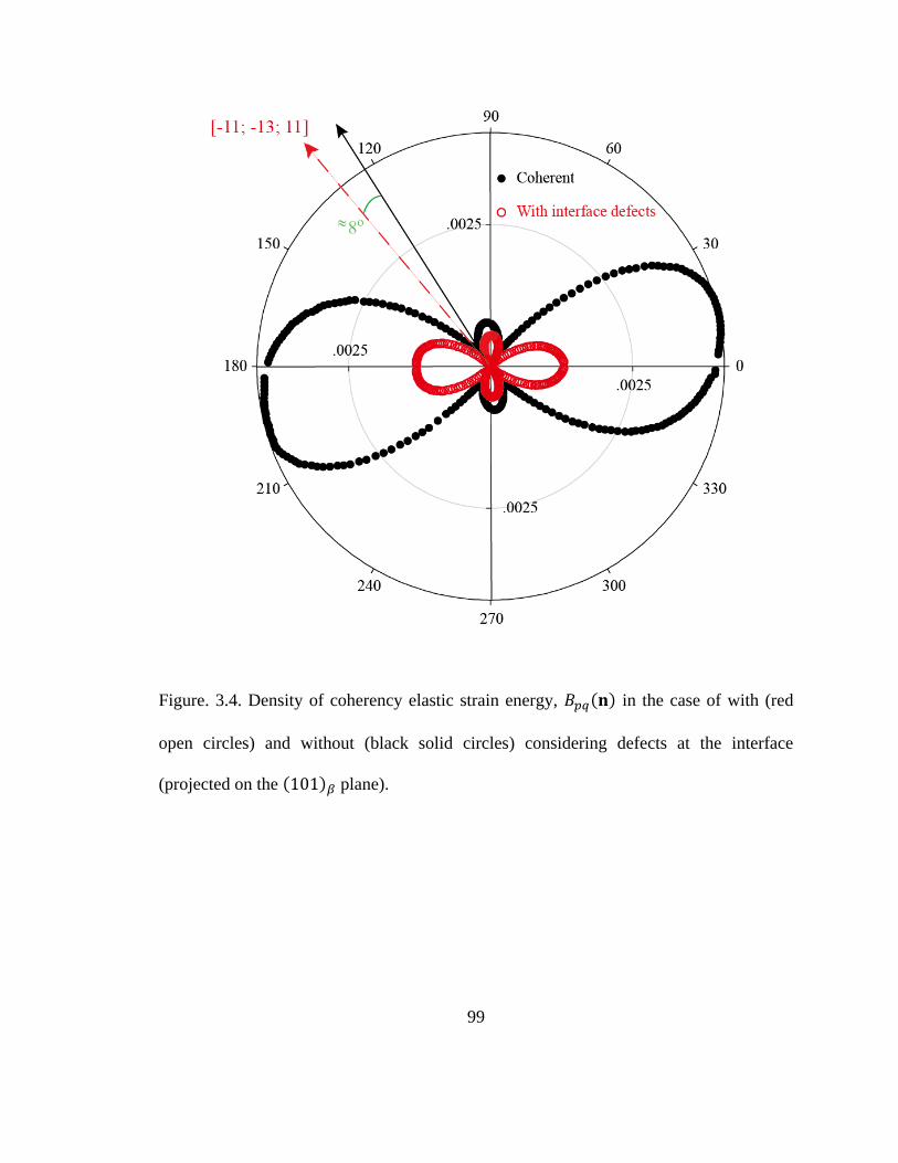
99
Figure. 3.4. Density of coherency elastic strain energy, in the case of with (red
open circles) and without (black solid circles) considering defects at the interface
(projected on the plane).

100
Continued
Figure. 3.5. Equilibrium shapes of an isolated -precipitate in different cases. (a)–(d)
isotropic interfacial energy with/without interfacial defects: (a) fully-coherent; (b) c-
dislocations on the broad face; (c) superposition of (a) and (b) showing the difference in
habit plane orientations; (d) all interfacial defects present.(e) Anisotropic interfacial
energy alone. (f) Both anisotropic interfacial energy and coherency elastic strain energy
with all interfacial defects considered. The transparent light yellow plane in each case on
the left column denotes the experimentally observed habit plane
[010][101]
[10-1]
(a)-1
16 nm
(b)-1
(a)-2
[010] [10-1]
(a)-2 (a)-3
(b)-2 (b)-3 (b)-4
[101]
(a)-4
(b)-4
(c)
[010]
[10-1]
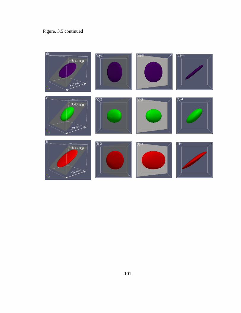
101
Figure. 3.5 continued
(d)
(e)
(f)
(e)-2 (e)-3 (e)-4
(d)-2 (d)-3 (d)-4
(f)-2 (f)-3
(d)-4
(e)-4
(f)-4
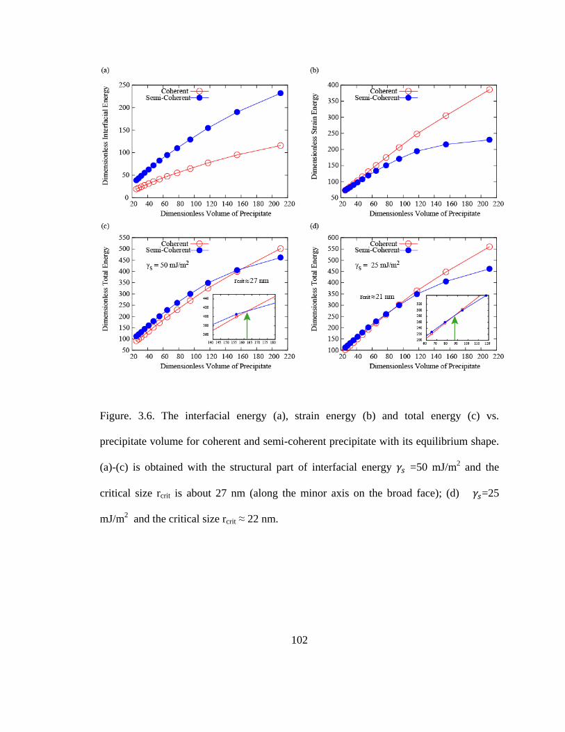
102
Figure. 3.6. The interfacial energy (a), strain energy (b) and total energy (c) vs.
precipitate volume for coherent and semi-coherent precipitate with its equilibrium shape.
(a)-(c) is obtained with the structural part of interfacial energy =50 mJ/m2 and the
critical size rcrit is about 27 nm (along the minor axis on the broad face); (d) =25
mJ/m2 and the critical size rcrit ≈ 22 nm.

103
Table 3.1 Effect of different types of line defects in inter-phase interface on coherency
strain energy and habit plane orientation Lattice parameter of the two phases 3.196a Å,
2.943a Å and 4.680c Å and I is unit tensor
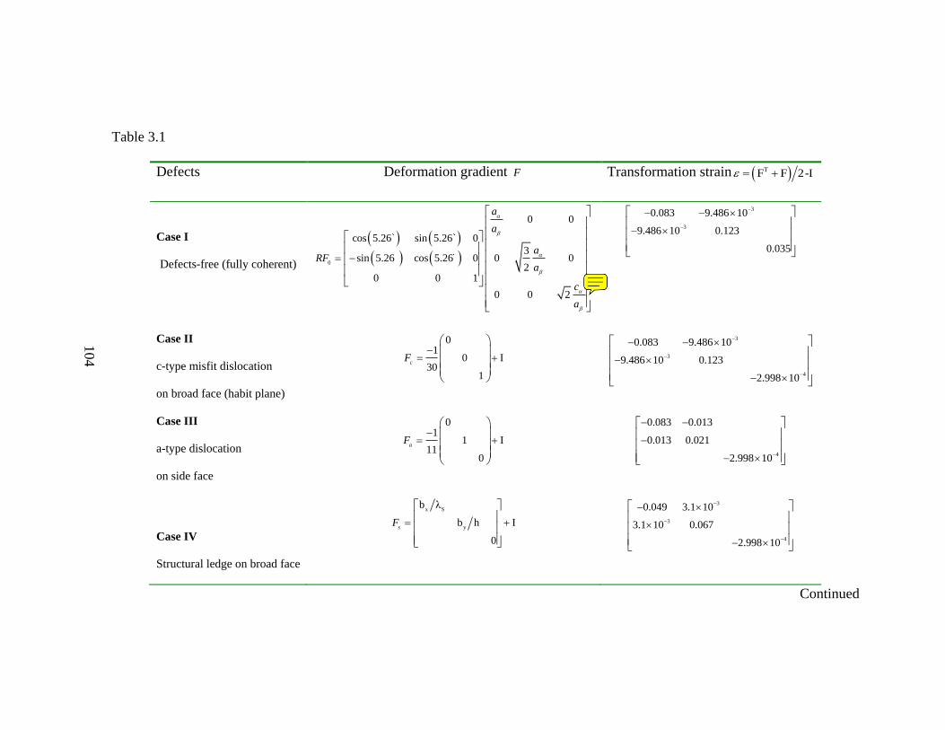
104
Table 3.1
Defects Deformation gradient F Transformation strain TF F 2-I
Case I
Defects-free (fully coherent)
0
0 0
cos 5.26 sin 5.26 0
3sin 5.26 cos 5.26 0 0 0
20 0 1
0 0 2
a
a
aRF
a
c
a
3
3
0.083 9.486 10
9.486 10 0.123
0.035
Case II
c-type misfit dislocation
on broad face (habit plane)
01
0 I30
1
cF
3
3
4
0.083 9.486 10
9.486 10 0.123
2.998 10
Case III
a-type dislocation
on side face
01
1 I11
0
aF
4
0.083 0.013
0.013 0.021
2.998 10
Case IV
Structural ledge on broad face
x S
y
b λ
b h I
0
sF
3
3
4
0.049 3.1 10
3.1 10 0.067
2.998 10
Continued
104
Sony
附注
sqrt(2)在分母;式(3.11)是对的! R矩阵应参考Eq.(3.12),R(1,2)和R(2,1)元素的正负号有误。 最终写的Epsilon矩阵是对的
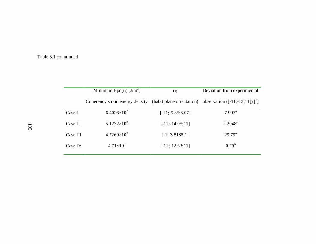
105
Table 3.1 countinued
Minimum Bpq(n) [J/m3]
Coherency strain energy density
n0
(habit plane orientation)
Deviation from experimental
observation ([-11;-13;11]) [o]
Case I 6.4026×10⁷ [-11;-9.85;8.07] 7.997
o
Case II 5.1232×10³ [-11;-14.05;11] 2.2048
o
Case III 4.7269×10³ [-1;-3.8185;1] 29.79
o
Case IV 4.71×10³ [-11;-12.63;11] 0.79
o
105
106
CHAPTER 4 Variant Selection during Precipitation in Ti-
6Al-4V under the Influence of Local Stress
Abstract:
Variant selection of (HCP) phase during its precipitation from (BCC) matrix plays a
key role in determining the microstructural state and mechanical properties of /
titanium alloys. In this work, we develop a three-dimensional (3D) quantitative phase
field model to predict microstructural evolution and variant selection during
transformation in Ti-6Al-4V (wt.%) under the influence of both external and internal
stresses. The model links its inputs directly to thermodynamic and mobility databases,
and incorporates the crystallography of BCC to HCP transformation, elastic anisotropy,
and defects within semi-coherent / interfaces in its total free energy formulation. It is
found that for a given undercooling, the development of a transformation texture (also
called micro-texture) of the phase due to variant selection during precipitation is
determined by the interplay between externally applied stress or strain and internal stress
generated by the precipitation reaction itself. For example, the growth of pre-existing
precipitates is accompanied by selective nucleation and growth of secondary plates of
107
certain variants that may not be the ones preferred by the initially applied stress. Possible
measures to reduce transformation texture are discussed.
4.1. Introduction
Titanium alloys have many advanced applications, ranging from aircraft engine
components [1] to medical implants [2], owing to their excellent combinations of high
strength-to-density ratio and excellent fracture toughness and corrosion resistance [3].
Among these alloys, two-phase /Ti alloys are the most widely used ones because a
rich variety of microstructures and mechanical properties can be obtained simply by
varying thermo-mechanical processing. For example, the -processed microstructure
consisting solely of widmanstätten [4] (HCP) plates in a BCC) matrix shows
superior resistance to creep and fatigue crack growth [1]. On the other hand, the /-
processed microstructure consisting of a combination of globular (or equiaxed) grains
with transformed structure (fine scale widmanstätten laths with adjacent ribs) offers
high ductility as well as good fatigue strength [1].
Microstructure engineering of / titanium alloys through thermo-mechanical
processing is based largely on the → + transformation upon cooling, which involves
both composition and structure changes. Usually precipitates form either as an
allotrimorph along prior -grain boundaries or as Widmanstätten plates nucleating either

108
from the grain boundary or in the interior of grain [1, 5, 6]. It is well known that the
plates usually maintain a specific orientation relationship (OR) with the matrix,
referred to as the Burgers OR [7], i.e., 101 || 0001
and 111 || 2110
.
According to the symmetry of the parent and product phases and the Burgers OR between
them [8], there are twelve crystallographically equivalent orientation variants of the
phase within a single prior grain. Since each of them has different transformation
strains, different variants may have different degree of elastic self-accommodation when
they are in contact with each other and different interfacial energy when they are in
contact with grain boundaries, variant selection (i.e. some variants appear more
frequently than the others) usually accompanies precipitation, leading to the formation
of transformation texture or micro-texture and relatively coarse microstructures.
Since the phase is highly anisotropic in its physical and mechanical properties, the
transformation texture of due to variant selection will determine, to a large extent, the
final mechanical properties of the / Ti alloys [9-12]. For example, the fatigue cracks
usually nucleate at and propagate through the longest and widest plate [5]. Also, micro-
cracks propagate much faster through a highly textured coarse colony microstructure as
compared to a fine colony one of random texture due to the increased tortuosity of crack
propagation paths [13]. Thus, it will be detrimental if, due to variant selection, plates of
a single or a few variants percolate through the whole matrix and it is not unreasonable to
assume that having more variants of plates in an microstructure would lead to

109
improved fatigue properties. Therefore, the control of variant selection during thermo-
mechanical processing is a key to control micro-texturing in the final products and hence
their fatigue properties.
A variety of factors could contribute to variant selection during precipitation,
including external or residual stresses within a polycrystalline matrix [14-16] due to
thermo-mechanical processing, heterogeneous nucleation on pre-existing defects in the
matrix such as grain boundaries [17-22], stacking faults and dislocations [21, 23, 24], and
correlated nucleation due to grain boundary [22] and pre-existing widmanstätten
[25]. For example, the nucleation and growth of coherent plates are accompanied by
significant lattice distortion in the surrounding matrix due to the transformation strain.
Therefore, the surrounding matrix will favor nucleation and growth of specific variants
to accommodate the strain [26]. Pre-existing dislocations in the matrix have been
shown to act frequently as preferential nucleation sites for specific variants. For
instance, dislocations belonging to the 112 111
slip systems would favor the
nucleation and growth of a single variant whose orientation relationship is described by
the components of the specific slip system [21, 23, 27]. Furthermore, stresses may also
arise from anisotropic thermal expansion of grains within a polycrystalline sample [28,
29] and initial texture of grains could enhance variant selection during precipitation
[30].
110
It is clear that the local stress state of an untransformed matrix, due to a variety of
sources, is a key factor in controlling variant selection during precipitation and the final
transformation texture. However, the challenges to study variant selection during
transformations under the influence of stress are two-folds: first, one needs to determine
stress distribution in an elastically anisotropic and inhomogeneous media under a given
applied stress or strain condition; second, one needs to describe interactions of local
stress with coherent and semi-coherent precipitates, i.e. to describe interactions of local
stress with evolving two-phase microstructures. In particular, the coherency state of an
precipitate may change during its growth and defect structures, including misfit
dislocations and structural ledges, at the interfaces may alter the coherency stress.
Because of these complications, limited work exists in literature on modeling variant
selection during transformation in titanium alloys. Moreover, most previous work
about effect of stress on precipitation deals with coherent precipitates only [31-34].
The main objective of this chapter is to develop a three-dimensional (3D) physics-
based phase field model for quantitative prediction of microstructural evolution and
variant selection during transformation in Ti-alloys under the influence of
both external and internal stresses. In the current study, we will focus on effects of a
constant externally applied strain (pre-strain) and internal stresses generated by pre-
existing precipitates on variant selection in a single grain of . Effects of elastic
inhomogeneity and grain boundaries in a polycrystalline sample and effects from other
111
stress-carrying defects such as dislocations and stacking faults on variant selection will be
investigated in a follow-up chapter.
The rest of the chapter is organized as the following. In section 4.2, a 3D quantitative
phase field model is formulated, which incorporates the crystallography of the
transformation and defect structures at interfaces, and links its model inputs directly
to available thermodynamic and mobility databases. All symmetry operations to generate
the 12 orientation variants that have Burgers OR with the matrix phase are derived. In
Section 4.3, the lengthening and thickening kinetics of a single plate are first compared
between simulation predictions and theoretical solutions. Then variant selection of
precipitates within a single grain of due to different applied strains is investigated.
Finally the effect of a growing pre-existing plate on variant selection of secondary
plates is studied. The results are analyzed in Section 4.4 and the main findings are
summarized in Section 4.5.
4.2. Method
4.2.1. Determination of number of variants of a low symmetry precipitate phase
For structural phase transformations, a low-temperature product phase usually has
lower symmetry than its high-temperature parent phase. Such a symmetry reduction (i.e.,
some of the symmetry elements of the parent phase are no longer shared by the product

112
phase) leads to multiple crystallographically equivalent domains of the product phase
referred to as orientation variants (OVs). The set of remaining common symmetry
elements between the parent and product phases is given by the intersection group, H, of
the parent group, Gm, and the product group, Gp, under a given OR between them [8], i.e.,
m pH G G . Note that Gm and Gp are the point groups rather than space groups since
all the common translations are usually destroyed by the transformation. Then the
number of all OVs, n, is given by the index of H in Gm, i.e.
Equation Chapter 4 Section 1
morder of G order of Hn (4.1)
The number of variants produced by the transformation in titanium alloys can
be determined readily by the above equation. For example, the point groups of the parent
(BCC) and product (HCP) phases are m3m and 6 mmm , respectively, and the orders of
m3m and 6 mmm are 48 and 24, respectively. The intersection group is thus
determined to be 2 m given that the Burgers OR is maintained between and phases,
as described by:
101 || 0001
; 111 || 1120
; 121 || 1100
. (4.2)
113
The order of H is 4 and thus the number of variants is n = 48/4=12. All the other OVs
can be obtained readily via symmetry operations on the variant described by Eq. (4.2)
(See Appendix A for details about the derivation of the intersection group H and all 12
symmetry operations associated with each OV). All 12 Burgers orientation variants used
in the current study and their corresponding symmetry operations to derive the other 11
from the one described by Eq.(4.2) are summarized in Table 4.1. The symmetry
operations are quite useful to obtain misorientations between different variant pairs, and
more importantly, to derive the transformation strain of others variants from that of the
variant described by Eq. (4.2), as will be described further latter.
4.2.2. Free energy formulation
Any given microstructure, no matter how complicate it is, can be described by two
types of order parameters that characterize, respectively, structural and chemical non-
uniformities [35, 36]. For example, for an + two-phase microstructure, twelve non-
conserved order parameters, 1,2,..., 12p p N r , are needed to describe the
structural non-uniformities associated with the twelve OVs and two conserved order
parameters, Al, VkX k r , are needed to describe the chemical non-uniformities of
components Al and V in the system. In the multi-phase field model, one more dependent
order parameter, 13p p r , is introduced to describe the spatial distribution of the
matrix phase. For example, 13 1 r and 1(r)=2(r)=…=12(r)=0 within the -matrix
114
and 1p r and qp(r) = 0 inside the p-th OV of precipitates under the constraint
that 1
1
1N
p
p
r [37, 38].
4.2.2.1. Chemical free energy
According to the gradient thermodynamics [39], the total chemical free energy of a
chemically and structurally non-uniform system can be formulated as a functional of the
order parameters introduced above:
2
, 1
1 1, ,
2 2
NT
chem cm k p k p p p
Vk Al V pm
F G T X X dVV
κκ (4.3)
where cκ and pκ are the gradient energy coefficient and gradient energy coefficient
tensors characterizing contributions from non-uniformities in concentration and structure,
respectively. In particular, different choices of eigenvalues for the κ tensors allow for the
consideration of interfacial energy anisotropy [40]. mG is the non-equilibrium local
molar free energy of the system defined in both concentration and structural order
parameter space. Even though it can be formulated by using Landau expansion
polynomials [41-43], it is approximated by [44, 45]:
115
1
, ,
1 1 1
, , , 1 ,N N N N
m k p p m Al V p m Al V pq p q
p p p q p
G T X h G T X h G T X
(4.4)
in the current study for simplicity. In the above equation, 3 26 15 10p p p ph is
an interpolation function used to connect the free energy curves (as function of
concentrations) of the and phases. The 1
1
N N
pq p q
p q p
term introduces a hump on
the free energy surface between two structurally degenerated states, i.e., between variants
p and q, and the hump height is proportional to pq . The advantage of using p q
p q
over the commonly used form, 2 2
p q
p q
, is that it creates an energy cusp at the
equilibrium values of the structural order parameters and hence prevents significant
deviations of the order parameters from 1 (or 0) in the bulk phases (i.e., creates higher
energetic penalty for deviation). ,,m Al VG T X and ,,m Al VG T X are the equilibrium
molar free energies of and phases as function of temperature and individual phase
concentration ,Al VX and ,Al VX
, respectively. In the current study, these equilibrium free
energies are formulated based on a pseudo-ternary thermodynamic database developed
for Ti64 [46].

116
4.2.2.2. Elastic strain energy
The theoretical treatment of elasticity problem associated with phase transformations
was due to Khachaturyan and Shatalov (KS) [47-49] who derived a close form of
coherency elastic strain energy of a system with arbitrary compositional and structural
non-uniformities by following Eshellby’s approach [50]:
* 0 0
3, 1
1( ) ( ) ( )
2 (2 ) 2
Nel T
pq p q ijkl ij kl ij ijkl kl
p q
d VE B C d C
g
n g g r r (4.5)
where ( )pqB n describes the elastic strain energy density of a thin precipitate plates with
n being its habit plane normal. The detailed form of ( )pqB n varies with external
boundary conditions. ( )p g denotes the Fourier transformation of ( )p r and *( )p g
stands for the complex conjugate of ( )p g . g is a vector in the reciprocal space.
In the current study, a clamped boundary condition is employed, where the system’s
boundary is fixed after applying an external load to the system. Then ( )pqB n reads
0 00 00
0 00 00 00 00
( ) ( ), =0( )
( ) ( ) ( ) ( ) ( ) , 0
ijkl ij kl
pq
ijkl ij kl i ij jk kl l
C p qB
C p q n p q n
gn
n g (4.6)

117
where 0
ijklC is the elastic modulus tensor of the matrix phase and 00
ij p is the stress-free
transformation strain (SFTS) or inelastic strain of the pth
orientation variant of the -
phase. 00 0 00( ) ( )ij ijkl ijp C p and 1
jk i ijkl ln C n n is the inverse of the Green’s function in
the reciprocal space, and n g g with in being its ith
component. In Eq.(4.5), the
macroscopic homogenous strain, ij , is equal to the pre-strain, appl
ij which is established
by the initial load applied to the system that has a volume V in the real space.
The last term in Eq. (4.5) represents the coupling between the pre-strain and the
transformation strain induced by the precipitates, T
ij r . T
ij r represents the spatial
distribution of the SFTS field associated with structural non-uniformities and can be
expressed by 00
1
( )N
T
ij ij p
p
p
r r , which is a linear superposition of all N types of
non-uniformities
The total strain energy of the system can be easily obtained and incorporated into the
total free energy of the system, i.e., chem elF F E .
4.2.3. Stress-free transformation strain for coherent and semi-coherent precipitates
Derivation of SFTS, 00
ij , associated with a phase transformation is one of the key steps
towards formulating the coherency elastic strain energy in the KS microelasticity theory
118
[48]. During nucleation and in the early stages of growth, precipitates tend to be coherent
with the matrix, which minimizes the interfacial energy. For coherent precipitates, the
transformation matrix [48] or deformation gradient matrix [51], F , associated with the
phase transformation could be determined by the lattice correspondence (LC) according
to the nearest neighbor principle [52] for a given OR between the precipitate and parent
phases. F is a discrete mapping from a Bravais lattice of the parent phase to a Bravais
lattice of the product phase and describes geometrical change between them under the
given OR via a uniform lattice deformation. Usually, it is expressed in a common
orthogonal coordinate system (usually chosen in the parent phase reference frame).
During their continued growth, coherent precipitates may lose coherency when the
elastic strain energy contribution to the total free energy of the system becomes
dominant. Line defects, such as misfit dislocations and structural ledges [53], are then
introduced within the interface to relieve misfit stress. Structural ledges, which exhibit
step character as well as dislocation properties, are also referred to as transformation
dislocations or disconnections to distinguish themselves from defects without the step
character in the topological model for structural phase transformations [54, 55]. Interface
between fully grown precipitate and matrix has been frequently observed to have
both types of defects within it [56-58]. For semi-coherent precipitates, the effect of misfit
dislocations and structural ledges on the transformation strain can be considered by
superposition of their eigenstrains with the SFTS calculated for fully coherent
precipitates, which can be achieved by treating the interfacial defects as successive
119
deformations, following the uniform lattice deformation, applied to the precipitate phase
[59].
Thus, the total deformation gradient resulting from the phase transformation
and defects on the / interfaces can be formulated as:
tot step disF F F F (4.7)
where stepF and dis
F represent the deformation gradient matrices due to structural ledges
and dislocations, respectively. Then, the transformation strain 00
ij can be derived from
the total transformation matrix. To be consistent with the assumptions made during the
derivation of the micro-elasticity theory [48, 60], the total strain in the system is given by
the sum of the elastic and inelastic strains: T
ij ij ije , and the total strain is related to
the displacement through , ,
1
2ij i j j iu u where iu is the ith component of the total
displacement field u and ,i ju represents it gradient.
,ij ij i jF u or
I F u where ij denotes the Kronecker delta. Thus, the SFTS for the orientation
variant described in Eq. (4.2) is given by (under small strain approximation)
:
120
tot tot
00
2
T
F F
I (4.8)
According to the aforementioned approach, the transformation strains for both coherent
and semi-coherent precipitate have been obtained [49] based on the LC [7] deduced from
the Burgers OR and detailed interface structure. Details of the derivation procedures
can be found in Ref. [59].
It is worth mentioning that the transformation strains should be altered when a
coherent nucleus grows beyond a critical size when the coherency is lost [59]. As a result,
the response of the precipitation process to the applied strain or pre-straining would vary
with the coherency state of precipitates in terms of the sign and magnitude of the
interaction energy density. Therefore, the derivation of SFTS for the coherent and semi-
coherent precipitate is an important first step towards variant selection study.
In fact, it has been shown that [59] the introduction of defects at the / interfaces
relaxes significantly the coherency strain energy according to the minimum elastic strain
energy density Bpq(n0) (from 6.426×10⁷ J/m
3 to 4.71×10
3 J/m
3) obtained when using
coherent and semi-coherent SFTSs. In addition, the minimum of Bpq(n0) is reached
respectively at n0=(-11,-9.85,8.07) and n0=(-11,-12.63,11) for coherent and semi-
coherent precipitates, which deviate respectively 8º and 0.8 º from the experimentally
observed habit plane orientation (-11,-13,11). Therefore, the introduction of defects
121
relaxes the coherency strain and alters the habit plane orientation at the expense of
increasing interfacial energy.
The transformation strain for all the other orientation variants of precipitate can be
obtained by symmetry operations, i.e.
T
00 00 p pp S S (4.9)
where the symmetry operations 1..12pS p are listed in Table 4.1. The SFTSs for all
12 variants of nuclei and semi-coherent plates are presented in Appendix B1 and
Appendix B2, respectively.
4.2.4. Effect of misfit dislocation on interfacial energy
Defects at the precipitate/matrix interfaces alter not only the elastic strain energy but
also interfacial energy and its anisotropy, and growth anisotropy as well. Contributions
from misfit dislocations at different facets of the precipitates to the structural part of the
interfacial energy s could be evaluated according to the Read-Shockley equation [61,
62]. Based on the misfit dislocation structure at different facets [57], the structural
components, s , of the interface energy due to the presence of misfit dislocations at the
122
broad, side and edge faces are m0.39E , m0.72E and mE , respectively, where mE is
assumed to be 250 mJ/m2. In addition, the chemical component c of the semi-coherent
interfacial energy for the three facets are assumed equal for simplicity and have a value
of 50 mJ/m2, which is reasonable for a fully coherent interface. Therefore, the interfacial
energies of the broad, side and end faces are 150, 230 and 300 mJ/m2, respectively. The
results are then incorporated in the gradient energy coefficients characterizing chemical
and structural non-uniformities in the phase field free energy formulated based on the
gradient thermodynamics (Eq.(4.3)). Neglecting the details of -plot, we further assume
that the interfacial energy is a quadratic function of direction vector in the local reference
frame attached to lath, which is referred to as N3, 1 : 353x
, 2 : 11 13 11x
and
3 : 101x
. In the global coordinate system where the SFTSs have been derived, , the
gradient energy coefficient tensor for the structural order parameters, has a form
1
2
3
R R
T , (4.10)
where i 1 3i denotes the eigenvalues of the gradient energy coefficients
associated with broad, edge and side faces, respectively, whose values (all listed in Table
4.2) are so chosen to account for the anisotropy in interfacial energy mentioned above. R
123
is the rotation operation from local to laboratory (global) coordinate system. There are
total twelve rotation matrices corresponding to the 12 orientation variants of the phase.
4.2.5. Kinetic equations
The temporal and spatial evolutions of concentration and structural order parameters
are governed by the Cahn-Hilliard generalized diffusion equations [63] and the time-
dependent Ginzburg-Landau equation [64], respectively. In particular, considering the
multi-variant of phase, we employ the multi-phase field method [37, 38], which was
developed to treat multi-phase and multi-component material systems:
1
21
,1, , ,
,
nk
kj i j k
jm j
X t FM T X t
V t X t
rr
r (4.11)
, 1,
, , ,
chem chem elp
p
p q p q p
t F F EL t
t t t t
r
rr r r
(4.12)
where 1...12, ,kj iM T X is the chemical mobility [65], L is the mobility of the long-
range order parameters characterizing interface kinetics, and k and p are the Langevin
noise terms for composition and long-range order parameter, respectively. If the interface
motion is diffusion-controlled, L can be determined at a vanishing kinetic coefficient

124
condition [66]. In Eq.(4.12), is the number of phases that co-exist locally, not the
number of all phases which is N+1. Note that similar to Eq. (4.11), Eq. (4.12) was also
derived [38] in a variational framework with the use of Lagrange multiplier to account for
the local constraint among p , i.e., 1
1
1N
p
p
.
In order to remove the length scale limit of the conventional phase field model,
the Kim-Kim-Suzuki-Steinbach model [37, 67] is implemented, where the diffuse-
interface region is treated as a homogeneous mixture of the precipitate and matrix phases
with different compositions but equal diffusion potentials [67].
4.2.6. Model inputs and parameters
All the parameters for the model and materials properties used in the simulations are
listed in Table 4.2.
4.3. Results
4.3.1. Growth behavior of a single plate
In order to demonstrate the quantitative nature of the model, the growth (thickening)
behavior of an precipitate (an infinite plate) in a supersaturated matrix at 1023K is
investigated and compared to DICTRA simulations. The initial thickness of the plate is
125
chosen to be 0.25 m and its composition is assumed to be at equilibrium (for Ti-64):
10.48 at.% Al and 2.38 at.% V. The initial composition of the supersaturated matrix is
10.19 at.% Al and 3.60 at.% V. The total system size is 10 m. The phase field
simulation results are compared with DICTRA simulations in Fig. 4.1(a), which shows a
good quantitative agreement. In addition, the thickening kinetics of an infinite plate is
found to follow a parabolic law, which confirms that the transformation is diffusion
controlled.
Then, the growth behavior of a single finite plate embedded in a supersaturated
matrix with anisotropy in both elastic strain energy and interfacial energy is investigated.
A super-critical nucleus (a spherical particle having a radius of 37.5 nm) is placed at the
center of the computation cell. During growth, the precipitate develops into a disk with
its broad face parallel to 11,13,11
(as indicated by the shaded plane) (Fig. 4.2(a)). The
kinetics of both lengthening along the invariant line 3;5;3
and thickening normal to
the habit plane 11,13,11
are investigated. The thickness and length of the disk are
measured using Ruler in Source Toolbar of ParaView [68], an open-source, multi-
platform data analysis and visualization software application, at the = 0.5 contour line.
The results are shown in Fig. 4.1(b)-(c). Note that in measuring the interfacial position
there are uncertainties in determining the exact position of = 0.5 and the exact position
of the broad face because it is not exact flat. However, the uncertainties should be smaller

126
than the interface width for the broad and edge faces. Therefore, the interface width is
used as a measure of the error bar shown in the plots and the fitting process has taken the
uncertainty into account. Also note that the amplitude of the error bar in Fig. 4.1(c) at the
first time step is larger than that of the others since the broad face of the plate at that
moment has not yet developed due to its relative small size.
The lengthening kinetic is linear with time, while the thickening follows a parabolic
law, which agrees with the growth kinetic of a widmanstatten plate [69, 70]. And the
lengthening is about 10 times faster than the thickening.
The shapes of the disk outlined by a constant contour of Al concentration is shown
in Fig. 2(b). The color bar indicates the relative value of Al concentration.
4.3.2. Effect of pre-strain on variant selection
To simulate the type of constraint and stress conditions that might be experienced by
a component during processing [71], we carry out simulations under an uniform pre-
strain that is realized by applying either an uniaxial tensile or compressive stress along
the x (i.e. [010]direction of the reference frame and then clamping the system. Such a
boundary condition parallels to the recent experimental study on variant selection in
and titanium alloys [71]. During the nucleation stage, the SFTS calculated for coherent

127
precipitates (Section 2.3) is used. When enough nuclei are generated, the Langevin
noise terms are removed from Eq. (4.12) and the SFTS calculated for semi-coherent
precipitates is used during the growth and coarsening stages. The interfacial energy
anisotropy associated with misfit dislocations is also introduced for each variant at this
moment.
4.3.2.1. Pre-strain due to compressive stress along [010]
The macroscopic strain appl
ij is introduced by a compressive stress that is applied
along the x-axis (i.e., [010] direction) before the system’s boundary is clamped. The
magnitude of the applied stress is -50MPa and the resulting principal pre-strain is:
32.13 10appl
x ;
31.02 10appl
y and
31.02 10appl
z . Figure 3(a) shows
microstructure evolution during (Red online) precipitation from matrix (Blue online)
viewed at x - [010], y - [-101] and z - [101] cross-sections, respectively. It is obvious
that only limited numbers of orientation variants are formed under this specific pre-strain
condition and a strong transformation texture develops with time (see the arrows in the
last row of Fig. 4.3(a)). The whole entire precipitate microstructure in the parent -grain
consists of a few colonies of parallel array of plates.
A 3D plot of the microstructure developed at time t=10s is shown in Fig. 4.3(b) and
the volume fraction of each variant as function of time is shown in Fig. 4.3(c). It is
128
readily seen that only 4 variants, i.e. V1, V2, V7 and V8 have finite volume fractions.
Note that V1 and V7 have a common basal plane (101)//(0001) and their habit plane are
11,13,11
and 11,13,11
, respectively. The angle between the two habit planes is
79.8º or 100.2 º. Hence, the two plates are nearly perpendicular to each other, so do the
two plates of V2 and V8, as shown in Figs. 3(a) and 3(b).
4.3.2.2. Pre-strain due to tensile stress along [010]
In case where the pre-strain is generated by a 50 MPa tensile stress applied along
[010], the results are shown in Fig. 4.4. Different from the previous case, there are more
variants present, which suggests that the variant selection is sensitive to the initial
stress state and has a tension-compression asymmetry. Nucleation and growth of phase
seems to be enhanced at early stages when more specific variants are selected
simultaneously. For example, the volume fraction of each selected variant is much larger
than that obtained under compressive stress at t=2s, as shown in Fig.3(c) and Fig.4(c).
However, the volume fraction of each favored variant at t=10s is almost the same in the
two cases, i.e. around 8%. Also, some V-shaped patterns of plates are observed at very
beginning in this case, as indicated by the arrows in Fig. 4(a). These patterns have been
observed in experiment [25]. The variants in the V-shape pattern are found to have a
misorientation of 60◦ rotation around their common [111] or [11-20] axes.
129
4.3.3. Variant selection due to pre-existing plates
For -processed Ti-alloys, the specimen is usually step quenched to a specific
temperature within the + phase region after solution heat treatment above transus.
After isothermal holding for certain period of time, the sample is aged at another lower
temperature within the + phase region or cooled continuously at different rates. The
plates formed at the higher aging temperature are referred to as primary and the ones
formed at the lower aging temperature or during continuous cooling are referred to as
secondary . Since the secondary plates are formed in the untransformed matrix in
between the primary plates, their variant selection process is affected strongly by the
present of the primary . Grain boundary may have a similar effect on variant selection
of the primary plates. It has been suggested by a recent experimental study on step-
quenched Ti-550 alloys [25] that the development of a basket-weave structure could be
associated with nucleation and growth of different variants of secondary from primary
one. However, the mechanism is still not well understood.
In order to investigate the effect of existing plates on variant selection of new
plates, a phase field simulation study was designed as the following: a single variant of
plate (V1) is allowed to grow at 1123K for certain period of time and then the system is
quenched to 1073K (Fig. 4.5(a)). The random noise terms are introduced to simulate the
nucleation process of the secondary . The amplitudes of the random noises are
specifically chosen (by trial-and-error) to avoid homogeneous nucleation (i.e., nucleation
130
uncorrelated to the presence of the primary ). The results are shown in Fig.5, where it is
readily seen that two secondary particles of variants V4 and V6 nucleate and grow on
the broad face and near the edge of a growing primary disk (V1) (Fig. 4.5(b) and 5(f)
show two different views of the same microstructure). Note that the shape of the
secondary particles is different from that of the primary particle; they have lath-like
shapes rather than the disk-like shape. It should also be noted that the orientation
relationship or the misorientation between variants V1, V4 and V6 is such that when
described by the axis/angle pair, 60 1120
, three of them share a common
111 // 1120
direction according to the Burgers OR.
As the primary and secondary precipitates continue to grow, new particles of the
same variant 4 and 6 are induced in an arrangement of edge-to-edge adjacent to the
previously formed secondary laths as shown in Fig. 5(c). The relative location between
the newly formed secondary laths and the initial primary plate or disk (Fig. 4.5(a)) is
shown in Fig. 4.5(g). At even later stages, new laths of variants 8, 9 and 11 are formed
near the interface between the primary and secondary of variant 4 and 6 as shown in
Fig. 4.5(d) and Fig. 4.5(h) (viewed from the other side of broad face as compared to Fig.
4.5(d)) at t=3s. It appears that the growth of a secondary plate formed at an early
moment can lead to the growth of new secondary alpha around them. The volume
fraction analysis of each variant at t=3s (Fig. 4.5(e)) suggests that the nucleation and

131
growth of secondary of variants V4, V6, V9, V11 and V8 would be favored by the
primary alpha of variant V1, and V4 and V6 are the most favored ones.
4.4. Discussion
4.4.1. Lengthening and thickening kinetics of plate
It is clear that the growth of an isolated plate is highly anisotropic since its
lengthening is much faster than its thickening. In our simulations, the growth anisotropy
results from a non-uniform distribution of solute depletion zone surrounding the growth
plate, as shown clearly in Fig. 4.2. The plate-like anisotropic shape is determined by
the anisotropy in interfacial energy and elastic strain energy. Quantitative studies of both
lengthening and thickening kinetics of a widmanstatten plate have been carried out in
literature. For example, the mechanism of lengthening (edgewise growth) has been
explored by Zener [69] and later by Hillert [70] in steels and linear growth kinetics was
derived. Our simulation results (Fig. 4.1(b)) also show that the plate lengthens at a
constant rate, GL, which agrees with the Zener and Hillert’s analysis. Since Al is an
stabilizer and V is a stabilizer, the growth of plates is controlled by partitioning of Al
and V between and phases. The plate shape ensures that the pilling-up of V or
depletion of Al by a growing plate takes place at the sides of the plate. Therefore, the
132
Al and V concentration profile ahead of the tips of an plate remains constant as it
lengthens. As a result, unlike the thickening process, the plate lengthens at a constant rate
GL.
The thickening (sidewise growth) of a plate is, however, less understood than its
lengthening. The current phase field simulation result obtained for the growth of an
isolated plate shows a parabolic thickening kinetics, which is self-consistence with the
diffusion-controlled growth condition assumed in the simulations. It should be
mentioned, however, that the broad face of an plate is comprised of terrace of good
atomic fit with steps at the atomic scale, which is beyond the resolution of the current
phase field method. According to Aaronson’s analysis [72], the more coherent broad face
could only grow perpendicular to itself by nucleation and migration of ledges. Enomoto
studies the migration of an array of steps using finite difference scheme [73, 74] and
showed that the thickening kinetics follows nearly a parabolic law at long reaction time.
More detailed discussion on ledge growth can be found in Refs. [72-74].
4.4.2. Elastic interaction between pre-strain and transformation strain of variants
In this Section we demonstrate that the simulation results on selective nucleation and
growth of specific variants presented in Section 3.2.1 and 3.2.2 can be rationalized by
the interaction between the pre-strain and the SFTS of each variant characterized through
the interaction energy density, int 0 00 ( )appl
p ij ijkl klE C p . In general, the SFTS of each OV,

133
00 ( )ij p , is different from each other when defined in a common reference frame and thus
the interaction energy density for each OV will be different. In other words, the
interaction is crystallographically anisotropic in nature. As a result, the nucleation and
growth of some variants will be favored over others by the applied strain, appl
ij . To be
specific, a variant whose growth reduces the strain energy (i.e., the interaction energy
density is negative) will be favored to nucleate and grow, while the variant whose growth
results in a positive interaction energy density will be suppressed. The resulted uneven
distribution of the different orientation variants of precipitate then gives rise to
transformation texture.
Since a coherent precipitate will lose its coherency when its size exceeds a critical
value [59], its interaction with the pre-strain will be size-dependent because of the change
in the SFTSs (see Section 2.3). In other words, the interaction energy also depends on the
coherency state of precipitate. When the pre-strain is produced by [010] tension or
compression, the coherency state alters only the magnitude but not the sign of the
interaction energy (see, e.g., Fig. 4.6 (a) and 6 (c)). In the case of tension along [010],
for example, variants V3-V6 and V9-V12 have the same negative interaction energy
while variants V1, V2, V7 and V8 have the same positive interaction energy for both
coherent and semi-coherent precipitates. In the case of compression, the interaction
energies reverse their signs, i.e., variants V1, V2, V7 and V8 have the same negative
interaction energy while variants V3-V6 and V9-V12 have the same positive interaction

134
energy. These interaction energy calculations agree well with the phase field simulation
results (Fig. 4.3 and Fig. 4.4), which means that such simple interaction energy
calculation could be used to predict variant selection behavior in this case.
Nevertheless, when a tensile or compressive stress is applied along the z-[101]
direction to obtain the pre-strain, the situation is much more complicated. When the pre-
strain is obtained via a compressive stress (50MPa) along z direction, its principal value
is: 31.02 10appl
x ;
30.28 10appl
y and
30.93 10appl
z . It can be readily seen
that the coherency state alters both the magnitude as well as the sign of the interaction
energy (see, e.g., Fig. 4.6 (b) and 6 (d)). In the case of tension (Fig. 4.6(b)), variants V2
and V8 have the most negative interaction energy for both coherent and semi-coherent
precipitates, but variants 9-12 have positive interaction energy if the precipitates are
semi-coherent and negative interaction energy if the precipitates are fully coherent.
Variants 1 and 7 have large negative interaction energy at the coherent stage and nearly
vanishing interaction energy when they lose coherency. If a compressive stress is applied
along the [101] (Fig. 4.6(d)), the variants favored during both coherent and semi-
coherent stages are only V3-V6. Variants V9-V12 are unfavored when they are coherent
but become favored when they are semi-coherent by the pre-strain. These complicated
interactions may alter the nucleation rate as well as the growth rate at different stages of a
precipitation process, making it impossible to predict transformation texture by simple
interaction energy density calculations.

135
From the results of interaction energy calculations shown in Fig. 4.6(b), one would
expect that V2 and V8 would be the dominant ones during precipitation. This is,
however, not the case according to the phase field simulation results. As can been seen
from Fig. 4.7(a), the most dominant two variants are V1 and V7, which have a much
smaller interaction energy than that of variant V2 and V8. The cause of this discrepancy
will be discussed in the following Section.
In case of compression, both interaction energy calculations and phase field
simulations predict that variants V3-V6 are the most dominant variants. In addition,
phase field simulations show that variants V1 and V7 become more favored than variants
V9-V12 by the evolving microstructure during their growth at semi-coherent stage even
though the interaction energy calculations show that they are less favored than variants
V9-12 (see Fig. 4.6(d)).
The 3D microstructures obtained in the two cases are shown in Figs. 4.7(c) and
4.7(d), respectively. There are many V-shaped precipitate configurations as well as a few
enclosed triangle configurations as indicated by the arrows in the Fig. 4.7(d).
4.4.3. Competition between pre-strain and evolving microstructure
From the examples discussed above, one can see that the interaction energy
calculations, though simple and fast, cannot predict the overall variant selection behavior

136
in all cases. This is because of the fact that the interaction energy calculations do not
consider how an evolving microstructure alters the local stress state. The total strain of a
system is the sum of elastic strain and inelastic strain, i.e. T
ij ij ije . Since the system
considered in this study is under a clamed boundary condition with a specific pre-strain
determined by an initially applied stress, the average total strain (over the whole system)
is equal to the pre-strain. As the microstructure and thus inelastic strain, T
ij , evolve, the
elastic strain fields of different variants evolve as well and nuclei of different variants
would become favored by the elastic interactions. For example, as have been shown
when the pre-strain is obtained by applying a 50MPa tensile stress along [101] (Fig.
4.7(a)), the most favored variants at later stages do not agree with the interaction energy
calculation. This situation would not occur if the boundary is stress-controlled since the
system is free to change its shape and volume.
In order to confirm these arguments, a microstructure is obtained by only switching
the boundary condition to be stress-controlled while keeping all the other simulation
parameters the same. In this case, the volume fraction of V2 and V8 will increase sharply
to 30% at t=1s. Assume that this microstructure can also exist under the clamped
boundary condition and the internal stress is calculated. The principle stress components
obtained are: 11=-102.4 MPa, 22=27.9MPa and 33=44.3MPa. It is obvious that the
magnitude of some of the internal stress components exceed 50MPa that is used to
generate the pre-strain. Based on the interaction energy calculation, such stress state will
favor two pair of variants, i.e., V1/V7 and V2/V8. Therefore, the precipitation of V1 and
137
V7 is favored by both the pre-strain and the internal stress. Moreover, the combination of
V1 + V2, and V7 + V8 could reduce the overall transformation strain by self-
accommodation. Thus, within a clamped system, internal stress generated by an evolving
microstructure could exceed the initially applied stress that generated the pre-strain,
inducing the formation of other variants and hence reducing the degree of transformation
texture. In this regard, a clamped boundary could be a way of preventing the development
of transformation texture and, in particular, preventing percolation of a single or a few
variant through a whole entire grain. It seems that the experimental results reported
in a recent study on effects of different processing variables on transformation texture
development (due to variant selection) in Ti-64 sheet during -processing by Semiatin et
al [71] support this simulation finding. On the other hand, the prediction from the
interaction energy calculation is valid only when the internal stress generated by the
evolving microstructure is significantly smaller that created by the pre-strain under a
clamped boundary condition.
To assess whether a combination of a group of plates of all the most and equally
favored variants is able to reduce significantly the overall transformation strain as
compared to an isolated one, we calculate the average transformation strain of all of the
most favored variants based on the interaction energy calculations. The results show that
when the pre-straining is obtained by an applied stress along the [010] axis (irrespective
tensile or compressive), the average transformation strain of a group of plates of the
most favored variants is reduced significantly as compared to the transformation strain of
138
a single plate. Nevertheless, when the pre-straining is obtained via tensile stress along
[101], the average transformation strain of the most favored variants V2 and V8 is
almost identical to that of a single variant in both coherent and semi-coherent state.
Thus, such a variant selection of only two variants sharing a common basal plane (V2 and
V8) cannot be driven by the pre-straining. In contrast, the average strain of variants V3-
V6 is much smaller than that of a single variant when the pre-straining is achieved via a
compressive stress along [101]. As a result, the variant selection behavior can be
predicted by the interaction energy calculation. This approach is similar to the method for
an approximate estimation of the effectiveness of self-accommodation among different
groups of martensitic plates, developed by Madangopal et al. [75]. It should be
mentioned that such an analysis is based on the assumption that the volume fractions of
the most favored variants are identical and the nature of the interfaces between the
variants has been ignored. In addition, the elastic interaction is assumed to play a more
important role than that by supersaturation. Thus, the analysis may not apply to systems
under relative large undercooling.
4.4.4. Variant selection due to pre-existing microstructure
It is obvious that the nucleation and growth of secondary laths occur at the interphase
boundary between the primary plate and the matrix. Such nucleation of secondary
laths off primary plates (same phase, but different orientation) is usually referred to

139
as sympathetic nucleation (SN) [76, 77]. Depending on the morphological configurations,
SN can be classified further into: a) face-to-face nucleation, leading to a structure known
as sheaves; b) edge-to-face nucleation, resulting in the formation of a branched structure;
and c) edge-to-edge nucleation, which end up with a larger plate-like structure with a
small angle grain boundary in it. According to this classification, the SN of V4 and V6
shown in Fig. 4.5 belongs to the edge-to-face one (with respect to the existing primary
plate), while the formation of the second-generation of V4 and V6 take places in a
manner of the edge-to-edge SN (with respect to the first-generation of V4 and V6). The
SN of V9 and V11 occurs in a face-to-face manner (with respect to the primary plate).
The orientation relationship between V1, V9 and V11 can be described by the angle/axis
pair of 63.26 10 5 5 3
.
To analyze the energetics of the nucleation processes observed in our simulations,
below we calculate contributions from the chemical free energy and self-elastic energy to
the driving force for nucleation. From the Gibbs free energy database employed in the
current study [46], the chemical driving force for nucleation of from , VG , can be
calculated as:
nucleus nucleus nucleus
Al V Al V
Al,V
, ,V i i
i i c
GG G c c c c G c c
c
(4.13)
140
where ic is the average composition of the matrix phase, nucleus
ic is the composition of the
nucleus, G and G
are the molar Gibbs free energy of and phase respectively from
the thermodynamic database. The results are shown in Fig. 4.8. It is obvious that the
nucleation driving force near the / interface has been consumed partially by the growth
of the primary plate. There is only 390J/mol left at the / interface as compared to
500J/mol in the bulk away from the interface as indicated by the white contour line in
Fig. 4.8. The minimum self-elastic strain energy density of a nucleus is 640.26 J/mol
[59]. Thus the formation of an nucleus at an existing / interface is
thermodynamically impossible without the consideration of contributions from interfacial
energy or elastic interaction energy.
Aaronson et al. [76, 77] have conducted a detailed analysis, from both energetics and
kinetics points of view, to evaluate the feasibility of SN as an alternative to grain
boundary (heterogeneous) or homogeneous nucleation. Using a pillbox (circular disc with
its height much less than its radius) to represent the critical nuclei configuration, they
showed that the nucleation activation barriers *G associated with SN are comparable
provided that the SN replace the matrix/precipitate (i.e. /) boundary with a
precipitate/precipitate (i.e. /) grain boundary of relatively low energy, which could be
the case of the edge-to-edge SN or a coincidence lattice type precipitate/precipitate
boundary in the cases of edge-to-face and face to face SN. In particular, SN can still
occur even when the driving force for SN is less than half of that for heterogeneous or
141
homogeneous nucleation when the interfacial energy of an / boundary, , is much
smaller than that of the coherent broad faces of the pillbox, c
, for instance,
0.2c
.
In our simulation, however, c
= = 150 mJ/m2. Thus, the replacement of an /
boundary by an / would not contribute to the reduction of *G for SN. Therefore, the
SN mechanisms discussed above cannot explain the correlated nucleation phenomena
observed in our simulations. Furthermore, based on the analysis made by Aaronson et al.
[76, 77], the edge-to-edge SN will have the lowest activation barrier *G according to
both supersaturation and interfacial energy considerations, followed by face-to-face and
then edge-to-face SNs. But this analysis cannot explain the replacement of the face-to-
face SN by the edge-to-face SN with increasing supersaturation observed in their
experiment [78]. On the other hand, our simulation result (Fig. 4.5(e)) does show that the
edge-to-face SN is more favorable than the face-to-face one.
It has been shown, by both experimental observations [79] and computer simulations
[34, 80-84] that contributions from elastic interactions between the strain fields
associated with a nucleus and a pre-existing microstructure to the nucleation process
could be significant and make certain locations preferred nucleation sites. Even though
the self-elastic strain energy associated with a nucleus has been considered, the analysis
by Aaronson et al. [76, 77] does not consider the long-range elastic interactions between

142
nucleating particles and pre-existing semi-coherent precipitates. In order to understand
the contributions from elastic interactions between a nucleating particle and an existing
microstructure, nucleation of phase particles in the stress field created by a pre-existing
precipitate is investigated through the calculation of the elastic interaction energy [80,
81]. The results are shown in Fig. 4.9. It is obvious that the interaction is highly
anisotropic around the pre-existing plate. Again, negative values of intE promote
nucleation while positive ones suppress it. One key finding is that for all variants the
maximum negative values of the elastic interaction energy (located right at the /
interface as shown in Fig. 4.11 are far more negative than the chemical driving force for
nucleation as indicated by the white contour line in each of the plots. Therefore, the “SN”
phenomena observed in our simulations are actually stress-induced nucleation caused by
the elastic interactions between the nucleating particles and the pre-existing one. The
most negative values are located at the edge of the plate. On the other hand, the
positive values of the interaction energy for all the 12 variants are located on top of the
broad face of the primary plate.
Despite the fact that nuclei with the most negative interaction energy belong to
variant 3, 5, 9 and 11, these variants are not the most frequently selected ones by the
primary plate according to the phase field simulation results (Fig. 4.5(d)). Note that the
growth of pre-existing plates (i.e., the primary plates) and nucleation of secondary
plates occur simultaneously in our simulations. If a secondary precipitate is formed by
an edge-to-edge SN process, it may simply be absorbed (via coarsening) by the

143
continuously growing primary . The nucleation rate is determined by both the
abundance of available nucleation sites and their nucleation barrier. Based on the
interaction energy calculations, the most likely SN nucleation sites available for
secondary to nucleate and grow are at certain locations on the broad face away from
the tips of a growing primary plate.
When stable nuclei of different variants of secondary start to grow, they will lose
their coherency at a critical size [59] and become semi-coherent. Their growth behavior
will still be affected by the continuously growing primary plate. As has been shown by
the interaction energy calculations presented in Fig. 4.6, a secondary selected by the
primary may not be favored anymore after it loses its coherency. The interaction
energies between semi-coherent particles of all 12 variants and a pre-existing primary
plate are shown in Fig. 10. One feature is found quite different from the coherent ones,
i.e., for some variants the negative values of the interaction energy are located on the
top of the broad face of the primary plate such as V2 (V8), V4 (V10), and V6 (V12), as
indicated by arrows. The continued growth of secondary of V4 and V6 on the broad
face of the primary plate (V1) will lead to the formation of a closed “triangle”, which
has been observed frequently in experiments.
When different plates of different orientations within a single grain meet with
each other, 5 distinct morphological patterns have been identified. The axis/angle pairs to
144
represent the misorientation between different plates and their occurrence frequencies
in a random situation are presented by Wang et al. [26]. However, some axis/angle pairs
(such as 60 1120
and 63.26 10 5 5 3
) occur far more frequently than their
counterparts in a random situation according to the misorientation distribution analysis
obtained using OIM for both pure Ti [26] and Ti-alloys system [17]. By treating the
as martensitic transformation, Wang et al. calculated the shape strain (assuming fully
coherent) for each of the 12 variants as well as the average shape strain resulting from a
cluster of three variants in different combinations. According to their analysis, the
largest degree of self-accommodation can be achieved by a combination of three specific
variants with 60 1120
and 63.26 10 5 5 3
misorientation between them. Self-
accommodation mechanism is thus believed to account for the relatively high frequency
of these two types of misorientations. According to the volume fraction analysis in our
simulations, the most favored misorientation occurs among plates of variant V1, V4
and V6, followed by V1, V9 and V11. The misorientation among V1, V4 and V6 is
described by 60 1120
angle/axis pair and that for V1, V9 and V11 is described by
63.26 10 5 5 3
angle/axis pair. Therefore, the current simulation results and
interaction energy analysis are consistent qualitatively with their analysis. The study
about whether or not the coupling between specific variants occurs during the nucleation
stage via collective or correlated nucleation [83], or during growth via variant selection
(i.e., the growth of an existing plate induces the nucleation and growth of a new, self-
accommodating plate) will be published in a follow-up paper.
145
4.5. Summary
A quantitative three-dimensional phase field model is developed to investigate
variant selection during precipitation from matrixin Ti-6Al-4V under the influence
of both external and internal stress fields such as those associated with, but not limited to,
pre-straining and pre-existing precipitates considered in this paper. The model
incorporates the crystallography of BCC to HCP transformation, elastic anisotropy and
interface defect structures in its total free energy formulations. Model inputs are
linked directly to thermodynamic and mobility databases. The main findings are:
1) Under a given undercooling, there is a competition between internal stress associated
with an evolving microstructure and external applied stress or pre-strain on the
development of micro-texture. If the transformation strain or internal stress produced
by variants selected by a specific external stress or pre-strain during early stages of
precipitation cannot be accommodated among themselves, the internal stress would
prevent further development of such a transformation texture and induce the
formation of other variants to achieve self-accommodation. Since self-
accommodation can be achieved only by multiple variants (minimum two variants not
sharing a common basal plane), any constraints on macroscopic shape change of a
sample (e.g., by clamping) will prevent effectively the development of strong micro-
texture or transformation texture.
2) The development of micro-texture is sensitive to the loading axis of an external stress
or strain. From the elastic interaction energy calculations, we have learned that when
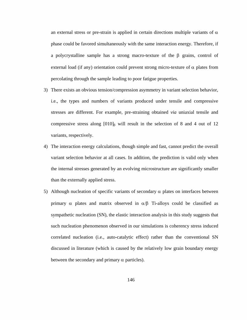
146
an external stress or pre-strain is applied in certain directions multiple variants of
phase could be favored simultaneously with the same interaction energy. Therefore, if
a polycrystalline sample has a strong macro-texture of the grains, control of
external load (if any) orientation could prevent strong micro-texture of plates from
percolating through the sample leading to poor fatigue properties.
3) There exists an obvious tension/compression asymmetry in variant selection behavior,
i.e., the types and numbers of variants produced under tensile and compressive
stresses are different. For example, pre-straining obtained via uniaxial tensile and
compressive stress along [010] will result in the selection of 8 and 4 out of 12
variants, respectively.
4) The interaction energy calculations, though simple and fast, cannot predict the overall
variant selection behavior at all cases. In addition, the prediction is valid only when
the internal stresses generated by an evolving microstructure are significantly smaller
than the externally applied stress.
5) Although nucleation of specific variants of secondary plates on interfaces between
primary plates and matrix observed in Ti-alloys could be classified as
sympathetic nucleation (SN), the elastic interaction analysis in this study suggests that
such nucleation phenomenon observed in our simulations is coherency stress induced
correlated nucleation (i.e., auto-catalytic effect) rather than the conventional SN
discussed in literature (which is caused by the relatively low grain boundary energy
between the secondary and primary particles).

147
6) Secondary plates having a misorientation of 60 1120
with the pre-existing (i.e.,
primary) ones (i.e. sharing a common 111 / / 1120
) tend to nucleate and grow on
the broad faces of the pre-existing plates, which could serve as an auto-catalytic
mechanism underlying the formation of basket-weave microstructures.
7) The stress-free transformation strain (SFTS) of precipitate varies with its coherency
state and variant selection rules (in terms of the sign and magnitude of elastic
interaction energy) are found different for coherent and semi-coherent precipitates.
When considering effect of primary plates whose sizes are usually above the
critical size for coherency (around 20 nm [59]), the SFTS for semi-coherent
precipitate should be employed for the primary precipitate while the SFTS for
coherent precipitate should be used for the nucleating secondary precipitates.
Applications of the model to study effects from other stress-carry defects such as
dislocations, stacking faults, grain boundaries, as well as effects from thermal stress on
variant selection during precipitation in polycrystalline samples are straight forwards
and corresponding work is underway.

148
Figures
Figure.4.1 Growth behavior of an plate. (a) Thickening kinetic of an infinite plate.
Results by phase field (symbol) and DICTRA (solid line) simulations are compared. (b)
Lengthening and (c) Thickening kinetics of a single finite plate embedded in a
supersaturated matrix. Error bars represent uncertainty in the determination of interface
position.
0.25 m
(a) (b) (c)
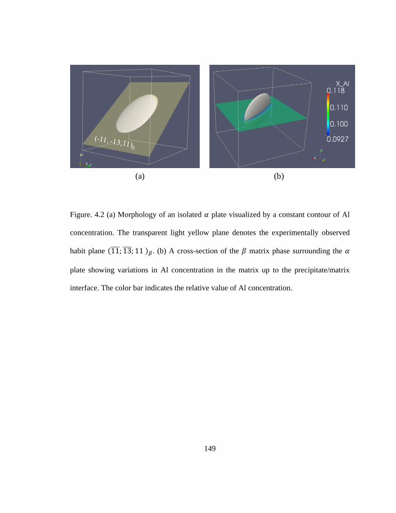
149
Figure. 4.2 (a) Morphology of an isolated plate visualized by a constant contour of Al
concentration. The transparent light yellow plane denotes the experimentally observed
habit plane . (b) A cross-section of the matrix phase surrounding the
plate showing variations in Al concentration in the matrix up to the precipitate/matrix
interface. The color bar indicates the relative value of Al concentration.
(a) (b)
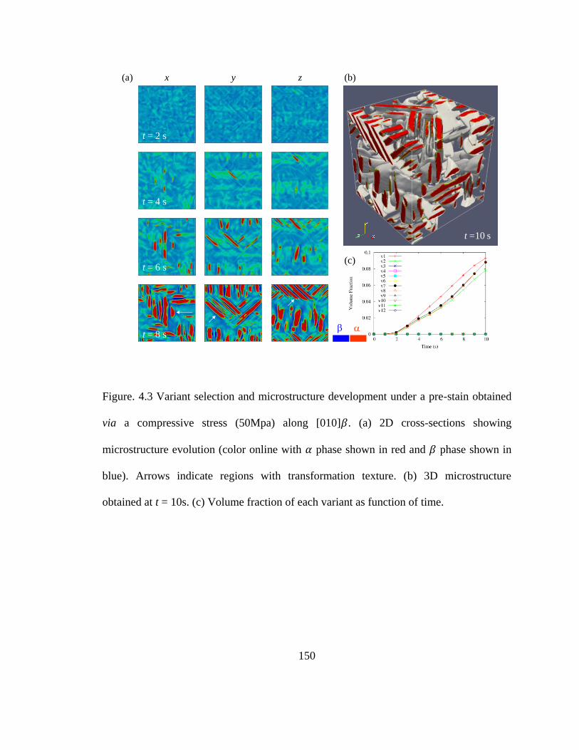
150
Figure. 4.3 Variant selection and microstructure development under a pre-stain obtained
via a compressive stress (50Mpa) along [010] . (a) 2D cross-sections showing
microstructure evolution (color online with phase shown in red and phase shown in
blue). Arrows indicate regions with transformation texture. (b) 3D microstructure
obtained at t = 10s. (c) Volume fraction of each variant as function of time.
x y z (b)(a)
t =10 s
(c)
t = 2 s
t = 4 s
t = 6 s
t = 8 s
151
Figure. 4.4 Variant selection and microstructure development under a pre-stain obtained
via a tensile stress (50Mpa) along [010] . (a) 2D cross-sections showing microstructure
evolution (color online with phase shown in red and phase shown in blue). Arrows
indicate regions with transformation texture. (b) 3D microstructure at t=10s. (c) Volume
fraction of each variant as a function of time
(b)(a) x y z
(c)
t =10 s
t = 2 s
t = 4 s
t = 6 s
t = 8 s
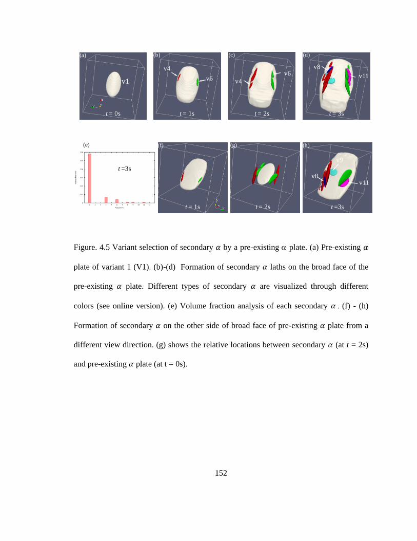
152
Figure. 4.5 Variant selection of secondary by a pre-existing plate. (a) Pre-existing
plate of variant 1 (V1). (b)-(d) Formation of secondary laths on the broad face of the
pre-existing plate. Different types of secondary are visualized through different
colors (see online version). (e) Volume fraction analysis of each secondary (f) - (h)
Formation of secondary on the other side of broad face of pre-existing plate from a
different view direction. (g) shows the relative locations between secondary (at t = 2s)
and pre-existing plate (at t = 0s).
(a) (c) (d)
(h)(e)
v11
v4
v6 v11
v8
v1
t = 0s t = 2s t = 3s
t =3s
t =3s
v4
v6
(b)
t = 1s
(g)
t = 2s
(f)
t = 1s
v9
v8
v9
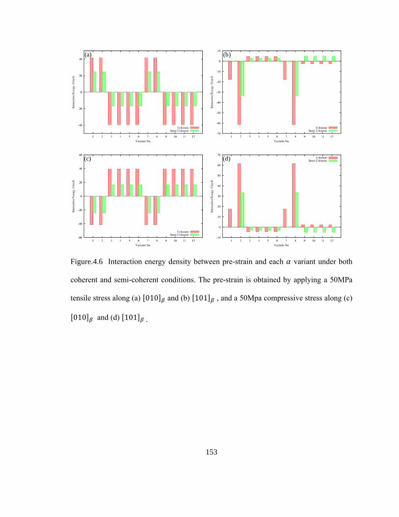
153
Figure.4.6 Interaction energy density between pre-strain and each variant under both
coherent and semi-coherent conditions. The pre-strain is obtained by applying a 50MPa
tensile stress along (a) [ ] and (b) [ ] , and a 50Mpa compressive stress along (c)
[ ] and (d) [ ]
(a) (b)
(c) (d)

154
Figure.4.7 Variant selection caused by a pre-stain obtained via uni-axial tension or
compression (50Mpa) along [ ] . Volume fraction of each variant as function of time
under tension (a) and compression (b). 3D microstructure (at t = 10s) under tension (c)
and compression (d).
t =10 s t =10 s
(a) (b)
(c) (d)
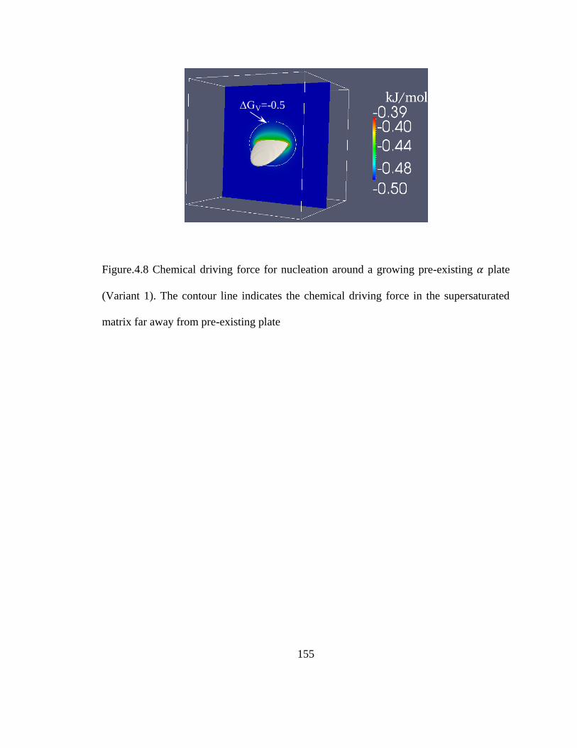
155
Figure.4.8 Chemical driving force for nucleation around a growing pre-existing plate
(Variant 1). The contour line indicates the chemical driving force in the supersaturated
matrix far away from pre-existing plate
∆GV=-0.5
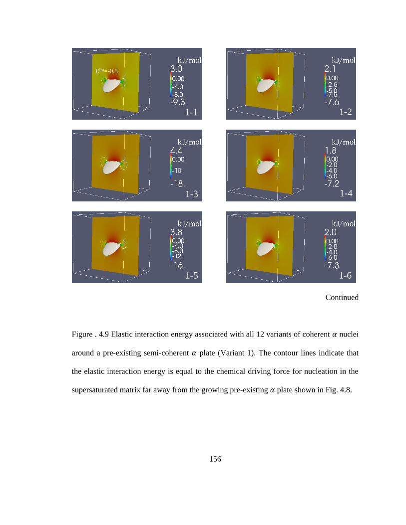
156
Continued
Figure . 4.9 Elastic interaction energy associated with all 12 variants of coherent nuclei
around a pre-existing semi-coherent plate (Variant 1). The contour lines indicate that
the elastic interaction energy is equal to the chemical driving force for nucleation in the
supersaturated matrix far away from the growing pre-existing plate shown in Fig. 4.8.
Eint=-0.5
1-1
1-3
1-5 1-6
1-4
1-2

157
Figure 4.9 continued
1-7 1-8
1-9
1-11 1-12
1-10

158
Continued
Figure. 4.10 Elastic interaction energy associated with all 12 variants of semi-coherent
laths around a pre-existing semi-coherent plate (Variant 1). The contour lines indicate
vanishing elastic interaction energy.
1-1 1-2
1-41-3
1-5 1-6
Eint=-0.0

159
Figure 4.10 continued
1-7
1-9
1-11 1-12
1-10
1-8

160
Fig. 4.11 (a) Elastic interaction energy between an nuclei (Variant 5) and a pre-existing
semi-coherent plate (Variant 1). (b) 1D structure order parameter profile (Blue) and
interaction energy (Red) along z-direction across ⁄ interface. It shows that the
maximum negative values of the elastic interaction energy are located right at the
⁄ interface.
Interaction V1-V5
Order parameter
Interaction Energy Eint
Maximum Eint
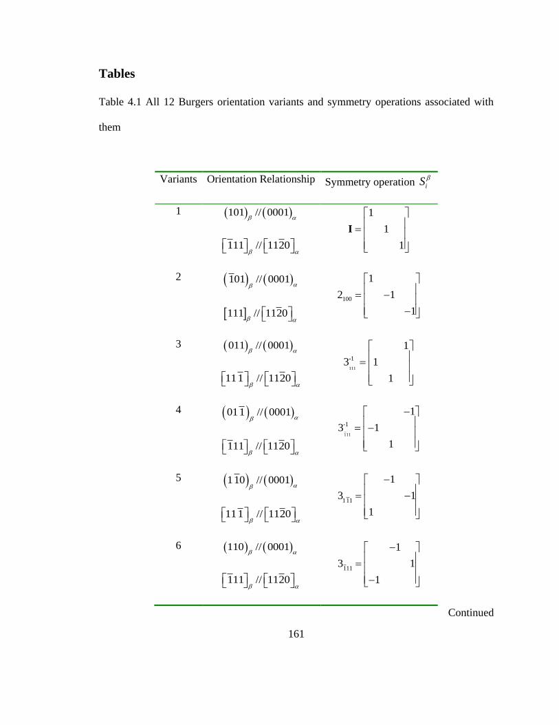
161
Tables
Table 4.1 All 12 Burgers orientation variants and symmetry operations associated with
them
Variants Orientation Relationship Symmetry operation iS
1 101 // 0001
111 // 1120
1
1
1
I
2 101 // 0001
111 // 1120
100
1
2 1
1
3 011 // 0001
111 // 1120
111
-1
1
3 1
1
4 011 // 0001
111 // 1120
111
-1
1
3 1
1
5 110 // 0001
111 // 1120
111
1
3 1
1
6 110 // 0001
111 // 1120
111
1
3 1
1
Continued

162
Table 4.1 continued
Variants Orientation Relationship Symmetry operation iS
7 101 // 0001
111 // 1120
010
1
2 1
1
8 101 // 0001
111 // 1120
001
1
2 1
1
9 011 // 0001
111 // 1120
111
-1
1
3 1
1
10 011 // 0001
111 // 1120
111
-1
1
3 1
1
11 110 // 0001
111 // 1120
111
1
3 1
1
12 110 // 0001
111 // 1120
111
1
3 1
1
uvwn denotes a n-fold rotation around axis uvw and superscript of -1
uvwn indicates inverse
of uvwn
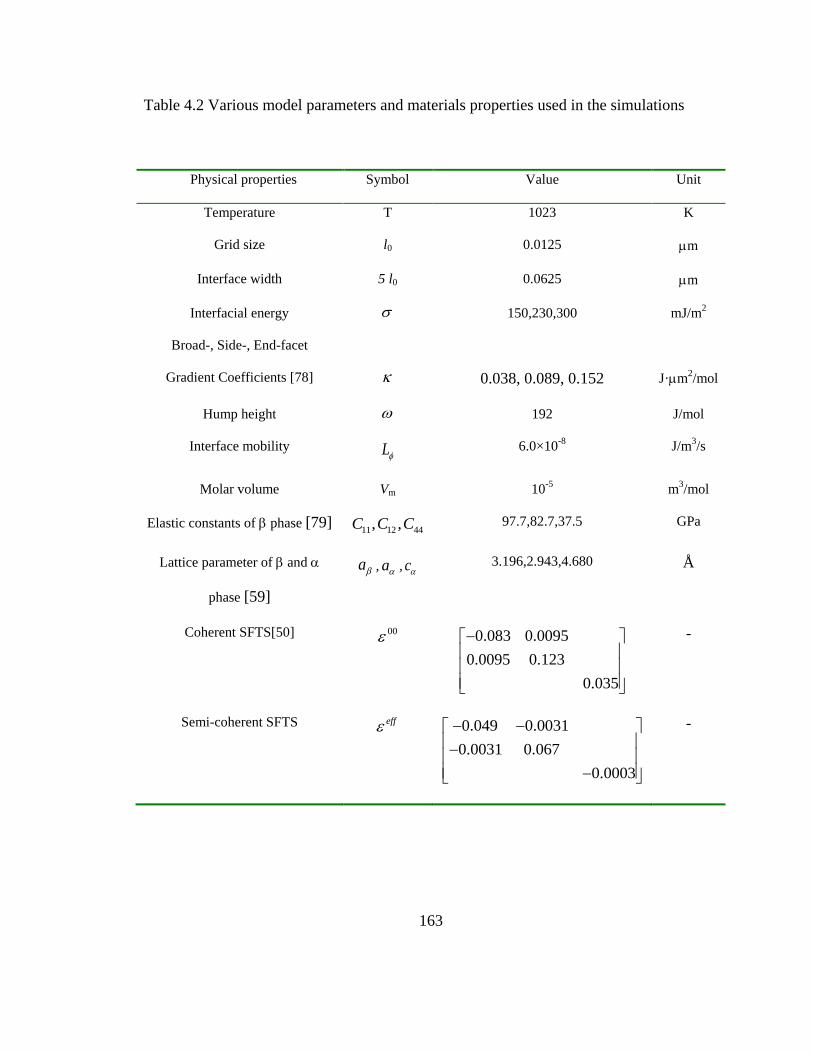
163
Table 4.2 Various model parameters and materials properties used in the simulations
Physical properties Symbol Value Unit
Temperature T 1023 K
Grid size l0 0.0125 m
Interface width 5 l0 0.0625 m
Interfacial energy
Broad-, Side-, End-facet
150,230,300 mJ/m2
Gradient Coefficients [78] 0.038, 0.089, 0.152 J·m2/mol
Hump height 192 J/mol
Interface mobility L 6.0×10⁻⁸
J/m3/s
Molar volume Vm 10-5
m3/mol
Elastic constants of phase [79] 11 12 44, ,C C C 97.7,82.7,37.5 GPa
Lattice parameter of and
phase [59]
a , a , c 3.196,2.943,4.680 Å
Coherent SFTS[50] 00 0.083 0.0095
0.0095 0.123
0.035
-
Semi-coherent SFTS eff 0.049 0.0031
0.0031 0.067
0.0003
-
164
4.6. References
[1] Lutjering G, Williams JC. Titanium (Engineering Materials and Processes).
Berlin: Springer, 2007.
[2] Geetha M, Singh AK, Asokamani R, Gogia AK. Ti based biomaterials, the
ultimate choice for orthopaedic implants - A review. Prog Mater Sci 2009;54:397.
[3] Froes FH. Titanium Alloys: Properties and Applications. In: Buschow KHJ,
Robert WC, Merton CF, Bernard I, Edward JK, Subhash M, Patrick V, editors.
Encyclopedia of Materials: Science and Technology. Oxford: Elsevier, 2001. p.9367.
[4] Purdy GR. Widmanstätten Structures. In: Editors-in-Chief: KHJB, Robert WC,
Merton CF, Bernard I, Edward JK, Subhash M, Patrick V, editors. Encyclopedia of
Materials: Science and Technology (Second Edition). Oxford: Elsevier, 2001. p.9575.
[5] Leyens C, Peters M, editors. Titanium and Titanium Alloys-Fundamentals and
Applications. Weinheim: WILEY-VCH, 2003.
[6] Ahmed T, Rack HJ. Phase transformations during cooling in alpha+beta titanium
alloys. Mater Sci Eng, A 1998;243:206.
[7] Burgers WG. On the process of transition of the cubic-body-centered
modification into the hexagonal-close-packed modification of zirconium. Physica
1934;1:561.
[8] Cahn JW, Kalonji GM. Symmetry in Solid-Solid Transformation Morphologies.
PROCEEDINGS OF an Interantional Conference On Solid-Solid Phase Transformations
1981:3.
165
[9] Peters M, Gysler A, LÜtjering G. Influence of texture on fatigue properties of Ti-
6Al-4V. Metall Mater Trans A 1984;15:1597.
[10] Bache MR, Evans WJ. Impact of texture on mechanical properties in an advanced
titanium alloy. Mater Sci Eng, A 2001;319-321:409.
[11] Bache MR, Evans WJ, Suddell B, Herrouin FRM. The effects of texture in
titanium alloys for engineering components under fatigue. Int J Fatigue 2001;23:153.
[12] Whittaker MT, Evans WJ, Lancaster R, Harrison W, Webster PS. The effect of
microstructure and texture on mechanical properties of Ti6-4. Int J Fatigue 2009;31:2022.
[13] Whittaker R, Fox K, Walker A. Texture variations in titanium alloys for
aeroengine applications. Mater Sci Technol 2010;26:676.
[14] Gey N, Humbert M, Philippe MJ, Combres Y. Investigation of the alpha- and
beta-texture evolution of hot rolled Ti-64 products. Mater Sci Eng, A 1996;219:80.
[15] Glavicic MG, Goetz RL, Barker DR, Shen G, Furrer D, Woodfield A, Semiatin
SL. Modeling of texture evolution during hot forging of alpha/beta titanium alloys.
Metall Mater Trans A 2008;39A:887.
[16] Bate P, Hutchinson B. The effect of elastic interactions between displacive
transformations on textures in steels. Acta Mater 2000;48:3183.
[17] van Bohemen SMC, Kamp A, Petrov RH, Kestens LAI, Sietsma J. Nucleation
and variant selection of secondary alpha plates in a beta Ti alloy. Acta Mater
2008;56:5907.
[18] Stanford N, Bate PS. Crystallographic variant selection in Ti-6Al-4V. Acta Mater
2004;52:5215.

166
[19] Bhattacharyya D, Viswanathan GB, Denkenberger R, Furrer D, Fraser HL. The
role of crystallographic and geometrical relationships between alpha and beta phases in
an alpha/beta titanium alloy. Acta Mater 2003;51:4679.
[20] Bhattacharyya D, Viswanathan GB, Fraser HL. Crystallographic and
morphological relationships between beta phase and the Widmanstatten and
allotriomorphic alpha phase at special beta grain boundaries in an alpha/beta titanium
alloy. Acta Mater 2007;55:6765.
[21] Furuhara T, Takagi S, Watanabe H, Maki T. Crystallography of grain boundary α
precipitates in a β titanium alloy. Metall Mater Trans A 1996;27:1635.
[22] Lee E, Banerjee R, Kar S, Bhattacharyya D, Fraser HL. Selection of alpha
variants during microstructural evolution in alpha/beta titanium alloy. Philos Mag
2007;87:3615.
[23] Moustahfid H, Humbert M, Philippe MJ. Modeling of the texture transformation
in a Ti-64 sheet after hot compression. Acta Mater 1997;45:3785.
[24] Gey N, Humbert M, Philippe MJ, Combres Y. Modeling the transformation
texture of Ti-64 sheets after rolling in the [beta]-field. Mater Sci Eng, A 1997;230:68.
[25] Kar S, Banerjee R, Lee E, Fraser HL. Influence of crystallography varaiant
selection on microstructure evolution in titanium alloys. In: Howe JM, Laughlin DE, Lee
JK, Dahmen U, Soffa WA, editors. Solid-Solid Phase Transformation in Inorganic
Materials 2005, vol. 1: TMS, 2005.
[26] Wang SC, Aindow M, Starink MJ. Effect of self-accommodation on alpha/alpha
boundary populations in pure titanium. Acta Mater 2003;51:2485.
167
[27] Furuhara T, Maki T. Variant selection in heterogeneous nucleation on defects in
diffusional phase transformation and precipitation. Mater Sci Eng, A 2001;312:145.
[28] Zeng L, Bieler TR. Effects of working, heat treatment, and aging on
microstructural evolution and crystallographic texture of [alpha], [alpha]', [alpha]'' and
[beta] phases in Ti-6Al-4V wire. Mater Sci Eng, A 2005;392:403.
[29] Winholtz RA. Residual Stresses: Macro and Micro Stresses. In: Buschow KHJ,
Robert WC, Merton CF, Bernard I, Edward JK, Subhash M, Patrick V, editors.
Encyclopedia of Materials: Science and Technology. Oxford: Elsevier, 2001. p.8148.
[30] Bate PS, Hutchinson WB. Imposed stress and variant selection: the role of
symmetry and initial texture. J Appl Crystallogr 2008;41:210.
[31] Li DY. Morphological evolution of coherent Ti11Ni14 precipitates under
inhomogeneous stresses. Philos Mag A 1999;79:2603.
[32] Guo W, Steinbach I, Somsen C, Eggeler G. On the effect of superimposed
external stresses on the nucleation and growth of Ni4Ti3 particles: A parametric phase
field study. Acta Mater 2011;59:3287.
[33] Wen YH, Wang Y, Chen LQ. Influence of an applied strain field on
microstructural evolution during the [alpha]2 --> O-phase transformation in Ti-Al-Nb
system. Acta Mater 2001;49:13.
[34] Zhou N, Shen C, Wagner MFX, Eggeler G, Mills MJ, Wang Y. Effect of Ni4Ti3
precipitation on martensitic transformation in Ti-Ni. Acta Mater 2010;58:6685.
[35] Wang Y, Li J. Phase field modeling of defects and deformation. Acta Mater
2010;58:1212.

168
[36] Chen L-Q. PHASE-FIELD MODELS FOR MICROSTRUCTURE
EVOLUTION. Annual Review of Materials Research 2002;32:113.
[37] Steinbach I, Pezzolla F, Nestler B, Seeßelberg M, Prieler R, Schmitz GJ, Rezende
JLL. A phase field concept for multiphase systems. Physica D 1996;94:135.
[38] Steinbach I, Pezzolla F. A generalized field method for multiphase
transformations using interface fields. Physica D 1999;134:385.
[39] Cahn JW, Hilliard JE. Free energy of a nonuniform system. I. Interfacial free
energy. The Journal of Chemical Physics 1958;28:258.
[40] Wheeler AA, McFadden GB. On the notion of a xi-vector and a stress tensor for a
general class of anisotropic diffuse interface models. P Roy Soc Lond a Mat
1997;453:1611.
[41] Wang Y, Wang H-Y, Chen L-Q, Khachaturyan AG. Microstructural Development
of Coherent Tetragonal Precipitates in Magnesium-Partially-Stabilized Zirconia: A
Computer Simulation. J Am Ceram Soc 1995;78:657.
[42] Wang YZ, Khachaturyan A. Microstructural Evolution during the Precipitation of
Ordered Intermetallics in Multiparticle Coherent Systems. Philos Mag A 1995;72:1161.
[43] Wu K, Chang YA, Wang Y. Simulating interdiffusion microstructures in Ni–Al–
Cr diffusion couples: a phase field approach coupled with CALPHAD database. Scr
Mater 2004;50:1145.
[44] Warren JA, Boettinger WJ. Prediction of dendritic growth and microsegregation
patterns in a binary alloy using the phase-field method. Acta Metall Mater 1995;43:689.

169
[45] Chen Q, Ma N, Wu KS, Wang YZ. Quantitative phase field modeling of
diffusion-controlled precipitate growth and dissolution in Ti-Al-V. Scr Mater
2004;50:471.
[46] Wang Y, Ma N, Chen Q, Zhang F, Chen SL, Chang YA. Predicting phase
equilibrium, phase transformation, and microstructure evolution in titanium alloys. Jom-
Us 2005;57:32.
[47] Khachaturyan AG. Some questions concerning the theory of phase
transformations in solids. Sov. Phys. Solid State 1967;8:2163.
[48] Khachaturyan AG. Theory of Structural Transformations in Solids. New York:
John Wiley & Sons, 1983.
[49] Khachaturyan AG, Shatalov GA. Elastic interaction potential of defects in a
crystal. Sov. Phys. Solid State 1969;11:118.
[50] Eshelby JD. The determination of the elastic field of an ellipsoidal inclusion, and
related problems. Proceedings of the Royal Society of London. Series A 1957;241.
[51] Bower AF. Applied Mechanics of Solids: CRC Press, 2009.
[52] Bollmann W. Crystal defects and crystalline interfaces. Berlin: Springer, 1970.
[53] Hall MG, Aaronson HI, Kinsma KR. The structure of nearly coherent fcc: bcc
boundaries in a Cu---Cr alloy. Surf Sci 1972;31:257.
[54] Pond RC, Ma X, Chai YW, Hirth JP. Topological Modelling of Martensitic
Transformations. Dislocations in Solids 2007;13:225.
170
[55] Pond RC, Celotto S, Hirth JP. A comparison of the phenomenological theory of
martensitic transformations with a model based on interfacial defects. Acta Mater
2003;51:5385.
[56] Furuhara T, Howe JM, Aaronson HI. Interphase boundary structures of
intragranular proeutectoid [alpha] plates in a hypoeutectoid Ti---Cr alloy. Acta Metall
Mater 1991;39:2873.
[57] M. J. Mills, D. H. Hou, S. Suri, Viswanathan GB. Orientation relationship and
structure of alpha/beta interface in conventional titanium alloys. In: R. C. Pond, W. A. T.
Clark, King AH, editors. Boundaries and Interfaces in Materials: The David A. Smith
Symposium: The Minerals, Metals & Materials Society, 1998, 1998. p.295.
[58] Ye F, Zhang WZ, Qiu D. A TEM study of the habit plane structure of
intragrainular proeutectoid alpha precipitates in a Ti-7.26wt%Cr alloy. Acta Mater
2004;52:2449.
[59] Shi R, Ma N, Wang Y. Predicting equilibrium shape of precipitates as function of
coherency state. Acta Mater 2012;60:4172.
[60] Mura T. Micromechanics of Defects in Solids,. Dordrecht: Martinus Nijhoff,
1982.
[61] Read WT. Dislocations in crystals. New York: Jr. McGraw-Hill, 1953.
[62] Read WT, Shockley W. Dislocation Models of Crystal Grain Boundaries. Phys
Rev 1950;78:275.
[63] Cahn JW. On spinodal decomposition. Acta Metall 1961;9:795.

171
[64] Gunton J. D., Miguel M. S., P.S. S. The dynamics of first-order phase transitions.
In: Domb C, L. LJ, editors. Phase transitions and critical phenomena, vol. 8, vol. 8. New
York: Academic Press, 1983.
[65] Andersson J-O, Agren J. Models for numerical treatment of multicomponent
diffusion in simple phases. J Appl Phys 1992;72:1350.
[66] Kim SG, Kim WT, Suzuki T. Phase-field model with a reduced interface
diffuseness. J Cryst Growth 2004;263:620.
[67] Kim SG, Kim WT, Suzuki T. Phase-field model for binary alloys. Phys Rev E
1999;60:7186.
[68] http://www.paraview.org/.
[69] Zener C. Trans. AIME 1946;167:950.
[70] Hillert M. Jernkontorets Annaler 1957;141.
[71] Semiatin SL, Kinsel KT, Pilchak AL, Sargent GA. Effect of Process Variables on
Transformation-Texture Development in Ti-6Al-4V Sheet Following Beta Heat
Treatment. Metall Mater Trans A 2013; online at 17 April 2013
[72] Aaronson HI, Enomoto M, Lee JK. Mechanisms of diffusional phase
transformations in metals and alloys: CRC Press New York, 2010.
[73] Enomoto M. Computer modeling of the growth kinetics of ledged interphase
boundaries—I. Single step and infinite train of steps. Acta Metall 1987;35:935.
[74] Enomoto M. Computer modeling of the growth kinetics of ledged interphase
boundaries—II. Finite train of steps. Acta Metall 1987;35:947.
172
[75] Madangopal K, Singh JB, Banerjee S. The nature of self-accommodation in Ni
Ti shape memory alloys. Scripta Metallurgica et Materialia 1993;29:725.
[76] Menon ESK, Aaronson HI. Overview no. 57 Morphology, crystallography and
kinetics of sympathetic nucleation. Acta Metall 1987;35:549.
[77] Aaronson HI, Spanos G, Masamura RA, Vardiman RG, Moon DW, Menon ESK,
Hall MG. Sympathetic nucleation: an overview. Mater Sci Eng, B 1995;32:107.
[78] Spanos G, Fang HS, Aaronson HI. A mechanism for the formation of lower
bainite. Metall Trans A 1990;21:1381.
[79] Russell KC. Nucleation in solids. Phase transformations. Metals Park, OH: ASM,
1970. p.219.
[80] Shen C, Simmons JP, Wang Y. Effect of elastic interaction on nucleation: I.
Calculation of the strain energy of nucleus formation in an elastically anisotropic crystal
of arbitrary microstructure. Acta Mater 2006;54:5617.
[81] Shen C, Simmons JP, Wang Y. Effect of elastic interaction on nucleation: II.
Implementation of strain energy of nucleus formation in the phase field method. Acta
Mater 2007;55:1457.
[82] Gao Y, Zhou N, Yang F, Cui Y, Kovarik L, Hatcher N, Noebe R, Mills MJ, Wang
Y. P-phase precipitation and its effect on martensitic transformation in (Ni,Pt)Ti shape
memory alloys. Acta Mater 2012;60:1514.
[83] Wang Y, Khachaturyan AG. Three-dimensional field model and computer
modeling of martensitic transformations. Acta Mater 1997;45:759.
173
[84] Teng CY, Zhou N, Wang Y, Xu DS, Du A, Wen YH, Yang R. Phase-field
simulation of twin boundary fractions in fully lamellar TiAl alloys. Acta Mater
2012;60:6372.
174
CHAPTER 5 Evolution of Microstructure and Transformation
Texture during Alpha Precipitation in Polycrystalline Titanium alloys
Abstract:
A previously developed three-dimensional phase field model of transformation in
single crystal Ti-6Al-4V is extended to polycrystals to study variant selection and
microstructure evolution under the influence of different processing conditions such as
pre-straining and boundary constraint. Effect of starting texture is also investigated.
Degrees of variant selection at both the individual grain and the whole polycrystalline
sample levels and their effects on the final macro-texture of precipitates are analyzed.
In particular, the effect of non-uniform local stress state, arising from elastic
inhomogeneity of a polycrystalline sample under a uniform external strain (thermal or
applied), on the variant selection behavior within individual grains is addressed. It is
found that when subjected to certain pre-strains, a sample having strong starting texture
could end up with a relatively small degree of micro-texture when local stresses
associated with the pre-strains promote multiple variants simultaneously within the
whole polycrystalline sample. The results could shed light on how to control processing
conditions to reduce transformation texture at both the individual grain and the overall
polycrystalline sample levels.
175
5.1. Introduction
Titanium and its alloys are currently finding increasingly wide application in the
aerospace, shipbuilding, automotive, sports, chemical and food processing industries due
to their desirable and versatile combination of good mechanical and chemical properties
such as extreme lightness, high specific strength and good corrosion resistance [1, 2].
Depending on the application, a specific property (or combination of properties) can be
obtained through tailoring / microstructure whose evolution and control depends
heavily on the allotropic transformation from phase (BCC structure) at high
temperature to phase (HCP structure) found at low temperatures [3]. The defining
characteristic of the transformation is the Burgers orientation relationship (BOR) [4]
between the two phases, i.e. { } and ⟨ ⟩ [ ] . Owing to the
symmetry of the parent and product phases and the BOR between them [5], there are
twelve possible crystallographically equivalent orientation variants of the phase within
a single parentgrain. If all 12 variants are able to form within each grain, the
resulting microstructure would be relatively fine, with large amount of boundaries,
and transformation texture would be relatively weak since matrix and its orientation
density needs to be partitioned by all 12 variants of phase. However, it is typically the
case that only a small subset of the 12 possible variants is formed preferentially within
each beta grain under different thermo-mechanical processing (TMP), i.e. combination of
working and heat treatment. In other words, variant selection occurs frequently, resulting

176
in a relative coarse microstructure with final texture of phase with various
strengths.
The statistical and spatial distribution of each orientation variants then determines the
texture state of alpha phase during the transformation. Since the sources of strength in
titanium is the barrier to dislocation movement represented by hetero-phase
interface, the density and orientation of hetero-phase interfaces, and their spatial
uniformity determine the deformation mechanisms and mechanical behavior of the alloys
[1, 6]. Variant selection, due to a wide variety of factors during TMP, would lead to the
formation of large regions of phase with a common crystallographic feature (such as
common basal pole, or common orientation), i.e. “macro-zone” or micro-
textured region, within individual grain or across grain boundaries, and thus would
result in a significant reduction in fatigue life of Ti-component that is undesirable in a
safety critical operating environment [7]. Consequently, understanding and thus control
of alpha phase size, morphology, and distribution including that of its orientation
variants, i.e. microstructure and texture state, under the influence of variant selection, are
of fundamental importance in control and tailoring the properties of titanium alloys[1, 6].
During TMP, there exists a rich variety of sources that are able to result in local stresses
and lead to variant selection within a sample during TMP. In other words, the
development of local stress could not be avoided during TMP. For instance, owing to the
anisotropy of thermal expansion coefficient of the phase (which is 20% larger than in

177
the ⟨ ⟩ than in the ⟨ ⟩ directions), substantial residual stresses are common in Ti
alloys even after a stress relief annealing treatment [8-10]. Moreover, defects such as
dislocations and stacking faults generated during TMP in either or phase region act
frequently as preferred nucleation sites for specific subset of variants[11-14]. Local
stress fields will also be generated by precipitation and autocatalysis has been shown
frequently to result in variant selection [15, 16]. Furthermore, for polycrystalline
materials under an external stress or strain field, local stress state within the sample will
vary significantly from grain to grain because of the elastic anisotropy in each grain that
leads to elastic inhomogeneity in the sample [17]. It is clear that the local stress state, due
to a rich variety of sources, is a key factor in controlling variant selection and hence the
final transformation texture during precipitation in Ti alloys.
Nevertheless, the main challenges to study variant selection during
transformations in polycrystalline sample under the influence of stress are three-folds:
first, one needs to determine stress distribution in an elastically anisotropic and
inhomogeneous polycrystalline matrix under a given applied stress/strain condition;
and second, one needs to describe interactions of local stress with precipitation of
coherent and semi-coherent precipitates, i.e., to describe interactions of local stress with
an evolving microstructures. In particular, defects structure, including misfit
dislocations and structural ledges, at the interfaces will alter not only the coherency
elastic strain energy associated with the precipitation, but also the interfacial energy
178
and its anisotropy. It could introduce growth anisotropy as well. These anisotropies,
together with the high volume fraction and multi-variants of the precipitate phase and
long-range elastic interactions between the precipitates and local stress, and among
precipitates themselves, lead to highly non-random spatial
distribution of precipitates with different variants. Third, in order to provide new insight
into materials processing- microstructure- properties relationship, microstructure and
texture needs to be considered together. In other words, variant selection behavior at the
scale of individual parent grains and scale of the whole polycrystalline sample, and their
influence on the microstructure evolution and final transformation texture need to
be considered simultaneously. In sum, variant selections depend on a wide variety of
interaction parameters and thus are very complex. Owing to this complexity, the
mechanisms of variant selection are very difficult to determine experimentally. And,
existing modeling attempts have been only taking care of one or two parameters.
Based on gradient thermodynamics [18-20] and microelasticity theory [21-25], the phase
field approach [26-32] (also called the diffuse-interface approach) offers an ideal
framework to deal rigorously and realistically with these difficult challenges. As has been
demonstrated in a recent phase field simulation study of the transformation in Ti-
6Al-4V (in wt%) [33, 34], the formulation of the total free energy functional, which
consists of the bulk chemical free energy, elastic strain energy and interfacial energy, has
accounted for the following: (a) a reliable thermodynamic data for the bulk chemical free
energy for Ti-6Al-4V system [34, 35]; (b) crystallography of the crystal lattice

179
rearrangement, including orientation relationship, i.e. BOR, and lattice correspondence
(LC) as functions of the lattice parameters of the precipitate and parent phases (i.e., the
effect of alloy chemistry); (c) accommodation of the transformation strain; (d)
development of defect structures (misfit dislocations and structural ledges) at
interfaces as precipitates grow in size; (e) elastic interaction of nucleating particles with
existing chemical and structural non-uniformities and other stress-carrying defects such
as dislocations [36]. In particular, in combination with orientation distribution function
(ODF) modeling [37] of the simulated microstructures, the phase field model allows
for a treatment of both micro- and macro-texture evolution accompanying the
microstructure evolution during different thermo-mechanical treatments, as we shall
discussed in greater details in the following sections.
The main objective is to explore the effect of different processing route on both
microstructure and transformation texture evolution. The paper is organized as the
following. In section 2, we first make an extension of a 3D quantitative phase field model
[33, 36] formulated by the authors to investigate both microstructure and texture
evolution in during precipitation in polycrystalline Ti-alloys. In Section 3, the model is
employed investigate variant selection behavior (i.e. degree of variant selection) under
the influence of different pre-strain, starting texture, and the type of boundary
constraint of the sample, and its effect on the evolution both microstructure and final
alpha texture in polycrystalline sample. The results will be analyzed in Section 4 via
considering variant selection behavior at the scale of both individual b grain and
polycrystalline sample. Main findings will be summarized in Section 5.

180
5.2. Model Formulation
5.2.1. Polycrystalline sample
In the current work, we consider a polycrystalline matrix that is assumed to be formed
by a periodical repetition of M grains that occupy a computation cell of 128×128×128.
Different grains have different orientations. An orientation, often given the letter , of
grain or crystal in sample reference frame can be described by the rotation matrix
between crystal and sample co-ordinates. In practice, it is convenient to describe the
rotation by a triplet of Euler angles, e.g. [ ] by Bunge [37]. A rotation
matrix field is then introduced to describe the polycrystalline structure [38],
where assumes a constant value but different within each grain depending on
its orientation.
5.2.2 Phase Field Model for precipitation in an elastically and structurally
inhomogeneous polycrystalline sample
In this section, we extend a three-dimensional quantitative phase field model developed
by current authors to predict variant selection and microstructure evolution during

181
transformation in polycrystalline Ti–6Al–4V (wt.%) sample under the influence
of pre-strain or external stress .
5.2.2.1 Chemical free energy for polycrystalline system
Arbitrary two-phase microstructure in polycrystalline parent sample includes both
structural and chemical non-uniformities. For Ti-Al-V ternary system, two conserved
phase field parameters, Al, VkX k r , are required to describe the chemical non-
uniformities of components Al and V in the system. At the scale of individual grain,
twelve non-conserved order parameters, , 1,2,..., 12p p N r , are needed to
describe the structural non-uniformities associated with the total N OVs. One more
dependent order parameter, , 13p p r , is also introduced to describe the spatial
distribution of the matrix phase with grain. In the frame work of multi-phase field
model, such all non-conserved order parameters are subjected to the constraint that
1
1
, 1N
p
p
r [39, 40]. For a polycrystalline consisting of grain, the number of non-
conserved order parameters to describe the spatial distribution of phase is .
The total free energy of such a system having an arbitrary coherent or semi-coherent
two-phase microstructure, including both chemical and structural non-uniformity, is
formulated on the basis of the gradient thermodynamics [18]. The chemical free energy
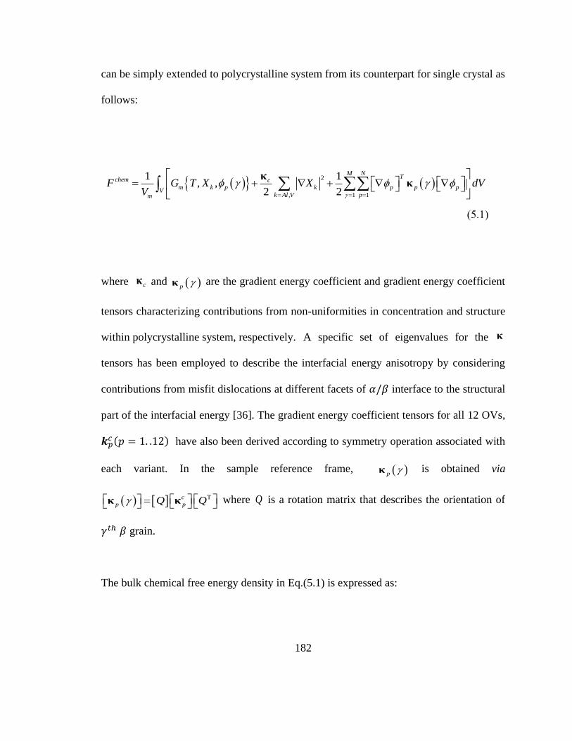
182
can be simply extended to polycrystalline system from its counterpart for single crystal as
follows:
Equation Chapter 5 Section 1
2
, 1 1
1 1, ,
2 2
M NT
chem cm k p k p p p
Vk Al V pm
F G T X X dVV
κκ
(5.1)
where and p κ are the gradient energy coefficient and gradient energy coefficient
tensors characterizing contributions from non-uniformities in concentration and structure
within polycrystalline system, respectively. A specific set of eigenvalues for the
tensors has been employed to describe the interfacial energy anisotropy by considering
contributions from misfit dislocations at different facets of interface to the structural
part of the interfacial energy [36]. The gradient energy coefficient tensors for all 12 OVs,
have also been derived according to symmetry operation associated with
each variant. In the sample reference frame, p κ is obtained via
Tc
p pQ Q κ κ where Q is a rotation matrix that describes the orientation of
grain.
The bulk chemical free energy density in Eq.(5.1) is expressed as:
cκ
κ

183
, ,
1 1 1 1
1
1
, , , 1 ,
M N M N
m k p p m Al V p m Al V
p p
M N N
pq p q
p q p
G T X h G T X h G T X
(5.2)
where, 3 26 15 10p p p ph is an interpolation function connecting
the free energy surface (as function of concentration and temperature) of and phase.
The term 1
1
N N
pq p q
p q p
introduces a hump on the free energy surface between
either variant and 𝑞, or variants and matrix, and hump height is proportional to
pq . ,,m Al VG T X and ,,m Al VG T X are the equilibrium molar free energies of and
phases as function of temperature and individual phase concentration ,Al VX and
,Al VX ,
respectively.
5.2.2.2. Strain energy of an elastically and structurally inhomogeneous system
Polycrystalline sample with two-phase microstructure is a typical elastically and
structurally inhomogeneous system. The system is characterized by an arbitrary
distribution of the crystalline lattice misfit strain, T
ij r , (transformation strain due to
precipitation), and an inhomogeneous distribution of elastic modulus ( )ijklC r due to of
184
elastic anisotropy and different orientations of individual grains, i.e., both ( )ijklC r and
T
ij r are functions of spatial coordinate r . Elastic strain energy of such an system
under external loading or pre-strain, ( ), , el T appl
ijkl ij ijE C r r , is obtained using the
iterative method developed by Wang et al. [17, 41]. By introducing a virtual strain field
0 ( )ij r and a reference modulus 0
ijklC , the exact elastic equilibrium, including total strain
and stress distributions, of an elastically and structural inhomogeneous system are
obtained [17, 41] by solving the elasticity problem in an equivalent elastically
homogeneous system. 0 ( )ij r is an energy minimizer of the total strain energy functional
that determines the equilibrium state of the elastically and structurally inhomogeneous
system. In practice, it can be obtained numerically through a solution of the time-
dependent Ginzburg-Landau (TDGL) type equation [41],
0
0
( , )
( , )
elij
ijkl
kl
EL
r
r (5.3)
where elastic strain energy of the system, elE , is given by:

185
0 0 0 0 0 3
0 0 0 3 0 0 3 0
1( ) ( )
2
1( ) ( ) ( )
2 2
1
2
el T T
V ijmn mnpq pqkl ijkl ij ij kl kl
V ijkl ij kl ij V ijkl kl ijkl ij kl
E C S C C d
VC d C d C
r r r r r r
r r r r r
3
0 0
3( ) ( ) ( )*
(2 )i ij jk kl l
dn n
gg n g
(5.4)
where ijklL is the kinetic coefficient tensor (a convenient choice is
10
ijkl ijklL L C
[42])
and the parameter describes the elastic relaxation process. In Eq.(5.4),
1
0
ijkl ijkl ijklS C C
r r .In order to ensure the convergence [43], 1
0
ijklL C
has been
chosen to be 1
0
ijnm mnklL C C
r during the iteration of Eq (5.3). Elastic inhomogeneity
rijklC defined in the sample reference is then described by
0T T T T
ijkl ip jq km nl pqmnC Q Q Q Q Cr r r r r , where stands for the transpose operator.
Einstein’s summation convention for repeated indices is assumed throughout.
0 0 0( )ij ijkl klC g g , 0
ij g is the Fourier transform of 0
ij r , 1 0
ij ijkl k lC n n n , and the
superscript asterisk denotes the complex conjugate. The last integral in Eq. (5.4)(?)
excludes a volume of 3
2 V around the point at g=0 . is the th component
of a unit vector , ⁄ ,in the reciprocal space. The strain energy in the form in
Eq. (5.4) is convenient when the body is fully clamped and thus its macroscopic
deformation is specified by the pre-strain appl
ij . The strain energy in Eq.(5.4) needs to be
modified if the macroscopic deformation of the body is controlled by the applied external
stress, appl
ij . In this case, the macroscopic shape is obtained by allowing the body to

186
relax at fixed appl
ij to minimize the strain energy with respect to ij . The energy
minimization is obtained when minimizer : 0 0 appl
ij ij ijkl ijS = + , 0 0 31
( )ij klV
dV
r r .
From Eq.(5.4), it is obvious that the stress-free transformation strain T
ij r from
precipitates in a whole system is a critical input in formulating the strain energy for such
an inhomgeneous system. In the sample reference frame, T
ij r is formulated upon
spatial distribution of the transformation strain field:
000
1 1
, ,M N
T
ij ij p
p
p
r r (5.5)
as a linear combination of individual phase field order parameter within each b grain,
,p r . 000 ,ij p is the SFTS tensor of variant in grain expressed in the
sample reference frame. It can be obtained through 000 00, T T
ij ik jl klp Q Q p
,where 00
kl p denotes SFTS tensor of variant in the crystal reference frame.
Thus, the elastic equilibrium is obtained through the converged value of the virtual misfit
strain 0 ( )rij in Eq.. Then, the total strain in the system is:
1
2ij ij r
30
32
i
i jk j ik kl l
dn n n e
g rg
n n g (5.6)
187
And the stress distribution ( )ij r in the polycrystalline system can be obtained through
0 0
ij ijkl kl klC r r r .
The elastically and structurally inhomogeneous polycrystalline sample during
precipitation is then equivalent to an elastic homogeneous system with modulus 0
ijklC with
the equilibrium internal stress distribution described by Eq. (5.3).
5.2.2.3 Kinetic equations
The temporal and spatial evolutions of both concentration and structural order
parameters, i.e. microstructure evolution, are governed by the Cahn-Hilliard equation and
the time-dependent Ginzburg-Landau equation, respectively. For simplicity, the
diffusion along grain boundaries and within bulk is treated as the same. The diffusion
equation is then the same as that within a single grain [36], i.e.
1
21
,1, , ,
,
nk
kj i j k
jm j
X t FM T X t
V t X t
rr
r (5.7)
There are total 1M N order parameters for precipitate in the polycrystalline
system and the governing equation is given as [38]:
188
, , 1, ,
, , , , , ,
elp
p
p q p q p
t F F EL t
t t t t
r
r rr r r
(5.8)
where , r defines the shape of individual grain that is equal to unity inside the th
grain and vanishes outside of it. 1...12, ,kj iM T X is the chemical mobility, L is the
mobility of the long-range order parameters characterizing interface kinetics, and k and
p are the Langevin noise terms for composition and long-range order parameter,
respectively. In Eq. (5.8), is the number of phases that co-exist locally.
It needs to be mentioned that the variation of the strain energy with respect to order
parameter is calculated based on the assumption that elastic relaxation occurs much faster
than precipitation. That is, the time-dependent Ginzburg-Landau equation Eq. (5.3) is
solved first to obtain a steady-state solution for the virtual strain 0
ij r with a clamped
order parameter and concentration field. In addition, it is also assumed that there would
be no grain growth within the polycrystalline sample. The effective strain and
inhomogeneous elastic modulus ijklC r is then treated as a constant in the calculation of
the functional variation of the strain energy with respect to order parameter field ,p r .
189
el
0 0 0 0
0 3
,
( ) ,
( ) , r1
2 ,
p
T
V ijmn mnpq pqkl ijkl ij ij p
T
kl kl p
p
E
C S C C
d
r
r r r
r r
r
(5.9)
All the parameters for the model and materials properties can be referred to Ref. [36].
5.2.3 Orientation Distribution Function modeling of microstructure in
polycrystalline sample
It has been realized that when characterizing titanium in general, texture should not be
ignored since its influence on mechanical properties can be significantly strong in
polycrystalline Ti-alloys due to low symmetry α phase with strong anisotropy in
properties. Therefore, microstructure and texture needs to linked together to obtain new
insight to materials processing.
Orientation of crystals in a polycrystalline is measured by individual orientation
measurements using a virtual electron back-scattered diffraction EBSD. A total of
individual orientations are measured. The orientation density of individual orientations of
grain in a polycrystalline sample describes starting texture. Similarly, the orientation
density of individual orientation variants represents its texture. To permit a quantitative

190
evaluation of textures for both phases, it is necessary to describe the orientation density
of each phase in a polycrystalline in an appropriate 3-D representation, that is, in terms of
its orientation density function (ODF) [44]. The ODF is defined as a probability density
function of orientation that models the relative frequencies of crystal orientations
within the specimen by volume [37]. Mathematically, the ODF is defined by the
following relationship:
dV
f g dgV
(5.10)
where is the sample volume and is the volume of all crystalline with the orientation
in the angular element . To be specific, ⁄ is the volume
of the region of integration in orientation space. Choice of such that ∫ to
normalize the ODF implies that the uniform random ODF, , which is then
consistent with the custom of expressing in terms of multiples of the uniform
random ODF (M.R.D.).
The ODF estimation from individual EBSD data in MTEX is implemented using the
function . The underlying statistical method is called kernel density estimation,
which can be interpreted as a generalized histogram. To be more precisely, assume be
a radially symmetric, unimodal model ODF [45]. Then the kernel density estimator for
the individual orientation data is defined as:

191
∑
The choice of the model ODF and in particular its half width has a great impacting in
the resulting ODF.
Experimentally, pole figures are frequently used to represent textures. The pole density
function (PDF) of a specimen models the relative frequencies of specific lattice plane
orientations , i.e. the relative frequencies of normal vectors of specified lattice planes,
within the specimen volume. For example, a pole that is defined by the direction in a
given 2-D pole figure, , corresponds to a region in the 3D-ODF that contains
all possible rotations with angle about this direction in the pole figure.
∫
where { } is the position of a given pole on the reference sphere.
The angle describes the azimuth of the pole and the angle characterizes the rotation
of the pole around the polar axis[44]. When ODF is obtained, pole figure for a set
specific plane can be readily obtained. For convenience, the freely available MTEX
Matlab Toolbox for Quantitative Texture Analysis [46] is utilized to make all pole
figures. As will be shown latter, a comparison of the alpha- and beta-phase textures,
represented respectively by and { } pole figures, is able to quantify
preferential variant selection during transformation due to BOR between two
phases.
192
5.3. Results
5.3.1. Starting polycrystalline and texture
A polycrystalline sample of Ti-6Al-4V (Fig. 5.1(a)) is first created by the Voronoi
algorithm [47] and, further relaxed by a phase field grain growth code [48] to obtain
equilibrium junctions among grains. The orientation of each beta grain with respect to
the sample reference is specified by a set of Euler angler [ ] using the Bunge
notation [37]. The estimation of orientation distribution functions (ODFs) of texture is
then made from sampled individual orientation data using MTEX Quantitative Texture
Analysis Software [46]. The chosen kernel is a de la Vallée Poussin kernel with a
smoothing half-width of 5 deg. The beta texture is then represented by { } pole
figures as shown in Fig. 1(b), whose intensity contours are represented in times-random
units. Since the starting texture of the grains may have a strong influence on the
transformation texture of the phase because of the BOR between the two phases, two
sets of initial texture are considered in the current study. One is a relatively random
texture referred to as “random-textured” sample and the other one has a relatively strong
texture and is referred to as “strong-textured” sample. Their textures are represented by
{ } pole figures shown in Fig. 5.1(b) and 5.1(c), respectively. As can be seen from
the pole figures, the strong-textured sample has a relatively larger maximum pole
intensity of the { } pole than that of the random-textured one.
193
5.3.2. Evolution of microstructure and texture during precipitation
Evolution of microstructure during precipitation is obtained by solving Eq. (5.7)
and Eq. (5.8) simultaneously. In case of clamped boundary without any pre-strain
(referred to as fix-end) in “random-textured” sample, microstructure evolution during
precipitation is shown Fig. 2 through (a)-(c). The red color represents phase, while blue
color denotes matrix phase. In particular, the matrix is set be transparent to make the
precipitation visible within the bulk. The white lines indicate the locations of grain
boundaries. It is clearly that nucleation of a phase occurs not only near grain boundaries
but also within the bulk. phase gradually fills the whole polycrystalline sample as
shown if Figs 2(b)-(c). Formation of closed-triangle pattern is also observed, as pointed
out by an arrow in Fig. 2(c).
In order to quantify the texture evolution during precipitation, a virtual EBSD scan is
preformed through the sample to read in orientation information of
individualprecipitates according to the index of the variants [36] and orientation of
its matrix grain based on BOR. The ODFs for phase are obtained using the same
approach as that used in describing texture [49]. The final textures are represented
by the pole figures as shown in Fig. 2(a′)-(c′). By comparing with { } pole
of starting texture (Fig. 5.1(b)), pole figures had similar locations of intensity
maxima, confirming the validity of the Burgers relationship during the decomposition of
the phase. The strength of the transformed texture is simply represented by the
194
texture-component maxima in these pole figures. It is found that maximum pole intensity
in pole figures larger than that in { } pole figure representing starting
texture, and the maxima is increasing, from 10.04 to 10.45, due to coarsening.
5.3.3. Effect of pre-strain on variant selection
In “random-textured” sample, when a pre-strain is introduced by a compressive stress,
50MPa, that is applied along the x-axis of the sample before the system’s boundary is
clamped, as we can seen clearly, nucleation of phase in different grains tend to occur at
grain boundaries as shown in Fig. 3(a). Formation of closed-triangle pattern is also
observed, as pointed out by an arrow in Figs.3(c)-(d). Precipitation behavior varies
significantly from one to another grain. For example, in some grains, multiple
variants are favored simutanously; while in other grains, only a limited number of
variants survive. The corresponding texture evolution of phase represented by
pole figures is shown through Figs. 3(a′)-(d′). When compared with { } pole of
starting texture (Fig. 5.1(b)), pole figures have much less number of intensity
maxima. In particular, there are clear quantitative differences in the intensities at specific
locations, which suggest orientation densities of parent phase are shared by only
limited numbers of variants in different grains. The strength of the transformation
texture is found to decrease with precipitation. The maxima of intensity in
pole figures decrease from 39.05 ( random) at 1.5 s to 23.2 ( random) at 9.0 s. While

195
in the mean time, several new texture components within the basal poles appear with
precipitation as pointed out by red arrows from Figs. 3(b)-(d). The evolution of texture
suggests that more variants come out during precipitation.
For “random-textured” sample, different pre-strains have been introduced to the sample
to investigate their influences on both microstructures and final texture. Pre-
strains are generated by applying a 50Mpa tensile/compressive along x, and z direction of
the sample that are referred to as x-comp, x-tensil, z-comp, and z-tensil, respectively. As
can been seen clearly from Fig. 4(a)-(d), when subjected to different pre-strain, final
microstructure at t =10.0 s are quite different in the sample in terms of numbers and types
of orientation variants within individual grains. So do the final textures in terms of
numbers of maxima, intensities and locations of maxima, Fig. 4(a′)-(d′).
5.3.4. Effect of starting texture on variant selection
Both grain-boundary geometry and parent texture would change due to grain growth or
hot deformation in phase region [8, 50]. Such grain growth may result in the weakening
of initial-stronger texture component and also the strengthening of initially-weaker
texture [51]. Thus, it has been noticed that preferential variant selection needs to be
interpreted according to the specific starting texture right prior to decomposition. In
order to focus to the effect of starting texture on variant selection, we consider a strong-
textured sample (Fig. 5.1(c)) with the same grain geometry as that of the random-
textured sample. Pre-strains are also generated by applying a 50Mpa tensile/compressive

196
along x, and z direction of the sample that are also referred to as x-comp, x-tensil, z-comp,
and z-tensil, respectively. When compared with random-textured sample, a similar trend
for variant selection behavior and microstructure can be easily found as well at the
scale of individual grain and overall polycrystalline sample in strong-textured sample,
as shown in Fig. 5(a′)-(d′). The final textures in terms of number of maxima,
intensities and locations of maxima are also sensitive the type of pre-strain, as shown in
Fig. 5(a′)-(d′). The evolution of texture strength represented by the maxima intensity in
pole figures in both random-textured and strong-textured sample is shown in
Fig. 6(a) and Fig. 6(b), respectively. In addition, the maxima pole intensity for
both random-textured and strong-textured sample under different pre-strain is
represented by red and green bars in Fig. 6(c). It is found that, when subjected to pre-
strains, the strength of texture will gradually decrease with precipitation process,
with different rates depending on both initial texture and type of pre-strain. Moreover,
final texture will be always stronger if there is a concurrent pre-strain during the
decomposition irrespective of starting texture. Since the phase acquires a specific
texture, from texture during phase transformation through Burgers orientation, it
is generally believed that the stronger is the starting texture, the stronger is the final
texture, which is also true in most of the cases considered in our simulations. However,
when the pre-strain is generated via a 50 MPa tensile stress, the final maximum intensity
of the basal pole in the strong-textured sample is smaller than that in the random-textured
sample, as shown in Fig. 6(c).

197
5.3.5. Quantifying the degree of variant selection
The differences in both microstructure and texture reflect the occurrence of
different variant selection behaviors resulting from the combined effect of the starting
texture and specific pre-strains. The degree of variant selection could be quantified using
the ratio of the maxima pole intensities in the and { } pole figures [50].
As shown in Fig.7, irrespective of the starting texture is, if there is no variant selection,
i.e. the orientation density of individual grain is distributed equally to all 12 variants
within it, the corresponding { } and pole figures will be identical (See
comparison between Fig. 7(a) and 7(c), and Fig. 7(b) and 7(d) ), and thus .
However, if variant selection occurs [50]. Thus, magnitude of is able to
characterize the overall degree of variant selection within sample. The degrees variant
selection associated with Fig. 6(a) is shown in Fig. 8. It can be seen from Fig. 8 that
in the strong-textured sample is smaller than that in the random-textured sample except
the one when the pre-strain is associated with a compression along the x direction. Thus,
when subjected to a certain pre-strain, the strong-textured sample could promote more
variants simultaneously within the whole polycrystalline sample and thus have a
relatively small degree of micro-texture. To sum up, the degree of variant selection and
the resulting strength of the transformed texture depend heavily on both the degree of
preferred orientation in the parent phase and type of pre-strain.
198
5.3.6. Effect of boundary constraint on variant selection
All the above simulations are performed in which the system’s boundary is fixed after
applying an external force to the system, followed by the precipitation process. Such a
boundary constraint has been referred to as strain-constraint [52], or Fix-end [50] that is
used in the current study. In practice, in order to prevent an axis stress/strain due to
thermal contraction, another type of constraint is also employed, in which the system is
subjected to a constant external force without fixing the system’s boundary. Such a
constraint is then referred to as stress-constraint [52] or Free-end [50] in the current
study. Type of boundary constraint has been found to have significant influence on the
degree of variant selection. For instance, in random-textured sample, when a 50Mpa
external stress is applied along the x-axis of the sample, the strength of final texture
will be larger in the case of Fix-end boundary irrespective of compressive or tensile
loading, as shown in Fig. 9(a). However, in strong-textured sample, when a 50Mpa
external stress is applied along the z-axis of the sample, the strength of final texture
will be much smaller in the case of Fix-end boundary irrespective of compressive or
tensile loading, as shown in Fig. 9(b). Thus, the effect of boundary constraint on the final
texture depends on the strength of starting texture and type of pre-strain.
5.4. Discussions
It has been demonstrated that the overall degree of variant selection and strength of final
texture depend sensitively on processing variables such as type of pre-strain, boundary
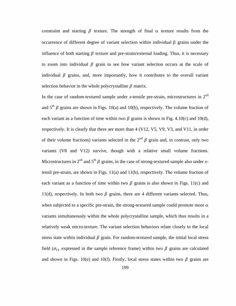
199
constraint and starting texture. The strength of final texture results from the
occurrence of different degree of variant selection within individual grains under the
influence of both starting texture and pre-strain/external loading. Thus, it is necessary
to zoom into individual grain to see how variant selection occurs at the scale of
individual grains, and, more importantly, how it contributes to the overall variant
selection behavior in the whole polycrystalline matrix.
In the case of random-textured sample under x-tensile pre-strain, microstructures in 2nd
and 5th
grains are shown in Figs. 10(a) and 10(b), respectively. The volume fraction of
each variant as a function of time within two grains is shown in Fig. 4.10(c) and 10(d),
respectively. It is clearly that there are more than 4 (V12, V5, V9, V3, and V11, in order
of their volume fractions) variants selected in the 2nd
grain and, in contrast, only two
variants (V8 and V12) survive, though with a relative small volume fractions.
Microstructures in 2nd
and 5th
grains, in the case of strong-textured sample also under x-
tensil pre-strain, are shown in Figs. 11(a) and 11(b), respectively. The volume fraction of
each variant as a function of time within two grains is also shown in Figs. 11(c) and
11(d), respectively. In both two grains, there are 4 different variants selected. Thus,
when subjected to a specific pre-strain, the strong-textured sample could promote more
variants simultaneously within the whole polycrystalline sample, which thus results in a
relatively weak micro-texture. The variant selection behaviors relate closely to the local
stress state within individual grain. For random-textured sample, the initial local stress
field ( expressed in the sample reference frame) within two grains are calculated
and shown in Figs. 10(e) and 10(f). Firstly, local stress states within two grains are
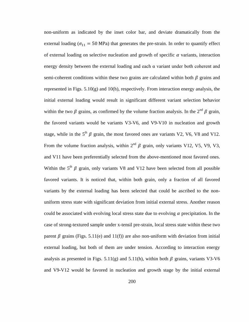
200
non-uniform as indicated by the inset color bar, and deviate dramatically from the
external loading ( ) that generates the pre-strain. In order to quantify effect
of external loading on selective nucleation and growth of specific variants, interaction
energy density between the external loading and each α variant under both coherent and
semi-coherent conditions within these two grains are calculated within both grains and
represented in Figs. 5.10(g) and 10(h), respectively. From interaction energy analysis, the
initial external loading would result in significant different variant selection behavior
within the two grains, as confirmed by the volume fraction analysis. In the 2nd
grain,
the favored variants would be variants V3-V6, and V9-V10 in nucleation and growth
stage, while in the 5th
grain, the most favored ones are variants V2, V6, V8 and V12.
From the volume fraction analysis, within 2nd
grain, only variants V12, V5, V9, V3,
and V11 have been preferentially selected from the above-mentioned most favored ones.
Within the 5th
grain, only variants V8 and V12 have been selected from all possible
favored variants. It is noticed that, within both grain, only a fraction of all favored
variants by the external loading has been selected that could be ascribed to the non-
uniform stress state with significant deviation from initial external stress. Another reason
could be associated with evolving local stress state due to evolving precipitation. In the
case of strong-textured sample under x-tensil pre-strain, local stress state within these two
parent grains (Figs. 5.11(e) and 11(f)) are also non-uniform with deviation from initial
external loading, but both of them are under tension. According to interaction energy
analysis as presented in Figs. 5.11(g) and 5.11(h), within both grains, variants V3-V6
and V9-V12 would be favored in nucleation and growth stage by the initial external

201
loading, while with different magnitude for each favored one. Again, not all favored
variants have been selected. Therefore, compared with random-textured sample, there
would be a relative uniform stress state that is possible to promote relative more variants
simultaneous within relative more grain in the strong-textured sample when subjected
to a specific pre-strain.
It has been found that boundary constraint of polycrystalline sample also have a
significant influence on the strength of final texture. For instance, in random-textured
sample, when a 50Mpa tensile stress is applied along the x-axis of the sample, the
strength of final texture will be larger in the case of fix-end boundary as shown in Fig.
5.9(a). Microstructures in 2nd
and 5th
grains are shown in Figs. 5.12(a) and 5.12(b),
respectively. The volume fraction of each variant as a function of time within two
grains is shown in Fig. 5.12(c) and 5.12(d), respectively. The interaction energy results
will be identical to those in Fig. 5.10 (g) and Fig. 5.10(h). It is clearly that, in the 2nd
grain, there are 7 variants (V12, V9, V5, V3, V11, V6, V10) have been selected out of all
8 possible favored variants, having volume fractions much larger than those in the fix-end
case. In the 5th
grain, there are still only two variants (V8 and V12) survived but,
almost percolating the whole grain according to their volume fraction. In the case of
the fix-end boundary constraint, there will be a competition between pre-strain and
evolving microstructure on variant selection [36]. In particular, it is possible that internal
stress generated by an evolving microstructure exceeds the initially applied stress that
generates the pre-strain. In the case of free-end boundary condition, the system would be
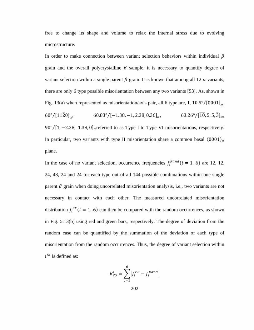
202
free to change its shape and volume to relax the internal stress due to evolving
microstructure.
In order to make connection between variant selection behaviors within individual
grain and the overall polycrystalline sample, it is necessary to quantify degree of
variant selection within a single parent grain. It is known that among all 12 variants,
there are only 6 type possible misorientation between any two variants [53]. As, shown in
Fig. 13(a) when represented as misorientation/axis pair, all 6 type are, , [ ]⁄ ,
[ ]⁄ , [ ] ⁄ , [ ] ⁄ ,
[ ] ⁄ referred to as Type I to Type VI misorientations, respectively.
In particular, two variants with type II misorientation share a common basal
plane.
In the case of no variant selection, occurrence frequencies are 12, 12,
24, 48, 24 and 24 for each type out of all 144 possible combinations within one single
parent grain when doing uncorrelated misorientation analysis, i.e., two variants are not
necessary in contact with each other. The measured uncorrelated misorientation
distribution can then be compared with the random occurrences, as shown
in Fig. 5.13(b) using red and green bars, respectively. The degree of deviation from the
random case can be quantified by the summation of the deviation of each type of
misorientation from the random occurrences. Thus, the degree of variant selection within
is defined as:
∑|
|
203
The physical meaning can be interpreted as: if there is no variant selection, there will be
no deviation from random occurrence frequencies for each type of misorientation, i.e.
; if a single variant is able to percolate through a whole single grain, maximum
degree of variant selection is reached with , as shown in Fig. 13(c). Thus,
the value of is able to characterize qutitatively the degree of variant selection within
a single grain. The computation of an uncorrelated misorientation distribution from the
EBSD data of all individual phase in a parent grain is performed using MTEX. For
random-textured sample under different processing conditions such as pre-strain and
boundary constraints, degree of variant selection within individual grains, is
calculated within the largest and the smallest grain represented respectively by red and
green bars in Fig. 5.14(a). The corresponding overall degree of variant selection is also
presented in Fig. 5.14(b). It can be found that, in most case, the larger the is, the
larger the overall degree of variant selection for the polycrystalline sample will be.
However, it is also noticed that with the largest and smallest grains under Z-Comp
pre-strain are larger than those under X-Comp-Free external loading, but the final is
almost identical. To be specific, in the case of Z-Comp pre-strain, in the
largest grain, while, in the case of X-Comp-Free, , as shown in Fig. 5.15(a)
and Fig. 5.15(b), respectively. Compared with the difference in (maximum value of
), the difference in corresponding maximum intensity in poles, and
thus is relatively small.
204
It has been stated that when there is no variant selection, and when variant
selection occurs, . It is then believed that the larger is, the larger the overall
degree of variant selection will be. However, there is a special case where even if variant
selection already occurs, one still has . For instance, the macro-texture of
random-textured sample is represented using three different pole figures, { } , { }
and { } poles, i.e. three component in describing BOR, as shown in Fig. 5.16. The
macro-texture of final phase without occurrence of variant selection is represented
using corresponding three different pole figures, , { } , and { }
according to BOR. As has been stated that { } pole is identical to { } one.
Another set of ODF for the final texture from random textured sample is obtained by
assuming a special variant selection occurring in a single grain that multiple random
distributions of six variants are 3 times of those of other 6 variants sharing common
pole. In other words, in the grain, variant selection occurs due to the bias
between any two variants with misorientation of [ ] ⁄ or having common
basal . While in all the other grains, their orientation density is shared equally
by all 12 variants within them. The resulting macro-texture of final phase is
represented using three different pole figures, , { } , and { } as well. It
is readily seen that { } pole is still identical to { } one even if variant selection
occurs. The occurrence of variant selection can be noticed by comparing the difference
between { } or { } poles in the case of with/without occurrence of variant
selection. Thus, when using to evaluate the influence of different set of processing
variables on the overall degree of variant selection, it is better to double check with
205
degree of variant selection within individual grain. As a matter of fact, as a 2-D
projection of the 3-D orientation distribution, pole figures may bear some losses in
information. Thus, the evaluation of degree of variant selection by comparing two sets of
pole figures could be inadequate.
Alpha precipitate has a strong anisotropy in shape that appears as a lath. This anisotropy
in shape may lead, even in the absence of variant selection, to an inhomogeneity in
variant distribution due to the morphological orientation of phase with respect to the
sample surface plane. For example, as shown in Fig. 17, three different cross-sections
have been made along x, y and z surface layer. It is obvious those microstructures are
significantly different among these three sections. Variant selection is then studied, from
a statistical point of view, using the average texture obtained by a virtual EBSD scan
through these sections. Apparently, the final texture varies significantly with cross-
sections in terms of maximum pole intensity and distribution with each basal pole figure.
This is due purely to the 2D stereology sampling artifact that has recently been referred to
as “pseudo variant selection” [54]. Thus, when analyzing experimental data in literature
one has to bear in mind this possible 2D sampling effect.
5.5. Summary
A three-dimensional quantitative phase field model (PFM) has been developed to study
the variant selection process during transformation in polycrystalline sample
under the influence of different processing variables such as pre-strains. The effect of

206
elastic and structural inhomogeneities on the local stress state and its interaction with
evolving microstructure is also considered in the model. In particular, microstructure and
transformation texture evolution are treated simultaneously via orientation distribution
function (ODF) modeling of ⁄ two-phase microstructure in polycrystalline systems
obtained by PFM. The variant selection behavior at the scale of individual grain and
the overall polycrystalline sample, and the resulting final texture are found to be
heavily dependent on type of pre-strain, boundary constraint of the sample, and strating
texture. It is found that, when subjected to a certain pre-strain, the sample with strong
texture component could promote more variants simultaneously within the whole
polycrystalline sample and thus lead to a relatively small degree of microtexture. The
results could shed light on how to control processing conditions to reduce the strength
micro-texture at both the individual grain level and the overall polycrystalline sample
level according to its starting texture.
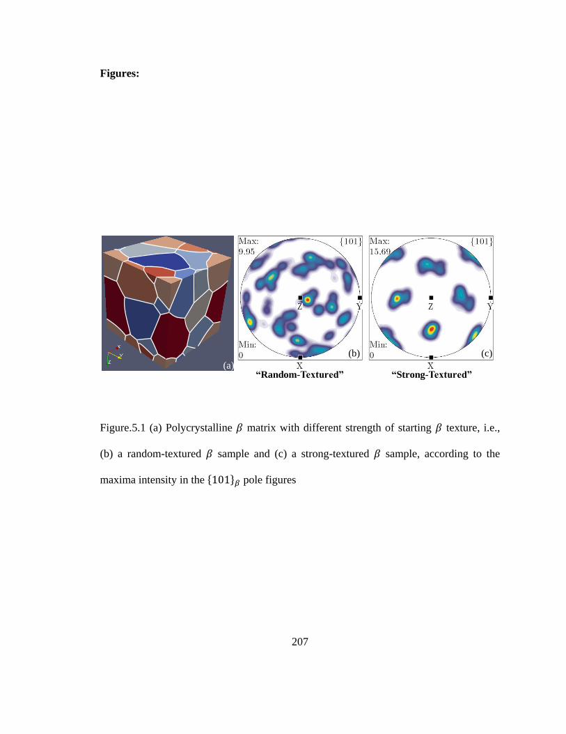
207
Figures:
Figure.5.1 (a) Polycrystalline matrix with different strength of starting texture, i.e.,
(b) a random-textured sample and (c) a strong-textured sample, according to the
maxima intensity in the { } pole figures
(a)
(b) (c)
“Random-Textured” “Strong-Textured”

208
Figure.5.2 (a)-(c) Microstructure evolution due to precipitation in random-texture
sample without any pre-strain, and (a′)-(c′) corresponding texture evolution represented
by { } pole figures
t=1.0s t=3.0s t=5.0s
(a) (b) (c)
(a′) (b′) (c′)

209
Figure.5.3 (a)-(d) Microstructure evolution due to precipitation in random-texture
sample under the pre-strain, and (a′)-(d′) corresponding texture evolution represented
by { } pole figures. The pre-strain is obtained by applying a 50Mpa compressive
stress along x-axis of the system
t=1.5s
(a) (b) (c) (d)
t=3.0s t=6.0s t=9.0s
(a’) (b’) (c’) (d’)
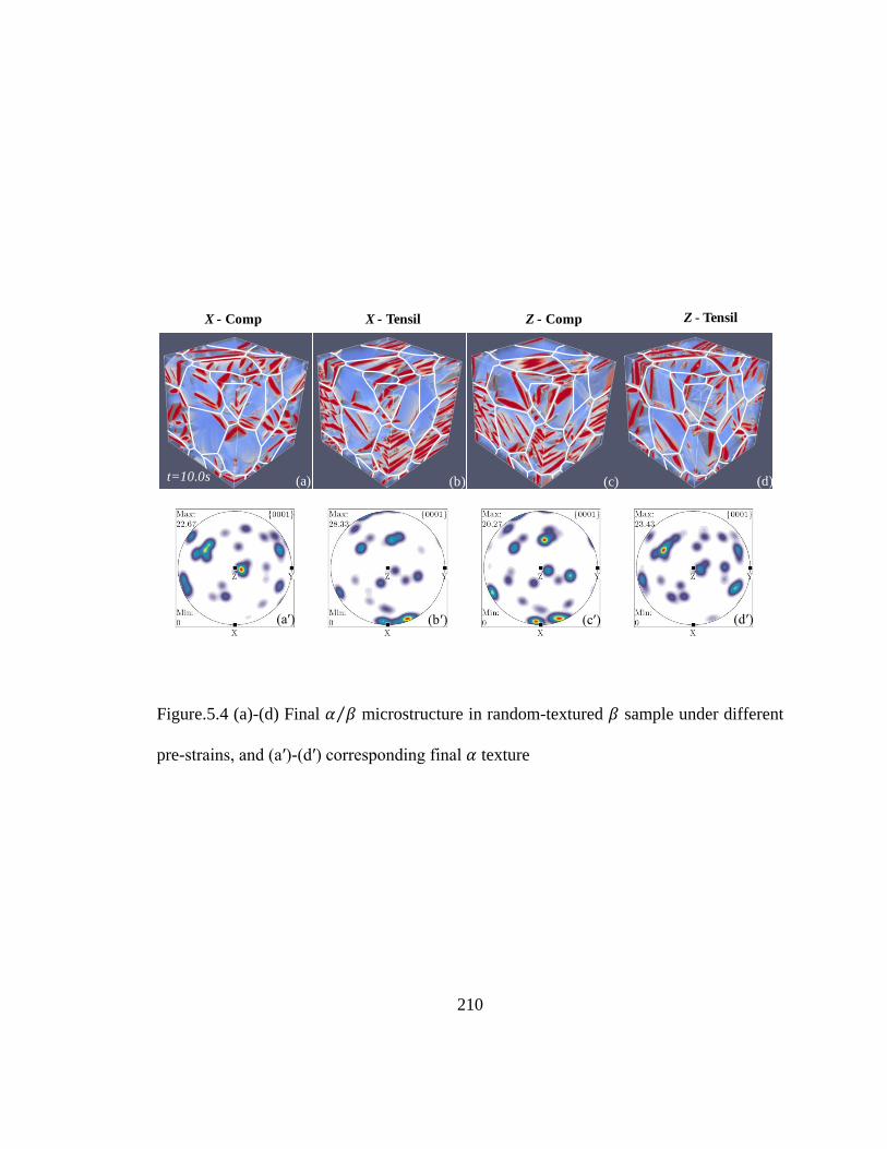
210
Figure.5.4 (a)-(d) Final ⁄ microstructure in random-textured sample under different
pre-strains, and (a′)-(d′) corresponding final texture
X - Comp X - Tensil Z - Comp Z - Tensil
(a) (b) (c) (d)
(a′) (b′) (c′) (d′)
t=10.0s

211
Figure.5.5 (a)-(d) Final ⁄ microstructure in strong-textured sample under different
pre-strains, and (a′)-(d′) corresponding final texture
X - Comp X - Tensil Z - Comp Z - Tensil
(a) (b) (c) (d)
(a′) (b′) (c′) (d′)
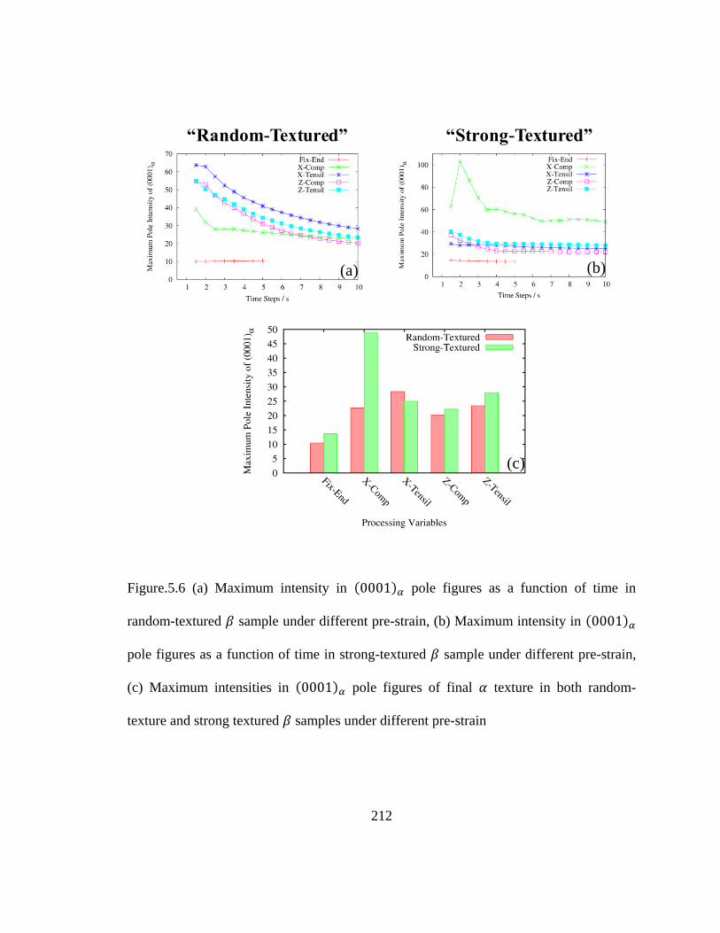
212
Figure.5.6 (a) Maximum intensity in pole figures as a function of time in
random-textured sample under different pre-strain, (b) Maximum intensity in
pole figures as a function of time in strong-textured sample under different pre-strain,
(c) Maximum intensities in pole figures of final texture in both random-
texture and strong textured samples under different pre-strain
“Random-Textured” “Strong-Textured”
(a) (b)
(c)

213
Figure.5.7 (a) and (b) { } pole figures for random-textured and strong-textured
sample; (c) and (d) corresponding pole figures of final texture in random-
textured and strong-textured sample without variant selection
“Random-Textured” “Strong-Textured”
(a) (b)
(c) (d)

214
Figure.5.8 Degree of variant selection in both random-texture and strong textured
samples under different pre-strain
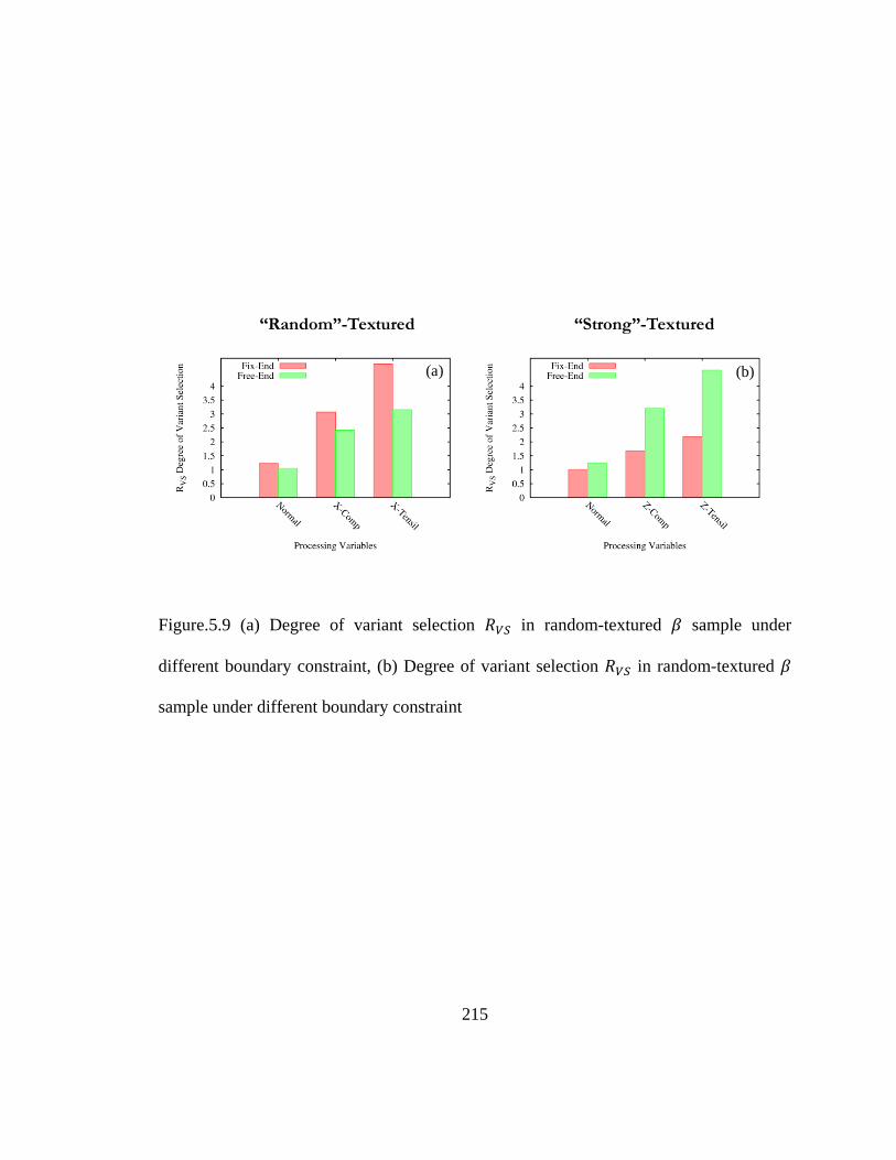
215
Figure.5.9 (a) Degree of variant selection in random-textured sample under
different boundary constraint, (b) Degree of variant selection in random-textured
sample under different boundary constraint
“Random”-Textured “Strong”-Textured
(a) (b)
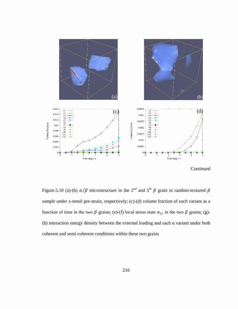
216
Continued
Figure.5.10 (a)-(b) ⁄ microstructure in the 2nd
and 5th
grain in random-textured
sample under x-tensil pre-strain, respectively; (c)-(d) volume fraction of each variant as a
function of time in the two grains; (e)-(f) local stress state in the two grains; (g)-
(h) interaction energy density between the external loading and each α variant under both
coherent and semi-coherent conditions within these two grains
(a) (b)
(c) (d)
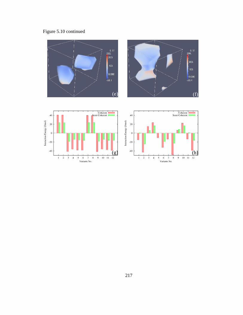
217
Figure 5.10 continued
(e) (f)
(g) (h)

218
Continued
Figure.5.11 (a)-(b) ⁄ microstructure in the 2nd
and 5th
grain in strong-textured
sample under x-tensil pre-strain, respectively; (c)-(d) volume fraction of each variant as a
function of time in the two grains; (e)-(f) local stress state in the two grains; (g)-
(h) interaction energy density between the external loading and each α variant under both
coherent and semi-coherent conditions within these two grains
(a) (b)
(c) (d)
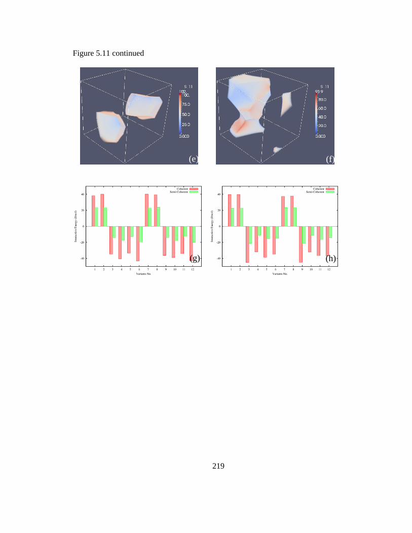
219
Figure 5.11 continued
(e) (f)
(g) (h)
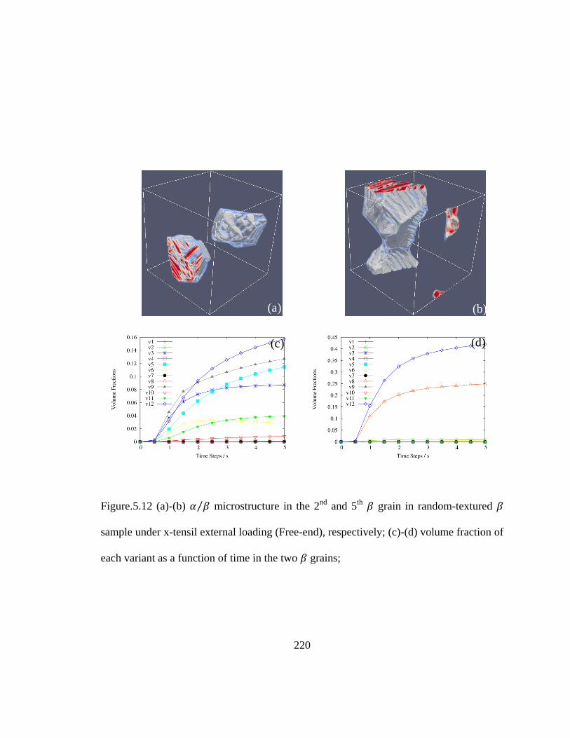
220
Figure.5.12 (a)-(b) ⁄ microstructure in the 2nd
and 5th
grain in random-textured
sample under x-tensil external loading (Free-end), respectively; (c)-(d) volume fraction of
each variant as a function of time in the two grains;
(a) (b)
(c) (d)
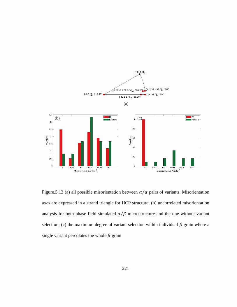
221
Figure.5.13 (a) all possible misorientation between ⁄ pairs of variants. Misorientation
axes are expressed in a strand triangle for HCP structure; (b) uncorrelated misorientation
analysis for both phase field simulated ⁄ microstructure and the one without variant
selection; (c) the maximum degree of variant selection within individual grain where a
single variant percolates the whole grain
(a)
(b) (c)

222
Figure.5.14 (a) degree of variant selection within the largest and the smallest grain in
random-texture sample under different pre-strains and boundary constraint, (b)
corresponding overall degree of variant selection
(a) (b)
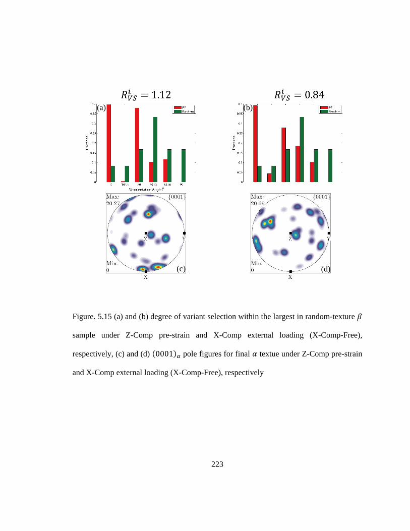
223
Figure. 5.15 (a) and (b) degree of variant selection within the largest in random-texture
sample under Z-Comp pre-strain and X-Comp external loading (X-Comp-Free),
respectively, (c) and (d) pole figures for final textue under Z-Comp pre-strain
and X-Comp external loading (X-Comp-Free), respectively
(a) (b)
(c) (d)
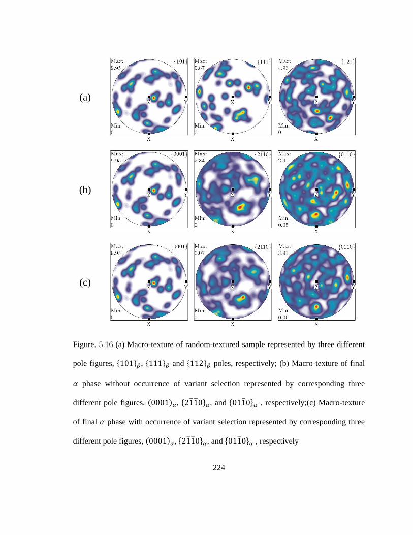
224
Figure. 5.16 (a) Macro-texture of random-textured sample represented by three different
pole figures, { } , { } and { } poles, respectively; (b) Macro-texture of final
phase without occurrence of variant selection represented by corresponding three
different pole figures, , { } , and { } , respectively;(c) Macro-texture
of final phase with occurrence of variant selection represented by corresponding three
different pole figures, , { } , and { } , respectively
(a)
(b)
(c)

225
Figure. 5.17 Examples showing the pseudo variant selection due to 2D sampling effect.
EBSD scan is performed along at different layers of the sample
(a)
(a′)
(b) (c)
(b′) (c′)

226
5.6. References:
[1] Banerjee D, Williams JC. Perspectives on Titanium Science and Technology.
Acta Materialia 2013;61:844.
[2] TITANIUM ALLOYS –TOWARDS ACHIEVING ENHANCED PROPERTIES
FOR DIVERSIFIED APPLICATIONS. Croatia: InTech, 2012.
[3] Semiatin SL, Furrer DU. Modeling of Microstructure Evolution during the
Thermomechanical Processing of Titanium Alloys. In: L. SS, U. FD, editors. ASM
Handbook Volume 22A: Fundamentals of Modeling for Metals Processing. 2009.
[4] Burgers WG. On the process of transition of the cubic-body-centered
modification into the hexagonal-close-packed modification of zirconium. Physica
1934;1:561.
[5] Cahn JW, Kalonji GM. Symmetry in Solid-Solid Transformation Morphologies.
PROCEEDINGS OF an Interantional Conference On Solid-Solid Phase Transformations
1981:3.
[6] Lutjering G, Williams JC. Titanium (Engineering Materials and Processes).
Berlin: Springer, 2007.
[7] Whittaker R, Fox K, Walker A. Texture variations in titanium alloys for
aeroengine applications. Materials Science and Technology 2010;26:676.
[8] Sargent GA, Kinsel KT, Pilchak AL, Salem AA, Semiatin SL. Variant Selection
During Cooling after Beta Annealing of Ti-6Al-4V Ingot Material. Metallurgical and
Materials Transactions a-Physical Metallurgy and Materials Science 2012;43A:3570.

227
[9] Winholtz RA. Residual Stresses: Macro and Micro Stresses. In: Buschow KHJ,
Robert WC, Merton CF, Bernard I, Edward JK, Subhash M, Patrick V, editors.
Encyclopedia of Materials: Science and Technology. Oxford: Elsevier, 2001. p.8148.
[10] Zeng L, Bieler TR. Effects of working, heat treatment, and aging on
microstructural evolution and crystallographic texture of [alpha], [alpha]', [alpha]'' and
[beta] phases in Ti-6Al-4V wire. Materials Science and Engineering: A 2005;392:403.
[11] Humbert M, Germain L, Gey N, Bocher P, Jahazi M. Study of the variant
selection in sharp textured regions of bimodal IMI 834 billet. Materials Science and
Engineering: A 2006;430:157.
[12] Moustahfid H, Humbert M, Philippe MJ. Modeling of the texture transformation
in a Ti-64 sheet after hot compression. Acta Materialia 1997;45:3785.
[13] Gey N, Humbert M, Philippe MJ, Combres Y. Modeling the transformation
texture of Ti-64 sheets after rolling in the [beta]-field. Materials Science and Engineering
A 1997;230:68.
[14] Gey N, Humbert M, Philippe MJ, Combres Y. Investigation of the alpha- and
beta-texture evolution of hot rolled Ti-64 products. Materials Science and Engineering a-
Structural Materials Properties Microstructure and Processing 1996;219:80.
[15] Kar S, Banerjee R, Lee E, Fraser HL. Influence of crystallography varaiant
selection on microstructure evolution in titanium alloys. In: Howe JM, Laughlin DE, Lee
JK, Dahmen U, Soffa WA, editors. Solid-Solid Phase Transformation in Inorganic
Materials 2005, vol. 1: TMS, 2005.
228
[16] Lee E, Banerjee R, Kar S, Bhattacharyya D, Fraser HL. Selection of alpha
variants during microstructural evolution in alpha/beta titanium alloy. Philosophical
Magazine 2007;87:3615.
[17] Wang YU, Jin YM, Khachaturyan AG. Three-dimensional phase field
microelasticity theory of a complex elastically inhomogeneous solid. Applied Physics
Letters 2002;80:4513.
[18] Cahn JW, Hilliard JE. Free energy of a nonuniform system. I. Interfacial free
energy. The Journal of Chemical Physics 1958;28:258.
[19] Landau LD, Lifshitz E. On the theory of the dispersion of magnetic permeability
in ferromagnetic bodies. Phys. Z. Sowjetunion 1935;8:101.
[20] Rowlinson JS. Translation of J. D. van der Waals' “The thermodynamik theory of
capillarity under the hypothesis of a continuous variation of density”. Journal of
Statistical Physics 1979;20:197.
[21] Eshelby JD. The determination of the elastic field of an ellipsoidal inclusion, and
related problems. Proceedings of the Royal Society of London. Series A 1957;241.
[22] Eshelby JD. The Elastic Field Outside an Ellipsoidal Inclusion. Proceedings of the
Royal Society A 1959;252:561.
[23] Khachaturyan A. Some questions concerning the theory of phase transformations
in solids. Soviet Phys. Solid State 1967;8:2163.
[24] Khachaturyan AG. Theory of Structural Transformations in Solids. New York:
John Wiley & Sons, 1983.
229
[25] Khachaturyan AG, Shatalov GA. Elastic interaction potential of defects in a
crystal. Sov. Phys. Solid State 1969;11:118.
[26] Boettinger WJ, Warren JA, Beckermann C, Karma A. Phase-field simulation of
solidification. Annual Review of Materials Research 2002;32:163.
[27] Chen L-Q. PHASE-FIELD MODELS FOR MICROSTRUCTURE
EVOLUTION. Annual Review of Materials Research 2002;32:113.
[28] Emmerich H. The diffuse interface approach in materials science: thermodynamic
concepts and applications of phase-field models: Springer, 2003.
[29] Karma A. Phase Field Methods. In: Buschow KHJ, Cahn RW, Flemings MC,
Ilschner B, Kramer EJ, Mahajan S, Veyssière P, editors. Encyclopedia of Materials:
Science and Technology (Second Edition). Oxford: Elsevier, 2001. p.6873.
[30] Shen C, Wang Y. Coherent precipitation - phase field method. In: Yip S, editor.
Handbook of Materials Modeling, vol. B: Models. Springer, 2005. p.2117.
[31] Wang Y, Chen LQ, Zhou N. Simulating Microstructural Evolution using the
Phase Field Method. Characterization of Materials. John Wiley & Sons, Inc., 2012.
[32] Wang YU, Jin YM, Khachaturyan AG. Dislocation Dynamics—Phase Field.
Handbook of Materials Modeling. Springer, 2005. p.2287.
[33] Shi R, Ma N, Wang Y. Predicting equilibrium shape of precipitates as function of
coherency state. Acta Materialia 2012;60:4172.
[34] Wang Y, Ma N, Chen Q, Zhang F, Chen SL, Chang YA. Predicting phase
equilibrium, phase transformation, and microstructure evolution in titanium alloys. JOM
Journal of the Minerals Metals and Materials Society 2005;57:32.
230
[35] Chen Q, Ma N, Wu KS, Wang YZ. Quantitative phase field modeling of
diffusion-controlled precipitate growth and dissolution in Ti-Al-V. Scripta Materialia
2004;50:471.
[36] Shi R, Wang Y. Variant selection during α precipitation in Ti–6Al–4V under the
influence of local stress – A simulation study. Acta Materialia 2013;61:6006.
[37] Bunge HJ. Texture Analysis in Materials Science- Mathematical Methods.
London, 1982.
[38] Artemev A, Jin YM, Khachaturyan AG. Three-dimensional phase field model and
simulation of cubic -> tetragonal martensitic transformation in polycrystals.
Philosophical Magazine a-Physics of Condensed Matter Structure Defects and
Mechanical Properties 2002;82:1249.
[39] Steinbach I, Pezzolla F, Nestler B, Seeßelberg M, Prieler R, Schmitz GJ, Rezende
JLL. A phase field concept for multiphase systems. Physica D: Nonlinear Phenomena
1996;94:135.
[40] Steinbach I, Pezzolla F. A generalized field method for multiphase
transformations using interface fields. Physica D: Nonlinear Phenomena 1999;134:385.
[41] Wang YU, Jin YMM, Khachaturyan AG. Phase field microelasticity theory and
modeling of elastically and structurally inhomogeneous solid. Journal of Applied Physics
2002;92:1351.
[42] Wang YU, Jin YMM, Khachaturyan AG. Mesoscale modelling of mobile crystal
defects - dislocations, cracks and surface roughening: phase tield microelasticity
approach. Philosophical Magazine 2005;85:261.
231
[43] Shen Y, Li Y, Li Z, Wan H, Nie P. An improvement on the three-dimensional
phase-field microelasticity theory for elastically and structurally inhomogeneous solids.
Scripta Materialia 2009;60:901.
[44] Engler O, Randle V. Introduction to texture analysis: macrotexture, microtexture,
and orientation mapping: CRC press, 2009.
[45] Hielscher R, Schaeben H, Siemes H. Orientation Distribution Within a Single
Hematite Crystal. Mathematical Geosciences 2010;42:359.
[46] Bachmann F, Hielscher R, Schaeben H. Texture Analysis with MTEX- Free and
Open Source Software Toolbox. Solid State Phenomena 2010;160:63.
[47] Rycroft CH. VORO plus plus : A three-dimensional Voronoi cell library in C
plus. Chaos 2009;19.
[48] Gruber J, Ma N, Wang Y, Rollett AD, Rohrer GS. Sparse data structure and
algorithm for the phase field method. Modelling and Simulation in Materials Science and
Engineering 2006;14:1189.
[49] Shi R, Wang Y. Evolution of Microstructure and Transformation Texture due to
Variant Selection during Alpha Precipitation in Polycrystalline Titanium alloys- A
Simulation Study. To be submitted Acta Materialia 2014.
[50] Semiatin SL, Kinsel KT, Pilchak AL, Sargent GA. Effect of Process Variables on
Transformation-Texture Development in Ti-6Al-4V Sheet Following Beta Heat
Treatment,. Metallurgical and Materials Transactions a-Physical Metallurgy and
Materials Science 2013;under review.

232
[51] Ivasishin OM, Shevchenko SV, Vasiliev NL, Semiatin SL. 3D Monte-Carlo
simulation of texture-controlled grain growth. Acta Materialia 2003;51:1019.
[52] Li DY, Chen LQ. Selective variant growth of coherent Ti11Ni14 precipitate in a
TiNi alloy under applied stresses. Acta Materialia 1997;45:471.
[53] Wang SC, Aindow M, Starink MJ. Effect of self-accommodation on alpha/alpha
boundary populations in pure titanium. Acta Materialia 2003;51:2485.
[54] Gourgues-Lorenzon AF. Application of electron backscatter diffraction to the
study of phase transformations. International Materials Reviews 2007;52:65.

233
CHAPTER 6 Variant Selection of Grain Boundary by
Special Prior Grain Boundaries in Titanium Alloys
Abstract
During -processing of / and titanium alloys, variant selection (VS) of grain
boundary GB is one of the key factors in determining the final transformation
texture and mechanical properties. It has been observed frequently that GB prefers its
⟨ ⟩ pole to be parallel to a common ⟨ ⟩ pole of the two adjacent grains and
results in a micro-textured region across the grain boundary (GB) and, as a consequence,
slip transmission may take place more easily across that GB. In order to investigate how
such a special prior GB contributes to VS of GB, we develop a crystallographic
model based on the Burgers orientation relationship (BOR) between GB and one of the
two grains. The model predicts all possible special grain boundaries at which GB is
able to maintain BOR with both grains. A new measure for VS of GB, ,
i.e. a measure of the deviation of the actual OR between the GB and the non-Burgers
grain from the BOR, is proposed. For the particular alloy chosen for experimental
observations, Ti-5553, it is found that when the misorientation angle of
(instead of the closeness between two closet { } poles between two grains widely
used in literature) is less than , misorientation between the two grains dominates the
VS of GB and, in particular, the variant with minimum is always selected for GB.
A possible effect due to grain boundary plane inclination on VS is also discussed.

234
6.1. Introduction
Similar to steels, the influence of grain boundary (GB) on subsequent intragranular
microstructure development and microstructure-properties relationships in Ti-alloys has
been an active area of research for decades [1-3]. In most cases, GB has the Burgers
orientation relationship (BOR) [4], i.e. and [ ] [ ] , with
one of the two adjacent grains that form the prior grain boundary (GB). The grain that
maintains BOR with GB is then referred to as the Burgers grain and the other as the
non-Burgers grain. There are 12 crystallographically equivalent orientation variants
available for the GBif it develops BOR with only one of the grains. In most cases,
however, only limited number of variants of GBare observed on most GBs [3, 5-7].
Such variant selection of GB not only has a direct influence on the overall
microstructure and transformation texture evolution [8, 9], but also has a significant
impact on the mechanical properties of the alloy [10]. For example, it has been
demonstrated frequently that different colonies (e.g. different in both orientation and
growth directions) growing from GB into the grains share common crystallographic
features such as a common basal plane orientation (though with their { } pole
being misoriented by a ~10.5˚ rotation about their common [ ] axis) provided that
the two grains have special misorientations [6, 7, 11]. An even more special case has
also been discovered recently [12] where colonies growing into two adjacent grains
have exactly the same orientation as that of the GB [3, 5-7]. This results in the
235
formation of large regions of colonies in multiple grains with a common
crystallographic feature, which are also referred to as “macro-zones” [2] or micro-
textured regions [3] that would have detrimental effect on the mechanical behavior of Ti-
alloys such as cold-dwell crack initiation and propagation [2]. Ample experimental
observations have shown that the formation of such macro-zones is closely related to
crystallographic characters of the prior grain boundaries [2, 6, 7, 11, 12]. For instance,
it has been reported repeatedly that if two adjacent grains share a common { } pole
with angular deviation within 10°, the preferred variant for GB always has its { }
pole parallel to one of the common { } poles [6, 7, 11]. In particular, when two
adjacent grains are misorientated by a 10.5˚ rotation about a common ⟨ ⟩ axis or a
60˚ rotation about a common ⟨ ⟩ axis [12], the selected GBis able to maintain BOR
with both adjacent grains. In this case, colonies in both grains will have the same
crystallographic orientation as that of the GB.
A statistical analysis [6, 7] of EBSD data has shown that variant selection for GB
usually obeys the following rule: when there exist two nearly common { } poles of
the two adjacent grains (with angular deviation within 10°), the normal of
plane of GB will be parallel to the common { } pole. Even though it was
mentioned in the literature [7, 11] that selection of specific variant for GB by such a
rule might minimize the interfacial energy between the selected GB and the two
grains and thus lower GB nucleation barrier, no fundamental argument or analysis has

236
been provided. In consequence, it is still not understood why the rule is not always
followed. For example, it has been observed that the { } pole of GB is parallel to
one of the { } pole that does not belong to one of the two closet { } poles though
still with an angular deviation less than 10˚ in between [6, 7]. Apparently, the parameter
describing angular deviation between two closest { } poles is not always a primary
factor in determining variant selection of GB. Thus, the application of the rule to
predict the overall transformation texture of phase would not necessarily lead to a
satisfactory result [13]. As a matter of fact, the single parameter may not be sufficient
considering the fact that it requires at least two independent parallelisms to describe an
orientation relationship, for example ⟨ ⟩ ⟨ ⟩ besides { } { } for the
BOR.
In this paper, we first formulate a crystallographic model which allows us to evaluate
quantitatively deviation of the OR between GB and grains from BOR. Then we
characterize experimentally ORs of GB with two adjacent grains at different prior
GBs using electron-backscatter diffraction (EBSD) and analyze the experimental results
against the specific rule. Cases that follow and do not follow the rule are identified and
analyzed, and new criteria of variant selection of GB by prior grain boundaries are
provided.
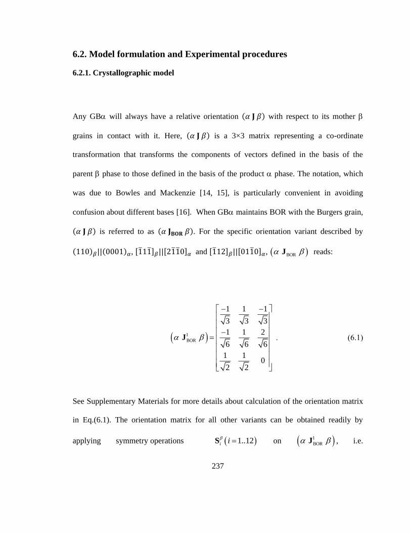
237
6.2. Model formulation and Experimental procedures
6.2.1. Crystallographic model
Any GB will always have a relative orientation with respect to its mother
grains in contact with it. Here, is a 3×3 matrix representing a co-ordinate
transformation that transforms the components of vectors defined in the basis of the
parent phase to those defined in the basis of the product phase. The notation, which
was due to Bowles and Mackenzie [14, 15], is particularly convenient in avoiding
confusion about different bases [16]. When GB maintains BOR with the Burgers grain,
is referred to as . For the specific orientation variant described by
, [ ] [ ] and [ ] [ ] , BOR J reads:
Equation Chapter 6 Section 1
1
BOR
1 1 1
3 3 3
1 1 2
6 6 6
1 10
2 2
J . (6.1)
See Supplementary Materials for more details about calculation of the orientation matrix
in Eq.(6.1). The orientation matrix for all other variants can be obtained readily by
applying symmetryoperations 1..12i i S on 1
BOR J , i.e.
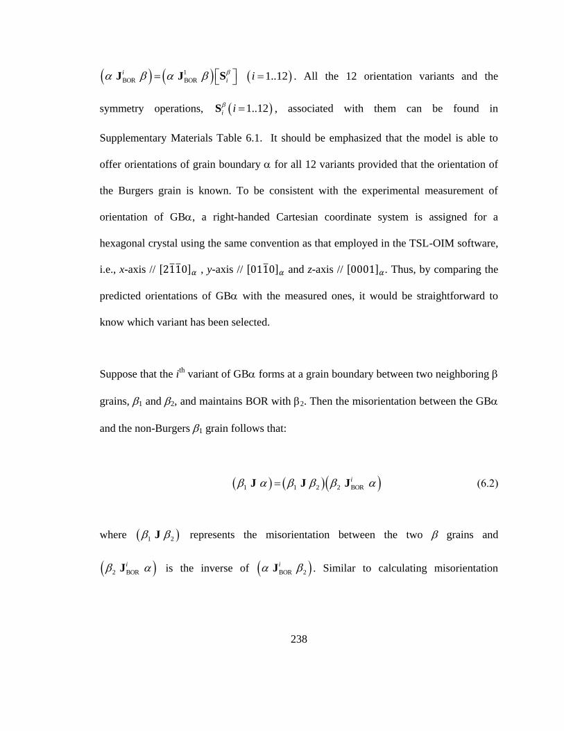
238
1
BOR BOR i
i
J J S 1..12i . All the 12 orientation variants and the
symmetry operations, 1..12i i S , associated with them can be found in
Supplementary Materials Table 6.1. It should be emphasized that the model is able to
offer orientations of grain boundary for all 12 variants provided that the orientation of
the Burgers grain is known. To be consistent with the experimental measurement of
orientation of GB, a right-handed Cartesian coordinate system is assigned for a
hexagonal crystal using the same convention as that employed in the TSL-OIM software,
i.e., x-axis // [ ] , y-axis // [ ] and z-axis // [ ] . Thus, by comparing the
predicted orientations of GB with the measured ones, it would be straightforward to
know which variant has been selected.
Suppose that the ith
variant of GB forms at a grain boundary between two neighboring
grains, 1 and 2, and maintains BOR with 2. Then the misorientation between the GB
and the non-Burgers 1 grain follows that:
1 1 2 2 BOR i J J J (6.2)
where 1 2 J represents the misorientation between the two grains and
2 BOR i J is the inverse of BOR 2 i J . Similar to calculating misorientation
239
between two adjacent grains, how 1 J deviates from the BOR can be evaluated
quantitatively by defining a “misorientation” matrix [17, 18] as the following:
BOR
1 1 1 BOR 1 1..6j j ΔJ J J (6.3)
where the superscript j in the right hand side of Eq. (6.3) describes the order of all 6
possible orientations for 1 if BOR is maintained between itself and GBsince there are
only 6 possible orientation variants of if BOR exists between the parent and product
phases during transformation. Combining Eqs. (6.2) and (6.3), we have
BOR
1 1 1 2 2 BOR BOR 1
11 1
1 2 BOR BOR
i j
j iS S
ΔJ J J J
J J J (6.4)
Thus, one only needs misorientation between two adjacent grains, symmetry operations
of and phases, and an orientation matrix describing BOR to evaluate the deviation of
the OR between GB and non-Burgers grain from the BOR for all 12 variants. Note that
symmetry operations of both and phase will result in multiple equivalent
misorientation matrices associated with . Thus, the misorientation matrix
such as or , is also described by the angle/axis (r pair with
misorientation angle and axis 1 2 3, , r r r being calculated from the misorientation
matrix [19], and the angle/axis pair that has the minimum misorientation angle, i.e., the
disorientation, is selected to represent the misorientation. The magnitude of the
240
disorientation angle characterizes the closeness between two orientations. The
misorientation between the measured and predicted orientations for GB is evaluated
through the misorientation matrix , where and represent the measured
(by Experiment) and predicted (by Model) orientation of GB, respectively. The matrix
is then also expressed by the disorientation angle/axis pairs.
6.2.2. Experimental procedures
Twenty-eight examples of GB at different prior grain boundaries are observed in the
experiment. They belong to only one or two specific variants. The material used is a
forged -Ti alloy, Ti-5553, i.e., Ti-5Al-5Mo-5V-3Cr-0.5Fe (wt. %). The as-received
alloy was sectioned to small samples (~20mm×20mm×40mm) for heat treatment. The
samples were initially -annealed at 1000˚C for 15 minutes using a conventional tube
furnace in an inert Argon atmosphere. The samples were wrapped in titanium foil to
further reduce the possibility of oxygen ingress. The samples were then cooled in the
furnace to 825˚C at a controlled rate of 5˚C/min, and were soaked for 2 hours to allow for
the phase transformation to complete. Finally, the samples were water-quenched to room
temperature. Since the -transus for this alloy is close to 850˚C, such a heat treatment
procedure would allow for only limited numbers of variants of GBform on a given
planar grain boundary if the precipitation would occur while the colony structure has
not developed from GB and thus allow us to avoid the influence of relative large under
241
cooling on the variant selection behavior. In other word, under such a small undercooling,
grain boundary characters would dominate the variant selection of GB. For subsequent
characterization, all specimens are further sectioned in the middle and the exposed
surfaces were subjected to mechanical polishing using standard metallographic
techniques. In the final step, the material is kept in a vibratory polisher in a suspension of
0.05 m silica particles for a number of hours to achieve a mirror-finish. The
crystallographic orientation of GB and the parent grains are determined using EBSD
data collection in Philips XL30 ESEM FEG SEM at 20kV, with a spot size of 4 and a
working distance of 20 mm. Suitable step-size (1.7m) in OIM-TSL software was
selected to allow for the collection of data from a large area (~1 mm × 1 mm) in a
reasonable amount of time. The reliability of this data collection was verified on a ⟨ ⟩
silicon sample under similar conditions.
6.3. Results
The orientations of two adjacent grains determined in the experiment are used as model
inputs to predict orientations of GB by evaluating for all 12 variants. By
comparing orientations of GB between the measured and predicted values, we then
further investigate variant selection of GB by a special grain boundary having a
nearly common { } pole between two adjacent grains.

242
6.3.1. Special grain boundaries where GB maintainsBOR with both adjacent
grains
The experimental observations have demonstrated that GB is able to hold BOR with
both adjacent grains. In this case, the misorientation matrix , i.e.,
J with respect to non-Burgers grain is coincident with BOR and then both
grains are Burgers grains. All possible special misorientations between the two Burgers
grains can be determined from Eq. (6.4) as follows:
BOR BOR
11 1
1 2 j iS S
J J J . (6.5)
The results are summarized in Table 6.1 and illustrated in Fig. 6.1. There are 4 types of
special misorientations between the two adjacent grains in total, among them Type I
and Type IV have been observed previously by Bhattacharyya et al. [12] and Type II and
Type III are observed in the current study as shown in Figs. 6.2 and 6.3, respectively. The
OIM images in Fig. 6.2(a) and Fig. 6.3(a) show two adjacent grains and GB in
between in different colors according to their orientations (i.e., Euler angles: Bunge
notation, [, , ]) for Type II and Type III special GBs, respectively. Orientations of
and misorientations between grains for these two cases are summarized in Tables 6.2
and III, respectively. The corresponding superimposed pole figures of the GB and two
adjacent grains for Fig. 6.2(a) are shown in Figs. 6.2(b) and 6.2(c) for {110}/{0001}
and {111} /{ } , respectively. From the pole-figures, it can be seen that the GB

243
appears to have its basal (0001) pole coincident with the nearly common (110) pole of
the two grains, i.e. and
, as indicated by an arrow in Fig. 6.2(b), while
its { } poles are parallel to different { } poles in the two grains,
i.e. and
with an angular spread of 61.8˚ in between
the two given { } poles. This suggests that the ORs of GB could be different with
respect to different grains (i.e. , [ ]
[ ] and
, [ ]
[ ] ) and also shows how GB maintains BOR with
both adjacent grains with such a misorientation. The same is true for the case of Type
III, whose pole figures are shown in Figs 6.3(b) and 6.3(c). Predicted orientations of GB
(GBM
) on these two types of special grain boundaries are also presented in Tables 6.2
and 6.3, respectively. The disorientation angles associated with the misorientation matrix
are only 2.01˚ and 1.53˚ in Type II and Type III, respectively. Such variant
selection of GB at special grain boundaries will result in the development of large
colony structures from the GB into two adjacent grains with identical orientation as
that of the GB.
244
6.3.2. Violation of variant selection rule derived from closeness between
poles
In the current work, we show two examples in Fig. 6.4 that demonstrates the violation of
the variant selection rule mentioned earlier, i.e., when there exist two nearly parallel
{ } poles between the two adjacent grains (with angular deviation within 10°), the
normal of plane of GB will be parallel to the common { } pole. The OIM
images for these two examples are shown in Figs. 6.4(a) and 4(b), respectively. As shown
in Fig. 6.4(c), the GB has its pole to be parallel to that is neither one
of the two nearly common { } poles, i.e., or
, though the angular
deviation between them is only 8.96° as indicated by the arrow. The results in Fig. 6.4(d),
in contrast, show that the pole is still parallel to one of two closet { } poles,
though the angular deviation between them is 12.40° (larger than 10°) as indicated by the
arrow. The relationships among the misorientation angle between two nearly common
{ } pole of two adjacent grains (with angular deviation up to 18°), variant of GB
selected, and deviation of the OR between the GB and the non-Burgers grain from the
Burgers orientation relationship described by are summarized in Table 6.4.
All the Euler angle sets for the two adjacent grains and the GB are presented in
Supplementary Materials Table 6.2.

245
It is clear that when the rule is followed, the misorientation angle, , associated with
is always larger than that between the two closet { } poles since it also
takes into account the deviation of other two poles, i.e. ⟨ ⟩ and ⟨ ⟩ , from the two
grains. Moreover, it is found that { } of the GB would be parallel to one of the
two closet { } poles only when of associated with such a GB is
less than 15°, as shown via the selection of GB1-6 and GB12 in Table 6.4. In contrast,
for those cases where the rule is violated, of associated with the selected
GBis always larger than 15°, no matter how close the two { } poles are, as
confirmed by the variant selection of GBandGB8. In fact, a minimum of
for all 12 possible variants in these cases is always larger than 15°. While
for those cases where the rule is followed, the minimum of is always
less than 15°, and the variant with the smallest is also the one selected for
GBCompared with the closeness of poles between two adjacent grains, the
parameter , that describes the deviation of the OR between GB and the non-
Burgers grain from the BOR, should be a more general criterion to serve as GBvariant
selection rule.
6.4. Discussion
The variant selected among all 12 possible variants by a prior GB during nucleation
should arrange itself to have the minimum interfacial energy and elastic strain energy

246
with the two contacting grains. Here, we refer to the interfacial energy between GB
and the non-Burgers grain and that between GB and the Burgers grain, as and
, respectively. In general, the nature of an interface between two phases with
different Bravais lattices depends on the composition, crystal structure and lattice
parameters of each phase, OR between the two crystals, and interface plane orientation
(inclination). For all 12 variants of GB, though the first three factors are identical for
each variant, there is still a preferred set of variants selected as observed in the current
study. It is thus concluded that it is the differences of the crystallographic orientation of
GB relative to the two adjacent grains and their interface inclinations among all 12
possible variants that have more significant influence on specific variant selection.
The minimum interfacial energy occurs, as has been demonstrated by Shiflet and Van der
Merwe [20], Nie [21], and Zhang et al [22], when rows of close-packed atoms in the two
phases match at the interface (habit plane), which may most likely provide the minimum
elastic strain energy as well [23]. The frequently observed BOR between GB
precipitates and Burgers grains results from the atom row matching between
⟨ ⟩ ⟨ ⟩ at the interface [22]. Analogous to the CSL introduced in the study of
grain boundaries between two grains with a special misorientation, when BCC and HCP
lattices penetrate into each other under BOR, there will be a reasonable fit among atomic
sites from the two crystals at the interface and thus the interfacial energy as well as the
elastic strain energy will be reduced. Following the assumption that BOR offers a
relatively low interfacial energy of as well as a low elastic strain energy, any
247
deviation from it, measured by associated with , will most likely result in
a rise in these energy terms up to certain critical value of . This is akin to the
relationship between grain boundary energy and misorientation angle. The critical angle
of seems to be about 15˚ for the alloy Ti-5553 considered in this study. The variant
with minimum of would have the lowest interfacial as well as the
elastic strain, energy and, thus, the lowest nucleation barrier among all 12 variants. It is
reasonable to assume that it would be selected for GB variant by the prior GB when
. This may explain why the variant with the smallest is always
selected as GB, such as GB1-6 and GB12 shown in Table 6.2 and, of course, the
special cases where GB maintains BOR with both grains, e.g., GB1 and 5.
Therefore, it suggests that when , the misorientation between two grains plays
a dominant role over grain boundary plane (GBP) inclination in determining GBvariant
selected.
For example, it can be seen from the OIM image shown in Fig. 6.5(a) that the two GB
precipitates with the same color (i.e., same orientation) appear at two different locations
with different GBP inclinations of the GB between 1 and 2. Superimposed pole figures
among poles of two adjacent grains and pole of GBfor GB6 is
shown in Fig. 6.5(c), while superimposed pole figures among poles of two
adjacent grains and pole of GBfor the same GB precipitate are shown in
Fig. 6.5(d). It is readily seen that is parallel to one of the two closest as
248
indicated by the arrow in Fig. 6.5(c). Moreover, GB6 maintains BOR with the 2 grain.
Disorientation angles associated with for all 12 variants are provided in
Fig. 6.5(b) when 1 or 2 servers as the Burgers grain. In the former,
measures the deviation of GB from the BOR with the non-Burgers grain 2, while in
the latter measures the deviation of GB from the BOR with the non-
Burgers grain 1. It is readily seen that variant V1 (See Supplementary Table 6.1 for
details) that has the minimum (less than 15°) has been selected for GB and
maintained BOR with Though the selection of GB near grain triple junction (upper
left of Fig. 6.5(a)) may be related to a third grain, a variation of GBP inclination (as
indicated by an arrow) does not changes the results of variant selection of GB.
When , however, the GBP inclination may play a dominant role over the
misorientation between two grains in determining GBvariant selected. As also shown
in Table 6.4, selection of a variant with its being parallel to a common
pole would not necessarily result in a with its . It should also be
noted that when the smallest associated with is greater than , such a
variant selection rule will never be valid. Still making the assumption that the interfacial
energy between GB and the non-Burgers grain becomes approximately independent of
misorientation when [24], then if of for all 12
variants are larger than the critical value of 15 , the difference in may not result in
significant differences in anymore (here the contribution of misorientation axis to
249
is also ignored since the system temperature is close to transus and hence the
degree of interfacial energy anisotropy is small and could be neglected as well). In such
cases, the other factor in quantifying nucleation barrier, i.e., inclination of interface
for a given variant with respect to the GBP, needs to be considered to determine variant
selection rules. In other words, the inclination of GBP would play a more important role
than that by misorientation between two adjacent grains when .
Variant selections of GB9 and GB10 observed in the experiments also support the
above analysis, as shown in Figure 6.6. It can be seen from the OIM image in Fig. 6.6(a)
that two GBs precipitate with different colors (i.e., different orientations) form at the
GB between 1 and 2, located at two different places having different GBP inclinations.
Superimposed pole figures among poles of the two grains and pole of
the GBfor GB9 and GB10 are shown in Figs. 6.6(c) and 6.6(e), respectively, while
superimposed pole figures among poles of the two grains and pole of
the GB are shown in Figs. 6(d) and 6(f), respectively. It is clear that is parallel
to neither one of the two closest as indicated by arrows in Fig. 6.6(c) and Fig.
6.6(e), respectively. Moreover, GB9 maintains the BOR with 1 grain, while GB10
keeps the BOR with 2 grain. Disorientation angles associate with for
all 12 variants are provided in Fig. 6.6(b) when either 2 or 1 serves as Burgers grain.
Obviously all 24 values are larger than and, more importantly, neither GB9 nor
GB10 listed in Table 6.4 is the one with minimum . All the above facts suggest that

250
inclination of GBP determines which variant will be selected and which grain will be
the Burgers one, though we are not clear about how without considering the information
of GBP inclination.
An unique interface inclination at a fixed OR that contains matching atom rows is
believed to allow a minimum energy state to be realized [22, 25]. The / interface
between precipitate and matrix has been characterized to have a broad facet, a side
facet and an edge facet [5, 11, 26]. The broad face is made of structural ledges with their
terrace plane parallel to and the habit plane of side facet is near
. Both of these facets probably are low energy interface portions of an
interface. In the Burgers grain , for different variants, the nucleation barrier would
vary with the inclination of low energy facets with respect to the grain boundary plane.
Lee and Aaronson have shown that a grain boundary precipitate should arrange its low
energy facet to be parallel as much as possible to the grain boundary plane in order to
minimize the nucleation barrier [27, 28]. Based on this argument, Furuhara et al. [5]
concluded that variant selection of GB is made in such a manner that the variant of
GB has its ⟨ ⟩ ⟨ ⟩ direction nearly parallel to the grain boundary plane by
arranging these low energy (broad and side) facets to eliminate as much as possible grain
boundary area.
It should also be mentioned that the broad face of / interface consists of structural
ledges (steps) [5, 11, 26] with their terrace plane parallel to . Under

251
such a microscopic configuration, the macroscopic broad face is generally an irrational
plane close to { } , e.g., that is also the habit plane that minimizes the
elastic strain energy [23]. Therefore, the macroscopic habit plane should also be parallel
to the grain boundary plane in order to reduce the elastic energy contribution to the
nucleation energy barrier. The relative contributions from alignment of the low energy
facets { } or the habit plane { } with the grain boundary plane will depend
on the size of the critical nucleus, i.e., whether it exceeds the spacing of structural ledges
or not. It thus suggests that both misorientation and inclination of a grain boundary plane
play a role in the selection of GB. A comprehensive study about how all grain boundary
parameters contribute to variant selection of GB on a general grain boundary will be
presented in a separate paper.
6.5. Conclusions
A crystallographic model based on the Burgers orientation relationship between GB and
one of two grains has been developed to study how variant selection occurs on prior
grain boundary in / and titanium alloys. In particular, a new parameter,
that describes quantitatively the deviation of OR between a GB and the non-Burgers
grain from BOR, is identified and a new GB selection rule is proposed. All possible
special misorientations between two grains that make GB in the Burgers orientation
relationship (BOR) with both grains have been predicted and confirmed by experimental
observations made for Ti-5553. Such variant selection of GB at special grain
252
boundaries will result in the development of large colony structures from the GB into
two adjacent grains with identical orientation as that of the GB. Through the analysis of
the experiment observations of GBin Ti-5553 using the model, it is found that when the
disorientation angle associated with is less than 15º, the variant with the
smallest of is always selected for GB, and the selected GBwill have
its ⟨ ⟩ pole parallel to a common ⟨ ⟩ pole of the two adjacent grains. When
, grain boundary plane inclination may play more important role for GB
variant selection in Ti-5553. Theoretical arguments why the parameter, , is a
better measure than the closeness between two closest { } from two grains widely
used in literature in analyzing GB variant selection are provided. It would be
straightforward to extend the model and approach to study variant selection of grain
boundary precipitate in other alloys.
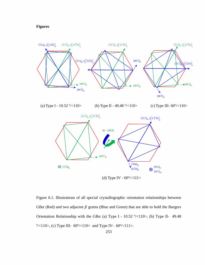
253
Figures
Figure 6.1. Illustrations of all special crystallographic orientation relationships between
GB (Red) and two adjacent grains (Blue and Green) that are able to hold the Burgers
Orientation Relationship with the GB (a) Type I - 10.52 º/<110>, (b) Type II- 49.48
º/<110>, (c) Type III- 60º/<110> and Type IV- 60º/<111>.
β2[001]
β1[001]
(a) Type I - 10.52 º/<110> (b) Type II - 49.48 º/<110> (c) Type III- 60º/<110>
β1[111] || 2110
β2[111] || 1120
β2[111] || 1210
β1[001] β1[001]
β2[001]
β2[001]
β1[111] || 2110
β1[111] || 2110
β2[111] || 1210
β1[001]
β1[111] || 2110
β2
β2
[100]
[0 10]
β2[111] || 2110
β1[110] β2
β2
[011]
[101]
(d) Type IV - 60º/<111>
60 / [ ]111

254
Figure 6.2. Experimental observations of a Type II special grain boundary where
GB maintains BOR with two adjacent grainsaOIM image of the Type II
boundary; (b) superimposed pole figures of the poles of the two grains and the
pole of the GB (c) Superimposed pole figures among the poles of the
two grains and the pole of the GB
1
2
(a)
(b) (c)
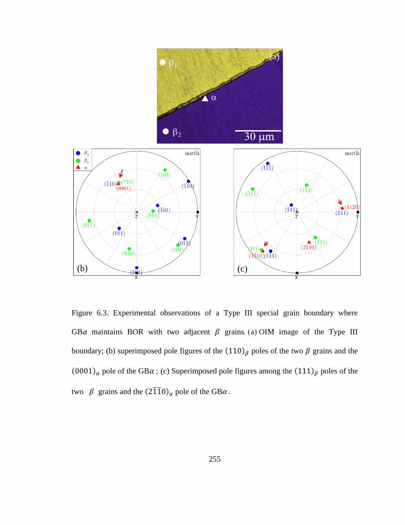
255
Figure 6.3. Experimental observations of a Type III special grain boundary where
GB maintains BOR with two adjacent grainsaOIM image of the Type III
boundary; (b) superimposed pole figures of the poles of the two grains and the
pole of the GB (c) Superimposed pole figures among the poles of the
two grains and the pole of the GB
1
2
(a)
(b) (c)
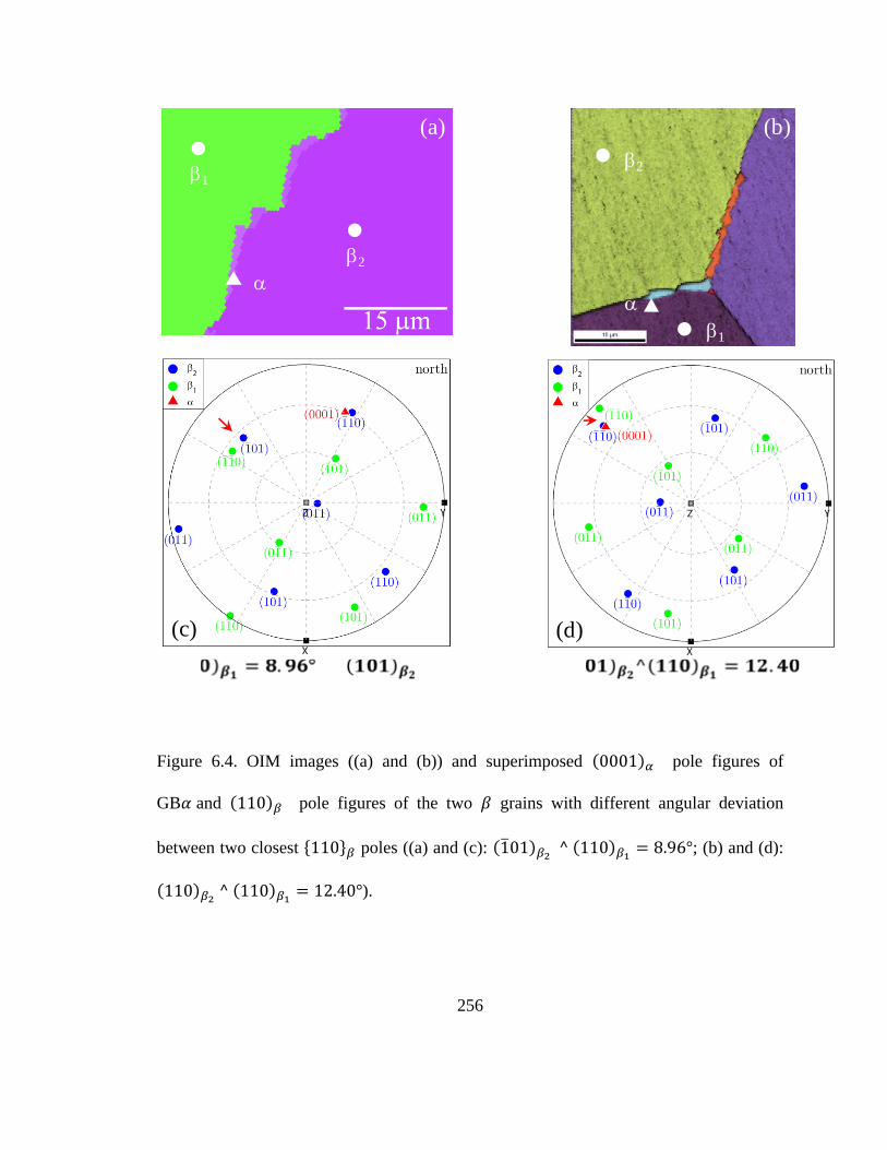
256
Figure 6.4. OIM images ((a) and (b)) and superimposed pole figures of
GB and pole figures of the two grains with different angular deviation
between two closest { } poles ((a) and (c):
; (b) and (d):
).
1
2
1
2
(a) (b)
(c) (d)
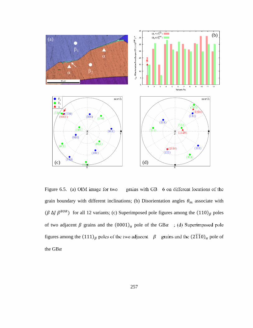
257
Figure 6.5. (a)
grain boundary with different inclinations; (b) Disorientation angles associate with
for all 12 variants; (c) Superimposed pole figures among the poles
of two adjacent grains and the pole of the GB
figures among the pole of
the GB
1
2
(a)
(c) (d)
(b)
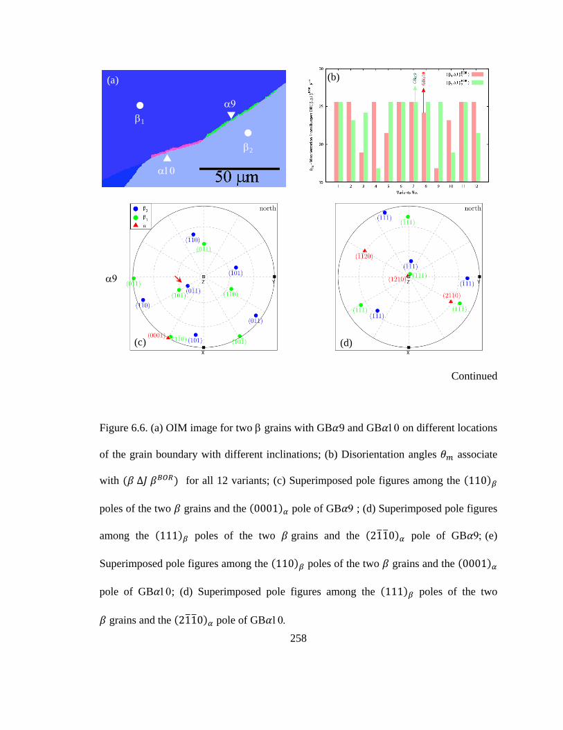
258
Continued
Figure 6.6. (a) OIM image for two grains with GB 9 and GB on different locations
of the grain boundary with different inclinations; (b) Disorientation angles associate
with for all 12 variants; (c) Superimposed pole figures among the
poles of the two grains and the pole of GB ; (d) Superimposed pole figures
among the poles of the two grains and the pole of GB (e)
Superimposed pole figures among the poles of the two grains and the
pole of GB ; (d) Superimposed pole figures among the poles of the two
grains and the pole of GB
1
2
(a) (b)
(c) (d)

259
Figure 6.6 continued
(b) (110) pole
(f)(e)
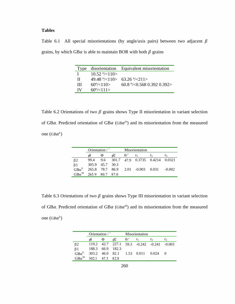
260
Tables
Table 6.1 All special misorientations (by angle/axis pairs) between two adjacent
grains, by which GB is able to maintain BOR with both grains
Type disorientation Equivalent misorientation
I 10.52 º/<110>
II 49.48 º/<110> 63.26 º/<211>
III 60º/<110> 60.8 º/<0.568 0.392 0.392>
IV 60º/<111>
Table 6.2 Orientations of two grains shows Type II misorientation in variant selection
of GB Predicted orientation of GB (GB ) and its misorientation from the measured
one (GB )
Orientation / ˚ Misorientation
˚ r1 r2 r3
2 99.4 9.6 301.7 47.9 0.3735 0.4214 0.0321 1 305.9 45.7 30.3
GB 265.8 78.7 86.9 2.01 -0.003 0.031 -0.002
GB
Table 6.3 Orientations of two grains shows Type III misorientation in variant selection
of GB Predicted orientation of GB (GB ) and its misorientation from the measured
one (GB )
Orientation / ˚ Misorientation
˚ r1 r2 r3
2 119.2 42.7 227.1 59.3 -0.242 -0.241 -0.003
1 188.3 66.9 182.3
GB 303.2 46.0 82.1 1.53 0.011 0.024 0
GB
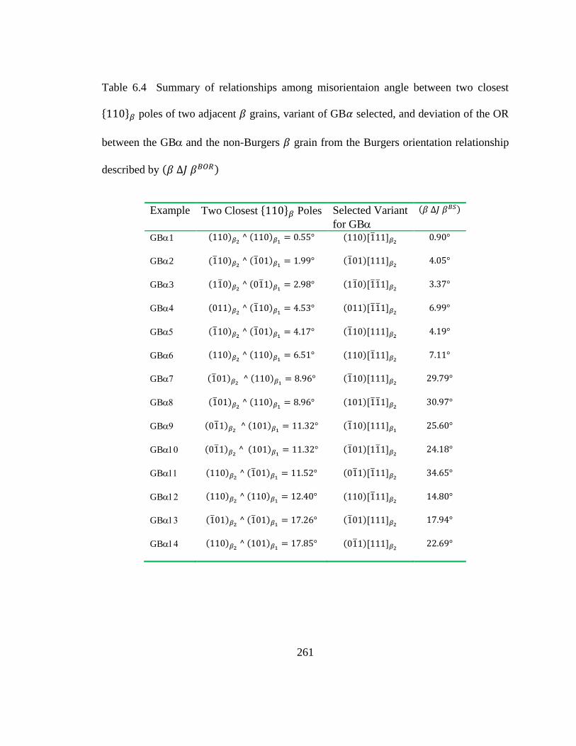
261
Table 6.4 Summary of relationships among misorientaion angle between two closest
{ } poles of two adjacent grains, variant of GB selected, and deviation of the OR
between the GBand the non-Burgers grain from the Burgers orientation relationship
described by
Example Two Closest { } Poles Selected Variant
for GB
GB1
[ ]
GB2
[ ]
GB3
[ ]
GB
[ ]
GB
[ ]
GB
[ ]
GB
[ ]
GB
[ ]
GB
[ ]
GB
[ ]
GB
[ ]
GB
[ ]
GB
[ ]
GB
[ ]

262
6.6 References:
[1] Bache MR. Processing titanium alloys for optimum fatigue performance.
International Journal of Fatigue 1999;21:S105.
[2] Whittaker R, Fox K, Walker A. Texture variations in titanium alloys for
aeroengine applications. Materials Science and Technology 2010;26:676.
[3] Banerjee D, Williams JC. Perspectives on Titanium Science and Technology.
Acta Mater 2013;61:844.
[4] Burgers WG. On the process of transition of the cubic-body-centered
modification into the hexagonal-close-packed modification of zirconium. Physica
1934;1:561.
[5] Furuhara T, Takagi S, Watanabe H, Maki T. Crystallography of grain boundary α
precipitates in a β titanium alloy. Metallurgical and Materials Transactions A
1996;27:1635.
[6] Stanford N, Bate PS. Crystallographic variant selection in Ti-6Al-4V. Acta Mater
2004;52:5215.
[7] van Bohemen SMC, Kamp A, Petrov RH, Kestens LAI, Sietsma J. Nucleation
and variant selection of secondary alpha plates in a beta Ti alloy. Acta Mater
2008;56:5907.
[8] Lee E, Banerjee R, Kar S, Bhattacharyya D, Fraser HL. Selection of alpha
variants during microstructural evolution in alpha/beta titanium alloy. Philosophical
Magazine 2007;87:3615.

263
[9] Kar S, Banerjee R, Lee E, Fraser HL. Influence of Crystallography Variant
Selection on Microstructure Evolution in Titnaium Alloys. In: Howe JM, Laughlin DE,
Dahmen U, Soffa WA, editors. Solid-to-Solid Phase Transformation in Inorganic
Materials, vol. 133-138: TMS (The Minerals, Metals & Materials Society), 2005.
[10] Lutjering G, Williams JC. Titanium (Engineering Materials and Processes).
Berlin: Springer, 2007.
[11] Bhattacharyya D, Viswanathan GB, Denkenberger R, Furrer D, Fraser HL. The
role of crystallographic and geometrical relationships between alpha and beta phases in
an alpha/beta titanium alloy. Acta Mater 2003;51:4679.
[12] Bhattacharyya D, Viswanathan GB, Fraser HL. Crystallographic and
morphological relationships between beta phase and the Widmanstatten and
allotriomorphic alpha phase at special beta grain boundaries in an alpha/beta titanium
alloy. Acta Mater 2007;55:6765.
[13] Semiatin SL, Kinsel KT, Pilchak AL, Sargent GA. Effect of Process Variables on
Transformation-Texture Development in Ti-6Al-4V Sheet Following Beta Heat
Treatment. Metallurgical and Materials Transactions A 2013;44:3852.
[14] Bowles JS, Mackenzie JK. The crystallography of martensite transformations I.
Acta Metallurgica 1954;2:129.
[15] Mackenzie JK, Bowles JS. The crystallography of martensite transformations II.
Acta Metallurgica 1954;2:138.
[16] Bhadeshia HKDH. Worked examples in the geometry of crystals, 2001.
264
[17] Kim D, Suh D-W, Qin RS, Bhadeshia HKDH. Dual orientation and variant
selection during diffusional transformation of austenite to allotriomorphic ferrite. Journal
of Materials Science 2010;45:4126.
[18] Kim DW, Qin RS, Bhadeshia HKDH. Transformation texture of allotriomorphic
ferrite in steel. Materials Science and Technology 2009;25:892.
[19] Engler O, Randle V. Introduction to texture analysis: macrotexture, microtexture,
and orientation mapping: CRC PressI Llc, 2010.
[20] Shiflet GJ, Merwe JH. The role of structural ledges as misfit- compensating
defects: fcc-bcc interphase boundaries. Metallurgical and Materials Transactions A
1994;25:1895.
[21] Nie JF. Crystallography and migration mechanisms of planar interphase
boundaries. Acta Mater 2004;52:795.
[22] Zhang M-X, Kelly PM. Crystallographic features of phase transformations in
solids. Progress in Materials Science 2009;54:1101.
[23] Shi R, Ma N, Wang Y. Predicting equilibrium shape of precipitates as function of
coherency state. Acta Mater 2012;60:4172.
[24] Read WT, Shockley W. Dislocation Models of Crystal Grain Boundaries.
Physical Review 1950;78:275.
[25] Zhang WZ, Weatherly GC. On the crystallography of precipitation. Progress in
Materials Science 2005;50:181.
265
[26] Ye F, Zhang WZ, Qiu D. A TEM study of the habit plane structure of
intragrainular proeutectoid alpha precipitates in a Ti-7.26wt%Cr alloy. Acta Materialia
2004;52:2449.
[27] Lee JK, Aaronson HI. Influence of faceting upon the equilibrium shape of nuclei
at grain boundaries—II. Three-dimensions. Acta Metallurgica 1975;23:809.
[28] Lee JK, Aaronson HI. Influence of faceting upon the equilibrium shape of nuclei
at grain boundaries—I. Two-dimensions. Acta Metallurgica 1975;23:799.

266
CHAPTER 7 Effects of Grain Boundary Parameters on
Variant Selection of Grain Boundary in Titanium Alloys
Abstract
In titanium alloys, variant selection (VS) of grain boundary (GB ) by prior grain
boundaries during precipitation has a significant influence on the transformation
pathway and transformation texture of phase and thus on the final mechanical
properties. In this paper, the applicability of all current empirical VS rules with respect to
grain boundary parameters such as misorientation and inclination on VS of GB has been
assessed systematically using experimental characterizations of Ti-5553. It is found that
when the minimum misorientation angle associated with , a measure of
deviation of the orientation relationship between the GB and the non-Burgers grain
from the Burgers orientation relationship, is less than , misorientation plays a
dominant role in VS of GB , and when grain boundary plane inclination plays
a more important role. The violations of the empirical VS rules related to inclination may
be attributed to the interplay among grain boundary energy and interfacial energies
between GB and the Burgers and non-Burgers grains in determining the nucleation
267
barrier for each variant. The violation could be associated with the characteristic of grain
boundary plane orientation population.
7.1. Introduction
Titanium and its alloys (Ti-alloys) are currently finding increasingly widespread use in
many applications, ranging from structural components in aircrafts, automobiles and
ships to bio-implants [1]. The effectiveness to tailor the microstructures of a given Ti-
alloy through relatively simple thermo-mechanical processing to meet selected
engineering requirements has contributed to their current dominance. Microstructure
evolution in most Ti-alloys during heat treatments is dominated by the (BCC) to
(HCP) transformation upon cooling. For both and + processing route,
microstructure evolution initiates from the formation of allotriomorphic on the prior
grain boundaries (GBs) that is referred to as grain boundary (GB). Similar to ferric
alloys, the influence of GB on the subsequent microstructure development and
microstructure-properties relationships in Ti-alloys has been an active area of research for
decades [1-3]. In most cases, GB has the Burgers orientation relationship (BOR) [4], i.e.
; [ ] [ ] , with one of two adjacent grains. The grain that
maintains BOR with the GB is referred to as Burgers grain and the other grain is
referred to as non-Burgers one. The BOR would result in 12 crystallographically
equivalent orientation variants available for GBwith respect to Burgers grain. However,
a trend of strong variant selection (VS) of GBhas been demonstrated frequently by
268
experimental observations that, instead of 12, only limited numbers of variants seem to
be dominant on most of GBs. VS of GB has [5] a direct influence on the overall
microstructure and transformation texture evolution [6, 7], and thus has a significant
impact on the mechanical properties [5]. For instance, when two adjacent grains are
specially misorientated [8-10], colonies developed from GB into the two grains
would have common crystallographic features such as common basal plane orientations
(though with their [ ] pole being misorientated by a ~10.5˚ rotation about their
common [ ] axis) and, even more specifically [11], may have exactly the same
orientation as that of GB. Large regions of phase with a common crystallographic
feature are also referred to as “macro-zones” [3] or micro-textured regions that would
result in a significant reduction in fatigue life of Ti-component [2, 12] for a given
operation stress. Thus the formation of macro-zone across grain boundaries due to VS of
GB is undesirable in a safety critical operating environment. It is of great importance to
investigate how a given grain boundary select a variant for GBfrom the 12 possible
candidates.
VS of GB by a specific grain boundary is determined by the structure of that grain
boundary, which depends on both misorientation and (GBP) inclination, defined in a five-
dimensional space. In terms of how the five parameters of a grain boundary contribute to
VS of GB, several empirical rules have been proposed. For example, it has been
commonly observed that GB maintains an OR with the non-Burgers grain that has only
a small deviation from the BOR [9, 10, 13]. In other words, deviation of the OR between
269
the GBand the non-Burgers grain from the BOR should be as small as possible. In
special cases, GBcould have BOR with both grains [11], which should be the most
preferred configuration. It is thus referred to as Rule I in the current study that variant
selection of GB is made to maintain BOR with both adjacent grains as much as
possible. Such an arrangement in orientations among a GB and the two grains may
lead to low energy interfaces with respect to both grains and thus result in a low
nucleation barrier for the GB. A new parameter, , that is a measure of
deviation of the OR between the GB and the non-Burgers grain from the BOR, has been
proposed [14]. The disorientation angle associated with the deviation matrix is able to
quantify the deviation, akin to the dependence of grain boundary energy on
misorientation angle. For the particular alloy, Ti-5553, considered in [14], it has been
found that when the misorientation angle (instead of the closeness between two closet
{ } poles between two grains widely used in literature) is less than ,
misorientation between the two grains dominates VS of GB and, in particular, the
variant with minimum is always selected for GB. For each variant,
depends on misorientation and BOR matrix associated with the variant. Thus, Rule I
accounts only for the effect of misorientation on VS of GB.
As for the influence of GBP inclination, two additional rules have been proposed so far.
It has been accepted in general that there exists a pronounced tendency for the low energy
facet or habit plane developed between GB and the matrix grains to be parallel to GBP.
270
As have been demonstrated by Lee and Aaronson [15, 16], the inclination angle, ,
between GBP and the low energy facet of an precipitate has a significant effect on the
nucleation barrier, . For two ratios between the grain boundary energy and the
interfacial energy (assumed to be the same for the two interfaces), 1.07 and 1.57,
the minimum of always occurs when for different ratios between the
interfacial energy of the low energy facet and , no matter whether the GBP is
planar or puckered. In other words, in order to reduce nucleation barrier, the low energy
facet needs to be parallel to the GBP as much as possible as such to maximize the area of
grain boundary eliminated by such GB nucleation. According to the interface
structure when BOR is maintained in between, the low energy facets have been
characterized to be { } { } (terrace plane orientation) and { } { }
(side facet orientation). Thus, we refer the above criterion to as Rule II, i.e., the major low
energy facet { } { } of the selected variant should have the minimum deviation
from GBP.
Nevertheless, in a crystallographic study of GB formed in a titanium alloy (Ti-15V-
3Cr-3Sn-3Al in wt.%), Furuhara et al [13] concluded that selection of a variant for GB
is made in a different manner that the matching direction (i.e. ⟨ ⟩ ⟨ ⟩ ) of the
selected variant makes the smallest deviation angle from the GBP, i.e., ⟨ ⟩
⟨ ⟩ tends to be parallel to the GBP. It is referred to as Rule III in the present work.
As has been argued by Furuhara et. al. [13], Rule III results from the requirement that the
271
two low energy facets, i.e., { } { } and { } { } developed into the
Burgers grain, make the smallest inclination angle with respect to the GBP to minimize
. Accordingly, the critical nucleus formed at a given grain boundary tends to
elongate along the intersection of these two facets, i.e., ⟨ ⟩ ⟨ ⟩ zone axis of
these two facets. According to reference [13], Rule III is a modified version of Rule II for
lath- or needle-shaped precipitates [17], in which the most effective way to eliminate
grain boundary area by grain boundary nucleation is making the growth direction of a
lath nuclei parallel to the GBP. Note that since [ ] is the zone axis of and
planes, even if [ ] is included in the grain boundary, there are still many
ways to arrange two planes with respect to the grain boundary. Thus, Rule III accounts
for how to arrange two different low energy facets developed in the Burgers grain with
respect to the GBP to reduce the nucleation barrier of GB, while keeping the zone axis
of the two facets included in the GBP.
Up to now, there is no critical assessment of the general applicability of these rules and,
hence, their predictive powers are limited. For example, for a given GB there will be
three variants that share a common ⟨ ⟩ and satisfy Rule III. Which one will be
finally selected will be determined by factors beyond what are considered in Rule III. As
has been suggested by Furuhara et al, Rule I and Rule III result in the selection of a single
variant of GB on a planar grain boundary [13]. Moreover, Rule III could be
predominant over Rule I when the minimum associated with is more
than since Rule III is more frequently (though not always) followed than Rule I in

272
variant selection of GB, while Rule I is more important when the minimum is less
than because in this case the variant with minimum is always selected as the
GB. It should be noted that Rule I is not able to determine the Burgers grain. In fact,
there are always two variants having the same minimum , e.g., when assuming
different adjacent grain to be the Burgers one during the prediction, corresponding to
with respect to the Burgers grain and
with respect to the
Burgers grain , respectively. Nevertheless, when the minimum , it is found
that GBP inclination is able to determine the Burgers grain, though the manner is still not
clear without considering the information of GBP inclination. In terms of predicting
capability, Rule II would predict a single variant to be selected by the Burgers grain. For
Rule III, there exist three variants with common ⟨ ⟩ meeting the requirement. For
Rule I, it would predict, at least, two variants with identical minimum of
but having BOR with respect to different grains. In other words, Rule I is not able to
predict the Burgers grains. In particular, as will be shown in the current study, there are
some cases where variant selection behavior follow none of three rules. There is no doubt
that all grain boundary parameters play their own roles in VS of GB, but how they
contribute to VS of GB on a given grain boundary has not yet been completely
understood. Therefore, further validation and consideration of these three criteria,
especially the physical mechanisms behind them, requires further investigation.
Apparently, the work first requires a complete description of grain boundary characters.
273
In order to make a precise prediction of VS of GB for a given set of grain boundary
parameters, the applicability and limitation of each rule needs to be clarified. In
particular, as will be shown in the current study, all VS rules could expire on a given
grain boundary. It is thus crucial to investigate why a rule is violated and also whether the
physic mechanism lying behind each rule is reasonable or not. Therefore, the objective of
the current study is to elucidate that, on a prior grain boundary, how to use all current
VS rules to make a right prediction of grain boundary nucleation, validities and
limitations of all rules, the reasons why a single or multiple rules are violated.
The chapter is organized as the follows. In Section 7.2, we first design an experiment that
highlights the effect of grain boundary parameters on the grain boundary nucleation.
Individual orientations of two adjacent grains and GB are measured using electron
backscattered diffraction (EBSD) technique, and GBP orientation is determined using a
three-dimensional two-surface trace approach. In Section 7.3, variant selection of GB at
different prior GBs are analyzed according to three aforementioned variant selection
rules. The analysis is conducted by comparing the measured orientation of GB and the
predict one by a crystallographic model developed by the present authors to investigate
how three rules are followed or violated. The effect of grain boundary parameters on
variant selection of GB and possible physical insights of different rules are then
discussed in Section 7.4. Finally, major findings are summarized in Section 7.5.
274
7.2. Experimental procedure
In current study, the material used is a forged -Ti alloy, Ti-5553, i.e., Ti-5Al-5Mo-5V-
3Cr-0.5Fe (wt. %). A -titanium alloy is selected in order to avoid the martensitic
transformation and thus retain phase during a thermal quench. The as-received alloy
was sectioned to small samples (~20mm×20mm×40mm) for heat treatment. The samples
were initially -annealed at 1000˚C for 15 minutes using a conventional tube furnace in
an inert Argon atmosphere. The samples were wrapped in titanium foil to further reduce
the possibility of oxygen ingress. The samples were then cooled in the furnace to 825˚C
at a controlled rate of 5˚C/min, and were soaked for 2 hours to allow for the phase
transformation to complete. Finally, the samples were water-quenched to room
temperature. Since the -transus for this alloy is close to 850˚C, such a heat treatment
procedure would allow for only limited one or two variants of GBform on a given
planar grain boundary if the precipitation would occur while colony structure has not
develop from GB and thus allow us to avoid the influence of relative large under
cooling on the variant selection behavior, and to determine the orientations of two grain
and GB . In other word, under such a small undercooling, grain boundary characters
would play a dominant role in the determination of variant selection of GB. For
subsequent characterization, all specimens are further sectioned in the middle and the
exposed surfaces were subjected to mechanical polishing using standard metallographic
techniques. In the final step, material is kept in a vibratory polisher in the suspension of
0.05 m silica particles for a number of hours to achieve a mirror-finish. The

275
crystallographic orientation of GB and the parent grains are measured at various
locations using EBSD data collection in Philips XL30 ESEM FEG SEM at 20kV, with a
spot size of 4 and a working distance of 20 mm. Suitable step-size (1.7m) in OIM-TSL
software is selected to allow for the collection of data from a large area (~1 mm × 1 mm)
in a reasonable amount of time. The reliability of this data collection was verified on a
⟨ ⟩ silicon sample under similar conditions.
The local orientations of GBP are determined by producing a site specific section into the
sample to expose trace of a GB on two mutually perpendicular surfaces, i.e. sample
surface and a trenched one. A combination of secondary electron imaging and focused-
ion beam (FIB) in FEI NOVA Dual BeamTM
(SEM/FIB) microscope is used for this
purpose. In other words, trenched sections are produced nearly perpendicular to the grain
boundary traces present on the sample surface using FIB. The crystallographic orientation
of the grain boundary relative to the adjacent grain has been determined by combining
their geometry with the crystallographic information provided by the EBSD data. The
accuracy of the method has been validated and analyzed using the knowledge of
crystallographic characteristics of twins present in both cubic (IN-100 Ni-based
superalloy) and hexagonal systems (commercially pure (CP)-titanium). A certain degree
of reorientation of grain boundary planes occurs as a result of the GBprecipitation. In
order to take this change into account, FIB sections have been produced nearly normal to
the site specific projection of trace of GB. Details on the experimental techniques and
276
measurements to determine local orientation of GBP can be found in referred to Ref.
[17].
7.3. Results
7.3.1. Overall Characteristics of variant selection of GB
In the current study, thirty five examples of GB at different prior grain boundaries are
observed and analyzed. For all grain boundaries, there is only one or two variants are
selected, as shown in Fig. 7.1. Details about all 5 grain boundary parameters of different
grain boundaries corresponding to selection of all GB in the current study are presented
in Table 7.1. In particular, grain boundary plane orientations are expressed in both crystal
reference frame of Burgers grain, i.e. [ ] ; [ ] ; and [ ] , and
Burgers reference frame associated with the selected variant in the Burgers grain, i.e.
[ ] [ ] ; [ ] [ ] ; and [ ] [ ] .
Results about 35 orientations of different GBs (i.e. 70 GB surfaces) are displayed in Fig.
7.2 in the form of solid circles in the standard stereographic triangle for the BCC
structure. The locations of circles indicate the orientation of surface normal of GB planes
with respect to the crystal reference frame in Burgers grain. It can be found that grain
boundary planes with the orientation have a relative large population areas, while
there is only one example where grain boundary plane orientation is close to .

277
Figure 7.3 shows orientations of all grain boundary planes displayed in a pole figure with
respect to the Burgers reference frame. Such a plot is really convenient to illustrated the
relationship among GBP orientation, ⟨ ⟩ axis and { } plane of the selected
variant, which are key parameters described by different empirical VS rules. For
example, the frequency of occurrence of variant selection as a function of the inclination
angle between GBP and { } planes ( ), and between GBP and ⟨ ⟩ direction
( ) are presented in Fig. 3(b) and Fig. 3(c), respectively. Inclinations angles within
[ ] are divided into six groups with interval of 15° for each. It is readily seen that
the distribution is quite randomly scattered. In particular, variant selection occurs most
frequently when falls in the group of [ ] , or when
is located within
[30-45]°. It should also be noted that there is only one case where is within [
] . In contrast, there are 6 examples where is within [ ] . On the basis of
this statistic, it seems that Rule III plays a more important role in the variant selection of
GB than Rule II. However, even more frequently, VS of GB does not follow either
Rule II or Rule III.
It has been suggested that when the minimum is less than 15°, misorientation between
two grain would be dominant over GBP inclination in the VS of GB, Thus, the same
analysis as that in Fig. 7.3, is furthered refined into two groups, one is for , and
the other one is for . The results are shown in Fig. 4 and Fig. 5, respectively. It
is readily seen that the similar trend as that in Fig. 7.3 is still followed. In the current
study on VS of GB in Ti5553 alloy, it seems that neither Rule II nor Rule III is

278
frequently followed. In contrast, as can be found in Figs. 7.4-7.5, there are some
examples that violate both Rule II and Rule III no matter is larger or less than 15°. For
example, there are 3 examples that is within [ ] , and 4 examples that
is within [ ] .
7.3.2. Variant selection of GB when different rules are dominant
It is worth mentioning that the above analysis only considers the relationship
among ⟨ ⟩ , { } of selected variant, and GBP. However, according to
aforementioned empirical rules, it should be the differences in , and
among all 24 possible variants that determine the VS of GB. Therefore, in this section,
several examples are analyzed individually to evaluate how these different parameters
contribute to VS of GB. Examples are divided into 4 groups, a) Rule I is dominant; b)
Rule II is dominant; c) Rule III is dominant; d) Abnormal cases where none of three rules
is followed. For a GB in a given grain boundary, the measured orientations of two
adjacent grains are also used as model inputs to predict all 24 possible orientations of
GBby assuming one of two adjacent grains to be the Burgers one alternatively. For
each variant, associated with , inclination angles between [ ] ,
, , and GBP, i.e. ,
, and , are all evaluated. By comparing
orientations of GB between the measured and predicted values, we would then have a
picture about how a variant follows or violates these three rules to make it selected for
279
GB, which would help to clarify how grain boundary parameters contribute to select
one or two variants of GBfrom 24 candidates.
7.3.2.1. Rule I is dominant
The OIM image in Fig. 7.6(a) shows two adjacent grains and a GB (Example 16 in
Table 7.1, or GB16) in between in different colors according to their orientations (i.e.,
Euler angles: Bunge notation, [, , ]). The corresponding superimposed pole figures
of the GB and two adjacent grains (with respect to sample reference frame) for Fig.
6(a) are shown in Figs.7.6(b)-7.6(d) for { } /{ } , { } / { } and
{ } /{ } ,respectively. In particular, orientation of grain boundary plane is also
superimposed in Fig. 7.6(c) and (d). In Fig. 7.6(b), trace of grain boundary plane is
superimposed. From the superimposed pole figures, it seems that GB exist BOR with
both grains, i.e. , [ ]
[ ] (V5) and ,
[ ] [ ] (V12). When comparing the predicted orientations for GB and the
measured ones, it is found that the variant V12 that has been selected for GB and
maintains BOR with 1, as shown in Table 7.2. Disorientation angles associated with
for all 12 variants are provided in Fig. 7.6(e) when 1 or 2 servers as the
Burgers grain, respectively. In the former, measures the deviation of GB
from the BOR with respect to the non-Burgers grain 2, while in the latter

280
measures the deviation of GB from the BOR with respect to the non-Burgers grain 1.
It is readily seen that the variant V5 (2 as Burgers grain) and the variant V12 (1 as
Burgers grain) have the same minimum (less than 15°). By comparing for V5
and V12 as shown in Fig. 7.6(f), it is found that V12 has a smaller value and thus meets
the requirement of Rule II. Note that neither V5 nor V12 has the minimum . The
variant V8 has the minium among 24 possible variants. however, it is not selected.
All the above facts seem to suggest that in this case, Rule I is dominant over Rule II while
Rule II may contribute to the determination of Burgers grain. Details about the effect of
all grain boundary parameters in the variant selection of GB 16 are referred to Table 7.3.
7.3.2.2. Rule II is dominant
The OIM image in Fig. 7.7(a) shows two adjacent grains and a GBGB28 in Table
7.1) in between. The corresponding superimposed pole figures of the GB and two
adjacent grains (with respect to sample reference frame) for Fig. 7.7(a) are shown in
Figs. 7.7(b)-(d) for { } /{ } , { } / { } and { } /{ } ,
respectively. For pole figure in Fig. 7.7(b), there are three ⟨ ⟩ poles , i.e. [ ]
and [ ] , that are very close to trace of GBP. However, only [ ]
pole is selected.
Details about , ,
, and
are referred to Table 7.4. Variant V9 has
been selected as GB and maintains BOR with 2, i.e., ,

281
[ ] [ ] , which is also confirmed by the comparison between predicted and
measured orientations for GB as presented in Table 7.5. As shown in Fig. 7.7(e), all 24
values are larger than 15°, the selected variant (V9) is not the one having the
minimum . However, the selected variant has its plane closet to GBP among
all 24 candidates, as indicate by an arrow in the Fig. 7.7(e). The analysis suggests that
Rule II is decisive in terms of selection of Burgers grain and variant for GB in the
example.
7.3.2.3. Rule III is dominant
The OIM image in Fig. 7.8(a) shows two adjacent grains and two GB s in different
locations with different GBP orientations in between. precipitate in the upper right is
GB7, and the one in the bottom left is GB8. The corresponding superimposed pole
figures of the GB and two adjacent grains for Fig. 7.8(a) are shown in Figs. 7.8(b)-
8(d) for { } /{ } , { } / { } and { } /{ } , respectively.
Superimposed pole figures for GBare shown in Figs. 7.8(e)-8(g).From the pole
figures and comparisons between predicted and measured orientations for GBTable
7.6), variant V7 is selected and holds BOR with 1, i.e. ,
[ ] [ ] ; for GB8 Table 7.7),, variant V8 is selected and maintains BOR
with 2, , [ ]
[ ] . Similar to the example in Sec 3.2.2, all
282
24 values are larger than 15°, neither one of two selected variants is the one with the
minimum . It suggests that, in this case, GBP orientation also determines VS of GB.
However, Rule II does not work. Note that neither V7 (for GB 7 with as Burgers
grain) nor V8 (for GB 8 with 2 as Burgers grain) has the minimum among all
24 candidates. But both two selected variants have their corresponding close to 90˚.
Details about the effect of all grain boundary parameter in the variant selection of GB7
and GB8 are referred to Table 7.8 and Table 7.9, respectively. It seems that Rule III
plays a leading role in the determination of VS of GB 7 and GB 8than Rule II. It
should be mentioned that Rule III would offer three candidate variants sharing a
common⟨ ⟩ . But how the Rule III results in the selection of a single variant on a
given planar GB with fixed GBP orientation is still not clear.
7.3.3. Abnormal cases
7.3.3.1 Abnormal variant selection when the minimum
An example is presented in this section to show how both Rule II and Rule III expires in
the determination of Burgers grain when the minimum associated with is
less or equal to 15°. For example, it can be seen from the OIM image shown in Fig.
7.9(a) that the two GB precipitates with the same color (i.e., same orientation) appear at
two different locations with different GBP inclinations of the GB between 1 and 2.
283
The corresponding superimposed pole figures of the GB and two adjacent grains
(with respect to sample reference frame) for Fig. 7.9(a) are shown in Figs. 7.9(b)-7.9(d)
for { } /{ } , { } / { } and { } /{ } , respectively. From the pole
figures and comparisons between predicted and measured orientations (Table 7.10), GB
selects variant V1 and maintains BOR with 2, i.e. ,
[ ] [ ] (V1). The variation in GBP orientation does not change the result of
VS that thus suggests that misorientation between two grains determines the variant
selection. The argument is supported by the fact that Variant (V5 with 1 as Burgers
grain) that has the minimum has not been selected for GB. Moreover, none of
variants having[ ] , [ ]
and [ ] that are closet to the GBP trace (
) has been selected. Variant V1 is one of the two candidates that have the
minimum associated with and, in particular, minimum . When
compared with variant V3 that maintains BOR with , ,
[ ] [ ] , the variant V1 has a relative lager
and smaller . Details
about the effect of all grain boundary parameter in the variant selection of GB 32 are
referred to Table 7.11. The above analysis confirms that when misorientation is dominant
in VS, Rule II and Rule III are not always able to further determine the Burgers grain.
284
7.3.3.2 Abnormal variant selection when
The example presented in this section is to show how both Rule II and Rule III are
violated in the determination of Burgers grain even when the minimum associated
with is larger than 15°. The OIM image for such an example is shown in
Fig. 7.10(a). The corresponding superimposed pole figures of the GB and two adjacent
grains for Fig. 7.10(a) are shown in Figs. 7.10(b)-10(d) for { } /{ } , { } /
{ } and { } /{ } , respectively. From the pole figures and comparisons
between predicted and measured orientations (Table 7.12), GB selects variant V7 and
maintains BOR with 2, i.e. , [ ]
[ ] . Details about the
effect of all grain boundary parameters in the variant selection of GB 26 are referred to
Table 7.13. Again, all 24 values are larger than 15°, the selected variant is not the one
with the minimum . Nevertheless, the selected variant does have neither the largest
nor the smallest
. In the case, all empirical VS rules, would mislead
predictions towards t VS of GB from all 24 candidacies.
7.4. Discussions
Existing studies suggest that heterogeneous nucleation of at prior grain boundaries
occurs as the following: for a given undercooling, an embryo/nucleus of phase
maintaining BOR with one of the grains (i.e., the Burgers grain ( )) nucleates on the

285
grain boundary between and . Low energy facets such as { } and { }
develop into the Burgers grain to minimize the interface energy between the GB and the
Burgers grain. A unique interface inclination at a fixed OR has been shown to have
the minimum energy state [19], i.e., singular or vicinal [20] interface in the 5-dimensional
space (misorientation and interface inclination between phases). On the non-Burgers
grain side, the nucleus adopts the shape of a spherical cap to minimize the interfacial
energy. Thus the nucleation barrier depends on the chemical driving force for nucleation
(determined by undercooling), grain boundary energy , interfacial energies between
the GB and the non-Burgers and Burgers (non-facet portion) grains, and
,
respectively, and interfacial energies of the low energy facets of the GB in the Burgers
grain,
and
. Among all these parameters, is variant sensitive since each
variant has different value of that links directly to the interfacial energy.
If nucleation occurs in the bulk of the Burgers grain, ,
and
and thus the
activation energy for nucleation will be identical for all 12 variants. However, for grain
boundary nucleation, low energy facets of different variants will have different
inclination angles, and
, with respect to the grain boundary plane (GBP). As a
result, the 2 interface will consist of different areas of a non-facet portion having
energy and facets portions having energy
and
[15, 16]. Thus, the
activation energy for each variant will depend on and
as well. Thus we have,
(
)
286
where is the activation energy for GB nucleation. This is the origin that leads to the
occurrence of VS of GBon prior GBs. In order to make a precise prediction of VS of
GB, therefore, a rule in general needs to take all these parameters into account and,
more importantly, demonstrate quantitatively how these parameters contribute to .
Nevertheless, none of the current VS rules discussed earlier has taken all these
parameters into consideration.
Through the analysis presented in the Results sections, the empirical rules of VS of
GBare valid only in limited cases. For example, Rule I considers only the differences in
misoriention for all possible variants and thus accounts only for .
Following the assumption that the BOR offers a relatively low interfacial energy of
as well as a low coherency elastic strain energy, any deviation from it, measured by
associated with , will most likely result in a rise in these energy terms up to
certain critical value of . This is akin to the Read-Shockley relationship between
grain boundary energy and misorientation angle [21]. The critical angle of seems to
be about 15˚ for the alloy Ti-5553 considered in this study. When , the variant
with minimum of seems to have the lowest interfacial energy, , as
well as the minimum elastic strain energy and, thus, the lowest among all the 12
variants. In this case, Rule I would be valid. In particular, there are four special grain
boundaries in terms of misoriention [14] at which certain GB variant is able to maintain

287
BOR with both grains, i.e., . As has been shown through VS of GB and
GB in Fig. 7.6 and Fig. 7.9, Rule I always shortlists the candidate variants from 24 to
2 that have identical minimum associated with . However, Rule I is not
capable of further discriminating against these two variants and thus cannot predict the
Burgers grain. The limitation of the predicting power of Rule I could be ascribed to the
fact that and the coherency elastic strain energy are only two among the many
parameters that determine .
Because of the relatively small undercooling considered in the current study, only one
variant of GB is able to nucleate at most of the GBs. Therefore, the other grain
boundary parameters such as the GBP inclination must be considered to further refine the
predictions offered by Rule I. One candidate variant of GB could maintain BOR with
and develops low-energy facets into , while the other one could maintain BOR with
and develop low-energy facets into . The low-energy facets developed on each side
may have different inclinations with respect to the same GBP, which results in different
that will then further shortlist the two candidates into a finally selected one.
However, the manner of the arrangement of the two low-energy facets that would lead to
a relatively low is still not clear. For example, the VS of GB shows that the one
with a smaller is selected while the VS of GBshows the opposite.
It is noticed from all the tables about the comparisons between experimental measured
and predicted orientations that two candidate variants with the two smallest always
288
share a common basal plane for a given Burgers grain. Thus, these two variants would be
able to decorate a grain boundary simultaneously under a relatively large undercooling. It
seems that the experimental observations reported in an orientation microscopy study on
the precipitation of GB in a laser deposited, compositionally graded Ti-8Al-xV by
Banerjee et al. [22] support this statement. It has been observed [22] that GB of such
two variants decorates the GB in a nearly alternating manner.
When , however, the GBP inclination may play a more dominant role over the
misorientation between two grains in determining variant selected for GB. For
example, it has been observed frequently that when , the variant with the
minimum was not selected for GB . Still making the assumption that the interfacial
energy between the GB and the non-Burgers grain becomes approximately independent
of misorientation when , then if of for all the 12
variants are larger than 15 , the difference in may not result in significant differences
in anymore (here the contribution of misorientation axis to
is also ignored
since the system temperature is close to transus and hence the degree of interfacial
energy anisotropy is small and could be neglected as well). In such cases, other factors in
quantifying the activation energy for nucleation such as inclination of interface for a
given variant with respect to the GBP needs to be considered.
Both Rule II and Rule III focus on the influence of GBP inclination with respect to the
low energy facets, i.e., or
, on . Rule II considers the influence of
289
inclination of a single low-energy facet, i.e., { } in the current study with respect to
the GBP. Rule III, on the other hand, addresses the influence of inclination of a closed-
packed direction with respect to the GBP. As stated by Furuhara et al.[13], Rule III is
essentially a modified version of Rule II. As a matter of fact, as the zone axis of { }
and { } facets, the orientation of ⟨ ⟩ relative to the GBP determines the relative
orientations of two low-energy facets with respect to the GBP. Thus, Rule III actually
addresses the problem about how to arrange two low-energy facets relative to the GBP to
reduce the activation energy of nucleation. It states that the two facets should be arranged
in such a manner that ensures ⟨ ⟩ to be included in the GBP, i.e., should be
close to 90°. It should be noticed that even if ⟨ ⟩ is included in the GBP (
), there are still numerous ways to arrange the two low energy facets.
As has been shown by GB28, the selected variant has the minimum among all 24
possible variants. Among all 35 examples of GB , Rule II only works in this case. More
frequently, Rule II and Rule III are violated according to the statistics presented in Figs.
7.2-7.4. The underlying mechanism for both Rule II and Rule III is that the fraction of
grain boundary area eliminated by a GB nucleus will be maximized by selecting a
variant with minimum . Both rules are derived based on Lee and Aaronson’s study
on the influence of faceting on the equilibrium shape of nuclei and activation energy of
nucleation at grain boundaries in both two- (2D) [16] and three-dimension (3D) [15]. The
facet is present only in one grain, i.e., the { } facets develops only in the Burgers
grain. In 2D the equilibrium shapes of critical nuclei at different inclination angles
290
between the low-energy facet and GBP, i.e., , are derived graphically through a new
generalization of the Wulff construction [16]. The dependence of on at
various ratios of
⁄ is then calculated based on the derived equilibrium shapes. It
is found that is significantly smaller at small values of under most
circumstances. Based on the exact equilibrium shapes of critical nuclei derived in 2D,
nucleus shapes and in 3D are also studied under the same conditions. It is also found
that is significantly smaller at small values of under different ratios of
⁄ ,
and increases rapidly with at small . Thus, it is believed that nucleation at a
disordered grain boundary should occur with pronounced preference parallel to only one
of all cyrstallographically equivalent low energy facet or habit plane, i.e. , as
described by Rule II.
However, it should also be mentioned that, though increases rapidly with
under most circumstances, it could be independent of as well [15, 16]. In particular
in the 3D cases studied [15], when
⁄ , first increases sharply with
till a critical value, and then decreases over a range of
, and further increases
up to . In this case, does not increase monotonically with
anymore.
It should be noted that the applicability of both Rule II and Rule III depends on GBP
population that is influenced strongly by GB energy and texture. In a random-textured
microstructure, the grain boundary population is expected to be inversely proportional to
the grain boundary energy. It has been observed in a ferritic steel [23] and also the

291
current study (See Fig. 7.2) that, when misorientation is ignored, GBP with the { }
orientation would have the minimum energy and the largest population area. This may
explain that in most examples VS of GB does not follow Rule II since GBs with { }
orientation is relative rare to meet. Thus, it is likely that the orientation of a grain
boundary relative to all the 12 equivalent low-energy facets is such that is
appreciable for all of them, i.e., within a region where is not increasing
monotonically with or is independent of
. In the former case, Rule II
expires; in the latter case, the orientation of secondary low-energy facets, { }, may
play a role in determining VS of GB that, however, has not been considered yet.
It worth mentioning that the dependence of on is calculated [15, 16] under a
representative condition of relative interfacial energy
and
for different ratios of
⁄ . The grain boundary
energy has been found to have a strong dependence on both misorientation and GBP
inclination [24]. Therefore, it is still not yet clear whether the findings (i.e. the minimum
nucleation occurs when ) by Lee and Aaronson are valid under all combination
among different values of , and
.
In addition, one should also be aware of several assumptions made during the derivation
[15, 16] of the equilibrium shape and thus the calculation of . In both 2D and 3D
cases, shapes of critical nuclei are investigated with an additional constraint, i.e., the
grain boundary plane is constrained to remain planar. As such, the force balance at
292
junctions among two grains and the nucleus could never be achieved. In 3D cases,
the equilibrium shape of a critical nucleus derived in 2D is assumed directly for the
faceted portion of the nucleus in the Burgers side. Though the grain boundary is also
allowed to be displaced, the exact force balance at the triple junction in 3D could not be
obtained. Furthermore, and
are always assumed to be equal to make the same
chemical potential all along the surface of a nucleus since solute redistribution cannot be
considered by a purely geometrical method used in the derivation. According to the
analyses on atomic site matching between two crystals [14], should be, in general,
smaller than . The effect of non-equal diffusion potential between the facetted
portions and non-facetted portions of an interface is then also ignored.
For nucleation of GB on arbitrary prior grain boundaries, both misorientation and
GBP inclination should play their roles in determining VS of GB . It is in general
difficult to predict which factors (e.g., or
for each variant) are dominant.
Therefore, using a rule that considers only the effect of either misorientation or GBP
inclination to predict VS of GB may result in frequently wrong predictions.

293
7.5. Summary
Variant selection of grain boundary (GB) by prior grain boundaries (GBs) in Ti-
5553 under small undercooling is investigated to understand the effects of grain boundary
structure characterized by misorientation and inclination. All existing empirical variant-
selection (VS) rules about the influence of grain boundary parameters and, in particular,
how a single or a combination of different rules contributes to the VS have been analyzed
and evaluated systematically against the experimental observations. It is found that when
the minimum misorientation angle associated with , a measure of
deviation of the orientation relationship (OR) between the GB and the non-Burgers
grain from the Burgers OR, is less than , the value of plays an dominant role in
determining the interfacial energy between the GB and the non-Burgers grain as well
as the coherency elastic strain energy associated with this interface and, thus, the
activation energy of nucleation of different variants of GB. When , the grain
boundary plane (GBP) inclination may play a more important role in determining VS of
GB than the value of . However, the rules commonly accepted, e.g., the variant of
selected at a given -grain boundary is the one that has the minimum possible angle
between one of the matching directions ⟨ ⟩ ⟨ ⟩ and the grain boundary plane,
or the one that has the minimum possible angle between the one of the matching planes
{ } { } and the GBP, are found to be violated frequently by the experimental
observations. The violations of the empirical VS rules could be associated with the fact
that the activation energy of nucleation of GB is determined by a complicated interplay
294
among the five parameters related to misorientation and inclination of a GB or an
interphase interface that define the structure and energy of the GB and interfaces,
while the individual empirical rules account for only a subset of these parameters. In
order to make more accurate predictions of VS of GB a general rule needs to be further
developed that take all the parameters (grain boundary energy, interfacial energies
between GB and two grains, interfacial energies of low-energy facets, and
orientations of the low-energy facets with respect to GBP) playing their roles during the
grain boundary nucleation and, more importantly, demonstrate quantitatively how these
parameters contribute to the activation energy of the nucleation.

295
Figure
Figure 7.1 Overall characteristic of grain boundary alpha (GB ) precipitation shown by
OIM. Presence of GB only occurs at certain grain boundaries
Figure 7.2 Standard stereographic triangle projection shows the orientation of grain
boundary (GB) planes (red solid circles) relative to the crystal reference frame in Burgers
grain
(a) (b) (b)
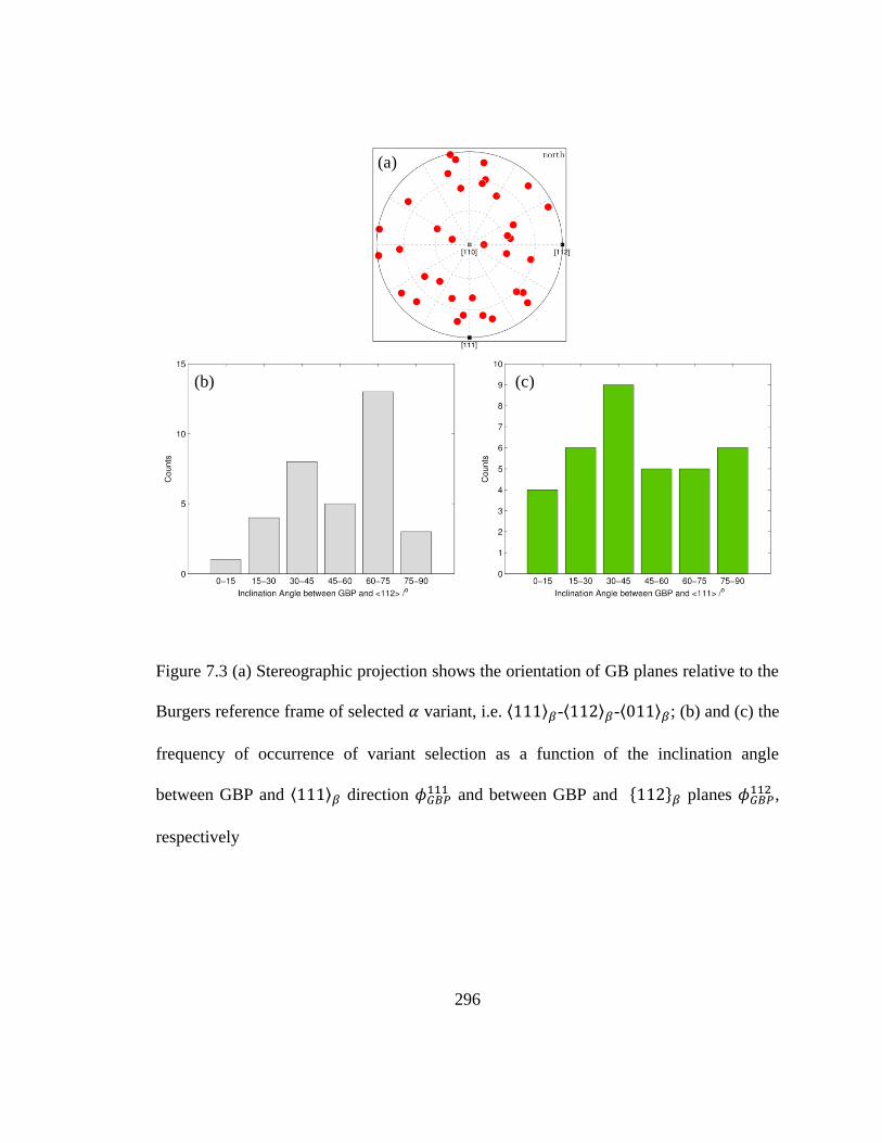
296
Figure 7.3 (a) Stereographic projection shows the orientation of GB planes relative to the
Burgers reference frame of selected variant, i.e. ⟨ ⟩ -⟨ ⟩ -⟨ ⟩ ; (b) and (c) the
frequency of occurrence of variant selection as a function of the inclination angle
between GBP and ⟨ ⟩ direction and between GBP and { } planes
,
respectively
(a)
(b) (c)
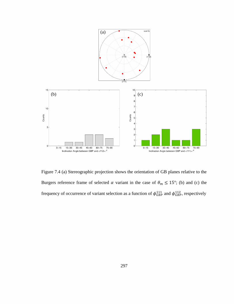
297
Figure 7.4 (a) Stereographic projection shows the orientation of GB planes relative to the
Burgers reference frame of selected variant in the case of ; (b) and (c) the
frequency of occurrence of variant selection as a function of and
, respectively
(a)
(b) (c)

298
Figure.7.5 (a) Stereographic projection shows the orientation of GB planes relative to the
Burgers reference frame of selected variant in the case of ; (b) and (c) the
frequency of occurrence of variant selection as a function of and
, respectively
(a)
(b) (c)
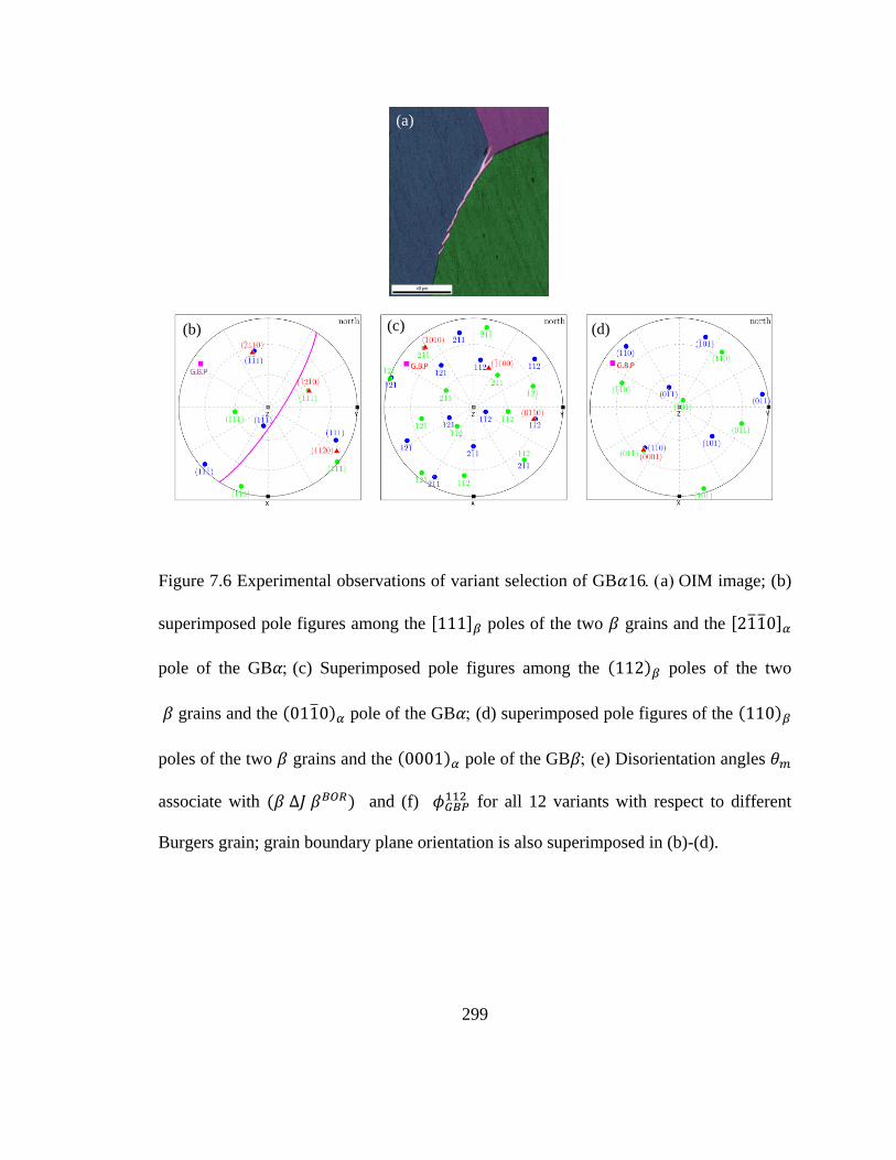
299
Figure 7.6 Experimental observations of variant selection of GB 16aOIM image; (b)
superimposed pole figures among the [ ] poles of the two grains and the [ ]
pole of the GB (c) Superimposed pole figures among the poles of the two
grains and the pole of the GB (d) superimposed pole figures of the
poles of the two grains and the pole of the GB (e) Disorientation angles
associate with and (f) for all 12 variants with respect to different
Burgers grain; grain boundary plane orientation is also superimposed in (b)-(d).
(a)
(b) (c) (d)
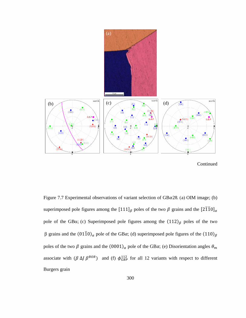
300
Continued
Figure 7.7 Experimental observations of variant selection of GB 28aOIM image; (b)
superimposed pole figures among the [ ] poles of the two grains and the [ ]
pole of the GB(c) Superimposed pole figures among the poles of the two
grains and the pole of the GB (d) superimposed pole figures of the
poles of the two grains and the pole of the GB (e) Disorientation angles
associate with and (f) for all 12 variants with respect to different
Burgers grain
(a)
(b) (c) (d)
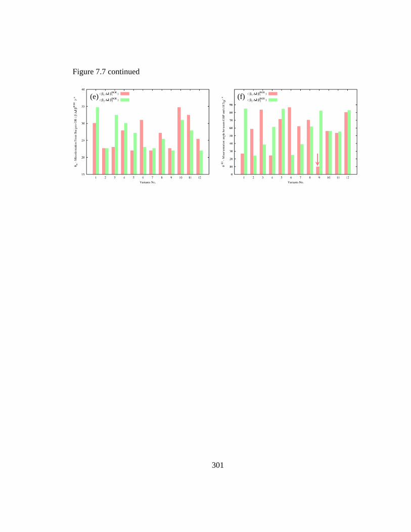
301
Figure 7.7 continued
(e) (f)
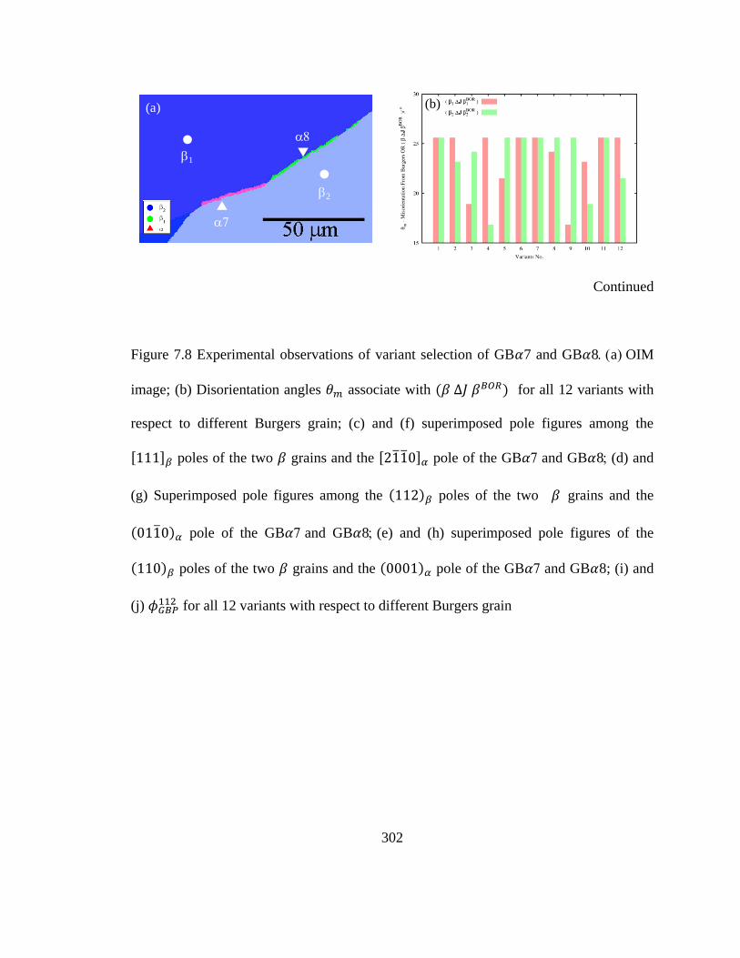
302
Continued
Figure 7.8 Experimental observations of variant selection of GB 7 and GB 8aOIM
image; (b) Disorientation angles associate with for all 12 variants with
respect to different Burgers grain; (c) and (f) superimposed pole figures among the
[ ] poles of the two grains and the [ ] pole of the GB and GB 8(d) and
(g) Superimposed pole figures among the poles of the two grains and the
pole of the GB and GB 8(e) and (h) superimposed pole figures of the
poles of the two grains and the pole of the GB and GB 8; (i) and
(j) for all 12 variants with respect to different Burgers grain
1
2
(a) (b)

303
Figure 7.8 continued
(c) (d) (e)
(f) (g) (h)
(i) (j)

304
Figure 7.9 Experimental observations of variant selection of GB 31aOIM image; (b)
superimposed pole figures among the [ ] poles of the two grains and the [ ]
pole of the GB(c) Superimposed pole figures among the poles of the two
grains and the pole of the GB (d) superimposed pole figures of the
poles of the two grains and the pole of the GB (e) Disorientation angles
associate with and (f) for all 12 variants with respect to different
Burgers grain
1
2
(a) (b) (c)
(e) (f)(d)

305
Figure 7.10 Experimental observations of variant selection of GB 26aOIM image;
(b) superimposed pole figures among the [ ] poles of the two grains and the
[ ] pole of the GB(c) Superimposed pole figures among the poles of the
two grains and the pole of the GB (d) superimposed pole figures of the
poles of the two grains and the pole of the GB (e) Disorientation
angles associate with and (f) for all 12 variants with respect to
different Burgers grain
(a) (b) (c)
(e) (f)(d)
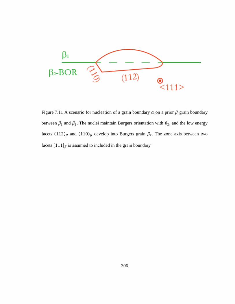
306
Figure 7.11 A scenario for nucleation of a grain boundary on a prior grain boundary
between and . The nuclei maintain Burgers orientation with , and the low energy
facets and develop into Burgers grain . The zone axis between two
facets [ ] is assumed to included in the grain boundary
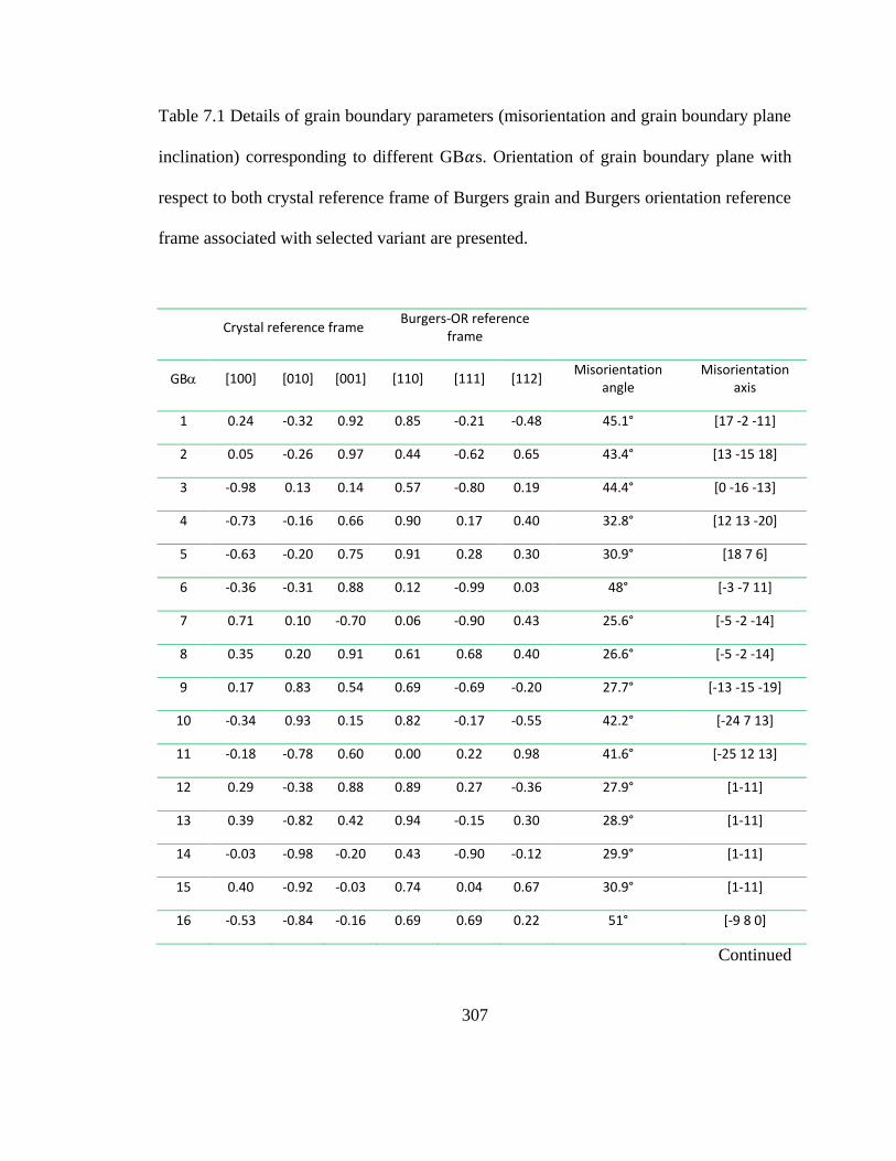
307
Table 7.1 Details of grain boundary parameters (misorientation and grain boundary plane
inclination) corresponding to different GB s. Orientation of grain boundary plane with
respect to both crystal reference frame of Burgers grain and Burgers orientation reference
frame associated with selected variant are presented.
Crystal reference frame
Burgers-OR reference frame
GB [100] [010] [001] [110] [111] [112] Misorientation
angle Misorientation
axis
1 0.24 -0.32 0.92 0.85 -0.21 -0.48 45.1° [17 -2 -11]
2 0.05 -0.26 0.97 0.44 -0.62 0.65 43.4° [13 -15 18]
3 -0.98 0.13 0.14 0.57 -0.80 0.19 44.4° [0 -16 -13]
4 -0.73 -0.16 0.66 0.90 0.17 0.40 32.8° [12 13 -20]
5 -0.63 -0.20 0.75 0.91 0.28 0.30 30.9° [18 7 6]
6 -0.36 -0.31 0.88 0.12 -0.99 0.03 48° [-3 -7 11]
7 0.71 0.10 -0.70 0.06 -0.90 0.43 25.6° [-5 -2 -14]
8 0.35 0.20 0.91 0.61 0.68 0.40 26.6° [-5 -2 -14]
9 0.17 0.83 0.54 0.69 -0.69 -0.20 27.7° [-13 -15 -19]
10 -0.34 0.93 0.15 0.82 -0.17 -0.55 42.2° [-24 7 13]
11 -0.18 -0.78 0.60 0.00 0.22 0.98 41.6° [-25 12 13]
12 0.29 -0.38 0.88 0.89 0.27 -0.36 27.9° [1-11]
13 0.39 -0.82 0.42 0.94 -0.15 0.30 28.9° [1-11]
14 -0.03 -0.98 -0.20 0.43 -0.90 -0.12 29.9° [1-11]
15 0.40 -0.92 -0.03 0.74 0.04 0.67 30.9° [1-11]
16 -0.53 -0.84 -0.16 0.69 0.69 0.22 51° [-9 8 0]
Continued

308
Table 7.1 continued
Crystal reference frame
Burgers-OR reference
frame
GB [100] [010] [001] [110] [111] [112] Misorientation
angle
Misorientation
axis
17 0.13 0.46 0.88 0.70 -0.65 0.30 35° [12 -7 -3]
18 -0.37 0.87 -0.31 0.54 0.77 -0.35 47.2° [5 -15 -13]
19 -0.65 -0.39 0.65 0.52 -0.42 0.74 51.4° [23 -12 -19]
20 -0.35 -0.93 0.10 -0.28 0.62 0.73 35.6° [25 14 6]
21 0.35 -0.63 0.69 0.97 -0.17 -0.20 39.9° [10 -6 -11]
22 -0.76 -0.38 0.53 0.09 -0.59 -0.80 57.7° [14 10 9]
23 0.51 0.74 0.44 0.13 0.54 0.83 22.3° [18 13 11]
24 -0.43 -0.73 0.53 0.98 0.16 -0.14 37.9° [-13 7 7]
25 -0.78 -0.60 -0.16 -0.20 -0.82 -0.54 34.5° [13 -2 9]
26 0.97 0.08 0.23 0.74 -0.24 0.63 37.1° [10 13 25]
27 -0.17 0.83 0.53 -0.08 -0.26 0.96 38° [-3 -8 10]
28 -0.71 0.52 0.48 0.17 0.99 -0.03 39° [-11 -19 -14]
29 0.26 0.95 -0.15 0.62 0.62 0.49 33.5° [-6 2 5]
30 0.54 0.52 0.66 -0.23 -0.47 0.85 34.5° [-6 2 5]
31 0.99 -0.09 0.09 0.67 -0.37 -0.64 47° [22 17 2]
32 0.84 0.04 0.55 0.77 0.12 -0.62 47° [22 17 2]
33 0.67 0.63 0.39 0.98 0.21 -0.02 48° [14 -16 -1]
34 0.20 0.79 0.59 0.91 -0.08 0.42 48° [14 -16 -1]
35 -0.73 -0.43 -0.52 -0.13 0.55 0.82 59.3° [110]
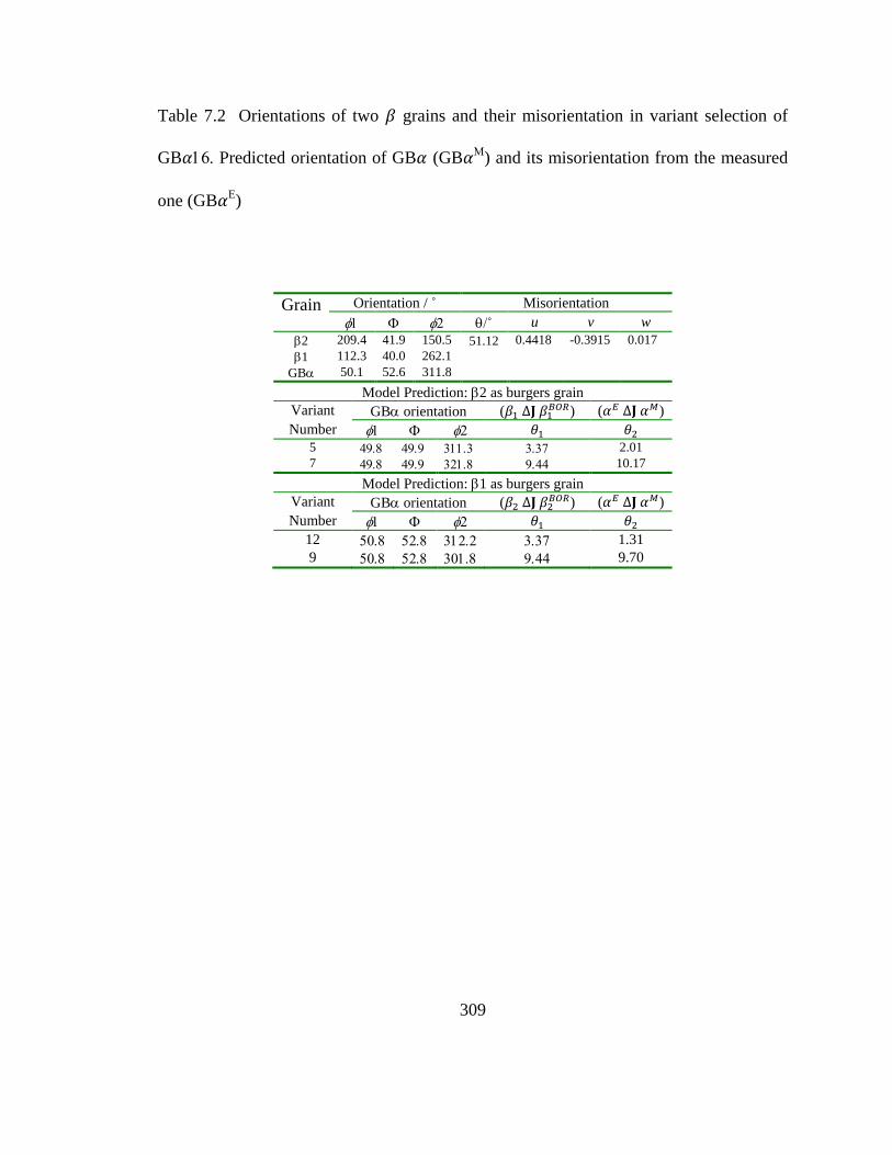
309
Table 7.2 Orientations of two grains and their misorientation in variant selection of
GB Predicted orientation of GB (GB ) and its misorientation from the measured
one (GB )
Grain Orientation / ˚ Misorientation
˚ u v w
2 209.4 41.9 150.5 51.12 0.4418 -0.3915 0.017
1 112.3 40.0 262.1
GB 50.1 52.6 311.8
Model Prediction:2 as burgers grain
Variant GBorientation ( ) ( )
Number
5 2.01
7 10.17
Model Prediction:1 as burgers grain
Variant GBorientation ( ) ( )
Number
12 1.31
9 9.70
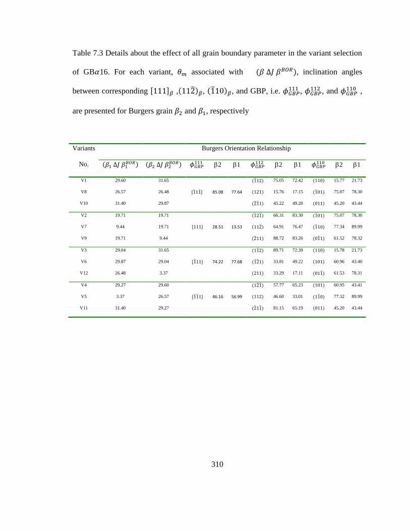
310
Table 7.3 Details about the effect of all grain boundary parameter in the variant selection
of GB 16. For each variant, associated with , inclination angles
between corresponding [ ] , , , and GBP, i.e. ,
, and ,
are presented for Burgers grain and , respectively
Variants Burgers Orientation Relationship
No.
2 1
2 1 2 1
V1 29.60 31.65 75.05 72.42 15.77 21.73
V8 26.57 26.48 [ ] 85.08 77.64 15.76 17.15 75.07 78.30
V10 31.40 29.87 45.22 49.20 45.20 43.44
V2 19.71 19.71 66.31 83.30 75.07 78.30
V7 9.44 19.71 [ ] 28.51 13.53 64.91 76.47 77.34 89.99
V9 19.71 9.44 88.72 83.26 61.52 78.32
V3 29.04 31.65 89.71 72.39 15.78 21.73
V6 29.87 29.04 [ ] 74.22 77.68 33.81 49.22 60.96 43.40
V12 26.48 3.37 33.29 17.11 61.53 78.31
V4 29.27 29.60 57.77 65.23 60.95 43.41
V5 3.37 26.57 [ ] 46.16 56.99 46.60 33.01 77.32 89.99
V11 31.40 29.27 81.15 65.19 45.20 43.44
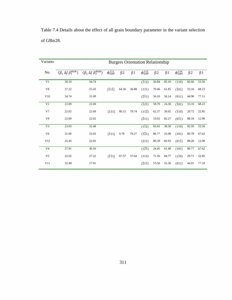
311
Table 7.4 Details about the effect of all grain boundary parameter in the variant selection
of GB 28.
Variants Burgers Orientation Relationship
No.
2 1
2 1 2 1
V1 30.10 34.74 26.84 85.10 82.60 53.56
V8 27.22 25.43 [ ] 64.36 36.88 70.46 61.85 33.16 68.23
V10 34.74 31.00 56.10 56.14 44.90 77.11
V2 22.69 22.69 58.70 24.30 33.16 68.22
V7 22.02 22.69 [ ] 80.15 79.74 62.27 39.02 29.72 52.85
V9 22.69 22.02 10.02 82.27 88.18 12.90
V3 23.03 32.48 83.65 38.50 82.59 53.56
V6 31.00 23.03 [ ] 9.78 79.27 86.77 25.08 80.78 67.62
V12 25.43 22.02 80.39 82.93 88.20 12.90
V4 27.91 30.10 24.45 61.48 80.77 67.62
V5 22.02 27.22 [ ] 67.57 37.64 71.56 84.77 29.71 52.85
V11 32.48 27.91 53.56 55.36 44.91 77.10

312
Table 7.5 Orientations of two grains and their misorientation in variant selection of
GB Predicted orientation of GB (GB ) and its misorientation from the measured
one (GB )
Grain Orientation / ˚ Misorientation
˚ u v w
2 181.2 16.4 151.4 39.04 -0.4344 -0.3344 -0.2762 1 57.5 55.5 319.6
GB 318.5 31.5 11.7
Model Prediction:2 as burgers grain
Variant GBorientation ( ) ( )
Number
9 22.69 1.15 12 25.43 10.51
Model Prediction:1 as burgers grain
Variant GBorientation ( ) ( )
Number
2 22.69 23.8
8 25.43 26.48

313
Table 7.6 Orientations of two grains and their misorientation in variant selection of
GB Predicted orientation of GB (GB ) and its misorientation from the measured
one (GB )
Grain Orientation / ˚ Misorientation
˚ u v w
2 122.3 39.8 210.4 25.6 0.065 0.0270 0.1825 1 328.7 55.0 49.4
GB 239.4 89.8 148.6
Model Prediction:2 as burgers grain
Variant GBorientation ( ) ( )
Number
4 25.60 29.17
6 25.60 30.29
Model Prediction:1 as burgers grain
Variant GBorientation ( ) ( )
Number
7 4.36
5 12.39

314
Table 7.7 Orientations of two grains and their misorientation in variant selection of
GB Predicted orientation of GB (GB ) and its misorientation from the measured
one (GB )
Grain Orientation / ˚ Misorientation
˚ u v w
2 122.3 39.8 210.4 25.6 0.065 0.0270 0.1825 1 328.7 55.0 49.4
GB 193.6 39.6 176.1
Model Prediction:2 as burgers grain
Variant GBorientation ( ) ( )
Number
8 1.85
2 25.60 11.52
Model Prediction:1 as burgers grain
Variant GBorientation ( ) ( )
Number
3 18.91 23.00
1 25.60 24.0

315
Table 7.8 Details about the effect of all grain boundary parameter in the variant selection
of GB 7.
Variants Burgers Orientation Relationship
No.
2 1
2 1 2 1
V1 25.60 25.60 44.26 35.07 48.35 55.10
V8 24.18 25.60 [ ] 77.69 86.97 21.00 85.05 73.26 5.81
V10 23.17 18.91 77.44 25.21 17.73 65.00
V2 25.60 23.17 83.67 85.49 73.26 5.81
V7 25.60 25.60 [ ] 17.96 86.34 78.80 25.73 76.14 64.57
V9 16.83 25.60 72.27 34.69 87.23 55.56
V3 18.91 24.18 63.92 71.18 48.35 55.10
V6 25.60 25.60 [ ] 52.83 41.06 69.17 48.94 44.51 89.99
V12 25.60 21.50 37.31 70.47 87.22 55.57
V4 25.60 16.83 46.51 60.53 44.52 89.99
V5 21.50 25.60 [ ] 82.30 29.47 15.93 76.10 89.99 64.73
V11 25.60 25.60 74.13 75.42 46.68 65.15

316
Table 7.9 Details about the effect of all grain boundary parameter in the variant selection
of GB 8.
Va Burgers Orientation Relationship
No.
2 1
2 1 2 1
V1 25.60 25.60 79.89 2.84 10.83 87.42
V8 24.18 25.60 [ ] 86.17 88.82 20.22 57.42 70.18 32.61
V10 23.17 18.91 40.28 62.59 49.98 27.44
V2 25.60 23.17 75.53 80.79 70.18 32.61
V7 25.60 25.60 [ ] 24.91 59.03 65.26 49.50 87.27 55.96
V9 16.83 25.60 80.29 35.94 67.30 73.60
V3 18.91 24.18 83.02 69.37 10.82 87.46
V6 25.60 25.60 [ ] 81.77 20.80 37.83 82.12 53.39 70.88
V12 25.60 21.50 24.31 77.57 67.30 73.59
V4 25.60 16.83 66.53 33.32 53.39 70.87
V5 21.50 25.60 [ ] 45.82 63.84 44.31 45.45 87.27 55.95
V11 25.60 25.60 71.50 82.30 49.97 27.44

317
Table 7.10 Orientations of two grains and their misorientation in variant selection of
GB Predicted orientation of GB (GB ) and its misorientation from the measured
one (GB )
Grain Orientation / ˚ Misorientation
˚ u v w
2 173.1 16.6 196.1 47.03 0.0514 0.0401 0.0048 1 65.1 39.5 302.0
GB 324.4 76.6 43.2
Model Prediction:2 as burgers grain
Variant GBorientation ( ) ( )
Number
1 2.45
3 14.89 11.08
Model Prediction:1 as burgers grain
Variant GBorientation ( ) ( )
Number
3 5.84
1 14.89 14.20
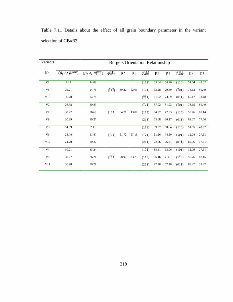
318
Table 7.11 Details about the effect of all grain boundary parameter in the variant
selection of GB 32.
Variants Burgers Orientation Relationship
No.
2 1
2 1 2 1
V1 7.11 14.89 83.04 54.76 51.64 48.02
V8 26.21 24.78 [ ] 39.22 62.05 53.28 29.80 78.13 80.49
V10 36.20 24.78 61.52 73.09 65.47 33.48
V2 26.68 30.89 57.92 81.22 78.15 80.49
V7 30.27 26.68 [ ] 34.71 13.00 84.97 77.33 55.76 87.14
V9 30.89 30.27 63.68 86.17 69.07 77.60
V3 14.89 7.11 39.57 50.64 51.65 48.02
V6 24.78 31.87 [ ] 81.72 67.18 81.26 74.80 12.08 27.91
V12 24.78 30.27 22.66 26.31 69.06 77.61
V4 30.21 33.24 85.11 63.06 12.09 27.91
V5 30.27 26.21 [ ] 78.97 83.23 36.46 7.35 55.76 87.15
V11 36.20 30.21 27.20 57.40 65.47 33.47
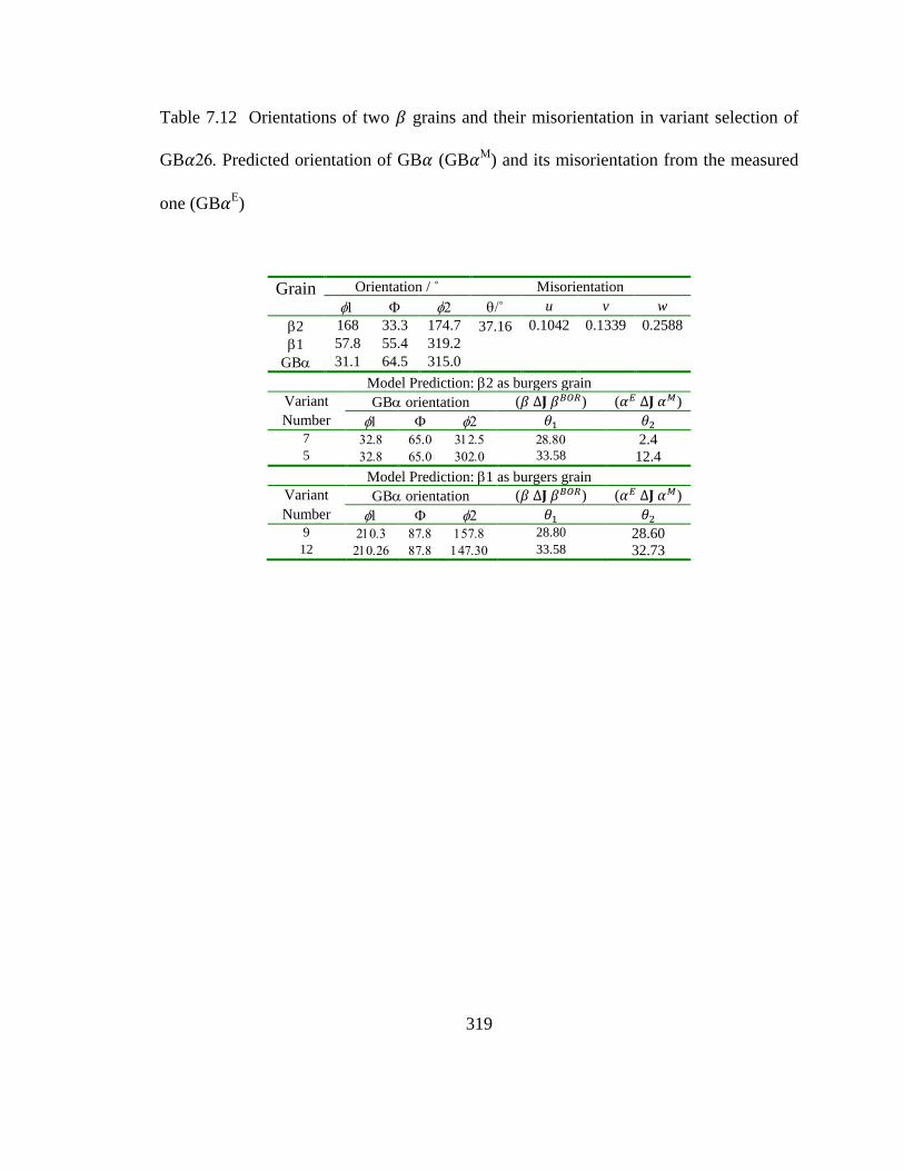
319
Table 7.12 Orientations of two grains and their misorientation in variant selection of
GB Predicted orientation of GB (GB ) and its misorientation from the measured
one (GB )
Grain Orientation / ˚ Misorientation
˚ u v w
2 168 33.3 174.7 37.16 0.1042 0.1339 0.2588 1 57.8 55.4 319.2
GB 31.1 64.5 315.0
Model Prediction:2 as burgers grain
Variant GBorientation ( ) ( )
Number
7 2.4 5 33.58 12.4
Model Prediction:1 as burgers grain
Variant GBorientation ( ) ( )
Number
9 28.80 28.60 12 33.58 32.73

320
Table 7.13 Details about the effect of all grain boundary parameter in the variant
selection of GB 32.
Variants Burgers Orientation Relationship
No.
2 1
2 1 2 1
V1 32.61 22.64 79.85 61.98 42.22 65.21
V8 25.54 32.18 [ ] 49.57 39.03 56.41 53.27 58.48 78.63
V10 22.64 29.01 43.17 82.63 77.41 51.94
V2 25.54 28.80 64.72 57.79 58.48 78.64
V7 28.80 25.54 [ ] 42.46 34.63 76.16 64.07 50.86 68.72
V9 28.80 28.80 48.22 84.50 83.76 55.93
V3 37.16 28.09 56.45 27.25 42.22 65.21
V6 29.01 37.16 [ ] 67.53 79.40 68.60 85.34 31.90 11.60
V12 32.18 33.58 23.41 36.13 83.77 55.93
V4 27.43 32.61 76.19 81.59 31.90 11.60
V5 33.58 25.54 [ ] 61.87 82.07 51.99 22.86 50.86 68.71
V11 28.09 27.43 31.29 39.18 77.42 51.94
321
7.6. Reference
[1] Banerjee D, Williams JC. Perspectives on Titanium Science and Technology.
Acta Mater 2013;61:844.
[2] Bache MR. Processing titanium alloys for optimum fatigue performance. Int J
Fatigue 1999;21:S105.
[3] Whittaker R, Fox K, Walker A. Texture variations in titanium alloys for
aeroengine applications. Mater Sci Tech-Lond 2010;26:676.
[4] Burgers WG. On the process of transition of the cubic-body-centered
modification into the hexagonal-close-packed modification of zirconium. Physica
1934;1:561.
[5] Lutjering G, Williams JC. Titanium (Engineering Materials and Processes).
Berlin: Springer, 2007.
[6] Lee E, Banerjee R, Kar S, Bhattacharyya D, Fraser HL. Selection of alpha
variants during microstructural evolution in alpha/beta titanium alloy. Philos. Mag.
2007;87:3615.
[7] Kar S, Banerjee R, Lee E, Fraser HL. Influence of Crystallography Variant
Selection on Microstructure Evolution in Titnaium Alloys. In: Howe JM, Laughlin DE,
Dahmen U, Soffa WA, editors. Solid-to-Solid Phase Transformation in Inorganic
Materials, vol. 133-138: TMS (The Minerals, Metals & Materials Society), 2005.
[8] Bhattacharyya D, Viswanathan GB, Denkenberger R, Furrer D, Fraser HL. The
role of crystallographic and geometrical relationships between alpha and beta phases in
an alpha/beta titanium alloy. Acta Mater 2003;51:4679.
322
[9] Stanford N, Bate PS. Crystallographic variant selection in Ti-6Al-4V. Acta Mater
2004;52:5215.
[10] van Bohemen SMC, Kamp A, Petrov RH, Kestens LAI, Sietsma J. Nucleation
and variant selection of secondary alpha plates in a beta Ti alloy. Acta Mater
2008;56:5907.
[11] Bhattacharyya D, Viswanathan GB, Fraser HL. Crystallographic and
morphological relationships between beta phase and the Widmanstatten and
allotriomorphic alpha phase at special beta grain boundaries in an alpha/beta titanium
alloy. Acta Mater 2007;55:6765.
[12] Wilson RJ, Randle V, Evans WJ. The influence of the Burgers relation on crack
propagation in a near alpha-titanium alloy. Philos Mag A 1997;76:471.
[13] Furuhara T, Takagi S, Watanabe H, Maki T. Crystallography of grain boundary α
precipitates in a β titanium alloy. MMTA 1996;27:1635.
[14] Shi R, Dixit V, Fraser HL, Wang Y. Variant Selection of Grain Boundary Alpha
by Special Prior Beta Grain Boundaries in Titanium Alloys. Acta Mater 2014:Submitted.
[15] Lee JK, Aaronson HI. Influence of faceting upon the equilibrium shape of nuclei
at grain boundaries—II. Three-dimensions. Acta Metall Mater 1975;23:809.
[16] Lee JK, Aaronson HI. Influence of faceting upon the equilibrium shape of nuclei
at grain boundaries—I. Two-dimensions. Acta Metall Mater 1975;23:799.
[17] Furuhara T, Kawata H, Morito S, Miyamoto G, Maki T. Variant selection in grain
boundary nucleation of upper bainite. Metall Mater Trans A 2008;39A:1003.

323
[18] Vikas D. Grain-Boundary Parameters Controlled Allotriomorphic Phase
Transformations in Beta-Processed Titanium Alloys. vol. Ph.D.: The Ohio State
University, 2013.
[19] Zhang WZ, Weatherly GC. On the crystallography of precipitation. Progress in
Materials Science 2005;50:181.
[20] Sutton AP, Balluffi RW. Interfaces in Crystalline Materials. Oxford: Clarendon
Press, 1995.
[21] Read WT. Dislocations in crystals. New York: Jr. McGraw-Hill, 1953.
[22] Banerjee R, Bhattacharyya D, Collins PC, Viswanathan GB, Fraser HL.
Precipitation of grain boundary alpha in a laser deposited compositionally graded Ti-8Al-
xV alloy - an orientation microscopy study. Acta Mater 2004;52:377.
[23] Beladi H, Rohrer GS. The relative grain boundary area and energy distributions in
a ferritic steel determined from three-dimensional electron backscatter diffraction maps.
Acta Mater 2013;61:1404.
[24] Rohrer GS. Grain boundary energy anisotropy: a review. J Mater Sci
2011;46:5881.
324
CHAPTER 8 Conclusions and Future Works
8.1 Conclusions
Mechanisms responsible for the occurrence of variant selection at different length scales
have been studied systematically in the current work as follows:
For a single variant, the phase forms as laths with broad faces that are semi-coherent
and contain structural ledges and dislocations. A general method has been formulated to
derive effective transformation strain during precipitation that considers the effect of
interfacial defects including misfit dislocations and structural ledges, which is an
important first step toward variant selection study since the coupling between
precipitation and external bias such as stress field varies with the coherency state of
precipitate. How the interfacial defects relax the coherency elastic strain energy and
affect the habit plane orientation are analyzed in detail by incorporating the effect of the
defects into the stress-free transformation strain. How the interfacial defects affect the
interfacial energy anisotropy and the final equilibrium shape of precipitates is also
investigated. The equilibrium shapes of an isolated precipitate generated by the
interplay between interfacial energy and elastic strain energy are obtained from phase
field simulations. The habit plane orientation is found to be dominated by the strain
325
energy minimization, while interfacial energy anisotropy contributes to the in-plane shape
(ratio of the two major axes). The present work may build a bridge between the O-line
theory of precipitate habit planes and interfacial dislocation structures based on pure
geometrical consideration and the theory of optimum shapes of precipitate based on the
consideration of strain energy that depends on precipitate size, coherency state, shape and
orientations.
For variant selection within individual grain, a quantitative three-dimensional phase
field model (PFM) is developed to investigate variant selection during precipitation
from matrixin Ti-6Al-4V under the influence of both external and internal stress fields
such as those associated with, but not limited to, pre-straining and pre-existing
precipitates considered in this work. The model incorporates the crystallography of BCC
to HCP transformation, elastic anisotropy and interface defect structures in its total
free energy formulations. Model inputs are linked directly to thermodynamic and
mobility databases. The main findings are:
1) Under a given undercooling, there is a competition between internal stress associated
with an evolving microstructure and external applied stress or pre-strain on the
development of micro-texture. If the transformation strain or internal stress produced
by variants selected by a specific external stress or pre-strain during early stages of
precipitation cannot be accommodated among themselves, the internal stress would
prevent further development of such a transformation texture and induce the
formation of other variants to achieve self-accommodation. Since self-
accommodation can be achieved only by multiple variants (minimum two variants not
sharing a common basal plane), any constraints on macroscopic shape change of a
sample (e.g., by clamping) will prevent effectively the development of strong micro-
texture or transformation texture.
326
2) The development of micro-texture is sensitive to the loading axis of an external stress
or strain. From the elastic interaction energy calculations, we have learned that when
an external stress or pre-strain is applied in certain directions multiple variants of
phase could be favored simultaneously with the same interaction energy. Therefore, if
a polycrystalline sample has a strong macro-texture of the grains, control of
external load (if any) orientation could prevent strong micro-texture of plates from
percolating through the sample leading to poor fatigue properties.
3) There exists an obvious tension/compression asymmetry in variant selection behavior,
i.e., the types and numbers of variants produced under tensile and compressive
stresses are different. For example, pre-straining obtained via uniaxial tensile and
compressive stress along [010] will result in the selection of 8 and 4 out of 12
variants, respectively.
4) The interaction energy calculations, though simple and fast, cannot predict the overall
variant selection behavior at all cases. In addition, the prediction is valid only when
the internal stresses generated by an evolving microstructure are significantly smaller
than the externally applied stress.
5) Although nucleation of specific variants of secondary plates on interfaces between
primary plates and matrix observed in ⁄ Ti-alloys could be classified as
sympathetic nucleation (SN), the elastic interaction analysis in this study suggests that
such nucleation phenomenon observed in our simulations is coherency stress induced
correlated nucleation (i.e., auto-catalytic effect) rather than the conventional SN
discussed in literature (which is caused by the relatively low grain boundary energy
between the secondary and primary particles).
6) Secondary plates having a misorientation of [ ] ⁄ with the pre-existing
(i.e., primary) ones (i.e. sharing a common ⟨ ⟩ or ⟨ ⟩ ) tend to nucleate and
grow on the broad faces of the pre-existing plates, which could serve as an auto-
catalytic mechanism underlying the formation of basket-weave microstructures.
7) The stress-free transformation strain (SFTS) of precipitate varies with its coherency
state and variant selection rules (in terms of the sign and magnitude of elastic
327
interaction energy) are found different for coherent and semi-coherent precipitates.
When considering effect of primary plates whose sizes are usually above the
critical size for coherency (around 20 nm ), the SFTS for semi-coherent precipitate
should be employed for the primary precipitate while the SFTS for coherent
precipitate should be used for the nucleating secondary precipitates.
For variant selection within polycrystalline sample, the three-dimensional quantitative
phase field model has been further developed to study the variant selection process
during transformation under the influence of different processing variables such as
pre-strains. The effect of elastic and structural inhomogeneities on the local stress state
and its interaction with evolving microstructure is also considered in the model. In
particular, microstructure and transformation texture evolution are treated simultaneously
via orientation distribution function (ODF) modeling of ⁄ two-phase microstructure in
polycrystalline systems obtained by PFM. The variant selection behavior at the scale of
individual grain and the overall polycrystalline sample, and the resulting final
texture are found to be heavily dependent on type of pre-strain, boundary constraint of
the sample, and strating texture. It is found that, when subjected to a certain pre-strain,
the sample with strong texture component could promote more variants simultaneously
within the whole polycrystalline sample and thus lead to a relatively small degree of
microtexture. The results could shed light on how to control processing conditions to
reduce the strength micro-texture at both the individual grain level and the overall
polycrystalline sample level according to its starting texture.
For variant selection of GB on prior grain boundaries, a crystallographic model based
on the Burgers orientation relationship between GB and one of two grains has been
328
developed to study how variant selection occurs on prior grain boundary in / and
titanium alloys. In particular, a new parameter, that describes quantitatively
the deviation of OR between a GB and the non-Burgers grain from BOR, is identified
and a new GB selection rule is proposed. All possible special misorientations between
two grains that make GB in the Burgers orientation relationship (BOR) with both
grains have been predicted and confirmed by experimental observations made for Ti-
5553. Such variant selection of GB at special grain boundaries will result in the
development of large colony structures from the GB into two adjacent grains with
identical orientation as that of the GB. Through the analysis of the experiment
observations of GBin Ti-5553 using the model, it is found that when the disorientation
angle associated with is less than 15º, the variant with the smallest of
is always selected for GB, and the selected GBwill have its ⟨ ⟩
pole parallel to a common ⟨ ⟩ pole of the two adjacent grains. When ,
grain boundary plane inclination may play more important role for GB variant selection
in Ti-5553. Theoretical arguments why the parameter, , is a better measure
than the closeness between two closest { } from two grains widely used in literature
in analyzing GB variant selection are provided.
All current empirical variant selection rules about the influence of grain boundary
parameters have been investigated systematically. For the precipitation of GB son
different prior grain boundaries, how a single rule or different rules combined together

329
contributes to the final variant selection are studied. It has been found that when the
minimum misorientation angle associated with is less than ,
misorientation between two adjacent grains plays a leading role in the VS of GB .
When , GBP inclination is more important in the determination of VS of GB
than misorientation. However, the common employed rules that the variant of a selected
at a given -grain boundary is the one that has the minimum possible angle between the
matching direction ⟨ ⟩ ⟨ ⟩ and the grain boundary plane, or the that has the
minimum possible angle between matching planes { } { } and the grain
boundary plane, are found to be frequently violated. The violations of VS rules are
associated with the influence of interplay between different parameters such as grain
boundary energy, interface energy between GB and Burgers grain, interface energy
between GB and non-Burgers grain, on nucleation barrier. The violations of the
empirical VS rules could be associated with the fact that the activation energy of
nucleation of GB is determined by a complicated interplay among the five parameters
related to misorientation and inclination of a GB or an interphase interface that define the
structure and energy of the GB and interfaces, while the individual empirical rules
account for only a subset of these parameters..
8.2 Direction for future research Conclusions
Applications of the developed PFM model to study effects from other stress-carry
defects such as dislocations, stacking faults, grain boundaries, as well as effects from
330
thermal stress on variant selection during precipitation in polycrystalline samples are
straight forwards and corresponding work is underway. During all the simulations for
precipitations in polycrystalline sample by PFM, the effect of cooling rate and variant
selection of GB have been ignored. To mimic real precipitation during TMP,
however, these two factors have to be considered.
The nucleation barrier of GB, , for each variant is a function of multiple
parameters, grain boundary energy , interfacial energy between GB and non-
Bugers grain, , interfacial energy between GB and non-Bugers grain,
,
interfacial energy of low-energy facets,
, and inclinations between low-energy
facets and grain boundary plane,
(
)
Nucleation is to be made easiest for the variant with the minimum . This is the origin
that leads to the occurrence of VS of GB. In order to make more accurate predictions of
VS of GB a general rule needs to be further developed that take all the parameters
(grain boundary energy, interfacial energies between GB and two grains, interfacial
energies of low-energy facets, and orientations of the low-energy facets with respect to
GBP) playing their roles during the grain boundary nucleation and, more importantly,
demonstrate quantitatively how these parameters contribute to the activation energy of
the nucleation. The work is currently on its way.
How to implement these variant selection mechanisms working at different scales
simultaneously to investigate their effects on both microstructure and transformation

331
texture evolution in a representative volume element of sample, also needs to be
addressed.
332
Reference
Chapter 1
[1-1] Burgers WG. On the process of transition of the cubic-body-centered modification into the
hexagonal-close-packed modification of zirconium. Physica 1934;1:561.
[1-2] Cahn JW, Kalonji GM. Symmetry in Solid-Solid Transformation Morphologies. PROCEEDINGS
OF an Interantional Conference On Solid-Solid Phase Transformations 1981:3.
[1-3] Banerjee D, Williams JC. Perspectives on Titanium Science and Technology. Acta Materialia
2013;61:844.
[1-4] Lutjering G, Williams JC. Titanium (Engineering Materials and Processes). Berlin: Springer,
2007.
[1-5] Bhattacharyya D, Viswanathan GB, Denkenberger R, Furrer D, Fraser HL. The role of
crystallographic and geometrical relationships between alpha and beta phases in an alpha/beta titanium
alloy. Acta Materialia 2003;51:4679.
[1-6] Bhattacharyya D, Viswanathan GB, Fraser HL. Crystallographic and morphological relationships
between beta phase and the Widmanstatten and allotriomorphic alpha phase at special beta grain
boundaries in an alpha/beta titanium alloy. Acta Materialia 2007;55:6765.
[1-7] Stanford N, Bate PS. Crystallographic variant selection in Ti-6Al-4V. Acta Materialia
2004;52:5215.
[1-8] van Bohemen SMC, Kamp A, Petrov RH, Kestens LAI, Sietsma J. Nucleation and variant
selection of secondary alpha plates in a beta Ti alloy. Acta Materialia 2008;56:5907.

333
[1-9] Shi R, Dixit V, Fraser HL, Wang Y. Variant Selection of Grain Boundary Alpha by Special Prior
Beta Grain Boundaries in Titanium Alloys. Submitted to Acta Materialia 2014.
[1-10] Sargent GA, Kinsel KT, Pilchak AL, Salem AA, Semiatin SL. Variant Selection During Cooling
after Beta Annealing of Ti-6Al-4V Ingot Material. Metallurgical and Materials Transactions a-Physical
Metallurgy and Materials Science 2012;43A:3570.
[1-11] Winholtz RA. Residual Stresses: Macro and Micro Stresses. In: Buschow KHJ, Robert WC,
Merton CF, Bernard I, Edward JK, Subhash M, Patrick V, editors. Encyclopedia of Materials: Science and
Technology. Oxford: Elsevier, 2001. p.8148.
[1-12] Zeng L, Bieler TR. Effects of working, heat treatment, and aging on microstructural evolution and
crystallographic texture of [1-alpha], [1-alpha]', [1-alpha]'' and [1-beta] phases in Ti-6Al-4V wire.
Materials Science and Engineering: A 2005;392:403.
[1-13] Kar S, Banerjee R, Lee E, Fraser HL. Influence of crystallography varaiant selection on
microstructure evolution in titanium alloys. In: Howe JM, Laughlin DE, Lee JK, Dahmen U, Soffa WA,
editors. Solid-Solid Phase Transformation in Inorganic Materials 2005, vol. 1: TMS, 2005.
[1-14] Lee E, Banerjee R, Kar S, Bhattacharyya D, Fraser HL. Selection of alpha variants during
microstructural evolution in alpha/beta titanium alloy. Philosophical Magazine 2007;87:3615.
[1-15] Wang YU, Jin YM, Khachaturyan AG. Three-dimensional phase field microelasticity theory of a
complex elastically inhomogeneous solid. Applied Physics Letters 2002;80:4513.
[1-16] Cahn JW, Hilliard JE. Free energy of a nonuniform system. I. Interfacial free energy. The Journal
of Chemical Physics 1958;28:258.
[1-17] Landau LD, Lifshitz E. On the theory of the dispersion of magnetic permeability in ferromagnetic
bodies. Phys. Z. Sowjetunion 1935;8:101.
[1-18] Rowlinson JS. Translation of J. D. van der Waals' “The thermodynamik theory of capillarity under
the hypothesis of a continuous variation of density”. Journal of Statistical Physics 1979;20:197.
[1-19] Eshelby JD. The determination of the elastic field of an ellipsoidal inclusion, and related
problems. Proceedings of the Royal Society of London. Series A 1957;241.

334
[1-20] Eshelby JD. The Elastic Field Outside an Ellipsoidal Inclusion. Proceedings of the Royal Society
A 1959;252:561.
[1-21] Khachaturyan A. Some questions concerning the theory of phase transformations in solids. Soviet
Phys. Solid State 1967;8:2163.
[1-22] Khachaturyan AG. Theory of Structural Transformations in Solids. New York: John Wiley &
Sons, 1983.
[1-23] Khachaturyan AG, Shatalov GA. Elastic interaction potential of defects in a crystal. Sov. Phys.
Solid State 1969;11:118.
[1-24] Boettinger WJ, Warren JA, Beckermann C, Karma A. Phase-field simulation of solidification.
Annual Review of Materials Research 2002;32:163.
[1-25] Chen L-Q. PHASE-FIELD MODELS FOR MICROSTRUCTURE EVOLUTION. Annual Review
of Materials Research 2002;32:113.
[1-26] Emmerich H. The diffuse interface approach in materials science: thermodynamic concepts and
applications of phase-field models: Springer, 2003.
[1-27] Karma A. Phase Field Methods. In: Buschow KHJ, Cahn RW, Flemings MC, Ilschner B, Kramer
EJ, Mahajan S, Veyssière P, editors. Encyclopedia of Materials: Science and Technology (Second Edition).
Oxford: Elsevier, 2001. p.6873.
[1-28] Shen C, Wang Y. Coherent precipitation - phase field method. In: Yip S, editor. Handbook of
Materials Modeling, vol. B: Models. Springer, 2005. p.2117.
[1-29] Wang Y, Chen LQ, Zhou N. Simulating Microstructural Evolution using the Phase Field Method.
Characterization of Materials. John Wiley & Sons, Inc., 2012.
[1-30] Wang YU, Jin YM, Khachaturyan AG. Dislocation Dynamics—Phase Field. Handbook of
Materials Modeling. Springer, 2005. p.2287.
[1-31] Shi R, Ma N, Wang Y. Predicting equilibrium shape of precipitates as function of coherency state.
Acta Materialia 2012;60:4172.
335
[1-32] Wang Y, Ma N, Chen Q, Zhang F, Chen SL, Chang YA. Predicting phase equilibrium, phase
transformation, and microstructure evolution in titanium alloys. JOM Journal of the Minerals Metals and
Materials Society 2005;57:32.
[1-33] Chen Q, Ma N, Wu KS, Wang YZ. Quantitative phase field modeling of diffusion-controlled
precipitate growth and dissolution in Ti-Al-V. Scripta Materialia 2004;50:471.
[1-34] Shi R, Wang Y. Variant selection during α precipitation in Ti–6Al–4V under the influence of local
stress – A simulation study. Acta Materialia 2013;61:6006.
[1-35] Bunge HJ. Texture Analysis in Materials Science- Mathematical Methods. London, 1982.
Chapter 2
[2-1] Leyens C, Peters M, editors. Titanium and Titanium Alloys-Fundamentals and Applications.
Weinheim: WILEY-VCH, 2003.
[2-2] Lutjering G, Williams JC. Titanium (Engineering Materials and Processes). Berlin: Springer,
2007.
[2-3] Boyer RR. Attributes, Characteristics, and Applications of Titanium and Its Alloys. JOM
2010;62:21.
[2-4] Boyer RR. An overview on the use of titanium in the aerospace industry. Materials Science and
Engineering a-Structural Materials Properties Microstructure and Processing 1996;213:103.
[2-5] Freese HL, Volas MG, Wood JR, Textor M. Titanium and its Alloys in Biomedical Engineering.
In: Buschow KHJ, Robert WC, Merton CF, Bernard I, Edward JK, Subhash M, Patrick V, editors.
Encyclopedia of Materials: Science and Technology. Oxford: Elsevier, 2001. p.9374.
[2-6] Froes FH. Titanium Alloys: Properties and Applications. In: Buschow KHJ, Robert WC, Merton
CF, Bernard I, Edward JK, Subhash M, Patrick V, editors. Encyclopedia of Materials: Science and
Technology. Oxford: Elsevier, 2001. p.9367.
336
[2-7] Geetha M, Singh AK, Asokamani R, Gogia AK. Ti based biomaterials, the ultimate choice for
orthopaedic implants - A review. Prog Mater Sci 2009;54:397.
[2-8] Froes FH. Titanium Alloys: Corrosion. In: Buschow KHJ, Robert WC, Merton CF, Bernard I,
Edward JK, Subhash M, Patrick V, editors. Encyclopedia of Materials: Science and Technology. Oxford:
Elsevier, 2001. p.9366.
[2-9] Lütjering G. Influence of processing on microstructure and mechanical properties of ([2-
alpha]+[2-beta]) titanium alloys. "Mater Sci Eng, A " 1998;243:32.
[2-10] Burgers WG. On the process of transition of the cubic-body-centered modification into the
hexagonal-close-packed modification of zirconium. Physica 1934;1:561.
[2-11] Wenk HR, Houtte PV. Texture and anisotropy. Rep Prog Phys 2004;67:1367.
[2-12] Peters M, Gysler A, LÜtjering G. Influence of texture on fatigue properties of Ti-6Al-4V.
Metallurgical and Materials Transactions A 1984;15:1597.
[2-13] Bache MR, Evans WJ. Impact of texture on mechanical properties in an advanced titanium alloy.
"Mater Sci Eng, A " 2001;319-321:409.
[2-14] Bache MR, Evans WJ, Suddell B, Herrouin FRM. The effects of texture in titanium alloys for
engineering components under fatigue. Int J Fatigue 2001;23:153.
[2-15] Furuhara T, Nakamori H, Maki T. Crystallography of alpha phase precipitated on dislocations and
deformation twin boundaries in a beta titanium alloy. Materials Transactions JIM 1992;33:585.
[2-16] Furuhara T, Takagi S, Watanabe H, Maki T. Crystallography of grain boundary α precipitates in a
β titanium alloy. Metallurgical and Materials Transactions A 1996;27:1635.
[2-17] Gey N, Humbert M, Philippe MJ, Combres Y. Modeling the transformation texture of Ti-64 sheets
after rolling in the [beta]-field. "Mater Sci Eng, A " 1997;230:68.
[2-18] Moustahfid H, Humbert M, Philippe MJ. Modeling of the texture transformation in a Ti-64 sheet
after hot compression. Acta Mater 1997;45:3785.
[2-19] Divinski SV, Dnieprenko VN, Ivasishin OM. Effect of phase transformation on texture formation
in Ti-base alloys. "Mater Sci Eng, A " 1998;243:201.
337
[2-20] Furuhara T, Maki T. Variant selection in heterogeneous nucleation on defects in diffusional phase
transformation and precipitation. Materials Science and Engineering a-Structural Materials Properties
Microstructure and Processing 2001;312:145.
[2-21] Bhattacharyya D, Viswanathan GB, Denkenberger R, Furrer D, Fraser HL. The role of
crystallographic and geometrical relationships between alpha and beta phases in an alpha/beta titanium
alloy. Acta Mater 2003;51:4679.
[2-22] Wang SC, Aindow M, Starink MJ. Effect of self-accommodation on alpha/alpha boundary
populations in pure titanium. Acta Mater 2003;51:2485.
[2-23] Banerjee R, Bhattacharyya D, Collins PC, Viswanathan GB, Fraser HL. Precipitation of grain
boundary alpha in a laser deposited compositionally graded Ti-8Al-xV alloy - an orientation microscopy
study. Acta Mater 2004;52:377.
[2-24] Stanford N, Bate PS. Crystallographic variant selection in Ti-6Al-4V. Acta Mater 2004;52:5215.
[2-25] Bhattacharyya D, Viswanathan GB, Fraser HL. Crystallographic and morphological relationships
between beta phase and the Widmanstatten and allotriomorphic alpha phase at special beta grain
boundaries in an alpha/beta titanium alloy. Acta Mater 2007;55:6765.
[2-26] Lee E, Banerjee R, Kar S, Bhattacharyya D, Fraser HL. Selection of alpha variants during
microstructural evolution in alpha/beta titanium alloy. Philos Mag 2007;87:3615.
[2-27] van Bohemen SMC, Kamp A, Petrov RH, Kestens LAI, Sietsma J. Nucleation and variant
selection of secondary alpha plates in a beta Ti alloy. Acta Mater 2008;56:5907.
[2-28] Kar S, Banerjee R, Lee E, Fraser HL. Influence of crystallography varaiant selection on
microstructure evolution in titanium alloys. In: Howe JM, Laughlin DE, Lee JK, Dahmen U, Soffa WA,
editors. Solid-Solid Phase Transformation in Inorganic Materials 2005, vol. 1: TMS, 2005.
[2-29] Whittaker R, Fox K, Walker A. Texture variations in titanium alloys for aeroengine applications.
Mater Sci Technol 2010;26:676.
[2-30] Mills MJ, Neeraj T. Dislocations in Metals and Metallic Alloys. In: Buschow KHJ, Robert WC,
Merton CF, Bernard I, Edward JK, Subhash M, Patrick V, editors. Encyclopedia of Materials: Science and
Technology. Oxford: Elsevier, 2001. p.2278.
338
[2-31] Froes FH. Titanium: Alloying. In: Buschow KHJ, Robert WC, Merton CF, Bernard I, Edward JK,
Subhash M, Patrick V, editors. Encyclopedia of Materials: Science and Technology. Oxford: Elsevier,
2001. p.9361.
[2-32] Purdy GR. Widmanstätten Structures. In: Buschow KHJ, Robert WC, Merton CF, Bernard I,
Edward JK, Subhash M, Patrick V, editors. Encyclopedia of Materials: Science and Technology. Oxford:
Elsevier, 2001. p.9575.
[2-33] Aaronson HI, Medalist RFM. Atomic mechanisms of diffusional nucleation and growth and
comparisons with their counterparts in shear transformations. Metall Trans A 1993;24A:241.
[2-34] Aaronson HI, Spanos G, Masamura RA, Vardiman RG, Moon DW, Menon ESK, Hall MG.
Sympathetic Nucleation - an Overview. Materials Science and Engineering B-Solid State Materials for
Advanced Technology 1995;32:107.
[2-35] Potter DI. The structure, morphology and orientation relationship of V3N in [alpha]-vanadium.
Journal of the Less Common Metals 1973;31:299.
[2-36] Furuhara T, Howe JM, Aaronson HI. Interphase boundary structures of intragranular proeutectoid
[alpha] plates in a hypoeutectoid Ti---Cr alloy. Acta Metall Mater 1991;39:2873.
[2-37] Furuhara T, Ogawa T, Maki T. Atomic-Structure of Interphase Boundary of an Alpha-Precipitate
Plate in a Beta-Ti-Cr Alloy. Philos Mag Lett 1995;72:175.
[2-38] M. J. Mills, D. H. Hou, S. Suri, Viswanathan GB. Orientation relationship and structure of
alpha/beta interface in conventional titanium alloys. In: R. C. Pond, W. A. T. Clark, King AH, editors.
Boundaries and Interfaces in Materials: The David A. Smith Symposium: The Minerals, Metals &
Materials Society, 1998, 1998. p.295.
[2-39] Miyano N, Ameyama K. Three dimensional near-coincidence site lattice analysis of orientation
relationship and interface structure in two phase alloys. J Jpn Inst Met 2000;64:42.
[2-40] Miyano N, Fujiwara H, Ameyama K, Weatherly GC. Preferred orientation relationship of intra-
and inter-granular precipitates in titanium alloys. Materials Science and Engineering a-Structural Materials
Properties Microstructure and Processing 2002;333:85.
[2-41] Pitsch W, Schrader A. Arch. Eisenhutt Wes 1958:715.
339
[2-42] Cahn JW, Kalonji GM. Symmetry in Solid-Solid Transformation Morphologies. PROCEEDINGS
OF an Interantional Conference On Solid-Solid Phase Transformations 1981:3.
[2-43] Dahmen U. Phase Transformations, Crystallographic Aspects. In: Robert AM, editor.
Encyclopedia of Physical Science and Technology. New York: Academic Press, 2001. p.821.
[2-44] Suri S, Viswanathan GB, Neeraj T, Hou DH, Mills MJ. Room temperature deformation and
mechanisms of slip transmission in oriented single-colony crystals of an alpha/beta titanium alloy. Acta
Mater 1999;47:1019.
[2-45] Ye F, Zhang WZ, Qiu D. A TEM study of the habit plane structure of intragrainular proeutectoid
[alpha] precipitates in a Ti-7.26 wt%Cr alloy. Acta Mater 2004;52:2449.
[2-46] Ye F, Zhang WZ. Dislocation structure of non-habit plane of [alpha] precipitates in a Ti-7.26 wt.%
Cr alloy. Acta Mater 2006;54:871.
[2-47] Aaronson H, Plichta M, Franti G, Russell K. Precipitation at interphase boundaries. Metallurgical
and Materials Transactions A 1978;9:363.
[2-48] Dahmen U. Orientation relationships in precipitation systems. Acta Metall 1982;30:63.
[2-49] Lin F, Starke E, Chakrabortty S, Gysler A. The effect of microstructure on the deformation modes
and mechanical properties of Ti-6Al-2Nb-1Ta-0.8Mo: Part I. Widmanstätten structures. Metallurgical and
Materials Transactions A 1984;15:1229.
[2-50] Zeng L, Bieler TR. Effects of working, heat treatment, and aging on microstructural evolution and
crystallographic texture of [alpha], [alpha]', [alpha]'' and [2-beta] phases in Ti-6Al-4V wire. Materials
Science and Engineering: A 2005;392:403.
[2-51] Lee JK, Aaronson HI. Influence of faceting upon the equilibrium shape of nuclei at grain
boundaries--I. Two-dimensions. Acta Metall 1975;23:799.
[2-52] Lee JK, Aaronson HI. Influence of faceting upon the equilibrium shape of nuclei at grain
boundaries--II. Three-dimensions. Acta Metall 1975;23:809.
[2-53] Mullins WW, Sekerka RF. Morphological Stability of a Particle Growing by Diffusion or Heat
Flow. J Appl Phys 1963;34:323.

340
[2-54] Wang Y, Ma N, Chen Q, Zhang F, Chen S, Chang Y. Predicting phase equilibrium, phase
transformation, and microstructure evolution in titanium alloys. JOM Journal of the Minerals, Metals and
Materials Society 2005;57:32.
[2-55] Otsuka K, Ren X. Physical metallurgy of Ti-Ni-based shape memory alloys. Prog Mater Sci
2005;50:511.
[2-56] Kar S, Banerjee R, Lee E, Fraser HL. Influence of crystallographic variant selection on
microstructure evolution in titanium alloys. Warrendale: Minerals, Metals & Materials Soc, 2005.
[2-57] Porter D, Easterling K. Phase transformations in metals and alloys: CRC, 1992.
[2-58] Robert WB, Allen SM, Carter WC. Kinetics of materials. Hoboken: John Wiley & Sons, 2005.
[2-59] Christian JW. The Theory of Transformations in Metals and Alloys. Oxford: Pergamon, 2002.
[2-60] Sutton AP, Balluffi RW. Interfaces in Crystalline Materials. Oxford: Oxford University Press,
1995.
[2-61] Shen C, Li J, Wang YZ. Finding critical nucleus in solid-state transformations. Metallurgical and
Materials Transactions a-Physical Metallurgy and Materials Science 2008;39A:976.
[2-62] Wang Y, Khachaturyan AG. Three-dimensional field model and computer modeling of martensitic
transformations. Acta Mater 1997;45:759.
[2-63] Courtesy of H.L. Fraser. Courtesy of H.L. Fraser in The Ohio state university.
[2-64] Lee E. Microstructure evolution and microstructure/mechanical properties relationships in
alpha+beta titanium alloys. vol. Ph.D. dissertation: The Ohio State University, 2004.
Chapter 3
[3-1] Brown LM, Ham RK. In: Kelly A, B. NR, editors. Strengthening methods in crystals. London:
Elsevier, 1971.
[3-2] Nie JF, Muddle BC, Polmear IJ. The effect of precipitate shape and orientation on dispersion
strengthening in high strength aluminium alloys. Mater. Sci. Forum 1996;217-222:1257.
341
[3-3] Lutjering G, Williams JC. Titanium (Engineering Materials and Processes). Berlin: Springer,
2007.
[3-4] Polmear IJ. Light alloys. Metallurgy of the light metals. London, 1995.
[3-5] Nie JF. Effects of precipitate shape and orientation on dispersion strengthening in magnesium
alloys. Scr. Mater. 2003;48:1009.
[3-6] Nie J, Muddle B. Microstructural design of high-strength aluminum alloys. Journal of Phase
Equilibria 1998;19:543.
[3-7] Kovarik L, Unocic RR, Li J, Sarosi P, Shen C, Wang Y, Mills MJ. Microtwinning and other
shearing mechanisms at intermediate temperatures in Ni-based superalloys. Prog. Mater Sci. 2009;54:839.
[3-8] Aaronson HI, Enomoto M, Lee JK. Mechanisms of Diffusional Phase Transformations in Metals
and Alloys. New York: CRC Press, 2010.
[3-9] Porter D, Easterling K. Phase transformations in metals and alloys: CRC, 1992.
[3-10] Hall MG, Aaronson HI, Kinsma KR. The structure of nearly coherent fcc: bcc boundaries in a Cu-
--Cr alloy. Surf. Sci. 1972;31:257.
[3-11] Pond RC, Celotto S, Hirth JP. A comparison of the phenomenological theory of martensitic
transformations with a model based on interfacial defects. Acta Mater. 2003;51:5385.
[3-12] Pond RC, Ma X, Chai YW, Hirth JP. Topological Modelling of Martensitic Transformations.
Dislocations in Solids 2007;13:225.
[3-13] Shiflet G, Merwe J. The role of structural ledges as misfit- compensating defects: fcc-bcc
interphase boundaries. Metallurgical and Materials Transactions A 1994;25:1895.
[3-14] Zhou N, Shen C, Wagner MFX, Eggeler G, Mills MJ, Wang Y. Effect of Ni4Ti3 precipitation on
martensitic transformation in Ti-Ni. Acta Mater. 2010;58:6685.
[3-15] Gao Y, Zhou N, Yang F, Cui Y, Kovarik L, Hatcher N, Noebe R, Mills MJ, Y. W. P-phase
precipitation and its effect on martensitic transformation in (Ni,Pt)Ti shape memory alloys. Acta Mater.
2011;In press.
[3-16] Dahmen U. The Role of the Invariant Line in the Search for an Optimum Interphase Boundary by
O-Lattice Theory. Scr. Metall. 1981;15:77.
342
[3-17] Dahmen U. Orientation relationships in precipitation systems. Acta Metall. 1982;30:63.
[3-18] Rigsbee JM, Aaronson HI. The interfacial structure of the broad faces of ferrite plates. Acta
Metall. 1979;27:365.
[3-19] Zhang M-X, Kelly PM. Crystallographic features of phase transformations in solids. Prog. Mater
Sci. 2009;54:1101.
[3-20] Zhang WZ, Weatherly GC. On the crystallography of precipitation. Prog. Mater Sci. 2005;50:181.
[3-21] Bollmann W. Crystal defects and crystalline interfaces. Berlin: Springer, 1970.
[3-22] Khachaturyan AG. Theory of Structural Transformations in Solids. New York: John Wiley &
Sons, 1983.
[3-23] Wang Y, Chen LQ, Khachaturyan AG. Kinetics of Strain-Induced Morphological Transformation
in Cubic Alloys with a Miscibility Gap. Acta Metall. Mater. 1993;41:279.
[3-24] Johnson WC, Voorhees PW. Elastically-induced precipitate shape transition in coherent solids.
Solid State Phenomena 1992;23-24:87.
[3-25] Shen C, Wang Y. Coherent precipitation - phase field method. In: Yip S, editor. Handbook of
Materials Modeling, vol. B: Models. Springer, 2005. p.2117.
[3-26] Wang YZ, Khachaturyan A. Microstructural Evolution during the Precipitation of Ordered
Intermetallics in Multiparticle Coherent Systems. Philosophical Magazine a-Physics of Condensed Matter
Structure Defects and Mechanical Properties 1995;72:1161.
[3-27] Eshelby JD. The determination of the elastic field of an ellipsoidal inclusion, and related
problems. Proceedings of the Royal Society of London. Series A 1957;241.
[3-28] Eshelby JD. The Elastic Field Outside an Ellipsoidal Inclusion. Proceedings of the Royal Society
A 1959;252:561.
[3-29] Khachaturyan AG. Some questions concerning the theory of phase transformations in solids. Sov.
Phys. Solid State 1967;8:2163.
[3-30] Khachaturyan AG, Shatalov GA. Elastic interaction potential of defects in a crystal. Sov. Phys.
Solid State 1969;11:118.
343
[3-31] Boettinger WJ, Warren JA, Beckermann C, Karma A. Phase-field simulation of solidification.
Annual Review of Materials Research 2002;32:163.
[3-32] Chen L-Q. PHASE-FIELD MODELS FOR MICROSTRUCTURE EVOLUTION. Annual Review
of Materials Research 2002;32:113.
[3-33] Wang Y, Li J. Phase field modeling of defects and deformation. Acta Mater. 2010;58:1212.
[3-34] Wang YU, Jin YMM, Khachaturyan AG. Phase field microelasticity theory and modeling of
elastically and structurally inhomogeneous solid. J. Appl. Phys. 2002;92:1351.
[3-35] Wang YU, Jin YMM, Khachaturyan AG. Phase field microelasticity modeling of dislocation
dynamics near free surface and in heteroepitaxial thin films. Acta Mater. 2003;51:4209.
[3-36] Bain EC, Dunkirk N. The nature of martensite. trans. AIME 1924;70:25.
[3-37] Burgers WG. On the process of transition of the cubic-body-centered modification into the
hexagonal-close-packed modification of zirconium. Physica 1934;1:561.
[3-38] Wayman CM. Introduction to the crystallography of martensitic transformations: Macmillan,
1964.
[3-39] Mura T. Micromechanics of Defects in Solids,. Dordrecht: Martinus Nijhoff, 1982.
[3-40] Howe JM. Interfaces in Materials. New York: Wiley, 1997.
[3-41] Read WT, Shockley W. Dislocation Models of Crystal Grain Boundaries. Physical Review
1950;78:275.
[3-42] Read WT. Dislocations in crystals. New York: Jr. McGraw-Hill, 1953.
[3-43] Ye F, Zhang WZ, Qiu D. A TEM study of the habit plane structure of intragrainular proeutectoid
alpha precipitates in a Ti-7.26wt%Cr alloy. Acta Mater. 2004;52:2449.
[3-44] Liang Q, Reynolds WT. Determining interphase boundary orientations from near-coincidence
sites. Metall. Mater. Trans. A-Phys. Metall. Mater. Sci. 1998;29:2059.
[3-45] Qiu D, Zhang WZ. An extended near-coincidence-sites method and the interfacial structure of
austenite precipitates in a duplex stainless steel. Acta Mater. 2008;56:2003.
[3-46] Zhang WZ, Qiu D, Yang XP, Ye F. Structures in irrational singular interfaces. Metall. Mater.
Trans. A-Phys. Metall. Mater. Sci. 2006;37A:911.

344
[3-47] Ye F, Zhang WZ, Qiu D. Near-coincidence-sites modeling of the edge facet dislocation structures
of alpha precipitates in a Ti-7.26 wt.% Cr alloy. Acta Mater. 2006;54:5377.
[3-48] Mou Y, Aaronson HI. O-lattice modeling of ledged, partially coherent b.c.c.:h.c.p. boundaries.
Acta Metall. Mater. 1994;42:2133.
[3-49] Furuhara T, Aaronson HI. Computer Modeling of Partially Coherent Bcc - Hcp Boundaries. Acta
Metall. Mater. 1991;39:2857.
[3-50] M. J. Mills, D. H. Hou, S. Suri, Viswanathan GB. Orientation relationship and structure of
alpha/beta interface in conventional titanium alloys. In: R. C. Pond, W. A. T. Clark, King AH, editors.
Boundaries and Interfaces in Materials: The David A. Smith Symposium: The Minerals, Metals &
Materials Society, 1998, 1998. p.295.
[3-51] Gottstein G, Shvindlerman LS. Grain boundary migration in metals: thermodynamics, kinetics,
applications. New York: CRC Press, 2010.
[3-52] Cahn JW, Hilliard JE. Free energy of a nonuniform system. I. Interfacial free energy. The Journal
of Chemical Physics 1958;28:258.
[3-53] Wang Y, Ma N, Chen Q, Zhang F, Chen SL, Chang YA. Predicting phase equilibrium, phase
transformation, and microstructure evolution in titanium alloys. JOM 2005;57:32.
[3-54] Sutton AP, Balluffi RW. Interfaces in Crystalline Materials. Oxford: Oxford University Press,
1995.
Chapter 4
[4-1] Lutjering G, Williams JC. Titanium (Engineering Materials and Processes). Berlin: Springer,
2007.
[4-2] Geetha M, Singh AK, Asokamani R, Gogia AK. Ti based biomaterials, the ultimate choice for
orthopaedic implants - A review. Prog Mater Sci 2009;54:397.

345
[4-3] Froes FH. Titanium Alloys: Properties and Applications. In: Buschow KHJ, Robert WC, Merton
CF, Bernard I, Edward JK, Subhash M, Patrick V, editors. Encyclopedia of Materials: Science and
Technology. Oxford: Elsevier, 2001. p.9367.
[4-4] Purdy GR. Widmanstätten Structures. In: Editors-in-Chief: KHJB, Robert WC, Merton CF,
Bernard I, Edward JK, Subhash M, Patrick V, editors. Encyclopedia of Materials: Science and Technology
(Second Edition). Oxford: Elsevier, 2001. p.9575.
[4-5] Leyens C, Peters M, editors. Titanium and Titanium Alloys-Fundamentals and Applications.
Weinheim: WILEY-VCH, 2003.
[4-6] Ahmed T, Rack HJ. Phase transformations during cooling in alpha+beta titanium alloys. Mater Sci
Eng, A 1998;243:206.
[4-7] Burgers WG. On the process of transition of the cubic-body-centered modification into the
hexagonal-close-packed modification of zirconium. Physica 1934;1:561.
[4-8] Cahn JW, Kalonji GM. Symmetry in Solid-Solid Transformation Morphologies. PROCEEDINGS
OF an Interantional Conference On Solid-Solid Phase Transformations 1981:3.
[4-9] Peters M, Gysler A, LÜtjering G. Influence of texture on fatigue properties of Ti-6Al-4V. Metall
Mater Trans A 1984;15:1597.
[4-10] Bache MR, Evans WJ. Impact of texture on mechanical properties in an advanced titanium alloy.
Mater Sci Eng, A 2001;319-321:409.
[4-11] Bache MR, Evans WJ, Suddell B, Herrouin FRM. The effects of texture in titanium alloys for
engineering components under fatigue. Int J Fatigue 2001;23:153.
[4-12] Whittaker MT, Evans WJ, Lancaster R, Harrison W, Webster PS. The effect of microstructure and
texture on mechanical properties of Ti6-4. Int J Fatigue 2009;31:2022.
[4-13] Whittaker R, Fox K, Walker A. Texture variations in titanium alloys for aeroengine applications.
Mater Sci Technol 2010;26:676.
[4-14] Gey N, Humbert M, Philippe MJ, Combres Y. Investigation of the alpha- and beta-texture
evolution of hot rolled Ti-64 products. Mater Sci Eng, A 1996;219:80.

346
[4-15] Glavicic MG, Goetz RL, Barker DR, Shen G, Furrer D, Woodfield A, Semiatin SL. Modeling of
texture evolution during hot forging of alpha/beta titanium alloys. Metall Mater Trans A 2008;39A:887.
[4-16] Bate P, Hutchinson B. The effect of elastic interactions between displacive transformations on
textures in steels. Acta Mater 2000;48:3183.
[4-17] van Bohemen SMC, Kamp A, Petrov RH, Kestens LAI, Sietsma J. Nucleation and variant
selection of secondary alpha plates in a beta Ti alloy. Acta Mater 2008;56:5907.
[4-18] Stanford N, Bate PS. Crystallographic variant selection in Ti-6Al-4V. Acta Mater 2004;52:5215.
[4-19] Bhattacharyya D, Viswanathan GB, Denkenberger R, Furrer D, Fraser HL. The role of
crystallographic and geometrical relationships between alpha and beta phases in an alpha/beta titanium
alloy. Acta Mater 2003;51:4679.
[4-20] Bhattacharyya D, Viswanathan GB, Fraser HL. Crystallographic and morphological relationships
between beta phase and the Widmanstatten and allotriomorphic alpha phase at special beta grain
boundaries in an alpha/beta titanium alloy. Acta Mater 2007;55:6765.
[4-21] Furuhara T, Takagi S, Watanabe H, Maki T. Crystallography of grain boundary α precipitates in a
β titanium alloy. Metall Mater Trans A 1996;27:1635.
[4-22] Lee E, Banerjee R, Kar S, Bhattacharyya D, Fraser HL. Selection of alpha variants during
microstructural evolution in alpha/beta titanium alloy. Philos Mag 2007;87:3615.
[4-23] Moustahfid H, Humbert M, Philippe MJ. Modeling of the texture transformation in a Ti-64 sheet
after hot compression. Acta Mater 1997;45:3785.
[4-24] Gey N, Humbert M, Philippe MJ, Combres Y. Modeling the transformation texture of Ti-64 sheets
after rolling in the [beta]-field. Mater Sci Eng, A 1997;230:68.
[4-25] Kar S, Banerjee R, Lee E, Fraser HL. Influence of crystallography varaiant selection on
microstructure evolution in titanium alloys. In: Howe JM, Laughlin DE, Lee JK, Dahmen U, Soffa WA,
editors. Solid-Solid Phase Transformation in Inorganic Materials 2005, vol. 1: TMS, 2005.
[4-26] Wang SC, Aindow M, Starink MJ. Effect of self-accommodation on alpha/alpha boundary
populations in pure titanium. Acta Mater 2003;51:2485.

347
[4-27] Furuhara T, Maki T. Variant selection in heterogeneous nucleation on defects in diffusional phase
transformation and precipitation. Mater Sci Eng, A 2001;312:145.
[4-28] Zeng L, Bieler TR. Effects of working, heat treatment, and aging on microstructural evolution and
crystallographic texture of [alpha], [alpha]', [alpha]'' and [4-beta] phases in Ti-6Al-4V wire. Mater Sci Eng,
A 2005;392:403.
[4-29] Winholtz RA. Residual Stresses: Macro and Micro Stresses. In: Buschow KHJ, Robert WC,
Merton CF, Bernard I, Edward JK, Subhash M, Patrick V, editors. Encyclopedia of Materials: Science and
Technology. Oxford: Elsevier, 2001. p.8148.
[4-30] Bate PS, Hutchinson WB. Imposed stress and variant selection: the role of symmetry and initial
texture. J Appl Crystallogr 2008;41:210.
[4-31] Li DY. Morphological evolution of coherent Ti11Ni14 precipitates under inhomogeneous stresses.
Philos Mag A 1999;79:2603.
[4-32] Guo W, Steinbach I, Somsen C, Eggeler G. On the effect of superimposed external stresses on the
nucleation and growth of Ni4Ti3 particles: A parametric phase field study. Acta Mater 2011;59:3287.
[4-33] Wen YH, Wang Y, Chen LQ. Influence of an applied strain field on microstructural evolution
during the [alpha]2 --> O-phase transformation in Ti-Al-Nb system. Acta Mater 2001;49:13.
[4-34] Zhou N, Shen C, Wagner MFX, Eggeler G, Mills MJ, Wang Y. Effect of Ni4Ti3 precipitation on
martensitic transformation in Ti-Ni. Acta Mater 2010;58:6685.
[4-35] Wang Y, Li J. Phase field modeling of defects and deformation. Acta Mater 2010;58:1212.
[4-36] Chen L-Q. PHASE-FIELD MODELS FOR MICROSTRUCTURE EVOLUTION. Annual Review
of Materials Research 2002;32:113.
[4-37] Steinbach I, Pezzolla F, Nestler B, Seeßelberg M, Prieler R, Schmitz GJ, Rezende JLL. A phase
field concept for multiphase systems. Physica D 1996;94:135.
[4-38] Steinbach I, Pezzolla F. A generalized field method for multiphase transformations using interface
fields. Physica D 1999;134:385.
[4-39] Cahn JW, Hilliard JE. Free energy of a nonuniform system. I. Interfacial free energy. The Journal
of Chemical Physics 1958;28:258.

348
[4-40] Wheeler AA, McFadden GB. On the notion of a xi-vector and a stress tensor for a general class of
anisotropic diffuse interface models. P Roy Soc Lond a Mat 1997;453:1611.
[4-41] Wang Y, Wang H-Y, Chen L-Q, Khachaturyan AG. Microstructural Development of Coherent
Tetragonal Precipitates in Magnesium-Partially-Stabilized Zirconia: A Computer Simulation. J Am Ceram
Soc 1995;78:657.
[4-42] Wang YZ, Khachaturyan A. Microstructural Evolution during the Precipitation of Ordered
Intermetallics in Multiparticle Coherent Systems. Philos Mag A 1995;72:1161.
[4-43] Wu K, Chang YA, Wang Y. Simulating interdiffusion microstructures in Ni–Al–Cr diffusion
couples: a phase field approach coupled with CALPHAD database. Scr Mater 2004;50:1145.
[4-44] Warren JA, Boettinger WJ. Prediction of dendritic growth and microsegregation patterns in a
binary alloy using the phase-field method. Acta Metall Mater 1995;43:689.
[4-45] Chen Q, Ma N, Wu KS, Wang YZ. Quantitative phase field modeling of diffusion-controlled
precipitate growth and dissolution in Ti-Al-V. Scr Mater 2004;50:471.
[4-46] Wang Y, Ma N, Chen Q, Zhang F, Chen SL, Chang YA. Predicting phase equilibrium, phase
transformation, and microstructure evolution in titanium alloys. Jom-Us 2005;57:32.
[4-47] Khachaturyan AG. Some questions concerning the theory of phase transformations in solids. Sov.
Phys. Solid State 1967;8:2163.
[4-48] Khachaturyan AG. Theory of Structural Transformations in Solids. New York: John Wiley &
Sons, 1983.
[4-49] Khachaturyan AG, Shatalov GA. Elastic interaction potential of defects in a crystal. Sov. Phys.
Solid State 1969;11:118.
[4-50] Eshelby JD. The determination of the elastic field of an ellipsoidal inclusion, and related
problems. Proceedings of the Royal Society of London. Series A 1957;241.
[4-51] Bower AF. Applied Mechanics of Solids: CRC Press, 2009.
[4-52] Bollmann W. Crystal defects and crystalline interfaces. Berlin: Springer, 1970.
[4-53] Hall MG, Aaronson HI, Kinsma KR. The structure of nearly coherent fcc: bcc boundaries in a Cu-
--Cr alloy. Surf Sci 1972;31:257.
349
[4-54] Pond RC, Ma X, Chai YW, Hirth JP. Topological Modelling of Martensitic Transformations.
Dislocations in Solids 2007;13:225.
[4-55] Pond RC, Celotto S, Hirth JP. A comparison of the phenomenological theory of martensitic
transformations with a model based on interfacial defects. Acta Mater 2003;51:5385.
[4-56] Furuhara T, Howe JM, Aaronson HI. Interphase boundary structures of intragranular proeutectoid
[alpha] plates in a hypoeutectoid Ti---Cr alloy. Acta Metall Mater 1991;39:2873.
[4-57] M. J. Mills, D. H. Hou, S. Suri, Viswanathan GB. Orientation relationship and structure of
alpha/beta interface in conventional titanium alloys. In: R. C. Pond, W. A. T. Clark, King AH, editors.
Boundaries and Interfaces in Materials: The David A. Smith Symposium: The Minerals, Metals &
Materials Society, 1998, 1998. p.295.
[4-58] Ye F, Zhang WZ, Qiu D. A TEM study of the habit plane structure of intragrainular proeutectoid
alpha precipitates in a Ti-7.26wt%Cr alloy. Acta Mater 2004;52:2449.
[4-59] Shi R, Ma N, Wang Y. Predicting equilibrium shape of precipitates as function of coherency state.
Acta Mater 2012;60:4172.
[4-60] Mura T. Micromechanics of Defects in Solids,. Dordrecht: Martinus Nijhoff, 1982.
[4-61] Read WT. Dislocations in crystals. New York: Jr. McGraw-Hill, 1953.
[4-62] Read WT, Shockley W. Dislocation Models of Crystal Grain Boundaries. Phys Rev 1950;78:275.
[4-63] Cahn JW. On spinodal decomposition. Acta Metall 1961;9:795.
[4-64] Gunton J. D., Miguel M. S., P.S. S. The dynamics of first-order phase transitions. In: Domb C, L.
LJ, editors. Phase transitions and critical phenomena, vol. 8, vol. 8. New York: Academic Press, 1983.
[4-65] Andersson J-O, Agren J. Models for numerical treatment of multicomponent diffusion in simple
phases. J Appl Phys 1992;72:1350.
[4-66] Kim SG, Kim WT, Suzuki T. Phase-field model with a reduced interface diffuseness. J Cryst
Growth 2004;263:620.
[4-67] Kim SG, Kim WT, Suzuki T. Phase-field model for binary alloys. Phys Rev E 1999;60:7186.
[4-68] http://www.paraview.org/.
[4-69] Zener C. Trans. AIME 1946;167:950.
350
[4-70] Hillert M. Jernkontorets Annaler 1957;141.
[4-71] Semiatin SL, Kinsel KT, Pilchak AL, Sargent GA. Effect of Process Variables on Transformation-
Texture Development in Ti-6Al-4V Sheet Following Beta Heat Treatment. Metall Mater Trans A 2013;
online at 17 April 2013
[4-72] Aaronson HI, Enomoto M, Lee JK. Mechanisms of diffusional phase transformations in metals
and alloys: CRC Press New York, 2010.
[4-73] Enomoto M. Computer modeling of the growth kinetics of ledged interphase boundaries—I.
Single step and infinite train of steps. Acta Metall 1987;35:935.
[4-74] Enomoto M. Computer modeling of the growth kinetics of ledged interphase boundaries—II.
Finite train of steps. Acta Metall 1987;35:947.
[4-75] Madangopal K, Singh JB, Banerjee S. The nature of self-accommodation in Ni Ti shape memory
alloys. Scripta Metallurgica et Materialia 1993;29:725.
[4-76] Menon ESK, Aaronson HI. Overview no. 57 Morphology, crystallography and kinetics of
sympathetic nucleation. Acta Metall 1987;35:549.
[4-77] Aaronson HI, Spanos G, Masamura RA, Vardiman RG, Moon DW, Menon ESK, Hall MG.
Sympathetic nucleation: an overview. Mater Sci Eng, B 1995;32:107.
[4-78] Spanos G, Fang HS, Aaronson HI. A mechanism for the formation of lower bainite. Metall Trans
A 1990;21:1381.
[4-79] Russell KC. Nucleation in solids. Phase transformations. Metals Park, OH: ASM, 1970. p.219.
[4-80] Shen C, Simmons JP, Wang Y. Effect of elastic interaction on nucleation: I. Calculation of the
strain energy of nucleus formation in an elastically anisotropic crystal of arbitrary microstructure. Acta
Mater 2006;54:5617.
[4-81] Shen C, Simmons JP, Wang Y. Effect of elastic interaction on nucleation: II. Implementation of
strain energy of nucleus formation in the phase field method. Acta Mater 2007;55:1457.
[4-82] Gao Y, Zhou N, Yang F, Cui Y, Kovarik L, Hatcher N, Noebe R, Mills MJ, Wang Y. P-phase
precipitation and its effect on martensitic transformation in (Ni,Pt)Ti shape memory alloys. Acta Mater
2012;60:1514.

351
[4-83] Wang Y, Khachaturyan AG. Three-dimensional field model and computer modeling of martensitic
transformations. Acta Mater 1997;45:759.
[4-84] Teng CY, Zhou N, Wang Y, Xu DS, Du A, Wen YH, Yang R. Phase-field simulation of twin
boundary fractions in fully lamellar TiAl alloys. Acta Mater 2012;60:6372.
Chapter 5
[5-1] Banerjee D, Williams JC. Perspectives on Titanium Science and Technology. Acta Materialia
2013;61:844.
[5-2] TITANIUM ALLOYS –TOWARDS ACHIEVING ENHANCED PROPERTIES FOR
DIVERSIFIED APPLICATIONS. Croatia: InTech, 2012.
[5-3] Semiatin SL, Furrer DU. Modeling of Microstructure Evolution during the Thermomechanical
Processing of Titanium Alloys. In: L. SS, U. FD, editors. ASM Handbook Volume 22A: Fundamentals of
Modeling for Metals Processing. 2009.
[5-4] Burgers WG. On the process of transition of the cubic-body-centered modification into the
hexagonal-close-packed modification of zirconium. Physica 1934;1:561.
[5-5] Cahn JW, Kalonji GM. Symmetry in Solid-Solid Transformation Morphologies. PROCEEDINGS
OF an Interantional Conference On Solid-Solid Phase Transformations 1981:3.
[5-6] Lutjering G, Williams JC. Titanium (Engineering Materials and Processes). Berlin: Springer,
2007.
[5-7] Whittaker R, Fox K, Walker A. Texture variations in titanium alloys for aeroengine applications.
Materials Science and Technology 2010;26:676.
[5-8] Sargent GA, Kinsel KT, Pilchak AL, Salem AA, Semiatin SL. Variant Selection During Cooling
after Beta Annealing of Ti-6Al-4V Ingot Material. Metallurgical and Materials Transactions a-Physical
Metallurgy and Materials Science 2012;43A:3570.
352
[5-9] Winholtz RA. Residual Stresses: Macro and Micro Stresses. In: Buschow KHJ, Robert WC,
Merton CF, Bernard I, Edward JK, Subhash M, Patrick V, editors. Encyclopedia of Materials: Science and
Technology. Oxford: Elsevier, 2001. p.8148.
[5-10] Zeng L, Bieler TR. Effects of working, heat treatment, and aging on microstructural evolution and
crystallographic texture of [alpha], [alpha]', [alpha]'' and [beta] phases in Ti-6Al-4V wire. Materials
Science and Engineering: A 2005;392:403.
[5-11] Humbert M, Germain L, Gey N, Bocher P, Jahazi M. Study of the variant selection in sharp
textured regions of bimodal IMI 834 billet. Materials Science and Engineering: A 2006;430:157.
[5-12] Moustahfid H, Humbert M, Philippe MJ. Modeling of the texture transformation in a Ti-64 sheet
after hot compression. Acta Materialia 1997;45:3785.
[5-13] Gey N, Humbert M, Philippe MJ, Combres Y. Modeling the transformation texture of Ti-64 sheets
after rolling in the [beta]-field. Materials Science and Engineering A 1997;230:68.
[5-14] Gey N, Humbert M, Philippe MJ, Combres Y. Investigation of the alpha- and beta-texture
evolution of hot rolled Ti-64 products. Materials Science and Engineering a-Structural Materials Properties
Microstructure and Processing 1996;219:80.
[5-15] Kar S, Banerjee R, Lee E, Fraser HL. Influence of crystallography varaiant selection on
microstructure evolution in titanium alloys. In: Howe JM, Laughlin DE, Lee JK, Dahmen U, Soffa WA,
editors. Solid-Solid Phase Transformation in Inorganic Materials 2005, vol. 1: TMS, 2005.
[5-16] Lee E, Banerjee R, Kar S, Bhattacharyya D, Fraser HL. Selection of alpha variants during
microstructural evolution in alpha/beta titanium alloy. Philosophical Magazine 2007;87:3615.
[5-17] Wang YU, Jin YM, Khachaturyan AG. Three-dimensional phase field microelasticity theory of a
complex elastically inhomogeneous solid. Applied Physics Letters 2002;80:4513.
[5-18] Cahn JW, Hilliard JE. Free energy of a nonuniform system. I. Interfacial free energy. The Journal
of Chemical Physics 1958;28:258.
[5-19] Landau LD, Lifshitz E. On the theory of the dispersion of magnetic permeability in ferromagnetic
bodies. Phys. Z. Sowjetunion 1935;8:101.

353
[5-20] Rowlinson JS. Translation of J. D. van der Waals' “The thermodynamik theory of capillarity under
the hypothesis of a continuous variation of density”. Journal of Statistical Physics 1979;20:197.
[5-21] Eshelby JD. The determination of the elastic field of an ellipsoidal inclusion, and related
problems. Proceedings of the Royal Society of London. Series A 1957;241.
[5-22] Eshelby JD. The Elastic Field Outside an Ellipsoidal Inclusion. Proceedings of the Royal Society
A 1959;252:561.
[5-23] Khachaturyan A. Some questions concerning the theory of phase transformations in solids. Soviet
Phys. Solid State 1967;8:2163.
[5-24] Khachaturyan AG. Theory of Structural Transformations in Solids. New York: John Wiley &
Sons, 1983.
[5-25] Khachaturyan AG, Shatalov GA. Elastic interaction potential of defects in a crystal. Sov. Phys.
Solid State 1969;11:118.
[5-26] Boettinger WJ, Warren JA, Beckermann C, Karma A. Phase-field simulation of solidification.
Annual Review of Materials Research 2002;32:163.
[5-27] Chen L-Q. PHASE-FIELD MODELS FOR MICROSTRUCTURE EVOLUTION. Annual Review
of Materials Research 2002;32:113.
[5-28] Emmerich H. The diffuse interface approach in materials science: thermodynamic concepts and
applications of phase-field models: Springer, 2003.
[5-29] Karma A. Phase Field Methods. In: Buschow KHJ, Cahn RW, Flemings MC, Ilschner B, Kramer
EJ, Mahajan S, Veyssière P, editors. Encyclopedia of Materials: Science and Technology (Second Edition).
Oxford: Elsevier, 2001. p.6873.
[5-30] Shen C, Wang Y. Coherent precipitation - phase field method. In: Yip S, editor. Handbook of
Materials Modeling, vol. B: Models. Springer, 2005. p.2117.
[5-31] Wang Y, Chen LQ, Zhou N. Simulating Microstructural Evolution using the Phase Field Method.
Characterization of Materials. John Wiley & Sons, Inc., 2012.
[5-32] Wang YU, Jin YM, Khachaturyan AG. Dislocation Dynamics—Phase Field. Handbook of
Materials Modeling. Springer, 2005. p.2287.
354
[5-33] Shi R, Ma N, Wang Y. Predicting equilibrium shape of precipitates as function of coherency state.
Acta Materialia 2012;60:4172.
[5-34] Wang Y, Ma N, Chen Q, Zhang F, Chen SL, Chang YA. Predicting phase equilibrium, phase
transformation, and microstructure evolution in titanium alloys. JOM Journal of the Minerals Metals and
Materials Society 2005;57:32.
[5-35] Chen Q, Ma N, Wu KS, Wang YZ. Quantitative phase field modeling of diffusion-controlled
precipitate growth and dissolution in Ti-Al-V. Scripta Materialia 2004;50:471.
[5-36] Shi R, Wang Y. Variant selection during α precipitation in Ti–6Al–4V under the influence of local
stress – A simulation study. Acta Materialia 2013;61:6006.
[5-37] Bunge HJ. Texture Analysis in Materials Science- Mathematical Methods. London, 1982.
[5-38] Artemev A, Jin YM, Khachaturyan AG. Three-dimensional phase field model and simulation of
cubic -> tetragonal martensitic transformation in polycrystals. Philosophical Magazine a-Physics of
Condensed Matter Structure Defects and Mechanical Properties 2002;82:1249.
[5-39] Steinbach I, Pezzolla F, Nestler B, Seeßelberg M, Prieler R, Schmitz GJ, Rezende JLL. A phase
field concept for multiphase systems. Physica D: Nonlinear Phenomena 1996;94:135.
[5-40] Steinbach I, Pezzolla F. A generalized field method for multiphase transformations using interface
fields. Physica D: Nonlinear Phenomena 1999;134:385.
[5-41] Wang YU, Jin YMM, Khachaturyan AG. Phase field microelasticity theory and modeling of
elastically and structurally inhomogeneous solid. Journal of Applied Physics 2002;92:1351.
[5-42] Wang YU, Jin YMM, Khachaturyan AG. Mesoscale modelling of mobile crystal defects -
dislocations, cracks and surface roughening: phase tield microelasticity approach. Philosophical Magazine
2005;85:261.
[5-43] Shen Y, Li Y, Li Z, Wan H, Nie P. An improvement on the three-dimensional phase-field
microelasticity theory for elastically and structurally inhomogeneous solids. Scripta Materialia
2009;60:901.
[5-44] Engler O, Randle V. Introduction to texture analysis: macrotexture, microtexture, and orientation
mapping: CRC press, 2009.

355
[5-45] Hielscher R, Schaeben H, Siemes H. Orientation Distribution Within a Single Hematite Crystal.
Mathematical Geosciences 2010;42:359.
[5-46] Bachmann F, Hielscher R, Schaeben H. Texture Analysis with MTEX- Free and Open Source
Software Toolbox. Solid State Phenomena 2010;160:63.
[5-47] Rycroft CH. VORO plus plus : A three-dimensional Voronoi cell library in C plus. Chaos
2009;19.
[5-48] Gruber J, Ma N, Wang Y, Rollett AD, Rohrer GS. Sparse data structure and algorithm for the
phase field method. Modelling and Simulation in Materials Science and Engineering 2006;14:1189.
[5-49] Shi R, Wang Y. Evolution of Microstructure and Transformation Texture due to Variant Selection
during Alpha Precipitation in Polycrystalline Titanium alloys- A Simulation Study. To be submitted Acta
Materialia 2014.
[5-50] Semiatin SL, Kinsel KT, Pilchak AL, Sargent GA. Effect of Process Variables on Transformation-
Texture Development in Ti-6Al-4V Sheet Following Beta Heat Treatment,. Metallurgical and Materials
Transactions a-Physical Metallurgy and Materials Science 2013;under review.
[5-51] Ivasishin OM, Shevchenko SV, Vasiliev NL, Semiatin SL. 3D Monte-Carlo simulation of texture-
controlled grain growth. Acta Materialia 2003;51:1019.
[5-52] Li DY, Chen LQ. Selective variant growth of coherent Ti11Ni14 precipitate in a TiNi alloy under
applied stresses. Acta Materialia 1997;45:471.
[5-53] Wang SC, Aindow M, Starink MJ. Effect of self-accommodation on alpha/alpha boundary
populations in pure titanium. Acta Materialia 2003;51:2485.
[5-54] Gourgues-Lorenzon AF. Application of electron backscatter diffraction to the study of phase
transformations. International Materials Reviews 2007;52:65.
356
Chapter 6
[6-1] Bache MR. Processing titanium alloys for optimum fatigue performance. International Journal of
Fatigue 1999;21:S105.
[6-2] Whittaker R, Fox K, Walker A. Texture variations in titanium alloys for aeroengine applications.
Materials Science and Technology 2010;26:676.
[6-3] Banerjee D, Williams JC. Perspectives on Titanium Science and Technology. Acta Mater
2013;61:844.
[6-4] Burgers WG. On the process of transition of the cubic-body-centered modification into the
hexagonal-close-packed modification of zirconium. Physica 1934;1:561.
[6-5] Furuhara T, Takagi S, Watanabe H, Maki T. Crystallography of grain boundary α precipitates in a
β titanium alloy. Metallurgical and Materials Transactions A 1996;27:1635.
[6-6] Stanford N, Bate PS. Crystallographic variant selection in Ti-6Al-4V. Acta Mater 2004;52:5215.
[6-7] van Bohemen SMC, Kamp A, Petrov RH, Kestens LAI, Sietsma J. Nucleation and variant
selection of secondary alpha plates in a beta Ti alloy. Acta Mater 2008;56:5907.
[6-8] Lee E, Banerjee R, Kar S, Bhattacharyya D, Fraser HL. Selection of alpha variants during
microstructural evolution in alpha/beta titanium alloy. Philosophical Magazine 2007;87:3615.
[6-9] Kar S, Banerjee R, Lee E, Fraser HL. Influence of Crystallography Variant Selection on
Microstructure Evolution in Titnaium Alloys. In: Howe JM, Laughlin DE, Dahmen U, Soffa WA, editors.
Solid-to-Solid Phase Transformation in Inorganic Materials, vol. 133-138: TMS (The Minerals, Metals &
Materials Society), 2005.
[6-10] Lutjering G, Williams JC. Titanium (Engineering Materials and Processes). Berlin: Springer,
2007.
[6-11] Bhattacharyya D, Viswanathan GB, Denkenberger R, Furrer D, Fraser HL. The role of
crystallographic and geometrical relationships between alpha and beta phases in an alpha/beta titanium
alloy. Acta Mater 2003;51:4679.
357
[6-12] Bhattacharyya D, Viswanathan GB, Fraser HL. Crystallographic and morphological relationships
between beta phase and the Widmanstatten and allotriomorphic alpha phase at special beta grain
boundaries in an alpha/beta titanium alloy. Acta Mater 2007;55:6765.
[6-13] Semiatin SL, Kinsel KT, Pilchak AL, Sargent GA. Effect of Process Variables on Transformation-
Texture Development in Ti-6Al-4V Sheet Following Beta Heat Treatment. Metallurgical and Materials
Transactions A 2013;44:3852.
[6-14] Bowles JS, Mackenzie JK. The crystallography of martensite transformations I. Acta Metallurgica
1954;2:129.
[6-15] Mackenzie JK, Bowles JS. The crystallography of martensite transformations II. Acta
Metallurgica 1954;2:138.
[6-16] Bhadeshia HKDH. Worked examples in the geometry of crystals, 2001.
[6-17] Kim D, Suh D-W, Qin RS, Bhadeshia HKDH. Dual orientation and variant selection during
diffusional transformation of austenite to allotriomorphic ferrite. Journal of Materials Science
2010;45:4126.
[6-18] Kim DW, Qin RS, Bhadeshia HKDH. Transformation texture of allotriomorphic ferrite in steel.
Materials Science and Technology 2009;25:892.
[6-19] Engler O, Randle V. Introduction to texture analysis: macrotexture, microtexture, and orientation
mapping: CRC PressI Llc, 2010.
[6-20] Shiflet GJ, Merwe JH. The role of structural ledges as misfit- compensating defects: fcc-bcc
interphase boundaries. Metallurgical and Materials Transactions A 1994;25:1895.
[6-21] Nie JF. Crystallography and migration mechanisms of planar interphase boundaries. Acta Mater
2004;52:795.
[6-22] Zhang M-X, Kelly PM. Crystallographic features of phase transformations in solids. Progress in
Materials Science 2009;54:1101.
[6-23] Shi R, Ma N, Wang Y. Predicting equilibrium shape of precipitates as function of coherency state.
Acta Mater 2012;60:4172.

358
[6-24] Read WT, Shockley W. Dislocation Models of Crystal Grain Boundaries. Physical Review
1950;78:275.
[6-25] Zhang WZ, Weatherly GC. On the crystallography of precipitation. Progress in Materials Science
2005;50:181.
[6-26] Ye F, Zhang WZ, Qiu D. A TEM study of the habit plane structure of intragrainular proeutectoid
alpha precipitates in a Ti-7.26wt%Cr alloy. Acta Materialia 2004;52:2449.
[6-27] Lee JK, Aaronson HI. Influence of faceting upon the equilibrium shape of nuclei at grain
boundaries—II. Three-dimensions. Acta Metallurgica 1975;23:809.
[6-28] Lee JK, Aaronson HI. Influence of faceting upon the equilibrium shape of nuclei at grain
boundaries—I. Two-dimensions. Acta Metallurgica 1975;23:799.
Chapter 7
[7-1] Banerjee D, Williams JC. Perspectives on Titanium Science and Technology. Acta Mater
2013;61:844.
[7-2] Bache MR. Processing titanium alloys for optimum fatigue performance. Int J Fatigue
1999;21:S105.
[7-3] Whittaker R, Fox K, Walker A. Texture variations in titanium alloys for aeroengine applications.
Mater Sci Tech-Lond 2010;26:676.
[7-4] Burgers WG. On the process of transition of the cubic-body-centered modification into the
hexagonal-close-packed modification of zirconium. Physica 1934;1:561.
[7-5] Lutjering G, Williams JC. Titanium (Engineering Materials and Processes). Berlin: Springer,
2007.
[7-6] Lee E, Banerjee R, Kar S, Bhattacharyya D, Fraser HL. Selection of alpha variants during
microstructural evolution in alpha/beta titanium alloy. Philos. Mag. 2007;87:3615.
359
[7-7] Kar S, Banerjee R, Lee E, Fraser HL. Influence of Crystallography Variant Selection on
Microstructure Evolution in Titnaium Alloys. In: Howe JM, Laughlin DE, Dahmen U, Soffa WA, editors.
Solid-to-Solid Phase Transformation in Inorganic Materials, vol. 133-138: TMS (The Minerals, Metals &
Materials Society), 2005.
[7-8] Bhattacharyya D, Viswanathan GB, Denkenberger R, Furrer D, Fraser HL. The role of
crystallographic and geometrical relationships between alpha and beta phases in an alpha/beta titanium
alloy. Acta Mater 2003;51:4679.
[7-9] Stanford N, Bate PS. Crystallographic variant selection in Ti-6Al-4V. Acta Mater 2004;52:5215.
[7-10] van Bohemen SMC, Kamp A, Petrov RH, Kestens LAI, Sietsma J. Nucleation and variant
selection of secondary alpha plates in a beta Ti alloy. Acta Mater 2008;56:5907.
[7-11] Bhattacharyya D, Viswanathan GB, Fraser HL. Crystallographic and morphological relationships
between beta phase and the Widmanstatten and allotriomorphic alpha phase at special beta grain
boundaries in an alpha/beta titanium alloy. Acta Mater 2007;55:6765.
[7-12] Wilson RJ, Randle V, Evans WJ. The influence of the Burgers relation on crack propagation in a
near alpha-titanium alloy. Philos Mag A 1997;76:471.
[7-13] Furuhara T, Takagi S, Watanabe H, Maki T. Crystallography of grain boundary α precipitates in a
β titanium alloy. MMTA 1996;27:1635.
[7-14] Shi R, Dixit V, Fraser HL, Wang Y. Variant Selection of Grain Boundary Alpha by Special Prior
Beta Grain Boundaries in Titanium Alloys. Acta Mater 2014:Submitted.
[7-15] Lee JK, Aaronson HI. Influence of faceting upon the equilibrium shape of nuclei at grain
boundaries—II. Three-dimensions. Acta Metall Mater 1975;23:809.
[7-16] Lee JK, Aaronson HI. Influence of faceting upon the equilibrium shape of nuclei at grain
boundaries—I. Two-dimensions. Acta Metall Mater 1975;23:799.
[7-17] Furuhara T, Kawata H, Morito S, Miyamoto G, Maki T. Variant selection in grain boundary
nucleation of upper bainite. Metall Mater Trans A 2008;39A:1003.
[7-18] Vikas D. Grain-Boundary Parameters Controlled Allotriomorphic Phase Transformations in Beta-
Processed Titanium Alloys. vol. Ph.D.: The Ohio State University, 2013.

360
[7-19] Zhang WZ, Weatherly GC. On the crystallography of precipitation. Progress in Materials Science
2005;50:181.
[7-20] Sutton AP, Balluffi RW. Interfaces in Crystalline Materials. Oxford: Clarendon Press, 1995.
[7-21] Read WT. Dislocations in crystals. New York: Jr. McGraw-Hill, 1953.
[7-22] Banerjee R, Bhattacharyya D, Collins PC, Viswanathan GB, Fraser HL. Precipitation of grain
boundary alpha in a laser deposited compositionally graded Ti-8Al-xV alloy - an orientation microscopy
study. Acta Mater 2004;52:377.
[7-23] Beladi H, Rohrer GS. The relative grain boundary area and energy distributions in a ferritic steel
determined from three-dimensional electron backscatter diffraction maps. Acta Mater 2013;61:1404.
[7-24] Rohrer GS. Grain boundary energy anisotropy: a review. J Mater Sci 2011;46:5881.

361
Appendix A: Determination of the number of variants of
precipitate phase
To find the intersection group H, it is necessary to specify the OR between and . In
Ti alloys, the precipitates usually hold the Burgers OR with the matrix, i.e.
101 // 0001
2 m∩ 6 m→ 2 m
111 // 1120
3∩ 2 m→ 1
121 // 1100
1 ∩ 2 m→ 1
The parallelism of 101 // 0001
places the symmetry element of 6 m in on top of the
symmetry element of 2 m in [1]. The other two parallelism relationships place
respectively 2 m on top of 3 and 2 m on top of 1 . The surviving symmetry element is
2 m , i.e. the intersection group H of the matrix Gm = m3m and the precipitate Gp =
6 mmm is 2 m when the Burgers orientation relationship is maintained between the
precipitate and matrix phases.
The 48 symmetry operations in the m3m point group can be divided into two groups:
first 24 proper rotational symmetry operations and second 24 improper rotational ones
that are obtained by a combination of first 24 rotations with the inversion center ( 1 ). The
24 proper rotational symmetry operations include, the identity I (monad); 3 rotations by
362
about the axes 100
(diad-3 2
4C ); 6 rotations by 2 about the axes 100
(tetrad-6
4C ); 6 rotations by about the axes 110
(diad-6 2C ) and 8 rotations by 2 3 about the
diagonals of the cube 111
(triad-8 3C ). From the Burgers OR., it can be readily seen
that 8 3C are missing in the product phase, which, thus, will generate 8 new variants by
operating them on the matrix. The remaining 3 unique symmetry operations for the new
variants are 3 2
4C because 4C can be generated by a combination of 3C about 111
and 2C
about 110
in the cube with m3m point group. Since the 1 is common to product and
matrix phases, the 24 improper symmetry operation will not generate new variants.

363
Appendix B: Stress free transformation strain for all 12
variants
B.1. Coherent nuclei
Table A1 SFTS for all 12 variants of nuclei
0.083 0.0095
V2= 0.035
0.0095 0.123
0.079 0.0359 0.0264
V3 0.0359 0.0047 0.0810
0.0264 0.0810 0.0087
0.079 0.0359 0.0264
V4 0.0359 0.0047 0.0810
0.0264 0.0810 0.0087
0.079 0.0359 0.0264
V5= 0.0359 0.0047 0.0810
0.0264 0.0810 0.0087
0.079 0.0359 0.0264
V6= 0.0359 0.0047 0.0810
0.0264 0.0810 0.0087
0.083 0.0095
V7= 0.0095 0.123
0.035
0.083 0.0095
V8= 0.035
0.0095 0.123
0.079 0.0264 0.0359
V9= 0.0264 0.0087 0.0810
0.0359 0.0810 0.0047
0.079 0.0264 0.0359
V10= 0.0264 0.0087 0.0810
0.0359 0.0810 0.0047
0.079 0.0264 0.0359
V11= 0.0264 0.0087 0.0810
0.0359 0.0810 0.0047
0.079 0.0264 0.0359
V12= 0.0264 0.0087 0.0810
0.0359 0.0810 0.0047
0.083 0.0095
V1 0.0095 0.123
0.035
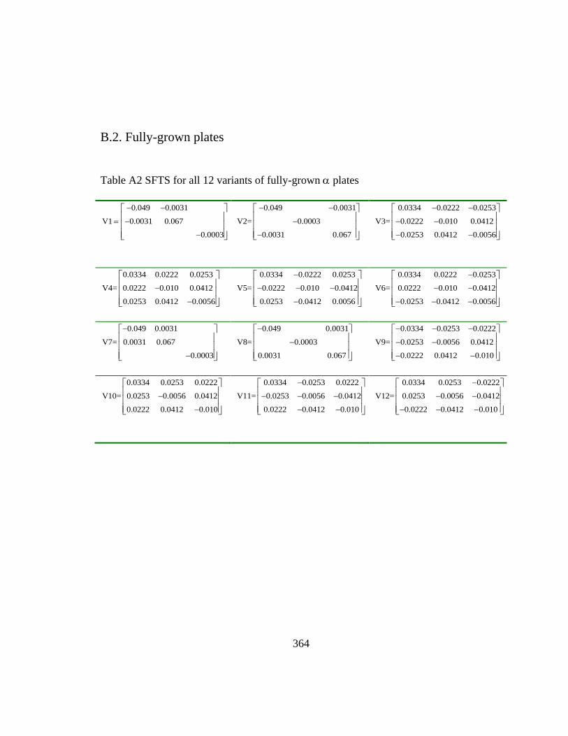
364
B.2. Fully-grown plates
Table A2 SFTS for all 12 variants of fully-grown plates
0.049 0.0031
V1 0.0031 0.067
0.0003
0.049 0.0031
V2= 0.0003
0.0031 0.067
0.0334 0.0222 0.0253
V3= 0.0222 0.010 0.0412
0.0253 0.0412 0.0056
0.0334 0.0222 0.0253
V4= 0.0222 0.010 0.0412
0.0253 0.0412 0.0056
0.0334 0.0222 0.0253
V5= 0.0222 0.010 0.0412
0.0253 0.0412 0.0056
0.0334 0.0222 0.0253
V6= 0.0222 0.010 0.0412
0.0253 0.0412 0.0056
0.049 0.0031
V7= 0.0031 0.067
0.0003
0.049 0.0031
V8= 0.0003
0.0031 0.067
0.0334 0.0253 0.0222
V9= 0.0253 0.0056 0.0412
0.0222 0.0412 0.010
0.0334 0.0253 0.0222
V10= 0.0253 0.0056 0.0412
0.0222 0.0412 0.010
0.0334 0.0253 0.0222
V11= 0.0253 0.0056 0.0412
0.0222 0.0412 0.010
0.0334 0.0253 0.0222
V12= 0.0253 0.0056 0.0412
0.0222 0.0412 0.010