Chemical Engineering Science ] (]]]]) ]]]–]]]

Contents lists available at ScienceDirect

Chemical Engineering Science

0009-25

doi:10.1

n Corr

E-m

Pleascons

journal homepage: www.elsevier.com/locate/ces

Rolling horizon based planning and scheduling integration with productioncapacity consideration

Zukui Li, Marianthi G. Ierapetritou n

Department of Chemical and Biochemical Engineering, Rutgers University, Piscataway, NJ 08854, USA

a r t i c l e i n f o

Article history:

Received 20 April 2010

Received in revised form

7 July 2010

Accepted 5 August 2010

Keywords:

Planning and scheduling integration

Rolling horizon method

Economics

Optimization

Mathematical modeling

Systems engineering

09/$ - see front matter & 2010 Elsevier Ltd. A

016/j.ces.2010.08.010

esponding author. Tel.: +1 732 445 2971; fax

ail address: marianth@soemail.rutgers.edu (M

e cite this article as: Li, Z., Ierapetritoideration. Chemical Engineering Scie

a b s t r a c t

The rolling horizon method has been proposed to address the integrated production planning and

scheduling optimization problem. Since the method can generally result in small-scale optimization

model and fast solution, it has been used in a number of applications in realistic industrial planning and

scheduling problems. In this paper, it is first pointed out that the incorporation of valid production

capacity information into the planning model can improve the solution quality in the rolling horizon

solution framework. A novel method is then proposed to derive the production capacity information

representing the detail scheduling model based on parametric programming technique. A heuristic

process network decomposition strategy is further applied to reduce the computational effort needed

for larger and more complex process networks. Several case studies have been studied, which illustrate

the efficiency of the proposed methodology in improving the solution quality of rolling horizon method

for integrated planning and scheduling optimization.

& 2010 Elsevier Ltd. All rights reserved.

1. Introduction

Production planning and scheduling belong to two of the mostimportant decision making levels in the process industry.Traditionally, planning and scheduling have been performedseparately as follows (Kallrath, 2002). The planning problem istypically solved to predict production targets and material flowover a mid-term horizon (e.g. several months) to satisfy thecustomer demand. The scheduling problem is usually addressedafter the production planning problem has been solved. The datagenerated by the production planning problem are input data tothe scheduling problem. The purpose of the scheduling problem isto transform the production plan into a feasible schedule ofall the production operations within a short-term time horizon(e.g., several days). However, treating the planning and schedulingactivities separately can lead to lower efficiency of the operationsperformed in the production plant. The aggregate productiontargets supplied by the planning model often overestimate theproduction capacity of the plant, and may result in infeasiblescheduling operations because they are made without considera-tion of short-term operational restrictions. Given the importanceof providing realistic production targets, a production planningmodel should take into account not only the customer demands,but also the production capacity of the plant. To address this issue,the integration of planning and scheduling has been proposed by

ll rights reserved.

: 1 732 445 2581.

.G. Ierapetritou).

u, M.G., Rolling horizon basnce (2010), doi:10.1016/j.c

the process systems engineering community (Maravelias andSung, 2009). The integration aims to address the inaccuracieswithin the planning model by allowing for the two-way interac-tion between planning and scheduling models. Ideally, anintegrated model should include not only the medium-termcapacity utilization and production level decisions, but also theshort-term production sequence and unit assignment decisions.

One simple approach is to use a scheduling model over theentire planning time horizon, which takes into account theproduction capacity of the plant. However, this approach resultsin problems of unrealistic size, which is often computationallyintractable. To ensure that the integration can be addressedefficiently, planning models are often formulated through varioustypes of aggregation or relaxation schemes, and the integrationproblem is often solved through decomposition algorithms(Maravelias and Sung, 2009; Grossmann et al., 2002). In theliterature, there are a number of decomposition based methodslike the hierarchical decomposition (Bassett et al., 1996; Munawarand Gudi, 2005; Erdirik-Dogan and Grossmann, 2006), periodicscheduling (Schilling and Pantelides, 1999; Zhu and Majozi, 2001;Castro et al., 2003; Wu and Ierapetritou, 2004), mathematicalprogramming based decomposition (Li and Ierapetritou, 2009), aswell as methods that are based on the rolling horizon idea whichis widely studied (Kreipl and Pinedo, 2004), because it cansignificantly reduce the computational requirements. The methodis based on iteratively solving the integrated problem in a rollingtime horizon mode. In every iteration of the solution procedure,the detailed scheduling requirements are imposed only for thecurrent or several recent planning periods. As the iterations

ed planning and scheduling integration with production capacityes.2010.08.010

Z. Li, M.G. Ierapetritou / Chemical Engineering Science ] (]]]]) ]]]–]]]2

proceed, planning decisions are updated with all the previousexecuted decisions fixed. This mode is repeated until all theplanning periods are studied. The above idea is supported by thefact that planning decisions for far future could not be accurateenough due to the unpredicted future uncertainty. So it isreasonable to consider a relative rough model for far futureplanning periods in the aggregate planning model. Thus, therolling horizon approach results in reduced size models and lowercomputation cost.

Rolling horizon method has received a lot of studies in theliterature. Wilkinson (1996) derived an MILP planning model thathas varying time resolution through dividing the horizon intoaggregate time periods. The first aggregate period is modeled infine detail scheduling and the subsequent periods are modeled,using the aggregate formulation. Rodrigues et al. (1996) used arolling horizon approach to take account of due-date changes andequipment unavailability to resolve infeasibilities. Dimitriadiset al. (1997) presented an RTN-based rolling horizon algorithm formedium-term scheduling of multipurpose plants. Sand et al.(2000) used a rolling horizon approach, in combination with aLagrangian relaxation algorithm, for the solution of a two-levelhierarchical planning and scheduling problem. Wu and Ierape-tritou (2007) decomposed the planning time horizon into threestages with various durations. The scheduling problem is solvedafter the solution of planning model to ensure a feasibleproduction schedule for the current period. Sand and Engell(2004) used a rolling horizon, two-stage stochastic programmingapproach to schedule an expandable polystyrene plant that issubject to uncertainty in processing times, yields, capacities anddemands. Verderame and Floudas (2008) solved the integrationproblem utilizing the medium-term scheduling model for large-scale batch plants and a forward rolling horizon approach. Rollinghorizon method has also been applied to address the long- andmedium-term scheduling problem. For those scheduling pro-blems, a rolling-horizon based decomposition scheme is used andusually two sub-problems are solved. At the upper-level, a variantof the model is used to find the optimal number of products, andthe length of the time horizon to be considered for solving theshort-term scheduling problem at the lower level. At the lowerlevel, short-term scheduling of continuous processes, using unit-specific event-based continuous-time representation are applied(Lin et al., 2002; Janak et al., 2006; Wu and Ierapetritou, 2003;Shaik et al., 2009).

Although rolling horizon framework has received a lot ofattention in the literature, a major drawback of most existingmethods is that they often rely on the simplistic or rather poorrepresentation of the scheduling problem within the aggregatepart. Within such a modeling framework, rolling horizonmethod is generally efficient in the computational manner.However, the method only generates feasible planning–schedul-ing decisions and the quality (optimality) of the solution cannotbe ensured. As what we will show in this paper, productioncapacity information representing the scheduling problem canhave great effect on the final solution’s quality. In the literature,Sung and Maravelias (2007) have proposed to derive the feasibleproduction regions for scheduling problem through a computa-tional geometry method, and then incorporate it into the rollinghorizon planning model. In this work, a new methodology isproposed to derive the production capacity constraints based onshort-term scheduling model through parametric programmingtechnique and those capacity information can be further usedin the rolling horizon framework to improve the finalsolution’s quality.

The content of this paper is organized as follows. The rollinghorizon solution framework and model are presented in Section 2,which is further illustrated through a motivation example

Please cite this article as: Li, Z., Ierapetritou, M.G., Rolling horizon basconsideration. Chemical Engineering Science (2010), doi:10.1016/j.c

studying the effect of production capacity constraints. In Section3, we present a parametric programming based method, which isable to generate an accurate boundary of the production capacityregion of scheduling problem, and also a heuristic processnetwork decomposition strategy to further reduce the computa-tion complexity. In Section 4, we illustrate the application of theproposed method on several problems, and the paper concludes inSection 5 with a summary of the presented work.

2. Rolling horizon framework

Rolling horizon methods solve the integrated planning andscheduling optimization problem with a sequence of iterations,each of which models only part of the planning horizon in detail,while the rest of the horizon is represented in an aggregatemanner. The rolling horizon solution framework involves succes-sively solving each scheduling sub-horizon and carrying over anyunsatisfied demand to the following sub-horizon. In principle, thisapproach produces feasible planning and scheduling solutionswith a significant reduction of the computational requirements.

Generally, discrete time representation is used for the planningtime domain. Consider the planning and scheduling integrationproblem over a time horizon H. In order to integrate both planningand scheduling into the optimization model, H is divided into anumber of planning periods, t¼1, y, T. The length of the planninghorizon is typically in the order of a few months. In the rollinghorizon framework, both uniform and non-uniform planningperiods of fixed or varying length can be applied. For example, inproduction planning, it is often required to determine weeklyproduction targets for the first month, while monthly productiontargets are sufficient for subsequent periods. Hence, we canconsider the non-uniform planning periods ranging weeks–months.

To describe the scheduling model, discrete and continuousmodels both can be applied. In a discrete time representation(which assumes that an event can occur only at the boundaries ofeach time interval), every planning period in the time horizon isdivided into a number of predefined scheduling periods, k¼1, y,K. The length of a scheduling period is typically in the order ofhours. In the continuous-time representation, an event can occurat any instant within the whole planning horizon. This makes themodel more flexible and decreases the total number of variables.

In the following paragraphs, we present a general multiperiodlinear programming based planning model and a continuous-timerepresentation based process scheduling model, which form abasis for the rolling horizon framework studied in this paper. Itshould be pointed out however that for long- or medium-termscheduling problems, similar formulation idea can be applied,whereas a planning problem is not involved.

2.1. Planning model

min TotalCost¼X

t

Xs

hsInvtsþX

s

usUtsþX

s

vsPts

!ð1aÞ

s:t: Invts ¼ Invt�1

s þPts�Dt

s 8sASP , 8t ð1bÞ

Uts ¼Ut�1

s þDemts�Dt

s 8sASP ,8t ð1cÞ

Pts ¼ P

t

s 8tATpre ð1dÞ

f ðPtsÞr0 8sASP ,8t ð1eÞ

Pts ,Invt

s,Dts,U

ts Z0 8sASP , 8t

ed planning and scheduling integration with production capacityes.2010.08.010

Z. Li, M.G. Ierapetritou / Chemical Engineering Science ] (]]]]) ]]]–]]] 3

The above planning model is similar to the one given by Sungand Maravelias (2007). In the problem, the objective function isthe total cost which is composed by three parts: inventory cost,backorder cost and production cost. Eq. (1b) represents theinventory balance and Eq. (1c) represents the backorder balance.Eq. (1d) fixes those planning decision that have been ‘‘executed’’by the scheduling model, where Tpre represents the set of planningperiods that has been studied.

2.2. Scheduling model

minX

s

ðeþs þe�s ÞþgProductionCost ð2aÞ

s:t: ProductionCost¼X

i

Xj

Xn

ðFixCostiwi,j,nþVar Costibi,j,nÞ

ð2bÞ

Ps�Ps ¼ eþs �e�s 8sASP ð2cÞ

sts,n ¼ N�stins ¼ Ps 8sASP ð2dÞ

XiA Ij

wvi,j,nr1 8jA J, 8nAN ð2eÞ

vmini,j wvi,j,nrbi,j,nrvmax

i,j wvi,j,n 8iA I, 8jA Ji, 8nAN ð2fÞ

Tfi,j,n ¼ Tsi,j,nþai,jwvi,j,nþbi,jbi,j,n 8iA I,8jA Ji,8nAN ð2gÞ

Tsi,j,nþ1ZTfi,j,n�Hð1�wvi,j,nÞ 8iA I, 8jA Ji, 8nAN ð2hÞ

Tsi,j,nþ1ZTfiu,j,n�Hð1�wviu,j,nÞ 8i,i0A Ij, 8jA J, 8nAN ð2iÞ

Tsi,j,nþ1ZTfiu,ju,n�Hð1�wviu,ju,nÞ 8i,iuA Ij, ia iu, 8j,juA J, 8nAN

ð2jÞ

Tsi,j,nþ1ZTsi,j,n 8iA I, 8jA Ji, 8nAN ð2kÞ

Tfi,j,nþ1ZTfi,j,n 8iA I, 8jA Ji, 8nAN ð2lÞ

Tsi,j,nrH 8iA I, 8jA Ji, 8nAN ð2mÞ

Fig. 1. State-task-network f

Please cite this article as: Li, Z., Ierapetritou, M.G., Rolling horizon basconsideration. Chemical Engineering Science (2010), doi:10.1016/j.c

Tfi,j,nrH 8iA I, 8jA Ji, 8nAN ð2nÞ

sts,n ¼ sts,n�1�XiA Is

rCs,i

XjA Ji

bi,j,nþXiA Is

rPs,i

XjA Ji

bi,j,n�1 8sAS, 8nAN

ð2oÞ

sts,nrstmaxs 8sAS, 8nAN ð2pÞ

wvi,j,nAf0,1g, bi,j,n, sts,n, Tfi,j,n, Tsi,j,nZ0

The objective (2a) aims at finding a feasible schedule minimizingthe sum of the absolute difference between the result generated bythe planning model Pt

s and feasible schedule, plus a weightedproduction cost (g is the weight coefficient). The production cost iscalculated in Eq. (2b) by a fixed part, which represents the basic costof a task, and a dynamic part which is proportional to the amount ofmaterial processed (batch size). Among the constraints of thescheduling level problem, Eq. (2c) uses slack variables to evaluatethe difference between given production target and actual produc-tion amount. Eq. (2d) defines the actual production amount. Eq. (2e)represents the allocation constraints which state that only one of thetasks can be performed in each unit at an event point (n); thecapacity limitations of production units are expressed by constraint(2f); constraint (2g) represents the duration constraints andconstraints (2h)–(2n) represent time limitations due to tasksequence requirements in the same or different production units;Eq. (2o) represents the material balances for each state (s)expressing that at each event point (n) the amount sts,n is equal tothat at event point (n�1), adjusted by any amounts produced andconsumed between event points (n�1) and (n). Constraint (2p)represents the storage capacity constraints. Detail explanations ofthe symbols in the above model can be referred from theNomenclature section at the end of the paper. Finally, it should benoticed that although the above scheduling formulation derivedfrom Ierapetritou and Floudas (1998) has been used, the proposedmethodology in this paper is not limited to this model becausethe proposed solution method is appropriate for general MILPscheduling model.

Based on the above planning and scheduling formulations,the following algorithm describes a rolling horizon algorithmfor the solution of the integrated planning and schedulingproblem.

or motivating example.

ed planning and scheduling integration with production capacityes.2010.08.010

Z. Li, M.G. Ierapetritou / Chemical Engineering Science ] (]]]]) ]]]–]]]4

2.3. Rolling horizon algorithm

Step 1. Set the first planning period as ‘‘current period,’’ solvethe planning problem.

Step 2. Using the production target solution obtained from step1, solve scheduling problem in current period. If ‘‘current period’’is the last planning period of the problem, stop. Otherwise, go tostep 3.

Step 3. Fix the production target in current period at the valuesobtained in step 2 and solve a new planning problem; update thecurrent period index; go to step 2.

In the following subsection, an example is used to illustrate theabove algorithm, and also the effect of the production capacityconstraints on the quality of the final solution.

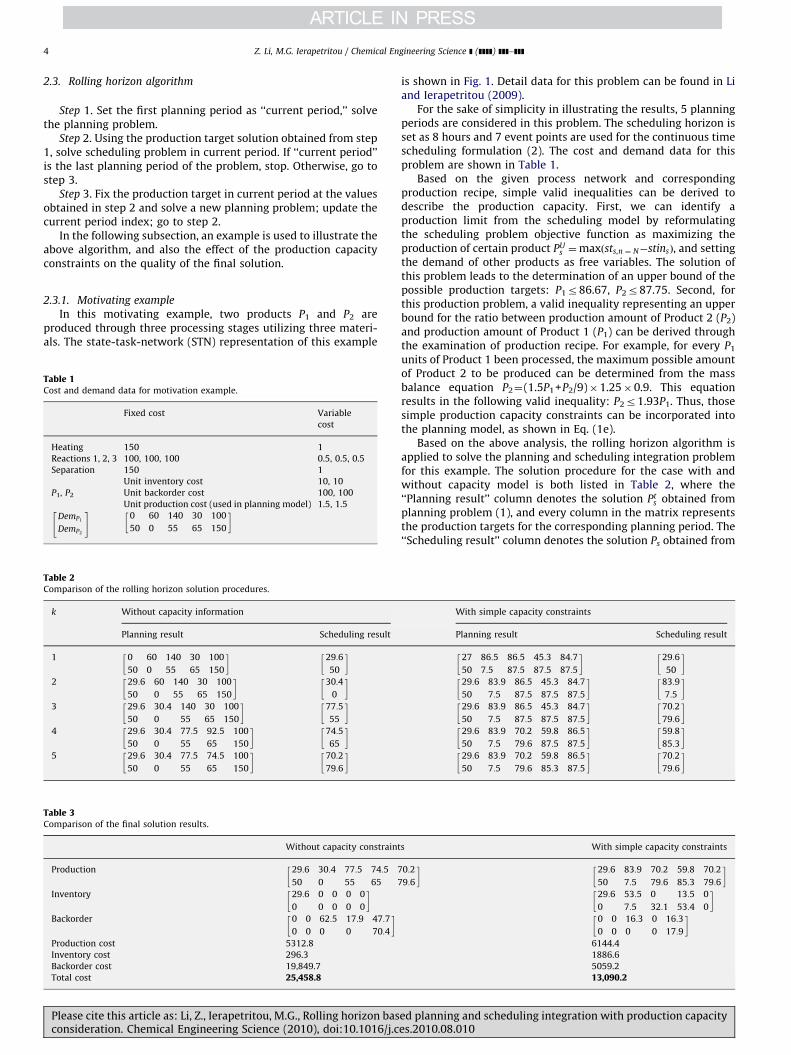
2.3.1. Motivating example

In this motivating example, two products P1 and P2 areproduced through three processing stages utilizing three materi-als. The state-task-network (STN) representation of this example

Table 1Cost and demand data for motivation example.

Fixed cost Variable

cost

Heating 150 1

Reactions 1, 2, 3 100, 100, 100 0.5, 0.5, 0.5

Separation 150 1

Unit inventory cost 10, 10

P1, P2 Unit backorder cost 100, 100

Unit production cost (used in planning model) 1.5, 1.5

DemP1

DemP2

" #0 60 140 30 100

50 0 55 65 150

� �

Table 2Comparison of the rolling horizon solution procedures.

k Without capacity information

Planning result Scheduling result

1 0 60 140 30 100

50 0 55 65 150

� �29:6

50

� �2 29:6 60 140 30 100

50 0 55 65 150

� �30:4

0

� �3 29:6 30:4 140 30 100

50 0 55 65 150

� �77:5

55

� �4 29:6 30:4 77:5 92:5 100

50 0 55 65 150

� �74:5

65

� �5 29:6 30:4 77:5 74:5 100

50 0 55 65 150

� �70:2

79:6

� �

Table 3Comparison of the final solution results.

Without capacity constraint

Production 29:6 30:4 77:5 74:5 7

50 0 55 65 7

�Inventory 29:6 0 0 0 0

0 0 0 0 0

� �Backorder 0 0 62:5 17:9 47:7

0 0 0 0 70:4

� �Production cost 5312.8

Inventory cost 296.3

Backorder cost 19,849.7

Total cost 25,458.8

Please cite this article as: Li, Z., Ierapetritou, M.G., Rolling horizon basconsideration. Chemical Engineering Science (2010), doi:10.1016/j.c

is shown in Fig. 1. Detail data for this problem can be found in Liand Ierapetritou (2009).

For the sake of simplicity in illustrating the results, 5 planningperiods are considered in this problem. The scheduling horizon isset as 8 hours and 7 event points are used for the continuous timescheduling formulation (2). The cost and demand data for thisproblem are shown in Table 1.

Based on the given process network and correspondingproduction recipe, simple valid inequalities can be derived todescribe the production capacity. First, we can identify aproduction limit from the scheduling model by reformulatingthe scheduling problem objective function as maximizing theproduction of certain product PU

s ¼maxðsts,n ¼ N�stinsÞ, and settingthe demand of other products as free variables. The solution ofthis problem leads to the determination of an upper bound of thepossible production targets: P1r86.67, P2r87.75. Second, forthis production problem, a valid inequality representing an upperbound for the ratio between production amount of Product 2 (P2)and production amount of Product 1 (P1) can be derived throughthe examination of production recipe. For example, for every P1

units of Product 1 been processed, the maximum possible amountof Product 2 to be produced can be determined from the massbalance equation P2¼(1.5P1+P2/9)�1.25�0.9. This equationresults in the following valid inequality: P2r1.93P1. Thus, thosesimple production capacity constraints can be incorporated intothe planning model, as shown in Eq. (1e).

Based on the above analysis, the rolling horizon algorithm isapplied to solve the planning and scheduling integration problemfor this example. The solution procedure for the case with andwithout capacity model is both listed in Table 2, where the‘‘Planning result’’ column denotes the solution Pt

s obtained fromplanning problem (1), and every column in the matrix representsthe production targets for the corresponding planning period. The‘‘Scheduling result’’ column denotes the solution Ps obtained from

With simple capacity constraints

Planning result Scheduling result

27 86:5 86:5 45:3 84:7

50 7:5 87:5 87:5 87:5

� �29:6

50

� �29:6 83:9 86:5 45:3 84:7

50 7:5 87:5 87:5 87:5

� �83:9

7:5

� �29:6 83:9 86:5 45:3 84:7

50 7:5 87:5 87:5 87:5

� �70:2

79:6

� �29:6 83:9 70:2 59:8 86:5

50 7:5 79:6 87:5 87:5

� �59:8

85:3

� �29:6 83:9 70:2 59:8 86:5

50 7:5 79:6 85:3 87:5

� �70:2

79:6

� �

s With simple capacity constraints

0:2

9:6

�29:6 83:9 70:2 59:8 70:2

50 7:5 79:6 85:3 79:6

� �29:6 53:5 0 13:5 0

0 7:5 32:1 53:4 0

� �0 0 16:3 0 16:3

0 0 0 0 17:9

� �6144.4

1886.6

5059.2

13,090.2

ed planning and scheduling integration with production capacityes.2010.08.010

Z. Li, M.G. Ierapetritou / Chemical Engineering Science ] (]]]]) ]]]–]]] 5

the scheduling problem (2), and it represents the final productiontargets for the specific planning period k, which is also theiteration index of the rolling horizon algorithm. The final solutionis shown in Table 3.

From the above results, it can be observed that the total costfor the case without production capacity information is muchhigher than that of the case with simple capacity constraints, andthe difference is mainly due to increased backorder cost. Thereason is that in the model without production capacityconstraints, the planning model cannot predict that the futureproduction will not satisfy the demand and optimisticallyassumes that the future demand will always be satisfied withenough production capacity, so it tends to produce as close aspossible to the demand in current period so as to minimize theinventory cost. Due to the production capacity limitation that isnot considered, the model without the capacity constraints resultsin higher backorder cost, and thus higher total cost.

The above simple implementation of a rolling horizonapproach, for this motivating example, illustrates that theincorporation of production capacity constraints representingproduction capacity at the planning level problem can result inhuge savings in terms of backorder cost (74% reduction) andsignificant reduction of the overall cost (49% reduction). Thus, it isimportant to point out that the consideration of productioncapacity information will improve the quality of the overallsolution for the case of a rolling horizon solution procedure.

In the above example problem, for illustrative purposes, theproduction capacity information is only derived from productionrecipe and represents a rough approximation of the realproduction capacity limitations. A more accurate method basedon parametric programming is presented in the next section,which will further improve the quality of the solution.

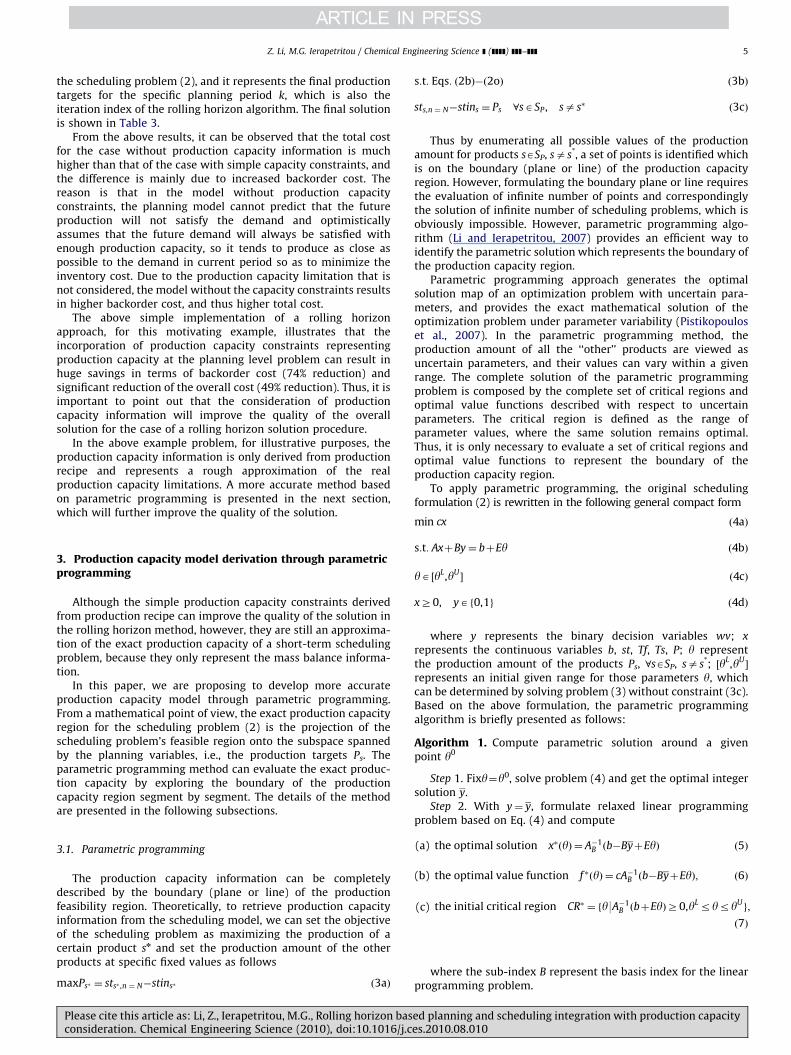
3. Production capacity model derivation through parametricprogramming

Although the simple production capacity constraints derivedfrom production recipe can improve the quality of the solution inthe rolling horizon method, however, they are still an approxima-tion of the exact production capacity of a short-term schedulingproblem, because they only represent the mass balance informa-tion.

In this paper, we are proposing to develop more accurateproduction capacity model through parametric programming.From a mathematical point of view, the exact production capacityregion for the scheduling problem (2) is the projection of thescheduling problem’s feasible region onto the subspace spannedby the planning variables, i.e., the production targets Ps. Theparametric programming method can evaluate the exact produc-tion capacity by exploring the boundary of the productioncapacity region segment by segment. The details of the methodare presented in the following subsections.

3.1. Parametric programming

The production capacity information can be completelydescribed by the boundary (plane or line) of the productionfeasibility region. Theoretically, to retrieve production capacityinformation from the scheduling model, we can set the objectiveof the scheduling problem as maximizing the production of acertain product sn and set the production amount of the otherproducts at specific fixed values as follows

maxPs� ¼ sts� ,n ¼ N�stins� ð3aÞ

Please cite this article as: Li, Z., Ierapetritou, M.G., Rolling horizon basconsideration. Chemical Engineering Science (2010), doi:10.1016/j.c

s:t: Eqs: ð2bÞ�ð2oÞ ð3bÞ

sts,n ¼ N�stins ¼ Ps 8sASP , sas� ð3cÞ

Thus by enumerating all possible values of the productionamount for products sASP, sas*, a set of points is identified whichis on the boundary (plane or line) of the production capacityregion. However, formulating the boundary plane or line requiresthe evaluation of infinite number of points and correspondinglythe solution of infinite number of scheduling problems, which isobviously impossible. However, parametric programming algo-rithm (Li and Ierapetritou, 2007) provides an efficient way toidentify the parametric solution which represents the boundary ofthe production capacity region.

Parametric programming approach generates the optimalsolution map of an optimization problem with uncertain para-meters, and provides the exact mathematical solution of theoptimization problem under parameter variability (Pistikopouloset al., 2007). In the parametric programming method, theproduction amount of all the ‘‘other’’ products are viewed asuncertain parameters, and their values can vary within a givenrange. The complete solution of the parametric programmingproblem is composed by the complete set of critical regions andoptimal value functions described with respect to uncertainparameters. The critical region is defined as the range ofparameter values, where the same solution remains optimal.Thus, it is only necessary to evaluate a set of critical regions andoptimal value functions to represent the boundary of theproduction capacity region.

To apply parametric programming, the original schedulingformulation (2) is rewritten in the following general compact form

min cx ð4aÞ

s:t: AxþBy¼ bþEy ð4bÞ

yA ½yL,yU� ð4cÞ

xZ0, yAf0,1g ð4dÞ

where y represents the binary decision variables wv; x

represents the continuous variables b, st, Tf, Ts, P; y representthe production amount of the products Ps, 8sASP, sas*; ½yL,yU

�

represents an initial given range for those parameters y, whichcan be determined by solving problem (3) without constraint (3c).Based on the above formulation, the parametric programmingalgorithm is briefly presented as follows:

Algorithm 1. Compute parametric solution around a givenpoint y0

Step 1. Fixy¼y0, solve problem (4) and get the optimal integersolution y.

Step 2. With y¼ y, formulate relaxed linear programmingproblem based on Eq. (4) and compute

(a)

ed pes.2

the optimal solution x�ðyÞ ¼ A�1B ðb�ByþEyÞ ð5Þ

(b)

the optimal value function f �ðyÞ ¼ cA�1B ðb�ByþEyÞ; ð6Þ

(c)

the initial critical region CR� ¼ fy9A�1B ðbþEyÞZ0,yLryryU

g;

ð7Þ

where the sub-index B represent the basis index for the linearprogramming problem.

lanning and scheduling integration with production capacity010.08.010

Z. Li, M.G. Ierapetritou / Chemical Engineering Science ] (]]]]) ]]]–]]]6

Step 3. Solve the following problem (y is treated as variable here)

max err¼ f �ðyÞ�cx ð8aÞ

s.t. Eqs. (4b)–(4d)

errre ð8bÞ

yACR� ð8cÞ

If the optimal objective err*r0, return (x*(y), f*(y), CR*) as theparametric solution around y0 and stop. Otherwise, store thesolution ( ~y, ~y) of problem (14) and go to step 4.

Step 4. Fix y¼ ~y, y¼ ~y, solve problem (4), identify a new set ofbasis index B0 and get the following optimal value function andcritical region

f ðyÞ ¼ cBuA�1Bu ðb�B ~yþEyÞ ð9Þ

CR ¼ fy9A�1B0 ðb�B ~yþEyÞZ0,yLryryU

g ð10Þ

Step 5. Define CREX ¼ CR� \ CR \ fy9f ðyÞr f �ðyÞg, update CR* byexcluding CREX from it, then go to step 3.

For the sake of simplicity in the presentation of this work, theproof of the validity and more details of the algorithm are notpresented in this paper, but it can be found in Li and Ierapetritou(2007). Using the above algorithm, a segment of the productioncapacity boundary can be derived once a set of values of theuncertain parameters is assigned. By varying the values of thoseparameters, the complete boundary can be identified.

Table 4Parametric solution for the motivating example.

max P2 Range of P1

1 1.6875P1 0rP1r52

2 87.75 52rP1r55.25

3 117.785�0.5436P1 55.25rP1r70.19

4 585.0�7.2P1 70.19rP1r71.52

5 104.62�0.4829P1 71.52rP1r73.32

6 317.647�3.388P1 73.32rP1r77.92

7 100.746�0.6045P1 77.92rP1r80.24

8 630�7.2P1 80.24rP1r81.77

9 214.412�2.118P1 81.77rP1r85.63

10 88.56�0.648P1 85.63rP1r86.67

Fig. 2. Illustration of the

Please cite this article as: Li, Z., Ierapetritou, M.G., Rolling horizon basconsideration. Chemical Engineering Science (2010), doi:10.1016/j.c

For the proposed parametric programming algorithm, thecritical regions are calculated one at a time, and thus the numberof parameters is not the limited step. The computationalcomplexity of the algorithm results from the number of criticalregions, which however can increase exponentially with thenumber of parameters considered.

To illustrate the application of the parametric programmingalgorithm for the solution of the production capacity region, themotivation example presented in Section 2 is studied in the nextsubsection.

3.2. Application of parametric programming in motivating example

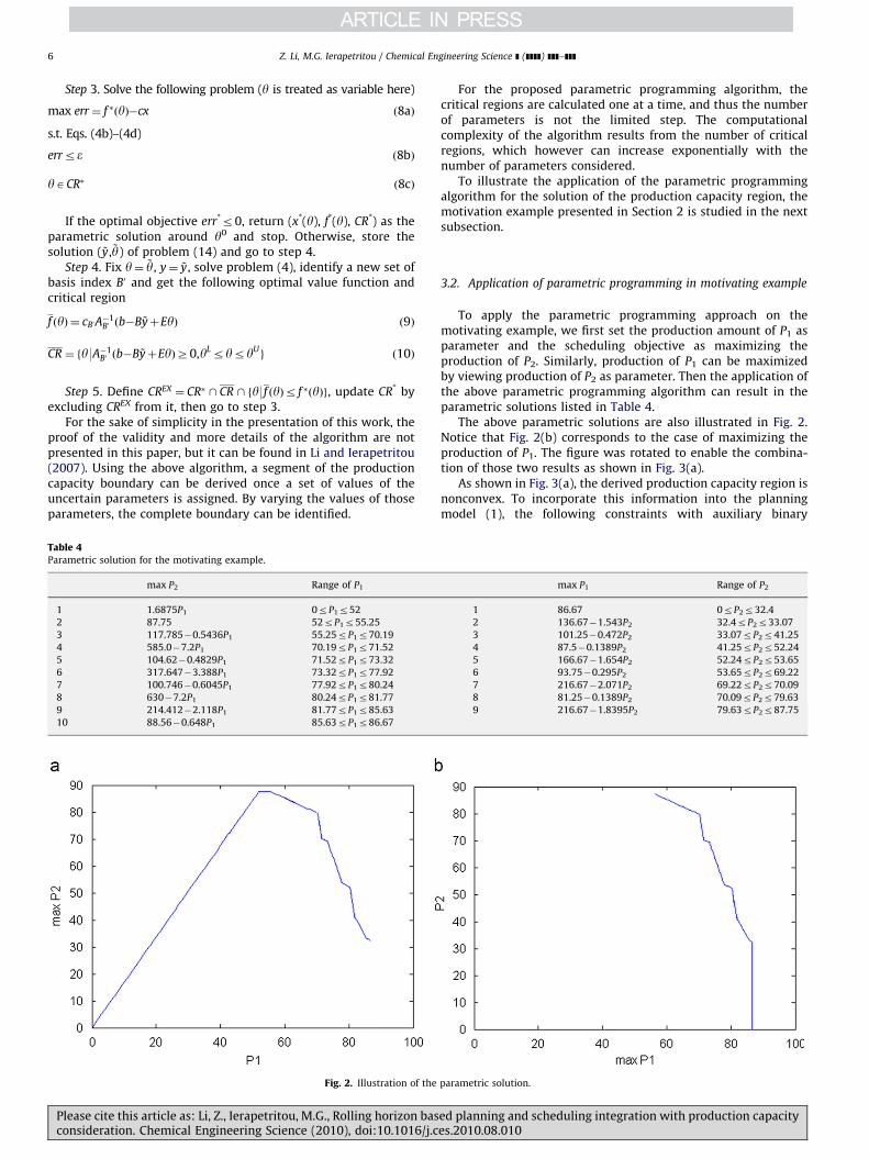
To apply the parametric programming approach on themotivating example, we first set the production amount of P1 asparameter and the scheduling objective as maximizing theproduction of P2. Similarly, production of P1 can be maximizedby viewing production of P2 as parameter. Then the application ofthe above parametric programming algorithm can result in theparametric solutions listed in Table 4.

The above parametric solutions are also illustrated in Fig. 2.Notice that Fig. 2(b) corresponds to the case of maximizing theproduction of P1. The figure was rotated to enable the combina-tion of those two results as shown in Fig. 3(a).

As shown in Fig. 3(a), the derived production capacity region isnonconvex. To incorporate this information into the planningmodel (1), the following constraints with auxiliary binary

max P1 Range of P2

1 86.67 0rP2r32.4

2 136.67�1.543P2 32.4rP2r33.07

3 101.25�0.472P2 33.07rP2r41.25

4 87.5�0.1389P2 41.25rP2r52.24

5 166.67�1.654P2 52.24rP2r53.65

6 93.75�0.295P2 53.65rP2r69.22

7 216.67�2.071P2 69.22rP2r70.09

8 81.25�0.1389P2 70.09rP2r79.63

9 216.67�1.8395P2 79.63rP2r87.75

parametric solution.

ed planning and scheduling integration with production capacityes.2010.08.010

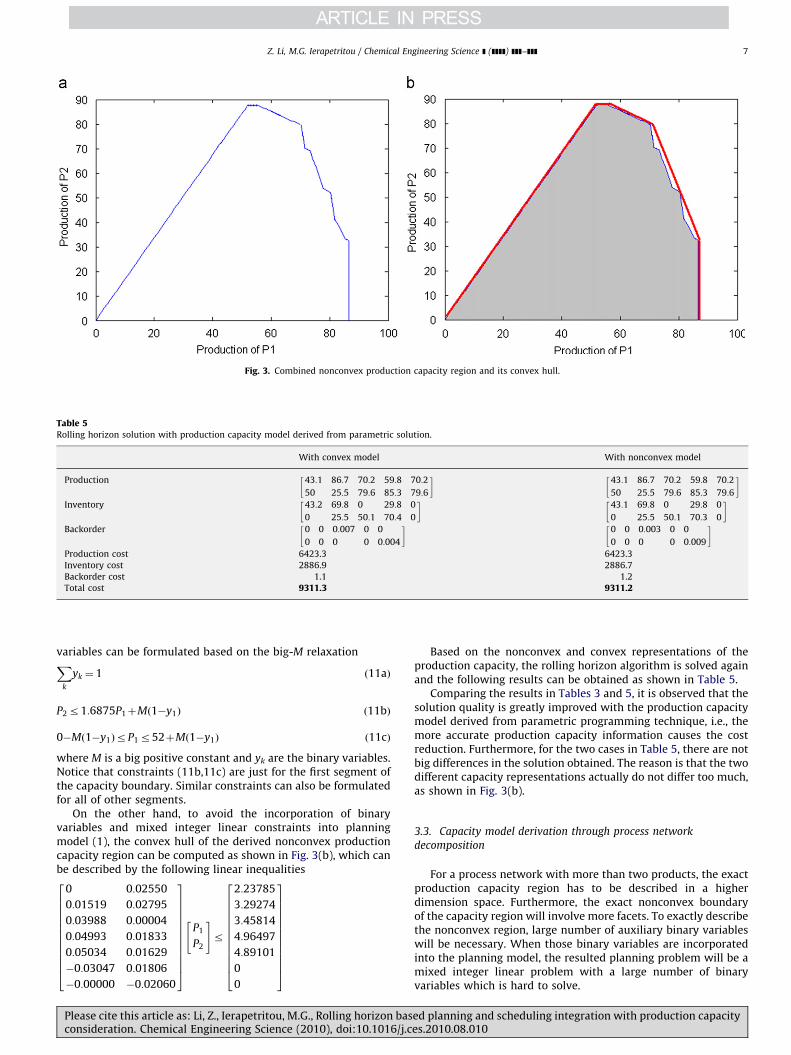
Fig. 3. Combined nonconvex production capacity region and its convex hull.

Table 5Rolling horizon solution with production capacity model derived from parametric solution.

With convex model With nonconvex model

Production 43:1 86:7 70:2 59:8 70:2

50 25:5 79:6 85:3 79:6

� �43:1 86:7 70:2 59:8 70:2

50 25:5 79:6 85:3 79:6

� �Inventory 43:2 69:8 0 29:8 0

0 25:5 50:1 70:4 0

� �43:1 69:8 0 29:8 0

0 25:5 50:1 70:3 0

� �Backorder 0 0 0:007 0 0

0 0 0 0 0:004

� �0 0 0:003 0 0

0 0 0 0 0:009

� �Production cost 6423.3 6423.3

Inventory cost 2886.9 2886.7

Backorder cost 1.1 1.2

Total cost 9311.3 9311.2

Z. Li, M.G. Ierapetritou / Chemical Engineering Science ] (]]]]) ]]]–]]] 7

variables can be formulated based on the big-M relaxationXk

yk ¼ 1 ð11aÞ

P2r1:6875P1þMð1�y1Þ ð11bÞ

0�Mð1�y1ÞrP1r52þMð1�y1Þ ð11cÞ

where M is a big positive constant and yk are the binary variables.Notice that constraints (11b,11c) are just for the first segment ofthe capacity boundary. Similar constraints can also be formulatedfor all of other segments.

On the other hand, to avoid the incorporation of binaryvariables and mixed integer linear constraints into planningmodel (1), the convex hull of the derived nonconvex productioncapacity region can be computed as shown in Fig. 3(b), which canbe described by the following linear inequalities

0 0:02550

0:01519 0:02795

0:03988 0:00004

0:04993 0:01833

0:05034 0:01629

�0:03047 0:01806

�0:00000 �0:02060

2666666666664

3777777777775

P1

P2

" #r

2:23785

3:29274

3:45814

4:96497

4:89101

0

0

2666666666664

3777777777775

Please cite this article as: Li, Z., Ierapetritou, M.G., Rolling horizon basconsideration. Chemical Engineering Science (2010), doi:10.1016/j.c

Based on the nonconvex and convex representations of theproduction capacity, the rolling horizon algorithm is solved againand the following results can be obtained as shown in Table 5.

Comparing the results in Tables 3 and 5, it is observed that thesolution quality is greatly improved with the production capacitymodel derived from parametric programming technique, i.e., themore accurate production capacity information causes the costreduction. Furthermore, for the two cases in Table 5, there are notbig differences in the solution obtained. The reason is that the twodifferent capacity representations actually do not differ too much,as shown in Fig. 3(b).

3.3. Capacity model derivation through process network

decomposition

For a process network with more than two products, the exactproduction capacity region has to be described in a higherdimension space. Furthermore, the exact nonconvex boundaryof the capacity region will involve more facets. To exactly describethe nonconvex region, large number of auxiliary binary variableswill be necessary. When those binary variables are incorporatedinto the planning model, the resulted planning problem will be amixed integer linear problem with a large number of binaryvariables which is hard to solve.

ed planning and scheduling integration with production capacityes.2010.08.010

Z. Li, M.G. Ierapetritou / Chemical Engineering Science ] (]]]]) ]]]–]]]8

Moreover for the parametric programming algorithm,although it can be performed off-line, the required computationeffort increases significantly for higher dimension problem (i.e.,the number of products is large), since it is proportional to thenumber of critical regions (Li and Ierapetritou, 2007). To avoid thelarge computational complexity of parametric programmingmethod for high dimensionality problems, we propose to usethe following heuristic network decomposition strategy and toapply the parametric programming method on the sub-networks,which involve relative small number of products. With adecomposed network, the complexity of the scheduling modelfor the sub-network is also reduced, which will also facilitate thesolution of the parametric problem.

Based on the STN representation of the production process, thefollowing guiding rules for the process network decompositioncan be applied:

(1)

Plco

Identify key connecting intermediate products in the processnetwork;

(2)

Identify sub-networks such that the resulted schedulingmodel can be solved efficiently.

The above network decomposition is a heuristic strategy,which is based on the specific problem, but the basic principle isto generate scheduling problems, which can be solved moreefficiently by decreasing the number of parameters (products)appeared in the scheduling problem. The different productioncapacity relationships that can be obtained from this kind ofdecomposition include:

(1)

The production capacity information between any twoproducts in each sub-network;

(2)

The production capacity information between the connectingproducts;

(3)

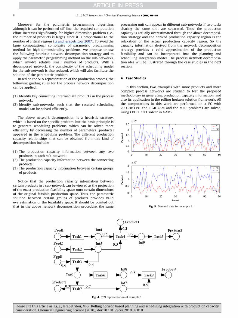
The production capacity information between certain groupsof products.

Fig. 5. Demand data for example 1.

Notice that the production capacity information betweencertain products in a sub-network can be viewed as the projectionof the exact production feasibility space onto certain dimensionsof the original feasible production space. Thus, the parametricsolution between certain groups of products provides validoverestimation of the feasibility space. It should be pointed outthat in the above network decomposition procedure, the same

Fig. 4. STN representa

ease cite this article as: Li, Z., Ierapetritou, M.G., Rolling horizon basnsideration. Chemical Engineering Science (2010), doi:10.1016/j.c

processing unit can appear in different sub-networks if two taskssharing the same unit are separated. Thus, the productioncapacity is actually overestimated through the above decomposi-tion strategy and the derived production capacity region is therelaxation of the actual production capacity region. So thecapacity information derived from the network decompositionstrategy provides a valid approximation of the productionfeasibility and can be incorporated into the planning andscheduling integration model. The process network decomposi-tion idea will be illustrated through the case studies in the nextsection.

4. Case Studies

In this section, two examples with more products and morecomplex process networks are studied to test the proposedmethodology in generating production capacity information, andalso its application in the rolling horizon solution framework. Allthe computations in this work are performed on a PC with2.8 GHz CPU and 1 GB RAM and the MILP problems are solved,using CPLEX 10.1 solver in GAMS.

tion of example 1.

ed planning and scheduling integration with production capacityes.2010.08.010

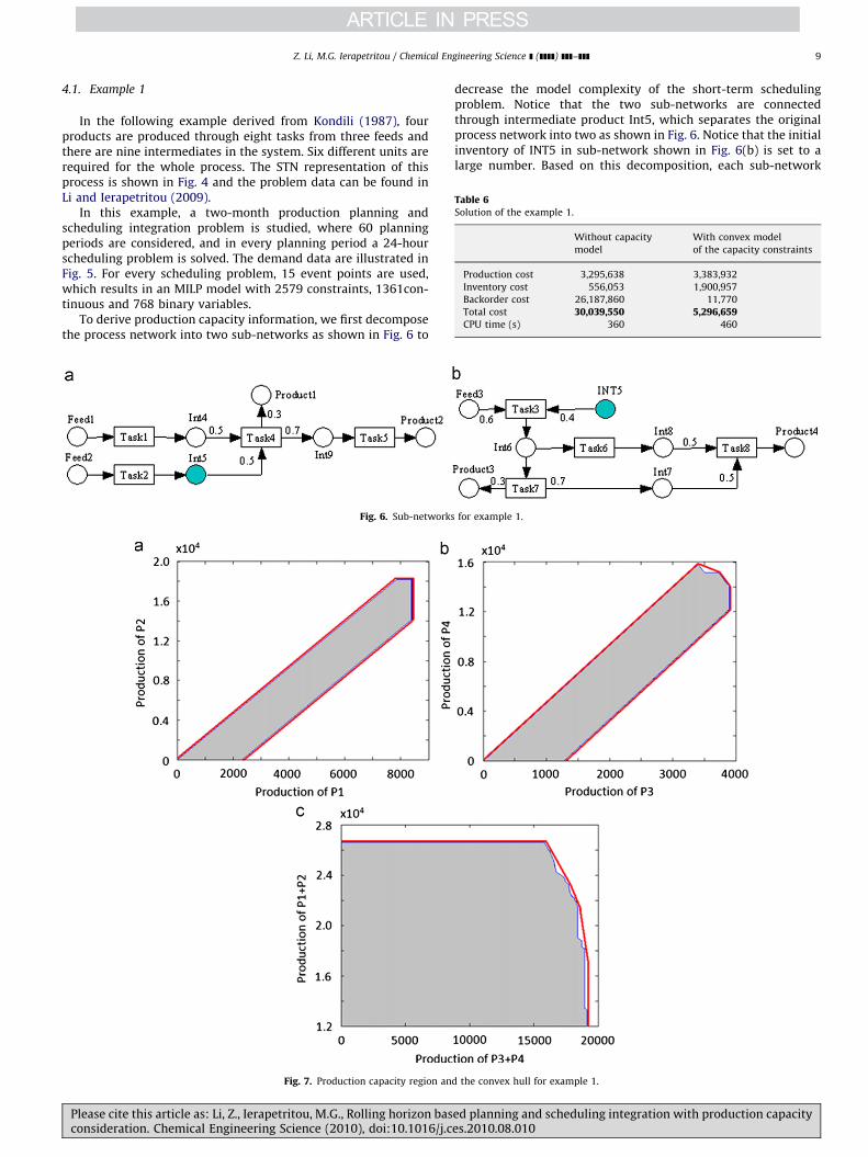
Table 6Solution of the example 1.

Without capacity

model

With convex model

of the capacity constraints

Production cost 3,295,638 3,383,932

Inventory cost 556,053 1,900,957

Backorder cost 26,187,860 11,770

Total cost 30,039,550 5,296,659CPU time (s) 360 460

Z. Li, M.G. Ierapetritou / Chemical Engineering Science ] (]]]]) ]]]–]]] 9

4.1. Example 1

In the following example derived from Kondili (1987), fourproducts are produced through eight tasks from three feeds andthere are nine intermediates in the system. Six different units arerequired for the whole process. The STN representation of thisprocess is shown in Fig. 4 and the problem data can be found inLi and Ierapetritou (2009).

In this example, a two-month production planning andscheduling integration problem is studied, where 60 planningperiods are considered, and in every planning period a 24-hourscheduling problem is solved. The demand data are illustrated inFig. 5. For every scheduling problem, 15 event points are used,which results in an MILP model with 2579 constraints, 1361con-tinuous and 768 binary variables.

To derive production capacity information, we first decomposethe process network into two sub-networks as shown in Fig. 6 to

Fig. 6. Sub-networks

Fig. 7. Production capacity region an

Please cite this article as: Li, Z., Ierapetritou, M.G., Rolling horizon basconsideration. Chemical Engineering Science (2010), doi:10.1016/j.c

decrease the model complexity of the short-term schedulingproblem. Notice that the two sub-networks are connectedthrough intermediate product Int5, which separates the originalprocess network into two as shown in Fig. 6. Notice that the initialinventory of INT5 in sub-network shown in Fig. 6(b) is set to alarge number. Based on this decomposition, each sub-network

for example 1.

d the convex hull for example 1.

ed planning and scheduling integration with production capacityes.2010.08.010

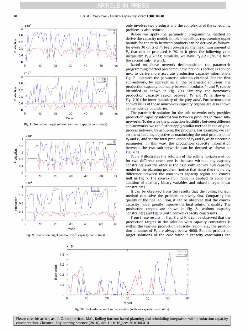
Fig. 8. Production target solution (without capacity constraints).

Fig. 9. Production target solution (with capacity constraints).

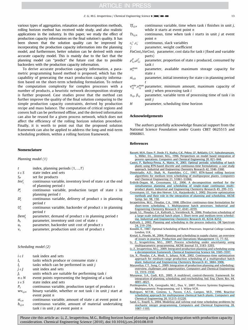
Fig. 10. Backorder amount in the solut

Z. Li, M.G. Ierapetritou / Chemical Engineering Science ] (]]]]) ]]]–]]]10

Please cite this article as: Li, Z., Ierapetritou, M.G., Rolling horizon basconsideration. Chemical Engineering Science (2010), doi:10.1016/j.c

only involves two products and the complexity of the schedulingproblem is also reduced.

Before we apply the parametric programming method toderive the capacity model, simple inequalities representing upperbounds for the ratio between products can be derived as follows:for every 30 units of P1 been processed, the maximum amount ofP2 that can be produced is 70, so it gives the following validinequality: P2r7P1/3; similarly, we have P4r2� (7P3/3) fromthe second sub-network.

Based on above network decomposition, the parametricprogramming method presented in the previous section is appliednext to derive more accurate production capacity information.Fig. 7 illustrates the parametric solution obtained. For the firstsub-network, by aggregating all the parametric solutions, theproduction capacity boundary between products P1 and P2 can beidentified as shown in Fig. 7(a). Similarly, the nonconvexproduction capacity region between P3 and P4 is shown inFig. 7(b) (the inner boundary of the grey area). Furthermore, theconvex hulls of those nonconvex capacity regions are also shownas the outside boundaries.

The parametric solution for the sub-networks only providesproduction capacity information between products in those sub-networks. To describe the production feasibility between differentsub-networks, we can further apply similar method in the originalprocess network, by grouping the products. For example, we canset the scheduling objective as maximizing the total production ofP1 and P2 and set the total production of P3 and P4 as an uncertainparameter. In this way, the production capacity informationbetween the two sub-networks can be derived as shown inFig. 7(c).

Table 6 illustrates the solution of the rolling horizon methodfor two different cases: one is the case without any capacityconstraints and the other is the case with convex hull capacitymodel in the planning problem (notice that since there is no bigdifference between the nonconvex capacity region and convexhull in Fig. 7, the convex hull model is applied to avoid theaddition of auxiliary binary variables and mixed integer linearconstraints).

It can be observed from the results that the rolling horizonmethod can solve the problem relatively fast. Comparing thequality of the final solution, it can be observed that the convexcapacity model greatly improve the final solution’s quality. Theproduction targets are shown in Fig. 8 (without capacityconstraints) and Fig. 9 (with convex capacity constraints).

From these results in Figs. 8 and 9, it can be observed that theproduction targets in the solution with capacity constraints iswithin the feasible production capacity region, e.g., the produc-tion amounts of P3 are always below 4000. But the productiontarget solutions of the case without capacity constraints can

ion (without capacity constraints).

ed planning and scheduling integration with production capacityes.2010.08.010

Z. Li, M.G. Ierapetritou / Chemical Engineering Science ] (]]]]) ]]]–]]] 11

violate the production feasibility, e.g., for some periods theproduction of P3 is more than 4000.

For the case without capacity constraints, the backorderamounts in the solution for P1 and P2 are shown in Fig. 10 andthe backorder amounts of P3 and P4 are all zero. For the case withcapacity constraints, the backorder of P1, P2 and P4 at all the

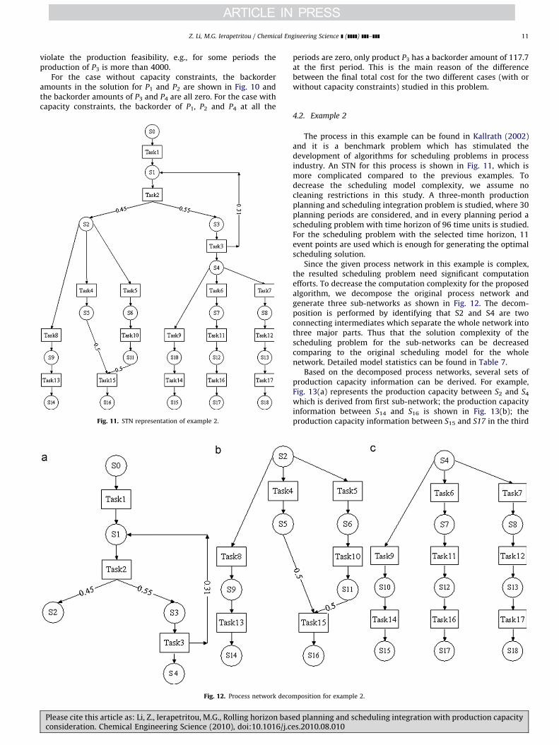
Fig. 11. STN representation of example 2.

Fig. 12. Process network deco

Please cite this article as: Li, Z., Ierapetritou, M.G., Rolling horizon basconsideration. Chemical Engineering Science (2010), doi:10.1016/j.c

periods are zero, only product P3 has a backorder amount of 117.7at the first period. This is the main reason of the differencebetween the final total cost for the two different cases (with orwithout capacity constraints) studied in this problem.

4.2. Example 2

The process in this example can be found in Kallrath (2002)and it is a benchmark problem which has stimulated thedevelopment of algorithms for scheduling problems in processindustry. An STN for this process is shown in Fig. 11, which ismore complicated compared to the previous examples. Todecrease the scheduling model complexity, we assume nocleaning restrictions in this study. A three-month productionplanning and scheduling integration problem is studied, where 30planning periods are considered, and in every planning period ascheduling problem with time horizon of 96 time units is studied.For the scheduling problem with the selected time horizon, 11event points are used which is enough for generating the optimalscheduling solution.

Since the given process network in this example is complex,the resulted scheduling problem need significant computationefforts. To decrease the computation complexity for the proposedalgorithm, we decompose the original process network andgenerate three sub-networks as shown in Fig. 12. The decom-position is performed by identifying that S2 and S4 are twoconnecting intermediates which separate the whole network intothree major parts. Thus that the solution complexity of thescheduling problem for the sub-networks can be decreasedcomparing to the original scheduling model for the wholenetwork. Detailed model statistics can be found in Table 7.

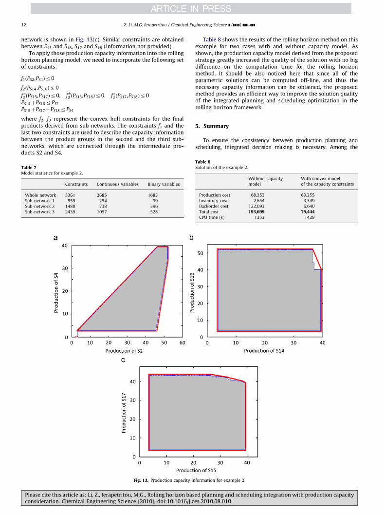
Based on the decomposed process networks, several sets ofproduction capacity information can be derived. For example,Fig. 13(a) represents the production capacity between S2 and S4

which is derived from first sub-network; the production capacityinformation between S14 and S16 is shown in Fig. 13(b); theproduction capacity information between S15 and S17 in the third

mposition for example 2.

ed planning and scheduling integration with production capacityes.2010.08.010

Z. Li, M.G. Ierapetritou / Chemical Engineering Science ] (]]]]) ]]]–]]]12

network is shown in Fig. 13(c). Similar constraints are obtainedbetween S15 and S18, S17 and S18 (information not provided).

To apply those production capacity information into the rollinghorizon planning model, we need to incorporate the following setof constraints:

f1ðPS2,PS4Þr0

f2ðPS14,PS16Þr0

f a3 ðPS15,PS17Þr0, f b

3 ðPS15,PS18Þr0, f c3 ðPS17,PS18Þr0

PS14þPS16rPS2

PS15þPS17þPS18rPS4

where f2, f3 represent the convex hull constraints for the finalproducts derived from sub-networks. The constraints f1 and thelast two constraints are used to describe the capacity informationbetween the product groups in the second and the third sub-networks, which are connected through the intermediate pro-ducts S2 and S4.

Table 7Model statistics for example 2.

Constraints Continuous variables Binary variables

Whole network 5361 2685 1683

Sub-network 1 559 254 99

Sub-network 2 1488 738 396

Sub-network 3 2439 1057 528

Fig. 13. Production capacity in

Please cite this article as: Li, Z., Ierapetritou, M.G., Rolling horizon basconsideration. Chemical Engineering Science (2010), doi:10.1016/j.c

Table 8 shows the results of the rolling horizon method on thisexample for two cases with and without capacity model. Asshown, the production capacity model derived from the proposedstrategy greatly increased the quality of the solution with no bigdifference on the computation time for the rolling horizonmethod. It should be also noticed here that since all of theparametric solutions can be computed off-line, and thus thenecessary capacity information can be obtained, the proposedmethod provides an efficient way to improve the solution qualityof the integrated planning and scheduling optimization in therolling horizon framework.

5. Summary

To ensure the consistency between production planning andscheduling, integrated decision making is necessary. Among the

formation for example 2.

Table 8Solution of the example 2.

Without capacity

model

With convex model

of the capacity constraints

Production cost 68,352 69,255

Inventory cost 2,654 3,549

Backorder cost 122,693 6,640

Total cost 193,699 79,444CPU time (s) 1353 1429

ed planning and scheduling integration with production capacityes.2010.08.010

Z. Li, M.G. Ierapetritou / Chemical Engineering Science ] (]]]]) ]]]–]]] 13

various types of aggregation, relaxation and decomposition methods,rolling horizon method has received wide study, and also realisticapplications in the industry. In this paper, we study the effect ofproduction capacity information on the final solution’s quality. It hasbeen shown that the solution quality can be improved byincorporating the production capacity information into the planningmodel, and furthermore, better solution can be derived with moreaccurate capacity model. This is mainly due to the fact that theplanning model can ‘‘predict’’ the future cost due to possiblebackorders with the production capacity information.

To derive accurate production capacity information, a para-metric programming based method is proposed, which has thecapability of generating the exact production capacity informa-tion based on the short-term scheduling formulation. To reducethe computation complexity for complex processes with anumber of products, a heuristic network decomposition strategyis further proposed. Case studies prove that the method canfurther improve the quality of the final solution comparing to thesimple production capacity constraints, derived by productionrecipe and mass balance. The computation of critical regions andconvex hull can be performed offline, and the derived informationcan also be reused for a given process network, which does notaffect the efficiency of the rolling horizon solution procedure.Finally, it is worth to point out that the proposed solutionframework can also be applied to address the long-and mid-termscheduling problem, within a rolling horizon framework.

Nomenclature

Planning model (1)

t index, planning periods (1, :::, T)sAS state index and setsSP set for productsInvt

s continuous variable, inventory level of state s at the endof planning period t

Pts continuous variable, production target of state s in

planning period t

Dts continuous variable, delivery of product s in planning

period t

Uts continuous variable, backorder of product s in planning

period t

Demts parameter, demand of product s in planning period t

hs parameter, inventory unit cost of state s

us parameter, backorder unit cost of product s

vs parameter, production unit cost of product s

Scheduling model (2)

iA I task index and setsIs tasks which produce or consume state s

Ij tasks which can be performed in unit j

jA J unit index and setsJi units which are suitable for performing task i

nAN event points representing the beginning of a tasksAS state index and setsPs continuous variable, production target of product s

wvi,j,n binary variable, whether or not task i in unit j start atevent point n

sts,n continuous variable, amount of state s at event point n

bi,j,n continuous variable, amount of material undertakingtask i in unit j at event point n

Please cite this article as: Li, Z., Ierapetritou, M.G., Rolling horizon basconsideration. Chemical Engineering Science (2010), doi:10.1016/j.c

Tfi,j,n continuous variable, time when task i finishes in unit j,while it starts at event point n

Tsi,j,n continuous, time when task i starts in unit j at eventpoint n

eþs ,e�s continuous, slack variablesg parameter, weight coefficientFixCosti,VarCosti parameter, cost data for task i (fixed and variable

parts)rP

s,i,rCs,i parameter, proportion of state s produced, consumed by

task i

stmaxs parameter, available maximum storage capacity for

state s

sts,0 parameter, initial inventory for state s in planning periodt

vmini,j ,vmax

i,j parameter, minimum amount, maximum capacity ofunit j when processing task i

ai,j, bi,j parameter, variable term of processing time of task i inunit j

H parameter, scheduling time horizon

Acknowledgements

The authors gratefully acknowledge financial support from theNational Science Foundation under Grants CBET 0625515 and0966861.

References

Bassett, M.H., Dave, P., Doyle, F.J., Kudva, G.K., Pekny, J.F., Reklaitis, G.V., Subrahmanyam,S., Miller, D.L., Zentner, M.G., 1996. Perspectives on model based integration ofprocess operations. Computers and Chemical Engineering 20, 821–844.

Castro, P., Barbosa-Povoa, A., Matos, H., 2003. Optimal periodic scheduling of batchplants using RTN-based discrete and continuous-time formulations: a case studyapproach. Industrial and Engineering Chemistry Research 42, 3346–3360.

Dimitriadis, A.D., Shah, N., Pantelides, C.C., 1997. RTN-based rolling horizonalgorithms for medium term scheduling of multipurpose plants. Computersand Chemical Engineering 21, S1061–S1066.

Erdirik-Dogan, M., Grossmann, I.E., 2006. A decomposition method for thesimultaneous planning and scheduling of single-stage continuous multi-product plants. Industrial and Engineering Chemistry Research 45, 299–315.

Grossmann, I.E., Van den Heever, S.A., Harjunkoski, I., 2002. Discrete optimizationmethods and their role in the integration of planning and scheduling. AIChESymp. Ser. 98, 150.

Ierapetritou, M.G., Floudas, C.A., 1998. Effective continuous-time formulation forshort-term scheduling. 1. Multipurpose batch processes. Industrial andEngineering Chemistry Research 37, 4341–4359.

Janak, S.L., Floudas, C.A., Kallrath, J., Vormbrock, N., 2006. Production scheduling ofa large-scale industrial batch plant. I. Short-term and medium-term schedul-ing. Industrial and Engineering Chemistry Research 45, 8234–8252.

Kallrath, J., 2002. Planning and scheduling in the process industry. OR Spectrum24, 219–250.

Kondili, E., 1987. Optimal Scheduling of Batch Processes. Imperial College London,London, U.K..

Kreipl, S., Pinedo, M., 2004. Planning and scheduling in supply chains: an overviewof issues in practice. Production and Operations Management 13, 77–92.

Li, Z., Ierapetritou, M.G., 2007. Process scheduling under uncertainty usingmultiparametric programming. AICHE Journal 53, 3183–3203.

Li, Z., Ierapetritou, M.G., 2009. Integrated production planning and scheduling usinga decomposition framework. Chemical Engineering Science 64, 3585–3597.

Lin, X., Floudas, C.A., Modi, S., Juhasz, N.M., 2002. Continuous-time optimizationapproach for medium-range production scheduling of a multiproduct batchplant. Industrial and Engineering Chemistry Research 41, 3884–3906.

Maravelias, C.T., Sung, C., 2009. Integration of production planning and scheduling:overview, challenges and opportunities. Computers and Chemical Engineering33, 1919–1930.

Munawar, S.A., Gudi, R.D., 2005. A multilevel, control-theoretic framework forintegration of planning, scheduling, and rescheduling. Ind. Eng. Chem. Res. 44,4001–4021.

Pistikopoulos, E.N., Georgiadis, M.C., Dua, V., 2007. Process Systems Engineering.Multiparametric Programming, vol 1. Wiley-VCH.

Rodrigues, M.T.M., Gimeno, L., Passos, C.A.S., Campos, M.D., 1996. Reactivescheduling approach for multipurpose chemical batch plants. Computers andChemical Engineering 20, S1215–S1220.

Sand, G., Engell, S., 2004. Modeling and solving real-time scheduling problems bystochastic integer programming. Computers and Chemical Engineering 28,1087–1103.

ed planning and scheduling integration with production capacityes.2010.08.010

Z. Li, M.G. Ierapetritou / Chemical Engineering Science ] (]]]]) ]]]–]]]14

Sand, G., Engell, S., Markert, A., Schultz, R., Schultz, C., 2000. Approximation of anideal online scheduler for a multiproduct batch plant. Computers andChemical Engineering 24, 361–367.

Schilling, G., Pantelides, C.C., 1999. Optimal periodic scheduling of multipurposeplants. Computers and Chemical Engineering 23, 635–655.

Shaik, M.A., Floudas, C.A., Kallrath, J., Pitz, H.-J., 2009. Production scheduling of alarge-scale industrial continuous plant: short-term and medium-term sche-duling. Computers and Chemical Engineering 33, 670–686.

Sung, C., Maravelias, C.T., 2007. An attainable region approach for effectiveproduction planning of multi-product processes. AICHE Journal 53, 1298–1315.

Verderame, P.M., Floudas, C.A., 2008. Integrated operational planning andmedium-term scheduling of a large-scale industrial batch plants. Industrialand Engineering Chemistry Research 47, 4845–4860.

Please cite this article as: Li, Z., Ierapetritou, M.G., Rolling horizon basconsideration. Chemical Engineering Science (2010), doi:10.1016/j.c

Wilkinson, S.J., 1996. Aggregate formulations for large-scale process schedulingproblems, Department of Chemical Engineering and Chemical Technology.Imperial College, London.

Wu, D., Ierapetritou, M., 2004. Cyclic short-term scheduling of multiproduct batchplants using continuous-time representation. Computers and ChemicalEngineering 28, 2271–2286.

Wu, D., Ierapetritou, M.G., 2003. Decomposition approaches for the efficientsolution of short-term scheduling problems. Computers and ChemicalEngineering 27, 1261–1276.

Wu, D., Ierapetritou, M.G., 2007. Hierarchical approach for production planningand scheduling under uncertainty. Chemical Engineering and Processing 46,1129–1140.

Zhu, X.X., Majozi, T., 2001. Novel continuous-time MILP formulation for multi-purpose batch plants. 2. Integrated planning and scheduling. Industrial andEngineering Chemistry Research 40, 5621–5634.

ed planning and scheduling integration with production capacityes.2010.08.010