rolling contact orthopaedic joint design - DSpace@MIT

ROLLING CONTACT ORTHOPAEDIC JOINT DESIGN

by

Alexander Henry Slocum, Jr.

S.M., Mechanical Engineering, Massachusetts Institute of Technology, 2010

S.B., Mechanical Engineering, Massachusetts Institute of Technology, 2008

Submitted to the Department of Mechanical Engineering

in Partial Fulfillment of the Requirements for the Degree of

Doctor of Philosophy in Mechanical Engineering at the

MASSACHUSETTS INSTITUTE OF TECHNOLOGY

February 2013

© 2013 Massachusetts Institute of Technology, All Rights Reserved

Author:_______________________________________________________________________

Alexander H. Slocum, Jr.

Department of Mechanical Engineering

January 11, 2013

Certified by:___________________________________________________________________

Prof. Kripa K. Varanasi

Associate Professor of Mechanical Engineering

Thesis Supervisor and Committee Chair

Accepted by:___________________________________________________________________

David E. Hardt

Professor of Mechanical Engineering

Chairman, Department Committee on Graduate Students

2

ROLLING CONTACT ORTHOPAEDIC JOINT DESIGN

by

Alexander Henry Slocum, Jr.

Submitted to the Department of Mechanical Engineering

on January 11th

, 2013 in Partial Fulfillment of the

Requirements for the Degree of Doctor of Philosophy in

Mechanical Engineering

Abstract

Arthroplasty, the practice of rebuilding diseased biological joints using engineering materials, is

often used to treat severe arthritis of the knee and hip. Prosthetic joints have been created in a

“biomimetic” manner to reconstruct the shape of the biological joint. We are at a disadvantage,

however, in that metals and polymers used to replace bone and articular cartilage often wear out

too soon, leading to significant morbidity. This thesis explores the use of kinetic-mimicry,

instead of bio-mimicry, to design prosthetic rolling contact joints, including knee braces, limb

prosthetics, and joint prostheses, with the intent of reducing morbidity and complications

associated with joint/tissue failure.

A deterministic approach to joint design is taken to elucidating six functional requirements for a

prosthetic tibiofemoral joint based on anatomical observations of human knee kinetics and

kinematics. Current prostheses have a high slide/roll ratio, resulting in unnecessary wear. A

rolling contact joint, however, has a negligible slide/roll ratio; rolling contact prostheses would

therefore be more efficient. A well-established four-bar linkage knee model, in a sagittal plane

that encapsulates with the knee’s flexion/extension degree of freedom, is used to link human

anatomy to the shape of rolling cam surfaces. The first embodiment of the design is a flexure

coupling-based joint for knee braces. Failure mode analysis, followed by cyclic failure testing,

has shown that the prototype joint is extremely robust and withstood half a million cycles during

the first round of tests.

Lubrication in the joint is also considered: micro- and nano-textured porous coatings are

investigated for their potential to support the formation of favorable lubrication regimes.

Hydrodynamic lubrication is optimal, as two surfaces are separated by a fluid gap, thus

mitigating wear. Preliminary results have shown that shear stress is reduced by more than 60%

when a coating is combined with a shear thinning lubricant like synovial fluid. These coatings

could be incorporated into existing joint prostheses to help mitigate wear in current technology.

This thesis seeks to describe improvements to the design of prosthetic joints, both existing and

future, with the intent of increasing the overall quality of care delivered to the patient.

Thesis Supervisor: Kripa K. Varanasi

Title: Doherty Associate Professor of Mechanical Engineering

3

Doctoral Thesis Committee

Thesis Supervisor and Committee Chair: Kripa K. Varanasi, PhD

Doherty Associate Professor of Mechanical Engineering

Massachusetts Institute of Technology

Martin L. Culpepper, PhD

Associate Professor of Mechanical Engineering


Douglas P. Hart, PhD

Professor of Mechanical Engineering


Just Herder, PhD

Associate Professor of Mechanical and Biomechanical Engineering

TU Delft, The Netherlands

4

This work is dedicated to

Bubsi, Marianna, Pat and John

Through this their memory lives on!

5

ACKNOWLEDGEMENTS

I am indebted to my creator, in whatever form that may be, for giving me the skill of mind and

hand used to execute this work

My wife, Sarah Slocum (7) SB ‘11, the patience, love, and support you have shown me from day

one have made me a better man. I have gotten more out of a class that I dropped than any other

endeavor I have ever pursued. Now that this is finished, I’m truly all yours and I look forward to

growing old with you. Also thanks to Mara and Rex.

My parents, Alexander H. Slocum, Sr. (2) SB ’82, SB ’83, PhD ‘85 and Debra L. T. Slocum (6)

SM ’88, for giving me life, teaching me to finish the things that I start, instilling in me both a

strong work ethic and the will to succeed, and for showing me the world.

Joshua (6) SB ‘10, SM ’11, and Jonathan Slocum (2) SB ’14 – a man could not ask for better

brothers. You both have grown into fine men and it is so awesome to see you succeeding.

Marianna P. Slocum, (8) SB '55, (18) SM '58 – you told me to never let anyone tell me I couldn’t

do something, and I listened. I love you grandma, and I miss you very much.

John and Patricia Thurston – Grandma and Grandpa Buffy, you were my inspiration to keep

playing the piano. The dexterity and determination I developed will enable me to achieve my

dreams. I love you both, and you are missed.

Richard W. Slocum, Jr., (Gramps) (8), SB ’55, PhD ’58 – for all those times we went flying

together, and our adventures at scout camp. Also, Spirulina!

The following is a list of individuals with whom I interacted during the course of this work, and

to whom I am grateful:

Prof. Lalit Anand, MIT – for his advice and guidance regarding brittle fracture analysis,

presented in Chapter 4, Section 4.4.1.

Esther Austin, MIT – for her infinite knowledge and for helping me to navigate my time as a

nonresident student.

Eric Blough, Marshall – for engaging me during the summer and fall of 2011, and allowing me

to work in his laboratory on parts of chapter 6.

Dr. Mary Bouxsein and Dr. Margaret Seton, HMS – instructors for the IAP 2011 course

HST.021 “Musculoskeletal Pathophysiology”. This was my first introduction to the field of

orthopaedics; thank you for allowing me to take this course as it served me well during the initial

stages of this thesis, and even later during medical school.

Brian Brown, RCBI - for laser cutting and fabrication work at the Robert C. Byrd Institute for

Advanced Flexible Manufacturing.

Dr. Dennis Burke, MGH – for allowing me to observe him in the operating room performing

total knee and total hip replacements, and giving me advice on the synthesis of the joint.

Tom Cervantes, MIT – one of my UROP students, he helped design the rolling contact testing

apparatus used to evaluate the adjustable bone plates, presented as the case study in Chapter 3.

6

Yuehua Cui, MIT – for her guidance and advice on the fabrication of etched and anodized porous

coatings, and for her time and efforts in helping Jad and Daniel when I was not there.

Prof. Marty Culpepper, MIT – a member of my committee, and my master’s thesis advisor, for

your time, thoughts, and guidance over the past 5 years, during which time I have learned a lot

from you. I hope to work with you again the future.

Tom Dolan – of Dolan’s Welding and Steel Fabrication, for his fantastic laser cutting services

and for fabricating the first prototype rolling contact joint.

Jad El-Khoury, MIT – one of my UROP students, for his time, dedication, and willingness to

learn, and for running countless numbers of lubrication experiments

Andrew Gallant, MIT – of the MIT Central Machine Shop, for the excellent, professional service

and outstanding product. Central Machine fabricated the components for the passive alignment

mechanism used to conduct tribological experiments, and also polished all of the coupons.

Prof. Lorna J. Gibson, MIT – taught the spring 2011 course 3.595 – Mechanics of Porous Media,

where the ideas on elastic averaging were developed; this became the first half of Chapter 6.

Daniel Goodman, MIT – one of my first UROP students, for helping me to design the rheological

testing apparatus, for helping me get the first images of the porous coatings,

Dr. Rajiv Gupta, MGH – my mentor for my bachelor’s thesis, he helped me to discover my

passion for the field of medicine.

Dr. Julio Guerrero, DRAPER – a close friend, long-time mentor and advisor. I learned much

from you during our time at Schlumberger together.

Pierce Hayward, MIT – for his assistance with the Instron used to evaluate the adjustable bone

plates, and the white light interferometer.

Prof. Doug Hart, MIT – a member of my committee, for your time, thoughts and guidance

regarding lubrication and for helping me figure out which experiments to run now and in the

future to adequately characterize lubrication.

Prof. Just Herder, TU Delft – I can honestly say that without that conversation on April 15th

,

2008, this thesis would most likely not exist. Thank you for your input and advice on this work,

and I hope we can continue to collaborate in the future.

Dr. Jonathan Hopkins – One of my old lab mates and now a post-doc at LLNL. He pointed out

the importance of shear angle in analyzing the slip condition discussed in Chapter 4, Section

4.3.2. Jon also wrote section 5.5.

Aditya Jaishankar, MIT – Aditya is a brilliant doctoral student in the Microfluidics laboratory

working on rheology of lubricants like synovial fluid, and I am grateful for his time, guidance

and expertise in operating the rheometer as well as for all things lubricant-related!

Christopher Love, MIT – one of my lab mates, and previously one of my teammates in the

Spring 2008 class 2.782, Design of Medical Devices and Implants, and for which I proposed the

idea of designing a rolling contact joint for knees.

Prof. Gareth McKinley, MIT – with whom I took 2.671 and where I learned how to properly

pronounce the word “solder”, 2.25 and learned the proper spelling and pronunciation of

Reynolds Number, and for his thoughts and guidance regarding building the passive alignment

mechanism for the rheometer.

Rich Morneweck, Boston Centerless – for his help sourcing CoCrMo alloy.

Eileen Ng-Ghavidel, MIT – she helped me get the details of my non-resident funding sorted out.

Dean Christine Ortiz, MIT – for allowing me the opportunity to pursue non-resident status and

go to medical school while completing my doctoral work.

7

Adam Paxson, MIT – one of my lab mates, he helped with the porous coatings work in the first

half of Chapter 6, and also supervised my UROPs in the lab several times. He was a great

resource and always had excellent critiques and ideas for further work.

Marie Pommet, MIT – for her help with setting up non-resident appointments.

Aaron Ramirez, MIT – a friend and masters candidate in the Precision Compliant Systems

Laboratory, for his help with setting up the capacitance probes for stability measurements of the

passive alignment mechanism during rheological tests.

Kevin Rice, Marshall – helped me with the cell culturing experiments, and helped me get

oriented to working in Prof. Blough’s lab.

Dr. Stephen Schachter, CIMIT – thank you for permitting me to use my fellowship to fund my

time as a non-resident at MIT. I am grateful for the faith and trust CIMIT has had in me and I

hope to continue working with you in the future.

Adam Schindzielorz, Marshall – for introducing me to crossfit, for those early morning swims,

Friday afternoons talking policy in the steam room, and for helping me assemble the train-drive

testing machine for the prosthetic joint.

Dr. Edward Seldin, MGH – a good friend and my pre-medical advisor. I have received no small

amount of sage advice from him, and he has very much helped me to grow as both an engineer

and a physician.

Diane Spiliotis, CIMIT – she was invaluable in helping me to navigate the financial nuances of

fellowship funding.

J. David Smith, MIT – for helping with the Goniometer, and his input regarding surface adhesion

and analysis of flow over nano-/micro-structures, from which I drew inspiration for parts of

Chapter 6.

Dr. Franklin Shuler, Marshall – my clinical advisor and mentor, an orthopaedic trauma surgeon

who has given me guidance and advice during my first two years of medical school.

Brian Tavares, MIT - he helped me work out the details of non-resident funding.

Elizabeth Turgeon, UNC School of Law – a law student, editor of the North Carolina Journal of

Law & Technology, significant other to Adam Schindzielorz, and a friend, she graciously spent

numerous hours editing several chapters of my thesis.

Prof. Franz J. Ulm, MIT – with whom I took the Spring 2011 course 1.570, and during which the

analysis of fatigue and fracture in the straps was performed. This work turned into Chapter 4.

Prof. Kripa Varanasi, MIT – most of all, for taking on a student who planned to leave and go to

medical school the very next semester. The amount of patience, faith, and trust you’ve had in me

since day one I am truly grateful for. Also, thank you for pushing me to pursue the lubrication

and bone growth aspects of my thesis. Your guidance has helped me to grow as an engineer and

as a scientist, and I look forward to many more fruitful years of collaboration!

Ed Warnock and Charles “Chuck” Cummings – for the excellent work that Hillside Engineering

always produces.

My lab mates in the Varanasi Research Group

My fellow classmates in the JCESOM Class of 2015

All of my colleagues and professors at Marshall who helped me to prepare for my thesis defense

8

Table of Contents______________________________________________________________

ACKNOWLEDGEMENTS ......................................................................................................... 5

TABLE OF CONTENTS ............................................................................................................. 8

LIST OF TABLES ...................................................................................................................... 12

LIST OF FIGURES .................................................................................................................... 13

CHAPTER 1 – INTRODUCTION ............................................................................................ 19

1.1 MOTIVATION ............................................................................................................. 20

1.2 TOTAL KNEE ARTHROPLASTY ........................................................................... 24

1.3 INSTITUTIONAL CONTRIBUTIONS ..................................................................... 30

1.4 THESIS CONTRIBUTIONS ...................................................................................... 31

1.5 THESIS ORGANIZATION ........................................................................................ 34

1.5.1 CHAPTER 1 – INTRODUCTION ........................................................................... 34

1.5.2 CHAPTER 2 – MUSCULOSKELETAL PATHOPHYSIOLOGY ............................ 34

1.5.3 CHAPTER 3 – DETERMINISTIC JOINT DESIGN................................................ 35

1.5.4 CHAPTER 4 – JOINT DURABILITY ...................................................................... 35

1.5.5 CHAPTER 5 – DESIGN OF ROLLING CONTACT JOINT PROSTHESES .......... 35

1.5.6 CHAPTER 6 – NANO-ENGINEERED SURFACE COATINGS ............................. 36

1.5.7 CHAPTER 7 – CONCLUSIONS AND FUTURE WORK ....................................... 36

1.6 REFERENCES ............................................................................................................. 37

CHAPTER 2 – THE MUSCULOSKELETAL SYSTEM ....................................................... 41

2.1 INTRODUCTION ........................................................................................................ 41

2.2 MUSCULOSKELETAL SYSTEM ............................................................................ 43

2.3 MACROSTRUCTURE ................................................................................................ 45

2.3.1 BONES .................................................................................................................... 46

2.3.2 MUSCLE ................................................................................................................. 50

2.3.3 JOINTS .................................................................................................................... 51

2.3.4 TENDONS AND LIGAMENTS ............................................................................... 53

2.4 MICRO-STRUCTURE ................................................................................................ 54

2.4.1 COLLAGEN ............................................................................................................ 54

2.4.2 CARTILAGE ........................................................................................................... 57

2.4.3 BONE ...................................................................................................................... 58

2.4.4 MUSCLE ................................................................................................................. 66

2.4.5 TENDONS & LIGAMENTS .................................................................................... 69

9

2.5 PATHOPHYSIOLOGY............................................................................................... 71

2.5.1 CARTILAGE FORMATION .................................................................................... 71

2.5.2 CONDUCTION ABNORMALITIES........................................................................ 72

2.5.3 JOINT INTEGRITY ................................................................................................. 72

2.5.4 BONE STRUCTURE ............................................................................................... 73

2.5.5 BIOMECHANICS ................................................................................................... 74

2.6 REMARKS ................................................................................................................... 74

2.7 REFERENCES ............................................................................................................. 75

CHAPTER 3 – DETERMINISTIC JOINT DESIGN ............................................................. 77

3.1 INTRODUCTION ........................................................................................................ 78

3.2 DETERMINISTIC ANALYSIS .................................................................................. 81

3.2.1 TYPES OF BIOLOGICAL JOINTS ......................................................................... 81

3.3 KINETICS AND KINEMATICS OF ROLLING CONTACT ................................ 85

3.4 MECHANICS OF ROLLING CONTACT................................................................ 87

3.4.1 CONTACT MECHANICS ....................................................................................... 88

3.4.2 HERTZ CONTACT.................................................................................................. 89

3.4.3 BUCKINGHAM LOAD STRESS FACTOR ............................................................. 90

3.5 CASE STUDY: ROLLING CONTACT JOINTS FOR FRACTURE FIXATION 91

3.5.1 DYNAMIC TESTING MACHINE ........................................................................... 93

3.5.2 BUCKINGHAM LOAD STRESS ANALYSIS .......................................................... 95

3.5.3 ERROR ANALYSIS.................................................................................................. 95

3.5.4 EXPERIMENTAL RESULTS ................................................................................ 101

3.6 REMARKS ................................................................................................................. 104

3.7 REFERENCES ........................................................................................................... 105

CHAPTER 4 – JOINT DURABILITY & MATERIALS SELECTION ............................. 109

4.1 INTRODUCTION ...................................................................................................... 109

4.2 MATERIALS SELECTION ..................................................................................... 114

4.2.1. HERTZ CONTACT STRESSES ............................................................................. 119

4.3 FATIGUE OF JOINT SURFACES .......................................................................... 121

4.3.1. BUCKINGHAM LOAD-STRESS FACTOR .......................................................... 123

4.3.2. STATIC SLIP ANALYSIS ...................................................................................... 123

4.3.3. SLIP BETWEEN ROLLING SURFACES.............................................................. 125

4.4 STRAP FRACTURE AND FATIGUE ..................................................................... 127

4.4.1. BRITTLE FRACTURE .......................................................................................... 127

10

4.4.2. CRACK PROPAGATION...................................................................................... 128

4.5 MECHANICAL TESTING ....................................................................................... 135

4.6 REMARKS ................................................................................................................. 138

4.7 REFERENCES ........................................................................................................... 140

CHAPTER 5 – ROLLING CONTACT KNEE JOINT PROSTHESES ............................. 143

5.1 INTRODUCTION ...................................................................................................... 143

5.2 DETERMINISTIC ANALYSIS ................................................................................ 147

5.2.1 FUNCTIONAL REQUIREMENTS........................................................................ 148

5.3 ROLLING CONTACT JOINT DESIGN ................................................................ 149

5.3.1 STATIC ANALYSIS ............................................................................................... 151

5.4 ROLLING CAM SYNTHESIS ................................................................................. 154

5.5 FLEXURE STRAP TOPOGRAPHY ....................................................................... 161

5.6 JOINT MANUFACTURE AND TESTING ............................................................ 163

5.6.1 FIRST-GENERATION PROTOTYPE JOINT ....................................................... 167

5.6.2 SECOND-GENERTION PROTOTYPE JOINT..................................................... 170

5.6.3 DURABILITY TESTING RESULTS ...................................................................... 173

5.7 REMARKS ................................................................................................................. 176

5.8 REFERENCES ........................................................................................................... 177

CHAPTER 6 – NANOENGINEERED SURFACE COATINGS ......................................... 181

6.1 INTRODUCTION ...................................................................................................... 181

6.2 IMPLANT INTEGRATION ..................................................................................... 183

6.2.1 SAMPLE PREPARATION .................................................................................... 190

6.2.2 ELASTICALLY-AVERAGED COATINGS ............................................................ 191

6.2.3 MECHANICS OF POROUS COATINGS ............................................................. 193

6.2.4 MICRO-INDENTATION TESTS ........................................................................... 198

6.2.5 CELL CULTURE .................................................................................................. 199

6.3 IMPLANT LUBRICATION ..................................................................................... 200

6.3.1 FLOW OVER TEXTURED SURFACES ............................................................... 206

6.3.2 SYNOVIAL FLUID MODELS AND PROTEIN ADSORPTION ........................... 210

6.3.3 SAMPLE PREPARATION .................................................................................... 211

6.3.4 SURFACE WETTING ........................................................................................... 216

6.3.5 TRIBO-RHEOLOGY OF NANOENGINEERED SURFACES .............................. 218

6.3.6 SLIP LENGTH ...................................................................................................... 226

6.4 REMARKS ................................................................................................................. 227

11

6.5 REFERENCES ........................................................................................................... 227

CHAPTER 7 – MENS ET MANUS ........................................................................................ 233

7.1 CONTRIBUTIONS OF THIS THESIS ................................................................... 233

7.2 CLINICAL CONSIDERATIONS ............................................................................ 235

7.2.1 KNEE BRACES ..................................................................................................... 235

7.2.2 METAL ION ALLERGIES..................................................................................... 237

7.2.3 ASEPTIC LOOSENING ........................................................................................ 238

7.2.4 INFECTION .......................................................................................................... 238

7.2.5 REVISION TKA ..................................................................................................... 239

7.3 FURTHER WORK .................................................................................................... 240

7.4 REFERENCES ........................................................................................................... 243

12

List of Tables__________________________________________________________________

CHAPTER 2

Table 2.1: Summary of collagen types and their respective uses within the body [4]................. 55

CHAPTER 3

Table 3.1: The four types of rolling contact joints, including the null condition. ....................... 88

Table 3.2: Dynamic testing machine error budget [4]. .............................................................. 100

CHAPTER 4

Table 4.1: Chapter 4 Nomenclature ........................................................................................... 113

Table 4.2: Estimation of total cycles a joint is subjected to during ADL. ................................. 114

Table 4. 3: Properties of four common Orthopaedic materials [15]. ......................................... 120

Table 4.4: Hertz contact stresses (MPa) for different orthopaedic material combinations. ....... 120

Table 4.5: Comparing total lifetime slip in rolling contact and conventional joints. ................ 126

Table 4.7: Calculating forces in the joint when flexed and loaded. ........................................... 130

Table 4.8: Summary of fracture analysis. .................................................................................. 133

Table 4.9: Summary of fatigue analysis..................................................................................... 134

CHAPTER 5

Table 5.1: Functional Requirements (FRs) for a rolling contact knee joint prosthesis. ............ 149

Table 5.2: Coordinates for each linkage pivot shown in Figure 5.9 [6]. ................................... 157

Table 5.3: Known, unknown, dependent and independent variables in Figure 5.9. .................. 158

CHAPTER 6

Table 6.1: Summary of common methods of manufacturing porous materials [17]. ................ 188

Table 6.2: Material properties of 25% dense trabecular bone. .................................................. 194

Table 6.3: Properties of the etched titanium foam. .................................................................... 196

Table 6.4: Material properties of Ti6Al4V foam coating. ......................................................... 197

Table 6.5: Nano-indentation testing parameters. ....................................................................... 198

Table 6.6: Characterization of three different surface treatments (smooth, etched, anodized). 214

Table 6.7: Summary of contact angles on different surfaces. .................................................... 217

13

List of Figures_________________________________________________________________

CHAPTER 1

Figure 1.1: (a) Conceptual SolidWorks™ solid model of a flexure coupling; (b) conceptual

sketches of the rolling contact knee prosthesis design. ................................................................. 21

Figure 1.2: A dual LVAD heart prosthesis [1]. ........................................................................... 22

Figure 1.3: (a) Knee anatomy [8]; (b) modern total knee replacement schematic [9]. ............... 24

Figure 1.4: A brief timeline of the history of total knee arthroplasty. ......................................... 25

Figure 1.5: Shiers' hinge joint prosthesis [11, 12]. ...................................................................... 26

Figure 1.6: Left: Gunston's metal-on-polymer prosthetic implant [15]; right: An example of a

metal-on-polymer total knee replacement available from Biomet, Inc. [16]. ............................... 27

Figure 1.7: (a) and (b) are gross anatomical prosections of human knees, illustrating the relative

size and location of soft tissue structures [20, 21]. ....................................................................... 28

Figure 1.8: (a) damaged articular cartilage in osteoarthritis [22]; (b) subsequent removal of

damaged cartilage and replacement with metal and polymer prosthesis components [23] .......... 29

CHAPTER 2

Figure 2.1: Anatomical position, showing the orientation of coronal, sagittal, and transverse

planes, as well as proximal, distal, medial, and lateral directions [5] ........................................... 42

Figure 2.2: Differentiation of the germ cell layers [4]. ................................................................ 44

Figure 2.3: Examples of (a) Bone, (b) Muscle, (c) Cartilage, (d) Tendon, (e) ligament [4]. ...... 46

Figure 2.4: Types of bones in the body, including (a) long bones like the femur, (b) short bones

like the navicular in the foot, (c) flat bones of the skull, and (d) the right half of the innominate

bone (pelvis) [3]. ........................................................................................................................... 47

Figure 2.5: A sketch showing structures which make up the long bones, including the diaphysis,

metaphysis, and epiphysis [9]. ...................................................................................................... 48

Figure 2.6: Cross-section through the proximal part of (a) the human femur and (b) the human

tibia [10] and (c) a sketch showing the organization of primary trabecular fibers [6, 7]. ............ 49

Figure 2.7: Skeletal muscle in the biceps (left), smooth muscle in an artery (middle), and cardiac

muscle (right) [11]. ....................................................................................................................... 50

Figure 2.8: The hip, an articulating cartilaginous joint (left); one of the fibrous joints in the spine,

found between each vertebral body and formed by an intervertebral disk made of fibro-cartilage

(right) [4]. ...................................................................................................................................... 52

Figure 2.9: (a) The cruciate ligaments, including the ACL and PCL [5]; (b) one image from a

CT scan of a torn ACL [5]; (c) an Achilles tendon from a cadaver [3]. ....................................... 54

Figure 2.10: Schematic of (a) the orientation of collagen α-chains in fibers, and (b) collagen

assembly, starting with the precursor α-chain, and ending with a collagen fiber [4]. .................. 56

Figure 2.11: Growth of hyaline cartilage showing chondrocytes in lacunae (left side), and the

fibrous perichondrium (right side) [4]. ......................................................................................... 57

Figure 2.12: Articular cartilage, showing periosteal chondrocytes and underlying bone [4]. ..... 58

Figure 2.13: Images of (a) osteoblasts and (b) osteoclasts in trabecular (cancellous) bone [13]. 59

Figure 2.14: Schematic showing trabecular bone, osteoclasts, osteoblasts, and osteocytes and

their various functions [13, 14]. .................................................................................................... 60

Figure 2.15: Images of a primary ossification center (top) and endochondral ossification

(bottom) [4]. .................................................................................................................................. 61

14

Figure 2.16: Images showing the hierarchical structure of (a) cortial (compact) bone and (b)

trabecular (cancellous) bone [4]. ................................................................................................... 64

Figure 2.17: A cutting cone, which results in the formation of new haversian canals [13, 14]. . 65

Figure 2.18: Histological preparations of (a) skeletal muscle, (b) cardiac muscle, and (c) smooth

muscle, with characteristic features of each labeled [4]. .............................................................. 66

Figure 2.19: The structure of skeletal muscle, with bundles of muscle fibers, a single muscle

fiber with a nucleus, down to the sarcomere and the myosin/actin crosslinking [4]. ................... 67

Figure 2.20: A histological section showing a sarcomere, the basic contractile unit of skeletal

muscle [15].................................................................................................................................... 68

Figure 2.21: (a) Dense regular connective tissue of a tendon; (b) fibrocartilage and the enthesis,

where a tendon or ligament attaches muscle to bone [4]. ............................................................. 70

Figure 2.22: Images of the microstructure of ligaments showing (a) elastic fibers (the dark blue

lines) in the extracellular matrix of a ligament that have relaxed with fixing and staining of the

tissue sample; (b) wavy collagen fibers in a ligament (red) surrounded by connective tissue and

elastin (blue/white non-staining) [4]. ............................................................................................ 71

CHAPTER 3

Figure 3.1: Sketches of different types of moving, uncoupled joints [6]. ................................... 78

Figure 3.2: Examples of different types of mechanical joints: (a) a ball joint from the front axle

of an automobile; (b) a universal joint connecting the wheel to the driveshaft2; (c) one of the train

wheels and railroad track, a rolling contact joint, supporting the crane in (d) [9, 10]; (d) the 325

ton main hoist and 50 ton backup hoist, used to stack the Saturn V and Space Shuttle components

in the Vehicle Assembly Building at NASA, both of which use pin joints [9, 10]; and e) a sliding

dovetail joint from a vertical milling machine. ............................................................................. 79

Figure 3.3: Examples of different classes of joints: (a) schematic of a synovial joint; (b) the

fibro-cartilageouns pubic symphisis [17]; syntharthroses in the skull where the skull bones fuse

(forming sutures) [18]; (d) amphiarthroses in the spine between vertebrae and disks [17]; (e) the

knee, a diarthrosis [19]. ................................................................................................................. 82

Figure 3.4: Different types of biological joints represented as mechanical structures [20]. ....... 83

Figure 3.5: Machine elements with coupled motions [6]. ........................................................... 84

Figure 3.6: Tangential rolling motion of one cam over another (top); sketch of fixed (M) and

moving polodes (Mo) of two cam surfaces, tangent at P (modified from [23]). ........................... 86

Figure 3.7: (a) two cylinders in line contact; (b) contact patch formation under load [25]. ........ 89

Figure 3.8: (a) rolling-contact joint testing apparatus; (b) adjustable bone plate [1]. ................. 91

Figure 3.9: Instrument for testing adjustable bone plates, with coordinate system shown. ........ 93

Figure 3.10: Constraint mechanism with front and top views of the bone plate fixture utilizing

shims and set screws. .................................................................................................................... 95

Figure 3.11: schematic diagram showing method of avoiding parasitic moments in the mounting

configuration [28]. ........................................................................................................................ 96

Figure 3.12: Schematic of shaft misalignment supporting the bone plate mounting arm [28]. ... 97

Figure 3.13: Schematic of variables for tolerance analysis of the mounting arms [28]. ............. 99

Figure 3.14: a) data showing plate slippage due to inadequate set-screw preload; b) successful

test up to 30mm of vertical displacement. .................................................................................. 102

Figure 3.15: Deformed and un-deformed bone plates, with measured stiffness values, before and

after experimental evaluation in the dynamic testing machine [5]. ............................................ 104

15

CHAPTER 4

Figure 4.1: a) Prototype rolling contact joint [1]; b) metal-on-polymer total knee prosthesis

(Biomet, Inc., Warsaw, IA) [2]. .................................................................................................. 110

Figure 4.2: Images of flexure couplings proposed for use in prosthetic inter-phalangeal (a) and

knee joints (b) [3, 4]; concept sketch of a flexure coupling prosthesis (c). ................................ 112

Figure 4.3: Beam bending schematic used to derive elasticity conditions for joint straps [10]. 115

Figure 4.4: Schematic showing femoral (FCS) and tibial coordinate systems (TCS) in a sketch

model of a rolling contact prosthesis. ......................................................................................... 117

Figure 4.5: Free-body diagram of forces due to squatting, in a rolling contact joint. ............... 118

Figure 4.6: Different types of wear seen in rolling contact, including: (a) surface-initiated

fatigue, (b) smearing, (c) surface fatigue spalling, and (d) edge wear due to sub-surface initiated

fatigue spalls [17]. ....................................................................................................................... 121

Figure 4.7: Brinnelling on the raceway of a tapered roller bearing [17]. .................................. 122

Figure 4.8: Comparison of conventional joint configuration (convex-concave) with the rolling

contact arrangement in a flexure coupling (convex-convex). ..................................................... 124

Figure 4.9: Plot showing decrease in stress around a crack; the yield stress of Grade 5 titanium

and the critical crack size are also labeled in the figure. ............................................................ 128

Figure 4.10: (a) schematic of stress states in steel-reinforce concrete, adapted from [22]; (b)

parasitic forces resultant on a bent strap (width w, thickness b) under compression. ................ 129

Figure 4.11: (a) rolling-contact prosthesis concept, the bulk supports weight, and the straps

enable constraint; (b) shows a sketch from [4] illustrating an identical configuration. .............. 135

Figure 4.12: A typical testing machine for biomimetic knee prostheses. .................................. 136

Figure 4.13: Machine for testing the first generation joint for a knee brace. ............................ 137

Figure 4.14: Detail view of the 304SS prototype rolling contact joint in the testing machine. . 137

Figure 4.15: Multi-axis testing apparatus for knee joint testing [30]. ....................................... 139

CHAPTER 5

Figure 5.1: A prototype rolling-contact joint, laser cut from 304SS, which accurately mimics

knee flexion and extension.......................................................................................................... 144

Figure 5.2: human knee joint anatomy with generalized coordinate system [14, p. 17]. .......... 145

Figure 5.3: Smith & Nephew's Genesis II total knee replacement (left) [17]; radiograph of

bilateral total knee replacements (right) [27]. ............................................................................. 148

Figure 5.4: Pin-joint knee prostheses introduced in the 1960’s by Shiers [30]. ........................ 150

Figure 5.5: Comparison of slip angle γ in a convex/concave joint (biological and current knee

prostheses) and a convex/convex rolling-contact knee joint [35]. .............................................. 151

Figure 5.6: Free-body diagram of the loading configurations illustrating shear and friction

forces; FR is the reaction force in the lower component. ............................................................ 153

Figure 5.7: Radiograph of a healthy knee with four-bar linkage overlaid showing origins and

insertions of the cruciate ligaments [37]. .................................................................................... 155

Figure 5.8: Sequence of four bar linkage motion as the knee is moved through 135 degrees of

flexion (a-c). The coarse dashed line is the normal to the follower link. ................................... 156

Figure 5.9: Schematic diagram illustrating parameters used to find the motion of the center of

rotation for the four-bar linkage. ................................................................................................. 157

Figure 5.10: Motion of the instantaneous center of rotation of the four-bar linkage constructed

from origins and insertions of the ACL and PCL. ...................................................................... 161

Figure 5.11: Front and back views of flexure straps for two different concepts (a-d). ............. 162

16

Figure 5.12: Curves defining motion of tibiofemoral joint instant center of rotation, the surface

of the tibial component, and the resultant femoral component curve. ........................................ 164

Figure 5.13: (a-b) Isometric view of a 3-D printed prototype joint using curves in Figure 5.12;

(c-d) achieving flexion/extension range of greater than 120° via rolling contact. ..................... 166

Figure 5.14: (a) Exploded view of components for the stainless steel rolling-contact joint seen in

Figure 5.1; (b) Isometric view of the assembled prototype. ....................................................... 167

Figure 5.15: Rolling contact knee brace joint in extended (a) and flexed (b) positions. ........... 168

Figure 5.16: Image of failure in the middle strap. ..................................................................... 170

Figure 5.17: Images of the SolidWorks™ models of the first and second generation joints,

highlighting the point of failure in the first and increased radius of curvature in the second. ... 171

Figure 5.18: (a) Metal components manufactured by Hillside Engineering [44]; (b) posterior and

anterior views of the joint assembled using Kevlar string. ......................................................... 172

Figure 5.19: Machine for cyclically flexing and extending the prototype joint in Figure 5.18: (a)

Metal components manufactured by Hillside Engineering [44]; (b) posterior and anterior views

of the joint assembled using Kevlar string. ................................................................................. 173

Figure 5.20: (a) timer showing 140 hours and 56 minutes of cycling, minus 4 hours of stoppage

and failure amounts to 493,002 cycles; (b) the bolts that loosened, causing failure. ................. 174

Figure 5.21: Damage to joint surfaces caused by loosening of the sex bolts. ........................... 175

CHAPTER 6

Figure 6.1: (a) a severely damaged polymer insert that has been worn through down to the

underlying tibial tray support [1]; (b) radiograph showing periprosthetic osteolysis most likely

induced by wear of joint materials and release of particles [2]. ................................................. 183

Figure 6.2: Femoral stems treated with (a) plasma spraying [6] and (b) grit blasting [7]. SEM

views of the resulting surface structure are also shown [8]. ....................................................... 184

Figure 6.3: Evidence of stress shielding in a hip prosthesis. ..................................................... 185

Figure 6.4: Radiographs showing examples of cemented (left) and un-cemented (right) hip

prostheses [11]. The asterisk denotes the location of a radio-lucent gap created by the polymer

bearing. The middle image shows a hip implant available from Zimmer [12, 13]. .................... 186

Figure 6.5: (a) SEM of trabecular bone; (b) trabecular metal available from Zimmer [15]. ..... 187

Figure 6.6: Biomet Regenerex® tibial tray, with plasma-sprayed titanium foam [19]. ............ 188

Figure 6.7: Histological section showing the seam present at the interface between the cup of a

hip prosthesis and adjacent bone, which has grown into the porous coating [20]. ..................... 189

Figure 6.8: Images of polished (left) and etched (right) Ti6Al4V coupons. ............................. 191

Figure 6.9: A kinematic coupling (left); Example of an elastically averaged joint [10]. .......... 192

Figure 6.10: Schematic of an implant with uniform stiffness (condition 1), and an implant with a

porous coating that has been contoured to match the stiffness of nearby bone. ......................... 193

Figure 6.11: SEM image of the etched titanium coupon seen in Figure 6.8.Figure 6.8: Images of

polished (left) and etched (right) Ti6Al4V coupons. .................................................................. 195

Figure 6.12: (a) schematic of the micro-indentation test set-up; (b) Plot of force (Fn) vs.

penetration depth (Pd) for a single test. ...................................................................................... 199

Figure 6.13: Images, taken with a dissecting microscope, of osteoblasts grown on polished and

etched titanium coupons. ............................................................................................................ 200

Figure 6.14: (a) schematic of a synovial joint; (b) cross-section of the gleno-humeral (shoulder)

joint, showing the thin layer of hyaline cartilage and the articular capsule. ............................... 201

Figure 6.15: Stribeck curve showing types of lubrication present in synovial joints [36]. ....... 202

17

Figure 6.16: (a) sketch of collagen fibers in articular cartilage adjacent to bone [42], and (b)

across the cartilage layer, oriented in line with the nominal direction of maximum stress. ....... 203

Figure 6.17: Schematic of lubrication between two surfaces (left), and SEM image of the surface

(right) for (a) standard polished metal surface and (b) etched surface showing nano-scale pores

for SF encapsulation. .................................................................................................................. 207

Figure 6.18: Visualizing the formation of oil core flows in the laboratory [43] ....................... 208

Figure 6.19: Sequence of images obtained with an SEM showing higher magnification views of

the alkaline etched samples, which resulted in a sub-micron scale porous coating ................... 212

Figure 6.20: 250x zoom images of the anodized surface coating, taken with an SEM. ............ 213

Figure 6.21: WLI measurement of roughness of (a) polished Ti6Al4V; (b) anodized coating; (c)

etched coating. ............................................................................................................................ 214

Figure 6.22: Graphical representation of the surface topology of the three tested coupons,

including RMS, RA, and Skew. .................................................................................................. 215

Figure 6.23: Contact angle measurements for (a) smooth Ti6Al4V; (b) etched Ti6Al4V; (c)

anodized Ti6Al4V; and d) UHMWPE. ....................................................................................... 217

Figure 6.24: Representative Stribeck diagram (friction coefficient versus Stribeck number). . 218

Figure 6.25: The precision passive alignment fixture designed to ensure planarity of different

sample pairings during experiments on the AR-2; (a) showing the conical clamp (center) used to

fix the base to the rheometer; (b) bottom sample on kinematic coupling, upper sampled fixed to

the machine’s rotating spindle; (c) detail view of the KC and accompanying flexural support. 220

Figure 6.26: Shear stress versus shear rate for three contact pairings lubricated by DIW. ....... 222

Figure 6.27: Log-log plot of shear stress vs. shear rate, illustrating the reduction in stress

achieved when an anodized coating, lubricated with synovial fluid, is in contact with a smoorth

surface (giving a known boundary condition for one side of the flow). ..................................... 223

Figure 6.28: Linear plot of shear stress vs shear rate (using the same data from Figure 6.27),

which better illustrates the degree of shear stress reduction ....................................................... 224

Figure 6.29: Stribeck plots for different surface coating pairs using de-ionized water and

synovial fluid as lubricants, including: (a) smooth on smooth; (b) smooth on anodized; (c)

smooth on etched; and etched on anodized................................................................................. 225

Figure 6.30: Dissipation in the synovial fluid for different lubricated contacts, including smooth

on smooth, smooth on etched, and smooth on anodized coatings. ............................................. 226

Figure 6.31: Schematic of a micro-textured surface illustrating the concept of slip length, which

in the figure is labeled as δ [67]. ................................................................................................. 227

CHAPTER 7 Figure 7.1: Photos of thesis contributions, including (a) rolling contact knee brace joint; (b)

rolling contact joint testing to half a million cycles; (c) rolling contact joints used for evaluating

new fracture fixation technology; (d) evaluation of nano-textured coatings for improving

lubrication, utilizing a passive rheological alignment mechanism. ............................................ 234

Figure 7.2: A conventional knee brace (left), and a rolling contact brace (right). .................... 236

Figure 7.3: Images of prostheses for use in revision surgery in cases of significant bone loss. 240

Figure 7.4: Carpenter Biodur® Cobalt Chrome stock (left); polished coupon (right) [18]. ...... 242

18

This page intentionally

left blank1

1 Except now it is no longer blank

19

CHAPTER

1 INTRODUCTION

(Why do I like to design machines?) "It is the pitting of one's brain against bits of iron, metals,

and crystals and making them do what you want them to do. When you are successful that is all

the reward you want." – Albert A. Michelson

The focus of this work is the design of rolling element mechanisms for use in articulating joint

prostheses and the evaluation of new fracture fixation devices using a rolling contact testing

instrument motivated by the joint prosthesis work. Different methods of achieving the necessary

kinetics and kinematics required to accurately support and mimic joint motion are investigated,

with a foundation based on the last four decades of research related to improving knee prostheses.

In theory, a rolling contact knee joint could allow a diseased biological joint to be replaced with

a prosthetic that benefits from all of the advantages of rolling contact: reduced sliding, increased

resistance to wear, and improved load transfer, leading to an increase in joint lifetime and

improved patient outcomes.

20

It is not a simple task, however, to design, build, and test a new replacement joint, particularly

without the resources of a large corporate entity. The intent of this work is thus not to try to re-

define the standard of care, but to investigate what a rolling contact prosthetic joint would look

like and begin laying the groundwork for development of such a device. This work has several

limitations, for example due to the complexity of knee motion only a flexion/extension degree of

freedom (DOF) in a sagittal plane is considered in the present model. Synthesis of the joint,

however, is rooted in an understanding of knee biomechanics, and is one of the important

contributions of this thesis.

The joint design presented herein is, on the other hand, intended to be an immediate

improvement to currently available knee braces, as the performance of a rolling contact knee

brace is relatively easier to validate. It is the author’s intention that the reader engages the

scientific method when reading this work; asking the question “What if…?”, and then working to

validate a hypothesis through analysis and experimentation has often led to some very

illuminating results.2 If just one person comes away inspired with a new idea that leads to an

improvements to the delivery of patient care, this work can be considered a success.

1.1 MOTIVATION

The motivation for this research first came from a short, five-minute conversation between the

author and Professor Just Herder at Delft University of Technology in Delft, Netherlands in

January 2008. It centered on a small mechanism called a flexure coupling, a toy-model of which

was on Professor Herder’s desk. A solid model of a flexure coupling can be seen in Figure 1.1a.

2 The light bulb is a good example

21

This sparked the question: “What if we were to try to design a total knee replacement, based on

this mechanism, from first principles?” Figure 1.1b shows an image from a conceptual

development meeting with Professor Herder a few months later at the 2008 ASME Design of

Medical Devices Conference. It would still be at least two years before the idea really began to

take root.

Figure 1.1: (a) Conceptual SolidWorks™ solid model of a flexure coupling; (b) conceptual

sketches of the rolling contact knee prosthesis design.

Furthermore, a good design engineer knows that sometimes it is quite all right to be a little weird

and go in a direction that not many others, perhaps no one, have gone before. One example of

this is the Dual Left Ventricular Assist Device (LVAD) heart prosthesis that was recently

developed at the Texas Heart Institute, and is seen in Figure 1.2. The purpose of an LVAD is to

work in parallel with the left ventricle of the heart to pump blood out to the body; they are

22

currently used in cases where a patient’s heart is failing (such as congestive heart failure or

dilated cardiomyopathy). In the Dual LVAD heart prosthesis, two LVADs are placed in series

with the pulmonary and systemic circulations, and thus are fully capable of continuously

pumping blood through the body.

Figure 1.2: A dual LVAD heart prosthesis [1].

It was previously thought that the body required pulsatile flow to ensure that blood was

adequately “massaged” deep into the tissues, but with the LVAD blood flow is continuous. Dr.

Billy Cohn, one of the developers of the prosthesis, said, “42 years after the first prosthetic heart,

it’s time to look past bio-mimicry. Wings that flap didn’t help mankind fly; so why must a

substitute heart beat like a natural one? Mother nature did the best she could” [1]. At the time of

this writing, trials in humans have commenced on the dual LVAD artificial heart. Experiences

like this one lend themselves to the motivation for exploring alternative solutions to creating

knee prostheses.

23

Current limitations to total knee arthroplasty stem, at least in part, from the fact that the

technology is biomimetic: a metal femoral component is used to re-create the geometry of the

distal femur, and a polyethylene bearing is used as a substitute for the meniscus and proximal

tibia geometry. Mother Nature has had quite a few years to develop articulating joints with a

coefficient of friction approaching 0.005 [2, p.12]; it is a testament to human ingenuity and those

who have come before that the technology available today lasts as long as it does. There still

remains, however, that nagging question of “What if one were to take everything that is known

now about knee biomechanics and TKA, and start designing a prosthetic joint from the ground

up, with input from precision engineering, nanotechnology, tribology, and rheology?”

Finally, there is an opportunity to improve upon the design of knee braces, which are often

prescribed to patients with osteoarthritis, or after surgical repair of trauma to a joint, to improve

an individual’s confidence in the joint and help slow the progression of disease [3-5]. Also, the

prevalence of degenerative changes like osteoarthritis increases significantly with increasing age

[6]. These joints are limited in that the ubiquitous double-hinge design does not adequately

mimic knee flexion-extension biomechanics. The lifetime of current joints is about fifteen to

twenty years, so patients who require a new joint and are greater than twenty years away from

normal life expectancy (generally those under the age of fifty-five) have a high probability of

requiring revision surgery. Such procedures have a high rate of complications and can lead to

significant morbidity. Use of a rolling-contact knee brace that exactly mimics the primary

degree of freedom of the knee, could better support the motion of a damaged knee and help

24

patients live well enough without pain until they reach an age at which subsequent knee

replacement would last for the remainder of their life.

1.2 TOTAL KNEE ARTHROPLASTY

Total Knee Arthroplasty (TKA), is one of the most common orthopaedic procedures in the

United States today, and in terms of efficacy is also one of the most efficient and effective

treatments for disease. Arthroplasty is from the Greek words arthron, referring to a joint, limb,

or articulation, and plassein, meaning to form, mold, or forge [7]. Thus, total knee arthroplasty is

the practice of forging a new articulating joint from different materials. Figure 1.3a shows a

sketch of the anatomy of the human knee, and Figure 1.3b shows a schematic depicting a modern

total knee replacement.

Figure 1.3: (a) Knee anatomy [8]; (b) modern total knee replacement schematic [9].

The first total knee replacement was performed by Ferguson in 18613 on a patient who had

suffered a traumatic knee injury, including excision of the diseased joint and replacement with a

"false joint". The patient was able to regain motion, "attend to her household duties… could

3 Later that same year, the Massachusetts Institute of Technology was founded by W. B. Rogers in Boston, MA.

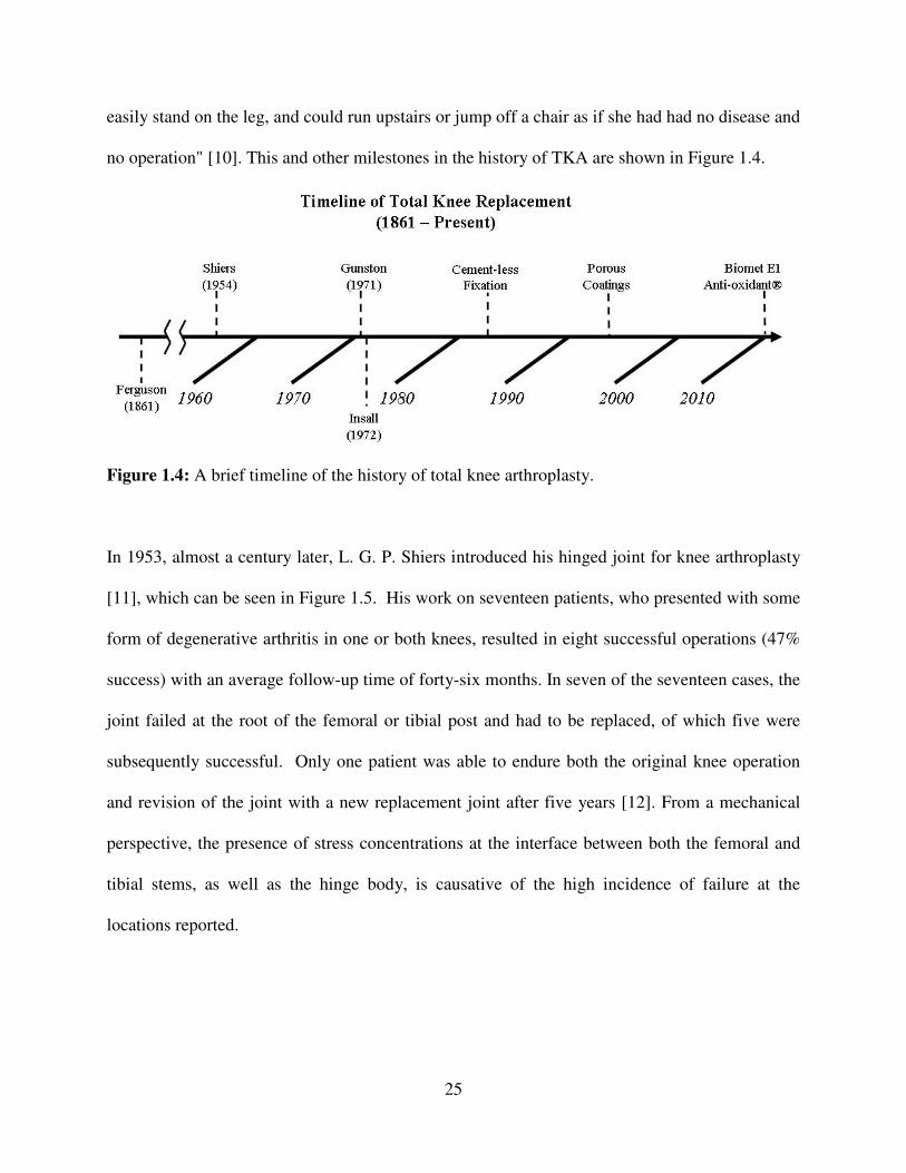
25

easily stand on the leg, and could run upstairs or jump off a chair as if she had had no disease and

no operation" [10]. This and other milestones in the history of TKA are shown in Figure 1.4.

Figure 1.4: A brief timeline of the history of total knee arthroplasty.

In 1953, almost a century later, L. G. P. Shiers introduced his hinged joint for knee arthroplasty

[11], which can be seen in Figure 1.5. His work on seventeen patients, who presented with some

form of degenerative arthritis in one or both knees, resulted in eight successful operations (47%

success) with an average follow-up time of forty-six months. In seven of the seventeen cases, the

joint failed at the root of the femoral or tibial post and had to be replaced, of which five were

subsequently successful. Only one patient was able to endure both the original knee operation

and revision of the joint with a new replacement joint after five years [12]. From a mechanical

perspective, the presence of stress concentrations at the interface between both the femoral and

tibial stems, as well as the hinge body, is causative of the high incidence of failure at the

locations reported.

26

Figure 1.5: Shiers' hinge joint prosthesis [11, 12].

Prior to Shiers, the “broad base of the operation remained the same” from 1914 until 1953;

during this time period, physicians utilized a wide array of materials in knee joint arthroplasty,

varying from circumcised pigs’ bladders [13], to sheets of nylon [14]. In that time span, 896

documented arthroplasty procedures were performed with a success rate of 46% [12]. In 1971

Gunston introduced the concept of a unicondylar (replace one condyle at a time) metal-on-plastic

knee replacement [15], wherein the metal surface was affixed to the distal femur and the plastic

bearing surface affixed to the proximal tibia. This basic configuration of artificial knee joints has

persisted for the past forty years. The similarities between Gunston’s original metal-on-polymer

design and the “state-of-the-art” metal-on-polymer implants available today from companies like

DePuy, Smith & Nephew, and Zimmer are readily apparent to the casual observer, as the

significant advances in materials selection and geometrical contouring are not as readily apparent.

Figure 1.6 juxtaposes Gunston's original design (left) with an example of the state-of-the-art in

knee replacement technology, the Vanguard® total knee available from Biomet, Inc.

27

Figure 1.6: Left: Gunston's metal-on-polymer prosthetic implant [15]; right: An example of a

metal-on-polymer total knee replacement available from Biomet, Inc. [16].

The similarities between two technologies separated by four decades of research are the result of

both scientific and economic factors. Metal-on-polymer TKA is an efficient and effective

method of joint arthorplasty that, once approved by the U.S. Food and Drug Administration

(FDA) and accepted by the scientific community, became the "state-of-the-art" and a focus of the

majority of research efforts directed at optimizing and improving implant function. Evidence of

some drawbacks to this iterative approach to designing joints were highlighted in a recent (at the

time of this writing) New York Times article describing the short-lived, troubled life of a new

implant, the DePuy A. S. R. hip replacement system. Due to the high cost of developing new

types of joints, manufacturers are able to obtain approval for “critical implants [which] can be

sold without [rigorous] testing if a device, like an artificial hip, resembles an implant already

approved and used on patients.” [17]. Thus, one of the major reasons that TKA systems have not

changed significantly over the years is because it makes more economic sense to optimize

existing design than to try to gain approval for a drastically different and new approach. From an

engineer’s standpoint, however, given the depth of knowledge regarding knee biomechanics

28

which has been accumulated over the past forty years of optimization, there could now be a

better option with significantly greater long-term efficacy.

TKA, in general considered to be an extraordinary success [18], is necessary in the event of

damage to the articular cartilage, meniscus, or other soft tissues in the human knee joint, whether

from trauma, genetic disease such as rheumatoid arthritis, or other factors. Knee function is

provided primarily by the soft tissues in the joint, shown in Figure 1.7a and b; thus, injury to

these structures will have the greatest impact on joint stability and treatment selection [19].

Figure 1.7: (a) and (b) are gross anatomical prosections of human knees, illustrating the relative

size and location of soft tissue structures [20, 21].

Articular cartilage is avascular and natural regeneration or repair does not occur; conversely,

when a bone is broken, it will heal and new tissue will grow to replace the damaged tissue.

Figure 1.8a shows what damaged articular cartilage looks like in cases of degenerative

29

osteoarthritis; replacement of the damaged tissue with metal and polymer prosthesis components

can bee seen in Figure 1.8b.

Figure 1.8: (a) damaged articular cartilage in osteoarthritis [22]; (b) subsequent removal of

damaged cartilage and replacement with metal and polymer prosthesis components [23]

Knee replacement in an adult over the age of sixty-five generally results in the replacement

lasting the lifetime of the patient. Due to several factors, including more active lifestyles and an

increase in the weight of the general population, TKA is being performed more frequently in

patients aged under the age of sixty-five. More than 350,000 primary TKA procedures and

29,000 revision procedures were performed in the United States in 2002 [24], the most recent

year for which data was available. This represents a tripling of the rate at which TKA

procedures were performed just twelve years earlier in 1990 [25].

The durability of current implants is such that over increasing lifetimes, the side effects of long-

term implantation eventually force the revision of artificial joints. Concerns associated with

implant loosening and the potential need for multiple revisions generally discourages the

30

widespread use of TKA in patients less than fifty years old [26]. According to the most recent

projections, the annual incidence of TKA is predicted to increase over 670%, to 3.48 million

procedures per year by 2030 [27]. Longer-term implantation, as well as increases in the total

number of implants, will require both significant improvements to existing implant technology as

well as methods of integrating the implant into the surrounding anatomy in order to reduce the

risks of complications such as periprosthetic osteolysis [8].

1.3 INSTITUTIONAL CONTRIBUTIONS

This thesis would not have been possible without those who have come before the author, many

of whom have gone on to other exciting work.4 Reading their theses and papers has provided

guidance and inspiration, and also helped to create neural connections and provoke thought

processes that otherwise would not have happened. Direct input from the late Professor Robert

Mann would have been invaluable; work by him and his students over several decades made

significant advancement in clinical and biological applications of engineering to joint design and

musculoskeletal biomechanics [28-31].

Work by Seering [32, 33] described contributions from the cruciate and collateral ligaments in

supporting a load, and will be used in further work to add additional degrees of freedom to the

existing joint. Work by Fijan, also a student of Prof. Mann’s, helped the author of this thesis to

develop a better understanding of the 3-D kinematics of the normal human knee [34], which led

to a hypothesis that a simple matrix model of the knee could be generated to represent range of

motion (ROM) and stiffness (C) in all 6 DOFs. This model could then be combined with a

4 “If I have seen further it is because I have stood on the shoulders of giants"”– Isaac Newton

31

synthesis method like Freedom and Constraint Topology [35] to generate a flexural mechanism

with the same kinetic and kinematic characteristics as a healthy knee joint.

Recent work in the Bioengineering Laboratory at MGH5 has also helped guide this thesis work.

A study of knee biomechanics using fluoroscopes to assess flexion after TKA [36] illustrated the

depth of knowledge surrounding the knee joint that has been acquired, and will be useful in

future work. Varadarajan’s research [37] supported the development of an understanding of joint

mechanics and how they can influence the design of new prostheses. Other work by Most and

colleagues, first in developing a 6-DOF robotic test system to evaluate TKA biomechanics [38],

and next investigating the mechanics of TKA at high flexion angles [39], was of great influence

in the creation of functional requirements for a rolling contact prosthesis presented in Chapter 5.

1.4 THESIS CONTRIBUTIONS

The contributions of this thesis are rooted in the application of machine design principles to

medical challenges, wherein machine elements can be brought to bear against limitations of

current biomedical technology, with the ultimate goal being to develop new bio-machines to help

improve patient care. These contributions are found in Chapters 3-6, while Chapters 1, 2 and 7

serve as the foundation off of which the others are based. Chapters 2 and 7 also provide an

introduction to general orthopaedic medicine and biomechanics as they relate to this work. This

thesis is focused on a mechanism called a rolling element joint, of which the flexure coupling is a

sub-type, as it is applied to problems in fracture fixation and repair, and the design of prostheses

5http://www.massgeneral.org/ortho/research/researchlab.aspx?id=1479; Director: Dr. Gouan Li, PhD.

32

for articulating joints. Additionally, lubrication, friction, and wear of joint prostheses can thus be

considered from the point of view of rolling element bearing design.

The first contribution of this thesis came from the author’s involvement in the development of an

adjustable bone plate. During evaluation of mechanical characteristics of the new plate,

conventional methods of testing bone plates were not able to properly characterize the new

design [40]. A deterministic analysis of bone plate testing methods showed that current practices

would have to be modified to accommodate the new technology [41]. Following this, the design

and manufacture of a new testing method allowed for characterization of adjustable bone plate

designs and comparison with existing technology using rolling element joints to simulate

fractures [42].

Next, a rolling contact prosthesis design is achieved using deterministic analyses of knee

biomechanics, combined with input from principles of good machine design. General functional

requirements for a knee joint are also defined to illustrate the results of the deterministic process.

The next step was to analyze the system by looking at optimal configurations for load

transmission between two elements of a joint for load transmission. Following this, kinetics of

the human knee in a sagittal (2-dimensional) plane is integrated into the mechanism, and rolling

cam surfaces are contoured to ensure that their relative motion is equivalent to the

rotation/translation seen in the flexion and extension of a human knee joint. A case study of

metallic rolling contact joints manufactured out of stainless steel for use in knee braces is also

presented, demonstrating its ability to withstand several hundred thousand cycles. The kinetics

of this new joint represent a significant biomechanical improvement over current brace designs.

33

It has been shown that knee biomechanics can be used to deterministically design a better knee

brace; at the time of this writing, a grant application for a clinical trial to evaluate the latest

prototype has been submitted.

Another contribution of this thesis is demonstrating that shear-thinning fluids, when combined

with a micro-scale porous coating, can significantly reduce shear stresses in a lubricated contact.

This was shown through investigating potential improvements at the different implant surfaces:

the implant-implant interface, where lubrication and wear govern material lifetimes, and the

implant-bone interface, where integration of native bone into the structure of the implant is

essential for long-term viability of the prosthesis. The implant-implant interface is the primary

focus of this research, as the author’s skill in a wet lab, as well as the required resources, limited

the amount of cell culture work that could be performed.

It is hypothesized that improvements to lubrication can be achieved through encapsulation of

synovial fluid, supporting protein-mediated boundary layer formation, through application of a

micro-scale hydrophilic coating onto implant materials. Boundary layer formation is well

documented to be supported by adsorption of hydrophilic proteins; increased friction leads to

protein denaturation and exposure of hydrophobic moieties of those proteins, which then adsorb

onto hydrophobic surfaces (i.e. the polymer) and disrupt flow in the boundary layer.

Encapsulation could help to prevent hydrophobic proteins from adsorbing onto surfaces, and will

also help to mitigate both increases in friction as well as dry contact between the two implant

surfaces [43, 44, 45].

34

Next, growth and proliferation of osteoblasts, which are the principle drivers of bone formation,

are investigated on micro-scale porous titanium coatings fabricated using alkaline etch and

anodization processes. Osteoblast growth, proliferation, and adhesion have been well-

documented to be improved by titanium micro- and nano-structures, often with complicated

hydroxy-apatite (HA) based coatings. Also, currently used coatings are generally “sprayed” onto

the surface of an implant, for example Trabecular Metal available from Zimmer (Zimmer, Inc.,

Warsaw, IN). Alkaline etching results in a coating that is fabricated directly into the surface,

integrated into the bulk structure of the solid. These have not yet been evaluated, when formed

on orthopaedic-grade titanium for their efficacy in supporting cell growth and proliferation, and

the results of preliminary studies are described.

1.5 THESIS ORGANIZATION

1.5.1 CHAPTER 1 – INTRODUCTION

Chapter 1 gives a description of the motivations for this work, as well as giving a brief overview

of the history of total knee arthroplasty. It also provides a concise explanation of the

contributions of this thesis, with brief descriptions of the contents of each chapter.

1.5.2 CHAPTER 2 – MUSCULOSKELETAL PATHOPHYSIOLOGY

Chapter 2 gives a brief introduction to the musculoskeletal system, starting with a gross

anatomical view, then descending to the cellular level. The biochemical basis of some important

aspects of regulation and growth are also discussed to provide a foundation for understanding the

interaction of implant materials and the adjacent human tissues. I am grateful to Dr. Mary

35

Bouxsein and Dr. Maragaret Seton, instructors for the January 2011 HST Course

Musculoskeletal Pathophysiology, for graciously allowing me to take the class while studying

for my doctoral qualifying exams. I drew much inspiration from what I learned there, and during

my first year of medical school, while writing Chapter 2 [46].

1.5.3 CHAPTER 3 – DETERMINISTIC JOINT DESIGN

Chapter 3 presents a deterministic method for designing rolling element joints for biomedical

applications. Different types of joints found in the musculoskeletal system are discussed, and

prosthetic mechanical substitutes are evaluated. The chapter ends with a case study in using a

deterministic design process to synthesize a rolling element joint for evaluating the performance

of a new deformable bone plate for mandible fracture repair [41, 42].

1.5.4 CHAPTER 4 – JOINT DURABILITY

Chapter 4 is an exercise in fatigue, fracture, and lifecycle analysis for a theoretical rolling contact

joint. Classical fatigue analysis of crack nucleation and propagation in the straps from Figure 1

is presented, as well as their ability to resist high cycle fatigue. Materials selection for a rolling

contact joint is also discussed from the point of view of Hertzian contact stresses, and the

Buckingham Load Stress factor is used to predict the lifetime of the rolling elements.

1.5.5 CHAPTER 5 – DESIGN OF ROLLING CONTACT JOINT PROSTHESES

Chapter 5 illustrates the use of a deterministic analysis of knee kinematics and biomechanics to

develop a set of functional requirements (FRs) for an articulating joint prosthesis. These FRs are

36

used to generate concepts with different types of joints, including a flexure coupling. From this,

a knee brace was constructed which imitated the same roll-back motion seen in a healthy human

knee. Knee biomechanics can be actively applied to prostheses design to develop a better joint

for knee braces, fixators for treating dislocations, and also prosthetic limbs, in addition to

implants for total knee arthroplasty. A rolling contact knee brace could help reduce pain,

improve support, provide additional stability and support rehabilitation by better matching the

biomechanics of the knee than the dual-hinge designs in use today.

1.5.6 CHAPTER 6 – NANO-ENGINEERED SURFACE COATINGS

Chapter 6 is focused on nanoengineered coatings, investigated for their ability to improve the

performance of implants at two key interfaces: the bone/implant interface and the

implant/implant interface. The implant/implant interface is the primary site of lubrication,

friction, and wear in joint prostheses, and its ability to withstand stress and support loads are

critical to determining an implant’s success. The bone/implant interface is critical to the long-

term success of the implant as integration of the surrounding bone can help prevent stress

shielding and subsequent periprosthetic bone loss. Nano-structured coatings for osseo-

integration are also discussed and the results of a brief foray into cell culture are described.

1.5.7 CHAPTER 7 – CONCLUSIONS AND FUTURE WORK

Chapter 7 presents final thoughts and a summary of potential future work that could be pursued,

for example clinical evaluation of the performance of the knee brace as compared to current

technology. Also, this chapter deals with clinical aspects of Total Knee Replacement (TKA),

37

such as indications and complications, as well as use of knee braces in patients who are

candidates for TKA. Specifically, aseptic loosening, metal ion allergies, and polyethylene wear

are discussed and additional resources for background reading provided. Finally, limitations of

the current joint are discussed, and suggestions are made for what further research must address

in order to create rolling-contact total knee prostheses.

1.6 REFERENCES

[1] “Next: Skipping a Beat”, National Geographic Magazine, Dec. 2011:30.

[2] Bartel, D. L., Davy, D. T., Keaveny, T. M., “Orthopaedic Biomechanics”, (2006), Pearson

Prentice Hall, Upper Saddle River, NJ.

[3] Briggs, K. K., et al.“Improvement in Quality of Life with Use of an Unloader Knee Brace in

Active Patients with OA: A Prospective Cohort Study”. Journal of Knee Surgery, 2012; 25(05):

pp. 417-422.

[4] Brandsson, S., et al. “Is a knee brace advantageous after anterior cruciate ligament surgery?”

Scandinavian Journal of Medicine and Science in Sports, Vol. 11;2, pp. 110-114, April 2001.

[5] Stanley, C. J., Creighton, A., Gross, M. T., Garret, W. E., “Effects of a knee extension

constraint brace on lower extremity movements after ACL reconstruction”. Clin Orthop Relat

Res (2011) 469:1774-1780.

[6] Felson, D. T., et al. “The prevalence of knee osteoarthritis in the elderly. The Framingham

Osteoarthritis Study”. Arthritis and Rheumatism, Vol. 30, Iss. 8, pp. 914-918, August 1987.

[7] The Free Dictionary – Medical Dictionary. Online URL: http://medical-

dictionary.thefreedictionary.com/

[8] Revel, P. A., Ed., “Joint Replacement Technology”, (2008), Woodhead Publishing, Ltd.,

Cambridge, UK.

[9] Orthopaedic Surgery India, Kerala, India. Online URL: http://www.orthopaedic-surgery-

india.com/primary-knee-joint-replacement.html

[10] Ferguson, M., "Excision of the Knee-Joint – Recovery with a False Joint and Useful Limb".

Medical Times & Gazette, 1861; 1:601.

[11] Shiers, L. G. P., "Arthroplasty of the Knee: Preliminary Report of a New Method". Journal

of Bone and Joint Surgery, November 1954, Vol. 36B:4, pp. 553-560.

[12] Shiers, L. G. P., "Arthroplasty of the Knee: Interim Report of a New Method". Journal of

Bone and Joint Surgery, February1960, Vol. 42B:1, pp. 31-39.

[13] Baer, W. S., "Arthroplasty with the Aid of Animal Membrane". American Journal of

Orthopaedic Surgery, 1918, 16:1.

[14] Kuhns, J. G., Potter, T. A., "Nylon Arthroplasty of the Knee Joint in Chronic Arthritis".

Surgery, Gynecology and Obstetrics, 1950, 91:351.

[15] Gunston, F. H., "Polycentric Knee Arthroplasty: Prosthetic Simulation of Normal Knee

Movement". The Journal of Bone and Joint Surgery, May 1971, Vol. 53B:2, pp. 272-277.

[16] Vanguard® Total Knee Replacement System, Biomet, Inc., Online URL:

http://www.biomet.at/at-corporate/news/vanguard-monobloc.

38

[17] Meier, B., "The Implants Loophole". The New York Times, Business Day, December 16,

2010. URL: http://www.nytimes.com/2010/12/17/business/17hip.html?pagewanted=1&_r=1.

[18] Einhorn, T. A., O'Keefe, R. J., Buckwalter, J. A., “Orthopaedic Basic Science: Foundations

of Clinical Practice”, 3rd

Ed. (2007), AAOS, Rosemont, IL.

[19] Wiesel, S. W., Delahay, J. N., “Essentials of Orthopaedic Surgery”, 4th

Ed. (2010), Springer,

New York, NY.

[20] Gadha, R., Summer Dissection Course, JCESOM, 2009.

[21] Zill, S. N., Gross Anatomy and Embryology, Course Materials, JCESOM, 2011-2012.

[22] Image Source: http://24.media.tumblr.com/tumblr_m9pt90Yw6o1rupesho2_400.jpg.

[23] Knee Surgery India, Chennai, India. Online URL: http://www.kneeindia.com/knee-

replacement-surgery-guide/.

[24] Mohamed, N. N., Barrett, J., Katz, J. N., Baron, J. A., Wright, J., Losina, E., "Epidemiology

of Total Knee Replacement in the United States Medicare Population". Journal of Bone and Joint

Surgery, June 2005, Vol. 87A:6, pp. 1222-1228.

[25] Diduch, D. R., Insall, J. N., Scott, W. N., Scuderi, G. R., Font-Rodriguez, D., " Total Knee

Replacement in Young, Active patients. Long-Term Follow-up and Functional Outcome".

Journal of Bone and Joint Surgery, April 1997, Vol. 79A:4, pp. 575-582.

[26] Kurtz, S., Mowat, F., Ong, K., Chan, N., Lau, E., Halpern, M., "Prevalence of Primary and

Revision Total Hip and Knee Arthroplasty in the United States from 1990 Through 2002".

Journal of Bone and Joint Surgery, July 2005, Vol. 87A:7, pp. 1487-1496.

[27] Kurtz, S., Ong, K., Lau, E., Mowat, F., Halpern, M., "Projections of Primary and Revision

Hip and Knee Arthroplasty in the United States from 2005 to 2030". Journal of Bone and Joint

Surgery, April 2007, Vol. 89A:4, pp. 780-785.

[28] Carlson, C. E. (1967). Measurement of Pressure Distribution in the Human Hip Joint. SM

Thesis, MIT.

[29] Flowers, W. C. (1972). A Man-Interactive Simulator System for Above-Knee Prosthetics

Studies. PhD Thesis, MIT.

[30] Hardt, D. E. (1978). A Minimum Energy Solution for Muscle Force Control During Walking.

PhD Thesis, MIT.

[31] Hogan, N. E. (1977). Myoelectric Prosthesis Control: Optimal Estimation Applied to E.M.G.

and the Cybernetic Considerations for its use in a Man-Machine Interface. PhD Thesis, MIT.

[32] Piziali, R. L., Seering, W. P., Nagel, D. A., Schurman, D. J., “The Function of the Primary

Ligaments of the Knee in Anterior-Posterior and Medial-Lateral Motions”. J Biomechanics, Vol.

13, pp. 777-784.

[33] Seering, W. P., Piziali, R. L., Nagel, D. A., Schurman, D. J., “The Function of the Primary

Ligaments of the Knee in Varus-Valgus and Axial Rotation”. J Biomechanics, Vol. 13, pp. 785-

794.

[34] Fijan, R. S. (1990). A Three-Dimensional Mathematical Model of the Human Knee Joint.

PhD Thesis, MIT.

[35] Hopkins, J. B. (2010). Design of Flexure-Based Motion Stages for Mechantronic Systems

via Freedom, Actuation and Constraint Topologies (FACT). PhD Thesis, MIT.

[36] Suggs, J. F. (2007). Investigation of In-vivo Total Knee Arthroplasty Biomechanics Using a

Dual Fluoroscopic Imaging System. ScD Thesis, MIT.

[37] Varadarajan, K. M. (2010). In Vivo Knee Biomechanics and Implications for Total Knee

Arthroplasty Implant Design. PhD Thesis, MIT.

39

[38] Most, E. (2000). Development of a 6-DOF Robotic Test System for Studying the

Biomechanics of Total Knee Replacement. SM Thesis, MIT.

[39] Most, E. (2004). The Biomechanics of Knees at High Flexion Angles Before and After Total

Knee Arthroplasty. ScD Thesis, MIT.

[40] Cervantes, T. M. (2011). Design of a Bone Plate for Mandible Fracture Fixation. SB Thesis,

MIT.

[41] Slocum, Jr., A. H., Cervantes, T. M., Seldin, E. B., Varanasi, K. K., "Analysis and Design of

Rolling-Contact Joints for Evaluating Bone Plate Performance". Medical Engineering & Physics,

Vol. 34, pp. 1009-1018, 2012.

[42] Cervantes, T. M., Slocum, Jr., A. H., Seldin, E. B., "Design and Experimental Evaluation of

Adjustable Bone Plates for Mandibular Fracture Fixation", Journal of Biomechanics, Vol. 45:1,

pp. 172-178, 2012.

[43] J. D. Smith, R. Dhiman, S. Anand, E. R. Garduno, R. E. Cohen, G. H. McKinley, K. K.

Varanasi, “Droplet Mobility on Lubricant-Impregnated Surfaces”. Soft Matter (Accepted).

[44] S. Anand, A. T. Paxson, R. Dhiman, J. D. Smith, K. K. Varanasi, “Enhanced Condensation

on Lubricant-Impregnated Nanotextured Surfaces“. ACS Nano, 2012 6 (11), pp. 10122-10129.

[45] Roba, M., Naka, M., Gautier, E., Spencer, N. D., Crockett, R., "The Adsorption and

Lubrication Behavior of Synovial Fluid Proteins and Glycoproteins on the Bearing-Surface

Materials of Hip Replacements". Biomaterials, 30:2072-2078, 2009.

[46] Bouxsein, M., Seton, M., HST.021 Class Materials, January/IAP 2011, Harvard Medical

School.

40


left blank

41

CHAPTER

2 THE MUSCULOSKELETAL SYSTEM

“Medicine’s silent teachers have entrusted to us their most private and valuable mortal

possession, so that in death they can teach us, and that we may help the living.” – Unknown

2.1 INTRODUCTION

In order to design prosthetics that interact with and support the human body, an understanding of

the underlying principles that govern its function must be obtained. This Chapter presents a very

brief introduction to both the gross and microscopic anatomy and function of the musculoskeletal

system, including joints, bone, muscle, and connective tissue. There are a plethora of texts

already devoted to these and related topics; some of which are drawn upon heavily in the

construction of this Chapter, and should be consulted for further details [1-4].

The primary difference between mechanical and biological joints is that most biological joints

are statically indeterminate systems. Unlike man-made mechanical joints, which are designed

based on physical models, one cannot consider the kinematics of a biological mechanism without

42

knowledge of the loads acting upon it or the forces being transmitted between two pieces of

opposing articular cartilage [1]. This makes for a particularly unique challenge in modeling

these structures; assumptions must often be made so that engineering models can be applied to

predict the performance of biological joints.

When referring to aspects of the human anatomy, it is also important to consider use of

appropriate terminology related to the location of different structures. This is done in reference to

what is called the “anatomical position,” a diagram of which can be seen on the left side of

Figure 2.1. In a right-handed coordinate system, the X-axis would be pointing out from an

individual’s navel, the Y-axis would be directed orthogonally to the person’s left, and the Z-axis

would point out of the top of their head. This is illustrated on the right hand side of Figure 2.1.

Figure 2.1: Anatomical position, showing the orientation of coronal, sagittal, and transverse

planes, as well as proximal, distal, medial, and lateral directions [5]

43

Anatomical position is defined as a person standing erect and relaxed with hands at their sides

and palms facing forward, and having three important reference planes: sagittal, coronal, and

transverse. A sagittal plane bisects the body (contains the X- and Z- axes), such that on each side

there are still one hand and one foot. The coronal plane is oriented vertically and is orthogonal

to the sagittal plane, and can be thought of as a crown worn on the head (there is a “C” in both

Coronal and Crown; contains the Y- and Z- axes). Finally, a transverse plane is horizontal and

located orthogonal to the sagittal plane; this is the view most commonly used to visualize the

body’s structures with imaging modalities like CT or MRI (contains the X and Y axes).

Three sections address different levels of detail in the musculoskeletal system; Section 2.2

briefly outlines musculoskeletal development and describes some basic functional properties.

Section 2.3 outlines the macrostructure, and gives gross anatomical examples of each tissue type

(bone, ligaments, muscle, etc.). Section 2.4 describes the macrostructure of various tissues, and

also presents a very brief discussion of certain aspects of the physiology of the musculoskeletal

system, while Section 2.5 focuses on related pathologies.6

These are important because

observations of the body at the macro-scale are often the direct result of micro-scale pathology;

understanding this link is critical to both the design of biomechanical systems as well as the

delivery of effective patient care.

2.2 MUSCULOSKELETAL SYSTEM

The musculoskeletal system consists of all the bone, muscle, tendons, ligaments, synovium, and

other components that enable motion, provide support and protection for vital organs, and allow

6 Pathology is defined as the precise study and diagnosis of disease; as a noun it refers to the presence of disease.

44

a person to interact with their surroundings and maintain homeostasis. The system as a whole is

derived from mesoderm, one of the three germ cell layers found in human embryos (along with

endoderm and ectoderm). Endoderm forms many structures found inside the body, and also

forms the lining of some body cavities. Ectoderm forms the skin, and also is the origin of the

central nervous system. Separation of the germ cell layers is summarized in Figure 2.2

.

Figure 2.2: Differentiation of the germ cell layers [4].

45

Mesoderm further differentiates into mesothelium, mesenchyme, and other embryological tissue;

mesothelium forms muscles and mesenchyme forms connective tissue, including bones and

cartilage. Overall, the functions of the musculoskeletal system can be grouped into four

categories [1] including (1) hematopoesis, (2) mineral storage, (3) protection of the vital organs,

and (4) support and motion.

One of the most intriguing aspects of bone is that it can respond to an applied load; this principle

has been described empirically as Wolff’s Law: Bone will preferentially grow in such a way as

to resist an applied load [6, 7]. On the microscopic level, transmembrane proteins within

osteoblasts sense small amounts of strain in the bone; these induce positive changes in cellular

physiology that lead to increased formation of new bone [8]. Wolff’s Law is part of the

motivation for preventative treatments for those at risk of developing osteoporosis (i.e., post-

menopausal women). It also provides a potential explanation for the loss of periprosthetic bone

seen in recipients of artificial joints.

2.3 MACROSTRUCTURE

An introduction to gross anatomy is the start of a top-down approach to learning about the

musculoskeletal system, including bone, muscle, cartilage, tendons, and ligaments. Bone forms

the support structure from which the rest of an individual’s soft tissues derive their shape, and

also provides protection for the vital organs. Muscle is found throughout the human body, in

everything from blood vessels, to the lungs, and the gastrointestinal and reproductive tracts.

Cartilage allows formation of a joint between two solid pieces of bone, and tendons and

46

ligaments allow for transmission of forces across joints. Examples of each type of tissue are

shown in Figure 2.3.

Figure 2.3: Examples of (a) Bone, (b) Muscle, (c) Cartilage, (d) Tendon, (e) ligament [4].

2.3.1 BONES

The human body contains 210 bones,7 generally organized into three groups: long bones, short

bones, and flat bones. Examples of long bones are the femur (the longest bone in the body) in the

leg, and the humerus in the upper arm; these bones are defined as having a large aspect ratio.

Short bones are found in the ankle and wrist, and generally have aspect ratios around 1. Flat

bones can be found in the skull, the sternum, and the pelvis, and also make up the transverse and

spinous processes of vertebrae. The pelvis is often also called the innominate bone as it is a

7 206 bones, plus two sesamoid bones under the head of the first metatarsal in each foot

47

fusion of three separate bones: the pubis, the ischium, and the ilium. Figure 2.4a—d show

examples of different types of bones found in the body.

Figure 2.4: Types of bones in the body, including (a) long bones like the femur, (b) short bones

like the navicular in the foot, (c) flat bones of the skull, and (d) the right half of the innominate

bone (pelvis) [3].

Most bones in the body have an outer layer of dense tissue referred to as cortical bone, and an

inner section of less dense, sponge-like tissue referred to as cancellous or trabecular bone.

Marrow, principally found adjacent to trabeculae in the internal structure of a bone, is the

principle site of hematopoiesis (growth of blood cells) which, in an adult, only occurs in the axial

skeleton.

48

In the long bones, there are three primary segments: the diaphysis, metaphysis, and epiphysis.

The epiphysis, at the end of the bone, contains the growth plate, which is closer to the

metaphysis than the end of the bone; long bones have articular cartilage covering their ends that

serves to form joints like the hip, shoulder, knee, or elbow. A schematic of segments of these

areas can be seen in Figure 2.5 [9]. The diaphysis is the middle segment, which is made up of

mostly cortical bone and is penetrated by a medullary artery that supplies nutrients to osteocytes,

osteoblasts, and other cells in the bone. The metaphysis and epiphysis are mostly made up of

trabecular bone covered by a thin layer of cortical bone. It should be noted that the ends of the

long bones are larger in area, making them well suited to transmit high body weight forces.

Figure 2.5: A sketch showing structures which make up the long bones, including the diaphysis,

metaphysis, and epiphysis [9].

49

The macrostructure of bones is directly influenced by their microstructure, as described

previously in the discussion of Wolff’s Law. The stresses placed on a piece of bone will

determine the resultant shape of the solid structures, as observed in Figure 2.6a, which shows a

cross-section through the proximal part of a human femur. Figure 2.6b is a cross-section through

the proximal tibia, illustrating how the ends of the long bones have increased horizontal cross-

sectional areas and larger amounts of trabecular bone, ideal for distributing forces transmitted

across the joint.

Figure 2.6: Cross-section through the proximal part of (a) the human femur and (b) the human

tibia [10] and (c) a sketch showing the organization of primary trabecular fibers [6, 7].

50

The major orientations of trabeculae in the human femur are seen in the sketch at the bottom of

Figure 2.6. This illustrates how stresses associated with supporting the body weight, like those

transmitted through the innominate bone to the hip joint and down the femur, are resisted by the

major orientation of trabeculae fibers as required by Wolff’s law.

2.3.2 MUSCLE

There are three different types of muscule: skeletal, smooth, and cardiac. Examples of each can

be seen in Figure 2.7. They are similar in their function, but all are different in their physiology

and response to hormones and chemical signals. Because it is difficult to visualize smooth

muscle in gross specimens, a histological section of the wall of a large, muscular artery is

presented.

Figure 2.7: Skeletal muscle in the biceps (left), smooth muscle in an artery (middle), and cardiac

muscle (right) [11].

51

Here, the focus is on skeletal muscle function; a detailed discussion and comparison of skeletal,

smooth, and cardiac muscle as well as their physiology is outside the scope of this work. From

here on, the word “muscle” will be used to refer to skeletal-type muscle. In general, a muscle can

be characterized by four features: origins, insertions, actions, and innervations. More

specifically, an origin is generally considered to be the more proximal attachment of the muscle

to the skeleton, and an insertion the more distal attachment. The action of a muscle is based on

which joint it affects; for example, one action of the biceps muscle is to flex the elbow joint

(decrease the angle between the forearm and the humerus).

Some muscles also have multiple origins and insertions. Groups of fibers are organized into

specific muscles, even if they share a common function, based on distinct patterns of innervation

by nerves. An example of this is the quadriceps muscle in the thigh, which has four heads (hence

the “quad”): rectus femoris, vastus medialis, vastus lateralis, and vastus intermedius. Each

muscle group works with the others in concert to extend the leg,8 but each is innervated by a

separate fiber of the femoral nerve, and can be stimulated separately from the others.

2.3.3 JOINTS

In the human body, different joint types enable various motions, falling into two structural

categories: fibrous and cartilaginous (articulating). Articulating joints are found in the fingers

(interphalangeal joints), spine (between superior and inferior spinous processes of vertebrae),

and the knee, and generally permit larger ranges of motion than fibrous joints. The bony surfaces

8 Anatomically, the leg refers to the tissues below the knee, while “lower extremity” refers to the entire limb.

52

in each case are covered with articular cartilage and the joint is surrounded by a synovial

membrane that produces synovial fluid which lubricates and bathes the joint.

An example of a fibrous joint is the pubic symphisis, at the anterior portion of the pelvis, formed

by fusion of the left and right pubic bones created by a piece of tough, fibrous cartilage (fibro-

cartilage). There are also fibrous joints between the twelve costal cartilages and the sternum (six

costal cartilages on each side), and between the surfaces of each vertebral body, which in

themselves are covered with articular cartilage. Examples of fibrous and cartilaginous joints can

be found in Figure 2.8.

Figure 2.8: The hip, an articulating cartilaginous joint (left)9; one of the fibrous joints in the

spine, found between each vertebral body and formed by an intervertebral disk made of fibro-

cartilage (right) [4].

There are twelve major joints found in the extremities where each limb meets the torso (shoulder

or hip), at the mid-portion of the limb (elbow or knee), and where the limb meets the hand or

9 Image source: http://www.jacksonvilleorthopaedicsurgeon.com/total-hip-replacement.php (downloaded:

12/29/2012).

53

foot (wrist or ankle). The skull sits on synovial joints formed by the occipital bone and the first

and second cervical vertebrae; each vertebra of the spinal column also has a synovial joint with

vertebrae above and below. Of all the joints in the human body, it is those of the limbs which are

generally affected by degenerative changes and are candidates for prostheses, i.e. the hip, knee,

shoulder, wrist, etc.

The development of prostheses for certain joints has followed the demand for the joints that most

often wear out, i.e., the hip and the knee. The hip is a ball-and-socket joint and so lends itself

rather nicely to bio-mimicry with engineering materials. The knee joint however, has motions

that are far more complex owing to its two polycentric, differently-sized condyles (the medial

condyle being larger than the lateral). Other joints in the body, such as the shoulder, ankle,

elbow, and wrist, are often replaced using prosthesis in cases where severe rheumatoid or osteo-

arthritis has damaged the joint to the point at which there is significantly reduced range of

motion. Here, prostheses can be used to restore function to an otherwise healthy individual.

Section 3.2.1 contains a more detailed discussion of the different types of joints found in the

human body and what types of prostheses are used to replace them.

2.3.4 TENDONS AND LIGAMENTS

Two common examples of these connective tissue structures are the Anterior Cruciate Ligament

(ACL) and the Achilles tendon. The former is well-known for its propensity to tear, which can

subsequently led to the development of arthritis of the knee, while the latter is the largest tendon

in the body, as it must be able to support the body’s entire weight and propel the foot forward

during walking. These soft-tissue structures hold the musculoskeletal system together: Tendons

54

connect muscle to bone0020and ligaments connect bone to bone. Images of different soft tissue

structures can be seen in Figure 2.9.

Figure 2.9: (a) The cruciate ligaments, including the ACL and PCL [5]; (b) one image from a

CT scan of a torn ACL [5]; (c) an Achilles tendon from a cadaver [3].

2.4 MICRO-STRUCTURE

The physical properties of each of the tissues that make up the musculoskeletal system are

defined by their microstructure, which also leads to differences between each tissue that are

apparent at the macro-scale. Histological examination of tissues can be used to understand the

physiological basis for their function, and how they influence homeostasis. For example,

observation of the microstructure of muscle would show that striations are made up of an

overlapping actin/myosin meshwork, which gives skeletal muscle the ability to pull with

substantial force compared to similarly sized man-made actuators. Collagen and connective

tissue are covered first, then cartilage, bone, muscle, and ligaments and tendons.

2.4.1 COLLAGEN

Collagen makes up multiple different tissues within the musculoskeletal system. The most

abundant types of collagen include types I–IV, and type VII, all of which are listed in Table 2.1,

55

with the primary structures in which they are found. The amino acid glycine is found every third

residue, and is important in the creation of hydrogen bonds to allow for formation of the triple

helix.

Table 2.1: Summary of collagen types and their respective uses within the body [4].

Collage Forms Structures Fibrillar Source

Type I Tendons; Ligaments; Bone Yes Fibroblasts, Osteoblasts,

Odontoblasts, Adipocytes

Type II Cartilage Yes Chondroblasts

Type III Reticular structure of organs Yes Fibroblasts, Adipocytes,

Schwann cells, Muscle cells

Type IV Lamina Densa No Fibroblasts, Muscle cells,

Adipocytes, Schwann cells

Type VII Anchors Lamina Densa to

Reticular fibers No

Fibroblasts, Muscle cells,

Adipocytes, Schwann cells

Each collagen molecule is composed of three polypeptide chains (called α-chains) in a right-

handed triple helix, hydrogen bonded together. The enzyme peptidase cleaves the ends of the α-

chains in the triple helix to form the final collagen molecule. The collagen fibrils are linked

together in an overlapping pattern, illustrated in Figure 2.10.

56

Figure 2.10: Schematic of (a) the orientation of collagen α-chains in fibers, and (b) collagen

assembly, starting with the precursor α-chain, and ending with a collagen fiber [4].

On a side note, Vitamin C is an important component involved in the synthesis of collagen and is

one reason that individuals who develop scurvy often have bleeding gums; the high rate of

turnover in the oral mucosa leads to bleeding as new connective tissue cannot easily be

synthesized. Thus, Vitamin C is an essential nutrient for maintenance of connective tissue.

Additional information on collagen synthesis and the different tissues it helps to create can be

found in a pathology text like Robbins and Coltran [12, pp. 437-438].

57

2.4.2 CARTILAGE

Cartilage, made from Type II collagen, provides both strength and flexibility to structures in the

human body, and also enables highly efficient articulation of joint surfaces. Cartilage is also

present as an intermediate during the growth of bone, as it atrophies and then undergoes

mineralization both during embryological developing of the skeleton, and during the fracture

healing process. During the growth of new cartilage, chondroblasts, differentiated from

mesenchymal stem cells, sequester themselves in lacunae (small pockets where the cells reside)

by secreting cartilage matrix proteins (Type II collagen, chondtroitin sulfate, keratin sulfate, and

hyaluronic glycosaminoglycans – GAGs). Figure 2.11 shows an image of hyaline cartilage in the

initial growth phase, with chondrocytes sequestering themselves in lacunae. Newly formed

chondrocytes are flat and found near the periphery, which blends with a superficial fibrous layer

on the right side of the image.

Figure 2.11: Growth of hyaline cartilage showing chondrocytes in lacunae (left side), and the

fibrous perichondrium (right side) [4].

58

Continued expansion of the tissue occurs through either interstitial or appositional growth;

interstitial describes the formation of new chondroblasts in the center of the tissue, and

appositional refers to new chondroblast growth at the periphery. One chondroblast will divide to

form two daughter chondroblasts. Once the growth is complete, minor injury can be

accommodated by growth of new chondroblasts from chondrogenic cells in the perichondrium;

extensive damage leads to differentiation of mesenchymal cells into fibroblasts and formation of

a fibrous scar. Cartilage is found in joints (articular cartilage), the ear and nose, the rib cage, and

as fibrocartilage in certain joints (i.e. the pubic symphisis). Figure 2.12 shows a cross section of

articular cartilage with calcified areas and the subchondral bone.

Figure 2.12: Articular cartilage, showing periosteal chondrocytes and underlying bone [4].

2.4.3 BONE

Bone serves as a functional support for soft tissues, is the site of proliferation for a majority of

the cellular components of the immune system, and is also the principal location for storage of

59

minerals like calcium and phosphate in the body. The two principal cell types involved in the

formation and degradation of bone are osteoblasts and osteoclasts, which can be seen in Figure

2.13; osteocytes are senescent osteoblasts that reside in lacunae and maintain mature bone.

Figure 2.14 shows a sketch of the different types of cells found in bone, including osteoblasts,

osteoclasts, and osteocytes. The distinction between osteoblasts and osteoclasts is important as it

forms the basis for several pathologies related to implant failure (e.g. periprosthetic osteolysis,

osteoporosis) and age-related bone loss (osteoporosis).

Figure 2.13: Images of (a) osteoblasts and (b) osteoclasts in trabecular (cancellous) bone [13].

60

Figure 2.14: Schematic showing trabecular bone, osteoclasts, osteoblasts, and osteocytes and

their various functions [13, 14].

Bone growth (ossification) in the fetus occurs via two methods: intramembranous and

endochondral, illustrated in Figure 2.15. In the primary ossification center, new bone is found at

the center of the image, and hyaline cartilage and the zone of hypertrophying chondrocytes is

found at the periphery. Endochondral ossification in the image on the right shows the diaphysis

(center) separating the two future epiphyseal areas currently formed by hyaline cartilage [4].

61

Figure 2.15: Images of a primary ossification center (top) and endochondral ossification

(bottom) [4].

Intramembranous ossification involves a thin sheet of mesenchymal tissue that eventually forms

flat bones, like those of the skull. Osteoblasts, derived from mesenchymal cells, secrete osteoid

(bone matrix proteins) and form lacunae. The mesenchymal cells, however, are initially

surrounded by GAGS and randomly oriented collagen fibrils, which will later give the “woven”

appearance to immature or “woven” bone. Osteoid calcifies into tiny spicules (“spicule” meaning

needle-like) which expand to form trabeculae, and then grow appositionally through the addition

of more bone by osteoblasts. As the trabeculae grow, the network of spicules can encircle blood

62

vessels and form immature (woven) primary bone. Periosteum, “peri-” meaning “outer” and

“osteum” referring to bone, is a fibrous sheet created by the outermost layer of cells of the

original mesenchymal sheet, which form fibroblasts, and then go on to create the fibrous

perisoteum.

Endochondral ossification, like that seen in the bottom image in Figure 2.15 forms the long and

short bones. The outline of the bone is created by hyaline cartilage formation within a

mesenchymal layer. Formation of a periosteal bony collar surrounding the hyaline cartilage is

the first indication that the structure will convert to bone; the outer cellular layer of the hyaline

cartilage structure is converted from perichondrium to periosteum, which forms osteoblasts.

This is followed by the subsequent laying-down of the bony collar and enables the next step of

bone formation. Cartilage relies on diffusion for nutrients, and as the bony collar forms,

diffusion is cut off. The chondrocytes will eventually hypertrophy and die, and the cartilage

matrix calcifies.

Blood vessels of the periosteum then pierce its surface and invade the parenchyma, enabling

osteoprogenitor cells to follow suit and colonize the calcified cartilage matrix. Osteoprogenitor

cells then differentiate into osteoblasts and secrete osteoid, which calcifies and forms immature

(woven) bone. Over time the woven bone is remodeled by osteoblasts and osteoclasts to form

compact (mature) bone. Cartilage remains at either end of the bone, both in the epiphyseal

(growth) plate (hyaline cartilage) separating the diaphysis and epiphysis, and as hyaline

(articular) cartilage enabling relative motion between opposing bone ends.

63

Fully developed bone has a hierarchical structure, shown in the histological slide of cortical and

trabecular bone seen in Figure 2.16. The major functional unit of cortical bone is the osteon, a

cylinder of bone with a central opening referred to as a haversian canal through which blood

vessels can grow. Osteoblasts and osteoclasts work in opposition of one another to create the

haversian canals. Both macrophages and osteoclasts are derived from macrophage progenitor

cells, descended from pro-monoblasts differentiated from bone marrow stem cells. This

common cellular ancestor means that forces acting on osteoclasts invariably will have some

influence on macrophages, and vice versa, ultimately influencing the macro-structure of bone.

Empirical observations of periprosthetic bone loss in joint replacement have linked the death of

macrophages, due to ingestion of micro-scale particles from implant components, to up-

regulation of osteoclast activity leading to increased bone resorption (osteolysis) near the implant

(periprosthetic).

64

Figure 2.16: Images showing the hierarchical structure of (a) cortial (compact) bone and (b)

trabecular (cancellous) bone [4].

65

Osteons and haversian canals are formed by the opposing actions of osteoblasts and osteoclasts

in what is referred to as a “cutting cone,” an example of which can be seen in Figure 2.17.

Osteoclasts are found at the front of the tear-drop-shaped cutting cone and dissolve bone by

secreting acids that break down the mineral matrix, which is resorbed and recycled to become a

source of calcium, or to make new bone. Osteoblasts cover the inner surface of the cutting cone

behind the osteoclasts, and secrete compounds that eventually mineralize and form new bone. A

cutting cone will progress at a rate of a few millimeters per every few weeks, resulting in a

person’s entire skeleton being remodeled every few years.

Figure 2.17: A cutting cone, which results in the formation of new haversian canals [13, 14].

66

2.4.4 MUSCLE

There are three different types of muscle: skeletal, cardiac, and smooth. They are classified based

on their histological characteristics as well as their functions; examples of each are shown in

Figure 2.18. Skeletal muscle can be identified by the presence of abundant striations, formed by

contractile filaments that overlap inside the cytoplasm of each individual muscle cell [4, 13-14].

Also, all of the muscle fibers and myocytes (muscle cells) are generally oriented in the same

direction as seen in the section in Figure 2.18a. Cardiac muscle is also striated, but is

differentiated from skeletal muscle by the presence of intercalated disks, seen in Figure 2.18b.

Smooth muscle, in Figure 2.18c, has neither striations nor intercalated disks.

Figure 2.18: Histological preparations of (a) skeletal muscle, (b) cardiac muscle, and (c) smooth

muscle, with characteristic features of each labeled [4].

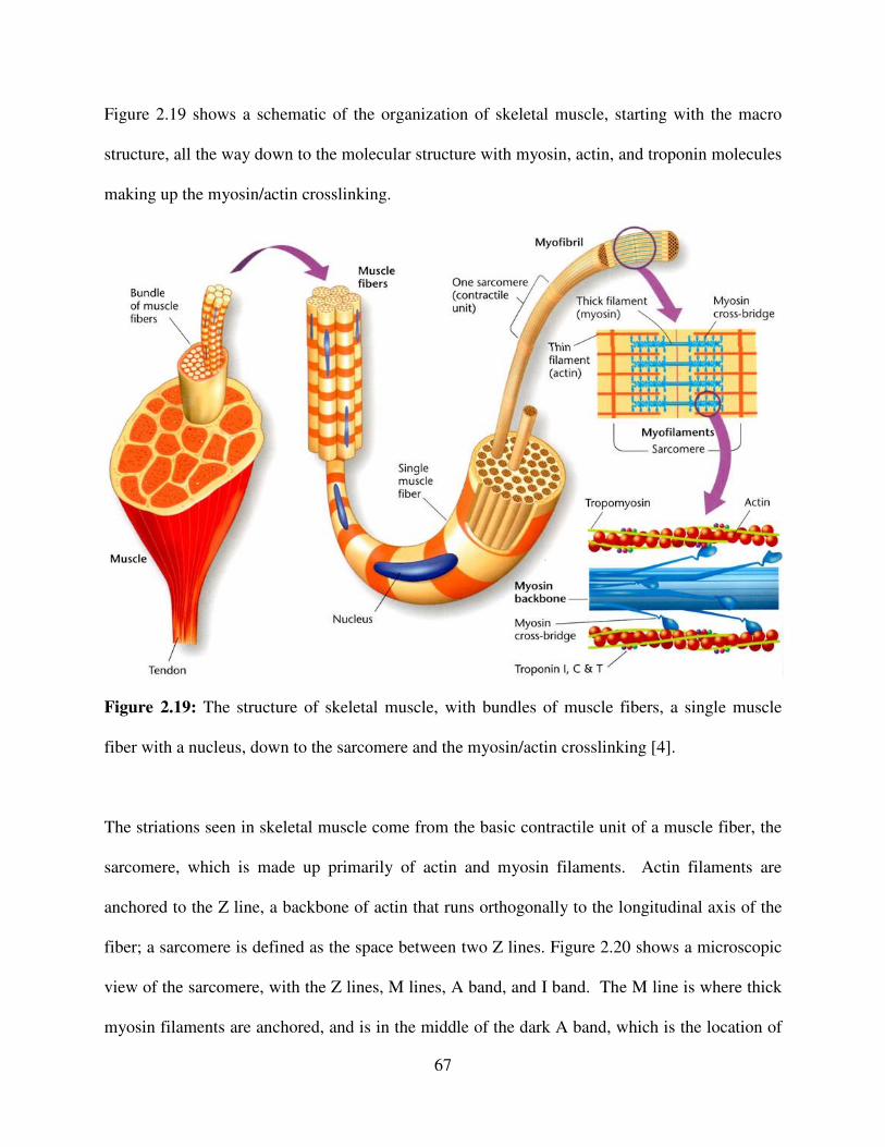
67

Figure 2.19 shows a schematic of the organization of skeletal muscle, starting with the macro

structure, all the way down to the molecular structure with myosin, actin, and troponin molecules

making up the myosin/actin crosslinking.

Figure 2.19: The structure of skeletal muscle, with bundles of muscle fibers, a single muscle

fiber with a nucleus, down to the sarcomere and the myosin/actin crosslinking [4].

The striations seen in skeletal muscle come from the basic contractile unit of a muscle fiber, the

sarcomere, which is made up primarily of actin and myosin filaments. Actin filaments are

anchored to the Z line, a backbone of actin that runs orthogonally to the longitudinal axis of the

fiber; a sarcomere is defined as the space between two Z lines. Figure 2.20 shows a microscopic

view of the sarcomere, with the Z lines, M lines, A band, and I band. The M line is where thick

myosin filaments are anchored, and is in the middle of the dark A band, which is the location of

68

myosin filaments. The I band is the location of thin actin filaments that have not yet overlapped

with myosin, and is thus lighter than the A band. Excessive stretching is resisted by the

intermediate filament protein desmin, which connects adjacent sarcomeres.

Figure 2.20: A histological section showing a sarcomere, the basic contractile unit of skeletal

muscle [15].

Cardiac muscle has striations, but is also characteristically different from skeletal muscle in that

it contains what are called intercalated disks, shown in Figure 2.18b. These are where cardiac

muscle cells are joined by inter-cellular gap junctions such that a depolarization of one cell

allows stimulation of subsequent myocytes without requiring an additional nerve impulse.

69

Intercalated disks, along with purkinje fibers10

, ensure that cardiac muscle cells contract in

relative unison. Finally, smooth muscle does not have striations, and is often observed to have a

stochastic arrangement of cells, as seen in Figure 2.18c. In-depth discussions of the differences

among the three types of muscle can be found in [4], and many more images of their structure

can be found in [4, pp. 137-160].

2.4.5 TENDONS & LIGAMENTS

Tendons and ligaments are arrangements of dense connective tissue, allowing the structures to

withstand substantial amounts of tensile force. Tendons are either composed of regular or

irregular connective tissue. In regular connective tissue, the fibers are generally organized in one

direction like a rope, whereas irregular connective tissue has a more stochastic three-dimensional

orientation of fibers, somewhat like a net. Figure 2.21a-b shows a histological slide of dense

regular connective tissue found in a tendon, and the enthesis, where the tendon inserts onto a

bone. Tendons that are made of dense irregular connective tissue, which usually attach muscle to

bone, can support many muscle fibers pulling in different directions and so must be relatively

isotropic. The achille’s tendon is one of the most well-known structures in the human body, for

its involvement in the death of the structure’s namesake.

10

Highly-conductive modified cardiac muscle cells that help electrical signals spread rapidly through the ventricles.

70

Figure 2.21: (a) Dense regular connective tissue of a tendon; (b) fibrocartilage and the enthesis,

where a tendon or ligament attaches muscle to bone [4].

Ligaments are made up of dense regular connective tissue, as they connect two pieces of bone

together and so usually resist loads applied nominally in a single direction. Examples of

ligaments are the anterior and posterior cruciate ligaments, which resist subluxation forces in the

knee joint and, with the lateral and medial collateral ligaments, hold the cartilaginous knee joint

together. Ligaments also generally have a higher content of elastic fibers, as it would not make

sense for a muscle to contract and have to take up slack in an elastic tendon when trying to run

away from a saber-tooth tiger. Because ligaments provide more structural support, having some

degree of elasticity decreases the chance that they will tear under adverse motions, i.e. a high

stiffness ACL would probably be more prone to tearing. Figure 2.22 shows images of the elastic

fibers in a ligament, and a section of a ligament with multiple collagen bundles making up its

structure.

71

Figure 2.22: Images of the microstructure of ligaments showing (a) elastic fibers (the dark blue

lines) in the extracellular matrix of a ligament that have relaxed with fixing and staining of the

tissue sample; (b) wavy collagen fibers in a ligament (red) surrounded by connective tissue and

elastin (blue/white non-staining) [4].

2.5 PATHOPHYSIOLOGY

Pathophysiology of the musculoskeletal system is often the result of biochemical imbalances in

cellular function resulting in defects in cartilage formation (marfan’s syndrome, osteogenesis

Imperfecta), nerve signal conduction impairments (myasthenia gravis), joint integrity problems

(arthritis, ankylosing spondylitis), loss of bone structure (osteoporosis), and various other

ailments. Most of these will be discussed here only briefly; multiple resources are available for

far more detailed coverage of musculoskeletal pathophysiology [2, 6, 9; 12, Ch. 22].

2.5.1 CARTILAGE FORMATION

Biochemical defects in the formation of cartilage lead to diseases of the connective tissues like

marfan’s and ehlers-danlos syndromes, and conditions like osteogenesis imperfecta, where the

72

bones are weak and brittle. In marfan’s syndrome, a defect in the gene for fibrillin leads to

formation of altered fibrillin molecules. A patient with marfan’s is typically tall and lanky, with

long fingers and is also commonly double-jointed. Because the defect is of elastic connective

tissue that is also found in the circulatory system (i.e. the aorta), these patients are at increased

risk for developing aneurysms, dissections, and other complications because the integrity of their

vessel’s walls are more easily compromised. An excellent discussion of marfan’s syndrome can

be found in Chapter 3 of Robbins and Coltran: Pathologic Basis of Disease [12, pp. 94-98].

2.5.2 CONDUCTION ABNORMALITIES

These types of diseases are often neurological, but have a direct impact on the musculoskeletal

system, the innervation of which by nerves enables induction of contractions. As described

earlier, groups of muscle fibers are innervated by individual nerve fibers, and in diseases like

myasthenia gravis, antibodies affect receptors at the neuromuscular junction. This results in

impaired stimulation of muscle fibers, manifesting as weakness and loss of function [12, pp.

1275-76].

2.5.3 JOINT INTEGRITY

Diseases affecting the integrity of joints include osteoarthritis, rheumatoid arthritis, and

ankylosing spondylitis. Osteoarthritis is a degenerative disease associated with the process of

aging, and has also been observed to have a high chance of developing in a young person with a

joint subjected to trauma (like an ACL tear) [16, 17]. Rheumatoid arthritis is an immune system-

related disease that leads to progressive degeneration of joints, causing significant morbidity

associated with loss of function.

73

2.5.4 BONE STRUCTURE

Diseases of the structure of bone can occur as developmental or metabolic disorders, or as

disorders in the formation of Type I collagen (the precursor of bone). Osteogenesis imperfecta

(OI), osteoporosis, paget’s disease, rickets (seen in children) or osteomalacia (seen in adults),

and Vitamin D deficiency all affect the strength of the composite tissue, resulting in weak,

fragile bones that are prone to fractures. Also, the long bones of children with Rickets are bowed

as they are unable to properly support the increasing weight of the growing individual. While

these conditions all have similar effects on the patient, they range from congenital defects (such

as OI), to age-associated diseases (like osteoporosis) to the result of changes in metabolic

function (as in Paget’s).

OI occurs when there is a defect in the formation of Type I collagen, which serves as a precursor

to bone formation (and is mineralized during the formation of bone); one of the prototypical

signs observed in a patient with OI is blue sclera (the normally white part of the eye surrounding

the iris). This is because the sclera has Type I collagen in it, and is thinner due to the defective

collagen that allows the underlying vasculature to show through, giving it a bluish hue.

Osteoporosis results from a dis-equilibrium in the formation and degradation of bone. These two

opposing processes are well-balanced in most individuals, leading to normal physiological

turnover of the bones every few years and the formation of subsequent layers of haversian

systems. As described in Section 2.4.3, osteoblasts and osteoclasts drive each of these opposing

processes (formation and degradation, respectively), so factors which influence the function of

74

either cell type can tip the balance in favor of one or the other process. In post-menopausal

women, lower levels of estrogen lead to a dis-inhibition of osteoclast activity, causing increased

rates of bone resorption. Wolff’s Law has some influence on bone homeostasis as well, as

patients can develop osteoporosis after significant periods of inactivity or bed rest. Further, it

can also be caused by low-mineral states as it is synonymous with low bone mineral density.

2.5.5 BIOMECHANICS

The study of the kinetics and kinematics of the musculoskeletal system is a very diverse field,

ranging from static analysis of bones for things like fracture fixation [18], to dynamic walking

models of the lower limbs used for developing bipedal robots and limp prostheses [19, 20]. The

Journal of Biomechanics [21] and the journal Clinical Biomechanics [22] are two excellent

sources of the latest in advanced research in the field and should be consulted for further study.

Also, Chapters 3—6 of this thesis all have a foundation rooted in some aspect of this field.

2.6 REMARKS

The human musculoskeletal system is the ultimate machine, capable of self-repair, with the

ability to remodel and also generate immense forces due to the high power density of muscle. As

an engineer with aspirations of designing mechanical prostheses to interact with this system, one

is humbled by its complexity but also inspired by its beauty. As with any other endeavor, the

design engineer must develop a detailed understanding of the systems with which they are

working, as often inspiration for ideas can be found through study of new concepts. An example

of this is the ideas presented in Chapter 6, related to enabling the body’s natural lubricants to

better function in a joint through coating its surfaces with micro- and nano-structures.

75

Another example is the modification of existing machine elements so that their kinetics exactly

match the kinematic motion of existing biological joints. Here, the mechanical joints which are

modified are readily at the disposal of a design engineer, and it is known how to make them very

durable.

2.7 REFERENCES

[1] Bartel, D. L., Davy, D. T., Keaveny, T. M., “Orthopaedic Biomechanics”. Pearson Prentice

Hall, Upper Saddle River, NJ, 2006.

[2] Brinkmann, P., Frobin, W., Leivseth, G., “Musculoskeletal Biomechanics” 1st Ed. (2002),

Thieme Medical Publishers, New York, NY.

[3] Gilroy, A. M., MacPherson, B. R., Ross, L. M., Eds., “Atlas of Anatomy”, 1st Ed. (2008),


[4] Kerr, J. B., “Functional Histology”, 2nd

Ed. (2010), Mosby Elsevier, New York, NY.


[6] Bucholz, R. W., Heckman J. D., Court-Brown, C. M., Tornetta, P., “Rockwood and Green’s

Fractures in Adults”, 7th

Ed. (2009), Lippincott Williams & Wilkins, Philadelphia, PA.

[7] Skedros, J. G., Baucom, S. L., “Mathematical Analysis of Trabecular ‘Trajectories’ in

Apparent Trajectorial Structures: The Unfortunate Historical Emphasis on the Human Proximal

Femur”. Journal of Theoretical Biology, Vol. 244:1, January 2007, pp. 15-45.

[8] Majeska, R. J., “Cell Biology of Bone”, In: Cowin, S. C., editor. Bone Mechanics Handbook,

2nd

Ed., CRC Press, 2001, pp.1-24.

[9] Thompson, J. C., “Netter’s Concise Orthopaedic Anatomy”, 2nd

Ed. (2010), Saunders

Elsevier, Philadelphia, PA.

[10] Gibson, L. J., 3.595 – Mechanics of Porous Materials, Course Material, MIT, Spring 2011.

[11] Berk, M., Gross Anatomy and Embryology, Course Material, JCESOM, 2011-2012.

[12] Kumar, V., Abbas, A. K., Fausto, N., Aster, J. C., “Robbins and Cotran Pathologic Basis of

Disease”, 8th

Ed. (2010), Saunders Elsevier, Philadelphia, PA.

[13] Berk, M., Microanatomy and Ultrastructure, Course Material, JCESOM, 2011-2012.

[14] Fish, S., Gross Anatomy and Embryology, Course Material, JCESOM, 2011-2012.

[15] Cooper, G. M., Hausman, R. E., “The Cell: A Molecular Approach”, 5th

Ed. (2009), Sinauer

Associates, Inc., Sunderland, MA.

[16] Lohmander, L. S., Ostenberg, A., Englund, M., Roos, H., “High Prevalence of Knee

Osteoarthritis, Pain, and Functional Limitations in Female Soccer Players Twelve Years after

Anterior Cruciate Ligament Injury”. Arthritis & Rheumatism, 2004, Vol. 50:10, pp. 3145-3152.

[17] Chaudhari, A. M., Briant, P. L., Bevill, S. L., Koo, S., Andriacchi, T. P., “Knee Kinematics,

Cartilage Morphology, and Osteoarthritis after ACL Injury”. Medicine and Science in Sports and

Exercise, 2008, 40(2):215-222.

76



pp. 172-178, 2012.

[19] Endo, K., Herr, H., “Human Walking Model Predicts Joint Mechanics, Electromyography

and Mechanical Economy”. IEEE/RSJ International Conference on Intelligent Robots and

Systems, 2009, pp. 4663-4668.

[20] Endo, K., and Herr, H., “A Model of Muscle-Tendon Function in Human Walking”. IEEE

International Conference on Robotics and Automation, 2009, pp. 1909-1915.

[21] The Journal of Biomechanics, Elsevier, Online URL: http://www.jbiomech.com/home.

[22] Clinical Biomechanics, Elsevier, Online URL: http://www.clinbiomech.com/.

77

CHAPTER

3 DETERMINISTIC JOINT DESIGN

“You can only obtain it with blood, sweat, tears, and design” – Alexander H. Slocum

Deterministic design is the practice of synthesizing a machine based on a set of requirements

describing the functions (functional requirements) which the mechanism must be able to perform

[1, 2]. It helps a design engineer remove any bias towards any particular concept or idea;

isolating and identifying the functional requirements is often the first step in developing a new

mechanism or machine. Axiomatic-based design is a similar method for designing machines and

utilizes several axioms to guide the definition of a machine’s functional requirements11

[3]. In

this chapter, aspects of rolling element joint design are discussed, including the kinetics,

kinematics, and dynamics of simple concepts related to rolling mechanisms. Then, a case study

in joint design for a biomechanical application is presented for a machine used to evaluate bone

plates for fracture fixation [4, 5]

11

An axiom is defined as “a fundamental truth that is always observed to be valid, and for which there are no

counterexamples or exceptions” [3].

78

3.1 INTRODUCTION

Joint are used to add degrees of freedom (DOFs) to a machine in order to satisfy the functional

requirements of a specific application. They can be used to transmit force, torque, or motion, and

also to construct mechanisms with known kinetics like linkages. There are many different types

of joints, sketches of which can be seen in Figure 3.1 and which also lists the degrees of freedom

of each [6]. It is important to note that not all types of joints permit motion, for example rigidly

joining two pieces of material by bolting, welding, or otherwise fixing them together creates a

rigid joint [7].

Figure 3.1: Sketches of different types of moving, uncoupled joints [6].

79

To the benefit of a design engineer working on prostheses for the human body, models of

mechanical joints have already been extensively studied in the laboratory setting, and the

dynamics and mechanics of each are well-known [7, 8]. It is no small challenge, however, to

figure out how to relate loads and motions found in the human body to those experienced in the

laboratory. Examples of joints found in existing machines can be seen in Figure 3.2

Figure 3.2: Examples of different types of mechanical joints: (a) a ball joint from the front axle

of an automobile12

; (b) a universal joint connecting the wheel to the driveshaft2; (c) one of the

train wheels and railroad track, a rolling contact joint, supporting the crane in (d) [9, 10]; (d) the

325 ton main hoist and 50 ton backup hoist, used to stack the Saturn V and Space Shuttle

12

Images of the from axle of author’s Ford F-250.

80

components in the Vehicle Assembly Building at NASA, both of which use pin joints [9, 10];

and e) a sliding dovetail joint from a vertical milling machine.

Rolling Contact Joints (RCJs), or Rolling Link Mechanisms (RLMs) as described by Montierth

[11], have unique characteristics that make them well-suited for certain biomedical or

biomechanical systems where other types of joints are inadequate. A rolling contact joint is

defined as "a system of constraints that allows a link to roll without slip over another link" [12].

While they increase a mechanism’s overall kinematic complexity, RCJs provide several benefits

over other types of joints. These include decoupled motions, increased Range of Motion (ROM),

compactness, potentially low friction, and local transmission ratios [12]. Design rules call for a

compressive force and a constraining system to keep convex-convex joints in constant contact;

these can be through the use of flexural straps, cables, linkages, or as will be shown a test

specimen held in each link using set screws.

Furthermore, high force applications of RCJs are limited by Hertzian contact stresses [11] and

lubrication is essential for the success of these mechanisms in systems sensitive to particulate

wear debris. Rolling joints are also subject to wear by multiple different modes, including slip

which can lead to fretting and spalling of the material surface which can be studied in the

laboratory under controlled conditions [13]. Different modes of failure in rolling contact have

been studied and written about extensively [14], and more in-depth discussions of rolling contact

failure modes can be found in texts relating to rolling bearing design [15, 16]. Rolling contact

joint configurations, including convex/concave surfaces and convex/convex surfaces, will be

81

evaluated and compared to one another with the intent of selecting one type of interface that will

be used in the prosthetic rolling contact knee joint.

3.2 DETERMINISTIC ANALYSIS

There are several factors which must be considered when designing a mechanical joint, including

the desired ROM, load capacity, lifetime, constraint mechanisms, materials selection for

durability and environmental compatibility, and overall joint stability. Each of these will be

discussed, and then a case study will be presented on designing a mechanism for testing a new

adjustable bone plate [5]. Use of a deterministic process allows the design engineer to

objectively evaluate each concept for its utility in satisfying the functional requirements of a

given application.

3.2.1 TYPES OF BIOLOGICAL JOINTS

Joints in the human body can be classified by both structure and function, relating to the tissues

that make up the joint or the degree of motion which it enables, respectively. A joint that permits

almost no relative motion, or a “fixed” joint, is referred to as a syntharthrosis, an amphiarthrosis

if there is a moderate amount of relative motion, and if the joint enables a large range of motion

it is called a diarthrosis, or diarthrodial joint. Examples of each can be seen in Figure 3.3,

including the pterion in the skull (a syntharthrosis), the pubic symphisis (an amphiarthrosis) and

the knee (a diarthrosis). Amphiarthroses often are called “cartilaginous”, and diarthroses referred

to as “synovial” joints.

82

Figure 3.3: Examples of different classes of joints: (a) schematic of a synovial joint13

; (b) the

fibro-cartilageouns pubic symphisis [17]; syntharthroses in the skull where the skull bones fuse

(forming sutures) [18]; (d) amphiarthroses in the spine between vertebrae and disks [17]; (e) the

knee, a diarthrosis [19].

Different joints in the body can be approximated by mechanical joints. For example, the hip is a

ball-and-socket joint, held together by ligaments and tendons, and actuated by muscles like the

gemelli and gluteus maximus. An interphalangeal joint (in the finger) is a hinge or pin joint with

relatively simple two-dimensional motion. The knee is an example of a hingle-like joint that has

13

Image source: http://classconnection.s3.amazonaws.com/981/flashcards/598981/jpg/joints11310423557211.jpg

83

additional DOFs, which increase the complexity of its kinetics and kinematics. Use of a

deterministic approach to bioprosthetic joint design begins with isolating the major degrees of

freedom for each joint, and choosing a simple mechanical joint that enables the maximum

number of degrees of freedom.

Figure 3.4: Different types of biological joints represented as mechanical structures [20].

Most biological joints have multiple degrees of freedom and operate via coupled motions

because of the nature of the tissues defining their constraints. The tibio-femoral joint, otherwise

known as the knee, is the focus of this thesis and a prime example of coupled motions. One

functional requirement (FR) for a biological joint is for it to have a large range of motion for

movement. This FR competes with size limitations driven by energy requirements. Therefore,

the knee joint developed (in multiple animals, including humans) to be a complicated

superposition of rolling, sliding, axial rotation, and translation. The major degree of freedom of

84

the knee joint is flexion/extension in a two-dimensional sagittal plane; additional degrees of

freedom involve rotation about the long bones that make up the leg. This results in motions of

the joint being coupled, i.e. the center of rotation will move antero-posteriorly while the limb

flexes, so translation is coupled to rotation. Several mechanical joints with coupled motions are

seen in Figure 3.5, most notably the cam pair with 2 degrees of freedom: Translation coupled to

rotation.

Figure 3.5: Machine elements with coupled motions [6].

Other smaller motions in biological joints result from deformation of soft tissue structures like

ligaments and, in the case of a knee, the meniscus. Small motions resulting from deformations in

soft tissue in the knee are also dependent on the loads placed on the joint, adding to the

complexity of its kinetics [21, 22]. In these cases assumptions must be made to select the major

DOFs of a joint, i.e. rotation/translation in the knee, sliding/rotation in the elbow, and multi-axis

rotation in the hip, and then an appropriate mechanical structure modified to match the kinetics

of the biological joint.

85

3.3 KINETICS AND KINEMATICS OF ROLLING CONTACT

The two elements of a rolling link mechanism can have different shapes, whether they both are

cylindrical, elliptical, or are a combination of both. For two equally sized elliptical rolling

elements, diagonally opposite foci can be connected by a rigid link of constant length equal to

the major axis of the ellipse [11]. This is analogous to the way two cylindrical elements can be

connected by a single rigid length equal to the sum of the radii of each element. The fact that the

foci of each element can be connected with a rigid link means that a four-bar linkage can be used

to approximate their motion, with the intersection of the rigid links coincident with the point of

contact of the two rolling elements. Here, the power of rolling contact is first seen: Motion of the

instant center of rotation of a linkage defines the path the point of contact between two cam

surfaces should follow such that those cams are able to replace the linkage in a mechanism.

One way to think about relative motion of cam surfaces is in terms of polodes. A “polode”

simply refers to one of the solid bodies under consideration. In the case of a rolling contact joint

there will be two polodes: One fixed and one moving. An “envelope” refers to the path over

which one curve will roll, so for cams A and B in, in rolling contact, cam B is the envelope for

cam A, and cam A is the envelop for B as seen in Figure 3.6 [23, pp. 65]. For more detail on

fixed and moving polodes, and other ways to model mechanism motion, the reader should

consult a text on the kinetics of mechanisms, for example Section 2.2 in Dijksman’s “Motion

Geometry of Mechanisms” [23, pp. 53, 65].

86

Figure 3.6: Tangential rolling motion of one cam over another (top); sketch of fixed (M) and

moving polodes (Mo) of two cam surfaces, tangent at P (modified from [23]).

In the case of a knee joint, the femur and the tibia (meniscus) are moving and fixed curves,

respectively; the moving curve rolls and slides over and about the fixed curve, making the

meniscus the envelope for the femur. While the envelope, however, is normally defined based on

rolling and sliding motion between two curves, for rolling contact (where sliding is expected to

be near zero) the envelope can be defined as stated above. In Chapter 5, it will be shown how a

four-bar linkage mechanism can be used to find the shapes of the fixed and moving polodes of a

rolling-contact joint mimicking the two-dimensional biomechanics of the human knee joint.

87

In the human body, articulation is a combination of rolling and sliding, enabled by articular

cartilage. The motion of elliptical rolling elements is almost equally complex, being a

combination of rotation and translation. It is this aspect of rolling link motion that makes these

types of mechanisms uniquely suited to replace articulating joints. There is an excellent

discussion of relative motion in rolling element joints by Montierth and Howell [11].

3.4 MECHANICS OF ROLLING CONTACT

Contact mechanics are especially important to consider when designing a mechanism to serve a

specific function, for example modifying an existing machine element like a rolling contact joint

to mimic the motion of a knee [6, 24]. There are two critical degrees of constraint required to

ensure proper function of a rolling contact joint [11]. The first is a no-slip condition between the

two link surfaces; this ensures low-friction rolling motion, and reduces the risk of fretting,

spalling, pitting or sub-surface wear inherent to rolling and sliding contact mechanisms [25,

pp.315-16]. The second constraint is that of normal contact between the links, the behavior of

which is determined mostly by Hertz contact theory [1, 2, 25]. It should be noted that these two

constraints are coupled; the risk of fretting or spalling increases if contact is lost and then made

again between links, while high contact stresses can also damage the contact area and increase

the risk and rate of both surface and sub-surface wear in the mechanism.

When evaluating different configurations for contact, flat-on-flat is the null condition, where the

radius of curvature is infinite and hertz contact stress goes to zero. Round-on-flat is another

example, along with both round-on-round cases: Convex-convex and convex-concave.

Kinematic analysis defines the useful range of motion for each, and modifications to the kinetics

88

enable modeling of certain joints, i.e. concave-convex is representative of a natural knee joint.

Table 3.1 shows the four cases of rolling element mechanisms and gives the relative slide/roll

ratios of each as well as joints for which they could be used to replace.

Table 3.1: The four types of rolling contact joints, including the null condition.

Configuration Flat on flat Convex on flat Convex on Convex Convex on Concave

Slide/roll ratio Infinite Moderate Low High

Prostheses None Shoulder, wrist Finger, knee Shoulder, wrist,

knee, hip

3.4.1 CONTACT MECHANICS

Considering the mechanics associated with contact between two links or surfaces is critical when

designing a rolling-contact joint. The mechanism relies on rolling contact to function, and

methods of constraint [11] are never infinitely stiff, yielding the potential for small amounts of

sliding contact. To design a mate between two machine elements in such a configuration requires

knowledge of the elastic yield strength, fracture toughness, fatigue strength, and most

importantly surface strength of the components. Additionally, there are factors that contribute to

surface wear in RCJs which must be considered in order to ensure a sound joint; these factors

include [25]:

1. Hertz contact stresses

2. Number of cycles

3. Surface finish

4. Hardness

5. Degree of Lubrication

6. Temperature

89

3.4.2 HERTZ CONTACT

Analysis of the contact stresses in a rolling element mechanism are critical to the success of the

mechanism; because they are often very high over a small area, Hertz contact stresses can be the

origination site for crack propagation, spalling, fretting, and other wear mechanisms [2]. Hertz

contact stresses are linked to the joint material’s hardness, which in turn influences its elastic

modulus, and in turn the size of the contact area and magnitude of contact stress. The RCJ here

can be modeled as a special case of the standard Hertz contact equations. Two cylinders in line

contact with each other, as in Figure 3.7a, develop a contact patch of width 2b and length l, as in

Figure 3.7b, when a load F is applied [25].

Figure 3.7: (a) two cylinders in line contact; (b) contact patch formation under load [25].

The half-width b is defined by Equation 3.1; it is a function of the poisson ratio ν, Young's

modulus E, cylinder radii d1 and d2, applied load F, and contact width l. The maximum contact

pressure is given by Equation 3.2. It is important to note that the principle failure mode in Hertz

90

contact is shear, as the highest stress associated with Hertz contact are sub-surface shear stresses

which can lead to crack generation, spalling, and other types of wear [2].

21

2

2

21

2

1

11

)1()1(2

dd

EE

l

Fb

+

−+−=

νν

πEq. (3.1)

bl

Fp

π

2max = Eq. (3.2)

3.4.3 BUCKINGHAM LOAD STRESS FACTOR

While Hertz contact can result in stresses well above the yield strength of a material, fatigue does

not require the stress state of the material to exceed the elastic limit. Also, component fatigue can

still contribute significantly to wear in the mechanism. Fatigue can be controlled for during the

design process by using the surface strength SC, given by Equation 3.3, to determine the contact

pressure which will cause yielding after a given number of cycles; w is used instead of l for the

contact length in this instance.

bw

FSC

π

2= Eq. (3.3)

It is important to note that surface strength SC is identical to the Hertz contact pressure pmax. Use

of the load-stress factor developed by Buckingham [25] provides insight into the limitations of

the current embodiment. It is derived using Equations 4 and 6 for cylinders in line contact, and is

given by Equation 3.4.

+=

21

2

1

11857.2

EESK C

Eq. (3.4)

The design equation which will ensure surface fatigue failure does not occur until after 108

cycles is given by Equation 3.5.

91

+=

21

1

11

rrw

FK Eq. (3.5)

3.5 CASE STUDY: ROLLING CONTACT JOINTS FOR FRACTURE FIXATION

This case study is adapted from an article by the author and colleagues, which described the

design of a dynamic testing machine for evaluation of the mechanical performance of bone plates

used in mandibular fracture fixation [4]. Figure 3.8a shows an image of the machine, and Figure

3.8b shows an image of a new bone plate design [1]. Bone plates are one of the most effective

methods of repairing mandible fractures [26]. They are applied using bone screws and require

surgical exposure of the fracture site. Initial fracture alignment is critical to prevent malocclusion,

or misalignment of teeth after healing. Malocclusions as small as 5 microns can be functionally

disruptive and cause significant patient morbidity; also, they cannot be objectively assessed by

physicians via bite paper or X-ray [27]. A new bone plate design gives surgeons direct control

over fracture alignment by deforming of a compliant structure to correct for observed

misalignment after the application of bone screws [5, 28].

Figure 3.8: (a) rolling-contact joint testing apparatus; (b) adjustable bone plate [1].

92

Rolling Contact Joints (RCJs), or Rolling Link Mechanisms (RLMs) as described by Montierth

[11], have unique kinematics that make them well-suited for certain biomedical/biomechanical

systems where other types of joints are inadequate. A rolling contact joint is defined as "a system

of constraints that allows a link to roll without slip over another link" [12]. While they increase a

mechanism’s overall kinematic complexity, RCJs provide several benefits over other types of

joints including: decoupled motions, increased Range of Motion (ROM), compactness,

potentially low friction, and local transmission ratios [12]. Design rules call for a compressive

force and a constraining system necessary to keep convex-convex joints in constant contact, as

used in the present mechanism. High force applications of RCJs are limited, however, by

Hertzian contact stresses [11].

A Rolling Contact Joint can be used to accurately simulate bending loads normally experienced

by bone plates used to join fractured mandible segments. Loads can be applied directly to the

plate, analogous to in vivo loading conditions. Oftentimes during the healing process bone plates

are subject to substantial loading prior to formation of a bony union [29]. Line contact between

the convex rolling surfaces is used as a simplification of bone fragments meshing together. In

order for this new plate to be adopted by oral & maxillofacial surgeons, the stiffness of the plate

must equal or exceed that of existing plates. The structure, considered a “one-use” compliant

mechanism, is deformed by the surgeon after the plate has been affixed in order to improve

fracture alignment. Because of this, it is important to evaluate the bone plate after it has been

subjected to clinically relevant deformations to ensure that they will not affect mechanism

efficiency.

93

3.5.1 DYNAMIC TESTING MACHINE

Figure 3.9 shows the machine on the laboratory bench, with a coordinate system used to define

error motions in the machine. It is oriented so that ex is colinear with the line contact between the

two mounting arms, ey is aligned with the direction of translation of the pin/slider joints, and ez is

normal to the plane containing the bone plate's neutral axis for this bending configuration. To

determine the stiffness of each interface an applied load of 400 N, equal to the measured peak

male bite force, was assumed to be placed on the machine.

Figure 3.9: Instrument for testing adjustable bone plates, with coordinate system shown.

Equations 3.1 and 3.2 can be used to model the machine as a cylinder on a plane surface by

making one of the diameters infinite (round-on-flat condition). Using an applied load F equal to

94

the maximum measured masseter muscle force of 400N, the maximum pressure in the rolling

contact joint can be calculated to be 176 Pa, and that for the pin/slider joint (with four contact

points) would be 278 Pa. The rolling contact joint is made of a 6061-T6 aluminum alloy, and the

pin/slider joint used a 316 stainless pin sliding on a machined Aluminum 6061-T6 surface. It is

assumed that a compressive force of 400N applied by an Instron® (Instron, Norwood,

Massachusetts) results in an equal compressive force within the rolling contact joint.

The analysis shows that neither the rolling contact joint, nor the pin/slider joint will yield under

an applied load of 400N (90lb-f). Testing will be performed on individual bone plates at a slow

rate of deformation, suggesting that the machine will be inherently low-cycle. In this instance,

however, consideration of the resistance of the mechanism to wear is important as contact forces

developed during evaluation of a bone plate can still result in fatigue.

Figure 3.10 shows the mechanism used to fixture bone plates to the mounting arms. The slot in

the mounting arm used to fixture the bone plate was milled using a 1.58mm (1/16in) endmill,

from a single piece of Aluminum 6061-T6 that had been waterjet cut to form the rolling link

surface. A feed rate of 6.35mm/min (0.25in/min) and cuts of 0.5mm (0.020in) were used to

ensure a good surface finish. To fixture the bone plate in the mounting arms, 8-32 set screws

with a seating torque of 2.26 Nm (20lb-in) were used, resulting in a holding power of 1712.6N

(385 lb-f) [28]. Tapped, counter-bored holes for support screws were made to apply a pre-load

and prevent loosening of the set-screws.

95

Figure 3.10: Constraint mechanism with front and top views of the bone plate fixture utilizing

shims and set screws.

3.5.2 BUCKINGHAM LOAD STRESS ANALYSIS

The surface strength of the rolling contact joint used in this instrument is 176MPa, and 139MPa

for the pin/slider joint. The value for the pin/slider contact is found assuming equal distribution

of load among the four contact regions, with two contact regions per shaft, and is used in

Equation 3.4. Using Equation 3.5, for this machine r1 is defined to be equal to r2, and the

minimum radius is 0.012m (0.47in). For the pin/slider joint r1 is considered to be infinite, so the

minimum radius for r2 is 0.025m (0.98in). As contact radii used in this machine are greater than

these values, the fatigue life of the machine can be assumed to be on the order of 108 cycles [25].

3.5.3 ERROR ANALYSIS

The most critical module of the machine is its ability to isolate the behavior of any given plate,

whether deformed or un-deformed. Misalignments in the mounting arms or method of plate

96

fixation during application of a test load could lead to development of parasitic forces and

moments, which in turn would affect the accuracy and repeatability of the test. As illustrated in

the schematic shown in Figure 3.11, loads are applied at the centerline of the bone plate to

minimize parasitic torques.

Figure 3.11: schematic diagram showing method of avoiding parasitic moments in the mounting

configuration [28].

The initial concept [4, 5] proposed that the bone plate be mounted to the face of the RCJ links,

which would have resulted in a parasitic moment Mp, given by Equation 3.6. To avoid this

adverse loading, the centerline of the bone plate should be in the same plane as the centerline of

the mounting arm. Shims of equal size, placed on either side of the plate, allow the use of set-

screws to provide flexibility to fixture the plate in different configurations.

dFMp ×= Eq. (3.6)

97

To determine the number of supports, consider the possibility of misalignment occurring at the

interface between the mounting arm shaft and the slotted support, illustrated by Figure 3.12a.

Each mounting arm has two needle bearings press-fit into precision-cut holes. If the slot height is

greater than the shaft diameter, then adverse loading conditions illustrated by Figure 3.12b can

result. There is also a length requirement for the slot based on the diameter of the shaft, as

defined by St. Venant [2].

Figure 3.12: Schematic of shaft misalignment supporting the bone plate mounting arm [28].

This is also used to define y-axis rotational error motions. This would cause the bone plate to be

offset from the point of load application, resulting in misalignment during loading with potential

to damage the machine. Using the small angle approximation, and assuming bearing constraint

length Lb to be 50.47mm (1.987in), Equation 3.7 yields the tolerance δs [28].

θθ ≈)sin(

98

b

s

L

δθ =)sin(

plate

s

h

δθ

2)sin( =

01.02

≤plate

s

h

δ

01.0sin ≤

b

s

L

δ

bs L01.0≤δ Eq. (3.7)

The machining tolerance for the pin/slider slot is δs≤0.49mm (0.0197in) to maintain an offset less

than 1% of bone plate height (which is easily attainable). Furthermore, two supports are used

instead of a single slot to further reduce misalignment. Alignment of the bone plate in the

mounting arms is also important. Parasitic forces are generated if the plate were not aligned with

the plane in which the arms rotate. Figure 5c illustrates the condition where the bone plate tilts in

the mounting arms. The height of the mounting arms is not listed because the drawing is not to

scale.

99

Figure 3.13: Schematic of variables for tolerance analysis of the mounting arms [28].

This is also used to analyze error motions in the ex direction, discussed later in the error budget.

Equation 3.8 shows that the mounting arm slot must be machined with a tolerance δm≤0.0635mm

(0.0025in) to ensure parasitic forces less than 1% of the applied load F, given plate width

w=12.7mm (0.5in).

w

mδθ

2)sin( =

applied

par

F

F=)sin(θ

01.0≤applied

par

F

F

01.02

sin ≤

w

mδ

100

( ) 0635.02

01.0arcsin =≤w

mδ

Eq. (3.8)

It should be noted that there are only 3 intended degrees of freedom for the machine: vertical

translation of the joint contact line δz, rotation about the joint interface θx, and translation of the

pin/slider δy. These are defined based on the coordinate system given in Figure 3.9.

Rotation about the y-axis is allowed due to machining tolerances. The stiffness of the other

rotational and translational degrees of freedom are assumed to be infinite in keeping with the

functional requirements of the machine. An error budget for the machine is shown in Table 3.2,.

The required accuracy for translation in the ey and ez directions is assumed to be 5 microns as it

is approximately the minimum maloclusion which can be functional disruptive; this is also well

within the resolution of the Instron test machine used to apply loads.

Table 3.2: Dynamic testing machine error budget [4].

Direction Accuracy Repeatability Expected Stiffness Interface

δx 32µm +/-32 µm n/a n/a

δy 5µm +/-2.5µm 36 N/µm Horizontal pin/slider

δz 5µm +/-2.5µm 1960N/µm Vertical pin/slider

θx 6.6µrad +/- 3.3µrad 0.46Nm/µrad Rolling contact joint

θy 4.35µrad +/-9.7µrad n/a n/a

θz n/a n/a n/a n/a

The highest measured bone plate stiffness was 709.22 N/mm, which translates to a bending

stiffness of 4.12e-3 Nm/µrad; this is two orders of magnitude smaller than the predicted

rotational stiffness in the θx direction of 0.46 Nm/µrad for the rolling contact joint under an

101

applied load of 400N. Thus, bone plate deformation will occur before any significant

deformations are induced the machine. Furthermore, the total vertical stiffness of the four

pin/slider joints, as determined by hertz contact theory, is 1960N/µm. Hooke's law can be used to

determine the required horizontal stiffness of the interface: if a steel/aluminum coefficient of

friction of 0.45 is used, a frictional force Ff of 180N results from an applied load F of 400N.

Assuming a required positional accuracy of x=5µm, the horizontal stiffness k can be determined

by k=Ff/x, and is equal to 36N/µm. The vertical and horizontal stiffness' of the pin/slider joint are

1.96e6N/mm, and 3.6e4N/mm, respectively, as compared to 7.06e2N/mm for the stiffest bone

plate [4, 5].

3.5.4 EXPERIMENTAL RESULTS

Experiments were performed at room temperature or approximately 72°F; the behavior of the

materials tested and the joint material do not change significantly between this and 98.6°F. The

mounting arms were fabricated using an Omax® waterjet with a Tilt-A-Jet™ to eliminate draft

angle. Wetted 400-grit sandpaper was then gently applied to the convex surfaces of the links to

improve surface finish. The pin-slider joints were milled as a single slot in 19.05mm (3/4in)

thick Aluminum 6061-T6 plate, and then halved to create a pair of supports with equal height

and consistent tolerance.

Performance of the bone plate was evaluated using the dynamic testing machine described

previously. Testing bone plates of differing geometries while keeping the material properties

constant will give insight into the performance of the new bone plate relative to those currently

used by surgeons. Bending stiffness and force to failure will be the metrics used to evaluate

102

relative performance of the bone plates. Bending stiffness is a standard of measurement specified

in ASTM-F382, and is calculated by finding the slope of the linear elastic region of the force-

displacement curve [5]. Plates with different geometries will have different bending stiffness;

therefore this parameter can be used to compare performance between different bone plate

embodiments. Force to failure will be measured by increasing the load until the plate fails. This

has been measured in the literature [30, 31] and will enable further comparison between new and

existing plates. Figure 3.14 shows results of two different tests.

a)

b)

Figure 3.14: a) data showing plate slippage due to inadequate set-screw preload; b) successful

test up to 30mm of vertical displacement.

103

Maintaining the minimum set screw torque is imperative for obtaining relevant data. Figure

3.14a shows results for a configuration in which the minimum torque was not achieved. This

caused slipping at the plate/shim interface. The coefficient of kinetic friction is less than the

coefficient of static friction, so a sharp decrease in force is observed. Any results with evidence

of slipping must be discarded. Next, the standard bone plate geometry is used to establish a

baseline so that results can be scaled to account for material difference, and compared to existing

data for conventional bone plates. Figure 3.14b shows force vs. displacement data for 5 different

bone plate configurations, as well as landmarks for peak masseter bite force and average post-

operative bite force [5]

Figure 3.19 shows before and after images of standard as well as deformed and un-deformed

adjustable bone plates; stiffness values are shown for each bone plate tested in the machine. The

rectangular adjustable bone plate had the highest stiffness in its un-deformed state, and still the

highest stiffness after deformation, of all bone plates tested. Further studies involving animals or

human clinical trials most likely would use this plate. Stiffness was calculated as specified in the

ASTM and ISO testing standards for testing bone plate [5].

104

Figure 3.15: Deformed and un-deformed bone plates, with measured stiffness values, before and after

experimental evaluation in the dynamic testing machine [5].

3.6 REMARKS

Rolling contact joints present inherent advantages over other types of joints, specifically for

biomechanical and biomedical applications. The kinematics of rolling contact joints can be

directly controlled by contouring the surfaces of the links, and degrees of freedom can be added

or removed by the addition of flexures, compliant members, or cables. Joints with relatively

complicated motions such as the elbow or knee, as well as the behavior of fractures under certain

loading conditions, can be simulated using rolling contact joints. The contact and constraint

requirements [11] also present a unique opportunity for integrated degrees of constraint and

compliance. Flexures designed to constrain two links to rolling contact can also have integrated

compliant structures allowing for small rotations, much the same way ligaments of a knee joint

allow for the same motions but constrain the joint to articulate.

105

In terms of designing new tools for fracture fixation, the kinetics and kinematics of multiple-link

rolling contact mechanisms can be accurately modeled [11, 12, 25]. Additionally, machines can

be designed to simulate loading conditions more accurately even in more complex fractures that

result in multiple bone fragments, or which span a joint. Here, a rolling-contact joint is used in a

testing machine to simulate in vivo loading conditions more accurately than current standards for

bone plate testing. It has allowed for validation of a prototype adjustable bone plate for reducing

the incidence of malocclusion. Because this machine is limited to in-plane deformations, further

improvements to the apparatus will be focused on enabling the evaluation of bone plates

subjected to multi-plane deformations.

Furthermore, usability studies are currently being conducted to determine the limits of

deformation of the adjustable segment and also to measure forces required to achieve various

deformations. These studies involve plating a synthetic mandible fixtured in a jig with pre-

determined misalignments, and then deforming the plate until the segments are re-aligned. The

deformation of the plate in 6 degrees of freedom is tracking with before and after scans taken

with a volumetric CT machine. A patent application has been filed at the time of this writing, for

which the author is listed as a co-inventor [32].

3.7 REFERENCES

[1] Slocum, A. H., “Precision Machine Design'” (1992), Prentice Hall, Englewood Cliffs, NJ.

[2] Slocum, A. H., 2008, FUNdaMENTALS of Design, Topic 3 – FUNdaMENTAL Principles,

Online URL: http://pergatory.mit.edu/resources/FUNdaMENTALS.html.

[3] Lee, D. G., Suh, N. P., “Axiomatic Design and Fabrication of Composite Structures” (2005),

Oxford University Press, New York, NY.

106



July 23rd, 2012.


Adjustable Bone Plates for Mandibular Fracture Fixation". Journal of Biomechanics (2011),

Published online October 31, 2011. DOI:10.1016/j.jbiomech.2011.09.010.

[6] Freudenstein, F., Maki, E. R., “The creation of mechanisms according to kinematic structure

and function”. Environment and Planning B, 1979, Vol. 6, pp. 375-391.

[7] Slocum, A. H., 2008, FUNdaMENTALS of Design, Topic 9 – Structural Connections &

Interfaces, Online URL: http://pergatory.mit.edu/resources/FUNdaMENTALS.html.

[8] Williams, J. H., “Fundamentals of Applied Dynamics”, 1st Ed (2006), John Wiley and Sons,

Hoboken, NJ.

[9] Personal Communication, General Jerald D. Stubbs, USAF Retired, Chief Counsel, Office of

the Chief Counsel, NASA John F. Kennedy Space Center, July 2012.

[10] National Aeronatucis and Space Administration, Kennedy Space Center, Vehicle Assembly

Building, Cape Canaveral Air Force Station, Cape Canaveral, Florida.

[11] Montierth, J. R., Todd, R. H., Howell, L. L., "Analysis of Elliptical Rolling Contact Joints

in Compression". ASME Journal of Mechanical Design, March 2011, 133:3, pp. 1-10.

[12] Collins, C. L., "Kinematics of Robot Fingers with Circular Rolling Contact Joints". Journal

of Robotic Systems, 20:6 (2003), pp. 285-296. DOI:10.002/rob.10087.

[13] Yamada, T., “Rolling Wear Characteristics of Annealed Carbon Steels under Dry Contact

Conditions”, Wear, 51 (1978), pp.279-288.

[14] Tallian, T. E., “On Competing Failure Modes in Rolling Contact”, ASLE Transactions

(1967), 10:4, pp.418-439.

[15] Harris, T. A., Kotzalas, M. N., “Essential Concepts of Bearing Technology”, 5th

Ed. (2007),

CRC Press, Taylor and Francis Group, Boca Raton, FL.

[16] Harris, T. A., Kotzalas, M. N., “Advanced Concepts of Bearing Technology”, 5th

Ed. (2007),


[17] Thompson, J. C., “Netter’s Concise Orthopaedic Anatomy”, 2nd

Ed. (2010), Saunders

Elsevier, Philadelphia, PA.

[18] Gilroy, A. M., MacPherson, B. R., Ross, L. M., Eds., “Atlas of Anatomy”, 1st Ed. (2008),



[20] Taghizadeh, K., Bastanfoard, M., “The Anatomy of a Human Body, a Model to Design

Smart High Building”. Science and Technology, 2(1):8-14, 2012.

[21] Piziali, R. L., Seering, W. P., Nagel, D. A., Schurman, D. J., “The Function of the Primary

Ligaments of the Knee in Anterior-Posterior and Medial-Lateral Motions”. J Biomechanics, Vol.

13, pp. 777-784.

[22] Seering, W. P., Piziali, R. L., Nagel, D. A., Schurman, D. J., “The Function of the Primary

Ligaments of the Knee in Varus-Valgus and Axial Rotation”. J Biomechanics, Vol. 13, pp. 785-

794.

[23] Dijksman, E. A., “Motion Geometry of Mechanisms”, Cambridge University Press, New

York, NY, 1976.

[24] Freudenstein, F., Woo, L. S., “Kinematics of the Human Knee Joint”. Bulletin of

Mathematical Biophysics, 1969, Vol. 31, pp. 215-232.

107

[25] Shigley, J. E., Mischke, C. R., Mechanical Engineering Design, 5th

ed., McGraw Hill, Inc.,

New York, 1989, pp. 73-74, 315-16.

[26] Fox, A. J., Kellman, R. M., "Mandibular Angle Fractures: Two-Miniplate Fixation and

Complications". Archives of Facial Plastic Surgery, 5:464-469, 2003.

[27] Cory Resnick, MD. Personal Communication, January 2011.

[28] Cervantes, T. M. (2011). Design of an Adjustable Bone Plate for Mandibular Fracture

Fixation. SB Thesis, MIT.

[29] Bartel, D. L., Davy, D. T., Keaveny, T. M., 'Orthopaedic Biomechanics: Mechanics and

Design in Musculoskeletal Systems'. Pearson Prentice Hall, Inc., Upper Saddle River, NJ, 2006,

pp.272-282.

[30] Jain, S., Simmons, O., Hanemann, M., Baratta, R., Guerra, A., Metzinger, S., "Comparison

of Tensile Strength of Resorbable Plating Systems Used in Monocortical Mandible Angle

Osteotomy Repair". Archives of Facial Plastic Surgery, 8:390-395, 2006.

[31] Karoglan, M., Shutz, K., Schieferstein, H., Horch, H., Neff, A., "Development of a static

and dynamic simulator for osteosyntheses of the mandible". Technology and Health Care,

14:449-455, 2006.

[32] Seldin, E and Slocum Jr., A. H., "Systems and Methods for an In Vivo Adjustable Bone

Plate". US Provision Patent Application, 61/317,884, January 2010.

108


left blank

109

CHAPTER

4 JOINT DURABILITY & MATERIALS SELECTION

“Nothing’s ever built to last, but that doesn’t mean it’s not worth building” – Unkown

4.1 INTRODUCTION

The rolling surfaces of a prototype rolling contact knee joint, seen in Figure 4.1a were

synthesized based on knee anatomy, through the use of a four-bar linkage model of simplified

knee biomechanics (flexion/extension) [1]. There are significant advantages to using rolling

contact when constructing a prosthetic joint made from engineering materials. In this chapter,

four candidate materials are evaluated for their potential use in rolling contact prostheses.

Possible failure modes are also assessed, including fatigue and fracture analysis of the constraints

and rolling surfaces. Also presented are methods of evaluating the flexural constraints using a

repetitive motion machine to subject the joint to several hundred thousand cycles.

110

Figure 4.1: a) Prototype rolling contact joint [1]; b) metal-on-polymer total knee prosthesis

(Biomet, Inc., Warsaw, IA) [2].

Conventional knee replacement utilizes a biomimetic arrangement of metal on polymer, in an

attempt to re-create the geometry of the articulating surfaces present in a healthy joint. An

example of a biomimetic joint, shown in Figure 1b, replaces the distal femur with a metallic

femoral component (often a Cobalt Chrome alloy), articulating on an Ultra-High Molecular

Weight Poly-Ethylene (UHMWPE) bearing surface affixed to a metallic (Titanium, Cobalt

Chrome or stainless steel alloy) tibial tray which replaces the proximal tibia.

The prototype joint seen in Figure 4.1a uses a convex/convex arrangement with three constraints,

based on the mechanism of a flexure coupling. Current prostheses based on sliding contact joints

that directly emulate the biological knee joint are very successful at reducing or even eliminating

111

pain in patients with degenerative joint diseases. As such must be acknowledged in any work

attempting to suggest an alternative design. They have a limited lifetime, however, because they

cannot take full advantage of biomechanical mechanisms such as mimicking the interaction of

synovial fluid with cartilage; this motivates the search for an improved synthetic joint.

As discussed here, a potential key to improving joint lifetime is replacing sliding with rolling

contact. In high performance machines rolling element joints yield the longest lifetimes. Figure

4.2a—b shows sketches from patents for rolling contact prosthesis for (a) inter-phalangeal joints

and (b) a knee joint [3, 4]. A sketch model of a rolling contact flexure-coupling knee joint is

shown in Figure 4.2c. This concept was the basis for synthesizing the rolling contact joint seen in

Figure 1a, based on the first-order flexion/extension degree of freedom (DOF) in a healthy knee.

A four-bar linkage model of knee biomechanics is used to link knee biomechanics to the shape of

the flexure coupling surfaces [1, 5]. The concept utilizes two anterior-posterior (AP) straps, and

one posterior-anterior (PA) strap to both constrain the joint and prevent subluxation of the

femoral or tibial components relative to one another when the joint is flexed under load.

112

Figure 4.2: Images of flexure couplings proposed for use in prosthetic inter-phalangeal (a) and

knee joints (b) [3, 4]; concept sketch of a flexure coupling prosthesis (c).

Herein, it will be shown that conventional orthopaedic materials can be used in a rolling contact

prosthetic joint to improve contact mechanics, which will lead to reduced wear and improved

joint lifetime. Loading conditions on the straps are analyzed using methods developed to model

stresses in steel reinforced concrete, providing a deterministic basis for placing the straps in a

"trochlear-like" groove to eliminate compressive stresses on the straps. Fracture in the straps is

also analyzed to determine the minimum crack length to ensure a lifetime equivalent to current

prostheses. Contact stresses and fatigue in the bulk surfaces of the joint are assessed using Hertz

Contact theory and Buckingham's Load Stress Factor. Table 4.1 provides a list of symbols for

this chapter.

113

Table 4.1: Chapter 4 Nomenclature

Symbol Description

Cd Cycles per day

Cy Cycles per year

C15 Steps over a 15-year period

C30 Steps over a 30-year period

εx Bending (engineering) strain in a curved beam

ρ Radius of curvature

σ Stress

y Height of a fiber relative to the neutral axis

NA Neutral axis

E Young’s modulus

υ Poisson ratio

rfemur Distance from femoral head contact to tibiofemoral center of rotation

rf Radius of femoral component at point of contact

rcontact Distance between P and point of contact

P Intersection of femoral and tibial axes

FBW Force due to body weight

Fc Reaction force at tibio-femoral contact point

Xo Origin of a strap (X=1, 2, 3)

Xi Insertion point of a strap (X=1, 2, 3)

po Hertz contact pressure

ao Area of contact patch

R Radius of contact patch

114

4.2 MATERIALS SELECTION

Selecting proper materials is critical to the lifetime of high performance mechanisms [6]. Knee

braces, and even more so total knee replacements, are subjected to hundreds of thousands of

cycles. The mechanism by which polymer debris is formed suggests a fracture failure mode in

the surface of the UHMWPE due to this high cycle loading [7, 8]. Polymer fracture can lead to

saturation of the joint capsule with particles ranging in size from a few nanometers to tens of

microns [7]. The immune response to these particles can lead to osteolysis, and subsequent

aseptic loosening, presenting a barrier to patients receiving implants at younger ages and who are

very active [9]

The first step in the process for selecting material for an artificial joint is to determine the

number of cycles it must undergo during its useful lifetime. It is assumed that a patient receiving

a prosthetic knee joint will continue to perform Activities of Daily Living (ADL), so a daily load

of about 5000 cycles will be placed on the joint, leading to 1.83 million cycles per year, and 27.4

million cycles over the lifetime of an implant that lasts 15 years. A knee brace worn for just 6

hours a day would then be subject to nearly half a million cycles each year. These calculations

are summarized in T

Table 4.2: Estimation of total cycles a joint is subjected to during ADL.

Parameter Value Symbol

Daily cycles 5000 Cd

Yearly cycles 1,825,000 Cy

Cycles over 15 years 27,400,000 C15

Cycles over 30 years 54,800,000 C30

115

In a rolling contact joint using straps as constraints, there must be an upper limit to strap

dimensions due to the fact they must deform as the joint flexes. A high degree of flexion is one

of the functional requirements of the joint, and thus a constraint should be placed on the

maximum achievable stress state in the straps. Figure 4.3 shows a sketch of a beam in bending

[10].

Figure 4.3: Beam bending schematic used to derive elasticity conditions for joint straps [10].

Plastic yielding through bending reduces the overall strength of a constraint and rapidly

precipitates failure. Equation 4.1 shows the relationship between strain in the strap as a function

of thickness and radius of curvature, and Equation 4.2 gives the resulting stress in the strap as a

function of thickness y [10, pp.420-421]. These can be used to define an upper limit to the

thickness of a strap based on the radius of the joint components; elasticity, at least in bending,

can be defined to exist.

ρε

yx −= Eq. (4.1)

ρεσ

EyE x −== Eq. (4.2)

116

Because the strap is very long, depending on the radius of curvature a condition of plane stress or

plane strain could exist. Once the geometry of the joint is defined, the state of stress in the strap

can be determined using both conditions and the larger of the two used to define the constraint

on thickness. These define an upper limit to the thickness of the strap as a function of the radius

of curvature of the prostheses' rolling surfaces (ρ). The elasticity requirement thus comes from

the fact that the bending stress resulting from the strap forming around the radius of curvature of

the cam surfaces must not exceed the yield stress of the material. Next, a coordinate system must

be established, which can be difficult as there are multiple conventions for coordinate systems

here.

A Femoral Coordinate System (FCS) generally assumes that the leg14

will move, while the body

remains fixed as happens during leg swing while walking; a Tibial Coordinate System (TCS)

assumes that the foot is "planted" and the rest of the body moves as in the next step taken during

walking. The FCS and TCS are illustrated in Figure 4.4, as well as the fact that at a high flexion

angle, the instant center of the joint P is in front of the joint. To determine the loads to which a

joint is subjected, and the resulting strap load (they are providing constraint), they must first be

applied to a more proximal joint. For example, a load must be transmitted through the hip in

order to reach the knee; in a deep squat this will be amplified by the length of the femur, and this

must be taken into account to ensure an accurate representation of joint loading during ADL.

14

The anatomical definition of the leg are those structures distal to the tibiofemoral joint

117

Figure 4.4: Schematic showing femoral (FCS) and tibial coordinate systems (TCS) in a sketch

model of a rolling contact prosthesis.

For the case of a knee joint, the body weight is transmitted through the hip to the femur. Here, a

prosthetic knee joint is assumed as this type of joint will see more load than a knee brace. Figure

4.5 shows a free body diagram of joint loading for a prosthetic knee in flexion to ~120 °.The

joints of an average human being weighing 80kg are subject to contact forces as high as eight

times body weight [11]; in the figure, the force Fc is on the order of 3000-4000N. Table 4.1

should be consulted for explanations of symbols in the figure.

118

Figure 4.5: Free-body diagram of forces due to squatting, in a rolling contact joint.

This model can also be used to determine the tensile loads in the straps. In the figure, the labels

“1” and “2” indicate the origins (subscript “o”) and insertions (subscript “i”) of two different

straps. There are three straps in a flexure coupling; 1 represents the path of the 1 inner strap, and

2 represents the path taken by the outer two straps. Subluxation of the femoral component (FCS)

to the left of the tibial component (TCS) is resisted by the straps connecting between points 2o

and 2i. Equation 4.3 shows the equilibrium condition for determining strap load based on action

of the body weight force, FBW.

�� = �� Eq. (4.3)

The equation assumes that only one strap is supporting the load, so that results are applicable to

both opposing sets of straps in the flexure coupling. For a body weight force on the joint of

3500N, the pure tensile stress in the strap will be proportional to the cross-section area of the

strap. This stress can be estimated using a representative strap; assuming the width of a human

knee joint is around 75-100 mm, three straps in a flexure-coupling based prosthesis will each

119

have a width of around 30 mm. The thickness of the strap is then determined by the modulus and

yield stress of the material. A design problem is now apparent, in which bending stresses

(proportional to thickness) and tensile stresses (inversely proportional to thickness) are working

against one another, providing a band-pass filter with which to isolate acceptable strap

thicknesses for a joint.

4.2.1. HERTZ CONTACT STRESSES

Rolling surfaces are subjected to contact stresses proportional to the equivalent modulus of the

material pairing, as well as the radius of curvature [12, 13, 14]. Equation 4.4 gives the contact

patch half-width, and Equation 4.5 gives the contact pressure.

21

2

2

21

2

1

11

)1()1(2

dd

EE

l

Fb

+

−+−=

νν

π Eq. (4.4)

bl

Fp

π

2max = Eq. (4.5)

If orthopaedic materials are used to fabricate a rolling contact joint, peak contact stresses will

result under the greatest applied load, which during ADL can be up to 8x an individual's

bodyweight. Table 4. 3 gives the relevant material properties for common materials used in

orthopaedic applications including titanium, stainless steel, ultra-high-molecular-weight

polyethylene (UHMWPE), and cobalt-chrome. The surgical metals described in the table are all

used in engineering applications for high-performance, long-lasting machine elements which are

often subjected to extreme environments and loading conditions.

120

Table 4. 3: Properties of four common Orthopaedic materials [15].

Material ρ (kg/m3) Ν σy (MPa) E (GPa) KIC (MPa-m

1/2)

Ti6Al4V 4400 0.34 960 110 75

CoCrMo 8500 0.30 1200 220 20

SS316 8000 0.28 600 200 225

UHMWPE 0.939 0.46 24 1.2 X

These incredibly high joint loads are often experienced when a patient stands up un-assisted (i.e.

no help from the arms) from a seated position. A flexed rolling contact joint in a 75kg individual

subjected to a high degree of flexion will result in 3600 N being transmitted between the joint

surfaces. Table 4.4 shows hertz contact stresses for different material combinations in this

representative joint, and can be considered "relative stresses" as they will all change in

proportion to component geometry.

Table 4.4: Hertz contact stresses (MPa) for different orthopaedic material combinations.

Femoral Component Ti6Al4V CoCrMo SS316 UHMWPE

Tibial Component

Ti6Al4V 23.87 27.44 26.92 3.71

CoCrMo 27.44 33.29 32.38 3.72

SS316 26.92 32.38 31.54 3.72

UHMWPE 3.71 3.72 3.72 2.64

Estimated Hertz stress in joints of different material combinations suggests that the optimal

material for a prosthetic metal on metal joint would be Titanium, and if a metal and polymer

121

were used then Titanium again would be the choice. We can look at models for lifetime of other

machine elements subjected to high cyclic loads, such as rolling element bearings.

4.3 FATIGUE OF JOINT SURFACES

This section focuses on surface wear and fatigue as a result of contact forces in a prosthetic joint

which can occur in both the surfaces of the joint due to contact stresses (two-body wear) and in

the straps due to both tensile and bending stresses caused by loading of the joint in flexion. If

particles are generated from components then three-body wear can occur. Types of wear often

seen in rolling element mechanisms are shown in Figure 4.6. A text on rolling element bearing

technology should be consulted for further discussion of wear types and mechanisms [16-17].

Figure 4.6: Different types of wear seen in rolling contact, including: (a) surface-initiated

fatigue, (b) smearing, (c) surface fatigue spalling, and (d) edge wear due to sub-surface initiated

fatigue spalls [17].

122

According to Talian [17, 18], a worn surface appears, to the naked eye, as “featureless, matte,

and nondirectional”. The original marks formed during the manufacturing process are worn away.

This often occurs in mild wear, and signs of other wear mechanisms like fretting and

micropitting are not present; as such mild wear is not a mode of bearing failure by itself, but

more serious forms of wear like smearing, galling, and fatigue can rapidly lead to failure of

rolling elements [17].

Finally, rolling surfaces in a prosthetic joint will continually be subjected to high compressive

loads in static situations, such as the heel strike in walking, or even when a person is standing

still. These types of loading conditions, even in a well-lubricated joint, could lead to brinnelling.

Brinnelling is defined as “plastic deformation caused by sudden impact [as in walking] during

[motion], or by heavy loading while [stationary]” [17]; it can be seen in Figure 4.7.

Figure 4.7: Brinnelling on the raceway of a tapered roller bearing15

[17].

A method of linking contact stresses to fatigue and wear rates in a rolling element joint would be

effective in helping to predict the useful lifetime of a mated pair in rolling contact.

15

Image from [17] Courtesy of Timken, Online URL: http://www.timken.com/en-us/Pages/Home.aspx.

123

4.3.1. BUCKINGHAM LOAD-STRESS FACTOR

As described in Chapter 3, Section 3.4.3, an advantage of utilizing rolling contact for a prosthetic

joint is that methods of modeling fatigue life in high-performance rolling-element bearings are

now applicable. Fatigue yielding does not require the stress state of the material to exceed the

elastic limit, can lead to significant wear in the mechanism, and as such must be assessed.

Buckingham's load stress factor K1, given by Equations 4.6a and 4.6b, uses the surface strength

of an interface SC (the contact pressure which will cause yielding after a given number of cycles)

to estimate the minimum radius of curvature, of the components in contact, to ensure a fatigue

life of at least 108 cycles (compared with current joint lifetimes of ~10

7 cycles) [12]. If both radii

are known, then K1 determined by Equation 4.6b must be less than the K1 Equation 4.6a to

ensure that failure by fatigue will not occur.

+=

21

2

1

11857.2

EESK C

Eq. (4.6a)

+=

21

1

11

rrw

FK Eq. (4.6b)

Buckingham's equations are normally used to predict lifetimes for rolling element bearings often

subjected to high radial loads and operating in extreme environments [12]. This concept was

developed based on Buckingham’s work with a machine for testing a standard rolling contact

pair during his investigations of wear in gear teeth.

4.3.2. STATIC SLIP ANALYSIS

Kinematic analysis of slip will enable a deterministic comparison of the conventional joint

configuration, which uses a biomimetic arrangement of a convex metal femoral component on a

124

concave polymer, with the convex-convex arrangement of a flexure coupling. Figure 4.8

illustrates this comparison, with a free body diagram of each arrangement also shown; Section

5.3.1 contains a more in-depth discussion. The slip angle γ is lower in the convex-convex

arrangement.

Figure 4.8: Comparison of conventional joint configuration (convex-concave) with the rolling

contact arrangement in a flexure coupling (convex-convex).

From the free body diagram, the normal force on the joint is FN = FBWcos(γ), and an equal and

opposite reaction force, FR = -FN, is generated in the lower component. The resulting friction

force, Ff = µFR, is the product of the coefficient of friction and the reaction force. Also, the shear

125

component of the body weight force is Fshear = FBWsin(γ). To prevent slip, there must either be a

high coefficient of friction in the joint (which is highly unadvisable), or the shear force must be

low. Thus, the static condition for no slip is when Ff>Fshear. The convex-convex arrangement

has a smaller shear angle γ2, a greater Ff=µFBWcos(γ2), but also Fshear is now a much smaller

component, and so overall is less likely to slip than the convex-concave configuration. Stability

will be provided by soft fabrics in a knee brace, or soft tissues in the body for joint replacement.

4.3.3. SLIP BETWEEN ROLLING SURFACES

Slip is inherent to all rolling elements due to changes in loads, direction of motion, and other

factors. It is dependent on the pre-load holding two rolling surfaces in contact, and is often the

cause of fretting fatigue, defined as “accelerated surface damage occurring at the interface

between contacting materials subjected to small oscillatory movements” [19]. It has been shown

that hertz stress induces wear in contacts, especially those subjected to high numbers of cycles,

and observations of increases in wear after certain numbers of cycles suggest that fatigue plays a

role [20].

Slip can lead to fretting and wear in joint surfaces, so the degree of slip reduction achieved

through the use of a rolling contact joint constrained by straps that do not possess infinite

stiffness (the requirement for pure rolling) should be compared to slip in current joints. This

enables quantification of the potential degree of improvement by utilizing a rolling contact joint.

Table 4.5 summarizes compares slip in a rolling contact joint to that in a conventional prosthesis.

Hooke’s law (δ=F/k) can be used wherein the stiffness of a constraint k (the tensile stiffness of

one strap) defines the ultimate slip length δ when loaded with a force F.

126

Table 4.5: Comparing total lifetime slip in rolling contact and conventional joints.

Rolling Contact Joint Slip Conventional Joint Slip

Parameter Value Units Parameter Value Units

Strap Material Ti6Al4V - Condyle Radius 0.025 m

Yield Strength 180 MPa Flexion Angle 100 Deg

Modulus 900 GPa Arc Length 0.043 m

Strap Width 0.006 m -

Strap Thickness 0.0001 m - - -

Strap Length 0.04 m - - -

Strap Stiffness 1.35E+7 N/m - - -

Load 3600 N - - -

Load per side 1800 N - - -

Slip Length (δ) 0.00027 m Slide Length 0.043 m

Daily Use 5000 Cycles Daily Use 5,000 Cycles

Daily Slip 1.33 m Daily Slip 218.17 m

Yearly slip 486.67 m Annual Slip 79,630.64 m

Est. Lifetime 20 years Est. Lifetime 20 years

Lifetime slip 9733.33 m Lifetime Slip 1,592,612.94 m

Reduction 99.39% - Reduction 0% -

The resultant “deflection” in the rolling contact joint is the maximum allowable slip given the

stiffness of a single strap (not counting traction or friction forces, which also resist slip, or

multiple straps). It should be noted that if a load of 1800N were placed on it, the strap would

127

yield plastically; this is half of the total body weight force of 3600N because there are two knee

joints. Overall, a reduction in the total slip over the lifetime of the joint is estimated to be greater

than 99%, which is important if the joint is to retain functionality for 20 years or more.

4.4 STRAP FRACTURE AND FATIGUE

The straps constraining the two rolling elements can fail by multiple ways, including tensile,

bending, fatigue, and brittle and elastic fracture. Tensile and bending were addressed in Section

4.2. Fatigue and fracture in the strap will now be discussed. Brittle strap fracture is first analyzed

using a macroscopic fracture criterion for globally brittle fracture [6, 21]. The brittle fracture

analysis in Section 4.4.1 links a material’s critical stress intensity factor KIC with a mode I stress

intensity factor KI. Elastic fracture, discussed in Section 4.4.2, also utilizes the same stress

intensity factor KIC, but allows a design engineer to evaluate yielding due to crack propagation,

ultimately leading to strap failure.

4.4.1. BRITTLE FRACTURE

“Globally brittle fracture is characterized by little or no macroscopically detectable inelastic

deformation” [21], and is dependent on the presence of cracks that are either found in the

material initially or develop during use. As a result, it is not based on observable deformation in

the strap. Because of this, the risk of brittle fracture is of particular importance to evaluate in

high-cycle, high-load applications including aircraft components and prosthetic joints. Equations

4.7 and 4.8 give expressions for the critical stress of failure, and critical crack size, respectively.

�� = ��√�� Eq. (4.7)

�� = �� Eq. (4.8)

128

Figure 4.9 shows a plot of fracture stress due to a crack, versus the length of the crack, found

using Equation 4.7. The yield strength for Grade 5 Ti6Al4V is shown in the figure as the

horizontal line (900 MPa). To find the critical crack size, this value is used in Equation 4.8 to

find the critical crack size, which is labeled in the figure (acrit = 2.31 mm).

Figure 4.9: Plot showing decrease in stress around a crack; the yield stress of Grade 5 titanium

and the critical crack size are also labeled in the figure.

4.4.2. CRACK PROPAGATION

For dynamic loads, a traction stress σtt can be defined in the strap as the reaction force Fc, which

can be as large as 8x the patient’s body weight [11], divided by the area of the contact patch ao,

as given in Equation 4.9. This stress is resultant from the strap preventing subluxation of the joint

components relative to one another as the patient stands.

o

Ctt

a

F=σ Eq. (4.9)

129

Here, an analogy can be made to pre-stressed steel beams used to reinforce concrete structures, a

schematic diagram of which is shown in Figure 4.10a. When the structure deforms, the steel

beam experiences tangential and normal forces due to interaction with the surrounding structure

[22], much in the same way that the straps in this joint used to constrain the prosthesis could

interact with the tibial and femoral components.

Figure 4.10: (a) schematic of stress states in steel-reinforce concrete, adapted from [22]; (b)

parasitic forces resultant on a bent strap (width w, thickness b) under compression.

In order to properly predict the mode, whether fracture or fatigue, by which a strap is most likely

to fail during dynamic loading (e.g. while walking, or cycling the joint), superposition of

"parasitic" forces induced by this interfacial phenomena must be considered. When the strap

forces have been determined, the fracture energy can be calculated and the most likely mode of

failure, given a set of loading conditions, can subsequently be predicted. The schematic shown in

Figure 4.10b illustrates the parasitic loads on a bent strap.

Equations 4.10a and 4.10b give an approximate relationship between the traction stress in the

strap, and the tangential force and normal forces experienced by the strap. Table 4.6 summarizes

130

the calculation of the tensile and tangential stress on the strap as it is deformed, stretched and

bent over the rounded surface of the implant. It should be noted that the normal force equation is

similar to that for the tensile stress in the wall of a thin-walled pressure vessel.

bf ttt σ= Eq. (4.10a)

ρYfn = Eq. (4.10b)

Table 4.6: Calculating forces in the joint when flexed and loaded.

Parameter Value Units Symbol

Strap width 10 mm W

Body weight 80 kg BW

Force body weight 800 N FBW

Contact Force 8000 N Fc

Contact Area 6.1e-5 m2 Ac

Contact Stress 131.5 MPa P

Tangential force 13.1 MN/m ft

Normal force 6.5 MN/m fn

A strap force Y is then equal to the product of the traction stress σtt, as given in Equations 4.10a

and b, and can be approximated as an equivalent to contact stress. The cross-sectional area of the

strap A, starting with Equation 4.11a, can then be linked to the strap force Y, as in Equation

4.11b.

0=+ tfds

dY Eq. (4.11a)

131

( )( )

( )( )

( ) ( )( ) ( ) ( )

A

sYsds

ssY

dY

dssds

dY

fffs

dY

l

ntn

=−=

=+

−==+

∫ ∫ σϕρ

ϕρ

ϕρ

;tan1

0tan1

tan;0

0

( ) ( )( ) ( ) ( )

A

sYsds

ssY

dYl

=−=∫ ∫ σϕρ

;tan1

0

Eq. (4.11b)

Subsequently, this relationship can be expanded to show that the potential energy stored in the

strap prior to fracture is a function of the total length of the strap l0, the Young's modulus E of

the material, and the cross-sectional area A, as shown in Equation 4.12. The "length condition"

here provides an upper limit on the length of the strap allowed to be in compression.

( )0

22

2

1

2

1lEAds

EA

sYspot εε == ∫

− Eq. (4.12)

Finally, this can be related to the fracture energy release rate G, as the difference in the potential

energy stored in the strap prior to fracture (Equation 4.13a) and the potential energy remaining in

the strap after fracture occurs, as seen in Equation 4.13b.

0; =−= ++−potpotpotG εεε Eq. (4.13a)

0

2

2

1lEG sε= Eq. (4.13b)

Once a value for G has been determined an approximation of Irwin's Formula, seen in Equation

4.14, can be used to estimate the stress intensity factor for the strap. This relates parasitic

tangential and normal forces to the resulting stress intensity surrounding a crack.

EGKI = Eq. (4.14)

132

Equation 4.14 can be used in concert with the Paris-Erdogan law [15, p.114], as in Equation 4.15,

to predict the number of cycles to yield a given material; ∆KI is the change in stress intensity.

n

IC

I

K

Kc

dN

ad

∆= Eq. (4.15)

The number of cycles required to reach fatigue failure in the strap is given by Equation 4.16 as a

function of the change in stress intensity in the strap based on the strap force Y.

( )

( )∫∫

∫∫

∆=

∆=

∆=∆

c

i

f

c

i

f

a

a

n

ICtt

N

a

a

n

ICI

N

I

KaYc

addN

KKc

addN

aYK

πσ

πσ

0

0

( )

∆

−

−=

−−

n

ICtt

n

i

n

f

f

KYC

aa

nN

πσ

)2/2()2/2(

2

2 Eq. (4.16)

The cycles to yield also depends on the critical stress intensity factor of the material, and the

initial and final crack sizes. Constraints on the geometry of the implant, such as the maximum

thickness and length of the strap, can then be incorporated into functional requirements to aid in

the design of the joint.

Now, the fracture energy, stress intensity, and number of cycles to fatigue a strap can be

determined, given a certain strap geometry and size. In the case of a strap subjected to a traction

stress of 131.5 MPa resulting from a patient with 80kg body weight standing up, the resulting

stress intensity in the strap with a crack of approximately 0.1 mm in size, given by Equation 4.17,

is 2.3 MPa-m1/2

.

EGKI = Eq. (4.17)

133

Table 4.7 summarizes the results of the fracture calculations. This is an order of magnitude less

than the critical stress intensity for Titanium, which depending on grade, is between 44 and 66

MPa-m1/2

.

Table 4.7: Summary of fracture analysis.


Stress 131.5 MPa σtt

Crack length 0.1 mm a

Ti modulus 100 GPa E

Ti Fracture Energy 54.3 J/m2 GTi

Stress Intensity 2.3 MPa-m-1/2

KIC

Ti Stress Intensity 75 MPa-m-1/2

KTi

Fracture? NO - -

Furthermore, using the critical stress intensity for Titanium of 75 MPa-m1/2

it can be shown that

the critical crack size is 7mm. Seven millimeters is used as the final crack length for the Paris-

Erdogan calculation, and values for c and n are also assumed. The minimum stress intensity is

approximately zero (under relaxed conditions) and the resulting fatigue life of the strap, from

Equation 4.16, is several orders of magnitude larger than the necessary lifetime, as outlined in

Table 4.8. The strap in this configuration would have essentially infinite fatigue life as the mean

stress is less than half of the yield stress.

134

Table 4.8: Summary of fatigue analysis.


Initial crack length 0.1 mm ao

Critical crack size 7 mm acrit

Scaling constant 0.9 n/a C

Exponential, 2 n/a N

Min. Stress Intensity 0 MPa-m-1/2

Kmin

Peak Stress Intensity 2.3 MPa-m-1/2

Kmax

Fatigue? NO - -

Failure mechanisms observed in existing implants are by fracture of the polymer bearing surface

[23]. The present work suggests that a rolling contact loading condition could result in a

significant increase in the overall lifetime of the joint. It has been shown that a prototype rolling

contact joint can achieve the required ROM utilized by a patient during ADL [1]. As mentioned

previously, during a design review [24] of this analysis it was suggested that the straps could be

moved into a groove in the middle of the implant to reduce traction stresses, and this

configuration can be seen in Figure 4.11. This configuration will be used during the design of a

rolling contact prosthesis presented in Chapter 5.

135

Figure 4.11: (a) rolling-contact prosthesis concept, the bulk supports weight, and the straps

enable constraint; (b) shows a sketch from [4] illustrating an identical configuration.

4.5 MECHANICAL TESTING

Total knee prostheses are subjected to the full weight of the body during locomotion, and as such

evaluating the durability of a rolling contact prosthesis should involve similar loading conditions.

An example of a testing machine for a biomimetic prosthesis is seen in Figure 4.12. In the case

of a rolling contact joint for a knee brace, compressive loads are significantly reduced, and here

are estimated to be around 10% of total body weight on each side. A brace worn by an 80kg

individual is estimated to experience 80N of compressive load, so each joint will see around 40N,

or around 10 pounds in compression.

136

Figure 4.12: A typical testing machine for biomimetic knee prostheses16

.

A testing machine was built using a chain-driven train-wheel mechanism to cyclically load and

unload a rolling contact knee brace. The first generation testing machine can be seen in Figure

4.13 with different components labeled. Figure 4.14 shows a close-up view of the prototype

joint mounted in the first generation testing machine. The results of durability testing for the

rolling contact prosthetic knee joint will be discussed in Chapter 5, Section

16

Image source: http://www.a-tech.ca/series.php?id=879

137

Figure 4.13: Machine for testing the first generation joint for a knee brace.

Figure 4.14: Detail view of the 304SS prototype rolling contact joint in the testing machine.

138

4.6 REMARKS

While fatigue is the most likely failure mode in the current configuration, this can be mitigated

by introducing compliant structures into the implant to allow for parasitic motions equivalent to

the normal motions in a healthy knee joint [25-27]. Methods of failure for UHMWPE bearing

components used in existing implants include sub-surface de-lamination at a critical depth of

about 1 mm (made worse by oxidation of the polymer) [28]. Additional failure methods include

the micro-fracture of surface particles [28] and propagation of micro-cracks in the polymer

implant [8].

The subsequent release of sub-micron and micron-sized particles can result in osteolysis and

loosening of the prosthesis [28]. This can be further instigated by evaluating the propagation of

surface cracks orthogonal to the direction of motion, for example mode I fracture under

sliding/rotating contact, or mode II crack propagation from sliding contact [29]. By utilizing a

well-designed rolling contact joint with adequate lubrication, risk of these failure modes

decreases significantly. Further work will include design of a testing machine similar to that

created by Dressler et al., seen in Figure 4.15 with various components labeled [30].

139

Figure 4.15: Multi-axis testing apparatus for knee joint testing [30].

140

4.7 REFERENCES

[1] Slocum, Jr., A. H., Herder, J. L., Varanasi, K. K., "Biomechanical Design of Rolling-Contact

Knee Joint Prostheses". Presented at the 2012 Annual Meeting of the American Society for

Biomechanics, Gainesville, FL, August 15-18, 2012.

[2] Vanguard® Total Knee Replacement System, Biomet, Inc., Warsaw, Indiana. Online URL:

http://www.biomet.at/at-corporate/news/vanguard-monobloc.

[3] Bora, Jr., F. W., "Prosthetic Joint", U.S. Patent #4,267,608, 1981.

[4] Hillberry, B.M., Hall, Jr., A.S., "Rolling Contact Prosthetic Knee Joint", U.S. Patent

#3,945,053, 1976.

[5] Jeanneau, A., Herder, J., Laliberte, T., Gosselin, C., “A compliant Rolling Contact Joint and

its Application in a 3-DOF Planar Parallel Mechanism with Kinematic Analysis”, Proc. ASME

Design Eng. Tech. Conf., Sept 28 - Oct 2, 2004, Salt Lake City, Utah, DETC2004-57264.

[6] Ashby Materials Selection Book ------------

[7] Utzschneider, S., Paulus, A., Datz, J.-C., Schroeder, C., Sievers, B., Wegener, B., Jansson, V.,

“Influence of Design and Bearing Material on Polyethylene Wear Particle Generation in Total

Knee Replacement”. Act Biomaterialia, 5, 2009, pp.2495-2502.

[8] Wang, A., Sun, D. C., Stark, C., Dumbleton, J. H., “Wear Mechanisms of UHMWPE in Total

Joint Replacements”. Wear 181-183, 1995, pp. 241-259.

[9] Diduch, D. R., Insall, J. N., Scott, W. N., Scuderi, G. R., Font-Rodriguez, D., "Total Knee



[10] Crandall, S. C., Dahl, N. C., Lardner, T. J., An Introduction to the Mechanics of Solids, 2nd

Ed., McGraw Hill, Inc., New York, 1999.

[11] Mundermann, A., Dyrby, C. O., D'Lima, D. D., Colwell Jr., C. W., Andriacchi, T. P., "In

Vivo Knee Loading Characteristics during Activities of Daily Living as Measured by an

Instrumented Total Knee Replacement". J Orthop Res 26:1167-1172, 2008.

[12] Shigley, J. E., Mischke, C. R., Mechanical Engineering Design, 5th

ed., McGraw Hill, Inc.,

New York, 1989, pp. 73-74, 315-16.


Rolling contact Joints for Evaluation of Bone Plates for Fracture Fixation". Submitted to Medical

Engineering and Physics, December 2011.

[14] Slocum, A. H., 2008, FUNdaMENTALS of Design, Topic 3 – FUNdaMENTAL Principles,

Online URL: http://pergatory.mit.edu/resources/FUNdaMENTALS.html.

[15] Revel, P. A., Ed., “Joint Replacement Technology” (2008), Woodhead Publishing, Ltd.,

Cambridge, UK.

[16] Harris, T. A., Kotzalas, M. N., “Essential Concepts of Bearing Technology”, 5th

Ed. (2007),


[17] Harris, T. A., Kotzalas, M. N., “Advanced Concepts of Bearing Technology”, 5th

Ed. (2007),


[18] Tallian, T. E., "Rolling Contact Failure Control Through Lubrication". Proceedings of the

Institute of Mechanical Engineers, 1967-68, Vol. 182:3A, pp.205-236.

[19] Elkholy, A. H., “Fretting Fatigue in Elastic Contacts Due to Tangential Micro-Motion”.

Tribology International, Vol. 29(4), pp. 265-273, 1996.

[20] Yamada, T., “Rolling Wear Characteristics of Annealed Carbon Steals Under Dry Contact

Conditions”. Wear, Vol. 52, pp. 279-288, 1978.

141

[21] Anand

[22] Ulm, F. J., “Modeling of Pre-setressing of Concrete Structures: A Boundary Condition

Problem of Slip at Interface”. Proceedings of the International Conference of Computational

Modeling of Concrete Structures, Euro-C 1994, Vol. 2, pp. 785-804.

[23] Gomoll, A., Wanich, T., Bellare, A., "J-Integral Fracture Toughness and Tearing Modulus

Measurement of Radiation Cross-Linked UHMWPE". J Orthop Res, 20:1152-1156, 2002.

[24] Graham, M., Slocum, A., Moreno-Sanchez, R., “Teaching High School Students and

College Freshman Product Development by Deterministic Design with PREP”, ASME J Mech

Des, 2007, 129, pp. 677-681, Special Issue on Design Engineering Education.

[25] Hopkins, J. B., Culpepper, M. L., “Synthesis of Multi–degree of Freedom, Parallel Flexure

System Concepts via Freedom and Constraint Topology (FACT) – Part I: Principles”. Precision

Engineering, Vol. 34(2), pp. 259-270, April 2010.

[26] Hopkins, J. B., Culpepper, M. L., “Synthesis of Multi–degree of Freedom, Parallel Flexure

System Concepts via Freedom and Constraint Topology (FACT) – Part II: Principles”. Precision

Engineering, Vol. 34(2), pp. 271-278, April 2010.

[27] Hopkins, J. B., Culpepper, M. L., “Synthesis of Precision Serial Flexure Systems Using

Freedom and Constraint Topologies (FACT)”. Precision Engineering, Vol. 35(4), pp. 638-649,

October 2011.

[28] Kennedy, F. E., Van Citters, D. W., Collier, J. P., “Tribological Characteristics of

Polyetheylene Bearings of Knee Prostheses”. Int J Surface Science and Eng, 4:2, pp.166-174.

[29] Eberhardt, A. W., Kim, B. S., “Stress Intensity Factors for a Vertical Surface Crack in

Polyethylene Subject to Rolling and Sliding Contact”. ASME Journal of Biomechanical

Engineering, December 2008, Vol. 120, pp. 778-782.

[30] Dressler, J. L., Ng, R. T., Amirfazli, A., Carey, J. P., “Development and Evaluation of a

Multi-Axis Biomechanical Testing Apparatus for Knee”. Int J Experimental and Computational

Biomechanics, Vol. 1, No. 3, 2010.

142


left blank

143

CHAPTER

5 ROLLING CONTACT KNEE JOINT PROSTHESES

“The worst thing I can be is the same as everybody else. I hate that.” – Arnold Schwarzenegger

5.1 INTRODUCTION

Durability, fracture, and fatigue in orthopaedic implants directly influences implant lifetime and

the morbidity and mortality associated with total knee replacement. The analysis, design, and

manufacture of a rolling-contact prosthetic joint that mimics the primary motion of flexion and

extension observed in a healthy knee will be described. A prototype joint, shown in Figure 5.1,

was laser-cut from 304 Stainless Steel (304SS) and used to create a rolling-contact knee brace;

flexural bands in a flexure-coupling type arrangement constrain the joint to rolling motion. This

joint design could also be used as an external fixator in the treatment of knee dislocations [1].

Rolling-contact is the most efficient method of load transmission when constrained to non-

biological materials (i.e., metals and polymers). While the general concept of a rolling-contact

joint prosthesis is not new, as illustrated by its use in interphalangeal joint prostheses [2] and as

hypothesized by Hillberry in 1976 [3], a method of achieving similar kinematics as existing

144

prostheses with an improved mechanical loading configuration has been developed using results

of prior studies of knee biomechanics [4-6]. A four-bar linkage model of the knee is used to

define the motion of the instant center of rotation of the joint based on a patient's unique

anatomy; this can then be used to drive the shaping of the rolling surfaces and synthesis of the

joint.

Figure 5.1: A prototype rolling-contact joint, laser cut from 304SS, which accurately mimics

knee flexion and extension.

The first documented total knee arthroplasty (TKA) was performed in 1861 at King's College

Hospital, London, UK [7]. The next major advance in technology for prosthetic articulating

joints was the introduction of Insall's duocondylar prosthesis in the 1970's; the basic biomimetic

configuration of a metal/polymer bearing joint persists today [8-10]. TKA it is a very successful

procedure, with recently documented success rates of greater than 90% being observed in a study

of several million joint replacements performed over a period of 12 years [11]. Furthermore,

145

TKA's use has increased from 129,000 to 381,000 cases per year between 1990 and 2002, and

the total number performed annually in the US is expected to reach 3.4 million by 2030 [12].

As Gunston wrote in 1971, "biomechanical study and cadaveric experience" are necessary to

validate the design of new prosthetic joints [9]. Through these practices, a wealth of knowledge

has been catalogued regarding the biomechanics, kinematics, and kinetics of the tibiofemoral and

patellofemoral joints as well as the soft tissues supporting knee motion, the anatomy of which is

illustrated in Figure 5.2. This has allowed for significant improvements to performance, most

dramatically in the last decade with the onset of cross-linked UHMWPE. Yet, despite these

improvements, wear of the polyethylene bearing, whether from fatigue, fracture, or oxidative

stresses, still remains the primary cause of implant failure, and often requires revision to replace

damaged or worn-out components [13].

Figure 5.2: human knee joint anatomy with generalized coordinate system [14, p. 17].

146

A prosthetic knee that lasts twenty years can theoretically be achieved using current technology

[15]; Smith and Nephew was recently granted approval by the FDA to market a "30-year knee".

This approval was granted based on results from wear simulation studies performed on the

VERILAST system (Smith & Nephew, London, UK),which consisted of an oxidized zirconium

femoral component and cross-linked polyethylene bearing surface [16, 17]. It should be noted,

however, that the reported lifetime of these prosthetic knees are based on simulated wear; failure

of total knee prostheses can also be caused by other factors like infection, aseptic loosening, or

yielding of periprosthetic bone [18, 19]. As patients are receiving implants at younger ages,

however, and staying more active later in life, improvements to not just joint materials, but also

the overall design of the joint, must be made to achieve significant increases in joint lifetimes

beyond the 20 year mark [14, 20].

The results of research focused on improving the performance of technology for total knee

replacement will be used to drive the synthesis of a simple planar rolling contact joint. This joint

is based on the concept of a flexure coupling [21]**, using flexural bands to constrain relative

motion of the surfaces, and will serve as a proof-of-concept for the development of future joints

with additional degrees of freedom (DOFs). Here, the design process used to construct a joint

with two DOFs for use outside of the body in a knee brace is described. Also, while the present

joint is suitable for use outside of the body, additional degrees of freedom must be added before

it can be considered appropriate as an implantable joint.

147

5.2 DETERMINISTIC ANALYSIS

It is well known that flexion/extension is the primary degree of freedom (DOF) of the

tibiofemoral joint. Articulation is enabled by articular cartilage on the proximal and distal ends

of the tibia and femur, respectively. A fibrous meniscus affixed to the tibia results in a concave

surface on the tibia, leading to increased joint stability; articulation of the surfaces (coupled

rolling/sliding motion) allows for a large range of motion (ROM) to be achieved in a compact

volume. The healthy knee joint has a convex-concave configuration, where the femur is convex

and the tibia/meniscus forms the concave portion. Soft tissues in the joint, namely the cruciate

(ACL and PCL) and collateral ligaments (LCL and MCL), provide further constraint during

motion and loading of the joint, making the knee an impressive feat of precision biological

engineering. These structures were illustrated in Figure 2.

Current total knee prostheses have a biomimetic design that generally possesses a UHMWPE

bearing surface, which is supported by a tibial tray that is usually made of Titanium, Cobalt

Chrome, or Stainless Steel alloys [14, pp. 81-104]. A modern total knee prosthesis can be seen in

Figure 5.3, as well as an A/P radiograph of a patient with bilateral prosthetic joints. Development

of these implants has followed an iterative model guided in part by increasingly more invasive

studies of knee biomechanics. These tests have ranged from non-invasive mechanical assessment

and mathematical models [5, 6, 22] to experimental apparatuses like multi-DOF robotically-

driven cadaver knee simulators or fluoroscopic imaging systems allowing measurement of knee

biomechanics in human subjects [23-26]. Making further improvements to current technology

will require first proving that the technology can work outside of body, as in the case of a

rolling-contact knee brace.

148

Figure 5.3: Smith & Nephew's Genesis II total knee replacement (left) [17]; radiograph of

bilateral total knee replacements (right) [27].

5.2.1 FUNCTIONAL REQUIREMENTS

Deterministic analysis of the joint shown in Figure 2, coupled with a literature review of

tibiofemoral joint biomechanics yielded six functional requirements (FRs) for rolling-contact

knee prostheses, as seen in Table 1. Assumptions were made to enable simplification of the

problem to the knee's primary flexion/extension degree of freedom. Once this initial concept is

evaluated and demonstrated to be durable enough to withstand millions of cycles, additional

degrees of freedom can be added. These additional degrees of freedom are conventionally

referred to, when considering a flexural system, as "parasitic error motions" [28; 29, pp. 521-

538]. Adding them in a deterministic manner to a rolling-contact design in order to match a

normal knee's additional degrees of freedom would ensure that the rolling contact joint mimics

all of the natural knee motions. It would also help mitigate bone loss that has been observed to be

often associated with over-constrained prostheses.

149

Table 5.1: Functional Requirements (FRs) for a rolling contact knee joint prosthesis.

1. Range of articulation: +5° extension and >-120° flexion

2. Lifetime: 30M+ cycle

3. A/P Translation: 2-5 cm

4. Internal/External Rotation: +15°/-15°

5. Support loads up to 4x body weight (4000 N)

6. Variable stiffness design to allow tuning to patient’s biomechanics

First principles and good machine design practices are used, in conjunction with the current body

of knowledge relating to knee biomechanics and implant technology, to guide the design of a

rolling-contact prosthesis "from the ground up". For example, a joint that utilizes a method of

load transmission which reduces fracture or fatigue of the joint surfaces, yet still enables a large

ROM, would not be subject to one of the main failure modes of current implants [30]. A

successful prosthesis must maintain a large Range of Motion (ROM) to also adequately support

the Activities of Daily Living (ADL). Furthermore, it should be able to withstand tens of

millions of cycles, under loads greater than the patient's bodyweight, in order to last the duration

of a patient's lifetime. An external joint is presented here which satisfies functional requirements

1 and 3, demonstrating that synthesis of such a joint is possible and setting the stage for further

development of 6-DOF rolling contact joints.

5.3 ROLLING CONTACT JOINT DESIGN

Rolling-element bearings would be excellent candidates for achieving large ranges of motion

with little resistance in a compact volume with high durability. A revolute (pin) joint, on the

other hand, does not lend itself to anatomically accurate knee kinematics. A pin joint was used

150

for the first knee arthroplasty in 1861 and similar designs were used as prostheses for several

knee replacements in the 1960s [7, 31, 32]. The latter joints failed not only due to stress

concentrations around non-filleted edges, as shown in Figure 5.4 [31], but also because they did

not adequately reproduce knee motion [32]. Additionally, the concept of a rolamite-based knee

joint was proposed in 1973 [33], using a single S-shaped band and two cylindrical rollers. The

rolamite knee is similar in principle to the design presented here in that they both use flexible

bands to constrain two bodies to rolling contact for significantly reduced friction. The rolamite

knee, however, is limited to simple linear motion and the use of cylinders, and the patient's

weight would be supported by only a single strap. Because the current design uses additional

straps it has an inherently greater degree of flexibility and can be expanded to include additional

DOFs; the rolamite knee is constrained to 1 DOF. In the present design bulk surfaces support the

patient's bodyweight, and their motion is constrained by flexural bands arranged in the

configuration of a flexure-coupling.

Figure 5.4: Pin-joint knee prostheses introduced in the 1960’s by Shiers [30].

151

5.3.1 STATIC ANALYSIS

Two types of rolling contact are evaluated for their ability to achieve a large ROM and maintain

rolling contact, as mentioned previously in Chapter 4. Figure 5.5 shows two types of rolling-

contact joints: one a convex-concave configuration (similar to a healthy knee) and the other a

convex-convex configuration. To increase the ROM of a convex-concave joint, nature added two

polycentric femoral condyles and coated them with articular cartilage. Using two condyles

decreases the Hertz contact stress as the load is halved, and also provides further lateral and

torsional stability. Cruciate ligaments provide constraint against subluxation (for example, an

individual with a damaged ACL would present with a positive drawer sign) and other adverse

motions, and other soft tissues (meniscus, MCL, LCL) constrain additional motions. Articular

cartilage enables high-efficiency rotation, with a coefficient of friction near zero, coupled with

translation (sliding) so that the convex-concave joint can achieve a large ROM [34].

Figure 5.5: Comparison of slip angle γ in a convex/concave joint (biological and current knee

prostheses) and a convex/convex rolling-contact knee joint [35].

152

The coefficient of friction within articulating joints has been measured to be near zero and thus

the knee can rotate efficiently about an axis within the polycentric femoral condyle [23, 24, 26].

This motion becomes less efficient if the cartilage is damaged or if it has been replaced by

arthroplasty [36]. The convex-convex configuration, however, allows for pure rolling-contact

and a large ROM coupled to anterior/posterior translation thus satisfying FRs 1-3. As illustrated

in Figure 5.5, there is a shear force generated in a prosthesis using the convex/concave

configuration as articular cartilage is no longer present to lubricate the joint surfaces. This force

is also larger than a similar force generated in the convex/convex arrangement. Equation 5.1

shows that the shear force is proportional to the shear angle γ according to:

)sin( 1γBWshear FF = Eq. (5.1)

Shear angle, as discussed in Chapter 4, Section4.3.2, is the angle between the line of action of a

load transmitted through the femoral component and a line drawn between the point of contact

and center of rotation. This angle is larger in the convex-concave configuration [34] resulting in

a larger shear force on the interface and, as is currently observed, high rates of polyethylene wear.

In the convex-convex configuration, shear stresses would be reduced and, because the

mechanism would be constrained to rolling contact rather than articulation, theoretical wear rates

should be lower.

Figure 5.6 shows a free-body diagram of the forces presented in the different configurations at

the point of contact (from Figure 5.5). Not only is the shear force Fshear lower in the convex-

convex configuration due to decreased shear angle γ2, but the friction force Ff resisting the action

of Fshear, generated at the interface, is greater in this configuration due to a larger normal force

between the surfaces. FR is the reaction force on the tibial component, and is equal and opposite

153

the normal force, FN. The convex-convex loading condition would improve an implant's

resistance to slip and could also lead to reduce wear.

Figure 5.6: Free-body diagram of the loading configurations illustrating shear and friction

forces; FR is the reaction force in the lower component.

The normal force FN is a function of FBW, given by Equation 5.2. Equation 5.3 gives the friction

force Ff as a function of FBW and the static coefficient of friction, µ, between the surfaces in

contact. Equation 5.4 gives the slip condition for the rolling contact joint.

)cos( γBWN FF = Eq. (5.2)

Nf FF µ= Eq. (5.3)

)sin(γBWf FF > Eq. (5.4)

This simple model shows that, based on first principles, a convex-convex joint is more

mechanically efficient in that it can be constrained to pure rolling and also reduces the chance of

slip, which could significantly reduce wear. There are also numerous examples where rolling

contact is used as a highly efficient means for achieving relative motion while supporting

immense loads. Such examples include rolling-element bearings for paper mills or the wheels of

154

a locomotive. Hertz contact stresses in the current joint can be considered once the appropriate

kinetics have been achieved, as this stress is dependent on the relative radii of the joint radius.

5.4 ROLLING CAM SYNTHESIS

The next step in the design process is to synthesize polycentric (cam) surfaces that will

accurately reproduce tibiofemoral flexion and extension. A flexure-coupling (the mechanism

behind a Jacob's Ladder) was chosen as the basic morphology of the current joint, as the straps

provide well-constrained flexion and extension coupled with antero-posterior translation

(analogous to a healthy knee) while maintaining rolling contact throughout the ROM [34, 35].

From a mechanical point of view, rolling contact has inherent advantages over sliding-contact.

Prior art for rolling-contact joints were either not subjected to significant compressive loads, as is

the case for interphalangeal joint prostheses [2], or did not match joint motions to the kinematics

of the natural joint and thus would not adequately restore normal joint function [3]. Freudenstein

and Woo [4] generated curves to describe the motion of the knee joint based off of measurements

of paths scribed on the tibia by points fixed to the femur, and vice versa. These curves were

consequently described using logarithmic-spiral centrodes to represent the relative tibio-femoral

motion, limited to just 92° of flexion. This was one of the first instances in which it was

demonstrated that knee motion could be described using rolling surfaces.

Here, a four-bar linkage model [5, 6] in a sagittal plane is used to define constraints on the

primary flexion/extension degree of freedom of the joint. What is different about this work is that

the motion of the instantaneous center of rotation is used to generate a reference curve, from

155

which two rolling surfaces can be determined and used to create the same motion as the four-bar

linkage. The surfaces in rolling-contact will be deterministically constrained to match the

motions of the natural joint by tracking the four-bar linkages center of rotation (COR), as shown

in Figure 5.7. This can be done in a reliable fashion based on the results of previous work [4, 5,

6] In an abstract sense, imaging of a patient's knee can be used to determine the relative locations

of the cruciate ligament origins and insertions; unique surfaces can then be created for that

patient without invasive measurement of relative tibio-femoral joint motion.

Figure 5.7: Radiograph of a healthy knee with four-bar linkage overlaid showing origins and

insertions of the cruciate ligaments [37].

A highly-efficient rolling-contact joint could mimic normal knee kinetics with cam surfaces that

maintain contact exactly at the center of rotation of the joint. By definition, rolling-contact

inherently minimizes sliding and thus excessive traction stresses and the resulting wear can be

mitigated. The origin and insertion coordinates of the ACL and PCL can be mathematically

156

related to vectors drawn between the points in the x, y, and z directions, and thus the center of

rotation can be found and traced from total extension (θ=0°) to significant flexion (θ>120°), as

illustrated in Figure 5.8a-c. Theta, θ, refers to the abstract angle between the tibia and femur and

is not shown in the figure. Total flexion angle is measured between the initial and final direction

of the normal vector to the follower link. The subscripts “o” and “i” refer to origin and insertion,

respectively.

Figure 5.8: Sequence of four bar linkage motion as the knee is moved through 135 degrees of

flexion (a-c). The coarse dashed line is the normal to the follower link.

157

Solving the forward kinematics problem for a four-bar linkage can be used to find the

instantaneous center of rotation of the mechanism. Once the motion of the COR is known, it can

be used to synthesize a set of cam surfaces which exactly mimic the motion of the knee joint in a

sagittal plane. Figure 9 shows a schematic diagram for a four-bar linkage representation of the

knee with relevant parameters labeled. The lengths for the ACL and PCL links are calculated

using values adapted from previous studies on knee motion [6] and the x and y-coordinates of

each point are summarized in Table 2.

Table 5.2: Coordinates for each linkage pivot shown in Figure 5.9 [6].

Pivot X-Coordinate Y-Coordinate

A 0 0

B 12.440 32.715

C 7.763 21.973

D 37.300 -5.000

Figure 5.9: Schematic diagram illustrating parameters used to find the motion of the instant

center of the coupler link for the four-bar linkage.

158

Table 5.3: Known, unknown, dependent and independent variables in Figure 5.9. lists the

independent and dependent variables. The points A, B, C, and D are coordinates of the origin or

insertion point of the ACL or PCL; these are used to construct vectors r1-4, and the angles θ1-4 are

between the vector and the horizontal. A closed-loop constraint for the four-bar linkage, the first

step in deriving the COR equations of motion, is given in Equation 5.5.

3241 rrrr +=+ Eq. (5.5)

Table 5.3: Known, unknown, dependent and independent variables in Figure 5.9.

Known Dependency Unknown Dependency

r1 Independent θ3 f{r1, r2, r3, r4, θ1, θ2}

r2 Independent θ4 f{r1, r2, r3, r4, θ1, θ2, θ3}

r3 Independent Bx f{r2, θ2}

r4 Independent By f{r2, θ2}

θ1 Independent Cx f{Dx, r4, θ4}

θ2 Independent Cy f{Dy, r4, θ4}

The values of θ1, r1, r2, r3, and r4 are constant. The angle between vector AB and the horizontal,

θ2, is indexed during the analysis. As AB rotates about point A, the follower link BC rotates

from its initial angle (fully flexed) through an angle of 135° to ensure adequate range of motion

of the cam surfaces. This ensures that the joint will fulfill the first functional requirement.

Imaginary numbers are introduced in Equation 5.6 to describe the position of each pivot A-D

with respect to its components in the x- and y-directions in terms of the variables listed in Table

5.3. These imaginary numbers will eventually be used to derive equations for θ3 and θ4 as

functions of the independent variables.

159

3241

3241

θθθθ iiiierererer +=+ Eq. (5.6)

Equation 5 can be rearranged and the r1 and r2 terms can be grouped into a single imaginary

variable z thus allowing for isolation of dependent variables according to Equations 5.7a-b.

Equations 5.7c-d are the real (x) and imaginary (y) components of z in terms of r1, r2, θ1, and θ2.

4321

4321

θθθθ iiiierererer −=− Eq. (5.7a)

4321

43213,12,1 ),(),(θθθθ iiii

ererereryxzyxz −=−==

43

43),(θθ ii

ereryxz −= Eq. (5.7b)

( ) ( )22112,12,1 coscos)Re( θθ rrzx −== Eq. (5.7c)

( ) ( )22112,12,1 sinsin)Im( θθ rrzy −== Eq. (5.7d)

Four substitutions are now made: r3 = R1, r4 = -R2, θ3 = φ, and θ4 = γ. Equation 5.7b will then be

expanded and elimination of φ is achieved through use of a trigonometric identity as described

below, resulting in Equation 5.8.

( ) ( )( ) ( )( )

( )

( ) ( ) ( ) ( )1

cossincossin

sin)sin(

cos)cos(

sinsin)Im(

coscos)Re(

),(

2

1

2

2

1

222

1

2

1

2

21

21

214343

=

−+

−=+

−=

−=

+==

+==

+=−=

R

Rx

R

Ry

R

Ry

R

Rx

RRzy

RRzx

eReRereryxz iiii

γγφφ

γφ

γφ

γφ

γφ

γφθθ

( ) ( ) ( ) ( ) 2

1

22

22

222

22

2 coscos2sinsin2 RRxRxRyRy =+−++− γγγγ Eq. (5.8)

Equation 8 can be further simplified, resulting in Equation 5.9.

( ) ( ) 2

1

2

222

22 cos2sin2 RRxRyRyx =+−−+ γγ

160

( ) ( )2

2

1

2

2

22

2cossin

R

RRyxxy

−++=+ γγ Eq. (5.9)

Using the trigonometric identity in Equation 5.10, an equation for γ as an explicit function of

independent variables can be found via substitution of Equation's 7c-d. This expression is given

by Equation 5.11.

( ) ( ) ))arctan(cos(cossin 22abxbaxaxb −+=+ Eq. (5.10)

( ) ( )2

2

1

2

2

2222

2))arctan(cos(cossin

R

RRyxxyyxxy

−++=−+=+ γγγ

+

−++±

==

22

2

2

1

2

2

22

4

2arccosarctan

yxR

RRyx

x

yθγ Eq. (5.11)

Now that γ can be described in terms of only independent variables, an equation for φ as a

function of independent variables and γ (now that γ is known) can be obtained from the

derivation of Equation 9; this relationship is provided in Equation 5.12.

( )( )

−

−==

γ

γθφ

cos

sinarctan

2

23

Rx

Ry Eq. (5.12)

Now that the kinematics of the pivots are known, motion of the CORi can be described

analytically for any given value of the links r1-4, and in turn any values derived from anatomical

analysis. The COR of the linkage is the point at which the links r2 and r4 intersect, as given by

Equation 5.13. Linear equations can be used to describe each segment for all values of θ2.

222111 yxmbxmy ==+= Eq. (5.13)

While points A and D are stationary, the slope m2 of link r2 is found by taking the tangent of θ2.

Equations 5.7c-d, 5.11, and 5.12 can be used to find the x- and y-coordinates of C (Cx, Cy) at the

current value of the flexion angle θ2. Coordinates Cx and Cy are then used to find the intercept, b,

and slope, m1, of the segment r4. Equation 5.14a gives the x-coordinate of the r2-r4 intersection,

161

and Equation 5.14b gives the y-coordinate. This method allows information about the geometry

of an individual's knee to be used to synthesize a unique curve mimicking the motion of that

person’s joint. Figure 5.10 shows the motion of the instantaneous center of rotation of the four-

bar linkage model of a knee.

12

21mm

bxxX

−=== Eq. (5.14a)

XmY 2= Eq. (5.14b)

Figure 5.10: Motion of the instantaneous center of rotation of the four-bar linkage constructed

from origins and insertions of the ACL and PCL.

5.5 FLEXURE STRAP TOPOGRAPHY

Once the contours of the polycentric surfaces have been obtained to mimic a healthy knee’s

kinematics, flexure straps or compliant rolling-contact elements [21, 38-40] must be synthesized

to guide the desired kinematics. These straps must effectively constrain unwanted DOFs, while

allowing the polycentric surfaces to roll along their contours with minimal sliding, satisfying

FR5 when the joint is flexed (the top surfaces would tend to slide off of the bottom surface when

162

the joint is flexed). They must also be durable enough to withstand tens of millions of

flexion/extension cycles to satisfy FR2. Two concepts for satisfying these requirements are

shown in Figure 5.11. The first concept, shown in Figure 5.11a-b, is constrained by three

centrally located flexure straps. The second concept, shown in Figure 5.11c-d, is constrained by

four flexure straps which are located along the outer sides of the rolling surfaces. The initially

flat straps of either concept must be thin enough such that they will not plastically deform as they

are bent along the surfaces of the cams. The widths of these straps may be adjusted such that

their opposing spring-back forces will balance and enable highly-efficient flexion.

Figure 5.11: Front and back views of flexure straps for two different concepts (a-d).

The straps should be tensioned such that they are always touching one of the two cams. The

straps should each be separated by a small amount horizontally, such that they do not rub past

each other as they lift up and lay down on the cam surfaces as the cams roll. Except for the

location of these small gaps between the straps, there is a single line of contact between the two

cams for either concept at every position of the joint. The advantage of the first concept shown

163

in Figure 5.10a-b is that it only possesses three straps. The advantage of the second concept

shown in Figure 5.10c-d is that it is capable of providing greater resistance to unwanted

rotational DOFs. The straps’ geometry and material properties in either concept, however, can

be adjusted to match the compliance in flexion/extension of a healthy knee.

5.6 JOINT MANUFACTURE AND TESTING

Deterministic synthesis of a rolling contact prosthetic tibiofemoral joint using knowledge of the

biomechanics of the healthy joint provides significant mechanical advantage over sliding contact

joints. A four-bar linkage model of the knee taken in a sagittal plane can be used to find a

solution to the forward kinematics problem of the mechanism [5, 6, 28]. Tracking the

instantaneous center of rotation (COR) as the intersection of the lines of action for the ACL and

PCL, as described analytically above, generates the COR curve in Figure 5.12. This section

details the synthesis of cam surfaces, prototyping of the joint using a 3-D printing process (Objet

Connex 50017

, Precision Compliant Systems Laboratory, MIT), and the manufacture and testing

of two generations of prototype joints.

17

Manufactured by Stratasys, Inc. Online URL: http://objet.com/3d-printers/connex/objet-connex500

164

Figure 5.12: Curves defining motion of tibiofemoral joint instant center of rotation, the surface

of the tibial component, and the resultant femoral component curve.

Based on the four-bar linkage model, the insertion of the ACL on the anterior proximal tibia

serves as the origin of the mechanism. This eliminates the need, at least preliminarily, to select a

certain tibial or femoral coordinate system as the knee joint is a statically indeterminate system

(i.e., knowing the degree of flexion/extension does not guarantee knowledge of soft tissue loads,

and vice versa). The tibial component surface in Figure 5.12 was selected to be a circle that

intersects the initial position of the linkage COR, adapted from [6], and is described by Equation

5.15a. This curve can realistically be any shape, and can be chosen in the first stages of joint

synthesis.

( )222028.8−−= xxy Eq. (5.15a)

165

The femoral component surface is found by taking the difference between the COR and tibial

component curves. The expression for the femoral component surface, a 3rd

order polynomial

(R2=0.999), is given in Equation 5.15b. Fitting a fourth-order polynomial (R

2=0.999) to the COR

curve yields an expression for its motion as a function of anterior/posterior position as is given

by Equation 5.15c. These curves will be important in the future when joint lubrication is

considered to ensure that surface integrity is maintained.

718.2683.0013.00009.0 23 +−+= xxxy Eq. (5.15b)

375.363579.32541.0009.00001.0 234 +−+−= xxxxy Eq. (5.15c)

As the femoral and tibial components roll relative to one another, the geometric summation of

their surfaces yields motion that is mathematically and anatomically equivalent to the primary

articulation DOF in a healthy knee joint. The curves in Figure 5.12 were used to create solid

models of the femoral and tibial components in SolidWorks™ (Dassault Systems, Waltham,

MA), and a prototype was fabricated using a Stereolithography 3-D printing process (American

Precision Prototyping, Tulsa, OK). A rolling-contact joint with a ROM of between 120° and

130° is shown in Figure 5.13.

166

Figure 5.13: (a-b) Isometric view of a 3-D printed prototype joint using curves in Figure 5.12;

(c-d) achieving flexion/extension range of greater than 120° via rolling contact.

167

5.6.1 FIRST-GENERATION PROTOTYPE JOINT

A rolling-contact joint for knee braces was then reduced to practice, based on the prototype in

Figure 13. 304 Stainless Steel was chosen for its high yield strength and low cost, and the joint

components were fabricated using a laser cutter and 6mm plate [41]. Figure 14a shows an

exploded view of the knee brace joint components. Sex bolts are used to maintain a low profile

and keep the assembly compressed together, while spring pins are used to maintain alignment.

The nature of the laser-cutting process required a gap size of about 0.8mm, which was filled with

appropriately sized aluminum shims.

Figure 5.14: (a) Exploded view of components for the stainless steel rolling-contact joint seen in

Figure 5.1; (b) Isometric view of the assembled prototype.

Proper flexure coupling constraint requires two straps running anterior-posterior, and one strap

posterior-anterior; these three components are slightly smaller in size than the femoral, tibial, and

outer surface components labeled in Figure 5.14a. The parts on the left labeled "outer surfaces"

168

are exact matches to the femoral and tibial components on the right, which are the physical

embodiments of the curves in Figure 5.12; together these four components provide rolling

support to the joint and are constrained by spring pins. Figure 5.14b shows an isometric view of

the assembled joint, with the flexure coupling straps labeled; the mounting arms on the femoral

and tibial components are used to attach the joint to the body of the knee brace.

Figure 5.15a and 5.15b show the joint from Figure 14b used in a commercially-available knee

brace (Donjoy Playmaker Brace, DJO, LLC, Vista, CA). As demonstrated by author AHS the

joint is capable of supporting motion within the normal range as encountered within the activities

of daily living. The straps seen in Figure 14a are fabricated in a "pre-bent" configuration to

attempt to reduce bending stresses, and the shims are required to enable the degree of constraint

provided by the flexures and fill in the gap created during the laser cutting process.

Figure 5.15: Rolling contact knee brace joint in extended (a) and flexed (b) positions.

169

During the first round of tests with the machine described in Chapter 4, Section 4.5, the joint’s

integral flexures failed due to a combination of extreme bending stresses and changes in the joint

material properties caused by the manufacturing process. Laser cutting melts and vaporizes

material while cutting. As such, the aerospace industry avoids the use of laser-cut aluminum

components because of deleterious effects on material properties like fatigue strength [42].

While the material used here is stainless steel, the empirical observation of significantly reduced

fatigue strength (failure after a very low number of cycles), it is hypothesized that the laser

cutting process had similar effects on the stainless steel’s material properties. Due to this fact,

conventional machining methods were used in the next generation joint, and a new method of

constraining the straps had to be designed.

Failure of the prototype joint during testing occurred at the bend in the middle constraint,

indicated by the white “*” in Figure 5.14, after just 9:53 minutes. Running at 1 Hz meant that

this was after only 593 cycles; the failed strap can be seen in Figure 5.16. The reduced fatigue

strength of the steel was likely caused by the fabrication method, which could have caused

formation of a heat-affected zone (HAV). The resultant decrease in KIC, combined with the tight

radius of the anterior surface of the tibial component led to failure of the strap.

170

Figure 5.16: Image of failure in the middle strap.

5.6.2 SECOND-GENERTION PROTOTYPE JOINT

From a deterministic perspective [29], the risk in this case is low cycle fatigue in the strap due to

too tight radii at the anterior portion of the joint. The countermeasure to this would be to

continue the curve and groove anteriorly to increase the radii of curvature into the mounting zone.

Further, other materials for the straps are now considered as a new manufacturing process will be

used to create the cam surfaces. These materials would include Kevlar, the use of thinner bands,

or possibly layered straps18

.

18

Analogous to the use of leaf springs in the suspension of most heavy duty pickup trucks.

171

Figure 5.17: Images of the SolidWorks™ models of the first and second generation joints,

highlighting the point of failure in the first and increased radius of curvature in the second.

The process of laser cutting straps directly into each component of the multi-layered first

generation joint was simple, fast, and enabled a rapid proof of concept for the kinematics. The

design and modeling of the straps to ensure proper spacing and placement of shims to close the

gaps created by the manufacturing process, however, was very time-consuming (and necessary).

During the evaluation of different strap materials, thinner titanium stock (12” x 12” and 0.1mm

thick) was sourced for several thousand dollars, far outside the monetary constraints of the

current work. Kevlar® string, however, was readily available from McMaster; Kevlar® has

already been used in various biomedical applications ranging from hernia repair mesh, sutures,

and even as a graft for ACL reconstruction [43]. The second generation rolling contact joint,

using Kevlar® string for constraint, is seen in Figure 5.18. The femoral and tibial components

172

seen on the left side of the figure were manufactured each as one piece on a milling machine,

with a groove for the Kevlar® string. To mount the joint in the testing machine, the tabbed

femoral and tibial components from the image on the left side of Figure 5.14 were bolted to the

solid tibial and femoral components using sex bolts.

Figure 5.18: (a) Metal components manufactured by Hillside Engineering [44]; (b) posterior and

anterior views of the joint assembled using Kevlar string.

Finally, the testing machine was updated, and the train-wheel mechanism was replaced by a lever

arm, and larger pulleys were added so that the forces on the femoral side of the joint were more

in line. In the previous version of the testing machine described in Chapter 4, Section 4.5, the

forces illustrated in Figure 5.19: Machine for cyclically flexing and extending the prototype joint

in Figure 5.18: (a) Metal components manufactured by Hillside Engineering [44]; (b) posterior

and anterior views of the joint assembled using Kevlar string., showing the updated machine,

were directed in significantly different directions than those shown in the figure. The larger

173

pulleys used in the updated version brought these two forces more in line, reducing parasitic

forces on the joint.

Figure 5.19: Machine for cyclically flexing and extending the prototype joint in Figure 5.18: (a)

Metal components manufactured by Hillside Engineering [44]; (b) posterior and anterior views

of the joint assembled using Kevlar string.

5.6.3 DURABILITY TESTING RESULTS

The second generation joint from Figure 5.18 was placed in the testing machine, and cycling was

begun at a rate of 1 cycle per second, which can be visualized in Figure 5.19. The joint was

cycled continuously for 119 hours and 30 minutes, at which point there was a 2 hour stoppage

174

due to a gear that slipped off of the motor shaft. The gear was replaced, re-tightened, and the

machine re-started. The joint ran for another 21 hours and 26 minutes before failing

catastrophically after almost 500,000 cycles. Images of the timer and the joint, with the cause of

failure labeled, can be seen in Figure 5.20. The failed joint was cycled in the machine for no

more than 2 hours, as no supervision was present when the joint failed.

Figure 5.20: (a) timer showing 140 hours and 56 minutes of cycling, minus 4 hours of stoppage

and failure amounts to 493,002 cycles; (b) the bolts that loosened, causing failure.

The mechanism for failure was loosening of the sex bolts, labeled as item c in Figure 5.20. After

the sex bolts came loose on one component, the tabbed components kept cycling and the Kevlar

string caused the femoral and tibial components to continuously slam into one another for an

unknown amount of time, but still ran for less than 2 hours. The damage caused by this can be

seen in Figure 5.21.

175

Figure 5.21: Damage to joint surfaces caused by loosening of the sex bolts.

As it stands, the results show that a rolling contact knee brace constructed using Kevlar® straps

can withstand at least 500,000 cycles. At the time of writing this thesis, a second round of parts

had been ordered from the machine shop. The next round of tests will include a stoppage of

cycling for tightening of all bolts, with Loctite used initially on cleaned bolts and threads. This

work sets the stage for development of a multi-axis testing machine for additional experiments

after other degrees of freedom are added to the present joint.

176

5.7 REMARKS

There are several factors that must be considered in the design of knee joint prostheses: joint kinematics

and kinetics, materials selection, as well as the bio-compatability of materials for implantable joints.

Semi-constrained knees, trochlear-groove retaining implants, and uni-compartmental knees have enabled

improvements in procedural outcomes and have maintained the morphological similarities between

healthy joints and prostheses.

A method of synthesizing rolling surfaces from a four-bar linkage model of a healthy knee has been

described. Using this method, a prototype rolling-contact joint with >120° of flexion/extension motion

has been fabricated from 304SS and used in a knee brace. This joint demonstrates that a convex-convex

configuration can be designed to accurately mimic the primary flexion/extension motion of a healthy knee.

These results will enable further development of a 6-DOF joint utilizing flexural straps for constraints,

and which has almost identical motions as a healthy knee joint.

A prototype joint has also been synthesized using knowledge of knee biomechanics and kinematic linkage

synthesis, and a rolling-contact joint for a knee brace has been reduced to practice and successfully tested.

Further analysis and experimentation on this prototype is essential, and will be focused on evaluating the

lifetime of the straps and wear on the rolling surfaces through several hundred thousand, or even several

million cycles.

One such material, Smith & Nephew's oxidized zirconium femoral components, could mitigate the risks

of complications associated with metal ion allergies [16, 17]. Additionally, improvements to joint

lubrication also must be investigated for optimizing the performance of this rolling contact joint. Work is

currently under way to evaluate different types of coatings in an attempt to ensure that an Elasto-

Hydrodynamic Lubrication (EHL) regime is always present in the rolling-contact joint, as boundary or

mixed lubrication regimes have been shown to lead to increased wear over other types of lubrication [36].

177

Matrix decomposition of loads and deflections of constraints (ACL, PCL, MCL, and LCL stresses) and

joint anatomy based on finite-element modeling could be used to generate two matrices describing the

motions and stiffnesses of a knee in 6-DOF. These matrices can then be used to create a flexural joint

with kinetics that better mimic those of a healthy knee joint, as flexion/extension is only the primary

degree of freedom [45-47]. In this way, secondary degrees of freedom in the coronal plane (varus/valgus

rotation) and around the axis of the femur (medial rotation associated with extension) can be added once

this simple model is validated.

5.8 REFERENCES

[1] Marcacci, M., et al., "Articulated External Fixator for Treatment of Complex Knee

Dislocation". Clin Orthop Relat Res (2012) 470:869-876.

[2] Bora, Jr., F. W., “Prosthetic Joint”, United States Patent #4,267,608, 1981.

[3] Hillberry, B. M., Hall, Jr., A. S., "Rolling Contact Prosthetic Knee Joint", U.S. Patent

#3,945,053, 1976.

[4] Freudenstein, F., Woo, L. S., "Kinematics of the Human Knee Joint". Bulletin of

Mathematical Biophysics, Volume 31, pp. 215-232, 1969.

[5] Smidt, G. L., “Biomechanical Analysis of Knee Flexion and Extension”. J Biomechanics

1973, Vol. 6, pp.79-92.

[6] Zavatsky, A. B., O’Connor, J. J., “A model of human knee ligaments in the sagittal plane Part

1: response to passive flexion”. Proc Instn Mech Engrs 1992, Vol 206, pp. 125-134.

[7] Furguson, W., "Excision of the Knee-Joint – Recovery with a False Joint and a Useful Limb".

The Medical Times and Gazzette, 1861, Vol. 1, p. 601.

[8] Ranawat, C. S., Insall, J., Shine, J., "Duo-Condylar Knee Arthroplasty: Hospital for Special

Surgery Design", Clinical Orthopaedics and Related Research, October 1976, Number 120, pp.

76-82.

[9] Gunston, F. H., "Polycentric Knee Arthroplasty: Prosthetic Simulation of Normal Knee

Movement", J Bone and Joint Surgery, May 1971, 53B:2, pp. 272-277.

[10] Insall, J. N., Ranawat, C. S., Aglietti, P., Shine, J., "A Comparison of Four Models of Total

Knee Replacement Prostheses". J Bone Joint Surg Am. 1976, 58:754-765.

[11] Kurtz, S., et al., "Prevalent of Primary and Revision Total Hip and Knee Arthroplasty in the

United States From 1990 Through 2002", J Bone Joint Surg Am., 2005, 87:1487-1497.


Hip and Knee Arthroplasty in the United States from 2005 to 2030", J Bone Joint Surg Am.,

2007, 89:780-785.

[13] Sharkey, P. F., Hozack, W. J., Rothman, R. H., Shastri, S., Jacoby, S. M., "Why Are Total

Knee Arthroplasties Failing Today?". Clinical Orthopaedics and Related Research, 2002, 404:7-

13.

178


Cambridge, UK.

[15] Ritter, M. A., Meneghini, R. M., "Twenty-Year Survivorship of Cementless Anatomic

Graduated Component Total Knee Arthroplasty", The Journal of Arthroplasty, 25:4, June 2010,

pp. 507-513.

[16] "Smith and Nephew Receives FDA 510k Clearance for a 30-year Knee", PR Newswire,

April 22, 2010. Online URL: http://www.prnewswire.com/news-releases/smith--nephew-receives-fda-

510k-clearance-for-a-30-year-knee-91815029.html.

[17] Smith & Nephew, London, UK. Online URL: http://global.smith-nephew.com.

[18] Bozic, K. J., et al., "The Epidemiology of Revision Total Knee Arthroplasty in the United

States", Clinical Orthopaedics and Related Research, 2010, 468:45-51.

[19] Mahomed, N. N., et al., "Epidemiology of Total Knee Replacement in the United States

Medicare Population", J Bone Joint Surg Am., 2005, 87:1222-1228.

[20] Beck, M., "Pushing Limits of New Knees", The Wall Street Journal, April 19, 2011.

Available Online:

http://online.wsj.com/article/SB10001424052748704004004576270844211718806.html.

[21] Jeanneau, A., Herder, J., Laliberte, T., Gosselin, C., “A compliant Rolling Contact Joint and

its Application in a 3-DOF Planar Parallel Mechanism with Kinematic Analysis”, Proc. ASME

Design Eng. Tech. Conf., Sept 28 - Oct 2, 2004, Salt Lake City, Utah, DETC2004-57264.

[22] Fijan, R. S., "A 3-Dimensional Mathematical Model of the Human Knee Joint", PhD Thesis,

1990, Massachusetts Institute of Technology.

[23] Sultan, P. G., Most, E., Schule, S., Li, G., Rubash, H. E., "Optimizing Flexion After Total

Knee Arthroplasty", Clinical Orthopaedics and Related Research, 2003, 416:167-173.

[24] Most, E., et al., "The Kinematics of Fixed- and Mobile-Bearing Total Knee Arthroplasty",

Clinical Orthopaedics and Related Research, 2003, 416:197-207.

[25] Most, E., "Development of a 6-DOF Robotic Test System for Studying the Biomechanics of

Total Knee Replacement", SM Thesis, 2000, Massachusetts Institute of Technology.

[26] Suggs, J. F., "Investigation of In-Vivo Total Knee Arthroplasty Biomechanics Using a Dual

Fluoroscopic Imaging System", PhD Thesis, 2007, Massachusetts Institute of Technology.

[27] McKee, J., "Finding Better Knee Implant Materials". American Academy of Orthopaedic

Surgeons Website, Retrieved on 12/26/2011. URL:

http://www.aaos.org/news/aaosnow/aug08/clinical3.asp.

[28] Slocum, FUNdaMENTALS of Design, Topic 10 – Bearings: Flexural Rolling, pp. 30-31.

Available online at: http://pergatory.mit.edu/resources/FUNdaMENTALS.html.

[29] Slocum, A. H., Precision Machine Design. Prentice-Hall, New York, 1992.

[30] Wang, A., Sun, D. C., Stark, C., Dumbleton, J. H., "Wear Mechanisms of UHMWPE in

Total Joint Replacements", Wear, 1995, Volume 181-183, pp. 241-249.

[31] Shiers, L. G. P., "Arthroplasty of the Knee: Preliminary Report of a New Method", J of

Bone and Joint Surg UK, November 1954, 36B:4, pp. 553-560.

[32] Shiers, L. G. P., "Arthroplasty of the Knee: Interim Report of a New Method", J of Bone

and Joint Surg UK, February 1960, 42B:1, pp. 31-39.

[33] Thornton, A. W., Predecki, P., "Design Considerations in a Rolamite Knee Joint Prosthesis".

J Biomed Mater Res Symposium, 4:419-433, 1973.

[34] Brinckmann, P., Frobin, W., Leivseth, Musculoskeletal Biomechanics, pp. 85-90, Thieme,

New York, NY, 2002.

179

[35] Montierth, J. R., Todd, R. H., Howell, L. L., "Analysis of Elliptical Rolling Contact Joints

in Compression". ASME Journal of Mechanical Design, March 2011, 133:3, pp. 1-10.

[36] Kennedy, F. E., Van Citters, D. W., Collier, J. P., "Tribological Characteristics of

Polyethylene Bearings of Knee Prostheses", Int J of Surface Science and Engineering, 2010, 4:2,

pp. 166-174.

[37] Personal Communication with Sasha Zill, PhD, 10/20/2011. Professor, Section of Anatomy,

Joan C. Edwards School of Medicine, Marshall University.

[38] Trease, B. P., Moon, Y.-M., and Kota, S., 2005. “Design of large-displacement compliant

joints,” Journal of Mechanical Design, Transactions of the ASME, 127(4), pp. 788 – 798.

[39] Cannon, J. R., Lusk, C. P., and Howell, L. L. “Compliant rolling-contact element

mechanisms,” Proceedings of the ASME International Design Engineering Technical

Conferences and Computers and Information in Engineering Conference, DETC2005-84073.

[40] Halverson, P.A., Howell, L.L., and Magleby, S.P., 2010, “Tension-Based Multi-stable

Compliant Rolling-Contact Elements,” Mechanism & Machine Theory 45(2), pp. 147-156.

[41] Dolan’s Welding & Steel Fabricating, 118 Venture Street, Johnstown, PA 15909. Online

URL: http://www.dolanswelding.com/.

[42] Riveiro, A., Quintero, F., et al., “Laser Cutting Aerospace Aluminum”, Industrial Laser

Solutions for Manufacturing, March 1, 2008. Online URL: http://www.industrial-

lasers.com/articles/print/volume-23/issue-3/features/application-report/laser-cutting-aerospace-

aluminum.html.

[43] Andersen, H. N., Amis, A. A., “Review on tension in the natural and reconstructed anterior

cruciate ligament”. Knee Surg, Sport Traumatol, Arthroscopy (1994), 2: pp. 192-202.

[44] Hillside Engineering, 10A Rainbow Terrace, Danvers, MA 01923. Online URL:

http://www.hillsideeng.com/.

[45] Miller, M. C., Berger, R. A., Petrella, A. J., Karmas, A., Rubash, H. E., "Optimizing

Femoral Component Rotation in Total Knee Arthroplasty", Clinical Orthopaedics and Related

Research, 2001, 392:38-45.

[46] Williams, A., Logan, M., "Understanding Tibio-Femoral Motion". The Knee, 11:2, pp. 81-

88, 2004.

[47] Williams, A., Phillips, C., "Functional In Vivo Kinematic Analysis of the Normal Knee". In:

Bellemans, J., Ries, M. D., Victor, J., eds. "Total Knee Arthroplasty: A Guide to Get Better

Performance". New York: Springer Medizin Verlag, 2005: 32-37.

180


left blank

181

CHAPTER

6 NANOENGINEERED SURFACE COATINGS

This chapter focuses on the application of porous coatings at each interface, with the goal of

improving implant integration and lubrication; while the focus of this thesis is developing a new

rolling-contact knee brace, this work has application to existing technology as well. The primary

contribution of this chapter is characterization of improvements to lubricity through application

of porous coatings. Results of lubrication studies and characterization of porous coatings from a

lubricity standpoint was more in-depth, and these are the primary contribution of this chapter.

Investigation of bone growth on porous coatings presented here is very preliminary and restricted

to observations of osteoblast proliferation.

6.1 INTRODUCTION

There are two interfaces in all prostheses that are critical to the implant’s long-term success: The

implant-implant interface and the implant-bone interface. An implant’s durability and useful

lifetime can be increased by application of porous coatings at two interfaces: to promote

182

ingrowth of bone, and improve lubrication between implant components in contact. On one hand,

characteristics of the implant-bone interfaces determine the degree of bone growth into the

coating, influencing the subsequent integrity of a relatively rigid prosthesis-bone joint. On the

other hand, lubrication between two opposing surfaces in an implant (the implant-implant

interface) directly affects wear in the prosthesis and in turn determines the lifetime of the joint.

Lubrication is especially important, based on empirical observation of current joints, as wear of

joint components can have a negative effect on the implant/bone interface – i.e. peripsothetic

osteolysis.

The importance of lubrication and integration in an implant is illustrated by Figure 6.1a, which

shows a severely worn polymer insert from a prosthetic knee joint, and a radiograph highlighting

the osteolysis that can result, in Figure 6.1b. The images are representative and are not from the

same patient. They highlight the potential morbidity associated with fatigue and fracture of the

polymer bearing, and subsequent release of micron and sub-micron scale particles from both the

polymer and metallic components. This pathologic process leads to up-regulation of osteoclast

activity and greater rates of bone degradation (periprosthetic osteolysis), otherwise known as

aseptic loosening19

. Aseptic loosening is briefly discussed in Chapter 7, Section 7.2.3.

19

It is called aseptic because another common cause of bone resorption is infection or “sepsis”; in the case of Figure

6.1b there is no evidence of infection, hence “aseptic” loosening.

183

Figure 6.1: (a) a severely damaged polymer insert that has been worn through down to the

underlying tibial tray support [1]; (b) radiograph showing periprosthetic osteolysis most likely

induced by wear of joint materials and release of particles [2].

A greater degree of integration can slow the progression of bone loss by taking advantage of

Wolff’s law, and improvements to lubrication between joint surfaces can further slow their rate

of wear. Achieving both of these goals can lead to longer-lasting, more durable joints and,

ultimately, improved patient outcomes.

6.2 IMPLANT INTEGRATION

Increased bone growth into the implant structure leads to a stronger static joint between the

implant and adjacent bone. Also, some orthopaedic metals like Titanium, are naturally

osteogenic for reasons that are currently unknown [3, 4], and as such are utilized to create a

majority of existing coatings. Several different types of coatings have been previously pursued

for use at the bone-implant interface to try to improve contact between the implant and adjacent

bone, the first of which debuted as early as the 1970s [5]. These include plasma spraying, grit

184

blasting, and treatment with chemicals like acids or alkaline solutions; examples of coatings that

have been applied to hip prostheses can be seen in Figure 6.2.

Figure 6.2: Femoral stems treated with (a) plasma spraying [6] and (b) grit blasting [7]. SEM

views of the resulting surface structure are also shown [8].

Biological tissue adjacent to the implant is mostly trabecular bone, which has a porosity,

otherwise known as relative density, of around 25% [9], and is usually the structure that resists a

majority of the load transmitted by the joint components. The hierarchical structure of bone was

described in Chapter 2; trabecular bone is the principal type present at the ends of the long bones,

which also contain marrow, blood vessels, and other softer tissues that help maintain

homeostasis. Wolff’s Law applies to this situation in that little to no force is transmitted across

areas of the joint where there is little contact or ingrowth of bone, and as such those areas of

bone will be resorbed over time. This is most often seen in patients receiving hip implants where

stress shielding is most prevalent; areas of bone adjacent to the femoral stem which are not

adequately loaded will resorb. In one case of a patient with a prosthetic hip, the bulk of tissue

making up the grater trochanter has been reabsorbed and an X-ray of the subject can be seen in

185

Figure 6.3. Thus, bone loss can be induced by both normal wear of the implant components as

well as inadequate distribution of loads from the implant to the trabecular bone support.

Figure 6.3: Evidence of stress shielding in a hip prosthesis.20

There is a dichotomy of sorts present, in that the metallic stem has to be stiff enough to support a

patient’s body weight, yet compliant enough to adequately distribute the load to adjacent bony

tissue to prevent reabsorption. Bone cement, when used in an implant, attempts to mitigate the

effects of stress shielding by helping to provide an improved interface between the implant and

the surrounding bone. Increasing the area of contact by using the cement helps to distribute load

to trabeculae that otherwise would not be loaded by the solid metal stem. When a porous coating

is used, sometimes bone cement is not necessary as the metallic foam adequately distribute the

load among many contacts, which can also be called “elastic averaging” [10]. Figure 6.4 shows

examples of cemented and non-cemented hip prostheses. The asterisk in the left image of the

20

Image source: http://www.radiologyassistant.nl/en/p431c8258e7ac3/hip-total-hip-arthroplasty.html.

186

figure highlights the radio-lucent polymer bearing, while in the right side image, the radio-lucent

gap is blocked because the implant is coated in titanium, which is radio-opaque.

Figure 6.4: Radiographs showing examples of cemented21

(left) and un-cemented (right) hip

prostheses [11]. The asterisk denotes the location of a radio-lucent gap created by the polymer

bearing. The middle image shows a hip implant available from Zimmer [12, 13].

As seen in the previous figure, stiff implants result in more focused load transmission, leading to

more bone resorption. Recent improvements to porous coatings, for example Trabecular Metal

available from Zimmer, have resulted in substantial improvements to bone ingrowth [14] by

increasing the contact area between the bone and implant. The porous titanium structures of

Trabecular Metal and native trabecular bone have similar porosity, on the order of 250 microns,

as illustrated in Figure 6.5. Trabecular metal, however, is fabricated in a similar manner to other

21

Image source: http://www.gentili.net/thr/totalhip.htm

187

porous coatings in that it is applied to the surface of the implant, specifically by a method called

vapor deposition [15, 16]. Other processes like sintering have been used to coat implants with

beads or particulate of other geometry.

Figure 6.5: (a) SEM of trabecular bone22

; (b) trabecular metal available from Zimmer [15].

Porous coatings applied to the surfaces of orthopaedic implants are essentially metallic foams

that serve to improve load distribution, and as such can be modeled as porous media [9]. From a

deterministic standpoint, the goal of the coating is to increase the number of contacts between the

implant and the surrounding bone. There must then be deformation of those points which first

come into contact to allow others to do the same. Hence, an “elastically averaged” state is ideal,

where there are a huge number of compliant contacts, rather than a few focal contacts with

higher stresses. An elastically averaged state can be reached if a porous coating is contoured such

that the local stiffness of the foam matches that of the closest trabecular structures. Table 6.1

gives examples of methods used to fabricate different types of foams, some of which are often

used to create current orthopaedic porous coatings (“orthopaedic foams”) [17]. As stated earlier,

plasma spraying of titanium or hydroxyapatite onto the smooth surface of an implant is often

used to create an orthopaedic foam which encourages bone ingrowth [18]. A plasma-sprayed

22

Image source: http://cbtrr.mst.edu/ (accessed 1/1/2013).

188

tibial tray, used to anchor the polymer bearing insert of a knee prosthesis, can be seen in Figure

6.6.

Table 6.1: Summary of common methods of manufacturing porous materials [17].

Closed-cell foam Open-cell foam

Method Pore Distribution Method Homogeneity Grading

Plasma spraying Graded Vapor Deposition Homogenous No

Gas Injection Random Rapid Prototyping Homogenous Yes

Foam

Decomposition Random Plasma spraying Non-homogenous No

Sintered metal

fibers/powders Non-homogenous No

Figure 6.6: Biomet Regenerex® tibial tray, with plasma-sprayed titanium foam [19].

While this and other porous coatings, like trabecular metal, are showing significant promise, they

are subject to several limitations. Coatings are usually applied to the surface of the implant,

creating a seam interface between the coating and the smooth surface of the implant, as

illustrated in Figure 6.7: Histological section showing the seam present at the interface between

the cup of a hip prosthesis and adjacent bone, which has grown into the porous coating [20].. A

189

sintered bead coating has been applied to the bone side of the acetabular component of a hip

prosthesis, with subsequent infiltration of osteoblasts and ingrowth of bone (stained basophilic,

or purple). Another co-morbid factor associated with the use of all coatings is the risk of

releasing metallic particles into the body. Delamination of the foam coating from the substrate

occurs when the resulting joint formed by growth of bone into the coating is stronger than the

bond between the coating and the smooth surface of the implant. A stress placed on the implant

that exceeds the strength of the bond at the seam labeled in Figure 6.7 increases the risk of the

implant shearing off of the coating, leading to catastrophic failure.

Figure 6.7: Histological section showing the seam present at the interface between the cup of a

hip prosthesis and adjacent bone, which has grown into the porous coating [20].

This significant risk then begs the question, “can a porous coating be created such that it is

intrinsic to the bulk metallic structure, with a stiffness that is equivalent to or near that of

adjacent trabecular bone?” Such a coating, manufactured directly into the surface of the implant

as opposed to adhered to the surface, would not have a distinct seam, or shear plane, meaning the

190

foam would be significantly less likely to fail by shear. Because of its inherent ability to be

osteogenic23

, titanium-based porous coatings appear to hold the most promise [3-5].

Different methods of fabricating coatings can now be evaluated to ensure that the resulting

material is both bio-active and supportive of progenitor cell differentiation and osteoblast

proliferation. Two different processes are considered here: Etching and anodizing. The resulting

orthopaedic foams created by etching or anodizing will then be assessed for their ability to

support osteoblast growth, as well as characterized to determine their strength and stiffness and

porous materials [9]. Etched and anodized titanium coatings are investigated in Grade 5 Titanium

(Ti6Al4V), which is often used in orthopaedic implants, as their methods of fabrication are

documented, and often involve commercially pure Titanium or Hydroxyapatite (HA) [21-25].

6.2.1 SAMPLE PREPARATION

Twelve 25 mm square coupons were produced from a 6mm thick piece of Grade 5 (Ti6Al4V)

titanium bar [26]. They were then polished by Mirror Finish Polishing [27]. Two coupons were

selected and then each was individually cleaned in an ultrasonic bath in deionized water, wiped

off with acetone, and placed in an individual petri dish. Next, an etching process similar to that

described by Tanaka [22] was used to fabricate a nano-scale coating on the surface of one of the

coupons. Figure 6.8 shows an image of a virgin, polished coupon and an etched coupon soaked

in 29M NaOH at 80°C for 29 hours. Scanning Electron Microscope views of the coatings can be

seen in Figure 6.11, Figure 6.19, and Figure 6.20. Anodized coatings have not yet been

23

Osteogenic generally refers to the ability of a substance to stimulate the growth of osteoblasts.

191

incorporated into this aspect of the work, but will continue when additional resources and

funding become available.

Figure 6.8: Images of polished (left) and etched (right) Ti6Al4V coupons.

The etching process creates a surface topology that is intrinsic to the bulk substrate, and therefore

does not have the shear plane seen in Figure 6.7. It is intended to be able to load individual bone

spicules, which could lead to localized stimulation of osteoblasts and better distribution of joint

forces across the implant/bone interface. Here, a smooth surface that contacts the trabecular bone

at a few locations is modified so that a compliant foam coating allows for a significantly larger

number of contacts; in essence, the implant would now have an elastically-averaged contact with

the surrounding bone.

6.2.2 ELASTICALLY-AVERAGED COATINGS

As described by [10], “Elastic averaging enables improved accuracy derived from the averaging

of errors over a large number of contacting surfaces”. Here, the pursuit of an elastically averaged

coating is driven by the potential for a large number of contacts to improve load distribution

between an implant and the surrounding bone. Significant prior work has focused on applying a

192

porous structure to a solid substrate [28-30], yet a majority of these and similar patents are still

subject to the limitations of the seam the porous coating and substrate.

Exact Constraint describes the use of a finite number of contacts to position a body in space, for

example a kinematic coupling24

seen in Figure 6.9. This is similar to a smooth implant in contact

with trabecular bone, while there are more than the six contacts of the kinematic coupling, there

is not adequate distribution of load and stress shielding occurs, as in Figure 6.3.

Figure 6.9: A kinematic coupling (left); Example of an elastically averaged joint [10].

An orthopaedic foam, fabricated directly into the surface of the implant to mitigate the risks of

shear failure, and that has been contoured so that the stiffness of the foam varies the match the

local stiffness of adjacent trabecular bone, should be able to develop essentially an “infinite”

number of contacts. Thus by Wolff’s Law stress shielding would be mitigated and ingrowth of

bone could take place. The foam requires a variable, contoured stiffness because the size and

24

For more information on kinematic couplings, the reader should visit www.kinematiccouplings.org.

193

shape of trabeculae in bone vary significantly, in addition to their orientation, as depicted in

Chapter 2, Figure 2.6, page 49. The relative density varies with changes in the size and shape of

the bone spicules, and thus variations in the modulus of the foam [9]. A simple model can be

constructed to describe the elastic averaged coating hypothesis, as seen in Figure 6.10.

Figure 6.10: Schematic of an implant with uniform stiffness (condition 1), and an implant with a

porous coating that has been contoured to match the stiffness of nearby bone.

If the modulus of an implant can be made to match that of the bone, it could more effectively

stimulate bone growth and regeneration, and prevent further degeneration.

6.2.3 MECHANICS OF POROUS COATINGS

Current methods of fabricating metal foams lead to a risk of delamination failure between the

foam and implant [31]. Porous coatings fabricated directly onto the surface of the implant offer a

reliable method of improving implant integration; intrinsic porous coatings could lead to stronger

194

structural joints. A model for the interface between the coating and the bone is devised so that

improved integration can be achieved with any coating.

The elastic yield stress σ*

el, and young's modulus E* of an open-cell foam are given by Equations

1 and 2, respectively. Equation 6.1 relates stress to the relative density of the foam and the

young's modulus of the solid from which the foam is manufactured; Equation 6.2 shows that the

modulus of the foam is the product of the foam relative density and modulus of the solid [9].

2*

* 05.0

=

s

sel Eρ

ρσ Eq. 6.1

2*

*

=

s

sEEρ

ρ Eq. 6.2

Under normal loading conditions, it is assumed that trabeculae will remain elastic. In the event

that an adverse loading condition is experience (e.g. a fall), it would be beneficial to prevent the

titanium foam from yielding, and thus a safety factor of 1.5 is used to determine the desired

elastic yield strength of the titanium foam. Table 6.2 provides the mechanical properties of

trabecular bone, with an assumed relative density of 25% [9]. The predicted elastic modulus can

be used to optimize the material properties of the implant before use.

Table 6.2: Material properties of 25% dense trabecular bone.


Trabeculae solid modulus 18 GPa Es

Relative density 0.25 (ρ*/ρs)

Elastic yield stress 56 MPa σ*

el

Elastic modulus 1.13 GPa E*

195

The first step in analyzing the material behavior of a porous foam coating is to determine

whether the foam is open-celled or closed-celled. From observing Figure 6.11, the size, shape,

and number of edges and vertices is very irregular, and the foam is open-celled. It is assumed

that most cells in the foam have faces with five edges [9]; a detailed statistical study of the

number of edges possessed by each face would be required to accurately determine the average

number of edges per face, nbar [9].

Figure 6.11: SEM image of the etched titanium coupon seen in Figure 6.8.Figure 6.8: Images of

polished (left) and etched (right) Ti6Al4V coupons.

Edge connectivity Ze is assumed to be 4, and Zf assumed to be 3, as this is a foam [9]; cell shape

is approximated as a tetrakaidecahedron, with f=14, and thus nbar=5.4. The ratio of average strut

length to thickness, from Figure 3, is approximated as 3:2, giving a t/l ratio of 0.66. Equation 6.3

gives the relationship between relative density and the aspect ratio of the struts, and Table 6.3

summarizes the properties of the NaOH-etched Titanium foam.

196

2*

=

l

t

sρ

ρEq. 6.3

Table 6.3: Properties of the etched titanium foam.


Edge connectivity 4 Ze

Face connectivity 3 Zf

Avg. sides per face 5.4 ̅n

Ti6Al4V Modulus 110 GPa Es

Strut aspect ratio 3:2 t/l

Relative density 0.44 (ρ*/ρs)

Foam elastic modulus 21.3 GPa E*

These feature sizes are of sub-micron order, however the porous nature of the coating, combined

with the natural osteogenicity of titanium, would allow for penetration of osteoblast cannaliculae

as well as other materials essential for bone mineralization. The required relative density of the

implant porous coating can now be calculated using Equations 6.2 and 6.3, and equating the

elastic moduli of the trabecular bone and titanium foam. Equation 6.4 gives the required strut

aspect ratio as a function of the elastic modulus of solid bone Eb, titanium Et, and the relative

density of trabecular bone (ρ*/ρs).

42*

**

42*

*

t

t

bs

b

tb

b

s

bb

l

tEE

EE

l

tEEE

=

=

=

=

ρ

ρ

ρ

ρ

197

4

2*

bst

b

t E

E

l

t

=

ρ

ρEq. 6.4

The titanium foams have a microstructure which is composed of features similar in shape to

regular hexagonal prisms, and as such it is assumed that the size of the pores is on the order of

strut length. Given a titanium modulus of 110 GPa, and a solid bone modulus of 18 GPa, the

struts in the titanium foam should have a length of between 5 and 10 microns, and a thickness of

between 1.6 and 3.2 microns. This will lead to osteogenic titanium foam which would support

adequate integration of the implant. Table 6.4 summarizes the calculation of optimal strut aspect

ratio for the titanium foam. Once the optimal foam modulus is found, it can be combined with

knowledge of the manufacturing process to enable fabrication of a contoured-foam implant. Use

of a non-destructive testing can be used to verify the resulting foam material properties.

Table 6.4: Material properties of Ti6Al4V foam coating.


Bone Elastic Modulus 18 GPa Eb

Bone relative density 0.25 (ρ*/ρs)

Titanium solid modulus 110 GPa Et

Ti strut aspect ratio 0.32 n/a

Required pore size 5-10 µm d

Strut thickness range 1.6-3.2 µm T

Relative density of bone varies (k1). Stiffness of implant vs. stiffness of cortical bone (kb1=ki1).

Use differences in stiffness to drive fabrication. Elastic averaging: contour implant to match

underlying bone. Significant over-constraint with compliant structures [10]. Increase number of

198

implant/trabeculae contacts. Potential to decrease stress-shielding. Can lead to improved osseo-

integration

6.2.4 MICRO-INDENTATION TESTS

Micro-indentation tests25

utilized a Vickers tip, with testing parameters listed in Table 6.5[32].

Force and displacement were measured and multiple trials were averaged to obtain an estimate

for the stiffness of the nano-scale coating.

Table 6.5: Nano-indentation testing parameters.

Paramater Value/Units

Contact load 1 N

Fmax 2 N

Pause 10 s

Vapproach 60 µm/min

Loading 30 s

Unloading 30 s

Indenter Vickers V-H-66

The stiffness of cancellous bone is predicted to be between 2-7 GPa, based on variations in

spicule width and length. The predicted stiffness of the porous titanium coating is 21 GPa, as

derived in Table 6.3. The modulus of the nano-scale foam was measured to be 912 GPa, a result

that is almost an order of magnitude higher than the modulus of the solid. It is postulated that this

resulted from surface energy effects due to the small length scale of the foam, and further work is

25

Performed in Prof. Franz Ulm’s lab in the Department of Civil and Environmental Engineering at MIT [32].

199

required to calibrate the indenter based on the material properties of the solid from which the

foam is made and to achieve a more accurate measurement of foam modulus [33]. Figure 6.12

shows a schematic of the test set-up and a plot of force vs. displacement for a single test.

Figure 6.12: (a) schematic of the micro-indentation test set-up; (b) Plot of force (Fn) vs.

penetration depth (Pd) for a single test.

6.2.5 CELL CULTURE

The etched and non-etched coupons from Figure 6.8 were plated with mouse mouse calvaria-

derived preosteoblastic cells (MC3T3-E1; ATCC CRL-2593) and cultured in alpha minimum

essential medium (Invitrogen Corp., Grand Island, NY), supplemented with 10% fetal bovine

serum (Invitrogen) and 1% antibiotics (comprising penicillin and streptomycin; Invitrogen). The

medium was changed every other day, and the cultures were incubated at 37 °C in a humidified

atmosphere containing 5% CO2. Growth was assessed after 2 days. Cells grew well on the

porous coating and can be seen in Figure 6.13. Unfortunately, after fixation most of the cells

released from surface so a better method of visualization needs to be used, most likely involving

sputtering and imaging with an SEM.

200

Figure 6.13: Images, taken with a dissecting microscope, of osteoblasts grown on polished and

etched titanium coupons.

The intent of further work will be to demonstrate that delamination risk has been mitigated,

while retaining the benefits of existing porous coatings technology. The method of testing the

modulus of the nano-scale coating will be adjusted according to [33] to better calibrate the

indenter. Also, additional wet lab work will focus on biological assays to measure differentiation

and proliferation of cells on etched and anodized coatings. These results are very preliminary,

but have laid the foundation for further investigation.

6.3 IMPLANT LUBRICATION

Lubrication is the key to life, for it enables sliding motion, and this section focuses on

applications of porous coatings to improve lubrication of prosthetic joints, which are often used

to replace synovial joints. Figure 6.14 shows examples of synovial joints, which are lubricated

by synovial fluid (SF), which is a water-based lubricant produced by the synovial membrane

surrounding the articular capsule. When a prostheses replaces a diseased or damaged synovial

201

joint, the articular capsule is usually preserved and the prosthesis becomes bathed in synovial

fluid. As discussed in previous chapters, wear of the joint components leads to significant

morbidity; if improvements to lubrication in a prosthetic joint can be achieved, there is the

potential to lessen the rate of wear of joint components, leadings to increased joint lifetimes and

improved outcomes.

Figure 6.14: (a) schematic of a synovial joint; (b) cross-section of the gleno-humeral (shoulder)

joint, showing the thin layer of hyaline cartilage and the articular capsule26

.

Porous coatings are unique in that when the coating is fabricated from a material that is non-

wetting or only slightly wetting (like smooth titanium), the resulting porous surface is usually far

more wetting, as will be shown. This is important because the coating can be used to stabilize a

water-based lubricant at the surface of the implant [34, 35]. Joints already have a lubricant

present; SF is 98% water and the other 2% are proteins like albumin and lubricin. Thus, a

26

Image source: http://classconnection.s3.amazonaws.com/990/flashcards/769990/jpg/picture51318462971093.jpg.

Accessed: 12/31/2012

202

wetting surface will encapsulate SF, and prevent “squeeze out” when two surfaces are brought

into close contact, as often occurs in prosthetic joints. To lubricate a prosthetic joint with a

porous coating, only a single fluid can be encapsulated as risks associated with a pre-

impregnated fluid leaking out are too high [34, 35].

There are two principle types of lubrication regimes present in synovial joints, illustrated by the

Stribeck Curve in Figure 6.15. When an individual is at rest, their joints settle, much like a

journal bearing, and when they start moving boundary layer lubrication is present; in the native

joint, this is dominated by the surface chemistry of articular cartilage.

Figure 6.15: Stribeck curve showing types of lubrication present in synovial joints [36].

Boundary lubrication has been found to be the dominant factor leading to wear of artificial joint

bearing components [36]. As motion continues, hydrodyanimc forces increase, leading to

formation of a hydrodynamic lubrication regime and separation of the joint components by a

fluid gap. The dynamics of synovial joint lubrication are made even more complicated by the

203

fact that the lubricant, synovial fluid, is shear-thinning: As the shear rate increases, the viscosity

will decrease [37, 38]

Figure 6.16 shows sketches of collagen fiber orientation. Cancellous bone, which supports

vertically-oriented collagen fibers, can be seen near the bottom of Figure 6.16a. At the

hydrophobic surface, the fibers are oriented in the nominal direction of greatest stress

(horizontal). Figure 6.16b shows how longer collagen fibers orient themselves near underlying

bone, and the surface. Lubrication and SF flow during joint motion is incredibly complex [36,

39-41], and simple models are used here to demonstrate potential improvements.

Figure 6.16: (a) sketch of collagen fibers in articular cartilage adjacent to bone [42], and (b)

across the cartilage layer, oriented in line with the nominal direction of maximum stress.

The lubrication of cartilaginous joints initially begins as hydrostatic and hydrodynamic, during

motion. When motion stops the joint settles and fluid eventually gets squeezed out of the contact

patch; cartilage is different from metal in that it is deformable and permeable to SF. Boundary

lubrication then becomes the dominant mode of lubrication as fluid support decreases and the

fluid is squeezed out. There are also significant molecular forces that help support compressive

204

loads in the synovial joint, like electrostatic repulsion of Glycosaminoglycans embedded in the

extracellular matric of articular cartilage [39, 40]. Porous coatings could be used to create an

“artificial cartilage” through fluid encapsulation. Shear-thinning synovial fluid, which is water

based, could then create self-induced shear thinning flows patterns similar to core flow [43].

Local decrease in friction could lead to formation of a single-fluid core flow, where the outer

layers of the fluid are encapsulated and shear-thin, while the core of the flow remains at a higher

viscosity.

Improvements to lubricity through the use of two similar nano-engineered hydrophilic coatings

are evaluated using principles of tribology and rheology. It is hypothesized that by modifying the

surface chemistry of a material to improve wettability, the surface will encapsulate synovial fluid,

leading to the presence of more mixed or elasto-hydrodynamic lubrication regimes. Increases in

hydrophilicity of the surface could also support adsorption of normal SF proteins, and prevent

adsorption of denatured proteins; the latter has been shown to have significant negative effects

on lubricity [44, 45].

Adsorption of native proteins, which are hydrophilic, is driven by Van der Waals forces; native

proteins will also form a thicker film because their hydrophilic moieties remain more hydrated

by the SF than would those of denatured, hydrophobic proteins [44]. Improvements to

lubrication of implant surfaces would lead to decreased wear, resulting in increased implant

lifetime and improved patient outcomes. Elastohydrodynamic (fluid film) lubrication is optimal,

as boundary layer lubrication can lead to significant wear [46]. Mixed lubrication has slightly

better wear characteristics than boundary layer lubrication, but is still non-optimal [47, 48].

205

Lubrication is key to the success of everything from high-performance precision machines to

prosthetic joints; the most common total joint replacements occur at the hip and the knee [49].

The combination of current limitations to prosthesis lifetime, an increasingly aging population,

and the fact that more patients are receiving joint replacements at a younger age, necessitate

investigation of improvements to joint performance on all fronts [50-53]. Current thrusts in joint

research are focused in the fields of materials science and materials selection, mechanical

component design, and improving the lubricity of the prosthesis' components when bathed in

synovial fluid (SF). Commonly used orthopaedic alloys include Cobalt-Chrome (CoCr),

Stainless Steel, Titanium, and Cross-Linked Ultra-High Molecular Weight Poly-Ethylene

(UHMWPE) [53].

Implant lubrication is achieved using synovial fluid, an ultrafiltrate of blood plasma containing

proteins and other small molecules which affect the normal lubrication regimes [44, 53, 54].

Denaturation of synovial fluid proteins, primarily albumin, has been attributed to friction and

heat generated at the metal/polymer interface [55]. In bovine synovial fluid, Bovine Serum

Albumin (BSA) is the most abundant protein [45, 56]; it is also, by convention, the most

common lubricant used for tribological testing of orthopaedic materials. Denatured albumin

preferentially adsorbs onto hydrophobic surfaces and forms a compact, passivating layer that

increases sliding friction leading to increased shear stress and greater wear [44, 45]. It has also

been shown that glycoproteins present in SF adsorb onto the hydrophobic polymer component by

way of their hydrophobic backbone, presenting their hydrophilic side chains to form a hydrated

boundary layer on the surface of the polymer. As such, due to the wide range of proteins found in

206

SF, and the variability in surface chemistryIt should be noted, however, that increasing friction

doesn't necessarily lead to increased wear rates [44].

Fluorescence microscopy and gel electrophoresis have been used to investigate the ability of

glycoproteins to adsorb onto UHMWPE and alumina in the presence of other synovial fluid

proteins [45]. This, combined with other studies, led us to believe that the wide range of proteins

present in SF, including albumin, glycoproteins, proteoglycans, and glycosaminoglycans (GAGs),

should be included in any tribo-rheological characterization of nano-engineered coatings. Using

SF would ensure that results accurately predict the behavior of the surfaces in relation to in-vivo

lubrication. Models of normal articulating joint lubrication suggest that a lubricating gel is

formed from thickly concentrated hyaluronic acid molecules, which acts as a boundary lubricant

preventing cartilage-to-cartilage contact very briefly during gait cycles [57]. In a prosthesis, a

similar boundary layer is formed from normal and denatured proteins. If a polymer bearing insert

is used, however, as in a total knee replacement, because polymers are not good conductors of

thermal energy this can result in heating and micro-melting at any points of contact where

increased friction is observed due to denatured protein adsorption. This results in further

increases to the rate of protein denaturing, and could suggest one mechanism leading to

increased wear of the hydrophobic surface of the polymer.

6.3.1 FLOW OVER TEXTURED SURFACES

Figure 6.17 shows a schematic of the proposed flow profile; by adding a porous encapsulating

surface to the system, the no-slip boundary condition is eliminated at the lower boundary and the

fluid encapsulation ensures that only hydrophilic native proteins adsorb onto the surface. This is

207

analogous to the way in which water is used to create core flows in the transport of viscous

heavy oils in the petroleum industry [43].

Figure 6.17: Schematic of lubrication between two surfaces (left), and SEM image of the surface

(right) for (a) standard polished metal surface and (b) etched surface showing nano-scale pores

for SF encapsulation.

Grade 5 titanium alloy (Ti6Al4V) is used as the primary material for tribo-rheological tests.

While cobalt chrome alloys are generally used for the metallic component paired with the

polymer bearing, their high cost made them unattractive for the current experiments; also, the

surface treatment processes have been proven to work in titanium, and remain to be proven in

Cobalt Chrome.

208

Figure 6.18: Visualizing the formation of oil core flows in the laboratory [43]

Starting with observations of fluid drainage in micro-textured surfaces [58], a model for

lubrication with nano- and micro-textured surfaces can be postulated with an effective fluid

viscosity ηeff=αη. The factor α is a function of the porosity, defined by ~1 + ℎ�/&�, where h is

often taken to be the length, and d the diameter, of the spicules making up the porous structure.

The effective viscosity of a fluid flowing through the nanotexture would be larger than the

normal viscosity of the fluid; for an equivalent gap height H; however, the coating changes the

couette flow boundary conditions at the interface between the free flow υf and that through the

porous medium υp, through fluid encapsulation [58]. In a lubricated system with one smooth

surface and one textured surface, there are three boundary conditions: 1) the no-slip condition at

the bottom of the porous coating ('( = 0), 2) the equal-stress condition at the boundary between

the porous and free flows (*+�� &'( &,⁄ = * &'� &,⁄ ), and 3) the no-slip condition at the smooth

contact ('� = Ω), but there is no free surface as in previous analyses [58].

Core flows are demonstrative of the flow conditions present; a low viscosity fluid (water) is used

to transport a high viscosity fluid (crude oil). The need for a single-fluid core flow system

becomes apparent when considering the risks associated with having an implant that has been

impregnated with a non-renewable fluid. . Here, a textured coating allows for the use of a single

209

fluid to achieve a modified boundary condition between essentially two fluids (defined by their

viscosities): in the core flow case they are oil and water, in this case the two “fluids” are the free

flow and that flowing through the porous coating [43], which necessitates the use of a shear-

thinning lubricant like synovial fluid.

The second boundary condition is significantly modified when shear-thinning lubricants, like

synovial fluid or serum albumin, are used. An equation for shear-dependence of viscosity was

given by Kavehpour [59] to be

*(01)3 = 4��15637 83 +

: ;<= >?@75A3 7B: ;<637 C Eq. (6.5)

From this, the equal-stress boundary condition can be modified as *(01)3 &'( &,⁄ =*(01)3 &'� &,⁄ . Now, because the shear in the fluid just at the interface is equal, the viscosity of

the shear-dependent fluid will be equal to that of the fluid in the gap, and the viscosity term can

be eliminated. This yields Equation 6.6, which relates the porosity to a ratio of the gradient of

velocity in the porous flow and the flow in the gap:

= :DE :F⁄:DG :F⁄ Eq. (6.6)

The effective viscosity of the fluid in the porous medium is greater than the viscosity of the fluid

in the free flow. By definition, both α and in turn the velocity gradient ratio given in Equation 6.6

must be greater than 1. While this is counter to the more uniform velocity profile in crude oil

found in core flows, because the single fluid we are using is shear-thinning, increased shear

stress on the fluid will result in a lower viscosity. The porous coating acts to increase the

effective viscosity of the boundary, inducing shear-thinning at the edge of the free-flow, and

resulting in overall improved lubrication. Additionally, at these length scales capillary forces

210

dominate under static loads, and prevent fluid from being squeezed out from between the two

surfaces.

In the case of two smooth surfaces where one is stationary and one rotating, there are two

boundary conditions: 1) no-slip at the stationary plate, and 2) no-shear at the rotating plate.

Because of the no-slip condition, the shear stress on the bottom plate with a fluid velocity

gradient of dυs/dy given by H = * &'I &,⁄ . If a shear-thinning lubricant is used, this equation

becomes H = *(03 ) &' &,⁄ . A system using only smooth surfaces with a shear thinning fluid will

have reduced friction at increased shear rates simply because of the nature of the lubricant. In

order for the porous coatings to improve upon this, the shear stress induced at the porous/free

flow boundary must be greater than the shear stress at the bottom smooth plate. The condition for

improving lubrication with a porous coating is defined by Equation 6.7

*(01)3 &'( &,⁄ = *(01)3 &'� &,⁄ > *(03) &'I &,⁄ Eq. (6.7)

6.3.2 SYNOVIAL FLUID MODELS AND PROTEIN ADSORPTION

While Kavehpour [59] proposed a model for the shear-dependence of a fluid viscosity, there

have been significant efforts to develop a model for the shear-dependency of synovial fluid.

Biological fluids are inherently complex, as evidenced by the fluid behavior of organic fluids

like blood, saliva, and synovial fluid [60, 61, 62]. Of these potential lubricants, we are most

concerned with synovial fluid; Hron proposed a model for it’s viscosity defined by * = *K L +0|N|� O(�). In this equation, the parameters α, β, γ, and n must be determined experimentally

[62], and they are also dependent on the concentrations of the various components of the

synovial fluid. It is interesting to note that these can be affected by various disease states, age,

211

and whether an individual has a prosthetic joint. Due to this complexity, this work relies

primarily on empirical measurements of synovial fluid to determine the viscosity at a given shear

rate [38, 63].

6.3.3 SAMPLE PREPARATION

Samples were manufactured as 40mm diameter coupons with a 6mm central relief hole; the relief

provides a place to mount the samples using a dowel pin for tribo-rheological experiments, as

well as to ensure a non-zero minimum radius for fluid flow. The coupons were roughed out by

laser cutting 3mm Ti6Al4V plate and 6mm UHMWPE plate [26]. These were then trued up and

faced off in a lathe to ensure concentricity of the central hole with outer diameter, flatness of the

surfaces, and parallelism between the top and bottom surface. The coupons were then polished to

ensure smoothness using and polished using a buffing wheel.

Each coupon was placed individually in an ultrasonic bath at room temperature for 20 minutes;

after cleaning they were placed in clean covered petri dishes for storage before chemical

treatment. All polymer coupons were placed in individual beakers filled with De-Ionized water at

room temperature, and the beakers were then placed in an ultrasonic bath at room temperature

for 20 minutes. These were then placed in clean covered petri dishes for storage before

experimentation. Porous coatings were then created on each sample via two surface treatment

methods: an alkaline etch (etched) and alkaline-based electrochemical anodizing (anodizing).

Etching consisted of placing the coupon in a solution of 29M NaOH at 80°C for 29 hours [22],

and led to the formation of nano-scale pores with a characteristic size on the order of 200-300

212

nm as seen in Figure 6.19. Anodizing utilized a 29M H3PO4 solution at 80°C combined with 24V

DC applied for the duration of the 28 hour treatment [24].

Figure 6.19: Sequence of images obtained with an SEM showing higher magnification views of

the alkaline etched samples, which resulted in a sub-micron scale porous coating

213

Figure 6.20: 250x zoom images of the anodized surface coating, taken with an SEM.

Surface roughness was measured for each sample (except the UHMWPE coupons) using a

white-light interferometer. For the polished coupons, mean surface roughness was approximately

50 nanometers; the etched coupons had a mean surface roughness of approximately 120

nanometers, and the anodized coupons had a mean surface roughness of approximately 200

nanometers. These are summarized in Table 6.6. Figure 6.21 and Figure 6.22 show the results of

white light interferometry of the smooth, anodized, and etched surfaces, including the peak-to-

valley measurement (PV), RMS roughness, average roughness (RA), and the skew (RSK). The

porous coatings should then, by the Wenzel equation, increase the wettability and hydrophilicity

214

of the smooth surface. Increasing the hydrophilicity of an orthopaedic metal would result in

greater resistance to adsorption of denatured synovial fluids proteins, and help to maintain a low-

friction surface [44].

Table 6.6: Characterization of three different surface treatments (smooth, etched, anodized).

PV RMS RA RSK

Smooth 2.913 +/-0.084 0.385 +/-0.021 0.280 +/-0.035 2.114 +/-0.583

Anodized 1.360 +/-0.075 0.074 +/-0.004 0.046 +/-0.003 -2.139 +/-0.445

Etched 0.732 +/-0.051 0.048 +/-0.003 0.038 +/-0.003 -0.805 +/-0.378

Figure 6.21: WLI measurement of roughness of (a) polished Ti6Al4V; (b) anodized coating; (c)

etched coating.

215

Figure 6.22: Graphical representation of the surface topology of the three tested coupons,

including RMS, RA, and Skew.

It also becomes important to mention the concept of surface skewness [64, pp. 80-82], which is

defined as the “ratio of the third moment of the amplitude distribution and the standard deviation

σ from the mean line draw through the surface roughness measurements”. Skew describes

whether there are more peaks or more valleys in the surface, and a negative value implies there

are more valleys than peaks. Two surfaces with equal RMS roughness can have different skew.

More peaks increases the risk of asperity contact between two surfaces, while more valleys

increases the space for fluid encapsulation [65]. Roughness directly affects flow in a lubricated

contact, and is an important characteristic of these systems which must be considered, along with

typical design considerations for sliding contact bearings [64, pp 425-444]. Flow in the

lubricated contact has been described previously by [59]; from the Couette description of flow

between two rotating disks, the shear rate in the fluid is given by 03 = ΩP/Q. A feedback system

216

in the rheometer allows for experiments to be run at either constant height, or constant normal

force (stress) [59]. In this experiment a constant gap height H was used, and the resultant normal

force FN was recorded and used to calculate normal stress by σ=AFN.

Starting with observations of fluid drainage in micro-textured surfaces [58], a model for

lubrication with nanotextured surfaces can be postulated. The effective viscosity of a fluid

flowing through the nanotexture would be larger than the normal viscosity of the fluid; for an

equivalent gap height h, however, the coating eliminates the zero-slip condition present in

normal couette flow at the solid surface, by encapsulating a fluid within its porous structure [58].

An analogous situation of oil core flows used to transport high-viscosity crude is demonstrative

of the conditions present. Using the principle of reciprocity, the system is now limited to a single

fluid so impregnation of the nanotexture will eliminate the no-slip boundary condition and result

in lower friction [43, 65]. Additionally, at these length scales capillary forces dominate under

static loading conditions and prevent fluid from being squeezed out from between the two

surfaces.

6.3.4 SURFACE WETTING

Hydrophilicity of each surface was measured by tracking the advancing and retreating contact

angle of a droplet using a Ramé-Hart Model 500 Advanced Goniometer with DROPimage

Advance v2.4 software (Ramé-Hart, Succasunna, NJ) and deionzed water (DIW). Each sample

was placed on the goniometer platform and contact angle was measured multiple times with a

6uL droplet. Contact angle images can be seen in Figure 6.23; the contact angles for each surface

217

are given in Table 6.7. From these measurements it can be observed that by creating a porous

coating in the smooth titanium surface, its wetting characteristics can be significantly improved.

Table 6.7: Summary of contact angles on different surfaces.

Material Advancing Contact Angle Retreating Contact Angle

Smooth Ti 95° 75°

Anodized Ti 25° 25°

Etched Ti 45° 40°

UHMWPE 100° 50°

Figure 6.23: Contact angle measurements for (a) smooth Ti6Al4V; (b) etched Ti6Al4V; (c)

anodized Ti6Al4V; and d) UHMWPE.

218

6.3.5 TRIBO-RHEOLOGY OF NANOENGINEERED SURFACES

Rheology is the study of fluid flow and viscosity, while tribology is the study of friction and

wear in a lubricated contact. Tribo-rheology utilizes a rheometer to study the characteristics of a

contact paring lubricated by a given fluid [59]. Typically, a Stribeck plot is used to describe a

lubricated contact; it gives the measured friction coefficient versus a non-dimensional velocity

termed the stribeck number. The stribeck number is equal to the product of viscosity and rotation

velocity, divided by normal stress; linearity in the plot typically is interpreted as indicating the

presence of hydrodyanimic lubrication [65, 66].

Figure 6.24: Representative Stribeck diagram (friction coefficient versus Stribeck number)27

.

Bovine Synovial Fluid (BSF, Lampire Biological Laboratories, Pipersville, PA), De-ionized

water (DIW), and Silicone Oil (SO) were obtained for use in lubricating the coupons. Tribo-

rheological characteristics of the system were assed in an AR-2 Rheometer (TA Instruments,

New Castle, DE) using a plate-on-plate configuration. Tribological characteristics of the

interface are determined based on previous methods described by [59]. Tribo-rheological testing

27

Image source: http://www.stle.org/resources/lubelearn/lubrication/default.aspx

219

of 7 different surface configurations was performed using different fluids: deionized water (νw =

1E-3 cSt), silicone oil (νo, = 50E-3 cSt), and bovine synovial fluid (SF, νs). Four experiments

were used to generate Stribeck curves for a lubricated contact, wherein the lubricant fluid was

compressed between two coupons: smooth-smooth, smooth-etched, smooth-anodized, and

etched-anodized.

"Smooth" refers to a polished coupon that has not had any chemical surface treatment, "etched"

refers to a coupon treated with alkaline etching, and "anodized" refers to a coupon treated with

alkaline anodization. The same battery of tests were performed, including range of shear rates,

using deionized water (a Newtonian fluid) as a lubricant to provide a baseline of comparison for

the synovial fluid tests. Any coating applied to a surface in an attempt to improve lubrication

must serve two purposes: 1) it must produce either an equivalent or lower coefficient of friction

as conventional implant surfaces, and 2) it must encapsulate the fluid in order that lubricant (in

this case, synovial fluid) is not squeezed out from between the components, in order to prevent

touch-down.

Determination of the coefficient of friction for a given system consisting of a pair of surfaces and

an intervening lubricant was based previous work by Kavehpour and McKinley [59] using the

same AR-2 rheometer (TA instruments, New Castle, DE). Because two different surfaces need to

be pre-fabricated, and different parings of coatings on surfaces are required to evaluate the full

number of potential pairings, a fixture had to be constructed so that different surfaces could be

rotated against one another. Taking inspiration from prior work using a wax-based mechanism to

maintain alignment [59], as well as previous work by the author on fixturing and alignment for

220

nanomanufacturing28

, a passive alignment mechanism was designed utilizing a kinematic

coupling (KC) supported by flexures28

. This mechanism can be seen in the series of images in

Figure 6.25; further publications will provide a detailed description of the work that went into

designing and fabricating the passive alignment fixture, along with additional data from

experiments with silicon oil and measurements of the stability of the fixture.

Figure 6.25: The precision passive alignment fixture designed to ensure planarity of different

sample pairings during experiments on the AR-2; (a) showing the conical clamp (center) used to

fix the base to the rheometer; (b) bottom sample on kinematic coupling, upper sampled fixed to

the machine’s rotating spindle; (c) detail view of the KC and accompanying flexural support.

Using the alignment fixture seen in Figure 6.25, multiple experiments were run on each material

pairing. Shear rate was varied between 0.01 and 1000 s-1

for each experiment, and a constant gap

height of 100 microns was used for all tests. While normally the gap height is allowed to change,

28

For more information on kinematic couplings, visit: www.kinematiccouplings.org, a copy of the author’s Master’s

thesis, “Design of Nanomanufacturing Systems”, can be found here: http://dspace.mit.edu/handle/1721.1/61920.

221

as determined by the dynamics of the fluid, it is not known what contact between, for example,

an etched coating and a smooth surface would do to the coating. Here, the fact that gap height is

kept constant means that boundary-level effects at lower shear rates, like a higher coefficient of

friction, are not expected to be seen on the Stribeck diagram. This also means that below a

certain shear rate, what should be boundary-layer type flow is only approximated as such.

Hydrodynamic lubrication is usually present at high shear-rates under steady-state conditions, so

those can be studied to determine any improvements, and later further experimentation can be

performed where the gap height is allowed to change as needed.

The first experiments performed involved Deionized water, which acts as a control because it is a

Newtonian fluid and the expected shape of the Stribeck diagram is known [65]. Plots of shear

stress versus shear rate will be presented first, and then stribeck diagrams for each situation will

be shown. Figure 6.26 gives a log-plot of shear stress versus shear rate for the case of deionized

water. The slope of the linear region above a shear rate of 10 should be the viscosity of water,

which is 1 x 10-3

; the slope of the plot in the figure is approximately 10-3

, which means that the

setup performs as expected.

SF is a visco-elastic non-newtonian shear-thinning fluid, so no single value for kinematic

viscosity is given. Synovial fluid viscosity is dependent on shear rate, control values for SF were

taken from previous studies by [63], where viscosity is given as a function of shear rate for

human synovial fluid. Here, the viscosity measured in the experiment measured from 6 – 0.01

Pa-s with increasing shear rate. Also, because SF is a non-newtonian shear-thinning lubricant,

222

the simple couette flow model of lubrication between two plates, seen in Figure 6.17 must be

modified [38].

Figure 6.26: Shear stress versus shear rate for three contact pairings lubricated by DIW.

Figure 6.27 shows a log-plot of synovial fluid versus shear rate. At low shear rates (<1/s), the

gap height would normally be determined by boundary layer lubrication, but because it is set to

100 µm, the shear stress is significantly reduced. Low-amplitude oscillations were observed

during collection of data, and because of the present of boundary layers the surface chemistry of

the smooth or coated coupon would also have an effect on the flow (whether or not it supported a

stable boundary layer). At higher shear rates (above 10/s), shear-thinning of the synovial fluid is

observed as the shear stress stays constant even as the shear rate increases. In the figure, the

anodized coating leads to a decrease in shear stress by an average of 63%.

223

Figure 6.27: Log-log plot of shear stress vs. shear rate, illustrating the reduction in stress

achieved when an anodized coating, lubricated with synovial fluid, is in contact with a smoorth

surface (giving a known boundary condition for one side of the flow).

The effects of the anodized coating can be further highlighted by plotting the data from Figure

6.27 on a linear scale, as seen in Figure 6.28. The value for shear stress indicated by the final

data point is given; the smooth-smooth sample pair sees a shear stress of 170 Pa, but when one is

replaced by a sample which has been anodized, the shear stress drops to below around 55 Pa, a

reduction of 68%.

224

Figure 6.28: Linear plot of shear stress vs shear rate (using the same data from Figure 6.27),

which better illustrates the degree of shear stress reduction

Based on observations of each experiment, spikes in shear stress and friction coefficient

appeared between shear rates of 1 and 10 across lubricants and contact pairs, seen in Figure 6.26

and Figure 6.27. Currently, it is hypothesized that this is due to resonant phenomena existing

with the compliant beams in the precision passive alignment mechanism used to ensure planarity

between coupons. In Figure 6.29, conditions suggesting the presence of hydrodynamic

lubrication (linearity) are seen more readily when synovial fluid is used, particularly when

combined with the anodized coating as in (b).

225

Figure 6.29: Stribeck plots for different surface coating pairs using de-ionized water and

synovial fluid as lubricants, including: (a) smooth on smooth; (b) smooth on anodized; (c)

smooth on etched; and etched on anodized.

Dissipation in the fluid gap can also be assessed by plotting the measured viscosity of the

synovial fluid versus shear rate. Spikes in the viscosity between shear rates of 1 and 10/s are

further suggestive of a resonant or other phenomena resulting from the presence of the compliant

flexures. The downward slope seen in Figure 6.30 after a shear rate of 1/s is illustrative of shear-

thinning, as the amount of dissipation and the anodized coating induces the greatest degree of

this effect as the viscosity of the lubricant is lowest.

226

Figure 6.30: Dissipation in the synovial fluid for different lubricated contacts, including smooth

on smooth, smooth on etched, and smooth on anodized coatings.

6.3.6 SLIP LENGTH

Previous experiments [67] utilized an angled platen, and glycerin and water as lubricants; Figure

6.31 shows a schematic of the micro textured coating impregnated with air used by [67].

Equation 6.8 gives an expression for slip length based on the shear stress at the top and bottom

contacts, and used to estimate a slip length of δ = 170 µm for the anodizing coating.

= RSTUGRVWXSTUGB�YZ+[[+ =�

�\(] ^⁄ ) Eq. (6.8)

227

Figure 6.31: Schematic of a micro-textured surface illustrating the concept of slip length, which

in the figure is labeled as δ [67].

6.4 REMARKS

The resonant phenomena mentioned previously will be a topic of further work, as damping

mechanisms will be added to the alignment mechanism in Figure 6.25 and the experiments re-

run. Also, cobalt chrome material will be procured and attempts will be made to use the etching

and anodizing processes to create micro- or nano-scale porous coatings. The cobalt chrome

coatings will then be evaluated for their potential to improve lubricity, in the same manner as

those presented here were characterized. Recent work [68-70] shows that studies are already

underway to evaluate the tribological characteristics of micro- and nano-textured coatings in

various applications and with many different lubricants.

6.5 REFERENCES

[1] Biohexagon, Retrieval Studies – TKA. Biohexagon, Varnis 36, Greece. Online URL:

http://www.biohexagon.com/main/index.php?option=com_content&view=category&layout=blo

g&id=39&Itemid=163. Image accessed January 9th

, 2013.

[2] Hug, K. T., Henderson, R. A., Hansen, B. J., Wellman, S. S., Vail, T. P., Bolognesi, M. P.,

“Polished Cobalt-Chrome vs Titanium Tibial Trays in Total Knee Replacement (a Comparison

using the PFC Sigma System)”. The Duke Orthopaedic Journal. Available Online:

228

http://www.jaypeejournals.com/eJournals/ShowText.aspx?ID=2919&Type=FREE&TYP=TOP&

IN=_eJournals/images/JPLOGO.gif&IID=228&isPDF=NO. Image accessed January 9th

, 2013.

[3] Geetha, M., Singh, A. K., Asokamani, R., Gogia, A. K., “Ti Based Biomaterials, the Ultimate

Choice for Orthopaedic Implants – A Review”, Progress in Materials Science, Vol. 54, pp. 397-

425, 2009.

[4] St-Pierre, J.-P., Gauthier, M., Lefebvre, L.-P., Tabrizian, M., “Three-Dimensional Growth of

Differentiating MC3T30E1 Pre-Osteoblasts on Porous Titanium Scaffolds”, Biomaterials, Vol.

26, pp. 7319-7328, 2005.

[5] Hahn, H., Palich, W., “Preliminary Evaluation of Porous Metal Surfaced Titanium for

Orthopaedic Implants”, Journal of Biomedical Materials Research, Vol. 4;4, pp. 571-577, 1970.

[6] M/L Taper Hip Prosthesis, Zimmer, Inc., Warsaw, IN. Image Source: Error! Hyperlink

reference not valid..

[7] DJO Surgical, CLP Hip Stem. Image Source: http://www.djosurgical.com/products/hip/CLP/

index.htm.

[8] Schwartz, et al., “Effect of Micrometer-Scale Roughness of Ti6Al4V Pedical Screws in Vitro

and in Vivo, JBJS, November 1, 2008.

[9] Gibson, L. J., Ashby, M. F., “Cellular Solids: Structure and Properties”, 2nd

ed. Cambridge

University Press, Cambridge, UK, 1999.

[10] Willoughby, P. J. (2005). Elastically Averaged Precision Alignment, PhD Thesis, MIT.

[11] Mallory, T. H., Lombari, A. V., et al. “Why a Taper?”, J Bone Joint Surg, 2002 Nov 1; Vol.

84(suppl 2):S81-89.

[12] Trabecular Metal coated Monoblock Acetabular component and Hip Stem, Zimmer, Inc.,

Warsaw, IN. Online URL: http://www.zimmer.com/en-US/hcp/hip/product/tm-primary-hip-

prosthesis.jspx.

[13] Levine, B., Della Valle, C. J., Jacobs, J. J., “Applications of Porous Tantalum in Total Hip

Arthroplasty”, J Am Acad Orthop Surg, November 2006; 14:646-655.

[14] Bobyn JD, Stackpool G, Toh K-K, et al. Bone ingrowth characteristics and interface

mechanics of a new porous tantalum biomaterial. J Bone Joint Surg. 1999;81-B:907-914.

[15] Trabecular Metal Material, Zimmer, Inc., Warsaw, IN. Accessed 1/1/2013. Online URL:

http://www.zimmer.com/z/ctl/op/global/action/1/id/9193/template/IN.

[16] Trabecular Metal Technology, Zimmer, Inc., Warsaw, IN. Accessed 1/1/2013. Online URL:

http://zimmermelia.com/ctl?template=MP&op=global&action=1&id=3147.

[17] Ryan, G., Pandit, A., Apatsidis, D. P., "Fabrication Methods of Porous Metals for Use in

Orthopaedic Applications", Biomaterials, Vol. 27, pp. 2651-2670, 2006.

[18] Sun, L., Berndt, C. C., Gross, K. A., Kucuk, A., "Material Fundamental and Clinical

Performance of Plasma-Sprayed Hydroxyapatite Coatings: A Review", Journal of Biomedical

Materials Research, 58:5, pp. 570-592, 2001.

[19] Regenerex® Porous Titanium Construct, Biomet, Inc., Warsaw, Indiana. Online URL:

http://www.biomet.com/orthopedics/productDetail.cfm?category=2&product=231.

[20] Long, P. H., “Medical Devices in Orthopaedic Applications”, Toxicologic Pathology,

January 2008, 36:1, pp.85-91.

[21] Habibovic, P., Barrere, F., van Blitterswijk, C. A., de Groot, K., Layrolle, P., "Biomimetic

Hydroxyapatite Coating on Metal Implants", Journal of the American Ceramic Society, 85:2, pp.

517-522, 2002.

229

[22] Tanaka, S., Hirose, N., Tanaki, T., "Effect of the Temperature and Concentration of NaOH

on the Formation of Porous TiO2", Journal of The Electrochemical Society, 152:2, pp. 789-794,

2005.

[23] Jonasova, L., Muller, F. A., Helebrant, A., Strnad, J., Greil, P., “Biomimetic Apatite

Formation on Chemical Treated Titanum”. Biomaterials, 25 (2004), pp. 1187-1194.

[24] Prakasam, H. E., et al., “A New Benchmark for TiO2 Nanotube Array Growth by

Anodization”. J Phys Chem C, 111 (2007), pp. 7235-7241.

[25] Shah, N. J., Hong, J., Hyder, M. N., Hammond, P. T., “Tissue Engineering: Osteophilic

Multilayer Coatings for Accelerated Bone Tissue Growth”, Adv Mater, March 12, 2012, Vol.

24;11, p. 1444.

[26] McMaster-Carr, Princeton, NJ. Online URL: http://www.mcmaster.com/.

[27] Mirror Finish Polishing, Kansas City, MO. Online URL: Error! Hyperlink reference not

valid..

[28] Zimmer patent #1: Charlebois, S. J., Gilbertson, L. N., et al., “Method for attaching a porous

metal layer to a metal substrate”. US Patent #7,918,382.

[29] Zimmer patent #2: Devanathan, T., “Implant having a metallic porous surface”. US Patent

#5,571,187.

[30] Biomet patent #1: Hamman, N. M., Fleming, J., et al., “Method and apparatus for forming

porous metal implants”. US Patent #7,635,447.

[31] Korkusuz, P., Korkusuz, F., "Hard Tissue-Biomaterial Interactions", in Biomaterials in

Orthopaedics, edited by M. J. Yaszemski, D. J. Trantolo, K.-U. Lewandrowski, V. Hasirci, D. E.

Altobelli, and D. L. Wise (Marcel Dekker, New York, NY, 2004) pp.1-6.

[32] Slocum, Jr. A. H., Adam Paxson, Agnes-Therese Akono, Eric Blough, Kripa Varanasi,

"Nano-Structured Contoured Surface Coatings for Orthopaedic Implants". Presented at the Fall

2011 Meeting of the Materials Research Society, November 27th

– December 2nd

, 2012.

[33] Hodge, A. M., Biener, J., Hayes, J. R., Bythrow, P. M., Volkert, C. A., Hamza, A. V.,

“Scaling Equation for Yield Strength of Nanoporous Open-Cell Foams”. Acta Materiala, Vol

55:4, February 2007, pp.1343-1349.

[34] Smith, J. D., Dhiman, R., Anand, S., Garduno, E. R., Cohen, R. E., McKinley, G. H.,

Varanasi, K. K., “Droplet Mobility on Lubricant-Impregnated Surfaces”. Soft Matter (Accepted).

[35] Anand, S., Paxson, A. T., Dhiman, R., Smith, J. D., Varanasi, K. K., “Enhanced

Condensation on Lubricant-Impregnated Nanotextured Surfaces”. ACS Nano, 2012 6 (11), pp.

10122-10129.

[36] Gleghorn, J. P., Bonassar, L. J., “Lubrication Mode Analysis of Articular Cartilage Using

Stribeck Surfaces”, Journal of Biomechanics, 2008, Vol. 41, pp. 1910-1918.

[37] Sharma, V., Jaishankar, A., Wang, Y.-C., McKinley, G. H., “Rheology of Globular

Proteins: Apparanet Yield Stress, High Shear Rate Viscosity and Interfacial Viscoelasticity of

Bovine Serum Albumin Solutions”, Soft Matter, 2011, 7, pp. 5150-5160.

[38] Jaishankar, A., Sharma, V., McKinley, G. H., “Interfacial Viscoelasticity, Yielding and

Creep Ringing of Globular Protein-Surfactant Mixtures”, 2011, 7, pp.7623-7634.

[39] Buschmann, M. D., Grodzinsky, A. J., “A Molecular Model of Proteoglycan-Associated

Electrostatin Forces in Cartilage Mechanics”. ASME Journal of Biomechanical Engineering,

May 1995, Vol. 117; pp.179-192.

[40] Eisenberg, S. R., Grodzinsky, A. J., “Swelling of Articular Cartilage and Other Connective

Tissues: Electromechanochemical Forces”. Journal of Orthopaedic Research, Vol. 3:2; pp. 148-

159, 1985.

230

[41] Schmidt, T. A., Sah. R. L., "Effect of synovial fluid on boundary lubrication of articular

cartilage". Osteoarthritis and Cartilage, 15:1, pp. 25-47, 2007.

[42] Hills, B. A., Crawford, R. W., “Normal and Prosthetic Synovial Joints are Lubricated by

Surface-Active Phospholipid”. The Journal of Arthroplasty, 2003, Vol. 18, No. 4, pp. 499-505.

[43] Bannwart, A. C., Rodriguez, O. M. H., De Carvalho, C. H. M., Wang, I. S., Vara, R. M. O.,

"Flow Patterns in Heavy Crude Oil-Water Flow". ASME Journal of Energy Resources and

Technology, 126:3, pp. 184-189, 2004.

[44] Heuberger, M. P., Widmer, M. R., Zobeley, E., Glockshuber, R., Spencer, N. D., "Protein-

mediated boundary lubrication in arthroplasty". Biomaterials, 26:1165-1173, 2005.

[45] Roba, M., Naka, M., Gautier, E., Spencer, N. D., Crockett, R.. "The Adsorption and

Lubrication Behavior of Synovial Fluid Proteins and Glycoproteins on the Bearing-Surface

Materials of Hip Replacements". Biomaterials, 30:2072-2078, 2009.

[46] Meng, Q., Gao, L., Liu, F., Yang, P., Fisher, J., Jin, Z., "Contact mechanics and

elastohydrodynamic lubrication in a novel metal-on-metal hip implant with an aspherical bearing

surface". Journal of Biomechanics, 43:5, pp. 849-857, March 2010.

[47] Jalali-Vahid, D., Jagatia, M., Jin, Z. M., Dowson, D., “Prediction of Lubricating Film

Thickness in UHMWPE Hip Joint Replacements”, J Biomech, 2001, 34(2):261-6.

[48] Liu, F., Jin, Z., Roberts, P., Grigoris, P., "Effect of Bearing Geometry and Structure Support

on Transient Elastohydrodynamic Lubrication of Metal-on-Metal Hip Implants". Journal of

Biomechanics, 40: 1340-1349, 2007.

[49] Kurtz, S., Mowat, F., Ong, K., Chan, N., Lau, E., Halpern, M., "Prevalence of Primary and

Revision Total Hip and Knee Arthroplasty in the United States from 1990 Through 2002".

Journal of Bone and Joint Surgery, July 2005, Vol. 87A:7, pp. 1487-1496.


Hip and Knee Arthroplasty in the United States from 2005 to 2030". Journal of Bone and Joint

Surgery, April 2007, Vol. 89A:4, pp. 780-785.

[51] Diduch, D. R., Insall, J. N., Scott, W. N., Scuderi, G. R., Font-Rodriguez, D., "Total Knee



[52] Shanbhag, A., Rubash, H. E., Jacobs, J. J., Eds., “Joint Replacement and Bone Resorption:

Pathology, Biomaterials and Clinical Practice”, 1st Ed. (2005), CRC Press, Taylor and Franics

Group.


Cambridge, UK.

[54] Pinchuk, L. S., Nikolaev, V. I., Tsvetkova, E. A., Goldade, V. A., “Tribology and

Biophysics of Artificial Joints”, 1st Ed. (2006), Briscoe, B. J. (Ed.), Elsevier, New York, NY.

[55] Mishina, H., Kojima, M., "Changes in Human Serum Albumin on Arthroplasty Frictional

Surfaces". Wear, 256:655-663, 2008.

[56] He, X. M., Carter, D. C., "Atomic-Structure and Chemistry of Human Serum-Albumin".

Nature 2003;425(6383):163-5.

[57] Tandon, P. N., Bong, N. H., Kushwaha, K., "A New Model for Synovial Joint Lubrication".

International Journal of Bio-Medical Computing, 35:2, 125-140, 1994.

[58] Seiwert, J., Maleki, M., Clanet, C., Quere, D., "Drainage on a Rough Surface". EPL,

94:16002, 2011.

[59] Kavehpour, H. P.., McKinley, G. H., “Triborheometry from Gap-Dependent Rheology to

Tribology”, Trib Lett, 17:2, pp. 327-336, 2004.

231

[60] Anand, M., Rajagopal, K. R., “A Shear-Thinning Viscoelastic Fluid Model for Describing

the Flow of Blood”, International Journal of Cardiovascular Medicine and Science”, 2004, Vol.

4;2, pp. 59-68.

[61] Roberts, G. P., Barnes, H. A., Carew, P., “Modelling the Flow Behaviour of Very Shear-

Thinning Liquids”, Chemical Engineering Science, 2001, Vol. 56, pp. 5617-5623.

[62] Hron, J., Malek, J., Pustejovska, P., Rajagopal, K. R., “On the Modeling of the Synovial

Fluid”, Advances in Tribology, Volume 2010, Article ID 104957. Onlune URL:

http://www.hindawi.com/journals/at/2010/104957/.

[63] Mazzucco, D., McKinley, G., Scott, R. D., Spector, M., “Rheology of Joint Fluid in Total

Knee Arthroplasty Patients”, Journal of Orthopaedic Research, 2002, Vol. 20:1157-1163.

[64] Slocum, A. H., “Precision Machine Design'” (1992), Prentice Hall, Englewood Cliffs, NJ.

[65] Hupp, S. J., Hart, D. P., “Experimental Method for Frictional Characterization of Micro-

Textured Surfaces”, Proceedings of the 2004 ASME/STLE International Joint Tribology

Conference, Long Beach, CA, October 24-27, 2004.

[66] Dowson, D., “Elastohydrodynamic Lubrication: An Introduction and a Review of

Theoretical Studies”. Proc. Inst. Mech. Eng., 1965-66, Vol. 180, Part 3B, pp. 7-16.

[67] Coi, C.-W., Kim, C.-J., “Large Slip of Aqueous Liquid Flow over a Nanoengineered

Superhydrophobic Surface”. PRL 96, 066001-4, 2006.

[68] Jiang, S. Y., Xie, H. J., "Tribological Behaviour of Plasma-Spray TiO2 Coating against

Metallic Bearing Materials Under Oil Lubrication". Journal of Engineering Tribology, 225:128-

138, March 2011.

[69] Luo, Y., Ge, S., Zhang, D., Wang, Q., Liu, H., "Fretting Wear of Carburized Titanium Alloy

Against ZrO2 under Serum Lubrication". Tribology International, 44:11, pp. 1471-1475,

October, 2011.

[70] Zhou, G., Ding, H., Zhang, Y., Liu, A., Lin, Y., Zhu, Y., "Fretting Wear Study on Micro-

Arc Oxidation TiO2 Coating on TC4 Titanium Alloys in Simulated Body Fluid". Tribology

Letters, 40:3, pp. 319-326, 2010.

232


left blank

233

CHAPTER

7 MENS ET MANUS

“Don’t judge each day by the harvest you reap, but by the seeds you plant” – Robert Stevenson

7.1 CONTRIBUTIONS OF THIS THESIS

The primary contribution of this thesis is demonstrating a method of synthesizing a prosthetic

rolling contact knee joint based on a four-bar linkage mechanism. This could lead to an improved

knee brace, and in the future potentially a rolling contact replacement knee joint. Further, the

method of synthesizing cam surfaces presented in Chapter 5 can be applied to other mechanisms

to eliminate the use of a linkage and instead utilize a rolling contact joint. This joint can be seen

in Figure 7.1a, and the durability testing machine in Figure 7.1b.

Second, as described in Chapter 6, it is demonstrated that micro-textured coatings encapsulating

a shear-thinning lubricant like synovial fluid can decrease shear stresses and reduce the chance of

squeeze out, potentially leading to more hydrodynamic lubrication and reduced joint wear. As

part of this work, a passive alignment mechanism for performing tribo-rheological studies was

234

developed, opening the door for further investigation of various other lubricated contacts as a

result of the increased flexibility attained by the rheometer. The fixture used to run tribo-

rheological experiments during this thesis can be seen in Figure 7.1d.

Thirdly, Chapter 3 of this thesis described the deterministic design of rolling contact joints for

biomedical applications, and described synthesis of a testing machine for evaluating new fracture

fixation technology [1]. This was used to characterize the performance of a deformable bone

plate [2] and demonstrate its equivalence with existing bone plate technology. This is important

in the evaluation of new medical technology because demonstrating equivalence is often required

in order to make new, better medical devices available to patients. The bone plate testing

machine can be seen in Figure 7.1c.

Figure 7.1: Photos of thesis contributions, including (a) rolling contact knee brace joint; (b)

rolling contact joint testing to half a million cycles; (c) rolling contact joints used for evaluating

new fracture fixation technology; (d) evaluation of nano-textured coatings for improving

lubrication, utilizing a passive rheological alignment mechanism.

235

7.2 CLINICAL CONSIDERATIONS

There are a significant number of factors influencing the evaluation of diseased and damaged

joints, indications for treatment, and types of treatments (brace, replacement, etc.). Here,

treatment with knee braces is discussed, along with aspects of joint replacement which much be

taken into consideration by patients and physician. Things like hypersensitivity reactions

(allergy) to metal ions, particle disease, and infection can all cause significant morbidity and

have negative impact on outcomes. This list is by no means complete; a design engineer should

at the very least consult a volume on surgery of the joint for which they are designing a

prosthesis. There are a number of resources for knee and hip surgery, like Insall & Scott [3], and

Callaghan [4]. Technical works like those by Revell, Shanbhag, and Kurtz are also great

resources, and contain comprehensive discussions of all different aspects of joint design and

implantation; such volumes are essential resources for the biomedical design engineer.

7.2.1 KNEE BRACES

Osteoarthritis is one of the leading causes of morbidity in the elderly, and the prevalence of this

disease increases by 60% from age 70-80 [5]. Knee braces are often given to patients with

arthritis to try to prevent the progression of the disease. They are also often used by individuals

who have suffered traumatic injury to the joint, like torn ligaments, or fractures that affect joint

integrity, as these injuries often require significant rehabilitation and have been shown to lead to

the development of early arthritis [6, 7]. Use of a knee brace can decrease the overall stress in the

joint, while not causing a significant detriment to the individual’s range of motion.

236

Stanley et al. showed that patients who wore a knee brace had increased range of motion in joints

subjected to ACL reconstruction, as use of the brace resulted in reduced ACL loading [8]. They

can also lead to decreased pain and disability [9], and on a more abstract level use of a knee

brace can improve an individual’s confidence in the joint, aiding in psychological rehabilitation

as well. Other uses of knee braces are to decrease post-operative pain [10]. Finally, one of the

most visible uses of knee braces is in professional athletes like football players, where they are

often used as prophylaxis against traumatic injury.

Figure 7.2: A conventional knee brace (left), and a rolling contact brace (right).

The dual-hinge design used in today’s prostheses works to simply approximate knee motion, and

any deficiency between the kinetics of the mechanical and biological joints is filtered by the

237

flexible fabric materials used to affix the joint to the individuals lower extremity. While

approximating the joint does not appear to have a detrimental effect on usage of the brace,

anecdotal evidence suggests that soreness in the joint while wearing the prosthesis is a

manifestation of adverse effects associated with use of the brace. Improving the design of the

joint used in the brace, such that it exactly matches the kinetics of the primary degree of freedom

in the knee, could lead to improved functional support and better long-term outcomes for patients

using the brace for rehabilitation.

7.2.2 METAL ION ALLERGIES

Approximately 10% of the population is hypersensitive (allergy) to metals, with a higher

incidence being reported in women than in men (17% to 3%) with regards to nickel, and similar

rates of 1-3% towards metals like cobalt and chromium [11]. Release of metal ions in

orthopaedics is especially important to consider as the implants are often semi-permanent, and

are only removed in cases of severe morbidity, for example significant metal allergy. Methods of

screening are currently being investigated [12]. Chronic hypersensitivity response in a patient

receiving an implant with an unknown allergy to metal ions can lead to significantly increased

morbidity and premature implant failure.

Stainless steel is a commonly used material in orthopaedics. This alloy, however, can release

nickel and other metal ions. Other commonly used items are cobalt-chrome and titanium. When

these alloys release metal ions, the ions induce an immune response, leading to tissue

inflammation and release of other factors, which all contribute to osteolysis and loss of bone near

238

the implant. This can require revision of the prosthesis, involving removal of the old prosthesis

and replacement with an updated prosthesis.

7.2.3 ASEPTIC LOOSENING

Implant Integration is critical to the long-term success of an implant. The surface of the metallic

components, used to anchor a prosthetic relative to bone, can be modified to support a porous

coating and improve ingrowth of bone and thus the chances that the implant will last. Further,

preventing coating delamination off of smooth implant surfaces is critical, as plasma-sprayed

coatings are the current state-of-the art. Some of the most recent data from the field highlight the

degree of improvement achieved with current technology [13]. These and other clinical aspects

of aseptic loosening were discussed in detail in Chapter 6, Section 6.2. Additional reading on the

subject of bone resorption can be found in [14].

7.2.4 INFECTION

The incidence of infection in patients receiving total joint replacement has decreased steadily

since the first procedures were performed, where the rate was about 10 %, to the current rate of

around 1 percent [15, pp. 350]. Also, studies have evaluated strategies for reducing risks of

complications like infection in patients receiving multiple joints, but have found little difference

in morbidity and mortality associated with simultaneous replacement or separate procedures [16].

Infection of the joint is a serious risk as the trauma associated with surgery can lead to

osteomyelitis (a bone infection), or even life threatening sepsis.

239

When infection is suspected, there are several methods available which can be used to confirm

the diagnosis, ranging from simple blood tests (will see elevated white cell count, or WCC), to

imaging (also to exclude other pathology like a fracture), and even aspiration of joint fluid with

subsequent culture [15]. In the case of revision surgery, histologic examination and culture of

samples taken from the implant/bone interface is often of interest to determine if an infection

was present and could have contributed to failure. Overall, infection is always a challenge for

surgical patients, and can cause significant morbidity in orthopaedic patients.

7.2.5 REVISION TKA

One of the many challenges facing patients and physicians involved in revision total knee

replacement is bone loss. This is often managed in the operating room by using bone grafts to

replace areas of significant reabsorption, or by augmenting the structure of normal prosthesis

components like those seen in Figure 7.3. In addition, significant preoperative planning is

required, along with procurement of tools designed to extract the old implant components while

causing minimal damage to the surrounding tissues [17]. In the figure, the label near each

prosthetic joint specifies which type of biologic joint it is designed to replace. Periprosthetic

osteolysis, as previously mentioned in Chapter 2, can be exacerbated by allergy to small particles

released from the implant, or a lack of integration and adequate stimulation of bone near the

implant.

240

Figure 7.3: Images of prostheses for use in revision surgery in cases of significant bone loss29

.

7.3 FURTHER WORK

Further work will include several different pursuits, such as additional tests on the prototype

joint in the testing machine presented in Chapters 4 and 5, more lubrication experiments with

cobalt chrome samples as discussed in Chapter 6, and clinical evaluation of the rolling contact

knee brace. Additionally, more in-depth experiments will be pursued in the wet lab to evaluate

the growth and proliferation of osteoblasts on the porous coatings discussed in Chapter 6.

29

Image source: http://www.zimmer.com/content/pdf/en-US/MOST_Options_System_Surgical_Technique_97-

5010-002-00_04_2009.pdf

241

Joint durability experiments will be conducted in a similar manner to previous exercises.

Femoral and tibial components will be assembled again using Kevlar® string; then they will be

affixed to new versions of the tabbed pieces for mounting in the testing machine, but with

generous application of Loctite™ to prevent loosening of the bolts as previously occurred.

Screws have also been purchased with nylon patches to further reduce the risk of loosening.

Also, cycling will be stopped at least once every 24 hours for assessment of all bolted interfaces

and loose bolts will be tightened and then documented. In parallel, a third iteration joint is being

designed utilizing fewer bolted interfaces and will be used for clinical experiments.

Carpenter Biodur® Cobalt Chrome was purchased from Boston Centerless30

and manufactured

into coupons for placement in the rheological fixture. Dimensions of the raw stock and one of the

ten coupons, with an example of a near mirror finish manufactured by MIT’s Central Machine

Shop, can be seen in Figure 7.4. At the time of this writing, two of the ten coupons had been

processed, one etched and one anodized. Work to characterize the surfaces is underway,

including contact angle measurements, white light interferometer images of the surface, and

microscopic imaging of the surface.

30

Boston Centerless, Woburn, MA; URL: www.bostoncenterless.com

242

Figure 7.4: Carpenter Biodur® Cobalt Chrome stock (left); polished coupon (right) [18].

Further work on clinically evaluating the performance of the rolling contact joint has

commenced in the form of a translational research grant to compare the performance of

conventional and rolling contact knee braces when used by patients both pre- and post-TKA.

Outcome measures will be assessed by having the subjects perform various tasks related to

Activities of Daily Living.

Finally, potentially improvements to the bone/implant interface will continue to be investigated,

focusing on both the etched and anodized coatings. Tests will focus on culturing osteoblasts, as

discussed in Chapter 6, and assaying them for growth and phenotype. This will be accomplished

with assays for things like alkaline phosphatase activity, osteocalcin release, total protein, and

calcium content [19].

243

7.4 REFERENCES



Vol. 34, pp. 1009-1018, 2012.



pp. 172-178, 2012.

[3] N. W. Scott, ‘Insall and Scott Surgery of the Knee’, 4th

Ed. (2005), Churchill Livingstone,

Philadelphia, PA.

[4] Callaghan, J. J., Rosenberg, A. G., Rubash, H. E., Simonian, P. T., Wickiewicz, T. L., “The

Adult Knee”, 1st Ed. (2002), Lippincott Williams & Wilkins, Philadelphia, PA.

[5] Felson, D. T., et al. “The prevalence of knee osteoarthritis in the elderly. The Framingham

Osteoarthritis Study”. Arthritis and Rheumatism, Vol. 30, Iss. 8, pp. 914-918, August 1987.

[6] Lohmander, L. S., Ostenberg, A., Englund, M., Roos, H., “High Prevalence of Knee

Osteoarthritis, Pain, and Functional Limitations in Female Soccer Players Twelve Years after

Anterior Cruciate Ligament Injury”. Arthritis & Rheumatism, 2004, Vol. 50:10, pp. 3145-3152.

[7] Chaudhari, A. M., Briant, P. L., Bevill, S. L., Koo, S., Andriacchi, T. P., “Knee Kinematics,

Cartilage Morphology, and Osteoarthritis after ACL Injury”. Medicine and Science in Sports and

Exercise, 2008, 40(2):215-222.

[8] Stanley, C. J., Creighton, A., Gross, M. T., Garret, W. E., “Effects of a knee extension

constraint brace on lower extremity movements after ACL reconstruction”. Clin Orthop Relat

Res (2011) 469:1774-1780.

[9] Briggs, K. K., et al.“Improvement in Quality of Life with Use of an Unloader Knee Brace in

Active Patients with OA: A Prospective Cohort Study”. Journal of Knee Surgery, 2012; 25(05):

pp. 417-422.

[10] Brandsson, S., et al. “Is a knee brace advantageous after anterior cruciate ligament surgery?”

Scandinavian Journal of Medicine and Science in Sports, Vol. 11;2, pp. 110-114, April 2001.

[11] Thyssen, J. P., Menne, T., “Metal Allergy – A Review on Exposures, Penetration, Genetics,

Prevalence, and Clinical Implications”. Chem Res Toxicol (2010), 23 (2), pp. 309-318.

[12] Niki, Y., Matsumoto, H., et al., “Screening for Symptomatic Metal Sensitivity: A

Prospective Study of 92 Patients Undergoing Total Knee Arthroplasty”, Biomaterials, March

2005, Vol. 26:9, pp. 1019-1026.

[13] Shah, N. J., Hong, J., Hyder, M. N., Hammond, P. T., “Tissue Engineering: Osteophilic

Multilayer Coatings for Accelerated Bone Tissue Growth”, Adv Mater, March 12, 2012, Vol.

24;11, p. 1444.

[14] Shanbhag, A., Rubash, H. E., Jacobs, J. J., Eds., “Joint Replacement and Bone Resorption:

Pathology, Biomaterials and Clinical Practice”, 1st Ed. (2005), CRC Press, Taylor and Franics

Group.

[15] Revel, P. A., Ed., “Joint Replacement Technology” (2008), Woodhead Publishing, Ltd.,

Cambridge, UK.

[16] Morrey, B. F., Adams, R. A., Ilstrup, D. M., Bryan, R. S., “Complications and mortality

associated with bilateral or unilateral total knee arthroplasty”. The Journal of Bone and Joint

Surgery, American Volume (1987), 69(4):484-488.

244

[17] Dennis, D. A., Berry, D. J., Engh, G., Fehring, T., MacDonald, S. J., Rosenberg, A. G.,

Scuderi, G., “Revision Total Knee Arthroplasty”, Journal of the American Academy of

Orthopaedic Surgeons”, August 2008, Vol. 16:8, pp. 442-454.

[18] Carpenter Technology Corporation, Inc., Reading, Pennsylvania, Online URL:

http://www.cartech.com/ssalloysprod.aspx?id=2868.

[19] St-Pierre, J.-P., Gauthier, M., Lefebvre, L.-P., Tabrizian, M., “Three-Dimensional Growth

of Differentiating MC3T30E1 Pre-Osteoblasts on Porous Titanium Scaffolds”, Biomaterials, Vol.

26, pp. 7319-7328, 2005.

- FIN -

rolling contact orthopaedic joint design - DSpace@MIT

Documents

Transcript of rolling contact orthopaedic joint design - DSpace@MIT