Robust Parameter Identification for Biological Circuit Calibration

Giuseppe Nicosia and Eva Sciacca

Abstract-The aim of this work is to compare some deter­ministic optimization algorithms and evolutionary algorithmson parameter estimation in a biological circuit design problem:the negative feedback loop between the tumor suppressorpS3 and the oncogene Mdm2. We compared deterministicoptimization algorithms and evolutionary algorithms in termsof robustness of the resulting parameters including all sourcesof uncertainty into the statistical representation of referencedata and evaluating the obtained solutions in terms of confidentlimits.

The experimental results obtained show as evolutionaryalgorithms are more robust with respect of deterministic op­timization algorithms in particular the algorithm DifferentialEvolution (DE) showed the best performance over the mini­mization of the fitting function.

I. INTRODUCTION

Accurately modeling and simulating biological networksis a challenging problem, due to the complex interactionbetween large numbers of interacting pathways, feedbackinherent to the system, and the stochastic nature of biologicalprocesses. However, recent techniques have been developedto model and simulate large-scale biological networks usinganalogies from electrical circuits [15], [11]. Exploiting thesimilarities between biological networks and electrical circuitnetworks is an efficient methodology that can be used torobust parameter identification of some circuit equivalentsof biological processes. The aim of this work is to give acomputational tool to analyze the robustness of the parame­ters of multivariate, multi-scale, hybrid biological networks.

The major problem is that the results of the computation,as with any complex simulation, are highly dependent notonly on the numerical accuracy of the simulation technique,but also on the particular values of model parameters as wellas the simulations initial conditions. Biological circuits areinherently hybrid, with both discrete and continuous compo­nents. Hybrid systems are notorious for their non-intuitivebehavior, and potentially high sensitivity to variations inmodel parameters.

Blindly choosing unknown parameters can make it impos­sible to simulate the desired behavior for example, it couldnot be possible for a model to reach a desired equilibriumfrom a given initial condition, even though the mechanics ofthe model are correct. Additionally, biological parameters

G. Nicosia is with the Department of Mathematics and ComputerScience, University of Catania, Viale A. Doria 6, I 95125 Catania, Italynicosia@dmi.unict.it

E. Sciacca is the corresponding author. She is with the Department ofMathematics and Computer Science, University of Catania, Viale A. Doria6, I 95125 Catania, Italy sciacca@dmi. unict. it and with theDepartment of Mechanical Engineering, Massachusetts Institute of Tech­nology, 77 Massachusetts Avenue, Cambridge, MA 02139-4307 , U.S.A.sciacca@mit.edu

that are not known experimentally (incomplete or noisydata), may have an unintentionally large effect on biologicalsimulation accuracy [15].

A variety of computational approaches, based on optimiza­tion [7], evolutionary algorithms [4], [12], and other method­ologies, have been used to estimate biological parameters.However, it has never been done a study on the robustnessof the reached set of parameters for each tested algorithmto provide a highly accurate, though often computationallyintensive, description of the systems behavior.

In this paper we present a methodology inspired by theelectronic circuit design described in [1] to study the mostrobust optimization algorithms (less sensitive to the noiseof the experimental data) for parameter identification thatare critical for matching the known experimental data. Inthis study the biological circuits are defined by quantita­tive system model through systems of Ordinary DifferentialEquations(ODE).

In order to compare the robustness of the sets of parame­ters and also the computational effort we have tested classicalmethods such as LSQNONLIN of MATLAB, DIRECT, anda Pattern Search Algorithm and two evolutionary algorithms:CMA-ES and DE.

We tested our methodology to one of the best-studiedprotein circuits in human cells: the negative feedback loopbetween the tumor suppressor p53 and the oncogene Mdm2In the p53 system, p53 transcriptionally activates Mdm2.Mdm2, in tum, negatively regulates p53 by both inhibitingits activity as a transcription factor and by enhancing itsdegradation rate. For different parameters of the feedbackloop, the dynamics can show either a monotonic response,damped oscillations, or undamped (sustained) oscillations inwhich each peak has the same amplitude as the previouspeak. The stronger the interactions between the proteins, themore oscillatory the dynamics. Other parameters, such ashigh basal degradation rates of the proteins, tend to dampout the oscillations.

II. METHODOLOGY

Parameter estimation problems of nonlinear dynamic sys­tems are stated as minimizing a cost function that measuresthe goodness of the fit of the model with respect to agiven experimental data set, subject to the dynamics of thesystem (acting as a set of differential equality constraints)plus possibly other algebraic constraints. Mathematically, theformulation is that of a nonlinear programming problem(NLP) with differential-algebraic constraints [12]:

Find p to minimize:

Authorized licensed use limited to: University of Catania. Downloaded on February 10, 2010 at 06:22 from IEEE Xplore. Restrictions apply.

Given

12

for parameters when there are several measurement curves.Second, how to choose the most convenient set of parametervalues to obtain the best approximation for the circuit model.

Preliminary investigations have been carried out with dif­ferent optimization software and they have yielded differentsets of parameters. This fitting is based on a initial estimationof the parameter. Comparison of this data shows largevariance of identified parameter values [7], [12]. Causes ofthese behaviors could be non-homogeneous kind of variables;variables can converge with different speed rates; merit func­tion of optimization on [2 norm can find different balancingamong errors; first and second derivative do not lead theoptimization in useful regions. Previous remarks compel toconsider the quality of results is sense of robustness.

In some previous works [2], [9], [3] focused on robustbiological circuit design, robustness is defined as a measureof tolerance of kinetic parameter variations with the existenceof the steady states of the biochemical network preserved.Sensitivity analysis are conventionally employed to assessthe robustness of biochemical networks [17].

In our case the concept of uncertainty wants to summarizevarious problem related to degree of model approximation,imprecisions on performing calculations, statistical represen­tation of data. In electronic circuit design problems [1],a general practice is to include all sources of uncertaintyinto the statistical representation of data and evaluate therobustness of solution in terms of confident limits. Theterm "robust" was coined in statistics by G.E.P. Box in1953. General, referring to a parameter extraction for fittinga statistical model of data, it means "insensitive to smalldepartures" from the idealized assumptions for which thedata model is optimized. The word "small" can have twodifferent interpretations, both important: either fractionallysmall departures for all data points, or else fractionallylarge departures for a small number of data points. It is thelatter interpretation, leading to the notion of outliers, that isgenerally the most stressful for statistical procedures. In thiswork we used the M-estimate obtained by minimizing themean square deviation.

The comparisons in this work want to be more explicitregarding the precise meaning of these quantitative uncertain­ties, and to give further information about how quantitativeconfidence limits on fitted parameters can be estimated.Through the Montecarlo simulation it is possible to repeatvirtually an experiment and to get a quality measure offitting robustness. The simulation starts with a initial fittingin order to identify a possible set of parameters. This set ofparameters is used to synthesize a new surrogated set of datawhich are perturbed by a white noise. In this study the noiseis a gaussian error with f.1 == 0 and a == 1/10 of the datamagnitude.

This process mimes artificially the statistical properties ofreal data. Then the fitting is processed on this surrogated datato get a new set of parameters. This kind of artificial processis repeated many times to get a large class of parameter.Finally, classical statistics are performed on this class ofparameters and confidence limit on parameters are calculated

o

Xo

o< 0< p::; pU

Find

such thati"*i+5i¥'i!····fi5'e'~

11"1]11111111

dxf( dt "x, y,p, '/), t)

~r( to)

h(x,y,p,v)

g(~r, y,p, IV)pL

-[SI](lo) Xl[S~)(to) or X 2

[.5'3](1 0) X3

rtfZ = in (Ymsd(t) - y(p, t)fW(t)(Ymsd(t) - y(p, t))dt

o (1)

subject to:

where Z is the cost function to be minimized, p is thevector of decision variables of the optimization problem, theset of parameters to be estimated, Yrnsd is the experimentalmeasure of a subset of the (so-called) output state variables,y(p, t) is the model prediction for those outputs, ~V (t) isa weighting (or scaling) matrix, x is the differential statevariables, v is a vector of other (usually time-invariant)parameters that are not estimated, f is the set of differentialand algebraic equality constraints describing the systemdynamics (i.e., the nonlinear process model), and hand g

are the possible equality and inequality path and point con­straints that express additional requirements for the systemperformance. Finally, p is subject to upper and lower boundsacting as inequality constraints. The formulation above is thatof a nonlinear programming problem (NLP) with differential­algebraic (DAEs) constraints. Because of the nonlinear andconstrained nature of the system dynamics, these problemsare very often multimodal (nonconvex).

This process is usually performed as a sequence of opti­mizations, usually based on the Levenberg-Marquard algo­rithm, which require a good initial guess and yield only localminimum (corresponding to different set of parameters). Inthis context two problems arise. First, get a robust estimation

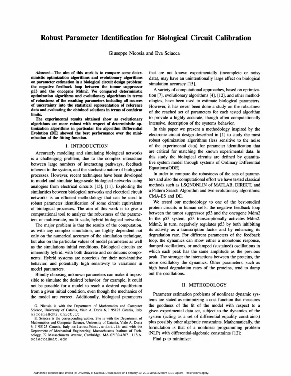
Fig. 1. Problem definition of the Optimization framework in BiologicalParameter Estimation

Authorized licensed use limited to: University of Catania. Downloaded on February 10, 2010 at 06:22 from IEEE Xplore. Restrictions apply.

from these simulations.

III. ALGORITHMS

In order to compare the robustness of the sets of param­eters and also the computational effort, the following threedeterministic methods have been considered.

LSQ The function LSQNONLIN of Matlab solves non­linear least-squares problems, including nonlineardata-fitting problems. In our case we use the al­gorithm with the default options of large scaleoptimization, which uses the subspace trust methodbased on the Levenberg-Marquardt [13] methodover Gauss-Newton algorithm to compute the de­creasing direction.

Direct Global search method that applies to Lipschitzcontinuous function and, after an initial implicitestimate of the Lipschitz constant chooses thepotentially optimal rectangles and resamples themacross their axis. Subsequently it divides theserectangles and proceed sampling and dividing untila stopping criteria is met [8]. This method exploitsthe estimation of Lipschitz constant to balanceglobal and local search and reaches quasi-globalsolution in large domain.

GPS Pattern Search algorithms [10] are known as Searchand Poll algorithms. In the search step, any finite setof mesh points can be evaluated. When the searchstep fails the algorithm calls the poll procedure thatconsists in evaluating the objective function at theneighboring mesh points to see if a lower functionvalue can be found.

We compared the results testing also two evolutionaryalgorithms:

CMA-ES The CMA-ES (Covariance Matrix AdaptationEvolution Strategy) [6] is an evolutionary algorithmfor difficult non-linear non-convex optimizationproblems in continuous domain. The CMA-ES is asecond order approach and estimates a covariancematrix within an iterative procedure. Adaptationof the covariance matrix amounts is similar tothe approximation of the inverse Hessian matrix.Restarts with increasing population size improvethe global search performance.

DE Differential Evolution (DE) was introduced byStorn and Price [16]. DE works as follow: aftera random initialization the objective function isevaluated and the following steps are repeateduntil a termination condition is satisfied. Eachindividual is updated using a weighted differenceof a number of selected parent solutions. If theoffspring replaces the parent only if it improvesthe fitness value, otherwise the parent is copied inthe new population. The crucial idea behind DEis this new scheme for generating trial parametervectors. DE generates new parameter vectors byadding the weighted difference vector between two

Mdm1..,Pf"

Nucleus

Cell

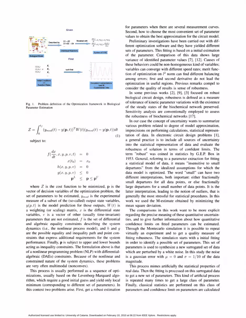
Fig. 2. Graphical model of the negative feedback loop between P53 andMdm2.

population members to a third member. If theresulting vector yields a lower objective functionvalue than a predetermined population member, thenewly generated vector replaces the vector withwhich it was compared. The comparison vectorcan, but need not be part of the generation processmentioned above. In addition the best parametervector is evaluated for every generation in orderto keep track of the progress that is made duringthe minimization process. Using Storn and Pricenaming convention we used the classical versionof DE DE/rand/I.

IV. CASE STUDY: A NEGATIVE FEEDBACK LOOP

The considered test case is the negative feedback loopbetween the tumor suppressor p53 and the oncogene Mdm2[14] which is one of the best-studied protein circuits in hu­man cells. In the p53 system, p53 transcriptionally activatesMdm2. Mdm2, in tum, negatively regulates p53 by both in­hibiting its activity as a transcription factor and by enhancingits degradation rate. For different parameters of the feedbackloop, the dynamics can show either a monotonic response,damped oscillations, or undamped (sustained) oscillations inwhich each peak has the same amplitude as the previouspeak. The stronger the interactions between the proteins, themore oscillatory the dynamics. Other parameters, such ashigh basal degradation rates of the proteins, tend to dampout the oscillations.

Figure 2 shows the graphical model of the negative feed­back loop between p53 and Mdm2.

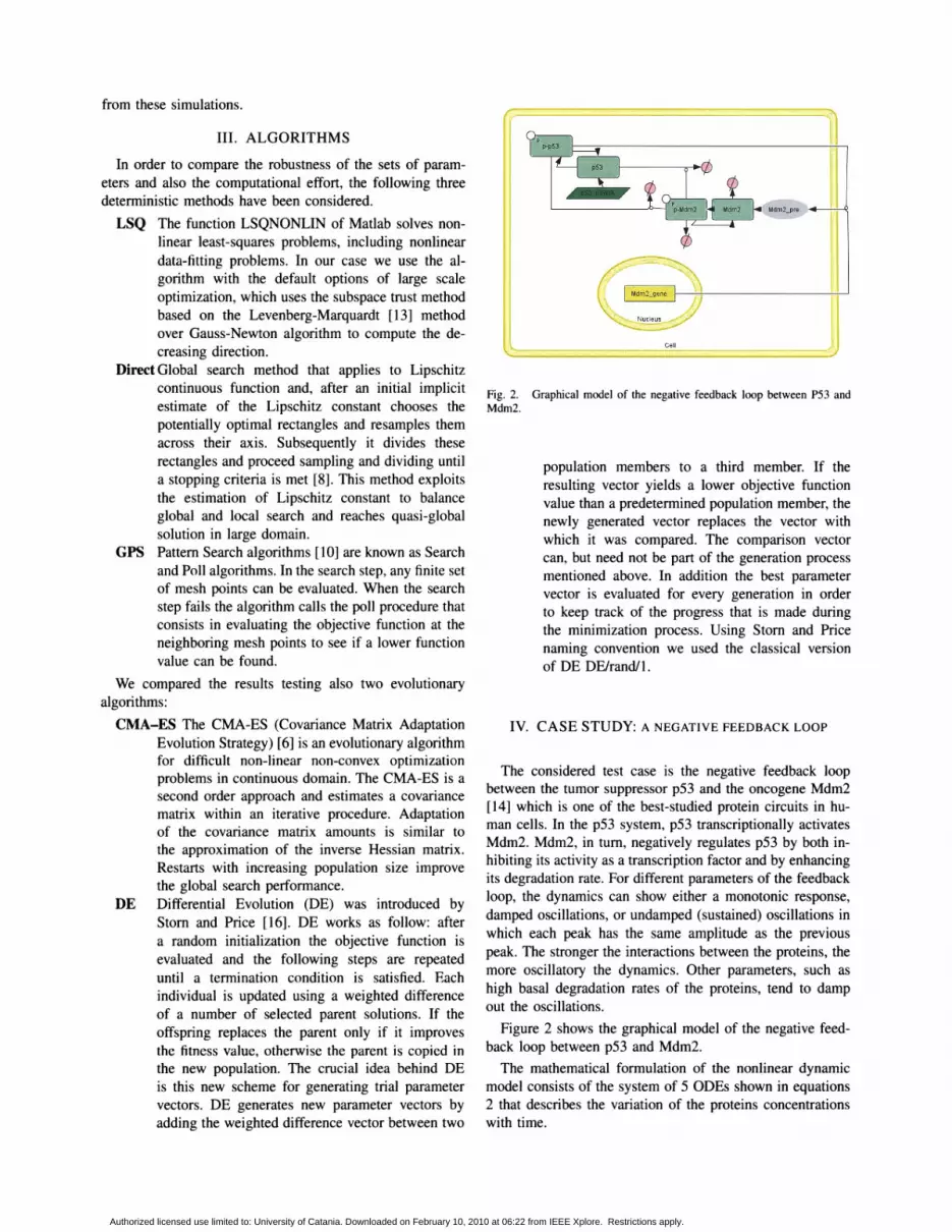
The mathematical formulation of the nonlinear dynamicmodel consists of the system of 5 ODEs shown in equations2 that describes the variation of the proteins concentrationswith time.

Authorized licensed use limited to: University of Catania. Downloaded on February 10, 2010 at 06:22 from IEEE Xplore. Restrictions apply.

Parameters Nominal Value

d[p53]dt

d[Mdm2]dt

d[p-p53]-d-t-

d[p-Mdm2]dt

kfi 0.9VI 4Kpl 2

kdpl 1kdl 8.5

Kdegl 0.1kd2 0.85

Kdeg2 0.01kf2 1.1kf3 0.8V2 0.8Kp2 0.2

kdp2 0.4kd3 0.08kd4 0.8

TABLE I

THE PARAMETERS OF THE MODEL AND THEIR NOMINAL VALUES.

From the biological point of view the above selectedparameters directly/indirectly control the steady state level ofp53, suggesting that, to maintain a stable p53 concentrationin the system, they are critical for proper cell response.

A. Results

These results show the best values obtained after per­forming 60 independent runs for each algorithm while theMontecarlo simulation used synthetic data set created addinga gaussian error with J.-l == 0 and a == 1/10 of data magnitudein the initial data set. All methods tackled use as terminationcondition the maximum number of objective function evalu­ations. In particular in this test case, the maximum numberof function evaluations has been fixed to 1000. The boundof each parameter was set to the same order of magnitudethat contains the reported values showed in Table I.

The tested algorithms demonstrated different degrees ofreliability in reaching the solutions over the all independentruns. For each method, after the Montecarlo simulation, wecalculated the percentage of success. Each success implied anidentification of a set of parameters which characterizes thebehavior of the curves (the variation of the concentrationsover the time) accurately with respect to the experimentaldata. Direct and DE showed 100% of success in the identi­fication of the parameters, PSearch and CMA had a 90% ofsuccess while LSQ only a 60%.

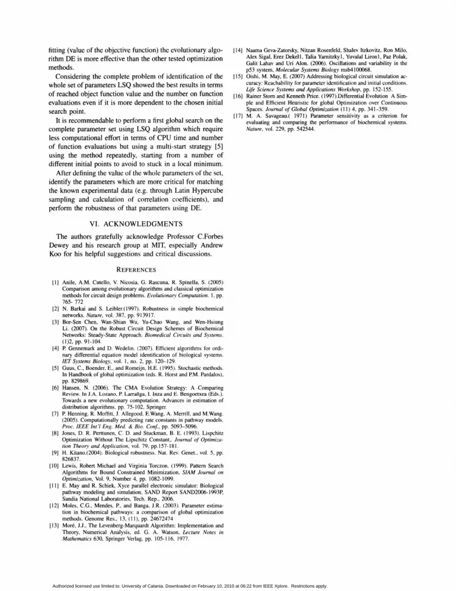
The LSQ method showed larger confidence limits inthe Montecarlo simulation for the parameters estimated inTable II as we can see through the standard deviation ofthe parameters. The most robust parameter are found byDE algorithm (first best algorithm) and Direct algorithmeven if Direct reaches a smaller value of the minimizedfunction slower than the other algorithms (see Figure 4). Theconfidence interval of the estimated parameters reached byDE and Direct algorithms are shown in Figure 3 in whichthe minimum, mean and maximum reached values are shownwhile the stars represent the nominal values.

In Table III are showed comparison among the testedoptimization algorithms on the mean value and standarddeviation of the minimized objective function Z during the

d[Mdm2_pre]dt

n m

Z == L L([Ypred(i) - Yexp(i)]j)2 (3)i=I j=I

where n is the number of data for each specie, m is thenumber of species, Yexp represents the known experimentaldata, and Ypred is the vector of states that corresponds to thepredicted theoretical evolution using the model with a givenset of the parameters.

To better assess the performance of the optimizationalgorithms for the solution of the inverse problem, pseudo­experimental data were generated by simulation from a set ofchosen parameters (to be considered as the true, or nominal,values) shown in Table I. Thus, pseudo-measurements ofthe concentrations of the species were the result of differentexperiments (simulations) in which their concentrations werevaried. These simulated data represent results of experimentswith the additional measurement noise.

In bold are showed the five parameters that were chosenfor the optimization because are critical in the calculation ofthe error between the simulated data and the known experi­mental data. This subset of parameters was identified throughLatin Hypercube sampling and calculating the correlationcoefficients with respect to the error residue.

- ~~'~~~I + kdp1· [p - p53] + kf1++ kdI· p53]· p-Mdm2]

p53 +kdegI

VI· [p53] kd 1 [p 53][p53J+kpI - p' - p +

kd2· [p-p53] .p-M dm2- [p-p53J+kdeg2

- ~~m~~~~2 + kdp2· [p - Mdm2] ++kf3· [Mdm2_pre] - kd3· [Mdm2]

kd4 [ Md 2] V2·[Mdm2]- . p - m + [Mdm2J+kp2 +-kdp2· [p - Mdm2]kf2 . [p - p53] - kf3 . [Mdm2_pre]

(2)The parameters involved in the mathematical formulation

of the problem are the following:kfl p53 translation rateVI Enzyme reaction rate for p53 phosphorylationKp1 Michaelis constant for p53 phosphorylationkdp1 p-p53 dephosphorylation ratekdI p-Mdm2 enzyme reaction rate for p53 degradationKdeg1Michaelis constant for p53 degradationkd2 p-Mdm2 enzyme reaction rate for p-p53 degrada-

tionKdeg2 Michaelis constant for p-p53 degradationkf2 Mdm2 transcription and translation ratekf3 Mdm2 post-translational modification rateV2 Enzyme reaction rate for Mdm2 phosphorylationKp2 Michaelis constant for Mdm2 phosphorylationkdp2 p-Mdm2 dephosphorylation ratekd3 Mdm2 degradation ratekd4 p-Mdm2 degradation rateIn our study the global optimization problem was stated

as the minimization of the following quadratic objectivefunction

Authorized licensed use limited to: University of Catania. Downloaded on February 10, 2010 at 06:22 from IEEE Xplore. Restrictions apply.

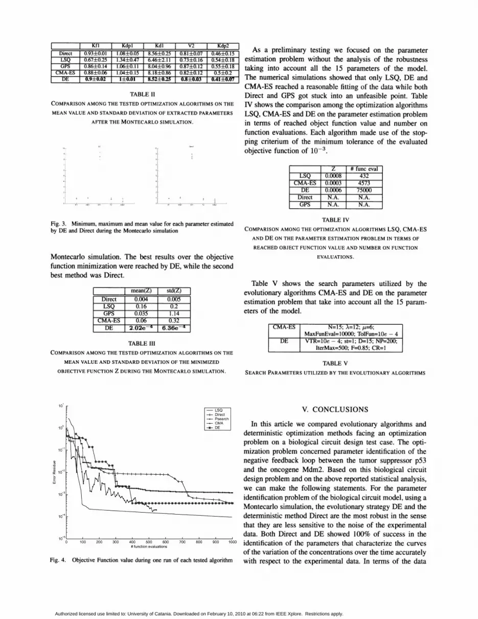
TABLE II

COMPARISON AMONG THE TESTED OPTIMIZATION ALGORITHMS ON THE

MEAN VALUE AND STANDARD DEVIATION OF EXTRACTED PARAMETERS

AFTER THE MONTECARLO SIMULATION.

DirectLSQGPS

CMA-ESDE

As a preliminary testing we focused on the parameterestimation problem without the analysis of the robustnesstaking into account all the 15 parameters of the model.The numerical simulations showed that only LSQ, DE andCMA-ES reached a reasonable fitting of the data while bothDirect and GPS got stuck into an unfeasible point. TableN shows the comparison among the optimization algorithmsLSQ, CMA-ES and DE on the parameter estimation problemin terms of reached object function value and number onfunction evaluations. Each algorithm made use of the stop­ping criterium of the minimum tolerance of the evaluatedobjective function of 10-3 .

Z # func evalLSQ 0.0008 432

CMA-ES 0.0003 4573DE 0.0006 75000

Direct N.A. N.A.

GPS N.A. N.A.

Fig. 3. Minimum, maximum and mean value for each parameter estimatedby DE and Direct during the Montecarlo simulation

Montecarlo simulation. The best results over the objectivefunction minimization were reached by DE, while the secondbest method was Direct.

TABLE IV

COMPARISON AMONG THE OPTIMIZATION ALGORITHMS LSQ, CMA-ES

AND DE ON THE PARAMETER ESTIMATION PROBLEM IN TERMS OF

REACHED OBJECT FUNCTION VALUE AND NUMBER ON FUNCTION

EVALUATIONS.

Direct 0.004 0.005LSQ 0.16 0.2

GPS 0.035 1.14CMA-ES 0.06 0.32

DE 2.02e .q 6.36e .q

TABLE III

COMPARISON AMONG THE TESTED OPTIMIZATION ALGORITHMS ON THE

MEAN VALUE AND STANDARD DEVIATION OF THE MINIMIZED

OBJECTIVE FUNCTION Z DURING THE MONTECARLO SIMULATION.

mean(Z) std(Z)Table V shows the search parameters utilized by the

evolutionary algorithms CMA-ES and DE on the parameterestimation problem that take into account all the 15 param­eters of the model.

CMA-ES N=15; A=12; 1-£=6;MaxFunEval=I0000; TolFun=10e - 4

DE VTR=10e - 4; st=l; D=15; NP=200;IterMax=500; F=0.85; CR=1

TABLE V

SEARCH PARAMETERS UTILIZED BY THE EVOLUTIONARY ALGORITHMS

10-5 '---_...1....-_-'--_--"--_--&...._..........._-""_---''---_'''--_''''''-------'

o 100 200 300 400 500 600 700 800 900 1000# function evaluations

Fig. 4. Objective Function value during one run of each tested algorithm

V. CONCLUSIONS

In this article we compared evolutionary algorithms anddeterministic optimization methods facing an optimizationproblem on a biological circuit design test case. The opti­mization problem concerned parameter identification of thenegative feedback loop between the tumor suppressor p53and the oncogene Mdm2. Based on this biological circuitdesign problem and on the above reported statistical analysis,we can make the following statements. For the parameteridentification problem of the biological circuit model, using aMontecarlo simulation, the evolutionary strategy DE and thedeterministic method Direct are the most robust in the sensethat they are less sensitive to the noise of the experimentaldata. Both Direct and DE showed 100% of success in theidentification of the parameters that characterize the curvesof the variation of the concentrations over the time accuratelywith respect to the experimental data. In terms of the data

Authorized licensed use limited to: University of Catania. Downloaded on February 10, 2010 at 06:22 from IEEE Xplore. Restrictions apply.

fitting (value of the objective function) the evolutionary algo­rithm DE is more effective than the other tested optimizationmethods.

Considering the complete problem of identification of thewhole set of parameters LSQ showed the best results in termsof reached object function value and the number on functionevaluations even if it is more dependent to the chosen initialsearch point.

It is recommendable to perform a first global search on thecomplete parameter set using LSQ algorithm which requireless computational effort in terms of CPU time and numberof function evaluations but using a multi-start strategy [5]using the method repeatedly, starting from a number ofdifferent initial points to avoid to stuck in a local minimum.

After defining the value of the whole parameters of the set,identify the parameters which are more critical for matchingthe known experimental data (e.g. through Latin Hypercubesampling and calculation of correlation coefficients), andperform the robustness of that parameters using DE.

VI. ACKNOWLEDGMENTS

The authors gratefully acknowledge Professor C.ForbesDewey and his research group at MIT, especially AndrewKoo for his helpful suggestions and critical discussions.

REFERENCES

[1] Anile, A.M. Cutello, V. Nicosia, G. Rascuna, R. Spinella, S. (2005)Comparison among evolutionary algorithms and classical optimizationmethods for circuit design problems. Evolutionary Computation. 1, pp.765- 772

[2] N. Barkai and S. Leibler.(1997). Robustness in simple biochemicalnetworks. Nature, vol. 387, pp. 913917.

[3] Bor-Sen Chen, Wan-Shian Wu, Yu-Chao Wang, and Wen-HsiungLi. (2007). On the Robust Circuit Design Schemes of BiochemicalNetworks: Steady-State Approach. Biomedical Circuits and Systems.(1)2, pp. 91-104.

[4] P. Gennemark and D. Wedelin. (2007). Efficient algorithms for ordi­nary differential equation model identification of biological systems.lET Systems Biology, vol. 1, no. 2, pp. 120-129.

[5] Guus, C., Boender, E., and Romeijn, H.E. (1995). Stochastic methods.In Handbook of global optimization (eds. R. Horst and P.M. Pardalos),pp. 829869.

[6] Hansen, N. (2006). The CMA Evolution Strategy: A ComparingReview. In l.A. Lozano, P. Larrafiga, I. Inza and E. Bengoetxea (Eds.).Towards a new evolutionary computation. Advances in estimation ofdistribution algorithms. pp. 75-102, Springer.

[7] P. Henning, R. Moffitt, 1. Allegood, E.Wang, A. Merrill, and M.Wang.(2005). Computationally predicting rate constants in pathway models.Proc. IEEE Int'l Eng. Med. & Bio. Con!, pp. 5093-5096.

[8] Jones, D. R. PerUunen, C. D. and Stuckman, B. E. (1993). LispchitzOptimization Without The Lipschitz Constant,. Journal of Optimiza­tion Theory and Application, vol. 79, pp.157-181.

[9] H. Kitano.(2004). Biological robustness. Nat. Rev. Genet., vol. 5, pp.826837.

[10] Lewis, Robert Michael and Virginia Torczon. (1999). Pattern SearchAlgorithms for Bound Constrained Minimization, SIAM Journal onOptimization, Vol. 9, Number 4, pp. 1082-1099.

[11] E. May and R. Schiek, Xyce parallel electronic simulator: Biologicalpathway modeling and simulation, SAND Report SAND2006-1993P,Sandia National Laboratories, Tech. Rep., 2006.

[12] Moles, C.G., Mendes, P., and Banga, J.R. (2003). Parameter estima­tion in biochemical pathways: a comparison of global optimizationmethods. Genome Res., 13, (11), pp. 24672474

[13] More, J.1., The Levenberg-Marquardt Algorithm: Implementation andTheory, Numerical Analysis, ed. G. A. Watson, Lecture Notes inMathematics 630, Springer Verlag, pp. 105-116, 1977.

[14] Naama Geva-Zatorsky, Nitzan Rosenfeld, Shalev Itzkovitz, Ron Milo,Alex Sigal, Erez Dekell, Talia Yamitzky1, Yuvalal Liron1, Paz Polak,Galit Lahav and Uri Alon. (2006). Oscillations and variability in thep53 system, Molecular Systems Biology msb4100068.

[15] Oishi, M. May, E. (2007) Addressing biological circuit simulation ac­curacy: Reachability for parameter identification and initial conditions.Life Science Systems and Applications Workshop, pp. 152-155.

[16] Rainer Stom and Kenneth Price. (1997).Differential Evolution A Sim­ple and Efficient Heuristic for global Optimization over ContinuousSpaces. Journal of Global Optimization (11) 4, pp. 341-359.

[17] M. A. Savageau.( 1971) Parameter sensitivity as a criterion forevaluating and comparing the performance of biochemical systems.Nature, vol. 229, pp. 542544.

Authorized licensed use limited to: University of Catania. Downloaded on February 10, 2010 at 06:22 from IEEE Xplore. Restrictions apply.