Robust output feedback control of nonlinear stochastic systems using neural networks

IEEE TRANSACTIONS ON NEURAL NETWORKS, VOL. 14, NO. 1, JANUARY 2003 103

Robust Output Feedback Control of NonlinearStochastic Systems Using Neural Networks

Stefano Battilotti, Senior Member, IEEE,and Alberto De Santis

Abstract—We present an adaptive output feedback controllerfor a class of uncertain stochastic nonlinear systems. The plant dy-namics is represented as a nominal linear system plus nonlineari-ties. In turn, these nonlinearities are decomposed into a part, ob-tained as the best approximation given by neural networks, plusa remaining part which is treated as uncertainties, modeling ap-proximation errors, and neglected dynamics. The weights of theneural network are tuned adaptively by a Lyapunov design. Theproposed controller is obtained through robust optimal design andcombines together parameter projection, control saturation, andhigh-gain observers. High performances are obtained in terms oflarge errors tolerance as shown through simulations.

Index Terms—Filtering (93E11, 93E20, 93D15, 93D21, 49K30,60H10), optimal control, robust stabilization, stochastic nonlinearsystems.

I. INTRODUCTION

I N modeling of dynamical systems, the stochastic frameworkis suitable for taking into account either randomly varying

system parameters or stochastic exogenous inputs. It is impor-tant in many practical situations to require, besides stability insome sense, some optimal and robustness performances, whichcan be usually described through a suitable cost functional.These performances may include tracking errors and physicalconstraints, due for example to control actuators or sensorswith limited range.

According to the existing literature (see [18]–[20], [22], [23]and the textbooks [15] and [21]), by stability it is usually meantthat

• the probability that the trajectory, stemming from,leaves an-ball around the origin goes to zero astendsto the origin;

• the trajectory, stemming from , goes asymptotically tozero almost surely.

This stability, usually known asstability in probability, is eitherlocal or global according to whether is in some (small)neighborhood of the origin or, respectively, it isany point of thestate space. In [15] Lyapunov-based conditions are given forguaranteeing stability in probability and require the solution ofpartial differential inequalities (PDIs). In [17] and [19], it hasbeen proved that a step-by–step algorithm (backstepping) canbe successfully implemented for solving globally these PDIs,whenever the state is available for feedback, while in [18], the

Manuscript received April 4, 2001; revised October 31, 2001 and April 12,2002. This work was supported by MURST under a grant from the Italian Min-istry of Scientific and Technological Research.

The authors are with the Dipartimento di Informatica e Sistemistica, 00184Rome, Italy (e-mail: [email protected], [email protected]).

Digital Object Identifier 10.1109/TNN.2002.806609

problem of global output feedback stabilization in probabilityis solved for a class of systems with output nonlinearities. Fordeterministic systems, the complexity and the conditions forsolving these PDIs can be weakened by relaxing the stabilityrequirements of the closed-loop system. In a deterministicsetting, semiglobal stabilizationwas introduced in [6] andrequires a local asymptotic stability of the closed-loop systemplus a region of attraction containing anya priori given com-pact set of the state space. The basic ingredients for achievingsemiglobal stability via output feedback arecontrol saturationsand high-gain observers[10], [11], [14]: Large values of theobserver gain guarantee that the error between the state andits estimate, generated by the observer itself, goes to zero“sufficiently fast,” while input saturations rule out destabilizingeffects such aspeaking[8], which is a phenomenon occurringwhen one is trying to force some state variables to zero as fastas possible causing an impulsive-like behavior of some others.

In this paper, we want to study the problem of stabilizing(in some probabilistic sense) the following class of nonlinearstochastic systems:

(1)

where is a Wiener process, is the con-trol, is the state, are the measurements,

are model uncertainties and nonlinearities, and

......

......

......

When (i.e., noiseless dynamics), the system (1) is thesame as the one considered in [1] with (i.e., no inputderivatives are taken into account).

By calling upon the neural-networks theory [2] for eachchoice of vector basis functions and , it is possibleto decompose the functions and as follows [29]:

(2)

where

(3)

1045-9227/03$17.00 © 2003 IEEE

104 IEEE TRANSACTIONS ON NEURAL NETWORKS, VOL. 14, NO. 1, JANUARY 2003

and and .The system

(4)

(i.e., system under nominal conditions plus best approximationof the nonlinear dynamics) can be understood as thenom-inal systemof (1). The model uncertainty is represented by

.Since the neural network approximations given in (2) are

valid for , one should ensure that the state trajectorystay inside for all at least with some guaran-

teed probability. This property is well-covered by the notionof -SPstability recently introduced in [4]. Given

, and some desired region of attraction andtarget set , this notion requires that the trajectories of theclosed-loop system, resulting from (1), with initial condition in

remain inside some compact set of the state space,eventually enter any given neighborhood of the target setin finite time and remain thereinafter with probability at least

. The numbers and arerisk margins: Thefirst one quantifies the risk of leaving with initial conditionin rather than getting close to the target, while the second onegives a risk margin for remaining close to the target. Ifand can be taken anya priori given compact set of the statespace and and any numbers in , our definition extendsto a stochastic setting the notion ofsemiglobal stabilizationasintroduced in [6], and in what follows, we will refer to this prop-erty assemiglobal stabilization in probability.

The values and are derived by solving the optimizationproblem (3). Typically, it is difficult to compute these vaules;however, by some off-line training, one can obtain “good ap-proximations” and of the optimal values and . Asa consequence, the nominal system can be written as

(5)

where and are on-line “estimates” of and , updated

through a suitable adaptive law, and and are

the estimation errors. The initial values of and may be setto and , respectively.

On the other hand, the functions and themselvesmay be known only up to some degree of accuracy so that it isimportant to take into account the presence of unmodeled dy-namics. To cope with these kinds of uncertainties, we definesuitable optimality and robustness criteria by means of some ad-missibility constraints. The optimality criteria are formulated interms of achieving either a guaranteed value or the minimumof some cost functionals, according to whether multiplicativeor additive noise is taken into account. These cost functionalspenalize the “distance” from a reference situation for which a“worst-case” controller is designed, and in the linear case, they

reduce to a standard quadratic cost (see [20] and [21] for com-parisons with other inverse optimal schemes for deterministicand stochastic nonlinear systems).

We show that the problem of finding a stabilizing controllerfor the class of systems (1) can be split into two lower dimen-sional problems: One is related to the case in which thestateis available for feedback(state feedback problem) and the otherto the possibility of constructing an observer for estimating thestate (output injection problem). This corresponds to anon-linear separationprinciple. First, we give a semiglobal in prob-ability backstepping design procedure for solving the state feed-back problem. While this procedure generalizes the classicalsemiglobal backstepping design for deterministic systems [14],it stands as apractical semiglobalversion of the correspondingglobal result proved in [17] and [19]. Finally, we give construc-tive tools for the observer design. It turns out thatcontrol satu-rationsandhigh-gain observersare instrumental to the controldesign exactly as in the case of [1]. In comparison with [1], wedo not take into account the presence of a zero dynamics; on theother hand, our control strategy has some important advantagesover [1] being robust against model uncertainties and randomnoise and optimal with respect to given performance indexes.We want to stress that the use of neural network approximationis important to better represent the nominal dynamics of (1) andsimplify the structure of what is to be considered as uncertainty.This is even more important in the case that and them-selves are known only up to some degree of accuracy.

II. NOTATIONS AND BASIC NOTIONS

First, we give some notations extensively used throughout thepaper.

• If denotes the 2–norm of any given vector, by ,we denote the induced 2–norm of any given matrix; by

, we denote the -norm of , i.e., ;let col be the column vector withth entryequal to .

• By (respectively, ), we denote the set ofpositive (respectively, negative) definite symmetric ma-trices; by , we denote the set of positivesemidefinite symmetric matrices; denotes the set ofpositive real numbers and the set of nonnegative realnumbers;

• For any vector-valued function , we denoteby (or ) its th component.

• For any given set , we denote by its closure andby its boundary; moreover, given and aset , by -neighborhoodof , we denote the set

;• For any sequence of sets ,

, and .It is easy to see that if , then thereexists such that for all . Similarly,if then there exists such that

for all .In the remaining part of this section, we shortly recall some

notions of stochastic processes, referring the reader for the basicconcepts to standard textbooks [25], [26]. We assume that the

BATTILOTTI AND DE SANTIS: ROBUST OUTPUT FEEDBACK CONTROL OF NONLINEAR STOCHASTIC SYSTEMS 105

reader is familiar with the basic notions of probability theoryand stochastic processes on a given probabilityspace (we assume that the probability space and allthe -algebras we consider are completed with all the subsets ofsets having null measure). We denote by the expectationand by the conditional probability (expecta-tion).

An important definition regards the notion ofMarkov time.Let be an increasing family of right continuous

-algebras contained in (filtration).Definition 2.1: A nonnegative random variable, ,

is called an Markov time if for all(i.e., it is adapted). If then is called astopping time.

A stochastic process is aWiener process(withrespect to ) if and

for . A stochastic processis a Markov process if for any collections

and

(6)

For the corresponding definitions in the multidimensional case,we refer to [27].

By astochastic differential equation, we mean the following:

(7)

with initial condition , where is aWiener process (with respect to ). The solution

of (7), whenever it exists, is a Markov process sat-isfying

(8)

almost surely (a.s.). The last integral is calledItô integral. It iswell known ([15]) that if

(9)

for all , , and in , with acompact set containing , then there exists an a.s. uniquestochastic process , sample continuous and satisfying (8)on , where and isthe Markov time (relatively to the -algebra generated by

) defined as the first time at which reachesthe boundary of [15].

An important property of solutions of stochastic differen-tial equations isregularity. Consider a sequence of increasingbounded domains , containing the origin, such that thedistance of the boundary from the origin goes to infinity astends to infinity, and let be the corresponding sequence

of Markov times. Since is nondecreasing, its limit ex-ists. We will say that the solution isregular if

a.s. Any regular solution can be uniquely (a.s.) extended forall .

Any solution of (7) satisfies the followingstrong Markovproperty[26]:

(10)

where is any given Markov time (relatively to the-algebragenerated by ). In (10), we can substitutewith its conditioned version as long is regular,i.e., it is a function , measurable for each fixed and aprobability for each fixed .

From now on, we will denote , if not otherwisestated, simply by . Given a (measurable) function

, define

(11)Proposition 2.1 (Dynkin’s Formula):Let a.s. The so-

lution of (7) satisfies on the following equa-tion:

(12)The integral appearing in the right-hand side of (12) is meant

in the sense that

where is the indicator function corresponding to theevent .

Also, we will use extensively the following (generalized)Chebyshev inequality

(13)

where , is real nonnegative, and is a givenrandom variable such that exists. Finally, we recallthe following fundamental formula of the differential calculus.

Proposition 2.2 (Itô Rule):Given a functionand if is a solution of (7), then

(14)

III. B ASIC ASSUMPTIONS ANDPROBLEM FORMULATION

The optimal and are contained in some known com-

pact sets. Off-line training allows to obtain good estimatesand of and , respectively. Correspondingly, one canselect some compact sets and in such a way that

and are comparable to

and , respectively.


Assume that and are convex hypercubes, i.e.,

(15)

and let . Moreover, let

(16)Similarly, define , and let . Let

.Assumption 1: for all and .Let and

. We consider nonlinearstochastic systems of the form (1), where , ,

, is an -dimensional Wiener process andrepresents model uncertainties and

nonlinearities. Moreover, for each sequence of real positiveextended numbers , with , we consider thefollowing class of controllers :

(17)

with (18), shown at the bottom of the page, where, ,

, , and are suitable sequences,with and , and , , aresuitable functions such that

(19)

(20)

for some and for . While , , are de-signed in such a way to counteract the destabilizing effects dueto large values of (peaking), accounts for possiblelimitations on the control (as an example, saturations of thecontrol actuators).

For the analysis of stability of the closed-loop system(1)–(17), we also define a class ofcandidate Lyapunov func-tions

(21)

where , and is a se-quence in , and are sequences of diagonalmatrices in and is a suitable (at least) ,positive definite and proper function such that

(22)

for all . Conditions (22) imply that over any compactset containing the origin anycandidate Lyapunov function isbounded from below and above by a quadratic functionandare is instrumental in enlarging the region of attraction of theclosed-loop system.

Next, we define someadmissibility constraintsfor the noisecoefficient and for the uncertainty term . For, define thefollowing compact sets:

(23)

Let , and be sequences in ,and , respectively. Define (24), shown at the bottom

of the page, where is the estimation error, and

(25)

Let be the class of functionssuch that for all for all , ,

and . Note that penalizes the distance offrom being the worst-case uncertainty

and, at the same time, from being a linear (parameterized by) function of and , representing a worst-case situation with

if and

if and

otherwise

(18)


respect to which the matrices and are designed. Notealso that accounts for additive uncertainty (i.e., ).

Let , , be a sequence in anda sequence in . Define

(26)

Note that penalizes the distance offrom a sum of quadratic

functions. Let be the class of functionssuch that , for

all , , and . Sinceand are compact sets, the admissibility constraintson and can be always met whenever and arelocally Lipschitz. Note also that accounts for additivenoise (i.e., ).

Let and be sequences in and re-spectively. Define as the class of triples of functions

, and satis-fying (19), (20), and (22) and such that

(27)

with diag , diag andis as in (17), for all , and

. The functions are typically designed to avoid thepeaking phenomenon, while is instrumental in enlarging theregion of attraction of the closed-loop system. Moreover, similarremarks can be repeated for the constants .

Finally, let

(28)

for some sequence in . Note that, by (22), (28)is nonnegative for all . Note also that penalizes thedistance from the situation for which is linear (i.e., quadraticLyapunov functions).

In what follows, we will refer to ,and as admissible functions. Moreover,any choice of , , , ,

, , , , , ,, , for which and

will be referred to asadmissible parameterization.Denote by

the trajectory of the closed-loop systemat time stemming from . Withsome abuse of notation, wherever there is no ambiguity,we will use instead of . Moreover, let

. We introduce a sequence of costfunctionals as follows:

(29)

Note that for any , and. Dividing by allows to cope with

the case of bothadditive and multiplicative noise, since other-wise for at least one would make the cost diverge.

The aim of this paper is to study under which conditions itis possible to modify the behavior of (1) in such a way that

achieves a guaranteed value and to obtain stability in some“stochastic” sense. To make the last point precise, let us give thefollowing definition.

(24)


Definition 3.1: Let andbe compact sets. The system (1) is said to be -sta-bilizable in probability (or -SP) if there exist a se-quence of admissible control laws , a sequence of com-pact sets and open sets of suchthat

1) there exists such that ;2) for each and

(30)

3) for each and

and

and

(31)

Note that the events in (30) and (31) are measurable by sep-arability and measurability (on the product-algebra ,where is the Borel -algebra on the line) of the processand being adapted to the -algebragenerated by .

The set gives theguaranteed region of attractionof theclosed-loop system , while represents thetarget set.From 1), it follows that there exists such that

for all . Property 2) is alocal prop-erty with respect to : For each -neighborhood of , thereexists sufficiently large for which the probability that the tra-jectories of the closed-loop system , starting from

, stay forever in is at least for all . Prop-erty 3) is a propertyin the largewith respect to : There ex-ists sufficiently large for which the trajectories ofstarting inside remain inside , eventually enter anygiven -neighborhood of the target set in finite time, and re-main thereinafter with probability at least for all

. The numbers and are givenrisk margins: the firstone quantifies the risk of leaving the compact set with ini-tial condition in rather than getting close to the target, whilethe second one gives a risk margin for remaining close to thetarget. Note also that 3) requires that .As it will be clear in Section IV, under the standard assump-tions of local existence and uniqueness a.s. of trajectories, eachMarkov time , conditioned tofor all , is always finite and as

as long as . In particular, thisimplies that, if , the trajectory approaches the originas .

The role of the risk margins, region of attraction, and targetset is peculiar of our setup and become unessential in the clas-sical definitions given in [15]. If ,and for all , Definition 3.1 recovers the clas-sical definition ofasymptotic stability in probability[15]. If inaddition , Definition 3.1 gives the notion ofasymptotic stability in probability in the large[15]. On the other

hand, if and can be taken anya priori givencompact set of and and any a priori givennumbers in , our definition gives a stochastic analog ofthe concept ofsemiglobal stabilization, as introduced in [6]. If

and can be taken anya priori given com-pact set of and and anya priori given numberin , Definition 3.1 extends to a stochastic setting the con-cept ofpractical stabilization.

All the above remarks can be straightforwardly extended tothe definition of stability in quadratic mean.

Remark 3.1:Definition 3.1 requires convergence of param-eter estimates to the optimal values in some probabilistic sense.However, if one is not interested in the parameter convergencethis definition should be slightly modified in 3) with regard tothe parameter estimation errorsby only requiring their bound-edness in probability. For sake of simplicity, in the rest of thepaper by -stability in probability, we will refer tothis situation, being only interested in the asymptotic stabilityof the state trajectories.

We are ready to formulate our problems.Nonlinear Stabilization in Probability with Guaranteed Cost

(NSPG): Let , , be compactsets of , , and and

given sequences in and , respectively. Findan admissible parameterization and suchthat

• (Guaranteed cost)along the trajectories of theclosed-loop systems

(32)

• (Stability) is -stable in probability.

IV. M AIN RESULTS

Let

(33)

Theorem 4.1:Assume that there exist an admissible param-eterization and such that

• state feedback (SF)

(34)

where

(35)

• output injection (OI)for all and

(36)


• risk margins (RM)if

(37)

and , a sequence of open sets of , aresuch that

(38)

then for each

(39)

(40)

for all and .Under the above assumptions, the controller (17) with

as in (35), and

(41)

solves NSPG with .Proof: Throughout the proof, unless otherwise stated, we

will omit and the arguments of and . Moreover, we canassume , where is such that forall (this is always possible by (38)).

Let as in Section III and . The closed-loopsystem is

(42)

where and are as in (17) and (25) and.

By (18) and (11)

(43)

with and.

Moreover

(44)Since , by (44) one has

(45a)

Using (36) and (45a), we have

(45b)

Moreover, for all by completing the square and using (34)

Proj (46)

Summing up together (45b) and (46), we conclude that

(47)

We are left with proving the following facts:

— , conditionally to the eventfor all ;

— for all;

— is stable in probability.First, we prove that , conditionally to the event

for all . By (47) and Dynkin’s formula foreach

(48)

for all . From (48), letting and since, we obtain .Next, we show that is stable in prob-

ability. Using (47) and (RM), the stability ofis a consequence of the following lemma, which can be

proved by suitably modifying the proof of lemma 5.1 in [5].


Lemma 4.1:The system (1) is -SP if thereexist a sequence of admissible control laws , a se-quence of (at least) , positive definite and proper functions

, a sequence of , positive definite functionsand open sets , ,

containing the origin, such that4) there exists such that ;,

where

5) for all , , and;

6) and

for each .Remark 4.1:We note that, as a consequence of (39), if

(49)

for each then the risk margin can be takenanynumber in, and anya priori given compact set can be included in

. Thus, (49), together with 4)–6) of Lemma 4.1, guaranteesemiglobal stabilization in probability.

On the other hand, if , then foreach

(50)

and the risk margin can be takenanynumber in . More-over, anya priori given compact set can be chosen as target setand (50), together with 4)–6) of Lemma 4.1, guaranteepracticalstabilization in probability.

Remark 4.2:The proof of Lemma 4.1 is based on aproba-bilistic invariance propertywhich extends to a stochastic setupthe following well-known property: If there exists a properand positive definite function such that,along the trajectories of , is definitenegative on and 4) and 6) hold, then any trajec-tory starting from stays forever in

, eventually enters any given-neighborhood of in fi-nite time and remains thereinafter. In our setting, this invarianceproperty corresponds to an event which occurs with probabilityat least . For the above reasons,and can bethought of asrisk margins. In the deterministic case, 6) corre-sponds to a precise geometric property of the level sets offorsufficiently large : one is that is contained in and theother is that is contained in some level set of whichis, on turn, contained in .

V. STOCHASTICSTABILIZATION WITH GUARANTEED COST FOR

FEEDBACK LINEARIZABLE SYSTEMS

The conditions of Theorem 4.1 do not provide any construc-tive procedure to find an admissible parameterization and thefunctions , and . In Sections V-A and B, we want tooutline algorithms for accomplishing this task for the class ofnonlinear stochastic systems (1), with andinvertible with no invariant zeroes, and norm-

bounded from above by a locally Lipschitz function ofand. Moreover, we will assume that and .

The case or as well as can betreated in a similar way but with more complicate calculations.

First, we give asemiglobal in probability backsteppingdesignprocedure for solving the state feedback problem (SF); then a re-cursive procedure to solve the filtering problem (OI) and (RM).Note that by assuming (A1), we can define as new control input

, and for simplicity, wedenote directly by . We also remark that Theorem 4.1 stillholds if one replaces (34) with

(51)

and

(52)

for some sequence of matrices and with. In order to keep the backstepping

algorithm as simple as possible, it is convenient to satisfy(51) rather than (34). Moreover, the choice of gives anadditional flexibility in the optimal control design.

Preliminarly, by [28], there exists a change of coordinatessuch that (1) reads out in the new coordinates

(53)

where

......

......

...

...

To simplify notations, we will omit the hats and denoteby .

A. Backstepping Design

The main result of this section is the following.Theorem 5.1:The system (53) is semiglobally stabilizable in

probability with guaranteed cost through a state feedback con-troller.

As a first step toward the proof of Theorem 5.1, rewrite (53)as

(54)


(55)

with and .Definition 5.1: We will say that

(56)

satisfies the property DI if there exist functions, ,

and such that , and for all

and one has

(57)

and

(58)

where

(59)

(60)

We have the following result, which roughly states that (55)satisfies the DI property in some new coordinates.

Lemma 5.1:There exists a function suchthat (56) satisfies DI, with

(61)

and and such that

(62)

Proof: For simplicity, throughout the proof and wheneverthere is no ambiguity, we omit the arguments of the functionsinvolved.

We have by our assumptions on

(63)

for all and such that , where denotesevaluated for and for some functions

and . We remark that can be chosenas function of only.

Pick such that

(64)

By the Îto rule

(65)

where

Pick , and such that ,and , and define

(66)

Find functions , ,and such that

• For all , such that , one has

(67)

with any function , and

(68)

• the following equality holds

(69)with

(70)


Let

, and . From (69)

(71)

Define

(72)

With our definitions

(73)

From (62), (64), (68), (70), (71) and (73), withand it follows that

(74)

for a suitably defined , with and shown in(75) at the bottom of the page. This proves (58).

Finally, from (63), (67), and (73), it follows that andfor all . This proves the admissibility of

and .We are ready to obtain Theorem 5.1. Note that each ,

and can be chosen in such a way that

(76)

which implies

(77)

for each . From (74), (77), and Theorem 4.1with (34) replaced by (51), since for all so that thesequence can be chosen arbitrarily, we conclude that(56) is semiglobally stabilizable in probability with arbitraryguaranteed costthrough the state feedback and

.Since is independent of , (76) is sufficient to conclude

that also the original system (53) issemiglobally stabilizable inprobability with arbitrary guaranteed costthrough state-feed-back, which proves Theorem 5.1.

B. Filter Design

In this section, we want to show that for some admissibleparameterization and also (OI) and (RM) canbe met for (55). First, let us prove (OI). Define

(78)

(75)


where is a function (to be specified later) suchthat .

In what follows, for sake of simplicity, we will omit the argu-ment when there is no ambiguity. We claim that there exists a

function such that and , defined in(78), solve (OI) with , for all functions

. Indeed, substituting in (OI), left and right-multiplyingby , and dividing both mem-bers by , we find out that solving (OI) amounts to satisfying

(79)

where are functions such that, , is symmetric and positive

semidefinite, and

......

......

...

It can be shown that there exists such that (79),and thus, (OI) holds for each and for some .Indeed, by continuity and since is controllableand is observable for sufficiently large, foreach sufficiently large and for some

(80)

Moreover, if , then . Finally, by stan-dard arguments, for large enough, it can be shown the ex-istence of some satisfying (79) and such that

and as . This proves(OI).

Next, we define an admissible pair .Choose if

ifotherwise (81)

ifotherwise (82)

where

(83)

(84)

where denotes the th component,, and and are as in (66).

Note that for all andthe functions , , are bounded and linear near the

origin. Moreover, the triple is admissible if thereexists a function such that for all

functions and , withbeing the entry (independent of) of .

In order to prove this, find a covering of, with

(85)

Pick such that for all.Note that since as , the term

can be rendered

positive over the set by choosing large enough.First of all, it is easy to see that there exists a function

such that holds for all functionsand .

Moreover, holds for all for someand for all . Indeed, since .

Thus, we have on . It follows that for anysuch by continuity, there exists such thatholds for all and for all functions . Since

is compact and , one cantake .

We are left with proving that there existssuch that holds for all and for allfunctions . On the other hand, this readily follows by theboundedness of and since

(86)

Pick .Finally, we will show how to satisfy (RM). Since

by (77) and the definition of , there exists a functionsuch that for all functions

(87)

for each , which proves (39). On the otherhand, by choosing properly the sequence , we canalso satisfy (40). We conclude that (OI)–(RM) hold as long as

is any function such that .By using Theorem 5.1, with (34) replaced by (51), and theabove results, we obtain the following theorem.

Theorem 5.2:Any system (54) and (55) is semiglobally sta-bilizable in probability with arbitrary guaranteed cost throughoutput feedback.


Fig. 1. Statex versus time in seconds.

We conclude with an example. Let us consider

(88)

It is known from [13] that (88) is not globally stabilizable by anycontinuous dynamic output feedback controller. However, weselect a guaranteed region of attraction

, and we approximate on the compact interval thefunction through a standard two-layer neural net-work

(89)

where the first layer consists of ten standard neurons (tanh) withinput weights

(90)

and , output weights

(91)

and biases

(92)

Fig. 2. Statex versus time in seconds.

Fig. 3. Controlu versus time in seconds.

Proceeding as in [1], one can show that (88) is stabilizablethrough a dynamic output feedback controller, based on controlsaturation and high gain observer, and with region of attractioncontaining . Assume that a Wiener process affects the secondequation of (88) as follows:

(93)

Using (2), we rewrite (93) as

(94)

Applying Theorem 5.2, we conclude that (93) is stabilizable inprobability with region of attraction containing. In Figs. 1–3,the evolution of the states and and the control of the


closed-loop system versusare plotted, starting from initial con-ditions , and with aGaussian random noise.

APPENDIX

Proof of Lemma 4.1

Throughout the proof, , where isthe Markov time (relatively to the -algebra generated by

) defined as the first time at which the trajectoryof (1) reaches the boundary of. By 4), we can assume ,with such that for all , and we fix any

.We have to show only 2) and 3) of Definition 3.1. As a con-

sequence of the Dynkin’s formula (with and), since is negative definite on

(95)

for all . By 4), for each , there existssuch that . By the Chebyshev inequality (with

, , ranging over therationals, and ), (95) and 5), we have

for some rational

(96)

for all and . Since, by for all

for some rational

for all and , by 6) and continuity ofwe conclude 2) of Definition 3.1.

To prove 3), we implicitly assume that . Firstof all, we prove

(97)

in the case that is regular, since otherwise, it istrivially true. Since is continuous on its domain, wehave for all andfor some . Directly from the Dynkin’s formula (with

and ), we obtain

(98)

Thus, by the Chebyshev inequality (with, ,

with ranging over the rationals, and)

(99)

Since as , from (99) and(sequential) continuity of , we obtain (97).

Next, we show that

(100)From the Dinkyn’s formula (with and as above) and since

is negative definite on , it follows that

(101)

By (101)

a.s. (102)

From (13) and (103)

(103)

By (103) and sinceby 6), we get

(104)By continuity of and since ,

, which along with (38)implies (39).

By (96) and (vi) and using the continuity of , foreach , there exists such that and

for some (105)

for all and .Finally, let denote the -algebra generated

by the events .

Since is a sub– -algebra of the one generated

by and by the strongMarkov property, for each and for all

for some

for some

(106)

which implies for each

(107)


REFERENCES

[1] S. Seshagiri and H. K. Khalil, “Output feedback control of nonlinearsystems using RBF neural networks,”IEEE Trans. Neural Networks,vol. 11, pp. 69–79, Jan. 2000.

[2] S. S. Haykin,Neural Networks: A Comprehensive Foundation. NewYork: MacMillan, 1994.

[3] S. Battilotti, “A unifying framework for the semiglobal stabilization ofnonlinear uncertain systems via measurement feedback,”IEEE Trans.Automat. Contr., vol. 46, pp. 3–16, Jan. 2001.

[4] S. Battilotti and A. De Santis, “A new notion of stabilization in proba-bility for nonlinear stochastic systems,” inMathematical Theory on Net-works and Systems. Perpignan, France: Perpignan, 2000.

[5] , “Stabilization in probability of nonlinear stochastic systems withguaranteed cost,” SIAM J. Contr. Optimization, 2002, to be published.

[6] A. Bacciotti, “Further remarks on potentially global stabilizability,”IEEE Trans. Automat. Contr., vol. 34, pp. 637–638, June 1989.

[7] J. C. Doyle, K. Glover, P. P. Khargonekar, and B. A. Francis, “Statespace solutions to standardH andH control problems,”IEEE Trans.Automat. Contr., vol. 34, pp. 831–847, May 1989.

[8] H. J. Sussmann and P. V. Kokotovic, “The peaking phenomenon and theglobal stabilization of nonlinear systems,”IEEE Trans. Automat. Contr.,vol. 36, pp. 424–439, Apr. 1991.

[9] P. Kokotovic and R. Marino, “On vanishing stability regions in nonlinearsystems with high gain feedback,”IEEE Trans. Automat. Contr., vol.AC-31, pp. 967–970, July 1986.

[10] F. Esfandiari and H. K. Khalil, “Output feedback stabilization of fullylinearizable systems,”Int. J. Contr., vol. 56, pp. 1007–1037, 1992.

[11] H. K. Khalil and F. Esfandiari, “Semiglobal stabilization of a class ofnonlinear system using output feedback,”IEEE Trans. Automat. Contr.,vol. 38, pp. 1412–1415, Sept. 1993.

[12] A. Saberi, Z. Lin, and A. Teel, “Control of linear systems with satu-rating actuators,”IEEE Trans. Automat. Contr., vol. 41, pp. 368–378,Mar. 1996.

[13] F. Mazenc, L. Praly, and W. P. Dayawansa, “Global stabilizationby output feedback: Examples and counterexamples,”IEEE Trans.Automat. Contr., vol. 22, 1994.

[14] A. R. Teel and L. Praly, “Tools for semiglobal stabilization by partialstate and output feedback,”SIAM J. Contr. Optim., vol. 33, pp.1443–1488, 1995.

[15] R. Z. Khas’minskii, Stochastic Stability of Differential Equa-tions. Rockville, MD: Sjithoff and Noordhoff, 1980.

[16] D. Hinrichsen and A. J. Pritchard, “StochasticH ,” SIAM J. Contr.Optim., vol. 36, pp. 1504–1538, 1998.

[17] Z. Pan and T. Basar, “Backstepping controller design for nonlinear sto-chastic systems under a risk sensitive cost criterion,”SIAM J. Contr.Optim., vol. 37, pp. 957–995, 1999.

[18] H. Deng and M. Krstic, “Output feedback stochastic nonlinear stabiliza-tion,” IEEE Trans. Automat. Contr., vol. 44, pp. 328–333, Feb. 1999.

[19] , “Stochastic nonlinear stabilization—Part I: A backstepping de-sign,” Syst. Contr. Lett., vol. 32, pp. 143–150, 1997.

[20] , “Stochastic nonlinear stabilization—Part II: Inverse optimality,”Syst. Contr. Lett., vol. 32, pp. 151–159, 1997.

[21] M. Krstic and H. Deng,Stabilization of Nonlinear Uncertain Sys-tems. London, U.K.: Springer-Verlag, 1998.

[22] P. Florchinger, “Lyapunov techniques for stochastic stability,”SIAM J.Contr. Optim., vol. 33, pp. 1151–1169, 1995.

[23] , “A universal formula for the stabilization of control stochastic dif-ferential equations,”Stoch. Anal. Applicat., vol. 11, pp. 155–162, 1993.

[24] M. Zakai, “On the optimal filtering of diffusion processes,”Z.Wahrscheinlich. Verw. Geb., vol. 11, pp. 230–243, 1969.

[25] E. Wong and B. Hajek,Stochastic Processes in Engineering Sys-tems. New York: Springer-Verlag, 1984.

[26] I. I. Gihman and A. V. Skorohod,Stochastic Differential Equa-tions. New York: Springer-Verlag, 1972.

[27] B. Øksendal,Stochastic Differential Equations: An Introduction WithApplications. New York: Springer Verlag, 1985.

[28] A. Saberi, Z. Lin, and A. Teel, “Control of linear systems with satu-rating actuators,”IEEE Trans. Automat. Contr., vol. 41, pp. 368–378,Mar. 1996.

[29] R. M. Sanner and J.-J. Slotine, “Gaussian networks for direct adaptivecontrol,” IEEE Trans. Neural Networks, vol. 3, pp. 837–863, June 1992.

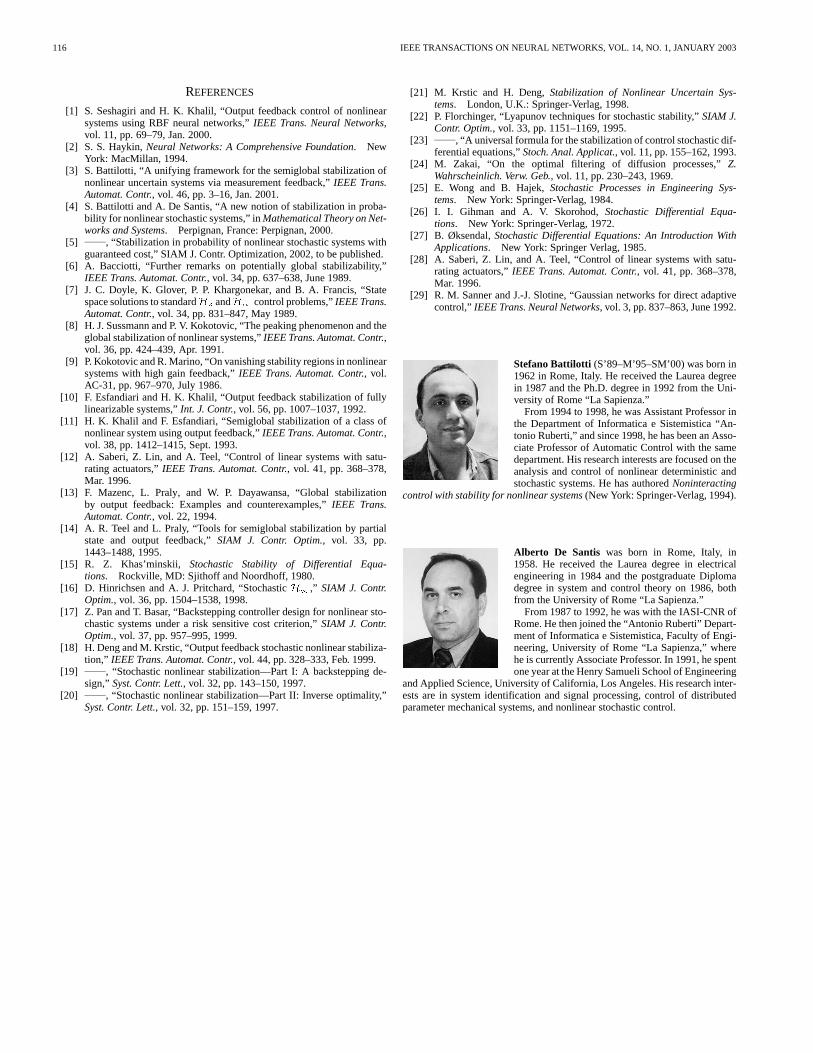
Stefano Battilotti (S’89–M’95–SM’00) was born in1962 in Rome, Italy. He received the Laurea degreein 1987 and the Ph.D. degree in 1992 from the Uni-versity of Rome “La Sapienza.”

From 1994 to 1998, he was Assistant Professor inthe Department of Informatica e Sistemistica “An-tonio Ruberti,” and since 1998, he has been an Asso-ciate Professor of Automatic Control with the samedepartment. His research interests are focused on theanalysis and control of nonlinear deterministic andstochastic systems. He has authoredNoninteracting

control with stability for nonlinear systems(New York: Springer-Verlag, 1994).

Alberto De Santis was born in Rome, Italy, in1958. He received the Laurea degree in electricalengineering in 1984 and the postgraduate Diplomadegree in system and control theory on 1986, bothfrom the University of Rome “La Sapienza.”

From 1987 to 1992, he was with the IASI-CNR ofRome. He then joined the “Antonio Ruberti” Depart-ment of Informatica e Sistemistica, Faculty of Engi-neering, University of Rome “La Sapienza,” wherehe is currently Associate Professor. In 1991, he spentone year at the Henry Samueli School of Engineering

and Applied Science, University of California, Los Angeles. His research inter-ests are in system identification and signal processing, control of distributedparameter mechanical systems, and nonlinear stochastic control.

Robust output feedback control of nonlinear stochastic systems using neural networks

Documents

Transcript of Robust output feedback control of nonlinear stochastic systems using neural networks