UNIVERSITY OF NAIROBI

School of Engineering

EVALUATING THE POTENTIAL OF OPENSOURCE

GEOSPATIAL DATA IN TOPOGRAPHICAL MAP

REVISION

Richard Odhiambo Owino

F56/35600/2019

A project report submitted to the Department of Geospatial and Space Technology in

partial fulfillment of the requirements for the award of the degree of:

Master of Science in Geographic Information Systems

August, 2021

ii

Abstract

Topographical maps are general reference maps that depict the planimetric position of

both natural and manmade features and the general terrain. In Kenya topographical map-

making dates back to the colonial period when the Directorate of Overseas Surveys was

mandated to carry out and regulate all the mapping activities in the country. These

topographical maps were produced and revised using the conventional method of

topographic map making. This process took a couple of years to conclude, it was labor-

intensive and the overall cost of the project was very high. This explains the slow pace

with which topographical map production and revision is being carried out in the country.

Geospatial advancements both software and hardware for data collection and processing

has greatly improved the quality of geospatial products and significantly reduced the

processing and production time. The continued improvement in the quality of satellite

imagery has seen many National Mapping Agencies Cross the world use satellite imagery

as an alternative source of data in compilation and revision of topographical maps. In

Kenya SPOT high resolution satellite images was used in 1996 to revise the 8th edition of

SK topographical map sheet Numbers: 148/1, 148/2, 148/3 and 148/4 covering the general

area of Nairobi. Developments in web technology have had a great contribution in the

field of geospatial and have continued to evolve to improve map user’s experience. Web

2.0 which allows users to create and share content online has led to the general growth of

crowd-sourced data and Volunteered Geographic Information in the geospatial sector.

National Mapping agencies across the world are putting in place systems to take advantage

of these developments.

This study aimed to evaluate the potential of Opensource geospatial data in topographical

map revision. Planimetric and elevation data quality specifications required for the

revision of SK topographical map at scale 1:50,000 was reviewed. Vector datasets from

OpenStreetMap were downloaded and assessed in terms of geometric accuracy, attribute

accuracy, and completeness. The research has provided means by which incompleteness

in the OSM data can be addressed using open-source satellite imagery available in OSM.

OSM imagery has also been used to visually validate the geometric accuracy, attribute

accuracy and completeness of the OSM data. The roads, building and vegetation datasets

were identified for evaluation. After evaluation process it was clear that only the roads

dataset met the data quality requirements needed for the compilation or revision of SK

topographical map at scale 1:50,000. The elevation dataset derived from SRTM V3 was

also evaluated and found to be suitable for revision of Nairobi topographical map sheet

No. 148/4. Cartographic processes of generalization and symbolization were then applied

to the vector data and this was used to present the open-source source datasets that met

the standards required for SK topographical map revision.

iii

…………………….…… …………….…………

Dr. D.N. Siriba Date

…………………….…… …………….…………

Richard Odhiambo Owino Date

Declaration of Originality

I, Richard Odhiambo Owino, hereby declare that this project is my original work. To the

best of my knowledge, the work presented here has not been presented for a degree in any

other Institution of Higher Learning.

This project has been submitted for examination with our approval as university

supervisors.

01.09.2021

iv

Acknowledgement

Many people have assisted me in developing the ideas for this research and I would like

to give them credit.

First and foremost, I would like to thank the University of Nairobi for allowing me to

pursue a

Degree of Master of Science in Geographic Information Systems, in the Department of

Geospatial

and Space Technology. Additionally, I would like to thank the departmental staff for

helping me during the years of my study.

Secondly, I wish to place on record my heartfelt and sincere thanks to my supervisors, Dr.

D. N. Siriba, who were always available for consultation. His contributions of time and

ideas made my work to be productive and stimulating.

I am also indebted to Mr. Abubakar, a cartographer at Survey of Kenya, who has offered

to share his experience in topographical map making.

A heartfelt thanks to my supportive and wonderful family members, for their constant and

unconditional support and encouragement during the period of taking this degree.

v

Table of Contents

Abstract .......................................................................................................................................... ii

Declaration of Originality ............................................................................................................. iii

Acknowledgement ........................................................................................................................ iv

Table of Contents ........................................................................................................................... v

List of Tables .............................................................................................................................. viii

List of Figures ............................................................................................................................... ix

List of Abbreviations ..................................................................................................................... x

CHAPTER 1: INTRODUCTION .......................................................................................... 1

1.1 Background ...................................................................................................................... 1

1.2 Problem Statement ........................................................................................................... 3

1.3 Objective .......................................................................................................................... 4

1.4 Research Matrix ............................................................................................................... 5

1.5 Justification of the study .................................................................................................. 6

1.6 Scope of Work ................................................................................................................. 6

1.7 Organization of Report ..................................................................................................... 6

CHAPTER 2: LITERATURE REVIEW ............................................................................... 7

2.1 Topographical Mapping ................................................................................................... 7

2.2 Data Collection Techniques for Topographical Mapping ................................................ 8

2.2.1 Field Sketching ............................................................................................................. 8

2.2.2 Conventional Ground surveying Methods .................................................................... 8

2.2.3 Aerial Photogrammetry ................................................................................................. 8

2.3.1 Satellite Imagery ........................................................................................................... 9

2.3.2 Point cloud by Light Detection and Ranging (LiDAR) surveys ................................... 9

2.5 Data Processing Techniques for Topographical Mapping ............................................... 9

2.2.4 Stereo Photogrammetry ................................................................................................. 9

2.2.4 Digital Photogrammetry Workstation (DPW)............................................................... 9

2.6 Emerging Trends in Topographical Mapping ................................................................ 10

2.6.1 Unmanned Aerial Vehicles ......................................................................................... 10

2.6.2 Volunteered Geographic Information ......................................................................... 11

2.6.3 Legal Framework Governing VGI .............................................................................. 11

2.7 Collaborative Mapping Projects ..................................................................................... 11

2.7.1 Wikimapia ................................................................................................................... 11

vi

2.7.2 OpenStreetMap ........................................................................................................... 12

2.7.3 OSM Vector Layer ...................................................................................................... 12

2.7.4 OSM Imagery Layer ................................................................................................... 13

2.8 Global Digital Elevation Models ................................................................................... 14

2.9 Sampling ........................................................................................................................ 14

2.10 Cartographic Process .................................................................................................... 15

2.10.2 Technologies ............................................................................................................. 15

2.10.3 Generalization and Symbolization ............................................................................ 15

2.11 Coordinate System ....................................................................................................... 16

2.12 Accuracy Standards ...................................................................................................... 17

2.13 Summary of Literature Review .................................................................................... 19

CHAPTER 3: MATERIALS AND METHODS .................................................................. 20

3.1 Methodology .................................................................................................................. 20

3.2 Study Area...................................................................................................................... 21

3.3 Requirements ................................................................................................................. 22

3.3.1 Software and Hardware Requirements ........................................................................ 22

3.3.2 Data Requirements ...................................................................................................... 22

3.4 Map Key Components of a Topographical Map ............................................................ 22

3.4.1 Map Details ................................................................................................................. 22

3.4.2 Map Scale .................................................................................................................... 22

3.4.3 Map Series ................................................................................................................... 22

3.4.4 Map Edition ................................................................................................................. 22

3.4.5 Sheet Name ................................................................................................................. 23

3.4.6 Sheet Number .............................................................................................................. 23

3.4.7 Symbol Legend ........................................................................................................... 23

3.4.8 Administrative index ................................................................................................... 23

3.4.9 Map Datum and Projection ........................................................................................ 23

3.5 Map Accuracy ................................................................................................................ 23

3.5.1 Graphical Resolution ................................................................................................... 23

3.5.2 Graphical National Map Accuracy Standards ............................................................. 24

3.6 Vector Datasets .............................................................................................................. 24

3.7 Aerial Photograph Accuracy .......................................................................................... 25

3.8 Elevation Datasets .......................................................................................................... 25

vii

3.9 Selecting Sample Area ................................................................................................... 25

3.10 OSM Data Quality Assessment .................................................................................... 27

3.10.1 Geometric accuracy ................................................................................................... 27

3.10.2 Attribute accuracy ..................................................................................................... 27

3.10.3 Completeness ............................................................................................................ 27

3.10.4 Assessing the Accuracy of OSM data ....................................................................... 27

3.11 Assessing the Accuracy of SRTM ............................................................................... 27

3.12 Cartographic Process .................................................................................................... 28

CHAPTER 4: RESULTS AND DISCUSSION ................................................................... 29

4.1 OSM Data Accuracy Analysis ....................................................................................... 29

4.1.1 Westlands .................................................................................................................... 29

4.2 Elevation Data Quality Assessment ............................................................................... 29

4.3 Addressing the Incompleteness of OSM data ................................................................ 31

4.4 Data Reclassification and Styling .................................................................................. 31

4.5 Testing the Accuracy Open-Source Data on the Final Maps ......................................... 32

CHAPTER 5: CONCLUSION AND RECOMMENDATION ............................................ 34

5.1 Conclusion ..................................................................................................................... 34

5.2 Recommendation ........................................................................................................... 35

References .................................................................................................................................... 36

APPENDICES ............................................................................................................................. 38

Appendix B: 1:50,000 Topographical Map Template ................................................................. 46

Appendix C: Contours Reproduction Material ............................................................................ 46

Appendix D: Roads and Contours Displayed on 1:50,000 Topographical Map Template .......... 46

viii

List of Tables

Table:1.1 Research Matrix ............................................................................................................. 5

Table 2.1 OSM tools for check data accuracy ............................................................................. 13

Table 2.2: Maxar Satellite Images ............................................................................................... 13

Table 2.3: Characteristics of GDEM ............................................................................................ 14

Table 2.4: MGRS Precision ......................................................................................................... 17

Table 2.5: Map Scale and its Allowable error .............................................................................. 18

Table 2.6: Map Scale and its Allowable error .............................................................................. 18

Table 2.7: Map scale and required minimum imagery accuracy ................................................. 19

Table 3.1: Software and hardware requirements .......................................................................... 22

Table 3.2: Data requirements ....................................................................................................... 22

Table 3.3: Datum Parameters ....................................................................................................... 23

Table 3.4 Layers that constitute a 1:50,000 topographical map ................................................... 24

Table 3.5 Satellite Resolution ...................................................................................................... 25

Table 3.6: Topographical map features to be analyzed for accuracy ........................................... 27

Table 3.7: Topographical map features to be analyzed for accuracy ........................................... 28

Table 4.1: Topographical map features analysis results for Westlands ....................................... 29

Table 4.2: Contour line value and corresponding SRTM cell values .......................................... 30

Table 4.3: OSM data reclassification ........................................................................................... 32

Table 4.4: SK data and OSM data comparison ............................................................................ 33

Topographical map features analysis results for Industrial Area ................................................. 38

Industrial Area Sample Area ........................................................................................................ 38

ix

List of Figures

Figure 1.1: Area Covered by Topographical maps at scale 1:50,000 ................................ 2

Figure 1.2: Sheet History of Leganishu ............................................................................. 3

Figure 2.1: Map revision workflow ................................................................................... 7

Figure 2.2: Flight plan for Aerial Photography ................................................................. 8

Figure 2.3: DPW work flow ............................................................................................ 10

Figure 2.4: Wikimapia collaborative map ....................................................................... 12

Figure 2.5: OSM collaborative map ................................................................................ 13

Figure 2.7: Methods of sampling 1 .................................................................................. 15

Figure 2.8: Generalization ............................................................................................... 16

Figure 2.9: MGRS Coordinate System ............................................................................ 17

Figure 3.1: Methodology ................................................................................................. 20

Figure 3.2: Study Area ..................................................................................................... 21

Figure 3.3: Sample areas .................................................................................................. 26

Figure 4.1: Westlands Sample Area ................................................................................ 29

Figure 4.2: Contour lines overlaid on SRTM .................................................................. 30

Figure 4.3: Westlands Sample Area before and after vectoring more features from sat

imagery ............................................................................................................................ 31

Figure 4.4: MGRS coordinate format reading guide ....................................................... 33

x

List of Abbreviations

OSM OpenStreetMap

GDEM Global Digital Elevation Model

GIS Geographic Information System

DOS Directorate of Overseas Survey

VGI Volunteered Geographic Information

LoD Level of Details

NMA National Mapping Agency

DEM Digital Elevation Model

AW3D30 ALOS World 3D - 30m

ALOS Advanced Land Observing Satellite

TanDEM-X TerraSAR-X add-on for Digital Elevation Measurement

SAR Synthetic-Aperture Radar

GPS Global Positioning System

SK Survey of Kenya

CAD Computer Aided Design

CE90 Circular Error at the 90th Percentile

RMSE Root Mean Square Error

USGS United States Geological Survey

1

CHAPTER 1: INTRODUCTION

1.1 Background

A topographical map is a two-dimensional accurate and elaborate representation of both natural

and man-made features on the earth’s surface. Through a combination of contour lines, colors,

symbols, labels, and other graphical representations, topographical maps portray the shapes and

locations of both natural and man-made features. In order to be useful, topographical maps must

show sufficient information on a map size that is convenient to use. This is accomplished by

selecting a map scale that is neither too large nor too small and by enhancing the map details

through the use of symbols and colors.

In Kenya topographical mapping dates back to the colonial period where Directorate of Overseas

Surveys (DOS) was responsible for all the mapping activities in Kenya. These functions were later

transferred to Survey of Kenya (SK). Survey regulations require that topographical mapping be

done at least after every five but this has not been possible due to various reasons key among them

being limited budgetary allocation to the Topographical mapping section.

Survey of Kenya has been involved in a number of projects aimed at producing new or updating

topographical maps of scale 1:50,000, 1: 100,000 and 1:250,000. The success of these efforts has

been to a limited extent and this can be seen in the fact that of the 845 topographical maps at scale

1:50,000 required to cover the whole country yet only 504 topographical maps had been done by

2017. This is clearly illustrated in figure 1.1.

This short fall is mainly attributed to the traditional conventional map making technology and

processes that are labor intensive and inefficient. Over reliance on commercial off the self-software

is also a factor that has been impacting negatively on effort to revise the old topographical maps.

National Mapping Agencies across the world have their policies and guidelines on how frequent

topographical map revision exercise should be carried out. In the USA, the United States

Geological Survey (USGS) updates the US topographical maps after every three years (Müller &

Seyfert, 2000). Likewise in Finland the topographical map revision exercise is done after every 5-

10 years period (Jakobsson, 2006). The National Mapping Agency of Brazil does not follow any

cycle in updating of the topographical maps but on average it’s after every 29 years (Sluter &

Camboim, 2009). Currently, Kenya Topographical map revision exercise is done on a need basis

and does not follow any known cycle this is mainly because of the cost involved in the whole

process. These challenges can be overcome by taking advantage of the availability of open-source

geospatial data that is of relatively good quality and the advancement in technology that have

simplified whole process of topographical map making.

There has been tremendous development in the both hardware and software used in the field of

geospatial. This has greatly reduced human resource required and the time taken to successfully

complete a topographical map revision exercise. The use of high-resolution satellite images in

topographical mapping is generally cost effective and has significantly reduced the production

time of the maps. High resolution satellite images offer a wide geographical coverage and short

revisit period making it more suitable for production of new topographical maps and revision of

the old ones at both medium and small-scale.

The Internet has also witnessed tremendous growth with web 2.0 allowing users to create and share

content. Web 2.0 enables the creation and sharing of interactive web maps and this can be used to

generate the required vector data for topographical map revision. OpenStreetMap, Tracks4Africa,

the Southern African Bird Atlas Project.2 and Wikimapia are some of the collaborative mapping

2

projects that are involved in the creation of web maps using crowd sourcing of volunteered

geographic information.

This research focused on Nairobi Topographical sheet 148/4 that was last revised in 1996 through

the partnership of SK and the French National Mapping agency. The French government provided

SPOT satellite imagery dated 1994 that was used in this exercise. The map history indicates that

it was first produced in 1969 before a map revision exercise was carried out in 1971 and 1973.

Figure 1.1: Area Covered by Topographical maps at scale 1:50,000

3

1.2 Problem Statement

Traditionally, the process of topographical mapping entailed the acquisition of aerial photography,

fieldwork to establish ground control points, photo interpretation, the application of

photogrammetry to create stereo compiled manuscript, employment of cartography for final

symbolization, editing, color separation, production and lithographic reproduction from the color

separation (Usery, et al., 2018). This process was generally expensive and time-consuming. Most

of these processes listed above are employed in topographical map revision, making it time-

consuming and expensive. This explains why most of the medium-scale and large-scale

topographical maps were last revised in the 60s, 70s and 80s. Figure 1.2 illustrates the sheet history

of the Leganishu topographical map (158/2), The first edition was produced in 1959 and the latest

map revision exercise was done in 1961. This has been the case in most parts of country with the

Northern and North Eastern parts of the country not covered by topographical maps at scale

1:50,000.

This research attempts to evaluate the extent to which open sources of geospatial data can be used

in the revision of topographical maps without negatively affecting the map user.

Figure 1.2: Sheet History of Leganishu

4

1.3 Objective

Main Objective

• The main objective is to evaluate the potential of open-source geospatial data in topographical

map revision.

Specific Objectives

1. Identify all the vector layers that constitute a SK topographical map

2. Review the data quality specification needed in the production of basic topographical maps

3. Evaluate the accuracy of the various layers from Open data sources that will used in map

revision within the study area.

5

1.4 Research Matrix

Table:1.1 Research Matrix

SNO. OBJECTIVE RESEARCH QUESTION

METHODOLOGY DATA EXPECTED OUTPUT

1. Identify all the vector features that constitute a topographical

What are the vector layers features that constitute a topographical map?

Get the required layers from existing topographical maps

Topographical map at scale 1:50,000.

List of all features that will be required to revise topographical map at scale 1:50,000

2. Identify the OSM layers that will be used in map revision.

What are the OSM layers that will be used in map revision?

From the downloaded OSM data identify the layers that are accurate and complete.

Downloaded OSM layers.

OSM data that has been validated in terms of accuracy and completeness.

3. Accuracy assessment

What is the Geometric accuracy, Attribute accuracy and level completeness Open-source data?

Identify sample areas within the area of study and get coordinates of a feature from OSM data and from the ground.

OpenStreetMap data GPS points

Analysis report on the degree of closeness of coordinates of the two datasets.

Are the attributes given to the OSM features, correct?

Comparing the OSM attribute of the sampled features with attributed from field data collection

OpenStreetMap data. GPS points with attribute.

A comparison report of OSM attributes and attributed from field data collection

Did the OSM data capture all the features of a given of a given theme?

Using a satellite image to digitize all features of a given theme and comparing with that of OMS data within the sample area.

Satellite images OSM data

Analysis report on number of features obtained by digitizing a satellite image and that of OSM data for the same area and theme.

6

1.5 Justification of the study

Nairobi topographical map sheet number 148/4 was last partially revised in 1994 using SPOT

satellite imagery data and the map published in 1996. Before that, there were efforts in 1971 and

1973 to revise the map that was first produced in 1969. According to the Survey requirement,

topographical maps should be updated after every five (5) years. Achieving this has always been

a problem due to the limited resources allocated to the department. Nairobi and its environs have

witnessed tremendous growth over the years and the current SK topographical map sheet number

148/4 is not a true representation of the area it covers.

Web 2.0 which allows for the creation and sharing of content through the web has led to the growth

of collaborative mapping projects such as Wikimapia and OpenStreetMap. The success of OSM

has made it possible to have vector data of different features covering most parts of the world. This

data can be checked for accuracy and corrections are done before it is used in the production of

topographical maps. Availability of high-resolution satellite imagery in OSM provides a platform

from which additional vector data can be extracted and be used in the production of topography.

This research combined these open-source geospatial developments in an effort to revise Nairobi

topographical maps sheet number 148/4 at a scale of 1:50,000.

1.6 Scope of Work

The scope of work defined here is meant to ensure the objectives of this research which are outlined

above are efficiently achieved leading to the evaluation of the potential of opensource geospatial

data topographical map revision. The research will assess the geometric accuracy, attribute

accuracy and completeness of OSM data and will focus on roads, buildings and vegetation

features. The project will use high-resolution satellite imagery provided by OSM to address any

gaps realized in OSM vector layers. Elevation data that will be used in the map revision exercise

will be generated from STRM. The vector data will then be generalized and symbolized and this

will presented on a 1:50,000 topographical map template. This research will greatly benefit from

the cartographic process in displaying and assessing the accuracy open-source data, but the scope

of the research will not cover the cartographic process in detail.

1.7 Organization of Report

Chapter One: This chapter will introduce the research topic by highlighting the problems

currently faced in topographical map revision. Using the research matrix this chapter will explain

how the research objectives will solve the map revision challenges.

Chapter two: The emerging trends in topographical map revision is discussed in this chapter.

Collaborative mapping projects and SRTM accuracy in relation to topographical mapping is

addressed.

Chapter Three: The methods and technologies that will be used to assess the quality of the OSM

data are presented in this chapter. The use of satellite imagery available in OSM to address the

incompleteness realized in the OSM data was applied.

Chapter Four: This chapter discusses the results of the accuracy assessment of the OSM data and

also discuss how the shortcoming of the OSM vector data using high-resolution satellite imagery

provided by OSM.

Chapter Five: Based on the research findings, conclusions are drawn and recommendations

proposed.

7

CHAPTER 2: LITERATURE REVIEW

2.1 Topographical Mapping

Mapping discipline has undergone a great evolution in both methodologies and technologies used

ever since it was first applied. Surveying techniques required for topographical map production

have developed to include the use of aerial photographs and improvement in cartographic map

production with color printing to enable topographic maps to be regarded as a great achievement

in cartography (Jervis, 1936). There has been advancement in all stages of mapping, from data

acquisition, data processing, cartography, product generations and dissemination platforms as well

as advancements in areas of application of the maps. Figure 2.1 below show the various processes

involved in the revision of a topographical map.

Figure 2.1: Map revision workflow

Data collection:

• Establishing of Ground Control Points

• Data collection through satellite images and aerial photographs

• Ground truthing

Data Processing:

• Orthorectification, Pansharpening and Georefrencing of images

• Processing of Ground truthing data

Production:

• Change detection

• Map revison

• Map production

8

2.2 Data Collection Techniques for Topographical Mapping

2.2.1 Field Sketching

Map sketching was done using an individual’s geographic ability to interpret locations of features

relative to each other. Field sketching involves data collection, processing and cartographic map

production process that results in a ready to use map. However, maps produced were not to scale

and lacked spatial accuracy. According to (Green, 1998) in a field sketching exercise what is

important is the ability to observe and record geographical (physical, human and environmental)

and not artistic skills.

2.2.2 Conventional Ground surveying Methods

These are surveying techniques employed to determine the latitude, longitude and height or

elevation of a few identifiable points such as hilltops, stream tributary intersections and others with

precise instruments for the time (Usery, et al., 2019). Feld sketching to fit both the visual image of

the landscape and surveying results was done to the rest of the terrain. Optical surveying

instruments, aneroid barometers, and chains for horizontal distance measurement were the

instruments used in this process. Significant geographic and cartographic skills and time to

interpret the terrain and its cultural adaptations for the production of an effective and accurate map

were very important in this method. The advancements in the field surveying methods brought

better instruments including levels, alidades, theodolites, steel tapes, electronic measuring devices

which have played a great role in the field of surveying.

2.2.3 Aerial Photogrammetry

Photogrammetry is the art, science, and technology of obtaining reliable information about

physical objects and the environment through processes of recording, measuring, and interpreting

photographic images and patterns of recorded radiant electromagnetic energy and other

phenomena ( McGlone, et al., 2004).

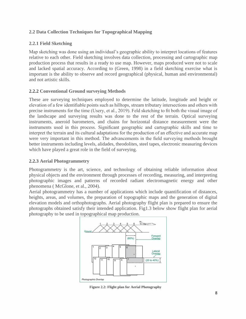
Aerial photogrammetry has a number of applications which include quantification of distances,

heights, areas, and volumes, the preparation of topographic maps and the generation of digital

elevation models and orthophotographs. Aerial photography flight plan is prepared to ensure the

photographs obtained satisfy their intended application. Fig1.3 below show flight plan for aerial

photography to be used in topographical map production.

Figure 2.2: Flight plan for Aerial Photography

9

Each vertical aerial photograph overlaps the next photograph in the flight-line by approximately

60% which refers to as stereoscopic overlap. The stereoscopic overlap enables the viewing of 3D.

A 20 to 40% side overlap is maintained between each line to ensure the photographs form a block

with no gaps in between.

2.3.1 Satellite Imagery

Up to the year 2000, high-resolution satellite images were not readily available for use in mapping.

Only low-resolution satellite images which required cumbersome processing steps were available

and could only be used for small-scale mapping. The years that followed saw increased availability

of high-resolution satellite images with very short revisit period Features extracted from the higher

resolution images are more accurate and can be used in the production of large scale maps.

2.3.2 Point cloud by Light Detection and Ranging (LiDAR) surveys

LiDAR is a spatial data acquisition technique that uses light detection and ranging technology to

capture features in a point cloud format. A focused beam of light is emitted and the time it takes

for the reflections to be captured by the sensor is measured and used to derive the planimetric

position and elevation of the point (Carter, et al., 2012). Digital elevation models for 3D mapping

can be produced from point clouds, elevation data from point clouds is also used in producing

contours and other relief data. It is also possible to cover a large area within a short period.

2.5 Data Processing Techniques for Topographical Mapping

2.2.4 Stereo Photogrammetry

The process involves the marking and recording of survey control information and initial field

classification, then followed by the creation of a stereo model on an analog instrument through

photogrammetric processes (Aber & Ries, 2010). Increased accuracy and production rates were

achieved through the stereo model leveling and registration to the field control, enabling the

compilation of each topographic feature. This involved two methods:

• Tracing the linear features and boundaries in three dimensions in the stereo model.

• Tracing the contours on the map by fixing the floating mark at a specified level (for

example, 700m above sea level) possible because of the survey control and a leveled and

geo-located stereo model.

2.2.4 Digital Photogrammetry Workstation (DPW)

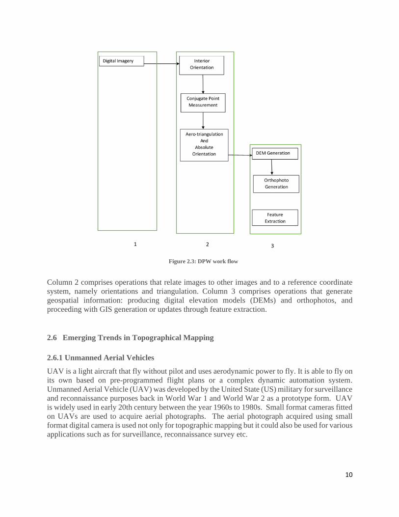
The early 1990s saw the advent of the end-to-end softcopy-based system, or Digital

Photogrammetric Workstation (DPW). A DPW system comprises software and hardware that

supports the storage, processing, and display of imagery and relevant geospatial datasets, and the

automated and interactive image-based measurement of 3-dimensional information. Figure 1.4

illustrates DPW work flow.

10

Figure 2.3: DPW work flow

Column 2 comprises operations that relate images to other images and to a reference coordinate

system, namely orientations and triangulation. Column 3 comprises operations that generate

geospatial information: producing digital elevation models (DEMs) and orthophotos, and

proceeding with GIS generation or updates through feature extraction.

2.6 Emerging Trends in Topographical Mapping

2.6.1 Unmanned Aerial Vehicles

UAV is a light aircraft that fly without pilot and uses aerodynamic power to fly. It is able to fly on

its own based on pre-programmed flight plans or a complex dynamic automation system.

Unmanned Aerial Vehicle (UAV) was developed by the United State (US) military for surveillance

and reconnaissance purposes back in World War 1 and World War 2 as a prototype form. UAV

is widely used in early 20th century between the year 1960s to 1980s. Small format cameras fitted

on UAVs are used to acquire aerial photographs. The aerial photograph acquired using small

format digital camera is used not only for topographic mapping but it could also be used for various

applications such as for surveillance, reconnaissance survey etc.

1 2 3

11

2.6.2 Volunteered Geographic Information

The widespread engagement of large numbers of private citizens, often with little in the way of

formal qualifications, in the creation of geographic information, a function that for centuries has

been reserved to official agencies (Goodchild, 2007). Open data policy has encouraged many

governments to freely share their data with some NMAs in Europe sharing their spatial data

(Brovelli et al., 2016). VGI is now the latest paradigm in mapping where private citizens are

engaged in mapping of different features and phenomena on the earth’s surface. Many National

Mapping agencies are exploring way of benefiting from this new development with the USA

setting up structures and systems to use VGI in their national mapping (Poore, et al., 2019). Web

2.0 has greatly impacted on VGI by allowing for content creation and sharing via the internet and

the smart mobile gadget with GPS that can be used in positioning of features and events. Despite

these gains data quality, legal issues and possible sabotage from contributors are some of the

challenges VGI continues to deal with (Raimond, et al., 2017). The rise of smartphones, tablets,

and other mobile devices has greatly contributed to people’s expectation of the use of geospatial

applications. User demand for increasing accuracy, currency, and detail is growing and will require

more automated data capture and feature extraction to keep pace with those requirements (Walter,

2020).

2.6.3 Legal Framework Governing VGI

Intellectual property right issues need to clearly be defined when dealing with volunteered

Geographic Information. Contributor should be encouraged to give full right to National mapping

Agency so that they can make maximum use of the contributed data (Raimond, et al., 2017). OSM

has a set of licenses under the Open Data License/Community Guideline. These licenses are meant

to define how to different parties involved in the OSM community relate with each other and the

data contributed.

2.7 Collaborative Mapping Projects

Collaborative mapping is a subset of neogeography where a group of people come together and

work toward a common goal of creating geographic information. This is usually achieved by

having a web map where the different members in the project can contribute by adding edits to the

existing web map layers. These collaborative mapping projects have been made possible by

technological advancements that have had a great impact in all areas of geospatial science in the

past few decades (Panek & Netek, 2019). Notable examples of collaborative mapping projects

include OpenStreetMap, Wikimapia, Ushahidi, Google Map Maker, and Google MyMaps.

2.7.1 Wikimapia

Wikimapia was started in 2006 by Alexandre Koriakine and Evgeniy Saveliev who were

entrepreneurs in Moscow, Russia (Ballatore & Arsanjani, 2018). The idea was to have users draw

polygons on a satellite image background and place names as the main attribute. Though studies

suggest that Wikimapia popularity is on a decline the project is still on and it aims at describing

the whole world by compiling as much useful information about places of interest on the earth

(Ballatore & Arsanjani, 2018). The level of details captured is very low compared to that of

OpenStreetMap which is also an open collaborative mapping project like Wikimapia (Ballatore &

Arsanjani, 2018).

12

Figure 2.4: Wikimapia collaborative map

2.7.2 OpenStreetMap

Steve Coast started OpenStreetMap in 2004 as a means to provide people of UK with an alternative

source of geospatial data given the restrictions on the use of Crown Copyright data from the

Ordnance Survey. OSM provides users with vector layers and an imagery background for users to

create new vector layers and validate the existing data.

2.7.3 OSM Vector Layer

OSM vector layer is created through crowd sourcing and collaborative mapping, members are

invited to contribute data from satellite imagery tracing or sharing their GPS data (Girres and

Touya, 2010). Satellite imagery tracing is the most common given the fact that it gives one the

advantage of editing the different layers in the OSM. OpenStreetMap has put in place quality

assurance and quality control measures to ensure contributors achieve the set standards. Data

quality is assessed in terms of geometric accuracy, attribute accuracy, Completeness, logical

consistency, semantic control measures accuracy, and temporal accuracy. The OpenStreetMap

tools used to achieve this are; MapCampaigner, OSMCha Osmose, and JOSM Validation.

MapCampaigner ensure mandatory attributes are filled before one is allowed to submit his edits,

this is important during layer validation of the data. OSMCha detects numerous edits or uploaded

files by one person that shows inconsistent with the existing data. Osmose check for tagging issues

with JOSM validator put upload or editing restrictions to data with geometry issues. Table 2.1

below shows the various OSM tools and the issues they detects.

13

Table 2.1 OSM tools for check data accuracy

SNo. Tool MapCampaigner OSMCha Osmose JOSM Validator

1. Attribute

completeness

×

2. Vandalism ×

3. Upload issues ×

4. Tagging issues ×

5. Geometry issues ×

Figure 2.5: OSM collaborative map

2.7.4 OSM Imagery Layer

OSM provides satellite imagery as base data for the existing vector layers. This imagery data

provides OSM users with a platform for vector layer validation and vectorization of new features

that had not been captured before. Bing maps imagery had been the sole provider of imagery for

OSM, this changed with the entry of Maxar formerly DigitalGlobe. Maxar is a commercial

imagery company based in the USA. The satellite imagery providers under Maxar are World View,

Quick Bird, Ikonos, and GeoEye. This gives OSM users a current and high-resolution satellite

imagery covering most parts of the world. DigitalGlobe performs Geolocation accuracy tests on a

regular basis by comparing images to highly accurate ground control points. An accuracy of 3.6 m

CE90 indicates a 90% confidence level that the identified feature is within a 3.6 meter radius of

where the image suggests it is, with most of the measured points being within 2.4m from actual

position as indicated by the RMSE for the case of World View-1. Table 2.2 show the CE90 and

RMSE of the four satellites.

Table 2.2: Maxar Satellite Images

SNo. Satellite CE90(m) RMSE(m)

1. WorldView-1 3.6 2.4

2. WorldView-2 5.1 3.1

3. WorldView-3 3.9 2.6

4. GeoEye-1 3.0 1.9

14

2.8 Global Digital Elevation Models

Over the past decade,many global digital elevation models have been made freely available to the

general public (Uuemaa, et al., 2020). ASTER and STRM were the most commonly used global

digital elevation models but AW3D30, TanDEM-X and MERIT global digital elevation models

have been gaining popularity. The method used to create these GDEMs was either through

Photogrammetry, Computational, aperture radar, or Interferometry synthetic aperture radar. Table

2.3 below shows the characteristics of some selected free GDEMs.

Table 2.3: Characteristics of GDEM

Dataset Horizontal

Resolution (m)

Method Estimated Vertical

Accuracy (m)

Data Collection

Period

ASTER GDEM V3

30 Photogrammetry 17 2011

AW3D30 30 Photogrammetry

5 2006 - 2011

TanDEM-X DEM 90 Interferometry

synthetic

Aperture radar

10 2011 - 2015

SRTM DEM V3 30 Interferometry

synthetic

Aperture radar

9 2000

NASADEM 30 Interferometry

synthetic

Aperture radar

- 2000

2.9 Sampling

Sampling deals with the selection of a subset of individuals from within a population to predict the

characteristics of the whole. Sampling is usually applied when trying to estimate the average or

total for a variable in an area, to optimize these variable estimations for unsampled places, or to

predict the location of a movable object (Wang, et al., 2012).

There are several methods of interpolation and this is critical in determining the outcome of the

subsequent interpolation. The following are some of the methods used in interpolation; regular,

random, transect, stratified, clustered/nested, and contoured. Figure 2.5 illustrates the various

sampling methods.

15

Figure 2.7: Methods of sampling 1

2.10 Cartographic Process

2.10.2 Technologies

Just like the advancement realized in spatial data acquisition methodologies and technologies,

there has been an advancement in cartographic technologies and methodologies from the ancient

field of sketching cartography to modern-day digital cartography. Advancement in computer

technology and distributed systems led to development and improvements in Computer Aided

Design (C.A.D) software. Commercial and open-source software such as Quantum GIS, Esri’s

ArcGIS, and other platforms have made on screen mapping faster and more efficient. Over the

years there has been a rapid and continuous change of new production technologies from the use

of peel-coats, typesetters, PostScript, Computer-Aided, and GIS. This new improvement in

production has given cartographers a set of tools for making increasingly better maps in less time

at less cost (Plewe, 2002). The continued growth and acceptance of GIS has had a great impact on

production of topographical maps as well as their increased use.

2.10.3 Generalization and Symbolization

Mapmakers design maps through generalization, symbolization, and production of the map. Emil

von Sydow in 1866 first defined the concept of cartographic generalization, this has greatly

changed to cover the modern understanding of generalization. Generalization can be achieved in

the following way:

• Semantic generalization: The main aim of semantic generalization is to ensure that the

complexity of the map does not make it difficult to read. Classification, and aggregation, as well

as symbolization and exaggeration, are closely related to semantic generalization and this is

usually performed on the information that has been chosen to be included in the map. According

16

to YING Shen a and LI Lin Semantic generalization normally takes place before geometric

generalization.

• Geometric generalization: By preserving the important parts of the data and deleting or

simplifying the less important ones to have a legible map that has good visual communication

characteristics geometric generalization is achieved. This is usually done because the complexity

of the graphic characteristics of map objects may still be too much to clearly show, especially in

small scale maps. Geometric generalization is closely related to simplification, omission, as well

as displacement and orientation (Stern, et al., 2014). Figure 2.1 explains the effect of generalization

at different scales.

Figure 2.8: Generalization

2.11 Coordinate System

A coordinate system is a methodology to define the location of a feature in space. On the ellipsoid,

positions are either expressed in Cartesian coordinates (X, Y, Z) or in curvilinear coordinates (φ,

λ, h), i.e., geodetic latitude, longitude and ellipsoidal height (Janssen, 2009).

Ellipsoid / Spheroid – A mathematical model of the earth that estimates the shape in order to best-

fit the model to the actual surface. For local datums, the ellipsoid fits well on primarily one area

of the world. For global datums, the ellipsoid is earth-centered and fits the entire globe as best it

can. SK topographical maps use Clarke 1800 as the spheroid.

Local Datum – A datum that is very accurate in only one part of the world. It is not compatible

with other local datums used elsewhere. New Arc 1960 is the datum used in SK topographical

maps.

Global Datum – A datum that provides fairly accurate coordinates in most parts on the globe (e.g.

WGS84). If we had all our maps in on datum this would eliminate the need to perform datum

transformations.

Military Grid Reference System (MGRS) coordinates

MGRS coordinate system is derived from the Universal Transverse Mercator (UTM). The military

uses the MGRS convention to simplify coordinate exchange for the soldiers in the field during

operations or military exercises. SK topographical maps at scale 1:50,000 are designed to take care

of MGRS coordinate system and each sheet has a guide on how to read in MGRS from the map

sheet. Figure 2.7 below show the various components of MGRS coordinate.

17

Figure 2.9: MGRS Coordinate System

The MGRS format is designed to support measurement precisions of 1m, 10m, 100, 1,000m, and

10,000m. Table 2.3 below show how values are truncated to give different precision levels.

Table 2.4: MGRS Precision

Coordinate Accuracy Topographical Map Scale

10S GJ 06832 44683 Locates a point within a 1 meter square

10S GJ 0683 4468 Locates a point within a 10 meter square

10S GJ 068 446 Locates a point within a 100 meter square 1:50,000 and 1:100,00

10S GJ 06 44 Locates a point within a 1,000meter square 1:250,000

10S GJ 0 4 Locates a point within a 10,000 meter square

10S GJ Locates a point within a 100,000 meter square

2.12 Accuracy Standards

Accuracy standards are set to guide collection of data meant for topographical map production and

to give the map user some level of confidence when using the map at the stated scale. According

to the American Society for Photogrammetry and Remote Sensing (ASPRS) horizontal accuracy

for maps on publication scales larger than 1:20,000 should be that not more than 10 percent of the

points sampled shall have an error of more than 1/30 inch, measured on the publication scale and

an error of 1/50 inch to maps on publication scale of 1:20,000 or smaller, ". For vertical accuracy

it is required that not more than 10 percent of the points examined shall have an error of more than

one half of the stated contour interval (Thapa & Bossler, 1992).

18

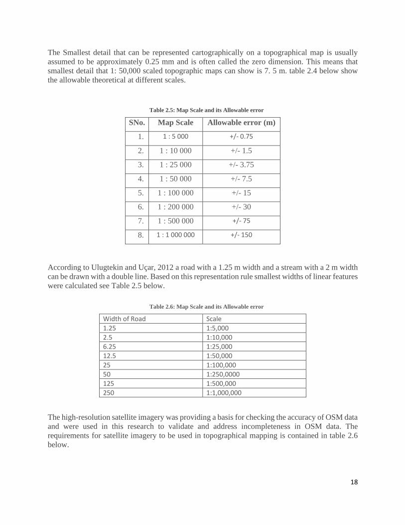
The Smallest detail that can be represented cartographically on a topographical map is usually

assumed to be approximately 0.25 mm and is often called the zero dimension. This means that

smallest detail that 1: 50,000 scaled topographic maps can show is 7. 5 m. table 2.4 below show

the allowable theoretical at different scales.

Table 2.5: Map Scale and its Allowable error

SNo. Map Scale Allowable error (m)

1. 1 : 5 000 +/- 0.75

2. 1 : 10 000 +/- 1.5

3. 1 : 25 000 +/- 3.75

4. 1 : 50 000 +/- 7.5

5. 1 : 100 000 +/- 15

6. 1 : 200 000 +/- 30

7. 1 : 500 000 +/- 75

8. 1 : 1 000 000 +/- 150

According to Ulugtekin and Uçar, 2012 a road with a 1.25 m width and a stream with a 2 m width

can be drawn with a double line. Based on this representation rule smallest widths of linear features

were calculated see Table 2.5 below.

Table 2.6: Map Scale and its Allowable error

Width of Road Scale

1.25 1:5,000

2.5 1:10,000

6.25 1:25,000

12.5 1:50,000

25 1:100,000

50 1:250,0000

125 1:500,000

250 1:1,000,000

The high-resolution satellite imagery was providing a basis for checking the accuracy of OSM data

and were used in this research to validate and address incompleteness in OSM data. The

requirements for satellite imagery to be used in topographical mapping is contained in table 2.6

below.

19

Table 2.7: Map scale and required minimum imagery accuracy

SNo. Map Scale Imagery resolution(m)

1. 1 : 5 000 0.5

2. 1 : 10 000 1

3. 1 : 25 000 2.5

4. 1 : 50 000 5

5. 1 : 100 000 10

6. 1 : 200 000 20

7. 1 : 500 000 50

8. 1 : 1 000 000 100

2.13 Summary of Literature Review

Topographical map-making has tremendously evolved over the years from the time when maps

were sketched based on one’s knowledge of an area and his drawing skills to the use of powerful

computer-aided design software. The use of high-resolution satellite images in topographical

mapping greatly reduced the time taken to acquire the image of an area. The availability of current

and high-resolution satellite imagery in OSM provide OSM contributors with a platform from

which they can generate up to date data. Mapping of places that are not accessible has now been

made possible using high-resolution satellite images. Volunteered Geographic Information is

increasingly becoming available in most parts of the world and national mapping agencies around

the world are finding ways of using this data in topographical map revision and other mapping

activities. Vector and imagery data standards provided by SK and international geospatial

organization can be used to assess the quality of OSM data to be used in topographic map

production. The field of cartography has also experienced a great transformation from hand-drawn

maps to the use of a light table to capture features and now the use of powerful Computer-Aided

Design software to capture details and design the map. The web also provides a means by which

the geospatial products can be shared through email or an interactive web platform that allows

creation and sharing of content by users.

This project will use OSM vector data and SRTM V3 as source open data needed in the revision

of topographical map 148/4. The vector data will be evaluated for completeness, attribute accuracy

and logical consistency in sampled in the sampled areas. Nested sampling method will be used to

identify the ideal location for sampling.

20

CHAPTER 3: MATERIALS AND METHODS

3.1 Methodology

In order to meet the objectives of this research, the methodology summarized in figure 3.1 was

followed.

Figure 3.1: Methodology

21

3.2 Study Area

The study area for this project is the area covered by Nairobi topographical map sheet 148/4. The

area is bounded by longitude 36O 45’’E and 36O 00’’E and Northing 1O 15’’S and 1O 30’’S figure

3.2 show the study area. The topographical sheet covers the CBD to the Northwest, Nairobi

National Park to the South, Jomo Kenyatta Airport to the East. Being the capital city of Kenya,

Nairobi is highly populated with a generally high rate of development. The sheet was last revised

in 1996 by the French National mapping agency using the SPOT satellite images with a resolution

of 20m for the multispectral (XS) and 10m for the panchromatic (P). This research will evaluate

the potential of open-source data in revision of SK topographical map at scale 1:50,000.

Figure 3.2: Study Area

22

3.3 Requirements

3.3.1 Software and Hardware Requirements

Table 3.1: Software and hardware requirements

SNO. Hardware Software

1. Laptop or PC QGIS

3.3.2 Data Requirements

Table 3.2: Data requirements

SNO. Data Type Data Data Source

1. Raster STRM USGS

2. 9th edition of Topomap 148/4 Survey of Kenya

3. 148/4 Contour reproduction map Survey of Kenya

4. 1:50,000 topographical map template Survey of Kenya

5. Cartographic Styles and Symbols Survey of Kenya

6. Satellite Image OSM

7. Vector OSM layer OSM

3.4 Map Key Components of a Topographical Map

3.4.1 Map Details

Map details are the ground features as they appear during data capture for map compilation or map

revision. This continually changes largely due to the human or environmental actives that take

place in a particular area. The level of detail that can be shown on a map varies with the scale of

representation. A large-scale map will show more details while a small scale will show fewer

details.

3.4.2 Map Scale

Map scale is the ratio of map distance to ground distance. We have three types of scale in the map

i.e., the statement scale, representative ratio and scale bar. A basic SK topographical has both

representative ratio scale and scale bar.

3.4.3 Map Series

Map series consists of maps of the same scale which collectively cover a specific area. Y731 is

map series for SK topographical maps at scale 1:50,000

3.4.4 Map Edition

Map Edition indicates the number of times a particular topographical map sheet has been revised.

The latest map edition for Nairobi topographical map sheet 148/4 is 9th Edition which was last

revised in 1996.

23

3.4.5 Sheet Name

The sheet name is usually given based on the name of a major town covered by the sheet or an

outstanding feature within the sheet extent. In SK topographical map the sheet name is normally

placed at the top center of the margin. The sheet name for this project area is NAIROBI.

3.4.6 Sheet Number

The sheet number for SK topographical maps at scale 1:50,000 is based on national Rectangular

Coordinate system covering the geographical area that define the republic of Kenya. The first digits

in the sheet number identifies the 1:100,000 sheet covering the area with the 1:50,000 sheet

identified by numbers 1, 2, 3 or 4.

3.4.7 Symbol Legend

The symbol legend is to describe the symbols that have been used to represent features such as

built-up areas, roads, vegetations etc.

3.4.8 Administrative index

The administrative index shows the major administrative boundaries that are within the map area.

SK topographical map at scale 1:50,000 have their administrative index appearing at the bottom

left part of the map.

3.4.9 Map Datum and Projection

The Universal Transverse Mercator (UTM) is used by the Kenyan Government for national

mapping in topographical mapping with the following parameters applicable within the study area.

Table 3.3 show the datum parameters used in project.

Table 3.3: Datum Parameters

Projection Type Universal Transverse Mercator (UTM)

Ellipsoid Clarke 1880

Datum Name Arc 1960

UTM Zone 37 South of Equator

Scale Factor at the central meridian 0.999600

False Easting 500,000.00m

False Northing 10,000,000.00m

3.5 Map Accuracy

Map accuracy refers to the degree of closeness of results of observation or measurements of

graphic map feature to their actual or true value or position.

3.5.1 Graphical Resolution

Graphical resolution of map refers to the minimum distance that can be measured of objects or

between objects. On a SK topographical map at scale 1:50,000, 2cm represent 1KM. The minimum

distance that can be estimated from a map is one fourth (1/4) of a millimeter. Based on this

estimation graphical resolution of SK topographical map at scale 1:50,000 is 12.5m.

24

3.5.2 Graphical National Map Accuracy Standards

The National Mapping Agency assures the public that the SK topographical map conform to the

internationally established accuracy specification. This guarantee consistency and confidence in

their use in various geospatial application. Map Accuracy standards is assessed horizontal accuracy

and vertical accuracy.

Horizontal Accuracy

For maps on publication at scale 1:50,000 or less, not more than 10% of the points tested shall be

in error by more than 0.051cm. This is applied in positions of well-defined points e.g., intersections

of roads, railroads etc.

The ground horizontal accuracy for SK topographical maps at scale 1:50,000 is computed by

multiplying the allowed plottable error of 0.051cm and then dividing by 100 to convert it to meters.

0.051 x 50,000 / 100 = 25.5meters.

Vertical Accuracy

For maps on publication at scale 1:50,000 or less, not more than 10% of the points tested shall be

in error by more than one half of the state contour interval. The contour interval of SK

topographical maps at scale 1:50,000 is 20m, meaning the vertical error should not be more than

10m.

3.6 Vector Datasets

The layers that constitute a 1:50,000 topographical map was obtained from the 9th edition of

Nairobi topographical map sheet 148/4. Table 3.4 below show all the layers that constitute

topographical map sheet 148/4.

The OSM data was downloaded in three separate layers of point, line, and area features. The

various layers that constitute an OSM layer were then extract from the point, lines and area

features.

The accuracy of the buildings, roads, and vegetation features was assessed before they are used in

the revision of Nairobi Topographical map sheet No. 148/4 at scale of 1:50,000.

Table 3.4 Layers that constitute a 1:50,000 topographical map

SNo. Feature Primitive Type

1. Annotation Point

2. Communication Point

3. Electricity Point

4. Railway Point

5. Relief Point

6. Road Point

7. Spot Heights Point

8. Trigonometric Station Point

9. Water Point

10. Communication Line

11. Electricity Line

12. Railway Line

13. Road Line

14. Water Line

25

SNo. Feature Primitive Type

15. Annotation Area

16. Boundary Area

17. Building Area

18. Electivity Area

19. Mining Area

20. Plantation Area

21. Relief Area

22. Vegetation Area

23. Water Area

3.7 Aerial Photograph Accuracy

Features and contours in SK topographical map at scale 1:50,000 were captured from vertical aerial

photographs at a scale of 1:30,000 (Nyadimo, 2003). The feature were then generalized to

produced data for SK topographical map at 1:50,000.

OSM data capture within the study area is mainly done from current high resolution satellite image

provided by World View and GeoEye satellite. Table 3.5 show the satellite resolution for the

different satellites.

Table 3.5 Satellite Resolution

SNo. Satellite Resolution(m)

1. WorldView-1 0.46

2. WorldView-2 0.46

3. WorldView-3 0.31

4. GeoEye-1 0.46

3.8 Elevation Datasets

Shuttle Radar Topography Mission (SRTM) will be the primary source of elevation that was used

in this project and was downloaded from USGS website to cover the area of study. In this research

STRM version, 3 was used, it has a horizontal resolution of 30m and an estimated vertical accuracy

of 9m with a near-global coverage of the earth from 56°S to 60°N. From the SRTM contours were

generated at a contour interval of 20m. The contours were then smoothened to ensure the contour

lines have smooth curves. This was done using QGIS software.

3.9 Selecting Sample Area

To effectively analyze the accuracy of the OSM data for carrying out the revision of the

topographical map, the project area was divided into the various developmental zones as defined

by the County government. Each of the identified zones will be targeted in the nested method of

sampling for data collection. A sample area measuring 2km by 2km was picked in each of the

mentioned zones and carried out the OSM data quality analysis test. The seven zones listed below

fall within the study area and will form the specific area from where sampling will be done. They

include:

a. Commercial/offices: CBD area

b. Industrial zone: Industrial area

26

c. Agricultural/ residential: Utawala, Loo Ntepes

d. High density residential development: Korogocho

e. Low density residential development: Karen, Syokimau

f. Old City Council buildings: Makongeni

g. Public Open Spaces Reserves and recreational facilities: Nairobi National Park

Figure 3.3 illustrate the identified sample areas overlaid on an old topographical map.

Figure 3.3: Sample areas

27

3.10 OSM Data Quality Assessment

The OSM data downloaded was assessed if it meets the minimum standards set for topographical

mapping. The following aspects of data quality were assessed; Geometric accuracy, Attribute

accuracy, and Completeness.

3.10.1 Geometric accuracy

Geometric accuracy was measured by checking how off a feature is from the correct planimetric

position it is expected to be. This will be guided by the international best practice that defines the

allowable theoretical position errors which is 25.5m at scale 1:50,000.

3.10.2 Attribute accuracy

Attribute accuracy will be checked by assessing the correct association of attribute for each feature

or a set of features. This was validated through the use of high-resolution satellite images provided

by OSM and information obtained during ground truthing. This will help ensure correct

symbolization of the features during map revision.

3.10.3 Completeness

The completeness of the OSM data was assessed based on the number of features e.g., OSM

buildings within the sample area compared to the number of buildings visible from the high-

resolution satellite image provided by OSM. How current the OSM data is determined by how

well the latest changes in different features is reflected in OSM layer.

3.10.4 Assessing the Accuracy of OSM data

This involved recording the observed or measured accuracy of the OSM data. This will be done

for roads, buildings and vegetation layers. The accuracy level was given on a scale of 1 to 10, with

1 being a feature with very poor accuracy while 10 being a feature with perfect accuracy. This

was done for all the three parameters that will be used to determine the accuracy levels of the OSM

features and they include; geometric accuracy, attribute accuracy and completeness. Table 3.6

below was used to record the findings in each of the sample areas identified.

Table 3.6: Topographical map features to be analyzed for accuracy

SNo. Feature Primitive

Type

Average

Geometric

Accuracy

Average

Attribute

Accuracy

Average

Completeness

1. Road Line

2. Building Area

3. Vegetation Area

3.11 Assessing the Accuracy of SRTM V3

The accuracy of the SRTM V3 generated contours was assessed by comparing the cell values with

that of the contours used in the production of topographical map sheet 148/4. STRM cell values

were obtained by averaging the cell values along SK topographical map contour, within the sample

area. These contours are generated by vectorizing the contour reproduction map used in the

28

reproduction of the topographical map sheet 148/4. Appendix C show the contour reproduction

map/sheet used in the reproduction of SK topographical maps sheet 148/4. The results were

tabulated in 3.7 below. The accuracy of the contours is expected not to exceed 10m for the case of

SK topographical maps as directed by American Society of Photogrammetry and remote Sensing.

Table 3.7: Topographical map features to be analyzed for accuracy

SNo. Sample Areas Contour Line Value Mean of SRTM Cell Values

1. Westlands

2. Industrial Area

3. Kariobangi

4. Karen

5. Utawala

6. Syokimau

7. Kitengela

8. Loo Ntepes

9. Nairobi National Park

Completeness issues in the data downloaded from the OSM layer were addressed by vectorizing

features from the high-resolution satellite images provided by OSM. The OSM imagery dataset

was be used to visually evaluate the accuracy of some of the attributes assigned to the OSM layer.

3.12 Cartographic Process

This involved the generalization and symbolization of the datasets to revise the Survey of Kenya

topographical map at a scale 1:50,000. The OSM roads datasets was Sematic generalized by

removing most of the roads under road class; other tracks or footpath. This was done to address

any illegibility that may be caused by too much map details. The 9th edition of SK topographical

map sheet 148/4 was also used to guide this process.

OSM data was then reclassified into their equivalent in SK topographical map at scale 1:50,000.

After the reclassification process, the OSM data and the contours generated from SRTM are

displayed in 1:50,000 SK topographical map template. Attachment 3 show 1:50,000 SK

topographical map template.

To ensure the OSM data is effectively symbolized and can be used in SK topographical map

revision, the feature in the

29

CHAPTER 4: RESULTS AND DISCUSSION

4.1 OSM Data Accuracy Analysis

Geometry accuracy, attribute accuracy and Completeness for roads, buildings and vegetation was

confirmed for each of the 9 sample areas. The results for the industrial area, Korogocho, Dandora,

Karen, Utawala, Loo Ntepes, Kitengela and Nairobi National Park are contained in appendix A.

The data analysis results for Westlands are contained Table 4.1 while figure 4.1 show Westlands

sample area.

4.1.1 Westlands

Table 4.1: Topographical map features analysis results for Westlands

SNo. Feature Primitive

Type

Geometric

Accuracy

Attribute

Accuracy

Completeness

1. Road Line 10 8 9

2. Building Area 9 1 7

3. Vegetation Area 0 0 0

Figure 4.1: Westlands Sample Area

4.2 Elevation Data Quality Assessment

The SRTM was first transformed from the global coordinate system of WGS 1984 to the local

system of Arc1960. Contour lines obtained from contour reproduction map sheet 148/4 were

overlaid on the SRTM and the corresponding contour values at each pixel was noted for each of

the sample areas. The. Figure 4.7 shows the overly of the contour line on SRTM. Table 4.10 below

shows the values obtained during this comparison exercise.

30

Figure 4.2: Contour lines overlaid on SRTM

Table 4.2: Contour line value and corresponding SRTM cell values

SNo. Sample Areas Contour Line Value Mean of SRTM Cell Values

1. Westlands 1760 1769

2. Industrial Area - -

3. Kariobangi 1600 1604

4. Karen 1800 1809

5. Utawala 1580 1571

6. Syokimau - -

31

SNo. Sample Areas Contour Line Value Mean of SRTM Cell Values

7. Kitengela 1560 1554

8. Loo Ntepes 1760 1752

9. Nairobi National Park 1640 1639

4.3 Addressing the Incompleteness of OSM data

The gaps realized in the OSM building and vegetation layer can be corrected by digitizing the

missing buildings and vegetation from high-resolution imagery in OSM.

Figure 4.3 OSM dataset features before and after the missing features were added by extracting

vector data from the high-resolution imagery in OSM (Muthangari area).

Figure 4.3: Westlands Sample Area before and after vectoring more features from satellite imagery

4.4 Data Reclassification and Styling

From the results, only the road data met the set standards for data quality to be used in

topographical map revision.

The 22-road classes in OSM were generalized by reclassifying them into the 5 classes in SK

topographical map at scale 1: 50,000, this was then validated using the high-resolution satellite

images provided by OSM. This was done to enable the symbolization of the roads data into the set

standard for topographic map production. Table 4.3 below shows the reclassification of OSM

roads data to topographical map classes.

Appendix D shows the roads data and contours displayed on 1: 50,000 topographical map

template.

The Contour for the study area were generated from the downloaded SRTM V3, and form part of

the open source data that were evaluated and found to be suitable for use in topographical map

revision.

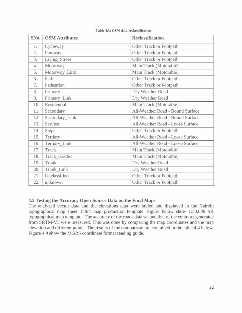
32

Table 4.3: OSM data reclassification

SNo. OSM Attributes Reclassification

1. Cycleway Other Track or Footpath

2. Footway Other Track or Footpath

3. Living_Street Other Track or Footpath

4. Motorway Main Track (Motorable)

5. Motorway_Link Main Track (Motorable)

6. Path Other Track or Footpath

7. Pedestrian Other Track or Footpath

8. Primary Dry Weather Road

9. Primary_Link Dry Weather Road

10. Residential Main Track (Motorable)

11. Secondary All-Weather Road - Bound Surface

12. Secondary_Link All-Weather Road - Bound Surface

13. Service All-Weather Road - Loose Surface

14. Steps Other Track or Footpath

15. Tertiary All-Weather Road - Loose Surface

16. Tertiary_Link All-Weather Road - Loose Surface

17. Track Main Track (Motorable)

18. Track_Grade1 Main Track (Motorable)

19. Trunk Dry Weather Road

20. Trunk_Link Dry Weather Road

21. Unclassified Other Track or Footpath

22. unknown Other Track or Footpath

4.5 Testing the Accuracy Open-Source Data on the Final Maps

The analyzed vector data and the elevations data were styled and displayed in the Nairobi

topographical map sheet 148/4 map production template. Figure below show 1:50,000 SK

topographical map template. The accuracy of the roads data set and that of the contours generated

from SRTM-V3 were measured. This was done by comparing the map coordinates and the map

elevation and different points. The results of the comparison are contained in the table 4.4 below.

Figure 4.9 show the MGRS coordinate format reading guide.

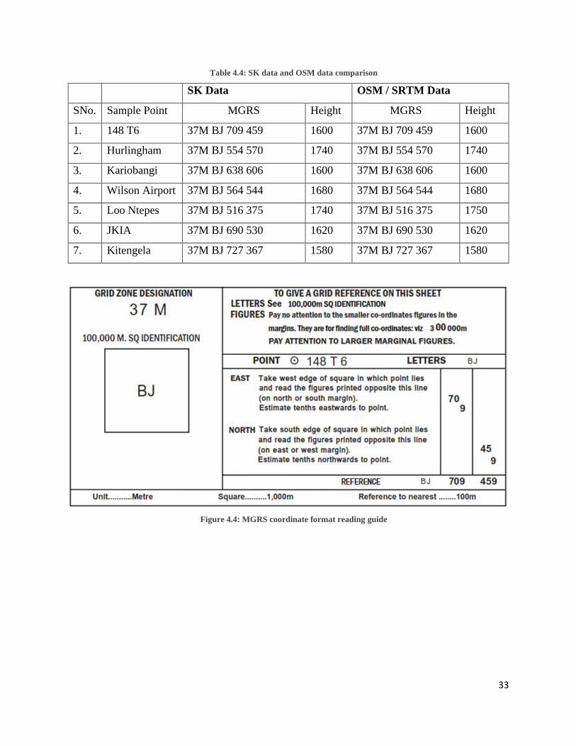
33

Table 4.4: SK data and OSM data comparison

SK Data OSM / SRTM Data

SNo. Sample Point MGRS Height MGRS Height

1. 148 T6 37M BJ 709 459 1600 37M BJ 709 459 1600

2. Hurlingham 37M BJ 554 570 1740 37M BJ 554 570 1740

3. Kariobangi 37M BJ 638 606 1600 37M BJ 638 606 1600

4. Wilson Airport 37M BJ 564 544 1680 37M BJ 564 544 1680

5. Loo Ntepes 37M BJ 516 375 1740 37M BJ 516 375 1750

6. JKIA 37M BJ 690 530 1620 37M BJ 690 530 1620

7. Kitengela 37M BJ 727 367 1580 37M BJ 727 367 1580

Figure 4.4: MGRS coordinate format reading guide

34

CHAPTER 5: CONCLUSION AND RECOMMENDATION

3.1 Conclusion

The objective of this research was to evaluate the potential Open-Source geospatial data in

topographical map revision and this was successfully achieved using OSM data, open-source

satellite imagery and SRTM data.

The vector data set from OSM was extensively evaluated and from the findings, it’s clear that the

geometric accuracy of the OSM dataset is within the set standards for topographical map

production. This can be attributed to the high-resolution satellite imagery that is used in vector

data extraction. The quality check put in place by OSM developers also plays a great role in

reducing errors related to geometry.

Roads, buildings, and vegetation layers were the main layers targeted in vector data quality

assessment and were carefully examined using high-resolution satellite imagery provided by OSM.

From the results in chapter 4, it is evident that the roads layer was well captured in terms of

geometry, attribute, and completion. The buildings were well captured in the CBD area and its

surroundings but incompleteness was noted in other areas. Vegetation was not well captured and

could not be used in the revision Nairobi Topographical map sheet No. 148/4.

Satellite imagery available in OSM provided current and high-resolution satellite imagery that can

be used to address the incomplete of data and validate attributes assigned to features.

Contour generated from the SRTM V3 were found to be within the acceptable error margin and

could be used in topographical map revision.

SK cartographic standards for map production were applied on the roads from OSM and contour

lines generated from SRTM V3 and this was displayed in SK 1:50,000 topographical map

template.

35

3.2 Recommendation

Collaborative mapping is the new trend in the geospatial sector and the National Mapping

Agencies can benefit from this by putting in place systems that utilize and take advantage of this

wealth of data and technology they offer.

Structured or customized collaboration by the national mapping agency will see the contributor

generate high-quality geospatial data that can be used in different sectors that rely on geospatial

data.

The growth of collaborative mapping projects like OSM can provide the National Mapping

Agency and other service providers who rely on geospatial data with a rich repository of vector

data for their day-to-day operations.

SRTM V3 provides very high accurate elevation data that can be used to generate contours that

can be used for production of topographical maps at scale of 1:50,000.

36

References

Aber, J. S. & Ries, J. B., 2010. Photogrammetry. Elsevier .

Ballatore, A. & Arsanjani, J. J., 2018. Placing Wikimapia: An exploratory analysis. International

Journal of Geographical Information Science.

Buhr, S., Kellagher, E. & Lynds, S., 2008. Geomagnetism in the MESA Classroom: An Essential

Science for Modern Society. s.l.:University of Colorado.

Carter, J., Schmid, K., Waters, K. & Betz, L., 2012. Lidar 101: An Introduction to Lidar

Technology. Charleston, SC: National Oceanic and Atmospheric Administration.

Clarke, K., 1986. Advances in Geographic Information Systems. Research Gate.

Girres, J. F. & Touya, G., 2010. Elements of quality assessment of French OpenStreetMap data.

Transactions in GIS.

Goodchild, M. F., 2007. Citizens as Sensors: The World of Volunteered Geography. GeoJourna,

p. 69:211–221.

Green, D. R., 1998. Mental Mapping and Field Sketching at the University of Aberdeen. 35(1).

Jakobsson, A., 2006. On the Future of Topographic Base Information Management in Finland

and Europe. Espoo: s.n.

Janssen, V., 2009. Understanding coordinate systems, datums and transformations in Australia.

ResearchGate.

Jervis, W., 1936. The World in Maps: A Study in Map Evolution London. London, s.n.

Müller, W. & Seyfert, E., 2000. Data Base Revision and Generation of Digital Topographic

Base Maps. Int. Arch.. s.l.:s.n.

Olteanu-Raimond, A.-M.et al., n.d. VGI in National Mapping Agencies: Experiences and

Recommendations. Mapping and the Citizen Sensor, p. 299–326.

Panek, J. & Netek, R., 2019. Collaborative Mapping and Digital Participation:. Multidisciplinary

Digital Publishing Institute.

Plewe, B., 2002. The Perfect Cartography Software, and How We Live Without It. Cartographic

Perspectives.

Poore, B. S. et al., 2019. Structures Data Collection for The National Map using Volunteered

Geographic Information, Virginia: U.S. Geological Survey.

Raimond, O. et al., 2017. VGI in National Mapping Agencies: Experiences and

Recommendations. In: Mapping and the Citizen Sensor. London: Ubiquity Press, pp. 299-326.

Rapp, R. H., 1974. The geoid: Definition and determination. Eos Science News, 55(3).

Shen a, Y. & Lin a, . L., n.d. Knowledge Representation of Cartographic Generalization.

37

Sluter, C. & Camboim, S., 2009. The National Topographic Mapping as an Indispensable

Database for a Brazilian. Santiago De Chile, s.n.

Stern, B., Hurni, L. & Marion , W., 2014. Generalisation of Map Data. s.l.:Geographic

Information Technology Training Alliance.

Thapa, K. & Bossler, J., 1992. Accuracy of Spatial Data Used In Geographic Information

Systems. PHOTOGRAMMETRIC ENGINEERING & REMOTE SENSING, 58(6), pp. 835-841.

Usery, E. L., Varanka , D. E. & Davis, L. R., 2019. Topographic Mapping Evolution: From Field

and Photographically Collected Data to GIS Production and Linked Open Data. The

Cartographic Journal, 55(4).

Usery, E. L., Varanka, D. E. & Davis, L. R., 2018. Topographic Mapping Evolution: From Field

and Photographically Collected Data to GIS Production and Linked Open Data, s.l.: s.n.

Uuemaa, E., Ahi, S., Muru, M. & Kmoch, A., 2020. Vertical Accuracy of Freely Available

Global Digital. Remote Sensing.

Walter, C., 2020. ‘Future Trends in geospatial, London: s.n.

Wang , J.-F., Stein, A., Gao, B.-B. & Ge , Y., 2012. A review of spatial sampling. Elsevier.

38

APPENDICES

Appendix A: OSM Data Accuracy Analysis Results

Industrial Area

Topographical map features analysis results for Industrial Area

SNo. Feature Primitive

Type

Geometric

Accuracy

Attribute

Accuracy

Completeness

1. Railway Point 10 10 10

2. Road Line 10 8 8

3. Vegetation Area - - -

Industrial Area Sample Area

39

Kariobangi

Topographical map features analysis results for Kariobangi

SNo. Feature Primitive

Type

Geometric

Accuracy

Attribute

Accuracy

Completeness

1. Road Line 10 9 9

2. Building Area 3 2 1

3. Vegetation Area - - -

Kariabangi Sample Area

40

Karen

Topographical map features analysis results for Karen

SNo. Feature Primitive

Type

Geometric

Accuracy

Attribute

Accuracy

Completeness

1. Road Line 10 10 10

2. Building Area 0 0 0

3. Vegetation Area - - -

Karen Sample Area

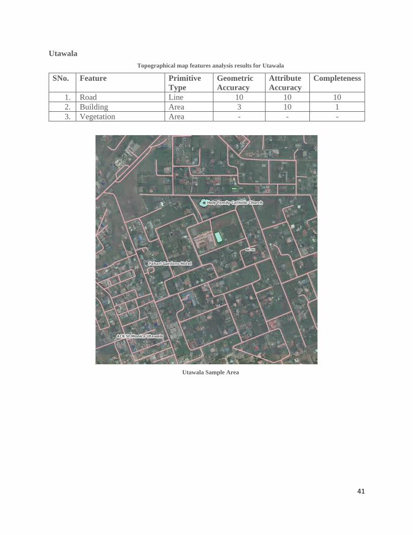
41

Utawala

Topographical map features analysis results for Utawala

SNo. Feature Primitive

Type

Geometric

Accuracy

Attribute

Accuracy

Completeness

1. Road Line 10 10 10

2. Building Area 3 10 1

3. Vegetation Area - - -

Utawala Sample Area

42

Syokimau

Topographical map features analysis results for Syokimau

SNo. Feature Primitive

Type

Geometric

Accuracy

Attribute

Accuracy

Completeness

1. Road Line 8 10 10

2. Building Area 0 0 0

3. Vegetation Area - - -

Syokimau Sample Area

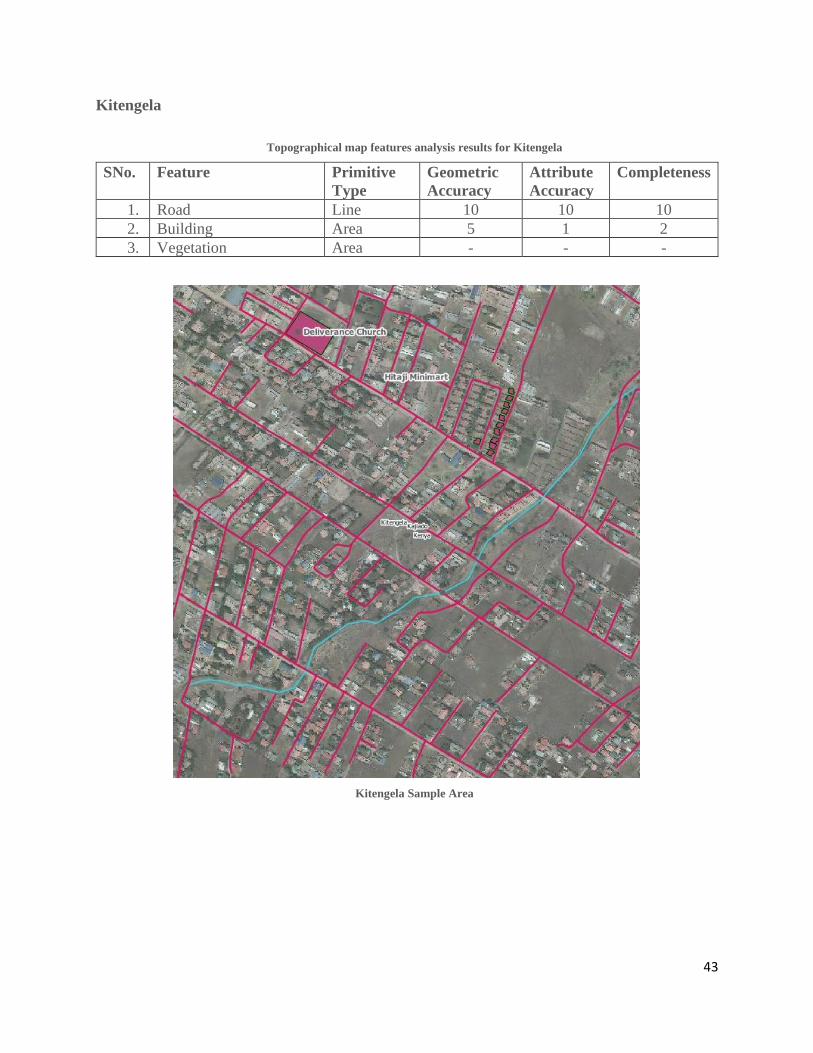
43

Kitengela

Topographical map features analysis results for Kitengela

SNo. Feature Primitive

Type

Geometric

Accuracy

Attribute

Accuracy

Completeness

1. Road Line 10 10 10

2. Building Area 5 1 2

3. Vegetation Area - - -

Kitengela Sample Area

44

Loo Ntepes

Topographical map features analysis results for Loo Ntepes

SNo. Feature Primitive

Type

Geometric

Accuracy

Attribute

Accuracy

Completeness

1. Road Line 10 6 10

2. Building Area 0 0 0

3. Vegetation Area 0 0 0

Loo Ntepes Sample Area

45

Nairobi National Park

Topographical map features analysis results for Nairobi National Park

SNo. Feature Primitive

Type

Geometric

Accuracy

Attribute

Accuracy

Completeness

1. Road Line 10 6 10

2. Building Area - - -

3. Vegetation Area 8 8 10

Nairobi National Park Sample Area

46

Appendix B: 1:50,000 Topographical Map Template

Appendix C: Contours Reproduction Material

Appendix D: Roads and Contours Displayed on 1:50,000 Topographical Map Template