
Revista Colombiana de Estad´ıstica - EMIS.de
210
Revista Colombiana de Estad´ ıstica Volumen 35. N´ umero 3 - diciembre - 2012 ISSN 0120 - 1751
-
Upload
khangminh22 -
Category
Documents
-
view
6 -
download
0
Transcript of Revista Colombiana de Estad´ıstica - EMIS.de

RevistaColombianade Estadıstica
Volumen 35. Numero 3 - diciembre - 2012 ISSN 0120 - 1751

Revista Colombiana de Estadısticahttp://www.estadistica.unal.edu.co/revista
http://es.wikipedia.org/wiki/Revista Colombiana de Estadistica
http://www.emis.de/journals/RCE/
revcoles [email protected]
Indexada en: Ulrichsweb, Scopus, Science Citation Index Expanded (SCIE), Web of
Science (WoS), SciELO Colombia, Current Index to Statistics, Mathematical Reviews
(MathSci), Zentralblatt Fur Mathematik, Redalyc, Latindex, Publindex (A1)
Editor
Leonardo Trujillo, Ph.D.Universidad Nacional de Colombia, Bogota, Colombia
Comite Editorial
Jose Alberto Vargas, Ph.D.Campo Elıas Pardo, Ph.D.B. Piedad Urdinola, Ph.D.Edilberto Cepeda, Ph.D.
Universidad Nacional de Colombia, Bogota, Colombia
Jorge Eduardo Ortiz, Ph.D.Universidad Santo Tomas, Bogota, Colombia
Juan Carlos Salazar, Ph.D.Universidad Nacional de Colombia, Medellın, Colombia
Monica Becue, Ph.D.Universitat Politecnica de Catalunya, Barcelona, Espana
Adriana Perez, Ph.D.The University of Texas, Texas, USA
Marıa Elsa Correal, Ph.D.Universidad de los Andes, Bogota, Colombia
Luis Alberto Escobar, Ph.D.Louisiana State University, Baton Rouge, USA
Camilo E. Tovar, Ph.D.International Monetary Fund, Washington D.C., USA
Alex L. Rojas, Ph.D.Carnegie Mellon University, Doha, Qatar
Comite Cientıfico
Fabio Humberto Nieto, Ph.D.Luis Alberto Lopez, Ph.D.
Liliana Lopez-Kleine, Ph.D.Universidad Nacional de Colombia, Bogota, Colombia
Sergio Yanez, M.Sc.Universidad Nacional de Colombia, Medellın, Colombia
Francisco Javier Dıaz, Ph.D.The University of Kansas, Kansas, USA
Enrico Colosimo, Ph.D.Universidade Federal de Minas Gerais, Belo Horizonte, Brazil
Fernando Marmolejo-Ramos, Ph.D.The University of Adelaide, Australia
Julio da Motta Singer, Ph.D.Universidade de Sao Paulo, Sao Paulo, Brazil
Edgar Acuna, Ph.D.Raul Macchiavelli, Ph.D.
Universidad de Puerto Rico, Mayaguez, Puerto Rico
Raydonal Ospina, Ph.D.Universidade Federal de Pernambuco, Pernambuco, Brasil
La Revista Colombiana de Estadıstica es una publicacion semestral del Departamento deEstadıstica de la Universidad Nacional de Colombia, sede Bogota, orientada a difundir conoci-mientos, resultados, aplicaciones e historia de la estadıstica. La Revista contempla tambien lapublicacion de trabajos sobre la ensenanza de la estadıstica.
Se invita a los editores de publicaciones periodicas similares a establecer convenios de canjeo intercambio.
Direccion Postal:Revista Colombiana de Estadısticac© Universidad Nacional de Colombia
Facultad de CienciasDepartamento de EstadısticaCarrera 30 No. 45-03Bogota – ColombiaTel: 57-1-3165000 ext. 13231Fax: 57-1-3165327
Adquisiciones:Punto de venta, Facultad de Ciencias, Bogota.Suscripciones:revcoles [email protected] de artıculos:Se pueden solicitar al Editor por correo fısico oelectronico; los mas recientes se pueden obteneren formato PDF desde la pagina Web.
Edicion en LATEX: Patricia Chavez R. E-mail: [email protected]
Impresion: Editorial Universidad Nacional de Colombia, Tel. 57-1-3165000 Ext. 19645, Bogota.

Revista Colombiana de Estadıstica Bogota Vol. 35 No 3
ISSN 0120 - 1751 COLOMBIA diciembre-2012 Pags. 331-521
Contenido
Jose Rafael Tovar & Jorge Alberto AchcarTwo Dependent Diagnostic Tests: Use of Copula Functions in theEstimation of the Prevalence and Performance Test Parameters . . . . . . . . . 331-347
Vıctor Leiva, M. Guadalupe Ponce, Carolina Marchant& Oscar BustosFatigue Statistical Distributions Useful for Modeling Diameter andMortality of Trees . . . . . . . . . . . . . . . . . . . . . . . . . . . . . . . . . . . . . . . . . . . . . . . . . . . . . . . 349-370
Marco MarozziA modified Cucconi Test for Location and Scale Change Alternatives . . . . 371-384
Ramon Giraldo, Jorge Mateu & Pedro Delicadogeofd: An R Package for Function-Valued Geostatistical Prediction . . . . . . 385-407
Vıctor Salinas, Paulino Perez, Elizabeth Gonzalez& Humberto VaqueraGoodness of Fit Tests for the Gumbel Distribution with Type II rightCensored data . . . . . . . . . . . . . . . . . . . . . . . . . . . . . . . . . . . . . . . . . . . . . . . . . . . . . . . . . . .409-424
Fabio G. GuerreroOn the Entropy of Written Spanish . . . . . . . . . . . . . . . . . . . . . . . . . . . . . . . . . . . . . .425-442
Mahdi MahdizadehOn the Use of Ranked Set Samples in Entropy Based Test of Fit forthe Laplace Distribution . . . . . . . . . . . . . . . . . . . . . . . . . . . . . . . . . . . . . . . . . . . . . . . . . 443-455
Jose R. Pereira, Leyne A. Marques & Jose M. da CostaAn Empirical Comparison of EM Initialization Methods and ModelChoice Criteria for Mixtures of Skew-Normal Distributions . . . . . . . . . . . . . . 457-478
Sergio Ocampo & Norberto RodrıguezAn Introductory Review of a Structural VAR-X Estimationand Applications . . . . . . . . . . . . . . . . . . . . . . . . . . . . . . . . . . . . . . . . . . . . . . . . . . . . . . . . 479-508
Radhakanta Nayak & Lokanath SahooSome Alternative Predictive Estimators of Population Variance . . . . . . . . . .509-521


Editorial
Leonardo Trujilloa
Department of Statistics, Universidad Nacional de Colombia, Bogotá, Colombia
Welcome to the third issue of the 35th volume of the Revista Colombiana de Esta-distica (Colombian Journal of Statistics). The first issue was published last Juneand the second one was a past Special Issue about Biostatistics with Professors Li-liana Lopez-Kleine and Piedad Urdinola as Guest Editors. We will keep also, as thefirst issue, the characteristic of being an issue entirely published in English langua-ge as part of the requirements of being the winners of an Internal Grant for a secondyear in a row at the National University of Colombia (Universidad Nacional deColombia) among many Journals (see editorial of December 2011). We are also veryproud to announce that the Colombian Journal of Statistics have maintained its ca-tegorization as an A1 Journal by Publindex (Colciencias) which ranges the journalsin the country, being A1 the maximum category. Thanks to all the Editorial andScientific Committees and Patricia Chávez, our assistant in the Journal, as this is aresult of the continuous help obtained from all of them. More information availableat http://201.234.78.173:8084/publindex/EnIbnPublindex/resultados.do.
The topics in this current issue range over diverse areas of statistics: two pa-pers in Survey Sampling by Mahdizadeh and Arghami and another one by Nayakand Sahoo; one paper in Biostatistics by Leiva, Ponce, Merchant and Bustos; onepaper in Censored Data by Salinas, Pérez, Gonzalez and Vaquera; one paper inExpectation Maximization by Pereira, Marques and da Costa; one paper in Geos-tatistics by Giraldo, Mateu and Delicado; one paper in Medical Statistics by Tovarand Achcar; one paper in Nonparametric Statistics by Marozzi; one paper in Tex-tual Statistics by Guerrero and one paper in Time Series Analysis by Ocampo andRodriguez.
The International Year of Statistics (Statistics2013) is now promoted aroundthe globe by the International Statistical Institute (ISI). It is important thatColombian and world organizations including government institutions, researchinstitutions and universities join this big event in order to promote our disci-pline throughout all over the world and its impact on all aspects of society.You can find more information available at http://www.statistics2013.org/.From Colombia, the following colleges and universities will be participants inStatistics2013: Corporacion Universitaria Empresarial Alexander von Humboldt,Universidad La Gran Colombia, Universidad Nacional de Colombia (Bogota andMedellin branches), Universidad Industrial de Santander. Also, the ColombianNational Department of Statistics - DANE (http://www.statistics2013.org/
aEditor in chief.E-mail: [email protected]

participants.cfm). More information about how to get involved in these activi-ties can be found at http://www.isi-web.org/recent-pages/621-statistics2013-update-november-2012. Additionally, more than 100 scientific societies,universities, research institutes, and organizations all over the world have ban-ded together to dedicate 2013 as a special year for the Mathematics of PlanetEarth (http://mpe2013.org/).
For 2014, the XIII CLAPEM (Latin American Congress of Probability andMathematical Statistics) will be held for the first time in Colombia at the city ofCartagena. It is held with the Latin American Chapter of the Bernoulli Society.CLAPEM is the largest conference gathering scientists in the particular areasof Probability and Mathematical Statistics in the region and takes place everytwo/three years. It has already been organized in Argentina, Brazil, Chile, Cuba,Mexico, Peru, Uruguay and Venezuela. The CLAPEM activities include lecturesheld by invited researchers, satellite meetings, sessions of oral and poster contri-butions, short courses, and thematic sessions. The XIII CLAPEM is organized bythe Bernoulli Society, Universidad Nacional de Colombia, Universidad del Rosario,Universidad de los Andes and Universidad de Cartagena. The Scientific Commit-tee is as follows: Alejandro Jara (Chile), Antonio Galves (Brazil), Graciela Boente(Argentina), José Rafael Leon (Venezuela), Karine Bertin (Chile), Leonardo Tru-jillo (Colombia), Pablo Ferrari (Argentina), Paola Belmolen (Uruguay), RamónGiraldo (Colombia), Serguei Popov (Brazil), Victor Perez Abreu (Mexico). TheLocal and Scientific Committees have started to work and further informationwill be available soon. If you are interested you can also get more details withRicardo Fraiman (president of the XIII CLAPEM, [email protected]) orLeonardo Trujillo ([email protected]).
This year, four eminent statisticians have passed away: David Binder, GeorgeCasella, James Durbin and Gad Nathan. We want to make recognition of theirwork in this Editorial. David Binder got his PhD in 1977 at the Imperial College,London, UK. He worked as a survey methodologist in Statistics Canada and deve-loped methods in order to make inference from data obtained from complex surveydesigns. These methods are now available in commercial statistical packages suchas SAS, SPSS, STATA and SUDAAN. He also published many papers at Biome-trika, the Journal of the American Statistical Association, Survey Methodologyand The Canadian Journal of Statistics, among other journals.
George Casella (1951-2012) was born in New York, USA and he got a PhD inStatistics from Purdue University. He was a Professor at the University of Florida.His research interests were on decision theory, environmental statistics, geneticstatistics, objective and empirical Bayes and statistical confidence.
James Durbin (1923-2012) was a British econometrican and statistician, verywell-known from his contributions on balanced incomplete experimental designs(Durbin test), Brownian motion, econometrics, estimating equations, goodness offit tests, linear algebra (Levinson-Durbin recursion), serial correlation in regression(Durbin and Watson test) and time series analysis. He was a Professor at theLondon School of Economics. He was president of the International StatisticalInstitute and the Royal Statistical Society.

Gad Nathan was a distinguished professor in survey sampling and got his PhDat the Case Institute of Technology in Cleveland, USA. His contributions rangedfrom analyses from complex survey designs for longitudinal analysis, regressionanalysis and tests of independence in contingency tables; non-response adjustmentsand treatment of sensitive questions in surveys. A memorial session for him willbe held in Hong Kong at the next ISI Statistical Congress.


Editorial
Leonardo Trujilloa
Departamento de Estadística, Universidad Nacional de Colombia, Bogotá,Colombia
Bienvenidos al tercer número del volumen 35 de la Revista Colombiana de Es-tadística. El primer número fue publicado en Junio pasado y el segundo númerocorresponde al Numero Especial en Bioestadística que conto con las ProfesorasLiliana López - Kleine y Piedad Urdinola como Editoras Invitadas. Hemos mante-nido, como en el primer numero anterior, la característica de contar con artículospublicados únicamente en idioma ingles como parte de los requerimientos de serganadores por segundo año consecutivo de una Convocatoria Interna en la Univer-sidad Nacional de Colombia entre otras revistas (ver editorial de Diciembre 2011).Estamos también muy gratos de anunciar que la Revista Colombiana de Estadís-tica ha mantenido su categoría A1 ante Publindex (Colciencias) que categorizalas revistas a nivel nacional y siendo esta la máxima categoría de calidad pararevistas nacionales. Gracias a todos los Comités Científico y Editorial y a PatriciaChávez, la asistente de la Revista, pues este es el resultado de la continua ayudaobtenida por parte de todos ellos. Mas información disponible en la página webhttp://201.234.78.173:8084/publindex/EnIbnPublindex/resultados.do.
Los temas del presente numero varían a través de diversas áreas de la estadís-tica: dos artículos en Muestreo por Mahdizadeh y Arghami y otro por Nayak ySahoo; un artículo en Análisis de Series de Tiempo por Ocampo y Rodríguez; unartículo en Bioestadística por Leiva, Ponce, Merchant y Bustos; un artículo en Da-tos Censurados por Salinas, Pérez, González y Vaquera; un artículo en EstadísticaMedica por Tovar y Achcar; un artículo en Estadística no Paramétrica por Ma-rozzi; un artículo en Estadística Textual por Guerrero; un artículo en ExpectationMaximization por Pereira, Marques y da Costa y un articulo en Geoestadísticapor Giraldo, Mateu y Delicado.
Se ha iniciado la promoción del Año Internacional de la Estadística (Statis-tics2013) alrededor del mundo por intermedio del International Statistical Institu-te (ISI). Es importante que organizaciones nacionales e internacionales incluyendoinstituciones del gobierno, institutos de investigación y universidades se unan a estegran evento con el fin de promover la disciplina estadística y su impacto en muchosde los aspectos de la sociedad. Se puede encontrar mas información en la pagi-na web http://www.statistics2013.org/. Por Colombia, las siguientes institucioneseducativas son participantes de Statistics2013: Corporación Universitaria Empre-sarial Alexander von Humboldt, Universidad La Gran Colombia, Universidad Na-cional de Colombia (sedes Bogotá y Medellín), Universidad Industrial de Santan-der. También, el Departamento Administrativo Nacional de Estadística - DANE
aEditorE-mail: [email protected]

(http://www.statistics2013.org/participants.cfm). Para obtener mas informaciónacerca de como participar en estas actividades se puede encontrar en http://www.isi-web.org/recent-pages/621-statistics2013-update-november-2012.Adicionalmente, más de 100 sociedades científicas, universidades, institutos deinvestigación y organizaciones alrededor del mundo se han unido con el fin de de-dicar el año 2013 como año especial para las Matemáticas en el Planeta Tierra(http://mpe2013.org/).
Para 2014, la XIII CLAPEM (Conferencia Latinoamericana de Probabilidad yEstadística Matemática) será organizada por primera vez en Colombia en la ciu-dad de Cartagena de Indias. Esta será organizada por el Capitulo Latinoamericanode la Sociedad Bernoulli. CLAPEM es la principal y mayor conferencia que reúnecientíficos en las áreas de Probabilidad y Estadística Matemática en la región ytoma lugar cada dos o tres años. Se ha llevado a cabo anteriormente en Argentina,Brasil, Chile, Cuba, México, Perú, Uruguay y Venezuela. La conferencia incluyeactividades como charlas a cargo de investigadores internacionales invitados, cur-sos cortos, reuniones satélites, sesiones de contribuciones orales y posters y sesionestemáticas. La XIII CLAPEM será organizada por la Sociedad Bernoulli, la Univer-sidad Nacional de Colombia, Universidad del Rosario, Universidad de los Andes yUniversidad de Cartagena. El Comité Científico esta conformado por: AlejandroJara (Chile), Antonio Galves (Brasil), Graciela Boente (Argentina), José RafaelLeón (Venezuela), Karine Bertín (Chile), Leonardo Trujillo (Colombia), Pablo Fe-rrari (Argentina), Paola Belmolen (Uruguay), Ramón Giraldo (Colombia), Ser-guei Popov (Brasil), Víctor Pérez Abreu (México). Los Comités Científico y Localhan comenzado a trabajar y más información acerca del evento estará disponiblepronto. Si esta interesado puede obtener mas detalles con Ricardo Fraiman (pre-sidente del XIII CLAPEM, [email protected]) o con Leonardo Trujillo([email protected]).
Este año, cuatro estadísticos eminentes han fallecido: David Binder, GeorgeCasella, James Durbin y Gad Nathan. En esta Editorial queremos hacer un re-conocimiento a su trabajo en Estadística. David Binder obtuvo su Doctorado enel Imperial College de Londres en 1977. Se desempeño como metodólogo de en-cuestas en Statistics Canada y desarrollo métodos para hacer inferencia en datosprovenientes de diseños muestrales complejos. Estos métodos se encuentran ahoradisponibles en paquetes estadísticos tales como SAS, SPSS, STATA y SUDAAN.Binder publico muchos artículos en revistas como Biometrika, la Journal of theAmerican Statistical Association, Survey Methodology y The Canadian Journalof Statistics, entre otras.
George Casella (1951-2012) nació en New York, USA y obtuvo su Doctorado enEstadística en Purdue University. Fue Profesor de la Universidad de Florida. Susáreas de investigación fueron principalmente confiabilidad estadística, estadísticaambiental, estadística Bayesiana, estadística genética y teoría de la decisión.
James Durbin (1923-2012) fue un econometrista y estadístico británico, muyconocido por sus contribuciones en algebra lineal (recursión de Levinson - Dur-bin), análisis de series de tiempo, autocorrelación en regresión (prueba de Durbiny Watson), diseños experimentales incompletos balanceados (test de Durbin), eco-

nometría, ecuaciones de estimación, movimiento Browniano y pruebas de bondadde ajuste. He was a Professor at the London School of Economics. He was presidentof the International Statistical Institute and the Royal Statistical Society.
Gad Nathan fue un profesor israelí muy distinguido en muestreo y obtuvo suDoctorado en el Case Institute of Technology en Cleveland, USA. Sus contribucio-nes se extendieron desde ajustes por no respuesta; análisis para datos provenientesde muestras complejas en análisis longitudinales, análisis de regresión y pruebas deindependencia para tablas de contingencia; y, tratamiento de preguntas sensiblesen encuestas. Una sesión en su memoria se organizara en Hong Kong en el próximoCongreso Estadístico del ISI (International Statistical Institute).


Revista Colombiana de EstadísticaDiciembre 2012, volumen 35, no. 3, pp. 331 a 347
Two Dependent Diagnostic Tests: Use of CopulaFunctions in the Estimation of the Prevalence and
Performance Test Parameters
Dos pruebas para diagnóstico clínico: uso de funciones copula en laestimación de la prevalencia y los parámetros de desempeño de las
pruebas
José Rafael Tovar1,a, Jorge Alberto Achcar2,b
1Centro de Investigaciones en Ciencias de la Salud (CISC), Escuela de Medicina yCiencias de la Salud, Universidad del Rosario, Bogotá, Colombia
2Departamento de Medicina Social FMRP, Faculdade de Saúde, Universidade deSão Paulo, Riberão Preto, Brasil
Abstract
In this paper, we introduce a Bayesian analysis to estimate the prevalenceand performance test parameters of two diagnostic tests. We concentratedour interest in studies where the individuals with negative outcomes in bothtests are not verified by a gold standard. Given that the screening testsare applied in the same individual we assume dependence between test re-sults. Generally, to capture the possible existing dependence between testoutcomes, it is assumed a binary covariance structure, but in this paper,as an alternative for this modeling, we consider the use of copula functionstructures. The posterior summaries of interest are obtained using standardMCMC (Markov Chain Monte Carlo) methods. We compare the results ob-tained with our approach with those obtained using binary covariance andassuming independence. We considerate two published medical data sets toillustrate the approach.
Key words: Bayes analysis, Copula, Dependence, Monte Carlo Simulation,Public health.
Resumen
En este articulo introducimos un análisis Bayesiano para estimar la preva-lencia y los parámetros de desempeño de pruebas para diagnóstico clínico,con datos obtenidos bajo estudios de tamizaje que incluyen el uso de dospruebas diagnósticas en los cuales, los individuos con resultado negativo en
aLecturer. E-mail: [email protected] Professor. E-mail: [email protected]
331
332 José Rafael Tovar & Jorge Alberto Achcar
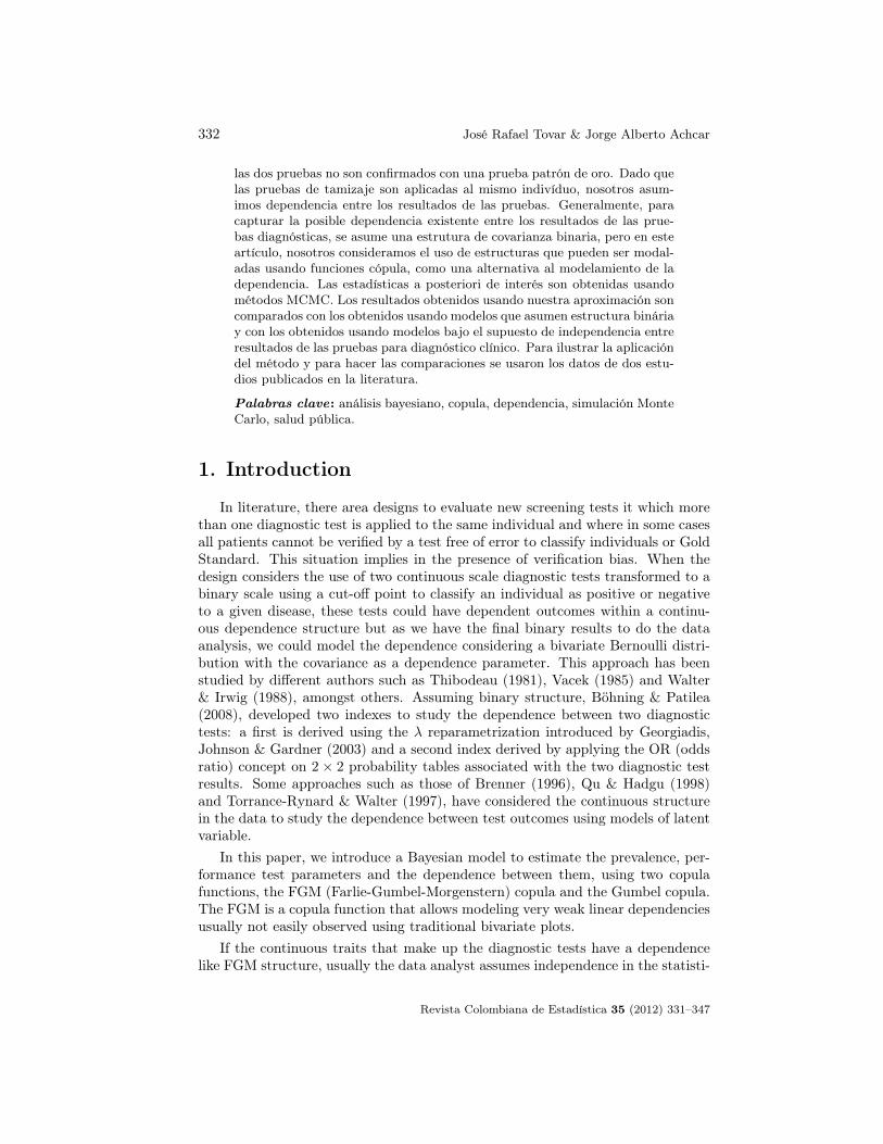
las dos pruebas no son confirmados con una prueba patrón de oro. Dado quelas pruebas de tamizaje son aplicadas al mismo indivíduo, nosotros asum-imos dependencia entre los resultados de las pruebas. Generalmente, paracapturar la posible dependencia existente entre los resultados de las prue-bas diagnósticas, se asume una estrutura de covarianza binaria, pero en esteartículo, nosotros consideramos el uso de estructuras que pueden ser modal-adas usando funciones cópula, como una alternativa al modelamiento de ladependencia. Las estadísticas a posteriori de interés son obtenidas usandométodos MCMC. Los resultados obtenidos usando nuestra aproximación soncomparados con los obtenidos usando modelos que asumen estructura bináriay con los obtenidos usando modelos bajo el supuesto de independencia entreresultados de las pruebas para diagnóstico clínico. Para ilustrar la aplicacióndel método y para hacer las comparaciones se usaron los datos de dos estu-dios publicados en la literatura.
Palabras clave: análisis bayesiano, copula, dependencia, simulación MonteCarlo, salud pública.
1. Introduction
In literature, there area designs to evaluate new screening tests it which morethan one diagnostic test is applied to the same individual and where in some casesall patients cannot be verified by a test free of error to classify individuals or GoldStandard. This situation implies in the presence of verification bias. When thedesign considers the use of two continuous scale diagnostic tests transformed to abinary scale using a cut-off point to classify an individual as positive or negativeto a given disease, these tests could have dependent outcomes within a continu-ous dependence structure but as we have the final binary results to do the dataanalysis, we could model the dependence considering a bivariate Bernoulli distri-bution with the covariance as a dependence parameter. This approach has beenstudied by different authors such as Thibodeau (1981), Vacek (1985) and Walter& Irwig (1988), amongst others. Assuming binary structure, Böhning & Patilea(2008), developed two indexes to study the dependence between two diagnostictests: a first is derived using the λ reparametrization introduced by Georgiadis,Johnson & Gardner (2003) and a second index derived by applying the OR (oddsratio) concept on 2× 2 probability tables associated with the two diagnostic testresults. Some approaches such as those of Brenner (1996), Qu & Hadgu (1998)and Torrance-Rynard & Walter (1997), have considered the continuous structurein the data to study the dependence between test outcomes using models of latentvariable.
In this paper, we introduce a Bayesian model to estimate the prevalence, per-formance test parameters and the dependence between them, using two copulafunctions, the FGM (Farlie-Gumbel-Morgenstern) copula and the Gumbel copula.The FGM is a copula function that allows modeling very weak linear dependenciesusually not easily observed using traditional bivariate plots.
If the continuous traits that make up the diagnostic tests have a dependencelike FGM structure, usually the data analyst assumes independence in the statisti-
Revista Colombiana de Estadística 35 (2012) 331–347

Dependence between Diagnostic Tests 333
cal model used to obtain the parameter estimates. The form of the Gumbel copulaused in this work, models relatively weak negative linear dependencies but the cop-ula parameter of dependence belongs in the space (0,1). In agreement with somesimulation results not showed in this paper, the bivariate plots obtained underdifferent levels of Gumbel copula dependence show a dispersion similar with thatobserved when the data are obtained under independence assumption, then, it isnot easy to observe the presence of a negative correlation between test outcomes.The use of this copula, also allows us to study dependencies with not necessar-ily linear structures which is possible in diagnostic situations whose results areobtained after dichotomization.
We compare the estimates obtained using copula models with those obtainedassuming binary covariance structure and independence assumption. In our ap-proach, we assume that the diagnostic procedure includes two (observable or not)variables measured on a continuous scale with some type of positive dependencebetween them that can be modeled using copula functions. Copula functions havebeen widely used for modeling the dependence between continuous scale variablesregardless the type of distribution underlying in the margins, in many other subjector topic areas as hydrology and finance.
To illustrate our proposed models, we use two data sets introduced in theliterature. The first one, was obtained from Smith, Bullock & Catalona (1997),who screened 19,476 men for prostate cancer using the Digital Rectal Exam (DRE)and the Prostate Specific Antigen (PSA) in serum. With that same data set,Böhning & Patilea (2008) and Martinez, Achcar & Louzada (2005) studied theassociation between diagnostic test results. The second data set was introducedby Ali, Moodambail, Hamrah, Bin-Nakhi & Sadeq (2007), where they evaluated afast method to detect urinary tract infection in 132 children of both genders withages ranging from three days to 11 years.
This paper is organized as follows: In Section 2 we introduce the model formu-lation for two associated diagnostic tests; in Section 3, we present our Bayesianestimation procedure; in Section 4, we introduce two examples; finally in section5, we present some discussion on the obtained results.
2. Model Formulation for Two DependentDiagnostic Tests
We consider four different models that can be used, the first model assumesconditionally independent tests results and the other three models assume thatthe tests are dependent conditionally on the disease status.
2.1. Model Under Independence Assumption
Two diagnostic tests are respectively denoted by T1 and T2 where Tν = 1 isrelated to a positive result for the test ν, ν = 1, 2 and Tν = 0 is related to anegative result. In Table 1 we have a generic representation of the tests compared
Revista Colombiana de Estadística 35 (2012) 331–347

334 José Rafael Tovar & Jorge Alberto Achcar
with an ideal reference test. If the study design implies that individuals withnegative outcome in both tests are not verified by a test free of error to classifythe individuals (“Gold Standard”), the values d, h, n+ and n− (showed in brackets),are unknown although the sum u = n+ + n− is known.
Table 1: Tests results. Values in brackets are unknown under verification bias.Diseased subjects Non-diseased subjects
T2 = 1 T2 = 0 Total T2 = 1 T2 = 0 TotalT1 = 1 a b a+ b e f e+ f
T1 = 0 c [d ] c+ [d ] g [h] g + [h]
Total a+ c b+ [d ] [n+] e+ g f + [h] [n−]
Let us denote by p the prevalence of a disease and by D the true status, whenD = 1 denotes a diseased individual and D = 0 denotes a non-diseased individual.That is, p = P (D = 1). The sensitivities are given by Sν = P (Tν = 1 | D = 1)and the specificities are given by Eν = P (Tν = 0 | D = 0).
For the independence assumption model, we use the Bayesian estimation pro-cedure developed by Martinez et al. (2005) to obtain the likelihood contributionsof the eight possible combinations of results among tests and true disease state asappear in the left column in Table 2.
2.2. Model Under Binary Dependence Structure
For a binary structure model, we assume as dependence parameter, a positivecovariance between tests based on the joint Bernoulli distribution. We assumedthat the dependence between tests is similar in diseased and non-diseased popula-tions in the same way as considered by Dendukuri & Joseph (2001) to obtain thecontributions to likelihood function of the eight combinations of results among thetwo diagnostic tests and the Gold Standard. The results are showed in Table 2.
Table 2: Likelihood contributions of all possible combinations of outcomes of T1, T2
and D. (fi = number of individuals in the cell i; i = 1, 2, . . . , 8. Values inbrackets are unknown under verification bias).
Contribution to likelihoodi D T1 T2 fi Independence assumption Binary dependence1 1 1 1 a pS1S2 p[S1S2 + ψD]
2 1 1 0 b pS1(1− S2) p[S1(1− S2)− ψD]
3 1 0 1 c p(1− S1)S2 p[(1− S1)S2 − ψD]
4 1 0 0 [d] p(1− S1)(1− S2) p[(1− S1)(1− S2) + ψD]
5 0 1 1 e (1− p)(1− E1)(1− E2) (1− p)[(1− E1)(1− E2) + ψND]
6 0 1 0 f (1− p)(1− E1)E2 (1− p)[(1− E1)E2 − ψND]
7 0 0 1 g (1− p)E1(1− E2) (1− p)[E1(1− E2)− ψND]
8 0 0 0 [h] (1− p)E1E2 (1− p)[E1E2 + ψND]
Revista Colombiana de Estadística 35 (2012) 331–347

Dependence between Diagnostic Tests 335
2.3. Model Assuming a Dependence Copula Structure
Let us assume that the test outcomes are realizations of the random variablesV1 and V2 measured on a positive continuous scale (V1 > 0 and V2 > 0) whichrepresent the expression of two biological traits whose behavior is altered by thepresence of disease or infection process. Also, let us assume that two cut-off valuesξ1 and ξ2 are chosen for each test in order to determine when an individual isclassified as positive or negative. In this way we assume that an individual isclassified as positive for test ν if Vν > ξν that is, Tν = 1 if and only if Vν > ξν forν = 1, 2. To model the dependence structure between the random variables V1 andV2, let us consider the use of copula functions, which has been studied by manyauthors ((Nelsen 1999) is a classical book on this topic). Multivariate distributionfunctions F can be written in the form of a copula function, that is, if F (v1, . . . vm)is a joint multivariate distribution function with univariate marginal distributionfunctions F1(v1), . . . , Fm(vm), thus there exists a copula function C(u1, . . . , um)such that,
F (v1, . . . , vm) = C(F1(v1), . . . , Fm(vm)) (1)
When the marginal distributions are continuous, a copula function always existsand can be found from the relation
C(u1, . . . , um) = F (F−11 (u1), . . . , F
−1m (um)) (2)
For the special case of bivariate distributions, we have m = 2. The approachto formulate a multivariate distribution using a copula is based on the idea thata simple transformation (U = F1(V1) and W = F2(V2)) can be made of eachmarginal variable in such a way that each transformed marginal variable has auniform distribution. Specifying dependence between V1 and V2 is the same asspecifying dependence between U and W , thus the problem reduces to specifyinga bivariate distribution between two uniform variables, that is a copula.
2.3.1. Model Considering Dependence Type FGM Copula
The third model considered for the study of the dependence structure for twotests, is based in the Farlie Gumbel Morgenstern (FGM) copula widely studied byauthors as Nelsen (1999), Amblard & Girard (2002, 2005, 2008). The FGM copulais defined by,
CI(u,w) = uw[1 + ϕ(1− u)(1− w)] (3)
where u = F1(v1), w = F2(v2) and ϕ is a copula parameter such that −1 ≤ ϕ ≤ 1.If ϕ = 0, we have two independent marginal random variables. We assume differentparameters ϕD and ϕND for diseased and non-diseased individuals, respectively.
From (3) the cumulative joint distribution and the join survival function forthe random variables V1 and V2 is given by,
FI(v1, v2) = CI(F1(v1), F2(v2))
= F1(v1)F2(v2)[1 + ϕ(1− F1(v1))(1− F2(v2))] (4)
Revista Colombiana de Estadística 35 (2012) 331–347

336 José Rafael Tovar & Jorge Alberto Achcar
S(v1, v2) = P (V1 > v1, V2 > v2) = 1− F1(v1)− F2(v2) + F (v1, v2) (5)
Within the diseased individuals group, we have,
FD1 (ξ1) = P (V1 ≤ ξ1|D = 1) = 1− S1
FD2 (ξ2) = P (V2 ≤ ξ2|D = 1) = 1− S2
From (4), we have
FD(ξ1, ξ2) = FD1 (ξ1)FD2 (ξ2)[1 + ϕ(1− FD1 (ξ1))(1− FD2 (ξ2))]
= (1− S1)(1− S2)(1 + ϕDS1S2)
and from (5) we have,
P (T1 = 1, T2 = 1|D = 1) = SD(ξ1, ξ2)
= 1− (1− S1)− (1− S2) + (1− S1)(1− S2)(1 + ϕDS1S2)
That is,
P (T1 = 1, T2 = 1|D = 1) = S1S2(1 + ϕD(1− S1)(1− S2))
andP (T1 = 1, T2 = 1, D = 1) = pS1S2(1 + ϕD(1− S1)(1− S2))
Observe that, if ϕD = 0 (independent test outcomes), we have
P (T1 = 1, T2 = 1, D = 1) = pS1S2
as given in Table 2.Also,
P (T1 = 1, T2 = 0, D = 1) = P (D = 1)P (T1 = 1, T2 = 0|D = 1)
= pP (V1 > ξ1, V2 ≤ ξ2|D = 1)
On the other hand,
P (V1 > ξ1, V2 ≤ ξ2|D = 1) = P (V2 ≤ ξ2|D = 1)− P (V1 ≤ ξ1, V2 ≤ ξ2|D = 1)
= FD2 (ξ2)− FD(ξ1, ξ2)
Thus,
P (T1 = 1, T2 = 1, D = 1) = p(1− S2)S1[1− ϕDS2(1− S1)]
If ϕD = 0, we have
P (T1 = 1, T2 = 0, D = 1) = pS1(1− S2)
as in the independent case (see Table 2).
Revista Colombiana de Estadística 35 (2012) 331–347

Dependence between Diagnostic Tests 337
Similarly,
P (T1 = 0, T2 = 1, D = 1) = P (D = 1)P (T1 = 0, T2 = 1|D = 1)
= pP (V1 ≤ ξ1, V2 > ξ2|D = 1)
Since,
P (V1 ≤ ξ1, V2 > ξ2|D = 1) = P (V1 ≤ ξ1|D = 1)− P (V1 ≤ ξ1, V2 ≤ ξ2|D = 1)
= FD1 (ξ1)− FD(ξ1, ξ2)
then,P (T1 = 0, T2 = 1, D = 1) = p(1− S1)S2[1− ϕDS1(1− S2)]
When ϕD = 0 we have P (T1 = 0, T2 = 1, D = 1) = pS2(1 − S1) as in theindependent case (see Table 2).
We also have,
P (T1 = 0, T2 = 0, D = 1) = P (D = 1)P (T1 = 0, T2 = 0|D = 1)
= pP (V1 ≤ ξ1, V2 ≤ ξ2|D = 1)
= pFD(ξ1, ξ2),
that is,
P (T1 = 0, T2 = 0, D = 1) = p(1− S1)(1− S2)[1 + ϕDS1S2]
Within the non-diseased individuals group, we have:
P (T1 = 1, T2 = 1, D = 0) = P (D = 0)P (T1 = 1, T2 = 1 | D = 0)
= (1− p)P (V1 > ξ1, V2 > ξ2|D = 0)
= (1− p)SND(ξ1, ξ2)= (1− p)(1− FND1 (ξ1)− FND2 (ξ2) + FND(ξ1, ξ2)
Observe that,
P (T1 = 0|D = 0) = P (V1 ≤ ξ1|D = 0) = FND1 (ξ1) = E1 and
P (T2 = 0|D = 0) = P (V2 ≤ ξ2|D = 0) = FND2 (ξ1) = E2
Using (4), we have
FND(ξ1, ξ2) = E1E2[1 + ϕND(1− E1)(1− E2)]
That is,
P (T1 = 1, T2 = 1, D = 0) = (1− p)(1− E1)(1− E2)[1 + ϕNDE1E2]
The contributions to the likelihood for all situations with diseased and non-diseased individuals are given in Table 3.
Revista Colombiana de Estadística 35 (2012) 331–347

338 José Rafael Tovar & Jorge Alberto Achcar
2.3.2. Model Considering Dependence Type Gumbel Copula
The last considered model, is derived from Gumbel copula function defined as;
CII(u,w) = u+ w − 1 + (1− u)(1− w) exp{−φ log(1− u) log(1− w)} (6)
In this model, the joint cumulative distribution function for the random vari-ables V1 and V2 is given by,
FII(v1v2) = F1(v1) + F2(v2)− 1 + (1− F1(v1))(1− F2(v2))
exp{−φ log(1− F1(v1)) log(1− F2(v2))} (7)
As pointed out by (Gumbel 1960) for this copula model, when φ = 1 thePearson correlation linear coefficient (ρ) takes the value −0.40365. In this case,the parameter of the Gumbel copula, does not models positive linear correlations.Also, when the two variables are independent, φ takes the zero value.
Employing the same arguments considered with the FGM copula and using (7)we obtain all the contributions for the likelihood function when it is assumed aGumbel copula dependence structure (Table 3).
Table 3: Likelihood contributions of all possible combinations of outcomes of T1, T2 andD when the dependence has the “FGM copula” or “Gumbel copula” structure.(fi = number of individuals in the cell i; i = 1, 2, . . . , 8. Values in brackets areunknown under verification bias).
Contribution to likelihoodi D T1 T2 fi “FGM copula” “Gumbel copula”1 1 1 1 a pS1S2[1 + ϕD(1 − S1)(1 − S2)] pS1S2Q1
2 1 1 0 b pS1(1 − S2)[1 − ϕD(1 − S1)S2] pS1[1 − S2Q1]
3 1 0 1 c p(1 − S1)S2[1 − ϕDS1(1 − S2)] pS2[1 − S1Q1]
4 1 0 0 [d] p(1 − S1)(1 − S2)[1 + ϕDS1S2] p[1 − S1 − S2 + S1S2Q1]
5 0 1 1 e (1 − p)(1 − E1)(1 − E2)[1 + ϕNDE1E2] (1 − p)(1 − E1)(1 − E2)Q2
6 0 1 0 f (1 − p)(1 − E1)E2[1 − ϕNDE1(1 − E2)] (1 − p)(1 − E1)[1 − (1 − E2)Q2]
7 0 0 1 g (1 − p)E1(1 − E2)[1 − ϕNDE2(1 − E1)] (1 − p)(1 − E2)[1 − (1 − E1)Q2]
8 0 0 0 [h] (1 − p)E1E2[1 + ϕND(1 − E1)(1 − E2)] (1 − p)[E1 + E2 − 1 + (1 − E1)(1 − E2)Q2]
Observe that; Q1 = exp(−φD logS1 logS2), Q2 = exp(−φND log(1 − E1) log(1 − E2))
3. Bayesian Approach
For a Bayesian analysis of the proposed models, we consider different Beta priordistributions on the prevalence, performance measure parameters (sensitivities andspecificities) and the copula parameters. In some cases, we could have some priorinformation on the parameters from experts in diagnostic medical tests or fromprevious studies on the subject.
For a Bayesian analysis of the models, we assumed positive dependence be-tween the diagnostic tests in the same way as it was considered by Dendukuri& Joseph (2001) (therefore P (ϕ < 0) = 0 and P (ψ < 0) = 0) we could assumeuniform U(a,b) as non-informative prior distributions and Beta(a,b) distributions
Revista Colombiana de Estadística 35 (2012) 331–347

Dependence between Diagnostic Tests 339
for the informative situation for FGM and Gumbel dependence parameters andfor prevalence and performance test parameters. If we need to elicit informativeprior distributions for binary covariance, we could use the Generalized Beta(a,b)distribution in the same way that was considered by Martinez et al. (2005). Forthe non-informative case the Uniform U(0,1) distribution should be a good option.
Usually, we do not have any kind of information about the copula parameters,that is, for both copula dependence parameters. In this case, we used the proceduredeveloped by Tovar (2012) to obtain the prior hyperparameters and we assume thatthe dependence takes values within of some interval (θ1, θ2) within of parametricspace. In this way, if we assumed that the dependence is weak, the parameter couldbelong to the interval (0, 1/4); when the dependence is moderate the parametershould be in to the interval (1/4, 3/4) and when the dependence is strong, theparameter should be in to the interval (3/4, 1). To obtain the hyperparametervalues, we take the midpoint of the interval as the mean E(θ) and we apply theChebychev’s inequality to approximate the variance V (θ), as follows:
P (|θ − E(θ)| ≥ kσ) ≤ 1
k2= γ
P ([θ − E(θ)]2 ≥ k2σ2) ≤ γ
P (α[θ − θ0]2 ≥ σ2) ≤ γ (8)
where γ is the prior probability of θ do not belong to the constructed interval.Therefore, the variance will be a function of the prior established probability
to interval values of the unknown quantity and the distance between θ0 and apercentile of the distribution. If it is replaced θ by some of the known values θ1 orθ2 in the equation (8) it is easy to obtain a approximated value for the varianceof the Beta prior distribution, as follows;
σ2 ≤ α[θ1 − θ0]2 ∼=ab
(a+ b)2(a+ b+ 1)(9)
And as the mean θ0 = E(θ) and the variance σ2 = V (θ) can be written asfunctions of the Beta prior hyperparameters, it is necessary to solve a system oftwo equations with two unknowns to find values of a and b i.e:
ω =θ0
(1− θ0)a = ωb
b =ω − [(ω + 1)2σ2]
(ω3 + 3ω2 + 3ω + 1)σ2(10)
In this way, assuming γ = 0.05 in (8), for the FGM and Gumbel dependenceparameters we have evaluated a Beta(17, 122) distribution, a Beta(39.5, 39.5) dis-tribution and a Beta(122, 17) distribution as informative prior distributions andfinally we have selected as selection criteria the Deviance Information CriteriaDIC Spiegelhalter, Thomas, Best & Lunn (2003) obtained within the WinBUGS
Revista Colombiana de Estadística 35 (2012) 331–347

340 José Rafael Tovar & Jorge Alberto Achcar
environment and a heuristic procedure that assumes two criteria: quality in theconvergence of the MCMC procedure and concentration of the posterior distri-bution using the coefficient of variation (CV). The best model should have thelower DIC, the best performance in MCMC convergence and highest concentra-tion around the posterior mean (lowest CV).
We have seven parameters to be estimated, two sensitivities, two specificities,one prevalence, one dependence parameter for diseased individuals and anotherone for non-diseased individuals. If we assume a design with the presence of ver-ification bias, we have only four degrees of freedom for the estimation processand if we assume a design without verification bias, we have six information com-ponents. Therefore, in both cases the model is non-identified. Using a classicalapproach, the problem has been addressed giving fixed values to a subset of pa-rameters and estimating the remaining unconstrained parameters (Vacek 1985),but since all parameters are typically unknown, the division into constrained andunconstrained sets is often quite arbitrary. Since the Bayesian paradigm someauthors as Joseph, Gyorkos & Coupal (1995), have proposed to construct informa-tive prior distribution over a subset or over all unknown quantities. In accordancewith Dendukuri & Joseph (2001), informative priors would be needed on at leastas many parameters as would be constrained when using the most frequent ap-proach. In this approach, the prior information is used to distinguish between thenumerous possible solutions for the non-identifiable problem. This approach isapproximately numerically equivalent to the most frequent approach when a de-generate (point mass) distribution is used that matches the constrained parametervalues and diffuse prior distributions are used for the non-constrained parameters.In order to treat the non-identifiability problem, first, we assume informative priordistributions over the subset of dependence parameters and non-informative priordistributions on prevalence and performance test parameters and next, we assumeinformative prior distributions on all set of parameters in accordance with whatwas suggested by Joseph et al. (1995).
As the posterior distributions do not have closed forms, we have used MCMCmethods, especially Metropolis-Hastings algorithm to obtain estimates for the pa-rameters. For all models, 500, 000 Gibbs samples were simulated from the condi-tional distributions. From these generated samples, we discarded the first 50, 000samples to eliminate the effect of the initial values and we also considered a spac-ing of 100. Convergence of the algorithm was verified graphically and also usingstandard existing methods implemented in the software CODA (Best, Cowles &Vines 1995).
4. Examples
4.1. Cancer Data
As a first example, we have used a data set introduced by (Smith et al. 1997).They screened 19,476 men for prostate cancer using Digital Rectal Examination(DRE) and Prostate-Specific Antigen (PSA) in serum. The PSA level was consid-
Revista Colombiana de Estadística 35 (2012) 331–347

Dependence between Diagnostic Tests 341
ered suspicious for cancer if it exceeded 4.0 ng/ml. Subjects with positive resultson either DRE or PSA were submitted to an ultrasound guided needle biopsy testwhich was considered as “gold standard”. This data set obtained under verificationbias is related to approximately 20,000 individuals, as such, it may be consideredas a large sample size.
For prior distribution elicitation, we have used the results introduced by Böh-ning & Patilea (2008). We get the values for the δ and λ indexes and from theseresults, we estimated the quantities d and h of non-verified subjects given in Table1. (See Table 4).
Table 4: Estimated values for the dependence indexes and quantities of non-verifiedindividuals using Böhning’s results. The values in brackets were calculatedusing δi index, the another one using λi index.
Diseased subjects λ1 = 2.42, δ1 = 3.08 Non-diseased subjects λ0 = 2.40, δ0 = 3.03
DRE+ DRE− Total DRE+ DRE− TotalPSA+ 189 292 481 141 755 896PSA− 145 1431[691] 1576[836] 1002 15521[16261] 16523[17263]
Total 334 1723[983] 2057[1317] 1143 16276[17016] 17419[18159]
Using the data in Table 4 we assumed prior independence between the com-ponents of the parameter vector [θ1 = S1, θ2 = S2, θ3 = E1, θ4 = E2, θ5 = p] toobtain estimates and intervals where it is possible assume to find each componentwith a probability 1− γ = 0.95. (See Table 5).
Table 5: Informative prior distribution hyperparameters for performance test parame-ters, prevalence and covariance (Martinez’s prior informative distributions forψ).PARAMETER INTERVAL E(θ) aθ bθ
S1 0.236 - 0.365 0.3006 303 704S2 0.162 - 0.254 0.2080 324 1232E1 0.949 - 0.951 0.950 902500 47500E2 0.934 - 0.937 0.9355 501758 34595p 0.068 - 0.106 0.0866 379 4002ψD 0.004659 - 0.004719 0.004689 486303 103225102ψND 0.080 - 0.133 0.1722 289 2421
Assuming prior independence, for each interval we take the midpoint of eachinterval as the expected value of the prior distribution and we use the Chebychevinequality to get approximations for the variance of each parameter in the waythat was described in Section 3 and we obtained the hyperparameter values thatappear in Table 5. For this set of parameters we have used U(0,1) distributions asnon-informative priors.
To elicit binary covariance prior distributions, we have used the results ob-tained by Martinez et al. (2005). They estimated the covariance parameter forthe same cancer data under a Bayesian approach assuming non-informative priordistributions for ψD and ψND. We have used the 95% credible regions obtainedby them and we applied the same procedure employed with the test parameters
Revista Colombiana de Estadística 35 (2012) 331–347

342 José Rafael Tovar & Jorge Alberto Achcar
and prevalence. As non-informative distributions we have used GenBeta(1/2, 1/2)distributions.
For the copula parameters θ2 = [ϕD, ϕND, φD, φND] we assumed the Betadistributions Beta(17, 122), Beta(39.5, 39.5) and Beta(122, 17) as prior distribu-tions and Uniform U(0,1) as non-informative prior distributions. To address thelack identifiability problem of we have putting informative prior distributions ona subset or on the complete set of parameters considering two set of models asfollows:
• Set 1 of models: informative prior distribution for the copula parameters andnon-informative prior distributions for the prevalence and test parameters
• Set 2 of models: informative prior distributions for all parameters (See Table6)
Table 6: Bayesian posterior summaries obtained by analyzing the data considering in-dependence between tests assumption and different dependence structures.(Posterior means and 95% credible intervals (95% CrI) for each parameter ofinterest).
Set 1 of models Set 2 of modelsModel Parameter Means 95% CrI Model Parameter Means 95% CrI
S1 0.567 0.529 - 0.605 S1 0.258 0.252 - 0.264M1,1 S2 0.394 0.363 - 0.394 M2,1 S2 0.226 0.208 - 0.244
DIC = 180.4 E1 0.952 0.950 - 0.954 DIC = 337.1 E1 0.948 0.946 - 0.950E2 0.946 0.943 - 0.949 E2 0.947 0.944 - 0.950p 0.044 0.041 - 0.047 p 0.080 0.075 - 0.085ψD 0.0316 0.019 - 0.046 ψD 0.046 0.037 - 0.055ψND 0.005 0.004 - 0.006 ψND 0.005 0.004 - 0.006
M1,2 S1 0.470 0.380 - 0.548 M2,2 S1 0.295 0.274 - 0.316DIC = 55.2 S2 0.335 0.273 - 0.393 DIC = 54.4 S2 0.211 0.196 - 0.227
E1 0.951 0.948 - 0.955 E1 0.950 0.950 - 0.950E2 0.937 0.933 - 0.940 E2 0.936 0.935 - 0.936p 0.051 0.044 - 0.062 p 0.082 0.076 - 0.088ϕD 0.156 0.136 - 0.176 ϕD 0.135 0.123 - 0.148ϕND 0.040 0.036 - 0.044 ϕND 0.041 0.039 - 0.043
M1,3 S1 0.538 0.480 - 0.595 M2,3 S1 0.320 0.300 - 0.343DIC = 156.5 S2 0.384 0.339 - 0.430 DIC = 225.5 S2 0.225 0.209 - 0.242
E1 0.952 0.948 - 0.955 E1 0.950 0.949 - 0.950E2 0.937 0.933 - 0.941 E2 0.936 0.935 - 0.936p 0.045 0.040 - 0.050 p 0.074 0.069 - 0.079φD 0.120 0.072 - 0.179 φD 0.047 0.028 - 0.072φND 0.017 0.010 - 0.026 φND 0.018 0.011 - 0.027
M1,4 S1 0.593 0.540 - 0.645 M2,4 S1 0.330 0.307 - 0.353DIC = 192.7 S2 0.424 0.379 - 0.469 DIC = 294.4 S2 0.228 0.211 - 0.245
E1 0.952 0.948 - 0.955 E1 0.950 0.949 - 0.951E2 0.937 0.933 -0.941 E2 0.936 0.935 - 0.936p 0.040 0.037 - 0.044 p 0.072 0.0671 - 0.0771
Mj,1, j = 1, 2: Models under assumption of independence between testsMj,2, j = 1, 2: Covariance parameters with informative prior distributionsMj,3, j = 1, 2: FGM dependence parameters with Beta(122, 17) prior distributionsMj,4, j = 1, 2: Gumbel dependence parameters with Beta (17, 122) prior distributions
From the results in Table 6, we observe that in this example with a largesample size (almost 20,000 individuals), we have great differences in the posteriorsummaries of interest, especially for the sensitivities Sν , ν = 1, 2 of the tests
Revista Colombiana de Estadística 35 (2012) 331–347

Dependence between Diagnostic Tests 343
considering different priors for the parameters and different modeling structures.It is also interesting to observe that the specificities Eν ν = 1, 2, that is, theprobabilities of negative tests given that the individuals are not diseased, arealmost not affected by the different priors and different modeling structures inpresence or not of an dependence parameter. These results could be of greatinterest for medical diagnostic tests.
We also observe a large variability on the obtained DIC values considering eachassumed model. The smallest DIC values are obtained for the class of models witha bivariate binary structure.
4.2. Urinary Tract Infection (UTI)
In this example, we consider a data set introduced by Ali et al. (2007) whoevaluated a fast method to detect urinary tract infection. In this case, we cansuspect an association between tests, since the results of the tests are more likelyto be positive when the individual has a greater presence of infection. The au-thors considered the presence of nitrites (N = test1), and the levels of leukocyteesterase in urine (LE = test2) as screening tests and a bacterial culture as theconfirmatory test. They applied the three methods in 132 children of both gen-ders with ages ranging from three days to 11 years. The obtained performance testand prevalence estimates were compared with those obtained in other five studies.Since one of those studies had incomplete data, we only considered the resultsof the four complete studies to elicit our prior distributions. For each estimatedparameter, we calculated the mean and variance of the results obtained in thefive studies (including Ali’s study) and used them as prior means and variancesof the parameters. Thus, the informative prior distributions for prevalence andperformance test parameters are given by:
S1 ∼ Beta(4.15, 4.5), S2 ∼ Beta(15.7, 2.4)
E1 ∼ Beta(0.5, 13), E2 ∼ Beta(8.3, 2.8)
andp ∼ Beta(2.1, 22.3)
For copula and covariance parameters, we assume the same informative pri-ors used for copula parameters considered in the first example. We also assumeuniform U(0,1) prior distributions for the performance test parameters as non-informative priors and applied the same procedure for the estimation process usedin the cancer data example. The results obtained are given in Table 7.
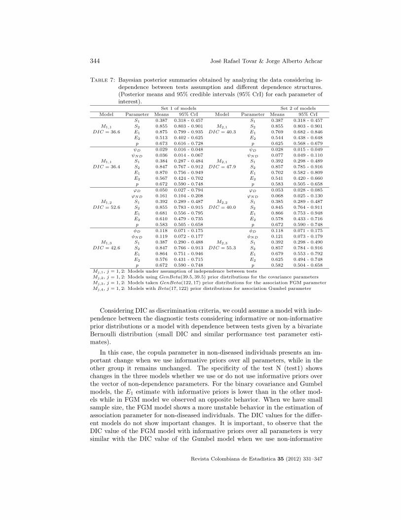
In this example with a small sample size, but not including missing data, weobserve from Table 7, that the sensitivities Sν ν = 1, 2 were not greatly affectedby the choice of prior distributions (informative or not) and modeling structures,but the specificities Eν ν = 1, 2 have a great variability considering the differentmodeling structures. We also observe that the prevalences have similar poste-rior summaries considering each model and the DIC values do not present greatdifferences for each modeling structure.
Revista Colombiana de Estadística 35 (2012) 331–347
344 José Rafael Tovar & Jorge Alberto Achcar
Table 7: Bayesian posterior summaries obtained by analyzing the data considering in-dependence between tests assumption and different dependence structures.(Posterior means and 95% credible intervals (95% CrI) for each parameter ofinterest).
Set 1 of models Set 2 of modelsModel Parameter Means 95% CrI Model Parameter Means 95% CrI
S1 0.387 0.318 - 0.457 S1 0.387 0.318 - 0.457M1,1 S2 0.855 0.803 - 0.901 M2,1 S2 0.855 0.803 - 0.901
DIC = 36.6 E1 0.875 0.799 - 0.935 DIC = 40.3 E1 0.769 0.682 - 0.846E2 0.513 0.402 - 0.625 E2 0.544 0.438 - 0.648p 0.673 0.616 - 0.728 p 0.625 0.568 - 0.679ψD 0.029 0.016 - 0.048 ψD 0.028 0.015 - 0.049ψND 0.036 0.014 - 0.067 ψND 0.077 0.049 - 0.110
M1,1 S1 0.384 0.287 - 0.484 M2,1 S1 0.392 0.298 - 0.489DIC = 36.4 S2 0.847 0.767 - 0.912 DIC = 47.9 S2 0.857 0.785 - 0.916
E1 0.870 0.756 - 0.949 E1 0.702 0.582 - 0.809E2 0.567 0.424 - 0.702 E2 0.541 0.420 - 0.660p 0.672 0.590 - 0.748 p 0.583 0.505 - 0.658ϕD 0.050 0.027 - 0.794 ϕD 0.053 0.028 - 0.085ϕND 0.161 0.104 - 0.208 ϕND 0.068 0.025 - 0.130
M1,2 S1 0.392 0.289 - 0.487 M2,2 S1 0.385 0.289 - 0.487DIC = 52.6 S2 0.855 0.783 - 0.915 DIC = 40.0 S2 0.845 0.764 - 0.911
E1 0.681 0.556 - 0.795 E1 0.866 0.753 - 0.948E2 0.610 0.479 - 0.735 E2 0.578 0.433 - 0.716p 0.583 0.505 - 0.658 p 0.672 0.590 - 0.748φD 0.118 0.071 - 0.175 φD 0.118 0.071 - 0.175φND 0.119 0.072 - 0.177 φND 0.121 0.073 - 0.179
M1,3 S1 0.387 0.290 - 0.488 M2,3 S1 0.392 0.298 - 0.490DIC = 42.6 S2 0.847 0.766 - 0.913 DIC = 55.3 S2 0.857 0.784 - 0.916
E1 0.864 0.751 - 0.946 E1 0.679 0.553 - 0.792E2 0.576 0.431 - 0.715 E2 0.625 0.494 - 0.748p 0.672 0.590 - 0.748 p 0.582 0.504 - 0.658
Mj,1, j = 1, 2: Models under assumption of independence between testsMj,2, j = 1, 2: Models using GenBeta(39.5, 39.5) prior distributions for the covariance parametersMj,3, j = 1, 2: Models taken GenBeta(122, 17) prior distributions for the association FGM parameterMj,4, j = 1, 2: Models with Beta(17, 122) prior distributions for association Gumbel parameter
Considering DIC as discrimination criteria, we could assume a model with inde-pendence between the diagnostic tests considering informative or non-informativeprior distributions or a model with dependence between tests given by a bivariateBernoulli distribution (small DIC and similar performance test parameter esti-mates).
In this case, the copula parameter in non-diseased individuals presents an im-portant change when we use informative priors over all parameters, while in theother group it remains unchanged. The specificity of the test N (test1) showschanges in the three models whether we use or do not use informative priors overthe vector of non-dependence parameters. For the binary covariance and Gumbelmodels, the E1 estimate with informative priors is lower than in the other mod-els while in FGM model we observed an opposite behavior. When we have smallsample size, the FGM model shows a more unstable behavior in the estimation ofassociation parameter for non-diseased individuals. The DIC values for the differ-ent models do not show important changes. It is important, to observe that theDIC value of the FGM model with informative priors over all parameters is verysimilar with the DIC value of the Gumbel model when we use non-informative
Revista Colombiana de Estadística 35 (2012) 331–347
Dependence between Diagnostic Tests 345
priors over test parameters. On the other hand, the DIC value obtained assum-ing non-informative priors over test parameters in one model is similar with thoseobtained using informative priors over complete set in the other one. It is alsointeresting to see that the behavior of the FGM model with small sample size datais similar to the behavior observed in the Gumbel model when we have a largesample size.
5. Conclusion and Remarks
The main goal of this paper was to develop a Bayesian procedure to estimatethe prevalence, performance test and copula parameters of two diagnostic tests inpresence of verification bias and considering the dependence between test results.
We proposed the use of copula structure models to get the estimation of theparameters under dependence assumption and specifically, we have used the Far-lie Gumbel Morgenstern (FGM) and the Gumbel copula models to compare theobtained results with a model under independence assumption between tests andanother one assuming dependent binary tests in designs that consider two diag-nostic tests with continuous outcome for screening, a perfect “gold standard” andverification bias presence. The estimation model obtained under verification biaspresence, implies a lack of identifiability problem, because we have more parame-ters than informative pieces in the likelihood function. Given that, our approachconsiders the continuous dependence structure in the data but the estimationprocess is made with the binary observations in presence of verification bias, weconsider that to estimate the parameters under the Bayesian approach is easierthan under the frequentist approach, because many times it is possible that we donot have the continuous values, for instance, when the measured continuous traitsare non-observable (they are latent variables).
We illustrated the procedure using two published data sets: one with a largesample size and another one with a small sample size of individuals. In bothcases, the better fit for the data was obtained assuming binary associated testsand taking the covariance as a parameter. The FGM model showed better fit whencompared to the Gumbel copula, regardless the sample size. With a large samplesize, the FGM model presented DIC values lower when it was fitted assumingnon-informative prior distributions on test parameters and the estimates are veryclose with those obtained using maximum likelihood method, reflecting the effectthat has the observed data in the estimation process.
However, to use informative prior on all parameters allow us to obtain sensi-tivity estimates with shorter credibility regions which is very good if we considerthat within the large sample used, the true positives are a small part. The pre-vious conclusion is reinforced by the results observed with the data of the smallsample size, which the informative prior on all parameters gave better fit. Withthe Gumbel model, we obtained similar results with large sample size, but the useof non-informative prior distributions on the test parameters gave better fit withsmall sample size. For binary covariance models the choice of prior distributionplays an important role in the estimation procedure, especially with large sample
Revista Colombiana de Estadística 35 (2012) 331–347
346 José Rafael Tovar & Jorge Alberto Achcar
sizes, where the posterior summaries of interest do not have important changes as-suming informative or non-informative prior distributions. With small sample sizesand binary covariance structure, we observed better fit assuming non-informativeprior distributions on the test parameters and informative prior distributions oncovariance parameter.
It is important to point out that we could consider other copula families intro-duced in the literature to model dependence between diagnostic tests. A specialcase is given by the Clayton copula which is useful when the dependence is mainlyconcentrated in the lower tail or the Frank copula which is radial symmetric. Theuse of these other copulas in dependent diagnostic tests will be the goal of a futurework, since an appropriate choice is essential in order to get an optimal result.
Acknowledgments
The second author was supported by grants of Conselho Nacional de Pesquisas(CNPq), Brazil. This paper is a part of the doctoral in statistics project of thefirst author. [
Recibido: noviembre de 2011 — Aceptado: abril de 2012]
References
Ali, S., Moodambail, A., Hamrah, E., Bin-Nakhi, H. & Sadeq, S. (2007), ‘Reliabil-ity of rapid dipstick test in detecting urinary tract infection in symptomaticchildren’, Kuwait Medical Journal 39, 36–38.
Amblard, C. & Girard, S. (2002), ‘Symmetry and dependence properties withina semiparametric family of bivariate copulas’, Journal of Non-parametricStatistics 14, 715–727.
Amblard, C. & Girard, S. (2005), ‘Estimation procedures for semiparametric fam-ily of bivariate copulas’, Journal of Computational and Graphical Statistics14, 363–377.
Amblard, C. & Girard, S. (2008), ‘A new extension of bivariate FGM copulas’,Metrika 70, 1–17.
Best, N., Cowles, M. & Vines, S. (1995), CODA: Convergence diagnosis and outputanalysis software for Gibbs sampling output, version 0.3;, MRC BiostatisticsUnit, Cambridge, U.K.
Böhning, D. & Patilea, V. (2008), ‘A capture-recapture approach for screeningusing two diagnostic tests with availability of disease status for the positivesonly’, Journal of the American Statistical Association 103, 212–221.
Brenner, H. (1996), ‘How independent are multiple diagnosis classifications?’,Statistics in Medicine 15, 1377–1386.
Revista Colombiana de Estadística 35 (2012) 331–347

Dependence between Diagnostic Tests 347
Dendukuri, N. & Joseph, L. (2001), ‘Bayesian approaches to modelling the condi-tional dependence between multiple diagnostic tests’, Biometrics 57, 158–167.
Georgiadis, M., Johnson, W. & Gardner, I. (2003), ‘Correlation adjusted estima-tion of sensitivity and specificity of two diagnostic tests’, Journal of the RoyalStatistical Society: Series C (Applied Statistics) 52, 63–76.
Gumbel, E. (1960), ‘Bivariate exponential distributions’, Journal of the AmericanStatistical Association 55, 698–707.
Joseph, L., Gyorkos, T. & Coupal, L. (1995), ‘Bayesian estimation of diseaseprevalence and the parameters of diagnostic tests in the absence of a goldstandard’, American Journal of Epidemiology 141, 263–272.
Martinez, E., Achcar, J. & Louzada, N. (2005), ‘Bayesian estimation of diagnostictests accuracy for semi-latent data with covariates’, Journal of Biopharma-ceutical Statistics 15, 809–821.
Nelsen, R. (1999), An Introduction to Copulas, Springer Verlag, New York.
Qu, Y. & Hadgu, A. (1998), ‘A model for evaluating sensitivity and specificity forcorrelated diagnostic test in efficacy studies with an imperfect reference test’,Journal of the American Statistical Association 93, 920–928.
Smith, D., Bullock, A. & Catalona, W. (1997), ‘Racial differences in operat-ing characteristics of prostate cancer screening tests’, Journal of Urology158, 1861–1865.
Spiegelhalter, D., Thomas, A., Best, N. & Lunn, D. (2003), Winbugs User Manualversion 1.4, MRC Biostatistics Unit, Cambridge, U.K.
Thibodeau, L. (1981), ‘Evaluating diagnostic tests’, Biometrics 37.
Torrance-Rynard, V. & Walter, S. (1997), ‘Effects of dependent errors in the as-sessment of diagnostic tests performance’, Statistics in Medicine 16.
Tovar, J. R. (2012), ‘Eliciting beta prior distributions for binomial sampling’,Revista Brasileira de Biometría 30, 159–172.
Vacek, P. (1985), ‘The effect of conditional dependence on the evaluation of diag-nostic tests’, Biometrics 41.
Walter, S. & Irwig, L. (1988), ‘Estimation of test error rates disease prevalenceand relative risk from misclassified data: a review’, Journal of Clinical Epi-demiology 41.
Revista Colombiana de Estadística 35 (2012) 331–347


Revista Colombiana de EstadísticaDiciembre 2012, volumen 35, no. 3, pp. 349 a 370
Fatigue Statistical Distributions Useful forModeling Diameter and Mortality of Trees
Distribuciones estadísticas de fatiga útiles para modelar diámetro ymortalidad de árboles
Víctor Leiva1,a, M. Guadalupe Ponce2,b, Carolina Marchant1,c,Oscar Bustos3,d
1Departamento de Estadística, Universidad de Valparaíso, Valparaíso, Chile2Instituto de Matemáticas y Física, Universidad de Talca, Talca, Chile
3Departamento de Producción Forestal, Universidad de Talca, Talca, Chile
Abstract
Mortality processes and the distribution of the diameter at breast height(DBH) of trees are two important problems in forestry. Trees die due to sev-eral factors caused by stress according to a phenomenon similar to materialfatigue. Specifically, the force (rate) of mortality of trees quickly increases ata first stage and then reaches a maximum. In that moment, this rate slowlydecreases until stabilizing at a constant value in the long term establishing asecond stage of such a rate. Birnbaum-Saunders (BS) distributions are mod-els that have received considerable attention currently due to their interestingproperties. BS models have their genesis from a problem of material fatigueand present a failure or hazard rate (equivalent to the force of mortality)that has the same behavior as that of the DBH of trees. Then, BS distribu-tions have arguments that transform them into models that can be useful inforestry. In this paper, we present a methodology based on BS distributionsassociated with this forest thematic. To complete this study, we perform anapplication of five real DBH data sets (some of them unpublished) that pro-vides statistical evidence in favor of the BS methodology in relation to theforestry standard methodology. This application provides valuable financialinformation that can be used for making decisions in forestry.
Key words: data analysis, force of mortality, forestry, hazard rate.
ResumenaProfessor. E-mail: [email protected] profesor. E-mail: [email protected] profesor. E-mail: [email protected] professor. E-mail: [email protected]
349

350 Víctor Leiva, M. Guadalupe Ponce, Carolina Marchant & Oscar Bustos
Los procesos de mortalidad y la distribución del diámetro a la altura delpecho (DAP) de árboles son dos problemas importantes en el área forestal.Los árboles mueren debido a diversos factores causados por estrés medianteun fenómeno similar a la fatiga de materiales. Específicamente, la fuerza(tasa) de mortalidad de árboles crece rápidamente en una primera fase yluego alcanza un máximo, momento en el que comienza una segunda faseen donde esta tasa decrece lentamente estabilizándose en una constante enel largo plazo. Distribuciones Birnbaum-Saunders (BS) son modelos quehan recibido una atención considerable en la actualidad debido a sus intere-santes propiedades. Modelos BS nacen de un problema de fatiga de mate-riales y poseen una tasa de fallas (equivalente a la fuerza de mortalidad)que se comporta de la misma forma que ésa del DAP de árboles. Entonces,distribuciones BS poseen argumentos que las transforman en modelos quepuede ser útiles en las ciencias forestales. En este trabajo, presentamos unametodología basada en la distribución BS asociada con esta temática fore-stal. Para finalizar, realizamos una aplicación con cinco conjuntos de datosreales (algunos de ellos no publicados) de DAP que proporciona una eviden-cia estadística en favor de la metodología BS en relación a la metodologíaestándar usada en ciencias forestales. Esta aplicación entrega informaciónque puede ser valiosa para tomar decisiones forestales.
Palabras clave: análisis de datos, fuerza de mortalidad, silvicultura, tasade riesgo.
1. Introduction
The determination of the statistical distribution of the diameter at breastheight (DBH) of trees, and its relationship to the age, composition, density andgeographical location where a forest is localized are valuable information for dif-ferent purposes (Bailey & Dell 1973, Santelices & Riquelme 2007). Specifically,the distribution of the DBH is frequently used to determine the volume of woodfrom a stand allowing us to make decisions about: (i) productivity (quantity); (ii)diversity of products (quality); (iii) tree ages (mortality); and (iv) harvest policyand trees pruning (regeneration). Then, to know the DBH distribution may helpto plan biological and financial management aspects of a forest in a more efficientway (Rennolls, Geary & Rollinson 1985). For example, trees with a large diame-ter are used for wood production, while trees with a small diameter are used forcellulose production. Thus, the four mentioned concepts (quality, quantity, mor-tality and regeneration) propose a challenge to postulate models that allow us todescribe the forest behavior based on the DBH distribution.
Several statistical distributions have been used in the forestry area mainly tomodel the DBH. These distributions (in chronological order) are the models:
(i) Exponential (Meyer 1952, Schmelz & Lindsey 1965);
(ii) Gamma (Nelson 1964);
(iii) Log-normal (Bliss & Reinker 1964);
Revista Colombiana de Estadística 35 (2012) 349–370

Distributions Useful for Modeling Diameter and Mortality of Trees 351
(iv) Beta (Clutter & Bennett 1965, McGee & Della-Bianca 1967, Lenhart &Clutter 1971, Li, Zhang & Davis 2002, Wang & Rennolls 2005);
(v) Weibull (Bailey & Dell 1973, Little 1983, Rennolls et al. 1985, Zutter, Oder-wald, Murphy & Farrar 1986, Borders, Souter, Bailey & Ware 1987, McEwen& Parresol 1991, Maltamo, Puumalinen & Päivinen 1995, Pece, de Benítez& de Galíndez 2000, García-Güemes, Cañadas & Montero 2002, Wang &Rennolls 2005, Palahí, Pukkala & Trasobares 2006, Podlaski 2006);
(vi) Johnson SB (Hafley & Schreuder 1977, Schreuder & Hafley 1977);
(vii) Log-logistic (Wang & Rennolls 2005);
(viii) Burr XII (Wang & Rennolls 2005) and
(ix) Birnbaum-Saunders (BS) (Podlaski 2008).
The most used distribution is the Weibull model and the most recent is theBS model. In spite of the wide use of different statistical distributions to describethe DBH, the model selection has been based in empirical arguments supportedby goodness-of-fit methods and not by theoretical arguments that justify its use.In order to propose DBH distributions with better arguments, mortality modelsbased on cumulative stress can be considered (Podlaski 2008).
A statistical distribution useful for describing non-negative data that has re-cently received considerable attention is the BS model. This two-parameter dis-tribution is unimodal and positively skewed. For more details about the BS dis-tribution, see Birnbaum & Saunders (1969) and Johnson, Kotz & Balakrishnan(1995, pp. 651-663). The interest for the BS distribution is due to its theoret-ical arguments based on the physics of materials, its properties and its relationto the normal distribution. Some extensions and generalization of the BS dis-tributions are attributed to Díaz-García & Leiva (2005); Vilca & Leiva (2006);Guiraud, Leiva & Fierro (2009). In particular, the BS-Student-t distribution hasbeen widely studied (Azevedo, Leiva, Athayde & Balakrishnan 2012). AlthoughBS distributions have their origin in engineering, these have been applied in sev-eral other fields, such as environmental sciences and forestry (Leiva, Barros, Paula& Sanhueza 2008, Podlaski 2008, Leiva, Sanhueza & Angulo 2009, Leiva, Vilca,Balakrishnan & Sanhueza 2010, Leiva, Athayde, Azevedo & Marchant 2011, Vilca,Santana, Leiva & Balakrishnan 2011, Ferreira, Gomes & Leiva 2012, Marchant,Leiva, Cavieres & Sanhueza 2013). Podlaski (2008) employed the BS model todescribe DBH data for silver fir (Abies alba Mill.) and European beech (Fagussylvatica L.) from a national park in Poland, using theoretical arguments. In ad-dition, based on goodness-of-fit methods, he discovered that the BS distributionwas the model that best described these data, displacing the Weibull distribution.
The aims of the present work are: (i) to introduce a methodology based on BSdistributions (one of them being novel) for describing DBH data that can be use-ful for making decisions in forestry and (ii) to carry out practical applications ofreal DBH data sets (some of them unpublished) that illustrate this methodology.The article is structured as follows: In the second section, we explain the methods
Revista Colombiana de Estadística 35 (2012) 349–370

352 Víctor Leiva, M. Guadalupe Ponce, Carolina Marchant & Oscar Bustos
employed in this study, including a theoretical justification for the use of the BSdistribution to model DBH data. In the third section, we establish an applicationwith five real data sets of DBH using a methodology based on BS distributions.This methodology furnishes statistical evidence in its favor, in relation to the stan-dard methodology used in forestry. This application provides valuable financialinformation that can be used for making decisions in forestry. Finally, we sketchsome discussions and conclusions.
2. Methods
2.1. A Fatigue Model
The BS distribution is based on a physical argument that produces fatiguein the materials (Birnbaum & Saunders 1969). This argument is the Miner orcumulative damage law (Miner 1945). Birnbaum & Saunders (1968) provided aprobabilistic interpretation of this law. The BS or fatigue life distribution wasobtained from a model that shows failures to occur due to the development andgrowing of a dominant crack provoked by stress. This distribution describes thetotal time elapsed until a type of cumulative damage inducted by stress exceeds athreshold of resistance of the material producing its failure or rupture. Birnbaum& Saunders (1969) demonstrated that the failure rate (hazard rate or force ofmortality) associated with their model has two phases. During the first phase,this rate quickly increases until a maximum point (change or critical point) andthen a second phase starts when the failure rate begins to slowly decrease until itis stabilized at a constant greater than zero. Fatigue processes have failure rateswhich usually present in this way. In addition, these processes can be divided intothree stages:
(A1) The beginning of an imperceptible fissure;
(A2) The growth and propagation of the fissure, which provokes a crack in thematerial specimen due to cyclic stress and tension; and
(A3) The rupture or failure of the material specimen due to fatigue.
The stage (A3) occupies a negligible lifetime. Therefore, (A2) contains mostof the time of the fatigue life. For this reason, statistical models for fatigue pro-cesses are primarily concerned with describing the random variation of lifetimesassociated with (A2) through two-parameter life distributions. These parametersallow those specimens subject to fatigue to be characterized and at the same timepredicting their behavior under different force, stress and tension patterns.
Having explained the physical framework of the genesis of the BS distribution,it is now necessary to make the statistical assumptions. Birnbaum & Saunders(1969) used the knowledge of certain type of materials failure due to fatigue todevelop their model. The fatigue process that they used was based on the following:
Revista Colombiana de Estadística 35 (2012) 349–370

Distributions Useful for Modeling Diameter and Mortality of Trees 353
(B1) A material specimen is subjected to cyclic loads or repetitive shocks, whichproduce a crack or wear in this specimen;
(B2) The failure occurs when the size of the crack in the material specimen exceedsa certain level of resistance (threshold), denoted by ω;
(B3) The sequence of loads imposed in the material is the same from one cycle toanother;
(B4) The crack extension due to a load li (Xi say) during the jth cycle is a randomvariable (r.v.) governed by all the loads lj , for j < i, and by the actual crackextension that precedes it;
(B5) The total size of the crack due to the jth cycle (Yi say) is an r.v. that followsa statistical distribution of mean µ and variance σ2; and
(B6) The sizes of cracks in different cycles are independent.
Notice that the total crack size due to the (j + 1)th cycle of load is Yj+1 =Xjm+1+· · ·+Xjm+m, for j,m = 0, 1, 2, . . . Thus, the accumulated crack size at theend of the nth stress cycle is Sn =
∑nj=1 Yj . Then, based on it, (B1)-(B6) and the
central limit theorem, we have Zn = [Sn−nµ]/√nσ2 ·∼ N(0, 1), as n approaches to
∞, i.e., Zn follows approximately a standard normal distribution. Now, let N bethe number of stress cycles until the specimen fails. The cumulative distributionfunction (c.d.f.) of N , based on the total probability theorem, is P(N ≤ n) =P(N ≤ n, Sn > ω) + P(N ≤ n, Sn ≤ ω) = P(Sn > ω) + P(N ≤ n, Sn ≤ ω).Notice that P(N ≤ n, Sn ≤ ω) > 0, because Sn follows approximately a normaldistribution, but this probability is negligible, so that P(N ≤ n) ≈ P(Sn > ω),and hence
P(N ≤ n) ≈ P(Sn−nµσ√n
> ω−nµσ√n
)= Φ
(√ωµ
σ
[√nω/µ −
√ω/µn
])(1)
where Φ(·) is the normal standard c.d.f. However, we must suppose the proba-bility that Yj given in (B5) takes negative values is zero. Birnbaum & Saunders(1969) used (1) to define their distribution, considering the discrete r.v. N as acontinuous r.v. T , i.e., the number of stress cycles until to fail N is replaced bythe total time until to fail T and the nth cycle by the time t. Thus, consideringthe reparameterization α = σ/
√ωµ and β = ω/µ, and that (1) is exact instead of
approximated, we obtain the c.d.f. of the BS distribution for the fatigue life withshape (α) and scale (β) parameters given by
FT (t) = Φ
(1α
[√tβ −
√βt
]), t > 0, α > 0, β > 0 (2)
To suppose (1) is exact, it means to suppose Yj follows exactly a N(µ, σ2) distri-bution in (B5).
Revista Colombiana de Estadística 35 (2012) 349–370

354 Víctor Leiva, M. Guadalupe Ponce, Carolina Marchant & Oscar Bustos
2.2. Birnbaum-Saunders Distributions
If an r.v. T has a c.d.f. as in (2), then it follows a BS distribution with shape(α > 0) and scale (β > 0) parameters, which is denoted by T ∼ BS(α, β). Here,the parameter β is also the median. Hence, BS (T say) and normal standard (Zsay) r.v.’s are related by
T = β
[αZ2
+√{
αZ2
}2+ 1
]2∼ BS(α, β) and Z = 1
α
[√Tβ−√
βT
]∼ N(0, 1) (3)
In addition, W = Z2 follows a χ2 distribution with one degree of freedom (d.f.),denoted by W ∼ χ2(1). The probability density function (p.d.f.) of T is
fT (t) = 1√2π
exp(− 1
2α2
[tβ + β
t − 2])
12αβ
[{tβ
}−1/2
+{tβ
}−3/2], t > 0 (4)
The qth quantile of T is tq = β[αzq/2 +√{αzq/2}2 + 1]2, for 0 < q < 1, where
tq = F−1T (q), with F−1
T (·) being the inverse c.d.f. of T , and zq the N(0, 1) qthquantile. The mean, variance and coefficient of variation (CV) of T are
E[T ] = β2
[2 + α2
], V[T ] = β2α2
4
[4 + 5α2
]and CV[T ] = α
√4+5α2
2+α2 (5)
Although the BS distribution can be useful to model the DBH, there are severalreasons to consider that the DBH distribution could start from a value greaterthan zero. In such a situation, a shifted version of the BS (ShBS) distribution,with shape (α > 0), scale (β > 0) and shift (γ ∈ R) parameters, is needed, which isdenoted by T ∼ ShBS(α, β, γ). Leiva et al. (2011) characterized this distributionassuming that if T = β[αZ/2 +
√{αZ/2}2 + 1]2 ∼ ShBS(α, β, γ), then, Z =
[1/α][√{T − γ}/β −
√β/{T − γ}] ∼ N(0, 1) and so again W = Z2 ∼ χ2(1).
Therefore, in this case, the p.d.f. and c.d.f. of T are
fT (t) = 1√2π
exp(− 1
2α2
[t−γβ + β
t−γ − 2])
12αβ
[{t−γβ
}−1/2
+{t−γβ
}−3/2]
(6)
and FT (t) = Φ([1/α][√{t− γ}/β −
√β/{t− γ}]), for t > γ, respectively. In
addition, the qth quantile of T is similar to that from the non-shifted case plusthe value γ at the end of such an expression. The mean, variance and CV of Tare now
E [T ] = β2
[2 + α2 + 2γ
β
], V[T ] = β2 α2
4 [4 + 5α2] and CV[T ] = αβ√
4+5α2
β[2+α2]+2γ (7)
2.3. Birnbaum-Saunders-t-Student Distributions
If an r.v. T follows a BS-t distribution with shape (α > 0, ν > 0) and scale(β > 0) parameters, then the notation T ∼ BS-t(α, β; ν) is used. Thus, if T =β[αZ/2+
√{αZ/2}2 + 1]2 ∼ BS-t(α, β; ν), then Z = [1/α][
√T/β−
√β/T ] ∼ t(ν),
Revista Colombiana de Estadística 35 (2012) 349–370

Distributions Useful for Modeling Diameter and Mortality of Trees 355
with ν d.f., and W = Z2 ∼ F(1, ν). Therefore, in this case, the p.d.f. and c.d.f.of T are
fT (t; ν) =Γ( ν+1
2 )√νπΓ( ν2 )
[1 +
{tβ + β
t − 2}/{2α2 ν}
]− [ν+1]2 1
2αβ
[{tβ
}−1/2
+{tβ
}−3/2]
FT (t; ν) = Φt(t) = 12
[1 + I [1/α2][t/β+β/t−2]
[1/α2][t/β+β/t−2]+ν
(12 ,
ν2
) ], t > 0 (8)
respectively, where Ix(a, b) = [∫ x
0ta−1{1 − t}b−1 dt]/
∫ 1
0ta−1{1 − t}b−1 dt is the
incomplete beta function ratio. The qth quantile of T is
tq = β[αzq/2 +√{αzq/2}2 + 1]2,
where zq is the qth quantile of the t(ν) distribution. The mean, variance and CVof T are now
E[T ] = β2
[2 +Aα2
], V[T ] = β2α2
4
[4A+ 5B α2
]and CV[T ] = α
√4A+5B α2
2+Aα2 (9)
where A = ν/[ν − 2], for ν > 2, and B = ν2[ν − 1]/[{ν − 6}{ν − 2}2], for ν > 6.Such as in the case of the BS distribution, we can define a new shifted version
of the BS-t (ShBS-t) distribution, with shape (α > 0, ν > 0), scale (β > 0) andshift (γ ∈ R) parameters, which is denoted by T ∼ ShBS-t(α, β, γ; ν). Thus, if T =β[αZ/2 +
√{αZ/2}2 + 1]2 ∼ ShBS-t(α, β, γ; ν), then Z = [1/α][
√{T − γ}/β −√
β/{T − γ}] ∼ t(ν) and so again W = Z2 ∼ F(1, ν). Therefore, in this case, thep.d.f. and c.d.f. of T are
fT (t; ν) =Γ(ν+1
2
)√νπΓ
(ν2
) [1 +
{t− γβ
+β
t− γ− 2
}/{2α2 ν}
]− [ν+1]2
1
2αβ
[{t− γβ
}−1/2
+
{t− γβ
}−3/2]
FT (t; ν) = Φt(t− γ) = 12
[1 + I [1/α2][{t−γ}/β+β/{t−γ}−2]
[1/α2][{t−γ}/β+β/{t−γ}−2]+ν
(12 ,
ν2
) ], t > γ (10)
respectively. The qth quantile of T is obtained in an analogous way as in the ShBScase. The mean, variance and CV of T respectively are now
E [T ] = β2
[2 +Aα2 + 2γ
β
], V[T ] = β2 α2
4 [4A+ 5Bα2] and CV[T ] = αβ√
4A+5B α2
β[2+Aα2]+2γ
(11)where A and B are as given in (9).
2.4. Force of Mortality
Hazard can be defined as the probability that a dangerous event that coulddevelop into an emergency or disaster. Origin of this event can be provoked by anenvironmental agent that could have an adverse effect. Then, hazard is a chance
Revista Colombiana de Estadística 35 (2012) 349–370
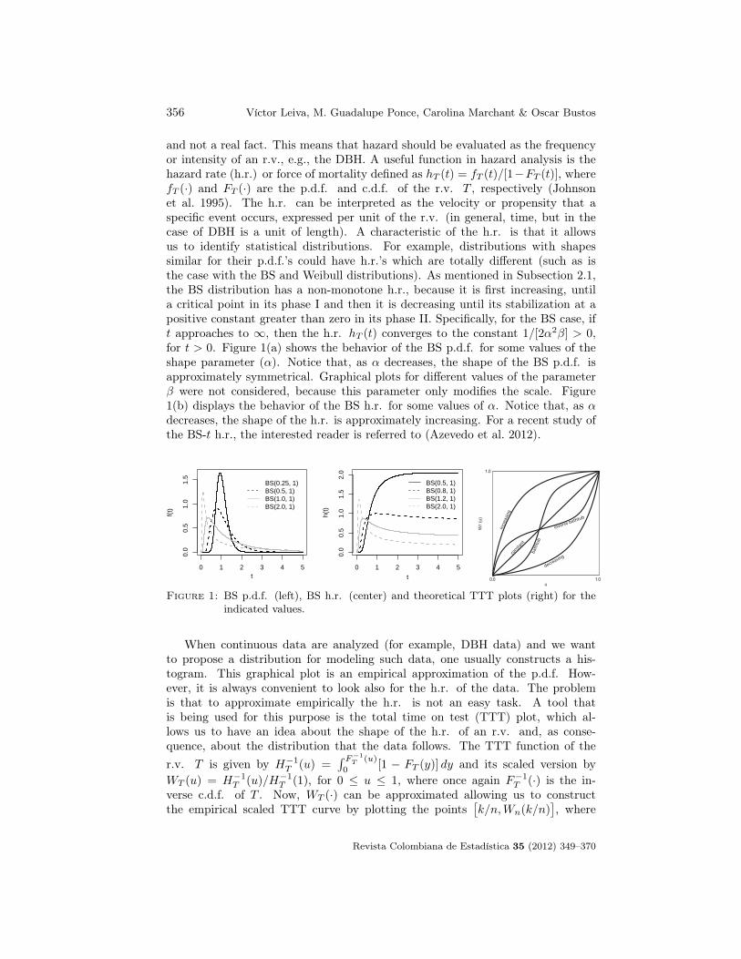
356 Víctor Leiva, M. Guadalupe Ponce, Carolina Marchant & Oscar Bustos
and not a real fact. This means that hazard should be evaluated as the frequencyor intensity of an r.v., e.g., the DBH. A useful function in hazard analysis is thehazard rate (h.r.) or force of mortality defined as hT (t) = fT (t)/[1−FT (t)], wherefT (·) and FT (·) are the p.d.f. and c.d.f. of the r.v. T , respectively (Johnsonet al. 1995). The h.r. can be interpreted as the velocity or propensity that aspecific event occurs, expressed per unit of the r.v. (in general, time, but in thecase of DBH is a unit of length). A characteristic of the h.r. is that it allowsus to identify statistical distributions. For example, distributions with shapessimilar for their p.d.f.’s could have h.r.’s which are totally different (such as isthe case with the BS and Weibull distributions). As mentioned in Subsection 2.1,the BS distribution has a non-monotone h.r., because it is first increasing, untila critical point in its phase I and then it is decreasing until its stabilization at apositive constant greater than zero in its phase II. Specifically, for the BS case, ift approaches to ∞, then the h.r. hT (t) converges to the constant 1/[2α2β] > 0,for t > 0. Figure 1(a) shows the behavior of the BS p.d.f. for some values of theshape parameter (α). Notice that, as α decreases, the shape of the BS p.d.f. isapproximately symmetrical. Graphical plots for different values of the parameterβ were not considered, because this parameter only modifies the scale. Figure1(b) displays the behavior of the BS h.r. for some values of α. Notice that, as αdecreases, the shape of the h.r. is approximately increasing. For a recent study ofthe BS-t h.r., the interested reader is referred to (Azevedo et al. 2012).
0 1 2 3 4 5
0.0
0.5
1.0
1.5
t
f(t)
BS(0.25, 1)BS(0.5, 1)BS(1.0, 1)BS(2.0, 1)
0 1 2 3 4 5
0.0
0.5
1.0
1.5
2.0
t
h(t)
BS(0.5, 1)BS(0.8, 1)BS(1.2, 1)BS(2.0, 1)
WT
(u)
1.0
1.00.0u
incr
easin
gco
nstant
bath
tub
decreasing
inverse bathtub
Figure 1: BS p.d.f. (left), BS h.r. (center) and theoretical TTT plots (right) for theindicated values.
When continuous data are analyzed (for example, DBH data) and we wantto propose a distribution for modeling such data, one usually constructs a his-togram. This graphical plot is an empirical approximation of the p.d.f. How-ever, it is always convenient to look also for the h.r. of the data. The problemis that to approximate empirically the h.r. is not an easy task. A tool thatis being used for this purpose is the total time on test (TTT) plot, which al-lows us to have an idea about the shape of the h.r. of an r.v. and, as conse-quence, about the distribution that the data follows. The TTT function of ther.v. T is given by H−1
T (u) =∫ F−1
T (u)
0[1 − FT (y)] dy and its scaled version by
WT (u) = H−1T (u)/H−1
T (1), for 0 ≤ u ≤ 1, where once again F−1T (·) is the in-
verse c.d.f. of T . Now, WT (·) can be approximated allowing us to constructthe empirical scaled TTT curve by plotting the points
[k/n,Wn(k/n)
], where
Revista Colombiana de Estadística 35 (2012) 349–370

Distributions Useful for Modeling Diameter and Mortality of Trees 357
Wn(k/n) = [∑ki=1 T(i) + [n − k]T(k)]/
∑ni=1 T(i), for k = 1, . . . , n, with T(i) being
the ith order statistic, for i = 1, . . . , n. Specifically, if the TTT plot is concave(convex), then a model with increasing (decreasing) h.r. is appropriate. Now,if the TTT plot is first concave (convex) and then convex (concave), an inversebathtub (IBT) shaped (bathtub –BT–) h.r. must be considered. If the TTT plotis a straight line, then the exponential distribution must be used. For example, thenormal distribution is in the increasing h.r. class, while the gamma and Weibulldistributions admit increasing, constant and decreasing h.r.’s. However, the BSand log-normal distributions have non-monotone h.r.’s, because these are initiallyincreasing until their change points and then decreasing (IBT shaped h.r.) to zero,in the log-normal case, or to a constant greater than zero, in the BS case. Thislast case must be highlighted because biological entities (such as humans, insectsand trees) have h.r.’s of this type (Gavrilov & Gavrilova 2001). In Figure 1(c), wesee several theoretical shapes of the TTT plot, which correspond to a particulartype of h.r. (Aarset 1987).
2.5. Model Estimation and Checking
Parameters of the BS, ShBS, BS-t and ShBS-t distributions can be estimated bythe maximum likelihood (ML) method adapted by a non-failing algorithm (Leivaet al. 2011). To obtain the estimates of the parameters of these distributions,their corresponding likelihood functions must be constructed using (4), (6), (8)and (10), respectively. When these parameters have been estimated, we mustcheck goodness-of-fit of the model to the data. Distributions used for describingDBH data can be compared using model selection criteria based on loss of in-formation such as Akaike (AIC) and Bayesian (BIC) information criteria. AICand BIC allows us to compare models for the same model and they are given byAIC = −2`(θ) + 2p and BIC = −2`(θ) + p log (n), where `(θ) is the logarithm ofthe likelihood function (log-likelihood) of the model with vector of parameters θ
evaluated at θ = θ, n is the size of the sample and p is the number of model pa-rameters. For the case of BS, ShBS, BS-t and ShBS-t models, as mentioned, `(θ)must be obtained by (4), (6), (8) and (10), respectively. AIC and BIC correspondto the log-likelihood function plus a component that penalizes such a function asthe model has more parameters making it more complex. A model with a smallerAIC or BIC is better.
Differences between two values of the BIC are usually not very noticeable.Then, the Bayes factor (BF) can be used to highlight such differences, if theyexist. Assume the data belongs to one of two possible models, according to prob-abilities P(Data | Model 1) and P(Data | Model 2), respectively. Given proba-bilities P(Model 1) and P(Model 2) = 1 − P(Model 1), the data produce condi-tional probabilities P(Model 1 | Data) and P(Model 2 | Data) = 1 − P(Model 1 |Data), respectively. The BF allows us to compare Model 1 (considered as cor-rect) to Model 2 (to be contrasted with Model 1) and it is given by B12 =P(Data | Model 1)/P(Data | Model 2), which can be approximated by 2 log(B12) ≈2[`(θ1) − `(θ2)
]− [d1 − d2] log (n), where `(θk) is the log-likelihood function for
Revista Colombiana de Estadística 35 (2012) 349–370

358 Víctor Leiva, M. Guadalupe Ponce, Carolina Marchant & Oscar Bustos
the parameter θk under the kth model evaluated at θk = θk, dk is the dimen-sion of θk, for k = 1, 2, and n is the sample size. Notice that the above ap-proximation is computed by sustracting the BIC value from Model 2, given byBIC2 = −2`(θ2) + d2 log (n), to the BIC value of Model 1, given by BIC1 =−2`(θ1) + d1 log (n). In addition, notice that if Model 2 is a particular case ofModel 1, then the procedure corresponds to applying the likelihood ratio (LR)test. In this case, 2 log(B12) ≈ χ2
12 − df12 log(n), where χ212 is the LR test statis-
tic for testing Model 1 versus Model 2 and df12 = d1 − d2 are the d.f.’s asso-ciated with the LR test, so that one can obtain the corresponding p-value from2 log(B12) ·∼ χ2(d1 − d2), with d1 > d2. The BF is informative, because it presentsranges of values in which the degree of superiority of one model with respect toanother can be quantified. An interpretation of the BF is displayed in Table 1.
Table 1: Interpretation of 2 log(B12) associated with the BF.2 log (B12) Evidence in favor of Model 1
< 0 Negative (Model 2 is accepted)[0, 2) Weak[2, 6) Positive[6, 10) Strong≥ 10 Very strong
2.6. Quantity and Quality of Wood
Because the DBH varies depending on the composition, density, geographiclocation and stand age, the diameter can be considered as an r.v. that we denote byT . As mentioned, information on the distribution of T in a forest plantation is animportant element to quantify the products come from thinning and clearcuttingactivities. This information can help to plan the management and use of forestresources more efficiently. It is important to model the distribution of the DBHsince this is the most relevant variable in determining the tree volume and thenthe forest production.
The forest volume quantification allows us to make decisions about the pro-duction and forest management, for example, to know when the forest should beharvested. However, the variable to maximize is diameter instead volume. Fur-thermore, the DBH is related to other variables such as cost of harvest, quality andproduct type. While the productivity is an important issue for timber industry,wood quality is also relevant in order to determine its use. Thus, volume and di-ameter distribution of trees determine what type of product will be obtained. Forexample, large diameter trees are used for saw wood and those of small diameterfor pulpwood. This implies a financial analysis of forest harvest, i.e., how andwhen to harvest and what method to use. Studies from several types of climatesand soils show trees growth as a function of the basal area. Making decisions usingthe forest basal area are related to pruning and thinning. These activities aim toimprove tree growth and produce higher quality wood. The basal area of a tree is
Revista Colombiana de Estadística 35 (2012) 349–370

Distributions Useful for Modeling Diameter and Mortality of Trees 359
the imaginary basal area at breast height (1.3 m above ground level) given by
B =π
4T 2
where B is the basal area and T the DBH.The sum of the individual basal area of all trees in one hectare leads to the
basal area per hectare. However, it is the volume which allows for the planning ofvarious forestry activities. There are several formulae to determine the volume oflogs using the mean diameter measured without bark, and the log length. Volumeallows for the planning of silvicultural and harvesting activities. In general, theformula used for the volume of a tree is given by
V = F BH =π
4F T 2H (12)
where V is the tree volume, B its basal area, H its height and F the form factor,which is generally smaller than a value equal to one depending on the tree species.
2.7. Mortality and Tree Regeneration
The DBH is related to tree mortality, which is affected by stress factors such aslight, nutrients, sunlight, temperature and water. The light and temperature cancause stress in minutes, whereas lack of water can cause stress in days or weeks.However, lack of nutrients in the soil can take months to generate stress. Themortality of a tree is similar to the material fatigue process described in Section2.1, because the force of mortality of trees is growing rapidly in phase I, reachinga maximum and then decreases slowly until it is stabilized in phase II, which isconsistent for almost all tree species.
Podlaski (2008) identified in a national park in Poland the following stressfactors: (i) abiotic factors, such as severe weather (frost, hail, humidity, snow,temperature, wind), deficiency or excess of soil nutrients and toxic substances inair and soil, and (ii) biotic factors, such as bacteria (canker), fungi (dumping-offspots, root rots, rusts), insects and worms (nematodes), mycoplasma (elm phloemnecrosis), parasitic plants (mistletoes) and viruses (elm mosaic). These factorscaused the death of trees of the species Abies alba. From a theoretical point ofview, the force of mortality of spruce could be more appropriately described bythe h.r. of the BS distribution rather than using other distributions employed tomodel DBH. Podlaski (2008) indicated that mortality of spruce stand caused moreopenings within the stand and the canopy. Thus, with more spaces and gaps, treesof the species Fagus sylvatica, a kind that grows in temperate zones of the planet,tended to regenerate.
The regeneration process has been closely connected with the death of fir,whose speed in phase I also resulted in a rapid regeneration of beech, and thesubsequent occurrence of understory vegetation in the stand. The decrease in theintensity of spruce mortality in phase II, as well as shading of soil by the understory,caused a gradual decrease in the intensity of the regeneration of beech. The standsgenerated by this process are characterized by a vertical structure of tree layers
Revista Colombiana de Estadística 35 (2012) 349–370

360 Víctor Leiva, M. Guadalupe Ponce, Carolina Marchant & Oscar Bustos
of different heights. These layers correspond to multiple layers of canopy whosestatistical distribution of the DBH is asymmetric and positively skewed, as in theBS model. Most of the spruce stands had diameters of approximately 0.15 mto 0.35 m. The interruption of the regeneration process resulted in the death ofthese stands, which had a DBH of less than 0.1 m. The necessary condition forthe creation of stands with DBH distributions approximated by the BS model isthe simultaneous death of fir at all levels of the stand with regeneration of beech,i.e., a death that considers the different forest layers and has a similar degree ofseasonality in the subsequent occurrence of the understory.
3. Application
Next, we apply the methodology outlined in this article using real data of theDBH and a methodology based on BS models. First, we perform an exploratorydata analysis (EDA) of DBH. Then, based on this EDA, we propose statisticaldistributions to model the DBH. We use goodness-of-fit methods to find the moresuitable distribution for modeling the DBH data under analysis. Finally, we make aconfirmatory analysis and furnish information that can be useful to make financialand forestry decisions.
3.1. The Data Sets
The five DBH data sets to be analyzed are presented next. These data (all ofthem given in cm) are expressed in each case with the data frequency in parenthesesand nothing when the frequency is equal to one.Giant paradise (Melia azedarach L.) This is an exotic tree species originatedfrom Asia and adapted to the province of Santiago del Estero, Argentina. Giantparadise produces wood of very good quality in a short time. We consider DBHdata of giant paradise trees from four consecutive annual measurements collectedsince 1994 in 40 sites located at a stand in the Departamento Alberdi to thenorthwest of the province of Santiago del Estero, Argentina. Specifically, we usemeasurements collected at Site 7 due to the better conformation and reliability ofthe database (Pece et al. 2000). The data are: 16.5, 16.6, 17.8, 18.0 18.4, 18.5,18.8, 18.9, 19.2, 19.3, 19.8, 20.3, 20.4, 20.6(2), 22.1, 22.2 23.5, 23.6, 26.7.Silver fir (Abies alba). This is a species of tree of the pine family originatedfrom mountainous regions in Europe. We consider DBH data of silver fir treesfrom 15 sites located at Swieta Katarzyna and Swiety Krzyzy forest sections ofthe Swietokrzyski National Park, in Swietokrzyskie Mountains (Central Poland).Specifically, we use measurements collected at Site 10 due to similar reasons tothat from Melia azedarach (Podlaski 2008). The data are: 11(2), 12, 13, 14(5),15(4), 16(5), 17(4), 18(4), 19(3), 20(8), 21(4), 22(3), 23(4), 24(5), 25(6), 26(5),27(5), 28(2), 29(5), 30(2), 31(7), 32(3), 33(2), 34(4), 35, 36(2), 37(2), 39(2), 40(3),41(2), 42, 43(2), 44(3), 46(3), 47(2), 48, 50(2), 51, 52, 53, 54, 55, 56, 57, 59, 61,66, 70, 89, 97.
Revista Colombiana de Estadística 35 (2012) 349–370

Distributions Useful for Modeling Diameter and Mortality of Trees 361
Loblolly pine (Pinus taeda L.) This variety of tree is one of several nativepines at the Southeastern of the United States (US). The data set corresponds toDBH of 20 year old trees from a plantation in the Western Gulf Coast of the US(McEwen & Parresol 1991). The data are: 6.2, 6.3, 6.4, 6.6(2), 6.7, 6.8, 6.9(3),7.0(2), 7.1, 7.2(2), 7.3(3), 7.4(4), 7.6(2), 7.7(3), 7.8, 7.9(4), 8.1(4), 8.2(3), 8.3(3),8.4, 8.5(3), 8.6(4), 8.7, 8.8(2), 8.9(3), 9.0(4), 9.1(5), 9.5(2), 9.6, 9.8(3), 10.0(2),10.1, 10.3.
Ruíl (Nothofagus alessandrii Espinosa). This is an endemic species of centralChile, which is at risk of extinction. This tree variety is the older species of thefamily of the Fagaceae in the South Hemisphere, i.e., these stands are the olderformations in South America. The data set of DBH was collected close to thelocality of Gualleco, Región del Maule, Chile (Santelices & Riquelme 2007). Thedata are: 16(2), 18(2), 20(2), 22, 24, 26(2), 28, 30(2), 32, 34.
Gray birch (Betula populifolia Marshall). This is a perennial species fromthe US that has its best growth during spring and summer seasons. Gray birchhas a short life in comparison with other plant species and a rapid growth rate.During its maturity (around 20 years), gray birch reaches an average height of 10m. The data used for this study correspond to DBH of gray birch trees that arepart of a natural forest of 16 hectares located at Maine, US. This data set waschosen because its collection is reliable and the database is complete, so it allowsan adequate illustration for the purpose of this study. The data are: 10.5(5),10.6, 10.7, 10.8(3), 10.9, 11.0, 11.2, 11.3(5), 11.4, 11.5(3), 11.6(2), 11.7(3), 11.9(2),12.0(3), 12.1(3), 12.2(2), 12.3, 12.4(3), 12.5(3), 12.6, 12.7(2), 12.8(3), 12.9(5),13.0(7), 13.1(4), 13.2(2), 13.3(3), 13.5(2), 13.6(3), 13.7(5), 13.8(2), 14.0(3), 14.1(4),14.2(3), 14.3, 14.4(2), 14.5(5), 14.6(3), 14.8(4), 14.9(3), 15.0, 15.1(3), 15.2, 15.3(2),15.6(2), 15.7(2), 15.8, 15.9(2), 16.0(2), 16.1(2), 16.4, 16.5, 16.6(2), 16.7, 16.9(2),17.0(2), 17.5(2), 17.8(2), 18.3, 18.4, 18.5, 19.2, 19.4(2), 19.9(2), 20.0, 20.3, 20.5,21.3, 21.9, 23.1, 24.4, 26.0, 28.4, 39.3.
We call S1, S2, S3, S4 and S5 to the DBH data sets of the varieties of Meliaazedarach, Abies alba, Pinus taeda, Nothofagus alessandrii, and Betula populifolia,respectively.
3.2. Exploratory Data Analysis
Table 2 presents a descriptive summary of data sets S1-S5 that includes me-dian, mean, standard deviation (SD), CV and coefficients of skewness (CS) andkurtosis (CK), among other indicators. Figure 2 shows histograms, usual and ad-justed for asymmetrical data boxplots (Leiva et al. 2011) and TTT plots for S1-S5.From Table 2 and Figure 2, we detect distributions with positive skewness, differ-ent degrees of kurtosis, increasing and IBT shaped h.r.’s and a variable number ofatypical DBH data. Specifically, the TTT plot of the DBH presented in Figure 2(fifth panel) shows precisely a h.r. as those that the tree DBH should theoreticallyhave and that coincides with the h.r. of the BS fatigue models. In addition, mini-mum values for S1-S5 indicate to us the necessity for considering a shift parameterin the modeling. As a consequence, based on this EDA, the different BS models
Revista Colombiana de Estadística 35 (2012) 349–370

362 Víctor Leiva, M. Guadalupe Ponce, Carolina Marchant & Oscar Bustos
presented in this paper seem to be good candidates for describing S1-S5, becausethey allow us to accommodate the different aspects detected in the EDA for thesedata sets. Particularly, BS-t and ShBS-t models allow us to accommodate atypicaldata in a robust statistically way. Also, BS distributions have a more appropriateh.r. to model such DBH data. This is a relevant aspect because DBH data havebeen widely modeled by the Weibull distribution. However, this distribution has adifferent h.r. to those that the tree DBH should theoretically have. Therefore, inthe next section of model estimation and checking, we compare usual and shiftedBS and Weibull models by means of a goodness-of-fit analysis in order to valuatewhether this theoretical aspect is validated by the data or not.
Table 2: Descriptive summary of DBH for the indicated data setSet Median Mean SD CV CS CK Range Minimum Maximum n
S1 19.55 20.09 2.53 12.58% 0.82 3.20 10.20 16.50 26.70 20S2 27.00 30.68 14.85 48.42% 1.52 6.33 86.00 11.00 97.00 134S3 8.20 8.19 1.01 12.37% 0.05 2.16 4.10 6.20 10.30 75S4 24.00 24.00 5.95 24.80% 0.14 1.50 18.00 16.00 34.00 15S5 13.70 14.54 3.61 24.85% 5.89 13.97 28.80 10.50 39.30 160
3.3. Model Estimation and Checking
As mentioned, the parameters of the BS, ShBS, BS-t, ShBS-t distributionscan be estimated by the ML method adapted by a non-failing algorithm (Leivaet al. 2011). The estimation of the parameters of the BS distributions, as wellas those of the usual and shifted Weibull distributions (as comparison), for S1-S5are summarized in Table 3 together with the negative value of the correspondinglog-likelihood function. In addition to the model selection criteria (AIC and BIC)presented in Section 2.1, the fit of the model to SI-S5 can be checked using theKolmogorov-Smirnov test (KS). This test compares the empirical and theoreticalc.d.f.’s (in this case of the BS and Weibull models). The p-values of the KS test,as well as the values of AIC, BIC and 2log(B12) are also provided in Table 3.Based on the KS test and BF results presented in Table 3, we conclude that theBS distributions fit S1-S5 better than Weibull distributions. All this informationsupports the theoretical justification given in Section 2.
Revista Colombiana de Estadística 35 (2012) 349–370

Distributions Useful for Modeling Diameter and Mortality of Trees 363
dbh
freq
uenc
y
16 18 20 22 24 26 28
01
23
45
67
1820
2224
26
Original boxplot
dbh
1820
2224
26
Adjusted boxplot
0.0 0.2 0.4 0.6 0.8 1.0
0.0
0.2
0.4
0.6
0.8
1.0
k/n
Wn(
k/n)
dbh
freq
uenc
y
0 20 40 60 80 100
010
2030
4050
6070
2040
6080
100
Original boxplot
dbh
2040
6080
100
Adjusted boxplot
0.0 0.2 0.4 0.6 0.8 1.0
0.0
0.2
0.4
0.6
0.8
1.0
k/n
Wn(
k/n)
dbh
freq
uenc
y
6 7 8 9 10 11
05
1015
2025
78
910
Original boxplot
dbh
78
910
Adjusted boxplot
0.0 0.2 0.4 0.6 0.8 1.0
0.0
0.2
0.4
0.6
0.8
1.0
k/n
Wn(
k/n)
dbh
freq
uenc
y
10 15 20 25 30 35 40
01
23
45
67
2025
30
Original boxplot
dbh
2025
30
Adjusted boxplot
0.0 0.2 0.4 0.6 0.8 1.0
0.0
0.2
0.4
0.6
0.8
1.0
k/n
Wn(
k/n)
dbh
freq
uenc
y
10 15 20 25 30 35 40
020
4060
8010
0
1015
2025
3035
40
Original boxplot
dbh
1015
2025
3035
40
Adjusted boxplot
0.0 0.2 0.4 0.6 0.8 1.0
0.0
0.2
0.4
0.6
0.8
1.0
k/n
Wn(
k/n)
Figure 2: Histograms, usual and adjusted boxplots and TTT plots for S1 (first panel)to S5 (fifth panel).
Revista Colombiana de Estadística 35 (2012) 349–370

364 Víctor Leiva, M. Guadalupe Ponce, Carolina Marchant & Oscar Bustos
Table 3: Indicators for the indicated data set and distribution.Indicator BS BS-t ShBS ShBS-t ShWeibull Weibull
S1α 0.118 0.117 0.374 0.443 1.587 7.736β 19.950 19.934 6.161 3.260 4.810 21.228ν - 87 - 1 - -γ - - 13.498 16.498 15.900 -−`(θ) 45.534 45.533 44.752 43.367 44.811 48.565AIC 95.069 97.067 95.503 94.733 95.622 101.131BIC 97.061 100.053 98.490 98.716 98.609 103.1212 log(B12) - 2.992 1.429 1.655 1.548 6.060KS p-value 0.806 0.829 0.986 0.963 0.882 0.385
S2α 0.452 0.448 0.590 0.588 1.440 2.193β 27.840 27.803 21.301 21.171 22.453 34.760ν - 100 - 100 - -γ - - 5.666 5.778 10.358 -−`(θ) 525.820 525.889 524.255 524.306 524.772 540.361AIC 1055.640 1057.777 1054.511 1056.612 1055.544 1084.721BIC 1061.436 1066.472 1063.204 1068.203 1064.238 1090.5182 log(B12) - 5.036 1.768 6.768 2.802 29.082KS p-value 0.899 0.912 0.959 0.815 0.828 0.129
S3α 0.124 0.123 0.124 0.124 2.514 8.952β 8.125 8.127 8.125 8.127 2.635 8.636ν - 100 - 100 - -γ - - 0.000 0.000 5.850 -−`(θ) 107.038 107.180 107.038 107.180 105.798 108.609AIC 218.076 220.360 218.076 222.360 217.596 221.219BIC 222.711 227.312 222.711 227.312 224.548 225.8532 log(B12) - 4.601 - 4.601 1.837 3.142KS p-value 0.876 0.874 0.876 0.874 0.918 0.840
S4α 0.245 0.2445 0.394 0.585 2.837 4.685β 23.298 23.304 14.625 9.207 16.568 26.282ν - 100 - 1 - -γ - - 8.240 15.995 9.300 -−`(θ) 47.327 47.377 47.292 44.460 47.098 47.515AIC 98.656 100.754 100.584 96.920 100.195 99.0294BIC 100.070 102.878 102.708 99.752 104.084 100.4462 log(B12) 0.319 3.126 2.956 - 4.332 0.694KS p-value 0.933 0.934 0.858 0.936 0.894 0.852
S5α 0.208 0.151 0.727 0.563 1.502 3.467β 14.230 13.817 3.774 4.232 4.749 15.920ν - 4 - 8 - -γ - - 9.761 9.439 10.180 -−`(θ) 399.776 389.438 380.330 378.912 386.075 448.921AIC 803.553 816.853 766.659 765.826 778.152 901.842BIC 809.702 794.102 775.886 778.125 787.376 907.9922 log(B12) 33.817 18.216 - 2.239 11.490 132.107KS p-value 0.052 0.400 0.530 0.773 0.467 < 0.001
Revista Colombiana de Estadística 35 (2012) 349–370

Distributions Useful for Modeling Diameter and Mortality of Trees 365
Due to space limitations, in order to visualize the model fit to the DBH data,we only focus on S5. In addition, we only depict three plots corresponding to theshifted versions of the BS, BS-t and Weibull distributions, which are those that fitthe data better. Comparison between the empirical (gray line) and ShBS, ShBS-tand ShWeibull theoretical (black dots) c.d.f.’s are shown in Figure 3. Histogramswith the estimated ShBS, ShBS-t and ShWeibull p.d.f. curve are shown in Figure 4.Probability plots with “envelopes” based on the BS, BS-t and Weibull distributionsfor S5 are shown in Figure 5. The term “envelope” is a band for the probability plotbuilt by means of a simulation process that facilitates the adjustment visualization.For example, for the BS distribution, this “envelope” is built using an expressiongiven in (3). From Figure 5, we can see the excellent fit that the ShBS-t modelprovides to S5 and the bad fit provided by the ShWeibull model. Then, once theShBS-t model has been considered as the most appropriate within the proposeddistributions to model S5, we provide information that can be useful to makeeconomical and forestry decisions based on this model and the methodology givenin this study.
10 15 20 25 30 35 40
0.0
0.2
0.4
0.6
0.8
1.0
dbh
cdf
10 15 20 25 30 35 40
0.0
0.2
0.4
0.6
0.8
1.0
dbh
cdf
10 15 20 25 30 35 40
0.0
0.2
0.4
0.6
0.8
1.0
dbh
cdf
Figure 3: Empirical (bold) and theoretical (gray) c.d.f.’s for S5 using the ShBS, ShBS-tand ShWeibull distributions.
3.4. Financial Evaluation
We select S5 for carrying out a financial analysis. In this case, the ShBS-tdistribution is considered as the best model. Then, we propose a forest productionproblem to illustrate the methodology presented in this article. Once the ShBS-tmodel parameters are estimated, we determine the mean volume per tree in a
Revista Colombiana de Estadística 35 (2012) 349–370

366 Víctor Leiva, M. Guadalupe Ponce, Carolina Marchant & Oscar Bustos
dbh
frec
uenc
y
10 15 20 25 30 35 40
0.00
0.05
0.10
0.15
0.20
dbh
frec
uenc
y
10 15 20 25 30 35 40
0.00
0.05
0.10
0.15
0.20
dbh
frec
uenc
y
10 15 20 25 30 35 40
0.00
0.05
0.10
0.15
0.20
Figure 4: Histogram with ShBS, ShBS-t and ShWeibull p.d.f.’s for S5.
0 2 4 6 8
05
1015
ShBS theoretical quantile
empi
rical
qua
ntile
0 2 4 6 8
05
1015
0 2 4 6 8
05
1015
0 2 4 6 8
05
1015
0 5 10 15
05
1015
2025
3035
ShBst theoretical quantile
empi
rical
qua
ntile
0 5 10 15
05
1015
2025
3035
0 5 10 15
05
1015
2025
3035
0 5 10 15
05
1015
2025
3035
10 15 20 25
1015
2025
3035
40
ShWeibull theoretical quantile
empi
rical
qua
ntile
10 15 20 25
1015
2025
3035
40
10 15 20 25
1015
2025
3035
40
10 15 20 25
1015
2025
3035
40
Figure 5: Probability plots with envelopes for S5 using the ShBS, ShBS-t and ShWeibulldistributions.
Revista Colombiana de Estadística 35 (2012) 349–370

Distributions Useful for Modeling Diameter and Mortality of Trees 367
stand by using (12) that leads to E[V ] = (250/3)πE[T 2], recalling that T is theDBH, H the known height of the tree equal to 10 m (1000 cm, because the dataare expressed in cm) and F the form factor being it equal to 1/3 due to the birchcase, which has conical shape, with the DBH equivalent to the diameter at thebase of the cone. Using the expected value and variance of T given in (11), we getthe expected volume as
E[V ] = 2503 π
[β2
{1 + α2(2A+ 5
4Bα2 + A2α2
4 )
}+ γ
{γ + β(2 +Aα2)
}]The stand considered in this study only produces native wood that can be sold tosawmills at a price of US$250 (international price in US dollars) per cubic meter.This stand of Maine, US, had in the spring of 2004 an amount of 3327 trees, ofwhich 160 (4.8%) were of the gray birch variety. Thus, the estimated expectedeconomical value for gray birch wood of this forest (stand) based on the ShBS-tmodel is
US$0.25× E[V ]× 160 = 10000π[β2
{1 + α2(2A+
5
4Bα2 +
A2α2
4)
}+ γ{γ+
β(2 +Aα2)}]
(13)
being its estimation based on the proposed methodology and S5 of US$7,342,267.
4. Concluding Remarks
In this paper, we have presented, developed, discussed and applied a statisticalmethodology based on Birnbaum-Saunders distributions to address the problemof managing forest production. Specifically, we have linked a fatigue model to aforestry model through Birnbaum-Saunders distributions. This linkage has beenpossible because the hazard rate of this distribution has two clearly marked phasesthat coincide with the force of mortality of trees. This mortality is related tothe diameter at breast height of trees. We have modeled the distribution of thisdiameter because this variable is the most relevant in determining the basal area ofa tree. For its part, the basal area allows the volume of a tree to be determinatedsetting thus the production of a forest. Finally, we have shown the applicability ofthis model using five real data sets, obtaining for one of them financial informationthat may be valuable in forest decision making. The unpublished data used inthe economical evaluation corresponded to the diameter at breast height of 10 mheight mature gray birch trees collected in 2004, which are part of the inventoryof a natural forest of area 16 hectares of different species located at Maine, US.
Acknowledgements
The authors wish to thank the Editor-in-Chief, Dr. Leonardo Trujillo, andtwo anonymous referees for their constructive comments on an earlier version of
Revista Colombiana de Estadística 35 (2012) 349–370

368 Víctor Leiva, M. Guadalupe Ponce, Carolina Marchant & Oscar Bustos
this manuscript which resulted in this improved version. Also, we wish to thankthe colleagues Celia Benítez (Argentina), Rafal Podlaski (Poland) and RómuloSantelices (Chile) for kindly providing us some of the data sets analyzed in thispaper. This research work was partially supported by grant FONDECYT 1120879from the Chilean government and by Universidad de Talca, Chile.[
Recibido: diciembre de 2011 — Aceptado: junio de 2012]
References
Aarset, M. V. (1987), ‘How to identify a bathtub hazard rate’, IEEE Transactionon Reliability 36, 106–108.
Azevedo, C., Leiva, V., Athayde, E. & Balakrishnan, N. (2012), ‘Shape and changepoint analyses of the Birnbaum-Saunders-t hazard rate and associated esti-mation’, Computational Statistics and Data Analysis 56, 3887–3897.
Bailey, R. & Dell, T. (1973), ‘Quantifying diameter distributions with the Weibullfunction’, Forest Science 19, 97–104.
Birnbaum, Z. & Saunders, S. (1968), ‘A probabilistic interpretation of miner’srule’, SIAM Journal of Applied Mathematics 16, 637–652.
Birnbaum, Z. & Saunders, S. (1969), ‘A new family of life distributions’, Journalof Applied Probability 6, 319–327.
Bliss, C. & Reinker, K. (1964), ‘A lognormal approach to diameter distributionsin even-aged stands’, Forest Science 10, 350–360.
Borders, B., Souter, R., Bailey, R. & Ware, K. (1987), ‘Percentile-based distribu-tions characterize forest stand tables’, Forest Science 33, 570–576.
Clutter, J. & Bennett, F. (1965), Diameter distributions in old-field slash pineplantation, Report 13, US Forest Service.
Díaz-García, J. & Leiva, V. (2005), ‘A new family of life distributions based onelliptically contoured distributions’, Journal of Statistical Planning and Infer-ence 128, 445–457. (Erratum: Journal of Statistical Planning and Inference,137, 1512-1513).
Ferreira, M., Gomes, M. & Leiva, V. (2012), ‘On an extreme value version of theBirnbaum-Saunders distribution’, Revstat-Statistical Journal 10, 181–210.
García-Güemes, C., Cañadas, N. & Montero, G. (2002), ‘Modelización de la dis-tribución diamétrica de las masas de Pinus pinea de Valladolid (España) me-diante la función Weibull’, Investigación Agraria-Sistemas y Recursos Fore-stales 11, 263–282.
Gavrilov, L. & Gavrilova, N. (2001), ‘The reliability theory of aging and longevity’,Journal of Theoretical Biology 213, 527–545.
Revista Colombiana de Estadística 35 (2012) 349–370

Distributions Useful for Modeling Diameter and Mortality of Trees 369
Guiraud, P., Leiva, V. & Fierro, R. (2009), ‘A non-central version of the Birnbaum-Saunders distribution for reliability analysis’, IEEE Transaction on Reliability58, 152–160.
Hafley, W. & Schreuder, H. (1977), ‘Statistical distributions for fitting diameterand height data in even-aged stands’, Canadian Journal of Forest Research7, 481–487.
Johnson, N., Kotz, S. & Balakrishnan, N. (1995), Continuous Univariate Distri-butions, Vol. 2, Wiley, New York.
Leiva, V., Athayde, E., Azevedo, C. & Marchant, C. (2011), ‘Modeling wind en-ergy flux by a birnbaum-saunders distribution with unknown shift parameter’,Journal of Applied Statistics 38, 2819–2838.
Leiva, V., Barros, M., Paula, G. & Sanhueza, D. (2008), ‘Generalized Birnbaum-Saunders distributions applied to air pollutant concentration’, Environmetrics19, 235–249.
Leiva, V., Sanhueza, A. & Angulo, J. (2009), ‘A length-biased version of theBirnbaum-Saunders distribution with application in water quality’, StochasticEnvironmental Research and Risk Assessment 23, 299–307.
Leiva, V., Vilca, F., Balakrishnan, N. & Sanhueza, A. (2010), ‘A skewed sinh-normal distribution and its properties and application to air pollution’, Com-munications in Statistics - Theory and Methods 39, 426–443.
Lenhart, J. & Clutter, J. (1971), Cubic foot yield tables for old-field loblolly pineplantations in the Georgia Piedmont, Report 22, US Forest Service.
Li, F., Zhang, L. & Davis, C. (2002), ‘Modeling the joint distribution of tree diam-eters and heights by bivariate generalized Beta distribution’, Forest Science48, 47–58.
Little, S. (1983), ‘Weibull diameter distributions for mixed stands of westernconifers’, Canadian Journal of Forest Research 13, 85–88.
Maltamo, M., Puumalinen, J. & Päivinen, R. (1995), ‘Comparison of beta andWeibull functions for modelling basal area diameter in stands of Pinussylvestris and Picea abies’, Scandinavian Journal of Forest Research 10, 284–295.
Marchant, C., Leiva, V., Cavieres, M. & Sanhueza, A. (2013), ‘Air contaminantstatistical distributions with application to PM10 in Santiago, Chile’, Reviewsof Environmental Contamination and Toxicology 223, 1–31.
McEwen, R. & Parresol, B. (1991), ‘Moment expressions and summary statis-tics for the complete and truncated Weibull dstribution’, Communications inStatistics - Theory and Methods 20, 1361–1372.
McGee, C. & Della-Bianca, L. (1967), Diameter distributions in natural yellow-poplar stands, Report 25, US Forest Service.
Revista Colombiana de Estadística 35 (2012) 349–370

370 Víctor Leiva, M. Guadalupe Ponce, Carolina Marchant & Oscar Bustos
Meyer, H. (1952), ‘Structure, growth, and drain in balanced uneven-aged forests’,Journal of Forestry 50, 85–92.
Miner, M. A. (1945), ‘Cumulative damage in fatigue’, Journal of Applied Mechan-ics 12, 159–164.
Nelson, T. (1964), ‘Diameter distribution and growth of loblolly pine’, Journal ofApplied Mechanics 10, 105–115.
Palahí, M., Pukkala, T. & Trasobares, A. (2006), ‘Modelling the diameter distri-bution of Pinus sylvestris, Pinus nigra and Pinus halepensis forest stands inCatalonia using the truncated Weibull function’, Forestry 79, 553–562.
Pece, M., de Benítez, C. & de Galíndez, M. (2000), ‘Uso de la función Weibull paramodelar distribuciones diamétricas en una plantación de Melia azedarach’,Revista Forestal Venezolana 44, 49–52.
Podlaski, R. (2006), ‘Suitability of the selected statistical distribution for fittingdiameter data in distinguished development stages and phases of near-naturalmixed forests in the Swietokrzyski National Park (Poland)’, Forest Ecologyand Management 236, 393–402.
Podlaski, R. (2008), ‘Characterization of diameter distribution data in near-natural forests using the Birnbaum-Saunders distribution’, Canadian Journalof Forest Research 18, 518–527.
Rennolls, K., Geary, D. & Rollinson, T. (1985), ‘Characterizing diameter distri-butions by the use of the Weibull distribution’, Forestry 58, 57–66.
Santelices, R. & Riquelme, M. (2007), ‘Forest mensuration of Nothofagus alessan-dri of Coipué provenance’, Bosque 28, 281–287.
Schmelz, D. & Lindsey, A. (1965), ‘Size-class structure of old-growth forests inIndiana’, Forest Science 11, 258–264.
Schreuder, H. & Hafley, W. (1977), ‘A useful bivariate distribution for describingstand structure of tree heights and diameters’, Biometrics 33, 471–478.
Vilca, F. & Leiva, V. (2006), ‘A new fatigue life model based on the family of skew-elliptical distributions’, Communications in Statistics - Theory and Methods35, 229–244.
Vilca, F., Santana, L., Leiva, V. & Balakrishnan, N. (2011), ‘Estimation of ex-treme percentiles in Birnbaum-Saunders distributions’, Computational Statis-tics and Data Analysis 55, 1665–1678.
Wang, M. & Rennolls, K. (2005), ‘Tree diameter distribution modelling: intro-ducing the logit-logistic distribution’, Canadian Journal of Forest Research35, 1305–1313.
Zutter, B., Oderwald, R., Murphy, P. & Farrar, R. (1986), ‘Characterizing diame-ter distributions with modified data types and forms of the Weibull distribu-tion’, Forest Science 32, 37–48.
Revista Colombiana de Estadística 35 (2012) 349–370

Revista Colombiana de EstadísticaDiciembre 2012, volumen 35, no. 3, pp. 371 a 384
A modified Cucconi Test for Location and ScaleChange Alternatives
Un prueba de Cucconi modificada para alternativas de cambio enlocalización y escala
Marco Marozzia
Dipartimento di Economia e Statistica, Università della Calabria, Italia
Abstract
The most common approach to develop a test for jointly detecting loca-tion and scale changes is to combine a test for location and a test for scale.For the same problem, the test of Cucconi should be considered because itis an alternative to the other tests as it is based on the squares of ranksand contrary-ranks. It has been previously shown that the Cucconi test isrobust in level and is more powerful than the Lepage test, which is the mostcommonly used test for the location-scale problem. A modification of theCucconi test is proposed. The idea is to modify this test consistently withthe familiar approach which develops a location-scale test by combining atest for location and a test for scale. More precisely, we will combine theCucconi test with the Wilcoxon rank test for location and a modified Levenetest following the theory of the nonparametric combination. A power com-parison of this modified Cucconi test with the original one, the Lepage testand the Podgor-Gastwirth PG2 test, shows that the modified Cucconi testis robust in size and markedly more powerful than the other tests for everyconsidered type of distributions, from short- to normal- and long-tailed ones.A real data example is discussed.
Key words: Combining tests, Location-scale model, Rank tests.
Resumen
La alternativa más común para implementar una prueba que detectacambios en localización y escala conjuntamente es combinar una prueba delocalización con una de escala. Para este problema, la prueba de Cucconies considerada como una alternativa de otras pruebas que se basan en loscuadrados de los rangos y los contrarangos. Esta prueba es robusta en nively es más poderosa que la prueba de Lepage la cual es la más usada parael problema de localización-escala. En este artículo se propone una modi-ficación de la prueba de Cucconi. La idea es modificar la prueba mediante
aProfessor. E-mail: [email protected]
371

372 Marco Marozzi
la combinación de una prueba de localización y uno de escala. Mas precisa-mente, se sugiere combinar la prueba de Cucconi con la prueba de rangos deWilcoxon para localizacion y una prueba modificada de Levene siguiendo lateoría de la combinación no paramétrica. Una comparación de la potenciade esta prueba modificada de Cucconi con la prueba original, la prueba deLepage y la prueba PG2 de Podgor-Gastwirth muestran que la prueba deCucconi modificada es robusta en tamaño y mucho más poderosa que lasanteriores para todas las distribuciones consideradas desde la normal hastaalgunas de colas largas. Se hace una aplicación a datos reales.
Palabras clave: combinación de pruebas, modelo de localización y escala,pruebas de rangos.
1. Introduction
The two sample Behrens-Fisher problem is to test that the locations, but notnecessarily the scales, of the distribution functions associated to the populationsbehind the samples are equal. There exist situations of practical interest, how-ever, when it is appropriate to jointly test for change in locations and change inscales. For example, Snedecor & Cochran (1989) emphasize that the applicationof a treatment (e.g. a drug) to otherwise homogeneous experimental units oftenresults in the treated group differing not only in location but also in scales. Thepractitioner generally has no a prior knowledge about the distribution functionsfrom which the data originate. Therefore, in such situations, an appropriate testdoes not require distributional assumptions. The test proposed by Perng & Littel(1976) for the equality of means and variances is not appropriate because is acombination of the t test and the F test, as the F test is not α robust for datafrom heavier than normal tailed distributions. According to Conover, Johnson &Johnson (1981) a test is α robust if its type one error rate is less than 2α. The cutoff point is set to 1.5α by Marozzi (2011). As the Perng & Littel (1976) test whichuses the Fisher combining function, the tests for the location-scale problem aregenerally expressed as functions of two tests, one sensitive to location changes andthe other to scale changes. The corresponding statistics are generally obtainedas direct combination of (i.e. by summing) a standardized statistic sensitive tolocation changes and a standardized statistic sensitive to scale changes. The mostfamiliar test statistic for the location-scale problem, due to Lepage (1971), whichis a direct combination of the squares of the standardized Wilcoxon and Ansari-Bradley statistics. It is important to note that Lepage-type tests can be obtainedfollowing Podgor & Gastwirth (1994). Marozzi (2009) compared several Podgor& Gastwirth (1994) efficiency robust tests and found that the PG2 test is themost powerful one. To perform the PG2 test it is necessary to regress the groupindicator on the ranks and on the squares of the ranks of the data and to test thatthe two regression coefficients are zero. The PG2 test can be recast as a quadraticcombination of the Wilcoxon test and the Mood squared rank test. For the sameproblem, the test of Cucconi (1968) should be considered because it is differentfrom the other tests being not based on the combination of a test for locationand a test for scale. It is a nonparametric test based on the squares of ranks
Revista Colombiana de Estadística 35 (2012) 371–384

Modified Cucconi Test 373
and contrary-ranks. Marozzi (2009) computed for the very first time exact criti-cal values for this test, compared its power to that of the Lepage and other teststhat included several Podgor-Gastwirth tests and showed that the test of Cucconimaintains the size very close to the nominal level and is more powerful than theLepage test. In this paper we are not interested in the general two sample problem,and therefore we do not consider tests like the Kolmogorov-Smirnov, Cramer-VonMises or Anderson-Darling tests. In Section 2 we introduce a modification of theCucconi test developed within the framework of the nonparametric combinationof dependent tests (Pesarin 2001). A power comparison of this modified Cucconitest with the original one, the Lepage test and the Podgor-Gastwirth PG2 test iscarried out in Section 3. These tests are applied to a real data set in Section 4.The conclusions are reported in Section 5.
2. The Modified Cucconi Test
In this section we introduce a modification of the Cucconi (Cucconi 1968)test. The idea is to modify this test consistently with the familiar approach whichdevelops a location-scale test by combining a test for location and a test for scale.More precisely, following the theory of the nonparametric combination (Pesarin2001) we will combine the Cucconi test with the Wilcoxon test for location andthe modified Levene test for scale proposed by Brown & Forsythe (1974). Weconsider the Wilcoxon test and the modified Levene test because they have goodproperties in addressing the location and the scale problem respectively. Amongother things, they are robust against non normality and they have good power,see Hollander & Wolfe (1999) and Marozzi (2011).
Let X1 = (X11, . . . , X1n1) and X2 = (X21, . . . , X2n2
) be independent randomsamples of iid observations. Let F1 and F2 denote the absolutely continuous dis-tribution functions associated to the populations underlying the samples. We wishto test
H0 : F1(g) = F2(g) for all g ∈ R (1)
versus the location-scale alternative
H1 : F2(g) = F1(g − ϑτ
) with ϑ ∈ R, τ > 0 (2)
Note that for ϑ = 0, H1 reduces to a pure scale alternative and for τ = 1 to a purelocation alternative. Let µj and σj denote the location and scale of Fj , j = 1, 2.H0 can be equivalently represented as
H0 = H0l ∩H0s where H0l : ϑ = µ1 − µ2 = 0 and H0s : τ = σ1/σ2 = 1 (3)
H1 can be equivalently represented as
H1 = H1l ∪H1s where H1l : µ1 − µ2 6= 0 and H1s : σ1/σ2 6= 1 (4)
This representation of the system of hypotheses emphasizes that it is composedby two partial systems of hypotheses: the location and the scale one.
Revista Colombiana de Estadística 35 (2012) 371–384

374 Marco Marozzi
The test of Cucconi (1968) is based on
C = C (U, V ) =U2 + V 2 − 2ρUV
2(1− ρ2)
where
U = U(S1) =
6n1∑i=1
S21i − n1(n+ 1)(2n+ 1)√
n1n2(n+ 1)(2n+ 1)(8n+ 11)/5,
V = V (S1) =
6n1∑i=1
(n+ 1− S1i)2 − n1(n+ 1)(2n+ 1)√
n1n2(n+ 1)(2n+ 1)(8n+ 11)/5
n = n1 + n2, S1 = (S11, . . . , S1n1)
S1i denotes the rank of X1i in the pooled sample
X = (X1,X2) = (X11, . . . , X1n1 , X21, . . . , X2n2) = (X1, . . . , Xn1 , Xn1+1, . . . , Xn)
and ρ = 2(n2−4)(2n+1)(8n+11) − 1. Note that U is based on the squares of the ranks S1i,
while V is based on the squares of the contrary-ranks (n + 1 − S1i) of the firstsample. Cucconi (1968) showed that under H0 (U, V ) has mean (0,0) because
E(n1∑i=1
S21i) = n1(n + 1)(2n + 1)/6, and that V AR(U) = V AR(V ) = 1 because
V AR(n1∑i=1
S21i) = n1n2(n + 1)(2n + 1)(8n + 11)/180. Of course, it is E(
n1∑i=1
(n +
1 − S1i)2) = E(
n1∑i=1
S21i) and V AR(
n1∑i=1
(n + 1 − S1i)2) = V AR(
n1∑i=1
S21i). U and V
are negatively correlated, more precisely, since CORR(U, V ) = COV AR(U, V ) =2(n2−4)
(2n+1)(8n+11)−1 = ρ then −1 ≤ CORR(U, V ) < −7/8, where the minimum occurswhen n = 2 and the supremum is reached when n → ∞. It has been also shownthat under H0 if n1, n2 → ∞ and n1/n → λ ∈]0, 1[ then Pr(U ≤ u) → Φ(u)and Pr(U ≤ v) → Φ(v), where Φ is the standard normal distribution function,moreover (U, V ) converges in distribution to the bivariate normal with mean (0,0)and correlation ρ0 = −7/8
Pr(U ≤ u, V ≤ v)→∫ u
−∞
∫ v
−∞
1
2π√
1− ρ20exp
(−q
2 + r2 − 2ρ0qr
2 (1− ρ20)
)dqdr
Therefore the points (u, v) outside the rejection region are close to (0,0), i.e. satisfy1
2π√
1−ρ20exp
(−u
2+v2−2ρ0uv2(1−ρ20)
)≥ k, where the constant k is chosen so that the
type-one error rate is α. Let k = α(
2π√
1− ρ20)−1
, then it follows that if the
point (u, v) is such that u2+v2−2ρ0uv2(1−ρ20)
< − lnα then we failed to have evidence
against H0. It is interesting to note that the rejection region E of the test is the
Revista Colombiana de Estadística 35 (2012) 371–384

Modified Cucconi Test 375
set of points (u, v) outside the ellipse u2 + v2 − 2ρ0uv = −2(1 − ρ20) lnα. The
test has size α because∫ ∫
E1
2π√
1−ρ20exp
(− q
2+r2−2ρ0qr2(1−ρ20)
)dqdr = α. Note that
in practice, unless you have large samples, ρ0 should be replaced by ρ. Cucconi(1968) proved also that the test is unbiased and consistent for the location-scaleproblem.
We develop the modified Cucconi MC∗ test following the nonparametric com-bination of dependent tests theory, which operates within the permutation frame-work, by combining the permutation version of the Cucconi test with the permuta-tion version of the Wilcoxon W test for comparing locations and the Levene W50test for comparing scales. The Wilcoxon W test is based on
W =|∑n2
i=1 S2i − n2 (n+ 1) /2|n1n2 (n+ 1) /12
The Levene W50 test is based on the Student t statistic computed on Rji =
|Xji − Xj | where Xj is the median of the jth sample. Let us denote the mean ofRji, i = 1, . . . , nj by Rj , j = 1, 2, the Levene statistic is
W50 =
∣∣R1 −R2
∣∣√(1n1
+ 1n2
) ∑n1i=1(R1i−R1)
2+∑n2
i=1(R2i−R2)2
n−2
Large values of W and W50 are evidence of difference in locations and scalesrespectively. It is desirable that the good performance in detecting separatelylocation and scale changes shown by the W and the W50 tests are transferred tothe combined test resulting in an improved power for jointly detecting locationand scale changes with respect to the original Cucconi test. It has been shownthat the nonparametric combination of dependent tests theory is very useful toaddress the location problem, see Marozzi (2004b), Marozzi (2004a) and Marozzi(2007), and the scale problem, see Marozzi (2011) and Marozzi (2012). We wouldlike to see whether this theory is also useful to address the location-scale problem.
We describe now the permutation version C∗ of the Cucconi test. Let X∗ =(X∗1,X
∗2) = (Xu∗
1, . . . , Xu∗
n) = (X∗1 , . . . , X
∗n) denote a random permutation of the
combined sample, where (u∗1, . . . , u∗n) is a permutation of (1, . . . , n), and so X∗1 =
(Xu∗1, . . . , Xu∗
n1) and X∗2 = (Xu∗
n1+1, . . . , Xu∗
n) are the two permuted samples. The
permutation version of the C statistic is
C∗ = C (X∗1) = C (U∗, V ∗) =(U∗)
2+ (V ∗)
2 − 2ρU∗V ∗
2(1− ρ)
where U∗ = U (S∗1), V ∗ = V (S∗1) and S∗1 contains the ranks of X∗1 elements. Theobserved value of C∗ is 0C = C(U, V ). To compute the p-value we compute thepermutation null distribution of the C statistic as the distribution function of itspermutation values: 1C
∗, . . . ,k C∗, . . . ,K C
∗ where kC∗ = C (kX∗1), kX∗1 contains
the first n1 elements of the kth permutation of X and k = 1, . . . ,K = n!/(n1!n2!).
Revista Colombiana de Estadística 35 (2012) 371–384

376 Marco Marozzi
Therefore the p-value is
LC∗(0C) =1
K
K∑k=1
I (kC∗ ≥0 C)
where I(.) denotes the indicator function.We briefly describe now the permutation version of the W and W50 tests. Let
Y = (X1/SD (X1) ,X2/SD (X2))
= (X1/SD (X1) , . . . , Xn/SD (X2))
= (Y1, . . . , Yn)
be the standardized pooled sample, and let
Z = (X1 − E (X1) ,X2 − E (X2))
= (X1 − E (X1) , . . . , Xn − E (X2))
= (Z1, . . . , Zn)
be the mean aligned pooled sample. Let Y ∗ and Z∗ be a random permutationof Y and Z respectively, it is important to emphasize that the Y and Z ele-ments are not exactly exchangeable under H0 and so the permutation solutionis approximate; however it becomes asymptotically exact. Z elements would beexchangeable if µ1 and µ2 were known and used in place of E(X1) and E(X2),see Pesarin & Salmaso (2010, pp. 73-74) and Good (2000, pp. 38-41). Y el-ements would be exchangeable if σ1 and σ2 were known and used in place ofSD(X1) and SD(X2), see Pesarin & Salmaso (2010, pp. 25 and 166-167). Al-ternatively, we considered also the median absolute deviation and the medianin place of the standard deviation and the mean respectively in transformingX and we obtained very similar results to those presented in section 3. It isalso to be emphasized that, in order to preserve the within individual depen-dence on the transformed data [X,Y ,Z], the permutations must be carried onthe n three-dimensional individual vectors [(X1, Y1, Z1), . . . , (Xn, Yn, Zn)]. So that[X∗,Y ∗,Z∗] = [(Xu∗
i, Yu∗
i, Zu∗
i), i = 1, . . . , n].
In the permutation version W ∗ of the W test, the p-value is computed asLW∗(0W ) = 1
K
∑Kk=1 I (kW
∗ ≥0 W ), where 0W is the observed value of theWilcoxon statistic (that is computed on Y ) and kW
∗ is the Wilcoxon statistic com-puted on the kth permutation kY
∗ of Y . In the permutation version W50∗ of theW50 test, the p-value is computed as LW50∗(0W50) = 1
K
∑Kk=1 I (kW50∗ ≥0 W50),
where 0W50 is the observed value of the W50 statistic (that is computed on Z)and kW50∗ is the W50 statistic computed on the kth permutation kZ
∗ of Z.To obtain the MC∗ test we combine the p-values of the C∗, W ∗ and W50∗
tests. This is equivalent to combine the test statistics being one to one decreasinglyrelated to the p-values. Pesarin (2001, pp. 147-149) reports several combiningfunctions, with the most familiar being
• the Fisher combining function ln (1/LC∗) + ln (1/LW∗) + ln (1/LW50∗);
Revista Colombiana de Estadística 35 (2012) 371–384

Modified Cucconi Test 377
• the Tippett combining function max(1− LC∗ , 1− LW∗ , 1− LW50∗);
• the Liptak combining function
Φ−1 (1− LC∗) + Φ−1 (1− LW∗) + Φ−1 (1− LW50∗) ;
and noted that the Tippett combining function has a good power behavior whenonly one among the partial alternatives is true; that the Liptak combining functionis generally good when the partial alternatives are jointly true; that the Fishercombining function has an intermediate behavior with respect to the Tippett andLiptak ones and therefore it is suggested when nothing is expected about thepartial alternatives. Since we would like a combined test that is sensitive in allthe three alternative situations: that are when H1l alone is true, when H1s aloneis true, when H1l and H1s are jointly true, we use the Fisher combining functionto obtain the test statistic for the null hypothesis H0 = H0l ∩H0s
MC∗ = ln (1/LC∗) + ln (1/LW∗) + ln (1/LW50∗)
Note that the Fisher combining function is used also by Perng & Littel (1976). Theobserved value of theMC∗ statistic is 0MC = ln (1/LC∗ (0C))+ln (1/LW∗ (0W ))+ln (1/LW50∗ (0W50)). The null distribution of the MC∗ statistic is the distribu-tion function of 1MC∗, . . . ,kMC∗, . . . ,KMC∗ where kMC∗ = ln (1/LC∗ (kC
∗)) +ln (1/LW∗ (kW
∗)) + ln (1/LW50∗ (kW50∗)). Large values of 0MC are evidenceagainst H0, that should be rejected if LMC∗(0MC) ≤ α where LMC∗(0MC) =1K
∑Kk=1 I (kMC∗ ≥0 MC). According to Pesarin (2001) it is possible to combine
even a large, although finite, number of tests. In our case, we limit the numberof tests to be combined to avoid the possibility that the type one error rate ofthe combined test may inflate too much, because under H0 Y and Z elements areonly approximately exchangeable.
3. Size and Power Study
We investigate via Monte Carlo simulation (5000 replications) the robustness ofthe significance level and the power of the modified CucconiMC∗ test in detectinglocation and scale changes, and we made comparisons with the classical CucconiC test, the Lepage L test and the PG2 test. The Lepage test is based on
L = W 2 +(A− E(A))
2
V AR(A)
where A =∑n2
i=1A2i is the Ansari-Bradley statistic, Aji denotes the Ansari-Bradley score of Xji in the combined sample. To compute the Ajis assign thescore 1 to both the smallest and largest observations in the pooled sample, thescore 2 to the second smallest and second largest, and so on. E(A) and V AR(A)denote the expected value and variance of A under H0. Since the scoring de-pends on whether n is even or odd, two cases should be distinguished, E(A) =n2(n+ 2)/4 and V AR(A) = n1n2 (n+ 2) (n− 2)/ (48 (n− 1)) when n is even, and
Revista Colombiana de Estadística 35 (2012) 371–384

378 Marco Marozzi
E(A) = n2(n+ 1)2/ (4n) and V AR(A) = n1n2 (n+ 1) (3 + n2)/(48n2
)when n is
odd.Let Ii i = 1, . . . , n be a group indicator so that Ii = 1 when the ith element
of the combined sample belongs to the first sample, Ii = 0 otherwise. The PG2test statistic is the F statistic with 2 and n− 3 df computed by regressing groupindicators Ii on the ranks Sji and the squared ranks S2
ji of the observations in thecombined sample
PG2 =
(bTST I − n21/n
)/2(
n1 − bTST I)/ (n− 3)
where T denotes the transpose operator, b is the 3× 1 column vector of the OLSestimate of the intercept term and the regression coefficients, S is a n× 3 matrixwith the first column of 1s, the second column of Sji and the third column of S2
ji,i = 1, . . . , nj , j = 1, 2, I is the nx1 column of the group indicators I1, . . . , In.
The nominal 5% level is used throughout. We consider the following distribu-tions that cover a wide range from short-tailed to very long-tailed distributions:
1. standard normal N(0,1);
2. uniform between −√
3 and√
3;
3. bimodal obtained as a mixture of a N(-1.5,1) with probability 0.5 and aN(1.5,1) with 0.5;
4. Laplace double exponential with scale parameter of 1/√
2;
5. 10% outlier obtained as a mixture of a N(0,1) with probability 0.9 and aN(1,10) with 0.1;
6. 30% outlier obtained as a mixture of a N(0,1) with probability 0.7 and aN(1,10) with 0.3;
7. Student’s t with 2 df;
8. standard Cauchy, which corresponds to a Student’s t with 1 df.
Note that distributions 7 and 8 have infinite second moment, and that distribu-tion 8 has an undefined first moment. We consider only symmetric distributionsbecause if one considers skewed distributions, a change in location is not qualita-tively different with respect to a change in scale and therefore the location-scalealternative is not well specified in terms of µ1 − µ2 and σ1/σ2. We consider thebalanced cases (n1, n2) = (10, 10) and (30, 30) as well as the unbalanced cases(n1, n2) = (10, 30) and (30, 10). We emphasize that p-values of the PG2 test havebeen computed exactly for all the sample size settings. p-values of the Lepageand Cucconi tests have been computed exactly for (n1, n2) = (10, 10) and havebeen estimated by considering a random sample of 1 million permutations in theremaining settings. p-values of the MC∗ test have been estimated by consideringa random sample of 1000 permutations. The results in terms of the proportion of
Revista Colombiana de Estadística 35 (2012) 371–384

Modified Cucconi Test 379
times H0 is rejected are reported in Table 1 and Table 2 for the estimates of thesize and power. The first two lines of the tables display the parameter choice: inthe first column we are under H0, while in the others we are under H1. Note thatall the tests are robust in size because their maximum estimated significance level(MESL) does not exceed 0.07. More precisely the MESL is 0.067, 0.058, 0.057 and0.058 for the MC∗, L, C and PG2 tests respectively. It is important to note thatthe MESL of all the tests is greater than .05 and that the MESL of theMC∗ test isthe greatest one. Note that the cut-off point for the robustness in size is set to 0.1by Conover et al. (1981) and more stringently to 0.075 by Marozzi (2011). Even ifwe caution that the results are obtained via simulations, they are very clear andshow that the MC∗ test is more powerful than the other tests for all distributionand sample size settings considered here. The results show that the combination ofthe Cucconi test with the Wilcoxon test for location and the modified Levene testfor scale markedly improve the power of the Cucconi test in detecting separatelylocation and scale changes, and in jointly detecting location and scale changes,for distributions that range from light-, to normal- and heavy-tailed distributions.The cost to be paid is the slightly liberality of the test that has a MESL of .067(the other tests have a MESL between .057 and .058).
4. Application
Table 3 shows expenditure in Hong Kong dollars of 20 single men and 20 singlewomen on the commodity group housing including fuel and light. This real dataexample is taken from Hand, Daly, Lunn, McConway & Ostrowski (1994, p. 44).Figure 1 presents the box plots of the data.
Men
Wom
en
500 1000 1500 2000
Figure 1: Box-plot of household expenditures.
We see from the box plots that the distributions of the data in the two groupsseem to have different locations as well as different scales. This example illustrates
Revista Colombiana de Estadística 35 (2012) 371–384

380 Marco Marozzi
Table 1: Size and power of some tests for location and scale changes, (n1, n2) = (10, 10)and (10, 30).
(n1, n2) = (10, 10) (n1, n2) = (10, 30)
Normal Normalµ1 − µ2 0 0 1 1 1 µ1 − µ2 0 0 0.75 0.75 0.75σ1/σ2 1 2 2 1 3 σ1/σ2 1 1.5 1.5 1 2.5MC∗ 0.055 0.423 0.646 0.595 0.821 MC∗ 0.057 0.349 0.628 0.544 0.896
L 0.050 0.249 0.383 0.415 0.585 L 0.044 0.201 0.427 0.383 0.690C 0.052 0.281 0.414 0.410 0.639 C 0.048 0.257 0.473 0.388 0.780
PG2 0.053 0.286 0.418 0.413 0.642 PG2 0.046 0.253 0.467 0.381 0.775Uniform Uniform
µ1 − µ2 0 0 1 1 1 µ1 − µ2 0 0 0.75 0.75 0.75σ1/σ2 1 2 2 1 3 σ1/σ2 1 1.5 1.5 1 2.5MC∗ 0.065 0.582 0.730 0.533 0.912 MC∗ 0.063 0.519 0.688 0.518 0.966
L 0.053 0.381 0.435 0.348 0.683 L 0.051 0.324 0.430 0.340 0.778C 0.053 0.456 0.489 0.327 0.764 C 0.050 0.430 0.503 0.343 0.882
PG2 0.054 0.462 0.494 0.331 0.767 PG2 0.049 0.424 0.497 0.339 0.879Bimodal Bimodal
µ1 − µ2 0 0 2.5 1.5 1.5 µ1 − µ2 0 0 2 1 1σ1/σ2 1 1.5 1.5 1 2.5 σ1/σ2 1 1.5 1.5 1 1.5MC∗ 0.062 0.285 0.718 0.431 0.824 MC∗ 0.061 0.489 0.801 0.356 0.634
L 0.048 0.174 0.453 0.261 0.587 L 0.051 0.305 0.555 0.222 0.379C 0.047 0.203 0.441 0.251 0.652 C 0.053 0.396 0.611 0.222 0.459
PG2 0.048 0.206 0.446 0.253 0.657 PG2 0.050 0.389 0.605 0.216 0.453Laplace Laplace
µ1 − µ2 0 0 1 1 1 µ1 − µ2 0 0 0.75 0.75 0.75σ1/σ2 1 2 2 1 3 σ1/σ2 1 1.5 1.5 1 2.5MC∗ 0.064 0.293 0.616 0.689 0.741 MC∗ 0.054 0.243 0.681 0.690 0.844
L 0.057 0.164 0.435 0.543 0.539 L 0.058 0.144 0.537 0.563 0.682C 0.055 0.175 0.449 0.547 0.572 C 0.053 0.177 0.554 0.560 0.739
PG2 0.056 0.176 0.452 0.549 0.576 PG2 0.051 0.174 0.548 0.554 0.73510% outlier 10% outlier
µ1 − µ2 0 0 1.5 1 1 µ1 − µ2 0 0 1 0.75 0.75σ1/σ2 1 2.2 2.2 1 3.5 σ1/σ2 1 2 2 1 2.2MC∗ 0.056 0.306 0.542 0.434 0.593 MC∗ 0.063 0.355 0.606 0.443 0.557
L 0.055 0.225 0.408 0.303 0.493 L 0.054 0.331 0.513 0.289 0.482C 0.050 0.235 0.423 0.310 0.501 C 0.053 0.370 0.549 0.294 0.526
PG2 0.051 0.238 0.427 0.312 0.505 PG2 0.051 0.365 0.541 0.288 0.52130% outlier 30% outlier
µ1 − µ2 0 0 3.6 1.3 1.3 µ1 − µ2 0 0 1.8 1 1σ1/σ2 1 3 3 1 6 σ1/σ2 1 2.2 2.2 1 3MC∗ 0.055 0.296 0.617 0.351 0.618 MC∗ 0.057 0.306 0.608 0.350 0.569
L 0.047 0.238 0.491 0.260 0.520 L 0.052 0.242 0.503 0.239 0.464C 0.046 0.224 0.502 0.270 0.488 C 0.052 0.259 0.506 0.243 0.480
PG2 0.047 0.227 0.504 0.271 0.494 PG2 0.049 0.255 0.500 0.238 0.475Student Student
µ1 − µ2 0 0 2 1 1 µ1 − µ2 0 0 1.1 0.8 0.8σ1/σ2 1 2.4 2.4 1 3.6 σ1/σ2 1 1.8 1.8 1 2.2MC∗ 0.055 0.369 0.669 0.376 0.671 MC∗ 0.058 0.310 0.608 0.410 0.605
L 0.046 0.242 0.506 0.252 0.490 L 0.049 0.234 0.474 0.264 0.464C 0.047 0.255 0.521 0.262 0.509 C 0.050 0.272 0.500 0.274 0.515
PG2 0.048 0.258 0.525 0.263 0.514 PG2 0.047 0.267 0.495 0.267 0.508Cauchy Cauchy
µ1 − µ2 0 0 3 1.5 1.5 µ1 − µ2 0 0 1.5 1 1σ1/σ2 1 3 3 1 5 σ1/σ2 1 2 2 1 3MC∗ 0.053 0.320 0.591 0.425 0.577 MC∗ 0.062 0.218 0.536 0.395 0.521
L 0.046 0.255 0.490 0.318 0.495 L 0.051 0.195 0.457 0.249 0.483C 0.048 0.250 0.494 0.321 0.488 C 0.051 0.217 0.466 0.244 0.503
PG2 0.049 0.255 0.498 0.324 0.493 PG2 0.050 0.214 0.460 0.239 0.496
Revista Colombiana de Estadística 35 (2012) 371–384

Modified Cucconi Test 381
Table 2: Size and power of some tests for location and scale changes, (n1, n2) = (30, 10)and (30, 30).
(n1, n2) = (30, 10) (n1, n2) = (30, 30)
Normal Normalµ1 − µ2 0 0 1 0.75 0.75 µ1 − µ2 0 0 0.5 0.5 0.5σ1/σ2 1 1.8 1.8 1 2.5 σ1/σ2 1 1.3 1.3 1 1.75MC∗ 0.059 0.416 0.726 0.512 0.854 MC∗ 0.060 0.256 0.578 0.470 0.858
L 0.046 0.240 0.427 0.391 0.579 L 0.050 0.144 0.374 0.357 0.641C 0.045 0.240 0.431 0.397 0.612 C 0.053 0.164 0.394 0.353 0.715
PG2 0.042 0.230 0.417 0.390 0.599 PG2 0.053 0.165 0.396 0.355 0.716Uniform Uniform
µ1 − µ2 0 0 1 0.75 0.75 µ1 − µ2 0 0 0.5 0.5 0.5σ1/σ2 1 1.8 1.8 1 2.5 σ1/σ2 1 1.3 1.3 1 1.75MC∗ 0.059 0.600 0.808 0.472 0.954 MC∗ 0.053 0.450 0.662 0.464 0.957
L 0.053 0.395 0.488 0.343 0.782 L 0.049 0.272 0.425 0.340 0.796C 0.053 0.458 0.470 0.345 0.844 C 0.051 0.376 0.478 0.327 0.896
PG2 0.052 0.446 0.458 0.339 0.836 PG2 0.052 0.379 0.480 0.330 0.896Bimodal Bimodal
µ1 − µ2 0 0 2 1 1 µ1 − µ2 0 0 1.1 0.75 0.75σ1/σ2 1 1.5 1.5 1 1.75 σ1/σ2 1 1.3 1.3 1 1.4MC∗ 0.067 0.328 0.740 0.318 0.671 MC∗ 0.054 0.385 0.742 0.356 0.724
L 0.057 0.218 0.487 0.217 0.403 L 0.047 0.242 0.512 0.246 0.493C 0.056 0.216 0.421 0.212 0.391 C 0.048 0.298 0.547 0.231 0.555
PG2 0.054 0.209 0.410 0.208 0.378 PG2 0.049 0.301 0.549 0.234 0.558Laplace Laplace
µ1 − µ2 0 0 1 0.75 0.75 µ1 − µ2 0 0 0.5 0.5 0.5σ1/σ2 1 1.8 1.8 1 2.5 σ1/σ2 1 1.3 1.3 1 1.75MC∗ 0.055 0.285 0.727 0.648 0.734 MC∗ 0.055 0.184 0.637 0.632 0.783
L 0.048 0.145 0.515 0.561 0.446 L 0.050 0.108 0.481 0.519 0.593C 0.048 0.129 0.531 0.554 0.469 C 0.052 0.118 0.482 0.514 0.624
PG2 0.046 0.124 0.522 0.550 0.455 PG2 0.052 0.119 0.485 0.517 0.62710% outlier 10% outlier
µ1 − µ2 0 0 1.5 0.75 0.75 µ1 − µ2 0 0 0.75 0.5 0.5σ1/σ2 1 2 2 1 3 σ1/σ2 1 1.5 1.5 1 1.8MC∗ 0.066 0.329 0.646 0.365 0.632 MC∗ 0.059 0.234 0.599 0.383 0.560
L 0.053 0.240 0.524 0.290 0.557 L 0.048 0.217 0.509 0.269 0.511C 0.052 0.218 0.523 0.295 0.514 C 0.051 0.233 0.514 0.272 0.518
PG2 0.050 0.211 0.514 0.288 0.507 PG2 0.051 0.235 0.516 0.273 0.52030% outlier 30% outlier
µ1 − µ2 0 0 3 1 1 µ1 − µ2 0 0 1.2 0.7 0.7σ1/σ2 1 2.5 2.5 1 4.5 σ1/σ2 1 1.8 1.8 1 2.3MC∗ 0.054 0.283 0.664 0.324 0.617 MC∗ 0.057 0.315 0.610 0.334 0.603
L 0.047 0.249 0.513 0.258 0.541 L 0.055 0.261 0.500 0.240 0.521C 0.047 0.189 0.513 0.260 0.454 C 0.057 0.246 0.487 0.241 0.487
PG2 0.046 0.184 0.506 0.254 0.447 PG2 0.058 0.247 0.491 0.244 0.489Student Student
µ1 − µ2 0 0 1.7 0.8 0.8 µ1 − µ2 0 0 0.8 0.6 0.6σ1/σ2 1 2.2 2.2 1 3 σ1/σ2 1 1.6 1.6 1 1.8MC∗ 0.060 0.414 0.712 0.344 0.703 MC∗ 0.056 0.331 0.660 0.406 0.632
L 0.048 0.278 0.506 0.260 0.515 L 0.051 0.248 0.512 0.300 0.502C 0.050 0.244 0.527 0.263 0.500 C 0.049 0.262 0.521 0.298 0.515
PG2 0.048 0.238 0.515 0.258 0.493 PG2 0.049 0.265 0.525 0.299 0.518Cauchy Cauchy
µ1 − µ2 0 0 2.5 1 1 µ1 − µ2 0 0 1.2 0.8 0.8σ1/σ2 1 2.5 2.5 1 4 σ1/σ2 1 1.8 1.8 1 2.2MC∗ 0.063 0.322 0.588 0.297 0.567 MC∗ 0.055 0.269 0.608 0.424 0.557
L 0.050 0.258 0.457 0.238 0.511 L 0.046 0.250 0.530 0.302 0.520C 0.048 0.208 0.473 0.238 0.441 C 0.044 0.245 0.519 0.300 0.505
PG2 0.046 0.202 0.465 0.232 0.435 PG2 0.044 0.246 0.522 0.302 0.508
Revista Colombiana de Estadística 35 (2012) 371–384

382 Marco Marozzi
Table 3: Household expenditures (Honk Kong dollars) of a group of men and a groupof women.
Men497 839 798 892 1585 755 388 617 248 1641
1180 619 253 661 1981 1746 1865 238 1199 1524Women
820 184 921 488 721 614 801 396 864 845404 781 457 1029 1047 552 718 495 382 1090
that in practice we may have situations where F1 and F2 are different in bothlocation and scale. With the aim at finding out whether household expendituresdiffer from men to women, we use the modified Cucconi test. By considering arandom sample of 1 million permutations, the estimated p-value of the MC∗ testis 0.0105, that suggests to reject the null hypothesis at level 5%. This result isconsistent with the results obtained using the original Cucconi test and the PG2test whose p-values are 0.0446 (estimated by considering a random sample of 1million permutations) and 0.0441 (exact computation) respectively. The estimatedp-value of the Lepage test is 0.0896 and suggests to reject H0 at level 10%. At thebasis of these results we conclude that household expenditures of men and womendiffer. It is worth noting that, with respect to the MC∗ test, the other tests needa higher level in order to reject H0. This might suggest a gain in power of themodified Cucconi test with respect to the original one and to the other tests.
5. Conclusion
We introduced a modification of the Cucconi test. The main objetive was tomodify this test consistently with the familiar approach which develops a location-scale test by combining a test for location and a test for scale. More precisely wecombined the Cucconi test with the Wilcoxon test for location and the modifiedLevene test for scale proposed by Brown & Forsythe (1974) following the theory ofthe nonparametric combination (Pesarin 2001). We compared the performance ofthe modified Cucconi test with the original one, the Lepage test and the Podgor-Gastwirth PG2 test in separately detecting location and scale changes as well as injointly detecting location and scale changes. The results show that the combinationof the Cucconi test with the Wilcoxon test for location and the modified Levenetest for scale gives rise to a test which is slightly more liberal and markedly morepowerful than the other tests for all the considered distributions, from short- tonormal- and long-tailed ones. In the light of our findings, we recommend thepractitioner to use the modified Cucconi test to address the location-scale problem,with caution on its type-one error rate.
[Recibido: diciembre de 2011 — Aceptado: agosto de 2012
]Revista Colombiana de Estadística 35 (2012) 371–384

Modified Cucconi Test 383
References
Brown, M. B. & Forsythe, A. B. (1974), ‘Robust tests for the equality of variantes’,Journal of the American Statistical Association 69, 364–367.
Conover, W. J., Johnson, M. E. & Johnson, M. M. (1981), ‘A comparative study oftests for homogeneity of variances, with applications to the outer continentalshelf bidding data’, Technometrics 23, 351–361.
Cucconi, O. (1968), ‘Un nuovo test non parametrico per il confronto tra due gruppicampionari’, Giornale degli Economisti 27, 225–248.
Good, P. (2000), Permutation Tests, a Practical Guide to Resampling Methods forTesting Hypotheses, 2 edn, Springer-Verlag, New York.
Hand, D. J., Daly, F., Lunn, A. D., McConway, K. J. & Ostrowski, E. (1994), AHandbook Of Small Data Sets, Chapman and Hall, London.
Hollander, M. & Wolfe, D. A. (1999), Nonparametric Statistical Methods, 2 edn,Wiley, New York.
Lepage, Y. (1971), ‘A combination of Wilcoxon and Ansari-Bradley statistics’,Biometrika 58, 213–217.
Marozzi, M. (2004a), ‘A bi-aspect nonparametric test for the multi-sample locationproblem’, Computational Statistics and Data Analysis 46, 81–92.
Marozzi, M. (2004b), ‘A bi-aspect nonparametric test for the two-sample locationproblem’, Computational Statistics and Data Analysis 44, 639–648.
Marozzi, M. (2007), ‘Multivariate tri-aspect non-parametric testing’, Journal ofNonparametric Statistics 19, 269–282.
Marozzi, M. (2009), ‘Some notes on the location-scale Cucconi test’, Journal ofNonparametric Statistics 21, 629–647.
Marozzi, M. (2011), ‘Levene type tests for the ratio of two scales’, Journal ofStatistical Computation and Simulation 81, 815–826.
Marozzi, M. (2012), ‘Combined interquantile range tests for differences in scale’,Statistical Papers 53, 61–72.
Perng, S. K. & Littel, R. C. (1976), ‘A test of equality of two normal popula-tion means and variances’, Journal of the American Statistical Association71, 968–971.
Pesarin, F. (2001), Multivariate Permutation Tests With Applications In Biostatis-tics, Wiley, Chichester.
Pesarin, F. & Salmaso, S. (2010), Permutation Tests for Complex Data, Wiley,Chichester.
Revista Colombiana de Estadística 35 (2012) 371–384

384 Marco Marozzi
Podgor, M. J. & Gastwirth, J. L. (1994), ‘On non-parametric and generalizedtests for the two-sample problem with location and scale change alternatives’,Statistics in Medicine 13, 747–758.
Snedecor, G. W. & Cochran, W. G. (1989), Statistical Methods, 8 edn, Iowa StateUniversity Press, Ames.
Revista Colombiana de Estadística 35 (2012) 371–384

Revista Colombiana de EstadísticaDiciembre 2012, volumen 35, no. 3, pp. 385 a 407
geofd: An R Package for Function-ValuedGeostatistical Prediction
geofd: un paquete R para predicción geoestadística de datosfuncionales
Ramón Giraldo1,a, Jorge Mateu2,b, Pedro Delicado3,c
1Department of Statistics, Sciences Faculty, Universidad Nacional de Colombia,Bogotá, Colombia
2Department of Mathematics, Universitat Jaume I, Castellón, Spain3Department of Statistics and Operations Research, Universitat Politècnica de
Catalunya, Barcelona, Spain
Abstract
Spatially correlated curves are present in a wide range of applied dis-ciplines. In this paper we describe the R package geofd which implementsordinary kriging prediction for this type of data. Initially the curves arepre-processed by fitting a Fourier or B-splines basis functions. After thatthe spatial dependence among curves is estimated by means of the trace-variogram function. Finally the parameters for performing prediction byordinary kriging at unsampled locations are by estimated solving a linearsystem based estimated trace-variogram. We illustrate the software analyz-ing real and simulated data.
Key words: Functional data, Smoothing, Spatial data, Variogram.
Resumen
Curvas espacialmente correlacionadas están presentes en un amplio rangode disciplinas aplicadas. En este trabajo se describe el paquete R geofd queimplementa predicción por kriging ordinario para este tipo de datos. Inicial-mente las curvas son suavizadas usando bases de funciones de Fourier o B-splines. Posteriormente la dependencia espacial entre las curvas es estimadapor la función traza-variograma. Finalmente los parámetros del predictorkriging ordinario son estimados resolviendo un sistema de ecuaciones basadoen la estimación de la función traza-variograma. Se ilustra el paquete anal-izando datos reales y simulados.
Palabras clave: datos funcionales, datos espaciales, suavizado, variograma.aAssociate professor. E-mail: [email protected]. E-mail: [email protected] professor. E-mail: [email protected]
385

386 Ramón Giraldo, Jorge Mateu & Pedro Delicado
1. Introduction and Overview
The number of problems and the range of disciplines where the data are func-tions has recently increased. This data may be generated by a large number of mea-surements (over time, for instance), or by automatic recordings of a quantity of in-terest. Since the beginning of the nineties, functional data analysis (FDA) has beenused to describe, analyze and model this kind of data. Functional versions for awide range of statistical tools (ranging from exploratory and descriptive data anal-ysis to linear models and multivariate techniques) have been recently developed(see an overview in Ramsay & Silverman 2005). Standard statistical techniques forFDA such as functional regression (Malfait & Ramsay 2003) or functional ANOVA(Cuevas, Febrero & Fraiman 2004) assume independence among functions. How-ever, in several disciplines of the applied sciences there exists an increasing interestin modeling correlated functional data: This is the case when functions are ob-served over a discrete set of time points (temporally correlated functional data)or when these functions are observed in different sites of a region (spatially cor-related functional data). For this reason, some statistical methods for modelingcorrelated variables, such as time series (Box & Jenkins 1976) or spatial dataanalysis (Cressie 1993), have been adapted to the functional context. For spatiallycorrelated functional data, Yamanishi & Tanaka (2003) developed a regressionmodel that enables to model the relationship among variables over time and space.Baladandayuthapani, Mallick, Hong, Lupton, Turner & Caroll (2008) showed analternative for analyzing an experimental design with a spatially correlated func-tional response. For this type of modeling an associate software in MATLAB(MATLAB 2010) is available at http://odin.mdacc.tmc.edu/∼vbaladan. Staicu,Crainiceanu & Carroll (2010) propose principal component-based methods for theanalysis of hierarchical functional data when the functions at the lowest level ofthe hierarchy are correlated. A software programme accompanying this methodol-ogy is available at http://www4.stat.ncsu.edu/∼staicu. Delicado, Giraldo, Comas& Mateu (2010) give a review of some recent contributions in the literature onspatial functional data. In the particular case of data with spatial continuity(geostatistical data) several kriging and cokriging predictors (Cressie 1993) havebeen proposed for performing spatial prediction of functional data. In these ap-proaches a smoothing step, usually achieved by means of Fourier or B-splines basisfunctions, is initially carried out. Then a method to establish the spatial depen-dence between functions is proposed and finally a predictor for carrying out spatialprediction of a curve on a unvisited location is considered. Giraldo, Delicado &Mateu (2011) propose a classical ordinary kriging predictor, but considering curvesinstead of one-dimensional data; that is, each curve is weighted by a scalar param-eter. They called this method “ordinary kriging for function-valued spatial data”(OKFD). This predictor was initially considered by Goulard & Voltz (1993). Onthe other hand; Giraldo, Delicado & Mateu (2010) solve the problem of spatialprediction of functional data by weighting each observed curve by a functionalparameter. Spatial prediction of functional data based on cokriging methods aregiven in Giraldo (2009) and Nerini, Monestiez & Manté (2010). All of above-mentioned approaches are important from a theoretical and applied perspective.
Revista Colombiana de Estadística 35 (2012) 385–407

geofd: An R Package for Function-Valued Geostatistical Prediction 387
A comparison of these methods based on real data suggests that all of them areequally useful (Giraldo 2009). However, from a computational point of view theapproach based on OKFD is the simplest because the parameters to estimate arescalars. In other cases the parameters are functions themselves and in addition itis necessary to estimate a linear model of coregionalization (Wackernagel 1995) formodeling the spatial dependence among curves, which could be restrictive whenthe number of basis functions used for smoothing the data set is large. For thisreason the current version of the package geofd implemented within the statisticalenvironment R (R Development Core Team 2011) only contains functions for do-ing spatial prediction of functional data by OKFD. However, the package will beprogressively updated including new R functions.
It is important to clarify that the library geofd allows carrying out spatial pre-diction of functional data (we can predict a whole curve). This software cannot beused for doing spatio-temporal prediction. There is existing software that analyzesand models space-time data by considering a space-time covariance model and us-ing to make this model predictions. There is no existing software for functionalspatial prediction except the one we present in this paper. We believe there isno reason for confusion and the context gives us the necessary information to useexisting space-time software or our software.
The package geofd has been designed mainly to support teaching materialand to carry out data analysis and simulation studies for scientific publications.Working in geofd with large data sets can be a problem because R has limitedmemory to deal with such a large object. A solution can be use R packages for bigdata support such as bigmemory (http://www.bigmemory.org) or ff (http://ff.r-forge.r-project.org/).
This work is organized as follows: Section 2 gives a brief overview of spatialprediction by means of OKFD method, Section 3 describes the use of the packagegeofd based on the analysis of real and simulated data and conclusions are givenin Section 4.
2. Ordinary Kriging for Functional Data
Ferraty & Vieu (2006) define a functional variable as a random variable Xtaking values in an infinite dimensional space (or functional space). Functionaldata is an observation x of X. A functional data set x1, . . . , xn is the observationof n functional variables X1, . . . , Xn distributed as X. Let T = [a, b] ⊆ R. Wework with functional data that are elements of
L2(T ) = {X : T → R, such that∫T
X(t)2dt <∞}
Note that L2(T ) with the inner product 〈x, y〉 =∫Tx(t)y(t)dt defines an Eu-
clidean space.Following Delicado et al. (2010) we define a functional random process as
{Xs(t) : s ∈ D ⊆ Rd, t ∈ T ⊆ R}, usually d = 2, such that Xs(t) is a func-tional variable for any s ∈ D. Let s1, . . . , sn be arbitrary points in D and assume
Revista Colombiana de Estadística 35 (2012) 385–407
388 Ramón Giraldo, Jorge Mateu & Pedro Delicado
that we can observe a realization of the functional random process Xs(t) at these nsites, xs1(t), . . . , xsn(t). OKFD is a geostatistical technique for predicting Xs0(t),the functional random process at s0, where s0 is a unsampled location.
It is usually assumed that the functional random process is second-order sta-tionary and isotropic, that is, the mean and variance functions are constant andthe covariance depends only on the distance between sampling points (however,the methodology could also be developed without assuming these conditions). For-mally, we assume that
1. E(Xs(t)) = m(t) and V (Xs(t)) = σ2(t) for all s ∈ D and all t ∈ T .
2. COV (Xsi(t), Xsj (t)) = C(‖si − sj‖)(t) = Cij(h, t), si, sj ∈ D, t ∈ T , whereh = ‖si − sj‖.
3. 12V (Xsi(t) − Xsj (t)) = γ(‖si − sj‖)(t) = γ(h, t), si, sj ∈ D, t ∈ T, whereh = ‖si − sj‖.
These assumptions imply that V (Xsi(t) −Xsj (t)) = E(Xsi(t) −Xsj (t))2 andγ‖si − si‖(t) = σ2(t)− C(‖si − sj‖)(t).
The OKFD predictor is defined as (Giraldo et al. 2011)
Xs0(t) =
n∑i=1
λiXsi(t), λ1, . . . , λn ∈ R (1)
The predictor (1) has the same expression as the classical ordinary krigingpredictor (Cressie 1993), but considering curves instead of variables. The predictedcurve is a linear combination of observed curves. Our approach considers the wholecurve as a single entity, that is, we assume that each measured curve is a completedatum. The kriging coefficients or weights λ in Equation (1) give the influenceof the curves surrounding the unsampled location where we want to perform ourprediction. Curves from those locations closer to the prediction point will naturallyhave greater influence than others more far apart. These weights are estimated insuch a way that the predictor (1) is the best linear unbiased predictor (BLUP). Weassume that each observed function can be expressed in terms ofK basis functions,B1(t), . . . , BK(t), by
xsi(t) =
K∑l=1
ailBl(t) = aTi B(t), i = 1, . . . , n (2)
where ai = (ai1, . . . , aiK), B(t) = (B1(t), . . . , BK(t))
In practice, these expressions are truncated versions of Fourier series (for peri-odic functions, as it is the case for Canadian temperatures) or B-splines expansions.Wavelets basis can also be considered (Giraldo 2009).
To find the BLUP, we consider first the unbiasedness. From the constantmean condition above, we require that
∑ni=1 λi = 1. In a classical geostatis-
tical setting we assume that the observations are realizations of a random field
Revista Colombiana de Estadística 35 (2012) 385–407

geofd: An R Package for Function-Valued Geostatistical Prediction 389
{Xs : s ∈ D,D ∈ Rd
}. The kriging predictor is defined as Xs0 =
∑ni=1 λiXsi , and
the BLUP is obtained by minimizing
σ2s0 = V (Xs0 −Xs0)
subject to∑ni=1 λi = 1. On the other hand in multivariable geostatistics (Myers
1982, Ver Hoef & Cressie 1993, Wackernagel 1995) the data consist of{Xs1 , . . . ,
Xsn
}, that is, we have observations of a spatial vector-valued process {Xs : s ∈ D},
where Xs = (Xs(1), . . . , Xs(m)) and D ∈ Rd. In this context V (Xs0 −Xs0) is amatrix, and the BLUP of m variables at an unsampled location s0 can be obtainedby minimizing
σ2s0 =
m∑i=1
V(Xs0(i)−Xs0(i)
)subject to constraints that guarantee unbiasedness conditions, that is, minimizingthe trace of the mean-squared prediction error matrix subject to some restrictionsgiven by the unbiasedness condition (Myers 1982). Extending the criterion given inMyers (1982) to the functional context by replacing the summation by an integral,the n parameters in Equation (1) are obtained by solving the following constrainedoptimization problem (Giraldo et al. 2011)
minλ1,...,λn
∫T
V (Xs0(t)−Xs0(t))dt, s.t.n∑i=1
λi = 1 (3)
which after some algebraic manipulation can be written asn∑i=1
n∑j=1
λiλj
∫T
Cij(h, t)dt+
∫T
σ2(t)dt− 2
n∑i=1
∫T
Ci0(h, t)dt+ 2µ(
n∑i=1
λi− 1) (4)
where µ is the Lagrange multiplier used to take into account the unbiasednessrestriction. Minimizing (4) with respect to λ1, . . . , λn and µ, we find the followinglinear system which enables to estimate the parameters
∫T γ‖s1 − s1‖(t)dt · · ·
∫T γ‖s1 − sn‖(t)dt 1
.... . .
......∫
T γ‖sn − s1‖(t)dt · · ·∫T γ‖sn − sn‖(t)dt 1
1 · · · 1 0
λ1...λn−µ
=
∫T γ‖s0 − s1‖(t)dt
...∫T γ‖s0 − sn‖(t)dt
1
(5)
The function γ(h) =∫Tγ‖si − sj‖(t)dt, is called the trace-variogram. In order
to solve the system in (5), an estimator of the trace-variogram is needed. Giventhat we are assuming that Xs(t) has a constant mean function m(t) over D,V (Xsi(t)−Xsj (t)) = E[(Xsi(t)−Xsj (t))2]. Note that, using Fubini’s theorem
γ(h) =1
2E
[∫T
(Xsi(t)−Xsj (t))2dt
], for si, sj ∈ D with h = ‖si − sj‖ (6)
Revista Colombiana de Estadística 35 (2012) 385–407

390 Ramón Giraldo, Jorge Mateu & Pedro Delicado
Then an adaptation of the classical method-of-moments (MoM) for this ex-pected value, gives the following estimator
γ(h) =1
2|N(h)|∑
i,j∈N(h)
∫T
(Xsi(t)−Xsj (t))2dt (7)
where N(h) = {(si, sj) : ‖si − sj‖ = h}, and |N(h)| is the number of distinctelements in N(h). For irregularly spaced data there are generally not enoughobservations separated by exactly a distance h. Then N(h) is modified to {(si, sj) :‖si − sj‖ ∈ (h− ε, h+ ε)}, with ε > 0 being a small value.
Once we have estimated the trace-variogram for a sequence of K values hk,a parametric model γ(h; θ) such as spherical, Gaussian, exponential or Matérn(Ribeiro & Diggle 2001) must be fitted.
The prediction trace-variance of the functional ordinary kriging based on thetrace-variogram is given by
σ2s0 =
∫T
V (Xs0(t)−Xs0(t))dt =
n∑i=1
λi
∫T
γ‖si − s0‖(t)dt− µ (8)
This parameter should be considered as a global uncertainty measure, in thesense that it is an integrated version of the classical pointwise prediction varianceof ordinary kriging. For this reason its estimation cannot be used to obtain aconfidence interval for the predicted curve. There is not, to the best of our knowl-edge, a method which allows us to do spatial prediction of functional data withan estimation of a prediction variance curve. We must take into account that wepredict a whole curve and is not possible with this methodology to get point-wiseconfidence intervals, as we can obtain by using space or space-time models. It isclear that spatial-functional data and spatial temporal models have a common linkin the sense that we have evolution of a spatial process through time or throughany other characteristic. But at the same time there is an important difference.Spatial temporal models consider the evolution of a spatial process through timeand models the interdependency of space and time. In this case we have X(s, t)a single variable and we want to predict a variable at an unsampled location. Inthe spatial-functional case Xs(t) is itself a function and thus we aim at predictinga function.
3. Illustration
Table 1 summarizes the functions of the package geofd. To illustrate its usewe analyze real and simulated data. Initially in Sections 3.1 and 3.2 we applythe methodology to temperature measurements recorded at 35 weather stationslocated in the Canadian Maritime Provinces (Figure 1, left panel). Then theresults with a simulated data set are shown in Section 3.3
The Maritime Provinces cover a region of Canada consisting of three provinces:Nova Scotia (NS), New Brunswick (NB), and Prince Edward Island (PEI). In par-ticular, we analyze information of daily mean temperatures averaged over the
Revista Colombiana de Estadística 35 (2012) 385–407

geofd: An R Package for Function-Valued Geostatistical Prediction 391
BertrandBathurst
MiramichiAroostook Alberton
Doaktown
Woodstock
FrederictonAccadia
Saint John
AnnapolisGrenwood
Kentville
LiverpollKeminkujik Bridgewater
Shearwater
RextonBouctouche Summerside
CharlottetownMoncton
Halifax
ParrsboroTruroParrsboro
NappanPugwash
AlmaSussex
OromoctoGagetown
Middle musquodoboit
Cheticamp IngonishBeach
Baddeck Sydney
Figure 1: Averages (over 30 years) of daily temperature curves (right panel) observedat 35 weather stations of the Canadian Maritime provinces (left panel).
Table 1: Summary of the geofd functions.Function Descriptionfit.tracevariog Fits a parametric model to the trace-variogram.geofd.viewer Graphical interface to plot multiple predictionsl2.norm Calculates the L2 norm between all pairs of curvesmaritimes.data Temperature values at 35 weather stations of Canadamaritimes.avg Average temperature at Moncton stationokfd Ordinary kriging for function-value dataokfd.cv Cross-validation analysis for ordinary kriging for function-value dataplot.geofd Plot the trace-variogram function and some adjusted modelstrace.variog Calculates the trace-variogram function
years 1960 to 1994 (February 29th combined with February 28th) (Figure 1, rightpanel). The data for each station were obtained from the Meteorological Service ofCanada (http://www.climate.weatheroffice.ec.gc.ca/climateData/). Our packagemakes use of the R libraries fda (Ramsay, Hooker & Graves 2009) for smooth-ing data (by Fourier or B-splines basis) and geoR (Ribeiro & Diggle 2001) forfitting a variogram model to the estimated trace-variogram function. The tem-perature data set considered (Figure 1, right panel) is periodic and consequentlya Fourier basis function is the most appropriate choice for smoothing it (Ramsay& Silverman 2005). However for illustrative purposes we also use a B-spline ba-sis function. We can make a prediction at only one site or at multiple locations.Both alternatives are considered in the examples (Figure 2). In Section 3.1 wesmooth the temperature data using a B-splines basis and, make a prediction at anunvisited location (left panel, Figure 2). In Section 3.2 we smooth the data usinga Fourier basis and predict the temperature curves at ten randomly chosen sites(right panel, Figure 2).
Revista Colombiana de Estadística 35 (2012) 385–407

392 Ramón Giraldo, Jorge Mateu & Pedro Delicado
Data locationsNon-data location
A �xed site
Data locationsNon-data locations
Ten randomly selected sites
Figure 2: Prediction sites. A fixed site considered in the first example (left panel) andten randomly selected sites considered in the second one (right panel).
3.1. Using a B-splines Basis
The following code illustrates how to use the library geofd for predicting atemperature curve at an unsampled location when the data are smoothed by usinga B-splines basis. Initially we read and plot the data set (Figure 1, right panel),plot the coordinates of visited sites and choose a site for carrying out a prediction(Figure 2, left panel). The R code is the following.
R> library (geofd)R> data(maritimes)
The library(geofd) command loads the package geofd (and other dependentpackages) into the R computing environment. The data(maritimes) commandloads the maritimes data set containing 35 temperature curves obtained at thesame number of weather stations of the maritime provinces of Canada. The firstfive temperature values for four weather stations are
R> head(maritimes.data[,1:4], n=5)
Fredericton Halifax Sydney Miramichi[1,] -7.9 -4.4 -3.8 -8.60[2,] -7.5 -4.2 -3.5 -8.32[3,] -9.3 -5.3 -4.6 -9.87[4,] -8.7 -5.4 -5.0 -9.55[5,] -9.1 -5.6 -4.1 -9.58
The next five lines of commands allow to plot the data and the coordinates.
R> matplot(maritimes.data,type="l",xlab="Day",ylab="degress C")R> abline(h=0, lty=2)
Revista Colombiana de Estadística 35 (2012) 385–407

geofd: An R Package for Function-Valued Geostatistical Prediction 393
R> plot(maritimes.coords)R> coord.cero <- matrix(c(-64.06, 45.79),nrow=1,ncol=2)R> points(coord.cero, col=2, lwd=3)
The main function of geofd is okfd (Table 1). This function allows to carry outpredictions by ordinary kriging for function-valued data by considering a Fourieror a B-splines basis as methods for smoothing the observed data set. This coversfrom the smoothing step and trace-variogram estimation to data prediction. Al-though the estimation of the trace-variogram can be obtained by directly usingthe function okfd, it is also possible to estimate it in a sequential way by usingthe functions l2.norm, trace.vari and fit.tracevariog, respectively (Table 1).Now we give an illustration in this sense. In this example the data set is smoothedby using a B-splines basis with 65 functions without penalization (Figure 3, leftpanel). The number of basis functions was chosen by cross-validation (Delicadoet al. 2010). We initially define the parameters for smoothing the data. We usehere the fda library. An overview of the smoothing functional data by means ofB-splines basis using the library fda library can be found in (Ramsay, Wickham,Graves & Hooker 2010). The following code illustrates how to run this processwith the maritime data set.
R> n<-dim(maritimes.data)[1]R> argvals<-seq(1,n, by=1)R> s<-35R> rangeval <- range(argvals)R> norder <- 4R> nbasis <- 65R> bspl.basis <- create.bspline.basis(rangeval, nbasis, norder)R> lambda <-0R> datafdPar <- fdPar(bspl.basis, Lfdobj=2, lambda)R> smfd <- smooth.basis(argvals,maritimes.data,datafdPar)R> datafd <- smfd$fdR> plot(datafd, lty=1, xlab="Day", ylab="Temperature (degrees C)")
The smoothed curves are shown in the left panel of Figure 3. Once wi havesmoothed the data, we can use the functions above for estimating the trace-variogram. First we have to calculate the L2 norm between the smoothed curvesusing the function l2.norm. The arguments for this function are the number s ofsites where curves are observed, datafd a functional data object representing asmoothed data set and M a symmetric matrix of order equal to the number of basisfunctions defined by the B-splines basis object, where each element is the innerproduct of two basis functions after applying the derivative or linear differentialoperator defined by Lfdobj (Ramsay et al. 2010).
R> M <- bsplinepen(bspl.basis,Lfdobj=0)R> L2norm <- l2.norm(s, datafd, M)
In the above commands the results are assigned to the variable L2norm. Thisone stores a matrix whose values correspond to the L2 norm between each pair
Revista Colombiana de Estadística 35 (2012) 385–407

394 Ramón Giraldo, Jorge Mateu & Pedro Delicado
Figure 3: Smoothed data of daily temperature by using a B-splines basis (left panel)and a Fourier basis (right panel) with 65 functions.
of functional data into the data set. This matrix is then passed to the functiontrace.variog for estimating the trace-variogram function. The output can be re-turned as a trace-variogram “cloud" or as a binned trace-variogram (see Equation7). The following code shows how this function can be used in combination withfit.tracevariog for fitting a model to the trace-variogram function obtainedwith the maritime data set. The main arguments of the function trace.variogare coords the geographical coordinates in decimal degrees where data whererecorded, L2 norm a matrix whose values are the L2 norm between all pair ofsmoothed functions (an output from the function l2.norm), bin which is a logicalargument indicating whether the output is a binned variogram, maxdist a nu-merical value defining the maximum distance for calculating the trace-variogram.Other arguments such as uvec, breaks and nugget.tolerance are defined as inthe function variog of the package geoR. In order to fit a theoretical model (ex-ponential, Gaussian, spherical or Matern) to the estimated trace-variogram wecan use the function fit.tracevariog. This function makes use of the functionvariofit of geoR. The arguments of these functions are the estimations of thetrace-variogram function (an output of the function trace.variog), model a listwith the models that we want to fit, and some initial values for the parameters inthese models. The command lines below show the use of these functions.
R> dista=max(dist(maritimes.coords))*0.9R> tracev=trace.variog(maritimes.coords, L2norm, bin=FALSE,+ max.dist=dista,uvec="default",breaks="default",nugget.tolerance)R> models=fit.tracevariog(tracev, models=c("spherical","exponential",+ "gaussian","matern"),sigma2.0=2000, phi.0=4, fix.nugget=FALSE,+ nugget=0, fix.kappa=TRUE, kappa=1, max.dist.variogram=dista)
The variable tracev above stores the output of the function trace.variog whichis used posteriorly in the function plot.geofd for plotting the trace-variogram
Revista Colombiana de Estadística 35 (2012) 385–407

geofd: An R Package for Function-Valued Geostatistical Prediction 395
Trac
e-va
riogr
am
Distance
Trace-variogram cloud
empirical trace variogramsphericalexponentialgaussianmatern
Distance
Trace-variogram bin
Trac
e-va
riogr
am
Figure 4: Estimated trace-variogram “cloud” and four fitted models (left panel). Esti-mated trace-variogram “bin” and the best fitted model (right panel).
“cloud”. On the other hand the variable model stores the results obtained with thefunction fit.tracevariog. The use of the function plot.geofd in combinationwith the command lines (models$fitted) produces the plot shown in Figure4 (left panel), this is, the estimated trace-variogram “cloud” and the four fittedmodels (exponential, Gaussian, spherical and Matern).
R> plot(tracev, xlab="Distancia", ylab="Trace-Variogram")R> lines(models$fitted[[1]], lwd=2)R> lines(models$fitted[[2]], lwd=2, col=4)R> lines(models$fitted[[3]], lwd=2, col=7)R> lines(models$fitted[[4]], lwd=2, col=6)R> legend("topleft", c("empirical trace variogram", "spherical",+ "exponential", "gaussian", "matern"), lty=c(-1,1,1,1,1),+ col=c(1,1,4,7,6), pch=c(1,-1,-1,-1,-1))
In Figure 4 (right panel) the estimated trace-variogram “bin” and the best fittedmodel are shown. This plot is obtained by using the code below. In this case weuse the option bin=TRUE in the function trace.variog, and the command linelines(models$fitted[[2]], lwd=2, col=4) to plot the exponential model.
R> tracevbin=trace.variog(maritimes.coords, L2norm, bin=TRUE,+ max.dist=dista)R> plot(tracevbin$u, tracevbin$v, ylim=c(0,3000), xlim=c(0, 7),+ xlab="Distance", ylab="Trace-Variogram")R> lines(models$fitted[[2]], lwd=2, col=4)
The numerical results of the function fit.tracevariog are stored in the ob-ject models. This list contains the estimations of the parameters (τ2, σ2, andφ) for each trace-variogram model and the minimized sum of squared errors (see
Revista Colombiana de Estadística 35 (2012) 385–407

396 Ramón Giraldo, Jorge Mateu & Pedro Delicado
variofit from geoR). According to the results below we can observe that the bestmodel (least sum of squared errors) is the exponential model.
R>models
[[1]]variofit: model parameters estimated by OLS (ordinary least squares):covariance model is: sphericalfixed value for tausq = 0parameter estimates:
sigmasq phi3999.9950 12.0886Practical Range with cor=0.05 for asymptotic range: 12.08865variofit: minimised sum of squares = 529334304[[2]]variofit: model parameters estimated by OLS (ordinary least squares):covariance model is: exponentialfixed value for tausq = 0parameter estimates:
sigmasq phi4000.0003 6.2689Practical Range with cor=0.05 for asymptotic range: 18.77982variofit: minimised sum of squares = 524840646[[3]]variofit: model parameters estimated by OLS (ordinary least squares):covariance model is: gaussianfixed value for tausq = 0parameter estimates:
sigmasq phi2092.8256 2.2886Practical Range with cor=0.05 for asymptotic range: 3.961147variofit: minimised sum of squares = 541151209fitted[[4]]variofit: model parameters estimated by OLS (ordinary least squares):covariance model is: Matern with fixed kappa = 1fixed value for tausq = 0parameter estimates:
sigmasq phi2693.1643 1.9739Practical Range with cor=0.05 for asymptotic range: 7.892865variofit: minimised sum of squares = 529431348
Once fitted, the best trace-variogram model we can use the okfd function forperforming spatial prediction at an unvisited location. The arguments of thisfunction are new.coords an n × 2 matrix containing the coordinates of the newn prediction sites, coords an s × 2 matrix containing the coordinates of the ssites where functional data were recorded, data an m × s matrix with values
Revista Colombiana de Estadística 35 (2012) 385–407

geofd: An R Package for Function-Valued Geostatistical Prediction 397
for the observed functions, smooth.type a string with the name of smoothingmethod to be used (B-splines or Fourier), nbasis a numeric value defining thenumber of basis functions used to smooth the discrete data set recorded at eachsite, argvals a vector containing argument values associated with the values tobe smoothed, lambda (optional) a penalization parameter for smoothing the ob-served functions, and cov.model a string with the name of the correlation function(see variofit from geoR). Other additional arguments are fix.nugget, nuggetvalue, fix.kappa, kappa (related to the parameters of the correlation model),and max.dist.variogram a numerical value defining the maximum distance con-sidered when fitting the variogram model. The code below allows to predict atemperature curve at the Moncton weather station (see Figure 1).
R> okfd.res<-okfd(new.coords=coord.cero, coords=maritimes.coords,+ cov.model="exponential", data=maritimes.data, nbasis=65,+ argvals=argvals, fix.nugget=TRUE)R> plot(okfd.res$datafd, lty=1,col=8, xlab="Day",+ ylab="Temperature (degrees C)",+ main="Prediction at Moncton")R> lines(okfd.res$argvals, okfd.res$krig.new.data, col=1, lwd=2,+ type="l", lty=1, main="Predictions", xlab="Day",+ ylab="Temperature (Degrees C)")R> lines(maritimes.avg, type="p", pch=20,cex=0.5, col=2, lwd=1)
A graphical comparison between real data (see maritimes.avg in Table 1) andthe predicted curve (Figure 5) allows to conclude that the method OKFD has agood performance with this data set.
Figure 5: Smoothed curves by using a B-splines basis with 65 functions (gray), realdata at Moncton weather station (red dots) and prediction at Moncton byordinary kriging for function-value spatial data.
Revista Colombiana de Estadística 35 (2012) 385–407

398 Ramón Giraldo, Jorge Mateu & Pedro Delicado
3.2. Using a Fourier basis
Now we use the package geofd for carrying out spatial prediction of temperaturecurves at ten randomly selected locations in the Canadian Maritimes Provinces(Figure 2, right panel). We use a Fourier basis with 65 functions for smoothing thedata set (the same number of basis functions K as in Section 3.1) . In this examplewe show how the function okfd allows both smoothing the data and estimatingdirectly a trace-variogram model. Posteriorly the estimation is used for performingspatial predictions of temperature curves on the ten locations already mentioned.The R code is the following
R> argvals<-seq(1,n, by=1)R> col1<-sample((min(maritimes.coords[,1])*100):(max(maritimes.coords[,1]) + *100),10, replace=TRUE)/100R> col2<-sample((min(maritimes.coords[,2])*100):(max(maritimes.coords[,2]) + *100),10, replace=TRUE)/100R> new.coords <- cbind(col1,col2)
The variable argvals contains argument values associated with the values to besmoothed by using a Fourier basis. The variables col1, col2, and new.coordsare used for defining the prediction locations (Figure 2, right panel). The variableargvals and new.coords are used as arguments of the function okfd in the codebelow
R> okfd.res<-okfd(new.coords=new.coords, coords=maritimes.coords,+ data=maritimes.data, smooth.type="fourier", nbasis=65,+ argvals=argvals, kappa=0.7)
In this example the arguments smooth.type="fourier" and nbasis=65 in thefunction okfd allows us to smooth the data by using a Fourier basis with 65 func-tions (the number of basis functions was determined by cross-validation). In theexample in Section 3.1 we use directly cov.model="exponential" in the functionokfd because we chose this model previously by using the functions trace.variogand fit.tracevariog. If we do not specify a covariance model the function okfdestimates several models and selects the model with the least sum of squared errors.The parameter kappa=.7 indicates that in addition to the spherical, exponentialand Gaussian model, a Matern model with κ = .7 is also fitted.
A list with the objects stored in the variable okfd.res is obtained with thecommand line
R> names(okfd.res)
[1] "coords" "data"[3] "argvals" "nbasis"[5] "lambda" "new.coords"[7] "emp.trace.vari" "trace.vari"[9] "new.Eu.d" "functional.kriging.weights"
Revista Colombiana de Estadística 35 (2012) 385–407

geofd: An R Package for Function-Valued Geostatistical Prediction 399
empirical trace variogramsphericalexponentialgaussianmatern
Trac
e-va
riogr
am
Trace-variogram cloud
Distance
Trac
e-va
riogr
am
Trace-variogram bin
Distance
Figure 6: Estimated trace-variogram “cloud” and four fitted models (left panel). Esti-mated trace-variogram “bin” and the best fitted model (right panel).
[11] "krig.new.data" "pred.var"[13] "trace.vari.array" "datafd"
We can use these objects for plotting the trace-variogram function, the esti-mated models and the predictions. A plot with the four fitted models and the bestmodel is shown in Figure 6. We obtain this figure by using the command lines
R> plot(okfd.res, ylim=c(0,6000))R> trace.variog.bin<-trace.variog(okfd.res$coords,+ okfd.res$emp.trace.vari$L2norm, bin=TRUE)R> plot(trace.variog.bin, ylim=c(0,6000), xlab="Distance",+ ylab="Trace-variogram", main="Trace-variogram Bin")R> lines(okfd.res$trace.vari, col=4, lwd=2)
Numerical results of the trace-variogram fitted models are obtained by using thecommand line
okfd.res$trace.vari.array
[[1]]variofit: model parameters estimated by OLS (ordinary least squares):covariance model is: sphericalparameter estimates:
tausq sigmasq phi178.4011 644834.9056 2328.6674
Practical Range with cor=0.05 for asymptotic range: 2328.667variofit: minimised sum of squares = 539799716[[2]]variofit: model parameters estimated by OLS (ordinary least squares):
Revista Colombiana de Estadística 35 (2012) 385–407

400 Ramón Giraldo, Jorge Mateu & Pedro Delicado
covariance model is: exponentialparameter estimates:
tausq sigmasq phi109.9118 11006.6152 23.1467
Practical Range with cor=0.05 for asymptotic range: 69.34139variofit: minimised sum of squares = 539566326[[3]]variofit: model parameters estimated by OLS (ordinary least squares):covariance model is: gaussianparameter estimates:
tausq sigmasq phi369.1311 2103.8708 3.3617
Practical Range with cor=0.05 for asymptotic range: 5.818404variofit: minimised sum of squares = 552739397[[4]]variofit: model parameters estimated by OLS (ordinary least squares):covariance model is: matern with fixed kappa = 0.7parameter estimates:
tausq sigmasq phi200.4886 4486.5365 5.8946
Practical Range with cor=0.05 for asymptotic range: 20.31806variofit: minimised sum of squares = 541310787
The model with least sum of squared errors is again a exponential model (Figure6, right panel). Consequently the function okfd above uses this model for solvingthe system in Equation 5 and for carrying out the predictions. Numerical valuesof predictions and prediction variances can be checked by using the commands
R> okfd.res[11]R> okfd.res[12]
The predictions can be plotted by using the following command line
R>.geofd.viewer(okfd.res, argnames=c("Prediction","Day","Temperature"))
The function .geofd.viewer implements a Tcl/Tk interface (Grosjean 2010) forshowing OKFD prediction results. This viewer presents two frames, the left onepresents the spatial distribution of the prediction sites. The right one presentsthe selected prediction curve based on the point clicked by the user on the leftframe. In Figure 7 we show the result of using this function. In the left panel ascatterplot with the coordinates of the prediction locations are shown. The darkpoint in the left panel is the clicked point and, the curve in the right panel showsthe prediction at this site.
On the other hand if we want to plot all the predicted curves and analyze themsimultaneously we can use the following command line
Revista Colombiana de Estadística 35 (2012) 385–407

geofd: An R Package for Function-Valued Geostatistical Prediction 401
Figure 7: An example of the function .geofd.viewer. Left panel: Scatterplot withthe coordinates of prediction locations. Right panel: Prediction on a clickedpoint (red point in left panel).
R> matplot(okfd.res$argvals, okfd.res$krig.new.data, col=1, lwd=1,type="l", + lty=1, main="Predictions", xlab="Day",ylab="Temperature (degrees C)")
We can observe that the predicted curves (Figure 8) are consistent with thebehavior of the original data set (Figure 1). This result indicates empirically thatthe OKFD method shows a good performance.
Predictions
Day
Tem
pera
ture
(deg
rees
C)
Figure 8: OKFD Predictions at ten randomly selected sites from Canadian MaritimesProvinces. Observed data were previously smoothed by using a Fourier basis.
Revista Colombiana de Estadística 35 (2012) 385–407

402 Ramón Giraldo, Jorge Mateu & Pedro Delicado
−3 −2 −1 0 1 2
−3−2
−10
12
x
y
Site 1 Site 2 Site 3 Site 4 Site 5 Site 6
Site 7 Site 8 Site 9 Site 10 Site 11 Site 12
Site 13 Site 14 Site 15 Site 16 Site 17 Site 18
Site 19 Site 20 Site 21 Site 22 Site 23 Site 24
Site 25 Site 26 Site 27 Site 28 Site 29 Site 30
Site 31 Site 32 Site 33 Site 34 Site 35 Site 36
0 100 200 300
0.0
0.2
0.4
0.6
0.8
1.0
Time
Figure 9: Left panel: Grid of simulated locations. Right panel: B-splines basis used inthe simulation algorithm.
3.3. Using Simulated Data
In this section we discuss algorithms proposed in our package and evaluate theperformance of the methodologies proposed in Section 2 by means of a simulationstudy.
We fixed the thirty six sites shown in Figure 9, and simulated a discretized setof spatially correlated functional data according to the model
Xsi(t) =
15∑l=1
ailBl(t) + εi(t), i = 1, . . . , 36 (9)
with B(t) = (B1(t), . . . , B15(t)) a B-splines basis (see right panel Figure 9), ail,a realization of a Gaussian random field al ∼ N36(10,Σ), where Σ is a 36 × 36covariance matrix defined according to the exponential model C(h) = 2 exp(−h8 )with h = ‖si − sj‖, i, j = 1, . . . , 36, and ε(t) ∼ N36(0.09, 1) is a random error foreach fixed t, with t = 1, . . . , 365. The number of basis functions and the parametersfor simulating coefficients and errors were chosen empirically.
The R code for obtaining the simulated curves is the following
R> coordinates<-expand.grid(x= c(-3,-2, -1, 0, 1, 2),+ y=c(-3,-2,-1,0, 1, 2))R> mean.coef=rep(10,36)R> covariance.coef <- cov.spatial(distance, cov.model=model,+ cov.pars=c(2,8))R> normal.coef=mvrnorm(15,mean.coef,covariance.coef)R> mean.error<-rep(0, 36)R> covariance.error <-cov.spatial(distance, cov.model=model,+ cov.pars=c(0.09,0))R> normal.error<-mvrnorm(365,mean.error,covariance.error)R> argvals=seq(1, 365, len = 365)
Revista Colombiana de Estadística 35 (2012) 385–407

geofd: An R Package for Function-Valued Geostatistical Prediction 403
R> nbasis=15R> lambda=0R> rangeval <- range(argvals)R> norder <- 4R> bspl.basis <- create.bspline.basis(rangeval, nbasis,+ norder)R> data.basis=eval.basis(argvals, bspl.basis, Lfdobj=0)R> func.data=t(normal.coef)%*%t(data.basis)R> simulated.data= func.data+ normal.error
A plot with the simulated data and smoothed curves (by using a B-splines basis)is obtained with the following code
R> datafdPar <- fdPar(bspl.basis, Lfdobj=2, lambda)R> smooth.datafd <- smooth.basis(argvals, simulated.data,+ datafdPar)R> simulated.smoothed=eval.fd(argvals, smooth.datafd$fd,+ fdobj=0)R> matplot(simulated.data, type="l", lty=1, xlab="Time",+ ylab="Simulated data")R> matplot(simulated.smoothed, lty=1, xlab="Time",+ ylab="Smoothed data", type="l")
The simulated data are shown in the left panel of Figure 10. These data weresmoothed by using a B-splines basis with 15 functions (right panel Figure 10).Once obtaining the smoothed curves we carry out a cross-validation predictionprocedure. Each data location in Figure 9 is removed from the dataset and asmoothed curve is predicted at this location using OKFD based on the remainingsmoothed functions.
Figure 10: Left panel: Simulated data. Right panel: Smoothed curves (by using aB-splines basis).
The R code for obtaining the cross-validation predictions is
R> predictions= matrix(0, nrow=365, ncol=36)
Revista Colombiana de Estadística 35 (2012) 385–407

404 Ramón Giraldo, Jorge Mateu & Pedro Delicado
R> for (i in 1:36)R> {R> coord.cero=matrix(coordinates[i,], nrow=1,ncol=2)R> okfd.res<-okfd(new.coords=coord.cero,+ coords=coordinates[-i,], cov.model="exponential",+ data=simulated.data[,-i], smooth.type="bsplines",+ nbasis=15, argvals=argvals, fix.nugget=TRUE)R> predictions[,i]=okfd.res$krig.new.dataR> }
We can plot the cross-validation predictions and the cross-validation residuals byusing the following code
R> matplot(predictions, lty=1, xlab="Time",ylab="Predictions",+ main="Cross-validation predictions", type="l")R> cross.residuals=simulated.smoothed-predictionsR> matplot(cross.residuals, lty=1, xlab="Time",+ ylab="Residuals", main="Cross-validation residuals",+ type="l")
The cross-validation predictions (left panel Figure 11) shows that the predictionshave the same temporal behavior as the smoothed curves (right panel Figure 10).Note also that the prediction curves have less variance. This is not surprising,because kriging is itself a smoothing method.
Figure 11 (right panel) shows cross-validation residuals. The predictions areplausible in all sites because all the residual curves are varying around zero.
Figure 11: Left panel: Simulated data. Right panel: Smoothed curves (by using aB-splines basis).
The cross-validation results based on simulated data show a good performanceof the proposed predictor, and indicate from a descriptive point of view that it canbe adopted as a valid method for modeling spatially correlated functional data.
Revista Colombiana de Estadística 35 (2012) 385–407

geofd: An R Package for Function-Valued Geostatistical Prediction 405
4. Conclusion
This paper introduces the R package geofd through an example. This packagecontains functions for modeling the trace-variogram function and for carrying outspatial prediction using the method of ordinary kriging for functional data. Theadvancements in this package would not be possible without several other impor-tant contributions to CRAN; these are reflected as geofd’s package dependencies.The fda package by (Ramsay et al. 2010) provides methods for smoothing data byusing basis functions. The geoR package (Ribeiro & Diggle 2001) provides func-tions to enable modeling the trace-variograma function. There remains scope forfurther extensions to geofd. We can consider other approaches for smoothing thedata. For example, the use of wavelets could be useful for smoothing data withrapid changes in behavior. We plan to continue adding methods to the package.Continuous time varying kriging (Giraldo et al. 2010) and methods based on multi-variable geostatistics (Giraldo 2009, Nerini et al. 2010) can be implemented in thepackage. However the use of these approaches could be restrictive when the num-ber of basis functions used for smoothing the data set is large. Computationallyefficient strategies are needed in this sense.
Acknowledgements
We would like to thank Andrés Pérez for his valuable contribution to upload thepackage geofd to CRAN. This work was partially supported by the Spanish Min-istry of Education and Science through grants MTM2010-14961 and MTM2009-13985-C02-01.[
Recibido: octubre de 2011 — Aceptado: agosto de 2012]
References
Baladandayuthapani, V., Mallick, B., Hong, M., Lupton, J., Turner, N. & Caroll,R. (2008), ‘Bayesian hierarchical spatially correlated functional data analysiswith application to colon carcinoginesis’, Biometrics 64, 64–73.
Box, G. & Jenkins, G. (1976), Time Series Analysis., Holden Day, New York.
Cressie, N. (1993), Statistics for Spatial Data, John Wiley & Sons, New York.
Cuevas, A., Febrero, M. & Fraiman, R. (2004), ‘An ANOVA test for functionaldata.’, Computational Statistics and Data Analysis 47, 111–122.
Delicado, P., Giraldo, R., Comas, C. & Mateu, J. (2010), ‘Statistics for spatialfunctional data: Some recent contributions’, Environmetrics 21, 224–239.
Ferraty, F. & Vieu, P. (2006), Nonparametric Functional Data Analysis. Theoryand Practice, Springer, New York.
Revista Colombiana de Estadística 35 (2012) 385–407

406 Ramón Giraldo, Jorge Mateu & Pedro Delicado
Giraldo, R. (2009), Geostatistical Analysis of Functional Data, PhD thesis, Uni-versitat Politècnica de Catalunya.
Giraldo, R., Delicado, P. & Mateu, J. (2010), ‘Continuous time-varying kriging forspatial prediction of functional data: An environmental application’, Journalof Agricultural, Biological, and Environmental Statistics 15(1), 66–82.
Giraldo, R., Delicado, P. & Mateu, J. (2011), ‘Ordinary kriging for function-valuedspatial data’, Environmental and Ecological Statistics 18(3), 411–426.
Goulard, M. & Voltz, M. (1993), Geostatistical interpolation of curves: A casestudy in soil science, in A. Soares, ed., ‘Geostatistics Tróia 92’, Vol. 2, KluwerAcademc Press, pp. 805–816.
Grosjean, P. (2010), SciViews-R: A GUI API for R, UMONS, Mons, Belgium.*http://www.sciviews.org/SciViews-R
Malfait, N. & Ramsay, J. (2003), ‘The historical functional linear model’, TheCanadian Journal of Statistics 31(2), 115–128.
MATLAB (2010), version 7.10.0 (R2010a), The MathWorks Inc., Natick, Mas-sachusetts.
Myers, D. (1982), ‘Matrix formulation of co-kriging’, Mathematical Geology14(3), 249–257.
Nerini, D., Monestiez, P. & Manté, C. (2010), ‘Cokriging for spatial functionaldata’, Journal of Multivariate Analysis 101(2), 409–418.
R Development Core Team (2011), R: A Language and Environment for StatisticalComputing, R Foundation for Statistical Computing, Vienna, Austria. ISBN3-900051-07-0.*http://www.R-project.org.
Ramsay, J., Hooker, G. & Graves, S. (2009), Functional Data Analysis with R andMATLAB, Springer, New York.
Ramsay, J. & Silverman, B. (2005), Functional Data Analysis. Second edition,Springer, New York.
Ramsay, J., Wickham, H., Graves, S. & Hooker, G. (2010), fda: Functional DataAnalysis. R package version 2.2.6.*http://cran.r-project.org/web/packages/fda
Ribeiro, P. & Diggle, P. (2001), ‘geoR: A package for geostatistical analysis’, R-NEWS 1(2), 15–18.*http://cran.R-project.org/doc/Rnews
Staicu, A., Crainiceanu, C. & Carroll, R. (2010), ‘Fast methods for spatially cor-related multilevel functional data’, Biostatistics 11(2), 177–194.
Revista Colombiana de Estadística 35 (2012) 385–407

geofd: An R Package for Function-Valued Geostatistical Prediction 407
Ver Hoef, J. & Cressie, N. (1993), ‘Multivariable spatial prediction’, MathematicalGeology 25(2), 219–240.
Wackernagel, H. (1995), Multivariate Geostatistics: An Introduction with Appli-cations, Springer-Verlag, Berlin.
Yamanishi, Y. & Tanaka, Y. (2003), ‘Geographically weighted functional multipleregression analysis: A numerical investigation’, Journal of Japanese Societyof Computational Statistics 15, 307–317.
Revista Colombiana de Estadística 35 (2012) 385–407


Revista Colombiana de EstadísticaDiciembre 2012, volumen 35, no. 3, pp. 409 a 424
Goodness of Fit Tests for the Gumbel Distributionwith Type II right Censored data
Pruebas de bondad de ajuste para la distribución Gumbel con datoscensurados por la derecha tipo II
Víctor Salinasa, Paulino Pérezb, Elizabeth Gonzálezc,Humberto Vaquerad
Estadística, Socio Economía Estadística e Informática, Colegio de Postgraduados,Texcoco, México
AbstractIn this article goodness of fit tests for the Gumbel distribution with type
II right censored data are proposed. One test is based in earlier works u-sing the Kullback Leibler information modified for censored data. The othertests are based on the sample correlation coefficient and survival analysisconcepts. The critical values of the tests were obtained by Monte Carlosimulation for different sample sizes and percentages of censored data. Thepowers of the proposed tests were compared under several alternatives. Thesimulation results show that the test based on the Kullback-Leibler informa-tion is superior in terms of power to the correlation tests.
Key words: Correlation coefficient, Entropy, Monte Carlo simulation, Powerof a test.
ResumenEn este artículo se proponen pruebas de bondad de ajuste para la dis-
tribución Gumbel para datos censurados por la derecha Tipo II. Una pruebase basa en trabajos previos en los que se modifica la información de Kullback-Leibler para datos censurados. Las otras pruebas se basan en el coeficientede correlación muestral y en conceptos de análisis de supervivencia. Los va-lores críticos se obtuvieron mediante simulación Monte Carlo para diferentestamaños de muestras y porcentajes de censura. La potencia de la pruebas secompararon bajo varias alternativas. Los resultados de la simulación mues-tran que la prueba basada en la Divergencia de Kullback-Leibler es superiora las pruebas de correlación en términos de potencia.
Palabras clave: coeficiente de correlación, entropía, potencia de una prueba,simulación Monte Carlo.
aStudent. E-mail: [email protected]. E-mail: [email protected]. E-mail: [email protected]. E-mail: [email protected]
409

410 Víctor Salinas, Paulino Pérez, Elizabeth González & Humberto Vaquera
1. Introduction
The Gumbel distribution is one of the most used models to carry out risk ana-lysis in extreme events, in reliability tests, and in life expectancy experiments. Thisdistribution is adequate to model natural phenomena, such as rainfall, floods, andozone levels, among others. In the literature there exist some goodness of fit testsfor this distribution, for example Stephens (1986), Lin, Huang & Balakrishnan(2008), Castro-Kuriss (2011). Several of these proposals modify well known tests,like the Kolmorogov-Smirnov and Anderson-Darling tests for type II censored data.
Ebrahimi, Habibullah & Soofi (1992), Song (2002), Lim & Park (2007), Pérez-Rodríguez, Vaquera-Huerta & Villaseñor-Alva (2009), among others, provide evi-dence that goodness of fit tests based on the Kullback-Leibler (1951) informationshow equal or greater power performance than tests based on the correlation co-efficient or on the empirical distribution function. Motivated by this fact, in thisarticle a goodness of fit test for the Gumbel distribution for type II right censoredsamples is proposed, using concepts from survival analysis and information theory.
This paper is organized as follows. Section 2 contains the proposed test basedon Kullback-Leibler information as well as tables of critical values. In Section 3we introduce two goodness of fit tests based on the correlation coefficient. Section4 contains the results of a Monte Carlo simulation experiment performed in orderto study the power and size of the tests against several alternative distributions.Section 5 presents two application examples with real datasets. Finally, someconclusions are given in Section 6.
2. Test Statistic Based on Kullback-LeiblerInformation
2.1. Derivation
Let X be a random variable with Gumbel distribution with location parameterξ ∈ R and scale parameter θ > 0, with probability density function (pdf) givenby:
f0(x; ξ, θ) =1
θexp
{−x− ξ
θ− exp
{−x− ξ
θ
}}I(−∞,∞)(x) (1)
Let X(1), . . . , X(n) be an ordered random sample of size n of an unknown dis-tribution F , with density function f(x) ∈ R and finite mean. If only the first r(fixed) observations are available X(1), . . . , X(r) and the remaining n− r are unob-served but are known to be greater than X(r) then we have type II right censoring.We are interested in testing the following hypotheses set:
H0 : f(x; ·) = f0(x; ξ, θ) (2)H1 : f(x; ·) 6= f0(x; ξ, θ) (3)
Revista Colombiana de Estadística 35 (2012) 409–424

GOF Tests for Type II right Censored Data 411
That is, we wish to test if the sample comes from a Gumbel distribution withunknown parameters ξ and θ. To discriminate between H0 and H1, the Kullback-Leibler information for type II right censored data will be used, as proposed byLim & Park (2007). To measure the distance between two known densities, f(x)and f0(x), with x < c; the incomplete Kullback-Leibler information from Lim &Park (2007) can be considered, which is defined as:
KL(f, f0 : c) =
∫ c
−∞f(x) log
f(x)
f0(x)dx (4)
In the case of complete samples, it is easy to see that KL(f, f0 :∞) ≥ 0, andthe equality holds if f(x) = f0(x) almost everywhere. However, the incompleteKullback-Leibler information does not satisfy non-negativity any more. That isKL(f, f0 : c) = 0 does not imply that f(x) be equal to f0(x), for any x within theinterval (−∞, c).
Lim & Park (2007) redefine the Kullback-Leibler information for the censoredcase as:
KL∗(f, f0 : c) =
∫ c
−∞f(x) log
f(x)
f0(x)dx+ F0(c)− F (c) (5)
which has the following properties:
1. KL∗(f, f0 : c) ≥ 0.
2. KL∗(f, f0 : c) = 0 if and only if f(x) = f0(x) almost everywhere for x in(−∞, c).
3. KL∗(f, f0 : c) is an increasing function of c.
In order to evaluate KL∗(f, f0 : c), f and f0 must be determined. So itis necessary to propose estimators of these quantities based on the sample andconsidering the hypothesis of interest. From equation (5), using properties oflogarithms we get:
KL∗(f, f0 : c) =
∫ c
−∞f(x) log f(x)dx−
∫ c
−∞f(x) log f0(x)dx︸ ︷︷ ︸
(?)
+F0(c)− F (c) (6)
To estimate f(x) for x < c, Lim & Park (2007) used the estimator proposedby Park & Park (2003), which is given by:
f(x) =
{0 if x < ν1
n−1 2mx(i+m)−x(i−m)
if νi < x ≤ νi+1, i = 1, . . . , r(7)
where νi=(x(i−m) + · · · + x(i+m−1))/(2m), i = 1, . . . , r and m is an unknownwindow size and a positive integer usually smaller than n/2. From (7) Lim &
Revista Colombiana de Estadística 35 (2012) 409–424

412 Víctor Salinas, Paulino Pérez, Elizabeth González & Humberto Vaquera
Park (2007), built an estimator for∫ c−∞ f(x) log f(x)dx = −H(f : c) in (6), which
is given by:
H(m,n, r) =1
n
r∑i=1
log[ n
2m
(x(i+m) − x(i−m)
)](8)
where x(i) = x(1) for i < 1, x(i) = x(r) for i > r.
To estimate (?) in (6), Lim & Park (2007) proposed∫ νr+1
−∞ f(x) log f0(x)dx,which can be written as:
νr+1∫−∞
f(x) log f0(x)dx =
ν2∫ν1
f(x) log f0(x)dx+ · · ·+νr+1∫νr
f(x) log f0(x)dx
=
r∑i=1
νi+1∫νi
f(x) log f0(x)dx
︸ ︷︷ ︸(??)
(9)
Substituting (1) and (7) in the i-th term of equation (9), we get:
(??) =2mn−1
x(i+m) − x(i−m)
νi+1∫νi
log f0 (x) dx
=2mn−1
x(i+m) − x(i−m)
νi+1∫νi
{− log θ − x− ξ
θ− exp
(−x− ξ
θ
)}dx
=2mn−1
x(i+m) − x(i−m)
[− log θx− 1
θ
(x2
2− ξx
)+ θ exp
(−x− ξ
θ
)]∣∣∣∣νi+1
νi
(10)
The estimator of F (c) in (6) can be obtained using (7), and it is given byr/n (Lim & Park 2007). Finally, the estimator of the incomplete Kullback-Leiblerinformation for type II right censored dataKL∗(f, f0 : c), denoted asKL∗(m,n, r),is obtained by substituting (8), (9), (10) and the Gumbel distribution function in(6):
KL∗ (m,n, r) = −H(m,n, r) + exp
{− exp
(−νr+1 − ξ
θ
)}
− r
n−
r∑i=1
2mn−1
x(i+m) − x(i−m)
[− log θx− 1
θ
(x2
2− x)]∣∣∣∣νi+1
νi
−r∑i=1
2mn−1
x(i+m) − x(i−m)
[θ exp
(−x− ξ
θ
)]∣∣∣∣∣νi+1
νi
(11)
where ξ and θ are Maximum Likelihood Estimators (MLE) of ξ and θ, respectively.In the context of censored data, the estimators of Θ = (ξ, θ)
′ are obtained by
Revista Colombiana de Estadística 35 (2012) 409–424

GOF Tests for Type II right Censored Data 413
numerically maximizing the following likelihood function:
L(Θ) =
n∏i=1
{f0(xi; Θ)}δi {1− F0(xi; Θ)}1−δi
where δi = 0 if the i-th observation is censored and δi = 1 otherwise. We usedthe Nelder & Mead (1965) algorithm included in optim routine available in R (RCore Team 2012) to maximize this likelihood.
2.2. Decision Rule
Notice that under H0 the values of the test statistic should be close to 0,therefore H0 is rejected at the significance level α if and only if KL∗(m,n, r) ≥Km,n,r (α), where the critical value Km,n,r (α) is the (1− α)×100% quantile of thedistribution of KL∗(m,n, r) under the null hypothesis, which fulfills the followingcondition:
α = P (Reject H0 | H0)
= P [KL∗(m,n, r) ≥ Km,n,r(α) | H0]
2.3. Distribution of the Test Statistic and Critical Values
The distribution of the test statistic under the null hypothesis is hard to obtainanalytically, since it depends on the unknown value of m and on non trivial trans-formations of certain random variables, and of course it also depends on the degreeof censorship. Monte Carlo simulation was used to overcome these difficulties. Thedistribution of KL∗(m,n, r) can be obtained using the following procedure.
1. Fix r, n, ξ, θ, m.
2. Generate a type II right censored sample of the Gumbel distribution, (x(1),. . . ,x(n)),(δ1, . . . , δn).
3. Obtain the maximum likelihood estimators of ξ and θ.
4. Calculate KL∗(m,n, r) using (11).
5. Repeat steps 2, 3 and 4, B times, where B is the number of Monte Carlosamples hereafter.
Figure 1 shows the distribution of the test statistic KL∗(m,n, r) for m = 3,n = 50, r = 45, B = 10, 000, and for different values of parameters ξ and θ.This figure deserves at least two comments. First of all, the distribution has a bigmass of probability close to 0 as expected under H0. Second, the distribution ofKL∗(m,n, r) is location and scale invariant under H0, that is, this distributiondoes not depend on ξ, neither on θ, so the critical values can be obtained by settingξ = 0 and θ = 1 or any other pair of possible values.
Revista Colombiana de Estadística 35 (2012) 409–424

414 Víctor Salinas, Paulino Pérez, Elizabeth González & Humberto Vaquera
0.05 0.10 0.15 0.20 0.25 0.30
02
46
810
12
Den
sity
KL(m,n,r) with Gumbel(0,1)KL(m,n,r) with Gumbel(3,10)KL(m,n,r) with Gumbel(1,20)KL(m,n,r) with Gumbel(−5,500)
Figure 1: Estimated empirical distributions of KL∗(m = 3, n = 50, r = 45) generatedwith B = 10, 000 samples from the Gumbel distribution for the parametersspecified in the legend.
The critical values Km,n,r (α) were obtained by Monte Carlo Simulation. Theused significance levels were α = 0.01, 0.02, 0.05, 0.10 and 0.15. Random samplesof the standard Gumbel distribution were generated for n ≤ 200, r/n = 0.5, 0.6,0.7, 0.8, 0.9, and B = 10, 000. The value of KL∗(m,n, r) was calculated foreach m < n/2. For each m, n and r, the critical values were obtained with the(1− α) × 100% quantiles of the empirical distribution function of KL∗(m,n, r).For fixed values of n and r, the m value that minimizes Km,n,r (α) was taken.Figure 2 plots the critical values Km,n,r(α) for n = 50, r = 40 and α = 0.05,corresponding to several values of m. The value of m that minimizes Km,n,r (α)in this case is m = 6. More details about how to fix m and get the critical valuescan be found in Song (2002) and in Pérez-Rodríguez et al. (2009), among others.
5 10 15 20
0.15
0.20
0.25
m
Km
,n,r(α
)
m=6Km,n,r(α) = 0.1301
Figure 2: Critical values Km,n,r for n = 50, r = 40 and α = 0.05.
Revista Colombiana de Estadística 35 (2012) 409–424

GOF Tests for Type II right Censored Data 415
Table 1 shows the critical values obtained by the simulation process describedabove. An R program (R Core Team 2012) to get the critical values for any samplesize and percentage of censored observations is available upon request from the firstauthor.
Table 1: Critical values Km,n,r (α) of KL∗(m,n, r) test obtained by Monte Carlo simu-lation.
α 0.01 0.02 0.05 0.10 0.15
n r m Km,n,r m Km,n,r m Km,n,r m Km,n,r m Km,n,r
8 6 0.1497 5 0.1393 5 0.1242 5 0.1145 4 0.107910 5 0.1662 6 0.1560 6 0.1361 5 0.1300 5 0.123712 8 0.1741 8 0.1688 7 0.1560 5 0.1460 5 0.1403
20 14 9 0.1912 8 0.1835 6 0.1724 6 0.1604 6 0.156616 7 0.2119 10 0.2061 9 0.1919 7 0.1845 7 0.174718 11 0.2470 11 0.2400 6 0.2225 5 0.2114 4 0.199015 10 0.1435 6 0.1379 6 0.1238 7 0.1122 6 0.108418 8 0.1592 7 0.1477 8 0.1381 7 0.1290 7 0.1220
30 21 10 0.1688 9 0.1609 8 0.1543 8 0.1424 5 0.149524 11 0.1865 10 0.1779 9 0.1708 8 0.1591 4 0.134227 14 0.2230 11 0.2075 6 0.1864 7 0.1732 4 0.158620 10 0.1302 10 0.1216 8 0.1105 8 0.1005 5 0.098124 10 0.1405 10 0.1337 12 0.1248 9 0.1152 6 0.1092
40 28 14 0.1540 11 0.1461 6 0.1385 8 0.1289 5 0.115532 13 0.1704 12 0.1640 10 0.1540 4 0.1371 6 0.124736 6 0.1989 7 0.1817 7 0.1604 7 0.1445 6 0.131825 11 0.1180 9 0.1107 10 0.1015 9 0.0954 7 0.088730 11 0.1273 12 0.1201 8 0.1148 7 0.1040 6 0.0956
50 35 12 0.1432 12 0.1342 6 0.1248 8 0.1103 5 0.103140 7 0.1597 7 0.1464 6 0.1301 6 0.1166 6 0.110245 6 0.1697 8 0.1559 7 0.1361 7 0.1274 6 0.115330 12 0.1084 12 0.1043 9 0.0949 5 0.0852 6 0.078436 12 0.1201 13 0.1144 6 0.1040 7 0.0920 6 0.0861
60 42 14 0.1342 11 0.1269 9 0.1116 7 0.0981 7 0.090048 6 0.1422 9 0.1325 7 0.1177 7 0.1069 8 0.098754 8 0.1499 8 0.1410 6 0.1248 7 0.1128 8 0.104335 12 0.1000 12 0.0953 5 0.0878 8 0.0787 5 0.069842 11 0.1129 9 0.1052 10 0.0974 6 0.0847 6 0.0797
70 49 8 0.1226 9 0.1116 6 0.1008 9 0.0922 7 0.083956 8 0.1289 9 0.1181 7 0.1084 7 0.0968 8 0.089363 7 0.1322 6 0.1282 9 0.1168 9 0.1027 7 0.096040 14 0.0949 7 0.0909 8 0.0827 6 0.0732 7 0.067048 11 0.1080 8 0.0988 7 0.0891 8 0.0793 7 0.0736
80 56 9 0.1051 9 0.1044 9 0.0940 8 0.0842 6 0.077964 10 0.1218 9 0.1114 7 0.0991 8 0.0884 8 0.081372 9 0.1251 6 0.1186 10 0.1028 9 0.0942 8 0.087345 10 0.0899 9 0.0854 7 0.0762 8 0.0680 9 0.064154 10 0.0949 10 0.0930 8 0.0804 8 0.0748 8 0.0700
90 63 10 0.1023 7 0.0954 9 0.0860 7 0.0785 10 0.073372 9 0.1115 10 0.1028 8 0.0933 10 0.0831 8 0.076781 9 0.1149 10 0.1085 8 0.0965 9 0.0866 8 0.082450 7 0.0877 8 0.0801 7 0.0709 7 0.0650 8 0.059660 7 0.0907 8 0.0849 9 0.0770 7 0.0691 9 0.0648
Revista Colombiana de Estadística 35 (2012) 409–424

416 Víctor Salinas, Paulino Pérez, Elizabeth González & Humberto Vaquera
Table 1. (Continuation)α 0.01 0.02 0.05 0.10 0.15
n r m Km,n,r m Km,n,r m Km,n,r m Km,n,r m Km,n,r
100 70 8 0.0981 9 0.0901 7 0.0817 7 0.0725 7 0.069480 8 0.0981 12 0.0948 8 0.0857 10 0.0773 9 0.072390 9 0.1077 11 0.1000 9 0.0899 8 0.0834 9 0.077260 8 0.0754 11 0.0711 8 0.0644 8 0.0573 8 0.053672 10 0.0791 9 0.0744 10 0.0696 8 0.0630 8 0.0586
120 84 7 0.0860 10 0.0809 8 0.0745 9 0.0659 8 0.062896 9 0.0869 10 0.0841 9 0.0771 10 0.0714 10 0.0659108 12 0.0943 10 0.0903 9 0.0810 10 0.0742 8 0.068270 8 0.0692 11 0.0652 9 0.0572 8 0.0534 9 0.049184 10 0.0746 11 0.0695 8 0.0632 8 0.0574 8 0.0524
140 98 10 0.0767 10 0.0737 8 0.0660 9 0.0599 9 0.0566112 10 0.0812 14 0.0791 11 0.0701 11 0.0636 11 0.0602126 12 0.0871 11 0.0807 10 0.0734 10 0.0659 9 0.064380 11 0.0638 11 0.0606 12 0.0542 10 0.0481 9 0.045296 8 0.0675 11 0.0622 10 0.0577 9 0.0530 9 0.0488
160 112 13 0.0731 9 0.0674 11 0.0601 10 0.0564 10 0.0529128 11 0.0750 11 0.0704 10 0.0635 9 0.0594 12 0.0561144 12 0.0762 11 0.0755 11 0.0675 11 0.0615 11 0.057590 8 0.0592 11 0.0561 9 0.0504 8 0.0448 9 0.0432108 14 0.0628 10 0.0578 10 0.0536 12 0.0483 10 0.0454
180 126 10 0.0652 13 0.0623 9 0.0565 9 0.0530 12 0.0486144 12 0.0709 14 0.0671 12 0.0600 11 0.0550 10 0.0523162 12 0.0723 13 0.0688 11 0.0628 10 0.0576 12 0.0555100 12 0.0548 10 0.0522 12 0.0466 9 0.0423 10 0.0403120 14 0.0582 12 0.0564 12 0.0506 11 0.0459 9 0.0436
200 140 13 0.0620 10 0.0591 12 0.0531 11 0.0488 13 0.0462160 10 0.0665 13 0.0623 12 0.0564 12 0.0523 13 0.0491180 13 0.0680 13 0.0631 14 0.0594 11 0.0541 13 0.0516
3. Correlation Tests
In this section we derive two tests based on the correlation coefficient for theGumbel distribution for type II right censored data. The proposed tests will allowus to test the set of hypotheses given in (2) and (3) with unknown parameters ξand θ. The first test is based on Kaplan & Meier (1958) estimator for the survivalfunction, and the second test is based on Nelson (1972) and Aalen (1978) estimatorfor the cumulative risk function. A similar test was proposed by Saldaña-Zepeda,Vaquera-Huerta & Arnold (2010) for assessing the goodness of fit of the Paretodistribution for type II right censored random samples.
Note that the survival function for the Gumbel distribution is:
S(x) = 1− F0(x) = 1− exp
{− exp
{−x− ξ
θ
}}Then
1− S (x) = exp
{− exp
{−x− ξ
θ
}}
Revista Colombiana de Estadística 35 (2012) 409–424

GOF Tests for Type II right Censored Data 417
Thus, taking logarithms twice on both sides of the last expression, we have
y = log {− log {1− S (x)}} =x− ξθ
(12)
Equation (12) indicates that, under H0, there is a linear relationship betweeny and x. Once a type II right censored random sample of size n is observed, it ispossible to obtain an estimation of S(x) using the Kaplan-Meier estimator:
S (x) =∏
x(i)≤x
(n− i
n− i+ 1
)δi(13)
where δi = 0 if the i−th observation is censored and δi = 1 otherwise.It is well known that the survival function can also be obtained from the cu-
mulative risk function H(x) since S(x) = exp(−H(x)). The function H(x) canbe estimated using Nelson (1972) and Aalen (1978) estimator, which for a typeII right censored random sample of size n from a continuous population, can becalculated as follows:
H(x(i)) =
i∑j=1
1
n− j + 1(14)
Substituting S(x) = exp(−H(x)) into equation (12) we have:
z = log {− log {1− exp(−H (x))}} =x− ξθ
(15)
Equation (15) indicates that, under H0, there is a linear relationship betweenz and x.
The sample correlation coefficient is used for measuring the degree of linearassociation between x and y (x and z), which is given by:
R =
∑ni=1 (xi − x) (yi − y)√∑n
i=1 (xi − x)2√∑n
i=1 (yi − y)2
where x =∑ni=1 xi/n and y =
∑ni=1 yi/n.
LetRK−M andRN−A denote the sample correlation coefficient based on Kaplan-Meier and Nelson-Aalen estimators, respectively. Notice that, underH0, the valuesof RK−M and RN−A are expected to be close to one. Therefore, the decision rulesfor the tests based on RK−M and RN−A are:
• Reject H0 at a significance level α if RK−M ≤ KK−M (α), where α =P (RK−M ≤ KK−M (α)|H0).
• Reject H0 at a significance level α if RN−A≤ KN−A(α), where α = P (RN−A ≤ KN−A(α)|H0).
Revista Colombiana de Estadística 35 (2012) 409–424

418 Víctor Salinas, Paulino Pérez, Elizabeth González & Humberto Vaquera
The critical values KK−M (α) and KN−A(α) are the 100α% quantiles of thenull distributions of RK−M and RN−A respectively. These values can be obtainedby Monte Carlo simulation using the following algorithm:
1. Fix n, r, ξ = 0, θ = 1.
2. Generate a type II right censored random sample from the Gumbel distri-bution,
(x(1), . . . , x(n)
), (δ1, . . . , δn).
3. Compute S (x) and H (x) using expressions (13) and (14).
4. Calculate y and z using expressions (12) and (15).
5. Calculate RK−M and RN−A.
6. Repeat steps 2 to 5 B times.
7. Take KK−M (α) and KN−A(α) equal to the αB-th order statistic of thesimulated values of RK−M and RN−A, respectively.
Figure 3 shows the null distributions of RK−M and RN−A for n = 100, r = 80and several values for the location and scale parameters, which were obtained usingB = 10, 000 Monte Carlo samples. Observe that the null distributions of RK−Mand RN−A are quite similar. Also notice that the mass of probability is concen-trated close to one, as expected. This Figure provides an empirical confirmationof the well known fact that the sample correlation coefficient is location-scale in-variant.
0.970 0.975 0.980 0.985 0.990 0.995 1.000
050
100
150
Den
sity K−M with Gumbel(0,1)
K−M with Gumbel(100,1000)K−M with Gumbel(−100,500)K−M with Gumbel(5,20)
0.970 0.975 0.980 0.985 0.990 0.995 1.000
050
100
150
Den
sity N−A with Gumbel(0,1)
N−A with Gumbel(100,1000)N−A with Gumbel(−100,500)N−A with Gumbel(5,20)
Figure 3: Null distribution of RK−M (left) and RN−A (right) for B = 10, 000, n = 100,r = 80 and different values of the location and scale parameters.
Tables 2 and 3 contain the critical values for RK−M and RN−A tests corres-ponding to n ≤ 100, % of censorship = 10(10)80 and α = 0.051. Notice that for
1An R program (R Core Team 2012) to get the critical values of RK−M and RN−A tests forany sample size, percentage of censorship and test size is available from the first author.
Revista Colombiana de Estadística 35 (2012) 409–424
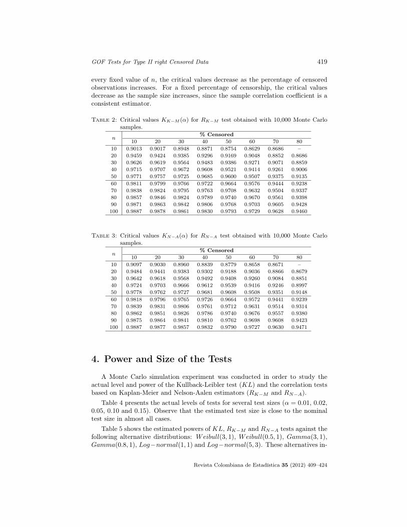
GOF Tests for Type II right Censored Data 419
every fixed value of n, the critical values decrease as the percentage of censoredobservations increases. For a fixed percentage of censorship, the critical valuesdecrease as the sample size increases, since the sample correlation coefficient is aconsistent estimator.
Table 2: Critical values KK−M (α) for RK−M test obtained with 10,000 Monte Carlosamples.
n% Censored
10 20 30 40 50 60 70 8010 0.9013 0.9017 0.8948 0.8871 0.8754 0.8629 0.8686 –20 0.9459 0.9424 0.9385 0.9296 0.9169 0.9048 0.8852 0.868630 0.9626 0.9619 0.9564 0.9483 0.9386 0.9271 0.9071 0.885940 0.9715 0.9707 0.9672 0.9608 0.9521 0.9414 0.9261 0.900650 0.9771 0.9757 0.9725 0.9685 0.9600 0.9507 0.9375 0.913560 0.9811 0.9799 0.9766 0.9722 0.9664 0.9576 0.9444 0.923870 0.9838 0.9824 0.9795 0.9763 0.9708 0.9632 0.9504 0.933780 0.9857 0.9846 0.9824 0.9789 0.9740 0.9670 0.9561 0.939890 0.9871 0.9863 0.9842 0.9806 0.9768 0.9703 0.9605 0.9428100 0.9887 0.9878 0.9861 0.9830 0.9793 0.9729 0.9628 0.9460
Table 3: Critical values KN−A(α) for RN−A test obtained with 10,000 Monte Carlosamples.
n% Censored
10 20 30 40 50 60 70 8010 0.9097 0.9030 0.8960 0.8839 0.8779 0.8658 0.8671 –20 0.9484 0.9441 0.9383 0.9302 0.9188 0.9036 0.8866 0.867930 0.9642 0.9618 0.9568 0.9492 0.9408 0.9260 0.9084 0.885140 0.9724 0.9703 0.9666 0.9612 0.9539 0.9416 0.9246 0.899750 0.9778 0.9762 0.9727 0.9681 0.9608 0.9508 0.9351 0.914860 0.9818 0.9796 0.9765 0.9726 0.9664 0.9572 0.9441 0.923970 0.9839 0.9831 0.9806 0.9761 0.9712 0.9631 0.9514 0.931480 0.9862 0.9851 0.9826 0.9786 0.9740 0.9676 0.9557 0.938090 0.9875 0.9864 0.9841 0.9810 0.9762 0.9698 0.9608 0.9423100 0.9887 0.9877 0.9857 0.9832 0.9790 0.9727 0.9630 0.9471
4. Power and Size of the Tests
A Monte Carlo simulation experiment was conducted in order to study theactual level and power of the Kullback-Leibler test (KL) and the correlation testsbased on Kaplan-Meier and Nelson-Aalen estimators (RK−M and RN−A).
Table 4 presents the actual levels of tests for several test sizes (α = 0.01, 0.02,0.05, 0.10 and 0.15). Observe that the estimated test size is close to the nominaltest size in almost all cases.
Table 5 shows the estimated powers of KL, RK−M and RN−A tests against thefollowing alternative distributions: Weibull(3, 1), Weibull(0.5, 1), Gamma(3, 1),Gamma(0.8, 1), Log−normal(1, 1) and Log−normal(5, 3). These alternatives in-
Revista Colombiana de Estadística 35 (2012) 409–424

420 Víctor Salinas, Paulino Pérez, Elizabeth González & Humberto Vaquera
Table 4: Estimated test size of the KL, RK−M and RN−A tests.n % Censored α RK−M RN−A KL
0.01 0.011 0.007 0.0110.02 0.019 0.016 0.019
20 50 0.05 0.055 0.050 0.0580.10 0.099 0.103 0.1130.15 0.150 0.146 0.1480.01 0.017 0.012 0.0140.02 0.018 0.019 0.025
50 20 0.05 0.047 0.050 0.0530.10 0.097 0.101 0.1070.15 0.150 0.146 0.145
clude monotone increasing, monotone decreasing and non-monotone hazard func-tions, just as in Saldaña-Zepeda et al. (2010). Every entry of this table wascalculated using B = 10, 000 Monte Carlo samples at a significance level α = 0.05.
The main observations that can be made from this table are the following:
• The powers of the tests increase as the sample size increases.
• Under every considered alternative distribution, the tests lose power as thepercentage of censorship gets larger for a fixed sample size.
• The KL test is in general more powerful than the correlation tests. RN−Ais slightly more powerful than RK−M .
• The tests RN−A and RK−M have little power against Gamma(3, 1) alterna-tives.
• The three tests have no power against Weibull(3, 1) alternatives.
Table 5: Estimated power of theKL, RK−M and RN−A tests under several alternatives,for a significance level α = 0.05.
Alternative n (%) Censored RK−M RN−A KL
Weibull(3, 1) 20 20 0.0950 0.0860 0.070150 0.0547 0.0541 0.0493
50 20 0.1636 0.1640 0.126450 0.0559 0.0543 0.0526
100 20 0.2989 0.2806 0.202350 0.0693 0.0623 0.0907
Weibull(0.5, 1) 20 20 0.8095 0.8445 0.964250 0.5890 0.6177 0.8151
50 20 0.9998 0.9995 1.000050 0.9844 0.9850 0.9996
100 20 1.0000 1.0000 1.000050 1.0000 1.0000 1.0000
Gamma(3, 1) 20 20 0.0330 0.0372 0.091350 0.0425 0.0444 0.1090
50 20 0.0390 0.0472 0.1344
Revista Colombiana de Estadística 35 (2012) 409–424

GOF Tests for Type II right Censored Data 421
Table 5. (Continuation)
Alternative n (%) Censored RK−M RN−A KL
50 0.0368 0.0420 0.1342100 20 0.0704 0.0697 0.1959
50 0.0527 0.0530 0.1504Gamma(0.8, 1) 20 20 0.2613 0.3034 0.6168
50 0.2091 0.2277 0.458850 20 0.7775 0.8081 0.9762
50 0.6054 0.6239 0.9321100 20 0.9957 0.9955 0.9998
50 0.9608 0.9632 0.9967Log − normal(1, 1) 20 20 0.2180 0.2666 0.4917
50 0.0964 0.1053 0.286450 20 0.6337 0.6641 0.8254
50 0.2242 0.2434 0.5691100 20 0.9543 0.9559 0.9887
50 0.5671 0.5569 0.7433Log − normal(5, 2) 20 20 0.7914 0.8280 0.9466
50 0.4237 0.4416 0.681550 20 0.9990 0.9997 1.0000
50 0.9059 0.9043 0.9929100 20 1.0000 1.0000 1.0000
50 0.9989 0.9991 1.0000
5. Application Examples
In this section, two application examples are presented, in which the hypothesesstated in equation (2) and (3) will be proven. This will allow us to carry outthe goodness of fit test of the Gumbel distribution, using the Kullback-Leibler,Kaplan-Meier, and Nelson-Aalen test statistics.
Example 1. The data used in this example are from a life expectancy experimentreported by Balakrishnan & Chen (1999). Twenty three ball bearings were placedin the experiment. The data corresponds to the millions of revolutions beforefailure for each of the bearings. The experiment was terminated once the twentiethball failed. The data are shown in Table 6.
Table 6: Millions of revolutions before failure for the ball bearing experiment.xi δi xi δi xi δi xi δi xi δi
17.88 1 45.60 1 55.56 1 84.12 1 105.84 028.92 1 48.48 1 67.80 1 93.12 1 105.84 033.00 1 51.84 1 68.64 1 96.64 1 105.84 041.52 1 51.96 1 68.65 1 105.12 142.12 1 54.12 1 68.88 1 105.84 1
The MLE for the location and scale parameters are ξ = 55.1535 and θ =26.8124. The critical values for n = 23 and r = 20 can be obtained from Tables1, 2 and 3 using interpolation. Table 7, shows the critical values for α = 0.05, the
Revista Colombiana de Estadística 35 (2012) 409–424
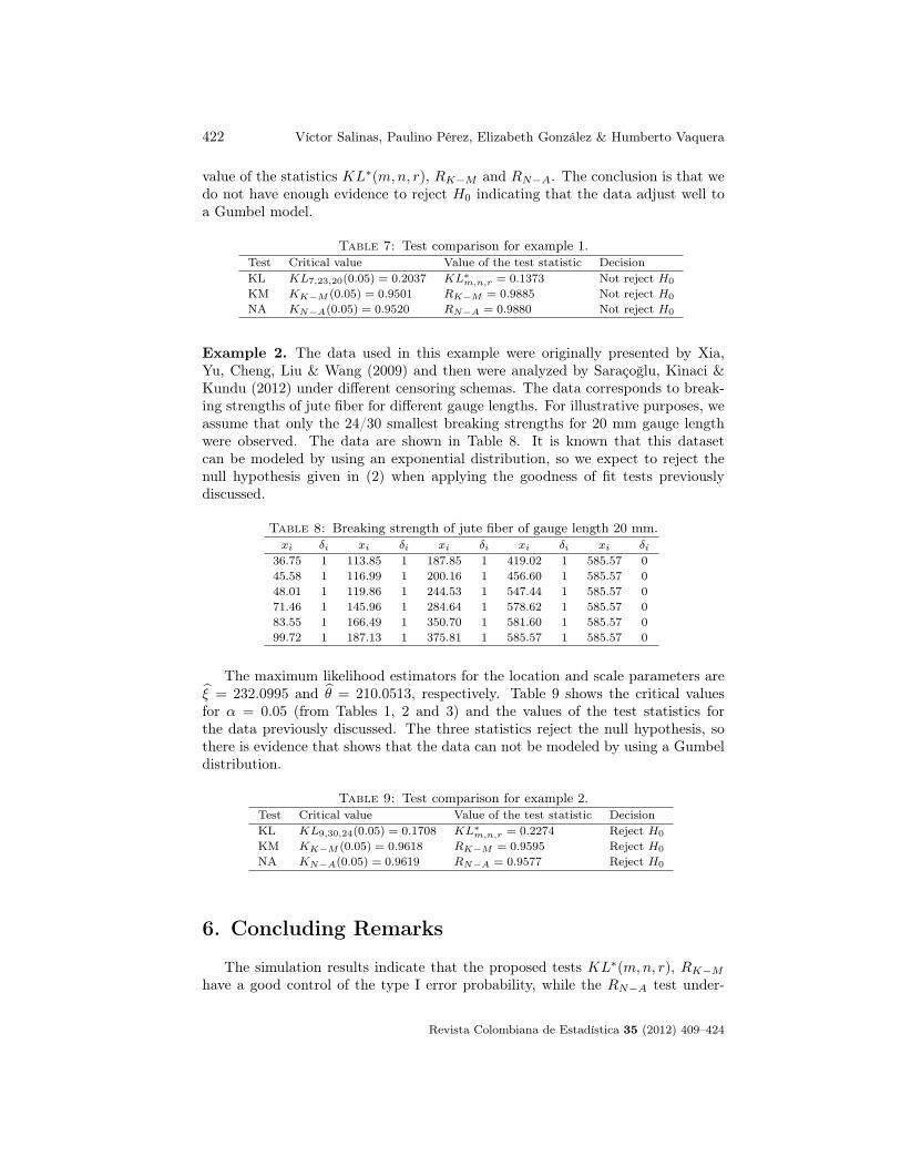
422 Víctor Salinas, Paulino Pérez, Elizabeth González & Humberto Vaquera
value of the statistics KL∗(m,n, r), RK−M and RN−A. The conclusion is that wedo not have enough evidence to reject H0 indicating that the data adjust well toa Gumbel model.
Table 7: Test comparison for example 1.Test Critical value Value of the test statistic DecisionKL KL7,23,20(0.05) = 0.2037 KL∗
m,n,r = 0.1373 Not reject H0
KM KK−M (0.05) = 0.9501 RK−M = 0.9885 Not reject H0
NA KN−A(0.05) = 0.9520 RN−A = 0.9880 Not reject H0
Example 2. The data used in this example were originally presented by Xia,Yu, Cheng, Liu & Wang (2009) and then were analyzed by Saraçoğlu, Kinaci &Kundu (2012) under different censoring schemas. The data corresponds to break-ing strengths of jute fiber for different gauge lengths. For illustrative purposes, weassume that only the 24/30 smallest breaking strengths for 20 mm gauge lengthwere observed. The data are shown in Table 8. It is known that this datasetcan be modeled by using an exponential distribution, so we expect to reject thenull hypothesis given in (2) when applying the goodness of fit tests previouslydiscussed.
Table 8: Breaking strength of jute fiber of gauge length 20 mm.xi δi xi δi xi δi xi δi xi δi
36.75 1 113.85 1 187.85 1 419.02 1 585.57 045.58 1 116.99 1 200.16 1 456.60 1 585.57 048.01 1 119.86 1 244.53 1 547.44 1 585.57 071.46 1 145.96 1 284.64 1 578.62 1 585.57 083.55 1 166.49 1 350.70 1 581.60 1 585.57 099.72 1 187.13 1 375.81 1 585.57 1 585.57 0
The maximum likelihood estimators for the location and scale parameters areξ = 232.0995 and θ = 210.0513, respectively. Table 9 shows the critical valuesfor α = 0.05 (from Tables 1, 2 and 3) and the values of the test statistics forthe data previously discussed. The three statistics reject the null hypothesis, sothere is evidence that shows that the data can not be modeled by using a Gumbeldistribution.
Table 9: Test comparison for example 2.Test Critical value Value of the test statistic DecisionKL KL9,30,24(0.05) = 0.1708 KL∗
m,n,r = 0.2274 Reject H0
KM KK−M (0.05) = 0.9618 RK−M = 0.9595 Reject H0
NA KN−A(0.05) = 0.9619 RN−A = 0.9577 Reject H0
6. Concluding Remarks
The simulation results indicate that the proposed tests KL∗(m,n, r), RK−Mhave a good control of the type I error probability, while the RN−A test under-
Revista Colombiana de Estadística 35 (2012) 409–424

GOF Tests for Type II right Censored Data 423
estimate this level. The test based on the Kullback-Leibler information is betterin terms of power than the tests based on the sample correlation coefficient underthe considered alternative distributions. In future work, it would be interestingto derive the null distribution of the test statistics for finite samples as well as forthe limit case.
Acknowledgments
The authors wish to express their thanks to three anonymous referees and theGeneral Editor for their constructive comments which helped to greatly improvethe presentation of the original version of this paper. The authors were partiallyfunded by Subdirección de Investigación: Línea 15, Colegio de Postgraduados,México.
[Recibido: septiembre de 2011 — Aceptado: septiembre de 2012
]References
Aalen, O. (1978), ‘Nonparametric inference for a family of counting processes’,Annals of Statistics 6(4), 701–726.
Balakrishnan, N. & Chen, W. (1999), Handbook of Tables for Order Statistics fromLognormal Distributions with Applications, Springer.*http://books.google.com/books?id=x1862WoJL2EC
Castro-Kuriss, C. (2011), ‘On a goodness-of-fit test for censored data from alocation-scale distribution with applications’, Chilean Journal of Statistics2, 115–136.
Ebrahimi, N., Habibullah, M. & Soofi, E. (1992), ‘Testing exponentiality basedon Kullback-Leibler information’, Journal of the Royal Statistical Society54, 739–748.
Kaplan, E. L. & Meier, P. (1958), ‘Nonparametric estimation from incompleteobservations’, Journal of the American Statistical Association 53(282), 457–481.*http://dx.doi.org/10.2307/2281868
Lim, J. & Park, S. (2007), ‘Censored Kullback-Leibler information and goodness-of-fit test with type II censored data’, Journal of Applied Statistics34(9), 1051–1064.
Lin, C.-T., Huang, Y.-L. & Balakrishnan, N. (2008), ‘A new method for goodness-of-fit testing based on type-II right censored samples’, IEEE Transactions onReliability 57, 633–642.
Revista Colombiana de Estadística 35 (2012) 409–424

424 Víctor Salinas, Paulino Pérez, Elizabeth González & Humberto Vaquera
Nelder, J. A. & Mead, R. (1965), ‘A simplex algorithm for function minimization’,Computer Journal 7, 308–313.
Nelson, W. (1972), ‘Theory and applications of hazard plotting for censored failuredata’, Technometrics 14, 945–965.
Park, S. & Park, D. (2003), ‘Correcting moments for goodness of fit tests basedon two entropy estimates’, Journal of Statistical Computation and Simulation73, 685–694.
Pérez-Rodríguez, P., Vaquera-Huerta, H. & Villaseñor-Alva, J. A. (2009), ‘Agoodness-of-fit test for the Gumbel distribution based on Kullback-Leiblerinformation’, Communications in Statistics: Theory and Methods 38, 842–855.
R Core Team (2012), R: A Language and Environment for Statistical Computing,R Foundation for Statistical Computing, Vienna, Austria. ISBN 3-900051-07-0.*http://www.R-project.org/
Saldaña-Zepeda, D., Vaquera-Huerta, H. & Arnold, B. C. (2010), ‘A goodness of fittest for the Pareto distribution in the presence of type II censoring, based onthe cumulative hazard function’, Computational Statistics and Data Analysis54(4), 833–842.
Saraçoğlu, B., Kinaci, I. & Kundu, D. (2012), ‘On estimation of R = P (Y < X)for exponential distribution under progressive type-II censoring’, Journal ofStatistical Computation and Simulation 82(5), 729–744.*http://www.tandfonline.com/doi/abs/10.1080/00949655.2010.551772
Song, K. S. (2002), ‘Goodness-of-fit-tests based on Kullback-Leibler discriminationinformation’, IEEE Transactions On Information Theory 48, 1103–1117.
Stephens, M. A. (1986), Tests based on edf statistics, in R. D’Agostino &M. Stephens, eds, ‘Goodness-of-Fit Techniques’, New York.
Xia, Z. P., Yu, J. Y., Cheng, L. D., Liu, L. F. & Wang, W. M. (2009), ‘Studyon the breaking strength of jute fibres using modified Weibull distribution’,Composites Part A: Applied Science and Manufacturing 40(1), 54 – 59.*http://www.sciencedirect.com/science/article/pii/S1359835X08002595
Revista Colombiana de Estadística 35 (2012) 409–424

Revista Colombiana de EstadísticaDiciembre 2012, volumen 35, no. 3, pp. 425 a 442
On the Entropy of Written Spanish
Sobre la entropía del español escrito
Fabio G. Guerreroa
Escuela de Ingeniería Eléctrica y Electrónica, Facultad de Ingeniería,Universidad del Valle, Cali, Colombia
AbstractA discussion on the entropy of the Spanish language by means of a practi-
cal method for calculating the entropy of a text by direct computer processingis presented. As an example of application, thirty samples of Spanish textare analyzed, totaling 22.8 million characters. Symbol lengths from n = 1 to500 were considered for both words and characters. Both direct computerprocessing and the probability law of large numbers were employed for cal-culating the probability distribution of the symbols. An empirical relationon entropy involving the length of the text (in characters) and the number ofdifferent words in the text is presented. Statistical properties of the Spanishlanguage when viewed as produced by a stochastic source, (such as originshift invariance, ergodicity and asymptotic equipartition property) are alsoanalyzed.
Key words: Law of large numbers, Shannon entropy, Stochastic process,Zipf’s law.
ResumenSe presenta una discusión sobre la entropía de la lengua española por
medio de un método práctico para el cálculo de la entropía de un texto me-diante procesamiento informático directo. Como un ejemplo de aplicación,se analizan treinta muestras de texto español, sumando un total de 22,8 mil-lones de caracteres. Longitudes de símbolos desde n = 1 hasta 500 fueronconsideradas tanto para palabras como caracteres. Para el cálculo de ladistribución de probabilidad de los símbolos se emplearon procesamiento di-recto por computador y la ley de probabilidad de los grandes números. Sepresenta una relación empírica de la entropía con la longitud del texto (encaracteres) y el número de palabras diferentes en el texto. Se analizan tam-bién propiedades estadísticas de la lengua española cuando se considera comoproducida por una fuente estocástica, tales como la invarianza al desplaza-miento del origen, ergodicidad y la propiedad de equipartición asintótica.
Palabras clave: entropía de Shannon, ley de grandes números, ley de Zipf,procesos estocásticos.
aAssistant Professor. E-mail: [email protected]
425

426 Fabio G. Guerrero
1. Introduction
Spanish is a language which is used by more than four hundred million peoplein more than twenty countries, and it has been making its presence increasinglyfelt on the Internet (Marchesi 2007). Yet this language has not been as extensivelyresearched at entropy level. The very few calculations which have been reportedhave been obtained, as for most languages, by indirect methods, due in part to thecomplexity of the problem. Having accurate entropy calculations for the Spanishlanguage can thus be considered a pending task. Knowing the value of H, ingeneral for any language, is useful for source coding, cryptography, language spacedimension analysis, plagiarism detection, and so on. Entropy calculation is at thelowest level of language analysis because it only takes into account source symbolstatistics and their statistical dependence, without any further consideration ofmore intelligent aspects of language such as grammar, semantics, punctuationmarks (which can considerably change the meaning of a sentence), word clustering,and so on.
Several approaches have been devised for several decades for finding the entropyof a language. Shannon (1948) initially showed that one possible way to calculatethe entropy of a language, H, would be through the limit H = limn→∞− 1
nH(Bi),where Bi is a sequence of n symbols. Finding H using methods such as the onesuggested by this approach is difficult since it assumes that the probability ofthe sequences, p(Bi), is an asymptotically increasing function of n, as n tendsto infinity. Another difficulty posed by this approach is that an extremely largesample of text would be required, one that considered all possible uses of the lan-guage. Another suggested way to calculate H is by taking H = limn→∞ Fn, whereFn = H(j|Bi) = H(Bij) −H(Bi). Bi is a block of n-1 symbols, j is the symbolnext to Bi, H(j|Bi) is the conditional entropy of symbol j given block Bi. In thisapproach, the series of approximations F1, F2, . . . provides progressive values ofconditional entropy. Fn, in bits/symbol, measures the amount of information in asymbol considering the previous n−1 consecutive symbols, due to the statistics ofthe language. The difficulty of using these previous methods in practice was putunder evidence when in his pioneering work Shannon (1951) used instead a hu-man prediction approach for estimating the entropy of English, getting 0.6 and 1.3bits/letter as bounds for printed English, considering 100-letter sequences. Gam-bling estimations have also been used, providing an entropy estimation of 1.25 bitsper character for English (Cover & King 1978). The entropy rate of a languagecould also be estimated using ideal source coders since, by definition, this kind ofcoder should compress to the entropy limit. A value of 1.46 bits per character hasbeen reported for the entropy of English by means of data compression (Teahan &Cleary 1996). The entropy of the fruit fly genetic code has been estimated usinguniversal data compression algorithms (Wyner, Jacob & Wyner 1998). As for theSpanish language, values of 4.70, 4.015, and 1.97 bits/letter for F0, F1, and FW
respectively were reported (Barnard III 1955) using an extrapolation techniqueon frequency data obtained from a sample of 6,513 different words. FW is theentropy, in bits/letter, based on single-word frequency.
Revista Colombiana de Estadística 35 (2012) 425–442
On the Entropy of Written Spanish 427
Another venue for finding H has been based on a purely mathematical frame-work derived from stochastic theory, such as the one proposed by Crutchfield &Feldman (2003). Unfortunately, as the same authors recognize it, it has lead, inpractice, to very limited results for finding the entropy of a language. In general,as all these results suggest, finding the entropy of a language by classic methodshas proved to be a challenging task. Despite some remarkable findings in the pastdecades, the search for a unified mathematical model continues to be an openproblem (Debowski 2011).
In the past it was implicitly believed that attempting to find the average un-certainty content of a language by direct analysis of sufficiently long samples couldbe a very difficult task to accomplish. Fortunately, computer processing capacityavailable at present has made feasible tackling some computing intensive problemssuch as the search in large geometric spaces employed in this work. Michel, Shen,Aiden, Veres, Gray, Team, Pickett, Hoiberg, Clancy, Norvig, Orwant, Pinker,Nowak & Aiden (2011) discuss, as an example of this trend, the use of huge com-putational resources to research the relationship between linguistics and culturalphenomena. This paper is organized as follows: In Section 2 the methodologyused to obtain all the values reported is discussed; in Section 3 the results of theobservations are presented; Section 4 presents a discussion and analysis of themost relevant results and, finally, in Section 5 the main conclusions of this workare summarized. All the samples and support material used in this work are pub-licly available at http://sistel-uv.univalle.edu.co/EWS.html. Aspects such as theanalysis of grammar, semantics, and compression theory are beyond the scope ofthis paper.
2. Methodology
Thirty samples of literature available in Spanish were chosen for this study.Tables 1 and 2 show the details of the samples and its basic statistics. The worksused in this paper as samples of written Spanish were obtained from public li-braries available on the Internet such as librodot 1 and the virtual library Miguelde Cervantes 2. The selection of the samples was done without any particular con-sideration of publication period, author’s country of origin, and suchlike. A file ofnews provided to the author by the Spanish press agency EFE was also includedin the samples for analysis. The selected material was processed using a T3500Dell workstation with 4 GB RAM. The software used to do the all the calculationspresented in this work was written in Mathematica R© 8.0. For simplicity, a slightpreprocessing was done on each sample, leaving only printable characters. Stringsof several spaces were reduced to one character and the line feed control character(carry return) was replaced by a space character, allowing for fairer comparisonsbetween samples. The samples were character encoded using the ISO 8859-1 stan-dard (8-bit single-byte coded graphic character sets - Part 1: Latin alphabet No.1) which has 191 characters from the Latin script, providing a full set of charac-
1http://www.librodot.com2http://www.cervantesvirtual.com
Revista Colombiana de Estadística 35 (2012) 425–442

428 Fabio G. Guerrero
ters for the Spanish language. For instance, the ñ letter corresponds to 0xf1, etc.The total amount of characters of the thirty samples in table 1 is 22,882,449 andthe total amount of words is 4,024,911. The rounded average for the number ofdifferent one-character symbols (uppercase, lowercase, and punctuation marks) forthe thirty samples was 93. The reason we consider the distinction between upper-case and lowercase symbols is that when characterizing an information source atentropy level, lowercase and uppercase symbols produce different message vectorsfrom the transmission point of view (e.g. the word HELLO produces a completelydifferent message vector than the word hello).
Table 1: Set of Text SamplesSample Name Author1 La Biblia Several authors2 efe-B2 EFE Press agency3 Amalia José Mármol4 Crimen y Castigo Fyodor Dostoevsky5 Rayuela Julio Cortázar6 Doña Urraca de Castilla F. Navarro Villoslada7 El Corán Prophet Muhammad8 Cien Años de Soledad Gabriel García Márquez9 La Araucana Alonso de Ercilla10 El Papa Verde Miguel Angel Asturias11 América Franz Kafka12 La Altísima Felipe Trigo13 Al Primer Vuelo José María de Pereda14 Harry Potter y la Cámara Secreta J.K. Rowling15 María Jorge Isaacs16 Adiós a las Armas Ernest Hemingway17 Colmillo Blanco Jack London18 El Alférez Real Eustaquio Palacios19 Cañas y Barro Vicente Blasco Ibáñez20 Aurora Roja Pío Baroja21 El Comendador Mendoza Juan C. Valera22 El Archipiélago en Llamas Jules Verne23 Doña Luz Juan Valera24 El Cisne de Vilamorta Emilia Pardo Bazán25 Cuarto Menguante Enrique Cerdán Tato26 Las Cerezas del Cementerio Gabriel Miró27 Tristana Benito Pérez Galdós28 Historia de la Vida del Buscón Francisco de Quevedo29 El Caudillo Armando José del Valle30 Creció Espesa la Yerba Carmen Conde
In Table 2 the parameter α is the average word length, given by∑Lipi, where
Li and pi are the length in characters and the probability of the i-th word respec-tively. The weighted average of α for the whole set of samples is 4.491 letters perword. The word dispersion ratio, WDR, is the percentage of different words overthe total number of words.
The values of entropy were calculated using the entropy formula∑pi log2 pi.
The frequency of the different symbols (n-character or n-word symbols) and the law
Revista Colombiana de Estadística 35 (2012) 425–442

On the Entropy of Written Spanish 429
of large numbers were used to find the symbol probabilities as pi ≈ ni/ntotal. First,we started considering word symbols, since words are the constituent elements ofthe language. However, a more refined analysis based on characters was alsocarried out. Entropy values for both n-character and n-word symbols from n=1to 500 were calculated. Considering symbols up to a length of five hundred was asuitable number for practical proposes, this will be discussed in the next section.
Table 2: Sample Details
Sample Number ofCharacters
AlphabetSize (AS)
Number ofWords
DifferentWords
WDR(%) α
1 5722041 100 1049511 40806 3.89 4.272 1669584 110 279917 27780 9.92 4.803 1327689 88 231860 18871 8.14 4.514 1215215 91 207444 17687 8.53 4.635 984129 117 172754 22412 12.97 4.506 939952 84 161828 17487 10.81 4.587 884841 93 160583 12236 7.62 4.328 805614 84 137783 15970 11.59 4.739 751698 82 129888 15128 11.65 4.63
10 676121 93 118343 16731 14.14 4.4511 594392 88 101904 11219 11.01 4.6612 573399 89 98577 14645 14.86 4.5313 563060 82 100797 13163 13.06 4.3514 528706 89 91384 10884 11.91 4.6015 499131 87 88376 12680 14.35 4.4516 471391 91 81803 10069 12.31 4.4917 465032 91 81223 10027 12.35 4.5818 462326 89 82552 10699 12.96 4.4319 436444 79 75008 10741 14.32 4.6620 393920 90 68729 10598 15.42 4.4721 387617 86 69549 10289 14.79 4.3822 363171 88 61384 8472 13.80 4.7323 331921 83 59486 9779 16.44 4.4124 312174 77 53035 11857 22.36 4.6525 304837 87 49835 12945 25.98 4.9526 302100 75 51544 10210 19.81 4.6427 299951 82 52571 10580 20.13 4.4828 232236 74 42956 7660 17.83 4.2329 224382 83 36474 7470 20.48 5.0030 159375 81 27813 6087 21.89 4.48
One worthwhile question at this point is “does entropy change when changingthe origin point in the sample?”. For this purpose, we calculated entropy valuesconsidering symbols for different shifts from the origin for non overlapping symbols,as illustrated by figure 1, for the case of trigrams.
It can easily be seen that, for symbols of length n, symbols start repeating (i.e.,symbols are the same as for shift=0, except for the first one) after n shifts. Asa result, the number of individual entropy calculations when analyzing symbolsfrom length n = 1 up to k was k(k+1)
2 . For the k = 500 case used in this work,this gives 125,250 individual entropy calculations for every sample analyzed. The
Revista Colombiana de Estadística 35 (2012) 425–442

430 Fabio G. Guerrero
Figure 1: Origin invariance analysis.
individual shift entropies so obtained were then averaged for every n. Values of nfor which the maximum value of entropy was produced were identified, as well asvalues of n from which all symbols present in the text become equiprobable withreasonable certainty, i.e., none of them repeat more than once in the sample.
3. Results
3.1. Entropy Values Considering Words
Figure 2 shows the values of average entropy for n-word symbols. For ease ofdisplay, only data for samples 1, 2, 12 and 30 and n = 1 to 20 are shown. The restof the literary works exhibited the same curve shapes with values in between. Allthe analyzed samples exhibited invariance to origin shift. For example, for sample8 (Cien Años de Soledad) the values for n = 4 were: 15.024492 (shift = 0),15.028578 (shift = 1), 15.025693 (shift = 2), 15.027212 (shift = 3). This meansthat P (w1, ..wL) = P (w1+s, ..wL+s) for any integer s, where {w1, ..wL} is a L-wordsequence. This is a very useful property to quickly find the entropy of a text itbecause it makes necessary to compute values for just one shift thus reducing theprocess to a few seconds for practical purposes.
Also since the weighted value for 1-word entropy for the set analyzed was10.0064 bits/character, the weighted value of FW is therefore 2.23 bits/character.
3.2. Entropy Values Considering n-Character Symbols
Figure 3 shows the averaged entropy values for n-character symbols. Again forease of display, only data for samples 1, 2, 12 and 30 and n = 1 to 100 are shown.All samples also exhibited the origin shift invariance property. For example, forsample 8 (Cien Años de Soledad), the values of entropy for n = 4 characters were:
Revista Colombiana de Estadística 35 (2012) 425–442

On the Entropy of Written Spanish 431
�
�
� � � � � � � � � � � � � � � � � �
�
�
� ��� � � � � � � � � � � � � � �
�
����� � � � � � � � � � � � � � �
�
� ���� � � � � � � � � � � � � � �
5 10 15 20
10
12
14
16
18
Symbol length �words�
Entr
opy�bit�sy
mbol�
� Sample 30� Sample 12� Sample 2� Sample 1
Figure 2: Entropy for n-word symbols for samples 1, 2, 12 and 30.
12.267881 (shift = 0), 12.264343 (shift = 1), 12.268751 (shift = 2), 12.269691(shift = 3). Therefore, P (c1, .., cL) = P (c1+s, .., cL+s) for any integer s. As inthe case of words, the rest of literary works exhibited the same curve shapes withvalues in between.
�
�
�
�
�
��� � � � � � �������
�
�
�
�
��
� � � � � � � � ������
�
�
�
�
�� � � � � � � � �������
�
�
�
�
�� � � � � � � � � � �����
1.0 10.05.02.0 20.03.01.5 15.07.0
10
15
Symbol length � characters�
Entr
opy�bit�sy
mbol�
� Sample 30� Sample 12� Sample 2� Sample 1
Figure 3: Log Plot of entropy for n-character symbols for samples 1, 2, 12 and 30.
3.3. Processing Time
Figure 4 shows the processing time of every sample for both words and charac-ters for all shifts of n (1 ≤ n ≤ 500), that is, 125,250 entropy calculations for eachsample. Due to the origin shift invariance property, only calculations for one shift(for instance shift = 0) are strictly required thus reducing the time substantially.For example, the processing time of sample 1 for only one shift was 433 secondswhile the processing time for sample 30 was just nine seconds. Analysis for allshifts of n were done in this work in order to see if entropy varied when changing
Revista Colombiana de Estadística 35 (2012) 425–442

432 Fabio G. Guerrero
the point of origin in the text. A carefully designed algorithm based on Math-ematica’s sorting functions was employed to obtain the probability of symbols,however, a discussion on the optimality of this processing is beyond the scope ofthis paper.
�
�
�
���
�
� � �� � �
� ��� �
� � � ���
� � �� �
�
�
�
� �
� � � � � � � �� � � � � � � � � �
� � � � � � � �
5 10 15 20 25 300
2
4
6
8
10
12
14
Sample number
Pro
cess
ing
tim
e�hours�
� Word processing
� Character processing
Figure 4: Processing time considering all shifts of n (125,250 entropy calculations)
3.4. Reverse Entropy
If we take the text in reverse order, for instance “yportne eht no” instead of “onthe entropy”, it is possible to evaluate the reverse conditional entropy, that is, theeffect of knowing how much information can be gained about a previous characterwhen later characters are known. It was observed that entropy of the reverse textcarried out for the same set of samples produced exactly the same values as forthe forward entropy case. This was first observed by Shannon for the case of theEnglish language in his classical work (Shannon 1951) on English prediction.
4. Discussion
4.1. Frequency of Symbols and Entropy
Figure 5 shows a plot of the fundamental measure function of information,pi log2 pi, which is at the core of the entropy formula. This function has its max-imum, 0.530738, at pi = 0.36788. Therefore, infrequent symbols, as well as veryfrequent symbols, add very little to the total entropy. This should not be con-fused with the value of pi = 1
n that produces the maximum amount of entropy fora probability space with n possible outcomes. The entropy model certainly hassome limitations because entropy calculation is based solely on probability distri-bution. In fact, two different texts with very different location of words can havethe same entropy, yet one of them can lead to a very much more efficient sourceencoding than the other.
Revista Colombiana de Estadística 35 (2012) 425–442

On the Entropy of Written Spanish 433
0.0 0.2 0.4 0.6 0.8 10.0
0.1
0.2
0.3
0.4
0.5
pi
p ilo
g 2p i
Figure 5: Fundamental function of information.
4.2. Log-log Plots and the Spanish Language Constant
The fact that the basic statistical properties of entropy are essentially the samefor short length symbols regardless of the sample (and the entropy is similar forany shift of the origin) means it is possible to use a sufficiently long sample, forinstance sample 2, to study the Spanish language constant. Figure 6 shows thelog-log plot for sample 2 which contained 82,656 different 3-word symbols, 79,704different 2-word symbols, and 27,780 different 1-word symbols. Log-log plots forthe rest of samples were found to be similar to those of figure 6, at least for 2-wordand 1-word symbols.
Figure 6: Symbol rank versus n-word probability in Sample 2.
Revista Colombiana de Estadística 35 (2012) 425–442

434 Fabio G. Guerrero
Smoothing the 1-word curve in figure 6, the probability of the r-th most fre-quent 1-word symbol is close to 0.08/r, assuming r is not too large. This behaviorcorresponds to the celebrated Zipf law first presented in 1939 (Zipf 1965) whichnowadays some authors also call the Zipf-Mandelbrot law (Debowski 2011). Fig-ure 7 shows the log-log plot for for sample 2 which contained 14,693 differenttrigrams, 2,512 different digrams, and 110 different characters; all values consid-ered for shift = 0. Log-log plots for the rest of the samples were found to be similarto those of figure 7. Even when a distinction between upper case and lower casesymbols is made in this work, no significant difference was found with the constantobtained when analyzing the database of the 81,323 most frequent words (whichmakes no distinction between upper case and lower case symbols). This databasewas compiled by Alameda & Cuetos (1995) from a corpus of 1,950,375 words ofwritten Spanish.
Figure 7: Symbol rank versus n-character probability for Sample 2.
4.3. Conditional Entropy
We now evaluate the uncertainty content of a character given some previoustext. Initially F0, in bits per character, is given by log2(AS), where AS is thealphabet size. F1 takes into account single-character frequencies and it is given byF1 =
∑i
pi log2 pi. F2 considers the uncertainty content of a character given the
previous one:
F2 = −∑i,j
p(i, j) log2 p(j|i) = −∑i,j
p(i, j) log2 p(i, j) +∑i
pi log2 pi (1)
Revista Colombiana de Estadística 35 (2012) 425–442

On the Entropy of Written Spanish 435
Similarly, F3 gives the entropy of a character given the previous two characters(digram):
F3 = −∑i,j,k
p(i, j, k) log2 p(k|ij) = −∑i,j,k
p(i, j, k) log2 p(i, j, k) +∑i,j
pi,j log2 pi,j
(2)and so on. Table 3 shows, for simplicity, values for Fn from F1 to F15 only,
rounded to two significant digits.
Table 3: Conditional Entropy Fnn
Si 1 2 3 4 5 6 7 8 9 10 11 12 13 14 151 4.51 3.43 2.76 2.18 1.72 1.33 0.98 0.68 0.43 0.26 0.14 0.06 0.01 -0.02 -0.042 4.52 3.46 2.82 2.13 1.52 1.05 0.69 0.42 0.22 0.09 0.01 -0.03 -0.06 -0.06 -0.073 4.39 3.34 2.73 2.11 1.57 1.11 0.72 0.42 0.21 0.08 -0.01 -0.05 -0.07 -0.08 -0.084 4.43 3.39 2.74 2.09 1.54 1.07 0.67 0.37 0.18 0.06 -0.01 -0.05 -0.06 -0.07 -0.085 4.40 3.41 2.81 2.16 1.55 1.02 0.59 0.30 0.12 0.01 -0.05 -0.08 -0.08 -0.09 -0.096 4.39 3.35 2.74 2.13 1.56 1.05 0.62 0.32 0.13 0.02 -0.04 -0.07 -0.08 -0.09 -0.097 4.46 3.31 2.57 1.93 1.40 0.96 0.61 0.36 0.20 0.09 0.03 -0.02 -0.04 -0.06 -0.068 4.27 3.27 2.67 2.06 1.50 1.02 0.63 0.34 0.16 0.05 -0.02 -0.06 -0.07 -0.08 -0.089 4.32 3.28 2.70 2.11 1.58 1.06 0.61 0.29 0.10 -0.01 -0.06 -0.09 -0.10 -0.10 -0.09
10 4.40 3.36 2.78 2.16 1.51 0.95 0.51 0.22 0.05 -0.04 -0.08 -0.09 -0.10 -0.10 -0.0911 4.33 3.32 2.66 2.00 1.43 0.93 0.54 0.28 0.11 0.01 -0.04 -0.07 -0.08 -0.09 -0.0912 4.44 3.38 2.74 2.11 1.46 0.90 0.47 0.20 0.03 -0.05 -0.09 -0.10 -0.10 -0.10 -0.1013 4.36 3.31 2.71 2.07 1.47 0.93 0.52 0.23 0.07 -0.03 -0.07 -0.09 -0.09 -0.10 -0.0914 4.44 3.40 2.69 1.98 1.35 0.84 0.47 0.22 0.08 -0.01 -0.05 -0.07 -0.08 -0.09 -0.0915 4.38 3.33 2.72 2.07 1.43 0.87 0.46 0.20 0.05 -0.04 -0.08 -0.09 -0.10 -0.10 -0.0916 4.46 3.35 2.69 2.00 1.37 0.83 0.44 0.19 0.05 -0.03 -0.07 -0.08 -0.09 -0.09 -0.0917 4.32 3.30 2.63 1.98 1.39 0.89 0.50 0.24 0.07 -0.01 -0.06 -0.08 -0.09 -0.09 -0.0918 4.35 3.33 2.71 2.05 1.41 0.86 0.45 0.19 0.04 -0.04 -0.08 -0.09 -0.10 -0.09 -0.0919 4.29 3.29 2.64 1.98 1.37 0.87 0.49 0.23 0.08 -0.01 -0.06 -0.08 -0.09 -0.09 -0.0920 4.44 3.37 2.73 2.03 1.34 0.78 0.37 0.14 0.01 -0.06 -0.08 -0.10 -0.10 -0.10 -0.0921 4.37 3.33 2.71 2.04 1.37 0.79 0.39 0.13 0.00 -0.05 -0.09 -0.09 -0.11 -0.06 -0.1222 4.38 3.34 2.65 1.91 1.26 0.75 0.40 0.17 0.05 -0.03 -0.05 -0.08 -0.08 -0.08 -0.0823 4.34 3.30 2.67 2.00 1.35 0.78 0.38 0.13 0.01 -0.06 -0.09 -0.10 -0.10 -0.10 -0.0924 4.38 3.36 2.78 2.08 1.34 0.71 0.30 0.06 -0.05 -0.09 -0.11 -0.11 -0.11 -0.10 -0.1025 4.32 3.37 2.80 2.09 1.32 0.69 0.29 0.06 -0.05 -0.09 -0.10 -0.11 -0.11 -0.10 -0.1026 4.42 3.35 2.71 2.01 1.28 0.71 0.32 0.10 -0.03 -0.07 -0.10 -0.11 -0.10 -0.10 -0.1027 4.37 3.34 2.74 2.06 1.33 0.72 0.31 0.08 -0.04 -0.09 -0.11 -0.11 -0.11 -0.10 -0.1028 4.33 3.25 2.63 1.94 1.26 0.71 0.32 0.10 -0.03 -0.09 -0.10 -0.11 -0.11 -0.10 -0.1029 4.28 3.28 2.62 1.89 1.21 0.68 0.32 0.11 0.00 -0.07 -0.09 -0.10 -0.10 -0.09 -0.0930 4.40 3.35 2.66 1.89 1.11 0.52 0.17 0.01 -0.08 -0.11 -0.12 -0.11 -0.11 -0.11 -0.10
We observe in table 3 that, at some point, conditional entropies become nega-tive. Although H(X,Y ) should always be greater or equal to H(Y ), the estimationon conditional entropy in this study becomes negative because the length of thetext is not sufficiently long, in contrast to the required condition of the theo-retical model n → ∞. This behavior has also been observed in the context ofbioinformatics and linguistics (Kaltchenko & Laurier 2004). The following ex-ample should help to clarify the explanation. Let’s consider first the followingtext in Spanish which has 1000 characters: 〈〈Yo, señora, soy de Segovia. Mipadre se llamó Clemente Pablo, natural del mismo pueblo; Dios le tenga en elcielo. Fue, tal como todos dicen, de oficio barbero, aunque eran tan altos sus pen-samientos que se corría de que le llamasen así, diciendo que él era tundidor demejillas y sastre de barbas. Dicen que era de muy buena cepa, y según él bebíaes cosa para creer. Estuvo casado con Aldonza de San Pedro, hija de Diego deSan Juan y nieta de Andrés de San Cristóbal. Sospechábase en el pueblo que noera cristiana vieja, aun viéndola con canas y rota, aunque ella, por los nombresy sobrenombres de sus pasados, quiso esforzar que era descendiente de la gloria.Tuvo muy buen parecer para letrado; mujer de amigas y cuadrilla, y de pocos en-emigos, porque hasta los tres del alma no los tuvo por tales; persona de valor y
Revista Colombiana de Estadística 35 (2012) 425–442

436 Fabio G. Guerrero
conocida por quien era. Padeció grandes trabajos recién casada, y aun después,porque malas lenguas daban en decir que mi padre metía el dos de bastos para sacarel as de oros〉〉. This text has 250 four-character symbols (e.g. {Yo, },{seño},{ra,}) with 227 of them being different. Factorizing common probability terms we find:H4−char = 209( 1
250 log21
250 )+14( 1125 log2
1125 )+3( 3
250 log23
250 )+2
125 log22
125 = 7.76bits/symbol. This text has 200 five-character symbols (e.g.{Yo, s},{eñora},{, soy})with 192 being different five-character symbols. Factorizing common probabilityterms we find: H5−char = 184( 1
200 log21
200 ) + 8( 1100 log2
1100 ) = 7.56 bits/symbol.
Thus the entropy of a character given the previous four characters are know andwould be H(X|Y ) = H5−char − H4−char = −0.20 bits/character. For sample1 (which has 5,722,040 characters) a similar behavior is observed: The greatestnumber of different symbols (418,993) occurs for n=10 (572,204 total 10-charactersymbols) for whichH=18.26 bits/symbol. The highest entropy, 18.47 bits/symbol,is produced by 13-character symbols (there are 440,156 total 13-character symbols,and 395,104 different 13-character symbols). For 14-character symbols (408,717total; 378,750 different) the entropy is 18.45 bits/symbol. Then the entropyof a character given the previous thirteen characters are know, in this case, is18.45− 18.47 = −0.02 bits/character. With increasing n, the probability distribu-tion tends to become uniform and H starts decreasing monotonically with n, asshown in figure 3 of the paper. When the symbols in the sample become equiproba-ble the value of H is given by log2b total number of characters
n c. Again, these seeminglyparadoxical values are explained by the differences between mathematical modelsand real world, as well as the assumptions on which they are based3.
4.4. Entropy Rate and Redundancy
To estimate the entropy rate, a polynomial interpolation of third degree is firstapplied to the values of Fn. As an example, figure 8 shows the interpolated curvesfor samples one and thirty.
Figure 8 shows that Fn becomes negative after crossing by zero, and from thispoint asymptotically approaches zero as n→∞. Therefore,
limn→∞
Fn = limn→NZ
Fn (3)
In equation 3, NZ is the root of the interpolated function Fn. The n-characterentropy values of figure 3 are also interpolated to find HNZ , the entropy valuecorresponding to NZ . The redundancy is given by R = HL
Hmax, where HL is the
source’s entropy rate, and Hmax = log2(AS). Finally, the value of HL is calculatedas HL ≈ HNZ
NZ. Table 4 summarizes the values of NZ , HNZ , HL, and R. It should
be clear that the previous interpolation process is used to get a finer approximationto the value of entropy. Just as in thermodynamics a system in equilibrium stateproduces maximum entropy, equation 3 captures the symbol distribution thatproduces the highest level of entropy (or amount of information) in the text.
3An insightful dissertation on real world and models is presented in Slepian (1976).
Revista Colombiana de Estadística 35 (2012) 425–442

On the Entropy of Written Spanish 437
5 10 15 20 25 30
0
1
2
3
4
n
Fn
Sample 30
Sample 1
Figure 8: Interpolated curves of conditional entropy (bits/character) for samples 1 and30.
In Table 4, the weighted average of HL is 1.54 bits/character. Since theweighted average of the alphabet size in Table 1 is 92.98 characters the average re-dundancy, R, for the analyzed sample set, comprising nearly 23 million characters,is:
R = 1− 1.54
log2 92.98≈ 76.486%
Taking H(X) equal to 1.54 bits/character, for a text of Spanish of 140 charac-ters, there would exist 2nH(X) ≈ 7.98× 1064 typical sequences. Because the rootsof Fn occur at small values of n and, as it has been observed this method permitsto find the value of entropy in a very short time (analysis for only one shift, forinstance shift=0, is required). As it can be observed in Table 4, in general, asample with lower WDR has more redundancy, the opposite also being true. Ingeneral, and as a consequence of Zipf’s, law the greater the size of a sample, thesmaller its WDR. An interesting empirical relation found in this work involvingHL, the length of the text (in characters) L, and the number of different words(V ) in the text is:
HL ≈2.192
logV L(4)
Equation 4 indicates that texts with small word dictionaries (compared tothe length of the text in characters) have smaller HL because there is higherredundancy. This corroborates the well known fact that larger documents are morecompressible than smaller ones. The compression factor4 using bzip compressionfor samples 1 and 30 is 0.25 and 0.33 respectively, which is in total agreement withsample 1 having more redundancy than sample 30. Equation 4 is a reasonableapproximation considering that in this work L takes into consideration punctuation
4The compression factor is defined in this work as the size after compression over the sizebefore compression.
Revista Colombiana de Estadística 35 (2012) 425–442

438 Fabio G. Guerrero
Table 4: Entropy Rate and RedundancySample NZ HNZ HL R(%)
1 13.23 18.47 1.40 78.992 11.23 16.91 1.51 77.803 10.92 16.67 1.53 76.384 10.82 16.53 1.53 76.545 10.10 16.36 1.62 76.436 10.22 16.28 1.59 75.087 11.54 15.91 1.38 78.928 10.60 15.95 1.50 76.469 9.90 16.05 1.62 74.4910 9.48 15.93 1.68 74.3111 10.14 15.61 1.54 76.1612 9.31 15.73 1.69 73.9213 9.64 15.64 1.62 74.4714 9.92 15.46 1.56 75.9415 9.49 15.50 1.63 74.6416 9.55 15.36 1.61 75.2817 9.79 15.30 1.56 75.9818 9.44 15.37 1.63 74.8619 9.81 15.23 1.55 75.3620 9.11 15.19 1.67 74.3221 9.01 15.14 1.68 73.8522 9.60 14.90 1.55 75.9823 9.06 14.96 1.65 74.1224 8.47 14.99 1.77 71.7725 8.48 14.94 1.76 72.6626 8.72 14.89 1.71 72.5827 8.58 14.93 1.74 72.6128 8.71 14.53 1.67 73.1429 9.01 14.40 1.60 74.9330 8.05 14.10 1.75 72.38
marks. Figure 9 is intended to illustrate that as a sample has a higher WDR, thereis a tendency to the equipartition of the sample space, increasing thus HL.
Figure 9: Illustration of Word Dispersion Ratio over word space: a) Lower WDR. b)Higher WDR.
The twenty-second version of the Dictionary of the Royal Academy of theSpanish Language (DRAS) has 88,431 lemmas (entries) with 161,962 definitions(i.e., meanings for the words according to the context in which they appear). If
Revista Colombiana de Estadística 35 (2012) 425–442

On the Entropy of Written Spanish 439
compared to the total number of lemmas of the DRAS, the works analyzed in thiswork use a relatively small number of words. For instance, literature’s Nobel Prizewinner Gabriel García Márquez in his masterpiece, Cien Años de Soledad, usedaround sixteen thousand different words. Because the vocabulary at the end isfinite, the WDR for larger texts has to be, in general, smaller.
Finally, when concatenating the whole set of thirty samples to form one largersample (22.9 million characters) the results were: α = 4.491 letter/word, HL =1.496 bits/character, and R = 78.92%. The computing time (shift = 0) was thirtyfour minutes.
Many other samples of Spanish can be analyzed (for instance, science, sports,etc.) but Table 4 should give a good indication of what to expect in terms of theentropy for ordinary samples of written Spanish. However, as Table 4 also shows,finding an exact value for the entropy of Spanish is an elusive goal. We can onlymake estimations of entropy for particular text samples. The usefulness of themethod presented here lies on its ability to provide a direct entropy estimation ofa particular text sample.
4.5. Character Equiprobability Distance
We define the character equiprobability distance of a text sample, naep, as thevalue of n such that for any n ≥ naep, all n-length symbols in the sample becomeequiprobable for all shifts of n. This means,
H = log2
⌊(Total number of characters)− shift
n
⌋for all n ≥ naep. This definition demands symbol equiprobability for all shifts forevery n ≥ naep, in other words, every substring of length n ≥ naep only appearsonce, not matter its position in the text.
Table 5 shows the values of naep evaluated from n = 1 to 500 characters and2naepHL , the number of typical sequences of length naep characters. Plagiarismdetection tools should take into account the value of naep, because for sequencesshorter than naep characters, it is more likely to find similar substrings of textdue to the natural restriction imposed by the statistical structure of the language.Large values of naep in Table 5 were found to be related to some text reuse suchas, for instance, sample 2 where some partial news are repeated as part of a largerupdated news report. As it is observed, the number of typical sequences is ofconsiderable size despite the apparently small number of characters involved.
5. Conclusions
The evidence analyzed in this work shows that the joint probability distributionof Spanish does not change with position in time (origin shift invariance). Due tothis property the method for finding the entropy of a sample of Spanish presentedin this work is simple and computing time efficient. Both, a redundancy of 76.5%
Revista Colombiana de Estadística 35 (2012) 425–442

440 Fabio G. Guerrero
Table 5: Equiprobable Distance (1 ≤ n ≤ 500)Sample naep 2naepHL
1 412 4.31E+1732 452 2.88E+2053 93 6.82E+0424 53 2.57E+0245 356 4.07E+1736 124 2.24E+0597 101 9.07E+0418 76 2.08E+0349 36 3.60E+017
10 116 4.62E+05811 39 1.20E+01812 255 5.36E+12913 189 1.48E+09214 84 2.80E+03915 50 3.42E+02416 61 3.67E+02917 118 2.59E+05518 208 1.15E+10219 37 1.84E+01720 43 4.14E+02121 453 1.25E+22922 69 1.57E+03223 43 2.28E+02124 29 2.83E+01525 55 1.38E+02926 38 3.64E+01927 27 1.39E+01428 32 1.22E+01629 50 1.21E+02430 43 4.49E+022
and a rate entropy of 1.54 bits/character were found for the sample set analyzed.A value of 2.23 bits/character was found for FW . In general, lower values ofWDR were observed for longer samples leading to higher values of redundancy,just in accordance with Zipf’s law. Evidence also shows that, for every day textsof the Spanish language, p(Bi) is not an asymptotically increasing function of nand the highest moment of uncertainty in a sample occurs for a relatively smallvalue of n. Considering n-word symbols, Hmax was found at a value of four orless words. When considering n-character symbols, H max was found at a valueof fourteen or less characters. An averaged value of naep close to 125 characterscan be a good indication of how constrained we are by the statistical structureof the language. The probability of the r-th most frequent word in Spanish isapproximately 0.08/r. If compared to the constant of English, 0.1/r, it can beconcluded that the total probability of words in Spanish is spread among morewords than in English. There is a clear indication of the relation between a text’sdictionary size (number of different words) and HL. In general, a text with alarger dictionary size causes HL to increase. Texts with small word dictionaries
Revista Colombiana de Estadística 35 (2012) 425–442

On the Entropy of Written Spanish 441
compared to the length of the text in characters have smaller HL and thus shouldbe more compressible. Since reverse entropy analysis produced exactly the samevalues as forward entropy, for prediction purposes the amount of uncertainty whenpredicting a text backwards is, despite being apparently more difficult, the sameas predicting the text forwards. Finally, despite the fact that the basic statisticalproperties are similar regardless of the text sample analyzed, since entropy dependssolely on probability distribution, every text of Spanish will exhibit its own valueof entropy, thus making it difficult to talk about the entropy of Spanish.
Acknowledgment
The author would like to thank Ms. Ana Mengotti, edition board director ofthe EFE press agency in Bogota (Colombia), for the news archive provided for thisresearch. Also thanks to the anonymous reviewers for their helpful comments.[
Recibido: noviembre de 2011 — Aceptado: septiembre de 2012]
References
Alameda, J. & Cuetos, F. (1995), ‘Diccionario de las unidades lingüísticas delcastellano, Volumen II: Orden por frecuencias’.*http://www.uhu.es/jose.alameda
Barnard III, G. (1955), ‘Statistical calculation of word entropies for four Westernlanguages’, IEEE Transactions on Information Theory 1, 49–53.
Cover, T. & King, R. (1978), ‘A convergent gambling estimate of the entropy ofEnglish’, IEEE Transactions on Information Theory IT-24(6), 413–421.
Crutchfield, J. & Feldman, D. (2003), ‘Regularities unseen, randomness observed:Levels of entropy convergence’, Chaos 13(6), 25–54.
Debowski, L. (2011), ‘Excess entropy in natural language: Present state and per-spectives’, Chaos 21(3).
Kaltchenko, A. & Laurier, W. (2004), ‘Algorithms for estimating information dis-tance with applications to bioinformatics and linguistics’, Canadian Confer-ence Electrical and Computer Engineering .
Marchesi, A. (2007), ‘Spanish language, science and diplomacy (In Spanish)’. In-ternational Congress of the Spanish Language, Cartagena.*http://corpus.canterbury.ac.nz
Michel, J., Shen, Y. K., Aiden, A., Veres, A., Gray, M., Team, T. G. B., Pickett,J., Hoiberg, D., Clancy, D., Norvig, P., Orwant, J., Pinker, S., Nowak, M. &Aiden, E. (2011), ‘Quantitative analysis of culture using millions of digitizedbooks’, Science 331, 176–182.
Revista Colombiana de Estadística 35 (2012) 425–442

442 Fabio G. Guerrero
Shannon, C. E. (1948), ‘A mathematical theory of communication’, Bell SystemTechnical Journal 27, 379–423.
Shannon, C. E. (1951), ‘Prediction and entropy of printed English’, Bell SystemTechnical Journal 30, 47–51.
Slepian, D. (1976), ‘On bandwidth’, Proceedings of the IEEE 34(3).
Teahan, W. & Cleary, J. (1996), ‘The entropy of English using PPM-based models’,Data Compression Conference pp. 53–62.
Wyner, A., Jacob, Z. & Wyner, A. (1998), ‘On the role of pattern matching ininformation theory’, IEEE Transactions on Information Theory 44(6), 2045–2056.
Zipf, G. K. (1965), The Psycho-Biology of Language: An Introduction to DynamicPhilology, Second Edition, The MIT Press.
Revista Colombiana de Estadística 35 (2012) 425–442

Revista Colombiana de EstadísticaDiciembre 2012, volumen 35, no. 3, pp. 443 a 455
On the Use of Ranked Set Samples in EntropyBased Test of Fit for the Laplace Distribution
Uso de muestras de rango ordenado en una prueba de ajuste basadaen entropía para la distribución Laplace
Mahdi Mahdizadeha
Department of Statistics, Hakim Sabzevari University, Sabzevar, Iran
AbstractStatistical methods based on ranked set sampling (RSS) often lead to
marked improvement over analogous methods based on simple random sam-pling (SRS). Entropy has been influential in the development of measures offit of parametric models to the data. This article develops goodness-of-fittests of the Laplace distribution based on sample entropy when data are col-lected according to some RSS-based schemes. For each design, critical valuesof the corresponding test statistic are estimated, by means of simulation, forsome sample sizes. A Monte Carlo study on the power of the new tests isperformed for several alternative distributions and sample sizes in order tocompare our proposal with available method in SRS. Simulation results showthat RSS and its variations lead to tests giving higher power than the testbased on SRS.
Key words: Entropy estimation, Goodness-of-fit test, Ranked set sampling.
ResumenLos métodos estadísticos basados en muestreo de rango ordenado a menudo
son una considerable mejora que el muestreo aleatorio simple. La medida deentropía ha sido influencial en el desarrollo de medidas de ajuste de mode-los paramétricos. Este artículo propone pruebas de bondad de ajuste de ladistribución Laplace basada en la entropía muestral cuando se usan estruc-turas basadas en muestras de rango ordenado. Para cada diseño, los valorescríticos del correspondiente estadístico de prueba son estimados por mediode simulaciones para diferentes tamaños de muestra. Un estudio de MonteCarlo de la potencia de los nuevos tests es implementado para diferentes dis-tribuciones alternas y tamaños de muestra con el fin de comparar el métodopropuesto con otros disponibles. La simulación muestra que el muestreo derango ordenado y sus variaciones brindan mayor potencia que los métodosbasados en muestreo aleatorio simple.
Palabras clave: entropía, muestreo rango ordenado, prueba de bondad deajuste.
aAssistant Professor. E-mail: [email protected], [email protected]
443

444 Mahdi Mahdizadeh
1. Introduction
The ranked set sampling (RSS) was introduced by McIntyre (1952) who builton the sample mean to obtain a more precise estimator of the population mean.In this design, the experimenter exploits inexpensive additional information aboutthe characteristic of interest for ranking randomly drawn sampling units and thenquantifies a selected subset of them. Auxiliary information may be provided by,for example, visual inspection, concomitant variables, expert opinion, etc., or somecombinations of these methods. This flexibility in the choice of ranking mechanismis an appealing feature which makes RSS a cost-efficient sampling technique po-tentially applicable in fields such as agriculture, biology, ecology, forestry, etc. Asan example, consider the following situation mentioned by Takahasi & Wakimoto(1968). Suppose that the quantity of interest is the height of trees in a orchard.While the actual measurement is going to be laborious, a simple glance can helpus to rank a handful of trees locating close to each other.
The RSS method can be summarized as follows:
1. Draw k random samples, each of size k, from the target population.
2. Apply judgement ordering, by any cheap method, on the elements of the ith(i = 1, . . . , k) sample and identify the ith smallest unit.
3. Actually measure the k identified units in step 2.
4. Repeat steps 1-3, h times (cycles), if needed, to obtain a ranked set sampleof size n = hk.
The set of n measured observations are said to constitute the ranked set sampledenoted by {X[i]j : i = 1, . . . , k ; j = 1, . . . , h}, where X[i]j is the ith judgement or-der statistic from the jth cycle. Current literature on RSS reports many statisticalprocedures, in both parametric and nonparametric settings, which are superior totheir counterparts in simple random sampling (SRS). For an excellent review ofmost previous works on RSS, see the recent book by Chen, Bai & Sinha (2004).The success of RSS can be traced to the fact that a ranked set sample consists ofindependent order statistics and contains more information than a simple randomsample of the same size, whose ordered values are correlated.
A basic version of RSS has been extensively modified to come up with schemesresulting in more accurate estimators of the population attributes. Multistageranked set sampling (MSRSS) introduced by Al-Saleh & Al-Omari (2002) is sucha variation surpassing RSS. The MSRSS scheme can be described as follows:
1. Randomly identify kr+1 units from the population of interest, where r is thenumber of stages.
2. Allocate the kr+1 units randomly into kr−1 sets of k2 units each.
3. For each set in step 2, apply 1-2 of RSS procedure explained above, to get a(judgement) ranked set of size k. This step gives kr−1 (judgement) rankedsets, each of size k.
Revista Colombiana de Estadística 35 (2012) 443–455

Ranked Set Samples in Entropy Based Test of Fit 445
4. Without actual measuring of the ranked sets, apply step 3 on the kr−1 rankedset to gain kr−2 second stage (judgement) ranked sets, of size k each.
5. Repeat step 3, without any actual measurement, until an rth stage (judge-ment) ranked set of size k is acquired.
6. Actually measure the k identified units in step 5.
7. Repeat steps 1-6, h times, if needed, to obtain an rth stage ranked set sampleof size n = hk.
Similarly, the rth stage ranked set sample will be denoted by {X(r)[i]j : i = 1, . . . , k;
j = 1, . . . , h}. It is to be noted that special case of MSRSS with r = 2 is knownas double ranked set sampling (DRSS) (Al-Saleh & Al-Kadiri 2000). Clearly, thecase r = 1 corresponds to RSS.
While testing hypotheses on the parameters of the normal, exponential anduniform distributions under RSS and its variations have been widely investigated,little effort has been made for developing a test of fit based on RSS. Stokes & Sager(1988) characterized a ranked set sample as a sample from a conditional distribu-tion, conditioning on a multinomial random vector, and applied RSS to the esti-mation of the cumulative distribution function. They proposed the Kolmogorov-Smirnov test in RSS setup and derived the null distribution of the test statistic.
Entropy of a distribution was proposed by Shannon (1948) as a measure ofuncertainty in information theory. He found that the entropy of the normal dis-tribution is maximum among all distributions with fixed variance. Based on thisresult, Vasicek (1976) developed a test for normality and, indeed, introduced anew approach for constructing test of fit. Similar tests have been suggested forother distributions based on their entropy characterization results. See Dudewicz& van der Meulen (1981), Gokhale (1983), Grzegorzewski &Wieczorkowski (1999),Mudholkar & Tian (2002), and Choi & Kim (2006).
The classical Laplace distribution introduced by Laplace in 1774 is one of thebasic symmetric distributions often used for modeling phenomena with heavierthan the normal tails. It has been applied in steam generator inspection, navi-gation, reliability, generalized linear regression and Bayesian analysis. For morerecent applications refer to Kotz, Kozubowski & Podgórski (2001). In this work,we deal with the problem of developing a goodness-of-fit test for the Laplace dis-tribution when the researcher obtains data using RSS and MSRSS. Mahdizadeh& Arghami (2010) suggested similar procedures for the inverse Gaussian law.
The layout of this article is as follows: In Section 2, entropy estimation isextended to RSS and MSRSS, goodness-of-fit tests for the Laplace distributionbased on these designs are introduced. Section 3 contains the results of simulationstudies carried out to expose the power properties of the new tests. Section 4is given to the effect of entropy estimator used in the test statistics on powerproperties. Some brief conclusions are provided in Section 5.
Revista Colombiana de Estadística 35 (2012) 443–455

446 Mahdi Mahdizadeh
2. Proposed Tests
To put the procedure into perspective, we first review some concepts frominformation theory. Suppose that a continuous random variable X has distributionfunction FX with density function fX . Shannon’s entropy of fX is given by
H(fX) = −∫ ∞−∞
fX(x) log fX(x) dx (1)
It is easy to show that using the quantile function F−1X (u) = inf{x : FX(x) ≥ u},(1) can be written as
H(fX) =
∫ 1
0
log( ddu
F−1X (u))du (2)
This entropy representation was used by Vasicek (1976) to define the sample en-tropy in terms of order statistics as follows: Let X(1), . . . , X(n) be the orderedvalues of a random sample of size n from FX . At each sample point (X(i),
in ), the
derivative in (2) is estimated by
si(m,n) =X(i+m) −X(i−m)
2m/n(3)
where m ∈ {1, . . . , n2 } is a window size to be determined. Vasicek’s entropy esti-mator is the mean of logarithm of di’s defined in the above, i.e.,
Vm,n(fX) =1
n
n∑i=1
log( n
2m(X(i+m) −X(i−m))
)(4)
where X(i−m) = X(1) for i ≤ m and X(i+m) = X(n) for i ≥ n−m.Since the entropy estimator (4) is based on spacings, we would need ordered
values of the ranked set sample to estimate entropy in RSS. Proceeding as in theSRS case, we first pool the units in all cycles and then form the estimator basedon the ordered pooled sample. The MSRSS analogue of Vm,n(fX) becomes
V (r)m,n(fX) =
1
n
n∑i=1
log( n
2m(X
(r)(i+m) −X
(r)(i−m))
)(5)
where X(r)(a) is the ath (a = 1, . . . , n) order statistic of the rth stage ranked set
sample. The reference to subscript k is not made here for conciseness in notation.From now on, we use V (0)
m,n(fX) to denote the estimator (4). So X(0)(a) represents
ath order statistic of a simple random sample of size n. In fact, {V (r)m,n(.)} is a
sequence of entropy estimators indexed by the stage number in MSRSS.A Monte Carlo experiment was conducted to compare the proposed estimators
of entropy when the underlying distribution is the standard Laplace with mean 0and variance 2. Generation of random samples is easily done based on a result from
Revista Colombiana de Estadística 35 (2012) 443–455

Ranked Set Samples in Entropy Based Test of Fit 447
distribution theory; difference a of two standard exponential random variables hasthe standard Laplace distribution. Figure 1 displays simulated biases and rootmean square errors (RMSEs) of V (r)
m,n for r = 0, 1, 2 based on 50,000 sampleswith n = 10, 20, 30, and k = 5 in MSRSS design (this setup will be used in therest of the paper). An empty circle is used as the plotting symbol, and pointscorresponding to SRS, RSS and DRSS are connected by solid, dashed and dottedlines, respectively. It is seen that given a sample size, MSRSS improves entropyestimation with respect to SRS. Moreover, the larger stage number r the smallerabsolute value of bias, and RMSE of the corresponding estimator. This propertyis helpful in distinguishing between the results of different designs when the typesof connecting lines are not visible because of compactness in Figure 1.
1 2 3 4 5
−0.6
−0.3
n=10
m
Bia
s
2 4 6 8 10
−0.4
−0.1
n=20
m
Bia
s
2 4 6 8 10
−0.4
−0.1
n=30
m
Bia
s
1 2 3 4 5
0.3
0.5
0.7
n=10
m
RM
SE
2 4 6 8 10
0.15
0.35
n=20
m
RM
SE
2 4 6 8 10
0.15
0.35
n=30
m
RM
SE
Figure 1: Bias and RMSE comparison for the entropy estimators Vm,n and E1m,n for
the standard Laplace distribution with H(f) = 1.6931.
Choi & Kim (2006) presented an entropy characterization of the Laplace dis-tribution and used the following result (Corollary 2) to establish an entropy basedtest of fit for the Laplace distribution.
Corollary 1. (Choi & Kim 2006). Suppose X has a Laplace distribution La(µ,θ)with density function
fX(x;µ, θ) =1
2θexp(−|x− µ|/θ) µ ∈ R , θ > 0
Then the entropy of fX is given by
H(fX) = log(2θ) + 1
Revista Colombiana de Estadística 35 (2012) 443–455

448 Mahdi Mahdizadeh
Corollary 2. (Choi & Kim 2006). Let X be a random variable with densityfunction fX(x) satisfying the restriction
EfX (|X|) =∫ ∞−∞|x| fX(x) dx ≡ θ
Under this restriction, the distribution of X maximizing Shannon’s entropy isLa(0,θ).
Consider a random sample X1, . . . , Xn from a population with density functionf and suppose it is of interest to test H0 : fX ∈ L = {La(µ, θ) : µ ∈ R, θ >0} against the general alternative H1 : fX /∈ L. Choi & Kim (2006) proposedrejecting the null hypothesis if
Tm,n(gY ) = exp(Vm,n(gY )
)/ θ ≤ T ∗m,n,α(gY ) (6)
where
Vm,n(gY ) =1
n
n∑i=1
log( n
2m(Y(i+m) − Y(i−m))
)is the estimate of the entropy of Y = X−µ based on Y(i) = X(i)− µ (i = 1, . . . , n)with µ being the median of Xi’s, θ =
∑ni=1 |Yi|/n, and T ∗m,n,α(gY ) is the 100α
percentile of the null distribution of Tm,n(gY ).In order to obtain the percentiles of the null distribution, Tm,n(gY ) was calcu-
lated using the estimators V (r)m,n(gY ) for r = 0, 1, 2 based on 50,000 samples of size
n generated from the La(0,1) distribution. The values were then used to determineT ∗m,n,0.05(gY ) in different designs and for different sample sizes. To estimate µ andθ in MSRSS, we simply plug the data into the formulae available in SRS. Tablesof 0.05 critical points for the tests could be requested from the author. They arenot reported here.
To implement the tests, we must first select the window size m associated witha given sample size. In general, there is no unanimous rule to choose the optimalm for each n. Previous studies, however, suggest to of use the window size whichleads to the least conservative test. Thus, using the window size giving the largestcritical value is advised to achieve higher power. The optimal window size, denotedby m∗, for sample sizes 10, 20 and 30 are approximately 3, 3 and 4, respectively.
3. Simulation Study
In this section, we shall use the Monte Carlo approach to evaluate the entropytests in terms of power. The distributions considered in the simulation study areas follows: (A) normal(0,1), (B) t(10), (C) logistic(0,1), (D) uniform(0,1), (E)Beta(2,2), (F) chi-square(4), (G) lognormal(0,0.5) and (H) Gamma(1.5,1). Wenote that (A)-(E) are symmetric and (F)-(H) are asymmetric.
Under each design, 50,000 samples of sizes n = 10, 20, 30 were generated fromeach alternative distribution and the power of the tests were estimated by the
Revista Colombiana de Estadística 35 (2012) 443–455

Ranked Set Samples in Entropy Based Test of Fit 449
fraction of the samples falling into the corresponding critical region. Figures 2-7depict the estimated power of the tests in which the same plotting symbol andconnecting lines of Figure 1 are employed.
1 2 3 4 5
0.05
0.15
0.25
A
m
pow
er
1 2 3 4 5
0.05
0.15
0.25
B
m
pow
er
1 2 3 4 5
0.05
0.15
0.25
C
m
pow
er
1 2 3 4 5
0.2
0.4
0.6
0.8
D
m
pow
er
Figure 2: Power comparison for the entropy tests of size 0.05 based on Vm,n and E1m,n
against alternatives A-D when n = 10.
1 2 3 4 5
0.1
0.2
0.3
0.4
0.5
E
m
pow
er
1 2 3 4 5
0.10
0.25
0.40
F
m
pow
er
1 2 3 4 5
0.10
0.20
0.30
G
m
pow
er
1 2 3 4 5
0.2
0.3
0.4
0.5
H
m
pow
er
Figure 3: Power comparison for the entropy tests of size 0.05 based on Vm,n and E1m,n
against alternatives E-H when n = 10.
Revista Colombiana de Estadística 35 (2012) 443–455

450 Mahdi Mahdizadeh
2 4 6 8 100.
10.
30.
5
A
m
pow
er2 4 6 8 10
0.1
0.2
0.3
0.4
B
m
pow
er2 4 6 8 10
0.05
0.20
0.35
C
m
pow
er
2 4 6 8 100.
60.
81.
0
D
m
pow
er
Figure 4: Power comparison for the entropy tests of size 0.05 based on Vm,n and E1m,n
against alternatives A-D when n = 20.
2 4 6 8 10
0.2
0.4
0.6
0.8
E
m
pow
er
2 4 6 8 10
0.3
0.5
0.7
0.9
F
m
pow
er
2 4 6 8 10
0.2
0.4
0.6
G
m
pow
er
2 4 6 8 10
0.3
0.5
0.7
0.9
H
m
pow
er
Figure 5: Power comparison for the entropy tests of size 0.05 based on Vm,n and E1m,n
against alternatives E-H when n = 20.
Revista Colombiana de Estadística 35 (2012) 443–455

Ranked Set Samples in Entropy Based Test of Fit 451
2 4 6 8 100.
10.
30.
5
A
m
pow
er2 4 6 8 10
0.1
0.3
0.5
B
m
pow
er2 4 6 8 10
0.1
0.2
0.3
0.4
C
m
pow
er
2 4 6 8 100.
750.
850.
95
D
m
pow
er
Figure 6: Power comparison for the entropy tests of size 0.05 based on Vm,n and E1m,n
against alternatives A-D when n = 30.
2 4 6 8 10
0.3
0.5
0.7
0.9
E
m
pow
er
2 4 6 8 10
0.4
0.6
0.8
1.0
F
m
pow
er
2 4 6 8 10
0.3
0.5
0.7
0.9
G
m
pow
er
2 4 6 8 10
0.5
0.7
0.9
H
m
pow
er
Figure 7: Power comparison for the entropy tests of size 0.05 based on Vm,n and E1m,n
against alternatives E-H when n = 30.
Revista Colombiana de Estadística 35 (2012) 443–455

452 Mahdi Mahdizadeh
It is observed that given a sample size, the entropy tests based on RSS andDRSS are more powerful than that based on SRS regardless of the alternativedistribution. More interestingly, the higher sampling effort the more powerfulresulting test would be. That is DRSS has the best performance among threeconsidered designs. Remember that a similar trait was reported earlier in thecontext of entropy estimation. This is fairly expected because the test statistic ineach design is constructed based on the corresponding entropy estimator. It shouldbe mentioned that against asymmetric distributions and for each n, maximumpower is gained at optimal m or at one of its neighboring values. This trend,however, does not hold for symmetric distributions where maximum power occursin m ≈ n
2 . Since the best m associated with a sample size varies according to thealternative, we may use a data histogram to decide on the best window size forapplying the tests.
It is interesting to examine whether a further increase in power is possibleby increasing the number of stages in MSRSS. To this end, testing proceduresunder MSRSS with r = 3, 4 were developed. Figure 8 displays the power ofthe tests, where alternatives A-H are denoted by integers 1-8 on the X axis, andpoints corresponding to r = 2, 3, 4 are connected by solid, dashed and dotted lines,respectively. Results of DRSS design were included to facilitate comparison. For agiven n, the result are provided only for optimal m, not for all m ∈ {1, . . . , n2 }, tosave space. From Figure 8, we can see as r increases, some improvement in powerhappens. Since the differences in results for r = 2 and r = 3, 4 are not marked for(A)-(C), we may confine ourselves to DRSS against these alternatives.
1 2 3 4 5 6 7 8
0.1
0.4
0.7
n=10 (m*=3)
Alternative
pow
er
1 2 3 4 5 6 7 8
0.2
0.6
1.0
n=20 (m*=3)
Alternative
pow
er
1 2 3 4 5 6 7 8
0.2
0.6
1.0
n=30 (m*=4)
Alternative
pow
er
Figure 8: Power comparison for the entropy tests of size 0.05 against alternatives A-Hunder MSRSS designs.
Revista Colombiana de Estadística 35 (2012) 443–455

Ranked Set Samples in Entropy Based Test of Fit 453
4. Effect of Entropy Estimator
As mentioned before, Vasicek’s estimator has been widely used for developingentropy based test of fit. Many authors have modified this test to come up withmore efficient estimators. In this section, power behavior of the tests employingsuch estimators are investigated. To this end, we consider two entropy estimatorsproposed by Ebrahimi, Pflughoeft & Soofi (1994).
The first estimator which modifies the denominator of (3) is defined as follows
E1m,n =
1
n
n∑i=1
log
(X(i+m) −X(i−m)
cim/n
)(7)
where
ci =
1 + i−1
m 1 ≤ i ≤ m,2 m+ 1 ≤ i ≤ n−m,1 + n−i
m n−m+ 1 ≤ i ≤ n
The second estimator, obtained by modifying both the numerator and denom-inator of (3), is given by
E2m,n =
1
n
n∑i=1
log
(Z(i+m) − Z(i−m)
dim/n
)(8)
where
di =
1 + i+1
m −im2 1 ≤ i ≤ m,
2 m+ 1 ≤ i ≤ n−m− 1,
1 + n−im+1 n−m ≤ i ≤ n,
the Z(i)’s are
Z(i) =
a+ i−1
m (X(1) − a) 1 ≤ i ≤ m,X(i) m+ 1 ≤ i ≤ n−m− 1,
b− n−im (b−X(n)) n−m ≤ i ≤ n,
and a and b are constants to be determined such that P (a ≤ X ≤ b) ≈ 1. Forexample, when F has a bounded support, a and b are lower and upper bound,respectively (for uniform(0,1) distribution, a = 0 and b = 1); if F is boundedbelow (above), then a(b) is lower (upper) support, a = x− ks (b = x+ ks), where
x =1
n
n∑i=1
xi, s2 =1
n− 1
n∑i=1
(xi − x)2
and k is a suitable number say 3 to 5 (for exponential distribution, a = 0 andb = x + ks); in the case that F has no bound on its support, a and b may bechosen as a = x− ks and b = x+ ks.
Simulation results show that both estimators have less bias and less RMSEthan Vasicek’s estimator (uniformly). Since E1
m,n has simpler form, we focus on
Revista Colombiana de Estadística 35 (2012) 443–455

454 Mahdi Mahdizadeh
that in the sequel. Simulated biases and RMSEs of E1(r)m,n (The MSRSS analogue
of E1m,n) for r = 0, 1, 2 are given in Figure 1, where a filled circle is used as the
plotting symbol, and points corresponding to SRS, RSS and DRSS are connectedby solid, dashed and dotted lines, respectively. Again, it is evident that as rincreases, E1(r)
m,n becomes more efficient. Also, the estimated power of the testsdeveloped using E1(r)
m,n for r = 0, 1, 2 appear in Figures 2-7 with the same displayconventions used for bias and RMSE of the corresponding entropy estimator. Ineach design, tests based on the new estimator is more powerful than those basedon the original estimator for all sample sizes and alternatives.
5. Conclusion
The aim of this paper was to develop goodness-of-fit tests for the Laplacedistribution under RSS and MSRSS designs. Motivated by the entropy basedtest of fit in SRS, we employed the sample entropy based on aforesaid designsto construct the corresponding tests of fit. An extensive simulation study wasconducted to provide insight into the finite sample power behavior of the proposedtests. The results indicate that using (multistage) ranked set samples in entropybased test of fit for the Laplace distribution result in higher power as comparedwith simple random samples. We have developed analogous tests for the uniform,normal, exponential, Weibull and some other distributions using improved entropyestimators whose results will be reported in future articles. Tables of critical pointsand power of the tests in different designs along with the corresponding computercodes are available on request from the author.
Acknowledgements
We thank the reviewers and the Editor for comments which led to presenta-tional improvements.[
Recibido: noviembre de 2010 — Aceptado: octubre de 2012]
References
Al-Saleh, M. F. & Al-Kadiri, M. (2000), ‘Double ranked set sampling’, Statistics& Probability Letters 48, 205–212.
Al-Saleh, M. F. & Al-Omari, A. I. (2002), ‘Multistage ranked set sampling’, Jour-nal of Statistical Planning and Inference 102, 273–286.
Chen, Z., Bai, Z. & Sinha, B. K. (2004), Ranked set sampling: Theory and Appli-cations, Springer, New York.
Choi, B. & Kim, K. (2006), ‘Testing goodness-of-fit for laplace distribution basedon maximum entropy’, Statistics 40, 517–531.
Revista Colombiana de Estadística 35 (2012) 443–455

Ranked Set Samples in Entropy Based Test of Fit 455
Dudewicz, E. J. & van der Meulen, E. C. (1981), ‘Entropy-based tests of unifor-mity’, Journal of the American Statistical Association 76, 967–974.
Ebrahimi, N., Pflughoeft, K. & Soofi, E. S. (1994), ‘Two measures of sampleentropy’, Statistics & Probability Letters 20, 225–234.
Gokhale, D. V. (1983), ‘On the entropy-based goodness-of-fit tests’, ComputationalStatistics & Data Analysis 1, 157–165.
Grzegorzewski, P. & Wieczorkowski, R. (1999), ‘Entropy based goodness-of-fittest for exponentiality’, Communications in Statistics: Theory and Methods28, 1183–1202.
Kotz, S., Kozubowski, T. J. & Podgórski, K. (2001), The Laplace Distribution andGeneralizations: A Revisit with Applications to Communications, Economics,Engineering, and Finance, Birkhäuser, Boston, USA.
Mahdizadeh, M. & Arghami, N. R. (2010), ‘Efficiency of ranked set sampling inentropy estimation and goodness-of-fit testing for the inverse gaussian law’,Journal of Statistical Computation and Simulation 80, 761–774.
McIntyre, G. A. (1952), ‘A method of unbiased selective sampling using rankedsets’, Australian Journal of Agricultural Research 3, 385–390.
Mudholkar, G. S. & Tian, L. (2002), ‘An entropy characterization of the inversegaussian distribution and related goodness-of-fit test’, Journal of StatisticalPlanning and Inference 102, 211–221.
Shannon, C. E. (1948), ‘A mathematical theory of communications’, Bell SystemTechnical Journal 27, 379–423.
Stokes, S. L. & Sager, T. W. (1988), ‘Characterization of a ranked-set samplewith application to estimating distribution function’, Journal of the AmericanStatistical Association 83, 374–381.
Takahasi, K. & Wakimoto, K. (1968), ‘On unbiased estimates of the populationmean based on the sample stratified by means of ordering’, Annals of theInstitute of Statistical Mathematics 21, 249–255.
Vasicek, O. (1976), ‘A test of normality based on sample entropy’, Journal of theRoyal Statistical Society Series B 38, 54–59.
Revista Colombiana de Estadística 35 (2012) 443–455

Revista Colombiana de EstadísticaDiciembre 2012, volumen 35, no. 3, pp. 457 a 478
An Empirical Comparison of EM InitializationMethods and Model Choice Criteria for Mixtures
of Skew-Normal Distributions
Una comparación empírica de algunos métodos de inicialización EM ycriterios de selección de modelos para mezclas de distribuciones
normales asimetricas
José R. Pereiraa, Leyne A. Marquesb, José M. da Costac
Departamento de Estatística, Instituto de Ciências Exatas, Universidade Federaldo Amazonas, Manaus, Brasil
Abstract
We investigate, via simulation study, the performance of the EM algo-rithm for maximum likelihood estimation in finite mixtures of skew-normaldistributions with component specific parameters. The study takes into ac-count the initialization method, the number of iterations needed to attain afixed stopping rule and the ability of some classical model choice criteria toestimate the correct number of mixture components. The results show thatthe algorithm produces quite reasonable estimates when using the methodof moments to obtain the starting points and that, combining them with theAIC, BIC, ICL or EDC criteria, represents a good alternative to estimate thenumber of components of the mixture. Exceptions occur in the estimationof the skewness parameters, notably when the sample size is relatively small,and in some classical problematic cases, as when the mixture componentsare poorly separated.
Key words: EM algorithm, Mixture of distributions, Skewed distributions.
Resumen
El presente artículo muestra un estudio de simulación que evalúa el de-sempeño del algoritmo EM utilizado para determinar estimaciones por máx-ima verosimilitud de los parámetros de la mezcla finita de distribuciones nor-males asimétricas. Diferentes métodos de inicialización, así como el númerode interacciones necesarias para establecer una regla de parada especificaday algunos criterios de selección del modelo para permitir estimar el número
aAssociate professor. E-mail: [email protected] professor. E-mail: [email protected] professor. E-mail: [email protected]
457

458 José R. Pereira, Leyne A. Marques & José M. da Costa
apropiado de componentes de la mezcla han sido considerados. Los resul-tados indican que el algoritmo genera estimaciones razonables cuando losvalores iniciales son obtenidos mediante el método de momentos, que juntocon los criterios AIC, BIC, ICL o EDC constituyen una eficaz alternativa enla estimación del número de componentes de la mezcla. Resultados insatis-factorios se verificaron al estimar los parámetros de simetría, principalmenteseleccionando un tamaño pequeño para la muestra, y en los casos conoci-damente problemáticos en los cuales los componentes de la mezcla estánsuficientemente separados.
Palabras clave: algoritmo EM, distribuciones asimétricas, mezcla de dis-tribuciones.
1. Introduction
Finite mixtures have been widely used as a powerful tool to model heteroge-neous data and to approximate complicated probability densities, presenting mul-timodality, skewness and heavy tails. These models have been applied in severalareas like genetics, image processing, medicine and economics. For comprehensivesurveys, see McLachlan & Peel (2000) and Frühwirth-Schnatter (2006).
Maximum likelihood estimation in finite mixtures is a research area with severalchallenging aspects. There are nontrivial issues, such as lack of identifiability andsaddle regions surrounding the possible local maxima of the likelihood. Anotherproblem is that the likelihood is possibly unbounded, which happens when thecomponents are normal densities.
There is a lot of literature involving mixtures of normal distributions, somereferences can be found in the above-mentioned books. In this work we considermixtures of skew-normal (SN) distributions, as defined by Azzalini (1985). Thisdistribution is an extension of the normal distribution that accommodates asym-metry.
The standard algorithm for maximum likelihood estimation in finite mixturesis the Expectation Maximization (EM) of Dempster, Laird & Rubin (1977), seealso McLachlan & Krishnan (2008) and Ho, Pyne & Lin (2012). It is well knownthat it has slow convergence and that its performance is strongly dependent onthe stopping rule and starting points. For normal mixtures, several authors havecomputationally investigated the performance of the EM algorithm by taking intoaccount initial values (Karlis & Xekalaki (2003); Biernacki, Celeux & Govaert(2003)), asymptotic properties (Nityasuddhi & Böhning 2003) and comparisons ofthe standard EM with other algorithms (Dias & Wedel 2004).
Although there are some purposes to overcome the unboundedness problem inthe normal mixture case, involving constrained optimization and alternative algo-rithms (see Hathaway (1985), Ingrassia (2004), and Yao (2010)), it is interesting toinvestigate the performance of the (unrestricted) EM algorithm in the presence ofskewness in the component distributions, since algorithms of this kind have beenpresented in recent works as Lin, Lee & Hsieh (2007), Lin, Lee & Yen (2007), Lin
Revista Colombiana de Estadística 35 (2012) 457–478

EM Initialization Methods and Model Choice Criteria for Mixtures of Skew-Normal 459
(2009), Lin (2010) and Lin & Lin (2010). Here, we employ the algorithm presentedin Basso, Lachos, Cabral & Ghosh (2010).
The goal of this work is to study the performance of the estimates producedby the EM algorithm, taking into account the method of moments and a randominitialization method to obtain initial values, the number of iterations needed toattain a fixed stopping rule and the ability of some classical model choice criteria(AIC, BIC, ICL and EDC) to estimate the correct number of mixture components.We also investigated the density estimation issue by analyzing the estimates of thelog-likelihood function at the true values of the parameters. The work is restrictedto the univariate case.
The rest of the paper is organized as follows. In Sections 2 and 3, for the sakeof completeness, we give a brief sketch of the skew-normal mixture model and ofestimation via the EM algorithm, respectively. In Section 4, the simulation studyabout the initialization methods, the number of iterations and density estimationare presented. The study concerning model choice criteria is presented in Section5. Finally, in Section 6 the conclusions of our study are draw and additionalcomments are given.
2. The Finite Mixture of SN Distributions Model
2.1. The Skew-Normal (SN) Distribution
The skew-normal distribution, introduced by (Azzalini 1985), is given by thedensity
SN(y|µ, σ2, λ) = 2N(y|µ, σ2)Φ
(λy − µσ
)where N(·|µ, σ2) denotes the univariate normal density with mean µ ∈ R andvariance σ2 > 0 and Φ(·) is the distribution function of the standard normaldistribution. In this definition, µ, λ ∈ R and σ2 are parameters regulating location,skewness and scale, respectively. For a random variable Y with this distribution,we use the notation Y ∼ SN(µ, σ2, λ).
To simulate realizations of Y and to implement the EM-type algorithm a con-venient stochastic representation is given by
Y = µ+ σδT + σ(1− δ2)1/2T1 (1)
where δ = λ/√
1 + λ2, T = |T0|, T0 and T1 are independent standard normalrandom variables and | · | denotes absolute value. (for proof see Henze (1986)). Toreduce computational difficulties related to the implementation of the algorithmsused for estimation, we use the parametrization
Γ = (1− δ2)σ2 and ∆ = σδ
which was first suggested by Bayes & Branco (2007). Note that (λ, σ2) → (∆,Γ)is a one to one mapping. To recover λ and σ2, we use
λ = ∆/√
Γ and σ2 = ∆2 + Γ
Revista Colombiana de Estadística 35 (2012) 457–478

460 José R. Pereira, Leyne A. Marques & José M. da Costa
Then, it follows easily from (1) that
Y |T = t ∼ N(µ+ ∆t,Γ) and T ∼ HN(0, 1) (2)
where HN(0, 1) denotes the half-normal distribution with parameters 0 and 1.
The expectation, variance and skewness coefficient of Y ∼ SN(µ, σ2, λ) arerespectively given by
E(Y ) = µ+ σ∆√
2/π, V ar[Y ] = σ2
(1− 2
πδ2), γ(Y ) =
κδ3
(1− 2π δ
2)3/2(3)
where κ = 4−π2 ( 2
π )3/2 (see Azzalini (2005, Lemma 2)).
2.2. Finite Mixture of SN Distributions
The finite mixture of SN distributions model, hereafter FM-SN model, is de-fined by considering a random sample y = (y1, . . . , yn)> from a mixture of SNdensities given by
g(yj |Θ) =
k∑i=1
piSN(yj |θi), j = 1, . . . , n (4)
where pi ≥ 0, i = 1, . . . , k are the mixing probabilities,∑ki=1 pi = 1, θi =
(µi, σ2i , λi)
> is the specific vector of parameters for the component i and Θ =((p1, . . . , pk)>, θ>1 , . . . , θ
>k )> is the vector with all parameters.
For each j consider a latent classification random variable Zj taking values in{1, . . . , k}, such that
yj |Zj = i ∼ SN(θi), P (Zj = i) = pi, i = 1, . . . , k; j = 1, . . . , n.
Then it is straightforward to prove, integrating out Zj , that yj has density (4). Ifwe combine this result with (2), we have the following stochastic representationfor the FM-SN model
yj |Tj = tj , Zj = i ∼ N(µi + ∆itj ,Γi),
Tj ∼ HN(0, 1),
P (Zj = i) = pi, i = 1, . . . , k; j = 1, . . . , n
where
Γi = (1− δ2i )σ2i , ∆i = σiδi, δi = λi/
√1 + λ2i , i = 1, . . . , k (5)
More details can be found in Basso et al. (2010) and references herein.
Revista Colombiana de Estadística 35 (2012) 457–478

EM Initialization Methods and Model Choice Criteria for Mixtures of Skew-Normal 461
3. Estimation
3.1. An EM-type Algorithm
In this section we present an EM-type algorithm for estimation of the param-eters of a FM-SN distribution. This algorithm was presented before in Bassoet al. (2010) and we emphasize that, in order to do this, the representation (5)is crucial. The estimates are obtained using a faster extension of EM called theExpectation-Conditional Maximization (ECM) algorithm (Meng & Rubin 1993).When applying it to the FM-SN model, we obtain a simple set of closed form ex-pressions to update a current estimate of the vector Θ, as we will see below. It isimportant to emphasize that this procedure differs from the algorithm presentedby Lin, Lee & Yen (2007), because in the former case the updating equationsfor the component skewness parameter have a closed form. In what follows weconsider the parametrization (5), and still use Θ to denote the vector with allparameters.
Let Θ(m) = ((p(m)1 , . . . , p
(m)k )>, (θ
(m)1 )>, . . . , (θ
(m)k )>)> be the current estimate
(at the mth iteration of the algorithm) of Θ, where θ(m)i = (µ
(m)i , ∆
(m)i , Γ
(m)i )>.
The E-step of the algorithm is to evaluate the expected value of the complete datafunction, known as the Q−function and defined as
Q(Θ|Θ(m)) = E[`c(Θ)|y, Θ(m)]
where `c(Θ) is the complete-data log-likelihood function, given by
`c(Θ) = c+
n∑j=1
k∑i=1
zij
(log pi −
1
2log Γi −
1
2Γi(yj − µi −∆itj)
2
)
where zij is the indicator function of the set (Zj = i) and c is a constant thatis independent of Θ. The M-step consists in maximizing the Q-function over Θ.As the M-step turns out to be analytically intractable, we use, alternatively, theECM algorithm, which is an extension that essentially replaces it with a sequenceof conditional maximization (CM) steps. The following scheme is used to obtainan updated value Θ(m+1). We can find more details about the conditional expecta-tions involved in the computation of the Q-function and the related maximizationsteps in Basso et al. (2010). Here, φ denotes the standard normal density and weemploy the following notations
zij = E[Zij |yj ; Θ], s1ij = E[ZijTj |yj ; Θ] and s2ij = E[ZijT2j |yj ; Θ]
Revista Colombiana de Estadística 35 (2012) 457–478

462 José R. Pereira, Leyne A. Marques & José M. da Costa
E-step: Given a current estimate Θ(m), compute zij , s1ij and s2ij , for j =1, . . . , n and i = 1, . . . , k, where:
z(m)ij =
p(m)i SN(yj |θ(m)
i )∑ki=1 p
(m)i SN(yj |θ(m)
i )(6)
s(m)1ij = z
(m)ij
µ(m)Tij
+
φ
(µ(m)
Tij/σ(m)
Ti
)Φ
(µ(m)Tij
/σ(m)Ti
) σ(m)Ti
s(m)2ij = z
(m)ij
(µ(m)Tij
)2 + (σ(m)Ti
)2 +
φ
(µ(m)
Tij/σ(m)
Ti
)Φ
(µ(m)Tij
/σ(m)Ti
) µ(m)Tij
σ(m)Ti
µ(m)
Tij=
∆(m)i
Γ(m)i + (∆
(m)i )2
(yj − µ(m)i ),
σ(m)Ti
=
(Γ(m)i
Γ(m)i + (∆
(m)i )2
)1/2
CM-steps: Update Θ(m) by maximizing Q(Θ|Θ(m)) over Θ, which leads tothe following closed form expressions:
p(m+1)i = n−1
n∑j=1
z(m)ij
µi(m+1) =
∑nj=1(yj z
(m)ij − ∆
(m)i s
(m)1ij )∑n
j=1 z(m)ij
Γ(m+1)i =
∑nj=1(z
(m)ij (yj − µ(m+1)
i )2 − 2(yj − µ(m+1)i )∆
(m)i s
(m)1ij + (∆
(m)i )2s
(m)2ij )∑n
j=1 z(m)ij
∆(m+1)i =
∑nj=1(yj − µ(m+1)
i )s(m)1ij∑n
j=1 s(m)2ij
The algorithm iterates between the E and CM steps until a suitable convergencerule is satisfied and several rules are proposed in the literature (see e.g., McLachlan& Krishnan (2008)). In this work our rule is to stop the process at stage m when|`(Θ(m+1))/`(Θ(m))− 1| is small enough.
3.2. Some Problems with Estimation in Finite Mixtures
It is well known that the likelihood of normal mixtures can be unbounded(see e.g., Frühwirth-Schnatter 2006, Chapter 6) and it is not difficult to verify
Revista Colombiana de Estadística 35 (2012) 457–478

EM Initialization Methods and Model Choice Criteria for Mixtures of Skew-Normal 463
that the FM-SN models also have this feature. One way to circumvent the un-boundedness problem is the constrained optimization of the likelihood, imposingconditions on the component variances in order to obtain global maximization(see e.g., Hathaway 1985, Ingrassia 2004, Ingrassia & Rocci 2007, Greselin &Ingrassia 2010). Thus, following Nityasuddhi & Böhning (2003), we investigateonly the performance of the EM algorithm when considered component specificparameters (that is, unrestricted) of the mixture and we mention the estimatesproduced by the algorithm of section 3.1 as “EM estimates”, that is, some sort ofsolution of the score equation, instead of “maximum likelihood estimates”.
Another nontrivial issue is the lack of identifiability. Strictly speaking, finitemixtures are always non-identifiable because an arbitrary permutation of the labelsof the component parameters lead to the same finite mixture distribution. Inthe finite mixture context, a more flexible concept of identifiability is used (see,Titterington, Smith & Makov 1985, Chapter 3 for details). The normal mixturemodel identifiability was first verified by Yakowitz & Spragins (1968), but it isinteresting to note that subsequent discussions in the related literature concerningmixtures of Student-t distributions (see e.g., Peel & McLachlan 2000, Shoham2002, Shoham, Fellows & Normann 2003, Lin, Lee & Ni 2004) do not presenta formal proof of its identifiability. It is important to mention that the non-identifiability problem is not a major one if we are interested only in the likelihoodvalues, which are robust to label switching. This is the case, for example, whendensity estimation is the main goal.
4. A Simulation Study of Initial Values
4.1. Description of the Experiment
It is well known that the performance of the EM algorithm is strongly depen-dent on the choice of the criterion of convergence and starting points. In thiswork we do not consider the stopping rule issue, we adopt a fixed rule to stop theprocess at stage m when ∣∣∣∣∣`(Θ(m+1))
`(Θ(m))− 1
∣∣∣∣∣ < 10−6
because we believe that this tolerance for the change in `(Θ) is quite reasonable inthe applications where the primary interest is on the sequence of the log-likelihoodvalues rather than the sequence of parameter estimates (McLachlan & Peel 2000,Section 2.11).
In the mixture context, the choice of starting values for the EM algorithm iscrucial because, as noted by Dias & Wedel (2004), there are various saddle regionssurrounding the possible local maximum of the likelihood function, and the EMalgorithm can be trapped in some of these subsets of the parameter space.
In this work, we make a simulation study in order to compare some methodsto obtain starting points for the algorithm proposed in section 3.1, where an inter-
Revista Colombiana de Estadística 35 (2012) 457–478

464 José R. Pereira, Leyne A. Marques & José M. da Costa
esting question is to investigate the performance of the EM algorithm with respectto the skewness parameter estimation for each component density in the FM-SNmodel. We consider the following methods to obtain initial values:
The Random Values Method (RVM): we first divide the generated randomsample into k sub-samples employing the k-means method. The initialization ofk-means algorithm is random, being recommended to adopt many different choicesand we employ five random initializations (see Hastie, Tibshirani & Friedman 2009,Section 14.3). Let ϕi be the sub-sample i. Consider the following points artificiallygenerated from uniform distributions over the specified intervals
ξ(0)i ∼ U(min {ϕi},max {ϕi})
ω(0)i ∼ U(0, var{ϕi}) , (7)
γ(0)i ∼ sgn(sc{ϕi})× |U(−0.9953, 0.9953)|
where min {ϕi}, max {ϕi}, var{ϕi} and sc{ϕi} denote, respectively, the mini-mum, the maximum, the sample variance and the sample skewness coefficient ofϕi, i = 1, .., k, also | · | denotes absolute value. These quantities are taken asrough estimates for the mean, variance and skewness coefficient associated to sub-population i, respectively. The suggested form for γ(0)i is due to the fact thatthe range for the skewness coefficient in SN models is (−0.9953, 0.9953) and tomaintain the sign of the sample skewness coefficient.
The starting points for the specific component locations, scale and skewnessparameters are given respectively by
µ(0)i = ξ
(0)i −
√2/πδ
(λ(0)i )σ(0)i
σ(0)i =
√√√√ ω(0)i
1− 2π δ
2
(λ(0)i )
(8)
λ(0)i = ±
√√√√ π(γ(0)i )2/3
21/3(4− π)2/3 − (π − 2)(γ(0)i )2/3
where δ(λ
(0)i )
= λ(0)i /
√1 + (λ
(0)i )2, i = 1, .., k and the sign of λ(0)i is the same of
γ(0)i . They are obtained by replacing E(Y ), V ar(Y ) and γ(Y ) in (3) with their
respective estimators in (7) and solving the resulting equations in µi, σi and λi.The initial values for the weights pi are obtained as
(p(0)1 , . . . , p
(0)k ) ∼ Dirichlet(1, . . . , 1)
a Dirichlet distribution with all parameters equal to 1, namely, a uniform distri-bution over the unit simplex
{(p1, . . . , pk); pi ≥ 0,
∑ki=1 pi = 1
}.
Method of Moments (MM): the initial values are obtained using equations (8),but replacing ξ(0)i , ω(0)
i and γ(0)i with the mean, variance and skewness coefficient
Revista Colombiana de Estadística 35 (2012) 457–478

EM Initialization Methods and Model Choice Criteria for Mixtures of Skew-Normal 465
of sub-sample i, i = 1, ..k, with the k sub-samples obtained by the k-means methodwith five random initializations . Let n be the sample size and ni be the size ofsub-sample i. The initial values for the weights are given by
p(0)i =
nin, i = 1, .., k.
We generated samples from the FM-SN model with k = 2 and k = 3 compo-nents, with sizes fixed as n = 500; 1000; 5000 and 1,0000. In addition, we considerdifferent degree of heterogeneity of the components, for k = 2 the “moderatelyseparated” (2MS), “well separated” (2WS) and “poorly separated” (2PS) casesand for k = 3 the “two poorly separated and one well separated” (3PWS) andthe “three well separated” (3WWS) cases. These degrees of heterogeneity wereobtained informally, based on the location parameter values and the reason toconsider them as an factor to our study is that the convergence of the EM algo-rithm is typically affected when the components overlap largely (see Park & Ozeki(2009) and the references herein). In Table 1 the parameters values used in thestudy are presented and the figures 1 and 2 show some histograms exemplifyingthese degrees of heterogeneity.
Table 1: Parameters values for FM-SN modelsCase p1 µ1 σ2
1 λ1 p2 µ2 σ22 λ2 p3 µ3 σ2
3 λ32MS 0.6 5 9 6 0.4 20 16 −4
2WS 0.6 5 9 6 0.4 40 16 −4
2PS 0.6 5 9 6 0.4 15 16 −4
3PWS 0.4 5 9 6 0.3 20 16 −4 0.3 28 16 43WWS 0.4 5 9 6 0.3 30 16 −4 0.3 38 16 4
(a)
simulated observations
Freq
uenc
y
5 10 15 20
050
100
150
200
250
300
350
(b)
simulated observations
Freq
uenc
y
10 20 30 40
020
040
060
0
(c)
simulated observations
Freq
uenc
y
0 5 10 15
010
020
030
0
Figure 1: Histograms of FM-SN data: (a) 2MS, (b) 2WS and (c) 2PS.
Revista Colombiana de Estadística 35 (2012) 457–478

466 José R. Pereira, Leyne A. Marques & José M. da Costa
(a)
simulated observations
Freq
uenc
y
10 20 30 40
010
020
030
040
0
(b)
simulated observations
Freq
uenc
y
10 20 30 40 50
010
020
030
040
0
Figure 2: Histograms of FM-SN data: (a) 3PWS and (b) 3WWS.
For each combination of parameters and sample size, samples from the FM-SN model were artificially generated and we obtained estimates of the parametersusing the algorithm presented in section 3.1 initialized by each method proposed.This procedure was repeated 5,000 times and we computed the bias and meansquared error (MSE) over all samples, which for µi are defined as
bias =1
5, 000
5,000∑j=1
µ(j)i − µi and MSE =
1
5, 000
5,000∑j=1
(µ(j)i − µi)
2,
respectively, where µ(j)i is the estimate of µi when the data is sample j. Definitions
for the other parameters are obtained by analogy. All the computations were madeusing the R system (R Development Core Team 2009) and the implementation ofthe EM algorithm was computed by employing the R package mixsmsn (Cabral,Lachos & Prates 2012), available on CRAN.
As a note about implementation, an expected consequence of the non-identifia-bility cited in section 3.2 is the permutation of the component labels when usingthe k-means method to perform an initial clustering of the data. This label-witching problem seriously affects the determination of the MSE and consequentlythe evaluation of the consistency of the estimates (on this issue see e.g Stephens2000). To overcome this problem we adopted an order restriction on the initialvalues of the location parameters and estimates for all parameters were sortedaccording to their true values before computing the bias and MSE. We emphasizethat we employ this order restriction order to ensure the determination of theMSE, impartially, to compare the initialization methods.
Revista Colombiana de Estadística 35 (2012) 457–478

EM Initialization Methods and Model Choice Criteria for Mixtures of Skew-Normal 467
4.2. Bias and Mean Squared Error (MSE)
Tables 2 and 3 present, respectively, bias and MSE of the estimates in the 2MScase. From these tables, we can see that, with both methods, the convergence ofthe estimates is evidenced, as we can conclude observing the decreasing values ofbias and MSE when the sample size increases. They also show that the estimates ofthe weights pi and of the location parameters µi have lower bias and MSE. On theother side, investigating the MSE values, we can note a different pattern of (slower)convergence to zero for the skewness parameters estimates. It is possibly due towell known inferential problems related to the skewness parameter (DiCiccio &Monti 2004), suggesting the use of larger samples in order to attain the consistencyproperty.
When we analyze the initialization methods performances, we can see that theMM showed better performance than the RVM, for all sample sizes and parameters.When using the RVM, in general, the absolute value of the bias and MSE of theestimates of σ2
i and λi are very large compared with that obtained using theMM. In general, according to our criteria, we can conclude that the MM methodpresented a satisfactory performance in all situations.
Table 2: Bias of the estimates - two moderately separated (2MS).n Method µ1 µ2 σ2
1 σ22 λ1 λ2 p1 p2
500 RVM 0.14309 −0.39956 −0.45779 1.30675 1.32753 −1.10056 0.01927 −0.01927MM −0.01842 −0.02842 0.39275 −0.12159 1.05604 −0.37835 0.00159 0.00159
1000 RVM 0.10815 −0.33814 −0.26339 1.09304 0.61695 −0.60402 0.01599 −0.01599MM −0.02194 −0.01214 0.39285 −0.25737 0.58058 −0.10558 0.00212 −0.00212
5000 RVM 0.10776 −0.26897 −0.21237 0.68574 0.27081 −0.10679 0.01412 −0.01412MM −0.02641 −0.01109 0.35592 −0.45453 0.44153 0.04753 0.00283 0.00283
10000 RVM 0.09904 −0.28784 −0.19722 0.67306 0.29762 0.04354 0.01451 −0.01451MM −0.02783 −0.01026 0.35406 −0.44957 0.42318 0.05692 0.00275 0.00275
Table 3: MSE of the estimates - two moderately separated (2MS).n Method µ1 µ2 σ2
1 σ22 λ1 λ2 p1 p2
500 RVM 0.69489 2.62335 5.70944 74.43050 55.24861 108.27990 0.00797 0.00797
MM 0.01509 0.09895 1.81950 13.41757 8.11938 5.48844 0.00071 0.00071
1000 RVM 0.49336 2.34634 4.40063 64.12685 13.10896 44.12675 0.00651 0.00651
MM 0.00732 0.03158 0.99780 6.14854 1.94043 0.72317 0.00035 0.00035
5000 RVM 0.51481 1.91370 2.94570 44.01847 12.20841 7.70399 0.00544 0.00544
MM 0.00203 0.00611 0.30162 1.24062 0.45855 0.11495 7.41e-05 7.41e-0510000 RVM 0.48098 2.14718 3.13302 38.22046 10.01400 4.01044 0.00564 0.00564
MM 0.00141 0.00598 0.22876 0.71719 0.30481 0.06338 3.97e-05 3.97e-05
The bias and MSE of the estimates for the 2WS case are presented in tables4 and 5, respectively. As in the 2MS case, their values decrease when the samplesize increases. Comparing the initialization methods, we can see again the poorperformance of RVM, notably when estimating σ2
i and λi. The performance of
Revista Colombiana de Estadística 35 (2012) 457–478

468 José R. Pereira, Leyne A. Marques & José M. da Costa
Table 4: Bias of the estimates - two well separated (2WS).n Method µ1 µ2 σ2
1 σ22 λ1 λ2 p1 p2
500 RVM 0.12911 −0.43583 −0.29445 7.32555 1.49636 −0.96377 0.01053 −0.01053MM −0.01943 −0.00087 0.12457 0.09558 0.78816 −0.51038 −0.00013 0.00013
1000 RVM 0.11189 −0.39592 −0.24494 6.83576 1.06715 −0.42096 0.00938 −0.00938MM −0.01896 0.00764 0.11564 0.09444 0.50192 −0.2533 0.00031 0.00031
5000 RVM 0.20668 −0.61846 −0.33728 8.68389 0.57418 −0.26060 0.01440 −0.01440MM −0.01863 0.00770 0.10208 0.09145 0.29384 −0.09125 3.87e-05 −3.87e-05
10000 RVM 0.24109 −0.64407 −0.33492 8.68057 0.37535 −0.15859 0.01457 −0.01457MM −0.01791 0.00615 0.10220 0.08006 −0.27967 −0.07295 −8.37e-05 8.37e-05
Table 5: MSE of the estimates - two well separated (2WS).n Method µ1 µ2 σ2
1 σ22 λ1 λ2 p1 p2
500 RVM 0.95939 6.72054 2.57082 2314.91800 204.77300 121.73630 0.00466 0.00466
MM 0.01411 0.08918 0.86552 5.30267 4.67931 6.21511 0.00047 0.00047
1000 RVM 0.86198 6.26880 2.01054 2385.87300 157.64460 38.02320 0.00411 0.00411
MM 0.00705 0.05053 0.45151 2.58499 1.64592 0.88093 0.00024 0.00024
5000 RVM 1.62846 10.58635 2.33173 2366.03700 80.19515 32.81540 0.00577 0.00577
MM 0.00164 0.03406 0.62874 0.11866 0.30607 0.16967 4.79e-05 4.79e-0510000 RVM 2.18692 10.97898 2.35874 2324.93000 31.51082 26.92428 0.00587 0.00587
MM 0.00099 0.03115 0.07153 0.37187 0.18739 0.10765 2.36e-05 2.36e-05
Table 6: Bias of the estimates - two poorly separated (2PS).n Method µ1 µ2 σ2
1 σ22 λ1 λ2 p1 p2
500 RVM 0.54135 −3.05044 −6.45635 −4.92197 0.54115 3.93878 0.10598 −0.10598MM 0.67462 −2.97859 −6.68560 −5.96459 3.41267 4.80134 0.09124 −0.09124
1000 RVM 0.47419 −3.24148 −6.49341 −5.12707 −0.84129 3.81489 0.09821 −0.09821MM 0.67263 −2.76804 −6.44084 −5.94106 −1.59226 4.52825 0.09288 −0.09288
5000 RVM 0.11827 −3.38188 −6.31995 −4.61048 −0.32021 4.27876 0.10485 −0.10485MM 0.43959 −2.63605 −6.54154 −5.28364 −1.61009 4.58531 0.10837 −0.10837
10000 RVM −0.01664 −3.32212 −6.26154 −4.56424 0.04022 4.33918 0.10793 −0.10793MM 0.34272 −2.58084 −6.36467 −5.15910 −0.35239 4.26839 0.11364 −0.11364
Table 7: MSE of the estimates - two poorly separated (2PS).n Method µ1 µ2 σ2
1 σ22 λ1 λ2 p1 p2
500 RVM 1.53553 12.77114 44.60716 61.74994 196.12690 48.65583 0.02622 0.02622
MM 1.56413 10.28718 46.61793 49.10880 343.77230 30.24965 0.01746 0.01746
1000 RVM 1.67311 14.41824 44.47786 63.53965 56.47113 51.72255 0.02561 0.02561
MM 1.39797 8.39757 42.72479 49.20213 25.63282 30.17503 0.01755 0.01755
5000 RVM 1.91642 16.52284 42.21555 60.68243 84.34230 37.77900 0.02987 0.02987
MM 0.72188 7.45145 43.16745 35.72524 17.52604 25.12349 0.01734 0.01734
10000 RVM 2.18807 16.37261 41.17759 57.61406 117.18120 37.92872 0.02981 0.02981
MM 0.48657 7.39552 41.31111 32.51687 19.04316 19.12946 0.01783 0.01783
Revista Colombiana de Estadística 35 (2012) 457–478

EM Initialization Methods and Model Choice Criteria for Mixtures of Skew-Normal 469
Table 8: Bias of the estimates - two poorly separated and one well separated (3PWS).n Method µ1 µ2 µ3 σ2
1 σ22 σ2
3
500 RVM 3.86197 −2.22030 0.34248 0.02341 0.01208 −0.03549MM −0.02634 −0.07339 0.00338 0.49861 −1.95137 1.98042
1000 RVM 0.13962 −0.32733 0.06264 −0.43484 −1.79386 4.25781
MM −0.02324 −0.04743 −0.01057 0.35349 −1.50284 1.19124
5000 RVM 0.09945 −0.27154 0.06481 −0.25861 −1.36352 3.16178
MM −0.02336 −0.04234 −0.01724 0.43048 −0.91359 0.40114
10000 RVM 0.08625 −0.25897 0.04110 −0.23192 −1.23694 3.24305
MM −0.02290 −0.04478 −0.01054 0.42927 −0.74921 0.32357
Table 9: Bias of the estimates - two poorly separated and one well separated (3PWS).n Method λ1 λ2 λ3 p1 p2 p3
500 RVM 3.86197 −2.22029 0.34248 0.02341 −0.03549 0.01208
MM 2.78183 −1.00171 0.37213 0.00378 −0.01641 0.01263
1000 RVM 1.46755 −0.59057 0.17228 0.01745 −0.02687 0.00941
MM 0.92051 −0.11912 0.22981 0.00218 −0.01139 0.00917
5000 RVM 0.66370 −0.05447 0.02601 0.01554 −0.01996 0.00441
MM 0.57731 0.10412 0.13295 0.00285 −0.00614 0.00328
10000 RVM 0.53239 0.12565 0.01455 0.01376 −0.01651 0.00274
MM 0.53269 0.10807 0.11858 0.00261 −0.00474 0.00212
Table 10: MSE of the estimates - two poorly separated and one well separated (3PWS).n Method µ1 µ2 µ3 σ2
1 σ22 σ2
3
500 RVM 0.73592 4.19665 1.33364 7.66927 13.88521 443.83960
MM 0.02326 0.11884 0.10291 2.91056 9.62248 16.26670
1000 RVM 0.63416 3.13945 1.31999 5.46298 9.99991 335.50440
MM 0.01062 0.12819 0.04066 1.56864 5.58594 6.68605
5000 RVM 0.46937 2.92722 1.35910 4.07581 5.74955 360.56410
MM 0.00305 0.08728 0.00844 0.68559 1.76444 5.77978
10000 RVM 0.38973 2.83554 1.24776 3.41887 5.16622 349.93790
MM 0.00204 0.07621 0.00434 0.54306 1.11403 3.81096
Table 11: MSE of the estimates - two poorly separated and one well separated (3PWS).n Method λ1 λ2 λ3 p1 p2 p3
500 RVM 401.77671 659.16871 15.66503 0.00691 0.00077 0.00633
MM 89.47438 57.35417 2.67579 0.00068 0.00043 0.00056
1000 RVM 74.62215 95.01346 8.04131 0.00553 0.00053 0.00506
MM 3.92305 1.23581 0.88842 0.00033 0.00022 0.00027
5000 RVM 19.78691 120.88661 1.57637 0.00433 0.00021 0.00427
MM 0.73751 0.30914 0.18520 7.20e-05 3.75e-05 6.93e-0510000 RVM 18.46118 7.03221 1.60081 0.00417 0.00031 0.00363
MM 0.50922 0.24319 0.09469 4.23e-05 1.82e-05 4.10e-05
Revista Colombiana de Estadística 35 (2012) 457–478

470 José R. Pereira, Leyne A. Marques & José M. da Costa
Table 12: Bias of the estimates - three well separated (3WWS).n Method µ1 µ2 µ3 σ2
1 σ22 σ2
3
500 RVM 0.24221 −0.48999 0.07992 −0.70713 −1.98125 11.24986
MM −0.02717 −0.02233 0.00361 0.19686 −1.50136 1.60453
1000 RVM 0.24327 −0.49722 0.04203 −0.63272 −1.46754 9.55012
MM −0.02742 −0.01908 −0.01276 0.10826 −0.97860 1.18908
5000 RVM 0.33293 −0.67092 0.01975 −0.65223 −1.02971 10.20861
MM −0.02265 −0.01872 −0.01604 0.11568 −0.39018 0.58417
10000 RVM 0.33457 −0.80115 −0.07909 −0.63707 −0.90179 8.87343
MM −0.02328 −0.01509 −0.01704 0.10738 −0.28876 0.43182
Table 13: Bias of the estimates - three well separated (3WWS).n Method λ1 λ2 λ3 p1 p2 p3
500 RVM 3.63818 −0.59785 0.16417 0.02216 0.01369 −0.03586MM 1.98187 −0.83366 0.31660 −0.00014 0.01385 −0.01371
1000 RVM 1.68173 −0.44696 0.07427 0.02026 0.00987 −0.03014MM 0.83325 −0.29503 0.25427 9.95e-05 0.00977 −0.00987
5000 RVM 0.85209 −0.16743 0.11006 0.02449 0.00285 −0.02735MM 0.38848 −0.08961 0.12745 −1.00e-05 0.00435 −0.00434
10000 RVM 0.45846 0.06753 0.13875 0.02299 0.00213 −0.02512MM 0.34917 −0.04635 0.10236 −1.45-e05 0.00308 −0.00306
Table 14: MSE of the estimates - three well separated (3WWS).n Method µ1 µ2 µ3 σ2
1 σ22 σ2
3
500 RVM 1.92196 9.35109 2.52362 6.19796 10.97185 1848.86500
MM 0.02247 0.17468 0.09472 1.43362 6.87787 8.26021
1000 RVM 2.02266 10.57483 2.68414 5.17628 9.12883 1517.61500
MM 0.01091 0.14971 0.04303 0.79533 3.51761 3.92717
5000 RVM 2.93899 12.82373 3.23907 5.17035 8.56857 1510.38300
MM 0.00249 0.14126 0.00836 0.21648 0.89455 0.81992
10000 RVM 3.08463 14.30240 2.85946 4.53532 9.51754 1383.25000
MM 0.00156 0.13665 0.00412 0.17027 0.79811 0.42657
Table 15: MSE of the estimates - three well separated (3WWS).n Method λ1 λ2 λ3 p1 p2 p3
500 RVM 361.45080 31.09128 9.18895 0.00727 0.00102 0.00712
MM 34.37280 18.59549 2.08116 0.00047 0.00042 0.00041
1000 RVM 132.29800 28.30730 3.20316 0.00656 0.00089 0.00632
MM 3.81642 0.92243 1.51732 0.00024 0.00022 0.00021
5000 RVM 41.27475 23.97153 1.03027 0.00845 0.00111 0.00684
MM 0.50781 0.30959 0.18493 4.86e05 4.15e-05 4.15e-0510000 RVM 22.70630 10.52715 1.66676 0.00754 0.00091 0.00647
MM 0.30177 0.29030 0.08916 2.41e-05 2.11e-05 2.07e-05
Revista Colombiana de Estadística 35 (2012) 457–478
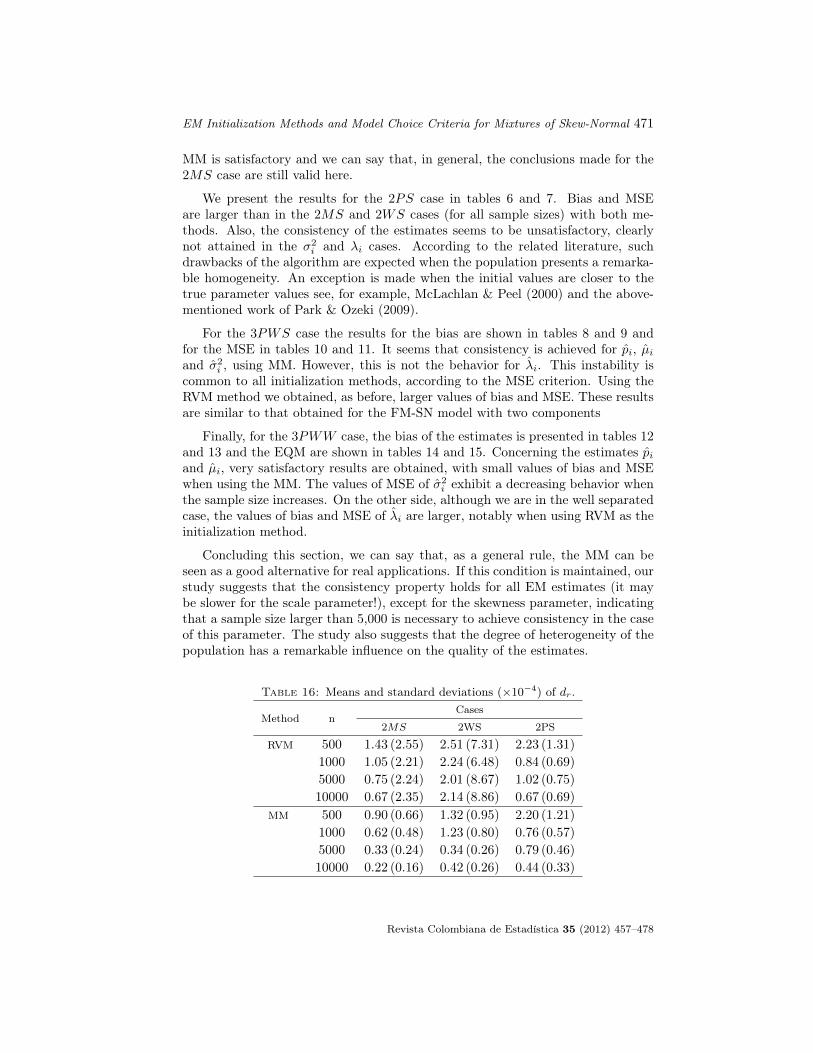
EM Initialization Methods and Model Choice Criteria for Mixtures of Skew-Normal 471
MM is satisfactory and we can say that, in general, the conclusions made for the2MS case are still valid here.
We present the results for the 2PS case in tables 6 and 7. Bias and MSEare larger than in the 2MS and 2WS cases (for all sample sizes) with both me-thods. Also, the consistency of the estimates seems to be unsatisfactory, clearlynot attained in the σ2
i and λi cases. According to the related literature, suchdrawbacks of the algorithm are expected when the population presents a remarka-ble homogeneity. An exception is made when the initial values are closer to thetrue parameter values see, for example, McLachlan & Peel (2000) and the above-mentioned work of Park & Ozeki (2009).
For the 3PWS case the results for the bias are shown in tables 8 and 9 andfor the MSE in tables 10 and 11. It seems that consistency is achieved for pi, µiand σ2
i , using MM. However, this is not the behavior for λi. This instability iscommon to all initialization methods, according to the MSE criterion. Using theRVM method we obtained, as before, larger values of bias and MSE. These resultsare similar to that obtained for the FM-SN model with two components
Finally, for the 3PWW case, the bias of the estimates is presented in tables 12and 13 and the EQM are shown in tables 14 and 15. Concerning the estimates piand µi, very satisfactory results are obtained, with small values of bias and MSEwhen using the MM. The values of MSE of σ2
i exhibit a decreasing behavior whenthe sample size increases. On the other side, although we are in the well separatedcase, the values of bias and MSE of λi are larger, notably when using RVM as theinitialization method.
Concluding this section, we can say that, as a general rule, the MM can beseen as a good alternative for real applications. If this condition is maintained, ourstudy suggests that the consistency property holds for all EM estimates (it maybe slower for the scale parameter!), except for the skewness parameter, indicatingthat a sample size larger than 5,000 is necessary to achieve consistency in the caseof this parameter. The study also suggests that the degree of heterogeneity of thepopulation has a remarkable influence on the quality of the estimates.
Table 16: Means and standard deviations (×10−4) of dr.Cases
Method n2MS 2WS 2PS
RVM 500 1.43 (2.55) 2.51 (7.31) 2.23 (1.31)
1000 1.05 (2.21) 2.24 (6.48) 0.84 (0.69)
5000 0.75 (2.24) 2.01 (8.67) 1.02 (0.75)
10000 0.67 (2.35) 2.14 (8.86) 0.67 (0.69)
MM 500 0.90 (0.66) 1.32 (0.95) 2.20 (1.21)
1000 0.62 (0.48) 1.23 (0.80) 0.76 (0.57)
5000 0.33 (0.24) 0.34 (0.26) 0.79 (0.46)
10000 0.22 (0.16) 0.42 (0.26) 0.44 (0.33)
Revista Colombiana de Estadística 35 (2012) 457–478

472 José R. Pereira, Leyne A. Marques & José M. da Costa
4.3. Density Estimation Analysis
In this section we consider the density estimation issue, that is, the pointestimation of the parameter `(Θ), the log-likelihood evaluated at the true value ofthe parameter. We considered FM-SN models with two components and restrictedourselves to the cases 2MS, 2WS and 2PS, with sample sizes n =500; 1,000; 5,000and 10,000. For each combination of parameters and sample size, 5000 sampleswere generated and the following measure was considered to compare the methodsof initialization
dr(M) =
∣∣∣∣∣`(Θ)− `(M)(Θ)
`(Θ)
∣∣∣∣∣× 100
where `(M)(Θ) is the log-likelihood evaluated at the EM estimate Θ, which wasobtained using the initialization method M . According to this criterion, an ini-tialization method M is better than M ′ if dr(M) < dr(M
′). Table 16 presents themeans and standard deviations of dr.
For 2MS case, we can see that these values decrease when the sample sizeincreases with both methods and that the MM presented the lowest mean valueand standard deviation for all sample sizes. For the 2WS case, we do not observea monotone behavior for dr, the mean values and the standard errors are largerthan that presented in the 2MS case, with poor performance of RVM. In this 2PScase, although we also do not observe a monotone behavior for dr, we can see thatthe MM presented a better performance than the TVM.
The main message is that the MM method seems to be suitable when we areinterested in the estimation of the likelihood values, with some caution when thepopulation is highly homogeneous.
4.4. Number of Iterations
It is well known that one of the major drawbacks of the EM algorithm isthe slow convergence. The problem becomes more serious when there is a badchoice of the starting values (McLachlan & Krishnan 2008). Consequently, animportant issue is the investigation of the number of iterations necessary for theconvergence of the algorithm. As in subsection 4.3, here we consider only the 2MS,2WS and 2PS cases, with the same sample sizes and number of replications. Foreach generated sample, we observed the number of iterations and the means andstandard deviations of this quantity were computed. The simulations results arereported in Table 17.
Results suggest that in the three cases, using MM, the mean number of itera-tions decreases as the sample size increases, but the same is not true when RVMis adopted as the initialization method. For the 2PS case, as expected, we havea poor behavior possibly due to the population homogeneity, as we commentedbefore. An interesting fact is that, in the 2PS case, the RVM has a smaller meannumber of iterations.
Revista Colombiana de Estadística 35 (2012) 457–478

EM Initialization Methods and Model Choice Criteria for Mixtures of Skew-Normal 473
Table 17: Means and standard deviations of number of iterations.Cases
Method n2MS 2WS 2PS
RVM 500 306.14 (387.70) 129.81 (117.01) 337.82 (289.01)
1,000 283.57 (289.32) 126.87 (130.61) 319.70 (242.08)
5,000 280.28 (260.36) 128.29 (213.99) 336.85 (206.38)
10,000 286.31 (271.83) 131.33 (190.77) 353.61 (211.99)
MM 500 147.53 (72.79) 126.62 (26.80) 457.97 (167.28)
1,000 129.37 (33.34) 119.70 (15.39) 429.42 (119.77)
5,000 116.35 (11.57) 113.91 (5.90) 372.14 (71.89)
10,000 115.10 (8.37) 113.29 (4.23) 352.33 (97.54)
5. A Simulation Study of Model Choice
There is a key issue with the use of finite mixtures to estimate the number ofcomponents in order to obtain a suitable fit. One possible approach is to use somecriteria function and compute
k = arg mink{C(Θ(k)), k ∈ {kmin, . . . , kmax}}
where C(Θ(k)) is the criterion function evaluated at the EM estimate Θ(k), ob-tained by modeling the data using the FM-SN model with k components, andkmin and kmax are fixed positive integers (for other approaches see McLachlan &Peel 2000).
Our main purpose in this section is to investigate the ability of some classicalcriteria to estimate the correct number of mixture components. We consider theAkaike Information Criterion (AIC) (Akaike 1974), the Bayesian Information Cri-terion (BIC) (Schwarz 1978), the Efficient Determination Criterion (EDC) (Bai,Krishnaiah & Zhao 1989) and the Integrated Completed Likelihood Criterion (ICL)(Biernacki, Celeux & Govaert 2000). The AIC, BIC and EDC criteria have theform
−2 `(Θ) + dk cn
where `(·) is the actual log-likelihood, dk is the number of free parameters thathave to be estimated under the model with k components and the penalty termcn is a convenient sequence of positive numbers. We have cn = 2 for AIC andcn = log(n) for BIC. For the EDC criterion, cn is chosen so that it satisfies theconditions
lim(cn/n) = 0 and limn→∞
(cn/(log log n)) =∞
Here we compare the following alternatives
cn = 0.2√n, cn = 0.2 log (n), cn = 0.2n/ log (n), and cn = 0.5
√n
The ICL is defined as−2 `∗(Θ) + dk log(n),
Revista Colombiana de Estadística 35 (2012) 457–478
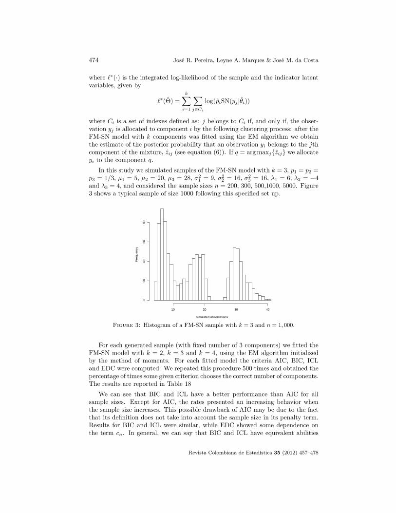
474 José R. Pereira, Leyne A. Marques & José M. da Costa
where `∗(·) is the integrated log-likelihood of the sample and the indicator latentvariables, given by
`∗(Θ) =
k∑i=1
∑j∈Ci
log(piSN(yj |θi))
where Ci is a set of indexes defined as: j belongs to Ci if, and only if, the obser-vation yj is allocated to component i by the following clustering process: after theFM-SN model with k components was fitted using the EM algorithm we obtainthe estimate of the posterior probability that an observation yi belongs to the jthcomponent of the mixture, zij (see equation (6)). If q = arg maxj{zij} we allocateyi to the component q.
In this study we simulated samples of the FM-SN model with k = 3, p1 = p2 =p3 = 1/3, µ1 = 5, µ2 = 20, µ3 = 28, σ2
1 = 9, σ22 = 16, σ2
3 = 16, λ1 = 6, λ2 = −4and λ3 = 4, and considered the sample sizes n = 200, 300, 500,1000, 5000. Figure3 shows a typical sample of size 1000 following this specified set up.
simulated observations
Fre
quen
cy
10 20 30 40
020
4060
80
Figure 3: Histogram of a FM-SN sample with k = 3 and n = 1, 000.
For each generated sample (with fixed number of 3 components) we fitted theFM-SN model with k = 2, k = 3 and k = 4, using the EM algorithm initializedby the method of moments. For each fitted model the criteria AIC, BIC, ICLand EDC were computed. We repeated this procedure 500 times and obtained thepercentage of times some given criterion chooses the correct number of components.The results are reported in Table 18
We can see that BIC and ICL have a better performance than AIC for allsample sizes. Except for AIC, the rates presented an increasing behavior whenthe sample size increases. This possible drawback of AIC may be due to the factthat its definition does not take into account the sample size in its penalty term.Results for BIC and ICL were similar, while EDC showed some dependence onthe term cn. In general, we can say that BIC and ICL have equivalent abilities
Revista Colombiana de Estadística 35 (2012) 457–478

EM Initialization Methods and Model Choice Criteria for Mixtures of Skew-Normal 475
Table 18: Percentage of times that the criteria chosen the correct model.EDC/ cn
n AIC BIC ICL0.2 log (n) 0.2
√n 0.2n/ log (n) 0.5
√n
200 94.2 99.2 99.2 77.8 98.4 99.4 99.4
300 94.0 98.8 98.8 78.2 98.4 98.8 98.8
500 95.8 99.8 99.8 86.4 99.8 99.8 99.8
1000 96.2 100.0 100.0 88.5 100.0 100.0 100.0
5000 95.6 100.0 100.0 92.8 100.0 100.0 100.0
to choose the correct number of components and that, depending on the choice ofcn, ICL can not be as good as AIC or better than ICL and BIC.
6. Final Remarks
In this work we presented a simulation study in order to investigate the perfor-mance of the EM algorithm for maximum likelihood estimation in finite mixturesof skew-normal distributions with component specific parameters. The resultsshow that the algorithm produces quite reasonable estimates, in the sense of con-sistency and the total number of iterations, when using the method of momentsto obtain the starting points. The study also suggested that the random initia-lization method used is not a reasonable procedure. When the EM estimates wereused to compute some model choice criteria (AIC, BIC, ICL and EDC), the resultssuggest that the EDC, with the penalization term appropriate, provides a goodalternative to estimate the number of components of the mixture. On the otherside, these patterns do not hold when the mixture components are poorly sepa-rated, notably for the skewness parameters estimates which, in addition, showeda performance strongly dependent on large samples. Possible extensions of thiswork include the multivariate case and a wider family of skewed distributions, likethe class of skew-normal independent distributions (see Cabral et al. (2012)).
[Recibido: agosto de 2011 — Aceptado: octubre de 2012
]
References
Akaike, H. (1974), ‘A new look at the statistical model identification’, IEEETransactions on Automatic Control 19, 716–723.
Azzalini, A. (1985), ‘A class of distributions which includes the normal ones’,Scandinavian Journal of Statistics 12, 171–178.
Azzalini, A. (2005), ‘The skew-normal distribution and related multivariate fami-lies’, Scandinavian Journal of Statistics 32, 159–188.
Revista Colombiana de Estadística 35 (2012) 457–478

476 José R. Pereira, Leyne A. Marques & José M. da Costa
Bai, Z. D., Krishnaiah, P. R. & Zhao, L. C. (1989), ‘On rates of convergenceof efficient detection criteria in signal processing with white noise’, IEEETransactions on Information Theory 35, 380–388.
Basso, R. M., Lachos, V. H., Cabral, C. R. B. & Ghosh, P. (2010), ‘Robust mix-ture modeling based on scale mixtures of skew-normal distributions’, Com-putational Statistics and Data Analysis 54, 2926–2941.
Bayes, C. L. & Branco, M. D. (2007), ‘Bayesian inference for the skewness param-eter of the scalar skew-normal distribution’, Brazilian Journal of Probabilityand Statistics 21, 141–163.
Biernacki, C., Celeux, G. & Govaert, G. (2000), ‘Assessing a mixture model forclustering with the integrated completed likelihood’, IEEE Transactions onPattern Analysis and Machine Intelligence 22, 719–725.
Biernacki, C., Celeux, G. & Govaert, G. (2003), ‘Choosing starting values forthe EM algorithm for getting the highest likelihood in multivariate Gaussianmixture models.’, Computational Statistics and Data Analysis 41, 561–575.
Cabral, C. R. B., Lachos, V. H. & Prates, M. O. (2012), ‘Multivariate mixture mod-eling using skew-normal independent distributions’, Computational Statisticsand Data Analysis 56, 126–142.
Dempster, A. P., Laird, N. M. & Rubin, D. B. (1977), ‘Maximum likelihood fromincomplete data via the EM algorithm’, Journal of the Royal Statistical So-ciety, Series B 39, 1–38.
Dias, J. G. & Wedel, M. (2004), ‘An empirical comparison of EM, SEM andMCMC performance for problematic gaussian mixture likelihoods’, Statisticsand Computing 14, 323–332.
DiCiccio, T. J. & Monti, A. C. (2004), ‘Inferential aspects of the skew exponentialpower distribution’, Journal of the American Statistical Association 99, 439–450.
Frühwirth-Schnatter, S. (2006), Finite Mixture and Markov Switching Models,Springer Verlag.
Greselin, F. & Ingrassia, S. (2010), ‘Constrained monotone EM algorithms formixtures of multivariate t distributions’, Statistics and Computing 20(1), 9–22.
Hastie, T., Tibshirani, R. & Friedman, J. (2009), The Elements of StatisticalLearning. Data Mining, Inference, and Prediction. Second Edition, Springer,USA.
Hathaway, R. J. (1985), ‘A constrained formulation of maximum-likelihood esti-mation for normal mixture models’, The Annals of Statistics 13, 795–800.
Henze, N. (1986), ‘A probabilistic representation of the skew-normal distribution’,Scandinavian Journal of Statistics 13, 271–275.
Revista Colombiana de Estadística 35 (2012) 457–478

EM Initialization Methods and Model Choice Criteria for Mixtures of Skew-Normal 477
Ho, H. J., Pyne, S. & Lin, T. I. (2012), ‘Maximum likelihood inference for mix-tures of skew Student-t-normal distributions through practical EM-type al-gorithms’, Statistics and Computing 22(1), 287–299.
Ingrassia, S. (2004), ‘A likelihood-based constrained algorithm for multivariatenormal mixture models’, Statistical Methods and Applications 13, 151–166.
Ingrassia, S. & Rocci, R. (2007), ‘Constrained monotone EM algorithms for fi-nite mixture of multivariate gaussians’, Computational Statistics and DataAnalysis 51, 5339–5351.
Karlis, D. & Xekalaki, E. (2003), ‘Choosing initial values for the EM algorithm forfinite mixtures’, Computational Statistics and Data Analysis 41, 577–590.
Lin, T. I. (2009), ‘Maximum likelihood estimation for multivariate skew normalmixture models’, Journal of Multivariate Analysis 100, 257–265.
Lin, T. I. (2010), ‘Robust mixture modeling using multivariate skew t distribu-tions’, Statistics and Computing 20(3), 343–356.
Lin, T. I., Lee, J. C. & Hsieh, W. J. (2007), ‘Robust mixture modelling using theskew t distribution’, Statistics and Computing 17, 81–92.
Lin, T. I., Lee, J. C. & Ni, H. F. (2004), ‘Bayesian analysis of mixture modellingusing the multivariate t distribution’, Statistics and Computing 14, 119–130.
Lin, T. I., Lee, J. C. & Yen, S. Y. (2007), ‘Finite mixture modelling using the skewnormal distribution’, Statistica Sinica 17, 909–927.
Lin, T. & Lin, T. (2010), ‘Supervised learning of multivariate skew normal mixturemodels with missing information’, Computational Statistics 25(2), 183–201.
McLachlan, G. J. & Krishnan, T. (2008), The EM Algorithm and Extensions, 2edn, John Wiley and Sons.
McLachlan, G. J. & Peel, G. J. (2000), Finite Mixture Models, John Wiley andSons.
Meng, X. L. & Rubin, D. B. (1993), ‘Maximum likelihood estimation via the ECMalgorithm: A general framework’, Biometrika 80, 267–278.
Nityasuddhi, D. & Böhning, D. (2003), ‘Asymptotic properties of the EM algo-rithm estimate for normal mixture models with component specific variances’,Computational Statistics and Data Analysis 41, 591–601.
Park, H. & Ozeki, T. (2009), ‘Singularity and slow convergence of the EM algo-rithm for gaussian mixtures’, Neural Process Letters 29, 45–59.
Peel, D. & McLachlan, G. J. (2000), ‘Robust mixture modelling using the t dis-tribution’, Statistics and Computing 10, 339–348.
R Development Core Team (2009), R: A language and environment for statisticalcomputing, R Foundation for Statistical Computing, Vienna, Austria.
Revista Colombiana de Estadística 35 (2012) 457–478

478 José R. Pereira, Leyne A. Marques & José M. da Costa
Schwarz, G. (1978), ‘Estimating the dimension of a model’, Annals of Statistics6, 461–464.
Shoham, S. (2002), ‘Robust clustering by deterministic agglomeration EM of mix-tures of multivariate t-distributions’, Pattern Recognition 35, 1127–1142.
Shoham, S., Fellows, M. R. & Normann, R. A. (2003), ‘Robust, automatic spikesorting using mixtures of multivariate t-distributions’, Journal of Neuro-science Methods 127, 111–122.
Stephens, M. (2000), ‘Dealing with label switching in mixture models’, Journal ofthe Royal Statistical Society. Series B 62, 795–809.
Titterington, D. M., Smith, A. F. M. & Makov, U. E. (1985), Statistical Analysisof Finite Mixture Distributions, John Wiley and Sons.
Yakowitz, S. J. & Spragins, J. D. (1968), ‘On the identifiability of finite mixtures’,The Annals of Mathematical Statistics 39, 209–214.
Yao, W. (2010), ‘A profile likelihood method for normal mixture with unequalvariance’, Journal of Statistical Planning and Inference 140, 2089–2098.
Revista Colombiana de Estadística 35 (2012) 457–478

Revista Colombiana de EstadísticaDiciembre 2012, volumen 35, no. 3, pp. 479 a 508
An Introductory Review of a Structural VAR-XEstimation and Applications
Una revisión introductoria de la estimación y aplicaciones de unVAR-X estructural
Sergio Ocampo1,a, Norberto Rodríguez2,3,b
1Research Department, Inter-American Development Bank, Washington, DC,United States of America
2Macroeconomic Modeling Department, Banco de la República, Bogotá, Colombia3Statistics Department, Universidad Nacional de Colombia, Bogotá, Colombia
AbstractThis document presents how to estimate and implement a structural
VAR-X model under long run and impact identification restrictions. Es-timation by Bayesian and classical methods is presented. Applications ofthe structural VAR-X for impulse response functions to structural shocks,multiplier analysis of the exogenous variables, forecast error variance decom-position and historical decomposition of the endogenous variables are alsodescribed, as well as a method for computing higher posterior density re-gions in a Bayesian context. Some of the concepts are exemplified with anapplication to US data.
Key words: Econometrics, Bayesian time series, Vector autoregression,Structural model.
ResumenEste documento cubre la estimación e implementación del modelo VAR-X
estructural bajo restricciones de identificación de corto y largo plazo. Se pre-senta la estimación tanto por métodos clásicos como Bayesianos. Tambiénse describen aplicaciones del modelo como impulsos respuesta ante choquesestructurales, análisis de multiplicadores de las variables exógenas, descom-posición de varianza del error de pronóstico y descomposición histórica delas variables endógenas. Así mismo se presenta un método para calcularregiones de alta densidad posterior en el contexto Bayesiano. Algunos delos conceptos son ejemplificados con una aplicación a datos de los EstadosUnidos.
Palabras clave: econometría, modelo estructural, series de tiempo Baye-sianas, vector autoregresivo.
aResearch Fellow. E-mail: [email protected] Econometrist and Lecturer. E-mail: [email protected]
479

480 Sergio Ocampo & Norberto Rodríguez
1. Introduction
The use of Vector Autoregression with exogenous variables (VAR-X) and struc-tural VAR-X models in econometrics is not new, yet textbooks and articles thatuse them often fail to provide the reader a concise (and moreover useful) descrip-tion of how to implement these models (Lütkepohl (2005) constitutes an exceptionof this statement). The use of Bayesian techniques in the estimation of VAR-Xmodels is also largely neglected from the literature, as is the construction of thehistorical decomposition of the endogenous variables. This document builds uponthe Structural Vector Autoregression (S-VAR) and Bayesian Vector Autoregres-sion (B-VAR) literature and its purpose is to present a review of some of the basicfeatures that accompany the implementation of a structural VAR-X model.
Section 2 presents the notation and general setup to be followed throughoutthe document. Section 3 discusses the identification of structural shocks in a VAR-X, with both long run restrictions, as in Blanchard & Quah (1989), and impactrestrictions, as in Sims (1980, 1986). Section 4 considers the estimation of theparameters by classical and Bayesian methods. In Section 5, four of the possi-ble applications of the model are presented, namely the construction of impulseresponse functions to structural shocks, multiplier analysis of the exogenous vari-ables, forecast error variance decomposition and historical decomposition of theendogenous variables. Section 6 exemplifies some of the concepts developed inthe document using Galí’s (1999) structural VAR augmented with oil prices as anexogenous variable. Finally Section 7 concludes.
2. General Setup
In all sections the case of a structural VAR-X whose reduced form is a VAR-X(p, q) will be considered. It is assumed that the system has n endogenous vari-ables (yt) and m exogenous variables (xt). The variables in yt and xt may be inlevels or in first differences, this depends on the characteristics of the data, thepurpose of the study, and the identification strategy, in all cases no co-integrationis assumed. The reduced form of the structural model includes the first p lagsof the endogenous variables, the contemporaneous values and first q lags of theexogenous variables and a constant vector.1 Under this specification it is assumedthat the model is stable and presents white-noise Gaussian residuals (et), i.e.et
iid∼ N (0,Σ), moreover, xt is assumed to be uncorrelated with et for all leadsand lags.
The reduced form VAR-X(p, q) can be represented as in equation (1) or equa-tion (2), where v is a n-vector, Bi are n × n matrices, with i ∈ {1, . . . , p}, andΘj are n × m matrices, with j ∈ {1, . . . , q}. In equation (2) one has B (L) =B1L+ · · ·+ BpL
p and Θ (L) = Θ0 + · · ·+ ΘqLq, both matrices of polynomials in
1The lag structure of the exogenous variables may be relaxed allowing different lags for eachvariable. This complicates the estimation and is not done here for simplicity. Also, the constantvector or intercept may be omitted according to the characteristics of the series used.
Revista Colombiana de Estadística 35 (2012) 479–508

An Introductory Review of a Structural VAR-X Estimation and Applications 481
the lag operator L.
yt = v + B1yt−1 + · · ·+ Bpyt−p + Θ0xt + · · ·+ Θqxt−q + et (1)yt = v + B (L) yt + Θ (L) xt + et (2)
Defining Ψ (L) = Ψ0 + Ψ1L + . . . = [I−B (L)]−1 with Ψ0 = I as an infinite
polynomial on the lag operator L, one has the VMA-X representation of the model,equation (3).2
yt = Ψ (1) v + Ψ (L) Θ (L) xt + Ψ (L) et (3)
Finally, there is a structural VAR-X model associated with the equations above,most of the applications are obtained from it, for example those covered in Section5. Instead of the residuals (e), which can be correlated among them, the structuralmodel contains structural disturbances with economic interpretation (ε), this iswhat makes it useful for policy analysis. It will be convenient to represent themodel by its Vector Moving Average (VMA-X) form, equation (4),
yt = µ+ C (L) εt + Λ (L) xt (4)
where the endogenous variables are expressed as a function of a constant n-vector(µ), and the current and past values of the structural shocks (ε) and the exogenousvariables. It is assumed that ε is a vector of white noise Gaussian disturbanceswith identity covariance matrix, i.e. εt
iid∼ N (0, I). Both C (L) and Λ (L) areinfinite polynomials in the lag operator L, each matrix of C (L) (C0,C1, . . .) is ofsize n× n, and each matrix of Λ (L) (Λ0,Λ1, . . .) is of size n×m.
3. Identification of Structural Shocks in a VAR-X
The identification of structural shocks is understood here as a procedure whichenables the econometrician to obtain the parameters of a structural VAR-X fromthe estimated parameters of the reduced form of the model. As will be clear fromthe exposition below, the identification in presence of exogenous variables is nodifferent from what is usually done in the S-VAR literature. Equating (3) and (4)one has:
µ+ Λ (L) xt + C (L) εt = Ψ (1) v + Ψ (L) Θ (L) xt + Ψ (L) et
then the following equalities can be inferred:
µ = Ψ (1) v (5)Λ (L) = Ψ (L) Θ (L) (6)
C (L) εt = Ψ (L) et (7)
2The models stability condition implies that Ψ (1) =
[I −
p∑i=1
Bi
]−1
exists and is finite.
Revista Colombiana de Estadística 35 (2012) 479–508

482 Sergio Ocampo & Norberto Rodríguez
Since the parameters in v, B (L) and Θ (L) can be estimated from the reducedform VAR-X representation, the values of µ and Λ (L) are also known.3 Only theparameters in C (L) are left to be identified, the identification depends on the typeof restrictions to be imposed. From equations (5), (6) and (7) is clear that theinclusion of exogenous variables in the model has no effect in the identification ofthe structural shocks. Equation (7) also holds for a structural VAR model.
The identification restrictions to be imposed over C (L) may take several forms.Since there is nothing different in the identification between the case presented hereand the S-VAR literature, we cover only two types of identification procedures,namely: impact and long run restrictions that allow the use of the Cholesky de-composition. It is also possible that the economic theory points at restrictionsthat make impossible a representation in which the Cholesky decomposition canbe used, or that the number of restrictions exceeds what is needed for exact iden-tification. Both cases complicate the estimation of the model, and the secondone (over-identification) makes possible to carry out tests over the restrictions im-posed. For a more comprehensive treatment of these problems we refer to Amisano& Giannini (1997).
There is another identification strategy that will not be covered in this docu-ment, identification by sign restrictions over some of the impulse response func-tions. This kind of identification allows to avoid some puzzles that commonly arisein the VAR literature. References to this can be found in Uhlig (2005), Mountford& Uhlig (2009), Canova & De Nicolo (2002), Canova & Pappa (2007) and preced-ing working papers of those articles originally presented in the late 1990’s. Morerecently, the work of Moon, Schorfheide, Granziera & Lee (2011) presents how toconduct inference over impulse response functions with sign restrictions, both byclassical and Bayesian methods.
3.1. Identification by Impact Restrictions
In Sims (1980, 1986) the identification by impact restrictions is proposed, theidea behind is that equation (7) is equating two polynomials in the lag operatorL, for them to be equal it must be the case that:
CiLiεt = ΨiL
iet
Ciεt = Ψiet (8)
Equation (8) holds for all i, in particular it holds for i = 0. Recalling thatΨ0 = I, the following result is obtained:
C0εt = et (9)
then, by taking the variance on both sides one gets:
C0C′
0 = Σ (10)3Lütkepohl (2005) presents methods for obtaining the matrices in Ψ (L) and the product
Ψ (L)Θ (L) recursively in Sections 2.1.2 and 10.6, respectively. Ψ (1) is easily computed bytaking the inverse on I − B1 − . . .− Bp.
Revista Colombiana de Estadística 35 (2012) 479–508

An Introductory Review of a Structural VAR-X Estimation and Applications 483
Algorithm 1 Identification by Impact Restrictions
1. Estimate the reduced form of the VAR-X.
2. Calculate the VMA-X representation of the model (matrices Ψi) and thecovariance matrix of the reduced form disturbances e (matrix Σ).
3. From the Cholesky decomposition of Σ calculate matrix C0.
C0 = chol (Σ)
4. For i = 1, . . . , R, with R given, calculate the matrices Ci as:
Ci = ΨiC0
Identification is completed since all matrices of the structural VMA-X are known.
Since Σ is a symmetric, positive definite matrix it is not possible to infer ina unique form the parameters of C0 from equation (10), restrictions over the pa-rameters of C0 have to be imposed. Because C0 measures the impact effect of thestructural shocks over the endogenous variables, those restrictions are called hereimpact restrictions. Following Sims (1980), the restrictions to be imposed ensurethat C0 is a triangular matrix, this allows to use the Cholesky decomposition ofΣ to obtain the non-zero elements of C0. This amount of restrictions accountn× (n− 1)/2 and make the model just identifiable.
In econometrics the use of the Cholesky decomposition with identifying impactrestrictions is also reffered to as recursive identification. This is because the pro-cedure implies a recursive effect of the shocks over the variables, thus making theorder in which the variables appear in the model matter for the interpretation ofthe results. Since the matrix C0 is restricted to be triangular, e.g. lower trian-gular, the first variable can only be affected at impact by the first shock (ε firstelement), whereas the second variable can be affected at impact by both the firstand second shocks. This is better illustrated in Christiano, Eichenbaum & Evans(1999) where the recursive identification is applied to determine the effects of amonetary policy shock.
Once C0 is known, equations (8) and (9) can be used to calculate Ci for all i:
Ci = ΨiC0 (11)
Identification by impact restrictions is summarized in Algorithm 1.
3.2. Identification by Long Run Restrictions
Another way to identify the matrices of the structural VMA-X is to impose re-strictions on the long run impact of the shocks over the endogenous variables. This
Revista Colombiana de Estadística 35 (2012) 479–508

484 Sergio Ocampo & Norberto Rodríguez
method is proposed in Blanchard & Quah (1989). For the model under considera-
tion, if the variables in yt are in differences, the matrix C (1) =∞∑i=0
Ci measures the
long run impact of the structural shocks over the levels of the variables.4 MatrixC (1) is obtained by evaluating equation (7) in L = 1. As in the case of impactrestrictions, the variance of each side of the equation is taken, the result is:
C (1) C′(1) = Ψ (1) ΣΨ
′(1) (12)
Again, since Ψ (1) ΣΨ′(1) is a symmetric, positive definite matrix it is not
possible to infer the parameters of C (1) from equation (12), restrictions overthe parameters of C (1) have to be imposed. It is conveniently assumed thatthose restrictions make C (1) a triangular matrix, as before, this allows to use theCholesky decomposition to calculate the non-zero elements of C (1). Again, thisamount of restrictions account n× (n−1)/2 and make the model just identifiable.It is important to note that the ordering of the variables matters as before. If, forexample, C (1) is lower triangular, the first shock will be the only one that canhave long run effects over the first variable, whereas the second variable can beaffected by both the first and second shock in the long run.
Finally, it is possible to use C (1) to calculate the parameters in the C0 matrix,with it, the matrices Ci for i > 0 are obtained as in the identification by impactrestrictions. Combining (10) with (7) evaluated in L = 1 the following expressionfor C0 is derived:
C0 = [Ψ (1)]−1
C (1) (13)
Identification by long run restrictions is summarized in Algorithm 2.
4. Estimation
The estimation of the parameters of the VAR-X can be carried out by classicalor Bayesian methods, as will become clear it is convenient to write the model in amore compact form. Following Zellner (1996) and Bauwens, Lubrano & Richard(2000), equation (1), for a sample of T observations, plus a fixed presample, canbe written as:
Y = ZΓ + E (14)
where Y =
y′
1...
y′
t...
y′
T
, Z =
1 y′
0 . . . y′
1−p x′
1 . . . x′
1−q...1 y
′
t−1 . . . y′
t−p x′
t . . . x′
t−q...1 y
′
T−1 . . . y′
T−p x′
T . . . x′
T−q
, E =
e′
1...e′
t...
e′
T
and Γ =
[v B1 . . . Bp Θo . . . Θq
]′.
4Of course, not all the variables of yt must be in differences, but the only meaningful re-strictions are those imposed over variables that enter the model in that way. We restrict ourattention to a case in which there are no variables in levels in yt.
Revista Colombiana de Estadística 35 (2012) 479–508

An Introductory Review of a Structural VAR-X Estimation and Applications 485
Algorithm 2 Identification by Long Run Restrictions
1. Estimate the reduced form of the VAR-X.
2. Calculate the VMA-X representation of the model (matrices Ψi) and thecovariance matrix of the reduced form disturbances e (matrix Σ).
3. From the Cholesky decomposition of Ψ (1) ΣΨ′(1) calculate matrix C (1).
C (1) = chol(Ψ (1) ΣΨ
′(1))
4. With the matrices of long run effects of the reduced form, Ψ (1), and struc-tural shocks, C (1), calculate the matrix of contemporaneous effects of thestructural shocks, C0.
C0 = [Ψ (1)]−1
C (1)
5. For i = 1, . . . , R, with R sufficiently large, calculate the matrices Ci as:
Ci = ΨiC0
Identification is completed since all matrices of the structural VMA-X are known.
For convenience we define the auxiliary variable k = (1 + np+m (q + 1)) asthe total number of regressors. The matrices sizes are as follow: Y is a T × nmatrix, Z a T × k matrix, E a T × n matrix and Γ a k × n matrix.
Equation (14) is useful because it allows to represent the VAR-X model as amultivariate linear regression model, with it the likelihood function is derived. Theparameters can be obtained by maximizing that function or by means of Bayestheorem.
4.1. The Likelihood Function
From equation (14) one derives the likelihood function for the error terms.Since et ∼ N (0,Σ), one has: E ∼ MN (0,Σ⊗ I), a matricvariate normal distri-bution with I the identity matrix with dimension T ×T . The following box definesthe probability density function for the matricvariate normal distribution.
Revista Colombiana de Estadística 35 (2012) 479–508

486 Sergio Ocampo & Norberto Rodríguez
The Matricvariate Normal Distribution. The probability density functionof a (p× q) matrix X that follows a matricvariate normal distribution with meanMp×q and covariance matrix Qq×q ⊗Pp×p (X ∼ MN (M,Q⊗P)) is:
MNpdf ∝ |Q⊗P|−1/2exp
(−1/2 [vec (X−M)]
′(Q⊗P)
−1[vec (X−M)]
)(15)
Following Bauwens et al. (2000), the vec operator can be replaced by a traceoperator (tr):
MNpdf ∝ |Q|−p/2 |P|−q/2
exp(−1/2tr
(Q−1 (X−M)
′P−1 (X−M)
))(16)
Both representations of the matricvariate normal pdf are useful when dealing withthe compact representation of the VAR-X model. Note that the equations aboveare only proportional to the actual probability density function. The missingconstant term has no effects in the estimation procedure.
Using the definition in the preceding box and applying it to E ∼ MN (O,Σ⊗ I)one gets the likelihood function of the VAR-X model, conditioned to the path ofthe exogenous variables:
L ∝ |Σ|−T/2exp
(−1/2tr
(Σ−1E
′E))
From (14) one has E = Y − ZΓ, replacing:
L ∝ |Σ|−T/2exp
(−1/2tr
(Σ−1 (Y − ZΓ)
′(Y − ZΓ)
))Finally, after tedious algebraic manipulation, one gets to the following expression:
L ∝[|Σ|−(T−k)/2
exp(−1/2tr
(Σ−1S
))][|Σ|−k/2
exp
(−1/2tr
(Σ−1
(Γ− Γ
)′Z′Z(Γ− Γ
)))]
where Γ =(Z′Z)−1
Z′Y and S =
(Y − ZΓ
)′ (Y − ZΓ
). It is being assumed
overall that matrix Z′Z is invertible, a condition common to the VAR and OLS
models (see Lütkepohl (2005) section 3.2).One last thing is noted, the second factor of the right hand side of the last
expression is proportional to the pdf of a matricvariate normal distribution for Γ,and the first factor to the pdf of an inverse Wishart distribution for Σ (see thebox below). This allows an exact characterization of the likelihood function as:
L = iWpdf (S, T − k − n− 1)MNpdf
(Γ,Σ⊗
(Z′Z)−1
)(17)
where iWpdf (S, T − k − n− 1) stands for the pdf of an inverse Wishart distribu-tion with parameters S and T − k − n− 1.
Revista Colombiana de Estadística 35 (2012) 479–508

An Introductory Review of a Structural VAR-X Estimation and Applications 487
The parameters of the VAR-X, Γ and Σ, can be estimated by maximizingequation (17). It can be shown that the result of the likelihood maximizationgives:
Γml = Γ Σml = S
Sometimes because practical considerations or non-invertibility of Z′Z, when no
restrictions are imposed, equation by equation estimation can be implemented (seeLütkepohl (2005) section 5.4.4).
The Inverse Wishart DistributionIf the variable X (a square, positive definite matrix of size q) is distributediW (S, s), with parameter S (also a square, positive definite matrix of size q),and s degrees of freedom, then its probability density function
(iWpdf
)is given
by:
iWpdf (S, s) =|S|
s2
2vq2 Γq
(s2
) |X|−(s+q+1)2 exp
(−1/2tr
(X−1S
))(18)
where Γq (x) = πq(q−1)
4
q∏j=1
Γ(x+ 1−j
2
)is the multivariate Gamma function. It
is useful to have an expression for the mean and mode of the inverse Wishartdistribution, these are given by:
Mean (X) =S
s− q − 1Mode (X) =
S
s+ q + 1
4.2. Bayesian Estimation
If the estimation is carried out by Bayesian methods the problem is to elect anadequate prior distribution and, by means of Bayes theorem, obtain the posteriordensity function of the parameters. The use of Bayesian methods is encouragedbecause they allow inference to be done conditional to the sample, and in par-ticular the sample size, giving a better sense of the uncertainty associated withthe parameters values; it also facilitate to compute moments not only for the pa-rameters but for their functions as is the case of the impulse responses, forecasterror variance decomposition and others; it is also particularly useful to obtain ameasure of skewness in this functions, specially for the policy implications of theresults. As mentioned in Koop (1992), the use of Bayesian methods gives an exactfinite sample density for both the parameters and their functions.
The election of the prior is a sensitive issue and will not be discussed in this doc-ument, we shall restrict our attention to the case of the Jeffreys non-informativeprior (Jeffreys 1961) which is widely used in Bayesian studies of vector auto-regressors. There are usually two reasons for its use. The first one is that in-formation about the reduced form parameters of the VAR-X model is scarce anddifficult to translate into an adequate prior distribution. The second is that it
Revista Colombiana de Estadística 35 (2012) 479–508

488 Sergio Ocampo & Norberto Rodríguez
might be the case that the econometrician does not want to include new infor-mation to the estimation but only wishes to use Bayesian methods for inferencepurposes. Besides the two reasons already mentioned, the use of the Jeffreys non-informative prior constitute a computational advantage because it allows a closedform representation of the posterior density function, thus allowing to make drawsfor the parameters by direct methods or by the Gibbs sampling algorithm (Geman& Geman 1984).5
For a discussion of other usual prior distributions for VAR models we refer toKadiyala & Karlsson (1997) and, more recently, to Kociecki (2010) for the con-struction of feasible prior distributions over impulse response in a structural VARcontext. When the model is used for forecast purposes the so called Minnesotaprior is of particular interest, this prior is due to Litterman (1986), and is gen-eralized in Kadiyala & Karlsson (1997) for allowing symmetry of the prior acrossequations. This generalization is recommended and is of easy implementation inthe Bayesian estimation of the model. It should be mentioned that the Minnesotaprior is of little interest in the structural VAR-X context, principally because themodel is conditioned to the path of the exogenous variables, adding difficulties tothe forecasting process.
In general the Jeffreys Prior for the linear regression parameters correspond toa constant for the parameters in Γ and for the covariance matrix a function of theform: |Σ|
−(n+1)2 , where n represents the size of the covariance matrix. The prior
distribution to be used is then:
P (Γ,Σ) = C |Σ|−(n+1)
2 (19)
where C is the integrating constant of the distribution. Its actual value will be ofno interest.
The posterior is obtained from Bayes theorem as:
π (Γ,Σ | Y,Z) =L (Y,Z | Γ,Σ)P (Γ,Σ)
m (Y)(20)
where π (Γ,Σ | Y,Z) is the posterior distribution of the parameters given the data,L (Y,Z | Γ,Σ) is the likelihood function, P (Γ,Σ) is the prior distribution of theparameters and m (Y) the marginal density of the model. The value and use ofthe marginal density is discussed in Section 4.2.1.
Combining equations (17), (19) and (20) one gets an exact representation ofthe posterior function as the product of the pdf of an inverse Wishart distributionand the pdf of a matricvariate normal distribution:
π (Γ,Σ | Y,Z) = iWpdf (S, T − k)MNpdf
(Γ,Σ⊗
(Z′Z)−1
)(21)
Equation (21) implies that Σ follows an inverse Wishart distribution withparameters S and T − k, and that the distribution of Γ given Σ is matricvariate
5For an introduction to the use of the Gibbs sampling algorithm we refer to Casella & George(1992).
Revista Colombiana de Estadística 35 (2012) 479–508

An Introductory Review of a Structural VAR-X Estimation and Applications 489
Algorithm 3 Bayesian Estimation
1. Select the specification for the reduced form VAR-X, that is to chose valuesof p (endogenous variables lags) and q (exogenous variables lags) such thatthe residuals of the VAR-X (e) have white noise properties. With this thefollowing variables are obtained: T, p, q, k, where:
k = 1 + np+m (q + 1)
2. Calculate the values of Γ, S with the data (Y,Z) as:
Γ =(Z′Z)−1
Z′Y S =
(Y − ZΓ
)′ (Y − ZΓ
)3. Generate a draw for matrix Σ from an inverse Wishart distribution with
parameter S and T − k degrees of freedom.
Σ ∼ iWpdf (S, T − k)
4. Generate a draw for matrix Γ from a matricvariate normal distribution withmean Γ and covariance matrix Σ⊗
(Z′Z)−1
.
Γ|Σ ∼ MNpdf
(Γ,Σ⊗
(Z′Z)−1
)5. Repeat steps 2-3 as many times as desired, save the values of each draw.
The draws generated can be used to compute moments of the parameters. Forevery draw the corresponding structural parameters, impulse responses functions,etc. can be computed, then, their moments and statistics can also be computed.The algorithms for generating draws for the inverse Wishart and matricvariatenormal distributions are presented in Bauwens et al. (2000), Appendix B.
normal with mean Γ and covariance matrix Σ ⊗(Z′Z)−1
. The following twoequations formalize the former statement:
Σ | Y,Z ∼ iWpdf (S, T − k) Γ | Σ,Y,Z ∼ MNpdf
(Γ,Σ⊗
(Z′Z)−1
)Although further work can be done to obtain the unconditional distribution of
Γ it is not necessary to do so. Because equation (21) is an exact representationof the parameters distribution function, it can be used to generate draws of them,moreover it can be used to compute any moment or statistic of interest, this canbe done by means of the Gibbs sampling algorithm.
Revista Colombiana de Estadística 35 (2012) 479–508

490 Sergio Ocampo & Norberto Rodríguez
4.2.1. Marginal Densities and Lag Structure
The marginal density (m (Y)) can be easily obtained under the Jeffreys priorand can be used afterward for purposes of model comparison. The marginal densitygives the probability that the data is generated by a particular model, eliminatingthe uncertainty due to the parameters values. Because of this m (Y) is oftenused for model comparison by means of the Bayes factor (BF): the ratio betweenthe marginal densities of two different models that explain the same set of data(BF12 = m(Y |M1)/m(Y|M2)). If the Bayes factor is bigger than one then the firstmodel (M1) would be preferred.
From Bayes theorem (equation 20) the marginal density of the data, given themodel, is:
m (Y) =L (Y,Z|Γ,Σ)P (Γ,Σ)
π (Γ,Σ|Y,Z)(22)
its value is obtained by replacing for the actual forms of the likelihood, prior andposterior functions (equations 17, 19 and 21 respectively):
m (Y) =Γn(T−k
2
)Γn(T−k−n−1
2
) |S|−n−12 2
n(n+1)2 C (23)
Although the exact value of the marginal density for a given model cannot beknown without the constant C, this is no crucial for model comparison if the onlydifference between the models is in their lag structure. In that case the constantC is the same for both models, and the difference between the marginal density ofone specification or another arises only in the first two factors of the right hand
side of equation (23)[
Γn(T−k2 )
Γn(T−k−n−12 )
|S|−n−1
2
]. When computing the Bayes factor
for any pair of models the result will be given by those factors alone.
The Bayes factor between a model,M1, with k1 regressors and residual covari-ance matrix S1, and another model,M2, with k2 regressors and residual covariancematrix S2, can be reduced to:
BF12 =
Γn(T−k12 )
Γn(T−k1−n−12 )
|S1|−n−1
2
Γn(T−k22 )
Γn(T−k2−n−12 )
|S2|−n−1
2
(24)
5. Applications
There are several applications for the structural VAR-X, all of them useful forpolicy analysis. In this Section four of those applications are covered, they all usethe structural VMA-X representation of the model (equation 4).
Revista Colombiana de Estadística 35 (2012) 479–508

An Introductory Review of a Structural VAR-X Estimation and Applications 491
5.1. Impulse Response Functions (IRF), MultiplierAnalysis (MA), and Forecast Error VarianceDecomposition (FEVD)
Impulse response functions (IRF) and multiplier analysis (MA) can be con-structed from the matrices in C (L) and Λ (L). The IRF shows the endogenousvariables response to a unitary change in a structural shock, in an analogous waythe MA shows the response to a change in an exogenous variable. The construc-tion is simple and is based on the interpretations of the elements of the matricesin C (L) and Λ (L).
For the construction of the IRF consider matrix Ch. The elements of thismatrix measure the effect of the structural shocks over the endogenous variablesh periods ahead, thus cijh (i-throw, j-th column) measures the response of the i-thvariable to a unitary change in the j-th shock h periods ahead. The IRF for thei-th variable to a change in j-th shock is constructed by collecting elements cijh forh = 0, 1, . . . ,H, with H the IRF horizon.
Matrices Ch are obtained from the reduced form parameters according to thetype of identification (Section 3). For a more detailed discussion on the construc-tion and properties of the IRF we refer to Lütkepohl (2005), Section 2.3.2.
The MA is obtained similarly from matrices Λh, which are also a function ofthe reduced form parameters.6 The interpretation is the same as before.
A number of methods for inference over the IRF and MA are available. Ifthe estimation is carried out by classical methods intervals for the IRF and MAcan be computed by means of their asymptotic distributions or by bootstrappingmethods.7 Nevertheless, because the OLS estimators are biased, as proved inNicholls & Pope (1988), the intervals that arise from both asymptotic theory andusual bootstrapping methods are also biased. As pointed out by Kilian (1998)this makes necessary to conduct the inference over IRF, and in this case overMA, correcting the bias and allowing for skewness in the intervals. Skewness iscommon in the small sample distributions of the IRF and MA and arises fromthe non-linearity of the function that maps the reduced form parameters to theIRF or MA. A double bootstrapping method that effectively corrects the bias andaccounts for the skewness in the intervals is proposed in Kilian (1998).
In the context of Bayesian estimation, it is noted that, applying Algorithm 1 or2 for each draw of the reduced form parameters (Algorithm 3), the distribution foreach cijh and λijh is obtained. With the distribution function inference can be doneover the point estimate of the IRF and MA. For instance, standard deviations ineach horizon can be computed, as well as asymmetry measures and credible sets(or intervals), the Bayesian analogue to a classical confidence interval.
In the following we shall restrict our attention to credible sets with mini-mum size (length), these are named Highest Posterior Density regions (HPDfrom now on). An (1− α) % HPD for the parameter θ is defined as the set I =
6See Lütkepohl (2005), Section 10.6.7The asymptotic distribution of the IRF and FEVD for a VAR is presented in Lütkepohl
(1990). A widely used non-parametric bootstrapping method is developed in Runkle (1987).
Revista Colombiana de Estadística 35 (2012) 479–508
492 Sergio Ocampo & Norberto Rodríguez
{θ ∈ Θ : π (θ/Y) ≥ k(α)}, where k(α) is the largest constant satisfying P (I|y) =∫θπ (θ/Y) dθ ≥ 1−α.8 From the definition just given is clear that HPD regions are
of minimum size and that each value of θ ∈ I has a higher density (probability)than any value of θ outside the HPD. The second property makes possible directprobability statements about the likelihood of θ falling in I, i.e., “The probabilitythat θ lies in I given the observed data Y is at least (1−α)%”, this contrast withthe interpretation of the classical confidence intervals. An HPD region can bedisjoint if the posterior density function (π (θ/Y)) is multimodal. If the posterioris symmetric, all HPD regions will be symmetric about posterior mode (mean).
Koop (1992) presents a detailed revision of how to apply Bayesian inferenceto the IRF in a structural VAR context, his results can be easily adapted to thestructural VAR-X model. Another reference on the inference over IRF is Sims &Zha (1999). Here we present, in Algorithm 4, the method of Chen & Shao (1998)for computing HPD regions from the output of the Gibbs sampler.9
It is important to note that Bayesian methods are by nature conditioned tothe sample size and, because of that, avoid the problems of asymptotic theory inexplaining the finite sample properties of the parameters functions, this includesthe skewness of the IRF and MA distribution functions. Then, if the intervalsare computed with the HPD, as in Chen & Shao (1998), they would be takinginto account the asymmetry in the same way as Kilian’s method. This is not thecase for intervals computed using only standard deviations although, with them,skewness can be addressed as in Koop (1992), although bootstrap methods can beused to calculate approximate measures of this and others moments, for instance,skewness and kurtosis, Bayesian methods are preferable since exact measures canbe calculated.
Another application of the structural VAR-X model is the forecast error vari-ance decomposition (FEVD), this is no different to the one usually presented in thestructural VAR model. FEVD consists in decomposing the variance of the forecasterror of each endogenous variable h periods ahead, as with the IRF, the matricesof C (L) are used for its construction. Note that, since the model is conditioned tothe path of the exogenous variables, all of the forecast error variance is explainedby the structural shocks. Is because of this that the FEVD has no changes whenapplied in the structural VAR-X model. We refer to Lütkepohl (2005), Section2.3.3, for the details of the construction of the FEVD. Again, if Bayesian methodsare used for the estimation of the VAR-X parameters, the density function of theFEVD can be obtained and several features of it can be explored, Koop (1992)also presents how to apply Bayesian inference in this respect.
8Integration can be replaced by summation if θ is discrete.9The method presented is only valid if the distribution of the parameters of interest is uni-
modal. For a more general treatment of the highest posterior density regions, including multi-modal distributions, we refer to the work of Hyndman (1996).
Revista Colombiana de Estadística 35 (2012) 479–508

An Introductory Review of a Structural VAR-X Estimation and Applications 493
Algorithm 4 Highest Posterior Density RegionsAs in Chen & Shao (1998), let
{θ(i), i = 1 , . . . , N
}be an ergodic sample of
π (θ/Y), the posterior density function of parameter θ. π (θ/Y) is assumed to beunimodal. The (1− α) % HPD is computed as follows:
1. Sort the values of θ(i). Define θ(j) as the j − th larger draw of the sample,so that:
θ(1) = mini∈{1,...,N}
{θ(i)}
θ(N) = maxi∈{1,...,N}
{θ(i)}
2. Define N = b(1− α)Nc the integer part of (1− α)N . The HPD will containN values of θ.
3. Define I(j) =(θ(j) , θ(j+N)
)an interval in the domain of the parameter θ,
for jε{
1, . . . , N −N}. Note that although I(j) contains always N draws of
θ, its size may vary.
4. The HPD is obtained as the interval I(j) with minimum size. HPD (α) =I(j?), with j? such that:
θ(j?+N) − θ(j?) = minj∈{1,...,N−N}
(θ(j+N) − θ(j)
)
5.2. Historical Decomposition of the Endogenous Variables(HD)
The historical decomposition (HD) consists in explaining the observed valuesof the endogenous variables in terms of the structural shocks and the path of theexogenous variables. This kind of exercise is present in the DSGE literature (forexample, in Smets & Wouters (2007)) but mostly absent in the structural VARliterature. There are nonotheless various exceptions, an early example is the workof Burbidge & Harrison (1985) on the role of money in the great depression, thereis also the textbook by Canova (2007), and the paper of King & Morley (2007),where the historical decomposition of a structural VAR is used for computing ameasure of the natural rate of unemployment for the US.
Unlike the applications already presented, the historical decomposition allowsto make a statement over what has actually happened to the series in the sampleperiod, in terms of the recovered values for the structural shocks and the observedpaths of the exogenous variables. It allows to have all shocks and exogenousvariables acting simultaneously, thus making possible the comparison over therelative effects of them over the endogenous variables, this means that the HDis particularly useful when addressing the relative importance of the shocks oversome set of variables. The possibility of explaining the history of the endogenous
Revista Colombiana de Estadística 35 (2012) 479–508

494 Sergio Ocampo & Norberto Rodríguez
variables instead of what would happen if some hypothetical shock arrives in theabsence of any other disturbance is at least appealing.
Here we describe a method for computing the HD in a structural VAR andstructural VAR-X context. The first case is covered in more detail and the secondpresented as an extension of the basic ideas.
5.2.1. Historical Decomposition for a Structural VAR Model
In a structural VAR context is clear, from the structural VMA representationof the model, that variations of the endogenous variables can only be explainedby variations in the structural shocks. The HD uses the structural VMA repre-sentation in order to compute what the path of each endogenous variable wouldhave been conditioned to the presence of only one of the structural shocks. It isimportant to note that the interpretation of the HD in a stable VAR model issimpler than the interpretation in a VAR-X. This is because in the former thereis no need for a reference value that indicates when a shock is influencing thepath of the variables. In that case, the reference value is naturally zero, and itis understood that deviations of the shocks below that value are interpreted asnegative shocks and deviations above as positive shocks. As we shall see, whendealing with exogenous variables a reference value must be set, and its election isnot necessarily “natural”.
Before the HD is computed it is necessary to recover the structural shocksfrom the estimation of the reduced form VAR. Define E = [e1 . . . et . . . eT ]
′as the
matrix of all fitted residuals from the VAR model (equation (14) in the absenceof exogenous variables). Recalling equation (9), the matrix C0 can be used torecover the structural shocks from matrix E as in the following expression:
E = E(C′
0
)−1
(25)
Because zero is the reference value for the structural shocks the matrix E =[ε1 . . . εt . . . εT ]
′can be used directly for the HD.
The HD is an in-sample exercise, thus is conditioned to the initial values ofthe series. It will be useful to define the structural infinite VMA representation ofthe VAR model, as well as the structural VMA representation conditional on theinitial values of the endogenous variables, equations (26) and (27) respectively.
yt = µ+ C (L) εt (26)
yt =
t−1∑i=0
Ciεt−i + Kt (27)
Note that in equation (26) the endogenous variables depend on an infinitenumber of past structural shocks. In equation (27) the effect of all shocks that arerealized previous to the sample is captured by the initial values of the endogenousvariables. The variable Kt is a function of those initial values and of the parameters
Revista Colombiana de Estadística 35 (2012) 479–508

An Introductory Review of a Structural VAR-X Estimation and Applications 495
of the reduced form model, Kt = ft(y0 , . . . , y−(p−1)
). It measures the effect of
the initial values over the period t realization of the endogenous variables, thusthe effect of all shocks that occurred before the sample. It is clear that if the VARis stable Kt −→ µ for t sufficiently large, this is because the shocks that are toofar in the past have no effect in the current value of the variables. Kt will be referto as the reference value of the historical decomposition.
Starting from the structural VMA representation, the objective is now to de-compose the deviations of yt from Kt into the effects of the current and past valuesof the structural shocks (εi for i from 1 to t). The decomposition is made over the
auxiliary variable yt = yt −Kt =t−1∑i=0
Ciεt−i. The information needed to compute
yt is contained in the first t matrices Ci and the first t rows of matrix E .The historical decomposition of the i-th variable of yt into the j-th shock is
given by:
y(i,j)t =
t−1∑i=0
ciji εjt−i (28)
Note that it must hold that the sum over j is equal to the actual value of the
i-th element of yt, yit =n∑j=1
y(i,j)t . For t sufficiently large, when Kt is close to µ,
y(i,j)t can be interpreted as the deviation of the i-th endogenous variable from itsmean caused by the recovered sequence for the j-th structural shock.
Finally, the endogenous variables can be decomposed as well. The historicaldecomposition for the i-th endogenous variable into the j-th shock is given by:
y(i,j)t = Ki
t + y(i,j)t = Ki
t +
t−1∑i=0
ciji εjt−i (29)
the new variable y(i,j)t is interpreted as what the i-th endogenous variable would
have been if only realizations of the j-th shock had occurred. The value of Kt canbe obtained as a residual of the historical decomposition, since yt is known andyt can be computed from the sum of the HD or from the definition.
The HD of the endogenous variables (y(i,j)t ) can be also used to compute what
transformations of the variables would have been conditioned to the presence ofonly one shock. For instance, if the i-th variable enters the model in quarterlydifferences, the HD for the annual differences or the level of the series can be com-puted by applying to y(i,j)
t the same transformation used over yit, in this example,a cumulative sum. Algorithm 5 summarizes the steps carried out for the historicaldecomposition.
5.2.2. Historical Decomposition for a Structural VAR-X Model
The structure already described applies also for a VAR-X model. The main dif-ference is that now it is necessary to determine a reference value for the exogenous
Revista Colombiana de Estadística 35 (2012) 479–508

496 Sergio Ocampo & Norberto Rodríguez
Algorithm 5 Historical Decomposition for a Structural VAR Model
1. Estimate the parameters of the reduced form VAR.
a) Save a matrix with all fitted residuals(E = [e1 . . . et . . . eT ]
′).
b) Compute matrices Ci according to the identifying restrictions (Algo-rithm 1 or 2).
2. Compute the structural shocks(E = [ε1 . . . εt . . . εT ]
′)with matrix C0 and
the fitted residuals of the reduced form VAR:
E = E(C′
0
)−1
3. Compute the historical decomposition of the endogenous variables relativeto Kt:
y(i,j)t =
t−1∑i=0
ciji εjt−i
4. Recover the values of Kt with the observed values of yt and the auxiliaryvariable yt:
Kt = yt − yt
5. Compute the historical decomposition of the endogenous variables:
y(i,j)t = Ki
t + y(i,j)t
Steps 3 and 5 are repeated for t = 1, 2, . . . , T , i = 1, . . . , n and j = 1, . . . , n. Step4 is repeated for t = 1, 2, . . . , T .
variables.10 It shall be understood that realizations of the exogenous variables dif-ferent to this value are what explain the fluctuations of the endogenous variables.We shall refer to xt as the reference value for the exogenous variables in t.
As before, it is necessary to present the structural VMA-X representation con-ditional to the initial values of the endogenous variables (equation 30), with Kt
defined as above. It is also necessary to express the exogenous variables as devia-tions of the reference value, for this we define an auxiliary variable xt = xt − xt.Note that equation (30) can be written in terms of the new variable xt as in
equation (31). In the latter, the new variable Kt =t−1∑i=0
Λixt−i + Kt has a role
10The reference value for the exogenous variables need not be a constant. It can be given bya linear trend, by the sample mean of the series,or by the initial value. When the exogenousvariables enter the model in their differences, it may seem natural to think in zero as a naturalreference value, identifying fluctuations of the exogenous variables in an analogous way to whatsdone with the structural shocks.
Revista Colombiana de Estadística 35 (2012) 479–508

An Introductory Review of a Structural VAR-X Estimation and Applications 497
analogous to that of Kt in the VAR context. Kt properties depend on those of xtand, therefore, it can not be guaranteed that it converges to any value.
yt =
t−1∑i=0
Ciεt−i +
t−1∑i=0
Λixt−i + Kt (30)
yt =
t−1∑i=0
Ciεt−i +
t−1∑i=0
Λixt−i + Kt (31)
The historical decomposition is now computed using matrices Ci, the recoveredmatrix of structural shocks E , matrices Λi and the auxiliary variables xi, for i from1 to T . Matrix E is still computed as in equation (25). The new reference valuefor the historical decomposition is Kt, and the decomposition is done to explainthe deviations of the endogenous variables with respect to it as a function ofthe structural shocks and deviations of the exogenous variables from their ownreference value, xt. For notational simplicity, variable xt is redefined: yt = yt −
Kt =t−1∑i=0
Ciεt−i +t−1∑i=0
Λixt−i. The decomposition of the i-th variable of yt into
the j-th shock is still given by equation (28), and the decomposition into the k-thexogenous variable is given by:
y(i,k)t =
t−1∑i=0
λiki xkt−i (32)
Variable y(i,k)t , for k from 1 to m, is interpreted as what the variable yit would
have been if, in the absence of shocks, only the k-th exogenous variable is allowedto deviate from its reference value. As in the VAR model, the following equation
holds: yit =n∑j=1
y(i,j)t +
m∑k=1
y(i,k)t . The variable Kt is recovered in the same way
used before to recover Kt.The historical decomposition of the endogenous variables can be computed by
using the recovered values for Kt . The decomposition of the i-th variable intothe effects of the j-th shock is still given by equation (29), if Ki
t is replaced by Kit .
The decomposition of the i-th variable into the deviations of the k-th exogenousvariable from its reference value is obtained from the following expression:
y(i,k)t = Ki
t + y(i,k)t (33)
Variable y(i,k)t has the same interpretation as y(i,k)
t but applied to the value ofthe endogenous variable, and not to the deviation from the reference value.
Although the interpretation and use of the HD in exogenous variables may seemstrange and impractical, it is actually of great utility when the reference value forthe exogenous variables is chosen correctly. The following example describes acase in which the interpretation of the HD in exogenous variables is more easilyunderstood. Consider the case in which the exogenous variables are introduced
Revista Colombiana de Estadística 35 (2012) 479–508

498 Sergio Ocampo & Norberto Rodríguez
Algorithm 6 Historical Decomposition for a Structural VAR-X Model
1. Estimate the parameters of the reduced form VAR-X.
a) Save a matrix with all fitted residuals(E = [e1 . . . et . . . eT ]
′).
b) Compute matrices Ci and Λi according to the identifying restrictions(Algorithm 1 or 2).
2. Compute the structural shocks(E = [ε1 . . . εt . . . εT ]
′)with matrix C0 and
the fitted residuals of the reduced form VAR-X:
E = E(C′
0
)−1
3. Compute the historical decomposition of the endogenous variables relativeto Kt:
y(i,j)t =
t−1∑i=0
ciji εjt−i y
(i,k)t =
t−1∑i=0
λiki xkt−i
4. Recover the values of Kt with the observed values of yt and the auxiliaryvariable yt:
Kt = yt − yt
5. Compute the historical decomposition of the endogenous variables:
y(i,j)t = Ki
t + y(i,j)t y
(i,k)t = Ki
t + y(i,k)t
Steps 3 and 5 are repeated for t = 1, 2, . . . , T , i = 1, . . . , n , j = 1, . . . , n andk = 1, . . . ,m. Step 4 is repeated for t = 1, 2, . . . , T .
in the model in their first differences. The person performing the study may beasking himself the effects of the shocks and the changes in the exogenous variablesover the endogenous variables. In this context, the criteria or reference value forthe exogenous variables arises naturally as a base scenario of no change in theexogenous variables and no shocks. Under the described situation one has, for allt, xt = 0 and Kt = Kt. This also allows to interpret both y
(i,k)t and y
(i,k)t as
what would have happened to the i-th endogenous variable if it were only for thechanges of the k-th exogenous variable.
Algorithm 6 summarizes the steps carried out for the historical decompositionin a structural VAR-X setup.
Revista Colombiana de Estadística 35 (2012) 479–508
An Introductory Review of a Structural VAR-X Estimation and Applications 499
6. An Example
In this Section some of the concepts presented in the document are exemplifiedby an application of Galí’s (1999) structural VAR, augmented with oil prices asan exogenous variable. The exercise has illustrative purposes only and does notmean to make any assessment on the economics involved.
The Section is organized as follows: first a description of the model to beused is made, then the lag structure of the reduced form VAR-X is chosen andthe estimation described. Finally, impulse response functions, multiplier analysisand the historical decomposition are presented for one of the model’s endogenousvariables.
6.1. The Model and the Data
The model used in this application is original from Galí (1999) and is a bi-variate system of labor productivity and a labor measure.11 The labor productiv-ity is defined as the ratio between gross domestic product (GDP) and labor. Theidentification of the shocks is obtained by imposing long run restrictions a la Blan-chard & Quah (1989). Two shocks are identified, a technology (productivity) shockand a non-technology shock, the former is assumed to be the only shock that canhave long run effects on the labor productivity. As pointed out in Galí (1999) thisassumption is standard in neoclassical growth, RBC and New-Keynesian modelsamong others.
The model is augmented with oil prices as an exogenous variable with theonly purpose of turning it into a structural VAR-X model, so that it can be usedto illustrate some of the concepts of the document. As mentioned in Section 3the presence of an exogenous variable does not change the identification of thestructural shocks.
All variables are included in the model in their first differences, this is donepartially as a condition for the long run identification (labor productivity) andpartially because of the unit root behavior of the observed series. It should beclear that, in the notation of the document, n = 2 (the number of endogenousvariables) and m = 1 (the number of exogenous variables).
Noting by zt the labor productivity, lt the labor measure and pot the oil price,the reduced form representation of the model is given by equation (1) with yt =[
∆zt ∆lt]′
and xt = ∆pot :
yt = v + B1yt−1 + . . .+ Bpyt−p + Θ0xt + . . .+ Θqxt−q + et
In the last equation vector v is of size 2 × 1, matrices Bi are of size 2 × 2 fori = 1 : p and all Θj are 2× 1 vectors. The structural VMA-X form of the modelis given (as in equation (4)) by:
11Galí uses total hours worked in the non-farm sector as labor measure in the main exercisebut also points at the number of employees as another possible labor measure, here we take thesecond option and use non-farm employees.
Revista Colombiana de Estadística 35 (2012) 479–508
500 Sergio Ocampo & Norberto Rodríguez
yt = µ+ C (L) εt + Λ (L)xt
with µ a 2× 1 vector, each matrix of C (L) is of size 2× 2, and the “coefficients”of Λ (L) are 2× 1 vectors. εt =
[εTt εNTt
]is the vector of structural shocks.
The identification assumption implies that C (1) is a lower triangular matrix,this allows us to use algorithm 2 for the identification of the shocks and the matricesin C (L). Equations (5), (6) and (7) still hold.
The data set used to estimate the model consists in quarterly GDP, non-farmemployees and oil price series for the US economy that range from 1948Q4 to1999Q1. The quarterly GDP is obtained from the Bureau of Economic Analysis,and the non-farm employees and oil price from the FRED database of the FederalReserve Bank of St. Louis. GDP and non-farm employees are seasonally adjusted.GDP is measured in billions of chained 2005 dollars, non-farm employees in thou-sands of people and oil prices as the quarterly average of the WTI price in dollarsper barrel.
6.2. Lag Structure and Estimation
Choosing the lag structure of the model consists in finding values for p and q sothat the estimated reduced form model satisfies some conditions. In this case weshall choose values for p and q so that the residuals (et) are not auto-correlated.12The tests indicate that four lags of the endogenous variables are necessary forobtaining non-auto-correlated residuals (p = 4), this result is independent of thelags of the exogenous variable. The change of the oil prices can be included onlycontemporary (q = 0) or with up to six lags (q = 6).
Since any number of lags of the exogenous variables makes the residuals satisfythe desired condition, the marginal density of the different models (under theJeffreys prior) is used to determined the value of q. Each possible model onlydiffers in the lags of exogenous variable, there are seven models indexed asMi (Y)with i = 0 . . . 6. The marginal density for each model is computed as in equation(23):
Mi (Y) =Γn(T−ki
2
)Γn(T−ki−n−1
2
) |Si|−n−12 2
n(n+1)2 C
A presample is taken so that all models have the same effective T , since allhave the same number of endogenous variables (n = 2), the only difference betweenthe marginal density of two models is in ki (the total number of regressors) andSi (the estimated covariance of the residuals). Recalling from Section 4: ki =
(1 + np+m (qi + 1)) and Si =(Y − ZiΓi
)′ (Y − ZiΓi
).
Table 1 presents the results of the marginal densities, it is clear that themarginal density does not increase monotonically in the exogenous lag and that
12The auto-correlation of the residual is tested whit Portmanteau tests at a 5% significancelevel. See Lütkepohl (2005), Section 4.4.3.
Revista Colombiana de Estadística 35 (2012) 479–508

An Introductory Review of a Structural VAR-X Estimation and Applications 501
M4 (Y) (q = 4) is preferred to the other models. Then, the VAR-X model is es-timated with four lags in both the endogenous and the exogenous variables, andthe contemporary value of the change in the oil price.
Table 1: Marginal Densities.M0 (Y) M1 (Y) M2 (Y) M3 (Y) M4 (Y) M5 (Y) M6 (Y)
6.1379 6.1268 6.1664 6.1817 6.2414 6.1733 6.1115
The values presented are proportional to the marginal densities of the models by a factor
of 1013C.
The estimation is carried out by Bayesian methods under the Jeffreys prior asin Section 4.2. Algorithm 3 is applied to obtain 10,000 draws of the reduced formparameters, for every draw Algorithm 2 is applied, along with the identificationrestriction over the technology shock, to obtain the parameters of the structuralVMA-X representation of the model.
6.3. Impulse Response Functions and Multiplier Analysis
From the output of the Bayesian estimation of the model the impulse responsefunction and multipliers are computed. Note that the distributions of the IRF andthe multipliers are available since the estimation allows to obtain both for eachdraw of the reduced form parameters. This makes possible to compute highestposterior density regions (HPD) as mentioned in Section 5.1. For doing so wepresented, in Algorithm 4, the steps to be carried out in the case in which thedistribution of the IRF and the multipliers in every period is unimodal. Here wepresent only the response of labor to a technology shock and a change in oil priceas the posterior mean of the responses generated for each of the 10,000 draws ofthe parameters, the responses are presented along with HPD regions at 68% and90% probability.
Before presenting the HPD for the IRF and the multipliers, it is necessaryto check if the distribution of the responses in every period are unimodal. Al-though no sufficient, a preliminary test of the mentioned condition is to check thehistograms of the IRF and the multipliers before computing the HPD. Figure 1presents the histograms for the response of labor to a technology shock (Figure1(a)) and to a change in oil price (Figure 1(b)) at impact, the histograms for upto 20 periods ahead are also checked, but not presented. In all cases Algorithm 4can be used.
The results are presented in Figure 2 and point to a decrease of labor in responseto both a positive technology shock and an increase in oil prices, although thedecrease is only significant for the response to a technology shock. The responseof labor to an increase in the oil price is never significant at 90% probability andonly significant at 68% probability after period 5.
Revista Colombiana de Estadística 35 (2012) 479–508

502 Sergio Ocampo & Norberto Rodríguez
−3 −2.5 −2 −1.5 −1 −0.5
x 10−3
0
50
100
150
200
250
300
350
Labor (Dev. from mean)
Fre
quen
cy
(a) IRF: Labor to tech shock at impact
−0.02 −0.015 −0.01 −0.005 0 0.005 0.01 0.0150
50
100
150
200
250
300
350
Labor (Dev. from mean)
Fre
quen
cy
(b) MA: Labor to oil price at impact
Histograms of the response of labor to a technology shock and a change in the oil price at impact. Thehistograms are obtained from 10000 draws of the parameters of the structural VAR-X model, and arecomputed with 100 bins.
Figure 1: Histograms.
0 2 4 6 8 10 12 14 16 18 20−4.5
−4
−3.5
−3
−2.5
−2
−1.5
−1
−0.5
0x 10
−3
Quarters
Log(
Em
ploy
men
t)
(a) IRF: Labor to tech shock
0 2 4 6 8 10 12 14 16 18 20−0.07
−0.06
−0.05
−0.04
−0.03
−0.02
−0.01
0
0.01
0.02
Quarters
Log(
Em
ploy
men
t)
(b) MA: Labor to oil price at impact
Response of labor to a unitary technology shock and a unit change in the oil price. The point estimate(dark line) corresponds to the posterior mean of the distribution of the IRF and the multipliers oflabor, the distributions are obtained from 10000 draws of the parameters of the structural VAR-Xmodel. HPD regions at 68% and 90% probability are presented as dark and light areas correspondingly.
Figure 2: Impuse Response Functions and Multiples Analysis.
6.4. Historical Decomposition
Finally, the historical decomposition of labor into the two structural shocksand the changes in the oil price is computed. As mentioned in Section 5.2 it isnecessary to fix a reference value for the exogenous variable. Since the oil priceenters the model in its first difference, the reference value will be set to zero(∀t xt = 0). This means that all changes in the oil price are understood by the
Revista Colombiana de Estadística 35 (2012) 479–508
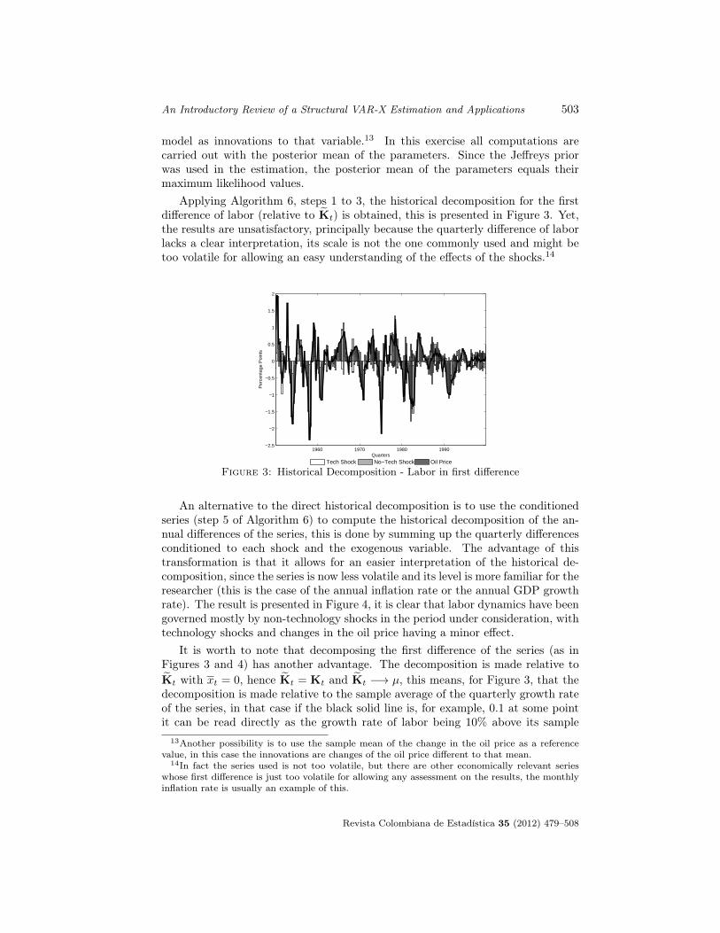
An Introductory Review of a Structural VAR-X Estimation and Applications 503
model as innovations to that variable.13 In this exercise all computations arecarried out with the posterior mean of the parameters. Since the Jeffreys priorwas used in the estimation, the posterior mean of the parameters equals theirmaximum likelihood values.
Applying Algorithm 6, steps 1 to 3, the historical decomposition for the firstdifference of labor (relative to Kt) is obtained, this is presented in Figure 3. Yet,the results are unsatisfactory, principally because the quarterly difference of laborlacks a clear interpretation, its scale is not the one commonly used and might betoo volatile for allowing an easy understanding of the effects of the shocks.14
1960 1970 1980 1990−2.5
−2
−1.5
−1
−0.5
0
0.5
1
1.5
2
Quarters
Per
cent
age
Poi
nts
Tech Shock No−Tech Shock Oil Price
Figure 3: Historical Decomposition - Labor in first difference
An alternative to the direct historical decomposition is to use the conditionedseries (step 5 of Algorithm 6) to compute the historical decomposition of the an-nual differences of the series, this is done by summing up the quarterly differencesconditioned to each shock and the exogenous variable. The advantage of thistransformation is that it allows for an easier interpretation of the historical de-composition, since the series is now less volatile and its level is more familiar for theresearcher (this is the case of the annual inflation rate or the annual GDP growthrate). The result is presented in Figure 4, it is clear that labor dynamics have beengoverned mostly by non-technology shocks in the period under consideration, withtechnology shocks and changes in the oil price having a minor effect.
It is worth to note that decomposing the first difference of the series (as inFigures 3 and 4) has another advantage. The decomposition is made relative toKt with xt = 0, hence Kt = Kt and Kt −→ µ, this means, for Figure 3, that thedecomposition is made relative to the sample average of the quarterly growth rateof the series, in that case if the black solid line is, for example, 0.1 at some pointit can be read directly as the growth rate of labor being 10% above its sample
13Another possibility is to use the sample mean of the change in the oil price as a referencevalue, in this case the innovations are changes of the oil price different to that mean.
14In fact the series used is not too volatile, but there are other economically relevant serieswhose first difference is just too volatile for allowing any assessment on the results, the monthlyinflation rate is usually an example of this.
Revista Colombiana de Estadística 35 (2012) 479–508

504 Sergio Ocampo & Norberto Rodríguez
average. Since Figure 4 is also presenting differences it can be shown that the newKt converges to the sample mean of the annual growth rate of the series, makinginterpretation of the decomposition easier to read.
1960 1970 1980 1990−8
−6
−4
−2
0
2
4
6
Quarters
Per
cent
age
Poi
nts
Tech Shock No−Tech Shock Oil Price
Figure 4: Historical Decomposition - Labor in annual differences
Another alternative is to accumulate the growth rates (conditioned to eachshock and the exogenous variable) starting from the observed value of the seriesin the first period, this generates the historical decomposition of the level of thevariable. The results of this exercise are presented in Figure 5.
There are several points to be made about the historical decomposition inlevels, the first one is that, since Kt is also being accumulated from some initialvalue, the decomposition is not made relative to a constant but relative to a line,this line corresponds to the linear tendency of the series. Figure 5(a) plots theactual path of labor along with paths conditioned to each shock and the exogenousvariable and the “Reference” line, which is the accumulation of Kt. Interpretationof Figure 5(a) is difficult because the effect of each shock and the exogenous variableis obtained as the difference between its conditioned path and the “Reference” line,because all are moving in each period identifying that effect becomes a challengingtask.
The second point arises from the interpretation of Figure 5(b), which presentsthe decomposition of the level of labor relative to the “Reference” line, this is similarto what was presented in Figures 3 and 4. The interpretation is nevertheless morecomplicated. In the former Figures the decomposition was made relative to aconstant, but the decomposition in levels is made relative to a line, whose valueis changing in each period, this makes the reading of the level of the bars and theline more difficult. If the line is in 3 it means that the observed series is 3 unitsabove its linear tendency.
Another characteristic of decomposition in level must be mentioned, althoughit is not clear from Figure 5(b), the accumulated effects of the shocks over anyseries in the first and last period are, by construction, equal to zero. This meansthat the bars associated with the structural shocks are not present in both thefirst and last period of the sample, and that the value of the observed variable
Revista Colombiana de Estadística 35 (2012) 479–508

An Introductory Review of a Structural VAR-X Estimation and Applications 505
has to be explained entirely by the exogenous variables, moreover, it means thatthe accumulated effect of the shocks has to be dis-accumulated when the sampleis getting to its end. This occurs because the accumulated effect of the shockshas to be zero at the beginning of the sample, since the effect of the shocks beforethat point is summarized in the initial value of the series, and because the meanof the shocks over the sample is zero (one of the properties of the estimation), this
implies thatT∑t=1
εit = 0. When the conditioned difference series is accumulated, the
effect of the shock is accumulated so that it also sums to zero. This last problemis not present in the historical decomposition in differences (or annual differences)and makes the results of the decomposition in levels to be unreliable.
1960 1970 1980 199011.5
12
12.5
13
Quarters
Log(
Em
ploy
men
t)
Employment Tech Shock No−Tech Shock Oil Price "Reference"
(a) Decomposition in level
1960 1970 1980 1990−0.08
−0.06
−0.04
−0.02
0
0.02
0.04
0.06
0.08
0.1
Quarters
Log(
Em
ploy
men
t)
Tech Shock No−Tech Shock Oil Price
(b) Decomposition around reference value
Figure 5: Historical Decomposition - Labor in level
7. Final Remarks
This paper presents a review of VAR-X topics with emphasis in Bayesian es-timation, and different applications of the model, covering impulse response func-tions, multiplier analysis, forecast error variance decomposition and historical de-composition calculations. The treatment and discussion of the latter constitutesa novelty in the literature, since it has been largely ignored (with few exceptions)despite its usefulness in the context of multivariate time series analysis. A shortexercise in presented using much of the technique reviewed.
Bayesian methods are presented with detail and shown as an easy to implementoption for overcoming the usual small sample restrictions faced by frequentistmethods. These methods are off course recommended to scholars when using theVAR or the VAR-X model.
Finally, this document is intended as an introductory review to the VAR-X model, and does not exhausts all the literature available about it. A coupleof examples of further topics in the literature are the VAR model with mixedfrequencies, like Rodriguez & Puggioni (2010) or Chiu, Eraker, Foerster, Kim &
Revista Colombiana de Estadística 35 (2012) 479–508

506 Sergio Ocampo & Norberto Rodríguez
Seoane (2011) (and the references therein), and the recently proposed Copula-VAR-X as in Bianchi, Carta, Fantazzini, Giuli & Maggi (2010), who use flexiblemultivariate distributions, different from the normal distribution, allowing a richdependence structure and more flexible marginal distributions for better fit ofempirical data, specially leptokurtosis.
Acknowledgements
We are in debt with the editor of the Colombian Journal of Statistics andthree anonymous referees, their suggestions where crucial for this paper. We wishto thank also Eliana González, Martha Misas, Andrés González, Luis FernandoMelo, and Christian Bustamante for useful comments on earlier drafts of thisdocument, of course, all remaining errors are our own. Needless to say, the resultsand opinions expressed in this document do not compromise in any way the Bancode la República, its board of governors or the Inter-American Development Bank.[
Recibido: enero de 2012 — Aceptado: noviembre de 2012]
References
Amisano, G. & Giannini, C. (1997), Topics in Structural VAR Econometrics,Springer.
Bauwens, L., Lubrano, M. & Richard, J.-F. (2000), Bayesian Inference in DynamicEconometric Models, Oxford University Press.
Bianchi, C., Carta, A., Fantazzini, D., Giuli, M. E. D. & Maggi, M. (2010), ‘A Cop-ula VAR-X Approach for Industrial Production Modelling and Forecasting’,Applied Economics 42(25), 3267–3277.
Blanchard, O. J. & Quah, D. (1989), ‘The Dynamic Effects of Aggregate Demandand Supply Disturbances’, American Economic Review 79(4), 655–73.
Burbidge, J. & Harrison, A. (1985), ‘A Historical Decomposition of the GreatDepression to Determine the Role of Money’, Journal of Monetary Economics16(1), 45–54.
Canova, F. (2007), Methods for Applied Macroeconomic Research, Princeton Uni-versity Press, Nueva Jersey.
Canova, F. & De Nicolo, G. (2002), ‘Monetary Disturbances Matter for BusinessFluctuations in the G-7’, Journal of Monetary Economics 49(6), 1131–1159.
Canova, F. & Pappa, E. (2007), ‘Price Differentials in Monetary Unions: The Roleof Fiscal Shocks’, Economic Journal 117(520), 713–737.
Casella, G. & George, E. I. (1992), ‘Explaining the Gibbs Sampler’, The AmericanStatistician 46(3), 167–174.
Revista Colombiana de Estadística 35 (2012) 479–508

An Introductory Review of a Structural VAR-X Estimation and Applications 507
Chen, M. & Shao, Q. (1998), ‘Monte Carlo Estimation of Bayesian Credible andHPD Intervals’, Journal of Computational and Graphical Statistics 8, 69–92.
Chiu, C. W. J., Eraker, B., Foerster, A. T., Kim, T. B. & Seoane, H. D. (2011),Estimating VAR’s Aampled at Mixed or Irregular Spaced Frequencies : aBayesian Approach, Research Working Paper RWP 11-11, Federal ReserveBank of Kansas City.
Christiano, L. J., Eichenbaum, M. & Evans, C. L. (1999), Monetary Policy Shocks:What Have We Learned and to What End?, in J. B. Taylor & M. Woodford,eds, ‘Handbook of Macroeconomics’, Vol. 1 of Handbook of Macroeconomics,Elsevier, chapter 2, pp. 65–148.
Galí, J. (1999), ‘Technology, Employment, and the Business Cycle: Do Technol-ogy Shocks Explain Aggregate Fluctuations?’, American Economic Review89(1), 249–271.
Geman, S. & Geman, D. (1984), ‘Stochastic Relaxation, Gibbs Distributions, andthe Bayesian Restoration of Images’, IEEE Transactions on Pattern Analysisand Machine Intelligence 6, 721–741.
Hyndman, R. J. (1996), ‘Computing and Graphing Highest Density Regions’, TheAmerican Statistician 50, 120–126.
Jeffreys, H. (1961), Theory of Probability, International Series of Monographs onPhysics, Clarendon Press.
Kadiyala, K. R. & Karlsson, S. (1997), ‘Numerical Methods for Estimation and In-ference in Bayesian VAR-Models’, Journal of Applied Econometrics 12(2), 99–132.
Kilian, L. (1998), ‘Small-Sample Confidence Intervals For Impulse Response Func-tions’, The Review of Economics and Statistics 80(2), 218–230.
King, T. B. & Morley, J. (2007), ‘In Search of the Natural Rate of Unemployment’,Journal of Monetary Economics 54(2), 550–564.
Kociecki, A. (2010), ‘A Prior for Impulse Responses in Bayesian Structural VARModels’, Journal of Business & Economic Statistics 28(1), 115–127.
Koop, G. (1992), ‘Aggregate Shocks and Macroeconomic Fluctuations: A BayesianApproach’, Journal of Applied Econometrics 7(4), 395–411.
Litterman, R. B. (1986), ‘Forecasting with Bayesian Vector Autoregressions - FiveYears of Experience’, Journal of Business & Economic Statistics 4(1), 25–38.
Lütkepohl, H. (1990), ‘Asymptotic Distributions of Impulse Response Functionsand Forecast Error Variance Decompositions of Vector Autoregressive Mod-els’, The Review of Economics and Statistics 72(1), 116–25.
Lütkepohl, H. (2005), New Introduction to Multiple Time Series Analysis,Springer.
Revista Colombiana de Estadística 35 (2012) 479–508

508 Sergio Ocampo & Norberto Rodríguez
Moon, H. R., Schorfheide, F., Granziera, E. & Lee, M. (2011), Inference for VARsIdentified with Sign Restrictions, NBER Working Papers 17140, NationalBureau of Economic Research, Inc.
Mountford, A. & Uhlig, H. (2009), ‘What are he Effects of Fiscal Policy Shocks?’,Journal of Applied Econometrics 24(6), 960–992.
Nicholls, D. F. & Pope, A. L. (1988), ‘Bias in the Estimation of MultivariateAutoregressions’, Australian Journal of Statistics 30A(1), 296–309.
Rodriguez, A. & Puggioni, G. (2010), ‘Mixed Frequency Models: Bayesian Ap-proaches to Estimation and Prediction’, International Journal of Forecasting26(2), 293–311.
Runkle, D. E. (1987), ‘Vector Autoregressions and Reality’, Journal of Business& Economic Statistics 5(4), 437–42.
Sims, C. A. (1980), ‘Macroeconomics and Reality’, Econometrica 48(1), 1–48.
Sims, C. A. & Zha, T. (1999), ‘Error Bands for Impulse Responses’, Econometrica67(5), 1113–1156.
Smets, F. & Wouters, R. (2007), ‘Shocks and Frictions in US Business Cycles: ABayesian DSGE Approach’, American Economic Review 97(3), 586–606.
Uhlig, H. (2005), ‘What are the Effects of Monetary Policy on Output? ResultsFrom an Agnostic Identification Procedure’, Journal of Monetary Economics52(2), 381–419.
Zellner, A. (1996), An Introduction to Bayesian Inference in Econometrics, WileyClassics Library, John Wiley.
Revista Colombiana de Estadística 35 (2012) 479–508

Revista Colombiana de EstadísticaDiciembre 2012, volumen 35, no. 3, pp. 509 a 521
Some Alternative Predictive Estimators ofPopulation Variance
Algunos estimadores predictivos alternativos de la varianzapoblacional
Radhakanta Nayak1,a, Lokanath Sahoo2,b
1Department of Statistics, Khallikote College, Berhampur, India2Department of Statistics, Utkal University, Bhubaneswar, India
Abstract
Using a predictive estimation procedure, an attempt has been made to de-velop some estimators for the finite population variance in the presence of anauxiliary variable. Analytical and simulation studies have been undertakenfor understanding the performance of the suggested estimators compared tosome existing ones.
Key words: Auxiliary variable, Bias, Efficiency, Prediction approach.
Resumen
Mediante el uso de un procedimiento de estimación predictivo, se desar-rollan algunos estimadores de la varianza poblacional en la presencia de unavariable auxiliar. Estudios analíticos y de simulación son implementadospara entender el desempeño de los estimadores sugeridos en comparacióncon otros ya existentes.
Palabras clave: variable auxiliar, sesgo, eficiencia, enfoque de predicción.
1. Introduction
Let U = {1, 2, . . . , i . . . , N} be a finite population, and y and x denote thestudy variable and the auxiliary variable taking values yi and xi respectively onthe ith unit (i = 1, 2, . . . , N). Let Y =
∑Ni=1 yi/N and X =
∑Ni=1 xi/N be the
population means, S2y =
∑Ni=1(yi−Y )2/(N −1) and S2
x =∑Ni=1(xi−X)2/(N −1)
be the population variances of y and x respectively. Assume that a sample s of nunits is drawn from U according to simple random sampling without replacement
aLecturer. E-mail: [email protected]. E-mail: [email protected]
509

510 Radhakanta Nayak & Lokanath Sahoo
(SRSWOR) in order to estimate the unknown parameter S2y . Let y =
∑i∈s yi/n
and x =∑i∈s xi/n be the sample means, s2y =
∑i∈s(yi − y)2/(n − 1) and s2x =∑
i∈s(xi − x)2/(n− 1) the sample variances.In certain situations, estimation of population variance S2
y has received consid-erable attention from survey statisticians. For example, in manufacturing indus-tries and pharmaceutical laboratories, sometimes the researchers are interested inthe variation of their products. Although, the literature describes a great vari-ety of techniques for using auxiliary information by means of ratio, and productand regression methods for estimating population mean, variance estimation us-ing auxiliary information has received scarce attention. This is perhaps due to thebelief that the gain in efficiency we could obtain by involving an auxiliary variablemay not be too much relevant to motivate the use of more complex estimators.However, some efforts in this direction are due to Das & Tripathi (1978), Isaki(1983), Prasad & Singh (1990)(1992), Singh & Kataria (1990), Srivastava & Jhajj(1980)(1995), Singh & Singh (2001), Ahmed, Walid & Ahmed (2003), Giiancarlo& Chiara (2004), Jhajj, Sharma & Grover (2005), Kadilar & Cingi (2006)(2007)and Grover (2007). Two notable estimators that are very much popular in theliterature are due to Isaki (1983) defined by
ν1 = s2yS2x/s
2x
andν2 = s2y + b∗(S2
x − s2x)
where b∗ is an estimate of the regression coefficient of s2y on s2x defined by b∗ =s2y(λ−1)
s2x(β2(x)−1), such that λ = m22/m20m02 and β2(x) = m40/m
220 with mrs =∑
i∈s(xi − x)r(yi − y)s/n [cf., Garcia & Cebrain (1996), and Kadilar & Cingi(2006)].
During the years that followed, much emphasis has been given on the predictionof population mean or total [cf., Srivastava (1983)]. But, little interest has beenshown towards the prediction of the population variance. Under this approach,the survey data at hand i.e., the sample observations are treated as fixed andunassailable. Uncertainty is then attached only to the unobserved values whichneed to be predicted. Bolfarine & Zacks (1992) indicated various techniques forpredicting population variance. Biradar & Singh (1998), using classical estimationtheory, provided some predictive estimators for S2
y . In this paper, using auxiliaryvariable x, we develop some more estimators under the prediction approach ofBasu (1971) with regards to a finite population setup.
2. Prediction Criterion
Let us decompose U into two mutually exclusive domains s and r of n andN − n units respectively, where r = U − s denotes the collection of units in Uwhich are not included in s. Then, under the usual prediction criterion given inBolfarine & Zacks (1992), it is possible to express
(N − 1)S2y = (n− 1)s2y + (N − n− 1)S2
y(r) + (1− f)n(y − Y r)2, (1)
Revista Colombiana de Estadística 35 (2012) 509–521

Some Alternative Predictive Estimators of Population Variance 511
where f = n/N , and Y r =∑i∈s yi/(N−n) and S2
y(r) =∑i∈r(yi−Y r)2/(N−n−1)
are respectively the mean and variance of y-values belonging to r.Notice that the first component on the right hand side of (1) is known while the
second and third components are unknown. Hence, the prediction of (N − 1)S2y
is possible when S2y(r) and Y r are simultaneously predicted by some means from
the sample data. Using Vr and Mr as their respective predictors, a predictor ofS2y can be provided by the equation:
(N − 1)S2y = (n− 1)s2y + (N − n− 1)Vr + (1− f)n(y −Mr)
2 (2)
Most of the predictions are based either on distributional forms or an assumedmodel [cf., Royall (1988), Bolfarine & Zacks (1992)]. However, Sampford (1978)argued that the consideration of a model free prediction can generate a new, esti-mator possessing some desirable properties. Basu (1971) also encouraged the useof tools of the classical estimation theory to find out suitable predictors for Y .Biradar & Singh (1998) formulated some estimators of S2
y from (2) by consideringsuitable choices of the predictors Vr and Mr in terms of the auxiliary variable xunder the tools of classical estimation theory. Defining Xr =
∑i∈r xi/(N − n)
and S2x(r) =
∑i∈r(xi −Xr)
2/(N − n− 1), we report below their estimators alongwith the corresponding selections of Vr and Mr:
ν3 =
(N − 2
N − 1
)s2y
when Vr = s2y and Mr = y,
ν4 =s2ys2xS2x +
nN(x−X)2
(N − n)(N − 1)
(y2
x2−s2ys2x
)
when Vr = s2yS2x(r)/s
2x and Mr = yXr/x, and
ν5 =s2ys2xS2x +
nN(x−X)2
(N − n)(N − 1)
(b2yx −
s2ys2x
)
when Vr = s2yS2x(r)/s
2x and Mr = y + byx(Xr − x), where byx = syx/s
2x.
Biradar & Singh (1998) also identified Isaki’s (1983) estimator ν1 as a specialcase of (2) for Vr = s2yS
2x(r)/s
2x and Mr = y+ sy(Xr − x)/sx. This shows that the
estimator possesses a predictive character.
3. Some New Predictive Estimators of S2y
In the following discussions, we introduce some alternative approaches in orderto develop a few more predictive estimators of S2
y .
Revista Colombiana de Estadística 35 (2012) 509–521

512 Radhakanta Nayak & Lokanath Sahoo
1. Consider the following alternative but equivalent representation of S2y :
(N − 1)S2y = (n− 1)s2y + (N − n)[σ2
y(r) + f(y − Y r)2] (3)
where σ2y(r) =
∑i∈r(yi − Y r)2/(N − n). Denoting V ∗r as a predictor of σ2
y(r)
and Mr, as the predictor of Y r, the following alternative predictive equationcan be considered:
(N − 1)S2y = (n− 1)s2y + (N − n)[V ∗r + f(y −Mr)
2] (4)
Then, for V ∗r =(n−1n
)s2y and Mr = y in (4) we get an estimator of S2
y
defined by
ν6 =
(n− 1
n
)(N
N − 1
)s2y
2. Biradar & Singh (1998) developed the estimator ν5 from (2) with Vr =s2yS
2x(r)/s
2x and Mr = y + byx(Xr − x). See that in such an attempt Vr has
been assumed a ratio version of the variance estimator while the connectedmean estimator is a regression estimator. Hence as a matter of curiosity,we may also think in the light of Isaki (1983) to use a regression version ofthe variance estimator i.e., Vr = s2y + b∗(S2
x(r) − s2x) along with the mean
estimator Mr = y + byx(Xr − x) in the predictive equation (2) to predictS2y . This operation, after a considerable simplification, leads to produce the
following estimator:
ν7 =N − 2
N − 1
[s2y + b∗
(N − 1
N − 2S2x − s2x
)]
3. Srivastava (1983) considered the predictive equation:
Y = fy + (1− f)Mr (5)
where Mr is the implied predictor of Y r, for predicting Y and shown thatwhen Mr = yXr/x, Y = yR = yX/x, the classical ratio estimator of Y , andwhenMr = y+byx(Xr−x), Y = yL = y+byx(X−x), the classical regressionestimator of Y . Thus, both the ratio and regression estimators (yR and yL)of the mean possess a predictive character, the origin of which actually liesin predicting yi’s, i ∈ r, by yi = yxi/x and yi = y + byx(xi − x) in thatorder. In view of this, we designate these two estimators as basic estimatorsof the population mean. Notice that the predictive estimators ν1, ν4, ν5 andν7 suggested so far have been obtained by using either Vr = s2yS
2x(r)/s
2x or
Vr = s2y + b∗(S2x(r) − s
2x) as the case may be. This means that the unknown
quantity S2y(r) is estimated as a whole with the same principle as that applied
to estimate Y r. But, such a choice of Vr seems to be arbitrary by nature.Rather, we feel that it is more appropriate if the variance is established by
Revista Colombiana de Estadística 35 (2012) 509–521

Some Alternative Predictive Estimators of Population Variance 513
predicting individual yi’s, i ∈ r, for which we need to express S2y in the
following form:
(N − 1)S2y = (n− 1)s2y +
∑i∈r
y2i − (N − n)Y2
r + (1− f)n(y − Y r)2 (6)
A number of new estimators can be easily generated from this equation on thebasis how
∑i∈r y
2i is predicted. But, for simplicity, here we consider the prediction
of yi, i ∈ r, either by yi = yxi/x = y + y(xi − x)/x or by yi = y + byx(xi − x) andprediction of Y r by yXr/x.
Then, accordingly after a considerable simplification, we obtain the followingtwo new estimators:
ν8 =
(n− 1
N − 1
)[s2y +
(y
x
)2(N − 1
n− 1S2x − s2x
)]
ν9 =
(n− 1
N − 1
)[s2y + b2yx
(N − 1
n− 1S2x − s2x
)]
4. Performance of the Proposed Estimators
Out of the nine estimators considered or proposed in the preceding sections,the estimators ν3 and ν6 were achieved without using any auxiliary informationwhereas others were achieved through the use of information on the auxiliaryvariable x. A desirable goal here is to study the performance of the proposedestimators ν6 to ν9 compared to ν1 to ν5 at least in respect of bias and mean squareerror (MSE) i.e., efficiency, where bias and MSE of an estimator νi of S2
y are definedrespectively by B(νi) = E(νi) − S2
y and M(νi) = E(νi − S2y)2(i = 1, 2, . . . , 9).
But, we see that some of the estimators are so complex that it is not possible toderive exact expressions for their bias and MSE. Biradar & Singh (1998) presentedasymptotic expressions for these performance measures for the estimators ν1 to ν5.On the other hand, Nayak (2009) derived these expressions in favor of ν1 to ν9.But, the sufficient conditions for superiority of one estimator over other derivedby the authors using asymptotic expressions are so complicated that it is notconducive to compare different estimators meaningfully. However, to facilitateour comparison, these expressions are considered under the following widely usedlinear regression model:
yi = βxi + ei, i = 1, 2, . . . , N (7)
where β(> 0) is the model parameter and ei is the error component such thatE(ei/xi) = 0, E(e2i /xi) = δxg(δ > 0, 0 ≤ g ≤ 1), and E(eiej/xi, xj) = 0 for i 6= j.Further, we also assume that E(e4i /xi) = ξxg and E(e3i /xi) = E(e3i ej/xi, xj) =E(eie
3j/xi, xj) = 0, (i 6= j). It may be pointed out here that the asymptotic
expressions for bias and MSE of different estimators under this assumed modelare derived through the Taylor linearization method.
Revista Colombiana de Estadística 35 (2012) 509–521

514 Radhakanta Nayak & Lokanath Sahoo
4.1. Comparison of Bias
After some algebraic manipulations (suppressed to save space), we get thefollowing model-based results in respect of the bias of different estimators up toO(n−1)
B(ν1) = CδE(xg) (8)B(ν2) = 0 (9)
B(ν3) = − 1
N − 1[β2S2
x + δE(xg)] (10)
B(ν4) = −(B − C)δE(xg) (11)B(ν5) = −(K − C)δE(xg) (12)
B(ν6) = −N − nN − 1
[β2S2x + δE(xg)] (13)
B(ν7) = − 1
N − 1
(n− 2
n− 1
)δE(xg) (14)
B(ν8) = −(N − n)BδE(xg) (15)
B(ν9) = −(N − nN − 1
)(n− 2
n− 1
)δE(xg) (16)
where B =1
N − 1
(1− C2
x
n
), C = 1
n (β2(x)−2) and K =
(n
n− 1
)(1
N − 1
), such
that Cx and β2(x) are respectively the coefficient of variation and β2- coefficient ofthe auxiliary variable x.
In the light of the expressions (8) to (16), we state the following comments onthe bias of the estimators:
(i) The regression estimator ν2 is model-unbiased, ν1 is positively biased andthe rest seven estimators are negatively biased.
(ii) |B(ν3)| < |B(ν6)|. This indicates that the bias of ν6 is always greater thanthat of ν3.
(iii) |B(ν8)| < |B(ν7)|i.e., ν8 is less biased than ν7.
(iv) |B(ν7)| < |B(ν9)|i.e., ν7 is less biased than ν9.
(v) |B(ν9)| ≶ |B(ν8)| according as C2x ≶
n
n− 1.
(vi) |B(ν4)| < |B(ν7)|, when |B − C| < 1
N − 1
(n− 2
n− 1
).
(vii) |B(ν5)| < |B(ν7)|, when |K − C| < 1
N − 1
(n− 2
n− 1
).
(viii) |B(ν7)| < |B(ν1)|, when C > K and n > 2.
Revista Colombiana de Estadística 35 (2012) 509–521

Some Alternative Predictive Estimators of Population Variance 515
In view of (iii) and (iv), although we can conclude that ν8 is less biased than ν7and ν9, we fail to obtain a clear-cut idea on the magnitude of bias of ν8 comparedto ν1,ν4 and ν5. Because, comparison of (15) with (8) or (11) or (12) does not leadto any meaningful conditions.
4.2. Comparison of Efficiency
We present below model-based asymptotic expressions of the MSEs of differentestimators up to O(n−1) together with the exact expression for the variance of thetraditional unbiased estimator s2y.
V (s2y) = V (ν2) + Cβ4S4x (17)
M(ν1) = M(ν2) + Cδ2E2(xg) (18)
M(ν2) = ξ(xg) + 4β2S2x
δE(xg)
n− 1− n− 3
n(n− 1)δ2E2(xg) (19)
M(ν3) =
(N − 2
N − 1
)2
V (s2y) ∼= V (s2y) (20)
M(ν4) = M(ν2) + Cδ2E2(xg) +2
N − 1δ2E2(xg) (21)
M(ν5) = M(ν2) + Cδ2E2(xg) +2
N − 1
(n
n− 1
)δ2E2(xg) (22)
M(ν6) =
(n− 1
n
)2(N
N − 1
)2
V (s2y) ∼={
1− 2
(1
n+
1
N − 1
)}V (s2y) (23)
M(ν7) = M(ν2) (24)
M(ν8) = M(ν2)− 4
(N − nN − 1
)2
β2S2x
δE(xg)
n− 1+ (25)
2
(N − nN − 1
)2C2x
n(2β2S2
x − 1)δE(xg)
M(ν9) = M(ν2) + 2
(1− 2
N − nN − 1
)δ2E2(xg)
n− 1+
(N − nN − 1
)2
δ2E2(xg). (26)
From these expressions, as ν2 appears to be more efficient than s2y, ν1, ν3, ν4and ν5, we present the following results concerning efficiencies of the suggestedestimators:
(ix) M(ν6) < M(ν3) < V (s2y). This indicates that ν6 is more efficient than boths2y and ν3.
(x) M(ν7) = M(ν2) i.e., ν7 and ν2 are equally efficient even though they areconfigurationally different.
(xi) ν8 is more efficient than ν2 when β2S2x < 1
2 which is very often satisfiedin practice. This means that there is a scope to improve upon the Isaki’sregression estimator ν2 through ν8.
Revista Colombiana de Estadística 35 (2012) 509–521
516 Radhakanta Nayak & Lokanath Sahoo
(xii) The estimator ν9 is less efficient than ν2 when n <N + 1
2.
(xiii) M(ν8) < M(ν2) = M(ν7) < M(ν9), when n <N + 1
2and β2S2
x <12 . This
shows that ν8 is preferred to ν2, ν7 and ν9 when the stated conditions aresatisfied. The first condition is not a serious one. The second condition iseasily satisfied for characters being measured in smaller magnitudes. Wecan also reduce the mean square error by considering transformations on theauxiliary variable and making the second condition more feasible.
4.3. Some Remarks
From the previous model-based comparisons, we see that the proposed estima-tor ν8 turns out to be more efficient than others. But no meaningful conclusioncould be drawn in favor of the four proposed estimators νi, i = 6, 7, 8, 9 in re-spect of bias. This negative finding may be discouraging but not very decisive asour comparisons are based on the asymptotic expressions derived through Tay-lor linearization. However, as a counterpart to these analytical comparisons, wedo carry out a simulation study in the next section with an objective to exam-ine the overall performance of the different variance estimators. The performancemeasures of an estimator νi taken into consideration in this study are (i) Abso-lute Relative Bias (ARB) = |B(νi)|/S2
y , and (ii) Percentage Relative Efficiency(PRE) = 100× V (s2y)/M(νi), (i = 1, 2, . . . , 9)
5. Description of the Simulation Study
Our simulation study involves repeated draws of simple random (without re-placement) samples from 20 natural populations described in Table 1. 2,000 inde-pendent samples, for n = 6, 8 and 10, were selected from a population and for eachsample several estimators were calculated. Then, considering 2,000 such combina-tions, simulated values of the performance measures were calculated and displayedin Tables 2 and 3. To save space, the numerical values of the performance mea-sures for n = 8 and 10 are not shown, but the results based on these values areonly reported. Major findings of the study are discussed in subsections 5.1 and5.2.
5.1. Results Based on the ARB
The numerical values on the ARB reveal that there is no definite pattern in theperformances of different estimators. The estimator ν1 possesses the least ARBin 7 populations for n = 6 and in 6 populations for n = 8 and 10. ν8 is found tohave least ARB in 8, 10 and 11 populations for n = 6, 8 and 10 respectively. Thisclearly indicates that the overall performance of ν8 improves with the increase insample size. Searching for an estimator as the third choice is difficult owing tovery erratic results in favor of the estimators (except ν1 and ν8).
Revista Colombiana de Estadística 35 (2012) 509–521

Some Alternative Predictive Estimators of Population Variance 517
Table 1: Description of the populations.Pop Source N y x
1 Cochran (1977) p. 152 49 no of inhabi-tants in 1930
no. of inhabi-tants in 1920
2 Sukhatme & Sukhatme (1977) p. 185 34 area underwheat in 1937
area underwheat in1936
3 Sukhatme & Sukhatme (1977) p. 185 34 area underwheat in 1937
area underwheat in1931
4 Sampford (1962) p. 61 35 acreage underoats in 1957
acreage ofcrops and grassin 1947
5 Wetherill (1981) p. 104 32 yield ofpetroleumsprit
petroleum frac-tion end point
6 Murthy (1967) p. 398 43 no of absentees no of workers7 Murthy (1967) p. 399 34 area under
wheat in 1964cultivated areain 1961
8 Murthy (1967) p. 399 34 area underwheat in 1964
area underwheat in 1963
9 Steel & Torrie (1960) p. 282 30 leaf burn insecs.
percentage ofpotassium
10 Shukla (1966) 50 fiber yield height of plant11 Shukla (1966) 50 fiber yield base diameter12 Murthy (1967) p. 178 108 area under win-
ter paddygeographicalarea
13 Dobson (1990) p. 83 30 cholesterol age in years14 Dobson (1990) p. 83 30 cholesterol body mass15 Yates (1960) p. 159 25 measured vol-
ume of timbereye estimatedvolume oftimber
16 Yates (1960) p. 159 43 no. of absen-tees
total no. ofpersons
17 Panse & Sukhatme (1985) p. 118 25 progeny mean parental plantvalue
18 Panse & Sukhatme (1985) p. 118 25 progeny mean parental plotmean
19 Dobson (1990) p. 69 20 total caloriesfrom carbohy-drate
calories as pro-tein
20 Horvitz & Thompson (1952) 20 actual no. ofhouseholds
eye estimatednumber ofhouseholds
5.2. Results Based on the PRE
Results on the PRE of the competing estimators show that the estimator ν8 isdecidedly more efficient than the rest of the estimators in all populations for n = 6and in 18 populations (except populations 1 and 17) for n = 8 and 10. Also theefficiency gain due to this estimator is noticeably high. The estimator ν9 is foundto be the second best estimator being more efficient than others (except ν8 ) in 12populations for n = 6 and in 10 populations for n = 8 and 10.
Revista Colombiana de Estadística 35 (2012) 509–521

518 Radhakanta Nayak & Lokanath Sahoo
Further, it is observed that both ν3 and ν6 i.e., the estimators exploiting noauxiliary information, perform satisfactorily with ν6 being better than ν3 in allpopulations. It may also be noted here that for n = 6, ν8 is the only estimatorusing auxiliary variable x that is better than s2y in all populations. However, thissituation slightly changes with the increase in the sample size as it is worse thans2y in one population for n = 8 and in two populations for n = 10. The estimatorsν1 ,ν2, ν4 and ν5 do not fare well in most of the cases.
Table 2: ARB of the estimators for n = 6.Pop No ν1 ν2 ν3 ν4 ν5 ν6 ν7 ν8 ν9
1 10.24 12.23 4.10 10.24 10.29 9.55 12.27 1.85 13.752 18.81 18.45 8.20 18.63 18.69 18.72 18.33 5.68 15.133 1.19 4.53 8.20 2.03 1.39 18.72 4.84 36.58 13.164 57.23 18.51 39.30 49.81 50.48 46.35 18.35 13.50 13.995 24.85 26.94 26.39 32.36 27.66 34.57 27.62 79.72 44.426 31.04 45.37 44.37 41.58 41.73 51.83 45.88 33.46 64.227 0.57 4.13 7.01 1.57 0.36 17.76 4.46 39.28 13.358 1.19 0.56 7.01 0.92 1.14 17.76 1.49 0.35 1.479 32.96 13.67 22.47 24.87 30.23 30.78 16.04 81.23 70.6810 19.36 24.10 35.40 20.17 19.76 43.93 24.67 78.83 49.5111 62.42 3.47 35.40 57.74 58.13 43.93 4.08 73.58 30.1012 25.10 11.15 51.06 23.71 22.81 58.44 11.19 8.64 15.6913 61.77 14.72 35.31 62.93 60.25 42.24 13.68 7.95 10.2314 27.91 34.55 35.31 28.71 28.75 42.24 36.14 72.76 72.5515 7.04 3.13 3.08 3.73 10.98 12.21 4.61 2.02 31.2516 43.05 46.28 44.62 44.10 54.08 51.59 46.77 67.22 63.7517 33.62 29.05 19.07 25.71 36.39 26.70 30.55 46.47 57.5818 40.92 18.98 19.07 21.61 21.92 26.70 11.23 8.13 51.7019 33.30 5.06 25.42 24.22 27.79 30.95 2.80 4.32 26.5720 0.74 2.34 16.31 1.27 1.34 22.51 2.97 15.91 11.19
6. Conclusions
Our model-assisted analytical and simulated studies lead to an overall con-clusion that the estimator ν8 is preferable to others on the ground of efficiency.Although the analytical comparison fails to conclude which estimator is decidedlybetter than others on the ground of bias, the simulation study gives an indicationthat on this ground ν8 is the better performer than other estimators. In viewof these findings, if computational difficulty is not a matter of great concern, thevariance estimator ν8 may be considered as the most suitable estimator. Of course,these findings are only indicative and are no able to reveal essential features of thecomparable estimators in a straightforward manner. Further investigations in thisdirection may be made for arriving at the conclusions.
Revista Colombiana de Estadística 35 (2012) 509–521
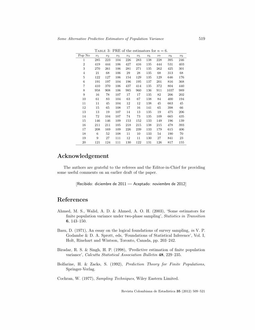
Some Alternative Predictive Estimators of Population Variance 519
Table 3: PRE of the estimators for n = 6.Pop No ν1 ν2 ν3 ν4 ν5 ν6 ν7 ν8 ν9
1 285 223 104 226 283 138 228 395 2462 419 444 106 427 416 135 444 531 4033 270 261 106 281 271 135 262 425 3014 21 68 106 29 28 135 68 313 685 122 127 106 154 129 135 129 646 1766 191 197 104 196 195 137 201 816 3687 410 370 106 437 414 135 372 804 4408 958 908 106 985 960 136 911 1037 9899 16 78 107 17 17 135 82 206 20210 61 83 104 63 67 138 84 400 19411 11 45 104 12 12 138 45 663 4512 15 65 108 17 16 141 65 398 6613 13 19 107 14 13 135 19 475 20614 72 104 107 74 73 135 109 665 43515 146 146 109 153 152 133 149 196 13916 211 211 105 218 215 138 215 478 39317 208 169 109 226 239 133 179 615 40618 6 52 108 11 10 133 54 190 7019 9 27 111 12 11 130 27 841 2320 121 124 111 130 122 131 126 817 155
Acknowledgement
The authors are grateful to the referees and the Editor-in-Chief for providingsome useful comments on an earlier draft of the paper.
[Recibido: diciembre de 2011 — Aceptado: noviembre de 2012
]
References
Ahmed, M. S., Walid, A. D. & Ahmed, A. O. H. (2003), ‘Some estimators forfinite population variance under two-phase sampling’, Statistics in Transition6, 143–150.
Basu, D. (1971), An essay on the logical foundations of survey sampling, in V. P.Godambe & D. A. Sprott, eds, ‘Foundations of Statistical Inference’, Vol. I,Holt, Rinehart and Wintson, Toronto, Canada, pp. 203–242.
Biradar, R. S. & Singh, H. P. (1998), ‘Predictive estimation of finite populationvariance’, Calcutta Statistical Association Bulletin 48, 229–235.
Bolfarine, H. & Zacks, S. (1992), Prediction Theory for Finite Populations,Springer-Verlag.
Cochran, W. (1977), Sampling Techniques, Wiley Eastern Limited.
Revista Colombiana de Estadística 35 (2012) 509–521

520 Radhakanta Nayak & Lokanath Sahoo
Das, A. & Tripathi, T. P. (1978), ‘Use of auxiliary information in estimating thefinite population variance’, Sankhya C40, 139–148.
Dobson, A. J. (1990), An Introduction to Generalized Linear Models, Chapmanand Hall, New York.
Garcia, M. R. & Cebrain, A. A. (1996), ‘Repeated substitution method: The ratioestimator for the population variance’, Metrika 43, 101–105.
Giiancarlo, D. & Chiara, T. (2004), ‘Estimation for finite population variance indouble sampling’, Metron 62, 223–232.
Grover, L. K. (2007), ‘A wide and efficient class of estimators of population vari-ance under sub-sampling scheme’, Model Assisted Statistics and Applications2, 41–51.
Horvitz, D. G. & Thompson, D. J. (1952), ‘A generalization of sampling with-out replacement from a finite universe’, Journal of the American StatisticalAssociation 47, 663–685.
Isaki, C. T. (1983), ‘Variance estimation using auxiliary information’, Journal ofthe American Statistical Association 78(117-123).
Jhajj, H. S., Sharma, M. K. & Grover, L. K. (2005), ‘An efficient class of chainestimators of population variance under sub-sampling scheme’, Journal of theJapan Statistical Society 35, 273–286.
Kadilar, C. & Cingi, H. (2006), ‘Improvement in variance estimation using auxil-iary information’, Hacettepe Journal of Mathematics and Statistics 35, 111–115.
Kadilar, C. & Cingi, H. (2007), ‘Improvement in variance estimation in simple ran-dom sampling’, Communications in Statistics-Theory and Methods 36, 2075–2081.
Murthy, M. N. (1967), Sampling Theory and Methods, Statistical Publishing Soci-ety, Kolkata.
Nayak, R. K. (2009), Some Estimation Strategies in Finite Population SurveySampling Using Auxiliary Information, PhD., Utkal University, India.
Panse, V. G. & Sukhatme, P. V. (1985), Statistical Methods for Agricultural Work-ers, Indian Council for Agricultural Research, New Delhi.
Prasad, B. & Singh, H. P. (1990), ‘Some improved ratio-type estimators of finitepopulation variance in sample surveys’, Communications in Statistics-Theoryand Methods 19, 1127–1139.
Prasad, B. & Singh, H. P. (1992), ‘Unbiased estimators of finite populationvariance using auxiliary information in sample surveys’, Communications inStatistics-Theory and Methods 21, 1367–1376.
Revista Colombiana de Estadística 35 (2012) 509–521

Some Alternative Predictive Estimators of Population Variance 521
Royall, R. M. (1988), The prediction approach to sampling theory, in P. R. Kr-ishnaish & C. R. Rao, eds, ‘Handbook of Statistics’, Vol. 6, North Holland,pp. 351–358.
Sampford, M. R. (1962), An Introduction to Sampling Theory, Oliver and Boyd,Edinburg.
Sampford, M. R. (1978), Predictive estimation and internal congruency, in H. A.David, ed., ‘Contribution to Survey Sampling and Applied Statistics’, Aca-demic Press, New York, pp. 29–39.
Shukla, G. K. (1966), ‘An alternative multivariate ratio estimate for finite popu-lation’, Calcutta Statistical Association Bulletin 15, 127–134.
Singh, H. P. & Singh, R. (2001), ‘Improved ratio-type estimators for variance usingauxiliary information’, Journal of the Indian Society of Agricultural Statistics54, 276–287.
Singh, S. & Kataria, P. (1990), ‘An estimator of the finite population variance’,Journal of the Indian Society of Agricultural Statistics 42, 186–188.
Srivastava, S. K. (1983), ‘Predictive estimation of finite population using productestimators’, Metrika 30, 93–99.
Srivastava, S. K. & Jhajj, H. S. (1980), ‘A class of estimators using auxiliaryinformation for estimating finite population variance’, Sankhya C42, 87–96.
Srivastava, S. K. & Jhajj, H. S. (1995), ‘Classes of estimators of finite populationmean and variance using auxiliary information’, Journal of the Indian Societyof Agricultural Statistics 47, 119–128.
Steel, R. G. D. & Torrie, J. H. (1960), Principles and Procedures of Statistics, Mc.Graw Hill Book Company.
Sukhatme, P. V. & Sukhatme, B. V. (1977), Sampling Theory of Surveys withApplications, Asia Publishing House, New Delhi.
Wetherill, G. B. (1981), Intermediate Statistical Methods, Chapman and Hall,London.
Yates, F. (1960), Sampling Methods for Censuses and Surveys, Charls and Griffin,London.
Revista Colombiana de Estadística 35 (2012) 509–521


Informacion para los autores
La Revista Colombiana de Estadıstica publica artıculos originales decaracter teorico o aplicado en cualquiera de las ramas de la estadıstica. Los artıcu-los puramente teoricos deberan incluir la ilustracion de las tecnicas presentadascon datos reales o por lo menos con experimentos de simulacion, que permitanverificar la utilidad de los contenidos presentados. Se consideran tambien artıculosdivulgativos de gran calidad de exposicion sobre metodologıas o tecnicas estadısti-cas aplicadas en diferentes campos del saber. Unicamente se publican artıculos enespanol e ingles, si el autor escribe en una lengua diferente a la nativa debe enviarun certificado de un traductor oficial o de un corrector de estilo que haya revisadoel texto.
El Comite Editor unicamente acepta trabajos para evaluacion que no han sidopublicados previamente y que no estan siendo propuestos simultaneamente parapublicacion en otros medios, ni lo seran sin previo consentimiento del Comite, amenos que, como resultado de la evaluacion, se decida no publicarlos en la Revista.Se supone ademas que cuando los autores hacen entrega de un documento confines de publicacion en la Revista Colombiana de Estadıstica, conocen lascondiciones anteriores y que estan de acuerdo con ellas.
Material
Los artıculos remitidos a la Revista Colombiana de Estadıstica deben serpresentados en archivo PDF o PS, con textos, graficas y tablas en color negro y,ademas, los autores deben agregar una version del artıculo sin nombres ni infor-macion de los autores, que se utilizara para el arbitraje. Se debe enviar una cartafirmada por cada uno de los autores, donde manifiesten estar de acuerdo con so-meter el artıculo y con las condiciones de la Revista. Si un artıculo es aceptado,los autores deben poner a disposicion del Comite Editorial los archivos: fuente enLATEX y de graficas en formato EPS en blanco y negro.
Para facilitar la preparacion del material publicado se recomienda utilizarMiKTEX1, usando los archivos de la plantilla y del estilo revcoles disponibles enla pagina Web de la Revista2 y siguiendo las instrucciones allı incorporadas.
Todo artıculo debe incluir:
Tıtulo en espanol y su traduccion al ingles.
Los nombres completos y el primer apellido, la direccion postal o electronicay la afiliacion institucional de cada autor.
Un resumen con su version en ingles (abstract). El resumen en espanol nodebe pasar de 200 palabras y su contenido debe destacar el aporte del trabajoen el tema tratado.
1http://www.ctan.org/tex-archive/systems/win32/miktex/2http://www.estadistica.unal.edu.co/revista

Palabras clave (Key words) en numero entre 3 y 6, con su respectiva traduc-cion al ingles, siguiendo las recomendaciones del Current Index to Statistics(CIS)3.
Cuando el artıculo se deriva de una tesis o trabajo de grado debe indicarsee incluirse como una referencia.
Si se deriva de un proyecto de investigacion, se debe indicar el tıtulo delproyecto y la entidad que lo patrocina.
Referencias bibliograficas, incluyendo solamente las que se hayan citado enel texto.
Referencias y notas al pie de pagina
Para las referencias bibliograficas dentro del texto se debe utilizar el formatoautor-ano, dando el nombre del autor seguido por el ano de la publicacion dentrode un parentesis. La plantilla LATEX suministrada utiliza, para las referencias, lospaquetes BibTEX y Harvard4. Se recomienda reducir el numero de notas de piede pagina, especialmente las que hacen referencia a otras notas dentro del mismodocumento y no utilizarlas para hacer referencias bibliograficas.
Tablas y graficas
Las tablas y las graficas, con numeracion arabiga, deben aparecer referencia-das dentro del texto mediante el numero correspondiente. Las tablas deben serdisenadas en forma que se facilite su presentacion dentro del area de impresion dela Revista. En este sentido, los autores deben considerar en particular la extensionde las tablas, los dıgitos representativos, los tıtulos y los encabezados. Las grafi-cas deben ser visualmente claras y debe ser posible modificar su tamano. Cuandoel artıculo sea aceptado para su publicacion, los autores deben poner la versiondefinitiva a disposicion del Comite Editorial. Todos los elementos como barras,segmentos, palabras, sımbolos y numeros deben estar impresos en color negro.
Responsabilidad legal
Los autores se hacen responsables por el uso de material con propiedad inte-lectual registrada como figuras, tablas, fotografıas, etc.
Arbitraje
Los artıculos recibidos seran revisados por el Comite Editorial y sometidos aarbitraje por pares especializados en el tema respectivo. El arbitraje es “dobleciego” (arbitros anonimos para los autores y viceversa). El Comite Editorial de-cide aceptar, rechazar o solicitar modificaciones a los artıculos con base en lasrecomendaciones de los arbitros.
3http://www.statindex.org/CIS/homepage/keywords.html4http://tug.ctan.org/tex-archive/macros/latex/contrib/harvard

Revista Colombiana de EstadısticaIndice de autores del volumen 35, 2012
Acosta-Baena, Natalia Vease Lopera-Gomez, Carlos Mario
Achcar, Jorge Alberto Vease Tovar, Jose Rafael
Adolfo J. Quiroz Vease Ojeda, Francisco M.
Alonso-Cifuentes, Julio CesarIntraday-patterns in the Colombian Exchange Market Index and VaR:Evaluation of Different Approaches . . . . . . . . . . . . . . . . . . . . . . . . . . . . . . . . . . . . . . . . . . . . . . . . 109
Alfredo J. Rıos Vease Ojeda, Francisco M.
Arellano-Valle, Reinaldo B. Vease Torres-Aviles, Francisco J.
Bustos, Oscar Vease Leiva, Vıctor
Carlos, Carreno Vease Llinas, Humberto
Catalan, MonicaMetodos de integracion de odds ratio basados en meta-analisis usandomodelos de efectos fijos y aleatorios utiles en salud publica . . . . . . . . . . . . . . . . . . . . . . . . . 205
da Costa, Jose M. Vease Pereira, Jose R.
Davila, EduardoA Statistical Model for Analyzing Interdependent Complex of Plant Pathogens . . . . . . 255
Delicado, PedroVease Giraldo, Ramon
Dıaz, Luis GuillermoVease Davila, EduardoVease Sosa, Juan Camilo
Dıaz, Maria Elena Vease Montero, Minerva
Dwivedi, S.N. Vease Singh, Rajvir
Elzo,Mauricio Vease Martınez, Carlos Alberto
Galindo, M. Purificacion Vease Catalan, Monica
Giraldo, Ramongeofd: An R Package for Function-Valued Geostatistical Prediction . . . . . . . . . . . . . . . . . 385
Goitıa, Arnaldo Vease Ponsot-Balaguer, Ernesto
Gonzalez, Elizabeth Vease Salinas, Vıctor
Grajales, Luis Fernando Vease Martınez, Carlos Alberto
Guerrero, Fabio G.On the Entropy of Written Spanish . . . . . . . . . . . . . . . . . . . . . . . . . . . . . . . . . . . . . . . . . . . . . . . . 425
Hernandez, Freddy Vease Usuga, Olga Cecilia

Hussain, ZawarAn Alternative Item Count Technique in Sensitive Surveys . . . . . . . . . . . . . . . . . . . . . . . . . . 39
Icaza, Gloria Vease Torres-Aviles, Francisco J.
Jaramillo-Elorza, Mario CesarVease Carlos Mario Lopera-Gomez
Jimenez, Ariel Vease Martınez, Carlos Alberto
Jimenez, Santa Vease Montero, Minerva
Kalaivani, Mani Vease Singh, Rajvir
Kozai, Keigo Vease Tahata, Kouji
Leiva, VıctorFatigue Statistical Distributions Useful for Modeling Diameter andMortality of Trees . . . . . . . . . . . . . . . . . . . . . . . . . . . . . . . . . . . . . . . . . . . . . . . . . . . . . . . . . . . . . . . . . 349
Vease Catalan, Monica
Lopera-Gomez, Carlos Mario¿Cuando inicia la enfermedad de Alzheimer? Kaplan-Meier versus Turnbull:una aplicacion a datos con censura arbitraria . . . . . . . . . . . . . . . . . . . . . . . . . . . . . . . . . . . . . . 239
Lopez, Luis Alberto Vease Davila, Eduardo
Llinas, HumbertoThe Multinomial Logistic Model for the Case in which the ResponseVariable Can Assume One of Three Levels and Related Models . . . . . . . . . . . . . . . . . . . . . 131
Mahdizadeh, MahdiOn the Use of Ranked Set Samples in Entropy Based Test of Fit forthe Laplace Distribution . . . . . . . . . . . . . . . . . . . . . . . . . . . . . . . . . . . . . . . . . . . . . . . . . . . . . . . . . . . 443
Manrique, Carlos Vease Martınez, Carlos Alberto
Marchant, Carolina Vease Leiva, Vıctor
Marın, Margarita Vease Zarate, Hector Manuel
Marozzi, MarcoA modified Cucconi Test for Location and Scale Change Alternatives . . . . . . . . . . . . . . . 371
Marques, Leyne A. Vease Pereira, Jose R.
Martın, Javier Vease Catalan, Monica
Martınez, Carlos AlbertoRandom Regression Models for Estimation of Covariance Functions, GeneticParameters and Prediction of Breeding Values for Rib Eye Area ina Colombian Bos indicus-Bos taurus Multibreed Cattle Population . . . . . . . . . . . . . . . . . 309
Mateu, JorgeVease Giraldo, Ramon
Montero, MinervaModelacion de indicadores del estado nutricional de la embarazada desdeun enfoque multinivel . . . . . . . . . . . . . . . . . . . . . . . . . . . . . . . . . . . . . . . . . . . . . . . . . . . . . . . . . . . . . . 271

Moreno, Vilma Vease Montero, Minerva
Nayak, RadhakantaSome Alternative Predictive Estimators of Population Variance . . . . . . . . . . . . . . . . . . . . 509
Ocampo, SergioAn Introductory Review of a Structural VAR-X Estimationand Applications . . . . . . . . . . . . . . . . . . . . . . . . . . . . . . . . . . . . . . . . . . . . . . . . . . . . . . . . . . . . . . . . . . . 479
Ojeda, Francisco M.Linearity Measures of the P-P Plot in the Two-Sample Problem . . . . . . . . . . . . . . . . . . . . . . 1
Pereira, Jose R.An Empirical Comparison of EM Initialization Methods and ModelChoice Criteria for Mixtures of Skew-Normal Distributions . . . . . . . . . . . . . . . . . . . . . . . . . 457
Perez, Paulino Vease Salinas, Vıctor
Ponce, M. Guadalupe Vease Leiva, Vıctor
Ponsot-Balaguer, ErnestoAggregation of Explanatory Factor Levels in a Binomial Logit Model:Generalization to the Multifactorial Unsaturated Case . . . . . . . . . . . . . . . . . . . . . . . . . . . . . . 139
Rao, Gadde SrinivasaEstimation of Reliability in Multicomponent Stress-strength Basedon Generalized Exponential Distribution . . . . . . . . . . . . . . . . . . . . . . . . . . . . . . . . . . . . . . . . . . . . . 67
Rodrıguez, Norberto Vease Ocampo, Sergio
Rosalva L. Pulido Vease Ojeda, Francisco M.
Sahoo, Lokanath Vease Nayak, Radhakanta
Salazar, Diego AlejandroComparison between SVM and Logistic Regression: Which One is Betterto Discriminate? . . . . . . . . . . . . . . . . . . . . . . . . . . . . . . . . . . . . . . . . . . . . . . . . . . . . . . . . . . . . . . . . . . 223
Salazar, Juan Carlos Vease Salazar, Diego Alejandro
Salinas, VıctorGoodness of Fit Tests for the Gumbel Distribution with Type II rightCensored data . . . . . . . . . . . . . . . . . . . . . . . . . . . . . . . . . . . . . . . . . . . . . . . . . . . . . . . . . . . . . . . . . . . . . 409
Sanchez, Katherine Vease Zarate, Hector Manuel
Serna-Cortes, Manuel Vease Alonso-Cifuentes, Julio Cesar
Shabbir, Javid Vease Hussain, Zawar
Shah, Ejaz Ali Vease Hussain, Zawar
Singh, Kalpana Vease Singh, Rajvir
Singh, RajvirDeterminants of Birth Intervals in Tamil Nadu in India: Developing CoxHazard Models with Validations and Predictions . . . . . . . . . . . . . . . . . . . . . . . . . . . . . . . . . . . 289

Sinha, Surendra Vease Ponsot-Balaguer, Ernesto
Sosa, Juan CamiloRandom Time-Varying Coefficient Model Estimation through RadialBasis Functions . . . . . . . . . . . . . . . . . . . . . . . . . . . . . . . . . . . . . . . . . . . . . . . . . . . . . . . . . . . . . . . . . . . .167
Tahata, KoujiMeasuring Degree of Departure from Extended Quasi-Symmetry for SquareContingency Tables . . . . . . . . . . . . . . . . . . . . . . . . . . . . . . . . . . . . . . . . . . . . . . . . . . . . . . . . . . . . . . . . . 55
Torres-Aviles, Francisco J.An Extension to the Scale Mixture of Normals for Bayesian Small-AreaEstimation . . . . . . . . . . . . . . . . . . . . . . . . . . . . . . . . . . . . . . . . . . . . . . . . . . . . . . . . . . . . . . . . . . . . . . . . 185
Tovar, Jose RafaelTwo Dependent Diagnostic Tests: Use of Copula Functions in theEstimation of the Prevalence and Performance Test Parameters . . . . . . . . . . . . . . . . . . . . 331
Usuga, Olga CeciliaBayesian Analysis for Errors in Variables with Changepoint Models . . . . . . . . . . . . . . . . . 15
Vaquera, Humberto Vease Salinas, Vıctor
Velez, Jorge Ivan Vease Salazar,Diego Alejandro
Vrijesh Tripathi Vease Singh, Rajvir
Wong, Iraida Vease Montero, Minerva
Zarate, Hector ManuelQuantification of Ordinal Surveys and Rational Testing: An Applicationto the Colombian Monthly Survey of Economic Expectations . . . . . . . . . . . . . . . . . . . . . . . . . 77