Structural Interpretation of Vector Autoregressionswith Incomplete Identification: Revisiting the Role of

Oil Supply and Demand Shocks∗

Christiane Baumeister

University of Notre Dame

cjsbaumeister@gmail.com

James D. Hamilton

University of California at San Diego

jhamilton@ucsd.edu

October 14, 2015

Revised: November 16, 2015

Abstract

Traditional approaches to structural interpretation of vector autoregressions can be viewed

as special cases of Bayesian inference arising from very strong prior beliefs about certain aspects

of the model. These traditional methods can be generalized with a less restrictive Bayesian

formulation that allows the researcher to summarize uncertainty coming not just from the data

but also uncertainty about the model itself. We use this approach to revisit the role of shocks

to oil supply and demand and conclude that oil price increases that result from supply shocks

lead to a reduction in economic activity after a significant lag, whereas price increases that

result from increases in oil consumption demand do not have a significant effect on economic

activity.

JEL codes: Q43, C32, E32

keywords: oil prices, vector autoregressions, sign restrictions, Bayesian inference, measure-

ment error

∗We are grateful to Lutz Kilian, Dan Murphy, and Eric Swanson for helpful suggestions.

1

1 Introduction.

Drawing structural inference from vector autoregressions requires making use of prior infor-

mation. In the usual approach to just-identified models, the researcher proceeds as if he or

she is absolutely certain that some structural coefficients are zero (assumptions viewed as nec-

essary to achieve identification) while having no useful information about other magnitudes.

Though this approach is extremely prevalent in the literature, most users of these methods

are willing to acknowledge that the identifying assumptions are rarely fully persuasive. The

structural assumptions that the usual econometric approach regards as known with certainty

are in fact almost always subject to serious challenge.

For this reason, it has recently become quite common to try to draw structural conclusions

from vector autoregressions using more minimal assumptions such as prior beliefs about the

signs of certain structural responses. Although the popular impression is that these methods

do not impose meaningful prior beliefs other than the sign restrictions, Baumeister and Hamil-

ton (2015a) demonstrated that the algorithms currently in use by applied researchers in fact

imply nonuniform prior distributions for both structural parameters and impulse-response

functions and that the influence of the priors does not vanish as the sample size becomes

infinite.

Once we acknowledge that prior beliefs necessarily play a role in any structural interpre-

tation of correlations, it becomes helpful to characterize the contribution of prior information

using the formal tools of Bayesian analysis. Baumeister and Hamilton (2015a) developed algo-

rithms for Bayesian inference that can be used whether the structural model is over-identified,

just-identified, or under-identified. In the latter case, the researcher is explicitly acknowl-

edging some doubts about the credibility of some of the identifying assumptions, and these

doubts will be accurately reflected in the posterior inference.

In this paper we use this approach to revisit efforts by Kilian (2009) and Kilian and

Murphy (2012) to assess the consequences of supply and demand shocks. We demonstrate

that their results can be obtained as special cases of formal Bayesian posterior inference

under particular specifications of prior beliefs, namely, near certainty about some functions of

parameters and near ignorance about others. We argue that the assumptions that they impose

with certainty are implausible, and further that we have additional information about other

objects that can significantly improve the inference. We show how these ideas can be adapted

in a generalization that allows for relaxation of the identifying assumptions, acknowledges the

role of measurement error in variables, and makes use of relations found in earlier data sets.

Notwithstanding, our core conclusions are in line with those in previous studies. We find that

2

an oil supply shock leads to a reduction in economic activity after a substantial lag, whereas

oil consumption demand shocks are not associated with significant effects.

The plan of the paper is as follows. Section 2 summarizes the Bayesian approach for a

model that need not be identified in the frequentist sense. Section 3 uses this framework to

revisit earlier studies on the role of oil supply and demand shocks. Section 4 shows how we

can allow for measurement error, while Section 5 illustrates how we can bring in information

from a variety of sources and data sets to help inform the inference about the role of shocks

to oil supply and demand.

2 Bayesian inference for structural vector autoregres-

sions.

Our interest is in dynamic structural models of the form

Ayt = Bxt−1 + ut (1)

for yt an (n×1) vector of observed variables, A an (n×n) matrix summarizing their contem-poraneous structural relations, xt−1 a (k× 1) vector (with k = mn+1) containing a constantand m lags of y (x′t−1 = (y

′

t−1,y′

t−2, ...,y′

t−m, 1)′), and ut an (n×1) vector of structural distur-

bances. As in the vast majority of applied studies, we take the variance matrix of ut (denoted

D) to be diagonal. To obtain a formal Bayesian solution we treat ut as Gaussian, though

Baumeister and Hamilton (2015a) showed that the resulting Bayesian posterior distribution

can more generally be interpreted as inference about population second moments even if the

true innovations are not Gaussian.

2.1 Representing prior beliefs.

From a Bayesian perspective, a researcher’s prior beliefs about A would be represented in the

form of a density p(A), where values of A that are regarded as more plausible a priori are

associated with a larger value for p(A), while p(A) = 0 for any values of A that are completely

ruled out. Implementation of our procedure requires only that p(A) be a proper density that

integrates to unity.1

1Actually our algorithm can be implemented even if one doesn’t know the constant of integration, so thepractical requirement is simply that p(A) is everywhere nonnegative and when integrated over the set ofall allowable A produces a finite positive number. Asymptotic results require p(A) to associate a positiveprobability with any open neighborhood around the true value A0.

3

While we allow the researcher to have arbitrary prior beliefs about A, to reduce computa-

tional demands we assume that prior beliefs about the other parameters can be represented

by particular families of parametric distributions that allow many features of the Bayesian

posterior distribution to be calculated with closed-form analytic expressions. Specifically,

we assume that prior beliefs about D conditional on A can be represented using Γ(κi, τi)

distributions for d−1ii ,2

p(D|A) =ni=1p(dii|A) (2)

p(d−1ii |A) =

τκi

i

Γ(κi)(d−1ii )

κi−1 exp(−τid−1ii ) for d−1ii ≥ 00 otherwise

,

where dii denotes the row i, column i element of D. Thus κi/τi denotes the analyst’s expected

value of d−1ii before seeing the data, while κi/τ2i is the variance of this prior distribution.

If we have a lot of confidence in these prior beliefs, we would choose κi and τi to be large

numbers to get a prior distribution tightly centered around κi/τi. A complete absence of

useful information about D could be represented as the limiting case as κi and τi approach

0. In the applications and formulas below we allow τi to depend on A but assume that κi

does not; for the more general case when both τi and κi depend on A see the treatment in

Baumeister and Hamilton (2015a). We offer some suggestions for how to choose the values

for κi and τi in Appendix A.

Prior beliefs about the lagged structural coefficients B are represented with conditional

Gaussian distributions, bi|A,D ∼ N(mi, diiMi):

p(B|D,A) =ni=1p(bi|D,A) (3)

p(bi|D,A) =1

(2π)k/2|diiMi|1/2exp[−(1/2)(bi −mi)

′(diiMi)−1(bi −mi)]. (4)

The vector mi denotes our best guess before seeing the data as to the value of bi, where b′

i

denotes row i of B, that is, bi contains the lagged coefficients for the ith structural equation.

The matrix Mi characterizes our confidence in these prior beliefs. A large variance would

represent much uncertainty, while having no useful prior information could be regarded as the

limiting case whenM−1i goes to zero. Again the applications and results in this paper allow

mi to depend on A but assume thatMi does not. Suggestions for specifying mi andMi are

offered in Appendix A.

2We will follow the notational convention of using p(.) to denote an arbitrary density, where the particulardensity being referred is implicit by the argument. Thus p(A) is shorthand notation for pA(A) and representsa different function from p(D|A), which in more careful notation would be denoted pD|A(D|A).

4

2.2 Sampling from the posterior distribution.

Although the Bayesian begins with prior beliefs about parameters p(A,D,B) represented by

the product of p(A) with (2) and (3), the goal is of course to see how observation of the

data YT = (y′1,y′

2, ...,y′

T )′ causes us to change these beliefs. The particular distributions

recommended above prove to be the natural conjugates. That is, if the prior for d−1ii given A

is Γ(κi, τi(A)), then the posterior for d−1ii given A and the data YT is Γ(κ

∗

i , τ∗

i (A)) where

κ∗i = κi + T/2 (5)

τ∗i (A) = τi(A) + (1/2)ζ∗

i (A) (6)

and where ζ∗i (A) can be calculated from the sum of squared residuals of a regression of Yi(A)

on Xi:

ζ∗i (A) =Y′

i(A)Yi(A)−Y′

i(A)Xi

X′

iXi

−1

X′

iYi(A)

(7)

Yi(A)[(T+k)×1]

=

y′1ai...

y′Tai

P′imi(A)

(8)

Xi[(T+k)×k]

=

x′0...

x′T−1

P′i

(9)

for Pi the Cholesky factor ofM−1i = PiP

′

i.

Likewise with a N(mi(A), diiMi) prior for bi|A,D, the posterior for bi given A, D, andthe data YT is found to be N(m

∗

i (A), diiM∗

i ) with

m∗

i (A) =X′

iXi

−1

X′

iYi(A)

(10)

M∗

i =X′

iXi

−1

. (11)

Baumeister and Hamilton (2015a) showed that the posterior marginal distribution for A is

given by

p(A|YT ) =kTp(A)[det(AΩTA

′)]T/2ni=1[(2/T )τ

∗

i (A)]κ∗i

ni=1τi(A)

κi . (12)

5

Here p(A) denotes the original prior density for A, ΩT is the sample variance matrix for the

reduced-form VAR residuals,

ΩT = T−1

T

t=1yty′

t −T

t=1ytx′

t−1

Tt=1xt−1x

′

t−1

−1 T

t=1xt−1x′

t−1

, (13)

and kT is a function of the data and prior parameters (but not dependent on A, D, or B)

such that the posterior density integrates to unity over the set of allowable values for A. The

value of kT does not need to be calculated in order to form posterior inference.

The posterior distribution

p(A,D,B|YT ) = p(A|YT )p(D|A,YT )p(B|A,D,YT )

summarizes the researcher’s uncertainty about parameters conditional on having observed the

sample YT . If the model is under-identified, some uncertainty will remain even if the sample

size T is infinite, as discussed in detail in Baumeister and Hamilton (2015a). Appendix B

describes an algorithm that can be used to generate N different draws from this joint posterior

distribution:

A(ℓ),D(ℓ),B(ℓ)Nℓ=1.

Our applications in this paper all set N equal to one million.

2.3 Impulse-response functions.

The structural model (1) has the reduced-form representation

yt = Φxt−1 + εt (14)

= Φ1yt−1 +Φ2yt−2 + · · ·+Φmyt−m + c+εt

Φ = A−1B (15)

εt = A−1ut. (16)

The (n× n) nonorthogonalized impulse-response matrix at horizon s,

Ψs =∂yt+s∂ε′t

, (17)

6

is then found from the first n rows and columns of Fs, where F is given by

F(nm×nm)

=

Φ1 Φ2 · · · Φm−1 Φm

In 0 · · · 0 0

0 In · · · 0 0...

... · · · ......

0 0 · · · In 0

.

The dynamic effects of the structural shocks at horizon s are given by

Hs =∂yt+s∂u′t

= ΨsA−1; (18)

see for example Hamilton (1994, pages 260 and 331).

Collect the elements of A and B in a vector θ and let hij(s;θ) denote the row i, column

j element of the matrix in (18). Baumeister and Hamilton (2015b) demonstrated that with

an L1 loss function over the impulse-response function H0,H1, ...,Hs, the optimal estimate of

the function from a statistical decision theory perspective is found by calculating the median

value of hij(s;θ(ℓ)) over ℓ = 1, ...,N separately for each i, j, and s. A 95% posterior credibility

set around this optimal point estimate is found from the upper and lower 2.5% quantiles of

hij(s;θ(ℓ)) across draws of θ(ℓ), again separately for each i, j, and s.

2.4 Variance decompositions.

We also might be interested in how much of the variability in each of the series could be

attributed to the various structural shocks. As in Hamilton (1994, equation [11.5.6]), for the

parameters associated with draw ℓ the (n× n) variance matrix of the s-period-ahead forecasterror for all the variables in the system can be written as

Q(ℓ)s =

nj=1Q

(ℓ)js (19)

Q(ℓ)js = d

(ℓ)jj

s−1k=0hj(s;θ

(ℓ))hj(s;θ(ℓ))′ (20)

where hj(s;θ) denotes the jth column of the impulse-response matrix Hs(θ) in (18). We

calculate the median value of the (i, i) element of (20) as the estimate of the contribution of

structural shock j to the MSE of an s-period-ahead forecast of variable i along with its upper

and lower 2.5% quantiles.

7

2.5 Historical decompositions.

Another feature of interest is the contribution of the various structural shocks to different

historical episodes. Recall that the value of yt+s can be written as a function of initial

conditions at time t plus the reduced-form innovations between t+1 and t+s (e.g., Hamilton,

1994, equation [10.1.14]):

yt+s = εt+s +Ψ1(θ)εt+s−1 +Ψ2(θ)εt+s−1 + · · ·+Ψs−1(θ)εt+1 +Ks(θ)xt.

Using (16), the reduced-form innovations can in turn be written as A−1(θ)ut(YT ;θ) for

ut(YT ;θ) = Ayt − Bxt−1. The contribution of structural shocks between t + 1 and t + s

to the value of yt+s can then be written as

A−1(θ)ut+s(YT ;θ) +Ψ1(θ)A−1(θ)ut+s−1(YT ;θ) + · · ·+Ψs−1(θ)A

−1(θ)ut+1(YT ;θ)

= H0(θ)ut+s(YT ;θ) +H1(θ)ut+s−1(YT ;θ) + · · ·+Hs−1(θ)ut+1(YT ;θ)

for Hs(θ) the matrix in (18). The contribution of the jth structural shock between dates

t− s and t to the value of yt is thus given by

ξj,t,t−s(YT ;θ) = hj(0;θ)ujt(YT ;θ) + hj(1;θ)uj,t−1(YT ;θ) + · · ·+ hj(s;θ)uj,t−s(YT ;θ) (21)

for hj(s;θ) the jth column of H(s;θ). Baumeister and Hamilton (2015b) demonstrated that

the optimal estimate of the ith element of (21) is obtained from the median value for each i, j,

and t across draws of θ(ℓ), and a 95% credibility set from its 2.5% and 97.5% quantiles.

3 Applications: The role of shocks to oil supply and

demand in a 3-variable model.

In this section we illustrate the Bayesian approach with a simple 3-variable description of the

global oil market. The first element of the observed vector yt is the quantity of oil produced,

the second is a measure of real economic activity, and the third captures the real price of oil:

yt = (qt, yt, pt)′.

The estimates reported in this section use the data sets from Kilian (2009) and Kilian and

Murphy (2012), in which qt is the growth rate of monthly world crude oil production, yt is a

8

cost of international shipping deflated by the U.S. CPI and then reported in deviations from

a linear trend, and pt is the log difference between the EIA series for the refiner acquisition

cost of crude oil imports and the U.S. CPI. For details on the various data sets used in this

paper see Appendix C.

The structural model of interest consists of the following three equations:

qt = αqyyt + αqppt + b′

1xt−1 + u1t (22)

yt = αyqqt + αyppt + b′

2xt−1 + u2t (23)

pt = αpqqt + αpyyt + b′

3xt−1 + u3t. (24)

Equation (22) is the oil supply curve, in which αqp is the short-run price elasticity of supply

and αqy allows for the possibility that economic activity could enter into the supply decision for

reasons other than its effect on price. Oil supply is also presumed to be influenced by lagged

values of all the variables over the preceding 2 years, with xt−1 = (y′t−1,y′

t−2, ...,y′

t−24, 1)′.

Equation (23) models the determinants of economic activity, with the contemporaneous effects

of oil production and oil prices given by αyq and αyp, respectively. Equation (24) governs

oil demand, written here in inverse form so that αpq is the reciprocal of the short-run price

elasticity of demand and αpy is negative one times the ratio of the short-run income elasticity

to the short-run price elasticity. One of the goals of the investigation is to distinguish between

the consequences of shocks to oil supply u1t and shocks to oil demand u3t.

3.1 A Bayesian interpretation of traditional identification.

As our first example we consider the model estimated by Kilian (2009), who used a familiar

recursive interpretation of the structural system with variables ordered as given. From a

Bayesian perspective, this amounts to assuming that we know with certainty that production

has no contemporaneous response to either price or economic activity, so that αqy = αqp = 0,

and further that there is no contemporaneous effect of oil prices on economic activity (αyp = 0).

In contrast to this certainty, the researcher acts as though he or she knows nothing at all about

how oil production might affect economic activity (αyq) or the demand parameters (αpq or αpy).

We could represent this from a Bayesian perspective using extremely flat priors for the last

3 parameters. For this purpose we used independent Student t distributions with location

9

parameter c = 0, scale parameter σ = 100, and ν = 3 degrees of freedom:

p(αyq) =Γ(ν+1

2)

Γ(ν2)√πνσ

1 +1

ν

αyq − cσ

2− ν+1

2

.

The specification is then a special case of the model described in Section 2 with

A =

1 0 0

−αyq 1 0

−αpq −αpy 1

(25)

p(A) = p(αyq)p(αpq)p(αpy).

We also set κi = 0.5, selected τi as described in Appendix A, and put a very weak weight on

the Doan, Litterman and Sims (1984) random walk prior for the lagged coefficients (λ0 = 109)

to represent essentially no useful prior information about D and B.

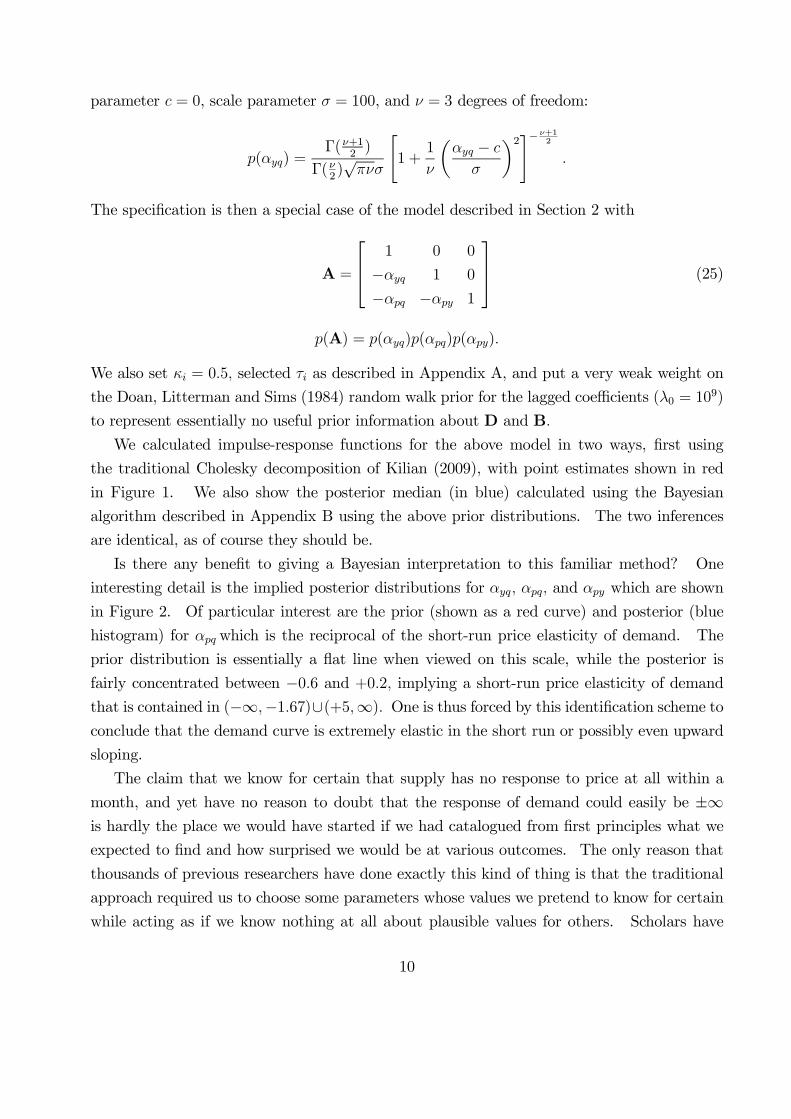
We calculated impulse-response functions for the above model in two ways, first using

the traditional Cholesky decomposition of Kilian (2009), with point estimates shown in red

in Figure 1. We also show the posterior median (in blue) calculated using the Bayesian

algorithm described in Appendix B using the above prior distributions. The two inferences

are identical, as of course they should be.

Is there any benefit to giving a Bayesian interpretation to this familiar method? One

interesting detail is the implied posterior distributions for αyq, αpq, and αpy which are shown

in Figure 2. Of particular interest are the prior (shown as a red curve) and posterior (blue

histogram) for αpq which is the reciprocal of the short-run price elasticity of demand. The

prior distribution is essentially a flat line when viewed on this scale, while the posterior is

fairly concentrated between −0.6 and +0.2, implying a short-run price elasticity of demandthat is contained in (−∞,−1.67)∪(+5,∞). One is thus forced by this identification scheme toconclude that the demand curve is extremely elastic in the short run or possibly even upward

sloping.

The claim that we know for certain that supply has no response to price at all within a

month, and yet have no reason to doubt that the response of demand could easily be ±∞is hardly the place we would have started if we had catalogued from first principles what we

expected to find and how surprised we would be at various outcomes. The only reason that

thousands of previous researchers have done exactly this kind of thing is that the traditional

approach required us to choose some parameters whose values we pretend to know for certain

while acting as if we know nothing at all about plausible values for others. Scholars have

10

unfortunately been trained to believe that such a dichotomization is the only way that one

could approach these matters scientifically.

The key feature in the data that forces us to impute such unlikely values for the demand

elasticity is the very low correlation between the reduced-form residuals for qt and pt. If we

assume that innovations in qt represent pure supply shifts, the lack of response of price would

force us to conclude that the demand curve is extremely flat and possibly even upward sloping.

3.2 A Bayesian interpretation of sign-restricted VARs.

Many researchers have recognized some of these unappealing aspects of the traditional ap-

proach to identification, and as a result have opted instead to use assumptions such as sign

restrictions to try to draw a structural inference in VARs. Examples include Baumeister and

Peersman (2013a) and Kilian and Murphy (2012), who began with the primitive assumptions

that (1) a favorable supply shock (increase in u1t) leads to an increase in oil production, in-

crease in economic activity, and decrease in oil price; (2) an increase in aggregate demand

or productivity (increase in u2t) leads to higher oil production, higher economic activity, and

higher oil price; and (3) an increase in oil-specific demand leads to higher oil production, lower

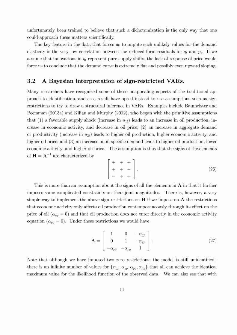
economic activity, and higher oil price. The assumption is thus that the signs of the elements

of H = A−1 are characterized by

+ + +

+ + −− + +

. (26)

This is more than an assumption about the signs of all the elements in A in that it further

imposes some complicated constraints on their joint magnitudes. There is, however, a very

simple way to implement the above sign restrictions on H if we impose on A the restrictions

that economic activity only affects oil production contemporaneously through its effect on the

price of oil (αqy = 0) and that oil production does not enter directly in the economic activity

equation (αyq = 0). Under these restrictions we would have

A =

1 0 −αqp0 1 −αyp

−αpq −αpy 1

. (27)

Note that although we have imposed two zero restrictions, the model is still unidentified—

there is an infinite number of values for αqp, αyp, αpq, αpy that all can achieve the identicalmaximum value for the likelihood function of the observed data. We can also see that with

11

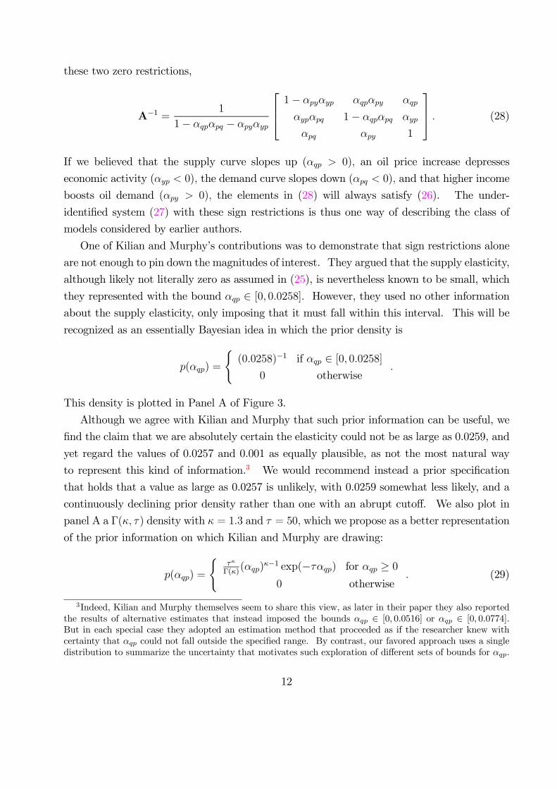
these two zero restrictions,

A−1 =1

1− αqpαpq − αpyαyp

1− αpyαyp αqpαpy αqp

αypαpq 1− αqpαpq αyp

αpq αpy 1

. (28)

If we believed that the supply curve slopes up (αqp > 0), an oil price increase depresses

economic activity (αyp < 0), the demand curve slopes down (αpq < 0), and that higher income

boosts oil demand (αpy > 0), the elements in (28) will always satisfy (26). The under-

identified system (27) with these sign restrictions is thus one way of describing the class of

models considered by earlier authors.

One of Kilian and Murphy’s contributions was to demonstrate that sign restrictions alone

are not enough to pin down the magnitudes of interest. They argued that the supply elasticity,

although likely not literally zero as assumed in (25), is nevertheless known to be small, which

they represented with the bound αqp ∈ [0, 0.0258]. However, they used no other informationabout the supply elasticity, only imposing that it must fall within this interval. This will be

recognized as an essentially Bayesian idea in which the prior density is

p(αqp) =

(0.0258)−1 if αqp ∈ [0, 0.0258]

0 otherwise.

This density is plotted in Panel A of Figure 3.

Although we agree with Kilian and Murphy that such prior information can be useful, we

find the claim that we are absolutely certain the elasticity could not be as large as 0.0259, and

yet regard the values of 0.0257 and 0.001 as equally plausible, as not the most natural way

to represent this kind of information.3 We would recommend instead a prior specification

that holds that a value as large as 0.0257 is unlikely, with 0.0259 somewhat less likely, and a

continuously declining prior density rather than one with an abrupt cutoff. We also plot in

panel A a Γ(κ, τ ) density with κ = 1.3 and τ = 50, which we propose as a better representation

of the prior information on which Kilian and Murphy are drawing:

p(αqp) =

τκ

Γ(κ)(αqp)

κ−1 exp(−ταqp) for αqp ≥ 00 otherwise

. (29)

3Indeed, Kilian and Murphy themselves seem to share this view, as later in their paper they also reportedthe results of alternative estimates that instead imposed the bounds αqp ∈ [0, 0.0516] or αqp ∈ [0, 0.0774].But in each special case they adopted an estimation method that proceeded as if the researcher knew withcertainty that αqp could not fall outside the specified range. By contrast, our favored approach uses a singledistribution to summarize the uncertainty that motivates such exploration of different sets of bounds for αqp.

12

Kilian and Murphy also explored the benefits of using prior information about the response

of economic activity to a change in price resulting from the third shock, arguing that we should

not expect this magnitude to be large, and presented results in which the product of the (2,3)

element of (28) with√d33 was restricted to fall in [−1.5, 0]. In terms of our motivating

structural model, this amounts to a complicated joint restriction on d33 and all the elements

of A, with some combinations ruled out with certainty but all combinations satisfying the

restrictions deemed equally likely. Again it seems more natural to approach such an idea

with a simple prior belief that the parameter αyp is small. We implemented this using a

gamma distribution with κ = 2.5 and τ = 10, shown in Panel B of Figure 3:

p(αyp) =

τκ

Γ(κ)(−αqp)κ−1 exp(ταyp) for αyp ≤ 0

0 otherwise. (30)

The figure also compares this with a prior distribution that insists that αypωpp ∈ [−1.5, 0],where ωpp = 5.44 is the square root of the (3,3) element of ΩT . Although this will not exactly

reproduce Kilian and Murphy’s method, it should be very similar.

By contrast, Kilian and Murphy do not use any prior information at all about the other

parameters (αpq and αpy), other than the sign restrictions mentioned above, for which we

again adopt the very uninformative Student t priors used in Section 3.1 now truncated by sign

restrictions. We then used the algorithm described in Appendix B to calculate the posterior

distribution given the prior

p(A) = p(αqp)p(αyp)p(αpq)p(αpy)

for p(aqp) given by (29), p(αyp) given by (30), p(αpq) a Student t (0,100,3) density truncated

by αpq < 0, and p(αpy) a Student t (0,100,3) density truncated by αpy > 0. The resulting

posterior medians for the impulse-response functions are shown in blue in Figure 4, and indeed

coincide almost exactly with the inference reported in Kilian and Murphy’s article calculated

using their original methodology, which is reproduced as the dashed red lines in Figure 4.4

Figure 5 compares prior and posterior distributions for the elements of A. The priors used

for αqp and αyp are quite tight and as a result the posterior distributions for these parameters

differ very little from the priors. By contrast, we have again used uninformative priors (apart

from sign restrictions) for αpq and αpy. We have now ruled out an upward-sloping demand

curve by assumption, but the specification would still lead the researcher to conclude that

4The dashed red lines were produced using the exact methodology of their paper, which is not the posteriormedian from their model.

13

monthly demand is extremely sensitive to the current price, with a 60% posterior probability

that the on-impact demand elasticity is greater than two in absolute value.

3.3 Do we really know nothing about the elasticity of demand?

In the two examples just discussed, the researchers implicitly proceeded as if we had extremely

reliable prior information about the supply elasticity but know nothing about the demand

elasticity in the first case and nothing but its sign in the second. In this section we argue

that in fact we have a great deal of useful information about the price-elasticity of petroleum

demand from other sources.

Figure 6 compares petroleum use per dollar of GDP with the price of gasoline in a cross-

section of 23 OECD countries.5 The relative price of gasoline differs substantially across

countries primarily due to differences in taxes. Residents in countries with higher taxes use

petroleum less, a finding that is well documented in the literature.6 The regression line in

the first panel of Figure 6 implies an absolute value for the demand elasticity of 0.51 with a

standard error of 0.23, statistically significantly greater than zero and less than one. Since

tax differentials tend to be stable over time, this coefficient is usually interpreted as a long-

run elasticity. For example, one obtains virtually the same regression if 2004 consumption is

regressed on 2000 prices, as seen in the second panel of Figure 6.

There also can be no doubt that the short-run price elasticity of demand is substantially

less than the long-run elasticity. Consider for example the evidence in Figure 7. The average

real retail price of gasoline doubled in the United States between 2002 and 2008, with the

price in 2013 still about what it was in 2008. But the average fuel economy of new vehicles

sold only increased 9% between 2002 and 2008, and increased an additional 14% after 2008.

Of course changes in the fuel economy of the average car on the road increased much more

slowly than that for new vehicles sold, as seen in the bottom panel of Figure 7. The changes

in petroleum demand that we would expect within one month of a change in price should be

significantly smaller than the long-run adjustments implied by the regression lines in Figure

6.

A huge literature has tried to estimate the long-run elasticity of gasoline demand. Haus-

man and Newey’s (1995) estimate from a cross-section of U.S. households was −0.81, while5Data for the price of gasoline and real GDP are from worldbank.org and data for petroleum consumption

are from the EIA’s Monthly Energy Review (Table 11.2). Countries included are Australia, Austria, Belgium,Canada, Denmark, Finland, France, Germany, Greece, Iceland, Ireland, Italy, Japan, the Netherlands, NewZealand, Norway, Portugal, South Korea, Spain, Sweden, Switzerland, the United Kingdom and the UnitedStates.

6See for example Darmstadter, Dunkerly, and Alterman (1977), Drollas (1984), and Davis (2014).

14

Yatchew and No’s (2001) study of a cross-section of Canadian households came up with −0.9.Dahl and Sterner’s (1991) survey of this literature suggested a consensus value of −0.86. Es-pey’s (1998) literature review came up with −0.58; Graham and Glaister (2004) settled on

−0.77, while Brons et al. (2008) proposed −0.84. Insofar as taxes and refining costs are asignificant component of the user cost for refined products, a 10% increase in the price of crude

petroleum should result in a less than 10% increase in the retail price of gasoline, meaning

that the price-elasticity of demand for crude oil should be less than that for gasoline. This

is indeed confirmed in the smaller literature on estimating the elasticity of oil demand. For

example, Dahl’s (1993) survey of the literature on developing countries estimated the long-run

elasticity at −0.30. We conclude that short-run oil demand elasticities above two in absolutevalue, such as were implied by the reciprocals of αpq in Figures 2 and 5, are highly implausible.

7

On the supply side, while it is true that most producers have limited immediate response

to changes in price incentives, some countries like Saudi Arabia historically have made quite

significant high-frequency adjustments to changing market conditions. Figure 8 shows that in

response to weaker demand during the recession of 1981-82, the kingdom reduced production

by 6 million barrels per day, implementing by itself an 11% drop in total global production.

The Saudis initiated another production decrease of 1.6 mb/d in December 2000 (a few months

before the U.S. recession started in March of 2001) and only started to increase production

in March of 2002 (four months after the recession had ended). The 1.6 mb/d drop in Saudi

production between June 2008 and February 2009 was another clear response to market con-

ditions in an effort to stabilize prices. Equally dramatic in the graph are the rapid increases

in Saudi production beginning in August 1990 and January 2003 which were intended to offset

some of the anticipated lost production from Iraq associated with the two Gulf Wars. Thus

although the response of global production to price increases within the month is likely small,

there does not seem to be a solid a priori basis for assuming that it would be significantly

smaller than the monthly response of demand.

4 Inventories and measurement error.

Kilian and Murphy (2014) note that another important factor in interpreting short-run co-

movements of quantities and prices is the behavior of inventories. Increased oil production

7An intriguing recent study by Coglianese et al. (forthcoming) used anticipated changes in gasoline taxesas a clever instrument. They estimated a short-run price-elasticity of U.S. gasoline demand of −0.37, with a95% confidence interval of (−0.85,+0.11).

15

in month t does not have to be consumed that month but might instead go into inventories:

QSt −QDt = ∆I∗t .

Here QDt is the quantity of oil demanded globally in month t, QSt is the quantity produced,

and ∆I∗t is the true change in global inventories. We append a * to the latter magnitude

in recognition of the fact that we have only imperfect observations on this quantity, the

implications of which we will discuss below.

Let qt = 100 ln(Qt/Qt−1) denote the observed monthly growth rate of production. We can

then approximate the growth in consumption demand as qt−∆i∗t for ∆i∗t = 100∆I∗t /Qt−1.Weare thus led to consider the following generalization of the system considered in Section 3.2:

qt = αqppt + b′

1xt−1 + u∗

1t (31)

yt = αyppt + b′

2xt−1 + u∗

2t (32)

qt = βqyyt + βqppt +∆i∗

t + b′

3xt−1 + u∗

3t (33)

∆i∗t = ψ∗

1qt + ψ∗

2yt + ψ∗

3pt + b∗′

4 xt−1 + u∗

4t. (34)

Here u∗1t, u∗

2t, and u∗

3t as before represent shocks to oil supply, economic activity, and oil-

specific demand, with the modification to equation (33) acknowledging that oil produced but

not consumed in the current period goes into inventories. The shock u∗4t in (34) represents

a separate shock to inventory demand, which has sometimes been described as a “speculative

demand shock” in the literature.

As noted above, we do not have good data on global oil inventories. There are data on

U.S. crude oil inventories and monthly OECD refined-product inventories, from which we can

construct a measure of crude oil inventories for OECD countries as in Kilian and Murphy

(2014, footnote 6); for details see Appendix C. We represent the fact that these numbers are

an imperfect measure of the true magnitude through a measurement-error equation

∆it = χ∆i∗

t + et (35)

where ∆it denotes our estimate of the change in OECD crude-oil inventories as a percent of

the previous month’s world production, χ < 1 is a parameter representing the fact that OECD

inventories are only part of the world total, and et reflects measurement error. Although the

problem of having imperfect measurements on key variables is endemic in macroeconomics, it

has been virtually ignored in most of the large literature on structural vector autoregressions

16

because it was not clear how to allow for it using traditional methods.8 However, it is

straightforward to incorporate measurement error in our Bayesian framework, as we now

demonstrate.

We can use (35) to rewrite (33) and (34) in terms of observables:

qt = βqyyt + βqppt + χ−1∆it + b

′

3xt−1 + u∗

3t − χ−1et (36)

∆it = ψ1qt + ψ2yt + ψ3pt + b′

4xt−1 + χu∗

4t + et (37)

where ψj = χψ∗

j for j = 1, 2, 3. Equations (31), (32), (36), and (37) will be recognized as a

system of the form

Ayt = Bxt−1 + ut (38)

yt = (qt, yt, pt,∆it)′

A =

1 0 −αqp 0

0 1 −αyp 0

1 −βqy −βqp −χ−1−ψ1 −ψ2 −ψ3 1

ut =

u∗1tu∗2t

u∗3t − χ−1etχu∗4t + et

.

Note that although we have explicitly modeled the role of measurement error in con-

tributing to contemporaneous correlations among the variables, we have greatly simplified the

analysis by specifying the lagged dynamics of the structural system directly in terms of the

observed variables. That is, we are defining xt−1 in (31)-(34) to be based on lags of ∆it−j

rather than ∆i∗t−j .

The system (38) is not quite in the form of (1) because even though the structural shocks

u∗jt are contemporaneously uncorrelated, the observed analogues ujt will be correlated as a

8Notable exceptions are Cogley and Sargent (2015) who allowed for measurement error using a state-spacemodel and Amir-Ahmadi, Matthes, and Wang (2015) who identified measurement error from the differencebetween preliminary and revised data.

17

result of the measurement error:

D =E(utu′

t) =

d∗11 0 0 0

0 d∗22 0 0

0 0 d∗33 + χ−2σ2e −χ−1σ2e

0 0 −χ−1σ2e χ2d∗44 + σ2ε

. (39)

However, it’s not hard to see that ΓDΓ′

= D is diagonal for

Γ =

1 0 0 0

0 1 0 0

0 0 1 0

0 0 ρ 1

ρ =χ−1σ2e

d∗33 + χ−2σ2e

. (40)

We can thus write (38) in the form of (1) simply by defining A = ΓA, B = ΓB, and

ut = Γut =

u∗1tu∗2t

u∗3t − χ−1etχu∗4t + ρu

∗

3t + (1− ρ/χ)et

(41)

whose variance matrix we denote D = diag(d11, d22, d33, d44). This is then exactly in the form

of the general class of models discussed in Section 2. Specifically, we summarize any prior

information about the contemporaneous coefficients in terms of the prior distribution

p(A) = p(ρ)p(αqp)p(αyp)p(βqy)p(βqp)p(χ)p(ψ1)p(ψ2)p(ψ3)

and then follow exactly the methods in Appendix B for inference about D and B to generate

posterior draws from p(A,D,B|YT ).

5 Inference for a 4-variable model with inventories and

measurement error.

In addition to making use of the prior information about price elasticities reviewed in Section

3.3, we propose to use prior information about coefficients involving the economic activity

18

measure yt. For this purpose it is very helpful to use a more conventional measure of economic

activity in place of the proxy based on shipping costs that was used in Kilian (2009) and Kilian

and Murphy (2012, 2014); among other benefits this allows us to draw directly on information

about income elasticities from previous studies. We developed an extended version of the

OECD’s index of monthly industrial production in the OECD and 6 major other countries as

described in Appendix C.

Of course, even more important than having good prior information is having more data.

Kilian (2009) and Kilian and Murphy (2012) used the refiner acquisition cost as the measure

of crude oil prices. Their series begins in January 1973. Taking differences and including

24 lags means that the first value for the dependent variable in their regressions is February

1975. Thus their analysis makes no use of the important economic responses in 1973 and

1974 to the large oil price increases at the time, nor any earlier observations.

Kilian and Vigfusson (2011) argued that use of the older data is inappropriate since struc-

tural relations may have changed over time, suggesting that this is a reason to ignore the

earlier data altogether. Moreover, their preferred oil price measure (U.S. refiner acquisition

cost, or RAC) is not available before 1974, which might seem to make use of earlier data

infeasible. Here again the Bayesian approach offers a compelling advantage, in that we can

use results obtained from estimating the model using earlier data for the price of West Texas

Intermediate as a prior for the analysis of the subsequent RAC data, putting as much or as

little weight as desired on the earlier data set. We describe how this can be done below.

5.1 Informative priors for structural parameters.

This section summarizes the prior information used in our structural inference about the

system (31)-(34).

5.1.1 Priors for A.

The discussion of the evidence from separate data sets in Section 3.3 leads us to expect that

both the short-run demand elasticity βqp and the short-run supply elasticity αqp should be small

in absolute value. We represent this with a prior for βqp that is a Student t(cβqp, σ

βqp, ν

βqp) with

mode at cβqp = −0.1, scale parameter σβqp = 0.2, νβqp = 3 degrees of freedom, and truncated

to be negative. Our prior for αqp is Student t(cαqp, σ

αqp, ν

αqp) with mode at c

αqp = 0.1, scale

parameter σαqp = 0.2, ναqp = 3 degrees of freedom, and truncated to be positive.

Because we use a conventional measure of industrial production we are able to make use

of other evidence about the income elasticity of oil demand. Gately and Huntington (2002)

19

reported a nearly linear relationship between log income and log oil demand in developing

countries with elasticities ranging between 0.7 and 1, but smaller income elasticities in indus-

trialized countries with values between 0.4 and 0.5. For oil-exporting countries they found

an income elasticity closer to 1. Csereklyei, Rubio, and Stern (2016) found that the income

elasticity of energy demand is remarkably stable across countries and across time at a value of

around 0.7. For our prior for βqy we use a Student t density with mode at 0.7, scale parameter

0.2, 3 degrees of freedom, and truncated to be positive.

We expect the effect of oil prices on economic activity αyp to be small given the small

dollar share of crude oil expenditures compared to total GDP (see for example the discussion

in Hamilton, 2013). We represent this with a Student t distribution with mode −0.05, scale0.1, 3 degrees of freedom, and truncated to be negative.

The parameter χ reflects the fraction of total world inventories that are held in OECD

countries. Since OECD countries account for around 60% of world petroleum consumption

on average over our sample period, a natural expectation is that they also account for about

60% of global inventory. Since χ is necessarily a fraction between 0 and 1, we use a Beta

distribution with parameters αχ = 15 and βχ = 10, which has mean 0.6 and standard deviation

of about 0.1.

For the parameters of the inventory equation, we assume that inventories depend on income

only through the effects of income on quantity or price. This allows us to set ψ2 = 0 to help

with identification. We use relatively uninformative priors for the other coefficients, taking

both ψ1 and ψ3 to be unrestricted Student t centered at 0 with scale parameter 0.5, and 3

degrees of freedom.

The parameter ρ in (40) captures the importance of inventory measurement error and is

also between 0 and 1 by construction. For this we use a Beta distribution with parameters

αρ = 3 and βρ = 9, which has a mean of 0.25 and standard deviation of 0.12.

The prior for the contemporaneous coefficients is then the product of the above densities:

p(A) = p(αqp)p(αyp)p(βqy)p(βqp)p(χ)p(ψ1)p(ψ3)p(ρ)

subject to the sign restrictions described above.

5.1.2 Priors for D given A.

Our priors for the reciprocals of the structural variances are independent Gamma distributions,

d−1ii |A ∼ Γ(κ, τi(A)), that reflect the scale of the data as measured by the standard deviationof 12th-order univariate autoregressions fit to the 4 elements of yt over t = 1, ..., T1 for T1

20

the number of observations in the earlier sample. Letting S denote the estimated variance-

covariance matrix of these univariate residuals, we set κ = 2 (which give the priors a weight

of about 4 observations in the first subsample) and τi(A) = κa′

iSai where a′

i denotes the ith

row of A.

5.1.3 Priors for B given A and D.

Our priors for the lagged coefficients in the ith structural equation are independent Normals,

bi|A,D ∼ N(mi, diiM). Our prior expectation is that the best predictor of the current oil

production, economic activity, oil price, or inventory level is its own lagged value, implying

that most coefficients for predicting the first-differences in these variables are zero. We allow

for the possibility that the 1-period-lag response of supply or demand to a price increase could

be similar to the contemporaneous magnitudes, and for this reason set the third element of

m1 to +0.1 and the third element of m3 to −0.1; this gives us a little more information totry to distinguish supply and demand shocks. All other elements of mi are set to zero for

i = 1, ..., 4. For M, which governs the variances of these priors, we follow Doan, Litterman

and Sims (1984) in having more confidence that coefficients on higher lags are zero. We

implement this by setting diagonal elements ofM to the values specified in equation (43) and

other elements of M to zero, as detailed in Appendix A. For our baseline analysis, we use a

value of λ0 = 0.5 to control the overall informativeness of these priors on lagged coefficients,

which amounts to weighting the prior on the lag-one coefficients equal to about 2 observations.

5.1.4 Using observations from an earlier sample to further inform the prior.

We propose to use observations over 1958:M1 to 1975:M1 to further inform our prior. The

observation vector yt for date t in this first sample consists of the growth rate of world oil

production, growth rate of OECD+6 industrial production, growth rate of WTI, and change

in estimated OECD inventories as a percent of the previous month’s oil production. We have

T1 observations in the first sample for this (n× 1) vector ytT1t=1 and associated (nm+1× 1)vector of lagged values and the constant term xt−1T1t=1. For the second sample (1975:M2

to 2014:M12) we use the percent change in the refiner acquisition cost (RAC) for the third

element of yt for which we have observations yt,xt−1T1+T2t=T1+1. Denote the observations for

the first sample by Y(1) and those for the second sample by Y(2) and collect all the unknown

elements of A, D, and B in a vector λ.

If we regarded both samples as equally informative about λ we could simply collect all the

data in a single sample YT = Y(1),Y(2) and apply our method directly to find p(λ|YT ).

This would be numerically identical to using our method to find the posterior distribution from

21

the first sample alone p(λ|Y(1)) and then using this distribution as the prior for analyzing the

second sample (see Appendix D for demonstration of this and subsequent claims). We propose

instead to use as a prior for the second sample an inference that downweights the influence

of the first-sample data Y(1) by a factor 0 ≤ µ ≤ 1. When µ = 1 the observations in the

first sample are regarded as equally important as those in the second, while when µ = 0 the

first sample is completely discarded. Our baseline analysis below sets µ = 0.5, which regards

observations in the first sample as only half as informative as those in the second.

Implementing this procedure requires a simple modification of the procedure described in

Section 2.2. We replace equations (8), (9) and (5) with

Yi(A)(T1+T2+k)×1

= (√µy′1ai, ...,

√µy′T1ai,y

′

T1+1ai, ...,y

′

T1+T2ai,mi

′P)′

X(T1+T2+k)×k

= √

µx0 · · · √µxT1−1 xT1 · · · x′T1+T2−1 P

′

κ∗ = κ+ (µT1 + T2)/2

for P the matrix whose diagonal elements are reciprocals of the square roots of (43). We then

calculate τ ∗i (A) and ζ∗

i (A) using expressions (6) and (7) and replace (12) and (13) with

p(A|YT ) =kTp(A)[det(AΩTA

′)](µT1+T2)/2ni=1[2τ

∗

i (A)/(µT1 + T2)]κ∗i

ni=1τi(A)

κi

ΩT = (µT1 + T2)−1(µζ(1) + ζ(2))

ζ(1) =T1

t=1yty′

t −T1

t=1ytx′

t−1

T1t=1xt−1x

′

t−1

−1 T1

t=1xt−1y′

t

ζ(2) =T2

t=T1+1yty

′

t −T2

t=T1+1ytx

′

t−1

T2t=T1+1

xt−1x′

t−1

−1 T2

t=T1+1xt−1y

′

t

.

For example, if we put zero weight on the Minnesota prior for the lagged structural coef-

ficients (P = 0) this would amount to using as a prior for the second sample

bi|A,D ∼ N(a′iΦ(1), µ−1diiM(1))

Φ(1) =T1

t=1ytx′

t−1

T1t=1xt−1x

′

t−1

−1

M(1) =T1

t=1xt−1x′

t−1

−1

.

Thus the mean for the prior used to analyze the second sample (a′iΦ(1)) would be the coefficient

from an OLS regression on the first sample. When µ = 1 our confidence in this prior comes

22

from the variance of the OLS regression estimate (diiM(1)), but the variance increases as µ

decreases. As µ approaches 0 the variance of the prior goes to infinity and the information

in the first sample would be completely ignored.

Likewise with no information about the structural variances other than the estimates from

the first sample (κ = τ = 0), the prior for the structural variances that we would use for the

second sample would be

d−1ii |A ∼ Γ(µT1, µ(a′iζ(1)ai)).

Again the mean of this distribution is the first-sample OLS estimate (T1/(a′

iζ(1)ai)) but the

variance goes to infinity as µ→ 0.

5.2 Empirical results.

The solid red curves in Figure 9 denote the priors in p(A) that we used for the contemporaneous

coefficients. The posterior distribution with the pre-1975 observations downweighted by

µ = 0.5 are reported as blue histograms in Figure 9.

The posterior median of the short-run supply price elasticity, αqp, is 0.16, a little higher

than anticipated by our prior. Values less than 0.05 or greater than 0.5 are substantially less

plausible after seeing the data than anticipated by our prior. The posterior median of the

short-run demand price elasticity, βqp, is −0.35, significantly more elastic than anticipated byour prior. But the data do not help us make a definitive statement about either parameter

beyond telling us that values near zero can likely be ruled out for both parameters.

The data also do not give us much information about the short-run income elasticity of

demand, βqy. The fraction χ of world inventories that is captured by our proxy may be slightly

larger than we anticipated, and ρ, which summarizes the importance of this measurement error,

is a little smaller than anticipated. Our prior for αyp, the short-run impact of oil prices on

economic activity, forced this coefficient to be negative. The data evidently favor a positive

value, causing the posterior to bunch near values just below zero.

Posterior structural impulse-response functions are plotted in Figure 10.9 An oil supply

shock (first row) lowers oil production and raises oil price on impact, whereas a shock to oil

consumption demand (third row) raises production and raises price. These four effects were

imposed by assumption as a result of the sign restrictions embedded in our priors. An oil

supply shock also leads to a significant decline in economic activity, though only after a lag

of a number of months, a result found in a large number of studies going back to Hamilton

9Note following standard practice these are accumulated impulse-response functions, plotting elements of(H0 +H1 + · · ·+Hs) as a function of s where Hs is given in (18). For example, panel (1,3) shows the effecton the level of oil prices s periods after an oil supply shock.

23

(1983). By contrast, if oil prices rise as a consequence of a shock to consumption demand,

there seems to be no effect on subsequent economic activity. An increase in oil prices that

results from an increase in inventory demand alone, which has sometimes been described as

a speculative demand shock, seems to have a persistent effect on both inventories and prices

and, after a long lag, a negative effect on economic activity as well.

Figure 11 shows the historical decomposition of oil price movements along with 95% cred-

ibility regions.10 Supply shocks were the biggest factor in the oil price spike in 1990, whereas

demand was more important in the price run-up in the first half of 2008. All four structural

shocks contributed to the oil price drop in 2008:H2 and rebound in 2009, but apart from this

episode, economic activity shocks and speculative demand shocks were usually not a big factor

in oil price movements. Interestingly, demand is judged to be a little more important than

supply in the price collapse of 2014:H2.11

Table 1 summarizes variance decompositions, reporting how much of the mean squared

error associated with a 12-month-ahead forecast of each of the four variables in the system

(represented by different columns of the table) is attributed to each of the four structural shocks

(represented by different rows).12 Oil supply shocks are the biggest single factor accounting

for movements in oil production, while oil supply and oil consumption demand shocks are

equally important in accounting for price changes. Consumption demand shocks are often

buffered by inventories, but supply shocks much less so. Oil-market factors, as represented

by the first, third, and fourth shocks combined, account for only 10% of the variation in world

industrial production.

5.3 Sensitivity analysis.

The above results achieved partial identification by drawing on a large number of different

sources of information. One benefit of using multiple sources is that we can examine the

10To our knowledge, the latter have never before been calculated in the large previous literature on sign-restricted vector autoregressions. The figure plots the contribution of the current and s = 100 previousstructural shocks to the value of yt for each date t plotted.11In comparing Figures 10 and 11, recall that Figure 10 plots the response to a 1-unit increase in the specified

structural shock, for example a shock to u∗2t that increases economic activity by 1% or a shock to u∗3t thatincreases real oil demand by 1%. The former corresponds almost to a 2-standard deviation event (the medianposterior value of (d∗22)

−0.5 is 0.54) while the latter is less than a third of one standard deviation (the medianposterior value of (d∗33)

−0.5 is 3.25). A 2-standard-deviation shock to u∗2t has a bigger effect of pt+s than a1/3-standard-deviation shock to u∗3t (as seen in the (2,3) and (3,3) panels of Figure 10) even though typicallyshocks to u∗3t are more important than shocks to u

∗2t in accounting for fluctuations in prices (as seen in the

second and third panels of Figure 11).12Note that these refer to forecasts of the variables as defined in yt, e.g., 12-month-ahead forecasts of the

rate of growth of oil prices as opposed to forecasts of the level of oil prices. At the 12-month horizon theseare very close to decompositions of the unconditional variance of the monthly change in oil prices.

24

effects of putting less weight on any specified components of the prior to see how it affects the

results.

Table 2 presents the posterior median and posterior 95% credibility sets for some of the

magnitudes of interest under alternative specifications for the prior. The first column presents

results from the baseline specification that were just summarized. Rows 1 and 2 report

inference about the short-run supply elasticity αqp and demand elasticity βqp. Row 3 looks

at the response of economic activity 12 months after a supply shock, row 4 the response to

an oil consumption demand shock, and row 5 the response to a speculative demand shock,

with each shock normalized for purposes of the table as an event that leads to a 1% increase

in the real oil price at time 0. Note that this is a different normalization from that used

in Figure 10, where the effect plotted was that of a one-unit change in the structural shock

∂yi,t+s/∂u∗

jt.13 Rows 6-8 look at the variance decomposition for the error forecasting the real

price of oil 12 months ahead, reporting the contribution to this variance of oil supply shocks,

economic activity shocks, and oil consumption demand shocks, respectively.

Table 3 reports a few summary statistics for the historical decomposition. Column 2

reports the actual cumulative magnitude of the oil price change (as measured by the refiner

acquisition cost) in three important episodes in the sample: the price collapse over January

to July 1986, the price run-up over January to June 2008, and the price collapse from July

to December 2014. Column 3 reports the posterior median and 95% credibility sets for the

predicted change over that interval if the only structural shocks had come from the oil supply

equation as inferred using the baseline prior.14 According to the baseline specification, supply

shocks accounted for about 46% of the price drop in 1986 but only 32% of the price drop in

2014:H2. The 95% credibility interval for the latter does not exceed 63%— factors in addition

to strong supply growth clearly contributed to the most recent oil price decline. Demand

factors were the single most important factor in the first half of 2008, accounting for 54% of

the run-up in prices observed at that time.

We next explored the consequences of using a much weaker prior for the short-run supply

and demand elasticities, replacing the scale parameter of σαqp = σβqp = 0.2 that was used in

the baseline analysis with the values σαqp = σβqp = 1.0. This change gives the prior for these

two parameters a variance that is 25 times larger than in the baseline specification. The

13Calculating the size of a shock that in equilibrium raises the price of oil by 1% potentially requires makinguse of all the parameters in A and D. For this reason, credibility sets for the magnitudes defined in rows 3-5of Table 2 are typically wider than those for the magnitudes plotted in Figure 10.14For example, column 2 reports the third element of yt1 + yt1−1 + · · · + yt0 for t0 = 1986:M1 and t1 =

1986:M7 while column 3 reports the median and 95% credibility interval across draws of θ(ℓ) for the thirdelement of ξj,t1,t0(YT ;θ

(ℓ)) + ξj,t1−1,t0(YT ;θ(ℓ)) + · · · + ξj,t0,t0(YT ;θ

(ℓ)) for ξj,t,t−s(YT ;θ) calculated from(21).

25

implications of these changes for inference about key parameters are reported in column 2 of

Table 2. If we had very little prior information about the elasticities themselves, we would

tend to infer a smaller short-run supply elasticity (row 1) and more elastic demand (row 2).

Our key conclusions about impulse responses (rows 3-5) would change very little. If we relied

less on prior information about the supply and demand elasticities, our point estimates would

imply a smaller role for supply shocks and a bigger role for demand shocks (rows 6 and 8

of Table 2). Note that credibility sets for the contributions to individual episodes become

significantly wider if we make less use of information about supply and demand elasticities

(see column 4 of Table 3). We nevertheless would still have 95% posterior confidence that

supply shocks contributed no more than 66% to the oil price decline in the second half of 2014.

Our prior beliefs about the role of measurement error were represented by the Beta(αχ, βχ)

distribution for χ (which summarizes the ratio of OECD inventories to world total) and

Beta(αρ, βρ) distribution for ρ (which summarizes the component of the correlation between

price and inventory changes that is attributed to measurement error). Our baseline specifica-

tion used αχ = 15, βχ = 10, αρ = 3, βρ = 9, which imply standard deviations for the priors of

0.1 and 0.12, respectively. In our less informative alternative specification we take αχ = 1.5,

βχ = 1, αρ = 1, βρ = 3, whose standard deviations are 0.26 and 0.19, respectively (recall that

each variable by definition is known to fall between 0 and 1). The implications of this weaker

prior about the role of measurement error are reported in column 3 of Table 2 and column 5

of Table 3. These results are uniformly very close to those for our baseline specification.

Next we examined the consequences of paying less attention to data prior to 1975. Our

baseline specification set µ = 0.5, which gives pre-1975 data half the weight of the more recent

data. Our less informative alternative uses µ = 0.25, thus regarding the earlier data as only

1/4 as important as the more recent numbers. The inferences are virtually identical to those

under our baseline specification.

The role of prior information about lagged structural coefficients bi is summarized by the

value of λ0 in (43). An increase in λ0 increases the variance on all the priors involving the

lagged coefficients. Our baseline specification took λ0 = 0.5, whereas the weaker value of

λ0 = 1 (which implies a variance 4 times as large) was used in column 5 of Table 2 and column

7 of Table 3. This has only a modest effect on any of the inferences.

The weight on prior information about structural variances is captured by the value of κ in

equation (5). Our baseline specification used κ = 2, which gives the prior a weight of about

4 observations. The alternative in column 6 of Table 2 and column 8 of Table 3 uses κ = 0.5.

This does not matter for any of the conclusions.

Finally, in making use of the historical data we relied on West Texas Intermediate as our

26

measure of the crude oil price prior to 1975, since the refiner acquisition cost is unavailable.

But our baseline analysis nevertheless used RAC as the oil price measure since 1975. An

alternative is to use WTI for both samples. Column 9 of Table 3 reports the measured size of

the oil price change recorded by WTI in three episodes of interest. The two oil price measures

can give quite different answers for the size of the move in any given month. Nevertheless, the

inference about key model parameters (column 7 of Table 2) is the same regardless of which

oil price measure we use.

6 Conclusion.

Prior information has played a key role in every structural analysis of vector autoregressions

that has ever been done. Typically prior information has been treated as "all or nothing",

which from a Bayesian perspective would be described as either dogmatic priors (details that

the analyst claims to know with certainty before seeing the data) or completely uninformative

priors. In this paper we noted that there is vast middle ground between these two extremes.

We advocate that analysts should both relax the dogmatic priors, acknowledging that we have

some uncertainty about the identifying assumptions themselves, and strengthen the uninfor-

mative priors, drawing on whatever information may be known outside of the dataset being

analyzed.

We illustrated these concepts by revisiting the role of supply and demand shocks in oil

markets. We demonstrated how previous studies can be viewed as a special case of Bayesian

inference and proposed a generalization that draws on a rich set of prior information beyond

the data being analyzed while simultaneously relaxing some of the dogmatic priors implicit in

traditional identification. Notwithstanding, we end up confirming some of the core conclusions

of earlier studies. We find that oil price increases that result from supply shocks lead to a

reduction in economic activity after a significant lag, whereas price increases that result from

increases in oil consumption demand do not have a significant effect on economic activity. We

also examined the sensitivity of our results to the priors used, and found that many of the key

conclusions change very little when substantially less weight is placed on various components

of the prior.

27

References

Amir-Ahmadi, Pooyan, Christian Matthes, and Mu-Chun Wang (2015). "Measurement

Errors and Monetary Policy: Then and Now," working paper, Goethe University Frankfurt.

Baumeister, Christiane, and James D. Hamilton (2015a). "Sign Restrictions, Structural

Vector Autoregressions, and Useful Prior Information," Econometrica 83: 1963—1999.

Baumeister, Christiane, and James D. Hamilton (2015b). "Optimal Inference about Impulse-

Response Functions and Historical Decompositions in Incompletely Identified Structural Vec-

tor Autoregressions," working paper, UCSD.

Baumeister, Christiane, and Gert Peersman (2013a). "The Role of Time-Varying Price

Elasticities in Accounting for Volatility Changes in the Crude Oil Market," Journal of Applied

Econometrics 28: 1087-1109.

Baumeister, Christiane, and Gert Peersman (2013b). "Time-Varying Effects of Oil Supply

Shocks on the US Economy," American Economic Journal: Macroeconomics 5: 1-28.

Brons, Martijn, Peter Nijkamp, Eric Pels, and Piet Rietveld (2008). "A Meta-Analysis of

the Price Elasticity of Gasoline Demand: A SUR Approach," Energy Economics 30: 2105-

2122.

Cogley, Timothy, and Thomas J. Sargent (2015), "Measuring Price-Level Uncertainty and

Instability in the U.S., 1850-2012," Review of Economics and Statistics 97: 827-838.

Coglianese, John, Lucas W. Davis, Lutz Kilian, and James H. Stock (forthcoming). "An-

ticipation, Tax Avoidance, and the Price Elasticity of Demand," Journal of Applied Econo-

metrics.

Csereklyei, Zsuzsanna, Maria del Mar Rubio Varas and David Stern (2016). "Energy and

Economic Growth: The Stylized Facts," Energy Journal 37: 223-255.

Dahl, Carol A. (1993). "A Survey of Oil Demand Elasticities for Developing Countries,"

OPEC Review 17: 399-419.

Dahl, Carol and Thomas Sterner (1991). "Analysing Gasoline Demand Elasticities: A

Survey," Energy Economics 13: 203-210.

Darmstadter, Joel, Joy Dunkerly, and Jack Alterman (1977). How Industrial Societies Use

Energy: A Comparative Analysis, Baltimore: Johns Hopkins University Press.

Davis, Lucas W. (2014). "The Economic Cost of Global Fuel Subsidies," American Eco-

nomic Review: Papers and Proceedings 104: 581-585.

Doan, Thomas, Robert B. Litterman, and Christopher A. Sims (1984). "Forecasting and

Conditional Projection Using Realistic Prior Distributions," Econometric Reviews 3: 1-100.

Doan, Thomas (2013). RATS User’s Guide, Version 8.2, www.estima.com.

28

Drollas, Leonidas (1984). "The Demand for Gasoline: Further Evidence," Energy Eco-

nomics 6: 71-83.

Espey, Molly (1998). "Gasoline Demand Revisited: An International Meta-Analysis of

Elasticities," Energy Economics 20: 273-295.

Gately, Dermot, and Hillard G. Huntington (2002). "The Asymmetric Effects of Changes

in Price and Income on Energy and Oil Demand," Energy Journal 23: 19-55.

Graham, Daniel J., and Stephen Glaister (2004). "Road Traffic Demand Elasticity Esti-

mates: A Review," Transport Reviews 24: 261-274.

Hamilton, James D. (1983). "Oil and the Macroeconomy Since World War II," Journal of

Political Economy, 91(2): 228-248.

Hamilton, James D. (1994). Time Series Analysis. Princeton: Princeton University Press.

Hamilton, James D. (2013). "Oil Prices, Exhaustible Resources, and Economic Growth,"

in Handbook on Energy and Climate Change, pp. 29-63, edited by Roger Fouqet, Cheltenham,

United Kingdom: Edward Elgar Publishing.

Hausman, Jerry A. and Whitney K. Newey (1995). "Nonparametric Estimation of Exact

Consumers Surplus and Deadweight Loss," Econometrica 63: 1445-1476.

Kilian, Lutz (2009). "Not All Oil Price Shocks Are Alike: Disentangling Demand and

Supply Shocks in the Crude Oil Market," American Economic Review 99: 1053-1069.

Kilian, Lutz, and Daniel P. Murphy (2012). "Why Agnostic Sign Restrictions Are Not

Enough: Understanding the Dynamics of Oil Market VAR Models," Journal of the European

Economic Association 10(5): 1166-1188.

Kilian, Lutz, and Daniel P. Murphy (2014). "The Role of Inventories and Speculative

Trading in the Global Market for Crude Oil," Journal of Applied Econometrics 29: 454-478.

Kilian, Lutz, and Robert J. Vigfusson (2011). "Nonlinearities in the Oil Price-Output

Relationship," Macroeconomic Dynamics 15(Supplement 3): 337—363.

Sims, Christopher A., and Tao Zha (1998). "Bayesian Methods for Dynamic Multivariate

Models," International Economic Review 39: 949-968.

Yatchew, Adonis and Joungyeo Angela No (2001). "Household Gasoline Demand in

Canada," Econometrica 69: 1697-1709.

29

Appendix

A. Reference priors for D and B.Prior for D|A. Prior beliefs about structural variances should reflect in part the scale of

the underlying data. Let eit denote the residual of an mth-order univariate autoregression fit

to series i and S the sample variance matrix of these univariate residuals (sij = T−1T

t=1eitejt).

Baumeister and Hamilton (2015a) proposed setting κi/τi (the prior mean for d−1ii ) equal to

the reciprocal of the ith diagonal element of ASA′; in other words, τi(A) = κia′

iSai. Given

equation (5), the prior carries a weight equivalent to 2κi observations of data; for example,

setting κi = 2 would give the prior as much weight as 4 observations.

Prior for B|A,D. A standard prior for many data sets suggested by Doan, Litterman andSims (1984) is that individual series behave like random walks. Baumeister and Hamilton

(2015a, equation 45) adapted Sims and Zha’s (1998) method for representing this in terms of

a particular specification for mi(A). For other data sets, such as the one analyzed in Section

5, a more natural prior is that series behave like white noise (mi = 0). For either case, we

recommend following Doan, Litterman and Sims (1984) in placing greater confidence in our

expectation that coefficients on higher lags are zero, implemented by using smaller values for

the diagonal elements forMi associated with higher lags. Define

v′1(1×m)

=1/(12λ1

, 1/(22λ1), ..., 1/(m2λ1)) (42)

v′2(1×n)

= (s−111 , s−122 , ..., s

−1nn)

′

v3 = λ20

v1 ⊗ v2λ23

. (43)

ThenMi is taken to be a diagonal matrix whose (r, r) element is the rth element of v3:

Mi,rr = v3r. (44)

Here λ0 summarizes the overall confidence in the prior (with smaller λ0 corresponding to

greater weight given to the prior), λ1 governs how much more confident we are that higher

coefficients are zero (with a value of λ1 = 0 giving all lags equal weight), and λ3 is a separate

parameter governing the tightness of the prior for the constant term, with all λk ≥ 0.Doan (2013) discussed possible values for these parameters. For the baseline specification

in Section 5 we set λ1 = 1 (which governs how quickly the prior for lagged coefficients tightens

to zero as the lag ℓ increases), λ3 = 100 (which makes the prior on the constant term essentially

30

irrelevant), and set λ0, the parameter controlling the overall tightness of the prior, to 0.5.

B. Details of Bayesian algorithm.For any numerical value of A we can calculate ζ∗i (A) and τ

∗

i (A) using equations (7) and

(6) from which we can calculate the log of the target

q(A) = log(p(A)) + (T/2) logdet

AΩTA

′

(45)

−ni=1κ

∗

i log[(2/T )τ∗

i (A)] +n

i=1κiτi(A).

We can improve the efficiency of the algorithm by using information about the shape of this

function calculated as follows. Collect elements of A that are not known with certainty in an

(nα× 1) vector α, and find the value α that maximizes (45) numerically. This value α offersa reasonable guess for the posterior mean of α, while the matrix of second derivatives (again

obtained numerically) gives an idea of the curvature of the posterior distribution:

Λ = −∂2q(A(α))

∂α∂α′

α=α

.

We then use this guess to inform a random-walk Metropolis Hastings algorithm to generate

candidate draws of α from the posterior distribution, as follows. As a result of step ℓ we have

generated a value of α(ℓ). For step ℓ+ 1 we generate

α(ℓ+1) = α(ℓ) + ξQ−1

′

vt

for vt an (nα × 1) vector of Student t variables with 2 degrees of freedom, Q the Cholesky

factor of Λ (namely QQ′

= Λ with Q lower triangular), and ξ a tuning scalar to be de-

scribed shortly. If q(A(α(ℓ+1))) < q(A(α(ℓ))), we set α(ℓ+1) = α(ℓ) with probability 1 −exp

q(A(α(ℓ+1)))− q(A(α(ℓ)))

; otherwise, we set α(ℓ+1) = α(ℓ+1). The parameter ξ is chosen

so that about 30% of the newly generated α(ℓ+1) get retained. The algorithm can be started by

setting α(1) = α, and the values after the first D burn-in draws α(D+1),α(D+2), ...,α(D+N)represent a sample of size N drawn from the posterior distribution p(α|YT ); in our applica-

tions we have used D = N = 106.

For each of these N final values for α(ℓ) we further generate δ(ℓ)ii ∼ Γ(κ∗i , τ ∗i (A(α(ℓ)))) for

i = 1, ..., n and take D(ℓ) to be a diagonal matrix whose row i, column i element is given by

1/δ(ℓ)ii . From these we also generate b

(ℓ)i ∼ N(m∗

i (A(α(ℓ))), d

(ℓ)ii M

∗

i ) for i = 1, ..., n and take

B(ℓ) the matrix whose ith row is given by b(ℓ)′i . The triple A(α(ℓ)),D(ℓ),B(ℓ)D+Nℓ=D+1 then

represents a sample of size N drawn from the posterior distribution p(A,D,B|YT ).

31

C. Data sources.The data sets used in the original studies by Kilian (2009) and Kilian and Murphy (2012)

are available from the public data archives of the Journal of the European Economic Associa-

tion (http://onlinelibrary.wiley.com/doi/10.1111/j.1542-4774.2012.01080.x/suppinfo) and we

used these exact same data for the statistical analysis reported in Sections 3.1 and 3.2. We

also reconstructed these data sets from the original sources ourselves as part of the process of

assembling extended time series as described below.

Monthly world oil production data measured in thousands of barrels of oil per day were

obtained from the U.S. Energy Information Administration’s (EIA) Monthly Energy Review

for the period January 1973 to December 2014. Monthly data for global production of crude

oil for the period 1958:M1 to 1972:M12 were collected from the weekly Oil and Gas Journal

(issue of the first week of each month) as in Baumeister and Peersman (2013b).

The nominal spot oil price for West Texas Intermediate (WTI) was retrieved from the Fed-

eral Reserve Economic Data (FRED) database maintained by the St. Louis FED (OILPRICE).

Prior to 1982 this equals the posted price. This series was discontinued in July 2013. From

August 2013 onwards data are obtained from the EIA website (http://www.eia.gov/dnav/

pet/hist/LeafHandler.ashx?n=pet&s=rwtc&f=m). To deflate the nominal spot oil price, we

use the U.S. consumer price index (CPIAUCSL: consumer price index for all urban consumers:

all items, index 1982-1984 = 100) which was taken from the FRED database.

For the extended data set our measure for global economic activity is the industrial pro-

duction index for OECD countries and six major non-member economies (Brazil, China, In-

dia, Indonesia, the Russian Federation and South Africa) obtained from the OECD Main

Economic Indicators (MEI) database in 2011. The index covers the period 1958:M1 to

2011:M10 and was subsequently discontinued. To extend the data set after October 2011,

we applied the same methodology used by the OCED. Specifically, we use OECD indus-

trial production and industrial production for the individual non-member countries which

are available in the MEI database and apply the weights reported by the OECD to ag-

gregate those series into a single index. The source of the weights data is the Interna-

tional Monetary Fund’s World Economic Outlook (WEO) database. The weights are up-

dated on a yearly basis and a link to a document containing the weights can be found at

http://www.oecd.org/std/compositeleadingindicatorsclifrequentlyaskedquestionsfaqs.htm#11.

Monthly U.S. crude oil stocks in millions of barrels (which include the Stragegic Petro-

leum Reserve) are available from EIA for the entire period 1958:M1-2014:M12. We obtain an

estimate for global stocks as in Kilian and Murphy (2012) by multiplying the U.S. crude oil

inventories by the ratio of OECD inventories of crude petroleum and petroleum products to

32

U.S. inventories of petroleum and petroleum products. Given that OECD petroleum inven-

tories only start in January 1988, we assume that the ratio before January 1988 is the same

as in January 1988. To calculate our proxy for ∆it, the change in OECD inventories as a

fraction of last period’s oil production, we convert the production data into millions of barrels

per month by multiplying the million barrels of crude oil produced per day by 30.

D. Using downweighted observations from an earlier sample.Let Y(1) denote observations from the first sample, Y(2) observations from the second and

λ the vector of parameters about which we wish to form an inference. If both samples are

regarded as equally informative about λ, the posterior would be calculated as

p(λ|Y(1),Y(2)) =p(Y(2)|Y(1),λ)p(Y(1)|λ)p(λ)p(Y(2)|Y(1),λ)p(Y(1)|λ)p(λ)dλ . (46)

Define p(Y(1)) =p(Y(1)|λ)p(λ)dλ. Then the posterior density based on the first sample

alone would be

p(λ|Y(1)) =p(Y(1)|λ)p(λ)p(Y(1))

.

Dividing numerator and denominator of (46) by p(Y(1)) we see that the full-sample posterior

could equivalently be obtained by using the posterior from the first sample as the prior for

the second:

p(λ|Y(1),Y(2)) =p(Y(2)|Y(1),λ)p(λ|Y(1))p(Y(2)|Y(1),λ)p(λ|Y(1))dλ

.

We propose instead to use as a prior for the second sample a distribution that downweights

the influence of the data from the first sample,

p(λ|Y(1)) ∝p(Y(1)|λ)

µp(λ)

for some 0 ≤ µ ≤ 1. In the present instance the likelihood for the first sample is given by

p(Y(1)|λ) =(2π)−T1n/2|det(A)|T1 |D|−T1/2n

i=1exp

−T1

t=1

(a′iyt − b′ixt−1)22dii

so the downweighted first-sample likelihood is

p(Y(1)|λ)µ=(2π)−µT1n/2|det(A)|µT1 |D|−µT1/2n

i=1exp

−T1

t=1

(a′i√µyt − b′i

√µxt−1)

2

2dii

.

Repeating the derivations in Baumeister and Hamilton (2015a) for this downweighted likeli-

hood leads to the algorithm described in Section 5.1.4.

33

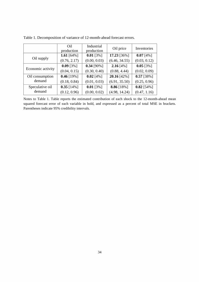
34

Table 1. Decomposition of variance of 12-month-ahead forecast errors.

Oil production

Industrial production

Oil price Inventories

Oil supply 1.61 [64%] (0.76, 2.17)

0.01 [3%] (0.00, 0.03)

17.23 [36%] (6.46, 34.55)

0.07 [4%] (0.03, 0.12)

Economic activity 0.09 [3%]

(0.04, 0.15) 0.34 [90%] (0.30, 0.40)

2.16 [4%] (0.88, 4.44)

0.05 [3%] (0.02, 0.09)

Oil consumption demand

0.46 [19%] (0.18, 0.84)

0.02 [4%] (0.01, 0.03)

20.16 [42%] (6.91, 35.50)

0.57 [38%] (0.25, 0.96)

Speculative oil demand

0.35 [14%] (0.12, 0.96)

0.01 [3%] (0.00, 0.02)

8.86 [18%] (4.98, 14.24)

0.82 [54%] (0.47, 1.16)

Notes to Table 1. Table reports the estimated contribution of each shock to the 12-month-ahead mean squared forecast error of each variable in bold, and expressed as a percent of total MSE in brackets. Parentheses indicate 95% credibility intervals.

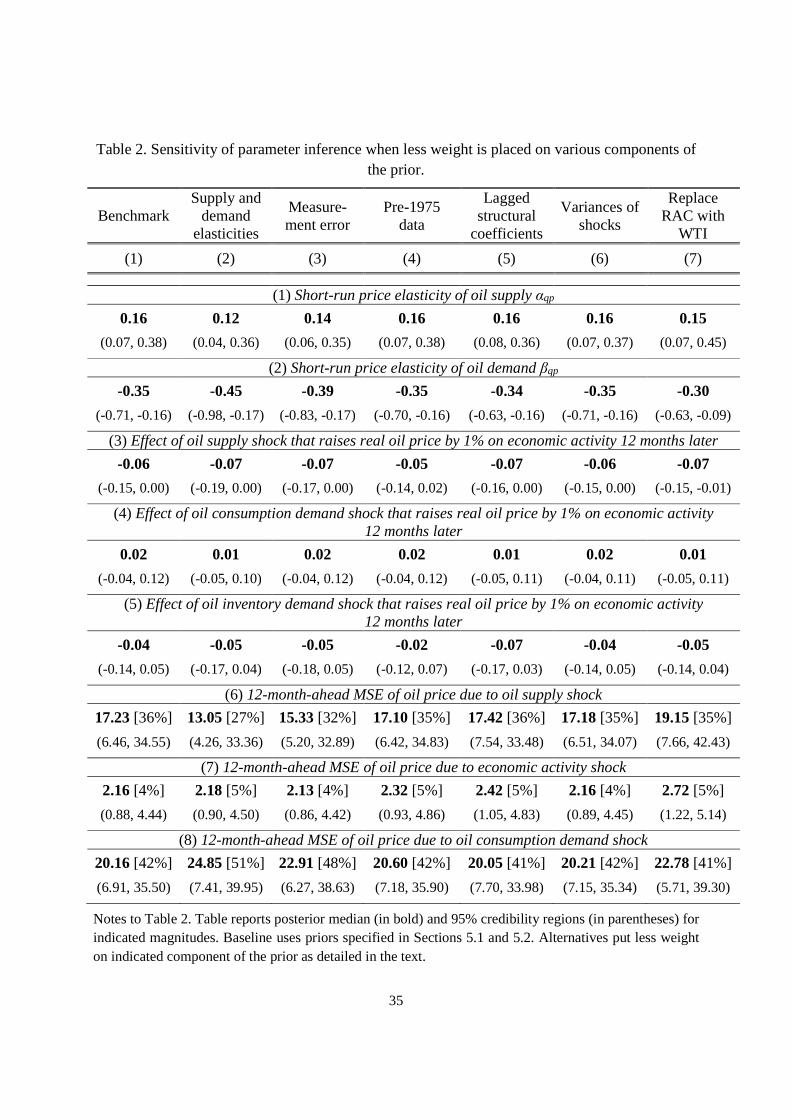
35

Table 2. Sensitivity of parameter inference when less weight is placed on various components of the prior.

Benchmark Supply and

demand elasticities

Measure-ment error

Pre-1975 data

Lagged structural

coefficients

Variances of shocks

Replace RAC with

WTI

(1) (2) (3) (4) (5) (6) (7)

(1) Short-run price elasticity of oil supply αqp

0.16 0.12 0.14 0.16 0.16 0.16 0.15

(0.07, 0.38) (0.04, 0.36) (0.06, 0.35) (0.07, 0.38) (0.08, 0.36) (0.07, 0.37) (0.07, 0.45)

(2) Short-run price elasticity of oil demand βqp

-0.35 -0.45 -0.39 -0.35 -0.34 -0.35 -0.30

(-0.71, -0.16) (-0.98, -0.17) (-0.83, -0.17) (-0.70, -0.16) (-0.63, -0.16) (-0.71, -0.16) (-0.63, -0.09)

(3) Effect of oil supply shock that raises real oil price by 1% on economic activity 12 months later

-0.06 -0.07 -0.07 -0.05 -0.07 -0.06 -0.07

(-0.15, 0.00) (-0.19, 0.00) (-0.17, 0.00) (-0.14, 0.02) (-0.16, 0.00) (-0.15, 0.00) (-0.15, -0.01)

(4) Effect of oil consumption demand shock that raises real oil price by 1% on economic activity 12 months later

0.02 0.01 0.02 0.02 0.01 0.02 0.01

(-0.04, 0.12) (-0.05, 0.10) (-0.04, 0.12) (-0.04, 0.12) (-0.05, 0.11) (-0.04, 0.11) (-0.05, 0.11)

(5) Effect of oil inventory demand shock that raises real oil price by 1% on economic activity 12 months later

-0.04 -0.05 -0.05 -0.02 -0.07 -0.04 -0.05

(-0.14, 0.05) (-0.17, 0.04) (-0.18, 0.05) (-0.12, 0.07) (-0.17, 0.03) (-0.14, 0.05) (-0.14, 0.04)

(6) 12-month-ahead MSE of oil price due to oil supply shock

17.23 [36%] 13.05 [27%] 15.33 [32%] 17.10 [35%] 17.42 [36%] 17.18 [35%] 19.15 [35%]

(6.46, 34.55) (4.26, 33.36) (5.20, 32.89) (6.42, 34.83) (7.54, 33.48) (6.51, 34.07) (7.66, 42.43)

(7) 12-month-ahead MSE of oil price due to economic activity shock

2.16 [4%] 2.18 [5%] 2.13 [4%] 2.32 [5%] 2.42 [5%] 2.16 [4%] 2.72 [5%]

(0.88, 4.44) (0.90, 4.50) (0.86, 4.42) (0.93, 4.86) (1.05, 4.83) (0.89, 4.45) (1.22, 5.14)

(8) 12-month-ahead MSE of oil price due to oil consumption demand shock

20.16 [42%] 24.85 [51%] 22.91 [48%] 20.60 [42%] 20.05 [41%] 20.21 [42%] 22.78 [41%]

(6.91, 35.50) (7.41, 39.95) (6.27, 38.63) (7.18, 35.90) (7.70, 33.98) (7.15, 35.34) (5.71, 39.30)

Notes to Table 2. Table reports posterior median (in bold) and 95% credibility regions (in parentheses) for indicated magnitudes. Baseline uses priors specified in Sections 5.1 and 5.2. Alternatives put less weight on indicated component of the prior as detailed in the text.

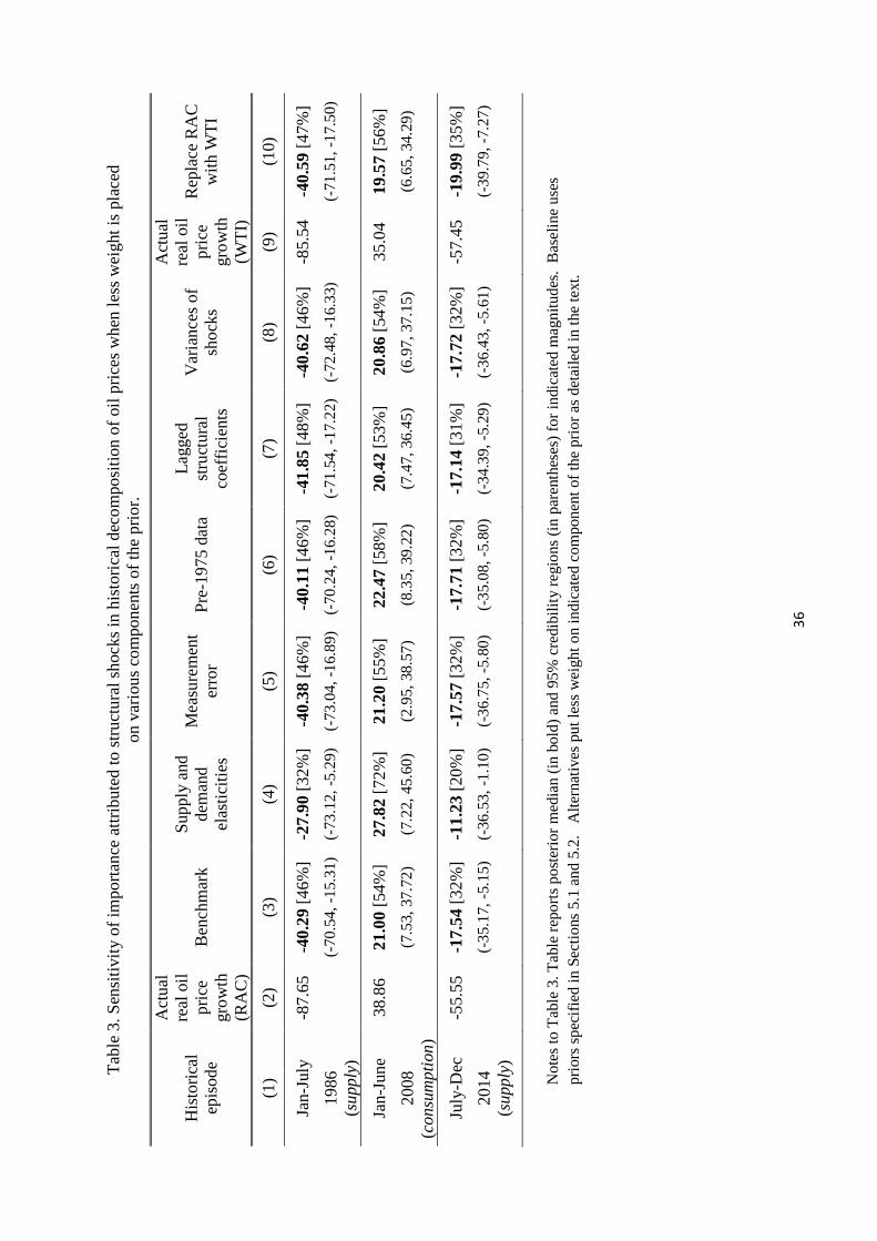
36

Tab

le 3

. S

ensi

tivity

of i

mp

ort

ance

att

ribu

ted

to s

tru

ctu

ral s

hoc

ks in

his

tori

cal d

eco

mpo

sitio

n o

f oi

l p

rices

wh

en le

ss w

eigh

t is

pla

ced

o

n va

riou

s co

mpo

nen

ts o

f th

e p

rior.

His

toric

al

epis

od

e

Act

ual

re

al o

il p

rice

gro

wth

(R

AC

)

Ben

chm

ark

Sup

ply

and

d

eman

d

elas

ticiti

es

Me

asu

rem

ent

erro

r P

re-1

97

5 da

ta

Lagg

ed

st

ruct

ural

co

effic

ien

ts

Var

ian

ces

of

sho

cks

Act

ual

re

al o

il p

rice

gro

wth

(W

TI)

Rep

lace

RA

C

with

WT

I

(1)

(2)

(3)

(4)

(5)

(6)

(7)

(8)

(9)

(10)

Jan-

July

-8

7.65

-4

0.29

[46

%]

-27.

90 [3

2%

] -4

0.38

[46

%]

-40.

11 [4

6%

] -4

1.85

[48

%]

-40.

62 [4

6%

] -8

5.54

-4

0.59

[47

%]

19

86

(-

70.5

4, -1

5.3

1)

(-73

.12,

-5.2

9)

(-73

.04,

-16.

89)

(-

70.2

4, -1

6.2

8)

(-71

.54,

-17.

22)

(-

72.4

8, -1

6.3

3)

(-

71.5

1, -1

7.5

0)

(sup

ply)

Jan

-Jun

e

38.8

6

21.0

0 [5

4%

] 27

.82

[72

%]

21.2

0 [5

5%

] 22

.47

[58

%]

20.4

2 [5

3%

] 20

.86

[54

%]

35.0

4

19.5

7 [5

6%

]

20

08

(7

.53,

37.

72)

(7.2

2, 4

5.6

0)

(2.9

5, 3

8.57

) (8

.35,

39.

22)

(7.4

7, 3

6.4

5)

(6.9

7, 3

7.15

)

(6.6

5, 3

4.29

) (c

onsu

mpt

ion)

July

-Dec

-5

5.55

-1

7.54

[32

%]

-11.

23 [

20%

] -1

7.57

[32

%]

-17.

71 [3

2%

] -1

7.14

[31

%]

-17.

72 [3

2%

] -5

7.45

-1

9.99

[35

%]

20

14

(-

35

.17,

-5.1

5)

(-36

.53,

-1.1

0)

(-3

6.7

5, -5

.80)

(-

35

.08,

-5.8

0)

(-3

4.3

9, -5

.29)

(-

36

.43,

-5.6

1)

(-

39

.79,

-7.2

7)

(sup

ply)

No

tes

to T

abl

e 3.

Ta

ble

repo

rts

po

ster

ior

me

dia

n (i

n bo

ld)

and

95%

cre

dibi

lity

regi

on

s (i

n p

are

nthe

ses

) fo

r in

dica

ted

ma

gnitu

des

. B

ase

line

use

s p

rior

s sp

ecifi

ed

in S

ect

ions

5.1

an

d 5.

2.

Alte

rna

tive

s pu

t le

ss w

eig

ht

on

indi

cate

d co

mp

one

nt o

f th

e p

rior

as

deta

iled

in t

he t

ext

.

37

Fig

ure

1.

Imp

ulse

-re

spo

nse

fun

ctio

ns fo

r 3-

vari

abl

e m

od

el u

nde

r tr

adi

tion

al C

hol

esk

y id

ent

ifica

tion.

R

ed

dash

ed

line

s: p

oint

est

imat

es a

rriv

ed

at

usi

ng

Kili

an’

s (2

009)

ori

gin

al m

etho

dol

og

y; b

lue

solid li

nes:

me

dia

n o

f Ba

yesi

an

pos

terio

r di

stri

bution; s

ha

ded

regi

ons

: 95

% p

ost

eri

or c

red

ible

set

.

05

10

15

-2.5

-1.5

-0.5

0.5

1.5

Oil production

Oil

sup

ply

sho

ck

05

10

15

-2.5

-1.5

-0.5

0.5

1.5

Oil production

Ag

gre

gat

e d

em

and

sho

ck

05

10

15

-2.5

-1.5

-0.5

0.5

1.5

Oil production

Oil-

spe

cific

de

man

d s

hock

Mo

nths

05

10

15

-505

10

Real activity

Oil

sup

ply

sho

ck

05

10

15

-505

10

Real activity

Ag

gre

gat

e d

em

and

sho

ck

05

10

15

-505

10

Real activity

Oil-

spe

cific

de

man

d s

hock

Mo

nths

05

10

15

-505

10

Real oil price

Oil

sup

ply

sho

ck

05

10

15

-505

10

Real oil price

Ag

gre

gat

e d

em

and

sho

ck

05

10

15

-505

10

Oil-

spe

cific

de

man

d s

hock

Real oil price

Mo

nths

38

Fig

ure

2.

Pri

or (

red

line

s) a

nd

po

ste

rior

(bl

ue

his

togr

ams)

dis

trib

utio

ns

for

the

unk

no

wn

ele

me

nts

in

A u

sing

tra

diti

ona

l 3-v

ari

abl

e C

hol

esk

y-ty

pe

id

ent

ifica

tion.

-1-0

.8-0

.6-0

.4-0

.20

0.2

0.4

0.6

0.8

10

0.51

1.52

2.53

3.5

α yq

-1-0

.8-0

.6-0

.4-0

.20

0.2

0.4

0.6

0.8

10

0.51

1.52

2.5

α pq

00.

10.

20.

30.

40.

501234567

α py

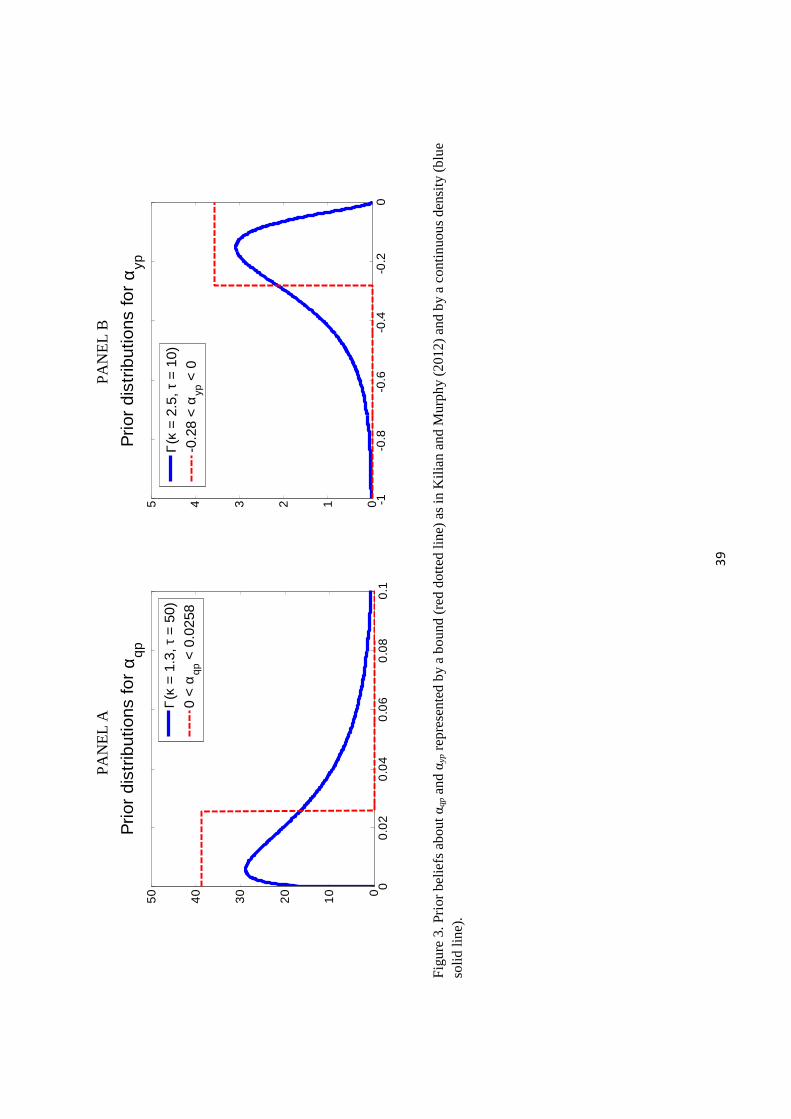
39

P

AN

EL

A

P

AN

EL

B

Fig

ure

3.

Pri

or b

elie

fs a

bou

t α

qp a

nd α

yp r

ep

rese

nte

d b

y a

bo

und

(re

d d

otte

d lin

e) a

s in

Kil

ian

an

d M

urp

hy

(201

2)

and

by

a c

ontin

uou

s d

ensi

ty (

blu

e so

lid li

ne)

.

00

.02

0.0

40

.06

0.0

80

.10

10

20

30

40

50

Prio

r di

strib

utio

ns fo

r α q

p

Γ (κ

= 1

.3, τ

= 5

0)0

< α

qp

< 0

.025

8

-1-0

.8-0

.6-0

.4-0

.20

012345

Prio

r di

strib

utio

ns fo

r α yp

Γ (κ

= 2

.5, τ

= 1

0)-0

.28

< α

yp <

0

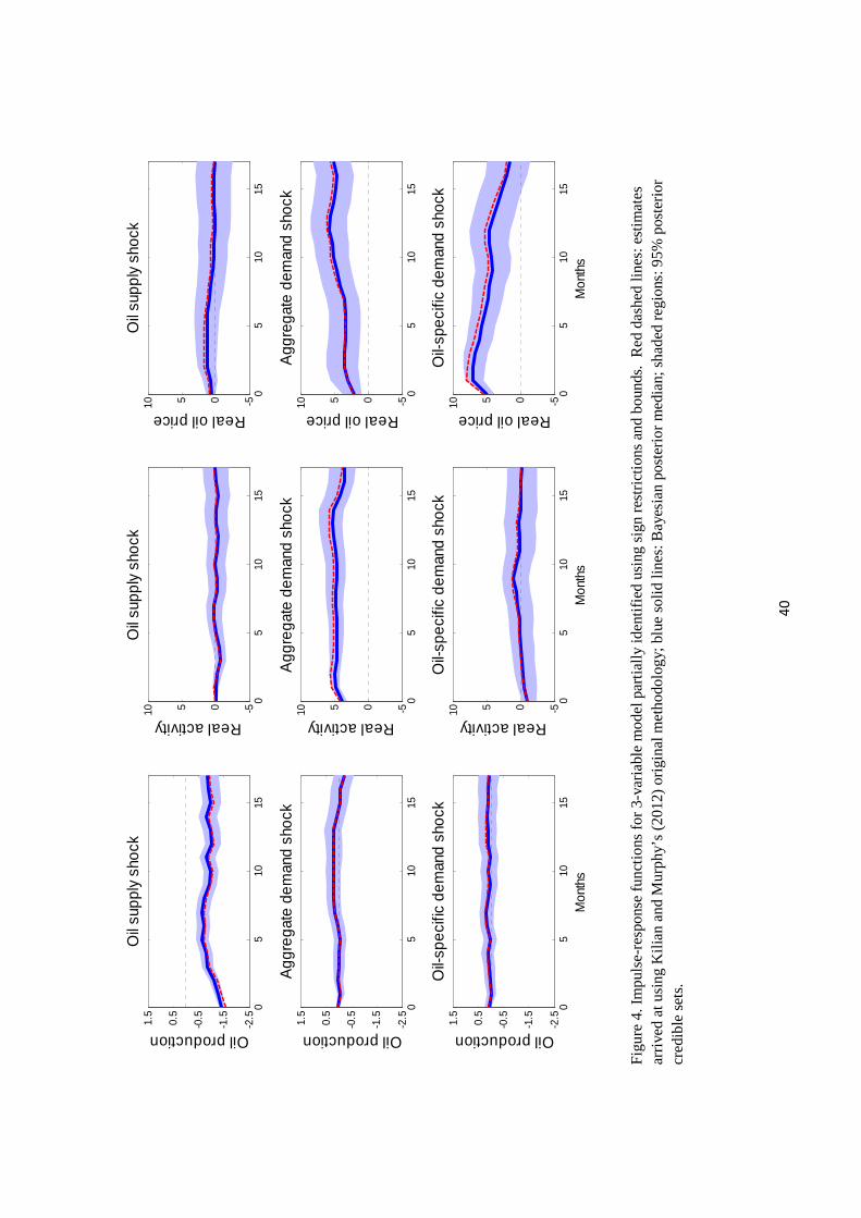
40

Fig

ure

4.

Imp

ulse

-re

spo

nse

fun

ctio

ns fo

r 3-

vari

abl

e m

od

el p

art

ially

ide

ntifi

ed u

sing

sig

n re

stri

ctio

ns

an

d b

oun

ds.

Re

d da

shed

lin

es:

estim

ate

s a

rriv

ed

at u

sin

g K

ilia

n a

nd

Mu

rph

y’s

(20

12)

orig

ina

l me

tho

dolo

gy;

blu

e so

lid li

nes:

Ba

yesi

an

pos

terio

r m

edi

an;

sh

ad

ed r

egi

ons

: 95

% p

oste

rior

cr

edi

ble

set

s.

05

1015

-2.5

-1.5

-0.50.5

1.5

Oil production

Oil

supp

ly s

hock

05

1015

-2.5

-1.5

-0.50.5

1.5

Oil production

Agg

rega

te d

eman

d sh

ock

05

1015

-2.5

-1.5

-0.50.5

1.5

Oil production

Oil-

spec

ific

dem

and

shoc

k

Mon

ths

05

1015

-50510 Real activity

Oil

supp

ly s

hock

05

1015

-50510 Real activity

Agg

rega

te d

eman

d sh

ock

05

1015

-50510 Real activity

Oil-

spec

ific

dem

and

shoc

k

Mon

ths

05

1015

-50510 Real oil price

Oil

supp

ly s

hock

05

1015

-50510 Real oil price

Agg

rega

te d

eman

d sh

ock

05

1015

-50510O

il-sp

ecifi

c de

man

d sh

ock

Real oil price

Mon

ths

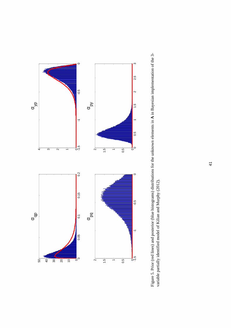
41

Fig

ure

5.

Pri

or (

red

line

s) a

nd

po

ste

rior

(bl

ue

his

togr

ams)

dis

trib

utio

ns

for

the

unk

no

wn

ele

me

nts

in

A in

Bay

esi

an

impl

em

ent

atio

n o

f th

e 3

-va

ria

ble

par

tially

iden

tifie

d m

od

el o

f Kili

an a

nd Mu

rphy

(2

01

2).

00.

050.

10.

150.

201020304050

α qp

-1.5

-1-0

.50

01234

α yp

-1.5

-1-0

.50

0

0.51

1.52

α pq

00.

51

1.5

22.

53

0

0.51

1.52

α py

42

Fig

ure

6.

Evi

denc

e on

de

ma

nd

ela

stic

ity f

rom

cro

ss-s

ectio

n of

23

coun

trie

s.

Left

pan

el:

log

of o

il c

on

sum

ptio

n p

er

do

llar

of r

eal

GD

P in

20

04

vers

us

pric

e of

ga

solin

e in

200

4.

Rig

ht

pane

l: lo

g o

f oil

cons

um

ptio

n pe

r d

olla

r of

re

al G

DP

in 2

00

4 ve

rsus

pri

ce o

f ga

solin

e in

200

0.

00.

51

1.5

22

2.53

3.54

slo

pe =

-0

.51

Log petroleum consumption(gallons/year/real GDP) in 2004

Lo

g g

asol

ine

pric

e (

$ p

er

gal

lon)

in 2

00

4

00.

51

1.5

22

2.53

3.54

slo

pe =

-0.5

7

Log petroleum consumption(gallons/year/real GDP) in 2004

Lo

g g

aso

line

pric

e (

$ p

er g

allo

n) in

200

0

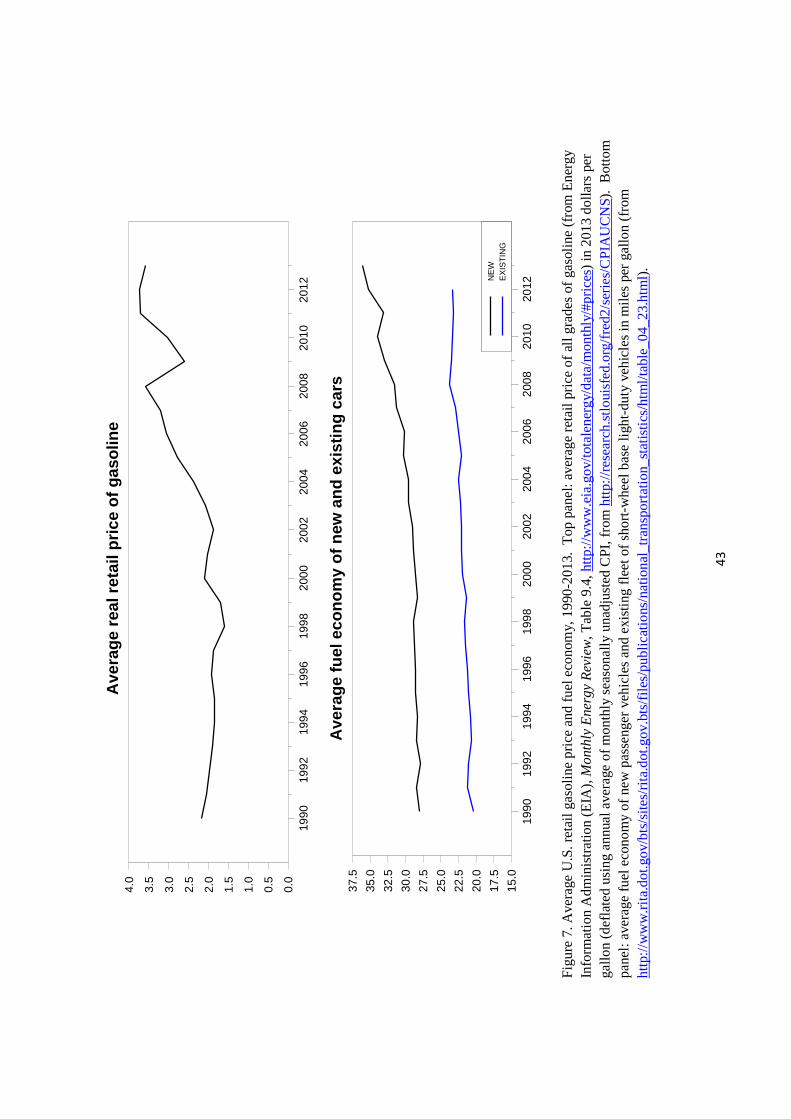
43

Fig

ure

7.

Ave

rage

U.S

. re

tail

gaso

line

pri

ce a

nd

fuel

eco

nom

y, 1

990

-20

13.

T

op

pan

el:

ave

rage

ret

ail

pri

ce o

f al

l gra

de

s of

ga

solin

e (f

rom

En

erg

y In

form

atio

n A

dm

inis

tra

tion

(EIA

), M

onth

ly E

nerg

y R

evie

w,

Tab

le 9

.4, h

ttp:

//w

ww

.eia

.go

v/to

tale

ner

gy/

da

ta/m

on

thly

/#p

rice

s)

in 2

01

3 d

olla

rs p

er

gallo

n (d

efla

ted

usin

g a

nnu

al a

vera

ge o

f mo

nth

ly s

eas

ona

lly u

na

dju

sted

CP

I, fr

om

htt

p://r

ese

arc

h.st

loui

sfe

d.or

g/fr

ed2

/ser

ies/

CP

IAU

CN

S).

Bot

tom

p

ane

l: a

vera

ge fu

el e

con

om

y o

f ne

w p

ass

eng

er

veh

icl

es a

nd

exi

stin

g fle

et

of s

hort

-whe

el b

ase

ligh

t-du

ty

veh

icle

s in

mile

s pe

r ga

llon

(fro

m

htt

p://w

ww

.rita

.do

t.go

v/b

ts/s

ites/

rita.

dot

.go

v.bt

s/fil

es/p

ub

licat

ions

/na

tion

al_t

ran

spo

rtat

ion

_st

atis

tics

/htm

l/ta

ble

_0

4_2

3.h

tml

).

Ave

rag

e re

al r

etai

l pri

ce o

f g

aso

line

1990

1992

1994

1996

1998

2000

2002

2004

2006

2008

2010

2012

0.0

0.5

1.0

1.5

2.0

2.5

3.0

3.5

4.0

Ave

rag

e fu

el e

con

om

y o

f n

ew a

nd

exi

stin

g c

ars

1990

1992

1994

1996

1998

2000

2002

2004

2006

2008

2010

2012

15.0

17.5

20.0

22.5

25.0

27.5

30.0

32.5

35.0

37.5

NE

WE

XIS

TIN

G

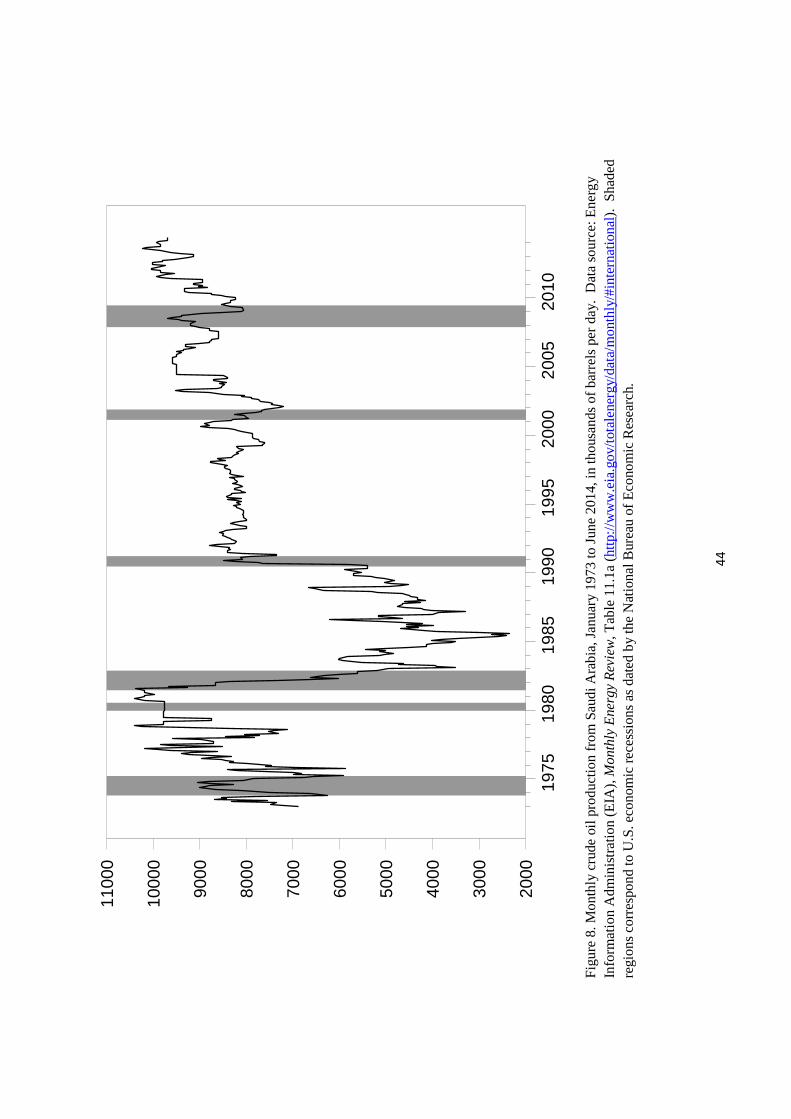
44

Fig

ure

8.

Mo

nth

ly c

rude

oil

pro

duc

tion

fro

m S

aud

i Arab

ia,

Janu

ary

197

3 to

Jun

e 20

14,

in t

ho

usa

nds

of b

arre

ls p

er

day.

Dat

a so

urc

e: E

ne

rgy

Info

rma

tion

Ad

min

istr

atio

n (E

IA),

Mon

thly

Ene

rgy

Rev

iew

, Tab

le 1

1.1

a ( ht

tp:/

/ww

w.e

ia.g

ov/

tota

lene

rgy/

data

/mo

nth

ly/#

inte

rnat

ion

al).

Sh

ad

ed

regi

on

s co

rre

spo

nd

to U

.S. e

con

omic

re

cess

ion

s as

dat

ed

by

the

Nat

ion

al B

urea

u of

Eco

nom

ic R

ese

arch

.

19

7519

8019

8519

9019

9520

0020

0520

1020

00

3000

4000

5000

6000

7000

8000

9000

1000

0

1100

0

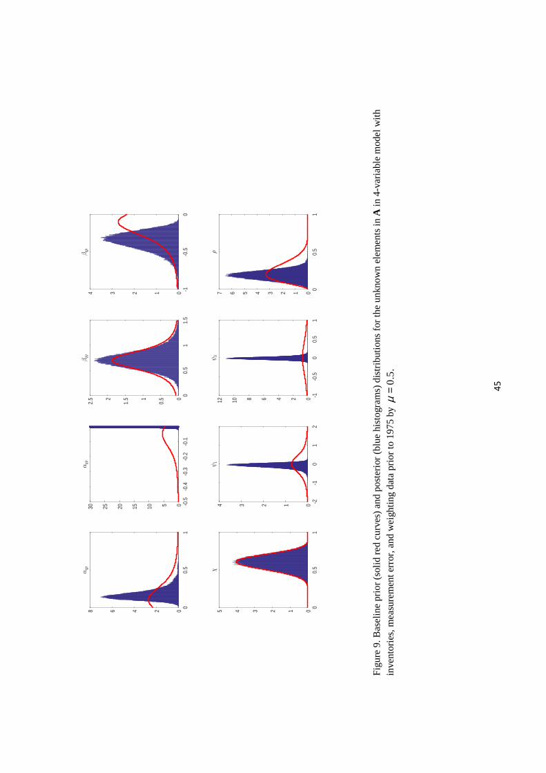
45

Fig

ure

9.

Bas

elin

e pr

ior

(sol

id r

ed

curv

es)

an

d p

os

teri

or (

blu

e hi

sto

gra

ms)

dis

trib

utio

ns f

or th

e u

nkn

ow

n e

lem

en

ts in

A in

4-v

ari

abl

e m

ode

l with

in

ven

torie

s, m

ea

sure

men

t err

or,

an

d w

eig

htin

g d

ata

prio

r to

19

75

by

0.5

.µ

=

00.

51

02468αqp

-0.5

-0.4

-0.3

-0.2

-0.1

051015202530αyp

00.

51

1.5

0

0.51

1.52

2.5

βqy

-1-0

.50

01234βqp

00.

51

012345χ

-2-1

01

201234

ψ1

-1-0

.50

0.5

1024681012

ψ3

00.

51

01234567ρ

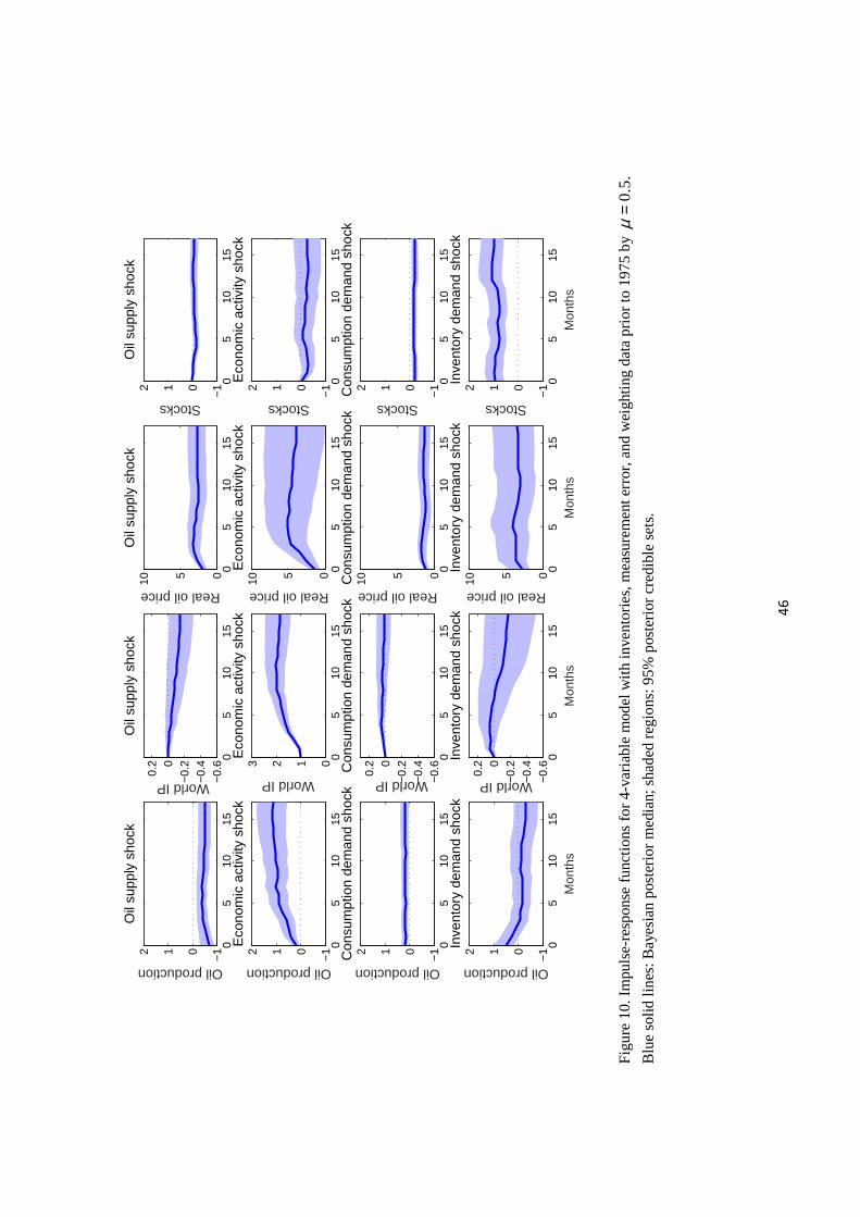
46

Fig

ure

10.

Impu

lse-

resp

onse

fun

ctio

ns f

or

4-v

ari

abl

e m

od

el w

ith in

ven

torie

s, m

eas

ure

me

nt e

rror

, a

nd

we

ight

ing

da

ta p

rior

to 1

97

5 b

y 0

.5.

µ=

Blu

e so

lid li

nes

: Ba

yesi

an

pos

terio

r m

edi

an;

sha

de

d r

egio

ns:

95%

pos

teri

or c

redi

ble

sets

.

05

1015

−1012

Oil production

Oil

supp

ly s

hock

05

1015

−1012

Oil productionE

cono

mic

act

ivity

sho

ck

05

1015

−1012

Oil production

Con

sum

ptio

n de

man

d sh

ock

05

1015

−1012

Mon

ths

Oil production

Inve

ntor

y de

man

d sh

ock

05

1015

−0.

6−

0.4

−0.

200.

2

World IP

Oil

supp

ly s

hock

05

1015

0123

World IP

Eco

nom

ic a

ctiv

ity s

hock

05

1015

−0.

6−

0.4

−0.

200.

2

World IP

Con

sum

ptio

n de

man

d sh

ock

05

1015

−0.

6−

0.4

−0.

200.

2

Mon

ths

World IP

Inve

ntor

y de

man

d sh

ock

05

1015

0510

Real oil price

Oil

supp

ly s

hock

05

1015

0510

Real oil price

Eco

nom

ic a

ctiv

ity s

hock

05

1015

0510

Real oil price

Con

sum

ptio

n de

man

d sh

ock

05

1015

0510

Mon

ths

Real oil price

Inve

ntor

y de

man

d sh

ock

05

1015

−1012

Stocks

Oil

supp

ly s

hock

05

1015

−1012

Stocks

Eco

nom

ic a

ctiv

ity s

hock

05

1015

−1012

Stocks

Con

sum

ptio

n de

man

d sh

ock

05

1015

−1012

Mon

ths

Stocks

Inve

ntor

y de

man

d sh

ock

47

Figure 11. Actual changes in oil prices (red dashed lines) and historical contribution of separate structural shocks with 95% posterior credibility regions (blue and shaded) based on the 4-variable model with inventories, measurement error, and weighting data prior to 1975 by 0.5.µ =