Resource management techniques aware ofinterference among high-performance

computing applications

a dissertation presentedby

Ana Jokanovićto

The Department of Computer Architecture

in partial fulfillment of the requirementsfor the degree of

Doctor of Philosophyin the subject ofComputer Science

Universitat Politècnica de CatalunyaBarcelona, SpainNovember 2014

©2014 – Ana Jokanovićall rights reserved.

Author: Ana JokanovićThesis director: Professor Jesus LabartaThesis co-directors: Jose Carlos Sancho and German Rodriguez

Resource management techniques aware of interference amonghigh-performance computing applications

Abstract

Network interference of nearby jobs has been recently identified as the dominant reason for the highperformance variability of parallel applications running on High Performance Computing (HPC)systems. Typically, HPC systems are dynamic with multiple jobs coming and leaving in an unpre-dictable fashion, sharing simultaneously the system interconnection network. In such environmentcontention for network resources is causing random stalls in the progress of application executiondegrading application’s performance. Eliminating interactions between jobs is the key for guaran-teeing both high performance and performance predictability of applications. These interactions aredetermined by the job location in the system. Upon arriving to the system, the job is allocated thecomputing and network resources by resource managers. Based on the job size requirements, the jobscheduler finds a set of available computing nodes. In addition, the subnet manager determines theallocation of the network resources such as paths between nodes, virtual lanes, link bandwidth. Typi-cally, resource managers are mainly focused on increasing utilization of the resources while neglectingjob interactions. In this thesis, we propose techniques for both, job scheduler and subnet manager,able tomitigate job interactions: 1) a job scheduling policy that reduces the node fragmentation in thesystem, and 2) a quality-of-service (QoS) policy based on a characterization of job’s network load; thispolicy is relaying on the virtual lanes mechanism provided by modern interconnection network (e.g.InfiniBand). In order to evaluate our job scheduling policywe use a simulator developed for this thesisthat takes as an input the job scheduler log from a production HPC system. This simulator performsthe node allocation for the jobs from the log. The proposed QoS policy is evaluated using a flit-levelnetwork simulator that is able to replay multiple traces from real executions of MPI applications. Ex-perimental results show that the proposed job scheduling policy leads to few jobs sharing networkresources and thus having fewer job’s interactions while the QoS policy is able to effectively reducethe degradation from the remaining job’s interactions. These two software techniques are comple-mentary and could be used together without additional hardware.

iii

iv

Contents

0 Introduction 1

1 Background 71.1 Inter-application network contention . . . . . . . . . . . . . . . . . . . . . . . 81.2 Interconnection network topologies . . . . . . . . . . . . . . . . . . . . . . . . 101.3 Resource management techniques . . . . . . . . . . . . . . . . . . . . . . . . . 12

2 Experimental methodology 172.1 HPC workload . . . . . . . . . . . . . . . . . . . . . . . . . . . . . . . . . . . 182.2 Toolchain . . . . . . . . . . . . . . . . . . . . . . . . . . . . . . . . . . . . . 212.3 Performance metrics for evaluating the interference impact on system performance 33

3 Characterizing applications at network-level 373.1 Simulation setup . . . . . . . . . . . . . . . . . . . . . . . . . . . . . . . . . . 393.2 Characterization of the applications network behavior . . . . . . . . . . . . . . . 423.3 Exploring the sensitivity to task placement and bisection bandwidth . . . . . . . . 443.4 Exploring the ways to reduce inter-application contention using task placement . . 563.5 Conclusions . . . . . . . . . . . . . . . . . . . . . . . . . . . . . . . . . . . . 60

4 System-level resource management 634.1 Network sharing as a function of job allocation . . . . . . . . . . . . . . . . . . 674.2 Quiet neighborhoods via Virtual network blocks . . . . . . . . . . . . . . . . . . 704.3 Experiments . . . . . . . . . . . . . . . . . . . . . . . . . . . . . . . . . . . . 764.4 Evaluation . . . . . . . . . . . . . . . . . . . . . . . . . . . . . . . . . . . . . 784.5 Conclusions . . . . . . . . . . . . . . . . . . . . . . . . . . . . . . . . . . . . 84

5 Link-level resource management 875.1 Proposed Quality-of-Service Policy . . . . . . . . . . . . . . . . . . . . . . . . . 905.2 Simulation . . . . . . . . . . . . . . . . . . . . . . . . . . . . . . . . . . . . . 945.3 Results of the proposed techniques . . . . . . . . . . . . . . . . . . . . . . . . . 1005.4 Conclusions . . . . . . . . . . . . . . . . . . . . . . . . . . . . . . . . . . . . 108

v

6 Related work 111

7 Conclusions 117

8 Future work 121

9 Publications 123

References 131

vi

Listing of figures

1 An illustration of inter-application contention. . . . . . . . . . . . . . . . . . . . 32 The impact of inter-application contention on the individual application perfor-

mance and on the system performance. . . . . . . . . . . . . . . . . . . . . . . . 33 The objective of the thesis. . . . . . . . . . . . . . . . . . . . . . . . . . . . . . 44 Interference-aware unified resource management. . . . . . . . . . . . . . . . . . 6

1.1 Switch ports at level l in XGFT(h;m1,...,mh;w1,...,wh) (top) and examples of a full-bisection fat-tree (left bootom) and its slimmed version (right bottom). . . . . . . 11

1.2 InfiniBand switch and its virtual lanes mechanism. . . . . . . . . . . . . . . . . . 15

2.1 Bytes loaded into network by each of the studied applications. . . . . . . . . . . 202.2 Bytes loaded into network by FT. . . . . . . . . . . . . . . . . . . . . . . . . . 212.3 Applications’ average average bytes in transit. . . . . . . . . . . . . . . . . . . . 212.4 Dynamic library calls intrumentation . . . . . . . . . . . . . . . . . . . . . . . . 232.5 Tracing internals of collective communications. The OpenMPI library adaptation

to allow for translation of MCA_PML_CALLmacro to standardMPI call format. 242.6 An example of the tracing scripts . . . . . . . . . . . . . . . . . . . . . . . . . . 252.7 Dimemas parameters relevant for our study. . . . . . . . . . . . . . . . . . . . . 272.8 Relation between tasks-to-nodes mapping in Dimemas and Venus. Ax and Bx are

the xth task of applicationsA andB, respectively. TaskB2 is placed on the node at the2ndposition of the B’sDimemasmapping vector, i.e., node 6; this node correspondsto Venus node on 6th line of Venus mapping file, i.e., node h3. . . . . . . . . . . 29

2.9 Dimemas & Venus co-simulation toolchain. . . . . . . . . . . . . . . . . . . . . 312.10 An example of Dimemas & Venus co-simulation script. . . . . . . . . . . . . . . 312.11 Toolchain for evaluation of system-level resource management policies. . . . . . . 322.12 An example of per-job information from MareNostrum scheduler log used in our

evaluation. . . . . . . . . . . . . . . . . . . . . . . . . . . . . . . . . . . . . . 322.13 Simulation experiments needed for quantifying the impact of the network interfer-

ence on the performance of each job. The case of two-applications workload. Tbase,Talone and Tsharing are the outputs of the simulation runs. . . . . . . . . . . . . . 34

2.14 Quantifying the impact of the jobs’ interference on the system performance. . . . 35

vii

3.1 Total available bandwidth per level of a fat-tree network xgft(3;16,16,8;1,S,S) for dif-ferent slimming factor S. . . . . . . . . . . . . . . . . . . . . . . . . . . . . . . 42

3.2 Methodology for characterization of application’s network utilization; bandwidthutilization of application per levels L1 and L2 is UL1 and UL2, respectively . . . . . 43

3.3 Applications’ injection rateper level of xgft(3;16,16,8;1,w,w)underdifferent taskplace-ments. . . . . . . . . . . . . . . . . . . . . . . . . . . . . . . . . . . . . . . . 44

3.4 Available bandwidth from the perspective of a job of size 256-nodes per each level ofa fat-tree network for different slimming factor. . . . . . . . . . . . . . . . . . . 45

3.5 Available bandwidth from the perspective of a job of size 512-nodes per each level ofa fat-tree network for different slimming factor. . . . . . . . . . . . . . . . . . . 45

3.6 Bandwidth utilization per level for applications on xgft(3;16,16,8;1,2,2) fat-tree net-work and node allocation on F2 fragmentation. . . . . . . . . . . . . . . . . . . 46

3.7 Classification of applications based on their maximum utilization. . . . . . . . . . 463.8 Impact of fragmentation and slimming to CGPOP performance variability when

running alone in the system. . . . . . . . . . . . . . . . . . . . . . . . . . . . . 473.9 Impact of fragmentation and slimming toWRF performance variability when run-

ning alone in the system. . . . . . . . . . . . . . . . . . . . . . . . . . . . . . . 483.10 Impact of fragmentation and slimming toGROMACSperformance variabilitywhen

running alone in the system. . . . . . . . . . . . . . . . . . . . . . . . . . . . . 483.11 Impact of fragmentation and slimming toBTperformance variabilitywhen running

alone in the system. . . . . . . . . . . . . . . . . . . . . . . . . . . . . . . . . . 493.12 Impact of fragmentation and slimming to FTperformance variabilitywhen running

alone in the system. . . . . . . . . . . . . . . . . . . . . . . . . . . . . . . . . . 503.13 Impact of fragmentation and slimming to CG performance variability when run-

ning alone in the system. . . . . . . . . . . . . . . . . . . . . . . . . . . . . . . 503.14 Impact of fragmentation and slimming toMILCperformance variability when run-

ning alone in the system. . . . . . . . . . . . . . . . . . . . . . . . . . . . . . . 513.15 Mixing all applications together on different random allocations for three different

slimmed topologies. . . . . . . . . . . . . . . . . . . . . . . . . . . . . . . . . 533.16 Mixing eight CGPOPs together on different random allocations for three different

slimmed topologies. . . . . . . . . . . . . . . . . . . . . . . . . . . . . . . . . 533.17 Mixing eightCGs together ondifferent randomallocations for three different slimmed

topologies. . . . . . . . . . . . . . . . . . . . . . . . . . . . . . . . . . . . . . 543.18 The mix of eight CGs on different allocations - random and regular. . . . . . . . . 583.19 Improvement due tomixinghigh sensitive and low sensitive applications. Themixes

of four applications: two FTs and two CGPOPs, two FTs and twoWRFs and twoFTs and two BTs on S8 topology. . . . . . . . . . . . . . . . . . . . . . . . . . 58

3.20 Comparing strategies of grouping and isolating for different slimming levels, S8, S4,S2. The mix of two FTs and two CGPOPs on F8 and NF allocations. . . . . . . . 59

viii

4.1 The small jobs spreadness in MareNostrum supercomputer. Percent of jobs of sizex (x-axis) spread on s switches (given in the legend). . . . . . . . . . . . . . . . . 65

4.2 The actual number of populated switches for the job sizes range from 19 to 72 com-puting nodes inMareNostrum; the jobs thatwould ideally fit in 2 to 4 switches. Thered lines are at the switches 2 and 4. 8% of jobs fit within the 2-4 switches boundary. 66

4.3 The actual number of populated switches for the job sizes range from 73 to 288 com-putingnodes inMareNostrum; the jobs thatwould ideally fit in 5 to 16 switches. Thered lines are at the switches 5 and 16. 19% jobs fit within the 5-16 switches boundary. 66

4.4 The relationship between the number of switches populated by a job and the num-ber of jobs it shared the second-level of the MareNostrum network with. The fourlines correspond to each of four typical job sizes, 8, 16, 32 and 64. For example, outof all jobs of size 16 that were spread on 10 switches, some job shared the second-levelwith 50 other jobs, being that the maximum number of jobs a job of size 16 spreadin 10 switches shared the second-level of the network with. . . . . . . . . . . . . . 68

4.5 The relationship between the number of subtrees populated by a job and the num-ber of jobs it shared third-level of MareNostrum network with. The four lines cor-respond to each of four typical job sizes, 8, 16, 32 and 64. . . . . . . . . . . . . . . 69

4.6 Fragmentation size at different levels of fat-tree. . . . . . . . . . . . . . . . . . . 704.7 Dynamically adjusted limit between thebig jobs block and small jobs block. The case

of a small system of 9 switches. Big jobs are populating system from the first switchon, whereas the small jobs are populating system from the last switch backwards. Inthe empty system the big jobs limit would be equal to the highest switch index, i.e.,8 for the system in the figure, and the small jobs limit would be equal to the lowestswitch index, i.e., 0 . . . . . . . . . . . . . . . . . . . . . . . . . . . . . . . . . 73

4.8 Change of dynamic limit in time. A value for each of the two limits was taken uponthe allocation of new arriving job. Maximum switch index is 171. The switches abovethe limit donot have tobe interconnected at higher levels; the percent of the switchesfor which higher level interconnect can be switched-off increases up to 19% over time 74

4.9 Illustration of the virtual partitions in the actual switches for the small jobs and thebig jobs blocks. In the small job’s block there are only fragmentable switches of size18 nodes without virtual switch partitions, whereas in the big job’s block there areboth virtually partitioned switches andnon-partitioned, rem switches. The exampleis given for the system with subtrees of three switches size. . . . . . . . . . . . . . 75

4.10 Overview of the MareNostrum system. . . . . . . . . . . . . . . . . . . . . . . . 764.11 Average number of jobs that shared the network with a single job during the execu-

tion of the 49107 jobs workload fromMareNostrum log for each of the four evalu-ated scheduling policies. . . . . . . . . . . . . . . . . . . . . . . . . . . . . . . 78

4.12 Percent of jobs that shared network with other jobs during the execution of the49107 jobs workload fromMareNostrum log for each of the four evaluated schedul-ing policies. . . . . . . . . . . . . . . . . . . . . . . . . . . . . . . . . . . . . . 79

ix

4.13 Number of job pairs that shared network at the 2nd and at the 3rd network levelduring the execution of the 49107 jobs workload fromMareNostrum log for each ofthe four evaluated scheduling policies. . . . . . . . . . . . . . . . . . . . . . . . 80

4.14 Completion time of the 49107 jobs workload fromMareNostrum log using each ofthe four evaluated scheduling policies. . . . . . . . . . . . . . . . . . . . . . . . 81

4.15 Average time a job was waiting in the queue for the allocation. The data shown forsmall and for big jobs. The data was obtained from the execution of the 49107 jobsworkload fromMareNostrum log for each of the four evaluated scheduling policies. 81

4.16 Average system computing node utilization during the execution of the 49107 jobsworkload fromMareNostrum log for each of the four evaluated scheduling policies. 82

4.17 First available policy. Status of the system population in the middle of simulation.Grey depicts the node that is not used by any job. Black color depicts small jobs, i.e.,less or equal than 18. Other colors depict big jobs. . . . . . . . . . . . . . . . . . 83

4.18 First contiguous policy. Status of the systempopulation in themiddle of simulation.Grey depicts the node that is not used by any job. Black color depicts small jobs, i.e.,less or equal than 18. Other colors depict big jobs. . . . . . . . . . . . . . . . . . 83

4.19 Virtual network block. Status of the system population in themiddle of simulation.Grey depicts the node that is not used by any job. Black color depicts small jobs, i.e.,less or equal than 18. Other colors depict big jobs. . . . . . . . . . . . . . . . . . 84

4.20 Exclusive policy. Status of the system population in the middle of simulation. Greydepicts the node that is not used by any job. Black color depicts small jobs, i.e., lessor equal than 18. Other colors depict big jobs. . . . . . . . . . . . . . . . . . . . 85

5.1 Techniques developed for the new proposed QoS policy. . . . . . . . . . . . . . 905.2 Algorithm for mapping applications into VLs. . . . . . . . . . . . . . . . . . . . 915.3 Timeline showing the progression of two applications, A and B, where to each ap-

plication is assigned the same bandwidth. . . . . . . . . . . . . . . . . . . . . . . 925.4 Timeline showing the progression of two applications where to A is assigned higher

bandwidth than B. . . . . . . . . . . . . . . . . . . . . . . . . . . . . . . . . . 925.5 Timeline showing the progression of two applications where to B is assigned higher

bandwidth than to A. . . . . . . . . . . . . . . . . . . . . . . . . . . . . . . . . 925.6 Bandwidth utilization per level for applications on xgft(3;16,16,4;1,4,4) fat-tree net-

work and node allocation on F8 fragmentation. . . . . . . . . . . . . . . . . . . 995.7 Bandwidth utilization per level for applications on xgft(3;16,16,4;1,4,4) fat-tree net-

work and node allocation on F4 fragmentation. . . . . . . . . . . . . . . . . . . 995.8 Total contention time when using one and two VLs for the two-application mixes. 1025.9 Impact on the execution time of each application when using one and two VLs for

the two-application mixes. . . . . . . . . . . . . . . . . . . . . . . . . . . . . . 1025.10 Total contention timewhenusingone and three/four virtual lanes for the three/four-

application mixes. In FT+CG+BT, FT on VL0, CG on VL1 and BT on VL2. InFT+CG+BT+MG, FT on VL0, CG on VL1, BT on VL2 andMG on VL3. . . . . 103

x

5.11 Impact of segregation on the execution time of each application in three/four appli-cation mixes. . . . . . . . . . . . . . . . . . . . . . . . . . . . . . . . . . . . . 103

5.12 Total contention timewhen assigning differentweights toVLs for the FT+CGmix.FT on VL0 and CG on VL1. . . . . . . . . . . . . . . . . . . . . . . . . . . . . 105

5.13 Total contention timewhen assigning different weights to VLs for the FT+BTmix.FT on VL0 and BT on VL1. . . . . . . . . . . . . . . . . . . . . . . . . . . . . 106

5.14 Total contention timewhen assigning differentweights toVLs for theCG+BTmix.CG on VL0 and BT on VL1. . . . . . . . . . . . . . . . . . . . . . . . . . . . . 106

5.15 Total contention timewhen assigning different weights toVLs for the FT+CG+BTmix. FT on VL0, CG on VL1 and BT on VL2. . . . . . . . . . . . . . . . . . . . 107

5.16 Total contention time for various application grouping decisions and also for fullysegregating applications for the three-application mixes. . . . . . . . . . . . . . . 107

5.17 Total contention timewhen assigning different weights toVLs for the FT+CG+BTmix where FT is on VL0, and CG and BT are on VL1. . . . . . . . . . . . . . . . 108

xi

Tomy parents/ Mami i tati

xii

Acknowledgments

This thesis would not have been achieved without my advisors.First of all, I would like to thank Professor Jesus Labarta for being strict and honest, for teaching

me to strive for simple and practical solutions and for making sure I never lose the sense of what thehigh quality research is.I would like to thank Jose Carlos Sancho for his enormous patience, time and energy to listen to

me and to discuss the ideas. His always positive attitude and support helpedme a lot to becomemoreconfident in my research.I would like to thank German Rodriguez for his tireless enthusiasm and dedication to work, and

for being a great friend, especially at the beginning of my Ph.D. when it was very much needed.I would like to thank CyrielMinkenberg from IBMResearch – Zurich for the collaboration on the

papers fromwhich I learned a great deal onhow towritemore comprehensively. I also thankCyriel forthe opportunity to do my four-months stay in the lab which was a rewarding experience in multipleways.Iwould like to thankmy friends and colleagues from the reading group for the engaging discussions

that helped me broaden my big picture on computer science and feel more comfortable doing myresearch.Also, I am grateful to all my friends at BSC/UPC who made my stay in Barcelona a truly fulfilling

experience.Finally, this thesis is supportedbyunconditional love frommy family and to themIowe the greatest

gratitude of all.

xiii

0Introduction

In today’s high-performance computing (HPC) systems a large number of processors is intercon-nected in order to solve advanced scientific and non-scientific computation problems. Commonly,many parallel applications are being executed simultaneously, arriving to and leaving the system in anunpredictable, dynamic fashion and sharing systems’ resources (e.g. interconnection network, I/O).One of the most critical shared resources for parallel application’s performance is the interconnectionnetwork.

Non-blocking network topologies are becoming an expensive solution in the exascale era due totheir large size. Therefore, the blocking networks will be applied to allow for affordable scalability. As

1

a consequence, we will face the increased criticality of network resources.

Typically, parallel applications communicate in a bursty fashion, and some of them send high loadinto the network causing the network links to be fully utilized.

There are several problems that arise in this sharing scenario, both from the user perspective andfrom the system perspective. On one side the users want high and stable applications’ performance,as well as, low waiting time in the job scheduler’s queue. On the other side, system administratorsstrive for high system utilization and system throughput. High-bandwidth demanding traffic createsa significant variability of user appplication’s performance due to their interferencewith other applica-tions in the network. Second, system throughput – number of applications executed in time – dropsseverely in the situation where the interconnection network is occupied by one or more applicationswith huge communication demands, slowing down and even stopping the progress of the rest of ap-plications running simultaneously in the system. This causes processors that run these applications tostop as well wasting a significant compute power of the system.

A situation of inter-application contention is depicted in Figure 1. Jobs B and C are being blockedin the switch S9 due to congestion that happened in other part of the network (switch S11) caused bythe traffic of jobA.As a consequence there is an increase in the completion time of jobs that contendedfor network resources as shown in Figure 2.

This is an undesirable situation since the cost of the system and its energy consumption are sohigh nowadays that these systems can only be amortized by guaranteeing a high system throughput.An intuitive approach in solving this problem would be always allocating exclusive resources to eachapplication (the case of jobD inFigure 1). In that case therewould be no interference between the jobs.However, this would increase the time application spends in the scheduler queue until the desiredexclusive allocationbecomes available. As a result, holding applications back in the queuewill decreaseboth system utilization and system throughput.

The main objective of this thesis is to protect HPC applications performance from interference inthe network by enabling the systemwith resourcemanagement techniques to either reduce or removeinterference completely without impacting severely system performance - system utilization and sys-

2

A1 A2 A3 A4 B3C1 C2 C3 C4 C5 C6D1D2D3D4 D5D6D7D8 A5 A6B1 B2

S1 S2 S3 S4 S5 S6 S7 S8

S9 S10 S11

S16S15S14

S12

Available nodes

A

B

D

C

Ax: Task x of job A

Job Fragmentation

RF

F1

F2

F4 (isolation)

S13B and C are blocked by A

Isolation → No interference

Inter-application contention

Congestionpoint

D is not affected

Slimmed fat-tree topology

Figure 1: An illustration of inter-application contention.

AB

C D

number of computing nodes

time

TinterA

TaloneA

The area represents the impact of inter-application network contention on system performance

The bigger the area the lower the system throughputand the predictability of applications' performance

Figure 2: The impact of inter-application contention on the individual application performance and on the system perfor-

mance.

3

Techniques to reduce inter-application network

contention

Jobs performance predictability

high for all

high for majority

high for all

Inter-application network contention

ideal

e.g., exclusive isolated allocation

objective

System performance

high

high or ~

low

Figure 3: The objective of the thesis.

tem throughput (Figure 3).The contributions of the thesis are the following:

• We propose a methodology for characterizing the applications that takes into account the ap-plications communication behavior and its actual task placement. This methodology allowsus to, at first place understand communication behavior of applications and to identify thepotential of an application to create interference in terms of both howmuch it can impact theother applications and howmany applications can be impacted.

• We show that the placement of the job’s tasks is one of the most important resource manage-ment decisions for reducing inter-application contention and can lead to high variability inboth application’s performance and system throughput. Several computation node fragmentsmight be available on arrival of a new application and the permeability of the network partitionthat connects each of the fragmentsmight vary a lot. We explore the job scheduler strategies forthe choice of the most suitable fragment based on the network permeability information andexplain the trade-offs incurred in this choice. However, application communication behavioris typically not known a priori, i.e., before it is allocated, executed and profiled. Additionally,network permeability status can be learned, but it cannot be guaranteed for how long it willlast. Due to the high cost of migration and unpredictability of the network state, we proposedan improved strategy for system-level resourcemanagement. Namely, taking into account net-

4

work topology and workload distribution, we propose creating virtual network topologies ontop of the physical topology, which help to increase locality of application’s tasks and thusreducing the number of applications sharing the same part of the network.

• We further reduce inter-application network contention applying other, more fine-grain re-source management techniques at the link-level based on virtual channels arbitration enabledinmodern interconnects (e.g. InfiniBand). We propose quality-of-service techniques based onidentifying bandwidth sensitiveness of applications and separating their traffic across differentvirtual channels. The applications are either fully segregated or partially segregated dependingon availability of the virtual channels. Finally, by tuning virtual channel quotas according tothe information gathered from the identification process we are able to shape the global trafficdemands to the system capabilities to achieve a fair progress for each applicationwhile improv-ing system throughput.

Figure 4 summarizes our top-down approach in interference-aware resource management. It con-sists of several techniques that could be implemented in the system software. Upon arrival of new ap-plication to the system job scheduling policy (number 1) solely based on job size information decideswhich computing nodes to allocate for the job and that in turn determines the network resources thatthe job is going to use (switches, links, etc.). As the job is being run, it can be profiled and its networktraffic can be characterized (number 2). Based on this information, proposed quality-of-service policy(number 3) decides how to share the network link using mechanism of virtual channels and weights.The thesis is organized as follows. In the first chapter the backround on network performance

issues, network topologies and resource management techniques is given. In the second chapter thetool chain used for experiments, as well as performancemetrics are described. In the third chapter ourworkonapplications characterizationmethodology aswell as quantifying the variability of applicationperformance under sharing resources scenario is discussed. In the forth chapter our work on system-level management of resources is discussed. In the fifth chapter we describe the work on quality-of-service policy and the link-level resource management. In the sixth chapter we give an overview of theprevious related work. In the seventh chapter, we give the main conclusion of the thesis. Finally, in

5

Network links

Resource managers (RM)

Job scheduler (node allocation)

Subnet manager(virtual channels & weights)

Mor

e fle

xibi

lity

Fin

e-gr

ain

ed

Less

fle

xibi

lity

Coa

rse-

grai

ned

RM decision

RM decision

Newly arriving application

System software System hardware

Job size information

Network switchesComputing nodes

Network adapters

3

1

Job trafficinformation

1

2

3

Application's network behavior characterization methodology

Quiet neighborhoods node allocation policy

HPC-QoS policy

MPI/InfiniBand

2

System libraries

Figure 4: Interference-aware unified resourcemanagement.

the eight chapter we give the ideas we would like to explore as future work.

6

1Background

Scientific applications solve complex problems by splitting the problem in several smaller parallel taskseach assigned to a single application’s process. In order to exchange their intermediate results appli-cation processes communicate sending messages through the network. Depending on the algorithmapplied to solve the problem, the tasks may communicate the messages following different patterns; asingle pair of processes at a time, i.e., point-to-point communication or all processes at time i.e., colec-tive communications. Further, depending on the problem size and scale, i.e., the number of processesinvolved in the computation, the message sizes vary, as well, making application’s communicationbandwidth or latency-sensitive.

7

Interconnection networks are designed with the objective to satisfy high throughput and low la-tency requirements. Typically, the network topologies are optimized for uniform random traffic; eachnode might send message to all other nodes with equal probability. The traffic of scientific applica-tions, usually, does not follow uniform pattern, therefore the problems of competition for networkresources from different flows, such as contention and congestion, may occur and lead to applicationsperformance loss. Resource management techniques, node allocation, routing, virtual lanes arbitra-tion and flow-control, are applied to provide better match between application traffic requirementsand underlying network bandwidth availability.

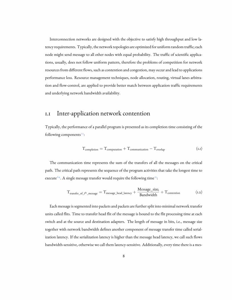
1.1 Inter-application network contentionTypically, the performance of a parallel program is presented as its completion time consisting of thefollowing components23:

Tcompletion = Tcomputation + Tcommunication − Toverlap (1.1)

The communication time represents the sum of the transfers of all the messages on the criticalpath. The critical path represents the sequence of the program activities that take the longest time toexecute64. A single message transfer would require the following time 15:

Ttransfer_of_ith_message = Tmessage_head_latency +Message_sizeiBandwidth + Tcontention (1.2)

Eachmessage is segmented into packets and packets are further split intominimal network transferunits called flits. Time to transfer head flit of the message is bound to the flit processing time at eachswitch and at the source and destination adapters. The length of message in bits, i.e., message sizetogether with network bandwidth defines another component of message transfer time called serial-ization latency. If the serialization latency is higher than the message head latency, we call such flowsbandwidth-sensitive, otherwise we call them latency-sensitive. Additionally, every time there is a mes-

8

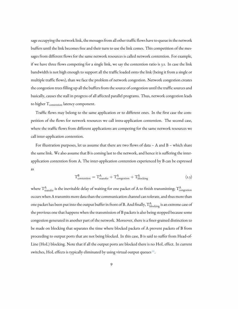
sage occupying the network link, themessages fromall other traffic flows have to queue in the networkbuffers until the link becomes free and their turn to use the link comes. This competition of the mes-sages from different flows for the same network resources is called network contention. For example,if we have three flows competing for a single link, we say the contention ratio is 3:1. In case the linkbandwidth is not high enough to support all the traffic loaded onto the link (being it from a single ormultiple traffic flows), than we face the problem of network congestion. Network congestion createsthe congestion trees filling up all the buffers from the source of congestion until the traffic sources andbasically, causes the stall in progress of all affected parallel programs. Thus, network congestion leadsto higher Tcontention latency component.

Traffic flows may belong to the same application or to different ones. In the first case the com-petition of the flows for network resources we call intra-application contention. The second case,where the traffic flows from different applications are competing for the same network resources wecall inter-application contention.

For illustration purposes, let us assume that there are two flows of data – A and B – which sharethe same link. We also assume that B is coming last to the network, and hence it is suffering the inter-application contention from A. The inter-application contention experienced by B can be expressedas

TBcontention = TAtransfer + TAcongestion + TAblocking (1.3)

where TAtransfer is the inevitable delay of waiting for one packet of A to finish transmitting; TAcongestionoccurswhenA transmitsmore data than the communication channel can tolerate, and thusmore thanone packet has been put into the output buffer in front of B. And finally, TAblocking is an extreme case ofthe previous one that happens when the transmission of B packets is also being stopped because somecongestion generated in another part of the network. Moreover, there is a finer-grained distinction tobe made on blocking that separates the time where blocked packets of A prevent packets of B fromproceeding to output ports that are not being blocked. In this case, B is said to suffer from Head-of-Line (HoL) blocking. Note that if all the output ports are blocked there is no HoL effect. In currentswitches, HoL effects is typically eliminated by using virtual output queues 39.

9

1.2 Interconnection network topologies

1.2.1 Fat-trees

Fat-trees are multi-stage tree-like topologies. Different kinds of fat trees have been proposed in theliterature 37,49 all of which can be described under the parametric family of Extended Generalized FatTrees (XGFT)45.The most common kind of fat trees found in supercomputers are k-ary n-trees49. k-ary n-trees are

full-bisection fat trees that require n · kn−1 switches to connect kn nodes that can be constructed using2 · k-port switches.It is possible to construct “slimmed” fat trees (Figure 1.1), which provide less than full bisection

bandwidth (with the corresponding saving in cost and complexity) at the expense of reducing theavailable bisectionbandwidth. This topology is used inRoadRunner 6, theworld’s first PETAFLOPSmachine, and proposed under name ”fit-tree” in the work of Kamil et al. 32.Such topologies can be described with the XGFT notation. An XGFT(h;m1, ...,mh;w1, ...,wh)

of height h has N =∏h

i=1mi leaf nodes that can accommodate communicating tasks, while the innernodes serve only as traffic routers. Each non-leaf node at level i has mi child nodes, and each non-roothas wi parent nodes45. An XGFT of height h has h+ 1 levels, level 1 being the leaf node level. XGFTsare constructed recursively, each sub-tree at level l being itself an XGFT.

1.2.2 Dragonflies

Dragonfly topologies 33 are highly scalable high-radix two-level direct networks with a good cost- per-formance ratio, used for example in the PERCS interconnect4 and likely to make up the future Ex-aflop/s machines. A dragonfly is a two-level hierarchical network, where a number of cliques (fully-connected groups) of low-radix switches at the first level forma virtual high-radix switch. These virtualhigh-radix switches form another fully-connected graph of first-level groups 33. The ports that the vir-tual high-radix switches use to connect to the other virtual switches are in fact distributed across the

10

XGFT (3 ;2,2,2 ;1,2,2) XGFT (3 ;2,2,2 ;1,1,1)

Level 1

Level 2

Level 3

0 1 ml−1

w l+1−10 1

.. .

.. .

1≤ l<h

Switch at Level l

XGFT (h ;m1 ,... ,mh ;w1 ,... ,wh)

Proc. Nodes

Figure1.1: Switchports at level l inXGFT(h;m1,...,mh;w1,...,wh) (top) andexamples of a full-bisection fat-tree (left bootom)

and its slimmed version (right bottom).

low-radix real switches that make up the virtual switch. Dragonflies can be described by means ofthree parameters: p, the number of nodes connected to each switch, a, the number of switches in eachfirst level group, and h, the number of channels that each switch uses to connect to switches in othergroups. For certain values for these parameters it can be shown that ideal throughput can be achievedfor uniform traffic. The longest possible shortest path is made up of a traversal of a local, L link in thefirst level group to get to the switch that has a global, R link towards the destination group, a traversalof the R link and a second local link traversal in the destination group to get to the switch directlyconnected to the destination node.

11

1.2.3 Infiniband technology

The adapter and switch architecture parameters used throughout the thesis are based on the currentInfiniband 1 adapter and switch architecture employed in many computing systems today. Infini-Band’s Maximum Unit Transfer (MTU) is 256B-4KB. The typical link bandwidth supported in In-finiBand is 10-40Gb/s and the switch latency 100ns. The main advantage of InfiniBand technologyfor the topic addressed in this thesis is its support for quality-of-service (QoS) mechanism.

1.3 Resource management techniques

1.3.1 Computing nodes allocation

The computing nodes allocation is performed by the system scheduler (e.g., SLURM66, LSF70). Thescheduler manages the allocation of computing nodes to jobs that are being submitted by the usersto the system. The choice of computing nodes determines the part of the network that is going tobe used by the job. Thus, the decission on node allocation may directly contribute to the amount ofinter-application contention.

By default, a computing node can be only used by one job (exclusive use of computing nodes).Users can change this default behavior allowing more jobs to be allocated per computing nodes but itis not common.

Once a set of computing nodes are found by job scheduler, the tasks of the parallel jobs are, bydefault, mapped sequentially to the allocated nodes. Optimization of mapping tasks to computingnodes, i.e., the order in which the tasks are placed to nodes based on communication pattern of thejob is out of the scope of this work.

When there are not enough available computing nodes to allocate a job then the scheduler holdsthe job on a queue until enough computing nodes become available, i.e., some running jobs finish andtheir nodes are released.

12

As we see, job schedulers have to deal with the selection (which job) in a spatial (where to allocatejobs) and a temporal axis (when to allocate). Job schedulers usually incorporate policies that deal wellwith the temporal axis, prioritization, resource reservation, backfilling, etc. On the other hand, jobschedulers generally have a poorer, if it all, view of the network topology and of how the placementdecisions could impact the performance of applications. The discussion on prior work is done inChapter 6.

1.3.2 Routing algorithms

The purpose of routing algorithms is to calculate a path between every pair of computing nodes.The routing algorithms are classified as folows: 1) adaptive or oblivious, depending whether the

network state is taken into account or not, 2) static or dynamic, depending whether a route for a pairof nodes is constant during the whole execution or not, 3) source-based or switch-based, depending atwhich place the decision on route is taken, 4) shortest-path or non-shortest path.Knowing the traffic pattern of the parallel application, it is possible to deduce an optimal rout-

ing algorithm69,54,53. Optimal routing algorithm is the one that calculates paths between computingnodes pairs for a given set of these nodes such that the contention for the links on the path is minimal,i.e., the traffic is balanced. Optimization is normally done for the traffic patterns (pattern-aware 54)that the application employs. In the ideal case we can know the traffic pattern a priori, or we can learnthe pattern fast enough after the execution starts. However, a supercomputer is a dynamic systemand optimizing routes for a single application may negatively impact another or even several otherapplications. In29 we have shown that, from the system point of view, a routing algorithm can rangefrom the best to the worst depending on the number and the behavior of other applications runningsimultaneously in the system.Applying a dynamic routing algorithmmay seem as a logical step for balancing traffic in a dynamic

system. However, the decision on changing the routes is taken based on the previous measurement ofnetwork state for which we do not have any gurantees on how long it will last; there is multitude ofapplications with different traffic patterns coming and leaving the system at every moment. Thus, by

13

applying the route change we are not sure whether we are solving the problem or making it worse.In order to make timely decision on route change an option would be to employ switch-based

adaptive routing. In this way, an application’s flow could be re-routed through another port everytime the flow would be delayed by other applications that use the first-choice port. This approachwould require re-calculating the route at the switch, thus additional complexity in the switch. Moreimportantly, in this way the problem would be solved locally, but could create a problem at anotherpoint in the network.The approach of re-routing based on feedback from the network is a good approach for balancing

the traffic in the direct network topology such as Dragonfly. We have shown the impact of adaptiverouting applied on various adversarial traffic patterns under sequential and random task placement 51.Balancing the traffic in this way is rather application-interference oblivious for the reasons previouslymentioned.

1.3.3 Virtual channels arbitration

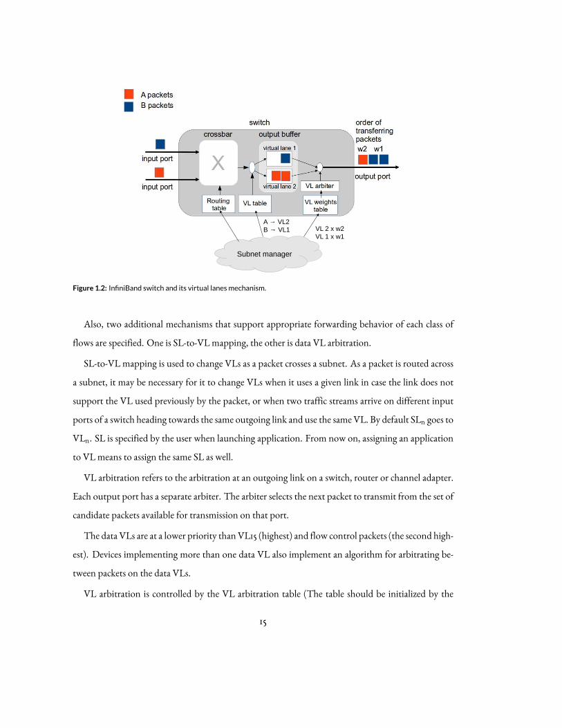
InfiniBand provides the concept of Service Level (SL) which is used to identify different flows withinan InfiniBand subnet. In this work we consider as a flow all packets sent by one application. An SLidentifier is carried in the local route header of the packet.Virtual lanes (VLs) provide a mean to implement multiple logical flows over a single physical link

(Figure 1.2). In InfiniBand one VL (VL15) is reserved for subnet management traffic (A fabric inter-connected with switches is called subnet). All other VLs are for regular data traffic. VL0 and VL15are default lanes, while VLs 1-14 may be implemented to support additional traffic segregation. Thenumber of data VLs configured has to be 1, 2, 4, 8 or 15. In current systems typically eight VLs areimplemented (e.g., Mellanox).For eachVL independent buffering resources are provided. Link-level flow control is implemented

on a per data VL basis. The sending port of an InfiniBand device identifies each packet with the VLto be used. The number of VLs used by a port is configured by the subnet manager. The port at theother end of the link may support a different number of VLs.

14

Subnet manager

A → VL2B → VL1 VL 2 x w2

VL 1 x w1

Figure 1.2: InfiniBand switch and its virtual lanesmechanism.

Also, two additional mechanisms that support appropriate forwarding behavior of each class offlows are specified. One is SL-to-VL mapping, the other is data VL arbitration.

SL-to-VL mapping is used to change VLs as a packet crosses a subnet. As a packet is routed acrossa subnet, it may be necessary for it to change VLs when it uses a given link in case the link does notsupport the VL used previously by the packet, or when two traffic streams arrive on different inputports of a switch heading towards the same outgoing link and use the same VL. By default SLn goes toVLn. SL is specified by the user when launching application. From now on, assigning an applicationto VLmeans to assign the same SL as well.

VL arbitration refers to the arbitration at an outgoing link on a switch, router or channel adapter.Each output port has a separate arbiter. The arbiter selects the next packet to transmit from the set ofcandidate packets available for transmission on that port.

The data VLs are at a lower priority thanVL15 (highest) and flow control packets (the second high-est). Devices implementing more than one data VL also implement an algorithm for arbitrating be-tween packets on the data VLs.

VL arbitration is controlled by the VL arbitration table (The table should be initialized by the

15

subnet manager prior to use by data traffic.) which consist of three components, high-priority, low-priority and limit of high-priority. The high-priority and low-priority components are each repre-sented by a list ofVL/weight pairs. Theweighting value indicates howmany unitsmay be transmittedfrom the VL when its turn in the arbitration occurs.

Arbitration between High and Low Priority VLs

The high-priority and low-priority components form a two level priority scheme. If the high-prioritytable has an available packet for transmission and the limit of high-priority is not reached then thehigh-priority is active and a packet may be sent from the high-priority table. If the high-priority tabledoes not have an available packet for transmission, or if the limit of high-priority is reached, then thethe low-priority table becomes active and a packet may be sent from the low-priority table.

Arbitration within High and Low Priority VLs

Within each high or low priority table, weighted fair arbitration is used, with the order of entriesin each table specifying the order of VL scheduling, and the weighting value specifying the amountof bandwidth allocated to that entry. Each entry in the table is processed in order. Weighted fairarbitration between the VLs of the same priority provides a mechanism to allow more sophisticateddifferentiation of service classes.Although InfiniBand provides mechanisms for QoS, it does not specify the policies for utilizing

these mechanisms. It is necessary to develop QoS strategies to support a highly varied set of HPCapplications.

16

2Experimental methodology

Simulation tools are typically employed to evaluate application and system performance for differentsystem parameters (e.g., network topologies, routing mechanisms, arbitration mechanisms, etc.). Asthis study requires analyzing HPC traffic in conjunction with the details of the network technology,we have used an MPI simulator driven by post-mortem traces of real MPI applications executions inconjunction with an event-driven network simulator. Besides, a scheduler simulator is developed forevaluating system-level resourcemanagement techniques. This chapter describes the set of simulationtools employed in the thesis, along with the workload used in evaluation.

17

Our experimental methodology consists of the following elements:

• HPC workload

• Extrae: Tracing tool

• Paraver: Visualization tool

• Dimemas: MPI simulator

• Venus: Network simulator

• Barrio: Scheduler simulator

• Performance metrics for quantifying the impact of applications’ interference on the systemperformance

Each of these elements will be described as follows in a different section of this chapter.

2.1 HPC workloadIn order to study inter-application contention it was important to choose a diverse set of HPC appli-cations. A variety of scientific kernels from theNAS parallel benchmarks 5 set such as FT, CG, BT andMG are used in this study.

• FT (Fast Fourier Transform) solves a three-dimensional partial differential equation using FastFourier transform (FFT).

• CG (ConjugateGradient) estimates the smallest eigenvalue of a large sparse symmetric positive-definite matrix using the inverse iteration with the conjugate gradient method as a subroutinefor solving systems of linear equations.

• BT (BlockTridiagonal) is one of the algorithmsused for solving a synthetic systemof nonlinearpartial differential equations.

18

• MG (MultiGrid) approximates the solution to a three-dimensional discrete Poisson equationusing the V-cycle multigrid method.

Additionally, a set of real production scientific applications such asWRF, CGPOP, GROMACS andMILC has been used for this study.

• WRF (Weather Research and Forecast model)41 is a numerical weather prediction system de-signed to serve the atmospheric research community. It is being used by an increasing commu-nity of researchers to implement and refine physical models.

• CGPOP 57 is a miniapp for the Parallel Ocean Program (POP) developed at Los Alamos Na-tional Laboratory, USA. POP is a global ocean modeling code and a component within theCommunity Earth SystemModel (CESM). CGPOP encapsulates the performance bottleneckof POP, which is the conjugate gradient solver.

• GROMACS 52 performs molecular dynamics, i.e. simulate the Newtonian equations of mo-tion for systemswith hundreds tomillions of particles. It is primarily designed for biochemicalmolecules like proteins, lipids andnucleic acids, but also for research onnon-biological systems,e.g. polymers.

• MILC26 is MIMD (Multiple-Instruction Multiple-Data) Lattice Computation code used tostudy quantum chromodynamics(QCD).

The selected workload consists of a wide spectrum of scientific applications characterized by dif-ferent communication traffic load. Figure 2.1 shows the aggregated number of bytes injected into net-work by an application’s task during its execution. Since duration of a single Alltoall communicationphase of FT application ( 4s) is longer than whole execution of some other applications from our set,we present all applications communication frequency at 4 seconds scale. Figure 2.2 in continuationshows the case of multiple iterations of FT application at larger time scale.Figure 2.3 shows the output of the Equation 2.1 , i.e., average bytes in transit at any time of each

application:

19

0.0 0.5 1.0 1.5 2.0 2.5 3.0 3.5 4.0time (ns) 1e9

105

106

107

108

109by

tes

in tr

ansi

tFT (Alltoall)

0.0 0.5 1.0 1.5 2.0 2.5 3.0 3.5 4.0time (ns) 1e9

105

106

107

108

109

byte

s in

tran

sit

CG

0.0 0.5 1.0 1.5 2.0 2.5 3.0 3.5 4.0time (ns) 1e9

105

106

107

108

109

byte

s in

tran

sit

BT

0.0 0.5 1.0 1.5 2.0 2.5 3.0 3.5 4.0time (ns) 1e9

105

106

107

108

109

byte

s in

tran

sit

MG

0.0 0.5 1.0 1.5 2.0 2.5 3.0 3.5 4.0time (ns) 1e9

105

106

107

108

109

byte

s in

tran

sit

CGPOP

0.0 0.5 1.0 1.5 2.0 2.5 3.0 3.5 4.0time (ns) 1e9

105

106

107

108

109

byte

s in

tran

sit

WRF

0.0 0.5 1.0 1.5 2.0 2.5 3.0 3.5 4.0time (ns) 1e9

105

106

107

108

109

byte

s in

tran

sit

GROMACS

0.0 0.5 1.0 1.5 2.0 2.5 3.0 3.5 4.0time (ns) 1e9

105

106

107

108

109

byte

s in

tran

sit

MILC

Figure 2.1: Bytes loaded into network by each of the studied applications.

∫ endTime0 bytesInTransit(t) dt

endTime . (2.1)

20

0.0 0.5 1.0 1.5 2.0 2.5 3.0 3.5time (ns) 1e10

105

106

107

108

109

byte

s in

tran

sit

Figure 2.2: Bytes loaded into network by FT.

0

10

20

30

40

50

60

70

Ap

plic

atio

n's

ave

rag

e b

yte

s in

tra

nsi

t (G

b/s

)

Figure 2.3: Applications’ average average bytes in transit.

2.2 ToolchainTwo sets of toolchains will be used in this thesis. The toolchain from Figure 2.9 will be used for ourcharacterization methodology, application’s performance analysis and QoS policies. The scheduler

21

simulator in Figure 2.11, developed for the purpose of this thesis, will be used for the evaluation of oursystem-level resource management policies.

2.2.1 Extrae: Tracing tool

In order to get information about an application communication behavior and its performance ingeneral it is necessary to insert instrumentation into it during its execution. An instrumented programgenerates a report that is called an application’s trace. An application trace consists of a sequenceof procedures called during application run, as well as information on how much time was spent invarious parts of the application. The applications’ traces were obtained using Extrae 11, tracing tooldeveloped at Barcelona Supercomputing Center (BSC).MPI standard includes a mechanism that enables users to profile MPI applications throughMPI’s

Profiling interface layer. The idea behind profiling interface is to allow a secondary entry point toMPIlibrary routines. Namely, while MPI function names have prefix MPI_, the secondary names for thesame function will have prefix PMPI_. The application calls with MPI prefix can be intercepted andrecorded, followed by the call of PMPI calls (Figure 2.4). PMPI calls are equivalent to MPI ones, theonly difference in application performance is a small overhead incurred due to two calls.Extrae intercepts theMPI calls that are coded withMPI prefix. However, the low-level operations

of MPI collective calls are not coded with MPI prefix, but with MCA_PML_CALL macro, thus,they are not being recorded by Extrae. These low-level calls are either the actual sequence of point-to-point communications performed by MPI collective calls (e.g., MPI_Send, MPI_Recv), or the timeanMPI task spentwaiting for themessage (MPI_Wait). For our study, these are very important piecesof information. Therefore, the OpenMPI22 library is adapted to allow translation of the macros toMPI_-like names (Figure 2.5).Inorder to instrument anMPI application at run time, Extraeuses theLD_PRELOADmechanism

to dynamically intercept calls toMPI library, as presented in the example scripts in Figure 2.6 This in-terposition is done by the runtime loader by substituting the original symbols (”MPI”) by those pro-videdby the instrumentationpackage (”PMPI”). Note that in the tracing script theMPI_INTERNALS

22

Figure 2.4: Dynamic library calls intrumentation

library is also loaded, to allow instrumentation of low-level communications of collective calls as pre-viously explained.

We obtain the traces of instrumented applications from their runs on MareNostrum supercom-puter.

The execution of a parallel application under Extrae generates a per-process record denoted as anmpit trace. Thempi2prv tool 11 developed at BSC canmerge all the individual mpit traces into a singlefile. This merged trace file is suitable for the Paraver visualization tool which will be described inSection 2.2.2.

During instrumentation, each consecutive sequence of computation activities from the same pro-cess is translated into a trace record indicating a busy time for a specific CPU whereas the details ofactual computation performed are not recorded. Communication operations are recorded as send,receive, or collective operation records, including the sender, receiver, message size, and type of oper-ation.

23

Traced

Traced

Cannot be traced

Name translation

Allr

educ

e O

penM

PI i

mpl

eme

ntat

ion

Inte

rnal

sIn

tern

als

tran

slat

ed

Figure 2.5: Tracing internals of collective communications. The OpenMPI library adaptation to allow for translation of

MCA_PML_CALLmacro to standardMPI call format.

The resulting traces normally consist of multiple iterations. Typically, each iteration has one com-putation and one communication phase. As the size of each trace can be several GBytes and thereforetoo big to be usedwith our simulators, a portion of each tracewill be extracted, namely a cut of around10-15% of the whole trace. The used trace cuts captures all the relevant characteristics of application’sexecution: communication patterns, computation/communication ratio, etc.

The records of high-level collectives and low-level internals of collectives cannot coexist in the tracesince the MPI simulator will not understand them. To avoid this, we remove high level collectives’records before translating the Paraver trace to its corresponding Dimemas format.

24

Figure 2.6: An example of the tracing scripts

2.2.2 Paraver: Visualization tool

Paraver 12,50 is a visualization tool developed at BSC to show the insights of the execution of parallelapplications, based on the traces obtained with Extrae. This visualization tool is very useful to detectload imbalance problems by simple inspection. Besides, we can visualize an application communica-tion pattern, number of bytes exchanged between each pair of tasks, bytes in transit sent by a singletask or total bytes sent by application at each point of its execution.

The mpi2prv tool described in Section 2.2.1 converts the multiple mpit individual trace files ob-tained with Extrae to a single file which can be understood by Paraver. However, the trace format ofthis tool differs from the trace format required for the Dimemas simulator described later in Section2.2.3. The prv2dim tool converts the required fields from the Paraver trace to the format expected byDimemas.

25

2.2.3 Dimemas: MPI simulator

Dimemas 10,36 is a tool developed at BSC to analyze the performance of message passing programs. Itis an event-driven simulator that reconstructs the time behavior of message passing applications on amachine modeled by a set of performance parameters.

The input to Dimemas is a trace containing a sequence of operations for each thread of each task.Each operation can be classified as either computation or communication. Dimemas replays a traceusing an architectural machine model consisting of a network of SMP nodes. The model is highlyparameterizable (Figure 2.7), allowing the specification of parameters such as number of nodes, num-ber of processors per node, relative CPU speed, number of communication buses, mapping tasks tonodes, etc.

The simulator is able to replay one or several MPI applications’ traces simultaneously. Each of thetraces contains a sequence of operations of each MPI application task as explained previously. Com-putation operations are not performed, but represented by the time the actual computation wouldlast. Communication operations are send and receive point-to-point communications.

Dimemas allows formultiple replays of the traceswithin one simulation run. We can set number ofrestarts with an option ”-r” followed by a number of replays. Setting ”-r 0” means that Dimemas willrestart traces as many times as needed until each trace has been played at least once. The difference induration of different traces cuts might have some impact on the level of inter-application contentionthat the longer applications experienced. To solve this problem, we simply performed additional re-play(s) of the trace of the application that finished earlier, immediately after its first execution. Thisway, applicationswere running concurrently at least until the end of their first execution. To calculatethe impact of inter-application contention, we take the time of the first execution.

Task allocation is an important parameter in the context of network interference problem. InDimemas, mappingMPI tasks to nodes is defined using a mapping vector. The mapping vector has aform {x,y,z,w}, where the lenght of the vector is the number of application’s tasks, and x, y, z andw arethe computing nodes. Themapping vector is interpreted as follows, a vector’s index is anMPI task of

26

Figure 2.7: Dimemas parameters relevant for our study.

application mapped to the node at that index. In the example given in the Figure 2.7 {0,1,2,3}, we willhave the following mapping for each application: task0 to node0, task1 to node1, task2 to node2 andtask3 to node3. Note that number of processors per node is set to 4. Thus, with the given mappingwe will have each node populated with four tasks each from different applications. On the other side,an alternative setting for ft mapping as {0,0,0,0}, cg as {1,1,1,1}, bt as {2,2,2,2} andmg as {3,3,3,3} wouldmap all tasks of one application on a single node.Dimemas outputs various statistics, such as execution time of each application, time spent in com-

putation and communication, as well as output Paraver trace.

2.2.4 Venus: Network simulator

Venus43,42 is an event-driven simulator based on OMNeT++61 developed at IBM Zurich that is ableto simulate up to the flit level any generic network topology of nodes and switches. It is able to pro-vide a detailed simulation of the network topology and the processing inside the switches. It has two

27

main configurable basic components, the Adapter and the Switch, that are used to build arbitrary net-work topologies. The adapter and switch are based on InfiniBand technology specification and haveimplemented QoS mechanism.

Network topology, routes and mapping of applications to nodes are specified in correspondingtopology, routing and mapping files. The creation of these files is explained in more detail as follows.

The applications are simulated using different network topologies: (i) fully connected one-hopnetwork (crossbar), (ii) full bisection fat tree, and (iii) slimmed fat trees with different degrees of slim-ming45,49 (Figure 1.1).

The topology file for fat tree topology is generated in two steps. First, by using Venus xgft toolwith option -m and passing the parameters that define the desired fat tree topology, the intermediatetopology file is generated. For instance, intermediate topology file xgft.map for a 3-level fat-tree withswitch radix 4 will be generated in this way:

xgft -m 3:4,4,4:1,4,4> xgft.map

and in case of a crossbar:xgft -m 1:4:1> xgft.map

where 4 is the radix of crossbar. Furter, we transform xgft.map file to actual topology files xgft.iniand xgft.ned using map2ned tool. Similarly, the route file is generated using xgft tool followed by -roption and a number that represents specific routing scheme (e.g., 3 for random routing, 1 for d-mod-krouting, etc.).

Venus task allocation file is a file with .scb extension and contains a list of computing nodes suchthat each line of the file contains only one node in the form hn where n takes values from 0 to totalnumber of computing nodes in the system. Relation in between taskmapping inDimemas andVenusis shown in the Figure 2.8. Basically, if the task is placed on Dimemas Nth node, in Venus it will beplaced on the node encountered in the Nth line of Venus mapping file.

The link bandwidth is set using two parameters unit_size and unit_time; unit_size is equivalent toflit size of the real network (it is possible to define min_unit_size, as well), where as unit_time is timeneeded to transfer amount of data defined by unit_size over the network link. The link bandwidth

28

{0, 1, 2, 3}

{0, 1, 2, 3}

A:

B:

Dimemasmapping

Venus mapping file

h0h1h2h3

{0, 0, 0, 0}A:

{1, 1, 1, 1}B:

h0

h3

h5h0h4h7h1h6h3h2

{4, 5, 6, 7}B:

{0, 1, 2, 3}A:

Dimemasmapping

Dimemasmapping

Venus mapping file

Venus mapping file

A0 B0 A1 B1 A2 B2 A3 B3

h0 h1 h2 h3

A0 A1

h0 h1 h2 h3

A2 A3

B0 B1B2 B3

A1

h0 h1 h2 h3

B0 B3 B2

h4 h5 h6 h7

A2 A0 A3B1

Figure 2.8: Relation between tasks-to-nodesmapping inDimemas andVenus. Ax andBx are the xth task of applications Aand B, respectively. Task B2 is placed on the node at the 2nd position of the B’s Dimemasmapping vector, i.e., node 6; this

node corresponds to Venus node on 6th line of Venusmapping file, i.e., node h3.

represents the ratio of the unit_size and the unit_time.

Each packet carries information on the application it belongs to. This allows us to apply differentper-packet policies based on its application QoS requirements.

Venus allows for defining different QoS policies through InfiniBand 1 mechanism of virtual lanes.Basically, virtual lanesmechanismdivides buffer physical space in several virtual partitions, where eachpartition is served according to a virtual lane arbitration policy. A different number of priorities, andvirtual lanes can be defined, as well as virtual lane arbitration policies. Namely, we can define howmany packets can be served from each virtual lane in one turn and in that way engineer and tune the

29

traffic differently based on its requirements. The buffer sizes are configurable, as well.The Adapter and the Switch model collect information during the simulation that gets sent to

a module that processes statistics. The output of Venus can either be a summarized collection ofstatistics or a detailed description of the point to point communications that took place during thesimulation time.WeuseDimemas integratedwithVenus. The complete tool chainofDimemas-Venus co-simulation

is given in the Figure 2.9. As previously described, Dimemas takes care of simulating the applicationat the MPI level, it feeds each individual communication to a proxy component built in Venus thatinstructs the Venus Adapter to inject the message. This proxy component in Venus also monitorsthe reception of messages and communicates this information to Dimemas. Venus and Dimemas to-gether act as a discrete-event simulator synchronized using the Null message protocol/algorithm62.Whenever there are messages in flight, Dimemas and Venus exchange messages with the look-aheadtime that they can continue the simulation until some event change the state arises.One of the main advantages of the integration is the possibility of using Paraver to analyze and

compare traces fromactual runswith traces obtained fromsimulations. The flexibility ofVenus allowsfor many topologies to be studied with relatively little extra developing effort. Another advantage ofthis model is that the MPI and the network level simulation are totally decoupled. This means thatdifferentMPImodels can be implemented independently of the network simulator. An example of ascript setup for running a Dimemas and Venus co-simulation is given in the Figure 2.10.

2.2.5 Barrio: Scheduler simulator

Barrio simulator has been built in order to evaluate the effectiveness of the proposed node allocationpolicies (Figure 2.11). The list of jobs to be simulated are taken from a trace recorded during normaloperation of a supercomputer. The trace is generated by the Marenostrum’s scheduler. For each jobthe scheduler recorded information such as the timewhen job arrived to the system, the duration of itsexecution, and the number of computing nodes used among other data. Figure 2.12 shows an exampleof a job record from the scheduler log. This information is enough to model the scheduling of jobs in

30

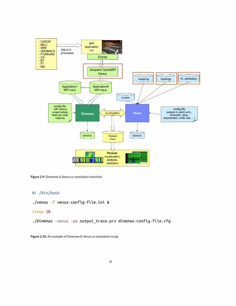
Figure 2.9: Dimemas &Venus co-simulation toolchain.

Figure 2.10: An example of Dimemas &Venus co-simulation script.

31

- Percent of sharing jobs- Sharing jobs per job- System throughput- System utilization, etc.

Statistics

Barrio

Job scheduler log

Node allocation policies:- First Available- First Contiguous- Virtual Networks- Exclusive

HPC workload executed on

MareNostrum during 32 days

Visualization

Node fragmentation & network sharing

analysis

Per job information:- jobID - queue arrival time - start time- end time- number of processors - number of computing nodes- list of allocated computing

nodes

Figure 2.11: Toolchain for evaluation of system-level resourcemanagement policies.

Job ID submit time start time end timenumber

processorsnumber

exec hosts

list of exec host

Figure 2.12: An example of per-job information fromMareNostrum scheduler log used in our evaluation.

the simulator.Note that the simulator does not replay the execution of jobs, it only accounts the time that every

computing node has been using the system. In the simulator we are measuring different parametersduring the executionof the job trace. Adescription of the key parameters reported are given as follows:

• Completion time. Reports the total elapsed time to process all the jobs in the input trace.

32

• System utilization. Reports the percentage of the system computing nodes that have an allo-cated job.

• Queue time. Reports the time that jobs are waiting for computing resources to become avail-able.

• Per job sharing. Measures the average number of jobs that a job shared the system networkwith.

• Sharing jobs. Reports the percentage of total jobs that share system network with other jobs.

• Sharing network per level. Reports the total number of job pairs that are sharing the networkat the second and at the third level.

2.3 Performancemetrics for evaluating the interference impacton system performance

To quantify the impact for a particular workload, the application was simulated in the same systemtwice (Figure 2.13). First, it was executed alone, i.e., without any interference. The completion time ofan application is Talone. Then, it was run simultaneously with another application (or several applica-tions) sharing the system and thus experiencing interference.We will refer to the completion time of an application in the latter scenario as Tsharing. Both Talone

and Tsharing, we get from Dimemas output statistics at the end of simulation. Note that due to ap-plication trace cuts not being of the same duration, we perform a replay of the shorter one while theexecution time of the first iteration only is considered. Therefore, the increase in completion time dueto interference for an application i can be calculated as:

Tiinter = Tisharing − Tialone (2.2)

33

time

Job 1

Talone1

time

Run#3: Job1 alone in the system

Job 2

time

accumulated delay of a job due to

inter-application contention

Talone2

Tsharing1

Tsharing2

Run#5: Job1 and Job2 sharing the system

Tinter

Tinter1

Tinter2

Run#4: Job2 alone in the system

Job 1

Tbase1

time

Run#1: Job1 in crossbar

Job 2

time

Tbase2

Run#2: Job2 in crossbar

accumulated delay of a job due to

intra-application contention Tintra

Tintra2

Tintra1

no contention in the network,

only end-point contention Tbase

Alone in the system Sharing the system

Figure 2.13: Simulation experiments needed for quantifying the impact of the network interference on the performance

of each job. The case of two-applications workload. Tbase,Talone andTsharing are the outputs of the simulation runs.

Also, note that all system parameters and settings (e.g., size of the network, task allocation, routing,MTU size, etc.) have to be the same in both scenarios so that the increase in the execution time of theapplication can be attributed solely to the interference, and not to a coupled effect of interference andother factors.To measure the impact of job’s interference on system performance we will use the computing

node time metrics defined in Figure 2.14.Ci being the size of ith job i.e. the number of computing nodes it is allocated to, we can calculate

total waste of computing node time due to interference in the workload of n jobs as:

Jinter =n∑i=1

Ci · Tiinter (2.3)

Finally, to quantify the effectiveness of our policy P in reducing the impact of interference, we usethe following formula:

E(P) = JinterJinter(P)

. (2.4)

34

J1J2

J3 J4J5

Computing node time in nodes*seconds

number of computing nodes

time

Completion time under performance isolation

T_inter_5

T_alone_5

C5

Increase in completion time due to interference with other jobs in the system

J5 = C5 * T5 = C5 * (T_alone_5 + T_inter_5) Computing node time of Job5

J_inter_5 = C5 * T_inter_5 Increase in computing node time of Job5 due to its interference with other jobs

Job-level metrics

System-level metrics

SUM(J_inter_i)

Computing node time waste due to jobs' interference

0

Number of computing nodes occupied by Job5

Figure 2.14: Quantifying the impact of the jobs’ interference on the system performance.

35

36

3Characterizing applications at network-level

Full bisection indirect topologies, such as fat trees, have been one of the preferred interconnectionnetworks for high-performance computing (HPC). However, with increasing system size the cost ofproviding full bisection bandwidth accounts for an increasing portion of the total system cost. An un-derutilization of the communication network has been observed for some HPC workloads 32 trigger-ing an effort to optimize the network in terms of cost and performance for the typical communicationcharacteristics of HPC workloads.

A commonly adopted approach to improve this situation is to deploy a slimmed fat-tree topol-

37

ogy. Such a network reduces cost by eliminating some switches in each level of the traditional fat-treetopology at the expense of reducing the available bisection bandwidth. These topologies are prone tohigher congestion.

Additionally, another factor that strongly impacts system throughput is job fragmentation. Thisoccurs when multiple jobs running in the system require different number of nodes and have differ-ent execution times. In this scenario, it is very likely that the job scheduler is unable to assign a setof contiguous nodes (i.e., nodes that are topological neighbors) to the next job, and instead assignsnodes that are spread throughout the system and are not topological neighbors. Unfortunately, thiseffect degrades system throughput, as the performance of various jobs can simultaneously be degradedby the contention produced among each other. This type of contention is commonly called inter-application contention. In contrast, we denote contention suffered internally by a single applicationas being intra-application. Today, job schedulers such as Moab support various job allocation poli-cies, including contiguous allocation, but to obtain a contiguous allocation the scheduler might haveto hold jobs for a long time in the scheduler queue, which may also severely degrade system through-put. Several recent works have studied this relationship between task mapping and job schedulingpolicies60,44. However, only the impact of intra-application contention on system throughput wasevaluated, not that of inter-application contention.

We have to be aware that the level of inter-application contention is impacted by several other fac-tors, such as routing, topology,MPI tasks ordering and relative starting timebetween the applications.In29 we evaluated the impact of several routing schemes on inter-aplication contention. The effect ofinterference between applications can be reduced using certain routing schemes. However, the com-munication characteristics of applications in the workload are the dominant factor regardless of therouting scheme.

Also, we should make distinction between task placement and task ordering. In this work we ex-periment with different task placements, both random and regular, but assuming sequential task or-dering. This is because schedulers order tasks sequentially by default on a chosen node allocation.Someworks have proposed topology and pattern-aware task orderings to reduce both intra- and inter-

38

application contention44,68. Further, the performance impact also depends on how much the com-munication phases of the applications overlap. The overlap could vary with every new execution of amix of the application depending on the starting time offset between them. These are all additionalfactors that influence inter-application contentionwhichmakes it a very complex problem to analyze.In order to understand the impact of every single factor our approach is to make some of the factorsconstant while varying the others.In this work we:

• Proposed the methodology for characterization of application’s network traffic demands tak-ing into account both applications nature and its actual task placement in the system,

• Classified applications based on the utilization metric obtained from the proposed methodol-ogy,

• Evaluated and understood the increase in intra-application contention of representative scien-tific applications as a function of slimming and fragmentation,

• Analyzed the performance of the applications in a shared environment,

• Classified the workloads based on the overall impact of sharing resources to the applications inthe workload,

• Identified trade-offs that the capacity systems are dealing with in order to get the best perfor-mance when running multiple applications,

• Explored the strategies to mitigate the problem of inter-application network contention.

3.1 Simulation setupTheMPI simulator Dimemas is used driven by post-mortem traces of real applications executions inconjunction with an event-driven network simulator (Venus) as described in Chapter 2. The systemparameters used in the simulations are given in Table 3.1.

39

Table 3.1: Simulatedmachines parameters.

Simulator Dimemas+VenusSystem size 2048 processing nodesTopologies Extended Generalized

Fat Trees45 and CrossbarConnectivity XGFT(3;16,16,8;1,W,W),

W=1,2,4,8,16Switch size 32 ports

Contention ratio 1:1, 2:1, 4:1, 8:1, 16:1Switch Technology InfiniBandInput Buffer Size 4 KB

Network Bandwidth 10 Gbits/sSegment size 4 KBFlit size 256B

MPI Latency 1 μsCPU Speedup 10xRouting scheme Random routing 24

The CPU speedup factor of 10 was applied, meaning that the simulated computation time of theapplication is ten times faster than themachine onwhich the trace was originally collected (MareNos-trum 2.5 GHz PowerPC 970 CPUs). This scaling is necessary to correlate results to the computationspeed of today’s processors. In addition, the simulated network (10 Gb/s) is five times faster than theoriginal network (2 Gb/s Myrinet).

The applications are simulated in three different network topologies: 1) fully connected network(crossbar), 2) full bisection fat tree, and 3) slimmed fat trees with different degrees of slimming

A set of real production applications such as GROMACS, CGPOP, MILC, and WRF, and somescientific kernels from NAS parallel benchmarks such as FT, CG, and BT has been used. Table 3.2gives the base execution time (simulated on a crossbar topology) for each of the application traces.

We have studied the sensitivity of the selected applications with respect to three aspects: i) net-work connectivity (degree of slimming) ii) task placement (fragmentation), and iii) with which otherapplications it is sharing network resources.

40

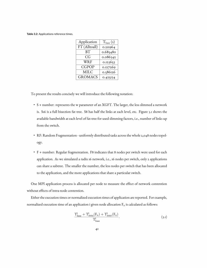
Table 3.2: Applications reference times.

Application Tbase (s)FT (Alltoall) 0.211964

BT 0.685480CG 0.086342WRF 0.123653CGPOP 0.127269MILC 0.586126

GROMACS 0.425134

To present the results concisely we will introduce the following notation:

• S + number: represents the w parameter of an XGFT. The larger, the less slimmed a networkis. S16 is a full bisection fat tree. S8 has half the links at each level, etc. Figure 3.1 shows theavailable bandwidth at each level of fat-tree for used slimming factors, i.e., number of links upfrom the switch.

• RF: Random Fragmentation - uniformly distributed tasks across the whole 2,048 nodes topol-ogy.

• F + number: Regular fragmentation. F8 indicates that 8 nodes per switch were used for eachapplication. As we simulated a radix 16 network, i.e., 16 nodes per switch, only 2 applicationscan share a subtree. The smaller the number, the less nodes per switch that has been allocatedto the application, and the more applications that share a particular switch.

One MPI application process is allocated per node to measure the effect of network contentionwithout effects of intra-node contention.Either the execution times or normalized execution times of application are reported. For example,

normalized execution time of an application i given node allocation Fn is calculated as follows:

Tibase + Tiintra(Fn) + Tiinter(Fn)Tibase

. (3.1)

41

S16 S8 S4 S20

5000

10000

15000

20000

25000

L0L1L2

Ava

ilabl

e ba

ndw

idth

(G

b/s)

Figure 3.1: Total available bandwidth per level of a fat-tree network xgft(3;16,16,8;1,S,S) for different slimming factor S.

where Tibase is the execution time of application i on a system with an “ideal” single-hop full bisectionnetwork (see Table 3.2). Tiintra(Fn) is the difference between the execution times obtained from ap-plication’s run alone on a fat tree topology (on fragmentation Fn) and Tibase. Tiinter(Fn) is differencebetween the execution times obtained from application’s run on the same fat tree topology mixedwith other applications (using the same fragmentation Fn) and the execution time of application’srun alone. The presentation of the sensitivity of applications is separated in two sets of graphs. Firstwe will analyze each application’s sensitivity to the topology and fragmentation when running alone,without considering interference from other applications, followed by discussion on the reasons be-hind observed variability. Then, the cases of multiple applications sharing the system simultaneouslywill be introduced.

3.2 Characterization of the applications network behaviorIn this section we will explain how we perform each step from our characterization methodology de-picted in Figure 3.2. The applications injection rate Figure 3.3 we obtain as follows. Using Paravertraces we have extracted the total injected load in bytes of each application per fat-tree level for a giventask placement. The load was averaged by reference times (crossbar execution times) from Table 3.2giving us the average injection rate that an application would communicate per level of a fat tree foreach of the task placements. Dividing by crossbar time gives us the injection rate an applicationwould

42

Application

Node allocation

Available bandwidth

per network level

Application'sinjection rate

per network level Calculatebandwidth utilization

per network level

Calculate MAX

High

Moderate

Low

UL1

UL2UMAX

UMAX = 1

0.1 <= UMAX < 1

UMAX < 0.1

Categorize application

Characterization methodology

Task placement

Figure3.2:Methodology for characterization of application’s network utilization; bandwidth utilization of application per

levels L1 and L2 isUL1 andUL2, respectively

produce if there was no any resource limitation in the network except end-point contention. L0 plotsshow the injection rates of the applications’ load at level 0 of the fat-tree, i.e., total traffic injection rate.In terms of total traffic, the order of applications’ communication intensity is the same as presented inFigure 2.3. L1 plots show the injection rate of the portion of the traffic that was sent outside of the firstlevel-switches, while L2 plots show the injection rate of the portion of the traffic that was sent outsideof the second-level switches. Therefore, observing the relation between L0 and L1 can give us insightwhether an application is communicating locally or globally. The case of F16 node allocation gives usthe information on application inherited locality. In that regard, FT, MILC and BT most of its traf-fic communicate outside of the first-level switch, while CG,WRF and CGPOP communicate locally.Note that the y-axis is at logarithmic scale. As we spread applications from F16 to F2, the locality ofthe applications changes and they start to communicate most of its traffic at L1 and L2. Thus, we cansay that node allocation deviates the nature of application communications behavior.

Figure 3.4 and Figure 3.5 show the available bandwidth when a job of the size 256 and 512 nodes,respectively, are allocated on different fragmentations. As the job is more spread in the system it can”see” more bandwidth both at L1 and at L2. However, the benefit in terms of more bandwidth whenspreading decreases as the network becomes slimmer. When allocated on F16, a job of size 256 neveruses L2 bandwidth.

The metric that we use to classify applications based on their network demands is bandwidth uti-lization. Bandwidth utilization we obtain by dividing injection rate (Figure 3.3) with available band-width for a given allocation (Figure 3.4 and Figure 3.5, the latter in the case ofMILC). Figure 3.6 shows

43

F1

6

F8

F4

F2

F1

6

F8

F4

F1

6

F8

F4

F2

F1

6

F8

F4

F2

F1

6

F8

F4

F2

F1

6

F8

F4

F2

F1

6

F8

F4

F2

FT(AlltoAll) MILC CG GROMACS BT WRF CGPOP

1

10

100

1000

10000

L0 L1 L2

Inje

ctio

n ra

te (

Gb/

s)

Figure 3.3: Applications’ injection rate per level of xgft(3;16,16,8;1,w,w) under different task placements.

the utilization per level for our seven applications of interest for a case of S2 network and F2 allocation.We cando a coarse grain classificationof applications (Figure 3.7) in extremely demanding applicationsas FT(Alltoall). followed by MILC and CG as moderately demanding and finally, GROMACS, BT,WRF and CGPOP having very low network demands.

3.3 Exploring the sensitivity to task placement and bisectionbandwidth

Wewill separate the presentation of the sensitivity of applications in two sets of graphs. First, we willanalyse each application’s sensitivity to the topology and fragmentationwhen running alone, withoutconsidering interference from other applications. Then we will introduce the cases of mixing withother applications.

3.3.1 Impact on intra-application contentionFigure 3.8 shows the sensitivity of CGPOP to fragmentation and slimming. From left to right, eachgroup shows the impact of decreasing connectivity. Five different topologies, i.e., slimming factors

44

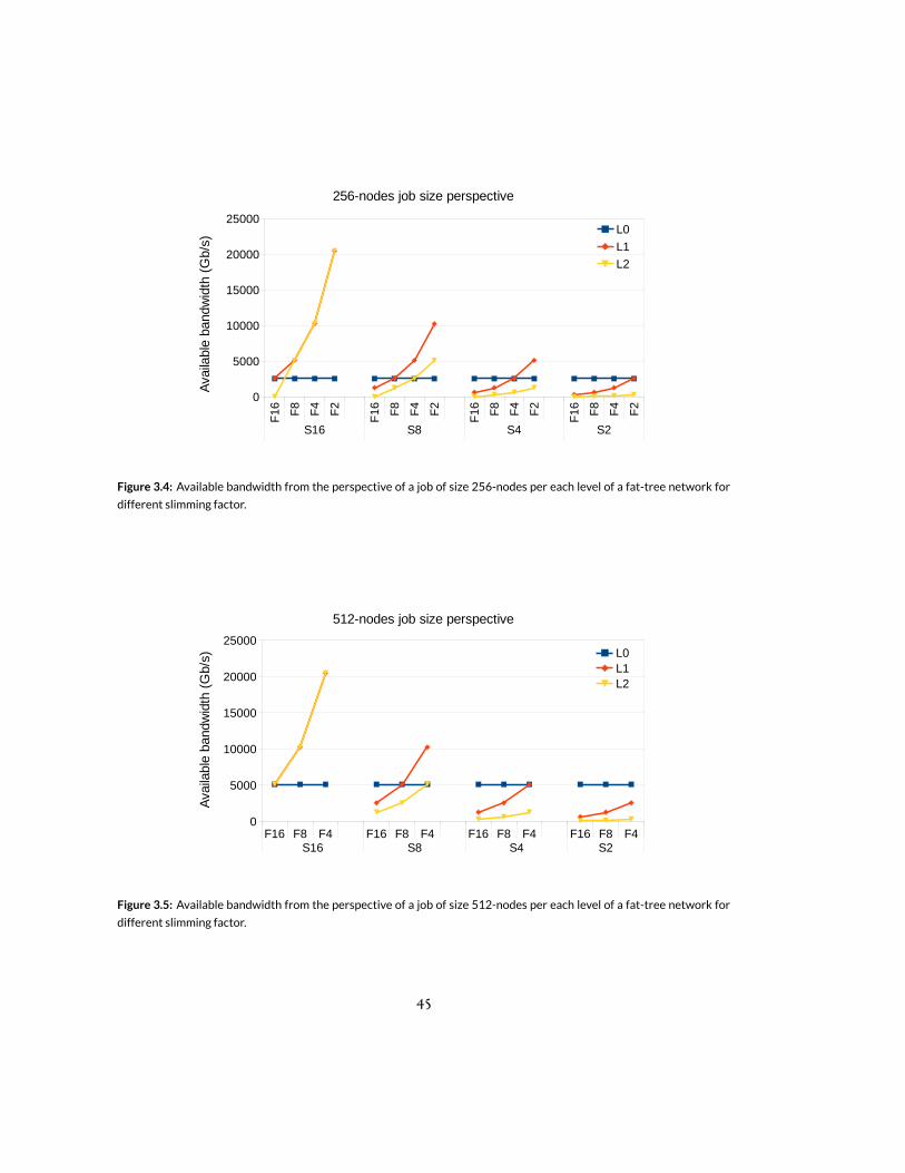
F1

6

F8

F4

F2

F1

6

F8

F4

F2

F1

6

F8

F4

F2

F1

6

F8

F4

F2

S16 S8 S4 S2

0

5000

10000

15000

20000

25000

256-nodes job size perspective

L0

L1

L2

Ava

ilabl

e ba

ndw

idth

(G

b/s)

Figure 3.4: Available bandwidth from the perspective of a job of size 256-nodes per each level of a fat-tree network for

different slimming factor.

F16 F8 F4 F16 F8 F4 F16 F8 F4 F16 F8 F4S16 S8 S4 S2

0

5000

10000

15000

20000

25000

512-nodes job size perspective

L0L1L2

Ava

ilabl

e ba

ndw

idth

(G

b/s)

Figure 3.5: Available bandwidth from the perspective of a job of size 512-nodes per each level of a fat-tree network for

different slimming factor.

45

FT(Alltoall) MILC CG GROMACS BT WRF CGPOP0

0.1

0.2

0.3

0.4

0.5

0.6

0.7

0.8

0.9

1L0L1L2

Ban

dwid

th u

tiliz

atio

n

Figure 3.6: Bandwidth utilization per level for applications on xgft(3;16,16,8;1,2,2) fat-tree network and node allocation

on F2 fragmentation.

Outline

High

Moderate

Low

Figure 3.7: Classification of applications based on their maximum utilization.

46

are presented, starting with the fat tree network with full bisection bandwidth and ending with thenetwork with the minimum connectivity. CGPOP experiences degradation of at most 3% due toslimming with respect to the case of full bisection fat tree. For each of the topologies the applicationwas simulated using several fragmented allocations – random and regular. RF_AVG is the averagevalue from ten runs under different random allocations. RF_STDEV is standard deviation for theseten runs. Finally, STDEV shows the standard deviation among all the presented task allocations. Thetrend of increasing variability when slimming the network is observed. Still, CGPOP’s sensitivityto fragmentation is very low – the maximum standard deviation of the execution times for one ofthe topologies is 0.14%. Overall, CGPOP may be categorized as an application insensitive to bothavailable bandwidth and fragmentation. WRF exhibits a similar behavior being less sensitive thanCGPOP (Figure 3.9). WRF’s degradation due to slimming is up to 2% and the standard deviation fordifferent fragmentations is up to 0.04%.

RF

_S

TD

EV

RF

_A

VG

F1

6

F8

F4

F2

RF

_S

TD

EV

RF

_A

VG

F1

6

F8

F4

F2

RF

_S

TD

EV

RF

_A

VG

F1

6

F8

F4

F2

RF

_S

TD

EV

RF

_A

VG

F1

6

F8

F4

F2

RF

_S

TD

EV

RF

_A

VG

F1

6

F8

F4

F2

S16 S8 S4 S2 S1

0

0.02

0.04

0.06

0.08

0.1

0.12

0.14

0.16

0.18

0.00%

0.02%

0.04%

0.06%

0.08%

0.10%

0.12%

0.14%

0.16%

0.18%

0.20%

CGPOP

RF_STDEVTintraTbaseSTDEV

Exe

cutio

n tim

e (s

) Standar d devia tion

Figure 3.8: Impact of fragmentation and slimming to CGPOP performance variability when running alone in the system.

Figure 3.10 shows the results for the same set of experiments donewith the applicationGROMACS.Regarding the effect of slimming, GROMACS can loose up to 47% of performance on the S1 topol-ogy, but in most of the presented cases (from S16 to S2) the loss is less than or around 10% comparedto the case of network with full bisection bandwidth. GROMACS has an increased sensitivity to the

47

RF

_S

TD

EV

RF

_A

VG

F1

6

F8

F4

F2

RF

_S

TD

EV

RF

_A

VG

F1

6

F8

F4

F2

RF

_S

TD

EV

RF

_A

VG

F1

6

F8

F4

F2

RF

_S

TD

EV

RF

_A

VG

F1

6

F8

F4

F2

RF

_S

TD

EV

RF

_A

VG

F1

6

F8

F4

F2

S16 S8 S4 S2 S1

0

0.02

0.04

0.06

0.08

0.1

0.12

0.14

0.16

0.18

0.00%

0.02%

0.04%

0.06%

0.08%

0.10%

0.12%

0.14%

0.16%

0.18%

0.20%

WRF

RF_STDEVTintraTbaseSTDEV

Exe

cutio

n tim

e (s

) Standar d devia tion

Figure 3.9: Impact of fragmentation and slimming toWRF performance variability when running alone in the system.

choice of fragmentation compared to CGPOP. The standard deviation is still less than 5%. BT fits inthis category of applications with an impact of slimming up to 14% and a standard deviation due tofragmentation of 0.90% (Figure 3.11).

RF

_S

TD

EV

RF

_A

VG

F1

6

F8

F4

F2

RF

_S

TD

EV

RF

_A

VG

F1

6

F8

F4

F2

RF

_S

TD

EV

RF

_A

VG

F1

6

F8

F4

F2

RF

_S

TD

EV

RF

_A

VG

F1

6

F8

F4

F2

RF

_S

TD

EV

RF

_A

VG

F1

6

F8

F4

F2

S16 S8 S4 S2 S1

0

0.1

0.2

0.3

0.4

0.5

0.6

0.7

0.8

0.9

0.0%

0.5%

1.0%

1.5%

2.0%

2.5%

3.0%

3.5%

4.0%

4.5%

5.0%

GROMACS

RF_STDEVTintraTbaseSTDEV

Exe

cutio

n tim

e (s

) Standar d devia tion

Figure 3.10: Impact of fragmentation and slimming to GROMACS performance variability when running alone in the sys-

tem.

Figure 3.12 presents the case of FT(Alltoall). FT shows extreme sensitivity to slimming. Only by

48

RF

_S

TD

EV

RF

_A

VG

F1

6

F8

F4

F2

RF

_S

TD

EV

RF

_A

VG

F1

6

F8

F4

F2

RF

_S

TD

EV

RF

_A

VG

F1

6

F8

F4

F2

RF

_S

TD

EV

RF

_A

VG

F1

6

F8

F4

F2

RF

_S

TD

EV

RF

_A

VG

F1

6

F8

F4

F2

S16 S8 S4 S2 S1

0

0.1

0.2

0.3

0.4

0.5

0.6

0.7

0.8

0.9

0.0%

0.5%

1.0%

1.5%

2.0%

2.5%

3.0%

3.5%

4.0%

4.5%

5.0%

BT

RF_STDEVTintraTbaseSTDEV

Exe

cutio

n tim

e (s

) Standar d devia tion

Figure 3.11: Impact of fragmentation and slimming to BT performance variability when running alone in the system.

halving the links i.e. going from S16 to S8 it experiences a degradation of 15%-66% and from S16 to S1of 2554.92%. FT’s variability due to different task allocations is extreme aswell, ranging from2.14% forS16 to 214% for S1. The FT belongs to category of extremely sensitive applications to both slimmingand fragmentation. The applications CG (Figure 3.13) andMILC (Figure 3.14) also present high sensi-tivity to fragmentation and slimming. The degradationswhen going fromS16 to S1 are 173% and 295%for CG andMILC, respectively. The standard deviation when using different allocations forMILC isup to 26%, while CG’s performance when running alone does not vary much - standard deviation isup to 5%.

In summary, the applications with extremely low bandwidth utilization at all levels of fat-tree(WRF and CGPOP) show extreme insensitiveness to both task placement and bisection bandwidth.GROMACS and BT start to show slight sensitiveness under very slimmed network which is in linewith their per-level utilization profile for the very slimmed network, i.e., they have slightly higher uti-lization than WRF and CGPOP. FT(Alltoall) is extremely sensitive to both fragmentation and slim-ming which is inline with its high-utilization at L2. The same conclusions hold for CG and MILC.

49

RF

_S

TD

EV

RF

_A

VG

F1

6

F8

F4

F2

RF

_S

TD

EV

RF

_A

VG

F1

6

F8

F4

F2

RF

_S

TD

EV

RF

_A

VG

F1

6

F8

F4

F2

RF

_S

TD

EV

RF

_A

VG

F1

6

F8

F4

F2

RF

_S

TD

EV

RF

_A

VG

F1

6

F8

F4

F2

S16 S8 S4 S2 S1

0

1

2

3

4

5

6

7

8

0%

50%

100%

150%

200%

250%

FT (Alltoall)

RF_STDEVTintraTbaseSTDEV

Exe

cutio

n tim

e (s

) Standar d devia tion

Figure 3.12: Impact of fragmentation and slimming to FT performance variability when running alone in the system.

RF

_S

TD

EV

RF

_A

VG

F1

6

F8

F4

F2

RF

_S

TD

EV

RF

_A

VG

F1

6

F8

F4

F2

RF

_S

TD

EV

RF

_A

VG

F1

6

F8

F4

F2

RF

_S

TD

EV

RF

_A

VG

F1

6

F8

F4

F2

RF

_S

TD

EV

RF

_A

VG

F1

6

F8

F4

F2

S16 S8 S4 S2 S1

0

0.05

0.1

0.15

0.2

0.25

0%

1%

2%

3%

4%

5%

6%

CG

RF_STDEV

Tintra

Tbase

STDEV

Exe

cutio

n tim

e (s

) Standar d devia tion

Figure 3.13: Impact of fragmentation and slimming to CG performance variability when running alone in the system.

50

RF

_S

TD

EV

RF

_A

VG

F1

6

F8

F4

RF

_S

TD

EV

RF

_A

VG

F1

6

F8

F4

RF

_S

TD

EV

RF

_A

VG

F1

6

F8

F4

RF

_S

TD

EV

RF

_A

VG

F1

6

F8

F4

RF

_S

TD

EV

RF

_A

VG

F1

6

F8

F4

S16 S8 S4 S2 S1

0

0.5

1

1.5

2

2.5

0%

5%

10%

15%

20%

25%

30%

MILC

RF_STDEVTintraTbaseSTDEV

Exe

cutio

n tim

e (s

) Standar d devia tion

Figure 3.14: Impact of fragmentation and slimming toMILC performance variability when running alone in the system.

Therefore, our characterizationmethodology is able to very well predict the sensitiveness of the appli-cations to these two important factors.

3.3.2 Impact on inter-application contention

Now that we have identified and decoupled the main factors, namely, fragmentation and slimming,that influence inter-application contention, we can present how these applications behave when theyshare network resources. First we categorize workloads depending on their demands and sensitivenessto bandwidth and task allocation and thus their sensitiveness to inter-application contention. In orderto do this, we ran different workloads consisting of the same or different applications on ten differentrandom allocations and on three different topologies (S8, S4 and S2).Figure 3.15 shows the broken-down application normalized execution times of a workload created

by mixing together all studied applications. The execution time of each application when runningwith other applications normalized with respect to Tbase (i.e., execution time in a one-hop fully con-nected network). The execution time is the average value of the runs on ten different random alloca-

51

tions. RF_STDEV_SHARED is the standard deviation of the ten runs, while RF_STDEV_ALONEis the standard deviation of the ten runs of the application running alone (the same value as shownper application in the previous Section 3.3.1). Comparing these two values we see a clear trend ofincrease in performance variability, when going from scenario ”alone” to a scenario of mixing applica-tions together sharing the network. In otherwords, inter-application contention leads tomore perfor-mance variability. Regarding slimming, from left to right we see the expected trend of performancedegradation for all applications when reducing the number of links in the fat tree topology. How-ever, not all applications “react” in the same way. We can recognize two groups: highly impactedones (FT, CG, MILC and GROMACS) and less impacted ones (BT, CGPOP and WRF) makingthis seven-applications workload moderately sensitive. Note that applications that were almost com-pletely insensitive when running alone, like CGPOP, now, sharing resources with other applicationsexperiences 80% degradation for topology S2. The reason is the presence of applications with highcommunication demands (Figure 2.1) in the network. Still, in the case of higher connectivity, S8, thedegradation is limited to 5% for insensitive applications and to 11% (the case of FT) for sensitive appli-cations. In summary, slimming makes the effect of inter-application contention the biggest problemin order to increase system throughput.

Figure 3.16 shows the broken-down normalized execution times of a workload created with eightinstances of the CGPOP application. The average values from ten runs on different random allo-cations are presented. When only CGPOPs run together the performance variability increases in theshared environment, but it is low and limited to 0.10% (standard deviation). Whendecreasing connec-tivity there is a slight increase in execution time due to inter-application contention. The maximumperformance degradation is limited to 5% (the case of S2). The workload created of eight insensitiveapplications is quite insensitive even with very low connectivity.

Figure 3.17 shows the broken-down normalized execution times of a workload consisting of eightCG instances. The performance variability between ten runs on different random allocations is nothigh, standard deviation is up to 0.9%. Slimming has a huge impact on performance of CGs. Evenwith S8 the performance loss is around 30% for each of CG instances. The results suggest that mixing

52

bt cg cgp ft gro mil wrf bt cg cgp ft gro mil wrf bt cg cgp ft gro mil wrf

S8 S4 S2

0

2

4

6

8

10

12

0%

2%

4%

6%

8%

10%

12%

All applications workload

Tinter

Tintra

Tbase

RF_STDEV_ALONE

RF_STDEV_SHARED

Nor

mal

i zed

exe

cutio

n t

ime

Stan

da rd

devia tion

Figure 3.15: Mixing all applications together on different random allocations for three different slimmed topologies.

cgp

_1

cgp

_2

cgp

_3

cgp

_4

cgp

_5

cgp

_6

cgp

_7

cgp

_8

cgp

_1

cgp

_2

cgp

_3

cgp

_4

cgp

_5

cgp

_6

cgp

_7

cgp

_8

cgp

_1

cgp

_2

cgp

_3

cgp

_4

cgp

_5

cgp

_6

cgp

_7

cgp

_8

S8 S4 S2

0

0.2

0.4

0.6

0.8

1

1.2

1.4

0.00%

0.05%

0.10%

0.15%

0.20%

Low demanding workload

Tinter

Tintra

Tbase

RF_STDEV_ALONE

RF_STDEV_SHARED

Nor

mal

i zed

exe

cutio

n t

ime

Stan

da rd

devia tion

Figure 3.16: Mixing eight CGPOPs together on different random allocations for three different slimmed topologies.

53

sensitive applications together on random fragmentations can lead to poor performance.

cg_1

cg_2

cg_3

cg_4

cg_5

cg_6

cg_7

cg_8

cg_1

cg_2

cg_3

cg_4

cg_5

cg_6

cg_7

cg_8

cg_1

cg_2

cg_3

cg_4

cg_5

cg_6

cg_7

cg_8

S8 S4 S2

0

0.5

1

1.5

2

2.5

3

3.5

4

4.5

0.00%

0.10%

0.20%

0.30%

0.40%

0.50%

0.60%

0.70%

0.80%

0.90%

1.00%

High demanding workload

Tinter

Tintra

Tbase

RF_STDEV_ALONE

RF_STDEV_SHARED

Nor

mal

i zed

exe

cutio

n t

ime

Stan

da rd

devia tion

Figure 3.17: Mixing eight CGs together on different random allocations for three different slimmed topologies.

3.3.3 Trade-offs of multiple applications in a shared environmentWhenever the job scheduler needs to decide on a node allocation for a new job, assuming that severaljobs are already running, several node allocations may be available; each of themmay have a differentimpact on system performance. This is due to two main factors, namely,

• the performance of the application running on this particular node allocation, which dependson the application’s communication demands and the available network bandwidth, and,

• the performance sensitivity of the mix of applications consisting of those present and the onebeing allocated.

To characterize these factors, let Tinter be the amount of time by which the application completiontime increases because of network resource sharing (inter-application network contention), and letTintra be the increase in completion time due to the contention produced in the system solely by the

54

messages that belong to the same application (intra-application contention). Finally, we will denoteby Tbase the time it would take an application to execute on a system with a crossbar network topol-ogy thus providing full bisection bandwidth and eliminating all types of contention except end-pointcontention. Therefore, the runtime of an application A given a particular job fragmentation FA canbe expressed as

TA(FA) = TAbase + TAintra(FA) + TAinter(FA). (3.2)

The completion time for all n applications plus the target application A running concurrently in thesystem at the moment of scheduling application A is described as

T(FA) = TA(FA) +n∑j=1

(Tjbase + Tjintra(Fj) + Tjinter(Fj) + Tjinter(FA)). (3.3)

Fj is a fragmentation allocated for application j. Note that Tjinter(Fj) is the inter-application producedin application j due to interference with all other applications in the system except A, while Tjinter(FA)is the additional inter-applicationproduced in application j owing to thenode allocationof applicationA, FA.

System throughput is inversely proportional to completion time. Therefore, an optimal node al-location Fopt for a given application Aminimizes T. Formally, we can express this optimization as thedifference in completion times fromall applications between two fragmentations, T(FA)−T(Fopt) >0 which results in

TAintra(FA)− TAintra(Fopt) +n∑

j=A,1Tjinter(FA)−

n∑j=A,1

Tjinter(Fopt) > 0, (3.4)

which can be rewritten as

n∑j=A,1

Tjinter(FA)−n∑

j=A,1Tjinter(Fopt) > TAintra(Fopt)− TAintra(FA). (3.5)

55

Therefore, obtaining a good node allocation of the target application (a node allocation that increasessystem throughput) assumes trade-off between intra- and inter-application contention. The increaseof intra-application contention should be lower than the aggregate reduction of the inter-applicationcontention for all the applications.Node allocations that distribute tasks overmore leaf switches have the advantage of providingmore

bisectionbandwidth fromthepoint of viewof a given application,whichmay reduce intra-applicationcontention. However, spreading tasks of the same job across the system induces the following twonegative effects: i) The probability to interfere with other applications increases, which will causemore inter-application contention, ii) The mean distance between tasks increases, implying that theload on the upper levels of the tree (which have the lowest bandwidth) will increase, thus also lead-ing to more inter-application contention. Therefore, spreading an application’s tasks throughout thenetwork is not likely to be a good node allocation policy for applications with high communicationdemands (unless it is alone in the system). In this case, a more contiguous node allocation would bemore desirable.

3.4 Exploring the ways to reduce inter-application contentionusing task placement

When allocating nodes for a new job, the scheduler has two basic options:

1. Use the nodes that are currently available, or

2. hold the job for a certain amount of time until the preferred node allocation becomes available.

The first option should be chosen when the node allocation for the target application is good enoughaccording to Equation 3.5. In the second case, the target application should be put on hold in thescheduler queue until the preferred node allocation is obtained i.e. the jobs currently running releaseneeded nodes. Here we explore the strategies a scheduler may consider when choosing among several

56

possible allocations in order to reduce interference between applications. The practical feasibility ofthe strategies will be discussed later.

Figure 3.18 shows the same case of eight CGs workload on different regular allocations includingthe already analyzed random allocation on a topology with contention ratio 2:1 (the case S8). Fromleft to right we show the trendwhen the spreadness of the applications’ tasks is reduced. Reducing thespreadness correlates with reducing number of applications sharing first level switch (F2 case - eightapplications per switch, F4 - four applications, F8 - two applications and F16 -only one application).However, the total number of applications in the system is always the same - eight. The results suggestthat in the case of high demanding workload assigning random available nodes to application’s tasksbrings the highest degradation to their performance (up to 30%). Further, the optimal case is isolatingeach applicationon its own sub-tree (F16 case). Practically this approach is hardly feasible, since findingthe non-fragmented allocations is not always available or it would require introducing certain waitingtime in the queue until non-fragmented allocation becomes available. However, according to theresults, anothermore feasible strategywould be to reduce number of applications sharing the first levelswitch as much as possible, since in that case the trend of reducing degradation is observed. When wemove from the RF case to other less spread allocations we can get improvements of 13%, 18% and 20%in the performance of each CG instance for the cases of F4, F8 and F16, respectively.

Figure 3.19 shows the cases of different decisions on applications that share a switch. The exper-iments are done on a topology S8 and all applications are allocated on F8 fragmentation, thus twoapplications are sharing a switch and there are four applications in total in the system. Grouping twoFTs on a switch even with high connectivity leads to a degradation of 47% with respect to the case ofrunning alone on the same allocation and topology. On the other hand, two CGPOPs, two WRFsor two BTs when sharing a switch experience negligible impact on each others performance. A de-cision of mixing FT and the other low sensitive applications (CGPOP, WRF or BT) using the sameresources leads to very significant improvement. FTs degradation in that case is only 2-3%, while forlow sensitivity applications it is negligible.

57

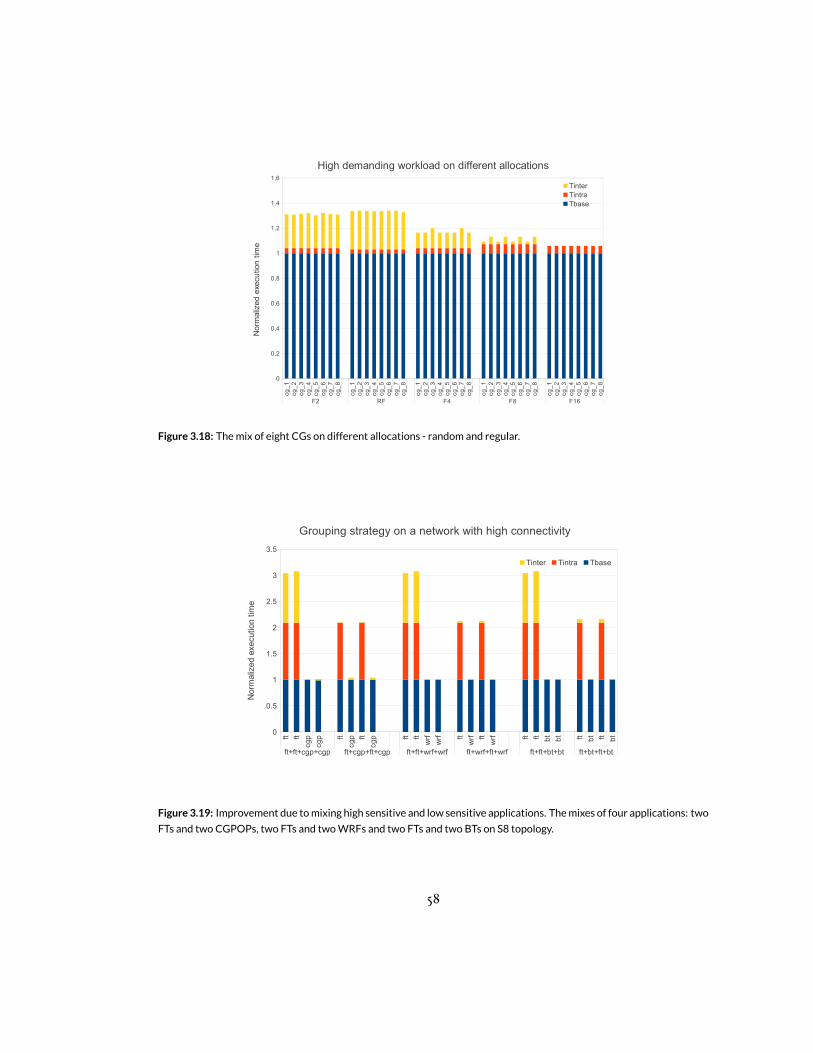
cg

_1

cg

_2

cg

_3

cg

_4

cg

_5

cg

_6

cg

_7

cg

_8

cg

_1

cg

_2

cg

_3

cg

_4

cg

_5

cg

_6

cg

_7

cg

_8

cg

_1

cg

_2

cg

_3

cg

_4

cg

_5

cg

_6

cg

_7

cg

_8

cg

_1

cg

_2

cg

_3

cg

_4

cg

_5

cg

_6

cg

_7

cg

_8

cg

_1

cg

_2

cg

_3

cg

_4

cg

_5

cg

_6

cg

_7

cg

_8

F2 RF F4 F8 F16

0

0.2

0.4

0.6

0.8

1

1.2

1.4

1.6

High demanding workload on different allocations

TinterTintraTbase

Nor

mal

i zed

exe

cutio

n t

ime

Figure 3.18: Themix of eight CGs on different allocations - random and regular.

ft ft

cgp

cgp ft

cgp ft

cgp ft ft

wrf

wrf ft

wrf ft

wrf ft ft bt bt ft bt ft bt

ft+ft+cgp+cgp ft+cgp+ft+cgp ft+ft+wrf+wrf ft+wrf+ft+wrf ft+ft+bt+bt ft+bt+ft+bt

0

0.5

1

1.5

2

2.5

3

3.5

Grouping strategy on a network with high connectivity

Tinter Tintra Tbase

Nor

mal

i zed

exe

cutio

n tim

e

Figure 3.19: Improvement due tomixing high sensitive and low sensitive applications. Themixes of four applications: two

FTs and two CGPOPs, two FTs and twoWRFs and two FTs and two BTs on S8 topology.

58

Figure 3.20 shows the case of two FTs and two CGPOPs workload. The case of grouping FT andCGPOPon the same switch is compared to the case of isolating eachof the four applications on its ownsub-tree. From left to right we show results obtained on different topologies, going from less to moreslimmed networks (S8 to S2). Note that the first group of the results (S8, F8 - case) is already analyzedin the previous figure. On S8 topology the high demanding applications (FT) may still benefit fromusing F8 fragmentations comparing to the case of non-fragmentation (F16). However, when movingtowards networks with lower connectivity (S4 and S2) isolation brings better performance to both FT(reducing intra- and inter-contention) and CGPOP (reducing its inter-application contention com-ponent). The improvements are for FT 22% and 55%, and for CGPOP 13% and 40%, for topologiesS4 and S2, respectively. Therefore, for the case of lower connectivity (S4 and S2) if a non-fragmentedallocation is available, the best strategy is to isolate the most demanding applications at least, since allthe applications will benefit from that.

ft

cgp ft

cgp ft

cgp ft

cgp ft

cgp ft

cgp ft

cgp ft

cgp ft

cgp ft

cgp ft

cgp ft

cgp

F8 F16 F8 F16 F8 F16S8 S4 S2

0

2

4

6

8

10

12

Grouping versus Isolating Strategy

Tinter Tintra Tbase

Nor

mal

i zed

exe

cutio

n tim

e

Figure 3.20: Comparing strategies of grouping and isolating for different slimming levels, S8, S4, S2. The mix of two FTs

and two CGPOPs on F8 andNF allocations.

59

3.5 Conclusions

It was demonstrated that scientific applications may be substantially degraded by the impact of inter-application network contention that occurs when multiple applications are running concurrently inthe system and thus sharing the same network resources. We have shown that the performance ofsome scientific applications experiences huge variability under different task allocations and fragmen-tation scenarios, and that this performance variability is tightly coupled to the degree of connectivity inblocking networks. We identified different classes of applications based on sensitiveness to these fac-tors. Theperformance degradationmay go fromup to 5% for insensitive applications toup to 20 timesincrease in execution time for sensitive applications. Also, we found a correlation between commu-nication intensity of applications at different network levels and their sensitiveness to fragmentationand slimming. Mixing an application with other applications in the system makes these two factorseven more important since the decision on task allocation of one application impacts other applica-tions due to inter-application contention and vice versa. The common trend in all applications is thatinter-application network contention is becoming themajor factor of performance degradationwhenthe network connectivity is reduced whichmight be the case in future exascale computers. The work-loads executed in HPC systems may be various in terms of communication intensity of their applica-tions. Having a communication intensive application in the workload may lead to inter-applicationcontention becoming a dominant factor in the degradation of all applications in the workload. Ourresults suggest two strategies for the workloads with applications of different characteristics: 1) whenthe network is not very slimmed the best strategy is to choose applications that share resources (e.g firstlevel switch) carefully, mixing communication intensivewith less comunication intensive applicationsand 2) when the network is very slimmed, then isolating application on a non-fragmented allocationis more important than careful mixing. For the workloads in which all applications are sensitive, ran-dom task allocation leads to the largest degradation - 30% in case of eight CGs workload even on atopology with high connectivity. The strategy for this kind of workloads is to keep the number ofapplications sharing a switch as few as possible, making the isolation of each application the optimal

60

case. Finally, the workloads of insensitive applications perform well even with low connectivity, andlow-cost networks are a good choice for the systems that execute this kind of workloads.However, in practice, the strategy of mixing applications based on their communication intensity

is hard to achieve due to the following reasons. First, at the point of scheduling the application itscommunication behavior is typically unknown and therefore it cannot be decided which applicationsthat are already running in the network is the best to mix it with. Second, due to the dynamic natureof the system, it is difficult to track for how long the applications that are already running will sharethe resources with the application to be scheduled. Third, even by being able to get the mentionedpieces of information, it is difficult to precisely predict which of the currently available fragmentationsor the ones available in near future is the best option without running the application before. Espe-cially, in the case of considering to wait for an allocation in the future, we cannot make good estimateon whether it pays off at all in terms of saving the performance. In summary, the mixing strategy isextremely complex approach. Thus, the strategy that remains more practically feasible is isolation. Aswe have seen isolation is a good strategy in the case of demanding workloads and also, isolation is be-coming the prefered strategy in the blocking networks with lower connectivity. However, providingan isolated (exclusive) portion of the network to the application does not come for free. Namely, itleads to increased queueing time. In the next chapter we describe the proposed technique for solvingthe trade-off between providing the isolated resources and achieving reasonable queueing time.

61

62

4System-level resource management

Supercomputers are typically shared by many parallel jobs with different resource requirements. Be-fore execution, each job is granted the desired number of computing nodes by the system resourcemanager. The allocated nodes communicate through the system interconnection network. Thus, thecomputing nodes’ physical locations will define the part of the network used by a job.

Ideally, jobswould be allocated on a set of nodes interconnected by aminimumnumber of switchesand separated by the minimum number of hops, keeping communication between tasks of the jobcontained within the minimum required part of the network that satisfies the job’s communications

63

demands. For example, if a job requires a number of nodes less or equal than a switch size, an optimalallocation would be a set of nodes within a single switch; if a job size fits in two switches it should beallocated only in two switches, preferably switches that are themselves also as close as possible (i.e., ina tree-like network, within the lowest encompassing sub-tree), etc. This kind of allocation is assumedto be ideal because it has a two-fold effect on job performance. By reducing the number of hopscommunication latency is reduced60, and by allocating job’s nodes as close as possible interferencefrom nearby jobs is also reduced, increasing performance predictability 38.However, as jobs with different resource requirements (mainly: number of nodes and execution

time) arrive and leave the system in an non-deterministic fashion, allocating them tomaximize systemutilization will lead to a fragmentation of the resources assigned to the jobs: e.g., a job requiring alarge node-count will be placed in nodes left free by previously running jobs requiring less nodes thathave already finished. This problem becomes even more important in multi-stage networks, such asfat-trees (a common network topology in both the commercial and HPC domains), where fragmen-tation becomes more relevant the more spread out a job is on the system, as every stage increases thecommunication latency (up to a factor of 1.5 in state-of-the-art three-level multi-stage supercomput-ers60), and it also increases the probability of harmful interference leading to significant applicationperformance degradation 30.Our own analysis of the system resource manager logs from the MareNostrum supercomputer*

reveals that the actual job allocations are far from the optimal ones described in the previous paragraphand that jobs are rather allocated on free fragments of switches (free portions of non-fully occupiedswitches) spread out onto a much higher number of switches than would be optimally required. Themore and the further the fragments allocated to a job are, the higher the fragmentation in the system.Looking only at the case of the jobs smaller than the switch size (each switch can accommodate 18

computing nodes in Marenostrum), reveals that a high percentage of the jobs that can fit in a singleswitch and thus not use the rest of network resources are actually spread on multiple switches (Fig-ure 4.1).

*TheMareNostrum supercomputer is a large supercomputing resource used for research in many differentareas. It is run by the Barcelona Supercomputing Center, Barcelona, Spain.

64

1 2 3 4 5 6 7 8 9 10 11 12 13 14 15 16 17 180

0.1

0.2

0.3

0.4

0.5

0.6

0.7

0.8

0.9

1

Small jobs fragmentation17 16

15 14

13 12

11 10

9 8

7 6

5 4

3 2

1job size

% jo

bs s

prea

d on

sw

itche

s

Figure 4.1: The small jobs spreadness in MareNostrum supercomputer. Percent of jobs of size x (x-axis) spread on sswitches (given in the legend).

Similar conclusions are drawn for job sizes greater than a switch. The jobs requiring between 2and 4 switches (between 36 and 72 nodes) can be found spread out to up to 55 switches (Figure 4.2),whereas the jobs whose size range from 5 to 16 switches can populate up to 96 switches (Figure 4.3).

This analysis and previous ones clearly highlight the high level of fragmentation that is being in-duced by the job management software in current supercomputers. Even more, as several authorshave noted in great detail 58,31,18, the most negative side-effect of fragmentation, i.e., interference fromother applications, cannot be accuratelymeasured in a running system. Impact of interference cannotbe accurately measured because it is unrealistic to reserve an isolated portion of the network to runthe same application with the same task placement, input parameters, the same routing function, etc.,to measure its execution time in the absence of interference and then compare its performance to thatobtained in the presence of interference.

However, although it is practically impossible to accurately measure the impact of interference di-rectly in a production system, several authors have managed to measure it indirectly, by looking atthe performance variability across several executions of the same job, arriving to the conclusion that

65

0 500 1000 1500 2000 2500 3000job

0

10

20

30

40

50

60

num

ber o

f sw

itche

s po

pula

ted

Job sizes fit 2 to 4 switches

Figure 4.2: The actual number of populated switches for the job sizes range from 19 to 72 computing nodes inMareNos-

trum; the jobs that would ideally fit in 2 to 4 switches. The red lines are at the switches 2 and 4. 8% of jobs fit within the

2-4 switches boundary.

0 200 400 600 800 1000job

0

20

40

60

80

100

num

ber o

f sw

itche

s po

pula

ted

Job sizes fit 5 to 16 switches

Figure 4.3: The actual number of populated switches for the job sizes range from73 to 288 computing nodes inMareNos-

trum; the jobs that would ideally fit in 5 to 16 switches. The red lines are at the switches 5 and 16. 19% jobs fit within the

5-16 switches boundary.

interference is a main contributor to performance loss 31,8,30.In part because of the difficulty to measure the impact of interference, and in part because there

66

hasn’t been any proposal that can maintain a high system utilization while providing isolation jobschedulers are to a great extent still oblivious to the spatial fragmentation induced by their policies.In thisworkwe attempt to reconcile systemutilization and application isolation. Themain insights

and contributions of this work are the following:

• A model that defines the relationship between the job’s allocation and the number of job’s itcould share network with per fat-tree level.

• We identify the causes of the high fragmentation inHPC systemsbased on the analysis of actualsystem resource manager logs from an HPC system.

• We propose and evaluate scheduling polices that can control fragmentation and reduce thenumber of jobs sharing the network.

• As the side-effect of the proposed policy, a portion of the network switches can be either turnedoff or eliminated reducing power and cost.

4.1 Network sharing as a function of job allocationHaving jobs spread out on ahighnumber of switches consequently increases the probability of sharingthe network with more jobs. Figure 4.4 shows the maximum number of jobs that a job spread onmultiple switches has been sharing the network with. In particular, a job of size 8 spread on 8 switchesis the worst case of fragmentation scenario for a job of this size. This means that a single node wasallocated at every switch used by the job. The number of sharing jobs at second-level was 50 in thiscase. Similarly, the data from the system reveals that the jobs of size 64 can be spread on up to 56switches and can share up to 120 jobs at the second level.At the third-level, as shown in Figure 4.5, the jobs are quite fragmented, as well. A small job of size 8

can populate up to 8 different subtrees and thus use all the tree levels for every single communication.Also, at the third level the number of sharing jobs is significantly increased comparing to the previously

67

0 10 20 30 40 50 60number of switches populated

0

20

40

60

80

100

120

140

num

ber o

f nei

ghbo

ring

jobs

sha

ring

job size 64job size 32job size 16job size 8

Figure 4.4: The relationship between the number of switches populated by a job and the number of jobs it shared the

second-level of theMareNostrum network with. The four lines correspond to each of four typical job sizes, 8, 16, 32 and

64. For example, out of all jobs of size 16 thatwere spread on10 switches, some job shared the second-levelwith 50other

jobs, being that themaximumnumber of jobs a job of size 16 spread in 10 switches shared the second-level of the network

with.

seen second-level case. In particular, it ranges from 158 jobs sharing in the worst case of job size 32 to176 sharing jobs in the worst case of job size 64.

In light of the results seen from the actual machine in Figures 4.4 and 4.5, we derive the maximumboundof the number of different jobs that could be sharing the fat tree at a certain level. Let us assumethat a job of size N is spread out in the network assuming that for this job the fragments of nk−1 nodesare allocated at the kth level. In case each of the remaining free nodes at the kth level is allocated to adifferent job that communicates through kth level our job will share the network with the maximumnumber of jobs. Then, the maximum number of sharing jobs at kth level can be calculated as:

#sharingJobsk = Nnk−1

· (m1 · ... ·mk−1 − nk−1) (4.1)

Simplifying formula by introducing number of populated switches and assuming equal switch radices

68

2 3 4 5 6 7 8 9 10number of subtrees populated

0

20

40

60

80

100

120

140

160

180

num

ber o

f nei

ghbo

ring

jobs

sha

ring

job size 8job size 16job size 32job size 64

Figure 4.5: The relationship between the number of subtrees populated by a job and the number of jobs it shared third-

level ofMareNostrum network with. The four lines correspond to each of four typical job sizes, 8, 16, 32 and 64.

at each level, we get:

#sharingJobsk = #populatedSwitches ·mk−1 −N (4.2)

Thus, the worst case in number of sharing jobs for the 2nd level (k = 2) is for n1 = 1:

#sharingJobsMAX = N · (m− 1) (4.3)

And similarly for the 3rd level (k = 3) links when n2 = 1:

#sharingJobsMAX = N · (m2 − 1) (4.4)

A simple example of theworst case fragmentations at the 2nd and the 3rd level in a xgft(3; 2, 2, 2; 1, 1, 1)are given in Figure 4.6. In the case of the example on the left maximum number of jobs that thejob A can share the 2nd level links with is 4 · (2 − 1) = 4, while the 3rd level links are shared with42 · (22− 2) = 4. In the case of the example on the right, 2nd level links are shared with 2 · (2− 1) = 2

69

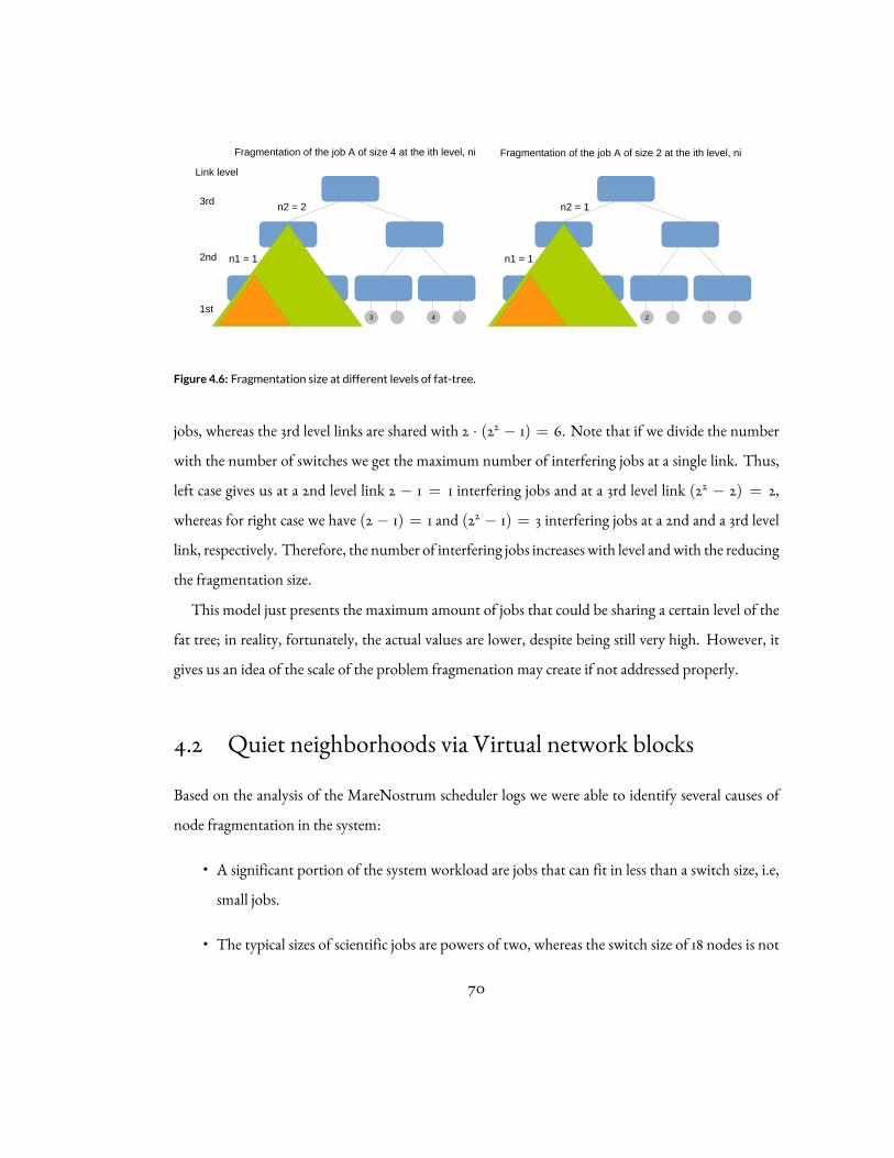
1 2 3 4

Link level

3rd

2nd

1st

Fragmentation of the job A of size 4 at the ith level, ni

1 2

n2 = 2

n1 = 1

Fragmentation of the job A of size 2 at the ith level, ni

n2 = 1

n1 = 1

Figure 4.6: Fragmentation size at different levels of fat-tree.

jobs, whereas the 3rd level links are shared with 2 · (22 − 1) = 6. Note that if we divide the numberwith the number of switches we get the maximum number of interfering jobs at a single link. Thus,left case gives us at a 2nd level link 2 − 1 = 1 interfering jobs and at a 3rd level link (22 − 2) = 2,whereas for right case we have (2 − 1) = 1 and (22 − 1) = 3 interfering jobs at a 2nd and a 3rd levellink, respectively. Therefore, the number of interfering jobs increases with level andwith the reducingthe fragmentation size.This model just presents the maximum amount of jobs that could be sharing a certain level of the

fat tree; in reality, fortunately, the actual values are lower, despite being still very high. However, itgives us an idea of the scale of the problem fragmenation may create if not addressed properly.

4.2 Quiet neighborhoods via Virtual network blocksBased on the analysis of the MareNostrum scheduler logs we were able to identify several causes ofnode fragmentation in the system:

• A significant portion of the system workload are jobs that can fit in less than a switch size, i.e,small jobs.

• The typical sizes of scientific jobs are powers of two, whereas the switch size of 18 nodes is not

70

power of two.

• Only 2% of the jobs bigger than switch size, i.e., big jobs, are multiple of switch size.

Therefore, for almost 100% of the workload, even an optimal contiguous job allocation will leavea number of free (not populated) nodes at the switches, i.e., fragments. We define the mechanisms toaddress each of the factors that contribute to fragmentation.

4.2.1 Removing the impact of fragmentation created by small jobs

To remove the fragmentation created by small jobs, two virtual network blocks are created on topof the physical topology, one block for small jobs and another for big jobs. The size of the blocks isadjusted in time based on the demand for resources from each of the two job-size groups. The limitbetween two virtual blocks is implemented as shown in Figure 4.7. The big jobs populate system fromthe first switch on, whereas the small jobs populate system from the last switch backwards. The bigjob’s block begins at the first switch and ends up at a switch before the lowest occupied switch of smalljob’s block. Similarly, the small job’s block begins at the last switch and ends up at a switch before thehighest occupied big job’s block. The limit between the big job’s block and the small job’s block isupdated dynamically. Each time a job arrives or leaves the system, the status of the highest occupiednode for big job’s block and the lowest occupied node for the small job’s block is checked and thelimits are updated if there was a change. Figure 4.8 shows the limits for small and big blocks at everytime a new job comes to the system. As it can be observed the limit for small jobs was at around 160at the begining and moved down to 139 switch index in order to accomodate more small jobs in thesystem.In addition, a constraint for small jobs allocation is built, i.e., always allocate a whole small job in

a single switch. Therefore, even though there will be a lot of fragmentation in the small job’s block,it is not a harmful fragmentation, since there the jobs will communicate within the switch and willnot use the upper levels of the network. Thus, small jobs will never experience nor create interferencewith nearby jobs.

71

One of the important benefits of this allocation algorithm is the possibility to switch-off the uppernetwork part of the small job’s block, since it will never be used. The portion of the network willdepend on the ratio of small jobs in the systemworkload. Figure 4.8 gives an insight on the size of thesmall jobs block for the workload in the MareNostrum scheduler log.

4.2.2 Addressing the mismatch between the switch size and power of twobig job sizes

In the big jobs block we introduce virtual switch partitions. On top of the switches we create two vir-tual switches containing each one 16 and 2 nodes, respectively. Based on these virtual switches we cre-ated two virtual partitions within big job’s virtual block, one that contains all 16-node virtual switchesand another that contains the 2-node virtual switches.A set of constraints are built on who and how can use these partitions in order to control the frag-

mentation of the jobs allocated to them. First, the 16-nodes partition is not fragmentable, i.e., it canonly be fully populated by a single job. Second, the 2-node partition is fragmentable.The scheduler allocates jobs to these partitions based on the following rules:

1. Big jobs that are power of two, i.e., of sizes 32, 64, 128, etc.; they will be allocated on n =jobsize16

16-node virtual partitions on n switches. Note that these jobs do not have any fragmentationat the second-level switches in a fat-tree.

2. Big jobs that are not a power of two; they will be allocated on both 16-node and 2-node virtualpartitions taking the whole physical switch size, thus they will need n =

jobsize18 full switches

and an additional switch for the remaining nodes. Note that the remaining nodes will createfragmentation; this issue is addresed in 4.2.3.

3. Small jobs of the size 1 and 2 nodes will be allocated only on the 2-node virtual partition if anallocation for them is not available at the small jobs virtual network block. The small jobsmust

72

Big job's perspective

Small job's perspective

Highest switch populated by

a big job

Small jobs limit

Big jobs limit

Lowest switchpopulated by a

small job

0 1 2 3 4 5 6 7 8

Small jobs block

Big jobs block

Switch index

Switch populatedSwitch empty Switch belongs to another blockand cannot be used

0 1 2 3 4 5 6 7 8

0 1 2 3 4 5 6 7 8

The system at a small job allocation:

The system at a big job allocation:

Virtual blocks Limit

Virtual blocks Limit

Space to search for allocation ( backwards)

Space to search for allocation( forwards)

Figure 4.7: Dynamically adjusted limit between the big jobs block and small jobs block. The case of a small system of 9

switches. Big jobs are populating system from the first switch on, whereas the small jobs are populating system from the

last switch backwards. In the empty system the big jobs limit would be equal to the highest switch index, i.e., 8 for the

system in the figure, and the small jobs limit would be equal to the lowest switch index, i.e., 0

73

0 10000 20000 30000 40000 50000job's order number

80

100

120

140

160

180

switc

h in

dex

Max switch indexbig job highest populated switchsmall job lowest populated switch

Figure4.8: Changeofdynamic limit in time. Avalue for eachof the two limitswas takenupon theallocationofnewarriving

job. Maximum switch index is 171. The switches above the limit do not have to be interconnected at higher levels; the

percent of the switches for which higher level interconnect can be switched-off increases up to 19% over time

always retain the constraint to fit in a single switch, thus there will be no sharing of networkresources even when a 16-node partition is occupied by another job.

4.2.3 Addressing the remainings nodes of other big jobs

To acommodate the remainings of the big jobs that are neither multiple of 16 nor of 18 several (rule 2)fragmentable switches are allowed per subtree, i.e., rem switches. The remainings follow the same ruleas small jobs to always fit in a single switch. Since, the nodes allocated for the remainings of big jobswill communicate outside of the switch and in addition, there can be several remainings fromdifferentjobs at the same rem switch, there will be sharing of network resources in this case. Therefore, the onlynetwork sharing at second-level will be at the switches that accomodate remainings of big jobs (remswitches). Figure 4.9 illustrate how the physical switches are divided into virtual partitions within thebig jobs block and the switch types in the small job’s and big job’s block.

74

A subtree in the small job's virtual block A subtree in the big job's virtual block

18 18 18181616 2 2

Switch within a subtree

Non-fragmentable virtual partition within a switch

Fragmentable virtual partition within a switch

rem switch

Figure 4.9: Illustration of the virtual partitions in the actual switches for the small jobs and the big jobs blocks. In the small

job’s block there are only fragmentable switches of size 18nodeswithout virtual switch partitions,whereas in thebig job’s

block there arebothvirtually partitioned switches andnon-partitioned, remswitches. Theexample is given for the system

with subtrees of three switches size.

4.2.4 Addressing the limit flexibility issue

Since the flexibility of the virtual blocks limit is bound to the duration of “the highest” job in a bigblockor “the lowest” job in a small block, an exception ismade for small jobs that cannot find a suitableallocation during the period of the locked limit. Thus, for these jobs it is allowed to look for allocationwithin the already fragmented rem switches of the big job’s block. Still, the small jobs in this case willretain all the constraints for small jobs and will not create any fragmentation. Moreover, allocatingsmall jobs that do not communicate outside of the switch at rem switches will reduce probability ofsecond-level sharing at these switches, that was identified as an issue in 4.2.3.

4.2.5 Addressing fragmentation at third-level

To reduce the fragmentation at the third-level in a fat-tree a contiguous allocation strategy is appliedthat gives priority to allocate switches that are contiguous in the system. This helps, for example, toprevent 32-nodes jobs being allocated in two switches, each one in a different subtree, even when twoswitches within the same subtree are available.

Note that the only source of sharing are due to the remainings nodes from big jobs allocations, andalso fragmentation at third-level from any job as well.

75

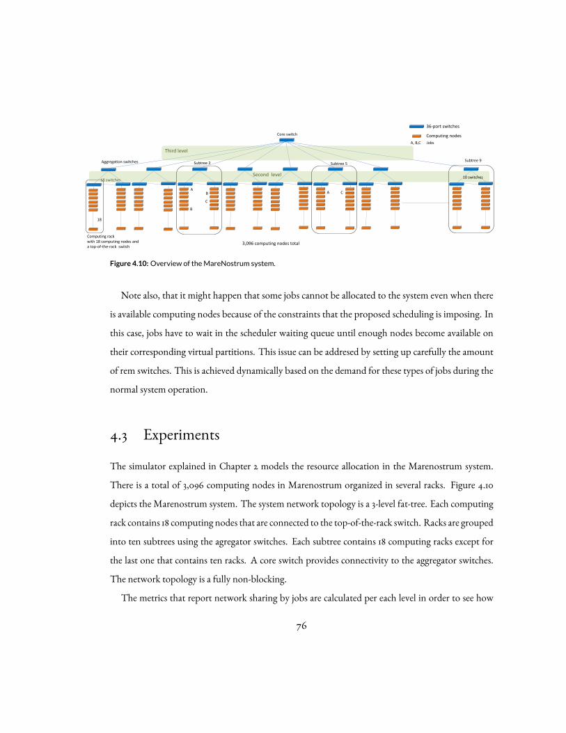
18 switches

3,096 computing nodes total

Third level

Second level

36-port switches

Computing nodes

Subtree 2 Subtree 5

A

Core switch

Aggregation switches

B

A C

C

B

18

Computing rack with 18 computing nodes and a top-of-the-rack switch

A, B,C Jobs

Subtree 9

10 switches

Figure 4.10: Overview of theMareNostrum system.

Note also, that it might happen that some jobs cannot be allocated to the system even when thereis available computing nodes because of the constraints that the proposed scheduling is imposing. Inthis case, jobs have to wait in the scheduler waiting queue until enough nodes become available ontheir corresponding virtual partitions. This issue can be addresed by setting up carefully the amountof rem switches. This is achieved dynamically based on the demand for these types of jobs during thenormal system operation.

4.3 ExperimentsThe simulator explained in Chapter 2 models the resource allocation in the Marenostrum system.There is a total of 3,096 computing nodes in Marenostrum organized in several racks. Figure 4.10depicts the Marenostrum system. The system network topology is a 3-level fat-tree. Each computingrack contains 18 computing nodes that are connected to the top-of-the-rack switch. Racks are groupedinto ten subtrees using the agregator switches. Each subtree contains 18 computing racks except forthe last one that contains ten racks. A core switch provides connectivity to the aggregator switches.The network topology is a fully non-blocking.The metrics that report network sharing by jobs are calculated per each level in order to see how

76

different policies are loading the different network levels. An example of the calculation of this metricis ilustrated in Figure 4.10 where three jobs (A,B,and C) each using two computing nodes are in differ-ent racks of the system. Jobs A and C are being placed in two different subtrees, 2 and 5, whereas jobB is being placed solely in subtree 2. Job A shares the up link at level 2 in the top-of-the-rack switchwith job B and the up link at level 3 in the aggregation switch with job C. Job B shares the up linkat level 2 in the top-of-the-rack switch with A and C. And finally, job C shares with B the up link atlevel 2 in the top-of-the-rack switch in subtree 2, but shares with only job A in the up link at level 3 inthe aggregation switch in the subtree 5. The resulting network sharing per job is two because each jobshares the network with other two different jobs. The total number of sharing jobs would be three,each job shares with another job. The network sharing per level 2 would be two job pairs (A with Band B with C), and for level 3 would be one job pair, only A and C share the network.For comparison purposes several scheduling policies have been implemented in order to compare

with our proposed policy. They are described below.

• First available. Jobs are allocated to the first available computing nodes starting from the firstswitch to the last switch in the system. This policy does not look if the job completely fits insome switch of the system so it is prone to generate fragmentation.

• First contiguous. This policy chooses switches that fit completely the job first and tries to al-locate computing nodes together in contiguous switches as much as possible. In case there areno contiguous switches then chooses computing nodes as in the First available policy.

• Exclusive. It allocates jobs in computing nodes that do not share the network with other jobs.Therefore, this policy achieves no network sharing at all, so it is the best policy in terms ofminimizing network sharing. In order to achieve that, small jobs must be allocated to a singleswitch and big jobsmust be allocated to one ormore subtrees where there are no other big jobsallocated there already. Note that small jobs and big jobs can share the same subtree becausesmall jobs will not use network resources. In case there is no available computing nodes thatfulfill the aforementioned rules then the jobs must wait on the queue. As it can be expected

77

First available First contiguos Virtual networks Exclusive0

2

4

6

8

10

12

14

16

18

Ave

rag

e n

um

be

r o

f jo

bs

sha

rin

g p

er

job

Figure 4.11: Average number of jobs that shared the network with a single job during the execution of the 49107 jobs

workload fromMareNostrum log for each of the four evaluated scheduling policies.

this policy is prone to increase job’s waiting queue time.

4.4 EvaluationThis section shows the evaluation of the proposed policy. The evaluation is performed using a traceof the workload obtained recently from the MareNostrum system during 32 consecutive days. Thistrace contains a list of 49,107 different jobs frommultiple users that were running during that periodin the system. The proposed policy is compared with the other traditional policies, First available andFirst contiguous. It is also compared with the Exclusive policy that achieves no job sharing at all.Figure 4.11 shows the average number of jobs that are shared per job for the different policies evalu-

ated. As it can be seen, the First available policy is the one that shows the highest value, 17 shared jobson average. On the other hand, the Exclusive policy shows no sharing per job because it guaranteesthat no other job will use the job’s part of the network before allocating the computing nodes to it.As we will see later, this advantage comes with a substantial penalty on the completion time.The First contiguous policy reduces by a factor of 4.3× the amount of network sharingwith respect

to First available policy. And even better is the reduction achieved by the Virtual network policy thatachieves an additional factor of 4× with respect to First contigous policy achieving on average only

78

First availableFirst contiguos

Virtual networksExclusive

0%

10%

20%

30%

40%

50%

60%

70%

80%

90%

100%

Not sharingSharing

Pe

rce

nt

of

tota

l nu

me

br

of

job

s

Figure 4.12: Percent of jobs that shared network with other jobs during the execution of the 49107 jobs workload from

MareNostrum log for each of the four evaluated scheduling policies.

0.9 jobs sharing per job.

Figure 4.12 shows the percent of jobs that shared network with other jobs from the whole tracetotaling 49,107 jobs. As expected, the Exclusive policy achieves no sharing at all, whereas First availablepolicy achieves the highest number of jobs shared. However, our proposedpolicy achieves a significantreduction on the total number of jobs sharing achieving only 5% which corresponds to a reductionfactor of 9×with respect to First available and a 45% reductionwith respect to First contiguous policy.

The above results clearly show that our proposed policy is quite efficient in achieving a significantreduction on the amount of jobs sharing the network simultaneously. The reason for this is the segre-gation of jobs per job-size in the isolated virtual networks blocks as described in Section 4.2. However,jobsmight be waitingmore time in the waiting queue in order to get space available on a virtual block.This effect is going to be evaluated as follows.

The results in Figure 4.13 show the number of job pairs that were sharing the network at each ofthe levels of the tree. First available is worse than the other policies at both the second and the thirdlevel. There is a huge improvement of First contiguous over First available, in both the second and thethird level. On the contrary from First available, First contiguous is having more sharing on the thirdlevel than on the second level, since it is not solving the fragmentation at the third level. Our policyimproves over First contiguous policy by a factor 8.4× at the second level and by the factor of 3.9× at

79

First available First contiguos Virtual networks Exclusive0

50000

100000

150000

200000

250000

300000Level2Level3

Nu

mb

er

of

sha

rin

g jo

b p

air

s p

er

ne

two

rk le

vel

Figure 4.13: Number of job pairs that shared network at the 2nd and at the 3rd network level during the execution of the49107 jobs workload fromMareNostrum log for each of the four evaluated scheduling policies.

the third level. The Exclusive policy, as previously seen, does not introduce any network sharing.

Figure 4.14 shows the completion time for the various scheduling policies. As can be seen, bothpolicies, First available and First contiguous, show the lowest completion time, 32 days. On the otherhand, the Exclusive policy shows the largest completion time, 39 days. A 23% increase of time dueto the restriction to allocate exclusive subtrees for parallel jobs larger than 18. This policy delays sub-stantially completion time. However, our policy obtains a completion time of only 33 days whichcorresponds an increase of only a 4% with respect to the first two policies. The increase in comple-tion time of our policy is almost negligible and significantly lower than for the Exclusive policy, whilemaintaing a high level of isolation between applications, effectively eliminating interference betweenapplications that in practice could reduce the execution time of each job.

This increase of the completion time is due to fact that our policy holds jobs on the queue longertime waiting for the proper computing nodes to become available. This is illustrated in Figure 4.15.As can be seen, Virtual networks policy increases the queue time of jobs on average around sixteenminutes. The Exclusive policy introduces an increase in the average waiting queue time per job of upto 28 minutes.

Figure 4.16 shows the portion of the system computing nodes being allocated to jobs in average forall fourpolicies. As canbe seen, althoughourpolicy increases the jobqueue time, the systemutilization

80

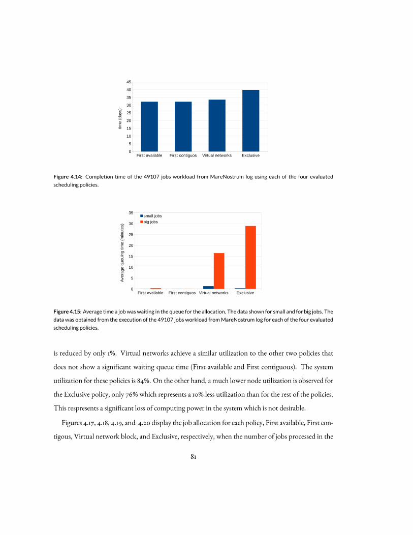
First available First contiguos Virtual networks Exclusive0

5

10

15

20

25

30

35

40

45

time

(d

ays

)

Figure 4.14: Completion time of the 49107 jobs workload from MareNostrum log using each of the four evaluated

scheduling policies.

First available First contiguos Virtual networks Exclusive0

5

10

15

20

25

30

35small jobs

big jobs

Ave

rag

e q

ue

uin

g t

ime

(m

inu

tes)

Figure 4.15: Average time a jobwaswaiting in the queue for the allocation. The data shown for small and for big jobs. The

data was obtained from the execution of the 49107 jobs workload fromMareNostrum log for each of the four evaluated

scheduling policies.

is reduced by only 1%. Virtual networks achieve a similar utilization to the other two policies thatdoes not show a significant waiting queue time (First available and First contiguous). The systemutilization for these policies is 84%. On the other hand, a much lower node utilization is observed forthe Exclusive policy, only 76% which represents a 10% less utilization than for the rest of the policies.This respresents a significant loss of computing power in the system which is not desirable.

Figures 4.17, 4.18, 4.19, and 4.20 display the job allocation for each policy, First available, First con-tigous, Virtual network block, and Exclusive, respectively, when the number of jobs processed in the

81

First available First contiguos Virtual networks Exclusive0

10

20

30

40

50

60

70

80

90

Ave

rag

e s

yste

m u

tiliz

atio

n (

%)

Figure 4.16: Average systemcomputing node utilization during the execution of the 49107 jobsworkload fromMareNos-

trum log for each of the four evaluated scheduling policies.

trace is around one half, i.e. at the 25000th job of the trace. The figures show all 172 computing racksinMarenostrum grouped into all ten subtrees. Every row of racks corresponds to a subtree. Thus, theracks within a row are interconnected with the second level network and the racks at different rowsare interconnected with the third level network. In order to easily visualize the job allocation in thesystem each job is colored with a different color. Black color is used for jobs with a number of com-puting nodes equal or less than the amount of computing nodes available per switch (18), i.e., smalljobs, whereas other colors, except grey color, is used to visualize jobs with a number of computingnodes larger than 18. Grey is a special color used to display that the computing node has not yet anyjob allocated on it.

In Figure 4.18 that shows the First avaible policy it can be observed that some computing racks aredisplayed with multiple different colors meaning that multiple different parallel jobs are being allo-cated to these racks increasing the sharing among jobs. Moreover, black colors are spread out amongmultiple different computing racks which may point out one of the cause of the high level of sharingof the racks identified before.

On the other hand, on Figure 4.18 that shows the First contiguous policy it shows a different ba-havior on job allocation than the First avaiable shown before. Now, the computing racks are clearlyshowingmuch less sharing of the computing racks bymultiple jobs as racks are not shown asmultiple

82

Figure 4.17: First available policy. Status of the system population in themiddle of simulation. Grey depicts the node that

is not used by any job. Black color depicts small jobs, i.e., less or equal than 18. Other colors depict big jobs.

Figure 4.18: First contiguous policy. Status of the system population in the middle of simulation. Grey depicts the node

that is not used by any job. Black color depicts small jobs, i.e., less or equal than 18. Other colors depict big jobs.

colors as before. Nevertheless, still jobs of the size equal or less than 18 are spread out through theentire system which may cause high fragmentation for larger job sizes.On the other hand, Figure 4.19 shows the Virtual network block policy where it can be seen that

jobs of the size equal or lower than 18 are more concentrate into an particular area of the system, onthe last two subtrees. This area is the small jobs virtual block, explained in 5.1 In addition, it can be

83

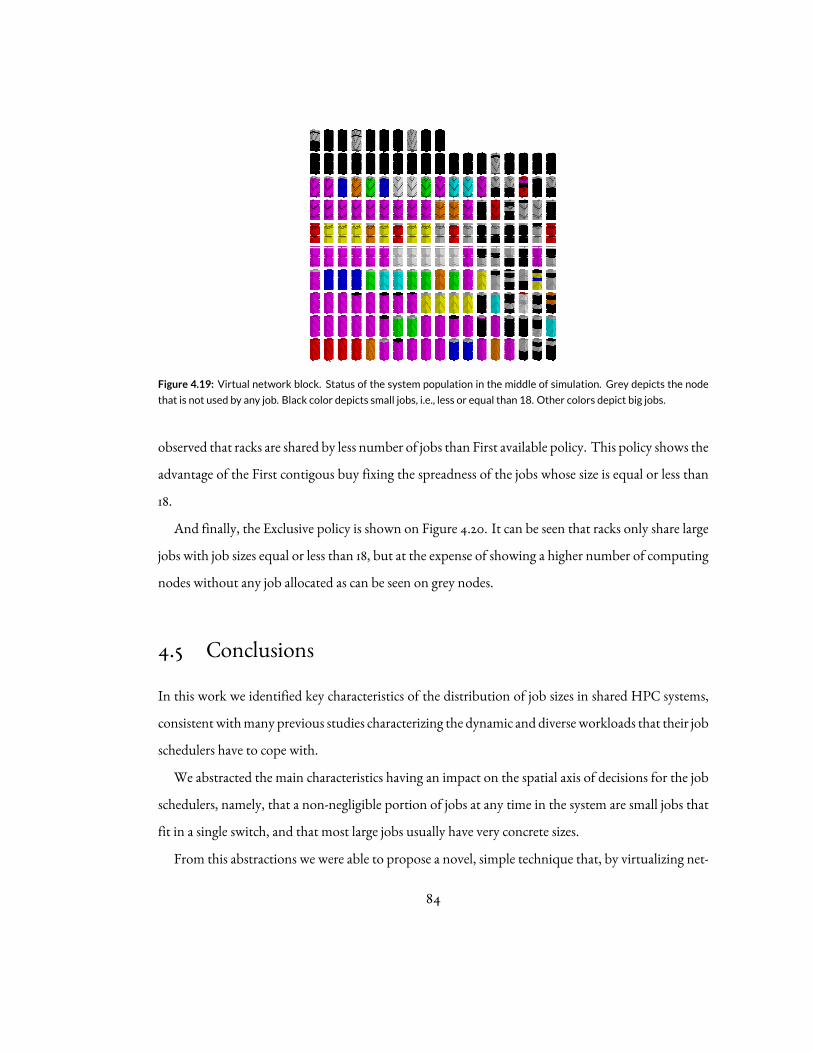
Figure 4.19: Virtual network block. Status of the system population in the middle of simulation. Grey depicts the node

that is not used by any job. Black color depicts small jobs, i.e., less or equal than 18. Other colors depict big jobs.

observed that racks are shared by less number of jobs than First available policy. This policy shows theadvantage of the First contigous buy fixing the spreadness of the jobs whose size is equal or less than18.And finally, the Exclusive policy is shown on Figure 4.20. It can be seen that racks only share large

jobs with job sizes equal or less than 18, but at the expense of showing a higher number of computingnodes without any job allocated as can be seen on grey nodes.

4.5 ConclusionsIn this work we identified key characteristics of the distribution of job sizes in shared HPC systems,consistentwithmany previous studies characterizing the dynamic and diverseworkloads that their jobschedulers have to cope with.We abstracted the main characteristics having an impact on the spatial axis of decisions for the job

schedulers, namely, that a non-negligible portion of jobs at any time in the system are small jobs thatfit in a single switch, and that most large jobs usually have very concrete sizes.From this abstractions we were able to propose a novel, simple technique that, by virtualizing net-

84

Figure 4.20: Exclusive policy. Status of the system population in the middle of simulation. Grey depicts the node that is

not used by any job. Black color depicts small jobs, i.e., less or equal than 18. Other colors depict big jobs.

work resources at different levels, is able to transform the chaotic arrival distribution of job sizes anddurations into a stable spatial segregation of jobs with a dynamic boundary that can adapt to changesin the arrival distribution.Our policy, by being able to hierarchically and flexibly place jobs within contained parts of the

network minimizing interference is able to achieve very high system utilization, similar to topologyand interference oblivious techniques, while at the same time achieving an unprecedented level ofisolation and thus performance predictability for the individual applications.Moreover, the segregation technique led to two very beneficial side-effects yet to be explored in

detail: 1) potential hardware savings, in the form of requiring less or no virtual channels to provideQuality of Service features to isolate applications, as we are able achieve it through the schedulingdecisions, or by reducing the capacity of the second-level and third-level switches for the part of thenetwork that accepts only small jobs, or alternatively, instead of reducing the capacity, 2) potentiallysaving power by selectively switching off the corresponding part of the network that accepts only thesmall jobs.Aswe have shown, our policy for the sake of flexibility and systemutilization allows a small percent

of jobs to share the network resorces. Potential interference impact on these jobs’ performance and

85

consequently the system performance is mitigated by additional resource management techniques atthe link-level described in the next chapter. The two techniques at system-level and at the link-levelare compatible.

86

5Link-level resource management

Interconnection networks for high-performance computers (HPC) have traditionally been operatedon a best-effort basis. Network capacity is based on peak traffic load estimates, so that networks havegenerally been over-provisioned. This approach is simple for systems with predictable traffic loadswhere the performance achieved fits the user expectations for a small set of selected applications ofinterest.

However, as systems are being scaled out, they can proportionally accommodatemore applicationsrunning concurrently, which implies that multiple messages of different applications compete for the

87

same network resources.

Inter-application contention depends on many factors such as routing, task mapping, applicationcommunication patterns, and the relative start times of applications. The lack of predictability of theeffects of inter-application contention leads to low throughput, high latency and high-jitter, as thecompetition of applications for network resources disrupts the performance of the applications moresensitive to contention degrading the overall system throughput. We evaluated the degradation inHPC systems reporting the system throughput loss of 10%-30%29.

The problem of inter-application contention is already well-known in the Internet arena wheredifferent data flows might compete for the same network resources. The solution in the context ofInternet applications was to use Quality-of-Service (QoS) mechanisms to guarantee certain levels ofperformance to specific data flows such as real-time video streaming. This effort was referred to asDif-ferentiated Services9 by the Internet Engineering Task Force (IETF). A classification of the differenttraffic types was performed in47 and revised and implemented in InfiniBand networks in 3. In partic-ular, the InfiniBandQoSmechanism is based on the use of virtual lanes (VLs) and the correspondingarbitration tables that define the bandwidth allocated to each VL. Additionally, InfiniBand supportsthree priority levels, where packets on the higher priority are served first regardless of the bandwidthallocated for the lower priority. By default the highest priority is reserved for subnet managementtraffic, and the rest for user traffic. The methodology used in 3 was based on allocating time-sensitivetraffic to high-priority VLs, and using low-priority VLs for other traffic. In the latter case, it attemptsto guarantee that traffic is allocated to the VL that matches its bandwidth needs.

Recently, QoS is being used inHPC, as well in order to reduce the impact of inter-application con-tention for scientific codes. HPC system administrators can apply specific QoS policies on a per-jobbasis bymeans of system resources management tools such as the Unified FabricManager Software40

(UFM) fromMellanox. However, the QoS policies employed are still quite basic and coarse-grained,and only benefit a small set of applications. Basically, applications are classified into two broad trafficclasses, namely latency-sensitive and bandwidth-sensitive applications, where latency-sensitive appli-cations are mapped to high-priority VLs and the rest to low-priority VLs.

88

In this work we propose an effective quality-of-service policy for capacity HPC systems. HPC ap-plications are usually not real-time and are different from the internet-like traffic analyzed in previ-ous works47,3. Depending on the application, its characteristics lie on a continuum between latency-sensitive and bandwith-sensitive traffic.

The technique that we propose provides a wider classification of applications, and hence can lever-ageQoSmechanisms for a largenumber of applications resulting in an increase of systemperformance.The proposed QoS policy provides a method to effectively map applications to VLs, and provides aneffective distribution of bandwidth for each of these VLs. The proposed techniques are fully sup-ported in InfiniBand and do not require any additional hardware capability. Specifically, the contri-butions of this work are as follows:

• A method to map applications into VLs focused on minimizing inter-application contention.Thismethoddynamicallymaps applications during runtime to approach the optimalmappingbased on behavior of the applications that are running using characterization methodologyproposed in Chapter 3.

• We show that segregating applications on different VLs significantly reduces inter-applicationcontention. Reductions in contention time from 10% - 60% are achieved.

• We also provide a method to group applications into virtual lanes in case there are more appli-cations than virtual lanes based on the previously presented characterization.

• We provide a technique to effectively distribute available network bandwidth to virtual lanes.It is demonstrated that for HPC codes it is very important to detect communication intenseapplications at the critical point of thenetwork and separate themfrom less intense applicationsby assigning an exclusive VL. In this way, the burstiness of such an application can be regulatedtuning the VL’s bandwidth.

89

A0

Applications

An

VL0

VLm

A1

Applicationmapping technique

BW0

BWm

Bandwidthallocation technique

Virtuallanes Bandwidth

Applicationcharacterization

methodology

Figure 5.1: Techniques developed for the new proposedQoS policy.

5.1 Proposed Quality-of-Service Policy

The proposed QoS policy is depicted in Figure 5.1. It is based on two techniques: (i) a mapping tech-nique that determines the most suitable VL for each application; (ii) a method to properly allocatebandwidth to each VL. The descriptions of these techniques are presented below.

5.1.1 ApplicationMapping to VLs

The method to properly map applications to the available VLs is depicted in Figure 5.2.The method distinguishes between two cases. When the number of applications is less than or

equal to the number of VLs, each application will be allocated to an independent VL to partiallyeliminate the performance degradation caused by inter-application contention. The reason for this is

90

Figure 5.2: Algorithm for mapping applications into VLs.

simple: segregating applications intoVLs helps to partially reduce the interactions between them. Forexample, if two streams of data – A and B – share the same VL and B is coming last to the network, itwill suffer the inter-application contention from A according to Equation 1.3.

Therefore, when B is allocated to another VL the VL arbiter can transmit B packets just after thecurrent A transmission finishes if it was not blocked. Therefore, segregating applications into VLseliminates theTAcongestion andTAblocking terms from the inter-application contention, but not the currentTAtransfer.

In the case of having more applications sharing network resources than available VLs, the methodof mapping applications into VLs is based on grouping applications that are compatible into groups,where number of groups are equal to number of available VLs. For a measure of compatibility, weuse the characterization described in Chapter 3.

91

A process BW=1

B process BW=1

time

21 slots progression

18 slots progression

Applications A and B same bandwidth

A packet transfer

A computation

B packet transfer

B computation

Figure 5.3: Timeline showing the progression of two applications,A andB, where to each application is assigned the same

bandwidth.

A process BW=3

B process BW=1

time

27 slots progression

21 slots progression

Application A higher bandwidth

A packet transfer

A computation

B packet transfer

B computation

Figure 5.4: Timeline showing the progression of two ap-

plications where toA is assigned higher bandwidth than

B.

A process BW=1

B process BW=4

time

14 slots progression

27 slots progression

Application B higher bandwidth

A packet transfer

A computation

B packet transfer

B computation

Figure 5.5: Timeline showing the progression of two ap-

plications where to B is assigned higher bandwidth than

toA.

5.1.2 Understanding the impact of VL weights on reducing of interferenceIn this section, we will show the necessity for bandwidth allocation technique on VLs in order tofurther reduce inter-application contention.The technique is based on assigning more bandwidth to VLs that have applications that have low

communication demands. This heuristicmay be seen counter-intuitive because onemight expect that

92

applications that are less communication demanding should be assigned less bandwidth. However,as we will see below, it is more beneficial to assign more bandwidth to the applications with low com-munication demands.

The principle behind this effect is illustrated in the following Figures. 5.3, 5.4 and 5.5. The examplesin figures are based onbehavior thatwe observed in the traces of two applications’ simultaneous execu-tions using our visualization tool and are simplified here for clarity. We will give concrete examples ofreal applications and their communicationbehavior later on. Each figure shows the execution timelineof two applications with quite different communication demands, A and B, when performing severaliterations over a period of 27 time slots. One iteration is composed of three packet transfers and fourcomputation slots for A, whereas for B, which has higher communication demands, each iterationcomprises four packet transfers and two computation slots. In each time slot, applications can eitherperform computation or communication, or stall waiting for the network to become available. Tomodel network contention, we assume that only one application can communicate in each time slot.As shown in Figure 5.3 when both applications are assigned the same bandwidth (BWA = BWB = 1),the transfer of packets of these applications are interleaved in time because they have the same band-width. This interleaving of packets due to network contention is unfortunately delaying both appli-cations. The resulting progression of A and B is 21 and 18, respectively, out of the total 27 availableslots.

In the other case shown in Figure 5.4, A is given three times more bandwidth than B, so it cantransfer three consecutive packets before B can transfer any packet (BWA = 3,BWB = 1). In this case,A is not suffering any network contention. Moreover, although the communication of B is delayedat the beginning, it is not suffering as much delay as in the previous case, because most of its transfersoccur when A is computing. The result is that both applications are able to make more progress, andhence the system achieves higher overall throughput. In particular, the progress of A and B is 27 and21 slots, respectively.

Finally, the example shown in Figure 5.5 shows that giving more bandwidth to B, which is morecommunication demanding, is not as efficient as the previous case. In particular, B can communicate

93

as much as it needs in each iteration so BWB = 4,BWA = 1. As a result, the performance of Bis boosted at the expense of A. The resulting progress for B and A is 27 and 14 slots, respectively.Therefore, assigning more bandwidth to the more communication demanding application is not thebest strategy.

The bandwidth allocation technique that we are proposing is based on assigning more bandwidthto applications that have a higher computation to communication ratio. Therefore, we can still usethe metric for characterization as proposed earlier.

Nevertheless, determining the optimal bandwidth for each VL might be quite complex, becausemultiple applicationsmay be assigned to a givenVL. And also, givingmore bandwidth than necessaryto low-communication demanding applications might degrade performance of high-bandwidth ap-plications. Therefore, we recommend in practice a trial-and-error approach to carefully assign morebandwidth to less communication-intensive applications and observe the impact on performance tomore communication-intensive applications to achieve an optimal balance.

To implement this bandwidth allocation technique in InfiniBand, applications have to bemappedto the available low-priorityVLs based on the grouping technique proposed in Section 5.1.1. Then, theweights in eachVL shouldbe assigned in such away thatVLs containing less communication-intensiveapplications have more weight than those containing more communication-intensive applications.

5.2 Simulation

In this section, we introduce the metric used to measure inter-application network contention, andwe describe the simulation environment and the applications used to evaluate our proposal. Subse-quently, we present the results showing a) the effect ofmapping applications toVLs and b) the impactof bandwidth allocation.

94

5.2.1 Inter-application contention metric

Impact of inter-application network contention is measured as an increase in the absolute executiontime that an application experiences due to sharing network resources with other applications. Wewant tomeasure this contention to identify the optimalQoS policy. As we know, aQoS policyQj is afunction of three factors: 1) assigning applications or groups of applications to SL classes, 2) mappingSLs to VLs and 3) allocating bandwidth (weight) assigned to VLs. Note that in our proposed QoSpolicy factors 1) and 2) are managed by our application-to-VL mapping technique. We employ thenotation “VLnxm” to indicate that VL n has relative weight m.To quantify this impact for a particular set of QoS policy parameters Qj, we used the metric ex-

plained in Chapter 2. Namely, the application was simulated in the same system twice. First, it wasexecuted alone, i.e., without any inter-application contention. The resulting execution time is usedas a reference time Talone (see Table 5.3). Then, it was run simultaneously with another application(or several applications) sharing the system and thus experiencing inter-application contention. Wewill refer to the completion time of an application in the latter scenario as Tsharing. Therefore, theinter-application contention for an application i can be calculated as

Ticontention(Qj) = Tisharing(Qj)− Tialone. (5.1)

Note that all system parameters and settings (e.g., size of the network, task allocation, routing,MTU size, etc.) have to be the same in both scenarios so that the increase in the execution time of theapplication can be attributed solely to the inter-application contention, and not to a coupled effectof contention and other factors. Moreover, to obtain a view of the amount of inter-application con-tention for a given combination of applications we compute the total inter-application contentiontime Ttotal-contention of n applications as follows:

Ttotal-contention(Qj) =n∑i=1

Ticontention(Qj). (5.2)

If all the applications use the same number of compute nodes C, each compute node having com-

95

pute power P GFLOPS, then the system-level compute power waste, Pw, in GFLOPs (s stands forplural, and not for ”per second”) is calculated as

Pw = C · P ·n∑i=1

Ticontention(Qj). (5.3)

The QoS policy Qopt is the most efficient one within a set of NQoS policies if it satisfies

Ttotal-contention(Qopt) = minj∈N

(Ttotal-contention(Qj)). (5.4)

5.2.2 Simulation setup

The simulated systems parameters are given in the Table 5.1. The network topology used is a block-ing (”slimmed”) three-level fat tree. We simulate networks of large scale (details in Table 5.2). Theslimmednetworks are usually characterized by contention factor—ratio between the input ports com-ing from the lower level of the fat-tree and the output ports that go to the upper level of fat-tree in aswitch.The trace was originally collected on amachine with IBM’s 2.5 GHz PowerPC 970 processors from

2005with apeakperformance of 27,6Gflopsper chip. Today’s IBMprocessors such asPower7 achievea peak of 264 Gflops. This results in roughly 10X faster computations, which is the speed up factorused in our simulations. In addition, the simulated network (10 Gb/s) is five times faster than theoriginal network (2 Gb/sMyrinet). The workloads executed on the system consisted of a mix of two,three, or four applications. The settings for the experiments with different number of applications inthe mix were different in terms of total number of nodes, task allocation, etc. (see Table 5.2).OneMPI application process is allocated per node in our simulator. We are assuming thatmultiple

cores within a node are fully utilized speeding up its computation phase which is the typical scenarioin emerging hybrid parallel programing languages, i.e. MPI+OpenMP, MPI+StarSs.To mimic the effects of non-contiguous node allocation (fragmentation), we interleave the tasks

belonging to different applications such that each set of nodes attached to the same first-level switch

96

are evenly distributed across the applications. For example, in the case of two applications, each ap-plication uses eight nodes per switch. We use the notations F4 and F8 to indicate that four and eightnodes are used per application at the switch, respectively.In the experiments, the SL and VL are set at the adapter and are not changed at any point in the

system during the whole execution of application. In our simulator the weights for each VL are set asthe number of packets that can be served per turn for that VL.

Table 5.1: Parameters used in the simulations

Simulator Venus-DimemasTopologies Extended Generalized

Fat Trees (XGFT)45,49Switch Technology InfiniBand

Switch Size 32-portsBuffers Input/Output

Network Bandwidth 10 Gbits/sSegment size 4 KBMPI Latency 1 μsCPU Speedup 10xRouting scheme Random routing 24,21

5.2.3 ApplicationsIn our experiments we employed four NAS Parallel Benchmarks from the NPB3.3-MPI release: FT,BT, CG and MG. The details on applications’ traces cuts used for the experiments are given in Ta-ble 5.3.The bandwidth utilization per level obtained by our characterization methodology is shown for

each of the considered applications in Figure 5.6 and Figure 5.7 for the case of node allocation F8 andF4, respectively. When on F8 fragmentation FT and CG fall into category of moderately intensive

97

Table 5.2: System settings and task allocations for various workload sizes

#Apps XGFT #Nodes Contention Task #VLs/Buffer Reference timestopology (used/idle) ratio allocation size per VL

2 (3; 16, 16, 2; 1, 4, 4) 512/0 4:1 F8 1/64KB, 2/32KB Talone(buff. 32KB)see Table 5.3

3 (3; 16, 16, 4; 1, 4, 4) 768/256 3:1 F4 1/64KB, Talone(buff. 16KB)4(3 used)/16KB see Table 5.3

4 (3; 16, 16, 4; 1, 4, 4) 1024/0 4:1 F4 1/64KB, 4/16KB Talone(buff. 16KB)see Table 5.3

Table 5.3: Applications traces details and reference times (Talone).

App.Problem Msg sizes #TasksOrig. Used #Iters. Talone Talonesize trace trace cut (buff.32KB,1VL,F8)(buff.16KB,1VL,F4)

FT Class D 512 KB 256 415 s 75 s 5 9.111861 s 8.192807 sCG Class D 732 KB 256 882 s 75 s 337 8.191318 s 7.95694 s

BT Class D 761 KB, 256 620 s 75 s 22 7.534967 s 7.459007 s158 KB, 26 KB

MG Class D 260 KB, 128 KB, 256 111 s 75 s 36 not used 7.304353 s65 KB, 32 KB

applications, while BT andMGare low communicating applications. In the case of F4 fragmentation,FT is still moderately intensive, whereas CG, BT andMG are low intesive applications. Note that theCG’s utilization at L0 of fat-tree is much higher than the one at other levels and also it is higher thanL0 utilization of the rest of applications. However, L0 traffic is not relevant for the inter-applicationcontention since all applications have exclusive computing node-switch network links at L0, i.e., anode is exclusively allocated to one application.

98

FT CG BT MG0

0.05

0.1

0.15

0.2

0.25

0.3

0.35On F8 fragmentation

L0L1L2

Ban

dwid

th u

tiliz

atio

n

Figure 5.6: Bandwidth utilization per level for applications on xgft(3;16,16,4;1,4,4) fat-tree network and node allocation

on F8 fragmentation.

FT CG BT MG0

0.05

0.1

0.15

0.2

0.25

0.3

0.35On F4 fragmentation

L0

L1

L2

Ban

dwid

th u

tiliz

atio

n

Figure 5.7: Bandwidth utilization per level for applications on xgft(3;16,16,4;1,4,4) fat-tree network and node allocation

on F4 fragmentation.

99

5.3 Results of the proposed techniques

5.3.1 The benefit from segregation of applications into VLs

We evaluate the scenario in which the number of VLs configured in the system is equal to or greaterthan the number of applications that are being executed on the system.For this scenario, we evaluate the benefits of segregating applications into VLs in such a way that

each application is assigned to an independent VL exclusively for its entire execution. Also, applica-tions are assigned to VLs in the following order, the first application in the workload indicated on thex-axis is mapped to VL0, the second to VL1, etc. Here we assume all VLs are of low priority unlessspecified differently.

Uniform bandwidth allocation

In this part we will evaluate the case when the weights assigned to all VLs are the same and allow eachVL to send one packet in each turn (we annotate it as vl0x1, vl1x1). We refer to this as interleaving ofVLs. We compare the results of segregating with those achieved by assigning all applications to thesameVL (vl0). Note that the total buffer space should remain the same size in the case of using oneVLand using several VLs. Table 5.2 provides the details on per VL buffer size for each set of experiments.Figure 5.8 shows the total inter-application contention time for the case of using only one VL and

the case of segregating applications on two VLs for the two-application mixes. As can be seen, bysegregating applications into two VLs a substantial improvement is achieved. In particular, reduc-tion of the contention time ranges from 7% for two FT applications executed together to 59% whenFT shares the network with BT. This result indicates that in the case where there are as many VLsas applications, each application should be mapped to a different VL. The case of CG and BT wherethe total contention time is increased upon segregation is most probably caused by dividing up theavailable buffer size. Namely, when CG runs with BT on VL0 they share 64KB buffer. As BT com-municates much less then CG, CG can use the whole buffer most of the time. Whenwe segregate two

100

applications on VL0 and VL1 each can use only half of the buffer space - 32KB.Figure 5.9 shows the normalized execution time for each application for the same mixes as before.

We can see that segregating onto different VLs significantly improves the performance of both ap-plications in most cases. Also, there are some cases in which the performance of one application issubstantially improved at the cost of slightly degrading the other one. In particular, when sharing thenetwork with FT, CG may be improved by 8% through segregation, and FT is only degraded by 1%.On the other hand, we can obtain improvements for both applications by segregation when the twoare the same applications (e.g., FT with FT, CG with CG).Figure 5.10 shows the total contention time for the three-application mixes. When increasing the

number of applications in theworkloadwe again obtain substantial reductions in the contention timeowing to the segregation. Specifically, this reduction is 22% for the case of a mix of FT, CG, andBT. Moreover, a workload comprising four applications increases the individual contention time ofeach application and thus total contention time. However, also in this scenario segregating achievesa reduction in inter-application contention. In particular, a reduction of 32% is observed comparedwith the case of non-segregating.Figure 5.11 shows the impact of segregation on each application’s overall performance in the three-

applications mix (on the left) and the four-applications mix (on the right). The improvement in per-formance is seen for all applications but one - FT.However, degradation of FT, around 1% is less thanthe improvement of any other application in both three- and four-application mixes.

Non-uniform bandwidth allocation

Figures 5.12, 5.13 and 5.14 show the total contention time for the FT+CG, FT+BT, andCG+BTmixes,respectively, when assigning different weights to VLs as explained in Sec. 5.1.2. Note that we are as-suming full segregation of applications intoVLs. Also, themapping of applications toVLs is constant(vl0 - blue, vl1- red). Additionally, we show the two extreme cases of assigning full link bandwidth toVL0 and VL1 which corresponds to assigning a high priority to these VLs. The inter-application con-tention gradually diminishes in the application as its bandwidth allocation increases, but at the same

101

FT+CG FT+BT CG+BT FT+FT CG+CG BT+BT0

1

2

3

4

5

6vl0vl0 x1, vl1 x1

To

tal c

on

ten

tion

tim

e (

s)

Figure 5.8: Total contention timewhen using one and two VLs for the two-applicationmixes.

FT CG FT BT CG BT FT FT CGCG BT BT1

1.05

1.1

1.15

1.2

1.25

1.3

1.35vl0vl0x1, vl1x1

No

rma

lize

d e

xec u

tion

tim

e

Figure 5.9: Impact on the execution time of each application when using one and two VLs for the two-applicationmixes.

time increases the contention of the other application. In other words, the ratio between individualapplication contention times is changing when favoring one VL (vl0, on the left) or another VL (vl1,on the right). However, a sweet spot is reached around the middle of the graphs on where the total

102

FT+CG+BT FT+CG+BT+MG

0

0.5

1

1.5

2

2.5vl0vl0x1,vl1x1,vl2x1,vl3x1

Tot

al c

ont e

ntio

n tim

e (s

)

Figure 5.10: Total contention time when using one and three/four virtual lanes for the three/four-application mixes. In

FT+CG+BT, FT on VL0, CG on VL1 and BT on VL2. In FT+CG+BT+MG, FT on VL0, CG on VL1, BT on VL2 andMGonVL3.

FT CG BT FT CG BT MG

1

1.02

1.04

1.06

1.08

1.1

1.12

1.14

1.16vl0vl0x1, vl1x1, vl2x1, vl3x1

Nor

mal

ize d

exe

cutio

n tim

e

Figure 5.11: Impact of segregation on the execution time of each application in three/four applicationmixes.

contention time is lowest.

In particular, for the FT+CGmix the optimal strategy is achieved when FT (vl0) sends one packetand CG (vl1) sends two packets per turn (vl0 x1 vl1 x2). The reduction of total contention time isaround 7% compared to case of equal-weight interleaving (each VL sends one packet in a turn). Inapplication classes terms, this is the case ofmoderate-intensity application (FT) sharing resources with

103

another moderate-intensity application (CG). By assigning less bandwidth to application of higherintensity we are, in fact, performing regulation of FT’s flow. Similar behavior is also observed forthe mixes FT+BT where the minimum total contention is observed at (vl0 x1 vl1 x4). Since BT isof lower intensity than CG the mutual impact is lower than in the case of FT+CG. The case of CGand BT sharing the network reaches minimum contention at (vl0 x1 vl1 x8), but overall the impact oftheir interference on the performance is not too high. This result suggest that the total contentiontime is smaller when the application that has lower communication demands is favored. Note thatthis bandwidth allocation strategy improves the performance of one application without excessivelydegrading the other one, thereby resulting in an overall decrease of the total contention time.

The case of three-application mixes is shown in Figure 5.15. For this case a similar behavior is ob-served. The largest reduction in contention is achieved when the bandwidth allocation favors theapplication with lower communication demand and restricts the bandwidth of applications of higherintensity (FT). In this case we can see that the optimum is achieved for vl0 x1 vl1 x2 vl2 x4 which givesmore weight to the lowest communication demanding application (BT), then to the second lowest(CG) and finally, the least weight to most demanding application (FT). The improvement observedis 9%with respect to the case of equal-weight interleaving (vl0 x1 vl1 x1 vl2 x1). Note that any deviationfrom this bandwidth allocation leads to a suboptimal QoS strategy. For example, applying the oppo-site strategy, i.e., giving more bandwidth to more demanding applications, leads to an increase of 23%in total contention time compared to interleaving.

5.3.2 The effect of non-fully segregation of applications (grouping) on VLs

When there are fewer VLs than applications our strategy is to group some applications on one VL aswe explained in Sec. 5.1.

104

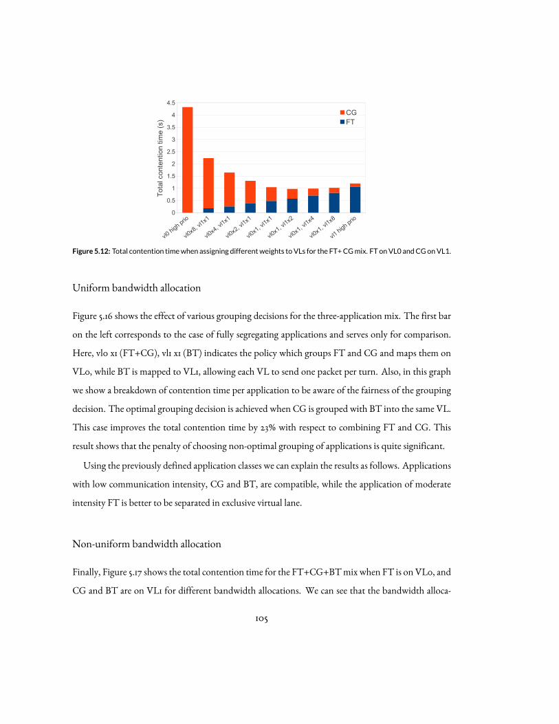
vl0 high prio

vl0x8

, vl1x1

vl0x4

, vl1x1

vl0x2

, vl1x1

vl0x1

, vl1x1

vl0x1

, vl1x2

vl0x1

, vl1x4

vl0x1

, vl1x8

vl1 high prio

0

0.5

1

1.5

2

2.5

3

3.5

4

4.5

CGFT

Tot

al c

ont e

ntio

n tim

e (s

)

Figure 5.12: Total contention timewhen assigning differentweights toVLs for the FT+CGmix. FT onVL0 andCGonVL1.

Uniform bandwidth allocation

Figure 5.16 shows the effect of various grouping decisions for the three-application mix. The first baron the left corresponds to the case of fully segregating applications and serves only for comparison.Here, vl0 x1 (FT+CG), vl1 x1 (BT) indicates the policy which groups FT and CG and maps them onVL0, while BT is mapped to VL1, allowing each VL to send one packet per turn. Also, in this graphwe show a breakdown of contention time per application to be aware of the fairness of the groupingdecision. The optimal grouping decision is achieved when CG is grouped with BT into the same VL.This case improves the total contention time by 23% with respect to combining FT and CG. Thisresult shows that the penalty of choosing non-optimal grouping of applications is quite significant.Using the previously defined application classes we can explain the results as follows. Applications

with low communication intensity, CG and BT, are compatible, while the application of moderateintensity FT is better to be separated in exclusive virtual lane.

Non-uniform bandwidth allocation

Finally, Figure 5.17 shows the total contention time for the FT+CG+BTmix when FT is on VL0, andCG and BT are on VL1 for different bandwidth allocations. We can see that the bandwidth alloca-

105

vl0

high

prio

vl0x8

, vl1x

1

vl0x4

, vl1x

1

vl0x2

, vl1x

1

vl0x1

, vl1x

1

vl0x1

, vl1x

2

vl0x1

, vl1x

4

vl0x1

, vl1x

8

vl1 hi

gh pr

io0

0.5

1

1.5

2

2.5

3

3.5

4

4.5BTFT

Tot

al c

ont e

ntio

n tim

e (s

)

Figure 5.13: Total contention timewhen assigning different weights to VLs for the FT+BTmix. FT on VL0 and BT on VL1.

vl0

high prio

vl0x8

, vl1x1

vl0x4

, vl1x1

vl0x2

, vl1x1

vl0x1

, vl1x1

vl0x1

, vl1x2

vl0x1

, vl1x4

vl0x1

, vl1x

8

vl1 high

prio0

0.5

1

1.5

2

2.5

3

3.5

4

4.5

BTCG

Tot

al c

ont e

ntio

n tim

e (s

)

Figure 5.14: Total contention timewhen assigning differentweights toVLs for theCG+BTmix. CGonVL0 andBTonVL1.

106

vl0

x1, v

l1 x

1, v

l2 x

1

vl0

x1, v

l1 x

2, v

l2 x

4

vl0

x1, v

l1 x

4, v

l2 x

2

vl0

x2, v

l1 x

4, v

l2 x

1

vl0

x2, v

l1 x

1, v

l2 x

4

vl0

x4, v

l1 x

2, v

l2 x

1

vl0

x4, v

l1 x

1, v

l2 x

2

0

0.2

0.4

0.6

0.8

1

1.2

1.4

1.6

1.8

2BTCGFT

Tot

al c

ont e

ntio

n tim

e (s

)

Figure 5.15: Total contention timewhen assigning differentweights to VLs for the FT+CG+BTmix. FT onVL0, CGonVL1

and BT on VL2.

vl0 x1

(FT),

vl1 x1

(CG),

vl2 x1

(BT)

vl0 x1

(FT+CG), v

l1 x1 (B

T)

vl0 x1

(FT+BT),

vl1 x1

(CG)

vl0 x1

(FT), v

l1 x1 (C

G+BT)0

0.2

0.4

0.6

0.8

1

1.2

1.4

1.6

1.8

2BTCGFT

Tot

al c

onte

ntio

n tim

e ( s

)

Figure 5.16: Total contention time for various application grouping decisions and also for fully segregating applications

for the three-applicationmixes.

tion that achieves lower contention is when higher bandwidth is assigned to VL1, the VL with twolow communication demanding applications. In particular, an improvement of 8% is achieved withrespect to interleaving.

107

vl0x1, vl1 x1 vl0 x1, vl1 x2 vl0 x1, v1x40

0.2

0.4

0.6

0.8

1

1.2

1.4

1.6

1.8

2BTCGFT

Tot

al c

ont e

ntio

n tim

e (s

)

Figure 5.17: Total contention time when assigning different weights to VLs for the FT+CG+BT mix where FT is on VL0,

and CG and BT are on VL1.

5.4 ConclusionsThe use ofQoS policies tomitigate the negative effects of inter-application network contention in ca-pacityHPC systemshas been explored. Wehave shown that the proposedQoSpolicy can significantlyreduce this contention, thus achieving higher throughput in large systems.The proposed QoS policy is based on an effective mapping of applications to VLs and allocating

bandwidth to eachVL. The proposed techniques formapping and bandwidth allocation are based onthe earlier proposed characterization of applications. This characterization can be easily performed atthe nodes following the methodology in Section 5.1 and the InfiniBand subnet manager can changedynamically at runtime the VLs of the application without stopping its execution.We have shown that segregating applications into VLs significantly reduces inter-application con-

tention. Improvements of the inter-application contention time of up to 59% are achieved. In addi-tion, significant improvements are observed when allocating bandwidth based on the proposed ap-plication characterization. We have shown that a strategy to assign less weights to VL with higher-intensity applications is more effective since in that way their traffic is being regulated. Additionalimprovements of up to 9% are observed for this technique.

108

Moreover, we have proposed amethod to group applications into VLs in case there aremore appli-cations than VLs. In this case, we have shown that applications can be effectively grouped by meansof the same characterization methodology. Applications with low intense communication behaviorshould be grouped into the same VL. Improvements of up to 23% are achieved by this strategy.

109

110

6Related work

Kramer and Ryan 35 studied the performance variability of parallel applications (NAS Parallel Bench-mark kernels) in four systems, a Cray 3TE, an IBM SP, a Compaq SC, and an Intel cluster. They runhundreds of times the same benchmarks, using fully packed nodes (but not all nodes) and found largervariation than expected. They found that a part of the varition could be attributed to the node alone(as one of the benchmarks, EP, did not use the network). Network performance variability was oneof responsible factors for variation. They concluded that there is not a single parameter alone that cancontrol or predict the variation, it is a combinations of many factors.

Evans et al. 19 concentratedmore specifically on the application performance variability introduced

111

by sharing the network. The authors used the user-requested wall-clock times (to assume similar in-put sizes to the jobs running the same application) and actual execution times (to study the variability)from the run-time logs obtained from the resource management systems in several clusters. The au-thors identified task allocation as one of the sources of the variability and run a synthetic benchmarkmeasuring themean and standard deviation of the send time for differentmessages sizes and increasingthe number of communicating pairs.

Petrini et al.48 discovered in the ASCI Qmachine that even a small amount of noise in the systemcould have a significant impact in the performance. The authors realized that increasing the perfor-mance of the communications alone does not lead to the expected improvement in time due to cou-pled effect of noise and synchronizations, implictly present in most parallel applications due to thedata exchanges.

Huerta et al.65 approached the analysis of application performance sensitivity from a more theo-retical perspective, using symbolic models of the parallel application and the resources, evaluating thismodel for a particular set of parameters. The authors proposed the use of the term external contentionto account for the contention sufferedby applications by factors external to their ownexecution. Theyclaim that amodel of external contention is extremely hard if not impossible. However, this techniqueis of very limited applicability to large systems and the authors did not apply the technique to evaluatethe effect of sharing the network resources with other applications.

Argawal et al.2 contributed a theoretical analysis of the effect of noise in the scalability of a singlecomputation phase. The authors analyzed the impact that a noise distribution and its intensity havein the weak-scalability of applications (increasing the number of nodes but maintaining the compu-tational load).

Chandu and Singh 13 did a systematic analysis of the impact of network noise on the performanceof a set of parallel applications by injecting controlled perturbations in the execution, in an attempttomodel non-local interference inMPI applications. The authors measured the ability of applicationto absorb noise.

Hoefler et al. in 27 used a microbenchmark that introduces a controlled perturbation during the

112

execution of several MPI collective operations and study the impact on performance for several per-turbation ratios and network sizes. By perturbation ratio the authors refer to the number of tasksinvolved in the perturbating MPI collective with respect to the number of tasks involved in the mea-sured MPI collective. A later work28 explores the impact of noise (Operating System noise) on thelarge scaling of collectives (up to millions of threads) and of applictions (up to tens of thousands ofthreads). This latter work shows that even a small amount of injection noise per task will introducean inflection point in the scalibility of collectives upon which the noise becomes the bottleneck. Asimilar conclusion had been obtained before by Ferreira et al.20 that also investigated the impact ofnoise in the scalability of large systems byMPI applications for sytems of up to 512 nodes.

Finally, Koop et al. 34 studied the impact on performance of mixes of NAS benchmarks sharing thesame node, i.e., intra-node contention. The authors found that, when maximizing node utilization,mixing applications with complementary communication characteristics could lead to a better globalperformance by breaking the synchronized nature in which tasks of the same application will accessthe network adapter. This study restricts itself to the study of the contention of tasks of the same ordifferent applications sharing the same multi-core node to access the network.

Our work, in contrast, focus on the impact of inter-application contention at the system level,using detailed simulation of the whole network topology with traces from actual HPC applications.We decouple the factors that can introduce variability and study their effect separately. We used sevenHPCapplication traceswith very different communication characteristics, that can clearly be classifiedin three groups depending on their perturbation power, and on the ability to absorb perturbations.

There have been a large number of proposals on job characterization and job scheduling to im-prove system utilization and user satisfaction of large shared computing centers. Subhlock 58 in 1996characterized, for three different systems, the typical workloads that job schedulers cope with in suchsystems, consisting in a mix of a relatively large fraction of small (in number of nodes) jobs that use asmall portion of the system competing for a smaller fraction of large jobs that occupy a larger fractionof the system for a considerable amount of time. Recent works show that such characterization, to asignificant extent, still holds today67,18.

113

These large facilities have to deal with a huge diversity in the characteristics and demands of sched-uled jobs: differentnode-counts,memory requirements, execution times, prioritizations, unpredictablearrival distribution, different sensitivity to noise, etc. 58,31. Due to all these factors, improving jobscheduling and measuring the impact of an improvement is a very challenging problem involving alarge number of factors (thoroughly analyzed in 31). It is extremely difficult to obtain a clear picture ofthe impact that interference has on a job or collection of jobs. Measuring the impact of interferencedirectly (by measuring the execution time in the presence and absence of interference) is impracti-cal, and researchers have resorted to indirect methods to measure interference (measuring variabilitywhen running with different jobs or under different allocations) to attempt to improve job schedul-ing in such systems 31,18. In 31 low-overhead monitoring is used to then proceed to structured pairwisecomparisons and application classification. In 18, targeted at heterogeneous systems, a machine learn-ing algorithm (singular value decomposition, SVD) is used, to, similarly to recommendation systems(Netflix Challenge7), extract features from the workloads and recommend the nodes or set of nodethat should best match the application.

Subhlok 58 claimed in 1996 that “in most modern parallel machines, the physical location of thenodes on which a job executes does not significantly affect the execution, and hence the logged exe-cution time can be taken as the execution time for simulations.”. Such a claim is not considered trueany more. Even for fat tree networks, where the assumption has been that, due to its high bisectionbandwidth, the allocation (fragmented or not) should have a minimal impact, it has been demon-strated 55,44,60 that the allocation strategy plays an important role in application performance: in re-ducing communication latency between communicating tasks60 and in reducing interference fromother applications 30. For other topologies, such as meshes or tori, the problem of interference is evenworse63,8,46,56. Delimitrou 18 show workloads slow-downs to up to 34% when interference-obliviousschedulers are used.

Someworks have suggested 18 that packing workloads “in a small number of servers when the over-all load is low, the rest of the servers can be turned off to save energy”. However none of these workshave provided a simple method, requiring very little information and interaction with the job sched-

114

uler, that can reduce interference and save energy for fat tree networks taking into consideration theconsistent distribution of job sizes in most of the workloads analyzed and the negative impact thatinterference between applications can cause. Our work attempts to fill this gap.

There have been a lot of work on dynamic application-aware QoS provisioning in on-chip net-works based on performance counters 17,14,16. Although some concepts from this works might be ap-plied to the area of computing clusters, application interference in live large-scale distributed systemsposes new challenges to even measure application interference, let alone to mitigate it 31.

The use of QoS in InfiniBand was mainly studied in the area of Internet applications. The classifi-cation of applications is made based on their latency and bandwidth requirements47,3.

Pelissier47 explains thebasicQoSmethod for four classes of application: latency-sensitive, bandwidth-sensitive, best-effort and challenged; it basically consists of assigning high priority lane to latency-sensitive applications and low priority lanes to the rest that maybe further differentiated by assigningweights to these lanes. The strategy would be to give more weights to applications that require morebandwidth. The study did not provide any evaluation of this QoS strategy.

Following the proposal in47, Alfaro et al. 3 point out the need for wider classification of bandwidthdemanding applications into low, very low, high and very high bandwidth demanding subclasses.In the same study they propose and evaluate the strategy for filling the arbitration table, assigningweights to virtual lanes based on mean bandwidth required by the application assigned to that vir-tual lane. Although a similar classification of applications based on the bandwidth may be used forHPC applications, giving more time slots to demanding application may slow down messages fromlower demanding applications. This delaymay greatly impact the performance of the parallel applica-tions. Therefore, a throughput fairness policy, such as the max-min algorithm 15 or similar, is neededto achieve equilibrium alocation. Our work is in that direction and it shows (Figs. 5.12, 5.13, 5.14) thatcommon Internet approach i.e. favoring high-demand applications is not feasible for HPC systems.

In25 a routing algorithmwasproposed fordistributing flowsbelonging todifferent source-destinationswitches pairs over different lanes to avoid the Head-of-Line blocking due to end point congestion.This approach does not guarantee fair sharing of the network resources when several applications are

115

running simultaneously. As we showed 5.1.1, there are other sources of contention between appli-cations besides HoL blocking. The proposal was evaluated using randomly generated traffic or oneapplication together with this synthetic traffic. Our experiments are based on simultaneous execu-tion of several real applications with real communication patterns and computation/communicationratios.In 59 the improvement was gained for one application in the system by using a basic technique of

evenly distributing bandwidth among the VLs in round-robin fashion. We went further showing(Figs. 5.16, 5.17) that with proper bandwidth allocation per virtual lane andmapping further improve-ments can be seen. They evaluate impact of contention whenmultiple microbenchmarks are compet-ing for resources for different message sizes, but using the same message size for all microbenchmarkswithin one experiment. These microbenchmarks do not include all the characteristics of real appli-cations. Message sizes may vary, as well as communication patterns during the application executionand thus the inter-application contention.

116

7Conclusions

Capacity computing systems are usually running a large variety of jobs that are arriving and leavingthe system in an unpredictable fashion having quite different compute and unpredictable networkresource requirements. In such a scenario, jobs end up sharing network resources between themselvessuffering the effect of network contention and congestion degrading their performance severely. Theproblemaddressed in this thesis is focusedonprotecting jobperformance from interferencewith otherjobswhilemaintaining high systemutilization and lowqueue time. Finding a solution to this problemis not trivial due to the dynamic behavior and lack of predictability described earlier.

In this thesis, we are providing promising solutions to address this problem that could be easily

117

deployed in current systems as they could improve the current system resource management tech-niques. In order to solve this complex problem, there is no a single technique to satisfy both individualjob performance and system performance. Therefore, our solutions are based on simple but efficientstrategies that combine the allocation of an application on isolated resources and selectively groupingseveral applications on the same shared resources such that the effect of job’s interference isminimizedor even fully removed. We propose the solutions based on a fully understanding gained through thisthesis on the main causes of the performance loss due to applications interference in the network –applications communication behavior and task placement. We have found that the job’s communi-cation requirements are fully defined by how logically distant communication peers are located andalso on how much traffic is exchanged between them. The task placement of the application furtherdetermines how physically distant are its communication peers are and consequentially, which part ofthe network and howmuch is utilized by the application.

In this thesis, we have proposed a methodology to characterize jobs based on, first, how much itutilizes the network and second, which part of the network. The former will be used to identify thejobs with high utilization, since, as we show, they can have a significant impact on other jobs perfor-mance. The latter defines with how many other jobs it will share the network. Thus, it reveals thecriticality of that job for overall effect of interference on the system performance. Having these piecesof information at any level of resource allocation decision would be of extreme importance for effec-tive protection of job performance. This job characterization is fundamental to implement groupingstrategies effectively to selectively choose jobs to share network resources from which system utiliza-tion would benefit. In order to isolate the critical applications or to selectively group the applicationsthat do not impact each other, the information on communication behavior is the key.

However, at the point of node allocation for a new-arriving job to the system, its communicationbehavior is typically unknown. Therefore, our approach is to apply isolation strategy to asmany appli-cations as possible using the pieces of information available at the point of node allocation such as thejob size. First, we identified the causes of node fragmentation, which is the main obstacle for havingisolated allocation timely available. We have addressed each of them through the proposed concept of

118

virtual network blocks enabling in that way more control over the node fragmentation and achievingisolation with a slight penalty in system utilization and queuing time. For the sake of flexibility, thisproposal allows network sharing among a small percent of applications.The impact of sharing can be further addressed by applying theQoSmechanismusing virtual chan-

nels available in InfiniBand networks employed in systems nowadays. The proposed policy is to ap-ply a strategy of isolation to the virtual channels available in each network link by segregating jobs todifferent virtual channels. Additionally, once the job is allocated on the selected set of nodes, its com-munication behavior can be profiled according to the proposed characterizationmethodology. Basedon the characterization the QoS mechanism of virtual channels can be enabled to effectively tune thebandwidth of each channel and further protect job performance by regulating the traffic of the toodemanding applications. Finally, in the case there are more jobs sharing the link than the virtual chan-nels, the information from the characterization process helps identify the applications that should begrouped together on a virtual channel in order to protect their performance.Overall, task placement is the resource management technique that is capable of reducing most

of the interference among applications, while quality-of-service techniques at the link-level can fur-ther help to protect the performance. The combination of both resource management techniques ispromising to guarantee job performance predictability effectively.

119

120

8Future work

As future work we would like to take several directions based on the knowledge gained in this thesis.First, we would like to extend our characterization methodology for parallel applications, explore itsfeasibility and implement it in run-time. In particular, we would like to achieve the following steps:

• Develop an efficient algorithm for obtaining a global characterization of the application basedon local information gathered at the computing nodes.

• Explore algorithms to characterize application sensitivity in order to extend the characteriza-tion methodology to a 2D characterization.

121

Having such an insightful run-time characterization and classification will open new directions inimproving our QoS policy. We would like to explore and implement the QoS mechanisms at thenetwork switch. Namely, the QoS policy will decide on proper VL weights settings based on eitherhardware counters at each VL in the switch (local information) or based on the classes of applicationsassigned to VLs in the switch (centralized entity information). The second approachmay increase theoverhead in the switch. However, the two approaches can be used in a hybrid way. For example, itwould bemore beneficial to use application-aware approach in the case of low-utilization applicationsand the hardware counter approach in the case of applications with high utilization.Regarding the job scheduling policy we would like to take our technique to the actual job sched-

uler used in MareNostrum, LSF. Also, we would like to continue exploring the interference-awareand energy-aware job scheduling policies and estimate potential savings, in cost and energy. Besidefat-trees, we would like to extend the research to other network topology families, such as, tori, drag-onflies, etc. Further, we learned in this thesis that the job scheduling decision is missing an importantpiece of information on application network requirements. An effort in developing algorithms totransfer the insights on application communication internals before actually running it in the systemwould be an interesting path of research since it would be possible to mix more efficiently the jobsthat are going to share the network. Or, based on the application classes and providing lower migra-tion costs in the future, it would make sense to explore the benefits of application node re-allocationtechniques after the application has been already scheduled, run for some time and profiled.

122

9Publications

• A. Jokanovic, J. C. Sancho, G. Rodriguez, C. Minkenberg, and A. Lucero. Quiet Neighbor-hoods: Key to Protect Job Performance. 29th IEEE International Parallel andDistributed Pro-cessing Symposium, 2015. [under review]

• B. Prisacari, G.Rodriguez, A. Jokanovic andC.Minkenberg. Randomizing task placement androute choice does not randomize traffic (enough). Journal Design Automation for EmbeddedSystems, 2014.

• A. Jokanovic, B. Prisacari, G. Rodriguez and C. Minkenberg. Randomizing task placementdoes not randomize traffic (enough). ACM 7 th Workshop on Interconnection Network Ar-

123

chitecture: On-Chip, Multi-Chip (INA-OCMC), 2013.

• A. Jokanovic, J. C. Sancho, G. Rodriguez, C. Minkenberg, R. Beivide and J. Labarta. On theTrade-off of Mixing Scientific Applications on Capacity High-Performance Computing Sys-tems. Journal IET Computers and Digital Techniques, 2013.

• A. Jokanovic, J. C. Sancho, G. Rodriguez, C. Minkenberg, and J. Labarta. Effective Quality ofService Policy for Capacity High-Performance Computing Systems. 14th International IEEEConference onHigh-Performance Computing andCommunications (HPCC), 2012. [Best Pa-per Award]

• A. Jokanovic, J.C. Sancho,G.Rodriguez, C.Minkenberg,R.Beivide and J. Labarta. Contention-aware node allocation policy for high-performance capacity systems. ACM 6 th WorkshoponInterconnection Network Architecture: On-Chip, Multi-Chip (INA-OCMC), 2012.

• Jose Carlos Sancho, Ana Jokanovic and Jesús Labarta. Scalable Fault-tolerant InterconnectionNetworks for Large-scale Computing Systems. In 4th Workshop on Design for Reliability(DFR), 2012.

• Ana Jokanovic. Network Contention Management for HPC Systems. In 7th ACM Interna-tional Conference onHigh-Performance Embedded Architectures and Compilers (HiPEAC),Poster Session, 2012.

• Jose Carlos Sancho, Ana Jokanovic and Jesús Labarta. Reducing the Impact of Soft Errors onFabric-based Collectives. In 4th Workshop on Resiliency in High Performance Computing(Resilience) in Clusters, Clouds, and Grids, 2011.

• A. Jokanovic, G. Rodriguez, J. C. Sancho, and J. Labarta. Impact of inter-application con-tention in current and future HPC systems. 18 th IEEE Symposium on High-PerformanceInterconnects (HOTI), 2010.

124

References

[1] (2007). Infiniband architecture specification, volume 1, release 1.2.1.

[2] Agarwal, S., Garg, R., & Vishnoi, N. (2005). The impact of noise on the scaling of collectives:A theoretical approach. In D. Bader, M. Parashar, V. Sridhar, & V. Prasanna (Eds.), HighPerformance Computing – HiPC 2005, volume 3769 of Lecture Notes in Computer Science(pp. 280–289). Springer Berlin Heidelberg.

[3] Alfaro, F. J. & Sánchez, J. (2002). A strategy to compute the infiniband arbitration tables. Inin International Parallel and Distributed Processing Symposium (IPDPS). April 2002.

[4] Arimilli, B., Arimilli, R., Chung, V., Clark, S., Denzel, W., Drerup, B., Hoefler, T., Joyner, J.,Lewis, J., Li, J., Ni, N., & Rajamony, R. (2010). The percs high-performance interconnect. InProceedings of the 2010 18th IEEE SymposiumonHigh Performance Interconnects, HOTI ’10(pp. 75–82). Washington, DC, USA: IEEE Computer Society.

[5] Bailey, D. H., Barszcz, E., Barton, J. T., Browning, D. S., Carter, R. L., Fatoohi, R. A., Freder-ickson, P. O., Lasinski, T. A., Simon, H. D., Venkatakrishnan, V., &Weeratunga, S. K. (1991).The nas parallel benchmarks. Technical report, The International Journal of SupercomputerApplications.

[6] Barker, K. J., Davis, K., Hoisie, A., Kerbyson, D. J., Lang,M., Pakin, S., & Sancho, J. C. (2008).Entering the petaflop era: the architecture and performance of roadrunner. In SC ’08: Pro-ceedings of the 2008 ACM/IEEE conference on Supercomputing (pp. 1–11). Piscataway, NJ,USA: IEEE Press.

[7] Bell, R. M. & Koren, Y. (2007). Lessons from the netflix prize challenge. SIGKDD Explor.Newsl., 9(2), 75–79.

[8] Bhatele, A., Mohror, K., Langer, S. H., & Isaacs, K. E. (2013). There goes the neighborhood:Performance degradation due to nearby jobs. In Proceedings of the International Conferenceon High Performance Computing, Networking, Storage and Analysis, SC ’13 (pp. 41:1–41:12).New York, NY, USA: ACM.

[9] Blake, S., Back, D., Carlson, M., Davies, E., &Wang, Z. (1998). An Architecture for Differen-tiated Services, RFC 2475.

125

[10] BSC (2014a). Dimemas: internals and details (slides).

[11] BSC (2014b). Extrae: User guide manual for version 2.5.0.

[12] BSC (2014c). Paraver internals and details (slides).

[13] Chandu, V. & Singh, K. (2007). Innovations and Advanced Techniques in Computer andInformation Sciences and Engineering, chapter Sensitivity analysis of parallel applications tolocal and non-local interference, (pp. 469 – 474).

[14] Chang, K. K.-W., Ausavarungnirun, R., Fallin, C., &Mutlu, O. (2012). Hat: Heterogeneousadaptive throttling for on-chip networks. In SBAC-PAD (pp. 9–18).

[15] Dally, W. & Towles, B. (2003). Principles and Practices of Interconnection Networks. SanFrancisco, CA, USA: Morgan Kaufmann Publishers Inc.

[16] Das,R., Ausavarungnirun,R.,Mutlu,O., Kumar,A.,&Azimi,M. (2013). Application-to-coremapping policies to reduce memory system interference in multi-core systems. In Proceedingsof the 2013 IEEE 19th International Symposium onHigh Performance Computer Architecture(HPCA), HPCA ’13 (pp. 107–118).

[17] Das, R., Mutlu, O., Moscibroda, T., & Das, C. R. (2009). Application-aware prioritizationmechanisms for on-chip networks. In Proceedings of the 42nd Annual IEEE/ACM Interna-tional Symposium on Microarchitecture, MICRO 42 (pp. 280–291). New York, NY, USA:ACM.

[18] Delimitrou, C.&Kozyrakis, C. (2013). Paragon: Qos-aware scheduling for heterogeneous dat-acenters. In Proceedings of the Eighteenth International Conference onArchitectural Supportfor ProgrammingLanguages andOperating Systems, ASPLOS ’13 (pp. 77–88).NewYork,NY,USA: ACM.

[19] Evans, J. J., Hood, C. S., & Gropp, W. D. (2003). Exploring the relationship between parallelapplication run-time variability and network performance in clusters. In Proceedings of the28th Annual IEEE Conference on Local Computer Networks (LCN’03).

[20] Ferreira, K. B., Bridges, P., & Brightwell, R. (2008). Characterizing application sensitivityto os interference using kernel-level noise injection. In Proceedings of the 2008 ACM/IEEEConference on Supercomputing, SC ’08 (pp. 19:1–19:12). Piscataway, NJ, USA: IEEE Press.

[21] Flich, J., Malumbres, M., Lopez, P., & Duato, J. (2000). Improving routing performance inmyrinet networks. In Parallel and Distributed Processing Symposium, 2000. IPDPS 2000.Proceedings. 14th International (pp. 27–32).

[22] Gabriel, E., Fagg, G. E., Bosilca, G., Angskun, T., Dongarra, J. J., Squyres, J. M., Sahay, V.,Kambadur, P., Barrett, B., Lumsdaine, A., Castain, R. H., Daniel, D. J., Graham, R. L., &

126

Woodall, T. S. (2004). Open MPI: Goals, concept, and design of a next generation MPI im-plementation. In Proceedings, 11th European PVM/MPIUsers’ GroupMeeting (pp. 97–104).Budapest, Hungary.

[23] Goedecker, S. & Hoisie, A. (2001). Performance optimization of numerically intensive codes.Software, environments, tools. Philadelphia, Pa. Society for Industrial and Applied Mathe-matics.

[24] Greenberg, R. I. & Leiserson, C. E. (1985). Randomized routing on fat-tress. In Proceedings ofthe 26th Annual Symposium on Foundations of Computer Science, SFCS ’85 (pp. 241–249).

[25] Guay, W. L., Bogdanski, B., Reinemo, S.-A., Lysne, O., & Skeie, T. (2011). vftree - a fat-treerouting algorithm using virtual lanes to alleviate congestion. In Proceedings of the 2011 IEEEInternational Parallel & Distributed Processing Symposium, IPDPS ’11 (pp. 197–208).

[26] He, J., Kowalkowski, J., Paterno, M., Holmgren, D., Simone, J., & Sun, X.-H. (2011). Layout-aware scientific computing: A case study using milc. In Proceedings of the SecondWorkshopon Scalable Algorithms for Large-scale Systems, ScalA ’11 (pp. 21–24). New York, NY, USA:ACM.

[27] Hoefler, T., Schneider, T.,&Lumsdaine, A. (2009). The impact of network noise at large-scalecommunicationperformance. InParallel andDistributedProcessing, 2009. IPDPS2009. IEEEInternational Symposium on (pp. 1–8).

[28] Hoefler, T., Schneider, T., & Lumsdaine, A. (2010). Characterizing the influence of systemnoise on large-scale applications by simulation. In Proceedings of the 2010 ACM/IEEE Inter-national Conference for High Performance Computing, Networking, Storage and Analysis,SC ’10 (pp. 1–11). Washington, DC, USA: IEEE Computer Society.

[29] Jokanovic, A., Rodriguez, G., Sancho, J. C., & Labarta, J. (2010). Impact of inter-applicationcontention in current and future hpc systems. In Proceedings of the 2010 18th IEEE Sympo-sium onHigh Performance Interconnects, HOTI ’10 (pp. 15–24).

[30] Jokanovic, A., Sancho, J. C., Rodriguez, G., Minkenberg, C., Beivide, R., & Labarta, J. (2013).On the trade-off of mixing scientific applications on capacity high-performance computingsystems. IET Computers & Digital Techniques, 7(2).

[31] Kambadur,M.,Moseley, T., Hank, R., &Kim,M. A. (2012). Measuring interference betweenlive datacenter applications. In Proceedings of the International Conference on High Perfor-mance Computing, Networking, Storage and Analysis, SC ’12 (pp. 51:1–51:12).

[32] Kamil, S., Oliker, L., Pinar, A., & Shalf, J. (2010). Communication requirements and inter-connect optimization for high-end scientific applications. IEEE Trans. Parallel Distrib. Syst.,21(2), 188–202.

127

[33] Kim, J., Dally, W., Scott, S., & Abts, D. (2008). Technology-driven, highly-scalable dragonflytopology. In Computer Architecture, 2008. ISCA ’08. 35th International Symposium on (pp.77–88).

[34] Koop,M., Luo,M.,&Panda,D. (2009). Reducing network contentionwithmixedworkloadsonmodern multicore, clusters. In Cluster Computing andWorkshops, 2009. CLUSTER ’09.IEEE International Conference on (pp. 1–10).

[35] Kramer,W.T.C.&Ryan,C. (2003). Performance variability of highly parallel architectures. InProceedings of the 2003 InternationalConference onComputational Science: PartIII, ICCS’03(pp. 560–569). Berlin, Heidelberg: Springer-Verlag.

[36] Labarta, J., Girona, S., Pillet, V., Cortes, T., & Gregoris, L. (1996). Dip: A parallel programdevelopment environment. In Proceedings of the Second International Euro-Par Conferenceon Parallel Processing-Volume II, Euro-Par ’96 (pp. 665–674).

[37] Leiserson, C. E. et al. (1992). The network architecture of the Connection Machine CM-5. InProc. of the Fourth Annual ACM Symposium on Parallel Algorithms and Architectures (pp.272–285). San Diego, CA, USA.

[38] Lysne, O., Reinemo, S.-A., Skeie, T., Solheim, A., Sodring, T., Huse, L., & Johnsen, B. (2008).Interconnection networks: Architectural challenges for utility computing data centers. Com-puter, 41(9), 62–69.

[39] McKeown, N., Mekkittikul, A., Anantharam, V., & Walrand, J. (1999). Achieving 100 Com-munications, IEEE Transactions on, 47(8), 1260–1267.

[40] Mellanox (2011). Unified fabric manager software for data center management.

[41] Michalakes, J., Dudhia, J., Gill, D., Henderson, T., Klemp, J., Skamarock, W., & Wang, W.(2004). The weather research and forecast model: software architecture and performance. InProceedings of the 11th ECMWFWorkshop on the Use of High Performance Computing InMeteorology, volume 25 (pp.2̃9).: World Scientific.

[42] Minkenberg, C., Denzel, W., Rodriguez, G., & Birke, R. (2012). End-to-end modeling andsimulation of high-performance computing systems. In S. Bangsow (Ed.), Use cases of discreteevent simulation: Springer.

[43] Minkenberg, C. & Rodriguez, G. (2009). Trace-driven co-simulation of high-performancecomputing systems using omnet++. In Proceedings of the 2nd International Conference onSimulation Tools and Techniques, Simutools ’09 (pp. 65:1–65:8).

[44] Navaridas, J., Pascual, J. A., &Miguel-Alonso, J. (2009). Effects of job and task placement onparallel scientific applications performance. InD. E. Baz, F. Spies, &T.Gross (Eds.), PDP (pp.55–61).: IEEE Computer Society.

128

[45] Öhring, S. R., Ibel, M., Das, S. K., & Kumar, M. J. (1995). On generalized fat trees. In Pro-ceedings of the 9th International Symposium on Parallel Processing, IPPS ’95 (pp.3̃7).

[46] Pascual, J., Navaridas, J.,&Miguel-Alonso, J. (2009). Effects of topology-aware allocationpoli-cies on scheduling performance. In E. Frachtenberg&U. Schwiegelshohn (Eds.), Job Schedul-ing Strategies for Parallel Processing, volume 5798 of Lecture Notes in Computer Science (pp.138–156). Springer Berlin Heidelberg.

[47] Pelissier, J. (2000). Providing quality of service over infiniband architecture fabrics. In InProceedings of the 8th Symposium onHot Interconnects (pp. 127–132).

[48] Petrini, F., Kerbyson, D. J., & Pakin, S. (2003). The case of the missing supercomputer per-formance: Achieving optimal performance on the 8,192 processors of asci q. In Proceedings ofthe 2003 ACM/IEEE Conference on Supercomputing, SC ’03 (pp. 55–). New York, NY, USA:ACM.

[49] Petrini, F. & Vanneschi, M. (1997). k -ary n -trees: High performance networks for massivelyparallel architectures. In Proceedings of the 11th International Symposium on Parallel Process-ing, IPPS ’97 (pp. 87–). Washington, DC, USA: IEEE Computer Society.

[50] Pillet, V., Labarta, J., Cortes, T., & Girona, S. (1995). PARAVER: A Tool To Visualise AndAnalyze Parallel Code. In Proceedings of WoTUG-18: Transputer and occamDevelopments,volume 44 (pp. 17–31). Amsterdam: IOS Press.

[51] Prisacari, B., Rodriguez, G., Jokanovic, A., &Minkenberg, C. (2014). Randomizing task place-ment and route selection do not randomize traffic (enough). Design Automation for Embed-ded Systems, (pp. 1–12).

[52] Pronk, S., Páll, S., Schulz, R., Larsson, P., Bjelkmar, P., Apostolov, R., Shirts, M. R., Smith,J. C., Kasson, P.M., van der Spoel, D., et al. (2013). Gromacs 4.5: a high-throughput and highlyparallel open source molecular simulation toolkit. Bioinformatics, 29(7), 845–854.

[53] Rodriguez, G. (2011). Understanding and Reducing Contention in Generalized Fat Tree Net-works for High Performance Computing. PhD thesis, Computer Architecture Department,Technical University of Catalonia (UPC), Barcelona, Spain. Advisors: Jesus Labarta and Ra-mon Beivide.

[54] Rodriguez, G., Beivide, R., Minkenberg, C., Labarta, J., & Valero, M. (2009). Exploringpattern-aware routing in generalized fat tree networks. In ICS ’09: Proceedings of the 23rdinternational conference on Supercomputing (pp. 276–285). New York, NY, USA: ACM.

[55] Sem-Jacobsen, F. O., Solheim, Å. G., Lysne, O., Skeie, T., & Sødring, T. (2011). Efficient andcontention-free virtualisation of fat-trees. In IPDPSWorkshops (pp. 754–760).: IEEE.

129

[56] Srinivasan, T., Seshadri, J., Chandrasekhar, A., & Jonathan, J. B. S. (2004). A minimal frag-mentation algorithm for task allocation inmesh-connectedmulticomputers. In Proceedings ofIEEE International Conference onAdvances in Intelligent Systems –Theory andApplications– AISTA 2004 in conjunction with IEEE Computer Society, IEEE Press , ISBN (pp. 2–9599).:Press.

[57] Stone, A., Dennis, J., & Strout, M. M. (2011). The CGPOPMiniapp, Version 1.0. TechnicalReport Technical Report CS-11-103, Colorado State University.

[58] Subhlok, J., Gross, T., & Suzuoka, T. (1996). Impact of job mix on optimizations for spacesharing schedulers. In Supercomputing, 1996. Proceedings of the 1996ACM/IEEEConferenceon (pp. 54–54).

[59] Subramoni, H., Lai, P., Sur, S., & Panda, D. K.D. (2010). Improving application performanceand predictability using multiple virtual lanes in modern multi-core infiniband clusters. InProceedings of the 2010 39th International Conference on Parallel Processing, ICPP ’10 (pp.462–471).

[60] Subramoni, H., Potluri, S., Kandalla, K., Barth, B., Vienne, J., Keasler, J., Tomko, K., Schulz,K., Moody, A., & Panda, D. (2012). Design of a scalable infiniband topology service to enablenetwork-topology-aware placement of processes. InHighPerformanceComputing,Network-ing, Storage and Analysis (SC), 2012 International Conference for (pp. 1–12).

[61] Varga, A. (2001). The omnet++ discrete event simulation system. In Proceedings of the Eu-ropean Simulation Multiconference (pp. 319–324). Prague, Czech Republic: SCS – EuropeanPublishing House.

[62] Varga, A., Sekercioglu, Y. A., & Egan, G. K. (2003). A practical efficiency criterion for the nullmessage algorithm. In Proceedings of the European Simulation Symposium (ESS 2003).

[63] Weisser, D., Nystrom, N., Vizino, C., Brown, S. T., & Urbanic, J. (2006). Optimizing jobplacement on the Cray XT3. In Proceedings of the Cray User GroupMeeting, CUG ’06.

[64] Yang, C.-Q. & Miller, B. (1988). Critical path analysis for the execution of parallel and dis-tributed programs. In Distributed Computing Systems, 1988., 8th International Conferenceon (pp. 366–373).

[65] Yero, E. J. H. &Henriques, M. A. A. (2006). Contention-sensitive static performance predic-tion for parallel distributed applications. Perform. Eval., 63(4), 265–277.

[66] Yoo, A., Jette, M., & Grondona, M. (2003). Slurm: Simple linux utility for resource manage-ment. InD. Feitelson, L. Rudolph, &U. Schwiegelshohn (Eds.), Job Scheduling Strategies forParallel Processing, volume 2862 of Lecture Notes in Computer Science (pp. 44–60). SpringerBerlin Heidelberg.

130

[67] You, H. & Zhang, H. (2013). Comprehensive workload analysis and modeling of a petascalesupercomputer. In W. Cirne, N. Desai, E. Frachtenberg, & U. Schwiegelshohn (Eds.), JobScheduling Strategies for Parallel Processing, volume 7698 of Lecture Notes in Computer Sci-ence (pp. 253–271). Springer Berlin Heidelberg.

[68] Zahavi, E. (2011). Fat-trees routing and node ordering providing contention free traffic formpi global collectives. In Parallel and Distributed Processing Workshops and Phd Forum(IPDPSW), 2011 IEEE International Symposium on (pp. 761–770).

[69] Zahavi, E., Johnson, G., Kerbyson, D. J., & Lang, M. (2007). Optimized infiniband fat-treerouting for shift all-to-all communication patterns.

[70] Zhou, S., Zheng, X., Wang, J., & Delisle, P. (1993). Utopia: A load sharing facility for large,heterogeneous distributed computer systems. Softw. Pract. Exper., 23(12), 1305–1336.

131