Resource Loading by Branch-and-Price Techniques
164
Resource Loading by Branch-and-Price Techniques
-
Upload
khangminh22 -
Category
Documents
-
view
4 -
download
0
Transcript of Resource Loading by Branch-and-Price Techniques

Resource Loading
by Branch-and-Price Techniques

This thesis is number D-45 of the thesis series of the Beta Research School forOperations Management and Logistics. The Beta Research School is a jointeffort of the departments of Technology Management, and Mathematics andComputing Science at the Eindhoven University of Technology and the Centrefor Production, Logistics, and Operations Management at the University ofTwente. Beta is the largest research centre in the Netherlands in the field ofoperations management in technology-intensive environments. The mission ofBeta is to carry out fundamental and applied research on the analysis, design,and control of operational processes.
Dissertation committee
Chairman / Secretary Prof.dr.ir. J.H.A. de SmitPromotor Prof.dr. W.H.M. Zijm
Prof.dr. S.L. van de Velde (Erasmus University Rotterdam)Assistant Promotor Dr.ir. A.J.R.M. GademannMembers Prof.dr. J.K. Lenstra (Eindhoven University of Technology)
Prof.dr. A. van HartenProf.dr. G.J. WoegingerDr.ir. W.M. Nawijn
Publisher: Twente University PressP.O. Box 217, 7500 AE Enschedethe Netherlandswww.tup.utwente.nl
Cover: branching of the Ohio river (satellite image)Cover design: Hana Vinduška, EnschedePrint: Grafisch Centrum Twente, Enschede
c© E.W. Hans, Enschede, 2001No part of this work may be reproduced by print, photocopy, or any othermeans without prior written permission of the publisher.
ISBN 9036516609

RESOURCE LOADINGBY BRANCH-AND-PRICE TECHNIQUES
PROEFSCHRIFT
ter verkrijging van
de graad van doctor aan de Universiteit Twente,
op gezag van de rector magnificus,
prof.dr. F.A. van Vught,
volgens besluit van het College voor Promoties
in het openbaar te verdedigen
op vrijdag 5 oktober 2001 te 16:45 uur
door
Elias Willem Hans
geboren op 28 juli 1974
te Avereest

Dit proefschrift is goedgekeurd door de promotoren:
prof.dr. W.H.M. Zijmprof.dr. S.L. van de Velde
en de assistent-promotor:dr.ir. A.J.R.M. Gademann

Voor mijn oudersen Hana


vii
Acknowledgements
If you would not be forgotten,as soon as you are dead and rotten,either write things worthy reading,
or do things worth the writing.
- Benjamin Franklin (1706-1790)
When, during the final stage of my graduation at the Faculty of AppliedMathematics at the University of Twente in late 1996, Henk Zijm approachedme to inquire whether I would be interested in becoming a Ph.D. student, Iimmediately told him that that was the last thing on my mind. At that timeI was developing a mathematical model of the liberalized electricity marketin Western Europe at the Energy Research Foundation (in Dutch: ECN). Al-though my interest in developing mathematical models and solution techniqueswas sparked, my image of Ph.D. students consisted of people spending all theirtime in dusty libraries doing research for four years. Henk quickly persuadedme. Looking back, nearly five years later, I am very glad I accepted the oppor-tunity he offered.
Many people contributed to this thesis. I thank them all. I like to thankthe people below in particular.
In the first place I express my gratitude to Henk for giving me the oppor-tunity to work under his inspiring supervision. I have learned a lot from him,and his enthusiasm was always a great motivation.
I consider myself very lucky to have had Noud Gademann as my supervisor.He has an amazing eye for detail, and an unremitting patience for repeatedlycorrecting my mistakes. Every meeting was a learnful experience, almost alwaysyielding fruitful ideas. It has been most pleasant to work with him, and I hopewe will be able to continue this in the coming years.
I thank Steef van de Velde, whose idea of using branch-and-price techniquesfor resource loading problems formed the starting point for this research. Al-though we met less often after he transferred to the Erasmus University, hisideas and comments contributed a lot to this thesis.
I thank Marco Schutten, who provided some great ideas, and Mark Giebels,with whom I had many instructive discussions. I also thank Tamara Borra,

viii Acknowledgements
who developed and implemented many resource loading heuristics during hergraduation.
I express my gratitude to prof.dr. A. van Harten, prof.dr. J.K. Lenstra, dr.ir.W.M. Nawijn, and prof.dr. G.J. Woeginger for participating in the dissertationcommittee.
During the last year of my research I became a member of the OMSTdepartment (faculty of Technology and Management) under supervision of Aartvan Harten. I thank all my OMST colleagues for offering a pleasant workingenvironment, and I hope to be able to make my contribution to the work ofthis department in the coming years.
During my time in Twente I met the closest of my friends, with whom I stillspend most of my free time. I thank Wim and Jeroen for the many occasions ofplaying pool and eating shoarma. I thank Richard for teaching me how to playthe guitar, and for all the wonderful time singing and playing guitar together.The ‘Grote Prijs van Drienerlo’: been there, won that! I thank Henk Ernst forhis useful comments on the thesis, and for all his help with the lay-out. I alsothank Marco for all the time we spent after work, in the mensa, at the cinema,or playing tennis together.
Finally, very special thanks go to my family. In particular I thank mygirlfriend Hana and my parents. I would not have been where I am now withouttheir unconditional support.
Enschede, October 2001Erwin Hans
ix
Contents
1 Introduction 1
1.1 Problem description . . . . . . . . . . . . . . . . . . . . . . . . 11.2 A planning framework for make-to-order environments . . . . . 3
1.2.1 Order acceptance . . . . . . . . . . . . . . . . . . . . . . 71.2.2 Resource loading . . . . . . . . . . . . . . . . . . . . . . 8
1.3 Production characteristics . . . . . . . . . . . . . . . . . . . . . 101.3.1 The resource loading problem . . . . . . . . . . . . . . . 101.3.2 The rough-cut capacity planning problem . . . . . . . . 12
1.4 Example . . . . . . . . . . . . . . . . . . . . . . . . . . . . . . . 151.5 Current practices . . . . . . . . . . . . . . . . . . . . . . . . . . 211.6 Outline of the thesis . . . . . . . . . . . . . . . . . . . . . . . . 23
2 Preliminaries 25
2.1 Introduction to integer linear programming . . . . . . . . . . . 252.2 Branch-and-price for solving large ILP models . . . . . . . . . . 29
2.2.1 Method outline . . . . . . . . . . . . . . . . . . . . . . . 292.2.2 Column generation strategies . . . . . . . . . . . . . . . 312.2.3 Implicit column generation . . . . . . . . . . . . . . . . 34
2.3 Lagrangian relaxation . . . . . . . . . . . . . . . . . . . . . . . 362.4 Combining Lagrangian relaxation and column generation . . . 382.5 Deterministic dynamic programming . . . . . . . . . . . . . . . 43
3 Model description 47
3.1 Introduction . . . . . . . . . . . . . . . . . . . . . . . . . . . . . 473.2 Model assumptions and notations . . . . . . . . . . . . . . . . . 483.3 Modeling resource capacity restrictions . . . . . . . . . . . . . . 513.4 Modeling precedence relations . . . . . . . . . . . . . . . . . . . 533.5 Modeling order tardiness . . . . . . . . . . . . . . . . . . . . . . 563.6 Synthesis . . . . . . . . . . . . . . . . . . . . . . . . . . . . . . 57
4 Branch-and-price techniques for resource loading 59
4.1 Introduction . . . . . . . . . . . . . . . . . . . . . . . . . . . . . 594.2 Restricted linear programming relaxation . . . . . . . . . . . . 61

x Contents
4.2.1 Basic form . . . . . . . . . . . . . . . . . . . . . . . . . 61
4.2.2 RLP initialization . . . . . . . . . . . . . . . . . . . . . 64
4.3 Pricing algorithm . . . . . . . . . . . . . . . . . . . . . . . . . . 65
4.3.1 Pricing algorithm for δ = 1 . . . . . . . . . . . . . . . . 67
4.3.2 Pricing algorithm for δ = 0 . . . . . . . . . . . . . . . . 70
4.4 Branching strategies . . . . . . . . . . . . . . . . . . . . . . . . 71
4.4.1 Branching strategy . . . . . . . . . . . . . . . . . . . . . 72
4.4.2 Branch-and-price based approximation algorithms . . . 74
4.5 Lower bound determination by Lagrangian relaxation . . . . . 75
4.6 Application of heuristics . . . . . . . . . . . . . . . . . . . . . . 76
4.6.1 Stand-alone heuristics . . . . . . . . . . . . . . . . . . . 76
4.6.2 Rounding heuristics . . . . . . . . . . . . . . . . . . . . 77
4.6.3 Improvement heuristic . . . . . . . . . . . . . . . . . . . 78
5 Resource loading computational results 81
5.1 Test approach . . . . . . . . . . . . . . . . . . . . . . . . . . . . 81
5.2 Test instance generation . . . . . . . . . . . . . . . . . . . . . . 83
5.3 Algorithm overview . . . . . . . . . . . . . . . . . . . . . . . . . 86
5.4 Preliminary test results . . . . . . . . . . . . . . . . . . . . . . 87
5.4.1 Preliminary test results for the heuristics . . . . . . . . 88
5.4.2 Preliminary test results for the branch-and-price methods 90
5.4.3 Conclusions and algorithm selection . . . . . . . . . . . 96
5.5 Sensitivity analyses . . . . . . . . . . . . . . . . . . . . . . . . . 97
5.5.1 Length of the planning horizon . . . . . . . . . . . . . . 97
5.5.2 Number of machine groups . . . . . . . . . . . . . . . . 99
5.5.3 Operator capacity . . . . . . . . . . . . . . . . . . . . . 100
5.5.4 Machine group capacity . . . . . . . . . . . . . . . . . . 101
5.5.5 Internal slack of an order . . . . . . . . . . . . . . . . . 102
5.5.6 Nonregular capacity cost parameters . . . . . . . . . . . 102
5.5.7 Parameter κ . . . . . . . . . . . . . . . . . . . . . . . . 103
5.6 Conclusions . . . . . . . . . . . . . . . . . . . . . . . . . . . . . 103
6 Rough Cut Capacity Planning 105
6.1 Introduction . . . . . . . . . . . . . . . . . . . . . . . . . . . . . 105
6.2 Pricing algorithm . . . . . . . . . . . . . . . . . . . . . . . . . . 107
6.2.1 Pricing by dynamic programming . . . . . . . . . . . . . 107
6.2.2 Pricing algorithm speed up . . . . . . . . . . . . . . . . 111
6.2.3 Pricing by mixed integer linear programming . . . . . . 113
6.2.4 Heuristic pricing algorithm . . . . . . . . . . . . . . . . 114
6.2.5 Hybrid pricing methods . . . . . . . . . . . . . . . . . . 115
6.3 Branching strategy . . . . . . . . . . . . . . . . . . . . . . . . . 115
6.4 Heuristics . . . . . . . . . . . . . . . . . . . . . . . . . . . . . . 116

xi
7 RCCP computational results 119
7.1 Introduction . . . . . . . . . . . . . . . . . . . . . . . . . . . . . 1197.2 Test instances . . . . . . . . . . . . . . . . . . . . . . . . . . . . 1207.3 Optimization of the initial LP . . . . . . . . . . . . . . . . . . . 121
7.3.1 Pricing by dynamic programming . . . . . . . . . . . . . 1217.3.2 Pricing by mixed integer linear programming . . . . . . 1247.3.3 Heuristic pricing . . . . . . . . . . . . . . . . . . . . . . 1257.3.4 Comparison of pricing algorithms . . . . . . . . . . . . . 126
7.4 Computational results of the branch-and-price methods . . . . 1267.5 Conclusions . . . . . . . . . . . . . . . . . . . . . . . . . . . . . 130
8 Epilogue 131
8.1 Summary . . . . . . . . . . . . . . . . . . . . . . . . . . . . . . 1328.2 Further research . . . . . . . . . . . . . . . . . . . . . . . . . . 134
Bibliography 137
A Glossary of symbols 143
A.1 Model input parameters . . . . . . . . . . . . . . . . . . . . . . 143A.2 Model ouput variables . . . . . . . . . . . . . . . . . . . . . . . 144
Index 145
Samenvatting 149
Curriculum Vitae 151

xii Contents

1
Chapter 1
Introduction
It is easier to go down a hill than up,but the view is from the top.
- Arnold Bennett (1867-1931)
1.1 Problem description
Many of today’s manufacturing companies that produce non-standard items,such as suppliers of specialized machine tools, aircraft, or medical equipment,are faced with the problem that in the order processing stage, order char-acteristics are still uncertain. Orders may vary significantly with respect toroutings, material and tool requirements, etc. Moreover, these attributes maynot be fully known at the stage of order acceptance. Companies tend to acceptas many customer orders as they can get, although it is extremely difficultto measure the impact of these orders on the operational performance of theproduction system, due to the uncertainty in the order characteristics. Thisconflicts with the prevailing strategy of companies to maintain flexibility andspeed as major weapons to face stronger market competition (Stalk Jr. andHout, 1988). Surprisingly enough, the majority of the companies in this situa-tion do not use planning and control approaches that support such a strategy.
A typical example of a way to maintain flexibility in situations with a highdata uncertainty is the cellular manufacturing concept (Burbidge, 1979). In cel-lular manufacturing environments, each cell or group corresponds to a groupof, often dissimilar, resources. Usually these are a group of machines and tools,controlled by a group of operators. Instead of planning every single resource,the management regularly assigns work to the manufacturing cells. The de-tailed planning problem is left to each individual cell, thus allowing a certaindegree of autonomy. The loading of the cells, the so-called resource loading ,

2 Chapter 1. Introduction
imposes two difficulties. In the first place, the manufacturing cells should notbe overloaded. Although often the cells have flexible capacity levels, i.e., theymay use nonregular capacity, such as overtime, hired staff, or even outsourcedcapacity, a too high load implies that the underlying detailed scheduling prob-lem within the cell can not be resolved satisfactorily. As a result, cells maynot be able to meet the due dates imposed by management, or only at highcost as a result of the use of nonregular capacity. Performing a well-balancedfinite capacity loading over the cells, while accounting for capacity flexibility(i.e., the use of nonregular capacity) where possible and/or needed, benefits theflexibility of the entire production system. In the second place, since productsare usually not entirely manufactured within one cell, parts or subassembliesmay have complex routings between the manufacturing cells. The managementshould thus account for precedence relations between product parts and othertechnological constraints, such as release and due dates, and minimal durations.
While much attention in research has been paid to detailed production plan-ning (scheduling) at the operational planning level (short-term planning), andto models for aggregate planning at the strategic planning level (long-term plan-ning), the availability of proper (mathematical) tools for the resource loadingproblem is very limited. The models and methods found in the literature for theoperational and strategic level are inadequate for resource loading. Schedul-ing algorithms are rigid with respect to resource capacity but are capable ofdealing with routings and precedence constraints. Aggregate planning modelscan handle capacity flexibility, but use limited product data, e.g., by only con-sidering inventory levels. Hence they ignore precedence constraints or othertechnological constraints.
In practice, many large companies choose material requirements planning(MRP) based systems for the intermediate planning level (Orlicky, 1975). Al-though MRP does handle precedence constraints, it assumes fixed lead timesfor the production of parts or subassemblies which results in rigid productionschedules for parts or entire subassemblies. A fundamental flaw of MRP is thatthe lead times do not depend on the amount of work loaded to the productionsystem. There is an implicit assumption that there is always sufficient capacityregardless of the load (Hopp and Spearman, 1996). In other words, MRP as-sumes that there is infinite production capacity. The main reason for the lackof adequate resource loading methods may be that models that impose bothfinite capacity constraints and precedence constraints are not straightforward,and computationally hard to solve.
Research at a few Dutch companies (Snoep, 1995; Van Assen, 1996; De Boer,1998) has yielded new insights with respect to the possibility of using ad-vanced combinatorial techniques to provide robust mathematical models andalgorithms for resource loading. These ideas are further explored in this thesis:we propose models that impose the aforementioned constraints, and, more im-portantly, we propose exact and heuristic solution methods to solve the resource

1.2. A planning framework for make-to-order environments 3
loading problem.
The manufacturing typology that we consider in this research is the make-to-order (MTO) environment. An MTO environment is typically characterizedby a non-repetitive production of small batches of specialty products, whichare usually a combination of standard components and custom designed com-ponents. The aforementioned difficulties with respect to the uncertainty ofdata in the order processing stage are typical of MTO environments. Thereis uncertainty as to what orders can eventually be acquired, while further-more order characteristics are uncertain or at best partly known. Moreover,the availability of some resources may be uncertain. We present the resourceloading models and methods in this thesis as tactical instruments in MTO en-vironments, to support order processing by determining reliable due dates andother important milestones for a set of known customer orders, as well as theresource capacity levels that are required to load this set on the system. Sincedetailed order characteristics are not available or only partly known, we donot perform a detailed planning, but we do impose precedence constraints ata less detailed level, e.g., between cells. Once the order processing has beencompleted, the resource loading function can be used to determine the availableresource capacity levels for the underlying scheduling problem. Note that inresource loading capacity levels are flexible, while in scheduling they are not.Hence resource loading can detect where capacity levels are insufficient, andsolve these problems by allocating orders (parts) more efficiently, or by tem-porarily increasing these capacity levels by allocating nonregular capacity, e.g.,working overtime. As a result, the underlying scheduling problem will yieldmore satisfactory results.
The remainder of this introductory chapter is organized as follows. In Sec-tion 1.2 we present a positioning framework for capacity planning to defineresource loading among the different capacity planning functions, and to placethis research in perspective. In Sections 1.2.1 and 1.2.2 we elaborate on the ca-pacity planning functions order acceptance and resource loading. Subsequently,in Section 1.3 we discuss the production characteristics of the manufacturingenvironments under consideration. In Section 1.4 we illustrate the resourceloading problem with an example. In Section 1.5, we discuss the existing toolsas they occur in practice for the tactical planning level. We conclude thischapter with an outline of the thesis in Section 1.6.
1.2 A planning framework
for make-to-order environments
The term capacity planning is collectively used for all kinds of planning func-tions that are performed on various production planning levels. The wordscapacity and resources are often used as substitutes in the literature. In this

4 Chapter 1. Introduction
Technological
planning
Company
management
Production
planning
Operational
Strategic
Tactical
Aggregate capacity planning
Resource
loading
Scheduling
Macro process
planning
Micro process
planning
Order
acceptance
Figure 1.1: Positioning framework (from: Giebels et al., 2000).
thesis we make a clear distinction. While resources comprise machines, op-erators and tools, capacity comprises more, e.g., facilities, material handlingsystems, and factory floorspace. Although much research has been devotedto the topic of capacity planning, there exists no unambiguous definition inthe literature. In this section we define the capacity planning functions, andposition the resource loading function.
To be able to distinguish the capacity planning functions, we propose thepositioning framework in Figure 1.1 (see also Giebels et al., 2000). In thisframework, we vertically distinguish the three levels/categories of managerialor planning activities as proposed by Anthony (1965): strategic planning, tacti-cal planning, and operational control (see also, e.g., Shapiro, 1993; Silver et al.,1998). Horizontally we distinguish three categories of planning tasks: tech-nological planning, company management, and production planning. In thissection we discuss the managerial and planning decisions in the framework rel-evant to the production area. Of course these decisions also have importantinteractions with other managerial activities, such as product development andbusiness planning, but these are beyond the scope of this thesis. Furthermore,the technological planning tasks are not discussed in this thesis. We refer toGiebels (2000) for an extensive discussion of this subject.
Strategic planning involves long-range decisions by senior management, suchas make-or-buy decisions, where to locate facilities, to determine the marketcompetitiveness strategy, and decisions concerning the available machining ca-pacity, or the hiring or release of staff (see, e.g., Silver et al., 1998). The basic

1.2. A planning framework for make-to-order environments 5
function of strategic planning is hence to establish a production environmentcapable to meet the overall goals of a plant. Generally, a forecasting module isused to forecast demand and other market information. This demand forecast,as well as additional process requirements, is used by a capacity/facility plan-ning module to determine the need for additional machines or tools. The sameanalysis is performed by a workforce planning module to support personnelhiring, firing or training decisions. Finally, an aggregate planning module de-termines rough predictions for future production mix and volume. In addition,it supports other structural decisions, regarding for example which externalsuppliers to use, and which products/parts to make in-house (i.e., make-or-buy decisions, see Hopp and Spearman, 1996). Hence, aggregate planning isdepicted in Figure 1.1 as both a company managerial activity, as well as aproduction planning activity. Linear programming (LP) often constitutes auseful tool that aims to balance resource capacity flexibility against inventoryflexibility. Typically, LP models contain inventory balance constraints, productdemand constraints, staff and machine capacity constraints, and an objectivefunction that minimizes inventory costs and the costs of staff working overtime(see, e.g., Shapiro, 1993; Hopp and Spearman, 1996). Workforce planning isusually performed with LP models with similar constraints, but with an ob-jective function that for example minimizes the costs of hiring and firing ofstaff.
Tactical planning on the medium-range planning horizon, is concerned withallocating sufficient resources to deal with the incoming demand, or the demandthat was projected in the (strategic) aggregate planning module, as effectivelyand profitably as possible. The basic problem to be solved is the allocationof resources such as machines, workforce availability, storage and distributionresources (Bitran and Tirupati, 1993). Although the basic physical productioncapacity is fixed in the long-term strategic capacity plans, on the tactical plan-ning level capacity can temporarily be increased or decreased between certainlimits. Typical decisions in resource loading hence include utilization of regularand overtime labor, hiring temporary staff, or outsourcing parts. We have sep-arated the tactical planning tasks in a managerial module, the (customer) orderacceptance, and a production planning module: resource loading. Order accep-tance is concerned with processing the immediate customer demand. On thearrival of each new customer order, a macro process planning step is executedto determine the production activities and the way they are performed (Shengand Srinivasan, 1996; Van Houten, 1991). Hence, a new production order issubdivided into jobs, with precedence relations, estimated process times, and,when applicable, additional production related constraints. Using this analysisof the order characteristics, and the current state of the production system, or-ders are accepted or rejected based on strategic or tactical considerations. Wediscuss order acceptance in more detail in Section 1.2.1. Resource loading onthe other hand is concerned with loading a given set of orders and determiningreliable internal due dates and other important milestones for these customer

6 Chapter 1. Introduction
orders, as well as determining the resource capacity levels that are needed toprocess these orders and their constituting jobs. Resource loading is an impor-tant planning tool for the order processing, since it can establish the feasibilityand suitability of a given set of accepted orders. In addition it may serve as atool for determining reliable customer due dates for order acceptance. Silveret al. (1998) distinguish two strategies in medium-range planning: level andchase. For firms that are limited or even completely constrained with regardto their ability to temporarily adjust resource capacity levels (e.g., when theproduction process is highly specialized), inventories are built up in periodsof slack demand, and decreased in periods of peak demand. This strategy iscalled level because of the constant workforce size. It is typical for make-to-stock manufacturers. Other firms that are able to adjust resource capacitylevels (e.g., by hiring staff) and that face high inventory costs or a high risk ofinventory obsolescence, pursue a strategy that keeps inventory levels at a mini-mum. This strategy is called chase, because production chases, or attempts toexactly meet demand requirements. Of course these situations are extremes,and in practice the strategy is usually a combination of the two. The resourceloading methods presented in this thesis have been designed to account fortemporary changes in resource capacity levels (by temporarily using nonregu-lar capacity) for at least a part of production. The aim is to minimize the useof nonregular resources, and to meet order due dates as much as possible. Wediscuss resource loading in more detail in Section 1.2.2.
Finally, operational planning is concerned with the short-term schedulingof production orders that are passed on by the resource loading module. Be-fore scheduling takes place, a micro process planning is performed to completethe process planning for the products in detail (Cay and Chassapis, 1997), toprovide among other things the detailed data for the scheduling module. Theresource loading module at the tactical level determines the (regular plus non-regular) operator and machine capacity levels available to scheduling. Baker(1974) defines scheduling as the allocation of resources over time to perform acollection of tasks. The resulting schedules describe the sequencing and assign-ment of products to machines. Scheduling is usually based on deterministicdata. Although many intelligent algorithms have been proposed for the (oftenNP-hard) scheduling problems (see, e.g., Morton and Pentico, 1993; Pinedo,1995; Brucker, 1995; Schutten, 1998), in practice scheduling systems are oftenbased on simple dispatching rules.
We propose the term capacity planning to comprehend the planning activ-ities aggregate planning, order acceptance, resource loading, and schedulingcollectively. Hence, capacity planning comprises the utilization and the ex-pansion or reduction of all capacity, as well as the planning of capacity on allmanagerial/planning levels. Although much research attention has been paidto the strategic level (e.g., facility planning, aggregate planning and workforceplanning) and operational level (scheduling) of planning, the tactical planninglevel has remained rather underexposed. We focus entirely on this planning

1.2. A planning framework for make-to-order environments 7
level, and on resource loading in particular. In the next two sections we fur-ther discuss the two tactical capacity planning functions order acceptance andresource loading.
1.2.1 Order acceptance
In compliance with the strategic decisions taken in strategic planning, orderacceptance is concerned with accepting, modifying, or rejecting potential cus-tomer orders in such a way, that the goals of management are met as much aspossible. Although order acceptance is not a subject of research in this thesis,in this section we point out that the models and methods for resource loadingas presented in this thesis may serve as effective tools in order acceptance.
In order processing the continuously incoming orders can be accepted orrejected for various reasons. Especially in make- or engineer-to-order man-ufacturing environments, orders may vary significantly with respect to theirproduction characteristics. Orders can be initiated in many ways, they maybe customer orders, internal orders, suborders, maintenance activities, or engi-neering activities. Because of the low repeat rates, small batches, and accompa-nying high product variety, orders in an order mix may vary significantly withrespect to the planning goals, priorities, and constraints. This makes the exe-cution of the resource loading and the order acceptance function more complexand asks for dynamic planning strategies that take the individual characteris-tics of the orders into account. Giebels et al. (2000) present a generic orderclassification model that is used to recognize these order characteristics. Theclassification model comprises seven generic dimensions that are of importancefor determining the aims, priorities and constraints in the planning of the in-dividual orders. An important dimension is, e.g., the state of acceptance (orprogress) of a customer order. An order may, for example, still be in the stateof order acceptance (i.e., the order is being drawn up), and the order prospectsmay still be uncertain, or it is already accepted and included in the capacityplans, or parts of the order have already been dispatched to the shop floor.Consequently, the state of acceptance shows the ease of cancelling the order orchanging its due date. Another example of an order dimension is the strategicimportance of the order, which, e.g., indicates that this customer order mayresult in a (profitable) follow-up order from the same customer.
The majority of the order dimensions concern the feasibility of a customerorder and the impact of an order on the production system. In this context it isimportant that order processing is carried out in cooperation with productioncontrol. Ten Kate (1995) analyzes the coordinating mechanism between or-der acceptance and production control in process industries, where uncertaintyplays a smaller role at the tactical planning level than in make-to-order envi-ronments. He notes that decisions taken by a sales department with respectto the acceptance of customer orders largely determine the constraints for the

8 Chapter 1. Introduction
scheduling function. Once too many orders have been accepted, it becomesimpossible to realize a plan in which all orders can be completed in time. Thisstresses the need to consider both the actual load and the related remainingavailable capacity in order to be able to take the right order acceptance de-cisions. Hence, in process industries scheduling must provide information onwhich the order acceptance can base its decisions. Analogously, in make-to-order manufacturing environments resource loading must provide informationon which the order acceptance can base its decisions. Resource loading canserve as a tool to measure the impact of any set of orders on the productionsystem, by determining the required resource capacity levels and the resultingnonregular production costs by loading such a set of orders. Not only can suchan analysis be used to determine what orders to accept from an order portfolio,it can also be used to determine realistic lead times, hence to quote reliable duedates/delivery dates for customer orders. Ten Kate (1995) distinguishes twoapproaches for the coordination mechanism for a combined use of customerorder acceptance and resource loading (or scheduling in process industries).An order acceptance function and resource loading function that are fully in-tegrated is referred to as the integrated approach for order acceptance. On theother hand, in the hierarchical approach these functions are separated, and theonly information that is passed through is the aggregate information on theworkload. In this thesis we focus on resource loading algorithms that do notcontain order acceptance decisions, i.e., these algorithms involve loading a fixedset of orders. Hence, our algorithms can be used in a hierarchical approach fororder acceptance.
The order classification makes clear that orders can not be treated uniformlyin order acceptance. The seven dimensions proposed by Giebels et al. (2000)serve as a template to define the objectives and the constraints of the ordersconcerned. Ideally, in the resource loading problem all these dimensions aretaken into account. The crux is that some characteristics are hard to quantify,which is required to impose these characteristics in any quantitative model ofthe resource loading problem. The resource loading methods presented in thisthesis are restricted to measuring the impact of a set of orders on the productionsystem. The methods determine whether a given set of orders can be loaded,given current resource capacity levels, and determine what additional nonregu-lar resources are required to do so. Moreover, the methods determine whetherorder due dates can be met. In Chapter 8 we outline possible extensions of themethods in this thesis, to further support other order characteristics in orderacceptance.
1.2.2 Resource loading
As mentioned before, resource loading is a tactical instrument that addressesthe determination of realistic due dates and other important milestones fornew customer orders, as well as the resource capacity levels that are a result

1.2. A planning framework for make-to-order environments 9
of the actual set of orders in the system. These resource capacity levels notonly include regular capacity, but also overtime work levels, outsourcing, or thehiring of extra workforce. Hence, resource loading can in the first place be usedin the customer order processing phase as an instrument to analyze the trade-offbetween lead time and due date performance on the one hand, and nonregularcapacity levels on the other hand. Moreover, once the order acceptance iscompleted and the set of accepted orders is determined, resource loading servesas a tool to define realistic constraints for the underlying scheduling problem.In the first place it determines the (fixed) resource capacity levels availableto the scheduling module. In addition, resource loading determines importantmilestones for the orders and jobs in the scheduling problem, such as (internal)release and due dates.
So far we have mentioned two important goals of resource loading: the de-termination of important milestones in time, and the determination of resourcecapacity levels. In fact, in resource loading, two clearly different approaches canbe distinguished: the resource driven and the time driven planning (Möhring,1984). In resource driven planning, the resource availability levels are fixed,and the goal is to meet order due dates. This can, e.g., be achieved by minimiz-ing the total/maximum lateness, or by minimizing the number of jobs that arelate. With time driven planning, the order due dates are considered as strict,i.e., as deadlines, and the aim is to minimize the costs of the use of nonregularcapacity. Since time and costs are equally important at this tactical planninglevel, in practice both approaches should be used simultaneously (monolithicapproach), or iteratively with some interaction (iterative approach). A resourceloading tool that uses this approach is an effective tactical instrument that canbe used in customer order processing to determine a collection of orders fromthe entire customer order portfolio, with a feasible loading plan, that yields themost for a firm. After the completion of the customer order processing phase,the resource capacity levels have been set, as well as the (external) releaseand due dates of the accepted collection of orders. These due dates are thenregarded as deadlines in scheduling. In this thesis we present a model thathandles time driven planning and resource driven planning simultaneously. Anadvantage of such an approach is that it can be adapted to time driven planningby regarding order due dates as deadlines, and it can be adapted to resourcedriven planning by fixing the resource availability levels.
With respect to the positioning framework discussed in Section 1.2, we re-mark that in the literaturemuch attention has been paid to scheduling problemsat a detailed (operational) level, and quite some research has been done in thearea of the (strategic) long-term capacity planning. However, the (tactical) re-source loading problem remains rather underexposed. The main reason for thisis that the LP models that were developed for aggregate planning or workforceplanning are not suitable for resource loading. These LP models were developedfor a higher planning level, where precedence constraints between productionsteps, and release and due dates for customer orders are not considered.
10 Chapter 1. Introduction
The second reason for the lack of adequate resource loading methods is theunsuitability of most scheduling methods for resource loading. These methodsrequire much detailed data, and it is not realistic to assume that all detaileddata is already known at the time resource loading is performed. Not only isthe progress of current production activities on the shop floor somewhat un-predictable in the long term, the engineering and process planning data thatis required to provide the detailed routings and processing times has usuallynot been generated completely at the time that resource loading should beperformed. Another disadvantage of scheduling methods is that they are in-flexible with respect to resource capacity levels, which, all things considered,make them unsuitable for resource loading.
Although resource loading uses less detailed data than scheduling, it usesmore detailed data than (strategic) aggregate planning. While aggregate plan-ning considers products only, in resource loading the products are disaggregatedinto (product) orders, which are further disaggregated in jobs. The jobs aredescribed in sufficient detail in macro process planning, such that resourceloading can assign them to machine groups or work cells. The jobs may havemutual precedence relations , minimal duration constraints, and release and duedates, which makes resource loading problems much more difficult to solve thanaggregate planning models. Ideally, resource loading accounts for as many ofthese additional constraints as possible, to ensure that when the jobs are fur-ther disaggregated (in tasks or operations) for the scheduling task, a feasibledetailed schedule for the given loading solution can still be determined. Hence,by first performing a resource loading, the scheduling problem is made easier.
In the next section we describe the production characteristics of the manu-facturing environments under consideration in more detail.
1.3 Production characteristics
1.3.1 The resource loading problem
We primarily address the resource loading problem in an MTO manufacturingenvironment. This problem is concerned with loading a known set of ordersonto a job shop in an MTO manufacturing environment. The job shop consistsof several machine groups, and several machine operators. The operators arecapable of operating one or more machine groups, and may even be capable ofoperating more than one machine group at the same time. In resource loadingboth regular and nonregular capacity can be allocated. Regular operator ca-pacity can be expanded with overtime capacity, or by hiring temporary staff.Machine capacity expansions are not allowed. Decisions regarding machinecapacity expansions are assumed to be taken at a higher (strategic) level ofdecision making. Since machines are available for 24 hours a day, all available
1.3. Production characteristics 11
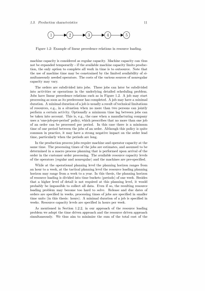
1 2 3 4 5
Figure 1.2: Example of linear precedence relations in resource loading.
machine capacity is considered as regular capacity. Machine capacity can thusnot be expanded temporarily - if the available machine capacity limits produc-tion, the only option to complete all work in time is to outsource. Note thatthe use of machine time may be constrained by the limited availability of si-multaneously needed operators. The costs of the various sources of nonregularcapacity may vary.
The orders are subdivided into jobs. These jobs can later be subdividedinto activities or operations in the underlying detailed scheduling problem.Jobs have linear precedence relations such as in Figure 1.2. A job may startprocessing as soon as its predecessor has completed. A job may have a minimalduration. A minimal duration of a job is usually a result of technical limitationsof resources, e.g., in a situation when no more than two persons can jointlyperform a certain activity. Optionally a minimum time lag between jobs canbe taken into account. This is, e.g., the case when a manufacturing companyuses a ‘one-job-per-period’ policy, which prescribes that no more than one jobof an order can be processed per period. In this case there is a minimumtime of one period between the jobs of an order. Although this policy is quitecommon in practice, it may have a strong negative impact on the order leadtime, particularly when the periods are long.
In the production process jobs require machine and operator capacity at thesame time. The processing times of the jobs are estimates, and assumed to bedetermined in a macro process planning that is performed upon arrival of theorder in the customer order processing. The available resource capacity levelsof the operators (regular and nonregular) and the machines are pre-specified.
While at the operational planning level the planning horizon ranges froman hour to a week, at the tactical planning level the resource loading planninghorizon may range from a week to a year. In this thesis, the planning horizonof resource loading is divided into time buckets (periods) of one week. Besidesthat a higher level of detail is not required at this planning level, it wouldprobably be impossible to collect all data. Even if so, the resulting resourceloading problem may become too hard to solve. Release and due dates oforders are specified in weeks, processing times of jobs are specified in smallertime units (in this thesis: hours). A minimal duration of a job is specified inweeks. Resource capacity levels are specified in hours per week.
As mentioned in Section 1.2.2, in our approach of the resource loadingproblem we adopt the time driven approach and the resource driven approachsimultaneously. We thus aim to minimize the sum of the total cost of the
12 Chapter 1. Introduction
1
2
3
4
5 6
7
8
9 10
Figure 1.3: Example of generalized precedence relations in RCCP.
use of nonregular capacity and the total cost incurred by tardiness of jobs.The tardiness of a job is defined as the lateness of the job (i.e., the differencebetween its completion time and its due date, measured in weeks), if it fails tomeet its due date, or zero otherwise. The job due date is an internal due date,i.e., it can be calculated from the order due date and the total minimal durationof the successors of the job. Job due dates may also be imposed externally, e.g.,to meet certain deadlines on components or parts of an order.
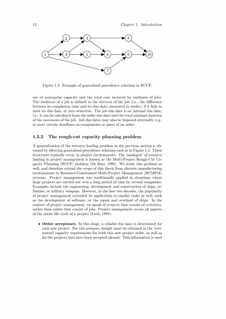
1.3.2 The rough-cut capacity planning problem
A generalization of the resource loading problem in the previous section is ob-tained by allowing generalized precedence relations such as in Figure 1.3. Thesestructures typically occur in project environments. The ‘analogon’ of resourceloading in project management is known as the Multi-Project Rough-Cut Ca-pacity Planning (RCCP) problem (De Boer, 1998). We study this problem aswell, and therefore extend the scope of this thesis from discrete manufacturingenvironments to Resource-Constrained Multi-Project Management (RCMPM)systems. Project management was traditionally applied in situations wherelarge projects are carried out over a long period of time by several companies.Examples include the engineering, development and construction of ships, re-fineries, or military weapons. However, in the last two decades, the popularityof project management extended its application to smaller tasks as well, suchas the development of software, or the repair and overhaul of ships. In thecontext of project management, we speak of projects that consist of activities,rather than orders that consist of jobs. Project management covers all aspectsof the entire life cycle of a project (Lock, 1988):
• Order acceptance. In this stage, a reliable due date is determined foreach new project. For this purpose, insight must be obtained in the (esti-mated) capacity requirements for both this new project order, as well asfor the projects that have been accepted already. This information is used

1.3. Production characteristics 13
as an input to make a rough-cut capacity plan. The rough-cut capacityplan estimates costs, and yields insight with respect to the expected duedates. It must be used to settle a contract with the customer, that isexecutable for the company.
• Engineering and process planning. In this stage, engineering activi-ties provide more detailed input for the material and resource schedulingof the next stage.
• Material and resource scheduling. The objective in this stage is touse scheduling to allocate material and activities to resources, and todetermine start and completion times of activities, in such a way thatdue dates are met as much as possible.
• Project execution. In this stage, the activities are performed. Re-scheduling is needed whenever major disruptions occur.
• Evaluation and service. In this stage, the customer and the organiza-tion evaluate the progress and the end result, to come closer towards thecustomer needs, and to improve the entire process in the future.
We address the rough-cut capacity planning (RCCP) problem in the orderacceptance stage of a project life cycle. In order to position RCCP as a mecha-nism of planning in project management, we use the framework for hierarchicalplanning for (semi)project-driven organizations (see Figure 1.4) as proposed byDe Boer (1998). Hierarchical production planning models are usually proposedto break down planning into manageable parts. At each level, the boundariesof the planning problem in the subsequent level are set. Ideally, multiple levelsare managed simultaneously, using information as it becomes available in thecourse of time. However, this means that uncertainty in information will bemore important as more decisions are taken over a longer period of time. Pos-sibly due to this complexity, project planning theory hardly concentrates onproblems at multiple levels. In the hierarchical planning framework in Figure1.4, vertically we observe the same distinction between strategic, tactical, andoperational planning activities as in the positioning framework in Figure 1.1.Again, at the highest planning level, the company’s global resource capacitylevels are determined. Strategic decisions are made with regard to machinecapacity, staffing levels, and other critical resources, using the company’s long-term strategy and strategic analyses like market research reports as the inputof the planning. The planning horizon usually varies from one to several years,and the review interval depends on the dynamics of the company’s environment.
At the RCCP level, decisions are made concerning regular and nonregularcapacity usage levels, such as overtime work and outsourcing. Also, due datesand other project milestones are determined. Just as resource loading is atool in order acceptance, the RCCP is used as a tool in the bidding and orderacceptance phase of new projects, to:

14 Chapter 1. Introduction
Strategic resourceplanning
Rough-cut capacityplanning
Detailed scheduling
Resource-constrainedproject scheduling
Strategic
Tactical
Tactical/operational
Operational
Rough-cutprocess planning
Engineering &process planning
Figure 1.4: Hierarchical planning framework (De Boer, 1998).
• determine the capacity utilization of new and accepted orders,
• perform a due date analysis on new or accepted orders, and/or to quoterealistic due dates,
• minimize the usage of nonregular capacity.
In order to support these analyses, just like in resource loading we distin-guish two problems in RCCP: resource driven and time driven RCCP. As inresource loading, with resource driven RCCP, all (non-)regular resource ca-pacity levels are fixed, and we try to minimize the maximum lateness of theprojects, preferably using regular capacity. The resource driven RCCP is ap-plicable in the situation where a customer requests a due date quotation fora project, while the company wants/has to fulfill strict resource constraints.With time driven RCCP, deadlines are specified for each activity in a project,while the company is flexible in the resource utilization, in that it may usenonregular capacity in order to meet the deadlines. In this case, the companywants to meet all deadlines, in such a way, that the usage of nonregular capacityis minimized. The input for the RCCP is generated by performing a rough-cutprocess planning. Based on customer demands, the rough-cut process planningbreaks up a project into a network (with generalized precedence constraints) ofwork packages (such as in Figure 1.3), with estimates on the resource utilization(number of work hours) and minimal durations. Minimal duration constraintsare a result of technical limitations of resources, e.g., in a situation when nomore than two people can be deployed for a certain activity. Depending on the

1.4. Example 15
project duration, the RCCP should cover a time horizon of half a year or more.
RCCP determines the detailed resource availability profiles for the nextplanning level, the resource-constrained project scheduling. Work packages arebroken into smaller activities, with given duration and resource rates, and morecomplex precedence relations. The planning horizon varies from several weeksto several months, depending on the project duration. Resource-constrainedproject scheduling determines when activities are performed, and it uses de-tailed scheduling to determine which operators or machines of a resource groupare assigned to each activity. The planning horizon of detailed planning mayvary from one week to several weeks, and is updated frequently, when distur-bances occur in the resource-constrained project scheduling plan, or on theshop floor.
From the literature we observe that, just as in the case of discrete man-ufacturing, the focus has been put primarily on a more detailed level, suchas the resource-constrained project scheduling problem RCPSP (e.g., Kolisch,1995). These techniques work fine at the operational level, but are not suitablefor the tactical planning level, for two reasons. First, the RCPSP is inflexiblewith respect to resource capacity levels, which is desirable at the tactical level.The second reason is that the information that is required to perform resource-constrained project scheduling is not available at the stage of tactical planning.Detailed engineering has not been performed yet at the stage of RCCP, so, e.g.,the exact number of required resources and the precedence relations are notknown in detail at this stage. Recently, some heuristics have been proposedfor RCCP (De Boer and Schutten, 1999; Gademann and Schutten, 2001). Inthis thesis we consider exact and heuristic methods to solve time driven andresource driven RCCP problems.
1.4 Example
Consider a furniture manufacturer, that produces large quantities of furnitureto order. The company has a product portfolio with numerous standard prod-ucts that can be assembled to order, but it is also capable of designing andsubsequently producing products to order.
The sales department of the company negotiates with the customers (e.g.,furniture shops and wholesalers) the prices and due dates of the products thatare to be ordered. Using up-to-date information and communication systems,the sales department is able to quote tight but realistic customer due datesbased upon the latest production information. If a customer order is (partly)non-standard, a macro process planning is performed to determine the produc-tion activities and the way they are performed. Each product is then processedin one or more production departments, in which the following production ac-tivities are performed:

16 Chapter 1. Introduction
• sawmilling (to prepare the lumber for assembly),
• assembly,
• cleaning (to sand and clean products),
• painting,
• decoration (e.g., to decorate products with glass, metal or soft furnish-ings),
• quality control.
The production planner breaks down the customer order into jobs, onefor each production activity. He then determines for all jobs in which weeka department should process a job. The head of the production departmentis responsible for subsequently scheduling the jobs over the resources in hisdepartment within the week. The processing of a job usually requires onlya fraction of the weekly capacity of the concerned production department.However, since more workload may be present in the department in the sameweek, the production planner gives the head of the production department oneweek to complete production of all assigned jobs. Consequently, at most onejob of the same order may be assigned to any particular week. The plannercalculates the lead time of a customer order by counting the number of jobs(in weeks), and he dispatches the customer order for production accordingly,to meet the negotiated customer due date.
After determining the order start times, the production planner performsa capacity check for each production department, to determine if there is suf-ficient weekly operator and machine capacity to execute his plan. Since themachines in a department are usually continuously available, the capacity ofthe department is mostly limited by operator capacity. The capacity check isdone by simply comparing for each week the capacity of the department withthe sum of the processing times of the assigned jobs (both are measured inhours).
We illustrate the planning approach of the planner with some example data.Consider the situation described in Table 1.1, where 7 customer orders are tobe dispatched for production. We have indicated the production activitiessawmilling, assembly, cleaning, painting, decorating, and quality control bytheir first letter, i.e., S, A, C, P , D and Q. The production planner calculatesthe order start times from the customer due date and the number of jobs ofthat order. The resulting start times are displayed in Table 1.2. As mentionedbefore, after determining the order start times, the production planner per-forms a capacity check for each production department, to determine if thereis sufficient weekly operator and machine capacity to execute his plan. InFigures 1.5 and 1.6 we see the capacity check for the decoration department(D) and the quality control department (Q) respectively. The bars in the fig-

1.4. Example 17
0
5
10
15
20
25
30
35
0 1 2 3 4 5 6 7 8 9
order1
order2
order3
order4
order5
order6
order7
hour
s
weeks
1
24
5
67
Figure 1.5: Loading of department D by production planner.
0
2
4
6
8
10
12
14
16
18
20
0 1 2 3 4 5 6 7 8 9
order1
order2
order3
order4
order5
order6
order7
hour
s
weeks
3
1
24
5
67
Figure 1.6: Loading of department Q by production planner.

18 Chapter 1. Introduction
customer job (processing time in hours) due dateorder 1 2 3 4 5 6 (week)1 S (37) A (19) C (14) D (32) Q (5) 72 S (18) A (12) C (15) P (10) D (14) Q (10) 83 S (20) A (21) C (17) Q (8) 54 A (10) C (25) D (16) Q (7) 55 S (16) A (33) C (14) P (16) D (15) Q (10) 96 S (36) A (16) C (20) P (15) D (15) Q (9) 97 S (15) A (10) C (15) P (15) D (20) Q (10) 6
Table 1.1: Example customer order data.
customer number due start timeorder of jobs date (week)1 5 7 32 6 8 33 4 5 24 4 5 25 6 9 46 6 9 47 6 6 1
Table 1.2: Customer order start times found by production planner.
ure represent jobs of customer orders assigned to certain weeks, and the boldline represents the available regular capacity of the department (in hours perweek). By letting operators work in overtime, the department can temporarilyincrease the available capacity. The dotted line above the bold line representsthe total available capacity of the department, i.e., the regular capacity plusthe nonregular capacity. Observe that in this example, the available capacityin the first few weeks is lower than in the other weeks. This typically occurs inpractice when capacity is reserved for (scheduled) orders that are already onthe shop floor, and that may not be shifted in time. In department Q we seethat capacity is insufficient in weeks 5, 8 and 9, and in department D in weeks6 and 8. This plan is thus infeasible. In general, if the production plannerestablishes that available capacity is insufficient, he has four options to cometo a feasible plan:
1. to shift jobs in time, or to split jobs over two or more weeks;
2. to increase the lead time of some customer orders (by decreasing theirstart time, or by increasing their due date), and then to reschedule;
3. to expand operator capacity in some weeks by hiring staff;
4. to subcontract jobs or entire orders.

1.4. Example 19
Although there may be excess capacity in other weeks, shifting or splittingjobs may have a negative effect on other departments. Consider for exampleweek 9 in department Q, where capacity is insufficient to complete the jobsof orders 5 and 6. Shifting the job of order 5 to week 7 (in which there issufficient capacity) implies that the preceding job of order 5 in department Dmust shift to week 6, where capacity is already insufficient. Moreover, the otherpreceding jobs of order 5 must shift to week 5 and before, which may result inmore capacity problems in other departments. Splitting the job of order 2 indepartment Q over week 7 and 8, implies that the preceding job of order 2 indepartment D must shift to week 6, where, as mentioned before, capacity isalready insufficient.
The option to increase customer order lead times is not desirable, sincethis may lead to late deliveries, which may result in penalties, imposed by thecustomers involved. Moreover, this does not guarantee that no overtime workor subcontracting is required to complete all orders in time. Since increasingthe lead times often does not lead to feasible plans, this option tends to increaseorder lead times more and more, which has several undesirable side effects, suchas an increasing amount of work-in-process.
The remaining options to make a feasible plan involve using nonregularoperator or machine capacity. Assigning nonregular operator capacity enablesthe use of machines in nonregular operator time. However, hired staff is oftennot readily available. Moreover, some work can not be subcontracted, andsubcontracting a job tends to increase the order lead time.
The example shows that even a small loading problem may be very hard tosolve. The approach of the planner is commonly used in practice. It appearsto be a reasonable approach, since it accounts for important aspects such as:
• the precedence relations between the jobs,
• meeting customer due dates,
• (regular and nonregular) operator and machine capacity availability.
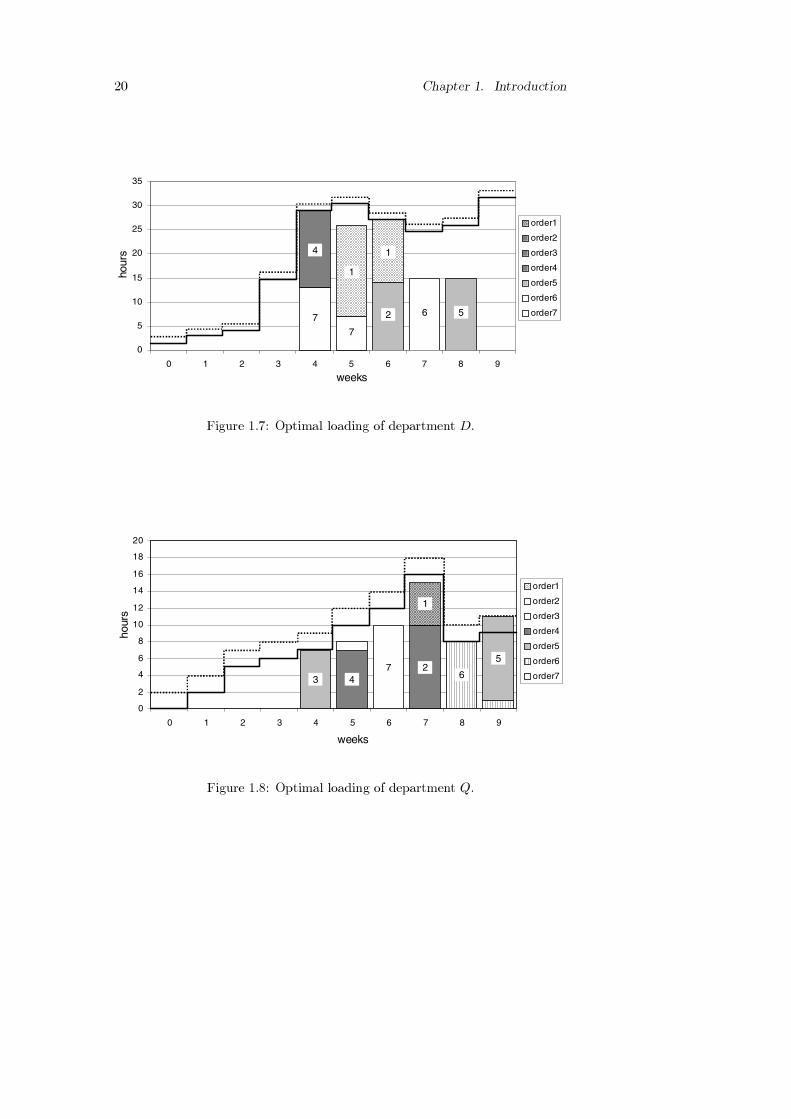
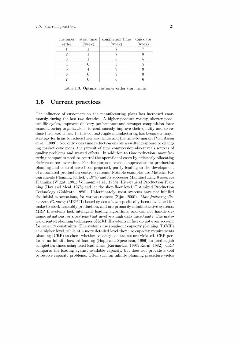
In this thesis we provide tools for solving similar loading problems, andloading problems that are much larger (with respect to the number of ordersand jobs) and more complex due to additional restrictions on jobs and orders.We have used one of our methods, which uses all four of the aforementionedoptions to come to a feasible plan, to optimally solve the loading problem inthis example. Figures 1.7 and 1.8 display a part of the solution, i.e., the opti-mal loading for the decoration department and the quality control departmentrespectively. Observe that in the optimal plan little overtime work is required inthe quality control department to produce all orders in time. Table 1.3 displaysthe optimal start times of the customer orders, as well as the completion timesin the optimal plan, in comparison with the (external) order due dates.
20 Chapter 1. Introduction
0
5
10
15
20
25
30
35
0 1 2 3 4 5 6 7 8 9
order1
order2
order3
order4
order5
order6
order7
hour
s
weeks
1
67
7
5
1
2
4
Figure 1.7: Optimal loading of department D.
0
2
4
6
8
10
12
14
16
18
20
0 1 2 3 4 5 6 7 8 9
order1
order2
order3
order4
order5
order6
order7
weeks
hour
s
3
1
24
5
67
Figure 1.8: Optimal loading of department Q.
1.5. Current practices 21
customer start time completion time due dateorder (week) (week) (week)1 1 7 72 1 7 83 1 5 54 0 5 55 4 9 96 0 9 97 0 6 6
Table 1.3: Optimal customer order start times
1.5 Current practices
The influence of customers on the manufacturing plans has increased enor-mously during the last two decades. A higher product variety, shorter prod-uct life cycles, improved delivery performance and stronger competition forcemanufacturing organizations to continuously improve their quality and to re-duce their lead times. In this context, agile manufacturing has become a majorstrategy for firms to reduce their lead times and the time-to-market (Van Assenet al., 1999). Not only does time reduction enable a swifter response to chang-ing market conditions, the pursuit of time compression also reveals sources ofquality problems and wasted efforts. In addition to time reduction, manufac-turing companies need to control the operational costs by efficiently allocatingtheir resources over time. For this purpose, various approaches for productionplanning and control have been proposed, partly leading to the developmentof automated production control systems. Notable examples are Material Re-quirements Planning (Orlicky, 1975) and its successor Manufacturing ResourcesPlanning (Wight, 1981; Vollmann et al., 1988), Hierarchical Production Plan-ning (Hax and Meal, 1975) and, at the shop floor level, Optimized ProductionTechnology (Goldratt, 1988). Unfortunately, most systems have not fulfilledthe initial expectations, for various reasons (Zijm, 2000). Manufacturing Re-sources Planning (MRP II) based systems have specifically been developed formake-to-stock assembly production, and are primarily administrative systems.MRP II systems lack intelligent loading algorithms, and can not handle dy-namic situations, or situations that involve a high data uncertainty. The mate-rial oriented planning techniques of MRP II systems in fact do not even accountfor capacity constraints. The systems use rough-cut capacity planning (RCCP)at a higher level, while at a more detailed level they use capacity requirementsplanning (CRP) to check whether capacity constraints are violated. CRP per-forms an infinite forward loading (Hopp and Spearman, 1996) to predict jobcompletion times using fixed lead times (Karmarkar, 1993; Karni, 1982). CRPcompares the loading against available capacity, but does not provide a toolto resolve capacity problems. Often such an infinite planning procedure yields

22 Chapter 1. Introduction
infeasible plans (Negenman, 2000). Moreover, the feasibility of the plans onthe lower planning levels can not be guaranteed satisfactorily, due to specificjob shop constraints like complex precedence relations that are not consideredon the aggregate planning level. As a result, the fixed lead times in infiniteplanning tend to inflate (the so-called ‘planning loop’, see, e.g., Zäpfel andMissbauer, 1993; Suri, 1994). While MRP II is primarily material oriented,ideally, the material in the production process and the use of resources areconsidered simultaneously in the planning process. To be able to solve themodels satisfactorily, the existing methods for this purpose either have a highlevel of aggregation, or are based on repairing a plan that is infeasible withrespect to capacity or precedence constraints (Baker, 1993; Negenman, 2000).A more detailed description of the major drawbacks of MRP II has been givenby Darlington and Moar (1996).
Hierarchical Production Planning (HPP) on the other hand, is strongly ca-pacity oriented. In HPP, problems are decomposed by first roughly planningcomplete product families and then scheduling individual items. Comparedto a monolithic system, this not only reduces the computational complexityof the mathematical models, it also reduces the need of detailed data (Bitranand Tirupati, 1993). As recognized by Schneeweiss (1995), high-level decisionsneed to anticipate the effect on future low-level problems. However, since HPPcan not handle complex product structures and product routings, this is hardlypossible. Finally, Optimized Production Technology (OPT) does consider rout-ing constraints but is primarily shop floor oriented, i.e., it assumes a mediumterm loading as given.
Workload control concepts buffer a shop floor against external dynamics(such as rush orders) by creating a pool of unreleased jobs (Bertrand andWortmann, 1981; Wiendahl, 1995). The use of workload norms should turnthe queueing of orders on the shop floor into a stationary process that is char-acterized by an equilibrium distribution. The development of workload controlsystems shows that adequate finite resource loading tools are needed to controlthe aforementioned dynamic production situations. However, although work-load control does yield more reliable internal lead times by not allowing work tobe loaded in the job shop in case of a high load already present, the problem isshifted to the buffers before the job shops, hence due dates still tend to increase(Hendry et al., 1998).
The models in the literature as well as the techniques used in the aforemen-tioned production planning and control systems that explicitly address loadingproblems are inadequate in situations that require more flexibility due to un-certainty in data. Linear programming (LP) is an accepted method in, e.g.,aggregate planning and workforce planning to decide upon capacity levels (oncea global long-term plan is determined), by considering overwork, hiring and fir-ing, and outsourcing options (see, e.g., Shapiro, 1993; Hopp and Spearman,1996). However, modeling complex precedence relations in LP models requires

1.6. Outline of the thesis 23
the introduction of many integer variables, which increases the size of the mod-els enormously, and makes them computationally hard to solve (Shapiro, 1993).For this reason, precedence constraints are often omitted in linear programmingapproaches (see, e.g., Graves, 1982; Bahl and Zionts, 1987). Although, as ar-gued in Section 1.1, at the resource loading level product routings should notbe considered in the same level of detail as in shop floor scheduling, it is es-sential to account for major precedence relations, e.g., with respect to machinegroups, in order to define work packages at the loading level that can indeed behandled at the shop floor level. In other words: approaches that ignore thesemajor constraints to reduce complexity may lead to production plans that cannot be maintained at a more detailed level. This holds in particular whenmultiple resources (e.g., machines and operators) are needed to simultaneouslyprocess jobs. Dealing with multiple resources without considering job routingsoften leads to inconsistencies, when eventually these different resources are notavailable at the same time.
Although we use a deterministic approach in this thesis, it is likely that infuture research also stochastic techniques (Kall and Wallace, 1994; Infanger,1994; Buzacott and Shanthikumar, 1993) will be used for resource loading(see, e.g., Giebels, 2000). This may particularly be the case for engineer-to-order (ETO) manufacturing planning, where even more uncertainty in data isinvolved than in MTO manufacturing planning. While generally at the tac-tical planning level in MTO environments processing times are deterministic,and routings are known, in ETO environments the macro process planning isgenerally incomplete at the tactical planning stage. Hence processing times areuncertain, and even the required machines, tools and materials are uncertain.A promising approach that deals with such situations is the EtoPlan-concept,proposed by Giebels (2000).
We conclude this section with a note on the role of material coordinationin resource loading. Compared to assemble-to-order (ATO) environments, inMTO environments material coordination plays a less significant role. We willnot consider material related constraints. For advanced models for materialcoordination under capacity constraints in ATO environments we refer to Ne-genman (2000).
1.6 Outline of the thesis
The remainder of this thesis is organized as follows. In Chapter 2 we presentsome mathematical preliminaries for the analysis in the next chapters. Thediscussed techniques include column generation, branch-and-price, Lagrangianrelaxation and deterministic dynamic programming. Some example problemsin Chapter 2 are tailored to the problems in the remainder of this thesis. InChapter 3 we discuss the modeling issues of resource loading, and present aMixed Integer Linear Programming (MILP) formulation. We present column

24 Chapter 1. Introduction
generation based solution methods for the resource loading problem in Chapter4. In this chapter we also discuss heuristics that can be used ‘stand-alone’, oras an integrated part of the column generation based methods. We pose severalbranch-and-price techniques to find feasible solutions to the entire MILPmodel.In Chapter 5 we discuss the results of computational experiments with themethods proposed in Chapter 4.
In Chapter 6 we present a generalization of the MILP model of Chapter3, and use it to solve the RCCP problem. The solution method presented inthis chapter is also based on column generation, but we present a generalizedpricing algorithm, that is able to generate schedules for projects, that complywith the additional constraints of the RCCP problem. In Chapter 7 we discussthe experiments with, and computational results of the methods proposed inChapter 6.
Finally, in Chapter 8, we summarize our experiences with the methodologypresented in this thesis, discuss its strengths and its weaknesses, and proposetopics of further research.
25
Chapter 2
Preliminaries
Only two things are infinite,the universe and human stupidity
- and I’m not sure about the former.
- Albert Einstein (1879-1955)
2.1 Introduction to integer linear programming
In this thesis we use several combinatorial optimization techniques to solvethe resource loading problem. In this chapter we discuss these techniques,such as branch-and-bound, column generation, Lagrangian relaxation, and dy-namic programming. For a more comprehensive overview of combinatorial op-timization techniques, we refer to, e.g., Wolsey (1998); Johnson et al. (1998);Nemhauser and Wolsey (1988); Winston (1993).
During the last 50 years, linear programming (LP) has become a well-established tool for solving a wide range of optimization problems. This trendcontinues with the developments in modeling, algorithms, the growing com-putational power of personal computers, and the increasing performance ofcommercial linear programming solvers (Johnson et al., 1998). However, manypractical optimization problems require integer variables, which often makesthem not straightforward to formulate, and extremely hard to solve. This isalso the case for the resource loading problem. The resource loading problemis formulated in Chapter 3 as a mixed integer linear program (MILP). A MILPis a generalization of a linear program, i.e., it is a linear program of which some

26 Chapter 2. Preliminaries
of the variables are integer, e.g.:
MILP : min cTx
s.t.Ax ≥ bl ≤ x ≤ uxj integer (j = 1, . . . , p;p ≤ n) .
(2.1)
The input data for this MILP is formed by the n-vectors c, l, and u, by m×n-matrix A, and m-vector b. The decision vector x is an n-vector. When p = nthe MILP becomes a pure integer linear program (PILP). When the integervariables are restricted to values 0 or 1, the problem becomes a (mixed) binaryinteger linear program (MBILP or BILP). Each ILP can be expressed as aBILP by writing each integer variable value as a sum of powers of 2 (see, e.g.,Winston, 1993). A drawback of this method is that the number of variablesgreatly increases. For convenience, in the remainder of this chapter we discussinteger linear programs that are minimization problems with binary variables.
Formulating and solving ILPs is called integer linear programming . Integerlinear programming problems constitute a subclass of combinatorial optimiza-tion problems. There exist many combinatorial optimization algorithms forfinding feasible, or even optimal solutions of integer linear programming mod-els (see, e.g., Wolsey, 1998; Johnson et al., 1998). When optimizing complexproblems, there is always a trade-off between the computational effort (andhence running time) and the quality of the obtained solution. We may eithertry to solve the problem to optimality with an exact algorithm, or settle for anapproximation (or heuristic) algorithm, which uses less running time but doesnot guarantee optimality of the solution. In the literature numerous heuristicalgorithms can be found, such as local search techniques (e.g., tabu search,simulated annealing, see Aarts and Lenstra, 1997), and optimization-based al-gorithms (Johnson et al., 1998).
The running time of a combinatorial optimization algorithm is measured byan upper bound on the number of elementary arithmetic operations it needs forany valid input, expressed as a function of the input size. The input is the dataused to represent a problem instance. The input size is defined as the numberof symbols used to represent it. If the input size is measured by n, then therunning time of an algorithm is expressed as O (f (n)), if there are constants cand n0 such that the number of steps for any instance with n ≥ n0 is boundedfrom above by cf (n). We say that the running time of such an algorithm isof order f (n). An algorithm is said to be a polynomial time algorithm whenits running time is bounded by a polynomial function, f (n). An algorithm issaid to be an exponential time algorithm when its running time is not boundedby a polynomial function (e.g., O (2n) or O (n!)). A problem can be classifiedby its complexity (see Garey and Johnson, 1979). A particular class of ‘hard’problems is the class of so-called NP -hard problems. Once established thata problem is NP -hard, it is unlikely that it can be solved by a polynomialalgorithm.

2.1. Introduction to integer linear programming 27
Before considering what algorithm to use to solve an ILP problem, it is im-portant to first find a ‘good’ formulation of the problem. Sometimes a differentILP formulation of the same problem requires fewer integer variables and/orconstraints, which may reduce or even increase computation time for some algo-rithms. Optimization algorithms for NP -hard problems always resort to somekind of enumeration. The complexity of NP -hard problems is nicely illustratedby Nemhauser and Wolsey (1988), who show that a BILP (which is proven tobe NP -hard) can be solved by brute-force enumeration in O (2nnm) runningtime. For example, a BILP with n = 50 and m = 50 that is solved by completeenumeration on a computer that can perform 1 million operations per secondrequires nearly 90,000 years of computing time. For n = 60 and m = 50 this isnearly 110 million years.
A generic categorization for exact algorithms for ILP problems is given byZionts (1974). He distinguishes three generic optimization methods: construc-tive algorithms, implicit enumeration, and cutting plane methods.
Constructive algorithms construct an optimal solution by systematicallyadjusting integer variable values until a feasible integer solution is obtained.When such a solution is found, it is an optimal solution. The group theoreticalgorithm is an example of a constructive algorithm (Zionts, 1974).
Implicit enumeration methods enumerate solutions in a highly efficient man-ner. They generally eliminate subsets of solutions without explicitly enumer-ating them. In this thesis we use two implicit enumeration methods: dynamicprogramming and branch-and-bound. Dynamic programming is a decompo-sition technique that first decomposes the problem into a nested family ofsubproblems. The solution to the original problem is then found by recursivelysolving the (generally easier) subproblems. We discuss dynamic programmingin more detail in Section 2.5. Branch-and-bound is structured by an enumera-tion scheme that involves partitioning the solution space. In the scheme, eachpartition is further analyzed and partitioned until a (better) feasible solution isfound or it is determined that the partition does not contain a (better) solution.The enumeration scheme can nicely be displayed by a branching tree. The rootnode of the tree corresponds to the original problem, and has a solution spacethat holds all feasible solutions to this problem. As the algorithm progresses,the solution space is partitioned by adding constraints to the problem in theroot node, forming two or more new problems in the child nodes. This processof partitioning the solution space, which is called branching, is continued in thechild nodes, which become parent nodes to new child nodes in a subsequentpartitioning of the solution space. A typical example is a branching strategybased on choosing either a value 0 or 1 for a single binary variable (see, e.g.,Figure 2.1). Hence in each node the feasible set of solutions is decomposedinto smaller (disjoint) subsets. At each node lower and upper bounds can bedetermined on the objective value of that subset. Lower bounds can be ob-tained, e.g., by relaxations of the original integer linear program. A relaxation
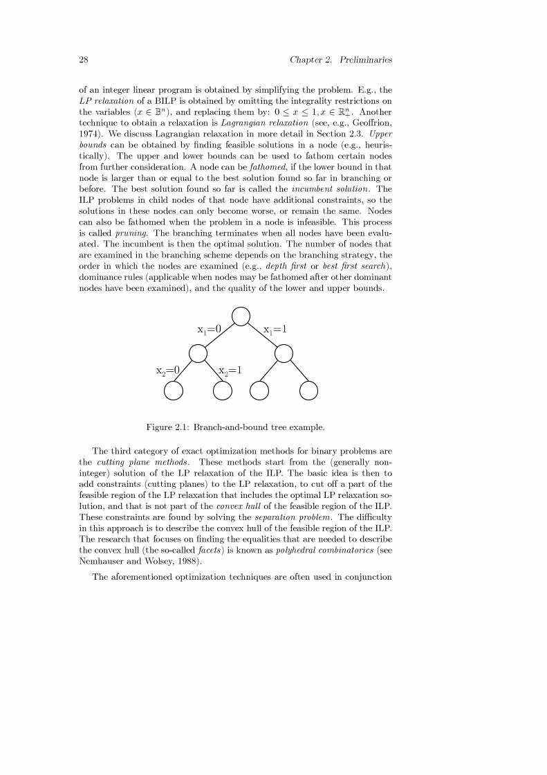
28 Chapter 2. Preliminaries
of an integer linear program is obtained by simplifying the problem. E.g., theLP relaxation of a BILP is obtained by omitting the integrality restrictions onthe variables (x ∈ B
n), and replacing them by: 0 ≤ x ≤ 1, x ∈ Rn+. Another
technique to obtain a relaxation is Lagrangian relaxation (see, e.g., Geoffrion,1974). We discuss Lagrangian relaxation in more detail in Section 2.3. Upperbounds can be obtained by finding feasible solutions in a node (e.g., heuris-tically). The upper and lower bounds can be used to fathom certain nodesfrom further consideration. A node can be fathomed, if the lower bound in thatnode is larger than or equal to the best solution found so far in branching orbefore. The best solution found so far is called the incumbent solution. TheILP problems in child nodes of that node have additional constraints, so thesolutions in these nodes can only become worse, or remain the same. Nodescan also be fathomed when the problem in a node is infeasible. This processis called pruning. The branching terminates when all nodes have been evalu-ated. The incumbent is then the optimal solution. The number of nodes thatare examined in the branching scheme depends on the branching strategy, theorder in which the nodes are examined (e.g., depth first or best first search),dominance rules (applicable when nodes may be fathomed after other dominantnodes have been examined), and the quality of the lower and upper bounds.
x1=0 x
1=1
x2=1x
2=0
Figure 2.1: Branch-and-bound tree example.
The third category of exact optimization methods for binary problems arethe cutting plane methods . These methods start from the (generally non-integer) solution of the LP relaxation of the ILP. The basic idea is then toadd constraints (cutting planes) to the LP relaxation, to cut off a part of thefeasible region of the LP relaxation that includes the optimal LP relaxation so-lution, and that is not part of the convex hull of the feasible region of the ILP.These constraints are found by solving the separation problem. The difficultyin this approach is to describe the convex hull of the feasible region of the ILP.The research that focuses on finding the equalities that are needed to describethe convex hull (the so-called facets) is known as polyhedral combinatorics (seeNemhauser and Wolsey, 1988).
The aforementioned optimization techniques are often used in conjunction

2.2. Branch-and-price for solving large ILP models 29
with each other. For example cutting plane methods are almost always usedin conjunction with branch-and-bound. In these so-called branch-and-cut al-gorithms, partial descriptions of the convex hull of feasible solutions of theILP are used to determine strong lower bounds in the branching scheme (see,e.g., Hoffman and Padberg, 1985). Branch-and-cut is the technique that mostcommercial ILP solvers use to solve (mixed) integer linear programs. In thisthesis we use the column generation method to solve the LP relaxation of theILP, a technique very similar to cutting plane methods. Whereas cutting planemethods add rows to the LP relaxation of the problem, column generationadds columns to a restricted version of the LP relaxation. The separationproblem in column generation is called the pricing problem. Column gener-ation can be interpreted as a cutting plane technique on the dual of the LPrelaxation of the ILP (see, e.g., Barnhart et al., 1998; Beasley, 1996; Bixbyet al., 1992). Dantzig and Wolfe (1960) proposed the column generation tech-nique as a scheme for solving large linear programming problems that have(exponentially) many variables. Since then it has been applied to a wide vari-ety of problems. The most well-known is the application to the cutting stockproblem (Gilmore and Gomory, 1963). In more recent research, column gen-eration has been applied to, e.g., vehicle routing problems with time windows(Desrosiers et al., 1984; Desrochers et al., 1992) and crew scheduling (Freling,1997; Desrochers and Soumis, 1989). When column generation is used in con-junction with branch-and-bound, it is referred to as branch-and-price (see, e.g.,Savelsbergh, 1997; Vance et al., 1994). In this thesis we use branch-and-pricemethods to determine a feasible solution to the ILP from the (fractional) LPrelaxation solution.
In the remainder of this chapter we elaborate on the techniques used in thisthesis. Since branch-and-price plays a central role in this thesis, we discuss thistechnique in more detail in Section 2.2. In the branching schemes used in thisthesis, we use Lagrangian relaxation to determine lower bounds. In Section2.3 we elaborate more on Lagrangian relaxation, and in Section 2.4 we discusshow to use Lagrangian relaxation in conjunction with column generation. Sincedynamic programming is used in this thesis for optimizing the pricing problemof the column generation algorithm we discuss this subject in Section 2.5.
2.2 Branch-and-price for solving large integer
linear programming models
2.2.1 Method outline
Successfully solving large integer linear programs often requires LP relaxationsthat give a good approximation of the convex hull of feasible solutions (Barn-hart et al., 1998). Approaches based on this idea that are often used to solve

30 Chapter 2. Preliminaries
large integer linear programs are the aforementioned branch-and-cut approach,and the branch-and-price approach. Typical ILP problems that are solved bybranch-and-cut have an LP relaxation with too many valid inequalities to han-dle efficiently. Since many of these valid inequalities are not binding in anoptimal solution anyway, the approach starts by finding a formulation of theLP relaxation where these valid inequalities are left out. This formulation is theso-called restricted LP relaxation (RLP). This RLP is then solved to optimality.A subproblem (the separation problem) is solved to determine if the resultingoptimal solution is feasible to the LP relaxation by identifying violated validinequalities. If the solution is not feasible to the LP relaxation, at least oneviolated inequality is identified and added to the RLP. This procedure contin-ues until no more violated inequalities exist. In that case, the optimal solutionto the RLP is also optimal to the LP relaxation. Generally this solution isfractional, and hence not feasible for the ILP. Branching can be performed inorder to find a feasible solution to the ILP.
The basic idea of branch-and-price is very similar to that of branch-and-cut,except that it involves column generation, instead of row generation. TypicalILP problems that are solved by branch-and-price have too many columnsto handle efficiently, and since the basis has a limited dimension, many ofthese columns do not play a role in an optimal solution anyway. Analogous tobranch-and-cut, the LP relaxation is solved to optimality by first considering arestricted LP relaxation (RLP), where many columns are left out. The RLP isalso called the restricted master problem. The solution of the RLP is optimalfor the LP relaxation if all variables of the LP relaxation have non-negativereduced cost . Since only a subset of the columns of the LP relaxation is explic-itly available, this can not be checked explicitly. A so-called pricing algorithmis used to verify optimality. If the solution is not optimal, the pricing algo-rithm identifies at least one column with negative reduced cost. This columnis added to the RLP, and the procedure continues. The column generationscheme terminates when no columns with negative reduced cost exist anymore.The optimal solution to the RLP is then also optimal to the LP relaxation.This process of adding columns to the RLP when they are needed is calledimplicit column generation. In explicit column generation, all columns are gen-erated in advance and kept in computer memory. Subsets of columns are thenpassed to the RLP until a subset is found that contains the optimal solution.
Analogous to branch-and-cut, the optimal solution to the LP relaxation isgenerally fractional (i.e., non-integer), and hence not feasible to the ILP, sobranching needs to be performed in order to find a feasible solution to the ILP.The column pool is partitioned by adding constraints. The type of constraintsthat work best for a problem is usually determined by performing experiments.Usually constraints are used that cut off the fractional (optimal) LP relaxationsolution, or that fix variables. By partitioning the column pool in the parentnode, each child node corresponds to a new LP relaxation. The column poolmust be updated accordingly, and the new LP relaxation is also solved by

2.2. Branch-and-price for solving large ILP models 31
column generation. When the optimal solution to the new LP relaxation isagain fractional, branching continues. A node is explored no further when inthat node a feasible ILP solution is found, or when the LP relaxation in the nodeis infeasible, or when the node can be fathomed. A node is fathomed when alower bound to the feasible ILP solution in that node has been determined thatexceeds the best ILP solution found this far. Lower bounds can be determinedin each node, e.g., by Lagrangian relaxation (we discuss the application ofLagrangian relaxation in Section 2.3).
In Figure 2.2 we illustrate the column generation procedure that is per-formed in each node. The entire branch-and-price procedure is illustrated inFigure 2.3. In the next section we will elaborate on possible branching strate-gies and speed ups of branch-and-price algorithms.
Add columns
to RLP
Solve RLP
Solve pricing algorithm
Columns exist with
negative reduced costs?
LP relaxation solved
yes
no
Figure 2.2: Column generation scheme in a node.
2.2.2 Column generation strategies
There are many ways to speed up a branch-and-price algorithm. Most ap-proaches try to reduce the number of nodes that must be examined to proveoptimality of an integer solution. There is a trade-off between finding a strongformulation on one hand, by trying to make the difference in the solutions to theLP relaxation and the integer linear program (the integrality gap) as small aspossible, and the number of nodes to explore in the branch-and-bound tree onthe other hand. The latter aspect is usually done by reformulation. Well-knownreformulation techniques are the preprocessing and probing techniques that fo-cus on identifying infeasibility and redundancy, improving variable bounds andcoefficients, and fixing variables (Savelsbergh, 1994; Nemhauser et al., 1994;Wolsey, 1998). These techniques, as well as other reformulation techniquessuch as constraint generation, have proven to be very effective in reducing boththe integrality gap, and the size of the branch-and-bound tree (Savelsbergh,

32 Chapter 2. Preliminaries
Generate new nodes
Go to next unexplored
node according to
branching strategy
All nodes
explored?
Apply column generation
on RLP to optimize LP
LP solution better
than incumbent solution?
ILP solution
found
Fathom node
Incumbent solution
is optimal for ILP
yes
Solution fractional?no
yes
no
yes
no
Formulate a feasible RLP
Feasible RLP exists?
yes
no
Go to root node
Figure 2.3: Branch-and-price scheme.

2.2. Branch-and-price for solving large ILP models 33
1994). Another technique that is used in advance of the branching processto speed up the algorithm is column management . By generating and stor-ing many columns in advance without adding them to the RLP, fewer pricingproblems have to be solved. In column management, a pricing strategy pre-scribes when columns must be added to the pool, and how many. There is notone ‘best’ pricing strategy for each problem, and hence computational exper-iments must be performed to provide insight. In the pricing strategy there isalso a trade-off between the number of columns to add in each iteration (hencethe computation time of the pricing algorithm) on one hand and the size ofthe column pool (hence the computation time of the RLP) on the other hand.Moreover, column management may prescribe to delete columns from the pool,e.g., when columns are redundant in the RLP (i.e., when columns are no longerin the basic RLP solution).
Another way to improve the speed of the branch-and-price algorithm is tofocus on both improving the lower bound in a node, and on finding good feasi-ble ILP solutions to the original problem as early as possible in the branchingprocess. Recall that a node is fathomed if a lower bound to the LP relaxationin that node exceeds the incumbent. Lower bounds thus apply to a node, andincumbent solutions apply to the entire branching tree. The stronger the lowerbounds, the fewer nodes have to be examined, in particular when a good feasibleincumbent solution has been found already. However, determining strong lowerbounds may be computationally intensive. In Section 2.3 we discuss Lagrangianrelaxation for determining a lower bound in a node with little additional com-putational effort every time the RLP is solved in the column generation scheme.Feasible ILP solutions can be found by solving primal heuristics, or by choos-ing a branch selection strategy that yields feasible ILP solutions fast (see, e.g.,Vanderbeck, 2000). Since such feasible solutions are more likely to be founddeep in the tree, a typical selection strategy to find feasible solutions fast is thedepth first strategy. Moreover, depth first requires relatively little computermemory. Once an incumbent solution is found, the branch selection strategymay be changed to, e.g., best bound search. In best-bound search all unfath-omed nodes are examined, and the node that has the smallest lower bound isselected as the branch node, since it most likely contains a solution that im-proves the incumbent. Primal heuristics are usually used to find an incumbentsolution in the root of the branching tree. When the heuristic does not requiretoo much computation time, it can also be used to improve the incumbentsolution in other nodes of the tree. Hence, as to how often a heuristic is usedin the branching scheme, there is always a trade-off between the computationtime of the heuristic and the resulting speed up of the branching algorithm.
One side effect of column generation that affects the speed of the branch-and-price algorithm is the so-called tailing-off effect, which is due to degener-acy . What occurs in such an event is that in each column generation iterationat least one column is found with negative reduced costs, which, after beingadded to the RLP, enters the basis with a value zero. As a result, it takes

34 Chapter 2. Preliminaries
many iterations before optimality can be proven, i.e., before column generationconverges. A performance gain can be achieved by detecting tailing-off, suchas for example in an approximation method that terminates column generationwhen the difference between the RLP solution (which is an upper bound onthe LP relaxation solution) and a lower bound to the LP relaxation solution issufficiently small.
2.2.3 Implicit column generation
Consider the following general integer minimization problem (ILP ):
ILP : min zILP = cTx
s.t.A1x ≥ b1A2x = b2
xj ∈ Z+ (j ∈ J ) ,
(2.2)
where the input data is formed by m1-vector b1, m2-vector b2, n-vector c,m1×n coefficient matrix A1 and m2 ×n coefficient matrix A2. J is an n-set ofvariable indices. We obtain its LP relaxation (LP ) by omitting the integralityconstraints xj ∈ Z+ (j ∈ J), and replacing them by xj ≥ 0 (j ∈ J). Hence wehave:
LP : min zLP = cTx
s.t.A1x ≥ b1A2x = b2
xj ≥ 0 (j ∈ J)
(2.3)
We show how to use (implicit) column generation to solve LP in a case wherethe set of columns in the coefficient matrix is large. More specifically, supposethe number of columns in ILP is too large to handle efficiently, and hence itsLP relaxation (LP ) can not be formulated and solved explicitly. To start thecolumn generation scheme, we formulate a restricted LP relaxation (RLP ) thatcontains a subset of the columns in coefficient matrices A1 and A2. For thispurpose, a set of columns is required that forms a feasible basis for LP . For themoment we assume that such a set of columns is available. These determinethe initial RLP , which can be formulated as follows:
RLP : min zRLP = cT x
s.t.A1x ≥ b1A2x = b2
xj ≥ 0(j ∈ J ⊆ J
).
(2.4)
The restricted LP model (RLP ) has the same form as LP , but has a subset J
of the variables, with corresponding submatrices A1 and A2, and cost vector c.

2.2. Branch-and-price for solving large ILP models 35
The corresponding dual problem (DRLP ) is given by:
DRLP : max zDRLP = bT1 u+ bT2 v
s.t. AT1 u+ AT
2 v ≤ cu ∈ R
m1
+ , v ∈ Rm2
where u is an m1-vector of dual variables, and v is an m2-vector of dual vari-ables. Observe that this problem can also be written in a compact form withan m-vector w of dual variables, where m = m1 +m2, and w = (u, v).
We start the column generation scheme by solving RLP to optimality. Notethat, since RLP has the same constraints as LP , any basic feasible solution(x∗) to RLP forms a basic feasible solution (x∗) to LP , by letting x∗
j = 0
(∀j ∈ J\J). However, an optimal solution to RLP is not necessarily optimalto LP . To determine if an optimal solution to RLP is also optimal to LP , weuse the following result (see, e.g., Wolsey, 1998) from duality theory:
Theorem 2.1 Let x∗ = (x∗1, x∗2, . . . , x
∗n) be a primal n-vector, and w∗ = (w∗
1 ,w∗2 , . . . , w
∗m) a dual m-vector. Then x∗ is an optimal primal solution and w∗ is
an optimal dual solution if and only if x∗ is primal feasible, w∗ is dual feasibleand cTx∗ = w∗T b.
Since any feasible solution to RLP is also feasible to LP , we have the primalfeasibility condition. Moreover, with x∗ optimal to RLP and the correspondingu∗ and v∗ optimal to DRLP , we also have that cT x∗ = u∗T b1+v∗T b2 and thusthat cTx∗ = u∗T b1 + v∗T b2. Hence, to determine if an optimal solution x∗
to RLP is also optimal to LP , it remains to verify that the corresponding(optimal) dual solution u∗ and v∗ to DRLP is feasible to the dual of LP(DLP ). The dual solution vectors (u∗, v∗) are feasible to DLP when:
AT1ju
∗ +AT2jv
∗ ≤ cj (∀j ∈ J),
or:cj −AT
1ju∗ −AT
2jv∗ ≥ 0 (∀j ∈ J). (2.5)
The term cj −AT1ju
∗ −AT2jv
∗ in (2.5) is in fact the reduced cost cj of variablexj. The reduced cost value cj of a variable xj, indicates the change ∆z in theobjective value z, resulting from a change ∆xj in non-basic variable xj:
∆z = cj∆xj
Clearly, cj ≥ 0 for all j ∈ J . Therefore, determining if an optimal solution toRLP is also optimal to LP boils down to determining if the reduced cost cj ofall variables xj in LP that are not included in RLP , is non-negative. Hencewe can formulate the optimality condition for column generation as follows(Gilmore and Gomory, 1961):
36 Chapter 2. Preliminaries
Theorem 2.2 Consider an LP model of a minimization problem with columnset J , denoted by LP (J). Let w∗ be an optimal dual solution of problem LP (J)
for J ⊂ J , and c∗ the corresponding reduced cost vector. The solution of LP (J)
is optimal for problem LP (J) if c∗j ≥ 0 (∀j ∈ J\J).
When columns have non-negative reduced costs, we say the columns priceout. The problem of identifying columns with negative reduced costs is calledthe pricing problem. A pricing algorithm either determines that all c∗j ≥ 0,or it provides at least one column with associated c∗j < 0. Such columns canbe added to RLP . Although more than one such column may exist, it is notnecessary to generate all columns with negative reduced costs. However, addingmore than one negative reduced cost column (called multiple pricing) reducesthe chance of cycling.
The column generation scheme thus solves the RLP and the pricing algo-rithm successively in each iteration, and terminates when no negative reducedcost columns can be found in the pricing algorithm. However, since the optimalsolution to LP is usually not integral, and thus not feasible to ILP , we needto perform branching or to use heuristics in order to find a feasible solution toILP .
2.3 Lagrangian relaxation
The basic idea of Lagrangian relaxation is to dualize (i.e., relax) those con-straints that make a problem hard to solve, in such a way, that good lowerbounds can be obtained for the original problem. The idea of dropping con-straints is brought about by introducing a Lagrangian multiplier/parameter foreach constraint that is dropped from the problem. These constraints are thenremoved from the problem, and put in the objective function, weighted by avector of Langrangian multipliers. Again, consider the (general) integer linearprogram ILP :
ILP : min zILP = cTxs.t. A1x ≥ b1 (duals u ∈ R
m1
+ )A2x = b2 (duals v ∈ R
m2
+ )x ∈ Z
n+
Suppose constraints A1x ≥ b1 are the constraints that make the problem hardto solve, and X =
{x|A2x = b2, x ∈ Z
n+
}has some computationally convenient
structure not shared by the entire problem. For the Lagrangian relaxationLILP (λ) of ILP , we dualize constraints A1x ≥ b1, and introduce a vector ofLagrangian multipliers λ ∈ R
m1
+ to form the following Lagrangian subproblem:
LILP (λ) : minx
zL,ILP (λ) = cTx+ λT (b1 −A1x)
s.t. x ∈ X.

2.3. Lagrangian relaxation 37
Let z∗L,ILP (λ) be the optimal objective function value of LILP (λ). Let x∗ denotethe optimal solution for ILP . Note that every x that is feasible for ILP is alsofeasible for LILP (λ). Therefore:
z∗L,ILP (λ) ≤ cTx∗ + λT (b1 −A1x∗) ≤ z∗ILP ,
and thus:
Theorem 2.3 z∗L,ILP (λ) is a lower bound on z∗ILP , the optimal solution toILP , for any λ ≥ 0, i.e., z∗L,ILP (λ) ≤ z∗ILP (∀λ ∈ R
m1
+ ).
The Langrangian multipliers λ∗ that provide the best lower bound are foundby solving the so-called Lagrangian dual problem:
z∗L,ILP (λ∗) = max
λ≥0
{z∗L,ILP (λ)
}.
In general, to find strong lower bounds to z∗ILP , it is required to have ap-propriate Lagrangian multipliers. Common (approximation) techniques forsolving the Lagrangian dual of an integer linear programming problem arethe subgradient method (Held and Karp, 1971) and the bundle method (see,e.g., Hiriart-Urruty and Lemarechal, 1993), that both involve iteratively up-dating the Lagrangian multipliers. In general it can not be guaranteed thatz∗L,ILP (λ
∗) = z∗ILP . The difference z∗ILP − z∗L,ILP (λ∗) is referred to as the La-
grangian duality gap. We refer to Geoffrion (1974) for a more comprehensivediscussion on Lagrangian relaxation techniques.
Another important relation in Lagrangian relaxation theory is that ofz∗L,ILP (λ
∗) with z∗LP , the optimal solution to the LP relaxation (LP ) of ILP(see, e.g., Geoffrion, 1974):
Theorem 2.4 If ILP is an integer linear programming problem, then z∗LP ≤z∗L,ILP (λ
∗).
Proof
z∗LP = minx
{cTx|A1x ≥ b1,A2x = b2, x ≥ 0
}= min
x
{cTx| −A1x ≤ −b1,−A2x = −b2, x ≥ 0
}= max
v,u
{−uT b1 − vT b2| − uTA1 − vTA2 ≤ cT , u ≥ 0
},
where u and v are decision variable vectors (of appropriate length) of the dualproblem of LP . Substituting for u the optimal dual solution vector (u∗) that

38 Chapter 2. Preliminaries
corresponds to constraints A1x ≥ b1 of LP , we have:
z∗LP = maxv
{−u∗T b1 − vT b2| − vTA2 ≤ cT + u∗TA1
}= min
x
{cTx+ u∗T (A1x− b1)|A2x = b2, x ≥ 0
}≤ min
x
{cTx+ u∗T (A1x− b1)|A2x = b2, x ∈ Z
n+
}= z∗L,ILP (u
∗)
≤ maxλ≥0
{z∗L,ILP (λ)
}= z∗L,ILP (λ
∗).
�
In particular, when the integrality constraints in LILP (λ) are redundant(we then say that the Lagrangian subproblem LILP (λ) possesses the integral-ity property), all ‘smaller than’-relations in the proof of Theorem 2.4 becomeequality-relations, since we have that:
z∗L,ILP (λ) = z∗L,LP (λ) ≤ z∗LP (∀λ), (2.6)
where LLP (λ) is the same as LILP (λ) without the integrality constraints, andz∗L,LP (λ) is its optimal objective value. Hence, combining (2.6) and Theorem2.4:
Corollary 2.1 If the Lagrangian subproblem LILP (λ) of integer linear pro-gramming problem ILP possesses the integrality property, then z∗L,ILP (λ
∗) =z∗L,ILP (u
∗) = z∗LP .
For integer linear programming problems for which the Lagrangian dualproblem does not possess the integrality property, the optimal dual solutionvector of the dual problem of LP provides a lower bound, since z∗L,ILP (u
∗) ≥z∗LP (see the proof of Theorem 2.4).
In the next section we apply the results of Theorem 2.4 and Corollary 2.1 toshow how to embed Lagrangian relaxation in a column generation algorithm toobtain lower bounds in a branch-and-price tree, and to speed up convergenceof the column generation algorithm (i.e., to alleviate the tailing-off effect).
2.4 Combining Lagrangian relaxation and
column generation
It is well known that Lagrangian relaxation can complement column generationin that it can be used in every iteration of the column generation scheme to

2.4. Combining Lagrangian relaxation and column generation 39
compute a lower bound to the original problem with little additional compu-tational effort (see, e.g., Van den Akker et al., 2000; Vanderbeck and Wolsey,1996). The comparison of the Langrangian lower bound to an upper bound forILP can be used to fathom nodes in a branch-and-price algorithm, to fix vari-ables, or to prove convergence of column generation to alleviate the tailing-offeffect of column generation. In this section we demonstrate the use of La-grangian relaxation on the integer linear programming problem ILP of theprevious section, for a specific constraint set A2x = b2, given by
∑j∈J(i)
xj = 1
(for i = 1, . . . ,m2, with J =m2⋃i=1
J(i), and J(i)∩ J(j) = φ for i �= j). This type
of problem will play an important role in the remainder of this thesis, since ithas the same form as the formulation of the resource loading problem. Hencewe have:
ILP : min zILP = cTxs.t. A1x ≥ b1∑
j∈J (i)
xj = 1 (i = 1, . . . ,m2)
xj ∈ Z+
(j ∈ J =
m2⋃i=1
J(i)
).
Note that constraints∑
j∈J(i)
xj = 1 (∀i) and xj ∈ Z+ imply that x ∈ {0,1}n.
The set of variable indices J is thus partitioned into m2 disjoint sets J(i), ofwhich precisely one corresponding variable xj (j ∈ J(i)) must be 1. Clearly, ifwe dualize A1x ≥ b1, the Lagrangian subproblem has the integrality property.Moreover, it can be solved greedily by identifying for each subset J(i) one cjwith the smallest value, and setting the corresponding xj to 1. We show howto use this in addition to column generation.
Suppose J and the subsets J(i) are exponentially large, and we use branch-and-price to solve the LP relaxation of ILP (LP ) to optimality. In each nodeof the branching tree we apply a column generation scheme to a restricted LPrelaxation (RLP ) of ILP , that has the following form:
RLP : minx
zRLP = cT x
s.t. A1x ≥ b1∑j∈J(i)
xj = 1 (i = 1, . . . ,m2, J(i) ⊆ J(i), J(i) �= φ)
xj ≥ 0
(j ∈ J =
m2⋃i=1
J(i)
),
where J is a non-empty subset of the variables, A1 is the coefficient matrix andc the cost vector corresponding to variable vector x.
The special structure of this problem implies that we can solve the pricingproblem by solving m2 separate pricing problems, one for each subset J (i). If

40 Chapter 2. Preliminaries
we solve all the separate pricing problems, we identify for i = 1, . . . ,m2 thevariable xj (j ∈ J(i) \ J(i)) that has the lowest reduced costs.
Consider problem ILP once again. By relaxing constraints A1x ≥ b1 andintroducing a Lagrangian multiplier vector λ (λ ∈ R
m1
+ ), we obtain the followingLagrangian subproblem of ILP :
LILP (λ) : minx
zL,ILP (λ) = cTx+ λT (b1 −A1x)
s.t.∑
j∈J(i)
xj = 1 (i = 1, . . . ,m2)
xj ∈ Z+ (j ∈ J) ,
where z∗L,ILP (λ) is the optimal objective value of LILP (λ). We can rewritez∗L,ILP (λ) as follows:
z∗L,ILP (λ) = minx
cTx+ λT b1 − λTA1x
= minx
(cT − λTA1
)x+ λT b1.
Hence we have:
LILP (λ) : minx
zL,ILP (λ) =(cT − λTA1
)x+ λT b1
s.t.∑
j∈J(i)
xj = 1 (i = 1, . . . ,m2)
xj ∈ Z+ (j ∈ J ) .
(2.7)
The term cT − λTA1 is referred to as the Lagrangian cost term. For a givenvector λ the optimal solution to LILP (λ) can be determined as follows. The
term λT b1 is a constant. We optimize the term(cT − λTA1
)x by finding for
each variable set J(i) the xj (j ∈ J(i)) that has the lowest Lagrangian costfactor. That xj is set to 1; all other variables xj (j ∈ J(i)) are set to 0.Hence we may conclude that LILP (λ) possesses the integrality property. Fromequation (2.6) and Corollary 2.1 we know that:
z∗L,ILP (λ) ≤ z∗LP = z∗L,ILP (u∗) = z∗L,ILP (λ
∗) ≤ z∗ILP , (2.8)
where u∗ is the optimal dual solution vector of the dual of LP correspondingto constraints A1x ≥ b1, and z∗L,ILP (λ
∗) = maxλ
{z∗L,ILP (λ)
}. The lower bound
z∗LP on z∗ILP is obtained upon convergence of the column generation scheme(recall from Section 2.2.3 that upon convergence of column generation we havethat z∗RLP = z∗LP ≤ z∗ILP ). In the remainder we show that the advantage ofusing Lagrangian relaxation in a column generation scheme is that a solution toLILP (λ) can easily be found in each iteration of the column generation scheme,thus providing a lower bound on both z∗LP and z∗ILP in each iteration. Thisallows nodes to be fathomed in an earlier stage.
The difficulty of solving LILP (λ) in each iteration of the column generationscheme is that it requires that all variable sets J(i) are entirely available, as

2.4. Combining Lagrangian relaxation and column generation 41
well as the entire coefficient matrix A1. However, column generation involvesa subset of the variables in an RLP . By rewriting zL,ILP (λ) into a convenientform, we show that we can determine a lower bound to ILP with little ad-ditional effort by using the information from a solution to an RLP and theinformation provided by solving a pricing algorithm for each variable set J(i)(i = 1, . . . ,m2) after solving the RLP .
Since∑
j∈J(i)
xj = 1 is a constraint in LILP (λ), without loss of generality we
can add a term∑i
(1−∑
j∈J(i)
xj)µi (with µi ∈ R) to zL,ILP (λ), so that we have:
z∗L,ILP (λ) = minx
(cT − λTA1
)x+
m2∑i=1
(1−∑
j∈J(i)
xj)µi + λT b1
= minx
(cT − λTA1
)x−
m2∑i=1
µi
∑j∈J(i)
xj +m2∑i=1
µi + λT b1
= minx
(cT − µT − λTA1
)x+
m2∑i=1
µi + λT b1,
where µ is an n-vector with elements µj =∑
i∈Rj
µi, where Rj is the set of
row indices that is covered by variable xj in constraint set∑
j∈J(i)
xj = 1 (i =
1, . . . ,m2). Note that in this example each Rj has one element, thus µj = µi ifj ∈ J(i) (i = 1, . . . ,m2). Hence (2.7) becomes:
LILP (λ) : minx
zL,ILP (λ) =(cT − µT − λTA1
)x+
m2∑i=1
µi + λT b1
s.t.∑
j∈J(i)
xj = 1 (i = 1, . . . ,m2)
xj ∈ Z+ (j ∈ J) .
(2.9)
Substituting the optimal dual solution vectors u∗ and v∗ of the dual of LP(DLP ) for Lagrangian multiplier λ and multipliers µ in (2.9) yields that cT −µT − λTA1 becomes the (non-negative) reduced cost vector of variable vector
x, andm2∑i=1
µi + λT b1 becomes the objective value of the dual of LP .
After optimizing an RLP and m2 subsequent pricing problems we optimize(2.9) as follows. Constraints
∑j∈J (i)
xj = 1 and xj ∈ Z+ (j ∈ J) require that we
set exactly one variable xj from each set J(i) to 1 (i = 1, . . . ,m2). The vector(cT − µT − λTA1
)with the substituted dual solution becomes the reduced cost
vector for variable vector x. Since RLP is solved to optimality, all variablesxj contained in RLP have non-negative reduced costs. For all other variablesnot contained in RLP , and divided over the sets J(i), we use the outcomes of

42 Chapter 2. Preliminaries
the pricing algorithms that were solved to find for each set J(i) the variablewith the lowest reduced cost. Hence, when the pricing algorithm regardinga set J(i) finds the variable xj with the most negative reduced costs, we setthat xj to 1 (and all other variables in that set to zero). If it finds no suchvariable, than an arbitrary variable of that set J(i) contained in RLP withzero reduced costs is set to 1 (and all other variables in that set to zero).
Finally, the termm2∑i=1
µi+λT b1 with the substituted dual solution vectors uRLP
and vRLP is equal to the objective value of DRLP . Since RLP is solved tooptimality, we know from linear programming theory that the dual solution isequal to the primal solution. Recall that as long as in an arbitrary columngeneration iteration columns exist with negative reduced costs that are notyet added to RLP , the optimal solution to DRLP is not feasible to DLP .Feasibility is obtained upon convergence of column generation. Hence from(2.8) we know that the lower bound obtained by using the solution to DRLPas Lagrangian multipliers in LILP (λ) is a lower bound on LP and ILP , i.e.,LILP (uRLP ) ≤ z∗LP ≤ z∗ILP . Only upon convergence of column generationwe have that z∗L,ILP (uRLP ) = z∗L,ILP (u
∗) = z∗LP ≤ z∗ILP . Hence, using theoutcomes of the pricing algorithms, and the objective value of RLP , withlittle effort a Lagrangian lower bound on z∗LP and z∗ILP can be obtained eachtime an RLP is optimized in branch-and-price. The lower bound obtained byLagrangian relaxation is known to zig-zag and converge slowly. However, eachlower bound found in a node of the branch-and-price scheme applies to eachcolumn generation in that node, and to all nodes below that node. In Figure2.4 we illustrate how to use this lower bound to interrupt the column generationscheme, to alleviate the tailing-off effect of column generation. In the figure weobserve that when the Lagrangian lower bound meets the RLP upper bound,column generation has converged. The Lagrangian lower bound can also beused to fathom a node, if it exceeds the incumbent solution (LB ≥ UB).Finally, the Lagrangian lower bound can also be used to fix variables. Whenthe reduced cost of a variable xj is larger than UB − LB (where UB is theupper bound/incumbent solution, and LB the Lagrangian lower bound), weknow from linear programming theory that xj = 0 in any solution with avalue less than UB. Hence, we can fix that variable in the current node andin all nodes below that node. The same result can also be applied to removecolumns from the column pool (see, e.g., Freling, 1997). Analogously, whenthe reduced cost is smaller than LB − UB then xj = 1 in any solution with avalue less than UB. There are other ways to exploit Lagrangian relaxation incombination with a column generation algorithm (Van den Akker et al., 2000),but these are beyond the scope of this thesis.

2.5. Deterministic dynamic programming 43
column
generation
convergence
RLP upper bound
Lagrangian lower bound
column generation iterations
z*LP
objective
value
Figure 2.4: Alleviation of tailing-off effect in column generation.
2.5 Deterministic dynamic programming
Dynamic programming (DP) is a technique for solving many optimization prob-lems (Bellman, 1957; Dreyfus and Law, 1977). DP is a decomposition techniquethat first decomposes the problem into a nested family of subproblems. Thesolutions to the original problem are obtained by either working backward fromthe end of the problem to the beginning (backward dynamic programming), orforward from the beginning to the end (forward dynamic programming). Adistinction can be made between deterministic and probabilistic dynamic pro-gramming problems. In stochastic or probabilistic DP, the decisions have astochastic outcome, and the goal is to determine the decisions that minimizethe expected cost (or maximize the expected reward), while in deterministicDP, all decision variables yield a deterministic contribution to the objective.In this thesis we only discuss deterministic DP problems, and hence in thissection we discuss this category of dynamic programming problems only. Forliterature concerning stochastic DP we refer to Ross (1983) and Sennott (1999).
Five characteristics can be distinguished that are common to dynamic pro-gramming applications:
1. The problem can be divided into stages t, with a decision xt required ateach stage.
2. Each stage t has a set of states {it} associated with it. At any stage, astate holds all the information that is needed to make a decision.

44 Chapter 2. Preliminaries
3. The decision chosen at any stage determines how the state at the cur-rent stage is transformed into the state at the next stage, as well as theimmediately earned reward or cost.
4. Given the current state, the optimal decision for each of the remainingstages must not depend on previously reached states or previously cho-sen decisions. This is the so-called principle of optimality for dynamicprogramming (Bellman, 1957).
5. If the states for the problem have been classified into one of T stages, theremust be a recursion that relates the cost or reward earned during stagest, t+1, . . . , T to the cost or reward earned from stages t+1, t+2, . . . , T .
In a forward DP algorithm, the recursion mentioned in the fifth character-istic can often be written as:
Ft (it) = minxt∈St
{ct (it, xt) +Ft−1 (it−1 (it, xt))} , (2.10)
where ct (it, xt) is the cost (or reward in a maximization problem) functionthat returns the cost (or reward) for moving from state it−1 (it, xt) to state itaccording to decision xt, where it−1 (it, xt) is the state from which it is reached,given decision xt, and where Ft(it) is the minimum cost (or maximum rewardin a maximization problem) incurred in stages 1,2, . . . , t, given state it in staget. Optimal decisions can be made as follows. In the forward DP we assumethere is a desired state we want the system to be in, in stage T (call it iT ). Wefirst compute the F1(i1) for all possible states in stage 1. We then apply (2.10)to calculate the F2(i2)’s in terms of the F1(i1)’s, and continue in this fashionuntil FT (iT ) (the desired state iT in T ) has been reached. We then determinethe optimal decision in stage T that attains FT (iT ). This decision determines astate iT−1 in stage T −1 from which we arrive to state iT during the last stage.We then determine the optimal stage T −1 decision, which in turn determinesa state iT−2 in stage T − 2, and continue until the optimal stage 1 decision isfound.
Analogously, in a backward DP algorithm, the recursion mentioned in thefifth characteristic can often be written as:
Ft (it) = minxt∈St
{ct (it, xt) + Ft+1 (it+1 (it, xt))} . (2.11)
In a backward DP, we assume that the initial state in stage 1, i1, is given.We begin by finding the optimal decision for each possible state in the finalstage, and subsequently use the recursion in (2.11) to determine the functionsFT−1(iT−1), . . . , F1(i1) (along with the optimal decisions for each stage). Wethen select the optimal decision from the set of decisions attaining F1(i1). Thisdecision determines a state i2 in stage 2. In stage 2 we then choose any decisionattaining F2 (i2), determining a state i3 in stage 3, and continue until a decisionhas been chosen for each stage.

2.5. Deterministic dynamic programming 45
Dynamic programming algorithms are computationally efficient, as long asthe state space does not become too large. E.g., for shortest path problems, dy-namic programming clearly outperforms enumeration (Dreyfus and Law, 1977).However, when the state space becomes too large, implementation problemsmay occur (e.g., insufficient computer memory), or excessive computationaltime may be required to use dynamic programming to solve the problem. Inthat case other algorithms (e.g., branch-and-bound algorithms) may be moresuitable.
In this thesis we use dynamic programming to solve pricing problems ofbranch-and-price algorithms. We show in Chapter 4 that finding a columnwith negative reduced costs can be translated into finding a longest path inan acyclic network with weights on the nodes. We solve these problems withforward dynamic programming.

46 Chapter 2. Preliminaries

47
Chapter 3
Model description
A theory has only the alternativeof being right or wrong.
A model has a third possibility:it may be right, but irrelevant.
- Manfred Eigen (1927-)
3.1 Introduction
In this chapter we formulate the resource loading problem presented in Chapter1 (Sections 1.2.2. and 1.3.1) as a mixed integer linear programming problem(MILP), and discuss the difficulties involved when modeling this problem.
The outline of this chapter is as follows. In Section 3.2 we formalize theproblem and discuss the modeling assumptions. In the subsequent two sectionswe discuss two aspects of modeling the resource loading problem. First, inSection 3.3 we discuss modeling the capacity restrictions, which can easilybe modeled with linear constraints and continuous variables. Subsequently, inSection 3.4 we discuss modeling the precedence relations, which is much lessstraightforward and requires the introduction of integer variables. In Section3.5 we discuss modeling order tardiness. In Section 3.6 we use the observationsof Sections 3.3 to 3.5 to formulate the mixed integer linear programming modelof the resource loading problem that will be used throughout the remainder ofthis thesis. We refer to Appendix A for a complete list of the notation that isintroduced in this chapter, and that is used throughout the remainder of thisthesis.

48 Chapter 3. Model description
3.2 Model assumptions and notations
We consider a job shop that consists of m independent machine groupsM1, . . . ,Mm. Independent in this context means that the machine groups do not sharetools. On these machine groups, a set of n orders has to be loaded. As usualat the resource loading level, we discretize the planning horizon T into timebuckets of (not necessarily) equal length (index t = 0, . . . , T ). In the remainder,we refer to these buckets as periods. Without loss of generality we assume thatthe unit of time is one hour, and that periods have a length of one week.Each order Jj (j = 1, . . . , n) consists of a chain of nj jobs (B1j , . . . , Bnj ,j).No job can be started unless all predecessors have been completed. Job Bbj
(b = 1, . . . , nj) needs to be performed on machine group µbj ∈ {M1, . . . ,Mm}for a given positive time pbj (hours). In the resource loading problem weregard a machine group as one type of resource, while it may consist of severalmachines. We assume that the further disaggregation of a job into operations,which must be performed on machines, is done at the operational planninglevel.
A job Bbj may have a prespecified minimal duration of wbj weeks (wbj
integer). A minimal duration is usually a result of technical limitations of re-sources, e.g., in a situation when no more than two persons can jointly performa certain activity. Each order has a release date rj before which its first job cannot be started and a due date dj (both are expressed in weeks) before which allits jobs should be completed. From the order release and due dates, and theminimal duration of the jobs, we calculate for each job Bbj its internal releasedate rbj and due date dbj . Preemption of jobs is allowed, i.e., the execution ofany job may be spread over different, not necessarily subsequent, weeks.
For the resource loading problem we consider two types of resource capac-ities: machine group capacity and operator capacity . Since machine capacityinvestments are made at a higher, strategic level of decision making, they areassumed to be fixed for the resource loading problem. Machine group capacityis thus considered as regular capacity, that can not be expanded temporarily atthe level of resource loading. We indicate the total capacity of machine groupMi in week t by mcit. Without loss of generality we assume that machineoperators are fully cross-trained and can thus operate any machine in any ma-chine group. An operator must be present at the machine group during theentire processing time. Moreover, we assume that an operator can operate onlyone machine at a time. For operators we distinguish regular and nonregularcapacity (i.e., working overtime and hiring staff). Machine groups can thus beoperated in regular and nonregular operator time. The total machine groupcapacity mcit of machine group Mi in week t is the machine group capacityin the sum of regular and nonregular operator time. The capacity of machinegroup Mi in week t in regular operator time is indicated by mcit. As a re-sult, mcit −mcit is the machine group capacity in nonregular operator time.To elucidate why it is necessary to make a distinction between machine group

3.2. Model assumptions and notations 49
capacity in regular and in nonregular time, consider the situation where a com-pany lets operators work on a machine group in 1 shift of 8 hours per day, 5days a week, i.e., mcit = 40. Suppose there are 3 operators, i.e., the operatorcapacity (indicated by ct) is 120 hours. The total machine group capacity ismcit = 100 hours, and the workload to be performed is 50 hours. Although to-tal operator capacity and total machine group capacity are sufficient to processthe workload (ct = 120 > 50 and mcit = 100 > 50), the machine group canbe operated in regular time for only 40 hours. The remaining 10 hours mustbe performed with nonregular operator capacity. In general, if capacity is in-sufficient to complete all jobs before their due date in regular time, short-termproduction capacity may be expanded at extra costs. There are three optionsto expand short-term production capacity:
• Working in overtime . Of course, extra labor costs are involved, and it isassumed that the unit overtime cost is a known constant. Furthermore,collective labor agreements put an upper bound on the number of over-time production hours per week. The assigned number of overtime hoursin week t is indicated by Ot.
• Hiring extra operators. It is assumed that the cost per hour of hiring oneextra operator is a known constant. We distinguish hiring operators inregular operator time and in nonregular operator time. The number ofhired production hours in week t in regular operator time is indicated byHR
t , and in nonregular time this is indicated by HNt . Without loss of
generality we assume that the cost of hiring in regular operator time isthe same as the cost of hiring in nonregular operator time. We assumethere is an upper bound on the total hirable operator capacity.
• Outsourcing (subcontracting). While certain jobs can not be outsourced,other jobs can. It is assumed that the total cost of outsourcing a job isproportional to the amount of work. The number of outsourced produc-tion hours for machine group Mi in week t is indicated by Sit.
To specify a feasible resource loading we use the concept of an order plan,and the concept of an order schedule. The concept of an order plan is cen-tral in our formulation. An order plan ajπ (π ∈ Πj) for an order Jj (j =1, . . . , n) specifies for each job Bbj (b = 1, . . . , nj) the weeks in which Bbj
is allowed to be performed. Accordingly, each order plan is a 0-1 vectorajπ =
(a1,j,0,π, . . . , a1,j,T,π , . . . , anj ,j,0,π , . . . , anj ,j,T,π
), where abjtπ = 1 (b =
1, . . . , nj, t = 0, . . . , T ) if job Bbj is allowed to be performed in week t. Afeasible order plan for order Jj is an order plan in which no job is allowed tobe performed before its release date, and in which all precedence relations aremet. We allow jobs to be tardy in the resource loading problem (recall that weaim to minimize both the use of nonregular capacity and the total tardiness ofjobs), so we do allow jobs Bbj to be performed after their due dates dbj. Wefurther discuss order tardiness in Section 3.5.

50 Chapter 3. Model description
There are two possibilities to deal with the precedence relations. First,they can be enforced at the resource loading level by forbidding jobs witha precedence relation to be processed in the same period. For this purposewe introduce a parameter δ that indicates the number of weeks between thecompletion time of a job, and the start time of its successor. We will onlyconsider the cases δ = 0 and δ = 1. When δ = 1, we speak of a one-job-per-week policy . This implies that predecessors (successors) of a job must complete(start) in the week before (after) this job starts (completes). Although theone-job-per-week policy is quite common in practice (for instance, the metalworking plant that motivated this research uses this policy), it may have quitea negative impact on the order lead time, particularly when the time bucketsare quite long compared to the work contents of the jobs. Therefore, we alsoconsider the case that the first week in which a specific job is allowed to beperformed overlaps with the last week in which its preceding job is allowed tobe performed. The precedence relation then has to be enforced in the detailedplanning. In this case we set δ to 0 weeks. As a result, order plans maybe generated in which a number of jobs of the same order are allowed to beperformed in the same week. This may be possible if these jobs were allowed tobe produced on different machine resources simultaneously. However, it doesnot guarantee that these jobs can be performed in succession in the same week.Hence it does not guarantee that precedence relations between these jobs aresatisfied within the week. For example when three jobs of the same order maybe performed in the same week, and the processing time of each of these jobsis 40 hours, their total duration is 120 hours. It is unlikely that these jobs canbe produced in succession in the same week. To limit these possibilities, whenδ = 0, we impose an additional restriction that at most κ jobs of the same orderare allowed to be performed in the same week. Either case (δ = 0 and δ = 1)is easily modeled using order plans, and this is a pro of using the concept. Thecon is that there are exponentially many order plans, and hence any such typeof formulation poses a formidable computation challenge.
We consider only order plans ajπ that can not be dominated by other orderplans. This implies that an order plan ajπ has no element abjtπ = 0 that canbe changed to 1 without making the order plan infeasible.
In addition to the order plans, which specify when jobs are allowed to beperformed, we use the concept of an order schedule . An order schedule specifiesa realization of an order plan, i.e., it specifies how many hours of each job areperformed in each week. An order schedule for an order Jj is characterizedby a vector Y =
(Y1j0, . . . , Y1jT , . . . , Ynjj0, . . . , YnjjT
), where Ybjt denotes the
fraction of job Bbj performed in week t. As a consequence, pbjYbjt denotes thenumber of hours processing time of job Bbj performed in week t. Obviously wewant to make sure that for each order Jj the order plan and order schedule areconsistent (we come back to this point in our mathematical model formulationin Section 3.4). A feasible resource loading implies that all order plans arefeasible, and there is sufficient (regular and nonregular) operator and machine

3.3. Modeling resource capacity restrictions 51
group capacity to process all (consistent) order schedules. The aim of theresource loading model is to find a feasible loading that minimizes the totalcosts that result from short-term capacity expansions and the penalties incurredby tardy orders.
The decision problem that corresponds to the resource loading problemis NP-complete. This can be proven by reduction to the 3-machine job shopproblem with unit processing times. This problem is proven to be NP-completeby Lenstra and Rinnooy Kan (1979).
3.3 Modeling resource capacity restrictions
Resource capacity restrictions can easily be modeled in linear constraints. Thisis the most straightforward part of our model. To model the capacity con-straints we use the aforementioned order schedule concept with decision vari-ables Ybjt (b = 1, . . . , nj , j = J1, . . . , Jn, t = 0, . . . , T ), that indicate the fractionof job Bbj that is assigned to week t. These variables play a key role in resourceloading, since all information concerning production schedules and capacity uti-lization can be calculated from these decision variables. The order schedulescan be read directly from the Ybjt variables. With respect to the capacity uti-lization, note that each (partial) assignment of a job Bbj to a week t requires amatching amount of operator and machine group capacity. With pbj denotingthe required production processing time (in hours) of job Bbj, pbjYbjt yields thenumber of hours that job Bbj is processed in week t. By adding the pbjYbjt’sfor a week t we can determine the assigned workload to machine groups andoperators in that week t, and with that the regular and nonregular capacitythat is required to meet the capacity demand in that week. The machine groupand operator capacity restrictions can now be formulated as follows (decisionvariables are denoted by capitals):
∑b,j
pbjYbjt ≤ ct +Ot +HRt +HN
t +m∑i=1
Sit (∀t) , (3.1)
∑{(b,j)|µbj=Mi}
pbjYbjt ≤ mcit + Uit + Sit (∀i, t) , (3.2)
Uit ≤ mcit −mcit (∀i, t) , (3.3)m∑i=1
Uit = Ot +HNt (∀t) , (3.4)
T∑t=rj
Ybjt = 1 (∀b, j) , (3.5)
Ybjt ≤1
wbj(∀b, j, t) , (3.6)

52 Chapter 3. Model description
Ot ≤ ot (∀t) , (3.7)
HRt +HN
t ≤ ht (∀t) , (3.8)m∑i=1
Sit ≤ st (∀i, t) , (3.9)
all variables ≥ 0. (3.10)
where t = 0, . . . , T, b = 1, . . . , nj , j = J1, . . . , Jn, i = 1, . . . ,m. Constraints(3.1) stipulate operator capacity restrictions. The left-hand side is the sum ofall assigned workload in a week t, and the right-hand side is the sum of all avail-able operator capacity: regular (ct), overtime (Ot), hiring staff in regular time(HR
t ), hiring staff in nonregular time (HNt ), and outsourcing capacity (Sit).
Constraints (3.2)-(3.4) form the machine group capacity restrictions. As men-tioned in Section 3.2 we distinguish machine group capacity in regular operatortime, and machine group capacity in nonregular operator time. Auxiliary vari-ables Uit indicate the used machine group capacity in nonregular operator time.Constraints (3.3) restrict variables Uit. The left-hand side of (3.2) is the totalamount of workload assigned to machine group Mi, and the right-hand sideis the sum of the available machine group capacity in regular operator time(mcit), the used machine group capacity in nonregular operator time (Uit),and the outsourcing capacity on machine group Mi (Sit). Constraints (3.4)stipulate that the used machine group capacity in nonregular operator timeis equal to the sum of the overtime capacity (Ot) and the hiring capacity innonregular operator time (HN
t ). Constraints (3.5) guarantee that all work isdone. Constraints (3.6) guarantee a minimal duration wbj for job Bbj by lim-iting the fraction Ybjt per week t to 1
wbj(wbj ≥ 1). The remaining constraints
(3.7)-(3.10) are the variable upper and lower bounds. Note that constraints(3.9) set an upper bound on the total subcontracted capacity in each week t.A case where a machine group Mi is unique in that no work assigned to thatmachine group can be outsourced is easily modeled by setting an additionalupper bound on outsourcing for this machine group Mi: Sit ≤ 0 (∀t).
Let parameters o, h, and s specify the costs of using one hour of nonregu-lar capacity (overtime, hiring staff, outsourcing respectively). When we omittardiness penalties, the objective function can be formulated as follows:
minT∑
t=0
(oOt + h
(HR
t +HNt
)+ s
m∑i=1
Sit
). (3.11)
Objective function (3.11) thus only minimizes the costs of the use of nonregularcapacity. In Section 3.5 we add a term to this objective function to penalizeorder tardiness.
Note that so far we have neglected the precedence constraints among jobs.They will be modeled in the next section, where we discuss the difficulties

3.4. Modeling precedence relations 53
in modeling precedence constraints by analyzing different formulations. Unlessstated otherwise, constraints (3.1)-(3.10) and objective function (3.11) are usedas a basis in all of these formulations.
3.4 Modeling precedence relations
By introducing precedence constraints in the (partial) model of the resourceloading in the previous section, the complexity of the problem is increased enor-mously. A straightforward formulation is to model the precedence constraintsin terms of an assignment problem. A difficulty is that we allow jobs to beassigned (partly) to more than one week. To illustrate this, consider the fol-lowing example formulation for the case where jobs are assigned to one weekonly:
T∑t=rj
Zbjt = 1 (∀b, j) , (3.12)
T∑t=rj
tZbjt + δ ≤T∑
t=rj
tZsjt (∀b, s ∈ DSb �= ∅, j) , (3.13)
∑b,j
pbjZbjt ≤ ct +Ot +HRt +HN
t +∑i
Sit (∀t) , (3.14)
∑{(b,j)|µbj=Mi}
pbjZbjt ≤ mcit +Uit + Sit (∀i, t) , (3.15)
Uit ≤ mcit −mcit (∀i, t) , (3.16)m∑i=1
Uit = Ot +HNt (∀t) , (3.17)
Zbjt ∈ {0, 1} , Ot,HRt ,HN
t , Sit ≥ 0 (∀i, t) , (3.18)
where binary variable Zbjt takes value 1 if and only if job Bbj is assigned toweek t. Constraints (3.12) assign each job Bbj to one week. Constraints (3.13)make sure that job Bbj is assigned in or before the week to which its directsuccessors s ∈ DSb are assigned. A minimum time lag between adjacent jobsis added as a parameter δ to the left hand side of this constraint. When δ = 1,two adjacent jobs may not be assigned to the same week (this is the so-calledone-job-per-week policy). When δ = 0, this policy is not imposed. Since the setDSb may contain more than one job, this formulation thus allows generalizedprecedence relations. Analogous to constraints (3.1)-(3.4), constraints (3.14)-(3.17) form the machine group and operator capacity constraints.
The number of binary variables ((T + 1)∑
j nj), and the number of con-straints (
∑j nj+
∑b,j |DSb|+(m+1)(T+1)) in this formulation is considerable.
The complexity increases even more when we allow jobs to be assigned to more

54 Chapter 3. Model description
than one week (recall from Section 3.2 that the number of order plans is ex-ponentially large). We illustrate this with the following example, in which weallow jobs to be assigned to more than one week. We introduce binary decisionvariables Abjt, that indicate whether a job Bbj may be started in week t. In thisformulation these variables can thus constitute the order plans, i.e., the timeintervals in which the jobs are allowed to be performed. The order schedule isformed by variable Ybjt that indicates the fraction of job Bbj that is assignedto week t.
T∑t=rj
Abjt = 1 (∀b, j) , (3.19)
T∑t=rj
tAbjt +wbj + δ − 1 ≤T∑
t=rj
tAsjt (∀b, s ∈ DSb �= ∅, j) , (3.20)
T∑t=rj
tAbjt +wbj − 1 ≤ dj (∀b, j|DSb = ∅) , (3.21)
Ybjt,Abjt = 0 (∀b, j, t < rj) , (3.22)T∑
t=rj
Ybjt = 1 (∀b, j) , (3.23)
Ybjt ≤
∑tτ=rj
Abjτ −∑t+δ−1
τ=rjAsjτ
wbj(3.24)
(∀b, s ∈ DSb �= ∅, j, t) ,
Ybjt ≤
∑tτ=rj
Abjτ
wbj(∀b, j, t|DSb = ∅) (3.25)
Abjt ∈ {0,1} (∀b, j, t) . (3.26)
Constraints (3.19) make sure that each job is started. Constraints (3.20) and(3.21) make sure that job Bbj is completed before its successor s (s ∈ DSb),
and due date dj respectively. In these constraints we use that∑T
t=rjtAbjt
is the week in which job Bbj may start. Constraints (3.22) stipulate thatvariables Ybjt and Abjt can have nonzero values only for t ∈ [rj , dj]. Con-straints (3.24) stipulate that job Bbj is not allowed to be performed, once job
Bsj may be started. The term∑t
τ=rjAbjτ −
∑t+δ−1τ=rj
Asjτ has value 1 for
t ∈ [∑T
τ=rjτAbjτ ,
∑Tτ=rj
τAbjτ +wbj + δ − 1] (i.e., the week in which job Bbj
is allowed to be performed), and value 0 for other t. Constraints (3.25) forman upper bound on the Ybjt-variables for jobs Bbj that have no direct succes-sors. Constraints (3.1)-(3.10) of the previous section must be added to thisformulation to model the capacity constraints. Although this formulation hasthe same number of binary variables as the previous example, the number ofconstraints has increased drastically ((T + 3)
∑j nj + (m + 1)(T + 1) in the

3.4. Modeling precedence relations 55
case of path-type precedence constraints). This formulation will demand hugecomputational effort, and optimal results for cases of reasonable size are notlikely to be found. Equivalent formulations are possible, e.g., using integer(non-binary) decision variables that indicate the allowed duration of job Bbj ,but these lead to formulations of equivalent size and complexity.
Snoep (1995) has tried to model precedence constraints in an LP-formu-lation for a similar problem by penalizing non-admissable overlap. However,this approach has the nasty side-effect that a job must always be performed inthe week just before the start time of its successor. Van Assen (1996) has alsomade an attempt to model precedence constraints in an LP formulation, byusing slack variables to model precedence relations as ‘soft’ constraints. Theslack variables, that measure the extent in which precedence constraints areviolated, are then added to the objective function with a penalty. This approx-imation method also did not lead to satisfactory results. The latter researchdid, however, lead to the idea to develop a mixed integer linear programmingmodel that uses binary variables to select a feasible order schedule for each or-der, thereby minimizing the use of nonregular capacity that is implied by theseorder schedules. In our research this idea was further explored, which resultedin a formulation where we use binary variables to select order plans. While thenumber of feasible order schedules is infinite, the number of feasible order plansis not infinite, yet still exponential. Instead of modeling these order plans inour formulation by constraints, such as in the example above, we represent theorder plans by binary columns (recall the 0-1 vector ajπ = (abjtπ) introducedin Section 3.2), and use these columns as input of the model. Since there areexponentially many order plans, we have opted for implicit column generation.Thus we work with a subset of all feasible columns, and generate new columnswhen they are needed (see Chapter 2 for a discussion on column generation).This leads to the following formulation:∑
π∈Πj
Xjπ = 1 (∀j) , (3.27)
Ybjt ≤
∑π∈Πj
abjtπXjπ
wbj(∀b, j, t) , (3.28)
T∑t=rj
Ybjt = 1 (∀b, j) , (3.29)
Xjπ ∈ {0,1} (∀j, π ∈ Πj), (3.30)
where binary variableXjπ takes value 1 if order plan ajπ is selected for order Jj(π ∈ Πj). Constraints (3.27) and (3.30) make sure that exactly one order planis selected for each order Jj. Constraints (3.28) make sure that the order sched-ule (formed by variables Ybjt) and the order plan (formed by
∑π∈Πj
abjtπXjπ)
are consistent. Constraints (3.29) make sure that all work is done. Constraints
56 Chapter 3. Model description
(3.1)—(3.4) and (3.7)-(3.10) of the previous section must be added to this for-mulation to model the capacity constraints. Note that in this formulation weno longer need integer variables to define the time intervals in which jobs areallowed to be performed. The order plans that define these are represented byvectors ajπ . In this formulation we have (T +1)
∑j nj continuous variables,∑
j |Πj| binary variables, and n+ (T +2)∑
j nj constraints.
3.5 Modeling order tardiness
The lateness of an order or job is the difference between its completion time andits due date, measured in weeks. The tardiness of an order or job is its latenessif it fails to meet its due date, i.e., if the lateness is positive, or zero otherwise.In the literature, there are several commonly used performance measures fororder lateness (see, e.g., Baker, 1974):
• maximum (weighted) order lateness,
• maximum (weighted) order tardiness,
• mean (weighted) tardiness,
• mean (weighted) lateness,
• number of tardy orders.
In our model we choose a strategy that complies with the concept of orderplans. In the objective function we penalize a selected order plan in which jobsare allowed to be tardy. We thus penalize the possibility of tardiness in an orderplan, rather than the real tardiness in an order schedule. Of course, if in anoptimal solution an order is not tardy in its order schedule, the solution willnot contain an order plan for this order in which tardiness is allowed.
We calculate for each order plan ajπ its tardiness ρjπ , which is defined asthe tardiness of job Bnj ,j in order plan ajπ with respect to the (external) orderdue date dj. Thus, when CTbjπ is the last week in which job Bbj is allowed tobe produced in order plan ajπ , the allowed tardiness is given by:
ρjπ = max{0,CTnj ,jπ − dj
}.
The tardiness penalty of order plan ajπ of order Jj is given as ρjπθ, where θ isa cost multiplier. Using binary variable Xjπ that indicates whether order planajπ of order Jj is selected, we formulate the objective function as follows:
minT∑
t=0
(oOt + h
(HR
t +HNt
)+ s
m∑i=1
Sit
)+
n∑j=1
∑π∈Πj
ρjπXjπθ. (3.31)

3.6. Synthesis 57
3.6 Synthesis
Combining the capacity constraints in Section 3.3, the precedence constraintsin Section 3.4 and the objective function in Section 3.5 yields the following(mixed) integer linear programming formulation (ILP ) of the resource loadingproblem:
ILP : z∗ILP =minT∑
t=0
(oOt + h
(HR
t +HNt
)+ s
m∑i=1
Sit
)+
n∑j=1
∑π∈Πj
ρjπXjπθ,
subject to: ∑π∈Πj
Xjπ = 1 (∀j) , (3.32)
Ybjt −
∑π∈Πj
abjtπXjπ
wbj≤ 0 (∀b, j, t) , (3.33)
T∑t=rj
Ybjt = 1 (∀b, j) , (3.34)
∑b,j
pbjYbjt ≤ ct +Ot +HRt +HN
t +m∑i=1
Sit (∀t) , (3.35)
∑{(b,j)|µbj=Mi}
pbjYbjt ≤ mcit +Uit + Sit (∀i, t) , (3.36)
Uit ≤ mcit −mcit (∀i, t) , (3.37)m∑i=1
Uit = Ot +HNt (∀t) , (3.38)
Ot ≤ ot (∀t) , (3.39)
HRt +HN
t ≤ ht (∀t) , (3.40)m∑i=1
Sit ≤ st (∀i, t) , (3.41)
all variables ≥ 0, (3.42)
Xjπ ∈ {0, 1} (∀j, π ∈ Πj ⊂ Π). (3.43)
The linear programming relaxation of this problem (LP ) is obtained by re-placing the integrality constraints (3.43) by Xjπ ≥ 0 (∀j, π ∈ Πj). In the nextchapter we discuss optimizing the ILP by various branch-and-price techniques.The general idea is that we first optimize the LP by performing column gener-ation on a restricted linear programming relaxation (RLP ) of the LP , in which
for each order Jj we consider a subset Πj of all feasible columns Πj for that
order. The pricing algorithm generates columns ajπ for order Jj (π ∈ Πj\Πj),

58 Chapter 3. Model description
and adds these columns to Πj when they have negative reduced costs. Afteroptimizing the LP we perform branch-and-bound in conjunction with columngeneration to find feasible solutions to the ILP .

59
Chapter 4
Branch-and-price
techniques for resource
loading
Life is what happens to youwhile you’re busy making other plans.
- John Lennon (1940-1980)
4.1 Introduction
In this chapter we discuss the branch-and-price techniques that we apply tosolve the mixed integer linear programming model (ILP ) of the resource load-ing problem of Section 3.6. Recall that in Section 2.2 we discussed the basicelements of the branch-and-price method applied to a large integer linear pro-gramming model. Figure 4.1 displays the basic steps of a branch-and-pricealgorithm. In this chapter we discuss each of these steps in detail for thebranch-and price algorithms for resource loading. The branch-and-price meth-ods solve the LP relaxation of the ILP (Section 3.6) of the resource loadingproblem by column generation. The column generation scheme starts from arestricted LP relaxation (RLP ) that contains at least one order plan for eachorder. The order plans for the initial RLP must constitute a primal solutionto the LP relaxation of the resource loading problem, which we find by ap-plying column generation to a Phase I LP relaxation equivalent to that of thetwo-phase simplex method.
The LP is optimized by performing column generation on the RLP . A

60 Chapter 4. Branch-and-price techniques for resource loading
Generate new nodes
Go to next unexplored
node according to
branching strategy
All nodes
explored?
Apply column generation
on RLP to optimize LP
LP solution better
than incumbent solution?
ILP solution
found
Fathom node
Incumbent solution
is optimal for ILP
yes
Solution fractional?no
yes
no
yes
no
Formulate a feasible RLP
Feasible RLP exists?
yes
no
Go to root node
Figure 4.1: Branch-and-price scheme.
4.2. Restricted linear programming relaxation 61
pricing algorithm determines whether order plans exist that may improve thesolution of the RLP , and, provided that such order plans exist, generates orderplans in each iteration. The column generation scheme terminates when noorder plans exist that may improve the solution of the RLP . In that case, anoptimal solution to the LP has been found.
When an optimal LP solution is found, it is usually not integral, and there-fore not feasible to the ILP . The methods presented in this chapter exploitdifferent branch-and-bound strategies to find an optimal or approximate solu-tion to the ILP . A branching scheme partitions the solution space of the LP ina node, and hence in each node we consider a new linear program. As a result,in each node of the branching tree we must perform the column generationscheme to optimize the new LP relaxation in that node. This leads to so-calledbranch-and-price methods.
In addition to the elements of the branch-and-price methods mentionedabove, heuristics can play an important role in these methods. We may use aheuristic to determine a primal solution to the resource loading problem to startup the column generation algorithm. We may also use heuristics to determineor improve the incumbent solution.
Another important element of our branch-and-price methods is the deter-mination of Lagrangian lower bounds, which are used in conjunction with theincumbent solution (upper bound) to fathom nodes or terminate the columngeneration scheme.
The outline of this chapter is as follows. In Section 4.2 we discuss the basicform of the RLP . In Section 4.3 we present the pricing algorithm, which is theprimary issue in the implementation of a column generation algorithm. Ourpricing algorithm is a dynamic programming algorithm that may generate morethan one candidate column per iteration. We discuss the issue of which andhow many columns should be added to the RLP in each column generationiteration. In Section 4.4 we discuss various branching strategies for finding afeasible solution to the ILP . In Section 4.5 we discuss how to obtain lowerbounds to the ILP by Lagrangian relaxation. In Section 4.6 we present severalheuristics that can be used stand-alone to solve the resource loading problem(e.g., to find the initial RLP ), and heuristics that can be used in conjunctionwith the branch-and-price algorithm to improve upper bounds to the ILP .
4.2 Restricted linear programming relaxation
4.2.1 Basic form
The linear programming relaxation of the ILP is obtained by omitting theintegrality constraints on the variables Xjπ. As mentioned before, the ILP ,and its linear programming relaxation LP have a huge number of columns,

62 Chapter 4. Branch-and-price techniques for resource loading
since the number of order plans for an order Jj (i.e., |Πj|) is exponentiallylarge. Consider for example an order Jj with nj jobs, release date rj and duedate dj. When we assign all jobs as early as possible, and allow them only to
be performed for their minimal duration, there are dj − rj + 1 −nj∑b=1
(wbj + δ)
weeks that remain unassigned for order Jj , where δ = 0 when a job may startin the week that its predecessor has completed. We refer to these weeks as slackweeks. If we allow only order plans that are not dominated, we must divide theslack weeks over the nj jobs. The number of ways to divide k slack weeks over
nj jobs is(nj+k−1
k
). In combinatorics this counting problem can be translated
into drawing k items from a collection of nj different items (the job numbers),where repetitions are allowed, and the arrangement of the items is irrelevant.The result of this problem is known as a redundant combination. Hence, whenan order has nj jobs and k slack weeks, there are
(nj+k−1
k
)different feasible
order plans for this order.
In the RLP we consider a subset Π of all feasible columns Π. The generalform of the RLP is as follows:
RLP : z∗RLP =minT∑
t=0
(oOt + h
(HR
t +HNt
)+ s
m∑i=1
Sit
)+
n∑j=1
∑π∈Πj
ρjπXjπθ,
subject to:
∑π∈Πj
Xjπ = 1 (∀j) , (4.1)
wbjYbjt −∑π∈Πj
abjtπXjπ ≤ 0 (∀b, j, t) , (4.2)
T∑t=rj
Ybjt = 1 (∀b, j) , (4.3)
∑b,j
pbjYbjt ≤ ct +Ot +HRt +HN
t +m∑i=1
Sit (∀t) ,
∑{(b,j)|µbj=Mi}
pbjYbjt ≤ mcit +Uit + Sit (∀i, t) ,
Uit ≤ mcit −mcit (∀i, t) ,m∑i=1
Uit = Ot +HNt (∀t) ,
Ot ≤ ot (∀t) ,
HRt +HN
t ≤ ht (∀t) ,

4.2. Restricted linear programming relaxation 63
m∑i=1
Sit ≤ st (∀t) ,
all variables ≥ 0,
where the sets Πj are non-empty. Since the constraint∑
π∈Πj
Xjπ = 1 (∀j) in LP
stipulates that for each order one order plan must be selected, any RLP mustcontain at least one order plan for each order. We discuss in Section 4.2.2 howwe obtain these order plans.
A feasible LP solution in general is not integral. Suppose in an LP solutionfor an order Jj there are at least two order plans ajπ (π ∈ Πj), for whichXjπ > 0. We call such an order a fractional order . In contrast, we call orderJj an integral order if there is a π ∈ Πj with Xjπ = 1. Observe that the orderschedule that corresponds with the selected order plan of an integral order isby definition feasible. For a fractional order this is usually not the case. Foreach order Jj we define an order plan ajπ′ as follows:
Definition 4.1 Consider any order Jj (j = 1, . . . , n) and consider the orderschedule determined by the realization of the Ybjt values. We define the corre-sponding order plan ajπ′ as follows: abjtπ′ = 1 if Ybjt > 0, else abjtπ′ = 0.
The following Lemma can be used to verify if the order schedule of a frac-tional order is feasible.
Lemma 4.1 The order schedule for order Jj is feasible if and only if ajπ′ is afeasible order plan. �
For each order Jj with a feasible order plan ajπ′ we define an order planajπ∗ as follows:
Definition 4.2 Consider any order Jj (j = 1, . . . , n) with a feasible order planajπ′ . We define the corresponding order plan ajπ∗ as follows: extend ajπ′ toajπ∗ in such a way, that no elements abjtπ∗ can be changed from 0 to 1 withoutmaking the order plan ajπ∗ infeasible.
Using Lemma 4.1, the following Lemma gives a simple but powerful methodto try to transform an LP solution into a completely integral or less fractionalsolution that has the same objective value.
Lemma 4.2 Consider any fractional order Jj (j = 1, . . . , n) with a feasi-ble order plan ajπ′ , and a corresponding order plan ajπ∗ . The solution ob-tained by setting Xjπ∗ = 1 and setting Xjπ = 0 for each π ∈ Πj (π �= π∗)is an alternative optimal solution to LP in which Jj has become an integralorder. �

64 Chapter 4. Branch-and-price techniques for resource loading
Thus if ajπ′ is feasible for all orders Jj (j = 1, . . . , n), then we can transformthe fractional solution to a feasible integer solution to the ILP . Observe thatthere generally is no unambiguous way to transform order plan ajπ′ into ajπ∗ .However, Lemma 4.2 holds for any order plan ajπ∗ that dominates ajπ′ .
Unfortunately in general not all fractional orders can be transformed tointegral orders. We illustrate this by a simple example. Suppose an or-der Jj consists of two jobs (i.e., nj = 2) where job B1j has to precede jobB2j . Suppose moreover that rj = 0, dj = 2, T = 2, and δ = 0 (i.e., ajob may start in the week in which its predecessor has completed). Recallfrom Section 3.2 that an order plan is characterized by a 0-1 vector ajπ =(a1,j,0,π , . . . , a1,j,T,π , . . . , anj ,j,0,π, . . . , anj ,j,T,π
), where abjtπ = 1 (b = 1, . . . , nj ,
t = 0, . . . , T ) when job Bbj is allowed to be performed in week t. Suppose wehave two order plans in Πj: aj1 = (1, 1, 1,0,0, 1) and aj2 = (1,0,0, 1, 1,1).Suppose moreover that both order plans are fractionally selected with a corre-sponding value Xjπ = 0.5. In that case we have that constraints (4.2) stipulatefor job B1:
Y1jt ≤1
w1j, for t = 0,
Y1jt ≤0.5w1j
, for t ∈ {1, 2} ,
and for job B2:Y2jt ≤
1w2j
, for t = 2,
Y2jt ≤0.5w2j
, for t ∈ {0,1}.
As a result, for both jobs and for all weeks Ybjt may be nonzero, for ex-
ample: Ybjt = 1/3wbj
(b = 1,2, t = 0,1, 2). The corresponding order plan
ajπ′ = (1, 1, 1, 1,1,1) is infeasible. Since this order plan does not satisfy theprecedence constraints we conclude that this order can not be transformed intoan integral order. As a result, in general, a feasible solution to the LP is notnecessarily feasible to the ILP . In the remainder of this chapter we proposeseveral methods to construct a feasible solution to the ILP from a fractionalLP solution. In Section 4.4 we propose several branch-and-bound strategies,and in Section 4.6 we propose several heuristics for finding a feasible solutionto the ILP .
4.2.2 RLP initialization
To obtain a feasible RLP of the aforementioned general form in any node ofthe branching tree we must find at least one feasible order plan ajπ for eachorder, in such a way, that a feasible solution to the RLP exists. One feasibleorder plan ajπ per order may not result in a feasible RLP because of the finitecapacity levels of the resources. We may use a primal heuristic for the ILP tofind a feasible set of order plans. Such a heuristic is not guaranteed to succeed.Note however, that we do not need to find a feasible integer solution, just afeasible RLP . Since it is easy to find a basic solution to the RLP we can find a
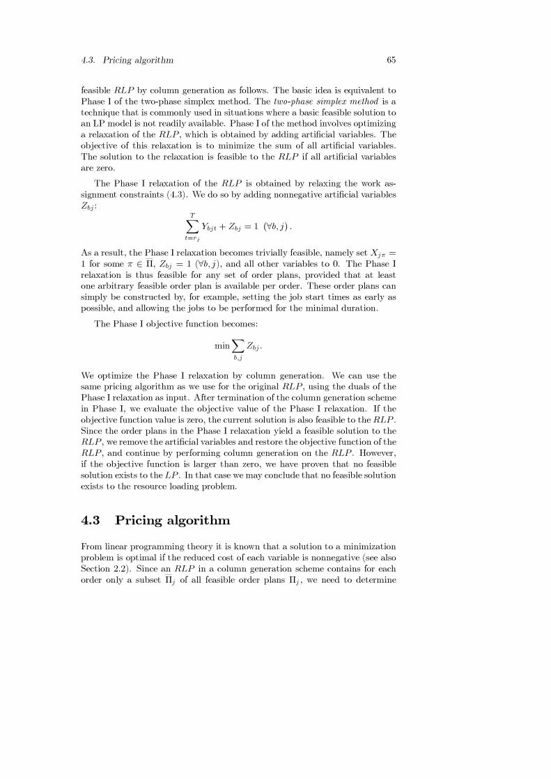
4.3. Pricing algorithm 65
feasible RLP by column generation as follows. The basic idea is equivalent toPhase I of the two-phase simplex method. The two-phase simplex method is atechnique that is commonly used in situations where a basic feasible solution toan LP model is not readily available. Phase I of the method involves optimizinga relaxation of the RLP , which is obtained by adding artificial variables. Theobjective of this relaxation is to minimize the sum of all artificial variables.The solution to the relaxation is feasible to the RLP if all artificial variablesare zero.
The Phase I relaxation of the RLP is obtained by relaxing the work as-signment constraints (4.3). We do so by adding nonnegative artificial variablesZbj:
T∑t=rj
Ybjt + Zbj = 1 (∀b, j) .
As a result, the Phase I relaxation becomes trivially feasible, namely set Xjπ =1 for some π ∈ Π, Zbj = 1 (∀b, j), and all other variables to 0. The Phase Irelaxation is thus feasible for any set of order plans, provided that at leastone arbitrary feasible order plan is available per order. These order plans cansimply be constructed by, for example, setting the job start times as early aspossible, and allowing the jobs to be performed for the minimal duration.
The Phase I objective function becomes:
min∑b,j
Zbj.
We optimize the Phase I relaxation by column generation. We can use thesame pricing algorithm as we use for the original RLP , using the duals of thePhase I relaxation as input. After termination of the column generation schemein Phase I, we evaluate the objective value of the Phase I relaxation. If theobjective function value is zero, the current solution is also feasible to theRLP .Since the order plans in the Phase I relaxation yield a feasible solution to theRLP , we remove the artificial variables and restore the objective function of theRLP , and continue by performing column generation on the RLP . However,if the objective function is larger than zero, we have proven that no feasiblesolution exists to the LP . In that case we may conclude that no feasible solutionexists to the resource loading problem.
4.3 Pricing algorithm
From linear programming theory it is known that a solution to a minimizationproblem is optimal if the reduced cost of each variable is nonnegative (see alsoSection 2.2). Since an RLP in a column generation scheme contains for eachorder only a subset Πj of all feasible order plans Πj , we need to determine

66 Chapter 4. Branch-and-price techniques for resource loading
whether order plans exist with negative reduced cost that are not in Πj. Thereduced cost cjπ of any order plan ajπ (π ∈ Πj , j = 1, . . . , n) in LP is givenby:
cjπ = ρjπθ + αj −
nj∑b=1
T∑t=rj
βbjtabjtπ , (4.4)
where αj is the (known) value of the dual variable corresponding to condi-tion (4.1) and βbjt are the (known) non-negative values of the dual variablescorresponding to conditions (4.2).
To test optimality of the current RLP solution, we determine whether thereexists an order plan ajπ (π ∈ Πj\Πj) for some order Jj (j = 1, . . . , n) withnegative reduce costs, that is, with cjπ < 0. To this end, we solve the pricingproblem of finding an order plan in Π\Π with minimum reduced cost, whichboils down to solving n independent subproblems, one for each order. Thesubproblem for order Jj (j = 1, . . . , n) is to minimize:
ρjπθ+ αj −
nj∑b=1
T∑t=rj
βbjtabjtπ ,
subject to the release date and due date of order Jj , the minimal duration of itsjobs, the precedence constraints between its jobs, and the minimum time lagδ. The (binary) decision variables in the pricing problem are the abjtπ ’s thatform the order plan ajπ for order Jj . These variables also determine the valuesρjπ (ρjπ ≥ 0), which denote the number of weeks that an order is allowed tobe tardy. When the order plan ajπ allows order Jj to be tardy by ρjπ weeks,a tardiness penalty ρjπθ is added to the pricing objective.
Note that an order plan may also be represented by the first and last weeksin which each job is allowed to be produced. For convenience we speak of thestart and completion times of jobs in the order plan, although the actual startand completion times in the order schedule may respectively be higher andlower.
In the pricing algorithm we account for internal release dates (rbj) and duedates (dbj) of jobs. These may be calculated from the minimal duration ofthe jobs, the δ parameter, and the (external) release date and due date of theorder, but these may also be imposed externally, e.g., to meet certain deadlineson components or parts of an order. Note that since we allow an order to betardy, we must also allow jobs to be produced after their internal due date dbj .We define the job deadline dbj as the last week in which a job is allowed to beproduced. This deadline is thus not externally given. Accordingly, we definethe order deadline dj as the deadline of job nj . By default we set: dj = dbj = T(b = 1, . . . , nj), however, we may also set dbj to some number smaller than T tolimit the number of feasible order plans, and thus simplify the pricing problem.
We use implicit column generation, i.e., we generate order plans as theyare needed. An explicit column generation approach would require that all

4.3. Pricing algorithm 67
order plans are generated in advance and kept in computer memory. Sincethe number of feasible order plans is exponentially large this is not a seriousoption. Our pricing algorithm for solving the subproblem for order Jj is basedon dynamic programming and uses a forward recursion. In this chapter weconsider the case of linear precedence relations. In Section 4.3.1 we discuss thepricing algorithm for δ = 1. As discussed in Section 3.2, in the case δ = 0we impose an additional restriction that at most κ jobs of the same order areallowed to be performed in the same week. In Section 4.3.2 we discuss thepricing algorithm for this special case. In Chapter 6 we present a generalizedpricing algorithm for the case with generalized precedence constraints.
4.3.1 Pricing algorithm for δ = 1
The pricing problem can be translated into finding a longest path (when max-imizing −cjπ) or shortest path (when minimizing cjπ) in a directed acyclicnetwork with weights on the nodes. Consider for example an order Jj with 3jobs, a release date rj = 1, due date dj = 3 and a planning horizon T = 4. Theminimal duration wbj of each job Bbj is 1 week. From these data, we calculatethe release dates and due dates of the jobs as follows:
r1j = rj , and rbj = rb−1j +wb−1j − 1 + δ (b = 2, . . . , nj), (4.5)
dnj ,j = dj , and dbj = db+1j − (wb−1j − 1)− δ (b = 1, . . . , nj − 1).
Hence, for jobs B1j , B2j and B3j the values (rbj, dbj) are (1, 1), (2, 2) and (3,3)respectively. The corresponding longest path problem can be described usingthe network depicted in Figure 4.2. We represent each job Bbj and each weekt in which it is allowed to be performed by a node (b, t). Hence we have nj = 3sets of T − rj + 1 = 4 nodes. A path through a node (b, t) indicates that jobb is allowed to be performed in week t, which results in a contribution −βbjt
to the reduced cost of the order plan. A path through a node (nj , t), witht > dnj ,j = dj , contributes a tardiness penalty ρjπθ = (t− dj)θ to the reducedcost of the order plan, in addition to the contribution −βnjjt for that job. Asource and a target node are added to complete the directed network. A pathfrom the source to the target node represents a complete order plan (see Figure4.2).
The reduced cost of the order plan is the sum of αj , the contributions −βbjt
on the longest path, and, if applicable, a tardiness penalty ρjπθ for job nj.
Since we only consider those order plans that can not be dominated by otherorder plans (see Section 3.2), in Figure 4.2 we have removed all redundant arcs.We could have, for example, drawn an arc from node (1,1) to (2,3). However,a path from (1, 1) to (2,3) via (2,2) or (1,2) will yield as least as much as apath from (1, 1) directly to (2, 3). Hence, all arcs not involving the source andtarget node connect node (b, t) with node (b+ 1, t+ δ) or node (b, t+ 1).

68 Chapter 4. Branch-and-price techniques for resource loading
1,1 3,12,1
3,22,21,2
1,3 3,32,3
src
tar
job 1 job 2 job 3
source
target
3,42,41,4
Figure 4.2: Example pricing problem (δ = 1).
We solve the pricing problem by dynamic programming (DP). Each job Bbj
represents a stage b. Since the information needed to represent an order planconsists of the allowed start and completion times of the jobs, the decision ineach stage must regard either the start time or the completion time of the job.Since the pricing problem is symmetric with respect to this decision (a starttime of a job implies the completion time of its predecessor, and vice versa), wesay that a decision in a stage concerns the start time of the job in that stage.A state (j, b, t) in a stage b describes a completion time t of job Bbj .
Let Fj(b, t) be the minimum reduced cost for all feasible partial order plansfor the jobs B1j, . . . ,Bbj with t the completion time of job Bbj, i.e., t is thelast week in which job Bbj is allowed to be performed (b ≤ nj , rbj +wbj − 1 ≤t ≤ dbj). Note that t must be at least rbj + wbj − 1 to comply with theminimal duration constraint. Let ajπ be an order plan in state (j, b, t) withvalue Fj(b, t). Then, ajπ must allow Bbj to be performed in weeks s, . . . , t forsome rbj ≤ s ≤ t−wbj+1 (i.e., s and t are the start and completion time of jobBbj). The start time s can be at most t−wbj +1 to comply with the minimalduration constraint. Accordingly, the previous state must be (j, b − 1, s − δ)for some s with rbj ≤ s ≤ t−wbj + 1. Allowing Bbj to be performed in weeks
s, . . . , t contributes −t∑
u=sβbju to the reduced cost of the partial order plan of
the previous state (Fj (b− 1, s− δ)).

4.3. Pricing algorithm 69
We now give the dynamic programming recursion to solve the j-th subprob-lem. The initialization is:
Fj(b, t) =
{αj, if b = 0,∞, otherwise.
The recursion for b = 1, . . . , nj, t = rbj +wbj − 1, . . . , dbj is then:
Fj(b, t) = minrbj≤s≤t−wbj+1
{Fj (b− 1, s− δ) +∆bjt −
t∑u=s
βbju
}. (4.6)
For all other t:Fj(b, t) =∞.
Where ∆bjt in (4.6) is defined as follows:
∆bjt =
{(t− dbj)θ, if b = nj and t > dbj0, otherwise.
(4.7)
Parameter ∆bjt thus adds a tardiness penalty to Fj(b, t). Note that withoutloss of generality this pricing algorithm may also be applied in cases whereδ > 1.
Lemma 4.3 The optimal solution to the j-th pricing subproblem is found as:
F∗j = min
dj≤t≤dj
Fj(nj, t), (j = 1, . . . , n).
�
Lemma 4.4 The optimal solution to the pricing problem is found as:
F ∗ = min1≤j≤n
F∗j .
�
Accordingly, if F ∗ ≥ 0, then the current RLP solution is optimal. If F∗ < 0,then the current RLP solution may not be optimal, and we need to introducenew columns (order plans) to the problem. Candidates are associated withthose orders Jj for which F ∗
j < 0, and they can be found by backtracking. Notethat the pricing algorithm for the j-th subproblem uses O(njT ) space and canbe solved in O(njT
2) time. Hence the pricing problem uses O(maxj
(nj)Tn)
space and can be solved in O(maxj
(nj)T 2n) time. Although the pricing algo-
rithm usually demands little computation time, some speed up can be obtainedby identifying jobs that can not contribute to the reduced cost of the order plan,that is, jobs Bbj for which βbjt = 0 (∀t). For such jobs, given their state (the

70 Chapter 4. Branch-and-price techniques for resource loading
completion time (b, t)), the corresponding decision (the start time s) is alwayschosen as s = t−wbj + 1, where wbj is the minimal duration of the job.
Solving the n pricing problems may give us more than one column withnegative reduced cost. Therefore, we face the issue to decide on the number ofcolumns to add to the linear program after having solved the pricing problem.In general, the more columns we add per iteration, the fewer linear programswe need to solve, but of course the bigger the linear programs become. As longas the size of the RLP remains manageable, we add all columns (at most oneper order) with negative reduced costs. However, when the computation timethat is required to solve the RLP increases too much, column disposal maybe required. We discuss in Section 4.4 that the growth of the ‘column pool’depends largely on the branching strategy.
4.3.2 Pricing algorithm for δ = 0
For the case δ = 0 we also use dynamic programming to solve the pricing prob-lem. The main difference in the pricing algorithm is caused by the additionalrestriction that we allow at most κ jobs of the same order to be performed inthe same week. Note that δ = 0, κ = 1 is equivalent to δ = 1. If we wouldrelax this constraint (κ = 0), we could use the pricing algorithm of the previoussection. Also, if the number of jobs nj of an order Jj is equal to or smallerthan κ, we may use the pricing algorithm of the previous section. Hence, inthe remainder of this section we assume that δ = 0, and nj > κ.
As in the previous section, each job Bbj represents a stage b. Moreover,the decision in a stage b regards the start time of job Bbj . The additionalrestriction that at most κ jobs of the same order are allowed to be performedin the same week implies that we may only allow a job Bbj to be started in aweek t, when at most κ − 1 predecessors are allowed to be produced in thatweek t. Thus to be able to make a decision regarding a start time of a job Bbj ,the state (j, b, t) must be extended with an additional parameter σ < κ, thatindicates the number of predecessors that are allowed to be produced in weekt. Note that since j is fixed in a pricing problem, the state (j, b, t, σ) is in fact3-dimensional.
Let ajπ be an order plan in state (j, b, t, σ) with value Fj(b, t, σ), and letb > 1. To determine from which possible previous states ajπ can be created, wemust distinguish two cases, i.e., σ = 0 and σ > 0. When σ = 0, the predecessor(Bb−1,j) is not allowed to be performed in week t, so the completion timeof the predecessor must be smaller than t. As a result, π must have beencreated by allowing Bbj to be performed in weeks s, . . . , t for some rbj ≤ s ≤t−wbj +1, and the completion time of the predecessor must be min {t− 1, s}.Accordingly, the previous state must be (j, b− 1,min {t− 1, s} , σ′) for some swith rbj ≤ s ≤ t − wbj + 1, and some σ′ < κ. When σ > 0, the completiontime of the predecessor of job Bbj is t. Accordingly, the previous state must be

4.4. Branching strategies 71
(j, b− 1, t, σ − 1).
We now give the dynamic programming recursion to solve the j-th subprob-lem. The initialization is:
Fj(b, t, σ) =
{αj , if b = 0,∞, otherwise.
The recursion for σ = 0, b = 1, . . . , nj , t = rbj +wbj − 1, . . . , dbj is then:
Fj(b, t,0) =
minrbj≤s≤t−wbj+1
{minσ′<κ
{Fj(b − 1,min {t− 1, s} , σ′)}+∆bjt −t∑
u=s
βbju
}
where ∆bjt is defined as in (4.7). The recursion for 0 < σ < κ, b = 1, . . . , nj ,t = rbj +wbj − 1, . . . , dbj is then:
Fj(b, t, σ) = minrbj≤s≤t−wbj+1
{Fj(b− 1, t, σ − 1) +∆bjt −
t∑u=s
βbju
}.
For all other σ, b, t:Fj(b, t, σ) = ∞.
Lemma 4.5 When δ = 0, and nj > κ, the optimal solution to the j-th pricingsubproblem is found as:
F ∗j = min
dj≤t≤dj ,0≤σ≤κFj(nj , t, σ), (j = 1, . . . , n).
�
Analogous to the pricing algorithm in the previous section, when F ∗j < 0,
a candidate order plan can be found by backtracking. The pricing algorithmfor the j-th subproblem uses O(njTκ) space and can be solved in O(njT
2κ2)time. Hence the pricing problem uses O(max
j(nj)Tκn) space and can be solved
in O(maxj
(nj)T2κ2n) time.
4.4 Branching strategies
After termination of the column generation scheme on an RLP we evaluatethe resulting optimal LP solution. If the optimal LP solution is integral withrespect to the Xjπ variables, the solution also forms an optimal solution to theresource loading problem, and we are done. If the solution is fractional, weapply the procedure of Lemma 4.2 to try to transform the fractional solution

72 Chapter 4. Branch-and-price techniques for resource loading
rbj dbj
rsj dsj
0 1 2 3 4 5 6 7 8
rbj lb
dsj
0 1 2 3 4 5 6 7 8
job Bbj
job Bsj
job Bbj
job Bsj
lb+δ
weeks weeks
Figure 4.3: Repair of a violated precedence relation (δ = 1)
into an integral solution without changing the objective function. If this isnot possible, i.e., a part of the solution remains fractional, we need a branch-and-bound algorithm to find an optimal integral solution. In the next sectionswe discuss the exact (Section 4.4.1) and heuristic (Section 4.4.2) branchingstrategies to find a feasible integral solution from an optimal fractional LPsolution.
4.4.1 Branching strategy
It is well known that a ‘direct’ partitioning of the solution space by fixing orbounding binary variables is generally not a good strategy, because it tendsto yield an unbalanced branch-and-bound tree (see, e.g., Barnhart et al., 1998;Vanderbeck, 2000). Hence, instead of branching on the fractional variablesXjπ
of an order Jj, we use a branching strategy (referred to as BS) that aims atfixing violated precedence relations between jobs of fractional orders. When, inan RLP solution in any node of the branching tree, an order plan ajπ′ (as de-fined in Definition 4.1) is not feasible, there is at least one pair of jobs, say jobsBbj and Bsj , for which a precedence relation is violated. In BS we alter theallowed intervals for jobs Bbj and Bsj such that they no longer overlap. We an-alyze each possible alteration in the child nodes. Recall that job Bbj is allowedto be performed in interval [rbj, dbj], and job Bsj is allowed to be performed inthe (overlapping) interval [rsj , dsj]. To repair the violated precedence relationbetween these jobs, we must alter job deadlines, which were introduced to limitthe number of feasible order plans and thus reduce the pricing problem size, andjob release and due dates as follows. Each child node corresponds to a new dead-line lb of jobBbj (lb ∈
[max {rbj +wbj − 1, rsj} ,min
{dbj, dsj −wsj + 1− δ
}]).
This is illustrated in Figure 4.3. The values(rbj, dbj, dbj
)for job Bbj thus
become (rbj,min {dbj, lb} , lb), and the values(rsj, dsj, dsj
)for job Bsj become(
max {rbj , lb + δ} , dsj, dsj). Subsequently, we eliminate all order plans ajπ that
do not comply with the updated job release dates, due dates and deadlines. As

4.4. Branching strategies 73
a consequence, the (modified) RLP or even the (modified) LP may no longerbe feasible. To determine whether the modified LP is feasible we apply columngeneration to the Phase I LP relaxation of the two-phase simplex method, asdescribed in Section 4.2.2, and account for the modified job release dates, duedates and deadlines in the pricing algorithm. When the modified LP is infea-sible, we prune the node. Otherwise, we continue in this node by performingcolumn generation on the RLP . When we prune a node, we return to theparent node in the branching tree.
We illustrate the branching strategy BS with an example. Consider an RLPsolution in which ajπ′ is infeasible for order Jj, due to a precedence relationviolation of jobs B1j and B2j . Suppose the values
(rbj , dbj , dbj
)for jobs B1j
and B2j are (0,2,3) and (1,3, 4) respectively, the minimal duration wbj of eachjob is 1 week, and δ = 1. Branching strategy BS imposes in each child node adeadline l1 for job B1j , with:
l1 ∈[max {r1j +w1j − 1, r2j} ,min
{d1j, d2j −w2j +1− δ
}]= [max {0,1} ,min {3,3}]
= [1, 3] .
Hence the branching strategy results in 3 child nodes, in which the modifiedvalues
(rbj, dbj, dbj
)for jobs B1j and B2j are:
(0, 1, 1) and (2,3, 4) in child node 1,
(0, 2, 2) and (3,3, 4) in child node 2,
(0, 2, 3) and (4,4, 4) in child node 3.
Note that the modified job release dates, due dates and deadlines exclude anoverlap of jobs B1j and B2j in any order schedule.
For the BS method we apply the depth-first node selection strategy. Whenwe select a violated precedence relation to be repaired in a node, we try toselect a fractional order for which the repair of a precedence relation viola-tion is most restrictive. We expect that this strategy reduces the depth of thebranching tree. There are probably many intuitive strategies that comply withthis strategy. We select in each node the fractional order Jj that maximizes∑π∈Πj
(Xjπ(1−Xjπ)). When there are more than one violated precedence re-
lation for this order, we repair the violated precedence relation for which theconcerned pair of jobs has the largest overlap (in weeks).
We may try to find an initial incumbent solution before we start the BSmethod by applying a heuristic. This usually enables to fathom nodes at anearly stage in the branching scheme, at the cost of little additional computationtime. We discuss the application of heuristics in Section 4.6. In Section 4.5 wediscuss the application of Lagrangian relaxation for lower bound determination.

74 Chapter 4. Branch-and-price techniques for resource loading
4.4.2 Branch-and-price based approximation algorithms
For large instances, branch-and-bound methods typically require a long compu-tation time to find an optimal solution, or to prove that the incumbent solutionis optimal. We found that this is also the case for the resource loading problem.We therefore tested some branch-and-price based heuristics to find a good so-lution in little time. We use the integrality gap as an indication of the qualityof the solutions of these algorithms.
The first and most straightforward branch-and-price based heuristic wetested is the truncated BS (TBS), that truncates the BS algorithm of Sec-tion 4.4.1 after a certain amount of time. The resulting solution of the TBSmethod is the incumbent solution at the moment of truncation. The TBSmethod enables to test the BS method on large problems.
Another heuristic based on the BS method is the ε-approximation strat-egy (EAS). In this heuristic we fathom all nodes in which the lower boundapproaches the incumbent (upper bound) within ε% (i.e., LB · (1 + ε) ≥ UB).On termination of EAS, its incumbent solution differs at most ε% from theoptimal ILP solution. Hence, this method allows us to find a compromise be-tween the computation time required, and the quality of the solution obtained.
We also tested six variants of an incomplete branching strategy that is notbased on the aforementioned BS method. This branching strategy is based onselecting one order plan for an order in each layer of the branching tree. Henceeach layer corresponds to an order Jj for which we set one Xjπ variable to 1.After selecting an order plan for an order in a node of the branching tree, weapply column generation on the remaining orders (i.e., the orders for which noorder plans have been fixed) to prevent that fixing variables leads to infeasibleRLP s. We use a depth-first node selection strategy to find a feasible solutionas fast as possible.
In the first two variants of this branching strategy we branch on the frac-tional order that has the highest number of (fractionally) selected order plansin the current RLP solution. In HBS1 we branch on all order plans thatare available for the selected order in the current RLP . In the second variant(HBS2) we branch only on those order plans that are (fractionally) selected inthe current RLP solution. Observe that the part of the solution space that isanalyzed by these branching strategies strongly depends on the number of orderplans that are available for each order at the moment the order is branched on.When an order that is branched on has few order plans available in the currentRLP , a large part of the solution space may be discarded. For this purpose weimplemented variant HBS1+ and HBS2+, which are are the same as HBS1and HBS2 respectively, except that before branching we add for each order upto five order plans to the column pool, so that sufficient order plans are avail-able to branch on. These order plans are found by five stand-alone heuristicsthat were proposed by Borra (see Borra, 2000, and Section 4.6.1). Variants

4.5. Lower bound determination by Lagrangian relaxation 75
HBS3 and HBS4 are the same as HBS1+ and HBS2+ respectively, exceptthat the next order to branch on in each layer is the order that has the mostorder plans in the current RLP .
4.5 Lower bound determination by Lagrangian
relaxation
Lagrangian relaxation can complement column generation, in that it can pro-vide a lower bound to the original problem in every iteration of the columngeneration procedure with little computational effort (cf. Section 2.4). Wenote that the example ILP model in Section 2.4 has the same basic form as theresource loading model, where the disjoint sets of variables J(i) ⊂ J in the ex-ample correspond to the setsΠj ⊂ Π of variablesXjπ . Hence we apply the sameprocedure to the resource loading model, and we obtain the Lagrangian relax-ation of the ILP by relaxing all constraints but constraints
∑π∈Πj
Xjπ = 1
(∀j) and variable restrictions Xjπ ∈ {0, 1} (∀j, π ∈ Πj ⊂ Π). The resultingLagrangian relaxation LILP (λ) possesses the integrality property. Hence, anal-ogous to the example in Section 2.4, we can obtain a Lagrangian lower boundto the linear programming relaxation LP each time an RLP has been solvedto optimality, by using the dual solution of the RLP as Lagrangian multipliers,and by performing a pricing algorithm on all orders. The lower bound can bedetermined as follows:
z∗RLP +∑j
cjΘj ,
where z∗RLP is the optimal objective value of the RLP , cj is the objective valueof the j-th pricing algorithm (i.e., the lowest reduced cost factor of all orderplans of order Jj), and Θj is a binary variable that is set to 1 when cj isnonnegative, and set to 0, otherwise.
We apply column generation in each node of the branching tree. Hence,in each column generation iteration in each node we may determine a lowerbound to the LP relaxation of the resource loading model for that node and forall nodes below that node (note that the branching changes the LP relaxationin every node). Hence, when branching downwards in the branching tree, wemust store the best lower bound found so far. We compare the best lowerbound to an upper bound (e.g., an incumbent solution, or a heuristic solutionof the resource loading problem) after every column generation iteration, andterminate column generation and fathom the node when the best lower boundexceeds the best upper bound. This also alleviates the tailing-off effect ofcolumn generation.
We also use the Lagrangian lower bound to fix variables. When the reducedcost of a variable is larger than UB − LB (i.e., the difference between theupper and lower bound), we fix that variable to 0, since we know from linear

76 Chapter 4. Branch-and-price techniques for resource loading
programming theory that that variable must be 0 in any solution with a valueless than UB. Analogously, we fix each variable with a reduced cost smallerthan LB − UB to 1.
4.6 Application of heuristics
We propose several heuristics to be used as ‘stand-alone’ heuristics that solvethe resource loading problem without using the linear programming model ofthe resource loading problem, as well as heuristics that we can use in vari-ous stages of the branch-and-price algorithm. The latter category of heuristicsaims either at finding an integral solution from a fractional solution (roundingheuristics), or at improving an existing integral solution (improvement heuris-tics).
4.6.1 Stand-alone heuristics
Stand-alone heuristics can be used to determine an a priori feasible solution tothe resource loading problem. Such heuristics can also be used in the branch-and-price algorithm, e.g., to find an initial feasible set of orders for the RLPin the root or in any node. The heuristic solutions serve as an upper bound tothe solution of the original problem, which, in conjunction with a Lagrangianlower bound, may reduce the number of nodes to explore in the branch-and-price algorithm. The heuristic solutions can also be used to evaluate the qualityof solutions found by heuristic branching strategies, such as the truncated BSmethod.
The stand-alone heuristics proposed by Borra (2000) are all priority rulebased heuristics, that load the jobs in a sequence determined by the priorityrule, and hereby construct an order schedule. As an example we mention theearliest due date (EDD) priority rule, that sorts orders or jobs according totheir due dates in an increasing order, and plans the orders or jobs accordingto this sequence. Since the objective here is to minimize the costs of extracapacity, we first try to process each job in regular operator time. If this is notpossible without exceeding its due date, we use whichever type of capacity ischeaper to complete the job in time. If we still can not meet the due date, thenwe subcontract the entire job.
The solution of a stand-alone heuristic determines exactly one feasible orderschedule for each order. When a heuristic solution is used to initialize an RLPin any node of the branching tree, order plans must be constructed from theseorder schedules. We construct the order plans ajπ∗ for each order Jj fromthe order schedule for Jj using the method described in Definition 4.2. Byoptimizing the initial RLP that only has the order plans ajπ∗ , we find a feasibleresource loading solution that is at least as good as the solution found by the

4.6. Application of heuristics 77
stand-alone heuristic that was used to generate the order plans. Hence, in thisway the RLP model can be used in conjunction with a stand-alone heuristicto improve its solution without much effort.
4.6.2 Rounding heuristics
We propose four rounding heuristics that are based on constructing an in-tegral solution from a fractional RLP solution by rounding variables Xjπ
(j = 1, . . . , n, π ∈ Πj). These heuristics may help to speed up the branch-and-price methods, by trying to find better incumbent solutions (with littlecomputational effort) in any node of the branching tree. All rounding heuris-tics attempt to converge to an integral solution in a number of iterations, inwhich we round a number of variables (i.e., fix variables Xjπ either to 0 orto 1), after which we re-optimize the (modified) RLP . In each iteration weapply the procedure of Lemma 4.2 to try to eliminate fractional orders. Sincewe do not add order plans in the iterations, rounding variables may lead to aninfeasible RLP . The rounding heuristics thus do not always lead to a feasibleintegral solution.
In the rounding heuristic that we refer to as RH1, we round in each iterationall variables Xjπ (j = 1, . . . , n, π ∈ Πj) with a value smaller than some positivethreshold ε to 0, and round each variableXjπ with a value larger than 1−ε to 1.When no variables can be rounded by this strategy, we round the variable Xjπ
with the highest value. The larger we set ε, the faster the heuristic becomes,however, too many variables may be rounded at once. This usually leads to aninfeasible RLP .
In heuristic RH2 we take into account that order plans that are not (frac-tionally) selected may for a large part comply with the order schedule (formedby variables Ybjt) in the current solution. In other words, these non-selectedorder plans may for a large part be the same as the order plan ajπ′ (definedin Definition 4.1). The Xjπ variables thus do not provide much information asto what order plans are appropriate. We calculate for each order plan of eachfractional order a valueQjπ (that takes a value between 0 and 1) that indicatesto what extent the order plan complies with the order schedule in the currentRLP solution. The value Qjπ is calculated as follows:
Qjπ =
dj∑t=rj
nj∑b=1
abjtπYbjt
nj. (4.8)
We thus sum up all the Ybjt’s that are matched by a corresponding 1 in theorder plan, and divide the sum by the number of jobs. Hence, when the orderplan matches the order schedule, the resulting Q-value is 1. Note that althoughan order plan may not be (fractionally) selected, it may still have a high Q-

78 Chapter 4. Branch-and-price techniques for resource loading
value. We use the value Qjπ instead of Xjπ as the rounding variable, and applythe same rounding strategy as in RH1.
Rounding heuristic RH3 is basically the same as RH2, but in addition itsolves a pricing algorithm in each iteration of the rounding scheme, for allfractional orders. Hereby we try to prevent that the rounding procedure yieldsan infeasible solution after some iterations.
In heuristic RH4 we round in each iteration a fixed number of variables, sayk, until no variables need to be rounded. For this purpose we calculate for eachvariable Xjπ that has not yet been fixed the value Q′
jπ = max {Qjπ, 1−Qjπ},with Qjπ as in (4.8). We then sort the variables on theirQ′
jπ value in decreasingorder, and we round the first k variables to:
1, when Q′jπ = Qjπ ,
0, when Q′jπ = 1−Qjπ.
When the first k variablesXjπ are integral, we round the subsequent k variablesas well, until the RLP basis is modified and it needs to be re-optimized. Wechoose k to be a small value. The higher the number k the faster the heuristic,however, the higher the risk of an infeasibility.
4.6.3 Improvement heuristic
In our computational experiments we also use the improvement heuristic pro-posed by Gademann and Schutten (2001). We refer to this heuristic as IH. IHstarts from a feasible solution and tries to improve the solution by iterativelychanging the start and completion times of the jobs in the order plans of thesolution. Suppose we want to change the start time sbj or the completion timetbj of job Bbj of order Jj in the time window [sbj , tbj] of that job. There arefour possible cases that result from decreasing or increasing sbj or tbj by oneweek:
• a decrease in the start time sbj of job Bbj is allowed when the completiontime of the predecessor Buj may be decreased by one. This conditionholds when (tuj − 1)−suj+1 ≥ wuj , i.e., when the modified time windowfor job Buj is at least as large as its minimal duration wuj .
• an increase in the start time sbj of job Bbj is allowed when the modifiedtime window satisfies tbj − (sbj +1) + 1 ≥ wbj , i.e., when the modifiedtime window for job Bbj is at least as large as its minimal duration. Thischange only makes sense if the completion time of the predecessor Buj
can be increased, i.e., tuj +1 ≤ duj.
• a decrease in the completion time tbj of job Bbj is allowed when themodified time window satisfies (tbj − 1) − sbj + 1 ≥ wbj , i.e., when the

4.6. Application of heuristics 79
modified time window for job Bbj is at least as large as its minimalduration. This change only makes sense if the start time of the successorBvj of job Bbj can be decreased, i.e., svj − 1 ≥ rvj .
• an increase in the completion time tbj of job Bbj is allowed when thestart time of the successor Bvj of job Bbj can be increased by one. Thiscondition holds when tvj − (svj + 1) + 1 ≥ wvj .
Each time we change a start or completion time of a job in an order plan,we determine the corresponding order schedules by solving an RLP that onlycontains the order plans of the initial solution. We use the dual solution ofthe RLP to evaluate the expected change in the objective function value forall possible changes in the order plans. Each of the aforementioned changesin an order plan results in two modified coefficients in the coefficient matrixof the model. More specific, in Constraints (4.2) one coefficient
∑π∈Πj
abjtπ of
a variable Xjπ is set from 1 to 0 (for a job Bbj), and one coefficient of thesame variable Xjπ is set from 0 to 1 (for a predecessor or successor Buj). Thuswith βbjt the given non-negative values of the dual variables corresponding toconditions (4.2), the expected change in the objective value is −βbjt + βujt.
In heuristic IH we evaluate all possible changes in the time windows of alljobs, and sort these by increasing value of the expected change in the objectivevalue.
We accept the first change according to this sorting that actually leads toan improvement. This is checked by reoptimizing the corresponding RLP . Werepeat this procedure until no more improvement is found. Gademann andSchutten propose several other strategies for accepting changes, each of whichleads to different heuristics. We do not use these other strategies.
We presented the heuristic for the case of linear precedence relations, al-though the heuristic was originally proposed by Gademann and Schutten forthe case of generalized precedence relations. The only difference in the case ofgeneralized precedence relations is that when we change the time window of ajob in the aforementioned procedure, it may have more than one successor orpredecessor.
Gademann and Schutten show that the search space is not connected, i.e.,IH may get stuck in a local minimum. For example, when the time windowof job Bbj in the initial order plan is [sbj, tbj ], the optimal time window is[sbj − 2, tbj ], and the expected change in the objective for changing sbj to sbj−1is positive, we may never find an optimal solution. The outcome of the heuristicthus depends on the initial feasible solution it starts from. It thus may pay offto perform this heuristic at various stages of the branch-and-price algorithm.

80 Chapter 4. Branch-and-price techniques for resource loading

81
Chapter 5
Resource loading
computational results
All of life is an experiment.The more experiments you make, the better.
- Ralph Waldo Emerson (1803-1882)
5.1 Test approach
In this chapter we present the computational results of the algorithms for re-source loading presented in Chapter 4. All algorithms have been coded andtested in the Borland Delphi 5.0 C/S programming language on a PentiumIII − 600 MHz personal computer, running Windows NT 4.0. The applica-tion interfaces with the ILOG CPLEX 7.0 callable library, which we use foroptimizing linear programming models and retrieving the optimization results.
By using different branching strategies and combining branch-and-price al-gorithms with heuristics, we obtain various algorithms for resource loading. Totest these, we implemented an instance generator that allows us to produceclasses of instances with various parameter settings. Table 5.1 lists the pa-rameters that characterize the test instances. Each parameter influences thecomplexity of the test instances. We aim at generating test instances that arenot too easy to solve with any parameter setting. Some parameters mainlydetermine the problem size (e.g., the length of the planning horizon), otherparameters only influence the solution space (e.g., the release and due datesof the orders determine how much slack the jobs have). Our test approach isto first perform preliminary experiments in which we test all algorithms on asmall number of instances. For these instances we vary the length of the plan-

82 Chapter 5. Resource loading computational results
n the number of orders.m the number of machine groups.nj the number of jobs of order Jj.T + 1 the length of the planning horizon (in weeks).rj release date of order Jj.dj due date of order Jj.µbj the machine group on which job Bbj must be processed.pbj the processing time of job Bbj .wbj minimal duration of job Bbj (in weeks).δ minimum time lag (0 or 1 week) between adjacent jobs,
to impose a one-job-per-week policy.mcit total regular capacity of machine group Mi in week t.mcit capacity of Mi in week t in regular operator time.ct available regular operator capacity in week t (in hours).ot available overtime capacity in week t (in hours).ht available hiring capacity in week t (in hours).st available subcontracting capacity in week t (in hours).ot cost of overtime per hour.ht cost of hiring one extra operator per hour.st cost of outsourcing one hour of work.κ maximum number of jobs of the same order that are
allowed to be produced in the same week.
Table 5.1: Test case parameters.
ning horizon, the number of orders to be loaded and the number of availablemachine groups. Based on the preliminary test results we aim to select the bestversion of the branch-and-price based algorithm for further evaluation. We alsochoose an interesting class of instances, which we use for more extensive testingof various other parameters.
We restrict ourselves to time driven resource loading problems. As a result,in the test instances, the orders are not allowed to be tardy. The testing of thealgorithms on resource driven resource loading problems is subject of furtherresearch.
The outline of this chapter is as follows. In Section 5.2 we discuss thetest instance generation procedure. In Section 5.3 we give an overview of allalgorithms that we tested. In Section 5.4 we determine the best version of thealgorithm by performing preliminary computational experiments with variousheuristics and branch-and-price methods. Finally, in Section 5.5 we presentthe extensive computational results of this algorithm, by performing sensitivityanalyses on various parameters.

5.2. Test instance generation 83
5.2 Test instance generation
In this section we discuss the test instance generation procedure. We categorizethe test instances in classes that correspond to different parameter settings. Weparticularly vary the length of the planning horizon T+1, the number of ordersn and the number of machine groups m. We consider the following values forT and m:
T ∈ {5,10,15,20,25,30} ,
m ∈ {3,5,7, 10} .
We generate the order data by simulating an order arrival process. The firstorder arrives in week 1, and the subsequent orders arrive with a Poisson arrivaldistribution at a mean rate of λ. This implies that the interarrival times havean exponential distribution with an average interarrival time of 1/λ weeks.Furthermore, for the number of orders n we have that E (n) = λ (T +1). Therelease date rj of an order Jj is found by rounding the arrival time of the orderto the nearest whole number. We consider the following values for parameterλ:
λ ∈ {0.5,1, 2} .
The remaining order data for an order Jj is then generated as follows:
• nj ∈ {1, 2, . . . , 10}.
The number of jobs of order Jj (nj) is uniformly drawn from {1,2, . . . ,10}.Observe that when we solve an instance for δ = 1, orders can have at mostT + 1 jobs.
• pbj ∈ {10,11, . . . , 60}.
We give the jobs a processing time of a similar magnitude as the size of a timeperiod (i.e., a week). Accordingly, we draw pbj uniformly from {10,11, . . . , 60}hours.
• µbj ∈ {1,2, . . . ,m}.
A machine group number µbj is uniformly drawn for each job Bbj from{1, 2, . . . ,m}. Subsequent jobs must have different machine group numbers.
• wbj = 1.
All jobs have a minimal duration wbj of 1 week, so that, when solving thetest instance for δ = 0, varying parameter κ (i.e., the maximum number ofjobs of the same order that are allowed to be produced in the same week) willgenerally have significant impact on the solution space.

84 Chapter 5. Resource loading computational results
• dj = rj + nj + k − 1, k ∈ {�0.5 · nj� , �0.5 · nj + 1�}.
The order due date dj must be large enough to allow the order to completebetween the release and due date. For this purpose we first calculate the orderminimal duration, and then add a number of slack weeks to determine the orderdue date. Although we solve the test instances for both δ = 0 and δ = 1, forthe determination of the order minimal duration we assume that δ = 1. As aresult, when we solve the test instance for δ = 0 (and κ > 1) instead of δ = 1,the order will have more slack weeks. Hence, for δ = 1 and wbj = 1 (∀b, j)
the order minimal duration isnj∑b=1
wbj − (nj − 1) (1− δ) = nj weeks. The order
due date thus becomes dj = rj + nj + k − 1, where k is the number of slackweeks that we add. Without adding slack weeks (i.e., k = 0), the planningof the order would be trivial. To prevent this, we give each order at least 1week slack. Also, we want orders with a small number of jobs to generally havefewer slack weeks than orders with more jobs. For this purpose, we relate thenumber of slack weeks of an order Jj to its number of jobs nj. Accordingly, weuniformly draw a value from {�0.5 · nj� , �0.5 · nj +1�}, and round the value toobtain the number of slack weeks k.
• δ = 0 ⇒ κ ∈ {2,3,10}.
The values we consider for the maximum number of jobs of the same orderthat are allowed to be produced in the same week (κ) are {2, 3, 10}. This onlyapplies when a test instance is solved for δ = 0. Note that, since nj ≤ 10 andwbj = 1 (∀b, j), we have that when κ = 10, all jobs are allowed to be processedin the same week.
From the order release date rj and the order due date dj we determine theinternal job release dates rbj and due dates dbj. We perform computationalexperiments for δ = 0 and δ = 1 on the same test instances. When δ = 0 andwbj = 1 (∀b, j) the minimal duration of the order is
⌈nj
κ
⌉. As mentioned before,
when δ = 0 and κ > 1, the order has more internal slack. Note that δ = 0 andκ = 1 corresponds to δ = 1.
The number of orders that are allowed to be processed in a week will besmaller in the first weeks of the aforementioned order arrival process. Wetherefore simulate an order arrival process for t = 0, . . . ,60, and discard thefirst 30 weeks and consider, for the test instances with parameter T , all ordersthat are allowed to be produced in weeks {30, 30 + T}. Each simulation of theorder arrival process generates one test instance for each value of the para-meter T (T ∈ {5, 10, 15, 20, 25, 30}). When the interval in which a job Bbj isallowed to be produced (i.e., {rbj , dbj}) falls partly inside the planning horizon{30, 30 + T}, we consider that job completely if at least half of the interval{rbj , dbj} falls inside the planning horizon {30,30 + T}.
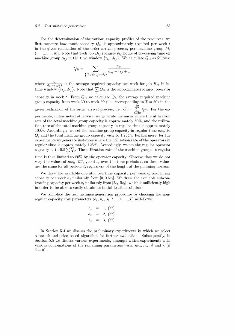
5.2. Test instance generation 85
For the determination of the various capacity profiles of the resources, wefirst measure how much capacity Qit is approximately required per week tin the given realization of the order arrival process, per machine group Mi
(i = 1, . . . ,m). Note that each job Bbj requires pbj hours of processing time onmachine group µbj in the time window {rbj , dbj}. We calculate Qit as follows:
Qit =∑
{(b,j)|µbj=Mi}
pbjdbj − rbj +1
,
wherepbj
dbj−rbj+1 is the average required capacity per week for job Bbj in its
time window {rbj , dbj}. Note that∑iQit is the approximate required operator
capacity in week t. From Qit we calculate Qi, the average required machinegroup capacity from week 30 to week 60 (i.e., corresponding to T = 30) in the
given realization of the order arrival process, i.e., Qi =60∑
t=30
Qit
31 . For the ex-
periments, unless noted otherwise, we generate instances where the utilizationrate of the total machine group capacity is approximately 80%, and the utiliza-tion rate of the total machine group capacity in regular time is approximately100%. Accordingly, we set the machine group capacity in regular time mcit toQi and the total machine group capacity mcit to 1.25Qi. Furthermore, for theexperiments we generate instances where the utilization rate of the operators inregular time is approximately 125%. Accordingly, we set the regular operatorcapacity ct to 0.8
∑iQi. The utilization rate of the machine groups in regular
time is thus limited to 80% by the operator capacity. Observe that we do notvary the values of mcit, mcit, and ct over the time periods t, so these valuesare the same for all periods t, regardless of the length of the planning horizon.
We draw the available operator overtime capacity per week ot and hiringcapacity per week ht uniformly from [0, 0.5ct]. We draw the available subcon-tracting capacity per week st uniformly from [2ct, 5ct], which is sufficiently highin order to be able to easily obtain an initial feasible solution.
We complete the test instance generation procedure by choosing the non-regular capacity cost parameters (ot, ht, st, t = 0, . . . , T ) as follows:
ot = 1, (∀t) ,
ht = 2, (∀t) ,
st = 3, (∀t) .
In Section 5.4 we discuss the preliminary experiments in which we selecta branch-and-price based algorithm for further evaluation. Subsequently, inSection 5.5 we discuss various experiments, amongst which experiments withvarious combinations of the remaining parameters mcit, mcit, ct, δ and κ (ifδ = 0).

86 Chapter 5. Resource loading computational results
Apply columngeneration on the
Phase I RLP
Apply stand-aloneheuristic
Feasible solutionfound?
Apply columngeneration scheme
Apply improvementheuristic
yes
no
Feasible solutionfound?
yes
No solution exists(STOP)
no
Apply branchingmethod
Apply roundingheuristics
Figure 5.1: Algorithm scheme.
5.3 Algorithm overview
In this section we give an overview of the algorithms that we use for preliminarytesting. We refer to Sections 4.4 to 4.6 for an extensive description of thesealgorithms.
Each branch-and-price algorithm that we tested is executed as a chain ofsubalgorithms. Figure 5.1 displays a scheme of the branch-and-price algorithm.We initialize the RLP in the root of the branching tree with order plans thatconstitute a feasible primal solution to the LP relaxation. We try to findsuch a feasible solution with a stand-alone heuristic. In all branch-and-pricealgorithms we apply the earliest due date heuristic (EDD) for this purpose. Ifthis heuristic fails to find a feasible solution, we apply column generation onthe Phase I RLP to either find a feasible primal solution to the LP relaxation,or prove that no such solution exists. In any other node of the branching tree,we do not use the EDD heuristic, because it tends to fail to find a feasiblesolution more often when more constraints are added to the problem in thebranching scheme. Instead, we immediately apply column generation on the

5.4. Preliminary test results 87
Phase I RLP .
Table 5.2 shows the approximate size of the initial RLP for instances withT ∈ {10,20,30}. It shows that the size of the RLP increases considerably withT .
T #nonzeros #variables #rows10 4000 1000 100020 11000 2800 280030 25000 6500 6500
Table 5.2: Size of the initial RLP .
After initializing the RLP , we apply column generation on the RLP inorder to determine the optimal solution to the LP . Since this solution isusually fractional, we may use one of the branch-and-price methods to find afeasible integral solution to the ILP . However, in order to find an incumbentsolution that may fathom many nodes in the branching scheme, we first applyvarious rounding heuristics and an improvement heuristic.
The branch-and-price methods use Lagrangian lower bounds (see Section4.5) to fathom nodes, and use a depth-first node selection strategy.
Table 5.3 gives an overview of the heuristics that we use to determine anincumbent solution before branching. Table 5.4 gives an overview of all branch-and-price algorithms that we use for the preliminary testing.
EDD stand-alone heuristic based on the earliest due date priority ruleIH improvement heuristic that uses the EDD solution as an initial
solutionRH1 (ε) rounding heuristic 1 with rounding threshold value 0 < ε < 1RH2 (ε) rounding heuristic 2 with rounding threshold value 0 < ε < 1RH3 (ε) rounding heuristic 3 with rounding threshold value 0 < ε < 1RH4 (k) rounding heuristic 4 with parameter k (k ∈ N)
Table 5.3: Overview of heuristics.
5.4 Preliminary test results
In this section we present the computational results for the preliminary ex-periments with various combinations of the algorithms on the instance classesdiscussed in Section 5.2.
For the preliminary experiments we repeat the order arrival process twicefor each value of parameters m (m ∈ {3, 5, 7,10}) and λ (λ ∈ {0.5,1,2}) to

88 Chapter 5. Resource loading computational results
TBS truncated (after 30 minutes) branching strategyBS with Lagrangian lower bound determination,
TBS(noLLB) TBS without Lagrangian lower bound,EAS (ε) TBS with an ε-approximation strategy,TBS+IH TBS algorithm that solves IH every 3 minutes
to improve the upperbound,TBS90 same as TBS, but truncated after 90 minutes,HBS1, . . . ,HBS4 incomplete branching strategies based on selecting
one order plan in each node of the branching tree,HBS1+,HBS2+ same as HBS1, HBS2, but with additional order
plans available for each order in the initial RLP .
Table 5.4: Overview of branch-and-price methods.
obtain 2 ∗ 12 classes, each containing 6 instances (one for each value of T ). Wesolve all 144 instances for both δ = 0 and δ = 1. When we solve an instancefor δ = 0, we allow only two jobs of the same order to be produced in the sameweek, i.e., in the preliminary experiments we set κ = 2. This parameter settingcomes closest to the parameter setting δ = 1.
In conjunction with the test instances, we generate two feasible order plans(i.e., for δ = 0 and δ = 1) for each order in each test instance, to form theinitial RLP for a branch-and-price algorithm. For this purpose we use theEDD heuristic, or, if this algorithm can not find a feasible solution, we applycolumn generation on the Phase I RLP .
The outline of this section is as follows. We first test the performance andspeed of the heuristics that are listed in Table 5.3. We present the computa-tional results of these experiments in Section 5.4.1. Subsequently, we test thebranch-and-price methods that are listed in Table 5.4. We present the compu-tational results of these experiments in Section 5.4.2. Finally, in Section 5.4.3we compare all computational results, and choose a branch-and-price algorithmthat we use for more extensive testing in Section 5.5.
5.4.1 Preliminary test results for the heuristics
In this section we compare the performance of the heuristics that are listed inTable 5.3. IH must start from a feasible solution. Gademann and Schuttentested IH, as well as various variants of this improvement heuristic, extensively,and showed that the heuristic performance strongly depends on the initial fea-sible solution that the heuristic starts from (Gademann and Schutten, 2001).They showed that IH performs well when it starts from an initial solution inwhich the slack of the jobs is divided evenly. Here we use the solution found bythe rounding heuristic RH4(1) as the initial solution for the rounding heuristicIH. The rounding heuristics each use the columns and the LP solution that

5.4. Preliminary test results 89
are found after solving the LP in the root node via column generation. We testthe performance of the rounding heuristics RH1 (ε), RH2 (ε) and RH3 (ε) forrounding parameter ε = 0.01, and ε = 0.05, and rounding heuristic RH4 (k)for parameter k ∈ {1,2,3}. Table 5.5 compares the average and maximumexecution times of the heuristics, tested on all 288 instances (i.e., 144 instancessolved for both δ = 0 and δ = 1). Table 5.5 shows that the rounding heuristics
Heuristic Average MaximumEDD 0 0.01IH 132.87 3608.89
RH1 (0.01) 27.14 1116.69RH1 (0.05) 30.10 1615.72RH2 (0.01) 31.85 2314.64RH2 (0.05) 37.98 2314.13RH3 (0.01) 100.44 7526.77RH3 (0.05) 103.53 6319.65RH4 (1) 74.81 5631.74RH4 (2) 32.78 2108.23RH4 (3) 27.87 1662.10
Table 5.5: Execution time of heuristics (in seconds).
all require small execution times. For RH4 (k) the computation time dropssignificantly when k increases. This may be expected, since a larger value ofk implies that in each iteration more variables are rounded at once, which willlead to a solution faster. Table 5.5 also shows that the improvement heuris-tic IH requires significantly more computation time than the other heuristics.Whether this leads to improved solution values is reflected in Table 5.6. Table5.6 compares the solution values found by the algorithms. We compare thenumber of times (again out of 288) that each heuristic finds the best solutionvalue among all the heuristic solutions, as well as the number of times it findsthe unique best solution value among all heuristic solutions. The last columndisplays the number of times that each heuristic finds a solution value that isproven to be optimal by one of the complete branching strategies.
Table 5.6 shows that IH finds a better solution value than the other heuris-tics for the majority of the instances. Its average solution value is significantlysmaller, and it finds the optimal solution for far more instances than the otherheuristics. The additional computational effort for the IH heuristic thus clearlypays off. We also note that IH almost always improves the solution value ofRH4 (1).
Observe that for k ∈ {2, 3}, RH4 (k) finds a solution for significantly fewerinstances than RH4 (1). The performance also drops for k ∈ {2,3}, so, basedon these aspects, k = 1 is clearly preferred.
There is not much difference in performance between the two parameter set-

90 Chapter 5. Resource loading computational results
Heuristic # Avg. # # # # #Solutions solution Best Unique Worsta Unique Provenfound value best worst optimal
EDD 288 1094.7 3 1 194 82 2IH 288 596.5 265 212 0 0 70
RH1 (0.01) 281 826.6 21 0 38 3 16RH1 (0.05) 279 815.0 21 0 36 4 16RH2 (0.01) 288 768.6 39 3 5 2 30RH2 (0.05) 288 773.0 36 0 6 1 30RH3 (0.01) 288 764.9 41 0 13 1 38RH3 (0.05) 287 762.3 50 4 20 3 41RH4 (1) 288 784.0 47 0 20 5 41RH4 (2) 196 702.4 30 1 96 2 24RH4 (3) 159 704.5 31 6 135 3 22
aWe subtracted the number of times that the solution found was also the best.
Table 5.6: Comparison of heuristic solutions.
tings for the rounding heuristics RH1 (ε), RH2 (ε) and RH3 (ε). For RH1 (ε)and RH2 (ε) the CPU-time/solution performance trade-off is best for ε = 0.01.For RH3 (ε) it is best for ε = 0.05. Finally, the tables show that although theEDD heuristic requires hardly any computation time, it clearly has the worstsolution performance of all heuristics. The EDD heuristic does perform betterafter we translate its order schedules into order plans using the method de-scribed in Lemma 4.1, and let the initial RLP find the optimal order schedulesalong with these order plans. Nevertheless, even with this improvement theEDD heuristic is outperformed by the other heuristics.
We thus conclude that the rounding heuristics RH1 (0.05), RH2 (0.05),RH3 (0.01) and RH4 (1) are the best rounding heuristics. In all branch-and-price based algorithms before we start branching we execute these heuristics inthis order, followed by IH, which uses the solution found by RH4 (1) as theinitial solution.
5.4.2 Preliminary test results for the branch-and-price
methods
In this section we compare the performance of the branch-and-price algorithmsthat are listed in Table 5.4. Before the branching starts, we optimize the LP inthe root by performing column generation on the initial RLP (see also Figure5.1). In other words, we start by solving the LP in the root node. Table 5.7displays some characteristics of this first column generation iteration. In thetable we compare the CPU-time that is required to solve the LP in the rootnode for both δ = 0 and δ = 1, as well as the average number of columns (order

5.4. Preliminary test results 91
plans) that are generated per order in the column generation scheme in orderto solve the LP . The final two columns compare the average LP solution valuefor both δ = 0 and δ = 1.
The size of the LP model is largely determined by the number of orders,as well as the size of the order plans. Since both are closely related to T , wedivide the 144 test instances in 6 classes of 24 instances, each class representinginstances with a different T (T ∈ {5,10,15,20,25,30}).
# Avg. CPU- Avg. #columns Avg. LPT Cases time (sec.) per order solution value
δ=0 1 0 1 0 15 24 0.07 0.09 1.62 1.79 269.95 318.1910 24 0.64 1.28 1.82 2.18 326.42 387.2415 24 2.55 5.01 1.93 2.53 252.95 338.3920 24 11.96 22.05 2.08 2.74 176.18 357.5725 24 21.42 39.09 2.12 2.84 234.94 457.2830 24 57.80 89.95 2.13 3.09 442.26 740.10
Table 5.7: Computational results of solving the LP in the root node.
Table 5.7 clearly shows that the CPU-time increases with the length ofthe time horizon. We note that the average CPU-time in the table is oftenincreased by a small number of instances in each class that require much moreCPU-time. This is a typical symptom of solving LP problems with the simplexmethod. For example, in the class of instances with T = 30 and δ = 0, there areonly 5 instances that require more CPU-time than the average. The maximumCPU-time of these 5 instances is 335.04 seconds. If we omit the 5 instances ofcycling for T = 30 and δ = 0, the average CPU-time is only 20.26 seconds.
For δ = 0, the jobs of the orders have more slack, and therefore, per def-inition, the LP solution value for δ = 0 is never larger than the LP solutionvalue for δ = 1. Table 5.7 shows that the average LP solution value is smallerfor δ = 0 (and κ = 2) than for δ = 1. The difference between the averageLP solution value for δ = 0 and δ = 1 increases non-proportionally with T .Apparently, the instances with δ = 0 benefit more from considering a longerplanning horizon.
Table 5.7 also shows that only few order plans are generated per order. Thisdemonstrates the strength of the approach: apparently only few order plansare needed to be able to find the optimal order schedules of the LP .
The difference between δ = 0 and δ = 1 is also apparent in the averagenumber of columns that are added per order in the column generation scheme.This can be attributed to the increase in slack: a dominant order plan for δ = 0allows more order schedules than an order plan for δ = 1. Thus, in general,fewer order plans are necessary for δ = 0.

92 Chapter 5. Resource loading computational results
We truncate each branch-and-price algorithm after 30 minutes, except forTBS90, which is truncated after 90 minutes. We first analyze the generalcomputational results for these algorithms. Tables 5.8 and 5.9 show the generalcomputational results for all 288 instances, i.e., 144 instances solved for bothδ = 0 and δ = 1, for all branch-and-price methods, except for TBS90. Since thecomputational results may diverge for δ = 0 and δ = 1, we have also comparedthe algorithms for both δ = 0 and δ = 1. This, however, leads to the sameconclusions for δ = 0 and δ = 1. Therefore we show the general results forδ = 0 and δ = 1 combined.
#Trun- Avg. Avg. #Improve- Avg. last #Provencated CPU-time solution ment improvement optimal
(sec.)a value found time (sec.)TBS 196 44.33 598.85 111 249.6 96
TBS(noLLB) 213 65.59 602.52 83 254.6 81EAS (0.05) 186 38.88 600.15 102 295.8 83TBS+IH 193 68.07 597.05 115 273.2 97TBS90 191 148.31 596.61 118 1068.9 98HBS1 127 102.91 590.26 250 483.7 87HBS2 72 120.73 593.06 248 323.6 82HBS1+ 136 118.80 596.95 252 438.8 85HBS2+ 72 155.79 595.91 262 355.2 83HBS3 153 105.98 597.87 240 472.6 82HBS4 80 154.19 597.63 257 368.5 82
aThese results concern the instances that were not truncated.
Table 5.8: General computational results of the branch-and price methods (1).
The first column of Table 5.8 shows the number of instances (out of 288)that are truncated after 30 minutes. The second column is the average CPU-time for the instances that are not truncated. This does not include the CPU-time required for the heuristics in the root node. The remaining columns inTable 5.8 indicate the average solution value, and the number of times thealgorithm finds an improvement over the best heuristic solution, the averagelast improvement time, and the number of times that the solution found is theoptimal solution. A solution is optimal if this is proven by one of the completebranching strategies. Table 5.9 shows the number of times the method findsthe best, unique best, worst and unique worst solution value of all methods.
From the first and second column of Table 5.8, the importance of the La-grangian lower bound determination is clear: TBS is not only truncated lessoften than TBS(noLLB), it also solves the non-truncated instances in lesstime.
EAS (0.05) shows a small decrease in the number of truncated instancesas compared to TBS, and a decrease in average CPU-time. The approach of

5.4. Preliminary test results 93
#Best #Unique #Worst #Uniquesolution best solutiona worst
solution solutionTBS 167 0 61 0
TBS(noLLB) 138 0 96 14EAS (0.05) 146 3 83 14TBS+IH 171 0 59 0TBS90 173 1 55 0HBS1 178 27 35 0HBS2 155 11 54 2HBS1+ 153 9 61 7HBS2+ 145 12 75 5HBS3 146 7 69 8HBS4 141 8 85 7
aWe subtracted the number of times that the solution found was also the best.
Table 5.9: General computational results of the branch-and price methods (2).
cutting off nodes in situations where the lower bound approaches the upperbound within 5% on the one hand speeds up the branching. On the otherhand, this same approach allows that nodes are discarded, below which a bettersolution value may be found. The incumbent solution (upper bound) thus mayimprove less often, which slows down the branching. Apparently, with respectto computation time, the former effect has the upper hand.
TBS+IH calls IH every 3 minutes to improve the current upper bound.As a result, fewer nodes can be evaluated since the method is truncated after 30minutes. Table 5.8 shows that the instances that are not truncated, on averagerequire more CPU-time because of applying IH. However, since TBS+IH doeshave a better solution performance, it is preferred over the TBS method.
The TBS90 method truncates 191 instances, which is only 5 instances fewerthan TBS. It finds a better solution value than TBS in 10 of the 288 instances.In these 10 instances the average solution improvement is 7.27%. The increasedbranching time thus hardly pays off.
The six incomplete branching strategies HBS are truncated significantlyless often than the best BS branching strategy TBS+IH. The best HBSmethod is HBS1, which finds the most unique best solution values of all meth-ods (see Table 5.9), and which finds the least number of (unique) worst solutionvalues among theHBS methods. The solution performance of the other 5HBSmethods diverges much more. On the one hand they find the unique best so-lution value more often, on the other hand they also find the (unique) worstsolution value more often. Recall from Chapter 4 that HBS1+ and HBS2+are the same as HBS1 and HBS2, except that before branching, we add up
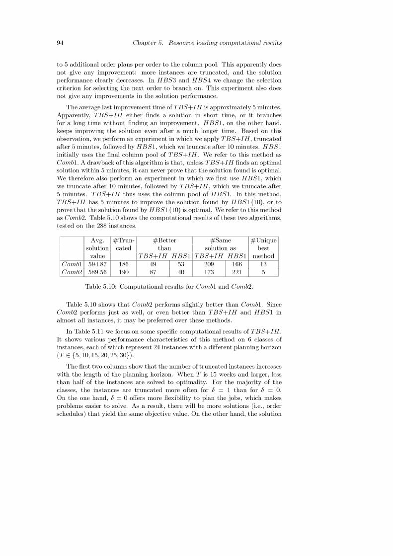
94 Chapter 5. Resource loading computational results
to 5 additional order plans per order to the column pool. This apparently doesnot give any improvement: more instances are truncated, and the solutionperformance clearly decreases. In HBS3 and HBS4 we change the selectioncriterion for selecting the next order to branch on. This experiment also doesnot give any improvements in the solution performance.
The average last improvement time of TBS+IH is approximately 5minutes.Apparently, TBS+IH either finds a solution in short time, or it branchesfor a long time without finding an improvement. HBS1, on the other hand,keeps improving the solution even after a much longer time. Based on thisobservation, we perform an experiment in which we apply TBS+IH, truncatedafter 5minutes, followed by HBS1, which we truncate after 10 minutes. HBS1initially uses the final column pool of TBS+IH. We refer to this method asComb1. A drawback of this algorithm is that, unless TBS+IH finds an optimalsolution within 5 minutes, it can never prove that the solution found is optimal.We therefore also perform an experiment in which we first use HBS1, whichwe truncate after 10 minutes, followed by TBS+IH, which we truncate after5 minutes. TBS+IH thus uses the column pool of HBS1. In this method,TBS+IH has 5 minutes to improve the solution found by HBS1 (10), or toprove that the solution found byHBS1 (10) is optimal. We refer to this methodas Comb2. Table 5.10 shows the computational results of these two algorithms,tested on the 288 instances.
Avg. #Trun- #Better #Same #Uniquesolution cated than solution as bestvalue TBS+IH HBS1 TBS+IH HBS1 method
Comb1 594.87 186 49 53 209 166 13Comb2 589.56 190 87 40 173 221 5
Table 5.10: Computational results for Comb1 and Comb2.
Table 5.10 shows that Comb2 performs slightly better than Comb1. SinceComb2 performs just as well, or even better than TBS+IH and HBS1 inalmost all instances, it may be preferred over these methods.
In Table 5.11 we focus on some specific computational results of TBS+IH.It shows various performance characteristics of this method on 6 classes ofinstances, each of which represent 24 instances with a different planning horizon(T ∈ {5,10, 15, 20, 25, 30}).
The first two columns show that the number of truncated instances increaseswith the length of the planning horizon. When T is 15 weeks and larger, lessthan half of the instances are solved to optimality. For the majority of theclasses, the instances are truncated more often for δ = 1 than for δ = 0.On the one hand, δ = 0 offers more flexibility to plan the jobs, which makesproblems easier to solve. As a result, there will be more solutions (i.e., orderschedules) that yield the same objective value. On the other hand, the solution

5.4. Preliminary test results 95
#Trun- Avg. Avg. Avg.cated #nodesa #cutsa tree deptha
T δ=0 1 0 1 0 1 0 15 1 0 190898 - 134878 - 37.0 -10 13 10 115426 109469 85857 70769 29.4 28.115 17 20 56268 59371 42323 40137 40.4 39.420 19 23 30826 40006 23181 27637 54.0 46.025 21 24 17505 20810 13338 14695 58.1 47.830 22 23 10380 14321 8067 10180 60.8 52.1
aThese results only concern the instances that were truncated.
Table 5.11: Computational results for TBS+IH.
space becomes larger, so more branching is required. Table 5.11 shows that theformer effect dominates the latter.
The average number of nodes that are explored generally decreases with T .This may be expected since the problem size (as well as the LP ) increases withT . For δ = 1 more nodes are cut off. As a result, the number of nodes thatare explored for δ = 0 is usually fewer than for δ = 1. Approximately 70% ofall nodes are cut off (i.e., fathomed or pruned), regardless of the length of theplanning horizon.
The average maximum tree depth significantly increases with the length ofthe planning horizon. The table shows that when the tree depth is too large,although good solutions may have been found, it becomes impossible to provethat the solution is optimal within 30 minutes. The average tree depth issignificantly smaller for the instances that are solved to optimality, althoughin a small number of instances the optimal solution is found even though thetree depth is large (i.e., up to 61).
The computational results of all methods together show that in 229 in-stances out of 288, the branching methods either improved the best heuristicsolution, or proved that it is optimal. This clearly demonstrates the contri-bution of the branching methods. We performed an experiment to analyze theimportance of using heuristics in the root node, for the performance of thebranching methods. For this purpose we tested a variant of TBS+IH in whichwe do not use EDD to initialize the RLP . Instead we start from an arbitrarysolution, which may not be feasible. Furthermore, in this algorithm we donot use the various rounding heuristics and IH before branching. The resultsshowed that this method finds a worse solution than TBS+IH in 211 out of the288 instances, and a better solution in 3 instances. The average solution foundby this method is 865.24, which is much larger than the average of 597.05 forTBS+IH. Finally, the method without the heuristics is also truncated moreoften: in 211 versus 193 instances. We conclude that the use of heuristics in
96 Chapter 5. Resource loading computational results
the root node clearly pays off.
The branching methods together solve 116 instances out of 288 to optimal-ity. For the remaining 172 instances we perform an additional experiment, inwhich we use TBS+IH and the best solution found this far as an initial upperbound. In this experiment, only for one instance optimality is proven. Forthe remaining 171 instances we use EAS(ε) to determine the size of the gapbetween the optimal solution and the best solution found. EAS (0.05) deter-mines that for 12 instances the gap is at most 5%, and EAS (0.1) determinesthat for 8 instances the gap is at most 10%. For the remaining 151 instanceswe are not able to prove within 30 minutes that the gap is less than 10%.
5.4.3 Conclusions and algorithm selection
In Section 5.4.2 we showed that the best branching strategy with respect to thesolution values is the HBS1 strategy. The biggest drawback of this methodis that it is an incomplete branching strategy. Hence, unless there is no gapbetween the LP lower bound and the best solution value found, it can not beproven that the solution that is found by HBS1 is optimal. The TBS+IHmethod is the best complete branching strategy. The best algorithm is Comb2,which combines the computational effectiveness of HBS1 with the possibil-ity (of TBS+IH) to prove optimality, while the computation times are stillacceptable. We thus use Comb2 for the remaining computational experiments.
The preliminary results show that the larger the number of machine groupsin the instances, the harder the instances are to solve. When the number ofmachine groups is smaller, there is more planning flexibility. Also, the smallerthe number of orders in the instances, the harder the instances are to solve. Forexample, the computational results (not mentioned in the previous sections)show that for the instances with λ = 0.5, 26 instances out of 96 are solved tooptimality, as opposed to 32 instances for λ = 1, and 58 instances for λ = 2.When there are more orders (and jobs) in an instance, the proportional sizeof the jobs is smaller with respect to the machine group capacity. As a result,there is more flexibility to plan the jobs. This is underlined by the fact thatfor 53 instances out of the 58 instances that are solved to optimality for λ = 2there is no gap between the LP lower bound and the optimal solution value.For λ = 0.5, there is no gap between the LP lower bound and the optimalsolution for only 9 instances out of the 26 that are solved to optimality. Ofcourse, the larger n, the larger the LP model will become. As a result, whenλ is increased further, the instances will eventually become harder to solve.
Based on the preliminary results we generate a class of instances with λ =1, m = 5 and T ∈ {5,10,15,20,25,30}. This class appears to be the mostinteresting of the instance classes: the instances are not too easy, and not toodifficult. In Section 5.5 we perform various analyses to determine how sensitiveComb2 is to various parameter settings.

5.5. Sensitivity analyses 97
5.5 Sensitivity analyses
In this section we present the results of various sensitivity analyses on variousparameters in the test instances. Unless noted otherwise, the experiments areperformed on a class of instances with λ = 1 andm = 5, which is determined byrepeatedly simulating an order arrival process. The class contains 120 instances,i.e., 20 instances for each value of T (T ∈ {5, 10, 15, 20,25,30}). In conjunctionwith the test instances, we generate two feasible order plans (i.e., for δ = 0and δ = 1) for each order in each test instance, to form the initial RLP for abranch-and-price algorithm. For this purpose we use the EDD heuristic.
When we solve an instance for δ = 0, we allow only two jobs of the sameorder to be produced in the same week, i.e., we set κ = 2.
5.5.1 Length of the planning horizon
Table 5.12 displays the computational results of the Comb2 method. The re-sults are divided into 6 categories, one for each value of T (T ∈ {5,10,15,20,25,30}). Each category thus contains 20 instances that are solved for both δ = 0(and κ = 2) and δ = 1.
#Optimal Avg. #nodesa Avg. #cutsa Avg. tree depthT δ=0 1 0 1 0 1 0 15 19 20 49684 - 33533 - 2.3 4.810 14 13 183988 143738 127801 94623 11.2 15.715 7 2 154986 233463 103510 156342 24.1 28.720 2 0 91833 108364 67057 73913 45.6 40.025 2 0 39923 39375 28153 27588 55.6 44.630 0 0 22792 19233 15355 13084 61.9 43.7
aThese results only concern the instances that were truncated.
Table 5.12: Computational results for various T .
From Table 5.12 we may draw the same conclusions as from Table 5.11 inSection 5.4.2: the complexity of the instances increases with the length of theplanning horizon. The model size increases with T , and as a result, the requiredCPU-time to optimize the LP in each node increases as well. The number ofnodes that are explored thus decreases with T . Also, the larger the problembecomes, the more violated precedence relations must be repaired. Table 5.12indeed shows that the average tree depth increases with T .
Table 5.12 shows that in general, instances with a planning horizon of up to10 weeks, and some instances with a planning horizon of 15 weeks can be solvedto optimality. Instances with a larger planning horizon are usually truncated.Note that it is questionable whether in practice, resource loading problems

98 Chapter 5. Resource loading computational results
with a planning horizon of more than 10 weeks are very relevant. The longerthe planning horizon, the less accurate the problem data may become, sincedisturbances in the production process may occur, or, more likely, changes inthe demand requirements may occur. Hence, from a practical point of view, aplanning horizon of 10 weeks is quite large, and solving instances with a largerplanning horizon is more a mathematical challenge.
Since all instances with a planning horizon of 30 weeks are truncated, weperform an additional experiment to determine if splitting up the planninghorizon in three, and solving the three ‘easier’ subproblems instead, will im-prove the overall solution. In other words, in this experiment we split up theproblems with T = 30 in three subproblems, and compare the solution valueof the problem with T = 30 to the sum of the solution values of the 3 sub-problems. When the interval in which a job Bbj is allowed to be produced (i.e.,{rbj , dbj}) falls partly inside the planning horizon of one of the subproblems, weonly consider that job in the subproblem if at least half of the interval {rbj , dbj}falls inside its planning horizon. Table 5.13 and 5.14 display the computationalresults of this experiment.
#Trun- Avg. Avg. #Bestcated solution CPU-time solution
value (sec.)T δ=0 1 0 1 0 1 0 130 20 20 588.6 932.1 900 900 12 11
3× 10 9a 17a 897.1 1013.7 496 1086 8 9
aThis is the number of times that at least one of the subproblems was truncated.
Table 5.13: Computational results for splitting up the planning horizon of 30weeks in three (1).
Avg. Avg. Avg. sub-operator hiring contracting
overtime (hrs.) (hrs.) (hrs.)T 0 1 0 1 0 130 421.3 584.9 75.5 140.0 5.5 22.4
3× 10 368.0 423.6 175.4 189.9 59.5 70.2
Table 5.14: Computational results for splitting up the planning horizon of 30weeks in three (2).
Note that splitting up the planning horizon reduces the planning flexibilityof the jobs. Nevertheless, Table 5.13 shows that the sum of the solution valuesof the 3 subproblems is smaller than the solution value found for the entireproblem in nearly 50% of the instances. This demonstrates that it is useful totry to solve the problems to optimality. If we would use overlapping periods

5.5. Sensitivity analyses 99
of 10 weeks, some planning flexibility can be regained. This is a more realisticapproach, which will likely yield even better solutions. The challenge of thisapproach is how to connect the solutions for the overlapping periods, and makethem consistent. This experiment is subject of further research.
5.5.2 Number of machine groups
Table 5.15 shows the computational results of four classes of instances, eachcontaining 60 instances with a different number of machine groups m (m ∈{3, 5, 7,10}). We solve each instance for δ = 0 and δ = 1. In the table wecompare the number of times the instances are solved to optimality, and theuse of nonregular machine group and operator capacity.
#Proven Avg. Avg. Avg. non- Avg. sub-optimal operator regular time regular time contracting
overtime (hrs.) hiring (hrs.) hiring (hrs.) (hrs.)m δ=0 1 0 1 0 1 0 1 0 13 45 30 214.0 253.4 1.7 3.8 15.3 38.1 3.5 4.95 30 19 223.1 331.9 0.0 1.3 11.9 42.6 1.3 4.77 12 12 303.3 362.4 1.0 0.5 44.5 102.7 8.4 40.910 10 11 380.6 419.0 0.0 0.2 51.4 140.7 36.0 123.7
Table 5.15: Sensitivity analysis of m.
The table shows that the larger the number of machine groups, the moredifficult it becomes to solve the instances to optimality. The larger m, thelarger the jobs are relative to the machine group capacity. As a result, there isless flexibility to plan the jobs. For the same reason, also the use of nonregularmachine group capacity increases. The increase in the use of machine groupcapacity in nonregular operator time is apparent in Table 5.15 from the increasein the use of operator overtime, and the use of hiring capacity in nonregularoperator time. Also the use of subcontracting clearly increases. For δ = 0 thereis more planning flexibility, and the machine group capacity can therefore beutilized more efficiently. As a result, the required nonregular operator andmachine group capacity is lower for δ = 0 in all instances.
We conclude that in general, instances with 3 machine groups, and a largepart of the instances with 5 machine groups can be solved to optimality. In theinstance generation procedure, jobs are assigned to machine groups randomly.As a result, there is no clear bottleneck. Instead, the instance generation pro-cedure makes that in fact all machine groups may have capacity problems, andform bottlenecks. It is likely that in practical situations, only a few machinegroups are bottlenecks. It is likely that such problems, with, e.g., more than 5machine groups, of which only a few (e.g., 3) are bottlenecks, are computation-ally easier than when all the machine groups are bottlenecks. This experiment

100 Chapter 5. Resource loading computational results
is subject of further research.
5.5.3 Operator capacity
In this section we analyze various regular operator capacity profiles. We solvethe 120 instances for both δ = 0 and δ = 1. In Table 5.16 we compare thecomputational results for these instances with various regular operator capacityprofiles. The first row corresponds to the experiment where the regular operatorcapacity per week is 0.7
∑i
Qi. In the second and third row the regular operator
capacity per week is 0.8∑iQi and
∑iQi respectively. This corresponds to
operator utilization rates 140%, 125% and 100% respectively. Observe thatincreasing the operator capacity per week to more than
∑iQi by definition
makes no sense, since the machine groups can not handle more workload than∑i
Qi in regular time. We note that the average sum of the processing times of
the jobs in the instances is approximately 3220 hours, i.e., on average:∑iQi ≈
3220.
Operator # Avg. Avg. Avg. Avg. Avg.capacity Proven solution operator regular nonregular subcon-per week optimal value overtime time hiring time hiring tracting
(hrs.) (hrs.) (hrs.) (hrs.)ct δ=0 1 0 1 0 1 0 1 0 1 0 1
0.7∑i
Qi 57 42 444.8 613.4 345.8 383.7 5.5 3.1 38.1 85.3 3.9 17.6
0.8∑iQi 44 35 263.4 439.6 209.2 299.4 0.2 1.4 23.7 52.6 2.1 10.8∑
i
Qi 35 32 132.8 291.0 112.3 201.0 0.0 0.0 9.4 36.5 0.6 5.7
Table 5.16: Sensitivity analysis of the operator capacity profile.
Table 5.16 shows that the number of instances that are solved to opti-mality decreases when the available regular operator capacity increases. Theadditional operator capacity on the one hand increases the planning flexibility,which should make the instances easier to solve. On the other hand, the sizeof the solution space also increases, which makes it harder to prove optimality.Since the nonregular capacity usage is much lower for the class of instanceswith the highest operator capacity, from a practical point of view, provingoptimality does not yield much.
As may be expected, the use of nonregular capacity decreases when theavailable regular operator capacity increases. This is most visible for the av-erage required operator overtime capacity: the machine groups can be utilizedmore in regular time, and as a result, less overtime work is required.

5.5. Sensitivity analyses 101
For δ = 0 there is more planning flexibility, and the operator capacitycan therefore be utilized more efficiently. As a result, the required nonregularoperator and machine group capacity is lower for δ = 0 in almost all instances.
5.5.4 Machine group capacity
Similar to the sensitivity analysis of the regular operator capacity profiles, inthis section we analyze various regular machine group capacity profiles. Table5.17 shows the computational results for three machine group capacity profiles.The first row corresponds to the experiment where the machine group capacityfor machine group Mi (i = 1, . . . ,m) in regular operator time per week mcitis 0.8Qi, and the total machine group capacity per week mcit is Qi. Thiscorresponds to a utilization rate of 125% for the machine group capacity inregular time, and a utilization rate of 100% for the total machine group capacity.The second row corresponds to the experiment in which the utilization ratesare 100% and 80% respectively. Finally, the third row corresponds to theexperiment in which the utilization rates are 80% and 60% respectively. Theoperator capacity per week ct in each row is 0.8
∑iQi. Each row corresponds
to 120 instances, which are solved for both δ = 0 and δ = 1.
Machine # Avg. Avg. Avg. Avg. Avg.group Proven solution operator regular nonregular subcon-
capacity optimal value overtime time hiring time hiring tractingper week (hrs.) (hrs.) (hrs.) (hrs.)
mcit mcit δ=0 1 0 1 0 1 0 1 0 1 0 10.8Qi Qi 25 30 420.1 659.9 307.2 367.6 0.3 0.0 39.1 90.2 11.3 37.3Qi 1.25Qi 44 35 263.4 439.6 209.2 299.4 0.2 1.4 23.7 52.6 2.1 10.8
1.25Qi 1.66Qi 79 60 200.5 316.8 163.3 228.9 4.2 4.7 13.4 31.8 0.7 5.0
Table 5.17: Sensitivity analysis of machine capacity profiles.
Table 5.17 shows that the number of instances that are solved to optimalityincreases with the machine group capacity. In the previous section we observedthe opposite effect with respect to the operator capacity. Since we assume thatoperators are generic, the solution space increases more when we increase theoperator capacity than when we increase the machine group capacity. Appar-ently with respect to machine group capacity this does not make it harder toprove optimality.
From a practical point of view, a production system where the machinegroup capacity utilization in regular time is 125%, is overloaded, which is notunusual. As may be expected, the average solution value clearly decreases withthe increase of machine group capacity. Also the use of nonregular machinegroup capacity and operator capacity decreases when the machine group ca-pacity increases. We note that the impact of increasing the machine group

102 Chapter 5. Resource loading computational results
capacity on the average solution value is generally smaller than the impact ofincreasing the operator capacity.
5.5.5 Internal slack of an order
In this section we analyze the relation between the average slack of the in-stances, and the solution performance. The average slack of an instance is
calculated as:∑
jkj
n, where kj is the slack of order Jj . We generated 100 in-
stances with λ = 1, T = 10 and m = 5, calculated their average slack, andcategorized the computational results of the instances in Table 5.18.
Average # %Proven Avg.slack Cases optimal treedepth
(range)δ=0 1 0 1 0 1
[1, 2) 0 31 - 51.6 - 12.5[2, 3) 20 53 65.0 45.3 5.4 6.3[3, 4) 50 15 66.0 53.3 4.7 0.0[4, 5) 27 1 66.7 100 2.8 1.0[5, 6) 3 0 66.7 - 0.0 -
Table 5.18: Sensitivity analysis of the average slack of jobs.
Per definition, the average slack is larger for the instances with δ = 0.Table 5.18 shows that there is no relation between the slack and the number ofinstances solved to optimality. Hence, the increase in planning flexibility doesnot make it harder to prove optimality.
5.5.6 Nonregular capacity cost parameters
In this section we analyze the nonregular capacity cost parameters. Table 5.19shows the computational results of 3 different settings of the cost parameters(o, h, s
): (1,1,1), (1, 2,3) and (1, 2,10) respectively. Table 5.19 shows that for
Cost #Proven Avg. Avg. Avg. non- Avg. sub-para- optimal operator regular time regular time contractingmeters overtime (hrs.) hiring (hrs.) hiring (hrs.) (hrs.)o h s δ=0 1 0 1 0 1 0 1 0 11 1 1 49 36 0.0 0.2 0.0 0.0 0.0 0.3 230.4 378.11 2 3 44 35 209.2 299.4 0.2 1.4 23.7 52.6 2.1 10.81 2 10 45 35 204.0 282.7 1.2 1.7 23.1 56.6 1.6 8.7
Table 5.19: Sensitivity analysis of the nonregular capacity cost parameters.
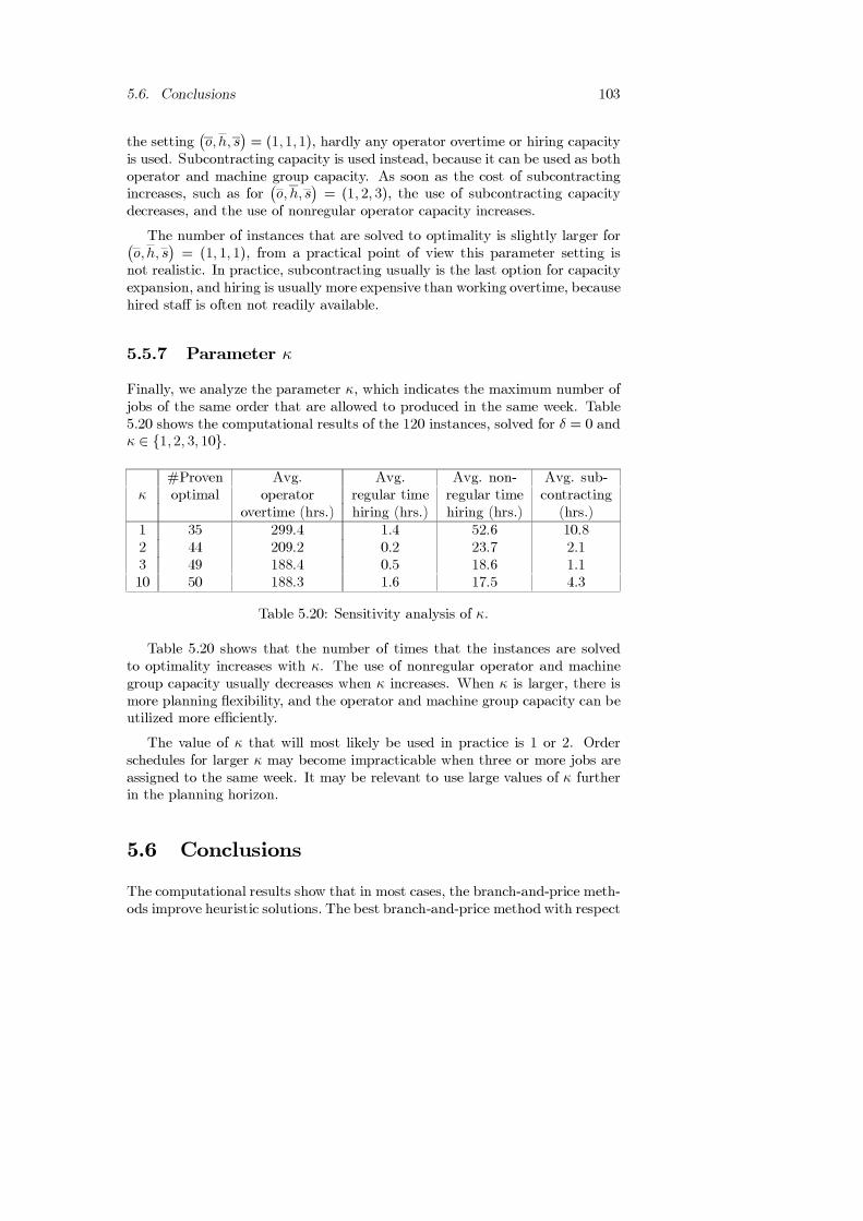
5.6. Conclusions 103
the setting(o,h, s
)= (1,1,1), hardly any operator overtime or hiring capacity
is used. Subcontracting capacity is used instead, because it can be used as bothoperator and machine group capacity. As soon as the cost of subcontractingincreases, such as for
(o, h, s
)= (1, 2, 3), the use of subcontracting capacity
decreases, and the use of nonregular operator capacity increases.
The number of instances that are solved to optimality is slightly larger for(o,h, s
)= (1, 1, 1), from a practical point of view this parameter setting is
not realistic. In practice, subcontracting usually is the last option for capacityexpansion, and hiring is usually more expensive than working overtime, becausehired staff is often not readily available.
5.5.7 Parameter κ
Finally, we analyze the parameter κ, which indicates the maximum number ofjobs of the same order that are allowed to produced in the same week. Table5.20 shows the computational results of the 120 instances, solved for δ = 0 andκ ∈ {1,2, 3, 10}.
#Proven Avg. Avg. Avg. non- Avg. sub-κ optimal operator regular time regular time contracting
overtime (hrs.) hiring (hrs.) hiring (hrs.) (hrs.)1 35 299.4 1.4 52.6 10.82 44 209.2 0.2 23.7 2.13 49 188.4 0.5 18.6 1.110 50 188.3 1.6 17.5 4.3
Table 5.20: Sensitivity analysis of κ.
Table 5.20 shows that the number of times that the instances are solvedto optimality increases with κ. The use of nonregular operator and machinegroup capacity usually decreases when κ increases. When κ is larger, there ismore planning flexibility, and the operator and machine group capacity can beutilized more efficiently.
The value of κ that will most likely be used in practice is 1 or 2. Orderschedules for larger κ may become impracticable when three or more jobs areassigned to the same week. It may be relevant to use large values of κ furtherin the planning horizon.
5.6 Conclusions
The computational results show that in most cases, the branch-and-price meth-ods improve heuristic solutions. The best branch-and-price method with respect

104 Chapter 5. Resource loading computational results
to the solution performance is Comb2. It embeds the best characteristics ofHBS1 and TBS+IH. HBS1 is a fast branching method, which improves thesolution value even after a longer branching time than the other branchingmethods. TBS+IH typically either improves the solution value within shorttime (and/or proves that the solution found is optimal), or it branches for along time. The computational results show that Comb2 clearly outperforms theother branch-and-price methods. Also, with respect to solution performance,the branch-and-price methods also clearly outperform the heuristics. Only theheuristic IH has a satisfactory performance.
One of the objectives of this thesis is to provide algorithms that can solveresource loading problems of a size that is typically encountered in practice.The most important parameters that determine whether an instance can besolved to optimality are T and m. The computational results show that, ingeneral, instances with a planning horizon of up to 10 weeks, and some instanceswith a planning horizon of 15 weeks can be solved to optimality. Furthermore,most instances with 3 machine groups and a large part of the instances with 5machine groups can be solved to optimality. In Section 5.5.2 we argued that theinstance generation procedure makes that in the resource loading instances allmachine groups form bottlenecks. We conclude that with the aforementionedparameter settings, even large size resource loading problems can be solved tooptimality. From a practical point of view, using a longer planning horizon(than 10 weeks) hardly makes sense, because the longer the planning horizon,the less accurate the problem data may become (see Section 5.5.1). It maybe a mathematical challenge to solve instances with a larger planning horizon.For this purpose we suggest further research into methods that use a rollinghorizon approach (see Section 5.5.1).

105
Chapter 6
Rough Cut Capacity
Planning
Every fact that is learnedbecomes a key to other facts.
- Edward L. Youmans (1821-1887)
6.1 Introduction
In Section 1.3.2 we introduced Multi-Project Rough-Cut Capacity Planning(RCCP) in project management as an analogue of resource loading in make-to-order production planning. In this chapter we show that with some modifi-cations we can use the algorithms for resource loading (see Chapter 4) to solveRCCP problems.
We use basically the same integer linear programming model (presented inSection 3.6) to formulate RCCP problems, but the terminology is somewhatdifferent. In the context of project management, we speak of projects subdi-vided into activities , rather than orders that consist of jobs. While in resourceloading both machine capacity and operator capacity is required simultane-ously to produce a job, in RCCP each activity is performed by one or more(renewable) resources. Typical resources in RCCP are labor, machines, equip-ment, space, and so on. We introduce parameter υbji to indicate the fractionof activity Bbj of project Jj that is performed on resource Mi (i = 1, . . . ,m).This yields the following ILP model for RCCP:
ILP : z∗ILP = min sT∑
t=0
m∑i=1
Sit +n∑
j=1
∑π∈Πj
ρjπXjπθ, (6.1)

106 Chapter 6. Rough Cut Capacity Planning
subject to:
∑π∈Πj
Xjπ = 1 (∀j) , (6.2)
Ybjt −
∑π∈Πj
abjtπXjπ
wbj≤ 0 (∀b, j, t) , (6.3)
T∑t=rj
Ybjt = 1 (∀b, j) , (6.4)
n∑j=1
nj∑b=1
pbjυbjiYbjt ≤ mcit + Sit (∀i, t) , (6.5)
m∑i=1
Sit ≤ st (∀i, t) , (6.6)
all variables ≥ 0, (6.7)
Xjπ ∈ {0, 1} (∀j, π ∈ Πj ⊂ Π). (6.8)
The objective function (6.1) minimizes the outsourcing costs and the total tar-diness penalty costs. Constraints (6.2), (6.3) and (6.6)-(6.8) are the same as inthe resource loading model ILP . Constraints (6.5) are the capacity restrictionsfor the resources. The term pbjυbjiYbjt in (6.5) is the number of hours thatactivity Bbj is performed on resource Mi in week t. Hence, the left hand side of(6.5) is the total workload assigned to resource Mi in week t. The right handside of (6.5) is the sum of the total resource capacity in week t (mcit) and thesubcontracting capacity Sit.
Note that the constraints that provide the duals for the pricing problem inresource loading are still embedded in the ILP for RCCP. In fact, the onlyalgorithmic implications are the generalized precedence relations in RCCP (seeSection 1.3.2), which have to be accounted for in the pricing algorithm, asopposed to the linear precedence relations in resource loading. We thereforeuse a generalization (with respect to the precedence relations) of the pricingalgorithm of Section 4.3.1 to solve RCCP problems with the branch-and-pricetechniques presented in Chapter 4, as well as two other pricing algorithms.
The outline of this chapter is as follows. In Section 6.2 we present threepricing algorithms for RCCP problems. In Section 6.3 we discuss the modifi-cations of the branching strategy, when we use the branch-and-price algorithmpresented in Chapter 4 to solve a RCCP problem. We conclude this chapterwith Section 6.4, where we discuss various existing heuristics for RCCP.

6.2. Pricing algorithm 107
1
2
3
4
5 6
7
8
9 10
Figure 6.1: Example project with 10 activities.
6.2 Pricing algorithm
In this section we describe three pricing algorithms for finding project plans (inRCCP terminology we refer to an order plan as a project plan) with negativereduced costs. As in Section 4.3, the pricing problem can be subdivided into nindependent subproblems, i.e., one for each project Jj (j = 1, . . . , n).
The outline of this section is as follows. In Section 6.2.1 we describe a pricingalgorithm that accounts for generalized precedence relations. It is based on aforward dynamic programming (DP) approach, which is in fact a generalizationof the algorithm of Section 4.3.1. The generalized DP has a multi-dimensionalstate space. For larger instances this may lead to computational problems, andtherefore we try to improve the DP based algorithm. In Section 6.2.2 we discussvarious ways to speed up the DP based algorithm. Furthermore, we present twoalternative ways to solve pricing problems. In Section 6.2.3 we discuss a mixedinteger linear programming based pricing algorithm, and in Section 6.2.4 wediscuss a heuristic pricing algorithm. In Section 6.2.5 we conclude this sectionwith a discussion on how to use a combination of exact pricing algorithms andheuristics to solve a pricing problem.
6.2.1 Pricing by dynamic programming
The generalized precedence constraints mainly influence the stages and thestate space. Recall that in the DP algorithm of Section 4.3.1 each job repre-sents a stage, and the state describes the completion time of a job. In Chapter4, stages were naturally introduced since all jobs must be performed subse-quently. This is no longer the case with generalized precedence constraints. Inparticular, several activities may be performed (partially) in parallel. This isbest illustrated by an example. Consider a project with 10 activities. Figure6.1 displays an acyclic directed graph representation of the precedence relationsof the activities. Suppose (just as in Section 4.3.1) we would let each activity

108 Chapter 6. Rough Cut Capacity Planning
stage 1 stage 2 stage 3 stage 4 stage 5 stage 6
1
2
3
4
5 6
7
8
9 10
Figure 6.2: Example project with 10 activities and 6 stages.
represent a stage, and let each state describe the completion time of an activ-ity in that state. In stage 2, the optimal decision for activity 2 (concerning itsstart time) restricts the completion time of activity 1 in stage 1. Since activity3 in stage 3 may only start after activity 1 is completed (just like activity 2),the optimal decision concerning the start time of activity 3 in stage 3 dependson the previously chosen decision in stage 2. This conflicts with the principleof optimality for DP, which states that in each stage, the optimal decision foreach of the remaining stages must not depend on previously reached states orpreviously chosen decisions (see Section 2.5). Hence the optimal decision foractivity 3 can not be made. We conclude that we must redefine stages andstates in the case of generalized precedence relations.
To define decisions and states properly, we first determine which activitiesshould be considered in each stage. Hereby we basically have to take intoaccount that an activity and its successors may never be in the same stagetogether. There are several ways to achieve this. We form the stages as follows.The activities that have no successors form the last stage (stage Γ). For theremaining activities we determine the length of the longest path to any ofthe activities in the final stage, where the length is defined as the number ofactivities on the path. Subsequently, we form the other stages by activities thathave the same longest distance to the last stage. This guarantees that a (notnecessarily immediate) successor of an activity is always in a later stage. Hence,the stage with the longest distance (distance Γ−1) is numbered as stage 1. Werefer to the activities of stage Γ as BΓ (Γ = 1, . . . ,Γ). The example precedencegraph in Figure 6.2 shows this for the aforementioned example project with 10activities in 6 stages. The 6 stages are formed by activity sets B1 = {B1j},B2 = {B2j ,B3j}, B3 = {B4j, B5j}, B4 = {B6j, B7j}, B5 = {B8j ,B9j} andB6 = {B10,j}.
With the aforementioned definition of stages, the decision that is to betaken for the activities in each stage concerns either the start times or the

6.2. Pricing algorithm 109
completion times of the activities of project Jj. Since the problem is symmetricwith respect to that decision, we choose that the decision xΓ in stage Γ definesthe starting times xΓb of the activities Bbj ∈ BΓ in that stage, i.e., xΓ ={xΓb|Bbj ∈ BΓ}. In forward dynamic programming, the decision xΓ describeshow state iΓ−1 in stage Γ − 1 is transformed into a state iΓ in stage Γ. Themaximum completion time of an activity follows directly from the earliest starttime of its successors. A decision xΓ in stage Γ determines the maximumcompletion times of all immediate predecessors of the activities BΓ in stageΓ. Note that these predecessors are not necessarily activities in stage Γ − 1,but these may also be activities from a stage before Γ− 1 (e.g., in Figure 6.2,activity 1 from stage 1, and activities 4 and 5 from stage 3 are predecessorsof stage 4). Accordingly, we form a state iΓ−1 by the maximum completiontimes iΓ−1,b of all activities Bbj in or before stage Γ− 1, that have a successorin stage Γ or in a stage after Γ. We denote this set of activities as B+
Γ . Weillustrate this with the aforementioned example project in Figure 6.2. The 6states are formed as follows: i1 = {i11}, i2 = {i21, i22, i23}, i3 = {i31, i34, i35},i4 = {i44, i46, i47}, i5 = {i58, i59} and i6 = {i6,10}. Hence, B+
1 = {B1j},B+
2 = {B1j, B2j, B3j}, B+3 = {B1j ,B4j ,B5j}, B+
4 = {B4j, B6j, B7j}, B+5 =
{B8j, B9j}, and B+6 = {B10,j}. Note that we included the completion time
of activity B4j in state i4 of stage 4. Activity B4j has immediate successorsin stage 4 (i.e., activity B6j) as well as in stage 5 (i.e., activity B8j). If wewould not include the completion time of activity B4j in state i4, we could notmake an optimal decision for activity B6j. Namely, this decision determinesthe completion time of activity B4j , which in turn determines the decision foractivity B8j . This would imply that in stage 5, the optimal decision woulddepend on the decision made in stage 4, and would conflict with the principleof optimality for DP. Consequently, we include the completion time of activityB4j in state i4 of stage 4, to be able to make an optimal decision in stage 5 thatdoes not depend on the decision in stage 4. Analogously, due to the precedencerelation between activity B1j and B7j we must include the completion time ofactivity B1j in the states of stages 2 and 3.
Let ajπ be a (partial) project plan for project Jj in stage Γ and state iΓ ={iΓb|Bbj ∈ B+
Γ
}with value Fj(iΓ). Then ajπ must allow activities Bbj ∈ BΓ
of project Jj to be performed in weeks xΓb, . . . , iΓb for some rbj ≤ xΓb ≤iΓb −wbj +1. Accordingly, the previous state iΓ−1 =
{iΓ−1,b|Bbj ∈ B+
Γ
}must
be defined as follows. When activity Bbj ∈ BΓ−1 has a successor in a stageafter Γ, we have that iΓ−1,b = iΓb. Otherwise, when activity Bbj ∈ BΓ−1 onlyhas successors in stage Γ, we have that iΓ−1,b = min
s∈DSbj∩BΓ
xΓs−δ, where DSbj
are the immediate successors of activity Bbj of project Jj . Hence in this casethe completion time of the activity is equal to the earliest start time of itssuccessors, minus δ to comply with the one activity per week policy. We thus

110 Chapter 6. Rough Cut Capacity Planning
have that:
iΓ−1 ={iΓ−1,b|Bbj ∈ B+
Γ
}, where: (6.9)
iΓ−1,b =
{iΓb, if iΓb ∈ iΓ,
mins∈DSbj∩BΓ
xΓs − δ, otherwise.
Allowing activity Bbj to be performed in the weeks xΓb, . . . , iΓb contributes
−iΓb∑
u=xΓb
βbju to the reduced cost of the project plan. We now give the dynamic
programming recursion to solve the j-th subproblem. The initialization is:
Fj(iΓ) =
{αj, if Γ = 0,∞, otherwise.
The recursion for Γ = 1, . . . ,Γ is then as follows. If ∀Bbj ∈ BΓ, rbj +wbj −1 ≤iΓb ≤ dbj :
Fj(iΓ) = minrbj≤xΓb≤iΓb−wbj+1
Bbj∈BΓ
Fj(iΓ−1) +∑
Bbj∈BΓ
∆bjiΓb−
∑Bbj∈BΓ
iΓb∑u=xΓb
βbju
,
(6.10)otherwise:
Fj(iΓ) = ∞.
Where iΓ−1 in (6.10) is defined as in (6.9), and:
∆bjt =
{(t − dbj)θbj , if t > dbj0, otherwise.
Parameter θbj = θ, when tardiness of activity Bbj must be penalized (forexample when the completion time of this activity is considered as a projectmilestone), and θbj = 0 for activities that are allowed to be tardy without apenalty cost. Parameter ∆bjt thus adds a tardiness penalty to Fj(iΓ).
Lemma 6.1 The optimal solution to the j-th pricing subproblem is found as:
F ∗j = min
dj≤t≤dj
Fj(iΓ), (j = 1, . . . , n).
�
Accordingly, if F ∗ = min1≤j≤n
F ∗j ≥ 0, then the current RLP solution is opti-
mal. If F∗ < 0, then the current RLP solution is not optimal, and we need tointroduce new columns (project plans) to the problem. Candidates are associ-ated with those projects Jj for which F∗
j < 0, and they can be found by back-tracking. The pricing algorithm for the j-th subproblem uses O(njT
ω) space,

6.2. Pricing algorithm 111
stage 1 stage 2 stage 3 stage 4 stage 5 stage 6
1
2
3
4
5 6
7
8
9 10
Figure 6.3: Example project with redundant activities.
where ω is the maximum number of activities in all states, i.e., ω = maxΓ
∣∣B+Γ
∣∣.The pricing algorithm can be solved in O(njT
2ω) time. As can be expected, thispricing algorithm requires significantly more computation time than the pricingalgorithms in Section 4.3 for instances of a similar size. This is mainly due tothe increase in the number of possible states in each stage. In the next sectionwe discuss some methods that significantly speed up the pricing algorithm.
6.2.2 Pricing algorithm speed up
In a pricing problem, there may be activities Bbj for which βbjt = 0 (∀t) andθbj = 0. Such activities will never contribute to the objective function of thepricing problem. We refer to these activities as redundant activities. Recallthat in each iteration of a column generation scheme a project plan is addedto the RLP , thereby introducing new possibilities to plan the activities. As aresult, typically after a number of column generation iterations the number ofredundant activities increases. We show that without affecting the solution wemay eliminate some redundant activities from the pricing problem and herebyreduce the problem size. We illustrate this with the example project fromSection 6.2.1 with 10 activities and 6 stages. Suppose in a certain columngeneration iteration the activities {1, 2,3,4, 6, 10} are redundant. We havemarked the redundant activities by a cross in Figure 6.3. We distinguish 3types of redundant activities:
1. Redundant activities to which there is no path from a non-redundant ac-tivity. These can be planned as early as possible. In the example projectthese are activities {1, 2, 3,4}.
2. Redundant activities from which there is no path to a non-redundant ac-tivity (activity 10 in the example project). These can be planned in

112 Chapter 6. Rough Cut Capacity Planning
5 6
7
9 8
stage 1 stage 3 stage 1stage 2
Figure 6.4: Subnetworks after eliminating redundant activities.
the project plan as late as possible. Note that such redundant activitiesdo not exist when the lateness of activities at the end of the project ispenalized.
3. The remaining redundant activities (activity 6 in the example project).These can not be planned as early or as late as possible, since this wouldalso fix some non-redundant activities. These redundant activities canthus not be removed from the pricing problem. However, given the stateiΓb (completion time) of such an activity Bbj in a stage Γ, the correspond-ing optimal decision is always xΓb = iΓb −wbj + 1, i.e., the start time isthe completion time minus the minimal duration of the activity.
Removing activities {1, 2, 3,4,10} from the example project yields two in-dependent subnetworks in the pricing problem (see Figure 6.4). For each sub-network we must redefine the sets of activities BΓ and B+
Γ that respectivelyform the stages and are involved in the states. The subnetworks can be opti-mized independently, and the solutions must be brought together to form theresulting project plan and calculate its reduced cost.
Another speed up of the pricing algorithm can be obtained by discardingredundant states . A redundant state may occur when certain activities haveexactly the same successors. Suppose for instance that an activity Bbj has acompletion time iΓb in state iΓ, and there are other activities that have thesame successors. In this case, the states in which these activities have the samecompletion time as activity Bbj dominate the states in which these activitieshave a smaller completion time, unless these activities have a deadline that issmaller than iΓb. We illustrate this with an example. In the example project inFigure 6.2 redundant states may occur in stage 4, with respect to activities 6and 7, and in stage 5, with respect to activities 8 and 9. Suppose for activities 6and 7 in stage 4 we have release dates r6j = 2 and r7j = 2, deadlines d6j = 5 andd7j = 6, and minimal durations w6j = 2 and w7j = 1. The possible completiontimes for activities 6 and 7 are {3,4,5} and {2, 3,4,5, 6} respectively. Thenon-redundant states i4 = {i46, i47} in stage 4 are: {3,3}, {4, 4}, {5,5}, and
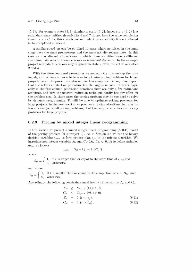
6.2. Pricing algorithm 113
{5, 6}. For example state {3,3} dominates state {3, 2}, hence state {3, 2} is aredundant state. Although activities 6 and 7 do not have the same completiontime in state {5,6}, this state is not redundant, since activity 6 is not allowedto be completed in week 6.
A similar speed up can be obtained in cases where activities in the samestage have the same predecessors and the same activity release date. In thiscase we may discard all decisions in which these activities have a differentstart time. We refer to these decisions as redundant decisions. In the exampleproject redundant decisions may originate in state 2, with respect to activities2 and 3.
With the aforementioned procedures we not only try to speed-up the pric-ing algorithms, we also hope to be able to optimize pricing problems for largerprojects, since the procedures also require less computer memory. We expectthat the network reduction procedure has the largest impact. However, typi-cally in the first column generation iterations there are only a few redundantactivities, and here the network reduction technique hardly has any effect onthe problem size. In these cases the pricing problem may be too hard to solveby dynamic programming. To still be able to optimize pricing problems forlarge projects, in the next section we propose a pricing algorithm that may beless efficient (on small pricing problems), but that may be able to solve pricingproblems for large projects.
6.2.3 Pricing by mixed integer linear programming
In this section we present a mixed integer linear programming (MILP) modelof the pricing problem for a project Jj . As in Section 4.3 we use the binarydecision variables abjtπ to form project plan ajπ in the pricing algorithm. Weintroduce non-integer variables Sbt and Cbt (Sbt,Cbt ∈ [0, 1]) to define variablesabjtπ as follows:
abjtπ = Sbt +Cbt − 1 (∀b, t) ,
where:
Sbt =
{1, if t is larger than or equal to the start time of Bbj , and0, otherwise,
and where:
Cbt =
{1, if t is smaller than or equal to the completion time of Bbj , and0, otherwise.
Accordingly, the following constraints must hold with respect to Sbt and Cbt:
Sbt ≥ Sb,t−1 (∀b, t > 0) ,
Cbt ≤ Cb,t−1 (∀b, t > 0) ,
Sbt = 0 (t < rbj) , (6.11)
Cbt = 0(t > dbj
). (6.12)
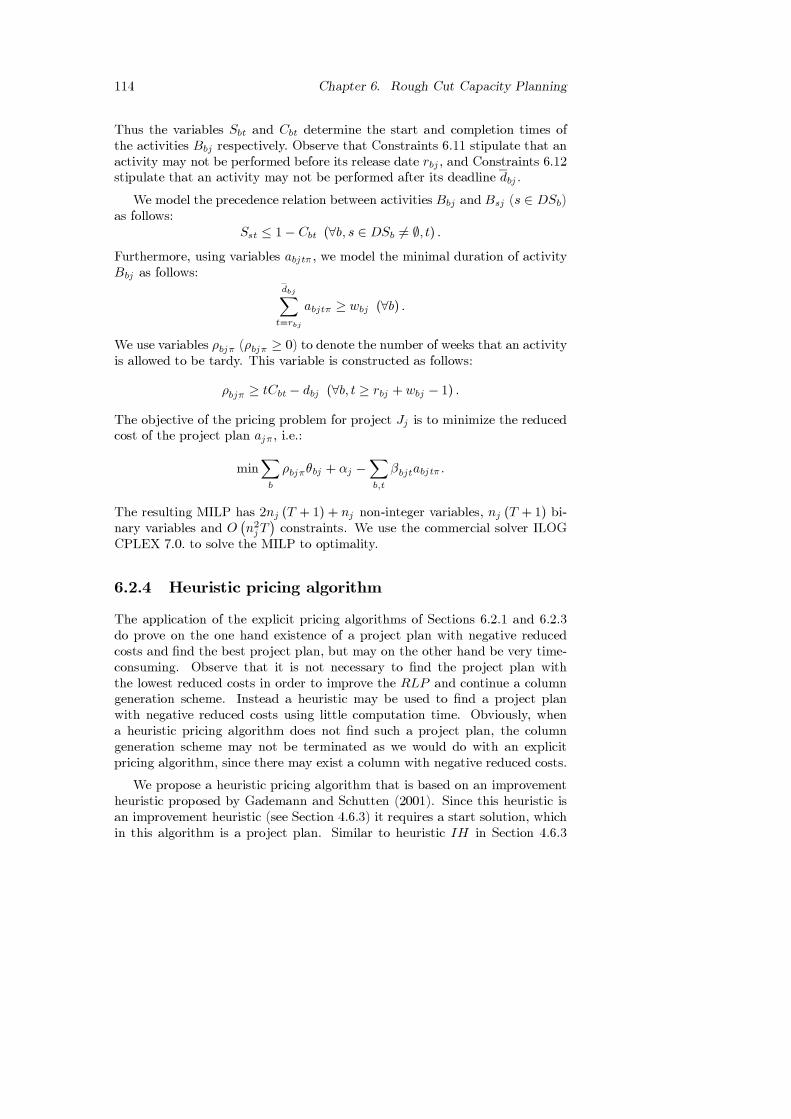
114 Chapter 6. Rough Cut Capacity Planning
Thus the variables Sbt and Cbt determine the start and completion times ofthe activities Bbj respectively. Observe that Constraints 6.11 stipulate that anactivity may not be performed before its release date rbj, and Constraints 6.12stipulate that an activity may not be performed after its deadline dbj .
We model the precedence relation between activities Bbj and Bsj (s ∈ DSb)as follows:
Sst ≤ 1−Cbt (∀b, s ∈ DSb �= ∅, t) .
Furthermore, using variables abjtπ , we model the minimal duration of activityBbj as follows:
dbj∑t=rbj
abjtπ ≥ wbj (∀b) .
We use variables ρbjπ (ρbjπ ≥ 0) to denote the number of weeks that an activityis allowed to be tardy. This variable is constructed as follows:
ρbjπ ≥ tCbt − dbj (∀b, t ≥ rbj +wbj − 1) .
The objective of the pricing problem for project Jj is to minimize the reducedcost of the project plan ajπ, i.e.:
min∑b
ρbjπθbj + αj −∑b,t
βbjtabjtπ .
The resulting MILP has 2nj (T + 1) + nj non-integer variables, nj (T +1) bi-nary variables and O
(n2jT
)constraints. We use the commercial solver ILOG
CPLEX 7.0. to solve the MILP to optimality.
6.2.4 Heuristic pricing algorithm
The application of the explicit pricing algorithms of Sections 6.2.1 and 6.2.3do prove on the one hand existence of a project plan with negative reducedcosts and find the best project plan, but may on the other hand be very time-consuming. Observe that it is not necessary to find the project plan withthe lowest reduced costs in order to improve the RLP and continue a columngeneration scheme. Instead a heuristic may be used to find a project planwith negative reduced costs using little computation time. Obviously, whena heuristic pricing algorithm does not find such a project plan, the columngeneration scheme may not be terminated as we would do with an explicitpricing algorithm, since there may exist a column with negative reduced costs.
We propose a heuristic pricing algorithm that is based on an improvementheuristic proposed by Gademann and Schutten (2001). Since this heuristic isan improvement heuristic (see Section 4.6.3) it requires a start solution, whichin this algorithm is a project plan. Similar to heuristic IH in Section 4.6.3

6.3. Branching strategy 115
it tries to improve the initial solution by iteratively changing the start andcompletion times of the activities in the project plan. It evaluates all possiblechanges in the time windows of all activities, and sorts these by increasingvalue of the expected change in the reduced cost. We accept the first changeaccording to this sorting that leads to an improvement, i.e., that leads to adecreasing reduced cost. We repeat this procedure until no more improvementis found. We may in fact stop when a project plan is found with marginalnegative reduced costs. However, such a project plan can only lead to a smallimprovement in the RLP . Since this may lead to many column generationiterations it seems better to find a project plan with significantly low reducedcosts.
6.2.5 Hybrid pricing methods
With the three pricing algorithms presented in this section we hope to be ableto optimize pricing problems of any reasonable size. We have shown that theefficiency of the DP based pricing algorithm of Section 6.2.1 depends rather onthe project structure than on the number of activities in the project. Espe-cially when a project network has a large ω-value (i.e., the highest number ofactivities in all states), the DP based algorithm may become less efficient. Theefficiency of the MILP based pricing algorithm Section 6.2.3 rather depends onthe number of activities and the number of precedence relations in the projectnetwork. This pricing algorithm may on the one hand be less efficient, but onthe other hand it may be able to solve larger pricing problems.
In addition to the aforementioned pricing methods we propose a hybridpricing strategy that uses the three aforementioned pricing methods in collab-oration. In this method we take into account that the complexity of the pricingproblem typically changes in each column generation iteration. Also, after ap-plying the network reduction technique a pricing problem may fall apart intosubproblems of different size and complexity. If the ω-value of the networkin the pricing (sub)problem is not too large, we use the DP based algorithm.If the ω-value is too large we use the MILP based pricing algorithm. If thepricing (sub)problem is even too large for this algorithm, i.e., the algorithmdoes not find a project plan with negative reduced costs or does not prove thatno such project plan exists within reasonable time, we use the heuristic pricingmethod as a final remedy to find a project plan with negative reduced costs. InChapter 7 we evaluate the different solution methods for the pricing problem.
6.3 Branching strategy
The branching strategy that we use to construct a feasible ILP solution fromthe LP relaxation solution is virtually the same as the BS strategy presented

116 Chapter 6. Rough Cut Capacity Planning
in Section 4.4.1. Recall that this branching strategy fixes a precedence relationin each node of the branching tree. Since we consider generalized precedencerelations in RCCP problems, usually other activities are involved when fixing aprecedence relation between two activities, and thus some small modificationsare needed to still be able to apply the BS strategy. Suppose in a node of thebranching tree we analyze in each child node a possible repair of the precedencerelation violation of activities Bbj and Bsj . In each child node we modify thedeadline (and if necessary the due date) of activity Bbj and the release dateof activity Bsj in such a way, that these activities can no longer overlap (seeSection 4.4.1). When there are activities that have the same predecessors asBsj , without affecting the solution we can modify the release date of theseactivities along with the release date rsj of activity Bsj, when these are smallerthan the modified release date rsj of activity Bsj. When a modification in therelease date of one of these other activities is not possible, e.g., due to a minimalduration restriction or a deadline restriction, we may prune the child node.Analogously, when there are activities that have the same successors as Bbj ,without affecting the solution we can modify the deadline (and if necessary thedue date) of these activities along with the deadline dbj of activity Bbj whendbj is smaller than the existing deadline of these activities. Again, when amodification in the deadline of one of these other activities is not possible, wemay prune the child node.
6.4 Heuristics
As far as we know, the first heuristics for the type of RCCP problems dis-cussed in this thesis are presented by De Boer and Schutten (1999). Theyhave presented various heuristics for time driven RCCP. Their first heuristic,called ICPA (incremental capacity planning algorithm), starts by sorting allactivities in order of non-decreasing deadlines, and subsequently plans the ac-tivities in this order in at most two phases. In the first phase each activityis planned in its time window as much as possible, without using nonregularcapacity. This is repeated for all unplanned activities. In the second phase theremaining unplanned (parts of) activities are planned in their time window byassigning nonregular capacity. De Boer and Schutten test two variants of thisheuristic, which result from different criteria for the order in which the activitiesare planned. The second heuristic proposed by these authors is an LP-basedheuristic. The LP formulation that is used determines the project schedulesthat minimize the use of nonregular capacity. However, the precedence con-straints between activities are ignored. The heuristic iteratively updates therelease dates and deadlines of activities in order to repair violated precedenceconstraints, and re-optimizes the LP model after each change to update theorder schedules. De Boer and Schutten present different variants of the heuris-tic, which result from different procedures to repair the violated precedence

6.4. Heuristics 117
constraints.
Gademann and Schutten (2001) propose several improvement heuristics,and several heuristics that start with infeasible solutions and convert these tofeasible solutions. All these heuristics are proposed for time driven RCCP. Theimprovement heuristics start from a feasible solution, and try to improve thesolution by iteratively changing the start and completion times of the activitiesin the project plans of the solution. The heuristics only differ in the procedureto obtain an initial feasible solution. We tested these heuristics on resourceloading problems as well as on RCCP problems. For a detailed description ofthe heuristic we refer to Section 4.6.3. The other type of heuristics proposedby Gademann and Schutten are basically variants of the LP based heuristicsproposed by De Boer and Schutten. They differ slightly with respect to theprocedure to repair violated precedence constraints.

118 Chapter 6. Rough Cut Capacity Planning

119
Chapter 7
RCCP computational
results
Get your facts first,and then you can distort them
as much as you please.
- Mark Twain (1835-1910)
7.1 Introduction
In this chapter we present the computational results for the branch-and-pricemethods for RCCP, presented in Chapter 6. As discussed in Chapter 6, weuse basically the same integer linear programming model for RCCP problems,as for resource loading. The only algorithmic implications are the generalizedprecedence relations in RCCP, which have to be accounted for in the pricingalgorithm. In Section 6.2 we proposed three pricing algorithms. The first isa dynamic programming based pricing algorithm (see Section 6.2.1), which isbasically a generalization of the pricing algorithm for resource loading. Thesecond is based on a mixed integer linear programming model (see Section6.2.3). Finally, the third is a heuristic pricing algorithm (see Section 6.2.4),which is based on IH. We refer to the three pricing algorithms as PDP ,PMILP and PH respectively.
In Chapter 5 we showed that for resource loading problems, the best branch-ing strategy is Comb2. It makes no sense to use this branching strategy forthe RCCP test instances, because each test instance holds the data for oneproject, as will be explained in Section 7.2. As a result, if we would use theComb2 method, we could only branch on the project plans of one project in the

120 Chapter 7. RCCP computational results
HBS1 method (which is embedded in Comb2). We therefore use the TBS+IHbranching strategy with one of the three pricing algorithms proposed in Section6.2.
Recall that in the TBS+IH method, we initialize the RLP with the EDDheuristic, or, if EDD does not lead to a feasible solution, we apply columngeneration on the Phase I RLP to either find a feasible primal solution tothe LP relaxation, or to prove that no such solution exists. Subsequently, weapply the rounding heuristics RH1 (0.01), RH2 (0.01), RH3 (0.05), RH4 (1)and the improvement heuristic IH. IH uses the solution found by RH4 (1) asinitial solution. We use the best solution value found by the heuristics as anupper bound, and use the branching strategy of TBS+IH. TBS+IH branchesby repairing violated precedence constraints in each node. We truncate thebranching scheme after 30 minutes.
We restrict ourselves to testing only time driven RCCP problems. As aresult, in the test instances discussed in this chapter, the projects are notallowed to be tardy. The testing of the algorithms on resource driven RCCPproblems is subject of further research.
The outline of this chapter is as follows. First, in Section 7.2 we discussthe test instances that we use for the experiments. In Section 7.3 we analyzethe computational results of optimizing the initial LP (i.e., the LP in theroot node) with the three pricing algorithms. Subsequently, in Section 7.4we analyze the computational results of the three pricing methods embeddedin the TBS+IH algorithm. We compare the three versions of the algorithmmutually, and compare the computational results with results known from theliterature.
7.2 Test instances
As compared to the instance generation procedure for resource loading (Chap-ter 5), the instance generation procedure for RCCP is even more complicateddue to the general precedence relations between activities in RCCP. For test-ing and benchmarking of the algorithms for RCCP we use the set of instancesgenerated by De Boer (1998). De Boer uses a network construction procedurethat was developed by Kolisch et al. (1992) to generate random networks.Each test instance holds the data for only one project. The test instances aresubdivided into classes, each of which is characterized by the parameters nj
(number of activities in the project), m (the number of resources) and φ (theaverage slack). The average slack is defined as:
φ =
nj∑b=1
(dbj −wbj − rbj + 1
)nj
,

7.3. Optimization of the initial LP 121
where dbj −wbj − rbj +1 is the slack of activity Bbj. The parameter values aredisplayed in Table 7.1. The test set contains 10 instances for each combinationof the parameters, which comes to a total of 450 instances. The length of theplanning horizon for these instances varies from 12 to 72 periods.
nj 10 20 50m 3 10 20φ 2 5 10 15 20
Table 7.1: Parameter values.
Table 7.2 shows the approximate size of the initial RLP for instances withnj ∈ {10,20,50}. It shows that the size of the RLP increases considerablywith nj .
nj #nonzeros #variables #rows10 3500 400 60020 6500 900 120050 21000 2400 2900
Table 7.2: Size of the initial RLP .
De Boer considers only time driven RCCP problems, with δ = 1. Gademannand Schutten use the same instances for their computational experiments. Al-though our algorithms work for the case δ = 0 and for resource driven problems,we restrict ourselves to testing the time driven problems for δ = 1. This allowsus to compare the computational results of our algorithm with the computa-tional results of the existing algorithms from the literature.
7.3 Optimization of the initial LP
In this section we analyze the computational results of optimizing the LP inthe root node. We first analyze the required CPU-time, and the number oftimes that the LP is solved to optimality using the pricing algorithms PDP(Section 7.3.1), PMILP (Section 7.3.2) and PH (Section 7.3.3). Finally, inSection 7.3.4 we compare the pricing algorithms mutually.
7.3.1 Pricing by dynamic programming
In this section we analyze the computational results of optimizing the initialLP in the root node using the dynamic programming based pricing algorithm(PDP ). Before we solve a pricing problem we apply the speed up techniquesdiscussed in Section 6.2.2 to reduce the problem size. The experiments show

122 Chapter 7. RCCP computational results
that when the problem size increases, it becomes more and more difficult tosolve pricing problems with PDP . Particularly when the maximum numberof activities in all states (ω) is large, the pricing problem becomes harder oreven impossible to solve. Without applying the speed up techniques, we areable to solve pricing problems for projects with up to 20 activities. The speedup techniques not only allow pricing problems of larger projects to be solved,they also significantly reduce the average required CPU-time to solve the LP .Table 7.3 shows the computational results for applying the TBS+IH branchingmethod on 30 RCCP instances with nj = 20, using the PDP pricing algorithmboth with and without the speed up techniques. Table 7.3 shows that theaverage CPU-time required in the root node to optimize the initial LP is muchhigher when the speed up techniques are not used. Also the CPU-time requiredfor branching is much higher when the speed up techniques are not used. Thespeed up techniques allow even some pricing problems for projects with 50activities to be solved. Furthermore, since the speed up techniques reducethe required CPU-time to solve a pricing problem, much more nodes can beexplored in the branching scheme in the same time span.
speed up avg. CPU- avg. CPU-timetechniques time root node branching
used (sec.) (sec.)yes 0.1 12.5no 18.5 52.0
Table 7.3: Computational results PDP with and without the speed up tech-niques.
Recall from Section 6.2.1 that the pricing problem uses O(njTω) space, and
can be solved in O(njT2ω) time. Without applying the speed up techniques,
the average ω for the instances with nj = 10 is 3.8. For nj = 20 and nj = 50the average ω is 6.9 and 18.0 respectively. We also measured the average ωfor the problem in the first column generation iteration in the root node, af-ter applying the speed up techniques. In this case, the average ω is 3.7, 6.3and 14.7 respectively. The speed up techniques thus have more effect whenthe projects have more activities. When applying the speed up techniques,ω usually decreases in subsequent column generation iterations. Without ap-plying the speed up techniques, ω remains the same in all column generationiterations. For example, when applying the speed up techniques, the average ωduring all column generation iterations in the root node is 1.9 for nj = 10, and2.0 for nj = 20, which is significantly lower than the ω in the first iteration.
In order to prevent computer memory problems that may stop the test-procedure we skip solving a pricing problem when we observe a priori that thestate space becomes too large to handle in computer memory. As a result,the column generation scheme may terminate, and the solution found is an
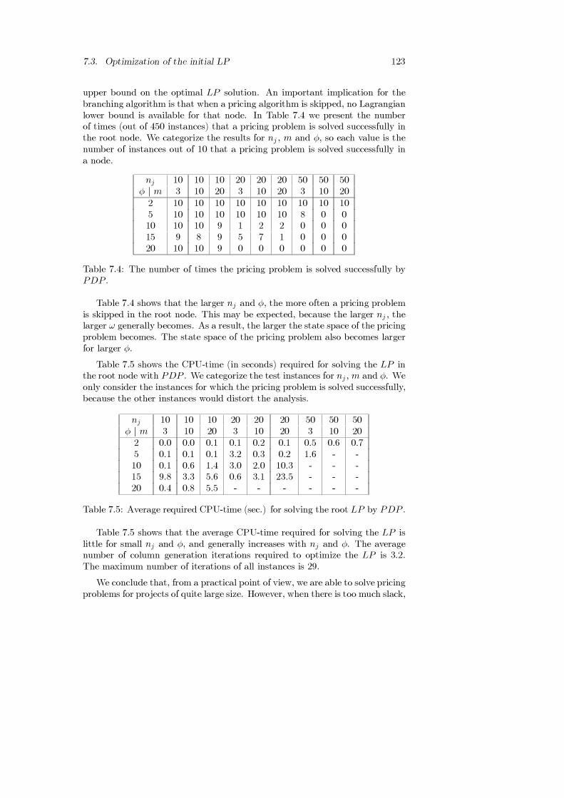
7.3. Optimization of the initial LP 123
upper bound on the optimal LP solution. An important implication for thebranching algorithm is that when a pricing algorithm is skipped, no Lagrangianlower bound is available for that node. In Table 7.4 we present the numberof times (out of 450 instances) that a pricing problem is solved successfully inthe root node. We categorize the results for nj , m and φ, so each value is thenumber of instances out of 10 that a pricing problem is solved successfully ina node.
nj 10 10 10 20 20 20 50 50 50φ | m 3 10 20 3 10 20 3 10 202 10 10 10 10 10 10 10 10 105 10 10 10 10 10 10 8 0 010 10 10 9 1 2 2 0 0 015 9 8 9 5 7 1 0 0 020 10 10 9 0 0 0 0 0 0
Table 7.4: The number of times the pricing problem is solved successfully byPDP .
Table 7.4 shows that the larger nj and φ, the more often a pricing problemis skipped in the root node. This may be expected, because the larger nj , thelarger ω generally becomes. As a result, the larger the state space of the pricingproblem becomes. The state space of the pricing problem also becomes largerfor larger φ.
Table 7.5 shows the CPU-time (in seconds) required for solving the LP inthe root node with PDP . We categorize the test instances for nj, m and φ. Weonly consider the instances for which the pricing problem is solved successfully,because the other instances would distort the analysis.
nj 10 10 10 20 20 20 50 50 50φ | m 3 10 20 3 10 20 3 10 202 0.0 0.0 0.1 0.1 0.2 0.1 0.5 0.6 0.75 0.1 0.1 0.1 3.2 0.3 0.2 1.6 - -10 0.1 0.6 1.4 3.0 2.0 10.3 - - -15 9.8 3.3 5.6 0.6 3.1 23.5 - - -20 0.4 0.8 5.5 - - - - - -
Table 7.5: Average required CPU-time (sec.) for solving the root LP by PDP .
Table 7.5 shows that the average CPU-time required for solving the LP islittle for small nj and φ, and generally increases with nj and φ. The averagenumber of column generation iterations required to optimize the LP is 3.2.The maximum number of iterations of all instances is 29.
We conclude that, from a practical point of view, we are able to solve pricingproblems for projects of quite large size. However, when there is too much slack,

124 Chapter 7. RCCP computational results
the pricing problem often becomes too hard to solve. It is questionable whetherit makes sense to give a project as much slack as φ ≥ 10. It is likely that whenthe project due date is made tighter, the pricing problem becomes easier tosolve. We also note that the pricing problems usually become easier to solvedeeper in the branching tree, because more and more constraints are addedto the problem. As a result, the activities will have less slack deeper in thebranching tree.
7.3.2 Pricing by mixed integer linear programming
In this section we analyze the computational results of optimizing the initialLP in the root node using the mixed integer linear programming based pricingalgorithm (PMILP ). The computational results for PMILP show that whenthe pricing problem size grows, it becomes harder to solve the pricing problemusing this method. When the solver can not solve the pricing problem withinone minute, we skip the pricing problem. This only occurs in two instances,both of which concern a project with 50 activities and φ = 20.
Table 7.6 shows the average CPU-time required for solving the LP in theroot node with PMILP . We again categorize the results for nj, m and φ, anddiscard the instances for which the pricing problem is skipped.
nj 10 10 10 20 20 20 50 50 50φ | m 3 10 20 3 10 20 3 10 202 0.2 0.1 0.1 0.5 0.6 0.4 5.4 4.4 4.05 0.3 0.3 0.3 2.9 3.3 1.3 27.2 66.0 39.710 0.8 1.3 1.0 4.0 7.4 8.7 404.4 452.5 1312.415 2.2 2.3 2.1 16.6 30.3 21.6 250.3 5194.2 4381.220 2.8 4.5 4.2 31.5 81.2 56.6 571.9 1366.4 18796.2
Table 7.6: Average required CPU-time (sec.) for solving the root LP byPMILP .
Table 7.6 shows that the CPU-time generally increases with nj and φ. Inparticular for the instances that could not be solved by PDP the CPU-times arelarge. For small nj and φ, PMILP on the one hand requires more CPU-timethan PDP . On the other hand, PMILP solves the LP in far more instancesthan PDP , and for larger nj and φ.
We note that the average number of column generation iterations requiredto optimize the LP is 10.2. The maximum number of iterations of all instancesis 66.
Just as forPDP , for PMILP the pricing problem becomes harder to solvefor larger nj and φ. We did not implement the speed up techniques for thispricing algorithm, so some speed up is possible. A faster variant of PMILP can

7.3. Optimization of the initial LP 125
also be obtained by stopping the integer program solver as soon as a solution hasbeen found that corresponds to a feasible project plan with negative reducedcosts. Such a solution is sufficient to continue the column generation scheme,however, it may require more column generation iterations to solve the pricingproblem. This method is subject of further research.
7.3.3 Heuristic pricing
In this section we analyze the computational results of optimizing the LP inthe root node using the heuristic pricing algorithm (PH). Table 7.7 shows theaverage required CPU-time (in seconds).
nj 10 10 10 20 20 20 50 50 50φ | m 3 10 20 3 10 20 3 10 202 0.0 0.1 0.1 0.2 0.2 0.1 0.2 0.2 0.15 0.0 0.1 0.1 0.0 0.0 0.0 0.1 0.1 0.110 0.1 0.1 0.1 0.1 0.1 0.1 0.1 0.1 0.115 0.0 0.0 0.0 0.1 0.2 0.1 0.1 0.7 0.220 0.1 0.1 0.1 0.0 0.1 0.1 0.3 0.2 0.2
Table 7.7: Average required CPU-time (sec.) for solving the root LP by PH.
Table 7.7 shows that the average CPU-time is less than one second for all theclasses of instances. This is an advantage of this method. Table 7.8 shows thesolution performance of this pricing algorithm. We categorize the instances fornj, so each row corresponds to 150 instances. Table 7.8 shows that the difference
Avg. Avg. #Timesoptimal LP solution LP
nj solutiona found by PH optimal10 1005.5 1462.4 4620 980.8 1657.7 2250 842.6 1623.4 0
aThis is the average optimal LP solution found by the other pricing algorithms.
Table 7.8: Root LP solution performance of PH.
between the optimal LP solution and the solution found by PH increaseswith nj . Furthermore, the number of times that the optimal LP solution isfound by PH decreases with nj. Both effects are similar for parameter φ.The average number of column generation iterations before termination of thecolumn generation scheme is 1.6.
We conclude that, although PH is fast, its solution performance is unsat-isfactory. We recommend it only to be used in cases when both PDP and

126 Chapter 7. RCCP computational results
PMILP can not solve a pricing problem.
7.3.4 Comparison of pricing algorithms
In the previous sections we showed that, when solving the LP for small projects,PMILP on the one hand requires more CPU-time than PDP . On the otherhand, PMILP solves the LP in far more instances than PDP . PMILPis therefore favorable for large instances, and PDP is favorable for small in-stances. In two instances the pricing problem is so large that it can not besolved by PMILP .
PH never skips a pricing problem, but it may not find a project plan withnegative reduced costs when such a project plan exists. In Section 7.3.3 weshowed that only in 68 of the 450 instances it finds the optimal LP solution.Even though this number is small, since its execution time is little, an advan-tage of using PH is that it may allow many more nodes to be explored in abranch-and-price algorithm, and may thus eventually lead to a better ILP so-lution. However, an important implication of using PH in a branch-and-pricealgorithm is that the Lagrangian lower bound is no longer valid. Hence, fewernodes may be fathomed in the branching scheme, which may cancel out theadvantage.
A hybrid approach, in which we would use PDP for small problems,PMILP for larger problems, and PH for problems that PMILP can notsolve, may be more efficient. We restrict ourselves, however, to using one pric-ing algorithm per method. The testing of a hybrid pricing approach is subjectof further research.
7.4 Computational results of the branch-and-
price methods
In this section we analyze the computational results for the branch-and-pricemethods. As discussed in Section 7.1, we use the three pricing algorithmsPDP , PMILP and PH in the TBS+IH branching method. We refer to thethree branch-and-price methods as BPD, BPM and BPH respectively. Wealso test a variant of BPM in which we add 3 project plans to the columnpool before branching. We refer to this branch-and-price method as BPM+.The 3 project plans are constructed as follows. One project plan is added inwhich all activities are allowed to be produced for wbj periods (i.e., as long astheir minimal duration), and as early as possible. Only the activities withoutsuccessors are allowed to be produced until the project due date. A similarproject plan is added, in which all activities are allowed to be produced for wbj
periods, and as late as possible. A third project plan is added, in which the
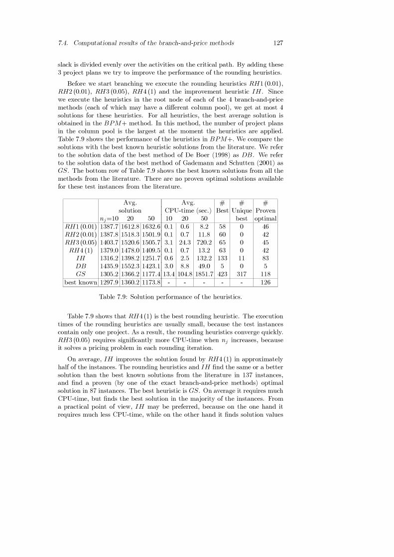
7.4. Computational results of the branch-and-price methods 127
slack is divided evenly over the activities on the critical path. By adding these3 project plans we try to improve the performance of the rounding heuristics.
Before we start branching we execute the rounding heuristics RH1 (0.01),RH2 (0.01), RH3 (0.05), RH4 (1) and the improvement heuristic IH. Sincewe execute the heuristics in the root node of each of the 4 branch-and-pricemethods (each of which may have a different column pool), we get at most 4solutions for these heuristics. For all heuristics, the best average solution isobtained in the BPM+ method. In this method, the number of project plansin the column pool is the largest at the moment the heuristics are applied.Table 7.9 shows the performance of the heuristics in BPM+. We compare thesolutions with the best known heuristic solutions from the literature. We referto the solution data of the best method of De Boer (1998) as DB. We referto the solution data of the best method of Gademann and Schutten (2001) asGS. The bottom row of Table 7.9 shows the best known solutions from all themethods from the literature. There are no proven optimal solutions availablefor these test instances from the literature.
Avg. Avg. # # #solution CPU-time (sec.) Best Unique Proven
nj=10 20 50 10 20 50 best optimalRH1 (0.01) 1387.7 1612.8 1632.6 0.1 0.6 8.2 58 0 46RH2 (0.01) 1387.8 1518.3 1501.9 0.1 0.7 11.8 60 0 42RH3 (0.05) 1403.7 1520.6 1505.7 3.1 24.3 720.2 65 0 45RH4 (1) 1379.0 1478.0 1409.5 0.1 0.7 13.2 63 0 42
IH 1316.2 1398.2 1251.7 0.6 2.5 132.2 133 11 83DB 1435.9 1552.3 1423.1 3.0 8.8 49.0 5 0 5GS 1305.2 1366.2 1177.4 13.4 104.8 1851.7 423 317 118
best known 1297.9 1360.2 1173.8 - - - - - 126
Table 7.9: Solution performance of the heuristics.
Table 7.9 shows that RH4 (1) is the best rounding heuristic. The executiontimes of the rounding heuristics are usually small, because the test instancescontain only one project. As a result, the rounding heuristics converge quickly.RH3 (0.05) requires significantly more CPU-time when nj increases, becauseit solves a pricing problem in each rounding iteration.
On average, IH improves the solution found by RH4 (1) in approximatelyhalf of the instances. The rounding heuristics and IH find the same or a bettersolution than the best known solutions from the literature in 137 instances,and find a proven (by one of the exact branch-and-price methods) optimalsolution in 87 instances. The best heuristic is GS. On average it requires muchCPU-time, but finds the best solution in the majority of the instances. Froma practical point of view, IH may be preferred, because on the one hand itrequires much less CPU-time, while on the other hand it finds solution values

128 Chapter 7. RCCP computational results
that on average require at most 74.3 (for nj = 50) more hours of nonregularcapacity.
Tables 7.10 and 7.11 show the computational results for the 4 branch-and-price methods. In Table 7.11 we also show the solutions of GS, and bestknown solutions from the literature. For the instances where a branch-and-price algorithm could not solve the LP in the root node, we obtain a solution byapplying IH on the initial RLP solution (i.e., the EDD solution). This allowsus to compare the solution performance of the algorithms in all instances.
# #Truncated Avg. #nodesa Avg.Solutions (×1000) tree depthfound nj=10 20 50 10 20 50 10 20 50
BPD 450 76 114 142 46.7 34.7 10.6 7.2 14.2 32.0BPM 448 76 119 149 21.9 9.3 1.3 7.2 13.4 18.4BPM+ 418 78 119 117 16.2 7.1 2.0 7.1 13.0 17.5BPH 450 97 123 150 34.7 22.8 8.6 7.4 14.5 29.3
aThese results concern the instances that were not truncated.
Table 7.10: Test results of the branch-and-price methods (1).
Avg. Avg. # # # #solution CPU-time (sec.)a Best UniqueUnique Proven
nj=10 20 50 10 20 50 best worst optimalBPD 1317.2 1518.9 1532.2 133.2 170.6 632.8 166 6 83 121BPM 1318.8 1431.2 1252.1 229.1 166.9 444.1 145 3 12 111BPM+ 1309.7 1397.6 1249.1 226.1 166.1 363.5 172 11 0 117BPH 1365.6 1541.4 1503.6 167.2 117.5 - 106 0 181 96GS 1305.2 1366.2 1177.4 13.4 104.8 1851.7 410 253 0 118
best known 1297.9 1360.2 1173.8 - - - - - - 126
aThese results concern the instances that were not truncated.
Table 7.11: Test results of the branch-and-price methods (2).
Table 7.10 shows that BPM+ finds a solution in fewer instances thanBPM .It also generally explores fewer nodes than BPM . On the other hand, thesolution performance of BPM+ is better than that of BPM .
BPH is truncated more often than the other methods. Only for nj = 50, itssolution performance is better than that of BPD. For nj ∈ {10,20} BPH isclearly outperformed by the other methods. BPH usually explores more nodes,however, it does not use Lagrangian relaxation to determine lower bounds.
For instances with nj = 10 the fastest method is BPD. The solutionperformance of BPD on these is only outperformed by BPM+. For instances

7.4. Computational results of the branch-and-price methods 129
with nj = 20, BPM+ also has the best solution performance. For instanceswith nj = 50, BPM has the best solution performance.
For 126 out of 450 instances optimality could be proven by BPD, BPMand BPM+. In 7 instances the best known solution from the literature isimproved, and in 174 instances the best solution of the branching methods isthe same as the best known solution from the literature. Table 7.12 shows thenumber of instances that are solved to optimality by BPM+. We categorizedthe results for nj, m and φ, so each number corresponds to the number of timesout of 10 that the instances are solved to optimality.
nj 10 10 10 20 20 20 50 50 50φ | m 3 10 20 3 10 20 3 10 202 10 10 10 10 10 10 6 2 05 10 9 10 6 0 0 0 0 010 9 3 4 0 0 0 0 0 015 1 0 2 0 0 0 0 0 020 1 1 1 0 0 0 0 0 0
Table 7.12: Number of times that an optimal solution is found by BPM+.
Table 7.12 shows that instances with small nj and φ can often be solvedto optimality. Instances with large nj and φ can almost never be solved tooptimality.
Considering the solution performance, BPM+ is the best branch-and-pricemethod, and GS is the best overall method. Table 7.13 compares the absolutedifference between the solution found by BPM+ and the solution found byGS. A positive number means that the average solution found by BPM+ islarger than that of GS. We categorize the results for nj , m and φ.
nj 10 10 10 20 20 20 50 50 50φ | m 3 10 20 3 10 20 3 10 202 0.0 0.0 0.0 0.0 0.0 0.0 0.1 −0.8 4.95 0.0 0.0 −1.2 1.3 9.5 2.5 9.6 26.5 19.810 1.5 1.6 −0.4 8.9 32.9 43.6 22.6 48.0 79.515 13.7 13.4 12.6 45.9 32.2 71.7 40.3 109.9 121.820 −2.4 7.7 21.6 41.7 103.4 78.5 89.1 223.1 279.8
Table 7.13: Absolute difference between the average solutions of BPM+ andGS.
Table 7.13 shows that BPM+ and GS perform comparably for small nj orfor small φ. The larger nj and φ, the more GS outperforms BPM+.
In Table 7.14 we show the number of times that BPM+ and GS find thebest solution. We categorize the results for nj , m and φ. For example ”6,8” in

130 Chapter 7. RCCP computational results
Table 7.14 means that BPM+ finds the best solution in 6 out of 10 instances,and GS in 8 instances out of 10.
nj 10 10 10 20 20 20 50 50 50φ | m 3 10 20 3 10 20 3 10 202 10,10 10,10 10,10 10,10 9,10 10,10 9,8 7,9 6,105 10,10 9,10 10,9 5,8 2,9 3,7 0,10 0,10 3,810 6,8 8,8 6,8 2,9 1,10 1,9 0,10 0,10 1,915 1,8 4,10 5,7 0,10 1,9 2,8 0,10 0,10 0,1020 1,7 4,6 4,6 1,9 0,10 1,9 0,10 0,10 0,10
Table 7.14: Number of times that BPM+,GS find the best solution.
Just as Table 7.13, also Table 7.14 shows that BPM+ and GS performcomparably for small nj and small φ. The larger nj and φ, the more GSoutperforms BPM+.
7.5 Conclusions
The heuristic pricing method PH performs unsatisfactorily. Research into al-ternative heuristic pricing methods is therefore recommended. A hybrid pricingapproach, in which we would use PDP for small problems, PMILP for largerproblems, and PH for problems that PMILP can not solve, may be the mostefficient pricing method. The testing of a hybrid pricing approach is subject offurther research.
The computational results show that the branch-and-price methods are suit-able for solving RCCP problems with nj ≤ 20, and with φ ≤ 10. For largerRCCP problems, the branch-and-price method BPM+ performs satisfactorily,but heuristics like GS are preferred. With respect to the solution performance,the best branch-and-price method is BPM+. The absolute difference betweenthe average solution values of BPM+ and GS is usually less than 50, which isquite small from a practical point of view.
The speed up techniques have not been implemented for PMILP . Hence,the performance of BPM+ may be improved further by using the speed uptechniques to split up the ILP model of the pricing problem whenever this ispossible. This extension is subject of further research.
131
Chapter 8
Epilogue
There never seems to be enough time to do the thingsyou want to do once you find them.
- Jim Croce (1943-1973)
The main objective of the research described in this thesis is to developmodels for resource loading problems with finite capacity constraints and com-plex precedence and routing constraints, and, more importantly, to proposeexact and heuristic solution methods to solve such models. The models andtechniques used were highly motivated by recent insights regarding the use ofadvanced combinatorial methods for these types of problems. Another motiva-tion of this research originates from shop floor scheduling research. Shop floorscheduling algorithms are rigid with respect to resource capacity. Without theuse of resource loading tools to determine the required resource levels and the(possible) size of the workload to be scheduled, shop floor scheduling problemsmay become too hard to solve and solutions may become unacceptable.
We propose resource loading methods that support shop floor schedulingby determining the resource capacity levels available to the scheduling level, aswell as important milestones for the orders and jobs in the scheduling problem,such as (internal) release and due dates. Resource loading can also be used tosupport order acceptance. It can be used as an instrument to make trade-offsbetween lead time and due date performance on the one hand, and nonregularcapacity levels on the other hand.
In this final chapter we give an overview of our results. In Section 8.1 wegive a summary of this thesis. We conclude this thesis in Section 8.2 withsuggestions for further research.

132 Chapter 8. Epilogue
8.1 Summary
The main contribution of this thesis is twofold. First, we propose a modelingapproach that offers a generic framework to formulate various types of resourceloading and RCCP problems as ILP models. Second, we propose various algo-rithms that can solve problems of reasonable size, i.e., typically encountered inpractice, to optimality.
We position resource loading between strategical capacity planning (aggre-gate planning) and operational capacity planning (scheduling) as a tacticalcapacity planning problem. Resource loading has been rather underexposedboth in the literature and in practice. As a tactical instrument it benefits theflexibility of the entire production system for various reasons. It serves as a toolin the customer order processing stage, which, in make-to-order manufacturingenvironments, is typically characterized by much uncertainty. On the demandside there is uncertainty as to what orders can eventually be acquired, whilefurthermore order characteristics are uncertain or at best partly known. Onthe supply side there is uncertainty in the availability of the resources. In thesesituations, a resource loading tool can be used to match production capacityand customer demand, while minimizing the cost of customer order tardinessand the use of nonregular capacity. Resource loading analyses can thus be usedto accept/reject orders, or to quote reliable due dates. Resource loading canalso serve as a tool to define realistic constraints for the underlying schedulingproblem. The resource capacity levels and important milestones (such as re-lease and due dates) are usually supposed to be fixed in scheduling. Resourceloading can detect when and where difficulties will occur in scheduling at anearly stage, and allocate orders or order parts more efficiently, and, if neces-sary, properly adjust resource capacity levels (by assigning nonregular capacity)and/or milestones.
In this thesis we propose a deterministic approach for modeling and solv-ing resource loading problems. In order to smooth out the aforementioneduncertainty in resource loading problems we formulate resource loading at ahigher level of aggregation than scheduling problems (i.e., the tactical level vs.the operational level). In resource loading problems we distinguish (customer)orders that consist of jobs. Jobs are in fact work packages at a higher levelof aggregation. In the underlying shop floor scheduling problem, jobs may befurther disaggregated into operations or tasks.
The difficulty of formulating the resource loading problem as an integer lin-ear programming model is that modeling precedence relations is not straight-forward, and the resulting formulations are often extremely hard to solve. Wepropose a modeling approach that offers a generic framework for modeling var-ious resource loading problems. The proposed model can handle a large varietyof practical aspects, such as generalized precedence constraints, various forms ofcapacity flexibility, tardiness penalties, and minimal duration constraints. The

8.1. Summary 133
model can handle resource driven resource loading and time driven resourceloading simultaneously, which allows making trade-off analyses between duedate performance on the one hand, and nonregular capacity levels on the otherhand. In this modeling approach we make a distinction between order plansand order schedules. Order plans indicate in which periods a job of an order isallowed to be processed. Order schedules indicate which (part of the) jobs ofthe order are actually processed in each period. We propose a mixed-integerlinear programming (MILP) model of the resource loading problem with anexponential number of integer variables. A relatively small and fixed part ofthese variables determine the required nonregular capacity usage per resourceper period. The remaining variables are binary variables that correspond toselecting an order plan for an order. The order plans are thus columns of thecoefficient matrix of the model, which are feasible with respect to precedenceconstraints and order release and due date constraints. The MILP model se-lects precisely one order plan per order, and determines order schedules thatare consistent with these order plans. The model determines the nonregularcapacity usage from the order schedules.
The precedence relations and release and due date constraints thus do nothave to be applied to the order schedules by the model, since they are embeddedin the order plans. However, since there are exponentially many feasible orderplans, an explicit model of a problem of regular size is impossible to formulateand solve. We therefore propose various exact and heuristic solution methods,which are all based on first solving the linear programming (LP) relaxationof this formulation by column generation. The pricing problem comprises thedetermination of feasible order plans with negative reduced costs. The idea ofa column generation scheme is that only a small set of variables are requiredto determine the optimal solution of the LP. It starts from a restricted LPformulation (RLP), which has at least one order plan per order. After eachRLP optimization, order plans with negative reduced costs are added to theRLP. The column generation scheme terminates when no order plans withnegative reduced costs exist. The optimal solution of the LP is then found.
Clearly, if the optimal solution of the linear programming relaxation hap-pens to be integral, we have found an optimal solution for the resource loadingproblem. Otherwise, we apply a branch-and-price algorithm to determine anoptimal solution. We propose various exact and heuristic branching strategies.Furthermore, we propose various approximation techniques that are based onthe column generation approach, such as approximation algorithms that pro-ceed by judiciously rounding the linear programming solution to obtain a fea-sible solution for the original problem.
Computational experiments with the resource loading methods show thatlarge resource loading problems with a planning horizon of up to 15 weeks and5 machine groups can usually be solved to optimality. For larger problems, thebranch-and-bound methods usually have to be truncated. Various sensitivity
134 Chapter 8. Epilogue
analyses show that adding planning flexibility in some cases makes cases easierto solve, and in other cases makes it harder to prove optimality. The bestresource loading method is a combination of two branching strategies. This(exact) method generally outperforms all approximation methods.
In resource loading problems we assume linear precedence relations. Wealso propose extensions of the algorithms that are able to deal with generalizedprecedence relations. This allows us to use the same model and solution meth-ods to solve Multi-Project Rough-Cut Capacity Planning (RCCP) problems,for which some heuristics have already been proposed in the literature. Themain algorithmic implication of the generalized precedence constraints is thegeneralization of the pricing algorithm. The pricing problem becomes muchharder to solve, especially when the project size increases. We propose threedifferent pricing algorithms, so that pricing problems of many sizes can besolved. We propose branch-and-bound algorithms that use one of these pricingalgorithms to solve the linear program. We also propose approximation tech-niques, such as the rounding heuristics that we proposed for resource loadingproblems, and an improvement heuristic, which tries to improve an existingfeasible solution.
Computational experiments with the branch-and-bound methods show thatRCCP problems for projects of reasonable size can be solved to optimality. Forlarger problems, the branch-and-bound methods compete with the heuristicsfrom the literature. For RCCP problems with very large projects solving thepricing problem often becomes too computational intensive. As a result, forlarge RCCP problems the branch-and-bound methods are outperformed by theheuristics from the literature. We note that, from a practical point of view, itis questionable whether it makes sense to solve such large problems to optimal-ity, since information regarding resource availability and project characteristicsare usually uncertain in the long term. Solving RCCP problems with a longplanning horizon is thus more a mathematical challenge.
8.2 Further research
An important question remains as to what extent a resource loading plan isconsistent with the next planning stage, i.e., the scheduling stage. Resourceloading tools give an indication of the resource usage and important milestonesof customer orders at a more aggregated level. As with other planning prob-lems, the data for a resource loading problem (especially problems with a longplanning horizon) will become less accurate towards the end of the planninghorizon. Disturbances in the production process may occur, or, more likely,changes in the demand requirements may occur (e.g., rush orders may arrive).Since long-term orders usually have less detailed (i.e., more aggregated) spec-ifications than short-term orders, ideally they are not treated uniformly bythe resource loading. As a result, resource loading preferably has a planning

8.2. Further research 135
horizon with various non-decreasing levels of aggregation, corresponding to theactual capacity flexibility. In such an approach we could, for example, considerperiods of a day in the first two weeks of the planning horizon, periods of aweek in the subsequent weeks, and perhaps even periods of a month after that.This would allow a more detailed loading for orders in the short term, and arough planning in the long term. Not only could we then distinguish orders ofvarious levels of aggregation; this would also bring the resource loading prob-lem closer to the underlying scheduling problem. In this thesis we make nosuch distinction of aggregation levels in the planning horizon, since we consid-ered planning horizons that consist of periods of equal size (i.e., a week). Asa result, we would ignore any available data for the short term that is at alower level of aggregation. It is likely that this will affect the consistency ofthe resource loading plan and the scheduling stage. This would be avoided if aresource loading method would be used that uses a more detailed loading in theshort term, and non-decreasing levels of aggregation for the remainder of theplanning horizon. Since there exist no proper resource loading methods evenwithin our problem definition, this is perhaps the logical next step in furtherresearch.
An approach in which the size of the planning periods increases during theplanning horizon can easily be adapted by the branch-and-price techniques pro-posed in this thesis. In fact the only implication is that the planning horizonmust be extended, and redefined. When, for example, we would consider peri-ods of a day in the first week of the planning horizon, and periods of a week inthe subsequent 10 weeks, we could redefine the planning horizon (t = 0, . . . , 10weeks) as follows: t = 0, . . . , 6 days, t = 7, . . . 16 weeks. An important impli-cation of this extension is that the size of the entire model increases, and maybecome harder to solve. Whether this extension leads to a higher consistencybetween resource loading and scheduling is subject of further research. An al-ternative approach that may be more appropriate for this extension is to splitup the planning horizon in parts that partly overlap, and that have an appro-priate level of aggregation. Instead of solving the entire problem we could solvethe problem in each part of the planning horizon, and connect the overlappingplans. The question as to whether this leads to a better solution than when wewould solve the problem in its entirety, is subject of further research.
In this research we primarily deal with resource loading problems from thesupply side (i.e., the demand is given): we consider the timing and coordina-tion of the resources in order to load a predetermined set of orders. In practice,especially when the planning horizon is long, it is often possible to reject orpostpone orders, possibly with additional costs. Further research is there-fore recommended into resource loading tools that support order acceptance orpostponement decisions.
An ideal environment to test resource loading tools would be a simulationmodel of an order processing environment. A simulation model allows a pro-
136 Chapter 8. Epilogue
duction system to be studied with a long time frame in compressed time, oralternatively to study the detailed workings of a system in expanded time (Lawand Kelton, 1991). It can be adapted easily, which allows experiments withdifferent factory layouts and operating policies. We could model the productionsystem that we used throughout this thesis for resource loading problems (seeSection 1.3.1). The simulation model could generate customer order arrivalsat irregular intervals. These orders may have various characteristics, such assize, several possible delivery dates (and corresponding prices), etc. A resourceloading tool can be embedded to aid a customer order processor to determinepossible delivery dates, and corresponding capacity usage, and (nonregular)capacity costs. Based on some decision criteria, such as costs or profit, thecustomer order processor may then accept or reject a customer order. If theorder is accepted, and the delivery date is agreed upon, the same resource load-ing tool may be used to load the new order, and adjust the capacity levels ifnecessary. Various online planning aspects must then be dealt with, such asthe question how to deal with existing orders after a new order is accepted,i.e., whether they should be fixed or reloaded. A scheduling tool can also beembedded in the simulation model to determine the short-term capacity plans.This allows the consistency of the resource loading plans with the schedulingplans to be studied.
The computational results for the three pricing algorithms for RCCP inChapter 7 show that each pricing algorithm is suitable for pricing problems ofa specific size. Since, because of the speed up techniques, the size of the pricingproblems vary significantly during the branch-and-price scheme, we believe thata hybrid pricing approach may be more efficient. The testing of a hybrid pricingapproach for RCCP problems, which selects one of the three pricing algorithmsdependent on the pricing problem size, is subject of further research.
In this thesis we studied resource loading problems in a make-to-order man-ufacturing environment. We argued in Chapter 1 that many manufacturingcompanies that produce non-standard items are faced with the problem that inthe order processing stage, order characteristics are still uncertain. This uncer-tainty can be even more eminent for engineer-to-order manufacturers. Thesemanufacturers even perform product design activities to order. Giebels (2000)proposes a stochastic resource loading model, which uses stochastic variablesto model the start and processing times. The optimization of such a stochasticmodel for resource loading, perhaps using some of the techniques proposed inthis thesis, is subject of further research.

137
Bibliography
Aarts, E.H.L. and J.K. Lenstra (Eds.) (1997). Local Search in CombinatorialOptimization. John Wiley & Sons, Chichester, UK.
Anthony, R.N. (1965). Planning and Control Systems: A Framework forAnalysis. Harvard University Graduate School Of Business, Boston,Mass.
Bahl, H.C. and S. Zionts (1987). Multi-item scheduling by Benders’ decom-position. Journal of the Operational Research Society 38 (12), 1141—1148.
Baker, K.R. (1974). Introduction to Sequencing and Scheduling. Wiley, NewYork.
Baker, K.R. (1993). Requirements Planning. Logistics of Production and In-ventory. North-Holland, Amsterdam.
Barnhart, C., E.L. Johnson, G.L. Nemhauser, M.W.P. Savelsbergh, andP. Vance (1998). Branch-and-price: Column generation for solving hugeinteger programs. Operations Research 46, 316—329.
Beasley, J.E. (1996). Advances in Linear and Integer Programming. OxfordLecture Series in Mathematics and its Applications. Clarendon Press,Oxford.
Bellman, R. (1957). Dynamic Programming. Princeton University Press.
Bertrand, J.W.M. and J.C. Wortmann (1981). Production Control and In-formation Systems for Component Manufacturing Shops. Elsevier.
Bitran, G.R. and D. Tirupati (1993). Hierarchical Production Planning, Vol-ume 4 of Logistics of Production and Inventory, Handbooks in OperationsResearch and Management Science. North-Holland, Amsterdam.
Bixby, R.E., J.W. Gregory, I.J. Lustig, R.E. Marsten, and D.F. Shanno(1992). Very large-scale linear programming: A case study in combininginterior point and simplex methods. Operations Research 40, 885—897.
Borra, T. (2000). Heuristic methods for the resource loading problem. Mas-ter’s thesis, University of Twente, Faculty of Applied Mathematics.
Brucker, P. (1995). Scheduling Algorithms. Springer-Verlag, Berlin.

138 Bibliography
Burbidge, J.L. (1979). Group Technology in the Engineering Industry. Me-chanical Engineering Publications LTD.
Buzacott, J.A. and J.G. Shanthikumar (1993). Stochastic Models of Manu-facturing Systems. Prentice Hall, Englewood Cliffs.
Cay, F. and C. Chassapis (1997). An IT view on perspectives of computeraided process planning research. Computers in Industry 34, 307—337.
Dantzig, G.B. and P. Wolfe (1960). Decomposition principles for linear pro-gramming. Operations Research 8, 101—111.
Darlington, J. and C. Moar (1996). MRP Rest in Peace. Management Ac-counting (UK).
De Boer, R. (1998).Resource-Constrained Multi-Project Management - A Hi-erarchical Decision Support System. Ph. D. thesis, University Of Twente.
De Boer, R. and J.M.J. Schutten (1999). Multi-project rough-cut capacityplanning. In Flexible Automation and Intelligent Manufacturing: Pro-ceedings of the Ninth International FAIM Conference, pp. 631—644. Cen-ter for Economic Research (CentER): Begell House Inc., New York.
Desrochers, M., J. Desrosiers, and M. Solomon (1992). A new optimizationalgorithm for the vehicle routing problem with time windows. OperationsResearch 40, 342—354.
Desrochers, M. and F. Soumis (1989). A column generation approach to theurban transit crew scheduling problem. Transportation Science 23, 1—13.
Desrosiers, J., F. Soumis, and M. Desrochers (1984). Routing with timewindows by column generation. Networks 14, 545—565.
Dreyfus, S.E. and A.M. Law (1977). The Art and Theory of Dynamic Pro-gramming. Academic Press, Inc. Ltd.
Freling, R. (1997). Models and Techniques for Integrating Vehicle and CrewScheduling. Ph. D. thesis, Erasmus University Rotterdam.
Gademann, A.J.R.M. and J.M.J. Schutten (2001). Linear programmingbased heuristics for multi-project capacity planning. Working paperTBK01W-004 OMST-002, University of Twente.
Garey, M.R. and D.S. Johnson (1979). Computers and Intractability: AGuide to the Theory of NP-Completeness. Freeman, San Francisco.
Geoffrion, A.M. (1974). Lagrangian relaxation for integer programming.Mathematical Programming Study 2, 82—114.
Giebels, M.M.T. (2000). EtoPlan: A Concept for Concurrent ManufacturingPlanning and Control. Ph. D. thesis, University of Twente.
Giebels, M.M.T., E.W. Hans, M.P.H. Gerritsen, and H.J.J. Kals (2000,June). Capacity planning for make- or engineer-to-order manufacturing;the importance of order classification. Stockholm. 33rd CIRP Manufac-turing Systems Conference.

139
Gilmore, P.C. and R.E. Gomory (1961). A linear programming approach tothe cutting stock problem. Operations Research 9, 849—859.
Gilmore, P.C. and R.E. Gomory (1963). A linear programming approach tothe cutting stock problem: Part II. Operations Research 11, 863—888.
Goldratt, E.M. (1988). Computerized shop floor scheduling. InternationalJournal of Production Research 26 (3), 433—455.
Graves, S.C. (1982). Using Lagrangian techniques to solve hierarchical pro-duction planning problems. Management Science 28 (3).
Hax, A.C. and H.C. Meal (1975). Hierarchical Integration of ProductionPlanning and Scheduling. Studies in Management Sciences, Vol. 1, Lo-gistics. North Holland TIMS.
Held, M. and R.M. Karp (1971). The traveling salesman problem and mini-mum spanning trees: Part II. Mathematical Programming 1, 6—25.
Hendry, L.C., B.G. Kingsman, and P. Cheung (1998). The effect of workloadcontrol (WLC) on performance in make-to-order companies. Journal ofOperations Management 16, 63—75.
Hiriart-Urruty, J.B. and C. Lemarechal (1993). Convex Analysis and Mini-mization Algorithms, Volume I and II. Springer Verlag, Berlin.
Hoffman, K. and M. Padberg (1985). LP-based combinatorial problem solv-ing. Annals of Operations Research 4, 145—194.
Hopp, W.J. and M.L. Spearman (1996). Factory Physics - Foundations ofManufacturing Management. IRWIN, Boston.
Infanger, G. (1994). Planning under Uncertainty. The Scientific Press.
Johnson, E.L., G.L. Nemhauser, and M.W.P. Savelsbergh (1998).Progress in linear programming based branch-and-bound algo-rithms: An exposition. submitted to INFORMS J. on Com-puting . Available for download at Savelsbergh’s webpage:http://tli.isye.gatech.edu/faculty/savelsbergh.cfm.
Kall, P. and S.W.Wallace (1994). Stochastic Programming. Wiley, New York.
Karmarkar, U.S. (1993). Manufacturing Lead Times, Order Release and Ca-pacity Loading. Logistics of Production and Inventory (Chapter 6). North-Holland, Amsterdam.
Karni, R. (1982). Capacity requirements planning - a systematization. In-ternational Journal of Production Research 20 (6), 715—739.
Kolisch, R. (1995). Project Scheduling under Resource Constraints: EfficientHeuristics for Several Problem Classes. Physica-Verlag, Heidelberg.
Kolisch, R., A. Sprecher, and A. Drexl (1992). Characterization and gener-ation of a general class of resource-constrained project scheduling prob-lems: Easy and hard instances. Technical Report 301, Manuskripte ausden Instituten fuer Betriebswirtschaftslehre.

140 Bibliography
Law, A.M. and W.D. Kelton (1991). Simulation Modeling and Analysis.McGraw-Hill Inc, New York.
Lenstra, J.K. and A.H.G. Rinnooy Kan (1979). Computational complexityof discrete optimization problems. Annals of Discrete Mathematics 4,121—140.
Lock, D. (1988). Project Management (4th ed.). Gower House.
Möhring, R.H. (1984). Minimizing costs of resource requirements in projectnetworks subject to a fixed completion time. Operations Research 32,89—120.
Morton, T.E. and D.W. Pentico (1993). Heuristic Scheduling Systems: WithApplications to Production Systems and ProjectManagement. Wiley, NewYork.
Negenman, E. (2000). Material Coordination Under Capacity Constraints.Ph. D. thesis, Eindhoven University of Technology.
Nemhauser, G.L., M.W.P. Savelsbergh, and G.S. Sigismondi (1994).MINTO, a Mixed INTeger Optimizer. Operations Research Letters 15,47—58.
Nemhauser, G.L. and L.A. Wolsey (1988). Integer and Combinatorial Opti-mization. Wiley, New York.
Orlicky, J. (1975). Material Requirements Planning. McGraw-Hill, London.
Pinedo, M. (1995). Scheduling: Theory, Algorithms, and Systems. PrenticeHall, Englewood Cliffs.
Ross, S. (1983). Introduction to Stochastic Dynamic Programming. AcademicPress.
Savelsbergh, M.W.P. (1994). Preprocessing and probing for mixed integerprogramming problems. ORSA Journal on Computing 6, 445—454.
Savelsbergh, M.W.P. (1997). A branch-and-price algorithm for the general-ized assignment problem. Operations Research 45, 831—841.
Schneeweiss, C. (1995). Hierarchical structures in organizations: A concep-tual framework. European Journal of Operational Research 86, 4—31.
Schutten, J.M.J. (1998). Practical job shop scheduling. Annals of O.R. 83,161—177.
Sennott, L.I. (1999). Stochastic Dynamic Programming and the Control ofQueueing Systems. Wiley, New York.
Shapiro, J.F. (1993). Mathematical Programming Models and Methods forProduction Planning and Scheduling. Logistics of Production and Inven-tory. North-Holland, Amsterdam.
Sheng, P. and M. Srinivasan (1996). Hierarchical part planning strategy forenvironmentally conscious machining. Annals of the CIRP 45 (1), 455—460.

141
Silver, E.A., D.F. Pyke, and R. Peterson (1998). Inventory Management andProduction Planning and Scheduling (3rd ed.). Wiley, New York.
Snoep, M. (1995). Produktiebesturing en -beheersing in MachinefabriekNoord-Oost Nederland (in Dutch). Master’s thesis, University of Twente,Faculty of Mechanical Engineering.
Stalk Jr., G. and T.M. Hout (1988). Competing against time: How time-based competition is reshaping global markets.Harvard Business Review ,41—51.
Suri, R. (1994, November). Common misconceptions and blunders in imple-menting quick response manufacturing. SME AUTOFACT ’94 Confer-ence.
Ten Kate, H.A. (1995). Order Acceptance and Production Control. Ph. D.thesis, University of Groningen.
Van Assen, M.F. (1996). Produktiebesturing van semi-autonome produktie-teams bij Urenco Nederland B.V. (in dutch). Master’s thesis, Universityof Twente, Faculty of Mechanical Engineering.
Van Assen, M.F., E.W. Hans, and S.L. Van de Velde (1999). An agileplanning and control framework for customer-order driven discrete partsmanufacturing environments. International Journal of Agile ManagementSystems 2 (1).
Van den Akker, M., H. Hoogeveen, and S.L. Van de Velde (2000). Combiningcolumn generation and Lagrangian relaxation. submitted to INFORMSJournal on Computing .
Van Houten, F.J.A.M. (1991). PART: A Computer Aided Process PlanningSystem. Ph. D. thesis, University of Twente.
Vance, P.H., C. Barnhard, E.L. Johnson, and G.L. Nemhauser (1994). Solv-ing binary cutting stock problems by column generation and branch-and-bound. Computational optimization and applications 3, 111—130.
Vanderbeck, F. (2000). On Dantzig-Wolfe decomposition in integer program-ming and ways to perform branching in a branch-and-price algorithm.Operations Research 48 (1), 111—128.
Vanderbeck, F. and L.A. Wolsey (1996). An exact algorithm for IP columngeneration. Operations Research Letters 19, 151—159.
Vollmann, T.E., W.L. Berry, and D.C. Whybark (1988). ManufacturingPlanning and Control Systems (2nd ed.). IRWIN, Homewood, Illinois.
Wiendahl, H.-P. (1995). Load-Oriented Manufacturing Control. Springer Ver-lag, Berlin.
Wight, O. (1981). MRP II: Unlocking America’s Productivity Potential. CBIPublishing, Boston.
Winston, W.L. (1993). Operations Research: Applications and Algorithms(3rd ed.). International Thomson Publishing.

142 Bibliography
Wolsey, L.A. (1998). Integer Programming. Wiley, New York.
Zäpfel, G. and H. Missbauer (1993). New concepts for production planningand control. European Journal of Operations Research 67, 297—320.
Zijm, W.H.M. (2000). Towards intelligent manufacturing planning and con-trol systems. OR Spektrum 22, 313—345.
Zionts, S. (1974). Linear and Integer Programming. Prentice-Hall, Inc., En-glewood Cliffs, New Jersey.

143
Appendix A
Glossary of symbols
A.1 Model input parameters
n the number of orders (index j = 1, . . . , n).m the number of machine groups (index i = 1, . . . ,m).nj the number of jobs of order Jj (index b = 1, . . . , nj).T the end of the planning horizon (index t = 0, . . . , T weeks).Bbj the b-th (b = 1, . . . , nj) job of order Jj.µbj the machine group on which job Bbj must be processed.vbji the fraction of Bbj that must be performed on resource Mi (RCCP).pbj the processing time of job Bbj .Π the set of all feasible order plans.Πj the set of feasible order plans for Jj (index π = 1, . . . ,Πj).ajπ π-th order plan for order Jj, with elements abjtπ .mcit total regular capacity of machine group Mi in week t.mcit capacity of machine group Mi in week t in regular operator time.ct regular operator capacity in week t.ot upper bound on the number of overtime hours in week t.ht upper bound on the number of hirable hours in week t.sit upper bound on the number of production hours
that can be outsourced in week t.ot cost of overtime per hour.ht cost of hiring one extra operator per hour.st cost of outsourcing one hour of work.
continued on next page

144 Appendix A. Glossary of symbols
continued from previous page
wbj minimal duration (weeks) of job Bbj (wbj ≥ 1).δ minimum time lag (0 or 1 week) between adjacent jobs,
to impose a one-job-per-week policy.rj release date of order Jj .dj due date of order Jj .dj deadline of order Jj .rbj internal release date of job Bbj .dbj internal due date of job Bbj.ρjπ tardiness of order plan ajπ for order Jj.θ penalty cost for one week of order tardiness.κ maximum number of jobs of the same order that are
allowed to be produced in the same week.
A.2 Model ouput variables
Ot number of overtime hours in week t.HR
t number of hired hours in week t in regular operator time.HN
t number of hired hours in week t in nonregular operator time.Sit number of outsourced production hours in week t for
machine group Mi (i = 1, . . . ,m).Uit number of hours on machine group Mi in week t in nonregular
operator time.Xjπ 0-1 variable that assumes the value 1 when order plan ajπ is
selected for order Jj.Ybjt the fraction of job Bbj processed in week t.
145
Index
Aactivity . . . . . . . . . . . . . . . . . . . . 12, 105aggregate planning . . . . . . . . . . . . . . 5assemble-to-order . . . . . . . . . . . . . . .23
Bbranch-and-bound . . . . . . . . . . . . . . 27branch-and-cut . . . . . . . . . . . . . 29, 30branch-and-price. . . . . . . . . . . .29, 30branching strategy . 28, 72, 73, 115
best bound . . . . . . . . . . . . . . . . 33best first . . . . . . . . . . . . . . . . . . .28depth first . . . . . . . . . . . . . 28, 33epsilon approximation. . . . . .74heuristic . . . . . . . . . . . . . . . . . . . 74truncated . . . . . . . . . . . . . . . . . . 74
bundle method . . . . . . . . . . . . . . . . . 37
Ccapacity
hiring . . . . . . . . . . . . . . . . . . . . . .49machine group . 11, 48, 51, 101nonregular . 10, 14, 48, 51, 116operator . . . . . . . 10, 48, 51, 100outsourcing . . . . . . . . . . . . . . . . 49overtime . . . . . . . . . . . . . . . . . . . 49regular . . . . . . . . . . .9, 10, 48, 51restrictions . . . . . . . . . . . . . . . . 51
capacity planning. . . . . . . . . . . . . . . .6framework . . . . . . . . . . . . . . . . . . 4infinite . . . . . . . . . . . . . . . . . . 2, 21
chase strategy . . . . . . . . . . . . . . . . . . . 6column generation . . . . . . . . . . . . . . 30
convergence . . . . . . . . . . . . . . . .39explicit . . . . . . . . . . . . . . . . . . . . 30implicit . . . . . . . . . . . . . . . . 30, 34
optimality condition . . . . . . . 35column management . . . . . . . . 33, 70completion time . . . . . . . . . . . . . . . . 66complexity. . . . . . . . . . . . . . . . . .26, 51computational results
RCCP . . . . . . . . . . . . . . . . . . . . 119resource loading . . . . . . . . . . . 81
constructive algorithm. . . . . . . . . . 27cutting plane methods . . . . . . . . . . 28
Ddeadline . . . . . . . . . . . . . 9, 14, 66, 116
job . . . . . . . . . . . . . . . . . . . . . . . . 66order . . . . . . . . . . . . . . . . . . . . . . 66
degeneracy . . . . . . . . . . . . . . . . . . . . . 33dual problem . . . . . . . . . . . . . . . . . . . 35due date . . . . . . . . . 9, 48, 49, 56, 116dynamic programming.27, 43, 107,
110, 121backward . . . . . . . . . . . . . . . . . . 43forward . . . . . . . . . . . . . . . . . . . . 43priciple of optimality . . 44, 108recursion . . . . . . 44, 69, 71, 110
Eearliest due date. . . . . . . . . . . . . . . .76engineer-to-order . . . . . . . . . . . . .7, 23
Hheuristic
algorithm . . . . . . . . . . . . . . . . . . 26earliest due date . . . . . . . . . . . 76improvement . . . . . . . . . . . . . . .78pricing . . . . . . . . . . . . . . . 114, 125rounding. . . . . . . . . . . . . . . . . . . 77stand-alone . . . . . . . . . . . . . . . . 76

146 Index
hierarchical production planning22
Iimplicit enumeration . . . . . . . . . . . 27incumbent solution . . . . . . . . . . . . . 28integer linear programming . . . . . 26integrality
constraints . . . . . . . . . . . . . . . . . 34gap . . . . . . . . . . . . . . . . . . . . . . . . 31property . . . . . . . . . . . . . . . 38, 40
Jjob . . . . . . . . . . . . . . . . . . . . . . . . . . 5, 11job shop . . . . . . . . . . . . . . . . . . . . 10, 48
LLagrangian
cost term . . . . . . . . . . . . . . . . . . 40dual problem . . . . . . . . . . . . . . 37duality gap . . . . . . . . . . . . . . . . 37lower bound. . . . . . . . . . . . 61, 75multiplier . . . . . . . . . . . . . . . . . . 36relaxation . . . . . . .28, 36, 38, 75subproblem . . . . . . . . . . . . . . . . 36
lateness. . . . . . . . . . . . . . . . . . . . . 12, 56level strategy . . . . . . . . . . . . . . . . . . . . 6linear programming . . . . . . 5, 22, 25LP relaxation . . . . . . . . . . . 28, 29, 57
Mmachine group . . . . . . . . . . . . . . 10, 48macro process planning . . . . . . . . . . 5make-to-order . . . . . . . . . 3, 7, 10, 23minimal duration . . . .10, 48, 52, 83MRP . . . . . . . . . . . . . . . . . . . . . . . . 2, 21MRP II. . . . . . . . . . . . . . . . . . . . .21, 22
NNP hard . . . . . . . . . . . . . . . . . . . . 26, 51
Oone-job-per-week policy. . . . . . . . .50operational planning . . . . . . . . . . 2, 6operator . . . . . . . . . . . . . . . . . . . . . . . . 10operator time
nonregular . . 19, 48, 49, 52, 99regular . . . . . . 48, 49, 52, 76, 85
order . . . . . . . . . . . . . . . . . . . . . . . . 5, 11acceptance. . . . . .1, 5, 7, 12, 13classification model . . . . . . . 7, 8fractional . . . . . . . . . . . . . . . . . . 63integral . . . . . . . . . . . . . . . . . . . . 63plan . . . . . . . . . . . . . . . . 49, 50, 55processing . . . . . . 1, 3, 6, 7, 135schedule. . . . . . . . . . . . . . . .50, 55
Pplanning horizon . . . . . . . 11, 48, 135precedence relations . 10, 23, 53, 55
generalized . . . . . . . 12, 106, 107linear . . . . . . . . . . . . . . . . . . 11, 67
preemption . . . . . . . . . . . . . . . . . . . . . 48pricing
algorithm . . . . . . . . . 30, 65, 107hybrid . . . . . . . . . . . . . . . . . . . . 115multiple . . . . . . . . . . . . . . . . . . . 36problem 29, 33, 36, 66—68, 106speed up. . . . . . . . . . . . . . . . . .111strategy . . . . . . . . . . . . . . .33, 115
project . . . . . . . . . . . . . . . . . . . . 12, 105life cycle . . . . . . . . . . . . . . . . . . . 12management . . . . . . . . . . . . . . . 12plan . . . . . . . . . . . . . . . . . . . . . . 107schedule . . . . . . . . . . . . . . . . . . 116
Rreduced cost 30, 35, 66, 70, 75, 115redundant
activity . . . . . . . . . . . . . . . . . . . 111decision. . . . . . . . . . . . . . . . . . .113state. . . . . . . . . . . . . . . . . . . . . .112
release date . . . . . . . . . . . . . . . . . . . . 48resource . . . . . . . . . . . . . . . . . . 4, 10, 51
capacity .2, 6, 9, 11, 13, 14, 51driven . . . . . . . . 9, 11, 14, 15, 82
resource loading . . . . . 1, 5, 7—10, 23example . . . . . . . . . . . . . . . . . . . 15
restricted LP relaxation . . . . .30, 61restricted master problem . . . . . . 30

147
rough-cut capacity planning12, 13,105
rough-cut process planning . . . . . 14
Sscheduling . . . . . . . . . . . .2, 3, 6, 9, 10separation problem . . . . . . . . . 28, 30slack weeks . . . . . . . . . . . . . . . . . . . . . 62start time . . . . . . . . . . . . . . . . . . . . . . 66strategic planning . . . . . . . . . . 2, 4, 7subgradient method . . . . . . . . . . . . 37
Ttactical planning . . . . . . . . . . . 5, 6, 8tailing-off effect . . . . . . . . . . . . . 33, 75tardiness. . .12, 56, 66, 82, 106, 110
penalty . . . . . . . . . 56, 66, 67, 69test instance generation . . . .83, 120time driven . . . . . . . . . . . 9, 14, 15, 82two-phase simplex method. . . . . .65
Wworkforce planning . . . . . . . . . . . . . . 5workload control . . . . . . . . . . . . . . . 22

148 Index

149
Samenvatting
Het resource loading probleem is een middellange termijn capaciteitsplannings-probleem, waarbij een job shop met verschillende resources, zoals machinesen operators, een aantal klantorders moet verwerken. We richten ons in ditonderzoek op het resource loading probleem in de make-to-order (MTO) pro-ductieomgeving. Deze productieomgeving wordt gekenmerkt door een niet-repetitieve productie van kleine batches van klantspecifieke producten, dieworden samengesteld uit bestaande componenten en speciaal voor de klantontworpen componenten. Bij de klantorderverwerking worden MTO bedrijvendoorgaans geconfronteerd met een grote mate van onzekerheid. Er is onzeker-heid over welke orders uiteindelijk verworven zullen worden, en bovendien zijnklantorderkarakteristieken vaak niet of slechts gedeeltelijk bekend. Daarnaastis de beschikbaarheid van machinecapaciteit en personeel op deze middellangeplanningstermijn vaak niet gegarandeerd.
Het doel van dit onderzoek is het ontwikkelen van wiskundige modellenen algoritmen die als tactische instrumenten de klantorderverwerking onder-steunen bij het bepalen van betrouwbare levertijden, en benodigde machine-en personeelscapaciteit om de klantorders te produceren binnen de gesteldelevertijden. Omdat gedetailleerde orderkarakteristieken vaak onzeker zijn engedetailleerde inputgegevens voor de resource loading daarom meestal nietbeschikbaar zijn, voeren we geen gedetailleerde planning of scheduling uit, maareen planning op een hoger aggregatieniveau. Hierbij houden we wel rekeningmet complexe technologische restricties, zoals routeringen en lineaire volgor-derelaties tussen machinegroepen. Bij de resource loading is de capaciteit vanmachines en personeel flexibel door het toestaan van overwerken, inhuren vantijdelijk personeel, en uitbesteden. Na de klantorderverwerking kan een re-source loading instrument worden ingezet om de capaciteitsniveaus vast testellen voor het onderliggende korte termijn schedulingsprobleem, waarin decapaciteitsniveaus niet meer flexibel zijn, en als gegeven worden verondersteld.Resource loading biedt daarom inzicht in waar capaciteitsniveaus onvoldoendezijn, en kan oplossingen bieden door efficiënte allocatie van klantordercom-ponenten en niet-reguliere capaciteit. Dit vereenvoudigt het onderliggendeschedulingsprobleem.
We positioneren het onderzoek in een raamwerk voor capaciteitsplanningfuncties, en analyseren bestaande instrumenten voor de resource loading

150 Samenvatting
(Hoofdstuk 1). Terwijl er in de literatuur veel aandacht is besteed aan dekorte termijn productieplanning (scheduling) op het operationele niveau, en degeaggregeerde lange termijn planning op het strategische niveau, is de beschik-baarheid van modellen en algoritmen voor de tactische planning zeer beperkt.Onderzoek bij een aantal Nederlandse bedrijven heeft nieuwe inzichten opge-leverd met betrekking tot het gebruik van geavanceerde combinatorische tech-nieken (Hoofdstuk 2) voor de resource loading. Deze ideeën worden verderuitgewerkt in dit proefschrift. We ontwikkelen een geheeltallig lineair program-meringsmodel van het resource loading probleem (Hoofdstuk 3), en presen-teren verschillende exacte methoden en approximatiemethoden (heuristieken)voor het oplossen van dit probleem. Het gepresenteerde model maakt een opkosten gebaseerde afweging tussen levertijd-performance enerzijds, en het ge-bruik maken van niet-reguliere capaciteit anderzijds. Hierbij houdt het modelrekening met de eerdergenoemde complexe technologische restricties.
De moeilijkheid van het formuleren van het resource loading probleem alseen (geheeltallig) lineair programmeringsmodel is dat de volgorderelaties nietrechtstreeks zijn te modelleren. De resulterende modellen zijn door hun om-vang niet of nauwelijks oplosbaar. Onze aanpak is gebaseerd op een geheeltalliglineair programmeringsmodel met een exponentieel aantal geheeltallige varia-belen. We lossen de lineaire programmeringsrelaxatie van dit model op meteen kolomgeneratiealgoritme, dat een dynamisch programmeringsalgoritme ge-bruikt voor het oplossen van het corresponderende pricing probleem (Hoofdstuk4). Wanneer de oplossing van de lineaire programmeringsrelaxatie geheeltalligis, hebben we een optimale oplossing gevonden van het resource loading pro-bleem. In het andere geval passen we een branch-en-bound algoritme toe, omde optimale oplossing te vinden. Naast enkele exacte methoden presenteren weenkele approximatiemethoden die gebaseerd zijn op het zoeken van geheeltal-lige oplossingen uit de fractionele oplossing van de lineaire programmerings-relaxatie.
Terwijl de eerder genoemde algoritmen uitgaan van lineaire volgorderela-ties, presenteren we tevens een generalisatie van de algoritmen, zodat deze omkunnen gaan met generieke volgorderelaties (Hoofdstuk 6). Deze algoritmenzijn geschikt voor het oplossen van middellange termijn capaciteitsplannings-problemen in projectomgevingen, i.e., de zogenaamde rough-cut capacity plan-ning (RCCP) problemen. Gebleken is dat instanties van een redelijke omvangoptimaal zijn op te lossen, echter grote instanties vergen te veel tijd om opti-maliteit van de oplossing te bewijzen.
We presenteren rekenresultaten voor zowel de resource loading algoritmen(Hoofdstuk 5) als de RCCP algoritmen (Hoofdstuk 7), en vergelijken de reken-resultaten met die van bestaande heuristieken.

151
Curriculum Vitae
Erwin Hans was born on July 28, 1974 in Avereest, the Netherlands. In 1992he obtained his Atheneum diploma at De Nieuwe Veste in Coevorden. FromAugust 1992 to October 1996 he studied Applied Mathematics at the Universityof Twente, and specialized in mathematical programming and combinatorialoptimization. From January 1996 until October 1996 he did his graduationassignment at the Energy Research Foundation in Petten, under supervisionof prof.dr. J.J. Bisschop. In November 1996 he graduated after completing hisMaster’s thesis, entitled ‘ELMA - model of a liberalized electricity market’.
In January 1997 he started as a Ph.D. student under the supervision ofprof.dr. W.H.M. Zijm, prof.dr. S.L. van de Velde, and dr.ir. A.J.R.M. Gade-mann. He started on a research project called ‘Capacity Planning and MaterialCoordination in Complex Manufacturing Systems’. The project resulted in thisthesis, entitled ‘Resource Loading by Branch-and-Price Techniques’. From Jan-uary 2001 he is employed as an assistant professor at the University of Twente.

152 Curriculum Vitae