Resilience Optimization of Systems of Interdependent ...

Resilience Optimization of

Systems of Interdependent Networks

Andrés D. González School of Engineering

Universidad de los Andes

A thesis submitted for the degree of

Doctor in Engineering

July 2017

1. Reviewer: Prof. Andrew J. Schaefer, Rice University

2. Reviewer: Prof. Ilinca Stanciulescu, Rice University

3. Reviewer: Prof. Kash A. Barker, The University of Oklahoma

4. Co-advisor: Prof. Leonardo Dueñas-Osorio, Rice University

5. Co-advisor: Prof. Andrés L. Medaglia, Universidad de los Andes

6. Advisor: Prof. Mauricio Sánchez-Silva, Universidad de los Andes

Day of the defense: July 27th, 2017

Place of the defense: Rice University, Houston, TX, USA

The proposed research presented in this thesis was developed within the Ph.D.

programs of the Civil & Environmental Engineering Department at Rice

University (Houston, Texas, USA) and the School of Engineering at

Universidad de los Andes (Bogotá, Colombia).

This thesis was submitted to Rice University and Universidad de los Andes, in

partial fulfillment of the requirements for the degree of Doctor of Philosophy

at both institutions.

To my beloved parents David and Concepcion,

my siblings Julio and Lilian,

and my faithful companion Carolina.

ABSTRACT

Resilience Optimization of Systems of Interdependent Networks

by

Andres D. Gonzalez

Critical infrastructure systems such as water, gas, power, telecommunications, and

transportation networks, among others, are constantly stressed by aging and natural

disasters. Just since 2001, adverse events such as earthquakes, landslides, and floods,

have accounted for economic losses exceeding US$1.68 trillion (UNISDR, 2013). Thus,

governments and other stakeholders are giving priority to mitigating the effects of

natural disasters over such critical infrastructure systems, especially when considering

their increasing vulnerability to interconnectedness. Studying the failure and recovery

dynamics of networked systems is an important but complex task, especially when

considering the emerging multiplex of networks with underlying interdependencies. In

particular, designing optimal mitigation and recovery strategies for networked systems

while considering their interdependencies is imperative to enhance their resilience,

thus reducing the negative effects of damaging events.

The present thesis describes a comprehensive body of work that focuses on modeling,

understanding, and optimizing the resilience of systems of interdependent networks.

To approach these concepts, we have introduced the Interdependent Network Design

Problem (INDP), which optimizes the resource allocation and recovery strategies of

interdependent networks after a destructive event, while considering limited resources

and operational constraints. To solve the INDP, we describe the time-dependent INDP

(td-INDP), which finds the least-cost recovery strategy for a system of physically

and geographically interdependent systems, while accounting for realistic operational

constraints associated with the limited availability of resources and the finite capacity

of the system’s elements, among others. Additional analytical and heuristic solution

strategies are also introduced, in order to extend and enhance the td-INDP solving

capabilities. Additionally, we propose diverse methodological approaches to incorporate

uncertainty in the modeling and optimization processes. Particularly, we present the

stochastic INDP (sINDP), which can be seen as an extension of the td-INDP that

considers uncertainty in parameters of the model, such as the costs, demands, and

resource availability, among others. Finally, we explore different multidisciplinary

techniques to allow modeling decentralized systems, as well as to enable compressing

the main recovery dynamics of a system of interdependent networks by using a

time-invariant linear recovery operator.

The proposed methodologies enable studying and optimizing pre- and post-event

decisions, to improve the performance, reliability, and resilience of systems of coupled

infrastructure networks, such that they can better withstand normal demands and

damaging hazards. To illustrate each of these methodologies, we study a realistic

system of interdependent networks, composed of streamlined versions of the water,

power, and gas networks in Shelby County, TN. This problem is of interest, since it

does not only describe physical and geographical interdependencies, but is also subject

to earthquake hazards due to its proximity to the New Madrid Seismic Zone (NMSZ).

We show that the proposed methodologies represent useful tools for decision makers

and stakeholders, which can support optimal mitigation and recovery planning.

v

Acknowledgment

I would like to sincerely thank Professor Leonardo Duenas-Osorio, Professor Mauricio

Sanchez-Silva, and Professor Andres L. Medaglia, for having offered me such an

unconditional support, patience, and guidance through all these years. I consider you

my mentors, both in the academic and the personal contexts.

Also, I would like to thank Professor Andrew J. Schaefer, Professor Ilinca Stan-

ciulescu, and Professor Kash Barker, for all their time, support, and invaluable

contributions to my research and my professional development.

Additionally, I would like to thank Professor Raissa D’Souza, Professor Mehran

Mesbahi, Professor Airlie Chapman, and Ph.D. candidate Andrew Smith, with whom

we worked in collaboration to explore and propose novel extensions and applications

of the models proposed in this thesis. Thanks to this collaboration, we were able to

show how the models proposed in this thesis could be used in fields such as system

identification and game theory.

The proposed research presented in this thesis was developed within the Ph.D

programs of the Civil & Environmental Engineering at Rice University (Houston,

Texas, USA) and the School of Engineering at Universidad de los Andes (Bogota,

Colombia). The ideas and contents included in this thesis are partly based on the

publications and presentations developed during my Ph.D. studies, which are listed as

follows:

Journal papers

• Gonzalez, A. D., Duenas-Osorio, L., Sanchez-Silva, M., and Medaglia, A. L.

(2016b). The Interdependent Network Design Problem for Optimal Infrastructure

System Restoration. Computer-Aided Civil and Infrastructure Engineering,

vi

31(5):334–350

• Smith, A., Gonzalez, A. D., D’Souza, R. M., and Duenas-Osorio, L. (2016).

Interdependent Network Recovery Games. Journal of Risk Analysis, (In review)

• Gonzalez, A. D., Chapman, A., Duenas-Osorio, L., Mesbahi, M., and D’Souza,

R. M. (2017a). Efficient Infrastructure Restoration Strategies using the Recovery

Operator. Computer-Aided Civil and Infrastructure Engineering, (In review)

• Abolghasem, S., Gomez-Sarmiento, J., Medaglia, A. L., Sarmiento, O. L.,

Gonzalez, A. D., Dıaz del Castillo, A., Rozo-Casas, J. F., and Jacoby, E. (2017).

A DEA-centric decision support system for evaluating Ciclovıa-Recreativa pro-

grams in the Americas. Socio-Economic Planning Sciences, (In press)

• Gonzalez, A. D., Medaglia, A. L., Schaefer, A. J., Duenas-Osorio, L. & Sanchez-

Silva, M.(2017). The Stochastic Interdependent Network Design Problem. (Wor-

king paper)

• Gonzalez, A. D., Medaglia, A. L., Sanchez-Silva, M. & Duenas-Osorio, L. (2017).

A hybrid algorithm to solve Interdependent Network Design and Recovery

Problems.(Working paper)

• Gonzalez, A. D., Sanchez-Silva, M., Medaglia, A. L., & Duenas-Osorio, L.

(2017). Optimal resilience-based ranking for Interdependent Networked Systems.

(Working paper)

• Chapman, A., Gonzalez, A.D., Mesbahi, M., Duenas-Osorio, L. & D’Souza, R.,

(2017). Understanding Restoration Dynamics and Controllability of Interdepen-

dent Networks using System Identification. (Working paper)

vii

• Gonzalez, A. D., Stanciulescu, I. & Duenas-Osorio, L. (2017) Fractal based

non-linear FEM analysis for trees bending under wind loading. (Working paper)

Peer-reviewed proceedings

• Gonzalez, A. D., Duenas-osorio, L., Sanchez-Silva, M., Medaglia, A. L., and

Schaefer, A. J. (2017b). Optimizing the Resilience of Infrastructure Systems

under Uncertainty using the Interdependent Network Design Problem. In 12th

International Conference on Structural Safety & Reliability (ICOSSAR2017),

pages 1–10, Vienna, Austria

• Chapman, A., Gonzalez, A. D., Mesbahi, M., Duenas-Osorio, L., and D’Souza,

R. M. (2017). Data-guided Control: Clustering , Graph Products, and Decentra-

lized Control. In 56th IEEE Conference on Decision and Control (CDC2017),

pages 1–8, Melbourne, Australia

• ∗Gonzalez, A. D., Duenas-Osorio, L., Medaglia, A. L., and Sanchez-Silva, M.

(2016a). The time-dependent interdependent network design problem (td-INDP)

and the evaluation of multi-system recovery strategies in polynomial time. In

Huang, H., Li, J., Zhang, J., and Chen, J., editors, The 6th Asian-Pacific Sym-

posium on Structural Reliability and its Applications, pages 544–550, Shanghai,

China


(2015). The Computational Complexity of Probabilistic Interdependent Network

Design Problems. In Proceedings of the 12th International Conference on Appli-

cations of Statistics and Probability in Civil Engineering (ICASP12), pages 1–8,

Vancouver, Canada

∗Wilson Tang Best Paper Award, APSSRA6 (2016)

viii

• Gonzalez, A. D., Sanchez-Silva, M., Duenas-Osorio, L., and Medaglia, A. L.

(2014b). Mitigation Strategies for Lifeline Systems Based on the Interdependent

Network Design Problem. In Beer, M., Au, S.-K., and Hail, J. W., editors, Vul-

nerability, Uncertainty, and Risk: Quantification, Mitigation, and Management,

pages 762–771. American Society of Civil Engineers (ASCE)

• Gonzalez, A. D., Duenas-Osorio, L., Medaglia, A. L., and Sanchez-Silva, M.

(2014a). Resource allocation for infrastructure networks within the context

of disaster management. In Deodatis, G., Ellingwood, B., and Frangopol, D.,

editors, Safety, Reliability, Risk and Life-Cycle Performance of Structures and

Infrastructures, pages 639–646, New York, USA. CRC Press

Technical reports

• †Duenas-Osorio, L., Gonzalez, A. D., Shepherd, K., and Paredes-Toro, R. (2015).

Performance and Restoration Goals across Interdependent Critical Infrastructure

Systems. Technical report, National Institute of Standards and Technology

(NIST), Houston, TX, USA

Technical talks

• Gonzalez, A. D., Duenas-Osorio, L., Medaglia, A.L., Sanchez-Silva, M., &

Schaefer, A. (2016). The Stochastic Interdependent Network Design Problem. In

Annual Meeting of the Institute for Operations Research and the Management

Sciences (INFORMS). Nashville, TN, USA.

• Gonzalez, A. D., Duenas-Osorio, L., Medaglia, A. L., & Sanchez-Silva, M. (2016).

A hybrid algorithm to solve the time-dependent Interdependent Network Design

†Chapter 8 of National Institute of Standards and Technology (NIST) (2016)

ix

Problem. In Probabilistic Mechanics & Reliability Conference 2016 (PMC2016).

Nashville, TN, USA.


Resilience Optimization as an Interdependent Network Design Problem. In MPE

2013+ Workshop on Natural Disasters, from the Center for Discrete Mathematics

& Theoretical Computer Science (DIMACS). Atlanta, GA, USA.

• Gonzalez, A. D., Duenas-Osorio, L., Sanchez-Silva, M., & Medaglia, A. L. (2015).

Recovery Dynamics based on the simultaneous use of System Identification and

the Interdependent Network Design Problem. In Workshop on Information

Engines / Control of Interdependent Networks. Santa Fe, NM, USA.

• Gonzalez, A. D., Medaglia, A. L., Duenas-Osorio, L., & Sanchez-Silva, M.

(2015). Efficient Resilience Optimization of Interdependent Networks. In Annual

Meeting of the Institute for Operations Research and the Management Sciences

(INFORMS). Philadelphia, PA, USA.

• Gonzalez, A. D., Medaglia, A. L., Duenas-Osorio, L., & Sanchez-Silva, M. (2014).

Improving the Computational Efficiency of the Interdependent Network Design

Problem MIP Model. In Annual Meeting of the Institute for Operations Research

and the Management Sciences (INFORMS). San Francisco, CA, USA.

• Gonzalez, A. D., Duenas-Osorio, L., Medaglia, A. L., & Sanchez-Silva, M.

(2014). Enhanced component ranking based on the Interdependent Network

Design Problem. In Network Science (NetSci) conference. Berkeley, CA, USA.

• Gonzalez, A. D., Medaglia, A. L., Duenas-Osorio, L., Sanchez-Silva, M. & Gomez,

Camilo (2013). The effect of surrogate networks on the Interdependent Network

x

Design Problem. In Annual Meeting of the Institute for Operations Research

and the Management Sciences (INFORMS). Minneapolis, MN, USA.

A more detailed list of the developed publications and technical talks, which inclu-

des their respective abstracts, is presented in Appendix B. I would like to acknowledge

the journal Computer-Aided Civil and Infrastructure Engineering, the journal of Risk

Analysis, John Wiley & Sons, Blackwell Publishing, Taylor & Francis Group, Elsevier,

the American Society of Civil Engineers (ASCE), and all other associated publishing

companies and subsidiaries, for granting the authorization to use the submitted pre-

prints in this thesis. The definitive versions of the referenced papers are available

at www.onlinelibrary.wiley.com, www.blackwell-synergy.com, www.sciencedirect.com,

www.taylorandfrancis.com, open.library.ubc.ca, press.tongji.edu.cn, and ascelibrary.org.

I gratefully acknowledge the support by the U.S. National Science Foundation

(Grant CMMI-1436845) and the U.S. Department of Defense (Grant W911NF-13-1-

0340). This research was partially funded by the “Research Program 2012” Grant

from the Office of the Vice President for Research - Universidad de los Andes (Bogota,

Colombia). I also gratefully acknowledge the support by Gurobi, IBM, and FICO, for

providing the Gurobi Optimizer, CPLEX, and Xpress-MP licenses, respectively, used

in the computational experiments.

Contents

Abstract iii

List of Illustrations xv

I Understanding the Proposed Research Problem and its

Importance 1

1 Introduction 2

1.1 Defining and optimizing resilience . . . . . . . . . . . . . . . . . . . . 3

1.2 Systems of interdependent networks . . . . . . . . . . . . . . . . . . . 5

1.3 Current challenges . . . . . . . . . . . . . . . . . . . . . . . . . . . . 8

1.4 Research objectives . . . . . . . . . . . . . . . . . . . . . . . . . . . . 9

1.5 Thesis structure . . . . . . . . . . . . . . . . . . . . . . . . . . . . . . 10

II Addressing Current Modeling Challenges 12

2 The Interdependent Network Design Problem 13

2.1 Recovery of networked infrastructure systems . . . . . . . . . . . . . 13

2.2 The Interdependent Network Design Problem (INDP) . . . . . . . . . 18

2.2.1 What should the INDP consider? . . . . . . . . . . . . . . . . 19

2.2.2 td-INDP mathematical formulation . . . . . . . . . . . . . . . 22

2.3 Illustrative examples . . . . . . . . . . . . . . . . . . . . . . . . . . . 28

xii

2.3.1 Case study 1: Colombian road network . . . . . . . . . . . . . 29

2.3.2 Case study 2: Utilities in Shelby County, TN. . . . . . . . . . 30

2.4 Conclusions . . . . . . . . . . . . . . . . . . . . . . . . . . . . . . . . 37

3 Understanding and Improving the Efficiency of the td-

INDP 40

3.1 Heuristic approach . . . . . . . . . . . . . . . . . . . . . . . . . . . . 41

3.1.1 The iterative INDP (iINDP) . . . . . . . . . . . . . . . . . . . 43

3.1.2 Illustrative example . . . . . . . . . . . . . . . . . . . . . . . . 50

3.2 Analytical approach . . . . . . . . . . . . . . . . . . . . . . . . . . . . 57

3.2.1 Sensitivity analysis . . . . . . . . . . . . . . . . . . . . . . . . 58

3.2.2 Analytical decomposition strategies . . . . . . . . . . . . . . . 65

3.3 Conclusions . . . . . . . . . . . . . . . . . . . . . . . . . . . . . . . . 72

4 Modeling Uncertainty 74

4.1 Uncertainty regarding the failure of components . . . . . . . . . . . . 75

4.2 Uncertainty regarding the system properties . . . . . . . . . . . . . . 82

4.2.1 The Stochastic INDP model (sINDP) . . . . . . . . . . . . . . 84

4.2.2 Structure of the sINDP . . . . . . . . . . . . . . . . . . . . . . 89

4.2.3 sINDP illustrative example . . . . . . . . . . . . . . . . . . . . 92

4.3 Conclusions . . . . . . . . . . . . . . . . . . . . . . . . . . . . . . . . 104

III Beyond the INDP 108

5 Expansions/Applications of the INDP 109

5.1 Socio-technical constraints / Decentralized optimization . . . . . . . . 111

xiii

5.2 System identification techniques applied to infrastructure recovery . . 119

5.2.1 Time-invariant recovery operator A . . . . . . . . . . . . . . . 120

5.2.2 Illustrative example . . . . . . . . . . . . . . . . . . . . . . . . 126

5.3 Conclusions . . . . . . . . . . . . . . . . . . . . . . . . . . . . . . . . 138

6 Conclusions and Future Work 141

Appendices 171

A Notation & Abbreviations 172

A.1 Abbreviations . . . . . . . . . . . . . . . . . . . . . . . . . . . . . . . 172

A.2 INDP notation . . . . . . . . . . . . . . . . . . . . . . . . . . . . . . 172

A.2.1 td-INDP sets . . . . . . . . . . . . . . . . . . . . . . . . . . . 172

A.2.2 td-INDP parameters . . . . . . . . . . . . . . . . . . . . . . . 173

A.2.3 td-INDP decision variables . . . . . . . . . . . . . . . . . . . . 174

A.3 sINDP notation . . . . . . . . . . . . . . . . . . . . . . . . . . . . . . 175

A.3.1 sINDP sets . . . . . . . . . . . . . . . . . . . . . . . . . . . . 175

A.3.2 sINDP parameters . . . . . . . . . . . . . . . . . . . . . . . . 175

A.3.3 sINDP decision variables . . . . . . . . . . . . . . . . . . . . . 177

B Summary of publications & presentations 178

B.1 Journal papers . . . . . . . . . . . . . . . . . . . . . . . . . . . . . . 178

B.2 Peer-reviewed proceedings . . . . . . . . . . . . . . . . . . . . . . . . 182

B.3 Technical reports . . . . . . . . . . . . . . . . . . . . . . . . . . . . . 188

B.4 Technical Talks . . . . . . . . . . . . . . . . . . . . . . . . . . . . . . 190

C INDP-based failure and recovery database 192

xiv

C.1 Folder 1 - Failure probabilities . . . . . . . . . . . . . . . . . . . . . . 193

C.2 Folder 2 - Failure and recovery scenarios . . . . . . . . . . . . . . . . 193

C.3 Folder 3 - INDP Input data . . . . . . . . . . . . . . . . . . . . . . . 196

Illustrations

1.1 Graphical definition of resilience (Ouyang and Duenas-Osorio, 2012) . 3

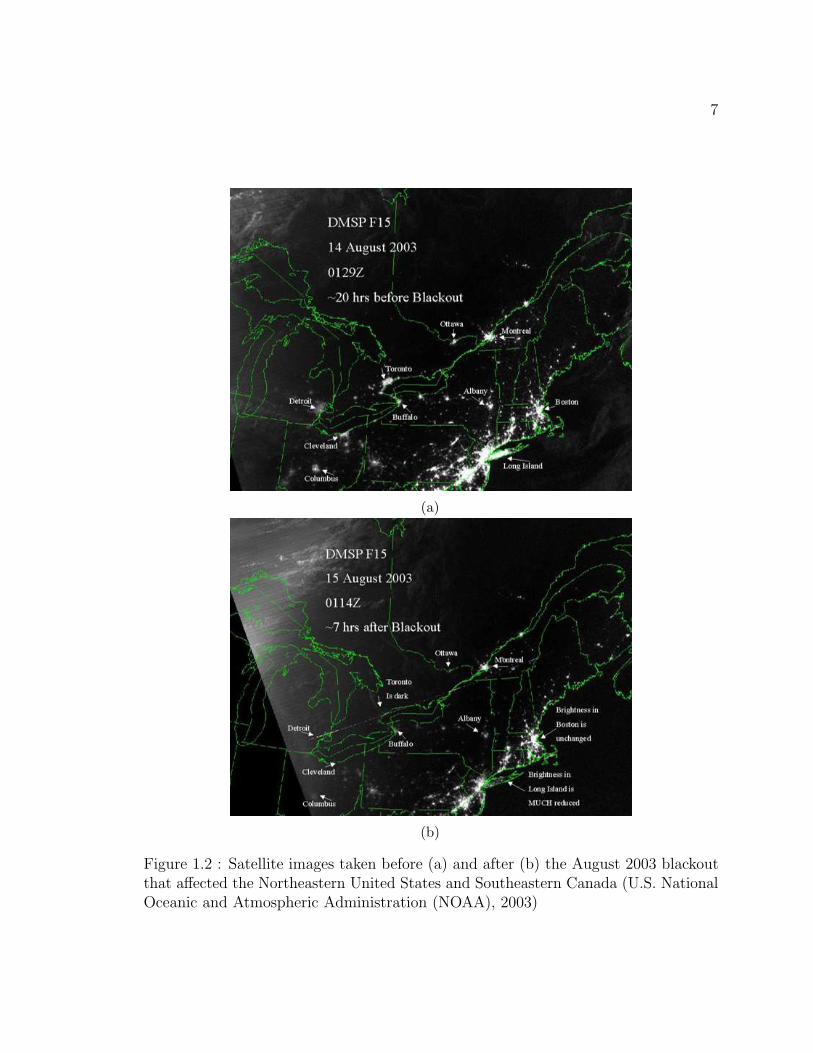
1.2 Satellite images taken before (a) and after (b) the August 2003

blackout that affected the Northeastern United States and

Southeastern Canada (U.S. National Oceanic and Atmospheric

Administration (NOAA), 2003) . . . . . . . . . . . . . . . . . . . . . 7

1.3 Papers on interconnected critical infrastructure (National Institute of

Standards and Technology (NIST), 2016) . . . . . . . . . . . . . . . . 8

2.1 Colombian primary road network . . . . . . . . . . . . . . . . . . . . 31

2.2 Graphical representation of the td-INDP iterative reconstruction of the

primary Colombian road network after a simulated natural disaster

(earthquake) . . . . . . . . . . . . . . . . . . . . . . . . . . . . . . . . 32

2.3 Critical infrastructure networks in Shelby County, TN. (Gonzalez

et al., 2016b) . . . . . . . . . . . . . . . . . . . . . . . . . . . . . . . 33

2.4 Optimal performance recovery for the (a) water, (b) power, and (c) gas

networks, as well as (d) the combined system of infrastructure

networks in Shelby County, TN., after a disaster consistent with an

earthquake of magnitude Mw = 8 (Gonzalez et al., 2016a) . . . . . . . 35

3.1 Average solving times for the proposed td-INDP model . . . . . . . . 42

xvi

3.2 Graphical representation of the (a) time-horizon decomposition, and

(b) illustrative flow chart for the iINDP algorithm . . . . . . . . . . . 45

3.3 Solving time scalability comparison between the proposed INDP MIP

model (td-INDP), and the iterative INDP (iINDP) . . . . . . . . . . 47

3.4 Performance recovery for the system of infrastructure networks in

Shelby County, TN., after a disaster consistent with an earthquake of

magnitude Mw = 8, using the td-INDP, the iINDP, and two

permutation-based heuristics . . . . . . . . . . . . . . . . . . . . . . . 49

3.5 Recovery of artificial power grid using the iINDP and a guided

percolation-based heuristic (Smith et al., 2017) . . . . . . . . . . . . . 49

3.6 Evolution of the flow costs, associated with earthquakes of magnitude

Mw = 6 (a), 7 (b), 8 (c) and 9 (d). For each magnitude, the maximum

number of repaired components by iteration v = 3, 6, 9 and 12

(Gonzalez et al., 2016b). . . . . . . . . . . . . . . . . . . . . . . . . . 52

3.7 Evolution of the reconstruction costs, associated with earthquakes of

magnitude Mw = 6 (a), 7 (b), 8 (c) and 9 (d). For each magnitude, the

maximum number of repaired components by iteration v = 3, 6, 9 and

12 (Gonzalez et al., 2016b). . . . . . . . . . . . . . . . . . . . . . . . 53

3.8 Evolution of the total costs of recovery, associated with earthquakes of



12 (Gonzalez et al., 2016b) . . . . . . . . . . . . . . . . . . . . . . . . 53

xvii

3.9 Evolution of the total costs of recovery, without considering the

unbalance costs, associated with earthquakes of magnitude Mw = 6 (a),

7 (b), 8 (c) and 9 (d). For each magnitude, the maximum number of

repaired components by iteration v = 3, 6, 9 and 12 (Gonzalez et al.,

2016b) . . . . . . . . . . . . . . . . . . . . . . . . . . . . . . . . . . . 54

3.10 Number of arcs (blue) and nodes (red) repaired on each recovery

period, after an earthquake of magnitude Mw = 9, assuming maximum

number of repaired components by iteration v = 3 (a), 6 (b), 9 (c) and

12 (d) (Gonzalez et al., 2016b). . . . . . . . . . . . . . . . . . . . . . 54

3.11 Evolution of the total performance, associated with earthquakes of



12 (Gonzalez et al., 2016b). . . . . . . . . . . . . . . . . . . . . . . . 55

3.12 td-INDP time-complexity sensitivity to different topology-related

parameters (Gonzalez et al., 2015). . . . . . . . . . . . . . . . . . . . 63

3.13 td-INDP time-complexity sensitivity to different

interdependence-related parameters (Gonzalez et al., 2015) . . . . . . 64

3.14 td-INDP coefficient matrices for the three studied topologies, with

standard configuration (Gonzalez et al., 2015). . . . . . . . . . . . . . 65

3.15 Graphical representation of the coefficient matrix associated with the

td-INDP . . . . . . . . . . . . . . . . . . . . . . . . . . . . . . . . . . 70

3.16 Decomposition of the coefficients associated with element functionality,

flow of commodities, and over/under supply, for each recovery period

(corresponding to a block off of Figure 3.15). . . . . . . . . . . . . . . 71

xviii

4.1 Resilience metrics for critical infrastructure networks in Shelby County,

TN. (Gonzalez et al., 2014b) . . . . . . . . . . . . . . . . . . . . . . . 78

4.2 Correlations between node failure ratios associated with different

earthquake magnitudes . . . . . . . . . . . . . . . . . . . . . . . . . . 80

4.3 Correlations between node recovery ratios associated with different


4.4 Correlations between node recovery periods associated with different


4.5 Decomposition of the sINDP MIP model as a two-stage stochastic

problem (Gonzalez et al., 2017c) . . . . . . . . . . . . . . . . . . . . . 91

4.6 Solution times for the sINDP as a function of |T |, using different

optimizers (Gonzalez et al., 2017c) . . . . . . . . . . . . . . . . . . . 95

4.7 Performance recovery for Mw ∈ 6, 6.5, 7 (Gonzalez et al., 2017c) . . 96

4.8 System perfomance for each recovery period, consistent with an

earthquake of magnitude Mw = 6.5 (Gonzalez et al., 2017c) . . . . . . 98

4.9 Undelivered supply as a function of time, consistent with an

earthquake of magnitude Mw = 6.5 (Gonzalez et al., 2017c) . . . . . . 99

4.10 Trade-off between undelivered supply and unsatisfied demand, for

diverse supply-surplus values (Gonzalez et al., 2017c) . . . . . . . . . 100

4.11 Probability of exceedance of different performance levels as a function

of the recovery period, consistent with an earthquake of magnitude

Mw = 6.5 (Gonzalez et al., 2017c) . . . . . . . . . . . . . . . . . . . . 101

xix

4.12 Comparison between three different performance recovery cases

(assuming supply surplus of 5% (column 1) and 10% (column 2)):

considering all scenarios simultaneously (row 1); using only the

expected value of the demands (row 2); and, assuming perfect

information (row 3) (Gonzalez et al., 2017c). . . . . . . . . . . . . . . 102

5.1 Histogram for the aggregate differences between element-wise recovery

times, associated with globally-oriented and individually-oriented

recovery strategies . . . . . . . . . . . . . . . . . . . . . . . . . . . . 114

5.2 Comparison between the solutions offered by the information-sharing

model, the iINDP method, and the INRG (Smith et al., 2016). . . . . 118

5.3 Price of anarchy computed using the information-sharing model and

the INRG framework (Smith et al., 2016). . . . . . . . . . . . . . . . 118

5.4 Recovery operator A representation (for nodes only) with matrix

entries with absolute value below 0.011 not displayed. The rows and

columns correspond to the assigned labels for each element (Gonzalez

et al., 2017a). . . . . . . . . . . . . . . . . . . . . . . . . . . . . . . . 127

5.5 Comparison between predicted recovery strategy for nodes (using the

recovery operator) and the benchmark strategies (based on the

td-INDP), using a = 0.5 (Gonzalez et al., 2017a). . . . . . . . . . . . 133

5.6 Comparison between predicted recovery strategy for nodes (from the

recovery operator) and the benchmark strategies (based on the

td-INDP), using a = 0.4 (Gonzalez et al., 2017a). . . . . . . . . . . . 134

5.7 Recovery state estimation for 10 randomly selected components

(Gonzalez et al., 2017a) . . . . . . . . . . . . . . . . . . . . . . . . . . 135

xx

5.8 Recovery operator A representation (including both nodes and arcs)

with matrix entries with absolute value below 0.0079 not displayed.

The rows and columns correspond to the assigned labels for each

element (Gonzalez et al., 2017a). . . . . . . . . . . . . . . . . . . . . 136

5.9 Comparison between predicted recovery strategy for nodes and arcs

(from the recovery operator) and the benchmark strategies (based on

the td-INDP), using a = 0.5 (Gonzalez et al., 2017a). . . . . . . . . . 137

6.1 Proposed research map divided by topics . . . . . . . . . . . . . . . . 150

1

Part I

Understanding the Proposed

Research Problem and its

Importance

2

Chapter 1

Introduction

Proper operation of critical infrastructure networks is vital to our society, supporting

the well-being of the population, while enabling adequate governance and safety. In

contrast, abnormal operation of such systems generates health and security issues, as

well as considerable economic loss. Each year, natural events such as earthquakes,

storms, and landslides, kill more than 75 000 people and affect more than 200 million

people, usually depriving them from food and housing (Van Wassenhove, 2005). Just

between 1996 and 2005, two earthquakes in Turkey and Japan accounted for US$95

billion in losses, three floods in China had an associated economic loss of US$46

billion, and one storm in United States accounted for US$125 billion (Sahin, 2011).

Similarly, between 2001 and 2011 adverse natural events have generated economic

losses larger than US$1.68 trillion (UNISDR, 2013), where just in 2011 the disaster

generated by the Tohoku earthquake and tsunami in Japan caused a direct economic

loss of more than US$171 billion, damaging 59 806 buildings and killing more than

13 000 people (Norio et al., 2012). Thus, developing adequate mitigation strategies

becomes imperative (Nagasaka, 2008), along with effective relief methodologies and

recovery planning for post-disaster response scenarios (Clay Whybark, 2007; Wrobel

and Wrobel, 2009).

3

Figure 1.1 : Graphical definition of resilience (Ouyang and Duenas-Osorio, 2012)

1.1 Defining and optimizing resilience

Reducing the vulnerability of a system while increasing its recoverability can be

captured by the concept of maximizing its resilience. There is no universal definition

of resilience, but literature predominantly describes it as the ability or capacity of a

system to withstand a hazard, contain its damage, and return to adequate performance

levels (Ouyang et al., 2012). Figure 1.1 depicts these three aspects of resilience for a

given system. This Figure shows a superposition of the performance level associated

with a system that is fully operational [TP (t)], and the performance level when the

system is affected by a given disaster [P (t)]. Once the disaster occurs (point A at time

t0), the damage and subsequent negative effects on the performance will propagate

trough the system (until a time t1). After that, the system invests time to gather

information regarding the disaster and prepare for the recovery process (from t1 to

4

t2). The recovery process (which takes place from t2 to tE), is carried out until

the system reaches a desired performance level (point B, at time tE). Figure 1.1

depicts a ‘recovered’ level at 100% performance, but in general such a level could be

associated with performances above or below 100%. Following this notation, Ouyang

and Duenas-Osorio (2012) define resilience [R(T )] as the ratio between the areas,

from times 0 to T , below the performance function associated with a fully operational

system [TP (t)], and the performance function associated with a system affected by a

disaster [P (t)], i.e.,

R(T ) ≡∫ T

0P (t)dt∫ T

0TP (t)dt

. (1.1)

Assuming that TP (t) is given and fixed, the resilience R(T ) is maximized when∫ T0P (t)dt is maximized. Moreover, if TP (t) is assumed to be 100% for all times t,

then∫ T

0TP (t)dt = T , and

R(T ) =

∫ T0P (t)dt

T= P (T ), (1.2)

where P (T ) represents the average of P (t) from times 0 to T .

Unfortunately, studying the resilience of realistic networked systems presents

multiple challenges associated with, among others, their constant expansion, both

in space and demand, and their increased interdependency, which directly impacts

their vulnerability and recoverability (Duenas-Osorio, 2005; Hernandez-Fajardo and

Duenas-Osorio, 2011). Moreover, for realistic applications, it is important to be able

to not only quantify the resilience of the studied systems, but also to determine the

decisions that maximize it (Ouyang and Duenas-Osorio, 2012; Hernandez-Fajardo and

Duenas-Osorio, 2013). By maximizing the resilience of real systems, these will be

5

able to both better endure diverse hazards and recover faster, ideally with minimum

economic and social impact.

1.2 Systems of interdependent networks

One of the most prevalent characteristics of realistic networked systems such as

critical infrastructure, is that these systems are often interconnected, and consequently

highly interdependent. Thus, modeling infrastructure networks as isolated systems

would not reflect important dynamics that impact their operation and performance

(Anderson et al., 2007). There are a plethora of examples that illustrate the effects

of interconnectedness and interdependencies between infrastructure networks, such

as the blackouts in Italy on September of 2003 (Schneider et al., 2013) and North

America on August 2013 (Veloza and Santamaria, 2016; Zhang and Peeta, 2011), or

the 2011 Japan earthquake and tsunami disaster (Norio et al., 2012), among others. In

each case, interdependencies between different infrastructure networks, such as power,

water, transportation, and telecommunications, exacerbated the damage propagation

and caused cascading failure effects. To illustrate the impact of these events, Figure 1.2

shows satellite images of Northeastern United States and Southeastern Canada, before

and after the August 2003 blackout, where it can be seen that, for more than 7 hours

after the event, the Long Island region had a major reduction on its power supply,

and cities such as Toronto, Ottawa, and Buffalo were almost completely left without

power. However, Figure 1.2 only illustrates the effects associated with the power

network. The loss of electricity supply also caused, among others, the inoperability of

water pumps, which left many people without ready access to potable water (Beatty

et al., 2006), and the reduced access and operation of the transportation network,

due to lack of signaling and illumination, as well as the nonviable operation of the

6

electricity-based trains (Deblasio et al., 2004). Just in New York City, around 11 600

road intersections collapsed due to complete inoperability of traffic lights and other

signaling, and all 413 train sets came to a halt due to lack of power, affecting more

that 400 000 train users (Deblasio et al., 2004).

Considering the importance of modeling and understanding interdependencies

and their effects on critical infrastructure networks, research on interconnected and

interdependent infrastructure systems has gained much interest in recent years. Figure

1.3 illustrates the number of papers written (and their citations), per year, related

to interconnected critical infrastructure, showing a growing research interest on

interdependent networks, despite being a relatively novel subject in the literature.

Early works on interconnected critical infrastructure started by acknowledging and

categorizing the diverse interdependecies observed in infrastructure systems (Rinaldi

et al., 2001). Later, some works focused on detecting and quantifying the vulnerability

caused by such interdependencies (Buldyrev et al., 2010; Vespignani, 2010; Gao et al.,

2011; Hernandez-Fajardo and Duenas-Osorio, 2013), and subsequently on reducing such

vulnerability (Brummitt et al., 2012). Simultaneously, other works started focusing

on describing and developing recovery strategies for damaged interdependent systems

(Lee II et al., 2007; Cavdaroglu et al., 2011). More recently, researchers have focused

on integrating these concepts, by studying the resilience of these interdependent

networked systems (Pant et al., 2013; Ouyang, 2014; Shafieezadeh et al., 2014; Baroud

et al., 2015). However, in order to optimize the resilience of systems of interdependent

networks, there are still multiple challenges that need to be addressed.

7

(a)

(b)

Figure 1.2 : Satellite images taken before (a) and after (b) the August 2003 blackoutthat affected the Northeastern United States and Southeastern Canada (U.S. NationalOceanic and Atmospheric Administration (NOAA), 2003)

8

Figure 1.3 : Papers on interconnected critical infrastructure (National Institute ofStandards and Technology (NIST), 2016)

1.3 Current challenges

From the diverse literature related to modeling and optimizing the vulnerability,

recoverability, and resilience of interdependent networks, the three most prevalent and

relevant challenges we observed are:

• Modeling realistic networks and their interdependencies: It is important to

adequately define the way in which the networks and their interdependencies

are modeled. It is crucial to evaluate to what level of detail we should model

the networks, in order to take into account their most important properties

and behaviors, while maintaining simplicity and manageability. For real in-

frastructure systems, it is imperative to include aspects such as the existence

of commodities flowing through the networks, being supplied and demanded.

Similarly, there must be a limit to the system capacities for its operation. The

9

system of networks should also be subjected to failures while recovering from

those failures must be limited by a finite amount of resources.

• Handling large-scale problems: Critical infrastructure systems are increasing

both in size and in demand of commodities. Thus, it is imperative that proposed

computational models are scalable and susceptible to enhancements, either by

analytical or heuristic methods.

• Considering uncertainty: Given that the studied systems are subject to fai-

lure and forecasting errors, it is important that the proposed computational

models can consider uncertainty. To this end, we must focus on developing

fast algorithms that facilitate the use of sampling techniques. Additionally, the

proposed algorithms should also be able to embed uncertainty in its paramaters,

to guarantee that resultant analyses agree with the expected behavior of the

system.

1.4 Research objectives

Considering the preceeding discussion, the main objective of this thesis is to develop

efficient theoretical and computational tools to model, quantify, and optimize the

resilience of systems of interdependent networks.

In particular, the proposed work focuses on developing tools applied to resource

allocation and emergency response for critical interdependent infrastructure systems,

in a disaster management context, while considering the three challenges previously

detailed.

This thesis presents a body of work that focuses on integrally addressing the

aforementioned challenges, in order to model and quantify the effects of interdepen-

10

dencies in realistic infrastructure networks, optimize their recovery, and ultimately

optimize their overall resilience. By virtue of doing so, the developed models provide

useful tools for decision makers and stakeholders, to support pre- and post-event

decisions associated with mitigation, resource allocation, and emergency response,

among others.

1.5 Thesis structure

Chapter 2 presents a detailed study on how to model and recover networked infra-

structures, as well as on how to model their associated interdependencies. Considering

the diverse existing approaches, their assumptions, and limitations, we detail what

are the desired characteristics and goals that an adequate interpendent-networks

recovery problem should consider. In particular, Section 2.2 presents the denominated

Interdependent Network Design Problem (INDP), as the problem associated with

determining the optimal recovery strategy of a system of interdependent networks,

while considering realistic constraints associated with its operation, and its resource

availability. Section 2.2 also proposes a mathematical formulation to solve the INDP,

denominated the time-dependent INDP model (td-INDP). The td-INDP is a Mixed

Integer Program (MIP) formulation, that focuses on minimizing the costs associa-

ted with the operation and recovery of a system of interdependent networks, while

considering constraints associated with resource availability, flows balance, systems’

capacities, and physical and geographical interdependencies, among others.

Chapter 3 explores diverse techniques to improve the computational capabilities

of the td-INDP, such that it can be solved faster and can handle larger systems.

On one hand, Section 3.1 presents a heuristic approach denominated the iterative

INDP (iINDP), which decomposes the studied planning horizon into smaller more

11

manageable time horizons, and solves iteratively for each of them. On the other hand,

Section 3.2 presents a comprehensive sensitivity analysis on the td-INDP parameters

and its structure. In particular, Section 3.2.2 shows that the td-INDP has a special

structure, which makes it suitable for analytical decomposition techniques.

Chapter 4 describes diverse methodological approaches to allow considering di-

verse sources of uncertainty. Section 4.1 describes the uncertainty associated with

the failure modes in the system, and presents a simulation-based study that offers

insightful element-wise information to facilitate pre-event decision making support. In

particular, we propose diverse resilience metrics that describe different aspects of the

studied system, such as the networks’ topologies, their flow of commodities, or the

specific hazard studied. Then, Section 4.2 details the importance of accounting for

the uncertainty related to the system properties, such as its demands and resource

availability. To account for this source of uncertainty, we propose a stochastic for-

mulation, denominated the stochastic INDP (sINDP) model, which determines the

recovery strategy that minimizes the expected recovery costs.

Chapter 5 presents additional multidisciplinary techniques to further expand the

td-INDP capabilities. Section 5.1 describes the importance of considering additional

realistic socio-technical aspects when studying multiple interdependent networks, such

as the existence of multiple interacting decision makers in charge of different networks

in the system. In addition, Section 5.2 presents a methodology that approximates the

td-INDP using a linear time-invariant operator, denominated the recovery operator.

This operator identifies key properties related to the recovery dynamics, and allows

constructing efficient recovery strategies in polynomial time.

Finally, Chapter 6 presents a summary of the main findings from this thesis,

and highlights opportunities for future research that build upon the proposed INDP

models.

12

Part II

Addressing Current Modeling

Challenges

13

Chapter 2

The Interdependent Network Design Problem

Properly modeling interdependent networks and their operation is vital to study and

understand the key factors associated with the performance of such systems and their

dependence on damaged components∗. In order to determine the key properties that

need to be modeled, as well as the best approach to model them, the next section

focuses on reviewing some of the most relevant literature in the field of infrastructure

recovery.

2.1 Recovery of networked infrastructure systems

Considering the importance of ensuring adequate performance of infrastructure sys-

tems, this topic has been extensively studied in different fields, such as civil engineering,

economics and political sciences, among others. Moreover, there are different met-

hodological approaches used to study these systems, such as dynamical systems

(Hallegatte and Ghil, 2008), complex systems (Comfort et al., 2004; Chu, 2009; Nejat

and Damnjanovic, 2012), and network analysis (Wang et al., 2013; National Institute

of Standards and Technology (NIST), 2016; Gomez et al., 2013; Duenas-Osorio and

Kwasinski, 2012). Considering that the main focus of the proposed research is to

optimize the resilience of interdependent networked systems, this literature review is

oriented towards the network analysis perspective.

∗This Chapter is based on the ideas and contents presented in Gonzalez et al. (2016b) and Gonzalezet al. (2016a). The definitive versions of these papers are available at www.onlinelibrary.wiley.comand press.tongji.edu.cn

14

Viswanath and Peeta (2003) developed a relief distribution algorithm, based on a

multicommodity maximal covering network design problem, to maximize the total

population covered while minimizing people’s travel time. Similarly, Sheu (2007)

designed an approach to emergency logistics for quick response to large-scale disasters,

based on a hybrid fuzzy clustering optimization problem. The model involves recursive

mechanisms associated with disaster-affected areas grouping and relief co-distribution.

Later, Sheu (2010) presented a dynamic model that incorporates imperfect informa-

tion, considering uncertain and dynamic features of the relief demands. Particularly,

the model focuses on treating related inconsistencies from multiple data sources, by

applying a data fusion technique. Yi and Kumar (2007) also developed a model

for disaster relief operations, using a hybrid optimization approach. The proposed

network-flows model solves the multicommodity dispatch to distribution centers, while

a metaheuristic based on ant-colony optimization designs the vehicle routing. Stepa-

nov and Smith (2009) developed a multi-objective evacuation routing model based

on optimization modeling and queueing theory. Saadatseresht et al. (2009) used a

multi-objective evolutionary optimization approach to develop an evacuation strategy;

they emphasized on spatial aspects such as safe areas selection.

In order to determine the location and allocation of several kinds of emergency

supplies, Rawls and Turnquist (2010) proposed a methodology for pre-positioning

emergency supplies based on a heuristic approach. To address large-scale instances,

they proposed a structure based on a minimum cost flow problem and solved its

Lagrangian relaxation. Bozorgi-Amiri et al. (2011) focused on the logistics associated

with the supply of relief commodities and different sources of uncertainty affecting

the relief chains; they developed a multi-objective stochastic optimization model.

Ozdamar and Demir (2012) proposed a hierarchical clustering method that reduces

large-scale routing networks into smaller ones, so as to enable linear optimization.

15

Ganapati (2012) showed the importance of long-term recovery and not only the rapid

reconstruction at early stages of the process. Even though he mentions the importance

of including the effects of the initial reconstruction phase, since it could lead to the

detriment of the long-term recovery goals and priorities, his work focused only on

a conceptual approach. Gomez et al. (2013) developed an algorithm based on a

hierarchical infrastructure network representation that reduces a realistic complex

networked system into a simpler one, while preserving the most significant information

and dynamics for effective decision support. However, their approach focused on

studying the reliability and propagation of damage on an infrastructure system,

without explicit methods to perform optimal recovery processes.

In general, the aforementioned references emphasize the importance of considering

the limited access to resources during the emergency-response phase, as well as the

limited capacities of each system. However, these works do not consider the effects

associated with interdependencies between different infrastructure systems.

Network Interdependencies

Understanding and managing interdependencies among infrastructure systems is

imperative to ensure their service continuity after disruptive events (Wallace et al.,

2001). In particular, the interdependency of infrastructure networks increases their

vulnerability to natural disasters, particularly when such disasters are neither too small

nor too large (Duenas-Osorio et al., 2007b,a). Hence, given that infrastructure systems

are increasingly interdependent, interdependence analysis is critical when studying

reliability and performance of systems of infrastructure, as well as when designing

recovery and mitigation plans (Duenas-Osorio and Kwasinski, 2012). However, before

focusing on developing strategies to study the impact of interdependencies on the

performance of a given system, it is important to determine which interdependencies

16

are the most relevant, and what is the specific goal of the developed models to capture

them.

On one hand, regarding the types of interdependence between networks that are

relevant in infrastructure systems, there are different classifications proposed in the

literature. Rinaldi et al. (2001) classify them as physical, cyber, geographic, and

logical interdependencies. Lee II et al. (2007) classify them as input, mutual, shared,

exclusive or, and co-located interdependencies. For the remaining of the thesis, we will

use the classification proposed by Rinaldi et al. (2001), given that it presents a more

general description of the interdependencies, which can be adapted to a broader range

of situations. Under such classification, physical interdependence refers to the case

when the performance of a given network depends on the outputs of other networks.

For instance, consider the existing interdependence between the power networks and

communication networks, where a power outage may affect some data centers and

routers in the latter depending on the extent of backup systems. Cyber interdependence

occurs when the interdependence between two networks is based on shared information.

The Smart Grid concept (Farhangi, 2010), which refers to how information about

supply and demand is automatically used to determine the production and distribution

of electricity, is an example of cyber interdependence between the power and the

telecommunication networks. Geographic interdependence denotes the cases when a

local event can create state changes in several networks simultaneously. For example,

fixing an underground water pipeline may affect the transportation network around

the intervened area, probably slowing traffic and increasing congestion. Finally, there

is logical interdependence when two or more systems are interconnected via control,

regulatory, or other mechanism that are not considered physical, geographical or cyber

(Setola and Porcellinis, 2009). Logical interdependence can be observed when human

decisions affect the state of the networks, for instance when designing a recovery or

17

expansion plan that prioritizes certain networks.

On the other hand, the existing methodologies for interdependent network analysis

can be grouped according to their goals as follows: analytical models, performance

evaluation models, design methodologies, mitigation models, and recovery methodo-

logies. Analytical and performance evaluation models focus on tools to understand

how interdependencies influence the systems behavior, performance, and reliability.

For instance, Amin (2002) focused on describing the complexity of networks (such as

transportation, power, telecommunications, and financial, among others) and their

ever increasing interdependence, vulnerability, and diminished security. Similarly,

Zevenbergen et al. (2012) emphasized the importance of understanding and tackling

the complex linkages between subsystems and services, and the cascading effects of

one subsystem upon another, since this deep relationship is imperative to establish

the full benefit and costs of any proposed disaster management strategy.

Design models are helpful to conceptualize and build infrastructure systems, taking

under consideration constraints such as the demand of the commodities, limited

resources, flow capacities, and costs of construction and transportation. Buldyrev

et al. (2010) explored how interdependent networks may collapse under the effect

of a catastrophic cascade of failures, due to their increased vulnerability. More

specific to infrastructure systems, models such as the ones proposed by Hernandez-

Fajardo and Duenas-Osorio (2011) and Wu and Duenas-Osorio (2013) quantify how

interdependencies impact the failure and performance of infrastructure systems, where

the complex connections between different networks lead to emergent response effects

on the performance of individual networks.

Mitigation models focus on preparing systems to handle future hazards, so they

can reduce the associated risks and enhance their resilience. For example, Yagan and

Zhang (2012) described a methodology to optimally allocate links in cyber-physical

18

systems, in order to improve their performance and robustness.

Finally, recovery models focus on taking systems with failing components to a

functional state, considering important aspects such as minimizing the recovery time

and the associated costs. Focusing on recovery, Lee II et al. (2007) presented a

general network flow model for infrastructure restoration using Mixed Integer Linear

Programming (MILP). Such a model focuses on determining which components should

be reconstructed to recover a damaged system, but does not indicate when to perform

the reconstruction jobs. Cavdaroglu and Nurre (2010), Cavdaroglu et al. (2011) and

Nurre et al. (2012) used MILP models to study network restoration and scheduling

for interdependent infrastructure systems, where an explicit time index is used to

assign reconstruction periods, while Sharkey et al. (2015) showed how to account

for information sharing when optimizing the recovery process of such interdependent

systems. Even though the presented models consider functional interdependencies,

they do not consider relevant issues associated with co-location and the availability

of different required resources, among others. In this chapter, we propose a recovery

model that can be easily expanded to be used for any of the other described goals,

while being able to consider co-location and resource-availability constraints.

2.2 The Interdependent Network Design Problem (INDP)

At the core of the proposed research, it is important to define a problem that focuses

on optimizing the recovery process of a partially destroyed system, such that the

resilience of the system is maximized. This problem, that designs recovery strate-

gies for interdependent systems, will be consequently defined as the Interdependent

Network Design Problem (INDP). Nevertheless, there are multiple approaches and

considerations that could be made when defining the INDP, depending on how the

19

performance of the system is measured, the properties and characteristics that will be

modeled from the real system, and particularly, the constraints that will take place.

2.2.1 What should the INDP consider?

The first aspect that must be defined refers to the objective of the INDP. By definition,

the INDP must focus on optimizing the recovery process of a destroyed system, such

that its resilience is maximized. Nevertheless, the quantified resilience will depend

directly on the performance metric used. In particular, critical infrastructure systems

should guarantee adequate operation to the community, that in the case of utilities

such as water, gas, and power, relates to the demand that the system is able to satisfy.

Thus, it is important that the INDP focuses on maximizing the percentage of demand

being supplied. But, even though managers in charge of such systems should have as a

priority properly covering the community demands on the diverse offered commodities,

they also are concerned about reducing their operation (and reconstruction) costs.

Thus, the INDP should focus on maximizing the supply of commodities (as first

priority), while also reducing the associated costs of recovery and operation.

Also, infrastructure systems are subject to constraints related to their operation

and recovery capacity. Regarding the operation, infrastructure systems will have to

supply certain demand of commodities at different locations, and will be subject to

limited transportation capabilities. Regarding the recovery process, infrastructure

systems must be efficient about their use of the limited resources at hand. Related to

both operation and recovery, infrastructure networks usually depend on the proper

operation of other networks.

Considering all these aspects, let us define the Interdependent Network Design

Problem (INDP) as the problem of finding the least-cost recovery strategy of a

partially destroyed system of infrastructure networks, subject to budget, resources,

20

and operational constraints, while considering interdependencies between the networks,

such as physical and geographical (Rinaldi et al., 2001). Under such a definition, the

reconstruction costs can include the costs of the resources used in the reconstruction,

labor costs, the costs of preparing the geographical locations for the reconstruction

process, and costs associated with the system not being able to perform adequately

(Gonzalez et al., 2016b).

Based on the previous discussion, in order to solve the INDP for generalized

practical applications, we propose formulating a Mixed Integer Programming (MIP)

model with the following features:

• Models a system of interdependent networks with multiple commodities, de-

mands, capacities, and functional and reconstruction constraints.

• Considers multiple network interdependencies (e.g., physical, geographical, etc.).

• Analyzes the impact of the interdependencies on the networks performance and

operative costs.

• Indicates the optimal time-dependent recovery strategy for a system of interde-

pendent networks after a damaging event.

The proposed MIP model, denominated the time-dependent INDP (td-INDP), is

based on the following assumptions, associated with the flows and capacities of the

system of networks, the costs related to the operation and restoration of the system,

and the interdependencies studied:

Network flows

• Each infrastructure network is composed by arcs and nodes subject to failure,

which can be repaired or reconstructed.

21

• Each infrastructure network transports one or several commodities, where there

is a known demand or supply pattern for each commodity associated with each

infrastructure network.

• Each commodity flows through only one infrastructure network.

• There is a known flow capacity for each arc in every infrastructure network,

shared by commodities flowing through that network.

• The flow capacities are independent between different infrastructure networks

since they transport different commodities.

Costs

• There is a known fixed cost associated with the lack of supply of each commodity.

• The flow costs for each commodity and the reconstruction costs for each arc in

each network are known and fixed.

• The reconstruction process involves costs for repairing the components (nodes

and arcs) and for preparing the reconstruction locations.

• All costs should be in equivalent units, and should reflect their real values to the

cost bearers, such that they already consider possible weighting skews among

them.

Interdependencies

• Infrastructure networks may be physically interdependent, i.e., the failure of

some nodes imply that other nodes may not function.

• Several infrastructure networks may have geographical interdependence, i.e.,

components (nodes and arcs) sharing physical space. When there are different

22

network components that have to be fixed, the cost of preparing the overlapping

locations is shared between the networks.

Based on these assumptions, the proposed td-INDP model uses as an input the

information associated with a partially destroyed system of interconnected infrastruc-

ture networks (costs, capacities, damaged components, etc), and returns the recovery

process that maximizes the resilience of the system. In particular, the proposed

td-INDP formulation is structured as follows.

2.2.2 td-INDP mathematical formulation

Let G = (N ,A) be a directed network defined by a set N of nodes, and a set A of arcs,

which represents the complete system of individual infrastructure networks. Let K be

the set of infrastructure networks, such as electrical, water, and telecommunication,

among others. Likewise, let L be the set of commodities flowing through the networks.

For each infrastructure network k ∈ K there is a related subset Lk ⊆ L, indica-

ting which commodities flow through network k. From the assumptions, note that

∪k∈KLk = L and that Lk ∩ Lk = ∅,∀k, k ∈ K | k 6= k. Also, for each infrastructure

network k ∈ K there is an associated subgraph Gk = (Nk,Ak), where Nk and Ak

are respectively the sets of nodes and arcs associated with that specific network. It

should be noted that ∪k∈KNk = N and ∪k∈KAk = A. Let N ′k ⊆ Nk and A′k ⊆ Ak

denote the set of destroyed nodes and arcs in each network k ∈ K after a disaster.

Correspondingly, N ′ = ∪k∈KN ′k and A′ = ∪k∈KA′k denote the set of nodes and arcs

destroyed in the entire system of systems. Also, for each network k ∈ K the set

N ∗k ⊆ Nk indicates the nodes that require full satisfaction of its demand to become

functional.

Now, assume that there is limited time horizon to perform the full recovery of the

23

system, divided into T time periods. Define T = 0, 1, .., T as the set of periods in

which the problem is defined, which means that the parameters and variables will

depend on the time t ∈ T . Time t = 0 indicates the moment right after the occurrence

of the damaging event, and times t ∈ T \0 indicate the periods in which the recovery

process takes place. For every period t ∈ T , infrastructure network k ∈ K and node

i ∈ Nk, let biklt be the demand or supply for commodity l ∈ Lk (if biklt > 0, i is a

supply node; if biklt < 0, i is a demand node; and if biklt = 0, i is a transshipment

node). The associated reconstruction cost of node i in network k is denoted by qikt.

For every arc (i, j) ∈ Ak in network k ∈ K, we define a reconstruction cost fijkt, an

associated capacity denoted by uijkt, and a cost cijklt that represents the cost per unit

flow of commodity l ∈ Lk. The parameter M−iklt represents the unit cost of commodity

l ∈ Lk that fails to be supplied in node i ∈ Nk of network k ∈ K in period t ∈ T ;

similarly, M+iklt represents the corresponding cost of excess supply.

The td-INDP model also considers a set of limited resources R involved in the

restoration process (e.g., budget, time, workforce) that prevents immediate total

reconstruction; hence, the availability of resource r ∈ R is represented by vr. For every

period t ∈ T , node i ∈ Nk and arc (i, j) ∈ Ak in network k ∈ K, let pikrt and hijkrt be

the amount of resource r ∈ R that the recovery of every node and arc would require,

respectively. In a general sense, the physical interdependence used in the model is

based on the idea that the functionality of a node i ∈ Nk is related to the functionality

of another node j ∈ Nk, where k, k ∈ K. To model the interdependence between any

pair of nodes, for every period t ∈ T there is a parameter γijkkt that relates them.

The parameter γijkkt allows the td-INDP model to account for four different cases of

physical interdependencies. The first case of physical interdependence is when node

j ∈ Nk can be functional only if another specific node i∗ ∈ Nk is functional; then γijkkt

is 1 when i = i∗, and 0 otherwise. The second case of interdependence is when node

24

j ∈ Nk can be functional only if there is at least one functional node from a subset

N ∗k ⊆ Nk; then γijkkt is 1 for i ∈ N ∗k , and 0 otherwise. The third case is when node

j ∈ Nk can be functional only if every node from a subset N ∗k ⊆ Nk is functional; then

γijkkt takes the value of 1/|N ∗k | for i ∈ N ∗k , and 0 otherwise. The fourth, and most

general case, is when node j ∈ Nk depends partially on the functionality of the nodes

from a subset N ∗k ⊆ Nk, where the dependence on each of them is not the same, i.e.,

each node from N ∗k provides only a fraction of functionality to node j; then γijkkt is

the fraction of functionality that each node i ∈ N ∗k provides to node j.

The interdependencies based on co-location assume that repairing one specific arc

in a network implies preparing a shared space with other networks. Preparing a space

refers to construction tasks required to access and repair elements of the system. These

tasks may include debris removal, excavation, shoring, soil improvement, temporary

detours, etc. Let S be the set of geographical spaces, where at each period t ∈ T , each

s ∈ S has an associated cost of preparation gst. There is a binary parameter αikst that

takes the value of 1 if node i ∈ Nk of network k falls inside space s; it takes the value

of 0, otherwise. There is also a binary parameter βijkst, which takes a value of 1 if for

network k, arc (i, j) ∈ Ak (or a part of it) is inside space s; it takes the value of 0,

otherwise. Hence, this parameter indicates whether the space s has to be prepared or

not when fixing the arc (i, j) ∈ Ak. If a given space s has to be prepared due to the

reconstruction of one or several arcs, or due to one or several nodes, then gst is defined

as the maximum of those individual preparation costs, and is due only once. Note

that the set of spaces S refers to a partition of the geographical extent that contains

the complete interdependent infrastructure system, but the size and shape of each

space may vary according to what each space is desired to represent. For example, if

we analyze an infrastructure network in a given county, S may represent the political

districts (e.g., by towns or neighborhoods), the service areas of each system component,

25

a geographical distribution based on the hazard levels due to floods or earthquakes,

and so on. Nevertheless the set S must always be a mutually exclusive and collectively

exhaustive collection that contains the system of infrastructure networks.

The decision variable denoted by xijklt represents the flow of commodity l ∈ Lk

through arc (i, j) ∈ Ak in network k ∈ K at period t ∈ T . For each arc (i, j) ∈ A′k in

network k ∈ K there is also a binary variable ∆yijkt that takes the value of 1 if the arc

is set to be reconstructed at period t ∈ T ; it takes the value of 0, otherwise. Similarly,

for every node i ∈ N ′k in network k ∈ K, there is a binary variable ∆wikt that takes

the value of 1 if the node is set to be reconstructed at period t ∈ T ; it takes the

value of 0, otherwise. Note that a component that is not destroyed is not necessarily

functional due to network dependence to another component. For each arc (i, j) ∈ A′k

in network k ∈ K there is a binary variable yijkt that takes the value of 1 if the arc is

functional at period t ∈ T ; it takes the value of 0, otherwise. Similarly, for every node

i ∈ N ′k in network k ∈ K, there is a binary variable wikt that takes the value of 1 if the

node is functional at period t ∈ T ; it takes the value of 0, otherwise. In addition, for

each space s ∈ S there is a binary variable zst to denote if the space was prepared for

at least one reconstruction process at period t ∈ T , taking the value of 1 if the space

is intervened; it takes the value of 0, otherwise. Also, we define the deviation variables

δ+iklt and δ−iklt to indicate the surplus or deficit supply of commodity l ∈ Lk at node

i ∈ Nk in network k ∈ K at period t ∈ T . Based on the previous description of the

variables and parameters involved, the proposed model for the INDP is represented as

follows:

26

minimize

(2.1a)

∑t ∈T |t>0

∑s∈S

gst∆zst +∑k∈K

∑(i,j)∈A′k

fijkt∆yijkt +∑i∈N ′k

qikt∆wikt

+∑t ∈T

∑k ∈K

∑l∈Lk

∑i∈Nk

(M+

ikltδ+iklt +M−

ikltδ−iklt

)+∑l∈Lk

∑(i,j)∈Ak

cijkltxijklt

subject to,

(2.1b)

∑j :(i,j) ∈Ak

xijklt−∑

j :(j,i) ∈Ak

xjiklt =biklt−δ+iklt+δ

−iklt,

∀k ∈ K,∀i ∈ Nk,∀l ∈ Lk,∀t ∈ T ,(2.1c)

∑l ∈Lk

xijklt ≤ uijktwikt, ∀k ∈ K,∀(i, j) ∈ Ak, ∀t ∈ T ,

(2.1d)∑l ∈Lk

xijklt ≤ uijktwjkt, ∀k ∈ K,∀(i, j) ∈ Ak,∀t ∈ T ,

(2.1e)∑l ∈Lk

xijklt ≤ uijktyijkt, ∀k ∈ K,∀(i, j) ∈ A′k,∀t ∈ T ,

(2.1f)∑i ∈Nk

wiktγijkkt ≥ wjkt, ∀k, k ∈ K,∀j ∈ Nk, ,∀t ∈ T ,

(2.1g)wik0 = 0, ∀k ∈ K,∀i ∈ N ′k,(2.1h)yijk0 = 0, ∀k ∈ K,∀(i, j) ∈ A′k,

(2.1i)wikt ≤t∑t=1

∆wikt, ∀k ∈ K, ∀i ∈ N ′k, ∀t ∈ T | t > 0,

(2.1j)yijkt ≤t∑t=1

∆yijkt, ∀k ∈ K,∀(i, j) ∈ A′k,∀t ∈ T | t > 0,

(2.1k)∑k ∈K

∑(i,j)∈A′k

hijkrt∆yijkt+∑i∈N ′k

pikrt∆wikt

≤ vrt, ∀r ∈ R,∀t ∈ T | t > 0,

(2.1l)∆wiktαikst ≤ ∆zst, ∀k ∈ K,∀i ∈ N ′k,∀s ∈ S,∀t ∈ T | t > 0,

(2.1m)∆yijktβijkst ≤ ∆zst, ∀k ∈ K,∀(i, j) ∈ A′k,∀s ∈ S,∀t ∈ T | t > 0,

(2.1n)wiktbiklt ≤ biklt − δ−iklt, ∀k ∈ K,∀i ∈ N ∗k , ∀l ∈ Lk,∀t ∈ T ,(2.1o)δ+

iklt ≥ 0, ∀k ∈ K, ∀i ∈ Nk, ∀l∈ Lk,∀t ∈ T ,(2.1p)δ−iklt ≥ 0, ∀k ∈ K, ∀i ∈ Nk, ∀l ∈ Lk,∀t ∈ T ,(2.1q)xijklt ≥ 0, ∀k ∈ K, ∀(i, j) ∈ Ak,∀l ∈ Lk,∀t ∈ T ,

27

(2.1r)wikt ∈ 0, 1, ∀k ∈ K, ∀i ∈ Nk, ∀t ∈ T(2.1s)yijkt ∈ 0, 1, ∀k ∈ K,∀(i, j) ∈ A′k,∀t ∈ T ,(2.1t)∆wikt ∈ 0, 1, ∀k ∈ K,∀i ∈ N ′k,∀t ∈ T | t > 0

(2.1u)∆yijkt ∈ 0, 1, ∀k ∈ K, ∀(i, j) ∈ A′k,∀t ∈ T | t > 0,

(2.1v)∆zst ∈ 0, 1, ∀s ∈ S, ∀t ∈ T | t > 0.

The objective function (2.1a) is composed by five different terms that are minimized

simultaneously. The first term is the cost of preparing the geographical spaces for the

recovery (drilling, excavations, etc.), the second and third term are the reconstruction

costs associated with the links and the nodes respectively, the fourth term is the cost

associated with the under or over supply of the given demands, and the fifth term

is the total cost flow in the system. Constraints (2.1b) guarantee the flow balance

in each of the networks, enforcing the correct net flow for each node in the system,

considering its demands and its under or over supply. Constraints (2.1c), (2.1d), and

(2.1e) guarantee that there can be flow trough each arc only if its starting node, its

ending node, and the arc itself are functional. Also, these constraints ensure that the

total flow trough each arc is under its maximum capacity. Constraints (2.1f) model

the physical and logical interdependence between nodes, guaranteeing that nodes are

functional only if their parent nodes are also functional. Constraints (2.1g) and (2.1h)

enforce that the initially damaged nodes and arcs (respectively) are not functional

right after the destructive event (time t = 0). Constraints (2.1i) and (2.1j) guarantee

that each initially damaged node or arc can become functional only after being

fully recovered. Constraints (2.1k) model the use of limited resources, guaranteeing

that the amount used of each resource type never surpasses its availability, at any

time. Constraints (2.1l) and (2.1m) enforce that at every time a node or an arc is

repaired, the geographical spaces that contain them must be prepared. Constraints

(2.1n) guarantee that, for the specified set of nodes that require it, each node can be

functional only when covering its full demands. Finally, constraints (2.1o) - (2.1v)

28

describe the type of each decision variable, being either binary or simply non-negative.

Note that the proposed td-INDP enforces integrality constraints for the variables

associated with the recovery and the functionality of each element, since these are

binary variables that indicate if a given element is recovered or is functional at each

recovery period. However, td-INDP allows relaxing such constraints in case the

modeled system permits partial functionality states or partial recovery of a damaged

element. If such a case is assumed, the proposed td-INDP could be used to model a

recovery process where each element has a different speed of recovery, that depends on

how much resources are devoted to it. Then, using constraints (2.1k), one could easily

consider different recovery speeds, by modeling the percentage in which each element

is recovered at each period. In this case, parameters hijkrt and pikrt would indicate

how much of resource r is required to recover 100% of each given link and node.

Moreover, if one defines a resource associated with ‘recovery time’, these parameters

could directly indicate how much time is required to recovery each element.

2.3 Illustrative examples

The proposed td-INDP formulation is intended to allow analyzing a broad range of

systems of networks. It permits having one or multiple commodities flowing through

one or more networks simultaneously, while considering multiple types of resources

simultaneously. To exemplify the capabilities and versatility of the proposed td-

INDP model, we present two different realistic case studies. First, we study the

recovery process associated with the Colombian road network, after being damaged

by an earthquake. This case shows how the proposed model can be used to optimize

the recovery process of a given infrastructure network, while considering multiple

commodities flowing through it. Second, we study the recovery of the water, power,

29

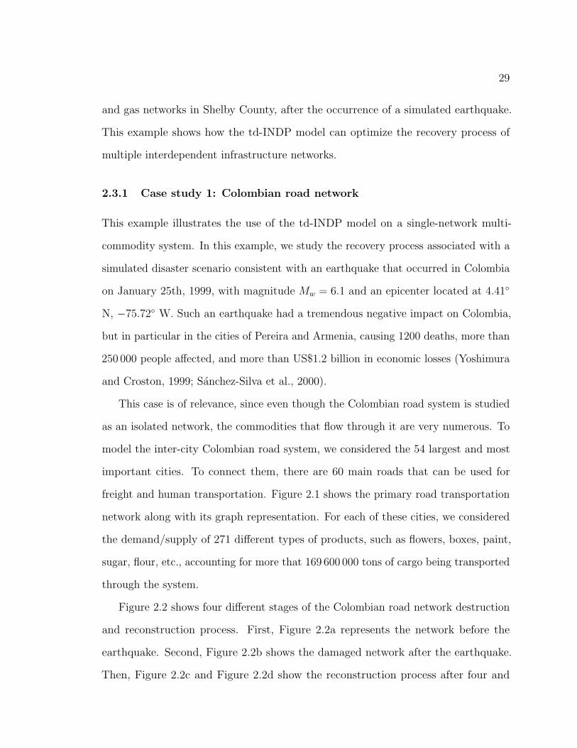
and gas networks in Shelby County, after the occurrence of a simulated earthquake.

This example shows how the td-INDP model can optimize the recovery process of

multiple interdependent infrastructure networks.

2.3.1 Case study 1: Colombian road network

This example illustrates the use of the td-INDP model on a single-network multi-

commodity system. In this example, we study the recovery process associated with a

simulated disaster scenario consistent with an earthquake that occurred in Colombia

on January 25th, 1999, with magnitude Mw = 6.1 and an epicenter located at 4.41

N, −75.72 W. Such an earthquake had a tremendous negative impact on Colombia,

but in particular in the cities of Pereira and Armenia, causing 1200 deaths, more than

250 000 people affected, and more than US$1.2 billion in economic losses (Yoshimura

and Croston, 1999; Sanchez-Silva et al., 2000).

This case is of relevance, since even though the Colombian road system is studied

as an isolated network, the commodities that flow through it are very numerous. To

model the inter-city Colombian road system, we considered the 54 largest and most

important cities. To connect them, there are 60 main roads that can be used for

freight and human transportation. Figure 2.1 shows the primary road transportation

network along with its graph representation. For each of these cities, we considered

the demand/supply of 271 different types of products, such as flowers, boxes, paint,

sugar, flour, etc., accounting for more that 169 600 000 tons of cargo being transported

through the system.

Figure 2.2 shows four different stages of the Colombian road network destruction

and reconstruction process. First, Figure 2.2a represents the network before the

earthquake. Second, Figure 2.2b shows the damaged network after the earthquake.

Then, Figure 2.2c and Figure 2.2d show the reconstruction process after four and

30

15 recovery periods, respectively. For this particular network, the amount of arcs

repaired by period –modeled with constraints (2.1k)– is limited to 1, so as to illustrate

a gradual step-by-step reconstruction process. As expected, the td-INDP gave high

priority in the early stages to reconnecting nodes that were totally disconnected from

the network after the earthquake, but after having reconnected the whole system it

focused on reducing operational costs.

2.3.2 Case study 2: Utilities in Shelby County, TN.

This example illustrates some of the td-INDP capabilities regarding the modeling of

multiple interdependent infrastructure networks and designing recovery strategies for

all of them simultaneously. In particular, this case study analyses streamlined versions

of the power, water, and gas networks in Shelby County, TN, USA. Shelby County is

known for containing the city of Memphis, and also for being at risk from earthquakes

due to the New Madrid Seismic Zone (NMSZ). The test network descriptions used

for this study were adapted from Hernandez-Fajardo and Duenas-Osorio (2010),

Hernandez-Fajardo and Duenas-Osorio (2013), and Song and Ok (2010). Regarding

the disaster realization, Adachi and Ellingwood (2009) presented a realistic earthquake

scenario for Shelby County, with epicenter at 35.3 N and 90.3 W (33 km from

Memphis center). For this example, we detail the recovery process associated with a

disaster realization consistent with an earthquake with magnitude Mw = 8.

In this case study, there are two main interdependencies of interest. First, there is a

physical interdependence between the power networks and the gas and water networks,

given that for a pumping station to be functional, it is required that at least one power

station (from a set of covering stations) is functional as well. Second, this case study

takes under consideration the geographical interdependence from co-location between

the water and the gas networks. Given that both networks are underground, there is a

31

Figure 2.1 : Colombian primary road network

32

(a) Representation of the Colombian roadnetwork before the natural disaster

(b) Status of Colombian road network af-ter a simulated natural disaster

(c) Status of the Colombian road networkafter 4 periods of the td-INDP

(d) Status of the Colombian road networkafter 15 periods of the td-INDP

Figure 2.2 : Graphical representation of the td-INDP iterative reconstruction of theprimary Colombian road network after a simulated natural disaster (earthquake)

33

3

9

1

2

10

11

6

15

8

5 17

7

4

12

16

13 1

4

9

8

76

5

4

3

21

0

15

14

13

12

11

10

3

12

11

0 6 12 18 24 303km

Gas service areas

Gas distribution stations

Gas pipelines

(a)

9

87

65

4

32 1

494847464544

4342

41

4039

38

37 36

353433

32

31 3029

282726

25 242322

2120 19

18

1716

15 14

1312

1110

3937

343311

0 6 12 18 24 303

km

Water service areas

Water distribution stations

Water pipelines

(b)

"

"

"

"

"

"

"

"

"

#

#

## ## #

###

##

##

#

#

#

X

XXXXXXX

XXX

XXX

!

!!

! !

! !

!

!!!!

!

!!

!!!!

!45

44434142394038

363435

33373132

3029272628

6

31

4

2

5

8 60

7

9

20

23

192122

17 181615 14 1312 1110

2425

±

Tributary Areas! 12kV Substations# 23kV SubstationsX Intersection Point" Gate Stations

Transmission Line

0 6 12 18 24 303km

"

#

# #

XX X

!

!!

!

!

!

! 5655542122

(c)

5

39

0 6 12 18 24 303km

Subareas

Gas distribution stations

Water distribution stations

Gas pipelines

Water pipelines

(d)

Figure 2.3 : Critical infrastructure networks in Shelby County, TN. (Gonzalez et al.,2016b)

34

shared-area preparation cost related to the reconstruction process of each component,

that is, there is a saving potential by repairing co-located components from the water

and the gas networks simultaneously. Note that even though some previous works on

interdependent infrastructure recovery (Lee II et al., 2007; Cavdaroglu et al., 2011;

Nurre et al., 2012; Sharkey et al., 2015) have mentioned the existence and importance

of geographical correlation, most have focused on the failure correlations between

components, but not in the savings in time, money, and efforts that could be made

if assigning simultaneous recovery jobs for co-located components. Given that this

example considers geographical interdependence, it is important to define a set of

geographical spaces S. In this case, S is defined as the set of areas resulting from

intersecting the service areas of the gas and water networks, which are the ones under

geographical interdependence. Figure 2.3 shows the gas, water, and power networks,

as well as the intersection areas that constitute S. Note that these intersection areas

are mutually exclusive and collectively exhaustive. The td-INDP model can now be

used to find the optimal recovery strategy for the system, which in this case consists

of multiple interdependent infrastructure networks.

The amount of elements that can be repaired are limited to 3 per period in this case

study, so as to enable the recovery of one element per network each time. To illustrate

the recovery process associated with the disaster scenario studied, Figure 2.4 shows

the performance evolution associated with the damage and subsequent recovery of

the studied water, power, and gas networks. For this study, the average performances

associated with each network are shown in Table 2.1. These performances were defined

as the average percentage of demand that is supplied, for each network, during the

recovery process. These can be determined using the fourth term of the objective

function (2.1a) of the td-INDP, if the under-supply costs for each commodity are

assumed to be equal, and the over-supply costs are zero.

35

(a) (b)

(c) (d)

Figure 2.4 : Optimal performance recovery for the (a) water, (b) power, and (c) gasnetworks, as well as (d) the combined system of infrastructure networks in ShelbyCounty, TN., after a disaster consistent with an earthquake of magnitude Mw = 8(Gonzalez et al., 2016a)

36

Figure 2.4d shows that the optimal performance recovery of the full system tends to

be smooth, relative to the recovery of each of the individual networks. This shows that

the recovery that optimizes the overall resilience of the system, does not necessarily

represent the strategy that optimizes the resilience of each individual network. In

fact, it can be seen that the scarce resources imply that, at some periods, while some

networks are recovered others have to wait with their performance unchanged. For

example, all three networks experience performance recovery during the first period,

but at the second period the gas network seems to have a priority over the others,

as it is recovered to almost full performance while the other two networks were not

repaired at all. Then, at period 3, only the power network was recovered, while the

others remain unchanged. This behavior, observed during the whole recovery process,

shows that in order to optimize the resilience of a system of interdependent networks,

it is important to consider all networks simultaneously, as opposed to optimizing for

each of them independently. Table 2.1 shows that the gas network indeed had priority

over the other networks, as its average performance was greater than the other two

networks. This can be explained by the fact that the gas network has much less

redundancies compared to the other networks, thus each time an element is repaired

on this network, there is a greater impact on its recovery compared to the other

networks.

Table 2.1 : Average performance of the optimal recovery strategies found (Gonzalezet al., 2016a)

Infrastructure systemWater Power Gas Full system

Av. Performance 0.747 0.770 0.856 0.788

Also, to showcase another possible application of the td-INDP, we used the obtained

optimal recovery strategies to fit a continuously-differentiable function for each network

37

–of the form described in equation (2.2)–, so as to provide useful benchmarks that can be

used by other researchers –such as for gradient descent algorithms and other methods

that are based on such continuously-differentiable functions. Table 2.2 describes the

coefficients for the optimally-fitted functions for each performance recovery, as well as

their associated coefficients of determination (R2).

(2.2)P (X) = A− BeE−CXD

Table 2.2 : Coefficients of fitted recovery functions (Gonzalez et al., 2016a)

Infrastructure systemCoeff. Water Power Gas Full system

A 1.38 0.996 0.955 0.996

B 0.65 0.862 0.832 0.917

C 0.133 0.11 0.286 0.111

D 0.825 1.639 3.063 1.633

E 0.58 0.062 0.03 0.001R2 0.954 0.986 0.97 0.986

Such utilization of the td-INDP solutions demonstrates that the proposed opti-

mization model not only can be used to inform decision-makers about the optimal

recovery strategies for a damaged system of interdependent networks, but also to

provide benchmarks for other academic and practical studies.

An analogous application of the td-INDP is detailed in Section 5.2, where the

td-INDP is used to provide benchmark failure/recovery time series, to feed input data

to a system identification framework, which focuses on extracting and recreating key

features of the recovery dynamics associated with interdependent networks.

2.4 Conclusions

This Chapter describes a new model for defining the optimal reconstruction strategy for

a partially destroyed system of interconnected infrastructure networks, that accounts

38

for functional interdependencies between the associated networks while incorporating

for the first time reconstruction savings due to co-located components that could be

repaired simultaneously.

First, we introduce the Interdependent Network Design Problem (INDP), which

seeks the minimum-cost reconstruction strategy, subject to budget, resources, and

operational constraints. Then, we propose a Mixed Integer Programming (MIP)

mathematical formulation denominated time-dependent INDP (td-INDP) model, that

extends the ideas of the widely known Network Design Problem (NDP) (Johnson

et al. (1978); Ahuja et al. (1993); Hu (2012)) to include interdependencies and other

operational constraints.

The proposed td-INDP model determines the optimal reconstruction strategy of

a damaged system of interdependent infrastructure networks, seeking the least-cost

recovery configuration while accounting for constraints related to the existence of limi-

ted resources (such as budget, time, manpower, etc.), flow capacities, demand/supply

of commodities, and functional relations between the networks, among others.

Even though the proposed td-INDP is defined as a post-event tool, this mathe-

matical model has the potential to also be used for pre-event assessments associated

with prevention and mitigation, to reduce the negative impact of natural and targeted

damaging events. Such a generalization can be achieved by extending the td-INDP

mathematical model to include uncertainty, particularly associated with the failure

modes of the system. To this end, Section 3.1 will introduce a simulation-based

approach that allows analyzing the expected recovery dynamics of a given system of

interdependent networks. This idea will be furthered discussed in Chapter 4, where

we address multiple sources of uncertainty, and show how the td-INDP can integrate

them in its analysis.

However, in order to facilitate using the td-INDP in simulation-based studies, it

39

is imperative that we understand the computational complexity associated with it,

and particularly, that we have tools to solve it in a time-efficient manner. To this end,

Chapter 3 presents a detailed study on the structure and complexity of the td-INDP,

and proposes heuristic and analytical approaches to enhance its solution times.

40

Chapter 3

Understanding and Improving the Efficiency of the

td-INDP

In Section 2.2, we described how the proposed td-INDP model can be used to quantify

the effects of a disaster over the performance of a system of interdependent networks.

More over, we showed how the td-INDP model can be used to determine the optimal

recovery strategy for a damaged system, such that the associated recovery costs are

minimized –or more specifically, such that the average performance is maximized–,

offering an invaluable tool for emergency-response and planning situations. However,

it is imperative to ensure that the td-INDP model can be solved in a time-efficient

manner, such that it can be used in realistic time-critical applications∗.

Moreover, as hinted at the end of the previous Chapter, the proposed td-INDP

model could be used for purposes beyond emergency response, such as mitigation

and preparedness, providing stakeholders useful information regarding the system

vulnerability. In particular, the td-INDP model could be used to perform probabilistic

studies on a given system, to detect critical elements, forecast recovery costs and

resource utilization, and estimate recovery times, among others. Nevertheless, these

probabilistic studies often require considering the effects of multiple damage scenarios,

thus increasing the computational complexity of the associated optimization processes.

Given this, it is imperative to understand and improve the computational efficiency

∗This Chapter is based on the ideas and contents presented in Gonzalez et al. (2016b) and Gonzalezet al. (2015). The definitive versions of these papers are available at www.onlinelibrary.wiley.comand open.library.ubc.ca

41

of the proposed td-INDP model. To achieve this, Section 3.1 presents a flexible

heuristic algorithm to solve the td-INDP. This heuristic approach is based on dividing

the set of recovery periods (which determines the recovery time horizon) into smaller

sets, such that the td-INDP can be solved systematically using these reduced time

sets on a running horizon scheme. Then, Section 3.2 presents an analytically-oriented

study on the properties and the structure of the td-INDP model. In particular,

we start by determining how diverse topological properties of the studied systems

influence the td-INDP solving times, performing a detailed sensitivity analysis of the

model parameters. Then, we describe the particular structure of the td-INDP model,

and show how this structure, which reflects a block-decomposable system, could be

exploited to enhance its solving speeds and size capabilities.

3.1 Heuristic approach

In Section 2.3.2, we showed how the td-INDP can be used to calculate the optimal

recovery strategy of the water, power, and gas networks in Shelby County, TN.

associated with an earthquake disaster scenario. However, in order to determine the

optimal recovery strategy, the td-INDP model requires that the recovery planning

horizon is given, as it is modeled by a set T that is fixed during the optimization

process. By looking closely at the td-INDP formulation, we can observe that both the

number of terms in objective function (2.1a) and the number of constraints (2.1b)-

(2.1v) increase linearly as a function of the cardinality of T . Thus, it is to be expected

that the number of recovery periods considered by the td-INDP will have a relevant

impact on its time-complexity.

To illustrate the relation between the cardinality of T and the solution times

associated with the td-INDP, we randomly generated 100 different damage realizations

42

Figure 3.1 : Average solving times for the proposed td-INDP model

consistent with a magnitude Mw = 9 earthquake and the realistic system of networks

described in Section 2.3.2, and measured their average solution times, while considering

multiple planning horizons. We selected this large earthquake magnitude, in order

to test the td-INDP efficiency in worst-case scenario conditions, related to highly

damaged systems. Figure 3.1 shows the average td-INDP solution times related to

the aforementioned disaster realizations, considering planning horizons that spanned

from 1 to 8 periods. As expected, the average td-INDP solving times highly increased

as a function of |T |. In particular, Figure 3.1 shows that the average solution times

increase exponentially with the size of the planning horizon. This exponential increase

would imply that, independently of the level of destruction and the size of the studied

network, there will be always a planning horizon limit, for which the td-INDP could

not be fully solved in a realistic time range. This property evidences the importance

of developing solution approaches to the td-INDP model that are scalable to large

planning horizons. In order to obtain efficient recovery strategies for scenarios defined

over long planning horizons, we propose a heuristic approach that improves the solving

time of the td-INDP by solving it using a piece-wise strategy. Such time-decomposition

43

approaches have been shown to be particularly successful for scheduling and routing

problems that involve planning for multiple periods in the future (Campbell, 2008),

but now we explore their suitability in recovery planning applications. The proposed

heuristic approach, denominated the iterative INDP (iINDP), is detailed as follows.

3.1.1 The iterative INDP (iINDP)

Instead of solving the td-INDP for all periods t ∈ T at once, we propose splitting

T into multiple smaller recovery periods, to then use the td-INDP to systematically

solve the recovery process associated with each of these reduced planning horizons.

Assume that each reduced planning horizon is of size thorizon ≤ |T |. Then, the

proposed algorithm starts by solving the td-INDP model focusing only on periods 0

to thorizon (even though it may not be optimal for all periods t ∈ T ). The obtained

recovery strategy is guaranteed to be the optimal for periods 0, 1, ..., thorizon, mini-

mizing the average recovery costs for these periods. Then, considering the recovery

strategy proposed for periods 0, 1, ..., thorizon, we update all sets associated with the

damaged nodes and arcs, N ′ and A′, respectively. Then, based on the updated sets of

damaged elements, and using time thorizon + 1 as the initial period, use the td-INDP

again to find the optimal recovery strategy for periods thorizon + 1 to 2thorizon. Using

the new recovery information for periods thorizon + 1, thorizon + 2, ..., 2thorizon, we

update again sets N ′ and A′, and repeat the same process until a recovery strategy

for the full planning horizon is obtained.

However, note that in some cases splitting the original time horizon into multiple

disjoint periods may not offer an accurate approximation of the optimal recovery

strategy for the whole time horizon studied. The quality of this approach will depend

on multiple factors, such as the level of interdependency between the studied networks,

how limited the resources are, or how large the initial destruction is, among others.

44

To circumvent this issue and allow ‘communication’ between the different reduced

planning horizons, we should allow certain overlapping between consecutive time

horizons. By including such overlaps, we may increase the quality of the overall

solutions, by letting the optimizer update the recovery plan for the final periods of one

reduced horizon, using information of the following reduced horizon. To model this,

define an additional parameter tlag, to indicate how many periods are being advanced

at each iteration in which the td-INDP is solved, such that tlag ≤ thorizon.

Considering these two parameters, the algorithm starts by solving the td-INDP

model using as time horizon the periods 0 to thorizon. Then, the proposed recovery

strategy from period 0 to tlag is saved, and the sets of destroyed nodes and destroyed

arcs are updated according to the saved recovery strategy (taking into account which

elements are repaired at each period). Then, for the next iteration, the starting

and ending periods will shift in tlag periods with respect to the previous ones. This

algorithm, denominated the iterative INDP (iINDP), iteratively uses the td-INDP

model until the original time horizon has been fully explored. In order to illustrate

the proposed algorithm, Figure 3.2 depicts the proposed decomposition of the time

horizon and presents a diagram that describes the iINDP. A more detailed description

of the iINDP is shown in Algorithm 1.

To illustrate the time savings involved in adopting the iINDP, Figure 3.3 shows a

comparison between the average solution times using the td-INDP and the iINDP,

for the scenarios previously depicted in Figure 3.1. For this case we used tlag = 0

and thorizon = 1, which is expected to be the most time-efficient iINDP configuration.

Figure 3.3 shows that, while the td-INDP times increase exponentially with the

cardinality of T , the iINDP times only increase linearly. This results in an average

speedup of more than 20 times when solving for 5 periods, and more than 300 times

when solving for 8 periods.

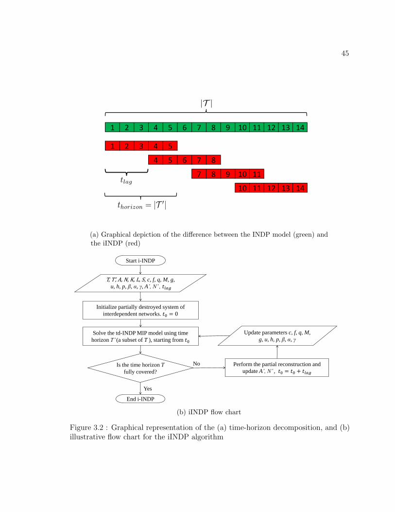
45

13 14

9 10 11

10 11 12

4 5 6 7 8

7 8

13 14

1 2 3 4 5

7 8 9 10 11 121 2 3 4 5 6

(a) Graphical depiction of the difference between the INDP model (green) andthe iINDP (red)

Solve the td-INDP MIP model using time

horizon T’ (a subset of T ), starting from 𝑡0

Is the time horizon T

fully covered?

Start i-INDP

End i-INDP

No

Yes

Perform the partial reconstruction and

update A’, N’ , 𝑡0 = 𝑡0 + 𝑡𝑙𝑎𝑔

Initialize partially destroyed system of

interdependent networks. 𝑡0 = 0

T, T’, A, N, K, L, S, c, f, q, M, g,

u, h, p, β, α, γ, A’, N’ , 𝑡𝑙𝑎𝑔

Update parameters c, f, q, M,

g, u, h, p, β, α, γ

(b) iINDP flow chart

Figure 3.2 : Graphical representation of the (a) time-horizon decomposition, and (b)illustrative flow chart for the iINDP algorithm

46

Algorithm 1 Iterative Interdependent Network Design Problem (iINDP)

Input: T , thorizon, tlag, A, N , K, L, S, R, A′, N ′, c, f , q, M , g, u, h, p ,b, v, α, β, γOutput: x, y, z, w,∆y,∆w

1: procedure iINDP2: t0 ← 03: while t0 ≤ |T | do4: Solve the td-INDP using periods t0 to thorizon5: for all ∀t ∈ t0...t0 + tlag do6: x, y, w, z,∆y,∆w ← x, y, w, z,∆y,∆w7: end for8: A′ ← A′\(i, j) : yijklt = 1,∀t ∈ t0...t0 + tlag9: N ′ ← N ′\i : wiklt = 1,∀t ∈ t0...t0 + tlag

10: update c, f , q, M , g, u, h, p ,b, v, α, β, γ . External changes11: t0 ← t0 + tlag12: end while13: return x, y, w, z,∆y,∆w14: end procedure

Even though the iINDP does not theoretically guarantee the optimality of the

obtained solution, it is expected to return good solutions for realistic applications. For

example, by inspecting the td-INDP performance recovery described in Figure 2.4d,

we can see that the system’s performance evolves with a monotonically decreasing

non-negative slope, i.e., the performance is always increasing, but the rate at which it

does reduces with time. Note that this property is observed only for the full system,

but not for the performance recovery associated with each individual network, where

the recovery processes have multiple points in which the rates of recovery oscillate,

and even stagnate.

Considering that our main objective is associated with optimizing the resilience

of the full system of interdependent networks, it is desirable for the iINDP that

the slope of the optimal performance is always non-negative and that it decreases

monotonically. This can be said since the iINDP is based on finding the recovery

47

strategy that maximizes the performance on the immediate subsequent periods, which

is analogous to finding the strategy that maximizes the slope at each time step. Thus,

in cases where the optimal performance recovery is smooth, it is likely that the iINDP

will return a strategy that approximates the behavior of the optimal one.

Figure 3.3 : Solving time scalability comparison between the proposed INDP MIPmodel (td-INDP), and the iterative INDP (iINDP)

To illustrate the quality of the iINDP solutions with respect to the td-INDP

and other heuristic approaches, Figure 3.4 shows the performance recovery for the

system of water, gas, and power networks in Shelby County, TN., associated with

a disaster realization consistent with an earthquake of magnitude Mw = 8. This

Figure shows the performance that would result after following the recovery strategies

proposed by the td-INDP, the iINDP, and two other heuristics based on Variable

Neighborhood Search (VNS) and permutations. It can be seen that the iINDP solution

results in a quasi-optimal recovery, only 0.49% from the optimal solution (despite

having used tlag = 0 and thorizon = 1), whereas the other heuristics achieved solutions

8.27% and 18.60% from the optimal. Since the optimal performance recovery for this

disaster realization depicted the desired features (non-negative slope that decreases

monotonically), the iINDP was expected to return a good solution. However, for

48

systems in which the performance recovery has multiple inflection points, the iINDP

may not return good quality solutions if a small thorizon is used, since the algorithm

may not have adequate information to account for the effects that decisions at close

periods will have in the long term.

Moreover, even if the shape of the optimal recovery strategy is ‘ideal’, the iINDP

solutions may loose quality for planning horizons that are too long, since the effects of

taking sub-optimal decisions will accumulate at each iteration. Figure 3.5 illustrates

this effect, when using the iINDP (with tlag = 0 and thorizon = 1) to recover a fully

disconnected power network composed of 1000 nodes, and recovering only one link per

iteration. This Figure shows the connectivity of the network (measured by the ratio

between the number of disconnected components –labeled as |C|– and the number of

nodes in the network –labeled as N–), using the iINDP and three other heuristics that

are based on selecting links from a predefined pool of links (of sizes 1, 2, and 1 –labeled

as M–). For this example, time t = 1 refers to the approximate total time required to

gain full connectivity, which corresponds to approximately 1000 recovery periods. It

can be seen that even though the iINDP reconnects the system in a relatively efficient

manner, the negative effects associated with the non-optimal decisions taken at each

recovery period accumulate in time.

Furthermore, given that each iteration of the iINDP is based on solving a separate

optimization problem, the iINDP allows for parameter updating, as opposed to the

td-INDP. This makes the iINDP a more flexible tool when studying problems where

parameters such as costs, resources, or capacities are difficult to forecast well in

advance. Moreover, the iINDP also allows updating all the associated sets at each

iteration, enabling modeling aftershock scenarios where there are multiple subsequent

destructive events. Additionally, note that parameters tlag and thorizon could also vary

at each iINDP iteration, such that they can adapt to the desired level of resolution

49

Time (period)0 1 2 3 4 5 6 7 8 9 10

Per

form

ance

0.4

0.45

0.5

0.55

0.6

0.65

0.7

0.75

0.8

td-INDPiINDPHeuristic AHeuristic B

Figure 3.4 : Performance recovery for the system of infrastructure networks in ShelbyCounty, TN., after a disaster consistent with an earthquake of magnitude Mw = 8,using the td-INDP, the iINDP, and two permutation-based heuristics

Figure 3.5 : Recovery of artificial power grid using the iINDP and a guided percolation-based heuristic (Smith et al., 2017)

50

and quality required at each recovery period. For example, one may give priority to

the quality of the recovery strategy at initial stages with respect to periods far from

the current period. In such a case, for the initial iterations one could choose relatively

large thorizon and small tlag values, whereas for the final recovery periods one could

use relatively small thorizon values. These time-adaptability features are desirable to

the end user of the iINDP, since he could adapt the algorithm to the desired quality

level, while considering time constraints in the solution times.

3.1.2 Illustrative example

As previously mentioned, one of the advantages of using the proposed iINDP is that

it enables performing simulation-based studies, thanks to the considerable associated

speedups. For this illustrative example, we perform a simulation study to estimate

the average costs and performance of the water, power, and gas networks in Shelby

County, TN., subject to diverse disaster scenarios. The simulated disaster realizations

are constructed following the propagation curves and other methodologies described

by Adachi and Ellingwood (2009), who presented a realistic earthquake scenario for

Shelby County, with an approximate average magnitude of Mw = 7.5. Considering

this magnitude, this study includes magnitudes within a range of Mw ∈ 6, 7, 8, 9.

For each of such magnitudes, the number of Monte-Carlo replications is limited to

1000, such that the results show steady behaviors.

For this example, we set different maximum amounts of components to be repaired

per iteration of the iINDP, in order to analyze the sensitivity of the solutions with

respect to these amounts. This number, denoted by v – as it is modeled using

constraints (2.1k)– spans from 3 to 12 components. We selected 3 components as the

lower bound of v, such that it is always feasible to reconstruct at least one component

from each of the three networks. Likewise, we selected 12 as the upper bound of

51

v, given that for greater values, constraints (2.1k) show a limited impact on the

reconstruction strategies.

Figures 3.6-3.9 show the results associated with the evolution of the costs involved

in the recovery process; as expected, note that the costs depend directly on the

magnitude of the earthquake. The cost evolution analysis is presented for the four

different values of the maximum number of reconstructed components per iteration

(v = 3, 6, 9, 12) and for each of the four magnitudes (Mw = 6, 7, 8, 9). We normalized

the cost values using as reference point the cost of reconstructing the complete system,

as we focus on studying the cost behavior, and not on their absolute values.

Figure 3.6 shows the evolution of the flow costs as a fraction of the minimum

feasible flow cost associated with a fully recovered network, i.e., the values in this

Figure correspond to the ratio between the actual flow cost and the minimum flow cost

related to a fully operational system (which would indicate the optimal configuration).

Note that for low-magnitude scenarios, such costs converge to the optimal, but for

high-magnitude scenarios, the costs converge to values up to 33.1% greater than the

optimal flow cost. This suggests that for high-magnitude earthquake events (where a

large number of components is destroyed), at the final stages of the reconstruction the

remaining feasible recovery jobs have a high cost, hence the savings in flow costs would

be less than the actual costs of reconstructing additional components. This is seen in

real life contexts, where some components cannot be repaired immediately due to cost

limitations. Nevertheless, posterior reduction in the operative and reconstructions

costs could enable repairing the remaining components as well. Note that a network

flows approach with an explicit time index (such as the td-INDP) would not be able

to adapt its costs to the current state of the network, but this can be easily carried

out by using the iINDP. Given that in the initial stages, where few reconstructions

have been performed, the flow costs are mostly an indicator of how much of the

52

demanded commodities are being supplied, where low initial flow costs (below 1)

indicate that there is an average lack-of-supply issue in the system (i.e., the flows are

not enough to cover the whole demand in the system). This is supported by the fact

that higher earthquake magnitudes have associated lower initial flow costs. Also, in

general the final flow costs do not seem to depend strongly on the parameter v, where

the highest difference between the final costs for a particular magnitude is only 5.3%.

This highlights the robustness of the iINDP and its results, since independently of

the parameter v used, the final costs tend to similar values, which correspond to the

optimal.

Iteration (recovery period)1 2 3 4 5 6

Nor

mal

ized

cos

ts

0

0.5

1

1.5

v = 3v = 6v = 9v = 12

(a)

Iteration (recovery period)1 2 3 4 5 6 7 8 9

Nor

mal

ized

cos

ts

0

0.5

1

1.5

v = 3v = 6v = 9v = 12

(b)

Iteration (recovery period)1 2 3 4 5 6 7 8 9 10 11 12 13 14 15 16

Nor

mal

ized

cos

ts

0

0.5

1

1.5

v = 3v = 6v = 9v = 12

(c)

Iteration (recovery period)1 2 3 4 5 6 7 8 9 10 11 12 13 14 15 16 17 18 19 20 21 22

Nor

mal

ized

cos

ts

0

0.5

1

1.5

v = 3v = 6v = 9v = 12

(d)

Figure 3.6 : Evolution of the flow costs, associated with earthquakes of magnitudeMw = 6 (a), 7 (b), 8 (c) and 9 (d). For each magnitude, the maximum number ofrepaired components by iteration v = 3, 6, 9 and 12 (Gonzalez et al., 2016b).

The curves of reconstruction costs shown in Figure 3.7 are normalized by the cost

associated with performing a full reconstruction (every node and arc) at once, since the

cost of reconstruction of a fully destroyed system is greater or equal than the cost of

reconstruction of any other destruction scenario. Then, the normalized reconstruction

53


Nor

mal

ized

cos

ts

0

0.01

0.02

0.03v = 3v = 6v = 9v = 12

(a)


Nor

mal

ized

cos

ts

0

0.01

0.02

0.03v = 3v = 6v = 9v = 12

(b)


Nor

mal

ized

cos

ts

0

0.01

0.02

0.03v = 3v = 6v = 9v = 12

(c)


Nor

mal

ized

cos

ts

0

0.01

0.02

0.03v = 3v = 6v = 9v = 12

(d)

Figure 3.7 : Evolution of the reconstruction costs, associated with earthquakes ofmagnitude Mw = 6 (a), 7 (b), 8 (c) and 9 (d). For each magnitude, the maximumnumber of repaired components by iteration v = 3, 6, 9 and 12 (Gonzalez et al.,2016b).


Nor

mal

ized

cos

ts

0

0.05

0.1

0.15v = 3v = 6v = 9v = 12

(a)


Nor

mal

ized

cos

ts

0

0.05

0.1

0.15v = 3v = 6v = 9v = 12

(b)


Nor

mal

ized

cos

ts

0

0.05

0.1

0.15v = 3v = 6v = 9v = 12

(c)


Nor

mal

ized

cos

ts

0

0.05

0.1

0.15v = 3v = 6v = 9v = 12

(d)

Figure 3.8 : Evolution of the total costs of recovery, associated with earthquakes ofmagnitude Mw = 6 (a), 7 (b), 8 (c) and 9 (d). For each magnitude, the maximumnumber of repaired components by iteration v = 3, 6, 9 and 12 (Gonzalez et al., 2016b)

54


Nor

mal

ized

cos

ts

0

0.02

0.04

0.06

0.08v = 3v = 6v = 9v = 12

(a)


Nor

mal

ized

cos

ts

0

0.02

0.04

0.06

0.08v = 3v = 6v = 9v = 12

(b)


Nor

mal

ized

cos

ts

0

0.02

0.04

0.06

0.08v = 3v = 6v = 9v = 12

(c)


Nor

mal

ized

cos

ts

0

0.02

0.04

0.06

0.08v = 3v = 6v = 9v = 12

(d)

Figure 3.9 : Evolution of the total costs of recovery, without considering the unbalancecosts, associated with earthquakes of magnitude Mw = 6 (a), 7 (b), 8 (c) and 9 (d).For each magnitude, the maximum number of repaired components by iteration v = 3,6, 9 and 12 (Gonzalez et al., 2016b)


No.

of

com

pone

nts

2

4

6

8

10

12

ArcsNodes

(a)


No.

of

com

pone

nts

2

4

6

8

10

12

ArcsNodes

(b)


No.

of

com

pone

nts

2

4

6

8

10

12

ArcsNodes

(c)


No.

of

com

pone

nts

2

4

6

8

10

12

ArcsNodes

(d)

Figure 3.10 : Number of arcs (blue) and nodes (red) repaired on each recovery period,after an earthquake of magnitude Mw = 9, assuming maximum number of repairedcomponents by iteration v = 3 (a), 6 (b), 9 (c) and 12 (d) (Gonzalez et al., 2016b).

55

Iteration (recovery period)-1 0 1 2 3 4 5 6

Perf

orm

ance

Lev

el

0

0.5

1

v = 3v = 6v = 9v = 12

(a)

Iteration (recovery period)-1 0 1 2 3 4 5 6 7 8 9

Perf

orm

ance

Lev

el

0

0.5

1

v = 3v = 6v = 9v = 12

(b)

Iteration (recovery period)-1 0 1 2 3 4 5 6 7 8 9 10 11 12 13 14 15 16

Perf

orm

ance

Lev

el

0

0.5

1

v = 3v = 6v = 9v = 12

(c)

Iteration (recovery period)-1 0 1 2 3 4 5 6 7 8 9 10111213141516171819202122

Perf

orm

ance

Lev

el

0

0.5

1

v = 3v = 6v = 9v = 12

(d)

Figure 3.11 : Evolution of the total performance, associated with earthquakes ofmagnitude Mw = 6 (a), 7 (b), 8 (c) and 9 (d). For each magnitude, the maximumnumber of repaired components by iteration v = 3, 6, 9 and 12 (Gonzalez et al.,2016b).

costs describe the fraction of the network that is being restored in each iteration. It

can be seen that these costs decrease as the iterations increase; except for the initial

iterations. This particular case corresponds to large earthquakes where there is a

large number of destroyed components. This is explained by the fact that the iINDP

assigns the cheapest high-importance recovery jobs at the beginning, and later some

more expensive recovery jobs. Note that the initial values of the reconstruction costs

in each magnitude studied do not differ much from each other, but as expected, for

low-magnitude scenarios the complete reconstruction process is achieved much faster.

The total costs (flow, arcs and nodes reconstruction, unbalance and geographical

preparation) associated with the recovery process are shown in Figure 3.8. These

values are normalized by a reference value equivalent to the total costs associated with

recovering a fully-destroyed network in just one iteration –obtained by solving the

56

td-INDP assuming unlimited resources. Then, the results show that as the magnitude

increases so does the initial total cost. Note that these costs correspond to the complete

objective function (2.1a) of the td-INDP model; hence, it is to be expected that the

model reduces as much cost as it can in every iteration. As desired, costs never

increase, and the reduction rate is higher as the iteration is closer to the initial state,

which is coherent to the fact that the iINDP model calculates the largest possible

reduction in each iteration. Nevertheless, the unbalance costs used in the example are

defined such that they are greater than any other cost (hence giving priority to ensure

supply).

Figure 3.9 shows that independently of the magnitude of the earthquake or the

amount of components repaired by iteration, the costs calculated with the iINDP

have a steady convergence to a similar value, where the maximum difference between

the calculated costs is only 0.3%. Such behavior is desirable, since it implies that

independently from the initial conditions, the iINDP converges to a similar solution

(in this case the optimal). This Figure summarizes the properties seen in the previous

analysis, such as that the initial costs are in general much higher than the ones in the

final stages (except in the high-magnitude cases where the initial disconnection does

not allow full operation of the network), or that for largely destructed scenarios there

is a fast initial growth in costs before all of them decrease to the final convergence

value.

Figure 3.10 shows the average amount of nodes and arcs reconstructed in every

iteration. As expected, the average amount of reconstructed components decreases as

the iterations increase. Also, in early stages of the reconstruction process, focusing

on the reconstruction of nodes is preferred to the reconstruction of arcs, which is an

expected property considering that each node may have several arcs depending on it.

Finally, in order to study the resilience of the system, Figure 3.11 shows the

57

evolution of the performance of the system. For this example, the performance level

at a given time is defined as the unbalance between the total supply capacity and

total demand, normalized by the total demand. For this Figure, recovery period

‘-1’ indicates the period right before the earthquake, iteration ‘0’ is related to the

period when the earthquake occurs, and the remaining periods are related to the

reconstruction process as before. As expected, the loss of performance is higher when

the earthquake has a larger magnitude, being on average 15.5% for Mw = 6, 34% for

Mw = 7, 61.5% for Mw = 8, and 87.3% for Mw = 9. It is possible to observe that the

iINDP provides reconstruction strategies that promptly improve the performance right

after the disaster, reaching in the worst case scenario (Mw = 9) a loss of performance

less than 15% after just one iteration, 10% after two iterations, and less that 5% after

four iterations. This exemplifies how the iINDP achieves its goal of quickly recovering

the system to its original capabilities.

3.2 Analytical approach

Even though heuristic approaches such as the iINDP are useful to find good quality

approximations to the optimal solution of the td-INDP, there are instances in which

it may be important to solve the problem to guaranteed optimality. This Section

focuses on analyzing the structure and properties of the td-INDP, in order to propose

analytical approaches that can be used to solve it more efficiently, without losing

guarantees of optimality. To this end, we start by performing a sensitivity analysis on

the td-INDP, such that we can determine how its structure and solution times are

affected by diverse parameters and network topologies.

58

3.2.1 Sensitivity analysis

The structure and computational complexity of the td-INDP model are related to

diverse parameters, such as the probability of failure, the size of the system, the level

of interdependency between networks, the availability of resources, and the number

of periods in the planning horizon. In the previous Section we discussed how the

time-complexity of the td-INDP increases exponentially with the number of periods

|T |. Keeping this in mind, let us focus on the case where T = 1, such that the

td-INDP model focuses on determining the optimal recovery strategy for a single

period (t = 1).

Considering this, we studied the behavior of the td-INDP model running time, as

a function of the following analysis parameters:

• Failure probabilities: The more components are initially destroyed, the larger

the number of constraints, since constraints (2.1g)-(2.1m) are defined for each

destroyed component. Also, the more destroyed components, the more terms

related to binary variables in the objective function.

• Nodes in the system of networks: The number of nodes studied determine the

number of variables and equations considered, independently of the type of

constraints.

• Links density: This term is defined as the ratio between the number of links in

the system, and the maximum number of links for the studied network topology.

The more links, the larger the number of flow variables.

• Interdependency density: This term is defined as the ratio between the compo-

nents that depend on other components, and the total number of components

59

in the system. The more dependent components, the larger the amount of

constraints (2.1f).

• Interdependency strength: This term is related to constraints (2.1f), and refers

to the average number of support components per dependent element. The

more support components there are, the easier to enable the functionality of

dependent components.

• Resource availability: Lower availability of resources implies less components

that can be recovered. Then, it is expected that the less resources available the

more difficult to find the optimal recovery strategy.

The study that follows assumes that there is a given system of interdependent

networks, with fully defined sets and parameters according to the td-INDP formulation.

Then, the exploration consists of varying each of the mentioned analysis parameters,

such that it is possible to measure their impact on computational complexity and

associated running times.

In order to obtain generalizable conclusions about the td-INDP time-complexity,

this study does not focus on a single particular case, but studies different idealized

topologies, some of which constitute the building blocks of realistic systems. In parti-

cular, this analysis focuses on the study of a multilayered system of two interdependent

networks, with similar sizes and topologies. We selected three different topologies:

• Grid: Frequently found substrate in city-level transportation and utilities distri-

bution networks.

• Wheel: Topology that is studied in communication networks (Mackenzie, 1966;

Callander and Plott, 2005), where there is one driving node connected to the

60

others. A wheel network with n nodes is composed by a single node connected

to all nodes of a cycle of size n− 1, resembling distribution within service areas.

• Erdos-Renyi: Related to graphs where all the links are randomly distributed. In

this particular case, we generated these networks to have the same number of

links of the grid, without ensuring connectivity.

Without loss of generality, the td-INDP input parameters were generated according

to the following uniform distributions, considering that this study is intended to be

general, with no prior information about the probabilistic behavior of the parameters:

biklt ∼ U(−10, 10); uijklt ∼ U(0, 10); cijklt ∼ U(1, 10); fijkt ∼ U(1, 100); qikt ∼

U(1, 100); gs ∼ U(1, 200); M±iklt = 1000; hijkrt = 1;and, pikrt = 1.

Such distributions describe a system with large variability, without bias or asym-

metry. For each topology and parameter configuration, the number of Monte-Carlo

simulations was fixed to 1000. The upper and lower bounds are chosen such that

in average the demands and capacities have similar magnitudes. Also, such that

the cost of preparing reconstruction jobs for multiple co-located components is on

average greater than the cost of repairing a single component. Note that the costs

are never zero or less, implying that all flows and repairing processes would increase

the objective function. This analysis was based on a multilayered system (Boccaletti

et al., 2014), where each component from one network has exactly one correspondent

component in the other network. Thus, it was assumed that repairing a component

implied repairing a unique space s ∈ S specific to each component.

For all topologies, the system analyzed had the following default analysis para-

meters: Failure probabilities = 0.5; order of the system = 32 nodes; links density =

0.5; interdependency density = 0.5; interdependency strength = 0.5; and, resource

availability = 6 units.

61

Figure 3.12a shows the running times for the studied topologies as a function of

the failure probabilities. As expected, the mean running times increased with the

probability of failure. Nevertheless, such an increment appears to be linear. Similarly,

the variability of the running times is also higher for larger failure probabilities. This

is expected, as the probability of failure is directly linked to the number of destroyed

components.

Similarly, Figure 3.12b shows the mean running times for diverse system sizes,

where it can be seen that the times (and their variability) seem to also increase linearly

with size. Figure 3.12c shows that, contrary to what one could expect, the link density

of the undamaged system appears to have no major impact on the running times.

This is explained by the fact that the constraints that include binary variables (which

are the ones that drive most of the complexity) are not related to the number of links,

but to the number of destroyed links and nodes.

Figure 3.13a shows that the larger the interdependency density, the larger the

running times. This was also expected, as the interdependency density determined the

number of constraints related to the physical interdependence. Similarly, Figure 3.13b

shows that the running times tend to increase with the interdependency strength.

Nevertheless, observe that this trend is almost non-existent for the grid topology. Such

a behavior may be related to how redundant and uniform the system’s structure is,

since the grid topology is in general highly redundant, whereas the other topologies

may get disconnected easier due to failing components.

Finally, Figure 3.13c shows that the running time is highly dependent on the

resource availability. Nevertheless, as opposed to the other scenarios, the relation

between the running times and the analysis parameter is not monotonic. In this case,

the complexity increases vastly as the resources increase, but only for resource levels

up to a value of approximately six. From that value on, the running times slightly

62

decrease with the resource availability. This is a most interesting behavior, related to

the ratio between the available resources vr and the resource utilization (hijkrt and

pikrt). Given that resource utilization was assumed to be one in this experiment, vr

could be seen as the number of components that could be fixed. Note that to fix

one link that is dependent on another, one needs to ensure functionality of at least

the parent link with its starting and ending nodes, and the dependent link with its

starting and ending nodes. This corresponds to six components, which is precisely the

found threshold.

In general, it was possible to observe that the time-complexity of the td-INDP model

increased with the size of the networks, the density and strength of interdependencies,

the resource availability (when resources are too limited), and the probability of failure.

Nevertheless, it was possible to observe that the time-complexity did not seem to

dependent greatly on the studied topology, except when studying the interdependency

strength, where a less reliable topology implied a larger negative impact on the running

times.

To give a sense of how the td-INDP structure depends on the underlying topology

studied, Figure 3.14 shows the matrix representations of the td-INDP constraints for

a each of the three topologies studied (assuming the standard configuration). Observe

that these matrices have almost identical structures, implying that the td-INDP model

may not depend strongly on the topology of the studied networks. Considering this,

the next Section provides a more detailed description of the structure of the td-INDP,

and presents possible analytical decomposition approaches that could be used to

exploit such a structure.

63

0 0.5 10.02

0.04

0.06

0.08

Failure probability

tim

e (s

)

Mean

0 0.5 10

0.01

0.02

0.03

Failure probabilityti

me

(s)

St.Dev.

GridWheelErdos-Renyi

(a) Failure probability

0 50 1000

0.05

0.1

0.15

0.2

0.25

N. of nodes

tim

e (

s)

Mean

0 50 1000

0.02

0.04

0.06

N. of nodes

tim

e (

s)

St.Dev.


(b) Number of nodes in the system

0 0.5 1

0.08

0.09

0.1

0.11

0.12

Links Density

tim

e (s

)

Mean

0 0.5 10.015

0.02

0.025

0.03

0.035

0.04

Links Density

tim

e (s

)

St.Dev.


(c) Average link density in the system

Figure 3.12 : td-INDP time-complexity sensitivity to different topology-related para-meters (Gonzalez et al., 2015).

64

0 0.5 1

0.08

0.09

0.1

0.11

0.12

Interdep. Density

tim

e (s

)

Mean

0 0.5 10.015

0.02

0.025

0.03

Interdep. Densityti

me

(s)

St.Dev.


(a) Average interdependency density between networks in the system

0 0.5 1

0.08

0.09

0.1

0.11

0.12

Interdep. Strength

tim

e (s

)

Mean

0 0.5 10.015

0.02

0.025

0.03

0.035

0.04

Interdep. Strength

tim

e (s

)

St.Dev.


(b) Average interdependency strength between networks in the system

0 10 200.04

0.06

0.08

0.1

0.12

Limited resources

tim

e (

s)

Mean

0 10 200

0.02

0.04

0.06

0.08

Limited resources

tim

e (

s)

St.Dev.


(c) Resource availability for recovery

Figure 3.13 : td-INDP time-complexity sensitivity to different interdependence-relatedparameters (Gonzalez et al., 2015)

65

Figure 3.14 : td-INDP coefficient matrices for the three studied topologies, withstandard configuration (Gonzalez et al., 2015).

3.2.2 Analytical decomposition strategies

In general, Mixed Integer Linear Programs (MILP) belong to the NP-hard computati-

onal complexity class. However, depending on the specific structure of the MILP to

be solved, there may be analytical approaches that permit reducing their expected

solution times. In particular, techniques such as Dantzig-Wolfe (Dantzig and Wolfe,

1960) and Benders (Benders, 1962) decompositions have been successful in reducing

the average solving times of diverse network flow problems, such as the Minimum

Cost Flow Problem (MCFP) (Tomlin, 1966; Vaidyanathan, 2010; Hamacher et al.,

2007), the classical Network Design Problem (NDP) (Poss, 2011; Dionne and Florian,

1979), and subsequent extensions of them. Given their relevance for our td-INDP

developments, a detailed literature on these decomposition techniques is described

below.

66

Dantzig-Wolfe decomposition

This decomposition was introduced by Dantzig and Wolfe (1960), as a decomposition

technique to specifically target linear programs. Dantzig and Wolfe (1960) proposed

a decomposition that reformulates a linear program into two subproblems, a master

problem and a pricing problem, that are iteratively solved and coordinated. Dantzig

and Wolfe (1960) showed that this decomposition always converges in a finite number

of iterations, and that its final result corresponds to the optimal solution of the original

linear problem. Later, Wollmer (1969) showed that Multicommodity Minimum Cost

Flow (MMCF) problems could be solved using the aforementioned decomposition.

In particular, Wollmer (1969) showed that MMCF formulations could be separated

in a block-diagonal structure, except for a set of constraints that coupled all these

blocks. Taking advantage of this property, Wollmer (1969) constructs a Dantzig-Wolfe

solution scheme, that coordinates the iterative solution of two separate sub-problems,

one associated with the coupling constraints and the other with the fully block-

diagonal structure. Since then, a plethora of studies have shown that Dantzig-Wolfe

decomposition schemes are usually successful for linear problems that, like the MMCF,

are composed of block-diagonal coefficient structures and a set of constraints that

couples them together (Assad, 1978; Kennington, 1978; Jones et al., 1993). In

recent years, diverse studies have shown further applications of the Dantzig-Wolfe

decomposition on diverse network flows and network design problems. For example,

Lin et al. (2011) developed a heuristic based on Dantzig-Wolfe decomposition to solve

a bi-level Network Design Problem (NDP). The master problem corresponds to a linear

budget allocation problem, whereas the pricing problem relates to flow assignment.

Also, Frangioni and Gendron (2013) introduced the stabilized structure Dantzig-Wolfe

decomposition, and showed its application to solve the multicommodity capacitated

67

network design. Ciappina et al. (2012) also showed how to apply the Dantzig-

Wolfe decomposition to solve multicommodity flow problems, but considering fuzzy

costs in the formulation. For general purposes, Bergner et al. (2014) showed how to

automatically reformulate mixed integer programs using Dantzig-Wolfe decompositions,

emphasizing that the quality of the reformulation highly depends on the structure of

the original problem, where network flow problems (such as INDP-related problems)

tend to be well suited.

Benders decomposition

This decomposition was introduced by Benders (1962), where he shows that mixed-

variables programming problems could be assessed by iteratively solving two coor-

dinated sub-problems. In particular, he showed that this decomposition could be

used to solve a Mixed Integer Linear Program (MILP), by constructing a sub-problem

associated with the integer variables, and the other sub-problem with the continuous

variables. Later, Magnanti et al. (1986) introduced conceptually the applicability of

Benders decomposition for uncapacitated network design, based on the generation of

Benders cuts for the NDP. Since then, multiple studies have shown the applicability

of Benders decomposition in network flow problems. For example, Sridhar and Park

(2000) showed how to use Benders cuts and polyhedral cuts for capacitated network

design in a branch-and-bound fashion (Benders-and-cut). They showed that the

proposed algorithm has a small integrality gap for low demands, but for large demands

in the system the gap increases, and the algorithm becomes slow. Binato et al. (2001)

showed an application of Benders cuts for the NDP in power transmission problems.

In order to improve the efficiency of the proposed approach, they also include Gomory

cuts. Costa (2005) presented a survey on Benders decomposition for fixed-charge

NDP, concluding that, in this context, Benders decomposition may outperform other

68

traditional techniques, such as Lagrangian relaxation and Branch-and-Bound. Costa

et al. (2007) studied the use of Benders, metric, and cutset inequalities to solve the

multicommodity NDP, where they observed that the use of strengthened Benders

inequalities highly accelerated to solution times. Fortz and Poss (2009) presented an

extension of Benders decomposition for a multi-layered NDP, showing the applicability

of Benders inequalities in a system of interconnected networks.

Based on the reviewed literature, we showed that the Dantzig-Wolfe and Benders

decompositions are usually well suited for network flow problems such as the MCFP

and the NDP. In the following Section we show that the proposed td-INDP can be

seen as an extension or a generalization of these well known problems, thus making it

susceptible to the aforesaid decompositions.

The structure of the td-INDP

In order to show that the proposed td-INDP is a generalization of the MCFP and

the NDP, let us study the following special cases of the td-IDNP. First, assume the

simple case where there is only one network. Now, consider a context where there

is no set of limiting resources, and the geographical preparation costs are negligible.

Then, the td-INDP would be solving a MCFP for period t = 0. Also, under this

context, variable ∆zs would not be relevant, and constraints (2.1k), (2.1l), (2.1m)

and (2.1v) would not exist. On one hand, if the studied network is fully functional

(i.e., there are no destroyed components), then ∆yijkt = 0 and ∆wikt = 0, for all

nodes and arcs, which in turn implies that ∆zst = 0, ∀s ∈ S. Then, only constraints

(2.1b)-(2.1e) would take place and the problem would not be MIP anymore, as all

the integer variables are known beforehand. Then, under this configuration, the

td-INDP would be solving multiple instances of a MCFP (one per period), which is

solvable in polynomial time (Orlin, 1997). On the other hand, if we assume a single

69

partially destroyed network, only constraints (2.1b)-(2.1e) would take place again.

Nevertheless, ∆yijkt and ∆wikt would be unknown. Then, under this configuration,

the td-INDP model would be solving a classical NDP for each time period (with

additional time-coupling constraints). Then, if solving for one recovery period, then

the td-INDP could be solved by first solving a MCFP for t = 0, and then a NDP for

t = 1, making the td-INDP NP-complete in this configuration (Johnson et al., 1978).

Now, assume that there are multiple interdependent networks being studied. Then,

the td-INDP model would be solving coupled NDPs for each network (and period).

The more interdependent the networks are, the more constraints (2.1f) will take place,

thus increasing the complexity of the overall model. Likewise, including a set of

limiting resources would also increase the complexity, as constraints (2.1k) depend on

the binary variables ∆yijklt and ∆wiklt. Finally, including geographical preparation

costs into the analysis would further increase the complexity of the MIP model, as it

depends on the additional binary variables ∆zs.

From the previous line of reasoning, we can conclude that the full td-INDP model,

which considers interdependence between networks and also geographical preparation

costs related to binary variables ∆zs, would indeed be in general NP-hard. However, we

can also conclude that the td-INDP can be described as a set of multiple coupled MCFP

and NDP formulations. Thus, the described coupled techniques could be applied to

decompose the td-INDP into multiple MCFP and NDP sub-problems, which in turn

may also be further decomposed. Furthermore, if we assume that the studied system

allows partial functionality states (wiklt and yijklt), then only the recovery variables

(∆wiklt, ∆yijklt, and ∆zst) would be binary. Then, a decomposition approach could be

applied to separate the td-INDP into recovery- and operation-oriented sub-problems.

Figure 3.15 illustrates the coefficient matrix associated with the td-INDP, show-

casing the special structure described above. From this Figure, it is easy to see that

70

if the recovery variables are the only binary variables, then we could use Benders to

separate the td-INDP into a sub-problem associated with the recovery of the system,

while the other sub-problem would focus on the operation of the system (determining

the flows of commodities, the functionality of each element, and the over/under supply).

The operation-oriented sub-problem could be then decomposed using Dantzig-Wolfe

decomposition, where one sub-problem would be associated with the operation of the

system at each individual period, and the other sub-problem with the time-coupling

constraints (the constraints that guarantee that any recovery done at time t is affecting

the operation at time t+ 1).

Each of these sub-sub-problems, represented in 3.16, would then be associated with

the operation of the system at each time. Note that this could be further decomposed

considering the different networks being modeled, and the interdependencies between

them.

...

Recoveryvariables

Element functionality, flow of commodities, and over/under supply

t = 0

t = 1

t = 2

t = N

...

Coupling constraints: - Time

Figure 3.15 : Graphical representation of the coefficient matrix associated with thetd-INDP

71

Flo

w (

1)

Flo

w (

2)

Ele

men

t fun

ctio

nali

ty

Und

er/o

vers

uppl

y (1

)

Flo

w

Ele

men

t fun

ctio

nali

ty

Und

er/o

vers

uppl

y

Decoupledconstraints: For each network: - Adjacency - Flow balance

Couplingconstraints: Interdependence

Und

er/o

vers

uppl

y (2

)

Figure 3.16 : Decomposition of the coefficients associated with element functionality,flow of commodities, and over/under supply, for each recovery period (correspondingto a block off of Figure 3.15).

72

3.3 Conclusions

In this Chapter we proposed diverse approaches that can be implemented to accelerate

the td-INDP. We showed that the td-INDP solving times increased exponentially

with the number of recovery periods considered in the planning horizon. Considering

this, we proposed a heuristic approach, denominated the iINDP, which decomposed

the planning horizon into multiple smaller horizons and iteratively solved a reduced

td-INDP for each of them. By solving for separate time horizons at each iteration,

the iINDP can include updates on the element capacities, flow and recovery costs,

resources, and even the damage states of each element. This enables, among other

things, modeling problems that consider multiple damaging events, such as earthquakes

with subsequent aftershocks. Additionally, we showed that with this heuristic approach

the solving times only increased linearly as a function of the periods in the planning

horizon. This allows performing simulation-based studies in a time-efficient manner, as

these require solving the several multiple damage and recovery instances. To showcase

the capabilities of the iINDP, we performed a Monte-Carlo-based analysis on the

system of power, gas, and water networks in Shelby County, TN., to study its expected

resilience, associated with an earthquake hazard. We showed that this approach

may also be used to study the expected recovery and operation costs, constituting

an insightful tool for decision makers and other stakeholders, regarding post-event

endeavors. However, note that the proposed simulation approach could also be used

for pre-event analysis, to support mitigation- and preparedness-oriented studies. Such

an analysis is presented in Section 4.1. Also, note that the proposed iINDP was

designed such that it could be easily implemented to enhance any interdependent

network recovery formulations beyond the td-INDP, such as the formulations proposed

by Lee II et al. (2007) and Cavdaroglu et al. (2011).

73

We also performed a comprehensive sensitivity analysis on the td-INDP, which

showed that its time complexity is highly dependent on the size of the analyzed system

of networks, its level of damage, and availability of resources, but not as much on its

link density, or its interdependency density and strength. Additionally, we showed

that, independently of the studied networks’ topologies, the proposed td-INDP depicts

a special structure, suitable for decomposition techniques, such as Dantzig-Wolfe and

Benders decompositions. This special structure, along with its respective proposed

decompositions, are further studied in Section 4.2, where we extend the proposed

td-INDP to include uncertainty in its parameters.

74

Chapter 4

Modeling Uncertainty

As we have discussed in previous sections, in order to quantify and optimize the

resilience of any given system, it is not only important to take into account the

constraints associated with its operation, but also to consider the different sources of

uncertainty that may impact the system’s operation and recovery∗. Among the several

diverse sources of uncertainty that affect the resilience of a system, there are two that

are prominent, particularly when studying realistic networked infrastructure systems:

• Uncertainty related to the failure modes of the system, their causes, and furt-

hermore, their implications.

• Uncertainty related to the physical and logical properties of the system, and

possible errors quantifying them.

Note that the MIP formulation that was defined at the core of the proposed

research, the td-INDP (Section 2.2.2), is fully deterministic. This means that the

td-INDP formulation assumes that all physical and logical properties of the studied

system are fixed and known, as well as the initial damage state. Then, in order

to include the mentioned sources of uncertainty into the analysis, it is necessary to

extend the capabilities of the current formulation. To this end, there are two major

approaches that could be used. On one hand, it is possible to rely on sampling-based

∗This Chapter is based on the ideas and contents presented in Gonzalez et al. (2014b), Gonzalezet al. (2014a), Gonzalez et al. (2017b), and the working paper Gonzalez et al. (2017c). The definitiveversions of these papers are available at ascelibrary.org and www.taylorandfrancis.com

75

methods, such as Monte-Carlo simulation (Rocco S and Zio, 2005; Cancela et al.,

2013), along with associated techniques such as importance sampling (Hurtado, 2007)

and latin-hypercube (Olsson et al., 2003), among others. On the other hand, it would

be possible to use optimization techniques with embedded uncertainty, which include

robust (Sim and Bertsimas., 2003; Beyer and Sendhoff, 2007; Gao and Zhang, 2009)

and stochastic optimization (Waller and Ziliaskopoulos, 2001; Hong et al., 2015).

In this Chapter, we show how these approaches can be used to extend the td-

INDP model capabilities, in order to consider the two main sources of uncertainty

discussed. First, Section 4.1 presents an approach to study the recovery and resilience

of interdependent systems, using the td-INDP while considering uncertainty associated

with failure of components. This approach builds upon the sampling-based study

introduced in Section 3.1. Later on, Section 4.2 presents a new approach that enables

extending the td-INDP model using stochastic optimization, to embed the uncertainty

associated with characteristics of the studied system of networks, such as unknown

demands and resources. In particular, we present a new stochastic MIP formulation

to solve the INDP, denominated the stochastic INDP (sINDP) model, along with an

illustrative example associated with the power, gas, and water networks in Shelby

County, TN.

4.1 Uncertainty regarding the failure of components

Uncertainty regarding failure of components of a given system —such infrastructure

networks— may come from the possible occurrence of a natural destructive event,

aging and deterioration of the system components, or even due to malicious attacks

and human errors in the operation. Related to the occurrence of natural events such

as hurricanes, floodings, or earthquakes, it is common to use fragility models that are

76

based on both historical data and analytical studies on the physical properties and

response of the system components (Adachi and Ellingwood, 2009, 2010). Following

this concept, the U.S. Department of Homeland Security develops manuals and relevant

software to calculate the fragility of diverse types of structures and facilities (FEMA,

2013). Regarding deterioration modeling, there are several techniques to study and

depict aging and degradation processes (Sanchez-Silva et al., 2011), including Bayesian

updating (Coluccia, 2011; Boudali and Dugan, 2005; Morales-Napoles et al., 2013) and

Markov Decision Processes, which also study intervention strategies, among others

(Alagoz et al., 2010). In this study, we focus primarily on analyzing the failure caused

by destructive events, considering that these are external to the system and their

occurrence cannot be directly controlled.

To study the uncertainty associated with the failure modes of the system, we can

directly apply sampling-based techniques in conjunction with the proposed td-INDP

model, since the uncertainty would be taken into account by the sampling process, and

not by the mathematical optimization model, which was designed to be a post-event

optimization tool. For example, the illustrative example presented in Section 3.1

(Gonzalez et al., 2016b) estimated the expected performance and recovery costs of

the water, gas, and power networks in Shelby County, TN, subject to an earthquake

hazard due to its proximity to the New Madrid Seismic Zone (NMSZ). In this Monte-

Carlo approach, we simulated multiple damage realizations consistent with earthquake

magnitudes Mw ∈ 6, 7, 8, 9, and determined their subsequent recovery strategies

using the iINDP. As previously mentioned, from the variety of methods available to

calculate the failure probabilities of the network’s components due to earthquakes, we

adopted the fragility models presented by Adachi and Ellingwood (2009) and Adachi

and Ellingwood (2010), given that they studied similar infrastructure systems and

hazards to the ones proposed in this example. In this case, failure probabilities were

77

calculated based on the location and magnitude of the earthquake, and the Peak

Ground Velocity (PGV) and Peak Ground Acceleration (PGA) on the affected areas,

among other characteristics.

This study shows that the td-INDP, despite being designed as a post-event tool, can

be used to perform pre-event analysis, to support budget planning and help evaluating

the possible impacts of a given disaster. Expanding on the idea of performing td-INDP-

based pre-event analyses, we perform a computational study on Shelby County with

the objective of providing component-wise information that would help supporting

mitigation and emergency planning (Gonzalez et al., 2014b). This study is centered

on measuring diverse component-wise performance metrics, to inform stakeholders

about their vulnerability and relative importance for resilience.

Resilience metrics

For any given networked system, there are three component-wise metrics of high

relevance that are often studied, which relate to the resilience of the system: the

failure likelihood of each component; the recovery likelihood of each component; and,

the recovery time of each component. Following the simulation-based study introduced

in Section 3.1, we estimated each of these resilience metrics for each component. As

expected, we observed that each of the three proposed metrics describe different

dynamics from the system of networks, hence the importance of studying all of them.

In order to showcase the different dynamics observed, Figure 4.1 depicts the three

aforementioned resilience metrics, related to an earthquake of magnitude Mw = 9.

Figure 4.1a shows the likelihood in which each component would fail subject to

the earthquake. As expected, it can be seen that this metric is related to the physical

properties of each component (such as its size), since the longer the linear components

are, the more prone to damage they are. However, it can also be observed that there

78

0 4 82kmWater Stations

0.00 - 0.25

0.25 - 0.50

0.50 - 0.75

0.75 - 1.00

Gas Stations

0.00 - 0.25

0.25 - 0.50

0.50 - 0.75

0.75 - 1.00

Power Stations

0.00 - 0.25

0.25 - 0.50

0.50 - 0.75

0.75 - 1.00

Shelby County, TN

Water Pipelines

0.00 - 0.25

0.25 - 0.50

0.50 - 0.75

0.75 - 1.00

Gas Pipelines

0.00 - 0.25

0.25 - 0.50

0.50 - 0.75

0.75 - 1.00

Power Transmission Lines

0.00 - 0.25

0.25 - 0.50

0.50 - 0.75

0.75 - 1.00

(a) Failure likelihood

(b) Recovery likelihood

0 4 82kmWater Stations

12.00 - 16.00

8.00 - 12.00

4.00 - 8.00

0.00 - 4.00

Gas Stations

12.00 - 16.00

8.00 - 12.00

4.00- 8.00

0.00 - 4.00

Power Stations

12.00 - 16.00

8.00 - 12.00

4.00 - 8.00

0.00 - 4.00

Shelby County, TN

Water Pipelines

12.00 - 16.00

8.00 - 12.00

4.00 - 8.000

0.00 - 4.00

Gas Pipelines

12.00 - 16.00

8.00 - 12.00

4.00 - 8.00

0.00 - 4.00

Power Transmission Lines

12.00 - 16.00

8.00 - 12.00

4.00 - 8.00

0.00 - 4.00

(c) Recovery times (periods)

Figure 4.1 : Resilience metrics for critical infrastructure networks in Shelby County,TN. (Gonzalez et al., 2014b)

79

is a specially high correlation between the failure likelihood and the location of the

earthquake (located at the Northwest area of the county). Thus, it could be said that

this metric is mostly guided by the hazard.

Figure 4.1b shows the likelihood in which the recovery of a given component is

part of the optimal recovery strategy. In this case, it is possible to see that mostly

those components that have little connectivity redundancy (connecting isolated nodes)

are the most critical ones. This is expected, as clearly redundancy provides more

options to supply a given area with the demanded commodities. Thus, it is said that

this resilience metric is mostly related to the topology of the system.

Finally, Figure 4.1c shows the average time in which each component is recovered

(if initially damaged). It can be seen that the nodes located at the center of the

depicted networks are the ones with higher priority for fast recovery. Note that this is

where most of the demands in the system are generated, since this is where the city of

Memphis is located. Thus, it is clear that this metric is mostly driven by the demand

configuration of the system.

Whenever studying realistic systems, it is important to ensure that the proposed

resilience metrics return consistent results, independently of the magnitude of the

simulated earthquake, since forecasting the magnitude of an earthquake accurately is

usually not feasible. To evaluate this consistency, we can assume that each resilience

metric provides a different ranking for the components in the system, such that we can

evaluate if the importance sorting proposed by each ranking is similar, independently

of the disaster level. To evaluate if the proposed resilience metrics are consistent

for different earthquake magnitudes, we compared the estimated metrics created

based on disaster realizations consistent with the four different proposed magnitudes

(Mw ∈ 6, 7, 8, 9). Figure 4.2 shows the correlation profile for the node failure-

likelihood metric evaluated for each magnitude. In particular, Figure 4.2 shows the

80

Rates of failure - Mw=9

0.2 0.3 0.4 0.5 0.6

Rat

es o

f fai

lure

- M

w=

6

0.02

0.04

0.06

0.08

0.1

WaterGasPower

Failure ratio - Mw=9

0.2 0.3 0.4 0.5 0.6

Fai

lure

rat

io -

Mw=

7

0

0.05

0.1

0.15

0.2

WaterGasPower

Failure ratio - Mw=9

0.2 0.3 0.4 0.5 0.6

Fai

lure

rat

io -

Mw=

8

0.1

0.2

0.3

0.4

WaterGasPower

Spearman Correlations

Mw

6 7 8 9M

w

6

7

8

90

0.2

0.4

0.6

0.8

1

Figure 4.2 : Correlations between node failure ratios associated with different earth-quake magnitudes

Recovery ratio - Mw=9

0.6 0.7 0.8 0.9 1

Rec

over

y ra

tio -

Mw=

6

0

0.5

1

WaterGasPower


0.6 0.7 0.8 0.9 1

Rec

over

y ra

tio -

Mw=

7

0.4

0.6

0.8

1

WaterGasPower


0.6 0.7 0.8 0.9 1

Rec

over

y ra

tio -

Mw=

8

0.7

0.8

0.9

1

WaterGasPower


Mw

6 7 8 9

Mw

6

7

8

90

0.2

0.4

0.6

0.8

1

Figure 4.3 : Correlations between node recovery ratios associated with differentearthquake magnitudes

81

Times of recovery - Mw=9

0 2 4 6 8 10 12Tim

es o

f rec

over

y -

Mw=

6

1

1.5

2

2.5

WaterGasPower


0 2 4 6 8 10 12Tim

es o

f rec

over

y -

Mw=

7

1

2

3

4

WaterGasPower


0 2 4 6 8 10 12Tim

es o

f rec

over

y -

Mw=

8

0

2

4

6

8

WaterGasPower


Mw

6 7 8 9M

w

6

7

8

90

0.2

0.4

0.6

0.8

1

Figure 4.4 : Correlations between node recovery periods associated with differentearthquake magnitudes

scatter diagrams for three different pair-wise comparisons (Mw = 6 vs Mw = 9,

Mw = 7 vs Mw = 9, and Mw = 8 vs Mw = 9), as well as the Spearman rank-order

correlation between all possible combinations. From Figure 4.2, it can be seen that

the proposed metrics are highly correlated, both in value and order. Thus, as desired,

the failure-likelihood metrics show they are consistent independently of the disaster

level simulated.

Likewise, Figures 4.3 and 4.4 show the correlation profiles for the recovery-likelihood

and recovery-time metrics, respectively, also associated with the nodes. As desired,

these Figures show that metrics’ values and their associated rank-orders are highly

correlated, showing that these are consistent as well. Similar high-correlation profiles

were also observed when studying the arcs, which indicates that their associated

resilience metrics were also consistent, independently of the type of element studied.

82

Considering that the proposed resilience metrics return consistent ranking values for

both types of components, we may infer that such metrics describe intrinsic properties

of the studied system of interdependent network, as well as the hazard effect on them.

Note that Figure 4.3 shows that the recovery likelihood is high for the majority of

nodes (where most of them reach values of 1, indicating that they are always recovered).

This indicates that recovering nodes is a priority to maintain adequate operation of

the system, in agreement with the findings made in Section 3.1.

Since we just showed that all the three proposed resilience metrics return consistent

rank-orders, we can conclude that these metrics determine importance rankings

associated with three relevant ’dimensions’ of the studied system: the studied hazard;

the topology of the system of networks; and, the demand of commodities in the

system. Thus, failure-likelihood ranking could be used to support decision makers

and stakeholders in determining which elements are more prone to failure, such that

they can retrofit them. Likewise, the recovery-likelihood ranking could be used to

indicate which areas of the system need to be redesigned or upgraded, to increase

their capacities and redundancies. Finally, the recovery-time ranking could be used to

estimate ideal locations for emergency response and resource supply centers, based on

the critical areas where the system needs to be recovered the fastest, such that most

of the demand (thus, performance) can be covered adequately after a disaster event.

4.2 Uncertainty regarding the system properties

In recent years, researchers have developed diverse mathematical methodologies to

understand, quantify, and optimize the the recovery of systems of interdependent

networks –such as Lee II et al. (2007), Cavdaroglu et al. (2011), and the td-INDP model

presented in Section 2.2.2 (Gonzalez et al., 2016b)–, acknowledging the importance

83

of guaranteeing their adequate operation and recovery. These methodologies have

proved to be useful for understanding and modeling the operation and recovery of

systems of interdependent networks; however, these methodologies tend to be limited

and often not suitable for general planning and recovery applications, as they often

assume that the characteristics of the studied systems are deterministic and static

(Galindo and Batta, 2013). Thus, for general applications, it is important to develop

models that can quantify and optimize the resilience of interdependent systems, while

considering the uncertainty associated with the system properties.

The uncertainty related to the properties of a system can be associated with several

different aspects, such as undetermined demand of goods and services that changes in

time, and variable operation and recovery costs caused by unknown availability to

labor and materials, among others. To model this source of uncertainty, in addition

to using sampling-based approaches (Helton and Davis, 2003; Poss, 2011), some

of the most relevant and widely used methodologies include embedded-uncertainty

optimization techniques. In the context of optimizing a networked system, these

embedded-uncertainty techniques are ofter used to determine optimal design strategies

that provide analytical guarantees on the associated system’s performance, either by

enforcing a given performance range or by maximizing the expected performance.

Even though pure sampling-based approaches could be used to understand and

quantify the effects of following an established recovery plan should a disaster occur,

they are often not practical to determine which recovery strategy maximizes the overall

resilience of the system, since the associated uncertainty is usually modeled externally

to the optimization models used. In contrast, embedded-uncertainty optimization

approaches, which include robust (Bertsimas and Sim, 2003; Mitra et al., 2005;

Ukkusuri et al., 2007; Beyer and Sendhoff, 2007) and stochastic optimization (Shapiro,

2007; Marti et al., 2008; Chen et al., 2010; Hong et al., 2015), allow the explicit

84

inclusion of stochastic parameters and variables in the optimization process (Sahinidis,

2004). In particular, we want to focus on maximizing the expected performance of

a system of interdependent networks, while considering the uncertainty associated

with the system properties. Thus, we propose a stochastic-optimization mathematical

formulation as described next.

4.2.1 The Stochastic INDP model (sINDP)

Particularly, the proposed td-INDP formulation modeled the functionality and the

damage state of each element separately, to allow for undamaged elements to be not

functional, which constitutes a realistic characteristic caused by the existing element

interdependencies within and between networks. Even though this formulation proved

to be able to assess multiple desirable characteristics of realistic infrastructure recovery

and resilience, such as being able to model diverse types of interdependencies (Rinaldi

et al., 2001), the td-INDP assumed that all its parameters were deterministic. Even

though this is a common assumption in Operations Research (OR) models for studying

disaster operations management and dynamics –in order to keep the models tractable–,

in real scenarios, infrastructure systems are subject to uncertainty (Galindo and Batta,

2013). In particular, it is not realistic to assume that parameters such as demands

and resources are static (constant in time) and known, thus it is important to develop

models that consider uncertainty and allow for time-dependent parameters (Galindo

and Batta, 2013), while being able to account for interdependencies and operational

constraints.

In order to address these concerns, we propose the Stochastic INDP (sINDP),

as the mathematical model that focuses on finding the least-cost time-dependent

recovery strategy of a partially destroyed system of interdependent infrastructure

networks, subject to budget, resources, and operational constraints, while considering

85

uncertainty associated with demands and resources in the system (Gonzalez et al.,

2017c).

sINDP Formulation

As with the td-INDP model, the proposed sINDP is an MIP formulation that uses as

input the information associated with a partially destroyed system of interconnected

infrastructure networks (costs, capacities, damaged components, etc.), and returns

the recovery process that maximizes the resilience of the system. Thus, the sINDP

formulation is based on the same sets used by the td-INDP. These sets include: L, the

set of commodities that flow through the system; K, the set of studied networks; N

and A, defined as the sets of nodes and arcs, respectively, that compose the system of

networks; Nk and Ak, which correspond to the sets of nodes and arcs, respectively,

that belong to network k ∈ K; N ′k and A′k, the sets of damaged nodes and arcs,

respectively, in network k ∈ K; Lk, the set of commodities that flow through network

k ∈ K; T , defined as the set of periods that compose the recovery time horizon; S,

the set of geographical spaces that contain the studied networks; and, R, the set of

resources used for the recovery process. Additionally, in order to model the uncertainty

associated with parameters such as demand and supply of commodities, availability of

resources, and resource utilization during the recovery process, the proposed sINDP

also assumes the existence of a finite set of representative scenarios, denominated Ω.

The parameters used by the proposed sINDP also mirror the ones associated with

the td-INDP model. However, while some of the sINDP parameters are considered

fixed (as in the td-INDP), other parameters are now stochastic, and will dependent on

the specific scenario ω ∈ Ω. The fixed parameters include: gst, the cost of preparing

geographical space s at time t; qikt and fijkt, which correspond to the cost of recovering

node i or arc (i, j), respectively, in network k at time t; uijkt, which is the flow capacity

86

of arc (i, j) in network k at time t; βikst and αijkst, which indicate if repairing node

i or arc (i, j), respectively, requires preparing space s, in network k at time t; and,

γijkkt, which indicates if at time t, node i in network k depends on node j in network

k ∈ K. Also, for each scenario ω ∈ Ω, the stochastic parameters include: cijkltω, the

commodity l unitary flow cost through arc (i, j) in network k at time t; vrtω, the

available amount of resource r at time t; pikrtω and hijkrtω, the amount of resource r

required to recovering node i or arc (i, j), respectively, in network k at time t; M+ikltω

and M−ikltω, the cost of excess or lack of supply, respectively, of commodity l in node i

in network k at time t; and, bikltω, the demand/supply of commodity l in node i in

network k at time t. Additionally, Pω is defined as the probability of occurrence (or

more generally, the weight) associated with each scenario ω ∈ Ω.

The sINDP decision variables are also analogous to the ones described in the

td-INDP. However, as with the parameters discussed above, some variables depend

on the scenario ω ∈ Ω, while others do not. On one hand, the variables that are not

associated with the set of scenarios, are the ones that indicate a recovery strategy, i.e.,

the variables that indicate when and which elements should be recovered and which

geographical spaces should be prepared. These variables are: ∆wikt and ∆yijkt, binary

variables to indicate if node i or arc(i, j), respectively, is reconstructed in network

k at time t; and, ∆zst, which is a binary variable that indicates if space s has to be

prepared at time t. On the other hand, the variables that depend of each scenario

ω ∈ Ω are the ones associated with the functionality and operation of each network.

These variables are: xijkltω, flow of commodity l through arc (i, j) in network k at

time t; wiktω and yijktω, the variables that indicate the functionality level of node i or

arc (i, j), respectively, in network k at time t; and, δ+ikltω and δ−ikltω, the excess or lack

of supply, respectively, associated with commodity l in node i in network k at time t.

Based on the previous description of the variables and parameters involved, the

87

proposed sINDP MIP model is described as follows:

minimize

(4.1a)

∑t ∈T |t>0

∑s∈S

gst∆zst +∑k∈K

∑(i,j)∈A′k


qikt∆wikt

+∑ω ∈Ω

Pω

∑t∈T

∑k∈K

∑l∈Lk

∑i∈Nk

(M+

ikltωδ+ikltω +M−

ikltωδ−ikltω

)+∑l∈Lk

∑(i,j)∈Ak

cijkltωxijkltω

subject to,

(4.1b)

∑j :(i,j) ∈Ak

xijkltω−∑

j :(j,i) ∈Ak

xjikltω =bikltω−δ+ikltω+δ−ikltω,

∀k ∈ K,∀i ∈ Nk,∀l ∈ Lk,∀t ∈ T ,∀ω ∈ Ω,

(4.1c)∑l ∈Lk

xijkltω ≤ uijktwiktω, ∀k ∈ K,∀(i, j) ∈ Ak,∀t ∈ T ,∀ω ∈ Ω,

(4.1d)∑l ∈Lk

xijkltω ≤ uijktwjktω, ∀k ∈ K,∀(i, j) ∈ Ak,∀t ∈ T ,∀ω ∈ Ω,

(4.1e)∑l ∈Lk

xijkltω ≤ uijktyijktω, ∀k ∈ K,∀(i, j) ∈ A′k,∀t ∈ T ,∀ω ∈ Ω,

(4.1f)∑i ∈Nk

wiktωγijkkt ≥ wjktω, ∀k, k ∈ K, ∀j ∈ Nk,∀t ∈ T , ∀ω ∈ Ω,

(4.1g)wik0ω = 0, ∀k ∈ K,∀i ∈ N ′k,∀ω ∈ Ω,

(4.1h)yijk0ω = 0, ∀k ∈ K,∀(i, j) ∈ A′k,∀ω ∈ Ω,

(4.1i)wiktω ≤t∑t=1

∆wikt, ∀k ∈ K,∀i ∈ N ′k,∀t ∈ T | t > 0,∀ω ∈ Ω,

(4.1j)yijktω ≤t∑t=1

∆yijkt, ∀k ∈ K, ∀(i, j) ∈ A′k, ∀t ∈ T | t > 0,∀ω ∈ Ω,

(4.1k)

∑k ∈K

∑(i,j)∈A′k

hijkrtω∆yijkt+∑i∈N ′k

pikrtω∆wikt

≤ vrtω, ∀r ∈ R,∀t ∈ T | t > 0,∀ω ∈ Ω,

88

(4.1l)∆wiktαikst ≤ ∆zst, ∀k ∈ K,∀i ∈ N ′k,∀s ∈ S,∀t ∈ T | t > 0,

(4.1m)∆yijktβijkst ≤ ∆zst, ∀k ∈ K,∀(i, j) ∈ A′k,∀s ∈ S,∀t ∈ T | t > 0,

(4.1n)δ+ikltω ≥ 0, ∀k ∈ K,∀i ∈ Nk,∀l∈ Lk,∀t ∈ T ,∀ω ∈ Ω,

(4.1o)δ−ikltω ≥ 0, ∀k ∈ K,∀i ∈ Nk,∀l ∈ Lk,∀t ∈ T ,∀ω ∈ Ω,

(4.1p)xijkltω ≥ 0, ∀k ∈ K, ∀(i, j) ∈ Ak,∀l ∈ Lk, ∀t ∈ T ,∀ω ∈ Ω,

(4.1q)wiktω ≥ 0, ∀k ∈ K,∀i ∈ Nk,∀t ∈ T ,∀ω ∈ Ω(4.1r)yijktω ≥ 0, ∀k ∈ K,∀(i, j) ∈ A′k,∀t ∈ T ,∀ω ∈ Ω,

(4.1s)∆wikt ∈ 0, 1, ∀k ∈ K,∀i ∈ N ′k,∀t ∈ T | t > 0

(4.1t)∆yijkt ∈ 0, 1, ∀k ∈ K,∀(i, j) ∈ A′k,∀t ∈ T | t > 0,

(4.1u)∆zst ∈ 0, 1, ∀s ∈ S,∀t ∈ T | t > 0.

The logic behind the proposed objective function (4.1a) is analogous to the one

associated with the td-INDP’s objective function (2.1a) presented in Section 2.2.2.

However, the objective function (4.1a) now focuses on optimizing the overall expected

recovery costs considering all scenarios ω ∈ Ω, as opposed to only optimizing for a

single scenario. Similarly, the sINDP constraints (4.1b)-(4.1m) are also analogous to

the td-INDP constraints (2.1b)-(2.1m). However, the proposed sINDP assumes that

multiple parameters are subject to uncertainty, including the costs of unitary flow,

the availability of resources, the demand and supply of commodities, the resource

utilization necessary to perform a recovery job, and the costs of excess supply and

unsatisfied demand. Given this, the sINDP formulation constructs a full set of td-

INDP-like constraints for each scenario ω ∈ Ω, to ensure that the proposed recovery

strategy guarantees that all operation and functionality constraints are complied for

each individual scenario studied. Considering this, note that the sINDP consists of

multiple coupled td-INDP-like constraints. Thus, building upon the unique properties

of the td-INDP (as shown in Section 3.2.2), it is expected that the proposed sINDP

formulation has a structure suitable for decomposition techniques, which is detailed

as follows.

89

4.2.2 Structure of the sINDP

First, let us note that the proposed sINDP formulation can be described as a two-stage

stochastic problem, where the first stage is associated with determining a suitable

recovery strategy for a damaged system, and the second stage is related to evaluating

the operation and performance of the system for each scenario ω ∈ Ω (if the suggested

recovery strategy takes place) (Gonzalez et al., 2017c). In general, such two-stage

stochastic problems can be associated with the following (extensive) form:

minimize(4.2a)cT x+

∑ω ∈Ω

PωQTω yω

subject to,(4.2b)Ax = B

(4.2c)Tωx+Wyω = hω, ω ∈ Ω;(4.2d)x ∈ 0, 1,(4.2e)yω ≥ 0, ω ∈ Ω.

For the particular case of the sINDP formulation, the sINDP binary recovery

variables are related to the first-stage stochastic variables, as described as follows:

(4.3)x ≡ ∆zst,∆wikt,∆yijkt

Similarly, the sINDP operational variables, associated with the functionality of the

elements and the operation of the system, are related to the second-stage variables, as

described below:

(4.4)yω ≡ δ+ikltω, δ

−ikltω, xijkltω, wiktω, yijktω

Considering this relation between the sINDP variables and the variables of the

two-stage program in extensive form, the associated first- and second-stage objective

functions are related as follows:

(4.5)cT x ≡∑

t∈T |t>0

∑s∈S

gst∆zst +∑k∈K

∑(i,j)∈A′k


qikt∆wikt

90

and

QTω yω ≡

∑t∈T

∑k∈K

∑l∈Lk

∑i∈Nk

(M+

ikltωδ+ikltω +M−

ikltωδ−ikltω

)+∑l∈Lk

∑(i,j)∈Ak

cijkltωxijkltω

(4.6)

Finally, regarding the constraints, constraints (4.2b) correspond to constraints

(4.1l)-(4.1m), and constraints (4.2c) correspond to constraints (4.1b)-(4.1k).

Following these equivalencies, Figure 4.5 describes a typical representation of

the sINDP structure, which shows its particular block structure. As described in

Section 3.2.2, having a mathematical formulation with a structure such as the one

exhibited by the sINDP, often indicates that the associated solution times can be

improved by applying diverse decomposition techniques, such as Benders and Dantzig-

Wolfe decomposition. In particular, two-stage stochastic programs such as the one

described by equations (4.2a)-(4.2e) have been shown to be specially susceptible

to a decomposition strategy denominated L-shaped method (Slyke and Wets, 1969;

Miller-Hooks et al., 2012; Faturechi et al., 2014), which could be seen as an extension

of Benders decomposition, but that exploits the fact that the coefficients in the

second-stage represent a fully block-diagonal structure, without coupling constraints.

Moreover, note that for the particular case of the proposed sINDP formulation, the

matrix W has a special structure on its own, caused by the co-existence of multiple

interdependent networks and multiple coupled recovery periods. In particular, each W

matrix is associated with a td-INDP-like set of constraints; thus, W could be further

decomposed as described in Section 3.2.2.

The proposed sINDP fits a two-stage stochastic problem, since we assumed that

the recovery strategy is determined immediately after the disaster occurs, and once

the recovery process starts, the recovery strategy is considered fixed, and only the

system’s operation is optimized for each period, depending on the observed demands,

91

...

First stage:Recoveryvariables

Second stage:Element functionality, flow of commodities, and

over/under supply variables

...

Resourceutilization andoperationalconstraints

...

Preparation of geographical spaces

Figure 4.5 : Decomposition of the sINDP MIP model as a two-stage stochastic problem(Gonzalez et al., 2017c)

costs, etc. In other words, the decisions associated with the first stage of the sINDP

–planning the recovery strategy that will be implemented in the subsequent periods–

would be taken between period 0 (when the disaster occurs) and period 1 (when

the recovery process starts), while the decisions associated with the second stage

–deciding the flows in the system and supply of demands, considering the elements

that are recovered at each period– would be taken between period 1 and the last

period in the planning horizon. However, in some instances, we may assume that

planning the recovery strategy involves a sequence of decisions, that are updated at

each period in response to realizations of outcomes that were initially unknown. In

92

this context, the resultant sINDP model could be expanded to a multi-stage stochastic

problem. For this case, at each period t the decision maker would have full knowledge

of the damage states of all elements in the system, and will focus on determining

the elements to be recovered at period t + 1, taking into account that the system

properties (demands, resources, costs, etc) are known up to period t, but unknown

for periods t + 1 and above. Nevertheless, it is important to note that in this case

the probability distributions for the random variables associated with time t+ 1 will

depend on the realizations observed for these variables at time t. Thus, it can be seen

how the complexity of such optimization problem would quickly increase with the

number of periods, reducing its tractability for large planning horizons.

4.2.3 sINDP illustrative example

To illustrate the use of the proposed sINDP model, we present a study on the system

of utility networks described in Section 2.3.2. For this example, we simulated different

earthquakes, again with epicenter at 35.3 N and 90.3 W (as described in Adachi

and Ellingwood (2009, 2010)) and magnitudes Mw ∈ 6, 6.5, 7. For each earthquake-

related disaster scenario, we applied the sINDP to find the associated optimal recovery

strategies, using planning horizons that span from 1 to 10 recovery periods.

In this computational experiment, we studied the effects of considering the uncer-

tainty associated with unknown demands. In particular, for each disaster realization

we considered 100 different demand scenarios. These demand scenarios were randomly

generated, assuming that the demands had a uniform distribution within an interval

of ±20% the estimated expected value of each demand. The estimated expected

demands, flow and recovery costs, as well as network flow capacities, are consistent

with the deterministic ones used in used in Section 2.3.2 (Gonzalez et al., 2016b).

In order to generate a representative set of demand scenarios that are adequately

93

spread over the input space, we used Latin Hypercube Sampling (Helton and Davis,

2003; Iman, 2008) while maximizing the minimimum distance between each pair

of sample points. To solve the sINDP formulation for each disaster scenario, we

used JuMP (Julia modeling language for Mathematical Optimization) (Bezanson

et al., 2017; Dunning et al., 2017), in conjunction with diverse leading commercial

optimizers, to show that the proposed sINDP formulation can be solved efficiently

in readily-available software used in practice. In particular, we solved the proposed

problems using Gurobi V7.0.1, Xpress-MP V7.9, and CPLEX V12.7, using their

default configurations†. Additionally, we also solved the proposed problems using

L-shaped decomposition in CPLEX V12.7. The solution times associated with each of

these four cases (denoted as C1, C2, C3a, and C3b, respectively) are shown in Table

4.1.

As expected, Table 4.1 shows that the larger the earthquake magnitude, the larger

the solving times. Also, Table 4.1 shows that the solving instances that use CPLEX

with L-Shaped decomposition result, on average, in faster solving times. In particular,

using CPLEX with L-Shaped decomposition was 41% faster than using CPLEX

with its default configuration, showing the usefulness of decomposition approaches to

solving the sINDP. Figure 4.6 shows these sINDP solving times as a function of the

periods in the planning horizon. This Figure shows that, as observed for the td-INDP

(Section 3.1), the sINDP solving times grow exponentially with the cardinality of T ,

independently of the optimizer or the solution approach.

To illustrate the optimal recovery strategies found for each disaster realization

(ω), Figure 4.7 shows the evolution of the expected performance associated with each

earthquake magnitude studied. The measured performance corresponds to the ratio

†For these computational experiments, we used a PC with Windows 7 Enterprise Service Pack 1of 64 bits, an Intel Core i7-4785T CPU @ 2.20GHz, and 16 GB of RAM

94

Table 4.1 : sINDP solution times for different earthquake magnitudes and timehorizons, using different leading optimizers (Gonzalez et al., 2017c)

Runtime (s) Speedup

MagnitudePeriods

(|T |)C1:

GurobiC2:

XpressC3a:Cplex

C3b:Cplex

(L-Shaped)C1/C3b C2/C3b C3a/C3b

6 1 19.72 10.87 7.16 7.58 2.60 1.43 0.956 2 13.59 20.41 13.30 10.11 1.34 2.02 1.326 3 21.40 33.12 28.15 22.01 0.97 1.50 1.286 4 67.93 46.92 61.81 69.44 0.98 0.68 0.896 5 88.85 64.40 96.48 35.90 2.47 1.79 2.696 6 120.42 83.20 150.47 191.12 0.63 0.44 0.796 7 142.95 72.59 206.31 472.08 0.30 0.15 0.446 8 210.31 76.73 269.63 640.63 0.33 0.12 0.426 9 199.67 444.49 412.81 201.80 0.99 2.20 2.056 10 277.97 166.66 499.11 296.74 0.94 0.56 1.68

6.5 1 27.75 8.43 7.56 9.63 2.88 0.88 0.796.5 2 64.20 19.95 20.19 24.23 2.65 0.82 0.836.5 3 82.21 35.51 74.28 30.64 2.68 1.16 2.426.5 4 92.53 66.97 126.52 50.95 1.82 1.31 2.486.5 5 164.85 79.02 240.84 192.15 0.86 0.41 1.256.5 6 268.23 87.95 321.42 253.88 1.06 0.35 1.276.5 7 235.70 189.43 476.37 326.54 0.72 0.58 1.466.5 8 443.37 182.12 711.96 578.20 0.77 0.31 1.236.5 9 456.15 269.25 771.56 394.54 1.16 0.68 1.966.5 10 614.34 333.14 690.20 874.40 0.70 0.38 0.797 1 168.83 17.84 19.75 13.85 12.19 1.29 1.437 2 591.49 59.96 141.17 59.45 9.95 1.01 2.377 3 1109.54 775.26 347.60 155.74 7.12 4.98 2.237 4 7426.07 8347.17 864.05 1051.90 7.06 7.94 0.82

Mean 2.63 1.37 1.41Mean (<1) 0.74 0.49 0.75Mean (>1) 4.23 2.42 1.81

95

between the total satisfied demands and the total demands in the system of networks.

Periods in the planning horizon (jT j)1 2 3 4 5 6 7 8 9 10

Runtim

e(s

)

100

101

102

103

104

Mw = 6

Mw = 6:5

Mw = 7

(a) Gurobi


Runtim

e(s

)

100

101

102

103

104

Mw = 6

Mw = 6:5

Mw = 7

(b) Xpress


Runtim

e(s

)

100

101

102

103

104

Mw = 6

Mw = 6:5

Mw = 7

(c) Cplex


Runtim

e(s

)

100

101

102

103

104

Mw = 6

Mw = 6:5

Mw = 7

(d) Cplex (Benders)

Figure 4.6 : Solution times for the sINDP as a function of |T |, using different optimizers(Gonzalez et al., 2017c)

This Figure shows that the optimal expected recovery tends to always increase,

with a slope that is non-negative and monotonically decreasing, as observed for the

deterministic td-INDP (Section 2.3.2). This serves as an indicator that heuristic

approaches such that the iINDP may be successfully applied to solving the sINDP.

As expected, Figure 4.7 shows that the larger the initial damage, the worse the

expected performance. Moreover, Figure 4.7 also shows a box-plot representation of

the performances associated with all individual demand scenarios. Note that not all

scenarios reach a full recovery, even after the recovery process has finished. This is

96

Period0 1 2 3 4 5 6 7 8 9 10

Per

form

ance

0.7

0.75

0.8

0.85

0.9

0.95

1

Average PerformanceMax. PerformanceMin. Performance

(a) Recovery across demand scenarios, forMw = 6

Period0 1 2 3 4 5 6 7 8 9 10

Per

form

ance

0.7

0.75

0.8

0.85

0.9

0.95

1


(b) Recovery across demand scenarios, forMw = 6.5

Period0 1 2 3 4

Per

form

ance

0.7

0.75

0.8

0.85

0.9

0.95

1


(c) Recovery across demand scenarios, for Mw =7

Figure 4.7 : Performance recovery for Mw ∈ 6, 6.5, 7 (Gonzalez et al., 2017c)

97

caused by the fact that in some scenarios, the total demand was higher than the total

supply capacity. Such cases can occur since we assumed that the total supply capacity

was perfectly balanced with the total average demand.

In order to gain some insight on how the total supply capacity influences the

performance of the studied system of networks, we also analyzed four different supply

capacity cases in which the total supply capacity had a surplus with respect to the total

average demand: supply surplus of 0% (i.e., the case where both supply and average

demand are perfectly balanced); supply surplus of 5%; supply surplus of 10%; and,

supply surplus of 20%. To illustrate the effects of considering a supply surplus –which

is customary in practical systems, where reserve capacity is expected for reliability

and management of peak demands– on the expected performance recovery, Figure 4.8

shows the expected performance recovery for the four supply surplus cases, assuming

an earthquake magnitude Mw = 6.5. As expected, it can be seen that the more the

considered supply surplus, the higher the associated expected performance at each

period. Moreover, note that the variability associated with the performance of each

individual demand scenario is also reduced when considering greater supply capacities.

In fact, for the cases modeling a surplus of 10% and 20%, the performance could be

fully recovered for all studied demand scenarios.

However, considering additional supply capacity may imply increasing the amount

of undelivered commodities. Figure 4.9 depicts the undelivered supply associated with

the previously described disaster realization. As expected, this Figure shows that the

amount of undelivered commodities increases dramatically with the magnitude of the

supply surplus. This analysis would offer decision makers and stakeholders important

information about the possible costs associated with a given disaster, related to both

having unmet demands and having undelivered commodities, depending on the level

of reserve capacity. To offer additional insights of the trade-offs between pre-event

98

Period0 1 2 3 4 5 6 7 8 9 10

Per

form

ance

0.85

0.9

0.95

1


(a) Supply surplus = 0%

Period0 1 2 3 4 5 6 7 8 9 10

Per

form

ance

0.85

0.9

0.95

1


(b) Supply surplus = 5%

Period0 1 2 3 4 5 6 7 8 9 10

Per

form

ance

0.85

0.9

0.95

1


(c) Supply surplus = 10%

Period0 1 2 3 4 5 6 7 8 9 10

Per

form

ance

0.85

0.9

0.95

1


(d) Supply surplus = 20%

Figure 4.8 : System perfomance for each recovery period, consistent with an earthquakeof magnitude Mw = 6.5 (Gonzalez et al., 2017c)

99

Period0 1 2 3 4 5 6 7 8 9 10

Und

eliv

ered

sup

ply

0

0.05

0.1

0.15

0.2

0.25

0.3

0.35

0.4

Average lost supplyMax. lost supplyMin. lost supply


Period0 1 2 3 4 5 6 7 8 9 10

Und

eliv

ered

sup

ply

0

0.05

0.1

0.15

0.2

0.25

0.3

0.35

0.4



Period0 1 2 3 4 5 6 7 8 9 10

Und

eliv

ered

sup

ply

0

0.05

0.1

0.15

0.2

0.25

0.3

0.35

0.4



Period0 1 2 3 4 5 6 7 8 9 10

Und

eliv

ered

sup

ply

0

0.05

0.1

0.15

0.2

0.25

0.3

0.35

0.4



Figure 4.9 : Undelivered supply as a function of time, consistent with an earthquakeof magnitude Mw = 6.5 (Gonzalez et al., 2017c)

100

Average unsatisfied demand0.01 0.015 0.02 0.025 0.03 0.035 0.04 0.045 0.05

Ave

rage

und

eliv

ered

sup

ply

0

0.05

0.1

0.15

0.2

0.25

0.3

Mean20th percentile80th percentileSupply surplus = 0%Supply surplus = 5%Supply surplus = 10%Supply surplus = 20%

Figure 4.10 : Trade-off between undelivered supply and unsatisfied demand, for diversesupply-surplus values (Gonzalez et al., 2017c)

decisions and post-event performance recovery, Figure 4.10 shows how sensitive is the

average undelivered supply as a function of the average unsatisfied demand. This

Figure shows that the performance of the system is highly sensitive to changes in

the supply capacity, when the supply surplus is below 10%. However, designing the

system with a supply surplus higher than 10%would have almost no effects on the

average performance of the system, but would highly impact the undelivered supply.

Another use of the proposed sINDP model is associated with estimating the

probability of exceeding a certain performance level, for each recovery period. These

exceedance plots are often used to depict and quantify the risk associated with

damaging events, such as earthquakes, floods, and hurricanes, among others. Figure

4.11 shows the probability of exceedance of different performance levels as a function

of the recovery period, consistent with an earthquake of magnitude Mw = 6.5. This

Figure shows that the risk related to the modeled earthquake is reduced with the size

of the supply surplus considered. For example, on one hand, Figure 4.11a shows that

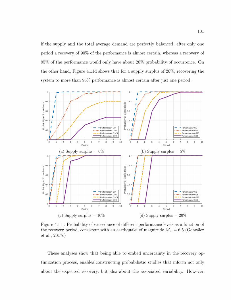
101

if the supply and the total average demand are perfectly balanced, after only one

period a recovery of 90% of the performance is almost certain, whereas a recovery of

95% of the performance would only have about 20% probability of occurrence. On

the other hand, Figure 4.11d shows that for a supply surplus of 20%, recovering the

system to more than 95% performance is almost certain after just one period.

Period0 1 2 3 4 5 6 7 8 9 10

Pro

babi

lity

of E

xcee

danc

e

0

0.2

0.4

0.6

0.8

1

Performance= 0.9Performance= 0.95Performance= 0.975Performance= 0.99


Period0 1 2 3 4 5 6 7 8 9 10

Pro

babi

lity

of E

xcee

danc

e

0

0.2

0.4

0.6

0.8

1



Period0 1 2 3 4 5 6 7 8 9 10

Pro

babi

lity

of E

xcee

danc

e

0

0.2

0.4

0.6

0.8

1



Period0 1 2 3 4 5 6 7 8 9 10

Pro

babi

lity

of E

xcee

danc

e

0

0.2

0.4

0.6

0.8

1



Figure 4.11 : Probability of exceedance of different performance levels as a function ofthe recovery period, consistent with an earthquake of magnitude Mw = 6.5 (Gonzalezet al., 2017c)

These analyses show that being able to embed uncertainty in the recovery op-

timization process, enables constructing probabilistic studies that inform not only

about the expected recovery, but also about the associated variability. However,

102

Period0 1 2 3 4 5 6 7 8 9 10

Per

form

ance

0.85

0.9

0.95

1


(a) sINDP solutions (Supply surplus = 5%)

Period0 1 2 3 4 5 6 7 8 9 10

Per

form

ance

0.85

0.9

0.95

1


(b) sINDP solution (Supply surplus = 10%)

Period0 1 2 3 4 5 6 7 8 9 10

Per

form

ance

0.85

0.9

0.95

1


(c) Solutions assuming average demands(Supply surplus = 5%)

Period0 1 2 3 4 5 6 7 8 9 10

Per

form

ance

0.85

0.9

0.95

1


(d) Solutions assuming average demands(Supply surplus = 10%)

Period0 1 2 3 4 5 6 7 8 9 10

Per

form

ance

0.85

0.9

0.95

1


(e) Solutions assuming perfect Information(Supply surplus = 5%)

Period0 1 2 3 4 5 6 7 8 9 10

Per

form

ance

0.85

0.9

0.95

1


(f) Solutions assuming perfect Information(Supply surplus = 10%)

Figure 4.12 : Comparison between three different performance recovery cases (assumingsupply surplus of 5% (column 1) and 10% (column 2)): considering all scenariossimultaneously (row 1); using only the expected value of the demands (row 2); and,assuming perfect information (row 3) (Gonzalez et al., 2017c).

103

solving the sINDP may be computationally taxing, as it requires finding the optimal

recovery process while considering all demand scenarios simultaneously, as opposed to

a simulation-based approach where one would solve for each scenario independently.

Moreover, it may be the case that considering uncertainty in the system would lead to

the same results to a case where perfect information was available. In order to better

quantify the advantages of using the proposed sINDP, let us compare three different

cases:

• Assuming the use of the proposed sINDP as previously discussed.

• Assuming knowledge about the expected demands only. For this case, first

solve the sINDP assuming that all demand scenarios are modeled using only the

expected demands. Then, using the obtained recovery strategy, evaluate the

performance of each of the 100 different demand scenarios previously described.

This case quantifies the value of using the proposed stochastic approach.

• Assuming full knowledge of perfect information. In this case, assume that all

information about each demand scenario is fully known before seeking the optimal

recovery strategy. This would imply that each demand scenario would represent

a deterministic case, and the td-INDP could be used to find its associated

optimal recovery strategy (independently on the other demand scenarios). This

case quantifies the benefits of having perfect information.

Figure 4.12 depicts the proposed comparison between these three cases, considering

a supply surplus of 5% and 10% for the disaster realization related to Mw = 6.5.

Figures 4.12a and 4.12b show the optimal performance recovery calculated using the

sINDP.

Figures 4.12c and 4.12d show the average performance recovery, assuming that the

recovery strategy imposed was found using only the expected values of the demands.

104

Note that the average performance recovery is less when implementing the recovery

strategy constructed using only the expected demands. Moreover, note that the

resultant performance uncertainty is also much greater, particularly at the end of

the recovery horizon. For example, assuming a supply surplus of 10%, if one uses

a recovery strategy based only on the expected demands, there would be multiple

scenarios in which the performance is not fully recovered from period 6 and beyond, as

opposed to the case of the sINDP, where all scenarios are recovered to full performance.

Figures 4.12e and 4.12f show the performance recovery if there was perfect in-

formation for each demand scenario. As expected, it can be seen that the average

recovery process would take place much faster, since for each studied scenario we

would be using its optimal recovery strategy. The shown results indicate that for this

particular problem, there would be great value in accurately measuring and forecasting

the demands.

4.3 Conclusions

In this Chapter we discuss the importance of considering different sources of uncertainty

when modeling and optimizing the resilience of a system of interdependent networks.

In particular, we detail two sources of uncertainty that are of relevance when studying

realistic scenarios: uncertainty associated with the failure modes of the system, and

uncertainty related to the properties of the system.

To address the first source of uncertainty, related to the failure modes of the system

given external hazards, we show that models proposed in previous Chapters (such

as the td-INDP, and its heuristic approach, the iINDP) could be integrated with

simulation-based techniques to perform both pre- and post-event analysis. By doing

so, we show that the proposed simulation approach can be used to inform stakeholders

105

and decision makers about system- and element-wise resilience metrics. In particular,

Section 4.1 illustrates how the proposed simulation approach can be used to construct

relevant resilience metrics associated with the expected failure likelihood, recovery

likelihood, and recovery times of each individual component in the system. This

Section demonstrates that the proposed resilience metrics could be used to construct

importance rankings that are consistent for different disaster levels, thus offering an

important tool for mitigation and preparedness.

To address the second source of uncertainty, related to the operational properties

of the system, Section 4.2.1 presents a new two-stage stochastic program, denominated

the stochastic INDP (sINDP). We show that the proposed sINDP could be used

to determine the optimal recovery strategy of a damaged system, while considering

uncertainty in multiple parameters such as demand of commodities and resource

availability. In particular, Section 4.2.1 presents an illustrative example based on the

system of water, power, and gas networks described in Section 2.3.2, where we show

the advantages of using the proposed sINDP. For example, we discuss how to use the

sINDP to optimize the expected recovery of a damaged system, while studying the

effects of increasing the system’s supply capacity.

Additionally, we show that the sINDP is susceptible to decomposition strategies,

such as the L-shaped method, in order to increase the average solution speeds. Note

that there are recent promising developments in decomposition techniques that could

be applied in the future to further accelerate the sINDP solving times. For example,

Tarvin et al. (2016) proposed an approach that uses enumeration and both serial

and parallel computing to exploit the structure of two-stage stochastic problems with

binary master problems. Also, note that heuristic approaches, such as the proposed

iINDP, may be applied to enhance the sINDP’s solving efficiency.

Conceptually, the proposed sINDP is consistent with a two-stage stochastic for-

106

mulation, since the recourse problem associated with the operation of the system (in

the second stage) results in an optimization problem that effectively minimizes the

expected costs (or maximizes the expected performance) of the system during the

recovery process. However, in some instances, optimizing the expected costs may not

be the priority of the decision maker. Other desirable objectives may include ensuring

that the performance of the system meets a desired threshold, or that the probability

of complying with a set of operational constraints is above a certain level. In order

to formulate such optimization problems, additional modeling approaches should be

explored, including robust optimization and chance-constrained optimization, among

others. For the context of infrastructure systems and their resilience, a stochastic

formulation would focus on optimizing the average or expected performance of the

system, whereas robust optimization would focus on guaranteeing that the performance

in the worst-case scenario is as high as possible.

Thus, in general, selecting the modeling approach to be used depends directly on

the specific goals of the decision maker, for which these approaches could be used

in isolation or combined. For example, when studying diverse risk measures widely

used in practice, such as the Value at Risk (VaR) or the Conditional Value at Risk

(CVaR), we may use one or multiple of these modeling approaches simultaneously.

If focusing on analyzing the performance of a given system, the VaR associated

with a certain confidence value α corresponds to the performance level PV aR such

that the probability of having a performance below PV aR is α. Similarly, the CVaR

associated with a certain confidence value α is defined as the expected performance

level calculated considering only performances below the worst α-percentage value

(Bertsimas et al., 2011; Rockafellar, 2007; Di Domenica et al., 2007). Developing

analytical and computational approaches that can quantify such risk measures in a

context of infrastructure resilience would enable studying how sensitive the pre- and

107

post-event decisions are as a function of the decision makers’ risk averseness level, in

order to determine adequate mitigation and recovery strategies that align with the

needs and constraints of infrastructure operators and stakeholders.

108

Part III

Beyond the INDP

109

Chapter 5

Expansions/Applications of the INDP

Previous Chapters have introduced the Interdependent Network Design Problem

(INDP), as the problem that focuses on finding the recovery strategy that minimizes

the costs associated with reconstruction and operation of a system of interdependent

networks. We also proposed diverse approaches to solve the INDP, including the

time-dependent INDP (td-INDP), the iterative INDP (iINDP), and the stochastic

INDP (sINDP) models. These models have proven useful in finding the optimal

recovery strategy for a system of networks, while considering diverse interdependencies

between them, as well as realistic operational constraints, such as limited resources

and finite capacities. Similarly, we showed how these models could be used to study

the resilience of a system, while taking into account diverse sources of uncertainty

associated with the system’s failure modes and with the system’s properties. In this

Chapter, we propose further extensions of the INDP models, such that they can

address the following additional challenges∗:

First, current recovery and resilience models available in academic literature often

assume that there is a single entity with complete decision power over all interdependent

networks. This may happen in a few selected cases, such as the illustrative example

related to the water, power, and gas networks in Shelby County, TN., since all these

∗This Chapter is based on the ideas and contents presented in Gonzalez et al. (2017a) and Smithet al. (2016). These publications are part of the collaborative Multidisciplinary University ResearchInitiative (MURI) work with the Ph.D. student Andrew Smith, Professor Raissa D’Souza, ProfessorMehran Mesbahi, and Professor Airlie Chapman. The definitive versions of these papers will beavailable at www.onlinelibrary.wiley.com and www.blackwell-synergy.com

110

utilities are handled by a single company: Memphis Light, Gas, and Water (MLGW).

However, this is often not the case, and in reality there may be multiple decision

makers involved in the operation and recovery of the system of systems. Thus, it

is important to develop models that enable studying the dynamics of a system of

interdependent networks as decentralized or distributed systems.

Second, available models often do not facilitate identifying the particular properties

and dynamics related to the recovery and resilience of the system, since they usually

only receive input information regarding the system’s damage state, and output the

associated optimal recovery strategies. Studies such as the one presented in Section

4.1, which analyzed diverse element-wise resilience metrics, provide important insights

about the relative importance of individual elements, which could be used for mitigation

and preparedness planning. However, these do not permit uncovering the intricate

recovery processes and relations between elements, which are product of multiple

relevant factors, such as the networks’ topologies and their diverse interdependencies.

Thus, it is important to propose strategies that allow not only determining efficient

recovery strategies for damaged systems of interdependent networks, but also that

enable identifying key properties and dynamics from the recovery process.

In this Chapter, we present different multidisciplinary applications developed

to address these emerging challenges. In Section 5.1 we discuss the importance of

considering decentralized decision making, and present modeling approaches in order

to depict more realistic recovery dynamics, associated with human-made and human-

managed systems. In Section 5.2 we propose a mathematical framework for system

identification oriented to extracting and modeling the main recovery dynamics and

processes of a system of interdependent networks.

111

5.1 Socio-technical constraints / Decentralized optimization

As we have discussed in previous Chapters, there is an important body of work associ-

ated with modeling and quantifying the vulnerability and reliability of infrastructure

networks. These methodologies have proven useful for analyzing the behavior and

dynamics of networked systems, such as transportation, telecommunication, power,

water, and other infrastructure networks. However, many of these methodologies

are often based on assumptions that may be impractical for realistic scenarios. For

example, in Chapter 4 we discussed how several of these methodologies often assume

deterministic and static parameters (Galindo and Batta, 2013). Unfortunately, many

of these models also assume the existence of a single entity in charge of taking all deci-

sions at a system level. Moreover, these methodologies are often based on centralized

optimization approaches, that assume that an all-powerful individual entity not only

takes all decisions in the system, but also counts with the information related to all

elements in the system, such as their current damage states.

For example, the proposed td-INDP focuses on determining the recovery strategy

that minimizes the costs associated with the reconstruction process, the system’s

operation, and unsupplied demands; the costs being minimized by the td-INDP

are related to the total costs of the system of interdependent networks. However,

minimizing the total global costs in general is not equivalent to minimizing the cost

for each individual infrastructure network. Thus, if each network implements the

suggested td-INDP strategy, they may not be minimizing their own particular costs.

Even though a recovery strategy that minimizes the global costs may be seen as

ideal from the population’s and the government’s point of view, it is likely that each

individual infrastructure network would not follow such a globally-oriented strategy,

as it may harm its own particular costs. In contrast, in realistic scenarios, each

112

infrastructure system may tend to take decisions separately, focusing on minimizing

their own individual costs.

Additionally, decision makers from each infrastructure system often do not disclose

full and detailed information about their networks (or particularly after a disaster,

about their damaged components). In such cases, decision makers from each infra-

structure network may implement strategies that will not consider their dependence

to other networks accurately. Thus, they may end up implementing strategies that

not only increase the global costs, but also increase their own individual costs (and

reduce performance).

To illustrate such a case, assume that after a certain disaster scenario, each network

in the system of interdependent utility networks studied earlier (the water, gas, and po-

wer networks from Shelby Count, TN.) designs their own recovery strategies, following

an individually-oriented optimization approach that does not consider interdependen-

cies with other networks. Then, it is easy to see that, when following such strategies,

the overall performance recovery of the full system would be worse than if following

a globally-oriented approach (proposed by the INDP models). However, it may be

the case that some individual networks may benefit from such individually-oriented

approach.

To study this case, we simulated 100 different disaster realizations (consistent with

the damage scenarios described in Section 4.1), for which we used the td-INDP to

find the recovery strategy that minimizes the global recovery and operation costs. For

this case, we assume that the system can repair as many as three elements per period.

Additionally, for the same disaster scenarios, we also found the recovery strategies that

minimize the recovery and operation costs for each individual infrastructure network,

assuming that each network does not take into account their interdependencies with

the others. This can be done by using the td-INDP as well, by simply solving the

113

single-network scenario for each network separately. For this case, we assume that

each network can repair only one element per period (such that the whole system can

recover up to three elements per period).

Now, determine the times in which each component regains functionality, related

to following either the globally-oriented or the individually-oriented recovery strategy.

For the globally-oriented strategies, determining the times in which each component

regains functionality is straightforward, as this is indicated directly by the variables

yijkt and wikt. However, in order to determine these times for the individually-oriented

strategies, it would be necessary to assume that each network follows their own

reconstruction plan, but the final element functionality states would depend on the

other networks’ functionality (as these networks are actually interdependent). Then,

for the individually-oriented case, it can be seen that the real time in which each

component regains functionality will defer from what was originally expected when

designing the reconstruction plan without acknowledging interdependencies.

Depending on the optimization strategy used (globally- or individually-oriented),

each component of each network will be recovered at a different time. If, for each

studied disaster scenario, we add up the differences in functionality-recovery times over

all components, we can estimate which strategy results in an overall faster recovery

for each infrastructure. Figure 5.1 shows a histogram of the aggregated functionality-

recovery time differences between the globally- and individually-oriented strategies,

related to each of the studied disaster realizations. A positive time difference (or

time distance) would indicate that the aggregate functionality-recovery time for the

globally-oriented strategy was greater than the corresponding individually-oriented

strategy, and a negative time difference would indicate the opposite.

Figure 5.1a shows that for all disaster realizations, the globally-oriented strategy

had an aggregate faster recovery than the individually-oriented strategies. Again,

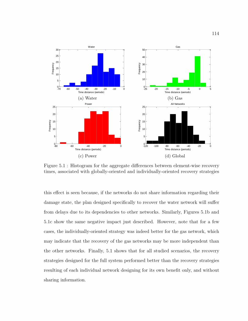
114

-70 -60 -50 -40 -30 -20 -10 00

5

10

15

20

25

30

Time distance (periods)

Fre

quency

Water

-25 -20 -15 -10 -5 0 50

10

20

30

40

50


Fre

quency

Gas

-80 -60 -40 -20 00

5

10

15

20

25


Fre

quency

Power

All components

-120 -100 -80 -60 -40 -20 00

5

10

15

20

25


Fre

quency

All Networks(a) Water

-70 -60 -50 -40 -30 -20 -10 00

5

10

15

20

25

30


Fre

quency

Water

-25 -20 -15 -10 -5 0 50

10

20

30

40

50


Fre

quency

Gas

-80 -60 -40 -20 00

5

10

15

20

25


Fre

quency

Power

All components

-120 -100 -80 -60 -40 -20 00

5

10

15

20

25


Fre

quency

All Networks(b) Gas-70 -60 -50 -40 -30 -20 -10 00

5

10

15

20

25

30


Fre

quency

Water

-25 -20 -15 -10 -5 0 50

10

20

30

40

50


Fre

quency

Gas

-80 -60 -40 -20 00

5

10

15

20

25


Fre

quency

Power

All components

-120 -100 -80 -60 -40 -20 00

5

10

15

20

25


Fre

quency

All Networks

(c) Power

-70 -60 -50 -40 -30 -20 -10 00

5

10

15

20

25

30


Fre

quency

Water

-25 -20 -15 -10 -5 0 50

10

20

30

40

50


Fre

quency

Gas

-80 -60 -40 -20 00

5

10

15

20

25


Fre

quency

Power

All components

-120 -100 -80 -60 -40 -20 00

5

10

15

20

25


Fre

quency

All Networks

(d) Global

Figure 5.1 : Histogram for the aggregate differences between element-wise recoverytimes, associated with globally-oriented and individually-oriented recovery strategies

this effect is seen because, if the networks do not share information regarding their

damage state, the plan designed specifically to recover the water network will suffer

from delays due to its dependencies to other networks. Similarly, Figures 5.1b and

5.1c show the same negative impact just described. However, note that for a few

cases, the individually-oriented strategy was indeed better for the gas network, which

may indicate that the recovery of the gas networks may be more independent than

the other networks. Finally, 5.1 shows that for all studied scenarios, the recovery

strategies designed for the full system performed better than the recovery strategies

resulting of each individual network designing for its own benefit only, and without

sharing information.

115

INDP & game theory

Recent works, such as Sharkey et al. (2015), acknowledge the importance of sharing

information between infrastructure systems, particularly when modeling the restoration

of interdependent systems. Nevertheless, they often assume that the information

shared by each network always reflects detailed and accurate recovery plans, without

taking into account that these plans may not take place in the exact proposed times

and places. In real infrastructure systems, rather than sharing such detailed recovery

plans, the networks would probably share estimates of the recovery times for each

component (or even per service areas), making it important to account for such an

uncertainty and imperfect information.

Additionally, such models assume that for each network the main incentive to

share their recovery plans is based on obtaining information that would improve

their own recoveries; however, additional types of incentives and dynamics should be

considered for realistic purposes, such as particular utility functions or non-cooperative

considerations.

In order to address these decentralization challenges, there are diverse approaches

that could be implemented, based on combining diverse decision theory approaches and

the proposed td-INDP. For example, one could use agent-based modeling (Casalicchio

et al., 2010; Permann, 2007; Nejat and Damnjanovic, 2012; Basak et al., 2011; Oliva

et al., 2010) or game-theory approaches, among others (Zhang et al., 2005; Yaıche

et al., 2000; von Neumann and Morgenstern, 2007).

In particular, Reilly et al. (2015) proposed a general game-theory framework

to model interdependent infrastructure systems. Using their model, they could

analytically study the differences between a decision maker with globally-oriented

goals and one with individually-oriented goals, providing useful tools to develop public

116

policies and incentives for improved resilience. However, their approach mostly focuses

on modeling and understanding strategic behaviors from each system, but it does not

model the actual operation and recovery of the systems.

Improving upon the models proposed by Sharkey et al. (2015) and Reilly et al.

(2015), we proposed an integrated game theory & INDP modeling approach (Smith

et al., 2016). This modeling approach, denominated the Interdependent Network

Recovery Games (INRG), enables modeling the operation and recovery process of

a system of interdependent networks, while also considering interactions between

different stakeholders. In particular, we assumed that each infrastructure network was

managed by a different decision maker. Each of these decision makers were modeled

as ‘players’ that interacted under a game-theory framework. To model the exchange

of imperfect information, we assumed that each player only had information about

the elements of its own network, as well as about the elements from other networks in

which they depend on (as they can observe them directly). Additionally, to model

the objective function of each player, we considered the cost structure proposed in

the td-INDP objective function, but calculated it only for each particular network

individually.

Figure 5.2 shows a comparison between the total recovery costs associated with an

iINDP approach using thorizon = 1 (labeled ‘td-INDP,‖T‖= 1’ ), an iINDP approach

using thorizon = 5 (labeled ‘td-INDP,‖T‖= 5’), the best-case-scenario information-

sharing model proposed by Sharkey et al. (2015) (labeled ‘InfoShare (Sum)’ ), and our

proposed game theory approach (labeled ‘Rand. INRG-BR’). The modeled recovery

process corresponds to the interdependent system of water and power networks in

Shelby County, TN. As expected, the Figure shows that the total cost associated

with the globally-oriented recovery were the lowest, while the INRG approach was the

highest. However, note that both decentralized optimization approaches had resultant

117

recovery costs of similar order, despite of one (the INRG) only considering imperfect

information.

In order to gain additional insights regarding the impact of considering a de-

centralized approach, Figure 5.3 shows an estimation of the Price of Anarchy (PoA)

–calculated as the ratio between the average cost of recovery in a decentralized approach

and the average cost of recovery in a centralized approach– using the information-

sharing model proposed by Sharkey et al. (2015) (labeled ‘InfoShare’), the proposed

game theory approach (INRG) with the players taking decisions in a random order

(labeled ‘Rand. INRG-BR’), the INRG approach with the power network taking

decisions only after the water network (labeled ‘INRG-BR (Water lead)’), and the

INRG approach with the water network taking decisions only after the power network

(labeled ‘INRG-BR (Power lead)’). This Figure shows that, independently of the

decentralized model used, the PoA increases with the magnitude of the earthquake.

This is expected, since the larger the earthquake, the more elements will tend to be

damaged, resulting in a larger number of possible recovery strategies for each player.

However, note that the price of anarchy calculated using the information-sharing

model increases much slower that the one calculated using the INRG approaches.

This is consistent with the fact that the information-sharing model assumes fully

cooperative individuals and perfect information, in contrast with the INRG where the

players may be non-cooperative, and where the information available to each player is

limited. Additionally, note that Figure 5.3 shows that the solving times associated

with the information-sharing model far surpass the ones associated with the INRG

approaches, which is expected considering that the information-sharing model would

only converge when it finds solutions that satisfy all players simultaneously, which is

not always achievable (Smith et al., 2016).

118

Figure 5.2 : Comparison between the solutions offered by the information-sharingmodel, the iINDP method, and the INRG (Smith et al., 2016).

Figure 5.3 : Price of anarchy computed using the information-sharing model and theINRG framework (Smith et al., 2016).

119

5.2 System identification techniques applied to infrastruc-

ture recovery

†Providing good recovery strategies for a given networked system is in general a

complex task. In particular, using time-dependent mixed-integer programming (MIP)

models (such as the models proposed by Lee II et al. (2007); Cavdaroglu et al. (2011);

Nurre et al. (2012), or the one presented in Section 2.2) may be computationally

expensive, and for scenarios in which it is necessary to obtain results in real time,

they may not be suitable. One option to overcome such a problem is to pre-calculate

prototypical disaster configurations and their respective recovery strategies, to identify

and assess the associated risks, vulnerabilities, and challenges, and to develop pre-

disaster recovery plans (U.S. Federal Emergency Management Agency (FEMA), 2011).

Unfortunately, given the large number of feasible disaster configurations, creating and

maintaining plans for a catalogue of possible disasters becomes a prohibitive task.

Thus, an alternative option described in this Section is to create a system identification

(system ID) framework that would take families of prototypical failure scenarios and

their respective optimal recovery strategies as the input/output data to be studied,

which in turn can be used to generate tailor-made recovery strategies. In particular,

we propose constructing a linear operator, following a truncated Koopman operator

approach –which has been proved to be able to approximate non-linear dynamics–

(Brunton et al., 2016; Koopman and von Neumann, 1932), to approximate the recovery

dynamics observed in a system of interconnected networks. The proposed system ID

framework uses td-INDP input/output ‘snap-shot’ data to divulge key features of the

system, its approximate recovery dynamics, and provide tools to analyze and generate

†This Section is based on the submitted pre-print of Gonzalez et al. (2017a). The definitive versionof this paper will be available at www.onlinelibrary.wiley.com and www.blackwell-synergy.com

120

good recovery strategies in an efficient manner.

5.2.1 Time-invariant recovery operator A

Assume there is a set of elements E for which we want to study and model their failure

and recovery dynamics. Without loss of generality, since the system of infrastructure

networks is being modeled using graphs, assume that the set of elements may refer to

the nodes in the system (i.e., E = N ), the arcs (i.e., E = A), or both (i.e., E = N ∪A).

Now, define φ(t) as the vector the describes the damage state information for all

elements e ∈ E at time t. Each entry φe(t) of such a vector is either 1 if the element e

is damaged at time t, or 0 otherwise.

Let us assume that the recovery process of the system is deterministic, implying that

given a disaster scenario the damage state of each element at each subsequent period

can be uniquely determined —this is indeed the case when a restoration sequence

is found by the td-INDP strategy (but we consider multiple scenarios subsequently).

Furthermore, assume that the damage states at a time t+ 1 can be fully determined

based only on the damage states at time t —this assumption will be examined in the

results section 5.2.2. Then, there is a memory-less mapping f such that:

φ(t+ 1) = f(φ(t)) (5.1)

In general, this mapping can be described with an operator A(t), such that

φ(t + 1) = A(t)φ(t). What we proposed (Gonzalez et al., 2017a), is approximating

A(t) with a time-invariant operator A, such that

(5.2)φ(t+ 1) ≈ Aφ(t)

The operator A is selected to minimize the approximation error over all time

periods, namely

121

(5.3)A = arg minA ∈R|E|×|E|

‖Φ0 − AΦ1‖

where (Φ0,Φ1) is the input-output history pair

(5.4)Φ0 = [φ(0), φ(1), ..., φ(|T |−1)](5.5)Φ1 = [φ(1), φ(2), ..., φ(|T |)] .

This operator is associated with a given disaster scenario. In order to construct an

analogue operator for a set of n disaster scenarios, we can construct Φ0 and Φ1 as

(5.6)Φ0 =[Φ1

0,Φ20, ...,Φ

n0

](5.7)Φ1 =

[Φ1

1,Φ21, ...,Φ

n1

]where (Φi

0,Φi1) is the input-output pair of disaster scenario i.

Then, it can be seen that in this case

(5.8)A = arg minA ∈R|E|×|E|

‖Φ1 − AΦ0‖

If we assume that the norm used to calculate the error term in Equation (5.8) is

the Frobenius norm (the square root of the sum of the squares of each entry), then the

optimization problem associated with finding A is highly efficient, and the minimizer

of this problem assumes the closed form

(5.9)A = Φ1ΦT0 (Φ0ΦT

0 )−1

where Φ1ΦT0 denotes the one-period temporal cross-correlation, and (Φ0ΦT

0 )−1 is

associated with the auto-correlation of the damage states. The operator A can be

viewed as a matrix of dimensions |E|×|E| composed of real values. In general, each

position Aij indicates the influence that the damage state of element i at any given

time t has over the damage state of element j at time t+ 1. This operator contains

important information about the recovery dynamics of the system. In particular,

diverse relevant analyses could be performed using the recovery operator, such as

finding the recovery modes of the system and their rates of convergence via dynamic

mode decomposition, based on the eigendecomposition of A.

122

Note that the proposed method to construct the recovery operator assumes that

each individual element has the same relative importance, thus errors in their individual

recovery times are weighted identically. The method could be expanded to consider

prior information about the relative importance of each element or each time period

modeled. Assuming there are positive diagonal matrices WE and WT that describe

the relative importance (weights) associated with the studied elements and recovery

periods, respectively, the general optimization problem to construct the recovery

operator would then be

(5.10)A = arg minA ∈R|E|×|E|

‖WE(Φ1 − AΦ0)WT ‖.

Efficient generation of recovery strategies

The simplicity of the linear dynamics (5.2) provides a computationally efficient method

to generate approximate recovery strategies given a set of initial damage conditions.

Assume that for a given time t, there is a known damage state φ(t), and we want

to generate a recovery strategy starting from it, namely φ(t), φ(t + 1), ..., φ(|T |)

with φ(t) = φ(t). Assuming that A has already been calculated (which in practice

can be done during non-time-critical periods), then we know that for the period t+ 1

the approximate damage state can be calculated by Aφ(t). As the approximation

dynamics is continuous then Aφ(t) will require a projection step to describe a binary

damage state. Thus, we can define a threshold value 0 < a < 1, that will determine

the ranges in which a non-integer damage state will be rounded to a binary state.

Then, the damage state for period t+ 1 would be

(5.11)φ(t+ 1) = d(Aφ(t)− 1a)e

Generalizing for any positive integer m periods in the future, we have that

(5.12)φ(t+m) = d(Amφ(t)− 1a)e.

123

The proposed method uses the recovery operator to replicate the recovery dynamics

from the generating data, without enforcing any constraint on the predicted recovery

strategy. If there are constraints that need to be enforced, such as a strict maximum

resource utilization per recovery period, it is possible to use the recovery operator to

formulate a general iterative approach as follows:

Assume that our current iteration starts from period t and its related damage

state is φ(t), then Aφ(t) can be interpreted as the relative ranking or importance of

recovering each node at time t+ 1. The ranking can then be used to determine which

set of elements should be recovered at period t, such that all desired constraints are

guaranteed. For example, if there is a strict maximum resource utilization, one could

select the set of elements with higher importance and an associated total resource

utilization less than the maximum allowed for that period. Considering the elements

selected to be recovered at time t, calculate φ(t + 1), update the vector of relative

importances (now Aφ(t+ 1)), and repeat.

Note that in the case of a recovery process, the spectral radius of the operator

(denoted as ρ(A)) is expected to be strictly less than one, in order to guarantee that

when using any disaster configuration as the initial damage state φ(0), the damage

states of the system will converge to a full recovery as t increases (since limm→∞Am = 0

if and only if ρ(A) < 1).

Measuring the quality of the generated recovery strategies

In order to use the strategies that are generated using the recovery operator, it is

important to quantify their quality. In general, it is desirable that the recovery

strategies generated using the recovery operator can resemble as close as possible

strategies considered to be optimal. Using the strategies generated by the td-INDP

model as a benchmark, it is possible to evaluate how much the recovery times deviate

124

from one strategy to the other. In particular, the ideal is that the recovery times

proposed for each individual component by the recovery operator approach deviate as

little as possible compared to the benchmark td-INDP strategy.

In some instances, focusing only on comparing the approximate strategies with the

optimal one may not be enough. In particular, even though the recovery times of an

approximate strategy may deviate little compared to the optimal one, the resultant

performance recovery and costs associated with implementing them may differ greatly.

Moreover, the approximate recovery strategy may be an unfeasible one. In particular,

if the elements of the studied system are highly interdependent, or if the available

resources are very limited, the feasibility of the solutions will be sensitive to changes

in the recovery times of each element. Thus, in addition to studying the errors in the

estimated recovery times, it is also important to compare the cumulative percentage

of repaired elements associated to the estimated and benchmark recovery strategies.

If this cumulative function describes different behaviors for the two strategies, this

would indicate that the performance recovery, the resource utilization, and the costs

associated to each strategy are not consistent.

Whenever there are inconsistencies in the predicted times of recovery or the cu-

mulative percentage of repaired elements, it is important to evaluate the impact of

these inconsistencies on the quality of the predicted recovery strategy. In order to

estimate the impact of these recovery time deviations in an efficient manner, we can

construct an optimization model to both evaluate the performance of a given recovery

strategy, and detect any infeasibility associated with it. Such an idea was introduced

by Gonzalez et al. (2016a), where a modified td-INDP formulation was presented

with these goals in mind. The modified td-INDP model resembles the td-INDP model

shown in Section 2.2, but ∆w, ∆y, and ∆z are no longer used as decision variables,

and instead are replaced by analogous parameters defined as ∇w, ∇y, and ∇z which

125

represent the fixed recovery strategy to be studied, where ∇w,∇y at time t is given

by φ(t + 1) − φ(t). ∇z is not encoded in φ(t), but it can be easily (and uniquely)

determined once ∇w and ∇y are fixed. Then, the performance F of the given recovery

strategy ∇w, ∇y, and ∇z, which measures the cost associated with implementing

such an strategy, is given by equation (5.13), and it is subject to the constraints

that result after replacing ∆w, ∆y, and ∆z with ∇w, ∇y, and ∇z, respectively, in

inequalities (2.1b)-(2.1s),

(5.13)

F (∇w,∇y,∇z) = minx,δ+,δ−,w,y

∑t∈T |t>0

∑s∈S

gst∇zst

+∑k∈K

∑(i,j)∈A′k

fijkt∇yijkt +∑i∈N ′k

qikt∇wikt

+∑t∈T

∑k∈K

∑l∈Lk

∑i∈Nk

(M+

ikltδ+iklt +M−

ikltδ−iklt

)+∑l∈Lk

∑(i,j)∈Ak

cijkltxijklt

.

In particular, the studied recovery strategy is unfeasible if the following inequalities

do not hold (note that these inequalities are analogous to constraints (2.1k)),

(5.14)∑k ∈K

∑(i,j)∈A′k

hijkrt∇yijkt+∑i∈N ′k

pikrt∇wikt

≤ vrt, ∀r ∈ R,∀t ∈ T | t > 0,

Then, for instances in which the predicted recovery strategies highly deviate from

the benchmark strategies, equation (5.13) could be used to evaluate if there was a

performance detriment, while inequalities (5.14) would determine if the predicted

strategies were not feasible, indicating the exact periods and elements associated with

such infeasibility.

126

5.2.2 Illustrative example

This illustrative example is based on the system of gas, water, and power networks in

Shelby County, TN., described in Section 2.3.2, and the disaster realizations described

in Section 3.1. For each magnitude Mw ∈ 6, 7, 8, 9, we generated 1000 disaster

scenarios, along with their benchmark recovery strategy using the td-INDP model

shown in Section 2.2. In order to allow for the number of simulations proposed, we

used a truncated td-INDP model, in which if a guaranteed optimal recovery strategy

was not found after a fixed running time (120 seconds per simulation), it returned

the best found recovery strategy (and its optimality gap). The average optimality

gaps between the returned benchmark solutions and their respective best known

bounds were 0%, 0%, 1.8%, and 18.8%, for earthquake magnitudes 6, 7, 8 and 9,

respectively. These provide analytical guarantees of the quality and accuracy of the

benchmark strategies used. To showcase the generality and versatility of the proposed

methodologies, the following subsections present two different cases, associated with

identifying and approximating the recovery dynamics of the nodes only and of both

the nodes and the arcs.

Recovery operator for nodes

Figure 5.4 represents the recovery operator A found as proposed in Section 5.2, based

on the full set of randomly generated disaster scenarios and their respective td-INDP

recovery strategies. Each entry Aee (value of A at row e and column e) shows the

strength with which the damage state of element e at any given time period influences

the damage state of element e in the next period. The coefficient of determination

associated to A was R2 = 0.7729, which is a good indicator of the accuracy of the

found operator and its predictability power. The spectral radius of this operator

127

is 0.9250, which indicates that the system will tend to full recovery, independently

of the initial damage state. Note that Figure 5.4 does not show the lowest values

in the operator or its diagonal entries, in order to highlight the non-trivial stronger

effects. To select the minimum value to display, first we took all the entries in A

(except for the diagonal) and sorted their absolute values (in increasing order). Then,

we calculated the knee (point of maximum curvature) of the curve associated to

this list. Since this point indicates the value for which the rate of growth in the

list changes the most, we used this value as the minimum to display. In particular,

this value was 0.011 for Figure 5.4. This recovery operator uses E = N , thus it is

showing the relation between the damage states of all pair of nodes, with |N |= 125.

Wa

ter

Water

Ga

s

Gas

Po

we

r

Power

20 40 60 80 100 120

20

40

60

80

100

120

0.02

0.03

0.04

0.05

0.06

0.07

Figure 5.4 : Recovery operator A representation (for nodes only) with matrix entrieswith absolute value below 0.011 not displayed. The rows and columns correspond tothe assigned labels for each element (Gonzalez et al., 2017a).

128

By drawing horizontal and vertical lines to separate the nodes in each axis into the

three infrastructure networks studied, we obtain nine different sections that depict the

intra- and inter-network recovery dependencies. For simplicity, let us name each block

as Akk : k, k ∈ K, which shows the strength in which the damage state of nodes in

network k affect the states of network k. The diagonal blocks (i.e., Akk : k ∈ K) depict

the strength in which the current damage state of the nodes in each given network

influence the recovery of the nodes of the same network, whereas the off-diagonal

blocks (i.e., Akk : k, k ∈ K|k 6= k) depict how the state of the nodes in each network

impact the recovery of the other networks. As expected, Figure 5.4 shows that the

states of the nodes in each network have a strong influence within the network, but

also that some networks have a strong influence on the recovery of the others. In

particular, it can be seen that Awater, gas and Apower, gas are dense compared to the

other blocks, showing that the states of the gas nodes have a notable influence over

the other networks. This can also be interpreted as a priority to repair the nodes in

the gas network before recovering the nodes of other networks —consistent with the

td-INDP training data which does not include safety constraints. Such trends can

be explained considering the relative topologies of each network, since the studied

gas network has fewer elements and much less redundancies than the other networks,

which implies that initial repairs in the gas networks have a larger influence on the

overall performance of the system of networks (assuming that M+iklt and M+

iklt are

equal for all networks). On the other side, blocks Agas, water and Agas, power are sparse

compared to the others, which indicates that states of the gas network do not strongly

depend on the states of the others. This also supports the interpretation that the gas

network had a priority to be recovered. Note that these influence relationships are

not trivially observable without relying on the recovery operator, since as mentioned,

the gas was not considered to be physically dependent on the power or the water in

129

the training td-INDP data. Note that the element ordering used in Figure 5.4 was

adequate to easily separate the elements from different networks, but other element

sorting may also be useful. For example, one could sort the elements such that their

closeness in the operator reflects its geographical co-location, providing a graphical

depiction that would facilitate finding the influence that each geographical region has

over others.

Generated recovery strategies for nodes

In order to evaluate the power and accuracy of the proposed methodology to efficiently

generate recovery strategies using the recovery operator, we separated all disaster

scenarios into ten different groups (of 100 scenarios each) and applied cross-validation.

In particular, for each group we generated recovery strategies, using a recovery operator

created using only the benchmark (td-INDP-generated) recovery strategies of the

other nine groups. For each disaster scenario in each group, seeded with the initial

disaster state φ(0) = φ(0), we used its associated recovery operator to efficiently

generate a recovery strategy as described in Section 5.2.1. The generated strategies

were compared with their associated td-INDP-based recovery strategies, to study

their quality of approximation for each time period. For this case study, assuming no

prior information was provided, we used a threshold value –number used in equation

(5.12) to round a non-integer damage state to a binary state– of a = 0.5. Figure

5.5a shows the box-plot of the errors between the predicted strategies with respect to

their benchmark, the number of elements with repair times accurately predicted for

each period, and the cumulative percentage of recovery for both the predicted and

the benchmark strategies. Figure 5.5b shows the associated histogram of the errors

between the two strategies. It can be observed that the predicted recovery strategies

can replicate the td-INDP recovery strategies very accurately, given that the median

130

error is less than one period, and in general the estimated recovery times have an error

below three periods. In fact, the overall distribution of errors shows that more than

50% of the errors are within only one period from the median, and more than 75%

within two periods of the median, indicating that the generated strategies are also

precise. Note that even though the accuracy is better for the starting recovery periods,

a good level of accuracy is achieved even when performing long range prediction (i.e.,

when estimating recovery times that are far from the current time).

Note that the quality of the estimated solutions depends directly on the threshold

value a used. For higher accuracy, parameter a could be tuned in order to minimize

the difference between the benchmark and the predicted recovery, i.e., by solving

an additional optimization problem of the form arg mina‖φ(t+ k)− (Akφ(t)− 1a)‖.

To exemplify the effects of choosing a ‘tuned-up’ a, Figures 5.6a and 5.6b show a

comparison between the benchmark and the predicted recovery times using a = 0.4.

From Figure 5.6a it can be seen that the relative number of outliers observed for

each recovery time is less than the one observed using a = 0.5. Similarly, the

predicted cumulative fraction of elements recovered is much more accurate than if

using a = 0.5. In particular, it is important to ensure that the predicted cumulative

fraction of elements recovered is not extensively far above the benchmark, as it would

be suggesting likely unfeasible recovery strategies that are using more resources than

available. Moreover, Figure 5.6b shows that the histogram of the observed errors is

better centered around zero, relative to its analogous in Figure 5.5b.

To provide some insight on how equation (5.12) is used to generate the recovery

strategies, Figure 5.7 shows the evolution of the failure states for a set of 10 nodes,

comparing their td-INDP recovery strategy and their associated values of Akφ(0).

For each component, a value of 1 describes a fully failed, whereas 0 describes a fully

recovered state. For each element in Figure 5.7, there is a gray box that highlights in

131

the horizontal axis the time period in which the element was recovered according to

the td-INDP strategy, and in the vertical axis the range of values that a can take such

that the generated recovery strategy perfectly replicates the td-INDP strategy. As

expected, the faster an element is recovered according to the td-INDP strategy, the

larger is the range of values that a can take to return an accurate recovery strategy

based on the recovery operator, since the slope of Akφ(0) for that particular element

would be higher. For example, it can be observed that the range of threshold values

that would generate an accurate recovery time for element 36 is much narrower than

the same range associated with element 5. Note that another approach to fine-tune a

would be finding the threshold value that better fits these accuracy ranges across all

elements and scenarios. In this case, a would maximize the number of times in which

the recovery periods were accurately predicted, instead of minimizing the overall error.

Recovery operator for nodes and arcs

Now, in order to model the recovery process of all the elements in the studied

system of networks, assume E = N ∪A. In this case, the total number of elements

increases from 125 to 289. Figure 5.8 shows the calculated recovery operator A for

this new set of elements, using a display threshold of 0.0079. The coefficient of

determination associated with this operator was R2 = 0.8857, which shows an increase

in its predictability power due to the inclusion of additional significant elements. The

spectral radius of this operator is 0.9944, which again provides theoretical guarantees of

a predicted full recovery of the system. As observed in the recovery operator associated

with nodes only, the blocks Awater, gas and Apower, gas are dense relative to other blocks,

whereas Agas, water and Agas, power are the most sparse. This shows that the recovery

operator provides consistent results regarding the relationships between networks.

Nevertheless, it can be seen that for each block in this operator, the upper-left corners

132

(associated with the node elements, as opposed to the arc elements) are densest. This

indicates that in general the recovery relationships between nodes tend to be stronger

than the ones observed for the arcs.

Generated recovery strategies for both nodes and arcs

Following the procedure detailed in Section 5.2.2, for each of the disaster scenarios,

we generated recovery strategies for both nodes and arcs simultaneously. For this

case, the threshold value a used was also 0.5. As in the previous examples, Figure

5.9 overviews different aspects associated with the errors of the generated recovery

strategies compared to the td-INDP strategies. Figures 5.9a and 5.9b show that the

generated strategies are also accurate, having a median error equal to 0, but with a

slightly increased variability. In particular, Figure 5.9 shows that the error distribution

has a reduced symmetry compared to the one associated with nodes only, favoring

outliers in the left tail. This may be explained by the weaker recovery relationships

observed in the arcs compared to the ones observed between the nodes, reducing the

predictability power for these types of elements. Nevertheless, despite this increased

variability, more than 50% of the proposed recovery times are within two periods with

respect to the td-INDP strategies, and more than 75% within 5 periods.

133

Repair Time

1 2 3 4 5 6 7 8 9 10 11 12 13 14 15 16 17 18 19 20

Pre

dic

tion E

rror

Negative: la

te r

ecovery

Positiv

e: early r

ecovery

-10

0

10

Repair Time

0 2 4 6 8 10 12 14 16 18 20

Num

ber

of

Repaired E

lem

ents

0

200

400

600

Within confidence interval

Outside confidence interval

Repair Time

0 2 4 6 8 10 12 14 16 18 20

Cum

ula

tive P

erc

enta

ge o

f

Repaired E

lem

ents

0

0.5

1

Predicted (using Recovery Operator)

Benchmark

(a) Box-plot of the errors, number of repaired elements, and cumulative percentage ofrecovery, respectively, for each recovery period.

Repair Error

-15 -10 -5 0 5 10 15

Num

ber

of R

epaired N

odes

0

100

200

300

400

500

600

700

800

900

1000

12.5%, 87.5% range

25%, 75% range

median

(b) Histogram of the errors

Figure 5.5 : Comparison between predicted recovery strategy for nodes (using therecovery operator) and the benchmark strategies (based on the td-INDP), using a = 0.5(Gonzalez et al., 2017a).

134

Repair Time

1 2 3 4 5 6 7 8 9 10 11 12 13 14 15 16 17 18 19 20

Pre

dic

tio

n E

rro

r

Ne

ga

tive

: la

te r

eco

ve

ry

Po

sitiv

e:

ea

rly r

eco

ve

ry

-10

0

10

Repair Time

0 2 4 6 8 10 12 14 16 18 20

Nu

mb

er

of

Re

pa

ire

d E

lem

en

ts

0

200

400

600



Repair Time

0 2 4 6 8 10 12 14 16 18 20

Cu

mu

lative

Pe

rce

nta

ge

of

Re

pa

ire

d E

lem

en

ts

0

0.5

1


Benchmark


Repair Error

-15 -10 -5 0 5 10 15

Num

ber

of R

epaired N

odes

0

100

200

300

400

500

600

700

800

900

1000 12.5%, 87.5% range

25%, 75% range

median


Figure 5.6 : Comparison between predicted recovery strategy for nodes (from therecovery operator) and the benchmark strategies (based on the td-INDP), using a = 0.4(Gonzalez et al., 2017a).

135

t

0 2 4 6 8 10 12

Ele

me

nt

87

Da

ma

ge

Sta

te

0

0.5

1

t

0 2 4 6 8 10 12Ele

me

nt

11

6

Da

ma

ge

Sta

te

0

0.5

1

t

0 2 4 6 8 10 12

Ele

me

nt

53

Da

ma

ge

Sta

te

0

0.5

1

t

0 2 4 6 8 10 12

Ele

me

nt

93

Da

ma

ge

Sta

te

0

0.5

1

t

0 2 4 6 8 10 12

Ele

me

nt

97

Da

ma

ge

Sta

te

0

0.5

1

t

0 2 4 6 8 10 12

Ele

me

nt

15

Da

ma

ge

Sta

te

0

0.5

1

t

0 2 4 6 8 10 12

Ele

me

nt

5

Da

ma

ge

Sta

te

0

0.5

1

Ideal threshold area

True

Predicted

t

0 2 4 6 8 10 12

Ele

me

nt

36

Da

ma

ge

Sta

te0

0.5

1

t

0 2 4 6 8 10 12

Ele

me

nt

27

Da

ma

ge

Sta

te

0

0.5

1

t

0 2 4 6 8 10 12

Ele

me

nt

75

Da

ma

ge

Sta

te

0

0.5

1

Figure 5.7 : Recovery state estimation for 10 randomly selected components (Gonzalezet al., 2017a)

136

Wa

ter

Water

Ga

s

Gas

Po

we

r

Power

50 100 150 200 250

50

100

150

200

250

0.02

0.04

0.06

0.08

0.1

0.12

0.14

Figure 5.8 : Recovery operator A representation (including both nodes and arcs) withmatrix entries with absolute value below 0.0079 not displayed. The rows and columnscorrespond to the assigned labels for each element (Gonzalez et al., 2017a).

137

Repair Time

1 2 3 4 5 6 7 8 9 10 11 12 13 14 15 16 17 18 19 20 21

Pre

dic

tion E

rror

Negative: la

te r

ecovery

Positiv

e: early r

ecovery

-20

0

20

Repair Time

0 2 4 6 8 10 12 14 16 18 20 22

Num

ber

of

Repaired E

lem

ents

0

200

400

600



Repair Time

0 2 4 6 8 10 12 14 16 18 20 22Cum

ula

tive P

erc

enta

ge o

f

Repaired E

lem

ents

0

0.5

1


Benchmark


Repair Error

-20 -15 -10 -5 0 5 10 15 20

Num

ber

of R

epaired N

odes

0

200

400

600

800

1000

1200

12.5%, 87.5% range

25%, 75% range

median


Figure 5.9 : Comparison between predicted recovery strategy for nodes and arcs (fromthe recovery operator) and the benchmark strategies (based on the td-INDP), usinga = 0.5 (Gonzalez et al., 2017a).

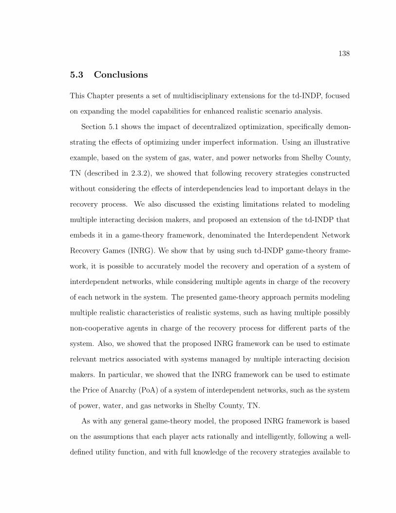
138

5.3 Conclusions

This Chapter presents a set of multidisciplinary extensions for the td-INDP, focused

on expanding the model capabilities for enhanced realistic scenario analysis.

Section 5.1 shows the impact of decentralized optimization, specifically demon-

strating the effects of optimizing under imperfect information. Using an illustrative

example, based on the system of gas, water, and power networks from Shelby County,

TN (described in 2.3.2), we showed that following recovery strategies constructed

without considering the effects of interdependencies lead to important delays in the

recovery process. We also discussed the existing limitations related to modeling

multiple interacting decision makers, and proposed an extension of the td-INDP that

embeds it in a game-theory framework, denominated the Interdependent Network

Recovery Games (INRG). We show that by using such td-INDP game-theory frame-

work, it is possible to accurately model the recovery and operation of a system of

interdependent networks, while considering multiple agents in charge of the recovery

of each network in the system. The presented game-theory approach permits modeling

multiple realistic characteristics of realistic systems, such as having multiple possibly

non-cooperative agents in charge of the recovery process for different parts of the

system. Also, we showed that the proposed INRG framework can be used to estimate

relevant metrics associated with systems managed by multiple interacting decision

makers. In particular, we showed that the INRG framework can be used to estimate

the Price of Anarchy (PoA) of a system of interdependent networks, such as the system

of power, water, and gas networks in Shelby County, TN.

As with any general game-theory model, the proposed INRG framework is based

on the assumptions that each player acts rationally and intelligently, following a well-

defined utility function, and with full knowledge of the recovery strategies available to

139

him and the other players at each recovery period. However, in certain circumstances

such assumptions may not be realistic, since human behavior often does not follow a

course of action defined by single well-known rational utility functions. In order to

address such concerns, one could use other approaches such as agent-based modeling,

which facilitate modeling irrational behavior and individual learning processes, among

others.

Section 5.2 presented a novel approach to efficiently generate approximate reco-

very strategies for interdependent infrastructure systems, using a linear memory-less

recovery operator. The recovery operator is generated from a set of high-fidelity

recovery scenarios, in order to identify and approximate their main recovery dynamics,

and then to develop tailor-made recovery strategies after specific disaster scenarios.

The shown illustrative example is also based on the system of utility networks in

Shelby County, TN., for which we used the td-INDP to generate the used benchmark

recovery strategies associated with the disaster realizations described in Section 4.1.

The recovery strategies generated using the proposed recovery operator approach

show good agreement with the td-INDP recovery dynamics, even for long-term plan-

ning, both in the times of recovery and the resources used. The proposed recovery

operator is expected to adequately approximate the recovery dynamics of a system

of interdependent networks, as long as these dynamics are consistent along the full

planning horizon. Nevertheless, if parameters such as costs, resources, or capacities

change abruptly in time, a single memory-less time-invariant operator may not be

appropriate to approximate the system dynamics. However, in such a case, it would

be possible to construct recovery operators specifically designed for different recovery

periods. In such a case, the full planning horizon would be divided into multiple

separate time-domains, and for each of these one could construct a separate recovery

operator. This would enable, for example, modeling recovery processes with multiple

140

inflections points (which is difficult to model with other approaches, such as the

iINDP). Note that the proposed recovery operator approach is a general data-driven

process that operates on ‘snap-shots’ of input/output data; thus, it is not restricted

to any particular optimal recovery model.

141

Chapter 6

Conclusions and Future Work

In this thesis we have discussed the importance of understanding, modeling, and

optimizing the resilience of systems of interdependent networks, such as critical infra-

structures. To this end, we presented multiple concepts and methods of analysis, in

line with three main observed challenges: modeling and optimizing interdependent

networks; facilitating the study of large problems; and, enabling the consideration of

multiple sources of uncertainty. Below is an overview of the main topics and methods

presented, along with their main conclusions.

Chapter 2: On properly defining the Interdependent Network Design Problem

(INDP), and developing computational models to solve it.

• We described the main characteristics that must be considered by a problem

related to maximizing the resilience of a system of interdependent networks. This

problem was defined as the Interdependent Network Design Problem (INDP).

• We defined the INDP as the problem of finding the least-cost recovery strategy of

a partially destroyed system of infrastructure networks, subject to budget, resour-

ces, and operational constraints, while considering interdependencies between

the studied networks.

• We proposed an MIP formulation to solve the INDP, denominated the time-

dependent INDP (td-INDP), which can be used to model and optimize the

142

recovery of interdependent systems, while considering realistic operational con-

straints. We showcased the td-INDP using two different illustrative examples,

which are subject to an earthquake hazard: the Colombian road network and its

multicommodity cargo flow; and, the system of interdependent infrastructure

networks composed by the gas, water, and power networks in Shelby County,

TN.

The proposed td-INDP is, to the best of our knowledge, the first optimization

model that can determine the minimum-cost recovery strategy associated with a

system of interdependent networks, which considers realistic operational, resource avai-

lability, and capacity constraints, while simultaneously accounting for multiple types

of interdependencies, such as physical and geographical. In particular, the proposed

physical-interdependency modeling enables determining critical recovery jobs that

result in a cascading-recovery effect. Additionally, the geographical-interdependency

modeling facilitates cost reductions due to simultaneous recovery of co-located compo-

nents with shared physical spaces.

Furthermore, the td-INDP model can also be used to provide benchmark recovery

strategies that can be used in other academic and practical studies. Considering this,

as part of our research, we developed a benchmark failure/recovery time-series dataset

associated with the system of water, gas, and power networks in Shelby County, TN.

(Appendix C). Taking into account that the proposed optimization model provides

optimality guarantees on the obtained solutions, this dataset has been used as a

reference by multiple research groups, for studies in diverse fields such as statistical

physics and system identification, among others.

Chapter 3: On exploring enhancement techniques for the computational capabi-

143

lities of the INDP models, such that they run faster and can handle larger systems.

• We developed the iterative INDP (iINDP), which is a heuristic approach that

relies on decomposing the full time horizon of a given problem into smaller more

manageable time horizons.

• We showed that the time complexity of the td-INDP model is highly dependent

on the size of the system analyzed, its level of damage, and availability of

resources, but not as much on its link density, or its interdependency density

and strength.

• We described the special structure associated with the td-INDP, which makes

it suitable for diverse decomposition techniques, such as Dantzig-Wolfe and

Benders decompositions.

The proposed td-INDP was carefully developed such that it not only features the

aforementioned modeling capabilities associated with realistic interdependent systems,

but also sustains a desirable block structure. This structure not only enables solving

the td-INDP more efficiently, but also facilitates building efficient modeling extensions,

which include stochastic and decentralized formulations.

Additionally, the features depicted by the proposed heuristic and analytical ap-

proaches may be combined in tailor-made hybrid methodologies, which can exploit

the advantages of each individual approach. For example, heuristic algorithms may

be used specifically to determine efficient reconstruction strategies, while analytical

methodologies focus on quantifying and optimizing the associated flow and supply of

commodities.

Chapter 4: On expanding the INDP models to allow the inclusion of multiple

sources of uncertainty.

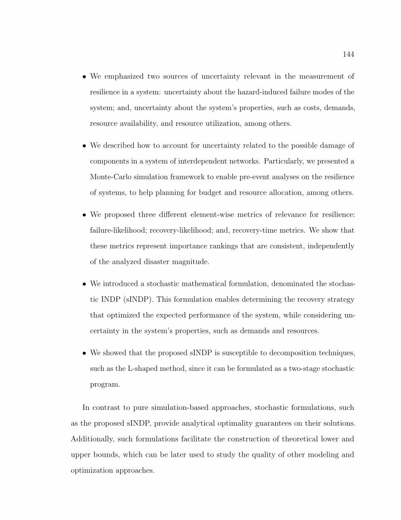
144

• We emphasized two sources of uncertainty relevant in the measurement of

resilience in a system: uncertainty about the hazard-induced failure modes of the

system; and, uncertainty about the system’s properties, such as costs, demands,

resource availability, and resource utilization, among others.

• We described how to account for uncertainty related to the possible damage of

components in a system of interdependent networks. Particularly, we presented a

Monte-Carlo simulation framework to enable pre-event analyses on the resilience

of systems, to help planning for budget and resource allocation, among others.

• We proposed three different element-wise metrics of relevance for resilience:

failure-likelihood; recovery-likelihood; and, recovery-time metrics. We show that

these metrics represent importance rankings that are consistent, independently

of the analyzed disaster magnitude.

• We introduced a stochastic mathematical formulation, denominated the stochas-

tic INDP (sINDP). This formulation enables determining the recovery strategy

that optimized the expected performance of the system, while considering un-

certainty in the system’s properties, such as demands and resources.

• We showed that the proposed sINDP is susceptible to decomposition techniques,

such as the L-shaped method, since it can be formulated as a two-stage stochastic

program.

In contrast to pure simulation-based approaches, stochastic formulations, such

as the proposed sINDP, provide analytical optimality guarantees on their solutions.

Additionally, such formulations facilitate the construction of theoretical lower and

upper bounds, which can be later used to study the quality of other modeling and

optimization approaches.

145

Moreover, by extending the capabilities of the proposed INDP models, so that they

can consider the aforesaid sources of uncertainty, the upgraded modeling approaches

provide efficient tools to support pre- and post-event decisions, which enhance and

facilitate mitigation and emergency response actions. Thus, used in combination, these

models enable examining and quantifying the effects of interdependencies in realistic

interdependent infrastructure systems, as well as optimizing their overall resilience.

Under such a context, the proposed models could be used to study the trade-offs

between pre-event mitigation processes and the post-event recovery actions, offering

important information to policy makers and stakeholders. For example, assuming that

the total budget invested on infrastructure retrofitting and recovery cannot surpass a

specific threshold level, one could use the proposed models to determine which type

of interventions would have a larger impact on the overall resilience of the system of

infrastructure networks studied.

Chapter 5: On studying diverse extensions and applications of the proposed

INDP computational models, either for practical or theoretical purposes.

• We described the importance of including socio-technical constraints in our

models, such that they better depict realistic systems, particularly regarding the

interaction between different decision makers in charge of different networks.

• We presented a system identification technique that allows extracting the main

recovery dynamics for any given system. In particular, we describe how the

recovery dynamics can be compressed in a time-invariant linear operator, deno-

minated the recovery operator. This operator can be used to provide insightful

information regarding the recovery relations between elements, as well as to

construct efficient recovery strategies in polynomial time.

146

The presented extensions and applications show that the proposed INDP models

are versatile, and can be used in combination with diverse approaches and techniques

from other fields and disciplines.

For example, methodologies such as the Interdependent Network Recovery Games

(INRG) show that game-theory and the proposed INDP models can be combined in

order to optimize the resilience of systems of interdependent networks, while modeling

realistic socio-technical features associated with decentralized decision making.

Moreover, the proposed recovery operator not only offers tools to understand and

recreate the dynamics related to the recovery of interdependent systems, but also

facilitates the development of future models and metrics for the observability and

controllability of such systems.

Figure 6.1 presents a conceptual map that summarizes the main areas and concepts

covered in this thesis, including some relevant topics for future research.

Opportunities for future research

Even though this thesis presents a comprehensive study on multiple computational and

modeling techniques designed to study and optimize the resilience of interdependent

networks, this field offers multiple research opportunities for future work.

On one hand, we believe it is important to develop adequate mechanisms to facilitate

the proliferation of optimization-based analytical and computational techniques (such

as the ones proposed in this thesis) in the field of Civil and Infrastructure Engineering.

For example, we could apply the proposed optimization techniques to study and

optimize the recovery dynamics of well known systems of infrastructure networks.

In line with this idea, as part of this research we developed a hazard-to-recovery

benchmark database associated with the system of water, gas, and power networks

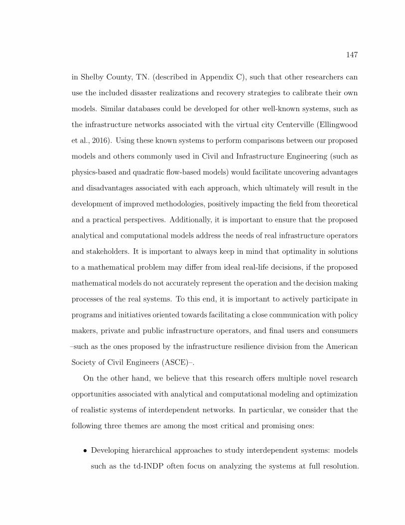
147

in Shelby County, TN. (described in Appendix C), such that other researchers can

use the included disaster realizations and recovery strategies to calibrate their own

models. Similar databases could be developed for other well-known systems, such as

the infrastructure networks associated with the virtual city Centerville (Ellingwood

et al., 2016). Using these known systems to perform comparisons between our proposed

models and others commonly used in Civil and Infrastructure Engineering (such as

physics-based and quadratic flow-based models) would facilitate uncovering advantages

and disadvantages associated with each approach, which ultimately will result in the

development of improved methodologies, positively impacting the field from theoretical

and a practical perspectives. Additionally, it is important to ensure that the proposed

analytical and computational models address the needs of real infrastructure operators

and stakeholders. It is important to always keep in mind that optimality in solutions

to a mathematical problem may differ from ideal real-life decisions, if the proposed

mathematical models do not accurately represent the operation and the decision making

processes of the real systems. To this end, it is important to actively participate in

programs and initiatives oriented towards facilitating a close communication with policy

makers, private and public infrastructure operators, and final users and consumers

–such as the ones proposed by the infrastructure resilience division from the American

Society of Civil Engineers (ASCE)–.

On the other hand, we believe that this research offers multiple novel research

opportunities associated with analytical and computational modeling and optimization

of realistic systems of interdependent networks. In particular, we consider that the

following three themes are among the most critical and promising ones:

• Developing hierarchical approaches to study interdependent systems: models

such as the td-INDP often focus on analyzing the systems at full resolution.

148

However, in some instances it may be a better idea to apply reduction techniques,

in order to simplify the studied networks and facilitate the analyses and the

implementation of strategies. By developing adequate hierarchical approaches

for interdependent networks, the associated solution times may drastically

reduce, and the modeling may better reflect realistic human-systems’ dynamics.

Hierarchical representation and hierarchical optimization approaches have been

successfully used to model and analyze diverse infrastructure systems, such as

power and transportation networks (Gomez et al., 2013; Alquthami et al., 2014;

Anandalingam and Friesz, 1992; Kong et al., 2017; Costantino et al., 2013; Sun,

2014). However such approaches have focused on single isolated systems, and

do not take into account features associated with interdependencies between

multiple networks. Thus, the main associated challenge is to develop analytical

and computational methodologies that enable analyzing and optimizing simplified

versions of a full-resolution system of interdependent networks, while being able

to quantify and guarantee the quality of the obtained solutions. A possible

approach to this problem could use system identification techniques to determine

the main dynamics present in the system, in order to reduce the number of

analyzed elements and variables. In particular, methodologies such as Dynamic

Mode Decomposition (DMD) could be use jointly with the proposed recovery

operator, to determine the main recovery modes of the system and guide a

dimensionality reduction process, while preserving as much information as

possible regarding the full-resolution system.

• Developing diverse distributed and decentralized optimization techniques specific

for interdependent networks: as described in Section 5.1, most of current models

do not consider diverse relevant characteristics of realistic networks, specially

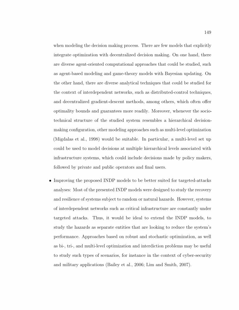
149

when modeling the decision making process. There are few models that explicitly

integrate optimization with decentralized decision making. On one hand, there

are diverse agent-oriented computational approaches that could be studied, such

as agent-based modeling and game-theory models with Bayesian updating. On

the other hand, there are diverse analytical techniques that could be studied for

the context of interdependent networks, such as distributed-control techniques,

and decentralized gradient-descent methods, among others, which often offer

optimality bounds and guarantees more readily. Moreover, whenever the socio-

technical structure of the studied system resembles a hierarchical decision-

making configuration, other modeling approaches such as multi-level optimization

(Migdalas et al., 1998) would be suitable. In particular, a multi-level set up

could be used to model decisions at multiple hierarchical levels associated with

infrastructure systems, which could include decisions made by policy makers,

followed by private and public operators and final users.

• Improving the proposed INDP models to be better suited for targeted-attacks

analyses: Most of the presented INDP models were designed to study the recovery

and resilience of systems subject to random or natural hazards. However, systems

of interdependent networks such as critical infrastructure are constantly under

targeted attacks. Thus, it would be ideal to extend the INDP models, to

study the hazards as separate entities that are looking to reduce the system’s

performance. Approaches based on robust and stochastic optimization, as well

as bi-, tri-, and multi-level optimization and interdiction problems may be useful

to study such types of scenarios, for instance in the context of cyber-security

and military applications (Bailey et al., 2006; Lim and Smith, 2007).

150

4

2

3

Exac

tH

euri

stic

s

Han

dlin

g u

nce

rtai

nty N

etw

ork

mo

de

ling

Larg

e sc

ale

p

rob

lem

s

Op

tim

izin

g re

silie

nce

of

syst

ems

of

inte

rdep

end

ent

net

wo

rks

Clu

ste

rin

g Top

olo

gica

lb

ased

Evo

luti

on

ary

algo

rith

ms

Ran

kin

g co

mp

on

en

ts

Co

ntr

ol

met

rics

Re

silie

nce

met

rics

Op

tim

izat

ion

w

ith

em

bed

de

d

un

cert

ain

ty

Sam

plin

gm

eth

od

s

IND

P

Ap

plic

atio

ns

Ch

alle

nge

sO

pti

miz

atio

n m

eth

od

sco

nsi

der

ing

un

cert

ain

ty

Tem

po

ral

clas

sifi

cati

on

Pro

po

sed

ap

pro

ach

es f

or

exac

t so

lvin

g

Imp

ort

ance

met

rics

Pro

ble

ms

to b

eso

lved

Pro

po

sed

ap

pro

ach

es f

or

heu

rist

ics

Pre

-eve

nt

An

alys

isP

ost

-eve

nt

An

alys

is

Mo

nte

-Car

losi

mu

lati

on La

tin

Hyp

erc

ub

eSa

mp

ling

Imp

ort

ance

Sam

plin

g

Pro

po

sed

ap

pro

ach

esfo

r sa

mp

ling

Pro

po

sed

ap

pro

ach

esfo

r em

bed

ded

un

cert

ain

ty

Dan

tzig

-Wo

lfe

dec

om

p.

Acc

eler

atin

g te

chn

iqu

esB

end

ers

dec

om

p.

Ap

plic

atio

ns

Mo

de

ling

Net

wo

rk

Top

olo

gyIn

fras

tru

ctu

resy

ste

ms

Ro

bu

sto

pti

miz

atio

nSt

och

asti

co

pti

miz

atio

n

Res

ou

rce

al

loca

tio

n

Job

assi

gnm

en

t &

sc

hed

ulin

g

Ob

ject

ive

equ

ilib

ria

& G

ame

th

eo

ry

Alg

ori

thm

en

han

cem

ent

Pro

po

sed

alg

ori

thm

s

1

Mo

del

ing

and

op

tim

izin

g in

terd

epen

den

t n

etw

ork

s

Un

der

stan

din

g an

d im

pro

vin

gth

e ef

fici

ency

of

the

pro

po

sed

mo

del

s

Prop

osed

res

earc

h ar

eas

Mo

del

ing

un

cert

ain

ty in

Inte

rdep

end

ent

Net

wo

rks

1 2 3 4St

ud

yin

g ex

ten

sio

ns

and

ap

plic

atio

ns

of

the

pro

po

sed

m

od

els

Figure 6.1 : Proposed research map divided by topics

151

Bibliography

Abolghasem, S., Gomez-Sarmiento, J., Medaglia, A. L., Sarmiento, O. L., Gonzalez,

A. D., Dıaz del Castillo, A., Rozo-Casas, J. F., and Jacoby, E. (2017). A DEA-

centric decision support system for evaluating Ciclovıa-Recreativa programs in the

Americas. Socio-Economic Planning Sciences, (In press).

Adachi, T. and Ellingwood, B. R. (2009). Serviceability Assessment of a Municipal

Water System Under Spatially Correlated Seismic Intensities. Computer-Aided Civil

and Infrastructure Engineering, 24(4):237–248.

Adachi, T. and Ellingwood, B. R. (2010). Comparative Assessment of Civil Infrastruc-

ture Network Performance under Probabilistic and Scenario Earthquakes. Journal

of Infrastructure Systems, 16(1):1–10.

Ahuja, R., Magnanti, T., and Orlin, J. (1993). Network flows: theory, algorithms and

applications. Prentice Hall.

Alagoz, O., Hsu, H., Schaefer, A. J., and Roberts, M. S. (2010). Markov decision

processes: a tool for sequential decision making under uncertainty. Medical decision

making : an international journal of the Society for Medical Decision Making,

30(4):474–83.

Alquthami, T., Huang, R., Polymeneas, E., and Meliopoulos, a. P. (2014). Hierarchical

optimization and control of a power system. Isgt 2014, pages 1–5.

152

Amin, M. (2002). Toward secure and resilient interdependent infrastructures. Journal

of Infrastructure Systems, (September):67–75.

Anandalingam, G. and Friesz, T. L. (1992). Hierarchical optimization: An introduction.

Annals of Operations Research, 34(1):1–11.

Anderson, C. W., Santos, J. R., and Haimes, Y. Y. (2007). A Risk-based InputOutput

Methodology for Measuring the Effects of the August 2003 Northeast Blackout.

Economic Systems Research, 19(2):183–204.

Assad, A. A. (1978). Multicommodity network flowsA survey. Networks, 8(1):37–91.

Bailey, M. D., Shechter, S. M., and Schaefer, A. J. (2006). SPAR: stochastic program-

ming with adversarial recourse. Operations Research Letters, 34(3):307–315.

Baroud, H., Barker, K., Ramirez-Marquez, J. E., and Rocco, C. M. (2015). Inherent

costs and interdependent impacts of infrastructure network resilience. Risk analysis,

35(4):642–62.

Basak, S., Modanwal, N., and Mazumdar, B. D. (2011). Multi-agent based disaster

management system: a review. International Journal of Computer Science &

Technology, 2(2):343–348.

Beatty, M. E., Phelps, S., Rohner, C., and Weisfuse, I. (2006). Blackout of 2003:

Public health effects and emergency response. Public Health Reports, 121(1):36–44.

Benders, J. F. (1962). Partitioning procedures for solving mixed-variables programming

problems. Numerische Mathematik, 4(1):238–252.

Bergner, M., Caprara, A., Ceselli, A., Furini, F., Lubbecke, M. E., Malaguti, E.,

and Traversi, E. (2014). Automatic Dantzig-Wolfe reformulation of mixed integer

programs.

153

Bertsimas, D., Brown, D. B., and Caramanis, C. (2011). Theory and Applications of

Robust Optimization. SIAM Review, 53(3):464–501.

Bertsimas, D. and Sim, M. (2003). Robust discrete optimization and network flows.

Mathematical Programming, 98(1-3):49–71.

Beyer, H.-G. and Sendhoff, B. (2007). Robust optimization A comprehensive survey.

Computer Methods in Applied Mechanics and Engineering, 196(33-34):3190–3218.

Bezanson, J., Edelman, A., Karpinski, S., and Shah, V. B. (2017). Julia: A Fresh

Approach to Numerical Computing. SIAM Review, 59(1):65–98.

Binato, S., Pereira, M., and Granville, S. (2001). A new Benders decomposition

approach to solve power transmission network design problems. IEEE Transactions

on Power Systems, 16(2):235–240.

Boccaletti, S., Bianconi, G., Criado, R., del Genio, C. I., Gomez-Gardenes, J., Romance,

M., Sendina-Nadal, I., Wang, Z., and Zanin, M. (2014). The structure and dynamics

of multilayer networks.

Boudali, H. and Dugan, J. (2005). A discrete-time Bayesian network reliability

modeling and analysis framework. Reliability Engineering & System Safety, 87(3):337–

349.

Bozorgi-Amiri, A., Jabalameli, M. S., and Mirzapour Al-e-Hashem, S. M. J. (2011).

A multi-objective robust stochastic programming model for disaster relief logistics

under uncertainty. OR Spectrum, pages 1–29.

Brummitt, C. D., D’Souza, R. M., and Leicht, E. a. (2012). Suppressing cascades of

load in interdependent networks. Proceedings of the National Academy of Sciences

of the United States of America, 109(12):E680–9.

154

Brunton, S. L., Brunton, B. W., Proctor, J. L., and Kutz, J. N. (2016). Koopman

Invariant Subspaces and Finite Linear Representations of Nonlinear Dynamical

Systems for Control. PLOS ONE, 11(2):e0150171.

Buldyrev, S. V., Parshani, R., Paul, G., Stanley, H. E., and Havlin, S. (2010).

Catastrophic cascade of failures in interdependent networks. Nature, 464(7291):1025–

8.

Callander, S. and Plott, C. R. (2005). Principles of network development and evolution:

an experimental study. Journal of Public Economics, 89(8):1469–1495.

Campbell, A. M. (2008). Inventory routing. PhD thesis, Georgia Institute of Techno-

logy.

Cancela, H., Robledo, F., Rubino, G., and Sartor, P. (2013). Monte Carlo estimation

of diameter-constrained network reliability conditioned by pathsets and cutsets.

Computer Communications, 36(6):611–620.

Casalicchio, E., Galli, E., and Tucci, S. (2010). Agent-based modelling of interdepen-

dent critical infrastructures. International Journal of System of Systems Engineering,

2(1):60.

Cavdaroglu, B., Hammel, E., Mitchell, J. E., Sharkey, T. C., and Wallace, W. a.

(2011). Integrating restoration and scheduling decisions for disrupted interdependent

infrastructure systems. Annals of Operations Research, 203(1):279–294.

Cavdaroglu, B. and Nurre, S. (2010). Restoring Infrastructure Systems: An Integrated

Network Design and Scheduling Problem. pages 1–3.

Chapman, A., Gonzalez, A. D., Mesbahi, M., Duenas-Osorio, L., and D’Souza, R. M.

(2017). Data-guided Control: Clustering , Graph Products, and Decentralized

155

Control. In 56th IEEE Conference on Decision and Control (CDC2017), pages 1–8,

Melbourne, Australia.

Chen, A., Kim, J., Lee, S., and Kim, Y. (2010). Stochastic multi-objective models for

network design problem. Expert Systems with Applications, 37(2):1608–1619.

Chu, C.-Y. (2009). A Computer Model for Selecting Facility Evacuation Design

Using Cellular Automata. Computer-Aided Civil and Infrastructure Engineering,

24(8):608–622.

Ciappina, J. R., Yamakami, A., and Silva, R. C. (2012). Decompositions Dantzig-

Wolfe applied to fuzzy multicommodity flow problems. Computers and Operations

Research, 39(12):3394–3407.

Clay Whybark, D. (2007). Issues in managing disaster relief inventories. International

Journal of Production Economics, 108(1-2):228–235.

Coluccia, A. (2011). Bayesian estimation of network-wide mean failure probability

in 3g cellular networks. In Hummel, K., Hlavacs, H., and Gansterer, W., editors,

Performance Evaluation of Computer and Communication Systems. Milestones and

Future Challenges, volume 6821, pages 167–178. Springer Berlin Heidelberg.

Comfort, L. K., Dunn, M., Johnson, D., Skertich, R., and Zagorecki, A. (2004).

Coordination in complex systems: increasing efficiency in disaster mitigation and

response. International Journal of Emergency Management, 2(1/2):62.

Costa, A. M. (2005). A survey on benders decomposition applied to fixed-charge

network design problems. Computers & Operations Research, 32(6):1429–1450.

Costa, A. M., Cordeau, J.-F., and Gendron, B. (2007). Benders, metric and cut-

156

set inequalities for multicommodity capacitated network design. Computational

Optimization and Applications, 42(3):371–392.

Costantino, N., Dotoli, M., Falagario, M., Fanti, M. P., Mangini, A. M., Sciancalepore,

F., and Ukovich, W. (2013). A hierarchical optimization technique for the strategic

design of distribution networks. Computers and Industrial Engineering, 66(4):849–

864.

Dantzig, G. B. and Wolfe, P. (1960). Decomposition Principle for Linear Programs.

Operations Research, 8(1):101–111.

Deblasio, A. J., Regan, T. J., Zirker, M. E., Fichter, K. S., and Lovejoy, K. (2004).

Effects of catastrophic events on transportation system management and opera-

tions. Technical Report April, U.S. Department of Transportation, Cambridge,

Massachusetts.

Di Domenica, N., Mitra, G., Valente, P., and Birbilis, G. (2007). Stochastic pro-

gramming and scenario generation within a simulation framework: An information

systems perspective. Decision Support Systems, 42(4):2197–2218.

Dionne, R. and Florian, M. (1979). Exact and approximate algorithms for optimal

network design. Networks, 9:37–59.

Duenas-Osorio, L., Craig, J., and Goodno, B. (2007a). Seismic response of critical

interdependent networks. Earthquake engineering & structural dynamics, 36(2):285–

306.

Duenas-Osorio, L., Craig, J. I., Goodno, B. J., and Bostrom, A. (2007b). Inter-

dependent Response of Networked Systems. Journal of Infrastructure Systems,

13(3):185–194.

157

Duenas-Osorio, L., Gonzalez, A. D., Shepherd, K., and Paredes-Toro, R. (2015).


Systems. Technical report, National Institute of Standards and Technology (NIST),

Houston, TX, USA.

Duenas-Osorio, L. and Kwasinski, A. (2012). Quantification of Lifeline System

Interdependencies after the 27 February 2010 M w 8.8 Offshore Maule, Chile,

Earthquake. Earthquake Spectra, 28(S1):S581–S603.

Duenas-Osorio, L. A. (2005). Interdependent Response of Networked Systems to

Natural Hazards and Intentional Disruptions Interdependent Response of Networked

Systems to Natural Hazards and Intentional Disruptions. PhD thesis.

Dunning, I., Huchette, J., and Lubin, M. (2017). JuMP: A Modeling Language for

Mathematical Optimization. SIAM Review, 59(2):295–320.

Ellingwood, B. R., Cutler, H., Gardoni, P., Peacock, W. G., van de Lindt, J. W., and

Wang, N. (2016). The Centerville Virtual Community: a fully integrated decision

model of interacting physical and social infrastructure systems. Sustainable and

Resilient Infrastructure, 1(3-4):95–107.

Farhangi, H. (2010). The path of the smart grid. IEEE Power and Energy Magazine,

8(1):18–28.

Faturechi, R., Levenberg, E., and Miller-Hooks, E. (2014). Evaluating and optimizing

resilience of airport pavement networks. Computers & Operations Research, 43:335–

348.

FEMA (2013). Multi-hazard Loss Estimation Methodology, Earthquake Model -

Technical Manual, Hazus - MH 2.1. Technical report, Washington D.C.

158

Fortz, B. and Poss, M. (2009). An improved Benders decomposition applied to a

multi-layer network design problem. Operations Research Letters, 37(5):359–364.

Frangioni, A. and Gendron, B. (2013). A stabilized structured Dantzig-Wolfe decom-

position method. Mathematical Programming, 140:45–76.

Galindo, G. and Batta, R. (2013). Review of recent developments in OR/MS research

in disaster operations management. European Journal of Operational Research,

230(2):201–211.

Ganapati, N. E. (2012). Measuring the processes and outcomes of post-disaster housing

recovery: lessons from Golcuk, Turkey. Natural Hazards, 65(3):1783–1799.

Gao, J., Buldyrev, S. V., Havlin, S., and Stanley, H. E. (2011). Robustness of a

network of networks. Physical Review Letters, 107(19):5.

Gao, L. and Zhang, Z. (2009). Robust Optimization for Managing Pavement Mainte-

nance and Rehabilitation. Transportation Research Record: Journal of the Trans-

portation Research Board, 2084(-1):55–61.

Gomez, C., Sanchez-Silva, M., Duenas-Osorio, L., and Rosowsky, D. (2013). Hierarchi-

cal infrastructure network representation methods for risk-based decision-making.

Structure and Infrastructure Engineering, 9(3):260–274.

Gonzalez, A. D., Chapman, A., Duenas-Osorio, L., Mesbahi, M., and D’Souza, R. M.

(2017a). Efficient Infrastructure Restoration Strategies using the Recovery Operator.

Computer-Aided Civil and Infrastructure Engineering, (In review).

Gonzalez, A. D., Duenas-Osorio, L., Medaglia, A. L., and Sanchez-Silva, M. (2014a).

Resource allocation for infrastructure networks within the context of disaster ma-

nagement. In Deodatis, G., Ellingwood, B., and Frangopol, D., editors, Safety,

159

Reliability, Risk and Life-Cycle Performance of Structures and Infrastructures, pages

639–646, New York, USA. CRC Press.

Gonzalez, A. D., Duenas-Osorio, L., Medaglia, A. L., and Sanchez-Silva, M. (2016a).

The time-dependent interdependent network design problem (td-INDP) and the

evaluation of multi-system recovery strategies in polynomial time. In Huang, H., Li,

J., Zhang, J., and Chen, J., editors, The 6th Asian-Pacific Symposium on Structural

Reliability and its Applications, pages 544–550, Shanghai, China.

Gonzalez, A. D., Duenas-Osorio, L., Sanchez-Silva, M., and Medaglia, A. L. (2015).

The Computational Complexity of Probabilistic Interdependent Network Design

Problems. In Proceedings of the 12th International Conference on Applications of

Statistics and Probability in Civil Engineering (ICASP12), pages 1–8, Vancouver,

Canada.

Gonzalez, A. D., Duenas-Osorio, L., Sanchez-Silva, M., and Medaglia, A. L. (2016b).

The Interdependent Network Design Problem for Optimal Infrastructure System

Restoration. Computer-Aided Civil and Infrastructure Engineering, 31(5):334–350.

Gonzalez, A. D., Duenas-osorio, L., Sanchez-Silva, M., Medaglia, A. L., and Schaefer,

A. J. (2017b). Optimizing the Resilience of Infrastructure Systems under Uncertainty

using the Interdependent Network Design Problem. In 12th International Conference

on Structural Safety & Reliability (ICOSSAR2017), pages 1–10, Vienna, Austria.

Gonzalez, A. D., Medaglia, A. L., Schaefer, A. J., Duenas-Osorio, L., and Sanchez-Silva,

M. (2017c). The Stochastic Interdependent Network Design Problem. Working

paper.

Gonzalez, A. D., Sanchez-Silva, M., Duenas-Osorio, L., and Medaglia, A. L. (2014b).

Mitigation Strategies for Lifeline Systems Based on the Interdependent Network

160

Design Problem. In Beer, M., Au, S.-K., and Hail, J. W., editors, Vulnerability,

Uncertainty, and Risk: Quantification, Mitigation, and Management, pages 762–771.

American Society of Civil Engineers (ASCE).

Hallegatte, S. and Ghil, M. (2008). Natural disasters impacting a macroeconomic

model with endogenous dynamics. Ecological Economics, 68(1-2):582–592.

Hamacher, H. W., Pedersen, C. R., and Ruzika, S. (2007). Multiple objective mi-

nimum cost flow problems: A review. European Journal of Operational Research,

176(3):1404–1422.

Helton, J. C. and Davis, F. J. (2003). Latin hypercube sampling and the propagation

of uncertainty in analyses of complex systems. Reliability Engineering and System

Safety, 81(1):23–69.

Hernandez-Fajardo, I. and Duenas-Osorio, L. (2010). Network-consistent seismic risk

assessment for interdependent infrastructure systems. Earthquake engineering &

structural dynamics, pages 1–19.

Hernandez-Fajardo, I. and Duenas-Osorio, L. (2011). Sequential Propagation of Seismic

Fragility across Interdependent Lifeline Systems. Earthquake Spectra, 27(1):23–43.

Hernandez-Fajardo, I. and Duenas-Osorio, L. (2013). Probabilistic study of cascading

failures in complex interdependent lifeline systems. Reliability Engineering & System

Safety, 111:260–272.

Hong, X., Lejeune, M. A., and Noyan, N. (2015). Stochastic network design for disaster

preparedness. IIE Transactions, 47(4):329–357.

Hu, B. (2012). Hybrid Metaheuristics for Generalized Network Design Problems:

161

Basics, Concepts, Methods. LAP Lambert Academic Publishing, Saarbrucken,

Germany.

Hurtado, J. E. (2007). Filtered importance sampling with support vector margin: A

powerful method for structural reliability analysis. Structural Safety, 29(1):2–15.

Iman, R. L. (2008). Latin Hypercube Sampling. In Encyclopedia of Quantitative Risk

Analysis and Assessment. John Wiley & Sons, Ltd, Chichester, UK.

Johnson, D., Lenstra, J., and Kan, A. (1978). The complexity of the network design

problem. Networks, 8:279–285.

Jones, K. L., Lustig, I. J., Farvolden, J. M., and Powell, W. B. (1993). Multicommo-

dity network flows: The impact of formulation on decomposition. Mathematical

Programming, 62:95–117.

Kennington, J. L. (1978). A Survey of Linear Cost Multicommodity Network Flows.

Operations Research, 26(2):209–236.

Kong, C., Jovanovic, R., Bayram, I., and Devetsikiotis, M. (2017). A Hierarchical

Optimization Model for a Network of Electric Vehicle Charging Stations. Energies,

10(5):675.

Koopman, B. O. and von Neumann, J. (1932). Dynamical systems of continuous

spectra. Proceedings of the National Academy of Sciences of the United States of

America, 18(3):255–263.

Lee II, E. E., Mitchell, J. E., and Wallace, W. a. (2007). Restoration of Services

in Interdependent Infrastructure Systems: A Network Flows Approach. IEEE

Transactions on Systems, Man and Cybernetics, Part C (Applications and Reviews),

37(6):1303–1317.

162

Lim, C. and Smith, J. C. (2007). Algorithms for discrete and continuous multicommo-

dity flow network interdiction problems. IIE Transactions, 39(1):15–26.

Lin, D.-Y., Karoonsoontawong, A., and Waller, S. T. (2011). A Dantzig-Wolfe De-

composition Based Heuristic Scheme for Bi-level Dynamic Network Design Problem.

Networks and Spatial Economics, 11:101–126.

Mackenzie, K. D. (1966). Structural centrality in communications networks. Psycho-

metrika, 31(1):17–25.

Magnanti, T., Mireault, P., and Wong, R. (1986). Tailoring Benders decomposition

for uncapacitated network design. In Gallo, G. and Sandi, C., editors, Netflow at

Pisa, pages 112–154. Springer Berlin Heidelberg.

Marti, J. R., Hollman, J. A., Ventura, C., and Jatskevich, J. (2008). Dynamic recovery

of critical infrastructures: real-time temporal coordination. International Journal

of Critical Infrastructures, 4(1/2):17.

Migdalas, A., Pardalos, P. M., and Varbrand, P., editors (1998). Multilevel Optimiza-

tion: Algorithms and Applications, volume 20 of Nonconvex Optimization and Its

Applications. Springer US, Boston, MA.

Miller-Hooks, E., Zhang, X., and Faturechi, R. (2012). Measuring and maximizing

resilience of freight transportation networks. Computers & Operations Research,

39(7):1633–1643.

Mitra, S., Seifert, N., Zhang, M., Shi, Q., and Kim, K. (2005). Robust system design

with built-in soft-error resilience. Computer, (February):43–52.

Morales-Napoles, O., Delgado-Hernandez, D. J., De-Leon-Escobedo, D., and Arteaga-

Arcos, J. C. (2013). A continuous Bayesian network for earth dams’ risk asses-

163

sment: methodology and quantification. Structure and Infrastructure Engineering,

(February):1–15.

Nagasaka, T. (2008). New problems in the study of disaster prevention based on

disaster risk governance. Quarterly Review, 27:77–92.

National Institute of Standards and Technology (NIST) (2016). Critical assessment of

lifeline system performance: understanding societal needs in disaster recovery.

Nejat, A. and Damnjanovic, I. (2012). Agent-Based Modeling of Behavioral Housing

Recovery Following Disasters. Computer-Aided Civil and Infrastructure Engineering,

27(10):748–763.

Norio, O., Ye, T., Kajitani, Y., Shi, P., and Tatano, H. (2012). The 2011 eastern

Japan great earthquake disaster: Overview and comments. International Journal

of Disaster Risk Science, 2(1):34–42.

Nurre, S. G., Cavdaroglu, B., Mitchell, J. E., Sharkey, T. C., and Wallace, W. A. (2012).

Restoring infrastructure systems: An integrated network design and scheduling

(INDS) problem. European Journal of Operational Research, 223(3):794–806.

Oliva, G., Panzieri, S., and Setola, R. (2010). Agent-based inputoutput interdepen-

dency model. International Journal of Critical Infrastructure Protection, 3(2):76–82.

Olsson, A., Sandberg, G., and Dahlblom, O. (2003). On Latin hypercube sampling

for structural reliability analysis. Structural Safety, 25(1):47–68.

Orlin, J. B. (1997). A polynomial time primal network simplex algorithm for minimum

cost flows. Mathematical Programming, 78(2):109–129.

Ouyang, M. (2014). Review on modeling and simulation of interdependent critical

infrastructure systems. Reliability Engineering & System Safety, 121:43–60.

164

Ouyang, M. and Duenas-Osorio, L. (2012). Time-dependent resilience assessment

and improvement of urban infrastructure systems. Chaos (Woodbury, N.Y.), 22,

033122(3):1–11.

Ouyang, M., Duenas-Osorio, L., and Min, X. (2012). A three-stage resilience analysis

framework for urban infrastructure systems. Structural Safety, 36-37:23–31.

Ozdamar, L. and Demir, O. (2012). A hierarchical clustering and routing procedure

for large scale disaster relief logistics planning. Transportation Research Part E:

Logistics and Transportation Review, 48(3):591–602.

Pant, R., Barker, K., and Zobel, C. W. (2013). Static and dynamic metrics of

economic resilience for interdependent infrastructure and industry sectors. Reliability

Engineering & System Safety, 125:1–11.

Permann, M. (2007). Genetic algorithms for agent-based infrastructure interde-

pendency modeling and analysis. Proceedings of the 2007 spring simulation . . . ,

1:169–177.

Poss, M. (2011). Models and algorithms for network design problems. 4OR, 10(2):215–

216.

Rawls, C. G. and Turnquist, M. a. (2010). Pre-positioning of emergency supplies for

disaster response. Transportation Research Part B: Methodological, 44(4):521–534.

Reilly, A. C., Samuel, A., and Guikema, S. D. (2015). Gaming the System: Decision

Making by Interdependent Critical Infrastructure. Decision Analysis, 12(4):155–172.

Rinaldi, S. M., Peerenboom, J. P., and Kelly, T. K. (2001). Identifying, understanding,

and analyzing critical infrastructure interdependencies. IEEE Control Systems

Magazine, 21(6):11–25.

165

Rocco S, C. M. and Zio, E. (2005). Solving advanced network reliability problems by

means of cellular automata and Monte Carlo sampling. Reliability Engineering &

System Safety, 89(2):219–226.

Rockafellar, R. T. (2007). Coherent Approaches to Risk in Optimization Under

Uncertainty. INFORMS Tutorials in Operations Research, (April 2015):38–61.

Saadatseresht, M., Mansourian, A., and Taleai, M. (2009). Evacuation planning using

multiobjective evolutionary optimization approach. European Journal of Operational

Research, 198(1):305–314.

Sahin, S. (2011). Estimation of Disasters’ Economic Impact in 1990-2007: Global

Perspectives. The World Bank, Washington, D.C.

Sahinidis, N. V. (2004). Optimization under uncertainty: State-of-the-art and oppor-

tunities. Computers and Chemical Engineering, 28(6-7):971–983.

Sanchez-Silva, M., Klutke, G.-A., and Rosowsky, D. V. (2011). Life-cycle performance

of structures subject to multiple deterioration mechanisms. Structural Safety,

33(3):206–217.

Sanchez-Silva, M., Yamın, L. E., and Caicedo, B. (2000). Lessons of the 25 January

1999 Earthquake in Central Colombia. Earthquake Spectra, 16(2):493–510.

Schneider, C. M., Yazdani, N., Araujo, N. A. M., Havlin, S., and Herrmann, H. J.

(2013). Towards designing robust coupled networks. Scientific Reports, 3(1):1969.

Setola, R. and Porcellinis, S. D. (2009). Complex networks and critical infrastructures.

In Modelling, Estimation and Control of Networked Complex Systems, pages 91–106.

Springer Berlin Heidelberg.

166

Shafieezadeh, A., Leelardcharoen, K., and Duenas-Osorio, L. (2014). A framework for

assessing the effectiveness of resilience enhancement strategies for interdependent

infrastructure systems. In Safety, Reliability, Risk and Life-Cycle Performance of

Structures and Infrastructures, pages 573–580. CRC Press.

Shapiro, A. (2007). Stochastic programming approach to optimization under uncer-

tainty. Mathematical Programming, 112(1):183–220.

Sharkey, T. C., Cavdaroglu, B., Nguyen, H., Holman, J., Mitchell, J. E., and Wallace,

W. A. (2015). Interdependent network restoration: On the value of information-

sharing. European Journal of Operational Research, 244(1):309–321.

Sheu, J.-B. (2007). An emergency logistics distribution approach for quick response

to urgent relief demand in disasters. Transportation Research Part E: Logistics and

Transportation Review, 43(6):687–709.

Sheu, J.-B. (2010). Dynamic relief-demand management for emergency logistics

operations under large-scale disasters. Transportation Research Part E: Logistics

and Transportation Review, 46(1):1–17.

Sim, M. and Bertsimas., D. (2003). Robust Discrete Optimization. Mathematical

Programming, 98:49–71.

Slyke, R. M. V. and Wets, R. (1969). L-Shaped Linear Programs with Applications

to Optimal Control and Stochastic Programming. SIAM Journal on Applied

MAthematics, 17(4):638–663.

Smith, A., Gonzalez, A. D., D’Souza, R. M., and Duenas-Osorio, L. (2016). Interde-

pendent Network Recovery Games. Journal of Risk Analysis, (In review).

167

Smith, A., Posfai, M., Rohden, M., and D’Souza, R. (2017). Percolation and recovery

processes. Private communication.

Song, J. and Ok, S.-Y. (2010). Multi-scale system reliability analysis of lifeline networks

under earthquake hazards. Earthquake Engineering & Structural Dynamics, 39:259–

279.

Sridhar, V. and Park, J. (2000). Benders-and-cut algorithm for fixed-charge capacitated

network design problem. European Journal of Operational Research, 125:622–632.

Stepanov, A. and Smith, J. M. (2009). Multi-objective evacuation routing in transpor-

tation networks. European Journal of Operational Research, 198(2):435–446.

Sun, H. (2014). Development of Hierarchical Optimization-based Models for Multiscale

Damage Detection. ProQuest Dissertations and Theses Global.

Tarvin, D. A., Wood, R. K., and Newman, A. M. (2016). Benders decomposition:

Solving binary master problems by enumeration. Operations Research Letters,

44(1):80–85.

Tomlin, J. (1966). Minimum-cost multicommodity network flows. Operations Research,

pages 45–51.

Ukkusuri, S. V., Mathew, T. V., and Waller, S. T. (2007). Robust Transportation Net-

work Design Under Demand Uncertainty. Computer-Aided Civil and Infrastructure

Engineering, 22(1):6–18.

UNISDR (2013). From Shared Risk to Shared Value The Business Case for Disaster

Risk Reduction. Global Assessment Report on Disaster Risk Reduction. Technical

report, United Nations Office for Disaster Risk Reduction (UNISDR), Geneva,

Switzerland.

168

U.S. Federal Emergency Management Agency (FEMA) (2011). National Disaster

Recovery Framework. Technical report, U.S. Department of Homeland Security.

U.S. National Oceanic and Atmospheric Administration (NOAA)

(2003). NOAA posts images online of Northeast blackout. URL

http://www.noaanews.noaa.gov/stories/s2015.html, 2017-06-01.

Vaidyanathan, B. (2010). Minimum Cost Flows. Wiley Encyclopedia of Operations,

6(v).

Van Wassenhove, L. N. (2005). Humanitarian aid logistics: supply chain management

in high gear. Journal of the Operational Research Society, 57(5):475–489.

Veloza, O. P. and Santamaria, F. (2016). Analysis of major blackouts from 2003 to

2015: Classification of incidents and review of main causes. Electricity Journal,

29(7):42–49.

Vespignani, A. (2010). Complex networks: The fragility of interdependency. Nature,

464(7291):984–5.

Viswanath, K. and Peeta, S. (2003). Multicommodity Maximal Covering Network De-

sign Problem for Planning Critical Routes for Earthquake Response. Transportation

Research Record, 1857(1):1–10.

von Neumann, J. and Morgenstern, O. (2007). Theory of games and economic behavior.

Princeton University Press.

Wallace, W. A., Mendonca, D., Lee, E. E., and Mitchell, J. E. (2001). Managing

disruptions to critical interdependent infrastructures in the context of the 2001 World

Trade Center attack. Doctoral dissertation, Rensselaer Polytechnic Institute.

169

Waller, S. and Ziliaskopoulos, A. (2001). Stochastic Dynamic Network Design Problem.

Transportation Research Record: Journal of the Transportation Research Board,

1771(01):106–113.

Wang, S., Hong, L., Ouyang, M., Zhang, J., and Chen, X. (2013). Vulnerability

analysis of interdependent infrastructure systems under edge attack strategies.

Safety Science, 51(1):328–337.

Wollmer, R. D. (1969). The Dantzig-Wolfe decomposition principle and minimum

cost multicommodity network flows. (No. RAND-P-4191).

Wrobel, L. A. and Wrobel, S. M. (2009). Disaster Recovery Planning for Communica-

tions and Critical Infrastructure. Artech House, Boston, MA.

Wu, J. and Duenas-Osorio, L. (2013). Calibration and Validation of a Seismic Damage

Propagation Model for Interdependent Infrastructure Systems. Earthquake Spectra,

29(3):1021–1041.

Yagan, O. and Zhang, J. (2012). Optimal Allocation of Interconnecting Links in

Cyber-Physical Systems: Interdependence, Cascading Failures, and Robustness.

IEEE Transactions on Parallel and Distributed Systems, 23(9):1708–1720.

Yaıche, H., Mazumdar, R., and Rosenberg, C. (2000). A game theoretic framework for

bandwidth allocation and pricing in broadband networks. IEEE/ACM Transactions

on Networking, 8(5):667–678.

Yi, W. and Kumar, A. (2007). Ant colony optimization for disaster relief operations.

Transportation Research Part E: Logistics and Transportation Review, 43(6):660–672.

Yoshimura, K. and Croston, T. (1999). Damage to building structures caused by the

170

1999 Quindio earthquake in Colombia. Reports of the Faculty of Engineering, Oita

University, 40:17–24.

Zevenbergen, C., Herk, S., Rijke, J., Kabat, P., Bloemen, P., Ashley, R., Speers, A.,

Gersonius, B., and Veerbeek, W. (2012). Taming global flood disasters. Lessons

learned from Dutch experience. Natural Hazards, 65(3):1217–1225.

Zhang, P. and Peeta, S. (2011). A generalized modeling framework to analyze

interdependencies among infrastructure systems. Transportation Research Part B:

Methodological, 45(3):553–579.

Zhang, P., Peeta, S., and Friesz, T. (2005). Dynamic Game Theoretic Model of

Multi-Layer. pages 147–178.

171

Appendices

172

Appendix A

List of Symbols & Abbreviations

A.1 Abbreviations

INDP Interdependent Network Design Problem

tdINDP Time-dependent Interdependent Network Design Problem

iINDP Iterative Interdependent Network Design Problem

sINDP Stochastic Interdependent Network Design Problem

NDP Network Design Problem

TN Tennessee

MIP Mixed Integer Programming

MILP Mixed Integer Linear Programming

PGV Peak Ground Velocity

PGA Peak Ground Acceleration

OR Operations Research

A.2 INDP notation

A.2.1 td-INDP sets

N Set of nodes before a destructive event

173

A Set of arcs before a destructive event

T Set of periods for the recovery process (time horizon)

S Set of geographical spaces (spatial distribution of the area that contains

the infrastructure networks)

L Set of commodities flowing in the system

R Set of limited resources to be used in the reconstruction process

K Set of infrastructure networks

Nk Set of nodes in network k ∈ K before a destructive event

N ′k Set of destroyed nodes in network k ∈ K after the event

Ak Set of arcs in network k ∈ K before a destructive event

A′k Set of destroyed arcs in network k ∈ K after the event

Lk Set of commodities flowing in network k ∈ K

A.2.2 td-INDP parameters

vrt Availability of resource r at time t

hijkrt Usage of resource r related to recovering arc (i, j) in network k at time t

pikrt Usage of resource r related to recovering node i in network k at time t

M+iklt Costs of excess of supply of commodity l in node i in network k at time t

M−iklt Costs of unsatisfied demand of commodity l in node i in network k at time

t

174

αijkst Indicates if repairing arc (i, j) in network k at time t requires preparing

space s

βikst Indicates if repairing node i in network k at time t requires preparing space

s

γijkkt Indicates if at time t node i in network k depends on node j in network k

gst Cost of preparing geographical space s at time t

fijkt Cost of recovering arc (i, j) in network k at time t

qikt Cost of recovering node i in network k at time t

cijklt Commodity l unitary flow cost through arc (i, j) in network k at time t

uijkt Total flow capacity of arc (i, j) in network k at time t

biklt Demand/supply of commodity l in node i in network k at time t

A.2.3 td-INDP decision variables

δ+iklt Excess of supply of commodity l in node i in network k at time t

δ−iklt Unmet demand of commodity l in node i in network k at time t

xijklt Flow of commodity l through arc (i, j) in network k at time t

wikt Binary variable that indicates if node i in network k is functional at time t

yijkt Binary variable that indicates if arc (i, j) in network k is functional at time

t

∆wikt Binary variable that indicates if node i in network k is not damaged at

time t

175

∆yijkt Binary variable that indicates if arc (i, j) in network k is not damaged at

time t

∆zst Binary variable that indicates if space s has to be prepared at time t

A.3 sINDP notation

A.3.1 sINDP sets

N Set of nodes before a destructive event

A Set of arcs before a destructive event

T Set of periods for the recovery process (time horizon)

S Set of geographical spaces (spatial distribution of the area that contains

the infrastructure networks)

L Set of commodities flowing in the system

R Set of limited resources to be used in the reconstruction process

K Set of infrastructure networks

Nk Set of nodes in network k ∈ K before a destructive event

N ′k Set of destroyed nodes in network k ∈ K after the event

Ak Set of arcs in network k ∈ K before a destructive event

A′k Set of destroyed arcs in network k ∈ K after the event

Lk Set of commodities flowing in network k ∈ K

A.3.2 sINDP parameters

gst Cost of preparing geographical space s at time t

176

fijkt Cost of recovering arc (i, j) in network k at time t

qikt Cost of recovering node i in network k at time t

uijkt Total flow capacity of arc (i, j) in network k at time t

αijkst Indicates if repairing arc (i, j) in network k at time t requires preparing

space s

βikst Indicates if repairing node i in network k at time t requires preparing space

s

γijkkt Indicates if at time t node i in network k depends on node j in network

k ∈ K

cijkltω Commodity l unitary flow cost through arc (i, j) in network k at time t in

scenario ω

vrtω Availability of resource r at time t in scenario ω

hijkrtω Usage of resource r related to recovering arc (i, j) in network k at time t

in scenario ω

pikrtω Usage of resource r related to recovering node i in network k at time t in

scenario ω

M+ikltω Costs of excess of supply of commodity l in node i in network k at time t

in scenario ω

M−ikltω Costs of unsatisfied demand of commodity l in node i in network k at time

t in scenario ω

bikltω Demand/supply of commodity l in node i in network k at time t in scenario

ω

177

Pω Weight/probability of occurrence of each scenario ω

A.3.3 sINDP decision variables

∆wikt Binary variable that indicates if node i in network k is not damaged at

time t

∆yijkt Binary variable that indicates if arc (i, j) in network k is not damaged at

time t

∆zst Binary variable that indicates if space s has to be prepared at time t

δ+ikltω Excess of supply of commodity l in node i in network k at time t in scenario

ω

δ−ikltω Unmet demand of commodity l in node i in network k at time t in scenario

ω

xijkltω Flow of commodity l through arc (i, j) in network k at time t in scenario ω

wiktω Variable that indicates the functionality level of node i in network k at

time t in scenario ω

yijktω Variable that indicates the functionality level of arc (i, j) in network k at

time t in scenario ω

178

Appendix B

Summary of publications & presentations

developed during the Ph.D. studies

B.1 Journal papers


(2016b). The Interdependent Network Design Problem for Optimal Infrastructure

System Restoration. Computer-Aided Civil and Infrastructure Engineering,

31(5):334–350

We introduce the Interdependent Network Design Problem (INDP), which is the

problem of defining the minimum-cost reconstruction strategy of a partially destroyed

system of infrastructure networks, subject to budget, resources, and operational con-

straints, while considering interdependencies between the networks. Based on a Mixed

Integer Programming (MIP) model of the INDP, we developed the algorithm denomi-

nated iterative INDP (iINDP) to optimize the full reconstruction process of a system

of interdependent infrastructure networks after a disaster, while exploiting for the first

time efficiencies and savings from joint restoration, due to co-location. In order to

account for uncertainty related to possible disaster scenarios, we present a simulation

framework that uses the iINDP to analyze the expected costs and performance asso-

ciated to reconstructing the system of networks. To exemplify the capabilities of the

presented methodology, we study the process of restoration of a set of interconnected

179

networks after a fictitious earthquake in Colombia and Shelby County, TN, USA. We

analyze the evolution of the system performance and the reconstruction costs, providing

an effective visualization tool for decision makers.

• Gonzalez, A. D., Chapman, A., Duenas-Osorio, L., Mesbahi, M., and D’Souza,

R. M. (2017a). Efficient Infrastructure Restoration Strategies using the Recovery

Operator. Computer-Aided Civil and Infrastructure Engineering, (In review)

Infrastructure systems are critical for society’s resilience, governments’ operation

and overall defense. Thereby, it is imperative to develop informative and computa-

tionally efficient analysis methods for infrastructure systems, while revealing their

vulnerability and recoverability. To capture practical constraints in systems analyses,

various different layers of complexity are required, such as limited element capacities,

restoration resources, and the presence of interdependence among systems. High-fidelity

modeling such as mixed integer programming and physics-based modeling can often be

computationally expensive, making time-sensitive analyses challenging. Furthermore,

the complexity of recovery solutions can reduce analysis transparency. An alternative,

presented in this work, is a reduced-order representation, dubbed a recovery operator, of

a high-fidelity time-dependent recovery model of a system of interdependent networks.

The form of the operator is assumed to be a memory-less linear dynamic model. The

recovery operator is generated by applying system identification techniques to numerous

disaster and recovery scenarios. The proposed compact representation provides simple

yet powerful information regarding the recovery dynamics, and enables generating fast

suboptimal recovery policies in time-critical applications.

• Abolghasem, S., Gomez-Sarmiento, J., Medaglia, A. L., Sarmiento, O. L.,

180

Gonzalez, A. D., Dıaz del Castillo, A., Rozo-Casas, J. F., and Jacoby, E. (2017).

A DEA-centric decision support system for evaluating Ciclovıa-Recreativa pro-

grams in the Americas. Socio-Economic Planning Sciences, (In press)

Ciclovıa-Recreativa (CR) is a community-based program with health and social

benefits including physical activity promotion, social capital development, improvement

in the population’s quality of life, and reduction of air pollution and street noise. It

is critical that these programs are evaluated through their operational performance

and efficient use of resources. In this paper, we develop a DEA methodology that

measures each CR efficiency relative to its peer programs, compares its performance

to a benchmark system, identifies its sources of inefficiencies and offers recommen-

dations for improvement. We examine the proposed methodology on programs in the

region of the Americas as a case study and demonstrate the results and the recom-

mendations. Finally, we present a spreadsheet-based DEA-centric Decision Support

System (DSS) that facilitates the evaluation of the CR programs. Based on this study,

an award called ‘Bicis de Calidad’ (in English ‘Bikes of Quality’) was created to be

granted to the best CR programs reaching full efficiency according to the DEA outcomes.

• Smith, A., Gonzalez, A. D., D’Souza, R. M., and Duenas-Osorio, L. (2016).

Interdependent Network Recovery Games. Journal of Risk Analysis, (In review)

Recovery of interdependent infrastructure networks in the presence of catastrophic

failure is crucial to the economy and welfare of society. Recently, centralized methods

have been developed to address optimal resource allocation in post-disaster recovery

scenarios of interdependent infrastructure systems that minimize total cost. In real-

world systems, however, multiple independent, possibly noncooperative, utility network

181

controllers are responsible for making recovery decisions, resulting in suboptimal decen-

tralized processes. With the goal of minimizing recovery cost, a best-case decentralized

model allows controllers to develop a full recovery plan and negotiate until all parties

are satisfied (an equilibrium is reached). Such a model is computationally intensive

for planning and negotiating, and time is a resource that is crucial in post-disaster

recovery scenarios. Furthermore, in this work, we prove that this best-case decentralized

negotiation process could continue indefinitely. Accounting for the network controllers’

urgency in repairing their system, we propose an ad-hoc sequential game theoretic

model of interdependent infrastructure network recovery represented as a discrete

time noncooperative game between network controllers that is guaranteed to converge

to an equilibrium. We further reduce the computation time needed to find a solution

by applying a best response heuristic and prove bounds on ε-Nash equilibrium. We

compare and contrast best-case and ad-hoc models on an empirical interdependent

infrastructure network in the presence of simulated earthquakes to demonstrate the

extent of the tradeoff between optimality and computational efficiency. Our model

provides a foundation for modeling socio-technical systems in a way that mirrors

restoration processes in practice.

• Gonzalez, A. D., Medaglia, A. L., Schaefer, A. J., Duenas-Osorio, L. & Sanchez-

Silva, M.(2017). The Stochastic Interdependent Network Design Problem. (Wor-

king paper)

• Gonzalez, A. D., Medaglia, A. L., Sanchez-Silva, M. & Duenas-Osorio, L. (2017).

A hybrid algorithm to solve Interdependent Network Design and Recovery

Problems.(Working paper)

• Gonzalez, A. D., Sanchez-Silva, M., Medaglia, A. L., & Duenas-Osorio, L.

182

(2017). Optimal resilience-based ranking for Interdependent Networked Systems.

(Working paper)

• Chapman, A., Gonzalez, A.D., Mesbahi, M., Duenas-Osorio, L. & D’Souza, R.,

(2017). Understanding Restoration Dynamics and Controllability of Interdepen-

dent Networks using System Identification. (Working paper)

• Gonzalez, A. D., Stanciulescu, I. & Duenas-Osorio, L. (2017) Fractal based

non-linear FEM analysis for trees bending under wind loading. (Working paper)

B.2 Peer-reviewed proceedings

• Gonzalez, A. D., Duenas-osorio, L., Sanchez-Silva, M., Medaglia, A. L., and

Schaefer, A. J. (2017b). Optimizing the Resilience of Infrastructure Systems

under Uncertainty using the Interdependent Network Design Problem. In 12th

International Conference on Structural Safety & Reliability (ICOSSAR2017),

pages 1–10, Vienna, Austria

Proper operation of critical infrastructure networks such as power, gas, water, and

telecommunications is imperative for modern societies. Unfortunately, these systems

are widely exposed to natural hazards, which combined with increased demands and

high interdependency, increase their vulnerability at the community level exacerbating

human and economic losses. In addition, interdependencies under disaster conditions

increase the analytical and computational complexity of the problem if analysts want to

probe systems ahead of time. In previous research, the Interdependent Network Design

Problem (INDP) was proposed to optimize the recovery of a partially damaged system

of interdependent networks, subject to resource and capacity constraints. However,

recovery strategies depended on a specific disaster under study, preventing the INDP

183

from optimizing the systems before the occurrence of a given uncertain event. In

this work, we introduce an approach to optimize systems both before and after the

occurrence of a disaster, by expanding the capabilities of the INDP to incorporate

uncertainty. This new approach simultaneously determines how to retrofit the system

to enhance its robustness (before the occurrence of a disaster), and the best recovery

strategies associated to a set of possible future damage scenarios. Thus, the proposed

model can effectively optimize the overall resilience of the analyzed system of systems.

This is achieved by developing a two-stage optimization model, where in the first

stage the optimal retrofitting strategy is found in preparation for the occurrence of

a disastrous event, while in the second, the INDP formulation determines adequate

recovery strategies associated to a set of possible disaster scenarios. To exemplify the

capabilities of the proposed methodology, an illustrative study is carried out on the

water, power, and gas networks of Shelby County, TN, subject to earthquake hazard

given their proximity to the New Madrid Seismic Zone. Results show how the presented

algorithm provides useful insights to decision makers to enhance the resilience of a

realistic system of interdependent infrastructure networks under uncertainty, so that

the impact of natural hazards is minimized.

• Chapman, A., Gonzalez, A. D., Mesbahi, M., Duenas-Osorio, L., and D’Souza,

R. M. (2017). Data-guided Control: Clustering , Graph Products, and Decentra-

lized Control. In 56th IEEE Conference on Decision and Control (CDC2017),

pages 1–8, Melbourne, Australia

This paper presents a novel approach to form an interdependent network model

from time-varying system data. The research incorporates system meta-data using

k-means clustering to form a layered structure within the dynamics. To compactly

encode the layering, a Cartesian product model is fit to time-varying data using convex

184

optimization. In fact, we show that under special situations a closed form solution of

this model can be acquired. The Cartesian form is particularly conducive to reasoning

about the role of the interdependent network layers within the dynamics. This is

illustrated through the derivation of a distributed LQR controller which requires only

knowledge of local layers in the network to apply. To demonstrate the work’s utility,

the proposed methods and analysis is applied to time-series data from a high-fidelity

interdependent infrastructure network simulation.

• ∗Gonzalez, A. D., Duenas-Osorio, L., Medaglia, A. L., and Sanchez-Silva, M.

(2016a). The time-dependent interdependent network design problem (td-INDP)

and the evaluation of multi-system recovery strategies in polynomial time. In

Huang, H., Li, J., Zhang, J., and Chen, J., editors, The 6th Asian-Pacific Sym-

posium on Structural Reliability and its Applications, pages 544–550, Shanghai,

China

Infrastructure systems are critical for societal resilience as well as government

operation and defense. Thereby, it is imperative to perform thorough yet computatio-

nally efficient analyses on infrastructure systems, while quantifying their vulnerability

and recoverability. Nevertheless, to be applicable in realistic scenarios, such analyses

must consider different layers of complexity not commonly dealt with together, such as

the existence of limited capacities and resources, and the presence of interdependence

among different systems. This paper presents a mathematical formulation to solve to

optimality the time-dependent Interdependent Network Design Problem (td-INDP),

which seeks the minimum-cost recovery strategy of a partially destroyed system of

infrastructure networks, subject to operational, resources, and budget constraints, while

considering interdependencies between them. In addition, given a disaster scenario, it

∗Wilson Tang Best Paper Award, APSSRA6 (2016)

185

is imperative to be able to evaluate in real time the feasibility and quality of pre-existing

recovery plans. To assess this issue, this paper also presents a polynomial-time algo-

rithm based on the td-INDP that determines the feasibility and optimal performance

of a given recovery strategy. A realistic illustrative example shows the application

of the presented td-INDP to optimally recover the interdependent system of water,

power, and gas networks in Shelby County, TN, USA, subject to earthquake hazards

due to its proximity to the New Madrid Seismic Zone (NMSZ). The results show the

applicability of the presented td-INDP to realistic scenarios, offering a robust tool to

support decision-makers in the design and evaluation of recovery strategies for multiple

infrastructure systems at once.


(2015). The Computational Complexity of Probabilistic Interdependent Network

Design Problems. In Proceedings of the 12th International Conference on Appli-

cations of Statistics and Probability in Civil Engineering (ICASP12), pages 1–8,

Vancouver, Canada

It is increasingly acknowledged that interdependence increases the vulnerability of

infrastructure systems. Thus, it is imperative to consider the impact of infrastruc-

ture interdependencies, in particular when developing mitigation and recovery plans.

Gonzalez et al. (2014) recently introduced the Interdependent Network Design Problem

(INDP), developed a Mixed Integer Programming (MIP) formulation to model and

solve such a problem, and embedded it into a Monte Carlo simulation framework

to account for uncertainties. The MIP and simulation framework allowed studying

systems of interdependent infrastructure networks in order to provide relevant metrics

quantifying the fragility and resilience of each of their components, and providing

relevant information for mitigation planning and emergency response after disasters

186

strike. Nevertheless, the used MIP model is based on the Network Design Problem

(NDP) which is an NP-complete problem, implying that the INDP model is at le-

ast equally computationally complex. Even more, given that the proposed framework

requires the iterative use of the INDP model and numerical simulation, the computati-

onal complexity of such optimization model has a major impact on the overall time

performance and problem size instances. Hence, we present a rigorous study of the

computational complexity of the INDP solution model, detailing how each constraint

in the formulation adds to the overall complexity and revealing how to tackle the

computational demands for large interdependent networks. Realistic computational

examples are presented, to illustrate the sensitivity of the INDP model to its parameters

and constraints. Specifically, it is shown how some algorithms that are used to enhance

the NDP, including decomposition techniques, can be adapted to the INDP model. In

particular, tailor-made algorithms are presented to improve the time efficiency and

handling of large size instances of the INDP model, and by extension, the overall

simulation framework, enabling practical decision support and resilience analyses.

• Gonzalez, A. D., Sanchez-Silva, M., Duenas-Osorio, L., and Medaglia, A. L.

(2014b). Mitigation Strategies for Lifeline Systems Based on the Interdependent

Network Design Problem. In Beer, M., Au, S.-K., and Hail, J. W., editors, Vul-

nerability, Uncertainty, and Risk: Quantification, Mitigation, and Management,

pages 762–771. American Society of Civil Engineers (ASCE)

Critical infrastructure systems, such as water, gas, and electric power, are con-

stantly stressed by aging and natural disasters among others. Between 2001 and 2011,

adverse events such as earthquakes, landslides, and floods, accounted for economic

losses exceeding USD 1.68 trillion, where around 30% is due to direct infrastructure

damages. Hence, governments and other stakeholders must give priority to mitigate

187

the effect of natural disasters over such critical infrastructure systems, especially

when considering their increasing vulnerability due to growing interconnectedness.

The objective of this paper is to present a methodology that integrates Mixed Integer

Programming (MIP) optimization methods into the calculation of metrics related to

the reliability and resilience of a system of interdependent infrastructure networks,

improving over mitigation strategies and vulnerability assessment that do not consider

interdependence relations within an optimization framework. This methodology aims to

provide tools to simulate diverse failure scenarios, assess their impact on the system’s

performance and recoverability, and quantify its sensitivity to adverse events. For the

system’s performance and recoverability measurement, this methodology builds upon

the Interdependent Network Design Problem (INDP), which focuses on finding optimal

recovery strategies given a disaster scenario. A computational experiment is carried

out on simplified versions of the water, power, and gas networks in Shelby County, TN,

which are geographically and physically interdependent. Results show that the approach

permits comprehensive analysis about the fragility and vulnerability of a system of

multiple correlated networks; hence, providing with useful information for decision

makers to determine efficient mitigation actions directed to resilience enhancement.

• Gonzalez, A. D., Duenas-Osorio, L., Medaglia, A. L., and Sanchez-Silva, M.

(2014a). Resource allocation for infrastructure networks within the context

of disaster management. In Deodatis, G., Ellingwood, B., and Frangopol, D.,

editors, Safety, Reliability, Risk and Life-Cycle Performance of Structures and

Infrastructures, pages 639–646, New York, USA. CRC Press

Just in 2011, the economic losses associated to natural disasters worldwide ac-

counted for more than USD 435 billion, which represents a significant 0.62% of the

Gross World Product. Natural disasters often occur without enough warning and their

188

impact in the infrastructure networks is widespread and severe. Even more, given that

infrastructure networks are ever increasingly interconnected, the problem of preventing,

mitigating, and recovering from disasters across human and physical systems becomes

a chronic difficult task. The objective of this paper is to present a new methodology to

optimize resource allocation in infrastructure networks after a disaster, thus helping

to prepare and recover systems of interconnected networks from a catastrophic event

while acknowledging uncertainties and, for the first time, co-location interdependencies.

The proposed methodology simulates disaster scenarios and their impact on a set of

networks, and iteratively reconstructs them by evaluating the optimal recovery strategy.

This strategy is developed subject to budget constraints and additional constructive and

functional constraints embedded in a Mixed Integer Programming (MIP) optimization

framework, denominated Interdependent Network Design Problem (INDP). This met-

hodology also allows integrating the reconstruction sequence for different interconnected

infrastructure networks simultaneously while exploiting efficiencies and savings from

joint restoration. Hence, the proposed approach can be used to analyze, design and

coordinate a repairing strategy for multiple geographically correlated utilities, instead of

treating each system separately. The optimization-based mitigation actions and efficient

responses after a disaster are summarized in evolution curves for the reconstruction,

providing an effective visualization of the restoration processes and a new tool for

decision makers in charge of multiple co-located infrastructure systems.

B.3 Technical reports

• † Duenas-Osorio, L., Gonzalez, A. D., Shepherd, K., and Paredes-Toro, R. (2015).


†Chapter 8 of National Institute of Standards and Technology (NIST) (2016)

189

Systems. Technical report, National Institute of Standards and Technology

(NIST), Houston, TX, USA

Infrastructure systems such as power, water, transportation, and telecommunication

networks are vital for modern societies. They are essential for the safety, economic

vitality, and overall governance and wellbeing of citizens. These systems continue to co-

evolve, resulting in increased operational interdependencies and shared expectations of

performance and restoration times. This co-evolution generally increases the reliability

and efficiency of each individual system during normal operation, but the effects of

interdependencies in the face of crises are not fully understood. Implementation of

principles from the nascent field of interdependent lifeline systems have all increased

dramatically over the last decade to help infrastructure owners, government agencies,

and users understand how interdependencies manifest, as well as how they can manage

them to support restoration efforts and fulfill community service expectations. However,

societal expectations of performance are highly variable and context-dependent requiring

empirical evidence as well as interdisciplinary modeling and analysis methods of

lifeline system interdependencies. For this reason, scholars and practitioners are

endeavoring to assess the gaps between desired multi-system performance from users,

and expected performance from operators, so as to better support community resilience.

This chapter provides initial trends on performance and restoration goals, along with

taxonomies of modeling and simulation methods for the study of interdependent critical

infrastructure systems and their restoration. We identify a need for research into

the socio-technical aspects of infrastructure systems, and start building a tensor-like

synthesis of restoration time gaps between utilities and societal functions or processes.

Additionally, we assess promising areas for future research and development that will

inform society and operators about performance and restoration times while supporting

190

the role of interdependent lifeline systems to community resilience.

B.4 Technical Talks

• Gonzalez, A. D., Duenas-Osorio, L., Medaglia, A.L., Sanchez-Silva, M., &

Schaefer, A. (2016). The Stochastic Interdependent Network Design Problem. In

Annual Meeting of the Institute for Operations Research and the Management

Sciences (INFORMS). Nashville, TN, USA.


A hybrid algorithm to solve the time-dependent Interdependent Network Design

Problem. In Probabilistic Mechanics & Reliability Conference 2016 (PMC2016).

Nashville, TN, USA.


Resilience Optimization as an Interdependent Network Design Problem. In MPE

2013+ Workshop on Natural Disasters, from the Center for Discrete Mathematics

& Theoretical Computer Science (DIMACS). Atlanta, GA, USA.

• Gonzalez, A. D., Duenas-Osorio, L., Sanchez-Silva, M., & Medaglia, A. L. (2015).

Recovery Dynamics based on the simultaneous use of System Identification and

the Interdependent Network Design Problem. In Workshop on Information

Engines / Control of Interdependent Networks. Santa Fe, NM, USA.

• Gonzalez, A. D., Medaglia, A. L., Duenas-Osorio, L., & Sanchez-Silva, M.

(2015). Efficient Resilience Optimization of Interdependent Networks. In Annual

Meeting of the Institute for Operations Research and the Management Sciences

(INFORMS). Philadelphia, PA, USA.

191

• Gonzalez, A. D., Medaglia, A. L., Duenas-Osorio, L., & Sanchez-Silva, M. (2014).

Improving the Computational Efficiency of the Interdependent Network Design

Problem MIP Model. In Annual Meeting of the Institute for Operations Research

and the Management Sciences (INFORMS). San Francisco, CA, USA.

• Gonzalez, A. D., Duenas-Osorio, L., Medaglia, A. L., & Sanchez-Silva, M.

(2014). Enhanced component ranking based on the Interdependent Network

Design Problem. In Network Science (NetSci) conference. Berkeley, CA, USA.

• Gonzalez, A. D., Medaglia, A. L., Duenas-Osorio, L., Sanchez-Silva, M. & Gomez,

Camilo (2013). The effect of surrogate networks on the Interdependent Network

Design Problem. In Annual Meeting of the Institute for Operations Research

and the Management Sciences (INFORMS). Minneapolis, MN, USA.

192

Appendix C

Failure and Recovery Database for a System of

Interdependent Networks

Introduction

Considering the limited data available to perform recovery and resilience analysis on

interdependent infrastructure networks, we have compiled relevant data to serve as a

benchmark for such analyses. In particular, the current version of this database is

developed using recovery strategies generated from the time-dependent Interdependent

Network Design Problem (td-INDP) (Gonzalez et al., 2016b,a). For future versions of

the database, we are planning on considering uncertainty not only associated with

the failure modes of the system, but also with the physical and logical properties of

the studied system of infrastructure networks –for which we will use the Stochastic

Interdependent Network Design Problem (sINDP)–. To generate this database, we

used Xpress-MP 7.9 solver, in a computer with Windows 7 Enterprise, 32GB of RAM,

and processor Intel Core i7-4770. The database is organized into three different folders.

Folder 1 contains data with failure probabilities for each component in the studied

system, folder 2 contains the recovery strategies generated using the td-INDP model,

and folder 3 contains the input data necessary to to run the td-INDP model if desired.

The studied system of systems includes stylized versions of the water, gas, and power

networks for Shelby County, TN, USA. Figure 2.3 shows the utility networks used.

The latest version of the full dataset can be found in http://duenas-osorio.rice.

edu/Content.aspx?id=2147483674. The rest of this Appendix details the specific

http://duenas-osorio.rice.edu/Content.aspx?id=2147483674

http://duenas-osorio.rice.edu/Content.aspx?id=2147483674

193

contents of each folder in the database.

C.1 Folder 1 - Failure probabilities

The probabilities of failure of each component (probMΞ.txt) are related to the magni-

tude of the disaster. File probMΞ.txt has the probability of failure of each component

for the gas, power and water networks in Shelby County, TN, given an earthquake

with magnitude Ξ ∈ 6, 7, 8, 9. Below follows the list of parameters found in these

files.

proba ← Probability of failure of each arc. Format: (starting node, ending node,

network) probability

probn ← probability of failure of each node. Format: (node, network) probability

The numbering for the networks is 1 for water, 2 for gas, and 3 for power, for

all the parameters described. The power and water networks were adapted from

Hernandez-Fajardo and Duenas-Osorio (2011, 2013), and the gas network from Song

and Ok (2010). To calculate the failure probabilities, we also used the fragility curves

and methods from Hazus (FEMA, 2013), and the works by Adachi and Ellingwood

(2009, 2010)

C.2 Folder 2 - Failure and recovery scenarios

There are folders VΘ, where Θ ∈ 6, 12 indicates the value of resources available

used in the simulations. Inside each folder, the files are named following the format

MΞVΘTΨRetCost200IterΓ.txt, where Ξ ∈ 6, 7, 8, 9 indicates the simulated earth-

quake magnitude, Θ ∈ 6, 12 indicates the available resources, Ψ indicates the maxi-

mum time horizon (calculated for each simulation separately), and Γ ∈ 1, 2, ..., 1000

194

indicates the label associated to each random simulation (of damage and associated

restoration) performed (for each possible configuration of magnitudes and resources).

Below follows the list of parameters found in these files.

M ← Moment magnitude

V ← Resources available (in this case, # of components that can be recovered per

period)

TimeHorizon ← # of periods to perform the recovery process

Iteration ← Randomly generated disaster scenario (based on M and the fragility of

each component)

ProblemStatus ← describes if the presented solution is the optimum

bestObjValue ← best objective function found (obtained by using the provided

recovery strategy)

LB ← best lower bound found for the objective function (i.e., the optimal solution

cannot be less that this value)

gap ← The percentage difference between the current solution and the best bound

time ← Time used by the optimizer to reach the provided solution

soltFOa ← Flow cost. Format: (period) value

soltFOb1 ← Construction cost associated to arcs. Format: (period) value

soltFOb2 ← Construction cost associated to nodes. Format: (period) value

soltFOb ← Total construction cost. Format: (period) value

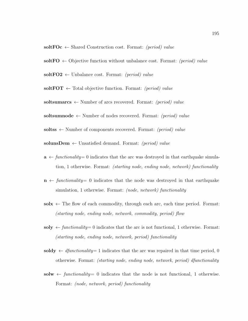
195

soltFOc ← Shared Construction cost. Format: (period) value

soltFO ← Objective function without unbalance cost. Format: (period) value

soltFO2 ← Unbalance cost. Format: (period) value

soltFOT ← Total objective function. Format: (period) value

soltsumarcs ← Number of arcs recovered. Format: (period) value

soltsumnode ← Number of nodes recovered. Format: (period) value

soltss ← Number of components recovered. Format: (period) value

solunsDem ← Unsatisfied demand. Format: (period) value

a ← functionality= 0 indicates that the arc was destroyed in that earthquake simula-

tion, 1 otherwise. Format: (starting node, ending node, network) functionality

n ← functionality= 0 indicates that the node was destroyed in that earthquake

simulation, 1 otherwise. Format: (node, network) functionality

solx ← The flow of each commodity, through each arc, each time period. Format:

(starting node, ending node, network, commodity, period) flow

soly ← functionality= 0 indicates that the arc is not functional, 1 otherwise. Format:

(starting node, ending node, network, period) functionality

soldy ← dfunctionality= 1 indicates that the arc was repaired in that time period, 0

otherwise. Format: (starting node, ending node, network, period) dfunctionality

solw ← functionality= 0 indicates that the node is not functional, 1 otherwise.

Format: (node, network, period) functionality

196

soldw ← dfunctionality= 1 indicates that the node was repaired in that time period,

0 otherwise. Format: (node, network, period) dfunctionality

soldp ← excess indicates the excess of commodity in each node, at each time period.

Format: (node, network, period) excess

soldm ← deficiency indicates the deficiency of commodity in each node, at each time

period. Format: (node, network, period) deficiency

C.3 Folder 3 - INDP Input data

In this folder there is a unique file name INDP data.txt, which contains all the data

associated to the costs, capacities, network structures, and others necessary to solve the

td-INDP (except for the initial disaster scenario to be studied) using the formulation

presented in Gonzalez et al. (2016b,a). The parameters shown in this file do not have

a time index, since for the recovery strategies presented in folder 2 it was assumed

that these parameters did not depend on the time period, i.e., they were constant

through the recovery process.

Below follows the list of parameters found in this file.

v ← Resource availability. Format: (resource) value

c ← Unitary flow costs. Format: (starting node, ending node, network, commodity)

cost

f ← Reconstruction cost of link. Format: (starting node, ending node, network) cost

q ← Reconstruction cost of node. Format: (starting node, network) cost

Mp ← Oversupply penalty. Format: (starting node, network, commodity) cost

197

Mm ← Undersupply penalty. Format: (starting node, network, commodity) cost

g ← Cost of space preparation. Format: (space) cost

b ← Demand. Format: (node, network, commodity) demand

u ← Link capacity. Format: (starting node, ending node, network) capacity

h ← Resource usage when reconstructing link. Format: (starting node, ending node,

network, resource) value

p ← Resource usage when reconstructing node. Format: (node, network, resource)

value

gamma ← Physical interdependence between components. Format: (starting node,

ending node, network 1, network 2) value

alpha ← Nodes belonging to each space. Format: (node, network, space) value

beta ← Links belonging to each space. Format: (starting node, ending node, net-

work,space) value

a ← Arcs in the system. Format: (starting node, ending node, network) value

n ← Nodes in the system. Format: (node, network) value

Resilience Optimization of Systems of Interdependent ...

Documents

Transcript of Resilience Optimization of Systems of Interdependent ...