Frontiers of BusinessResearch in China

Diao et al. Frontiers of Business Research in China (2020) 14:8 https://doi.org/10.1186/s11782-020-00076-4

RESEARCH Open Access

Research on a stock-matching trading

strategy based on bi-objective optimization Haican Diao, Guoshan Liu* and Zhuangming Zhu

* Correspondence: liuguoshan@rmbs.ruc.edu.cnBusiness School, Renmin Universityof China, 59 Zhongguancun Street,Beijing 100872, China

©poolsc

Abstract

In recent years, with strict domestic financial supervision and other policy-orientedfactors, some products are becoming increasingly restricted, including nonstandardproducts, bank-guaranteed wealth management products, and other products thatcan provide investors with a more stable income. Pairs trading, a type of stablestrategy that has proved efficient in many financial markets worldwide, has becomethe focus of investors. Based on the traditional Gatev–Goetzmann–Rouwenhorst(GGR, Gatev et al., 2006) strategy, this paper proposes a stock-matching strategybased on bi-objective quadratic programming with quadratic constraints (BQQ)model. Under the condition of ensuring a long-term equilibrium between paired-stock prices, the volatility of stock spreads is increased as much as possible,improving the profitability of the strategy. To verify the effectiveness of the strategy,we use the natural logs of the daily stock market indices in Shanghai. The GGRmodel and the BQQ model proposed in this paper are back-tested and compared.The results show that the BQQ model can achieve a higher rate of returns.

Keywords: Pairs trading, Bi-objective optimization, Minimum distance method,Quadratic programming

IntroductionSince the A-share margin trading system opened in 2010, there has been a gradual im-

provement in short sales of stock index futures (Wang and Wang 2013) and investors

are again favoring prudent investment strategies, which include pairs-trading strategies.

As a kind of statistical arbitrage strategy (Bondarenko 2003), the essence of pairs trad-

ing (Gatev et al. 2006) is to discover wrongly priced securities in the market, and to

correct the pricing through trading means to earn a profit from the spreads. However,

with the increase in statistical trading strategies and the gradual improvement of mar-

ket efficiency (Hu et al. 2017), profit opportunities using existing trading strategies

have become more scarce, driving investors to seek new trading strategies. At present,

academic research on pairs trading has mainly concentrated on the construction of

pairing models and the optimization design of trading parameters, with a greater focus

on the latter. However, merely improving trading parameters does not guarantee a

The Author(s). 2020 Open Access This article is licensed under a Creative Commons Attribution 4.0 International License, whichermits use, sharing, adaptation, distribution and reproduction in any medium or format, as long as you give appropriate credit to theriginal author(s) and the source, provide a link to the Creative Commons licence, and indicate if changes were made. The images orther third party material in this article are included in the article's Creative Commons licence, unless indicated otherwise in a creditine to the material. If material is not included in the article's Creative Commons licence and your intended use is not permitted bytatutory regulation or exceeds the permitted use, you will need to obtain permission directly from the copyright holder. To view aopy of this licence, visit http://creativecommons.org/licenses/by/4.0/.

Diao et al. Frontiers of Business Research in China (2020) 14:8 Page 2 of 14

high return for the strategy, and this drives researchers back to the foundations of the

pairs-trading model.

There are three main methods for screening stocks: the minimum distance method,

the cointegration pairing method, and the stochastic spread method. The minimum dis-

tance method was proposed by Gatev et al. (2006)—hence its common name, the GGR

model. Gatev et al. (2006) used the distance of a price series to measure the correlation

between the price movements of two stocks. When making a specific transaction, the

strategy user determines the trading signal by observing the magnitude of the change

in the Euclidean distance between the normalized price series of two stocks (the sum

of the squared deviations, or SSD). Perlin (2007) promoted GGR as a unitary method

rather than a pluralistic one; testing it in the Brazilian financial market, he found that

risk can be lessened by increasing the number of pairs and stock. Do and Faff (2010)

found that the length of a trading period can affect strategy returns; their study laid the

foundation for later research. Jacobs and Weber (2011) found that the GGR model’s

revenue comes from the difference in the speed of paired-stock information diffusion.

Chen et al. (2017) revised the measurement method of the GGR model, changing the

original measure (SSD) to the correlation coefficient, and increased the reliability of the

multi-pairing strategy. Wu and Cui (2011) first applied the GGR model to the A-share

market; conducting a back-test on the stock markets in Shanghai, they found that the

GGR model can generate considerable returns, and its profits come from a market’s

non-validity. Wang and Mai (2014) measured the return on stock markets in Shanghai,

Shenzhen, and Hong Kong respectively, and found that improvements to the original

approach can bring portfolio construction strategic benefits but can also increase the

risk of exploitation of the GGR model.

The cointegration pairing method was first used by Vidyamurthy (2004) to find stock

pairs with a cointegral relationship. He used cointegrating vectors as the weight of pairs

when trading. To solve the problem of single-stock pairing risks, Dunis and Ho (2005)

extended the cointegration method from unitarism to pluralism and proposed an en-

hanced index strategy based on cointegration. By extracting sparse mean–return port-

folios from multiple time series, D’Aspremont (2007) found that small portfolios had

lower transaction costs and higher portfolio interpretability than the original intensive

portfolios. Peters et al. (2010) and Gatarek et al. (2014) applied the Bayesian process to

the cointegration test and found that the pairing method can be applied to high-

frequency data.

The stochastic spread method first appeared in a paper by Elliott et al. (2005), who

used the continuous Gauss–Markov model to describe the mean return process of

paired-stock spreads, thus theoretically predicting stock spreads. Based on the research

by Elliott et al. (2005). Do et al. (2006) first linked the capital asset pricing model

(CAPM) with the pairs-trading strategy and achieved a higher strategic benefit than

when using the traditional random spread method. Bertram (2010), assuming that the

price differences of stock obey the Ornstein–Uhlenbeck process, derived the expression

of the mean and variance of the strategic return on the position and found the param-

eter value when the expected return was maximized.

Based on above approaches, many scholars have begun to study mixed multistage

pairing-trading strategies. Miao (2014) added a correlation test to the traditional cointe-

gration method and found that screening stock-correlation analysis improved the

Diao et al. Frontiers of Business Research in China (2020) 14:8 Page 3 of 14

profitability of the strategy. Xu et al. (2012) combined cointegration pairing with the

stochastic spread model and conducted a back-test on the stock markets in both

Shanghai and Shenzhen; they found that higher returns could be obtained. Following

Bertram’s (2010) research, Zhang and Liu (2017) examined a pairs-trading strategy

based on cointegration and the Ornstein–Uhlenbeck process and found the strategy to

be robust and profitable.

In recent years, most scholars have focused on improving the long-term equilibrium

of paired-stock prices in the stock-matching process continuously. Few studies have

considered the short-term fluctuations of paired-stock spreads, which has led to poor

profitability of the strategy. Therefore, this paper focuses on the stock matching of pairs

trading and constructs a bi-objective optimized stock-matching strategy based on the

traditional GGR model. The strategy introduces weight parameters, conducts long-term

stock price volatility spreads, and adjusts the equalizer to match investors’ preferences,

enhancing the flexibility and practicality of the strategy.

The remainder of this paper is organized as follows. Basic theory and model section

provides the basic theories and models of pairs-trading strategies and double bi-

objective optimization. Optimized pairing model section establishes an optimized

pairing model. Pairing strategy empirical analysis section provides an empirical analysis

of the optimal matching strategy proposed in this paper. Finally, Conclusions section

presents conclusions and suggests future research direction.

Basic theory and modelBased on theories of pairs trading, stock-pairing rules in the minimum distance

method, and multi-objective programming, we propose a strategy to improve profits

based on the minimum distance method.

Pairs trading

Pairs-trading parameters

Using a pairs-trading strategy requires a focus on the following trading parameters:

Formation period: the time interval for stock-pair screening using the stock-matching

strategy.

Trading period: the time interval in which selected stock pairs are used for actual

trading.

Configuration of opening: the value of the portfolio construction triggered. For

example, we can start a transaction by satisfying the following conditions: (1) The user

is in the short position state; (2) the degree to which the paired-stock spread deviates

from the mean changes; and (3) the degree changes from less than a given standard

deviation to more than a given standard deviation.

Closing threshold: the value of the position closing triggered. For example, when the

strategy user is in position and the paired-stock spread hits the mean.

Stop-loss threshold: the value of the stop-loss triggered; that is, when the rules are en-

gaged for exiting an investment after reaching a maximum acceptable threshold of loss

or for re-entering after achieving a specified level of gains.

Diao et al. Frontiers of Business Research in China (2020) 14:8 Page 4 of 14

Minimum distance method

When using the minimum distance method to screen stocks, it is necessary to

standardize the stock price series first. Suppose the price sequence of stock A in period

T is PAi ði ¼ 1; 2; 3;…;TÞ ; rAt is the daily rate of return of stock A. By compounding r,

we can get the cumulative rate of return of stock A in period T, which is recorded as:

CPAt ¼

Yti¼1

1þ rAt� �

; ð1Þ

where t = 1, 2, 3, …, T. When we record the standardized stock price series as SPAt ,

the distance SSD of each two-stock normalized price series can be calculated as follows

(Krauss 2016):

SSDAB ¼Xnt¼1

SPAt −SP

Bt

� �: ð2Þ

Multi-objective programming

The multi-objective optimization problem was first proposed by economist Vilfredo Pa-

reto (Deb and Sundar 2006). It means that in an actual problem, there are several ob-

jective functions that need to be optimized, and they often conflict with each other. In

general, the multi-objective optimization problem can be written as a plurality of ob-

jective functions, and the constraint equation and the inequality can be expressed as

follows:

minF xð Þ ¼ f 1 xð Þ; f 2 xð Þ;⋯; f v xð Þ½ �; ð3Þs:t:gi xð Þ≤0; i ¼ 1; 2;⋯; p; ð4Þhj xð Þ ¼ 0; j ¼ 1; 2;⋯; q; ð5Þ

where, x ∈ Ru, fi : Rn→ R(i = 1, 2, ..., n) is the objective function; and gi : R

n→ R and hi :

Rn→ R are constraint functions. The feasible domain is given as follows:

X ¼ x∈Rujgi xð Þ≤0; i ¼ 1; 2;⋯; p; hj xð Þ ¼ 0; j ¼ 1; 2;⋯; q� �

: ð6Þ

If there is not an x ∈ X, such that

f xð Þ≤ f x�ð Þ; ð7Þ

then x∗ ∈ X is called an effective solution (Bazaraa et al. 2008) to the multi-objective

optimization problem.

Optimized pairing modelPrevious studies on the GGR model have mostly focused on similarities in stock trends

and have cared less about the volatility of stock spreads. Such studies could not present

ways to achieve higher returns. This paper, however, is based on the traditional GGR

model, and can thus propose a new pairs-trading model, namely bi-objective quadratic

programming with quadratic constraints (BQQ) model. By adjusting the weights be-

tween maintaining a long-term equilibrium of paired-stock prices and increasing the

volatility of stock spreads (Whistler 2004), we can achieve equilibrium.

Diao et al. Frontiers of Business Research in China (2020) 14:8 Page 5 of 14

Mean-variance minimization distance model

Assume that there are m stocks in the alternative stock pool, and the formation period

of the stock pairing is n days. Take the daily closing price of the stock as the original

price series, recorded as P1, P2, ⋯, Pm. To make the price sequence smoother, we use

the average price series over the past 30 days: P1; P2;⋯; Pm (instead of the original

price series), to eliminate short-term fluctuations in stock prices. Then, in the moment,

t can be expressed as follows:

Pi;t ¼ 130

X29j¼0

Pi;t− j; t ¼ 1; 2;⋯; n: ð8Þ

First we considerP

αiPi.

Let α be the weight of the stock in the stock pool, and then let

f αþi ¼ αi αi > 0; i ¼ 1; 2;⋯; nð Þ

−α−i ¼ αi αi < 0; i ¼ 1; 2;⋯; nð Þ : ð9Þ

Then, we divide the stock into two groups according to the positive and negative

weights. The stock combination with a positive weight is called Pþt , while the stock

combination with a negative weight is called P−t , so

fPþt ¼

Xαþi Pi;t

P−t ¼

Xα−i Pi;t

: ð10Þ

According to the GGR method, as long as we are in the formation period n, we can

consider that the groups’ prices have to represent a long-term equilibrium relationship.

Therefore, we get the bi-objective optimization model as follows:

minXnt¼1

Xmi¼1

αipi;t

!2

: ð11Þ

The volatility of the paired-stock spread is a source of revenue for the pairs-trading

strategy. Variances are used to describe the volatility of a time series. Therefore, we use

the formula below to measure the stock spread:

max1n

Xnt¼1

Xmi¼1

αipi;t−1n

Xnt¼1

Xmi¼1

αipi;t

!2

: ð12Þ

Avoiding the case that α = 0, we increase the regularity constraint; that is, the second-

order modulus is 1, so we can obtain the BQQ model as:

minXnt¼1

Xmi¼1

αipi;t

!2

; max1n

Xnt¼1

Xmi¼1

αipi;t−1n

Xnt¼1

Xmi¼1

αipi;t

!2

: ð13Þ

s:t:Xmi¼1

α2i ¼ 1: ð14Þ

This paper uses a linear weighting method by introducing weight λ(λ > 0), transform-

ing the bi-objective optimization problem into a single-objective optimization problem.

The model is denoted as revised quadratic programming with quadratic constraints

(RQQ):

Diao et al. Frontiers of Business Research in China (2020) 14:8 Page 6 of 14

minXnt¼1

Xmi¼1

αipi;t

!2

−λ1n

Xnt¼1

Xmi¼1

αipi;t−1n

Xnt¼1

Xmi¼1

αipi;t

!2

: ð15Þ

s:t:Xmi¼1

α2i ¼ 1: ð16Þ

Since users of the matching strategy have different risk preferences, λ can be seen as

an important indicator of strategic risk. When λ is large, the model magnifies the vola-

tility of the paired-stock spread sequence, and the strategy may obtain higher returns,

but it also raises the risk of divergence in the stock spread. Therefore, users can adjust

λ to match their risk preferences, which increases the usefulness of the pairing

strategy.

Let p ¼ 1n

Pnt¼1

pt .

To facilitate the model solution, we perform matrix transformation as follows:

f αð Þ ¼ nαT1n

Xnt¼1

Pt Pt� �T !

α−λ αT1n

Xnt¼1

Pt Pt� �T !

α−αTP P� �T

α

" #: ð17Þ

That is,

f αð Þ ¼ αT ½ n−λð Þð1n

Xni¼1

Pt Pt� �T þ λPt Pt

� �T �α: ð18Þ

For a given αk, we get the sub-problem of the model as this:

min f s αkð Þ ¼ dTHαk þ 12dTHd: ð19Þ

s:t:2dTαk þ αkTαk−1 ¼ 0: ð20Þ

The sequential quadratic programming algorithm

Since the objective and constraints of RQQ are quadratic functions, these are typical

nonlinear programming problems. Therefore, the sequential quadratic programming al-

gorithm can solve the original problem by solving a series of quadratic programming

sub-problems (Jacobs and Weber 2011; Zhang and Liu 2017). The solution process is

as follows:

Step 1: Give α1∈ Rm, ε > 0, μ > 0, δ > 0, k = 1, B1∈ Rm ×m.

Step 2: Solve sub-question sub(αk), and we get its solution dk and the Lagrange multi-

plier μk in the case of ∣dk∣ ≤ ε, terminating the iteration; therefore, let sk∈ [0, δ]

and μ = max (μ, μk). By solving this:

P αk þ skdk ; μð Þ≤ min0≤ s≤δ

P xk þ αdk ; μð Þ þ εk ; ð21Þ

we get sk, where εk(k = 1, 2,⋯) satisfies the non-negative condition and

Diao et al. Frontiers of Business Research in China (2020) 14:8 Page 7 of 14

X∞k¼1

εk < þ∞: ð22Þ

Equation (21) is the exact penalty function.

Step 3: Let αk + 1 = αk + skdk, and use the Broyden–Fletcher–Goldfarb–Shanno

algorithm (BFGS, Zhu et al. 1997) to find Bk + 1, then let k = k + 1 and go back to Step 2.

Thus, we find the optimal sub-solution dk. Make dk the search direction and perform

a one-dimensional search in direction dk on the exact penalty function of the original

problem; we get the next iteration point of the original problem as αk + 1. The iteration

is terminated when the iteration point satisfies the given accuracy, obtaining the opti-

mal solution of the original problem.

Pairing strategy empirical analysisTo verify the profitability of the BQQ strategy, this paper compares the empirical in-

vestment effects of the BQQ strategy and the GGR strategy with the same transaction

parameters and applies a profit-risk test for the arbitrage results of the two strategies.

Data selection and preprocessing

We use SSE 50 Index constituent stocks in the Shanghai stock market as the sample

set for this study. We choose this sample set for its high circulation market value and

large market capitalizations. Since the stock-pairing method proposed in this paper is

based on an improvement of the traditional minimum distance method, this is consist-

ent with the GGR model in the time interval selection of the sample: The paired stocks

for trading are selected during the formation period of 12 months, and the stocks are

traded in the next 6 months. To verify the effectiveness of the strategy, the paper con-

ducts a strategic back-test from January 2016 to December 2018. Within the period,

the broader market experienced a complete set of ups and downs.

Due to the existence of share allotments and share issues by listed companies, and

because the suspension of stocks will also lead to a lack of market data, the raw data

needs to be preprocessed. By reversing the stock price forward, the stock price changes

caused by the allotments and stock offerings are eliminated. In addition, we exclude

stocks that have been suspended for more than 10 days in the formation period. These

missing data are replaced by the closing price of the nearest trading day.

Parameters settings

Transaction parameters setting

The implementation of a pairs-trading strategy relies on setting trading parameters. To

compare this strategy with the traditional minimum distance method and verify the val-

idity of the BQQ strategy, this paper uses the same parameters used in the GGR model

for setting the trading parameters. We set the stop-loss threshold to 3 to prevent exces-

sive losses due to excessive strategy losses and transaction costs. We set the number of

paired shares to 10. For convenience, we divide the stocks into groups according to

their weights, positive and negative.

Diao et al. Frontiers of Business Research in China (2020) 14:8 Page 8 of 14

Portfolio construction

After determining the trading parameters and cost parameters, we also need to deter-

mine the stock opening method; assuming that the final selected pair of stocks is fSþ1 ;Sþ2 ;⋯; Sþ5 g; fS−1 ; S−2 ;⋯; S−5g (corresponding to two sets of paired stocks), and the corre-

sponding weight is fαþ1 ; αþ2 ; :::; αþ3 g and fα−1 ; α−2 ; :::; α−3g . When the trading strategy is-

sues a trading signal for opening, closing, or stop-loss, the trading begins. The user

needs to trade αi/α1(i = 2, 3, 4,…, 10) units of stock fS−1 ; S−2 ;⋯; S−5g for each unit of fSþ1 ;Sþ2 ;⋯; Sþ5 g. Then, the strategy user has a net position, which is the paired-stock spread.

Performance evaluation

To compare the effects of the GGR model and the proposed BQQ model, we verify the

effectiveness of the proposed optimization pairing strategy. This paper selects the in-

come coefficient α, risk coefficient β, and the Sharpe ratio as evaluation indicators, and

the two strategies are back-tested and compared on the JoinQuant platform.

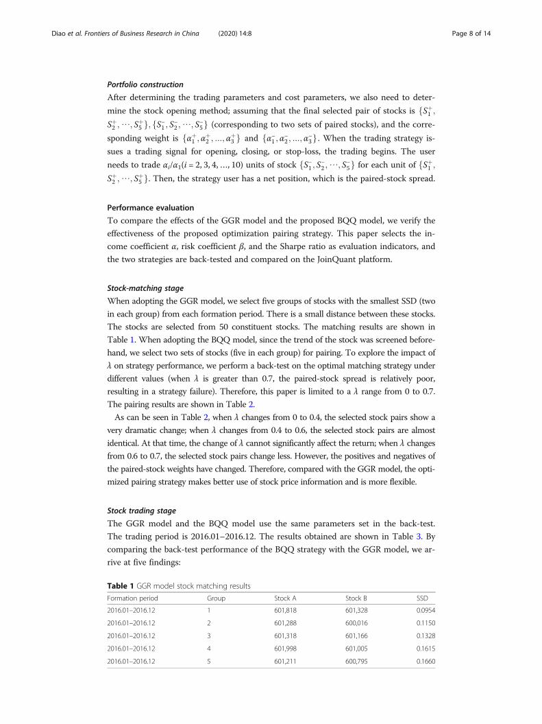
Stock-matching stage

When adopting the GGR model, we select five groups of stocks with the smallest SSD (two

in each group) from each formation period. There is a small distance between these stocks.

The stocks are selected from 50 constituent stocks. The matching results are shown in

Table 1. When adopting the BQQ model, since the trend of the stock was screened before-

hand, we select two sets of stocks (five in each group) for pairing. To explore the impact of

λ on strategy performance, we perform a back-test on the optimal matching strategy under

different values (when λ is greater than 0.7, the paired-stock spread is relatively poor,

resulting in a strategy failure). Therefore, this paper is limited to a λ range from 0 to 0.7.

The pairing results are shown in Table 2.

As can be seen in Table 2, when λ changes from 0 to 0.4, the selected stock pairs show a

very dramatic change; when λ changes from 0.4 to 0.6, the selected stock pairs are almost

identical. At that time, the change of λ cannot significantly affect the return; when λ changes

from 0.6 to 0.7, the selected stock pairs change less. However, the positives and negatives of

the paired-stock weights have changed. Therefore, compared with the GGR model, the opti-

mized pairing strategy makes better use of stock price information and is more flexible.

Stock trading stage

The GGR model and the BQQ model use the same parameters set in the back-test.

The trading period is 2016.01–2016.12. The results obtained are shown in Table 3. By

comparing the back-test performance of the BQQ strategy with the GGR model, we ar-

rive at five findings:

Table 1 GGR model stock matching results

Formation period Group Stock A Stock B SSD

2016.01–2016.12 1 601,818 601,328 0.0954

2016.01–2016.12 2 601,288 600,016 0.1150

2016.01–2016.12 3 601,318 601,166 0.1328

2016.01–2016.12 4 601,998 601,005 0.1615

2016.01–2016.12 5 601,211 600,795 0.1660

Table 2 BQQ model stock matching results

λ Serial No. Stock A Stock weight Serial No. Stock B Stock weight

0 1 600,795 0.5028 6 600,016 0.0136

2 601,398 0.1417 7 601,766 −0.0224

3 601,328 0.1249 8 600,028 −0.0504

4 601,390 0.031 9 601,669 −0.0523

5 601,166 0.0241 10 601,988 −0.8392

0.1 1 600,050 0.7513 6 601,336 −0.0657

2 600,999 0.4585 7 600,150 −0.1127

3 600,036 0.1822 8 601,688 −0.1165

4 600,887 0.1213 9 600,104 −0.201

5 601,318 −0.0251 10 601,800 −0.3252

0.2 1 601,888 0.3566 6 600,519 0.019

2 600,606 0.2937 7 600,547 −0.0345

3 601,601 0.0848 8 600,340 −0.1763

4 601,336 0.0747 9 601,211 −0.4097

5 601,688 0.0299 10 600,703 −0.7566

0.3 1 601,628 0.2169 6 600,109 0.0275

2 600,893 0.1016 7 600,050 −0.009

3 601,688 0.0875 8 600,150 −0.0099

4 601,186 0.0665 9 600,999 −0.2757

5 600,887 0.0381 10 601,857 −0.9232

0.4 1 600,050 0.8067 6 600,887 −0.0156

2 601,186 0.249 7 601,601 −0.0225

3 600,999 0.2128 8 601,628 −0.1203

4 600,893 0.0647 9 600,150 −0.1544

5 601,688 0.0181 10 601,800 −0.4454

0.5 1 600,050 0.7972 6 600,109 −0.0174

2 601,186 0.2569 7 601,601 −0.0246

3 600,999 0.2342 8 601,628 −0.1251

4 600,893 0.0651 9 600,150 −0.1548

5 601,688 0.0044 10 601,800 −0.4459

0.6 1 600,050 0.7886 6 601,601 0.0168

2 601,186 0.2794 7 601,601 −0.1138

3 600,999 0.1789 8 601,628 −0.1197

4 601,688 0.0691 9 600,150 −0.1589

5 600,893 0.065 10 601,800 −0.4542

0.7 1 601,800 0.2475 6 601,601 0.0522

2 601,688 0.1843 7 600,893 −0.0448

3 600,150 0.1535 8 600,111 −0.1994

4 601,601 0.1162 9 600,999 −0.3851

5 601,186 0.07 10 600,050 −0.8185

Diao et al. Frontiers of Business Research in China (2020) 14:8 Page 9 of 14

(1) The ability of the BQQ strategy to obtain revenue is significantly stronger than of

the GGR model, which shows that the BQQ strategy is effective in increasing the

volatility of the spread to improve the profitability of the pairs-trading strategy.

Table 3 BQQ strategy performance

Tradingperiod

λ BQQ strategy performance SSE 50rangeupsanddowns

Strategicincome

Annualizedincome

Coefficientα

Coefficientβ

Sharperatio

Winrate

Maximumwithdrawal

2016.01–2016.12

0 5.11% 5.24% 0.99 −0.035 0.334 0.449 1.35% −5.53%

0.1 5.64% 5.78% 0.012 −0.057 0.186 0.520 5.06% −5.53%

0.2 11.13% 11.41% 0.068 −0.065 1.028 0.633 2.28% −5.53%

0.3 25.49% 26.19% 0.209 −0.131 2.292 0.667 2.17% −5.53%

0.4 19.26% 19.78% 0.160 0.025 1.889 0.500 1.51% −5.53%

0.5 17.64% 18.11% 0.144 0.029 1.557 0.529 3.03% −5.53%

0.6 18.74% 19.24% 0.155 0.026 1.931 0.544 1.69% −5.53%

0.7 9.66% 9.91% 0.060 0.010 0.920 0.681 1.81% −5.53%

GGR 2.67% 2.74% −0.014 0.010 −0.406 0.438 2.27% −5.53%

Diao et al. Frontiers of Business Research in China (2020) 14:8 Page 10 of 14

Figure 1 shows the average annualized rate of return of the BQQ strategy and the

GGR strategy for different λ values (both in-sample data and out-of-sample data, re-

spectively). For the in-sample rate of return, both strategies were carried out for a total

of 32 back-tests, with a total of 31 positive gains. The return of the BQQ strategy is

better than that of the GGR strategy in 87.5% of the cases. For the out-of-sample rate

of return, the return of the BQQ strategy is better than that of the GGR strategy in

68.8% of the cases. To rule out the deviation of income caused by the different ways of

opening a position, we also need to examine the coefficient of the two strategies and

the Sharpe ratio.

As shown in Figs. 2 and 3, the BQQ model performs significantly better than the

GGR model, both in terms of the coefficient α and the Sharpe ratio. This result indi-

cates that the BQQ model bears the average return of nonmarket risk during the four

trading periods, and the average return on unit risk is higher than with the GGR model.

Therefore, the better perfomance of the BQQ strategy is not from the strategy taking

more market risk; rather, it is independent of the way the strategy is opened.

Fig. 1 Average annualized rate of return of the two strategies

Fig. 2 Coefficient α of the two strategies

Diao et al. Frontiers of Business Research in China (2020) 14:8 Page 11 of 14

(2) The BQQ strategy has a strong ability to hedge the market. Table 4 shows the

average value of the coefficient β of the BQQ strategy under different values of λ. It

can be seen that the absolute value of β is below 0.1, which indicates and proves

that the performance of the strategy is not affected by market fluctuations, which

in turn proves that the pairs-trading strategy based on the minimum distance

method can hedge market risk well. Compared with the GGR model, the coeffi-

cient β of the BQQ strategy is magnified because the GGR model uses a capital-

neutral approach when in the opening position, while the BQQ strategy uses a

coefficient-neutral approach. Due to the existence of the spread, the BQQ strategy

cannot guarantee that the market value of the bought stock will be equal to the

market value of the sold stock when the position is opened, which is equivalent to

the fact that some net positions follow market ups and downs and the coefficient

will increase.

(3) Similar to the GGR model, the BQQ strategy performs poorly in out-of-sample

data. In the 32 out-of-sample back-tests, the annualized return of the BQQ strategy

was positive only six times, and the coefficient α was positive only eight times. The

main reason for this phenomenon is the lack of rationality in the length of the for-

mation period used at the stock-matching stage and the trading parameters used in

the stock-trading stage. The yield of the GGR model is affected by trading

Fig. 3 Sharpe ratio of the two strategies

Table 4 Coefficient β of the two strategies

In-sample Out-of-sample

Period 1 Period 2 Period 3 Period 4 Period 5 Period 6 Period 7 Period 8

BQQ −0.025 −0.014 0.029 0.020 −0.076 −0.040 0.008 −0.039

GGR 0.010 0.006 0.039 −0.003 0.089 0.003 −0.036 −0.013

Diao et al. Frontiers of Business Research in China (2020) 14:8 Page 12 of 14

parameters in many cases, such as the formation period, trading period, and open-

ing threshold. Since this article presents only a methodological improvement for

the stock-pairing trading model, it does not provide a more in-depth study of trad-

ing parameters.

(4) Performance of the BQQ strategy is very sensitive to the value of λ. Adjustable λ

enhances the practicality of the strategy. In the same trading period, the return of

the BQQ strategy does not show a monotonous change with λ. When the value of

λ is too large, the stock-matching strategy is invalid because when λ increases, the

volatility of the paired-stock spread is increasing, which means that the strategy is

likely to obtain higher returns. Conversely, the increase of λ raises the risk of diver-

gence in the spread, making it easier for the strategy to trigger a stop-loss signal

and cause losses. Therefore, λ is a significant parameter to adjust the risk of the

strategy, and the strategy user can adjust λ to match risk preferences, which en-

hances the usefulness of the strategy.

(5) The optimal λ value is time dependent. The benefit of the BQQ strategy are non-

monotonic changes in λ. Excessive λ assembly leads to the invalidation of the

stock-matching strategy, which means that for a specific trading period, there is an

optimized λ that maximizes the strategy’s return. From the perspective of revenue

indicators and risk indicators, there are no obvious rules about the performance of

the strategy and the change of λ. That is, the optimal λ value varies with the trad-

ing period and is time dependent.

Table 5 shows the values of coefficient α and the Sharpe ratio from four out-of-

sample back-tests. When λ is 0.5, coefficient α and the Sharpe ratio take the maximum

value at the same time.

The results show that when λ is 0.5, the average matching revenue of the optimized

matching strategy for non-market risk in the four trading periods and the average re-

turn from unit risk are the largest, but the value needs to be verified by large-scale

data.

ConclusionsBy introducing multi-objective optimization to the GGR model, this paper considers

the long-term equilibrium of stock prices and the volatility of spreads and establishes a

BQQ model. This novel pairs-trading model provides a new perspective for pairs-

trading strategy research. At the same time, it provides investors with a stock-matching

Table 5 Values of coefficient α and the Sharpe ratio for different λλ = 0 λ = 0.1 λ = 0.2 λ = 0.3 λ = 0.4 λ = 0.5 λ = 0.6 λ = 0.7

Coefficient α −0.113 −0.076 − 0.070 −0.112 − 0.099 −0.062 − 0.101 −0.139

Sharpe ratio −3.268 −2.191 −1.833 −2.294 −1.913 − 1.683 − 2.243 −2.747

Diao et al. Frontiers of Business Research in China (2020) 14:8 Page 13 of 14

method that effectively improves the profitability of the trading strategy. This paper in-

troduces the weight λ when solving bi-objective optimization problems, and these prob-

lems are transformed into single-objective optimization problems and solved by a

sequential quadratic programming algorithm. To verify the effectiveness of the opti-

mized pairing strategy, this paper selects the traditional GGR model as model for com-

parison and conducts back-testing on multiple time intervals on the SSE 50

constituents. We find that the BQQ strategy was able to obtain significantly higher rev-

enue than the GGR model, and the adjustment of the weight λ increases the flexibility

and practicality of the strategy.

This paper has some limitations. We used the SSE 50 Index as the research target in

our empirical analysis. However, this was subject to the limitation of financing and se-

curities lending; the small number of stocks may have affected the performance of the

trading strategy. Additionally, when we performed the validity check of the optimized

pairing strategy, there was scarce in-depth research available on the trading parameters

and optimal values of the strategy, and this may have affected the profitability of the

strategy to some extent. Therefore, subsequent research work should include these as-

pects. In the future, we will expand the number of stock share pools. In addition, the

screening method for the transaction parameter of pairs-trading strategy requires in-

depth research to find the right trading parameters for the BQQ strategy. Finally, we

will try to establish an optimized pairing strategy by attaining the function of risk indi-

cator λ through extended empirical analysis.

AbbreviationsBFGS: The Broyden–Fletcher–Goldfarb–Shanno algorithm; BQQ: Bi-objective quadratic programming with quadraticconstraints; CAPM: Capital asset pricing model; GGR: The distance approach proposed by Gatev, Goetzmann andRouwenhorst in 2006; RQQ: Revised quadratic programming with quadratic constraints; SSD: Sum of squareddeviations; SSE: Shanghai Stock Exchange

AcknowledgementsNot applicable.

Authors’ contributionsDiao contributed to the overall writing and the data analysis; Liu conceived the idea; Zhu contributed to the datacollection and the data analysis. All authors read and approved the final manuscript.

FundingThe research is supported by the Fundamental Research Funds for the Central Universities, and the Research Funds ofRenmin University of China (No. 19XNH089).

Availability of data and materialsShanghai Composite IndexPlease contact authors for data requests.

Competing interestsThe authors declare that they have no competing interests.

Received: 9 July 2019 Accepted: 25 February 2020

ReferencesBazaraa, M. S., Sherali, H. D., & Shetty, C. M. (2008). Nonlinear programming: Theory and algorithms (3rd ed.). Hoboken: Wiley.Bertram, W. K. (2010). Analytic solutions for optimal statistical arbitrage trading. Physica A: Statistical Mechanics and its

Applications, 389(11), 2234–2243.Bondarenko, O. (2003). Statistical arbitrage and securities prices. Review of Financial Studies, 16(3), 875–919.Chen, H., Chen, S., Chen, Z., & Li, F. (2017). Empirical investigation of an equity pairs trading strategy. Management Science,

65(1), 370–389.D’Aspremont, A. (2007). Identifying small mean reverting portfolios. Quantitative Finance, 11(3), 351–364.Deb, K., & Sundar, J. (2006). Reference point based multi-objective optimization using evolutionary algorithms. In Proceedings

of the 8th annual conference on conference on genetic & evolutionary computation (pp. 635–642).Do, B., & Faff, R. (2010). Does simple pairs trading still work? Financial Analysts Journal, 66(4), 83–95.

Diao et al. Frontiers of Business Research in China (2020) 14:8 Page 14 of 14

Do, B., Faff, R., & Hamza, K. (2006). A new approach to modeling and estimation for pairs trading. In Proceedings of 2006financial management association European conference (pp. 87–99).

Dunis, C. L., & Ho, R. (2005). Cointegration portfolios of European equities for index tracking and market neutral strategies.Journal of Asset Management, 6(1), 33–52.

Elliott, R. J., van der Hoek, J., & Malcolm, W. P. (2005). Pairs trading. Quantitative Finance, 5(3), 271–276.Gatarek, L. T., Hoogerheide, L. F., & van Dijk, H. K. (2014). Return and risk of pairs trading using a simulation-based Bayesian

procedure for predicting stable ratios of stock prices. Electronic, 4(1), 14–32 Tinbergen Institute Discussion Paper 14-039/III.

Gatev, E., Goetzmann, W. N., & Rouwenhorst, K. G. (2006). Pairs trading: Performance of a relative-value arbitrage rule. SocialScience Electronic Publishing, 19(3), 797–827.

Hu, W., Hu, J., Li, Z., & Zhou, J. (2017). Self-adaptive pairs trading model based on reinforcement learning algorithm. Journal ofManagement Science, 2(2), 148–160.

Jacobs, H., & Weber, M. (2011). Losing sight of the trees for the forest? Pairs trading and attention shifts. Working paper, October2011. University of Mannheim. Available at https://efmaefm.org/0efmsymposium/2012/papers/011.pdf.

Krauss, C. (2016). Statistical arbitrage pairs trading strategies: Review and outlook. Journal of Economic Surveys, 31(2), 513–545.Miao, G. J. (2014). High frequency and dynamic pairs trading based on statistical arbitrage using a two-stage correlation and

cointegration approach. International Journal of Economics and Finance, 6(3), 96–110.Perlin, M. (2007). M of a kind: A multivariate approach at pairs trading (working paper). University Library of Munich, Germany.Peters, G. W., Kannan, B., Lasscock, B., Mellen, C., & Godsill, S. (2010). Bayesian cointegrated vector autoregression models

incorporating alpha-stable noise for inter-day price movements via approximate Bayesian computation. Bayesian Analysis,6(4), 755–792.

Vidyamurthy, G. (2004). Pairs trading: Quantitative methods and analysis. Hoboken: Wiley.Wang, F., & Wang, X. Y. (2013). An empirical analysis of the influence of short selling mechanism on volatility and liquidity of

China’s stock market. Economic Management, 11(3), 118–127.Wang, S. S., & Mai, Y. G. (2014). WM-FTBD matching trading improvement strategy and empirical test of Shanghai and

Shenzhen ports. Economy and Finance, 26(1), 30–40.Whistler, M. (2004). Trading pairs: Capturing profits and hedging risk with statistical arbitrage strategies. Hoboken: Wiley.Wu, L., & Cui, F. D. (2011). Investment strategy of paired trading. Journal of Statistics and Decision, 23, 156–159.Xu, L. L., Cai, Y., & Wang, L. (2012). Research on paired transaction based on stochastic spread method. Financial Theory and

Practice, 8, 30–35.Zhang, D., & Liu, Y. (2017). Research on paired trading strategy based on cointegration—OU process. Management Review,

29(9), 28–36.Zhu, C., Byrd, R. H., Lu, P., & Nocedal, J. (1997). Algorithm 778: L-BFGS-B: Fortran subroutines for large-scale bound-constrained

optimization. ACM Transactions on Mathematical Software (TOMS), 23(4), 550–560.

Publisher’s NoteSpringer Nature remains neutral with regard to jurisdictional claims in published maps and institutional affiliations.