RESEARCH NOTE FROM COLLABORATION: Discovery potential for supersymmetry in CMS*

arX

iv:h

ep-p

h/98

0636

6v1

15

Jun

1998

Available on CMS information server CMS NOTE 1998/006

The Compact Muon Solenoid Experiment

Mailing address: CMS CERN, CH-1211 GENEVA 23, Switzerland

CMS NoteApril 1998

Discovery potential for supersymmetry in CMS

For the CMS Collaboration

S. Abdullina, Z. Antunovicb, F. Charlesc, D. Denegrid, U. Dydake, M. Dzelalijab,V. Genchevf , D. Grahamg, I. Iashvilih,i, A. Kharchilavah,i, R. Kinnunenj ,

S. Kunorik, K. Mazumdarl, C. Raccai, L. Ruruah,e, N. Stepanova, J. Womersleym

Abstract

This work summarizes and puts in an overall perspective studies done within CMS concerningthe discovery potential for squarks and gluinos, sleptons, charginos and neutralinos, SUSYdark matter, lightest Higgs, sparticle mass determination methods and the detector designoptimisation in view of SUSY searches. It represents the status of our understanding of thesesubjects as of Summer 1997.

As a benchmark model we used the minimal supergravity-inspired supersymmetric standardmodel (mSUGRA) with a stable LSP. Discovery of supersymmetry at the LHC should be rel-atively straightforward. It may occur through the observation of a large excesses of events inmissing ET plus jets, or with one or more isolated leptons. An excess of trilepton events or ofisolated dileptons with missing ET , exhibiting a characteristic signature in the l+l− invariantmass distribution could also be the first manifestation of SUSY production. Squarks and gluinoscan be discovered for masses in excess of 2 TeV. Charginos and neutralinos can be discoveredfrom an excess of events in dilepton or trilepton final states. Inclusive searches can give earlyindications from their copious production in squark and gluino cascade decays. Indirect evi-dence for sleptons can be obtained also from inclusive dilepton studies. Isolation requirementsand a jet veto would allow detection of both, the direct chargino/neutralino production and ofdirectly-produced sleptons. Squark and gluino production may also represent a copious sourceof Higgs bosons through cascade decays. The lightest SUSY Higgs h → bb may be reconstructedwith a signal/background ratio of order 1 thanks to hard cuts on Emiss

T justified by escapingLSP’s. The lightest supersymmetric particle of SUSY models with conserved R-parity representsa very good candidate for the cosmological dark matter. The region of parameter space wherethis is true is well-covered by our searches, at least for tanβ = 2.

If supersymmetry exists at electroweak scale it could hardly escape detection in CMS, and

the study of supersymmetry will form a central part of our physics program.

http://arXiv.org/abs/hep-ph/9806366v1

a Institute for Theoretical and Experimental Physics, Moscow, Russiab University of Split, Split, Croatiac Universite de Haute Alsace, Mulhouse, Franced Centre d‘Etudes Nucleaire de Saclay, Gif-sur-Yvette, Francee Institut fur Hochenergiephysik, Wien, Austriaf Institute for Nuclear Research and Nuclear Energy, Sofia, Bulgariag Imperial College, University of London, London, United Kingdomh Institute of Physics, Georgian Academy of Sciences, Tbilisi, Georgiai Institut de Recherches Subatomiques, Strasbourg, Francej Helsinki Institute of Physics, Helsinki, Finlandk University of Maryland, College Park, USAl Tata Institute of Fundamental Research-EHEP, Bombay, Indiam Fermi National Accelerator Laboratory, Batavia, USA

1

Contents

1 Introduction 1

2 SUSY model employed 22.1 Charginos and neutralinos . . . . . . . . . . . . . . . . . . . . . . . . . . . 22.2 Sleptons . . . . . . . . . . . . . . . . . . . . . . . . . . . . . . . . . . . . . 42.3 Gluinos and squarks . . . . . . . . . . . . . . . . . . . . . . . . . . . . . . 7

3 Experimental signatures considered 26

4 Detector issues 274.1 CMS detector optimisation for SUSY studies . . . . . . . . . . . . . . . . . 274.2 HCAL optimisation and tail catcher . . . . . . . . . . . . . . . . . . . . . . 284.3 The role of the tracker in SUSY searches . . . . . . . . . . . . . . . . . . . 304.4 Lepton isolation . . . . . . . . . . . . . . . . . . . . . . . . . . . . . . . . . 304.5 Tagging of b-jets in CMS . . . . . . . . . . . . . . . . . . . . . . . . . . . . 314.6 CMSJET – an approximate description of detector response . . . . . . . . 31

5 Leptons + jets+ EmissT channel –

search for gluinos and squarks 47

6 Search for next-to-lightest neutralino 656.1 Inclusive 2 leptons + Emiss

T + (jets) channel . . . . . . . . . . . . . . . . 656.2 Inclusive 3 leptons channel . . . . . . . . . . . . . . . . . . . . . . . . . . . 666.3 Inclusive 3 leptons + Emiss

T channel . . . . . . . . . . . . . . . . . . . . . . 68

7 Exclusive 2 leptons + no jets + EmissT channel –

search for sleptons 81


search for chargino/neutralino pair production 95

9 Possibility of observing h → bb in squark and gluino decays 108

10 Sensitivity to sparticle masses andmodel parameters 12310.1 Establishing the SUSY mass scale . . . . . . . . . . . . . . . . . . . . . . . 12310.2 Constraints from χ0

2 leptonic decays . . . . . . . . . . . . . . . . . . . . . . 12310.3 Determination of the squark mass . . . . . . . . . . . . . . . . . . . . . . . 12610.4 Sensitivity to model parameters in 3l + no jets + Emiss

T final states . . . . 12710.5 Sensitivity to model parameters in inclusive l+l− + Emiss

T + jets final states 130

11 Summary and conclusions 146

1 Introduction

There are strong arguments that the Standard Model (SM), despite its phenomenologicalsuccesses [1], is only a low energy effective theory of spin-1/2 matter fermions interactingvia spin-1 gauge bosons. A good candidate for “new physics” is the Supersymmetric(SUSY) extension of the SM which in its minimal version (MSSM) doubles the numberof known particles, introducing scalar and fermion partners to ordinary fermions andbosons and relating their couplings. This scheme provides the necessary cancellation ofquadratic divergences which appear in loop corrections to the masses provided the massesof super-partners are of the order of electroweak (EW) scale, i.e. ∼0.1 to 1 TeV.

One of the main motivations of the experiments at the Large Hadron Collider (LHC)is to search for SUSY particles (“sparticles”). Previous studies [2] have shown that atthe LHC the observation of an excess in event rates of specific final states over the SMexpectations would signal the production of SUSY particles. The present study is basedon a more precise description of the Compact Muon Solenoid (CMS) detector and covers awider spectrum of physics channels. The primary goal is to understand the experimentallimiting factors for SUSY studies and contribute to the detector optimisation while itsdesign is not entirely frozen. The emphasis is put on leptonic channels, which are asinteresting in terms of discovery potential, if not more, as the classical multi-jets +Emiss

T signature. The latter is more sensitive to instrumental backgrounds which can befully understood only once the cracks, dead areas and volumes of diminished instrumentalresponse due to detector services, mechanical supports are fully specified and evaluated.Another motivation for this study was the need to evaluate the discovery potential of anLHC detector in terms of accessible sparticle spectrum, sparticle mass reach, possibilitiesto determine the SUSY model scenario at work and possibilities to determine sparticlemasses and model parameters in comparison and competition with a future e+e− colliderand dedicated SUSY (WIMP) dark matter search experiments [3].

This work summarizes and puts in an overall perspective specific studies done withinCMS concerning the observability and discovery potential for squarks and gluinos [4, 5],sleptons [6, 7], charginos and neutralinos [8, 9, 10], SUSY dark matter [11], the lightestHiggs [12], sparticle mass determination methods [9, 10, 7], detector design optimisationin view of SUSY searches [13], etc., and represents the status of our understanding ofthese subjects as of summer 1997.

We discuss the specific SUSY model employed in section 2 and the experimentalsignatures investigated in section 3. Detector issues and simulations of detector responseare described in section 4. Searches for SUSY in lepton(s)+jets + Emiss

T final states fromstrongly interacting sparticle production are discussed in section 5 followed by inclusivesearches for the next-to-lightest neutralino in section 6. Exclusive 2 leptons + no jets+Emiss

T and exclusive 3 leptons+no jets+ (EmissT ) channels are discussed in sections 7 and

8. Possibilities to observe h → bb in squark and gluino decays are discussed in section 9.The methods to measure sparticle masses and restrict model parameters are addressed insection 10. Results and conclusions are summarized in section 11.

The potential of CMS to study the Higgs sector of SUSY has been extensively discussedelsewhere [14] and we do not address this problem here. Obtained results are based ontwo-loop level calculations [15]. To summarize, in the search of the various MSSM Higgsbosons, most of the mA, tanβ parameter space will be explored through at least onechannel, provided an integrated luminosity of Lint = 105 pb−1 is available. A difficulty

1

still exists in the region of 120 GeV <∼ mA <∼ 240 GeV and 2 <∼ tanβ <∼ 10, which wouldrequire Lint = 6÷ 10× 105 pb−1 to be fully explored (though section 9 indicates that theHiggs sector may also be detectable in the decays of other SUSY particles).

2 SUSY model employed

Since the phenomenological implications of SUSY are model-dependent, the discovery po-tential of a detector has to be studied resorting to some particular model, preferably witha limited number of free parameters. This implies some loss of “generality”, but ensurestractable predictions. Once the possibilities and problems have been well understoodwithin a defined scheme it is easier to evaluate its generality.

We have chosen to make the investigation in the minimal Super Gravity constrainedversion of the MSSM (mSUGRA) [16] as implemented in ISAJET [17]. This mSUGRAscheme has a limited number of parameters, has well established and simple mass re-lations, and is implemented in event generators, besides having definite phenomenolog-ical/theoretical attractiveness and plausibility. In the mSUGRA model only five extraparameters, which are not present in the SM, need to be specified: the universal scalarm0 and gaugino m1/2 masses, the SUSY breaking universal trilinear coupling A0, the ratioof the vacuum expectation values of the Higgs fields tanβ and the sign of the Higgsinomixing parameter sign(µ). The first three parameters are fixed at the gauge couplingunification scale and the sparticle spectrum at the EW scale are then obtained via renor-malization group equations [18].

Throughout this study except for cases specially mentioned we largely limit ourselvesto the set:

tanβ = 2, A0 = 0, µ < 0, (1)

and also consider five representative parameter space points suggested by theorists, andlisted in Table 1.1.

Table 1.1: Representative mSUGRA points suggested by theorists.

Point m0 (GeV) m1/2 (GeV) A0 (GeV) tanβ µ

1 100 300 300 2.1 > 02 400 400 0 2 > 03 400 400 0 10 > 04 200 100 0 2 < 05 800 200 0 10 > 0

In the following we discuss the mass relations among sparticles in mSUGRA, displayisomass curves in terms of model parameters, discuss production mechanisms and decaymodes accessible to experimental observations.

2.1 Charginos and neutralinos

The mixing of the fermionic partners of the electroweak gauge and Higgs bosons, thegauginos and the Higgsinos, gives rise to the physical mass eigenstates called the charginos

2

(χ±1,2) and neutralinos (χ0

1,2,3,4). They are among the lightest expected SUSY particles andtherefore present particular interest. The two lightest neutralinos and the lightest chargino(χ0

1, χ02, χ±

1 ) have as their largest mixing component the gauginos, and their masses aredetermined by the common gaugino mass, m1/2. Within mSUGRA:

Mχ01≈ 0.45m1/2 (2)

Mχ02≈ Mχ±

1≈ 2Mχ0

1(3)

Mχ02≈ (0.25 ÷ 0.35)Mg (4)

Figure 2.1 shows the isomass contours of (χ01, χ0

2, χ±1 ) and of (χ0

3, χ04, χ±

2 ) in the(m0, m1/2) plane. We remind the reader that in most of parameter space and in the moreplausible scenarios the lightest neutralino, χ0

1, is the Lightest Supersimmetric Particle(LSP) and as such is particularly interesting as it is one of the most plausible cosmic darkmatter candidates particle physics provides.

The lightest chargino χ±1 has several leptonic decay modes, giving an isolated lepton

and missing energy due to the undetectable neutrino and LSP (χ01 in mSUGRA):

• χ±1 −→ χ0

1 l± ν three-body decay

• χ±1 −→ l±L ν

→ χ01 l±

• χ±1 −→ νL l± two-body decays

→ χ01 ν

• χ±1 −→ χ0

1 W±

→ l± ν

Figure 2.2 shows the branching ratios for the above listed χ±1 decay channels as a

function of (m0, m1/2). One can see that in different regions these different leptonicdecay modes are complementary, amounting to a larger than 20% branching in the entire(m0, m1/2) plane (for l = e, µ). Three-body decays are open in the region m1/2

<∼ 200GeV and m1/2

>∼ 0.5m0, whereas in the rest of parameter space the two-body decays aredominant.

Leptonic decays of χ02 give two isolated leptons and missing energy (χ0

1):

• χ02 −→ χ0

1 l+ l−

• χ02 −→ χ±

1 l∓ ν three-body decays→ χ0

1 l± ν

• χ02 −→ l±L,R l∓ two-body decay

→ χ01 l±

Figure 2.3 shows the χ02 leptonic branching ratios as a function of (m0, m1/2). Like

the χ±1 case, the three-body decay branching ratios are sizable at m1/2

<∼ 200 GeV andm1/2

>∼ 0.5m0. Beyond m1/2 ≃ 200 GeV, the three-body decay of χ02 is suppressed due to

the opening up of the channels χ02→χ0

1 h and χ02→ χ0

1 Z (“spoiler” modes). The two-bodydecay branchings are significant if m0

<∼ 0.5m1/2.

3

In hadronic collisions, the charginos and neutralinos can be produced directly viaa Drell-Yan mechanism or, more abundantly, through the cascade decays of stronglyinteracting sparticles. There is also the possibility of associated production χ±

i /χ0j +

g/q. There are 21 different reactions (8 χ±i χ0

j , 3 χ±i χ±

j and 10 χ0i χ

0j ) for direct chargino-

neutralino pair production among which χ±1 χ0

2 production followed by leptonic decaysof χ±

1 and χ02 is most easy from the detection point of view, yielding a 3 leptons +

no jets+EmissT event topology.

Figure 2.4 shows the cross-section times branching ratio, σ× B(3l + invisible), whereσ is the χ±

1 χ02 direct production cross-section and B(3l + invisible) is the convolution of

all the leptonic decays of χ±1 and χ0

2 listed above. Within a relatively small region of m1/2

and for m0>∼ 400 GeV, the σ× B(3l + invisible) drops by several orders of magnitude

and vanishes at m1/2 ≃ 200 GeV. For m0<∼ 400 GeV the slope is less sharp thanks to the

presence of two-body decay modes.Probabilities for production of χ±

1 and χ02 from gluinos and squarks are shown in

Figs. 2.5a and 2.5b for tanβ = 2, µ < 0. One sees that these two sources of charginos andneutralinos are complementary in (m0, m1/2) parameter space. This abundant productionof χ0

2 from strongly interacting sparticles over the whole (m0, m1/2) plane has very usefulexperimental implications, which will be discussed in detail later in this paper. Theconvolution of the χ0

2 indirect production cross-section with its leptonic decay branchingratio is shown in Fig. 2.5d. Clearly, over a large portion of the (m0, m1/2) plane, oneexpects rather large rates of same-flavor opposite-sign dileptons originating from χ0

2.Similarly to the χ0

2, the lightest chargino χ±1 is predominantly produced from strongly

interacting sparticles, as illustrated in Figs. 2.6a,b. Moreover, the leptonic decay branch-ing of the χ±

1 always exceeds 0.1 per lepton flavor (Fig. 2.6c). For low values of m0, inthe region where decay to sleptons are kinematically allowed, the χ±

1 decays to a leptonwith a probability close to 1.

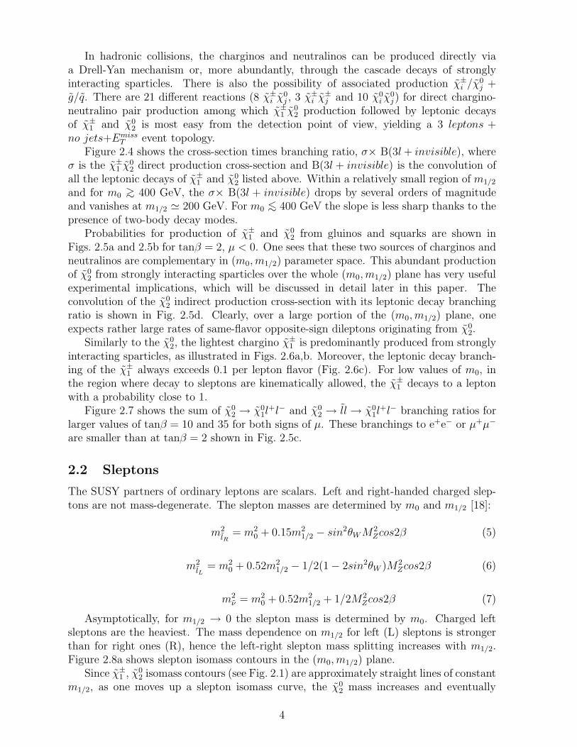
Figure 2.7 shows the sum of χ02 → χ0

1l+l− and χ0

2 → ll → χ01l

+l− branching ratios forlarger values of tanβ = 10 and 35 for both signs of µ. These branchings to e+e− or µ+µ−

are smaller than at tanβ = 2 shown in Fig. 2.5c.

2.2 Sleptons

The SUSY partners of ordinary leptons are scalars. Left and right-handed charged slep-tons are not mass-degenerate. The slepton masses are determined by m0 and m1/2 [18]:

m2

lR= m2

0 + 0.15m2

1/2 − sin2θW M2

Zcos2β (5)

m2

lL= m2

0 + 0.52m2

1/2 − 1/2(1 − 2sin2θW )M2

Zcos2β (6)

m2

ν = m2

0 + 0.52m2

1/2 + 1/2M2

Zcos2β (7)

Asymptotically, for m1/2 → 0 the slepton mass is determined by m0. Charged leftsleptons are the heaviest. The mass dependence on m1/2 for left (L) sleptons is strongerthan for right ones (R), hence the left-right slepton mass splitting increases with m1/2.Figure 2.8a shows slepton isomass contours in the (m0, m1/2) plane.

Since χ±1 , χ0

2 isomass contours (see Fig. 2.1) are approximately straight lines of constantm1/2, as one moves up a slepton isomass curve, the χ0

2 mass increases and eventually

4

becomes higher than that of the slepton. Thus we may identify two domains in the(m0, m1/2) parameter plane: one is where left sleptons are more massive than χ±

1 , χ02

(m0>∼ 0.45 · m1/2, domain I), and the other, where they are lighter (m0

<∼ 0.45 · m1/2,domain II). These mass relations, shown Fig. 2.8b are responsible for distinct contributionsto slepton production and decay mechanisms. In domain I sleptons can be producedonly through a Drell-Yan mechanism (direct slepton production), via qq annihilationwith neutral or charged gauge boson exchange in the s-channel. Pairs with the same“handedness” can be produced, namely, lL lL, lR lR, νν, νl lL. In this part of parameterspace both direct and cascade decays of sleptons to LSP are possible:

i) the left sleptons can decay to charginos and neutralinos via the following decays:

l±L → l± + χ01,2

l±L → νl + χ±1

νl → νl + χ01,2

νl → l± + χ∓1

ii) for right sleptons, only decays to neutralinos are possible; they dominantly decaydirectly to the LSP:

l−R → l− + χ01

If decays to the second neutralino or lightest chargino are kinematically allowed, thedecay to the LSP can proceed through several decay paths (cascade decays) with missingenergy and/or isolated leptons in final state:

χ02 → χ0

1 + l+l−

χ02 → χ0

1 + νν

χ02 → χ0

1 + Z0

χ±1 → χ0

1 + l± + ν

χ±1 → χ0

1 + W±

In domain II indirect slepton production, from directly or indirectly produced

charginos/neutralinos is also possible:

χ02 → l±L,Rl∓

χ02 → νlνl

χ±1 → νll

±

χ±1 → l±L νl

When allowed, indirect l production arising from decays of strongly produced g, q to χ02

or χ±1 , is the predominant production mode. With increasing m1/2 along a slepton isomass

curve, the fraction of direct decays into the LSP increases as the mass difference betweensleptons and charginos-neutralinos decreases, until in domain II sleptons can only directlydecay to the LSP. Sneutrinos in this domain thus decay totally invisibly, i.e. no component(ν, χ0

1) from sneutrino decay can be directly detected. The slepton production and decayfeatures described above give rise to several characteristic experimental signatures:

• two leptons+EmissT +no jets event topology arises from direct charged slepton pair

lLlL, lR lR production, followed by direct decays to the LSP. The same signature is

5

found in νν production when one of the sneutrinos decays invisibly and the otherhas a cascade decay with two leptons in final state. This signature can also befound when sleptons are produced among decay products of directly or indirectlyproduced charginos-neutralinos. In the case of indirectly produced sleptons thereare the following differences compared with direct production: i) single productionis also possible, for example in χ±

1 χ02 production followed by decay of the χ0

2 to aslepton; ii) a νl lL pair can be produced from direct χ±

1 χ∓1 ; iii) left handed sleptons

production is favored;

• three leptons + EmissT + no jets final states are expected only from νl lL production

followed by cascade decays to LSP;

• four leptons + EmissT + no jets comes from lL lL, νν, νl lL production followed by

cascade decays to LSP.

The last two topologies can also be found when sleptons are produced in the decayof directly produced charginos-neutralinos.

• Indirect slepton production from gluinos and squarks through charginos, neutrali-nos (domain II), leads to a two (or more) leptons + Emiss

T + jets signature. Thisproduction has the largest cross-section because of the strongly interacting g and q,and again sleptons can be singly produced.

The largest contribution to the two leptons with no jets final state in charged sleptonpair production comes from their direct decays to the LSP, lL → l χ0

1. However, withdecreasing m1/2 along an isomass curve the fraction of slepton direct decays to LSP

decreases as shown in Fig. 2.9a. Figure 2.9b The σ(lLlL)×B(2l + invisible) for directlyproduced left sleptons and Fig. 2.9c shows the same for right sleptons: σ(lRlR)×B(2l +invisible). As right sleptons decay directly into LSP’s the cross-section times branchingratio is constant along an isomass curve. One can see that the topological cross-sectionσ(lR lR)×B(2l + invisible) is larger than σ(lL lL)×B(2l + invisible) in almost the entire(m0, m1/2) plane.

For sneutrino pair production, the main contribution to the 2 leptons and no jetstopology comes from one sneutrino decaying directly to the LSP and the second to χ±

1

or χ02 followed by their leptonic decays. The sneutrino decay branching ratios are shown

in Figs. 2.10a-c. The σ(νν)×B(2l + invisible), shown in Fig. 2.10d, is limited along them1/2 axis by the χ±

1 , χ02 leptonic decay branching ratios (see Figs. 2.1 and 2.2), and along

the m0 axis by the sneutrino production cross-section.Figure 2.11 shows the total cross-section times branching ratio for two lepton+Emiss

T +no jets event topology arising from all possible combinations of directly produced sleptonpairs, lLlL, lRlR, νν. It drops rapidly with increasing m0 and m1/2, from a maximumvalue of the order of a few pb down to a few fb for m0 ∼ m1/2 ∼ 500 GeV. In almost theentire (m0, m1/2) parameter plane slepton pair production is dominated by right sleptons.

To illustrate the additional contribution from χ±1 χ∓

1 direct production and the poten-tial contribution from χ±

1 χ02 to the two same-flavor opposite-sign leptons+ Emiss

T + nojets event topology, we show σ(χ±

1 χ∓1 )×B(χ±

1 χ∓1 → l+l− + invisible), σ(χ±

1 χ02)×B(χ0

2 →l±L + l∓) and σ(χ±

1 χ02)×B(χ0

2 → l±R + l∓) in Figs. 2.12a, b and c, respectively. One can seethat the contribution from electroweak indirectly produced sleptons is not negligible, andin some areas of the (m0, m1/2) parameters space is even higher than for direct production.

6

Indirect slepton production from strongly produced g, q is larger still, when allowed, butis (almost) always accompanied by jets in the final state, so will not contribute unless thejets somehow escape detection.

2.3 Gluinos and squarks

In mSUGRA the gluino mass is determined mainly by m1/2 [18]:

Mg ≈ 2.5m1/2 (8)

The five squark flavors (d, u, s, c, b) with their left and right chiral states are assumedto be mass degenerate, giving altogether ten degenerate squark flavors with:

Mq ≈√

m20 + 6m2

1/2(9)

The tL and tR are however treated differently. Through their mixing they give rise to twomass eigenstates t1 and t2 with t1 most often significantly lighter than all other q states,which requires a separate discussion in terms of both, production and decay. Mixingalso introduces a small non-degeneracy among the b1 and b2 states, but this is usuallyneglected compared to behavior of the stop system.

At LHC energies, the total SUSY particle production cross-section is dominated bystrongly interacting gluinos and squarks, which through their cascade decays, (Figs. 2.13and 2.14) can produce many jets and leptons, with missing energy due to at least 2 escap-ing LSPs and possibly neutrinos. Figure 2.15 shows the total squark/gluino productioncross-section contours versus m0 and m1/2. Figure 2.16 shows the (m0,m1/2) parameterspace subdivided into several domains corresponding to the characteristic kinematic con-figurations of gluino and squark events and the predominant sources of lepton production.Isomass contours for squarks, gluinos, light and pseudoscalar Higgses are also shown inFig. 2.16 for tanβ = 2, A0 = 0, µ < 0, with h masses calculated at the two-loop radiativecorrection level.

The first domain is characterised by mg > mq and mχ02> ml. This means that gluinos

decay to quark-squark pairs but the contribution from gluino production to the totalsquark/gluino cross-section is small compared to the squarks. Both the χ0

2 and χ±1 in this

domain decay via sleptons (see Figs. 2.2 and 2.3) giving rise to a significant number ofleptons in the final state. This region extends to higher values of m0 at fixed m1/2 thanjust two-body decays of χ0

2 and χ±1 to sleptons, since the three-body decays (e.g. χ0

2 →χ0

1 l+l−) still remain even when two-body modes χ02 → χ0

1h and χ±1 → χ0

1W± are open.

In the second domain of the (m0,m1/2) plane, the gluino mass is still somewhat largerthan the squark masses, so that gluinos still decay into quark-squark pairs. The yield ofstop-top final states is however higher than in the first domain since the contribution of thegg process in the total g/q production cross-section is larger and the g → tt branchingratio is also higher. This results in an increase of the jet multiplicity and in a higherfraction of b-jets in the final state. The χ0

2 and χ±1 are now lighter than the sleptons, and

they decay to LSP + h/W±, respectively, which means a reduced yield of isolated leptonswhen compared to the first domain.

In the third characteristic region of the (m0,m1/2) plane, the gluino mass is smaller

than the mass of squarks, except for t1 and bL, and hence the stop-top final state dominatesin overall production. The cross section for qq is significantly smaller than that for gg.

7

All this gives rise to a significant jet multiplicity in the event and some increase of theyield of isolated leptons, as a result of t → Wb → lνb decays, and an enrichment in thefraction of b-jets. Compared with the previous domain, nothing changes from the pointof view of the χ0

2 and χ±1 decays.

The fourth domain is characterised by very massive squarks compared to gluinos, thusgg production dominates and the gluino decays predominantly via three-body final states(mainly LSP + tt). This increases further the jet (and b-jet) multiplicity of the event.Again the decays of the χ0

2 and χ±1 are the same as in domains 2 and 3.

There is a fifth domain which has approximately the shape of a band along the m0

axis, under domains 2-4, for m1/2 ≤ 180 - 190 GeV. In this region the masses of χ±1 and

χ02 are smaller than χ0

1 + W and χ01 + h, respectively, and smaller than the slepton and

sneutrino masses, thus 3-body decays of χ02 (→ χ0

1q˜q/χ01l

+l−) and χ±1 (→ χ0

1q˜q′/χ0

1l±ν)

take place. However, the yield of leptons does not differ significantly from that of domain1.

8

χ0 (350)

1~

χ 0 (400)3

~

χ 0 (700)

3~

χ 0 (1100)

3~

χ 0 (1500)

3~

χ± ,χ0

(750)1 2

~ ~

χ± ,χ0

(600)1 2

~ ~

χ± ,χ0

(400)1 2

~ ~

χ± ,χ0

(200)1 2

~ ~

χ ± ,χ 0

(550)2

4

~~

χ ± ,χ 0

(850)2

4

~~

χ ± ,χ 0

(1250)

2 4

~~

χ ± ,χ 0

(1650)

24

~~

χ0 (250)1

~

χ0 (150)

1~

χ0 (50)1

~

200 400 600 800 1000

1000

900

800

700

600

500

400

300

200

100

1200 1400 1600 1800 2000

m0 GeV

200 400 600 800 1000 1200 1400 1600 1800 2000

m0 GeV

m1/

2GeV

1000

900

800

700

600

500

400

300

200

100

m1/

2GeV

D_D

_101

8n

mSUGRA parameters: tan β= 2, A0= 0, µ < 0

Figure 2.1: Isomass contours for: a) light (χ±1 , χ0

1, χ02) and b) heavy (χ±

2 , χ03, χ0

4)charginos/neutralinos.

9

mSUGRA parameters: tanβ = 2, A0 = 0, µ < 0

500

1000

1500

2000

200

400

600

800

1000

10-1

1

m 0 (

GeV)m1/2 (GeV)

B(χ~

± 1→ χ~

0 1 l ν

)

a)

500

1000

1500

2000

200

400

600

800

1000

10-1

1

m 0 (

GeV)m1/2 (GeV)

B(χ~

± 1 →

l~ L ν

→ χ~

0 1 l ν

)

b)

500

1000

1500

2000

200

400

600

800

1000

10-1

1

m 0 (

GeV)m1/2 (GeV)

B(χ~

± 1 →

ν~

L l→

χ~0 1

l ν)

c)

500

1000

1500

2000

200

400

600

800

1000

10-1

1

m 0 (

GeV)m1/2 (GeV)

B(χ~

± 1 →

χ~0 1

W± →

χ~0 1

l ν)

d)

Figure 2.2: Chargino decay branching ratio versus (m0, m1/2): a) χ±1 →χ0

1 l± ν, b) χ±1

→ l±L ν → χ01 l± ν, c) χ±

1 → l±R ν → χ01 l± ν and d) χ±

1 → χ01 W± → χ0

1 l± ν.

10


500

1000

1500

2000

200

400

600

800

1000

10-1

1

m 0 (

GeV)m1/2 (GeV)

B(χ~

0 2→ χ~

0 1 l l

)

a)

500

1000

1500

2000

200

400

600

800

1000

10-1

1

m 0 (

GeV)m1/2 (GeV)

B(χ~

0 2→ l~ L

l→ χ~

0 1 l l

)

b)

500

1000

1500

2000

200

400

600

800

1000

10-1

1

m 0 (

GeV)m1/2 (GeV)

B(χ~

0 2→ l~ R

l→ χ~

0 1 l l

)

c)

Figure 2.3: Neutralino decay branching ratio versus (m0, m1/2): a) χ02 → χ0

1 l+ l−, b) χ02

→ l±L l∓ → χ01 l+ l− and c) χ0

2 → l±R l∓ → χ01 l+ l−.

11


200400

600800

10001200

14001600

18002000

100200

300400

500600

700800

9001000

10-3

10-2

10-1

1

10

m 0 (

GeV)m1/2 (GeV)

σB (

χ~± 1

χ~0 2

→ 3

l + in

v.)

, pb

Figure 2.4: Cross-section times branching ratio versus (m0, m1/2) for χ±1 χ0

2 direct produc-tion followed by leptonic decays.

12


500

1000

1500

2000

200

400

600

800

1000

10-1

1

B(g~

→ χ~

0 2 +

x)

a)

500

1000

1500

2000

200

400

600

800

1000

10-1

1

B(u~

L →

χ~0 2

+ x

)

b)

500

1000

1500

2000

200

400

600

800

1000

10-1

1

B(χ~

0 2 →

l+l- +

inv.

)

c)

500

1000

1500

2000

200

400

600

800

1000

10-2

10-1

1

10

10 2

10 3

σ•B

(χ~0 2

→ l+

l- + in

v.),

pb

d)

Figure 2.5: χ02 inclusive production and decay: a) branching ratio B(g → χ0

2+ x),b) B(uL → χ0

2+ x), c) B(χ02 → l+l− + invisible) and d) χ0

2 inclusive productioncross-section times branching ratio into l+l−.

13


500

1000

1500

2000

200

400

600

800

1000

10-1

1

B(g~

→ χ~

± 1 +

x)

a)

500

1000

1500

2000

200

400

600

800

1000

10-1

1

B(u~

L →

χ~± 1

+ x

)

b)

500

1000

1500

2000

200

400

600

800

1000

10-1

1

B(χ~

± 1 →

l± + in

v.)

c)

500

1000

1500

2000

200

400

600

800

1000

10-1

1

10

10 2

10 3

σ•B

(χ~± 1

→ l± +

inv.

), p

b

d)

Figure 2.6: χ±1 inclusive production and decay: a) branching ratio B(g → χ±

1 + x),b) B(uL → χ±

1 + x), c) B(χ±1 → l± + invisible) and d) χ±

1 inclusive productioncross-section times branching ratio into l±.

14

Br ( χ χ20

10

L,R

~ ~l l l l;

~ )

Figure 2.7: The sum of χ02 → χ0

1l+l− and χ0

2 → ll → χ01l

+l− branching ratios forvarious values of tanβ = 10 and 35 for both signs of µ.

15

m0

1/2

, GeV m0

, GeV

m0

, GeV

m, G

eV

1/2

m, G

eV

1/2

m, G

eV

Left charged sleptons Right charged sleptons

Sneutrinos

100

150

200

250

300

350

400

450 GeV

Slepton isomass contours:

400

450 G

eV

350

300250200150

100

100

150

200

250

300

350

400

450 GeV

( ν )∼

( l )~

L( l )

~R

+ +

Figure 2.8a: Isomass contours for a) left charged sleptons, b) right charged sleptonsand c) sneutrinos in mSUGRA parameter space (m0, m1/2) for tanβ = 2, A0 = 0, µ < 0.

16

TH

m0 GeV,

m

,

GeV

1/2

1

2

3

4

5

6

7

dom

ain

II

domain I

Figure 2.8b: Slepton isomass contours for mlL= mlR

= mχ02=150 GeV corresponding

to lines 1-3 respectively and mlL= mlR

= mχ02=400 GeV, lines 4-6 respectively. Line

7 separates domains I and II of (m0, m1/2) parameter space; in domain II charginos,neutralinos can decay to left sleptons.

17

Br(

l ~ L →

lsp+

l )

σ*

Br(

l~ Ll~ L

→ 2

l+in

v)

σ*

Br(

l~ Rl~ R

→ 2

l+in

v)

a)

b) c)

Figure 2.9: a) Branching ratio of lL → χ01 + l; b) cross-section times branching ratio

for 2 leptons + EmissT + no jets events from direct left slepton pair production; c) cross-

section times branching ratio for 2 leptons + EmissT + no jets events from direct right

slepton pair production.

18

Br(

ν∼ →

lsp+

ν)

Br(

ν∼ →

χ∼0 +

ν)

Br(

ν∼ →

χ∼±+

l–)

σ*

Br(

ν∼ν∼

→ 2

l+in

v)

a) b)

c) d)

Figure 2.10: Decay branching ratios of sneutrinos: a) ν → χ01 + ν, b) ν → χ0

2 + ν andc) ν → χ±

1 + l∓ as a function of (m0, m1/2); d) cross-section times branching ration for2 leptons + Emiss

T + no jets events topology from sneutrino pair production.

19

σ*B

r(l~ l~ →

2l+

inv),pb

Figure 2.11: Total cross-section times branching ratio for 2 leptons + EmissT events

arising from all possible combinations of directly produced slepton pairs, namely lLlL,lR lR and νν.

20

σ*B

r(χ~

1χ~

1 →

2l +

inv)

σ(χ~

1χ~

2)*

Br(

χ~

2 →

l~ L +

l )

σ(χ~

1χ~

2)*

Br(

χ~

2 →

l~

R +

l )

,pb

,pb

,pb

a)

b) c)

Figure 2.12: Cross-section times branching ratio for a) χ±1 χ±

1 direct production fol-lowed by leptonic decays of at least one of the charginos; b) single sleptons productionfrom directly produced χ±

1 χ02 with χ0

2 decays to left sleptons χ02 → lLl (b); c)single sleptons

production from directly produced χ±1 χ0

2 with χ02 decays to right sleptons χ0

2 → lRl (c).

21

g~g~

~ q~ b q

~ q q~ q q

~

~ ~

~

~

~ ~

~ ~

~~~ ~ ~

~

b q ~~qrb~b

: 1000 GeV

: 950 GeV: 950 GeV

: 950 GeV: 950 GeV

11

r

r r

χ0qχ±q χ±

χ0

2χ0q

2

χ0qχ0q

χ0h0 χ0h0

χ0Z0χ0W± χ0W±2

χ0

χ±q: 312 GeV

: 312 GeV

: 155 GeV

0

200

100% 10% 1%

400

600

800

1000

39 25 9.8 6.1 2.9 2.0

Branching ratios

D-D

-834

n

Mas

s of

SU

SY

-par

ticle

s (G

eV)

masses:

1

1

111

11

1

1 1

1

Figure 2.13: Typical decay modes for the massive (1 TeV) gluino illustrating thevariety of possible cascade decays.

100 % 10 % 1%

Branching ratio Branching ratio

masses:

qr:950 GeVqr~

:155GeVχ0

1∼

χ01

∼q

900

800

700

600

500

400

300

200

100

0

Mas

s of

SU

SY

- pa

rtic

les

/GeV

Decay modes of q~

100 % 10 % 1%

masses:

:950 GeVqq~

:155GeV

:312GeV

:510GeV

χ±

χ01

∼

χ02

∼

q q

χ01

1

∼ qχ01

∼Z0χ01

∼χ01

∼

χ02

∼∼χ±:312GeV1∼

χ±q2∼

χ±2

∼

W±

900

800

700

600

500

400

300

200

100

0

Mas

s of

SU

SY

- pa

rtic

les

/GeV

65 27 4.9 1.4

h0

D_D_835n

Figure 2.14: Typical decay modes of the massive (0.95 TeV) squark.

22

0

100

200

300

400

500

600

700

800

0 200 400 600 800 1000 1200 1400

A0 = 0 , tanβ = 2 , µ < 0

m0 (GeV)

m1/

2 (

GeV

)

1000 pb

100 pb

10 pb

1 pb

0.1 pb

Figure 2.15 Gluino/squark production cross-section versus (m0, m1/2).

23

0

200

400

600

800

1000

1200

0 200 400 600 800 1000 1200 1400 1600 1800 2000

m1/2 , GeV

m0 , GeV

χ ~ ±

1 → l~ ± ν

→ ν ~

l ±

χ ~0

2 → l ~ ± l ±

①

χ ~ ±

1 → χ ~0

1 W±

χ ~0

2 → χ ~0

1 h

②

g~ → t

~

1 t

mg~ < mq

~

③

g~ → χ

~01 t t

–

④

①

②

③

④

g~(500)

g~(1000)

g~(1500)

g~(2000)

g~(2500)

q ~(2500)q~

(2000)

q ~(1500)

q ~(1000)

q ~(500)

h(80)

h(85)

h(90)

h(95)

A(500)

A(1000)

A(1500)

A(2000)

A0 = 0 , tanβ = 2 , µ < 0

Figure 2.16: Domains of the (m0, m1/2) parameter space with charachteristic predom-inant decay modes. Isomass contours for squarks, gluinos, light and pseudoscalar higgsesare also shown. The shaded region near the m1/2 axis shows the theoretically forbiddenregion of parameter space, and a similar region along the m0 axis corresponds to both,theoretically and experimentally excluded portions of parameter space.

24

0

500

1000

1500

250

500

7500

0.20.40.60.8

µ < 0

m 0 (G

eV)m

1/2 (GeV)

tan β = 2

0

500

1000

1500

250

500

7500

0.20.40.60.8

µ > 0

m 0 (G

eV)m

1/2 (GeV)

0

500

1000

1500

250

500

7500

0.20.40.6

m 0 (G

eV)m

1/2 (GeV)

tan β = 10

0

500

1000

1500

250

500

7500

0.20.40.60.8

m 0 (G

eV)m

1/2 (GeV)

0

500

1000

1500

250

500

7500

0.20.40.60.8

m 0 (G

eV)m

1/2 (GeV)

tan β = 30

0

500

1000

1500

250

500

7500

0.20.40.60.8

m 0 (G

eV)m

1/2 (GeV)

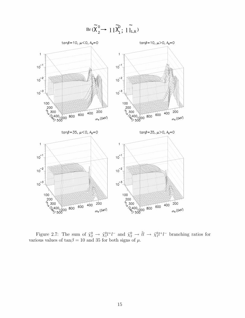
Figure 2.17: χ02 → χ0

1h branching ratio versus (m0, m1/2) for fixed A0 = 0 and differentvalues of tanβ and µ.

25

3 Experimental signatures considered

As discribed earlier, the highest cross-section for high mass R-parity conserving SUSYat hadron colliders is due to squarks and/or gluinos which decay through a number ofsteps to quarks, gluons, charginos, neutralinos, sleptons, W, Z, Higgses and ultimatelya stable LSP (lightest neutralino in mSUGRA), which is weakly interacting and escapesdetection. The final state has missing energy (2 LSP’s + neutrinos), a number of jets,and a variable number of leptons, depending on the decay chain. Due to the escapingLSP’s, which appear at the end of each sparticle decay chain, the masses of sparticlescan not generally be reconstructed explicitely. However, the sparticle production anddecay characteristics, discussed in the previous section, lead to a number of specific eventtopologies, which should allow the discovery of SUSY in general, and specifically theseparation of certain SUSY sparticles and processes from SM and other SUSY processes.The LHC must therefore not only be able to discover SUSY, if it is realized at electroweakscale, and if it has not yet been discovered at the Tevatron (which covers a very promisingenergy/mass range), but the LHC experiments sholud also be able to disantagle thevarious SUSY production mechanisms and reconstruct most of the sparticle spectrum,determine or limit the models/scenarios, constrain model parameters, etc. Our presentunderstanding shows that all this is possible at the LHC, but a lot of methodical studiesare still required. Usually, one characterizes the general SUSY signal significance by anexcess over the expected SM event rates, while for specific SUSY processes the backgroundincludes besides SM processes other SUSY reactions contributing to the same final statetopology.

The following final states have been investigated in substantial detail in CMS:1) leptons + jets + Emiss

T final states with a variable number of leptons and jetsand possible requirements on b-jets. These channels provide the maximum mass andparameter reach of SUSY through the production of strongly interacting particles, whichin their cascade decays can give rise to many leptons and jets.

2) inclusive 2 leptons + EmissT + (jets) and 3 leptons + (Emiss

T ) final states. In thesechannels SUSY reveals itself through χ0

2 inclusive production with subsequent decay –directly or via a slepton – into two leptons and χ0

1. For some regions of parameter space,the two lepton invariant mass with its characteristic shape, a sharp edge at the end pointof the spectrum, allows the determination of the sparticle masses, including the sleptonmass, and model parameters. These channels could well be the first indication/signaturefor SUSY production at the LHC.

3) exclusive 2 leptons + no jets + EmissT final state, which is enriched in direct

(Drell-Yan) slepton pair production as discussed in section 2.2. The main issue here isto understand and keep under control both the SM background (with many processes tobe considered) and internal SUSY backgrounds. This channel could allow discovery andstudy of slepton production.

4) exclusive 3 leptons + no jets + EmissT final state, which is the signature for direct

χ±1 χ0

2 production in a Drell-Yan process. It is therefore theoretically most reliable (alongwith slepton production). For this and the slepton study, to suppress the SM and internalSUSY backgrounds a good response to jets down to Ejet

T ∼ 30 GeV, with a calorimetriccoverage up to |η| ∼ 4.5, is required. This exclusive channel could also play a central rolein a precise determination of the χ0

1 – the SUSY dark matter candidate.For the present study, production of SUSY processes has been simulated using the

26

ISAJET 7.14 Monte Carlo event generator [17] and the SM backgrounds by PYTHIA5.7 [19], both with the CTEQ2L structure functions [20]. Before presenting the physicsexpectations, we discuss the CMS detector optimisation studies done specifically withSUSY searches in mind.

4 Detector issues

4.1 CMS detector optimisation for SUSY studies

The design goals of CMS are to measure muons, electrons and photons with a resolutionof <∼ 1% over a large momentum range (≤100 GeV), to measure jets with a resolutionof 10% at ET = 100 GeV and to be highly hermetic, with a missing ET performance asrequired for SUSY searches. The central element of CMS is a 13 m long, 6 m diametersolenoid generating a uniform magnetic field of 4 T [21, 22], Fig. 4.1. The magnetic fluxis returned through a 1.8 m thick saturated iron yoke instrumented with muon chambers.Muons are precisely measured in the inner tracker and are identified and measured infour muon stations inserted in the return yoke. Precision tracking in the muon stationsis carried out with drift tube planes in the barrel and with cathode strip chambers inthe endcaps [23]. The goal is to achieve a spatial resolution of ∼100 µm and an angularaccuracy on a local muon track segment of ∼1 mrad per station. Excellent time resolutionis needed to identify the bunch crossing (with a periodicity of 25 nsec). Muon stationstherefore also include resistive plate chamber triggering planes with time resolution ∼2nsec [23].

The inner tracking system of CMS is designed to reconstruct high-pT muons, isolatedelectrons and hadrons over |η| < 2.5 with a momentum resolution of ∆pT /pT ≃ 0.15pT ⊕0.5% (pT in TeV). Silicon and gas microstrip detectors are used to provide the requiredprecision and granularity. In the present design there are about 9×106 MSGC detectorchannels, about 4×106 Si microstrip channels and about 8×107 Si pixel channels [24].For high momentum muons the combination of tracker and muon chamber measurementsgreatly improves the resolution: ∆pT /pT ≃ 0.06 for a p ≃ 1 TeV muon in |η| < 1.6 [21].

The calorimeter system of CMS is made of a high resolution lead-tungstate (PbWO4)crystal electromagnetic calorimeter and a copper-scintillator hadron calorimeter behindit. The primary function of the electromagnetic calorimeter is to precisely measure elec-trons and photons, and in conjunction with the hadron calorimeter to measure also jets.The arrangement of crystals is shown in Fig. 4.1. In the barrel the crystals are 25 ra-diation lengths (X0) deep and the lateral granularity is ≃ 2 cm × 2 cm correspondingto ∆η × ∆φ = 0.014 × 0.014. They are read out with Si avalanche photodiodes [25].The electromagnetic calorimetry extends over |η| < 3. The total number of crystals is∼ 1.1 × 105. With a prototype PbWO4 calorimeter in a test beam, an energy resolutionof σE/E ≃ 0.6% has been obtained for electrons of E = 120 GeV [26]. Hadron calorime-try with large geometrical coverage for measurement of multi-jet final states and missingtransverse energy (Emiss

T ) is essential in all sparticle searches, as it is the EmissT which

provides evidence for the escaping LSP’s (lightest neutralinos). The hadron calorimeterof CMS is made of copper absorber plates interleaved with scintillator tiles read out withembedded wavelength shifting fibers [27]. The readout in the 4 Tesla field is done withhybrid photodetectors [28]. The tiles are organized in towers (Fig. 4.1) giving a lateral

27

segmentation of ∆η×∆φ ≃ 0.09×0.09. The hadronic resolution obtained in a test beamis σE/E ≃ 100%/

√E ⊕ 5% for the combined PbWO4 and hadronic calorimeter system

[29]. This central hadron calorimetry extends up to |η| = 3.0. It is complemented inthe forward region 3.0 < |η| < 5.0 by quartz-fiber “very forward calorimeters” (Fig. 4.1)[27, 30]. Their function is to ensure detector hermeticity for good missing transverseenergy resolution, and to extend the forward jet detection and jet vetoing capability ofCMS which is essential in slepton, chargino, neutralino searches as discussed in the fol-lowing. Detector hermeticity is particularly important for processes where the physical(real) missing ET is on the order of few tens of GeV as is the case in h, H, A → ττ , W→ lν, t → lνb, t → H±b → τνb, etc. and in particular in slepton, chargino and neutralinosearches connecting the LEP2/Fermilab and the LHC search ranges.

4.2 HCAL optimisation and tail catcher

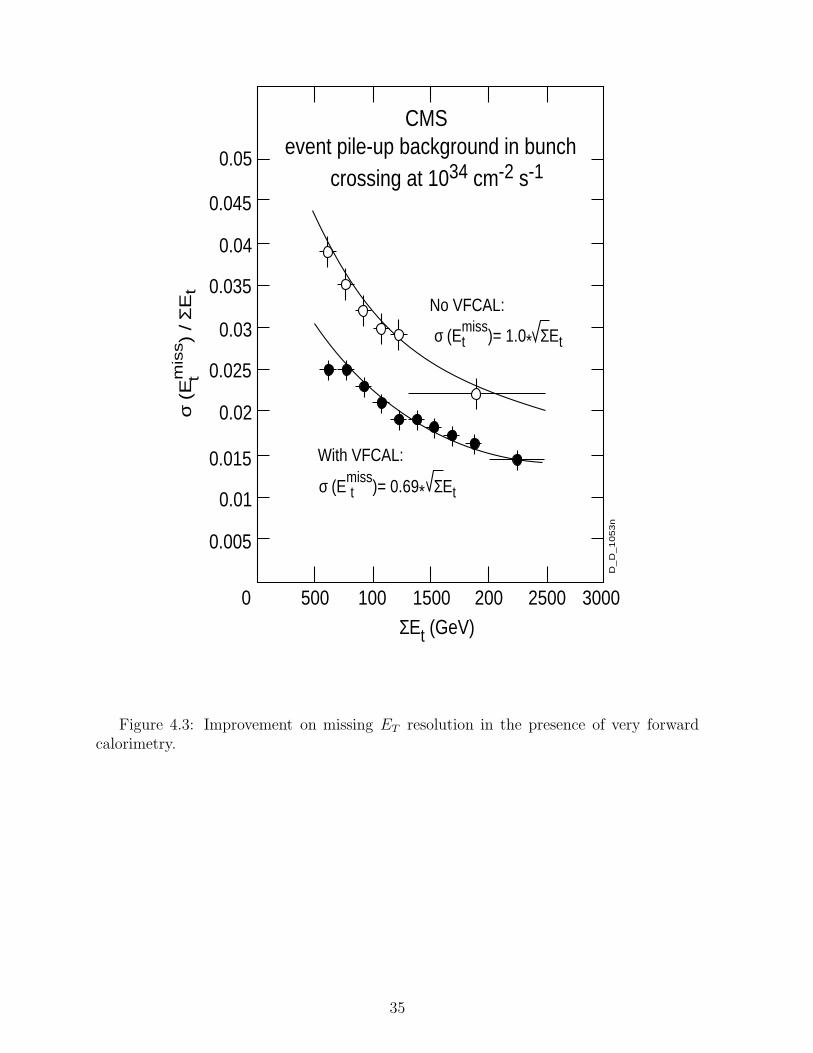
A number of steps have been undertaken in the design of CMS to optimise its EmissT

response in view of SUSY searches. These include the inclusion of very forward calorime-try, the addition of a tail catcher behind the coil [31] and optimisation of the crack forthe passage of services between the barrel and endcap calorimeters. We now briefly dis-cuss these issues. The central (|η| <3.0) calorimetry of CMS is complemented by veryforward quartz-fiber calorimeters [30] covering the rapidity range 3 < |η| < 5, Fig. 4.1.Figure 4.2 illustrates the effect of the forward energy flow containment and its effect onmissing ET measurements. It shows the expected instrumental (fake) missing ET distri-butions for QCD di-jet events as a function of calorimetric coverage at large rapidities.Calorimetry extending up to |η| ≃ 5 reduces the fake (instrumental) Emiss

T by an or-der of magnitude in the 20 - 120 GeV range. Furthermore, the missing ET resolution,σ(Emiss

T )/ΣET where ΣET is the calorimetric transverse energy sum, is also much reducedin the presence of very forward calorimetry, see Fig. 4.3. There is a second requirement onforward calorimetry which turns out to be essential if we hope to eventually extract slep-ton and chargino/neutralino signals. In the search for direct DY slepton pair productionll → l+l−χ0

1χ01, or for the associated direct (DY) chargino/neutralino χ±

1 χ02→ l±νχ0

1l+l−χ0

1

production, leading to final states with two or three isolated leptons, no jets, and missingET , it is essential to have the capability to recognise and veto on forward jets. This isneeded to suppress the large backgrounds due to tt, qq, gq, gg and the associated pro-duction modes qχ, gχ which would otherwise overwhelm the signals. The extension intothe forward direction of the central jet vetoing capability provides the needed additionalrejection factors to keep these backgrounds under control.

Figure 4.4a shows for the case of direct χ±1 χ0

2 production, (discussed in more detail insection 8), the expected rejection factors against the main backgrounds as a function of therapidity range and detection threshold over which the jets can be recognized. Figure 4.4bshows the rejection factors against internal SUSY and the SM tt backgrounds. Here the jetveto is applied after lepton isolation and an Emiss

T cut, thus the value of the rejection factoris much reduced. In both cases, the jet coverage needed to obtain sufficient backgroundrejection is |η| up to ≃ 4 and the loss of signal acceptance due to the jet veto is typically∼10%.

The locations of the tail-catcher scintillator layers, two in the barrel region behind thecoil and one in the endcap, are shown on the longitudinal cut through the CMS detectorin Fig. 4.1. Figure 4.5 shows the depth in interaction lengths λ of calorimetry in CMS,

28

and the total sampled depth including the tail catcher layers, as a function of rapidity [32].Whilst the total calorimetric absorber thickness within the coil is somewhat marginal atrapidity η ∼ 0 for full hadronic shower containment, inclusion of tail-catcher layers allowshadron energy measurements with at least 10.5 interaction lengths everywhere.

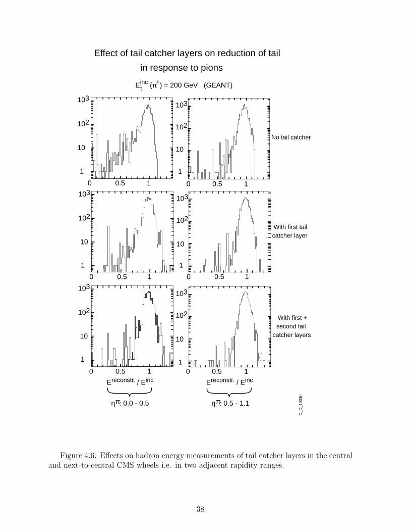
Figure 4.6 shows the effects on hadron energy measurements of the inclusion of thetail-catcher layers, specifically on the reduction of the low-energy tail in the response to(200 GeV) hadrons [33]. What is shown is the ratio of the (GEANT) simulated response tothe incident energy for single pions in the rapidity range 0.33 to 0.86 with no tail catcher,with one, and with two tail catcher layers included in the readout. Mismeasurementsof hadronic energies, and in particular the presence of low-energy tails in hadronic (jet)energy measurements is one of the main sources of fake instrumental missing ET . Whendue to insufficient shower containment in depth, inclusion of the tail-catcher layers curesthis problem to a large extent.

There are two other sources of hadronic mismeasurements and low-energy tails: deadareas and volumes due to detector cracks and matching the hadronic response of ECALto HCAL.

Special attention has been paid in CMS to the effects on hadronic energy measurements– and thus on missing ET – of the main crack for services between the barrel and endcapcalorimetry at rapidity ∼ 1.2 - 1.5 (Fig. 4.1). The various configurations which have beenstudied for this crack are shown in Fig. 4.7 [13]. The aim was to minimize the degradationof the hadronic energy resolution and the level of the low energy tail for hadrons andjets straddling the region of the gap. The optimal choice, from the point of view ofhadron response, weight of the cantilevered endcap hadron calorimeter, manoeuvrabilityof endcaps and margin of freedom to close the detector, is a conical endcap shape witha non-pointing crack at 52 degrees from the beam line labeled TP7 in Fig. 4.7. Figure4.8 shows the reconstructed energy response (GEANT) to single pions of 100 GeV whenincident on and off the crack region, for three crack widths of 11, 18 and 25cm. Withthe present estimate of the volume of services a gap of 12 cm is needed, plus 2 cm forclearance.

An essential ingredient to obtain optimal EmissT response of a detector is the linearity

of its response as a function of incident hadron (jet) energy. The non-compensatingmixed calorimeter of CMS – with a PbWO4 crystal ECAL compartment followed by aCu/scintillator sampling HCAL – has significantly different electromagnetic to hadronic(e/h) responses in the two parts, e/h ∼ 1.8 in the ECAL vs. 1.2 in the HCAL. Linearity ismore difficult to achieve in such a mixed calorimeter than in a more homogeneous system.To restore linearity as much as possible, and to compensate for the effects of dead materialin the space between the ECAL and HCAL, weighting techniques for responses must beused between ECAL and HCAL, and within HCAL compartments and tail catcher layers.An essential limiting factor is the number of readout channels we can afford for thelongitudinal HCAL tower segmentation. The optimal set of weighting factors must bedetermined on basis of test beam data and detailed simulations of responses to hadronsand jets, taking into account financial limitations. In the present HCAL design [27]a good compromise between expected performance and cost is found by having a veryshallow (1 scintillator plane) front HCAL tower readout and second deep (≃ 5 λ) HCALsegment readout. The first shallow HCAL segment just behind the ECAL detects hadroninteractions in the ECAL – where their energy deposition is underestimated (e/h ∼ 2) –and compensates by overweighting this layer. Present investigations show that with this

29

technique the expected non-linearity should not exceed 4% for pions between 20 and 300GeV [27].

4.3 The role of the tracker in SUSY searches

The inner tracking system of CMS is primarily designed to reconstruct high-pT muons,isolated electrons and hadrons over |η| < 2.5 with a momentum resolution of ∆pT /pT ∼0.15pT ⊕0.5% (pT in TeV). Hadrons must be reconstructed down to ∼ 1 - 2 GeV, as leptonand photon isolation is a very important selection criterion for a number of physics signals,and in particular in the SUSY searches for sleptons, charginos and neutralinos. Anotherimportant task of the tracker is to measure track impact parameters allowing the detectionand measurement of long-lived particles and the tagging of b-jets. The main problem intracking is that of pattern recognition. At a luminosity of 1034 cm−2s−1, interestingevents will be superimposed on a background of about 500 soft charged tracks within therapidity range considered, coming from ∼ 15 minimum bias events which occur in thesame bunch crossing. To solve the pattern recognition problem, detectors with small cellsizes are required. Silicon and gas microstrip detectors provide the required precision andgranularity to maintain cell occupancies below 1%, but the number of detector channelsis large (∼ 1.5 × 107). The design of the CMS tracker is shown in Fig. 4.9.

A track in the barrel part of the tracker, in its present design (summer 1997), first en-counters two layers of pixel detectors, then four layers of microstrip Si detectors of 67 and100 µm pitch followed by seven layers of 200 µm pitch microstrip gas chambers (MSGC;∼50 µm precision) [24]. Alternate MSGC and Si microstrip layers are double-sided toallow determination of the z coordinate of a track by a small-angle stereo measurement.The inner cylindrical volume (r <∼ 50 cm) with Si detectors will be kept at ∼ −50 Ctemperature, whilst the outer (MSGC) part at ∼ 180 C. Figure 4.10 shows the expectedtrack momentum resolutions in the CMS tracker alone. As already mentioned, for highmomentum muons the combination of tracker and muon chamber measurements greatlyimproves the resolution: ∆pT /pT ≃ 0.06 for a p ≃ 1 TeV muon in |η| < 1.6 [21]. Thisrequires that the relative alignment of the inner and outer systems be known to within∼100 µm [23]. The pixel layers, at radii of 7.7 and 11 cm in the high luminosity pixel de-tector option, ensure precise impact parameter measurements, with an asymptotic (highmomentum) accuracy of σIP = 23 µm in the transverse plane (Fig. 4.10), and of ≃ 90µm along the z axis [21]. For the initial “low luminosity” (<∼ 1033 cm−2s−1) running, theimpact parameter performance is improved by having the pixel layers at 4 and 7.7 cmradii.

4.4 Lepton isolation

In the search for direct DY slepton pair production ll → l+l−χ01χ

01 or for the associated

direct (DY) chargino/neutralino χ±1 χ0

2→ lνχ01l

+l−χ01 production leading to a final state

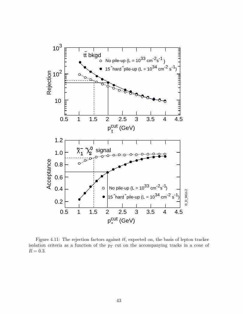
with two or three isolated leptons, no jets and missing ET , there are two essential instru-mental requirements allowing separation of the signal. The first is lepton isolation, tosuppress the copious backgrounds from processes such as tt, Zbb, bb. The rejection factorsexpected on basis of tracker isolation criteria as a function of the pT cut on the accompa-nying tracks are shown in Fig. 4.11 for low and high luminosity running conditions. Thesecond requirement, as discussed previously, is on the detector capability to veto on jets.

30

4.5 Tagging of b-jets in CMS

As discussed in Section 2.3, an important ingredient for SUSY physics studies is thecapability of the detector to tag b-jets. Figures 2.13, 2.14 and 2.15 illustrate the manyways b-jets can serve as final state signatures of b, t, t production in the g/q cascades.Particularly important is the possibility to detect h → bb in g/q → χ0

2→ χ01h decay channel

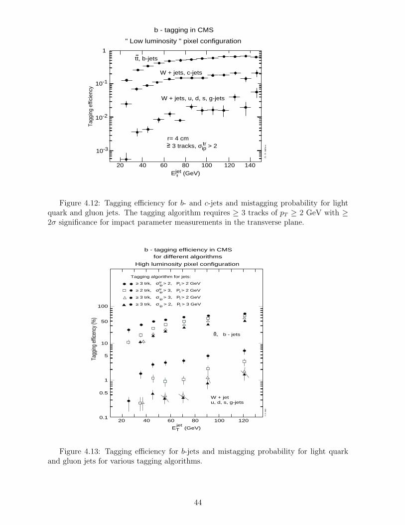
with S/B ∼ 1 and potentially with much lower integrated luminosity than required toobserve h → γγ. Techniques for b-tagging have been studied in detail in CMS. Theinner part of the CMS tracker, in particular the two pixel layers, has been optimisedin detector positioning and required resolution with b-tagging performance as the maincriterion [34]. The expected b-tagging efficiency and sample purity has been studied withseveral tagging algorithms based on track impact parameter measurements. Figure 4.12shows, for example, the expected tagging efficiency as a function of jet ET averaged overthe pixel detector acceptance. For b-jets in tt events it is ∼ 30%, whilst the expected fakerate probability is ∼ 1%. The tagging algorithm used for Fig. 4.12 requires ≥ 3 tracks ofpT ≥ 2 GeV with ≥ 2 σ significance for impact parameter measurements in the transverseplane.

How much the expected tagging efficiency is dependent on the tagging algorithmand what is the possible trade-off between efficiency and sample purity is illustrated byFig. 4.13 where several tagging algorithms have been exercised. Figure 4.14 shows howthe tagging efficiency and purity depends on the radius of the first barrel pixel layer,changing it from 4 cm as possible for the low luminosity running to 7.7 cm as requiredto sustain the radiation damage at 1034 cm−2s−1. There would be an important gain intagging efficiency if the first pixel layer could be always kept at 4 cm radius, at a cost ofreplacing it (almost) every year. This is particularly important for channels like h → bbwhich go with the square of the tagging efficiency. Whilst the tagging efficiency is asimple function of the pixel point resolution and the radial position of the barrel pixellayers, the mistagging probability is dependent on the non-Gaussian part of the measuredimpact parameter distribution and is more difficult to control as it depends on the overallpattern recognition performance and multiple scattering of the tracker. All the b-taggingefficiencies discussed here rely on impact parameter measurements; further improvementsin b-tagging efficiency are possible, including explicit reconstruction of secondary vertices,lepton tags, etc.

4.6 CMSJET – an approximate description of detector response

Understanding of the detector response with an adequate simulation is a very importantpart of correctly estimating the SUSY discovery potential of the CMS experiment. Wehave used the CMSJET program, which is a fast, non-GEANT simulation package forthe CMS detector [35, 36]. CMSJET provides a satisfactory approximate description ofdetector components and of the response to hadrons, leptons and gammas. It is a goodcompromise between performance speed and precision. The following aspects of CMSJETare relevant to this study:

• Charged particles are tracked in a 4 T magnetic field. A reconstruction efficiency of90% per charged track with pT > 1 GeV and |η| < 2.5 is assumed.

• The geometrical acceptances for µ and e are |η| < 2.4 and 2.5, respectively. Thelepton momentum is smeared according to parameterizations obtained from full GEANT

31

simulations. For a 10 GeV lepton the momentum resolution ∆pT /pT is better than 1%over the full η coverage. For a 100 GeV lepton the resolution becomes ∼ 1÷5% dependingon η. We have assumed a 90% triggering plus reconstruction efficiency per lepton withinthe geometrical acceptance of the CMS detector. This value is probably pessimistic formuon tracks, but more realistic for electrons.

• The electromagnetic calorimeter of CMS extends up to |η| = 2.61. There is a pointingcrack in the ECAL barrel/endcap transition region between |η| = 1.479− 1.566 (6 ECALcrystals) with significantly degraded resolution. The hadronic calorimeter covers |η| < 3.The Very Forward calorimeter extends from |η| = 3 to |η| = 5. The full granularity ofthe calorimetric system is implemented in CMSJET. The granularity, assumed energyresolutions and electronic noise of calorimeters are listed in Table 4.1. Noise terms havebeen simulated with Gaussian distributions and zero suppression cuts have been applied.

Table 4.1: CMS calorimeter description

η region ∆η × ∆φ ∆E/E Noise (MeV)

ECAL |η| < 1.479 0.0145×0.0145 5%/√

E ⊕ 0.5% 25, 3σ zero sup.1.566<|η|<2.00 0.0217×0.02182.00<|η|<2.35 0.0292×0.02912.35<|η|<2.61 0.0433×0.0436

Crack 1.479<|η|<1.566 0.0870×6.283 50%/√

E ⊕ 2% –

HCAL |η| < 2.262 0.087×0.087 η dependent 250, 2σ zero sup.2.262<|η|<2.61 0.174×0.175 parameterization;

2.61<|η|<3.0 0.195×0.349 82%/√

E ⊕ 6.5% at η=0

VF 3 < |η| < 5 0.17×0.17 ÷ 172%/√

E ⊕ 9% 250, 2σ zero sup.0.175×0.175 for hadrons

• e/γ and hadron shower developments are taken into account by parameterizationof the lateral and longitudinal profiles of the showers. The starting point of a shower isfluctuated according to an exponential low.

• Jets are reconstructed using a cone algorithm, with a cone radius R = 0.4÷ 0.9 andvariable transverse energy threshold on jets depending on event kinematics.

• For the high luminosity (L = 1034 cm−2s−1) study, event pile-up is taken into accountby superposition of “hard” pile-up events on top of signal and background. These arerepresented by PYTHIA QCD jet events with pT > 5 GeV. The number of superimposedpile-up events has been fluctuated with a Poisson distribution having a mean value of 15.

The CMSJET model of the CMS detector is depicted in Fig. 4.15.

32

ME

/ 1/

3

1.290 m

1.941 m

2.864 m2.950 m

4.020 m

4.905 m

7.000 m

1.26

8 m

4.00

4 m

6.66

0 m

10.8

30 m

10.6

30 m

9.75

0 m

8.49

5 m

6.66

0 m

6.45

0 m

5.68

0 m

3.90

00 m

2.93

5 m 0

7.380 m

1.185 m

0

CMS DETECTOR

14.5

80 m

14.5

50 m

14.9

80 m

7.24

0 m

5.975 m

3.800 m

1.811 m

MB / 2/4 MB / 1/4

YB / 2/3

MB / 0/4

MB / 0/1

MB / 0/2

YB / 0/2

YB / 0/3

MB / 0/3

YB / 0/1

MB / 1/1

MB / 1/2

YB / 1/2

MB / 1/3

YB / 1/3

YB / 1/1

MB / 2/1

YB / 2/2

MB / 2/3

MB / 2/2

YB / 2/1

Coil

EE / 1

HE / 1

HB / 1

ME

/ 1/

1

Tracker

ME

/ 4/

1

ME

/ 3/

1

ME

/ 2/

1

NO

SE

ME

/ 1/

2

YE

/ 3

YE

/ 2

YE

/ 1

ME

/ 4/

2

ME

/ 2/

2

ME

/ 3/

2

η = .087 η = .174 η = .261 η = .348 η = .435 η = .522 η = .609 η = .696 η = .783 η = .957 η = .870

η = 2.262

η = 2.088

η = 2.001

η = 1.914

η = 1.827

η = 1.740

η = 1.653

η = 1.566

η = 1.479

η = 1.392

η = 1.305

η = 1.218

η = 1.131 η = 1.044 η = .000

D_D_1041n1.

0 1.00.5

(meters)

η = 3.000

η =5.310

η = 2.805

η = 2.610

η = 2.436

HF / 1

EB / 1

Figu

re4.1:

Lon

gitudin

alcu

tth

rough

the

CM

Sdetector.

The

tower

structu

reof

the

had

roncalorim

eteran

dth

earran

gemen

tof

the

electromagn

eticcalorim

etercry

stalsis

indicated

,as

well

asth

elo

cations

ofth

etail

catcher

layers.

33

detector, |η| < 5.0






QCD dijet, ET>=

jet80 GeV

1012

1011

1010

109

108

107

106

105

104

1 nb =

1 pb =

0 50 100 150 200 250 300 350

Missing Et GeV

Eve

nts

/ 20

GeV

/ 10

0 fb

-1

D.D

.992

n

Figure 4.2: Missing ET distributions for QCD di-jet events as a function of calorimetriccoverage at large rapidities.

34

No VFCAL:

With VFCAL:

σ (Emiss)= 0.69* ΣEtt

σ (Emiss)= 1.0* ΣEtt

tσ

(E

mis

s)

/ Σ

Et

CMSevent pile-up background in bunch

crossing at 1034 cm-2 s-1

0.005

0.015

0.025

0.035

0.045

0.05

0.04

0.03

0.02

0.01

500 100 1500 200 2500 30000ΣEt (GeV)

D_

D_

10

53

n

Figure 4.3: Improvement on missing ET resolution in the presence of very forwardcalorimetry.

35

250 6

7

8

9

10

11

100

200

300

400

500

3 4 52.5 3.5 4.5|η jet| |η jet|

2 3 4 52.5 3.5 4.5

Rej

ectio

n

Rej

ectio

n

gg, gq, qq bkgd.~~ ~~ ~~ tt bkgd.

m0 = 100 GeV, m1/2 = 100 GeVm(g) = 294 GeV, m(q) = 270 GeV~ ~

D_D

_967

n1

Et > 30 GeVjet

Et > 25 GeVjetEt > 25 GeVjet

Et > 30 GeVjet

Figure 4.4a: Rejection factors which can be achieved in chargino/neutralino searchusing a jet veto, as a function of jet acceptance and jet detection threshold.

gq, gg,qq

80

60

40

20

02 32.5 43.5 4.5

No jets with Et

5

30 GeV

35 GeV

SU

SY

- r

ejec

tion

tt

20

15

10

5

02 32.5 43.5 4.5 5

tt -

reje

ctio

n

IηjetI IηjetI

D_D_1011n

m0= 86 GeV, m1/2= 85 GeV; m = 112 GeV, m = 98 GeV, mν= 93 GeV

~~ ~~ ~~

Events with two isolated leptons of p > 20 GeV, Emiss > 50 GeV, ∆Φ(Emisst tt

bkgd bkgd

> 160°

>

),L R

Figure 4.4b: Jet veto rejection factors against squark/gluino and tt backgrounds inslepton searches in two-lepton final states.

36

ECAL + HCAL+ tail catcher

ECAL + HCAL

Depth of Calorimetry

λ

η

16

14

12

10

8

6

4

2

0

0.52

2

1.04

4

1.56

6

2.08

8

2.61

0

3.04

5

0.00

0

D_D

_979

n

CMSconical endcap (52o)

12 cm gap

Figure 4.5: Depth of calorimetry and total sampled depth including the tail catcherlayers as a function of rapidity in CMS.

37

103

102

10

1

103

102

10

1

103

102

10

1

1

0 010.5

0 010.5

103

102

10

1

103

102

10

1

103

102

10

10.5

10.5

0 010.5 10.5

No tail catcher

With first tail

With first +

catcher layer

second tailcatcher layers

Einc (π+) = 200 GeV (GEANT)t

Ereconstr. / Einc Ereconstr. / Einc

ηπ: 0.0 - 0.5 ηπ: 0.5 - 1.1

Effect of tail catcher layers on reduction of tail

in response to pions

D_D

_100

3n

Figure 4.6: Effects on hadron energy measurements of tail catcher layers in the centraland next-to-central CMS wheels i.e. in two adjacent rapidity ranges.

38

HCAL Barrel / endcap designs

D_D

_738

n

TP1

TP3

TP0

TP2

TP5TP4

TP7TP6

Cu 6 cm

Cu 8 cm

Figure 4.7: Various configurations of the barrel/endcap calorimetry transition regionconsidered.

39

103

102

10

1

103

102

10

1

103

102

10

1

Num

ber

of e

vent

sN

umbe

r of

eve

nts

Num

ber

of e

vent

sTP7

11 cm. crack

TP718 cm. crack

TP725 cm. crack

pions 100 GeV

pions 100 GeV

pions 100 GeV

η = 1.3 - 1.5on crack

η = 1.3 - 1.5on crack

η = 1.0 - 1.2off crack

η = 1.3 - 1.5on crack



0 50 100 150 200E ( GeV )

0 50 100 150 200E ( GeV )

0 50 100 150 200 E ( GeV )

D_D

_981

n

Effects of crack size on responseto pions in "conical endcap" design

Figure 4.8: Effects on hadron energy measurements of the crack for services betweenthe barrel and the endcap calorimetry for three crack sizes.

40

CMS tracker - longitudinal cut

D_D_1019n

-3.0 Z0 (cm) +3.0

MSGG Si - StripsSi - Pixels

1.3

-1.3

0

r (m

)

Figure 4.9: Layout of the CMS tracker.

41

η = 2.25η = 1.80η = 0

With vertex point

10–1

10–2

101 102 103

pT GeV

Mom

entu

m R

esol

utio

n ∆p

/p

η = 2.25η = 1.80η = 0

No vertex point

10–1

10–2

101 102 103

pT GeV

Mom

entu

m R

esol

utio

n ∆p

/p

Momentum resolution of CMS tracker versus pt

D.D 656n

η = 2.25η = 1.3η = 0

In transverse plane103

102

10101 102

pT GeV

Impa

ct p

aram

eter

res

olut

ion

(µm

)

Impact parameter resolution of CMS

D.D 657n

Figure 4.10: Momentum and impact parameter resolutions as a function of pT atvarious rapidities.

42

tt bkgdNo pile-up (L = 1033 cm-2s-1

15 hard pile-up (L = 1034 cm-2 s-1)

χ– χ0 signal1 2

~ ~

0.5 1

102

103

10

0.2

0.4

0.6

0.8

1.2

1.0

1.5 2 2.5 3 3.5 4 4.5

Rej

ectio

n

pcut (GeV)

0.5 1 1.5 2 2.5 3 3.5 4 4.5

pcut (GeV)

Acc

epta

nce

D_D

_961

n.2

t

t

" " )

No pile-up (L = 1033 cm-2s-1

15 hard pile-up (L = 1034 cm-2 s-1)" "

)

Figure 4.11: The rejection factors against tt, expected on, the basis of lepton trackerisolation criteria as a function of the pT cut on the accompanying tracks in a cone ofR = 0.3.

43

tt, b-jets

W + jets, c-jets

W + jets, u, d, s, g-jets

> 3 tracks, σip > 2=

20 40 60 80 100 120 140Ejet (GeV)t

1

10-2

10-3

10-1

Tagg

ing

effic

ienc

y

r= 4 cm

D_D

_983

cn

b - tagging in CMS

" Low luminosity " pixel configuration

tr

Figure 4.12: Tagging efficiency for b- and c-jets and mistagging probability for lightquark and gluon jets. The tagging algorithm requires ≥ 3 tracks of pT ≥ 2 GeV with ≥2σ significance for impact parameter measurements in the transverse plane.

20

1

10

50

5

0.5

0.1

100

40 60 80

W + jetu, d, s, g-jets

tt, b - jets

100

Tagg

ing e

fficen

cy (%

)

120

ET (GeV)jet

Tagging algorithm for jets:

≥ 3 trk, σ

tr > 2, P > 2 GeVip t

t

t

t

≥ 2 trk, σ

tr > 3, P > 2 GeVip

≥ 3 trk, σ

> 3, P > 2 GeVip

≥ 3 trk, σ > 2, P > 3 GeVip

D_D_

989c

b - tagging efficiency in CMSfor different algorithms

High luminosity pixel configuration

Figure 4.13: Tagging efficiency for b-jets and mistagging probability for light quarkand gluon jets for various tagging algorithms.

44

> 3 tracks, σip > 3




Tagging efficiency for b-jets from ttMistagging probability for jets from W + jet

21 3 5

b)

64

Mistagging probability (%)

Ta

gg

ing

effic

ien

cy (

%)

70

60

50

40

30

Microvertex option:

r= 7.7 cm

r= 4.0 cm

D_

D_

98

6.n

Figure 4.14: Tagging efficiency for b-jets and mistagging probability as a function ofthe inner barrel pixel layer radius.

45

VFCAL

3.17 m 11.1 m

1.479 1.566

2.61

3.0

5.0

ECAL

HCAL

VFCAL

ηhadr.

e -

hadr

e -

γ

γ

40 % 3 %

V.Genchev, L.Litov, CMS TN/94-272.

D.Litvintsev, CMS TN/95-98.

1.44 m

gap of 6 ECAL Xtals

4 T field no field

crack

+E

σ / E =

σ / E =

σ / E =

σ / E =

σ / E = f ( )

σ / E = f ( E )

CMSJET 3.5 calorimetry model

5 % 0.5 %+E

172 % 9 %+E

114 % 3.3 %+E

82 % 6.5 % +Eσ / E =η = 0

e , γ

degraded to ~ 50 % E

η

crack

at :

< 3.02.61 <

degraded response

90% 10 % +Eσ / E degraded to ~

2 % +

ECAL

HCAL

HCAL

Figure 4.15: The CMS calorimetry model in CMSJET 3.5

46

5 Leptons + jets+ EmissT channel –

search for gluinos and squarks

To investigate the maximum reach in parameter space for SUSY via the production ofstrongly interacting sparticles we study multilepton+multijet + Emiss

T final states, result-ing from the cascade decays of these sparticles [4, 5]. As mentioned previously, a completemass reconstruction of gluinos and squarks is impossible due to the presence of escapingparticles, two LSP’s plus possibly neutrinos. So SUSY signal observability is based onan excess of events of a given topology over known (expected) backgrounds. Among theleptonic final states studied, including always at least 2 jets + Emiss

T in the final state,are one lepton (1l), two leptons of the same sign (2l SS), two leptons of opposite sign (2lOS), and 3,4,5 leptons regardless the sign (3l, 4l, 5l). As discussed in the following, thesetopologies have been investigated both with and without explicit requirements on muonisolation. The jets + Emiss

T topology, with no isolated leptons, is not discussed, since it isthe most sensitive one to detailed detector simulation, and preliminary studies show thatthe mass reach is inferior to one of the channels discussed here [2].

In order to establish the limits of the SUSY reach in the (m0, m1/2) parameter spacefor various integrated luminosities, the signal was generated at more than 100 points. Ateach point the signal is generated as a mixture of all possible combinations of the stronglyinteracting sparticle production processes (gg, gq, qq) with masses and decay branchingratios corresponding to this point. The set of m0, m1/2 points where the signal sampleswere generated for tanβ = 2, A0 = 0, µ < 0 is shown in Fig. 5.1. Figures 5.2a-d give, atfour representative points in the parameter space, the main sparticle masses and decaychains with corresponding branching ratios.

The backgrounds considered in this study are: tt, W + jets, Z + jets, WW, ZZ,ZW, Zbb and QCD (2 → 2 processes including bb). There could be some double count-ing between Z + jets and Zbb processes, but in practice this means more conservativebackground estimates.

No pseudorapidity cuts are applied during background generation to avoid distortionof the event kinematics. All processes were generated in the following pT intervals: 40 -100, 100 - 200, 200 - 400, 400 - 800, ≥ 800 GeV. This allows the accumulation of significantstatistics in the high-pT range in a more economical way than without subdivision of thegeneration pT range [4].

The kinematics of signal events is usually harder than for the SM backgrounds, inparticular for the interesting regions corresponding to the maximum reach in terms ofsquark/gluino masses. The cross-sections of the background processes can however behigher by orders of magnitude, and the high-pT tails of different backgrounds can have akinematics similar to that of the signal. Figures 5.3-5.5 illustrate kinematical distributionsfor the signal at three different points in parameter space and compare it to background.More specifically in Fig. 5.3 one can see the comparison between kinematical distributionsfor the signal point (m0 = 200 GeV, m1/2 = 760 GeV) and the distributions for thesum of backgrounds in 2l SS, 2l OS and 3l final states. Both signal and backgroundhistograms contain only events satisfying first level selection criteria described below.Only the hardest jet and lepton in the event are shown in distributions. The last histogramin each Figure shows the distribution of Esum

T , the scalar sum of all relevant transverseenergies for leptons, jets and Emiss

T . It reflects the overall transverse energy flow in the

47

event, the event “hardness”. This variable is also rather insensitive to the transverseenergy flow induced by event pile-up since it accounts only for those calorimeter cellswhich are attached to a jet, and is thus a useful quantity to cut on in the high luminosityregime.

The topology of signal and background events is already rather similar after the firstlevel selection cuts, in terms of angular distributions and circularity, as can be seen inFig. 5.3a, thus it is not very useful to apply explicit cuts on these variables. The differencebetween signal and background in the lepton pT distributions is also not as pronounced asmight have been expected, as signal leptons are produced in cascade decays, thus losing“memory” of the hardness of the original process. For extremely high masses of squarksor gluinos in the ∼ 2 TeV mass range, the difference in the angular and pl

T distributionsbetween signal and the total SM background is still significant and helps in obtaining aneffective data selection. Ultimately, all the cuts have to be justified from the point of viewof the best observability of the signal over expected background.

Since the kinematics of the signal vary significantly with the variation of m0 and m1/2

parameters, Figs. 5.3-5.5, the set of different cuts is applied and optimised independentlyin each point investigated. These cuts are listed in Table 5.1. The optimisation proceduretakes into account the number of jets per event, and parameters of lepton isolation, asdiscussed in details in the next subsection. The Emiss

T cut can be incremented beyondthe values listed in Table 5.1, keeping all other cuts untouched, to take advantage of thelarge values this variable can take when the signal is close to the boundaries of explorableparameter space where masses of squarks and gluino are in the 1-2 TeV range.

We find that requiring more than 2 jets (up to ≥ 4-5 for 1, 10 fb−1, up to ≥ 6 for100 fb−1) in the event is useful in many cases, especially in domains 3 and 4 as definedin Fig. 2.16. The exception is domain 1, where requiring ≥ 2 jets (as well as requiringmuon isolation for all cases except for 4 and 5 lepton final states) is sufficient to get thebest signal observability.

Table 5.1: The various cuts applied to optimise the reach.

CUT peT (GeV) pµ

T (GeV) pjet1,2,3T (GeV) Emiss

T (GeV) EsumT (GeV)

C1 20 10 40 100 -C2 20 10 150,80,40 150 500C3 40,20,20 150,80,40 150 500C4 40,20,20 200,120,40 200 700C5 50,30,20 250,150,40 200 1000C6 80,50,20 300,200,40 250 1200C7 100,70,20 300,200,40 250 1200

It is also found that some moderate cuts:

• Circularity > 0.1

• δϕ (hardest lepton, EmissT ) > 10-15 deg

are useful to improve signal observability everywhere in 1l final states, and in 2l OS finalstates, primarily in the region m1/2 > 600 GeV for an integrated luminosity ≥ 10 fb−1.

48

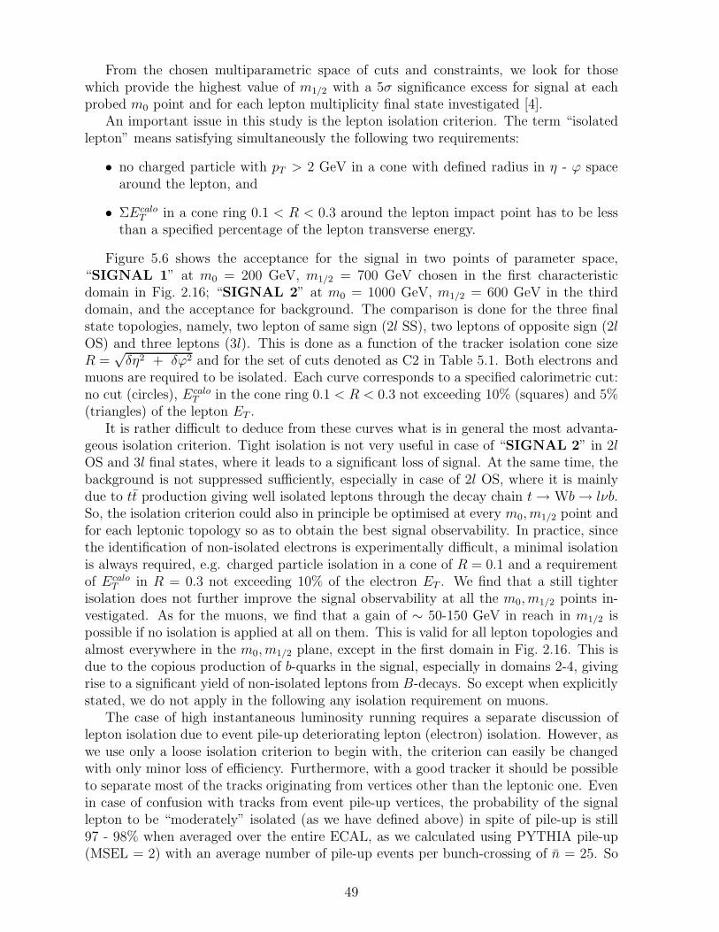
From the chosen multiparametric space of cuts and constraints, we look for thosewhich provide the highest value of m1/2 with a 5σ significance excess for signal at eachprobed m0 point and for each lepton multiplicity final state investigated [4].

An important issue in this study is the lepton isolation criterion. The term “isolatedlepton” means satisfying simultaneously the following two requirements:

• no charged particle with pT > 2 GeV in a cone with defined radius in η - ϕ spacearound the lepton, and

• ΣEcaloT in a cone ring 0.1 < R < 0.3 around the lepton impact point has to be less

than a specified percentage of the lepton transverse energy.

Figure 5.6 shows the acceptance for the signal in two points of parameter space,“SIGNAL 1” at m0 = 200 GeV, m1/2 = 700 GeV chosen in the first characteristicdomain in Fig. 2.16; “SIGNAL 2” at m0 = 1000 GeV, m1/2 = 600 GeV in the thirddomain, and the acceptance for background. The comparison is done for the three finalstate topologies, namely, two lepton of same sign (2l SS), two leptons of opposite sign (2lOS) and three leptons (3l). This is done as a function of the tracker isolation cone sizeR =

√δη2 + δϕ2 and for the set of cuts denoted as C2 in Table 5.1. Both electrons and

muons are required to be isolated. Each curve corresponds to a specified calorimetric cut:no cut (circles), Ecalo

T in the cone ring 0.1 < R < 0.3 not exceeding 10% (squares) and 5%(triangles) of the lepton ET .

It is rather difficult to deduce from these curves what is in general the most advanta-geous isolation criterion. Tight isolation is not very useful in case of “SIGNAL 2” in 2lOS and 3l final states, where it leads to a significant loss of signal. At the same time, thebackground is not suppressed sufficiently, especially in case of 2l OS, where it is mainlydue to tt production giving well isolated leptons through the decay chain t → Wb → lνb.So, the isolation criterion could also in principle be optimised at every m0, m1/2 point andfor each leptonic topology so as to obtain the best signal observability. In practice, sincethe identification of non-isolated electrons is experimentally difficult, a minimal isolationis always required, e.g. charged particle isolation in a cone of R = 0.1 and a requirementof Ecalo

T in R = 0.3 not exceeding 10% of the electron ET . We find that a still tighterisolation does not further improve the signal observability at all the m0, m1/2 points in-vestigated. As for the muons, we find that a gain of ∼ 50-150 GeV in reach in m1/2 ispossible if no isolation is applied at all on them. This is valid for all lepton topologies andalmost everywhere in the m0, m1/2 plane, except in the first domain in Fig. 2.16. This isdue to the copious production of b-quarks in the signal, especially in domains 2-4, givingrise to a significant yield of non-isolated leptons from B-decays. So except when explicitlystated, we do not apply in the following any isolation requirement on muons.

The case of high instantaneous luminosity running requires a separate discussion oflepton isolation due to event pile-up deteriorating lepton (electron) isolation. However, aswe use only a loose isolation criterion to begin with, the criterion can easily be changedwith only minor loss of efficiency. Furthermore, with a good tracker it should be possibleto separate most of the tracks originating from vertices other than the leptonic one. Evenin case of confusion with tracks from event pile-up vertices, the probability of the signallepton to be “moderately” isolated (as we have defined above) in spite of pile-up is still97 - 98% when averaged over the entire ECAL, as we calculated using PYTHIA pile-up(MSEL = 2) with an average number of pile-up events per bunch-crossing of n = 25. So

49

event pile-up at high instantaneous luminosity does not affect significantly the results ofour study.

Figures 5.7-5.9 show the final results of our study of squark and gluino observabilityand mass search in m0, m1/2 parameter space in the various multilepton + multijet +Emiss

T final states for our standard set of parameters tanβ = 2, A0 = 0, µ < 0. The resultsare shown for increasing values of integrated luminosity from 1 to 100 fb−1. All the 5σboundaries shown are obtained relaxing muon isolation whenever possible, but keepingalways the minimal electron isolation criteria needed for unambiguous instrumental elec-tron identification. The maximal squark and gluino mass reach is obtained in 1 leptonfinal states. With 105 pb−1 the maximal gluino mass reach varies from ≈ 2.5 to 2.0 TeV,depending on m0, whilst the squark mass reach varies between 2.1 - 2.5 TeV. What isimportant is that already with 103 pb−1 the <∼ 1 TeV domain can be thoroughly explored,and according to the “no-fine tuning” arguments this mass domain is the most plausibleone.

In Fig. 5.8 one can see that the cosmologically interesting region [37] is entirely con-tained within the domain explorable already with 10 fb−1 in all topologies considered.The Figure shows the relic neutralino dark matter density contours corresponding to Ωh2

values of 0.25, 0.5 and 1, where Ω is the neutralino density relative to the critical densityof the Universe and h is the Hubble constant scaling factor (h ∼ 0.7). The prefered mixeddark matter scenario corresponds to values of Ωh2 between 0.15 and 0.4.

Figure 5.10 illustrates the gain in mass reach which can be obtained when non-isolatedmuons are taken into account in the analysis. Figure 5.11 shows the expected signal-to-background ratio at the 5σ boundaries in each topology. It is always bigger than 1,thus we may expect that the maximum reach will not be very sensitive to a possible un-derestimation of the background cross-sections. To estimate the influence of systematicuncertainties on the background cross-sections on the g, q observability contours, we in-creased all the background cross-sections by a factor of 2, and the W/Z + jets backgroundby a factor of 5. Figure 5.12 shows how the 5σ significance contours are modified underthese conditions for an integrated luminosity of 10 fb−1. The loss of reach is small in allcases.

We also checked the sensitivity of our results to changes in some of our basic param-eters. The change of the sign of µ, keeping tanβ = 2, A0 = 0, affects primarily charginosand neutralinos. It changes their masses, decay modes and branching ratios, and thesealter the final state kinematic and topology. In the squark sector, a positive sign of µdecreases the t1 mass by ≈ 30 – 50 GeV compared to the µ < 0 case. Consequently, finalstate leptons coming from stops and top quarks will be slightly “softer”, thus requiringlower threshold cuts and causing modified background levels compared to the µ < 0 case.Figure 5.13 gives the maximum expected reach of the CMS detector for squark and gluinosearches in different multilepton final states for 104 pb−1 with µ > 0 [5]. The reach isagain greatest in the single lepton channel, and extends up to gluino and squark masses of∼ 2 TeV. Relaxation of the muon isolation requirements increases the reach by ≈ 50 GeVin the single lepton case, and by ≈ 200 GeV in the trilepton case. The 4l channel with104 pb−1 has an interesting explorable domain only if muons are not isolated [38]. Figure5.14 gives the same results for Lint = 105 pb−1 [5]. With this luminosity and with fullmuon isolation (not shown), the 4l maximal reach region in fact becomes “a band ofobservability” approximately between m1/2 ≈ 200 GeV and m1/2 ≈ 350 GeV [38]. Thelower boundary is mainly caused by a decrease of the branching ratio for g → χ0

1tt. For

50

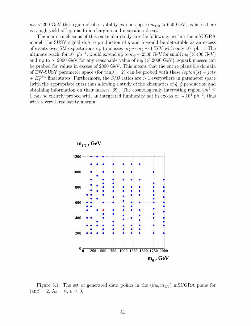
m0 < 200 GeV the region of observability extends up to m1/2 ≈ 650 GeV, as here thereis a high yield of leptons from chargino and neutralino decays.

The main conclusions of this particular study are the following: within the mSUGRAmodel, the SUSY signal due to production of q and g would be detectable as an excessof events over SM expectations up to masses mq ∼ mg ∼ 1 TeV with only 103 pb−1. Theultimate reach, for 105 pb−1, would extend up to mq ∼ 2500 GeV for small m0 (<∼ 400 GeV)and up to ∼ 2000 GeV for any reasonable value of m0 (<∼ 2000 GeV); squark masses canbe probed for values in excess of 2000 GeV. This means that the entire plausible domainof EW-SUSY parameter space (for tanβ = 2) can be probed with these lepton(s) + jets+ Emiss

T final states. Furthermore, the S/B ratios are > 1 everywhere in parameter space(with the appropriate cuts) thus allowing a study of the kinematics of q, g production andobtaining information on their masses [39]. The cosmologically interesting region Ωh2 ≤1 can be entirely probed with an integrated luminosity not in excess of ∼ 103 pb−1, thuswith a very large safety margin.

0

200

400

600

800

1000

1200

0 250 500 750 1000 1250 1500 1750 2000

m1/2 , GeV

m0 , GeV

Figure 5.1: The set of generated data points in the (m0, m1/2) mSUGRA plane fortanβ = 2, A0 = 0, µ < 0.

51

m = 200 GeV, m = 760 GeV0 1/2

m = 1765 GeVg~ m <

q~ m = 1208 GeV

t~

m = 333 GeV~

m = 647 GeV m = 566 GeVe~

m g~

1

L

χ 1

~χ 1

+_

0

~ 32 %

~ 1/3

~

~ 65 %

~ 2/3

~ 92 %

~ 20 %

g qq ( t t ~ 24 %, t t ~ 10 %, b b ~ 11 % )21

_ _ __

qL

~χ 1

+_q

l v

v l

~ ~ ~ ~

~~

~

+_

+_~χ 1

0 l v+_

~χ 2

q

l l~+_

χ 10 l l

+_ +_

+_

t1

~

~

χ 10~

t

W b+

l v+

L

~b

~χ 1

t

0

~χ 2

0 b

t1

~W

_

~ 59 %

~ 31 %

~ 8 %

qR

~χ 1

0~q ~ 100 %

_

L

~

m = 500 GeV, m = 500 GeV0 1/2

m = 1221 GeVg~ m <

q~ m = 856 GeV

t~

m = 217 GeV~

m = 427 GeV m = 611 GeVe~

m g~

1

L

χ 1

~χ 1

+_

0

~ 93 %

~ 1/3

~

~ 100 %

~ 2/3

~ 91 %

~ 20 %

g qq ( t t ~ 50 %, b b ~ 18 % )1

_ _

qL

~χ 1

+_q

~ ~ ~

~

~χ 2

q

t1

~χ 1

0~ t

W b+

l v+

0

qR

~χ 1

0~q ~ 100 %

~

χ 10~

W+_

χ 10~

χ 10~

h

Z ~ 3 %

m = 101 GeVh

_

b b_

~ 87 %

m = 1000 GeV, m = 620 GeV0 1/2

m = 1519 GeVg~ m >

q~ m = 1087 GeV

t~

m = 271 GeV~

m = 530 GeV m = 1088 GeVe~

m g~

1

L

χ 1

~χ 1

+_

0

~ 98 %

~ 1/3

~

~ 100 %

~ 2/3

g t t ~ 89 %,

b ~ 9 % L

1_

qL

~χ 1

+_q

~

~

~

~χ 2

q

χ 10~

t

0

qR

~χ 1

0~

q

~

χ 10~

W+_

χ 10~

h

W+_

l+_

v W

+_q q

~ 8 %

~ 24 %

b

t ~ 98 %, _

~χ 1

_t ~ 2/3

~χ 2

0 b ~ 1/3

~g

_

_

q

m = 2000 GeV, m = 480 GeV0 1/2

m = 1261 GeVg~ m

q~ m = 1106 GeV

t~

m = 211 GeV~

m = 415 GeV m = 2027 GeVe~

m g~

1

L

χ 1

~χ 1

+_

0

~ 100 %

~ 8 %

~

~ 100 %

g

qL

~χ 1

+_ q q

~

~χ 2

q

χ 10~

t

0

qR

~

χ 10~

W+_

χ 10 h

W+_

l+_

v

W+_

q q

~ 8 %

~ 24 %

t ~ 72 %, _

~χ 2

0

2~

~ 20 %,

q q ~ 8 %,

W+_

v 4 % τ+_

~

~χ 1

+_ q

g q~

~ 75 %

~ 16 %

g q~

~ 94 - 98 %

t 1

~

~

χ 10~

t ~ 100 %

8 %

63 %

24 % ( ~χ 1

+_t ) b L

~

Figure 5.2: Some typical points in parameter space.

52

1

10

10 2

10 3

10 4

10 5

0 5 10 15

Bkgd

Signal

m0 = 200 GeV , m1/2 = 760 GeV 2 l OS case, both leptons are isolated

Njet

Nev

1

10

10 2

10 3

10 4

0 100 200 300 400 500 Pt

l , GeV

Nev

/ 10

GeV

1

10

10 2

10 3

10 4

0 50 100 150∆φ ( Pt

l , Et miss) , deg

Nev

/ 5

deg

1

10

10 2

10 3

10 4

0 500 1000 1500 Pt

jet , GeV

Nev

/ 30

GeV

1

10

10 2

10 3

10 4

0 50 100 150∆φ ( Pt

jet , Et miss) , deg

Nev

/ 5

deg

1

10

10 2

10 3

10 4

10 5

0 500 1000 1500 Et

miss , GeV

Nev

/ 30

GeV

1

10

10 2

10 3

10 4

0 0.2 0.4 0.6 0.8 1Circularity

Nev

/ 0.

05

1

10

10 2

10 3

10 4

0 1000 2000 3000 Et

sum , GeV

Nev

/ 60

GeV

Figure 5.3a: Comparison of the signal and background kinematics at one point inmSUGRA parameter space, after requiring two leptons of opposite sign (plus jet andEmiss

T ).

53

1

10

10 2

10 3

0 5 10 15

Bkgd

Signal

2 l SS case, both leptons are isolated

Njet

Nev

1

10

10 2

0 200 400 Pt

l , GeV

Nev

/ 10

GeV

1

10

10 2

0 500 1000 1500 Pt

jet , GeV

Nev

/ 30

GeV

1

10

10 2

10 3

0 500 1000 1500 Et

miss , GeV

Nev

/ 30

GeV

1

10

10 2

0 1000 2000 3000 Et

sum , GeVN

ev /

60 G

eV

Figure 5.3b: Comparison of the signal and background kinematics in the same point asin in Fig. 5.3a, but for 2l SS final state topology.

1

10

10 2

0 5 10 15

Bkgd

Signal

3 l case, all leptons are isolated

Njet

Nev

1

10

0 200 400 Pt

l , GeV

Nev

/ 10

GeV

1

10

10 2

0 500 1000 1500 Pt

jet , GeV

Nev

/ 30

GeV

1

10

10 2

0 500 1000 1500 Et

miss , GeV

Nev

/ 30

GeV

1

10

10 2

0 1000 2000 3000 Et

sum , GeV

Nev

/ 60

GeV

Figure 5.3c: Comparison of the signal and background kinematics in the same point asin in Fig. 5.3a, but for 3l final state topology.

54

1

10

10 2

10 3

0 5 10 15

Bkgd

Signal

m0 = 500 GeV , m1/2 = 500 GeV 2 l SS case, both leptons are isolated

Njet

Nev

1

10

10 2

0 200 400 Pt

l , GeV

Nev

/ 10

GeV

1

10

10 2

0 500 1000 1500 Pt

jet , GeV

Nev

/ 30

GeV

1

10

10 2

10 3

0 500 1000 1500 Et

miss , GeV

Nev

/ 30

GeV

1

10

10 2

0 1000 2000 3000 Et

sum , GeVN

ev /

60 G

eV

Figure 5.4: Comparison of the signal and background kinematics for a secondpoint in parameter space.

1

10

10 2

10 3

0 5 10 15

Bkgd

Signal

m0 = 2000 GeV , m1/2 = 400 GeV 2 l SS case, both leptons are isolated

Njet

Nev

1

10

10 2

0 200 400 Pt

l , GeV

Nev

/ 10

GeV

1

10

10 2

0 500 1000 1500 Pt

jet , GeV

Nev

/ 30

GeV

1

10

10 2

10 3

0 500 1000 1500 Et

miss , GeV

Nev

/ 30

GeV

1

10

10 2

0 1000 2000 3000 Et

sum , GeV

Nev

/ 60

GeV

Figure 5.5: Comparison of the signal and background kinematics for a third pointin parameter space.

55

10

10 2

0 0.2Risol

Acc

epta

nce,

%

- no calo isolation limit

- 10 %

- 5 %

SIGNAL 1 SIGNAL 2 BACKGROUND

10

10 2

0 0.2Risol

10-1

1

10

10 2

0 0.2Risol

2l SS

10

10 2

0 0.2Risol

Acc

epta

nce,

%

10

10 2

0 0.2Risol

1

10

10 2

0 0.2Risol

2l OS

1

10

10 2

0 0.2Risol

Acc

epta

nce,

%

1

10

10 2

0 0.2Risol

10-2

10-1

1

10

10 2

0 0.2Risol

3l

Figure 5.6: Effect of the lepton isolation criterion on signal and background, at twodifferent points in parameter space: “SIGNAL 1” is m0 = 200 GeV, m1/2 = 700 GeV,“SIGNAL 2” is m0 = 1000 GeV, m1/2 = 600 GeV, as a function of Risol, the trackerisolation cone size Risol =

√δη2 + δϕ2. The results are shown for three choices of calori-

metric isolation parameter (sum of calorimeter energy deposit in a cone ring 0.1 < R < 0.3around the lepton impact point) and for three event topologies.

56

0

200

400

600

800

1000

1200

0 200 400 600 800 1000 1200 1400 1600 1800 2000

m1/2 (GeV)

m0 (GeV)

g~(500)

g~(1000)

g~(1500)

g~(2000)

g~(2500)

q ~(2500)q~

(2000)

q ~(1500)

q ~(1000)

q ~(500)

∫ L dt = 1 fb-1

A0 = 0 , tanβ = 2 , µ < 0

3l

2l SS

2l OS

1l

Figure 5.7: 5σ gluino/squark contours in various lepton multiplicity final states for 1fb−1 and our standard set of model parameter values tanβ = 2, A0 = 0, µ < 0. Squarkand gluino isomass curves shown by dash-dotted lines.

57

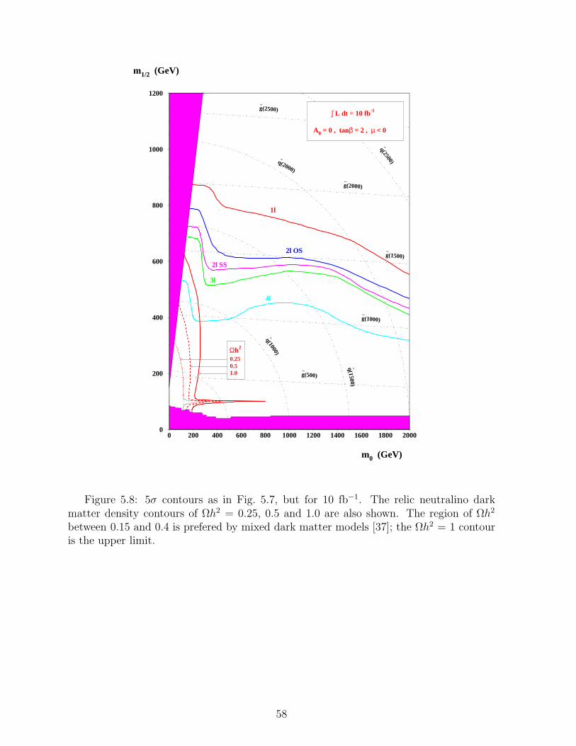
0

200

400

600

800

1000

1200

0 200 400 600 800 1000 1200 1400 1600 1800 2000

m1/2 (GeV)

m0 (GeV)

g~(500)

g~(1000)

g~(1500)

g~(2000)

g~(2500)

q ~(2500)q~

(2000)

q ~(1500)

q ~(1000)

∫ L dt = 10 fb-1

A0 = 0 , tanβ = 2 , µ < 0

4l

3l

2l SS

2l OS

1l

Ωh2

0.250.51.0

Figure 5.8: 5σ contours as in Fig. 5.7, but for 10 fb−1. The relic neutralino darkmatter density contours of Ωh2 = 0.25, 0.5 and 1.0 are also shown. The region of Ωh2

between 0.15 and 0.4 is prefered by mixed dark matter models [37]; the Ωh2 = 1 contouris the upper limit.

58

0

200

400

600

800

1000

1200

0 200 400 600 800 1000 1200 1400 1600 1800 2000

m1/2 (GeV)

m0 (GeV)

g~(500)

g~(1000)

g~(1500)

g~(2000)

g~(2500)

q ~(2500)q~

(2000)

q ~(1500)

q ~(1000)

q ~(500)

∫ L dt = 100 fb-1

A0 = 0 , tanβ = 2 , µ < 0

5l

4l

3l2l SS

2l OS

1l

Figure 5.9: Ultimate squark and gluino mass reach, in terms of a ≥ 5σ observationcontour for 100 fb−1, in various lepton multiplicity final states .

59

0

200

400

600

800

1000

0 500 1000 1500 2000

1 l

m1/2 (GeV)

m0 (GeV)

Muon isolation relaxed

when possible

With muon isolation

0

200

400

600

800

1000

0 500 1000 1500 2000

2 l OS

m1/2 (GeV)

m0 (GeV)

0

200

400

600

800

1000

0 500 1000 1500 2000

2 l SS

m1/2 (GeV)

m0 (GeV)

0

200

400

600

800

1000

0 500 1000 1500 2000

3 l

m1/2 (GeV)

m0 (GeV)

Figure 5.10: Influence of muon isolation on the 5σ contours in various topologies for10 fb−1.

60

0

200

400

600

800

1000

1200

0 200 400 600 800 1000 1200 1400 1600 1800 2000

m1/2 (GeV)

m0 (GeV)

g~(500)

g~(1000)

g~(1500)

g~(2000)

g~(2500)

q ~(2500)q~

(2000)

q ~(1500)

q ~(1000)

q ~(500)

∫ L dt = 10 fb-1

A0 = 0 , tanβ = 2 , µ < 0

4l

3l

2l SS

2l OS

1l

2.7

1.6

2.4

4.0

1.8

2.6

4.5

11.3

2.6

2.4

14.1

3.02.5

2.1

2.2

3.6

2.9

Figure 5.11: Signal to SM background ratio on the 5σ reach boundaries in in variouslepton multiplicity final state topologies, for 10 fb−1.

61

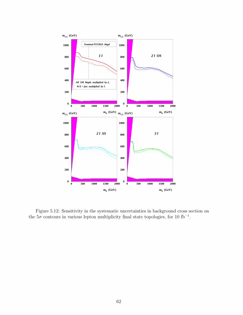
0

200

400

600

800

1000

0 500 1000 1500 2000

1 l

m1/2 (GeV)

m0 (GeV)

Nominal PYTHIA bkgd

All SM bkgds multiplied by 2,

W/Z + jets multiplied by 5

0

200

400

600

800

1000

0 500 1000 1500 2000

2 l OS

m1/2 (GeV)

m0 (GeV)

0

200

400

600

800

1000

0 500 1000 1500 2000

2 l SS

m1/2 (GeV)

m0 (GeV)

0

200

400

600

800

1000

0 500 1000 1500 2000

3 l

m1/2 (GeV)

m0 (GeV)

Figure 5.12: Sensitivity in the systematic uncertainties in background cross section onthe 5σ contours in various lepton multiplicity final state topologies, for 10 fb−1.

62

0

200

400

600

800

1000

1200

0 200 400 600 800 1000 1200 1400 1600 1800 2000

m1/2 (GeV)

m0 (GeV)

g~(500)

g~(1000)

g~(2000)

g~(2500)

q ~(2500)q~

(2000)

q ~(1500)

q ~(1000)

∫ L dt = 10 fb-1

A0 = 0 , tanβ = 2 , µ > 0

4l

3l

2l SS2l OS

1l

Ωh2

0.250.51.0

Figure 5.13: Maximal squark/gluino reach for µ > 0 for 10 fb−1 in different final statetopologies. The relic neutralino dark matter density contours of Ωh2 = 0.25, 0.5 and 1.0are also shown for this set of model parameters.

63

0

200

400

600

800

1000

1200

0 200 400 600 800 1000 1200 1400 1600 1800 2000

m1/2 (GeV)

m0 (GeV)

g~(500)

g~(1000)

g~(1500)

g~(2500)

q ~(2500)

q ~(2000)

q ~(1500)

q ~(1000)

∫ L dt = 100 fb-1

A0 = 0 , tanβ = 2 , µ > 0

4l

3l

2l SS

2l OS

1l

Ωh2

0.250.51.0

Figure 5.14: Same as in Fig. 5.13, but for 100 fb−1.

64

6 Search for next-to-lightest neutralino

Leptonic decays of the second-lightest neutralino, χ02 have a useful kinematical feature:

the dilepton invariant mass spectrum has a sharp edge near the kinematical upper limitwith Mmax

l+l− = Mχ02− Mχ0

1in the case of direct three-body decays χ0

2→ l+l−χ01 and

Mmaxl+l− =

√

(M2

χ02

− M2

l)(M2

l− M2

χ01

)/Ml in the case of two-body cascade decays χ02→

l±l∓L,R → l+l−χ01. This feature was first discussed in Ref. [40] for χ±

1 χ02 direct (EW)

production. On the other hand, at LHC, the χ02 is abundantly produced from gluinos and

squarks over whole (m0, m1/2) plane, see e.g. Figs. 2.5a-b, and this source of χ02 is much

more prolific than direct EW production. Therefore, we propose to perform an inclusivesearch for χ0

2 and to use the specific shape of the dilepton mass spectrum as evidence forSUSY [41, 9]. For the SM background suppression, besides two same-flavor opposite-signleptons, one can ask for an additional signature characterizing SUSY. This can be: missingenergy taken away by escaping LSPs, or additional jets coming from gluinos and squarkscascade decays, or an extra high-pT lepton from charginos, neutralinos, sleptons, vectorbosons, or b-quarks copiously produced in SUSY. Depending on the sparticle masses andpredominant decay modes one of these extra requirements can turn out to be more advan-tageous than the others, or to be complementary. In the following we discuss the inclusive2 leptons + Emiss

T + (jets) and 3 leptons + (EmissT ) channels and determine the region

of (m0, m1/2) parameter space where the dilepton invariant mass edge is visible in thesefinal states.

6.1 Inclusive 2 leptons + EmissT + (jets) channel

The most straightforward signature for selecting the χ02 decays is provided by the topology

with two same-flavor opposite-sign leptons accompanied by large missing transverse energyand usually accompanied by a high multiplicity of jets. Here we concentrate on the2 leptons + Emiss

T + (jets) channel, where the final state leptons are electrons and muons[7, 42].

The largest SM background is due to tt production, with both W ’s decaying intoleptons, or one of the leptons coming from a W decay and the other from the b-decayof the same t-quark. We also considered other SM backgrounds: W + jets, WW , WZ,Wtb, bb and ττ -pair production, with decays into electrons and muons. Chargino pairproduction χ±

1 χ∓1 is the largest SUSY background but gives a small contribution compared

to the signal.To observe an edge in the Ml+l− distributions with the statistics provided by an inte-

grated luminosity Lint = 103 pb−1 in a significant part of the (m0, m1/2) parameter plane,

it is enough to require two hard isolated leptons (pl1,2

T > 15 GeV) accompanied by largemissing energy, Emiss

T > 100 GeV. Our criterion for observing an edge in the Ml+l− distri-bution contains two requirements: (NEV − NB)/

√NEV ≥ 5 and (NEV − NB)/NB ≥ 1.3,

where NEV is the number of events with Ml+l− ≤ Mmaxl+l− , and NB is number of the ex-

pected background events. Fig. 6.1a shows the invariant mass spectra of the two leptonsat various (m0, m1/2) points for tanβ = 2, µ < 0. The observability of the “edge” variesfrom 77σ and signal to background ratio 31 at point (200,160) to 27σ and a signal tobackground ratio 2.3 at point (60,230). The appearance of the edges in the distributionsis sufficiently pronounced already with Lint = 103 pb−1 in a significant part of (m0, m1/2)

65

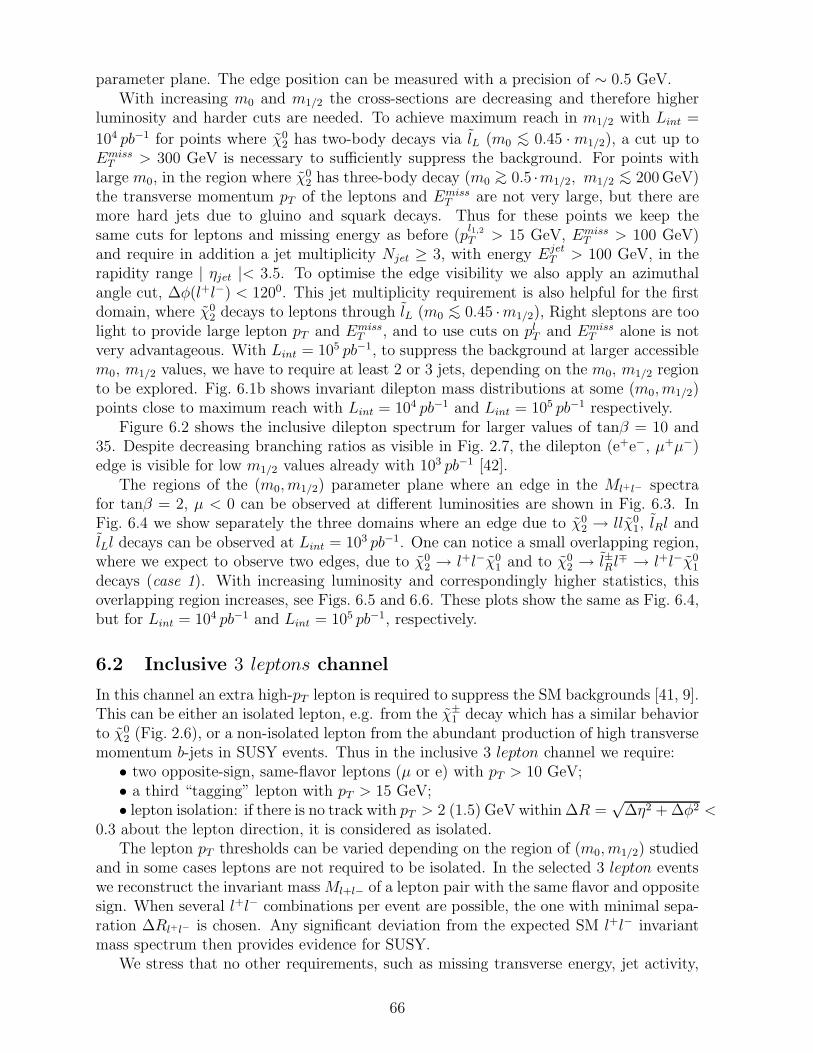
parameter plane. The edge position can be measured with a precision of ∼ 0.5 GeV.With increasing m0 and m1/2 the cross-sections are decreasing and therefore higher

luminosity and harder cuts are needed. To achieve maximum reach in m1/2 with Lint =

104 pb−1 for points where χ02 has two-body decays via lL (m0

<∼ 0.45 · m1/2), a cut up toEmiss

T > 300 GeV is necessary to sufficiently suppress the background. For points withlarge m0, in the region where χ0

2 has three-body decay (m0>∼ 0.5 ·m1/2, m1/2

<∼ 200 GeV)the transverse momentum pT of the leptons and Emiss

T are not very large, but there aremore hard jets due to gluino and squark decays. Thus for these points we keep thesame cuts for leptons and missing energy as before (p

l1,2

T > 15 GeV, EmissT > 100 GeV)

and require in addition a jet multiplicity Njet ≥ 3, with energy EjetT > 100 GeV, in the

rapidity range | ηjet |< 3.5. To optimise the edge visibility we also apply an azimuthalangle cut, ∆φ(l+l−) < 1200. This jet multiplicity requirement is also helpful for the firstdomain, where χ0

2 decays to leptons through lL (m0<∼ 0.45 ·m1/2), Right sleptons are too

light to provide large lepton pT and EmissT , and to use cuts on pl

T and EmissT alone is not

very advantageous. With Lint = 105 pb−1, to suppress the background at larger accessiblem0, m1/2 values, we have to require at least 2 or 3 jets, depending on the m0, m1/2 regionto be explored. Fig. 6.1b shows invariant dilepton mass distributions at some (m0, m1/2)points close to maximum reach with Lint = 104 pb−1 and Lint = 105 pb−1 respectively.

Figure 6.2 shows the inclusive dilepton spectrum for larger values of tanβ = 10 and35. Despite decreasing branching ratios as visible in Fig. 2.7, the dilepton (e+e−, µ+µ−)edge is visible for low m1/2 values already with 103 pb−1 [42].

The regions of the (m0, m1/2) parameter plane where an edge in the Ml+l− spectrafor tanβ = 2, µ < 0 can be observed at different luminosities are shown in Fig. 6.3. InFig. 6.4 we show separately the three domains where an edge due to χ0

2 → llχ01, lRl and

lLl decays can be observed at Lint = 103 pb−1. One can notice a small overlapping region,where we expect to observe two edges, due to χ0

2 → l+l−χ01 and to χ0

2 → l±Rl∓ → l+l−χ01

decays (case 1). With increasing luminosity and correspondingly higher statistics, thisoverlapping region increases, see Figs. 6.5 and 6.6. These plots show the same as Fig. 6.4,but for Lint = 104 pb−1 and Lint = 105 pb−1, respectively.

6.2 Inclusive 3 leptons channel

In this channel an extra high-pT lepton is required to suppress the SM backgrounds [41, 9].This can be either an isolated lepton, e.g. from the χ±

1 decay which has a similar behaviorto χ0

2 (Fig. 2.6), or a non-isolated lepton from the abundant production of high transversemomentum b-jets in SUSY events. Thus in the inclusive 3 lepton channel we require:

• two opposite-sign, same-flavor leptons (µ or e) with pT > 10 GeV;• a third “tagging” lepton with pT > 15 GeV;• lepton isolation: if there is no track with pT > 2 (1.5) GeV within ∆R =

√∆η2 + ∆φ2 <

0.3 about the lepton direction, it is considered as isolated.The lepton pT thresholds can be varied depending on the region of (m0, m1/2) studied

and in some cases leptons are not required to be isolated. In the selected 3 lepton eventswe reconstruct the invariant mass Ml+l− of a lepton pair with the same flavor and oppositesign. When several l+l− combinations per event are possible, the one with minimal sepa-ration ∆Rl+l− is chosen. Any significant deviation from the expected SM l+l− invariantmass spectrum then provides evidence for SUSY.

We stress that no other requirements, such as missing transverse energy, jet activity,

66

etc., are imposed in the inclusive 3 leptons channel. The price for this simplicity is adecrease of signal acceptance due to the requirement on the third lepton, and somewhathigher pT of leptons needed to sufficiently suppress the SM backgrounds. Thus thereis complementarity between this search which relies on lepton (e, µ) measurements andthe tracker for lepton isolation and momentum measurement, and the search, in inclusive2 leptons + Emiss

T channel which relies on lepton detection and overall calorimetry, HCALin particular, for Emiss

T measurement.The main SM sources of three leptons considered are production of WZ, tt, ZZ and

Zbb. The expected SM background to 3 leptons final states at an integrated luminosityof Lint = 104 pb−1 is shown in Fig. 6.7. Near the Z mass the main contribution comesfrom the WZ production, while tt production dominates at lower invariant masses.

Dilepton spectra for the mSUGRA “Point 4” (see Table 1.1), superimposed on the SMbackground, are shown in Fig. 6.8. The number of events corresponds to an integratedluminosity of Lint = 20 pb−1, i.e. just a few hours of initial LHC running. The pT

threshold on all three leptons is 15 GeV. In Fig. 6.8a no isolation requirement is applied,whereas in Fig. 6.8b the two leptons entering the dilepton mass distribution are isolated.The contribution from the SM background is negligible in the latter case. In both casesthe specific shape of the l+l− distribution, with its sharp edge, reveals χ0

2 production.At this mSUGRA point the χ0

2 has a three-body decay mode with a branching ratioB(χ0

2 → l+l− + χ01) = 0.32 (l = e, µ) and the masses are Mχ0

2= 97 GeV, Mχ0

1= 45 GeV.

The sharp edge is situated at the expected value of Mmaxl+l− = 52 GeV.

Figure 6.9 shows the Ml+l− distribution for mSUGRA “Point 1” (see Table 1.1) withan integrated luminosity of Lint = 104 pb−1. The pT thresholds for leptons are 15, 15, 30GeV and all three leptons are isolated. At this mSUGRA point the χ0

2 possesses a two-body decay mode with the branching ratio B(χ0

2 → lR+l) = 0.24. The sparticle masses areMχ0

2= 231 GeV, Mχ0

1= 122 GeV, MlR

= 157 GeV. The “edge” of the distribution is sit-

uated near 108 GeV, as expected. We define a signal significance as S = NS/√

NS + NB,where NS and NB are the numbers of signal and background events, respectively, in amass window below the edge. In this particular case signal and background events arecalculated in a mass window of 100 GeV< Ml+l− < 110 GeV, NS = 140 and NB = 39,resulting in signal significance of S = 10.5. NB consists of 18, 8, 11 and 2 events comingfrom WZ, tt, ZZ and Zbb production, respectively.

An example for the mSUGRA “Point 5” is shown in Fig. 6.10. The cuts are the sameas in the previous case. At this point χ0

2 has three-body decay modes with B(χ02 → l+l−+

χ01) = 0.06 and the masses are Mχ0

2= 124 GeV, Mχ0

1= 73 GeV. The observed value of

Mmaxl+l− is close to the expected value of 51 GeV. In a mass window of 20 GeV< Ml+l− < 52

GeV the numbers of signal and background events are NS = 588 and NB = 402 giving asignal significance of S = 19. NB consists of 113, 139, 65 and 85 events coming from WZ,tt, ZZ and Zbb production, respectively.

By the same procedure the mSUGRA parameter space (m0, m1/2) was scanned forfixed tanβ = 2, A0 = 0 and µ < 0 [9]. Figures 6.11a-c show the Ml+l− distributions forthree different mSUGRA points with the optimal thresholds on lepton pT and isolationrequirement in inclusive 3 lepton events. Generally, with increasing m1/2 the observationof the edge becomes more difficult due to the rapidly decreasing gluino and squark produc-tion cross-sections. Nonetheless, this spectacular structure in the dilepton mass spectrumreflecting χ0

2 decays, may be among the first ways through which presence of SUSY mayreveal itself. It may appear with very modest statistics, in a non-sophisticated analysis

67

and with only modest demands on detector performance. The precision for “edge” mea-surement in most of the region, where it is detectable is expected to be <∼ 0.5 GeV. Note,that the Z peak seen in Figs. 6.8-6.11 serves as an overall calibration signal; it allows tocontrol the mass scale as well as the production cross-section.

Asking for a statistical significance S > 7 with at least 40 signal events calculatedin a mass interval > 10 GeV below the edge the domain explorable with an integratedluminosity of Lint = 104 pb−1 is shown in Fig. 6.12. It entirely covers the cosmologicallyprefered region 0.15 < Ωh2 < 0.4 [37]; here Ω is the ratio of the relic particle density tocritical density, h is the Hubble constant scaling factor and bounds are obtained assumingχ0

1 is the cold dark matter particle in the mixed dark matter scenario for the Universe,varying h over the allowed range 0.5 < h < 0.8.

For some regions of mSUGRA parameter space Mmaxl+l− is close to, or even hidden by

the Z signal. At these points the accuracy of an edge measurement is ∼10 GeV. Applyinga cut on missing transverse energy (and/or jets) suppresses the contribution from the SMZ production, improving signal visibility.

6.3 Inclusive 3 leptons + EmissT channel

With increasing m1/2, gluino and squark masses increase and the missing transverse energybecomes larger. Requiring Emiss

T > 200 (300) GeV rejects most of the SM backgroundleaving a big fraction of signal events. Figures 6.11d-e show the dilepton spectra forvarious mSUGRA points in the 3 lepton + Emiss

T final states. In the region of highm1/2, dileptons are mainly produced in the cascade decays of χ0

2. The third, “tagging”lepton predominantly comes from χ±

1 which also has cascade leptonic decays. Thus in thisregion of parameter space a large fraction of 3 lepton + Emiss

T events are in fact inclusivelyproduced χ±

1 χ02 pairs. Therefore all three leptons are required to be isolated. The lepton

pT thresholds are chosen to be quite asymmetric: 50, 25, 10 GeV, to account for thecascade nature of the χ0

2 and χ±1 decays. The region of mSUGRA parameter space, where

the χ02 is observable from the dilepton mass distribution shape in the 3 lepton + Emiss

T

events at Lint = 105 pb−1 luminosity is shown in Fig. 6.12 [9]. The reach extends up tom1/2 ∼ 900 GeV and a detectable edge is seen as long as σ·B >∼ 10−2 pb (see Fig. 2.5).

We conclude that• Observation of an edge in the dilepton invariant mass spectrum reflects the produc-

tion of χ02 and hence establishes the existence of SUSY; this observation in some cases is

possible with very small statistics and could be the first evidence for SUSY at LHC.• With no great demand on detector performance a large portion of mSUGRA parame-

ter space including the cosmologically prefered domain can be explored with an integratedluminosity as low as Lint = 104 pb−1.

68

a)

c) d)

(200,160)

(110,187) (60,230)

b)

(500,120)

Figure 6.1a: Invariant mass distribution of two same-flavor, opposite-sign leptons at var-ious (m0, m1/2) points for tanβ = 2, µ < 0 with Lint = 103 pb−1. SM background is alsoshown (dashed line).

69

(100,500) (2000,160)

L =10 pb 4 -1

intL =10 pb

4 -1

int

L =10 pb 5 -1

int

(350,800)

a) b)

c)

Figure 6.1b: Invariant mass distribution of two same-flavor, opposite-sign leptons at(m0, m1/2) points close to the experimental reach at corresponding luminosities Lint = 104

pb−1 and 105 pb−1 for tanβ = 2, µ < 0. SM background is also shown (dashed line).

70

Figure 6.2: Invariant mass distribution of two same-flavor, opposite-sign leptons at variousm0, m1/2, tanβ and µ points for Lint = 103 pb−1. SM background is also shown.

71

104 pb-1

105 pb-1

900

800

700

600

500

400

300

200

100

0 50 100 150 200 250 300 350 400 450 500

m0 (GeV)

m1

/2 (G

eV

) tanβ = 2, A0 = 0,µ < 0

D_

D_

10

61

n

TH

LEP2 + Tevatron (sparticle searches)

TH

EX

103 pb-1

Figure 6.3: Observability of edges in invariant dilepton mass distribution with luminosities103 pb−1 (dashed line), 104 pb−1 (solid line) and 105 pb−1 (dashed-dotted line). Also shownare the explorable domain in sparticle searches at LEP2 (300 pb−1) and the Tevatron (1fb−1), theoretically and experimentally excluded regions.

72

LEP2 + Tevatron

900

800

700

600

500

400

300

200

100

0 50 100 150 200 250 300 350 400 450 500

m0 (GeV)

m1

/2

(Ge

V)

tanβ = 2, A0 = 0,µ < 0

D_

D_

10

64

n

TH

TH EX

103 pb-1

χ0 ~2 χ0 ~

1+ -

χ0 ~ ~

2 R

χ0 ~ ~2 L

Figure 6.4: Domains where the observed edge in the Ml+l− distribution is due to thedecays χ0

2 → l±L l∓ → χ01l

+l− (solid line), χ02 → l±R l∓ → χ0

1l+l− (dashed-dotted line),

χ02 → χ0

1l+l− (dashed line), Lint = 103 pb−1.

73

104 pb-1

900

800

700

600

500

400

300

200

100

0 50 100 150 200 250 300 350 400 450 500

m0 (GeV)

m1

/2 (G

eV

)

D_

D_

10

62

n

TH

TH EX

LEP2 + Tevatron

tanβ = 2, A0 = 0,µ < 0

χ0 ~ ~2 L

~R

χ0 ~2

χ0 ~2

χ0 ~1

+ -


2 → l±L l∓ → χ01l



χ02 → χ0


74

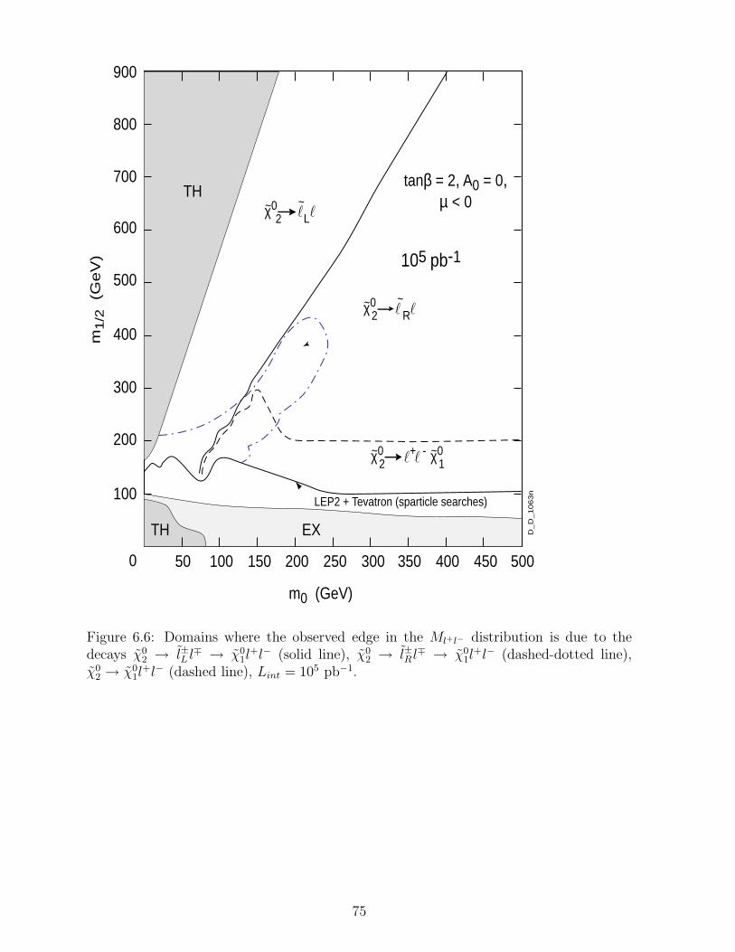
900

800

700

600

500

400

300

200

100

0 50 100 150 200 250 300 350 400 450 500

m0 (GeV)

m1

/2 (G

eV

)

D_

D_

10

63

n

TH

TH EX

105 pb-1

LEP2 + Tevatron (sparticle searches)

tanβ = 2, A0 = 0,µ < 0χ0 ~ ~

2 L

χ0 ~ ~2 R

χ0 ~2 χ0 ~

1+ -


2 → l±L l∓ → χ01l



χ02 → χ0


75

0

100

200

300

400

500

600

0 20 40 60 80 100 120 140 160

Ml+l- (GeV)

Eve

nts

/ 2 G

eVLint=104 pb-1

pT1,2,3>15 GeV

No tracks withpT>2 GeV in ∆R<0.3

Three isolated lepton events from SM

W Zt t

_

Z ZZ b b

_

W Z

Figure 6.7: Expected Standard Model background in inclusive 3 lelpton final state.

76

0

20

40

60

80

100

120

140

160

180

200

0 20 40 60 80 100 120 140 160

Ml+l- (GeV)

Eve

nts

/ 2 G

eV

Lint=20 pb-1

pT1,2,3>15 GeV

mSUGRA Point 4m0=200 GeV, m1/2=100 GeV, tanβ=2, A0=0, µ<0

M(χ~0) = 45 GeV

M(χ~0) = 97 GeV

1

2

Expected Mllmax = 53 GeV

SUSY + SM

SM

0

10

20

30

40

50

60

70

80

90

100

0 20 40 60 80 100 120 140 160

Ml+l- (GeV)

Eve

nets

/ 2

GeV

Lint=20 pb-1

pT1,2>15 GeV

No tracks with

pT>2 GeV in ∆R<0.3

pT3>15 GeV

SUSY + SM

Figure 6.8: Expected l+l− mass spectrum for mSUGRA Point 4: m0 = 200 GeV, m1/2 =100 GeV, tanβ=2, A0 = 0 and µ < 0. a) Leptons with pT > 15 GeV in |η| < 2.4 areconsidered; b) as in previous case, but two leptons which enter invariant mass spectrumare required to be isolated. The dotted histogram corresponds to the SM background.

77

0

20

40

60

80

100

120

140

0 20 40 60 80 100 120 140 160

Ml+l- (GeV)

Eve

nts

/ 2 G

eV

Lint=104 pb-1

pT1,2>15 GeV

pT3>30 GeV

No tracks withpT>2 GeV in ∆R<0.3

mSUGRA Point 1

m0=100 GeV, m1/2=300 GeV, tanβ=2.1, A0=300, µ>0

M(χ~0) = 122 GeV

M(χ~0) = 231 GeV

M(l~

R) = 157 GeV


1

2

Figure 6.9: Expected l+l− mass spectrum for mSUGRA Point 1: m0 = 100 GeV,m1/2 = 300 GeV, tanβ=2.1, A0 = 300 GeV and µ > 0. The dotted histogram correspondsto the SM background.

0

20

40

60

80

100

120

140

0 20 40 60 80 100 120 140 160

Ml+l- (GeV)

Eve

nts

/ 2 G

eV

Lint=104 pb-1

pT1,2>15 GeV

pT3>30 GeV

No tracks with

pT>2 GeV in ∆R<0.3

mSUGRA Point 5

m0=800 GeV, m1/2=200 GeV, tanβ=10, A0=0, µ>0

M(χ~ 0) = 72 GeV

M(χ~ 0) = 124 GeV


1

2

Figure 6.10: Expected l+l− mass spectrum for mSUGRA Point 5: m0 = 800 GeV,m1/2 = 200 GeV, tanβ=10, A0 = 0 and µ > 0. The dotted histogram corresponds to theSM background.

78

0

20

40

60

0 50 100 150 200Ml+l- (GeV)

Eve

nts

/ 2 G

eV a)Lint=103 pb-1

pT > 15, 15, 15 GeV

Isolation

m0=400 GeV, m1/2=150 GeV

0

20

40

60

80

0 50 100 150 200Ml+l- (GeV)

Eve

nts

/ 4 G

eV b)

m0 = 1800 GeV, m1/2= 100 GeV

pT > 15, 15, 15 GeV

Isolation

Lint = 103 pb-1

0

20

40

60

80

100

0 50 100 150 200Ml+l- (GeV)

Eve

nts

/ 2 G

eV c)Lint=104 pb-1

pT > 15, 15, 30 GeV

Isolation

m0=100 GeV, m1/2=400 GeV

0

5

10

15

20

25

0 100 200 300 400Ml+l- (GeV)

Eve

nts

/ 10

GeV

d)

m0 = 190 GeV, m1/2= 450 GeV

pT > 50, 25, 10 GeV

Isolation

ET miss

> 200 GeV

Lint = 104 pb-1

0

10

20

30

40

50

0 100 200 300 400Ml+l- (GeV)

Eve

nts

/ 25

GeV e)

m0 = 100 GeV, m1/2= 500 GeV

pT > 50, 25, 10 GeV

Isolation

ET miss

> 200 GeV

Lint = 104 pb-1

0

20

40

60

0 100 200 300 400Ml+l- (GeV)

Eve

nts

/ 10

GeV f)

m0 = 250 GeV, m1/2= 600 GeV

pT > 50, 25, 15 GeV

isolation

ET miss

> 300 GeV

Lint = 105 pb-1

0

10

20

30

0 100 200 300 400Ml+l- (GeV)

Eve

nts

/ 10

GeV g)

m0 = 150 GeV, m1/2= 700 GeV

pT > 50, 25, 10 GeV

isolation

ET miss

> 300 GeV

Lint = 105 pb-1

0

10

20

30

0 100 200 300 400Ml+l- (GeV)

Eve

nts

/ 25

GeV

h)

m0 = 200 GeV, m1/2= 800 GeV

pT > 50, 25, 10 GeV

Isolation

ET miss

> 300 GeV

Lint = 105 pb-1

0

10

20

30

0 100 200 300 400Ml+l- (GeV)

Eve

nts

/ 25

GeV

i)

m0 = 200 GeV, m1/2= 900 GeV

pT > 50, 25, 10 GeV

Isolation

ET miss

> 300 GeV

Lint = 105 pb-1

Figure 6.11: Dilepton mass spectrum for mSUGRA Point from different (m0, m1/2)regions in inclusive 3 leptons and 3 leptons + Emiss

T channels. Contribution from SM back-ground is shown with dashed histogram. The other mSUGRA parameters are: tanβ=2,A0 = 0 and µ < 0.

79

100

200

300

400

500

600

700

800

900

1000

100 200 300 400 500 600 700 800 900 1000

m0 (GeV)

m1/

2

(G

eV)

mSUGRA parameters: tanβ=2, A0=0, µ<0

T

H

E

O

R

Y

E X P E R I M E N T

Ωh2 = 1

Ωh20.4

0.15 .. . . . .. . . . . ...

.

. . ... ... . .. .

. . .. . .. .

3 lepton, Lint = 104 pb-1

3 lepton + ETmiss, Lint = 105 pb-1

Figure 6.12: Explorable region of mSUGRA in inclusive 3 leptons and 3 leptons +Emiss

T channels at Lint = 104 pb−1 and Lint = 105 pb−1, respectively. Shaded regions areexcluded by theory (m0

<∼ 80 GeV) and experiment (m1/2<∼ 90 GeV). The cosmologically

preferable region 0.15 < Ωh2 < 0.4 is also given. Simulated mSUGRA Points are shownas well.

80


search for sleptons

The previous two sections described inclusive searches suitable for the discovery of SUSY.We now focus on more exclusive final states where individual SUSY particles may betargeted.

The slepton production and decay features described in section 2.2 give rise to severalinteresting experimental signatures. In this study we concentrate on the possibilitiesto detect a slepton signal in the simplest event topology two leptons + Emiss

T + no jetstaking into account all possible SUSY and SM contributions to this topology [6]. Theobservability of the slepton signal is evaluated summing all flavors and all productionmechanisms which contribute to the two same-flavor opposite-sign leptons + Emiss

T + nojets final state. Evidence for a slepton signal will be judged from an excess over fullSUSY and SM backgrounds, but presence of a SUSY signal will be estimated from anexcess over only the expected SM backgrounds.

The main expected Standard Model background is tt production, with both W ’s de-caying to leptons, or one of the leptons coming from a W decay and the other from theb-decay of the same t-quark. The other SM backgrounds considered are Wtb, WW, WZ, bband ττ -pair production, with decays to electrons and muons. The assumed cross-sectionsare: σtt=660 pb (Mt = 175 GeV), σWtb=160 pb, σWW=70 pb, σWZ=26 pb, σττ=7.5 pb,σbb=5000 pb (pb

T ≥ 100 GeV). No forcing of decay modes is implemented.As internal SUSY backgrounds we consider processes qq, gq, gg which, through cascade

decays with jets outside the acceptance, below the detection threshold, or lost in cracks,can also lead to two leptons + Emiss

T + no jets final states. The χ±1 χ0

2 process for exampleleads mainly to three-lepton final states. However, it can also contribute to two-leptonfinal states if one of the leptons is outside the acceptance or is misidentified, or if onlythe χ0

2 decays to leptons, and jets from the χ±1 decay are not reconstructed.

We perform a mapping of the mSUGRA parameter space to determine the optimalset of signal selection cuts in the various regions of (m0, m1/2) plane, taking into accountevent kinematical properties, and evaluate the observability of the signal. An importantissue is to find out if there is a gap in slepton detectability, especially in the low mass rangeat the junction between the observability domains at LEP2, Tevatron and the LHC. ThemSUGRA-parameter space points (m0, m1/2) probed are shown in Fig. 7.1. This figurealso shows the masses mlL

and mχ01

at each point, the theoretically and experimentally

excluded regions and the explorable domains in sparticle searches at LEP2 (300 pb−1)and the Tevatron (1 fb−1).

Taking into account the signal and background event topologies the following kine-matical variables are found useful for slepton signal extraction:

i) for leptons:•pl

T -cut on leptons and lepton isolation (Isol), which is defined here as the calori-metric energy flow around the lepton in a cone of ∆R < 0.5 divided by the lepton energy;

• effective mass of two same-flavor opposite-sign leptons, to suppress WZ andpotential ZZ backgrounds by rejecting events in a mZ ± δMZ band;

• ∆φl+l− , the relative azimuthal angle between two same-flavor opposite-sign lep-tons;

81

ii) for EmissT :

• EmissT -cut,

•∆φ(EmissT , l+l−), the relative azimuthal angle between Emiss

T and vector sum ofthe transverse momenta of the two leptons.

iii) for jets:• “jet veto”-cut: no jet with Ejet

T lower than certain threshold, in some rapidityinterval, typically | ηjet |< 4.5.

The data selection cuts based on these variables are separately optimised in variousparts of the explored parameter space [6]. For illustration we show some typical distribu-tions. Figure 7.2 shows the Emiss

T distributions for signal and various SUSY backgroundsat two (m0, m1/2) points, one with low and one with high slepton masses. The hardestspectra in both figures correspond to qq production and the softest ones to chargino-neutralino production. This figure also shows the main SM backgrounds. For low sleptonmass there is no big difference in shape between signal and SM-background spectra, thusit is not very advantageous to apply a hard Emiss

T cut.Figure 7.3 shows the ∆φ(Emiss

T , l+l−) distribution at the point from the low slepton

mass region, m0 = 86 GeV, m1/2 = 85 GeV, after pl1,2

T , cuts on lepton isolation and EmissT .

The internal SUSY and SM backgrounds are still much larger in magnitude than thesignal. Keeping only events with large relative azimuthal angles significantly improvesthe signal to background ratio.

Figure 7.4 illustrates the expected rejection factors which can be obtained by a “cen-tral” jet veto for two Ejet

T thresholds as a function of jet acceptance at point m0 = 86 GeV,m1/2 = 85 GeV. Signal acceptance decreases slightly with increasing |ηjet| of the jet vetoregion, whilst for sufficient rejection of SUSY and SM backgrounds (tt) it is important tohave calorimetric coverage up to | η |= 3.5 − 4.0. The rejection power against g, q and ttimproves by a factor of 1.5-1.8 with increasing coverage from | η |< 2.5 to | η |< 3.5. Toachieve significant background rejection reliable jet detection down to ET ≈ 30 GeV isalso essential.

Figure 7.5 shows the ∆φl+l− distribution for the main SM and SUSY backgroundsand events with direct slepton production at the same point m0 = 86 GeV, m1/2 = 85GeV. For the signal, small ∆φl+l− events come from νl

¯νl production whilst events withlarge ∆φl+l− are due to charged slepton production. The main contribution to the sleptonsignal from χ±

1 χ02 production in the two-lepton final state comes from decays of χ0

2, thusthe distribution of these events also peaks at low relative azimuthal angles. All processeswhich go through χ0

2 decays to leptons, including g, q contributions have almost the sameshape ∆φ-distribution. In some parts of parameter space it may be more advantageous tokeep only events with large ∆φl+l−, which rejects most of the internal SUSY backgrounds.However, this cut also eliminates direct ν production events and the indirect contributionfrom χ0

2 decays. Only χ±1 χ±

1 events with leptons coming from different parent charginossurvive as a significant SUSY background.

To extract the slepton signal at points from domain I in Fig. 2.8b (m0>∼ 0.5m1/2)

with mlL∼ 100 GeV, just beyond of the LEP2 and Tevatron sparticle reaches, where the

SM backgrounds are dominant, the selection Set 0 is appropriate at low luminosity. TheSet 0′ is better adapted for the points from domain II (m0

<∼ 0.5m1/2), see Table 7.1.The expected number of signal and background events in this particular difficult region,

after all cuts, is shown in Table 7.2. We also give the signal to background ratio and

82

Table 7.1. Low mass slepton selection criteria

Set 0 Set 0′

Isol < 0.1 0.1

pl1,2

T > (GeV) 20 20Emiss

T > (GeV) 50 50∆φ(Emiss

T , l+l−) > (0) 160 160No jets in |ηjet| < 4.5

with EjetT > (GeV) 30 30

No Mll ∈ MZ ± δm (GeV) 91 ± 5 91 ± 5∆φl+l− > (0) 130 no cut

significance for slepton production and the same quantities for overall SUSY production.It is clear that in this domain of parameter space, the slepton (ml ∼ 100 GeV) con-

tribution to the finale state topology is only a modest one. The slepton signal can bedetected from an excess of events over background expectations, but not from any par-ticular kinematical feature. The S/B is about 0.3. Of the SM backgrounds, WW is thelargest and essentially irreducible, tt and Wtb are comparable and at the same level as thesignal after hard jet veto cuts. The main SUSY background is due to χ±

1 χ∓1 . For the point

m0 =85 GeV, m1/2 =86 GeV, from domain I, the total number of signal events NSl−totS is

just due to direct slepton production, i.e. there are no indirect slepton contributions, butthere are additional SUSY contributions to this topology.

For points with m0<∼ 0.5m1/2 (domain II), no ∆φl+l− cut is applied so as to take

advantage of all SUSY processes contributing to slepton production. NSl−totS in this case

has contributions from both direct and indirect slepton production. The contributionfrom indirect slepton production is comparable to the direct one and helps to reach a 5σsignificance level needed for slepton signal visibility. In this region the only backgroundsare SM contributions. The irreducible WW is still the dominant, and Wtb increasessignificantly.

To achieve the highest mass reach with 104 pb−1 a somewhat harder set of cuts isappropriate, (Set 1 in Tab. 7.3). The reach in parameter space with 104 pb−1 is shownin Fig. 7.6; it corresponds to left-slepton masses up to ≃ 160 − 180 GeV, i.e. well abovethe LEP2 reach (ml

<∼ 95 GeV). In the region m0<∼ 0.5m1/2 (domain II) the total slepton

signal coincides with the overall SUSY signal, but for points from region m0>∼ 0.5m1/2

(domain I) the additional SUSY processes contribute to the overall SUSY signal, but notto the slepton signal.

With 105 pb−1, a significantly higher slepton mass range becomes accessible. Theaverage lepton transverse momentum and missing energy increasing with ml become sig-nificantly harder than for the main backgrounds. Harder kinematical cuts are thereforepreferable. Slepton production becomes the main and ultimately the dominant contribu-tion to this topology. We use four main different sets of cuts (Table 7.3) optimised fordifferent regions of (m0, m1/2) parameters space. These sets are chosen taking into ac-count the mass relations, production mechanisms and decay patterns discussed in section2.2.

“Set 2” is used to explore the mlL∼ 200 GeV domain. The tt, Wtb backgrounds are

83

Table 7.2: Expected number of direct (NSl−dirS ) and indirect (NSl−indir

S ) slepton signalevents, and SM (NSM

B ) and SUSY background (NSUSYB ) events, after cuts, at 104 pb−1.

The signal to background ratio NSl−totS /N tot

B and significance of slepton signal

NSl−totS /

√

NSl−totS + N tot

B are also given; the same for overall SUSY signal NSUSYS /NSM

B ,

NSUSYS /

√

NSUSYS + NSM

B .

(m0, m1/2) → (86,85) (4,146) (20,160) (20,190)

Set 0 Set 0′ Set 0′ Set 0′

ll 323 315 319 214

χ±1 χ0

2 14 45 48 40χ±

1 χ∓1 46 253 217 168

gq 13 8 − −qq 35 6 − −gg 0 2 − −

WW 454 1212 1212 1212Wtb 163 577 577 577tt 345 574 574 574

WZ 15 43 43 43ττ 15 15 15 15

NSl−dirS 323 315 319 214

NSl−indirS − 314 265 208

NSUSYS 431 629 584 422

NSUSYB 108 − − −

NSMB 992 2421 2421 2421

NSlS /N tot

B 0.3 0.26 0.24 0.17

NSl−totS /

√

NSl−totS + N tot

B 8.6 11.4 10.7 7.9

NSUSYS /NSM

B 0.4 0.26 0.24 0.17

NSUSYS /

√

NSUSYS + NSM

B 11.4 11.4 10.7 7.9

suppressed with hard cuts on pT of the leptons, EmissT and the “jet veto”. This last cut

eliminates entirely the backgrounds from strongly interacting sparticles. We keep eventswith small relative azimuthal angle between the leptons ∆φl+l− mainly to improve therejection of SM backgrounds, and to eliminate χ±

1 χ∓1 production when it is necessary. The

slepton S/B ratio is about 1.“Set 3” is used for mlL

∼ 300 GeV at points with m0<∼ 0.5m1/2, whilst for points

with m0<∼ 0.5m1/2 “Set 4” is more appropriate, as the cross-sections are smaller. Fur-

thermore, there is no source of indirect slepton production. “Set 4” is also used toexplore the slepton mass range 300 GeV <∼ mlL

<∼ 350 GeV. “Set 4′” is used for masses350 GeV <∼ mlL

<∼ 440 GeV, and “Set 4′′” for mlL>∼ 440 GeV. Details of the signal and

background contribution at each simulated point can be found in [6].Figure 7.6 summarizes the results of this study. At each point investigated the expected

slepton signal significance, nσ, and the signal to background ratio (in parentheses) is given,

84

Table 7.3. High mass slepton selection criteria

Set 1 Set 2 Set 3 Set 4 Set 4′

Set 4′′

Isol < 0.1 0.1 0.1 0.1 0.1 0.03

pl1,2

T > (GeV) 20 50 50 60 60 60

EmissT > (GeV) 100 100 120 150 150 150

∆φ(EmissT , l+l−) > (0) 150 150 150 150 150 150

No jets in |ηjet| < 4.5

with EjetT > (GeV) 30 30 30 45 45 45

No Mll ∈ MZ ± δm (GeV) 91 ± 5 91 ± 5 91 ± 5 91 ± 5 91 ± 5 91 ± 5

∆φl+l− < (0) 130 130 130 130 140 130

for an integrated luminosity of 105 pb−1. The 5σ reach is shown as well. Recall that theselection procedure has been optimised in terms of signal significance NS/

√NS + NB to

investigate the maximum slepton mass reach, and not in terms of sample purity (i.e.S/B ratio). The reason is that if SUSY were found at Fermilab where g/q masses up to<∼ 400− 450 GeV can be probed, sleptons can be probed at the Tevatron and LEP2 onlyup to a mass of ml

<∼ 100 GeV, thus the main task of LHC would be to explore sleptonspectroscopy, with masses up to mq/g <∼ 400 GeV. Figure 7.7 shows the same informationas Fig. 7.6, but in terms of left slepton and lightest neutralino LSP masses. The domainthat can be explored extends up to mlL

∼ 340 GeV for all allowed mLSP (< 200 GeV),and up to mlL

∼ 340 − 440 GeV only if mLSP >∼ (0.45 − 0.6) · mlLfor a given mlL

. Themass reach for right sleptons is up to 340 GeV. As the main SM background is WWproduction, to study the stability of our results we assumed a 50% uncertainty in theWW cross-section. Figure 7.8 shows how much the 5σ reach boundary would be modifiedif the WW cross-section were twice as large as predicted by PYTHIA.

A very interesting aspect of slepton searches at LHC from the cosmological point ofview is that, in this topologically simplest channel, the explorable domain for 105 pb−1

almost coincides with the regions of parameter space where the LSP would be cosmo-logically relevant (Figs. 7.6 and 7.7). The boundaries for the domains we can probe inslepton searches and the neutralino dark matter Ωh2 density contours have shapes similarto slepton isomass curves as both are largely determined by slepton masses. In particular,neutralino annihilation is governed by slepton exchange with σann ∼ 1/m4

l. Too large a

slepton mass would induce too small an annihilation cross-section and thus too large arelic density which would overclose the Universe. The Ωh2 range prefered by mixed darkmatter scenarios is for 0.15 <∼ Ωh2 <∼ 0.4 (with the Hubble scaling constant 0.5 <∼ h2 <∼0.8) which corresponds to a slepton mass range 100 GeV <∼ ml

<∼ 250 GeV, (see [11], [37].)We conclude that to search for direct production of sleptons the most appropriate

channel is 2 leptons+ EmissT and no jets. In regions of low m0, m1/2, just beyond the

sparticle reaches at LEP2 and the Tevatron, the slepton signal can be detected, but thesearch will be difficult as l is not the dominant contribution to this final state. In signifi-cant parts of the explorable (m0, m1/2) space, however, direct slepton pair production isthe main contribution to this final state, with non-negligible contributions from indirectproduction too, mostly through χ±

1 , χ02. The inclusion of this indirect slepton production

improves the mass reach. With 104 pb−1 luminosity, CMS is sensitive up to mlL<∼ 160

85

GeV. With 105 pb−1 luminosity the reach extends up to mlL∼ 340 GeV for all allowed

mLSP (< 200 GeV), and up to mlL∼ 340−440 GeV if mLSP ∼ (0.45−0.6)·mlL

for a givenmlL

. Throughout the domain where the slepton signal should be detectable, it is alwayscontaminated by backgrounds. The dominant background is always WW production. Inthe mlL

∼ 100 GeV domain the WW background exceeds the number of signal events,whilst for mlL

>∼ 200 GeV the number of background events is comparable or smaller thanthe expected number of signal events. The “jet veto” cut effectively eliminates the g, qbackgrounds, but also the potentially important indirect slepton production from g andq. This issue requires a separate study.

In the region m0<∼ 0.45 ·m1/2 sleptons decay directly into the LSP and sneutrinos thus

decay invisibly, ν → χ01ν. In this portion of parameter space only charged sleptons can

be detected. As right sleptons are also significantly lighter than left ones they are mostlyeliminated by the hard selection cuts needed to suppress the backgrounds, so mainly leftsleptons are present in the final event sample. Left sleptons will thus be detectable in theentire region where a slepton signal is seen, whilst right sleptons will be detectable mainlyin domain m0

>∼ 0.45 · m1/2. Sneutrinos will contribute to this final state only in a verylimited area with m1/2

<∼ 160 GeV and m0<∼ 150 GeV.

The search for sleptons is important and significant, as LEP2 and the Tevatron canonly explore the slepton mass range up to mlL

≃ 100 GeV. The domain of (m0, m1/2)parameter space explorable through this simplest experimental channel, with two same-flavor, opposite-sign leptons + Emiss

T + no jets, covers almost the entire domain of param-eter space where SUSY is plausible in general terms (minimal fine-tuning) and covers allof the parameter space where SUSY would be of cosmological significance (at least fortanβ = 2, A0 = 0, µ < 0), with > 104pb−1 of integrated luminosity.

86

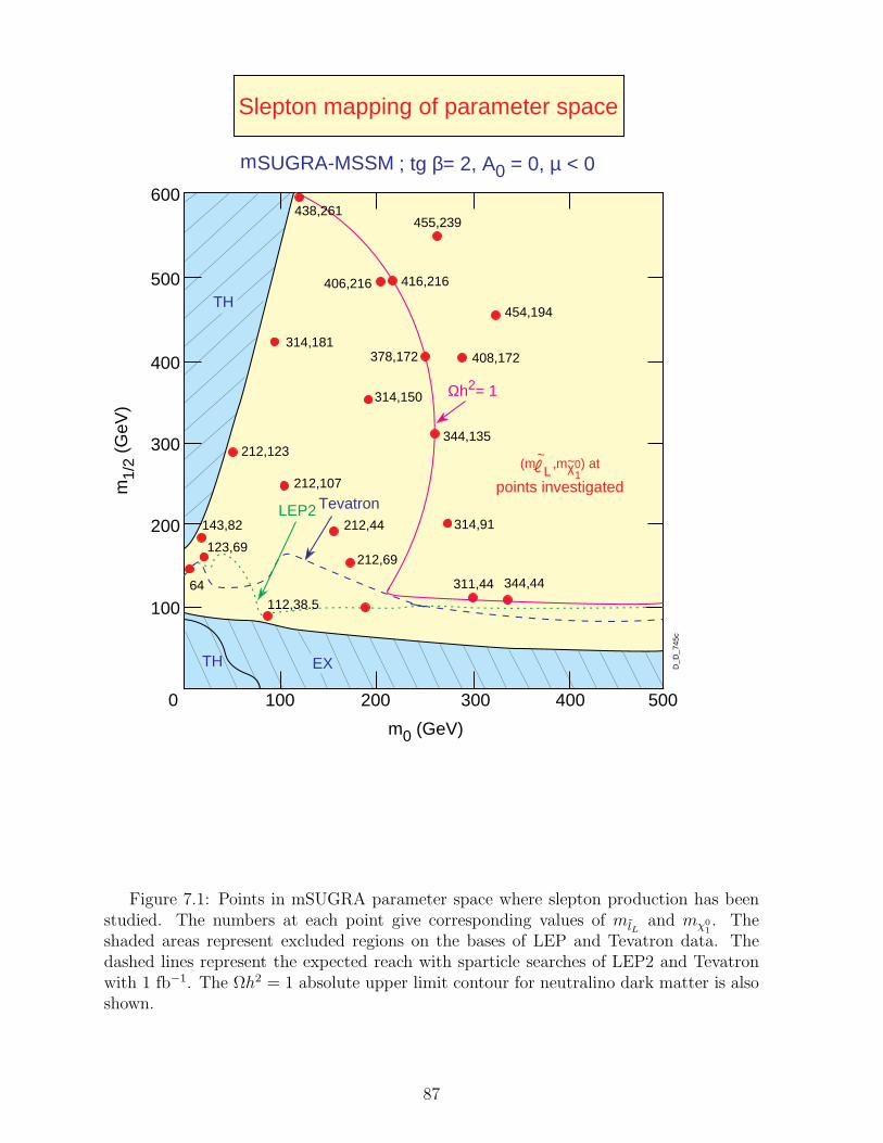
Ωh2= 1

TevatronLEP2

TH

TH

EX

0 100 200 300 400 500

100

200

300

400

500

600

m0 (GeV)

m1/

2 (G

eV)

D_D

_745

c

SUGRA-MSSM

Slepton mapping of parameter space

314,181

314,150

212,123

143,82

123,69

314,91

; tg β= 2, A0 = 0, µ < 0m

438,261455,239

406,216 416,216

454,194

408,172

344,135

378,172

311,44 344,44

212,107

212,44

212,69

112,38.564

points investigated

(mL

~ ~,mχ0) at1

Figure 7.1: Points in mSUGRA parameter space where slepton production has beenstudied. The numbers at each point give corresponding values of mlL

and mχ01. The

shaded areas represent excluded regions on the bases of LEP and Tevatron data. Thedashed lines represent the expected reach with sparticle searches of LEP2 and Tevatronwith 1 fb−1. The Ωh2 = 1 absolute upper limit contour for neutralino dark matter is alsoshown.

87

E distributions at points:T

miss

m = 86 GeV, m = 85 GeV:0 1/2

ml

L

~ = 112 GeV, ml

R

~ = 98 GeV,

mν~ = 93 GeV

m = 97 GeV, m = 420 GeV:0 1/2

ml

L

~ = 314 GeV, ml

R

~ = 192 GeV,

mν~ = 308 GeV

tt–

q~q~ 0.6

a) b)

c)

Figure 7.2: EmissT distribution for slepton signal (DY production), SUSY backgrounds

(g, q, χ±1 χ0

2) at two parameter space points: a) m0 = 86 GeV, m1/2 = 85 GeV, b) m0 = 97GeV, m1/2 = 420 GeV and c) the main SM backgrounds (WW, tt).

88

7000

6000

5000

4000

3000

2000

1000

0 20 40 60 80 100 120 140 160180

Signal

qq - SUSY bkgd~~

Lint = 104 pb-1

t t - SM bkgd-

∆ϕ (Emiss, )+ -

tD

_D_1

095.

n

Num

ber

of e

vent

s(86,85)

Figure 7.3: Relative azimuthal angle between EmissT and the resulting dilepton mo-

mentum for the slepton signal and main SM and SUSY backgrounds in 2leptons + EmissT

+ nojets final states.

89

gq, gg,qq (86,85)

80

60

40

20

02 32.5 43.5 4.5

No jets with Et >

5

30 GeV35 GeV

SU

SY

- r

ejec

tion tt

20

15

10

5

02 32.5 43.5 4.5 5

tt -

reje

ctio

n

1

0.8

0.6

0.4

0.2

02 32.5 43.5 4.5 5

IηjetI

D_D

_101

1.n1

Acceptance of signal

after JET VETO

~~

Sig

nal a

ccep

tanc

e

~~ ~~ ~~

(86,85)

Figure 7.4: Rejection factors a) for internal SUSY backgrounds, b) for SM backgroundsby central “jet veto”, and c) slepton signal acceptance, as a function of jet rapidityacceptance | ηjet | and for two jet detection thresholds.

90

m = 86 GeV, m = 85 GeV:0 1/2

ml

L

~ = 112 GeV, ml

R

~ = 98 GeV, mν~ = 93 GeV

two isolated leptons,

P >20 GeV, ET

Events with

lT

miss>50 GeV,

χ~±

1χ~0

2

Relative azimuthal angle between the two leptons

∆ϕ(E , ll) > 160miss

T

o

lL,R~

lL,R~

χ 10l

χ 10l

ν~

χ 0

1ν

ν

χ 0

2ν

~

χ 0

1ll

~

~

~

~

~

SUSY

SM

a)

b)

Figure 7.5: Relative azimuthal angle between two same-flavor opposite-sign leptons atone point on parameter space, a) for the various contributions to the SUSY slepton signaland for a SUSY background (χ±

1 χ02), and b) for the main SM backgrounds, in 2leptons +

EmissT + no jets final states.

91

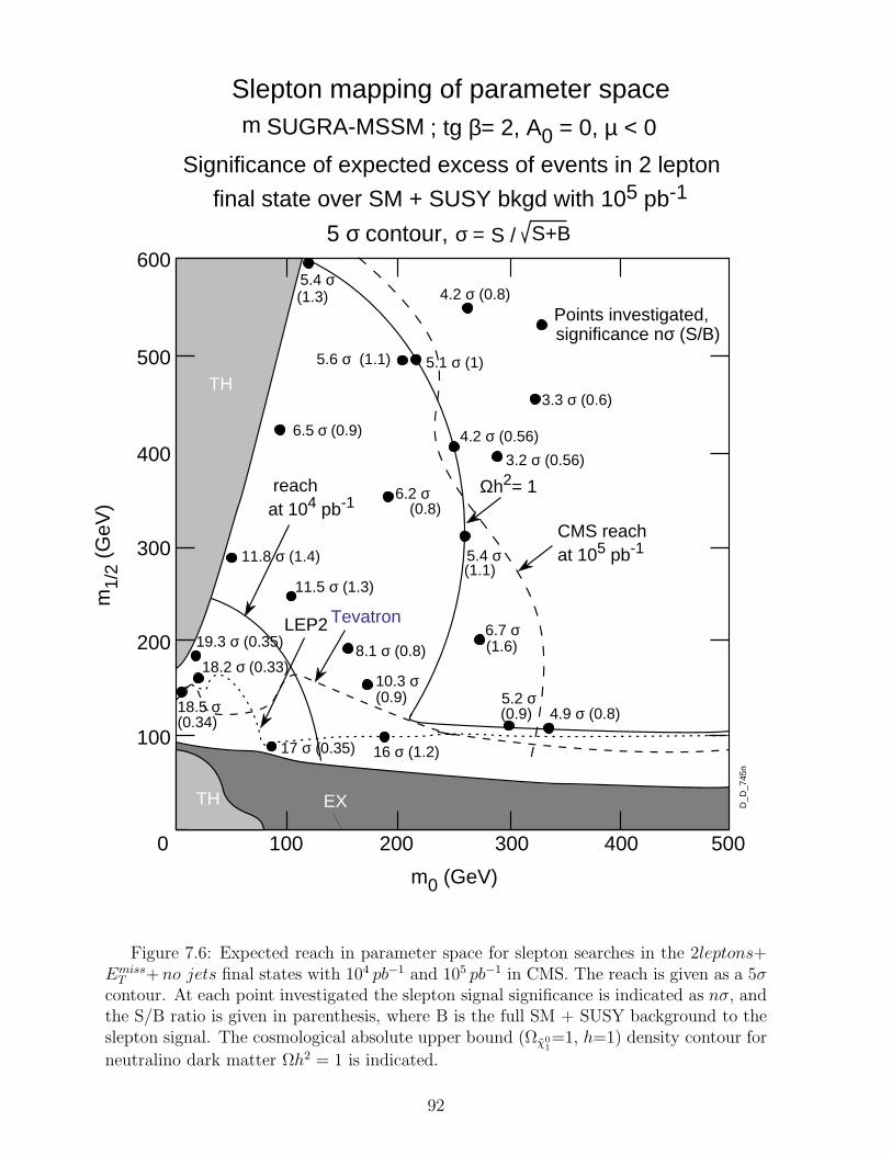
Ωh2= 1

TevatronLEP2

TH

TH

EX

0 100 200 300 400 500

100

200

300

400

500

600

m0 (GeV)

m1/

2 (G

eV)

D_D

_745

n

SUGRA-MSSM


5.4 σ(1.3)

6.5 σ (0.9)

3.3 σ (0.6)

3.2 σ (0.56)

6.2 σ(0.8)

11.8 σ (1.4)

11.5 σ (1.3)

18.5 σ (0.34)

8.1 σ (0.8)

10.3 σ(0.9)

17 σ (0.35)

19.3 σ (0.35)

18.2 σ (0.33)

5.4 σ

6.7 σ(1.6)

5.2 σ(0.9) 4.9 σ (0.8)

(1.1)

CMS reachat 105 pb-1

reachat 104 pb-1

Points investigated,significance nσ (S/B)

Significance of expected excess of events in 2 lepton

final state over SM + SUSY bkgd with 105 pb-1

σ = S / S+B

5.6 σ (1.1) 5.1 σ (1)

4.2 σ (0.8)

4.2 σ (0.56)

16 σ (1.2)

; tg β= 2, A0 = 0, µ < 0

5 σ contour,

m

Figure 7.6: Expected reach in parameter space for slepton searches in the 2leptons+Emiss

T + no jets final states with 104 pb−1 and 105 pb−1 in CMS. The reach is given as a 5σcontour. At each point investigated the slepton signal significance is indicated as nσ, andthe S/B ratio is given in parenthesis, where B is the full SM + SUSY background to theslepton signal. The cosmological absolute upper bound (Ωχ0

1=1, h=1) density contour for

neutralino dark matter Ωh2 = 1 is indicated.

92

tan β= 2A0= 0; µ < 0

320

280

240

200

112 212 312 412

160

120

80

40

m

m

D_D

_746

n

Points investigated,significance nσ

L,GeV

χ0 1

~, G

eV

Model: mSUGRA-MSSM

Explorable range of , χ0 masses

in slepton searches in CMS

~ ~1

Excluded re

gion

Explorable at LEP2 and Tevatron

Ωh2= 1

5.4 σ

4.2 σ5.1 σ5.6 σ

6.5 σ3.3 σ

3.3 σ

6.2σ

5.4 σ

6.7 σ

4.9 σ

5.2 σ

11.8 σ

11.5 σ8.1 σ10.3 σ

19.3 σ18.2 σ18.5 σ

17 σ

CMS reachat 105 pb-1

EXP-excluded

Figure 7.7: Same mapping as in Fig. 7.6, but in terms of masses of the left sleptonand the LSP.

93

TevatronLEP2

TH

TH

EX

0 100 200 300 400 500

100

200

300

400

500

600

m0 (GeV)

m1/

2 (G

eV)

D_D

_101

6n

mSUGRA-MSSM, tan β= 2 A0= 0; µ < 0


Modification ofboundary ifσ WW * 2

CMS reach

at 105 pb-1

Figure 7.8: Modification of the 5σ reach in slepton searches if the production cross-section for the main SM background of WW pair production is increased by a factor of2.

94


search for chargino/neutralino pair production

Direct production of χ±1 χ0

2 followed by leptonic decays of both sparticles (see section 2.1)gives three high-pT isolated leptons accompanied by missing energy. These events are freefrom jet activity except for those coming from initial-state QCD radiation. Therefore wesearch for χ±

1 χ02 pair production in 3 leptons + no jets+ Emiss

T final states [8].We have considered the following SM processes contributing to the background: WZ,

ZZ, tt, Wtb, Zbb, bb with the cross-sections σWZ = 26 pb, σZZ = 15 pb, σtt = 670 pb fora top mass of 170 GeV, σWtb = 160 pb, σZbb = 600 pb, σbb = 500 µb. Three leptons inthe final state are obtained by folding the appropriate leptonic decay modes. We haveforced Z → l+l−, W± → l±ν and b → clν decays, where l = µ, e, τ . In case of tt andWtb only one W has been forced. These SM backgrounds, except ZZ production, can besuppressed by requiring that all three leptons be isolated, and vetoing central jets. ZZevents contain four isolated leptons and asking for exactly three isolated leptons in theevent leaves only a small fraction of the ZZ continuum, when one of the leptons escapesdetector acceptance. The WZ, ZZ and Zbb backgrounds can be suppressed by removingevents with a dilepton invariant mass close to the Z mass. At each investigated pointin the (m0, m1/2) plane we have studied all SUSY production processes which can leadultimately to three leptons in the final state. These are the strong interaction productionof gg, gq, qq pairs; associated production of gχ, qχ pairs; chargino-neutralino χχ pairproduction, and slepton pair production, ll, lν, νν. The SUSY event sample with threehigh-pT isolated leptons is dominated by strong production; but, of course, the jet vetorequirement is very efficient in reducing g and q events which in their cascade decaysproduce many central high-ET jets. It has to be pointed out that SUSY events other thanthe directly produced χ±

1 χ02and which survive all selection criteria, may still contain some

χ±1 χ0

2’s produced in cascade decays of heavier sparticles. These events can be consideredas an “indirect” χ±

1 χ02 signal, a situation similar to the one encountered in discussing

slepton searches.In Fig. 8.1 we show the fully simulated SUSY points in the (m0, m1/2) plane, as

representatives of various regions according to the predominant or characteristic decaymodes. In order to illustrate event kinematics we choose three points from different(m0, m1/2) regions among those shown in Fig. 8.1:

S1 (m0, m1/2) = (100 GeV, 100 GeV) withM(χ±

1 ) ≃ M(χ02) = 98 GeV, M(χ0

1) = 45 GeV,M(g) = 294 GeV, M(q) = 270 GeV


1 ) ≃ M(χ02) = 154 GeV, M(χ0

1) = 76 GeV,M(g) = 551 GeV, M(q) = 2032 GeV


1 ) ≃ M(χ02) = 341 GeV, M(χ0

1) = 172 GeV,M(g) = 983 GeV, M(q) = 861 GeV

Figure 8.2 shows the dσ/dplT distribution in the three-lepton event sample with pl

T > 15GeV. Distributions are shown for signal and SM background. At this stage the dominantSM backgrounds are tt and Zbb. For high m1/2, e.g. point S3, the lepton pT cut can beset at 20 GeV. The loss in signal acceptance is ∼12% compared to a 15 GeV cut, whilst

95

tt and Zbb are reduced by an additional factor of ∼2.To suppress background events with leptons originating from semileptonic decays

of b-quarks, we apply tracker isolation, requiring all three leptons to be isolated. Ifthere is no charged track with pT greater than a certain threshold pcut

T in a cone ofR =

√∆η2 + ∆φ2 = 0.3 about the lepton direction, it is considered as isolated. Figure

8.3 a shows the lepton isolation rejection factor against tt background versus the pcutT

on charged tracks. The two curves correspond to two different instantaneous luminosityregimes, L = 1033 cm−2s−1 and L = 1034 cm−2s−1. In the latter case we have superimposed15 “hard” pile-up events. Figure 8.3 b shows signal acceptance versus pcut

T . We choose pcutT

= 1.5 GeV and 2 GeV for low and high luminosity running, respectively. The correspond-ing rejection factors against tt are about 60 and 50, whereas signal acceptance decreasesfrom about 90% to 70%. The next requirement is the central jet veto, which allows usreject the internal SUSY background coming from g and q cascade decays overwhelmingχ±

1 χ02 direct production. This cut also reduces some SM backgrounds. In Fig. 8.4 we show

jet multiplicity and jet ET distributions for signal, SUSY gg, gq, qq background events atpoint S1, and for the tt background. Since at this (m0, m1/2) point the gluino is heavierthan the squark, it decays to a squark-quark pair. Therefore gluino events are richer injets compared to squark events. Figure 8.5 shows jet veto rejection factors against gg,gq, qq and tt backgrounds and the signal acceptance as a function of jet pseudorapidity,|ηjet|, for two jet detection thresholds: Ejet

T > 25 GeV and EjetT > 30 GeV. As the jet veto

region is decreased down to |ηjet| ≃ 3.5, the rejections/acceptance are not too sensitiveto jet rapidity coverage, but below this value of |ηjet|, rejection factors decrease rapidly,degrading significantly the separation of direct χ±

1 χ02 production from internal SUSY and

SM backgrounds. The reconstruction of jets at |ηjet| ∼ 3.5 implies calorimetric coverageup to |η| ∼ 4.3 at least, as the jets are collected in a cone of ∆R = 0.8.With increasingm0 and/or m1/2 squarks and/or gluinos become heavier. Thus jets are harder and SUSY

events are easier to suppress by a jet veto with relaxed requirement on |ηjet| and EjetT .

Furthermore, for the signal events the QCD radiation becomes harder (χ±1 , χ0

2 are moremassive) and the low production cross-section requires the highest LHC luminosity, withan event pile-up contaminated environment. For this region, the jet veto threshold can beset with Ejet

T as high as 50 GeV and is justified by the need to suppress the SM (mainlytt) background.

Despite the fact that missing energy is always present in SUSY signals (at least inR-parity conserving models), for some regions of mSUGRA parameter space, it is advan-tageous not to apply any specific cut on it. Figure 8.6 shows the distribution of Emiss

T inevents with three isolated high-pT leptons and no jets for the signal and the two main SMbackgrounds: tt and WZ. For point S1 the shape of the distribution is very similar tothat of the background and therefore no cut on Emiss

T is applied. For point S3 requiringEmiss

T > 80 GeV significantly reduces tt and WZ backgrounds whilst keeping more than75% of signal events [8].

For WZ background suppression, which after all the previous requirements remainsthe dominant SM background, an MZ cut is necessary. In the signal events, the shape ofthe (same-flavor opposite-sign) dilepton invariant mass Ml+l− distribution is determinedby the χ0

2 decay kinematics and has a very sharp edge. Figure 8.7 shows the Ml+l−

distribution for the signal at three parameter space points S1, S2, S3 and for WZ events.In events having all leptons of the same flavor, the combinatorial background obscuresthe sharp mass edge in the signal events. A rejection factor of ∼ 17 for WZ is obtained by

96

Table 8.1: Selection criteria

Set 1 pT cut 3l with plT > 15 GeV in |ηl| < 2.4(2.5)

appropriate for Isolation No track with pT > 1.5 GeV in R = 0.3

m1/2<∼ 140 GeV Jet veto No jet with Ejet

T > 25 GeV in |ηjet| < 3.5Z-mass cut Ml+l− < 81 GeV


appropriate for Isolation No track with pT > 1.5 GeV in R = 0.3

140 GeV <∼ m1/2 Jet veto No jet with EjetT > 30 GeV in |ηjet| < 3

<∼ 180 GeV Z-mass cut Ml+l− < 81 GeV


appropriate for Isolation No track with pT > 2 GeV in R = 0.3

180 GeV <∼ m1/2 Jet veto No jet with EjetT > 40 GeV in |ηjet| < 3

<∼ 300 GeV missing ET EmissT > 50 GeV

Z-mass cut MZ ± 10 GeV


appropriate for Isolation No track with pT > 2 GeV in R = 0.3

m1/2>∼ 300 GeV Jet veto No jet with Ejet

T > 50 GeV in |ηjet| < 3missing ET Emiss

T > 80 GeVZ-mass cut MZ ± 10 GeV

removing events with Ml+l− > MZ −10 GeV, whilst the small loss of signal events, <∼ 10%for point S1, comes from events when all three leptons have the same flavor. However,for higher values of m1/2, e.g. point S3, the endpoint of the Ml+l− distribution is abovethe Z peak; in this case we cut only events falling within the Z mass window: MZ − 10GeV < Ml+l− < MZ + 10 GeV.

On the basis of the above considerations we adopt four sets of selection criteria, ap-propriate for different (m0, m1/2) regions, given in Table 8.1.

The m1/2 boundaries are approximate and, for optimal cuts, they depend also on m0.Except for Set 4, which we apply for rather massive χ±

1 χ02, the pT cuts on leptons are

the same, i.e. plT > 15 GeV. Set 1 and Set 2 are appropriate for the regions where the

signal is accessible already at low luminosity. In the regions where we apply the cuts ofSet 3 or Set 4 a high luminosity is required, as they correspond to smallest cross-sections;the luminosity determines the isolation requirement. With increasing m1/2 the jet veto is

relaxed, varying the EjetT threshold from 25 to 50 GeV. A cut on Emiss

T is applied only forSet 3 and Set 4; and finally, the MZ cut is looser for higher m1/2.

Table 8.2 gives the SM background cross-sections for these selection criteria after eachcut. The two main SM backgrounds surviving these cuts are WZ and tt. With Set 1 andSet 2 the dominant background is WZ and with Set 3 and Set 4 it is tt.

Details on each simulated point can be found in [8]. The signal significance is definedas the number of signal events divided by the square root of all events (SUSY + SM)passing our selection criteria. With this definition we give: i) evidence for existence ofSupersymmetry in 3l + no jets+ Emiss

T channel; ii) overall evidence for χ±1 χ0

2 productionand iii) evidence for direct production of χ±

1 χ02. The ratio of direct χ±

1 χ02 events over other

97

Table 8.2: SM background cross-sections (in fb) at each step of applied cuts.

Set of cuts Cuts WZ ZZ tt Wtb Zbb bb

Set 1 plT 111 21.7 2544 139.1 731 9300

Isolation 102 19.7 39.8 4.09 28.8 < 0.30Jet veto 73.8 11.6 4.12 1.71 14.6 < 0.15MZ 4.19 0.89 2.18 0.86 0.76 < 0.15

Set 2 plT 111 21.7 2544 139.1 731 9300

Isolation 102 19.7 39.8 4.09 28.8 < 0.30Jet veto 76.1 12.7 4.84 1.90 16.1 < 0.15MZ 4.49 0.99 2.48 1.05 0.91 < 0.15

Set 3 plT 111 21.7 2544 139.1 731 9300

Isolation 75.4 14.7 46.3 4.82 32.9 < 0.45Jet veto 51.3 8.69 4.77 1.91 15.7 < 0.40Emiss

T 22.0 2.61 3.01 0.48 1.42 < 0.01MZ 1.93 0.35 2.63 0.40 0.06 < 0.01

Set 4 plT 88.4 16.6 1330 65.2 378 2800

Isolation 60.5 11.4 19.0 1.33 10.3 < 0.04Jet veto 46.4 7.92 3.25 0.53 4.78 < 0.04Emiss

T 5.77 0.68 0.73 0.05 0.30 < 0.001MZ 0.45 0.09 0.60 < 0.05 < 0.04 < 0.001

events surviving the cuts, Ndirχ±

1χ0

2

/(NALL- Ndirχ±

1χ0

2

), is also given. All investigated points are

analyzed in a similar manner and 5σ significance contours are obtained in the (m0, m1/2)plane, as shown in Fig. 8.8.

In the regions of small m0 and m1/2 (<∼ 200 GeV and <∼ 150 GeV, respectively) indi-rectly produced χ±

1 χ02 events contribute significantly in the 3l + no jets+ Emiss

T channel.However, this contribution is expected to be less than ∼15% of the overall χ±

1 χ02 produc-

tion. Therefore, we can give 5σ significance contours for direct χ±1 χ0

2 production.From Fig. 8.8 one can see that at a low integrated luminosity of Lint = 104 pb−1 the

direct production of χ±1 χ0

2 can be distinguished from background up to m1/2<∼ 150 GeV

for all m0. A further increase of luminosity up to Lint = 105 pb−1 extends the explorableregion only by about 10 ÷ 20 GeV for m0

>∼ 120 GeV. However,for m0<∼ 120 GeV the

gain in parameter space is much larger – up to m1/2<∼ 420 GeV, reflecting the more

advantageous behavior of the production cross-section times branching ratio shown inFig. 2.4.

It should be pointed out that the internal SUSY backgrounds are particularly dan-gerous for small m0, m1/2, in the region m0

<∼ 200 GeV, m1/2<∼ 150 GeV, generating a

background higher or comparable to the SM contribution because of the high productioncross-sections of the relatively light gluinos and squarks. Softness of these gluino/squarkevents makes it difficult to suppress them below the SM level, even with a very strict jetveto requirement (selection criteria Set 1). For some regions of the (m0, m1/2) parameterplane, chargino/neutralino and slepton pair productions are comparable to gluino/squarkcontributions. As m0 and m1/2 increase, more massive gluinos and squarks result in

98

harder jets, and decreased cross-sections, and hence the SUSY background becomes neg-ligible. At the 5σ boundary with an integrated luminosity of 105 pb−1, background eventsdominantly consist of SM processes. At this boundary the signal to background ratiois expected to be >∼ 0.20 with about 150 signal events (Lint = 105 pb−1) for m0

>∼ 120GeV. In this region the dominant SM background is WZ production which cannot besuppressed by a stronger jet veto or lepton isolation requirements. For m0

<∼ 120 GeVthe signal to background ratio is >∼ 0.60 with about 70 signal events. Here the dominantSM background is tt production. The lower number of signal events needed to attain a5σ significance and the higher signal to background ratio in this region is the result of theharder event kinematics of χ±

1 χ02, allowing for more stringent selection criteria (Set 4). As

a consequence the SM contamination is smaller [8].At small m0, the χ±

1 χ02 reach in parameter space is very luminosity-dependent. This

region of small m0 is of particular importance, since it is the prefered one from thecosmological point of view, where χ0

1 is the candidate for the cold dark matter in theUniverse. With the present lifetime of the Universe (>∼ 1010 years) and the estimateof the relic neutralino abundance at freeze-out time as a function of (m0, m1/2), onecan determine regions of parameter space where Ωh2 < 1; here Ω is the ratio of therelic neutralino density to the critical density which closes the Universe and h is theHubble constant scaling factor, 0.5 <∼ h <∼ 0.8. In Fig. 8.8, the Ωh2 = 0.15 and Ωh2 =0.4 contours mark the most probable region of the parameter space, corresponding to amixed dark matter scenario with 60% of neutralino dark matter. One can see that χ±

1 χ02

direct production covers a significant part of this prefered region of parameter space.We can conclude, that:• by measuring the excess of events in the 3l + no jets+ Emiss

T channel over SM andinternal SUSY backgrounds, χ±

1 χ02 direct production can be investigated in mSUGRA

parameter space up to m1/2<∼ 170 GeV (150 GeV) for all m0 at a luminosity Lint = 105

pb−1 (104 pb−1);• with a high integrated luminosity of Lint = 105 pb−1 and for m0

<∼ 120 GeV, thediscovery region for direct production of χ±

1 χ02 extends up to m1/2

<∼ 420 GeV.

99

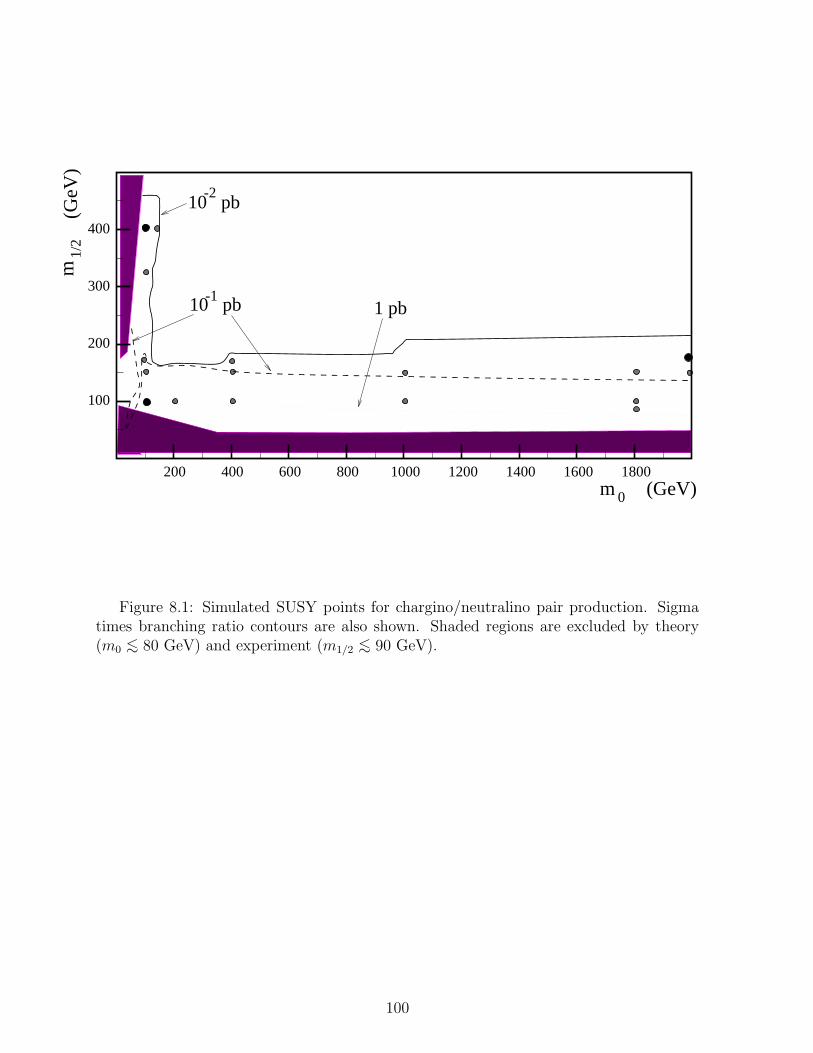
1 pb

100

200

300

400

800600 1000 1200 1400 1600200 400

(GeV

)

10 pb-1

10 pb-2

1800(GeV)0m

1/2

m

Figure 8.1: Simulated SUSY points for chargino/neutralino pair production. Sigmatimes branching ratio contours are also shown. Shaded regions are excluded by theory(m0

<∼ 80 GeV) and experiment (m1/2<∼ 90 GeV).

100

10-1

1

10

10 2

0 50 100 150

pTl (GeV)

dσ/d

p Tl

(fb

/ 2

GeV

)direct χ

~ ±1 χ

~ 02

S1(100,100)

S2(2000,175)

S3(100,400)

All three leptons

10-1

1

10

10 2

0 50 100 150

direct χ~ ±1 χ

~ 02

S1(100,100)

S2(2000,175)

S3(100,400)

pTl3 (GeV)

dσ/d

p Tl3

(

fb /

2 G

eV)

Softest lepton

1

10

10 2

10 3

0 50 100 150

SM background

tt–

Zbb–

WZ

ZZ

pTl (GeV)

dσ/d

p Tl

(fb

/ 2

GeV

)

1

10

10 2

10 3

0 50 100 150

SM Backgroundtt–

Zbb–

WZ

ZZ

pTl3 (GeV)

dσ/d

p Tl3

(

fb /

2 G

eV)

Figure 8.2: dσ/dplT distributions for signal and SM background. Left plots show

distributions for all three leptons and the right ones for softest lepton in the event.

101

10

10 2

10 3

0.5 1 1.5 2 2.5 3 3.5 4 4.5

pTcut (GeV)

Rej

ecti

on tt–a)

No pile-up15 ’hard’ pile-up

0.2

0.4

0.6

0.8

1

1.2

0.5 1 1.5 2 2.5 3 3.5 4 4.5

pTcut (GeV)

Acc

epta

nce

direct χ~ ±1 χ

~ 02b)

No pile-up

15 ’hard’ pile-up

Figure 8.3: Tracker isolation: a) tt background rejection versus pcutT on charged track,

b) signal acceptance versus pcutT on charged track. Events are selected with three leptons of

pT > 15 GeV and all of them are required to be isolated. Full and open circles correspondto low, L = 1033 cm−2 s−1, and high, L = 1034 cm−2 s−1, luminosity regimes, respectively.

102

0

0.02

0.04

0.06

0.08

0 2 4 6 8

Njet

dσ/d

Nje

t (

pb)

direct χ~ ±1 χ

~ 02

10-4

10-3

10-2

0 50 100 150 200

direct χ~ ±1 χ

~ 02

ETjet (GeV)

dσ/d

ET

jet

(pb

/ 3

GeV

)

0

0.5

1

1.5

0 2 4 6 8

Njet

dσ/d

Nje

t (

pb)

g~g~

g~q~

q~q~

SUSY bkgd.

10-2

10-1

0 50 100 150 200

ETjet (GeV)

dσ/d

ET

jet

(pb

/ 3

GeV

)g~g~

g~q~

q~q~

SUSY bkgd.

0

0.005

0.01

0.015

0 2 4 6 8

Njet

dσ/d

Nje

t (

pb)

tt–

10-4

10-3

10-2

0 50 100 150 200

tt–

ETjet (GeV)

dσ/d

ET

jet

(pb

/ 3

GeV

)

Figure 8.4: Jet multiplicity and transverse energy distributions for the signal and inter-nal SUSY background at mSUGRA point S1(100 GeV, 100 GeV) and the tt background.Events are selected with three isolated leptons of pT > 15 GeV.

103

250 6

7

8

9

10

11

100

200

300

400

500

3 4 52.5 3.5 4.5|η jet| |η jet|

2 3 4 52.5 3.5 4.5

Rej

ectio

n

Rej

ectio

n

gg, gq, qq bkgd.~~ ~~ ~~ tt bkgd.

m0 = 100 GeV, m1/2 = 100 GeVm(g) = 294 GeV, m(q) = 270 GeV~ ~

D_D

_967

n1

Et > 30 GeVjet

Et > 25 GeVjetEt > 25 GeVjet

Et > 30 GeVjet

Figure 8.5: Jet veto rejection/acceptance versus |ηjet| in χ±1 χ0

2 searches. Full circlescorrespond to Ejet

T > 25 GeV and the open ones to EjetT > 30 GeV.

104

1

10

10 2

0 25 50 75 100 125 150 175 200 225 250ET

miss (GeV)

Arb

itra

ry u

nits

direct χ~ ±1 χ

~ 02

S3(100,400)

S2(2000,175)

S1(100,100)

10 2

10 3

0 25 50 75 100 125 150 175 200 225 250ET

miss (GeV)

Arb

itra

ry u

nits

SM background

tt–

WZ

Figure 8.6: Missing transverse energy distributions in signal and background eventswith three isolated leptons of pT > 15 GeV and no jets.

105

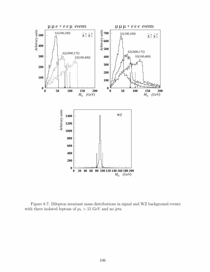
0

100

200

300

400

500

0 50 100 150 200Mll (GeV)

Arb

itra

ry u

nits

χ~ ±1 χ

~ 02

S1(100,100)

S2(2000,175)S3(100,400)

0

100

200

300

400

500

600

700

0 50 100 150 200Mll (GeV)

Arb

itra

ry u

nits

µ µ µ + e e e eventsµ µ e + e e µ events

χ~ ±1 χ

~ 02

S1(100,100)

S2(2000,175)

S3(100,400)

0

200

400

600

800

1000

1200

1400

0 20 40 60 80 100 120 140 160 180 200Mll (GeV)

Arb

itra

ry u

nits

WZ

Figure 8.7: Dilepton invariant mass distributions in signal and WZ background eventswith three isolated leptons of pT > 15 GeV and no jets.

106

500

450

400

350

300

250

200

150

100

50

200 400 600 800 1000 1200 1400 1600 1800 2000

TH

EX

105 pb-1

104 pb-1

103 pb-1

tanβ = 2, A0 = 0, µ < 0

σ = N / Nall χ1 χ2∼ ± ∼ 0

D_D

_995

n1

m0 (GeV)

m1/

2 (G

eV)

Direct Chargino - Neutralino Production5σ sinificance contours at different luminosities

Ω h2

0.4

0.15

:

Figu

re8.8:

5σsign

ifican

cecon

tours

atdiff

erent

lum

inosities.

107

9 Possibility of observing h → bb in squark and gluino

decays

The usual way to search for the lightest CP-even Higgs (h) of the MSSM is through itsdirect production by gluon fusion or in association with W, bb or tt and its decay into γγ,ZZ∗ → 4l, µµ or bb [14, 21, 43]. All these production mechanisms are Electroweak. Eachof these channels has some limitations, such as high tanβ for the µµ mode, or high mass,mh >∼ 130 GeV and large stop mixing for the ZZ∗ → 4l mode, for example. The mostgeneral way is to search for inclusive h → γγ, which, with Lint = 105 pb−1, would allowus to explore a domain approximately given by mA >∼ 250 GeV and tanβ >∼ 3 [14]. Withthe h → γγ mode we expect a signal on top of a large irreducible γγ background with asignal to background ratio of <∼ 1/20. The instrumental requirements on the ECAL arevery demanding, a γγ effective mass resolution better than ≃1 GeV at mh ≃ 100 GeV[43]. In the associated production modes Wh and tth with h → γγ, the S/B ratio is oforder 1 and calorimeter performance is less demanding: but these channels require ≥ 105

pb−1 [44]. Evaluations of ways to exploit the h → bb decay mode in the Wh or tth finalstates leave little hope − no way to get a really significant signal has been found up tonow [45].

It is well known that the MSSM h can be abundantly produced in the decays ofcharginos and neutralinos (primarily χ0

2). In turn, the χ02 is a typical decay product of

squarks and gluinos (see Figs. 2.5a,b) which are also produced abundantly. The idea isthus to use strongly produced q/g and to look for the dominant decay mode h → bb, ifχ0

i → χ0jh is kinematically allowed, and require Emiss

T and jet multiplicity to suppress thebackground [12, 46].

In this study we fix only one of the mSUGRA parameters, A0 = 0, and vary theother four: m0, m1/2, tanβ, sign(µ). The most pronounced variation of physics quantities(masses, branching ratios, cross-section) is with m0 and m1/2, thus the investigation isdone in the m0, m1/2 parameter plane for several representative values of tanβ and sign(µ).When Mχ0

2− Mχ0

1> mh the main source of Higgs is the decay χ0

2 → χ01h. This decay

has a significant (≃20-90%) branching ratio in a large portion of the parameter space, seeFig. 2.17. In regions of m1/2

<∼ 200-300 GeV (depending on tanβ) the three body decaysχ0

2 → χ01 qq, χ0

2 → χ01 l+l− take over because the χ0

2 → χ01h decays are not kinematically

allowed. The boundary at m0 ∼ 200-300 GeV, on the other hand, corresponds to theopening of two-body cascade modes, e.g. χ0

2 → l±L,Rl∓ → χ01 l+l−. Figure 2.17 also shows

that the tanβ = 2, µ < 0 case looks the most promising one, whereas the tanβ = 10, 30, µ< 0 seem the least favorable among the possibilities considered, the χ0

2 → χ01h branching

ratio being the smallest on average in these latter cases. Depending on tanβ, there ispotentially a gap between the upper limit explored up to now or foreseeable at LEP2 andTevatron at m1/2 ≃ 100 GeV (mh <∼ 100 GeV) and the lower limit at m1/2 ≃ 200-250GeV where χ0

2 → χ01h opens up. This comes about because within mSUGRA there are

simple mass relations: Mχ02≃ 2Mχ0

1≃ m1/2, and the LSP mass is typically >∼ 100 GeV

in the regions where χ02 → χ0

1h is allowed. The range of the h mass varies from ≃ 80 to≃ 120 GeV and the exact upper limit is determined by the order to which the radiativecorrections have been calculated.

With increasing m0 (at fixed m1/2) squarks become more massive than gluino at somepoint (see, e.g. Fig. 2.16) and thus gluino decays into squarks are not allowed anymore,

108

decreasing significantly the yield of χ02 from squark decays. Furthermore, the B(q →

χ02q) also decreases with increasing m0 because the decay q → gq plays an increasingly

important role. These factors, with the variation of the total production cross-section(shown in Fig. 2.15) and the variation of the kinematics of the decay chains, require thatfor a quantitative evaluation of the regions where h → bb could be observed one needs toinvestigate the parameter space point by point and optimise cuts accordingly [12].

We considered the following SM background processes: QCD 2 → 2 (including bb),tt and Wtb. The pT range of all these processes is subdivided into several intervalsto facilitate accumulation of statistics in the high-pT region: 100-200 GeV (except forQCD), 200-400 GeV, 400-800 GeV and > 800 GeV. The accumulated statistics for allchannels correspond to 100 fb−1, except for the QCD jet (instrumental mismeasurement)background where the statistics correspond to 0.2 - 50 fb−1 depending on the pT interval.It is very time consuming to produce a representative sample of QCD jets in the low-pT

range, since the cross section is huge and we need extreme kinematical fluctuations andnon-Gaussian tail instrumental contributions for this type of background to be withinthe signal selection cuts. On the other hand, our simulation of instrumentally inducedmissing transverse energy is not yet fully reliable as it strongly depends on the still evolvingestimates of dead areas, volumes due to services, non-Gaussian calorimeter response, etc.So we cannot go confidently below ≃100 GeV with the cut on Emiss

T , where the QCD jetbackground becomes the dominant contribution.

Initial requirements for all the SM and SUSY samples are the following:

• at least 4 jets with EjetT > 20 GeV in | ηjet | < 4.5,

• EmissT > 100 GeV,

• Circularity > 0.1.

No specific requirements are put on leptons. If there are isolated muons or electrons withpµ,e

T > 10 GeV within the acceptance they are also recorded. The term “isolated lepton”here means satisfying simultaneously the following two requirements:

• no charged particle with pT > 2 GeV in a cone R = 0.3 around the direction of thelepton,

• ΣEcaloT in the annular region 0.1 < R < 0.3 around the lepton impact point has to

be less than 10% of the lepton transverse energy.

At a later stage we investigate whether selection or vetoing on isolated leptons can beused to help suppress the SM or internal SUSY backgrounds.

In this study we used an evaluation of the b-tagging performance of CMS from impactparameter measurement in the tracker [34]. An example is shown in Fig. 4.11. Theb-tagging efficiency and mistagging probability for jets is evaluated as a function of ET

and jet pseudorapidity. It is obtained from a parameterized Gaussian impact parameterresolution, dependent on the pixel point resolution, radial position of the pixel layers andthe effects of multiple scattering on intervening materials, with the addition of a non-Gaussian impact parameter measurement tail based on CDF data. Although there aresome specific assumptions made concerning the tails of the impact parameter distributionsextending beyond the parameterized Gaussian parts in [34], the presently on-going study

109

of the expected impact parameter resolution, with full pattern recognition and trackfinding in CMS [47] is in a very good agreement with the results used as an input in thepresent study.

The b-jet tagging efficiency is parameterized as a function of EjetT in 3 intervals of η:

0 - 1, 1 - 1.75 and 1.75 - 2.4. A typical b-tagging efficiency at η ≃ 0 for EjetT = 40 GeV

is ≃ 30%, reaching a maximal efficiency of ≃ 60% for high-ET jets. Charm-jets have atypical tagging efficiency of about 10%, and for light quarks and gluons the b-tagging(mistagging) efficiency reaches a maximum of about 3% for high-ET jets. At the analysisstage the jets produced by the event generator are “b-tagged” according to the taggingefficiency for b-jets and mistagging probability for quark and gluon jets. If not speciallymentioned otherwise, h → bb decay jets are tagged only in the barrel | η | < 1.75 intervaland in all di-jet mass distributions we take only one pair of b-jets per event, those closestto each other in η − ϕ space. No attention is paid to jet “charge” or “leading charge”.More details can be found in [12].

As an example let us consider a representative mSUGRA point m0 = m1/2 = 500GeV, tanβ = 2, µ < 0. Here the masses of relevant sparticles are: mg = 1224 GeV, muL

= 1170 GeV, mχ02

= 427 GeV, mχ01

= 217 GeV, mh = 89.7 GeV. In Fig. 9.1 we compare

kinematical distributions for this point with the SM background for Lint = 100 fb−1. TheEmiss

T distributions show the most pronounced difference between signal and background,this then being the most important variable for the background suppression. A significantdifference exists also in the jet multiplicity distributions. A specific optimisation of cutson Emiss

T , EjetT , etc., is however performed in various regions of mSUGRA parameter space.

Figure 9.2 shows the b-b (jet-jet) mass distribution for the sum of the SUSY and SMevents assuming an ideal b-tagging performance, i.e. 100% b-tagging efficiency with 0%mistagging probability for jets. The cuts are Emiss

T > 400 GeV and EjetT > 40 GeV. The

SM background shown in Fig. 9.2 separately as a shaded histogram is small compared tothe internal SUSY background. The bb mass distribution is fitted with a sum of a Gaussianand a quadratic polynomial. The width of the signal peak is determined entirely by thejet-jet effective mass resolution of the detector (the intrinsic h width varies from 3.2 to4.3 MeV over the entire mSUGRA parameter space). The position of the peak is shiftedto lower mass since energy losses in jets (finite cone size, neutrinos generated in hadronicshowers, etc.) are not corrected for. The three distributions in the lower half in Fig. 9.2are for events in the Mbb mass window 70 - 100 GeV to illustrate the kinematics of theh → bb decay. The average b-jet transverse energy is ∼110 GeV, and the b-jets are verycentral as they result from the decay of massive (∼1200 GeV) squarks and gluinos whichare centrally produced. Clearly, b-tagging beyond | ηjet | ≃ 1.5 is not very helpful in thissearch.

If one now applies the nominal b-tagging performance expectations described previ-ously, we obtain the bb mass distribution given in Fig. 9.3a. Under these nominal condi-tions and with 100 fb−1 the expected signal significance calculated as S/

√B within a ±1σ

interval around the peak value is 18.3. The background is dominated by the internal SUSYbackground which is largely irreducible, originating mainly from additional real b-jets inthe event, rather than from mistagged jets. An improvement could possibly be obtainedby taking into account “jet charge” and thus enriching the sample in bb pairs as comparedto bb + bb/bb. This however requires track reconstruction and charge determination forfast tracks in jets, a task still under study in CMS [47].

Figures 9.3-9.5 illustrate the expected sensitivity of the h → bb signal to various

110

instrumental factors [12]. In Fig. 9.3b all bb-combinations per event are included inthe distribution (instead of just the one with the closest distance in η − ϕ space) andthe signal significance is now worse by ≃12%. Figures 9.3c and 9.3d show the effectof increasing, or decreasing, the b-tagging efficiency by 15% in absolute value, whilstkeeping mistagging at the nominal level. The dependence on the b-tagging efficiencyis very pronounced, the signal significance varying by respectively ±25%. This is notsurprising as the b-tagging efficiency enters quadratically in the number of signal events.Figures 9.4a and 9.4b illustrate the effect of the η acceptance of the silicon pixel detector.As can be expected on the basis of Fig. 9.2, increased acceptance beyond | ηjet | ≃ 1.5 doesnot bring a significant improvement as the signal b-jets are very central. With taggingacceptance increasing from | ηjet |= 1.0 to 1.75 and 2.4, signal significance improves from17.2 to 18.3 and 18.8, respectively. Figures 9.4c and 9.4d illustrate the dependence ontagging purity, where one keeps the nominal b-tagging efficiency unchanged, but variesthe mistagging probability for all non-b-jets. Increasing the mistagging probability by afactor of 3 degrades signal significance by ≃25%.

Since the observed width of the h → bb peak is entirely determined by the calorimetricjet-jet effective mass resolution, one can expect dependence of the signal observability onthe energy resolution. This is illustrated in Fig. 9.5. The upper plot is for the nominalHCAL performance, corresponding to σE/E = 82%/

√E ⊕ 6.5% at η = 0 and the lower

plot corresponds to the HCAL energy resolution degraded to 120%/√

E ⊕ 10%. Theresolution of the Gaussian fit to the Higgs peak is 7.6 GeV in the first case and 11 GeVin the second. The difference in S/B between Figs. 9.5a and 9.5b is significant, but notdramatic. This is due to the fact that the h → bb pair has a significant boost, pbb

T ∼ 200GeV (Fig. 9.2) and the jet-jet opening angle, whose measurement precision is determinedby calorimeter granularity plays an important role in the effective mass resolution. Themass resolution also contains irreducible contributions from final state gluon radiation,jet cone size and fragmentation effects.

Figure 9.6 illustrates the h → bb signal observability as a function of mh over theallowed range of ∼80 to 120 GeV. For this we select the points all at the same m0 = m1/2

= 500 GeV, but different values of tanβ and µ, with nominal b-tagging performance andLint = 100 fb−1. One can clearly see that the signal becomes broader with increasingHiggs mass since the jet ET > 40 GeV cut-off does not play such a role as for a low-mass.

It is worth mentioning, that a significant part of the mSUGRA parameter space canbe explored already at a very low luminosities. For example, Fig. 9.7 shows the expectedHiggs signal with Lint = 3 fb−1 for a few points. All the distributions in this Figure areobtained with the cuts: Emiss

T > 200 GeV and EjetT > 40 GeV. For comparison, searches

in the h → γγ channel at the corresponding mSUGRA points would require ∼10 timeshigher integrated luminosity [12].

Let us turn to the main problem, how general is the possibility to observe this h →bb signal in q, g decays. Figure 9.8 shows the domain of parameter space where the h →bb signal is visible with S/

√B > 5 for the case tanβ = 2, A0 = 0, µ < 0 with nominal

b-tagging performance of CMS, for 10 and 100 fb−1 integrated luminosities. The isomasscurves for the CP-even (h) and CP-odd (A) Higgses are also shown in Fig. 9.8 by thedash-dotted lines. The bold broken line denotes the region where B(χ0

2 → χ01h) = 50%.

The shaded regions along the axes denote the present theoretically (TH) or experimentally(EX) excluded regions of parameter space not yet including LEP 96/97 results. The LEP2and Tevatron (with 1 fb−1) sparticle reaches are also shown by solid lines. With Lint ≤ 1

111

fb−1 the threshold of visibility of h → bb at lowest m1/2 = 170-180 GeV corresponds tomg,q ≥ 400-450 GeV, i.e. it begins just where the Tevatron searches will stop with ∼5 fb−1.With 100 fb−1 the reach extends up to mh ≃ 90 GeV, mA <∼ 1500 GeV. Figures 9.9 and9.10 show the domains of h signal visibility for tanβ = 10, µ < 0 and tanβ = 30, µ > 0,respectively. In both cases there seems to be a significant observability gap between theupper reach of LEP2 or the Tevatron and the LHC/CMS low mh reach using this methodto look for h. This has to be studied in more detail in the future.

We conclude that the search for the h → bb decay, when the lightest Higgs is producedin the cascade decays of the strongly interacting sparticles, seems to be a promisingchannel. The large rejection factor needed to suppress backgrounds and achieve a S/B of∼1 is here provided by the Emiss

T cut. Nothing similar can be obtained in the search forthe SM Higgs in H → bb nor for MSSM h → bb in inclusive h, Wh and tth final states.mass in the ≃450 to 700 GeV range for this search to be possible. The study carried outhere in the mSUGRA framework shows that there is a significant domain of parameterspace, just beyond the g/q mass reach of the Tevatron (∼400-450 GeV), where observationof the h → bb decay would be possible with an integrated luminosity of only 1-3 fb−1.This parameter space domain can be significantly extended with 100 fb−1, where g, q withmasses in 1.5 TeV range are probed. The h mass range from ≃80 GeV up to ≃125 GeVcan be covered.

Our investigations show that for the observation of the h → bb signal a calorimetricenergy resolution of ≃ 100%/

√E ⊕ 10% is adequate, but it should not be significantly

worse than this. The signal visibility depends most critically on the b-tagging efficiencyand to a lesser extent on the mistagging probability; the acceptance of the b-taggingpixel devices is not a real issue, provided the coverage is no smaller than | η | ≃ 1.5.A significant improvement in b-tagging efficiency could be obtained with a third pixellayer, or by having pixel layer at a radius of 4 cm even for high luminosity running, to bereplaced every (few) year(s). The mistagging probability depends on the non-Gaussianpart of the impact parameter measurement distribution, and thus on the overall patternrecognition performance in the region close to the beam, e.g. on the balance between Siand MSGC layers in the tracker. Optimisation of this aspect might then involve increasingthe number of Si layers from 4 to 5, possibly 6, reducing correspondingly the MSGC layersand deserves a dedicated study.

If this method is to become a viable alternative to the h → γγ search, it is importantto evaluate how general are the results of the present study, i.e. what happens outsidethe mSUGRA scheme where masses are not so constrained, for example in the MSSM.Presumably what is found here in the framework of mSUGRA-MSSM is valid as soon asthe g/q → χ0

2 → χ01h, or even more generally, the g/q → χ0

i → χ0jh chains are kinematically

allowed and the χ0i χ

0jh couplings non-vanishing. A particular point of interest in this

respect is the gap at the lower q/g masses, between the domains where SUSY can beexplored at the Tevatron with 5-6 fb−1, the LEP2 reach in terms of mh and the lowermass reach of this channel, if it exists in mSUGRA, can it be overcome in the MSSMwhere mass relations are less rigid?

112

1

10

10 2

10 3

10 4

10 5

0 5 10 15 20

Background

Signal

M(g~) = 1224 GeV M(u

~

L) = 1170 GeV M(t~

1) = 852 GeV

M(χ ~0

2) = 427 GeV M(χ ~0

1) = 217 GeV M(h) = 89.7 GeV

ET miss > 200 GeV

≥ 4 jets , pT jet > 40 GeV, |ηjet| < 4.5

circularity > 0.1

Njet

Nev

1

10

10 2

10 3

10 4

0 200 400 600 800 1000 Pt

l , GeV

Nev

/ 20

GeV hardest lepton

1

10

10 2

10 3

10 4

0 50 100 150∆φ ( Pt

l , Et miss) , deg

Nev

/ 5

deg hardest lepton

1

10

10 2

10 3

10 4

10 5

0 500 1000 1500 2000 2500 Pt

jet , GeV

Nev

/ 50

GeV hardest jet

1

10

10 2

10 3

10 4

10 5

0 50 100 150∆φ ( Pt

jet , Et miss) , deg

Nev

/ 5

deg hardest jet

1

10

10 2

10 3

10 4

10 5

0 500 1000 1500 2000 Et

miss , GeV

Nev

/ 40

GeV

1

10

10 2

10 3

10 4

10 5

0 0.2 0.4 0.6 0.8 1Circularity

Nev

/ 0.

05

1

10

10 2

10 3

10 4

10 5

0 1000 2000 3000 4000 5000 Et

sum , GeV

Nev

/ 10

0 G

eV

Figure 9.1: Comparison of mSUGRA signal at m0 = m1/2 =500 GeV, tanβ=2, µ < 0.and SM background distributions.

113

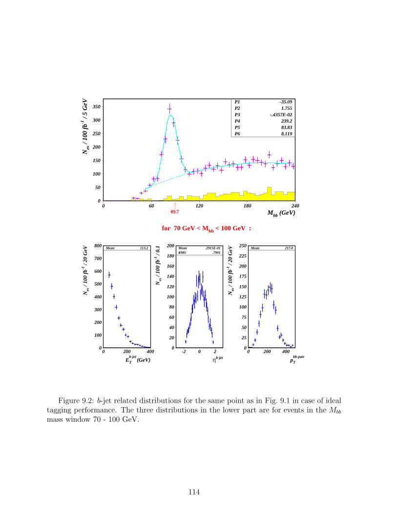
0

50

100

150

200

250

300

350

0 60 120 180 240

P1 -35.09P2 1.755P3 -.4357E-02P4 239.2P5 83.83P6 8.119

Mbb (GeV)

Nev

/ 10

0 fb

-1 /

5 G

eV

89.7

0

100

200

300

400

500

600

700

800

0 200 400

Mean 113.2

Eb-jet

T (GeV)

Nev

/ 10

0 fb

-1 /

20 G

eV

0

20

40

60

80

100

120

140

160

180

200

-2 0 2

MeanRMS

.2915E-01 .7901

ηb-jet

Nev

/ 10

0 fb

-1 /

0.1

for 70 GeV < Mbb < 100 GeV :

0

25

50

75

100

125

150

175

200

225

250

0 200 400

Mean 217.0

pbb-pair

T

Nev

/ 10

0 fb

-1 /

20 G

eV

Figure 9.2: b-jet related distributions for the same point as in Fig. 9.1 in case of idealtagging performance. The three distributions in the lower part are for events in the Mbb

mass window 70 - 100 GeV.

114

0

20

40

60

80

100

120

140

160

180

200

0 60 120 180 240

P1 -56.58P2 1.491P3 -.4116E-02P4 79.61P5 85.30P6 7.569

Mbb (GeV)

Nev

/ 1

00 f

b-1 /

5 G

eVS / √ B = 18.3

a)

89.7

0

20

40

60

80

100

120

140

160

180

200

0 60 120 180 240

P1 -79.81P2 1.960P3 -.5095E-02P4 81.01P5 85.24P6 7.464

Mbb (GeV)

Nev

/ 1

00 f

b-1 /

5 G

eV

S / √ B = 16.6

b)

0

20

40

60

80

100

120

140

160

180

200

0 60 120 180 240

P1 -54.92P2 1.801P3 -.5060E-02P4 118.9P5 85.43P6 7.739

Mbb (GeV)

Nev

/ 1

00 f

b-1 /

5 G

eV

S / √ B = 22.3

c)

0

20

40

60

80

100

120

140

160

180

200

0 60 120 180 240

P1 -33.91P2 .8943P3 -.2427E-02P4 42.02P5 85.15P6 8.242

Mbb (GeV)

Nev

/ 1

00 f

b-1 /

5 G

eV

S / √ B = 12.9

d)

Figure 9.3: Influence of the various instrumental factors on signal observability inthe same parameter space point as in Fig. 9.2 with 100 fb−1: a) with “nominal” b-tagging performance and data selection, b) all bb-combinations per event are included inhistogram, c) b-tagging efficiency increased by 15% and d) b-tagging efficiency decreasedby 15%. The nominal mistagging probability is assumed in all cases.

115

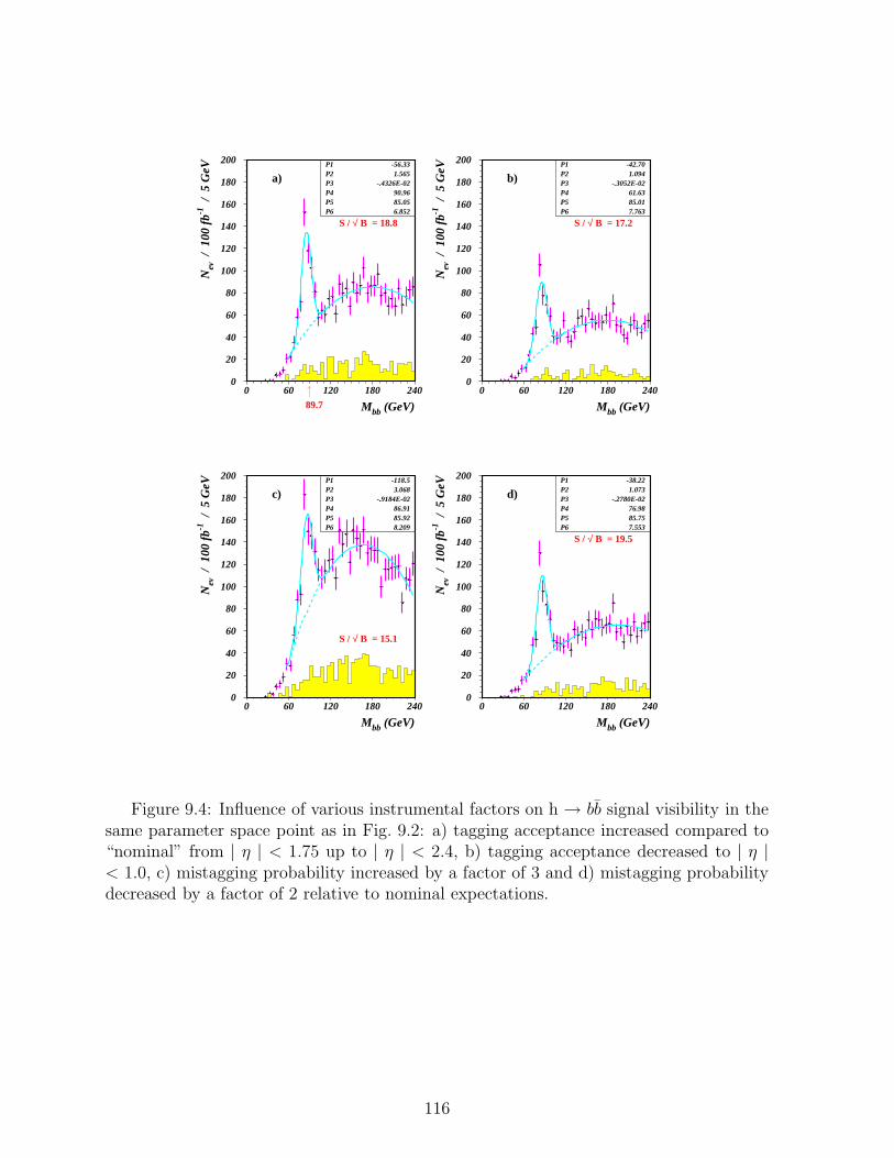
0

20

40

60

80

100

120

140

160

180

200

0 60 120 180 240

P1 -56.33P2 1.565P3 -.4326E-02P4 90.96P5 85.05P6 6.852

Mbb (GeV)

Nev

/ 1

00 f

b-1 /

5 G

eVS / √ B = 18.8

a)

89.7

0

20

40

60

80

100

120

140

160

180

200

0 60 120 180 240

P1 -42.70P2 1.094P3 -.3052E-02P4 61.63P5 85.01P6 7.763

Mbb (GeV)

Nev

/ 1

00 f

b-1 /

5 G

eV

S / √ B = 17.2

b)

0

20

40

60

80

100

120

140

160

180

200

0 60 120 180 240

P1 -118.5P2 3.068P3 -.9184E-02P4 86.91P5 85.92P6 8.209

Mbb (GeV)

Nev

/ 1

00 f

b-1 /

5 G

eV

S / √ B = 15.1

c)

0

20

40

60

80

100

120

140

160

180

200

0 60 120 180 240

P1 -38.22P2 1.073P3 -.2780E-02P4 76.98P5 85.75P6 7.553

Mbb (GeV)

Nev

/ 1

00 f

b-1 /

5 G

eV

S / √ B = 19.5

d)

Figure 9.4: Influence of various instrumental factors on h → bb signal visibility in thesame parameter space point as in Fig. 9.2: a) tagging acceptance increased compared to“nominal” from | η | < 1.75 up to | η | < 2.4, b) tagging acceptance decreased to | η |< 1.0, c) mistagging probability increased by a factor of 3 and d) mistagging probabilitydecreased by a factor of 2 relative to nominal expectations.

116

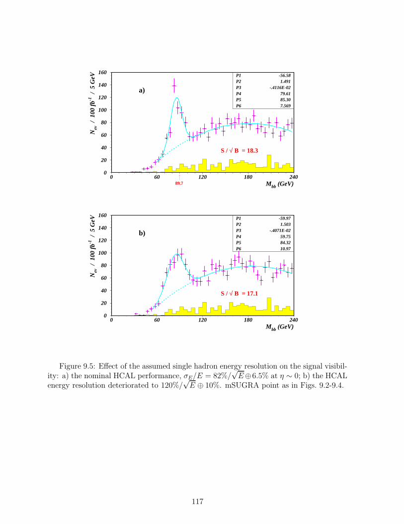
0

20

40

60

80

100

120

140

160

0 60 120 180 240

P1 -56.58P2 1.491P3 -.4116E-02P4 79.61P5 85.30P6 7.569

Mbb (GeV)

Nev

/ 1

00 f

b-1 /

5 G

eV

S / √ B = 18.3

a)

89.7

0

20

40

60

80

100

120

140

160

0 60 120 180 240

P1 -59.97P2 1.503P3 -.4071E-02P4 59.75P5 84.32P6 10.97

Mbb (GeV)

Nev

/ 1

00 f

b-1 /

5 G

eV

S / √ B = 17.1

b)

Figure 9.5: Effect of the assumed single hadron energy resolution on the signal visibil-ity: a) the nominal HCAL performance, σE/E = 82%/

√E⊕6.5% at η ∼ 0; b) the HCAL

energy resolution deteriorated to 120%/√

E ⊕ 10%. mSUGRA point as in Figs. 9.2-9.4.

117

0

20

40

60

80

100

120

140

160

180

200

0 60 120 180 240

P1 -56.58P2 1.491P3 -.4116E-02P4 79.61P5 85.30P6 7.569

Mbb (GeV)

Nev

/ 1

00 f

b-1 /

5 G

eVS / √ B = 18.3

a)

tan β = 2 , µ < 0

89.7

0

20

40

60

80

100

120

140

160

180

200

0 60 120 180 240

P1 -54.83P2 1.380P3 -.3734E-02P4 69.26P5 92.39P6 9.989

Mbb (GeV)

Nev

/ 1

00 f

b-1 /

5 G

eV

S / √ B = 18.2

b)

tan β = 2 , µ > 0

99.5

0

20

40

60

80

100

120

140

160

180

200

0 80 160 240

P1 -40.35P2 1.314P3 -.3651E-02P4 49.40P5 108.0P6 12.55

Mbb (GeV)

Nev

/ 1

00 f

b-1 /

5 G

eV

S / √ B = 12.1

c)

tan β = 10 , µ < 0

117.5

0

20

40

60

80

100

120

140

160

180

200

0 80 160 240

P1 -22.06P2 1.018P3 -.2582E-02P4 64.06P5 111.4P6 12.22

Mbb (GeV)

Nev

/ 1

00 f

b-1 /

5 G

eV

S / √ B = 15.5

d)

tan β = 30 , µ < 0

119.1

Figure 9.6: Dependence of the h → bb signal visibility on mh over the allowed range∼ 80 to 120 GeV, varying tanβ and sign(µ) at a fixed m0 = m1/2 = 500 GeV. NominalCMS instrumental performance, 100 fb−1 integrated luminosity.

118

0

20

40

60

80

100

120

140

0 60 120 180 240

P1 -31.87P2 1.086P3 -.3069E-02P4 41.48P5 79.16P6 7.343

Mbb (GeV)

Nev

/ 3

fb-1

/ 5

GeV

S / √ B = 10.1

a)

m0 = 200 GeV, m1/2 = 300 GeV

m (g~) = 770 GeV, m (u

~

L) = 705 GeV

84.5

0

25

50

75

100

125

150

175

200

225

250

0 60 120 180 240

P1 -64.11P2 2.529P3 -.8235E-02P4 75.38P5 78.73P6 6.609

Mbb (GeV)

Nev

/ 3

fb-1

/ 5

GeV

S / √ B = 11.2

b)

m0 = 300 GeV, m1/2 = 250 GeV

m (g~) = 659 GeV, m (u

~

L) = 642 GeV

82.4

0

50

100

150

200

250

300

0 60 120 180 240

P1 -20.63P2 2.023P3 -.5491E-02P4 142.2P5 76.02P6 7.379

Mbb (GeV)

Nev

/ 3

fb-1

/ 5

GeV

S / √ B = 20.4

c)

m0 = 400 GeV, m1/2 = 180 GeV

m (g~) = 505 GeV, m (u

~

L) = 577 GeV

A0 = 0 , tanβ = 2 , µ < 0

79.1

Figure 9.7: Some points in parameter space accessible already with 3 fb−1. Nominalb-tagging performance of CMS is assumed.

119

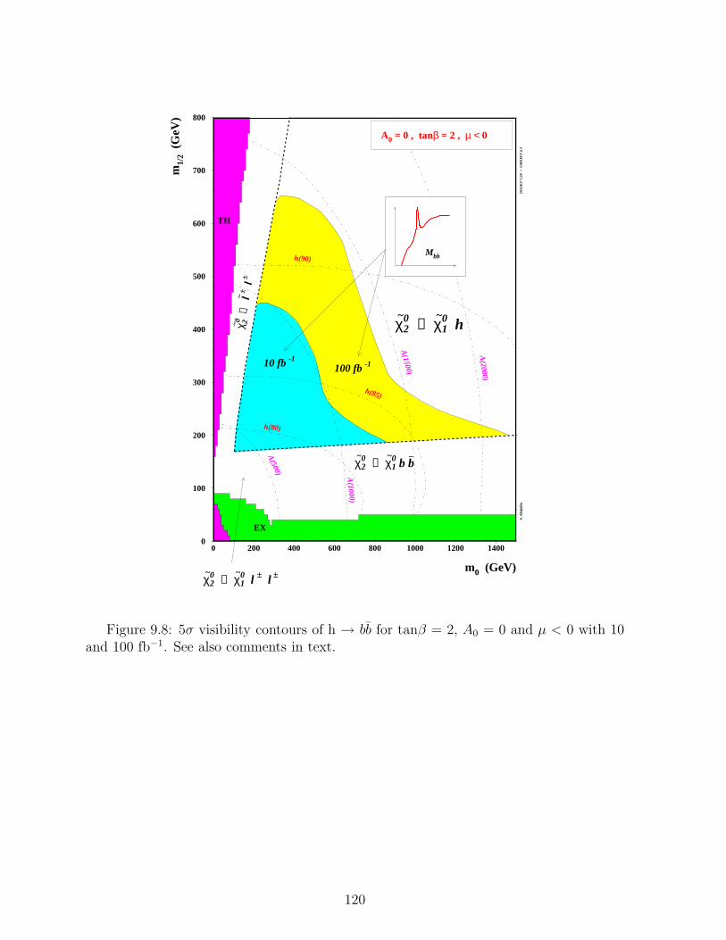
0

100

200

300

400

500

600

700

800

0 200 400 600 800 1000 1200 1400

m0 (GeV)

m1/

2 (

GeV

)

h(80)

h(85)

h(90)

A(500) A

(1000)

A(1500)

A(2000)

TH

EX

Mbb

100 fb -110 fb -1

A0 = 0 , tanβ = 2 , µ < 0

χ ~0 2 →

l ~ ± l ±

χ ~0

2 → χ ~0

1 h

χ ~0

2 → χ ~0

1 b b–

χ ~0

2 → χ ~0

1 l ± l ±

S. A

bdul

linIS

AJE

T 7

.29

+ C

MSJ

ET

4.3

Figure 9.8: 5σ visibility contours of h → bb for tanβ = 2, A0 = 0 and µ < 0 with 10and 100 fb−1. See also comments in text.

120

0

100

200

300

400

500

600

700

800

0 200 400 600 800 1000 1200 1400

m0 (GeV)

m1/

2 (

GeV

)

h(115)

h(117)

h(119)A(1000)

A(500)

χ ~0 2

→ 2

bod

y

χ ~0

2 → 3 body

χ ~0

2 → χ ~0

1 Z

χ ~0

2 → χ ~0

1 h

Br (χ~0

2 → χ~0

1h) = 50 %

TH

EX

Mbb

100 fb -1

10 fb -1

A0 = 0 , tanβ = 10 , µ < 0

S. A

bdul

linIS

AJE

T 7

.29

+ C

MSJ

ET

4.3

Figure 9.9: 5σ visibility contours of h → bb for tanβ = 10, A0 = 0 and µ < 0 with 10and 100 fb−1. See also comments in text.

121

0

100

200

300

400

500

600

700

800

0 200 400 600 800 1000 1200 1400

m0 (GeV)

m1/

2 (

GeV

)

h(116)

h(118)

h(120)

A(800)

A(500)

χ ~0 2 →

2 b

ody

(τ ∼ τ)

χ ~0

2 → 3 body ( χ ~0

1bb- )

χ ~0

2 → χ ~0

1 Z

χ ~0

2 → χ ~0

1 h

Br (χ~0

2 → χ~0

1 h) = 50 %

EX

TH

Mbb

100 fb -1

10 fb -1

A0 = 0 , tanβ = 30 , µ > 0

S. A

bdul

linIS

AJE

T 7

.29

+ C

MSJ

ET

4.3

Figure 9.10: 5σ visibility contours of h → bb for tanβ = 30, A0 = 0 and µ < 0 with10 and 100 fb−1. See also comments in text.

122

10 Sensitivity to sparticle masses and

model parameters

10.1 Establishing the SUSY mass scale

Once a deviation from the SM expectations is established in a number of final states indi-cating the presence of SUSY, the determination of the “SUSY mass scale” would becomethe first objective. The production and decay of high mass strongly interacting particles,as would be the case for gluinos and squarks, would lead to hard event kinematics, with anumber of hard central jets in the final state accompanied by significant missing transverseenergy due to escaping LSPs and neutrinos. As suggested in [48], we can characterize the“hardness” of an event by the scalar sum of transverse energies of the four hardest jetsand the missing transverse energy:

EsumT = E1

T + E2

T + E3

T + E4

T + EmissT (10)

This variable is rather insensitive to the transverse energy flow induced by event pile-upsince it takes into account only the calorimetric cells which are attached to a jet.

The following SM processes have been considered as a background to SUSY strongproduction: tt, W/Z + jets and QCD jet production (PYTHIA 2 → 2 processes includingbb). Events are selected by requiring:

• EmissT > max(100 GeV, 0.2Esum

T );

• ≥ 4 jets with ET > 50 GeV, the hardest with ET > 100 GeV in |η| < 5;

• Lepton veto: events are rejected if they contain an isolated lepton with pT > 10GeV.

Figure 10.1 shows the EsumT distributions for a representative mSUGRA point (with m0 =

300 GeV, m1/2 = 150 GeV, A0 = −600 GeV, tanβ = 2, µ > 0) and the SM background.The background, which is dominated by tt and W/Z + jets productions, is small comparedto the SUSY signal.

The peak value of the EsumT spectrum for the inclusive SUSY signal provides a good

estimate of the SUSY mass scale, defined as in [48]:

MSUSY = min(Mg, Mq) (11)

and where Mq is the mass of squarks from the first two generations. Figure 10.2 shows therelationship between the peak value of the Esum

T spectrum and MSUSY for 100 mSUGRAmodels chosen at random with 100 < m0 < 500 GeV, 100 < m1/2 < 500 GeV, −1000 <A0 < 1000 GeV, 1 < tanβ < 12 and sign(µ) = ±1 [49]. At each point the peak value ofEsum

T was found by a Gaussian fit. The very strong correlation between the peak value ofEsum

T and MSUSY as can be seen in Fig. 10.2 could provide a first estimate of the relevantSUSY mass scale.

10.2 Constraints from χ02 leptonic decays

Establishing the sparticle spectrum, the measurement of sparticle masses and the modelparameters will be the next step in uncovering SUSY, once its existence and its mass scale

123

have been established. In R-parity conserving models undetectable LSP’s make this tasknontrivial.

As mentioned previously, some specific SUSY decays are particularly useful for thedetermination of sparticle masses. The χ0

2 leptonic decays may not only provide thefirst indication for SUSY in significant regions of mSUGRA parameter space, but alsoallow us to obtain information on some sparticle masses by measuring the endpoint of thedilepton invariant mass spectrum and exploiting its specific kinematics. Before discussinghow to exploit this feature in inclusive two- and three-lepton final states, which is arecent development, let us first review the l+l− invariant mass spectrum in the exclusiveχ±

1 χ02→ 3l± + no jets+ Emiss

T final state, first described in [40] for three-body decaysχ0

2 → l+l−χ01. In this case the upper limit of dilepton invariant mass spectrum is:

Mmaxl+l− = Mχ0

2− Mχ0

1(12)

Figure 10.3 shows the expected l+l− mass spectrum for mSUGRA “Point 1” (see Table 1.1)in the exclusive χ±

1 χ02→ 3l± +no jets+ (Emiss

T ) channel arising from direct (Electroweak)χ±

1 χ02 production. The SM and internal SUSY backgrounds are also shown, all for Lint =

104 pb−1 [10]. The edge is at 52 GeV and with these statistics it could be measured with aprecision better than 1 GeV. This measurement of Mmax

l+l− = Mχ02−Mχ0

1= 52 GeV should

allow, within mSUGRA, estimation of Mχ01, Mχ0

2, Mχ±

1, Mg and m1/2 through eqs. (2) –

(4) as discussed in section 2.1.Even more information can be extracted from the χ0

2 two-body (cascade) decays χ02 →

l±l∓L,R → l+l−χ01. The kinematical upper limit in this case is:

Mmaxl+l− =

√

(M2

χ02

− M2

l)(M2

l− M2

χ01

)

Ml

(13)

i.e. it is sensitive also to the intermediate slepton mass. In this case, however, themeasurement of only the edge position does not provide information on the masses of allthe involved particles unambiguously. Nonetheless, as discussed in the following, throughanalyses of some kinematical distributions, the masses of χ0

1, χ02 and of the slepton can

be determined with reasonable precision [9]. Therefore, with two-body decays one canconstrain m1/2 and m0 through eqs. (2), (3) and (5)/(6), if the information on tanβ isavailable, for example from the Higgs sector of the model.

Direct leptonic decays of the χ02 dominate below m1/2

<∼ 200 GeV for nearly all valuesof m0; there is also a small region of high m1/2 where direct three-body decays are open,

as can be seen from Fig. 2.3a. Cascade leptonic decays of χ02 via lL (Fig. 2.3b) or lR

(Fig. 2.3c) occur at almost any m1/2 as soon as m0<∼ 0.5m1/2, where χ0

2 is heavier thanthe sleptons.

The expected position of the edge as a function of m1/2 is given in Fig. 10.4 for twodifferent values of the common scalar mass: m0 = 400 GeV and 100 GeV. The box size inthe Figure is proportional to the branching ratio B(χ0

2 → l+l− + invisible). At m0 = 400GeV the χ0

2 has only direct three-body decays for all values of m1/2 up to m1/2 ∼ 180 GeV,where “spoiler” modes open up. Measurement of Mmax

l+l− thus yields the common gauginomass parameter m1/2 unambiguously in this region. For m0 = 100 GeV the situationis more complicated. Here at different values of m1/2 different leptonic decay modes of

χ02 dominate: direct decays up to m1/2

<∼ 130 GeV; cascade decays via lR at 130 GeV

124

<∼ m1/2<∼ 250 GeV and, finally, cascade decays via lL at m1/2

>∼ 250 GeV. In some regionstwo χ0

2 decay channels coexist.The essential issue, for the exploitation of an observed edge, is knowing whether the χ0

2

decay chain is three-body or two-body. In general, the pT spectra of leptons from χ02 two-

body decays are more asymmetric compared to the three-body decays. To characterizethe asymmetry we introduce the variable [9]:

A =pmax

T − pminT

pmaxT + pmin

T

(14)

where pmaxT (pmin

T ) corresponds to the lepton of maximum (minimum) transverse momen-tum.

An example of decay type determination is discussed for the mSUGRA point m0 = 100GeV, m1/2 = 150 GeV. The sparticle masses are Mχ0

2= 135 GeV, Mχ0

1= 65 GeV MlR

=

120 GeV and χ02 decays via χ0

2 → l±l∓R → l+l−+ χ01 with a probability of 0.54. Figure 10.5

shows the dilepton mass spectrum for this parameter space point in the inclusive 3 leptonevents for an integrated luminosity of Lint = 5× 103 pb−1. The expected SM backgroundis also shown. Of the three leptons with pT > 15 GeV only the two of opposite charge andsame flavor, which enter the invariant mass distribution, are required to be isolated. Avery spectacular edge is situated at ≃ 52 GeV. There is a second and much weaker edgeat ≃ 69 GeV which is due to direct three-body decays with B(χ0

2 → l+l− + χ01) = 0.05.

Thus at this mSUGRA point there are two leptonic decay modes with very differentbranching ratios. To identify the decay chain responsible for the first edge, we look atthe asymmetry A distribution of the lepton pairs with Ml+l− < 52 GeV. Figure 10.6(full line) shows the A distribution for these events. The pronounced asymmetry in pT

indicates the cascade nature of decays. If we now pick up the lepton pairs from themass interval 55 < Ml+l− < 69 GeV below the second edge, then the corresponding Adistribution peaks near zero, as seen in Fig. 10.6 (dashed-dotted line), indicating thethree-body decay type of these events. To illustrate the generality of this approach, twomore examples of A distributions are also shown in Fig. 10.6 for mSUGRA parameterspace points m0 = 100 GeV, m1/2 = 400 GeV with pure 2-body decays (dashed line) andm0 = 400 GeV, m1/2 = 150 GeV with pure 3-body decays (dotted line), respectively.

Once the decay type is determined, the next step is to extract the masses of theparticles involved, the χ0

2, χ01 and l. In our example case of two-body decay the l+l−

kinematical upper limit is

Mmaxl+l− =

√

(M2

χ02

− M2

l)(M2

l− M2

χ01

)

Ml

= 52 GeV. (15)

This equation can be satisfied by an infinite number of Mχ01, Mχ0

2and Ml mass combi-

nations. To find a solution, we assume Mχ02

= 2Mχ01

and generate χ02 → l±l∓ → l+l−χ0

1

two-body sequential decays for various assumptions on Ml (Mχ01), e.g. from 70 GeV to 150

GeV in 10 GeV steps, with the χ01 mass constrained to provide the “observed” position

of the edge. For each value of Ml, one obtains two series of solutions for equation (15).Some of them are shown in Fig 10.7 in terms of dilepton invariant mass and pT -asymmetrydistributions, in Figs. 10.7a,c for “low mass” solutions and Figs. 10.7b,d for “high mass”solutions [9]. The solid lines in Figs. 10.7a-c correspond to the “observed” spectra and the

125

dotted histograms are the results obtained from eq. (15). Clearly, the “observed” l+l−

invariant mass spectrum itself and the pT -asymmetry distributions allow us to eliminatethe “high mass” solutions of eq. (15). To find the best combination of Mχ0

1, Mχ0

2and

Ml among the “low mass” solutions, we perform a χ2-test on the pT -asymmetry distri-butions, taking into account only the difference in shapes, but not the normalization.The result is shown in Fig. 10.8. The horizontal line in this Figure corresponds to theexpected uncertainty of simulations due to the detector resolution, background estimates,initial/final state radiations, etc. We obtain the following precisions on masses: δMχ0

1

<∼5 GeV, δMl

<∼ 10 GeV. The use of the total number of observed events, as well as thedilepton invariant mass spectrum itself in a combined χ2-test would further improve theseresults.

As shown above for the mSUGRA point under consideration, the second edge inthe dilepton mass spectrum at Mmax

l+l− = 69 GeV (see Fig. 10.6) is due to direct three-body decays of χ0

2. Using now two measured edge position values and assuming againMχ0

2= 2Mχ0

1, two solutions for the slepton mass can be directly obtained Ml = 120 GeV

and Ml = 77 GeV. The corresponding dilepton mass spectra for these two solutions areshown in Fig. 10.9. The clear difference in the predicted spectra (the first edge in Fig. 10.5which proceeds through l vs. Fig. 10.9) allows us to eliminate the Ml = 77 GeV solution.At this particular mSUGRA point the use of two observable edges provides a precision ofδMχ0

1,l

<∼ 1 GeV [41, 9].Another example of a double edge is given in Fig. 10.10 for the mSUGRA point

(50 GeV, 125 GeV). Here the sparticle masses are Mχ02

= 116 GeV, Mχ01

= 55 GeV,MlL

= 110 GeV, MlR= 78 GeV. In this case two two-body decays, via left and right

sleptons coexist with the comparable branching ratios B(χ02 → l±l∓L → l+l−χ0

1) = 0.037and B(χ0

2 → l± l∓R → l+l−χ01) = 0.013 and their analysis could proceed as indicated above

providing a strong constraint on the underlying model.

10.3 Determination of the squark mass

The observation of an edge in the dilepton mass spectrum, resulting from χ02 leptonic

decays allows not only the determination of χ01, χ0

2, (l) masses, but also enables themomenta to be fixed. At the upper limit of the l+l− spectrum in direct three-body decaysχ0

2 → l+l−χ01, the χ0

1 is produced at rest in the χ02 rest frame. Assuming knowledge of the

χ01 mass (or, equivalently, knowledge of a relation between χ0

1 and χ02 masses), one can

then, for events at the l+l− edge, reconstruct the χ02 momentum vector in the laboratory

frame:pχ0

2= (1 + Mχ0

1/Ml+l−) × pl+l− (16)

Once the four-momentum vector of the χ02 is determined, one can search for a resonance

structure in, e.g. the χ02 + jet(s) invariant mass distributions. This technique can be

put to a good use to reconstruct g/q masses [48] as the next-to-lightest neutralinos areabundantly produced in gluino and squark decays, see e.g. Figs. 2.5a,b.

An example of the q mass reconstruction is given for mSUGRA point with m0 = 300GeV, m1/2 = 150 GeV, A0 = −600 GeV, tanβ = 2 and µ > 0, discussed in section 10.1.The masses of relevant sparticles are 463 GeV, 495 GeV, 151 GeV, 425 GeV, 112 GeV and57 GeV for qL,R (squarks of the first two generations), t2, t1, g, χ0

2 and χ01, respectively, and

the total SUSY cross-section (452 pb) is largely dominated by σt1 t1 = 195 pb, σgqL,R= 109

126

pb, σgg = 77 pb productions. Gluinos are lighter than squarks of the first two generations,but their decays to stop and sbottom are kinematically allowed, giving several b-jets atthe end of the decay chain. Right squarks qR predominantly decay to χ0

1 + q or to g+q.Finally, the Left squarks qL have the interesting for us decay mode to χ0

2+ q with abranching ratio of 0.27. To extract this latter decay chain from internal SUSY and SMbackgrounds we have adopted the following procedure [49].

• Require two isolated leptons with pT > 10 GeV; and an angular separation ∆Rl+l− =√∆η2 + ∆φ2 < 1.

• The scalar sum of calorimeter cell transverse energies and of muon transverse mo-menta, ΣEcalo

T + pµT > 600 GeV to ensure production of hard events. Require Emiss

T

> 100 GeV.

• The l+l− invariant mass has been reconstructed and the edge position at ≃54 GeVhas been observed. The pT -asymmetry distribution of dilepton pairs indicates it isdue to a the three-body decay of type χ0

2 → l+l−χ01.

• Events with a dilepton mass close to the kinematical limit, i.e. 49 GeV < Ml+l− < 54GeV, have been selected for further analysis; the χ0

2 momentum has been determinedusing eq. (16).

• The invariant mass of the χ02 and each non-b-jet with Ejet

T > 300 GeV has thenbeen reconstructed. Such a hard jet is unlikely to originate from a QCD radiation.Furthermore, due to the large mass difference MqL

− Mχ02

= 351 GeV the ET -spectrum of quark-jets from the qL decay is harder than both the inclusive SUSYand SM jet spectra. Hence this requirement enhances the qL signal.

Figure 10.11 shows the reconstructed χ02 + jet mass spectrum for SUSY and SM events

for an integrated luminosity of Lint = 104 pb−1. As a source of the SM backgrounds wehave considered tt, W/Z + jets, WW, ZZ, ZW and bb processes. Their contribution isnegligible compared to the internal SUSY background. A peak at ∼450 GeV is clearlyvisible and a Gaussian plus polynomial fit yields a value of 447 ± 4 GeV (statistical error)for the reconstructed qL mass. Significant systematic uncertainties are associated withthis measurement due to the jet reconstruction algorithm, energy scale, approximationsin determining the χ0

2 four-momentum, in particular the dilepton mass interval whichhas been chosen for analysis, etc. The overall systematic uncertainty is estimated to beabout ±5%. A much more detailed analysis is needed to understand fully the achievableprecision [49].

As a concluding remark, the observation of a resonance peak in the χ02 + jet invariant

mass spectrum would be interpreted as a squark undergoing a two-body decay to χ02 and

a quark. The technique described here is also applicable for gluino mass reconstruction,for example in g → qq′χ0

2 with subsequent decay of χ02 → χ0

1.

10.4 Sensitivity to model parameters in 3l + no jets + EmissT final

states

Since information on m1/2 can be obtained from the l+l− edge position in regions ofparameter space where it is visible, one can then attempt to constrain the m0 parameter

127

Table 10.1: SUSY cross-sections (in fb) after selection. Events are counted below“observed” edge at 54 GeV.

Point χ±1 χ0

2 gg gq qq gχ qχ χχ ll lν νν

(100,100) 71.6 14.1 11.3 5.9 14.5(150,100) 53.8 15.9 5.3 2.6 5.3(200,100) 45.6 11.9 6.0 4.0 0.0(300,100) 29.7 0.5 1.0 0.5 0.0(400,100) 23.0 0.0 0.0 0.0 0.0

(1000,100) 15.7 0.0 0.0 0.0 0.0(1800,100) 12.3 0.0 0.0 0.0 0.0

Table 10.2: SM cross-sections (in fb) after selection. Events are counted below“observed” edge at 54 GeV.

WZ ZZ tt Wtb Zbb bb1.42 0.48 1.07 0.46 0.27 < 0.15

from the event rates. Let us first discuss the case of 3l + no jets + EmissT events [10]. For

a fixed m1/2 the σ·B(χ±1 χ0

2 → 3l + invisible) decreases monotonically with increasing m0

in the region where χ02 has direct three-body decays. Table 10.1 gives the expected SUSY

event rates for a series of points with different m0 but with fixed m1/2 = 100 GeV, i.e.corresponding to approximately the same Mmax

l+l− . The remaining parameters are tanβ = 2,A0 = 0, µ < 0. All expected SUSY sources of such events are included. The applied cutsare (Set 1 in section 8):

• 3l with plT > 15 GeV in |ηl| < 2.4(2.5) for muons (electrons);

• Isolation: no track with pT > 1.5 GeV in a cone R = 0.3 about the lepton direction,for all leptons;

• Jet veto: no jet with EjetT > 25 GeV in |ηjet| < 3.5;

• Z-mass cut: no lepton pair with Ml+l− > 81 GeV.

Table 10.3: statistical (Lint = 104 pb−1) and systematic errors on m0 measurement form1/2 ∼ 100 GeV.

Source m0 ∈ [100 GeV; 300 GeV] m0 ∈ [300 GeV; 400 GeV]

statistical error 8 ÷ 20 GeV 20 ÷ 55 GeV

edge measurement precision 4 ÷ 8 GeV 8 ÷ 25 GeVuncertainty on SM background 2.5 ÷ 9 GeV 9 ÷ 30 GeV

uncertainty on luminosity 27 ÷ 35 GeV 35 ÷ 85 GeV

statistical ⊕ systematic error 30 ÷ 45 GeV 45 ÷ 105 GeV

128

Table 10.4: SUSY cross-sections (in fb) after selection. Events are counted below the“observed” edge at 72 GeV.

Point χ±1 χ0

2 gg gq qq gχ qχ χχ ll lν νν

(150,150) 26.3 0.3 1.5 1.3 2.9(200,150) 19.9 0.7 0.8 0.8 0.8(300,150) 10.7 0.5 0.1 0.1 0.0(400,150) 6.4 0.0 0.0 0.1 0.0(1000,150) 3.6 0.0 0.0 0.0 0.0(1800,150) 3.3 0.0 0.0 0.0 0.0

Table 10.5: SM cross-sections (in fb) after selection. Events are counted below the“observed” edge at 72 GeV.

WZ ZZ tt Wtb Zbb bb1.53 0.42 1.66 0.50 0.33 < 0.15

From the selected events we count the ones with Ml+l− < Mmaxl+l− = 54 GeV. Con-

tributions from different SUSY sources – χ±1 χ0

2 direct production, strong production,gluino/squark associated production, gaugino pair and slepton pair productions – aregiven separately. The main contribution is always due to χ±

1 χ02 direct production, but

below m0 ∼ 300 GeV other SUSY processes also contribute significantly.The expected SM event rates after selection cuts are given in Table 10.2. All SM pro-

cesses together amount 3.85 fb, which is always smaller than the χ±1 χ0

2 direct productionrate at m1/2 = 100 GeV, and much smaller than that for m0

<∼ 300 GeV (Table 10.1).Table 10.1 shows that the data selection does not wash out significantly the event

rate sensitivity to m0 expected from the behavior of σ·B for χ±1 χ0

2 direct production(Fig. 2.4). Figure 10.12a shows NSUSY versus m0 for m1/2 = 100 GeV, where NSUSY

is the SM-background-subtracted number of 3l + no jets + EmissT events surviving cuts

for an integrated luminosity of Lint = 104pb−1. The error band includes both statisticaland systematic uncertainties; The systematic uncertainties include effects due to the edgemeasurement precision, the uncertainty on the rate of SM processes and a 10% uncertainty

Table 10.6: statistical (Lint = 105 pb−1) and systematic errors on m0 measurement form1/2 ∼ 150 GeV.

Source m0 ∈ [150 GeV; 300 GeV] m0 ∈ [300 GeV; 400 GeV]

statistical error 5 ÷ 10 GeV 10 ÷ 18 GeV

edge measurement precision 2 ÷ 8 GeV 5 ÷ 8 GeVuncertainty on SM background 9 ÷ 24 GeV 24 ÷ 55 GeV

uncertainty on luminosity 28 ÷ 30 GeV 30 ÷ 40 GeV

statistical ⊕ systematic error 32 ÷ 40 GeV 40 ÷ 75 GeV

129

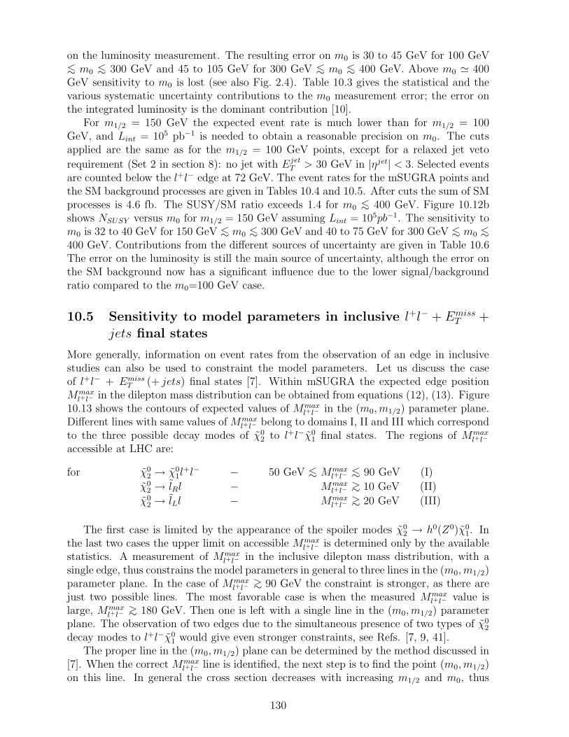
on the luminosity measurement. The resulting error on m0 is 30 to 45 GeV for 100 GeV<∼ m0

<∼ 300 GeV and 45 to 105 GeV for 300 GeV <∼ m0<∼ 400 GeV. Above m0 ≃ 400

GeV sensitivity to m0 is lost (see also Fig. 2.4). Table 10.3 gives the statistical and thevarious systematic uncertainty contributions to the m0 measurement error; the error onthe integrated luminosity is the dominant contribution [10].

For m1/2 = 150 GeV the expected event rate is much lower than for m1/2 = 100GeV, and Lint = 105 pb−1 is needed to obtain a reasonable precision on m0. The cutsapplied are the same as for the m1/2 = 100 GeV points, except for a relaxed jet veto

requirement (Set 2 in section 8): no jet with EjetT > 30 GeV in |ηjet| < 3. Selected events

are counted below the l+l− edge at 72 GeV. The event rates for the mSUGRA points andthe SM background processes are given in Tables 10.4 and 10.5. After cuts the sum of SMprocesses is 4.6 fb. The SUSY/SM ratio exceeds 1.4 for m0

<∼ 400 GeV. Figure 10.12bshows NSUSY versus m0 for m1/2 = 150 GeV assuming Lint = 105pb−1. The sensitivity tom0 is 32 to 40 GeV for 150 GeV <∼ m0

<∼ 300 GeV and 40 to 75 GeV for 300 GeV <∼ m0<∼

400 GeV. Contributions from the different sources of uncertainty are given in Table 10.6The error on the luminosity is still the main source of uncertainty, although the error onthe SM background now has a significant influence due to the lower signal/backgroundratio compared to the m0=100 GeV case.

10.5 Sensitivity to model parameters in inclusive l+l− + EmissT +

jets final states

More generally, information on event rates from the observation of an edge in inclusivestudies can also be used to constraint the model parameters. Let us discuss the caseof l+l− + Emiss

T (+ jets) final states [7]. Within mSUGRA the expected edge positionMmax

l+l− in the dilepton mass distribution can be obtained from equations (12), (13). Figure10.13 shows the contours of expected values of Mmax

l+l− in the (m0, m1/2) parameter plane.Different lines with same values of Mmax

l+l− belong to domains I, II and III which correspondto the three possible decay modes of χ0

2 to l+l−χ01 final states. The regions of Mmax

l+l−

accessible at LHC are:

for χ02 → χ0

1l+l− − 50 GeV <∼ Mmax

l+l−<∼ 90 GeV (I)

χ02 → lRl − Mmax

l+l−>∼ 10 GeV (II)

χ02 → lLl − Mmax

l+l−>∼ 20 GeV (III)

The first case is limited by the appearance of the spoiler modes χ02 → h0(Z0)χ0

1. Inthe last two cases the upper limit on accessible Mmax

l+l− is determined only by the availablestatistics. A measurement of Mmax

l+l− in the inclusive dilepton mass distribution, with asingle edge, thus constrains the model parameters in general to three lines in the (m0, m1/2)parameter plane. In the case of Mmax

l+l−>∼ 90 GeV the constraint is stronger, as there are

just two possible lines. The most favorable case is when the measured Mmaxl+l− value is

large, Mmaxl+l−

>∼ 180 GeV. Then one is left with a single line in the (m0, m1/2) parameterplane. The observation of two edges due to the simultaneous presence of two types of χ0

2

decay modes to l+l−χ01 would give even stronger constraints, see Refs. [7, 9, 41].

The proper line in the (m0, m1/2) plane can be determined by the method discussed in[7]. When the correct Mmax

l+l− line is identified, the next step is to find the point (m0, m1/2)on this line. In general the cross section decreases with increasing m1/2 and m0, thus

130

Table 10.7: Mmaxl+l− values (in GeV) at the investigated (m0, m1/2) points from domain I,

χ02 → χ0

1 + l+ + l−.

(120,160)(130,160)(180,160)(200,160)(220,160)(240,160) (290,160)(350,160)

Mmaxl+l− 74 74 74 74 74 74 74 73.7

Table 10.8: Mmaxl+l− values (in GeV) at the investigated (m0, m1/2) points from domain II,

χ02 → l±R + l∓ → χ0

1 + l+ + l−.

(m0, m1/2) → (80,162) (90,170) (105,180) (110,187) (120,195)

Mmaxl+l− 74 74 73 75 73

Table 10.9: Mmaxl+l− values (in GeV) at the investigated (m0, m1/2) points from domain

III, χ02 → l±L + l∓ → χ0

1 + l+ + l−.

(m0, m1/2) → (20,195) (40,210) (60,230) (80,255)

Mmaxl+l− 73 73 73 73

the study of the event rate along the corresponding Mmaxl+l− lines will determine the point

in parameter space. As an example of the general situation let us discuss the case ofMmax

l+l− = 74± 1 GeV, with three lines corresponding to domains I,II and III, respectively.The (m0, m1/2) points analysed are given in tables 10.7-10.9.

As this is an inclusive analysis, we assume a low luminosity of Lint = 103 pb−1. Wediscuss first domain III, where the situation is simplest. To minimize the uncertaintiesdue to background, we require p

l1,2

T > 15 GeV and EmissT > 130 GeV. The dependence of

the resulting event rate on m0 is shown in Fig. 10.14. The errors are calculated taking intoaccount the statistical error and assuming a systematic error of 30 % for the backgrounduncertainty; a systematic error due to the precision of the edge position measurementis also taken into account. From the observed event rate m0 can be determined withgood precision, δm0 ≃ 4 GeV. The parameter m1/2 is then given by the Mmax

l+l− -line in the(m0, m1/2) plane (Fig. 10.13). The precision obtained in such a way is δm1/2 ≃ 4 GeV.

In domain II, the event rate along a line of definite Mmaxl+l− first increases and then

decreases with increasing m0, Fig. 10.15. This is mainly due to the change in the branchingratios. The event rate thus does not determine m0 uniquely: a given event rate correspondsin general to two m0 values. The ambiguity can, however, be solved at high luminosityLint = 105 pb−1, when two edges in the Ml+l− distribution can be observed [7].

For domain I, the m0 dependence of the event rate is shown in Fig. 10.16a, again forMmax

l+l− ≃ 74 ± 1 GeV. There is a steep increase of the rate at m0 ≃ 120 − 130 GeV. Thisis due to the decay channel χ0

2 → l+l−χ01 just opening up in this region. As can be seen

from Fig. 10.16a, there is an ambiguity in the determination of m0 if the event rate is inthe region 3700 <∼ NEV <∼ 5600 or 120 GeV <∼ m0

<∼ 240 GeV. Additional informationcan however be obtained from the average number of jets <Njet> in the events. Figure10.16b shows <Njet> as a function of m0. <Njet> is increasing with m0 as more jets areproduced with increasing squark-mass. With the measured <Njet> we can resolve theambiguity in the region 120 GeV <∼ m0

<∼ 240 GeV and determine m0 with δm0 ≃7-3 GeV.

131

0

10000

20000

30000

40000

50000

0 500 1000 1500 2000 2500 3000

ETsum (GeV)

Even

ts/15

0 Ge

V

Lint=104pb-1

SUSY

Standard Model

≥ 4 jets with ET ≥ 50 GeV, ET1 ≥ 100 GeV

E/ T ≥ max(100GeV,2×ETsum)

Lepton veto

Figure 10.1: EsumT distribution for both the inclusive SUSY and the SM backgrounds after

the event selection cuts have been applied.

0 500

200

400

600

800

1000

1000

1200

1500 2000ET sum ( GeV )

MS

US

Y (

GeV

)

D_D

_109

9.n

Figure 10.2: The relationship between the peak value of the EsumT distribution and the

SUSY mass scale, as defined in the text.

132

SUSY bkgd.

Sum

SM bkgd.

χ± χ01 2

~~

0

10

20

30

40

50

60

70

80

20 40

Eve

nts

/ 4 G

eV

60 80 100 120

Lint = 104 pb–1

140

Mmax ≈ M (χ0) – M (χ0) ≈ M (χ0) ⇒ m1/2 ≈ 2.5 M (χ0)

in m-SUGRA

~ ~ ~ ~1 1 12

Pt > 15 GeVIsolationCentral jet vetoM + – < 81 GeV

D-

D-9

80n

m0 = 200 GeV, m1/2 = 100 GeV, tanβ = 2, A0 = 0, µ < 0

M (χ0) - M (χ0) ≈ M (χ0) ≈ 52 GeV1 12~ ~ ~

Cuts:

1 2

χ0 mass determination in 3 ± + no jets + Emiss

final state from χ± χ0 productiont1

~

~ ~

+ - M GeV

Figure 10.3: Dilepton invariant masses distribution for mSUGRA point (m0=200 GeV,m1/2=100 GeV) with Lint = 104 pb−1 in the 3l + no jets + (Emiss

T ) events. Contributionsfrom SM and SUSY backgrounds are also shown.

133

0

20

40

60

80

100

120

25 50 75 100 125 150 175 200 225 250

m1/2 (GeV)

Mll

max

(G

eV)

m0 = 400 GeV Box size ∝ B(χ~0→l+l-+inv.)2

0

20

40

60

80

100

120

140

160

180

200

50 100 150 200 250 300 350 400 450 500

m1/2 (GeV)

Mll

max

(G

eV)

χ~ 0 →l

+ l- +χ

~ 0

2

1

χ~ 0 →ll~

R→l

+ l- +χ~ 0

2

1χ~ 0 →ll

~L→l

+ l- +χ~ 0

2

1

m0 = 100 GeV Box size ∝ B(χ~0→l+l-+inv.)2

Figure 10.4: Correlation between Mmaxl+l− and m1/2 for fixed m0 = 400 GeV and m0 = 100

GeV. The other mSUGRA parameters are: tanβ=2, A0 = 0 and µ < 0.

134

Lint = 5×103 pb-1104

103

102

0 20 40 60 80 100

SUSY + SM

SM

EV

EN

TS

/ 2

GeV

D_D

_996

n

+ -M GeV

pt > 15 GeV, IηI < 2.4 1.2

pt > 2 GeV, in ∆R < 0.3 Isol: no tracks with

pt > 15 GeV, IηI < 2.43

M (χ ) = 135 GeV0∼ M (χ1 ) = 65 GeV0∼

χ2 0∼ χ1

0∼

M ( R

) = 120 GeV∼m0 = 100 GeV, m1/2 = 150 GeV, tanβ = 2, A0 = 0, µ < 0

2; ;

+ -

χ2 0∼ ∼

χ1 0∼ + -

Figure 10.5: l+l− mass distribution for mSUGRA point (m0 = 100 GeV, m1/2 = 150GeV); the other mSUGRA parameters are: tanβ=2, A0 = 0 and µ < 0. The shadedhistogram corresponds to the SM background.

135

0

0.01

0.02

0.03

0 0.1 0.2 0.3 0.4 0.5 0.6 0.7 0.8 0.9 1

χ~0

2 decay asymmetry at various (m0, m1/2) points

Figure 10.6: Lepton transverse momentum asymmetry distributions in χ02 decays.

mSUGRA parameters (m0, m1/2) are the following: 100 GeV, 150 GeV (full and dashed-dotted lines); 100 GeV, 400 GeV (dashed line) and 400 GeV, 150 GeV (dotted line).

136

0

500

1000

1500

2000

0 20 40 60 80

a)

“Low mass“ solutions

0

500

1000

1500

2000

0 20 40 60 80

b)

“High mass“ solutions

0

200

400

600

0 0.2 0.4 0.6 0.8 1

c)

0

200

400

600

0 0.2 0.4 0.6 0.8 1

d)

Figure 10.7: The dotted lines correspond to the invariant mass spectra and transversemomentum asymmetry distributions in χ0

2 two-body decays for several “low mass” and“high mass” solutions of eq. (10). The full line corresponds to the initial (observed)spectrum.

137

1

10

10 2

90 100 110 120 130 140 150 160

Ml ~ (GeV)

χ2 / N

DF

63.6 GeV

76.6 GeV

72.1 GeV

Figure 10.8: Results of the χ2 test of the shape of pT -asymmetry distributions as afunction of slepton mass. The corresponding values of Mχ0

1are also indicated.

138

10 2

10 3

10 4

0 20 40 60 80 100

Ml ~ = 120 GeV

Ml ~ = 77 GeV

Figure 10.9: Predicted l+l− invariant mass spectra for two values of slepton masses:Ml = 120 GeV (full line) and Ml = 77 GeV (dashed line); mSUGRA parameters as inFig. 10.6.

139

0

20

40

60

80

100

120

0 20 40 60 80 100 120 140

Ml+l- (GeV)

Eve

nts

/ 2 G

eV

m0 = 50 GeV, m1/2= 125 GeV, tanβ=2, A0=0, µ< 0

M(χ~ 0

1) = 55 GeV, M(χ~ 0

2) = 116 GeV

M(l~

L) = 110 GeV, M(l~

R) = 78 GeV

pT1,2 > 15 GeV

IsolationpT

3 > 15 GeV

Lint = 103 pb-1

0

10

20

30

40

50

60

70

80

0 20 40 60 80 100 120 140

Ml+l- (GeV)

Eve

nts

/ 4 G

eV

pT1,2,3 > 15 GeV

Isolation

Lint = 103 pb-1

Figure 10.10: Expected l+l− mass spectrum for mSUGRA Point: m0 = 50 GeV,m1/2 = 125 GeV, tanβ=2, A0 = 0 and µ < 0. a) Leptons with pT > 15 GeV in |η| < 2.4are considered. Two leptons which enter invariant mass spectrum are required to beisolated; b) as in previous case, but all three leptons are isolated. The dotted histogramcorresponds to the SM background.

140

0

20

40

60

80

100

120

0 100 200 300 400 500 600 700 800M(χ2

0+jet) (GeV)

Eve

nts/

27 G

eV

Lint=104pb-149 ≤Mll ≤ 54 GeV

∆Rll ≤1.0

Σ|ET| ≥600 GeV

ET(jet) ≥300 GeV

SUSY+SM

SM

Figure 10.11: The reconstructed χ02+jet mass spectrum for the SUSY + SM events.

141

0

200

400

600

800

1000

1200

1400

1600

0 100 200 300 400 500 600 700 800 900 1000 1100

m0 (GeV)

NSU

SY a)

Sensitivity to m0

in the exclusive 3l + no jets + (ET miss

) channel

Lint = 104 pb-1

m1/2 ∼ 100 GeV

0

500

1000

1500

2000

2500

3000

3500

4000

4500

5000

0 100 200 300 400 500 600 700 800 900 1000 1100

m0 (GeV)

NSU

SY b)

Lint = 105 pb-1

m1/2 ∼ 150 GeV

Figure 10.12: a) Number of SUSY 3l + no jets + (EmissT ) events with Lint = 104pb−1

as a function of common scalar mass m0 for m1/2 ∼ 100 GeV. b) Number of SUSY3l + no jets + (Emiss

T ) events with Lint = 105pb−1 as a function of common scalar massm0 for m1/2 ∼ 150 GeV.

142

900

800

700

600

500

400

300

200

100

0 50 100 150 200 250 300 350 400 450 500

m0 (GeV)

m1/

2 (

GeV

)

tanβ = 2, A0 = 0,µ < 0

D_D

_106

6n

TH

TH EX

300

170

90

75

6020

75

90

170

60

60

7510

Mmax = 90 GeV

LEP2 + Tevatron

Figure 10.13: Contour lines of expected Mmaxl+l− values (in GeV) in the invariant dilepton

mass distribution corresponding to the three different χ02 decay modes in the region of the

(m0, m1/2) parameter plane accessible with 105 pb−1.

143

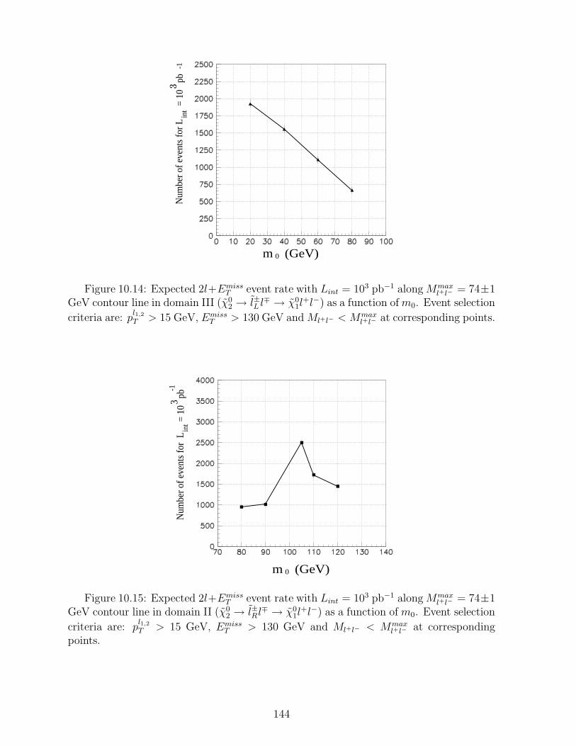
m 0

Num

ber o

f eve

nts

for L

int

= 10

pb

3

(GeV)

-1

Figure 10.14: Expected 2l+EmissT event rate with Lint = 103 pb−1 along Mmax

l+l− = 74±1GeV contour line in domain III (χ0

2 → l±L l∓ → χ01l

+l−) as a function of m0. Event selection

criteria are: pl1,2

T > 15 GeV, EmissT > 130 GeV and Ml+l− < Mmax

l+l− at corresponding points.

m 0

Num

ber o

f eve

nts

for

L int=

10

pb

3 -1

(GeV)

Figure 10.15: Expected 2l+EmissT event rate with Lint = 103 pb−1 along Mmax

l+l− = 74±1GeV contour line in domain II (χ0

2 → l±Rl∓ → χ01l


criteria are: pl1,2


l+l− at correspondingpoints.

144

Num

ber o

f eve

nts f

or L

int=

10

pb

3 -1

m 0 (GeV)

(512,452)

(402,440)

(m ,m q g~ ~ )

a)

b)

<N

> j

et

m 0 (GeV)

Figure 10.16: a) Expected 2l + EmissT event rate with Lint = 103 pb−1 along Mmax

l+l− =74 ± 1 GeV contour line in domain I (χ0

2 → χ01l


criteria are: pl1,2


l+l− at correspondingpoints; b) Average number of jets (Ejet

T > 30 GeV, | ηjet |< 3) at investigated points fromdomain I. The numbers in parenthesis show the masses of squarks and gluinos (in GeV)at corresponding points.

145

11 Summary and conclusions

We have investigated the ability of the CMS detector at the Large Hadron Collider todiscover and characterise supersymmetry. As a benchmark model, we used the minimalsupergravity-inspired supersymmetric standard model (mSUGRA). In the investigatedscenarios the lightest supersymmetric particle (LSP) is stable and is the χ0

1.Discovery of supersymmetry at the LHC will be relatively straightforward. It would

be revealed by large excesses of events over the standard model expectations in a numberof characteristic signatures – for example missing ET plus jets, with one or more isolatedleptons; an excess of trilepton events; a very characteristic signature in the l+l− invariantmass distribution.

Because of the importance of missing ET signatures, considerable effort has beenexpended in optimising the performance of the CMS detector for Emiss

T measurements.In particular we have tried to minimize sources of non-Gaussian tails in the calorimeterresponse due to cracks and dead materials.

For the cases we have studied in detail and for 105 pb−1 integrated luminosity,

• Squarks and gluinos can be discovered up to masses well in excess of 2 TeV, i.e.for a parameter space region m0

<∼ 2 − 3 TeV and m1/2<∼ 1 TeV (see Fig. 11.1).

This covers the entire parameter space over which supersymmetry can plausibly berelevant to electroweak symmetry breaking without excessive fine-tuning. Over thelifetime of LHC experiments these searches would probe the ≃ 3 TeV region.

• Charginos and neutralinos can be discovered from an excess of events in dileptonor trilepton final states. Inclusive searches could give early indications from theircopious production in squark and gluino cascade decays just from the l+l− spectrumshapes. With 105 pb−1 the dilepton edge due to the χ0

2 leptonic decays can be seenup to m1/2 ∼ 900 GeV for m0

<∼ 400 GeV (see Fig. 11.2). Applying isolationrequirements and a jet veto would enable direct chargino/neutralino production tobe selected; the mass reach in this case covers up to ∼ 170 GeV for χ±

1 , χ02 and

∼ 90 GeV for χ01. The region of sensitivity (Fig. 11.1) is entirely determined by the

production cross section and decay branching ratios rather than by any detectorlimitations.

• Directly-produced sleptons can be detected up to masses of ∼ 350 GeV using dilep-ton signatures. Again, the use of a jet veto is crucial, and the lepton openingangle can be used to discriminate between the slepton signal and other SUSY back-grounds. The region of sensitivity (Fig. 11.1) is once again largely determined bythe production cross section and decay branching ratios. It is also interesting toremark that the domain of parameter space explorable through direct slepton pro-duction searches matches closely the χ0

1 cosmological dark matter favored regionof parameter space. This is due to relic χ0

1 densities being largely determined byslepton masses. Observation of a dilepton edge up to m1/2 ∼ 900 GeV gives indirectaccess to slepton production for masses up to Ml ∼ 700 GeV.

• Squark and gluino production may in addition be a copious source of Higgs bosonsthrough the cascade decays of the SUSY intermediate particles. In this case it willbe relatively simple to reconstruct the lightest SUSY Higgs from its decay h → bb

146

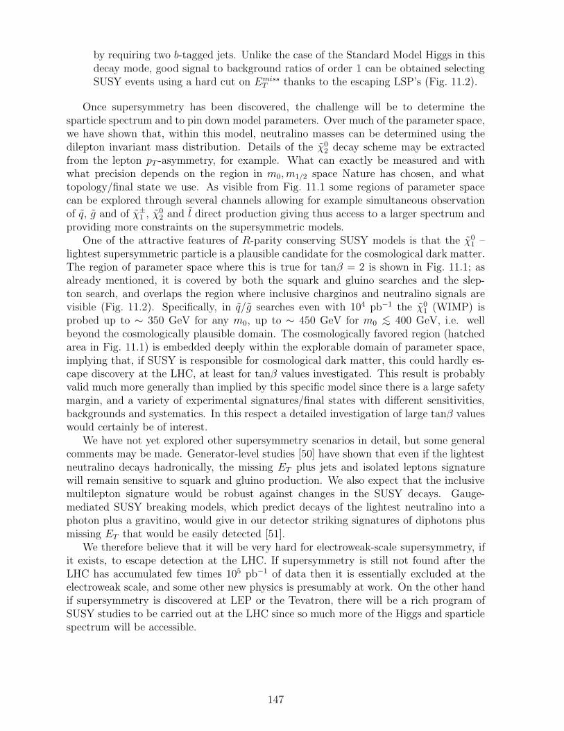
by requiring two b-tagged jets. Unlike the case of the Standard Model Higgs in thisdecay mode, good signal to background ratios of order 1 can be obtained selectingSUSY events using a hard cut on Emiss

T thanks to the escaping LSP’s (Fig. 11.2).

Once supersymmetry has been discovered, the challenge will be to determine thesparticle spectrum and to pin down model parameters. Over much of the parameter space,we have shown that, within this model, neutralino masses can be determined using thedilepton invariant mass distribution. Details of the χ0

2 decay scheme may be extractedfrom the lepton pT -asymmetry, for example. What can exactly be measured and withwhat precision depends on the region in m0, m1/2 space Nature has chosen, and whattopology/final state we use. As visible from Fig. 11.1 some regions of parameter spacecan be explored through several channels allowing for example simultaneous observationof q, g and of χ±

1 , χ02 and l direct production giving thus access to a larger spectrum and

providing more constraints on the supersymmetric models.One of the attractive features of R-parity conserving SUSY models is that the χ0

1 –lightest supersymmetric particle is a plausible candidate for the cosmological dark matter.The region of parameter space where this is true for tanβ = 2 is shown in Fig. 11.1; asalready mentioned, it is covered by both the squark and gluino searches and the slep-ton search, and overlaps the region where inclusive charginos and neutralino signals arevisible (Fig. 11.2). Specifically, in q/g searches even with 104 pb−1 the χ0

1 (WIMP) isprobed up to ∼ 350 GeV for any m0, up to ∼ 450 GeV for m0

<∼ 400 GeV, i.e. wellbeyond the cosmologically plausible domain. The cosmologically favored region (hatchedarea in Fig. 11.1) is embedded deeply within the explorable domain of parameter space,implying that, if SUSY is responsible for cosmological dark matter, this could hardly es-cape discovery at the LHC, at least for tanβ values investigated. This result is probablyvalid much more generally than implied by this specific model since there is a large safetymargin, and a variety of experimental signatures/final states with different sensitivities,backgrounds and systematics. In this respect a detailed investigation of large tanβ valueswould certainly be of interest.

We have not yet explored other supersymmetry scenarios in detail, but some generalcomments may be made. Generator-level studies [50] have shown that even if the lightestneutralino decays hadronically, the missing ET plus jets and isolated leptons signaturewill remain sensitive to squark and gluino production. We also expect that the inclusivemultilepton signature would be robust against changes in the SUSY decays. Gauge-mediated SUSY breaking models, which predict decays of the lightest neutralino into aphoton plus a gravitino, would give in our detector striking signatures of diphotons plusmissing ET that would be easily detected [51].

We therefore believe that it will be very hard for electroweak-scale supersymmetry, ifit exists, to escape detection at the LHC. If supersymmetry is still not found after theLHC has accumulated few times 105 pb−1 of data then it is essentially excluded at theelectroweak scale, and some other new physics is presumably at work. On the other handif supersymmetry is discovered at LEP or the Tevatron, there will be a rich program ofSUSY studies to be carried out at the LHC since so much more of the Higgs and sparticlespectrum will be accessible.

147

1000

800

600

400

200

0 400 800 1200 1600 2000m0 GeV

m1/

2, G

eV

q (2000)

~q (1500)~

q (1000)

~

g (1500)

g (2000)~

~

g (1000)~

g (500)~

105pb-1

D_D

_925

.n

Expected reach in various channels

m SUGRA; tg β = 2, A0 = 0, µ < 0

5 σ contours, Nσ = Nsig / Nsig+Nbkgd for 105pb-1

h(90)

(400)

CMS;

Ω h2= 1Ω h2= 0.4

Ω h2= 0.15 χ0 χ± ~ ~12

muons notisolated

g,q in: 4 ,3 ,2 SS,2 0S,1~~

~

~L

Figure 11.1: 5σ significance contours at Lint = 105 pb−1 for different SUSY channels.

148

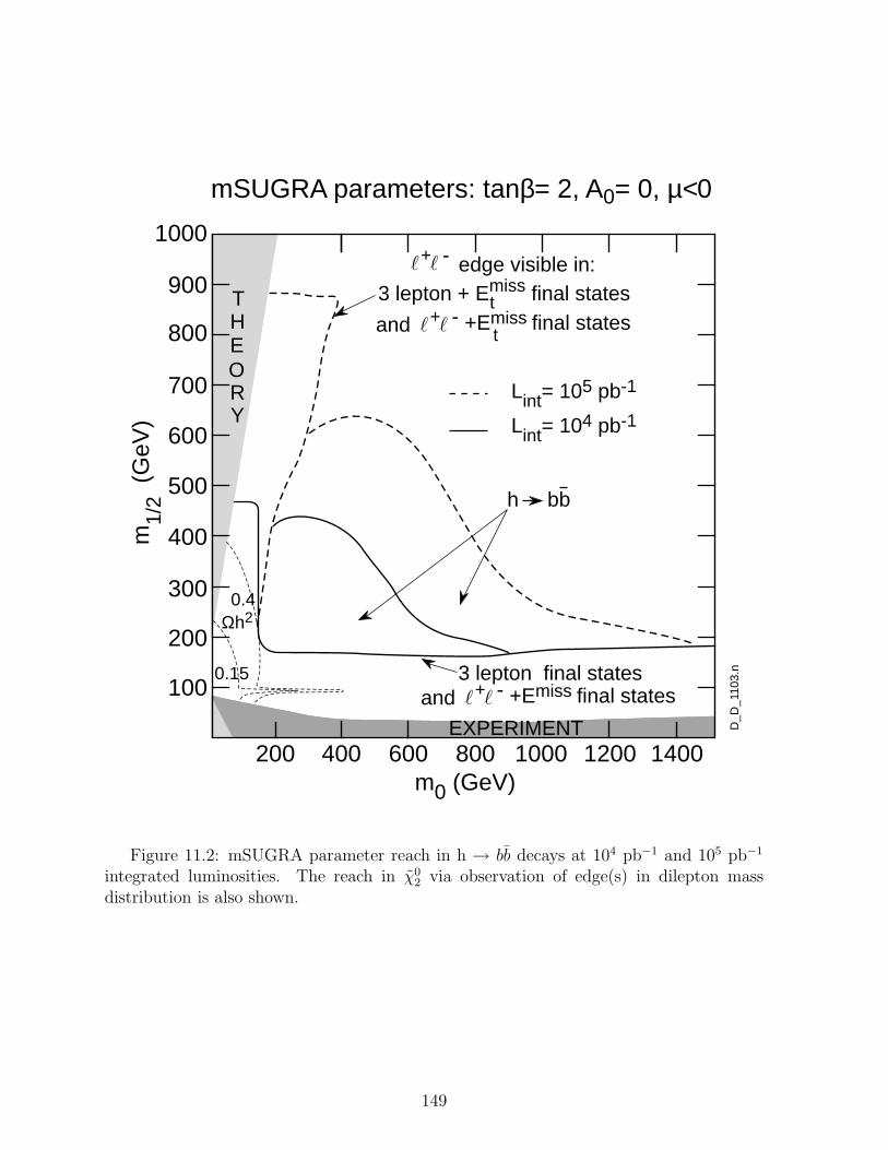
200

200

300

400

500

600

700

800

900

1000

100

400 600 800 1000 1200 1400EXPERIMENT

0.15

0.4Ωh2

m1/

2 (G

eV)

m0 (GeV)

mSUGRA parameters: tanβ= 2, A0= 0, µ<0

THEORY

D_D

_110

3.n

3 lepton + Emiss final states

h bb

Lint= 105 pb-1

Lint= 104 pb-1

t

t+ -

edge visible in:+ -

and +Emiss final states

3 lepton final states+ -and +Emiss final states

Figure 11.2: mSUGRA parameter reach in h → bb decays at 104 pb−1 and 105 pb−1

integrated luminosities. The reach in χ02 via observation of edge(s) in dilepton mass

distribution is also shown.

149

Acknowledgements

Over the past few years we have benefited from numerous discussions with our col-leagues, from their suggestions and criticism. It is a pleasure for us to thank in first placeH. Baer who has spent many hours in discussions with us and in following our studies.We are also grateful to A. Bartl, W. Majerotto, F. Pauss, C. Seez, M. Spira, T. Virdeefor useful discussions and comments.

150

References

[1] D. Abbaneo et al. (LEP Electroweak Working Group, SLD Heavy Flavour Group),preprint CERN-PPE/97-154.

[2] H. Baer, C. Chen, F. Paige and X. Tata, Phys. Rev. D49, (1994) 3283.

[3] SUSY Studies in CMS, in: LHCC SUSY Workshop, CERN, October 29−30, 1996,CMS Document 1996-149; Copies of transparencies are available on WEB underhttp://www.cern.ch/Committees/LHCC/SUSY96.html.

[4] S. Abdullin, Squark and gluino searches in leptons + jets + EmissT final state, CMS

TN/96-095.

[5] S. Abdullin, Z. Antunovic and M. Dzelalija, Squarks and gluino searches in multilep-ton final states: A0 = 0, tanβ = 2, µ > 0 case, CMS Note 1997/016.

[6] D. Denegri, L. Rurua and N. Stepanov, Detection of sleptons in CMS, mass reach,CMS TN/96-59.

[7] D. Denegri, W. Majerotto and L. Rurua, Determining the parameters of the minimalsupergravity model from 2l + Emiss

T + (jets) final states at LHC, CMS Note 1997/094and references therein; HEPHY-Pub 678/97; hep-ph/9711357.

[8] I. Iashvili, A. Kharchilava and K. Mazumdar, Study of χ±1 χ0

2 pair production with theCMS detector at LHC, CMS Note 1997/007.

[9] I. Iashvili and A. Kharchilava, Search for the Next-To-Lightest Neutralino, CMS Note1997/065; hep-ph/9712393.

[10] I. Iashvili, A. Kharchilava and C. Racca, Sensitivity to sparticle masses and modelparameters in direct χ±

1 χ02 production, CMS Note 1997/069.

[11] D. Denegri, SUSY and dark matter searches at the LHC, in Proc. of Int. Workshopon Dark Matter in Astro and Particle Physics, Heidelberg, Germany, Sept. 96, WorldScientific, eds. H. V. Klapdor and Y. Ramachers, pp 583-604; CMS CR 1997/009.

[12] S. Abdullin and D. Denegri, On the possibility to observe h → bb with S/B ∼ 1 inSUSY (mSUGRA), and implications for tracker and HCAL, CMS Note 1997/070.

[13] D. Denegri and V. Genchev, Study of the CMS hadron calorimeter barrel/endcaptransition region, CMS Note 1996/020;D. Green, HCAL ”tailcatcher” decision, CMS TN/96-008;S. Banerjee et al., Towards a design of the CMS barrel hadron outer calorimeter,TIFR/CMS-96-01, Nov. 1996;J. Womersley, Study of Emiss

T resolution in CMS, presentation at the CMS/Physicsworking group meeting, March 1996;I. Gaines et al., Missing ET + jets signals for supersymmetry in the CMS detector atthe LHC, CMS TN/96-058.

151

http://www.cern.ch/Committees/LHCC/SUSY96.html

http://arXiv.org/abs/hep-ph/9711357


[14] R. Kinnunen et al., Expected SM/SUSY Higgs observability in CMS, CMS Note1997/057 and references therein;R. Kinnunen and A. Nikitenko, Study of HSUSY → ττ → l± + τ jet+Emiss

T in CMS,CMS Note 1997/106;S. Lehti, R. Kinnunen and J. Tuominiemi, Study of h0, H0, A0 → ττ → eµ in theCMS detector, CMS Note 1998/019.

[15] J. F. Gunion et al., UCD-95-28, ILL-(TH)-95-28;M. Carena, Phys. Lett. B355 (1994) 209.

[16] For a review, see e.g., H. P. Nilles, Phys. Rep. 110 (1984) 1;P. Nath, R. Arnowitt and A. Chamseddine, Applied N=1 Supergravity, ICTP seriesin Theoretical Physics (World Scientific, Singapore, 1984);M. Drees and S. P. Martin, hep-ph/9504324.

[17] H. Baer, F. Paige, S. Protopopescu and X. Tata, in: Proceedings of the Workshopon Physics at Current Accelerators and Supercolliders, eds. J. Hewett, A. White andD. Zeppenfeld (Argonne National Laboratory, Argonne, Illinois, 1993).

[18] K. Inoue, A. Kakuto, H. Komatsu and S. Takeshita, Prog. Theor. Phys. 68 (1982)927.

[19] T. Sjostrand, Comp. Phys. Comm. 82 (1994) 74.

[20] H. L. Lai et al., Phys. Rev. D51 (1995) 4763.

[21] CMS Collaboration, Technical Proposal, CERN/LHCC 94-38, December 1994;Meeting with CMS LHCC Referees, CMS Document 1996-132, Aug. 1996.

[22] CMS, The Magnet Project, TDR, CERN/LHCC 97-10.

[23] CMS, The Muon Project, TDR, CERN/LHCC 97-32;F. Gasparini et al., Nucl. Instrum. Methods A336 (1993) 91;R. Cardarelli et al., Nucl. Instrum. Methods A340 (1994) 466.

[24] F. Angelini et al., Nucl. Instrum. Methods A343 (1994) 441;CMS Meeting with LHCC Referees/Tracking, CMS Document 96-59, March 1996.

[25] CMS, The Electromagnetic Calorimeter Project, TDR, CERN/LHCC 97-33;P. Lecoq et al., Lead Tungstate (PbWO4) scintillators for LHC EM-Calorimetry,CMS TN/94-308.

[26] CMS ECAL group, CMS Lead Tungstate ECAL: Test Beam Results 1995. Report tothe CMS Referees, CMS TN/96-004;J. P. Peigneux et al., Results from tests on matrices of lead tungstate crystals usinghigh energy beams, CMS TN/95-166.

[27] CMS, The Hadron Calorimeter Project, TDR, CERN/LHCC 97-31.

152


[28] For example: HPMT from DEP (Delft Electronische Producten, Netherlands), orHPD from Hamamatsu;P. Cushman et al., Multi-Pixel Hybrid Photodiode Tubes for CMS Hadron Calorime-ter, in Proc. of the Conf. on New Developments in Photodetection, Beaune 1996,NIM, to be published.

[29] D. Green, Hadron calorimeter performance with a PbWO4 EM compartment, FNAL,TM-1958, Dec. 1995;D. Green, A. Skuja and J. Freeman, HCAL test beam results, CMS/HCAL workinggroup meetings 1996 and 1997.

[30] A. Ferrando et al., Designing a compensating quartz fibre calorimeter for the CMSlow angle calorimetry, CMS TN/96-82;S. Doulas et al., Beam test results from a fine sampling quartz fibre calorimeter forlepton, hadron and jet detection, CMS TN/95-144;VFCAL General Meeting, CMS Document 1996-212, Dec. 10-11, 1996.

[31] D. Green, HCAL ”tailcatcher” decision, CMS TN/96-08;S. Banerjee et al., Towards a design of the CMS barrel hadron outer calorimeter,TIFR/CMS-96-01, Nov. 1996.

[32] M. Murbach and A. Skuja, presentation at the CMS/HCAL working group meetings,1996.

[33] D. Green, S. Kunori and A. Skuja, presentations at the CMS/HCAL/Physics workinggroup meetings, 1996.

[34] D. Denegri et al., Justifications for a Microvertex Detector in CMS, CMS TN/94-258;R. Kinnunen and D. Denegri, B-tagging with impact parameter in the CMS tracker,CMS TN/96-045.

[35] V. Genchev and L. Litov, Study of the CMS TP calorimetry system, CMS TN/94-272.

[36] S. Abdullin, A. Khanov and N. Stepanov, CMSJET, CMS TN/94-180.

[37] H. Baer and M. Brhlik, Phys. Rev. D53 (1996) 597.

[38] S. Abdullin, Z. Antunovic and M. Dzelalija, Squarks and gluino searches in fourlepton final states, CMS Note 1997/015.

[39] F. Paige, Search for SUSY at LHC: precision measurements, talk given at In-ternational Europhysics Conference on High Energy Physics, 19-26 August 1997,Jerusalem, Israel.

[40] H. Baer, C.-H. Chen, F. Paige and X. Tata, Phys. Rev. D50 (1994) 4508 and refer-ences therein.

[41] A. Kharchilava, Search for next-to-lightest neutralino, in: LHCC SUSY Work-shop, CERN, October 29−30, 1996; Copies of transparencies available underhttp://www.cern.ch/Committees/LHCC/SUSY96.html; CMS Document 1996-149.

153

http://www.cern.ch/Committees/LHCC/SUSY96.html

[42] L. Rurua, presentation to CMS Physics Meeting, CMS Week, March 1998, CMSDocument 1998-042.

[43] C. Seez and T. S. Virdee, The Higgs two photon decay in CMS: an update, CMSTN/94-289;D. J. Graham, An algorithm using tracks to locate the two photon vertex at highluminosity, CMS TN/95-115;K. Lassila-Perini, Reconstruction of Higgs → γγ in CMS, in Proc. of VI Int. Conf.on Calorimetry in HEP, Frascati, June 8-14, 1996, p 487; CMS CR 1997/006.

[44] S. Abdullin, A. Starodumov and N. Stepanov, Search for heavy Higgs via the H →llνν channel, CMS TN/93-087;M. Dzelalija et al., Study of the associated production modes Wh, tth in the MinimalSupersymmetric Standard Model in CMS, CMS TN/96-091.

[45] D. Drollinger, T. Muller, R. Kinnunen, presentation at CMS Week Physics meeting,June, 27, 1997, CMS Note 1998 (in preparation);D. Froidevaux and E. Richter-Was, Is the channel H → bb observable at LHC?,ATLAS Internal Note Phys-No-043 (1994).

[46] L. Didenko and B. Lund-Jensen, B-tagging of light Higgs boson in cascade decays ofgluino, ATLAS Internal Note Phys-No-42 (1994);I. Hinchliffe et al., Phys. Rev. D55 (1997) 5520.

[47] A. Khanov and N. Stepanov, Full pattern recognition and track reconstruction inCMS tracker, CMS Note 1998 (in preparation);N. Stepanov, b-tagging with full pattern recognition, presentation at the CMS/Physicsmeeting, June 27, 1997;A. Caner, CMS tracker optimisation study, presentation at the CMS Collaborationmeeting, March 1998.

[48] F. Paige, Determining SUSY particle masses at LHC, Proc. of the 1996 DPF/DPBSummer Study on High-Energy Physics “New Directions for High-Energy Physics”,Snowmass, Colorado, 1996.

[49] D. J. Graham, Ph. D. Thesis, Imperial College, University of London, London, 1997.

[50] H. Baer, C. Chen and X. Tata, Phys. Rev. D55 (1997) 1466.

[51] F. Charles, Inclusive search for light gravitino with the CMS detector, CMS Note1997/079;M. Kazana and P. Zalewski, Measurement of the stau mass in the GMSB model viatime of flight determination in the CMS, presentation at CMS Physics Meeting, CMSWeek, December 1997, CMS Document 1997-169;G. Wrochna and P. Zalewski, Proposal for detecting χ0

1 → Gγ and τ1 → Gτ decays inthe CMS muon detector, presentation at the CMS/Physics working group meeting,February 1998, CMS Note 1998 (in preparation).

154

RESEARCH NOTE FROM COLLABORATION: Discovery potential for supersymmetry in CMS*

Documents

Transcript of RESEARCH NOTE FROM COLLABORATION: Discovery potential for supersymmetry in CMS*