Reproducibility of GPS radio occultation data for climate monitoring: Profile-to-profile...

Reproducibility of GPS radio occultation data for climatemonitoring: Profile-to-profile inter-comparison of CHAMPclimate records 2002 to 2008 from six data centers

Shu-peng Ho,1 Doug Hunt,1 Andrea K. Steiner,2 Anthony J. Mannucci,3

Gottfried Kirchengast,2 Hans Gleisner,4 Stefan Heise,5 Axel von Engeln,6

Christian Marquardt,6 Sergey Sokolovskiy,1 William Schreiner,1

Barbara Scherllin-Pirscher,2 Chi Ao,3 JensWickert,5 Stig Syndergaard,4 Kent B. Lauritsen,4

Stephen Leroy,7 Emil R. Kursinski,8 Ying-Hwa Kuo,1 Ulrich Foelsche,2 Torsten Schmidt,5

and Michael Gorbunov4,9

Received 20 February 2012; revised 6 August 2012; accepted 10 August 2012; published 25 September 2012.

[1] To examine the claim that Global Positioning System (GPS) radio occultation (RO)data are useful as a benchmark data set for climate monitoring, the structural uncertaintiesof retrieved profiles that result from different processing methods are quantified.Profile-to-profile comparisons of CHAMP (CHAllenging Minisatellite Payload) datafrom January 2002 to August 2008 retrieved by six RO processing centers are presented.Differences and standard deviations of the individual centers relative to the inter-centermean are used to quantify the structural uncertainty. Uncertainties accumulate in derivedvariables due to propagation through the RO retrieval chain. This is reflected in theinter-center differences, which are small for bending angle and refractivity increasing todry temperature, dry pressure, and dry geopotential height. The mean differences of thetime series in the 8 km to 30 km layer range from �0.08% to 0.12% for bending angle,�0.03% to 0.02% for refractivity, �0.27 K to 0.15 K for dry temperature, �0.04% to0.04% for dry pressure, and �7.6 m to 6.8 m for dry geopotential height. Thecorresponding standard deviations are within 0.02%, 0.01%, 0.06 K, 0.02%, and2.0 m, respectively. The mean trend differences from 8 km to 30 km for bendingangle, refractivity, dry temperature, dry pressure, and dry geopotential height are within�0.02%/5 yrs, �0.02%/5 yrs, �0.06 K/5 yrs, �0.02%/5 yrs, and �2.3 m/5 yrs,respectively. Although the RO-derived variables are not readily traceable to theinternational system of units, the high precision nature of the raw RO observablesis preserved in the inversion chain.

Citation: Ho, S., et al. (2012), Reproducibility of GPS radio occultation data for climate monitoring: Profile-to-profile inter-comparison of CHAMP climate records 2002 to 2008 from six data centers, J. Geophys. Res., 117, D18111,doi:10.1029/2012JD017665.

1. Introduction

[2] Long-term Climate Data Records (CDRs) constructedfrom stable and accurate measurements with adequate tem-poral and spatial coverage are essential for monitoring globaland regional climate variability and understanding their

forcing mechanisms. Current long-term measurements usedto generate CDRs are mainly derived from satellite observa-tions and in situ measurements [see Intergovernmental Panelon Climate Change (IPCC), 2007]. These satellite sensorswere originally designed to provide measurements for short-

1COSMIC Program Office, University Corporation for AtmosphericResearch, Boulder, Colorado, USA.

2Wegener Center for Climate and Global Change and Institute forGeophysics, Astrophysics, and Meteorology, Institute of Physics, Universityof Graz, Graz, Austria.

3Jet Propulsion Laboratory, California Institute of Technology, Pasadena,California, USA.

4Danish Meteorological Institute, Copenhagen, Denmark.5Department of Geodesy and Remote Sensing, German Research Centre

for Geosciences, Potsdam, Germany.6EUMETSAT, Darmstadt, Germany.7School of Engineering and Applied Sciences, Harvard University,

Cambridge, Massachusetts, USA.8Institute of Atmospheric Physics, University of Arizona, Tucson, Arizona,

USA.9Institute of Atmospheric Physics, Russian Academy of Sciences, Moscow,

Russia.

Corresponding author: S. Ho, COSMIC Project Office, UniversityCorporation for Atmospheric Research, PO Box 3000, Boulder, CO 80307-3000, USA. ([email protected])

©2012. American Geophysical Union. All Rights Reserved.0148-0227/12/2012JD017665

JOURNAL OF GEOPHYSICAL RESEARCH, VOL. 117, D18111, doi:10.1029/2012JD017665, 2012

D18111 1 of 38

term weather and environmental predictions, not long-termclimate monitoring. As a result, extra effort must be spenton data re-processing, inter-satellite calibration, and multiplesatellite data merging procedures in order to account forpossible on-board calibration drift and degradation of satel-lite sensors. Because instrument calibrations lack traceabilityto the International System of Units (SI), the possible deg-radation of the sensors and the on-board calibration createsa source of uncertainty that can alias into the climate signalbeing sought. Even using the same satellite data, climate trendsprovided by different groups may be very different. Forexample, to construct consistent temperature CDRs usingmultiple Microwave Sounding Units (MSU) and AdvancedMicrowave Sounding Units (AMSU) on the NOAA TIROSOperational Vertical Sounders (TOVS), various calibrationand tuning methods from different groups were used to cor-rect the inter-satellite residual biases among the sensors [e.g.,Christy et al., 2000; Mears et al., 2003; Grody et al., 2004;Zou et al., 2006; Zou and Wang, 2011; Prabhakara et al.,2000]. However, because on-board calibration is unable tofully constrain inter-satellite biases, substantial uncertaintiesstill exist in temperature trends reported from different groups[IPCC, 2007; Thorne et al., 2005, 2011]. Many studies havebeen conducted to investigate the causes of the structuraluncertainty among MSU/AMSU data derived from differentgroups [Christy et al., 2000; Mears et al., 2003, 2011; Karlet al., 2006; Prabhakara et al., 2000; Zou et al., 2006; Zouand Wang, 2011].[3] Radiosonde observations have been used as benchmarks

to validate satellite-derived soundings. However, changinginstruments and observation practices and limited spatialcoverage complicate climate signals from this data set [Freeet al., 2005; Haimberger et al., 2008; Thorne et al., 2011].[4] Global Positioning System (GPS) Radio Occultation

(RO) data are currently the only satellite data that maintain SItraceability [Ohring, 2007]. By flying a GPS receiver in the lowearth orbit (LEO), GPS RO is the first technique to providemeasurements that are traceable to the international standard oftime, i.e., the SI second [Hardy et al., 1994; Kursinski et al.,1997]. This traceability makes GPS RO a strong candidatefor use as a climate benchmark [Goody et al., 1998, 2002].[5] Accurate RO retrievals of atmospheric variable pro-

files depend on the adequate calculation of the atmosphericexcess phase of two GPS L-band frequencies (1575.42 MHz(L1) and 1227.6 MHz (L2)) due to signal delay and bendingin the Earth’s atmosphere and ionosphere [Kursinski et al.,1997; Ho et al., 2009a]. Possible error sources of RO-derived products include i) observation errors and ii) inver-sion errors. Observation errors in RO phase measurementsare related to GPS RO signal strength combined with receivernoise for a particular RO mission and local multipath effect[Kursinski et al., 1997]. Theoretical error analyses of ROsounding techniques based on simulations have been con-ducted [see Kursinksi et al., 1997; Rieder and Kirchengast,2001; Steiner and Kirchengast, 2005] and were used toexplain causes of errors in retrieved variables. The observa-tion errors consist of random and systematic errors that maybe mission-dependent. Error analyses with real RO data wereperformed to characterize observational errors of individualprofiles [Kuo et al., 2004; Scherllin-Pirscher et al., 2011b]and errors of climatological fields [Scherllin-Pirscher et al.,2011a].

[6] Structural uncertainties of RO-retrieved variables for aparticular RO mission are mainly due to the inversion errors,which include errors in precise orbit determination (POD),removal of clock fluctuations, and other inversion procedures.While the fundamental phase measurement is synchronized tothe ultra-stable atomic clocks on the ground, the RO-derivedvariables (e.g., refractivity, pressure, temperature) are not.The retrieval results may differ for different processingalgorithms and implementations as used in the excess phaseprocessing and inversion procedures, such as noise filteringand profile initializations [Ho et al., 2009a]. RO inversionalgorithms are used to convert the RO atmospheric excessphase into atmospheric variables, including bending angle,refractivity, pressure, geopotential height, and temperature inthe upper troposphere and lower stratosphere, by assuming adry atmosphere (defined in section A5).[7] Currently, multiyear GPS RO data can be obtained

from the following centers: the Radio Occultation Meteo-rology (ROM) Satellite Application Facility (SAF) (formerlyGRAS (Global Navigation Satellite System Receiver forAtmospheric Sounding) SAF) at the Danish MeteorologicalInstitute (DMI) in Copenhagen, Denmark; the EuropeanOrganisation for the Exploitation of Meteorological Satellites(EUMETSAT, hereafter EUM), in Darmstadt, Germany; theGerman Research Centre for Geosciences (GFZ) in Potsdam,Germany; the Jet Propulsion Laboratory (JPL) in Pasadena,CA, USA; the University Corporation for AtmosphericResearch (UCAR) in Boulder, CO, USA; and the WegenerCenter/University of Graz (WEGC) in Graz, Austria. Thesecenters use different assumptions, initializations, and imple-mentations in the excess phase processing and inversionprocedures (see Appendix A).[8] To use RO data as a benchmark data set for climate

monitoring, it is critically necessary to quantify the reproduc-ibility of RO retrieved profiles. The reproducibility of RO datais defined by the consistency (small structural uncertainty) ofi) global averages, ii) monthly zonal averages, and iii) anom-aly time series of the RO retrieval profiles among centers dueto different assumptions and inversion methods. A first studyto this end was performed by Ho et al. [2009a] who used fiveyears (2002 to 2006) of refractivity climatologies fromCHAMP (CHAllenging Minisatellite Payload) generated byGFZ, JPL, UCAR, and WEGC. Each center used the profilesthat passed their own quality control criteria to generatemonthly mean climatologies. Results showed that the uncer-tainty of the trend for the fractional refractivity anomaliesamong the centers is between (�0.03 to 0.01)%/5 yrs. Thus0.03%/5 yrs was considered an upper bound in the processingscheme-induced uncertainty for global refractivity trendmonitoring. In that study, sampling errors were regarded as thedominant error source at high-latitudes because differentquality control mechanisms cause a different number of pro-files in climatologies. Numerical weather model re-analysisdata were used to determine sampling errors, which weresubtracted. Remaining differences among centers containedresidual sampling errors and inversion-related structuraluncertainty.[9] The objective of this study is to quantify the reproduc-

ibility of RO data from six RO processing centers for all (dry)atmospheric variables. To estimate the reproducibility of ROdata, in this study we quantify i) the structural uncertainties,and ii) long-term consistency of retrieved profiles that result

HO ET AL.: REPRODUCIBILITY OF GPS RO DATA D18111D18111

2 of 38

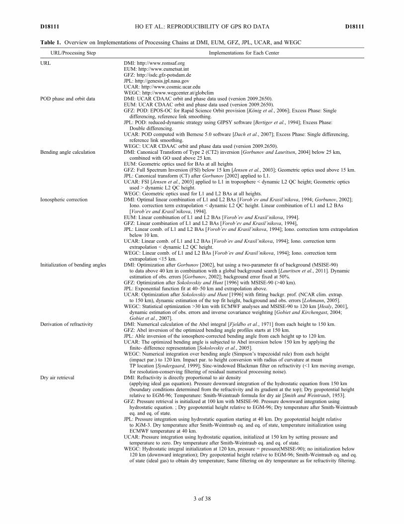
Table 1. Overview on Implementations of Processing Chains at DMI, EUM, GFZ, JPL, UCAR, and WEGC

URL/Processing Step Implementations for Each Center

URL DMI: http://www.romsaf.orgEUM: http://www.eumetsat.intGFZ: http://isdc.gfz-potsdam.deJPL: http://genesis.jpl.nasa.govUCAR: http://www.cosmic.ucar.eduWEGC: http://www.wegcenter.at/globclim

POD phase and orbit data DMI: UCAR CDAAC orbit and phase data used (version 2009.2650).EUM: UCAR CDAAC orbit and phase data used (version 2009.2650).GFZ: POD: EPOS-OC for Rapid Science Orbit provision [König et al., 2006]; Excess Phase: Single

differencing, reference link smoothing.JPL: POD: reduced-dynamic strategy using GIPSY software [Bertiger et al., 1994]; Excess Phase:

Double differencing.UCAR: POD computed with Bernese 5.0 software [Dach et al., 2007]; Excess Phase: Single differencing,

reference link smoothing.WEGC: UCAR CDAAC orbit and phase data used (version 2009.2650).

Bending angle calculation DMI: Canonical Transform of Type 2 (CT2) inversion [Gorbunov and Lauritsen, 2004] below 25 km,combined with GO used above 25 km.

EUM: Geometric optics used for BAs at all heightsGFZ: Full Spectrum Inversion (FSI) below 15 km [Jensen et al., 2003]; Geometric optics used above 15 km.JPL: Canonical transform (CT) after Gorbunov [2002] applied to L1.UCAR: FSI [Jensen et al., 2003] applied to L1 in troposphere < dynamic L2 QC height; Geometric optics

used > dynamic L2 QC height.WEGC: Geometric optics used for L1 and L2 BAs at all heights.

Ionospheric correction DMI: Optimal linear combination of L1 and L2 BAs [Vorob’ev and Krasil’nikova, 1994; Gorbunov, 2002];Iono. correction term extrapolation < dynamic L2 QC height. Linear combination of L1 and L2 BAs[Vorob’ev and Krasil’nikova, 1994].

EUM: Linear combination of L1 and L2 BAs [Vorob’ev and Krasil’nikova, 1994].GFZ: Linear combination of L1 and L2 BAs [Vorob’ev and Krasil’nikova, 1994],JPL: Linear comb. of L1 and L2 BAs [Vorob’ev and Krasil’nikova, 1994]; Iono. correction term extrapolation

below 10 km.UCAR: Linear comb. of L1 and L2 BAs [Vorob’ev and Krasil’nikova, 1994]; Iono. correction term

extrapolation < dynamic L2 QC height.WEGC: Linear comb. of L1 and L2 BAs [Vorob’ev and Krasil’nikova, 1994]; Iono. correction term

extrapolation <15 km.Initialization of bending angles DMI: Optimization after Gorbunov [2002], but using a two-parameter fit of background (MSISE-90)

to data above 40 km in combination with a global background search [Lauritsen et al., 2011]. Dynamicestimation of obs. errors [Gorbunov, 2002]; background error fixed at 50%.

GFZ: Optimization after Sokolovskiy and Hunt [1996] with MSISE-90 (>40 km).JPL: Exponential function fit at 40–50 km and extrapolation above.UCAR: Optimization after Sokolovskiy and Hunt [1996] with fitting backgr. prof. (NCAR clim. extrap.

to 150 km), dynamic estimation of the top fit height, background and obs. errors [Lohmann, 2005].WEGC: Statistical optimization >30 km with ECMWF analyses and MSISE-90 to 120 km [Healy, 2001],

dynamic estimation of obs. errors and inverse covariance weighting [Gobiet and Kirchengast, 2004;Gobiet et al., 2007].

Derivation of refractivity DMI: Numerical calculation of the Abel integral [Fjeldbo et al., 1971] from each height to 150 km.GFZ: Abel inversion of the optimized bending angle profiles starts at 150 km.JPL: Able inversion of the ionosphere-corrected bending angle from each height up to 120 km.UCAR: The optimized bending angle is subjected to Abel inversion below 150 km by applying the

finite- difference representation [Sokolovskiy et al., 2005].WEGC: Numerical integration over bending angle (Simpson’s trapezoidal rule) from each height

(impact par.) to 120 km. Impact par. to height conversion with radius of curvature at meanTP location [Syndergaard, 1999]; Sinc-windowed Blackman filter on refractivity (<1 km moving average,for resolution-conserving filtering of residual numerical processing noise).

Dry air retrieval DMI: Refractivity is directly proportional to air density(applying ideal gas equation). Pressure downward integration of the hydrostatic equation from 150 km(boundary conditions determined from the refractivity and its gradient at the top); Dry geopotential heightrelative to EGM-96; Temperature: Smith-Weintraub formula for dry air [Smith and Weintraub, 1953].

GFZ: Pressure retrieval is initialized at 100 km with MSISE-90. Pressure downward integration usinghydrostatic equation. ; Dry geopotential height relative to EGM-96; Dry temperature after Smith-Weintraubeq. and eq. of state.

JPL: Pressure integration using hydrostatic equation starting at 40 km. Dry geopotential height relativeto JGM-3. Dry temperature after Smith-Weintraub eq. and eq. of state, temperature initialization usingECMWF temperature at 40 km.

UCAR: Pressure integration using hydrostatic equation, initialized at 150 km by setting pressure andtemperature to zero. Dry temperature after Smith-Weintraub eq. and eq. of state.

WEGC: Hydrostatic integral initialization at 120 km, pressure = pressure(MSISE-90); no initialization below120 km (downward integration); Dry geopotential height relative to EGM-96; Smith-Weintraub eq. and eq.of state (ideal gas) to obtain dry temperature; Same filtering on dry temperature as for refractivity filtering.


3 of 38

from different processing methods. Here we conduct profile-to-profile comparisons (PPCs) (i.e., contain no samplingdifferences) to quantify the structural uncertainties of RO-retrieved variables and to understand how those uncertaintiespropagate from bending angle profiles to pressure andtemperature profiles. This should help identify the causes ofprocess-dependent errors from each center.[10] We describe the data sources obtained from six centers

in section 2. The method of generating CHAMP PPCs isdescribed in section 3. Results on the differences of globaland monthly zonal averages as well as anomaly time seriesand trends are presented in section 4. Possible causes for thestructural differences among the six centers are discussed insection 5. Conclusions are drawn in section 6.

2. Data Sources

[11] CHAMP profiles from GFZ used in this study havebeen reprocessed with the latest version (006) of GFZ’soperational occultation analysis system. It is planned to pro-vide these data via the Information System and Data Center(ISDC, http://isdc.gfz-potsdam.de). Details and related refer-ences on the operational standard near-real time orbit andoccultation processing can be found inKönig et al. [2006] andWickert et al. [2009].[12] CHAMP profiles from JPL were downloaded from the

JPL Genesis website: http://genesis.jpl.nasa.gov. The inver-sion procedures used to process CHAMP data for this studyare the same as those used in Ho et al. [2009a].[13] UCARoperational CHAMPprofiles (version 2009.2650)

were downloaded from the UCAR COSMIC (ConstellationObserving System for Meteorology, Ionosphere, and Climate)Data Analysis and Archive Center (CDAAC) website: http://cosmic-io.cosmic.ucar.edu/cdaac/index.html. An updated PODcode is developed and implemented in this version [Schreineret al., 2009] (also see section A1.5). A general description ofUCAR inversion procedures can be found in Kuo et al. [2004],Ho et al. [2009a], and Schreiner et al. [2011].[14] RO atmospheric profiles provided by the Wegener

Center were retrieved with the WEGC Occultation Proces-sing System (OPS) retrieval software [Borsche et al., 2006;Kirchengast et al., 2007; Borsche, 2008; Foelsche et al.,2008a, 2009; Ho et al., 2009a]. A short overview on thecurrent retrieval version OPSv5.4 is given by Steiner et al.[2009], a detailed description can be found in Pirscher[2010]. The WEGC OPSv5.4 retrieval is based on inputdata of RO phase and orbit information provided by UCARCDAAC. WEGC profile and climatology data are availablefrom its global climate monitoring website: http://www.

globclim.org. Information on error characteristics is given byScherllin-Pirscher et al. [2011a, 2011b].[15] EUM and DMI constructed the CHAMP retrievals

specifically for this study. Like WEGC, both EUM andDMI started with excess phase and amplitude data, as well asCHAMP orbit data, from UCAR CDAAC. EUM processinggenerally focuses on level 0 to bending angle processing;hence, they only provided bending angle profiles for thisstudy.[16] A sequence of processing steps is used by individual

centers to inverse time delays to physical parameters. Theseprocessing steps include: i) POD and atmospheric excess phaseprocessing, ii) bending angle calculation, iii) ionosphericcorrection, iv) optimal estimation of the bending angles inthe stratosphere, v) calculation of refractivity by Abel inver-sion, vi) calculation of pressure, temperature, and geopoten-tial height, and vii) quality control (QC). Table 1 summarizesthe retrieval methods used in this study for each processingstep for the individual centers. Though implementation ofthese procedures is different, the main processing steps are, toa large extent, common. Detailed implementations of theinversion methods for each processing step used by individ-ual centers are described in Appendix A so as not to detractfrom the quantitative analysis.

3. Method of Profile-to-Profile Comparison (PPC)

[17] The inter-center statistical comparisons are basedon differences of profile-to-profile pairs of bending angle,refractivity, dry temperature, dry pressure, and dry geopo-tential height profiles. The PPC pairs were first obtained bymatching the profiles produced by all six centers. Each centersupplied CHAMP processed profiles from January 2002 toAugust 2008 in a common netCDF file format. The occulta-tion time and occulting GPS satellite identifiers from eachprofile were then compared with a database of all geometri-cally possible occultations to obtain standard occultationtimes. The provided profile files from each center were thengiven canonical names using the standard occultation times.Only high-quality profiles from individual centers that passedtheir Quality Controls (QCs) (see section A7) for all retrievedvariables are included in the common PPC files. This match-ing was done within a 5-min time window for occultationsusing the same GPS satellite. In this way the profile files fromall centers were matched and assigned common occultationidentifiers. All the centers provided their RO data products ona fixed vertical altitude grid of 200 m from 8 km to 30 km. Itshould be noted that this does not imply that profiles from all

Table 1. (continued)

URL/Processing Step Implementations for Each Center

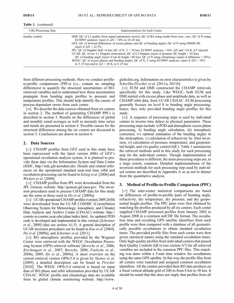
Quality control DMI: QC of L2 quality from impact parameters (noise); QC of BA using model from iono. corr.; QC of N usingECMWF analyses: reject if DN > 10% in 10–45 km.

GFZ: QC of forward differences of excess phases and QC of bending angles; QC of N using MSISE-90:reject if DN > 22.5%.

JPL: QC of Doppler shift <6 km; QC of N, T < 30 km: ECMWF analyses, >10% DN and >10 K DT rejected.UCAR: QC of raw L1 Doppler (truncation); QC of L2 Doppler (reject if dynamic QC height > 20 km);

QC of bending angle (reject if top fit height <40 km); QC of N using climatology (reject if difference > 50%).WEGC: QC of excess phases and bending angles; QC of N, T using ECMWF analyses: reject if DN > 10%

in 5–35 km and/or DT > 20 K in 8–25 km.


4 of 38

data centers have an intrinsic vertical resolution of 200 m. Thedata centers applied different smoothing/filtering algorithmson the data so that the intrinsic vertical resolutions wouldvary from one data set to another and could also be altitudedependent.[18] Due to the different QC procedures, the total number of

profiles varies from center to center. This is demonstrated inthe monthly mean sample numbers for each individual centerin zonal bins of 5� latitudinal width for 2007 in Figure 1. Withthe restriction of all QCs from different centers, only 50%of the total available CHAMP profiles are included in thecommon set.[19] To quantify the latitudinal and temporal comparisons

of inter-center differences, we further compare the monthlymean profile-to-profile climatologies (MPCs) of the commonset of CHAMP profiles. For each center we group the matchedprofiles in zonal bins of 5� latitudinal width (i.e., 36 bins) atthe 200 m vertical grid for each month from January 2002to August 2008. Hereafter we use a common set of CHAMP

data whereas Ho et al. [2009a] used monthly mean cli-matologies including a different number of profiles per cen-ter. Thus, different from Ho et al. [2009a], the sampling errordue to temporal and spatial mismatches is not an issue in thisstudy.

4. Quantification of the Structural UncertaintiesAmong Centers

[20] All comparisons are performed for bending angle (a),refractivity (N), dry temperature (T), dry pressure (p), anddry geopotential height (Z) from January 2002 to August2008. A global PPC of all matched pairs is conducted insection 4.1 to estimate the mean difference among centers inthe investigated period.MPCs are used to investigate the zonalaverage differences as summarized in section 4.2. Anomalytime series are compared in section 4.3. Trend differencesof anomaly time series with respect to the inter-center meantrend are presented in section 4.4. This study seeks to

Figure 1. The monthly mean number of samples in latitudinal bins of 5� at 20 km altitude for DMI,EUM, GFZ, JPL, UCAR, and WEGC for the year 2007.


5 of 38

determine the sources for differences in zonal average fields,anomaly time series, and trends for all RO-derived variables.

4.1. Comparison of Mean Global Differences

4.1.1. Analysis Method[21] Using the PPC files for all six centers, we generate the

global comparison for all variables from January 2002 toAugust 2008. We first compute the difference for eachcenter to the inter-center mean at each vertical level from8 km to 30 km. The multiple years of global RO temperatureand geopotential height anomalies are computed using thefollowing equation

DX PPC jð Þ ¼ 1=nð Þ �Xs¼n

s¼1X PPC s; jð Þ � X PPC

Mean s; jð Þ� �: ð1Þ

[22] Because bending angle, refractivity, and dry pressuredecrease exponentially with height, we present DaPPC,DN PPC, and DpPPC in a fractional sense (i.e., DX/X) tobetter visualize the results. The fractional differences (in %)are computed using the following equation:

DX PPC jð Þ ¼ 100%� 1=nð Þ�Xs¼n

s¼1X PPC s; jð Þ � X PPC

Mean s; jð Þ� �=X PPC

Mean s; jð Þ: ð2Þ

[23] Here j is the index of the vertical levels from 8 km to30 km and s is the index of all matched pairs. X PPC(s, j) arethe individual profile pairs and X Mean

PPC (s, j) is the mean pro-file of all six centers for matched pair s at vertical level j. Therefractivity, dry temperature, dry pressure, and dry geopo-tential height comparisons are for DMI, GFZ, JPL, UCAR,and WEGC and the bending angle comparison is for allsix centers including EUM. The total number of matched pairsis n.Here we compute the mean global differences of bendingangle (DaPPC in %), refractivity (DN PPC in %), temperature(DT PPC in K), pressure (DpPPC in %), and geopotential height(DZ PPC in m) for all matched pairs. The corresponding zonalaverage differences (section 4.2) and anomaly time series dif-ferences (section 4.3) are computed also but the correspondingequations for fractional differences are not specifically listedhereafter.4.1.2. Bending Angle (a) Difference[24] Figure 2 depicts the global bending angle differences

for DMI, EUM, GFZ, JPL, UCAR, and WEGC (i.e.,DaDMIPPC ,

DaEUMPPC , DaGFZ

PPC, DaJPLPPC, DaUCAR

PPC , DaWEGCPPC , respectively).

The mean differences and the median absolute deviation(MAD) for the 8 km to 30 km layer are listed in Table 2 foreach year and for 01/2002 to 08/2008. Structural uncertaintypresented here contains the cumulative errors from POD,atmospheric excess phase processing, and intermediate stepsfor calculation of bending angle among centers (Table 1). Ingeneral, the mean Da for all matched pairs among centersagree to within �0.04% (where the mean DaJPL

PPC from 2002to 2008 is equal to 0.04% and that for WEGC is equal to�0.03%). The MAD for DMI, EUM, GFZ, JPL, UCAR, andWEGC from the inter-center mean is 0.47%, 0.63%, 0.51%,0.74%, 0.34%, and 0.32%, respectively. There is an obviouschange of the standard deviation for JPL (Std(aJPL

PPC)) at20 km altitude (Figure 2d) where Std(aJPL

PPC) ranges from 1%

to 0.5% below 20 km. As a result, all the other centers alsohave a spike near the same height to offset DaJPL

PPC. Thereason for the sudden change of Std(aJPL

PPC) at 20 km altitudeis due to the change in vertical smoothing interval for the L1bending angles from 200 m below 20 km impact altitude to1 km above 20 km impact altitude. DaGFZ

PPC has an obviouspositive mean bias below 13 km which is mainly offset byDaWEGC

PPC in the same height and shows a seasonal depen-dence, especially in sub-tropical region (see Figure 9a).These biases below 13 km are probably due to differences ingeometric optics and wave optics retrievals as well as dif-ferent approaches for downward extrapolation of L1–L2 forionospheric correction (see section A3) [cf. Steiner et al.,1999]. The choice of the data interval used for extrapola-tion of ionospheric correction is especially different betweenthe centers and may introduce differences in the observedmagnitude.[25] The relatively small MADs from DMI, UCAR, and

WEGC is primarily due to all these three centers using thesame UCAR CHAMP orbit data, excess phase, and ampli-tude data. Although EUM is also using the same UCARCHAMP orbit and excess phase data, the MAD of EUM forthe 8 km to 30 km layer is larger (�0.63%) than those fromDMI, UCAR, and WEGC. These MAD differences are alsolikely caused by the different processing and smoothingapproaches of the centers.4.1.3. Refractivity (N) Difference[26] Although different methods are used by each center

for bending angle initialization of the upper boundary con-dition of the Abel integral [Phinney and Anderson, 1968], themean refractivity anomalies among DMI, GFZ, JPL, UCAR,and WEGC (e.g., DN DMI

PPC , DN GFZPPC, DN JPL

PPC, DN UCARPPC , and

DNWEGCPPC ) agree within �0.01% except for JPL (Table 2).

We note that all centers incorporate MSIS (Mass Spectrom-eter Incoherent Scatter Radar model) climatology in someform for the initialization, except for JPL and UCAR. Themean fractional refractivity differences for DNDMI

PPC , DNGFZPPC,

DNJPLPPC, DNUCAR

PPC , and DNWEGCPPC are equal to (0.01, �0.01,

0.02, �0.01, and �0.01)%, respectively. Figures 3a and 3bdepict the DN UCAR

PPC and DNJPLPPC for all 80 months, respec-

tively, whereDNUCARPPC is representative of centers with small

meandifferencesandDN JPLPPCrepresentsacenterwith relatively

larger mean differences to the inter-center mean (see Table 2).Figure 3b shows that DN JPL

PPC has a slightly positive meandifference relative to all the other centers. The yearly meanDN DMI

PPC ,DN GFZPPC,DN JPL

PPC,DN UCARPPC , andDNWEGC

PPC , and theircorresponding MADs are almost the same from 2002 to 2008(Table 2). This indicates the long-term consistency (repro-ducibility) of RO data generated from individual centers.4.1.4. Dry Temperature (T), Dry Pressure (p), and DryGeopotential Height (Z) Differences[27] The global mean temperature differences for DMI,

GFZ, JPL, UCAR, andWEGC (i.e.,DTDMIPPC ,DT GFZ

PPC,DT JPLPPC,

DT UCARPPC , and DTWEGC

PPC ) are listed in Table 2. Figures 3cand 3d depict DT UCAR

PPC and DT JPLPPC from 8 km to 30 km

altitude, respectively. Table 2 shows that the mean DT DMIPPC ,

DT GFZPPC, DT UCAR

PPC , and DTWEGCPPC are equal to 0.13 K,

0.01 K, 0.03 K and 0.10 K, respectively and offset thenegative DT JPL

PPC (�0.27 K) that increases exponentiallyfrom 15 km to 30 km (Figure 3d). The obvious negative


6 of 38

Figure 2. The mean global difference (red) and standard deviation (blue) of bending angle for (a) DMI,(b) EUM, (c) GFZ, (d) JPL, (e) UCAR, and (f) WEGC relative to the inter-center mean, for January 2002to August 2008. The number of the matched profile pairs is denoted by the green line.


7 of 38

DT JPLPPC relative to the inter-center mean above 15 km

reflects the significant difference in the initialization of thehydrostatic equation between JPL and the other data centers(see section A5). JPL starts the hydrostatic equation at40 km by assuming temperature from ECMWF, whereas theother data centers start the hydrostatic integration at 120 km.The reason that the mean MADs for DMI, UCAR, andWEGC during the period 2002 to 2008 are all close to0.5 K is mainly that all these three centers use the sameexcess phase and orbit data from UCAR (see section A1).Here the inversion errors and possible impacts of hydro-static boundary effects for temperature profile derivation arealso included in the inter-center comparisons.

[28] Since the dry pressure is derived together with drytemperature from the refractivity profile (the ratio of drypressure and dry temperature is proportional to refractivity,N = a1 p/T, a1 = 77.6 K/hPa), the mean differences of drypressure for each center more or less compensate both therefractivity differences and dry temperature differences(Table 2). The mean dry pressure differences for all centersare within 0.07% (mean bias from DMI) and �0.11% (meanbias from JPL). The mean dry pressure differences for UCARare depicted in Figure 3e. Again, DMI, GFZ, UCAR, andWEGC show mean dry pressure differences that offset the�0.11% difference of JPL (Figure 3f).

Table 2. The Mean Differences for DMI, EUM, GFZ, JPL, UCAR, WEGC Derived RO Variables From the 8 km to 30 km Layer and theMedian Absolute Deviation (MAD) in the Same Height Range for Each Year and That for All the Yearsa

Center YearFractional Bending Angle

(%) Mean (MAD)Fractional Refractivity(%) Mean (MAD)

Temperature (K)Mean (MAD)

Fractional Dry Pressure(%) Mean (MAD)

Geopotential Height(m) Mean (MAD)

DMI 2002 0.0 (0.45) 0.01 (0.1) 0.14 (0.51) 0.08 (0.24) 10 (20.0)2003 0.0 (0.46) 0.01 (0.1) 0.14 (0.51) 0.08 (0.24) 10 (20.0)2004 0.0 (0.47) 0.01 (0.1) 0.15 (0.51) 0.08 (0.24) 10 (10.0)2005 �0.01 (0.46) 0.01 (0.1) 0.15 (0.50) 0.08 (0.24) 10 (10.0)2006 0.0 (0.47) 0.01 (0.1) 0.09 (0.51) 0.08 (0.24) 10 (10.0)2007 0.0 (0.49) 0.01 (0.1) 0.12 (0.53) 0.07 (0.26) 10 (20.0)2008 0.0 (0.47) 0.01 (0.1) 0.10 (0.51) 0.06 (0.25) 10 (10.0)2002–2008 0.0 (0.47) 0.01 (0.1) 0.13 (0.51) 0.07 (0.24) 10 (20.0)

GFZ 2002 0.01 (0.51) 0.00 (0.18) 0.04 (0.87) 0.02 (0.49) �10 (30.0)2003 0.02 (0.52) �0.01 (0.18) 0.05 (0.91) 0.03 (0.51) �10 (30.0)2004 0.01 (0.52) �0.01 (0.18) 0.0 (0.89) �0.01 (0.50) �10 (30.0)2005 0.01 (0.51) �0.01 (0.18) 0.01 (0.91) 0.0 (0.52) �10 (30.0)2006 0.01 (0.51) �0.01 (0.18) �0.01 (0.96) �0.01 (0.55) �10 (30.0)2007 0.0 (0.51) �0.02 (0.18) �0.05 (0.98) �0.04 (0.56) �10 (30.0)2008 0.0 (0.50) �0.01 (0.18) 0.02 (0.95) 0.0 (0.55) �10 (30.0)2002–2008 0.01 (0.51) �0.01 (0.18) 0.01 (0.92) 0.0 (0.52) �10 (30.0)

JPL 2002 0.06 (0.75) 0.02 (0.17) �0.29 (0.66) �0.11 (0.30) �5.8 (17.8)2003 0.04 (0.75) 0.02 (0.17) �0.28 (0.65) �0.11 (0.30) �5.8 (17.8)2004 0.03 (0.75) 0.02 (0.16) �0.29 (0.65) �0.12 (0.30) �5.8 (17.8)2005 0.06 (0.75) 0.02 (0.16) �0.30 (0.66) �0.12 (0.31) �5.8 (17.8)2006 0.03 (0.75) 0.02 (0.16) �0.26 (0.65) �0.11 (0.31) �5.8 (17.8)2007 0.05 (0.75) 0.02 (0.16) �0.23 (0.65) �0.09 (0.32) �5.8 (17.8)2008 0.06 (0.73) 0.01 (0.15) �0.22 (0.63) �0.09 (0.30) �5.8 (17.8)2002–2008 0.04 (0.74) 0.02 (0.16) �0.27 (0.65) �0.11 (0.31) �5.8 (17.8)

UCAR 2002 �0.01 (0.34) �0.02 (0.09) 0.02 (0.42) 0.0 (0.21) 2.3 (13.2)2003 �0.01 (0.34) �0.02 (0.09) 0.02 (0.43) �0.01 (0.22) 2.3 (13.2)2004 �0.01 (0.35) �0.01 (0.09) 0.06 (0.43) 0.02 (0.22) 2.3 (13.2)2005 �0.01 (0.34) �0.01 (0.09) 0.04 (0.43) 0.01 (0.22) 2.3 (13.2)2006 �0.01 (0.34) �0.01 (0.09) 0.04 (0.44) 0.01 (0.23) 2.3 (13.2)2007 �0.01 (0.35) �0.01 (0.09) 0.02 (0.44) 0.0 (0.23) 2.3 (13.2)2008 �0.01 (0.34) �0.01 (0.09) 0.03 (0.42) 0.0 (0.22) 2.3 (13.2)2002–2008 �0.01 (0.34) �0.01 (0.09) 0.03 (0.43) 0.0 (0.22) 2.3 (13.2)

WEGC 2002 �0.04 (0.32) �0.02 (0.10) 0.08 (0.37) 0.02 (0.18) 3.5 (10.0)2003 �0.03 (0.33) �0.02 (0.10) 0.07 (0.39) 0.01 (0.20) 3.5 (10.0)2004 �0.03 (0.32) �0.01 (0.10) 0.09 (0.37) 0.03 (0.19) 3.5 (10.0)2005 �0.04 (0.32) �0.01 (0.09) 0.10 (0.38) 0.03 (0.18) 3.5 (10.0)2006 �0.03 (0.32) 0.00 (0.09) 0.15 (0.40) 0.06 (0.20) 3.5 (10.0)2007 �0.03 (0.33) 0.00 (0.09) 0.14 (0.41) 0.06 (0.21) 3.5 (10.0)2008 �0.03 (0.32) �0.01 (0.09) 0.08 (0.41) 0.03 (0.21) 3.5 (10.0)2002–2008 �0.03(0.32) �0.01 (0.09) 0.10 (0.39) 0.03 (0.20) 3.5 (10.0)

EUM 2002 �0.01 (0.56)2003 �0.01 (0.6)2004 0.00 (0.64)2005 �0.03 (0.64)2006 0.00 (0.64)2007 �0.02 (0.69)2008 �0.03 (0.69)2002–2008 �0.01 (0.63)

aThe RO-derived variables include fractional bending angle (%), fractional refractivity (%), temperature (K), fractional dry pressure (%), and geopotentialheight (m). To be more visible for readers, the mean differences and MADs for the period 2002 to 2008 are highlighted in bold.


8 of 38

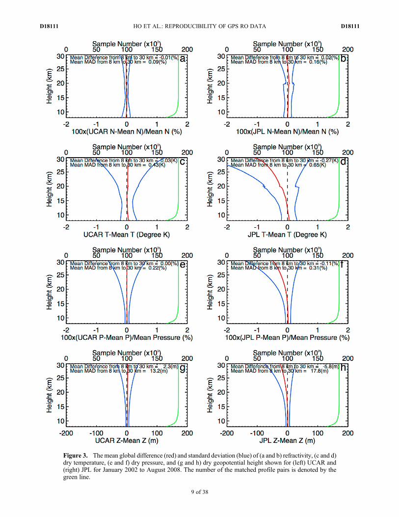
Figure 3. The mean global difference (red) and standard deviation (blue) of (a and b) refractivity, (c and d)dry temperature, (e and f) dry pressure, and (g and h) dry geopotential height shown for (left) UCAR and(right) JPL for January 2002 to August 2008. The number of the matched profile pairs is denoted by thegreen line.


9 of 38

[29] In Figure 3g we depict geopotential height differencesfor UCAR (DZUCAR

PPC ). The standard deviation of DZUCARPPC at

8 km altitude is about 10 m and increases to about 50 m at30 km altitude. The results of the global comparison forpressure and geopotential height are also listed in Table 2.

4.2. Comparison of Mean Zonal Differences

[30] The above comparisons from different centers arebased on global means from 2002 to 2008. In this section wecompare zonal mean differences in order to investigate smallbut nonzero differences among centers at different latitudesand times. Similar to Ho et al. [2009a], we use the followingequation to generate zonal average differences for RO-derivedvariables for individual centers:

DX i; jð Þ ¼ 1=80ð Þ �Xk¼80

k¼1XMPC i; j; kð Þ � XMPC i; j; kð Þ� �

; ð3Þ

where i is the index of latitude bins (5-degree), j is the indexof the altitude levels (200 m from 8 km to 30 km), andk is the month index (from January 2002 to August 2008).XMPC(i, j, k) is the mean of MPC of the compared variablefor all centers (inter-center mean) in each latitude-, height-, andmonth-bin. Because there are few CHAMP data in July 2006,MPCs from that month are set to zero for all centers. Inaddition, we compute the MAD of differences using thefollowing equation:

DXMAD i; jð Þ ¼ 1=80ð Þ �Xk¼80

k¼1XMPC i; j; kð Þ � XMPC i; j; kð Þ�� :

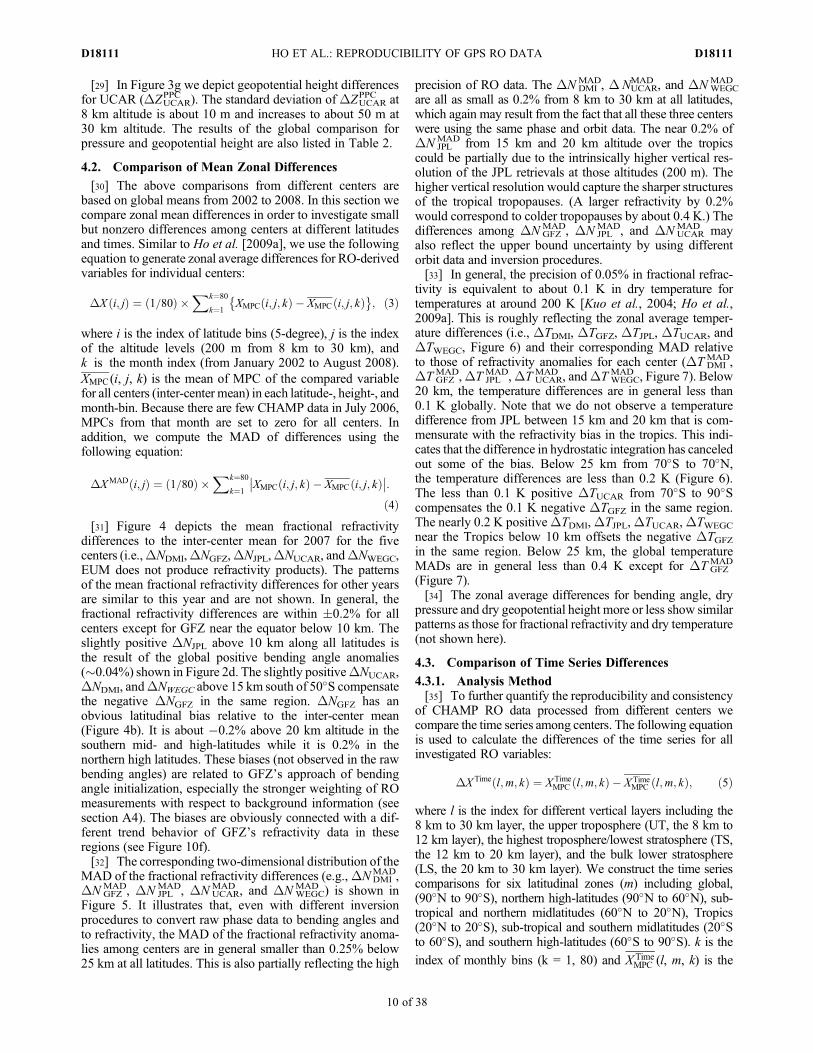
ð4Þ[31] Figure 4 depicts the mean fractional refractivity

differences to the inter-center mean for 2007 for the fivecenters (i.e.,DNDMI,DNGFZ,DNJPL,DNUCAR, andDNWEGC,EUM does not produce refractivity products). The patternsof the mean fractional refractivity differences for other yearsare similar to this year and are not shown. In general, thefractional refractivity differences are within �0.2% for allcenters except for GFZ near the equator below 10 km. Theslightly positive DNJPL above 10 km along all latitudes isthe result of the global positive bending angle anomalies(�0.04%) shown in Figure 2d. The slightly positiveDNUCAR,DNDMI, andDNWEGC above 15 km south of 50�S compensatethe negative DNGFZ in the same region. DNGFZ has anobvious latitudinal bias relative to the inter-center mean(Figure 4b). It is about �0.2% above 20 km altitude in thesouthern mid- and high-latitudes while it is 0.2% in thenorthern high latitudes. These biases (not observed in the rawbending angles) are related to GFZ’s approach of bendingangle initialization, especially the stronger weighting of ROmeasurements with respect to background information (seesection A4). The biases are obviously connected with a dif-ferent trend behavior of GFZ’s refractivity data in theseregions (see Figure 10f).[32] The corresponding two-dimensional distribution of the

MAD of the fractional refractivity differences (e.g.,DNDMIMAD,

DN GFZMAD, DN JPL

MAD, DN UCARMAD , and DNWEGC

MAD ) is shown inFigure 5. It illustrates that, even with different inversionprocedures to convert raw phase data to bending angles andto refractivity, the MAD of the fractional refractivity anoma-lies among centers are in general smaller than 0.25% below25 km at all latitudes. This is also partially reflecting the high

precision of RO data. The DN DMIMAD, DNUCAR

MAD , and DNWEGCMAD

are all as small as 0.2% from 8 km to 30 km at all latitudes,which again may result from the fact that all these three centerswere using the same phase and orbit data. The near 0.2% ofDN JPL

MAD from 15 km and 20 km altitude over the tropicscould be partially due to the intrinsically higher vertical res-olution of the JPL retrievals at those altitudes (200 m). Thehigher vertical resolution would capture the sharper structuresof the tropical tropopauses. (A larger refractivity by 0.2%would correspond to colder tropopauses by about 0.4 K.) Thedifferences among DN GFZ

MAD, DN JPLMAD, and DN UCAR

MAD mayalso reflect the upper bound uncertainty by using differentorbit data and inversion procedures.[33] In general, the precision of 0.05% in fractional refrac-

tivity is equivalent to about 0.1 K in dry temperature fortemperatures at around 200 K [Kuo et al., 2004; Ho et al.,2009a]. This is roughly reflecting the zonal average temper-ature differences (i.e., DTDMI, DTGFZ, DTJPL, DTUCAR, andDTWEGC, Figure 6) and their corresponding MAD relativeto those of refractivity anomalies for each center (DT DMI

MAD,DT GFZ

MAD,DT JPLMAD,DT UCAR

MAD , andDTWEGCMAD , Figure 7). Below

20 km, the temperature differences are in general less than0.1 K globally. Note that we do not observe a temperaturedifference from JPL between 15 km and 20 km that is com-mensurate with the refractivity bias in the tropics. This indi-cates that the difference in hydrostatic integration has canceledout some of the bias. Below 25 km from 70�S to 70�N,the temperature differences are less than 0.2 K (Figure 6).The less than 0.1 K positive DTUCAR from 70�S to 90�Scompensates the 0.1 K negative DTGFZ in the same region.The nearly 0.2 K positiveDTDMI,DTJPL,DTUCAR,DTWEGC

near the Tropics below 10 km offsets the negative DTGFZin the same region. Below 25 km, the global temperatureMADs are in general less than 0.4 K except for DT GFZ

MAD

(Figure 7).[34] The zonal average differences for bending angle, dry

pressure and dry geopotential height more or less show similarpatterns as those for fractional refractivity and dry temperature(not shown here).

4.3. Comparison of Time Series Differences

4.3.1. Analysis Method[35] To further quantify the reproducibility and consistency

of CHAMP RO data processed from different centers wecompare the time series among centers. The following equationis used to calculate the differences of the time series for allinvestigated RO variables:

DX Time l;m; kð Þ ¼ X TimeMPC l;m; kð Þ � X Time

MPC l;m; kð Þ; ð5Þ

where l is the index for different vertical layers including the8 km to 30 km layer, the upper troposphere (UT, the 8 km to12 km layer), the highest troposphere/lowest stratosphere (TS,the 12 km to 20 km layer), and the bulk lower stratosphere(LS, the 20 km to 30 km layer). We construct the time seriescomparisons for six latitudinal zones (m) including global,(90�N to 90�S), northern high-latitudes (90�N to 60�N), sub-tropical and northern midlatitudes (60�N to 20�N), Tropics(20�N to 20�S), sub-tropical and southern midlatitudes (20�Sto 60�S), and southern high-latitudes (60�S to 90�S). k is theindex of monthly bins (k = 1, 80) and X Time

MPC (l, m, k) is the


10 of 38

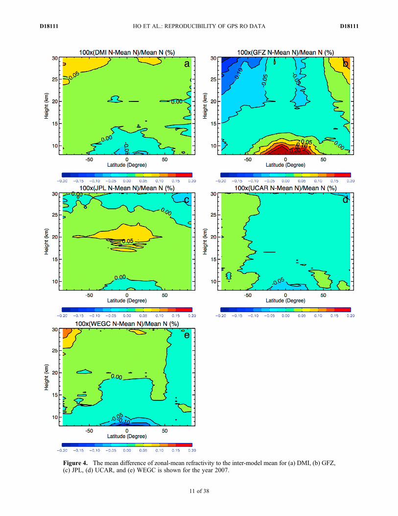
Figure 4. The mean difference of zonal-mean refractivity to the inter-model mean for (a) DMI, (b) GFZ,(c) JPL, (d) UCAR, and (e) WEGC is shown for the year 2007.


11 of 38

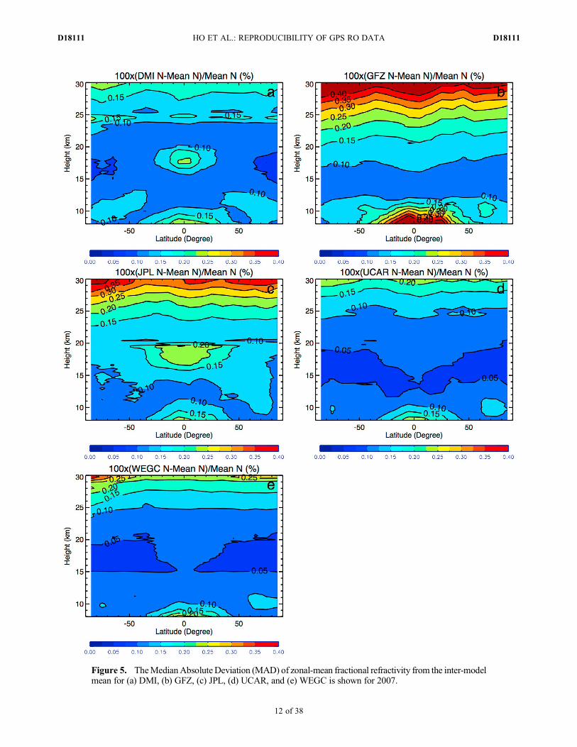
Figure 5. TheMedianAbsolute Deviation (MAD) of zonal-mean fractional refractivity from the inter-modelmean for (a) DMI, (b) GFZ, (c) JPL, (d) UCAR, and (e) WEGC is shown for 2007.


12 of 38

Figure 6. The mean difference of zonal-mean dry temperature to the inter-model mean for (a) DMI,(b) GFZ, (c) JPL, (d) UCAR, and (e) WEGC is shown for 2007.


13 of 38

Figure 7. The Median Absolute Deviation (MAD) of zonal-mean dry temperature to the inter-modelmean for (a) DMI, (b) GFZ, (c) JPL, (d) UCAR, and (e) WEGC is shown for 2007.


14 of 38

inter-center mean MPC for each layer-, zone-, and month-bin.Fractional time series differences (in %) are computed forbending angle, refractivity, and dry pressure. The mean andstandard deviations of the time series for each center to themean of all centers for six latitudinal zones, and at four ver-tical layers for fractional bending angle (%), fractional refrac-tivity (%), fractional dry pressure (%), dry temperature (K),and dry geopotential height (m) are summarized in Tables 3–7,respectively.[36] Note that, as mentioned in Ho et al. [2009a], because

the inter-center mean is subtracted, results from each centerneed to offset the persistent or varying anomalies from anindividual center by compensating behavior. The magnitudeof the mean anomalies is merely used to indicate the devia-tion of individual centers from the inter-center mean ratherthan the accuracy of the time series. Here we focus onquantifying the systematic inter-center difference and inter-monthly variability among centers.4.3.2. Time Series Differences for Bending Angle (a)[37] Figure 8 depicts the differences of bending angle time

series to the inter-center mean for DMI, EUM, GFZ, JPL,UCAR, and WEGC for the 8 km to 30 km layer (i.e.,DaDMI

Time, DaEUMTime, DaGFZ

Time, DaJPLTime, DaUCAR

Time , DaWEGCTime )

for all six latitudinal zones, Figure 8a for the global, andFigures 8b–8f for the northern high-latitudes, sub-tropicaland northern midlatitudes, Tropics, sub-tropical and southernmidlatitudes, and southern high-latitudes, respectively. Allthese figures present similar qualitative features: (i) theanomalies from individual centers are persistent in time andthere are no obvious latitudinal dependent biases except forDaGFZ

Time in the tropical region (�0.29%, Figure 8d) and smallDaJPL

Time in the northern high-latitudes (0.14%, Table 3) and inthe southern high-latitudes (�0.17%, Table 3), and (ii) indi-vidual center’s differences show no obvious inter-monthlyand inter-seasonally variance except for DaGFZ

Time in theTropics (the standard deviation is �0.06%, Table 3), and inthe midlatitudes (the standard deviation is�0.07%, Table 3).[38] The mean differences for DaDMI

Time, DaEUMTime, DaGFZ

Time,DaJPL

Time, DaUCARTime , and DaWEGC

Time in the 8 km to 30 km layerare�0.01%,�0.02%, 0.12%, 0.02%, �0.02%, and�0.08%(Table 3), respectively. The mean standard deviations in thesame layer for all centers are within 0.02%. The smallestbending angle differences among centers are found in the12 km to 20 km layer where the mean is between �0.01%and 0.02% and the standard deviation is less than �0.02%(Table 3).[39] Figure 9 depicts the time series MPC fractional

bending angle differences for all six centers for northernmidlatitudes, the Tropics, and the southern high-latitudes,Figures 9a, 9c, and 9e for the 8 km to 12 km layer, andFigures 9b, 9d, and 9f for the 20 km to 30 km layer. Thefractional bending angle anomalies for other latitudinalzones are summarized in Table 3 and are not shown here.Figure 9a shows that DaGFZ

Time has a larger inter-seasonalvariability with a difference of up to �0.5% in borealhemispheric summer months (also in austral hemisphericsummer months, not shown). The positive DaGFZ

Time bias inthe 8 km to 12 km layer in the Tropics of 0.65% (Figure 9c)is mainly offset by DaWEGC

Time (�0.38%) and DaEUMTime

(�0.15%). The reason for the inter-seasonal bias below

12 km near the Tropics and sub-tropical region is probablydue to differences in geometric optics and wave opticsretrievals as well as differences in downward extrapolationof L1�L2 for ionospheric correction (see section A3).Obviously, GFZ’s processing shows stronger deviationsunder tropical atmospheric conditions and in sub-tropical tomid-latitudinal summer. In the 20 km to 30 km layer, theinter-monthly variation of DaTime is low for all centers(Figures 9b, 9d, and 9f). DaJPL

Time shows a small bias of0.19% in the northern high-latitudes and of �0.13% in thesouthern high-latitudes in the 20 km to 30 km layer(Table 3). The reason for this is not presently understood.4.3.3. Time Series Differences for Refractivity (N)[40] The time series of fractional refractivity differences

(DNTime) show similar qualitative features as bending anglebut with a different magnitude. The mean global differencesamong centers in the 8 km to 30 km layer are within�0.03%with about 0.01% standard deviation (Table 4). Figure 10depicts DNTime for five centers (except EUM) for thenorthern midlatitudes, the Tropics, and the southern high-latitudes, Figures 10a, 10c, and 10e for the 8 km to 12 kmlayer, and Figures 10b, 10d, and 10f for the 20 km to 30 kmlayer. The anomalies from individual centers are in generalpersistent in time except at northern midlatitudes in the 8 kmto 12 km layer (Figure 10a). A 0.65% of fractional bendingangle bias (e.g.,DaGFZ

Time in the Tropics for the 8 km to 12 kmlayer in Table 3, also see Figure 9c) is likely leading to a�0.2% of fractional refractivity bias (e.g., DNGFZ

Time in thesame region shown in Table 4, also see Figure 10c). Theobvious inter-seasonal bias for DNGFZ

Time in the sub-tropicaland midlatitudes in the 8 km to 12 km layer reflects thebehavior of bending angle bias in these regions.4.3.4. Time Series Differences for Dry Pressure (p)and Dry Temperature (T)[41] The statistics of the MPC time series differences to

the inter-center mean for dry pressure and dry temperatureare shown in Tables 5 and 6, respectively. Like the timeseries MPC for refractivity shown above, the global drypressure time series MPC in the 8 km to 30 km layer forDMI, GFZ, JPL, UCAR, and WEGC (DpDMI

Time, DpGFZTime,

DpJPLTime, DpUCAR

Time , and DpWEGCTime ) show a small standard

deviation of less than 0.02%. The mean global differencesfor DpDMI

Time, DpGFZTime, DpJPL

Time, DpUCARTime , and DpWEGC

Time are(0.04,�0.04,�0.02, 0.00, and 0.01)%, respectively. Largestdifferences occur in the 20 km to 30 km layer.[42] The global mean temperature time series differences

in the 8 km to 30 km layer for DMI, GFZ, JPL, UCAR, andWEGC (DT DMI

Time,DT GFZTime,DT JPL

Time,DT UCARTime , andDTWEGC

Time )are 0.15 K, 0.00 K, �0.27 K, 0.04 K, and 0.09 K, respec-tively (Table 6). The variations, i.e., the correspondingstandard deviations are 0.04 K, 0.06 K, 0.05 K, 0.04 K, and0.04 K, respectively. The mean anomaly differences amongcenters are even smaller in the 12 km to 20 km layers (within�0.08 K, standard deviation less than 0.03 K). Differencesare larger in the 20 km to 30 km layer and the 8 km to 12 kmlayers.[43] Figure 11 depicts the temperature time series differ-

ences for all five centers for the northern midlatitudes, theTropics, and the southern high-latitudes, Figures 11a, 11c,and 11e for the 8 km to 12 km layer, and Figures 11b, 11d,


15 of 38

Tab

le3.

MeanandStand

ardDeviatio

nsof

theTim

eSeriesof

FractionalBending

Ang

leDifferences

forDMI,EUM,G

FZ,JPL,U

CAR,and

WEGCto

theMeanof

AllSix

CentersforSix

Latitu

dinalZon

es,andat

Fou

rVertical

Layersa

Latitu

deZon

eHeigh

tLayers

MeanTrend

(%/5

yrs)

Mean(std)/DMI–

MeanTrend

Mean(std)/EUM–

MeanTrend

Mean(std)/GFZ–

MeanTrend

Mean(std)/JPL–

MeanTrend

Mean(std)/UCAR–

MeanTrend

Mean(std)/WEGC–

MeanTrend

90� N

to90

� S8to

30km

0.01

�0.01(0.01)/0.00

�0.02(0.02)/0.00

0.12

(0.02)/�

0.01

0.02

(0.02)/0.00

�0.02(0.01)/0.00

�0.08(0.01)/0.02

8to

12km

0.06

�0.03(0.01)/�

0.01

�0.03(0.02)/0.00

0.26

(0.05)/�

0.01

0.00

(0.02)/�

0.01

�0.03(0.02)/�

0.01

�0.16(0.02)/0.03

12to

20km

0.06

0.00

(0.00)/0.00

0.00

(0.02)/�

0.01

0.00

(0.01)/�

0.02

0.02

(0.02)/0.00

0.00

(0.00)/0.00

�0.01(0.01)/0.01

20to

30km

�0.25

�0.01(0.0)/0.00

�0.01(0.02)/�

0.01

�0.04(0.01)/0.0

0.09

(0.03)/0.00

�0.02(0.00)/0.00

�0.01(0.01)/0.01

60� N

to90

� N8to

30km

�0.11

�0.02(0.01)/0.00

0.0(0.02)/�

0.01

�0.02(0.03)/�

0.01

0.14

(0.03)/�

0.01

�0.03(0.02)/�

0.01

�0.06(0.03)/0.02

8to

12km

0.22

�0.02(0.02)/�

0.01

0.02

(0.03)/�

0.01

�0.01(0.06)/�

0.02

0.12

(0.03)/0.00

�0.03(0.03)/�

0.02

�0.08(0.04)/0.03

12to

20km

0.13

�0.02(0.01)/0.01

�0.02(0.02)/0.00

�0.03(0.01)/0.00

0.15

(0.03)/�

0.01

�0.03(0.01)/0.00

�0.04(0.02)/0.02

20to

30km

�0.49

�0.04(0.01)/0.00

�0.04(0.01)/�

0.01

�0.04(0.03)/0.02

0.19

(0.03)/�

0.02

�0.04(0.01)/�

0.02

�0.04(0.01)/0.0

60� N

to20

� N8to

30km

0.15

0.00

(0.02)/�

0.01

0.00

(0.04)/�

0.01

0.09

(0.07)/0.00

�0.01(0.04)/�

0.01

�0.01(0.02)/�

0.01

�0.06(0.03)/0.02

8to

12km

�0.11

�0.02(0.03)/0.0

0.00

(0.05)/0.00

0.20

(0.14)/0.02

�0.03(0.04)/�

0.01

�0.03(0.04)/�

0.01

�0.12(0.06)/0.02

12to

20km

0.44

0.01

(0.0)/0.00

0.01

(0.03)/0.00

0.00

(0.01)/0.00

�0.01(0.04)/0.00

0.0(0.01)/0.00

�0.02(0.02)/0.02

20to

30km

0.17

0.00

(0.01)/0.00

�0.01(0.02)/0.00

�0.02(0.01)/0.01

0.05

(0.04)/0.00

�0.01(0.01)/0.0

0.00

(0.01)/0.00

20� N

to20

� S8to

30km

0.1

�0.04(0.02)/0.00

�0.07(0.02)/0.01

0.29

(0.06)/�

0.03

0.02

(0.04)/0.00

�0.04(0.02)/0.0

�0.17(0.02)/0.03

8to

12km

0.19

�0.08(0.04)/0.00

�0.15(0.05)/0.03

0.65

(0.14)/�

0.05

0.01

(0.05)/�

0.02

�0.06(0.04)/�

0.01

�0.38(0.05)/0.06

12to

20km

�0.12

�0.01(0.01)/0.00

�0.01(0.02)/�

0.01

0.03

(0.02)/�

0.02

0.03

(0.02)/0.01

�0.01(0.01)/0.00

�0.01(0.01)/0.02

20to

30km

�0.35

�0.01(0.01)/0.00

�0.02(0.02)/�

0.01

�0.01(0.01)/�

0.01

�0.04(0.01)/0.02

�0.04(0.01)/0.00

�0.01(0.01)/0.01

20� S

to60

� S8to

30km

0.03

�0.03(0.02)/0.00

�0.04(0.01)/�

0.02

0.10

(0.07)/0.00

0.09

(0.05)/0.01

�0.04(0.02)/0.0

�0.09(0.03)/0.02

8to

12km

0.04

�0.05(0.03)/�

0.01

�0.06(0.05)/�

0.01

0.26

(0.15)/0.01

0.05

(0.05)/�

0.01

�0.06(0.03)/�

0.01

�0.16(0.05)/0.02

12to

20km

�0.05

�0.01(0.01)/0.00

�0.02(0.04)/�

0.03

�0.03(0.02)/�

0.02

0.10

(0.05)/0.01

�0.02(0.01)/0.00

�0.03(0.01)/0.02

20to

30km

0.18

�0.02(0.01)/0.00

�0.04(0.05)/�

0.03

�0.06(0.01)/�

0.01

0.19

(0.06)/0.01

�0.03(0.01)/0.00

�0.02(0.01)/0.00

60� S

to90

� S8to

30km

�0.17

0.05

(0.01)/0.00

0.06

(0.02)/0.01

0.01

(0.02)/�

0.03

�0.17(0.04)/�

0.01

0.04

(0.01)/0.00

0.01

(0.03)/0.03

8to

12km

�0.09

0.05

(0.01)/0.01

0.08

(0.03)/�

0.01

0.02

(0.03)/�

0.02

�0.17(0.04)/�

0.01

0.04

(0.02)/�

0.01

�0.01(0.04)/0.03

12to

20km

0.3

0.05

(0.01)/0.00

0.05

(0.02)/0.00

0.01

(0.02)/�

0.03

�0.18(0.04)/�

0.01

0.04

(0.01)/0.00

0.03

(0.02)/0.02

20to

30km

�1.03

0.04

(0.01)/0.01

0.04

(0.02)/0.01

�0.01(0.03)/�

0.04

�0.13(0.04)/�

0.01

0.03

(0.01)/0.01

0.03

(0.01)/0.02

a The

values

ofstandard

deviations

oftim

eseries

offractio

nalbend

ingangledifferencesareshow

nin

theparentheses.The

correspo

ndingmeantrends

fortheperiod

2002

to20

08of

de-seasonalized

fractio

nal

bend

ingangleanom

alies(in%/5

yrs)

forallcentersandtheDMI-meantrendof

allsixcenters,

theEUM-m

eantrendof

allsixcenters,

theGFZ-m

eantrendof

allsixcenters,

theJPL-m

eantrendof

allsix

centers,theUCAR-m

eantrendof

allsixcenters,andtheWEGC-m

eantrendof

allsixcenters.Tobe

morevisibleforreaders,thenu

mbers

forthe8km

to30

kmlayerarehigh

lighted

inbo

ld.


16 of 38

and 11f for the 20 km to 30 km layer. As for bending angleand refractivity, the temperature differences of individualcenters are persistent in time, especially in the troposphere(the 8 km to 12 km layer). A positive DNGFZ

Time in the 8 km to12 km layer leads to a small negative DTGFZ

Time in the sameheight (Figures 11a, 11c, and 11e). In the LS at midlatitudesand in the Tropics (Figures 11b and 11d), the temperatureanomalies from individual centers are also persistent in time,

consistent with refractivity behavior. The inter-seasonalvariance hardly visible in DNDMI

Time propagates to DTDMITime in

the 20 km to 30 km layer at high-latitudes (Figure 11f). Thereason for the obvious inter-seasonal variability in DTDMI

Time

most likely originates from the inability of the MSISE-90 cli-matology (used in the statistical optimization, see section A4)to represent the real stratosphere and mesosphere at high-latitudes [Gobiet and Kirchengast, 2004; Gobiet et al., 2005,

Table 5. The Same as Table 3, but for Fractional Dry Pressure (%)

Latitude ZoneHeightLayers

Trend(%/5 yrs)

Mean (std)/DMI–Mean Trend

Mean (std)/GFZ–Mean Trend

Mean (std)/JPL–Mean Trend

Mean (std)/UCAR–Mean Trend

Mean (std)/WEGC–Mean Trend

90�N to 90�S 8 to 30 km �0.20 0.04 (0.01)/�0.01 �0.04 (0.02)/�0.02 �0.02 (0.01)/0.00 0.00 (0.01)/�0.01 0.01 (0.01)/0.028 to 12 km �0.07 0.02 (0.00)/0.00 �0.04 (0.01)/�0.02 0.02 (0.00)/0.00 0.01 (0.01)/0.00 �0.01 (0.0)/0.0212 to 20 km �0.23 0.04 (0.01)/�0.01 �0.05 (0.02)/0.02 �0.01 (0.01)/0.00 0.00 (0.01)/0.00 0.01 (0.01)/0.0220 to 30 km �0.44 0.11 (0.03)/�0.03 0.03 (0.05)/�0.06 �0.19 (0.03)/0.03 0.00 (0.03)/0.01 0.05 (0.03)/0.04

60�N to 90�N 8 to 30 km �0.47 0.05 (0.07)/�0.05 0.01 (0.10)/0.12 �0.05 (0.05)/�0.02 0.01 (0.06)/�0.01 �0.02 (0.04)/0.008 to 12 km �0.16 0.03 (0.03)/�0.03 �0.04 (0.05)/0.04 0.00 (0.02)/�0.01 0.02 (0.03)/�0.01 �0.02 (0.02)/0.0012 to 20 km �0.38 0.05 (0.07)/�0.05 0.01 (0.10)/0.08 �0.04 (0.05)/�0.02 0.01 (0.06)/0.00 �0.02 (0.04)/0.0020 to 30 km �0.59 0.15 (0.23)/�.15 0.18 (0.3)/0.23 �0.27 (0.15)/�0.03 0.01 (0.20)/�0.01 �0.05 (0.11)/�0.03

60�N to 20�N 8 to 30 km 0.26 0.05 (0.02)/�0.03 �0.04(0.04)/0.03 �0.01 (0.02)/0.00 0.00 (0.02)/�0.01 0.01 (0.02)/0.018 to 12 km 0.30 0.03 (0.01)/�0.01 �0.06 (0.02/0.02 0.02 (0.01)/0.00 0.01 (0.01)/�0.02 �0.01 (0.01)/0.0012 to 20 km 0.30 0.05 (0.02)/�0.03 �0.05 (0.04)/0.02 �0.01 (0.02)/�0.01 0.00 (0.02)/0.00 0.02 (0.01)/0.0220 to 30 km 0.05 0.12 (0.05))/�0.08 0.04 (0.09))/0.08 �0.17 (0.05))/0.01 �0.04 (0.06))/�0.03 0.04 (0.04)/0.02

20�N to 20�S 8 to 30 km �0.11 0.01 (0.01)/0.01 0.02 (0.03)/�0.03 �0.01(0.01)/0.00 �0.03 (0.02)/�0.01 0.0 (0.01)/0.018 to 12 km �0.13 0.00 (0.01)/0.01 0.02 (0.02)/�0.02 0.02 (0.01)/0.00 �0.02 (0.01)/0.00 �0.02 (0.01)/0.0212 to 20 km �0.27 0.02 (0.01)/0.00 �0.01 (0.03)/�0.02 0.01 (0.01)/0.00 �0.02 (0.01)/�0.01 0.01 (0.01)/0.0220 to 30 km �0.04 0.04 (0.05)/0.01 0.10 (0.09)/�0.06 �0.17 (0.05)/0.03 �0.04 (0.05)/�0.05 0.07 (0.04)/0.05

20�S to 60�S 8 to 30 km 0.01 0.05 (0.02)/0.00 �0.08 (0.04)/�0.05 0.00 (0.02)/0.00 0.01 (0.02)/0.01 0.02 (0.02)/0.028 to 12 km 0.02 0.03 (0.01)/0.00 �0.07 (0.02)/�0.03 0.03 (0.01)/0.00 0.01 (0.01)/0.00 0.0 (0.01)/0.0212 to 20 km 0.03 0.05 (0.02)/0.00 �0.09 (0.04)/�0.04 0.01 (0.01)/0.00 0.01 (0.02)/0.01 0.02 (0.02)/0.0220 to 30 km �0.10 0.14(0.06)/�0.01 �0.09 (0.11)/�0.12 �014 (0.05)/0.03 0.01 (0.05)/0.03 0.08 (0.05)/0.06

60�S to 90�S 8 to 30 km �0.93 0.06 (0.05)/0.02 �0.1 (0.08)/�0.15 �0.03 (0.04)/0.02 0.05 (0.03)/0.04 0.02 (0.04)/0.048 to 12 km �0.42 0.04 (0.02)/0.02 �0.1 (0.04)/�0.08 0.02 (0.02)/0.01 0.04 (0.02)/0.02 0.01 (0.02)/0.0212 to 20 km �0.96 0.06 (0.05)/0.02 �0.11 (0.08)/�0.14 �0.02 (0.04)/0.03 0.05 (0.03)/0.05 0.02 (0.04)/0.0420 to 30 km �2.1 0.16 (0.20)/0.10 �0.1 (0.23)/�0.40 �0.23 (0.13)/0.10 0.13 (0.10)/0.20 0.05 (0.11)/0.10

Table 4. The Same as Table 3, but for Fractional Refractivity (%)


Trend(%/5 yrs)






90�N to 90�S 8 to 30 km 0.02 0.00 (0.0)/0.00 0.02 (0.00)/�0.01 0.02 (0.00)/0.00 �0.01 (0.00)/0.00 �0.03 (0.01)/0.028 to 12 km 0.08 �0.01 (0.01)/0.01 0.07 (0.02)/�0.01 0.01 (0.01)/0.00 �0.01 (0.01)/0.00 �0.05 (0.01)/0.0212 to 20 km 0.46 0.01 (0.0)/0.00 �0.02 (0.01)/0.00 0.03 (0.00)/0.00 �0.01 (0.00)/0.00 �0.01 (0.01)/0.0120 to 30 km �0.31 0.02 (0.0)/0.00 �0.02 (0.01)/�0.01 0.03 (0.01)/�0.01 �0.02 (0.01)/0.00 0.00 (0.01)/0.01

60�N to 90�N 8 to 30 km 0.0 0.01 (0.01)/�0.01 0.00 (0.02)/0.01 0.02 (0.01)/�0.01 0.00 (0.01)/�0.01 �0.03 (0.01)/0.018 to 12 km 0.24 0.01 (0.01)/0.00 0.00 (0.02)/0.00 0.02 (0.01)/�0.01 0.01 (0.02)/�0.01 �0.03 (0.02)/0.0212 to 20 km �0.06 0.00 (0.01)/�0.01 �0.01 (0.02)/0.00 0.02 (0.01)/�0.01 0.00 (0.01)/0.00 �0.01 (0.01)/0.0020 to 30 km �0.54 0.02 (0.02)/�0.02 0.02 (0.06)/0.05 0.01 (0.03)/�0.04 �0.02 (0.02)/0.00 �0.02 (0.02)/�0.01

60�N to 20�N 8 to 30 km 0.26 0.00 (0.01)/�0.01 0.02 (0.02)/0.00 0.02 (0.01)/�0.01 �0.01 (0.01)/�0.01 �0.03 (0.01)/0.028 to 12 km 0.13 0.00 (0.01)/0.00 0.05 (0.04)/0.00 0.01 (0.02)/�0.01 0.00 (0.02)/�0.01 �0.05 (0.02)/0.0312 to 20 km 0.76 0.01 (0.0)/0.00 �0.02 (0.01)/0.00 0.02 (0.01)/0.00 �0.01 (0.01)/0.00 �0.01 (0.01)/0.0020 to 30 km 0.09 0.01 (0.01)/�0.01 �0.02 (0.03)/0.03 0.02 (0.01)/�0.01 0.02 (0.03)/0.00 0.00 (0.01)/0.01

20�N to 20�S 8 to 30 km �0.13 0.00 (0.01)/�0.01 0.08 (0.02)/�0.01 0.02 (0.01)/0.00 �0.03 (0.01)/0.00 �0.05 (0.01)/0.028 to 12 km 0.02 �0.05 (0.01)/0.01 0.20 (0.02)/�0.03 �0.01 (0.01)/�0.01 �0.05 (0.01)/0.00 �0.09 (0.02)/0.0212 to 20 km �0.49 0.01 (0.0)/0.00 �0.01 (0.01)/�0.01 0.04 (0.01)/0.00 �0.01 (0.00)/0.00 �0.02 (0.01)/0.0020 to 30 km �0.26 0.01 (0.01)/0.01 �0.02 (0.02)/�0.01 0.04 (0.01)/�0.01 �0.02 (0.01)/0.00 0.01 (0.01)/0.01

20�S to 60�S 8 to 30 km 0.05 0.00 (0.01)/0.00 0.01 (0.02)/�0.02 0.02 (0.01)/�0.01 �0.01 (0.01)/0.00 �0.02 (0.01)/0.018 to 12 km 0.02 �0.01 (0.01)/0.00 0.06(0.02)/�0.02 0.01 (0.01)/0.00 �0.02 (0.02)/0.00 �0.05 (0.02)/0.0212 to 20 km 0.24 0.01 (0.0)/0.01 �0.03 (0.01)/�0.02 0.03 (0.01)/0.01 0.00 (0.0)/0.01 �0.01 (0.01)/0.0120 to 30 km 0.15 0.02 (0.01)/0.01 �0.06 (0.02)/�0.02 0.04 (0.01)/�0.01 �0.04 (0.01)/0.01 0.01 (0.01)/0.02

60�S to 90�S 8 to 30 km �0.22 0.01 (0.01)/0.02 �0.03 (0.01)/�0.04 0.02 (0.01)/0.01 0.01 (0.01)/0.01 �0.02 (0.02)/0.038 to 12 km 0.02 0.01 (0.01)/0.02 �0.02 (0.02)/�0.03 0.02 (0.01)/0.0 0.01 (0.02)/�0.01 �0.03 (0.02)/0.0212 to 20 km �0.04 0.01 (0.01)/0.00 �0.03 (0.02)/0.01 0.03 (0.01)/�0.01 0.00 (0.01)/0.00 0.00 (0.01)/0.0020 to 30 km �1.47 0.03 (0.02)/0.03 �0.06 (0.06)/�0.10 0.02 (0.03)/0.01 �0.01 (0.01)/0.04 0.01 (0.02)/0.03


17 of 38

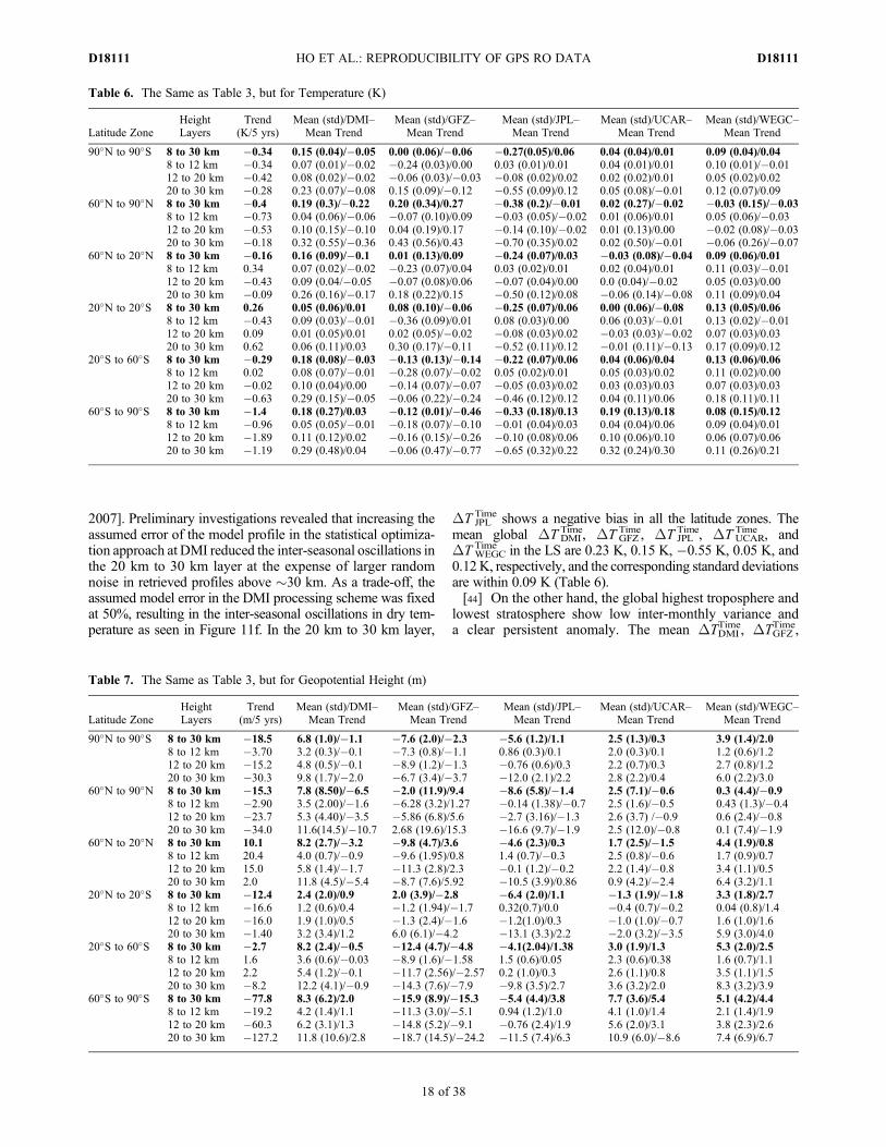
2007]. Preliminary investigations revealed that increasing theassumed error of the model profile in the statistical optimiza-tion approach at DMI reduced the inter-seasonal oscillations inthe 20 km to 30 km layer at the expense of larger randomnoise in retrieved profiles above �30 km. As a trade-off, theassumed model error in the DMI processing scheme was fixedat 50%, resulting in the inter-seasonal oscillations in dry tem-perature as seen in Figure 11f. In the 20 km to 30 km layer,

DT JPLTime shows a negative bias in all the latitude zones. The

mean global DT DMITime, DT GFZ

Time, DT JPLTime, DT UCAR

Time , andDTWEGC

Time in the LS are 0.23 K, 0.15 K, �0.55 K, 0.05 K, and0.12K, respectively, and the corresponding standard deviationsare within 0.09 K (Table 6).[44] On the other hand, the global highest troposphere and

lowest stratosphere show low inter-monthly variance anda clear persistent anomaly. The mean DTDMI

Time, DTGFZTime,

Table 6. The Same as Table 3, but for Temperature (K)


Trend(K/5 yrs)






90�N to 90�S 8 to 30 km �0.34 0.15 (0.04)/�0.05 0.00 (0.06)/�0.06 �0.27(0.05)/0.06 0.04 (0.04)/0.01 0.09 (0.04)/0.048 to 12 km �0.34 0.07 (0.01)/�0.02 �0.24 (0.03)/0.00 0.03 (0.01)/0.01 0.04 (0.01)/0.01 0.10 (0.01)/�0.0112 to 20 km �0.42 0.08 (0.02)/�0.02 �0.06 (0.03)/�0.03 �0.08 (0.02)/0.02 0.02 (0.02)/0.01 0.05 (0.02)/0.0220 to 30 km �0.28 0.23 (0.07)/�0.08 0.15 (0.09)/�0.12 �0.55 (0.09)/0.12 0.05 (0.08)/�0.01 0.12 (0.07)/0.09

60�N to 90�N 8 to 30 km �0.4 0.19 (0.3)/�0.22 0.20 (0.34)/0.27 �0.38 (0.2)/�0.01 0.02 (0.27)/�0.02 �0.03 (0.15)/�0.038 to 12 km �0.73 0.04 (0.06)/�0.06 �0.07 (0.10)/0.09 �0.03 (0.05)/�0.02 0.01 (0.06)/0.01 0.05 (0.06)/�0.0312 to 20 km �0.53 0.10 (0.15)/�0.10 0.04 (0.19)/0.17 �0.14 (0.10)/�0.02 0.01 (0.13)/0.00 �0.02 (0.08)/�0.0320 to 30 km �0.18 0.32 (0.55)/�0.36 0.43 (0.56)/0.43 �0.70 (0.35)/0.02 0.02 (0.50)/�0.01 �0.06 (0.26)/�0.07

60�N to 20�N 8 to 30 km �0.16 0.16 (0.09)/�0.1 0.01 (0.13)/0.09 �0.24 (0.07)/0.03 �0.03 (0.08)/�0.04 0.09 (0.06)/0.018 to 12 km 0.34 0.07 (0.02)/�0.02 �0.23 (0.07)/0.04 0.03 (0.02)/0.01 0.02 (0.04)/0.01 0.11 (0.03)/�0.0112 to 20 km �0.43 0.09 (0.04/�0.05 �0.07 (0.08)/0.06 �0.07 (0.04)/0.00 0.0 (0.04)/�0.02 0.05 (0.03)/0.0020 to 30 km �0.09 0.26 (0.16)/�0.17 0.18 (0.22)/0.15 �0.50 (0.12)/0.08 �0.06 (0.14)/�0.08 0.11 (0.09)/0.04

20�N to 20�S 8 to 30 km 0.26 0.05 (0.06)/0.01 0.08 (0.10)/�0.06 �0.25 (0.07)/0.06 0.00 (0.06)/�0.08 0.13 (0.05)/0.068 to 12 km �0.43 0.09 (0.03)/�0.01 �0.36 (0.09)/0.01 0.08 (0.03)/0.00 0.06 (0.03)/�0.01 0.13 (0.02)/�0.0112 to 20 km 0.09 0.01 (0.05)/0.01 0.02 (0.05)/�0.02 �0.08 (0.03)/0.02 �0.03 (0.03)/�0.02 0.07 (0.03)/0.0320 to 30 km 0.62 0.06 (0.11)/0.03 0.30 (0.17)/�0.11 �0.52 (0.11)/0.12 �0.01 (0.11)/�0.13 0.17 (0.09)/0.12

20�S to 60�S 8 to 30 km �0.29 0.18 (0.08)/�0.03 �0.13 (0.13)/�0.14 �0.22 (0.07)/0.06 0.04 (0.06)/0.04 0.13 (0.06)/0.068 to 12 km 0.02 0.08 (0.07)/�0.01 �0.28 (0.07)/�0.02 0.05 (0.02)/0.01 0.05 (0.03)/0.02 0.11 (0.02)/0.0012 to 20 km �0.02 0.10 (0.04)/0.00 �0.14 (0.07)/�0.07 �0.05 (0.03)/0.02 0.03 (0.03)/0.03 0.07 (0.03)/0.0320 to 30 km �0.63 0.29 (0.15)/�0.05 �0.06 (0.22)/�0.24 �0.46 (0.12)/0.12 0.04 (0.11)/0.06 0.18 (0.11)/0.11

60�S to 90�S 8 to 30 km �1.4 0.18 (0.27)/0.03 �0.12 (0.01)/�0.46 �0.33 (0.18)/0.13 0.19 (0.13)/0.18 0.08 (0.15)/0.128 to 12 km �0.96 0.05 (0.05)/�0.01 �0.18 (0.07)/�0.10 �0.01 (0.04)/0.03 0.04 (0.04)/0.06 0.09 (0.04)/0.0112 to 20 km �1.89 0.11 (0.12)/0.02 �0.16 (0.15)/�0.26 �0.10 (0.08)/0.06 0.10 (0.06)/0.10 0.06 (0.07)/0.0620 to 30 km �1.19 0.29 (0.48)/0.04 �0.06 (0.47)/�0.77 �0.65 (0.32)/0.22 0.32 (0.24)/0.30 0.11 (0.26)/0.21

Table 7. The Same as Table 3, but for Geopotential Height (m)


Trend(m/5 yrs)






90�N to 90�S 8 to 30 km �18.5 6.8 (1.0)/�1.1 �7.6 (2.0)/�2.3 �5.6 (1.2)/1.1 2.5 (1.3)/0.3 3.9 (1.4)/2.08 to 12 km �3.70 3.2 (0.3)/�0.1 �7.3 (0.8)/�1.1 0.86 (0.3)/0.1 2.0 (0.3)/0.1 1.2 (0.6)/1.212 to 20 km �15.2 4.8 (0.5)/�0.1 �8.9 (1.2)/�1.3 �0.76 (0.6)/0.3 2.2 (0.7)/0.3 2.7 (0.8)/1.220 to 30 km �30.3 9.8 (1.7)/�2.0 �6.7 (3.4)/�3.7 �12.0 (2.1)/2.2 2.8 (2.2)/0.4 6.0 (2.2)/3.0

60�N to 90�N 8 to 30 km �15.3 7.8 (8.50)/�6.5 �2.0 (11.9)/9.4 �8.6 (5.8)/�1.4 2.5 (7.1)/�0.6 0.3 (4.4)/�0.98 to 12 km �2.90 3.5 (2.00)/�1.6 �6.28 (3.2)/1.27 �0.14 (1.38)/�0.7 2.5 (1.6)/�0.5 0.43 (1.3)/�0.412 to 20 km �23.7 5.3 (4.40)/�3.5 �5.86 (6.8)/5.6 �2.7 (3.16)/�1.3 2.6 (3.7) /�0.9 0.6 (2.4)/�0.820 to 30 km �34.0 11.6(14.5)/�10.7 2.68 (19.6)/15.3 �16.6 (9.7)/�1.9 2.5 (12.0)/�0.8 0.1 (7.4)/�1.9

60�N to 20�N 8 to 30 km 10.1 8.2 (2.7)/�3.2 �9.8 (4.7)/3.6 �4.6 (2.3)/0.3 1.7 (2.5)/�1.5 4.4 (1.9)/0.88 to 12 km 20.4 4.0 (0.7)/�0.9 �9.6 (1.95)/0.8 1.4 (0.7)/�0.3 2.5 (0.8)/�0.6 1.7 (0.9)/0.712 to 20 km 15.0 5.8 (1.4)/�1.7 �11.3 (2.8)/2.3 �0.1 (1.2)/�0.2 2.2 (1.4)/�0.8 3.4 (1.1)/0.520 to 30 km 2.0 11.8 (4.5)/�5.4 �8.7 (7.6)/5.92 �10.5 (3.9)/0.86 0.9 (4.2)/�2.4 6.4 (3.2)/1.1

20�N to 20�S 8 to 30 km �12.4 2.4 (2.0)/0.9 2.0 (3.9)/�2.8 �6.4 (2.0)/1.1 �1.3 (1.9)/�1.8 3.3 (1.8)/2.78 to 12 km �16.6 1.2 (0.6)/0.4 �1.2 (1.94)/�1.7 0.32(0.7)/0.0 �0.4 (0.7)/�0.2 0.04 (0.8)/1.412 to 20 km �16.0 1.9 (1.0)/0.5 �1.3 (2.4)/�1.6 �1.2(1.0)/0.3 �1.0 (1.0)/�0.7 1.6 (1.0)/1.620 to 30 km �1.40 3.2 (3.4)/1.2 6.0 (6.1)/�4.2 �13.1 (3.3)/2.2 �2.0 (3.2)/�3.5 5.9 (3.0)/4.0

20�S to 60�S 8 to 30 km �2.7 8.2 (2.4)/�0.5 �12.4 (4.7)/�4.8 �4.1(2.04)/1.38 3.0 (1.9)/1.3 5.3 (2.0)/2.58 to 12 km 1.6 3.6 (0.6)/�0.03 �8.9 (1.6)/�1.58 1.5 (0.6)/0.05 2.3 (0.6)/0.38 1.6 (0.7)/1.112 to 20 km 2.2 5.4 (1.2)/�0.1 �11.7 (2.56)/�2.57 0.2 (1.0)/0.3 2.6 (1.1)/0.8 3.5 (1.1)/1.520 to 30 km �8.2 12.2 (4.1)/�0.9 �14.3 (7.6)/�7.9 �9.8 (3.5)/2.7 3.6 (3.2)/2.0 8.3 (3.2)/3.9

60�S to 90�S 8 to 30 km �77.8 8.3 (6.2)/2.0 �15.9 (8.9)/�15.3 �5.4 (4.4)/3.8 7.7 (3.6)/5.4 5.1 (4.2)/4.48 to 12 km �19.2 4.2 (1.4)/1.1 �11.3 (3.0)/�5.1 0.94 (1.2)/1.0 4.1 (1.0)/1.4 2.1 (1.4)/1.912 to 20 km �60.3 6.2 (3.1)/1.3 �14.8 (5.2)/�9.1 �0.76 (2.4)/1.9 5.6 (2.0)/3.1 3.8 (2.3)/2.620 to 30 km �127.2 11.8 (10.6)/2.8 �18.7 (14.5)/�24.2 �11.5 (7.4)/6.3 10.9 (6.0)/�8.6 7.4 (6.9)/6.7


18 of 38

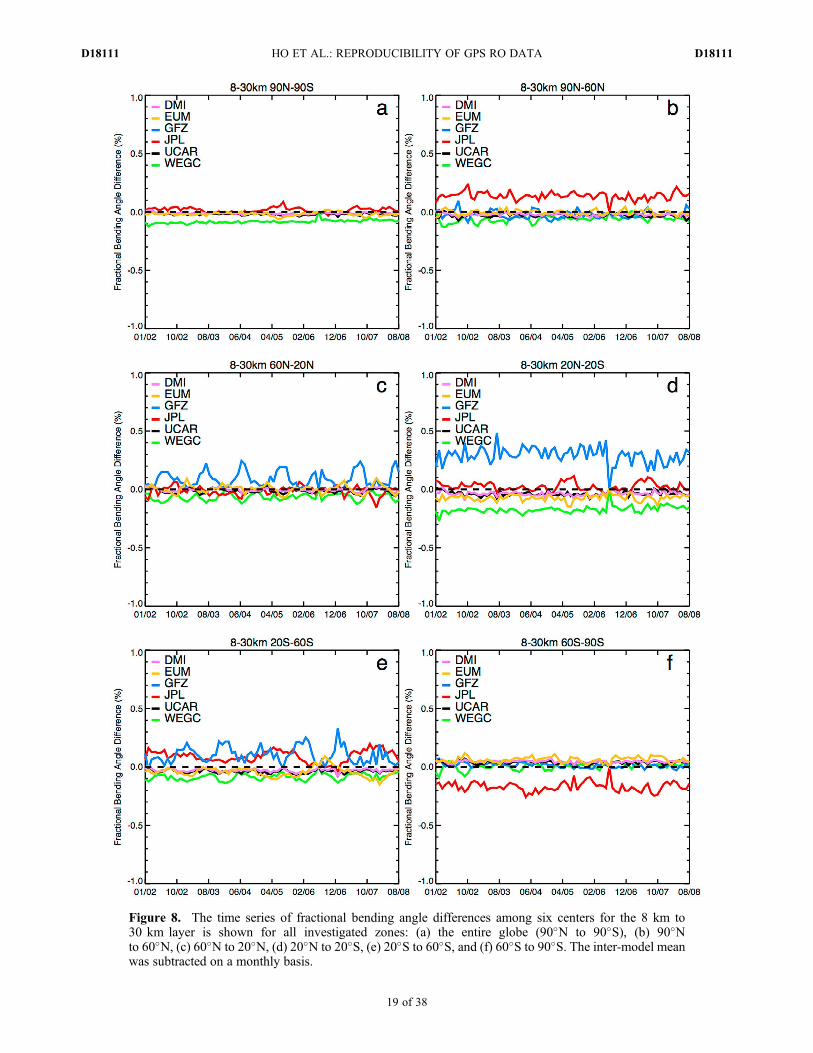
Figure 8. The time series of fractional bending angle differences among six centers for the 8 km to30 km layer is shown for all investigated zones: (a) the entire globe (90�N to 90�S), (b) 90�Nto 60�N, (c) 60�N to 20�N, (d) 20�N to 20�S, (e) 20�S to 60�S, and (f) 60�S to 90�S. The inter-model meanwas subtracted on a monthly basis.


19 of 38

Figure 9. The time series of fractional bending angle differences among six centers are shown for the8 km to 12 km layer for (a) the 60�N to 20�N zone, (c) the 20�N to 20�S zone, and (e) the 60�S to90�S zone, and for the 20 km to 30 km layer for (b) the 60�N to 20�N zone, (d) the 20�N to 20�S zone,and (f) the 60�S to 90�S zone.


20 of 38

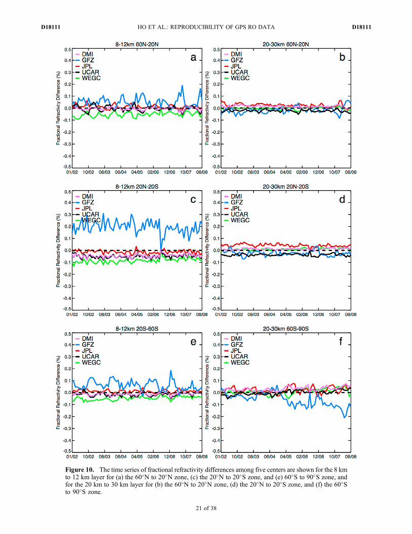
Figure 10. The time series of fractional refractivity differences among five centers are shown for the 8 kmto 12 km layer for (a) the 60�N to 20�N zone, (c) the 20�N to 20�S zone, and (e) 60�S to 90�S zone, andfor the 20 km to 30 km layer for (b) the 60�N to 20�N zone, (d) the 20�N to 20�S zone, and (f) the 60�Sto 90�S zone.


21 of 38

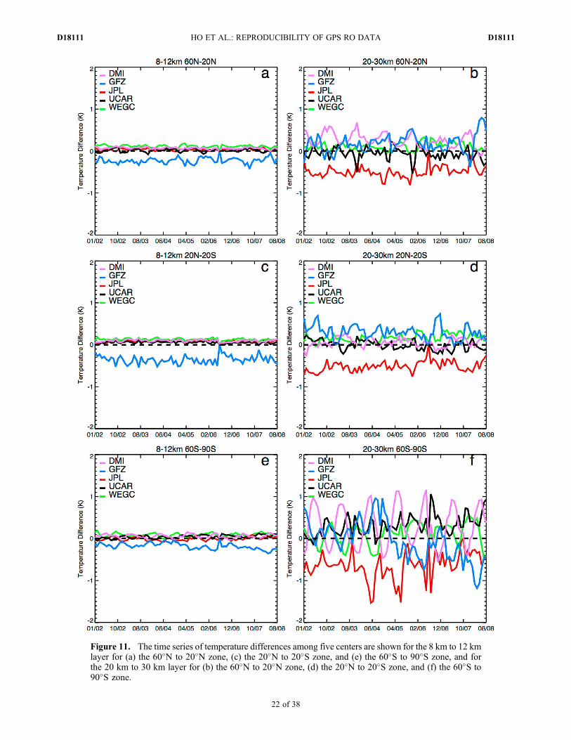
Figure 11. The time series of temperature differences among five centers are shown for the 8 km to 12 kmlayer for (a) the 60�N to 20�N zone, (c) the 20�N to 20�S zone, and (e) the 60�S to 90�S zone, and forthe 20 km to 30 km layer for (b) the 60�N to 20�N zone, (d) the 20�N to 20�S zone, and (f) the 60�S to90�S zone.


22 of 38

DTJPLTime, DTUCAR

Time , and DTWEGCTime in the 12 km to 20 km

layer are 0.08 K, �0.06 K, �0.08 K, 0.02 K, and 0.05 K,respectively, and the corresponding standard deviations arewithin 0.02 K to 0.03 K (Table 6).4.3.5. Time Series Differences for Dry GeopotentialHeight (Z)[45] In Figure 12 we show the MPC geopotential height

time series for all five centers (DZDMITime, DZGFZ

Time, DZJPLTime,

DZUCARTime , andDZWEGC

Time ) in the same layout as for temperaturein Figure 11. In Figure 12 the pattern of the inter-monthlyvariance for each center relative to the inter-center mean isvery similar to that of temperature time series, especially athigh-latitudes in the 20 km to 30 km layer. DZDMI

Time is offsetby DZJPL

Time in the LS region at northern midlatitudes(Figure 12b). In the southern high-latitude LS region (also inthe UT and TS), DZGFZ

Time shows a trend relative to the inter-center mean particularly after 2006 (Figure 12f). The globalmean differences in the 8 km to 30 km layer for DZDMI

Time,DZGFZ

Time, DZJPLTime, DZUCAR

Time , and DZWEGCTime are 6.8 m, �7.6 m,

�5.6 m, 2.5 m and 3.9 m, respectively (Table 7).

4.4. Comparison of Anomaly Differences and Trends

4.4.1. Analysis Method[46] We quantify anomaly differences and trends of the

de-seasonalized time series of the six centers. The followingequation is used to derive the de-seasonalizedMPC anomalies:

DXDeseason l;m; kð Þ ¼ XMPC l;m; kð Þ � XMPC l;m; kð Þ; ð6Þ

where l, m, and k are the indices for each layer (l), zone (m),and month for the whole time series (k = 1 to 80), respectively,and t is the index of the month bin of the year (t = 1 to 12).XMPC(l, m, t) is the mean MPC for each layer (l), zone (m),and averaged over all years for a particular month (t). Herethe XMPC (l, m, t) is computed for the period from January2002 to December 2005 since the MPC for July 2006 is notavailable. The mean trends of all centers and the trenddifference to the mean trend for each individual center aresummarized in Tables 3�7 for bending angle, refractivity,dry temperature, dry pressure, and dry geopotential heightfor the investigated latitudinal zones and vertical layers.4.4.2. Anomaly Differences and Trends for BendingAngle (a) and Refractivity (N)[47] While the trends of bending angle and refractivity

anomalies from 8 km to 30 km altitudes indicate the varia-tion of atmospheric density with time, the trends of tem-perature, pressure, and geopotential height represent thecorresponding dry air variation in the same vertical layerunder the constraint of hydrostatic equilibrium. Because thetime series differences to the inter-center mean either con-tain systematic inter-seasonal variations (Figures 9a, 10a,and 10e) or are nearly constant with time (see Figures 8–12), the trend differences among centers are in general verysmall. The trends of the global de-seasonalized bending angleanomalies in the 8 km to 30 km layer for DMI, EUM, GFZ,JPL, UCAR, andWEGC (DaDMI

Deseason,DaEUMDeseason,DaGFZ

Deseason,DaJPL

Deseason, DaUCARDeseason, and DaWEGC

Deseason) are (0.01, 0.01, 0.0,0.01, 0.01, and 0.03)%/5 yrs, respectively, where the trenddifferences to the mean trend are within �0.02%/5 yrs inthe same layer (Table 3). Even though DaJPL

Time has a persis-tent bias at southern (�0.17%) and northern high-latitudes

(0.14%) in the 8 km to 30 km layer, the trend of DaJPLDeseason

is very close to the trends of the other centers (the trenddifference of DaJPL

Deseason is equal �0.01%/5 yrs, Table 3),because the variation of DaJPL

Time is very small (less than0.04%, Table 3).[48] Although the DaGFZ

Time contains obvious inter-seasonalvariation in the 8 km to 12 km layer in the northern mid-latitudes (Figure 9a), the trend difference between GFZ andthe mean trend is equal to 0.02%/5 yrs. Because DaGFZ

Time

in the Tropics for the 8 km to 12 km layer is slightly decreasedafter August 2006 (Figure 9c), DaGFZ

Deseason shows a slightlydecreasing trend (�0.05%/5 yrs) relative to the mean trends(Table 3). The largest trend variability is over southern high-latitudes where DaGFZ

Time also shows a decreasing trend(�0.04%/5 yrs) relative to the mean trend. The fractionalbending angle trend difference among centers is within�0.01%/5 years for the 20 km to 30 km layer (Table 3).[49] Ho et al. [2009a] used daily NCEP (National Centers

for Environmental Prediction) reanalysis [Saha et al., 2010](on a 6-h and 1-degree bin) to estimate sampling errors fromthe respective monthly mean climatologies (similar toPirscher et al. [2007] and Foelsche et al. [2008b]). Afterremoving the representative sampling errors,Ho et al., 2009ashowed that the uncertainty of the trend for fractionalrefractivity anomalies among centers was between �0.03%/5 yrs and 0.01%/5 yrs. As stated in Ho et al., 2009a, thesampling errors estimation may be less accurate at high alti-tudes over southern/northern high-latitudes due to possibletemporal and spatial representation errors from NCEPreanalysis. In this study sampling error is not an issue sincewe use matched profile pairs. We identify that the uncer-tainty of the trend of the fractional refractivity is within�0.01%/5 yrs to 0.02%/5 yrs (less than �0.02%/5 yrs)globally (Table 4) which is even smaller than that fromHo et al., 2009a. The mean trend for global DN DMI

Deseason,DN GFZ

Deseason, DN JPLDeseason, DN UCAR

Deseason, and DNWEGCDeseason in the

8 km to 30 km layer is (0.02, 0.01, 0.02, 0.02, and 0.04)%/5 yrs, respectively.[50] Figure 13 depicts de-seasonalized fractional refrac-

tivity anomalies for each center for the northern midlati-tudes, the Tropics, and the southern high-latitudes.Figures 13a, 13c, and 13e are for the 12 km to 20 km layerand Figures 13b, 13d, and 13f are for the 20 km to 30 kmlayer. In general, the trend differences in the 12 km to 20 kmlayer in all latitudinal zones are very close to zero, except forin the southern midlatitudes (Table 4). In this region, thetrend difference to the mean trend for GFZ is equal to�0.02%/5 yrs whereas those for all the other centers areclose to 0.00%/5 yrs (the rounded values). Over the Tropicsin the LS region, the trend differences among the centers arewithin �0.01%/5 yrs (Table 4). Over the southern high-latitudes in the LS region (Figure 13f), the trend ofDN GFZ

Deseason is equal to �1.57%/5 yrs whereas the trends ofthe other centers are all within �1.43%/5 yrs (DN UCAR

Deseason)and �1.46%/5 yrs (DN JPL

Deseason). This relatively large trenddifference for GFZ in this region is mainly due to the largenegative fractional refractivity differences (DT GFZ

Time) after2004 (Figure 10f). This is more pronounced in the temper-ature trend differences (see below).[51] To quantify the degree of deviation among the centers,

we also compute the RMS difference betweenDN Deseason and


23 of 38

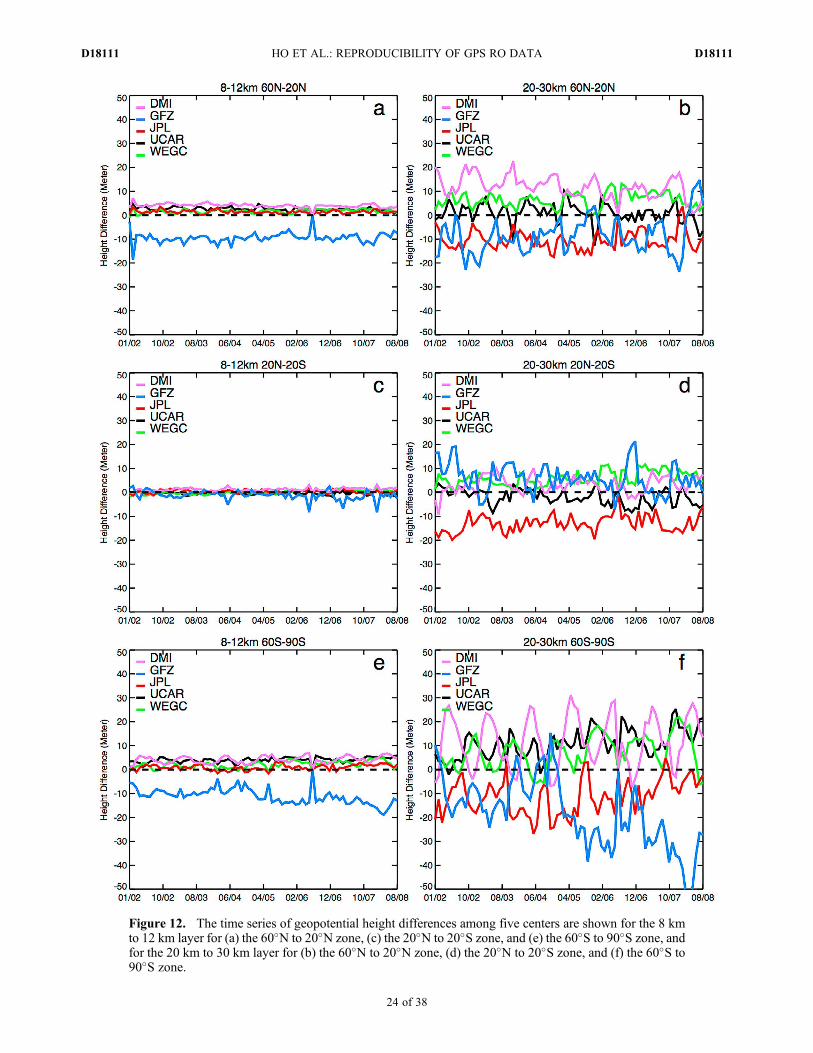
Figure 12. The time series of geopotential height differences among five centers are shown for the 8 kmto 12 km layer for (a) the 60�N to 20�N zone, (c) the 20�N to 20�S zone, and (e) the 60�S to 90�S zone, andfor the 20 km to 30 km layer for (b) the 60�N to 20�N zone, (d) the 20�N to 20�S zone, and (f) the 60�S to90�S zone.


24 of 38

Figure 13. The de-seasonalized fractional refractivity anomalies for each center in the 12 km to 20 kmlayer for (a) the 60�N to 20�N zone, (c) the 20�N to 20�S zone, and (e) the 60�S to 90�S zone, and forthe 20 km to 30 km layer for (b) the 60�N to 20�N zone, (d) the 20�N to 20�S zone, and (f) the 60�Sto 90�S zone. The 5-yr trend of the inter-center mean is shown as well. Note that the ordinate range inFigures 13e and 13f is enlarged to �4% (relative to �2% of Figures 13a–13d).


25 of 38

the mean ofDN DMIDeseason,DN GFZ

Deseason,DN JPLDeseason,DNUCAR

Deseason,and DNWEGC

Deseason for each center (i.e., DN DMIRMS, DN GFZ

RMS,DN JPL

RMS, DN UCARRMS , DN WEGC

RMS , see Table 8). The global RMSfor all centers are within 0.02% for all latitudinal zones exceptfor RMSGFZ at high-latitudes and mostly in the 8 km to12 km layer.4.4.3. Anomaly Differences and Trends for DryTemperature (T), Dry Pressure (p), and DryGeopotential Height (Z)[52] Similar to Ho et al. [2009a], the trend derived by each

individual center is still statistically insignificant although intotal only 80 months of data are used. It may take about10 years of RO data to obtain statistically significant trends[Leroy et al., 2006; Foelsche et al., 2008a; Ringer andHealy, 2008]. Here we aim at quantifying the trend differ-ences among centers when the sampling errors and the nat-ural variability, which is common on individual centertrends, are completely removed.[53] Figure 14 depicts the de-seasonalized temperature

anomalies for DMI, GFZ, JPL, UCAR, and WEGC(DT DMI

Deseason, DT GFZDeseason, DT JPL

Deseason, DT UCARDeseason, and

DTWEGCDeseason) for the northern midlatitudes, the Tropics, and

the southern high-latitudes. Figures 14a, 14c, and 14e are forthe 12 km to 20 km layer, and Figures 14b, 14d, and 14f arefor the 20 km to 30 km layer. The temperature anomalies forother latitudinal zones are similar to those in Figure 14 and arenot shown here. The trends for DT DMI

Deseason, DT GFZDeseason,

DT JPLDeseason, DT UCAR

Deseason, and DTWEGCDeseason in the 12 km to

20 km layer agree within �0.03 K/5 yrs, because their dif-ferences are constant over time with a standard deviation of0.03 K (Table 6). The global trend differences for each centerin the 8 km to 12 km layer are within �0.02 K/5 yrs andwithin �0.06 K/5 yrs in the 8 km to 30 km layer (Table 6).

[54] The trends of DT DMIDeseason, DT GFZ

Deseason, DT JPLDeseason,

DT UCARDeseason, andDTWEGC

Deseason in the 20 km to 30 km layer showlarger deviations (Figures 14b, 14d, and 14f) especially at high-latitudes. Figures 14b, 14d, and 14f show that the systematictemperature biases to the inter-center mean for JPL and GFZover northern midlatitudes (Figure 11b), Tropics (Figure 11d),and in northern high-latitude zone (not shown), and the sys-tematic inter-seasonal temperature biases for DMI in thesouthern high-latitudes (Figure 11f) are largely removed in thede-seasonalized anomalies. The trend difference forDT DMI

Deseason

to the mean trend in the southern high-latitudes is equalto 0.04 K/5 yrs in the LS (Table 6). However, the anomalytrend differences for DT DMI

Deseason in northern high-latitudesand northern midlatitudes are still as large as �0.36 K/5 yrsand �0.17 K/5 yrs, respectively (Table 6).[55] In addition, Figure 15 shows the differences of de-

seasonalized temperature anomalies (DT Deseason) for eachcenter to the mean de-seasonalized temperature anomaliesfor the northern midlatitudes, the Tropics, and the southernhigh-latitudes. Figures 15a, 15c, and 15e are for the 8 km to12 km layer, and Figures 15b, 15d, and 15f are for the 20 kmto 30 km layer. RMS differences between DT Deseason andthe mean of DT DMI

Deseason, DT GFZDeseason, DT JPL

Deseason, DT UCARDeseason,

and DTWEGCDeseason (i.e., DT DMI

RMS, DT GFZRMS, DT JPL

RMS, DT UCARRMS ,

DT WEGCRMS ) for each center in different vertical layers are shown

in Table 8. Due to decreasing negative temperature anomalies(DT GFZ

Time) after 2004 (Figure 11f) particularly over southernhigh-latitudes in the 20 km to 30 km layer, the trend differ-ence forDT GFZ

Deseason to the mean trend is as large as�0.77 K/5 yrs (Table 6) where the RMS temperature difference forGFZ (i.e., DT GFZ

RMS) in the same region is equal to 0.42 K

(Table 8).

Table 8. The Same as Table 3, but for Mean Root Mean Square (RMS) of the Differences of De-seasonalized Time Series Anomalies tothe Inter-center Mean for DMI, GFZ, JPL, UCAR, and WEGC for Fractional Refractivity (%) and Temperature (K)

Latitude ZoneHeightLayer

DMI-MeanN (%)/T (K)

GFZ-MeanN (%)/T (K)

JPL-MeanN (%)/T (K)

UCAR-MeanN (%)/T (K)

WEGC-MeanN (%)/T (K)

90�N to 90�S 8 to 30 km 0.00/0.03 0.01/0.04 0.00/0.05 0.00/0.04 0.01/0.048 to 12 km 0.01/0.01 0.02/0.03 0.01/0.01 0.01/0.01 0.01/0.0112 to 20 km 0.00/0.02 0.01/0.02 0.00/0.02 0.00/0.02 0.00/0.0220 to 30 km 0.00/0.06 0.01/0.08 0.01/0.09 0.00/0.07 0.00/0.07

60�N to 90�N 8 to 30 km 0.01/0.13 0.02/0.25 0.01/0.19 0.01/0.23 0.01/0.118 to 12 km 0.01/0.03 0.02/0.08 0.01/0.04 0.02/0.05 0.02/0.0412 to 20 km 0.01/0.07 0.02/0.15 0.01/0.09 0.01/0.11 0.01/0.0620 to 30 km 0.01/0.23 0.02/0.41 0.01/0.32 0.01/0.39 0.01/0.19

60�N to 20�N 8 to 30 km 0.01/0.05 0.02/0.12 0.01/0.06 0.01/0.07 0.01/0.058 to 12 km 0.01/0.02 0.03/0.05 0.01/0.02 0.02/0.03 0.02/0.0312 to 20 km 0.00/0.03 0.01/0.07 0.01/0.03 0.01/0.04 0.01/0.0320 to 30 km 0.01/0.1 0.03/0.2 0.01/0.11 0.01/0.12 0.01/0.08

20�N to 20�S 8 to 30 km 0.01/0.05 0.02/0.10 0.01/0.07 0.01/0.06 0.01/0.058 to 12 km 0.02/0.03 0.05/0.09 0.01/0.03 0.01/0.03 0.02/0.0212 to 20 km 0.01/0.02 0.01/0.05 0.01/0.03 0.00/0.02 0.01/0.0220 to 30 km 0.01/0.09 0.02/0.16 0.01/0.11 0.01/0.11 0.01/0.08

20�S to 60�S 8–30 km 0.01/0.05 0.02/0.12 0.01/0.06 0.01/0.06 0.01/0.058 to 12 km 0.01/0.02 0.03/0.06 0.01/0.02 0.01/0.02 0.01/0.0212 to 20 km 0.00/0.02 0.01/0.06 0.01/0.03 0.00/0.03 0.01/0.0220 to 30 km 0.01/0.09 0.02/0.20 0.01/0.11 0.01/0.09 0.01/0.08

60�S to 90�S 8 to 30 km 0.01/0.07 0.02/0.25 0.01/0.14 0.01/0.12 0.02/0.108 to 12 km 0.01/0.02 0.03/0.07 0.01/0.03 0.02/0.04 0.02/0.0312 to 20 km 0.00/0.40 0.02/0.14 0.0/10.06 0.01/0.06 0.01/0.0520 to 30 km 0.01/0.12 0.06/0.42 0.01/0.25 0.02/0.20 0.02/0.17


26 of 38

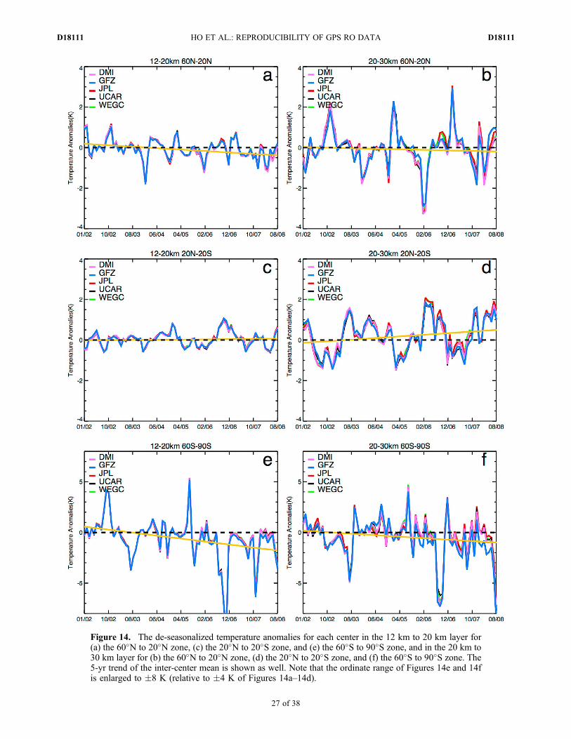
Figure 14. The de-seasonalized temperature anomalies for each center in the 12 km to 20 km layer for(a) the 60�N to 20�N zone, (c) the 20�N to 20�S zone, and (e) the 60�S to 90�S zone, and in the 20 km to30 km layer for (b) the 60�N to 20�N zone, (d) the 20�N to 20�S zone, and (f) the 60�S to 90�S zone. The5-yr trend of the inter-center mean is shown as well. Note that the ordinate range of Figures 14e and 14fis enlarged to �8 K (relative to �4 K of Figures 14a–14d).


27 of 38

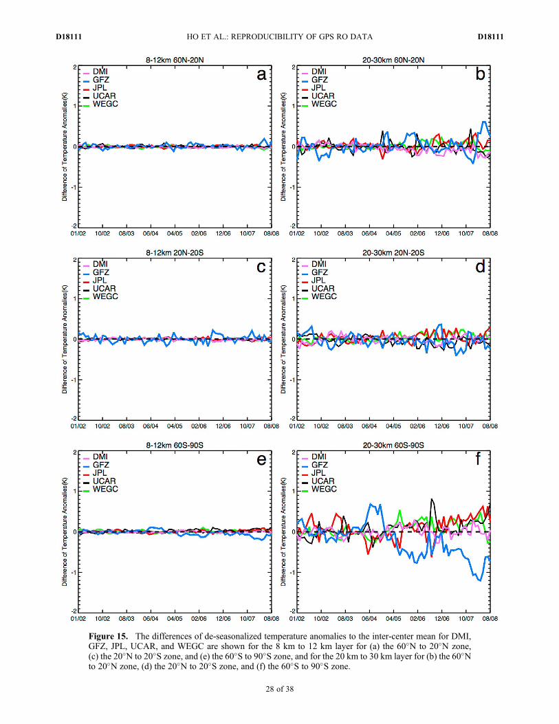
Figure 15. The differences of de-seasonalized temperature anomalies to the inter-center mean for DMI,GFZ, JPL, UCAR, and WEGC are shown for the 8 km to 12 km layer for (a) the 60�N to 20�N zone,(c) the 20�N to 20�S zone, and (e) the 60�S to 90�S zone, and for the 20 km to 30 km layer for (b) the 60�Nto 20�N zone, (d) the 20�N to 20�S zone, and (f) the 60�S to 90�S zone.


28 of 38

[56] The global trend differences to the mean trends amongcenters for dry pressure and dry geopotential height in 8 kmto 30 km layer are within �0.02%/5 yrs (Table 5) and�2.3 m/5 yrs (Table 7), respectively. Again, the largest trenddifferences to the mean trends are fromGFZ at southern high-latitudes.

5. Discussions and Applications

5.1. Propagation of Structural UncertaintyFrom Bending Angle (a) to Temperature (T)

[57] We quantified structural uncertainties of RO data fromthe statistics of trend differences among centers based onPPCs of bending angle, refractivity, temperature, pressure,and geopotential height. Uncertainties are actually accumu-lating in derived variables due to propagation through theretrieval chain. We reiterate here that four centers (UCAREUM, DMI, and WEGC) share the same excess phase andamplitude data whereas JPL, UCAR and GFZ derive theseindependently. Uncertainties in the derived variables reflectboth an accumulation of uncertainty in the processing chainand uncertainties in the raw amplitudes and phases.[58] Thus, when an individual center shows a larger mean

anomaly in bending angle, it is likely the same center will alsocontain larger mean anomalies in the other derived variables.For example, the mean global differences for bending anglesfrom January 2002 to August 2008 among six centers arewithin �0.04% for the 8 km to 30 km layer, where the globalmean bending angle difference for JPL (DaJPL

PPC) is 0.04% andthat for WEGC is �0.03% (Table 2). The 0.04% of DaJPL

PPC

represents the combined effects from different implementa-tions of RO excess phase processing, POD, ionosphericcorrection, and initialization of the bending angle for Abelinversion at different centers. The 0.04% upper bound ofDaJPL

PPC then leads to an upper bound of �0.02%, �0.27 K,�0.11%, and �5.8 m in global mean differences of refrac-tivity, dry temperature, dry pressure, and dry geopotentialheight, respectively. We note that JPL possessing the largestbending angle difference is consistent with the fact thatthe other centers share the use of climatology for bendingangle initialization, whereas the JPL procedure is indepen-dent of such climatology. Further studies are needed tounderstand how the bending angle initialization affectsabsolute accuracy.[59] Although the derived variables from bending angle to

temperature and geopotential height are not traced to SIunits, the high precision of the raw RO observables is pre-served through the processing steps. Even for the accumu-lated structural uncertainties, the anomaly time series for theindividual centers are in general persistent in time. Standarddeviations of the difference time series during the CHAMPera from January 2002 to August 2008 of bending angle,refractivity, dry temperature, dry pressure, and dry geopo-tential height for all centers are within 0.02%, 0.01%, 0.06 K,0.02%, and 2 m, respectively. These standard deviations foreach variable quantify the structural uncertainty of RO-derived variables for climate monitoring.

5.2. Inter-center PPC for Monitoring RO Data Quality

[60] Although the PPC results cannot be used to indicatethe accuracy of retrieved variables derived by individual

centers, we have demonstrated that the inter-comparisonmethod provides useful information as to how the anomaliesof individual centers deviate from the inter-center mean. Thebehavior of anomaly time series, e.g., an offset change or apossible drift in the anomalies with time relative to the inter-center mean, is clearly identified. The PPC approach is auseful tool to monitor the quality of RO-derived variables in aprocessing chain and to identify processing-related incon-sistencies among centers. We can detect impacts to the dataof each inversion step, which is more challenging if only onecenter’s data are used. Results of the inter-center comparisonsalso provide valuable feedback to the RO processing centersand help to further advance the processing chain development.

5.3. Causes of Structural Uncertainty in RetrievedVariables Due to Inversion Algorithms

[61] In the PPC, the structural uncertainty quantifiedvaries depending on the different data sets used. Since thesame orbital data, excess phase, and amplitude data are used,mean differences and MADs among DMI, UCAR, EUM andWEGC are in general smaller than those from JPL and GFZ.Although detailed processing implementations are largelydifferent among centers, the anomalies of the retrievedproducts from bending angle to pressure and temperatureare in general constant in time relative to the inter-centermean and show no obvious inter-annual variations.[62] The 7-year trends derived from CHAMP RO data

cannot be considered as climate trends.Ho et al. [2009a] usedmonthly mean climatologies with a different number ofoccultations for each center and thus had to quantify thesampling error. Residual sampling error related to samplingdifferences among centers was the dominant error source athigh-latitude regions. The resulting structural uncertaintycontained contributions from both retrieval error and residualsampling error, which was hard to quantify separately. Sincesampling error does not exist in PPC studies using matchedprofile pairs, finer structural uncertainty information due toinversion procedures implemented by each center can beidentified. The uncertainty of refractivity trends is within�0.02%/5 yrs (�0.01% and 0.02%/5 yrs) from 2002 to 2008in this study and consistent with the results of Ho et al.[2009a] of �0.03%/5 yrs globally (�0.03% and 0.01%/5 yrs). In Ho et al. [2009a], the standard deviations of thetime series of fractional refractivity differences for monthlymean climatologies for four centers (GFZ, JPL, UCAR, andWEGC) is about 0.02% after subtraction of the samplingerrors. In this study it is less than 0.01% and the differencescan be explained by the residual sampling errors in monthlymean climatologies used in Ho et al. [2009a].[63] In a complementary study (A. K. Steiner et al., Quan-

tification of structural uncertainty in climate data records fromGPS radio occultation, submitted to Atmospheric Chemistryand Physics, 2012) the structural uncertainty of such monthlymean climatological fields is quantified for all six centers. Inthat study the sampling error is estimated based on the ERA(ECMWF re-analysis) Interim reanalysis [Dee et al., 2011]and subtracted from the RO climatologies. Results show thattrends for all RO-derived variables are consistent with theresults of this PPC study in regions where background vari-ation is not significant, which generally applies within 50�Nto 50�S. The consistency of findings from the different


29 of 38

studies, which use different data versions and a differentmethodological approach, further underlines the quality ofRO data and their utility for climate studies [Ho et al., 2007,2010; Lackner et al., 2011; Steiner et al., 2011].

6. Conclusions

[64] In this study we utilized CHAMP RO data processedby six RO processing centers to quantify structural uncer-tainty of RO-derived atmospheric variables and to examinetheir suitability for climate monitoring. While the funda-mental phase delay observed from the GPS RO technique issynchronized to the ultra-stable atomic clocks on the ground,the derived RO variables (bending angle, refractivity, drypressure, dry geopotential height, and dry temperature) arenot. The retrieved results may vary when different proces-sing algorithms and implementations are used. In this study,profile-to-profile CHAMP variables from January 2002 toAugust 2008 retrieved from common approaches but withdifferent implementations at the centers are compared. Ouranalyses reach the following conclusions.[65] 1. Although the PPC results cannot be used to indi-

cate the accuracy of retrieved variables derived by individualcenters, the mean differences and the standard deviations ofeach individual center relative to the inter-center meandetermine the structural uncertainty among centers due todifferent implementations and assumptions used in the ROinversion procedures along the processing chain. Resultsshow that different implementations in the inversion proce-dures do introduce small but stable retrieval differencesamong centers. In addition, when a center contains a largemean anomaly in bending angle, the same center is alsolikely to contain larger mean anomalies in the other derivedvariables in the inversion chain. For example, the 0.04%upper bound of mean global differences of bending anglefrom JPL in the 8 km to 30 km layer for 01/2002 to 08/2008also leads to an upper bound of �0.02%, �0.27 K, �0.11%,and �5.8 m in global mean differences of refractivity, drytemperature, dry pressure, and dry geopotential height,respectively. The mean global differences of bending angle,refractivity, dry temperature, dry pressure, and dry geopo-tential height in the 8 km to 30 km layer for 01/2002 to 08/2008 are between �0.03% and 0.04%, �0.01% and 0.02%,�0.27 K and 0.13 K, �0.11% and 0.07%, and �10 m and10 m, respectively. The corresponding MAD in the sameheight range are within 0.74% for bending angle, 0.18% forrefractivity, 0.92 K for temperature, 0.52% for pressure, and30 m for geo-potential height, respectively.[66] 2. Although the derived variables from bending angle to

temperature and geopotential height are not readily traceable toSI units, the high precision nature of the raw RO observablesis preserved in the inversion chain. The standard deviation ofall variables is smallest at about 15 km altitude and growsexponentially to 30 km. The estimated standard deviationsnear 15 km vary slightly among centers and themean standarddeviation from all centers near 15 km for bending angle,refractivity, dry temperature, dry pressure, and dry geopo-tential height is within 0.5%, 0.1%, 0.3 K, 0.02%, and 10 m,respectively.[67] 3. Uncertainties accumulate in derived variables due to

propagation through the RO retrieval chain. This is reflectedin the inter-center differences, which are small for bending

angle and refractivity increasing to dry temperature, dry pres-sure, and dry geopotential height. Although there are smallmean anomaly differences among centers, they are more or lessconstant in the time series comparisons. The mean anomalydifferences of the time series in the 8 km to 30 km layer forbending angle, refractivity, dry temperature, dry pressure, anddry geopotential height for all centers are �0.08% to 0.12%,�0.03% to 0.02%,�0.27 K to 0.15 K,�0.04% to 0.04%, and�7.6 m to 6.8 m, respectively. The corresponding standarddeviation is within 0.02%, 0.01%, 0.06 K, 0.02%, and 2.0 m,respectively.[68] 4. With systematic inter-monthly time series anoma-

lies among centers, the trend differences among centers aregenerally very small. The mean trend differences in the 8 kmto 30 km layer for bending angle, refractivity, dry tempera-ture, dry pressure, and dry geopotential height are within�0.02%/5 yrs,�0.02%/5 yrs,�0.06 K/5 yrs, �0.02%/5 yrs,and �2.3 m/5 yrs, respectively. The largest uncertainties ofinter-annual and intraseasonal anomalies stem from high-latitude regions in the 20 km to 30 km layer (mainly above25 km) that are primarily due to different initialization meth-ods used by the six centers. This encouraging consistencysuggests that, once inter-center differences are better under-stood, RO can provide very accurate trend information.[69] 5. Unlike atmospheric profiles retrieved from most

satellite sounders, GPS RO-derived atmospheric profiles donot usually contain significant a priori information below25 km. The PPC results demonstrate that the computed ROinter-center mean time series are very useful for monitoringthe quality of RO data products from individual centers. Thestandard deviation of trends in anomaly time series providesimportant information on the structural uncertainty of RO-derived variables for climate monitoring. This provides uniqueapplications of RO data for climate monitoring that is a strongadvantage of RO.[70] Besides CHAMP (2001 to 2008), several other inter-

national RO missions are also available and are processedby some of the above centers. These RO missions includeGPS/Meteorology (GPS/MET, from 1995 to 1997), COSMIC(launched in April 2006), Gravity Recovery And ClimateExperiment (GRACE, launched in 2004), Satélite de Aplica-ciones Científicas-C (SAC-C, launched in 2000), MetOp/GRAS (launched in 2006), Communication/Navigation Out-age Forecast System (C/NOFS, launched in 2008), and TerraSynthetic Aperture Radar (SAR) operating in the X-band(TerraSAR-X, launched in 2007). It has been shown that ROdata from different satellites are highly consistent in terms ofmonthly mean climatologies [Foelsche et al., 2009; Steineret al., 2011; Foelsche et al., 2011] and PPCs [Hajj et al.,2004; Ho et al., 2009b] when applying the same processingscheme. Near future work is to further quantify the long-termstructural uncertainties of the RO data from multiple ROmissions that result from different processing methods touse RO-derived variables from multiple RO missions for cli-mate monitoring.

Appendix A: Description of Processing Schemesat DMI, EUM, GFZ, JPL, UCAR, and WEGC

[71] Processing schemes used by DMI, EUM, GFZ, JPOL,UCAR and WEGC are summarized in this appendix. Theseprocessing steps include: i) POD and atmospheric excess


30 of 38

phase processing, ii) bending angle calculation, iii) iono-spheric correction, iv) optimal estimation of the bendingangles in the stratosphere, v) calculation of refractivity byAbel inversion, vi) calculation of pressure, temperature, andgeopotential height, and vii) quality control (QC).

A1. Precise Orbit Determinations (POD)and Atmospheric Excess Phase Processing

[72] To generate the accurate atmospheric excess L1 andL2 phase, the effects of the relative motions and satelliteclock fluctuations of the GPS and CHAMP satellites must beremoved from the raw GPS L1 and L2 phase measurements.The dominant kinematic Doppler effect on the atmosphericexcess phase is removed with knowledge of the satelliteorbit positions and velocities obtained from POD proces-sing. The CHAMP receiver clock fluctuations are removedby performing a single-difference between occultation linkand clock reference link measurements [Wickert et al., 2002;Beyerle et al., 2005; Schreiner et al., 2009]. The GPS sat-ellite transmitter clock fluctuations can be removed with adouble-difference procedure [Hajj et al., 2002] using GPSmeasurements from a single ground receiver, or by applyingclock offsets that have been previously estimated with datafrom a ground network of GPS receivers.

A1.1. DMI Procedure

[73] DMI obtained excess phase and amplitude data andCHAMP orbit data fromUCARCDAAC (version 2009.2650).These data are processed with the UCAR procedure describedin section A1.5.

A1.2. EUM Procedure

[74] EUM also obtained excess phase and amplitude dataand CHAMP orbit data from UCAR CDAAC (version2009.2650).

A1.3. GFZ Procedure

[75] Precise orbits of the GPS and CHAMP satellites weregenerated by GFZ’s POD software EPOS-OC (Earth Param-eter and Orbit System – Orbit Computation) [König et al.,2006]. The related orbit product (provided to the ISDC) usedfor the standard occultation processing is denoted as RapidScience Orbit (RSO). Comparisons between CHAMP RSOdata and satellite laser tracking measurements showed a meandeviation of 5.9 cm in error estimation of altitude [Wickertet al., 2009]. A single-difference approach (occultation linkto reference link) removing the LEO clock offsets is usedto derive the L1 and L2 atmospheric excess phases. The GPSsatellite clock errors are removed by interpolating the 5 minclock data provided with GFZ’s GPS orbit products. Toreduce the impact of the reference link L2 phase noise, GFZuses a L1–L2 smoothing technique [Beyerle et al., 2005].

A1.4. JPL Procedure

[76] JPL uses the reduced-dynamic strategy and the GIPSY(GPS-Inferred Positioning System) software package to deter-mine the precise orbits of the GPS and CHAMP satellites[Bertiger et al., 1994]. GPS satellite orbits and transmitterclock biases are based on the FLINN (Fiducial Laboratoriesfor International Natural Science Network) solution generatedat JPL using global ground tracking data [Hajj et al., 2004].

The transmitter and receiver clocks are calibrated using thedouble-differencing technique [Hajj et al., 2002].

A1.5. UCAR Procedure

[77] UCAR uses the Bernese software (v5.0) packageto estimate precise orbits of the CHAMP satellite [Dachet al., 2007]. Ionosphere-free phase observations from a27-h period are used in a zero-difference reduced-dynamicfiltering approach to estimate the position, velocity, and clockoffset [Švehla and Rothacher, 2003]. Results of orbit over-laps for adjacent solutions show consistency in velocity at the0.07 mm/s 3D root mean square (RMS), and orbit overlapswith other agencies show agreement at a level of 0.15 mm/s3D RMS [Schreiner et al., 2009]. The atmospheric excessphases for the L1 and L2 signals are computed using thesingle-difference processing strategy detailed in Schreineret al. [2009]. The ionospheric correction of L1 and L2 onthe non-occulting link is performed by smoothing L1–L2 tosuppress the effect of LEO clock distribution errors and L2noise of the CHAMP GPS receiver [Schreiner et al., 2009].

A1.6. WEGC Procedure

[78] CHAMP RO excess phase data and orbit data pro-vided by UCAR CDAAC (version 2009.2650) were usedas input to the WEGC OPSv5.4 processing.

A2. Calculation of Bending Angles (a)

[79] A series of processing procedures is needed to convertthe raw L1 and L2 excess phases into L1 and L2 bending angleprofiles [Vorob’ev and Krasil’nikova, 1994; Kursinski et al.,1997; Rocken et al., 1997; Hajj et al., 2002; Kuo et al.,2004]. These steps include i) outlier rejection, noise filtering,and differentiation of excess phases to compute filteredDopplers, which is necessary to eliminate multiple values ofbending angle as a function of the impact parameter, ii)transferring the reference frame to the local center of theEarth’s curvature to better satisfy the assumption of sphericalsymmetry, and iii) calculation of L1 and L2 bending anglesfrom the filtered Doppler. As described in Ho et al. [2009a],above a height where atmospheric multipath is not significant(usually above the lower troposphere), one can derive L1 andL2 bending angles in the geometric optics approximation. Inthe lower troposphere, especially in moist environmentswhere multipath propagation may be significant, wave opticstechniques are usually applied to invert the L1 complex signal(phase and amplitude) to bending angle. Here we brieflydescribe the methods used by each center to calculate L1and L2 bending angles. In this study, we focus our com-parisons on the region from 8 km to 30 km, where atmo-spheric multipath effects are not significant.

A2.1. DMI Procedure

[80] Before processing into bending angle, the calibratedexcess phases and amplitudes are corrected. This correctionis partly mission-specific. For CHAMP data, the correctionincludes replacement of the observed L2 amplitudes bymodeled amplitudes, and filtering of the noisy L2 excessphase and amplitude data using a radioholographic filteringtechnique [Gorbunov et al., 2006]. Above 25 km altitude,a geometrical optics approach is used. For the differentiationof noisy phase excess, the measurement data are de-trended,


31 of 38

where the smooth trend can be differentiated analytically,and the noisy de-trended part of the signal is differentiatedby applying the statistical optimization as described byUstinov [1990]. Below 25 km, the CT2 (Canonical Transformof Type 2) wave optics method is applied to both L1 and L2to obtain bending angles and impact parameters [Gorbunovand Lauritsen, 2004].

A2.2. EUM Procedure

[81] Atmospheric excess phase and orbit data as providedby the UCAR CDAAC archive were used as a starting point.Doppler profiles were calculated from excess phase data byapplying a Savitzky-Golay smoothing filter (degree 4 over70 points) [Savitzky and Golay, 1964]. Bending angle profilesare computed from Doppler shift profiles based on geometricoptics [e.g., Kursinski et al., 1997].

A2.3. GFZ Procedure

[82] A single value decomposition fit [Press et al., 1996]is used for excess phase noise filtering and numerical dif-ferentiation to derive Doppler shift profiles. This filteringprocedure applies a third order polynomial and encompasses101 data samples of the 50 Hz data. Bending angle compu-tation is based on geometric optics, below 15 km (smoothtransition down to 11 km) the Full Spectrum Inversion (FSI)technique is applied to correct for multipath effects in thelower troposphere.

A2.4. JPL Procedure

[83] JPL uses different methods to compute bending anglefor the L1 and L2 frequencies: the CT (Canonical Transform)technique and the non-CT technique. The CT technique isapplied to the received phase and amplitude data for the L1frequency, which is often available down to the surface. Anon-CT version of L1 bending angles is also calculated inthe same fashion as the L2 bending angles (non-CT) for usein the ionospheric correction.


[84] L1 and L2 bending angles are calculated in a referenceframe centered at the local center of sphericity of the referenceellipsoid [Syndergaard, 1999] in the direction of the occulta-tion plane at the estimated “occultation point” that correspondsto the estimated tangent point of the ray GPS-LEO, wherethe excess phase is equal to 500 m (3–4 km above the surface).In order to truncate the part of RO signal affected by trackingerrors, the smoothed L1 excess Doppler is differenced withthe Doppler model calculated based on GPS and LEO orbitsand “wet” refractivity climatology [Kirchengast et al., 1999].The earliest time when the difference exceeds 10 Hz is foundand then the signal is truncated at an earlier time when thedifference reduces to 5 Hz. The bending angles are calculateddifferently above and below the so-called “transition height”which is determined dynamically for each occultation basedon the following criteria: either the deviation of raw fromsmoothed L2Doppler exceeds 6 Hz, or the difference betweensmoothed L2 and L1 (multiplied by the ratio of L2 to L1frequencies) Dopplers exceeds 1 Hz. These criteria are checkedbelow 40 km. Above the transition height the L1 and L2bending angles are calculated in the approximation of geometricoptics [Vorob’ev and Krasil’nikova, 1994; Kursinski et al.,1997] after smoothing L1 and L2 excess phases with 3-pass

sliding window polynomial regression of 3rd order. The L1excess phase is smoothed with an equivalent window width ofabout 1 km. Additionally, for the ionospheric correction, bothL1 and L2 bending angles are calculated after smoothingthe excess phases with a different window (explained insection A3.5). Below the transition height, L1 bending angle iscalculated by the FSI [Jensen et al., 2003] from raw complexRO signal without smoothing. The FSI-retrieved bending angleis smoothed by the same filter as excess phase (see above) butwith an equivalent window of about 0.15 km and truncatedbased on least squares fit of the step-function to the raw FSI-transformed amplitude.


[85] In the OPSv5.4, first an outlier rejection is performedon the L1 and L2 excess phase profiles at 50 Hz sampling rate.Data points outside three times the standard deviation aresubstituted by the interval’s mean of a one-second runningwindow. The excess phase profiles are smoothed by a regu-larization method after Syndergaard [1998] and then con-verted via numerical differentiation to Doppler shift profiles.Bending angle profiles are computed from Doppler shift pro-files based on geometric optics [e.g., Kursinski et al., 1997].

A3. Ionospheric Correction

[86] All centers apply ionospheric correction by forming alinear combination of L1 and L2 bending angles at a com-mon impact parameter, generally following the approach byVorob’ev and Krasil’nikova [1994] with some differences inimplementations discussed below.

A3.1. DMI Procedure

[87] DMI uses Optimal Linear Combination (OLC),an algorithm devised by Gorbunov [2002]. The ionosphericcorrection, upper level noise reduction, and provision of anupper limit to the Abel integral are obtained within a singleframework based on a statistically optimal combination ofobserved and modeled bending angles.

A3.2. EUM Procedure

[88] For lower tropospheric data, where only L1 bendingangles are available, the following processing is used: (1) alinear fit in L1–L2 is performed for the lowest few kilometerswhere both bending angles are available; (2) the linear fit isthen extrapolated down to the lowest altitude where L1bending angles are available.

A3.3. GFZ Procedure

[89] The FSI technique (applied below 15 km) uses theionosphere-free linear combination of L1 and L2. Here L1–L2is linearly extrapolated downward from higher altitudes tocontinue the ionospheric correction down to the Earth’ssurface. The extrapolation is based on the longest availableinterval of connected data samples (minimum of 650 reques-ted) for which the quotient of the L1 and L2 excess phaseforward differences lies within the range between 0.97 and1.03 [see Beyerle et al., 2004].

A3.4. JPL Procedure

[90] At altitudes below approximately 10 km (based on aminimum signal-to-noise ratio (SNR) criterion applied to


32 of 38

the L2 data), ionospheric L1–L2 is linearly extrapolateddownward from higher altitudes to continue the ionosphericcorrection to the surface.


[91] Above the transition height, the L1 bending angle,obtained with an approximate 1 km smoothing window (seesection A2.5), is corrected by L4 = L1–L2 bending angleobtained with a different smoothing window. The latterwindow, defined in the range of approximately 1 km to 4 km,is determined individually for each occultation by minimiz-ing fluctuation of the L3 (ionosphere-free) bending anglebetween 60 km and 80 km [Sokolovskiy et al., 2009]. Thisreduces the combined effect of L2 noise and the small-scaleionospheric residuals. Below the transition height, the FSI-retrieved L1 bending angle is corrected by a constant obtainedby a least squares fit of L4 bending angle in the 3 s intervalimmediately above the transition height.


[92] Below 15 km impact height, the ionospheric correc-tion is linearly extrapolated downward from higher altitudes(i.e., the L1–L2 bending angle difference profile is linearlyfitted at 15 km to 25 km and extended downward) to continuethe ionospheric correction as deep as needed into the tropo-sphere. This latter measure ensures that the resulting neutralatmospheric bending angle profile is independent of the L2data quality in the troposphere, which is frequently degradeddue to lower signal-to-noise ratio of L2 data compared to L1data [e.g., Steiner et al., 1999].

A4. Initialization of the Bending Angle (a)for Abel Inversion

[93] This section summarizes the methods used by eachcenter for optimal estimation of the bending angle for Abelinversion.

A4.1. DMI Procedure

[94] The OLC of L1 and L2 bending angles includesthe merging of the observations at high altitudes with amodel profile in a statistically optimized solution [Gorbunov,2002]. The model profile used in this process is foundthrough a global search [Gobiet and Kirchengast, 2004](every 10 degrees latitude, every 20 degrees longitude, formonthly mean profiles) for bending angles constructed fromthe MSISE-90 (Mass Spectrometer Incoherent Scatter Radarextended model 1990) climatological model [Hedin, 1991].The logarithm of the model bending angles are scaled andshifted in a least squares fit to the observed bending angleabove 40 km, and the profile requiring the least scaling andshifting is chosen as described in Lauritsen et al. [2011]. Inthe OLC, the L1 and L2 bending angle observation errors anda priori ionospheric bending are estimated as described byGorbunov [2002], whereas the error of the model profile isset to a fixed value. Correlations between errors in the verticalare neglected. Above 100 km, the bending angle is assumed todecrease exponentially with altitude, allowing an approximateanalytical solution of the Abel integral to infinity [e.g.,Gorbunov et al., 2011].

A4.2. GFZ Procedure

[95] The algorithm described by Sokolovskiy and Hunt[1996] is applied for the bending angle optimization. Thebackground model is based on the MSISE-90 climatology.The observation error variance is estimated from observation-background deviation between 60 km and 70 km. To reduceinfluence from the background model in the weighting pro-cedure, the observation error is divided by 4. Below 40 kmaltitude, no bending angle optimization is applied. Above100 km, optimized bending angles are replaced by the pureclimatology. The Abel inversion of the optimized bendingangle profiles starts at 150 km.

A4.3. JPL Procedure

[96] As described in Ho et al. [2009a], the JPL approach isto assume that the bending angle decays exponentially withheight at high altitudes. Bending angle measurements within40 km and 50 km altitudes are fit to a simple exponentialfunction. Bending angles above 50 km are extrapolatedupward from the fitted exponential function.


[97] In order to reduce the effect of error propagation inthe refractivity retrieved by Abel inversion, the observa-tional ionosphere-free bending angle is optimally combinedwith a fitted background bending angle model by applyingdynamic error estimation and neglecting vertical error cor-relations [Sokolovskiy and Hunt, 1996; Lohmann, 2005].The background bending angle model is calculated fromNational Center for Atmospheric Research (NCAR) clima-tology with exponentially extrapolated density above the topheight (approx. 90 km). The fitted background model isobtained by log linear least squares fit of the backgroundmodel to observations between 20 km and a maximumheight (<60 km, estimated individually for each occultation).Above 60 km, the fitted background model smoothlytransitions to the background model. The weighting func-tions in this optimal linear combination depend on the obser-vational and background errors estimated individually for eachoccultation. The observational error variance is estimated fromthe difference between the observation and the backgroundbetween 60 km and 80 km. The background error variance isestimated from the difference between the observation and thefitted background between 20 km and the maximum height.The optimized bending angle is subject to Abel inversionbelow 150 km.


[98] Above 30 km impact height the retrieved bendingangle profiles are combined with background informationderived from ECMWF (European Centre for Medium-RangeWeather Forecasts) short-range forecast fields (24 h to 30 hforecasts), which are extended with MSISE-90 data up to120 km. Statistical optimization is performed with inversecovariance weighting [Healy, 2001; Rieder and Kirchengast,2001; Gobiet and Kirchengast, 2004]. The error of thebackground profile is assumed to amount to 15% of thebackground bending angle with a vertical error correlationlength of 10 km. The observation error is estimated from thevariance of the observed profile between 65 km and 80 km


33 of 38

(generally amounting to 3 mrad to 4 mrad for CHAMP data at�2 km vertical resolution), with a vertical error correlationlength of 2 km assumed. The retrieval-to-background errorratio indicates that the atmospheric profiles are background-dominated above the stratopause and observation dominatedbelow about 40 km [Gobiet and Kirchengast, 2004; Gobietet al., 2007; Pirscher, 2010].

A5. Derivation of Refractivity (N), Dry Pressure (p),and Dry Temperature (T)

[99] Similar approaches are used by all centers to derivedry pressure and dry temperature from refractivity obtainedby Abel inversion.

A5.1. DMI Procedure

[100] The dry pressure and dry temperature profiles areobtained by assuming a completely dry atmosphere, consistingof an ideal gas in hydrostatic equilibrium, with the gravita-tional acceleration g given as a specific function of latitude andaltitude. The refractivity profile is extended up to the height of150 km using the model profile after the global search andfitting procedure as described above in section A4.1. Thehydrostatic equation is vertically integrated downward from150 km, with the top boundary conditions determined from therefractivity and its gradient at the top of the profile. In eachintegration step, the dry pressure is first calculated fromhydrostatic equilibrium and the dry temperature is then cal-culated from the dry pressure and the observed refractivity.

A5.2. GFZ Procedure

[101] GFZ uses the standard dry temperature/pressureretrieval: Assuming dry air conditions, refractivity is directlyproportional to air density (applying ideal gas equation). Thepressure profile is derived by downward integration of thedensity profile assuming hydrostatic equilibrium. Pressureretrieval is initialized at 100 km with MSISE-90. The tem-perature profile is calculated consecutively applying theSmith-Weintraub formula [Smith and Weintraub, 1953].

A5.3. JPL Procedure

[102] Using the dry refractivity equation (N = a1 p/T, wherea1 = 77.6 K/hPa), the dry temperature (or pressure) is obtainedby integrating the hydrostatic equation downward assumingknown temperature value at height zm. For this integration,density is derived from the measured refractivity and the idealgas law. The interpolated ECMWF temperature is used at zm =40 km. The gravitational acceleration is computed based onequation 5–50 from Turcotte and Schubert [1982].


[103] Refractivity is retrieved by Abel inversion as a func-tion of refractional radius. The refractional radius is convertedto radius, then to the height above the reference ellipsoid(by subtracting the local radius of curvature), then to theheight above mean sea level (MSL) (by subtracting the JGM2(Joint Gravity Model-2) geoid undulation at the occultationpoint). The dry density is derived from refractivity under theassumption of dry air by using the equation for refractivity[Smith and Weintraub, 1953] and the equation of state of dryair. Dry pressure is retrieved from dry density by integrationof the hydrostatic equation. The gravitational acceleration is

a function of height over the reference ellipsoid and latitude(3-term expansion) [Lambeck, 1988]. Dry temperature iscalculated from the retrieved dry density and pressure byuse of the equation of state of dry air.


[104] The Abel inversion, implemented as a numericalintegration, is applied to the optimized bending angle profilestarting at 120 km and yields the refractivity profile. Therefractivity profile is finally smoothed by a Blackman win-dow filter (<1 kmwidth, moving average), providing filteringof potential residual numerical noise while conserving thebasic Fresnel-scale resolution of the data (�1 km resolution).[105] The subsequent atmospheric profile retrieval is a

dry air retrieval (for a detailed discussion of dry versusactual atmospheric parameters see Scherllin-Pirscher et al.[2011a]). The latitude- and height-dependent accelerationof gravity is used in the hydrostatic equation. Here theupper bound of the integral, ztop, is set to 120 km (the upperbound of the refractivity profile), since contributions frombeyond have been shown to be negligible for the results ofinterest below the stratopause [Steiner et al., 1999]. Drytemperature is obtained by utilizing the equation of state. Thedry temperature profile is finally smoothed by a Blackmanwindow filter in the same way as refractivity, for filtering ofpotential residual numerical noise.

A6. Derivation of Geopotential Height (Z)

A6.1. DMI Procedure

[106] The geometric height above the World GeodeticSystem-84 (WGS-84) reference ellipsoid is converted toMSL altitude by subtracting the geoid undulation, obtainedfrom a spectral description of the EGM-96 (Earth Gravita-tional Model 1996) geoid of order and degree 360 (NationalImagery and Mapping Agency - NIMA). The spectral coef-ficients are expanded as Legendre polynomials and applied tothe nominal latitude and longitude of the occultation. Thealtitude is then converted to a geopotential height through anexpression derived from the Somigliana equation, whichgives the gravity as a function of latitude and altitude. Theresulting profiles of dry pressures as a function of geopo-tential heights can be interpolated to give the geopotentialheights of (dry) isobaric surfaces.

A6.2. GFZ Procedure

[107] Geopotential height is derived by upward integrationof the local altitude dependent gravitational acceleration (g).Integration step size is 200 m. The gravitational accelerationat local geoid surface (gsurf) is derived from the EGM-96geoid model. Altitude dependence follows g(i) = gsurf*(r/(r +h(i)))2 where r is the local geoid radius and h is altitude abovegeoid surface.

A6.3. JPL Procedure

[108] The geometric height is converted to geopotentialheight as described in Leroy [1997, equation 1]. The gravitymodel JGM-3 (Joint Gravity Model-3) is used to convert analtitude z to a potential energyU. The potential energy is thenconverted to geopotential height by subtracting a constantcorresponding to the potential energy of MSL and dividing


34 of 38

this difference by a standard gravitational acceleration g =9.80665 m/s2. The JGM-3 gravity model is truncated at amaximum spherical harmonic degree of 36.


[109] Dry pressure (discussed in section A5.4) is computedas a function of geometric height and, additionally, as afunction of geopotential height (the integral of gravity accel-eration normed by the gravity acceleration at the surface).Then the inverse function provides the geopotential height ofa given pressure.


[110] Geopotential height Z is computed by first integratingthe acceleration of gravity over the RO-derived altitude z,divided by the standard acceleration of gravity at sea level(g0 = 9.80665 m s�1). Geopotential heights Z(z) are thenlinearly interpolated to a standard “pressure altitude” grid zp(equivalent to a pressure level grid but a convenient altitude-type scale), defined by zp = �H0 ⋅ ln(p/p0), where H0 = 7 kmis a standard atmospheric scale height, p0 = 1013.25 hPais the standard surface pressure, and p is the atmosphericpressure provided here by the dry pressure profile pdry(z). Theinterpolation result is Zdry(zp), the desired dry geopotentialheight profile at the pressure altitude grid associated withthe dry pressure level grid pdry(zp) = p0 ⋅ exp(zp/H0).

A7. Quality Control (QC) Methods

A7.1. DMI Procedure

[111] The processing from raw data to bending angle andrefractivity profiles implicitly and explicitly includes severalquality screening steps in which data may be totally or partlyrejected [Gorbunov et al., 2006, 2011]. These quality checksaddress different aspects of noise and multipath effects. Thefinal refractivity profiles are compared to collocated ECMWFanalysis profiles and the whole profile is discarded if anypoint in the profile deviates by more than 10% from theECMWF value somewhere in the altitude range 10 km to35 km.

A7.2. EUM Procedure

[112] No specific quality control procedure is performed ingenerating the bending angle profiles.

A7.3. GFZ Procedure

[113] Occultation events shorter than 20 s are generally notprocessed. A minimum of 650 connected data samples arerequested for which the quotient of the L1 and L2 excessphase forward differences has to be in the range between 0.97and 1.03 [see Beyerle et al., 2004]. This criterion, applied forL1–L2 extrapolation in the troposphere, excludes occulta-tions with early loss of L2 tracking mainly due to ionosphericdisturbances. The fractional refractivity deviation fromMSISE-90 is requested to be less than 22.5% in the altituderange between 8 km and 31 km. If this criterion is violated atany point within this altitude range, the profile is rejected.

A7.4. JPL Procedure

[114] For each occultation, upper altitude data are removedwhere the ionosphere-corrected bending angle has the wrongsign or where the bending angle deviates significantly from

an exponential fit (c2 > 0.02). This typically occurs between60 and 80 km. Post-retrieval QC is then applied basedon comparison with ECMWF with the following criteria:(i) |N � N(ECMWF)| < 0.1 N(ECMWF) over the wholeprofile below 30 km and (ii) |T � T(ECMWF)| < 10 Kbetween �8 km to 30 km. The QC criteria are less strict thanthe previous data set fromHo et al. [2009a] where the criteriawere applied up to 40 km, which resulted in the eliminationof many high-latitude profiles [Ho et al., 2009a].


[115] Data affected by receiver tracking errors are trun-cated based on deviation of the smoothed L1 Doppler fromthe model based on orbits and refractivity climatology(see section A2.5). The whole occultation is discarded if(i) the transition height (see section A2.5) is larger than20 km; (ii) the maximum height used for fitting of the back-ground profile (defined in section A4.4) is less than 40 km;(iii) the retrieved refractivity differs fractionally from back-ground by more than 50% between 10 km and 40 km; (iv) thestandard deviation of the ionosphere-free bending angle frombackground between 60 km and 80 km is larger than 1.5E–4 rad and/or mean deviation is larger than 1E–4 rad.


[116] The OPS QC includes internal (early stage) andexternal (final stage) QC. Internal QC is applied down tobending angle level and probes technical and consistencyparts of the data and adjusts error estimates or rejects profilesduring the retrieval as found needed [Pirscher, 2010]. Theexternal QC compares retrieved refractivity results to collo-cated ECMWF analysis profiles. Profiles featuring a relativerefractivity difference to the ECWMF profiles >10% at anyaltitude level between 5 km and 35 km, and/or a temperaturedifference >20 K between 8 km and 25 km, are rejected. Intotal the QC removes about 35% of the CHAMP RO profilesentering the retrieval at excess phase level.

Notation

a Bending Angle.AMSU Advanced Microwave Sounding Units.

BA Bending Angle.CDR Climate Data Record.

CHAMP CHAllenging Minisatellite Payload.CDAAC COSMIC Data Analysis and Archive Center.COSMIC Constellation Observing System for Meteo-

rology, Ionosphere, and Climate.C/NOFS Communication/Navigation Outage Forecast

System.CT Canonical Transform.

CT2 Canonical Transform of Type 2.DMI Danish Meteorological Institute.

ECMWF European Centre for Medium-Range WeatherForecasts.

EGM-96 Earth Gravitational Model 1996.EPOS-OC Earth Parameter and Orbit System – Orbit

Computation.ERA ECMWF re-analysis.

EUMETSAT European Organisation for the Exploitation ofMeteorological Satellites.


35 of 38

EUM European Organisation for the Exploitation ofMeteorological Satellites.

FLINN Fiducial Laboratories for International Natu-ral Science Network.

FP7 Seventh Framework Programme for Researchand Technological Development of the Euro-pean Commission.

FSI Full Spectrum Inversion.FWF Austrian Science Fund.

g gravitational acceleration.g0 standard acceleration of gravity at sea level.

gsurf gravitational acceleration at local geoid surface.GFZ German Research Centre for Geosciences.

GIPSY GPS-Inferred Positioning System.GPS Global Positioning System.

GPS/MET GPS/Meteorology.GRACE Gravity Recovery And Climate Experiment.GRAS Global Navigation Satellite System RO

Receiver for Atmospheric Sounding.h altitude above geoid surface.

H0 a standard atmospheric scale height.ISDC Information System and Data Center.

JGM-2 Joint Gravity Model-2.JGM-3 Joint Gravity Model-3.

JPL Jet Propulsion Laboratory.L1 GPS L-band frequency in 1575.42 MHz.L2 GPS L-band frequency in 1227.6 MHz.

LEO low earth orbit.LS lower stratosphere.

MAD median absolute deviation.MPC mean profile-to-profile climatology.MSL mean sea level.MSIS Mass Spectrometer Incoherent Scatter Radar

Model.MSISE-90 Mass Spectrometer Incoherent Scatter Radar

Extended Model 1990.MSU Microwave Sounding Units.

N refractivity.NCEP National Centers for Environmental Prediction.NIMA National Imagery and Mapping Agency.NCAR National Center for Atmospheric Research.OLC Optimal Linear Combination.OPS Occultation Processing System.

p pressure.p0 standard surface pressure.

POD precise orbit determination.PPC profile-to-profile comparison.QC quality control.

r local geoid radius.RMS root mean square.RO radio occultation.

ROM Radio Occultation Meteorology.RSO Rapid Science Orbit.

SAC-C Satélite de Aplicaciones Científicas-C.SAF Satellite Application Facility.SAR Synthetic Aperture Radar.

SI System of Units.SNR signal-to-noise ratio.

T temperature.TerraSAR-X Terra SAR operating in the X-band.

TOVS TIROS Operational Vertical Sounders.

TS highest troposphere/lowest stratosphere.U potential energy.

UT upper troposphere.UCAR University Corporation for Atmospheric

Research.WEGC Wegener Center/University of Graz.

WGS-84 World Geodetic System-84.Z geopotential height.

[117] Acknowledgments. We thank all the scientists, engineers andtechnicians of the CHAMP satellite mission for their successful work, whichis the basis for our investigations. The DMI work was supported by theRadio Occultation Meteorology (formerly GRAS) Satellite ApplicationFacility, which is an operational RO processing center under EUMETSAT.DMI thanks K. R. Larsen for assistance in the processing of data. The workof EUM was partially funded by the ERA-CLIM project, under the SeventhFramework Programme for Research and Technological Development ofthe European Commission (FP7). The work of GFZ was supported byGEOTECHNOLOGIEN grant 03G0728A. The work of JPL, CaliforniaInstitute of Technology, was carried out under a contract with the NationalAeronautics and Space Administration. The work of UCAR was supportedby the National Science Foundation under cooperative agreement AGS-0918398/CSA AGS-0939962. The National Center for AtmosphericResearch is sponsored by the National Science Foundation. Shu-peng Hoacknowledges NOAA support under grant NA07OAR4310224. The workof WEGC was funded by the Austrian Science Fund (FWF) grants P21642-N21 and P22293-N21 and partially by European Space Agency and FFG-ALR Austria contracts.

ReferencesBertiger,W. I., et al. (1994), GPS precise tracking of TOPEX/Poseidon: Resultsand implications, J. Geophys. Res., 99, 24,449–24,464, doi:10.1029/94JC01171.

Beyerle, G., J. Wickert, T. Schmidt, and C. Reigber (2004), Atmosphericsounding by GNSS radio occultation: An analysis of the negative refrac-tivity bias using CHAMP observations, J. Geophys. Res., 109, D01106,doi:10.1029/2003JD003922.

Beyerle, G., T. Schmidt, J. Wickert, and C. Reigber (2005), GPS radio occul-tation with GRACE: Atmospheric profiling utilizing the zero differencetechnique, Geophys. Res. Lett., 32, L13806, doi:10.1029/2005GL023109.

Borsche, M. (2008), Global atmospheric climatologies from radio occulta-tion data and derivation of diagnostic parameters for climate monitoring,Sci. Rep., 22-2008, Wegener Cent., Graz, Austria.

Borsche, M., A. Gobiet, A. K. Steiner, U. Foelsche, G. Kirchengast,T. Schmidt, and J. Wickert (2006), Pre-operational retrieval of radiooccultation based climatologies, in Atmosphere and Climate: Studies byOccultation Methods, edited by U. Foelsche, G. Kirchengast, and A. K.Steiner, pp. 315–323, Springer, Berlin, doi:10.1007/3-540-34121-8_26.

Christy, J. R., R. W. Spencer, and W. D. Braswell (2000), MSU Tropo-spheric temperatures: Data set construction and radiosonde comparisons,J. Atmos. Oceanic Technol., 17, 1153–1170, doi:10.1175/1520-0426(2000)017<1153:MTTDCA>2.0.CO;2.

Dach, R., U. Hugentobler, P. Fridez, and M. Meindl (Eds.) (2007), BerneseGPS software version 5.0, user manual, Astron. Inst., Univ. of Bern, Bern.

Dee, D. P., et al. (2011), The ERA-Interim reanalysis: Configurationand performance of the data assimilation system, Q. J. R. Meteorol.Soc., 137, 553–597, doi:10.1002/qj.828.

Fjeldbo, G. F., V. R. Eshleman, and A. J. Kliore (1971), The neutral atmo-sphere of Venus as studied with the Mariner V radio occultation experi-ments, Astron. J., 76, 123–140, doi:10.1086/111096.

Foelsche, U., G. Kirchengast, A. K. Steiner, L. Kornblueh, E. Manzini, andL. Bengtsson (2008a), An observing system simulation experiment forclimate monitoring with GNSS radio occultation data: Setup and testbed study, J. Geophys. Res., 113, D11108, doi:10.1029/2007JD009231.

Foelsche, U., M. Borsche, A. K. Steiner, A. Gobiet, B. Pirscher, andG. Kirchengast (2008b), Observing upper troposphere-lower stratosphereclimate with radio occultation data from the CHAMP satellite, Clim.Dyn., 31, 49–65, doi:10.1007/s00382-007-0337-7.

Foelsche, U., B. Pirscher, M. Borsche, G. Kirchengast, and J. Wickert(2009), Assessing the climate monitoring utility of radio occultationdata: From CHAMP to FORMOSAT-3/COSMIC, Terr. Atmos. OceanicSci., 20, 155–170, doi:10.3319/TAO.2008.01.14.01(F3C).

Foelsche, U., B. Scherllin-Pirscher, F. Ladstädter, A. K. Steiner, andG. Kirchengast (2011), Refractivity and temperature climate records frommultiple radio occultation satellites consistent within 0.05%, Atmos. Meas.Tech., 4, 2007–2018, doi:10.5194/amt-4-2007-2011.


36 of 38

Free, M., D. J. Seidel, J. K. Angell, J. Lanzante, I. Durre, and T. C. Peterson(2005), Radiosonde Atmospheric Temperature Products for AssessingClimate (RATPAC): A new data set of large-area anomaly time series,J. Geophys. Res., 110, D22101, doi:10.1029/2005JD006169.

Gobiet, A., and G. Kirchengast (2004), Advancements of GNSS radio occul-tation retrieval in the upper stratosphere for optimal climate monitoringutility, J. Geophys. Res., 109, D24110, doi:10.1029/2004JD005117.

Gobiet, A., G. Kirchengast, J. Wickert, C. Retscher, D.-Y. Wang, andA. Hauchecorne (2005), Evaluation of stratospheric radio occultationretrieval using data from CHAMP, MIPAS, GOMOS and ECMWF anal-ysis field, in Earth Observation With CHAMP: Results From Three Yearsin Orbit, edited by C. Reigber et al., pp. 531–536, Springer, Berlin,doi:10.1007/3-540-26800-6_84.

Gobiet, A., G. Kirchengast, L. Manney, M. Borsche, C. Retscher, andG. Stiller (2007), Retrieval of temperature profiles from CHAMPfor climate monitoring: Intercomparison with Envisat MIPAS andGOMOS and different atmospheric analyses, Atmos. Chem. Phys., 7(13),3519–3536, doi:10.5194/acp-7-3519-2007.

Goody, R., J. Anderson, and G. North (1998), Testing climate models: Anapproach, Bull. Am. Meteorol. Soc., 79(11), 2541–2549, doi:10.1175/1520-0477(1998)079<2541:TCMAA>2.0.CO;2.

Goody, R., J. Anderson, T. Karl, R. B. Miller, G. North, J. Simpson,G. Stephens, and W. Washington (2002), Why monitor the climate?,Bull. Am. Meteorol. Soc., 83(6), 873–878, doi:10.1175/1520-0477(2002)083<0873:WWSMTC>2.3.CO;2.

Gorbunov, M. E. (2002), Ionospheric correction and statistical optimization ofradio occultation data, Radio Sci., 37(5), 1084, doi:10.1029/2000RS002370.

Gorbunov, M. E., and K. B. Lauritsen (2004), Analysis of wave fields byFourier integral operators and their application for radio occultations,Radio Sci., 39, RS4010, doi:10.1029/2003RS002971.

Gorbunov, M. E., K. B. Lauritsen, A. Rhodin, M. Tomassini, and L. Kornblueh(2006), Radio holographic filtering, error estimation, and quality controlof radio occultation data, J. Geophys. Res., 111, D10105, doi:10.1029/2005JD006427.

Gorbunov, M. E., V. Shmakov, S. S. Leroy, and K. B. Lauritsen (2011),COSMIC radio occultation processing: Cross-center comparison and val-idation, J. Atmos. Oceanic Technol., 28, 737–751, doi:10.1175/2011JTECHA1489.1.

Grody, N. C., K. Y. Vinnikov, M. D. Goldberg, J. Sullivan, and J. D. Tarpley(2004), Calibration of Multi-satellites observations for climate studies,Microwave Sounding Unit (MSU), J. Geophys. Res., 109, D24104,doi:10.1029/2004JD005079.

Haimberger, L., C. Tavolato, and S. Sperka (2008), Towards eliminationof the warm bias in historic radiosonde temperature records: Somenew results from a comprehensive intercomparison of upper air data,J. Clim., 21, 4587–4606, doi:10.1175/2008JCLI1929.1.

Hajj, G. A., E. R. Kursinski, L. J. Romans, W. I. Bertiger, and S. S. Leroy(2002), A technical description of atmospheric sounding byGPS occultation,J. Atmos. Sol. Terr. Phys., 64(4), 451–469, doi:10.1016/S1364-6826(01)00114-6.

Hajj, G. A., C. O. Ao, B. A. Iijima, D. Kuang, E. R. Kursinski, A. J. Mannucci,T. K.Meehan, L. J. Romans, M. de la Torre Juarez, and T. P. Yunck (2004),CHAMP and SAC-C atmospheric occultation results and intercomparisons,J. Geophys. Res., 109, D06109, doi:10.1029/2003JD003909.

Hardy, K. R., G. A. Hajj, and E. R. Kursinski (1994), Accuracies of atmo-spheric profiles obtained from GPS occultations, Int. J. Satell. Commun.Networking, 12, 463–473, doi:10.1002/sat.4600120508.

Healy, S. B. (2001), Smoothing radio occultation bending angles above40 km, Ann. Geophys., 19, 459–468, doi:10.5194/angeo-19-459-2001.

Hedin, A. E. (1991), Extension of theMSIS thermosphere model into the mid-dle and lower atmosphere, J. Geophys. Res., 96, 1159–1172, doi:10.1029/90JA02125.

Ho, S.-P., Y. H. Kuo, Z. Zeng, and T. Peterson (2007), A comparison oflower stratosphere temperature from microwave measurements withCHAMP GPS RO data, Geophys. Res. Lett., 34, L15701, doi:10.1029/2007GL030202.

Ho, S.-P., et al. (2009a), Estimating the uncertainty of using GPS RO datafor climate monitoring: Inter-comparison of CHAMP refractivity climaterecords 2002–2006 from different data centers, J. Geophys. Res., 114,D23107, doi:10.1029/2009JD011969.

Ho, S.-P., W. He, and Y.-H. Kuo (2009b), Construction of consistent tempera-ture records in the lower stratosphere using Global Positioning System radiooccultation data and microwave sounding measurements, in New Horizonsin Occultation Research, edited by A. K. Steiner et al., pp. 207–217,Springer, Berlin.

Ho, S.-P., Y.-H. Kuo, W. Schreiner, and X. Zhou (2010), Using SI-traceableGlobal Positioning System radio occultation measurements for climatemonitoring, Bull. Am. Meteorol. Soc., 91(7), S36–S37.

Intergovernmental Panel on Climate Change (IPCC) (2007), ClimateChange: The Physical Science Basis. Contribution of Working Group Ito the Fourth Assessment Report of the Intergovernmental Panel onClimate Change, edited by S. Solomon et al., 996 pp., Cambridge Univ.Press, Cambridge, U. K.

Jensen, A. S., M. Lohmann, H.-H. Benzon, and A. Nielsen (2003), Fullspectrum inversion of radio occultation signals, Radio Sci., 38(3), 1040,doi:10.1029/2002RS002763.

Karl, T. R., S. J. Hassol, C. D. Miller, and W. L. Murry (Eds.) (2006),Temperature Trends in the Lower Atmosphere: Steps for Understandingand Reconciling Differences, Clim. Change Sci. Program, Washington,D. C.

Kirchengast, G., J. Hafner, and W. Poetzi (1999), The CIRA-86aQ_UoGmodel: An extension of the CIRA-86 monthly tables including humiditytables and a Fortran 95 global moist air climatology model, IMG/UoGTech. Rep., 8, Eur. Space Agency, Paris.

Kirchengast, G., S. Schweitzer, J. Ramsauer, and J. Fritzer (2007), End-to-end Generic Occultation Performance Simulator version 5.2 (EGOPSv5.2)software user manual (overview, reference, and file format manual), Tech.Rep., ESA/ESTEC-4/2007, Wegener Cent., Univ. of Graz, Graz, Austria.

König, R., G. Michalak, K. Neumayer, and S. Zhu (2006), Remarks onCHAMP orbit products, in Observation of the Earth System From Space,edited by J. Flury et al., pp. 17–26, Springer, Berlin, doi:10.1007/3-540-29522-4_2.

Kuo, Y. H., T. K. Wee, S. Sokolovskiy, C. Rocken, W. Schreiner, andD. Hunt (2004), Inversion and error estimation of GPS radio occultationdata, J. Meteorol. Soc. Jpn., 82, 507–531, doi:10.2151/jmsj.2004.507.

Kursinski, E. R., G. A. Hajj, J. T. Schofield, R. P. Linfield, and K. R. Hardy(1997), Observing Earth’s atmosphere with radio occultation measurementsusing the Global Positioning System, J. Geophys. Res., 102, 23,429–23,465,doi:10.1029/97JD01569.

Lackner, B. C., A. K. Steiner, G. C. Hegerl, and G. Kirchengast (2011),Atmospheric climate change detection by radio occultation data using a fin-gerprintingmethod, J. Clim., 24, 5275–5291, doi:10.1175/2011JCLI3966.1.

Lambeck, K. (1988), Geophysical Geodesy: The Slow Deformations of theEarth, Oxford Univ. Press, Oxford, U. K.

Lauritsen, K. B., S. Syndergaard, H. Gleisner, M. E. Gorbunov, F. Rubek,M. B. Sørensen, and H. Wilhelmsen (2011), Processing and validationof refractivity from GRAS radio occultation data, Atmos. Meas. Tech., 4,2065–2071, doi:10.5194/amt-4-2065-2011.

Leroy, S. S. (1997), Measurement of geopotential heights by GPS radio occul-tation, J. Geophys. Res., 102(D6), 6971–6986, doi:10.1029/96JD03083.

Leroy, S. S., J. G. Anderson, and J. A. Dykema (2006), Testing climatemodels using GPS radio occultation: A sensitivity analysis, J. Geophys.Res., 111, D17105, doi:10.1029/2005JD006145.

Lohmann,M. (2005), Application of dynamical error estimation for statisticaloptimization of radio occultation bending angles, Radio Sci., 40, RS3011,doi:10.1029/2004RS003117.

Mears, C. A.,M. C. Schabel, and F. J.Wentz (2003), A reanalysis of theMSUchannel 2 tropospheric temperature record, J. Clim., 16, 3650–3664,doi:10.1175/1520-0442(2003)016<3650:AROTMC>2.0.CO;2.

Mears, C. A., F. J. Wentz, P. Thorne, and D. Bernie (2011), Assessinguncertainty in estimates of atmospheric temperature changes fromMSU and AMSU using a Monte‐Carlo estimation technique, J. Geophys.Res., 116, D08112, doi:10.1029/2010JD014954.

Ohring, G. (Ed.) (2007), Achieving Satellite Instrument Calibration forClimate Change, 144 pp., NOAA, Camp Springs, Md.

Phinney, R. A., and D. L. Anderson (1968), On the radio occultation methodfor studying planetary atmospheres, J. Geophys. Res., 73, 1819–1827,doi:10.1029/JA073i005p01819.

Pirscher, B. (2010), Multi-satellite climatologies of fundamental atmosphericvariables from radio occultation and their validation, Sci. Rep., 33-2010,Wegener Cent., Graz, Austria.

Pirscher, B., U. Foelsche, B. C. Lackner, and G. Kirchengast (2007), Localtime influence in single-satellite radio occultation climatologies from sun-synchronous and non sun-synchronous satellites, J. Geophys. Res., 112,D11119, doi:10.1029/2006JD007934.

Prabhakara, C., R. Iacovazzi, J. M. Yoo, and G. Dalu (2000), Global warm-ing: Evidence from satellite observations, Geophys. Res. Lett., 27(21),3517–3520, doi:10.1029/2000GL011719.

Press, W. H., S. A. Teukolsky, W. T. Vetterling, and B. P. Flannery (1996),Numerical Recipes in Fortran 77: The Art of Scientific Computing,Cambridge Univ. Press, Cambridge, U. K.

Rieder, M. J., and G. Kirchengast (2001), Error analysis and character-ization of atmospheric profiles retrieved from GNSS occultation data,J. Geophys. Res., 106, 31,755–31,770.

Ringer, M. A., and S. B. Healy (2008), Monitoring twenty-first centuryclimate using GPS radio occultation bending angles, Geophys. Res.Lett., 35, L05708, doi:10.1029/2007GL032462.


37 of 38

Rocken, C., et al. (1997), Analysis and validation of GPS/MET data in the neu-tral atmosphere, J. Geophys. Res., 102(D25), 29,849–29,866, doi:10.1029/97JD02400.

Saha, S., et al. (2010), The NCEP climate forecast system reanalysis, Bull.Am. Meteorol. Soc., 91, 1015–1057, doi:10.1175/2010BAMS3001.1.

Savitzky, A., and M. J. E. Golay (1964), Smoothing and differentiation ofdata by simplified least squares procedures, Anal. Chem., 36(8), 1627–1639,doi:10.1021/ac60214a047.

Scherllin-Pirscher, B., G. Kirchengast, A. K. Steiner, Y.-H. Kuo, andU. Foelsche (2011a), Quantifying uncertainty in climatological fields fromGPS radio occultation: An empirical-analytical error model, Atmos. Meas.Tech., 4, 2019–2034, doi:10.5194/amt-4-2019-2011.

Scherllin-Pirscher, B., A. K. Steiner, G. Kirchengast, Y.-H. Kuo, andU. Foelsche (2011b), Empirical analysis and modeling of errors of atmo-spheric profiles from GPS radio occultation, Atmos. Meas. Tech., 4,1875–1890, doi:10.5194/amt-4-1875-2011.

Schreiner, W., C. Rocken, S. Sokolovskiy, and D. Hunt (2009), Qualityassessment of COSMIC/FORMOSAT-3 GPS radio occultation dataderived from single- and double-difference atmospheric excess phaseprocessing, GPS Solut., 14(1), 13–22, doi:10.1007/s10291-009-0132-5.

Schreiner, W., S. Sokolovskiy, D. Hunt, C. Rocken, and Y.-H. Kuo (2011),Analysis of GPS radio occultation data from the FORMOSAT-3/COSMICand Metop/GRAS missions at CDAAC, Atmos. Meas. Tech., 4(10),2255–2272, doi:10.5194/amt-4-2255-2011.

Smith, E., and S. Weintraub (1953), The constants in the equation for atmo-spheric refractive index at radio frequencies, Proc. IRE, 41, 1035–1037,doi:10.1109/JRPROC.1953.274297.

Sokolovskiy, S., and D. Hunt (1996), Statistical optimization approach forGPS/MET data inversion, paper presented at GPS/MET Workshop, Int.Union of Radio Sci., Tucson, Ariz.

Sokolovskiy, S., Y.-H. Kuo, and W. Wang (2005), Assessing the accuracyof a linearized observation operator for assimilation of radio occultationdata: Case simulations with a high-resolution weather model, Mon.Weather Rev., 133, 2200–2212, doi:10.1175/MWR2948.1.

Sokolovskiy, S., W. Schreiner, C. Rocken, and D. Hunt (2009), Optimalnoise filtering for the ionospheric correction of GPS radio occultation sig-nals, J. Atmos. Oceanic Technol., 26(7), 1398–1403, doi:10.1175/2009JTECHA1192.1.

Steiner, A. K., and G. Kirchengast (2005), Error analysis for GNSS radiooccultation data based on ensembles of profiles from end-to-end simula-tions, J. Geophys. Res., 110, D15307, doi:10.1029/2004JD005251.

Steiner, A. K., G. Kirchengast, and H.-P. Ladreiter (1999), Inversion,error analysis, and validation of GPS/MET occultation data, Ann.Geophys., 17, 122–138.

Steiner, A. K., G. Kirchengast, B. C. Lackner, B. Pirscher, M. Borsche,and U. Foelsche (2009), Atmospheric temperature change detection with

GPS radio occultation 1995 to 2008, Geophys. Res. Lett., 36, L18702,doi:10.1029/2009GL039777.

Steiner, A. K., B. C. Lackner, F. Ladstädter, B. Scherllin-Pirscher,U. Foelsche, and G. Kirchengast (2011), GPS radio occultation for climatemonitoring and change detection, Radio Sci., 46, RS0D24, doi:10.1029/2010RS004614.

Švehla, D., and M. Rothacher (2003), Kinematic and reduced-dynamic pre-cise orbit determination of low earth orbiters, Adv. Geosci., 1, 47–56,doi:10.5194/adgeo-1-47-2003.

Syndergaard, S. (1998), Modeling the impact of the Earth’s oblateness onthe retrieval of temperature and pressure profiles from limb sounding,J. Atmos. Sol. Terr. Phys., 60, 171–180, doi:10.1016/S1364-6826(97)00056-4.

Syndergaard, S. (1999), Retrieval analysis and methodologies in atmosphericlimb sounding using the GNSS radio occultation technique, Sci. Rep., 99-6,Dan. Meteorol. Inst., Copenhagen.

Thorne, P.W., D. E. Parker, J. R. Christy, and C. A.Mears (2005), Uncertain-ties in climate trends: Lessons from upper-air temperature records, Bull.Am. Meteorol. Soc., 86, 1437–1442, doi:10.1175/BAMS-86-10-1437.

Thorne, P. W., J. R. Lanzante, T. C. Peterson, D. J. Seidel, and K. P. Shine(2011), Tropospheric temperature trends: History of an ongoing contro-versy, WIREs Clim. Change, 2, 66–88, doi:10.1002/wcc.80.

Turcotte, D. L., and G. Schubert (1982), Geodynamics: Application ofContinuum Physics to Geological Problems, John Wiley, New York.

Ustinov, E. A. (1990), To the solution of the problem of the numericaldifferentiation by the statistical optimization method, Cosmic Res.,Engl. Transl., 28(4), 545–554.

Vorob’ev, V. V., and T. G. Krasil’nikova (1994), Estimation of the accu-racy of the atmospheric refractive index recovery from Doppler shift mea-surements at frequencies used in the NAVSTAR system, Phys. Atmos.Ocean, 29, 602–609.

Wickert, J., G. Beyerle, G. A. Hajj, V. Schwieger, and C. Reigber (2002),GPS radio occultation with CHAMP: Atmospheric profiling utilizingthe space-based single difference technique, Geophys. Res. Lett., 29(8),1187, doi:10.1029/2001GL013982.

Wickert, J., et al. (2009), GPS radio occultation: Results from CHAMP,GRACE and FORMOSAT-3/COSMIC, Terr. Atmos. Oceanic Sci., 20,35–50, doi:10.3319/TAO.2007.12.26.01(F3C).

Zou, C. Z., and W. Wang (2011), Intersatellite calibration of AMSU-A observations for weather and climate applications, J. Geophys. Res.,116, D23113, doi:10.1029/2011JD016205.

Zou, C. Z., M. D. Goldberg, Z. Cheng, N. C. Grody, J. T. Sullivan, C. Cao,and D. Tarpley (2006), Recalibration of microwave sounding unit for cli-mate studies using simultaneous nadir overpasses, J. Geophys. Res., 111,D19114, doi:10.1029/2005JD006798.


38 of 38

Reproducibility of GPS radio occultation data for climate monitoring: Profile-to-profile...

Documents

Transcript of Reproducibility of GPS radio occultation data for climate monitoring: Profile-to-profile...