Climate Profile for the Cayman Islands

Climate Profile for the Cayman Islands

Variability, Trends and Projections

Prepared by

Climate Studies Group, Mona

The University of the West Indies

For

Smith Warner International Ltd

June 2014

i

ACKNOWLEDGEMENT

The following authors contributed to the compilation of this report:

Michael A. Taylor Tannecia S. Stephenson Jayaka D. Campbell Christina Douglas Theron Lumsden Jhordanne J. P. Jones Natalie McLean

ii

ABOUT THIS DOCUMENT

This report is a summary premised primarily on an assessment of literature and limited data analysis.

The aim is to create a climate profile for the Cayman Islands by reporting on what is known about

variability, trends and projections. Specifically the document:

1. Reviews the current state of knowledge related to observed climate variability, trends and

projections for the Cayman Islands from authoritative literature and sources.

2. Presents results from limited analyses of meteorological and model data for the target region.

3. Provides tables and figures for reference.

Special emphasis is placed on the key climate variables of rainfall and temperature, as well on hurricane

statistics and sea levels.

iii

Contents

LIST OF FIGURES ................................................................................................................................ V

LIST OF TABLES ............................................................................................................................... VII

LIST OF ABBREVIATIONS AND ACRONYMS ...................................................................................... VIII

1. ONE PAGE SUMMARY .................................................................................................................1

2. APPROACH .................................................................................................................................2

2.1 LAYOUT OF DOCUMENT ...................................................................................................................... 2

2.2 ABOUT THE STATION DATA ................................................................................................................. 2

2.3 OBTAINING FUTURE PROJECTIONS FROM MODELS .................................................................................. 2

GCMs ..................................................................................................................................................... 2

RCMs ..................................................................................................................................................... 3

Emission Scenarios ................................................................................................................................ 4

Perturbed Physics Experiments ............................................................................................................. 7

2.4 EXTREME INDICES .............................................................................................................................. 7

2.5 PRESENTING THE DATA ....................................................................................................................... 8

3. TEMPERATURES ..........................................................................................................................9

3.1 CLIMATOLOGY ................................................................................................................................... 9

3.2 HISTORICAL TRENDS ........................................................................................................................... 9

3.3 PROJECTIONS .................................................................................................................................. 12

GCMs ................................................................................................................................................... 12

RCM ..................................................................................................................................................... 15

Future Temperature Extremes ............................................................................................................ 18

4. RAINFALL.................................................................................................................................. 19

4.1 CLIMATOLOGY ................................................................................................................................. 19

4.2 HISTORICAL TRENDS ......................................................................................................................... 20

4.3 PROJECTIONS .................................................................................................................................. 23

GCMs ................................................................................................................................................... 23

RCM ..................................................................................................................................................... 26

Future Rainfall Extremes ..................................................................................................................... 28

5. SEA LEVELS ............................................................................................................................... 29


Globe ................................................................................................................................................... 29

Caribbean ............................................................................................................................................ 29

Cayman ............................................................................................................................................... 29

5.2 PROJECTIONS .................................................................................................................................. 31

5.3 SEA LEVEL EXTREMES ....................................................................................................................... 33

6. HURRICANES ............................................................................................................................ 35


iv

Atlantic ................................................................................................................................................ 35

Cayman ............................................................................................................................................... 36

6.2 PROJECTIONS .................................................................................................................................. 38

7. REFERENCES ............................................................................................................................. 42

v

LIST OF FIGURES

Figure 2.1 PRECIS RCM grid boxes over the Cayman Islands. 4

Figure 2.2: Special Report on Emission Scenarios (SRES) schematic and storyline summary.

5

Figure 2.3: Total global annual CO2 emissions from all sources (energy, industry, and land-use change) from 1990 to 2100 (in gigatonnes of carbon (GtC/yr) for the families and six SRES scenario groups (Nakicenovic et al, 2000).

5

Figure 2.4: Radiative Forcing of the Representative Concentration Pathways. 6

Figure 3.1: Temperature climatology of Cayman, Owen Roberts International Airport. 9

Figure 3.2: Monthly temperature of Cayman 1982-2010. 10

Figure 3.3: (a)Average July-October temperature anomalies over the Caribbean from the late 1800s with trend line imposed. Box Inset: Percentage of variance explained by trend line, decadal variations > 10 years, interannual (year-to-year) variations. (b) Percentage variance in July-October temperature anomalies (from late 1800s) accounted for by the ‘global warming’ trend line for gridboxes over the Caribbean.

11

Figure 3.4: (a) Mean annual temperature change (oC) (b) Mean annual minimum temperature change (oC) (c) Mean annual maximum temperature change for Cayman (oC) with respect to 1986-2005 AR5 CMIP5 subset.

14

Figure 3.5: PRECIS RCM grid boxes over the Cayman islands. 15

Figure 4.1: Rainfall climatologies for select sites around Cayman. 19

Figure 4.2: Total annual rainfall for Cayman 1982-2010. 20

Figure 4.3: (a)Average July-October rainfall anomalies over the Caribbean from the late 1800s with trend line imposed. (b)Trend and decadal components of the average July-October rainfall anomalies over the Caribbean from the late 1800s.

21

Figure4.4: (a) Relative Annual Precipitation change (%) (b) Relative July-October Precipitation change (%) for Cayman with respect to 1986-2005 AR5 CMIP5 subset

25

Figure 4.5: PRECIS RCM grid boxes over the Cayman islands. 26

Figure 4.6: (a) Mean rcp45to85 relative precipitation (%) (b) Mean rcp45to85 relative summer precipitation (%) (c) Mean rcp45to85 relative dry season (Jan-Mar) precipitation (%) 2081-2100 minus 1986-2005 AR5 CMIP5 subset.

27

Figure 5.1:

(a) Location of tide gauge stations and time series start and end year. 30

Figure 5.2: Projections of global mean sea level rise over the 21st century relative to 1986–2005 from the combination of the CMIP5 ensemble with process-based models, for RCP2.6 and RCP8.5.

33

vi

Figure 5.3: The estimated multiplication factor (shown at tide gauge locations by red circles and triangles), by which the frequency of flooding events of a given height increase for (a) a mean sea level rise of 0.5 m (b) using regional projections of mean se level for the RCP4.5 scenario.

34

Figure 6.1: Atlantic hurricane PDI, (green) and tropical Atlantic SST (blue). 35

Figure 6.2: Tracks of Atlantic hurricanes August to October 1959-2001 for El Niño years (top) and La Niña years (bottom).

36

Figure 6.3: Storms passing with 150 miles (241 km) of Georgetown between 1950 and 2012. Only Category 1 - 5 storms are shown.

37

Figure 6.4: Number of named storms passing with 150 miles (241 km) of Georgetown between 1950 and 2012 sorted by decade.

38

Figure 6.5: Rainfall rates (mm/day) associated with simulated tropical storms in a) a present climate b) warm climate c) warm minus present climate.

39

Figure 6.6: Late 21st century warming projections of category 4 and 5 hurricanes in the Atlantic.

40

Figure 6.7: IPCC AR5 Summary Diagram 41

vii

LIST OF TABLES

Table 2.1: Extreme Indices 8

Table 3.1: Trends in extreme temperature indices. 10

Table 3.2: Mean annual temperature change for Cayman with respect to 1986-2005 AR5 CMIP5 subset.

12

Table 3.3: Mean annual minimum temperature change for Cayman with respect to 1986

13

Table 3.4: Mean annual maximum temperature change for Cayman with respect to 1986

13

Table 3.5: Projected change (oC) in minimum temperature for specific grid boxes over Cayman for the 2040s.

15

Table 3.6: Projected change (oC) in maximum temperature for specific grid boxes over Cayman for the 2040s.

16

Table 3.7: Projected change (oC) in mean temperature for specific grid boxes over Cayman for the 2040s.

17

Table 3.8: Future temperature extremes as calculated from an ensemble of 9 GCMs using the A2 scenario.

18

Table 3.9: Change in temperature trends for 2071-2099 relative to a 1961-1989 baseline. Positive values indicate increasing trend.

18

Table 4.1: Trends in extreme rainfall indices. 22

Table 4.2: Mean percentage change in annual rainfall for Cayman with respect to 1986-2005 AR5 CMIP5 subset.

23

Table 4.3: Mean percentage change in summer rainfall (July-October) for Cayman with respect to 1986-2005 AR5 CMIP5 subset.

24

Table 4.4: Projected change (%) in rainfall for specific grid boxes over Cayman for the 2040s.

26

Table 4.5: Change in rainfall trends for 2071-2099 relative to a 1961-1989 baseline. Positive values indicate increasing trend.

28

Table 5.1: Mean rate of global averaged sea level rise 29

Table 5.2: Mean rate of sea level rise averaged over the Caribbean basin. 29

Table 5.3: Tide gauge observed sea-level trends for Caribbean stations shown in Figure 5.1a.

31

Table 5.4: Projected changes in temperature per grid box by 2090s from a regional climate model

32

Table 5.5: Projected increases in global mean sea level (m). 32

Table 6.1: Storms passing with 150 miles (241 km) of Georgetown between 1950 and 2012.

37

viii

LIST OF ABBREVIATIONS AND ACRONYMS

AR4 Fourth Assessment Report AR5 Fifth Assessment Report ASO August-September-October DJF December-January-February GCM Global Climate Model IPCC Intergovernmental Panel on Climate Change JJA June-July-August MAM March-April-May MJJ May-June-July MSD Mid Summer Drought NAH North Atlantic High NDJ November-December-January PPE Perturbed Physics Experiment PRECIS Providing Regional Climates for Impact Studies RCM Regional Climate Model RCP Representative Concentration Pathway SLR Sea Level Rise SON September-October-November SRES Special Report on Emissions Scenarios

1

1. One Page Summary

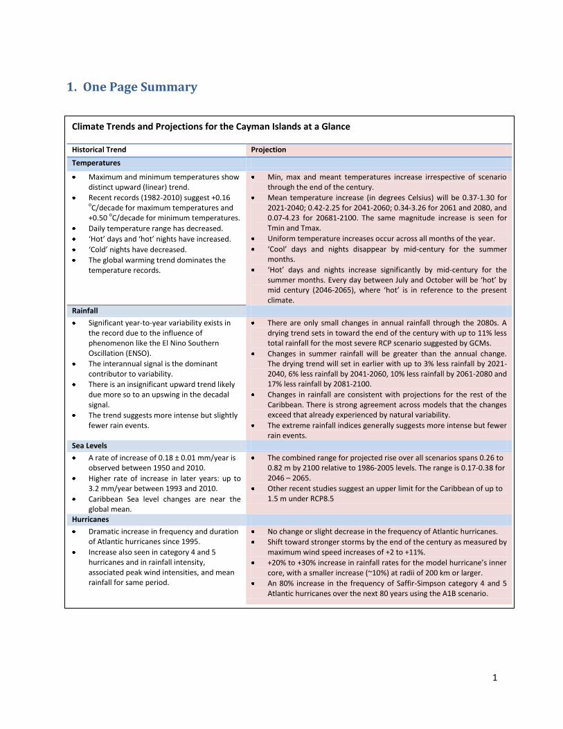
Climate Trends and Projections for the Cayman Islands at a Glance

Historical Trend Projection

Temperatures

Maximum and minimum temperatures show distinct upward (linear) trend.

Recent records (1982-2010) suggest +0.16 oC/decade for maximum temperatures and

+0.50 oC/decade for minimum temperatures.

Daily temperature range has decreased.

‘Hot’ days and ‘hot’ nights have increased.

‘Cold’ nights have decreased.

The global warming trend dominates the temperature records.

Min, max and meant temperatures increase irrespective of scenario through the end of the century.

Mean temperature increase (in degrees Celsius) will be 0.37-1.30 for 2021-2040; 0.42-2.25 for 2041-2060; 0.34-3.26 for 2061 and 2080, and 0.07-4.23 for 20681-2100. The same magnitude increase is seen for Tmin and Tmax.

Uniform temperature increases occur across all months of the year.

‘Cool’ days and nights disappear by mid-century for the summer months.

‘Hot’ days and nights increase significantly by mid-century for the summer months. Every day between July and October will be ‘hot’ by mid century (2046-2065), where ‘hot’ is in reference to the present climate.

Rainfall

Significant year-to-year variability exists in the record due to the influence of phenomenon like the El Nino Southern Oscillation (ENSO).

The interannual signal is the dominant contributor to variability.

There is an insignificant upward trend likely due more so to an upswing in the decadal signal.

The trend suggests more intense but slightly fewer rain events.

There are only small changes in annual rainfall through the 2080s. A drying trend sets in toward the end of the century with up to 11% less total rainfall for the most severe RCP scenario suggested by GCMs.

Changes in summer rainfall will be greater than the annual change. The drying trend will set in earlier with up to 3% less rainfall by 2021-2040, 6% less rainfall by 2041-2060, 10% less rainfall by 2061-2080 and 17% less rainfall by 2081-2100.

Changes in rainfall are consistent with projections for the rest of the Caribbean. There is strong agreement across models that the changes exceed that already experienced by natural variability.

The extreme rainfall indices generally suggests more intense but fewer rain events.

Sea Levels

A rate of increase of 0.18 ± 0.01 mm/year is observed between 1950 and 2010.

Higher rate of increase in later years: up to 3.2 mm/year between 1993 and 2010.

Caribbean Sea level changes are near the global mean.

The combined range for projected rise over all scenarios spans 0.26 to 0.82 m by 2100 relative to 1986-2005 levels. The range is 0.17-0.38 for 2046 – 2065.

Other recent studies suggest an upper limit for the Caribbean of up to 1.5 m under RCP8.5

Hurricanes

Dramatic increase in frequency and duration of Atlantic hurricanes since 1995.

Increase also seen in category 4 and 5 hurricanes and in rainfall intensity, associated peak wind intensities, and mean rainfall for same period.

No change or slight decrease in the frequency of Atlantic hurricanes.

Shift toward stronger storms by the end of the century as measured by maximum wind speed increases of +2 to +11%.

+20% to +30% increase in rainfall rates for the model hurricane’s inner core, with a smaller increase (~10%) at radii of 200 km or larger.

An 80% increase in the frequency of Saffir-Simpson category 4 and 5 Atlantic hurricanes over the next 80 years using the A1B scenario.

2

2. Approach

2.1 Layout of document

The approach to this document is simple and hinges on presentation of the available data. In this

document we consider each climate variable or feature (i.e. temperature, rainfall, sea levels, hurricanes)

separately. Generally, historical data are presented first followed by projections. We also note the

following:

For temperature and rainfall the climatology is first presented followed by an analysis of

historical trends and extremes as gleaned from available station data. Thereafter future

projections for are provided as gleaned from climate models.

Information from both global climate models (GCMs) and a regional climate models (RCM) are

presented. GCMs and RCMs are briefly discussed in the following subsections. There is also a

discussion on how future projections are obtained and the use of scenarios.

For sea level rise and hurricanes, historical and future projections for the Caribbean region are

largely gleaned from a survey of the latest literature. Where possible historical trends for

Cayman are also provided from data for comparison with the regional data.

The immediately following subsections provide brief overviews in order to aid with interpreting the

data. This includes an overview of (i) the available station data (ii) climate models - both GCMs and

RCMs – including those used in the results presented, and (iii) scenarios – including those used in the

results presented.

The remainder of the document presents the climate profile in the briefest and most concise way. The

narrative is deliberately kept short and the reader is encouraged to consult the multiple resources

outlined in the reference section provided.

2.2 About the Station Data

For most of the historical analyses presented, station data from the Owen Roberts International Airport

are used. The dataset spans 1976 to 2010. A few additional precipitation stations are also analysed.

2.3 Obtaining Future Projections from Models

GCMs

Global Circulation Models (GCMs) are useful tools for providing future climate information. GCMs are

mathematical representations of the physical and dynamical processes in the atmosphere, ocean,

3

cryosphere and land surfaces. Their physical consistency and skill at representing current and past

climates make them useful for simulating future climates under differing scenarios of increasing

greenhouse gas concentrations (Scenarios are discussed further below).

GCM projections of rainfall and temperature characteristics for the Cayman Islands are extracted from

the subset of CMIP5 models used to develop the regional atlas of projections presented as a part of the

Intergovernmental Panel on Climate Change (IPCC) Fifth Assessment report (AR5) (IPCC 2013). Data from

in excess of 20 GCMs were analyzed and projected annual change extracted for the GCM grid box over

the Cayman Islands for the periods 2021-2040, 2041-2060, 2061-200 and 2081-2100. Extraction was

done for the four Representative Concentration Pathways (RCPs) (see following subsection on

scenarios). The projections are presented in Figures and summary Tables.

RCMs

An inherent drawback of the GCMs, however, is their coarse resolution relative to the scale of required

information. The size of the Cayman Islands precludes them being physically represented in the GCMs,

and there is a need for downscaling techniques to provide more detailed information on a country or

station level. The additional information which the downscaling techniques provide do not however

devalue the information provided by the GCMs especially since (1) Cayman’s climate is largely driven by

large-scale phenomenon (2) the downscaling techniques themselves are driven by the GCM outputs,

and (3) at present the GCMs are the best source of future information on some phenomena e.g.

hurricanes.

Data from downscaling methods are applied. Dynamical downscaling employs a regional climate model

(RCM) driven at its boundaries by the outputs of the GCMs. Like GCMs, the RCMs rely on mathematical

representations of the physical processes, but are restricted to a much smaller geographical domain (the

Caribbean in this case). The restriction enables the production of data of much higher resolution

(typically < 100 km). Available RCM data for the Cayman islands were obtained from the PRECIS

(Providing Regional Climates for Impact Studies) model (see Taylor et al. 2013 for an extensive

description of the PRECIS-Caribbean project). The PRECIS model resolution is 25 km.

The main PRECIS RCM results are derived from PRECIS driven perturbed physics experiments (PPE).

Created using the A1B SRES scenario (see following section), PPE’s provide an alternative to using

several driving GCM boundary conditions (McSweeney et al 2012). PRECIS PPEs comprise a 17 member

ensemble (HadCM3Q0-Q16), however for the purposes of this study a subset of 6 representative of the

overall range of key climate features were used. The 6 used are the ensemble members Q0, Q3, Q4,

Q10, Q11 and Q14.

Figure 2.1 shows how the islands of Cayman are represented by the PRECIS RCM. Ensuing results will

seek to detail temperature (mean, maximum and minimum) and precipitation changes associated with

grid boxes 3, 4, and 5 for the 2030’s (2030-2039). The emphasis is on grid box 4 which is largely land. For

each of these variables the average of the 6 perturbations is presented as well as the minimum and

maximum associated change in the monthly, seasonal and annual time scales.

4

A second downscaling method is Statistical downscaling. Statistical downscaling enables the projection

of a local variable using statistical relationships developed between that variable and the large scale

climate. The relationships are premised on historical data and are assumed to hold true for the future.

Statistical downscaling is especially useful for generating projections at a location, once sufficient

historical data are available. Statistical downscaling was undertaken for some rainfall and temperature

data for the Airport station. The process was facilitated using the Statistical Downscaling Model (SDSM)

(Wilby et al. 2002).

Emission Scenarios

The GCMs, RCM, and statistical downscaling model are run using either the Special Report Emission

Scenarios (SRES) (Nakicenovic et al. 2000) or Representative Concentration Pathways (RCPs).

Each SRES scenario is a plausible storyline of how a future world will look. The scenarios explore

pathways of future greenhouse gas emissions, derived from self-consistent sets of assumptions about

energy use, population growth, economic development, and other factors. They however explicitly

exclude any global policy to reduce emissions to avoid climate change. Scenarios are grouped into

families according to the similarities in their storylines as shown in Figure 2.2.

The RCM results presented in the following section are for the A1B scenario using the Perturbed Physics

Ensembles (PPE) approach. The A1B scenario is characterized by an increase in carbon dioxide emissions

through mid-century followed by a decrease (Figure 2.3). The future extremes (see subsection 2.5) are

derived from GCMs run using the A2 scenario. A2 (as opposed to B2) is representative of a high

emissions scenario (see Figure 2.2). Note that A1B is often seen as a compromise between the A2

(‘worst case’) and B2 (‘better case’) scenarios.

Figure 2.1: PRECIS RCM grid boxes over the Cayman Islands.

5

Figure 2.3: Total global annual CO2 emissions from all sources (energy, industry, and land-use change) from 1990 to 2100 (in gigatonnes of carbon (GtC/yr) for the families and six SRES scenario groups (Nakicenovic et al, 2000).

A1 storyline and scenario family: a future world of very rapid economic growth, global population that peaks in mid-century and declines thereafter, and rapid introduction of new and more efficient technologies.

A2 storyline and scenario family: a very heterogeneous world with continuously increasing global population and regionally oriented economic growth that is more fragmented and slower than in other storylines.

B1 storyline and scenario family: a convergent world with the same global population as in the A1 storyline but with rapid changes in economic structures toward a service and information economy, with reductions in material intensity, and the introduction of clean and resource-efficient technologies.

B2 storyline and scenario family: a world in which the emphasis is on local solutions to economic, social, and environmental sustainability, with continuously increasing population (lower than A2) and intermediate economic development.

Figure 2.2: Special Report on Emission Scenarios (SRES) schematic and storyline summary (Nakicenovic et al, 2000).

6

In the IPCC Fifth Assessment Report (AR5), outcomes of climate simulations use new scenarios (some of

which include implied policy actions to achieve mitigation) referred to as “Representative Concentration

Pathways” (RCPs) (Figure 2.4). These RCPs represent a larger set of mitigation scenarios and were

selected to have different targets in terms of radiative forcing of the atmosphere at 2100 (about 2.6, 4.5,

6.0 and 8.5 W/m2). They are defined by their total radiative forcing (cumulative measure of human

emissions of greenhouse gases from all sources expressed in Watts per square metre) pathway and level

by 2100. i.e. RCP2.6. RCP4.5, RCP6.0 and RCP8.5. The scenarios should be considered plausible and

illustrative, and do not have probabilities attached to them.

Whereas the SRES scenarios resulted from specific socio-economic scenarios from storylines about

future demographic and economic development, regionalization, energy production and use,

technology, agriculture, forestry and land use, the RCPs are new scenarios that specify concentrations

and corresponding emissions, but not directly based on socio-economic storylines like the SRES

scenarios. These four RCPs include one mitigation scenario leading to a very low forcing level (RCP2.6),

two stabilization scenarios (RCP4.5 and RCP6), and one scenario with very high greenhouse gas

emissions (RCP8.5). The RCPs can thus represent a range of 21st century climate policies, as compared

with the no-climate policy of the Special Report on Emissions Scenarios (SRES) used in the Third

Assessment Report and the Fourth Assessment Report (Figure 2.3). It is to be noted that many do not

believe RCP2.6 is feasible without considerable and concerted global action.

The GCM results presented in the following section are for the four RCPs.

RCP Comments Radiative Forcing Behaviour

RCP2.6 Lowest Peaks at 3 Wm-2

and then declines to approximately 2.6 Wm

-2

RCP4.5 Medium-low

Stabilization at 4.5 Wm-2

RCP6 Medium-high

Stabilization at 6 Wm-2

RCP8.5 Highest RF of 8.5 Wm-2

by 2100 but implies rising RF beyond 2100

Figure 2.4: Radiative Forcing of the Representative Concentration Pathways. Taken from van Vuuren et al (2011). The light grey area captures 98% of the range in previous IAM scenarios, and dark grey represents 90% of the range.

7

Perturbed Physics Experiments

Perturbed Physics Experiments (PPEs) are designed by varying uncertain parameters in the model’s

representation of important physical and dynamical processes. PPEs are used to capture some major

sources of modelling uncertainty by running each member using identical climate forcings. It provides an

alternative to using GCMs developed at different modelling centres around the world (e.g. a multi-

model ensemble, MME), like those in the CMIP3 (Coupled Model Intercomparison Project 3). The Hadley

Centre’s PPE includes 17 members which are formulated to systematically sample parameter

uncertainties under the A1B emissions scenario – this is referred to as the QUMP (Quantifying

Uncertainties in Model Projections) ensemble. The QUMP ensemble was designed for use in the UK’s

own climate projections and is described in detail in the UKCP report available online at

http://ukclimateprojections.defra.gov.uk/content/view/944/500/. Globally, and for many regions and

variables, the range of climate futures projected by the QUMP PPE is equivalent or greater than those

based on the CMIP3 MME. The PPE systematically samples the parameter uncertainties, exploring a

wider range of possible variation in the formulation of a single model, leading to a wider range of

physically plausible future climate outcomes than the MME. It is important to remember that PPE

(similarly for MME) does not account for all of the sources of model uncertainty. 1

The following 6 QUMP experiments were evaluated: Q0, Q3, Q4, Q10, Q11, and Q14. All were run at 25

km and from 1960 through 2100. For each experiment the deviation of a future decade e.g. 2020s,

2030s, 2040s from the experiments baseline (1960-1990) were determined. This gave an ensemble of 6

future changes for each decade. The ensemble results are summarised and presented in Tables for the

2030s (2030-2039) i.e. representative of a more detailed near term projection.

2.4 Extreme Indices

Extreme temperature and rainfall indices tables are calculated for present and future climates of the

Cayman Islands. The indices are a subset of those made available to the international scientific

community via the ETCCDI website http://etccdi.pacificclimate.org/data.html. Some of the indices

calculated are shown in Table 2.1.

For the historical climate, the indices are calculated using data from the airport station. For the future

climate, the indices are derived from one of two sources: (i) The grid box over the Cayman Islands from

an ensemble of 9 GCMs and presented as change from a 40 year historical control period covering the

years 1960-1999. In this instance the more extreme A2 scenario is used in the derivation of the

extremes.2 (ii) The data from the PRECIS RCM Caribbean project detailed previously using both the A2

and B2 scenarios.

1 Portions of the narrative are adapted from narrative on the PRECIS webpage http://www.metoffice.gov.uk/precis/qump 2 GCM data for the extremes was downloaded from the Climate Change Knowledge Portal of the World Bank group

http://sdwebx.worldbank.org/climateportal/.

http://ukclimateprojections.defra.gov.uk/content/view/944/500/

http://www.metoffice.gov.uk/precis/qump

http://sdwebx.worldbank.org/climateportal/

8

Table 2.1: Extreme Indices

Element Index Descriptive name Definition Unit

Temperature TXmean Annual maximum temperature (TX)

Annual mean of TX °C

TNmean Annual minimum temperature (TN)

Annual mean of TN °C

TX90 Warm days Percentage of days when TX > 90th percentile

%

TX10 Cool days Percentage of days when TX < 10th percentile

%

TN90 Warm nights Percentage of days when TN > 90th percentile

%

TN10 Cool nights Percentage of days when TN < 10th percentile

%

Precipitation CDD Consecutive dry days Maximum number of consecutive dry days

days

CWD Consecutive wet days Maximum number of consecutive wet days

days

R10mm Days above 10 mm Annual count of days when RR > 10 mm

days

RX5day Max 5-days precipitation

Annual highest 5 consecutive days precipitation

mm

R95p Very wet days Annual total precipitation when RR > 95th percentile

mm

2.5 Presenting the Data

The future climate is presented as absolute or percentage deviations from the present day climate

which is in turn represented by averaging over a baseline period of 20 or 30 years. Results are

presented for near, medium and long term time slices (20 or 30 year bands depending on available

modeled data) in the future up to the end of the current century (2100).

http://onlinelibrary.wiley.com/doi/10.1002/joc.3889/full#joc3889-note-0003






9

3. Temperatures

3.1 Climatology

Surface temperature in the Caribbean is controlled largely by the variation in the earth’s orbits around

the sun which gives rise to variations in temperatures. The climatological (mean annual) pattern for the

Cayman Islands is shown in Figure 3.2.1. Cooler months occur in northern hemisphere winter and

warmer months in summer. There are occasional surges of cooler air from continental North America

from October through early April during the passage of cold fronts. After the passage of a strong cold

front, temperatures can fall as low as 20 degrees. Temperatures peak in July. The mean annual range

between coolest and warmest months is about 4 degrees.

3.2 Historical Trends

Global mean surface temperatures have increased by 0.85 °C ± 0.20°C when a linear trend is used to

estimate the change over 1880-2012. Average annual temperatures for Caribbean islands have similarly

increased by just over 0.5 °C over the period 1900 – 1995 (IPCC, 2007). The annual mean of day time

temperatures for the Caribbean region also shows a significant increase of 0.19 oC/decade over the

period 1961-2010 (Stephenson et al. 2014). This is however, smaller than the increase in mean night

Figure 3.1: Temperature climatology of Cayman, Owen Roberts International Airport. The averaging period is 1960-1990. Data source: Meteorological Service of Cayman.

10

time temperatures (~ 0.28 oC/decade) over the same period. The result is a decrease in the mean annual

daily temperature range over the period.

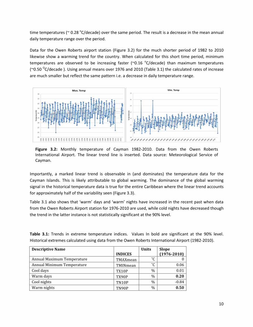
Data for the Owen Roberts airport station (Figure 3.2) for the much shorter period of 1982 to 2010

likewise show a warming trend for the country. When calculated for this short time period, minimum

temperatures are observed to be increasing faster (~0.16 oC/decade) than maximum temperatures

(~0.50 OC/decade ). Using annual means over 1976 and 2010 (Table 3.1) the calculated rates of increase

are much smaller but reflect the same pattern i.e. a decrease in daily temperature range.

Importantly, a marked linear trend is observable in (and dominates) the temperature data for the

Cayman Islands. This is likely attributable to global warming. The dominance of the global warming

signal in the historical temperature data is true for the entire Caribbean where the linear trend accounts

for approximately half of the variability seen (Figure 3.3).

Table 3.1 also shows that ‘warm’ days and ‘warm’ nights have increased in the recent past when data

from the Owen Roberts Airport station for 1976-2010 are used, while cold nights have decreased though

the trend in the latter instance is not statistically significant at the 90% level.

Table 3.1: Trends in extreme temperature indices. Values In bold are significant at the 90% level.

Historical extremes calculated using data from the Owen Roberts International Airport (1982-2010).

Descriptive Name INDICES

Units Slope (1976-2010)

Annual Maximum Temperature TMAXmean ˚C 0

Annual Minimum Temperature TMINmean ˚C 0.06

Cool days TX10P % 0.01

Warm days TX90P % 0.20

Cool nights TN10P % -0.84

Warm nights TN90P % 0.50

Figure 3.2: Monthly temperature of Cayman 1982-2010. Data from the Owen Roberts International Airport. The linear trend line is inserted. Data source: Meteorological Service of Cayman.

11

Figure 3.3: (a)Average July-October temperature anomalies over the Caribbean from the late 1800s with trend line imposed. Box Inset: Percentage of variance explained by trend line, decadal variations > 10 years, interannual (year-to-year) variations. (b) Percentage variance in July-October temperature anomalies (from late 1800s) accounted for by the ‘global warming’ trend line for gridboxes over the Caribbean. Data source: CRU data. Acknowledgements: IRI Map Room.

Trend 54%

Decadal 17%

Inter-Annual 29%

12

3.3 Projections

Data are presented for both GCM and RCM derived projections in Tables 3.2-3.9 and Figures 3.4 and 3.5.

Some major summary points are:

From the GCMs, mean annual temperatures are projected to increase irrespective of scenario

through the end of the century.

Mean temperature increase (in degrees Celsius) will be 0.37-1.30 for 2021-2040; 0.42-2.25 for

2041-2060; 0.34-3.26 for 2061 and 2080, and 0.07-4.23 for 20681-2100.

Increases will be of the same magnitude for maximum temperatures and minimum

temperatures.

The RCM suggests similar magnitude increases in the near term (2030s) for grid box 4. Annual

mean temperature increases range from 0.8-1.4 degrees. The magnitude change is similar for

minimum and maximum temperatures.

Temperature change is uniform across all three month seasons. August-September-October

(ASO) has negligibly higher values than other times of the year.

‘Cool’ days and nights disappear by mid-century for the summer months. There are no ‘cool

days’ or ‘cool nights’ between May and November by mid century (2046-2065), where ‘cool’ is in

reference to the present climate.

‘Hot days and nights increase significantly by mid-century for the summer months. There are

approximately 30 ‘hot days’ and ‘hot nights’ (or every day for the respective months) in every

month between July and October by mid century (2046-2065), where ‘hot’ is in reference to the

present climate.

GCMs

Table 3.2: Mean annual temperature change for Cayman with respect to 1986-2005 AR5 CMIP5 subset.

Change shown for four RCP scenarios.

Tmean 2021-2040 2041-2060 2061-2080 2081-2100

min mean max min mean max min mean max min mean max

rcp26 0.39 0.69 1.16 0.42 0.86 1.55 0.34 0.86 1.67 0.07 0.81 1.64

rcp45 0.37 0.74 1.22 0.57 1.11 1.77 0.78 1.40 2.27 0.81 1.53 2.47

rcp60 0.41 0.66 1.10 0.72 1.01 1.61 0.98 1.44 2.18 1.13 1.86 2.87

rcp85 0.49 0.86 1.30 0.95 1.54 2.25 1.60 2.32 3.26 2.12 3.09 4.23

Range: 0.37-1.30 0.42-2.25 0.34-3.26 0.07-4.23

13

Table 3.3: Mean annual minimum temperature change for Cayman with respect to 1986-2005 AR5

CMIP5 subset. Change shown for four RCP scenarios.

Tmin 2021-2040 2041-2060 2061-2080 2081-2100


rcp26 0.39 0.69 1.16 0.41 0.86 1.56 0.33 0.86 1.67 0.04 0.81 1.65

rcp45 0.36 0.74 1.22 0.55 1.11 1.77 0.76 1.40 2.27 0.78 1.53 2.47

rcp60 0.35 0.64 1.09 0.72 0.99 1.61 0.96 1.41 2.18 1.10 1.83 2.88

rcp85 0.48 0.86 1.30 0.94 1.54 2.26 1.58 2.32 3.26 2.08 3.09 4.24

Range: 0.36-1.30 0.41-2.26 0.33-3.26 0.04-4.24

Table 3.4: Mean annual maximum temperature change for Cayman with respect to 1986-2005 AR5

CMIP5 subset. Change shown for four RCP scenarios.

Tmax 2021-2040 2041-2060 2061-2080 2081-2100


rcp26 0.39 0.69 1.17 0.43 0.87 1.54 0.36 0.87 1.66 0.09 0.82 1.64

rcp45 0.38 0.74 1.21 0.58 1.12 1.78 0.79 1.41 2.26 0.83 1.54 2.47

rcp60 0.45 0.66 1.10 0.73 1.01 1.61 0.99 1.44 2.18 1.15 1.85 2.86

rcp85 0.50 0.87 1.29 0.97 1.55 2.24 1.63 2.34 3.25 2.16 3.11 4.22

Range: 0.38-1.29 0.43-2.24 0.36-3.25 0.09-4.22

14

Figure 3.4: (a) Mean annual temperature change (oC) (b) Mean annual minimum temperature change (oC) (c) Mean annual maximum temperature change for Cayman (oC) with respect to 1986-2005 AR5 CMIP5 subset. On the left, for each scenario one line per model is shown plus the multi-model mean, on the right percentiles of the whole dataset: the box extends from 25% to 75%, the whiskers from 5% to 95% and the horizontal line denotes the median (50%).

(a)

(c)

(b)

15

RCM

Table 3.5: Projected change (oC) in minimum temperature for specific grid boxes over Cayman for the

2030s. Data is from PRECIS RCM for an ensemble of 5 runs using perturbed physics and for the A1B

scenario.

MIN MEAN MAX MIN MEAN MAX MIN MEAN MAX

JAN 0.814 1.052 1.260 0.877 1.204 1.426 0.817 1.067 1.278

FEB 0.815 1.052 1.257 0.878 1.205 1.425 0.818 1.068 1.276

MAR 0.817 1.054 1.255 0.879 1.206 1.423 0.820 1.070 1.274

APR 0.816 1.055 1.252 0.877 1.208 1.422 0.818 1.071 1.272

MAY 0.818 1.057 1.251 0.880 1.209 1.421 0.820 1.073 1.271

JUN 0.820 1.059 1.252 0.883 1.211 1.422 0.822 1.075 1.272

JUL 0.822 1.061 1.253 0.887 1.213 1.424 0.825 1.077 1.273

AUG 0.825 1.063 1.256 0.893 1.216 1.427 0.829 1.080 1.276

SEP 0.828 1.066 1.259 0.897 1.219 1.430 0.832 1.082 1.279

OCT 0.833 1.068 1.262 0.902 1.221 1.434 0.837 1.084 1.281

NOV 0.837 1.067 1.270 0.904 1.219 1.441 0.840 1.083 1.289

DEC 0.813 1.055 1.255 0.883 1.209 1.428 0.818 1.071 1.274

NDJ 0.822 1.058 1.262 0.888 1.211 1.432 0.825 1.074 1.281

FMA 0.816 1.054 1.255 0.878 1.206 1.423 0.819 1.070 1.274

MJJ 0.820 1.059 1.252 0.883 1.211 1.422 0.823 1.075 1.272

ASO 0.829 1.066 1.259 0.897 1.219 1.430 0.833 1.082 1.279

ANNUAL 0.822 1.059 1.257 0.887 1.212 1.427 0.825 1.075 1.276

GRID BOX 3 GRID BOX 4 GRID BOX 5


16

Table 3.6: Projected change (oC) in maximum temperature for specific grid boxes over Cayman for the


scenario.


JAN 0.832 1.075 1.280 0.824 1.075 1.304 0.828 1.074 1.288

FEB 0.834 1.076 1.279 0.822 1.075 1.303 0.829 1.075 1.287

MAR 0.835 1.077 1.277 0.821 1.077 1.302 0.830 1.076 1.285

APR 0.834 1.079 1.274 0.818 1.078 1.302 0.828 1.077 1.282

MAY 0.836 1.080 1.274 0.815 1.079 1.303 0.829 1.079 1.282

JUN 0.837 1.082 1.274 0.818 1.079 1.306 0.831 1.080 1.283

JUL 0.839 1.084 1.276 0.820 1.081 1.308 0.832 1.082 1.284

AUG 0.842 1.086 1.278 0.825 1.084 1.311 0.836 1.084 1.287

SEP 0.845 1.088 1.281 0.829 1.086 1.314 0.839 1.087 1.289

OCT 0.849 1.091 1.283 0.833 1.088 1.315 0.844 1.089 1.292

NOV 0.854 1.090 1.290 0.841 1.088 1.318 0.849 1.088 1.299

DEC 0.830 1.078 1.276 0.821 1.078 1.311 0.827 1.077 1.286

NDJ 0.839 1.081 1.282 0.829 1.081 1.311 0.834 1.080 1.291

FMA 0.834 1.077 1.277 0.820 1.077 1.303 0.829 1.076 1.284

MJJ 0.837 1.082 1.275 0.818 1.080 1.305 0.831 1.080 1.283

ASO 0.845 1.088 1.281 0.829 1.086 1.313 0.840 1.087 1.289

ANNUAL 0.839 1.082 1.279 0.824 1.081 1.308 0.834 1.081 1.287


17

Table 3.7: Projected change (oC) in mean temperature for specific grid boxes over Cayman for the


scenario.


JAN 0.827 1.065 1.273 0.858 1.140 1.371 0.824 1.071 1.285

FEB 0.828 1.066 1.271 0.857 1.141 1.370 0.825 1.072 1.283

MAR 0.830 1.067 1.268 0.857 1.142 1.369 0.826 1.073 1.281

APR 0.828 1.069 1.266 0.853 1.143 1.367 0.825 1.075 1.278

MAY 0.830 1.070 1.265 0.853 1.144 1.367 0.826 1.076 1.278

JUN 0.832 1.072 1.266 0.856 1.145 1.369 0.828 1.078 1.278

JUL 0.833 1.074 1.267 0.859 1.147 1.371 0.830 1.080 1.280

AUG 0.837 1.076 1.269 0.863 1.149 1.373 0.834 1.083 1.282

SEP 0.840 1.079 1.272 0.867 1.152 1.377 0.837 1.085 1.285

OCT 0.844 1.081 1.275 0.872 1.154 1.380 0.841 1.087 1.288

NOV 0.850 1.080 1.283 0.877 1.153 1.384 0.846 1.086 1.295

DEC 0.825 1.068 1.268 0.857 1.143 1.373 0.823 1.074 1.281

NDJ 0.834 1.071 1.275 0.864 1.145 1.376 0.831 1.077 1.287

FMA 0.829 1.067 1.268 0.856 1.142 1.369 0.826 1.073 1.281

MJJ 0.832 1.072 1.266 0.856 1.145 1.369 0.828 1.078 1.279

ASO 0.840 1.079 1.272 0.867 1.152 1.377 0.837 1.085 1.285

ANNUAL 0.834 1.072 1.270 0.861 1.146 1.373 0.831 1.078 1.283


18

Future Temperature Extremes

Table 3.8: Future temperature extremes as calculated from an ensemble of 9 GCMs using the A2

scenario. Numbers represent the number of days per month meeting the criterion outlined in the

column heading. ‘Cool’ and ‘Hot’ are relative to present day conditions (i.e. < 10th percentile or > 90th

percentile).

no. of cool days no. of hot days no. of cool nights no. of hot nights

2046-2065

2081-2100

2046-2065

2081-2100

2046-2065

2081-2100

2046-2065

2081-2100

Jan 4 1 0 0 4 1 0 12

Feb 4 1 0 5 5 1 0 5

Mar 2 0 0 7 4 1 0 23

Apr 0 0 4 22 0 0 2.8 21

May 0 0 19 29 0 0 18 30

Jun 0 0 25 30 0 0 25 30

Jul 0 0 30 31 0 0 31 31

Aug 0 0 31 31 0 0 31 31

Sep 0 0 30 30 0 0 30 30

Oct 0 0 29 31 0 0 29 31

Nov 0 0 14 29 0 0 13 29

Dec 1 0 3 22 1 0 3 21

Table 3.9: Change in temperature trends for 2071-2099 relative to a 1961-1989 baseline. Positive values

indicate increasing trend. Data source: PRECIS RCM.


Units Change in Slope (A2)

Change in Slope (B2)

80.0˚W; 19.5˚N

81.5˚W; 19.5˚N

81.0˚W; 19.5˚N

80.0˚W; 19.5˚N

81.5˚W; 19.5˚N

81.0˚W; 19.5˚N

Cool days TX10P % 0.754 0.659 0.685 0.257 0.224 0.268

Warm days TX90P % 0.794 0.891 0.868 0.792 0.879 0.861

Cool nights TN10P % 0.607 0.622 0.631 0.224 0.338 0.314

Warm nights TN90P % 0.869 0.867 0.868 0.870 0.894 0.846

19

4. Rainfall

4.1 Climatology

The rainfall has a bimodal (‘double peak’) pattern with an early rainfall season occurring in May-June

and a late rainfall season centered in October. (See Figure 3.1) The bimodality is a feature of the rainfall

cycle of most of the northern Caribbean territories.

The early rainfall season is generally shorter (May-June) and receives less rainfall than the later season

(August through November). About 70-80% of total annual rainfall falls between May and November,

and about 40-50% falls between September and November (the late wet season). The late wet season

also coincides with the peak in Atlantic hurricane activity.

There is a brief drier period in July which separates the early and late wet seasons, and which is often

referred to as the midsummer drought (MSD). The longer dry season runs from December through April,

with March and April being the driest months of the year. Mean number of rain days vary widely

annually.

Figure 4.1: Rainfall climatologies for select sites around Cayman. Base period vary for stations.

20

Cayman’s rainfall climatology is largely conditioned by changes in features of the tropical Atlantic such

as the position of the North Atlantic High (NAH) pressure system, the tropical sea surface temperatures

(SSTs), the passage of mid-latitude cold fronts early in the year, the strength of the trade winds and the

passage of easterly tropical waves. Tropical easterly waves are significant climate features which travel

from the west coast of Africa and through the Caribbean between June and November. Their

significance arises not only because of the rain that accompanies their passage over the island, but also

because the waves often develop into tropical depressions, storms and hurricanes under conducive

conditions.


Interannual variability is a dominant part of the Cayman rainfall record. Figure 4.2 shows total rainfall for

the years 1992-2010 using data from the airport station. Though there is a slight upward trend it is not

significant. The record is too short to attribute the upward trend to global warming as Caribbean rainfall

is dominated by interannual and decadal variability as well (Figure 4.3). With respect to the latter

timescale of variability, the Atlantic Multidecadal Oscillation (AMO) swung into its warm phase toward

the end of the 1990s and likely accounts for the upward trend in the data shown in Figure 4.2 i.e. as

opposed to a significant climate change signal.

Short term (interannual climate variability) is however clearly evident and accounts for most of the

variability in the Cayman rainfall record. The El Niño/La Niña is a significant driver of interannual

variability in the Caribbean. El Niño events tend to occur every 3 to 5 years, though increases in the

frequency, severity and duration of events have been noted since the 1970s. Because an El Niño

represents a significant influence on Caribbean climate it is not unusual to find its timescale of variability

(i.e. 3 to 5 year cycles) in regional rainfall and temperature records.

Figure 4.2: Total annual rainfall for Cayman 1982-2010. Data from the Owen Roberts International Airport. The linear trend line is inserted. Data source: Meteorological Service of Cayman.

21

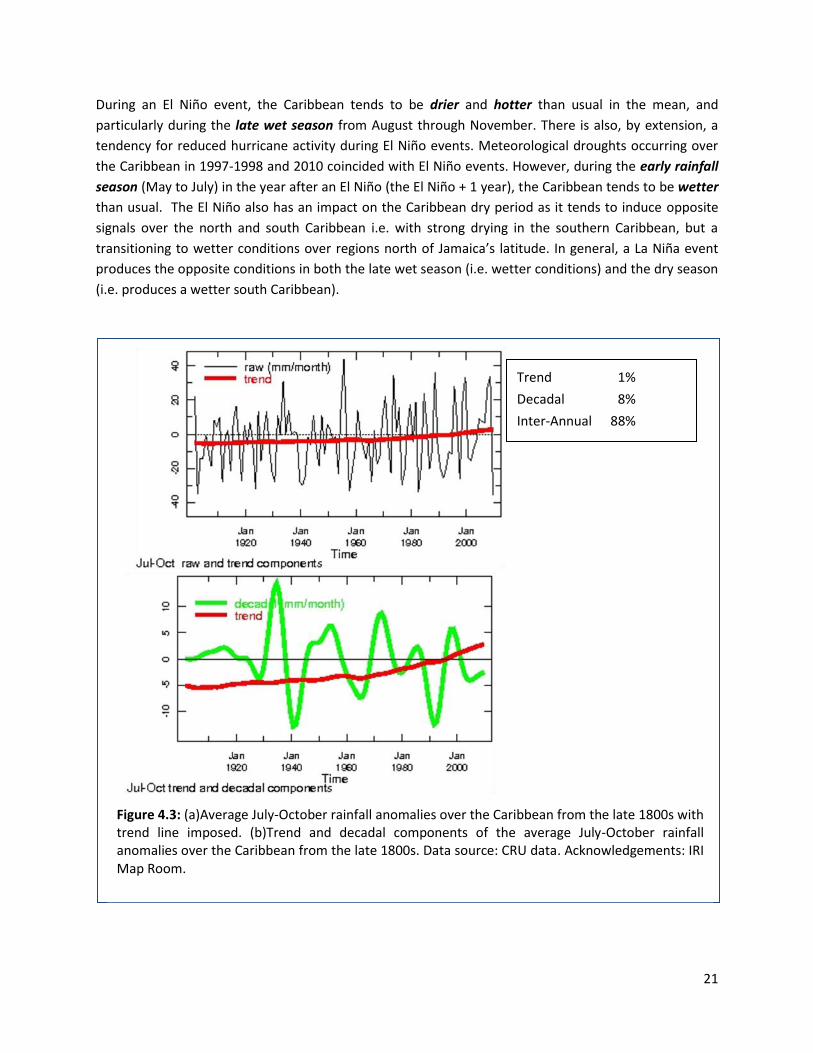
During an El Niño event, the Caribbean tends to be drier and hotter than usual in the mean, and

particularly during the late wet season from August through November. There is also, by extension, a

tendency for reduced hurricane activity during El Niño events. Meteorological droughts occurring over

the Caribbean in 1997-1998 and 2010 coincided with El Niño events. However, during the early rainfall

season (May to July) in the year after an El Niño (the El Niño + 1 year), the Caribbean tends to be wetter

than usual. The El Niño also has an impact on the Caribbean dry period as it tends to induce opposite

signals over the north and south Caribbean i.e. with strong drying in the southern Caribbean, but a

transitioning to wetter conditions over regions north of Jamaica’s latitude. In general, a La Niña event

produces the opposite conditions in both the late wet season (i.e. wetter conditions) and the dry season

(i.e. produces a wetter south Caribbean).

Figure 4.3: (a)Average July-October rainfall anomalies over the Caribbean from the late 1800s with trend line imposed. (b)Trend and decadal components of the average July-October rainfall anomalies over the Caribbean from the late 1800s. Data source: CRU data. Acknowledgements: IRI Map Room.

Trend 1%

Decadal 8%

Inter-Annual 88%

22

The extreme rainfall indices calculated form the data for teh airport stations are generally reflective of

the swing toward wetter conditions in the most recent decade. Almost all indices have positive slopes

though only very wet days and consecutive dry days are significant athe 90% level. The trend suggests

more severe but fewer rain events. These ‘trends’ should, however, be interpreted cautiously given the

relatively short period over which they are calculated, and the large year-to-year variability in rainfall

and its extremes.

Table 4.1: Trends in extreme rainfall indices. Values In bold are significant at the 90% level. Historical

extremes calculated using data from the Owen Roberts International Airport (1982-2010).


Units Slope (1976-2010)

Max 5-day precipitation RX5day mm 0.98

Days above 10mm R10mm days -0.17

Consecutive dry days CDD days 0.53

Consecutive wet days CWD days 0.04

Very wet days R95P mm 7.03

Extremely wet days R99P mm 1.95

Annual precipitation PRCPTOT mm 4.01

23

4.3 Projections

Results are presented for both GCM and RCM derived projections in tables 4.2-4.5 and Figure 4.4-4.5..

Some major summary points are:

From the GCMs, the scenario means suggest that there is little change in annual rainfall through

the 2080s. A drying trend sets in toward the end of the century with up to 11% less total rainfall

for the year for the most severe RCP scenario (RCP8.5).

The GCMs suggest that changes in summer rainfall will be greater than the annual change. The

drying trend will set in earlier with up to 3% less rainfall by 2021-2040, 6% less rainfall by 2041-

2060, 10% less rainfall by 2061-2080 and 17% less rainfall by 2081-2100.

RCM projections do not show significant changes in rainfall across seasons for the near term

(2030s).

Projected GCM changes in annual rainfall and summer rainfall for Cayman are consistent across

the Caribbean basin and there is strong agreement across models that the changes exceed that

already experienced by natural variability (see Figure xx). This is as opposed to changes seen in

the dry months early in the year (January-March) which do not exceed one standard deviation

of natural variability.

The extreme rainfall indices generally suggest more intense but fewer rain events.

GCMs

Table 4.2: Mean percentage change in annual rainfall for Cayman with respect to 1986-2005 AR5 CMIP5

subset. Change shown for four RCP scenarios.

(a) Rain 2021-2040 2041-2060 2061-2080 2081-2100


rcp26 -10.98 2.22 13.9 -16.02 2.16 32.38 -15.78 2.9 21.59 -24.51 2.55 22.11

rcp45 -19.55 -0.04 15.94 -21.74 -1.5 17.25 -23.99 -2.74 19.72 -28.92 -1.21 35.27

rcp60 -14.89 -0.82 18.48 -16.65 -0.22 13.22 -16.6 -0.99 30.68 -29.81 -2.8 19.98

rcp85 -19.61 -1.03 16.41 -18.37 -2.18 25.46 -34.65 -4.53 23.98 -47.98 -11.25 31.9

Range for the Means: -1 - +2% -2 - +2% -4-+3% -11+3%

24

Table 4.3: Mean percentage change in summer rainfall (July-October) for Cayman with respect to

1986-2005 AR5 CMIP5 subset. Change shown for four RCP scenarios.

(b) Summer Rain 2021-2040 2041-2060 2061-2080 2081-2100


rcp26 -12.26 0.24 15.65 -15.95 -0.39 20.85 -22.23 1.07 18.29 -33.46 0.29 24.4

rcp45 -23.87 -2.91 13.84 -36.02 -4.57 15.23 -34.73 -5.48 19.31 -33.37 -4.47 36.86

rcp60 -16.55 -1.36 30.61 -16.9 -2.73 10.9 -25.46 -3.66 24.84 -36.55 -5.4 16.93

rcp85 -24.61 -2.75 14.39 -34.66 -5.91 20.51 -51.8 -9.52 27.7 -67.61 -16.71 23.68

Range for the Means: -3 - +0% -6- +0% -10- +1% -17 - +0%

25

Figure 4.4: (a) Relative Annual Precipitation change (%) (b) Relative July-October Precipitation change (%) for Cayman with respect to 1986-2005 AR5 CMIP5 subset. On the left, for each scenario one line per model is shown plus the multi-model mean, on the right percentiles of the whole dataset: the box extends from 25% to 75%, the whiskers from 5% to 95% and the horizontal line denotes the median (50%).

(a)

(b)

26

RCM

Table 4.4: Projected change (%) in rainfall for specific grid boxes over Cayman for the 2030s. Data is

from PRECIS RCM for an ensemble of 5 runs using perturbed physics and for the A1B scenario.


JAN -5.170 0.505 11.510 -3.079 1.718 10.881 -6.060 0.818 13.309

FEB -4.926 0.508 11.643 -2.845 1.732 11.002 -5.997 0.841 13.486

MAR -4.906 0.506 11.697 -2.723 1.746 11.063 -6.163 0.854 13.586

APR -4.886 0.565 11.882 -2.586 1.811 11.287 -6.135 0.904 13.742

MAY -5.256 0.611 12.245 -2.581 1.987 11.678 -6.516 0.985 14.104

JUN -4.934 0.800 12.052 -2.263 2.150 11.549 -6.199 1.064 13.903

JUL -5.568 0.833 12.143 -2.273 2.259 11.868 -6.771 1.091 13.982

AUG -5.546 0.804 12.069 -2.236 2.307 11.913 -6.777 1.069 13.926

SEP -5.481 0.799 11.866 -2.233 2.280 11.675 -6.727 1.038 13.647

OCT -5.125 0.705 11.121 -2.062 2.234 11.366 -6.353 0.967 12.852

NOV -6.062 0.688 12.974 -2.742 2.034 12.148 -7.277 0.853 14.121

DEC -4.564 0.640 10.925 -2.530 1.980 10.945 -5.418 0.911 12.707

NDJ -4.907 0.609 11.803 -2.689 1.910 11.324 -6.134 0.859 13.380

FMA -4.837 0.526 11.740 -2.718 1.763 11.117 -6.098 0.866 13.605

MJJ -5.253 0.748 12.147 -2.301 2.132 11.698 -6.495 1.047 13.996

ASO -5.383 0.769 11.684 -2.145 2.274 11.651 -6.619 1.024 13.473

ANNUAL -5.096 0.663 11.843 -2.384 2.020 11.448 -6.337 0.949 13.613



27

Figure 4.6: (a) Mean rcp45to85 relative precipitation (%) (b) Mean rcp45to85 relative summer

precipitation (%) (c) Mean rcp45to85 relative dry season (Jan-Mar) precipitation (%) 2081-

2100 minus 1986-2005 AR5 CMIP5 subset. The hatching represents areas where the signal is

smaller than one standard deviation of natural variability .

(a)

(c)

(b)

28

Future Rainfall Extremes

Table 4.5: Change in rainfall trends for 2071-2099 relative to a 1961-1989 baseline. Positive values

indicate increasing trend. Data source: PRECIS RCM.


Units Change in Slope (A2)

Change in Slope (B2)

80.0˚W; 19.5˚N

81.5˚W; 19.5˚N

81.0˚W; 19.5˚N

80.0˚W; 19.5˚N

81.5˚W; 19.5˚N

81.0˚W; 19.5˚N

Max 5-day precipitation RX5day mm 0.239 1.254 1.112 0.889 0.560 0.827

Days above 10mm R10mm days 0.179 0.143 0.227 -0.511 0.471 0.542

Consecutive dry days CDD days -0.258 0.023 0.018 -1.000 0.096 0.376

Consecutive wet days CWD days -0.157 -0.007 -0.008 0.172 -0.497 -0.694

Very wet days R95P mm -1.716 0.558 0.247 0.627 0.315 0.896

29

5. Sea Levels


Globe

It is estimated that between 1901and 2010 global mean sea level rose by 0.19 ± 0.02 m (IPCC 2013).

Table 5.1: Mean rate of global averaged sea level rise

Period Rate (mm/year) Information source

1901 and 2010 1.7 ± 0.2 Tide gauge IPCC (2013)

1993 and 2010 3.2 ± 0.4 Satellite Altimeter IPCC (2013)

Caribbean

Rates of sea-level rise are not uniform across the globe and large regional differences exist. Estimates of

observed sea level rise from 1950 to 2000 suggest that sea level rise within the Caribbean appears to be

near the global mean (Church et al. 2004).

Table 5.2: Mean rate of sea level rise averaged over the Caribbean basin.

Period Rate (mm/year) Information source

1950 and 2009 1.8 ± 0.1 Palanisamy et al. (2012)

1993 and 2010 1.7 ± 1.3 Torres & Simples (2013)

1993 and 2010 2.5± 1.3 Torres & Simples (2013), after correction for Global Isostatic Ajustment (GIA)

*GIA describes the slow part of the response of the earth to the redistribution of mass following the last deglaciation.

Cayman

Table 5.3 shows the rates of sea level rise for a number of locations (Figure 5.1) as derived from tide

gauges in the Caribbean. The tide gauge coverage in the Caribbean islands is poor with only 7 gauges

having data >30 years between 1950 and 2009. All values suggest an upward trend for the period of

record available.

Cayman has two gauges in the long term historical record (North Sound and South Sound). The trend for

each station is not statistically different from the basin trend and the record too short to justify

suggesting otherwise. Additionally Palamisamy et al. (2013) interpolate sea level reconstruction grids at

different Caribbean island sites where gauges exist but have are very short records and show that locally

the sea level trend is of the order 2 mm/year which is only slightly larger than the mean basinwide

averaged trend.

30

Interannual sea-level variability accounts for one third of the total sea-level variability and can be partly

explained by the influence of El Niño-Southern Oscillation at different time and spatial scales

(Palanisamy et al. 2013; Torres & Simples 2013). Palanisamy et al. (2013) observe that Interannual sea-

level variability in the north Caribbean (including Cayman) is higher than for the southern Caribbean and

strongly correlated with El Nino.

Figure 5.1: (a) Location of tide gauge

stations and time series start and end year.

(b) Tide gauge observed sea-level trends computed from all available data (Table 1). Monthly time series after the removal of the seasonal cycle (gray), the linear trend (blue), and the annual series (red) are also shown. The trends (and 95% error) in mm/yr. From Torres & Tsimples (2013)

31

Table 5.3: Tide gauge observed sea-level trends for Caribbean stations shown in Figure 5.1a. Computed

using all available data. From Torres & Simples (2013)

Lat (N) Lon (W) Span years

% of data

Trend Months Gauge corrected

P. Limon 10 83 20.3 95.1 1.76±0.8 216 2.16±0.9

Cristobal 9.35 79.9 101.7 86.9 1.96±0.1 566 2.86±0.2

Cartagena 10.4 75.6 44 90 5.36±0.3 463 5.46±0.3

Riohacha 11.6 72.9 23.8 95.8 4.86±1.1 273 4.86±1.1

Amuay 11.8 70.2 33 93.4 0.26±0.5 370 0.26±0.5

La Guaira 10.6 66.9 45 98.9 1.46±0.3 534 1.56±0.3

Cumana 10.5 64.2 29 98.6 0.96±0.5 331 0.76±0.6

Lime Tree 17.7 64.8 32.2 81.9 1.86±0.5 316 1.56±0.5

Magueyes 18 67.1 55 96.2 1.36±0.2 635 1.06±0.2

P. Prince 18.6 72.3 12.7 100 10.76±1.5 144 12.26±1.5

Guantanamo 19.9 75.2 34.6 89.9 1.76±0.4 258 2.56±0.6

Port Royal 17.9 76.8 17.8 99.5 1.66±1.6 212 1.36±1.6

Cabo Cruz 19.8 77.7 10 90 2.26±2.8 108 2.16±2.8

South Sound 19.3 81.4 20.8 87.6 1.76±1.5 219 1.26±1.5

North Sound 19.3 81.3 27.7 89.2 2.76±0.9 296 2.26±0.9

C. San Antonio 21.9 84.9 38.3 76.7 0.86±0.5 353 0.36±0.5

Santo Tomas 15.7 88.6 20 85.4 2.06±1.3 205 1.76±1.3

P. Cortes 15.8 87.9 20.9 98 8.66±0.6 224 8.86±0.7

P. Castilla 16 86 13.3 100 3.16±1.3 160 3.26±1.3

5.2 Projections

Table 5.4 provides a range of estimates for end-of-century sea level rise globally and in the Caribbean

Sea under a number of scenarios. The values are taken from the IPCC’s Fourth Assessment Report. The

future rise in the Caribbean is not significantly different from the projected global rise.

The combined range over all scenarios spans 0.18-0.59 m by 2100 relative to 1980-1999 levels. A

number of other studies (e.g. Rahmstorf, 2007; Rignot and Kanargaratnam, 2006; Horton et al., 2008)

including the recently released Summary of the Fifth Assessment Report (IPCC 2013) suggest that the

upper bound for the global estimates in Table 2 are conservative and could be up to 0.98 m, with a rate

of 8 to16 mm/ year during 2081–2100. Diagrams from Perret et al. (2013) suggest the same for

estimates for the Caribbean Sea i.e. a higher upper bound of up to 1.5 m by the end of the century.

32

Table 5.4: Projected changes in temperature per grid box by 2090s from a regional climate model

Scenario Global Mean Sea Level Rise by 2100 relative to

1980 – 1999

Caribbean Mean Sea Level Rise by 2100 relative to 1980 – 1999 (± 0.05m relative to global mean)

IPCC B1 0.18 – 0.38 0.13 – 0.43

IPCC A1B 0.21 – 0.48 0.16 – 0.53

IPCC A2 0.23 – 0.51 0.18 – 0.56

Rahmstorf, 2007 Up to 1.4m Up to 1.45 m

Perret et al., 2013

Up to 1.50 m

The AR5 does not provide projections for the Caribbean separate from that for the Global mean.

Nonetheless, the same assumption of SLR being similar for the region as for the globe is taken.

Projections for the globe under the four RCPs are provided in Table 5.5. Through mid century the mean

increase is similar for all RCPs. Distinctions arise toward the end of the century. For Cayman the

assumption is also that rise will be near the global mean.

Table 5.5: Projected increases in global mean sea level (m). Projections are taken from IPCC (2013) and are relative to 1986-2005.

2046 – 2065 2081– 2100

Variable Scenario Mean Likely range Mean Likely range

Global Mean Sea Level Rise (m)

RCP2.6 0.24 0.17 – 0.32 0.40 0.26 – 0.55

RCP4.5 0.26 0.19 – 0.33 0.47 0.32 – 0.63

RCP6.0 0.25 0.18 – 0.32 0.48 0.33 – 0.63

RCP8.5 0.30 0.22 – 0.38 0.63 0.45 – 0.82

33

5.3 Sea Level Extremes Adapted from IPCC (2013) Higher mean sea levels can significantly decrease the return period for exceeding given threshold levels.

Hunter (2012) determined the factor by which the frequency of sea levels exceeding a given height

would be increased for a mean sea level rise of 0.5 m for a network of 198 tide gauges covering much of

the globe (Figure 5.3). The AR5 repeats the calculations using regional sea level projections and their

uncertainty under the RCP4.5 scenario. The multiplication factor depends exponentially on the inverse

of the Gumbel scale parameter (a factor which describes the statistics of sea level extremes caused by

the combination of tides and storm surges) (Coles and Tawn, 1990). The scale parameter is generally

large where tides and/or storm surges are large, leading to a small multiplication factor, and vice versa.

Figure 5.3 shows that a 0.5 m MSL rise would likely result in the frequency of sea level extremes

increasing by an order of magnitude or more in some regions. The multiplication factors are found to be

slightly higher, in general, when accounting for regional MSL projections. In regions having higher

regional projections of mean sea level the multiplication factor is higher, whereas in regions having

lower regional projections of mean sea level the multiplication factor is lower.

Figure 5.2: Projections of global mean sea level rise over the 21st century relative to 1986–2005 from the combination of the CMIP5 ensemble with process-based models, for RCP2.6 and RCP8.5. The assessed likely range is shown as a shaded band. The assessed likely ranges for the mean over the period 2081–2100 for all RCP scenarios are given as coloured vertical bars, with the corresponding median value given as a horizontal line. From IPCC (2013).

34

Figure 5.3: The estimated multiplication factor (shown at tide gauge locations by red circles and triangles), by which the frequency of flooding events of a given height increase for (a) a mean sea level rise of 0.5 m (b) using regional projections of mean se level for the RCP4.5 scenario. The Gumbel scale parameters are generally large in regions of large tides and/or surges resulting in a small multiplication factor and vice versa. From IPCC (2013)

35

6. Hurricanes


Atlantic

Most measures of Atlantic hurricane activity show a substantial increase since the early 1980s i.e. when

high-quality satellite data became available (Bell et al. 2012; Bender et al. 2010; Emanuel 2007; Landsea

and Franklin 2013). These include measures of intensity, frequency, and duration as well as the number

of strongest (Category 4 and 5) storms. Though the historic record of Atlantic hurricanes dates back to

the mid-1800s, and indicates other decades of high activity, there is considerable uncertainty in the

record prior to the satellite era (early 1970s). The ability to assess longer-term trends in hurricane

activity is therefore limited by the quality of available data.

The recent increases in activity are linked, in part, to higher sea surface temperatures in the tropical

Atlantic. PDI is an aggregate measure of hurricane activity, combining frequency, intensity, and duration

of hurricanes in a single index. Both Atlantic sea surface temperatures (SSTs) and Atlantic hurricane PDI

have risen sharply since the 1970s (Figure 6.1). There is also evidence that PDI levels in recent years are

higher than in the previous active Atlantic hurricane era in the 1950s and 60s. There is little consensus

that the increases in hurricane activity is attributable primarily to global warming, especially since other

modulators of SST such as the AMO are in a positive (enhancement) phase.

Figure 6.1: Atlantic hurricane PDI, (green) and tropical Atlantic SST (blue). From Emanuel (2007).

Increasing data uncertainty

36

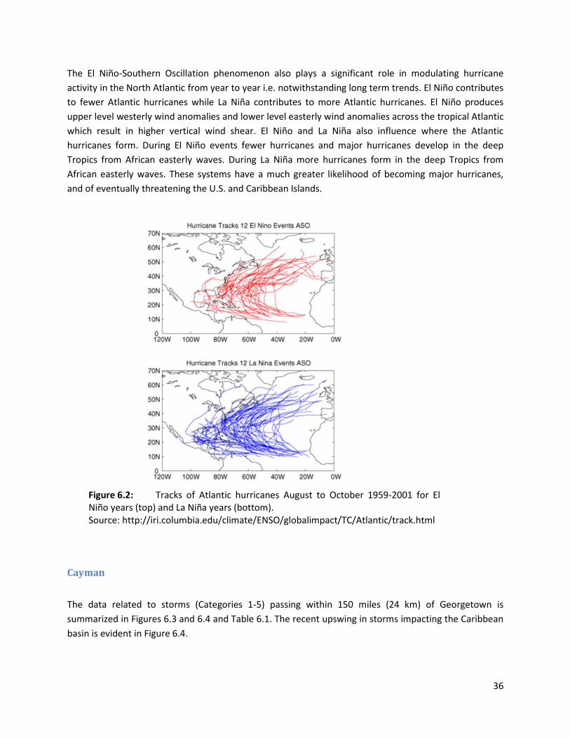
The El Niño-Southern Oscillation phenomenon also plays a significant role in modulating hurricane

activity in the North Atlantic from year to year i.e. notwithstanding long term trends. El Niño contributes

to fewer Atlantic hurricanes while La Niña contributes to more Atlantic hurricanes. El Niño produces

upper level westerly wind anomalies and lower level easterly wind anomalies across the tropical Atlantic

which result in higher vertical wind shear. El Niño and La Niña also influence where the Atlantic

hurricanes form. During El Niño events fewer hurricanes and major hurricanes develop in the deep

Tropics from African easterly waves. During La Niña more hurricanes form in the deep Tropics from

African easterly waves. These systems have a much greater likelihood of becoming major hurricanes,

and of eventually threatening the U.S. and Caribbean Islands.

Cayman

The data related to storms (Categories 1-5) passing within 150 miles (24 km) of Georgetown is

summarized in Figures 6.3 and 6.4 and Table 6.1. The recent upswing in storms impacting the Caribbean

basin is evident in Figure 6.4.

Figure 6.2: Tracks of Atlantic hurricanes August to October 1959-2001 for El Niño years (top) and La Niña years (bottom). Source: http://iri.columbia.edu/climate/ENSO/globalimpact/TC/Atlantic/track.html

37

Table 6.1: Storms passing with 150 miles (241 km) of Georgetown between 1950 and 2012. Only

Category 1 - 5 storms are shown. Source: HURDAT database.

Name of Storm Year Maximum Category Achieved within

Diameter

Gustav 2008 H3

Paloma 2008 H3

Dean 2007 H4

Emily 2005 H5

Ivan 2004 H5

Charlery 2004 H2

Lili 2002 H1

Isidore 2002 H1

Michelle 2001 H4

Iris 2001 H1

Lili 1996 H1

Gilbert 1988 H5

Katrina 1981 H1

Allen 1980 H5

Carmen 1974 H2

Alma 1970 H1

Beulah 1967 H3

Hattie 1961 H4

Hilda 1955 H2

Fox 1952 H4

Item 1951 H2

Charlie 1951 H2

King 1950 H1

Figure 6.3: Storms passing with 150 miles (241 km) of Georgetown between 1950 and 2012. Only Category 1 - 5 storms are shown. Source: HURDAT database.

38

6.2 Projections

The IPCC Special Report on Extremes (IPCC 2012) offers five summary statements with respect to

projections of future hurricane under global warming which are of relevance to the Cayman Islands.

They are reiterated below as major conclusions and supported with additional information (where

available) specific for the Atlantic basin.

Conclusion 1: There is low confidence in projections of changes in tropical cyclone genesis, location,

tracks, duration, or areas of impact.

Tropical cyclone genesis and track variability is modulated in most regions by known modes of

atmosphere–ocean variability. The details of the relationships vary by region (e.g., El Niño events tend

to suppress Atlantic storm genesis and development). The accurate modeling, then, of tropical cyclone

activity fundamentally depends on the model’s ability to reproduce these modes of variability i.e. to

produce reliable projections of the behaviour of these modes of variability (e.g., ENSO) under global

warming, as well as on a good understanding of their physical links with tropical cyclones. At present

there is still uncertainty in the model’s ability to project these behaviours.

Conclusion 2: Based on the level of consistency among models, and physical reasoning, it is likely that

tropical cyclone related rainfall rates will increase with greenhouse warming.

Figure 6.4: Number of named storms passing with 150 miles (241 km) of Georgetown between 1950 and 2012 sorted by decade. Only Category 1 - 5 storms are shown. Source: HURDAT database.

39

Observed changes in rainfall associated with tropical cyclones have not been clearly established.

However, as water vapor in the tropics increases there is an expectation for increased heavy rainfall

associated with tropical cyclones. Models in which tropical cyclone precipitation rates have been

examined are highly consistent in projecting increased rainfall within the area near the tropical cyclone

center under 21st century warming, with increases of 3 to 37% (Knutson et al., 2010). Typical projected

increases are near 20% within 100 km of storm centers (see Figure 6.5). More recent work premised on

RCP 4.5 suggest that rainfall rates increase robustly for the CMIP3 and CMIP5 scenarios (Knutson et al.

2013). For the late-twenty-first century, the increase amounts to +20% to +30% in the model hurricane’s

inner core, with a smaller increase (~10%) at radii of 200 km or larger.

Conclusion 3: It is likely that the global frequency of tropical cyclones will either decrease or remain

essentially unchanged.

Hurricane research done at NOAA’s GFDL laboratory using regional models projects that Atlantic

hurricane and tropical storms are substantially reduced in number, for the average 21st century climate

change projected by current models, but will have higher rainfall rates, particularly near the storm

center. http://www.gfdl.noaa.gov/global-warming-and-hurricaneshttp://www.gfdl.noaa.gov/global-

warming-and-hurricanes

Conclusion 4: An increase in mean tropical cyclone maximum wind speed is likely, although increases

may not occur in all tropical regions.

Figure 6.5: Rainfall rates (mm/day) associated with simulated tropical storms in a) a present climate b) warm climate c) warm minus present climate. Average warming is 1.72 oC. From Knutson et al. (2010).

Present Climate Warm Climate

Warm Climate - Present Climate

http://www.gfdl.noaa.gov/global-warming-and-hurricaneshttp:/www.gfdl.noaa.gov/global-warming-and-hurricanes

http://www.gfdl.noaa.gov/global-warming-and-hurricaneshttp:/www.gfdl.noaa.gov/global-warming-and-hurricanes

40

Assessments of projections by Knutson et al. (2010), Bender et al.,2010) and statistical-dynamical

models (Emanuel, 2007) are consistent that that greenhouse warming causes tropical cyclone intensity

to shift toward stronger storms by the end of the 21st century as measured by maximum wind speed

increases by +2 to +11%.

Conclusion 5: While it is likely that overall global frequency will either decrease or remain essentially

unchanged, it is more likely than not that the frequency of the most intense storms will increase

substantially in some ocean basins.

The downscaling experiments of Bender et al. (2010) project a 28% reduction in the overall frequency of

Atlantic storms and an 80% increase in the frequency of Saffir-Simpson category 4 and 5 Atlantic

hurricanes over the next 80 years using the A1B scenario. Downscaled projections using CMIP5 multi-

model scenarios (RCP4.5) as input (Knutson et al. 2013) still show increases in category 4 and 5 storm

frequency, but these are only marginally significant for the early 21st century (+45%) or the late 21st

century (+40%) using CMIP5 scenarios.

Figure 6.6: late 21st century warming projections of category 4 and 5 hurricanes in the Atlantic. Average of 18 CMIP3 models. From Bender et al. (2010).

41

It is noted that sea level rise will likely exacerbate storm surge impacts, even if the storms themselves do

not change.

Figure 6.7: IPCC AR5 Summary Diagram General consensus assessment of the numerical experiments described in IPCC (2013) Supplementary Material Tables 14.SM.1 to 14.SM.4. All values represent expected percent change in the average over period 2081–2100 relative to 2000–2019, under an A1B-like scenario, based on expert judgement after subjective normalization of the model projections. Four metrics were considered: the percent change in (I) the total annual frequency of tropical storms, (II) the annual frequency of Category 4 and 5 storms, (III) the mean Lifetime Maximum Intensity (LMI; the maximum intensity achieved during a storm’s lifetime) and (IV) the precipitation rate within 200 km of storm centre at the time of LMI. For each metric plotted, the solid blue line is the best guess of the expected percent change, and the coloured bar provides the 67% (likely) confidence interval for this value (note that this interval ranges across –100% to +200% for the annual frequency of Category 4 and 5 storms in the North Atlantic). Where a metric is not plotted, there are insufficient data (denoted ‘insf. d.’) available to complete an assessment. A randomly drawn (and coloured) selection of historical storm tracks are underlain to identify regions of tropical cyclone activity.

42

7. References

Bell, G. D., E. S. Blake, C. W. Landsea, T. B. Kimberlain, S. B. Goldenberg, J. Schemm, and R. J. Pasch,

2012: [Tropical cyclones] Atlantic basin [in “State of the Climate in 2011”]. Bulletin of the American

Meteorological Society, 93, S99-S105, doi:10.1175/2012BAM State of the Climate.

Bender, M. A., T. R. Knutson, R. E. Tuleya, J. J. Sirutis, G. A. Vecchi, S. T. Garner, and I. M. Held, 2010:

Modeled impact of anthropogenic warming on the frequency of intense Atlantic hurricanes. Science,

327, 454-458, doi:10.1126/science.1180568.

Emanuel, K., 2007: Environmental factors affecting tropical cyclone power dissipation. Journal of

Climate, 20, 5497-5509, doi:10.1175/2007JCLI1571.1.

Horton, R., C. Herweijer, C. Rosenzweig, J. Liu, V. Gornitz and A. C. Ruane, (2008): Sea level rise

projections for current generation CGCMs based on the semi-empirical method. Geophysical

Research Letters, 35, L02715.

IPCC, 2012: Managing the Risks of Extreme Events and Disasters to Advance Climate Change

Adaptation. A Special Report of Working Groups I and II of the Intergovernmental Panel on Climate

Change [Field, C.B., V. Barros, T.F. Stocker, D. Qin, D.J. Dokken, K.L. Ebi, M.D. Mastrandrea, K.J.

Mach, G.-K. Plattner, S.K. Allen, M. Tignor, and P.M. Midgley (eds.)]. Cambridge University Press,

Cambridge, UK, and New York, NY, USA, 582 pp.

Knutson, T. R., J. L. McBride, J. Chan, K. Emanuel, G. Holland, C. Landsea, I. Held, J. P. Kossin, A. K.

Srivastava, and M. Sugi, 2010: Tropical cyclones and climate change. Nature Geoscience, 3, 157-

163,doi:10.1038/ngeo779.

Knutson, Thomas R., and Coauthors, 2013: Dynamical Downscaling Projections of Twenty-First-

Century Atlantic Hurricane Activity: CMIP3 and CMIP5 Model-Based Scenarios. J. Climate, 26, 6591–

6617. doi: http://dx.doi.org/10.1175/JCLI-D-12-00539.1

Landsea, C. W., and J. L. Franklin, 2013: Atlantic hurricane database uncertainty and presentation of

a new database format. Monthly Weather Review, 141, 3576-3592, doi:10.1175/MWR-D-12-00254.1

McSweeney, C., New, M., Lizcano, G. & Lu, X. 2010. The UNDP Climate Change Country Profiles

Improving the Accessibility of Observed and Projected Climate Information for Studies of Climate

Change in Developing Countries. Bulletin of the American Meteorological Society, 91, 157-166.

Nakićenović, N., and R. Swart (eds.), 2000: Special Report on Emissions Scenarios. A Special Report of

Working Group III of the Intergovernmental Panel on Climate Change. Cambridge University Press,

Cambridge, United Kingdom and New York, NY, USA, 599 pp.

Palanisamy, H., M. Becker, B. Meyssignac, O. Henry, and A. Cazenave, 2012: Regional sea level

change and variability in the Caribbean sea since 1950. Journal of Geodetic Science, 2(2), 125-133.

Perrette, M. et al., 2013: A scaling approach to project regional sea level rise and its uncertainties.

Earth Syst. Dynam., 4, 11–29.

43

Rahmstorf, S., (2007): A semi-empirical approach to projecting future sea level rise. Science, 315

(5810), 368-370.

Rignot, E. and P. Kanagaratnam, (2006): Changes in the velocity structure of the Greenland Ice

Sheet. Science, 311(5763), 986-990.

Stephenson, T. S., L. A. Vincent, T. Allen, C. J. Van Meerbeeck, N. McLean, T. C. Peterson, M. A. Taylor, A. P. Aaron-Morrison, T. Auguste, D. Bernard, J. R. I. Boekhoudt, R. C. Blenman, G. C. Braithwaite, G. Brown, M. Butler, C. J. M. Cumberbatch, S. Etienne-Leblanc, D. E. Lake, D. E. Martin, J. L. McDonald, M. O. Zaruela, A. O. Porter, M. S. Ramirez, G. A. Tamar, B. A. Roberts, S. Sallons Mitro, A. Shaw, J. M. Spence, A. Winter and A. R. Trotman, 2014: Changes in extreme temperature and precipitation in the Caribbean region, 1961–2010. Int. J. Climatol. DOI: 10.1002/joc.3889.

Torres, R. R., and M. N. Tsimplis (2013), Sea-level trends and interannual variability in the Caribbean

Sea, J. Geophys. Res. Oceans, 118, 2934–2947, doi:10.1002/jgrc.20229.

Taylor, M. A., A. Centella, J. Charlery, A. Benzanilla, J. Campbell, I. Borrajero, T. Stephenson, and R.

Nurmohamed, 2013: The PRECIS-Caribbean Story: Lessons and Legacies. Bull. Amer. Meteor. Soc doi:

10.1175/BAMS-D-11-00235

Climate Profile for the Cayman Islands

Documents

Transcript of Climate Profile for the Cayman Islands