Representations of Quiver Hecke Algebras via Lyndon Bases
37
arXiv:0912.2067v2 [math.RT] 30 Dec 2009 REPRESENTATIONS OF QUIVER HECKE ALGEBRAS VIA LYNDON BASES DAVID HILL, GEORGE MELVIN, AND DAMIEN MONDRAGON Abstract. A new class of algebras has been introduced by Khovanov and Lauda and indepen- dently by Rouquier. These algebras categorify one-half of the Quantum group associated to arbitrary Cartan data. In this paper, we use the combinatorics of Lyndon words to construct the irreducible representations of those algebras associated to Cartan data of finite type. This completes the classification of simple modules for the quiver Hecke algebra initiated by Kleshchev and Ram. 1. Introduction 1.1. Recently, Khovanov and Lauda [KL1, KL2] and Rouquier [Rq] have independently introduced a remarkable family of graded algebras, H (Γ), defined in terms of quivers associated to the Dynkin diagram, Γ, of a symmetrizable Kac-Moody algebra, g. These algebras have been given several names, including Khovanov-Lauda-Rouquier algebras, quiver nil-Hecke algebras, quiver Hecke al- gebras, and “the rings R(ν )” (here ν refers to an element in the positive cone Q + inside the root lattice of g). The main property of these algebras is that K(Γ) ∼ = U ∗ A (n) as twisted bimodules, where K(Γ) is the Grothendieck group of the full subcategory, Rep(Γ), of finite dimensional graded H (Γ)-modules, n is a maximal nilpotent subalgebra of g, and U ∗ A (n) is an integral form of the quantized enveloping algebra, U q (n). Further evidence of the importance of these algebras was obtained in [BK2]. In this work, Brundan and Kleshchev showed that when Γ is of type A ∞ or A (1) ℓ−1 , there is an isomorphism between blocks of cyclotomic Hecke algebras of symmetric groups, and blocks of a corresponding quotient of H (Γ). Moreover, this isomorphism applies equally well to the Hecke algebra and its rational degeneration, depending only on Γ and the underlying ground field. In light of the work [BK1], it is expected that a similar relationship should hold between interesting quotients of H (Γ) and cyclotomic Hecke-Clifford algebras when Γ is of type B ∞ and A (2) 2ℓ . For these reasons, we choose to use the name “quiver Hecke algebra ” to describe H (Γ). 1.2. In [HKS], Hill, Kujawa and Sussan investigated the representation theory of the (degenerate) affine Hecke-Clifford algebra, HC(d), over C. In this paper, the authors constructed an analogue of the Arakawa-Suzuki functor [AS] between the category O for the Lie superalgebra q(n) and a certain category, RepHC(d), of integral finite dimensional modules for HC (d). By considering small rank instances of the functor, the authors obtained analogues of Zelevinsky’s segment representations, [BZ, Z], for HC(d). More generally, the Verma modules for q(n) correspond under the functor to certain induced modules, which by [HKS, Theorem 4.4.10] have unique irreducible quotients. The 2000 Mathematics Subject Classification. Primary 20C08; Secondary 17B37. Research of the first author was partially supported by NSF EMSW21-RTG grant DMS-0354321. 1
Transcript of Representations of Quiver Hecke Algebras via Lyndon Bases
arX
iv:0
912.
2067
v2 [
mat
h.R
T]
30
Dec
200
9
REPRESENTATIONS OF QUIVER HECKE ALGEBRAS VIA LYNDON BASES
DAVID HILL, GEORGE MELVIN, AND DAMIEN MONDRAGON
Abstract. A new class of algebras has been introduced by Khovanov and Lauda and indepen-
dently by Rouquier. These algebras categorify one-half of the Quantum group associated to
arbitrary Cartan data. In this paper, we use the combinatorics of Lyndon words to construct
the irreducible representations of those algebras associated to Cartan data of finite type. This
completes the classification of simple modules for the quiver Hecke algebra initiated by Kleshchev
and Ram.
1. Introduction
1.1. Recently, Khovanov and Lauda [KL1, KL2] and Rouquier [Rq] have independently introduced
a remarkable family of graded algebras, H(Γ), defined in terms of quivers associated to the Dynkin
diagram, Γ, of a symmetrizable Kac-Moody algebra, g. These algebras have been given several
names, including Khovanov-Lauda-Rouquier algebras, quiver nil-Hecke algebras, quiver Hecke al-
gebras, and “the rings R(ν)” (here ν refers to an element in the positive cone Q+ inside the root
lattice of g). The main property of these algebras is that
K(Γ) ∼= U∗A(n)
as twisted bimodules, where K(Γ) is the Grothendieck group of the full subcategory, Rep(Γ), of
finite dimensional graded H(Γ)-modules, n is a maximal nilpotent subalgebra of g, and U∗A(n) is an
integral form of the quantized enveloping algebra, Uq(n).
Further evidence of the importance of these algebras was obtained in [BK2]. In this work,
Brundan and Kleshchev showed that when Γ is of type A∞ or A(1)ℓ−1, there is an isomorphism
between blocks of cyclotomic Hecke algebras of symmetric groups, and blocks of a corresponding
quotient of H(Γ). Moreover, this isomorphism applies equally well to the Hecke algebra and its
rational degeneration, depending only on Γ and the underlying ground field. In light of the work
[BK1], it is expected that a similar relationship should hold between interesting quotients of H(Γ)
and cyclotomic Hecke-Clifford algebras when Γ is of type B∞ and A(2)2ℓ . For these reasons, we
choose to use the name “quiver Hecke algebra” to describe H(Γ).
1.2. In [HKS], Hill, Kujawa and Sussan investigated the representation theory of the (degenerate)
affine Hecke-Clifford algebra, HC(d), over C. In this paper, the authors constructed an analogue of
the Arakawa-Suzuki functor [AS] between the category O for the Lie superalgebra q(n) and a certain
category, RepHC(d), of integral finite dimensional modules for HC(d). By considering small rank
instances of the functor, the authors obtained analogues of Zelevinsky’s segment representations,
[BZ, Z], for HC(d). More generally, the Verma modules for q(n) correspond under the functor to
certain induced modules, which by [HKS, Theorem 4.4.10] have unique irreducible quotients. The
2000 Mathematics Subject Classification. Primary 20C08; Secondary 17B37.
Research of the first author was partially supported by NSF EMSW21-RTG grant DMS-0354321.
1
2 DAVID HILL, GEORGE MELVIN, AND DAMIEN MONDRAGON
authors went on to obtain a construction of all the irreducible integral representations using the
combinatorics of Lyndon words together with [BK1, Theorem 7.17].
It is instructive to describe their result in more detail. To this end, let Γ be a Dynkin diagram
of finite type with nodes labelled by the index set I, fix a total ordering, ≤, on I. Let F be
the free associative algebra generated by the letters [i], i ∈ I, with the concatenation product
[i1] · · · [ik] = [i1, . . . , ik], and give the monomials in F the lexicographic ordering determined by
I. It was first notices in [LR] that certain monomials in F associated to this ordering, called
good Lyndon words, and their non-increasing products, called good words, naturally determine
various bases of the quantized enveloping algebra, Uq(n), of a maximal nilpotent subalgebra of the
semisimple Lie algebra g associated to Γ. This observation was further developed in the prophetic
paper of Leclerc, [Le], where it was first suggested that the bases arising from these combinatorics
should naturally correspond to representations of affine Hecke algebras, cf. [Le, Sections 6-7],
specifically [Le, Theorem 47, Conjecture 52].
In [HKS], the authors noticed that the character of each segment representation of HC(d) corre-
sponds in a natural way to a dual canonical basis element labeled by a good Lyndon word in type
B with respect to the standard Dynkin ordering on I (specialized at q = 1), see [HKS, Proposition
4.1.3, Theorem 4.1.8, Proposition 8.2.12]. This was a nontrivial observation since it applied only
after redeveloping the theory so that monomials are ordered lexicographically from right-to-left, a
technicality imposed by the functor, cf. [HKS, Lemma 8.2.13]. This choice had the effect of drasti-
cally simplifying both the good Lyndon words in type B, and their associated dual canonical basis
elements. More generally, the characters of standard modules naturally correspond to dual PBW
basis elements labeled by good words (again, at q = 1), [HKS, Theorem 8.5.1]. Finally, applying
[HKS, Theorem 4.4.10] completed the construction, [HKS, Theorem 8.5.5].
Motivated by the results of [HKS] and the conjectured connection between HC(d) and quiver
Hecke algebras of type B, we initiated a study of the representation theory of the category Rep(Γ),
for Γ of classical finite type, using the combinatorics of Lyndon words with respect to the standard
Dynkin ordering on I and the right-to-left lexicographic ordering described in [HKS]. Indeed, we
first observed that this simplified the good Lyndon words in every type (except for the long roots
in type C, which remain the same). Subsequently, we worked out the corresponding dual canonical
basis elements, b∗l , associated to each good Lyndon word, l, and constructed representations, 1l,
with character b∗l . The standard module, M(g), associated to a good word g is the module obtained
by parabolic induction:
M(g) = Ind1l1 ⊠ · · · ⊠ 1lk{cg},
where g = l1 · · · lk is the canonical factorization of g as a non-increasing product of good Lyndon
words and the term {cg} refers to a grading shift. These standard modules have the property that
their characters are given by dual PBW basis elements labelled by the corresponding good word,
and, therefore, give a basis for the Grothendieck group, K(Γ).
1.3. While this paper was in production, Kleshchev and Ram completed their own investigation
of Rep(Γ) using the combinatorics of Lyndon words, for Γ of arbitrary finite type. To describe
this paper in more detail, give I an arbitrary total ordering. The authors called an irreducible
H(Γ)-module cuspidal if its character is given by a dual canonical basis element associated to a
REPRESENTATIONS OF QUIVER HECKE ALGEBRAS VIA LYNDON BASES 3
good Lyndon word, cf. [KR2, Lemma 6.4]. They went on to prove an amazing lemma. Namely,
given a cuspidal representation, 1l, the module
M(lk) = Ind 1l ⊠ · · · ⊠ 1l︸ ︷︷ ︸k times
{clk}
remains irreducible for all k > 1, [KR2, Lemma 6.6]. We want to point out that this lemma applies
equally well to all possible orderings on I and all finite root systems. Combining [KR2, Lemma 6.6]
with a straightforward Frobenius reciprocity argument shows that the standard module M(g) has
a unique irreducible quotient L(g), [KR2, Theorem 7.2]. In this way, Kleshchev and Ram reduced
the study of Rep(Γ) to the construction of cuspidal representations. They went on to construct
all cuspidal representations in types ABCDG as well as E6 and E7 using the standard Dynkin
ordering, the good Lyndon words in [LR, Le], and the corresponding root vectors in [Le, Section
8], cf. [KR2, Section 8]. In type A they produced cuspidal representations for all orderings on I.
1.4. Given the beautiful results in [KR2], we expanded the goal of this paper. In particular, our
main result is a complete determination of the cuspidal representations of H(Γ) in all finite types
using our ordering, Theorem 4.1.1. We would like to point out several advantages of our approach.
First, in classical type, our cuspidal representations tend to be much simpler than those appearing
in [KR2]. More specifically, in types BCD, our representations generally have dimension at most 2
(with the exception of the long roots in type C). In contrast, the cuspidal modules constructed by
Kleshchev an Ram generally have dimensions that grow with the height of an associated positive
root. Another advantage can be seen when considering the case of E8. The main difficulty for
Kleshchev and Ram is that not all the E8 root vectors are homogeneous in the sense of [KR1],
see [KR2, Section 8]. On the other hand, in our ordering, all good Lyndon words in type E8
are homogeneous. Finally, in §2.5, 3.4, and 4.3 we explain exactly how to relate the right-to-left
lexicographic ordering used here to the more standard left-to-right lexicographic ordering in [Le]
and [KR2].
In this paper, we only use the half of the bialgebra structure of K(Γ) coming from parabolic
induction. It would also be interesting to consider the structure coming from restriction and
compare the work here to that of Lauda and Vazirani, [LV].
Finally, we would like to point out that the description of the simple modules for the quiver
Hecke algebra of type B is nearly identical to the description of the irreducible HC(d)-modules
appearing in [HKS]. In particular, it is possible to define an action of (an appropriately defined)
quiver Hecke-Clifford superalgebra of type B on the segment representations of HC(d). Moreover,
this action extends easily to standard modules. Based on small rank calculations, we conjecture
that this action factors through the unique simple quotients. We feel that an investigation of this
phenomenon should shed light into the relationship between the type B quiver Hecke algebra and
the Hecke-Clifford algebra, but this is a topic of another paper.
1.5. The remainder of the paper is organized as follows. In Section 2 we describe the embedding of
the quantum group Uq(n) inside the q-shuffle algebra F and describe the combinatorics of Lyndon
words in our set-up following [Le] and [HKS, Section 8] closely. In Section 3 we introduce the quiver
Hecke algebra and describe some of the basic properties of the category Rep(Γ). In Section 4 we
4 DAVID HILL, GEORGE MELVIN, AND DAMIEN MONDRAGON
introduce cuspidal representations, and standard representations and state the main theorem of the
paper, Theorem 4.1.1. In Section 5 we determine the good Lyndon words and corresponding root
vectors, and Section 6 contains the construction of cuspidal representations. Finally, Appendix A
contains the calculations relevant to Section 5.
Acknowledgement. We would like to thank both Alexander Kleshchev and Arun Ram for encour-
aging us to work out the cuspidal representations in types E and F , as well as for their extremely
useful comments on an earlier draft of the paper. The first author would additionally like to thank
the algebra group in the department of Mathematics at the University of California, Berkeley, and
particularly his sponsor, Mark Haiman, for giving him the opportunity to teach a graduate course
in the spring of 2009, where the idea to write this paper was first realized.
2. Quantum Groups
2.1. Root Data. Let g be a simple finite dimensional Lie algebra of rank r over C, with Dynkin
diagram Γ and let I denote the set of labels of the nodes of Γ. Let Uq(g) be the corresponding
quantum group over Q(q) with Chevalley geneators ei, fi, i ∈ I. Let n ⊆ g be the subalgebra
generated by the ei, i ∈ I. Let ∆ be the root system of g relative to this decomposition, ∆+
the positive roots, and Π = {αi|i ∈ I} the simple roots. Let Q be the root lattice and Q+ =∑
i∈I Z≥0αi. Let A = (aij)i,j∈I be the Cartan matrix of g and (·, ·) denote symmetric bilinear form
on h∗ satisfying
aij =2(αi, αj)
(αi, αi), di =
(αi, αi)
2∈ {1, 2, 3}.
Let qi = qdi . Define the q-integers and q-binomial coefficients:
[k]i =qki − q−kiqi − q−1
i
, [k]i! = [k]i · · · [2]i[1]i,[mk
]
i=
[m]i!
[k]i![m− k]i!.
For later purposes, we also define the following. Let ν ∈ Q+, say ν =∑i∈I ciαi. Define the
height of ν:
ht(ν) =∑
i∈I
ci.
Next, given i = (i1, . . . , id) ∈ Id, define the content of i by
cont(i) =∑
i∈I
niαi, ni = #{j = 1, . . . , d | ij = i}.
Finally, if ht(ν) = d, set Iν = {i ∈ Id|cont(i) = ν}. Let Sd denote the symmetric group on d letters,
generated by simple transpositions s1, . . . , sd−1. Then, Sd acts Id by place permutation and we
denote this action by w · i, w ∈ Sd, i ∈ Id. Observe that the orbits of this action are precisely the
sets Iν with ht(ν) = d.
2.2. Embedding of Uq(n) in the Quantum Shuffle Algebra. The algebra Uq := Uq(n) is a
quotient of the free algebra generated by the Chevalley generators ei, i ∈ I by the relations
∑
r+s=1−aij
(−1)r[1 − aijr
]
i
eri ejesi = 0.
It is naturally Q+-graded by assigning to ei the degree αi. Let |u| be the Q+-degree of a homoge-
neous element u ∈ Uq.
REPRESENTATIONS OF QUIVER HECKE ALGEBRAS VIA LYNDON BASES 5
In [K], Kashiwara proved that there exist q-derivations e′i, i ∈ I given by
e′i(ej) = δij and e′i(uv) = e′i(u)v + q−(αi,|u|)ue′i(v)
for all homogeneous u, v ∈ Uq. For each i ∈ I, e′i(u) = 0 if, and only if |u| = 0.
Now, let F be the free associative algebra over Q(q) generated by the set of letters {[i]|i ∈
I}. Letters should not be confused with q-integers, which always occur with a subscript. Write
[i1, . . . , ik] := [i1] · [i2] · · · [ik], and let [] denote the empty word. The algebra F is Q+ graded by
assigning the degree αi to [i] (as before, let |f | denote the Q+-degree of a homogeneous f ∈ F).
Notice that F also has a principal grading obtained by setting the degree of a letter [i] to be 1; let
Fd be the dth graded component in this grading.
Now, define the (quantum) shuffle product, ∗, on F inductively by
(x · [i]) ∗ (y · [j]) = (x ∗ (y · [j]) · [i] + q−(|x|+αi,αj)((x · [i]) ∗ y) · [j], x ∗ [] = [] ∗ x = x. (2.2.1)
Iterating this formula yields
[i1, . . . , iℓ] ∗ [iℓ+1, . . . , iℓ+k] =∑
w∈D(ℓ,k)
q−e(w)[iw−1(1), . . . , iw−1(k+ℓ)] (2.2.2)
where D(ℓ,k) is the set of minimal coset representatives in Sℓ+k/Sℓ × Sk and
e(w) =∑
s≤ℓ<tw(s)<w(t)
(αis , αit),
see [Le, §2.5]. The product ∗ is associative and, [Le, Proposition 1],
x ∗ y = q−(|x|,|y|)y∗x (2.2.3)
where ∗ is obtained by replacing q with q−1 in the definition of ∗.
Now, to f = [i1, . . . , ik] ∈ F , associate ∂f = e′i1 · · · e′ik
∈ EndUq, and ∂[] = IdUq. Then,
Proposition 2.2.1. [R1, R2, G] There exists an injective Q(q)-linear homomorphism
Ψ : Uq → (F , ∗)
defined on homogeneous u ∈ Uq by the formula Ψ(u) =∑∂f (u)f , where the sum is over all
monomials f ∈ F such that |f | = |u|.
Therefore Uq is isomorphic to the subalgebra W ⊆ (F , ∗) generated by the letters [i], i ∈ I.
Let A = Q[q, q−1], and let UA denote the A-subalgebra of Uq generated by the divided powers
eki /[k]i! (i ∈ I, k ∈ Z≥0). Let (·, ·)K : Uq × Uq → Q(q) denote the unique symmetric bilinear form
satisfying
(1, 1)K = 1 and (e′i(u), v)k = (u, eiv)K (2.2.4)
for all i ∈ I, and u, v ∈ Uq. Let
U∗A = { u ∈ Uq | (u, v)K ∈ A for all v ∈ UA } (2.2.5)
and let u∗ ∈ U∗A denote the dual to u ∈ UA relative to (·, ·)K . It is well known that for u ∈ UA,ν ,
the map u∗ 7→ (u∗, ?)K defines an isomorphism U∗A,ν
∼= HomA(UA,ν ,A).
6 DAVID HILL, GEORGE MELVIN, AND DAMIEN MONDRAGON
Remark 2.2.2. Observe that the form we are using differs slightly from Lustig’s bilinear form
(·, ·)L. They are related by the formula
(u, v)L =∏
i∈I
1
(1 − q2i )ci
(u, v)K ,
if |u| = |v| =∑
i ciαi. In particular, if B is a basis of Uq consisting of homogeneous vectors, then
the adjoint basis of B with respect to (·, ·)K and (·, ·)L differ only by some normalization factors.
In particular, B is orthogonal with respect to (·, ·)K if, and only if it is orthogonal with respect to
(·, ·)L.
Throughout this paper, we will shall follow Leclerc and use the form (·, ·)K . In §3.5 we will
explain how both forms arise in representation theory, cf. Example 3.5.5 and Lemma 3.5.6.
Now, given a monomial
[ia11 , i
a22 , . . . , i
ak
k ] = [i1, . . . , i1︸ ︷︷ ︸a1
, i2, . . . , i2︸ ︷︷ ︸a2
, . . . , ik, . . . , ik︸ ︷︷ ︸ak
]
with ij 6= ij+1 for 1 ≤ j < k, let ca1,...,ak
i1,...,ik= [a1]i1 ! · · · [ak]ik !, so that (ca1,...,ak
i1,...,ik)−1ea1
i1· · · eak
ikis a
product of divided powers. Let
F∗A =
⊕Aca1,...,ak
i1,...,ik[ia1
1 , ia22 , . . . , i
ak
k ]
and W∗A = W ∩F∗
A. It is known that W∗A = Ψ(U∗
A), [Le, Lemma 8].
We close this section by describing some simple involutions of F which correspond, on restriction
to W , to important involutions on Uq. To this end, for ν =∑i ciαi ∈ Q+, define
N(ν) =1
2
((ν, ν) −
r∑
i=1
ci(αi, αi)
). (2.2.6)
Proposition 2.2.3. [Le, Proposition 6] Let f = [i1, . . . , ik], |f | = ν. Then,
(i) Let τ : F → F be the Q(q)-linear map defined by τ(f) = [ik, . . . , i1]. Then, τ(x ∗ y) =
τ(y) ∗ τ(x) for all x, y ∈ F . Hence, τ(Ψ(u)) = Ψ(τ(u)), where τ : Uq → Uq is the Q(q)-linear
anti-automorphism which fixes the generators ei.
(ii) Let − : F → F be the Q-linear map defined by q = q−1 and
f = qN(ν)[ik, . . . , i1].
Then, x ∗ y = x ∗ y for all x, y ∈ F . Hence, Ψ(u) = Ψ(u), where − is the bar involution on Uq.
(iii) Let σ : F → F be the Q-linear map such that σ(q) = q−1 and
σ(f) = qN(ν)f.
Then, σ(x) = τ(x) for all x ∈ F . Hence, Ψ(σ(u)) = σ(Ψ(u)), where σ : Uq → Uq is the Q-linear
anti-automorphism which sends q to q−1 and fixes the Chevalley generators ei.
REPRESENTATIONS OF QUIVER HECKE ALGEBRAS VIA LYNDON BASES 7
2.3. Good Words and Lyndon Words. In what follows, our conventions differ from those in
[Le]. In particular, we order monomials in F lexicographically reading from right to left. Except for
the type A case, this convention leads to some significant differences in the good Lyndon words that
appear. For the convenience of the reader, we include §2.5 which explains the connection between
the combinatorics developed using this ordering to those which arise using the more common left
to right lexicographic ordering.
The next two sections parallel [Le, Sections 3,4] with the statements of the relevant propositions
adjusted to conform to our choice of ordering.
For the remainder of the section, fix an ordering on the set of letters {[i]|i ∈ I} in F , denoted ≤,
and order Π accordingly. Give the set of monomials in F the associated lexicographic order read
from right to left, also denoted ≤. That is, set [i] < [] for all i ∈ I and
[i1, . . . , ik] < [j1, . . . , jℓ] if ik < jℓ, or for some m, ik−m < jℓ−m and ik−s = jℓ−s for all s < m.
Note that since the empty word is larger than any letter, every word is smaller than all of its right
factors:
[i1, . . . , ik] < [ij, . . . , ik], for all 1 < j ≤ k. (2.3.1)
(For those familiar with the theory, this definition is needed to ensure that the induced Lyndon
ordering on positive roots is convex, cf. §2.4 below.)
For a homogeneous element f ∈ F , let min(f) be the smallest monomial occurring in the
expansion of f . A monomial [i1, . . . , ik] is called a lower good word if there exists a homogeneous
w ∈ W such that [i1, . . . , ik] = min(w), and we say that it is Lyndon on the right if it is larger than
any of its proper left factors:
[i1, . . . , ij] < [i1, . . . , ik], for any 1 ≤ j < k.
Except for §2.5, we refer to these special words simply as good and Lyndon. Let G denote the set of
good words, L the set of Lyndon words, and GL = L∩ G ⊂ G the set of good Lyndon words. Also,
let GLd ⊂ Gd ⊂ Fd denote the degree d components of GL and G in the principal grading. Finally,
for ν ∈ Q+, let GLν ⊂ Gν ⊂ Fν be the homogeneous components of GL and G in the Q+ grading.
Lemma 2.3.1. [Le, Lemma 13] Every factor of a good word is good.
Because of our ordering conventions, [Le, Lemma 15, Proposition 16] become
Lemma 2.3.2. [Le, Lemma 15] Let l ∈ L, w a monomial such that w ≥ l. Then, min(w ∗ l) = wl.
and
Proposition 2.3.3. [Le, Proposition 16] Let l ∈ GL, and g ∈ G with g ≥ l. Then gl ∈ G.
Hence, we deduce from Lemma 2.3.1 and Proposition 2.3.3 [Le, Proposition 17]:
Proposition 2.3.4. [LR, Le] A monomial g is a good word if, and only if, there exist good Lyndon
words l1 ≥ . . . ≥ lk such that
g = l1l2 · · · lk.
As in [Le], we have
8 DAVID HILL, GEORGE MELVIN, AND DAMIEN MONDRAGON
Proposition 2.3.5. [LR, Le] The map l → |l| is a bijection GL → ∆+.
Given β ∈ ∆+, let β → l(β) be the inverse of the above bijection (called the Lyndon covering of
∆+).
We now define the bracketing of Lyndon words, that gives rise to the Lyndon basis of W . To
this end, given l ∈ L such that l is not a letter, define the standard factorization of l to be l = l1l2
where l2 ∈ L is a proper left factor of maximal length. Define the q-bracket
[f1, f2]q = f1f2 − q(|f1|,|f2|)f2f1 (2.3.2)
for homogeneous f1, f2 ∈ F in the Q+-grading. Then, the bracketing 〈l〉 of l ∈ L is defined
inductively by 〈l〉 = l if l is a letter, and
〈l〉 = [〈l1〉, 〈l2〉]q (2.3.3)
if l = l1l2 is the standard factorization of l.
Example 2.3.6. For g of type Br with I given in Table 5.1 below, we have
(1) 〈[0]〉 = [0];
(2) 〈[12]〉 = [[1], [2]]q = [12] − q−2[21];
(3) 〈[012]〉 = [[0], [12]− q−2[21]]q = [012]− q−2[021] − q−2[120] + q−4[210].
As is suggested in this example, we have
Proposition 2.3.7. [Le, Proposition 19] For l ∈ L, 〈l〉 = l + r where r is a linear combination of
words w such that |w| = |l| and w < l.
Any word w ∈ F has a canonical factorization w = l1 · · · lk such that l1, . . . , lk ∈ L and l1 ≥ · · · ≥
lk. We define the bracketing of an arbitrary word w in terms of this factorization: 〈w〉 = 〈l1〉 · · · 〈lk〉.
Define a homomorphism Ξ : (F , ·) → (F , ∗) by Ξ([i]) = [i]. Then, Ξ([i1, . . . , ik]) = [i1] ∗ · · · ∗ [ik] =
Ψ(ei1 · · · eik). In particular, Ξ(F) = W . We have the following characterization of good words:
Lemma 2.3.8. [Le, Lemma 21] The word w is good if and only if it cannot be expressed modulo
kerΞ as a linear combination of words v < w.
For g ∈ G, set rg = Ξ(〈g〉). Then, we have
Theorem 2.3.9. [Le, Propostion 22, Theorem 23] Let g ∈ G and g = l1 · · · lk be the canonical
factorization of g as a nonincreasing product of good Lyndon words. Then
(1) rg = rl1 ∗ · · · ∗ rlk ,
(2) rg = Ψ(eg) +∑
w<g xgwΨ(ew) where, for a word v = [i1, . . . , ik], ev = ei1 · · · eik , and
(3) {rg|g ∈ G} is a basis for W.
The basis {rg | g ∈ G} is called the Lyndon basis of W . An immediate consequence of Proposition
2.3.7 and Theorem 2.3.9 is the following:
Proposition 2.3.10. [Le, Proposition 24] Assume β1, β2 ∈ ∆+, β1 + β1 = β ∈ ∆+, and l(β1) <
l(β2). Then, l(β1)l(β2) ≥ l(β).
REPRESENTATIONS OF QUIVER HECKE ALGEBRAS VIA LYNDON BASES 9
This gives an inductive algorithm to determine l(β) for β ∈ ∆+ (cf. [Le, §4.3]):
For αi ∈ Π ⊂ ∆+, l(αi) = [i]. If β is not a simple root, then there exists a factorization
l(β) = l1l2 with l1, l2 Lyndon words. By Lemma 2.3.1, l1 and l2 are good, so l1 = l(β1) and
l2 = l(β2) for some β1, β2 ∈ ∆+ with β1 + β2 = β. Assume that we know l(β0) for all β0 ∈ ∆+
satisfying ht(β0) < ht(β). Define
C(β) = { (β1, β2) ∈ ∆+ × ∆+ | β = β1 + β2, and l(β1) < l(β2) }.
Then, Proposition 2.3.10 implies
Proposition 2.3.11. [Le, Proposition 25] We have
l(β) = min{ l(β1)l(β2) | (β1, β2) ∈ C(β) }
2.4. PBW and Canonical Bases. The lexicographic ordering on GL induces a total ordering on
∆+, which is convex, meaning that if β1, β2 ∈ ∆+ with β1 < β2, and β = β1 + β2 ∈ ∆+, then
β1 < β < β2 (cf. [R3, Le]). Indeed, assume β1, β2, β = β1 + β2 ∈ ∆+ and β1 < β2. Proposition
2.3.10 and (2.3.1) imply that l(β) ≤ l(β1)l(β2) < l(β2). If l(β) = l(β1)l(β2), then the definition
of Lyndon words implies l(β1) < l(β). We are therefore left to prove that l(β1) < l(β) even if
l(β) < l(β1)l(β2). This can be checked easily in all cases. We call this ordering a (right) Lyndon
ordering on ∆+.
Now, [Le, Corollary 27] becomes
Corollary 2.4.1. Let β ∈ ∆+. Then, l(β) is the largest good word of weight β.
Each convex ordering, β1 < · · · < βN , on ∆+ arises from a unique decomposition w0 =
si1si2 · · · siN of the longest element of the Weyl group of g via
β1 = αi1 , β2 = si1αi2 , · · · , βN = si1 · · · siN−1αiN .
Lusztig associates to this data a PBW basis of UA denoted
E(a1)(β1) · · ·E(an)(βN ), (a1, . . . , aN) ∈ ZN≥0.
Leclerc [Le, §4.5] describes the image in W of this basis for the convex Lyndon ordering. We use
the same braid group action as Leclerc and the results of [Le, §4.5, 4.6] carry over, making changes
in the same manner indicated in the previous section. We describe the relevant facts below.
For g = l(β1)a1 · · · l(βk)
ak , where β1 > · · · > βk and a1, . . . , ak ∈ Z>0 set
Eg = Ψ(E(ak)(βk) · · ·E(a1)(β1)) ∈ WA
and let E∗g ∈ W∗
A be the image of (E(ak)(βk) · · ·E(a1)(β1))
∗ ∈ U∗A. Observe that the order of the
factors in the definition of Eg above are increasing with respect to the Lyndon ordering. Leclerc
shows that if β ∈ ∆+, then
κl(β)El(β) = rl(β), (2.4.1)
For some κl(β) ∈ Q(q), [Le, Theorem 28] (the proof of this theorem in our case is obtained by
reversing all the inequalities and using the standard factorization as opposed to the costandard
10 DAVID HILL, GEORGE MELVIN, AND DAMIEN MONDRAGON
factorization). More generally, let g = la11 · · · lak
k ∈ G, l1 > · · · > lk ∈ GL. If l = l(β), write dl := di
if (β, β) = (αi, αi), and define
κg =k∏
i=1
κai
li[ai]li !. (2.4.2)
Then, Eg = κgσ(rg), where σ is defined in Propsition 2.2.3, [Le, §4.6]. Moreover,
E∗g = qcg(E∗
lm)∗am ∗ · · · ∗ (E∗l1)
∗a1 (2.4.3)
where cg =∑mi=1
(ai
2
)dli , [Le, §5.5.3].
It is well known that using the bar involution (Proposition 2.2.3) we obtain a canonical basis
{bg | g ∈ G} for WA via the PBW basis {Eg | g ∈ G}, see [Le, Lemma 37]. It has the form
bg = Eg +∑
h∈Gh<g
χghEh. (2.4.4)
The dual canonical basis then has the form
b∗g = E∗g +
∑
h∈Gh>g
χ∗ghE
∗h. (2.4.5)
As in [Le] we have the following very important theorem:
Theorem 2.4.2. [Le, Theorem 40, Corollary 41]
(i) We have min(b∗g) = g for all g ∈ G. Moreover, the coefficient of g in b∗g is equal to κg.
(ii) For each l ∈ GL, E∗l = b∗l .
To describe the coefficient κl precisely, transport the symmetric bilinear form (2.2.4) to W via the
isomorphism Ψ. Let g = l(β1)a1 · · · l(βN )aN and h = l(β1)
b1 · · · l(βN )bN , where a1, . . . , aN , b1, . . . , bN ∈
Z≥0. Then, the form is given by
(Eg , Eh)K = δgh
n∏
j=1
(E(βj), E(βj))aj
K
{aj}(βj,βj)!(2.4.6)
where, for β =∑ri=1 ciαi ∈ ∆+,
(E(β), E(β))K =
∏ri=1(1 − q(αi,αi))ci
1 − q(β,β)(2.4.7)
and for a, b ∈ Z≥0,
{a}b! =
a∏
j=1
1 − qjb
1 − qb. (2.4.8)
Then, [Le, §5.5.2],
E∗l =
(−1)ℓ(l)−1κ−1l
qN(|l|)(El, El)Krl, (2.4.9)
where N(|l|) is given by (2.2.6)
REPRESENTATIONS OF QUIVER HECKE ALGEBRAS VIA LYNDON BASES 11
2.5. The Anti-Automorphism τ . We continue with a fixed ordering, ≤, on I and corresponding
sets G, L, and GL as described in §2.3. Define the opposite ordering on I by
x � y if, and only if, y ≤ x.
Given this opposite ordering, define the corresponding opposite total ordering on the monomials in
F by
[i1, . . . , ik] ≺ [j1, . . . , jℓ] if i1 ≺ j1, or for some m, im ≺ jm and is = js for all s < m,
and [] ≺ [i] for all i ∈ I.
For f ∈ F , max(f) is the largest monomial occuring in the expansion of f . Call a monomial
gτ = [i1, . . . , ik] ∈ F an upper good word if gτ = max(u) for some u ∈ Uq, and we say that it is
Lyndon on the left if it is smaller than all of its proper right factors:
[i1, . . . , ik] ≺ [ij , . . . , ik] for j > 1.
Let Gτ denote the set of upper good words, let Lτ denote the set of words that are Lyndon on the
left, and GLτ = Gτ ∩ Lτ .
Observe that the total ordering on GLτ induces a convex total ordering on ∆+ which we call
a (left) Lyndon ordering. Also, the bijection ∆+ → GLτ provides a means to compute lτ(β) for
each β ∈ ∆+, see [Le, Section 4]. Finally, given lτ ∈ Lτ , define its costandard factorization to be
lτ = lτ1 lτ2 , where lτ1 is the maximal proper word which is Lyndon on the left. Note that lτ2 is also
Lyndon on the left. Using the data above we may define a Lyndon basis {rgτ |gτ ∈ Gτ}, dual PBW
basis {E∗gτ | gτ ∈ Gτ} and dual canonical basis {b∗gτ | gτ ∈ Gτ} exactly as in [Le, Sections 4-5].
The next lemma gives the precise connection between the combinatorics appearing here and
those developed in [Le]:
Lemma 2.5.1. Under the anti-automorphism τ : F → F ,
(1) τ(W) = W;
(2) τ(G) = Gτ and τ(L) = Lτ ;
(3) τ(E∗g ) = E∗
τ(g);
(4) τ(b∗g) = b∗τ(g).
Proof: Property (1) is immediate from Proposition 2.2.3, and property (2) is clear from the
definitions.
We now turn to property (3). Observe that if g = l1 · · · lk, then τ(g) = τ(lk) · · · τ(l1). Therefore,
by equation (2.4.3), it is enough to show that τ(E∗l ) = E∗
τ(l) for all l ∈ GL. We prove this by
induction on the degree of l in the principal grading on F . The base case is clear since E∗[i] = r[i] =
[i].
For the inductive step, assume we have shown that τ(rl0 ) = rτ(l0) and τ(E∗l0
) = E∗τ(l0)
for all
l0 of degree less than the degree of l. Let l = l1l2 be the standard factorization of l. Then, by
(2), τ(l) = τ(l2)τ(l1) is the costandard factorization of τ(l). Then, it follows from (2.3.3) and the
12 DAVID HILL, GEORGE MELVIN, AND DAMIEN MONDRAGON
relevant definitions that
τ(rl) = τ(rl1 ∗ rl2 − q(|l1|,|l2|)rl2 ∗ rl1)
= τ(rl2 ) ∗ τ(rl1 ) − q(|l1|,|l2|)τ(rl1 ) ∗ τ(rl2 )
= rτ(l2) ∗ rτ(l1) − q(|l2|,|l1|)rτ(l1) ∗ rτ(l2)
= rτ(l).
It now follows that τ(E∗l ) = E∗
τ(l) by applying τ to equation (2.4.9) and observing that equations
(2.2.6) and (2.4.6)-(2.4.8) imply that the coefficient on the right-hand-side of (2.4.9) depend only
on |l| ∈ Q+.
Finally, property (4) for follows by applying τ to equation (2.4.5) and uniqueness.
From now on, we will write gτ = τ(g).
3. Quiver Hecke Algebras
In this section, we give a presentation of the quiver Hecke algebras following the notation of
[KR2]. Throughout, we work over an arbitrary ground field F.
3.1. Quivers with Compatible Automorphism. Let Γ be a graph. We construct a Dynkin
diagram Γ by giving Γ the structure of a graph with compatible automorphism in the sense of [L,
§12, 14]. To define the quiver Hecke algebra, we will use the notion of a quiver with compatible
automorphism as described in [Rq, §3.2.4].
Let I be the labelling set for Γ, and H be the (multi)set of edges. An automorphism a : Γ → Γ
is said to be compatible with Γ if, whenever (i, j) ∈ H is an edge, i is not in the orbit of j under a.
Fix a compatible automorphism a : Γ → Γ, and set I to be a set of representatives of the obits
of I under a and, for each i ∈ I, let αi ∈ I/a be the corresponding orbit. For i, j ∈ I, i 6= j define
(αi, αi) = 2|αi| and let
(αi, αj) = −|{(i′, j′) ∈ H | i′ ∈ αi, j′ ∈ αj}|.
For all i, j ∈ I, let aij = 2(αi, αj)/(αi, αi). Then, [L, Proposition 14.1.2] A = (aij)i,j∈I is a Cartan
matrix and every Cartan matrix arises in this way. Let Γ be the Dynkin diagram corresponding to
A. Moreover, the pairing (αi, αj) defined above agrees with the pairing on Q in §2.1.
Assume further that Γ is a quiver. That is, we have a pair of maps s : H → I and t : H → I
(the source and the target). We say that a is a compatible automorphism if s(a(h)) = a(s(h)) and
t(a(h)) = a(t(h)) for all h ∈ H . Set
dij = |{h ∈ H | s(h) ∈ αi and t(h) ∈ αj}/a|
and let m(i, j) = lcm{(αi, αi), (αj , αj)}. As noted in [Rq],
dij + dji = −2(αi, αj)/m(i, j). (3.1.1)
This data defines a matrix Q = (Qij(u, v))i,j∈I , where each Qij(u, v) ∈ F[u, v]. The polynomial
entries in Q are defined by Qii(u, v) = 0, and for i 6= j,
Qij(u, v) = (−1)dij(um(i,j)/(αi,αi) − vm(i,j)/(αj ,αj))−2(αi,αj)/m(i,j) (3.1.2)
REPRESENTATIONS OF QUIVER HECKE ALGEBRAS VIA LYNDON BASES 13
Specialize now to the case where Γ is of finite type. Then, as explained in [KR2, §3.1], the
polynomialsQij(u, v) (i 6= j) are completely determined by the Cartan matrix and a partial ordering
on I such that i→ j or j → i if aij 6= 0. In this case,
Qij(u, v) =
0 if i = j;
1 if aij = 0;
u−aij − v−aji if aij < 0 and i→ j;
v−aji − u−aij if aij < 0 and j → i.
(3.1.3)
3.2. Generators and Relations. Assume from now on that g is as in §2.1. Define the quiver
Hecke algebra
H(Γ) =⊕
ν∈Q+
H(Γ; ν),
where H(Γ; ν) is the unital F-algebra, with identity 1ν , given by generators and relations as de-
scribed below.
Assume that ht(ν) = d. The set of generators are
{e(i)|i ∈ Iν} ∪ {y1, . . . , yd} ∪ {φ1, . . . , φd−1}.
We refer to the e(i) as idempotents, the yr as Jucys-Murphy elements, and the φr as intertwining
elements. Indeed, these generators are subject to the following relations for all i, j ∈ Iν and all
admissible r, s:
e(i)e(j) = δi,je(i); (3.2.1)∑
i∈Iν
e(i) = 1ν ; (3.2.2)
yre(i) = e(i)yr; (3.2.3)
φre(i) = e(sr · i)φr ; (3.2.4)
yrys = ysyr; (3.2.5)
φrys = ysφr if s 6= r, r + 1; (3.2.6)
φrφs = φsφr if |s− r| > 1; (3.2.7)
φryr+1e(i) =
(yrφr + 1)e(i)
yrφre(i)
ir = ir+1,
ir 6= ir+1;(3.2.8)
yr+1φre(i) =
(φryr + 1)e(i)
φryre(i)
ir = ir+1,
ir 6= ir+1.(3.2.9)
Additionally, the intertwining elements satisfy the quadratic relations
φ2re(i) = Qir ,ir+1(yr, yr+1)e(i) (3.2.10)
14 DAVID HILL, GEORGE MELVIN, AND DAMIEN MONDRAGON
for all 0 ≤ r < d, and the braid-like relations
(φrφr+1φr − φr+1φrφr+1)e(i) (3.2.11)
=
(Qir,ir+1
(yr+2,yr+1)−Qir,ir+1(yr,yr+1)
yr+2−yr
)e(i) if ir = ir+2,
0 otherwise.
Finally, this algebra is graded via
deg e(i) = 0, deg yre(i) = (αir , αir ), and deg φre(i) = −(αir , αir+1). (3.2.12)
3.3. Basis Theorem. Let ν ∈ Q+ with ht(ν) = d. Given w ∈ Sd, fix a reduced decomposition
w = sk1 · · · sktfor w and define
φw = φk1 · · ·φkt.
Relations (3.2.10) and (3.2.11) imply that, in general, φw depends on the choice of reduced decom-
position.
Finally, we have
Theorem 3.3.1. [KL1, Theorem 2.5][Rq, Theorem 3.7] The set
{φwym11 · · · ymd
d e(i) |w ∈ Sd, m1, . . . ,md ∈ Z≥0, i ∈ Iν }
forms an F-basis for H(Γ; ν).
3.4. An Automorphism and Anti-Automorphism of H(Γ; ν). Let ν ∈ Q+, ht(ν) = d. As
observed in [KL1, §2.1], we have the following
Proposition 3.4.1. There is a unique F-linear automorphism τ : H(Γ; ν) → H(Γ; ν) given by
τ(e(i1, . . . , id)) = e(id, . . . , i1), τ(yr) = yd−r+1, and τ(φr) = −φd−r.
and
Proposition 3.4.2. There is a unique F-linear anti-automorphism ψ : H(Γ; ν) → H(Γ; ν) defined
by ψ(e(i)) = e(i), ψ(yr) = yr, and ψ(φr) = φr for all i ∈ Iν and admissible r.
3.5. Modules and Graded Characters. Given a finite dimensional Z-graded vector space V =⊕
k∈Z V [k], define the graded dimension of V to be
dimq V =∑
k∈Z
(dim V [k])qk ∈ Z≥0[q, q−1].
Let V{s} denote the vector space obtained from V by shifting the grading by s. That is,
dimq V{s} = qsdimq V.
The algebra H(Γ; ν) is Z-graded by (3.2.12). Let Rep(Γ; ν) denote the category of all finite
dimensional gradedH(Γ; ν)-modules. LetM be in Rep(Γ; ν). For each i ∈ Iν , define the generalized
i-eigenspace by Mi := e(i)M . We have the decomposition
M =⊕
i∈Iν
Mi.
Moreover, by (3.2.4), φrMi = Msr·i. Finally, note that since the elements yre(i) have positive
degree, they act nilpotently on all objects in Rep(Γ; ν).
REPRESENTATIONS OF QUIVER HECKE ALGEBRAS VIA LYNDON BASES 15
Morphisms are degree 0 H(Γ; ν)-homomorphisms. That is, for eachM,N ∈ Rep(Γ; ν), homν(M,N)
denotes the set of degree 0 homomorphisms.
Let K(Γ; ν) = K(Rep(Γ; ν)) be the Grothendieck group of the category Rep(Γ; ν), and
K(Rep(Γ)) := K(Γ) =⊕
ν∈Q+
K(Γ; ν).
This is a free Z[q, q−1]-module with basis given by isomorphism classes of simple H(Γ)-modules.
Note that since morphisms have degree 0, L ≇ L{s} for any simple module L ∈ Rep(Γ; ν) and any
s 6= 0. We write [M ] ∈ K(Γ; ν) for the image of M ∈ Rep(Γ; ν) in the Grothendieck group. Finally,
observe that qs[M ] = [M{s}]. Define the formal character ch : Rep(Γ; ν) → F by
chM =∑
i∈Iν
(dimqMi) · [i].
Theorem 3.5.1. [KL1, Theorem 3.17] The character map induces an injective Q(q)-linear map
ch : K(Γ; ν) → F .
Now, let ν, ν′ ∈ Q+ and let H(Γ; ν, ν′) := H(Γ; ν) ⊗ H(Γ; ν′). Given i = (i1, . . . , id) ∈ Iν and
j = (j1, . . . , jd′) ∈ Iν′
, let ij = (i1, . . . , id, j1, . . . , jd′). Then, there exists an embedding
ιν,ν′ : H(Γ; ν, ν′) → H(Γ; ν + ν′) (3.5.1)
given by ιν,ν′ (e(i)⊗ e(j)) = e(ij) and, for appropriate r and s, and for a and b among the symbols
y or φ,
ιν,ν′ (ar ⊗ bs) = arbs+d.
If M ∈ Rep(Γ; ν) and N ∈ Rep(Γ; ν′), let M ⊠ N ∈ Rep(Γ; ν) ⊗ Rep(Γ; ν′) denote the outer
tensor product of M and N . We have
Proposition 3.5.2. [KL1, Proposition 2.16] We have ιν,ν′ (1ν ⊗ 1ν′)H(Γ; ν + ν′) is a free graded
left H(Γ; ν, ν′)-module.
Therefore, we may define the exact functors
Resν+ν′
ν,ν′ : H(Γ; ν + ν′) → H(Γ; ν, ν′) (3.5.2)
by Resν+ν′
ν,ν′ M = ιν,ν′(1ν ⊗ 1ν′)M , and
Indν+ν′
ν,ν′ : H(Γ; ν, ν′) → H(Γ; ν + ν′), (3.5.3)
by
Indν+ν′
ν,ν′ M ⊠N = H(Γ; ν + ν′) ⊗H(Γ;ν,ν′) M ⊠N.
We have
Lemma 3.5.3. [KL1, Lemma 2.20] Assume that M ∈ Rep(Γ; ν), N ∈ Rep(Γ; ν′),
chM =∑
i∈Iν
mi[i] and chN =∑
i∈Iν′
nj [j].
Then,
ch Indν+ν′
ν,ν′ M ⊠N =∑
i∈Iν ,i∈Iν′
minj[j] ∗ [i]
where [j] ∗ [i] is the shuffle product given by (2.2.2).
16 DAVID HILL, GEORGE MELVIN, AND DAMIEN MONDRAGON
Remark 3.5.4. Observe that the order of the segments in the shuffle lemma is reversed. This is a
consequence of the definition (2.2.1) and is so that the terms in the character formula coming from
1 ⊗ (M ⊠ N) are not shifted in degree. Note that this is slightly different than the shuffle product
in [KR2]. The products are related by the formula
x ◦ y = y ∗ x
for x, y ∈ W.
Let Proj(Γ) (resp. Proj(Γ; ν)) denote the category of finitely generated, graded, projective (left)
H(Γ)-modules (resp. H(Γ; ν)-modules). Let K0(Γ) (resp. K0(Γ; ν)) denote Grothendieck group of
Proj(Γ) (resp. Proj(Γ; ν)), and set K0(Γ)Q(q) = K0(Γ)⊗AQ(q). Also, define the analogous functors
Indν+ν′
ν,ν′ and Resν+ν′
ν,ν′ to those for Rep(Γ).
Given a left H(Γ; ν)-module M , let Mψ be the right H(Γ; ν)-module given by mx = ψ(x)m for
all x ∈ H(Γ; ν) and m ∈ M . Define the Kashiwara-Khovanov-Lauda pairing (KKL), (·, ·)KKL :
K0(Γ; ν) ×K(Γ; ν) → A by
([P ], [M ])KKL =∏
i∈I
(1 − q2i )ci dimq (Pψ ⊗M), (3.5.4)
if ν =∑
i∈I ciαi. This form is evidently related to the Lusztig-Khovanov-Lauda pairing (LKL),
(·, ·)LKL, appearing in [KL1, (2.43),(2.44)] by the formula
([P ], [M ])KKL =∏
i∈I
(1 − q2i )ci ([P ], [M ])LKL, (3.5.5)
see Remark 2.2.2. Define the map ω : K(Γ) → K0(Γ)Q(q),
ω([M ]) =∑
[P ]∈B
([P ], [M ])KKL[P ], (3.5.6)
where the sum is over a basis B of K0(Γ), and M ∈ Rep(Γ).
Example 3.5.5. Let 1αidenote the unique irreducible H(Γ;αi)-module concentrated in degree 0.
It is one dimensional with the action of H(Γ;αi) given by e(j)1αi= δij1αi
, y11αi= {0}. Let Pαi
denote its projective cover. Then,
([Pαi], [1αi
])KKL = (1 − q2i ).
In particular, under the identification of K(Γ) with K∗0 (Γ), we have ω([1αi
]) = [Pαi] − [Pαi
{2di}].
That is, [1αi] is mapped by ω to its projective resolution
0 // Pαi{2di} // Pαi
// 1αi// 0 .
More generally, using [KR2, Lemma 3.2], we deduce that if L ∈ Rep(Γ; ν) is a simple module
satisfying σ(chL) = chL, PL ∈ Proj(Γ; ν) is its projective cover, and ν =∑i ciαi, then
([PL], [L])KKL =∏
i∈I
(1 − q2i )ci ,
so ω([L]) =∏i(1−q
2i )ci [PL]. On the other hand, if L,L′ ∈ Rep(Γ) are two simple modules as above,
([PL], [L′])LKL = δL,L′ ,
REPRESENTATIONS OF QUIVER HECKE ALGEBRAS VIA LYNDON BASES 17
so identifying K(Γ) with the dual lattice to K0(Γ) using the Lusztig-Khovanov-Lauda pairing does
not contain any representation theoretic information.
We identify K(Γ) with its image under ω. The following lemma shows that this image is the
dual lattice
K∗0 (Γ) = {X ∈ K0(Γ)Q(q) | (Y,X)LKL ∈ A for all Y ∈ K0(Γ)},
where
(·, ·)LKL : K0(Γ)Q(q) ×K0(Γ)Q(q) → Q(q) (3.5.7)
is the Lusztig-Khovanov-Lauda bilinear form, given by ([P ], [Q])LKL = dimq (Pψ ⊗H(Γ;ν) Q) for
P,Q ∈ Proj(Γ; ν), cf. [KL1, (2.45),(2.46),(2.47)].
Lemma 3.5.6. Under the identification above, the simple modules are dual to their projective
covers with respect to the Lusztig-Khovanov-Lauda bilinear form. In particular, the map X 7→
(ω(X), ?)LKL identifies the dual lattice K∗(Γ; ν) with the dual space HomA(K0(Γ; ν),A).
Proof: Let ν =∑
i ciαi ∈ Q+. Assume that {La|a ∈ A} is a basis for K(Γ; ν) for some indexing
set A, and let B in (3.5.6) be the basis forK0(Γ; ν) consisting of the projective coversPa of La, a ∈ A.
Then, by the definitions ([Pa], [Lb])KKL = δab∏i(1− q2i )
ci . Therefore, ω([La]) =∏i(1− q2i )
ci [Pa].
Also, ([Pb], [Pa])LKL = δba(1 − q2i )−ci . Hence,
(ω([Lb]), [Pa])LKL = (([Pb], [Lb])KKL[Pb], [Pa])LKL = ([Pb], [Lb])KKL([Pb], [Pa])LKL = δba.
Identifying U∗A,ν with HomA(UA,ν ,A) using Kashiwara’s bilinear form, we obtain the following
result which is dual to the main results in [KL1, KL2]:
Theorem 3.5.7. [KL1, Theorem 1.1],[KL2, Theorem 8] In the notation of §2.1-2.2, there is an
isomorphism of Q+-graded twisted bialgebras
γ∗ : K(Γ) → U∗A.
Define multiplication ◦ : K(Γ; ν) ⊗K(Γ; ν′) → K(Γ; ν + ν′) by
[M ] ∗ [N ] = [Indν+ν′
ν′,ν N ⊠M ].
Define multiplication on Proj(Γ) by [P ] · [Q] = [Indν+ν′
ν,ν′ P ⊠Q]. In light of Remark 3.5.4, we have
the following slight modification of [KR2, Lemma 3.5]:
Lemma 3.5.8. [KR2, Lemma 3.5] For P ∈ Proj(Γ; ν + ν′), M ∈ Rep(Γ; ν) and N ∈ Rep(Γ; ν′),
([P ], [M ] ∗ [N ])KKL = ([Resν+ν′
ν′,ν P ], [N ] ⊗ [M ])KKL.
For P ∈ Proj(Γ; ν), Q ∈ Proj(Γ; ν′), and M ∈ Rep(Γ; ν + ν′),
([P ] · [Q], [M ])KKL = ([P ] ⊗ [Q], [Resν+ν′
ν,ν′ M ])KKL.
Remark 3.5.9. We note that using (3.5.5) does not affect the lemma above, since the renormal-
ization factor on both sides of the equations above is the same.
18 DAVID HILL, GEORGE MELVIN, AND DAMIEN MONDRAGON
Observe that the order of ν and ν′ in the first equation of Lemma 3.5.8 have been reversed, but not
in the second. This implies that γ∗◦mult = mult◦(γ∗⊗γ∗)◦flip, where mult denotes the appropriate
multiplication map, and flip : K(Γ)⊗K(Γ) → K(Γ)⊗K(Γ) is the map flip([M ]⊗ [N ]) = [N ]⊗ [M ].
In particular, we have the following property of γ∗ as proved in [KR2].
Theorem 3.5.10. [KR2, Theorem 4.4(5)] For [M ], [N ] ∈ K(Γ),
γ∗([M ] ∗ [N ]) = γ∗([M ])γ∗([N ]).
We also record the following, which was proved in [KR2].
Theorem 3.5.11. [KR2, Theorem 4.4(3)] The following diagram commutes:
K(Γ)
ch""EE
EEEE
EE
γ∗
// U∗A
Ψ}}{{
{{{{
{{
W∗A
Proof: It is more convenient to show that ch ◦ (γ∗)−1 = Ψ. To this end, assume that u ∈ U∗A,ν .
Then, u may be written as
u =∑
ni1,...,idei1 · · · eid ,
where the sum is over all (i1, . . . , id) ∈ Iν .
Now, let 1αi∈ Rep(Γ;αi) be the unique irreducible representation, see Example 3.5.5. It is clear
from Theorem 3.5.7 that γ∗([1αi]) = ei. Therefore,
ch ◦ (γ∗)−1(u) = ch ◦ (γ∗)−1(∑
ni1,...,idei1 · · · eid
)
= ch(∑
ni1,...,id [1αi1] ∗ · · · ∗ [1αid
])
= ch(∑
ni1,...,id [Indναi1 ,...,αid1αid
⊠ · · · ⊠ 1αi1])
=∑
ni1,...,id [i1] ∗ · · · ∗ [id]
= Ψ(u).
Remark 3.5.12. We point out that Kleshchev and Ram prove several other important properties
of the isomorphism γ∗ in [KR2, Theorem 4.4]. However, as we do not use these properties, we refer
the reader to their paper for the details.
4. Standard Representations and their Simple Quotients
4.1. Cuspidal Representations. Following Kleshchev and Ram, we call a monomial f ∈ F a
weight of M ∈ Rep(Γ) if Mif6= 0, where if ∈ I∞ is the reading of the work f . That is, f = [if ].
Since the set of words in F is totally ordered, it makes sense to speak of the lowest weight of a
module.
Fix a (right) Lyndon ordering on ∆+. Continuing with the terminology of Kleshchev and Ram,
we call an irreducible module cuspidal if it has lowest weight l(β) ∈ GL for some β ∈ ∆+.
REPRESENTATIONS OF QUIVER HECKE ALGEBRAS VIA LYNDON BASES 19
Theorem 4.1.1. For the (right) Lyndon order on ∆+ used in Section 5, cuspidal representations
exist in all finite types. Moreover, for each l ∈ GL, ch1l = b∗l .
Proof: For types ABCDF , the representations are constructed explicitly in Section 6. We deduce
the E8 case from [KR1, Lemma 3.3, Theorems 3.6,3.10], since the corresponding Lyndon words are
homogeneous. Finally, the G2 case follows easily from the construction in [KR2] since the characters
are identical.
4.2. Standard Representations and Unique Irreducible Quotients. We continue to use the
ordering from Section 5. Given g ∈ G, g = l(β1) · · · l(βk), with β1 ≥ · · · ≥ βk define
M(g) = (Indβ1+···+βk
β1,...,βk1β1 ⊠ · · · ⊠ 1βk
){cg}.
The following is a consequence of Lemma 3.5.3, (2.4.3) and the definition.
Proposition 4.2.1. For each g ∈ G,
chM(g) = E∗g .
In particular, dimqM(g)ig
= κg.
The next theorem now follows from the previous proposition using Theorem 3.5.11.
Theorem 4.2.2. The set
{[M(g)] | g ∈ G}
forms a basis for K(Γ).
The following crucial lemma is proved in [KR2].
Lemma 4.2.3. [KR2, Lemma 6.6] Let g = lk for some l = l(β) ∈ GLd, then M(g) is irreducible.
The above lemma, together with a Frobenius reciprocity argument yields the main result of
[KR2]:
Theorem 4.2.4. [KR2, Theorem 7.2(i)] Let g ∈ Gd. Then M(g) has a unique maximal submodule
R(g) and unique simple quotient L(g).
As noted in [KR2], Khovanov and Lauda prove that for every simple module L, there is a unique
grading shift such that σ(chL{s}) = chL{s}, [KL1, §3.2]. Therefore, by Theorems 4.1.1 and 2.4.2,
and [Le, Proposition 32],
Theorem 4.2.5. [KR2, Theorem 7.2(iii)] We have σ(chL(g)) = chL(g).
Finally, we have
Theorem 4.2.6. [KR2, Theorem 7.2(iv)] The set
{[L(g)] | g ∈ G}
forms a basis for K(Γ).
20 DAVID HILL, GEORGE MELVIN, AND DAMIEN MONDRAGON
4.3. Twisting by the Automorphism τ . Finally, we close by relating the representation theory
coming from the (right) Lyndon orderings on ∆+ to the (left) Lyndon orderings that appear in
[KR2]. To this end, given M ∈ Rep(Γ), let M τ be the module obtained by twisting by the
automorphism τ , cf. Proposition 3.4.1. That is, M τ = M as graded vector spaces with x · m =
τ(x)m for all m ∈M τ .
Recall the opposite ordering and related notation developed in §2.5. We have the following:
Theorem 4.3.1. Let g ∈ G. Then, L(g)τ = L(gτ ).
Proof: First, it is immediate by character considerations that the cuspidal representations satisfy
1τl = 1lτ , see Lemma 2.5.1(4). Therefore, it follows that M(g)τ = M(gτ ) for all g ∈ G. The result
now follows since R is a submodule of M(g) if, and only if, Rτ is a submodule of M(gτ ).
5. Identification of Good Lyndon Words and Associated Root Vectors
We now give explicit descriptions of the good Lyndon words and associated root vectors for g
of classical type and type F4. In type E8 we determine the good Lyndon words. Throughout, we
write b∗[i] := b∗[i] for good Lyndon words l = [i].
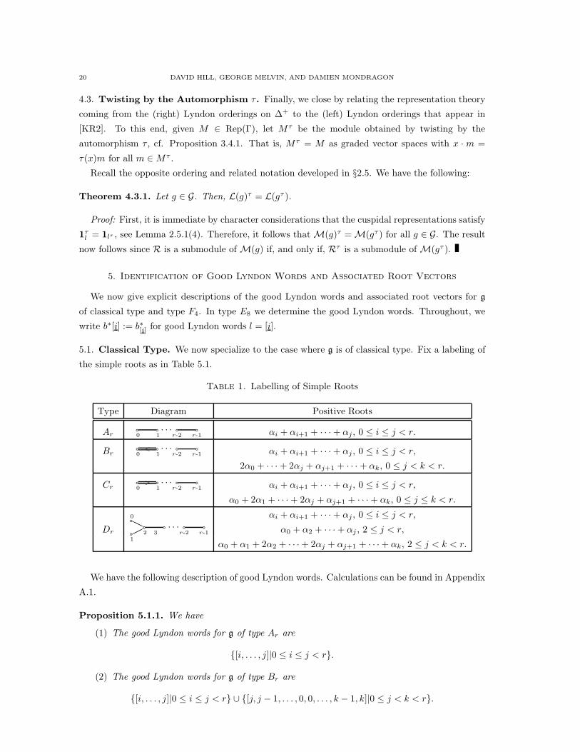
5.1. Classical Type. We now specialize to the case where g is of classical type. Fix a labeling of
the simple roots as in Table 5.1.
Table 1. Labelling of Simple Roots
Type Diagram Positive Roots
Ara a a a. . .0 1 r-2 r-1 αi + αi+1 + · · · + αj , 0 ≤ i ≤ j < r.
Bra a a a. . .<0 1 r-2 r-1 αi + αi+1 + · · · + αj , 0 ≤ i ≤ j < r,
2α0 + · · · + 2αj + αj+1 + · · · + αk, 0 ≤ j < k < r.
Cra a a a. . .>0 1 r-2 r-1 αi + αi+1 + · · · + αj , 0 ≤ i ≤ j < r,
α0 + 2α1 + · · · + 2αj + αj+1 + · · · + αk, 0 ≤ j ≤ k < r.
αi + αi+1 + · · · + αj , 0 ≤ i ≤ j < r,
Dr
a
a��
HH a a a a. . .
1
0
2 3 r-2 r-1 α0 + α2 + · · · + αj , 2 ≤ j < r,
α0 + α1 + 2α2 + · · · + 2αj + αj+1 + · · · + αk, 2 ≤ j < k < r.
We have the following description of good Lyndon words. Calculations can be found in Appendix
A.1.
Proposition 5.1.1. We have
(1) The good Lyndon words for g of type Ar are
{[i, . . . , j]|0 ≤ i ≤ j < r}.
(2) The good Lyndon words for g of type Br are
{[i, . . . , j]|0 ≤ i ≤ j < r} ∪ {[j, j − 1, . . . , 0, 0, . . . , k − 1, k]|0 ≤ j < k < r}.
REPRESENTATIONS OF QUIVER HECKE ALGEBRAS VIA LYNDON BASES 21
(3) The good Lyndon words for g of type Cr are
{[i, . . . , j]|0 ≤ i ≤ j < r} ∪ {[j, . . . , 1, 0, 1, . . . , k]|1 ≤ j < k ≤ r− 1}∪ {[0, . . . , j, 1, . . . , j]|1 ≤ j < r}.
(4) The good Lyndon words for g of type Dr are
{[0, 2, . . . , i]|2 ≤ i < r} ∪ {[i, . . . , j]|1 ≤ i ≤ j ≤ r − 1} ∪ {[j, . . . , 1, 0, 2, . . . , k]|1 ≤ j < k < r}.
We now list the root vectors associated to the good Lyndon words. Calculations can be found
in Appendix A.2
Proposition 5.1.2. (1) In type Ar,
b∗[i, . . . , j] = [i, . . . , j], 0 ≤ i ≤ j < r.
(2) In type Br:
b∗[i, . . . , j] = [i, . . . , j], 0 ≤ i ≤ j < r
b∗[j, . . . , 0, 0, . . . , k] = [2]0[j, . . . , 0, 0, . . . , k], 0 ≤ j < k < r.
(3) In type Cr:
b∗[i, . . . , j] = [i, . . . , j], 0 ≤ i ≤ j < r,
b∗[j, . . . , 1, 0, 1, . . . , k] = [j, . . . , 1, 0, 1, . . . , k], 1 ≤ j < k < r,
b∗[0, . . . , j, 1, . . . , j] = q[0] · ([1, . . . , j] ∗ [1, . . . , j]), 1 ≤ j < r.
(4) In type Dr:
b∗[0] = [0]
b∗[0, 2, . . . , i] = [0, 2, . . . , i], 2 ≤ i < r,
b∗[i, . . . , j] = [i, . . . , j], 1 ≤ i ≤ j < r,
b∗[1,0,2,...,j] = [1, 0, 2, . . . , j] + [0, 1, 2, . . . , j], 2 ≤ j < r,
b∗[j, . . . , 2, 1, 0, 2, . . . , k] = [j, . . . , 2, 1, 0, 2, . . . , k] + [j, . . . , 2, 0, 1, 2, . . . , k], 2 ≤ j < k < r.
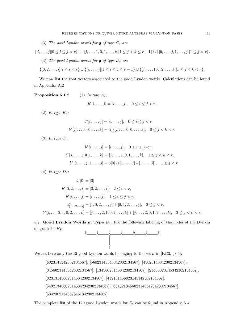
5.2. Good Lyndon Words in Type E8. Fix the following labeling of the nodes of the Dynkin
diagram for E8.0◦ ◦
2◦
1◦
3◦4
◦5
◦6
◦7
We list here only the 12 good Lyndon words belonging to the set E in [KR2, §8.3]:
[6023145342302134567], [56023145345342302134567], [45623145342302134567],
[3456023145342302134567], [13456023145342302134567], [23456023145342302134567],
[323131456023145342302134567], [432131456023145342302134567],
[543213456023145342342302134567], [6543213456023145342342302134567],
[53423021345676451342302134567].
The complete list of the 120 good Lyndon words for E8 can be found in Appendix A.4.
22 DAVID HILL, GEORGE MELVIN, AND DAMIEN MONDRAGON
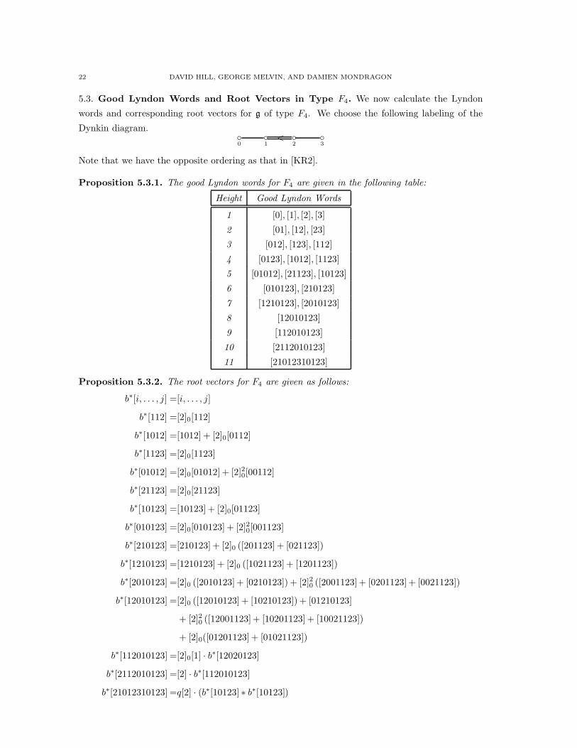
5.3. Good Lyndon Words and Root Vectors in Type F4. We now calculate the Lyndon
words and corresponding root vectors for g of type F4. We choose the following labeling of the
Dynkin diagram.◦ ◦ ◦< ◦0 1 2 3
Note that we have the opposite ordering as that in [KR2].
Proposition 5.3.1. The good Lyndon words for F4 are given in the following table:
Height Good Lyndon Words
1 [0], [1], [2], [3]
2 [01], [12], [23]
3 [012], [123], [112]
4 [0123], [1012], [1123]
5 [01012], [21123], [10123]
6 [010123], [210123]
7 [1210123], [2010123]
8 [12010123]
9 [112010123]
10 [2112010123]
11 [21012310123]
Proposition 5.3.2. The root vectors for F4 are given as follows:
b∗[i, . . . , j] =[i, . . . , j]
b∗[112] =[2]0[112]
b∗[1012] =[1012] + [2]0[0112]
b∗[1123] =[2]0[1123]
b∗[01012] =[2]0[01012] + [2]20[00112]
b∗[21123] =[2]0[21123]
b∗[10123] =[10123] + [2]0[01123]
b∗[010123] =[2]0[010123] + [2]20[001123]
b∗[210123] =[210123] + [2]0 ([201123] + [021123])
b∗[1210123] =[1210123] + [2]0 ([1021123] + [1201123])
b∗[2010123] =[2]0 ([2010123] + [0210123]) + [2]20 ([2001123] + [0201123] + [0021123])
b∗[12010123] =[2]0 ([12010123] + [10210123]) + [01210123]
+ [2]20 ([12001123] + [10201123] + [10021123])
+ [2]0([01201123] + [01021123])
b∗[112010123] =[2]0[1] · b∗[12020123]
b∗[2112010123] =[2] · b∗[112010123]
b∗[21012310123] =q[2] · (b∗[10123] ∗ b∗[10123])
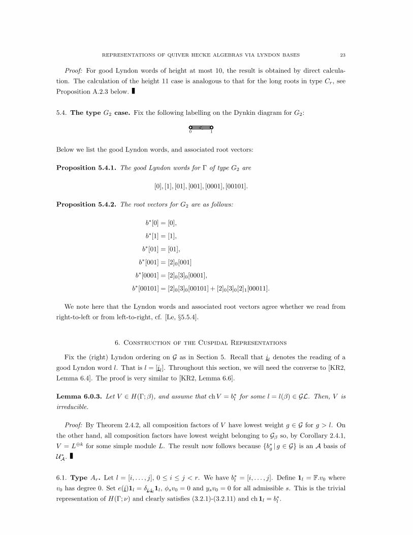
REPRESENTATIONS OF QUIVER HECKE ALGEBRAS VIA LYNDON BASES 23
Proof: For good Lyndon words of height at most 10, the result is obtained by direct calcula-
tion. The calculation of the height 11 case is analogous to that for the long roots in type Cr, see
Proposition A.2.3 below.
5.4. The type G2 case. Fix the following labelling on the Dynkin diagram for G2:
0 1<
Below we list the good Lyndon words, and associated root vectors:
Proposition 5.4.1. The good Lyndon words for Γ of type G2 are
[0], [1], [01], [001], [0001], [00101].
Proposition 5.4.2. The root vectors for G2 are as follows:
b∗[0] = [0],
b∗[1] = [1],
b∗[01] = [01],
b∗[001] = [2]0[001]
b∗[0001] = [2]0[3]0[0001],
b∗[00101] = [2]0[3]0[00101] + [2]0[3]0[2]1[00011].
We note here that the Lyndon words and associated root vectors agree whether we read from
right-to-left or from left-to-right, cf. [Le, §5.5.4].
6. Construction of the Cuspidal Representations
Fix the (right) Lyndon ordering on G as in Section 5. Recall that il denotes the reading of a
good Lyndon word l. That is l = [il]. Throughout this section, we will need the converse to [KR2,
Lemma 6.4]. The proof is very similar to [KR2, Lemma 6.6].
Lemma 6.0.3. Let V ∈ H(Γ;β), and assume that chV = b∗l for some l = l(β) ∈ GL. Then, V is
irreducible.
Proof: By Theorem 2.4.2, all composition factors of V have lowest weight g ∈ G for g > l. On
the other hand, all composition factors have lowest weight belonging to Gβ so, by Corollary 2.4.1,
V = L⊕k for some simple module L. The result now follows because {b∗g | g ∈ G} is an A basis of
U∗A.
6.1. Type Ar. Let l = [i, . . . , j], 0 ≤ i ≤ j < r. We have b∗l = [i, . . . , j]. Define 1l = F.v0 where
v0 has degree 0. Set e(i)1l = δi,il1l, φsv0 = 0 and ysv0 = 0 for all admissible s. This is the trivial
representation of H(Γ; ν) and clearly satisfies (3.2.1)-(3.2.11) and ch1l = b∗l .
24 DAVID HILL, GEORGE MELVIN, AND DAMIEN MONDRAGON
6.2. Type Br. The case l = [i, . . . , j], 0 ≤ i ≤ j < r is the trivial representation as in type Ar.
Let l = [j, . . . , 0, 0, . . . , k], 0 ≤ j < k < r. Then, b∗l = (q + q−1)[j, . . . , 0, 0, . . . , k]. Set 1l =
Fv1⊕Fv−1, where deg vi = i for i = ±1. Define e(i)11 = δi,il1l. Set yrv1 = 0 for all s, for s 6= j+1,
set φsv1 = 0, and define φj+1v1 = v−1. Set φrv−1 = 0 for all s, for s 6= j + 1, j + 2, set φrv−1 = 0,
and set yj+1v−1 = −v1 and yj+2v−1 = v1. We leave it as an easy exercise to the reader to check
that this satisfies (3.2.1)-(3.2.11) and ch1l = b∗l
6.3. Type Cr. For l 6= [0, . . . , j, 1, . . . , j], 1l is the trivial representations and may be computed as
in type Ar.
Assume l = [0, . . . , j, 1, . . . , j]. Then b∗l = q[0]([1, . . . , j] ∗ [1, . . . , j]). Let β = α1 + · · · + αj , and
consider the H(Γ;α0, 2β) module 1α0 ⊠ (Ind2ββ,β1β⊠1β){1}. Extend this to a H(Γ; 2β+α0) module
by insisting that φ1 acts as 0, and e(i) acts as 0 if i1 6= 0. It is very easy to check that this is the
desired cuspidal representation, 1l, cf. [KR2, §8.6].
6.4. Type Dr. For l 6= [1, 0, 2, . . . , k], 1 ≤ j < k < r, 1l is the trivial representation and can be
computed as in type Ar.
Assume l = [j, . . . , 1, 0, 2, . . . , k]. Define 1l = Fv0 ⊕ Fw0, where v0 and w0 have degree 0. Define
e(i)1l = δi,ilFv0 + δi,sj ·il
Fw0.
Define yr1l = 0. For r 6= j, define φr1l = 0 and set φjv0 = w0. It is elementary to check that this
is indeed a representation and ch1l = b∗l .
6.5. Type E8. We simply note here that in our ordering all Lyndon words for type E8 are ho-
mogeneous in the sense of [KR1] and the corresponding cuspidal representations can be computed
using [KR1, Theorems 3.6,3.10]. The 12 outstanding cases from [KR2] are listed in subsection 5.2
and are evidently homogeneous. An entire list of the good Lyndon words for E8 can be found in
Appendix A.4.
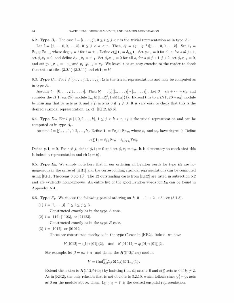
6.6. Type F4. We choose the following partial ordering on I: 0 → 1 → 2 → 3, see (3.1.3).
(1) l = [i, . . . , j], 0 ≤ i ≤ j ≤ 3.
Constructed exactly as in the type A case.
(2) l = [112], [1123], or [21123].
Constructed exactly as in the type B case.
(3) l = [1012], or [01012].
These are constructed exaclty as in the type C case in [KR2]. Indeed, we have
b∗[1012] = ([1] ∗ [01])[2], and b∗[01012] = q([01] ∗ [01])[2].
For example, let β = α0 + α1 and define the H(Γ; 2β, α2)-module
V = (Ind2ββ,β1β ⊠ 1β) ⊠ 1α2{1}.
Extend the action to H(Γ; 2β+α2) by insisting that φ4 acts as 0 and e(i) acts as 0 if i5 6= 2.
As in [KR2], the only relation that is not obvious is 3.2.10, which follows since y24 − y5 acts
as 0 on the module above. Then, 1[01012] = V is the desired cuspidal representation.
REPRESENTATIONS OF QUIVER HECKE ALGEBRAS VIA LYNDON BASES 25
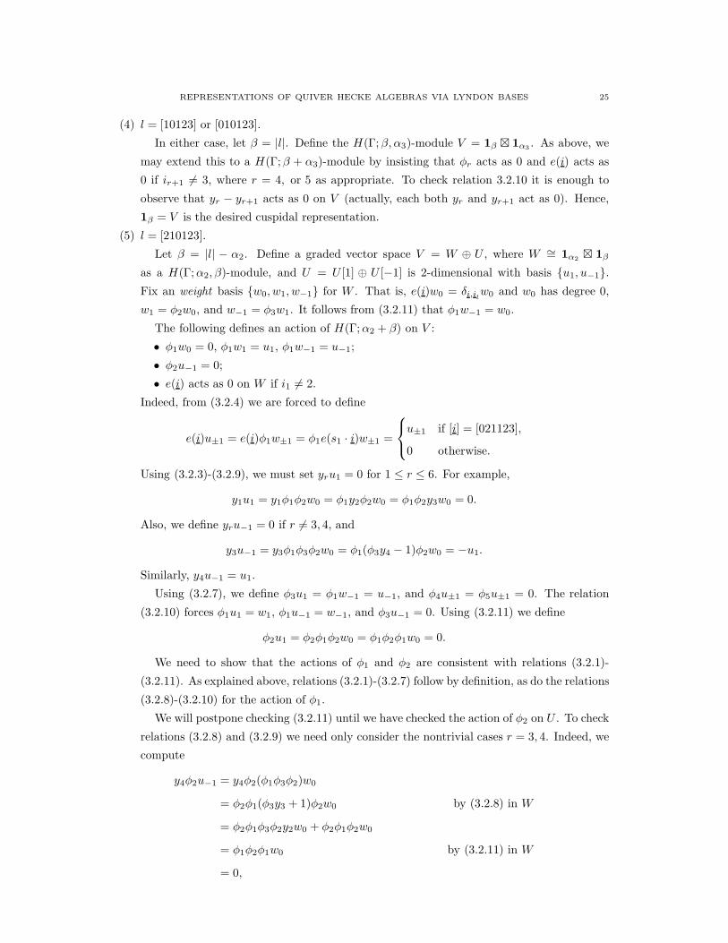
(4) l = [10123] or [010123].
In either case, let β = |l|. Define the H(Γ;β, α3)-module V = 1β ⊠ 1α3 . As above, we
may extend this to a H(Γ;β + α3)-module by insisting that φr acts as 0 and e(i) acts as
0 if ir+1 6= 3, where r = 4, or 5 as appropriate. To check relation 3.2.10 it is enough to
observe that yr − yr+1 acts as 0 on V (actually, each both yr and yr+1 act as 0). Hence,
1β = V is the desired cuspidal representation.
(5) l = [210123].
Let β = |l| − α2. Define a graded vector space V = W ⊕ U , where W ∼= 1α2 ⊠ 1β
as a H(Γ;α2, β)-module, and U = U [1] ⊕ U [−1] is 2-dimensional with basis {u1, u−1}.
Fix an weight basis {w0, w1, w−1} for W . That is, e(i)w0 = δi,ilw0 and w0 has degree 0,
w1 = φ2w0, and w−1 = φ3w1. It follows from (3.2.11) that φ1w−1 = w0.
The following defines an action of H(Γ;α2 + β) on V :
• φ1w0 = 0, φ1w1 = u1, φ1w−1 = u−1;
• φ2u−1 = 0;
• e(i) acts as 0 on W if i1 6= 2.
Indeed, from (3.2.4) we are forced to define
e(i)u±1 = e(i)φ1w±1 = φ1e(s1 · i)w±1 =
u±1 if [i] = [021123],
0 otherwise.
Using (3.2.3)-(3.2.9), we must set yru1 = 0 for 1 ≤ r ≤ 6. For example,
y1u1 = y1φ1φ2w0 = φ1y2φ2w0 = φ1φ2y3w0 = 0.
Also, we define yru−1 = 0 if r 6= 3, 4, and
y3u−1 = y3φ1φ3φ2w0 = φ1(φ3y4 − 1)φ2w0 = −u1.
Similarly, y4u−1 = u1.
Using (3.2.7), we define φ3u1 = φ1w−1 = u−1, and φ4u±1 = φ5u±1 = 0. The relation
(3.2.10) forces φ1u1 = w1, φ1u−1 = w−1, and φ3u−1 = 0. Using (3.2.11) we define
φ2u1 = φ2φ1φ2w0 = φ1φ2φ1w0 = 0.
We need to show that the actions of φ1 and φ2 are consistent with relations (3.2.1)-
(3.2.11). As explained above, relations (3.2.1)-(3.2.7) follow by definition, as do the relations
(3.2.8)-(3.2.10) for the action of φ1.
We will postpone checking (3.2.11) until we have checked the action of φ2 on U . To check
relations (3.2.8) and (3.2.9) we need only consider the nontrivial cases r = 3, 4. Indeed, we
compute
y4φ2u−1 = y4φ2(φ1φ3φ2)w0
= φ2φ1(φ3y3 + 1)φ2w0 by (3.2.8) in W
= φ2φ1φ3φ2y2w0 + φ2φ1φ2w0
= φ1φ2φ1w0 by (3.2.11) in W
= 0,
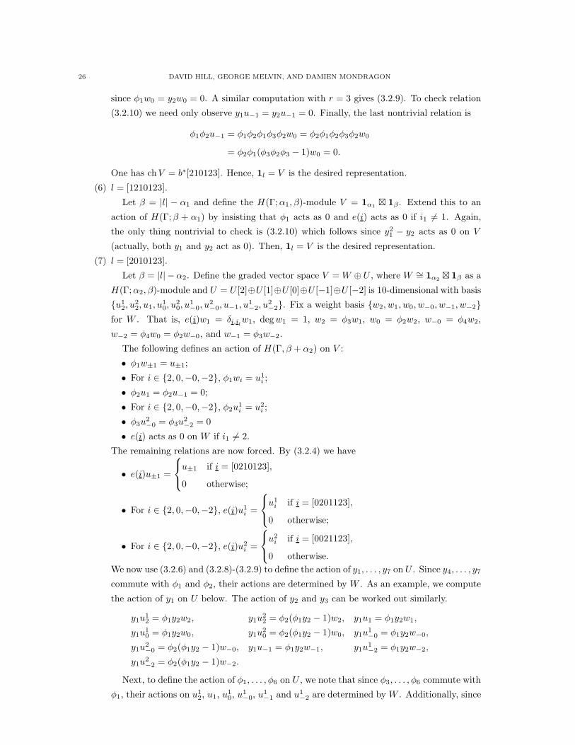
26 DAVID HILL, GEORGE MELVIN, AND DAMIEN MONDRAGON
since φ1w0 = y2w0 = 0. A similar computation with r = 3 gives (3.2.9). To check relation
(3.2.10) we need only observe y1u−1 = y2u−1 = 0. Finally, the last nontrivial relation is
φ1φ2u−1 = φ1φ2φ1φ3φ2w0 = φ2φ1φ2φ3φ2w0
= φ2φ1(φ3φ2φ3 − 1)w0 = 0.
One has chV = b∗[210123]. Hence, 1l = V is the desired representation.
(6) l = [1210123].
Let β = |l| − α1 and define the H(Γ;α1, β)-module V = 1α1 ⊠ 1β . Extend this to an
action of H(Γ;β + α1) by insisting that φ1 acts as 0 and e(i) acts as 0 if i1 6= 1. Again,
the only thing nontrivial to check is (3.2.10) which follows since y21 − y2 acts as 0 on V
(actually, both y1 and y2 act as 0). Then, 1l = V is the desired representation.
(7) l = [2010123].
Let β = |l| − α2. Define the graded vector space V = W ⊕U , where W ∼= 1α2 ⊠ 1β as a
H(Γ;α2, β)-module and U = U [2]⊕U [1]⊕U [0]⊕U [−1]⊕U [−2] is 10-dimensional with basis
{u12, u
22, u1, u
10, u
20, u
1−0, u
2−0, u−1, u
1−2, u
2−2}. Fix a weight basis {w2, w1, w0, w−0, w−1, w−2}
for W . That is, e(i)w1 = δi,ilw1, degw1 = 1, w2 = φ3w1, w0 = φ2w2, w−0 = φ4w2,
w−2 = φ4w0 = φ2w−0, and w−1 = φ3w−2.
The following defines an action of H(Γ, β + α2) on V :
• φ1w±1 = u±1;
• For i ∈ {2, 0,−0,−2}, φ1wi = u1i ;
• φ2u1 = φ2u−1 = 0;
• For i ∈ {2, 0,−0,−2}, φ2u1i = u2
i ;
• φ3u2−0 = φ3u
2−2 = 0
• e(i) acts as 0 on W if i1 6= 2.
The remaining relations are now forced. By (3.2.4) we have
• e(i)u±1 =
u±1 if i = [0210123],
0 otherwise;
• For i ∈ {2, 0,−0,−2}, e(i)u1i =
u1i if i = [0201123],
0 otherwise;
• For i ∈ {2, 0,−0,−2}, e(i)u2i =
u2i if i = [0021123],
0 otherwise.
We now use (3.2.6) and (3.2.8)-(3.2.9) to define the action of y1, . . . , y7 on U . Since y4, . . . , y7
commute with φ1 and φ2, their actions are determined by W . As an example, we compute
the action of y1 on U below. The action of y2 and y3 can be worked out similarly.
y1u12 = φ1y2w2, y1u
22 = φ2(φ1y2 − 1)w2, y1u1 = φ1y2w1,
y1u10 = φ1y2w0, y1u
20 = φ2(φ1y2 − 1)w0, y1u
1−0 = φ1y2w−0,
y1u2−0 = φ2(φ1y2 − 1)w−0, y1u−1 = φ1y2w−1, y1u
1−2 = φ1y2w−2,
y1u2−2 = φ2(φ1y2 − 1)w−2.
Next, to define the action of φ1, . . . , φ6 on U , we note that since φ3, . . . , φ6 commute with
φ1, their actions on u12, u1, u
10, u
1−0, u
1−1 and u1
−2 are determined by W . Additionally, since
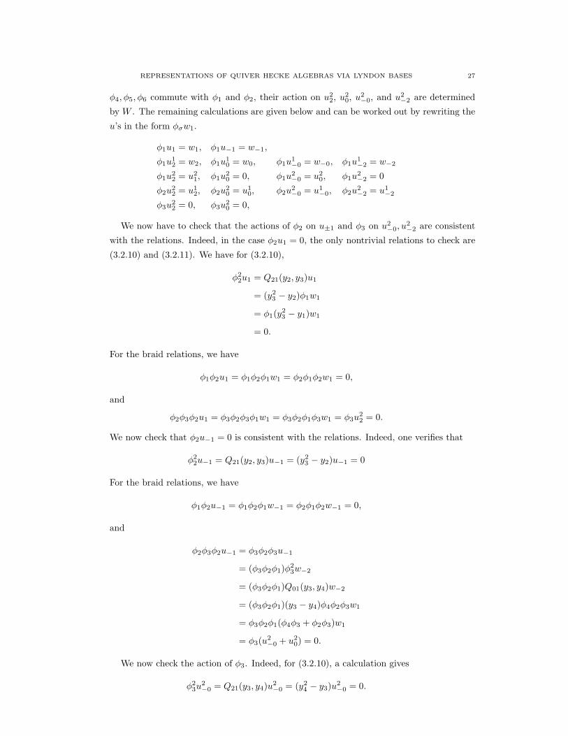
REPRESENTATIONS OF QUIVER HECKE ALGEBRAS VIA LYNDON BASES 27
φ4, φ5, φ6 commute with φ1 and φ2, their action on u22, u
20, u
2−0, and u2
−2 are determined
by W . The remaining calculations are given below and can be worked out by rewriting the
u’s in the form φσw1.
φ1u1 = w1, φ1u−1 = w−1,
φ1u12 = w2, φ1u
10 = w0, φ1u
1−0 = w−0, φ1u
1−2 = w−2
φ1u22 = u2
1, φ1u20 = 0, φ1u
2−0 = u2
0, φ1u2−2 = 0
φ2u22 = u1
2, φ2u20 = u1
0, φ2u2−0 = u1
−0, φ2u2−2 = u1
−2
φ3u22 = 0, φ3u
20 = 0,
We now have to check that the actions of φ2 on u±1 and φ3 on u2−0, u
2−2 are consistent
with the relations. Indeed, in the case φ2u1 = 0, the only nontrivial relations to check are
(3.2.10) and (3.2.11). We have for (3.2.10),
φ22u1 = Q21(y2, y3)u1
= (y23 − y2)φ1w1
= φ1(y23 − y1)w1
= 0.
For the braid relations, we have
φ1φ2u1 = φ1φ2φ1w1 = φ2φ1φ2w1 = 0,
and
φ2φ3φ2u1 = φ3φ2φ3φ1w1 = φ3φ2φ1φ3w1 = φ3u22 = 0.
We now check that φ2u−1 = 0 is consistent with the relations. Indeed, one verifies that
φ22u−1 = Q21(y2, y3)u−1 = (y2
3 − y2)u−1 = 0
For the braid relations, we have
φ1φ2u−1 = φ1φ2φ1w−1 = φ2φ1φ2w−1 = 0,
and
φ2φ3φ2u−1 = φ3φ2φ3u−1
= (φ3φ2φ1)φ23w−2
= (φ3φ2φ1)Q01(y3, y4)w−2
= (φ3φ2φ1)(y3 − y4)φ4φ2φ3w1
= φ3φ2φ1(φ4φ3 + φ2φ3)w1
= φ3(u2−0 + u2
0) = 0.
We now check the action of φ3. Indeed, for (3.2.10), a calculation gives
φ23u
2−0 = Q21(y3, y4)u
2−0 = (y2
4 − y3)u2−0 = 0.
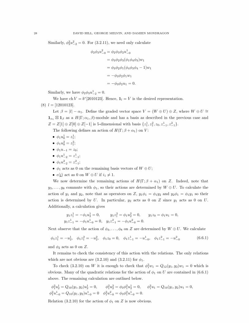
28 DAVID HILL, GEORGE MELVIN, AND DAMIEN MONDRAGON
Similarly, φ23u
2−2 = 0. For (3.2.11), we need only calculate
φ2φ3u2−0 = φ2φ3φ2u
1−0
= φ3φ2φ3(φ1φ4φ3)w1
= φ3φ2φ1(φ4φ3φ4 − 1)w1
= −φ3φ2φ1w1
= −φ3φ2u1 = 0.
Similarly, we have φ2φ3u1−2 = 0.
We have chV = b∗[2010123]. Hence, 1l = V is the desired representation.
(8) l = [12010123].
Let β = |l| − α1. Define the graded vector space V = (W ⊕ U) ⊕ Z, where W ⊕ U ∼=
1α1 ⊠ 1β as a H(Γ;α1, β)-module and has a basis as described in the previous case and
Z = Z[1]⊕ Z[0] ⊕ Z[−1] is 5-dimensional with basis {z11 , z
21 , z0, z
1−1, z
2−1}.
The following defines an action of H(Γ;β + α1) on V :
• φ1u10 = z1
1 ;
• φ1u20 = z2
1 ;
• φ1u−1 = z0;
• φ1u1−2 = z1
−1;
• φ1u2−2 = z2
−1;
• φ1 acts as 0 on the remaining basis vectors of W ⊕ U ;
• e(i) act as 0 on W ⊕ U if i1 6= 1.
We now determine the remaining actions of H(Γ;β + α1) on Z. Indeed, note that
y3, . . . , y8 commute with φ1, so their actions are determined by W ⊕ U . To calculate the
action of y1 and y2, note that as operators on Z, y1φ1 = φ1y2 and y2φ1 = φ1y1 so their
action is determined by U . In particular, y2 acts as 0 on Z since y1 acts as 0 on U .
Additionally, a calculation gives
y1z11 = −φ1u
12 = 0, y1z
21 = φ1u
22 = 0, y1z0 = φ1u1 = 0,
y1z1−1 = −φ1u
1−0 = 0, y1z
2−1 = −φ1u
2−0 = 0.
Next observe that the action of φ3, . . . , φ8 on Z are determined by W ⊕ U . We calculate
φ1z11 = −u1
2, φ1z21 = −u2
2, φ1z0 = 0, φ1z1−1 = −u1
−0, φ1z2−1 = −u2
−0 (6.6.1)
and φ2 acts as 0 on Z.
It remains to check the consistency of this action with the relations. The only relations
which are not obvious are (3.2.10) and (3.2.11) for φ1.
To check (3.2.10) on W it is enough to check that φ21w1 = Q12(y1, y2)w1 = 0 which is
obvious. Many of the quadratic relations for the action of φ1 on U are contained in (6.6.1)
above. The remaining calculation are outlined below.
φ21u
12 = Q10(y1, y2)u
12 = 0, φ2
1u22 = φ3φ
21u
12 = 0, φ2
1u1 = Q10(y1, y2)u1 = 0,
φ21u
1−0 = Q10(y1, y2)u
1−0 = 0 φ2
1u2−0 = φ3φ
21u
1−0 = 0.
Relation (3.2.10) for the action of φ1 on Z is now obvious.
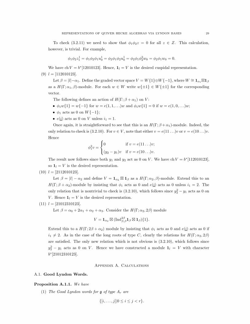
REPRESENTATIONS OF QUIVER HECKE ALGEBRAS VIA LYNDON BASES 29
To check (3.2.11) we need to show that φ1φ2z = 0 for all z ∈ Z. This calculation,
however, is trivial. For example,
φ1φ2z11 = φ1φ2φ1u
10 = φ2φ1φ2u
10 = φ2φ1φ
22w0 = φ2φ1w0 = 0.
We have chV = b∗[12010123]. Hence, 1l = V is the desired cuspidal representation.
(9) l = [112010123].
Let β = |l|−α1. Define the graded vector space V = W{1}⊕W{−1}, whereW ∼= 1α1⊠1β
as a H(Γ;α1, β)-module. For each w ∈ W write w{±1} ∈ W{±1} for the corresponding
vector.
The following defines an action of H(Γ;β + α1) on V :
• φ1w{1} = w{−1} for w = e(1, 1, . . .)w and φ1w{1} = 0 if w = e(1, 0, . . .)w;
• φ1 acts as 0 on W{−1};
• e(i) acts as 0 on V unless i1 = 1.
Once again, it is straightforward to see that this is an H(Γ;β+α1)-module. Indeed, the
only relation to check is (3.2.10). For v ∈ V , note that either v = e(11 . . .)v or v = e(10 . . .)v.
Hence
φ21v =
0 if v = e(11 . . .)v;
(y2 − y1)v if v = e(10 . . .)v.
The result now follows since both y1 and y2 act as 0 on V . We have chV = b∗[112010123],
so 1l = V is the desired representation.
(10) l = [2112010123].
Let β = |l| − α2 and define V = 1α2 ⊠ 1β as a H(Γ;α2, β)-module. Extend this to an
H(Γ;β + α2)-module by insisting that φ1 acts as 0 and e(i) acts as 0 unless i1 = 2. The
only relation that is nontrivial to check is (3.2.10), which follows since y22 − y1 acts as 0 on
V . Hence 1l = V is the desired representation.
(11) l = [21012310123].
Let β = α0 + 2α1 + α2 + α3. Consider the H(Γ;α2, 2β) module
V = 1α2 ⊠ (Ind2ββ,β1β ⊠ 1β){1}.
Extend this to a H(Γ; 2β + α2) module by insisting that φ1 acts as 0 and e(i) acts as 0 if
i1 6= 2. As in the case of the long roots of type C, clearly the relations for H(Γ;α2, 2β)
are satisfied. The only new relation which is not obvious is (3.2.10), which follows since
y22 − y1 acts as 0 on V . Hence we have constructed a module 1l = V with character
b∗[21012310123].
Appendix A. Calculations
A.1. Good Lyndon Words.
Proposition A.1.1. We have
(1) The Good Lyndon words for g of type Ar are
{[i, . . . , j]|0 ≤ i ≤ j < r}.
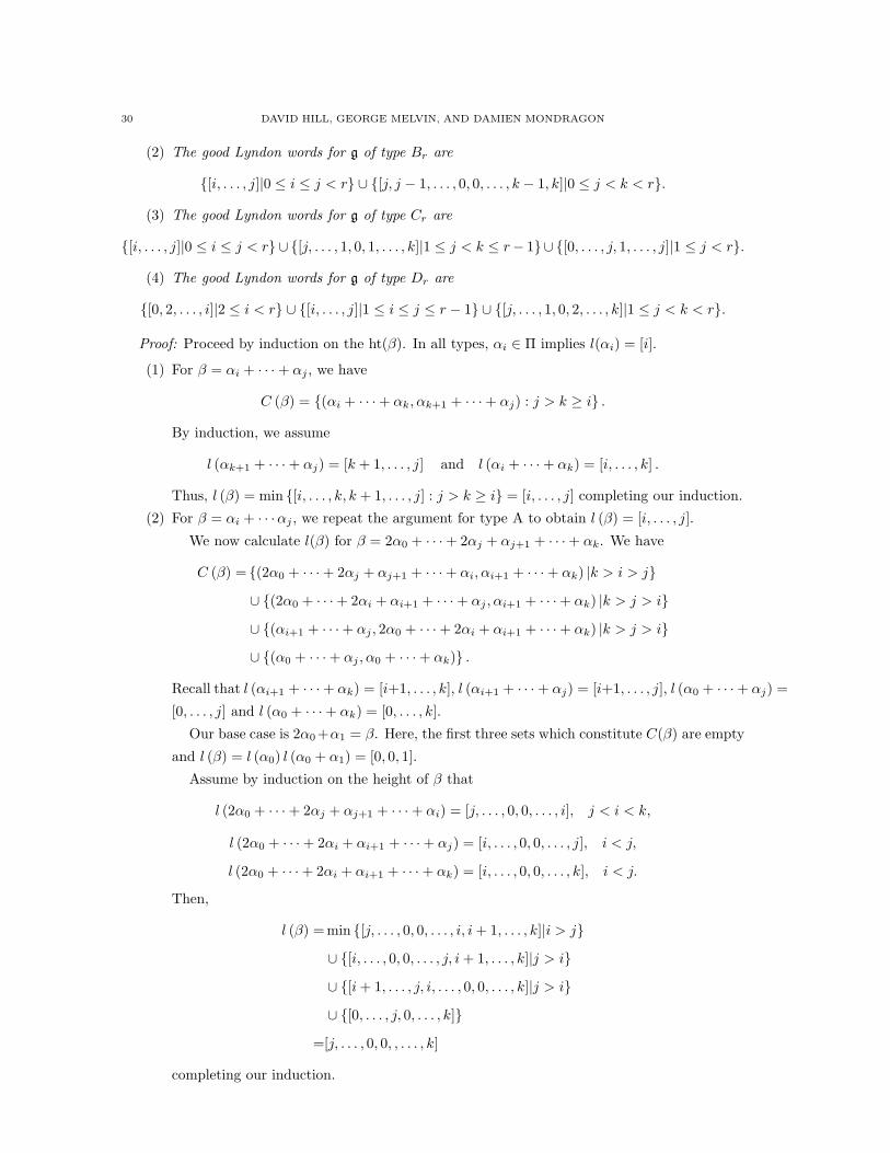
30 DAVID HILL, GEORGE MELVIN, AND DAMIEN MONDRAGON
(2) The good Lyndon words for g of type Br are
{[i, . . . , j]|0 ≤ i ≤ j < r} ∪ {[j, j − 1, . . . , 0, 0, . . . , k − 1, k]|0 ≤ j < k < r}.
(3) The good Lyndon words for g of type Cr are
{[i, . . . , j]|0 ≤ i ≤ j < r} ∪ {[j, . . . , 1, 0, 1, . . . , k]|1 ≤ j < k ≤ r− 1}∪ {[0, . . . , j, 1, . . . , j]|1 ≤ j < r}.
(4) The good Lyndon words for g of type Dr are
{[0, 2, . . . , i]|2 ≤ i < r} ∪ {[i, . . . , j]|1 ≤ i ≤ j ≤ r − 1} ∪ {[j, . . . , 1, 0, 2, . . . , k]|1 ≤ j < k < r}.
Proof: Proceed by induction on the ht(β). In all types, αi ∈ Π implies l(αi) = [i].
(1) For β = αi + · · · + αj , we have
C (β) = {(αi + · · · + αk, αk+1 + · · · + αj) : j > k ≥ i} .
By induction, we assume
l (αk+1 + · · · + αj) = [k + 1, . . . , j] and l (αi + · · · + αk) = [i, . . . , k] .
Thus, l (β) = min {[i, . . . , k, k + 1, . . . , j] : j > k ≥ i} = [i, . . . , j] completing our induction.
(2) For β = αi + · · ·αj , we repeat the argument for type A to obtain l (β) = [i, . . . , j].
We now calculate l(β) for β = 2α0 + · · · + 2αj + αj+1 + · · · + αk. We have
C (β) = {(2α0 + · · · + 2αj + αj+1 + · · · + αi, αi+1 + · · · + αk) |k > i > j}
∪ {(2α0 + · · · + 2αi + αi+1 + · · · + αj , αi+1 + · · · + αk) |k > j > i}
∪ {(αi+1 + · · · + αj , 2α0 + · · · + 2αi + αi+1 + · · · + αk) |k > j > i}
∪ {(α0 + · · · + αj , α0 + · · · + αk)} .
Recall that l (αi+1 + · · · + αk) = [i+1, . . . , k], l (αi+1 + · · · + αj) = [i+1, . . . , j], l (α0 + · · · + αj) =
[0, . . . , j] and l (α0 + · · · + αk) = [0, . . . , k].
Our base case is 2α0+α1 = β. Here, the first three sets which constitute C(β) are empty
and l (β) = l (α0) l (α0 + α1) = [0, 0, 1].
Assume by induction on the height of β that
l (2α0 + · · · + 2αj + αj+1 + · · · + αi) = [j, . . . , 0, 0, . . . , i], j < i < k,
l (2α0 + · · · + 2αi + αi+1 + · · · + αj) = [i, . . . , 0, 0, . . . , j], i < j,
l (2α0 + · · · + 2αi + αi+1 + · · · + αk) = [i, . . . , 0, 0, . . . , k], i < j.
Then,
l (β) =min {[j, . . . , 0, 0, . . . , i, i+ 1, . . . , k]|i > j}
∪ {[i, . . . , 0, 0, . . . , j, i+ 1, . . . , k]|j > i}
∪ {[i+ 1, . . . , j, i, . . . , 0, 0, . . . , k]|j > i}
∪ {[0, . . . , j, 0, . . . , k]}
=[j, . . . , 0, 0, , . . . , k]
completing our induction.
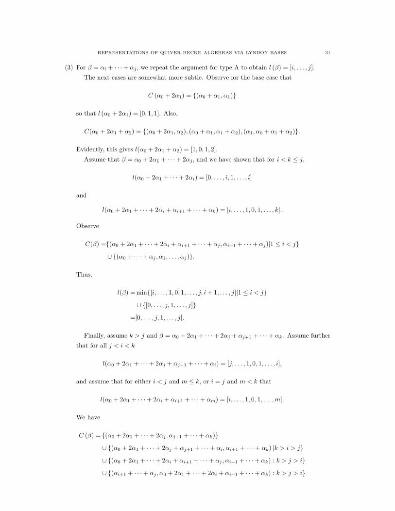
REPRESENTATIONS OF QUIVER HECKE ALGEBRAS VIA LYNDON BASES 31
(3) For β = αi + · · · + αj , we repeat the argument for type A to obtain l (β) = [i, . . . , j].
The next cases are somewhat more subtle. Observe for the base case that
C (α0 + 2α1) = {(α0 + α1, α1)}
so that l (α0 + 2α1) = [0, 1, 1]. Also,
C(α0 + 2α1 + α2) = {(α0 + 2α1, α2), (α0 + α1, α1 + α2), (α1, α0 + α1 + α2)}.
Evidently, this gives l(α0 + 2α1 + α2) = [1, 0, 1, 2].
Assume that β = α0 + 2α1 + · · · + 2αj, and we have shown that for i < k ≤ j,
l(α0 + 2α1 + · · · + 2αi) = [0, . . . , i, 1, . . . , i]
and
l(α0 + 2α1 + · · · + 2αi + αi+1 + · · · + αk) = [i, . . . , 1, 0, 1, . . . , k].
Observe
C(β) ={(α0 + 2α1 + · · · + 2αi + αi+1 + · · · + αj , αi+1 + · · · + αj)|1 ≤ i < j}
∪ {(α0 + · · · + αj , α1, . . . , αj)}.
Thus,
l(β) =min{[i, . . . , 1, 0, 1, . . . , j, i+ 1, . . . , j]|1 ≤ i < j}
∪ {[0, . . . , j, 1, . . . , j]}
=[0, . . . , j, 1, . . . , j].
Finally, assume k > j and β = α0 + 2α1 + · · · + 2αj + αj+1 + · · · + αk. Assume further
that for all j < i < k
l(α0 + 2α1 + · · · + 2αj + αj+1 + · · · + αi) = [j, . . . , 1, 0, 1, . . . , i],
and assume that for either i < j and m ≤ k, or i = j and m < k that
l(α0 + 2α1 + · · · + 2αi + αi+1 + · · · + αm) = [i, . . . , 1, 0, 1, . . . ,m].
We have
C (β) = {(α0 + 2α1 + · · · + 2αj, αj+1 + · · · + αk)}
∪ {(α0 + 2α1 + · · · + 2αj + αj+1 + · · · + αi, αi+1 + · · · + αk) |k > i > j}
∪ {(α0 + 2α1 + · · · + 2αi + αi+1 + · · · + αj , αi+1 + · · · + αk) : k > j > i}
∪ {(αi+1 + · · · + αj , α0 + 2α1 + · · · + 2αi + αi+1 + · · · + αk) : k > j > i}
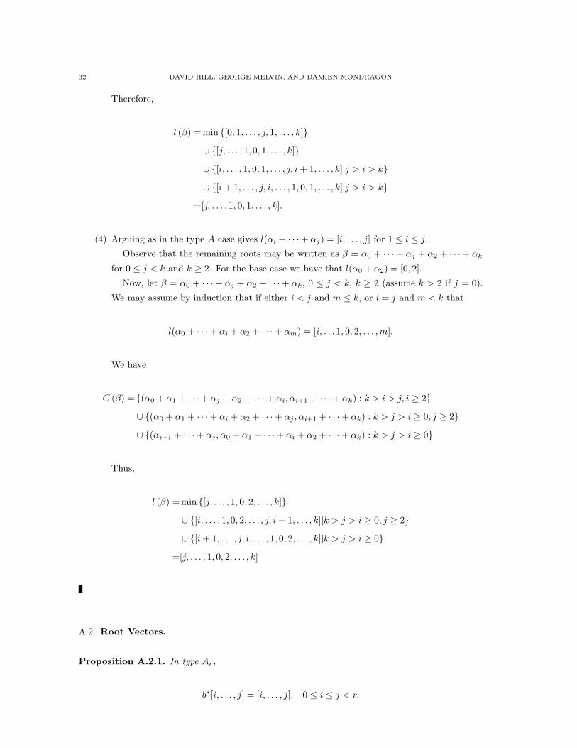
32 DAVID HILL, GEORGE MELVIN, AND DAMIEN MONDRAGON
Therefore,
l (β) = min {[0, 1, . . . , j, 1, . . . , k]}
∪ {[j, . . . , 1, 0, 1, . . . , k]}
∪ {[i, . . . , 1, 0, 1, . . . , j, i+ 1, . . . , k]|j > i > k}
∪ {[i+ 1, . . . , j, i, . . . , 1, 0, 1, . . . , k]|j > i > k}
=[j, . . . , 1, 0, 1, . . . , k].
(4) Arguing as in the type A case gives l(αi + · · · + αj) = [i, . . . , j] for 1 ≤ i ≤ j.
Observe that the remaining roots may be written as β = α0 + · · · + αj + α2 + · · · + αk
for 0 ≤ j < k and k ≥ 2. For the base case we have that l(α0 + α2) = [0, 2].
Now, let β = α0 + · · · + αj + α2 + · · · + αk, 0 ≤ j < k, k ≥ 2 (assume k > 2 if j = 0).
We may assume by induction that if either i < j and m ≤ k, or i = j and m < k that
l(α0 + · · · + αi + α2 + · · · + αm) = [i, . . . 1, 0, 2, . . . ,m].
We have
C (β) = {(α0 + α1 + · · · + αj + α2 + · · · + αi, αi+1 + · · · + αk) : k > i > j, i ≥ 2}
∪ {(α0 + α1 + · · · + αi + α2 + · · · + αj , αi+1 + · · · + αk) : k > j > i ≥ 0, j ≥ 2}
∪ {(αi+1 + · · · + αj , α0 + α1 + · · · + αi + α2 + · · · + αk) : k > j > i ≥ 0}
Thus,
l (β) =min {[j, . . . , 1, 0, 2, . . . , k]}
∪ {[i, . . . , 1, 0, 2, . . . , j, i+ 1, . . . , k]|k > j > i ≥ 0, j ≥ 2}
∪ {[i+ 1, . . . , j, i, . . . , 1, 0, 2, . . . , k]|k > j > i ≥ 0}
=[j, . . . , 1, 0, 2, . . . , k]
A.2. Root Vectors.
Proposition A.2.1. In type Ar,
b∗[i, . . . , j] = [i, . . . , j], 0 ≤ i ≤ j < r.
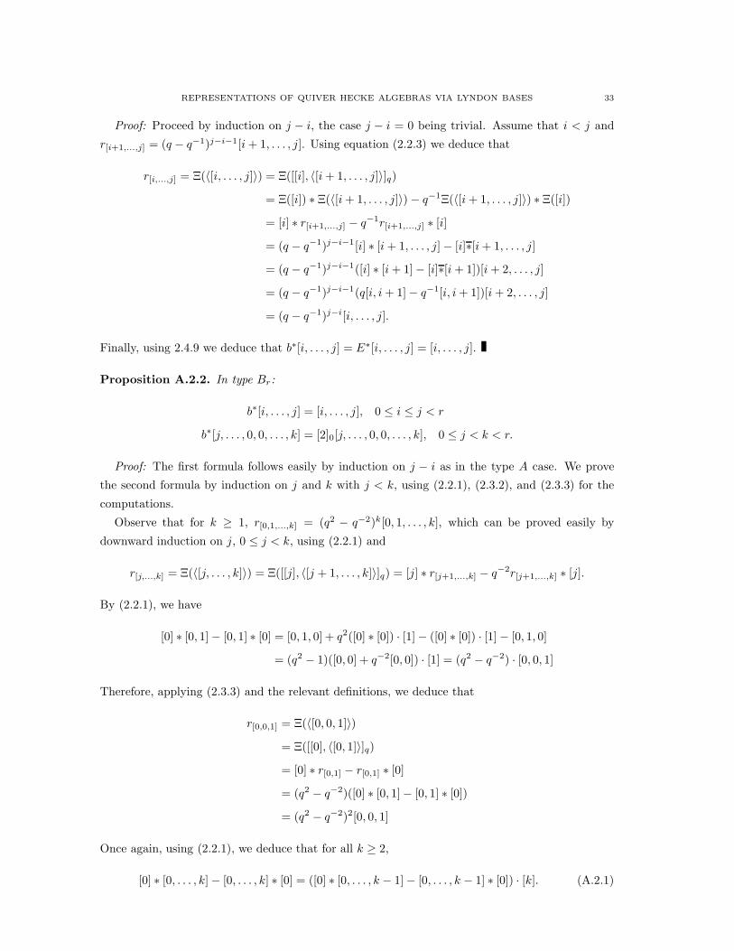
REPRESENTATIONS OF QUIVER HECKE ALGEBRAS VIA LYNDON BASES 33
Proof: Proceed by induction on j − i, the case j − i = 0 being trivial. Assume that i < j and
r[i+1,...,j] = (q − q−1)j−i−1[i+ 1, . . . , j]. Using equation (2.2.3) we deduce that
r[i,...,j] = Ξ(〈[i, . . . , j]〉) = Ξ([[i], 〈[i+ 1, . . . , j]〉]q)
= Ξ([i]) ∗ Ξ(〈[i+ 1, . . . , j]〉) − q−1Ξ(〈[i+ 1, . . . , j]〉) ∗ Ξ([i])
= [i] ∗ r[i+1,...,j] − q−1r[i+1,...,j] ∗ [i]
= (q − q−1)j−i−1[i] ∗ [i+ 1, . . . , j] − [i]∗[i+ 1, . . . , j]
= (q − q−1)j−i−1([i] ∗ [i+ 1] − [i]∗[i+ 1])[i+ 2, . . . , j]
= (q − q−1)j−i−1(q[i, i+ 1] − q−1[i, i+ 1])[i+ 2, . . . , j]
= (q − q−1)j−i[i, . . . , j].
Finally, using 2.4.9 we deduce that b∗[i, . . . , j] = E∗[i, . . . , j] = [i, . . . , j].
Proposition A.2.2. In type Br:
b∗[i, . . . , j] = [i, . . . , j], 0 ≤ i ≤ j < r
b∗[j, . . . , 0, 0, . . . , k] = [2]0[j, . . . , 0, 0, . . . , k], 0 ≤ j < k < r.
Proof: The first formula follows easily by induction on j − i as in the type A case. We prove
the second formula by induction on j and k with j < k, using (2.2.1), (2.3.2), and (2.3.3) for the
computations.
Observe that for k ≥ 1, r[0,1,...,k] = (q2 − q−2)k[0, 1, . . . , k], which can be proved easily by
downward induction on j, 0 ≤ j < k, using (2.2.1) and
r[j,...,k] = Ξ(〈[j, . . . , k]〉) = Ξ([[j], 〈[j + 1, . . . , k]〉]q) = [j] ∗ r[j+1,...,k] − q−2r[j+1,...,k] ∗ [j].
By (2.2.1), we have
[0] ∗ [0, 1] − [0, 1] ∗ [0] = [0, 1, 0] + q2([0] ∗ [0]) · [1] − ([0] ∗ [0]) · [1] − [0, 1, 0]
= (q2 − 1)([0, 0] + q−2[0, 0]) · [1] = (q2 − q−2) · [0, 0, 1]
Therefore, applying (2.3.3) and the relevant definitions, we deduce that
r[0,0,1] = Ξ(〈[0, 0, 1]〉)
= Ξ([[0], 〈[0, 1]〉]q)
= [0] ∗ r[0,1] − r[0,1] ∗ [0]
= (q2 − q−2)([0] ∗ [0, 1]− [0, 1] ∗ [0])
= (q2 − q−2)2[0, 0, 1]
Once again, using (2.2.1), we deduce that for all k ≥ 2,
[0] ∗ [0, . . . , k] − [0, . . . , k] ∗ [0] = ([0] ∗ [0, . . . , k − 1] − [0, . . . , k − 1] ∗ [0]) · [k]. (A.2.1)
34 DAVID HILL, GEORGE MELVIN, AND DAMIEN MONDRAGON
Assume k ≥ 2. Then, (α0, α0 + · · · + αk) = 0, so iterated applications of (A.2.1) yields
r[0,0,...,k] = [0] ∗ r[0,...,k] − r[0,...,k] ∗ [0]
= (q2 − q−2)k([0] ∗ [0, . . . , k] − [0, . . . , k] ∗ [0])
= (q2 − q−2)k([0] ∗ [0, 1] − [0, 1] ∗ [0]) · [2, . . . , k]
= (q2 − q−2)k+1[0, 0, . . . , k]
Now, assume that k ≥ 2, and 0 < j < k. To compute r[j,...,0,0,...,k], we need the following. For
|j − k| > 1,
[j] ∗ [j − 1, . . . ,k] − q−2[j − 1, . . . , k] ∗ [j] (A.2.2)
= ([j] ∗ [j − 1, . . . , k − 1] − q−2[j − 1, . . . , k − 1] ∗ [j]) · [k].
For j = k − 1,
[j] ∗ [j − 1, . . . , 0,0, . . . , j + 1] − q−2[j − 1, . . . , 0, 0, . . . , j + 1] ∗ [j] (A.2.3)
= (q2[j] ∗ [j − 1, . . . , 0, 0, . . . , j] − q−2[j − 1, . . . , 0, 0, . . . , j] ∗ [j]) · [j + 1].
Finally,
q2[j] ∗ [j − 1, . . . , 0,0, . . . , j] − q−2[j − 1, . . . , 0, 0, . . . , j] ∗ [j] (A.2.4)
= ([j] ∗ [j − 1, . . . , 0, 0, . . . , j − 2] − q−2[j − 1, . . . , 0, 0, . . . , j − 2] ∗ [j]) · [j, j + 1].
Indeed, (A.2.2) and (A.2.3) are straightforward applications of (2.2.1). Equation (A.2.4) involves
a little more calculation:
q2[j] ∗ [j − 1, . . . , 0,0, . . . , j] − q−2[j − 1, . . . , 0, 0, . . . , j] ∗ [j]
=q2[j − 1, . . . , 0, 0, . . . , j, j] + q−2([j] ∗ [j − 1, . . . , 0, 0, . . . , j − 1]
− [j − 1, . . . , 0, 0, . . . , j − 1] ∗ [j]) · [j] − q−2[j − 1, . . . , 0, 0, . . . , j, j]
=(q2 − q−2) · [j − 1, . . . , 0, 0, . . . , j, j] + q−2([j − 1, . . . , 0, 0, . . . , j]
+ q2([j] ∗ [j − 1, . . . , 0, 0, . . . , j − 2]) · [j − 1] − ([j − 1, . . . , 0, 0, . . . , j − 2] ∗ [j]) · [j − 1]
− q4[j − 1, . . . , 0, 0, . . . , j]) · [j]
=([j] ∗ [j − 1, . . . , 0, 0, . . . , j − 2] − q−2[j − 1, . . . , 0, 0, . . . , j − 2] ∗ [j]) · [j, j + 1],
Note that (A.2.2) holds for both [j − 1, j, . . . , k] and [j − 1, . . . , 0, 0, . . . , k].
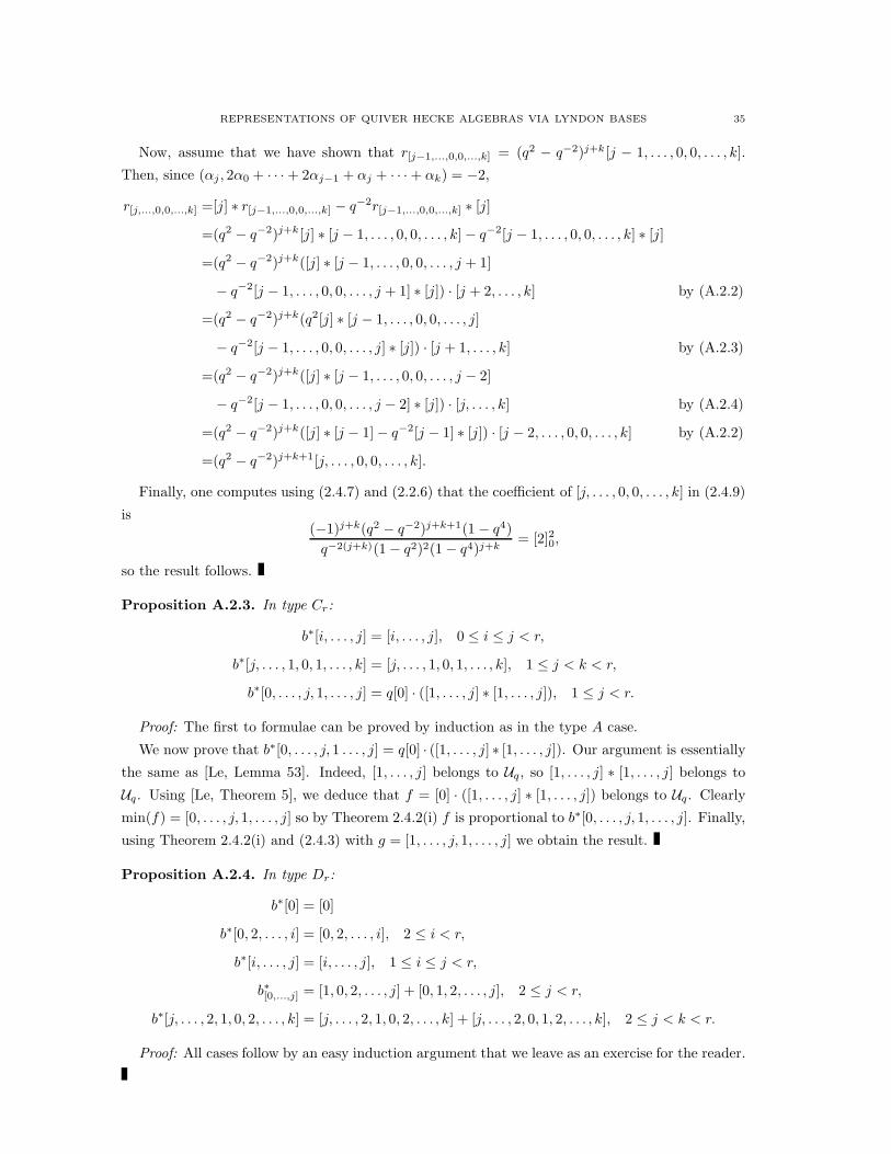
REPRESENTATIONS OF QUIVER HECKE ALGEBRAS VIA LYNDON BASES 35
Now, assume that we have shown that r[j−1,...,0,0,...,k] = (q2 − q−2)j+k[j − 1, . . . , 0, 0, . . . , k].
Then, since (αj , 2α0 + · · · + 2αj−1 + αj + · · · + αk) = −2,
r[j,...,0,0,...,k] =[j] ∗ r[j−1,...,0,0,...,k] − q−2r[j−1,...,0,0,...,k] ∗ [j]
=(q2 − q−2)j+k[j] ∗ [j − 1, . . . , 0, 0, . . . , k] − q−2[j − 1, . . . , 0, 0, . . . , k] ∗ [j]
=(q2 − q−2)j+k([j] ∗ [j − 1, . . . , 0, 0, . . . , j + 1]
− q−2[j − 1, . . . , 0, 0, . . . , j + 1] ∗ [j]) · [j + 2, . . . , k] by (A.2.2)
=(q2 − q−2)j+k(q2[j] ∗ [j − 1, . . . , 0, 0, . . . , j]
− q−2[j − 1, . . . , 0, 0, . . . , j] ∗ [j]) · [j + 1, . . . , k] by (A.2.3)
=(q2 − q−2)j+k([j] ∗ [j − 1, . . . , 0, 0, . . . , j − 2]
− q−2[j − 1, . . . , 0, 0, . . . , j − 2] ∗ [j]) · [j, . . . , k] by (A.2.4)
=(q2 − q−2)j+k([j] ∗ [j − 1] − q−2[j − 1] ∗ [j]) · [j − 2, . . . , 0, 0, . . . , k] by (A.2.2)
=(q2 − q−2)j+k+1[j, . . . , 0, 0, . . . , k].
Finally, one computes using (2.4.7) and (2.2.6) that the coefficient of [j, . . . , 0, 0, . . . , k] in (2.4.9)
is(−1)j+k(q2 − q−2)j+k+1(1 − q4)
q−2(j+k)(1 − q2)2(1 − q4)j+k= [2]20,
so the result follows.
Proposition A.2.3. In type Cr:
b∗[i, . . . , j] = [i, . . . , j], 0 ≤ i ≤ j < r,
b∗[j, . . . , 1, 0, 1, . . . , k] = [j, . . . , 1, 0, 1, . . . , k], 1 ≤ j < k < r,
b∗[0, . . . , j, 1, . . . , j] = q[0] · ([1, . . . , j] ∗ [1, . . . , j]), 1 ≤ j < r.
Proof: The first to formulae can be proved by induction as in the type A case.
We now prove that b∗[0, . . . , j, 1 . . . , j] = q[0] · ([1, . . . , j] ∗ [1, . . . , j]). Our argument is essentially
the same as [Le, Lemma 53]. Indeed, [1, . . . , j] belongs to Uq, so [1, . . . , j] ∗ [1, . . . , j] belongs to
Uq. Using [Le, Theorem 5], we deduce that f = [0] · ([1, . . . , j] ∗ [1, . . . , j]) belongs to Uq. Clearly
min(f) = [0, . . . , j, 1, . . . , j] so by Theorem 2.4.2(i) f is proportional to b∗[0, . . . , j, 1, . . . , j]. Finally,
using Theorem 2.4.2(i) and (2.4.3) with g = [1, . . . , j, 1, . . . , j] we obtain the result.
Proposition A.2.4. In type Dr:
b∗[0] = [0]
b∗[0, 2, . . . , i] = [0, 2, . . . , i], 2 ≤ i < r,
b∗[i, . . . , j] = [i, . . . , j], 1 ≤ i ≤ j < r,
b∗[0,...,j] = [1, 0, 2, . . . , j] + [0, 1, 2, . . . , j], 2 ≤ j < r,
b∗[j, . . . , 2, 1, 0, 2, . . . , k] = [j, . . . , 2, 1, 0, 2, . . . , k] + [j, . . . , 2, 0, 1, 2, . . . , k], 2 ≤ j < k < r.
Proof: All cases follow by an easy induction argument that we leave as an exercise for the reader.
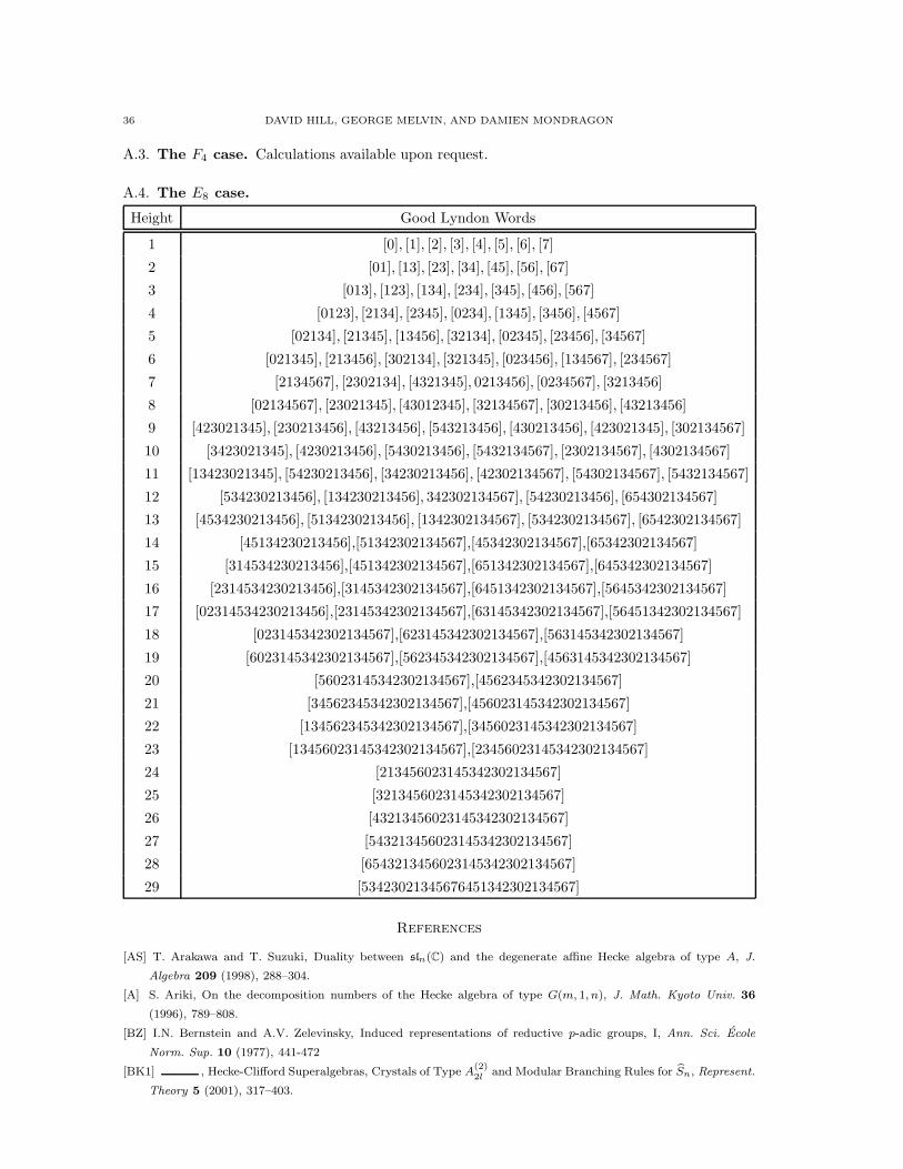
36 DAVID HILL, GEORGE MELVIN, AND DAMIEN MONDRAGON
A.3. The F4 case. Calculations available upon request.
A.4. The E8 case.
Height Good Lyndon Words
1 [0], [1], [2], [3], [4], [5], [6], [7]
2 [01], [13], [23], [34], [45], [56], [67]
3 [013], [123], [134], [234], [345], [456], [567]
4 [0123], [2134], [2345], [0234], [1345], [3456], [4567]
5 [02134], [21345], [13456], [32134], [02345], [23456], [34567]
6 [021345], [213456], [302134], [321345], [023456], [134567], [234567]
7 [2134567], [2302134], [4321345], 0213456], [0234567], [3213456]
8 [02134567], [23021345], [43012345], [32134567], [30213456], [43213456]
9 [423021345], [230213456], [43213456], [543213456], [430213456], [423021345], [302134567]
10 [3423021345], [4230213456], [5430213456], [5432134567], [2302134567], [4302134567]
11 [13423021345], [54230213456], [34230213456], [42302134567], [54302134567], [5432134567]
12 [534230213456], [134230213456], 342302134567], [54230213456], [654302134567]
13 [4534230213456], [5134230213456], [1342302134567], [5342302134567], [6542302134567]
14 [45134230213456],[51342302134567],[45342302134567],[65342302134567]
15 [314534230213456],[451342302134567],[651342302134567],[645342302134567]
16 [2314534230213456],[3145342302134567],[6451342302134567],[5645342302134567]
17 [02314534230213456],[23145342302134567],[63145342302134567],[56451342302134567]
18 [023145342302134567],[623145342302134567],[563145342302134567]
19 [6023145342302134567],[562345342302134567],[4563145342302134567]
20 [56023145342302134567],[4562345342302134567]
21 [34562345342302134567],[456023145342302134567]
22 [134562345342302134567],[3456023145342302134567]
23 [13456023145342302134567],[23456023145342302134567]
24 [213456023145342302134567]
25 [3213456023145342302134567]
26 [43213456023145342302134567]
27 [543213456023145342302134567]
28 [6543213456023145342302134567]
29 [53423021345676451342302134567]
References
[AS] T. Arakawa and T. Suzuki, Duality between sln(C) and the degenerate affine Hecke algebra of type A, J.
Algebra 209 (1998), 288–304.
[A] S. Ariki, On the decomposition numbers of the Hecke algebra of type G(m, 1, n), J. Math. Kyoto Univ. 36
(1996), 789–808.
[BZ] I.N. Bernstein and A.V. Zelevinsky, Induced representations of reductive p-adic groups, I, Ann. Sci. Ecole
Norm. Sup. 10 (1977), 441-472
[BK1] , Hecke-Clifford Superalgebras, Crystals of Type A(2)2l
and Modular Branching Rules for bSn, Represent.
Theory 5 (2001), 317–403.
REPRESENTATIONS OF QUIVER HECKE ALGEBRAS VIA LYNDON BASES 37
[BK2] J. Brundan and A. Kleshchev, Blocks of cyclotomic Hecke algebras and Khovanov-Lauda Algebras, Invent.
Math. 178 (2009), 451-484.
[G] J. A. Green, Quantum groups, Hall algebras and quantum shuffles. In: Finite reductive groups (Luminy 1994),
273–290, Birkhuser Prog. Math. 141, 1997.
[HKS] D. Hill, J. Kujawa, and J. Sussan, Affine Hecke-Clifford algebras and type Q Lie superalgebras, arX-
ive:0904.0499.
[K] M. Kashiwara, On crystal bases of the q-analogue of universal enveloping algebras. Duke Math. J. 63 (1991),
465–516.
[KL1] M. Khovanov and A. Lauda, A diagrammatic approach to categorification of quantum groups I, Represent.
Theory 13 (2009), 309-347.
[KL2] , A diagrammatic approach to categorification of quantum groups II. arXiv:0804.2080.
[Kl] A. Kleshchev, Linear and projective representations of symmetric groups, Cambridge University Press, 2005.
[KR1] A. Kleshchev and A. Ram, Homogeneous representations of Khovanov-Lauda algebras, arXiv:0809.0557.
[KR2] , Representations of Khovanov-Lauda-Rouquier algebras and combinatorics of Lyndon words,
arXiv:0909.1984.
[LR] P. Lalonde and A. Ram, Standard Lyndon bases of Lie algebras and enveloping algebras. Trans. Am. Math.
Soc. 347 (1995), 1821–1830.
[LV] A. Lauda and M. Vazirani, Crystals from categorified quantum groups, arXiv:0909.1810v1.
[Le] B. Leclerc, Dual canonical bases, quantum shuffles and q-characters. Math. Z. 246 (2004), no. 4, 691–732.
[L] G. Lusztig, Introduction to quantum groups, volume 110 of Progress in Mathematics. Birkhauser Boston Inc.,
Boston, MA, 1993.
[R1] M. Rosso, Groupes quantiques et algbres de battage quantiques. C. R. Acad. Sci. Paris 320, (1995), 145–148.
[R2] , Quantum groups and quantum shuffles. Invent. Math. 133, (1998), 399–416.
[R3] , Lyndon bases and the multiplicative formula for R-matrices. Preprint, 2002.
[Rq] R. Rouquier, 2-Kac-Moody Algebras. arXiv:0812.5023.
[Z] A. Zelevinsky, Induced representations of reductive p-adic groups II. Ann. Sci. E.N.S. 13 (1980), 165–210.
Department of Mathematics, University of California, Berkeley, Berkeley, CA 94720-3840
E-mail address: [email protected]
Department of Mathematics, University of California, Berkeley, Berkeley, CA 94720-3840
E-mail address: [email protected]
Department of Mathematics, University of California, Berkeley, Berkeley, CA 94720-3840
E-mail address: [email protected]