Report on Financial Condition Economic Experience Study
60
Report on Financial Condition and Economic Experience Study Prepared for the Pension Funding Council August 30, 2013 Office of the State Actuary “Securing tomorrow’s pensions today.”
-
Upload
khangminh22 -
Category
Documents
-
view
0 -
download
0
Transcript of Report on Financial Condition Economic Experience Study

Report on Financial Condition
and
Economic Experience Study
Prepared for the Pension Funding Council
August 30, 2013Office of the State Actuary
“Securing tomorrow’s pensions today.”


Matthew M. Smith, FCA, EA, MAAA State Actuary
Trent AlsinKelly BurkhartGraham DyerAaron Gutierrez, MPA, JDMichael HarbourElizabeth HydeDevon Nichols, MPADarren PainterChristi SteeleKyle StinemanKeri WallisLisa Won, ASA, FCA, MAAA
Office of the State ActuaryPO Box 40914Olympia, Washington 98504-0914
2100 Evergreen Park Drive SWSuite 150
Phone: 360.786.6140TDD: 711Fax: 360.586.8135
Find us on social media!Click the images below.
Office of the State Actuary“Securing tomorrow’s pensions today.”


Contents
Executive Summary . . . . . . . . . . . . . . . . . . . . . . . . . . . . . . . . . . . . . . . . . . 1Report on Financial Condition . . . . . . . . . . . . . . . . . . . . . . . . . . . . . . . . . . . 7 Certification Letter . . . . . . . . . . . . . . . . . . . . . . . . . . . . . . . . . . . . . . . . 14Economic Experience Study. . . . . . . . . . . . . . . . . . . . . . . . . . . . . . . . . . . . 17 Certification Letter . . . . . . . . . . . . . . . . . . . . . . . . . . . . . . . . . . . . . . . . 37Appendices . . . . . . . . . . . . . . . . . . . . . . . . . . . . . . . . . . . . . . . . . . . . . . . 39

1
Office of the State Actuary: 2013 Report on Financial Condition and Economic Experience Study
Executive Summary
Executive Summary
RCW 41.45.030 requires the Office of the State Actuary (OSA) to prepare and submit a report on financial condition and long-term economic experience every two years by September 1. The focus of the Report on Financial Condition is on the health of the pension systems, whereas the Report on Long-Term Economic Assumptions involves comparing actual economic experience with the assumptions made. Pursuant to statute, the Report on Long-Term Economic Assumptions also includes a set of recommended long-term economic assumptions made by the state actuary. Both reports are attached to this executive summary.
The primary purpose of the attached reports is to assist the Pension Funding Council (Council) in evaluating whether to adopt changes to the long-term economic assumptions identified in RCW 41.45.035. We do not recommend using the attached reports for other purposes.
Summary of Reports
Since our 2011 Report on Financial Condition, the financial status of the pension systems has declined, but that decline is expected to be short-term and followed by an improvement in the funded status of the plans. Recent investment returns and changes in benefits for new-hires will improve the financial condition of the affected plans. Additionally, the continued phase-in of lower assumed rates of investment return will reduce the long-term risks we expect for the retirement systems. Recent reporting changes adopted by the Governmental Accounting Standards Board (GASB) and Moody’s will not affect the financial condition of the plans unless they lead to changes in future funding policy. The outcome of current litigation may change the financial condition of the affected plans.
All current economic assumptions are considered reasonable and fall within our best estimate range. The state actuary’s best estimate for total inflation, general salary growth, and growth in system membership match the assumptions prescribed in statute. No changes are recommended for these assumptions. The state actuary’s best estimate regarding assumed rate of investment return is 7.5 percent and is below the rate prescribed in statute. However, the recommendation is for a continued phase-in of the rate of investment return assumption, over the next eight years, until 7.5 percent is achieved.
Summary of Financial Condition
At the time of our 2011 Report on Financial Condition, we saw an overall improvement in financial condition of our pension systems from the previous report in 2009. This was largely due to improved investment performance, funding, and benefit changes during the 2011 Legislative Session.

Office of the State Actuary: 2013 Report on Financial Condition and Economic Experience Study
2
Since our 2011 Report on Financial Condition, the financial status of the pension systems has declined slightly. However, that decline is expected to be short-term and followed by an improvement in the funded status of the plans due, in part, to steps that have been taken to improve the overall financial condition of the plans.
Investment Return Experience Expected to Improve Long-Term Financial Condition, Short-Term Decline in Funded Status Still Expected
During the Great Recession of 2009, nearly all public pension plans experienced large investment losses from 2008-2009, including Washington’s. We saw investment returns for the fiscal years ending June 30, 2008, and June 30, 2009, at -1.2 percent and -22.8 percent, respectively.
Since the Great Recession of 2009, short-term investment returns have continued to, on average, exceed expectations. We expected an 8 percent return on investments for 2008-2011 and 7.9 percent return on investments for 2012 and 2013. We saw higher than expected investment returns for Washington’s Commingled Trust Fund (CTF) for the fiscal years ending June 30, 2010, June 30, 2011, and June 30, 2013, at 13.2 percent, 21.1 percent, and 12.4 percent, respectively. Since the recession, we have only seen one year with lower than expected investment returns at 1.4 percent in 2012. However, with the recession factored in, on average we have seen investment returns below long-term expectations over the past six years at 2.95 percent.
While higher than expected returns since the Great Recession have helped the funded status of the plans, we continue to see the funded status decline overall due to the continued impact of investment losses seen during the Great Recession.
We present the funded status measured at June 30, 2010, June 30, 2011, and June 30, 2012, in the table to the left.
The decline in funded status shown to the left is less than expected in our previous report, mainly due to the recent higher than expected investment returns. We also expect the funded status to improve for all plans in the future. However, future funded status will depend on actual investment performance and future contribution and benefit levels.
Lower Investment Return Assumption Increases Liabilities in the Short Term, Improves Long-Term Risk
During the 2012 Session, the Legislature lowered the prescribed rate of investment return assumption from 8.0 percent to 7.7 percent over three biennia, beginning in 2013-15. As a result of this lowered assumption, downward pressure was placed on the funded status and financial condition of the plans in the short-term. However, financial risk is subsequently lowered when our assumption for future returns is closer to actual experience, which will result in better long-term financial health.
Plan 2010* 2011 2012**PERS 1 74% 71% 69%PERS 2/3 113% 112% 111%TRS 1 84% 81% 79%TRS 2/3 116% 113% 114%SERS 2/3 113% 110% 110%PSERS 2 129% 132% 134%LEOFF 1 127% 135% 135%WSPRS 1/2 118% 115% 114%
Funded Status as of June 30
**Based on 2012 AVR results.
*After Uniform Cost Of Lliving Adjustment repeal (consistent with 2010 Actuarial Valuation Report).

3
Office of the State Actuary: 2013 Report on Financial Condition and Economic Experience Study
Recent Benefit Changes Will Improve Financial Condition
The same legislation mentioned previously (Chapter 7, Laws of 2012, First Special Session) also included a provision that reduced subsidized early retirement benefits (ERFs) for members hired after May 1, 2013, in Plans 2/3 of PERS, TRS, and SERS. Generally, lowering benefits lowers the liabilities of a plan, which subsequently increases the funded status. We expect to see an increase in funded status in the future as a result of this legislation, but it will take some time for new hires to replace existing members.
Litigation May Change Financial Condition
There are currently two pending Supreme Court cases - gain-sharing and Plan 1 Uniform Cost Of Living Adjustment (UCOLA) — that are scheduled to be heard as companion cases in the fall of 2013.
The potential reinstatement of gain-sharing benefits or the UCOLA would change the results of the attached report on financial condition. The tables on this page demonstrate how current funded status and budget impacts could change should the court reinstate gain-sharing, the UCOLA, or both.
(Dollars in Millions)
Increase in Contributions
After Restoration of Gain-Sharing1
Increase in Contributions After
Restoration of UCOLA2
Increase in Contributions After Restoration of Gain-Sharing and UCOLA3
PERS $24 $67 $95 TRS $139 $293 $447 SERS $35 $28 $65 PSERS $2 $7 $9 Total $199 $395 $616
2015-17 Estimated Employer Contributions from the State General Fund
1 Based on AVR results after restoration of gain-sharing and continuation of replacement benefits.2 Based on AVR results after restoration of UCOLA.3 Based on AVR results after restoration of gain-sharing and UCOLA.
SERSPlan 1 Plan 2/3 Plan 1 Plan 2/3 Plan 2/369% 111% 79% 114% 110%66% 111% 76% 108% 103%60% 111% 65% 114% 110%57% 111% 63% 108% 103%
4 Based on AVR results after restoration of gain sharing and UCOLA.
PERS TRSEstimated Funded Status on an Actuarial Value Basis
(Dollars in Millions)
2012 AVR1 w/ Gain Sharing (GS) 2
w/ UCOLA3 w/ GS & UCOLA4
1 Based on 2012 Actuarial Valuation results (AVR).
3 Based on AVR results after restoration of UCOLA.
2 Based on AVR results after restoration of gain sharing and continuation of replacement benefits.

Office of the State Actuary: 2013 Report on Financial Condition and Economic Experience Study
4
Upcoming Reporting Changes Will Not Change the Funded Status of the Pension Systems
State and local governments will soon be required to distinguish several separate pension measurements due to recent announcements by GASB and certain credit rating agencies (Moody’s).
GASB and Moody’s measurements each have a specific purpose and neither is meant to be used in the calculation that determines the appropriate annual contribution that employers and members must make in order to maintain the soundness of the pension systems. Therefore, an important thing to keep in mind is that none of these reporting and calculation changes will actually alter the financial condition of the pension systems unless they lead to changes in future funding policy.
Summary
While the financial condition of the pension systems has declined in recent years, steps have been taken to improve the overall financial condition of the pension system. We advise the Council to consider the following three outstanding issues when contemplating future pension action.
1. We expect contribution rates to increase, as remaining asset losses from 2008-2009 are recognized and lower rate of return assumptions are phased-in, before approaching expected long-term levels. While higher contribution rates result in additional prefunding and improved long-term financial condition of the plans, they put pressure on near-term budgets. If increasing contribution levels cannot be met, the financial condition of the plans will most likely decline.
2. A court reinstatement of recently repealed benefits would negatively impact the financial condition of the pension systems.
3. Volatility or swings in financial markets can weaken or improve the financial condition of a pension system over a short period of time. Continued full funding and the maintenance of affordable/sustainable plan designs will help the pension systems weather such volatility.
(Dollars in Millions)
Increase in Contributions
After Restoration of Gain-Sharing1
Increase in Contributions After
Restoration of UCOLA2
Increase in Contributions After Restoration of Gain-Sharing and UCOLA3
PERS $126 $356 $502 TRS $209 $441 $675 SERS $79 $62 $145 PSERS $3 $10 $14 Total $417 $871 $1,336
2015-17 Estimated Total Employer Contributions
3 Based on AVR results after restoration of gain-sharing and UCOLA.
1 Based on AVR results after restoration of gain-sharing and continuation of replacement benefits.2 Based on AVR results after restoration of UCOLA.
5
Office of the State Actuary: 2013 Report on Financial Condition and Economic Experience Study
Please see the attached Report on Financial Condition for further discussion and supporting data.
Summary of Long-Term Economic Assumptions
According to RCW 41.45.030(2), the Pension Funding Council may adopt changes to the long-term economic assumptions every two years by October 31. As an example, the assumptions adopted by October 31, 2013, will be effective July 1, 2015, for contribution rate-setting purposes. Any changes adopted by the Council are subject to revision by the Legislature.
Guided by applicable actuarial standards of practice, OSA performed an economic experience study to develop a best estimate range for each long-term economic assumption. The recommended assumptions represent the state actuary’s best estimate from within each range. We developed them as a consistent set of economic assumptions and it is recommended to review them as a set of assumptions.
Lower Long-Term Rate of Return Recommended
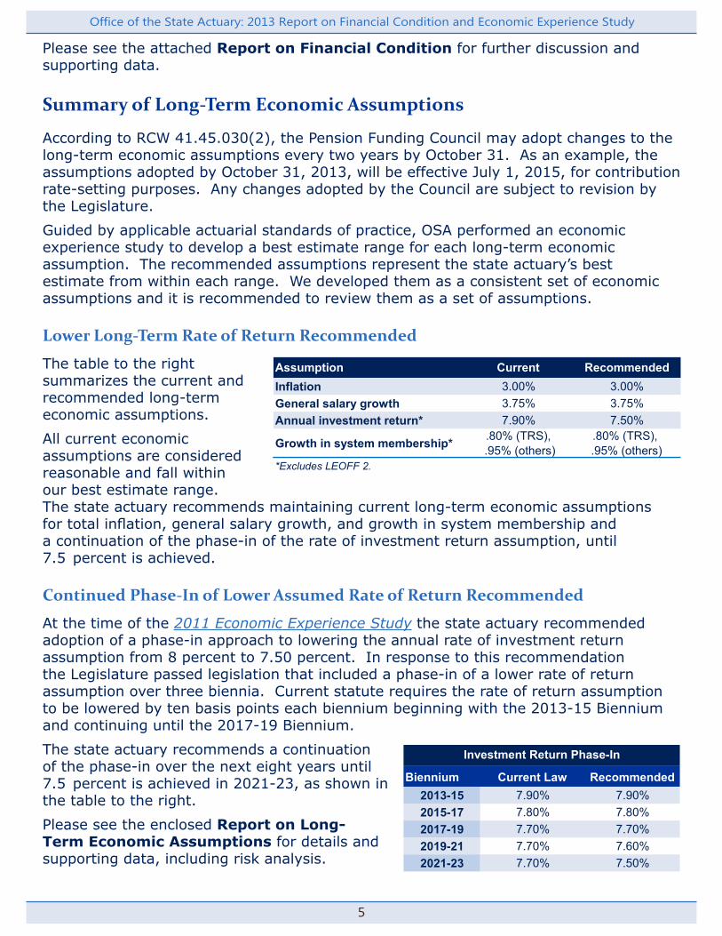
The table to the right summarizes the current and recommended long-term economic assumptions.
All current economic assumptions are considered reasonable and fall within our best estimate range. The state actuary recommends maintaining current long-term economic assumptions for total inflation, general salary growth, and growth in system membership and a continuation of the phase-in of the rate of investment return assumption, until 7.5 percent is achieved.
Continued Phase-In of Lower Assumed Rate of Return Recommended
At the time of the 2011 Economic Experience Study the state actuary recommended adoption of a phase-in approach to lowering the annual rate of investment return assumption from 8 percent to 7.50 percent. In response to this recommendation the Legislature passed legislation that included a phase-in of a lower rate of return assumption over three biennia. Current statute requires the rate of return assumption to be lowered by ten basis points each biennium beginning with the 2013-15 Biennium and continuing until the 2017-19 Biennium.
The state actuary recommends a continuation of the phase-in over the next eight years until 7.5 percent is achieved in 2021-23, as shown in the table to the right.
Please see the enclosed Report on Long-Term Economic Assumptions for details and supporting data, including risk analysis.
Assumption Current RecommendedInflation 3.00% 3.00%General salary growth 3.75% 3.75%Annual investment return* 7.90% 7.50%
Growth in system membership* .80% (TRS), .95% (others)
.80% (TRS), .95% (others)
*Excludes LEOFF 2.
Biennium Current Law Recommended2013-15 7.90% 7.90%2015-17 7.80% 7.80%2017-19 7.70% 7.70%2019-21 7.70% 7.60%2021-23 7.70% 7.50%
Investment Return Phase-In

Office of the State Actuary: 2013 Report on Financial Condition and Economic Experience Study
6

7
Office of the State Actuary: 2013 Report on Financial Condition
Report on Financial Condition
As required under RCW 41.45.030, we present this Report on Financial Condition (Report), along with the Economic Experience Study, to assist the Pension Funding Council in evaluating whether to adopt changes to the long-term economic assumptions identified in RCW 41.45.035. We do not advise readers of this report to use the information contained herein for other purposes. Please see the Actuarial Certification Letter for additional considerations.
In this report, we focus on the funded status as a measure of the plans’ health and financial condition. We measured the funded status by dividing the plan’s assets by the liabilities at a single point in time. The assets of the plan are based on the actuarial or smoothed value, which helps limit the fluctuation in results from year to year that would occur if the market value of assets was used in this measure. The liabilities are today’s value (present value) of all future benefits that will be paid out to current members and retirees based on what has been “earned” as of the measurement date. In determining the present value, we discount future benefit payments by the expected annual rate of return on assets.
At the highest level, this funded status measurement helps evaluate whether a plan is on target with its funding policy (or financing plan). A plan with a funded status of at least 100 percent is on target with its financing plan; whereas a plan with a funded status below 100 percent is off target. Generally speaking, a plan that’s off target will require additional contributions over time to get back on track. The degree of increase and the length of time required will depend on other measurements (i.e., plan maturity, amount of remaining benefits, salary and revenue available to collect additional contributions, etc.) However, it’s important to note that a plan with less than a 100 percent funded status is not automatically “at risk” of not being able to meet future benefit obligations. Conversely, a plan with a funded status above 100 percent is not necessarily over funded.
In reviewing the financial condition of the plans, we also look at the changes since the 2011 Report on Financial Condition and how we expect the financial condition to change in the future. This helps determine the path of financial health the plans are on and identify certain risks the plans face in the future. We discuss these changes in the context of the funded status and what is impacting either the assets or liabilities.
Under current funding policy, investment returns primarily drive changes to asset levels while the main drivers to changes in the liabilities include the discount rate (or future investment return expectations) and changes to the current benefit structure. The following sections discuss these key drivers and their impact on the financial condition of the plans.

Office of the State Actuary: 2013 Report on Financial Condition
8
Recent Investment Return Experience Expected To Improve Financial Condition, Short Term Decline in Funded Status Still Expected
Since the Great Recession of 2009, short-term investment returns have continued to, on average, exceed long-term expectations. We saw higher than expected investment returns in 2010, 2011, and 2013 with 13.22 percent, 21.14 percent, and 12.36 percent respectively. Since the recession, we have seen only one year (2012) with lower than expected investment returns at 1.4 percent. However, on average, we have seen investment returns below long-term expectations over the past six years.
The higher than expected returns since the Great Recession improved the funded status of the plans. However, primarily because average annual investment returns over the past six years are below expectations, we are continuing to see the funded status for some plans decline as shown in the table below.
Although we’re seeing a decline in the funded status for some plans, this decline is less than we expected in our last report due to the higher than expected returns over the past few years. We also expect to see the funded status begin to improve for all plans. However, actual funded status in the future will depend on future contribution levels, actual future investment returns, and actual future benefit levels, which may vary from our expectations.
Fiscal YearEnding30-Jun2008 (1.24%) 8.00%2009 (22.84%) 8.00%2010 13.22% 8.00%2011 21.14% 8.00%2012 1.40% 7.90%2013 12.36% 7.90%
Average 2.95% 7.97%
Historical Plan PerformanceActual
Investment Return
Expected Investment
Return
Plan 2010* 2011 2012**PERS 1 74% 71% 69%PERS 2/3 113% 112% 111%TRS 1 84% 81% 79%TRS 2/3 116% 113% 114%SERS 2/3 113% 110% 110%PSERS 2 129% 132% 134%LEOFF 1 127% 135% 135%WSPRS 1/2 118% 115% 114%
Funded Status as of June 30
**Based on 2012 AVR results.
*After Uniform Cost Of Lliving Adjustment repeal (consistent with 2010 Actuarial Valuation Report).
9
Office of the State Actuary: 2013 Report on Financial Condition
Lower Investment Return Assumption Increases Liabilities in the Short Term, Improves Long-Term Risk
Chapter 7, Laws of 2012, First Special Session lowered the prescribed rate of investment return assumption from 8.0 percent to 7.7 percent over a three-biennia period beginning in 2013-15. Lowering the investment return assumption (discount rate) increases the present value of the liabilities and puts downward pressure on the funded status and financial condition of the plans in the short-term. However, the closer the investment return assumption is to our best estimate for future returns, the lower the financial risk we expect for the plans. While we expect the plans will experience a short term decline in funded status during the phase-in of the lower investment return assumption, we expect they will be in a better financial position over the longer-term due to the lower investment return assumption.
Recent Benefit Changes For New Hires Will Improve Financial Condition
Chapter 7, Laws of 2012, First Special Session also reduced subsidized Early Retirement Factors (ERFs) for members hired after May 1, 2013, in Plans 2/3 of PERS, TRS, and SERS retirement systems. All else being equal, lowering benefits lowers the liabilities of the plan which increases the funded status. However, because this recent benefit change is effective after the date of our measurements we do not see any impact to the liabilities in this report. Also, since this benefit change only impacts new members joining the plan after May 1, 2013, it will take some time before this change will start to impact the liabilities and funded status.
Current Litigation May Increase Benefits and Impact the Financial Condition
We assessed the financial condition of the pension systems based on the plan provisions that exist in current law. However, there are currently two pending Supreme Court cases scheduled to be heard in the fall of 2013. The decisions in those cases could impact the financial condition of the pension systems.
The Legislature repealed gain-sharing provisions available to certain members of the state retirement systems in 2007 and adopted replacement benefits, including alternate early retirement benefits, for PERS, TRS, and SERS Plans 2/3 members, and an addition to the PERS and TRS Plan 1 Uniform Cost Of Living Allowance (UCOLA) (collectively, the "replacement benefits"). In 2011, the Legislature repealed the UCOLA benefit, an annual benefit increase for PERS 1 and TRS 1 retirees. The trial court reinstated gain-sharing, but found constitutional the repeal of the replacement benefits for Plan 1 and Plan 3 members, and reinstated the UCOLA for those Plan 1 members who worked at any time after the UCOLA was enacted. Both the state and the plaintiffs appealed these decisions. The Supreme Court will hear both the gain-sharing and UCOLA lawsuits as companion cases. Should the Supreme Court uphold lower court decisions, gain-sharing and UCOLA benefits would be reinstated for certain members, and the replacement benefits would continue only for PERS, TRS, and SERS Plan 2 members.
The potential reinstatement of these benefits would pose a unique risk to the pension systems. Generally, when we model risks to the pension systems and show a range of
Office of the State Actuary: 2013 Report on Financial Condition
10
possible outcomes, most of the outcomes occur between the extremes. In other words, a broad spectrum of possibilities exists and the worst-case scenario is highly unlikely to occur. Also, each risk usually occurs many times (e.g., investment returns occur each year), and a bad outcome one year can be offset in the future. However, for purposes of modeling, these litigation risks have only two possible outcomes — either the repeal of the benefits stands or the benefits are reinstated. They are also, for purposes of modeling, one-time decisions that would not be offset in future years.
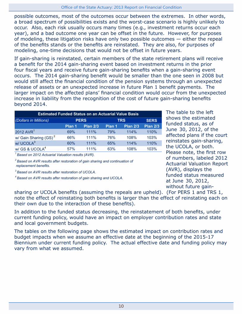
If gain-sharing is reinstated, certain members of the state retirement plans will receive a benefit for the 2014 gain-sharing event based on investment returns in the prior four fiscal years and receive future gain-sharing benefits when a gain-sharing event occurs. The 2014 gain-sharing benefit would be smaller than the one seen in 2008 but would still affect the financial condition of the pension systems through an unexpected release of assets or an unexpected increase in future Plan 1 benefit payments. The larger impact on the affected plans’ financial condition would occur from the unexpected increase in liability from the recognition of the cost of future gain-sharing benefits beyond 2014.
The table to the left shows the estimated funded status, as of June 30, 2012, of the affected plans if the court reinstates gain-sharing, the UCOLA, or both. Please note, the first row of numbers, labeled 2012 Actuarial Valuation Report (AVR), displays the funded status measured at June 30, 2012, without future gain-
sharing or UCOLA benefits (assuming the repeals are upheld). (For PERS 1 and TRS 1, note the effect of reinstating both benefits is larger than the effect of reinstating each on their own due to the interaction of these benefits).
In addition to the funded status decreasing, the reinstatement of both benefits, under current funding policy, would have an impact on employer contribution rates and state and local government budgets.
The tables on the following page shows the estimated impact on contribution rates and budget impacts when we assume an effective date at the beginning of the 2015-17 Biennium under current funding policy. The actual effective date and funding policy may vary from what we assumed.
SERSPlan 1 Plan 2/3 Plan 1 Plan 2/3 Plan 2/369% 111% 79% 114% 110%66% 111% 76% 108% 103%60% 111% 65% 114% 110%57% 111% 63% 108% 103%
4 Based on AVR results after restoration of gain sharing and UCOLA.
PERS TRSEstimated Funded Status on an Actuarial Value Basis
(Dollars in Millions)
2012 AVR1 w/ Gain Sharing (GS) 2
w/ UCOLA3 w/ GS & UCOLA4
1 Based on 2012 Actuarial Valuation results (AVR).
3 Based on AVR results after restoration of UCOLA.
2 Based on AVR results after restoration of gain sharing and continuation of replacement benefits.
11
Office of the State Actuary: 2013 Report on Financial Condition
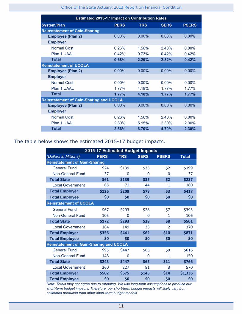
The table below shows the estimated 2015-17 budget impacts.
System/Plan PERS TRS SERS PSERSReinstatement of Gain-Sharing Employee (Plan 2) 0.00% 0.00% 0.00% 0.00% Employer
Normal Cost 0.26% 1.56% 2.40% 0.00%Plan 1 UAAL 0.42% 0.73% 0.42% 0.42%
Total 0.68% 2.29% 2.82% 0.42%Reinstatement of UCOLA Employee (Plan 2) 0.00% 0.00% 0.00% 0.00% Employer
Normal Cost 0.00% 0.00% 0.00% 0.00%Plan 1 UAAL 1.77% 4.18% 1.77% 1.77%
Total 1.77% 4.18% 1.77% 1.77%Reinstatement of Gain-Sharing and UCOLA Employee (Plan 2) 0.00% 0.00% 0.00% 0.00% Employer
Normal Cost 0.26% 1.56% 2.40% 0.00%Plan 1 UAAL 2.30% 5.15% 2.30% 2.30%
Total 2.56% 6.70% 4.70% 2.30%
Estimated 2015-17 Impact on Contribution Rates
(Dollars in Millions) PERS TRS SERS PSERS TotalReinstatement of Gain-Sharing
General Fund $24 $139 $35 $2 $199Non-General Fund 37 0 0 0 37
Total State $61 $139 $35 $2 $237Local Government 65 71 44 1 180
Total Employer $126 $209 $79 $3 $417Total Employee $0 $0 $0 $0 $0
Reinstatement of UCOLAGeneral Fund $67 $293 $28 $7 $395Non-General Fund 105 0 0 1 106
Total State $172 $293 $28 $8 $501Local Government 184 149 35 2 370
Total Employer $356 $441 $62 $10 $871Total Employee $0 $0 $0 $0 $0
Reinstatement of Gain-Sharing and UCOLAGeneral Fund $95 $447 $65 $9 $616Non-General Fund 148 0 0 1 150
Total State $243 $447 $65 $11 $766Local Government 260 227 81 3 570
Total Employer $502 $675 $145 $14 $1,336Total Employee $0 $0 $0 $0 $0
Note: Totals may not agree due to rounding. We use long-term assumptions to produce our short-term budget impacts. Therefore, our short-term budget impacts will likely vary from estimates produced from other short-term budget models.
2015-17 Estimated Budget Impacts

Office of the State Actuary: 2013 Report on Financial Condition
12
Important Note: The estimated impacts for the reinstatement of gain-sharing also include continuation of the replacement benefits for members of PERS and TRS Plans 1, 2, and 3 and SERS Plans 2/3 members. Should the Supreme Court uphold the lower court decision restoring gain-sharing, but repeal the replacement benefits for all members of PERS, TRS, and SERS, (including Plans 2) the early retirement benefits would not be available to anyone who had not yet retired and received his or her first monthly retirement allowance. Furthermore, the estimated impacts for the reinstatement of the UCOLA benefits assume reinstatement for all members in PERS 1 and TRS 1. Should the Supreme Court uphold the lower court decision on the UCOLA, the UCOLA would be reinstated for only certain Plan 1 members. As a result, the actual impacts of any reinstatement of benefits could be lower than estimated above.
Upcoming Reporting Changes Will Not Affect the Funded Status of the Pension Systems
There are multiple changes coming to how we will calculate and report pension liabilities due to recent announcements by the Governmental Accounting Standards Board (GASB) and certain credit rating agencies (Moody's). State and local governments will soon be required to distinguish several separate pension measurements, each for their own different purpose. The important thing to keep in mind is that none of these changes will actually change the financial condition of the pension systems unless they lead to changes in future funding policy.
GASB and Moody’s measurements each have a specific purpose and neither is meant to be used in the calculation that determines the appropriate annual contribution that employers and members must make in order to maintain the soundness of the pension systems.
GASB changes are to take place in phases beginning in Fiscal Year 2014 and include new reporting requirements for local employers. New measurements from Moody’s are aimed at creating more consistency between the states (and municipal plans) when calculating pension obligations for the purpose of government bond ratings. These upcoming reporting changes do not affect current funding policies or statutes for the state.
Summary
Since our 2011 Report on Financial Condition, the financial status of the pension systems has continued to decline but that decline is expected to be short-term and followed by an improvement in the funded status. Recent investment returns and changes in benefits for new hires will improve the financial condition of the affected plans. The continued phase-in of lower assumed rates of investment return will reduce the long-term risks we expect for the retirement systems. Recent reporting changes adopted by GASB and Moody’s will not affect the financial condition of the plans unless they lead to changes in future funding policy.
While the financial condition of the pension systems has declined in recent years and steps have been taken to improve the overall financial condition, we advise the Council to consider the following three outstanding issues when contemplating future pension action.

13
Office of the State Actuary: 2013 Report on Financial Condition
1. We expect contribution rates to increase, as remaining asset losses from 2008-2009 are recognized and lower rate of return assumptions are phased-in, before approaching expected long-term levels. While higher contribution rates result in additional prefunding and improved long-term financial condition of the plans, they put pressure on near-term budgets. If increasing contribution levels cannot be met, the financial condition of the plans will most likely decline.
2. A court reinstatement of recently repealed benefits would negatively impact the financial condition of the pension systems.
3. Volatility or swings in financial markets can weaken or improve the financial condition of a pension system over a short period of time. Continued full funding and the maintenance of affordable/sustainable plan designs will help the pension systems weather such volatility.
Data, Assumptions, and Methods Used
We performed this analysis consistent with the June 30, 2012, Actuarial Valuation Report (AVR). We used asset information and participant data as of June 30, 2012. We have provided the June 30, 2013 asset returns for informational purposes only. Assets and liabilities measured at June 30, 2013, will be reflected in the 2013 Actuarial Valuation Report.
In estimating the cost of reinstating the UCOLA, we added back the liability (adjusted with interest) that was removed in 2011 when the UCOLA was removed prospectively. We compared the funded status and contribution rates with this additional liability to the funded status and contribution rates without this liability to determine the change in funded status and contribution rates. We applied the change in contribution rates to projected payroll to estimate the budget impacts for 2015-17. For purposes of this estimate, we assumed the UCOLA would be reinstated immediately. We did not include a liability for any back payments. Please see the actuarial fiscal note for SHB 2021 (2011) for a complete description of the data, assumptions and methods we used to determine the liability removed when the UCOLA was repealed.
In estimating the cost of reinstating gain-sharing benefits, we added back the liability (adjusted with interest) that was removed in 2007 when gain-sharing was removed prospectively. We compared the funded status and contribution rates with this additional liability to the funded status and contribution rates without this liability to determine the change in funded status and contribution rates. We applied the change in contribution rates to projected payroll to estimate the budget impacts for 2015-17. For purposes of this estimate, we assumed gain-sharing benefits would be reinstated only for members who were eligible to receive the 2008 gain-sharing event. The method for calculating the cost of gain sharing is consistent with the method used in our actuarial fiscal note for EHB 2391 from the 2007 Legislative session (the repeal of gain-sharing). For measuring the cost of reinstating gain-sharing benefits, we used a reduction in the assumed rate of investment return of 0.40 percent for PERS and TRS Plans 1, 0.04 percent for PERS 2/3, 0.33 percent for TRS 2/3, and 0.44 percent for SERS 2/3. Please see the actuarial fiscal note for EHB 2391 (2007) for a complete description of the data, assumptions and methods we used to determine the liability removed when gain-sharing was repealed.

Office of the State Actuary: 2013 Report on Financial Condition
14
PO Box 40914 Phone: 360.786.6140 Olympia, Washington, 98504-0914 Fax: 360.586.8135 osa.leg.wa.gov TDD: 711 Office of the State Actuary August 30, 2013

15
Office of the State Actuary: 2013 Report on Financial Condition
PO Box 40914 Phone: 360.786.6140 Olympia, Washington, 98504-0914 Fax: 360.586.8135 osa.leg.wa.gov TDD: 711 Office of the State Actuary August 30, 2013

Office of the State Actuary: 2013 Report on Financial Condition
16
17
Office of the State Actuary: 2013 Economic Experience Study
General Approach to Setting Economic Assumptions
Actuarial Standard of Practice Number 27 (ASOP 27), titled Selection of Economic Assumptions for Measuring Pension Obligations, identifies the following process for selecting economic assumptions:
◊ Identify components, if any, of each assumption and evaluate relevant data.
◊ Develop a best-estimate range for each economic assumption.◊ Select a specific point estimate within the best-estimate range.◊ Review the set of economic assumptions for consistency.
For each economic assumption, the best-estimate range is “the narrowest range within which the actuary reasonably anticipates that the actual results, compounded over the measurement period, are more likely than not to fall.” The measurement period is the time period after the valuation date when a particular economic assumption will apply. Pension funding occurs over long time periods; therefore, the measurement period for economic assumptions can easily exceed fifty years.
The “building block” method is one acceptable method for setting economic assumptions identified in ASOP 27. Using this method, the actuary determines the individual components for each economic assumption. Then the actuary may combine estimates for each applicable component to arrive at a best-estimate range for the given economic assumption. With the exception of annual growth in system membership assumption, we used the building block method to develop each assumption in the 2013 Economic Experience Study.
Experience Study and Recommended Assumptions
We will identify the following for each assumption we studied:
◊ How the assumption is used for funding in our model.◊ The single point best-estimate and its best-estimate range.◊ The data we studied and how we analyzed the data.◊ How we developed each assumption.
Economic Experience Study
Office of the State Actuary: 2013 Economic Experience Study
18
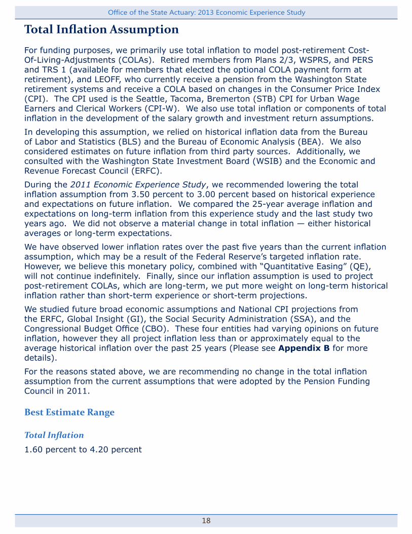
Total Inflation Assumption
For funding purposes, we primarily use total inflation to model post-retirement Cost-Of-Living-Adjustments (COLAs). Retired members from Plans 2/3, WSPRS, and PERS and TRS 1 (available for members that elected the optional COLA payment form at retirement), and LEOFF, who currently receive a pension from the Washington State retirement systems and receive a COLA based on changes in the Consumer Price Index (CPI). The CPI used is the Seattle, Tacoma, Bremerton (STB) CPI for Urban Wage Earners and Clerical Workers (CPI-W). We also use total inflation or components of total inflation in the development of the salary growth and investment return assumptions.
In developing this assumption, we relied on historical inflation data from the Bureau of Labor and Statistics (BLS) and the Bureau of Economic Analysis (BEA). We also considered estimates on future inflation from third party sources. Additionally, we consulted with the Washington State Investment Board (WSIB) and the Economic and Revenue Forecast Council (ERFC).
During the 2011 Economic Experience Study, we recommended lowering the total inflation assumption from 3.50 percent to 3.00 percent based on historical experience and expectations on future inflation. We compared the 25-year average inflation and expectations on long-term inflation from this experience study and the last study two years ago. We did not observe a material change in total inflation — either historical averages or long-term expectations.
We have observed lower inflation rates over the past five years than the current inflation assumption, which may be a result of the Federal Reserve’s targeted inflation rate. However, we believe this monetary policy, combined with “Quantitative Easing” (QE), will not continue indefinitely. Finally, since our inflation assumption is used to project post-retirement COLAs, which are long-term, we put more weight on long-term historical inflation rather than short-term experience or short-term projections.
We studied future broad economic assumptions and National CPI projections from the ERFC, Global Insight (GI), the Social Security Administration (SSA), and the Congressional Budget Office (CBO). These four entities had varying opinions on future inflation, however they all project inflation less than or approximately equal to the average historical inflation over the past 25 years (Please see Appendix B for more details).
For the reasons stated above, we are recommending no change in the total inflation assumption from the current assumptions that were adopted by the Pension Funding Council in 2011.
Best Estimate Range
Total Inflation
1.60 percent to 4.20 percent

19
Office of the State Actuary: 2013 Economic Experience Study
Recommendation
Total Inflation
3.00 percent**Includes 2.40 percent broad economic inflation, 0.30 percent national price inflation differential, and 0.30 percent regional price inflation differential
Current Assumption
Total Inflation
3.00 percent
Data
Historical Inflation Data (Appendix A)
Projected Gross Domestic Product (GDP) Deflator and National CPI (Appendix B)
Methodology
We use the building block method to develop our total inflation assumption, which requires the actuary to determine the components of each assumption and make an estimate for each component. The estimated components for each assumption are then combined to arrive at a best estimate for the assumption.
For the total inflation assumption we used three building block components to create our assumption: broad economic inflation, National CPI-W adjustment (national price differential), and STB CPI-W adjustment (regional price differential). The combination of all three components will be referred to as total inflation in this report. We made a recommendation on total inflation only; however, we studied each inflation component individually and how they compare to each other (please see the Analysis section for a detailed discussion).
In addition to using the building block method to develop our total inflation assumption, we also used it to develop our nominal investment return assumption and our general salary growth assumption. Nominal investment return and general salary growth both use total inflation or components of total inflation as one of their building block components.
Analysis
Broad Economic Inflation
Assumption
2.40 percent

Office of the State Actuary: 2013 Economic Experience Study
20
Best Estimate Range
1.50 percent to 3.30 percent
The base for our total inflation assumption is the GDP deflator for Personal Consumption Expenditures (PCE). The GDP deflator measures the changes in both price and quantity of the goods produced in a country and provides an indication of whether an economy is growing or shrinking. The GDP deflator was used as our broad economic inflation component because it does not react solely to changes in price like a CPI.
Our annual investment return assumption uses the GDP deflator as one of its two building block components since the GDP deflator measures an economy’s growth. Please see the Investment Return section for additional details.
We studied the historical GDP deflator produced by the BEA as well as GDP deflator projections from the ERFC, GI, SSA, and the CBO. Our best estimate assumption for broad economic inflation, 2.40 percent per year, corresponds with the average GDP deflator over the past 25 years rounded to the nearest tenth (please see Appendix A for more details). Our best estimate broad economic inflation assumption is also equal to SSA’s ultimate GDP deflator under intermediate-cost projections. SSA expects their intermediate-cost GDP deflator to reach an ultimate rate of 2.40 percent in 2015. Our best estimate broad economic inflation is greater than CBO and GI’s ultimate GDP deflators which reflect the Federal Reserve’s inflation target of approximately 2 percent. We don’t believe this policy, combined with QE, will continue indefinitely. QE generally consists of increasing the monetary base through large-scale asset purchasing and lending programs by the Federal Reserve to stimulate economic growth and put downward pressure on longer-term interest rates.*
Given the inherent uncertainty of long-term future inflation, we believe it is reasonable to select 2.40 percent as our best estimate.
The low end of the best estimate range corresponds to SSA’s low-cost ultimate GDP deflator assumption. SSA projects the low-cost GDP deflator to reach its ultimate rate of 1.50 percent in 2017.
The high end of the best estimate range corresponds to SSA’s high-cost ultimate GDP deflator assumption. SSA projects the high-cost GDP deflator to reach its ultimate rate of 3.30 percent in 2019.*Sources: Board of Governors of the Federal Reserve; Federal Reserve Bank of St. Louis, Four Stories of QE.
National CPI-W Price Differential
Assumption
0.30 percent
Best Estimate Range
0.10 percent to 0.50 percent
The CPI provides another measure of inflation. It measures changes in price for a fixed basket of goods. A CPI strictly measures price inflation. It does not take into account changes in consumption habits. The BLS produced the CPI that we studied. BLS

21
Office of the State Actuary: 2013 Economic Experience Study
produces different CPIs based on different baskets of goods, for different regions of the country, or both.
The National CPI-W price differential is the difference between the National CPI-W and the GDP deflator. Our best estimate assumption for National CPI-W price differential, 0.30 percent per year, corresponds with historical and projected price differentials.
We observed the National CPI-W price differential over the past 25 years to be approximately 0.40% (2.84% - 2.42 % = 0.41%). The best estimate National CPI-W price differential is higher than the average GI projected National CPI price differential (0.15 percent) and the average ERFC projected National CPI price differential (0.19 percent). The best estimate National CPI price differential is equal to the projected ultimate CBO National CPI price differential, but lower than the ultimate SSA intermediate-cost price differential (0.40 percent). The average National CPI price differential of these four publications is 0.26 percent; which, rounded to the nearest tenth, corresponds with our best estimate.
The National CPI-W price differential’s best estimate range includes all projected National CPI price differentials we studied. The GI National CPI-W price differential and the ultimate SSA high cost National CPI price differential represent the low and high ends of the best estimate range respectively. Please see Appendix B for a table illustrating annually projected National-CPI price differentials from each publication.
The addition of our best estimates for broad economic inflation and National CPI-W price differential creates a National CPI-W best estimate of 2.70 percent (2.40 percent plus 0.30 percent). The National CPI-W best estimate corresponds with the 2.70 percent inflation assumed in WSIB’s 2013 Capital Market Assumptions (CMAs).
Seattle, Tacoma, Bremerton (STB) CPI-W Price Differential
Assumption
0.30 percent
Best Estimate Range
0.00 percent to 0.40 percent
We based the STB CPI-W regional price differential on the rounded average difference between STB CPI-W and national CPI-W over the last 25 years (3.19% - 2.84% = 0.35%). The lower end of the best estimate range is consistent with the average STB CPI-W adjustment over the last ten years (rounded up), and the higher end of the best estimate range is consistent with the average STB CPI-W adjustment over the last twenty-five years (rounded up).
STB CPI-W has been larger, on average, than the National CPI-W since 1950. However, STB CPI-W may not always be larger than the National CPI-W. For instance, National CPI-W was larger than the STB CPI-W during the 1970s and 1980s. We will continue to monitor this and consider adjusting or potentially removing our STB regional price differential if the historical STB regional price differential begins to narrow considerably over longer-term experience periods.

Office of the State Actuary: 2013 Economic Experience Study
22
Total Inflation
We studied both the National CPI-W and the STB CPI-W and reviewed how they compared to the GDP deflator. In general, National CPI-W has a higher inflation than the GDP Deflator and the STB CPI-W has a higher inflation than National CPI-W. We built our total inflation assumption by adding National and regional CPI-W price differentials to our broad economic inflation assumption. We assume the GDP deflator is embedded in CPI so we applied “price inflation differentials” to develop our total inflation best estimate.
The best estimate single-point assumption for total inflation, 3 percent per year, is 19 basis points lower than the average STB CPI-W over the last 25 years.
The average GDP deflator has decreased from 5.06 percent during 1980-1989, to 2.42 percent during 1990-1999, to 2.21 percent during 2000-2009, and was 2.03 percent during 2010-2012. This may be due to a strict United States monetary policy designed to keep inflation low. The Federal Reserve has been attempting to keep the GDP deflator around 2 percent. However, the Federal Reserve cannot control inflation on all items. For example, food and energy prices are independent of the Federal Reserve and may fluctuate depending on external forces. Furthermore, this monetary policy, combined with QE, will not continue indefinitely.
CBO assumes that inflation during 2019-2023 will be determined generally by monetary policy. CBO’s projected inflation during 2019-2023 reflects the Federal Reserve’s 2 percent target for inflation. While 2 percent is within our broad economic inflation best estimate range, we believe it would be an overly optimistic assumption in the long-run as a single point, best estimate. Furthermore, we believe it creates too large of a decrease from our currently recommended broad economic inflation assumption. However, we will continue to monitor actual inflation experience and revisit the broad economic inflation assumption again in two years.
Our total inflation assumption will be used in the salary growth section to help determine “productivity growth.” Productivity growth represents the difference between our general salary growth and total inflation. Please see the Salary Growth section for additional detail.
Recommendation
For the reasons stated above, we recommend no change in the total inflation assumption from the currently assumed total inflation assumption of 3 percent.

23
Office of the State Actuary: 2013 Economic Experience Study
General Salary Growth
We use this assumption to project salaries to determine future retirement benefits and contribution rates as a percent of payroll. We also use it to determine employer contributions to the Plan 1 UAAL for PERS and TRS as a level percentage of future system payrolls. Generally, a participant’s salary will change over the long term in accordance with inflation, productivity growth, merit (or longevity increases), and promotional increases.
In developing this assumption, we relied on data from the Bureau of Labor and Statistics (BLS) for historical inflation. We also reviewed historical salary data from the Department of Retirement Systems.
During the 2011 Economic Experience Study, we recommended lowering the general salary growth assumption from 4.00 percent to 3.75 percent to remain consistent with the recommended lower (and now adopted) rate of future inflation. For this experience study, we compared historical salary experience, based on our recommended study period (1984-2009), to the last study two years ago. We did not observe a material change in general salary growth.
We did observe lower than expected salary growth from 2010 through 2012, which is a result of temporary salary practices that occurred during the 2009-11 and 2011-13 Biennia. We believe these temporary salary practices do not reflect future long-term salary experience so our general salary growth assumptions were developed using historical salary growth data from 1984-2009, rather than from 1984-2012.
We study general salary growth and merit (or longevity) separately. Total inflation and productivity are the two key building block components of the general salary growth assumption. We formed our best estimate for total inflation in the Inflation section of this report. We calculated the productivity such that the cumulative observed merit approximately equals cumulative assumed merit. Please see the Analysis section for details on how we developed our best estimate for productivity.
For the reasons stated above, we are recommending no change in the general salary growth assumption from the current assumption that was adopted by the Pension Funding Council in 2011.
Best Estimate Range1.50 percent to 5.20 percent
Recommendation3.75 percent**Includes 3.00 percent total inflation and 0.75 percent productivity.
Current Assumption3.75 percent

Office of the State Actuary: 2013 Economic Experience Study
24
DataGrowth in Salaries for Members Active for Two Consecutive Years (Appendix C)****Appendix C was mislabeled in the 2011 Economic Experience Study. We did not change methods in this area.
Methodology
Our actuarial model assumes two separate sources of salary increases: general salary growth and merit (or longevity) increases. We study the general salary growth and merit (or longevity) increases separately because we apply the assumptions in different ways. Actuarial Standards of Practice (ASOP) 27 defines productivity growth as “the rates of change in a group’s compensation attributable to the change in real value of goods or services per unit of work.” Merit (or longevity) increases are defined as “the rates of change in an individual’s compensation attributable to personal performance, promotion, seniority, or other individual factors.” In other words, general salary growth applies broadly to many different groups, while merit or longevity increases apply to specific groups and individuals.
We review general salary growth as part of the economic experience study when we look at broad trends. We typically study merit (or longevity) increases as part of the demographic experience study process when we focus more on trends within individual plans. Ideally, the combination of the two assumptions would model total salary growth.
We used the building block method to model general salary growth. Total inflation and productivity growth are general salary growth’s two building block components. The total inflation assumption as developed in the Inflation section. To develop our productivity growth, we reviewed growth in salaries for active members employed for two consecutive years.
Analysis
We took the following steps to develop our best estimate recommendation.
1. Chose the time period for studying general salary growth. We observed lower than expected general salary growth over the past three valuation reports (2010-2012). This reflects temporary salary practices that we do not believe are representative of future long-term salary experience. Some examples of these temporary salary practices that occurred during the 2009-11 and 2011-13 Biennia include salary reductions and salary freezes. The temporary salary practices primarily impacted state employees, although local employees may have been impacted as well. Furthermore, salary reductions during 2011-13 for state employees were restored during the 2013-15 Biennium and are not included in this analysis (data not yet available for study). Because 2010-2012 includes short-term salary practices that we believe are not indicative of long-term salary practices, we elected to study the general salary growth assumption during the 1984 through 2009 time period. However, we have provided the calculated

25
Office of the State Actuary: 2013 Economic Experience Study
productivity, for each system, when we include the most recent three years of data. Please see Step 4 for more information.
2. Assembled historical system salary growth by years of service from 1984 through 2009. We display this data in Appendix C. It represents total salary growth, by years of service, for active members consecutively employed for two or more years during the period 1984 through 2009. For example, for all PERS active members who were employed at least two consecutive years during 1984 through 2009, the average increase in total salary from their first to second year of service was 8.81 percent.
3. Identified the portion of historical salary growth attributable to inflation and productivity. Since the data in Step 2 represents total salary growth by year of service, we then determined the portion attributable to general salary growth. Under our building block method, that means increases attributable to inflation and productivity. We input the average increase for the STB CPI-W for the period 1984 through 2009, 3.13 percent, and solved for the observed productivity increase so the cumulative observed merit increases equaled the cumulative assumed merit increases over the period of assumed merit increases. Under this method, the productivity increase represents the change in total salary increase not attributable to inflation and observed merit (or longevity) increases. For example, if all PERS active members who were employed at least two consecutive years during 1984 through 2009 experienced an average 8.81 percent increase in total salary from their first to second year of service, then about 0.89 percent is attributable to productivity since average inflation as 3.13 percent over the experience study period and the observed merit (or longevity) increase was 4.61 percent.
4. Reviewed the observed productivity for reasonableness. Overall, we found the results, based on 1984-2009 data (Recommended Study Period), reasonable for each system with observed productivity increases ranging from 0.57 percent for SERS to 0.89, 0.92, and 0.97 percent for PERS, WSPRS, and TRS respectively. We would expect an observed productivity between 0.00 and 1.00 percent and less credible results for smaller systems like SERS and WSPRS. As we mentioned in Step 1, we elected to omit data from 2010 through 2012 because it includes short-term salary practices that we don’t believe are consistent with long-term salary growth expectations. However, for your reference, we provide a comparison of observed productivity rates using data from 1984-2009 (Recommended Study Period) to observed productivity rates using data from 1984-2012 (All Years) in the table at the top of the next page.

Office of the State Actuary: 2013 Economic Experience Study
26
As discussed above, the inclusion of temporary salary practices during 2010-12 significantly reduces the observed productivity under the building block approach we used for setting this assumption. Under this approach, inflation and merit increases remain constant during the study so any reduction in salary growth due to short-term salary practices is entirely attributed to decreases in observed productivity. That is why we decided to exclude 2010-12 from the development of our best estimate. However, we did consider this experience when selecting the best estimate range.
5. Selected our best estimate. With the results from Step 4, we now have observed general salary growth rates (total inflation plus productivity) by system for the period 1984 to 2009. Next, we considered expectations for the future. The observed inflation during the study period for general salary growth, 3.13 percent, is consistent with our best estimate recommendation for total inflation of 3.00 percent. The average observed productivity came in around 0.90 percent for the larger (and more credible) systems. The economic forecasts we reviewed for our total inflation assumption, and the capital market assumptions from WSIB, suggest lower economic growth over the next fifteen to twenty years than what occurred in the past. With that in mind, we selected a best estimate productivity assumption of 0.75 percent (0.15 percent below the productivity observed from 1984 to 2009). We will continue to monitor this assumption and may recommend lowering the assumption further when we have additional historical data to support the reduction (or if short-term salary practices continue for extended time periods).
6. Selected our best estimate range. We set the low end of the best estimate range equal to the low end of the best estimate range for total inflation, 1.50 percent, with 0.00 percent productivity. The high end of the best estimate range equals the high end of the best estimate range for total inflation, 4.30 percent, with 1.00 percent productivity.
We did not separately study general salary growth in PSERS due to insufficient data. We also did not separately study general salary increases in TRS from bonuses paid for national board certification due to insufficient historical data. However, we plan to monitor and separately study this form of salary growth in future studies.
Recommendation
For the reasons stated above, we recommend no change in the general salary increase assumption from the currently assumed general salary increase assumption of 3.75 percent.
Data Time Period PERS TRS SERS WSPRS
2011 EES 1984-2010 0.82% 0.83% 0.37% 0.74%2013 EES All Years 1984-2012 0.51% 0.48% (0.02%) 0.40% Recommended Study Period 1984-2009 0.89% 0.97% 0.57% 0.92%
Comparison of Productivity Rates

27
Office of the State Actuary: 2013 Economic Experience Study
Annual Rate of Investment Return
The annual rate of investment return assumption is a key input for determining contribution rates for the ongoing retirement systems. We calculate contribution rates by comparing today’s value of future benefit pyments to the assets we have on hand at the same point in time. We determine today’s value of future benefit pyments and salaries using an assumed rate of future investment returns. In developing this assumption, we consulted with and relied on data provided by WSIB.
We are recommending a decrease in the annual rate of investment return assumption from the assumption currently in statute. This recommendation is consistent with our recommendation during the 2011 Economic Experience Study and is based on WSIB’s expectations for future investment returns. We also considered past investment returns and whether the historical conditions that produced the strong investment markets over the past twenty to thirty years will continue in the future. The recommended rate of investment return assumption represents a single rate that applies to all plans invested in the Commingled Trust Fund (CTF). As the membership of the Plans 1 moves to 100 percent retired status and the Plans 1 remain in the CTF, it may become necessary to use separate investment return assumptions for these plans. We considered making this change, but do not recommend plan specific rate of return assumptions at this time.
Best Estimate Range6.13 percent to 8.62 percent
Recommendation7.50 percent
Current Assumption7.90 percent during the 2013-15 Biennium
7.80 percent during the 2015-17 Biennium
7.70 percent beginning in the 2017-19 Biennium
DataHistorical Plan Performance (Appendix D)
Historical Investment Data - Current Allocations (Appendix E)
Historical Investment Data - Alternate Allocations (Appendix F)
WSIB Simulated Future Investment Returns (Appendix G)
Methodology
The annual rate of investment return assumption reflects anticipated returns on the retirement plan’s current and future assets, net of expenses. ASOP 27 identifies two methods for setting the rate of return assumption. We described the first method, the “building block” method in the General Approach to Setting Economic Assumptions section of this report. ASOP 27 also describes the “cash-flow matching” method for setting the annual rate of investment return assumption. Under this method, we

Office of the State Actuary: 2013 Economic Experience Study
28
project the expected benefit and expense disbursements for all plans invested in the CTF. We then identify a highly diversified U.S. bond portfolio with interest and principal payments, which approximately match our expected benefit payments in the CTF. However, due to the asset allocation of the CTF, this option is not a reasonable method for setting the annual rate of investment return assumption.
In addition to the items discussed in the General Approach to Setting Economic Assumptions section, we consider several key factors when selecting this assumption, namely the:
◊ Purpose of measurement (i.e. on-going plan valuation, plan termination, etc).
◊ Measurement period.◊ Investment or asset allocation policy.
We intend to use this assumption to determine the contribution requirements for the ongoing retirement systems. A different measurement (i.e., plan termination or settlement liability) would require use of a different annual investment return assumption.
The recommended rate of investment return assumption represents a single rate that applies to all plans invested in the CTF. We base that rate on the average future measurement period—referred to as duration—for all plans combined. However, not all plans have the same duration. Plan 1 liabilities have a shorter duration than the liabilities of the Plans 2/3. This occurs because the Plans 1 for all systems, except WSPRS, have been closed to new entrants since 1977 (WSPRS Plan 1 closed in 2002), while the Plans 2/3 are still open to new entrants. This means that all Plan 1 benefits will be paid well before the last Plans 2/3 benefits are paid — hence the shorter future measurement period or duration for the Plans 1.
Ideally, the rate of investment return assumption would be coordinated with WSIB’s current asset allocation policy, or targets, for the CTF. We based the recommendation on WSIB’s current asset allocation policy. Future changes to the CTF asset allocation policy may require a new recommendation for the rate of investment return assumption.
Analysis
We reviewed the historical experience data provided in Appendices D through F, considered the historical conditions that produced past annual investment returns, and relied upon Capital Market Assumptions (CMAs) and simulated expected investment returns provided by the WSIB.
The CMAs include three pieces of information for each class of assets the WSIB might choose to invest in.
◊ Expected annual return.◊ Standard deviation of the annual return.◊ Correlations between the annual returns of each asset class with
every other asset class.WSIB uses the CMAs and their target asset allocation (Please see Appendix G for more details) to simulate future investment returns. We used WSIB’s simulated returns to set the best estimate range and the recommended rate of investment return assumption.

29
Office of the State Actuary: 2013 Economic Experience Study
WSIB provided us with simulated expected investment returns over short and long time horizons ranging from one year to fifty years. WSIB simulated the expected investment returns using a “log stable” distribution.
The log stable distribution approximates future returns based on actual historical data as opposed to assuming a normal distribution or “bell-shaped” curve. Using actual historical data incorporates “fat tails” into the distribution profile. Such fat tails contribute to positive and negative skews (a measure of the extent to which a distribution is distorted from a symmetrical bell-shaped curve), both of which are taken into account under the log stable distribution methodology. WSIB prefers the log stable modeling because it more accurately reflects actual returns. However, the log stable model relies on historical relationships and will not provide accurate estimates of future investment returns if actual future investment returns are vastly different from historical investment returns.
We set the best estimate range equal to the 25th and 75th percentile of the WSIB simulated fifty-year compounded annual rate of investment return distribution: 6.13 percent and 8.62 percent respectively. We selected the best estimate as 7.50 percent — approximately equal to the median of the simulated investment returns, 7.40 percent, but increased slightly to remove WSIB’s implicit and small short-term downward adjustment due to assumed mean reversion. WSIB’s implicit short-term adjustment, while small and appropriate over a ten- to fifteen-year period, becomes amplified over a fifty-year measurement period. Please see Appendix G for additional information regarding simulated future investment returns.
The annual rate of investment return assumption uses broad economic inflation as its base building block. Since the best estimate for the broad economic inflation assumption equals 2.40 percent, the remaining building block, the assumed real rate of investment return, equals 5.10 percent.
Often, the starting point for creating an assumption about the future would be to use historical data. For example, over a thirty- to eighty-year period, typical pension plan asset allocations would have averaged investment returns of 9 to 11 percent per year. However, the implicit assumption being made is that conditions, or in this case the structure of the economy, are the same now as they were in the past. When historical investment return data is used in setting a forward-looking assumption, extra attention is required to determine whether past conditions are likely to repeat in the future.
The following list demonstrates how conditions have changed and their potential impact on future returns:
◊ Higher than normal growth is no longer expected. Economies generally move from agricultural, to industrial, to service based. As a country moves along this progression they experience higher than normal growth and innovation. Many developed countries have progressed to the point where higher than normal growth is no longer expected.
◊ Stock market returns will likely revert back to the historical average. Price to Earnings ratios (P/E) state the price of stocks relative to their earnings. We looked at the Standard & Poor’s 500 (S&P 500) historical P/E ratios. We noticed that S&P 500’s P/E ratios grew substantially from 1980-2010, meaning investors were willing to pay more for a stock given an equal amount of earnings. When P/E
Office of the State Actuary: 2013 Economic Experience Study
30
ratios increase, this creates extra return for stocks (without actual business growth). No one knows where P/E ratios will go from here, but they are likely to revert back to the historical average. We do not expect to see another thirty-year period of increase as seen from 1980 to 2010.
◊ We will likely see lower future dividend yields. Similar to P/E ratios, decreasing or increasing dividend yields add or subtract from investment returns. We looked at the S&P 500 dividend yields and observed that since the early 1980s, dividend yields have steadily decreased from about 5.50 percent to around 2.00 percent in 2013. Lower future dividend yields will mean lower future investment returns.
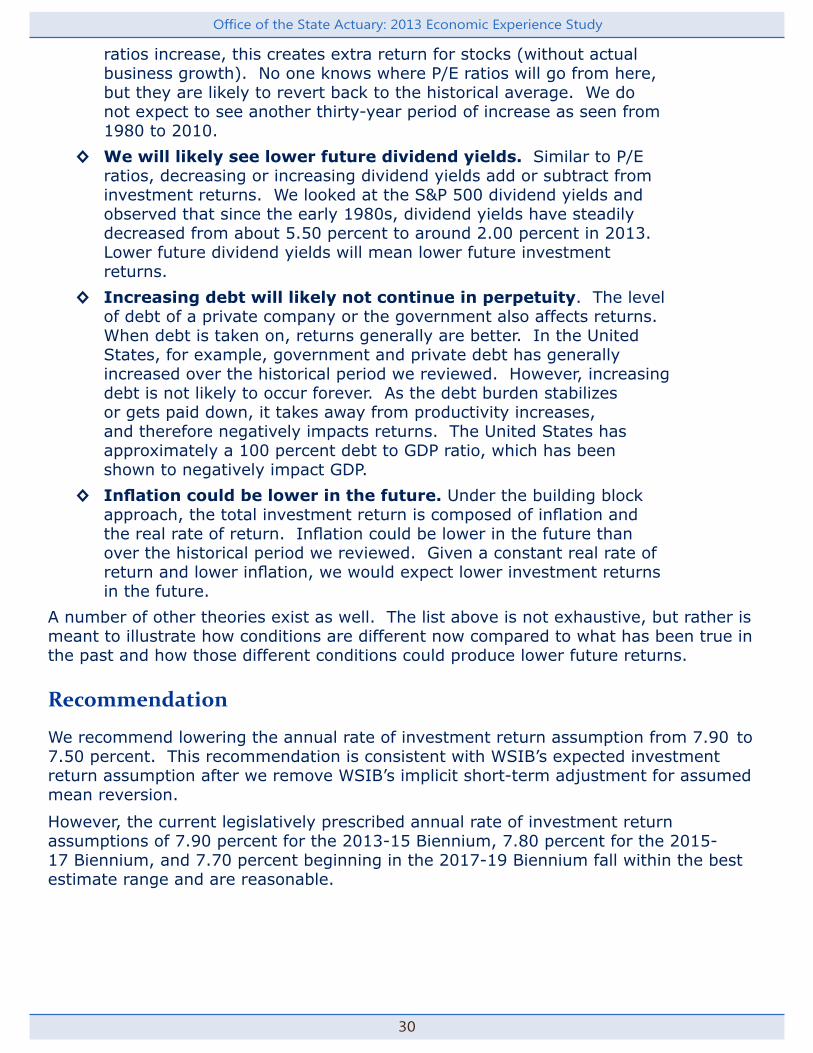
◊ Increasing debt will likely not continue in perpetuity. The level of debt of a private company or the government also affects returns. When debt is taken on, returns generally are better. In the United States, for example, government and private debt has generally increased over the historical period we reviewed. However, increasing debt is not likely to occur forever. As the debt burden stabilizes or gets paid down, it takes away from productivity increases, and therefore negatively impacts returns. The United States has approximately a 100 percent debt to GDP ratio, which has been shown to negatively impact GDP.
◊ Inflation could be lower in the future. Under the building block approach, the total investment return is composed of inflation and the real rate of return. Inflation could be lower in the future than over the historical period we reviewed. Given a constant real rate of return and lower inflation, we would expect lower investment returns in the future.
A number of other theories exist as well. The list above is not exhaustive, but rather is meant to illustrate how conditions are different now compared to what has been true in the past and how those different conditions could produce lower future returns.
Recommendation
We recommend lowering the annual rate of investment return assumption from 7.90 to 7.50 percent. This recommendation is consistent with WSIB’s expected investment return assumption after we remove WSIB’s implicit short-term adjustment for assumed mean reversion.
However, the current legislatively prescribed annual rate of investment return assumptions of 7.90 percent for the 2013-15 Biennium, 7.80 percent for the 2015-17 Biennium, and 7.70 percent beginning in the 2017-19 Biennium fall within the best estimate range and are reasonable.
31
Office of the State Actuary: 2013 Economic Experience Study
Growth in System Membership
The growth in system membership assumption impacts the amortization of the Plan 1 UAAL. Under current law, the UAAL in PERS Plan 1 and TRS Plan 1 must be amortized over a rolling ten-year period, as a percentage of projected payrolls. We use the growth in system membership assumption to estimate the payroll for future new members. In developing this assumption, we relied upon system membership data from the Department of Retirement Systems (DRS) and Washington State population data and forecasts from the Office of Financial Management (OFM).
The projected payroll for the PERS Plan 1 UAAL includes pay from current PERS, SERS, and PSERS members as well as projected payroll from future members of PERS Plans 2/3, SERS, and PSERS. Hereafter, for the discussion of growth in system membership, we will use the term “PERS” to apply to the combined system growth of PERS, SERS, and PSERS. The projected payroll for the TRS Plan 1 UAAL includes pay from current TRS members as well as projected payroll from future TRS Plans 2/3 members.
We observed negative average system growth rates over the past five years due to state and local government budget cuts in response to lingering effects of the most recent recession. As a result, we expect the system growth rates will take a few years to recover to assumed long-term levels. OFM projects Washington State population growth rates to moderately increase over the next ten years (Please see Appendix H for more details). Since our analysis (see Analysis section below) shows a high correlation between system and population growth, we developed a magnitude factor that represents the historical relationship between system growth and Washington State population growth. Applying the magnitude factor and short-term recovery factor to OFM’s projected population growth, we arrive at the recommended PERS and TRS system growth assumptions shown below.
We are recommending no change in the PERS and TRS system growth assumptions from the current assumptions that were adopted by the Pension Funding Council in 2011.
Best Estimate Range0.50 percent to 1.00 percent for TRS
0.50 percent to 1.20 percent for PERS
Recommendation0.80 percent for TRS
0.95 percent for PERS
Current Assumption0.80 percent for TRS
0.95 percent for PERS
Data
Growth in Washington State Population - Historical and Projected (Appendix H)
Historical System Growth (Appendix I)

Office of the State Actuary: 2013 Economic Experience Study
32
Annual Magnitude of System Growth Relative to State Population Growth (Appendix J)
Analysis
We took the following steps to develop our best estimate recommendation.
1. Examined correlation between system growth and state population data. During 1990-2012, we found a strong correlation between same-year retirement system growth and population growth. PERS had a 0.86 correlation to same-year Washington State population growth while TRS had a 0.54 correlation to same-year Washington State ages 5-17 population growth (Please see Appendix I for more details). Our correlations were based on annual growth rates. Correlation is a statistical technique that allows us to calculate how a pair of data sets moves in proportion to each other. A correlation will range from -1 to 1 where each reflects a strong negative correlation and strong positive correlation, respectively. In general, a strong relationship, whether positive or negative, tells us that the two data sets we are studying are moving in the same direction for each database year and move proportionately with each other. Based on the observed correlations, we felt confident setting our system growth assumption as a function of population growth in a year.
2. Reviewed the annual magnitude of system growth relative to state population growth. Using historical data we calculated system growth as a percent of population growth. The system growth as a percent of population growth represents our magnitude factor over a designated time period. In this approach the magnitude factor tells us how the system growth moves in a relation to the population growth. We divided the 1990-2012 average system growth for PERS and TRS by the applicable average population growth for the same period. PERS grew at an annual rate of 107.79 percent of general Washington State population growth. TRS grew at an annual rate of 103.30 percent of Washington State ages 5-17 population growth. Please see Appendix J for more details.
3. Used OFM’s population projections to determine future system growth by year. We relied on OFM’s state population forecasts for our assumed 2013-2022 population growth. Our method for calculating our projected annual system growth is as follows: We used OFM’s 2013-2022 projected population growth by year and multiplied it by our assumed long-term ratio of system growth as a percent of state population growth (Step 2). We used general Washington State population growth (for PERS) and Washington State ages 5-17 population growth (for TRS) due to their high correlations (Step 1).
4. Took the average annual system growth from 2013 to 2022 to determine our best-estimate. We now had projected system growth through 2022 based on the long-term magnitude of system growth relative to state population growth. We decided to create a
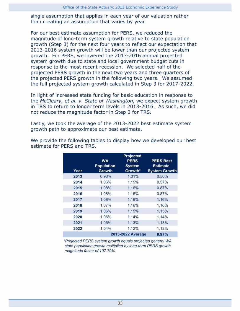
33
Office of the State Actuary: 2013 Economic Experience Study
single assumption that applies in each year of our valuation rather than creating an assumption that varies by year. For our best estimate assumption for PERS, we reduced the magnitude of long-term system growth relative to state population growth (Step 3) for the next four years to reflect our expectation that 2013-2016 system growth will be lower than our projected system growth. For PERS, we lowered the 2013-2016 annual projected system growth due to state and local government budget cuts in response to the most recent recession. We selected half of the projected PERS growth in the next two years and three quarters of the projected PERS growth in the following two years. We assumed the full projected system growth calculated in Step 3 for 2017-2022. In light of increased state funding for basic education in response to the McCleary, et al. v. State of Washington, we expect system growth in TRS to return to longer term levels in 2013-2016. As such, we did not reduce the magnitude factor in Step 3 for TRS. Lastly, we took the average of the 2013-2022 best estimate system growth path to approximate our best estimate. We provide the following tables to display how we developed our best estimate for PERS and TRS.
Year2013 0.93% 1.01% 0.50%2014 1.06% 1.15% 0.57%2015 1.08% 1.16% 0.87%2016 1.08% 1.16% 0.87%2017 1.08% 1.16% 1.16%2018 1.07% 1.16% 1.16%2019 1.06% 1.15% 1.15%2020 1.06% 1.14% 1.14%2021 1.05% 1.13% 1.13%2022 1.04% 1.12% 1.12%
0.97%
PERS Best Estimate
System Growth
Projected PERS
System Growth*
WA Population
Growth
*Projected PERS system growth equals projected general WA state population growth multiplied by long-term PERS growth magnitude factor of 107.79%.
2013-2022 Average
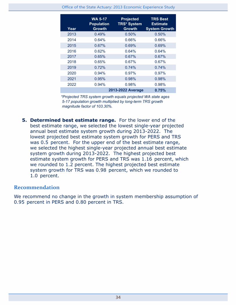
Office of the State Actuary: 2013 Economic Experience Study
34
Year2013 0.49% 0.50% 0.50%2014 0.64% 0.66% 0.66%2015 0.67% 0.69% 0.69%2016 0.62% 0.64% 0.64%2017 0.65% 0.67% 0.67%2018 0.65% 0.67% 0.67%2019 0.72% 0.74% 0.74%2020 0.94% 0.97% 0.97%2021 0.95% 0.98% 0.98%2022 0.94% 0.98% 0.98%
0.75%
Projected TRS* System
Growth
TRS Best Estimate
System Growth
WA 5-17 Population
Growth
*Projected TRS system growth equals projected WA state ages 5-17 population growth multiplied by long-term TRS growth magnitude factor of 103.30%.
2013-2022 Average
5. Determined best estimate range. For the lower end of the best estimate range, we selected the lowest single-year projected annual best estimate system growth during 2013-2022. The lowest projected best estimate system growth for PERS and TRS was 0.5 percent. For the upper end of the best estimate range, we selected the highest single-year projected annual best estimate system growth during 2013-2022. The highest projected best estimate system growth for PERS and TRS was 1.16 percent, which we rounded to 1.2 percent. The highest projected best estimate system growth for TRS was 0.98 percent, which we rounded to 1.0 percent.
Recommendation
We recommend no change in the growth in system membership assumption of 0.95 percent in PERS and 0.80 percent in TRS.

35
Office of the State Actuary: 2013 Economic Experience Study
Note: The score card above is based on data from our 2009 projections, which includes the UCOLA benefit. If the UCOLA were removed from our risk analysis, and we included recent asset returns, the risk and affordability scores would improve. However, we don’t expect the relative differences between the two assumption scenarios and resulting findings to change.
Affordability
Affordability compares the single most unaffordable points over the projected fifty-year period between the two annual rate of investment return assumptions. We found that lowering the rate of investment return assumption will increase affordability risk (less affordable), in the short-term, due to increased contribution requirements. However, we would expect an assumed increase in overall assets to help pay for benefits as a result of collecting higher contribution rates, which improves the long-term affordability of the plans under the recommended annual investment return of 7.50 percent. In other words, contributing higher contribution rates in the short-term will lead to more assets, which would lead to less required future contributions relative to the current annual rate of investment return assumption.
Contribution rates become less volatile under the recommended 7.50 percent annual rate of investment return assumption than under the current assumption. The long-term annual change in effective employer contribution rates, for all systems, become narrower in the long-term for the 7.50 percent annual rate of investment return assumption. In other words, the contribution rates become more stable over the long-term with the
Risk Analysis
We chose not to update the Risk Analysis from the 2011 Economic Experience Study (EES) because we expect the results would not be materially different. Had we updated the risk analysis in this EES, we would have studied the impact on the Washington state pension systems resulting from lowering the annual investment return assumption from 7.90 percent to 7.50 percent. In comparison, for the 2011 EES we studied the impact from lowering the assumption from 8.00 percent to 7.50 percent.
Below we show the Pension Score Card results from the 2011 EES followed by a brief description of some of the high-level takeaways.
Value Score Value Score
Chance Pensions will Consume More than 8% of GF-S1 18.0% 37 18.0% 355% Chance GF-S1 Consumption will Exceed 9.9% 39 10.0% 385% Chance Employer Contribution Rate will Exceed 20.1% 44 20.3% 43
Chance of PERS 1, TRS 1 in Pay-Go2 41% 19 39% 21Chance of Open Plan in Pay-Go2 13% 47 11% 495% Chance Annual Pay-Go Cost3 in PERS 1, TRS 1 Exceed $1.70 38 $1.70 385% Chance Annual Pay-Go Cost3 in Open Plans Exceed $4.00 11 $3.60 16Chance of Total Funded Status Below 60% 34% 24 31% 29
33 34
8.00% 7.50%Category (Dollars in Billions) Affordability
Risk
Total Weighted Score1 Currently 2.7% of GF-S.2 When today's value of annual cost exceeds $50 million.3 Pay-Go costs on top of normal pension costs.
Pension Score Card
Office of the State Actuary: 2013 Economic Experience Study
36
lower assumption. This occurs because under the current annual investment return assumption, actuarial losses (returns below the assumption) are expected to occur more often than actuarial gains (returns above the assumption). If more actuarial losses occur than gains then this puts upward pressure on contribution rates over time as the actuarial losses are recognized. In addition, the additional contributions made under the 7.50 percent assumption help offset increasing contribution rates due to either assumed future funding shortfalls or assumed future benefit improvements.
Risk
Lowering the rate of return assumption will decrease “pay-go”(or chance of the plan running out of money) and “low funded status” risks as measured under the Pension Score Card. As we discussed in the Affordability section, this occurs because funding at a 7.50 percent assumed rate of investment return increases required contributions in the short-term and increases the overall assets available to pay for plan benefits. Having additional assets on hand improves funded status and therefore lowers pay-go and low funded status risks.
Please see the 2011 Economic Experience Study for additional analysis and a more in depth discussion of the Risk Analysis measures and Pension Score Card results.

37
Office of the State Actuary: 2013 Economic Experience Study
PO Box 40914 Phone: 360.786.6140 Olympia, Washington, 98504-0914 Fax: 360.586.8135 osa.leg.wa.gov TDD: 711
Office of the State Actuary: 2013 Economic Experience Study
38
Office of the State Actuary August 30, 2013

39
Office of the State Actuary: 2013 Economic Experience Study
Appendices

Office of the State Actuary: 2013 Economic Experience Study
40

41
Office of the State Actuary: 2013 Economic Experience Study
Appendix A
*Data sources: Department of Labor, Bureau of Labor Statistics (BLS) and Department of Commerce, Bureau of Economic Analysis (BEA).
Seattle CPI-W
U.S. CPI-W
GDP PCE
1950-2012 3.77% 3.67% 3.35%Last 30 years 2.92% 2.87% 2.60%Last 25 years 3.19% 2.84% 2.42%Last 20 years 2.78% 2.50% 2.06%Last 10 years 2.49% 2.55% 2.24%Last 5 years 2.27% 2.21% 1.88%
2013 EESGeometric Averages*
U.S. GDPCPI-W PCE
1983 293.2 297.4 55.868 (0.27%) 3.05% 4.30%1984 302.8 307.6 57.981 3.27% 3.43% 3.78%1985 309.1 318.5 59.882 2.08% 3.54% 3.28%1986 311.3 323.4 61.341 0.71% 1.54% 2.44%1987 318.6 335.0 63.618 2.35% 3.59% 3.71%1988 329.1 348.4 66.151 3.30% 4.00% 3.98%1989 344.5 365.2 69.025 4.68% 4.82% 4.34%1990 369.0 384.4 72.180 7.11% 5.26% 4.57%1991 389.4 399.9 74.789 5.53% 4.03% 3.61%1992 403.2 411.5 76.989 3.54% 2.90% 2.94%1993 415.2 423.1 78.679 2.98% 2.82% 2.20%1994 430.4 433.8 80.302 3.66% 2.53% 2.06%1995 442.9 446.1 82.078 2.90% 2.84% 2.21%1996 457.5 459.1 83.864 3.30% 2.91% 2.18%1997 471.7 469.3 85.433 3.10% 2.22% 1.87%1998 484.1 475.6 86.246 2.63% 1.34% 0.95%1999 499.1 486.2 87.636 3.10% 2.23% 1.61%2000 517.8 503.1 89.818 3.75% 3.48% 2.49%2001 536.2 516.8 91.530 3.55% 2.72% 1.91%2002 545.9 523.9 92.778 1.81% 1.37% 1.36%2003 553.6 535.6 94.659 1.41% 2.23% 2.03%2004 562.3 549.5 97.121 1.57% 2.60% 2.60%2005 579.3 568.9 100.000 3.02% 3.53% 2.96%2006 600.9 587.2 102.723 3.73% 3.22% 2.72%2007 623.7 604.0 105.499 3.79% 2.86% 2.70%2008 651.6 628.7 108.943 4.48% 4.09% 3.26%2009 654.5 624.4 109.004 0.44% (0.67%) 0.06%2010 659.6 637.3 111.087 0.78% 2.07% 1.91%2011 680.5 660.0 113.790 3.17% 3.56% 2.43%2012 697.8 673.9 115.789 2.54% 2.10% 1.76%
Annual % ChangeSeattle-Tacoma-
Bremerton, WA CPI-W
U.S. City Average CPI-W
GDP Deflator for Personal
Consumption ExpendituresYear
Seattle CPI-W
Historical Inflation Data*

Office of the State Actuary: 2013 Economic Experience Study
42
Appendix B
*SSA did not provide an annual national forecast. We linearly interpolated the years between 2013 and the ultimate rate year when the annual rate change was not provided.
CBO ERFC GI SSA Int* SSA Low* SSA High*
2013 1.70% 1.42% 1.37% 1.80% 1.70% 1.90%2014 1.70% 1.76% 1.64% 2.20% 1.70% 2.22%2015 2.10% 1.52% 1.69% 2.35% 1.70% 2.53%2016 2.10% 1.56% 1.87% 2.50% 1.70% 2.85%2017 2.20% 1.53% 1.85% 2.65% 1.80% 3.17%2018 2.30% 1.82% 2.80% 1.80% 3.48%2019 2.30% 1.88% 2.80% 1.80% 3.80%2020 2.30% 1.97% 2.80% 1.80% 3.80%2021 2.30% 1.94% 2.80% 1.80% 3.80%2022 2.30% 1.94% 2.80% 1.80% 3.80%2023 2.30% 1.97% 2.80% 1.80% 3.80%2024 1.98% 2.80% 1.80% 3.80%2025 1.99% 2.80% 1.80% 3.80%2026 2.02% 2.80% 1.80% 3.80%2027 2.02% 2.80% 1.80% 3.80%2028 1.95% 2.80% 1.80% 3.80%2029 1.94% 2.80% 1.80% 3.80%2030 1.95% 2.80% 1.80% 3.80%2031 2.04% 2.80% 1.80% 3.80%2032 2.05% 2.80% 1.80% 3.80%2033 2.09% 2.80% 1.80% 3.80%2034 2.13% 2.80% 1.80% 3.80%2035 2.10% 2.80% 1.80% 3.80%2036 2.11% 2.80% 1.80% 3.80%2037 2.13% 2.80% 1.80% 3.80%2038 2.14% 2.80% 1.80% 3.80%2039 2.15% 2.80% 1.80% 3.80%2040 2.16% 2.80% 1.80% 3.80%2041 2.17% 2.80% 1.80% 3.80%2042 2.17% 2.80% 1.80% 3.80%2043 2.18% 2.80% 1.80% 3.80%
Annual Projected National CPI Increase
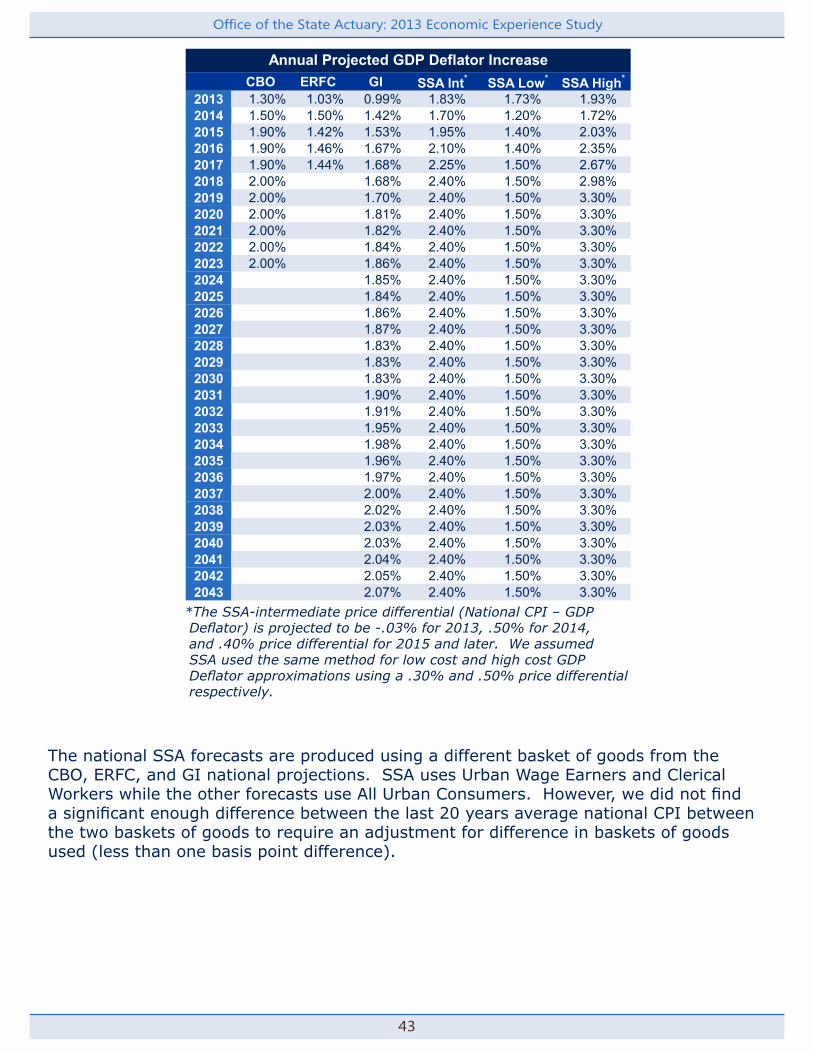
43
Office of the State Actuary: 2013 Economic Experience Study
The national SSA forecasts are produced using a different basket of goods from the CBO, ERFC, and GI national projections. SSA uses Urban Wage Earners and Clerical Workers while the other forecasts use All Urban Consumers. However, we did not find a significant enough difference between the last 20 years average national CPI between the two baskets of goods to require an adjustment for difference in baskets of goods used (less than one basis point difference).
*The SSA-intermediate price differential (National CPI – GDP Deflator) is projected to be -.03% for 2013, .50% for 2014, and .40% price differential for 2015 and later. We assumed SSA used the same method for low cost and high cost GDP Deflator approximations using a .30% and .50% price differential respectively.
CBO ERFC GI SSA Int* SSA Low* SSA High*
2013 1.30% 1.03% 0.99% 1.83% 1.73% 1.93%2014 1.50% 1.50% 1.42% 1.70% 1.20% 1.72%2015 1.90% 1.42% 1.53% 1.95% 1.40% 2.03%2016 1.90% 1.46% 1.67% 2.10% 1.40% 2.35%2017 1.90% 1.44% 1.68% 2.25% 1.50% 2.67%2018 2.00% 1.68% 2.40% 1.50% 2.98%2019 2.00% 1.70% 2.40% 1.50% 3.30%2020 2.00% 1.81% 2.40% 1.50% 3.30%2021 2.00% 1.82% 2.40% 1.50% 3.30%2022 2.00% 1.84% 2.40% 1.50% 3.30%2023 2.00% 1.86% 2.40% 1.50% 3.30%2024 1.85% 2.40% 1.50% 3.30%2025 1.84% 2.40% 1.50% 3.30%2026 1.86% 2.40% 1.50% 3.30%2027 1.87% 2.40% 1.50% 3.30%2028 1.83% 2.40% 1.50% 3.30%2029 1.83% 2.40% 1.50% 3.30%2030 1.83% 2.40% 1.50% 3.30%2031 1.90% 2.40% 1.50% 3.30%2032 1.91% 2.40% 1.50% 3.30%2033 1.95% 2.40% 1.50% 3.30%2034 1.98% 2.40% 1.50% 3.30%2035 1.96% 2.40% 1.50% 3.30%2036 1.97% 2.40% 1.50% 3.30%2037 2.00% 2.40% 1.50% 3.30%2038 2.02% 2.40% 1.50% 3.30%2039 2.03% 2.40% 1.50% 3.30%2040 2.03% 2.40% 1.50% 3.30%2041 2.04% 2.40% 1.50% 3.30%2042 2.05% 2.40% 1.50% 3.30%2043 2.07% 2.40% 1.50% 3.30%
Annual Projected GDP Deflator Increase

Office of the State Actuary: 2013 Economic Experience Study
44
Appendix C
Year of Service
Average Increase in
Salary
Average Observed Inflation*
Average Observed
Productivity
Average Observed
Merit Increase
Currently Assumed Merit
Increase
Cumulative Observed Merit
Increase
Cumulative Assumed Merit
Increase01 10.27% 3.13% 0.89% 6.01% 6.10% 106.01% 106.10%2 8.81% 3.13% 0.89% 4.61% 4.80% 110.89% 111.19%3 7.73% 3.13% 0.89% 3.57% 3.80% 114.85% 115.42%4 6.98% 3.13% 0.89% 2.84% 2.90% 118.11% 118.77%5 6.32% 3.13% 0.89% 2.21% 2.20% 120.72% 121.38%6 5.65% 3.13% 0.89% 1.57% 1.50% 122.62% 123.20%7 5.27% 3.13% 0.89% 1.20% 1.10% 124.09% 124.55%8 5.04% 3.13% 0.89% 0.98% 0.90% 125.30% 125.67%9 4.81% 3.13% 0.89% 0.76% 0.70% 126.25% 126.55%10 4.61% 3.13% 0.89% 0.57% 0.50% 126.97% 127.19%11 4.51% 3.13% 0.89% 0.47% 0.40% 127.56% 127.70%12 4.41% 3.13% 0.89% 0.38% 0.30% 128.05% 128.08%13 4.27% 3.13% 0.89% 0.24% 0.20% 128.36% 128.34%14 4.23% 3.13% 0.89% 0.20% 0.20% 128.62% 128.59%15 4.24% 3.13% 0.89% 0.21% 0.20% 128.88% 128.85%16 4.22% 3.13% 0.89% 0.19% 0.20% 129.13% 129.11%
01 9.27% 3.13% 0.97% 4.97% 5.80% 104.97% 105.80%2 8.01% 3.13% 0.97% 3.76% 4.30% 108.92% 110.35%3 7.95% 3.13% 0.97% 3.70% 4.10% 112.95% 114.87%4 7.64% 3.13% 0.97% 3.41% 3.50% 116.80% 118.89%5 7.19% 3.13% 0.97% 2.97% 3.10% 120.27% 122.58%6 6.99% 3.13% 0.97% 2.78% 2.80% 123.61% 126.01%7 6.94% 3.13% 0.97% 2.73% 2.60% 126.99% 129.29%8 6.89% 3.13% 0.97% 2.68% 2.40% 130.39% 132.39%9 6.65% 3.13% 0.97% 2.45% 2.20% 133.58% 135.30%10 6.46% 3.13% 0.97% 2.27% 2.00% 136.61% 138.01%11 6.25% 3.13% 0.97% 2.07% 1.90% 139.44% 140.63%12 6.02% 3.13% 0.97% 1.85% 1.70% 142.01% 143.02%13 5.71% 3.13% 0.97% 1.55% 1.50% 144.21% 145.17%14 5.24% 3.13% 0.97% 1.09% 1.00% 145.79% 146.62%15 5.04% 3.13% 0.97% 0.90% 0.80% 147.11% 147.79%16 4.68% 3.13% 0.97% 0.56% 0.40% 147.93% 148.38%17 4.35% 3.13% 0.97% 0.25% 0.10% 148.30% 148.53%18 4.24% 3.13% 0.97% 0.14% 0.10% 148.50% 148.68%19 4.22% 3.13% 0.97% 0.12% 0.10% 148.68% 148.83%20 4.20% 3.13% 0.97% 0.10% 0.10% 148.83% 148.98%21 4.17% 3.13% 0.97% 0.07% 0.10% 148.93% 149.13%22 4.20% 3.13% 0.97% 0.10% 0.10% 149.08% 149.28%23 4.31% 3.13% 0.97% 0.20% 0.10% 149.39% 149.43%24 4.35% 3.13% 0.97% 0.24% 0.10% 149.75% 149.58%25 4.11% 3.13% 0.97% 0.01% 0.10% 149.77% 149.73%
*Average change in the CPI-W, Seattle, Tacoma, Bremerton, from 1984 to 2009. Increase in salary = (1 + observed inflation + observed productivity) * (1 + observed merit) - 1
Growth in Salaries for Members Active for Two Consecutive YearsPERS - 1984 to 2009
TRS - 1984 to 2009

45
Office of the State Actuary: 2013 Economic Experience Study
Year of Service
Average Increase in
Salary
Average Observed Inflation*
Average Observed
Productivity
Average Observed
Merit Increase
Currently Assumed Merit
Increase
Cumulative Observed
Merit Increase
Cumulative Assumed Merit
Increase01 10.28% 3.13% 0.57% 6.34% 6.90% 106.34% 106.90%2 7.65% 3.13% 0.57% 3.81% 3.90% 110.39% 111.07%3 6.54% 3.13% 0.57% 2.74% 2.90% 113.41% 114.29%4 5.99% 3.13% 0.57% 2.21% 2.30% 115.91% 116.92%5 5.73% 3.13% 0.57% 1.96% 2.20% 118.18% 119.49%6 5.32% 3.13% 0.57% 1.56% 1.60% 120.02% 121.40%7 4.98% 3.13% 0.57% 1.23% 1.30% 121.50% 122.98%8 5.01% 3.13% 0.57% 1.25% 1.20% 123.02% 124.46%9 4.69% 3.13% 0.57% 0.95% 0.90% 124.20% 125.58%10 4.64% 3.13% 0.57% 0.90% 0.80% 125.32% 126.58%11 4.42% 3.13% 0.57% 0.69% 0.70% 126.19% 127.47%12 4.22% 3.13% 0.57% 0.49% 0.40% 126.81% 127.98%13 4.09% 3.13% 0.57% 0.37% 0.40% 127.29% 128.49%14 4.08% 3.13% 0.57% 0.36% 0.30% 127.75% 128.87%15 4.08% 3.13% 0.57% 0.36% 0.10% 128.20% 129.00%16 3.80% 3.13% 0.57% 0.09% 0.10% 128.31% 129.13%17 4.01% 3.13% 0.57% 0.30% 0.10% 128.70% 129.26%18 3.94% 3.13% 0.57% 0.23% 0.10% 128.99% 129.39%19 4.13% 3.13% 0.57% 0.41% 0.10% 129.53% 129.52%
01 13.57% 3.13% 0.92% 9.14% 7.10% 109.14% 107.10%2 10.72% 3.13% 0.92% 6.41% 5.90% 116.13% 113.42%3 9.54% 3.13% 0.92% 5.27% 5.20% 122.25% 119.32%4 9.01% 3.13% 0.92% 4.77% 5.20% 128.08% 125.52%5 8.91% 3.13% 0.92% 4.67% 5.20% 134.05% 132.05%6 7.31% 3.13% 0.92% 3.13% 4.50% 138.26% 137.99%7 5.17% 3.13% 0.92% 1.07% 0.80% 139.74% 139.09%8 4.11% 3.13% 0.92% 0.06% 0.80% 139.82% 140.21%9 4.28% 3.13% 0.92% 0.22% 0.80% 140.12% 141.33%10 5.13% 3.13% 0.92% 1.03% 0.80% 141.56% 142.46%11 4.64% 3.13% 0.92% 0.56% 0.80% 142.36% 143.60%12 4.20% 3.13% 0.92% 0.14% 0.40% 142.56% 144.17%13 4.21% 3.13% 0.92% 0.15% 0.40% 142.77% 144.75%14 3.60% 3.13% 0.92% -0.43% 0.40% 142.15% 145.33%15 4.44% 3.13% 0.92% 0.38% 0.40% 142.68% 145.91%16 5.02% 3.13% 0.92% 0.92% 0.40% 144.00% 146.49%17 4.16% 3.13% 0.92% 0.10% 0.40% 144.15% 147.08%18 4.15% 3.13% 0.92% 0.10% 0.40% 144.29% 147.67%19 4.44% 3.13% 0.92% 0.37% 0.40% 144.83% 148.26%20 4.94% 3.13% 0.92% 0.86% 0.40% 146.06% 148.85%21 4.78% 3.13% 0.92% 0.70% 0.40% 147.09% 149.45%22 5.30% 3.13% 0.92% 1.20% 0.40% 148.85% 150.05%23 4.64% 3.13% 0.92% 0.56% 0.40% 149.69% 150.65%24 4.96% 3.13% 0.92% 0.87% 0.40% 150.99% 151.25%25 4.68% 3.13% 0.92% 0.60% 0.40% 151.89% 151.85%
*Average change in the CPI-W, Seattle, Tacoma, Bremerton, from 1984 to 2009. Increase in salary = (1 + observed inflation + observed productivity) * (1 + observed merit) - 1
WSPRS - 1984 to 2009
Growth in Salaries for Members Active for Two Consecutive YearsSERS - 1984 to 2009
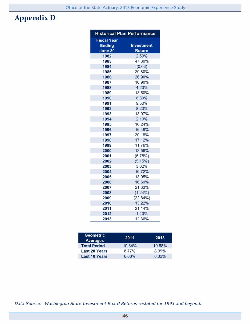
Office of the State Actuary: 2013 Economic Experience Study
46
Appendix D
Data Source: Washington State Investment Board Returns restated for 1993 and beyond.
Geometric Averages 2011 2013
Total Period 10.84% 10.58% Last 20 Years 8.77% 8.39% Last 10 Years 6.68% 8.32%
Fiscal YearEndingJune 30
1982 2.50%1983 47.30%1984 (0.03)1985 29.80%1986 26.90%1987 16.90%1988 4.20%1989 13.50%1990 8.30%1991 9.50%1992 8.20%1993 13.07%1994 2.10%1995 16.24%1996 16.49%1997 20.18%1998 17.12%1999 11.76%2000 13.56%2001 (6.75%)2002 (5.15%)2003 3.02%2004 16.72%2005 13.05%2006 16.69%2007 21.33%2008 (1.24%)2009 (22.84%)2010 13.22%2011 21.14%2012 1.40%2013 12.36%
Investment Return
Historical Plan Performance

47
Office of the State Actuary: 2013 Economic Experience Study
Appendix E
2011 2013Total Period 9.36% 9.30%Last 60 years 9.88% 9.98%Last 50 years 9.63% 9.70%Last 40 years 10.21% 10.69%Last 30 years 10.84% 9.80%
Geometric AveragesMinimum 7.72%Maximum 12.65%Average 10.19%* Starting in 1926. Last period ending 2013.
Rolling 30-year Averages*
Investment Investment Investment Investment InvestmentYear Return Year Return Year Return Year Return Year Return1926 6.87% 1947 1.53% 1968 13.47% 1989 13.50% 2010 13.22%1927 22.10% 1948 2.75% 1969 (11.58%) 1990 8.30% 2011 21.14%1928 26.54% 1949 13.51% 1970 2.16% 1991 9.50% 2012 1.40%1929 (14.85%) 1950 21.78% 1971 13.42% 1992 8.20% 2013 12.36%1930 (16.67%) 1951 9.75% 1972 10.27% 1993 13.07%1931 (29.66%) 1952 8.33% 1973 (13.14%) 1994 2.10%1932 0.19% 1953 (0.82%) 1974 (14.56%) 1995 16.24%1933 57.40% 1954 36.69% 1975 30.91% 1996 16.49%1934 9.46% 1955 16.66% 1976 29.01% 1997 20.18%1935 30.10% 1956 1.45% 1977 3.86% 1998 17.12%1936 31.10% 1957 (4.96%) 1978 8.09% 1999 11.76%1937 (26.97%) 1958 30.90% 1979 16.80% 2000 13.56%1938 21.64% 1959 7.99% 1980 20.86% 2001 (6.75%)1939 1.57% 1960 3.12% 1981 1.76% 2002 (5.15%)1940 (3.34%) 1961 18.93% 1982 2.50% 2003 3.02%1941 (5.93%) 1962 (3.75%) 1983 47.30% 2004 16.72%1942 19.62% 1963 14.89% 1984 (0.03%) 2005 13.05%1943 32.49% 1964 13.35% 1985 29.80% 2006 16.69%1944 21.99% 1965 15.09% 1986 26.90% 2007 21.33%1945 34.34% 1966 (4.84%) 1987 16.90% 2008 (1.24%)1946 (5.62%) 1967 27.44% 1988 4.20% 2009 (22.84%)
Historical Investment Data - Current Allocations
Actual investment return for fiscal years ending June 30, 1982 and thereafter. Returns restated for 1993 and beyond. Estimated investment return prior to 1982.
2011 201337% 37% S&P 50020% 20%25% 25% U.S. small cap stock index13% 13%
Tangible 5% 5% CPI + 200 basis points*Constant asset allocation from 1926 through 1981. Based on WSIB's asset allocation for the given year. For the 2013 Economic Experience Study, we used WSIB's 2012 target asset allocation.
Allocation Return
Private EquityReal Estate
Average of long-term corporate and government bond index
Average of long-term corporate and government bond index
Asset Class
Fixed IncomeGlobal Equity
Assumptions*

Office of the State Actuary: 2013 Economic Experience Study
48
Appendix F
2011 2013Total Period 8.56% 8.51%Last 60 years 9.08% 9.10%Last 50 years 8.68% 8.72%Last 40 years 9.46% 9.71%Last 30 years 10.84% 9.80%
Geometric Averages
Investment Investment Investment Investment InvestmentYear Return Year Return Year Return Year Return Year Return1926 10.00% 1947 2.43% 1968 7.10% 1989 13.50% 2010 13.22%1927 25.77% 1948 4.81% 1969 -7.73% 1990 8.30% 2011 21.14%1928 26.75% 1949 13.23% 1970 8.50% 1991 9.50% 2012 1.40%1929 -3.71% 1950 19.46% 1971 13.43% 1992 8.20% 2013 12.36%1930 -12.41% 1951 13.09% 1972 13.98% 1993 13.07%1931 -27.44% 1952 11.96% 1973 -8.79% 1994 2.10%1932 0.62% 1953 0.82% 1974 -15.62% 1995 16.24%1933 34.46% 1954 34.09% 1975 27.09% 1996 16.49%1934 3.91% 1955 18.77% 1976 21.38% 1997 20.18%1935 31.52% 1956 1.46% 1977 -4.10% 1998 17.12%1936 23.20% 1957 -3.23% 1978 3.69% 1999 11.76%1937 -20.42% 1958 24.35% 1979 9.98% 2000 13.56%1938 21.00% 1959 6.53% 1980 18.11% 2001 -6.75%1939 1.74% 1960 4.85% 1981 -2.82% 2002 -5.15%1940 -3.97% 1961 17.29% 1982 2.50% 2003 3.02%1941 -6.22% 1962 -2.27% 1983 47.30% 2004 16.72%1942 13.37% 1963 14.36% 1984 -0.03% 2005 13.05%1943 16.52% 1964 11.54% 1985 29.80% 2006 16.69%1944 13.36% 1965 7.52% 1986 26.90% 2007 21.33%1945 24.83% 1966 -5.27% 1987 16.90% 2008 -1.24%1946 -4.52% 1967 11.56% 1988 4.20% 2009 -22.84%
Historical Investment Data - Alternate Allocations
Actual investment return for fiscal years ending June 30, 1982, and thereafter. Returns restated for 1993 and beyond. Estimated investment return prior to 1982.
Equity 60% S&P 500
40%
*Constant asset allocation from 1926 through 1981. Based on Washington State Investment Board's 2004 asset allocation.
Fixed Income
ReturnAssumptions*
Asset Class Allocation
Average of long-term corporate and government bond index.
Minimum 7.04%Maximum 11.67%Average 9.05%* Starting in 1926. Last period ending 2013.
Rolling 30-year Averages*

49
Office of the State Actuary: 2013 Economic Experience Study
Appendix G
Target Expected StandardAllocation 1-Year Return Deviation
37% 8.75% 18.50%5% 6.80% 7.30%
20% 3.50% 5.75%25% 11.75% 28.00%13% 8.00% 15.50%
Cash 0% 2.50% 2.00%Total 2013 Target CTF 100%2011 Asset Class
37% 8.65% 17.62%5% 6.50% 8.00%
20% 4.25% 5.00%25% 11.50% 27.00%13% 8.00% 15.00%
Cash 0% 3.00% 2.00%100%
Portfolio Statistics & Capital Market Assumptions
WSIB Simulated Future Investment Returns
2013 Asset ClassGlobal EquityTangible AssetsFixed IncomePrivate EquityReal Estate
Global EquityTangible AssetsFixed IncomePrivate EquityReal Estate
Total 2011 Target CTF
2013 15 Years 50 Years9.65% 8.62%8.31% 7.86%7.90% 7.63%7.49% 7.40%7.08% 7.17%6.67% 6.93%5.27% 6.13%
2011 15 Years 50 Years10.14% 8.95%8.50% 8.04%8.01% 7.76%7.52% 7.49%7.04% 7.22%6.55% 6.94%4.94% 6.03%
*Source: Washington State Investment Board.
60th percentile
Simulated Future Investment Returns*
40th percentile25th percentile
Measurement Period
Measurement Period
55th percentileExpected Return45th percentile
75th percentile60th percentile
40th percentile25th percentile
55th percentileExpected Return45th percentile
75th percentile

Office of the State Actuary: 2013 Economic Experience Study
50
Appendix H
Year Count Annual Growth Year Count Annual
GrowthGeometric Averages 2011 2013
1982 4,276,549 2013 6,881,504 0.93% Last 25 years 1.71% 1.65%1983 4,307,247 0.72% 2014 6,954,668 1.06% Last 20 years 1.65% 1.42%1984 4,354,067 1.09% 2015 7,029,758 1.08% Last 15 years 1.41% 1.24%1985 4,415,785 1.42% 2016 7,105,670 1.08% Last 10 years 1.37% 1.19%1986 4,462,212 1.05% 2017 7,182,231 1.08% Last 5 years 1.53% 0.88%1987 4,527,098 1.45% 2018 7,259,406 1.07% Next 5 years 1.19% 1.05%1988 4,616,886 1.98% 2019 7,336,680 1.06% Next 10 years 1.19% 1.05%1989 4,728,077 2.41% 2020 7,414,437 1.06% Next 15 years 1.15% 1.03%1990 4,866,692 2.93% 2021 7,492,433 1.05% Next 20 years 1.10% 0.99%1991 5,021,339 3.18% 2022 7,570,617 1.04%1992 5,141,178 2.39% 2023 7,648,943 1.03%1993 5,265,691 2.42% 2024 7,726,324 1.01%1994 5,364,342 1.87% 2025 7,802,649 0.99%1995 5,470,108 1.97% 2026 7,877,749 0.96%1996 5,567,764 1.79% 2027 7,951,595 0.94%1997 5,663,763 1.72% 2028 8,024,209 0.91%1998 5,750,030 1.52% 2029 8,095,464 0.89%1999 5,830,833 1.41% 2030 8,165,376 0.86%2000 5,894,143 1.09% 2031 8,234,011 0.84%2001 5,970,330 1.29% 2032 8,301,548 0.82%2002 6,059,316 1.49%2003 6,126,885 1.12%2004 6,208,515 1.33%2005 6,298,816 1.45%2006 6,420,258 1.93%2007 6,525,086 1.63%2008 6,608,245 1.27%2009 6,672,159 0.97%2010 6,724,540 0.79%2011 6,767,900 0.64%2012 6,817,770 0.74%
*Source: Office of Financial Management. Additional computations have been performed to summarize data.
Projected GrowthHistorical GrowthGrowth in Washington State Population - Historical and Projected*

51
Office of the State Actuary: 2013 Economic Experience Study
Appendix I
Year# of Active Members
Annual Growth # of People
Annual Growth
# of Active
MembersAnnual Growth # of People
Annual Growth
1990 150,241 7.97% 4,866,692 2.93% 51,323 4.34% 893,252 3.54%1991 165,008 9.83% 5,021,339 3.18% 52,779 2.84% 930,866 4.21%1992 171,947 4.21% 5,141,178 2.39% 55,276 4.73% 960,367 3.17%1993 174,576 1.53% 5,265,691 2.42% 56,571 2.34% 992,179 3.31%1994 177,456 1.65% 5,364,342 1.87% 57,731 2.05% 1,020,268 2.83%1995 178,833 0.78% 5,470,108 1.97% 59,103 2.38% 1,050,730 2.99%1996 182,603 2.11% 5,567,764 1.79% 59,425 0.54% 1,077,440 2.54%1997 186,440 2.10% 5,663,763 1.72% 60,815 2.34% 1,101,252 2.21%1998 191,850 2.90% 5,750,030 1.52% 61,828 1.67% 1,113,531 1.12%1999 196,382 2.36% 5,830,833 1.41% 62,684 1.38% 1,119,908 0.57%2000 199,986 1.84% 5,894,143 1.09% 63,858 1.87% 1,119,533 (0.033%)2001 201,283 0.65% 5,970,330 1.29% 66,220 3.70% 1,121,086 0.14%2002 203,976 1.34% 6,059,316 1.49% 66,063 (0.24%) 1,125,692 0.41%2003 203,764 (0.10%) 6,126,885 1.12% 66,075 0.02% 1,125,535 (0.01%)2004 206,110 1.15% 6,208,515 1.33% 66,634 0.85% 1,127,775 0.20%2005 205,928 (0.09%) 6,298,816 1.45% 67,270 0.95% 1,132,190 0.39%2006 207,918 0.97% 6,420,258 1.93% 67,736 0.69% 1,143,545 1.00%2007 211,602 1.77% 6,525,086 1.63% 64,939 (4.13%) 1,148,590 0.44%2008 217,423 2.75% 6,608,245 1.27% 66,524 2.44% 1,145,629 (0.26%)2009 216,049 (0.63%) 6,672,159 0.97% 67,388 1.30% 1,140,370 (0.46%)2010 213,075 (1.38%) 6,724,540 0.79% 66,325 (1.58%) 1,141,697 0.12%2011 208,936 (1.94%) 6,767,900 0.64% 66,203 (0.18%) 1,135,372 (0.55%)2012 206,398 (1.21%) 6,817,770 0.74% 65,357 (1.28%) 1,135,966 0.05%
1990-2012 1.73% 1.60% 1.24% 1.20%Last 20 Years 0.92% 1.42% 0.84% 0.84%Last 10 Years 0.12% 1.19% (0.11%) 0.09%Last 5 Years (0.50%) 0.88% 0.13% (0.22%)
86% 54%*Source: Department of Retirement Systems and Office of Financial Management. Additional computations have been performed to summarize data.
1990-2012 PERS Annual Growth and WA Population Growth
1990-2012 TRS Annual Growth and WA Population Ages 5-17
TRSWA Population Ages
5-17WA PopulationPERS
Historical System Growth*
Geometric Averages
Correlations

Office of the State Actuary: 2013 Economic Experience Study
52
Appendix J
PERS System Growth
WA Population Growth
TRS System Growth
WA 5-17 Population
Growth1990 7.97% 2.93% 4.34% 3.54%1991 9.83% 3.18% 2.84% 4.21%1992 4.21% 2.39% 4.73% 3.17%1993 1.53% 2.42% 2.34% 3.31%1994 1.65% 1.87% 2.05% 2.83%1995 0.78% 1.97% 2.38% 2.99%1996 2.11% 1.79% 0.54% 2.54%1997 2.10% 1.72% 2.34% 2.21%1998 2.90% 1.52% 1.67% 1.12%1999 2.36% 1.41% 1.38% 0.57%2000 1.84% 1.09% 1.87% (0.03%)2001 0.65% 1.29% 3.70% 0.14%2002 1.34% 1.49% (0.24%) 0.41%2003 (0.10%) 1.12% 0.02% (0.01%)2004 1.15% 1.33% 0.85% 0.20%2005 (0.089%) 1.45% 0.95% 0.39%2006 0.97% 1.93% 0.69% 1.00%2007 1.77% 1.63% (4.13%) 0.44%2008 2.75% 1.27% 2.44% (0.26%)2009 (0.63%) 0.97% 1.30% (0.46%)2010 (1.38%) 0.79% (1.58%) 0.12%2011 (1.94%) 0.64% (0.18%) (0.55%)2012 (1.21%) 0.74% (1.28%) 0.05%
Geometric Average 1.73% 1.60% 1.24% 1.20%
107.79% = 1.73% / 1.60%
103.30% = 1.24% / 1.20%
Annual Magnitude of System Growth Relative to State Population Growth
Magnitude Factor


Office of the State ActuaryPO Box 40914Olympia, Washington 98504-0914
2100 Evergreen Park Drive SW, Suite 150 [email protected]
osa.leg.wa.gov