Relativity.pdf - The Mysearch Website
238
1
-
Upload
khangminh22 -
Category
Documents
-
view
4 -
download
0
Transcript of Relativity.pdf - The Mysearch Website
1
the mysearch.org.uk website All great truths begin as blasphemies
copyright ©: 2004-2015 _______________________________________________________________________________________________________
2 of 238

the mysearch.org.uk website All great truths begin as blasphemies
copyright ©: 2004-2015 _______________________________________________________________________________________________________
3 of 238
Contents
1. A RELATIVE PERSPECTIVE ............................................................................................................................................ 7
1.1 HISTORICAL BACKGROUND ................................................................................................................................................. 8
1.2 THE THEORY OF SPECIAL RELATIVITY .................................................................................................................................... 10
1.2.1 Basic Principles ...................................................................................................................................................... 11
1.2.1.1 Galilean Transforms.............................................................................................................................................. 14
1.2.1.2 Lorentz Transforms............................................................................................................................................... 16
1.2.1.3 4-Vector Notation ................................................................................................................................................. 20
1.2.2 The Implications of Special Relativity ..................................................................................................................... 25
1.2.2.1 The Light Clock...................................................................................................................................................... 26
1.2.2.2 Introduction to Spacetime .................................................................................................................................... 28
1.2.2.2.1 Concepts in Spacetime .................................................................................................................................... 34
1.2.2.2.2 Separation in Spacetime ................................................................................................................................. 37
1.2.2.2.3 Simultaneity and Causality .............................................................................................................................. 41
1.2.2.3 Mass and Energy effects ....................................................................................................................................... 46
1.2.3 Paradoxes .............................................................................................................................................................. 53
1.2.3.1 The Twin Paradox ................................................................................................................................................. 55
1.2.3.1.1 Spacetime Diagram Analysis ........................................................................................................................... 56
1.2.3.1.2 Signalling Analysis ........................................................................................................................................... 58
1.2.3.1.3 Simultaneity Analysis ...................................................................................................................................... 60
1.2.3.2 The Triplet Paradox .............................................................................................................................................. 62
1.2.4 Summary and Closing Notes .................................................................................................................................. 70
1.3 THE THEORY OF GENERAL RELATIVITY ................................................................................................................................... 72
1.3.1 Declaration of Assumptions ................................................................................................................................... 74
1.3.2 Classical Foundations ............................................................................................................................................. 75
1.3.3 Basic Concepts ....................................................................................................................................................... 82
1.3.3.1 The Geometry of Spacetime ................................................................................................................................. 83
1.3.3.2 Inertial and Gravitational Mass ............................................................................................................................ 84
1.3.3.3 The Equivalence Principle ..................................................................................................................................... 85
1.3.3.4 Spacetime Curvature ............................................................................................................................................ 87
1.3.3.5 The Nature of Gravity? ......................................................................................................................................... 89
1.3.4 Basic Model ........................................................................................................................................................... 91
1.3.4.1 Model Concept ..................................................................................................................................................... 93
1.3.4.2 Basic Assumptions ................................................................................................................................................ 94
1.3.4.3 Concepts & Implications ....................................................................................................................................... 97
1.3.4.4 Wider Analysis .................................................................................................................................................... 100
1.3.4.5 Free-Fall Velocity ................................................................................................................................................ 105
1.3.4.6 The Transition to Curved Spacetime .................................................................................................................. 108

the mysearch.org.uk website All great truths begin as blasphemies
copyright ©: 2004-2015 _______________________________________________________________________________________________________
4 of 238
1.3.5 The Schwarzschild Metric .................................................................................................................................... 112
1.3.5.1 Introduction to the Metric.................................................................................................................................. 113
1.3.5.2 Coordinate radius ............................................................................................................................................... 117
1.3.5.3 Radial Paths ........................................................................................................................................................ 120
1.3.5.3.1 The Observed Free-Falling Perspective ......................................................................................................... 121
1.3.5.3.2 The Onboard Free-Falling Perspective .......................................................................................................... 124
1.3.5.4 Orbits & Trajectories .......................................................................................................................................... 126
1.3.5.4.1 Effective Potential ......................................................................................................................................... 130
1.3.5.4.1.1 Classical Effective Potential ................................................................................................................... 132
1.3.5.4.1.2 Relativistic Effective Potential ............................................................................................................... 135
1.3.5.4.1.3 Implications of Effective Potential ......................................................................................................... 139
1.3.5.4.2 Java Trajectories ........................................................................................................................................... 144
1.3.5.5 Gullstrand-Painleve Coordinates ........................................................................................................................ 146
1.3.5.5.1 The Schwarzschild Free-Fall Velocity ............................................................................................................ 151
1.3.5.5.2 The Gullstrand-Painlevé Free-Fall Velocity ................................................................................................... 155
1.3.5.5.3 The Spreadsheet Model ................................................................................................................................ 158
1.3.5.5.4 Wider Implications ........................................................................................................................................ 161
1.3.5.6 Black Holes ......................................................................................................................................................... 166
1.3.5.6.1 The Limits of Inference ................................................................................................................................. 167
1.3.5.6.2 Fundamental Assumptions ........................................................................................................................... 169
1.3.5.6.3 Fundamental Issues ...................................................................................................................................... 173
1.3.5.6.4 A Black Hole Universe ................................................................................................................................... 174
1.3.5.7 Summary So Far .................................................................................................................................................. 176
1.3.6 A Mathematical Overview ................................................................................................................................... 178
1.3.6.1 Basic Concepts .................................................................................................................................................... 179
1.3.6.1.1 Scalars ........................................................................................................................................................... 179
1.3.6.1.2 Vectors .......................................................................................................................................................... 180
1.3.6.1.3 Vector Space ................................................................................................................................................. 181
1.3.6.1.4 Invariance, Contravariance, Covariance ....................................................................................................... 181
1.3.6.2 Arrays and Matrices............................................................................................................................................ 182
1.3.6.2.1 Matrix Algebra : ............................................................................................................................................ 182
1.3.6.2.2 Matrix Products ............................................................................................................................................ 183
1.3.6.2.3 Inner Product ................................................................................................................................................ 184
1.3.6.2.4 Outer Product ............................................................................................................................................... 185
1.3.6.3 Tensor Concepts ................................................................................................................................................. 185
1.3.6.3.1 Type and Rank............................................................................................................................................... 186
1.3.6.3.2 Type: ............................................................................................................................................................. 188
1.3.6.3.3 Rank: ............................................................................................................................................................. 188
1.3.6.4 Differential Geometry ........................................................................................................................................ 189
1.3.6.4.1 Contravariance and Covariant Coordinates .................................................................................................. 190
1.3.6.4.2 Coordinate Components ............................................................................................................................... 195
1.3.6.4.3 Coordinate Transforms ................................................................................................................................. 197

the mysearch.org.uk website All great truths begin as blasphemies
copyright ©: 2004-2015 _______________________________________________________________________________________________________
5 of 238
1.3.6.5 Notation and Manipulation ................................................................................................................................ 200
1.3.6.6 Metric Tensors .................................................................................................................................................... 202
1.3.6.6.1 2-Space Metric Tensors ................................................................................................................................ 204
1.3.6.6.2 4-Space Metric Tensor .................................................................................................................................. 209
1.3.6.7 Curvature and Energy Tensors ........................................................................................................................... 211
1.3.6.7.1 Defining Curvature ........................................................................................................................................ 212
1.3.6.7.1.1 Riemann Curvature Tensor .................................................................................................................... 214
1.3.6.7.1.2 Interpretative Meaning of Curvature .................................................................................................... 216
1.3.6.7.1.3 Adding Energy to Curvature .................................................................................................................. 218
1.3.6.8 Einstein’s Field Equation ..................................................................................................................................... 219
1.3.6.8.1 Solutions to the Equation ............................................................................................................................. 221
1.3.6.8.2 The Point-Mass Solution ............................................................................................................................... 222
1.3.6.8.3 The Homogeneous Solution .......................................................................................................................... 228
1.4 CLOSING REMARKS ........................................................................................................................................................ 235

the mysearch.org.uk website All great truths begin as blasphemies
copyright ©: 2004-2015 _______________________________________________________________________________________________________
6 of 238
the mysearch.org.uk website All great truths begin as blasphemies
copyright ©: 2004-2015 _______________________________________________________________________________________________________
7 of 238
Albert Einstein
"I must observe that the theory of relativity
resembles a building consisting of two
separate stories, the special theory and the
general theory. The special theory, on
which the general theory rests, applies to
all physical phenomena with the exception
of gravitation; the general theory provides
the law of gravitation and its relations to
the other forces of nature. "
Douglas Sirk
And it really began with Einstein. We
attended his lectures. Now the theory of
relativity remained - and still remains - only
a theory. It has not been proven. But it
suggested a completely different picture of
the physical world.
1. A RELATIVE PERSPECTIVE
Einstein's theories of relativity and quantum mechanics form two cornerstones of accepted science. However, the theory of
relativity is based on two separate works commonly referred to as the 'Special Theory of Relativity' published in 1905 and
the 'General Theory of Relativity' published in 1916. Almost from the outset, these theories have challenged our intuitive
worldview of time and space, which subsequently lead to the idea of an expanding universe. While this latter idea may, today,
not seem that controversial, it contains the suggestion that the universe is still ‘a work in progress’ that is often in direct conflict
with many religions.
Both theories of relativity will be reviewed and to some extent challenged, as part of the on-going `duty of inquiry` rather than
simply accepting that established science must always be right. However, there is no subliminal intention to suggest that
established science has to be wrong. Therefore, it is possibly appropriate to state, from the outset, that most scientists believed
the theory of relativity has already been proven beyond any reasonable doubt. These scientists can rightly point to the
mathematics, deductive logic and experimental observations, which they believe support all the basic assumptions of relativity.
Of course, on what might appear to be a sceptical note, history tells us that this is often the established position before an
accepted axiom is proved wrong or, at least, incomplete. So while the `weight of authority` would seem to firmly support the
theory of relativity, it still carries the inference of being a theory and not fully verified fact.
the mysearch.org.uk website All great truths begin as blasphemies
copyright ©: 2004-2015 _______________________________________________________________________________________________________
8 of 238
Albert Einstein was born in Ulm in
Germany on 14 March 1879. His
family later moved to Italy after
his father's electrical equipment
business failed. Einstein studied
at the Institute of Technology in
Zurich and received his doctorate
in 1905 from the University of
Zurich. In the same year he
published four groundbreaking
scientific papers.
1.1 Historical Background
In the 17th century, Isaac Newton developed three basic laws of motion that can be
tied to Galileo's principle of relativity. However, a key issue concerning the nature of
light remained. Newton thought that light behaved as a particle and, in part, he was
right, although his reasoning was later to be proved wrong. The idea of light as a
particle did not explain how light worked in other respects and so attempts to
describe light as a wave were made. At the time, the wave theory of light also
encountered a problem in that the speed of any wave depends on the 'stiffness' of the
medium through which it is thought to propagate. Given that light travelled so fast, the
property of the medium, i.e. the ether, through which light was thought to pass had to
be incredibly 'stiff', while also being so insubstantial that nobody could even detect it.
In the middle of the 19th century, James Clerk Maxwell unified the phenomena of
electrical charge and magnetism. In so doing, he predicted that when there was a
change in an electric field, a disturbance would travel out into the surrounding space
at the speed of light [c]. Based on the accepted science of that time, it was assumed
that the speed of light would depend on how fast the observer was moving through
the ether. To confirm this assumption, Michelson-Morley devised a famous
experiment to measure the speed of light relative to the ether, but to almost
everybody's surprise it failed. At first many thought Maxwell's equations might be
wrong, and given that they had then only been recently published, it was quite
plausible for this to be the case. However, all changes to Maxwell's equation did not
fit with other observations. In 1904, after a series of earlier papers, Hendrik Lorentz
published the mathematical transforms that he hoped would, in part, explain the
failure of the Michelson-Morley experiment by showing that objects shortened in the
direction of travel by a certain amount, at least mathematically. These equations are still referenced in the Special Theory of
Relativity as the `Lorentz Transforms`. Subsequently, Henri Poincaré suggested that there was no way to tell whether you were
moving or at rest; or equally how fast you were moving, except relative to something else, and so resurrected the principle of
relativity, originally outlined by Galileo. However, there was still the conflict to be resolved between Newton's laws, Maxwell's
equations and the results of the Michelson-Morley experiment. The permutations can be summarised as follows:
Model Source Observer Measured velocity depends on:
1 Y Y Speed of source & observer
2 Y N Speed of source only
3 N Y Speed of observer only
4 N N Speed of neither
From a classical perspective, based on Galilean relativity and intuitive experience, the measured velocity of an object was based
on model-1, as defined in the table above, where the speed of the source and observer both contribute to the measured speed
of the object. While this worked fine for objects, it appeared inconsistent with Maxwell's equations, when applied to light. In

the mysearch.org.uk website All great truths begin as blasphemies
copyright ©: 2004-2015 _______________________________________________________________________________________________________
9 of 238
Einstein family was Jewish and
became the focus of hostile Nazi
propaganda. In 1933, when the
Nazis took power in Germany,
Einstein emigrated to America. He
accepted a position at the Institute
of Advanced Study in Princeton and
took US citizenship. At the end of
the WW2, in 1945, Einstein retired
from the institute, but continued to
work towards a unified field theory
that would merge his work on
relativity with quantum theory. He
continued to be active in the peace
movement and a supporter of
Zionist causes. in 1952, he was
offered the presidency of Israel,
which he declined. Einstein died on
18 April 1955 in Princeton, New
Jersey.
In 1909, Einstein became associate
professor of theoretical physics at
Zurich. By 1911, he was professor
of theoretical physics at the
German University in Prague. In
1914, he was appointed director of
the Kaiser Wilhelm Institute for
Physics in Berlin. In 1916, he
published his theory of general
relativity. Einstein received the
1921 Nobel Prize in Physics for his
work on the photoelectric effect.
contrast, special relativity would suggest that the measured speed depends neither
on the speed of the source nor on the speed of the observer, i.e. model-4 in the table
above. While this was then consistent with both Maxwell's equations and the results
of the Michelson-Morley experiment, it seems incompatible with the experience of
everyday objects. In order to have consistency between what had been observed and
Maxwell's equations, the speed of light had to be independent of both the speed of
the source and the speed of the observer. So while ordinary matter appeared to
work as per model-1, light appeared to work as per model-4, and would be become a
fundamental postulate of Einstein's Special Theory of Relativity. However, while
many people helped develop the supporting ideas behind relativity; it was Einstein's
consolidation of these ideas into the theory of relativity, which is considered to be
main work of genius that has now withstood observations and experimentation over
the last 100 years.
So what experimental evidence is being cited?
One example of experimental verification, which is often quoted, relates to a particle
called the mu-meson that spontaneously disintegrates after an average lifetime of
2.2*10-6
seconds. These particles are only created in the upper atmosphere, some
10km above the Earth and should, at near light speed, only be able to travel 600m.
So how these particles come to be detected at ground level laboratories was thought
to be problematic, but apparently resolved by the effect of time dilation. Of course, if
we accept this explanation, we must also accept the implication that any physical
objects subject to relativistic effects, caused by velocity and/or gravitational, might
exist outside our normal timeline of perception. However, we need to simply table
this issue, until after we have considered the combined implications of both special
and general relativity in more detail.
What other physical implications resulted from relativity?
In his initial paper, related to special relativity, Einstein argued that if the speed of
light is a constant in all frames of reference, then both time and space are relative. It
is the physical implications of this conclusion, based on the mathematics of the
Lorentz transforms, which some still contest. For example, there are many who still
claim that Einstein's use of these transforms is mathematically inconsistent. Equally,
it is said that Lorentz himself only used his transforms to account for the apparent
failure of the Michelson-Morley experiment and, as such, the contraction of space
was only meant as a mathematical abstraction. However, Einstein's theory refuted this abstract interpretation and believed
that the changes to both time and space, as measured by a stationary observer, must be a physical effect, if the speed of light is
to remain consistent. As result, the last 100 years has thrown up many apparent paradoxes, although supporters of the theory
will highlighted have all been resolved and that the ‘weight of authority’ is now firmly behind relativity. Even so, the 'duty of
inquiry' still requires we review of both special and general relativity.

the mysearch.org.uk website All great truths begin as blasphemies
copyright ©: 2004-2015 _______________________________________________________________________________________________________
10 of 238
Albert Einstein:
“I sometimes ask myself how it came
about that I was the one to develop
the theory of relativity. The reason, I
think, is that a normal adult never
stops to think about problems of space
and time. These are things which he
has thought about as a child.”
1.2 The Theory of Special Relativity
The diagram below tries to set the scene for the following discussion of special
relativity, which will then be followed by a discussion of general relativity. In part,
Einstein’s publication of the theory of special relativity, in 1905, established the
relativity of space and time, plus its implications on mass and energy. Ten years
later, in 1915, would Einstein complete the general theory of relativity inclusive of
`Einstein Field Equations` which went onto describe the properties of a
gravitational field associated with a given mass. These equations also help
describe how an object curves space and how this curvature can cause a spatial
distortion of matter. However, as indicated, the discussion of this aspect of
relativity will be deferred to a separate discussion specifically covering `General Relativity`. In the context of special relativity,
we shall proceed on the initial assumption that spacetime is flat.
So, it was Einstein's special theory that forwarded the idea that both space and time are relative, rather than absolute
concepts, in the absence of a gravitational field. This theory is based on two fundamental postulates:
1. The laws of physics are the same in all reference frames that move uniformly and without rotation.
2. The speed of light in a vacuum has the same constant value in all inertial systems.
However, the second postulate, which implies that nothing can travel faster than the speed of light, was incompatible with
Newton's Law of Universal Gravitation. It was the implication of this postulate that took Einstein a further 10 years to resolve in
his General Theory of Relativity. Initially, in the context of special relativity, Einstein proposed that two observers in motion

the mysearch.org.uk website All great truths begin as blasphemies
copyright ©: 2004-2015 _______________________________________________________________________________________________________
11 of 238
Albert Einstein:
"The important thing is not to stop
questioning. Curiosity has its own
reason for existing. One cannot help
but be in awe when he contemplates
the mysteries of eternity, of life, of the
marvellous structure of reality. It is
enough if one tries merely to
comprehend a little of this mystery
every day. Never lose a holy curiosity."
Albert Einstein
"If we knew what it was we were
doing, it would not be called research,
would it?"
could have a different perception of time and space, but in accordance with the
1st
postulate, the laws of physics had to remain consistent to both observers. As a
consequence of the second postulate, i.e. the speed of light must remain constant
to all observers, and required the relative perception of time and space to change
as an object approaches the speed of light. The implications of these observed
changes can be described in terms of a number of effects:
Time dilation
Length contraction
Effective Mass & Energy
Simultaneity & Causality
However, we will begin by outlining the basic principles behind the first two effects, before proceeding to address some of the
wider issues associated special relativity.
1.2.1 Basic Principles
One of the biggest problems with special relativity relates to the terminology
called `frames of reference`. While the actual concept is not difficult in itself,
keeping track of how each frame is being referenced in any given context can
become confusing. In essence, any description of special relativity usually involves
two reference frames:
The stationary frame
The moving frame
Possibly the easiest way to visualise the two frames is to consider a man sitting in
a train and a man standing on a platform. The man sitting in the train is judging
the speed and position of all other objects relative to where he is sitting, i.e. he
feels he is stationary even though he might know the train is moving.
This frame might also referred to as an `inertial` frame of reference, which
simply means that the frame is either stationary or moving with constant
velocity, i.e. there is no acceleration and because force [F=ma], there is no
force acting on a person sitting still within an inertial frame of reference.
As the train passes through a station, the man in the train sees another man
standing on the platform initially speeding towards him and then away again, in
the opposite direction. Of course, the man on the platform has another
perspective, as he would logically argue that he was the one stand still, while the
man on the train sped past.

the mysearch.org.uk website All great truths begin as blasphemies
copyright ©: 2004-2015 _______________________________________________________________________________________________________
12 of 238
So which is the stationary frame and which is the moving frame?
Well, neither and both is the initial answer. Conceptually, either man might claim to occupy a stationary frame and therefore
argue that the other is moving relative to their position and, in essence, this is the principle of special relativity. However,
special relativity gets a little more interesting due to Einstein’s 2nd postulate, i.e. nothing can move faster than the speed of
light. Again, let us try to initially visualise the basic concept before we proceed to any of the mathematical details. If our man on
the train was to throw something out of the train in the direction the train was travelling, we might logically calculate the
velocity of the object by adding the velocity of the object thrown to the velocity of the train, but what of the next scenario?
A descendent of the man on the train is travelling in a spaceship at 90% light speed. The spaceship is racing towards a
space station on which a descendent of the man on the platform is standing. At the front of the ship is a light shining
ahead and therefore moving away from the spaceship towards the man on the space station. What is the velocity of the
light beam with respect to the man on the spaceship and the man on the space station?
Unlike classical (Galilean) relativity, special relativity tells us that the velocity in both cases is [c=3*108 m/s] and it is from this
postulate that so many of apparent spacetime paradoxes associated with special relativity originate. Without any introduction
of the mathematics of Lorentz transformations, at this stage, let us simply introduce the equation that appears to cause all the
problems:
[ 1]
All we need to note, at this stage, is that the denominator will approach zero as the velocity [v] approaches the speed of light
[c] and therefore [γ → ∞] as [v → c]. As this occurs, the values of length, time and the mass of objects within the moving frame
of reference, as measured by an observer, will begin to significantly differ from those of an observer within the moving frame. If
we initially define frame [A] to be stationary, any observer who is also stationary with respect to [A] will see no relativistic
effects. However, another observer in frame [B], moving relative to frame [A], could then declare that it is frame [B] that is
stationary and frame [A] to be moving with velocity [v]. It is the observer within frame [B] who sees the effects of relativity
associated with frame [A]. Unfortunately, within this symmetrical definition, the label ‘stationary frame’ and ‘moving frame’ are
also relative and keeping track of which frame is being referenced can become confusing. For this reason, the following
discussions will try to use frame [A] and [B] consistently, as described above. To summarise these points:
We shall assume that [A] is always the frame to which the effects are being associated by an observer in frame [B].
However, the decision as to who is stationary and who is moving can be quite arbitrary, at least, in principle.
Before we discuss the details of any relativistic effects, it is possibly useful to try to visualise the basic difference between
Galilean and special relativity. In the diagram below, there are two different versions of relative motion; the top diagram
corresponds to what might be described as Galilean relativity, while the bottom diagram reflects the requirement of special
relativity. In the top diagram, [A] and [X] are standing on a moving train, while [B] is standing on a stationary tower. If we
initially assume that [A] and [B] both fire bullets at [X], the relative velocity of the train with respect to [B] means his bullets hit

the mysearch.org.uk website All great truths begin as blasphemies
copyright ©: 2004-2015 _______________________________________________________________________________________________________
13 of 238
Erich Fromm
“Sanity - that which is within
the frame of reference of
conventional thought”
[X] at 100-50=50m/s, while the bullets from [A] hit [X] at 100m/s. However, in the second diagram, [A] and [B] now fire lasers,
i.e. light, which special relativity requires hit [X] at velocity [c], irrespective of the source.
Let us now transposed this discussion into a more futuristic context, where two identical
spaceships [A] and [B] both head off into the depths of space with a constant velocity [v],
which is some appreciable fraction of the speed of light [c]. An observer onboard [A] has a
metre ruler and a clock with which to measure length [xA] and time [tA]. The observer
onboard [B] also has an identical metre ruler and clock with which to measure length [xB]
and time [tB]. Now the second postulate tells us that these two observers should always agree on the speed of light [c]. Now to
check this postulate, both observers use the equation for the speed of light [c] in vacuum based on the frequency [f] and
wavelength [λ] of a given light source, i.e.
[2]
In-line with the 1st
postulate, neither observer sees any change in their metre rulers or the ticking of their clocks. Now let us
assume that due to some earlier course changes, the two ships eventually find themselves heading straight towards each other
with a relative, but constant velocity [v=0.866c], which conveniently gives us a Lorentz Factor of [γ=2]. However, due to the

the mysearch.org.uk website All great truths begin as blasphemies
copyright ©: 2004-2015 _______________________________________________________________________________________________________
14 of 238
Karl von Clausewitz
“Principles and rules are intended
to provide a thinking man with a
frame of reference.”
In essence, the Galilean
transforms encompass the
intuitive experience in which
velocity is subject to addition and
subtraction. However, this
assumption is anchored on the
premise that time can be treated
as absolute quantity.
constant velocity of both ships and the absence of any other frame of reference in our conceptual universe, the observer
onboard [A] may consider his ship to be at rest [v=0] and therefore attributes all the relative velocity to [B] and, as a
consequence, observer [A] measures a difference in the rulers [xA : xB ] and the ticking of the clocks [tA : tB ] given by the
following equations:
[3]
To observer [A], the length of the metre ruler onboard [B] is shorter by the factor of
[γ=2]. Equally, the ticking of the pendulum clock onboard [B] appears slower, i.e. time
is dilated, by the factor of [γ=2] to observer [A]. However, it can be seen that [xB] and
[tB] are equally affected by the same factor and therefore the ratio by which [c] is
determined in [2] remain consistent in both frames of reference. It is highlighted again,
that these effects are only perceived by [A] when looking at [B], whereas [B] detects no change in [xB] or [tB]. In fact, by the
rules of special relativity, observer [B] could equally claim his ship was at rest and it is [A] who is moving at [v=0.866c]. In which
case, observer [B] would perceive the exact opposite:
[4]
This reversal of the perception of time and space onboard [A] and [B] appears to lead to what has become known as the `twin
paradox`, which will be discussed in more detail in a following section.
1.2.1.1 Galilean Transforms
The classical (Galilean) view of relativity is based on the measured speed depending on
both the speed of the source and the observer. In this context, we can still define
different frames of reference, e.g. the man on the train and the man on the platform,
but there is an important difference. An object moving with respect to two different
frames cannot have the same velocity within each frame of reference, if these frames
have different velocities. We can provide some initial mathematical form to the
Galilean transforms as follows:
[1]

the mysearch.org.uk website All great truths begin as blasphemies
copyright ©: 2004-2015 _______________________________________________________________________________________________________
15 of 238
As such, the Galilean
transforms can be used
to transpose the
coordinates of two
reference frames, which
differ only by constant
relative motion
constrained within the
limits of Newtonian
physics.
The key aspect of the Galilean transforms lies in the first expression in [1], which implies that time [t=t’] is absolute, i.e. 1
second is the same period in both frames of reference. For simplicity, the velocity [vx] is aligned to the x-axis so that we can
initially avoid the complexity of 3-dimensional [xyz] coordinates. The subsequent expressions describe the transform between
the spatial [x, x’] coordinates, which essentially reflects the reversal of the direction of velocity [vx], when considered from the
perspective of the other frame. The following diagram tries to clarify the situation:
The diagram above represents the perspective of two `relative` observers yellow [A] and pink [B]. We will consider [X], in blue,
to be an event in space and time, whose position we wish to define. As such, we actually have three points of relative motion:
[X] is an event moving with velocity vX with respect to [A]
[A] is seen as a moving frame with respect to [B] moving with velocity vA
[B] is the stationary observer of [A]
Initially, [A], [B] and [X] are all collocated in space and time at [x0, x0`] and [t0, t0`], as per [A] top left, but then begins to
separate due to the relative velocities in the time represented by [t1, t1`]. We can express this situation by stating:
[2]
However, we may wish to simplify this notation by letting [x0=x0`=0] and [t0=t0`=0] so that we can align with the form as shown
in equation [1]:
[3]
In the context of this Galilean transform, [x`] represents the spatial separation between [A] and [X], while the distance [x] is the
corresponding spatial separation between [B] and [X] after a time [t=t`] seconds. We might also highlight that:
[4]

the mysearch.org.uk website All great truths begin as blasphemies
copyright ©: 2004-2015 _______________________________________________________________________________________________________
16 of 238
The Lorentz transforms are named after the
Dutch physicist Hendrik Lorentz. They
describe how, according to the theory of
special relativity, the measurements of
space and time by two observers can be
converted to the others frame of reference
1.2.1.2 Lorentz Transforms
Having introduced Galilean relativity, we will now consider the Lorentz
transforms, which support the assumptions of special relativity, i.e. time and
space are relative due to the constancy of [c]. We will start with a diagram
that you might, at first glance, believe to be identical to the previous diagram
used to describe the Galilean transforms:
However, closer inspection of the two diagrams will show that the relative velocity between [A] and [X] has been changed from
[vx] to [c]. This change reflects an open question about any perceived differences in the velocity of [X] between [A] and [B]
when we assume that [X] is now travelling at the speed of light [c].
It is not unreasonable to wonder how just changing the velocity of [X] can lead to any profound change in the Galilean
transform. However, this change has to now be considered in the context of Einstein’s ideas about the constancy of the
speed of light to all observers plus the fact that no physical mass can attain the velocity [c].
If we are to assume that the speed of light [c] is the same for all observers, we need to clarify the relative velocity between [A]
and [X] as well as [B] and [X], which by virtue of the assumption [vx=c] requires the constancy of [c] be maintain with respect to
[A] and [B].
[1]
However, if we comply with the postulates of special relativity, we can no longer proceed with the Galilean assumption about
universal time [t=t’] implicit in the original Galilean transforms:

the mysearch.org.uk website All great truths begin as blasphemies
copyright ©: 2004-2015 _______________________________________________________________________________________________________
17 of 238
The Lorentz transforms originated as
an attempt to explain how the speed
of light was observed to be
independent of the reference frame
and to understand the implications
of Maxwell's equations. However,
Einstein interpreted the transforms
within the context of special
relativity, such that they superseded
the Galilean transforms of
Newtonian physics.
[2]
Consideration of [1] and [2] leads to the following conflicting expression, which we need to resolve:
[3]
The inequality reflected in the equation above cannot be resolved by the Galilean transforms and to proceed, we must try to
formulate a new set of transforms that will preserve [c] in both frames of reference. As such, we might wish to start with
equations similar in form to the Galilean transforms in [2], but which contains some factor, which we might just label [γ]:
[4]
Based on our assumption about the constancy of the speed of light, i.e. c = x’/t’ = x/t,
we can then substitute this relationship into [4]:
[5]
If we re-arrange [5], we can obtain equations for [t’] and [t]:
[6]
At this point, you might reasonably believe that [6] is already an expression that transforms time [t] to [t`]. However, based on
the substitution of [x=ct] and [x`=ct`], this variant of the transform is specific to [X], not [A]. As such, it really reflects the relative
time of a frame of reference travelling at [v=c]. If you substitute this value into [6], it would suggest that [t`] must equal zero,
irrespective of the value [γ]. This is not an erroneous result, but corresponds to the concept of proper time [τ] within [X].
Although we have not explained the idea of proper time, as yet, it leads to the suggestion that there is no concept of time for
anything moving at the speed of light [c]. However, we shall defer further discussion of this issue until after we establish the
basic concepts at work. Therefore, we will continue by substituting [5] into [6], then cancelling out [t’] and re-arranging:

the mysearch.org.uk website All great truths begin as blasphemies
copyright ©: 2004-2015 _______________________________________________________________________________________________________
18 of 238
[7]
Of course, whether this value of [γ] is a meaningful result is dependent on the validity of Einstein’s two postulates, but we now
have some mathematical support of the Lorentz transforms. On this basis, we may proceed to define Lorentz’s transforms for
all three spatial dimensions. However, in principle, we have already shown the transform for [x’] and [x] in [4].
But what of time [t] and [t’]?
We still need to derive a solution for [t`] in connection to [B]. We proceed by substituting first expression in [4] into the other:
[8]
We now need to rearrange this equation and solved for time [t’]. In practice, this is a somewhat messy process requiring several
steps, which have been included for completeness:
[9]
At this point, we need to expand (1-γ2) as follows:
[10]
We can now substitute [10] back into [9] to arrive at the general time transform between [A] and [B]:

the mysearch.org.uk website All great truths begin as blasphemies
copyright ©: 2004-2015 _______________________________________________________________________________________________________
19 of 238
[11]
We might also like to add one more transform to the list, which relates to the relative velocity of both [A] and [B]. For example,
if two objects were speeding away from a stationary observer at 90% of light speed [c], what is the relative velocity between
the two objects? The Galilean transform would suggest 0.9c+0.9c=1.8c, which would break the 2nd
postulate of special
relativity. However, on the basis that v’=x’/t’, we can divide equation [4] by [11]:
[12]
Cancelling out the Lorentz factor [γ] and substituting x=ut to reflect that the second frame of reference is also moving with
velocity [±u], we get:
[13]
For completeness, the following table lists the Lorentz transforms derived:
Variable Transform
x’ = γ(x – vt)
y’ = y
z’ = z
t’ = γ[t – vx/c2 ]
v’ = (u - v)/(1 - uv/c2)

the mysearch.org.uk website All great truths begin as blasphemies
copyright ©: 2004-2015 _______________________________________________________________________________________________________
20 of 238
Within the context of relativity, spacetime
coordinates are defined in terms of 4
dimensions, 3 spatial and 1 of time. As
such, position and velocity plus energy
and momentum of a particle can all be
defined in terms of 4-vectors.
1.2.1.3 4-Vector Notation
To some extent, this discussion of 4-vector notation might be running a bit ahead of the introduction of some of the
key implications of special relativity. However, there are a number of key aspects of special relativity, associated with space-
time and energy-momentum, which 4-vectors can help to explain. Of course, you can always use the link above to jump ahead
and then return to the idea of 4-vectors at a later point. With this said, we will start anchored in the idea of the Lorentz
transforms that were described as a logical extension of the Galilean transforms, which imposed the requirement that the
speed of light [c] be the same in all frames of reference. For the purposes of this
discussion, we will simply re-state the primary Lorentz transforms as reference:
[1]
The concept of a 4-vector is not unsurprisingly linked to the definition of
spacetime in 4-dimensions, i.e. time plus 3 spatial direction. As such, we might
introduce a position 4-vector [X] as follows:
[2]
In the first set of brackets [x0..xn], we see the generalisation of the 4
components that describe spacetime normalised to the units of distance, such
that [x0=ct]. In contrast [x1,x2,x3] represent the spatial vectors that we might associated with the unit vectors [ijk] and
magnitude [xyz], which in turn can be simplified to the vector sum [R]. If we consider the form of [2] and apply this logic to [1],
we end up with the Lorentz transforms aligned to requirements of 4-vectors:
[3]

the mysearch.org.uk website All great truths begin as blasphemies
copyright ©: 2004-2015 _______________________________________________________________________________________________________
21 of 238
At this point, we will simply introduce the concept of a ‘spacetime interval [s]’ that corresponds to a separation in spacetime,
which we might initially consider to be normalised to the units of distance:
[4]
However, for the sake of simplicity, we shall continue the discussion by only considering one spatial axis [x] and adopt the
nomenclature introduced in [3] to produce [5] as the equivalence of [4]:
[5]
For the spacetime interval [s] to have the property of ‘invariance’, such that all observers determine [s] to be the same in all
frames of reference, then we would need to show that the following equation is true:
[6]
We can demonstrate this property by substituting the equations in [3] into [6]:
[7]
So, based on the Lorentz transforms, the quantity defined as the spacetime interval [s] is
shown to be invariant to all observers, irrespective of their relative velocity [v].
However, let us return to the form of [4] and consider the initial implications of this
definition of spacetime in terms of a simple graph of observed time [t] against distance
[x]. In the diagram right, an observer see an object travel from [A] to [B], which
corresponds to 3 light-seconds in distance in a time of 5 seconds. In this local frame, the
velocity [v] of this object is 0.6 of the speed of light [c]. Within the context of this
diagram, the speed of light [c] is shown as a line at 45° to the vertical, which is a maxima
under special relativity. As such, we have created the basis of what is called a spacetime
diagram, which is presenting a view of the spacetime interval [s] between [A] and [B].

the mysearch.org.uk website All great truths begin as blasphemies
copyright ©: 2004-2015 _______________________________________________________________________________________________________
22 of 238
So how might we initially interpret the spacetime interval [s]?
Actually, there are several interpretations that will be discussed in another section, but for now, we might focus on 2
perspectives. One perspective represents the time and distance, as shown by the time and distance axes, in which the object
moves from [A] to [B] with velocity [v=0.6c]. The second perspective could be described as an observer co-moving with the
object from [A] to [B], such that the relative velocity [v] of the object is zero. What we might realise from this description is that
the distance offset [x] in this secondary frame remains zero for the co-moving observer, such that the spacetime interval [s]
must be perceived in terms of time [t] only. However, we have also shown that the measure of the spacetime interval [s] is
invariant for all observers. Given the information provide about the first frame of reference, we can calculate [s] as follows:
[8]
However, for the reasons stated above, the secondary co-moving observer must perceive the spacetime interval [s] in terms of
time [t] only. In fact, we might better describe this situation in terms of a clock travelling between [A] and [B], where the
elapsed time on the clock would be 4 seconds, while 5 seconds would have elapsed in the stationary frame selected. To gain
some further insight, we might re-arrange [8] by substituting for [x=vt]:
[9]
In [9], we have retained the consistency of the units, in terms of distance, by adopting [ct] to normalise the units of time.
However, by definition, it is clear that the spacetime interval can be a composite of both time and distance, plus we have cited
a specific example in which this interval is perceived in terms of time only. We might formalise this ‘duality’ as follows:
[10]
The term [dt] relates to the ‘proper time [τ] ’ and corresponds to the time on the clock co-moving between 2 points in
spacetime. This concept will now allow us to extend the description of 4-vectors beyond the initial description of the position 4-
vector [X].
[11]

the mysearch.org.uk website All great truths begin as blasphemies
copyright ©: 2004-2015 _______________________________________________________________________________________________________
23 of 238
An important property of a four-vector is
that it is invariant under a coordinate
transformation. The invariance of a
spacetime 4-vector is associated with the
fact that the speed of light is a constant.
However, the invariance of the energy-
momentum 4-vector is associated with the
fact that the rest mass of a particle is
invariant under coordinate transformations.
As in classical physics, any change in the position 4-vector with time [t] also suggests some form of velocity [v]. However, the
velocity 4-vector [V] requires the time to be invariant for all frames of reference and, as such, we might consider the previous
definition of ‘proper time [τ]’ along with the assumption that velocity [V] is orientated along the [x1] axis:
[12]
However, we might recognise that [dx0=c.dt] such that we might substitute [10] into [12]:
[13]
We might also realise that we can use the chain rule to expand the spatial vector component:
[14]
If we now substitute for [14] back into [13]:
[15]
Having established a definition for the velocity 4-vector, we might in-turn extend this definition to momentum [P]:
[16]
The vector component of [16] might be readily interpreted as the relativistic momentum of a particle of mass [m0] moving
along the x-axis with velocity [v]. As the velocity [v] reduces to non-relativistic speed, the denominator approaches unity and
momentum converges back towards the Newtonian form [ρ=mv]. However, the interpretation of the first scalar component [P0]
is not so obvious, as simply collapsing the velocity [v], implicit in [β=v/c], to zero presents the form [P0=mc], which does not
necessarily convey any obvious physical meaning. However, we might be able to pursue an inference of [P0] if we first expand
the expression using a binomial series of the form:

the mysearch.org.uk website All great truths begin as blasphemies
copyright ©: 2004-2015 _______________________________________________________________________________________________________
24 of 238
[17]
In isolation, this expansion might not actually appear to help, but we might get another insight into the relationship between
energy and momentum by multiplying both sides of [17] by [c], such that the units of momentum become the units of energy:
[18]
What might now begin to emerge from [18] is that the scalar [P0] is representative of the total energy of a particle with a rest
mass [m0]. The first terms reflects Einstein’s famous equation that relates mass and energy, while the second term corresponds
to the Newtonian expression for kinetic energy.
But what are the implications of the additional terms in the binomial series in [18]?
The introduction of 4-vectors is highlighting that the Newtonian expression for kinetic energy is only an approximation, which
requires the higher order terms as [v] approaches [c]. However, by dividing [18] by [c] allows us to attach some physical
meaning to [P0=E/c] and substitute this meaning back into [16]:
[19]
We can take the physical interpretation of [19] one step further, but first we need to clarify that all 4-vectors obey the same dot
product arithmetic that was implicit in the spacetime interval, when restricting the definition to just the x-axis.
[20]

the mysearch.org.uk website All great truths begin as blasphemies
copyright ©: 2004-2015 _______________________________________________________________________________________________________
25 of 238
The two postulates of special relativity also lead to other
implications, such that matter and energy are
equivalent, as expressed in the formula E=mc2, where [c]
is the speed of light in a vacuum. However, special
relativity also suggests that [c] is not just the velocity of
light, but rather has wider implications that extend to
the propagation of all electromagnetic fields and the
very fabric of spacetime.
However, special relativity still remains aligned with
Newtonian mechanics, while the velocity [v] remains
small in comparison to the speed of light [c]. Even so,
one of the consequences of the theory is that it is
impossible for any particle that has rest mass to be
accelerated to the speed of light.
If we now substitute the solution in [16] into [20]:
[21]
We can verify the solution on the right by remembering that the solution of [21] must be invariant in all frame of reference,
including the co-moving case, where [v=0], which then simplifies [21] to [m2c
2]. We can now generalise the solution by
replacing [P0] as indicated in [19] and simply presenting [P1] as
the momentum vector [ρ]:
[22]
As such, we have arrived at the relativistic energy of a particle
expressed in terms of its extended kinetic energy linked to the
momentum vector and scalar rest mass energy. So coupling the
Lorentz transforms, as shown in [3], with the idea of 4-vectors
has demonstrated how special relativity came to change
Newtonian physics, not only in terms of space and time, but
equally in terms of momentum and energy.
1.2.2 The Implications of Special Relativity
Having established some of the basic principles of special relativity,
we are now in a better position to discuss some of the physical
implications that the Lorentz transforms might have on space and
time plus the knock-on effects on other physical quantities that
underpin our understanding of the universe, such as mass. The
scope of this section is divided into the following discussions:
The Light Clock
Spacetime
Mass and Energy Effects
Paradoxes
The first discussion of the light clock is a useful example because it combines the issue of length contraction, which only applies
to the direction of motion, and time dilation, which applies to the moving frame as a whole. After which the discussion expands
to include the compositional notion of ‘spacetime’ in which the idea of ‘proper time’ and the ‘spacetime interval’ are then

the mysearch.org.uk website All great truths begin as blasphemies
copyright ©: 2004-2015 _______________________________________________________________________________________________________
26 of 238
Speculative Note
An alternative review of the
Light Clock within the WSM
model may be of interest.
Henry Austin Dobson
Time goes, you say? Ah no!
Alas, Time stays, we go.
expanded. However, the implications of spacetime go beyond just the implication of a clock ticking more slowly in the moving
frame of reference, because it comes to question our very notion of the sequence of events in time. Such issues are therefore
considered in a little more details in the discussion of the simultaneity and causality of events. In the context of special relativity
only, Einstein outlined 2 key concepts. The first related to space and time, which was effectively combined into the single
concept of spacetime. The second concept related to the relationship between mass and energy symbolised by his famous
equation [E=mc2]. However, there is also a relativistic effect on mass, which then has knock-on effect on the concept of energy,
such that we need to answer the question:
Are mass and energy relative to a given frame of reference?
Finally, we will discuss a number of paradoxes that seem to arise out of the relativistic effects of spacetime. Possibly, the most
famous is described in terms of the ‘twin paradox’ that considers the relative age of 2 twins, one that remains within the
stationary frame of Earth and another who undergoes a journey at near light speed and
then returns.
1.2.2.1 The Light Clock
The constancy of the speed of light [c] in all frames of reference is one of the basic
assumptions of special relativity. As such, we should be able to design a light clock on the basis of the time [t] taken by light
[v=c] to travel a given distance [d=ct]. The following diagram attempts to illustrate the key components of our light clock, i.e. a
light source emits a beam at [t0], which is reflected back in [t1] seconds.
This diagram is initially considering the propagation of a light beam in the stationary
frame only, where the time [t1] measures the round trip delay for a distance [2d=ct1]. In
the stationary frame, there is no obvious reason why the light clock would be affected by
its orientation along either the [x] or [y] axis. Of course, there is nothing to stop another
system, e.g. [B], from declaring frame [A] to be a moving with a constant velocity [v] with respect to [B].
So how would this configuration look from [B]?

the mysearch.org.uk website All great truths begin as blasphemies
copyright ©: 2004-2015 _______________________________________________________________________________________________________
27 of 238
From the previous discussion of time dilation, we might assert that time in frame [A] must be running slower from the
perspective of frame [B]. We might also realize that only the configuration moving along the x-axis would be subject to space
contraction.
Of course, special relativity still requires the constancy of the speed of light [c] in both frames, i.e. [A] and [B]. So the question is
whether we can resolve the geometry such that [c] equals distance divided by time in both frames [A] and [B]?
Let us first try to address the apparent discrepancy in the y-axis configuration. To simplify matters, the diagram above has
reduced the configuration to a 1-way trip where, on the left, we have the stationary view from within [A], where the velocity [c]
is normalized to unity [c=1]. We can also simplify the comparative arithmetic by setting distance [d=1] and time [t=1], such that
[c=d/t=1]. Now we can turn our attention to the same configuration, as perceived from [B], which is based on [v=0.6c] giving a
Lorentz factor [γ=1.25]. If time in [A], from the perspective of [B], is dilated then [t1`>t1] due to the factor [γ=1.25]. Therefore,
we can now resolve [d’] by the fact that it must correspond to the distance cover by [c] time [t1’]. Now let us consider the issues
in the x-axis:

the mysearch.org.uk website All great truths begin as blasphemies
copyright ©: 2004-2015 _______________________________________________________________________________________________________
28 of 238
Zall's Second Law
How long a minute is,
depends on which side of the
bathroom door you're on.
Douglas Adams
The whole fabric of the
spacetime continuum is not
merely curved, it is in fact
totally bent.
With reference to the diagram above, similar simplifications have been made, although we are again considering the round trip
path of the light beam. Hence, the time [t1=2] and the corresponding distance [2d]. In the moving frame, as perceived by [B],
the forward path towards the mirror must recede at [+vt], effectively elongating the forward path, whilst the opposite is true
on the backward path. However, both the forward and backward paths are subject to space contraction, as denoted by the
inclusion of [γ]. In practice, we need not have calculated the round-trip path in terms of [d1+d2]; although it was useful to prove
consistency, because distance has to correspond to the propagation time [t1’] multiplied by
[c]. Of course, the time [t1`] taken to complete the round trip will have been affected by
time dilation, when viewed from [B]. As such, the effect of [γ] causes the round-trip
distance [2d’] to be equal to [c*γ(t1)=2.5], which is also shown to correspond to [d1+d2]. As
such, the Lorentz transforms, as previously derived, allows the stationary and moving
frames to be reconciled.
Therefore, despite the apparent 1-dimensional effect of space contraction in comparison to time, the light clock appears
to work consistently to theory in both the stationary and moving frames, e.g. [A] and [B].
1.2.2.2 Introduction to Spacetime
The concept of space and time merging to become four dimensional spacetime is fundamental consequence of Einstein's
theory of special relativity. However, Hermann Minkowski was one of the first to expand on this implications of Einstein’s
theory as early as 1908:
Henceforth space by itself, and time by itself, are doomed to fade away into mere
shadows, and only a kind of union of the two will preserve an independent reality.
However, while the Minkowski quote may indeed be the case, it overlooks one important
aspect, which is that human beings do not intuitively think in terms of spacetime. Our
human senses have evolved to survive in a world of 3 spatial dimensions, which appear to move through time. So while a
musician may hear a symphony from just the written score, so might a mathematician perceive spacetime from just an

the mysearch.org.uk website All great truths begin as blasphemies
copyright ©: 2004-2015 _______________________________________________________________________________________________________
29 of 238
Hermann Minkowski
Was born in 1864 at Alexotas in Russia,
although his parents were of German origin.
The family returned to Germany in 1872
and he was educated at Königsberg, gaining
his PhD in 1885. Later, his academic career
took him to posts at Bonn (1885), Zürich
(1896), and Göttingen (1902). While
Minkowski was to become a renown
mathematician in his own right, today, he is
possibly best remembered for his work on
relativity. Minkowski formalised his ideas on
spacetime, or Minkowski space, in his book
entitled 'Space and Time' published in 1907.
Einstein acknowledged the contribution of
Minkowski's work to the development of
relativity. However, Minkowski died in 1909
prior to Einstein publishing his extended
general theory of relativity in 1915.
equation, but generally any presentation of these ideas needs to remember that the understanding of spacetime is not an
intuitive skill. In this context, the main problem is not so much the Lorentz transforms themselves, which are mathematically
quite straightforward, but rather orientating the results to a specific frame of reference.
The diagram above is trying to represent what might appear to be only 2
frames of reference, i.e. [A] and [B] corresponding to the stationary and
moving frames. However, we might visualise [A] as a person within a
spaceship of a given length [L], which from inside, has no sensation of
movement, i.e. [A] believe itself to be stationary In contrast, [B] is another
person standing on planet Earth watching the spaceship moving across the
night sky with a relativistic velocity [v=0.6c]. So, within the initial context of
spacetime relativity, we might wish to start with two very basic questions:
How do [A] and [B] perceive the length of the spaceship?
How do [A] and [B] perceive the velocity of the spaceship?
Of course, we may realise that the answers to these questions will depend
on which frame of reference we choose to align ourselves. However, we
should first clarify the various permutations of measurements being linked to
[A] and [B] at 3 different points, i.e. [x0, x1, x2] to which is added the
inference of 3 different suffices, e.g. [xA0, xB0, xB0’]. In the context of the
stationary frame [A], the spatial offset [xA0=xA1=xA2] all equal zero for the
simple reason that [A] perceives itself to be stationary and therefore will
have no perception length contraction or time dilation. In contrast, [B] can
be said to perceive two sets of measurements, first relative to its own local frame, e.g. planet Earth, then secondly as an
observer of the moving [A] frame, which we will denote as [B’]. While the diagram shows 3 sets of measurements of [x] and [t],
associated with A, B and B’, it does not necessarily explain how they were determined using the Lorentz transforms. The key
equations of interest being summarised below:

the mysearch.org.uk website All great truths begin as blasphemies
copyright ©: 2004-2015 _______________________________________________________________________________________________________
30 of 238
[1]
For the purposes of this overview, let us assume that [B] as marked out 3 offsets relative to its own local frame, i.e. xB0=0, xB1=6,
xB2=12, against which it will take measurements with respect to [A] at times: tB0=0, tB1=10, tB2=20. We will also initially assume
all measurements to be normalised to [x0=0, t0=0], such that [x1] implies [x1-x0] and [t1] implies [t1-t0]. As indicated, the moving
frame has a velocity [v=0.6c], such that the Lorentz factor given in [1] is [γ=1.25]. Therefore, we shall first apply the transforms
in [1] to transpose the measurements taken from within the local frame of [B] and try to determine which frame of reference
they match:
[2]
What we might recognise from the results in [2], and the diagram above, is that the Lorentz transforms effectively provide us
with the measurements associated with [A] as a stationary frame. What we see is that the spatial offsets [x1’, x2’] both resolve
to zero and while [A] might not be aware of the fact, [t1’, t2’] suggest that relative to the time in [B], time in [A] is ticking slower,
i.e. the tick of the clock is dilated with respect to [B].
So what is the inference of the middle set of measurements in the diagram?
As indicated earlier, while [B] has its own local frame of reference, which is stationary, it is also perceives [A] to be a moving
frame in which length contraction and time dilation is occurring due to the relative velocity of [A]. So let us now turn our
attention to the earlier question related to the velocity of the spaceship, which [A] thinks is stationary, but [B] perceives to be
moving at a relativistic velocity [v] across its night sky. Initially, we might calculate the velocity of [A] from the measurement
taken by [B] with respect to its local frame measurements:

the mysearch.org.uk website All great truths begin as blasphemies
copyright ©: 2004-2015 _______________________________________________________________________________________________________
31 of 238
[3]
However, [B] is said to be aware of another set of spatial measurements that reflect the length contraction of [x0, x1, x2], which
when correlated to the observed dilated time must also suggest a velocity [v] of [A]:
[4]
While we might recognise that the values of [xB1’, XB2’] may have been calculated by simply dividing the correspond
measurement of taken by [B] by [γ] to account for length contraction, we have not really justified this assumption or the
context in which this contraction is said to have occurred.
Note: In some respect, the middle set of measurements, shown in the diagram above, are misrepresenting the situation
in terms of offsets. In this context, the upper and lower measurements correctly reflect the spatial offsets in the
stationary and moving frames. In contrast, the middle set of measurements may be better described in term of the
length of the spaceship [L].
So, let us be a little more specific about how we actually measure length [L, L’], not as a single offset, but as the difference
between 2 offsets. As such, we need to revisit the generalised Lorentz transform in [1b]:
[5]
However, the measurements of [x1, x0] can be said to be taken at the same moment in time, such that [t1=t0=t], which allows us
to simplify [5]:
[6]
As the orientation of which frame is which can get a little confusing at this point, we might try to clarify the situation by looking
at [6] and asking ourselves the question:
the mysearch.org.uk website All great truths begin as blasphemies
copyright ©: 2004-2015 _______________________________________________________________________________________________________
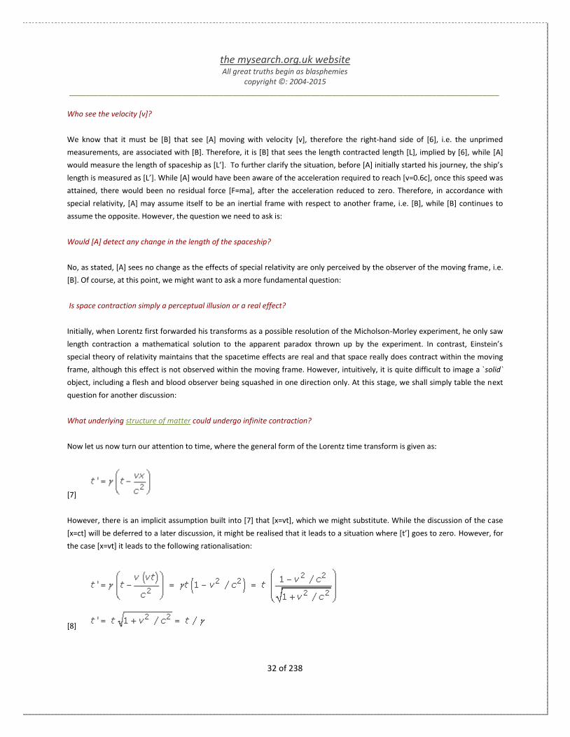
32 of 238
Who see the velocity [v]?
We know that it must be [B] that see [A] moving with velocity [v], therefore the right-hand side of [6], i.e. the unprimed
measurements, are associated with [B]. Therefore, it is [B] that sees the length contracted length [L], implied by [6], while [A]
would measure the length of spaceship as [L’]. To further clarify the situation, before [A] initially started his journey, the ship’s
length is measured as [L’]. While [A] would have been aware of the acceleration required to reach [v=0.6c], once this speed was
attained, there would been no residual force [F=ma], after the acceleration reduced to zero. Therefore, in accordance with
special relativity, [A] may assume itself to be an inertial frame with respect to another frame, i.e. [B], while [B] continues to
assume the opposite. However, the question we need to ask is:
Would [A] detect any change in the length of the spaceship?
No, as stated, [A] sees no change as the effects of special relativity are only perceived by the observer of the moving frame, i.e.
[B]. Of course, at this point, we might want to ask a more fundamental question:
Is space contraction simply a perceptual illusion or a real effect?
Initially, when Lorentz first forwarded his transforms as a possible resolution of the Micholson-Morley experiment, he only saw
length contraction a mathematical solution to the apparent paradox thrown up by the experiment. In contrast, Einstein’s
special theory of relativity maintains that the spacetime effects are real and that space really does contract within the moving
frame, although this effect is not observed within the moving frame. However, intuitively, it is quite difficult to image a `solid`
object, including a flesh and blood observer being squashed in one direction only. At this stage, we shall simply table the next
question for another discussion:
What underlying structure of matter could undergo infinite contraction?
Now let us now turn our attention to time, where the general form of the Lorentz time transform is given as:
[7]
However, there is an implicit assumption built into [7] that [x=vt], which we might substitute. While the discussion of the case
[x=ct] will be deferred to a later discussion, it might be realised that it leads to a situation where [t’] goes to zero. However, for
the case [x=vt] it leads to the following rationalisation:
[8]

the mysearch.org.uk website All great truths begin as blasphemies
copyright ©: 2004-2015 _______________________________________________________________________________________________________
33 of 238
Let us just summarise [6] and [8] before discussing any further implications:
[9]
Now we appear to have 2 very simply equations in [9], which you would assume cannot really cause any confusion, i.e. length in
the moving frame is contracted, while time is dilated. While the orientation of length contraction has hopefully been resolved,
the idea of time dilation may need some additional clarification in order to explain the invariance of the speed of light [c], which
can be summarised as follows:
[10]
The implication that follows from [10] is that space [x, x’] and time [t, t’] must be equally affected in the stationary and moving
frame, if [c] is to remain invariant. So, at first glance, [9] might appear to contradict this requirement, as the [γ] factor appears
in the numerator and then the denominator in these equations. However, the implication of time dilation is that it is the ticking
of the clock in the moving [A] frame that gets dilated, i.e. slows down, relative to the ticking of the clock in the stationary [B]
frame. Therefore, with reference to our original diagram above, the tick of 1 second in the [B] frame equates to 1.25 seconds in
the [A] frame. So, for example, the measure of time equated to [tB1=10] in the [B] frame corresponds to only [tB1’=tA1=8] in the
[A] frame.
So how do the Lorentz transforms really affects [A] and [B]?
Let us first consider the implications on the occupant of the spaceship, which is now moving with the relativistic velocity
[v=0.9c], such that [γ] increases to [2.294]. The planned journey distance of the spaceship prior to departure has been
measured in the stationary [B] frame of planet Earth to be 1 lightyear, which is therefore expected to take 1.11 years, assuming
[v=0.9c], if acceleration is ignored. However, on return, the occupant of the spaceship has timed the journey to only taken
0.484 years, which would suggest that the velocity of the spaceship was approximate 2 times greater than [c] and in direct
violation of special relativity. In this context, the only way to resolve the apparent violation is to assume that the actual distance
travelled by the spaceship, i.e. 1 lightyear, was subject to length contract to 0.436 lightyears, which then preserves the velocity
[0.436/.484=0.9c]. However, it might be argued that only the effects of time dilation was empirically verify, at the end of the
journey, based on the clock on the wall of the spaceship, as the effects of space contraction would not have been measured,
only calculated based on the invariance of the velocity [v].
Is this a valid assumption?
Of course, as suggested by the diagram, [B] might be able been able to verify the real effect of length contraction by
determining the length of the spaceship as it passes at [v=0.9]. Again, if we assume that the length of the spaceship is 100 units,
while at rest in the [B] frame, it should be subject to a ‘visible’ length contraction to 43.6 units along its axis of motion, when
observed from [B]. Of course, [A] has no perception of the ship being squashed along this axis. As such, we might again be led
to question the actual reality of length contraction.

the mysearch.org.uk website All great truths begin as blasphemies
copyright ©: 2004-2015 _______________________________________________________________________________________________________
34 of 238
The Minkowski or spacetime diagrams were
developed in 1908 by Hermann Minkowski and
provides an illustration of the properties of space
and time in the special theory of relativity. It allows a
quantitative understanding of the corresponding
phenomena of time dilation and length contraction
without the rigor of mathematical equations.
So could there be any other explanation of length contraction?
While speculative in the face of the weight of authority supporting special relativity, should matter have some fundamental
wave structure, it might raise the issue as to whether the perception of length contraction is simply a manifestation of the
Doppler effect. However, at this time, we shall simply table this issue and turn our attention to the techniques of plotting
spacetime.
1.2.2.2.1 Concepts in Spacetime
Having established the basics of spacetime in previous discussions, we can now turn our attention to some of concepts used
describe spacetime. First, we possibly need to reflect on the fact that spacetime is a 4-dimensional union of the classical
concept of 3-dimensional space plus absolute time, as inferred by the Galilean transforms.
So what new concepts emerge from the union of space and time into a single 4-dimensional continuum?
Possibly, the key issue to consider is the concept of the ‘spacetime
interval’, which we shall initially, and possibly misleading, describe
as the ‘distance’ between two events in 4-dimensional spacetime.
We might also try to visualise this ‘distance’ in terms of the diagram
above, which plots ‘time interval [t]’ on the vertical axis and ‘spatial
distance [d]’ on the horizontal axis, where the different units of [t]
and [d] are unified via the relationship [d=ct] with [c] being the
speed of light. So, with reference to the diagram above, event [A]
at the origin of the axes is separated in spacetime from events [B] and [C]. Just by way of general observation, we may note that
the time component of the ‘distance’ between [A-B] is greater than its spatial component. In contrast, the spatial component of
the ‘distance’ between [A-C] seems to be greater than its time component. However, in contradiction to what the diagram

the mysearch.org.uk website All great truths begin as blasphemies
copyright ©: 2004-2015 _______________________________________________________________________________________________________
35 of 238
Light cones come in two basic favours, i.e. past and
future. A past light cone of the spacetime event [A]
consists of all the paths that can converge at [A]
under the constraint of the finite speed of light [c]
within past time [-t]. Likewise, a future light cone
associated with event [A] consists of all the paths of
light that begin at [A] and travel into the future [+t]
at the speed of light [c].
might suggest, the axial components of time [t] and space [d] do not combine in some form of vector addition analogous to
Pythagoras’ theorem. Therefore, the following bullets will try to clarify some of the basic rules that do apply:
The spatial distances [d] is still constructed from its 3-dimensional [xyz] components via [d2=x
2+y
2+z
2], i.e. this aspect
does conform to Pythagoras’ theorem.
However, the ‘spacetime interval [s]’ is a 4-dimensional measure that is defined by [s2=t
2-d
2], where the square of the
components [t] and [d] are subtracted, not summed.
In essence, the diagram above is a simplistic example of a 2-
dimensional spacetime diagram, which features the ‘light-
cone’ formed when plotting [c] in terms of a series of time [t] versus
distance [d] values. While it is not possible to fully illustrate 4-
dimensional spacetime, we can extend the previous diagram by
extending the representation of space along the x-axis to the xz-
plane, while still retaining time along the vertical axis. In the 3-
dimensional spacetime diagram below, the path of 3 chronological
events, i.e. [-A, A, +A] are shown, where [-A] represents some event
in the past, which is able to affect [A] because it originates within the past light cone. In a similar fashion, [A] is able to affect
[+A] in the future, because [+A] is inside the light cone of [A]. Typically, the speed of light is normalised to [c=1], which then
allows an offset in space to be equate to an offset in time, where [c] acts as a conversion factor between the units of distance
and the units of time. On this basis, anything travelling at the speed of light [c] moves along the surface of the light cone at an
angle 45o
to the origin.
However, the purpose of the diagram is to try to further illustrate some of the spacetime concepts at work. By way of a
reference, let us assume that the red-orange dots, in the diagram above, corresponds to a clock travelling a distance of 3 light-
years in 5 years at a constant velocity [v=0.6]. Relativity tells us that the time on the moving clock [+A] must be slower than a
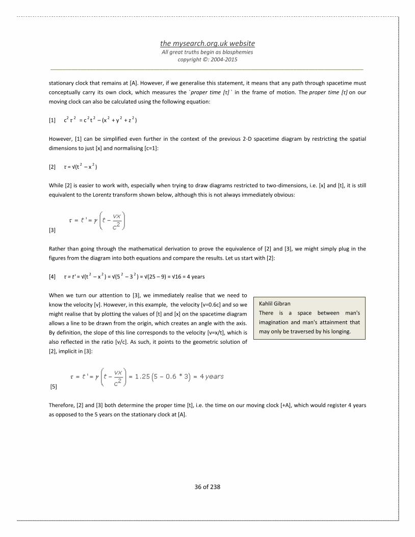
the mysearch.org.uk website All great truths begin as blasphemies
copyright ©: 2004-2015 _______________________________________________________________________________________________________
36 of 238
Kahlil Gibran
There is a space between man's
imagination and man's attainment that
may only be traversed by his longing.
stationary clock that remains at [A]. However, if we generalise this statement, it means that any path through spacetime must
conceptually carry its own clock, which measures the `proper time [τ] ` in the frame of motion. The proper time [τ] on our
moving clock can also be calculated using the following equation:
[1] c2 τ
2 = c
2 t
2 – (x
2 + y
2 + z
2 )
However, [1] can be simplified even further in the context of the previous 2-D spacetime diagram by restricting the spatial
dimensions to just [x] and normalising [c=1]:
[2] τ = √(t 2
– x 2
)
While [2] is easier to work with, especially when trying to draw diagrams restricted to two-dimensions, i.e. [x] and [t], it is still
equivalent to the Lorentz transform shown below, although this is not always immediately obvious:
[3]
Rather than going through the mathematical derivation to prove the equivalence of [2] and [3], we might simply plug in the
figures from the diagram into both equations and compare the results. Let us start with [2]:
[4] τ = t' = √(t 2
– x 2
) = √(5 2
– 3 2
) = √(25 – 9) = √16 = 4 years
When we turn our attention to [3], we immediately realise that we need to
know the velocity [v]. However, in this example, the velocity [v=0.6c] and so we
might realise that by plotting the values of [t] and [x] on the spacetime diagram
allows a line to be drawn from the origin, which creates an angle with the axis.
By definition, the slope of this line corresponds to the velocity [v=x/t], which is
also reflected in the ratio [v/c]. As such, it points to the geometric solution of
[2], implicit in [3]:
[5]
Therefore, [2] and [3] both determine the proper time [t], i.e. the time on our moving clock [+A], which would register 4 years
as opposed to the 5 years on the stationary clock at [A].

the mysearch.org.uk website All great truths begin as blasphemies
copyright ©: 2004-2015 _______________________________________________________________________________________________________
37 of 238
Carl Sagan
It seems to me what is called for is an
exquisite balance between two conflicting
needs: the most sceptical scrutiny of all
hypotheses that are served up to us and at
the same time a great openness to new
ideas … If you are only skeptical, then no
new ideas make it through to you … On the
other hand, if you are open to the point of
gullibility and have not an ounce of skeptical
sense in you, then you cannot distinguish
the useful ideas from the worthless ones.
1.2.2.2.2 Separation in Spacetime
In the previous discussion, we ended up referring to a number of different
measures of time and space, which all had something to do with spacetime
separation. The following list extends the vocabulary of terms that are
used in the description of spacetime, although in many cases, it can simply
lead to confusion about the basic principles at work:
Coordinate time, Coordinate distance
Time interval [t], spatial distance [d]
Spacetime Interval [s]
Proper Time [τ]; Proper Distance [σ]
We shall not really use the terms ‘coordinate’ time and distance because it
essentially aligns to the definition of time interval [t] and spatial distance
[d]. The term ‘coordinate’ relates to the coordinate system or frame of reference of the observer making the measurement of
time and distance, i.e. [t] and [d]. Overall, the term ‘spacetime interval [s] ’ is intended as the unambiguous measure of the
separation between 2 events in spacetime, if anything in special relativity can really be described as unambiguous. Within the
definition of the spacetime interval [s], we might describe ‘proper time [τ] ’ and ‘proper distance [σ] ’ as two sub-classes that
depend on the separation being ‘time-like’ or ‘space-like’. Of course, simply introducing another couple of pseudo-terms does
not really help clarify the situation, so we will outline these concepts using the following diagram:
The left-hand diagram reflects a space-like configuration, in which 2 events are separated in space [d] only, at least, in the
frame of reference or coordinate system shown. In contrast, the right-hand diagram reflects a time-like configuration where 2
events are separated in time [t] only. We can overlay the definition of proper time onto this description because the measure of
the ‘proper’ time requires the events to only be separated in time, i.e. the events are collocated in space. In this way, the spatial
distance [d] is zero and the time interval [t] is a measure of the proper time [τ], which in-turn corresponds to the spacetime

the mysearch.org.uk website All great truths begin as blasphemies
copyright ©: 2004-2015 _______________________________________________________________________________________________________
38 of 238
interval [s]. This possibly makes more sense if you consider a clock within a frame considered to be at rest by [A], but moving
with respect to [B]. For [A], the clock does not change its position in space, only time; although [B] will have another relative
perspective. By a similar line of argument, the ‘proper’ distance [σ] is measured in a frame, where the events are collocated in
time, i.e. simultaneous. In this case, the time interval [t] is zero, such that the spatial distance [d] is a measure of the proper
distance [σ], which in-turn corresponds to spacetime interval [s] for this specific case. Of course, such descriptions can all seem
convoluted, so we will try to step back from the ambiguity of the terminology to ask a more basic question:
How do you measure time interval [t] and spatial distance [d] in relativity?
Normally, at this point, we might start looking for our stop-watches and tape-measures, but if we are to measure the time and
distance between two ‘events’ in relativity, we need to consider what factors are ‘invariant’, i.e. unchanged, across all frames of
reference. In the context of special relativity, we have but one central axiom that requires the speed of light [c] to be invariant
in all frames of reference. As such, we can use the speed of light to help determine the spatial distance [d] between 2 events.
Note: The term ‘events’ is used rather than ‘points’ in space, because in spacetime a point in space is relative to the
observer’s coordinate system, while an ‘event’ is something that can be uniquely identified in all frames of reference,
although it might have different values of [t] and [d].
Let us try to consider the implication of all the previous terminology with reference to the following diagram. If we begin with
the diagram on the left, here we are simply trying to establish the initial frame of reference between [A] and [B]. By definition,
the shortest distance in spacetime between [A-B] is defined by the speed of light [c]. Conceptually, we might determine the
spatial distance [d] by the time taken for light to go from [A-B-A] from which we might proceed to establish all the spacetime
coordinates for the events shown in the diagram on the right.

the mysearch.org.uk website All great truths begin as blasphemies
copyright ©: 2004-2015 _______________________________________________________________________________________________________
39 of 238
In essence, the diagram on the right is a 2-dimensional spacetime diagram showing the relative coordinates of a number of
events, i.e. A to E, corresponding to a given frame or coordinate system. The time intervals [t] and spatial distances [d] can be
determined for all events within this reference frame, i.e. coordinate system; therefore we should be able to calculate the
spacetime separation between all events from the following equation:
[1]
When we initially introduced this equation, it was described in terms of the ‘proper time [τ]’ , which has now been changed
to the ‘spacetime interval [s]’. However, in the general context of the current discussion, [1] always defines the spacetime
interval [s], but does not always equate to the proper time [τ] for reasons that we now need to clarify. This can possibly be best
achieved by producing a table showing the spacetime separation for all permutations of events, in the diagram above, and then
explaining any caveats that apply to each.
- A B C D E
A - 0 3 -3 2
B c - -3 3 4
C 0 0 - 0 5
D 0 0 c -- -2.27
E 0 0.6c 0 0 -
The table above shows all permutations between all events [ABCDE]. The entries in the top half of the table contain the values
obtain from [1], while the bottom half contains an implied velocity [v], where applicable or local time. The negative values
associated with some spacetime intervals [s] are as a direct result of [1], where the spatial distance [d] is greater than the time
interval [t], which implies that the separation in question is space-like, rather than time-like, when positive. In addition, some
values of the spacetime intervals [s] are zero, which implies that they are light-like, according to the definition given in the first
diagram above. Only when the value of the spacetime intervals [s] is positive can it been associated with the concept of proper
time [τ] providing that certain caveats are considered. Before, clarifying some of these issues, let consider a more basic issues?
Why do the results in the top-half of the table bear little resemblance to the distances between the events in the right-hand
diagram above?
In the diagram above, the separation between any 2 events is defined by Pythagoras’ theorem, i.e. the sum of the squares, but
looking at [1], we see that the resulting squares of time [t] and distance [d] is subtracted. So, for all positive values of the
spacetime interval [s], we might correlate the results derived from [1] to the Lorentz transform of time:
[2]

the mysearch.org.uk website All great truths begin as blasphemies
copyright ©: 2004-2015 _______________________________________________________________________________________________________
40 of 238
So, for all non-negative values in the table, the inference is that the spacetime interval [s] reflects the measure of time within
another frame moving between the 2 events in question at a given velocity [v] that results in a straight line in the local frame.
However, let us consider the 3 categories of results that all fits the description of being time-like:
AC, AE, CE:
The separations between these pairs of events are all defined by time only. Therefore, in the local frame, there is no
spatial separation [d] and no implied velocity.
AB, CD:
While these pairs of events do fit the classification of being light-like, they are actually light-like because they imply a
velocity equal to [c] in order that a straight line can be drawn between them.
BE:
This pair of events reflects the example used in earlier discussions of an object moving between 2 points in spacetime
with a velocity [v=0.6c]. This velocity can be determined within the local frame from [v=d/t=3/5]. However, because
the proper time [τ] reduces to 4 in the moving frame, there is also the inference that the spatial distance [d’] must be
length contracted by an equivalent amount to compensate, if speed [v] is to remain invariant.
OK, that seems to explain most of the results in the table, except those that have a negative value of the spacetime interval [s].
The negative value results because the spatial distance [d] is greater than the time interval [t]. However, it is clear that a
negative value is the result of applying [2] to determine a spacetime interval [s] that is space-like rather than time-like. To avoid
this problem, the definition of ‘proper distance [σ]’ is introduced by revising [1] as follows:
[3]
So, with this equation in mind, let us consider the specific event pairs in the table above that generate negative values using [1],
which are now said to define proper distance [σ] using [3]:
AD, BC:
The separations between these pairs of events are unambiguously defined terms of distance [d] only within the local
coordinate frame. The implication of this statement is that both pairs of events must occur simultaneously in time.
For example, if these events were defined by an explosion, both explosions would be seen to occur at the same time,
in the local frame, such that the time interval [t] would be zero.
DE:
The situation, in this case, appears less clear in the sense that the separation does still involves a time interval [t]
component. However, the spatial distance [d] is greater than the time interval [t], such that the resulting spacetime
interval [s] or the proper distance [σ] can be described as space-like.
the mysearch.org.uk website All great truths begin as blasphemies
copyright ©: 2004-2015 _______________________________________________________________________________________________________
41 of 238
Stephen Hawking
"Any physical theory is always provisional,
in the sense that it is only a hypothesis: you
can never prove it. No matter how many
times the results of experiments agree with
some theory, you can never be sure that the
next time the result will not contradict the
theory. On the other hand, you can disprove
a theory by finding even a single
observation that disagrees with the
predictions of the theory... Each time new
experiments are observed to agree with the
predictions the theory survives, and our
confidence in it is increased; but if ever a
new observation is found to disagree, we
have to abandon or modify the theory"
In his 1905 paper on Special Relativity,
Einstein wrote: "We have not defined a
common 'time' for A and B, for the latter
cannot be defined at all unless we establish
by definition that the 'time' required by light
to travel from A to B equals the 'time' it
requires to travel from B to A".
The ambiguity that arises out of the definition of proper distance is that it
difficult to link [3] back to any of the Lorentz transforms, which all require
velocity [v] to be defined. By definition, any separation that is space-like either
implies an infinite velocity [v], as in the case of [AD, BC] or one that exceeds
[c], as in [DE]. As such, the Lorentz factor [γ] cannot be resolved.
So how are we meant to interpret proper distance [s]?
Let us again reflect on the 2 cases above, i.e. [AD, BC] and [DE]. In the former
cases, it was stated that the separation in the coordinate frame was
unambiguous in the sense that the spacetime interval [s] was defined solely in
terms of the spatial distance [d]. However, this measurement required the
spatial distance between the 2 events to occur simultaneously in time. While
this is true for the coordinate frame in question, it would not be true for any
other frame moving relative to it with velocity [v]. In any other frame moving
with velocity [v], the events would not be simultaneous and therefore look
more like the case [DE] in which there is also a time interval [t] between the
events. However, what is key to the definition of the proper distance [σ] is that it is constant or invariant in all other frames of
reference, irrespective of the velocity. Of course, within each frame of reference, the values of the spatial distance [d] and the
time interval [t] will differ; although the result of [3] is constant.
So can we further clarify the inference of proper time [τ]?
As might be guessed, proper time [τ] is also invariant within all other frames of reference, irrespective of their velocity [v].
Conceptually, the idea of proper time [τ] is easier to visualise in the form of a clock moving with velocity [v] between 2 events.
The time on this moving clock can be viewed by any other frame of reference moving relative to it, but all see the same time,
i.e. the proper time [τ], but again, each frame will determine difference value for the time interval [t] and the spatial distance
[d]:
[4]
What we realise from [4] is that for the proper time [τ] to remain invariant, different frames of reference moving with different
velocities, e.g. [v, v’], must measure different spatial distances [d, d’] separating the 2 events in question.
1.2.2.2.3 Simultaneity and Causality
First, let us introduce the initial scope and meaning of ‘simultaneity’ and
‘causality’ in the context of special relativity. We might begin by describe
the meaning of ‘simultaneity’ in terms of 2 events in spacetime linked to 2
explosions that occur simultaneously in the current frame of reference. As
such, the spacetime interval [s] is defined solely in terms of the spatial
distance [d], as the time interval [t] is by definition zero. Likewise, the

the mysearch.org.uk website All great truths begin as blasphemies
copyright ©: 2004-2015 _______________________________________________________________________________________________________
42 of 238
meaning of ‘causality’ might simply be described in terms of ‘cause and
effect’ where we always expect the ‘effect’ to follow the ‘cause’. However,
the scope of both, as currently being defined, only extends to the local
frame of reference and so the open question is:
What is the perception of simultaneity and causality from another frame of
reference?
There is the implication that events, which are simultaneous in one frame,
will not be so in another. However, if this is the case, we need to show
how and why the simultaneity is affected and whether this can have any
knock effect on causality. Possibly, one of the easiest ways to consider
these questions is to use the idea of a spacetime diagram onto which we
can overlay a second moving frame of reference. In the diagram above, the
stationary frame [A] linked to the black axes is labelled [t, d]. However, a secondary frame [B] perceives [A] to be moving with a
velocity [v], as identified by the red axes is labelled [t’, d’]. So what we are representing is an observer [B] who could be looking
at the same events as observer [A], but from a relative frame where [A] is moving with velocity [v] with respect to [B]. As such,
measurements from the [B] frame are subject to a ‘distortion’ that is proportional to the velocity [v] of frame [A] with respect to
[B], which results in the length contraction of the spatial distance [d] to [d’] and time dilation of the time interval [t] to [t’]. The
geometry of the spacetime diagram allows the ‘distortion’ of the moving frame [B] to be represented by rotating the time
interval [t’] axis and the spatial distance [d’] axis toward the invariant axis create by [v=c].
The diagram above is simply a clarification of the scope of the first diagram, which includes the previous idea of the ‘light
cones’. If we look at event [X] from the perspective of frame [A], it sits central within its light-cone and can be described at a
time-like event. However, due to the tilting effect associated with [tanθ=v/c], event [X] is not within the light-cone of frame [B]
and has become a space-like event within frame [B]. As such, we might consider using the spacetime diagram to help visualise
the issue of simultaneity of events in the sense of being able to make a comparison of an event in both the stationary and
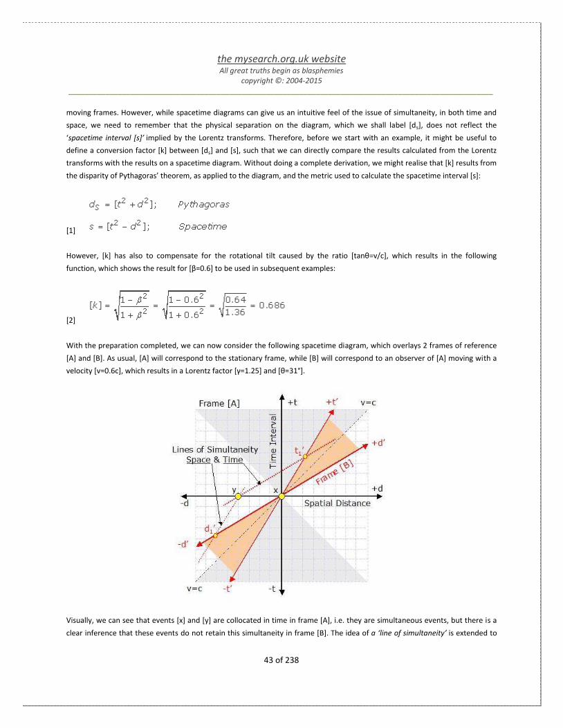
the mysearch.org.uk website All great truths begin as blasphemies
copyright ©: 2004-2015 _______________________________________________________________________________________________________
43 of 238
moving frames. However, while spacetime diagrams can give us an intuitive feel of the issue of simultaneity, in both time and
space, we need to remember that the physical separation on the diagram, which we shall label [ds], does not reflect the
‘spacetime interval [s]’ implied by the Lorentz transforms. Therefore, before we start with an example, it might be useful to
define a conversion factor [k] between [ds] and [s], such that we can directly compare the results calculated from the Lorentz
transforms with the results on a spacetime diagram. Without doing a complete derivation, we might realise that [k] results from
the disparity of Pythagoras’ theorem, as applied to the diagram, and the metric used to calculate the spacetime interval [s]:
[1]
However, [k] has also to compensate for the rotational tilt caused by the ratio [tanθ=v/c], which results in the following
function, which shows the result for [β=0.6] to be used in subsequent examples:
[2]
With the preparation completed, we can now consider the following spacetime diagram, which overlays 2 frames of reference
[A] and [B]. As usual, [A] will correspond to the stationary frame, while [B] will correspond to an observer of [A] moving with a
velocity [v=0.6c], which results in a Lorentz factor [γ=1.25] and [θ=31°].
Visually, we can see that events [x] and [y] are collocated in time in frame [A], i.e. they are simultaneous events, but there is a
clear inference that these events do not retain this simultaneity in frame [B]. The idea of a ‘line of simultaneity’ is extended to

the mysearch.org.uk website All great truths begin as blasphemies
copyright ©: 2004-2015 _______________________________________________________________________________________________________
44 of 238
Einstein's definition assumes that the one-
way speed of light is the same in every
inertial frame and then use this to define
simultaneity for every inertial frame. In this
way inertial frames in relative motion have
different definitions of simultaneity, but
are guaranteed to get the same one-way
speed of light in every measurement. This
in itself makes both simultaneity and the
one-way speed of light conventional.
both time and space, because in the context of spacetime, it can be used to imply collocation in time or space; where the line of
time simultaneity runs parallel to the [d’] axis and the line of space simultaneity runs parallel to the [t’] axis. The time and
spatial offsets in frame [A] for this example are [x=0,0] and [y=-4,0] and we can apply the Lorentz transforms to [y] calculate its
relative offsets in the moving [B] frame:
[3]
We can also ‘scale’ the results above to the grid shown on the previous
spacetime diagram by dividing by the factor [k=0.686] for the specific
example where [v/c=0.6]:
[4]
Again, to clarify the orientation of the results in [3] and [4], frame [A] is initially described as the stationary frame in which an
observer is unaware of any velocity and therefore has no perception of length contraction or time dilation. In contrast, an
observer in frame [B] is aware of the relative velocity [v] of frame [A] with respect to itself and therefore observes the effects of
length contraction and time dilation in frame [A] from [B]. As such, the spatial offset of event [y=-4] should be seen as the
contracted measure in [A], as seen by [B]. When we apply the Lorentz transforms, we are therefore transposing the contracted
value back into the coordinate system of [B], which is why [d1’>d1].
Note: In previous discussion, it was stated that the spacetime interval [s] is invariant in all frames of reference. If you
calculate [s] via the difference between the squares of [t] and [d], you will see that the value of the spacetime interval
always has the value [s=4]. This is fairly obvious when [d=-4] and [t=0] in frame [A], but frame [B] offers up the same
results with [d=-5] and [t=3], where the negative sign is lost when squared.
As such, we have provided the basic evidence, within the assumptions of relativity, such that if simultaneity exists in a given
frame of reference, e.g. [A], it will not exist in another frame moving with a relative velocity [v] with respect to [A], e.g. [B]. On
the assumption that we have generally answered the question about simultaneity, let us now consider the question of
causality:
What is the perception of causality from another frame of reference?
The following spacetime diagram includes the previous frames of reference, i.e. [A] and [B], but extends the picture to include
frame [C], which has the same velocity as [B], but is travelling in the opposite direction. The only purpose of including this extra
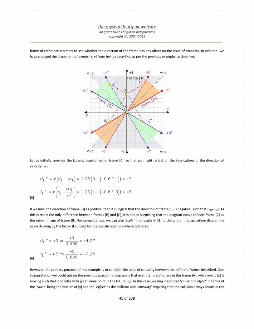
the mysearch.org.uk website All great truths begin as blasphemies
copyright ©: 2004-2015 _______________________________________________________________________________________________________
45 of 238
frame of reference is simply to see whether the direction of the frame has any affect on the issue of causality. In addition, we
have changed the placement of events [x, y] from being space-like, as per the previous example, to time-like.
Let us initially consider the Lorentz transforms for frame [C], so that we might reflect on the implications of the direction of
velocity [-v]:
[5]
If we label the direction of frame [B] as positive, then it is logical that the direction of frame [C] is negative, such that [vB=-vC]. As
this is really the only difference between frames [B] and [C], it is not so surprising that the diagram above reflects frame [C] as
the mirror image of frame [B]. For completeness, we can also ‘scale’ the results in [5] to the grid on the spacetime diagram by
again dividing by the factor [k=0.686] for the specific example where [v/c=0.6]:
[6]
However, the primary purpose of this example is to consider the issue of causality between the different frames described. One
interpretation we could put on the previous spacetime diagram is that event [y] is stationary in the frame [A], while event [x] is
moving such that it collides with [y] at some point in the future [tY]. In this case, we may described ‘cause and effect’ in terms of
the ‘cause’ being the motion of [x] and the ‘effect’ as the collision and ‘causality’ requiring that the collision always occurs in the

the mysearch.org.uk website All great truths begin as blasphemies
copyright ©: 2004-2015 _______________________________________________________________________________________________________
46 of 238
Albert Einstein
It followed from the special theory of
relativity that mass and energy are both but
different manifestations of the same thing,
a somewhat unfamiliar conception for the
average mind. Furthermore, the equation
E=mc², in which energy is put equal to mass,
multiplied by the square of the velocity of
light, showed that very small amounts of
mass may be converted into a very large
amount of energy and vice versa.
future. As such, if causality is to be maintained, the time of event [x], e.g. [tx, tx’, tx’’], has always to precede the time of event
[y], e.g. [tY, tY’, tY’’]. While the lines of simultaneity do not provide a rigorous proof, it seems clear that [tx<ty] will always be true
in all frames of reference, irrespective of the magnitude or direction of the velocity [v]. The only caveat being a case where
[v=c] and the whole notion of time and space collapses to a ‘singularity’ with no dimensions. However, we can provide a more
mathematical approach to causality by considering the implications of the following Lorentz transform:
[7]
In order for causality to be a problem the value of [t’] has to be negative with respect to some other frame. This can only occur
if the following condition exists with [7]:
[8]
However, this condition can only occur if [v>c], which is in contradiction of one of the fundamental postulates of special
relativity. So while simultaneity is an issue, causality is preserved.
1.2.2.3 Mass and Energy effects
It is said that there are only four fundamental quantities in physics: time,
length, mass and charge. So far, we have mainly focused on the basic
principles by which special relativity appears to affect time and space,
where space is defined in terms of length in three dimensions:
So what are the implications on other fundamental quantities?
While we may intuitively feel we understand mass, the development of
science, over the last 100 years, suggests that mass may be a far more
puzzling quantity than was first imagined. Our intuitive understanding of
mass is based on things that we can touch and see, i.e. they have substance
and this substance has mass. However, Einstein’s famous equation
E=mc2 suggests that mass is also a form of energy, which is not so easily
associated with anything tangible. Likewise, when Planck’s energy equation
[E=hf] is combined with Einstein’s energy equation [E=mc2], it might suggest
that there is a correlation between mass and frequency, i.e.
[1] E=mc2 = hf where [c] & [h] are constants
If we follow this logic, [1] implies that mass [m] and frequency [f] may have some sort of equivalence, but given that frequency
is also a function of time, then any change in the perception of time will change frequency [f=cycles/time] that would in-turn

the mysearch.org.uk website All great truths begin as blasphemies
copyright ©: 2004-2015 _______________________________________________________________________________________________________
47 of 238
affect our perception of mass [m]. Likewise, another fundamental unit is charge [e], which is associated with a force of
attraction, or repulsion, between particles with an associated charge; the strength of which is a function of distance that is
subject to length contraction. Of course, if there is some ambiguity about the absolute measure of these fundamental units,
then maybe we need to table the following question:
What is the impact on all composite quantities dependent on these fundamental units?
While velocity [v=d/t] is fairly fundamental to classical physics, it is still a composite quantity. However, we know that the
invariance of the speed of light [c] is a postulate of relativity, although its direction as a vector will depend on the frame of
reference. In contrast, the velocity of any physical object in one frame of reference, e.g. [A], moving relative to another, e.g. [B]
cannot be invariant in either speed or direction, but there are specific cases where the speed of an object can remain invariant.
For example, the occupant of a spaceship travelling at relativistic speed will be subject to time dilation, which unless
compensated by space contraction would suggest a speed greater than [c]. As a consequence, the speed of the spaceship is
thought to be invariant in both [A] and [B], i.e. v=d/t=d’/t’, even though the measure of space contraction [d’] disappears when
the spaceship returns to the stationary frame, but time dilation [t’] persists. Therefore, we may need to be careful in our
definition of velocity and given that momentum [ρ] is defined as a function of mass [m] and velocity [v], it is probably a safe bet
to assume that it is also subject to relativistic effects. Likewise, in a knock-on process, our perception of force [F] and energy [E]
must also be subject to the dependencies on our measurement of time, space, mass and charge. So while we have only outlined
some of the rationale supporting the concept of space contraction and time dilation, it would appear that special relativity may
also affect other key concepts in physics. As an extension of the implication of special relativity, the following discussion
attempts to show how the acceptance of its postulates change other composite quantities through which science has come to
describe the universe at large. However, the starting point for this discussion will still begin anchored in the determinism of
Newton’s 2nd
law of motion:
[2]
The equations above are all equivalent ways of expressing Newton’s 2nd
law of motion, first in the normal form [F=ma], but
finally as the rate of change of momentum with time. The only purpose being to highlight the dependence on time [t], which is
the ‘persistent’ relativistic quantity. The following table highlights some other important quantities that are also dependent on
time [t].
Entity Units Abbreviation
Velocity [v] metres/second v = m/s
Acceleration [a] velocity/second a = m/s2
Momentum [p] kilograms*metres/seconds p = kg.m/s
Force [F] mass * acceleration F = kg.m/s2
Energy [E] force * metres E = kg.m2/s
2

the mysearch.org.uk website All great truths begin as blasphemies
copyright ©: 2004-2015 _______________________________________________________________________________________________________
48 of 238
Stephen Hawking
At 10 percent of the speed of light an
object's mass is only 0.5 percent more
than normal, while at 90 percent of the
speed of light it would be more than
twice its normal mass. As an object
approaches the speed of light, its mass
rises ever more quickly, so it takes more
and more energy to speed it up further.
It can in fact never reach the speed of
light, because by then its mass would
have become infinite, and by the
equivalence of mass and energy, it would
have taken an infinite amount of energy
to get it there. For this reason, any
normal object is forever confined by
relativity to move at speeds slower than
the speed of light. Only light, or other
waves that have no intrinsic mass, can
move at the speed of light,
In terms of classical physics, we might start with the assumption that a given
mass [m] is constant, which [2] in isolation cannot refute, because any or all
quantities may account for any relativistic effects observed. As such, we shall try
to determine whether mass itself is subject to any relativistic effects by starting
with Einstein’s famous mass-energy equation:
[3]
If you multiply both sides of [3] by velocity [v], we can rearrange to produce an
equation that links velocity, momentum and energy. While this equation is a
little contrived, it reflects a relationship between momentum [ρ] and energy [E],
which we can subsequently substitute into [5]:
[4]
As the next step, we can describe energy [E] as force [F] over distance [x] and then substitute force [F] for the rate of change of
momentum [ρ] with time [t], which allows us to create an direct relationship between energy [E] and momentum [ρ]
[5]
At this point, we proceed by integrating both sides of [5]:
[6]

the mysearch.org.uk website All great truths begin as blasphemies
copyright ©: 2004-2015 _______________________________________________________________________________________________________
49 of 238
In [6], C1 and C2 are both constants of integration, which we can aggregate into a single unknown [X]. However, to resolve any
meaning from [6] we possibly need to stop and reflect on Einstein’s relationship between mass and energy, i.e. E=mc2. At one
level, this equation is really only defining the energy associated with a mass at rest, because a moving mass would also acquires
kinetic energy. Therefore, when looking at [6], we might realise that [c2ρ
2] is dependent on velocity through the definition of
momentum [ρ], which will go to zero, if mass [m] is zero. Now, by definition [X] must be a constant, which in the context of an
energy expression can be rationalised in terms of the rest mass energy, i.e. m0c2. So let us proceed on this assumption to see
what results:
[7]
So based on the speculative substitution for [X] in [6], we appear to have ended up with a relativistic expression for energy [E]
that we can cross-reference with the earlier derivation in terms of 4-vectors. However, we might also realise that we can use
Einstein’s equation to transpose [7] into a relativistic mass equation:
[8]
At this point, let us stop to reflect further on the implications of [7] and [8]. First, there is an implication in [8] that there are 2
forms of mass being discussed, i.e. rest mass [m0] and some form of relativistic mass [m], where [m=m0+mV]. However, the
sensitivity of Lorentz factor [γ] to velocity [v] suggests that this relativistic mass [mV] would be virtually negligible in comparison
to rest mass [m0] at most speeds; although this statement would be frame-dependent. Of course, if the velocity [v] of the mass
[m] were to approach [c], the relativistic mass [mV] would become increasingly significant, even in comparison to the rest mass
[m0].
Note: Today, most texts refrain from using the terms ‘relativistic mass’ and reserve the idea of mass in connection with
its rest mass [m0]. The logic of this position can possibly be best summed up when realising that any relativistic increase
in mass does not change the number of atoms present.

the mysearch.org.uk website All great truths begin as blasphemies
copyright ©: 2004-2015 _______________________________________________________________________________________________________
50 of 238
With this said, let us continue to discuss the effects of relativity on mass and energy in the context of an example, albeit a
hypothetical one. We will start by assuming a small spaceship of mass [m2] is travelling at 99.5% of light speed with respect to
another much larger spaceship of mass [m1], which we will consider to be the stationary frame of reference. At [v2=0.995c], the
relativity factor becomes [γ=10] and we may do some initial calculations of the relative mass and energy associated with each
system, if we assign rest masses of [m2=100] and [m1=10] and apply the following equations:
[9]
As indicated, the `total energy` comprises of the `rest energy` plus the `kinetic energy` associated with its relative velocity [v],
therefore:
[10]
In the following example, we will simplify the numbers involved by defining the speed of light [c=1] and express any relative
velocities as a fraction of [c]. While the resulting numbers are not absolute, they are comparative. Our comparison will be based
on the initial mass-energy state of the two spaceships, as defined above, versus a combined mass-energy state, after the larger
and smaller spaceships have been tied together. To simplify the description, we will simply assume the that larger spaceship
`lassoes` the smaller spaceship with a very special piece of rope, come conceptual ‘tractor’ beam , so that their resulting
velocity [v3] applies to both spaceships, i.e. they share a common frame of reference.
Large Spaceship Small Spaceship
m1 = 100.0 m2 = 10.0
v1 = 0.0 v2 = 0.995
γ = 1.0 γ = 10.013
m1` = 100.0 m2` = 100.13
Rest Energy = 100.0 Rest Energy = 10.0
Kinetic Energy = 0.0 Kinetic Energy = 90.125
Total Energy = 100.0 Total Energy = 100.125
The table above shows the respective mass-energy state of the two spaceships from the perspective of a stationary observer,
who is positioned outside the larger spaceship. To this observer, the larger spaceship has no velocity, i.e. [v1=0], and therefore it
has no kinetic energy. In comparison, the smaller spaceship is travelling at near light speed, i.e. [v2=0.995c], giving a relativity
factor [γ=10.013], which implies a relative mass [m2=100.13]. We can now calculate the total, kinetic and rest energy associated
with both systems from the perspective of our stationary observer. If we assume that the larger spaceship `lassoes’ the smaller
spaceship, we can describe them as a single system with velocity [v3]. However, the conservation of energy, momentum and
mass are fundamental concepts of physics, which states that these quantities cannot be created nor destroyed. Clearly, given
any basic intuition about the inertia of these systems would suggest that one system must gain velocity, while the other loses

the mysearch.org.uk website All great truths begin as blasphemies
copyright ©: 2004-2015 _______________________________________________________________________________________________________
51 of 238
There are a number of questions
concerning the interpretation of E=mc2
that have occupied both philosophers
and physicists:
1) Are mass and energy the same
property of a physical system and what is
inferred by equivalence”?
2) Is mass converted into energy via
some physical interactions, and if so, by
what means?
3) Does E=mc2 have any wider
consequences, and if so, what are they?
velocity, when initially tied together. However, the conservation of energy tells us that the total energy of the two systems, in
this closed example, must remain constant. On this basis we can calculate the final mass-energy state of the combined system:
Large Spaceship Small Spaceship
m1 = 100.0 m2 = 10.0
V3 = 0.835 V3 = 0.835
γ = 1.818 γ = 1.818
m1‘ = 181.786 m2‘ = 18.179
Rest Energy = 100.0 Rest Energy = 10.0
Kinetic Energy = 81.786 Kinetic Energy = 8.179
Total Energy = 181.786 Total Energy = 18.179
In order to balance the conservation of energy requirement, the total energy before and after, must be 200 units, i.e.
181.786+18.179 . However, this requires a residual velocity [v3= 0.835c], which is still an appreciably percentage of light speed,
although [γ] falls to 1.818. However, strictly speaking, this is new mass-energy state would only be perceived by our stationary
observer, who is outside both spaceships.
So how do we physically interpret these results?
First, if we look at the before and after results in terms of mass, it would
suggest that there has been a net loss of kinetic mass from the smaller
spaceship, only to reappear in terms of a net gain of kinetic mass in the larger
spaceship.
So, given that the only thing connecting the two spaceships was a piece of rope,
should we assume the kinetic mass has somehow travelled down the rope?
Clearly, this does not seem to be a very plausible answer and we might
conclude that this effect is best explained as an energy transfer between the
two spaceships, as one slowed down and the other sped up, when connected
via our hypothetical rope.
However, can we really say that energy travelled down the rope, any more than mass?
Clearly, the rope caused a force to be exerted between the two ships, which decayed to zero as the speed of the two
spaceships converged. However, the new mass-energy state is not really as described by the table below, which is only the
perception of our stationary observer, whereas an observer on-board either spaceship might perceived the final mass-energy
state to be:

the mysearch.org.uk website All great truths begin as blasphemies
copyright ©: 2004-2015 _______________________________________________________________________________________________________
52 of 238
Large Spaceship Small Spaceship
m1 = 100.0 m2 = 10.0
V3 = 0.0 V3 = 0.0
γ = 1.0 γ = 1.0
m1‘ = 100.0 m2‘ = 10.0
Rest Energy = 100.0 Rest Energy = 10.0
Kinetic Energy = 0.0 Kinetic Energy = 0.0
Total Energy = 100.0 Total Energy = 10.0
Of course, both observers on-board the spaceships would have felt acceleration and could calculate their new relative velocity
with respect to the stationary observer, now left far behind. However, as an inertial system, they might equally assume that
their new frame of reference is at rest, i.e. [v3=0]. If so, neither system would have any kinetic mass-energy and the net energy
of the combine system would have fallen from 200 to 110 units, which resides in the rest mass only.
So what conclusion can be drawn at this stage?
Possibly, we need to consider that kinetic or relativistic mass is simply something that appears out of the equations rather than
necessarily having any tangible existence, and as suggested, we might be better restricting our concept of mass to rest mass
[m0] only. However, it also appears to be misleading to consider energy as a tangible substance, as it corresponds to a relative
velocity with respect to our original stationary observer, who has long since vanished over the metaphorical horizon.
So can we say that energy was transferred between the two systems given that we discounted the transference of any tangible
mass down the rope?
As such, it might be that energy is simply a quantity that appears on an energy account ledger for some given frame of
reference. However, at this point, we possibly need to consider the arguments within a much wider context than our present
discussion. So far, we have only considered rest and kinetic energy, but there is a third form, which relates to potential energy.
As such, equation [9] was incomplete, as it did not take potential energy into account. On the macroscopic scale, this energy
can be explained in terms of a change in the gravitation potential of any given mass with respect to the rest of the universe. If
we put aside rest energy, gravitational potential energy would cause a mass to accelerate towards the centre of gravity within
in a given region of space, i.e. potential energy is converted into kinetic energy. As such, one could argue that there is no such
thing as an inertial frame of reference; as any frame must have some, albeit unmeasured, gravitational acceleration towards
the centre of mass of the local universe. From this perspective, the table above is incomplete and the mass-energy of the
combined system is changed in terms of its position with respect to the centre of gravity and this has changed its potential
energy. Therefore, you cannot just declare any frame of reference to be stationary, implying that the rest of the universe to be
moving relative to it, without resolving how the balance of kinetic and potential energy came to be in it current state.
So what is the relativistic energy of a given system?

the mysearch.org.uk website All great truths begin as blasphemies
copyright ©: 2004-2015 _______________________________________________________________________________________________________
53 of 238
Galileo Galilei
By denying scientific principles,
one may maintain any paradox.
As we continue to widen the scope of our frame of reference, the energy of any given system has to account for its potential
gravitational energy with respect to some conceptual centre of mass of the rest of the universe. If so, the kinetic energy
associated with velocity [v] must also be related to this point. As such, two arbitrary frames of reference cannot just declare
themselves as inertial systems, whereby the relative motion of the other implies a net increase in mass and energy. See the
discussion of ‘Paradoxes’ for an expansion of this line of thought.
1.2.3 Paradoxes
In this section, the intention is to focus the discussion around a number of inter-related
paradoxes that arise out of the postulates of special relativity. However, in doing so, some of the discussions may go beyond
the `accepted model` and possibly even beyond the `limit of inference` so often referred to throughout this website. However,
such discussion will be highlighted as speculative.
The diagram above alludes to possibly the most famous paradox of special relativity, which is often referred to as `The Twin
Paradox’ . While Einstein was aware of the potential for various paradoxes from the outset of the publication of his special
theory of relativity, in 1905, he initially considered the issue of the twin paradox addressed in terms of simultaneity. However,
in 1911, French physicist Paul Langevin formalised the idea of the twin paradox and forwarded a resolution based on the effects
of acceleration to identify the moving frames of reference. During this time, Einstein position on the twin paradox was still
evolving as he worked towards the publication of his theory of general relativity, in 1915, by which time he appeared to be
expressing some doubts as to whether the twin paradox could be completely resolved within the constraints of special
relativity. In 1918, Einstein finally published a response to the issues embodied within the twin paradox entitled ‘Dialogue
about objections to the Theory of Relativity’ in which he basically uses some of the ideas within general relativity to address the
key issues within the twin paradox. However, before we can continue with the detailed arguments related to the paradox, we
first need to provide a basic description:
The twin paradox concerns the apparent dichotomy of time dilation with respect to two twins, one of which undertakes
a journey at near light speed before returning to Earth. If both can argue that they have travelled at constant velocity,
then each might also argue that it was the other in motion and therefore subject to time dilation. As such, much of the

the mysearch.org.uk website All great truths begin as blasphemies
copyright ©: 2004-2015 _______________________________________________________________________________________________________
54 of 238
"His older self had taught his
younger self a language which
the older self knew because
the younger self, after being
taught, grew up to be the older
self and was, therefore,
capable of teaching."
debate surrounding the twin paradox centres on whether asymmetric or symmetric time dilation applies to these two
frames of reference. For it would seem the paradox is based on the premise that both twins can equally claim to be
within an inertial or non-accelerating frame of reference, i.e. both frame are
symmetrically equivalent. However, at one level, it would appear that the twin who
accelerates away from the Earth cannot maintain the claim of being an inertial
frame throughout the entire journey; hence the issue of acceleration appearing
within the debate. As such, the asymmetry of the inertial status of each twin might
be consider resolved, along with the paradox, so that we might simply declare
unambiguously that the space-faring twin is the one subject to time dilation and
returns to Earth younger than his twin sibling - QED.
Unfortunately, the assumption that the Earth can be considered as some sort of ‘absolute’ frame of reference is now known to
be problematic in light of present-day understanding of cosmology. For the Earth itself spins on its axis, while orbiting the Sun,
while rotating within the Milky galaxy, which is moving within an expanding universe. As such, the status of the Earth as an
inertial frame of reference will require some additional examination. However, it is still clear that the rocket carrying the space-
faring twin was subject to acceleration, by virtue of the measurable G-force [F=ma]. Therefore, the scope of the subsequent
discussions needs to consider the wider issues surrounding the twin paradox within the context of the following questions:
What is the net effect of time dilation at the end of the journey?
What are the relativistic effects within each frame during the journey?
Embedded in the questions above is the potential issue of verifiable science versus subjective opinion. In the first case, science
should simply be able to verify whether one of the twins is younger or not. However, the issue of relative time on-route may
prove to be more subjective, at least, if the perception of time is localised within a specific frame and cannot be directly
compared to time in another frame. However, this potential impasse is just conjecture at this point and we need to explore
some of the details of the different arguments forwarded to see whether they fully explain the fundamental nature of the twin
paradox:
Langevin’s acceleration description
Einstein’s GR based description
Inertial versus non-inertial frames of reference
Spacetime diagrams and lines of simultaneity
Light signalling and Doppler analysis
All of the above
While we will start with the standard description of the twin paradox, the intention is to extend this paradox to include triplet
siblings. As in the twin paradox, one of the siblings will be considered to remain at ‘home’ subject to no acceleration, while the
other 2 siblings undergo a journey at near light-speed that is identical in every aspect, i.e. distance, velocity and acceleration,
with the exception that their direction is reversed. As such, all three siblings occupy different frames of reference moving with
different relative velocities and we are left to question the relative age of the siblings at the end of the journey and on-route,
i.e.

the mysearch.org.uk website All great truths begin as blasphemies
copyright ©: 2004-2015 _______________________________________________________________________________________________________
55 of 238
"Kedar Joshi
The world is a contradiction;
the universe a paradox."
Einstein's Approach: 1918
Einstein addressed the twin paradox in special
relativity in a relatively unknown and rarely cited
paper written in 1918, in the form of a dialogue
between a critic and a relativist. Contrary to
most textbook versions of the resolution,
Einstein admitted that the special relativistic
time dilation was symmetric for the twins, and
he had to invoke, asymmetrically, the general
relativistic gravitational time dilation during the
brief periods of acceleration to justify the
asymmetrical aging. Notably, Einstein did not
use any argument related to simultaneity or
Doppler shift in his analysis.
Can the 2 travelling sibling explain their relative age to each other?
If the conclusion is that these 2 siblings must age at the same rate compared to
their ‘stationary’ sibling, because the reversal of direction by itself should have no net
effect on the outcome of time dilation, then a secondary problem is raised. For it
suggests that relative motion in itself does not immediately lead to any tangible time
dilation, as you need understand the ‘history’ of the journey, i.e.
What is the relativity of 2 frames of reference, which have a common start and end points?
Again, it will be highlighted that this discussion is raised in the spirit of honest inquiry rather than implying any weight of
authority.
1.2.3.1 The Twin Paradox
As indicated in the opening section, there are really 2 aspects to the
twin paradox. The first relates to resolving whether the frames of
reference in question are subject to asymmetric or symmetric time
dilation. The second relates to how and where the time dilation in a
given frame takes place. In principle, resolving which frame does not
remain inertial, i.e. subject to no acceleration, is not really problematic,
although the issue of an ‘absolute’ frame of reference will require
some further discussion. As such, the actual paradox of which twin
should be younger is not really a paradox, as the weight of authority is
pretty well unanimous that it should be the space-faring twin who ends
up being younger. However, the second aspect of explaining how and
where time dilation takes place on-route is not as easily explained
given that there are several approaches to consider:
Spacetime Diagram Analysis
Signalling Analysis
Simultaneity Analysis
While the list above is not exhaustive, it generalises a broad range of approaches that have been used to help try to explain the
relative perception of time within each frame of reference under discussion. However, there is one omission that may be
surprising, as it is the one adopted by Einstein in his 1918 paper based on his idea of General Relativity, which is the subject of
another section in this website. However, the reason for not elaborating Einstein’s approach, at this point, is because adopting
the arguments of general relativity seems to imply that special relativity cannot resolve the twin paradox. While the analysis of
twin paradox in terms of the equivalence principle in which general relativity links acceleration and gravitation is possible, the
issue of relative time in each frame still appears to remain a matter of debate. However, there will be some further footnotes
on the equivalence principle in the following discussion of ‘simultaneity analysis’.

the mysearch.org.uk website All great truths begin as blasphemies
copyright ©: 2004-2015 _______________________________________________________________________________________________________
56 of 238
1.2.3.1.1 Spacetime Diagram Analysis
So we will start by considering the implications that can be drawn from analysing 2 potential spacetime diagrams, as shown
below. While these diagrams might appear to reflect a mirror-image under the rules of symmetric time dilation; although only
one of them is valid in the case of the twin paradox.
The spacetime diagram on the left represents the case where the Earth is considered to be the inertial frame from which the
space-faring twin accelerates away in order to achieve a constant velocity of 60% light speed, i.e. v=0.6c. In fact, we might
realise that there must be 4 periods of acceleration: the initial period of acceleration away from the Earth, the period of
deceleration and acceleration at the mid-point [B] in order to turn round, plus the final period of deceleration on returning to
Earth. However, it is worth noting that while special relativity puts an upper limit of velocity, i.e. [c], there is no upper limit on
acceleration. As such, we might initially assume that the required acceleration for this journey takes place in almost infinitely
small periods of time. While there are implications within this assumption, we will return to the details later in the discussion,
but for now, we might simply assume that the presence of a G-force [F=ma] allows the rocket to be ‘unambiguously’ identified
as the moving frame of reference.
On the assumption that the inertial and non-inertial frames have been identified, what can we say about time dilation?
Well, based on the spacetime diagram on the left above, we know that the Earth-bound twin should experience 10 years of
elapsed time and, as a consequence of time dilation, the moving frame should only experience 8 years of elapsed time. For the

the mysearch.org.uk website All great truths begin as blasphemies
copyright ©: 2004-2015 _______________________________________________________________________________________________________
57 of 238
moment, we shall simply accept that the reality of this difference in elapsed time can be verified at the end of the journey,
based on the weight of evidence currently supporting special relativity. However, the identification of the Earth as the inertial
frame immediately throws doubt on the second spacetime diagram, on the right above, because it is based on the assumption
that both frames can be treated as symmetrical, i.e. the space-faring twin perspective can equally claim to be an inertial frame.
However, given our assumption that the journey time for the space-twin can be
verified to have taken 8 years, then the elapsed time on the Earth, moving with
a relative velocity [v=0.6c], would have to be time dilated with respect to 8 years,
i.e. only 6.4 years. Of course, this figure appears to conflict with the expectation
that the earthbound twin should experience 10 years.
So can we draw any other spacetime diagram with respect to the moving frame?
We can, but we have to recognise that the moving frame represented by the
rocket can never be shown within one single stationary frame. The easiest way to
describe the spacetime diagram above is to start with the frame of the Earth
twin, which now has to move away from the space twin now considered to be at
rest with a velocity of [v=0.6c]. This initial phase is consistent with symmetrical
time dilation for the outward phase of the journey to point-B, which the space
twin would also have to view as moving toward him with a velocity of [v=0.6c].
However, at this point, the reality of asymmetric time dilation has to be resolved,
because the Earth frame must continue to move with constant velocity [v=0.6c].
As such, the space twin has to ‘catch-up’ with the moving Earth by acceleration
to a relative velocity of [0.88c]. So, in effect, we have created a third frame that
is subject to further time dilation due to the higher relative velocity. However,
the net effect is that the space and Earth twin are reunited after 10 years in the
Earth frame, while only 8 years have elapsed for the space twin.
So what is the inference of the simultaneity gap on the diagrams?
The simultaneity gap is referring to the grey-shaded zones on the 2 previous diagrams, where the upper and lower dashed lines
are known as ‘lines of simultaneity’ . While we have previously discussed some of the implications of these lines, they will
require some specific analysis later in this discussion. However, if we look at the first set spacetime diagram, on the left, it can
be seen that when the space twin reaches point-B, his perception of elapsed time corresponds to 4 years. However, the lines of
simultaneity drawn from this point coincide with 2 different times in the Earth frame, which claim to be simultaneous in this
frame, i.e. 3.2 and 6.8 years?
How can 1 point in time be simultaneous to 2 points in time in another frame?
Actually, the diagrams are misleading because they reflect the change in velocity from [v=+0.6c] to [v=-0.6c] to have taken place
instantaneously. One potential implications of the simultaneity gap that has been suggested is that it corresponds to the actual
time of deceleration and acceleration at [B], i.e. [6.8-3.2=3.6] years elapsed. Whether this statement can be supported will be
taken up in the ‘simultaneity analysis’ discussion below.

the mysearch.org.uk website All great truths begin as blasphemies
copyright ©: 2004-2015 _______________________________________________________________________________________________________
58 of 238
1.2.3.1.2 Signalling Analysis
So, on the basis of the previous spacetime diagram analysis, we may feel there is a strong
case for declaring that the Earth to be the inertial frame from which the space twin is seen to
move with velocity [v=0.6c]. However, while this may then lead to the conclusion that this is
an asymmetric time dilation system in which the space twin ages less than this Earth bound
twin, the issue of relative time on-route remains.
How might we try to gain some insight of relative time on-route?
Well, the ability to send time-encoded light signals between the Earth-bound and space twin
might prove useful. However, before we get into some of the details, let us consider the
general situation, as shown in the diagram right, which may help to highlight the differences
in the time signals caused by time dilation plus the propagation delay of the signal itself, due
to the finite speed of light. In essence, this is the same spacetime diagram that we
established in the previous discussion, which shows the inertial Earth frame and the frame of
the space twin moving with a velocity [v=0.6c]. As such, our preferred reference will be the
Earth frame and, as such; the line of simultaneity becomes a horizontal line in this frame. We
can establish a known reference point at [B] by virtue of the Minkowski metric that might be
considered as shorthand for the Lorentz time transforms in this case:
[1]
In order for a signal to arrive at [B], synchronised to this point in spacetime, it will require 3 years of elapsed time, as measured
by the Earth frame, to propagate the 3 light-years to [B]. We might assume that this signal has its departure time encoded onto
the light signal such that it can be decoded by the space twin, when he arrives at [B] after 4 years elapsed time in the moving
frame. On receipt of this signal, the space twin immediately transmits his local elapsed time, i.e. 4 years, back towards Earth,
which will take another 3 years according to Earth time, i.e. a total of 8 years. Now there are 2 ways in which to interpret the
values in the signals:
If the space twin was able to look back at a clock on Earth through powerful telescope, when arriving at [B], he might
think that Earth time was running slower than his local space time, i.e. 2 years versus 4 years.
Likewise, if the Earth twin was able to see a clock on the rocket, when arriving at [B], he might think the opposite in
that Earth time would appear to be running faster than space time, i.e. 8 years versus 4 years.
However, there is not really any ambiguity in this situation as both the Earth twin and his space twin are both well aware of i)
the effects of time dilation, ii) can both agree which is the inertial frame and iii) know the propagation delay due to the speed of
light. It might also be worth pointing out that the relative speed [v=0.6c] is invariant in both frames of reference, which the

the mysearch.org.uk website All great truths begin as blasphemies
copyright ©: 2004-2015 _______________________________________________________________________________________________________
59 of 238
space twin can calculate via the duration of the G-force measured onboard the rocket. All in all, both twins are capable of
drawing and interpreting the previous spacetime diagram in terms of propagation delay and time dilation. As such, we can
extend the previous diagram to show a series of light-based signals being sent in both directions, which would be subject to
Doppler shifting to the red or blue end of the spectrum depending on the relative directions of the 2 frames, as shown below:
While the arrival rates of these signals may initially appear somewhat asynchronous in the receiving frame, they can be shown
to reflect the consistent ticking of the clocks in both the Earth or space twin frames. Again, there are 2 factors at work, i.e. time
dilation and propagation delay due to the finite speed of light [c]. The Lorentz transforms allow the time and distance travelled
in both frames of references to be calculated and compared, and because the Earth frame is the inertial frame, the diagrams
above will be resolved in terms of the distance measured in the Earth frame. The diagram on the left shows signals being sent
from Earth to the space twin, while the diagram on the right shows signals being sent from the moving rocket back to Earth. It
can be seen that some of the signals have been labelled, for illustration purpose, in the form X(Y), where [X] identifies the time
in the source frame and [Y] the distance with respect to the Earth frame. As such, we can calculate the required time, with
respect to the Earth frame, for the light signal [c] to propagate this distance, i.e. [t=d/c]. If we then remove this delay, caused by
the propagation of the signal, the only discrepancy between the timing of the signals in either frame appears to be entirely due
to time dilation. Therefore, again, there does not appear to be any paradox provided we anchor our interpretation to the
inertial frame and consistently apply the Lorentz transforms

the mysearch.org.uk website All great truths begin as blasphemies
copyright ©: 2004-2015 _______________________________________________________________________________________________________
60 of 238
Footnote: To some extent, the reference to Doppler red and blue shifting was an unnecessary detail within this particular
discussion, although it provides some useful background to the extension of the twin paradox that follows. However, it
might be useful to note that ‘redshifting’, i.e. where the frequency or wavelength of an electromagnetic wave shifts up
or down the EM spectrum range, can be caused by more than one reason. Where time dilation is involved, a relativistic
Doppler shift has to account for all physical processes linked to the source, such as the atomic emission of photons,
which are also slowed in time, which in-turn shifts the emitted light towards the red-end of the spectrum. In addition,
there is gravitational and cosmological redshifting, where the former is also linked to time dilation effects due to present
of a large mass-density and the latter linked to the expansions of the universe.
1.2.3.1.3 Simultaneity Analysis
The first part of this description outlines some potential simultaneity effects within the
twin paradox that do not really seem to make sense, but the idea is presented because it
seems to illustrate some of the convolutions special relativity can cause. In the basic
spacetime diagram analysis for our twin paradox example, the issue of the simultaneity
gap was raised, but not really explained. However, it was suggested that the gap might
reflect the rate of deceleration and acceleration at the turning point [B]. It was also
highlighted that while, in practice, any period of acceleration or deceleration would take
a finite time, in principle, these periods could be reduced to an infinitely short duration.
In order to discuss some of the potential implications of this line of thought, the diagram
on the right has superimposed a third frame of reference onto the original example. The
purpose of the diagram is to provide two comparative frames in which the simultaneity
gaps created by the lines of simultaneity are linked to turning points, e.g. [B] and [C],
caused by the same change in relativistic velocity [v=±0.6c]. However, it might be noted
that the relative span of each simultaneity gap appears to grow as a function of distance,
which cannot be directly linked to the periods of acceleration and deceleration, if they
are identical in both frames 2 and 3.
What inference might be drawn from the simultaneity gap?
Well, one suggestion forwarded is that the simultaneity gap spans a period of time in the
inertial frame that is effectively compressed into the turn-round time in the moving
frame. In the case of frame-2, this would imply that 3.6 years of time, i.e. 6.8-3.2 years, is
compressed into the turn-round at year 4. While, in contrast, frame-3 would ‘see’ 7.2
years of time, i.e. 13.6-6.4 years, compressed into the turn-round at year 8.
How might this time effect be explained?
One initial line of thought might be that the periods of acceleration somehow align to
the equivalence principle linking acceleration and gravity; as it is known that gravitation
creates an additional time dilation effect. However, if this were the case, then the Lorentz transforms would not calculate the
correct time dilation factor in isolation of general relativity and does not explain why identical periods of acceleration leads to

the mysearch.org.uk website All great truths begin as blasphemies
copyright ©: 2004-2015 _______________________________________________________________________________________________________
61 of 238
different simultaneity gaps based on the distance travelled. Given these concerns, the following explanation of the lines of
simultaneity is preferred because it seems to avoid the paradoxical perception of time implicit in the description above, which
the previous signal analysis seemed to refute anyway. Let us step back and ask a question:
What is the scope of a line of simultaneity between 2 frames of reference?
In many respects, the line of simultaneity simply identifies 2 points in spacetime that are space-separated, i.e. they occur at the
same time, in one given frame. In the spacetime diagram below, we are basically replicating the same twin paradox example
used throughout this discussion. According to the inertial frame, the space twin travels at velocity [v=+0.6c] for 5 years,
then ‘instantaneously’ turns around and travels back at velocity [v=-0.6c] for 5 years. At this turn round point, we see 2 lines of
simultaneity linking frame-2 and frame-3 with frame-1. In some respect, the diagram above is replicating the previous
discussion on ‘simultaneity’ by showing the axes of 3 frames of reference at [A]. The turn round point, at [B], is where the space
twin switches from frame-2 to frame-3 and where we see the 2 lines of simultaneity linked to the 2 points on the time axis of
frame-1, i.e. 3.2 and 6.8 years.
So, again, what inference might be put on these points?
Well, in many respects they are simply telling us that these points in the spacetime of frame-1 would be seen as simultaneous
in time in frames 2 and 3 respectively. The first key point here is that the lines of simultaneity originate in two different frames
of reference. So when the space twin first at arrives at [B] in frame-2, the line of simultaneity is linked to frame-1 at 3.2 years;
but when the space twin leaves [B] in frame-3, the line of simultaneity is linked to frame-1 at 6.8 years.
OK, but can we reconcile the meaning of simultaneity in these different frames?

the mysearch.org.uk website All great truths begin as blasphemies
copyright ©: 2004-2015 _______________________________________________________________________________________________________
62 of 238
Based on the current description, the 2 points, shown on the time axis of frame-1, are 2 points separated by distance only in
frames 2 and 3.However, when the space twin is in frames 2 or 3, he considers himself stationary; therefore the arrival of a light
signal from the spacetime positions indicated by the lines of simultaneity should intersection the actual trajectory of the space
twin moving with velocity [v=±0.6c] at points that can be cross-checked with the idea of simultaneity. While the actual
calculation are not reproduced here, the shaded triangles and the figures attached to the diagram above allude to the fact that
the simultaneity lines do correspond to a space separation, such that we might again conclude that there is no paradox
involved. However, we shall defer drawn any further conclusions about the scope of the twin paradox until after the next
discussion, which extends this paradox to encompass a similar journey undertaken by a set of triplets!
1.2.3.2 The Triplet Paradox
In the previous discussion of the twin paradox, an attempt was made to look at what seem to be a range of interrelated
paradoxes, which further analysis seem to explain within the constraints of special relativity. However, we did much of this
analysis based on the general premise that the Earth frame could be described as an inertial frame, i.e. not subject to
acceleration. This was not unreasonable in view of the fact that the acceleration of the rocket carrying the space twin could
basically be verified from Newton’s 2nd
law, i.e. F=ma. However, in this discussion, the intention is to widen the scope of the
twin paradox to include a 3rd
sibling, who travels an identical journey to the previous space twin, except that his journey is in
the opposite direction; which should make no difference in terms of the Lorentz transforms that only reference the magnitude
of the velocity, not its direction.
While the diagram above outlines the basic topology of the journey to be undertaken by the triplets, Tom, Dick and Harry, in
the central grey inset, it also alludes to a wider context. For there is another general axiom that surrounds special relativity,
which states that there are no ‘absolute’ frames of reference and while this position is will be debated, some consideration of a
‘preferred’ frame of reference might be considered in terms of the ‘Cosmic Microwave Background (CMB)’. Given that scope of
some of the issues to be discussed extends beyond special relativity, and possibly beyond even accepted science, it may be
sensible to detail some of the key assumptions before proceeding with the description of the actual triplet paradox example:
the mysearch.org.uk website All great truths begin as blasphemies
copyright ©: 2004-2015 _______________________________________________________________________________________________________
63 of 238
Cosmic Microwave Background
As the earlier universe cooled under
expansion to approximately 3000K,
the photons within the primordial
plasma ceased to have enough energy
to ionise atoms. This event called
'decoupling' marked a phase
transition from a universe that was
opaque to light to one that was
essentially transparent. So, as space
continued to expand, the associated
CMB wavelength also expanded by
the same factor, such that the peak
wavelength of the CMB spectrum is
inversely proportional to the
temperature of the CMB. So, a drop
in temperature from 3000K to 2.7K
corresponds to an expansion of the
universe by a factor of 1090 from the
moment of decoupling until now.
While a full definition of the CMB radiation will be addressed under
the Cosmology section of this website, it is essentially the remnant energy
left over from the formation of the universe, according to the Big Bang
theory, which has now cooled under the expansion of the universe to 2.3
degrees Kelvin above absolute zero.
By analysing the data collected by astronomical observation, it would seem
that the local group of galaxies, which includes the Milky Way, is moving at
~627 km/s relative to the reference frame of the CMB. This motion results
in the CMB appearing ‘slightly’ warmer in the direction of motion.
However, the solar system within this larger system, which includes the
Earth-frame, is only moving at ~360km/s with respect to the CMB frame
and it is this motion that is best detected with respect to the CMB. In this
context, the direction in which the Earth frame is heading is blueshifted,
i.e. hotter by about 3*10-3
Kelvin, while in the opposite direction it is
redshifted or colder by the same amount.
As a consequence, in the field of cosmology, the definition of
a ‘stationary’ frame is often used in reference to what is called the ‘Hubble
flow’ that is thought to align with the expansion of the universe and the
CMB frame.
In contrast, in the field of relativity, it might be more acceptable to call the CMB a ‘preferred’ reference frame with
the proviso that it is also accepted that the CMB frame has no 'privileged' view of the universe. For it is argued that
there is nothing more 'absolute' about the velocity of an object with respect to the CMB frame than with respect to
any other inertial reference frame. As a consequence, all the laws of physics should operate exactly as they do in the
Earth’s inertial frame or, for that matter, any other inertial reference frame.
So, returning to the diagram above, the frames of reference associated with each of the triplets sits within the wider reference
frame of CMB. In this frame, the starting location [A] is at rest with the CMB, as are 2 distant galaxies [X] and [Y]. Within this
hypothetical universe, [X] and [Y] are both 1 million light-years from [A] along an arbitrary x-axis against which all motion takes
place. However, although galaxies [X] and [Y] are also at rest with respect to the CMB, the expansion of the universe can be
taken into account by using the current ‘Hubble Constant [H]’, where [H=2.13*10-18
[m/s/m]. As such, these galaxies would be
receding away from [A] with a velocity of ~20km/s, i.e. 0.00007c, and while this might be detectable, it is assumed that this
figure will not be significant in the following example. We might also wish to minimise the role of general relativity in this
example by positioning the location of [A] in the interstellar vacuum between the 2 distant galaxies, such that any gravitational
curvature of space is negligible. As such, we might proceed on the assumption that the local spacetime around [A] is flat and in-
line with the basic descriptions of special relativity. Finally, based on the previous analysis of the twin paradox, it will be
assumed that acceleration will only affect the outcome of this example in as much as it affects the resulting velocity; while
noting that both moving frames will be subject to identical distance, velocity and acceleration.

the mysearch.org.uk website All great truths begin as blasphemies
copyright ©: 2004-2015 _______________________________________________________________________________________________________
64 of 238
It can be seen that the example right is broadly identical to the twin paradox,
except that there are now two space siblings, i.e. Tom and Harry, who undergo
identical journeys in terms of distance, velocity and acceleration, albeit in
opposite directions. Therefore, we might immediately conclude that the effects
of time dilation must also align to the analysis already carried out against the
twin paradox. As such, there seems to be no reason not to use the same
arguments associated with the previous spacetime diagrams and signalling
analysis to help resolve the relative time measured in all the frames of
reference above. However, we shall drop the use of lines of simultaneity as they
did not appear to add any particular insight to the relative ticking of the clocks
in the frames analysed in connection with the twin paradox. As before, we
might wish to start by considering the spacetime diagram perspective from the
moving frame. However, while the diagram below is thought to be logically
consistent with the diagram above linked to the inertial frame, it is questionable
whether the perspective above is helpful or even correct in respect to CMB.
Therefore, we shall not dwell on the details, but simply provide it for future
reference and continue on with the broader implications of the triplet example.
So what can we say about time dilation in this example?
Based on the information given, the stationary sibling, i.e. Dick, who remains
stationary with respect to the CMB throughout, becomes the natural choice for
the inertial frame from which the other 2 siblings journey. The total elapsed time
for the journey in the inertial frame is 10 years from which we can calculate the
relative time in the moving frame based on a constant velocity [v=±0.6c], which
we have previously shown to be 8 years.
So what if any paradoxes need to be resolved?
Well, while the 2 space siblings have been travelling with a relative velocity
[v=0.6c] with respect to ‘Dick' they have also be travelling with a constant
relative velocity with respect to each other, except for the near instantaneous
periods of acceleration, such that we might expect to calculated the relativistic
velocity [v’] between Tom and Harry via the following Lorentz transform:
[1]

the mysearch.org.uk website All great truths begin as blasphemies
copyright ©: 2004-2015 _______________________________________________________________________________________________________
65 of 238
Hubble's Law
In 1929, Edwin Hubble published the law of
spectral displacements, which is now called
Hubble's Law. This law can be expressed as a
function of distance [d] and shift [z] plus a
constant [H], where r=z/H. The equation led
Hubble to the basic interpretation that the
redshift of objects, such as a galaxy, was
proportional to its distance. However,
Hubble went on to suggest that [z] could be
multiplied by the speed of light [c], in order
to transform a dimensionless number into a
velocity [v]. In so doing, Hubble pointed out
that this procedure allowed the redshift to
also be interpreted as a Doppler effect and
that the cause of the redshift was
recessional velocity [v] of the galaxy.
Hubble Constant
The proportionality between recession
velocity and distance is linked to Hubble's
Law. In recent years the value of the Hubble
constant has been considerably refined, and
the current value given by the WMAP
mission is 71 km/s per megaparsec or
2.31*10-18
m/s/m.
Of course, based on [1], we also have to recalculate the relativistic factor [γ]
for the new relative velocity [v’=0.88c]:
[2]
The simplistic implication of [1] and [2], if applied in terms of symmetric
time dilation, is that time in both moving frames must be running slower
with respect to the other by a factor of 2.12. However, we know that when
the 2 space siblings return to [A], they have to resolve time to the tick of a
single clock. In this context, the consensus of most experts in this field
seems to be that the 2 space siblings are the exactly same age
corresponding to an elapsed time of 8 years in comparison to the 10 years
that has passed in the inertial frame.
What about the relative ticking of the clocks on-route?
As before, we might use timed light signals to try to determine whether
there might be any relative shift in the perception of time in the moving
frames. However, even a cursory glance of the diagrams above seems to
suggest that the signals sent from both moving frames arrive synchronously
at the inertial frame. The previous analysis of these time signals showed that
once the variable propagation delay, caused by the finite speed of light, was
removed, the only difference in time was in-line with the time dilation
predicted by special relativity, as defined by the Lorentz transforms. Also, in
the diagram above, the first timed light signal sent from frame-2, at year-1,
has been extended through to frame-3. In terms of the moving frames, the propagation delay for this signal between frames 2
and 3 is 3 years, which if added to the start elapsed time of 1 year matches the arrival elapsed time of 4 years in frame-3,
adding to the suggestion that both frames keep equal time throughout the journey.
So what is the problem?
We seem to have a situation where the relative velocity between 2 frames does not automatically imply a net or even relative
time dilation, although time dilation is always present with respect to the inertial frame from which the velocity is measured
and detectable as a G-force [F=ma] or, as in this specific case, a spectrum shift with respect to the CMB.
So how might we explain the conclusions being drawn at this point?
Note: There will be more than a degree of speculation in the following section of this discussion, which has no ‘weight of
authority’ and must therefore be subject to its own ‘duty of inquiry’ as the ‘limits of inference’ of accepted science may
have been exceeded.

the mysearch.org.uk website All great truths begin as blasphemies
copyright ©: 2004-2015 _______________________________________________________________________________________________________
66 of 238
Having issue this warning, we might now proceed to speculate as to what relativity might actually be implying in this example,
because the initial assumption that time dilation always exists between any two frames of reference moving with respect to
each other with a constant velocity [v], at any instance in time, does not seem to hold true in this case.
The diagram above is trying to show a more expansive view of all the possible spacetime paths between [A] and [A’], which
corresponds to the inertial sibling, i.e. Dick, waiting at [A] for 10 years. In this time, we know that his siblings, i.e. Tom and
Harry, also travel the 3 light-years to [B] and [C] and back again to [A’] at a relative velocity [v=0.6c], i.e. a total of 6 light-years,
which should also take 10 years, but time dilation reduces to 8 years in the moving frames. Of course, we could have selected
any velocity between zero and the speed of light [c], but in doing so, each spacetime path would have required a different
spatial distance [d] and incurred a different time interval [t] with respect to the inertial frame. Note, in terms of the moving
frame, 2 variables [t] and [d] can be combined via the Minkowski metric to reflect the proper time [τ] on-route:
[3]
So, in this case, the proper time [τ], or dilated time [t’], shown in the diagram above has to be aligned to different values of
velocity [v]. Where, at the upper limit is defined by the speed of light [c], the dilated time [t’] is reduced to zero, as is the
contracted distance [d’=ct’].
What else can be inferred from the dilated time curve in the graph above?

the mysearch.org.uk website All great truths begin as blasphemies
copyright ©: 2004-2015 _______________________________________________________________________________________________________
67 of 238
The vertical and horizontal axes of the graph above reflect the same axes as used on all the spacetime diagrams, i.e. time versus
distance. However, all the information is now being calculated based the velocity [v=d/t], where the upper limit of [d] is defined
by the maximum distance [ct] and [t] is fixed to the 10 years of elapsed time used in this specific example. Therefore, a
stationary [v=0] observer would perceive the path between [A] and [A’] measured in time only, i.e. 10 years, while at the other
end of the velocity spectrum, an observer approaching the speed of light would experience essentially no time, due to time
dilation, but would have covered 10 light-years in respect to the inertial frame. In fact, this relationship can be specified for all
values of velocity in the following form:
[4]
The term ‘ spacetime path [λ]’ is not a standard expression in special relativity and should not be interpreted as the ‘spacetime
interval [s]’ in either its time-like form [τ] or its space-like form [σ]. However, it is a quantity that appears to suggest that every
path between [A] and [A’] travelled at any velocity [v], ranging from [0-c], has a constant value given by [4], e.g.
v/c g t d t'= t d' s= t λ
0.00 1.00 10.00 0.00 10.00 0.00 10.00 10.00
0.10 1.01 10.00 1.00 9.95 0.99 9.95 10.00
0.20 1.02 10.00 2.00 9.80 1.96 9.80 10.00
0.30 1.05 10.00 3.00 9.54 2.86 9.54 10.00
0.40 1.09 10.00 4.00 9.17 3.67 9.17 10.00
0.50 1.15 10.00 5.00 8.66 4.33 8.66 10.00
0.60 1.25 10.00 6.00 8.00 4.80 8.00 10.00
0.70 1.40 10.00 7.00 7.14 5.00 7.14 10.00
0.80 1.67 10.00 8.00 6.00 4.80 6.00 10.00
0.90 2.29 10.00 9.00 4.36 3.92 4.36 10.00
1.00 ∞ 10.00 10.00 0.00 0.00 0.00 10.00
It needs to be highlighted that [4] is using a measure of time [τ=t’] and space [d] from 2 different frames of reference, although
these value are consistent to all siblings when they all return to the inertial frame at [A’]. This idea is being pursued because it
raises some interesting issues about how we might move through spacetime in terms of its time and spatial components. For,
at one extreme, when the frame is stationary, it appears to only move through time, while in contrast at the upper limit [v=c],
the frame only appears to move through space. If so, we might wish to reflect on the following question:
Are the effects of relativity real?
Of course, the implication of the word ‘real’ is only intended in the limited context of which the effects, i.e. time dilation and
space contraction, persist after all the siblings return to the CMB inertial frame at [A’]. Based on the previous analysis, it would

the mysearch.org.uk website All great truths begin as blasphemies
copyright ©: 2004-2015 _______________________________________________________________________________________________________
68 of 238
appear that time dilation is a persistent effect, if the difference in age of the twins/siblings can be verified at the end of the
journey. Equally, it would also appear that the proper time [τ], within the moving frame, can be established by a co-moving
clock. Of course, if we know the time [t’] in the moving frame, we might then measure distance [d’] in the moving frame using
the invariant speed of light [c] to reflect a light signal off an object and then use [d’=ct’/2] to calculate its distance. However,
the total round trip distance of [d’=4.8 lightyears], as measured by one of the space sibling, moving at [v=0.6c] for [t’=8 years],
might be said to be transitory effect given that this distance is not persistent after returning to the inertial frame at [A’], where
all agree with the distance [d=6 lightyears]. In this context, [4] might be said to be more informative than [3], which ends up
only giving us a measure of one component of spacetime [s]. For example, in the case of the twin/triplet paradox, [3] resolves
the proper time [τ=8 years] from the measurement of both time [t=10 years] and distance [d=6 lightyears] in the inertial frame,
when travelling at [v=0.6c]. However, the proper time [τ]
doesn’t really help clarify the situation when all siblings met
at [A’]. At this point, the table above, in conjunction with [4],
tells the siblings that they have all moved 10 units through
spacetime. The stationary sibling, i.e. Dick, having moved 10
units through time only, while his space siblings have also
moved 10 units, where the make-up of the journey consists of
moving through 8 years of time plus 6 lightyears of space. In
contrast, a photon of light would have only moved through 10
lightyears of space, but zero time.
So what about the wider implications of CMB and an
expanding universe?
This discussion has described CMB as a preferred frame, not
an absolute frame, and to some extent there is no reason to
change this position at this stage. However, the CMB does
appear to represent a useful frame of reference in respect to
the expansion of the universe, at least, as defined by present-
day Big Bang cosmology. We might illustrate this by first
changing the description of the triplet paradox, so that
neither space sibling returns to [A’], but rather simply keeps
moving away at some velocity [v]. Then, in principle, we might draw an analogy with the expansion of space in which the
galaxies [X] and [Y] move away from each other, as alluded to in the first diagram above. In contrast, the diagram above tries to
build on the initial image by presenting a generalised spacetime diagram in which the 2 galaxies, i.e. X and Y, are at rest with
respect to the CMB, as is location [A]. Based on the current value of the Hubble Constant [H=2.31*10-18
m/s/m], a galaxy 1
million lightyears from [A] would have an effective velocity [v=20km/s]. Of course, over time, this distance would increase and
so would the ‘effective’ velocity [v]. By this process, it is believed possible that some galaxies may now receding faster than the
speed of light [c] without violating the postulates of special relativity. Clearly, we have a situation where anybody within either
galaxy [X] or [Y] might claim to be within an inertial frame of reference. Therefore, they might attribute the other galaxy as
receding with a relative velocity [v] and so we are left to consider the question:
Is time ticking slower in this remote galaxy as a function of its relative velocity [v]?

the mysearch.org.uk website All great truths begin as blasphemies
copyright ©: 2004-2015 _______________________________________________________________________________________________________
69 of 238
Analysis of the twin/triplet paradox
suggests that there might be some
caveats, which leads to the notion that
time dilation might only occur when the
velocity [v] is relative to some proven
inertial frame to which no force of
acceleration can be associated. When we
consider frames [A], [X] and [Y], all have
remained inertial with respect to CMB
and, as such, there is no obvious
justification for there to be any relative
change in the ticking of time.
Well, if this situation is analogous to the twin/triplet paradox, we might have to question the conclusion that the ticking of the
clock in each galaxy slows relative to each other. For while the galaxies [X] and [Y] will never return to [A], we are again
assuming that the distance, velocity and acceleration of each remains identical, as per the paradox example, and only differs in
direction. However, if we consider the implications of the example outlined in the diagram above, it might be that time does
not change even with respect to [A], which is a deviation from the previous paradox example such that we need to consider the
wider context of the following question:
Does the entire universe evolve at the same rate?
In the previous analysis of the twin paradox, it was suggested that the twin who remained at rest with respect to the CMB could
be identified as the preferred and inertial frame of reference from which we might measure the relative velocity [v] of the
space twin. However, in this case, location [A] plus galaxies [X] and [Y] all remain stationary with respect to CMB and the only
cause of the relative velocity [v], measured as an increasing redshift as a function of time, is the expansion of the universe. If we
accept the Lorentz transforms at face value, we are led to the conclusion that time dilation must result from the relative
velocity [v] between two frames of reference. However, the analysis of the twin/triplet paradox suggests that there might be
some caveats associated with this statement, which leads to the notion that time dilation might only occur when the velocity
[v] is relative to some proven inertial frame to which no force of acceleration can be associated. When we consider frames [A],
[X] and [Y], all have remained inertial with respect to CMB and, as such, there is no obvious justification for there to be any
relative change in the ticking of time. Of course, in the real universe, astronomers do measure red/blue shifts with respect to
the CMB, as in the case of our own galaxy, the Milky Way. However, the relative velocity of the Earth with respect to CMB is
approximate 320km/s, which corresponds to [v=0.001c] and, as such, the effect of time dilation on the Earth frame with respect
to the preferred CMB frame would be negligible. Of course, if we aggregated this effect over the entire existence of the Earth, it
might suggest that evolution on Earth might lag behind other points in the universe by about 2844 years. Even so, the deviation
from the concept of universal time would be small and confined to what
amounts to an aberrant velocity of a specific system and not the velocity
perceived due to an expanding universe. As such, this leads to another question,
which we might not be able to answer, at this point, but might wish to reflect on:
What actually determines the rate of time within the universe?
Based on previous speculation, the expansion of the universe may not appear to
have any obvious effect on the rate of time, only small deviations due to the
local aberrant velocity [v] of a given system with respect to the CMB. However, in
the next section, we shall also have to consider the effects of general relativity,
which can also cause time dilation due the gravitation associated with the mass-
density in a region of space, such that time is thought to run slower within its
gravitational field. Of course, the universe as a whole has a mass-density, which has changed a function of time within an
expanding universe. So let us table one final question, for the moment, until after we have reviewed general relativity:
Does the dilution of the mass-density of the universe change rate of time within the universe?

the mysearch.org.uk website All great truths begin as blasphemies
copyright ©: 2004-2015 _______________________________________________________________________________________________________
70 of 238
Albert Einstein
"Anyone who has never made a
mistake has never tried anything new."
1.2.4 Summary and Closing Notes
Within the confines of special relativity, spacetime has been assumed to be flat,
such that we may draw an analogy to a 2-dimensional flat surface. Such a
surface has the geometric property in which parallel lines never meet and the
angles of a triangle add up to 180° . However, when we consider the surface of
a sphere, e.g. planet Earth, these properties no longer hold true. For example, if
you started at the North Pole and walked due south to the equator, then turn
90° due west for a while, then turn 90° due North, you will arrive back at the
North Pole. You will also have traversed a triangle where the sum of the angles
is greater than 180 ° . Likewise, two people walking due north from the equator,
in a straight line, will converge to a point at the North Pole, i.e. two straight,
parallel lines have converged on this curved 2-dimensional surface.
So what are the potential implications in terms of relativity, as a whole?
The curvature of 3-dimensional space is the subject of General Relativity, which
considers the effects of gravitational mass-density on spacetime. In fact, the
ideas in this theory leads to the notion that mass itself is an effect of the
curvature of spacetime. For example, consider Newton’s equation of universal
gravitation:
[1]
The gravitation constant [G] has units of metre3/kilogram*second
2. However, if you divide [G] by [c
2], you end up with another
constant that converts mass from kilograms to metres:
[2]
However, the wider implications of this conversion will be deferred to the discussion that addresses general relativity, although
one point could be highlighted as a prelude to this discussion. Modern cosmology often makes calculations based on the
assumption that the universe is homogeneous, i.e. the density of the universe is considered uniform on the very large scale.
However, this density equates to about 20 atomic particles per cubic metre, and if you scaled one of these particles up to the
size of a beach ball, its nearest neighbour would be outside our solar system – see macroscopic calculator for details. As such, it
might not be unreasonable to suggest that the universe must be essentially flat and only `punctuated` by the presence of mass
or what might otherwise be described as curved spacetime. As such, the assumption of special relativity about spacetime being
flat may not be a premature one.
the mysearch.org.uk website All great truths begin as blasphemies
copyright ©: 2004-2015 _______________________________________________________________________________________________________
71 of 238
Albert Einstein
"Reality is merely an illusion,
albeit a very persistent one."
So what is the status of special relativity?
As stated at the outset, the weight of evidence in support of special relativity seems to be substantive, as borne out by the
following links, and over 100 years of experimentation:
What is the experimental basis of Special Relativity?
Experiments that apparently are NOT consistent with SR/GR
Publication Bias
Not surprisingly, this discussion does not challenge the central premise of special relativity, where verification seems to have
already been established. However, there aspects that have been discussed in connection with twin paradox, which appear to
extend beyond what has been verified and therefore still legitimately open to debate. Of course, such discussions have to carry
the necessary warning about the degree of speculation attached, but it is felt the concept of time cannot be described as
symmetric with respect to any 2 arbitrary frames of reference, which simply appear to be inertial at some point in time. So,
while the concept of an absolute frame of reference may be challenged, the conservation of energy, in its widest sense, would
seem to require some frame of reference to account for not only the kinetic energy, but the potential energy of the frame of
reference considered to be inertial. In this context, potential energy suggests that some form of gravitational acceleration must
exist with respect to the mass-density of the universe and no physical system is totally inertial. However, on a more practical
level, the idea of using the CMB as a preferred frame of reference seems to be a concept that allows some valued judgement of
the scope of an inertial system to be made. If so, we might have to also assess what has been called the ‘persistence’ of a
relativistic effect. In this context, time dilation appears to persist after returning to the preferred CMB frame, but length
contract does not. So while on-route, special relativity might logical argue that the speed of light [c] is not violated as a result of
a physical contraction of space in the moving frame, there is still the fact that after
returning to the preferred frame [d/t] suggests a velocity [v] that contradicts this
position. As such, while there is much experimental evidence in support of special
relativity, the full implications of this theory may still require verification.
Note: The following link provides a basic review of various types of Doppler effects associated with wave mechanics.
While outside the timeline sequence that this discussion of special relativity was initially developed, the speculative idea
of matter having a wave-like structure has also been subsequently investigated. Although this idea appears to have
many unresolved issues, there is a suggestion that many of the relativistic effects associated with time dilation and
space contraction may possibly be explained in terms of the Doppler effect.
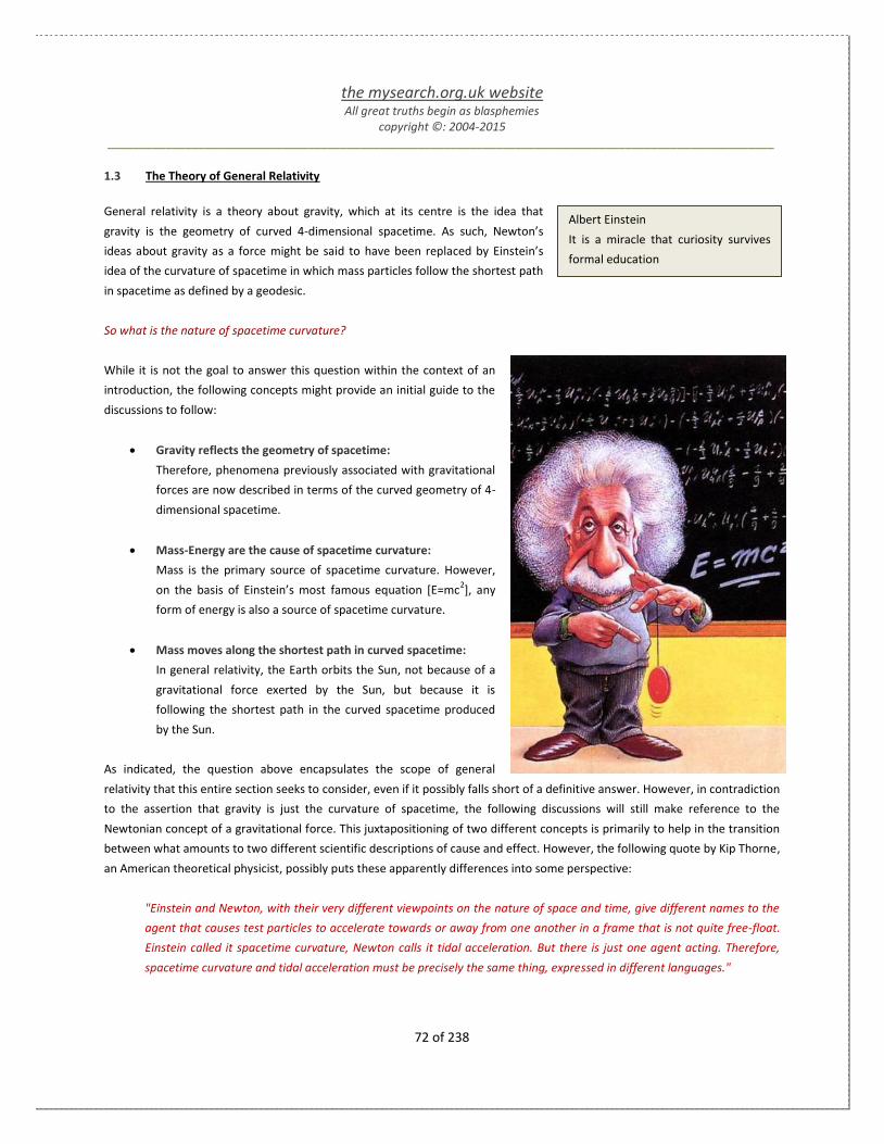
the mysearch.org.uk website All great truths begin as blasphemies
copyright ©: 2004-2015 _______________________________________________________________________________________________________
72 of 238
Albert Einstein
It is a miracle that curiosity survives
formal education
1.3 The Theory of General Relativity
General relativity is a theory about gravity, which at its centre is the idea that
gravity is the geometry of curved 4-dimensional spacetime. As such, Newton’s
ideas about gravity as a force might be said to have been replaced by Einstein’s
idea of the curvature of spacetime in which mass particles follow the shortest path
in spacetime as defined by a geodesic.
So what is the nature of spacetime curvature?
While it is not the goal to answer this question within the context of an
introduction, the following concepts might provide an initial guide to the
discussions to follow:
Gravity reflects the geometry of spacetime:
Therefore, phenomena previously associated with gravitational
forces are now described in terms of the curved geometry of 4-
dimensional spacetime.
Mass-Energy are the cause of spacetime curvature:
Mass is the primary source of spacetime curvature. However,
on the basis of Einstein’s most famous equation [E=mc2], any
form of energy is also a source of spacetime curvature.
Mass moves along the shortest path in curved spacetime:
In general relativity, the Earth orbits the Sun, not because of a
gravitational force exerted by the Sun, but because it is
following the shortest path in the curved spacetime produced
by the Sun.
As indicated, the question above encapsulates the scope of general
relativity that this entire section seeks to consider, even if it possibly falls short of a definitive answer. However, in contradiction
to the assertion that gravity is just the curvature of spacetime, the following discussions will still make reference to the
Newtonian concept of a gravitational force. This juxtapositioning of two different concepts is primarily to help in the transition
between what amounts to two different scientific descriptions of cause and effect. However, the following quote by Kip Thorne,
an American theoretical physicist, possibly puts these apparently differences into some perspective:
"Einstein and Newton, with their very different viewpoints on the nature of space and time, give different names to the
agent that causes test particles to accelerate towards or away from one another in a frame that is not quite free-float.
Einstein called it spacetime curvature, Newton calls it tidal acceleration. But there is just one agent acting. Therefore,
spacetime curvature and tidal acceleration must be precisely the same thing, expressed in different languages."

the mysearch.org.uk website All great truths begin as blasphemies
copyright ©: 2004-2015 _______________________________________________________________________________________________________
73 of 238
Percy Williams Bridgman
Every new theory as it arises believes in the
flush of youth that it has the long sought goal;
it sees no limits to its applicability, and
believes that at last it is the fortunate theory
to achieve the 'right' answer. This is true of
general relativity theory with its belief that we
can formulate a mathematical scheme that
will extrapolate to all past and future time
and the unfathomed depths of space. When
will we learn that logic, mathematics, physical
theory, are all only inventions for formulating
in compact and manageable form what we
already know, like all inventions do not
achieve complete success in accomplishing
what they were designed to do, much less
complete success in fields beyond the scope
of the original design, and that our only
justification for hoping to penetrate at all into
the unknown with these inventions is our past
experience that sometimes we have been
fortunate enough to be able to push on a
short distance by acquired momentum.
While the implications of special relativity were a radical departure from
classical physics, the mathematics that support its assumptions can still be
generally understood by most people. However, it is probably true to say
that this is not the case with general relativity.
Does this mean that a person without an understanding of advance
mathematics cannot understand the implications of general relativity?
While it is true that mathematics is an essential tool of modern science, it
should be possible to translate the knowledge it imparts into terms that
can be more generally understood. For example, [1] is representative of
the mathematical form of Einstein’s field equation of general relativity,
where the left-hand side defines the curvature of spacetime with the
energy-momentum of matter on the right:
[1]
In practice, [1] is masking the complexity of 10 non-linear, partial
differential equations for any given solution in the form of a spacetime
metric, but comprehending this shorthand demands an understanding of
the tensor notation embedded in differential geometry. Therefore, fully
understanding the mathematical implications of [1] is non-trivial and, as
such, the overview of the mathematics associated with general relativity will be deferred until after some of the more basic
concepts have been outlined. Of course, some may argue that mathematics associated with general relativity is essential from
the outset, if any real understanding of the theory is to be acquired. However, the counter argument is that if something cannot
be generally explained without the abstraction of advanced mathematics, then maybe it is not so well understood after all.
With this basic argument tabled, the intention is to begin with an initial introduction of some of the basic principles, which
underpin general relativity. The next step will be to examine some of the key implications of a specific solution of Einstein’s field
equations of general relativity, known as the `Schwarzschild Metric`, which will also examine some of the most extreme
relativistic effects associated with objects referred to as ‘black holes’. The intention is that the first 2 sections will only require a
basic understand of algebra in order to manipulate some of the established equations. Finally, in the last section, an attempt
will be made to introduce ‘some’ of the complexity of the mathematics used to describe the curvature of spacetime by mass-
energy, as formulated in Einstein field equations. Here is a summary of the discussions to follow:
Classical Foundations:
o Newtonian Equations
o Basic Concepts
o Basic Model
The Schwarzschild Solution:

the mysearch.org.uk website All great truths begin as blasphemies
copyright ©: 2004-2015 _______________________________________________________________________________________________________
74 of 238
Free-Float Frame
In special relativity, a free-float frame
is the classic inertial frame which
obeys Einstein's postulates of special
relativity. In general relativity, the
free-float frame follows the space-
time geodesic.
E. T. Bell
Euclid taught me that without
assumptions there is no proof.
Therefore, in any argument,
examine the assumptions.
o The Metric
o Effective Potential
o Gullstrand-Painleve Coordinates
o Black Holes
Mathematical Overview:
o Basic Concepts
o Differential Geometry
o Curvature and Energy
o Solutions to the Field Equations
Closing Remarks
Note, although general relativity also underpins the idea of an expanding universe,
which is characterised as `Friedmann Cosmology`, this subject will be addressed under
the Cosmology section of this website.
1.3.1 Declaration of Assumptions
In-line with the `duty of inquiry` that motivates much of the work of this website, the
ideas behind relativity will be challenged, whenever it seems to contradict what might
be described as a more ‘intuitive’ understanding of the world. However, this said, the
following discussions do not presume to fly in the face of the `weight of authority`
that has grown in support of general relativity over the last 100 years. However, there
are grounds to believe that its application in the field of cosmology may have gone
beyond the `limits of inference`. In this context, some people can become as polarised
in their `beliefs` about science as much as any other aspect of life. Therefore, the
following list of assumptions is highlighted upfront so that they are open to
correction. However, the first statement is not an assumption but rather an assertion:
If a theory is true, it will withstand any level of questioning. Of course, a wrong assumption can lead to the wrong
conclusion, which is why assumptions, along with hypothesis, must always be declared as such and be open to
questioning.
Therefore, the following assumptions are open to criticism and possibly the
accusation of bias. However, in my own defence, should any assumptions be proved
to be wrong, it was not bias, only an honest mistake made in ignorance, which may
hopefully be corrected.
1. In the context of the universe as a whole, extreme concentrations of energy in the form of matter may be considered to be
the exception rather than the norm. Therefore, if gravitational mass is a primary cause of the curvature of spacetime, then
most of spacetime may be considered to be essentially flat, at least, on the macroscopic scale?

the mysearch.org.uk website All great truths begin as blasphemies
copyright ©: 2004-2015 _______________________________________________________________________________________________________
75 of 238
John W. Gardner
The creative individual has the
capacity to free himself from the
web of social pressures in which the
rest of us are caught. He is capable
of questioning the assumptions that
the rest of us accept.
George Bernard Shaw
What a man believes may be
ascertained, not from his creed, but
from the assumptions on which he
habitually acts.
2. We can define a relative frame of reference in which an observer feels virtually
no gravitational pull or acceleration. We might therefore describe this frame as
a distant stationary observer in respect to some gravitational event horizon?
3. On approaching a gravitational mass [M], time slows and length expands in the
direction of gravitational pull as a function of radius [r], at least, with respect to
the distant observer?
4. As velocity [v] approaches the speed of light [c], time slows and length contracts in the direction of motion, at least, with
respect to the stationary observer. This velocity is also a function of radius [r] for a free-falling observer?
5. The perception of time always appears to slow with respect to the distant observer, when approaching any large mass?
6. In the case of a black hole, the slowing of time is so extreme that it slows to a stop at the event horizon, at least, with
respect to the distant observer, although presumably this observer would never live long enough for this to happen?
7. Time dilation is not a relativistic illusion, but a real effect. However, the ticking of the clock of an observer free-falling
towards an event horizon cannot be decoupled from the timeline of the rest of the universe, i.e. it remains relative?
8. Whether the effect of space contraction is ‘real’ is more subjective as it is not maintained when 2 observers are reunited in
a common frame of reference. However, this does not mean it does not occur?
9. While some clarification is required regarding a free-falling observer and the equivalence principle, as conceptually, the
free-falling observer feels no gravitational pull or acceleration and may therefore argue that he is no different to the
distant observer. However, this frame of reference is subject to the effects of
tidal forces, which become ever more apparent as [r] approaches [Rs]?
10. In the same way as the twin paradox of special relativity is resolved by
determining which twin is subject to acceleration, it is the free-falling twin that
experiences time dilation with respect to the stationary distant twin even
though he may have no perception of the effect?
1.3.2 Classical Foundations
Although a previous discussion of special relativity introduced concepts that challenge our perception of space and time, there
is nothing in the mathematics that is unduly taxing. In fact, it might be suggested that the real complexity simply lies in trying to
understand the implications of just one equation associated with the Lorentz transform:
[1]

the mysearch.org.uk website All great truths begin as blasphemies
copyright ©: 2004-2015 _______________________________________________________________________________________________________
76 of 238
There is also a basic assumption that any modification of Newton’s laws should not affect
its general accuracy, when the effects of relativity are negligible, i.e. in weak gravitational
fields and low relative velocity. This is reflected in [1] going to unity when [v] is small in
comparison to the speed of light [c]. Even when we start to introduce the concept of
general relativity, via the principle of equivalence, we can still start anchored in the
familiarity of Newton’s laws of motion and gravitation.
[2]
We can combine Newton’s 2nd
law and the equation for gravitational attraction because of
the equivalence of inertial and gravitational mass, which then suggests equivalence
between acceleration and gravity, which we can derive from equation [2]:
[3]
Again, from classical physics, we can extrapolate the relationship between inertial and gravitational force [F] to energy [E] by
virtue of its definition being related to force per unit distance [x], i.e. energy can be determined by integrating force with
distance:
[4]
The solution to this equation leads to the classical concept of kinetic energy [Ek]:
[5]
We can follow a similar line of reasoning with the expression on the right-hand side of [2], although the energy in this case is
now related to the potential energy [Ep] of gravitation:
[6]
We might wish to illustrate, by example, how we might equate [5] and [6] when an object of mass [m] is directed away from a
planet, e.g. Earth, so that the kinetic energy [Ek] just equals the potential energy [Ep] of gravitation:

the mysearch.org.uk website All great truths begin as blasphemies
copyright ©: 2004-2015 _______________________________________________________________________________________________________
77 of 238
[7]
If we re-arrange this equation, we arrive at an equation that expresses the escape velocity [ve] of an object from the surface of
a planet:
[8]
It is worth highlighting that although equation [8] is often defined as the escape velocity, it is also the velocity of an object that
falls from infinity to a radius [r] with respect to a central gravitational mass [M]. As such, it represents the conversion of
potential energy into kinetic energy, while the escape velocity is more representative of kinetic energy being converted back
into potential energy. To determine the escape velocity for an object launched from the surface of the Earth, ignoring air
resistance, we need to insert the mass of the Earth [M=5.98*1024
kg] and its radius [r=6.37*106 metres] into [8], which
approximates to 11,192 metres/second or 25,183 miles/hour. Of course, if we were to do the same experiment at the
conceptual `horizon` where the Earth’s atmosphere becomes space, the escape velocity would be smaller, due to the change in
radius [r]. We shall return to this point later, when discussing the escape velocity of light. However, returning to the current
thread, we can combine equations [3] and [8], allowing us to show a relationship between the escape velocity [ve] and
gravitational acceleration [g]:
[9]
At this point, we might wish to make some initial speculation as to what this might mean in terms of some correspondence
between special and general relativity. Much of special relativity is based on the implications of [1], while general relativity is
based on the basic assumption of the equivalence between acceleration and gravity. In principle, we have an equation that
might replace the velocity [v] in [2] with what might `appear` to be an equivalent form linked to [8] or [9]:
[10]
In the context of special relativity, we know that [10] dealing with relative velocity [v] leads to time dilation and space
contraction. However, the equations in [10] also appear to suggest that acceleration and gravity could lead to similar effects.
Within the concept of special relativity, the speed of light [c] is not only constant, but also the upper limit of any relative
motion. So let us consider the effect of substituting [c] for [ve] in [8] and [9]:
[11]

the mysearch.org.uk website All great truths begin as blasphemies
copyright ©: 2004-2015 _______________________________________________________________________________________________________
78 of 238
There is an issue as to whether the speed of light [c] is constant within a gravitational field, but we shall defer discussion of this
point until after we have completed the introduction of some of the fundamental ideas. However, it should be noted that the
equations above were derived from the basic assumption that kinetic energy [Ek] can equal the gravitational potential energy
[Ep] based on a given velocity [v] and radius [r]. As such, this is the equation of the escape velocity [ve=c]. However, if we re-
arrange this equation in terms of [r], we arrive at what has become known as the Schwarzschild radius [Rs] of a black hole:
[12]
While this equation has been derived from classical physics, it is said that the Schwarzschild radius [Rs] really requires general
relativity to provide a description of the effects of the event horizon, which occurs when [r=Rs]. However, it may be useful to
continue with the classical perspective and derive some reference points with respect to the free-fall velocity of a body moving
along a radial path and a number of associated energy interpretations. We can start by substituting equation [12] into [8]:
[13]
It will also be useful to note that we might now redefine [10] into the following form:
[14]
However, the root of [13] is linked to the assumption in [7], i.e. the kinetic energy [Ek] associated with a free-falling object,
falling from an infinite radius [r], corresponds to the gravitational potential energy [Ep] between infinity and radius [r]. In
practice, it is quite easy to determine this value because, by definition, [Ep] equals zero at an infinite radius [r]. Therefore, by
subtracting the value of [Ep], at any given radius [r], from zero results in the amount of potential energy given up to kinetic
energy for a free-falling object between infinity and [r]:
[15]
As such, we can present an expression of the total energy [ET] associated with a unit mass free-falling from infinity towards a
central mass [M] in terms of its rest energy [ER], its kinetic energy [Ek] and potential [EP]:
[16]

the mysearch.org.uk website All great truths begin as blasphemies
copyright ©: 2004-2015 _______________________________________________________________________________________________________
79 of 238
However, it is possibly easier to visualise the net result of all these component energy levels if presented in a graph showing the
kinetic and potential energy against radius [r] normalised to the Schwarzschild radius [Rs]. In first graph below, the mass of the
Sun is used as mass [M], which is some 1.98*1030
kg contained with a radius of 6.96*108metres. As such, the physical radius of
the Sun is much larger than the Schwarzschild radius [Rs] of the Sun at 2.95*103 metres. Therefore, the normalised radius [r/Rs]
axis reflects this as a large number range:
In the example represented by the graph above, a mass of 1kg conceptually falls from infinity into the surface of the Sun. As the
1kg mass falls under the influence of gravity, it acquires kinetic energy, i.e. velocity, from the potential energy field of
gravitation. The sum of the kinetic and potential energy remains constant and, as such, the energy can be said to have been
conserved. While the classical perspective is capable of calculating the Schwarzschild radius [Rs], the concept of a black hole,
where all the mass of the Sun might be contained within this radius, was not originally considered possible. However, today,
this idea is now readily accepted and we might consider this case in the next graph:

the mysearch.org.uk website All great truths begin as blasphemies
copyright ©: 2004-2015 _______________________________________________________________________________________________________
80 of 238
In the example above, the mass [M] is still that of our Sun, but it is now assumed to be all contained within the Schwarzschild
radius [Rs]. As a result, the 1kg can continue to fall towards the event horizon defined by [Rs], which itself is not a physical
barrier as a black hole assumes that all the mass has collapsed into a singularity that remains hidden behind the event horizon
at [Rs]. What also needs to be highlighted with respect to the graph above is that the velocity, defined in [13], can conceptually
increase beyond [c], which also occurs at [Rs]. However, the implications of [10] might suggest otherwise. At this point, we shall
simply table a question for further consideration as we proceed with the discussion of
general relativity:
What is the physical significance of the event horizon?
Before rushing into the ideas of general relativity, it might also be useful to establish some
of the classical or Newtonian physics, previously used to describe planetary orbits. In this
context, orbits were often described in terms of a balance of an outward `centrifugal
force` countered by an inward gravitation force:
[1]
If we re-arrange this equation, we can see that a given orbital velocity [vo] will maintain a
stable orbital radius [r]:
[2]
In [2] we can see a comparison of the orbital velocity and escape velocity; the latter also
corresponds to the radial velocity of a free-falling object. The importance of this statement
becomes more apparent when we try to aggregate the relativistic effects of gravity and
velocity, i.e. we have to be clear about which velocity is being referenced in any solution of the Schwarzschild metric of general
relativity. As such, the diagram right might be useful in highlighting that we are, in fact, dealing with 3 conceptual velocities,
which are being held in balance when linked to circular obits. The diagram shows that in addition to an orbital velocity [vo], a
small mass [m] can move on a radial path with respect to the larger central mass [M], which would then give rise to the
resultant vector velocity [v] of a trajectory rather than an orbit. The inference of equation [2] is that any decrease in the orbital
velocity [vo] will result in an increase in the radius [r], which then implies a radial velocity [vr=dr/dt]. The resultant velocity [v]
being defined by:
[3]

the mysearch.org.uk website All great truths begin as blasphemies
copyright ©: 2004-2015 _______________________________________________________________________________________________________
81 of 238
Centrifugal Force
The term 'centrifugal force' is used to
describe the tendency of an object
following a curved path to fly away
from the centre of curvature.
However, centrifugal force is not a
true force; it is a form of inertia, i.e.
objects moving in a straight line tend
to continue moving in a straight line.
However, centrifugal force is referred
to as a force for convenience,
because it balances centripetal force,
which is a true force.
Escape Velocity
An escape velocity is the speed at
which the kinetic energy plus the
gravitational potential energy of an
object is zero. It also refers to the
speed needed to "break free" from a
gravitational field without further
propulsion.
Orbital Velocity
In the current context, the orbital
velocity of a body is the speed at
which it orbits around some central
mass. In a wider context, it can be
used to refer to either the mean
orbital speed, the average speed as it
completes an orbit, or instantaneous
orbital speed, the speed at a
particular point in its orbit.
We might now translate this statement into the following energy equation:
[4]
We can again introduce the potential energy associated with the gravitational force:
[5]
As such, we may now write down an equation expressing the total energy of mass
[m], ignoring its rest mass-energy, with respect to mass [M] in terms its kinetic and
potential energy:
[6]
We might then proceed by substituting the expression for the orbital velocity [vo] in
equation [2] into equation [6]:
[7]
Of course, in the case of a stable orbit, the radial velocity [vr] would be zero, which
allows equation [7] to reduce to:
[8]
It can be seen from [8] that the energy of this system corresponds to half the
potential energy [Ep] and we can now express both total and kinetic energy as a
function of the gravitational potential:
[9]
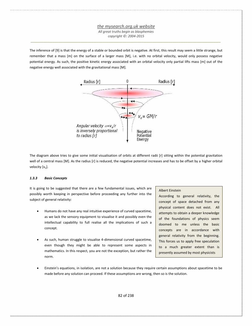
the mysearch.org.uk website All great truths begin as blasphemies
copyright ©: 2004-2015 _______________________________________________________________________________________________________
82 of 238
Albert Einstein
According to general relativity, the
concept of space detached from any
physical content does not exist. All
attempts to obtain a deeper knowledge
of the foundations of physics seem
doomed to me unless the basic
concepts are in accordance with
general relativity from the beginning.
This forces us to apply free speculation
to a much greater extent than is
presently assumed by most physicists
The inference of [9] is that the energy of a stable or bounded orbit is negative. At first, this result may seem a little strange, but
remember that a mass [m] on the surface of a larger mass [M], i.e. with no orbital velocity, would only possess negative
potential energy. As such, the positive kinetic energy associated with an orbital velocity only partial lifts mass [m] out of the
negative energy well associated with the gravitational mass [M].
The diagram above tries to give some initial visualisation of orbits at different radii [r] sitting within the potential gravitation
well of a central mass [M]. As the radius [r] is reduced, the negative potential increases and has to be offset by a higher orbital
velocity [vo].
1.3.3 Basic Concepts
It is going to be suggested that there are a few fundamental issues, which are
possibly worth keeping in perspective before proceeding any further into the
subject of general relativity:
Humans do not have any real intuitive experience of curved spacetime,
as we lack the sensory equipment to visualise it and possibly even the
intellectual capability to full realise all the implications of such a
concept.
As such, human struggle to visualise 4-dimensional curved spacetime,
even though they might be able to represent some aspects in
mathematics. In this respect, you are not the exception, but rather the
norm.
Einstein’s equations, in isolation, are not a solution because they require certain assumptions about spacetime to be
made before any solution can proceed. If these assumptions are wrong, then so is the solution.

the mysearch.org.uk website All great truths begin as blasphemies
copyright ©: 2004-2015 _______________________________________________________________________________________________________
83 of 238
Albert Einstein
We are now in a position to see how far the transition to the
general theory of relativity modifies the concept of space. In
accordance with classical mechanics and according to the special
theory of relativity, spacetime has an existence independent of
matter or field. On the basis of the general theory of relativity,
on the other hand, space as opposed to “what fills space” has no
separate existence. If we imagine the gravitational field to be
removed, there does not remain a space of the type-1, but
absolutely nothing, and also no 'topological space'.
As a broad general statement, Einstein’s field equation is probably meaningless to most people, but it seems appropriate to, at
least, introduce the general form, e.g.
[1]
Although, it should also be noted that the equations
above can be written in more abbreviated forms, it is
sufficient to introduce [Gαβ] as Einstein’s tensor and
[Tαβ] as a stress-energy tensor. We will eventually come
back to what this notation might actually represents,
when we discuss the ‘Mathematical Overview’ , but for
now we might just accept that the Einstein tensor is a
mathematical entity representing the curvature of
spacetime, while the stress-energy tensor describes the
energy-density of spacetime. The other factors should
be more meaningful with [G] being the gravitational
constant and [c] the speed of light. Given that both [G]
and [c] are constants, their units are often set to unity,
which reduces the form of [1] to:
[2]
Of course,[8π] is also a constant, therefore some people
generalise [2] even further:
[3]
Unfortunately, while the form of [3] looks deceptively simple, scientists have struggled for the last 100 years to understand all
its implications and most solutions are now are highly dependent on computer computation. Therefore, most texts on this
subject either generalise on the implications or focus on the mathematics to the extent that the physical meaning can be lost in
the complexity of tensor calculus. However, we are going to start with some general implications, before proceeding trying to
outline some of the mathematics.
1.3.3.1 The Geometry of Spacetime
So let us start by saying that general relativity builds on the assumptions of special relativity, but makes some additional
assumptions about the geometry of spacetime, i.e. it does not necessarily have to be flat. Therefore, when we define a velocity
[v] as a vector having both magnitude and direction, it exists in 4-dimensional spacetime that is initially assumed to have
a `flat` geometry. As such, switching to another inertial system can change the relative magnitudes of two velocity vectors, but

the mysearch.org.uk website All great truths begin as blasphemies
copyright ©: 2004-2015 _______________________________________________________________________________________________________
84 of 238
Gravitation
In general relativity, gravitational effects are
described in terms of the geometry or
curvature of spacetime. As such, there is no
gravitational force or field. However, it is
recognised that Newtonian gravity still works in
most case, such that general relativity must still
reduce to the description of Newtonian theory
within a weak gravitational field.
Gravitational Trajectories
In flat spacetime and the absence of any forces,
the trajectory of a particle would normally be
described by straight lines. However, in the
presence of gravity, particle trajectories that
start out in parallel can approach each other as
time increases. It is this effect that general
relativity seeks to describe in terms of the
geometry of spacetime.
not their relative direction. However, this statement does not necessarily
hold true in general relativity, because the geometry of spacetime does
not have to be flat. The potential effect of a curved geometry can lead to
a vector changing its direction with position. The result of this process
means that it can be ambiguous to ask whether two objects have the
same velocity vector, unless they are located at the same point of
spacetime. As a consequence, the Lorentz transforms of special relativity
are not directly applicable within general relativity, as it appears that we
cannot unambiguously define the relative velocity between two general
frames of reference, at least, when the geometry is curved. However, we
might be able to make some initial assumptions, if we consider the
relative acceleration of two test particles in free fall:
These test particles have some idealised properties in that
they are point particles with negligible mass, so that they have
no effect on the curvature of spacetime.
We will also assume that these test particles are in `free
fall' and only being affected by gravity, i.e. they are following a
geodesic path. In this context, the geodesic is the equivalent of
a straight line in curved spacetime.
General relativity assumes that gravity is not a force, but rather
an effect resulting from the curvature of spacetime.
So while we might not, as yet, understand any of the mathematical
complexity that surrounds these ideas, we might start to gain some
initial understanding of the physical rationale, which drove Einstein in
the direction of general relativity. So, the intention is to try to discuss the
principles of general relativity, in a stepwise process, which is more
reflective of the learning process that even Einstein himself must have gone through has he tried to progress from the axioms
of special relativity towards a more generalised concept of relativity. As such, it is highlighted that general relativity is an
extension of special relativity, which proceeds from an inertial to non-inertial frame of reference, i.e. a volume of spacetime
where no force is acting on our objects to one in which the objects are accelerating.
1.3.3.2 Inertial and Gravitational Mass
The consideration of an accelerating frame of reference must, in many ways, return to Newton’s 2nd law of motion, which
provides us with the classical relationship between mass and acceleration:
[1]

the mysearch.org.uk website All great truths begin as blasphemies
copyright ©: 2004-2015 _______________________________________________________________________________________________________
85 of 238
Gravitational Mass
This form of mass is that which interacts with a
`gravitational field' to give a body its apparent
weight. A body is given that weight by the
product of its density and volume plus the
gravitational field.
Inertial Mass
This form of mass is the product of a body's
volume and density which gives the resulting
moment of inertia and therefore the kinetic
energy of a body moving relative to another.
Inertia
Is an attribute of any body of matter, which
must be overcome to start or stop an object
moving. Inertia is unaffected by 'gravitational
fields' and remains the same for a given mass
whether on Earth or in Space
This equation relates the force [F] required to accelerate a mass [m] and,
as such, is describing the inertial mass [mi] of an object. However, we
can also introduce the equally important Newtonian law of universal
gravitation at this point:
[2]
In this case, [2] is describing a gravitational force [Fg] between two
masses, which makes no direct reference to acceleration and, as such,
we might describe the mass involved as a gravitational mass [mg].
However, let us be a little more precise about our definitions of these
two types of mass:
1. Inertial mass [mi] measures how strongly an object resists a change in its motion.
2. Gravitational mass [mg] measures how strongly it attracts and is attracted by other objects.
Obviously, we need to understand the relationship between these two types of mass and we might start by making an
assumption that [mi] equals [mg], which would allow us to equate [1] and [2] as follows:
[3]
For [3] to hold true, then [g] must equal [GM/r2] and imply that any
mass [m] must accelerate towards mass [M] at the same rate. However,
this is exact the experiment that Galileo is ‘reputed’ to have done by
dropping objects from the Leaning Tower of Pisa to prove that objects
of different mass fall at the same rate under gravity. In the intervening
years, far more accurate experiments have been done, all of which
verify that inertial and gravitational masses do appear to be equivalent.
This equivalence between inertial acceleration and gravitational acceleration was the catalysis in Einstein’s thinking, which led
him towards the general theory of relativity, albeit after 11 years and a lot of very complex mathematics.
1.3.3.3 The Equivalence Principle
Historical documents suggest that Einstein was thinking along the lines of the `equivalence principle` as early as 1907, some 9
years before he actually published his general theory; see quote below. Einstein later recalled that he liken the idea to a person
in gravitational free-fall who does not feel their own weight, such that the gravitational field ceases to exist. Historically, this
idea is similar to Galileo’s realization, some 3 centuries earlier, that for a person in uniform motion, it is as if the motion does
not exist.
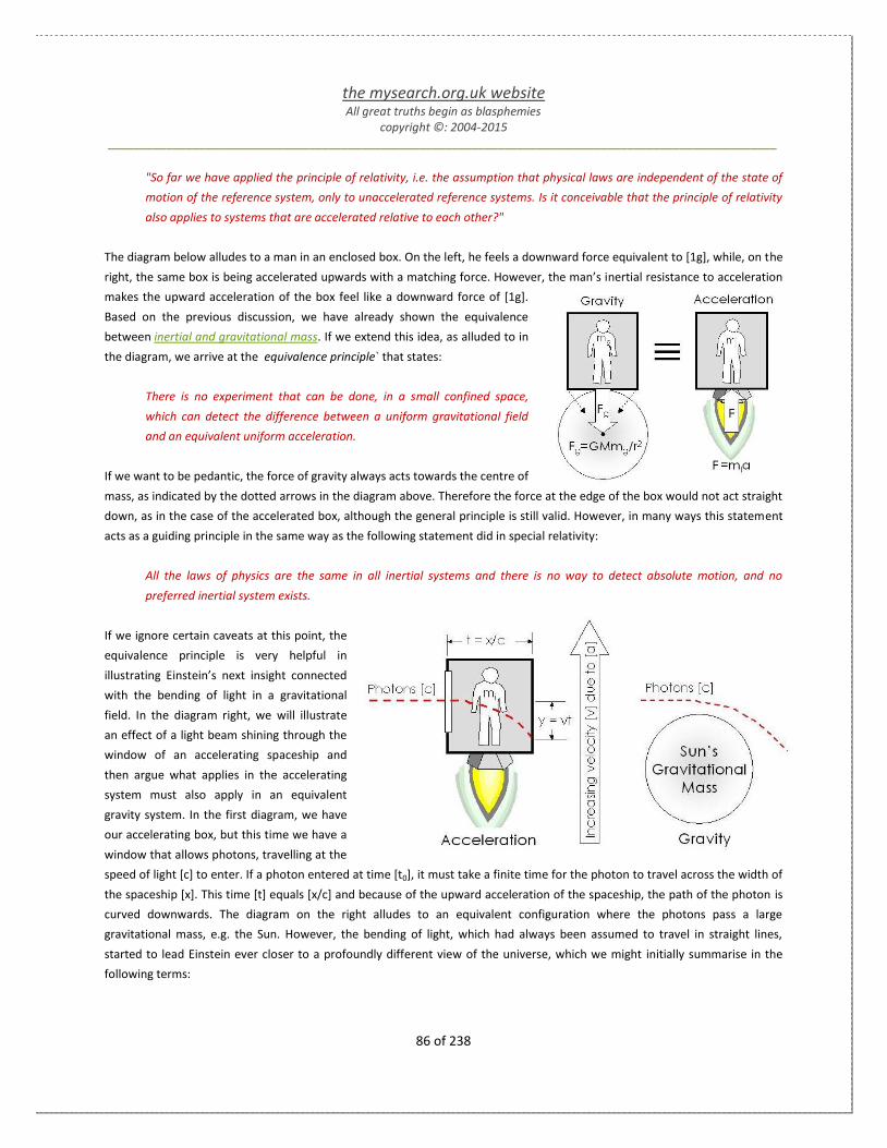
the mysearch.org.uk website All great truths begin as blasphemies
copyright ©: 2004-2015 _______________________________________________________________________________________________________
86 of 238
"So far we have applied the principle of relativity, i.e. the assumption that physical laws are independent of the state of
motion of the reference system, only to unaccelerated reference systems. Is it conceivable that the principle of relativity
also applies to systems that are accelerated relative to each other?"
The diagram below alludes to a man in an enclosed box. On the left, he feels a downward force equivalent to [1g], while, on the
right, the same box is being accelerated upwards with a matching force. However, the man’s inertial resistance to acceleration
makes the upward acceleration of the box feel like a downward force of [1g].
Based on the previous discussion, we have already shown the equivalence
between inertial and gravitational mass. If we extend this idea, as alluded to in
the diagram, we arrive at the equivalence principle` that states:
There is no experiment that can be done, in a small confined space,
which can detect the difference between a uniform gravitational field
and an equivalent uniform acceleration.
If we want to be pedantic, the force of gravity always acts towards the centre of
mass, as indicated by the dotted arrows in the diagram above. Therefore the force at the edge of the box would not act straight
down, as in the case of the accelerated box, although the general principle is still valid. However, in many ways this statement
acts as a guiding principle in the same way as the following statement did in special relativity:
All the laws of physics are the same in all inertial systems and there is no way to detect absolute motion, and no
preferred inertial system exists.
If we ignore certain caveats at this point, the
equivalence principle is very helpful in
illustrating Einstein’s next insight connected
with the bending of light in a gravitational
field. In the diagram right, we will illustrate
an effect of a light beam shining through the
window of an accelerating spaceship and
then argue what applies in the accelerating
system must also apply in an equivalent
gravity system. In the first diagram, we have
our accelerating box, but this time we have a
window that allows photons, travelling at the
speed of light [c] to enter. If a photon entered at time [t0], it must take a finite time for the photon to travel across the width of
the spaceship [x]. This time [t] equals [x/c] and because of the upward acceleration of the spaceship, the path of the photon is
curved downwards. The diagram on the right alludes to an equivalent configuration where the photons pass a large
gravitational mass, e.g. the Sun. However, the bending of light, which had always been assumed to travel in straight lines,
started to lead Einstein ever closer to a profoundly different view of the universe, which we might initially summarise in the
following terms:

the mysearch.org.uk website All great truths begin as blasphemies
copyright ©: 2004-2015 _______________________________________________________________________________________________________
87 of 238
Concept:
The principle of equivalence might be expressed in several ways, but one of the simplest is Einstein's own original insight in
which he suddenly realized that if he were to free-fall in a gravitational field he would be unable to feel his own weight.
Einstein later recounted that this insight was the 'happiest moment in his life' for it helped him understand how to extend
special relativity to include the effects of gravitation.
Importance:
The equivalence principle also suggests that in any small localised region of spacetime, it is possible to formulate the
physical laws such that the effect of gravitation can be neglected. This also implied that special relativity is valid in that
small region.
Consequence:
By applying the equivalence principle to a light beam travelling across a freely falling elevator, it was possible to infer that
light would also follow a curved path in a gravitational field. Likewise, a light beam travelling upwards in an elevator in free
fall would be would be redshifted in a gravitational field.
1.3.3.4 Spacetime Curvature
Prior to the theory of relativity, it was generally assumed that space and
time were absolute concepts that provided the framework against which
objects moved. This absolute framework allowed physics to describe the
interactions of physical objects in a deterministic way, which matched the
intuitive experience of the world. However, general relativity, in conjunction
with special relativity, represented a very profound change in the apparent
nature of the macroscopic universe. So while the normal motion of objects
appeared to be described by forces acting along straight lines, this motion
might be better described as a path curved by the presence of a mass. The
potential for curved space implied that the angles of a triangle may no
longer add up to 180 degrees, due to the presence of some large
gravitational mass. Later, it would even be suggested that the entire universe could be curved back on itself, providing some
initial visualisation of a universe that is finite, but without any spatial boundaries. However, we are possibly getting ahead of
ourselves, but it is true to say that it was becoming increasing apparent that Einstein’s theory of relativity was a major catalyst
in scientific thinking, which would change the way science looked at the wider universe. To get some feel for the implications of
curving spacetime, we might imagine an insect crawling over the surface of sphere. From our perspective we can see that the
surface is not flat, although this would not be obvious to the insect, for all sorts of reasons, but from our advantage we can
perceive that the geometry of a spherical surface has some properties that differ from a flat surface:
The shortest distance between two points is not a straight line
The sum of the angles in a triangle is more than 180 o
Parallel lines converge
The spatial surface is not bounded

the mysearch.org.uk website All great truths begin as blasphemies
copyright ©: 2004-2015 _______________________________________________________________________________________________________
88 of 238
Stephen Hawking
The mass of the sun curves space-time in
such a way that although the earth follows
a straight path in 4-dimensional space-
time, it appears to us to move along a
circular orbit in 3-dimensional space.
While general relativity is not necessarily implying that the universe is analogous to the surface of a sphere, it does suggest its
geometry need not always be flat, at least, around large celestial masses. Given the assumption that matter in the universe is
homogeneous and isotropic, i.e. The Cosmological Principle`, it can be shown that the corresponding distortion of spacetime,
due to the gravitational effects of matter, can have one of three basic forms,
shown right.
It can be `positively` curved like the surface of a ball and finite in extent
It can be `negatively` curved like a saddle and infinite in extent
It can be `flat` and 'infinite' in extent - our "normal" concept of space.
Of course, a key limitation of the picture shown here is that we have only
portrayed a 2-dimensional representation of 4-dimensional curved spacetime.
However, we might still reasonably conclude that light cannot always travel in
straight lines, at least, in curved spacetime. In order to address this anomaly,
Einstein expanded the notion of a straight line, such that a new definition of a
straight line should include any minimized distance between two points, e.g. the
minimal distance on a curved surface is called a `geodesic`. This way of thinking led
Einstein to the conclusion that a gravitational mass can change the geometry of spacetime, while the geometry of spacetime
guides matter. As such, gravity is no longer a force, but rather a property of curved spacetime. In essence, all the mathematical
complexity of Einstein’s field equations is said to be summed as follows:
Matter tells spacetime how to curve.
Spacetime curvature tells matter how to move.
As such, general relativity is a theory of gravity that changes the flat geometry of spacetime, as defined by special relativity, into
curved spacetime. So while Newton's law of gravity was able to explain the motions of the planets about the sun, general
relativity does so, and more, in a very different way. For example, in general relativity, the gravitational mass of the Sun causes
the spacetime around it to curve, and it is this curvature that determines the
motion of the planets, which causes them to orbit the Sun according to the
rules of geodesic spacetime.
Footnote:
To-date, there is no conclusive evidence to support a universe defined
by a closed geometry and, in fact, there is much evidence that
suggests that the universe has a `flat-geometry`. However, many of
the predictions of general relativity, such as the bending of light by the gravitation of the Sun and perturbations in the
orbits of the planets, such as Mercury, have been verified, by experiment, and have been showed to comply with the
theory of general relativity.

the mysearch.org.uk website All great truths begin as blasphemies
copyright ©: 2004-2015 _______________________________________________________________________________________________________
89 of 238
1.3.3.5 The Nature of Gravity?
Gravity has some very curious properties, one being that it is independent of the mass of the
body moving under gravity, i.e. g=GM/r2, such that all objects fall in a gravitational field with
equal acceleration. Another is the seemingly infinite range of the gravitational ‘force’, which
raises questions as to how an infinite force can be conveyed via by a propagating media or by
some force particle of finite size and speed. Of course, it is highlighted that general relativity
does not describe gravity in terms of a force, but rather as an effect of curved spacetime.
So why the implied question in the title?
As stated on many occasions, the goal of this website is not to just accept the weight of
authority, which undoubtedly supports general relativity, but to question it within the process
of trying to understand it. So while my opinion may not carry any weight of authority, there
does seem to be some open questions still to be resolve before science can claim to truly
understand the nature of gravity. Therefore, the intention of this discussion is simply to
outline the 2 different views on offer:
Newtonian Physics
General Relativity
The Newtonian view clearly provides a good
approximation under most circumstances and much
astronomical data was explained by it up until the
beginning of the 20th
century. It is a view that is based
on the classical concept of force, which acts between
the centres of mass of any two objects. One useful
example of this concept, which also has some
relevance to the `equivalence principle` is the
explanation of tidal forces. We might describe this
force in terms of test particles, which have negligible
gravitational effect on each other, but which are now
arranged into a group shaped like a spherical ball. In
the absence of any other `force` the test particles will
maintain their position and allow us to describe the effects of gravity on our spherical ball of test particles. So, although we are
not going to use general relativity, it has been suggested that Newton’s law of universal gravitations are still a good
approximation in most cases and, more importantly, intuitively understandable. Based on this assumption, the acceleration
[a=g] of our test particles along a geodesic, defined by relativity, is proportional to the inverse square law of force, i.e. [g∝1/r2].
This definition of force allows us to predict the motion of our test particles towards some centre of gravity. On the left of the
diagram above is our original spherical configuration of test particles, although we have only shown four instances. However,
these particles are under the influence of a gravitational attraction towards the centre of mass of a near-by object. Remember,
at this point, we are working from the known model of Newtonian physics, i.e.
the mysearch.org.uk website All great truths begin as blasphemies
copyright ©: 2004-2015 _______________________________________________________________________________________________________
90 of 238
Kip Thorne
Einstein and Newton, with their very
different viewpoints on the nature of space
and time, give different names to the agent
that causes test particles to accelerate
towards or away from one another in a
frame that is not quite free-float. Einstein
called it spacetime curvature, Newton calls
it tidal acceleration. But there is just one
agent acting. Therefore, spacetime
curvature and tidal acceleration must be
precisely the same thing, expressed in
different languages.
Ambrose Bierce
Gravitation: The tendency of all bodies to
approach one another with a strength
proportioned to the quantity of matter
they contain. The quantity of matter they
contain being ascertained by the strength
of their tendency to approach one another.
This is a lovely and edifying illustration of
how science, having made A the proof of B,
makes B the proof of A.
[1]
Where [M] is the mass of the larger object and [m] is the insignificant mass of
our test particles. Of course, we know from Newton’s 2nd
law of motion that
F=ma, where acceleration [a] can be equated to [g] giving:
[2]
The implication, shown on the right of the diagram above, is that the particle
[m1] nearest the centre of mass [M] must undergo the greater acceleration [g]
due to its closer proximity, while the particle [m2] undergoes the least.
Particles [m3 & m4] are effectively at some mid-point distance, therefore subject to an acceleration [g] that is less than [m1], but
greater than [m4], while at the same time subject to an inward acceleration following the radial path towards the centre of
gravity. The net effect is that our spherical ball of test particles is now an ellipsoid, which has retained the same volume as the
original spherical ball. While this example has historically been able to predict the tidal motion of the oceans, it hides a key
problem:
What is the propagation speed of gravity?
In physics, action at a distance is the interaction of two objects that are separated in space with no interactive media. In the
context of Newtonian physics, the propagation speed of gravity requires that each particle respond instantaneously to every
other mass particle, irrespective of the distance between them. As such, any change in the mass distribution of a system
requires the speed of gravity to be infinite. However, in contrast, general relativity describes gravity in terms of a gravitational
field associated with the curvature of spacetime. It also predicts that gravitational radiation should exist and propagate as a
wave at the speed of light [c]. However, there are also consequences to introducing any delay into the gravitational
interactions. Light from the Sun has an `aberration` caused by its propagation delay and the true position of the Sun is about 20
arcseconds east of its visible position As a consequence, orbit computations must use true position of planetary masses with
the visible position being subsequently calculated by allowing for the known propagation speed of light. This difference is not
just an optical effect as the propagation delay changes the observed
momentum. For example, dust particles in circular orbit around the Sun are
subject to a radial force due to the radiation pressure of sunlight, but due to
the finite speed of light, a component of that radial force acts in a transverse
direction, which slows the orbital speed of the dust particles and causes them
to eventually spiral into the Sun. This phenomenon is known as the 'Poynting-
Robertson effect'. If gravity were a simple force that propagated outwards
from the Sun at the speed of light, it would also have a small transverse
component. This component force would act continuously, but tend to speed
the Earth up, rather than slow it down, because gravity is attractive force. The
net effect of such a force would double the Earth’s radius from the Sun in

the mysearch.org.uk website All great truths begin as blasphemies
copyright ©: 2004-2015 _______________________________________________________________________________________________________
91 of 238
Eykhoff
A mathematical model is a
representation of the essential
aspects of a system, which
presents knowledge of that
system in usable form'
approximately 1200 years. Without explaining the details at this stage, the absence of this effect, leads to the suggestion that
the propagation speed of gravity would have to exceed the speed of light, which is in direct violation of one of the basic
postulates of relativity. General relativity may highlight, yet again, that gravity is not a force that propagates and, as such, the
Sun would curve spacetime around it and the Earth would simply follow the geodesic equivalent of a straight line. However,
some have argued that a purely geometric explanation of gravity ignores causality issues. For example, how does spacetime far
from a large mass get its curvature updated without detectable delay so that orbiting bodies accelerate through space toward
the true position of the source of gravity?
1.3.4 Basic Model
While possibly overly simplistic, relativity could be said to come in two favours, i.e. special and general, which corresponds to
the relativistic effects caused by velocity and gravity. A fast trajectory around a gravitational mass will therefore be subject to
both effects, which in turn have an aggregated effect on space and time.
So, by way of initial summary of the 2 key effects of velocity and gravity are:
1. As velocity [v] approaches the speed of light [c], time slows and length
contracts in the direction of motion, at least, with respect to a stationary
observer.
2. On approaching a gravitational mass [M], time slows and length expands in the
direction of gravitational pull, as a function of radius [r], at least, with respect
to a distant observer.
It should be noted that the second bullet above will have an impact on the measure of the radius [r] determined by observers at
different positions within the gravitational field of mass [M]. However, we shall return to this point and for now simply highlight
the mysearch.org.uk website All great truths begin as blasphemies
copyright ©: 2004-2015 _______________________________________________________________________________________________________
92 of 238
Special Relativity
As velocity [v] approaches the
speed of light [c], time slows and
length contracts in the direction
of motion, at least, with respect
to a stationary observer.
General Relativity
On approaching a gravitational
mass [M], time slows and length
expands in the direction of
gravitational pull, as a function
of radius [r], at least, with
respect to a distant observer.
that in both cases above, the observed time slows, while the measure of distance seems
to be affected in opposite directions. If so, it also raises another issue:
How do these effects combine in cases when velocity and gravity are both present?
For example, if gravity and acceleration are essentially equivalent, then it might also
suggest that an accelerating object, which must also have velocity, is subject to both
special and general relativity. It is known that the accuracy of timing is critical within the GPS system, which involves the
synchronisation of time within the satellites orbiting the Earth, at relatively high velocities [v], with respect to the stationary
receivers on Earth. As such, this system would appear to need two corrections with respect to the time onboard the satellite:
Time onboard the orbiting satellite runs faster due to its increased radius [r].
Time onboard the orbiting satellite runs slower due to its higher velocity [v].
Of course, we should also mention the effects on spatial distance:
Orbital circumference expands due to its increased radius [r].
Orbital circumference contracts due to its velocity [v].
The first of the bullets above needs to be clarified in terms of the general effects of gravity on spatial distance. Proximity to a
gravitational mass curves space such that the circumference of a circle, i.e. circular orbit, does not comply with the geometry of
flat space:
[1]
Again, we will need to come back to this issue, but for now we will simply highlight that the deployment of the GPS system does
receive correction for these effects and, as such, is often highlighted as evidence supporting the overall concept of relativity. So,
at this point, let us consider the following question:
Can a simple illustrative example of the effects of gravity and velocity be constructed to
help people to visualise the overall concept of special and general relativity?
As the question implies, the example that follows is not being constructed for the benefit
of mathematical theorists, but rather for people trying to initially reconcile their intuitive
experience of space and time with Einstein’s theory of spacetime, i.e. they are trying to
understand an entirely new perspective.

the mysearch.org.uk website All great truths begin as blasphemies
copyright ©: 2004-2015 _______________________________________________________________________________________________________
93 of 238
1.3.4.1 Model Concept
The following diagram tries to illustrate the perspective of three observers:
1. A distant observer [A] far from any gravitational mass [M].
2. A shell observer [B] at distance [r] from the gravitational mass [M].
3. A free-falling observer [C] accelerating towards the gravitational mass [M].
By way of clarifications, the distant observer [A] is conceptually an observer that is at an infinite distant from the gravitational
mass [M] with no relative velocity. As such, it is a conceptual point from which our other observers can reference spacetime,
free from the effects of either special or general relativity.
In contrast, a shell observer is more tangible and can be defined at any fixed radius [r] from the central gravitational mass [M],
although the measure of [r] needs to be clarified. The shell observer [B] is assumed to have no orbital velocity, but must be
effectively accelerating away from the mass [M] at a rate that equals the pull of gravity. Finally, a free-falling observer [C] is one
that is accelerating towards the mass [M] at a rate equal to the pull of gravity,
[1]

the mysearch.org.uk website All great truths begin as blasphemies
copyright ©: 2004-2015 _______________________________________________________________________________________________________
94 of 238
Paul Broca
The least questioned assumptions
are often the most questionable.
The advantage of considering an observer free-falling from an infinite radius [r] is that the velocity is always proportional to
radius [r] and therefore the effect of gravity and velocity will be shown to be proportional and synchronised. At this initial stage,
the relativistic effects of gravity and velocity will simply be presented without any proof, although confirmation of the
assumptions being forwarded will require verification.
[2]
So, with respect to the diagram above, there are 3 perspectives or frames of reference, i.e. [A], [B] and [C], which the diagram
implies might all measure time [t] and space [s] differently based on the proximity [r] or velocity [v] to some event horizon
defined by the distance [Rs] from mass [M]. So, by way of clarification:
Distant Observer [A]
Based on the inverse square law of gravitation, the spacetime effects of gravity quickly fall off with distance. Likewise, the
frame of reference of mass [M] and the distant observer can be considered stationary with respect to the cosmic
microwave background radiation.
Shell Observer [B]
In principle, the shell observer represent a network of observers armed with rulers and clocks at different radii from mass
[M]. These observers send back their measurements of localised spacetime to the distant observer, who is sometimes
known as the Schwarzschild observer because this observer translates all the information from the shell observers into the
Schwarzschild metric.
Free-Fall Observer [C]
One of the key advantage of considering the perspective of this observer is that the effects of velocity and gravity are both
proportional to the radius from mass [M].
Again, it is accepted that this may appear to be an overly simplistic model, so we might still have to question whether this idea
is conceptually sound. However, for now, we shall proceed to examine the model to see whether it throws up any interesting
insights about the effects of special and general relativity in combination.
1.3.4.2 Basic Assumptions
The use of Newtonian equations is not intended to imply entrenchment in classical
thinking; simply that it might be a better starting point for many people trying to understand the general implications of
relativity. In addition, these equations have the advantage that they are more anchored in our intuitive experience of the world,
but can still be use to defined cosmic phenomena. For example, the basic definition of the Schwarzschild radius [Rs] can be used
to define the event horizon of a black hole:

the mysearch.org.uk website All great truths begin as blasphemies
copyright ©: 2004-2015 _______________________________________________________________________________________________________
95 of 238
Don Miguel Ruiz
The way to keep yourself from making
assumptions is to ask questions.
[1]
Here [G] is the gravitational constant, [M] is the central mass and [c] is the
speed of light. As previously outlined, while the velocity being defined in
[2] below is often described as the escape velocity, it also corresponds to
the velocity of a free-falling object that starts at an infinite radius [r] and
falls towards a gravitational mass [M]. As such, we can describe its
derivation in terms of the conversion of gravitational potential energy into
kinetic energy associated with the velocity [v] of the free-falling object:
[2]
Therefore, if we combine equations [1] and [2], the speed of a free-falling
object seems to conform to the following equation, which is primarily
based on the distance [r] from some event horizon [Rs]:
[3]
Of course, given the implication that each observer in our basic model is subject to a relative perspective of time and space, we
might wish to raise the following question:
To which frame of reference is [3] applicable, i.e. [A], [B] or [C]?
Now, according to the theory of special relativity, the relative velocity [v] of an object affects spacetime, while general relativity
makes similar claims about the effects of gravity. As such, the 2 quantities that define velocity, i.e. distance and time, will be
subject to relativistic effects caused by an increasing velocity and an increasing gravitational field in the case of a free-falling
frame [C].
Note: While we might initially assume the components of [Rs], as defined by [1], to be invariant in all frames, this cannot
be the case for the measured radius [r] in [3]. In fact, the radius [r] is not measured, but rather inferred from measuring
the circumference and dividing by [2π]. Of course, how you actually measure the circumference might not be without it
practical difficulties; the bottom line being that in curved spacetime [rA] will not equal [rB].
While no substantive explanation linking the effects of special and general relativity has yet been made, we might substitute
the velocity defined in [3] into the relativity factor previously derived from the Lorentz transforms:

the mysearch.org.uk website All great truths begin as blasphemies
copyright ©: 2004-2015 _______________________________________________________________________________________________________
96 of 238
[4]
As such, [4] suggests some correlation between the effects of special and general relativity in the specific case of a free-falling
observer. However, it is highlighted that the equivalence between these relativistic factors does not imply that the effects on
spacetime are the same for both gravity and velocity. However, as a consequence of special relativity it is assumed that the
proper time [τ] of an object moving with velocity [v] will slow in respect to the time [t] being measured by the distant observer
[A] subject to neither velocity nor gravity in connection to mass [M]. As such, we might define the tick of the clock and measure
of distance as unity:
[5]
However, relativity assumes that the proper time [τ] of an object subject to gravitational mass [M] or velocity [v] will slow with
respect to the time [t] of the distant observer [A]:
[6]
In essence, [6] reflects the equivalence of the effects of velocity and gravity on time [t] perceived by observer [A] that results
from [1] through [4] linked to a free-falling object [C]. Of course, we have already define proper time [τ] as the measure of time
within the free-falling frame. In both forms of [6], the suggestion is that observer [A] perceives time slowing in the observed
frame of [C], which must clearly question whether [3] is applicable to [A] or [C]. However, we also need to taken into
consideration any relativistic effects on space caused by the free-fall velocity and the growing gravitational field of [M].
By way of clarification, it is not clear that any real distinction need be made, at this stage, between the terms `space’
and `length`. Therefore, it seems sensible to simply refer to space and time effects when initially discussing of the
aggregation of spacetime.
The next set of assumptions follow similar arguments, which are now apply to space [s] rather than time [t]. What is a key point
of interest is that velocity and gravity seem to imply opposing effects on space. The assumption of special relativity is that the
observed space interval [σ] of an object moving with velocity [v] will contract in the direction of motion with respect to a
stationary observer [A]:
[7]

the mysearch.org.uk website All great truths begin as blasphemies
copyright ©: 2004-2015 _______________________________________________________________________________________________________
97 of 238
Orville Wright
If we worked on the assumption that what
is accepted as true really is true, then there
would be little hope for advance.
In contrast, the assumption of general relativity is that the observed space
interval [σ] of an object moving deeper into a stronger gravitational field will
expand in the direction of falling radius [r] with respect the distant observer:
[8]
If we accept the equivalence of the relativistic factors defined in [4], then for a free-falling object, the relativistic effects on
space would cancel as suggested by [9] below:
[9]
As such, observer [A] would share the same measure of space as observer [C], although the determination of velocity [sA/tA]
would be different from [sC/tC] due to the different perception of time.
[10]
Whether this is the case will be discussed further under the heading ‘Radial Paths’ that expands on the implications of the
Schwarzschild metric. However, for now, we are still in the process of simply outlining some of the basic equations and
assumptions, which we wish to use in support of the basic model that encompasses the perspectives of 3 frames of references.
Therefore, the next discussion will now try to review the concepts and some of the initial implications of this model.
1.3.4.3 Concepts & Implications
As before, the diagram right is suggesting that observers [A], [B] and
[C] are separated by a combination of gravity and velocity effects. The
theory of relativity requires that these effects change the perception
of space and time relative to each observer such that the separate
Newtonian concepts of `space` and `time` merge into the unified
concept of `spacetime`. As such, the theory of relativity requires a new
definition of the ‘distance’ that separates 2 events in spacetime. This
separation must now unify our measure of time and space within the
definition of what is called the ‘metric’ of spacetime. In practice, there
are many different definitions of the metric of spacetime, which
depends on the geometry assumed and the coordinate systems used
to define measurements within this geometry. However, at this point,
we are trying to avoid the complexity of differential geometry, which

the mysearch.org.uk website All great truths begin as blasphemies
copyright ©: 2004-2015 _______________________________________________________________________________________________________
98 of 238
Event Horizon
In general relativity, an event
horizon is a boundary in
spacetime, typically associated
with an enclosed volume
surrounding a black hole,
behind which events cannot
affect an outside observer
will be discussed in the context of ‘A Mathematical Overview’. Therefore, we will begin by
introducing two definitions of the separation in `flat` spacetime, which are normally
associated with special relativity:
[1]
In many descriptions, the speed of light [c] is normalized to unity and therefore not included in the expression; but has been
included here to show the consistency of units in terms of either time or distance. At this point, cross-referencing an earlier
discussion entitled ‘Separation in Spacetime’ might clarify the distinction between the ‘time-like’ and ‘space-like’ separation
implied in [1]. For the purposes of this discussion, we will define the measure of `time` and `distance` with respect to the distant
stationary observer [A] from which the proper time [τ] for either observer [B] or [C] can then be derived. The initial advantage
of focusing on the proper time [τ] is that it can be more easily visualized as the time on a wristwatch worn by observers [B] or
[C], who are being subjected to relativistic effects from the perspective of observer [A]. As we shall see, the form of the
equations in [1] will require further modification in order to account for the curvature of spacetime by gravity. Therefore, at this
point, the following table is not intended to be a rigorous description of spacetime, but might provide some initial visualisation
of the effects on spacetime due to gravity and velocity based on the model presented in the diagram above.
The first row in the table above essentially corresponds to the conceptual spacetime of our distant inertial observer [A],
i.e. no velocity, and far from the influence of any gravitation mass, i.e. no gravity. As such, the measure of time [tA] and
space [rA] has been set to unity. The angle of the diagonal line is simply indicative of the magnitude of any localised
velocity [vA=rA/tA].
The second row reflects the perspective of observers [B-C]. For the brief moment as [C] pasts [B], they share a common
position in the gravity well and, as such, we might describe their separation in spacetime in terms of only the relative
velocity between [B] and [C]. However, in the basic model, we only have one frame in motion; therefore [vC] represents

the mysearch.org.uk website All great truths begin as blasphemies
copyright ©: 2004-2015 _______________________________________________________________________________________________________
99 of 238
Black Holes
The nearest black hole, yet
detected, is some 1600 light-
years from Earth, but there is
the possibility that a galactic
black hole with a mass of the
order of some 2 million of
solar masses might reside at
the centre of our galaxy, the
Milky Way. Such a black hole
would have a Schwarzschild
radius [Rs=6*106 km], but is
safely positioned some
30,000 light-years from
Earth.
the velocity of the free-falling observer [C] in each respective frame of reference. The
inset diagram reflects that time [tC] and space [rC] are both contracted with respect to
[B] by the same amount. As such, the magnitude of the velocity [vC] is invariant
between [B] and [C].
The third row reflects the perspective of observers [A-B]. Observer [B] is stationary with
respect to [A], but sits deeper within the gravity well. As such, time [tB] is dilated with
respect to [A], but space [rB] expands with respect to [A]. As we will discuss, the wider
implications of the composite relativistic effects of velocity and gravity in a subsequent
section, we will not spell out the net effect on the measured velocity at this point,
although it is alluded to in the table.
The last row reflects the perspective of observers [A-C]. Observer [C] is free-falling with
respect to [A] and its frame of reference is subject to increasing velocity and gravity.
While the effects of velocity and gravity both contribute to time dilation, the spatial
effects cancel out.
It is probably worth pointing out one other aspect that puts the effects of relativity into some sort of overall perspective. As
described, the effects of relativity caused by both velocity and gravity are extreme exceptions that normally fall outside human
experience. So while the following graphs show the eventually implications of both relativistic velocity and gravity, all of human
existence essentially takes place in weak gravitational fields and low speeds, where the theory of relativity collapses back into
Newtonian physics.
The solid curves in the graph above correspond to the two key relativistic effects used in the basic model linked to the various
combinations of velocity and gravity. The horizontal scale of (r/Rs) might be interpreted as the relative position of the free-
falling observer [C] who is perceived to be falling with a relative velocity [v/c], at least, by a series of [B] observers on-route. The
value [β] is reflective of both the relative velocity and radial position of the free-falling frame [C].

the mysearch.org.uk website All great truths begin as blasphemies
copyright ©: 2004-2015 _______________________________________________________________________________________________________
100 of 238
Mass-Energy
In the context of relativity, mass is just a form
of energy, which can take on a variety of
forms, including energy that is associated
with the curvature of spacetime itself and
not just with its contents.
[2]
So, at a radius of [r=10Rs], the free-fall velocity corresponds to ~32% of light speed [c]. Even at this relatively high velocity in
human terms, the relativity factors only fall in the range of [90-95%] of our reference with respect to [A]. In fact, the knee of
these curves, which might be approximated to a radius [r=2.5*Rs], the relativistic factor is still only in the range of 0.8-0.6
depending of the curve referenced. It should be noted that these figures are based on the gravitational pull of a black hole,
which will be addressed in more detail in a later discussion. However, a typical black hole that might form from the collapse of a
single star having a mass greater than 3 solar masses would have a Schwarzschild radius [Rs=10km]. The nearest black hole yet
detected is some 1600 light-years from Earth, but there is the possibility that a galactic black hole with a mass of the order of
some 2 million of solar masses might reside at the centre of our galaxy, the
Milky Way. Such a black hole would have a Schwarzschild radius
[Rs=6*106
km], but is safely positioned some 30,000 light-years from Earth.
1.3.4.4 Wider Analysis
In the context of a homogeneous universe, a large concentration of matter
may be considered to be the exception rather than the rule. So if we think
of gravitational mass as the primary cause of spacetime curvature, we might conclude that most of the spacetime universe
must be essentially flat, at least, from the effects of gravity. Of course, human existence is defined by the interaction of matter
and energy; therefore human ambition may ultimately be defined by our ability to understand the true scope of the spacetime
universe. So, based on previous assumptions, let us try to summarise some of the wider implications of the model being
introduced:

the mysearch.org.uk website All great truths begin as blasphemies
copyright ©: 2004-2015 _______________________________________________________________________________________________________
101 of 238
Nature of Matter
Results from the WMAP survey estimate that
only 4.6% of the universe's mass is made up
of normal atoms. The fraction of these atoms
that make up stars is probably less than 10%.
Again, we might start by characterising the separation of observers [A], [B]
and [C] in terms of the implied velocity and gravitational effects:
[A] and [B] are separated by gravity only
[A] and [C] are separated by gravity and velocity
[B] and [C] are separated by velocity only
As such, we have the basis of a model against which we can characterise the effects of both special and general relativity.
Within the context of the model, observer [A] is assumed to be stationary, although in a wider context this definition may also
be relative. However, all that is being implied is that observer [A] is far removed from all gravitational influences and remains
stationary with respect to some large mass [M] against which the event horizon [Rs] is being defined. Therefore, we will assume
that the frame of reference of the distant observer [A] exists in flat spacetime, where the tick of the clock and a measure of
space is set to unity, such that we can make the following assumption:
[1]
Therefore, observer [A] becomes the reference frame against which the effects of relativity will be measured in [B] and [C].
Although our shell observer [B] may also be considered stationary, we have noted that this observer would have to maintain its
position by effectively accelerating against the pull of gravity. Based on earlier assumptions, the spacetime at [B], as observed
by [A], would be affected by gravity only, i.e.
[2]
While the subscripts of time [t] and space [s] is an attempt to clarify the associated frame of reference, there may still be some
confusion of who determines the Schwarzschild and coordinate radius [r].
[3]
Well, we can see from [3] that all the parameters used to defined [Rs] are invariant in all frames of reference, but there is a
suggestion that the coordinate radius [r] would be subject to any effectively curvature of space.

the mysearch.org.uk website All great truths begin as blasphemies
copyright ©: 2004-2015 _______________________________________________________________________________________________________
102 of 238
4.6% Atoms
As a consequence, it would appear
that more than 95% of the energy
density in the universe is in a form that
has not been explained by the particle
model of physics. The actual density of
atoms is ~1 proton per 4 cubic meters.
How do you measure [r] in curved spacetime?
In the flat spacetime represented by [A], the circumference [C] of a circle is given by [2πr] and, as such, we might also
conceptually determine [r] any given shell [B] within the gravity well of mass [M] by measuring and dividing the orbital
circumference by [2π].
What are the implications of this method?
Assume that we have 2 shells positions for which the circumference has been determined and the coordinate radius [r]
calculated. Let us assume, according to these calculations, that the difference in the radii [r1] and [r2] is 1 kilometre:
But what would be the actual difference measured between [r1] and [r2]?
Well it seems that general relativity requires this distance to be greater than 1
kilometre due to the curvature space within the gravity well of mass [M].
This 'expansion' of space increases as we get closer to mass [M] as the geometry
of physical space curves with respect to flat space. The details of this issue will be
expanded in a specific discussion entitled ‘Coordinate Radius’; therefore it will
simply be stated that the coordinate radius will be established relative to flat
spacetime, i.e. [B] will disagree with [A] as to the value of [r]. The equivalent
equations for [A] to [C] are a composite of the effects of a relativistic velocity and
gravitation, such that the spacetime at [C], as observed by [A], is now defined by [4]:
[4]
At first glance, it may not be obvious as to how the composite effects of velocity and gravity have been combined in [4], as it
depends on the specific conditions that only apply to a free-falling observer [C], where the effects of velocity and gravity are a
synchronised function of radius [r]:
[5]
To understand [4], we need to first consider the separate effects of velocity and gravity, then apply the rationalisation that
results from [5]. So, the measure of spacetime at [C], as observed by [A], needs to combine both relativistic factors:

the mysearch.org.uk website All great truths begin as blasphemies
copyright ©: 2004-2015 _______________________________________________________________________________________________________
103 of 238
23% Cold Dark Matter
At this time, the composition of
dark matter is essentially
unknown, but assumed to be
composed of sub-atomic particles
that have a very weak interaction
with ordinary matter.
[6]
While it has been implied that only the distant observer perceives these effects, there is
also the implication that the shell observer [B] can look back out at [A] and across to [C]
and observe different perceptions of spacetime. If so, it is assumed that the shell observer
would `see` time ticking faster in [A], but slower in [C]. However, the implication is that the
relativistic effects with respect from [B] to [C] are due to velocity only, as the diagram
implies that [B] and [C] represent a snapshot at the same radius [r], as [C] passes with
velocity [v] towards the event horizon at [Rs]. As such, the gravity effects are assumed to
be comparable within this localised region of spacetime and only relativistic velocity of [C]
with respect to [B] results in the effects observed in [C] by [B].
[7]
The equations in [7] also translate the measure of time and space at [B], back into [A], which can be cross-checked against [4].
However, in the confines of a free-falling spaceship, observer [C] would appear to be floating in zero gravity and not necessarily
aware of its relativistic velocity with respect to [A] or [B]. This is because the acceleration of the spaceship equals [g] and
everything inside the ship is moving at constant (zero) velocity to everything else, such that it appears to be a zero-gravity
frame of reference.
Some clarification is required at this point regarding a free-falling observer and the equivalence principle within general
relativity. Conceptually, the free-falling observer could argue he feels no gravitational pull or acceleration, i.e. he is no
different to the distant observer. However, this statement is only true within the finite limits of local spacetime. In
practice, the effects of tidal forces on the free-falling observer become ever more apparent as [r] approaches [Rs]. In
many respects, the description of tidal acceleration can be considered as an equivalent description of spacetime
curvature, but more on this topic later.

the mysearch.org.uk website All great truths begin as blasphemies
copyright ©: 2004-2015 _______________________________________________________________________________________________________
104 of 238
72% Dark Energy
In almost all respects, dark energy
is another unknown 'quantity'
that is required to support the
current cosmological model. The
figure of 72% corresponds to the
requirement of a spatially 'flat'
universe, which started to
undergo accelerated expansion
some 7 billion years ago.
It is a postulate of special relativity that the speed of light [c] is constant in all moving frames of reference in the absence of
acceleration. To support this assumption, special relativity requires the magnitude of the velocity to be invariant in both frames
of reference, i.e.
[8]
Basically, this means that while time might dilate with increasing velocity, a comparable
effect is happening to space in the direction of motion in order to maintain the
invariance of the speed of light [c]. Of course, the situation in the diagram above is not
that clear cut, as the effects of gravity and velocity are different with respect to [A], [B]
and [C]. Therefore, we may wish to reflect on the permutations some more. For
example, if we assume that local spacetime looks as normal at [B] as it does at [A], we
might also assume any difference in perception must be reversible, i.e. when
rationalised from [B-A]:
[9]
The implication of [9], when disconnected from any frame of reference, is that space expands as the radius [r] approaches [Rs],
i.e. as it approaches a large gravitational mass [M]. Therefore, a metre ruler at [B] would appear elongated to [A] by the
inference of [9], while a metre ruler at [A] would look contracted to [B]. In the case of [A-B], the relativistic effects on space
were only defined by gravity, i.e. [9].
[10]
However, in the case of [A-C], both [9] and [10] apply and because the velocity of the free-falling observer [C] is proportional to
the radius [r], the effects of [9] and [10] cancel out, such that [s=s’]. Unlike [A-B], observers [A-C] are separated by gravity and
velocity, so there is an assumption that gravitational and velocity effects would be combined. If so, the time dilation has to be
described by equation [11a], rather than [11b] which is linked to [A-B].
[11]
In the case of [B-C], we have assumed that for a brief moment in time, [C] is in the same localised spacetime as [B] and so the
gravity effects are comparable. However, [B] and [C] are still separated by a relative velocity [v], which means that perception
of spacetime in [B] and [C] must differ based on the effects of special relativity. Of course, if each observer has a different
perception of space and time, they might all have a different perception of the free-fall velocity, which is the issue taken up in
the next discussion - Free-Fall Velocity

the mysearch.org.uk website All great truths begin as blasphemies
copyright ©: 2004-2015 _______________________________________________________________________________________________________
105 of 238
1.3.4.5 Free-Fall Velocity
Based on the assumptions made in the basic model, defined in terms of 3 observers [A], [B] and [C], we have established some
basic rules governing the perception of space and time in each frame of reference. Clearly, if we have a relative measure of
space and time for each frame, we should be able to determine the perception of the relative velocity in each frame associated
with the free-falling observer [C]. Earlier, we determine the magnitude of the free-fall velocity based on the conversion of
potential energy to kinetic energy, which gave:
[1]
In the context of classical physics there is normally no ambiguity about the definition of time and space between different
observers. However, we need to make some initial assessment as to which observer would actual perceive the velocity alluded
to in [1]. Based on the basic model, we have determine that the measure of space remains consistent between [A] and [C], i.e.
SA=SC=r. As such, it is not obvious from the parameters in [1], who measures the velocity [v]; although we might realize that
time dilation between [A] and [C] will be the key factor. However, we might assume that because [1] is derived from a
Newtonian model, it should hold true in any localized region of space, i.e. [B] or [C], not [A], i.e.
[2]
Of course, at this point, [2] must be considered to be speculative, but we might test this assumption further by assigning the
velocity in [2] to observer [C] and then extrapolating the velocity seen with respect to [A] and [B]:
[3]
Based on the various mappings of time [t] and space [s] between the 3 observers, which have been detailed in the previous
discussions, we see that the initial assumption that the velocity [vBC=vCB] appears to hold true. On this basis, it would seem that

the mysearch.org.uk website All great truths begin as blasphemies
copyright ©: 2004-2015 _______________________________________________________________________________________________________
106 of 238
relativistic effects of the free-falling observer are perceived by observer [A], as [C] falls deeper into the gravity well of mass [M].
However, our basic model tells us that the relative perception of velocity is only a reflection of the relative measurement of
time and space in each frame of reference. The implication of graph below is that the free-falling observer will be travelling at
light speed when it reaches the event horizon [Rs], but the effects of time dilation cause the distant observer [A] to `see` this
velocity fall to zero, i.e. the red curve.
How can we resolve this apparent disparity?
While we are only making assumptions based on a simple model, the results are not really any different when solved using
more sophisticated model based on the 'Radial Paths' defined by the `Schwarzschild Metric`, which will be the subject of later
discussions. As such, the next graph shows that time in both [B] and [C] slows with respect to the distant observer [A] and while
observer [B] and [C] still perceive time passing at a rate of 1 second per second, the observers in [A], [B] and [C] are all aging at
physically different rates.

the mysearch.org.uk website All great truths begin as blasphemies
copyright ©: 2004-2015 _______________________________________________________________________________________________________
107 of 238
Black Holes
Thirty years ago, Roger Penrose and Stephen
Hawking showed that, according to general
relativity, any object that collapses to form a
black hole will go on to collapse to a
singularity, which is assumed to be a
dimensionless object of infinite density that is
hidden behind the event horizon. According to
general relativity, space and time becomes
severely 'warped' near a black hole and as the
horizon is approached from outside, time
slows down relative to that of distant
observers, stopping completely on the horizon.
So, although the measured velocity in [C] reaches the speed of light, if time is normalized to the distant observer [A], the
velocity would reduce to zero, due to the effects of time dilation slowing time to zero. Finally, we might want to also represent
the apparent effects on space, i.e. distance, which affects the calculation of velocity, i.e. v=r/t. In the graph below, we again
show the relative change in radius as perceived in frames [B] and [C].
In the case of [B] sitting stationary in the gravity well of mass [M], the relativistic effects are entirely based on gravity, which
causes space to ‘expand’ in the sense of its curvature. While this effect applies equally to the free-falling observer [C], it is
exactly countered by the contracting effect of velocity on space-distance.
As a result, [A] and [C] share the same perception of space, but a very
different perception of relative time.
Note: There is an issue described as a `coordinate singularity` that
is said to exist at r=Rs. Theorist of relativity argued that this type
of singularity does not represent the reality at the event horizon
and the free-falling observer will pass through the event horizon.
One specific example of this interpretation will be examined in
the discussion entitled `Gullstrand-Painleve Coordinates`.
Earlier, it was implied that the free-falling velocity could be measured by
either the onboard observer or shell observer at the same radius [r].
Equations in [3] above suggest that observers [B] and [C] do indeed
resolve the same velocity; even though their perceptions of space and time differ, because the difference in space is cancelled
by the difference in time. However, there are still many questions left unanswered, e.g.
What happens at and beyond the event horizon?

the mysearch.org.uk website All great truths begin as blasphemies
copyright ©: 2004-2015 _______________________________________________________________________________________________________
108 of 238
Our simple model appears to suggest that time stops for both the onboard observer [C] and the shell observer [B] positioned at
the event horizon, at least, as measured by observer [A]. While the distant observer is conceptual, the physical implication is
that a distant observer will perceive time onboard the free-falling frame [C] to slow to a stop at the event horizon. The natural
conclusion might be to assume that the event horizon is an effective barrier, which nothing can cross. Of course, if this
conclusion were right, it would lead to an unresolved paradox in the sense that the last atom falling into a black hole must get
`stuck` just outside the horizon. Equally, once a small black hole was formed due to the collapse of a single star, requiring a
mass of approximate 3 solar masses, all subsequent matter would also get stuck on the outside of the event horizon [Rs].
However, the debate surrounding this question will be the subject of a subsequent discussion, once we have had a chance to
examine some more details of general relativity.
1.3.4.6 The Transition to Curved Spacetime
Before discussing the Schwarzschild metric itself, it is possibly worth highlighting some of
the transitional steps between Pythagoras’ theorem and Cartesian coordinates and the
development of spacetime metrics based on spherical coordinates. In this context, a metric
represents the notion of ‘distance’ in some definition of metric space, where ‘space’ can be
as simple as a flat 2-dimensional graph, as tangible as 3-dimensional space or as seemingly
abstract as curved 4-dimensional spacetime. However, we will start by considering the
definition of a space metric in the form of Pythagoras’ theorem, which we can present in
either 2D or 3D Cartesian coordinates.
[1]
If we want to convert the metrics in [1] to spherical coordinates, we will need transforms
for [x,y,z] into [r, θ, φ], as presented in [2] below:
[2]
However, in order to transition the idea of a space metric into a potential spacetime metric subject to curvature, we will need
to restrict the linear form of [1] in flat space to a differential form shown in [3].
[3]

the mysearch.org.uk website All great truths begin as blasphemies
copyright ©: 2004-2015 _______________________________________________________________________________________________________
109 of 238
Relativity on Earth
General relativity predicts that clocks in
a stronger gravitational field will tick at
a slower rate. Special relativity predicts
that moving clocks will appear to tick
slower than non-moving ones.
However, these two effects cancel each
other for clocks located at sea level
anywhere on Earth. So if a hypothetical
clock at the Earth’s north or south pole
is used as a reference, a clock at Earth’s
equator would tick slower because of
its relative speed due to Earth’s spin,
but faster because of its greater
distance from Earth’s centre of mass
due to the flattening of the Earth.
However, clocks at any altitude above
sea level do tick faster than clocks at
sea level; and clocks on fast rocket
sleds do tick slower than stationary
clocks.
For simplicity, we shall continue the discussion of [3] in just 2-dimensions, because
in 3-dimensions some of the expanded terms become very large and unwieldy,
while the basic steps can still be illustrated within a 2-dimensional example.
[4]
We now have to expand the differential terms [dx, dy] in [3] with the respective
functions in [4]. We will start with the expansion of [dx2]:
[5]
We now need to do the expansion of [dy2]:
[6]
On examination of the results in [5] and [6], we see that the middle terms in each will cancel in the addition implied by [3], this
leads to:
[7]
At this point, we can further simplify [7] using a known trigonometric identity:
[8]
If we had extended this process to 3-dimensions, the result would have involved the extra term in [2], and although unwieldy,
the previous steps lead to the following result:
[9]

the mysearch.org.uk website All great truths begin as blasphemies
copyright ©: 2004-2015 _______________________________________________________________________________________________________
110 of 238
GPS & Relativity
GR predicts that the atomic clocks at GPS
orbital altitudes will tick faster by about
45,900 ns/day because they are in a
weaker gravitational field than atomic
clocks on Earth's surface. SR predicts that
atomic clocks moving at GPS orbital
speeds will tick slower by about 7,200
ns/day than stationary ground clocks.
Therefore, the satellite clocks are reset in
rate before launch to compensate for
these predicted effects. If the predictions
are right, the satellite clocks should run at
the same rates as ground clocks
As such, [9] defines the spatial separation of 2 points in 3-dimensional spherical
coordinates, which we need to take into consideration in the development of
any spacetime metric. However, earlier discussions have already highlighted
the concept of spacetime separation and introduced a definition for the `proper
time [τ]` in connection with the Minkowski metric of flat spacetime as defined
by special relativity:
[10]
The form of [10] appears to be another extension of Pythagoras’ theorem, as
applied to the 3 spatial dimensions [dx, dy & dz], plus an additional separation linked to time [ct]. Given that this metric has
been discussed under the heading of ‘Concepts in Spacetime’ , we shall only outline the implications of this metric. In the
example right, space is simplify to just 1-dimension, i.e. the horizontal [x] axis and time [t] runs along the vertical axis. You are
then asked to imagine that you are watching a spaceship moving from point [A] to [B]. From the perspective of [t-x] axes, the
ship arrives at [B] after 5 seconds and covers 3 light-seconds of distance, corresponding to a velocity of [v=0.6c].
What would be the elapsed or proper time [τ] onboard the spaceship?
If we apply [10], we get the proper time [τ=4] that corresponds to the wristwatch time of an observer onboard the spaceship.
What might not be immediately obvious is that [10] implicitly accounts for the space contraction and time dilation associated
with the velocity of the spaceship travelling from [A] to [B]. On further reflection, it might be seen that the velocity is implicitly
represented because it correspond to the slope of the line A-B.
What happens if we want to also account for gravity?
Well, if [10] gives the answer for velocity only, it may require some
modification if it is to be updated to account for gravity. In connection with
the basic model, we have already outlined the idea of 2 different relativistic
factors as follows:
[11]
However, before proceeding, we may wish to change the form of [10] to spherical coordinates, as shown in [9], in order
describe the relative position of an object in a gravitational field as a function of the radius [r] from a central mass:
[12]

the mysearch.org.uk website All great truths begin as blasphemies
copyright ©: 2004-2015 _______________________________________________________________________________________________________
111 of 238
GPS verification?
The data suggests that the on-board
atomic clock rates do indeed agree with
ground clock rates to the predicted
extent, which varies slightly from
nominal because the orbit actually
achieved are not necessarily as
planned. The accuracy of this
comparison is also limited because
atomic clocks do change frequency by
small, random amounts of order 1
ns/day for reasons that are not fully
understood. Even so, the assertion is
that the predictions of relativity are
verified to high accuracy over time
periods of many days.
While [10] and [12] reflect the use of different coordinate systems, they both assume that the 3 axes are orthogonal to each
other in flat spacetime. However, general relativity is based on the idea that the shortest distance between two points is a
geodesic curve. Therefore, we can only directly apply [10] and [12] to very small regions of spacetime, which might still be
considered to be approximately flat. However, if we are to introduce the gravity factor in [11], we then need to consider how
this factor might affect both space and time. Again, based on the earlier basic model, it has been suggested that, unlike velocity,
gravity causes space to expand not contract, although it has the same dilation effect on time. Therefore, we might reasonably
speculate on adapting [12] as follows:
[13]
If we initially restrict [13] to a radial path, the presence of the last two terms is not required and simplifies to the following
form:
[14]
In [14], we more easily see the suggestion that the measure of time slows as the
coordinate radius [r] decreases, but the opposite effect is happening to the
measure of space. While this is hardly a derivation of the Schwarzschild metric,
equations [13] and [14] essentially represent the Schwarzschild solution to
Einstein’s field equations of general relativity. In later discussions, we will need to
consider the implications of angular velocity [dφ/dt] in order to understand the
both orbital and radial solutions of the Schwarzschild metric. However, before we
leave this basic introduction of curved spacetime, as defined by the Schwarzschild
metric, it is possibly useful to normalise the units of [14] to time rather than
distance by dividing through by [c2]:
[15]
If we assumed that the approximation of flat spacetime within curved spacetime is limited to just small measures of time, eg.
dt=1 second, and space, e.g. dr=1 metre, we might see that the second term on the right of [14] will essentially collapse
towards zero, when divided through by [c2], as shown in [15]. As such, the Schwarzschild metric collapses towards the time of
the shell observer [B] as defined by the basic model. Of course, another way of interpreting this observation is that the velocity
[dr/dt] is negligible in the case cited and so the result is reflective of only gravitational effects.

the mysearch.org.uk website All great truths begin as blasphemies
copyright ©: 2004-2015 _______________________________________________________________________________________________________
112 of 238
1.3.5 The Schwarzschild Metric
This metric is named after Karl Schwarzschild, a German astrophysicist, who
found a solution to Einstein’s field equations for an uncharged, non-rotating,
spherically symmetric body of mass [M]. In many respects, it might be argued
that this metric, more than any other, highlights the relativistic effects of mass
on spacetime. Therefore, from a learning perspective, this metric is worthy of
some investigation because it allows the mathematics abstraction of general
relativity to be anchored in physical phenomena, which science seeks to
understand and verify. Schwarzschild was born in 1873 and published his first
paper on celestial mechanics at the age of just 16, before going on to gain his
doctorate in 1896. From 1901-1909, he held the position of professor at the
prestigious Göttingen institute, working alongside some significant
mathematicians of the day, e.g. David Hilbert and Hermann Minkowski. Later,
Schwarzschild became the director of the observatory in Göttingen. In 1915,
Einstein published his theory of general relativity, containing the famous, or
possibly infamous, field equations given their apparent complexity. Therefore, it
came, as somewhat of a surprise that somebody was able to derive an exact
solution in the same year. While a solution for a charged, spherical, non-rotating
body was discovered shortly after Schwarzschild death in 1916, the exact
solution was to remain unsolved until 1963, when resolved by Roy Kerr. Therefore, in retrospect, Schwarzschild’s solution is
even more remarkable given the conditions under which he was working. At the time, Schwarzschild was serving on Russian
front, during the First World War, as an artillery officer in the German army. During this time, he wrote two papers, addressing
the exterior and interior space of a star. The first, which has become the most famous, addresses the idea of exterior space and
outlines the concept of `Schwarzschild Geometry` that is applicable to the Earth, Sun and many other types of stars, as well as
black holes, albeit without rotation.
Scope of Work:
Schwarzschild wrote two papers on Einstein's relativity theory and one on Planck's quantum theory. The quantum theory
paper explained the Stark effect and showed that the splitting of the spectral lines of hydrogen by an electric field
aligned to the postulates of quantum theory. Schwarzschild's relativity papers gave the first exact solution of Einstein's
field equation and defined the geometry of space near a point mass. The work presented in these two papers formed the
basis for a later study of black holes, showing that bodies of sufficiently large mass would have an escape velocity
exceeding the speed of light. However, Schwarzschild himself made it clear that he thought this theoretical solution to be
physically meaningless, i.e. he did not believe in the physical reality of black holes.
He sent both papers to Einstein to which Einstein relied, as follows, just before Schwarzschild’s early death in May 1916:
I have read your paper with the utmost interest. I had not expected that one could formulate the exact solution of the
problem in such a simple way. I liked very much your mathematical treatment of the subject. Next Thursday I shall
present the work to the Academy with a few words of explanation

the mysearch.org.uk website All great truths begin as blasphemies
copyright ©: 2004-2015 _______________________________________________________________________________________________________
113 of 238
Birkhoff's Theorem
The Schwarzschild metric describes
spacetime outside any spherically
symmetric mass distribution, even if it
is not static. This implies that a radially
pulsating spherically symmetric star
does not produce gravitational
radiation.
To-date, there have been thousands of dissertations, articles, and books written
on the subject of Schwarzschild's solution to the Einstein field equations. In this
context, this discussion cannot and does not aspire to be a critique of the
`Schwarzschild Metric`, simply an honest attempt to come to some
understanding of its meaning and implications. As such, there will be the usual
bias towards presenting some of the foundation ideas in terms of Newtonian
mechanics, not because they are thought to be better, but simply because
these concepts are more widely understood and may help highlight where
modern science continues to deviate from classical determinism. Initially, the
Schwarzschild solution was originally seen as a curiosity, but was to later
underpin the hypothesis of a gravitational black hole. However, the roots this
solution can still be shown in terms of Newton laws of motion and universal
gravitational, although the ideas are really based on Einstein’s field equations
within general relativity. It has been known from the time of Newton and Kepler
that a planet orbiting the sun, under the influence of gravity, would follow an
elliptical orbit. In addition, the presence of the other planets could cause an
elliptical orbit to rotate or precess. Over the centuries, the rate of precession of
the planets has been very accurately measured, although this assumption needs to be founded on a full understanding of all the
gravitational source acting in, and on, the solar system. Given this caveat, the measured observation of Mercury’s precession
about the Sun does not exactly match the Newtonian theory, albeit by the apparently minuscule deviation of 43 arcseconds of
rotation every century. Initially, in defence of Newton laws, it was suggested
that unobserved gravitational bodies might exist in the solar system, while
others even considered the possibility that the inverse square law of gravitation
may not be an exact power of 2. However, it would be the publication of the
special theory of relativity, in 1905, which suggested that nothing could go
faster than the speed of light that began to highlight the most serious conflict
with Newtonian mechanics. For if gravity could not propagate faster than light,
then it also suggested that some of the energy associated with gravity must lie
in the field of propagation itself and not just within the concept of mass.
1.3.5.1 Introduction to the Metric
So, as previous outlined, the following equation is the basic form of the Schwarzschild metric:
[1]
For reasons that will become more apparent we shall drop the generalised definition of the spacetime interval [ds] and
substitute the equivalent form of proper time [c.dτ]. Many texts also drop the velocity of light [c] by setting its value to unity,
but we shall retain its presence so that the normal SI units can be directly resolved. In fact, let us initially expand the form of [1]

the mysearch.org.uk website All great truths begin as blasphemies
copyright ©: 2004-2015 _______________________________________________________________________________________________________
114 of 238
Schwarzschild Radius
The significance of the event horizon
at [Rs] was first raised by Jacques
Hadamard at a conference in Paris in
1922, when asked what might
happen if a physical system could
ever collapse to a singularity.
Subsequently, in response, Einstein
insisted that it was not possible and
pointed out the dire consequences
for the universe, which he jokingly
called the 'Hadamard disaster'.
so that we can more easily perceive the central effect of mass [M] in this solution plus specifically highlight the reciprocal effect
on time [dt] and radius [dr]:
[2]
At this point, we should also try to introduce all the variables before expanding on the validity of the relativistic factor and what
it infers:
Group Variable Units Comments
1 r metres Coordinate radius
dτ seconds Tick of Proper time
2
dt seconds Change in time
dr metres Change in radius
dφ radian Change in longitude
3
θ radians Latitude, i.e. North-South
Rs metres Schwarzschild radius = 2GM/c2
M kg Mass of object
3 G metres
3/kg*sec
2 Gravitational constant
c metres/sec Speed of Light
As indicated earlier, the Schwarzschild metric is a specific solution of Einstein’s field
equations of general relativity for an uncharged, non-rotating, spherically symmetric
body of mass [M]. One of the difficulties when first looking at the Schwarzschild
metric is trying to associated the variables to some given frame of reference:
1. The coordinate radius [r] relates to the radial proximity to the mass [M],
which in-turn affects the spacetime separation [ds] between 2 events.
2. The variables [dt, dr, dφ] are the differential changes in the spacetime
position of some object at the coordinate radius [r] taken by some distant
observer in flat spacetime. As such, these measurements are subject to the
relativistic effects caused by gravity.
3. The variables [θ, Rs, M] can be described as fixed variables for some given gravitational system. For example, we want
to describe the gravitational effects around some specific mass [M], e.g. a star, for which we can calculate [Rs]. If we
set [θ=π/2], we can restrict the description of the Schwarzschild metric to equatorial orbits.

the mysearch.org.uk website All great truths begin as blasphemies
copyright ©: 2004-2015 _______________________________________________________________________________________________________
115 of 238
4. The final grouping identifies the gravitational constant [G] and the speed of light [c], which many texts set to unity,
but will be retained so that the units associated with any equation can be resolved.
We might guess that the relativistic effects of gravity are characterised by just one term within the Schwarzschild metric:
[3]
On the basis of [3], we might therefore draw two immediate inferences:
1. As the coordinate radius [r] increases to infinity, the relativistic factor in [3] must approach unity, which corresponds
to flat spacetime, i.e. when nowhere near a gravitational mass [M], spacetime is flat.
2. As the mass [M] decreases to zero, the relativistic factor in [3] must again approach unity, which also corresponds to
flat spacetime, i.e. when there is no gravitational mass [M], spacetime is flat.
Therefore, the effects of the Schwarzschild metric in [2] on time [dt] and space [dr] is in addition to that previously define by
special relativity in terms of the Minkowski metric, which does not address the effects of a gravitational mass [M] on spacetime,
i.e.
[4]
So while we have not actually provided a derivation of the Schwarzschild metric, we might still realise that the introduction of
the new relativistic factor in [3] now represents the curvature of spacetime by mass [M]. The requirement for the differential
notation is due to the restriction on the size of the variables associated with the potential curvature of spacetime by the
presence of a spherical gravitational field of mass [M].
Note: Determining the separation [ds] in spacetime does not implicitly resolve to a proper time [dτ] as it depends of the
characteristics of this separation being time-like or space-like. We are initially using proper time [dτ] simply because it is
easier to perceive as the time experienced by a local observer subject to a gravitational field or velocity.
We can reduce the complexity of [1] or [2] by only considering radial motion and equatorial orbits, such that θ=90° or π/2, so
that the [sinθ] term goes to unity as does the [dθ] term.
[5]
Again, with reference to special relativity, proper time [dτ] is derived from variables determined by an observer, who sits at rest
in flat spacetime. In the context of general relativity, we might initially wish to place our observer far from the gravitational
effects of the central mass [M] in question.

the mysearch.org.uk website All great truths begin as blasphemies
copyright ©: 2004-2015 _______________________________________________________________________________________________________
116 of 238
Schwarzschild Metric
According to the metric, at [Rs], the
proper radial distance interval
become infinite, and proper time
passes infinitely slowly. So, it would
seem reasonable to ask how long
would it take to get inside the event
horizon?
How many frames of reference are being represented?
What the Schwarzschild metric appears to be telling us depends on the frame of reference being considered, i.e. distant
observer [dt] or onboard observer [dτ]. In part, the difference between the perception of spacetime between the distant and
onboard observer results from the spacetime curvature factor in [3], which in-turn is linked to the definition of [Rs]. For
consistency within the present discussion, we shall try to put the scale of Schwarzschild radius [Rs] into some better
perspective, starting with a derivation based on the classical idea that the kinetic energy associated with an escape velocity has
to overcome the potential energy of gravitation
[6]
However, in a sense, there are two ways of interpreting the meaning being associated with the Schwarzschild radius [Rs] for any
given mass [M]. One interpretation is this radius contains all of the mass, such that escape speed would equal the speed of light
[c]. This radius effectively defines the event horizon of a black hole, but this does not stop us from calculating an equivalent
Schwarzschild radius [Rs] for any given mass [M], even though its escape velocity [v] may be less than [c], as illustrated in the
table below:
Black Hole Neutron Star Sun Earth Units
mass = 1.98E+30 1.98E+30 1.98E+30 5.98E+24 kg
radius = 2.95E+03 9.81E+03 6.95E+08 6.37E+06 m
volume = 1.08E+11 3.96E+12 1.41E+27 1.08E+21 m3
density = 1.83E+19 5.00E+17 1.41E+03 5.53E+03 kg/m3
v = 2.99E+08 1.64E+08 6.16E+05 1.12E+04 m/s
Rs = 2.95E+03 2.95E+03 2.95E+03 8.92E-03 m
g = 1.51E+13 1.37E+12 2.73E+02 9.84E+00 m/s2
Rs/r = 1.00E+00 3.01E-01 4.25E-06 1.40E-09
(1-Rs/r) = 0 0.698969996 0.999996 0.9999999986
What can be seen in the table above is that the definition black hole requires it to have an escape velocity [v] equal to the
speed of light [c]. This requirement really depends on the density of the object, rather than its mass [M]. Therefore, while a
black hole can have the same mass [M] as the sun, it requires a much higher density, e.g. smaller volume. It should also be
clarified that the actual density of a black hole is assumed to collapse to a spacetime singularity and, as such, it density would
be infinite, as its physical radius is zero. Therefore, the density shown for the black hole, in the table above, corresponds to the

the mysearch.org.uk website All great truths begin as blasphemies
copyright ©: 2004-2015 _______________________________________________________________________________________________________
117 of 238
Radial distance
In concept, the coordinate radius [r]
has to be measured by a succession
of shell [B] observers. They then pass
back the determination of their
radial position to observer [A] who
normalises the coordinate radius for
the effect of spatial curvature at [B].
However, the real implication of the
local measurements taken by each
[B] observer is that they appear to
get further away from a black hole as
they approach it! See the
spreadsheet model for a graph of
radial [B] distance against [r/Rs]
mass [M] contained within the event horizon that hides the singularity. For the purposes of the Schwarzschild metric, we can
calculate a corresponding Schwarzschild radius [Rs], even though there is no associated event horizon, as the escape velocity is
always below the [c] threshold. Only the black hole contains all its mass [M] within the definition of the Schwarzschild radius
[Rs]. However, the general point of interest is that we now have a value for the ratio [Rs/r], which can be used to determine the
relativistic effects due to the gravitational mass of any object [M], as indicated in the table above.
Clearly, a black hole is an extreme gravitational object that appears to have
the ability to distort spacetime to the point where the normal laws of physics
may breakdown entirely. However, it is highlighted that the acceleration due
to gravity [g] is a function of the mass:
[7]
Therefore, while the value of [g] for the example black hole in the table above
might appear extreme, a black hole might have the mass of billions of sun-like
stars, which might suggest that it is physically possible to pass through an
event horizon and survive, at least, for a while. It should be noted in
connection with [7] that the radius [r] does not constitute a physical surface as
in the case of all the other mass objects in the table above. However, we will
defer any further discussion of black hole until later.
The following discussions will initially consider a free-falling radial path towards mass
[M] from the perspective of an observer on-board and then from the perspective of
a distant observer far from the effects of the gravitational mass [M]. Afterwards, we
will review the implications of a orbital path around mass [M].
1.3.5.2 Coordinate radius
In basic terms, we have shown that the Schwarzschild metric is essentially an update
of the Minkowski metric of flat spacetime, which accounts for the curvature of
spacetime due to the gravitational effects of mass, or possibly more accurately
energy. However, before we use this metric, it is possibly useful to provide some
further clarification of the coordinate radius [r] used in the metric. In the following
diagram, we are again making reference to the observers in the basic model. So, for
all practical purposes, we can consider observer [A] to be so far removed from the
gravitational effects of mass [M] that we may describe [A] as being positioned in flat
spacetime.

the mysearch.org.uk website All great truths begin as blasphemies
copyright ©: 2004-2015 _______________________________________________________________________________________________________
118 of 238
Spatial cancellation
While observer [B] see an ever
increasing spatial distance to the
event horizon, the free-fall
observer [C], at the same position,
has a different perception.
Observer [C] is affected by both
velocity and gravity; so while
gravity causes the radial distance
to expand, the velocity of the free-
fall observer causes a spatial
contraction, which exactly cancels
the effect of gravity. Therefore,
observers [A] and [C] are both
synchronised to the coordinate
radius [r].
But how do we define the position of observer [C] free-falling towards mass [M]?
Clearly, the implication of the Schwarzschild metric is that the position of [C] has to be
affected by the curvature of space and time as it approaches mass [M]. As such, we
need to establish how we might conceptually measure the radial position of [C] and
then define a coordinate parameter to which this measure is to be linked. The first
practical problem is that each [B] observer cannot simply extend a tape measure to the
event horizon. So what the diagram is suggesting is that we might establish a series of
radial observers, e.g. [B1, B2, B3], which maintain a stationary position with respect to
mass [M]. Each of these radial observers would then calculate their radial position [rB1,
rB2, rB3] by measuring the circumference of their orbital position and then dividing by
[2π]. The practicality of this method is not questioned at this point, but even so:
How might these radial positions be affected by the curvature of spacetime?
In the top half of the diagram is a representation of the geometry of flat space, while in
the lower half is a representation of curved spacetime. If spacetime surrounding mass
[M] were flat, we could cross-check the radius [r] calculated by each [B] observer as
follows:
[1]

the mysearch.org.uk website All great truths begin as blasphemies
copyright ©: 2004-2015 _______________________________________________________________________________________________________
119 of 238
As suggested by [1], [rB2] would be calculated from the circumference, while the radial distance to its neighbouring [B]
observers could be directly measured, i.e. x1, x2. In flat space, we would expect the expression in [1] to hold true, although we
might have to question this method in curved space. In the lower half of the diagram, we can see that if we project the flat
measurement of [x1, x2] onto the curvature of space, the actual measurements would be [x1’, x2’], so:
[2]
Of course, this discrepancy is exactly what the Schwarzschild metric predicts and, as such, we may segregate out the relativistic
effects on time [dt] and space [dr] as follows:
[3]
We might realise that the implications that follow from [3] is that the observed time in [B] is dilated with respect to an observer
[A] sitting in flat spacetime, while the observed distance is expanded. However, we still need to answer the question:
Who determines the coordinate radius [r] used in [3]?
What [3] tells us is that the radius calculated by each [B] observer can be normalised to flat spacetime and used as the basis of a
coordinate system associated with the Schwarzschild metric.
[4]
At this point, we might also highlight that the form [4] aligns to the assumption of the 'basic model' previously introduced.
However, while the methodology suggested by the diagram above is conceptually possible, in practice, it is observer [A] who
establishes the coordinate framework against which the Schwarzschild metric then uses to determine the effects of relativity on
observers [B] and [C]. Therefore, the following discussions will often use the form [r/Rs] to denote the relative position with
respect to mass [M], where:
[5]

the mysearch.org.uk website All great truths begin as blasphemies
copyright ©: 2004-2015 _______________________________________________________________________________________________________
120 of 238
If we go with the assumption that [M] corresponds to the rest mass, then the Schwarzschild radius [Rs] will be an invariant
definition in all frames of reference. As such, we might summarise the positions of [B1, B2, B3] in the diagram above in the
following way:
Bn rA=r/Rs 1-Rs/r rB
B1 6 0.8333 6.57
B2 4 0.7500 4.62
B3 2 0.5000 2.83
Bn 1.0001 0.0001 100.02
In the table above, we have aligned the coordinate radius [r] to the distant observer [A] in flat spacetime and normalised the
radial position of [B1, B2, B3] in terms of the integer ratio [r/Rs]. The curvature of space, implied by the Schwarzschild metric,
means that the shell observers at [B1, B2, B3] would calculate a different radius based on [Cn/2π] that aligns to the values of [rB]
shown in the table above, which are also expressed as a ratio of [r/Rs]. The last value in the table is simply to show the extreme
curvature of space as [r] approaches the event horizon defined by [Rs].
1.3.5.3 Radial Paths
In some ways, the subject of relativity is based on perspective, i.e. one or more observers that occupy different frames of
reference may have a different perspective of spacetime. To provide some cross-reference to 3 distinct perspectives, the
following model has been used by way of an introduction. Given that this basic model has already been outlined, we will only
mention the salient points in this thread before expanding on some of the implications of the Schwarzschild metric on each of
the following perspectives:
The distant observer [A] infinitely far from any gravitational mass [M].
A shell observer [B] at a finite distance from the gravitational mass
[M].
A free-falling observer [C] accelerating towards the gravitational mass
[M].
In essence, the distant observer represents a conceptual frame of
reference, which the Schwarzschild metric can use to transpose the radial
distant [dr] and time [dt] into some measure of spacetime in another
frame of reference. There is an argument that the use of the distant
observer, as a preferred frame of reference, leads to interpretative
anomalies that are an effect of the coordinate system being used rather than a real effect of spacetime curvature. This criticism
is discussed in a later section entitled `Gullstrand-Painleve Coordinates` that also outlines several solutions of the Schwarzschild
metric for a free-falling observer constrained to a radial path. So, having previously introduced the Schwarzschild metric, we
might now ask ourselves what it tells us about the nature of spacetime around uncharged, non-rotating, spherically symmetric

the mysearch.org.uk website All great truths begin as blasphemies
copyright ©: 2004-2015 _______________________________________________________________________________________________________
121 of 238
body of mass [M]. Initially, we shall examine solutions that only consider a radial path so that we might get some understanding
of the perspectives from each of the frames of reference previously outlined in connection with the basic model. However, let
us start with the full metric:
[1]
A radial path in-line with the equator of a gravitational body allows us to simplify the metric as follows:
[2]
In the case of a free-falling observer [C], the change in the time [dt] and radius [dr] are being associated with [C], but measured
by [A]. As such, we might clarify this specific example by subscripting the relevant variables to identify the corresponding frame
of frames as shown in [3]:
[3]
You can test the orientation implied in [3] by considering the case where the velocity of [C] is very high, such that the distant
travelled in 1 second would be very small. In this example, [drA] might be thought to approach zero, such that [3] reduces to the
form:
[4]
We might cross-check the form of [4] with the equations in the diagram above and realise that it represents the observed time
dilation in [C] by observer [A]. While the subscript notation is a bit clumsy, it will be repeated on occasions to clarify the frames
of reference associated with any specific example being discussed, i.e.
The Observed Free-Falling Perspective
The Onboard Free-Falling Perspective
1.3.5.3.1 The Observed Free-Falling Perspective
As previous explained, the differential notation is inferring a constraint on the size of [dt] and [dr] in curved spacetime. To
resolve larger values of spacetime distances requires the integration of the metric along a specific path. However, we can still
use the metric to gain the relative perspective of a distant observer [A] measuring space and time events in [C]. If we divide
through by [dt2], we correlate the rate of change in [C] to the distant observer [A]:

the mysearch.org.uk website All great truths begin as blasphemies
copyright ©: 2004-2015 _______________________________________________________________________________________________________
122 of 238
Differentials
In the present context, the
differentials, e.g. dt, dr, are
mathematical infinitesimals, which
limit the change in a variable to the
degree of curvature in spacetime.
Therefore, in curved spacetime,
calculus is normally employed to
determine the total change in time
[t] and space [r] over some large
region of curved spacetime.
[1]
What [1] now reflects is the ratio of proper time [τ] or the wrist-watch time of
observer [C] with respect to the time of the distant observer [A] in the form [dτ/dt].
While the free-fall path of [C] could be observed by any number of shell observers
[B], we are initially considering this observer to be the distant observer [A].
Note: In the case of [A] observing [B], [1] can be simplified even further as the
[dr/dt] term would go to zero given that [B] has no relative velocity with
respect to [A]. Therefore:
This result reflects the perception of the time observed by [A] with respect to [B]. As such, it reflects the time dilation
caused by gravity only, as there is no associated velocity, i.e. radial or orbital with [B]. However, general relativity implies
that this is not just the perceptual illusion of [A], but rather reflects the actual slowing of time in [B] with respect to [A].
Of course, in the current thread where [dr/dt] is not zero, we have to consider a wider solution of [1], inclusive of the [dr/dt]
term. Now, [dr/dt] is the observed radial velocity [vR] of the free-falling observer [C] with respect to our distant observer [A]
and, as such, it could be argued that [A] should see an additional time dilation effect due to the relative radial velocity as
defined by special relativity.
[2]
Therefore [2] implies that the proper time [dτ], as perceived by [C], will run slower than [dt] due to effects of velocity,
irrespective of any additional effects caused by gravity. We may also transpose the form of [2], in the case of a free-falling
observer, because this velocity is always proportional to radius [r], as previously explained via [3]:
[3]
Substituting [3] into [2] leads to equivalence between the relativistic effects caused by gravity and velocity for the specific case
of a free-falling object:

the mysearch.org.uk website All great truths begin as blasphemies
copyright ©: 2004-2015 _______________________________________________________________________________________________________
123 of 238
From [A] to [C]
In attempting to interpret the
difference in perspective
between [A] and [C], it is worth
remembering that both these
observers share a common
perception of the coordinate
radius [r]. As such, it would seem
to imply that the difference in
their perspective must lie in the
effects of time dilation.
Time Dilation
It is assumed that the effects of
time dilation are real in the sense
that twins at [A] and [C] would be
aging at different rate, which would
be measurable , if [C] return to [A]
before actually crossing the event
horizon. However, if the time
between [A] and [C] is relative, it
cannot become disconnected in the
sense that any passage of time in
[C] still has to have some meaning
when related back to [A].
[4]
On this basis, we may wish to make the assumption that the effects of gravity and
velocity will have an accumulating effect on time in [C], as observed by [A], such that:
[5]
We can now proceed with the general solution of equation [1] by substituting for [5]:
[6]
As such, we have arrived at a solution for the velocity of our free-falling observer [C] plunging towards an event horizon, as
observed by a distant observer [A]. The implication of [6] suggests that observer [A] would see the velocity of [C] increase from
an initial near-zero velocity, but only to then fall again to zero as [r] approaches [Rs]. However, we can get a better overall
picture of the perceived velocity of [C] from [A] by plotting the relative velocity as a fraction of the speed of light [c] against the
ratio [r/Rs]. However, this result is not intuitive, for while it initially shows the velocity increasing under the increasing pull of
gravity, it then strangely tails off to zero as the event horizon is approached. Of course, we might speculate that the
accumulated effects of gravity and velocity with respect to time dilation have caused this effect. However, it seems to imply
that nothing will ever reach the event horizon, which may explain why black holes were originally called `frozen stars`. The
correlation of [vA] to [vC], as shown on the right on the following diagram, uses the results of the next section, but the key issue
being highlighted is the equivalent of [rA] to [rC] due to the negating effects of gravity and velocity on space in comparison to
the combined time dilation effects on [tA] to [tC].

the mysearch.org.uk website All great truths begin as blasphemies
copyright ©: 2004-2015 _______________________________________________________________________________________________________
124 of 238
The Constancy of [c]
It is a postulate of special relativity
that the speed of light [c] is
constant in all frames of reference.
While there appears to be no
explicit refutation of this postulate
by general relativity, it would
appear that Einstein himself left the
door open for further speculation
on this issue .
As such, it suggests that the perception of velocity at [A] is a direct result of time dilation in [C]. From a sanity perspective, our
distant observer would not actually see this effect, as the light returning from the free-falling object would disappear due to
gravitational redshift.
But how does this perspective compare to that of the onboard observer?
1.3.5.3.2 The Onboard Free-Falling Perspective
In order to describe the onboard perspective, we need to find a solution to the
Schwarzschild metric with respect to proper time [dτ] rather than [dt], which is
achieved by dividing by [dτ]:
[1]
To progress [1], we need to again substitute for [dt/dτ] and given that both gravitational and velocity time dilation are a factor,
we will again apply the same arguments that led to the previous solution of [dτ/dt], but now inverted:
[2]

the mysearch.org.uk website All great truths begin as blasphemies
copyright ©: 2004-2015 _______________________________________________________________________________________________________
125 of 238
Relative Time
Again, if the time between [A] and
[C] is still relative, it cannot become
disconnected in the sense that any
passage of time in [C] has to have
some correspondence to time in [A].
Substituting [2] into [1]:
[3]
As such, we have a solution for the free-falling velocity of an onboard observer [C]
with respect to a series of shell observer [B] positioned at ever-smaller radii from
mass [M]. The implication of our derived equation suggests that the free-falling
observer [C] would start from a zero velocity at an infinite radius, as per observer
[A], but the relative velocity with respect to the series of shell observers would
increase towards the light speed [c], as the coordinate radius [r] approached [Rs].
Therefore, this result seems to be in conflict with the perspective of [A], but we
might again get a better overall picture of the velocity of [C] with respect to proper time [dτ] by plotting the relative velocity as
a fraction of [c] against the ratio [r/Rs]. In contrast to the previous graph , the following graph appears more intuitive in that the
free-fall velocity continues to rise in line with the increasing pull of gravity as it approaches the event horizon.
This time, the velocity [vC] is correlated to the observer [B]. While it is noted that the velocity determined from this solution of
the Schwarzschild metric conforms to the following free-fall velocity, grounded in Newtonian physics, there might still be an
open question as to how any physical object would achieve the speed of light [c], when the radius [r] corresponds to [Rs].

the mysearch.org.uk website All great truths begin as blasphemies
copyright ©: 2004-2015 _______________________________________________________________________________________________________
126 of 238
Kepler's Laws
1) The Law of Orbits:
All planets move in elliptical orbits, with the
sun at one focus.
2) The Law of Areas:
A line that connects a planet to the sun
sweeps out equal areas in equal times.
3) The Law of Periods:
The square of the period of any planet is
proportional to the cube of the semi-major
axis of its orbit.
[4]
There is also the suggestion in [4], and the diagram, that the velocity of the free-falling would not equal [c], but somehow
exceed it as it passed through the event horizon towards the singularity at [r=0]. Therefore, these solutions of the Schwarzschild
metric are not necessarily answering all our questions, as to some extent we might not really be sure of the validity of either
perspective. In many ways, we seem to have a dichotomy in the sense that the perspective from [A] would appear to align to
flat spacetime, where we might assume the tick of the clock and the measure of space are undistorted by gravity and velocity.
However, viewing [C] from the perspective of [A] appears to suggest that time for observer [C] effectively stops relative to [A] at
radius [r=Rs]. On the other hand, the velocity of [C] within its own frame of reference seems to obey the basic principles of
classical physics, at least, up until [Rs], but the implied velocity at and beyond [r=Rs] seems problematic.
1.3.5.4 Orbits & Trajectories
A trajectory can be described as the path taken by an object, which has both
radial [vR] and orbital [vO] components of velocity. In part, the previous
discussion has reviewed some of the implications associated with a mass
[m] free-falling towards mass [M] along a radial path based on the
Schwarzschild metric. What is observed in this situation depended on the
position of the observer, which we aligned to our basic model:
A distant observer [A] far from any gravitational mass [M].
A shell observer [B] at a stationary distance from the gravitational
mass [M].
A free-falling observer [C] accelerating towards the gravitational
mass [M].
While this model appears to be generally useful in respect to the free-fall
case, it needs to be modify in order to discuss orbital paths and composite
trajectories involving radial and orbital components. So, we might begin by
considering a small mass [m] orbiting a much larger mass [M], such that we
may assume the orbit to be circular around the larger mass [M]. We can
label the frames of reference in a similar fashion to the basic
model introduced earlier, although orbital paths were not really
represented. Therefore, it should be noted that [C] is no longer free falling
towards mass [M] under gravity, but rather orbiting it at some coordinate
radius [rC]. Simply to maintain a constant perspective between [A] and [C],
we might placed observer [A] centrally above the rotating orbit of [C].
Observer [B] is positioned at the same radius [r] as the orbit of [C], so as to
represent an equivalent position within the gravity well, but remembering that [C] will also have to account for the effects of its
orbital velocity [vO]. As such, we now have a basic framework in which to discuss the effects of gravity in the context of general
relativity, where the mass [M] has curved spacetime such that the shortest geodesic path through spacetime becomes a circular

the mysearch.org.uk website All great truths begin as blasphemies
copyright ©: 2004-2015 _______________________________________________________________________________________________________
127 of 238
Classical Orbits
While Newton demonstrated that
Kepler's laws could be derived from his
theory of gravitation, there was an
implication that the force of gravity had
to propagate instantaneously. However,
Newton also demonstrated that for a
pair of masses [M] and [m], the orbit
size of each mass would be inversely
proportional to the mass and that both
would revolve around a common centre
of mass. However, when one mass is
much larger than the other, it is a
convenient approximation to take the
centre of mass to align with the larger
mass [M].
orbit. However, this does not mean that we cannot continue to use the visualization of a gravitational force [F] between two
masses [M] and [m], as defined by Newtonian physics:
[1]
In the context of [1], a stable orbit between objects of mass [M] and [m] requires a balance between the inward force of
gravitation to that of an outward `centrifugal force`. While this configuration typically leads to elliptical orbits, as defined
by Kepler’s laws, we can ignore this complexity by making the assumption that mass [M] is very much larger than mass [m]. As
such, any circular orbit must balance the force of gravitational attraction defined in [1], which leads to the definition of the
centrifugal force:
[2]
If we re-arrange [2], we see that a given orbital velocity [vo] will maintain a stable
orbit of radius [r] around mass [M]:
[3]
However, the diagram on the right suggests that we are still conceptually dealing
with radial [vR] and orbital [vO] components of velocities, even though the radial
component is being held in check to maintain a stable circular orbit. We can also
see from the diagram that the orbital velocity [vO] can be described as the
instantaneous tangential velocity at any point, which is ‘forced’ to follow a
curved path in Newtonian space, although relativity would describe this as the
shortest geodesic path in curved spacetime. However, if we wish to continue to
cross-reference Newtonian concepts, we need to translate the orbital tangential
velocity [vO] into its angular velocity [ω]:
[4]
In [4], we see both the conversion between the angular and linear forms of
velocity, which is then linked to the idea of a rate of change of an angular
displacement [dφ] with time [dt], as used in the Schwarzschild metric. Now, at
this point, it might also be useful to express the total energy [Et] of a closed
system in terms of the kinetic energy connected to the velocity of mass [m] in respect to the potential energy connected with
the gravitation of mass [M]:

the mysearch.org.uk website All great truths begin as blasphemies
copyright ©: 2004-2015 _______________________________________________________________________________________________________
128 of 238
[5]
Of course, [5] is predicated on Newtonian concepts, which we might guess are subject to modification when reviewed in the
context of the Schwarzschild metric, although it might not be obvious as to how energy is associated with this metric, at this
stage. Therefore, let us address this issue by considering an equatorial orbital, where [θ=π/2], which allows us to reduce the
Schwarzschild metric to the form:
[6]
If we divide through by [dτ2], we then need to consider the solution in terms of the rates of change of [dr] and [dφ] with respect
to the proper time [dτ]. The subscripts attached to the various variables in [7] are again used to simply identify the distant [A]
and orbiting [C] frames:
[7]
At this point, we can make some substitutions to highlight that [7] is making reference to both the radial and orbital
components of a trajectory in spacetime affected by mass [M].
[8]
If we now substitute the forms in [8] back into [7]:
[9]
The next steps are primarily re-arranging the form of [9] to separate the various components of velocity, i.e. [vR, vO] or [c] onto
one side:

the mysearch.org.uk website All great truths begin as blasphemies
copyright ©: 2004-2015 _______________________________________________________________________________________________________
129 of 238
Relativistic Orbits
In contrast, Einstein describes gravity
in terms of a curvature of spacetime,
which then removed Newton's
requirement for instantaneous
propagation of a gravitational force.
Therefore, in relativity theory, orbits
are described as following a geodesic
trajectory, which is aligns to the
Newtonian predictions in most
practical cases. However there are
differences that have been used to
determine which theory describes
reality more accurately.
[10]
Now remember, we started the process of modifying the Schwarzschild metric in [6] so that we might develop some form of
energy equation that could be compared to the Newtonian form in [5]. We might finally do this by multiplying the result in [10]
through by the factor [1/2m]:
[11]
What we might first recognise is that [11] is now an energy equation based on the
Schwarzschild metric associated with the timeframe [dτ], which we might initially
associate with the onboard observer [C]. We might also wish to have an adjacent
comparison with the previous classical energy equation:
[12]
By comparing [11] and [12], we can see that there are comparable kinetic energy
[Ek] terms associated with the radial [vR] and orbital [vO] components of the
trajectory in both [11] and [12]. There is also a terms that looks like the potential
energy [Ep] associated with mass [M], although it now appears to be linked to some
relativistic factor. However, there are also some other expressions which we might
initially assume align to the total energy [Et].
So how do we solve [11] for a given radius?
Before we can really address this question we need to consider some basic implications of the conservation of energy and
momentum associated with a given trajectory and then outline the concept of effective potential, both for the classical and
relativistic systems.

the mysearch.org.uk website All great truths begin as blasphemies
copyright ©: 2004-2015 _______________________________________________________________________________________________________
130 of 238
Conservation of Energy
Is an empirical law of physics,
which states that the total
energy of a closed system
remains constant over time. A
consequence of this law is that
energy can neither be created or
destroyed, which is to say that it
can only be transformed from
one state to another. The only
thing that can happen to energy
in a closed system is that it can
change form, e.g. from potential
energy to kinetic energy or vice
versa.
1.3.5.4.1 Effective Potential
From the discussion so far, we might realise that spacetime around a gravitational body
like a black hole will be subject to extreme curvature. However, we might choose to
describe this gravitational effect in terms of a gravitational potential energy as stylised in
the diagram opposite. Therefore, orbits and trajectories around gravitational bodies can
also be described in terms of an opposing energy, i.e. kinetic energy. As previously
stated, a trajectory normally involves a mass [m] having both radial [vR] and orbital [vO]
components of velocity. As such, mass [m] has kinetic energy [Ek] associated with its
velocity components and potential energy [Ep] based on its radial distance [r] from mass
[M]. If we describe the interactions between mass [m] and [M] as a closed system, we
would normally expect the total energy [Et] of the system to be conserved. However, we
possibly need to highlight some differences between a free-falling observer and an
orbiting observer. A free-falling observer is often conceptually described as falling from
an infinite distance [r] towards mass [M]. As such, the free-falling observer starts with
zero energy, but then proceeds to convert negative potential energy into positive kinetic
energy, while at all times complying with the conservation of energy. Of course, we can
engineer a free-falling scenario which starts at some realistic distance by giving mass [m]
some initial velocity, which aligns to the profile of a free-falling object. However, this
radial path, driven by the negative potential energy of gravitation, always has a total
energy [Et] of zero. From this energy relationship, we can infer the velocity [vR] as a
function of radius [r]:
[1]
However, the stability of a circular orbit is normally shown anchored in relationship between gravitational force and the
centrifugal force:
[2]

the mysearch.org.uk website All great truths begin as blasphemies
copyright ©: 2004-2015 _______________________________________________________________________________________________________
131 of 238
Conservation of Momentum
This law also only applies to
closed systems that has no
external forces acting on it. So, if
a system has no external forces
acting on it, the total momentum
of the system must be
conserved, i.e. it can neither
increase nor decrease.
By comparing the solutions for the radial velocity [vR] in [1] against the orbital velocity [vO] in [2], we might realise that the
energy balance associated with a circular orbit differs from the free-fall case, i.e. the total energy is not zero:
[3]
In [3], we see that both the kinetic [Ek] and total energy [Et] can be expressed in terms of the potential energy [Ep], where the
total energy [Et] is always half the potential energy. As such, mass [m] can be said to orbit within the negative potential energy
well of mass [M]. Of course, the previous statements are all being made in the context of classical flat space and not relativistic
curved spacetime. For example, it is the assertion of special relativity that time dilates and length contracts as a function of
velocity, at least, as perceived by a stationary observer. In the context of classical circular orbits, we may define the relationship
between linear velocity [v] and angular velocity [ω] via the simple equation [ω=v/r], where [r] corresponds to the radius of the
orbit. As such, an object orbiting a central point at radius [r=1] with a linear velocity of 6.284m/s will have a period of 1 second
based on the assumption that the circumference of a circle to equal 2πr.
But what happens when we introduce a relativistic velocity?
If we consider the effects when [v=0.866c], which conveniently gives a relativistic factor [γ] of 2, the onboard time [dτ] would
dilate or tick at half the rate of a stationary clock [dt] and, likewise, the distance would contract by half. Now, in terms of linear
velocity, the two effects cancel out and the velocity remains invariant to both the orbiting [C] and stationary [B] frames of
reference positioned at the same radius within the gravity well of mass [M].
But what of the angular velocity [ω]?
Angular velocity [ω] is measured in degrees or radians of rotation per second. It has been assumed that [ω=v/r], where the
linear velocity [v] is invariant under special relativity. If we transpose the equation for the circumference of a circle, i.e. C=2πr,
we get that r=C/2π. However, the orbiting measure of circumference is affected by length contraction and, in our example, the
circumference would be half that of the stationary shell observer [B]. As such, an orbiting
observer [C] might calculate the radius as r=0.5 in comparison to the stationary shell
observer measure of r=1. Therefore, given [ω=v/r], the angular velocity [ω] would double
for the orbiting observer in our example.
How does this affect the conservation of angular momentum [L]?
In physics, angular momentum [L] is assumed to be another conserved vector quantity
within a closed system, where the angular momentum of mass [m] rotating at a radius [r]
with linear velocity [vO] is given by:

the mysearch.org.uk website All great truths begin as blasphemies
copyright ©: 2004-2015 _______________________________________________________________________________________________________
132 of 238
Momentum
Angular and linear momentum
are reflective of rotational and
linear motion. They have the
same form and are subject to the
same fundamental laws of
conservation.
[4]
However, if angular momentum, like energy, is to remain a conserved quantity in both classical and relativistic closed systems,
where the velocity [vO] between the observers [B] and [C] is invariant, we might have to modify [4] as follows:
[5]
On the assumption laid out in this introduction, we shall proceed to discuss the concept of effective potential [Veff] in both a
classical and relativistic closed system. Comparison of the results from these two perspectives is surprising and leads to very
different trajectory paths for a mass [m] for a given angular momentum [L].
1.3.5.4.1.1 Classical Effective Potential
Classical physics in the form of Newton’s law are still used in many orbital calculations
because the relativistic effects of velocity and gravity are so small in respect to most
human activity. As such, we might start by outlining the concept of effective potential
(Veff) as described by classical physics and show its derivation so that we might later see
the differences between classical and relativistic physics. The following energy equation
is the starting point in classical physics:
[1]
In the context of the notation used by the Schwarzschild metric, we might wish to write
this expression in a slightly different format using the expressions in the first line of [2]
below:
[2]
Of course, irrespective of the notation, [2] shows the balance between kinetic energy
associated with velocity and the potential energy of gravitation. By definition, the two
terms on the right of [1] or [2] are combined to become the `effective potential` such that:
[3]

the mysearch.org.uk website All great truths begin as blasphemies
copyright ©: 2004-2015 _______________________________________________________________________________________________________
133 of 238
Angular Momentum
The angular momentum of a closed system
remains constant in both magnitude and
direction. It is defined as the product of the
moment of inertia and the angular velocity.
As far as it is known, the conservation of
angular momentum appears to be a
fundamental law of the universe, i.e. there
is no evidence of anything in nature
violating this principle.
Classical Perspective
In the context of classical physics, the minimum orbit
appears to align to [r=0.5Rs] in as much as the orbital
speed would corresponds to [c]. However, as the main
text suggests, we may need to question this classical
conclusion as it would take place inside the event horizon
of a black hole and is possibly suggesting that a relativistic
solution needs to be investigated.
Note that [1] relates to both the radial and angular velocities associated with
any given trajectory around the central mass [M], which conforms to the
conservation of energy and angular momentum [L]. However, by restricting
the complexity to a circular orbit, i.e. no radial velocity, some important
principles can be highlighted. The restriction of a circular orbit also allows the
relationship between angular momentum and the linear and angular orbital
velocity [vo, ω] to be expressed as:
[4]
Based on equation [4], we can express the effective potential as a function of angular momentum:
[5]
As such, [5] will become our reference point by which to judge any relativistic version derived from the Schwarzschild metric.
However, we may gain some further insight by using [5] as the basis of a graph in which some value of angular momentum [L] is
assigned to an orbiting mass [m] and then plotted as a function of radius [r].
But what value of angular momentum [L] might we choose?
Well, on the assumption that angular momentum [L=mvr] is conserved and we let the mass [m=1], we might initially be
interested in the most extreme situation, where [v=c] and [r=Rs]. However, to make it easier to evaluate the following graph, let
us be specific about all the variables:
G = 6.67E-11 m3/kg.s
2 Sun Mass = 1.98E+30 Solar mass
Light c = 2.99E+08 m/s BH Mass = 1.98E+30 1 Solar mass
Rs = 2.95E+03 2GM/c2 L = 8.83E+11 m*c*Rs
The table above shows that we are to base the example on a
black hole with the same mass [M] as our sun, although this
mass is now confined with the Schwarzschild radius [Rs]. As
indicated, we were trying to select a value of angular
momentum [L=mvr] that might represent some extreme
situation at the event horizon of this black hole, by setting [v=c]
and [r=Rs]. However, we might wish to use the following
equation to evaluate the orbital velocity around a black hole
based on classical assumptions only:

the mysearch.org.uk website All great truths begin as blasphemies
copyright ©: 2004-2015 _______________________________________________________________________________________________________
134 of 238
[6]
As it turns out, [6] seems to predict an orbital velocity less than [c] at the event horizon [Rs], which we may subsequently have
to question. However, for now, let us plot the graph based on [5] and [6] using the variables presented in the table above and
then consider the results:
We can correlate the various plots in the graph above with [5] by noting that the kinetic energy is associated with the orbital
velocity in the form [L2/2mr
2] and the potential energy is between mass [M] and [m] in the form [GMm/r], which when
combined gives the effective potential [V]. However, based on the minima of the effective potential curve, the graph suggests
that the mass [m=1] having an angular momentum [L=8.83E11] will only find a stable circular orbit at [r=2Rs]. We can see from
the graph above that any deviation from the stable orbit at [r=2Rs] requires an increase in energy as the orbit sits in the lowest
energy state for this specific configuration of angular momentum [L].
r/Rs L2/2mr
2 GMm/r Veff v=√(GM/r) L=mvr
0.5 1.79E+17 -8.94E+16 8.94E+16 2.99E+08 4.42E+11
1.0 4.47E+16 -4.47E+16 0.00E+00 2.11E+08 6.25E+11
2.0 1.12E+16 -2.24E+16 -1.12E+16 1.50E+08 8.83E+11
3.0 4.97E+15 -1.49E+16 -9.93E+15 1.22E+08 1.08E+12
4.0 2.79E+15 -1.12E+16 -8.38E+15 1.06E+08 1.25E+12

the mysearch.org.uk website All great truths begin as blasphemies
copyright ©: 2004-2015 _______________________________________________________________________________________________________
135 of 238
So, as verified in the table above, the specific value of angular momentum [L=8.83E+11] aligns with the stable orbit at [r=2Rs] at
Vmin. While the value of [L] was kept constant in the graph above, the table is also highlighting that other stable orbits are
possible against different values of angular momentum [L], where each orbit requires a different orbital radius and associated
angular velocity. In the context of classical physics, the minimum orbit appears to align to [r=0.5Rs] in as much as the orbital
speed would corresponds to [c]. However, as indicated, we may need to question this classical conclusion as it would take place
inside the event horizon of a black hole and is possibly suggesting that a relativistic solution now needs to be investigated.
1.3.5.4.1.2 Relativistic Effective Potential
The intention is to split the discussion of the relativistic effective potential into 2 parts. In this first section, we shall address the
relativistic derivation of the effective potential [V], after which the implication of this potential will be discussed. After which
we will discuss how the relativistic solution leads to revised trajectory plots around a black hole as shown below. A java
applet is also provided that outputs an interactive animation of the trajectory plots for different inputs of angular momentum
[L].
In order to derive an equivalent relativistic version of effective potential [V], we need to start with the Schwarzschild metric,
albeit in a simplified form:
[1]
However, to consider the effective potential associated with [1], we need to convert the metric into an equivalent energy
equation. As we have already cover some of this ground in the opening discussion entitled ‘Orbits and Trajectories’ ; therefore
we will only replicate a few of the steps for continuity, starting with the substitution for the component radial [vR] and orbital
[vO] velocities and then dividing through by [dτ]

the mysearch.org.uk website All great truths begin as blasphemies
copyright ©: 2004-2015 _______________________________________________________________________________________________________
136 of 238
[2]
We might now move directly to the equivalent energy equation by re-arranging [2] and multiplying through by [½m]:
[3]
As before, it may be useful to compare the relativistic energy equation in [3] to the classical energy equation in [4] below:
[4]
On comparison, we can see that there is an additional [½mc2] term on the right-hand side of [3] that appears to have nothing to
do with either kinetic or potential energy. As such, we will move this term to the left-hand side and assume that it is a
component of the total energy without necessarily proving this is the case:
[5]
While some aspects of [5] may be questionable, we shall proceed on the basis that it allows us to infer the form of the
relativistic effective potential, which can be directly compared to the classical variant:
[6]
As a final step, we could now substitute the linear orbital velocity [vo] for angular momentum as previously defined in the
classical variant:

the mysearch.org.uk website All great truths begin as blasphemies
copyright ©: 2004-2015 _______________________________________________________________________________________________________
137 of 238
[7]
Again, we may wish to make a direct comparison between the relativistic form above and the classical variant below:
[8]
We can see the obvious similarities between [7] and [8] with the exception of one additional term on the right of [7]. Therefore,
we might assume that it is this term which must account for the difference between the classical and relativistic perspectives,
which may initially suggests that the outward `centrifugal force` must simply increase under relativity and require a greater
gravitational pull to maintain the balance of a stable circular orbit. It is highlight that some standard texts derive an expression
of effective potential that differs in form to that shown in [7], although both appear to lead to the same conclusions as
discussed in the next section. However, it is argued that the derivation shown is more consistent with the classical definition
and therefore preferred in the current context. However, we now need to proceed from the form in [7] in order to find a
solution for the orbital radius [r], As such, the next step is to substitute [Rs] back into [8] and to simplify the overall expression
in terms of radius [r]:
[9]
This form can be simplified further by a notational substituting:
[10]
We can now derive an equivalent force equation by differentiating with respect to radius [r]:
[11]

the mysearch.org.uk website All great truths begin as blasphemies
copyright ©: 2004-2015 _______________________________________________________________________________________________________
138 of 238
Steven Weinberg
The effort to understand the universe is one of the very
few things that lifts human life a little above the level of
farce, and gives it some of the grace of tragedy.
However, for the specific case of a circular orbit, the net force is zero, as the inward gravitational force is balanced by the
outward `centrifugal` force such that:
[12]
We can convert [12] into the form of a quadratic by multiplying through by r4:
[13]
Of course, the implication of a quadratic form suggests that two solutions might exist for the orbit radius [r], which runs
contrary to classical thinking:
[14]
While the substitutions are a bit messy, they do eventually fall out to give a solution in terms of an outer and inner radius:
[15]
In terms of [7], [9] and [15], we now have a set of equations that
we can used to analyse the implications of relativity on the
orbital path taken by mass [m] around a much large mass [M].
However, this will be the focus of the next discussion.

the mysearch.org.uk website All great truths begin as blasphemies
copyright ©: 2004-2015 _______________________________________________________________________________________________________
139 of 238
Relativistic Solution
Whilst dependent on the angular
momentum, the relativistic
solution of effective potential
suggests 2 possible orbital states
associated with an inner and
outer radius. However, the inner
radius is inherently unstable and
is described as a knife-edge
orbit. In contrast, the outer
radius essentially corresponds to
the stable orbit defined by
classical theory
1.3.5.4.1.3 Implications of Effective Potential
In the first part of this discussion, we derive a number of key equations, i.e. [1], [2] & [3], which can now be used to discuss
some of the implications of effective potential that account for relativistic effects.
[1]
The 2nd
equation in [1] was then differentiated to give the corresponding force relationship for a circular orbit:
[2]
Finally, [2] was solved as a quadratic equation, which offered up two possible
solutions for the orbital radius [r]:
[3]
So how might we begin to interpret these equations?
First, we need to remind ourselves that the premise of the derivation of effective
potential (Veff) started out by dividing the Schwarzschild metric by the proper time [dτ]. As such, the solution is orientated to
an onboard observer orbiting at radius [r] within the gravity well of mass [M] with an orbital velocity corresponding to a given
angular momentum [L]. We should also highlight the fact that we are proceeding on the assumption that angular momentum
[L] is conserved in both the classical and relativistic solutions. Therefore, based on this assumption, we might also proceed in a
similar fashion to that adopted in the classical discussion by asking the question:
What values of angular momentum [L=mvr] are possible?
However, before we can address this question, it would be useful to develop a basic relationship linking the radii, as defined in
[3], and the orbital velocity [v]. As such, we might expand [2] in terms of the angular momentum [L]:

the mysearch.org.uk website All great truths begin as blasphemies
copyright ©: 2004-2015 _______________________________________________________________________________________________________
140 of 238
[4]
Now we can substitute for angular momentum [L=mvr] and solve in terms of the velocity [v] and radius [r]:
[5]
The form of [5] allows us to compare the relativistic force equation with the previous classical solution. However, we will
continue with the solution for [v] using [Rs]:
[6]
Of course, there must also be 2 solutions for [6] associated with the inner and outer radii predicted by [3]. However, we might
initially proceed based on a speculative assumption that the inner radius has an orbital velocity [v] equal to the speed of light
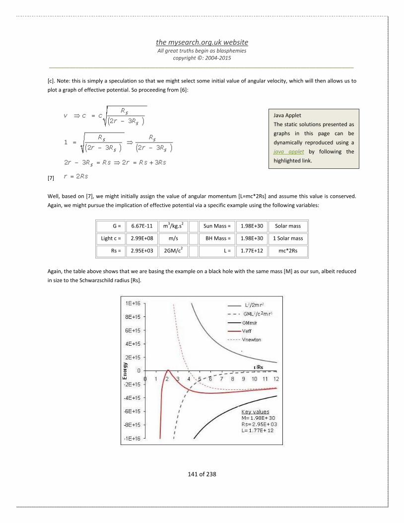
the mysearch.org.uk website All great truths begin as blasphemies
copyright ©: 2004-2015 _______________________________________________________________________________________________________
141 of 238
Java Applet
The static solutions presented as
graphs in this page can be
dynamically reproduced using a
java applet by following the
highlighted link.
[c]. Note: this is simply a speculation so that we might select some initial value of angular velocity, which will then allows us to
plot a graph of effective potential. So proceeding from [6]:
[7]
Well, based on [7], we might initially assign the value of angular momentum [L=mc*2Rs] and assume this value is conserved.
Again, we might pursue the implication of effective potential via a specific example using the following variables:
G = 6.67E-11 m3/kg.s
2
Sun Mass = 1.98E+30 Solar mass
Light c = 2.99E+08 m/s
BH Mass = 1.98E+30 1 Solar mass
Rs = 2.95E+03 2GM/c2
L = 1.77E+12 mc*2Rs
Again, the table above shows that we are basing the example on a black hole with the same mass [M] as our sun, albeit reduced
in size to the Schwarzschild radius [Rs].

the mysearch.org.uk website All great truths begin as blasphemies
copyright ©: 2004-2015 _______________________________________________________________________________________________________
142 of 238
First, the dotted red curve is the effective potential as calculated by classical physics, which we might use as reference. The
relativistic effective potential is the solid red curve, which is the sum of the 3 component curves that align to the definition in
[1], but can be shown to still represent kinetic and potential energy:
[8]
However, we now see that the shape of the relativistic effective potential curve differs dramatically in shape, in comparison to
the Newtonian curve, especially as the radius [r] approaches [Rs] and the relativistic effects are magnified. So, instead of having
a curve with just a minimum corresponding to the stable orbits radius, we have a curve with a maximum and minimum that
reflects the inner and outer radii predicted by [3]. The following table shows the data used to drawn the graph above:
r/Rs L2/2mr
2 GMm/r GML
2/c
2mr
3 Veff v L=mvr
1.0 1.79E+17 -4.47E+16 -1.79E+17 -4.47E+16
2.0 4.47E+16 -2.24E+16 -2.24E+16 0.00E+00 2.99E+08 1.77E+12
3.0 1.99E+16 -1.49E+16 -6.62E+15 -1.66E+15 1.73E+08 1.53E+12
4.0 1.12E+16 -1.12E+16 -2.79E+15 -2.79E+15 1.34E+08 1.58E+12
5.0 7.15E+15 -8.94E+15 -1.43E+15 -3.22E+15 1.13E+08 1.67E+12
6.0 4.97E+15 -7.45E+15 -8.28E+14 -3.31E+15 9.97E+07 1.77E+12
Remember that the graph above is drawn using a constant value of angular moment [L=1.77E+12] and that this value was
speculatively selected based on radius determined in [6], i.e. r=2Rs, and that that the orbital velocity [v] would corresponds to
the speed of light [c] at this radius. Well, it appears that this speculation was right, up to a point, as the table above does
suggest that an orbit does exist at [r=2Rs] with an orbital velocity [v=c].
But what about the second value at [r=6Rs]?
As predicted by [3], we have both an inner and outer radius to explain. The inner radius corresponds to [r=2Rs] as predicted by
[6], but [3] also predicts an outer radius of [r=6Rs] for the specific value of [L] used to draw the graph. This radius [r=6Rs]
corresponds to a minimum of the effective potential curve and therefore it is the outer radius that actually represents the
stable orbit rather than the inner radius [r=2Rs]. We can see that the inner radius [r=2Rs] exist only as a knife-edge orbit at a
very specific value of angular momentum [L] and any deviation will cause the mass [m] to either fall through the event horizon
or oscillate within the potential energy well centred on the outer radius [r=6Rs]. However, the table above suggests that we
would get a different scenario if we select a different value of angular momentum, e.g. [L=1.53E12], which corresponds to the
minimum value in the table above and is now used to draw the following graph:

the mysearch.org.uk website All great truths begin as blasphemies
copyright ©: 2004-2015 _______________________________________________________________________________________________________
143 of 238
In the graph above, the maximum and minimum shape of the effective potential curve disappears as the outer and inner radius,
as defined by [3] returns the same result [r=3Rs]. However, this curve has the same attribute as the inner orbit of the previous
graph in that it is inherently unstable, i.e. any loss of angular momentum [L] will cause the mass [m] to fall into the black hole.
In fact, we can extrapolate a number of different orbits and trajectories from the basic shape of the effective potential curve as
illustrated below:
The stable circuit obit labelled [1] corresponds with the mass [m] having exactly the minimum effective potential, i.e. energy. In
contrast, [2] has more energy than the minimum and as a consequence precesses in an elliptical orbit between an inner and
outer limit. The trajectory labelled [3] corresponds to the graph above in that it has enough energy to just reach the inner obit,

the mysearch.org.uk website All great truths begin as blasphemies
copyright ©: 2004-2015 _______________________________________________________________________________________________________
144 of 238
but in practice this knife-edge orbit cannot be maintain and it eventually falls towards the black hole. Finally, [4] is
representative of a trajectory with so much energy it cannot be contain be contained within the upper and lower limits of the
effective potential curve and plunges directly into the black hole. However, you can experiment with all these variant
trajectories by following the link to the java applet.
1.3.5.4.2 Java Trajectories
The output from a Java applet below allows the dynamics of a trajectory encompassing both radial and orbital velocity
components to be visualised. The angular momentum [L] as represented on the applet is normalised in terms of geometric
units.
Therefore, if you want to convert angular momentum back into units used in previous discussions, the following conversion is
required:
[1]
Note, the applet assumes the black hole mass to be 1 solar mass [M=1.98E30kg] in line with the previous discussions. However,
the initial starting point of the applet positions the mass [m] at the inner radius, which is displayed as a ratio with respect to the
Schwarzschild radius [Rs] and corresponds to the angular momentum [N=3.57] as shown.
[2]

the mysearch.org.uk website All great truths begin as blasphemies
copyright ©: 2004-2015 _______________________________________________________________________________________________________
145 of 238
However, as can be seen, the position at the inner radius corresponds to an unstable knife-edge orbit, which is shown toppling
into the energy well of the effective potential. As the mass [m] falls to the minimum of the effective potential curve, the radius
[r] increases and, in so doing, it loses kinetic energy in the form of its velocity [v], which now comprises of both radial and
orbital components. Given that energy and angular momentum are both assumed to be conserved in this closed system, the
loss of kinetic energy is compensated by an increase in gravitational potential, as shown by its the position on the grey curve.
However, the effects on kinetic energy can probably be best visualised on the right of the applet animation, i.e. the mass [m]
can be seen to slow down as the radius [r] increases and vice versa as the radius [r] decreases. However, when the mass [m]
reaches the minimum effective potential, at what might now be seen to be confusingly called the outer radius [Ro], it has
acquire sufficient radial momentum that the trajectory extends to an even larger radii. Of course, in so doing, mass [m] loses
kinetic energy and gains gravitational potential and eventually reaches some maximum radial distance [Rmax], after which the
gravitational potential energy exceeds the kinetic energy and mass [m] falls back to some lower radial distance [Rmin]. In this
process, the applet shows that mass [m] precesses around the larger mass [M], although in other examples, the mass [m] can
either escape the gravitational pull of mass [M] or plunge into the implied black hole.
Can we use the applet to visualise the previous graphs?
If you change the angular momentum on the applet to [4.00], the values of the inner and outer radii will change and align to the
first graph under the heading ‘Implications of Effective Potential’.
[3]
However, to do a direct comparison to this previous discussion of circular orbits, you will also have to set the position of mass
[m] at the outer radius [Ro]. This can be done by simply clicking on the green vertical line on the applet, which marks the outer
radius on the effective potential curve. The following table highlights the data used and the applet should now allow you to see
that a stable circular orbit is indeed possible at [r/Rs=6], but you will be hard pressed to repeat this stability on the knife-edge
orbit at [r/Rs=2]:
r/Rs v L=mvr
1.00
2.00 2.99E+08 1.77E+12
3.00 1.73E+08 1.53E+12
4.00 1.34E+08 1.58E+12
5.00 1.13E+08 1.67E+12
6.00 9.97E+07 1.77E+12
However, the table above also suggest another special case, for this specific configuration, where [L=1.53E12] is a minimum.
This value can again be converted to a value [3.4642] as follows:

the mysearch.org.uk website All great truths begin as blasphemies
copyright ©: 2004-2015 _______________________________________________________________________________________________________
146 of 238
Gullstrand–Painlevé (GP)
This coordinate system was proposed by Paul Painlevé and
Allvar Gullstrand in 1921. It is based on the Schwarzschild
metric, but uses the proper time [dτ] of the free-falling
observer, i.e. [C]. The Schwarzschild metric is said to only
describe spacetime outside the event horizon of a static
black hole, because its coordinates are only valid outside
of the event horizon. In contrast, the GP coordinates are
described as the first coordinate system that could be
extended across the event horizon.
[4]
The resulting plot of effective potential only has 1 possible circular orbit as the inner and outer values of radius have converged
to the same value [r/Rs=3].
If you click of the green line, it is possible to get a stable orbit. However, if you deviate too far either way from this point, the
mass [m] will eventually fall into the black hole. In essence, you should be able to re-create the scenarios previously suggested
by the diagram above.
1.3.5.5 Gullstrand-Painleve Coordinates
First and foremost, the Gullstrand-Painlevé coordinates are not
an independent solution of Einstein’s field equation, but rather
an adjustment of the Schwarzschild solution to a different
coordinate reference, such that the apparent coordinate
singularity at [r=Rs] is avoided. The interpretation of what a
‘coordinate singularity’ actually might mean shall be deferred
until after the basic derivation. As always, we shall start with
the Schwarzschild metric:
[1]

the mysearch.org.uk website All great truths begin as blasphemies
copyright ©: 2004-2015 _______________________________________________________________________________________________________
147 of 238
Coordinate systems
Define the position of a point in space
and time using a system of numbers,
i.e. the coordinates. The order of the
coordinates is significant, but are
sometimes referenced by letters, e.g.
[x,y,z]. In basic mathematics, the
coordinates are normally taken to be
real numbers, but in more advanced
applications, the coordinates can
taken on complex values associated
with more mathematically abstract
systems. The use of a coordinate
system allows problems in geometry
to be translated into problems about
numbers and vice versa; this is the
bases of analytic geometry. An
everyday example is the system of
assigning longitude and latitude to
geographical locations.
As indicated, the parameters [dt] and [dr] are linked to measurements of the distant
observer and are constrained in size by the effects of spacetime curvature, hence
the differential prefix [d]. However, in order simplify the notation and allow cross
reference to our basic model, the following notion is also used at key points:
[tA] and [rA] correspond to the distant observer
[tB] and [rB] correspond to the shell observer
[tc] and [rc] correspond to the free-falling observer
To simplify matters even further, we shall focus on a free-falling observer restricted
to a radial path conceptually starting, at rest, from an infinite distance [r], but then
accelerating towards a central mass [M] due to gravity.
Note: while Newtonian physics would describe the acceleration as being
associated with a gravitational force [F=mg], general relativity describes the
motion due to the geodesic curvature of spacetime.
Given the restriction to a radial path, we can reduce [1] to the form:
[2]
You might reasonably think that if the goal is to simply transpose [dtA] to [dtC], we already have an expression that we might
substitute, i.e.
[3]
However, the problem of the coordinate singularity at [r=Rs] is not resolved by this approach. Therefore, a two-step approach is
adopted by the Gullstrand-Painlevé solution of the Schwarzschild metric, i.e. [C] to [B] then [B] to [A]. As indicated in the 'basic
model', aligning [B] and [C] at the same radius [r] allows the separation to be considered in terms of velocity only, i.e. as
a Lorentz transform:

the mysearch.org.uk website All great truths begin as blasphemies
copyright ©: 2004-2015 _______________________________________________________________________________________________________
148 of 238
Coordinate singularity
This concept is a mathematical
anomaly, rather than a physical
anomaly, which occurs when an
apparent discontinuity occurs in
one coordinate system, which
can be removed by choosing a
different system. An example is
the apparent singularity at the 90
degree latitude in spherical
coordinates. An object moving
due north on the surface of a
sphere will suddenly experience
an instantaneous change in
longitude at the pole, e.g. 0 to
180 degrees. However, a
different coordinate system could
eliminate the apparent
discontinuity by replacing
latitude/longitude with another
coordinate convention.
[4]
In terms of the Lorentz transform, the relativistic factor [γ] equals:
[5]
However, as already shown, the velocity of a free-falling observer can be calculated as a
function of [r], which when substituted into [5] leads to the equivalence in the relativistic
factor [γ] caused by gravity and velocity in the specific case of a free-falling observer:
[6]
This assumption re-affirmed, we can now complete the transposition from [C] to [A] by including the transforms from [B] to [A],
as defined by the basic model:
[7]
We can now substitute for [rB, tB] in [4]:
[8]

the mysearch.org.uk website All great truths begin as blasphemies
copyright ©: 2004-2015 _______________________________________________________________________________________________________
149 of 238
As stated, the goal is to transpose [tA to tC], therefore we still need to rearrange [8]:
[9]
While we could now directly substitute [9] into [2 ], this is a somewhat messy process that most texts simply jump over.
However, in order to see how we get to the accepted form of the Gullstrand-Painlevé coordinates, we need to expand [γ] and
[v] as follows:
[10]
We can now substitute the equations in [10] back into [9]:
[11]
However, we need to actually substitute (tA)2 into [2], but it is easier to expand this expression before substitution:
[12]
However, there is one more preliminary expansion required before we can substitute [12] back into [2]:
[13]
Now we can substitute [13] into [2]:

the mysearch.org.uk website All great truths begin as blasphemies
copyright ©: 2004-2015 _______________________________________________________________________________________________________
150 of 238
[14]
We still have a little way to go to get [14] into a form that would generally be recognised as the Gullstrand-Painlevé solution.
First, we can merge the last two terms in [14] above:
[15]
If we reverse the sign of the new terms at the end of [15], we get the form:
[16]
This final expression will actually reduce to just rA2 so that:
[17]
It should be noted that while we initially started this derivation rooted in the flat spacetime of the Lorentz transform, we now
need to update [17] to reflect the differential restriction of the curved spacetime on the Schwarzschild metric, albeit in the form
of the Gullstrand-Painlevé solution. Therefore, the form shown in [18] restores the differential prefix, but retains the
subscripting [dtC] to highlight the change of frame from [A] to [C]:
[18]
The scope of incrementing time is now linked to the free-falling observer [C], but [17] may still suggest that the measure of
space being linked to the distant observer [A]. However, as outlined in the basic model, [drA=drC], because the expansive
curvature of space due gravity is exactly cancelled out by the contracting effect of velocity in the free fall case.
So what can be now said about the issue of coordinate singularity?

the mysearch.org.uk website All great truths begin as blasphemies
copyright ©: 2004-2015 _______________________________________________________________________________________________________
151 of 238
Definition of Metre
Distance, along with time, is one of
the four fundamental quantities of
physics. However, at the 1983
Conference Generale des Poids et
Mesures, the following SI
definition of the metre was
adopted: The metre is the length
of the path travelled by light in
vacuum during a time interval of
1/299,792,458 of a second.
Well, even a cursory examination of equation [18] suggests that not all the terms will go to zero as [r] approaches [Rs], but the
implications of this statement still requires some level of physical interpretation, if it is to be meaningful. On a more
fundamental level, it might not be unreasonable to ask:
What does proper time [dτ] in equations [19] and [20] relate to?
In the context of the normal Schwarzschild metric, we say that [dt] and [dr] are measurements taken by observer [A] of a
change in position in spacetime associated with an observed frame of reference. If this position is associated with the free-
falling observer [C], then [dτ] is an increment in the proper time measured on the wristwatch of observer [C], while [dt]
corresponds to an equivalent increment in time in [A]. However, it might be best not to jump to any conclusions until after we
have reflected on the solutions of both the Schwarzschild metric and the Gullstrand-Painlevé variant.
1.3.5.5.1 The Schwarzschild Free-Fall Velocity
It was explained in the opening section on Gullstrand-Painlevé coordinates that the
Schwarzschild metric generates what are called ‘coordinate singularities’ as [r]
approaches [Rs]. If we look at the following simplified form of this metric, we can see
that the [dt] term will collapse to zero, while the [dr] term will expand to infinity,
implying that the tick of the clock [dt] becomes infinitely large.
[1]
However, this is not the case with Gullstrand-Painlevé solution in which [dtA] has been replaced by [dtC]. Even so, it is not
obvious as to how this change has affected the overall perception of spacetime. One way of considering the collective effect on
space and time may be to consider the resulting velocity, i.e. the rate of change of
position in space with time, when calculated by the distant observer [A] and the
onboard observer [C]. If we divide [1] by [dt2], we end up with a term [dr/dt] that
reflects the velocity of the free-falling observer [C] from the perspective of the distant
observer [A]. This derivation has already been done under the heading ‘The Observed
Free-Falling Perspective’, so only the result is presented at this point:
[2]
The implication of this equation appears to suggest that the observed velocity must
fall to zero as the radial position [r] of the free-falling observer approaches [Rs], i.e.
the event horizon. Given that the negative sign infers the inward direction of the velocity vector, the equation then appears to
give nonsensical results when [r<Rs]. As [r] falls below [Rs], not only would the velocity appear to start increasing from zero, but
also the sign of the result would be positive and infer that the direction had changed. However, before commenting any further
on this result, we might wish to rationalise [1] in terms of [dr/dτ] by dividing through by [dτ] instead of [dt]. Again, this

the mysearch.org.uk website All great truths begin as blasphemies
copyright ©: 2004-2015 _______________________________________________________________________________________________________
152 of 238
Definition of Velocity
Velocity is a derived quantity
calculated as product of
distance divided by time. As
such, the definition of the
metre above may appear
somewhat strange; especially in
the context of relativity, where
space and time are considered
relative. Of course, it is also the
assumption of special relativity
that the speed of light [c] is
constant in all frames of
reference. However, whether
this postulate holds true in the
gravitational field of a black
hole may be questioned.
derivation has already been done under the heading ‘The Onboard Free-Falling Perspective’ and so we will again only present
the final result:
[3]
The most obvious implication of [3] in comparison to [2] is the fact that this velocity will
not collapse to zero as the radius [r] approaches [Rs]. In fact, the suggestion is that the
velocity will equal the speed of light [c], when [r=Rs], with the further implication that it
will continue to rise as the free-falling observer continues through the event horizon
towards the central black hole singularity. This result can also be linked to a classical
conversion of potential gravitational energy into kinetic energy:
[4]
Of course, at this point we might wish to highlight the postulate of special relativity that nothing can go faster than light [c]. As
such, we may wish to explore the implications on the speed of light [c] as perceived by our distant observer [A] and the free-
falling observer [C]. We can do this by returning to [1] and proceeding on the basis that the proper time [dτ] in the frame of the
photon is always zero.
[5]
If we wish to consider the implications of [5] with respect to the distant observer [A], we need to divide by [dt]:
[6]
Note, the inclusion of the central zero term is simply to allow [6] to be presented in terms of a quadratic equation with a known
solution:

the mysearch.org.uk website All great truths begin as blasphemies
copyright ©: 2004-2015 _______________________________________________________________________________________________________
153 of 238
Albert Einstein
According to the general theory of
relativity, the law of the constancy of
the velocity of light in vacuum, which
constitutes one of the two
fundamental assumptions in the
special theory of relativity cannot claim
any unlimited validity. A curvature of
rays of light can only take place when
the velocity of propagation of light
varies with position.
Geometric Interpretation
While the Einstein quote may appear
to throw doubt of the constancy of [c],
subsequent interpretations appear to
support the SI definition. For if the
causal structure of the universe is
determined by the geometry of some
coordinate system, then the speed [c]
means following a worldline define by
this coordinate system. Therefore, the
use of [c] as a conversion factor
between the units of metres and
seconds, as in the SI definition, can be
justified on theoretical grounds,
because [c] is not merely the speed of
light, it is a fundamental assumption of
the spacetime geometry.
[7]
The solution of equation [7], after substituting for the various components,
reflects the inward and outward radial velocity of light [c]:
[8]
However, to consider the implications with respect to the free-falling observer
[C], we need to return to [5] and divide by [dτ]
[9]
However, we can use the relationship established by the basic model to resolve
the value of [dt/dτ] and verify the velocity of a photon in the free-falling frame
[C]:
[10]
So, based on [2] and [3] respectively, we have now established not only the velocity of the free-falling observer [C] in the
frames of [A] and [C]; plus the perceived velocity of light in these frames via [8] and [10]. We have previously interpreted [2]
and [3] in terms of the effects on space and time caused by the combination of gravity and velocity. We might also reasonably
explain [10] as the normal speed of light [c] in the local space of the free-falling observer [C].
But what interpretation would explain [8]?

the mysearch.org.uk website All great truths begin as blasphemies
copyright ©: 2004-2015 _______________________________________________________________________________________________________
154 of 238
Well, the first thing to point out is that we need to compare the speed of light, given in [8], with the observed speed of the free-
falling observer in [2]. It should also be noted that both of these equations correspond to the perception of time and space as
measured by a distant observer [A]:
[11]
The fundamental issue in [11] seems to be that the ‘observed’ speed of light from [A] also collapses to zero at the event
horizon. Of course, the key word in the previous sentence is ‘observed’ as we might realise that we only infer the velocity of
photons from indirect effects. This said, the following graph shows the relative velocity established in [2] and [8] as
consolidated in [11] plus the normal speed of light [c] usually assumed to be invariant in all frames of reference.
The solid black curve in the graph above corresponds to the observed velocity of the free-falling observer [C] as determined by
the distant observer [A]. However, the implication of the dashed curve suggests that at the event horizon [r=Rs], the outward
velocity of light also falls to zero in contradiction invariance of [c].
[12]
Without going into the details of another topic at this point, we might realise that [12] reflects the basic energy [E] assumptions
of matter and photons. By analogy, we might see that any change in [c] would affect energy in the matter domain, while in the
photon domain we might interpret this as a change in the frequency [f] of the photon. If we accept the postulate of special

the mysearch.org.uk website All great truths begin as blasphemies
copyright ©: 2004-2015 _______________________________________________________________________________________________________
155 of 238
Anatole France
An education isn't how much
you have committed to
memory, or even how much
you know. It's being able to
differentiate between what you
do know and what you don't.
relativity that the speed of light [c] remains invariant in all frames of reference, then the dash curve in the graph above is
misleading and is more representative of a change in energy. Again, without going into the details, we might recognise that the
photons being emitted by [C] towards [A] might still be said to have a velocity [c] in that localised region of spacetime, but the
received frequency [f] changes in accordance with the idea of Doppler shifting. So, we might summarise the observed effect as
follows, velocity is a calculated quantity based on the perceived measure of distance [dr], divided by the perceived measure of
time [dt]. From the perspective of [A], the spacetime of [C] is affected by both gravity and velocity. Again, if we assume that
gravity causes space to expand, while velocity causes space to contract, then, in the case of a free-falling object, these effects
cancel, such that [rA= rC]. However, the effects of gravity and velocity both caused time to dilate and, at the extreme limit where
[r] approaches [Rs], the perception of time [tA] slows to stop. As such, the velocity curve [vA] is a composite of the growth of the
distance [rA] covered per unit time based on the increasing velocity defined by [11] being eventually offset by the slowing of
time [tA].
1.3.5.5.2 The Gullstrand-Painlevé Free-Fall Velocity
In part, we are going to repeat some of the discussion of the previous page, but now
replacing the Schwarzschild metric with the variant know as the Gullstrand-Painlevé
solution. The goal of this solution is to avoid the problem of a coordinate singularity at
[r=Rs]:
[1]
However, this time we will start by dividing through by (dtC)2:
[2]
If we are to proceed, we need to substitute for [dt/dtC], but as yet, we have not really
speculated on how replacing [dtA] with [dtC] has changed the implication of proper time
[dτ]. Previously, [dtA] and [drA] were measurements taken by observer [A] of a change in
the position of [C], where [dτ] corresponded to the wristwatch time of [C]. Of course, on
this basis, the implication is that [dτ] and [dtC] are in fact the same. While no proof of
this statement is made at this stage, let us make this assumption and rationalise
equation [2] accordingly:
[3]
We might be able to proceed with [3] if we rationalise to a quadratic form:

the mysearch.org.uk website All great truths begin as blasphemies
copyright ©: 2004-2015 _______________________________________________________________________________________________________
156 of 238
[4]
We can solve [4] in the form as follows:
[5]
By replacing the parameters of the quadratic forms with the values specified, we end up with the velocity of the free-falling
frame [C]:
[6]
At face value, the result in [6] appears consistent with previous results for the velocity of the free-falling observer [C] and
therefore seems to support our earlier assumptions about [dt=dtC]. However, let us again defer further speculation until after
we consider the speed of light [c] in regard to the Gullstrand-Painlevé solution. Again, we can proceed by making the
assumption that the proper time [dτ] is always zero for a photon and making this substitution into [1]:
[7]
Again, we can proceed by dividing through by (dtC)2 and arranging in the form of quadratic:
[8]
Again, we can solve equation [8] using the quadratic form:

the mysearch.org.uk website All great truths begin as blasphemies
copyright ©: 2004-2015 _______________________________________________________________________________________________________
157 of 238
[9]
The solution of [9] after substitution gives:
[10]
If we substitute [r=Rs], then [10] would reduce to [c ± c] and suggests an inwards velocity of [c=2c] and outward velocity [c=0].
If we now consider the implication of our free-falling observer [C] passing through this event horizon at a velocity [vC=c], it
might be suggested that this observer would now `see` light travelling at [c] in both the inwards and outward directions.
Of course, whether this suggestion really explains in what manner light has a zero velocity may still be an open question.
Therefore, we will now turn our attention finally to some of the wider implications of the Gullstrand-Painlevé solution.

the mysearch.org.uk website All great truths begin as blasphemies
copyright ©: 2004-2015 _______________________________________________________________________________________________________
158 of 238
Spreadsheet Model
Both the Schwarzschild and the
GP solutions constrain the size
of any change in [dt] and [dr]
due to the curvature of
spacetime. Therefore, the total
time and distance involved in
any trajectory requires the
summation of the differential
increments. In essence, this is
what the spreadsheet model
does via a process of numeric
integration rather than
calculus.
Frames of Reference
In part, the assumptions of the
basic model are encapsulated
in equation [5] and allow the
respective value of [dt] and [dr]
to be calculated in each frame
of reference, i.e. [A], [B] or [C].
1.3.5.5.3 The Spreadsheet Model
At this point, we really need to extend the basic model to account for the specific
predictions of the Schwarzschild metric, but we will continue to present this metric in
the simplified form that only considers the radial path:
[1]
At the same time, we also want to compare the results of [1] with those predicted by
the Gullstrand-Painlevé solution. Again, shown in reduced form:
[2]
From a learning perspective, it is often useful to be able to substantiate the predictions of theory against a practical example. In
this specific case, the practical example will also be hypothetical one, as it is based on the mass [M] being associated with a
black hole with an equivalent mass of 100,000 suns. So, let us begin by summarising some of the key variables to be used:
G = 6.67E-11 m3/kg.s
2
Light c = 2.99E+08 m/s
Sun mass = 1.98E+30 kg
BH mass = 1.98E+35 100,000
Rs = 2.95E+08 2GM/c2
Of course, we also need to be able to define the differential values used in [1] and [2]. In
this context, it has proved useful to be able to display the relativistic effects on time and
space as a function of the coordinate radius [r] normalised to the Schwarzschild radius,
i.e. [r/Rs]. Therefore, we shall step the value of [r/Rs] from some suitable starting point,
e.g. [r=10Rs] towards the black hole horizon and beyond by using a step value of
[dr=0.01Rs].
How is the differential change in time [dt] determined?
Well, the previous discussion of the Schwarzschild metric and the Gullstrand-Painlevé solution have already defined the velocity
[v] in the 2 key frames of reference, i.e.

the mysearch.org.uk website All great truths begin as blasphemies
copyright ©: 2004-2015 _______________________________________________________________________________________________________
159 of 238
[3]
While the free-fall frame [C] might assume itself to be stationary, any observer within the frame of [C] would see a sequence of
stationary [B] observers passing by with velocity [vC]. However, from the overall perspective, we can recognise that it is [C] that
is falling towards the mass [M] with velocity [vC], although in practice, the only observers who see this velocity have to be
located in one of the sequential [B] frames. What possibly makes this even more confusing is that while the same velocity [vC] is
associated with the [B] and [C] frames, the measure of time [t] and space [r] in each is different.
[4]
However, [4] points the way in which we can synchronise the values of [dt] and [dr] in all 3 logical frames of reference using the
equations established in the basic model. One of the key to the spreadsheet model being described is that the change in the
coordinate radius [r] can be used as the change in the free-falling frame [C] radius [drC], because the relativistic effects on space
due to gravity are exactly cancelled by the velocity. As such, we can proceed to calculate all the predicted values as a function
of [r/Rs] in all frames using equations derived from the basic model .
[5]
So, in principle, we can now calculate all the variables required by [1] and [2] as a function of the normalised radius [r/Rs]. An
example based on the principles outlined above has been developed using a spreadsheet approach that has yielded a number
of graphs, which might provide the foundation for some further analysis:

the mysearch.org.uk website All great truths begin as blasphemies
copyright ©: 2004-2015 _______________________________________________________________________________________________________
160 of 238
Graphic Results
The graphs shown provide a basic presentation
of the results and highlight the relative
perception of the differential change in time and
space in each frame of reference. In some ways,
the graphs are orientated towards frame [C]
from which the relative values of time [dt] and
space [dr] in [A] and [B] are determined.
The graph above reflects the relative change in differential time [dt] in each
of the 3 frames. As indicated, the differential time [dtC] is calculated by
dividing the fixed step in [r/Rs] by the velocity [vC], because space in frame
[C] is unaffected due to the cancelling of gravity expansion by velocity
contraction. The differential time [dtA] can also be calculated by the same
method, i.e. dividing [drA=drC] by the velocity [vA] and cross-checked by
dividing [dtC] by the appropriate relativistic factor given in [5]. By way of
orientation, the graph above reflects the observed time in [C] by [A] and [B]
and, as such, time in [C] is running slower than in [A] or [B].
In a similar fashion, we can now plot the relative change in differential distance [dr] in each of the 3 frame. As indicated, [drA]
and [drC] are equal and so superimpose onto the same curve; although the [drA] curve effectively terminates at [r=Rs] because
observation of the free-falling [C] frame also terminate at [r=Rs]. However, there is an implication that the [drC] curve does
continue through then event horizon and onto the central singularity thought to exist at [r=0].

the mysearch.org.uk website All great truths begin as blasphemies
copyright ©: 2004-2015 _______________________________________________________________________________________________________
161 of 238
Robert T. Pirsig
One geometry cannot be more true than
another; it can only be more convenient.
Geometry is not true, it is advantageous.
For completeness, we can also show the relative velocities of the free-falling [C] frames from the perspective of each of the 3
frames. As indicated, the velocity of the falling frame in [B] and [C] is equal, although [4] shows that the calculation is based on
different measures of time and space. However, the observed velocity of [C] from [A], i.e. [vA], is ultimately overwhelmed by the
effects of time dilation caused by both gravity and velocity. Again, there is an
implication that the free-falling observer [C] will pass through the event
horizon, although it might be unclear as to what is happening in frames [A] and
[B]. However, having now presented the basic results of this spreadsheet
model; we will now defer the discussion of the wider implications of this model
on the next page.
1.3.5.5.4 Wider Implications
The hope was that the Gullstrand-Painlevé solution would resolve many of the apparent anomalies arising from the
Schwarzschild metric. Of course, one can point to Gullstrand-Painlevé solution and highlight that it does not collapse into a
coordinate singularity, when [r=Rs].
[1]
However, there is still the nagging doubt that this approach simply ignores the perspective of the distant observer [A] and
therefore is only interpreting spacetime from one perspective, i.e. the free-falling observer [C]. So let us begin by summarising
the position of the two key perspectives of interest:
Observer [A]:
From a more practical perspective, this observer does not have to be positioned at an infinite distance from the event
horizon; only at a sufficient distance that we might say the effects of gravity are negligible.

the mysearch.org.uk website All great truths begin as blasphemies
copyright ©: 2004-2015 _______________________________________________________________________________________________________
162 of 238
Observer [C]:
Likewise, our free-falling observer does not have to start from an infinite distance, only that it sets off from [A] with a
velocity [v] that conforms to required free-fall velocity at some given radius [r].
In practice, observer [B] might be considered as a series of observers positioned along the radial free-fall path of [C]. In the
context of the following discussion, we might also like to populate all frames of reference with identical siblings, which then
allows us to consider whether the effects of time dilation are ‘real’ or simply an aberration of the coordinate system. Overall,
there seems to be little argument that the sibling who free-falls into a black hole is taking a one-way trip, i.e. at some point
there will be no escaping the pull of gravity :
Note: Linking the event horizon to the pull of gravity may be somewhat misleading in that sense that the gravitational
pull at the event horizon of super-massive black may be little more than Earth’s gravity, but this specific issue is deferred
to another discussion.
However, let us start by asking a question based on the assumption that that the free-falling sibling does not initially plunge
into the black hole, but only goes as close as possible before returning to [A].
Will the free-falling twin be younger?
Theory and consensus seems to suggest that sibling [C] will indeed be younger than sibling [A]. As such, the time dilation
predicted by our gravity-velocity model would appear to be a real effect and not just an aberration of the coordinate system
being used. This difference in age would presumably be reflected in the time taken for the free-falling observer [C] to reach the
event horizon from the starting point of our model, i.e. r=10Rs, from the perspective of [A] and [C]. We can make a first-order
approximation of these figures by a process of numeric integration, i.e. summation of [dtA and dtC]:
From the starting point of [r=10Rs] the free-falling observer will reach and pass through the event horizon in 20.16 second and
then go on to reach the central singularity in another 0.6546 seconds. However, in the time frame of [A], the free-falling will
only approach within 1.01Rs after 30.16 second, but will never reach the event horizon as the effects of time dilation
extrapolates towards infinite time.

the mysearch.org.uk website All great truths begin as blasphemies
copyright ©: 2004-2015 _______________________________________________________________________________________________________
163 of 238
So, if this time dilation occurs, what are the wider implications?
We can show that the results implied in the graph above are supported by both our basic and extended spreadsheet models.
However, at this point, we might also wish to reflect on the perception of the speed of light [c], as calculated in the [A] and [C]
frames:
[2]
Based on the assumptions of the spreadsheet model, we can calculate the values for all the equations in [2] as a function of
[r/Rs]. The graph below is identical to the previous graph of relative velocity, but now the plots for the speed of light have been
superimposed.
Clearly, there is the suggestion that the perspective of observer [A] is an aberration caused by the extreme time dilation, as
both the velocity of the free-falling observer [C] and any photons emitted from this point fall to zero. At one level, we might
view this situation to violate the postulate of special relativity, because the relative speed of light falls below the invariant
speed [c]. So while the velocity was determined from the Schwarzschild metric, the speed of light is assumed to take
precedence in this case and, in the context of general relativity, the effect of time dilation on photons within a gravitational well
is described in terms of a gravitational redshift [z]. The gravitation redshift associated with a mass [M] conformant to the
assumption of the Schwarzschild metric is given as follows:
[3]

the mysearch.org.uk website All great truths begin as blasphemies
copyright ©: 2004-2015 _______________________________________________________________________________________________________
164 of 238
Time Paradox?
Depending on your model of the
cosmology, the universe may exist forever
in entropy decay or collapse back into a
singularity. While second option does not
align to current thinking, it conceptually
raises an interesting point. If time in [A],
i.e. in flat spacetime, effectively ends up
running infinity faster with respect to [C],
then we might have to speculate whether
the universe connected to [A] would
‘hypothetically’ have time to collapse back
on itself before [C] reaches the event
horizon. Of course, while we appear to be
creating an even more convolved
spacetime paradox, the other alternative is
that [C] never actually reaches the horizon,
which is not without its own set of issues.
Therefore, in accordance with [3], photons are described as being emitted at
a lower frequency due to time dilation, which implies that photons continue
to travel at [c], but at an ever-reduced levels of energy [E=hf]. However, at
the event horizon, time dilation would ultimately reduce the frequency to
zero and no photon energy would be emitted. In many ways, this explanation
appears to provide some form of physical interpretation and ties in with the
assumption that [A] would never see [C] actually reach the event horizon due
to the ever-increasing gravitational redshifting of light as [r] approaches [Rs].
Of course, just because [C] would no longer be visible to [A], as it approaches
the horizon, this does not necessarily mean we can just ignore the other
implications of time dilation:
But does it make sense to conclude that [C] freezes in time at the event
horizon?
In many respect, the purpose of the Gullstrand-Painlevé solution was to try
and avoid the apparent coordinate singularity, which manifests itself in the
Schwarzschild metric at [r=Rs]. However, based on the previous derivation of
the Gullstrand-Painlevé solution shown in [1], it would appear to suggest that
the essential difference is that the time [dtA] has been transposed into [dtC]. As such, this solution provides a consistent
perspective from within frame [C] and suggests that [C] would indeed pass through event horizon. In fact, we can use the free-
fall velocity of [C] to calculate how long it will take from passing through the event horizon to disappearing to the central
singularity of the black hole as follows:
[4]
In the case of our spreadsheet model, we did this integration by the summation of all [dtC] values calculated. We can use [4] as
a cross-check of the value of 0.6546 seconds determined by the model:
[5]

the mysearch.org.uk website All great truths begin as blasphemies
copyright ©: 2004-2015 _______________________________________________________________________________________________________
165 of 238
Teague's Paradox
Nothing is so simple that it cannot
be misunderstood.
So, it would appear that the model is adequate enough as a first-order approximation, at least, within the isolated confines of
frame [C]. However, these calculations appear to make no reference to the perception of time with respect to frame [A] or [B].
So we are still left with the question:
So is it possible to reconcile the passage of time in [C] with [A]?
To be honest, the answer to this question appears to be unclear. There are several respected references, which seem to be
quite happy to discuss the prospects of a hypothetical one-way journey into a black hole. While the prospects of this journey do
not look good based on the result in [5] above, the fall time from the horizon to the singularity can be increased by ‘simply’
increasing the mass [M] of the black hole, e.g.
Solar Mass Rs Gravity Fall Time
3.83 1*104 4.47*10
12 2.2*10
-5 sec
3*109, 9*10
12 4.97*10
3 6 hours
1.5*1012
4.55*1015
9.82 117 days
As indicated, the value of [Rs] is a function of the mass of the black hole and allows the journey time from the event horizon to
the central singularity to be extended by 6.59*10-6
seconds for each solar mass consumed by the black hole. The first entry
corresponds to a single star black hole; the second to a large galactic black hole, while the third is simply a reference to a black
hole with the same gravitational pull as Earth’s gravity at the event horizon. However, it is unclear how this sort of theorising
helps to answer previous question, if we cannot reconcile the timeframe of [C] with the rest of the universe.
So how is the timeframe of [C] connected to the universe?
Depending on your model of the cosmology, the universe may exist forever in entropy
decay or collapse back into a singularity. While second option does not align to current
thinking, it conceptually raises an interesting point. If time in [A], i.e. in flat spacetime,
effectively ends up running infinity faster with respect to [C], then we might have to
speculate whether the universe connected to [A] would ‘hypothetically’ have time to collapse back on itself before [C] reaches
the event horizon. Of course, while we appear to be creating an even more convolved spacetime paradox, the other alternative
is that [C] never actually reaches the horizon, which is not without its own set of issues. In many respects, we have possibly
taken this aspect of the discussion as far as necessary, but we might simply leave an open question for further consideration
What age is the twin located at [A] when his twin in [C] reaches the event horizon?

the mysearch.org.uk website All great truths begin as blasphemies
copyright ©: 2004-2015 _______________________________________________________________________________________________________
166 of 238
Black Holes
At one level, black holes might be
described as very simple objects having
only three properties: mass, spin and
electrical charge. However, it is
highlighted that the nature of the
energy-matter within a black hole is
essential unknown, partly because it is
hidden from the exterior universe, and
partly because matter would, in theory,
continue to collapse until it has infinite
density and zero volume, at least,
according to general relativity.
1.3.5.6 Black Holes
Indirectly, we have been making reference to the idea of a black hole through the basic
models used to describe the effects of general relativity. However, we have not really
made any attempt to justify the thinking that lies behind this concept. So let us ask the
most obvious question:
What is a black hole?
In 1783, an English geologist John Michell suggested that it would be theoretically possible
for gravity to be so strong that nothing, not even light, could escape it pull. However, to
generate the necessary gravitational field, an object would have to be unimaginably
dense. At the time, the necessary conditions for what were initially called ‘dark stars’
seemed physically impossible. Although the idea was published by the French
mathematician and philosopher, Pierre-Simon Laplace, in two successive editions of an
astronomy guide, it was eventually dropped from the third edition. However, in 1916, the
concept was revived when the German astrophysicist Karl Schwarzschild computed the
gravitational fields of a star, using Einstein's new field equations. The solution reduced the
complexity of the field equations based on the assumption that the gravitational object was perfectly spherical, uncharged and
non-rotating. His calculations then yielded a solution that seems to suggest what has become known as a ‘singularity’. While
scientists theorized that a singularity could lie at the centre of a black hole, the term ‘black hole’ was not introduced until the
1971 and normally attributed to the physicist John Wheeler.
The `Schwarzschild metric` is essentially a generalization of the geometric and
causal structure of spacetime around a gravitational body. In general terms, this
metric defines a measure between 2 points in spacetime that accounts for the
curvature caused by gravity. The coordinates used by the metric can generally be
thought of in terms of spherical coordinates with an extra time coordinate [t]. In
many examples, the complexity of the spatial coordinates can be reduced to the
radial distance [r] from the singularity; although the practical problem of how
the coordinate radius [r] is measured needs to be considered. However, when [r]
becomes increasingly small, the metric starts to suggest some very puzzling
results, which subsequently led to the definition of the event horizon, which
implies that the curvature of spacetime would become infinite. Equally puzzling
is the region within the event horizon, which suggests that anything, including
light, would be obliged to fall towards the singularity and ultimately be crushed
as the tidal forces grow without limit. As such, this region becomes effectively
isolated from the rest of the universe, although the Gullstrand-Painlevé coordinates suggest that there is nothing intrinsically
wrong with the curvature of spacetime in that region. This region is defined by its event horizon, because any event, which
takes place within this region, is forever hidden to anyone outside the event horizon. The Schwarzschild metric allows the
radius of the event horizon, from the singularity, for a given mass [M] to be calculated. However, initially, nobody worried too
much about these implications because there was, at that time, no ‘real’ object thought to be dense enough to have a
the mysearch.org.uk website All great truths begin as blasphemies
copyright ©: 2004-2015 _______________________________________________________________________________________________________
167 of 238
Limit of Inference
Almost everything written about
black holes in this discussion should
be considered as speculation, albeit
speculation supported by generally
accepted mathematical conjecture.
So while the existence of black holes
is now often taken for granted, it is
still important to understand where
the limits of inference should be
applied in this entire discussion.
Stephen Hawking
A black hole with a mass of a few
times that of the sun would have a
temperature of only one ten
millionth of a degree above absolute
zero... If the universe is destined to
go on expanding forever, the
temperature of the microwave
radiation will eventually decrease to
less than that of such a black hole,
which will then begin to lose mass.
But, even then, its temperature
would be so low that it would take
about a million million million
million million million million million
million million million years to
evaporate completely.
Schwarzschild radius [Rs] that existed outside the radius occupied by its mass [M]. As a consequence, black holes were not
really taken serious until 1939, when Oppenheimer and Snyder considered the possibility that stars, a few times more massive
than the sun, might collapse under the force of gravity during the end-stage of their life cycle. This process will be discussed
further, but for now, the assumption being followed is that once a certain stage is reached, there is no known process that can
prevent the collapse of matter towards the singularity.
As such, a black hole might be described as a very simple object having only three
properties: mass, spin and electrical charge; although due to the way black holes are
thought to form, their electrical charge is probably zero. It is highlighted that the
nature of energy-matter within a black hole is essential unknown, partly because it
is hidden from the exterior universe, and partly because the matter would, in
theory, continue to collapse until it has infinite density and zero volume. However,
while mathematics of relativity might be capable of defining a point singularity, it
contradicts another accepted axiom of science, i.e. quantum physics, and to-date
the primary evidence is still based on the indirect observation that some very small
volumes of space have incredibly high gravitational fields. However, this has not
prevented astronomers from identifying many objects they think to be black holes.
The evidence typically being based on deduction relating to the gravitational effects
on other objects, which may also emit X-rays, assumed to be generated by the
phenomenal acceleration of in-falling matter. However, it should be noted that this
initial description of a black holes is entirely based on general relativity and does not
include the probable effects of quantum mechanics. Therefore, almost everything
written about black holes in this discussion should be considered as speculation,
albeit speculation supported by generally accepted mathematical conjecture. So
while the existence of black holes is now often taken for granted, it is still important to understand where the limits of
inference should be applied in this entire discussion.
1.3.5.6.1 The Limits of Inference
We need to remind ourselves that much of what is called `leading-edge science` is
either at, or beyond, the limits of inference. However, speculation can be both
interesting and useful provided the assumptions being made are declared and
challenged. So, on the basis of this declaration, we might also begin to speculate
and question certain assumptions.
The premise of a black hole is based on the assumption that the strong nuclear
forces supporting the structure of a star can be overcome by gravity. Einstein’s
general relativity also appears to support the suggestion that a collapsed star,
normally referred to as a `black hole`, would be hidden behind an event horizon,
where time would slow to a standstill, at least, with respect to the timeframe of a
distant observer.

the mysearch.org.uk website All great truths begin as blasphemies
copyright ©: 2004-2015 _______________________________________________________________________________________________________
168 of 238
Black Hole 'Fact'
When material falls into black hole via
the process of accretion, about 10% of
the energy gets radiated away as the
material approaches the black hole. The
other 90% gets absorbed into the black
hole and simply adds to its mass.
Quasars may represent instances where
black holes have swallowed significant
fractions of an entire galaxy, i.e. billions
of solar masses.
The assumption that the time dilation effects predicted by the
Schwarzschild metric can be ignored by citing the argument that
gravitational redshift effectively decouples any observed event at the
event horizon, and thus made `invisible` to the distant observer, is
challenged.
The description of what happens at the event-horizon depends on the
perspective of the observer. As outlined in previous discussion of the
spreadsheet model, a distant observer [A] or [B] would perceive time onboard
the free-falling object slowed to a halt and become effectively frozen in time at
the event horizon. In contrast, the viewpoint from the free-falling observer [C]
suggests nothing unusual is happening as the event horizon is crossed, except
that `outgoing` contact with the external universe is lost and the local [C] observer is then destined to fall towards the central
singularity. However, some have argued that it is unreasonable to assume that time comes to a halt with respect to an external
reference frame, while producing no observable consequences in the free-falling observer’s frame of reference and therefore
suggest that quantum effects may have a role to play near the event horizon. Of course, it has to be highlighted that this
suggestion may not be supported by mainstream science, although given the ‘limits of inference’ being applied to general
relativity in this situation, some licence must be also given to other ideas.
Conventional wisdom normally assumes that quantum effects are only significant on the sub-microscopic scale of the atom and
therefore can be effectively ignored on the super-macroscopic scale of stellar objects. However, as outlined, some argue that
the infinite time dilation at the event horizon of a black hole creates a situation in which quantum effects may apply. It is also
highlighted that quantum theory, which is recognised not to be fully compatible with general relativity, requires some notion of

the mysearch.org.uk website All great truths begin as blasphemies
copyright ©: 2004-2015 _______________________________________________________________________________________________________
169 of 238
Black Hole 'Fact'
There is some evidence that a black
hole may exist at the centre of
almost galaxy. As such, the black
hole at the centre of the Milky Way
galaxy may have more than 4 million
solar masses.
synchronized time throughout the system. Of course, time dilation near the event horizon would prevent this synchronization,
which quantum theory might address as a `phase transition` within matter as it approaches the event horizon. Apparently,
there is an effect seen in a vertical column of super-fluid helium, which has more pressure at the bottom due to the weight of
the liquid, where the speed of sound goes to zero. As such, the effects of sound waves approaching this barrier might be
considered analogous to in-falling particles approaching the event horizon of a black hole. In the super-fluid case, when the
sound waves come within a critical distance of the barrier, two things happen.
1. The relationship of frequency to wavelength equalling wave speed breaks down.
2. Waves above a certain frequency become unstable, and their energy is dissipated in the liquid.
As consequence, the suggestion is that the structure of the in-falling particles may
also become `unstable`, as they approach the event horizon.
As a slight aside, one might also consider whether the structure of matter is
actually a manifestation of an underlying interaction of waves, which could
then help explain the apparent ability of matter to lose all spatial
dimensions at the singularity, i.e. in a manner analogous to an inference
pattern creating light and shade.
For example, heavier particles like protons can decay into lighter particles, e.g. positrons and mesons, followed by the energy
associated with quarks and leptons being `dissipated` into the vacuum. As such, it is possible that there is no concept of matter
particles existing at the event horizon, only an energy region where the cosmological constant is much larger than it is in the
universe at large. This energy might then effectively create a large enough negative pressure that is sufficient to stabilize the
collapsing star. If so, we might have to reconsider what might be hidden behind the
event horizon.
Of course, at this stage, this suggestion is only speculation, but the idea
does not seem to contradict the evidence of there being some vast
gravitational object at the centre of many galaxies, simply that we may still
have a lot to learn about the real nature of the structure hiding behind the
event horizon.
1.3.5.6.2 Fundamental Assumptions
A star, powered by a fusion process, generates enormous amounts of energy that
effectively radiates outwards causing a `pressure` that counters the force of gravity
at a given radius. The lifetime of a star is governed by its mass, but ultimately the
fusion process must cease and, at this point, the radiant pressure countering the
gravitational pull fails. This can then cause certain types of stars to collapse under
the force of gravity leading to different types of matter degeneracy:

the mysearch.org.uk website All great truths begin as blasphemies
copyright ©: 2004-2015 _______________________________________________________________________________________________________
170 of 238
Limits of Degeneracy
There is an upper limit to the mass
of a neutron-degenerate object,
the Tolman-Oppenheimer-Volkoff
limit, which is analogous to the
Chandrasekhar limit for electron-
degenerate objects. The precise
limit is unknown, as it depends on
the equations of state of nuclear
matter, for which a highly accurate
model is not yet available. Above
this limit, a neutron star may
collapse into a black hole, or into
other, denser forms of degenerate
matter, if these forms exist, e.g.
quark degeneracy.
Electron degeneracy
Normally, no two electrons can occupy identical states. For stars having a
mass less than about 1.44 solar mass, the energy from the gravitational
collapse is not sufficient to produce a neutron star, therefore the collapse is
halted by electron degeneracy to form white dwarfs. As the star contracts,
all the lowest electron energy levels are filled and the electrons are forced
into higher and higher energy levels, filling the lowest unoccupied energy
levels. This creates a new effective pressure, which prevents further
gravitational collapse.
Neutron degeneracy
When the limit of 1.44 solar masses is exceeded, the collapse is thought to
continue until stopped by neutron degeneracy and the formation of a
neutron star. Neutron degeneracy is analogous to electron degeneracy, but
the energy levels are so high that the electrons combine with protons to
produce neutrons. However, this is not necessarily the ultimate limit, as
neutron degeneracy could be overcome in stars with greater than 3 solar
masses, which might then continue to collapse into a black hole.
Today, there is no known mechanism for countering gravitational collapse beyond a neutron star, although there are several
speculative hypotheses relating to quark degeneracy. As such, the collapse of a neutron star may continue towards the concept
of a singularity, where the laws of physics, as we know them, would cease to exist. In general terms, the mass of a black hole
would be compressed into a region with zero volume, which also has infinite density. Of course, quantum theory might
challenge the concept of anything below the size of the Planck length, i.e. ~10-35
m. In terms of general relativity, the curvature
of space-time at the singularity would simply become infinite, although this does not really explain how any object can have
attributes that are simultaneously infinitely small and infinitely large. In contrast, quantum mechanics would argue that the
singularity is mass compressed into the smallest possible volume, i.e. the Planck volume. At present, there is no accepted
theory that can unify all aspects of both quantum theory and general relativity. Therefore, we probably need to accept that
science is not really certain about what goes on near a black hole or, for that matter, whether they really exist, at least, in the
way normally described. However, we shall assume for the moment that the singularity is essentially hidden from the universe
behind the event horizon, a boundary from which it is said that not even light can escape. As such, the event horizon might be
described as the boundary between a black hole and the rest of the universe. The radius of the event horizon, which hides the
central black hole singularity, is defined by the Schwarzschild radius [Rs] that we have shown can be derived from classical
physics in the form:
[1]
However, this equation, along with the Schwarzschild metric are based on a model of a black hole being spherical, symmetrical
and non-rotating, which should probably be viewed as only an approximate model of the physical reality of a black hole.
However, we shall proceed on the basis of this model because it is relatively simple and allows most of the general principles to

the mysearch.org.uk website All great truths begin as blasphemies
copyright ©: 2004-2015 _______________________________________________________________________________________________________
171 of 238
be described. While it may be possible that some stars may be 100 times larger than our sun, a more typical range would be
0.8-20, but we shall start by assuming a star of mass 3 times that of our sun, e.g. 3*(1.98*1030
kg):
[2]
By definition, we have assumed that the mass of the black hole has collapsed to a singularity, where the Schwarzschild radius
[Rs] defines an event horizon, i.e. a point where the escape velocity [v] exceeds the speed of light [c]. However, we can also use
this result to calculate the gravity [g] at the event horizon simply using Newton’s law of motion:
[3]
If we compare this figure to [g=9.81 m/s2], i.e. gravity on the surface of planet Earth, we can get some comparative feel for the
enormous tidal effects gravity would have at this event horizon. In fact, if we look at the value of [g], we might realise that at
this rate of acceleration, we would exceed the speed of light [c] in less 1/1000th
of a second. While it is possible that microscopic
black holes may have been created in the earlier universe, our example represents the smallest black holes formed by the
collapse of a single star. However, it is clear that very large stars might account for black holes some 100 larger, but really
massive black holes are believed to exist at the centre of certain types of galaxies, probably through the acquisition of smaller
black holes. The following table illustrates some current assumptions based on a survey of galactic black holes
Galaxy Constellation Light-years Solar Masses
Milky Way Local 28,000 2 million
NGC 224 (M31) Andromeda 2.3 million 30 million
NGC 4258 Canes Venatici 24 million 40 million
NGC 4261 Virgo 90 million 400 million
NGC 4594 (M104) Virgo 30 million 1 billion
NGC 3115 Sextans 27 million 2 billion
NGC 4486 (M87) Virgo 50 million 3 billion
We could rationalise the Schwarzschild equation further, given that [G] and [c] are constants into the following form, which
reflects that the radius is directly proportional to the mass of the black hole:

the mysearch.org.uk website All great truths begin as blasphemies
copyright ©: 2004-2015 _______________________________________________________________________________________________________
172 of 238
Quark Degeneracy
Quark-degenerate matter may or may
not occur in the cores of neutron
stars, depending on the equations of
state of neutron-degenerate matter.
Whether quark-degenerate matter
forms would depend on the
equations of state of both neutron-
degenerate matter and quark-
degenerate matter, both of which are
poorly understood.
[4]
If we then plug in the value for the M87 galaxy, we get an increased radius of [Rs≈9*1012
m], but interestingly the gravity at this
event horizon has fallen to [g≈5*103m/s
2]. Of course, this is still some 500 times greater than the gravity on Earth, but suggests
that a black hole with a mass of about 1500 billion suns would have a gravitational attraction, at its event horizon, comparable
to Earth’s gravity.
Ref Solar Masses Radius Mass g=GM/r2 Volume Density Pressure
1 3.38E+00 1.00E+04 6.70E+30 4.47E+12 4.19E+12 1.60E+18 1.43E+35
2 2.35E+05 6.95E+08 4.66E+35 6.43E+07 1.41E+27 3.31E+08 2.96E+25
3 2.03E+06 6.00E+09 4.02E+36 7.45E+06 9.05E+29 4.44E+06 3.97E+23
4 3.05E+09 9.00E+12 6.03E+39 4.97E+03 3.05E+39 1.98E+00 1.77E+17
5 1.54E+11 4.55E+14 3.05E+41 9.81E+01 3.95E+44 7.73E-04 6.91E+13
6 1.54E+12 4.55E+15 3.05E+42 9.81E+00 3.95E+47 7.73E-06 6.91E+11
7 4.79E+22 1.41E+26 9.48E+52 3.16E-10 1.19E+79 8.00E-27 7.15E-10
As indicated in [4], the Schwarzschild radius is directly proportional to mass from
which we can also extrapolate a number of key quantities as a function of radius,
as shown in the table above. The significance of each entry is explained below, but
the increasing size of the black holes can best be seen in comparison to the
number of solar masses that would be swallowed up:
1. Our starting point is a minimal black hole of some 3.38 solar masses with
an event horizon of some 10km. It can be seen that the gravity [g] at the
event horizon is enormous. The volume, based on the event horizon, is
then used to calculate the average density and pressure, although both
might be infinite after collapsing into the central singularity.
2. This black hole is the size of our sun, but its mass is equivalents to ~20,000 solar masses. However, its gravity [g] at its
event horizon has begun to fall, albeit that it is still over six million times greater than normal Earth gravity.
3. The next black hole is comparable in size to the one thought to exist at the centre of our local galaxy, i.e. the Milky
Way. It mass is equivalent to 2 million solar masses.
4. Number (4) in the list of black holes above contains some 3 billion solar masses and is comparable to the one thought
to exist in the M87 galaxy. As such, it is the largest known possibility to-date, but the list is constantly being updated.

the mysearch.org.uk website All great truths begin as blasphemies
copyright ©: 2004-2015 _______________________________________________________________________________________________________
173 of 238
Preon Degeneracy
Preons are a speculative constituent
of quarks, which become composite
particles in preon-based models. If
preons exist, preon-degenerate
matter might occur at densities
greater than that which can be
supported by quark-degenerate
matter. However, there is a suspicion
that the limits of inference have not
only been exceeded at this point, but
have been almost completely
forgotten!
5. The next example is essentially hypothetical and would have swallowed up
all the stars in an average size galaxy, i.e. 11 billion stars. Our galaxy has a
radius of 50,000 light-years, but this black hole would be hidden behind an
event horizon less than 1/1000th
of a light-year.
6. This is another hypothetical example, which would have gravity
comparable to Earth’s at its event horizon. As such, it would require over
1500 billion solar masses with an event horizon of about 0.5 light-years.
7. The final example equates to all the stars in the visible universe.
What is quite interesting about the last example is that the event horizon is
comparable to the size of the visible universe, although this probably falls out from
the dependency of the Schwarzschild radius on the speed of light [c]. However, the
average density hidden behind this hypothetical event horizon, i.e. 10-20 particle/m3, is also comparable to assumed
homogeneous density of the universe as used in association with the Friedmann equations, which are discussed under the
heading of Cosmology.
1.3.5.6.3 Fundamental Issues
As already discussed, the Schwarzschild metric allows a black hole to be modelled as a spherical, symmetrical, non-rotating,
gravitational object. However, solutions linked to this metric allude to different outcomes for a `hypothetical spaceship`
approaching the event horizon, i.e.
1. It will appear to stop due to time dilation before hitting the event horizon
2. It disappears, due to the redshifting of light, before reaching the event horizon
3. It passes through the event horizon
While the somewhat contradictory nature of the list
above has already been discussed in terms of the basic
model and its wider implications, we never really
answered the following question:
How old is my twin?
This question was formed around the idea that the
distant observer [A] and the free-falling observer [C] are
twins. In this context, the effects of time dilation would
become apparent in the physical aging of the twins. One of the advantages of considering a free-fall observer is that the
velocity is always proportional to radius [r] and therefore the relativistic effects of velocity and gravity can both be described as
a ratio of the radius [r] to the Schwarzschild radius [Rs].

the mysearch.org.uk website All great truths begin as blasphemies
copyright ©: 2004-2015 _______________________________________________________________________________________________________
174 of 238
Rudyard Kipling
I keep six honest serving men, They
taught me all I know. Their names are
What and Why and When, And How
And Where And Who.
[1]
As such, bullets (1,2) above are the perception of the distant observer [A], which we might initially described in terms of time
dilation caused by gravity and velocity as the free-fall observer [C] approaches the event horizon. With respect to bullet (1), the
tick of the clock in [C], as seen by the distant observer [A], slows to a stop at the event horizon [Rs]. However, bullet (2)
suggests that photons emitted from [C] must also be affected by this time dilation on the basis that photon energy is a function
of time [E=hf]. Therefore, all photons are not only `shifted` out of the visible spectrum, but eventually have no energy at all and,
to some extent, this effect seems to have been verified in limited experiments. In contrast, bullet (3) is based on a solutions of
the Schwarzschild metric with respect to proper time [dτ=dtC], which in conjunction with the arguments of coordinate
singularity, linked to the Gullstrand-Painleve solution, suggests that the onboard observer will simply `sail` through the event
horizon given the caveat that the gravitational tidal force are not too large. While the arguments for each solution have been
generally examined, the dichotomy of bullets (1,2) in comparison to (3) can be summed up as follows:
Let our two observers [A] and [C] be twins. As twin [C] free-falls towards
the event horizon, the effects of time dilation suggests that time must
slow for [C] in comparison to [A]. As such, we are left to ponder about the
relative time of twin [A], but clearly there is a suggestion that the twin [A]
will die of old age before twin [C] reaches the event horizon.
While there is no doubt that the tidal forces of `normal` black holes would tear apart almost anything long before the event
horizon, it has been shown that super massive black holes, in theory, could have a pull of gravity [g] that might be survived.
However, this train of thought also raises some questions about whether the nature of spacetime at the event horizon might be
fundamentally different. While theory, with respect to proper time [dτ], suggests
that the onboard observer [C] detects nothing special as the event horizon is
crossed, twin [C] can no longer turn round and return to his twin at [A]. In fact,
spacetime at the event horizon is sometimes described in terms of a reversal of
space and time, such that anybody attempting to reverse their spatial direction,
after crossing the event horizon, is effectively trying to travel back in time.
1.3.5.6.4 A Black Hole Universe
It has been highlighted that the Schwarzschild radius [Rs] of a black hole event
horizon is directly proportional to the mass [M] contained within its radius.
[1]
We might manipulate [1] in terms of mass [M] so that it can be expressed in
terms of the average density [ρ] multiplied by the volume [V] defined by [Rs]:

the mysearch.org.uk website All great truths begin as blasphemies
copyright ©: 2004-2015 _______________________________________________________________________________________________________
175 of 238
Cross Reference
See open debate within the Physics
Forum entitled: We are in a
Schwarzschild black hole: True or False?
Post #3
Provides a reference to a paper by
Fulvio Melia, who is Professor of
Physics and Astronomy at the
University of Arizona.
Post #15
Makes some useful clarifications of the
definition of a cosmic horizon. By and
large, cosmic horizons appear to infer a
barrier to information, but do not
necessarily imply a one-way transition
as in the case of a black hole horizon.
Post #17
Points to an article by Paul J. Steinhardt
and Neil Turok of Princeton University,
which takes speculation to another
level.
Note of Warning
The author cited above also posted the
warning: "we should never accept
something simply because most people
say it is true, but should constantly
challenge and look for alternatives to
any picture that cannot be rigorously
proven." This may be very good advice
in the current context.
[2]
What might also be extrapolated from [2] is that a very large volume of space
with a very low density could still constituent a black hole. If we wanted to apply
this line of speculation in-line with the ideas behind an expanding universe, it
would seem reasonable to define [V] in terms of a spherical volume, such that:
[3]
At this point, we have two terms that relate to radius [Rs, r], where [r] now
corresponds to some given volume of space. However, if we set [r=Rs] we would
seem to be defining the volume of space with a given density [ρ] necessary to
form a black hole:
[4]
Today, much of modern cosmology is still based on the ideas leading from
Friedmann’s solution of Einstein’s field equations of general relativity. Central to
this idea is an expanding universe linked to Hubble’s constant [H], the value of
which is based on a first order estimate of the homogeneous density of the
universe, i.e. [ρ=9.82*10-27
]. Insertion of this value into [4] leads to [Rs=13.7
billion lightyears], which would also have some correspondence to the size of
our visible universe. As such, we might be led to ask:
Does our universe exist within a black hole?
Of course, if we assume that our universe is now a closed system, it must have
had the necessary critical density-volume from the beginning. Alternatively, we
might speculate further and consider the possibility that our universe is not a
closed system, but simply an enclosed system.
So, it is possible that our universe is a black hole?
How we address this question depends on the assumptions science is prepared to endorse about the underlying physics of the
universe and black holes. However, we might characterise this issue in terms of a question:

the mysearch.org.uk website All great truths begin as blasphemies
copyright ©: 2004-2015 _______________________________________________________________________________________________________
176 of 238
What is the difference between a black hole singularity and the Big Bang singularity?
At one level, both appear to be described as having infinite density confined within an infinitely small volume, at least, in the
context of general relativity. However, it is probably accepted that most of the assumptions that underpin such mathematical
models may ultimately be proved to be only gross simplification of true nature of these speculative objects. Of course, accepted
models cannot be simply disregarded as, at any given point in time, they provide a necessary framework for any 'sensible'
discussion to begin. Therefore, to provide some balance between the various arguments for and against the speculative
question posed above, reference will be made to a similar question discussed in open debate with the Physics Forum entitled:
We are in a Schwarzschild black hole: True or False?
At the time of writing there were over 130 contributions to this poll/debate. Depending on your set-up, accessing the Physics
Forum via the link above may take you to the first or last contribution posted. The top line of each posting is time stamped on
the left with a reference number on the right, e.g. #1. At this point, we have probably speculated enough about black holes to
the extent that we now run the risk of disappearing down one, metaphorically speaking.
1.3.5.7 Summary So Far
The discussion of general relativity has so far only briefly mentioned the
complexity of the mathematics that surrounds the subject of general relativity in
terms of differential geometry; although this will be the focus of the next section.
However, it is believed that there is much to be gained by first coming to some
understanding of the implications of general relativity through the use
of simplified models. While it is openly admitted that the models used so far are
gross simplification of the mathematics normally stated as a requirement
to ‘understand’ general relativity, it would seem that these models can still
provide a significant insight to many of the complex issues associated
with gravitational trajectories and the fundamental effects on time and space. Of
course, some may also frown on the overt use of Newtonian equation anchored
in the idea of a gravitational force, which general relativity essentially rejects in
favour of geodesics and geometry. However, we might choose to describe the
process of cause and effect in many ways, analogous to the duality of light as a
wave or a particle, when one is more intuitively informative to the description at
hand. Equally, it is worth remembering that the results of general relativity must still conform to the results provided by
Newtonian physics, when the effects of relativity are negligible, i.e. in weak gravitational fields and low relative velocity. As
such, we may wish to summarise some of the key assumptions and conclusion related to the basic models:
In the absence of gravity and velocity spacetime is essentially flat.
Gravity is defined by the proximity and quantity of mass-energy.
Gravity causes an expansive curvature of space.
Velocity causes a contraction of space in the direction of motion.
Gravity and velocity both cause time dilation.
The perception of spacetime is relative to the observer.

the mysearch.org.uk website All great truths begin as blasphemies
copyright ©: 2004-2015 _______________________________________________________________________________________________________
177 of 238
However, many of these effects only occur outside normal human experience. Therefore, while it is true that relativity
supersedes the Newtonian description, classical physics is still a good approximation in most cases in the absence of extreme
gravity or velocity. For example, the following graph illustrates that the relativistic factors associated with gravity only become
appreciable as the radius [r] comes within the relatively close proximity of a energy-density in the form of a black hole.
Of course, it is clear that the overwhelming weight of authority stands in support the conclusion of both special and general
relativity, but it is difficult not to feel that some of the extrapolations of this composite theory may have overstepped the limits
of inference. For example, there are many respected sources that appear to present the physics operating inside the event
horizon of a black hole, as statements of almost factual science rather than speculation. However, before embarking on the
journey into the complexity of differential geometry, it seems appropriate to end this section of the discussion with the
somewhat worrying words of Albert Einstein himself:
“Since the mathematicians have invaded the theory of relativity,
I do not understand it myself anymore.”
Albert Einstein

the mysearch.org.uk website All great truths begin as blasphemies
copyright ©: 2004-2015 _______________________________________________________________________________________________________
178 of 238
David Deutsch
The next chapter is likely to provoke many
mathematicians. This can't be helped.
Mathematics is not what they think it is.
1.3.6 A Mathematical Overview
It was stated at the outset that we would first tried to outline the concepts
supporting general relativity without resorting too much mathematical
abstraction. It is hoped that the previous sections have gone some way
towards that goal. However, much of the detail of general relativity is written
in the language of `Differential Geometry`. This is a fairly specialist area of
mathematics and, for many, it may simply cloud the issues already outlined. However, for those interested, the following
discussion will try to provide an initial overview of the implications introduced by this facet of general relativity.
As a generalisation, one of the purposes of mathematics is to find generalised solutions to physical problems. This perspective
seems especially applicable to general relativity, which seeks to find a solution in which the geometry of spacetime is not
assumed, but rather taken as an input parameter into the equations. The only problem with this approach is that the physical
reality of the original problem space can get lost in the hieroglyphics of advanced mathematics, describing potential realities
that may eventually be shown not to exist. However, in order to calculate geodesic distances and velocities in both curved
space and curved spacetime, science needed a mathematical language capable of describing the underlying complexity of any
given geometric model. In broad terms, this language is differential geometry. Another challenge was how to model the
presence of matter and energy and its effects on the geometry of the spacetime model. In essence, this is what `Einstein's Field
Equations` attempt to encapsulate. However, adding curvature to four-dimensional spacetime was never an intuitive exercise
for anybody, even Einstein, because it exists outside normal human experience. So there is much in relativity, both special and
general, that appears to contradict our normal intuition, which is why we have become so dependent on mathematics to guide
us to some sort of conclusion. However, to be meaningful, the abstractions of any mathematical model still requires some sort
of physical interpretation that can be verified and understood within the limitations of human perception. Therefore, one of the

the mysearch.org.uk website All great truths begin as blasphemies
copyright ©: 2004-2015 _______________________________________________________________________________________________________
179 of 238
Albert Einstein
As far as the laws of mathematics refer to
reality, they are not certain; and as far as
they are certain, they do not refer to reality.
Rudimentary Principles
Mathematics and science combine to
describe and understand a world that
appears to be constructed of 4-dimensions,
i.e. time and three spatial dimensions.
Through such devices, we can describe
quantities and processes that depend on
direction and others do not.
major problems for anybody attempting to understand the mathematics of
general relativity is the risk of simply reviewing, by rote, an ever-growing
list of topics under the broad canopy of modern mathematics, i.e.
Calculus
Vectors
Tensors
Differential Calculus
Differential Geometry
These are non-trivial topics to fully understand, even in isolation, but are compounded when brought together and applied to
the question of relativity, as even Einstein himself admitted. However, the mistake of any endeavour to understand general
relativity is not in the admission of ignorance, but rather the pretence of understanding. For this reason, we shall try to provide
some physical context, which then hopefully allows us to make more sense of some of the mathematical abstraction associated
with general relativity. Equally, for obvious reasons, the discussion will be restricted to what are believed to be the main
foundation concepts.
1.3.6.1 Basic Concepts
Any discussion of the mathematics of general relativity will normally quickly
introduce the concepts of scalars, vectors and tensors. While the concept of
vectors is not too problematic, the introduction of contravariant and
covariant vectors is often seen as a prerequisite before proceeding on to
any extended concepts linked to tensors and differential calculus.
1.3.6.1.1 Scalars
We might initially describe a scalar in terms of a physical quantity, such as
temperature [T] within 3-dimensional space. As such, this quantity would
not be changed by a change of the coordinate system and we might extend
the idea of a scalar quantity to a scalar field as being a collection of different
temperatures associated with a range of connected points in space.
Therefore, it should be possible to visualise the change in temperature as a
field of scalar values like a contour map, where the gradient at any point
become a vector having both magnitude and direction. However, things
might not remain so consistent for all scalars, if we extend our definition of
3-dimensional space to 4-dimensional spacetime. For example, the
frequency of a light source might be defined as a scalar, but special relativity
might then suggest that this quantity would not remain constant, i.e. invariant, if perceived in another frame subject to time
dilation. Therefore, we may start to understand that even relatively simple quantities need to be defined with care within the
expanding description of general relativity.

the mysearch.org.uk website All great truths begin as blasphemies
copyright ©: 2004-2015 _______________________________________________________________________________________________________
180 of 238
Cartesian Coordinates
Are typically defined in terms of a 3
dimensional coordinate system. The
3 axes of a Cartesian system are
conventionally denoted as [x,y,z], see
Descartes, and are linear and
mutually perpendicular.
1.3.6.1.2 Vectors
As a basic definition, a vector is a quantity that has both magnitude and a direction, which we might initially define in 2-
dimensions, i.e. [x,y]. The magnitude and direction of this vector can still be described in terms of basic trigonometry:
[1]
The form above expresses the 2D vector [r] in terms of its Cartesian coordinates,
which can also be presented in the form below, where the direction is defined by
the unit vectors [x,y] with corresponding magnitudes |a,b|.
[2]
Of course, this coordinate system can be extended to 3-dimensional space, where it
is often more convenient to switch to spherical coordinates.
[3]
Again, we have an expression of the magnitude and direction with reference to the 3-
dimensional axes [x,y,z]. In many respects, spherical coordinates [r,θ,φ] are simply a
re-orientation of the 3-dimensional Cartesian coordinates [x,y,z]. However, vectors do
not have to be limited to just 3-dimensions, especially in the context of general
relativity, which may wish to use a coordinate system better suited to curved space. As
such, the need for a more extendible system of notation was quickly realised and
introduced along the following lines:
[4]

the mysearch.org.uk website All great truths begin as blasphemies
copyright ©: 2004-2015 _______________________________________________________________________________________________________
181 of 238
Euclidean Space
Essentially comprises of 3 spatial dimensions
that is described in terms of Euclidean
geometry. The term 'Euclidean' distinguishes
this spaces from the curved spaces of
Einstein's general theory of relativity and is
named after the Greek mathematician Euclid
of Alexandria.
Vector Space
Is a mathematical construct formed by a
collection of vectors, which can be added and
multiplied by scalars. While scalars are often
assumed to be real numbers, they can also be
complex numbers, rational numbers or even
fields. The most basic example of a vector
space are associated with Euclidean vectors,
which are used to represent physical
quantities.
The first form in [4] is analogous to the vector form of [2], except the
direction implied by the unit vector is now denoted by [xn], while the
magnitude corresponds to [an], which simply allows this notation to be
extended to any number of dimensions. However, all the forms in [4] are
equivalent and are simply subsequent inventions to reduce the overhead of
writing out more complex forms of vectors, which were perceived to be
required by general relativity. In fact, the final form is called Einstein
notation and simply recognises that the indexing in the 2nd
form extends
over the same range.
1.3.6.1.3 Vector Space
A very basic introduction of vector arithmetic was presented in the
foundation discussion of mathematics, so this aspect will not be replicate at
this point. However, the main issue of vector arithmetic that will be
highlighted is the idea of the dot product of 2 vectors, which is also referred
to as the inner product. This vector or inner product helps defines a vector
space associated with a set of vectors, which provides the means of
quantifying the ‘orthogonality’ of the vector space. A vector space is a
mathematical structure formed by a collection of vectors, which can be
added and multiplied by scalars. While scalars are often assumed to be real
numbers, they can also be complex numbers, rational numbers or even
fields. The most basic example of a vector space are associated with Euclidean vectors, which are used to represent physical
quantities, e.g. forces, which may be added or multiplied to yield a resultant force.
1.3.6.1.4 Invariance, Contravariance, Covariance
The term ‘invariance’ is associated with quantities that do not change, irrespective of the coordinate system being used, e.g. a
scalar value is typically invariant. The definition of ‘contravariance’ and ‘covariance’ can become quite involved, but we might
introduce the idea with respect to vectors as follows:
A contravariant vector, or just a vector, is a quantity that changes with position [x] with respect to some other
quantity, e.g. time [t]. Velocity is an example of a vector defined by the change of position [dx] with time [dt], which
results in [v=dx/dt].
A covariant vector, or covector, is a quantity that is subject to a rate of change with position [x]. A scalar field of
changing temperature [g=dT/dx] might be used as an initial example.
As a generalisation, we can see that a contravariant vector has position [x] in the numerator, while the covariant vectors has
position [x] in the denominator, Therefore, in the context of relativity, it is possible that these two types of vectors might be
affected differently if we need switch to another frame of reference defined in terms of another coordinate system. See the
discussion of ‘contravariance and covariant coordinates’ for a more comprehensive definition of these terms.

the mysearch.org.uk website All great truths begin as blasphemies
copyright ©: 2004-2015 _______________________________________________________________________________________________________
182 of 238
Coordinate transformations
While matrices have many applications,
one of the most important in connection
with relativity is the ability to facilitate
coordinate transformations.
1.3.6.2 Arrays and Matrices
The scope of matrices and determinants within mathematics is quite a lengthy subject in its own right, so the intention is only
to provide the briefest introduction, which may help explain their use within the scope of general relativity, i.e. the
manipulation of coordinate space.
In the diagram above, a single position is defined in 2 different coordinate systems as [p,P]. One of the things we might want to
do is switch between these 2 coordinate systems as they might be representative of 2 different frames of reference.
Manipulating the transforms between 2 such coordinate systems can be awkward, if we always have to use the underlying
trigonometric functions, e.g.
[1]
Therefore, it is often convenient to use another form of notation:
[2]
However, it is worth noting that this notation in-turn will be subject to further abbreviation, but at this moment, the primary
goal is simply to highlight how matrices come to be used within the mathematical description of spacetime.
1.3.6.2.1 Matrix Algebra :
What we might realise from the description above is that we can transform linear algebra into matrix algebra, which comes
with its own set of rules regarding the addition and multiplication of matrix arrays. However, the intention is only to highlight
the basic rules, which may then be referenced in more extensive description of each topic.
[3]

the mysearch.org.uk website All great truths begin as blasphemies
copyright ©: 2004-2015 _______________________________________________________________________________________________________
183 of 238
N-dimensional Spacetime
So, in the current context, we are
mainly considering matrices as a
convenient way of expressing
quantities that may be extended to n-
dimensions. As such, matrices offer a
concise way of representing linear
transformations between different
vector spaces, e.g. coordinate
systems.
The addition of matrices can be extended to an infinite number [n], although there is no meaning to the addition of matrices of
different order. However, both the commutative and associative laws hold true, i.e.
[4]
A matrix can also be multiplied by a scalar such that every element is multiplied by the scalar;
[5]
While we have alluded to the process of multiplying 2 matrices, it might be useful to provide an example, which uses real
numbers rather than abstracted notations:
[6]
We can extend the example above to infer that if (A) is of the order [m,n], then (AB) and (BA) can both exist if (B) is of the order
[n,m]. The resulting product (AB) will be of the order [m,m], while (BA) will be of
the order [n,n]. As such, the products (AB) and (BA) are of different order if [m≠n]
and therefore will not generally be commutative.
The topic of matrix multiplication will be continued within the discussion
of inner and outer products, which can be applied to vector and tensors, as
well as matrices.
1.3.6.2.2 Matrix Products
Having now introduced the basic idea of vectors, vector space and matrices, this
might be a good point to simply outline the extended concept of inner and outer
products. The idea of the inner and outer products can encompass both vectors and matrices plus be extended into a
subsequent discussion of tensors. However, in the current context, we are mainly considering matrices as a convenient way of
expressing quantities that may be extended to n-dimensions. As such, matrices offer a concise way of representing linear
transformations between different vector spaces, e.g. coordinate systems. The basic rule of any matrix product is:
The number of the columns of the first matrix matches the number of the rows of the second matrix.

the mysearch.org.uk website All great truths begin as blasphemies
copyright ©: 2004-2015 _______________________________________________________________________________________________________
184 of 238
Therefore, the product of a [m×p] matrix [A] with a [p×n] matrix [B] is a [m×n] matrix denoted [AB], whose entries can also be
expressed in the form of a summation:
[7]
The Euclidean inner product and outer product are the simplest special cases of the matrix product. The inner product of two
column vectors A and B is [A.B=ATB], where [T] denotes the matrix transpose, and the outer product is [A⊗B=AB
T].
1.3.6.2.3 Inner Product
Let us continue by expanding the definition of an inner product of 2 vectors [A] and [B]:
[8]
However, we can also describe [A] and [B] as column vectors, i.e. matrices, each having [n] elements, where [ A’=AT ] and
[ B’=BT ] are the transpose of [A] and [B], which we can describe as row vectors, i.e. matrices.
[9]
The result of [8] is a scalar [s], which we might initially consider in terms of a dot product of 2 vectors, but we can also present
this inner product in terms of the matrix definition in [9]:
[10]
The dimension of the resulting inner product matrix still follows the basic rule of matrix multiplication, i.e. [m,n][n,m]=[m,m],
which is this case collapses to [1,1] that aligns to a scalar value. We will explain the use of the inner product when we discuss
the metric tensor under the heading ‘2-Space Metric Tensors’.
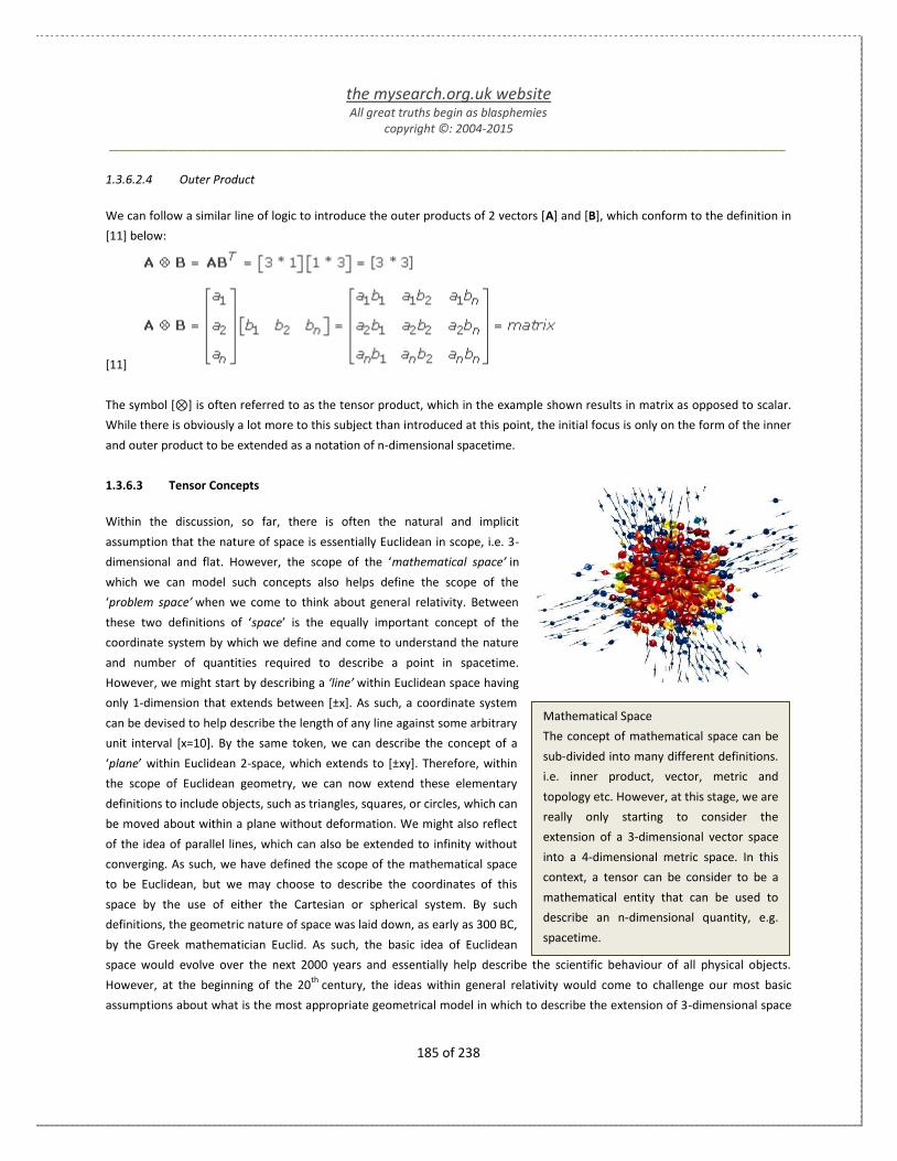
the mysearch.org.uk website All great truths begin as blasphemies
copyright ©: 2004-2015 _______________________________________________________________________________________________________
185 of 238
Mathematical Space
The concept of mathematical space can be
sub-divided into many different definitions.
i.e. inner product, vector, metric and
topology etc. However, at this stage, we are
really only starting to consider the
extension of a 3-dimensional vector space
into a 4-dimensional metric space. In this
context, a tensor can be consider to be a
mathematical entity that can be used to
describe an n-dimensional quantity, e.g.
spacetime.
1.3.6.2.4 Outer Product
We can follow a similar line of logic to introduce the outer products of 2 vectors [A] and [B], which conform to the definition in
[11] below:
[11]
The symbol [⊗] is often referred to as the tensor product, which in the example shown results in matrix as opposed to scalar.
While there is obviously a lot more to this subject than introduced at this point, the initial focus is only on the form of the inner
and outer product to be extended as a notation of n-dimensional spacetime.
1.3.6.3 Tensor Concepts
Within the discussion, so far, there is often the natural and implicit
assumption that the nature of space is essentially Euclidean in scope, i.e. 3-
dimensional and flat. However, the scope of the ‘mathematical space’ in
which we can model such concepts also helps define the scope of the
‘problem space’ when we come to think about general relativity. Between
these two definitions of ‘space’ is the equally important concept of the
coordinate system by which we define and come to understand the nature
and number of quantities required to describe a point in spacetime.
However, we might start by describing a ‘line’ within Euclidean space having
only 1-dimension that extends between [±x]. As such, a coordinate system
can be devised to help describe the length of any line against some arbitrary
unit interval [x=10]. By the same token, we can describe the concept of a
‘plane’ within Euclidean 2-space, which extends to [±xy]. Therefore, within
the scope of Euclidean geometry, we can now extend these elementary
definitions to include objects, such as triangles, squares, or circles, which can
be moved about within a plane without deformation. We might also reflect
of the idea of parallel lines, which can also be extended to infinity without
converging. As such, we have defined the scope of the mathematical space
to be Euclidean, but we may choose to describe the coordinates of this
space by the use of either the Cartesian or spherical system. By such
definitions, the geometric nature of space was laid down, as early as 300 BC,
by the Greek mathematician Euclid. As such, the basic idea of Euclidean
space would evolve over the next 2000 years and essentially help describe the scientific behaviour of all physical objects.
However, at the beginning of the 20th
century, the ideas within general relativity would come to challenge our most basic
assumptions about what is the most appropriate geometrical model in which to describe the extension of 3-dimensional space

the mysearch.org.uk website All great truths begin as blasphemies
copyright ©: 2004-2015 _______________________________________________________________________________________________________
186 of 238
into 4-dimensional spacetime. It was this change in perspective that forced Einstein to abandon Euclidean space in favour of a
differential metric that could be extended to accommodate non-Euclidean space, as and when required. For instance, we might
use the surface of a sphere as an example of non-Euclidean 2-space, which is analogous to a Euclidean plane in that it has 2-
dimensions, but is a surface that does not extend to infinity. However, in such cases, a differential metric can still be adopted,
when a linear metric cannot be scaled across the entire coordinate system.
In a Euclidean plane, the algebraic metric embodied in Pythagoras’ theorem [s2=x
2+y
2] describes the relationship between the
hypotenuse [s] and the two sides [x] and [y] of an orthogonal triangle. Since the plane is being described in flat space, any
vector quantity does not have to be restricted to a differential quantity. However, if we wish to extend the idea of Pythagoras’
theorem to the surface of a sphere, we need to add an additional term, i.e. [s2=αx
2+βy
2+γxy]. What we might realise in this
latter metric is that as [x] and [y] become increasingly small, the 3rd
terms approaches zero faster than the exponential terms
[x2, y
2], i.e. we start to approach a differential approximation of Pythagoras’ theorem. In essence, we are making the
assumption that we can always choose a sufficiently small portion of a non-Euclidean space, which approximates to the rules of
Euclidean geometry. However, because there can be no straight lines on this spherical surface, the geometry of this non-
Euclidean space also determines the nature of the coordinate system that can be used. Of course, in the context of general
relativity and its application within cosmology, there are higher dimensional analogies to the plane or sphere; where each
mathematical space will be defined in terms of a set of points to which specific geometric characteristics can be assigned, which
then require the use of different coordinate systems. However, physical quantities must be independent of the particular
coordinate system chosen, even although these quantities are not necessarily independent on the space that helps defines
them. In this context, tensor analysis provides coordinate independence, while supporting the introduction of more complex
definitions of ‘space’. However, the key benefit of tensors is that the mathematical formalism remains consistence, regardless
of the number of dimensions required to model the geometry of space.
The term tensor is derived from the Latin word ‘tensus’ meaning stress or tension and was a mathematical concept first used by
scientists and engineers studying stress. However, the ideas of both tensors and stress were also adopted within the description
of general relativity, which unfortunately leads to the complexity we are about to review. While the basic concept of a tensor as
a function, encompassing the concepts of scalars and vectors is not, in principle, too daunting, the subject can quickly extend to
include the additional notation of matrix coordinates and the subscripts and superscripts associated with contravariant and
covariant vectors. So, even before the notation of differential calculus and metric tensors are added to this apparently ever-
growing list of complexity, many people may decide they have better things to do in life. However, while it may not be
successful, the goal is to try to provide some sort of introduction to the mathematical abstractions used in the description of
general relativity via the use of tensors.
1.3.6.3.1 Type and Rank The first and most obvious questions when being introduced to the idea of a tensor is:
What is a tensor?
To this direct question, you might get an equally direct answer, i.e. a tensor is a linear function. However, whether this
response really answers the question above might be debated, so let us enquire further:
What does a tensor do?

the mysearch.org.uk website All great truths begin as blasphemies
copyright ©: 2004-2015 _______________________________________________________________________________________________________
187 of 238
The Mathematics of Spacetime
If we defined the scope of mathematical
space to be Euclidean, we may choose to
describe the coordinates of this space by
the use of either the Cartesian or spherical
system. By such definitions, the geometric
nature of space was laid down, as early as
300 BC, by the Greek mathematician
Euclid. As such, the basic idea of Euclidean
space would evolve over the next 2000
years and essentially help describe the
scientific behaviour of all physical objects.
However, at the beginning of the 20th
century, the ideas within general relativity
would come to challenge our most basic
assumptions about what is the most
appropriate geometrical model in which to
describe the extension of 3-dimensional
space into 4-dimensional spacetime.
Again, on an equally terse level, the reply might be that a tensor can take a
vector and turn it into another vector or alternatively it can turn a vector into
a scalar or even a scalar into a vector. While there may still be some
ambiguity in the scope of this response, we might start to get the idea about
the somewhat abstract and varying nature of tensors. In many ways, the
exact nature of a tensor is defined by the specific context in which it is being
used, i.e. a tensor is defined by what it does. However, let us try a little harder
to capture the apparently elusive nature of a tensor via an example. Given the
attributes of speed and direction, the wind can be described as a velocity
vector [w]. When the wind hits the sail of a yacht, it imparts a force, i.e.
another vector quantity [F]. However, the force on the sail does not typically
act in the direction of the wind, although the relationship between the wind
speed and the force on the sail is a linear function, i.e. double the wind speed,
double the force. Therefore, we can define this relationship in a mathematical
form via the introduction of a tensor [T].
[1]
The complexity of the tensor [T] really depends on how many factors are
taken into account when mapping the relationship between the force [F] and
the wind speed [w]. However, the introduction of tensors allows this complexity to be encapsulated into one entity, i.e. the
tensor, which comes with a set of mathematical rules for the manipulation of the entities involved. As such, a tensor is a
collective name for a function involving one or more of the following components:
Scalars: a magnitude
Vectors: magnitude and direction
Matrices: an array of elements.
At this point, there may be the suggestion that any vector can be tensor. However, to be a tensor, the vector components must
transform according to certain rules when mapping from one coordinate system to another. As another generalisation, a tensor
can inherit the contravariant or covariant nature of any assigned vector elements, i.e. how it transforms relative to a change in
the coordinate system. Let us summarise this specific aspect of a tensor and some associated notation:
A tensor can contain both contravariant and covariant vectors.
Contravariant tensors are annotated with superscripts, e.g. [Tm
].
Covariant tensors are annotated with subscripts, e.g. [Tn].
Use of both subscripts and superscripts leads to the tensor notation:
However, a tensor can also have the form of a matrix, where each element can be as simple as a scalar, or involve contravariant
and covariant vectors or even more complex functions. Part of this complex nature is described in terms of the `type` or `rank`
of a tensor.

the mysearch.org.uk website All great truths begin as blasphemies
copyright ©: 2004-2015 _______________________________________________________________________________________________________
188 of 238
So what is a tensor?
A tensor can be arrays of numbers or
functions, which transform according
to certain rules under a change of
coordinates. As such, a tensor may be
defined at a single point or collection
of points in space or, more
importantly, spacetime.
An Example of a Tensor
Given the attributes of speed and
direction, the wind can be described
as a velocity vector [w]. When the
wind hits the sail of a yacht, it imparts
a force, i.e. another vector quantity
[F]. However, the force on the sail
does not typically act in the direction
of the wind, although the relationship
between the wind speed and the
force on the sail is a linear function,
i.e. double the wind speed, double the
force. However, we might define this
relationship in a mathematical form
via the introduction of a tensor [T].
1.3.6.3.2 Type: Let us initially consider a tensor in terms of covariant and contravariant vectors. A tensor with one superscripted contravariant
and two subscripted covariant indices would be written as [ ]. As such, the `type` of a tensor is defined in terms of a pair
numbers, which reflects how many vectors, of each type, are used by the tensor. So, in our example tensor [ ], the `type`
equals (1,2) and as a general definition, a tensor with [m] contravariant and [n] covariant indices has `type=(m,n)` . In this
context, the tensor type also defines its rank, where the rank is the sum of the type indices, i.e. [m+n].
1.3.6.3.3 Rank: However, if we consider a tensor as an array of elements in a matrix, the rank corresponds to the number of dimensions within
the array. If we start with a 2-dimensional table, this can be likened to a rank-2 tensor, while the form of a 3-dimensional cube
would corresponds to a rank-3 tensor. Working back from a rank-2 tensor, a vector only requiring a single row for magnitude
and direction would be defined as a rank-1 tensor; while, by the same logic, a scalar requiring only a single element for
magnitude is defined as a rank-0 tensor. At this point, the general idea of a tensor, as outlined in terms of the force vector [F]
and the wind velocity vector [w] being resolved by a tensor [T], may have started to become a bit blurred by the complexity
being introduced. So it is possibly worth introducing another basic example, before adding any more details, by saying that
some physical quantities do not change when measured in another frame of reference. For example, the temperature [T], i.e. a
scalar quantity, at some point in space, will remain unchanged irrespective of
what coordinate system is used when measuring its value. If we put this concept
into symbols, we have a transformation rule, i.e. T=T’, where [T] is now used to
denote the temperature measured in frame [S] and [T’] is the temperature
measured in frame [S’]. This condition of invariance is one that is required by a
mathematical object to be a tensor. Of course, we might realise that we may have
an entire ‘set’ of quantities associated with a point in space, which transform
according to an unchanging or invariant rule between any two coordinate
systems. However, we can describe temperature as both a scalar quantity and a
tensor of rank-0; noting that while every rank-0 tensor is a scalar, not every scalar
is a rank-0 tensor, e.g. frequency is a scalar but not a rank-0 tensor.
So what is a tensor?
A tensor can be arrays of numbers or functions, which transform according to
certain rules under a change of coordinates. As such, a tensor may be defined at a
single point or collection of points in space or, more importantly, spacetime. As a
continuum of points, i.e. a coordinate system, the elements of the tensor are
functions of position and the tensor forms what is called a tensor field.
When a tensor consists of only a single number, it is called a rank-0 tensor of
order zero, which is essentially a scalar. While we have used temperature as
an example of a scalar, which can then be considered as a scalar field as a
function of position, another example of a scalar field would be the value of
the gravitational potential energy as a function of position. In this context,

the mysearch.org.uk website All great truths begin as blasphemies
copyright ©: 2004-2015 _______________________________________________________________________________________________________
189 of 238
the scalar quantities are considered to vary continuously from point-to-point, thereby defining a scalar field within some
defined coordinate system.
The next most complicated tensor is a rank-1 tensor, which aligns to the concept of a vector. Just as a rank-0 tensor can be
defined at a point, i.e. a scalar value, and as a scalar field, a vector can be described at a point and as field of vector values.
Typically, vectors are defined using just 3 spatial components [x,y,z] in Cartesian coordinates, or possibly [r,θ,φ] in polar
coordinates. However, in the context of relativity, the coordinate system is extended to 4-dimensional spacetime and, as
such; a vector is also extended to have 4 components. In this context, a vector may also be described in terms of a 1-
dimensional array, i.e. 1 row of [n] elements. At this point, we might cite the gravitational field strength as an example of a
vector field, which has magnitude and direction at every point in space or spacetime.
Of course, one of the fundamental reasons for developing the idea of a tensor is that the concept can be extended to
higher dimensions, if required. As might be expected, the extension of a rank-2 tensor describes a 2-dimensional array or
matrix.
There are yet more complex phenomena that require tensors of even higher order, one of which exists in general relativity, i.e.
the curvature of space-time. The Riemann curvature tensor is of order four, since it is used to help defined 4-dimensional
spacetime, although it requires 44=256 components. The rest of this section will now try to expand on this initial overview.
1.3.6.4 Differential Geometry
As the name might imply, differential geometry augments the study of geometry
using techniques of calculus and, in many ways, its earliest history aligns to
developments in calculus. However, over time, calculus would become more
algebraic in form, which eventually led to a clearer distinction between what are now
two distinct fields of mathematics. By way of a historical backdrop, in 1818, while
engaged in a geographic survey of Hanover, the famous mathematician Carl Friedrich
Gauss became interested in the computational problems relating to the curvature of
various tracts of land. In this context, Gauss devised an intrinsic measure of
curvature, which depended on only how the distance was measured on the surface
and not on the way it was embedded in space. Later, as the formalism of differential
geometry evolved, such ideas would become fundamental to the development of
Riemannian geometry and Einstein's theory of relativity. However, while differential
geometry has become an important foundation stone of general relativity, it is not an
easy subject to summarise, such that it provides a useful initial guide to anybody new
to this subject. Therefore, by way of an introduction to the basic concepts of
differential geometry, the following discussions have already been outlined:
Scalars
Vectors
Matrices
Tensors

the mysearch.org.uk website All great truths begin as blasphemies
copyright ©: 2004-2015 _______________________________________________________________________________________________________
190 of 238
Oblique
In geometry, an oblique angle
refers to one that is not a multiple
of 90 degrees.
The goal of the following series of discussions is to first try to explain
how the basic concepts above are integrated into the overarching ideas
of differential geometry. Hopefully, having established some basic
principles underpinning differential geometry, we might then be in a
better position to understand its specific application within general
relativity. In this way, much of the complexity associated with higher
order tensors will either be deferred until required or omitted. As such,
the intention is to proceed from a description of 2-dimensional flat
space, which basically aligns to Pythagoras’ Theorem:
[1]
The form of [1] can be described as a metric, which is a function that
defines a distance between two events in metric space. As such, this
metric also helps define the characteristics of the underlying space in
question, e.g. 2-dimensional and flat. However, as you might realise, [1] is just the first step along the road towards a much
more complex definition of 4-dimensional spacetime, which may have the characteristics of both spatial and spacetime
curvature. In this context, [1] will increasingly evolve towards the following mathematically form, which can appear very
abstract at the outset:
[2]
At this point, there will be no attempt to explain [2], other than to say that [ds] is simply some distance equivalent to [s], which
is now restricted to a differential separation of 2 points in what might be curved space. However, as stated, the goal is to
proceed from [1] in a series of steps that essentially involves only the basic concepts of vectors, albeit that we will quickly start
to migrate away from our normal assumption of Euclidean space and Cartesian coordinates, where all dimensions, e.g. [x,y] in
2D and [x,y,z] in 3D, are orthogonal to each other. Clearly, as the diagram above tries to illustrate, there is scope in the universe
for more far more complex geometries.
1.3.6.4.1 Contravariance and Covariant Coordinates
It is possible to describe the same vector [A] using both Cartesian and non-Cartesian
coordinates. For the initial purposes of this discussion, the non-Cartesian coordinates
will simply be described in terms of coordinates axes that are ‘oblique’ to each other
by some angle [φ]:

the mysearch.org.uk website All great truths begin as blasphemies
copyright ©: 2004-2015 _______________________________________________________________________________________________________
191 of 238
Parallelogram Method
To obtain a resultant vector from
two or more component vectors,
the two component vectors are
taken to form the adjacent sides of
a parallelogram. The resultant
vector is given by the direction and
length of the diagonal of the
parallelogram.
The vector [A] has the same magnitude and direction in both sets of coordinates, but
it is clear that the components with respect to the [ax, ay] and [au, av] axes are
different. Initially, the subscripting on the vector components simply implies an index
for identification purposes. However, it might be observed that vector [A] is still the
vector sum of its [x,y] or [u,v] components based on the parallelogram method. In
this context, we might describe the ‘oblique’ case as being more representative of a
parallelogram with the ‘Cartesian’ case aligning to the specific instance when the axes
are at right-angles to each other. So while both cases in the diagram above represent
a parallelogram of components, one set of components is projected perpendicular to
the [x,y] axes, while the other set is projected parallel to the [u,v] axes. In fact, we
could consider superimposing both the perpendicular and parallel projection within a single diagram as shown below. While
this diagram has some obvious similarities to the previous oblique case, we have now generalised the labelling of the axes [x1,
x2] simply because it allows the number of dimensions to be extended to [n]. We might also recognise that [a1, a
2] must be
equivalent to [au, av] even though the change to superscripted indices might infer some additional meaning. However, before
explaining the actual meaning associated with the use of both subscripted
and superscripted indices on the component vectors, first imagine
rotating the [x2] axes, in the diagram above, from its oblique position back
towards the vertical, such that it is again equivalent to the Cartesian case.
What happens to the subscripted and superscripted components?
In the Cartesian case, we might visualise both sets of components
superimposed on each other, such that any separate meaning given to
these indices would not necessarily be apparent in the special case of
Cartesian coordinates, where the axes are orthogonal.
So what meaning is associated with the subscripted and superscripted
components in the oblique case?

the mysearch.org.uk website All great truths begin as blasphemies
copyright ©: 2004-2015 _______________________________________________________________________________________________________
192 of 238
Invariant Vectors
As has been previously discussed, a vector
is often described in terms of being
contravariant or covariant, when the
direction and magnitude of a vector are
actually invariant with respect to
coordinate changes. This aspect highlights
an issue with applying the terminology of
contravariance and covariance to a vector,
and subsequently a tensor, when it really
applies to the contravariant and covariant
components of the vector. For example, a
velocity vector has a direction and
magnitude that is essentially independent
of the coordinate system used to define it.
Therefore, the velocity vector itself does
not really change when changing to
another coordinate systems, rather it is
the components of the vector that change.
In fact, these components better reflect the idea of contravariance and
covariance, which was briefly outlined in connection with the introduction of
vectors. However, in the present context, the idea of contravariance and
covariance now seems to have more to do with the coordinate components of
the vector [A], rather than the vector itself. While the terminology of
contravariance or covariance is linked to the descriptions of vectors, these
terms are really identifying the nature of the changes to the components of a
vector object with respect to a given coordinate system. The vector [A] does
not change with respect to the coordinate system, even although the
component coordinates that define this vector will differ. So while the vector
itself is coordinate independent, its individual components are not. Therefore,
the components of the vector will vary from system to system, but must do so
in such a way that the vector quantity itself remains unchanged. This
statement will be expanded when we come to consider tensors in more detail,
but for now, we should simply realise that the components of any vector, in
any coordinate system, are nothing more than the projections of that vector
onto the local coordinate axes. However, for the purpose of trying to describe
the relationship between the contravariant and covariant components, we
shall assume that the vector in the diagram above is a displacement vector,
which extends from one point to another. As such, this vector is being
described within some arbitrary, but non-orthogonal coordinate system with axes [x1] and [x2]. It can be seen that the
contravariant [a1, a
2] components of vector [A] are projected parallel to the [x1, x2] axes, while covariant [a1, a2] components of
vector [A] are projected perpendicular to the [x1, x2] axes. If the coordinate system was orthogonal, such that the [x1, x2] axes
were mutually perpendicular, then the contravariant and covariant components would be identical as indicated in Cartesian
case.
It is possibly worth highlighting that ‘orthogonal’ does not
mandate Cartesian coordinates. For example, while polar
coordinates are not based on straight lines, they are still
orthogonal, because all angles [θ,φ] are measured
perpendicular to the radial axis.
To understand in more detail how the representations of vectors in
different coordinate systems are related to each other, consider the
vector [A] in 2 different oblique coordinates systems as shown right.
The first set of oblique axes, shown in green and labelled lowercase
[x1, x2] essentially replicate the earlier oblique example, where the
subscripting and superscripting aligns to whether the component
vector is a perpendicular or a parallel projection with respect to the
green axes. The second set of oblique axes, shown in red and labelled
uppercase [X1, X2] again show the subscripted and superscripted
components. Note that red axis [X2] is perpendicular to green axis [x1], while red axis [X1] is perpendicular to green axis [x2]. In
terms of the green [x] coordinate system, the contravariant components of [A] are [a1, a
2] and the covariant components are

the mysearch.org.uk website All great truths begin as blasphemies
copyright ©: 2004-2015 _______________________________________________________________________________________________________
193 of 238
[a1, a2]. In the second set of oblique red coordinates, the contravariant components of [A] are [A1, A
2] and the covariant
components are [A1, A2]. The symbol [φ] reflects the oblique angle between green axes [x1, x2], while the symbol [φ’] reflects
the oblique angle between red axes [X1, X2] and relationship between these angles is as follows:
[1]
However, the primary purpose of the previous diagram is simply to show that much of the apparent complexity that will
develop in the following discussion of contravariant and covariant tensors is still ultimately linked to basic geometry and
trigonometry. In fact, the goal is to generalise a solution for the metric of flat, 2-dimensional space in terms of both sets of the
contravariant components linked to the previous diagram.
We are going to proceed essentially using only the cosine rule of a triangle, as shown in [2] below, with respect to the yellow
triangle in the diagram above:
[2]
The red and green triangles on the right of the diagram above correspond to the two sets of oblique coordinates, i.e. green: [x1,
x2] and red:[X1, X2], previously introduced. If we apply the cosine rule in [2] to both of the shaded triangles, as shown above, we
can determine the length of the vector [A], which we will now described in terms of some separation distance [s]:
[3]
We might consider proceeding from the form in [3] by generalising the parameters which align to the contravariant
components, e.g. [xu, x
v]. At the same time, we will replace the other values by a coefficient [guv]:

the mysearch.org.uk website All great truths begin as blasphemies
copyright ©: 2004-2015 _______________________________________________________________________________________________________
194 of 238
[4]
As such, [4] shows both the expanded and generalised form of both equations in [3], which align to 2 different variants of
oblique coordinates. As such, we appear to be on the way towards the form adopted within differential geometry. However, at
this point, we possibly need to explain the scope of the coefficient [guv] in terms of what is referred to as a covariant metric
tensor, e.g.
[5]
The use of subscripts identifies the covariant nature of [guv], but in the present context, we can simply consider [5] as a matrix
required as a solution to [3], although the symbol for the angles [φ,φ’] has now been normalised to [θ]. While the equations in
[3], [4] and [5] are reflective of the contravariant components within an oblique coordinate system, we might quickly consider
how these equations would be modified for the Cartesian or orthogonal case. With reference to diagram above, when the
angles [θ=φ or φ’] are set to a right-angle its leads to [cosθ=0] and a revision of [5]:
[6]
As such, [6] appears to have returned to the form of Pythagoras’ Theorem, which represents the metric of 2-dimensional flat
space. However, we now have a form that can be applied to both Cartesian and oblique coordinate systems, which might also
be extended to higher dimensions which require metrics that go beyond the Pythagorean form. However, in principle, we have
outlined some of the basic geometry, linked to vectors, which can now be extended to the concept of a tensor with any number
of indices, including some with both contravariant and some covariant indices. Finally, it should be noted that the distance
formula in [6] still applies when changed to a differential form, i.e. the incremental distance [ds] along a path is related to small
incremental components [dx], such that it can be generalised as:
[7]
However, when using [7] in curved spacetime, we will need to integrate over some given path to determine the total length [s].
So, in principle, the form of [7] can now be applied to 4-dimensional spacetime to determine the spatial and temporal
separation between events as defined by general relativity.

the mysearch.org.uk website All great truths begin as blasphemies
copyright ©: 2004-2015 _______________________________________________________________________________________________________
195 of 238
Oblique Coordinates
Are simply being used to represent
some 'other' set of coordinates,
which ultimately may be used to
described curved spacetime. The
real point being highlighted is that
when switching to a coordinate
system that is not necessarily
orthogonal, both the contravariant
and covariant components of a
vector have to be taken into
consideration.
1.3.6.4.2 Coordinate Components
In part, the previous discussion was intended to provide some insight to the potential transition from the standard geometry of
flat space to the differential geometry of curved spacetime. However, while some people are happy to just accept the
mathematical abstraction implicit in much of differential geometry, its application in the field of general relativity needs to
retain some perspective of a physical science. In this respect, it is hoped that the previous discussion of contravariant and
covariant coordinates highlighted the transition from Cartesian coordinates to oblique coordinates, where the physical reality
of the contravariant and covariant axes emerged. However, the latter part of the discussion might have appeared orientated to
just the contravariant components and therefore the following discussion is intended to highlight how the contravariant and
covariant components become part of an extended geometry when using non-Cartesian coordinates.
The diagram above is trying to show how two vectors [A, B] might be represented in two different coordinate systems, i.e.
Cartesian and oblique. The red and black axes show the components vectors of [A, B] in the Cartesian system with the
background grid suggesting the magnitude of each component vector [a1, a
2] and [b
1, b
2]. As previous explained the
contravariant and covariant components overlap into the same space within the orthogonal system of Cartesian coordinates.
However, it makes more sense to describe the component vectors in the orthogonal space of the Cartesian system in terms of
superscripted contravariant vectors rather than subscripted covariant vectors, because we are essentially describing them in
the context of the parallelogram method of vector addition. This becomes more obvious when we consider the same vectors
[A, B] in the context of the oblique green axes. Now, the contravariant and covariant components of vector [A] become
apparent as [a1, a
2] and [a1, a2] respectively. However, the shaded parallelogram associated with vector [A] in the oblique
system still corresponds to just the contravariant components [a1, a
2]; although it needs to be highlighted that vector arithmetic
might also be subject to change when moving to the oblique coordinate system. Let us consider two aspects of vector
arithmetic in the orthogonal space of the Cartesian system:

the mysearch.org.uk website All great truths begin as blasphemies
copyright ©: 2004-2015 _______________________________________________________________________________________________________
196 of 238
Coordinate Systems
In a orthogonal coordinate system,
where the axes are considered to be
perpendicular to each other, the
contravariant and covariant essentially
align. So, when using an orthogonal
coordinate system, we are by default
using both contravariant and covariant
coordinates, because the only
difference between them is some
arbitrary scale factor. However, it
should be noted that the definition of
orthogonal, in this context, does not
implicitly mean 'rectilinear' as in
Cartesian. For example, polar
coordinates are not rectilinear in that
the axes are not straight lines, but they
are orthogonal, because the angle
between the axes are always
perpendicular to the local radial axis.
Therefore, the metric of a polar
coordinate system is a diagonal, as per
the metric of a Cartesian coordinate
system. So, only when we consider
systems of coordinates that are not
mutually perpendicular do the
contravariant and covariant forms
differ, which is at the root of the
geometry of curved spacetime that
general relativity seeks to address.
[1]
Again, superscripted indices have been used within the Cartesian system, for the
reasons cited above, but it is highlighted that the primary focus within [1] relates
to the definition and magnitude of the component vectors of [A, B]. So, in the
context of Cartesian coordinates, we see that the resultant vector is linked to its
component vector via the standard geometry of Pythagoras’ theorem, while the
dot product of [A, B] can be apparently defined, as shown, in terms of just the
contravariant values [a1b
1+a
2b
2].
But are the equations in [1] a generalised solution for other coordinate system?
The simply answer to this question is no, but we can used the diagram above to
not only prove this statement, but to highlight that a general solution requires a
combination of both the contravariant and covariant components. What the
diagram above illustrates is that the magnitudes of [A, B] do not change when we
switch to the oblique coordinates and, as such, we might initially establish the
answers to the [A, B] examples in [1] with respect to the Cartesian system:
[2]
Now even a cursory review of the diagram above will indicate that simply substituting the contravariant values with respect to
the oblique system cannot possibly arrive at the same answers, as given in [2].
So how do we perform the vector arithmetic implied by [1] and [2]?
Clearly, the formulations given in [1] have to be modified and although we will not provide an actual proof, it is possibly
informative and reassuring to simply know that the answers can still be resolved using basic geometry, albeit extended to
reflect the oblique system:

the mysearch.org.uk website All great truths begin as blasphemies
copyright ©: 2004-2015 _______________________________________________________________________________________________________
197 of 238
Coordinate Transforms
The rules of coordinate transforms
outlined in this discussion are one of
the key attributes of a tensor. This
attribute is based on the fact that its
presentation in different coordinate
systems depends only on a relative
change with respect to the coordinate
axes in use and not on the absolute
values of the coordinates. This is why
an absolute position vector, defined
in terms of the origin of some specific
vector space, is not a tensor, for its
components would then also depend
on the absolute values of the
coordinate system. In contrast, the
coordinate transforms outlined are
based solely on local information.
[3]
If we now compare [3] with [1], we see that the definition of the vectors [A, B] has been extended to include both contravariant
and covariant components. The magnitude of the vectors [A, B] is now the sum of the products of the contravariant and
covariant components, which collapses back to Pythagoras’ theorem only when the axes are orthogonal. We also see that the
dot product now requires a combination of both the contravariant and covariant components. Based on the scale of the
background grid in diagram above, the values of the contravariant and covariant components in the oblique can be
approximated as shown to align with the answers given in [2]. Another practical example can be seen in the discussion entitled
'2-Space Metric Tensor'
1.3.6.4.3 Coordinate Transforms
In the previous couple of discussions, we introduced the idea of different
coordinate systems and types of components, albeit in the restricted sense of 2D
flat space. Of course, within the wider context of general relativity, space and
spacetime might be assumed to be curved and the scope of the variables,
associated with a given function, may have to be restricted to small or differential
increments. This is in contrast to special relativity, which assumes spacetime to be
flat, such that the spacetime metric could be written in the linear form:
[1]
However, this metric is clearly different from the basic form of 2D flat space
associated with Pythagoras’ theorem, although this theorem is still reflected in the
spatial terms [xyz]. However, the metric in [1] has now been extended to 4D
spacetime by the introduction of the [ct] term, while also noting the ‘sum’ of the
squares does not extend to the [ct] term. The metric in [1] is sometimes described
as the Minkowski metric of flat spacetime that is valid within the constraints of
special relativity. However, in the context of general relativity, which seeks to describe curved spacetime, the metric of special
relativity may only be valid in a small volume of spacetime, which is approximately flat and therefore [1] is modified to a
differential form:
[2]
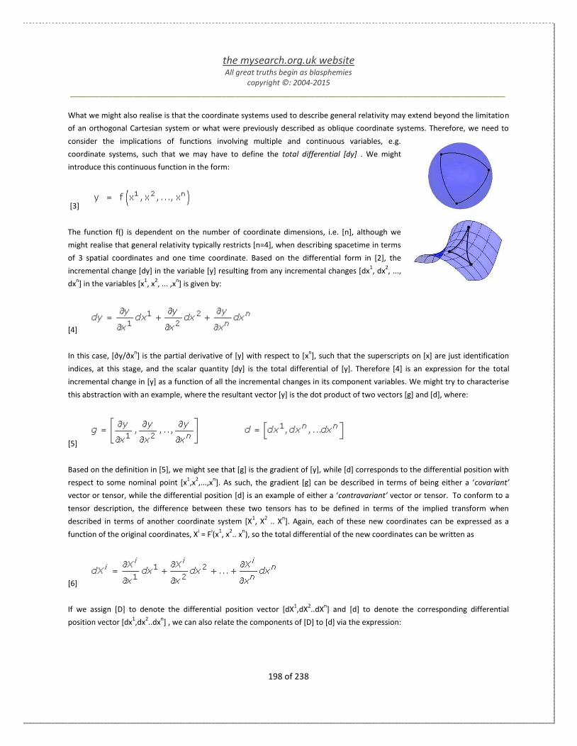
the mysearch.org.uk website All great truths begin as blasphemies
copyright ©: 2004-2015 _______________________________________________________________________________________________________
198 of 238
What we might also realise is that the coordinate systems used to describe general relativity may extend beyond the limitation
of an orthogonal Cartesian system or what were previously described as oblique coordinate systems. Therefore, we need to
consider the implications of functions involving multiple and continuous variables, e.g.
coordinate systems, such that we may have to define the total differential [dy] . We might
introduce this continuous function in the form:
[3]
The function f() is dependent on the number of coordinate dimensions, i.e. [n], although we
might realise that general relativity typically restricts [n=4], when describing spacetime in terms
of 3 spatial coordinates and one time coordinate. Based on the differential form in [2], the
incremental change [dy] in the variable [y] resulting from any incremental changes [dx1, dx
2, ...,
dxn] in the variables [x
1, x
2, ... ,x
n] is given by:
[4]
In this case, [∂y/∂xn] is the partial derivative of [y] with respect to [x
n], such that the superscripts on [x] are just identification
indices, at this stage, and the scalar quantity [dy] is the total differential of [y]. Therefore [4] is an expression for the total
incremental change in [y] as a function of all the incremental changes in its component variables. We might try to characterise
this abstraction with an example, where the resultant vector [y] is the dot product of two vectors [g] and [d], where:
[5]
Based on the definition in [5], we might see that [g] is the gradient of [y], while [d] corresponds to the differential position with
respect to some nominal point [x1,x
2,...,x
n]. As such, the gradient [g] can be described in terms of being either a ‘covariant’
vector or tensor, while the differential position [d] is an example of either a ‘contravariant’ vector or tensor. To conform to a
tensor description, the difference between these two tensors has to be defined in terms of the implied transform when
described in terms of another coordinate system [X1, X
2 .. X
n]. Again, each of these new coordinates can be expressed as a
function of the original coordinates, Xi = F
i(x
1, x
2.. x
n), so the total differential of the new coordinates can be written as
[6]
If we assign [D] to denote the differential position vector [dX1,dX
2..dX
n] and [d] to denote the corresponding differential
position vector [dx1,dx
2..dx
n] , we can also relate the components of [D] to [d] via the expression:

the mysearch.org.uk website All great truths begin as blasphemies
copyright ©: 2004-2015 _______________________________________________________________________________________________________
199 of 238
Minkowski Spacetime
Minkowski was one of Einstein's
lecturers, who also poineered the
concept of 4-dimensional specetime.
He is often remembered for starting a
conference in 1908 with the statement:
"The views of space and time which I
wish to lay before you have sprung
from the soil of experimental physics,
and therein lies their strength. They are
radical. Henceforth space by itself, and
time by itself, are doomed to fade away
into mere shadows, and only a kind of
union of the two will preserve an
independent reality."
[7]
At this point, we can highlight that the form of [7] is representative of the transformation rule for a ‘contravariant’ tensor of the
first order, i.e. a vector. However, based on an earlier introduction of the basic nature of contravariance and covariance, we
might realise that we will need a separate transformation rule for our covariant tensor [g]. In order to find the correct
transformation rule for a covariant tensor, the original coordinates have to be expressed as some functions of the new
coordinates, i.e. xi = f
i(X
1, X
2.. X
n), which then enables us to write the total differential of the original coordinates as:
[8]
If we now substitute these expressions for the total coordinate differentials into
[4]:
[9]
Now the components of the gradient [g] with respect to the new [Xi] coordinates
are defined in the parentheses of [9]. If we now assign [G] to denote the
gradient of [y] in the new coordinates system:
[10]
As such, [10] is representative of the transformation rule for covariant tensor of the first order. At this point, we can compare
the contravariant rule given in [7] with the covariant rule given in [10]. On examination, we can see that both define the
transformed components as a linear combination of the original components. However, in the contravariant case, the
coefficients are the partial derivatives of the new coordinates [X] with respect to the original coordinates [x]. In contrast, in the
covariant case, the coefficients are the partial derivatives of the original coordinates [x] with respect to the new coordinates [X].
These transformation rules highlight one of the key attributes of a tensor, i.e. its representation in different coordinate
systems depends only on the relative change with respect to the coordinate axes in use and not on the absolute values of
the coordinates. This is why an absolute position vector, defined in terms of the origin of some specific vector space, is
not a tensor, because its components would also depend on the absolute values of the coordinate system. In contrast,
the coordinate differentials transform based solely on local information, which should also be considered in respect of
the scope implied by [1] and [2].

the mysearch.org.uk website All great truths begin as blasphemies
copyright ©: 2004-2015 _______________________________________________________________________________________________________
200 of 238
1.3.6.5 Notation and Manipulation
Indirectly, through the using of vectors as rank-1 tensors, we have
been establishing some of the basic rules governing tensors and
coordinate systems. In this discussion, we shall simply try to
consolidate some of notation used to describe the nature of a
tensor and how they may be manipulated as a single mathematical
object. Given that tensors can be closely associated with vectors, it
is not unreasonable to assume that tensors may share some of the
same basic requirements when it comes to manipulating them. For
example, a vector may be multiplied by a scalar to form a new
vector with the same direction. We can also multiple two vectors
in the form of a dot or cross product, where the former produces a
scalar and the latter another vector orthogonal to both, at least in
a Cartesian system. Of course, we can also add two vectors to
obtain a third vector, which is a good starting point when it comes
to rank-1 tensors, providing we add tensors of the same type. For
example, two covariant tensors can be added together to form a
new covariant tensor:
[1]
By the same logic, two contravariant tensors can be added and while the symbols chosen to identify the tensors [a, b, c] are
arbitrary, the superscript and subscript orientation also reflect the rules for contravariant and covariant tensors:
[2]
In contrast, we might consider multiplying two vectors which are not of the same type, but share the same index, i.e. unvn.
Equally, by a rule known as ‘summation’, we can multiple two tensors of different type providing we have a repeated index [n],
which appears once as a subscript and once as a superscript.
[3]
Previously, prior to the need to consider more than 3 spatial orthogonal dimensions, we might have quite happily written [3] in
the form of dot product of 2 vectors, but clearly we are now in a process that wants to consider the potential of n-dimensions.
In this respect, the dot product is also referred to as the inner product and, in some ways; it is simply importing the idea of
vector space into our discussion of tensors, which is being described in terms of some given coordinate system of spacetime. In
the previous discussion of Coordinate Transforms, we outlined the basis of the transform rules for both contravariant and
covariant tensors, which we can now present in the summation form of [4]:

the mysearch.org.uk website All great truths begin as blasphemies
copyright ©: 2004-2015 _______________________________________________________________________________________________________
201 of 238
Alice in Wonderland
"Alice laughed: "There's no use trying," she
said; "one can't believe impossible things." "I
daresay you haven't had much practice,"
said the Queen. "When I was younger, I
always did it for half an hour a day. Why,
sometimes I've believed as many as six
impossible things before breakfast."
[4]
At this point, we might wish to consider the attribute of an inner (dot)
product of 2 rank-1 tensors of the form in [4]:
[5]
In the context of general relativity, we are assuming that the use of differential notation, which allows the scope of the
coordinate systems [x, X] to be collapse to flat spacetime on a small local scale. However, what [5] is also suggesting is that an
inner product of a covariant and contravariant tensor is invariant.
But what of the process of multiplying 2 contravariant rank-1 tensors [aj] and [b
k]?
In this case, we cannot use the process linked to the inner product, but we can present the product of [aj] and [b
k] as follows:
[6]
We might also consider using the contravariant form in [4] to evaluate the scope of [ajb
k]
[7]
In essence, this is the definition of a rank-2 contravariant tensor, which we can now extrapolate and generalise, not only for
contravariant tensors, but covariant and mixed tensors;

the mysearch.org.uk website All great truths begin as blasphemies
copyright ©: 2004-2015 _______________________________________________________________________________________________________
202 of 238
Pierre-Simon de Laplace
Such is the advantage of a well
constructed language that its
simplified notation often becomes
the source of profound theories.
W.B. Frankland
Whereas at the outset geometry is
reported to have concerned
herself with the measurement of
muddy land, she now handles
celestial as well as terrestrial
problems: she has extended her
domain to the furthest bounds of
space.
[8]
However, another key feature of a tensor, as implied by [7], is that the form can be extended to tensors of n-dimensions, which
is a requirement of general relativity.
1.3.6.6 Metric Tensors
One of the primary focuses of this discussion is the use of tensors within the
definition of various spacetime metrics, which are of central importance to general
relativity. As already outlined, a metric is a function that helps define the distance
between ‘events’ within a given coordinate system. Within this concept, the
definition of space may be described in terms of its topology, which is then defined
by its metric. While this description can involve all the mathematical complexity
outlined in the previous discussions, the concept of a metric can be also be so simple
that it can be capture with the idea of basic geometry, e.g.
[1]
Pythagoras’ theorem, as encapsulated in [1], can also be interpreted as a metric that
describes 2-dimensional space, which is geometrically flat and orthogonal with
respect to the [x-y] axes. However, we can immediately extended the basic form of
[1] to 3-dimensional space, which is also geometrical flat with orthogonal axes [x,y,z]:
[2]
However, we have also implied that we can extend part of [2] to represent 4-
dimensional spacetime and get the first glimpse of the need of a metric tensor:
[3]

the mysearch.org.uk website All great truths begin as blasphemies
copyright ©: 2004-2015 _______________________________________________________________________________________________________
203 of 238
Johannes Kepler
Where there is matter, there is geometry.
William Shakespeare
O God! I could be bounded in a nutshell,
and count myself king of infinite space,
were it not that I have bad dreams.
In [3], we see the introduction of time into the definition of 4-dimensional
spacetime, which is then normalised using the notation [x0,x1,x2,x3]. However,
the presence of the minus (-) sign in [3] does not allow us to simply extend the
form of [2], which implies that we may need a different description to cover spacetime geometry, even though the spatial
geometry is still flat. Of course, we might wish to change the implicit use of Cartesian coordinates to spherical coordinates at
this point, as well as making some reference to the possibility of both spatial and spacetime curvature as described by the
Schwarzschild metric:
[4]
While the metric in [4] has be discussed, the form of its metric coefficients will also discussed separately under the heading
‘Point-Mass Solution’ but its basic significance is still best described in terms of the proximity to a very large gravitational mass.
However, there are other metrics, such as the Friedmann-Robertson-Walker metric, which attempt to describe the curvature
spacetime in connection with the large-scale expansion of the universe - see 'Homogeneous Solution':
[5]
Clearly, the complexity being suggested by [4] and [5] is increasing in comparison to [1], but if for example, we set the spatial
curvature to zero, i.e. k=0, and then only consider the metric in [5] at one instance in time restricted to a radial path [dr], we
will return to a metric that is comparative to the previous simpler metrics:
[6]
However, the problem with all these different approaches is that the form of the metric keeps changing with each additional
assumption made about the geometry of space and time. In comparison, the use of a metric tensor [g] might allow all the
different versions to be normalised using the same notation, e.g.
[7]
Now the superscript and subscripts infers meaning in terms of their
contravariance and covariance nature, which can be extended to any number
of dimensions. In the form shown in [7], the differential quantities implied by

the mysearch.org.uk website All great truths begin as blasphemies
copyright ©: 2004-2015 _______________________________________________________________________________________________________
204 of 238
[dx] can be thought of as contravariant position vectors between which the separation [ds] exists. As such, we have the basic
idea of a generic metric tensor [g], which might initially be considered in terms of a 2-dimensional matrix that helps map the
metric in [7] to some specific solution.
1.3.6.6.1 2-Space Metric Tensors
The notion of 2-space is simply another ‘shorthand’ description of
2-dimensional space, which can be extended to 3-space, 4-space
and n-space. In the physical world, we can only perceive 3 spatial
dimensions, but in the context of relativity, the dimension of time
is integrated into the concept of 4-dimensional spacetime.
However, we will again restrict our initial discussion to 2-space in
order to allows us to introduce some of the key concepts
underpinning a 2-space metric tensor in terms of standard
geometry. However, before we consider the basic geometry, it
might be useful to quickly review some of the shorthand notation
we have arrived at through all the previous mathematical concepts
introduced. In the discussion ‘Contravariance and Covariant
Coordinates’ it was shown that Pythagoras’ theorem was a solution
in flat space specific to Cartesian coordinates, which could be
generalised to other coordinates systems, e.g. the oblique
example, in the differential form:
[1]
The form of [1] is a solution that uses just the contravariant positional vectors of 2 points in 2-space, as measured in one
coordinate system, which specifies the separation [ds] in another coordinate system.
Note: In the original example using Cartesian and oblique coordinate systems, we might have perceived the measure of
distance to be the same in both coordinate systems. However, this assumption may not necessarily hold true in relativity.
The scope of [1] is specific to 2-space and will expand when extend to 3-space and 4-space. As such, this notation would
become quite unwieldy as its application within general relativity is extended to 4-space. However, we might initial reduce the
overhead of the notation by using the summation form:
[2]
In essence, [2] is equivalent to [1], but simply presented in a more compact form. When Einstein was developing the theory of
general relativity, he introduced another notation that removed the summation symbol under certain conditions. According to

the mysearch.org.uk website All great truths begin as blasphemies
copyright ©: 2004-2015 _______________________________________________________________________________________________________
205 of 238
this convention, when an index variable appears twice in a single term, once in superscript and once in a subscript, it can be
assumed that a summation takes places all possible values. As such, the form of [2] reduces to:
[3]
This is the form in which the metric tensor [g] is often represented, which we can also explain in terms of a inner product of 2
matrices as previously discussed under the heading of ‘Matrix Products’.
[4]
The form of [4] starts with [3], which is then expanded into matrix forms that are subject to a series of matrix multiplications
resulting in the scalar value [ds]. However, for clarity, we can substitute the actual indexed values in [1] into the dimensioned
matrices in a stepwise manner:
[5]
So [5] represents the inner product of the first two implied matrices in [4], which results in an immediate [1*2] matrix, which is
then multiplied by the remaining [2*1] matrix as follows:
[6]
Of course, we can tidy up the form of [6] such that we return to the form of [1]:
[7]

the mysearch.org.uk website All great truths begin as blasphemies
copyright ©: 2004-2015 _______________________________________________________________________________________________________
206 of 238
For those who already understand the notation of differential geometry, steps [1] through [7] may appear to belabour the
obvious, but those new to this subject; it is this sort of detail that helps anchor the abstraction of the notation back into
something tangible. So, for this reason, the remaining discussion will also be anchored in the following practical geometric
example. The diagram overlays an orthogonal grid against which are mapped the Cartesian coordinates of vector [A] in terms of
the [x,y] axes. There are also a set of oblique axes, in green, onto which are
projected the contravariant [a1, a
2] and covariant [a
1, a
2] coordinates of the
same vector [A]. While this is similar to the earlier oblique examples, the lower
[a1, a1] axis is now aligned to the horizontal [x] axis, so that we might develop
another metric tensor that allow us to switch between the Cartesian,
contravariant and covariant coordinates.
But doesn’t differential geometry provide the transformation rule?
While it is true that mathematics has come to underpin general relativity, it is
still a subject that requires an interpretation within some physical
configuration of spacetime. Equally, for many, the learning process can be best
served by some tangible solutions, rather total reliance on abstracted notation.
So, for these reasons, the diagram above has been extended to contain some additional information that may help explain the
trigonometry employed. Given that we have restricted the context to 2-space, the form of the metric aligns with [7], but which
we might initially interpret with respect to the Cartesian coordinates [x,y]:
[8]
However, in order for [8] to comply with the definition of Pythagoras’ theorem as a metric of 2-space, we need a specific
solution of the metric tensor [g]:
[9]
By applying [9] to [8], we can restore the form of Pythagoras’ theorem:
[10]
The numeric values of the [x,y] component have been aligned to the grid in the diagram above as a basic reference. However,
we have also shown that that this a specific solution based on the orthogonal nature of the Cartesian coordinate system, which
can be generalised to the form of [8], when considered in terms of the contravariant components of [A] with respect to the
oblique coordinates:
[11]

the mysearch.org.uk website All great truths begin as blasphemies
copyright ©: 2004-2015 _______________________________________________________________________________________________________
207 of 238
However, in order to arrive at the same result for [ds2=25], it is clear we have to resolve the value of [a
1, a
2] in terms of the
geometry of the oblique coordinate system. The angle [θ] can be defined by the value [y=4] and [x=3], such that
[tanθ=4/3=53.1°]. We can also specify the value of the contravariant and covariant components of [A] with respect to [x,y]:
[12]
The values in [12] are reasonably straight forward to resolve using standard trigonometry and the geometry implied in the
diagram above, although the last value [a2] is quite involved. However, the focus of this discussion is primarily on resolving the
values of the metric tensor [g], which is why the numeric value of each component is also listed in [12]. At this point, it might be
useful to present the contravariant [a1, a
2] values in [12] in a matrix form:
[13]
Of course, we can apply the same logic to the covariant components [a1, a2]:
[14]
By presenting the information in [12] in the form of the matrices in [13] and [14], we have effectively defined the metric tensors
[f] and [h], which map the component values between the Cartesian and oblique coordinate systems. At this point, we might
remind ourselves that Pythagoras’ theorem only applies within the orthogonal coordinates of the Cartesian system, but can be
generalised by combining the contravariant and covariant values as follows:

the mysearch.org.uk website All great truths begin as blasphemies
copyright ©: 2004-2015 _______________________________________________________________________________________________________
208 of 238
[15]
As one final permutation, we might try to resolve the general expanded equation for [ds], which we have presented in the form
of contravariant components. Of course, we might now realise that we can equally present this equation in terms of its
covariant components if we applied the appropriate metric tensor. However, we have not got a metric tensor that will directly
convert covariant components into contravariant components; but the following diagram outlines the permutations:
In a sense, the diagram above represents the permutations of the various ‘coordinate transforms’ discussed earlier. The matrix
form of [f] and [h] were outlined in [13] and [14] respectively and given that the purpose of this discussion is only to outline the
salient issues, we will only present the form of [g]. In order to convert the covariant coordinates [a1, a2] into the contravariant
coordinates [a1, a
2], we need to develop another metric tensor [g]. However, if we follow the path via [f
-1] and [h], we might see
that the metric tensor [g] is the product of matrix [h] and the inverse matrix of [f], which is simply presented below:
[16]
For completeness, we might reverse the form of [3] from contravariant vectors to covariant vector value via applying a
contravariant tensor [g]:
[17]

the mysearch.org.uk website All great truths begin as blasphemies
copyright ©: 2004-2015 _______________________________________________________________________________________________________
209 of 238
Homer Simpson
Facts are meaningless. You could use facts to
prove anything that's even remotely true!
Again, we have ended up with the length [ds=5], which has been show to be invariant in all coordinate systems. While some of
the steps were a little convoluted, they were all essentially based on standard geometry and trigonometry. As such, it may
appear that differential geometry introduces a lot of abstract mathematical notation that does not do very much and, in the
context of flat 2-space, this conclusion may not so far from the mark. However, the use of the different geometry becomes
more evident when we turn our attention to the 4-space of general relativity.
1.3.6.6.2 4-Space Metric Tensor
In many respect, the previous discussion of ‘2-space metrics’ has tried to
consolidate many of the mathematically concepts introduced so far. As such,
there was a deliberate attempt to ground some of the abstraction of the
mathematical notation in the tangible geometry of flat 2-space and then
anchor the idea of the separation [ds] in real numeric values. However, we
will now start to consider some of the implications of both spatial and
spacetime curvature in the 4-dimensions required by general relativity. As
already outlined, a vector is normally defined in terms of three orthogonal
axes, i.e. [x,y,z] or [r,θ,φ] based on Cartesian or spherical coordinates. In such
systems, the spatial separation [ds] can be defined by the 3-space form of
Pythagoras’s theorem:
[1]
However, [1] does not hold true, when we extend the discussion to include
4-dimensional spacetime, i.e. 4-space. At this point, we might initially
introduce the Minkowski metric that aligns to the theory of special
relativity, i.e. flat spacetime:
[2]
When comparing [1] and [2], we see that the essence of Pythagoras’ theorem is still retained and describes the spatial
separation in terms of its [x,y,z] components. However, there is now an additional separation defined by [ct], where [c] is the
speed of light, although this terms will be normally be reduced to dt=d(ct) for simplicity based on setting [c=1]. We might also
note that the form of [2] now contains a negative sign [-] between the time and spatial components, which is subsumed into
the following mathematical notation:
[3]

the mysearch.org.uk website All great truths begin as blasphemies
copyright ©: 2004-2015 _______________________________________________________________________________________________________
210 of 238
This equation is identical to the form described under 2-space with the exception that the summation is now over 4-
dimensions, where the form on the right adopts Einstein’s summation convention. As such, we might also replicate the form of
the matrix expansion, which is now also extended to 4-dimensional matrices:
[4]
In the form of [4], a displacement vector [A] now has 4 contravariant components, which are labelled [x0, x
1, x
2, x
3], where
[x0=ct] corresponds to the new time dimension and [x
1, x
2, x
3] continue to correspond to the 3 spatial dimensions. As described
in the discussion of 2-space, we can expand [4] by matrix multiplication, but initially we will explicitly identify each element in
terms of [t,x,y,z] rather than [x0, x
1, x
2, x
3] for easier cross-reference with [2]:
[5]
However, in order to make equations [2] and [5] equivalent, we will need another specific metric tensor that is labelled [η],
which effectively removes the redundant terms for the specific case of flat spacetime defined by the Minkowski metric of
special relativity:
[6]
Therefore, we can now simply combine [5] and [6] to get the form of [2]:
[7]

the mysearch.org.uk website All great truths begin as blasphemies
copyright ©: 2004-2015 _______________________________________________________________________________________________________
211 of 238
Differential geometry
In its widest scope, differential geometry is a
mathematical discipline that combines the
techniques of calculus, algebra and
geometry to study problems in geometric
space. Initially, in the 18th and 19th century,
the primary focus was on describing
geometric objects in 3-dimensional
Euclidean space. However, due to general
relativity, it has subsequently expanded to
encompass any 'structure' in N-dimensional
spacetime.
While there was some inference of contravariant components in the form of
[4], we are still making use of orthogonal Cartesian coordinates in the form
of [xyz]; therefore the contravariant and covariant values align. Later, in the
context of general relativity, the metric tensor will be labelled [g], not [η],
because the metric tensor [g] does not necessarily have to be constant, i.e.
it can change in form with position. However, it is worth remembering that
general relativity still has to converge to the Newtonian approximation
under the following conditions:
In weak gravitational fields and low speeds, [g] must still approach [η]
Clearly, switching to 4-dimensional vectors could become confusing if we do
not clarify this situation in the notation. The following conventions often
applied to clarify the situation;
Vectors normally adopt contravariant superscripts.
If the superscript is a Latin letter, the vector is 3-dimensional.
If the superscript is a Greek letter, the vector is 4-dimensional.
It might be realised that the scope of differential geometry is much, much wider than outlined in this overview. However, it is
hope that the discussion, so far, has provided some insight to the mathematical notation adopted by general relativity. Having
now provided some introduction of the ideas that will be used to described the geometry of spacetime, we now need to turn
our attention on how mass-energy might affect the curvature of spacetime. This is the focus of the next of the discussion, after
which we will consider two specific solutions of Einstein field equation.
1.3.6.7 Curvature and Energy Tensors
We still have a way to go before we can actually introduce
Einstein's field equations of general relativity in any
meaningful way. Therefore, before proceeding with the
next instalment, it might be worth reminding ourselves
that 4-dimensional spacetime curvature is not an intuitive
concept and that many aspects of general relativity will
contradict our normal intuition. Unfortunately, the
mathematical concepts that underpin Einstein’s idea can
also appear to be equally baffling and not always readily understood without first having served a lengthy apprenticeship in
mathematics. However, we shall continue to try to provide an ‘interpretative framework’ of the mathematics in which general
relativity has been formulated. While we have outlined some of the mathematical tools in differential geometry for describing
spacetime in terms of a metric, we have not really addressed curved spacetime or the role of mass-energy on this curvature.
We will start using an initial analogy to aid the present discussion by imagining an insect crawling over the surface of a large
sphere, which from our perspective we can see is not flat, although this fact may be far from obvious to the insect. As such, the
geometry of our spherical surface will have some properties that differ from a flat surface:

the mysearch.org.uk website All great truths begin as blasphemies
copyright ©: 2004-2015 _______________________________________________________________________________________________________
212 of 238
Shortest distance between two points is not a straight line
Sum of the angles in a triangle is more than 180 o
Parallel lines converge and distance is not bounded
In this context, differential geometry provides the mathematical notation to
extend the description of flat spacetime, as outlined in terms of the Pythagorean
and Minkowski metrics of flat space and flat spacetime to many different types of
curved spacetime, which may then help us answer questions such as:
What is the length of a line in a given curved geometry?
Most of us will have some understanding of the basic concepts of calculus, which allows us to address such problems and, in
some ways, differential geometry is an extension of this concept. For example, we might start with a small area of flat
spacetime, for which we know the rules, and then integrate the results over a larger area of curved spacetime.
1.3.6.7.1 Defining Curvature
We have defined a vector as having both magnitude and direction, which in
the case of special relativity, exists in 4-dimensional spacetime that is
geometrically flat. As such, switching to another inertial system can change
the relative magnitudes of a vector, but not its relative direction. However,
this statement does not necessarily hold true in general relativity, because
the geometry of spacetime does not have to be flat. The potential effect of
a curved geometry is illustrated in the java applet right, which leads to the
vector changing its direction with position on the curved geometry of the
sphere. This effect is called ‘parallel transport’ and is an operation that
takes a tangent vector and moves it along a path in space without turning it
or changing its length. The fact that parallel transport along a closed loop
changes the direction of a vector in a curved spacetime, but not in a flat
spacetime, leads to the idea of using this concept as a way of measuring
the curvature of spacetime. The basic idea is that if we choose a loop, small
enough, around a point in curved spacetime, the amount of change in the direction of a vector, under parallel transport, will be
proportional to the area enclosed by the loop. So let us highlight this point as follows:
The ratio between the area of the loop and the amount of change in the direction of the vector can be used as a measure
of the curvature.
However, the central proposition of general relativity is that gravity is due to the curvature in spacetime rather than a
gravitational force. Of course, even if we accept this position, we are still left with the practical question:
How do we describe the path of an object in a gravitation field using just the ‘vocabulary’ of curve spacetime?

the mysearch.org.uk website All great truths begin as blasphemies
copyright ©: 2004-2015 _______________________________________________________________________________________________________
213 of 238
Clearly, the introduction of curved spacetime into general
relativity makes not only the mathematics more complex,
but increasingly less intuitive, given that the human brain
primarily evolved to visualize 3-dimensional flat space
rather than 4-dimensional curved spacetime. This inability
to visualise 4-dimensional spacetime can also be
explained by the fact that we need one dimension in
which to curve n-dimensional space, therefore the most
we can really visualize is a curved 2-dimensional surface.
As such, science has become highly dependent on
theoretical mathematics to describe the nature of curved
spacetime as defined by general relativity. In differential
geometry, a curved surface can be sub-divided into an
infinite number of smaller surfaces, which we might
consider to be approximately flat. Each piece can be quantified in terms of a metric [ds], which relates to the separation
between two points that are infinitesimally close together. Differential geometry then allows us to define a metric that is valid
anywhere on the curved surface. In general, in the four dimensions of spacetime, the equation for the metric assumes the
following form:
[1]
There are sixteen coefficients [gαβ] where the use of Greek subscripts denotes 4-dimensional spacetime, i.e. functions of
[t,x,y,z]. However, this complexity is normally reduced for 3-dimensional space by setting 3 coefficients to 1, while the others
are set to zero, i.e.
[2]
Based on these assumptions, we are effectively returning to Cartesian geometry and the familiarity of Pythagoras’ theorem:
[3]
To find the distance [ds] between two points separated by a finite distance, we need to sum the differentials by integrating the
metric along the geodesic, which connects two points. In Cartesian space, a geodesic may be a straight line connecting the two
points, thereby negating the complexity of integration. However, the technique of taking the line integral of the metric along
the geodesic between two points to find the distance will work in any geometry, irrespective of whether it is flat or curved. As a

the mysearch.org.uk website All great truths begin as blasphemies
copyright ©: 2004-2015 _______________________________________________________________________________________________________
214 of 238
Parallel Transport Method
Measures the change in direction of a vector,
while traversing a small area to reflect the
curvature of an enclosed point in spacetime
first step, we can change the geometry to address the flat 4-dimensional spacetime of special relativity by setting the
coefficients as follows:
[4]
In this geometry, the other coefficients are still set as zero and leads to the Minkowski metric of the spacetime interval [ds] of
special relativity
[5]
When acceleration is present, e.g. gravitation, the metric becomes more complex, but is still considered to be invariant in all
frames of reference. However, to change from one frame to another, still requires the coefficients [gαβ] to undergo a
transform. This is where tensors come into the picture, because they are
real-valued, multi-dimensional functions that remain invariant in all frames
of reference.
1.3.6.7.1.1 Riemann Curvature Tensor
The Riemann tensor is a rank (1,3) tensor that describes the curvature at a given point in space. It takes 3 vectors as input and
returns a single vector. Einstein's field equations can be constructed from components of the Riemann curvature tensor, where
the Einstein tensor [G] approximates to an average of the Riemann curvature over all directions and, as such, the Riemann
curvature can be used as a description of a gravitational field. As a more physical example, a sphere has a positive curvature,
which is the same in all coordinate systems, while a flat plane is a zero curvature, equally independent of any coordinate
system. Thus, although the metric may differ in different coordinate systems, the curvature characterized in terms of a metric is
invariant.
The Riemann curvature is a generalisation extended to spacetime with more than 3 dimensions. We might describe a method
of measuring the curvature of the surface in the following diagram using the following method, which corresponds to the
description of parallel transport previously introduced:

the mysearch.org.uk website All great truths begin as blasphemies
copyright ©: 2004-2015 _______________________________________________________________________________________________________
215 of 238
Riemann Tensor
This tensor can be thought of as a measure
of curvature, which is then subsequently
expressed in term of the Ricci scalar in 2-
dimensions and in terms of the Ricci tensor
in 3-dimensions
Ricci and Weyl Tensors
The Ricci tensors can be thought of as
providing a measure of volume, while the
Weyl tensor is a measure of the shape.
Parallel transport a unit vector, i.e. arrows 1- 6, around the
triangle labelled A,B,C.
Start with input arrow (1), the vector returned is illustrated at (6).
The change in direction between (1) and (6) in comparison to the
area of the triangle traversed reflects the curvature at this point.
Again, this is not intended as a rigorous definition, but does help provide
some sort of basic visualisation of how curvature can be mathematically
defined. Of course, as you might expect, the actual mathematics tends to
become more dependent on the use of tensors.
Ricci Tensor, Weyl Tensor and Ricci Scalar:
So the Riemann tensor can be thought of as a measure of curvature, which
is then subsequently expressed in term of the Ricci scalar in 2-dimensions
and in terms of the Ricci tensor in 3-dimensions. In 4-dimensions, the
Riemann tensor requires 20 components, while the Ricci tensor has only ten
independent components. However, in 4-dimensions, the Weyl tensor has
ten independent components and can be thought of as containing the
information in the Riemann tensor missing from the Ricci tensor or Ricci
scalar. In fact, as a very broad generalisation, the Ricci tensor can be thought of as providing a measure of volume, while the
Weyl tensor is a measure of the shape. In general, the number of independent components required for a given dimensionality
can be determined by the following general rule:
[1]
Riemann Tensor can have 256 components in 4-dimensional spacetime, but as with the 4-space metric tensor, this complexity
can be reduced because some groups have the same or negative values of others, while other groups have a zero sum. In fact,
aggregating these groups leaves only 20 independent components, as indicated in [1], from which the entire Riemann tensor
can be reconstructed. We shall now introduce the Ricci and Weyl tensors by saying that the Ricci tensor represents 10
independent components of the Riemann tensor and the Weyl tensor the remaining 10. The Ricci tensor is a rank (0,2) tensor
that is defined with respect to the Riemann tensor as follows:

the mysearch.org.uk website All great truths begin as blasphemies
copyright ©: 2004-2015 _______________________________________________________________________________________________________
216 of 238
4-Dimensional Curvature
In 4-dimensions, the Riemann tensor
requires 20 components, while the Ricci
tensor has only ten independent
components. However, the Weyl tensor
has ten independent components and can
be thought of as containing the
information in the Riemann tensor missing
from the Ricci tensor or Ricci scalar.
Spacetime Curvature
The geodesic deviation of 4-dimensional
spacetime can be described in terms of a
small ball. The ball can change its volume
and can also change its shape to an ellipsoid.
So if the Weyl tensor is all zeros, but the Ricci
tensor is not, the ball will only change its
volume but not its shape. If Ricci tensor is all
zeros, but the Weyl tensor is not, the ball will
be changed into an ellipsoid without
changing its volume. Therefore, we have
effectively defined two independent types of
curvature, i.e. the Ricci and Weyl curvature,
with the complete curvature of the
spacetime being a combination of both.
[2]
Confusingly, the Ricci scalar, the Ricci tensor and the Riemann tensor all use
the letter [R] and we can only distinguish them by the number of indices, i.e.
4 for the Riemann tensor and 2 for Ricci tensor and 0 for Ricci scalar. The
Weyl tensor has the same form as Riemann tensor, but in addition to all the
dependencies in Riemann tensor, all the components of its Ricci tensor are
zeros, i.e.
[3]
So, the Weyl tensor is also a 256 components tensor, but has only 10 independent components. . Ricci scalar is a number that is
calculated from Ricci tensor by this formula:
[4]
Where gij is called the metric inverse and can be calculated from the
metric gij . Having now introduced the key tensors used by general relativity
to define curvature, the next discussion will tried to provide some level of
interpretative meaning to spacetime curvature.
1.3.6.7.1.2 Interpretative Meaning of Curvature
While some attempt has been made to introduce the key mathematical
concept of tensors, they often do not initially infer much in the way of any
intuitive meaning. Therefore, it may be worth providing some level of
geometric interpretation to the curvature tensors:
A point has zero dimensions and therefore cannot have any curvature.
A line has 1-dimension and therefore can only have external curvature,
i.e. there is no loop along which we can parallel transport. The local
radius at a given point characterizes the external curvature of a line.
A surface has 2-dimensions and therefore we can have internal
curvature. We may cite a spherical surface as an example, which has
the same radius in every direction and at every point. However,
generally curved surfaces may have different radii in different
directions, e.g. a saddle, but these radii can only be perceived from an

the mysearch.org.uk website All great truths begin as blasphemies
copyright ©: 2004-2015 _______________________________________________________________________________________________________
217 of 238
Scope of Perception
The human brain evolved in 3-
dimensional space and since we
need one dimension in which to
curve any notion of n-dimensional
space, the most we can visualize is a
curved 2-dimensional surface. So
while we can visualise the concept of
a 2-dimensional curved surface,
mathematically this surface only
requires a scalar definition with no
need for the Ricci or Weyl curvature.
However, to describe higher
dimensional curvature, the
mathematics simply calls upon both
Ricci and Weyl curvature definitions
in the form of tensors. However,
most people will struggle to
understand, let alone visualise, the
full meaning of Ricci or Weyl
curvature.
external point of view; internally we have to refer to the concept of parallel transport. In 2-dimensions, the length of the
vector does not change during parallel transport, so the returned vector can only differ from the original by the angle
between them. In differential geometry, the Ricci scalar describes everything about the curvature of a 2-dimensional
surface, i.e. all 4 components of 2-dimensional Ricci tensor and the 16 components of the Riemann tensor can be
calculated from this single scalar.
A 3-dimensional space needs 6 numbers to completely describe the curvature at a point. As such, a Ricci scalar is
inadequate and requires a Ricci tensor with 9 elements, but since it is diagonally symmetric, only 6 of them are
independent. A Ricci tensor can describe everything about 3-dimensional curvature and all the 81 elements of the
Riemann tensor can be calculated from the Ricci tensor.
4-dimensional spacetime is associated with a Riemann tensor with 256 components, although only 20 independent
numbers are required to fully describe its curvature. The geodesic deviation of 4-dimensional spacetime can be described
in terms of a small ball. The ball can change its volume and can also change its shape to an ellipsoid. In some respect, this
description was outlined in an earlier introduction of the Nature of Gravity. A physical characterisation of this description
can be visualised as follows:
The 10 independent components of Ricci tensor describe how the volume of
the ball changes in any given direction, while the Weyl tensor describes how
it changes its shape.
So if the Weyl tensor is all zeros but the Ricci tensor is not, the ball will only change
its volume but not its shape. If the Ricci tensor is all zeros, but the Weyl tensor is
not, the ball will be changed into an ellipsoid without changing its volume.
Therefore, we have effectively defined two independent types of curvature, i.e. the
Ricci and Weyl curvature, with the complete curvature of the spacetime being a
combination of both.
So what are we exactly describing as curvature?
As indicated previously, the human brain evolved in 3-dimensional space and since
we need one dimension in which to curve any notion of n-dimensional space, the
most we can visualize is a curved 2-dimensional surface. The mathematics behind
this limitation is illustrated further in the discussion of the Homogeneous Solution.
So while we can visualise the concept of a 2-dimensional curved surface,
mathematically this surface only requires a scalar definition with no need for the
Ricci or Weyl curvature. However, to describe higher dimensional curvature, the
mathematics simply calls upon both Ricci and Weyl curvature definitions in the
form of tensors. Unfortunately, most people struggle to understand, let alone
visualise, the full meaning of Ricci or Weyl curvature; although some attempt has been made in terms of volume and shape.
However, while it is true that some may become very adept at manipulating the mathematics, it is not clear that they are any
better at visualising 4-dimensional curved spacetime as described by general relativity.

the mysearch.org.uk website All great truths begin as blasphemies
copyright ©: 2004-2015 _______________________________________________________________________________________________________
218 of 238
A Central Tenet
In general relativity, the curvature
of spacetime is tied to the presence
of matter, energy and pressure.
Therefore, the observed
gravitational attraction between
masses results from the warping of
space and time, not the presence of
a gravitational force.
Supporting Evidence
Experiments have shown that
Einstein's description of gravitation
appears to account for several
effects that are unexplained by
Newton's law, such as minute
anomalies in the orbits of Mercury
and other planets. There are also
additional predictions for the
existence of gravitational waves,
gravitational lensing and the effect
of gravity on time in the form of
gravitational time dilation. Many of
these predictions have been
confirmed by experiment, while
others are still the subject of
ongoing research.
Does classical physics provide any analogy?
Well, it would seem that even Einstein required the use of the equivalence principle to link acceleration and gravity. Therefore,
in this context, we might again make reference to the quote by Kip Thorne, an American theoretical physicist:
Einstein and Newton, with their very different viewpoints on the nature of space and time, give different names to the
agent that causes test particles to accelerate towards or away from one another in a frame that is not quite free-float.
Einstein called it spacetime curvature, Newton calls it tidal acceleration. But there is just one agent acting. Therefore,
spacetime curvature and tidal acceleration must be precisely the same thing,
expressed in different languages.
1.3.6.7.1.3 Adding Energy to Curvature
Up to now, most of this discussion as been focused on the idea of a curvature tensor,
which can be used to calculate distance and angles required to analyse the geodesic
path through spacetime. However, tensors can also be used to determine how much
energy and momentum exists at a particular location and its direction of flow.
As such, we also need to define a tensor in the form of a multi-dimensional array for a
particular point in spacetime, such that these attributes can also be assigned. In
general relativity, the metric tensor is a fundamental object of interest as it
encapsulates the concept of the gravitational field in terms of distance, volume,
curvature and angle with time, i.e. past, present and future. However, it is still important to remember that general relativity is
a theory of gravity founded on two core principles:
The laws of physics are the same in all frames of reference,
Acceleration and a uniform gravitational field are equivalent.

the mysearch.org.uk website All great truths begin as blasphemies
copyright ©: 2004-2015 _______________________________________________________________________________________________________
219 of 238
Note of Caution
While general relativity is not the only
relativistic theory of gravity, it is the
simplest that remains consistent with
the bulk of experimental data to-date.
Nevertheless, there are still a number
of open questions, the most
fundamental being how general
relativity can be reconciled with the
laws of quantum physics to produce a
complete and self-consistent theory of
quantum gravity.
Einstein's Field equation
While the tensors [Gαβ] and [Tαβ] are
representative of the curvature and
the stress-energy of spacetime; it
should be noted that the validity of
any solution of the field equation still
depends on the assumptions
embedded in these tensors.
Scope of Solutions
In the context of this website, we are
only considering the implications of 2
metrics, which assume that the stress-
energy tensor of a unit volume of
spacetime is essentially defined by just
its energy density [ρ] and pressure [P].
As a broad description, the mathematics of general relativity is based on a form of
geometry, albeit a somewhat esoteric form, where gravity is not treated as a
force, but rather as acceleration caused by the curvature of spacetime. As a
consequence, a free-falling particle in the presence of a uniform gravitational field
will follow a geodesic that is the shortest path between two points in spacetime.
However, without any sensory intuition of curved spacetime, we perceive a free-
falling particle in a gravitational field to be accelerating, although according to
general relativity it is only following the shortest path geodesic through curved
spacetime. However, Newton’s 2nd
law of motion, relating a force [F] to mass [m]
and acceleration [a=g], can still be applied given certain caveats, as it often more
intuitive than the mathematics, at least, to begin with. This said: it is a central
tenet of general relativity that the curvature of spacetime is tied to the presence
of matter, energy and pressure. So having made this introduction, let us finally
turn to the discussion of Einstein’s field equation.
1.3.6.8 Einstein’s Field Equation
In the context of general relativity, tensors are used to represent the curvature of
spacetime and the stress-energy content of spacetime, i.e. matter, energy and
pressure. By this line of reasoning, we can now finally introduce 3 equivalent
forms of Einstein’s field equation for general relativity, which simply reflect
differing levels of abbreviation.
Given the context of the overall discussion, we shall focus on the tensors [Gαβ]
and [Tαβ], which represent the curvature and the stress-energy content of
spacetime. However, it should be noted that this equation is not a solution, as any solution depends on the initial conditions
and assumptions embedded into the tensors for any interpretation subsequently extrapolated from the mathematics. In the
case of flat spacetime, i.e. special relativity, zero acceleration or no gravitational field is an assumption, which leads to the
Minkowski metric. When general relativity is applied to curved spacetime geometry in the proximity of a large gravitational
mass, e.g. black hole, the result is the more complex form of the Schwarzschild metric. However, Einstein’s field equation not
only underpin general relativity, but in many respects how we have come to model the universe. In the somewhat stylised

the mysearch.org.uk website All great truths begin as blasphemies
copyright ©: 2004-2015 _______________________________________________________________________________________________________
220 of 238
forms of the field equation above, [Gαβ] corresponds to Einstein’s tensor and [Tαβ] corresponds to a stress-energy tensor, which
collectively attempt to relate the presence of matter, i.e. energy density and pressure, to the curvature of spacetime. As
explained, the Einstein tensor [Gαβ ] is really a form of shorthand that represents some specific description of spacetime
curvature.
[1]
As such, [1] shows that the Einstein tensor [Gαβ] can be expanded to show the role of the Ricci Tensor [Rαβ], Ricci scalar [R] and
the metric tensor [gαβ]. Collectively, these terms represent the description of the curvature of spacetime, which is then equated
to the Stress-Energy tensor [Tαβ]. Of course, one of the purposes of introducing the concept of a tensors was the fact that it can
represent a collection of attributes associated with some point in spacetime. As a generalisation, the Stress-Energy tensor [Tαβ]
can collectively describe the energy density, momentum, flux, pressure and shear stress associated with any unit volume of
spacetime. The diagram below is representative of the potential scope of the stress-energy tensor:
Like the Ricci tensor, the stress-energy tensor is a rank (0,2) tensor and therefore can be expressed in the form of 4x4 matrix
associated with the [t,x,y,z] components of spacetime.
In isolation, the 3x3 matrix [T11-T33] is sometimes referred to as the stress tensor as every element corresponds to the
stress, i.e. force per unit area, in the [a] direction that acts on a surface normal to the [b] direction.
With reference to the table above, the suffix [1,2 or 3] might be loosely associated with directions [x,y,z], where [T13]
is the stress acting in the [x] direction and [T33] is the stress acting on it in the [z] direction with respect to a surface
in the [xy] plane.

the mysearch.org.uk website All great truths begin as blasphemies
copyright ©: 2004-2015 _______________________________________________________________________________________________________
221 of 238
Basic Solutions
In its most basic form, the field equation may only
define how matter and energy affect the curvature
at some given point in spacetime based on just the
energy-density [ρ] of matter and any associated
pressure [P]. This description then only involves the
Ricci tensor, because the Weyl curvature is actually
associated with matter and energy at other points in
spacetime, which the field equation tells us nothing.
The diagonal elements of this 3x3 matrix, i.e. [T11, T22, T33], are stresses that can be interpreted as pressure, i.e. force
per unit area. The remaining elements are shear stresses, which for simplicity can be set to zero for the scope of most
discussions.
In contrast, the element [T00] is the energy density, i.e. energy per unit volume, at a given point in spacetime.
While the elements [T01, T02, T03] correspond to the density momentum, e.g. [T01] is the density momentum in the [x]
direction per unit volume.
Alternatively, the element [T10, T20, T30] correspond to the energy flow through a surface normal to a given unit area
per unit time.
This can initially appear to be leading towards a very complicated description of spacetime, but in the context of cosmology,
spacetime is often modelled on the idea of a perfect fluid, where the complexity of the previous table reduces to:
In this case, the stress-energy tensor is defined by the energy density [ρ] and pressure [P] of a unit volume of spacetime that
can be correlated to a specific solution of Einstein field equation known as the Friedmann solution. In the next section, two
solutions of Einstein’s field equation are outlined that are possibly the most applicable to general applications, i.e.
the Schwarzschild point-mass and the Friedmann homogeneous solutions.
1.3.6.8.1 Solutions to the Equation
So, we have finally reached a point where we might say that we
have introduced all the tensors, such that we might broadly
understand Einstein’s field equation of general relativity, which was
first published in October 1915, although the original version had a
mistake that was quickly rectify by November in 1915:
[1]
While this equation can be abbreviated to just represent the equality between the spacetime curvature in the form of the
Einstein tensor [Gαβ] and the stress-energy tensor [Tαβ], there is still some benefit in showing the equivalence of Einstein’s
curvature [G] to the Ricci tensor and Ricci scalar plus the need for Newton's gravitational constant [G] and the speed of light [c].

the mysearch.org.uk website All great truths begin as blasphemies
copyright ©: 2004-2015 _______________________________________________________________________________________________________
222 of 238
Exact Solutions
While the Schwarzschild metric is often described
as an exact solution of Einstein's field equation; it is
a solution predicated on the simplifying
assumptions of a symmetric non-rotating spherical
star, which also ignores the effects of the star's
interior. If the solution were extended to include
only axial symmetry, the equations expand
dramatically. If we were to consider a solution that
had no obvious symmetry, the problem explodes
into equations with literally thousands of terms in
each equation.
Without going into the details, it was previously outlined that
a Riemann tensor could define the curvature of an abstract
spacetime manifold, which required 256 elements. However, it was
also shown how the key aspects of the Riemann tensor could be
reduced to the Ricci and Weyl tensors, each requiring only 10
elements. As such, [1] actually infers a set of 10 partial differential
equations. Again, as a generalisation, the stress-energy tensor [Tαβ]
has been shown to represent the distribution of energy and mass in
spacetime, which then causes the curvature encapsulated by the
Einstein tensor [Gαβ]. Of course, in its most basic form, the field
equation is only defining how the matter and energy affect the
curvature at some given point in spacetime based on the energy-
density [ρ] of matter and any associated pressure [P]. However, this
description only involves the Ricci tensor, because the Weyl
curvature is actually associated with matter and energy at other
points in spacetime, which the field equation tells us nothing. For
example, if we were to define a volume of space with no matter or
energy, any curvature at this point would have to be caused by some
remote energy density, therefore the only thing the field equation
can tell us about empty space is that the Ricci curvature there is
zero. So having made this introduction, let us now turn our attention
to two specific solutions of Einstein field equation.
Schwarzschild Point Mass
Friedmann Homogeneous Universe
In a sense, both of the solutions above are a pragmatic applications
of general relativity to what might be called 'real world' problems,
which do not necessarily require a full mathematical solution. In this
way, the theory has been successfully used to find examples in the universe where objects or processes exhibit the behaviours
predicted by the theory of general relativity.
1.3.6.8.2 The Point-Mass Solution
In naming this section the 'point-mass` solution, the intention was to reflect the nature of the assumptions that underpins this
solution of Einstein’s field equation. However, it is often better known as the `Schwarzschild metric` in honour of Karl
Schwarzschild, who first proposed the solution within a year of Einstein publishing his theory of general relativity in 1915. While
any solution of Einstein’s field equation may appear to be rather daunting in terms of all the mathematical symbols, many of
the underpinning ideas are essentially analogous to the Newtonian concept of a centre of mass.

the mysearch.org.uk website All great truths begin as blasphemies
copyright ©: 2004-2015 _______________________________________________________________________________________________________
223 of 238
Metric Coefficients
In essence, we have already discussed the physical
implications of the Schwarzschild metric.
Therefore, this discussion is more orientated
towards describing how the metric coefficients
[gαβ] of the metric tensor [g] are defined.
[1]
Given that we have already introduced and discussion many of the key implications of [1], the focus of this discussion is more
orientated on how [1] evolves from the mathematical form:
[2]
As the earlier discussions have outlined, [2] is a form of mathematical
shorthand, where [gαβ] represent the metric coefficients of the metric tensor [g]. However, it was shown that this shorthand
could be expanded into the form of a series of matrices, which simply returns a scalar value corresponding to the separation of
2 events in 4-dimensional spacetime [ds]:
[3]
While [1] is presented in spherical coordinates, the values [x0, x
1, x
2, x
3] can still be related to Cartesian coordinates [t, x, y, z],
where [3] expands to the form:
[4]
The form of [4] can be cross referenced back to the discussion of the 4-space metric tensor, which showed us how the metric
tensor rationalised [4] to the following form in the case of flat spacetime:
[5]
However, at this point, we need to switch [5] back into spherical coordinates used to define the Schwarzschild metric in [1] and
present both form of the Schwarzschild metric for comparison in [6]:

the mysearch.org.uk website All great truths begin as blasphemies
copyright ©: 2004-2015 _______________________________________________________________________________________________________
224 of 238
[6]
By comparing the equations in [6], we might immediately see the required values of the metric coefficients in order to satisfy
the Schwarzschild metric. However, this is simply working back from the answer and it might be more instructive to see
whether some basic derivation of the metric coefficients can be made, even if we do resort to some Newtonian
approximations. To gain some initial insight of the metric coefficients, we might rationalise the form of the Schwarzschild metric
in [6] by only considering the spacetime curvature along the equatorial radial path, i.e. [φ=0, θ=π/2]:
[7]
As such, [7] allows us to focus on the additional term that general relativity imposes over and above the requirements of the
flat spacetime assumed by special relativity. In this respect [8] below encapsulates the spacetime curvature defined by the
Schwarzschild metric over and above the Minkowski metric of flat spacetime:
[8]
As such, we might recognise that the metric coefficients [gφφ] and [gθθ] have no direct role in the curvature of spacetime and we
can immediately establish their values by the direct comparison in [6] and update the generic metric being developed:
[9]
At this point, we might step back to [6] and invoke the argument that a circular orbit around mass [M] must align to a geodesic
path in general relativity. If so, a circular orbit would set both [dr] and [dθ] to zero and reduced the generic metric to the
following form:
[10]
We might now divide [10] through by [c2 dτ
2 ]:

the mysearch.org.uk website All great truths begin as blasphemies
copyright ©: 2004-2015 _______________________________________________________________________________________________________
225 of 238
Freeman Dyson
For a physicist, mathematics is not
just a tool by means of which
phenomena can be calculated, it is
the main source of concepts and
principles by means of which new
theories can be created.
Freeman Dyson
I am acutely aware of the fact that
the marriage between mathematics
and physics, which was so
enormously fruitful in past centuries,
has recently ended in divorce.
[11]
Re-arranging [11] in terms of [gtt] and multiplying through by (dτ/dt)2:
[12]
However, we are really interested in how [gtt] changes as a function of different orbital radii, which we can infer by partially
differentiating [12] with respect to [∂r]:
[13]
By definition, [dφ/dt] corresponds to the orbital angular velocity [ω], which we shall only approximate using the Newtonian
requirements for a stable orbit:
[14]
Now we can substitute for [ω] in [14] back into [13]:
[15]

the mysearch.org.uk website All great truths begin as blasphemies
copyright ©: 2004-2015 _______________________________________________________________________________________________________
226 of 238
However, our goal is still [gtt], which now requires the integration of [15]:
[16]
Equation [16] introduces a constant of integration [k]. However, we can infer that [gtt=1] when mass [M] is zero and/or as [r]
approaches infinity, because under these conditions, the Schwarzschild metric must approach the flat spacetime metric of
special relativity. Therefore, we can write:
[17]
So, by only considering a circular-geodesic orbit, we have made a derivation, of sorts, of the time coefficient [gtt] of the metric
tensor. However, we now want to determine the radial coefficient [grr] of the metric tensor, which involves the change in radius
with respect to mass [M]. However, we might be able to use a similar approach, but now restricting [6] to a radial path, i.e. no
orbital velocity:
[18]
In this case, we might proceed by dividing [18] by [c2dτ
2 ]:
[19]
At this point, it might be useful from an overall perspective to take a bit of a detour back into special relativity. If we further
simplify [19] by considering a static point in space at radius [r] from mass [M], the [dr] terms must go to zero.
[20]
Given that we now have an expression for [gtt], we might assume that we have an expression for the time dilation implicitly
associated with the terms [dτ/dt]. While this is correct, it is restricted to the time dilation due to gravity alone, i.e. there is no
motion, and we know from special relativity that time dilation also occurs, in the absence of a mass [M], due to the relative
velocity [v] with respect to the speed of light [c]:
[21]
the mysearch.org.uk website All great truths begin as blasphemies
copyright ©: 2004-2015 _______________________________________________________________________________________________________
227 of 238
The equation above implies that the proper time [dτ] will run slower than [dt] due to effects of velocity irrespective of any
additional effects caused by gravity. However, as already discussed in the basic model, we may transpose the form of this
expression, in the case of a free-falling observer [C], because this velocity is always proportional to radius [r]. Substituting for
velocity in [21] provides the following equivalence between the relativistic effects caused by gravity and velocity:
[22]
Therefore, when considering the value of [dr/dτ] subject to time dilation by mass [M] and velocity [v] for the special free-falling
case, we can combine the effects in terms of the same ratio, i.e. [Rs/r]:
[23]
Inverting the result in [23] back into [19] along with the value of [gtt] in [17] and value of [v=dr/dt ] in [22] gives:
[24]
Resolving [24] in terms of [grr] is a little messy, as we need to multiply through by (1-Rs/r), but is probably worth doing for
completeness:
[25]

the mysearch.org.uk website All great truths begin as blasphemies
copyright ©: 2004-2015 _______________________________________________________________________________________________________
228 of 238
So we have all the various coefficient values associated with the metric tensor [g] required by the point-mass or Schwarzschild
metric. As such we might wish to revert to the matrix form of [3], which was originally discussed in terms of the ‘4-Space Metric
Tensor’ :
[26]
Of course, replicating and manipulating the form of [26] soon becomes very unwieldy, which is why Einstein adopted his
summation convention.
[27]
So while the form of [27] may not have conveyed anything meaningful when first introduced, it is hoped that this overview has
provided some insight to its logic.
1.3.6.8.3 The Homogeneous Solution
Again, naming this section the homogeneous solution is
intended to reflect the nature of the assumptions that
underpin this next solution of Einstein’s field equation.
However, it is also better known by another name, i.e. the
`Friedmann-Lemaître-Robertson-Walker(FLRW) metric `, in
honour of those who collectively developed the idea.
However, most of original work is normally attributed to
Alexander Friedmann who, in 1922, suggested there was no
unique solution to Einstein's field equation in terms of the
universe, only a set of possible solutions dependent on the
assumption of any given model. The assumption or premise that underpins the solution to be discussed is that on the largest
scale of the universe, we can ignore localised differences in the density of the matter, i.e. galaxies and star systems, and model
the universe as a perfect fluid. The essence of this premise is often referred to as the cosmological principle and states that the
universe is:
Homogenous: everything is the same at every point of the universe.
Isotropic: everything looks the same in all directions at every point of the universe.

the mysearch.org.uk website All great truths begin as blasphemies
copyright ©: 2004-2015 _______________________________________________________________________________________________________
229 of 238
Comoving Coordinates
A system of coordinates synchronised to the
Hubble flow of the universe, so that a given
galaxy's location in comoving coordinates does
not change as the universe expands. This allows
distances and locations in an expanding
homogeneous and isotropic cosmology to be
related solely in terms of the scale factor.
Spacetime Curvature
Spacetime might be said to curve when two
photons initially perceived to be moving in
parallel to each other, diverge due to the
expansion of space between them over time.
It is this curvature that is essentially
described by the scale factor a(t).
As far as it is known, these assumptions have been broadly verified by
observations within the constraints of the ‘observable` universe, but
the extent of the universe beyond the observable horizon must be
classed as speculation. The model in question is also based on the
assumption that the energy density of the universe can change with
time due to expansion. The key property of a homogeneous and
isotropic universe is that we can choose any point as the origin and use
spherical coordinates as a frame of reference. In this context, the
metric for such a universe is called the FLRW metric:
[1]
Clearly, there are similarities with the Schwarzschild metric, at least, with in respect to the form of the spherical coordinates,
but there are some equally distinct differences that need to be explained. First, what was previous called the curvature
coefficient [C] does not seem to be present, although there are 2 new variables that might allude to some form of curvature:
The first is the `scale factor a(t)` that corresponds to the expansion of the universe as a function of time.
The second relates to the `spatial curvature (k)` and corresponds to the overall geometry of the universe in terms of it
being open, flat or closed.
As these concepts are the subject of the cosmology section, the details will not be replicated at this point. However, it might be
worth highlighting that the geometry of the universe is essentially being defined in terms of the ratio between the rate of
expansion a(t) and the energy density [ρ]. For a given rate of expansion there is a critical density [ρC] for which the geometry of
the universe is said to be spatially flat, i.e. k=0. A density lower than the critical threshold will result in negative curvature or an
open universe, while a density higher than the critical threshold will result in a positive curvature or a closed universe.
Therefore, the geometry in these terms would also determine the future of the universe.
An open universe continues to expand forever.
A closed universe stops expanding and then undergoes contraction.
At present, observations appear to support a spatially flat universe,
although this is still subject to much speculation. However, for the
purposes of this discussion, we might initially wish to only consider an
expansion along an equatorial radial path and set [k=0]. As such, we can
simplify equation [1] to:
[2]

the mysearch.org.uk website All great truths begin as blasphemies
copyright ©: 2004-2015 _______________________________________________________________________________________________________
230 of 238
Spatial Curvature
Can be described in terms of the physical
curvature of space due to some large
gravitational mass. As such, spatial
curvature and spacetime curvature
describe 2 different effects.
Space Curvature (k)
(k) is a constant representing the
curvature of space of the universe as a
whole. Current measurements suggest
that (k) must be zero or very close to
zero. As such, the implication is that
space on the scale of the universe has no
spatial curvature.
In the context of [2], general relativity is simply describing a universe that is
expanding in space, i.e. there is no implied effect on time, although spatial
expansion is a function of time. Of course, when Einstein first developed his
theory of general relativity, he assumed that the universe had to be static, i.e.
essentially infinite in time and space. After the FLRW metric was accepted,
primarily based on the observational work of Edwin Hubble, most scientists
came to accept the expansion of space and the inference that the universe was
finite in both space and time. However, while cosmological models have put an age on the universe, there is only a lower limit
place on the size of the universe. Up until 1998, most scientists while accepting the expansion of space would have generally
agreed that the expansion of the universe was slowing under the influence of gravity. However, fairly recent observations of
Type-1A supernovae has suggested that the expansion of the universe is actually accelerating due to the influence of what is
commonly referred to as `dark energy`. This said, we will now return to the details of the FLRW metric:
[3]
The form of the equation above is the most appropriate starting point as it
contains all the essential elements to be discussed. We can explain the concept
of the scale factor a(t) without necessarily resorting to any mathematics,
although it does involve the mathematical idea of `comoving coordinates`. If
you imagine a very large volume of space, as defined by the corners of an
enormous cube, at which 8 galaxies are located. If these 8 galaxies are at rest
with respect to themselves, and what is known as the Cosmic Microwave
Background (CMB) frame, the cube will not change shape, but within an
expanding universe the cube must still expand. However, this cube can be
considered as a comoving frame of reference, where any change in distance [dr] is directly attributable to the expansion as a
function of time, i.e. a(t). In practice, the scale factor is a measurable quantity because it is directly related to the redshift of key
events in the timeline of the universe, e.g. CMB redshift z=1089:
[4]
As such, we shall now turn our attention to the remaining term within the FLRW metric that might suggest some form of
curvature that general relativity needs to explain:
[5]
As a reference, we will start by simply summarising the effects of the three values of [k] introduced and the effects on the radial
increment [dr]:

the mysearch.org.uk website All great truths begin as blasphemies
copyright ©: 2004-2015 _______________________________________________________________________________________________________
231 of 238
Geometry [k] Denominator [dr]
Flat k = 0 = 1 unchanged
Closed k = +1 < 1 expanded
Open k = -1 > 1 contracted
Although we have established some of the basic attributes under discussion, no mathematical justification of this aspect of the
FLRW metric has been made. Therefore, we shall now try and address this issue, albeit in a slightly generalised approach. As
explained, [k] corresponds to the curvature of 3D space, although it is very difficult to actually visualise what this means.
Therefore, we shall try to draw some analogy to a 1-dimensional entity existing on a curved line as illustrated in the diagram
right. Our entity perceives this universe only as a line and has no perception of
the curvature defined by [r]. As such, the Cartesian coordinates [x,y] simply
allow us to mathematically define [r] based on Pythagoras’ theorem:
[6]
Therefore, any measure of distance [dl] along the circle universe not undergoing expansion, i.e. [r] is constant, can be
transposed to the external coordinate system [x,y] by differentiating equation [6]:
[7]
Re-arranging and substituting for [y]:
[8]
Therefore, the measure of any length [ds] along the circle by our 1-dimensional entity can now be expressed in terms of our
higher, external coordinate system, i.e. [x.y]
[9]
This last expression can be reduced to the following simplified form:

the mysearch.org.uk website All great truths begin as blasphemies
copyright ©: 2004-2015 _______________________________________________________________________________________________________
232 of 238
[10]
Without having explained why, it might be seen that we are beginning to define a mechanism by which the curvature in a 1-
dimensional universe can be expressed in terms of a higher dimensional coordinate system. In principle, this might then allow
us to express 3-dimensional spatial curvature in terms of a higher 4-dimensional coordinate system.
[11]
Of course, we can define any subset of the vectors of the previous equation to simplify the form:
[12]
Again, any measure of distance [ds] within 3D space not undergoing expansion, i.e. [R] is constant, can be transposed to the 4D
coordinate system [x,y,z,w] by differentiating [12]:
[13]
Re-arranging and substituting for [w]:
[14]
Therefore, the measure of any length [ds] in 3D space can now be expressed in terms of 4D coordinate system, i.e. [x,y,z,w].
[15]
In part, equation [15] can simply be viewed as being in polar coordinates where [θ,φ] are both zero, as we have done in
previous derivations to simplify the form of the equations.
[16]

the mysearch.org.uk website All great truths begin as blasphemies
copyright ©: 2004-2015 _______________________________________________________________________________________________________
233 of 238
So we have ended up with an expression that defines a measure [ds] in 3D space that accounts for spatial curvature in terms of
a 4D radius [R]. We can take [16] a bit closer to our goal, i.e. the FLRW metric, by making the following substitutions:
[17]
At this point, it might be useful to substitute [17] into the form of the general spacetime metric:
[18]
Now we can make a comparison of equations [3] and [18] and note the similarities with the one exception of the constant [k],
which might simply be thought of as an index with a value in the range [1..3]:
Geometry [k]
Flat k = 0
Closed k = +1
Open k = -1
Therefore, we might add this to [18] and describe it as the geometric model index, while at the same time simply changing the
notation R(t) to a(t):
[19]
However, if we go along with the current assumption that the universe must be essentially spatially flat, i.e. k=0, the FLRW
metric would simplify to the form:
[20]

the mysearch.org.uk website All great truths begin as blasphemies
copyright ©: 2004-2015 _______________________________________________________________________________________________________
234 of 238
David Hilbert
Physics is much too hard for physicists.
In essence, this equation is now analogous to the flat spacetime of special relativity, except that space defined by [dr] is subject
to expansion. In this context, spacetime might be said to curved because two photons initial moving in parallel to each other
will diverge due to the expansion of space between them. However, for completeness, we shall revert back to the full form of
the FLRW metric:
[21]
Again, we might wish to summarise the various values of the components of the metric tensor required by the homogeneous
metric of expanding spacetime. We can translate [21] into its expanded form as follows:
[22]
As such, this form defines the separation [ds] in 4-space, which we can reduce using the following matrix notation into which
we can substitute the value of the metric tensor coefficients:
[23]
Again, we can also reduce the notation in [23] to the shorthand tensor form supplemented with Einstein’s summation
convention.
[24]
While it is accepted that neither the point-mass or homogeneous solution align
to the accepted derivation, which would normally be associated with the
mathematics of general relativity, it is hoped that they provide a starting point
anchor to more classical concepts, which may initially be more readily understood. The final discussion ‘Closing Remarks’ will
now summarise some of the issues perceived with both special and general relativity.

the mysearch.org.uk website All great truths begin as blasphemies
copyright ©: 2004-2015 _______________________________________________________________________________________________________
235 of 238
Norbert Wiener
The modern physicist is a quantum
theorist on Monday, Wednesday, and
Friday and a student of gravitational
relativity theory on Tuesday, Thursday,
and Saturday. On Sunday he is neither,
but is praying to his God that someone,
preferably himself, will find the
reconciliation between the two views.
Empirical Evidence
In practical terms, the scope of empirical
evidence is gained by means of
observation, experience, or experiment.
It is/was a central premise of modern
science that the weight of evidence
should be empirical.
1.4 Closing Remarks
First and foremost, this entire discussion of relativity represents my own
learning process, which started in ‘relative’ ignorance and in some eyes may
not have progressed that far. However, it would appear that the scope of
relativity might be described in terms of the Pareto 80/20 rule in that it appears
that 80% of relativity can be generally understood with an approximate 20%
effort. However, the remaining effort, which mainly lies in the area of the
mathematics of general relativity, appears to have the potential to consume a
lifetime of learning, let alone another 80%. In many respects, the issue of
complexity returns to one of the key themes of this website as articulated
by William Clifford:
“It is wrong always, everywhere, and for anyone, to believe anything on
insufficient evidence`
However, in truth, it is very difficult for anybody to evaluate all the detailed
evidence of theoretical physics and, as such; we are inevitably forced to rely on
the weight of authority of mainstream science, wherever that lies, or have no
opinion at all. This said; it is clear that the development of relativity was hailed
as one of the scientific achievement of the 20th
century, which has caused a
profound change in the way science now describes the universe and its
perception of time and space.
So, in the case of relativity, should we simply assume that the weight of
authority is overwhelming?
Let consider this question separately in terms of special relativity and then
general relativity. Special relativity has been shown to correctly predict the
behaviour of objects in motion in the presence of a constant or zero gravitational field, as well as those in a rotating frame of
reference. However, by this admission, it is not capable of accurately describing motion in varying or strong gravitational fields;
where it is essentially replaced by general relativity. However, exceptions also occur at the very small scale of quantum physics,
where it is believed to lead to inconsistency due to the effects of quantum gravity. However, as a broad generalisation, special
relativity is now accepted as a mainstream science, verified to some degree by experimental results, at least, on a macroscopic
scale and in the absence of any strong gravitational fields. To date, the efforts of
potentially thousands of amateur physicists to devise thought-experiments that
lead to genuine logical paradoxes have all been refuted on examination by
experts. Possibly the most famous of the thought-experiments is known as
the twin paradox, which was outlined in some detail in an earlier discussion.
However, while it was agreed that the relative age of each twin was not a
paradox, many of the suggested descriptions of how and where time dilation
takes place on-route did not always appear to provide a satisfactory explanation,

the mysearch.org.uk website All great truths begin as blasphemies
copyright ©: 2004-2015 _______________________________________________________________________________________________________
236 of 238
What is the experimental
basis of Special Relativity?
Experimental Evidence
Physics is an experimental science, and,
as such, experimental verification of any
theory is of key importance. This said,
the relationship between theory and
experiments can be open to
interpretation. However, it is required
that the theory not be refuted by any
'undisputed' experiment within what is
sometimes called the 'domain of
applicability'. It is also expected that the
theory be confirmed by a number of
experiments that are spread across the
entire 'domain of applicability'
Tests of general relativity
e.g. simultaneity gap analysis. In this context, it was felt that there was a
tendency in many references to simply forward the idea that special relativity
demanded symmetrical time dilation between two inertial frames of reference
separated by velocity [v], irrespective of any initial condition.
But what is meant by symmetrical time dilation?
Conceptually, you can describe a situation where 2 apparently inertial frames of
reference pass each other with some constant velocity [v] which is approaching
the speed of light [c]. By the logic of special relativity, both can claim that time
in the other frame of reference is running slower. However, signalling analysis
of the twin paradox seems to suggest that some caveats must be attached with
this interpretation, for while time does appear to be relative it is not
paradoxical in sense that both twins cannot end up younger than the other. In a
subsequent discussion, the twin paradox was extended and described as
the triplet paradox. In this extension, 2 of the 3 triplets undertake an identical journey, except their paths are reversed, such
that they eventually pass each other at near light velocity [c]. Signalling analysis of this case suggested that the relative time in
each of the moving frames ticked at the same rate throughout the entire journey, although slower than that of their stay-at-
home sibling. This model was then extended again, where the triplets were replaced by galaxies that were receding away from
each other at near light speed [c], which then raised the following question:
Is the aging of the universe the same everywhere?
This question was raised based on the cosmological observation that different parts of the universe end up receding away from
each other at relativistic velocities. However, given the scope of this discussion can be reviewed by following the link to
the triplet paradox; it will not be replicated at this point. Applying special relativity to a cosmological model also raised the issue
as to whether the universe does have a ‘preferred’ frame of reference in terms of the ‘Cosmic Microwave Background Radiation
(CMBR) ’. Again, the questions this discussion raised can be reviews by following the link above. So while there are websites
that will cite all the experimental evidence supporting special relativity, see inset right by way of an example, it is still suggested
that some of the wider implications may still require some further consideration, if we are
to stay true to Clifford axiom above.
But what, if any, conclusions might be drawn about general relativity?
When Einstein first presented his general theory of relativity, in 1915, there was no
empirical evidence to support its theoretical foundation. Later, it was shown to correctly account for the anomalous precession
of the perihelion of Mercury and, to some extent, it satisfied the requirement to unify Newton's law of universal gravitation
with special relativity. Subsequently, in 1919, it was shown that light did indeed appear to bend in gravitational fields in line
with the predictions of general relativity, but it was only in 1959 that a program of precision tests was started to try to verify
general relativity against more exacting tests. The net result of these tests still appears to support the theory, while also putting
severe limitations on any opposing theory. At this point, one might also expect the weight of observation from cosmology and

the mysearch.org.uk website All great truths begin as blasphemies
copyright ©: 2004-2015 _______________________________________________________________________________________________________
237 of 238
astrophysics to also be cited in support of general relativity and while this evidence is not being refuted, the scope of evidence
under this heading needs to be examined more closely and will be the focus of the cosmology section.
But what of the logic examined in all the previous discussions of general relativity?
Well, in truth, these discussions were more about understanding the implications of general relativity rather than challenging
its underlying assumptions and mathematical principles. However, it was felt that the basic model, as illustrated below, did
provide a simple way of consolidating some of the key implications of both special and general relativity in way that could be
readily understood.
Falling Towards the Event Horizon?
By and large, this model is predicated on the same assumptions that underpin the Schwarzschild metric, but highlights the basic
effects of velocity and gravity on spacetime. We may also reference some of the tests above as representative of the
verification of the relativistic effects on time and space. However, even this simple model leads to situations that extend far
beyond the verification testing cited above, as we explored the extreme situation of a free-falling observer plunging towards
the event horizon of a black hole. In this context, the argument forwarded under the heading of ‘Gullstrand-Painlevé
coordinates’ that suggested the event horizon was only a 'coordinate singularity' did not really seem totally convincing, as it
appear to simply ignore the relative time of the distant observer [A]. Of course, this issue alone cannot refute all the evidence in

the mysearch.org.uk website All great truths begin as blasphemies
copyright ©: 2004-2015 _______________________________________________________________________________________________________
238 of 238
Hermann Weyl
A modern mathematical proof is not very
different from a modern machine, or a
modern test setup: the simple fundamental
principles are hidden and almost invisible
under a mass of technical details.
support of general relativity, but it may suggest that there are still issues
that are beyond relativity to explain and certain beyond its ability to verify
at this stage. As such, there may still be grounds on which to ask whether
there is truly sufficient evidence to elevate relativity from its status
of 'theory' to 'accept fact'. In this context, there is a sense that much of
general relativity can quickly be subsumed into the mechanical manipulation
of mathematical expressions that have little to no correlation to any known
physical reality. As such, this mathematical process might be likened to a software program, which may be equally susceptible
to the adage:
Garbage In, Garbage Out
Of course, those completely familiar with all the mathematical complexities of general relativity may have good grounds to
refute any such suggestion.