Forest Ecology and Management 259 (2010) 1741–1753

Relating MODIS vegetation index time-series with structure, light absorptionand stem production of fast-growing Eucalyptus plantations

Claire Marsden a,b,*, Guerric le Maire a,d, Jose-Luiz Stape c, Danny Lo Seen d, Olivier Roupsard a,e,Osvaldo Cabral f, Daniel Epron g, Augusto Miguel Nascimento Lima h, Yann Nouvellon a,b

a CIRAD, Persyst, UPR80, TA10/D, 34398 Montpellier Cedex 5, Franceb Departamento de Ciencias Atmosfericas, IAG, Universidade de Sao Paulo, Brazilc Department of Forestry and Environmental Sciences, North Carolina State University, Raleigh, NC 27695, United Statesd CIRAD, UMR TETIS, Maison de la Teledetection, 34093 Montpellier Cedex 5, Francee CATIE, 7170 Turrialba, Costa Ricaf EMBRAPA Meio Ambiente, Lab Solo & Agua, BR-13820000 Sao Paulo, Brazilg Nancy Universite, Universite Henri Poincare, UMR 1137 Ecologie et Ecophysiologie Forestieres, BP 239, F-54506 Vandoeuvre les Nancy, Franceh International Paper do Brasil, Chamflora Mogi Guacu Agroflorestal Ltda, Brazil

A R T I C L E I N F O

Article history:

Received 25 March 2009

Received in revised form 15 June 2009

Accepted 20 July 2009

Keywords:

E. urophylla � E. grandis

Spectral reflectance index

Biomass production

Radiation-use efficiency

Short-rotation tree crop

Site index

A B S T R A C T

By allowing the estimation of forest structural and biophysical characteristics at different temporal and

spatial scales, remote sensing may contribute to our understanding and monitoring of planted forests.

Here, we studied 9-year time-series of the Normalized Difference Vegetation Index (NDVI) from the

Moderate Resolution Imaging Spectroradiometer (MODIS) on a network of 16 stands in fast-growing

Eucalyptus plantations in Sao Paulo State, Brazil. We aimed to examine the relationships between NDVI

time-series spanning entire rotations and stand structural characteristics (volume, dominant height,

mean annual increment) in these simple forest ecosystems. Our second objective was to examine spatial

and temporal variations of light use efficiency for wood production, by comparing time-series of

Absorbed Photosynthetically Active Radiation (APAR) with inventory data.

Relationships were calibrated between the NDVI and the fractions of intercepted diffuse and direct

radiation, using hemispherical photographs taken on the studied stands at two seasons. APAR was

calculated from the NDVI time-series using these relationships.

Stem volume and dominant height were strongly correlated with summed NDVI values between

planting date and inventory date. Stand productivity was correlated with mean NDVI values. APAR

during the first 2 years of growth was variable between stands and was well correlated with stem wood

production (r2 = 0.78). In contrast, APAR during the following years was less variable and not

significantly correlated with stem biomass increments. Production of wood per unit of absorbed light

varied with stand age and with site index. In our study, a better site index was accompanied both by

increased APAR during the first 2 years of growth and by higher light use efficiency for stem wood

production during the whole rotation. Implications for simple process-based modelling are discussed.

� 2009 Elsevier B.V. All rights reserved.

Contents lists available at ScienceDirect

Forest Ecology and Management

journa l homepage: www.e lsevier .com/ locate / foreco

1. Introduction

Fast-growing Eucalyptus plantations are extending rapidly inmany tropical regions (e.g., close to 300,000 ha planted per year inBrazil since 2004, for a total of about 4 million ha; ABRAF, 2009).Biomass exportation represents the largest carbon sink in theseecosystems and can vary more than tenfold between stands and

* Corresponding author. Present address: Maison de la Teledetection, 500 rue J.-F.

Breton, 34093 Montpellier Cedex 5, France. Tel.: +33 4 67 54 87 64;

fax: +33 4 67 54 87 00.

E-mail address: claire.marsden@cirad.fr (C. Marsden).

0378-1127/$ – see front matter � 2009 Elsevier B.V. All rights reserved.

doi:10.1016/j.foreco.2009.07.039

years: annual wood production varied from 2 to 51 Mg DM (drymatter) ha�1 year�1 on 40 fertilized and unfertilized stands insouth-eastern Brazil (Stape et al., 2004b), for example. As a resultthere is a high demand for spatialized tools allowing themonitoring and prediction of the dynamics and determinants ofwood production in these plantations. Such tools could be used forregional carbon balance accounting and environmental impactassessment studies, as well as for forest management. Plantationecosystems present unique features in comparison with naturalforests, that offer interesting opportunities for monitoring, and inparticular, for the use of remote-sensing techniques. Shortrotations (5–7 years), terminated by clear-felling and planting ofa new crop, cause strong temporal dynamics. Spatial variability

Fig. 1. Flowchart representing the design of our study. The oval represents the study object. Grey boxes depict data input and white boxes represent the results of treatments

and calculations. The final results of our study are represented in round-cornered boxes.

C. Marsden et al. / Forest Ecology and Management 259 (2010) 1741–17531742

inside a plantation is characterised principally by a mosaic ofstands with different planting dates and small within-standvariability, due to the use of homogeneous genetic material(clones or mono-progeny seedlings).

The use of a remotely sensed vegetation index gains newinterest for the monitoring of these plantations. Vegetation indices,of which the best-known is the Normalized Difference VegetationIndex (NDVI), are built by combining measured surface reflectancein certain spectral bands, in order to be sensitive principally tochanges in vegetation properties. The NDVI is defined byNDVI = (rNIR � rR)/(rNIR + rR), where rNIR and rR are reflectancesin the near infrared and red spectral bands, respectively (Rouseet al., 1974; Tucker, 1979). This index has been shown to present anon-linear relationship with leaf area index (LAI) and a near-linearrelationship with the fraction of photosynthetically active radia-tion absorbed by a canopy (fAPAR) (Gallo et al., 1985; Goward andHuemmrich, 1992; Law and Waring, 1994; Myneni and Williams,1994; Myneni et al., 1995; WalterShea et al., 1997). It has beenused in many applications, for instance in monitoring of ecosystemfAPAR and crop production (e.g., Asrar et al., 1984; Daughtry et al.,1992; Fensholt et al., 2004), detection of ecosystem phenology(e.g., Soudani et al., 2008), and modelling of local or global primary

production (Prince and Goward, 1995; Cramer et al., 1999; Goetzet al., 1999; Coops and Waring, 2001). This success has beenmirrored by various studies showing the limitations of the NDVI:the index is affected by varying background reflectance, atmo-spheric effects and viewing and sun angle configurations (cf.,Epiphanio and Huete, 1995; Huete et al., 2002). Differentasymptotic behaviours of rNIR and rR lead to a loss of sensitivityof the index, or saturation, in the presence of dense vegetation (cf.,Tucker, 1979; Baret and Guyot, 1991; Begue, 1993; Huete et al.,2002; Olofsson et al., 2008). Moreover by construction, the use ofthe NDVI is only sensitive to green biomass, meaning, for example,that it is not possible to use this index (or others built with thesame spectral bands) to discriminate zones of different woody(non-green) biomasses. However, in contrast to one-date values,cumulative values of NDVI over a long period can be expected toreflect integrated light absorption and therefore to be related towood production, according to the light use efficiency conceptoriginally proposed by Monteith (1972). In various studiestemporal values of NDVI during a growing season have beenrelated with forest growth achieved over the same period (Goetzand Prince, 1996; Malmstrom et al., 1997; Wang et al., 2004;Olofsson et al., 2007). However, as far as we know, no study of this

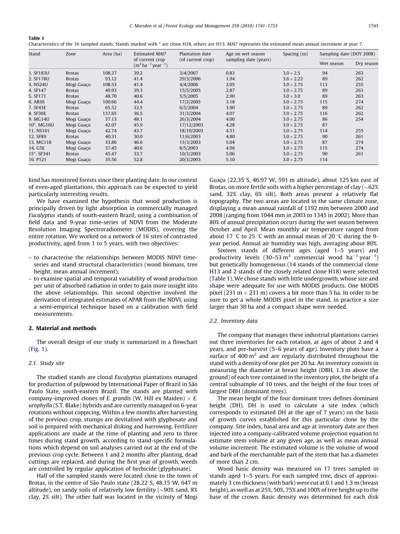
Table 1Characteristics of the 16 sampled stands. Stands marked with * are clone H18, others are H13. MAI7 represents the estimated mean annual increment at year 7.

Stand Zone Area (ha) Estimated MAI7

of current crop

(m3 ha�1 year�1)

Plantation date

(of current crop)

Age on wet season

sampling date (years)

Spacing (m) Sampling date (DOY 2008)

Wet season Dry season

1. SF183U Brotas 108.27 39.2 3/4/2007 0.83 3.0�2.5 94 263

2. SF178U Brotas 93.12 41.4 29/3/2006 1.94 3.6�2.22 89 262

3. NS24U Mogi Guacu 108.53 41.4 4/4/2006 2.05 3.0�2.75 113 255

4. SF147 Brotas 49.93 39.3 15/5/2005 2.87 3.0�2.75 89 263

5. SF171 Brotas 48.70 40.6 5/5/2005 2.90 3.0�3.0 89 263

6. AB36 Mogi Guacu 100.66 44.4 17/2/2005 3.18 3.0�2.75 115 274

7. SF43E Brotas 65.52 32.5 6/5/2004 3.90 3.0�2.75 89 262

8. SF36E Brotas 137.65 36.5 31/3/2004 4.07 3.0�2.75 116 262

9. MG14U Mogi Guacu 37.13 48.1 26/3/2004 4.00 3.0�2.75 86 254

10*. MG16U Mogi Guacu 42.07 45.9 17/12/2003 4.28 3.0�2.75 87

11. NS101 Mogi Guacu 42.74 43.7 18/10/2003 4.51 3.0�2.75 114 255

12. SF89 Brotas 40.31 30.0 11/6/2003 4.80 3.0�2.75 90 261

13. MG118 Mogi Guacu 33.86 46.6 13/3/2003 5.04 3.0�2.75 87 274

14. G5E Mogi Guacu 37.45 40.6 8/5/2003 4.96 3.0�2.75 115 274

15*. SF341 Brotas 45.47 33.7 10/3/2003 5.06 3.0�2.75 90 261

16. P121 Mogi Guacu 35.56 52.8 20/3/2003 5.10 3.0�2.75 114

C. Marsden et al. / Forest Ecology and Management 259 (2010) 1741–1753 1743

kind has monitored forests since their planting date. In our contextof even-aged plantations, this approach can be expected to yieldparticularly interesting results.

We have examined the hypothesis that wood production isprincipally driven by light absorption in commercially managedEucalyptus stands of south-eastern Brazil, using a combination offield data and 9-year time-series of NDVI from the ModerateResolution Imaging Spectroradiometer (MODIS), covering theentire rotation. We worked on a network of 16 sites of contrastedproductivity, aged from 1 to 5 years, with two objectives:

– to characterise the relationships between MODIS NDVI time-series and stand structural characteristics (wood biomass, treeheight, mean annual increment);

– to examine spatial and temporal variability of wood productionper unit of absorbed radiation in order to gain more insight intothe above relationships. This second objective involved thederivation of integrated estimates of APAR from the NDVI, usinga semi-empirical technique based on a calibration with fieldmeasurements.

2. Material and methods

The overall design of our study is summarized in a flowchart(Fig. 1).

2.1. Study site

The studied stands are clonal Eucalyptus plantations managedfor production of pulpwood by International Paper of Brazil in SaoPaulo State, south-eastern Brazil. The stands are planted withcompany-improved clones of E. grandis (W. Hill ex Maiden) � E.

urophylla (S.T. Blake) hybrids and are currently managed on 6-yearrotations without coppicing. Within a few months after harvestingof the previous crop, stumps are devitalised with glyphosate andsoil is prepared with mechanical disking and harrowing. Fertilizerapplications are made at the time of planting and zero to threetimes during stand growth, according to stand-specific formula-tions which depend on soil analyses carried out at the end of theprevious crop cycle. Between 1 and 2 months after planting, deadcuttings are replaced, and during the first year of growth, weedsare controlled by regular application of herbicide (glyphosate).

Half of the sampled stands were located close to the town ofBrotas, in the centre of Sao Paulo state (28.228S, 48.158W, 647 maltitude), on sandy soils of relatively low fertility (�90% sand, 8%clay, 2% silt). The other half was located in the vicinity of Mogi

Guacu (22.358S, 46.978W, 591 m altitude), about 125 km east ofBrotas, on more fertile soils with a higher percentage of clay (�62%sand, 32% clay, 6% silt). Both areas present a relatively flattopography. The two areas are located in the same climate zone,displaying a mean annual rainfall of 1192 mm between 2000 and2008 (ranging from 1044 mm in 2003 to 1345 in 2002). More than80% of annual precipitation occurs during the wet season betweenOctober and April. Mean monthly air temperature ranged fromabout 17 8C to 25 8C with an annual mean of 20 8C during the 9-year period. Annual air humidity was high, averaging about 80%.

Sixteen stands of different ages (aged 1–5 years) andproductivity levels (30–53 m3 commercial wood ha�1 year�1)but genetically homogeneous (14 stands of the commercial cloneH13 and 2 stands of the closely related clone H18) were selected(Table 1). We chose stands with little undergrowth, whose size andshape were adequate for use with MODIS products. One MODISpixel (231 m � 231 m) covers a bit more than 5 ha. In order to besure to get a whole MODIS pixel in the stand, in practice a sizelarger than 30 ha and a compact shape were needed.

2.2. Inventory data

The company that manages these industrial plantations carriesout three inventories for each rotation, at ages of about 2 and 4years, and pre-harvest (5–6 years of age). Inventory plots have asurface of 400 m2 and are regularly distributed throughout thestand with a density of one plot per 20 ha. An inventory consists inmeasuring the diameter at breast height (DBH, 1.3 m above theground) of each tree contained in the inventory plot, the height of acentral subsample of 10 trees, and the height of the four trees oflargest DBH (dominant trees).

The mean height of the four dominant trees defines dominantheight (DH). DH is used to calculate a site index (whichcorresponds to estimated DH at the age of 7 years) on the basisof growth curves established for this particular clone by thecompany. Site index, basal area and age at inventory date are theninjected into a company-calibrated volume projection equation toestimate stem volume at any given age, as well as mean annualvolume increment. The estimated volume is the volume of woodand bark of the merchantable part of the stem that has a diameterof more than 2 cm.

Wood basic density was measured on 17 trees sampled instands aged 1–5 years. For each sampled tree, discs of approxi-mately 3 cm thickness (with bark) were cut at 0.1 and 1.3 m (breastheight), as well as at 25%, 50%, 75% and 100% of tree height up to thebase of the crown. Basic density was determined for each disk

C. Marsden et al. / Forest Ecology and Management 259 (2010) 1741–17531744

using the maximum moisture content method (Smith, 1954). Treebasic density was then estimated by weighting the value measuredfor each disk by the volume of the corresponding trunk piece, andwas found to be linearly related to age (density(Mg m�3) = 0.032 � age (years) + 0.393, r2 = 0.87). Tree biomasswas obtained after multiplication of tree volume by the age-specific wood density deduced from this linear relationship.

We obtained company inventory data for all the stands wesampled and for all dates between 2000 and 2008. Inventorieswere also carried out following the same technique in April andSeptember 2008 on the inventory plots that we sampled. Whole-stand values of biomass, mean annual increment and DH wereestimated as the mean values from the inventory plots containedin the stand.

2.3. Hemispherical photography

Ground-truth measurements of the fraction of intercepted PARwere obtained using hemispherical photography. Digital hemi-spherical photographs were taken in the 16 stands in March–April2008 and in 14 stands in September 2008 (one stand was harvestedbetween the two sampling periods and another was inaccessible inSeptember), using a Fuji FinePix S5000 camera (3 mega pixels)fitted with a Nikon Fish-Eye FC–E9 lens in April, and a Nikon D40camera (6 mega pixels) with a Sigma EX DG Fisheye 1:3.5 lens inSeptember. Both camera-lens systems were calibrated accordingto the method proposed on http://www.avignon.inra.fr/can_eye inorder to determine their optical centre. A total of 24 photographsper stand and season combination were taken, in three inventoryplots per stand. In each 400 m2 inventory plot, eight positions weresampled, located on two diagonal transects. On each transect eachof the four following positions was represented: (1) on the row,between two trees; (2) on the inter-row, between two trees; (3) onthe inter-row, at the intersection of the diagonals between fourtrees; and (4) in the immediate vicinity of a tree. The camera wasplaced 1 m above the ground using a tripod, oriented and levelled.Photographs were taken in the early morning or late afternoon inlow-wind conditions, and exposition was adjusted in order toobtain maximum contrast between leaves and the sky. Thephotographs were stored as maximum quality JPEG files andtreated using the Can-Eye software (Jonckheere et al., 2004; Weisset al., 2004; Demarez et al., 2008) which allows the user to classifyeach pixel as a plant or sky (or mixed) element according to itscolour, rather than using a brightness threshold technique. Thissoftware also enables the user to define masks over trunks (forphotos taken in the immediate vicinity of a tree) or over regions ofthe photo of contrasted exposition, which could affect the qualityof the classification process. The eight photographs from eachinventory plot were treated simultaneously using the same colourclassification. The mean gap fraction per zenith angle of eachtreatment was recovered from the software output and the threeinventory plots were averaged in order to obtain the mean gapfraction per zenith angle of the stand, with a zenith angleresolution of 2.58 and a field of view of 578. The use of thedirectional gap fractions for the estimation of the fraction ofintercepted PAR is explained in a subsequent section.

2.4. MODIS data

We used data from the MODIS Terra Vegetation Index 16-Day250 m resolution V005 series (MOD13Q1), from March 2000 toJanuary 2009. This product is generated using daily surfacereflectance values which are corrected for atmospheric effects(molecular scattering, ozone absorption and aerosols, cf., Vermoteet al., 2002) and the daily values available during a 16-day periodare composited to provide one ‘‘best value’’ for each 16-day period.

Each ‘‘image’’ corresponding to a 16-day period contains, for eachpixel, the composited best NDVI value acquired during the periodand the corresponding EVI (enhanced vegetation index), red, nearinfrared and blue reflectance (red and NIR acquired at 250 mspatial resolution, blue acquired at 500 m resolution andresampled), the date of acquisition, sun and viewing angles, pixelreliability and vegetation index quality. Readers can refer to Hueteet al. (2002) and to the MODIS website (http://modis.gsfc.nasa.gov/data/atbd/land_atbd.php) for a synthetic overview of the MODIScompositing algorithm.

16-Day best NDVI values were interpolated to daily valuesrepresentative of each stand in three steps: (1) one representativeMODIS pixel position was selected for each stand; (2) atmo-spherically corrected, 16-day NDVI values, viewing geometryinformation and quality indices were extracted for these particularpixel positions; and (3) a smoothing curve was fitted on the data ofeach stand.

The studied stands are all large enough to encompass one ormore MODIS pixel (median size: 47 ha), but only one MODIS pixelposition was chosen to represent each stand during the 9-yeartime-series, following a systematic procedure involving the use ofhigh-resolution images, detailed in the Appendix A.

Once the MODIS pixel position was chosen for each stand, a 9-year time-series of 16-day MODIS NDVI was extracted for theseparticular pixels. The time-series were smoothed in order toeliminate variation that occurs on a short time scale, not reflectingcanopy changes but imputable to varying view angles and residualerrors from atmospheric correction, and to derive daily inter-polated values for subsequent use. We excluded data that did nothave both the best quality and pixel reliability flags. Data thatcorresponded to viewing zenith angles>408 were also excluded, aswell as values that were more than 10% lower than both thepreceding and following value, finally leaving about 92–99% of thedata for the curve-fitting process. We fitted a smoothing cubicspline function to the data, by minimizing both roughness (integralof the second derivative) and distance to data (sum of squarederrors). The relative importance of the two contributions dependson the value of a smoothing parameter which can vary from 0(linear regression: roughness minimized) to 1 (linear interpola-tion: distance to data minimized). We modulated the smoothingparameter around a baseline of 10�4 in order to ensure a close fitaround the lowest annual NDVI values.

2.5. Calculation of APAR

2.5.1. Summary of the procedure

Absorbed photosynthetically active radiation was obtainedfrom intercepted PAR after applying a correction to account forabsorption of non-intercepted or transmitted radiation reflectedupwards by the soil. An estimate of the fraction of photosynthe-tically active radiation intercepted by the canopy (fIPAR) was madefor every date between 2 March 2000 and 31 December 2008, usinga relationship between NDVI and canopy transmittance which wasestablished using gap fraction data obtained in March–April andSeptember 2008 by hemispherical photography. The fraction ofincoming radiation which is intercepted by the canopy varies withthe solar zenith angle (and therefore time of day) and with theproportion of direct radiation, and can be separated into diffuseand direct terms. While the fraction of intercepted diffuse PAR (fd)is constant during the day and only depends on canopy structure,the fraction of intercepted direct, or beam, PAR (fb) also depends onsun elevation. Our Eucalyptus stands intercept radiation all yearround, with variable solar elevations, and their clumped canopiesand high average leaf inclination angle mean directional effectsshould be taken into account. For this reason we distinguished fd

and fb in our calculations. Our field measurements of directional

C. Marsden et al. / Forest Ecology and Management 259 (2010) 1741–1753 1745

gap fractions were made at two periods of the year of similarmaximum daily solar elevation, so they did not allow us tocalibrate a direct relationship between NDVI, sun angle and fb. Inorder to estimate fb all year round, a procedure based on the shapeof the curve of gap fractions as a function of solar angle wasdeveloped.

2.5.2. Gap fractions as a function of zenith angle

The following equation (Warren Wilson, 1963; Anderson, 1966)describes gap fractions (GF) as a function of zenith angle u:

GFðuÞ ¼ exp½�kðuÞAP� (1)

where AP is the ‘‘effective plant area index’’ (Chen and Black, 1991;Kucharik et al., 1999: AP = PAI � l, where l is the clumping index(Nilson, 1971) and PAI is the plant area index), and k(u) is theextinction coefficient (for a ‘‘homogeneous’’ canopy; i.e., with arandom spatial distribution of leaves) for the angle u:

kðuÞ ¼ GðuÞcos u

(2)

The G(u) function (fraction of foliage projected in direction u) canbe expressed as follows:

GðuÞ ¼Z p=2

0Aðu; ulÞgðulÞdul (3)

where ul is leaf inclination angle, A is given in Nouvellon et al.(2000) and g (leaf angle distribution function) is a two parameterbeta distribution (Goel and Strebel, 1984).

NDVI viewed at a zenith angle uv can be empirically related tothe effective plant area index by the following equation (adaptedfrom Baret et al., 1995):

NDVIðuvÞ � NDVIveg

NDVIsðuvÞ � NDVIveg¼ exp½�kNDVIðuvÞAP� (4)

where NDVIveg is the maximum NDVI (the NDVI of densevegetation that would completely cover the soil surface, i.e.,AP!1), assumed independent of viewing angle; NDVIs is theminimum NDVI (corresponding to soil NDVI), and kNDVI(uv) is anextinction coefficient that depends on canopy structure and onsatellite viewing conditions (Baret and Guyot, 1991; Baret et al.,1995; Garrigues et al., 2006). Both terms in Eq. (4) increase with thefraction of soil background seen in viewing direction uv, from zerofor a fully covering vegetation, up to one for bare soil. NDVI canfurther be related to directional canopy gap fractions by combiningEq. (4) with Eq. (1) (Baret et al., 1995):

GFðuÞ ¼ NDVIðuvÞ � NDVIveg

NDVIsðuvÞ � NDVIveg

� �kðuÞ=kNDVIðuvÞ(5)

The value of k for any angle can be estimated using a priori

knowledge on canopy structure, but not kNDVI. However, since fora given u, k(u) and kNDVI(u) vary in a similar way with varyingcanopy structure, their ratio a can be expected to depend little oncanopy structure and was accordingly assumed to be constant,although it may depend on the sun angle (see Section 4). The valueof a can be obtained by non-linear fitting of measured GF(uv)values versus NDVI (see below, Step 2), allowing kNDVI to beinferred from k:

kNDVIðuvÞ ¼kðuvÞa

(6)

By replacing kNDVI from Eq. (6) in Eq. (5), gap fractions can beexpressed for any angle as a function of NDVI, a and k:

GFðuÞ ¼ NDVIðuvÞ � NDVIveg

NDVIsðuvÞ � NDVIveg

� �aðkðuÞ=kðuvÞÞ(7)

2.5.3. Fraction of intercepted photosynthetically active radiation

Welles and Norman (1991) proposed that fd could be calculatedby integrating directional GF from zero to p/2:

f d ¼ 2

Z p=2

0ð1� GFðuÞÞ cos u sin u du (8)

According to Nouvellon et al. (2000), fd can also be related to theeffective plant area index AP:

f d ¼ f max � ð1� expð�kd � APÞÞ (9)

where fmax corresponds to the asymptotic value of fd and kd is thediffuse extinction coefficient. A similar equation was used inseveral previous studies (e.g., Hipps et al., 1983; Asrar et al., 1984)to relate daily values of fIPAR to plant area index.

Using Eqs. (9) and (1), fd can be rewritten:

f d ¼ f max � ½1� GFðuÞkd=kðuÞ� (10)

In turn, Eqs. (7) and (10) yield:

f d ¼ f max � 1� NDVI� NDVIveg

NDVIs � NDVIveg

� �aðkd=kðuvÞÞ" #

(11)

The fraction of intercepted beam PAR (fb) at a given solar angleus can be calculated from GF(us) as its complement:

f bðusÞ ¼ 1� GFðusÞ (12)

Finally, Eqs. (7) and (12) can be combined to give:

f bðusÞ ¼ 1� NDVI� NDVIveg

NDVIs � NDVIveg

� �aðkðusÞ=kðuvÞÞ(13)

2.5.4. Estimation of fIPAR in three steps

Step 1: Calibration of the relationship between AP and fd.The three parameters of Eq. (1) (AP and two parameters of g)

were adjusted against measured directional gap fractions obtainedfrom the treatment of hemispherical photographs. The calibratedEq. (1) was then used in conjunction with Eq. (8) to obtain ahemispherical photography-derived estimation of fd for each standand season. Adjusted beta distribution parameters were found tovary with stand age, so a set of parameters were obtained for eachage class (0–1.5, 1.5–2.5, and >2.5 years) by fitting Eqs. (1)–(3)simultaneously on all data of that age class. This allowed thecalculation (using Eq. (2)) of age-dependent directional extinctioncoefficients k(u), specific to all stands of a given age class. A value ofAP was then obtained for each stand and season by fitting Eq. (1) onthe measured gap fraction curves. Note that, as we used arithmetic(suited for the study of fIPAR) rather than logarithmic (suited forstudy of PAI; Lang and Xiang, 1986) averaging of gap fractionsbetween photographs of the same stand, and as we made noattempt to model foliage clumping, the fitted parameters shouldnot be interpreted as estimations of PAI, effective PAI, leaf angledistribution parameters or canopy extinction coefficients and forthis reason are not presented. Eq. (9) was finally adjusted to fd andAP values in order to estimate fmax and kd.

Step 2: Calibration of the relationship between NDVI andcanopy gap fraction at viewing angle.

Eq. (5) was fitted to values of GF(uv) (obtained from fittedEq. (1)) and NDVI of the corresponding days (obtained from thesplined curves) in order to estimate a. Viewing angle, uv, was theaverage MODIS viewing angle during the study period (12.468).NDVIveg was set to 0.99 (5% more than the maximal observedNDVI), and the stand-specific NDVIs was taken as the minimumNDVI value attained between harvest and start of growth of thenext crop on the corresponding stand.

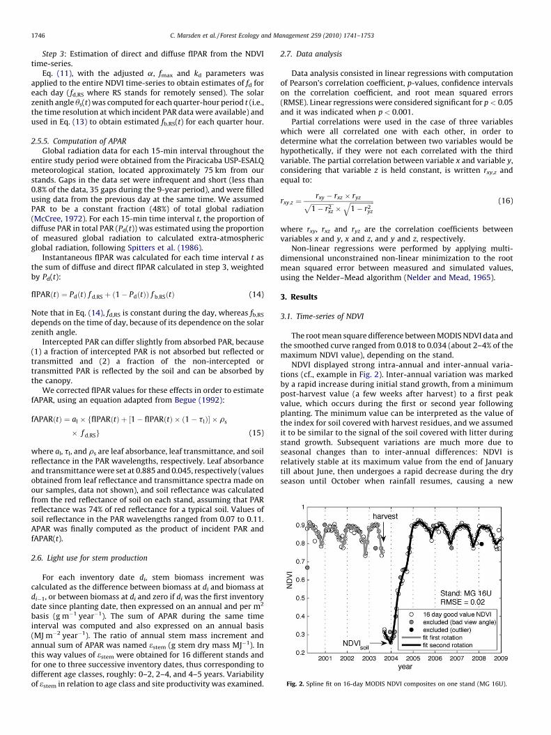
Fig. 2. Spline fit on 16-day MODIS NDVI composites on one stand (MG 16U).

C. Marsden et al. / Forest Ecology and Management 259 (2010) 1741–17531746

Step 3: Estimation of direct and diffuse fIPAR from the NDVItime-series.

Eq. (11), with the adjusted a, fmax and kd parameters wasapplied to the entire NDVI time-series to obtain estimates of fd foreach day (fd,RS where RS stands for remotely sensed). The solarzenith angle us(t) was computed for each quarter-hour period t (i.e.,the time resolution at which incident PAR data were available) andused in Eq. (13) to obtain estimated fb,RS(t) for each quarter hour.

2.5.5. Computation of APAR

Global radiation data for each 15-min interval throughout theentire study period were obtained from the Piracicaba USP-ESALQmeteorological station, located approximately 75 km from ourstands. Gaps in the data set were infrequent and short (less than0.8% of the data, 35 gaps during the 9-year period), and were filledusing data from the previous day at the same time. We assumedPAR to be a constant fraction (48%) of total global radiation(McCree, 1972). For each 15-min time interval t, the proportion ofdiffuse PAR in total PAR (Pd(t)) was estimated using the proportionof measured global radiation to calculated extra-atmosphericglobal radiation, following Spitters et al. (1986).

Instantaneous fIPAR was calculated for each time interval t asthe sum of diffuse and direct fIPAR calculated in step 3, weightedby Pd(t):

fIPARðtÞ ¼ PdðtÞ f d;RS þ ð1� PdðtÞÞ f b;RSðtÞ (14)

Note that in Eq. (14), fd,RS is constant during the day, whereas fb,RS

depends on the time of day, because of its dependence on the solarzenith angle.

Intercepted PAR can differ slightly from absorbed PAR, because(1) a fraction of intercepted PAR is not absorbed but reflected ortransmitted and (2) a fraction of the non-intercepted ortransmitted PAR is reflected by the soil and can be absorbed bythe canopy.

We corrected fIPAR values for these effects in order to estimatefAPAR, using an equation adapted from Begue (1992):

fAPARðtÞ ¼ al � ffIPARðtÞ þ ½1� fIPARðtÞ � ð1� tlÞ� � rs

� f d;RSg (15)

where al, tl, and rs are leaf absorbance, leaf transmittance, and soilreflectance in the PAR wavelengths, respectively. Leaf absorbanceand transmittance were set at 0.885 and 0.045, respectively (valuesobtained from leaf reflectance and transmittance spectra made onour samples, data not shown), and soil reflectance was calculatedfrom the red reflectance of soil on each stand, assuming that PARreflectance was 74% of red reflectance for a typical soil. Values ofsoil reflectance in the PAR wavelengths ranged from 0.07 to 0.11.APAR was finally computed as the product of incident PAR andfAPAR(t).

2.6. Light use for stem production

For each inventory date di, stem biomass increment wascalculated as the difference between biomass at di and biomass atdi�1, or between biomass at di and zero if di was the first inventorydate since planting date, then expressed on an annual and per m2

basis (g m�1 year�1). The sum of APAR during the same timeinterval was computed and also expressed on an annual basis(MJ m�2 year�1). The ratio of annual stem mass increment andannual sum of APAR was named estem (g stem dry mass MJ�1). Inthis way values of estem were obtained for 16 different stands andfor one to three successive inventory dates, thus corresponding todifferent age classes, roughly: 0–2, 2–4, and 4–5 years. Variabilityof estem in relation to age class and site productivity was examined.

2.7. Data analysis

Data analysis consisted in linear regressions with computationof Pearson’s correlation coefficient, p-values, confidence intervalson the correlation coefficient, and root mean squared errors(RMSE). Linear regressions were considered significant for p < 0.05and it was indicated when p < 0.001.

Partial correlations were used in the case of three variableswhich were all correlated one with each other, in order todetermine what the correlation between two variables would behypothetically, if they were not each correlated with the thirdvariable. The partial correlation between variable x and variable y,considering that variable z is held constant, is written rxy,z andequal to:

rxy;z ¼rxy � rxz � ryzffiffiffiffiffiffiffiffiffiffiffiffiffiffi

1� r2xz

p�

ffiffiffiffiffiffiffiffiffiffiffiffiffiffiffi1� r2

yz

q (16)

where rxy, rxz and ryz are the correlation coefficients betweenvariables x and y, x and z, and y and z, respectively.

Non-linear regressions were performed by applying multi-dimensional unconstrained non-linear minimization to the rootmean squared error between measured and simulated values,using the Nelder–Mead algorithm (Nelder and Mead, 1965).

3. Results

3.1. Time-series of NDVI

The root mean square difference between MODIS NDVI data andthe smoothed curve ranged from 0.018 to 0.034 (about 2–4% of themaximum NDVI value), depending on the stand.

NDVI displayed strong intra-annual and inter-annual varia-tions (cf., example in Fig. 2). Inter-annual variation was markedby a rapid increase during initial stand growth, from a minimumpost-harvest value (a few weeks after harvest) to a first peakvalue, which occurs during the first or second year followingplanting. The minimum value can be interpreted as the value ofthe index for soil covered with harvest residues, and we assumedit to be similar to the signal of the soil covered with litter duringstand growth. Subsequent variations are much more due toseasonal changes than to inter-annual differences: NDVI isrelatively stable at its maximum value from the end of Januarytill about June, then undergoes a rapid decrease during the dryseason until October when rainfall resumes, causing a new

Fig. 3. Variability of NDVI curves during first 2 years of growth. All curves have been

placed so that values corresponding to day of year (DOY) 1 have the same abscissa.

Vertical dashed lines indicate DOY 1 of first (year n + 1) and second (year n + 2)

years after planting. The vertical arrow indicates DOY 150 (end of the wet season) of

year n + 1.

Fig. 5. Mean NDVI since planting date versus MAI7, calculated at different ages. The

linear regression equation (solid line) is given for mean NDVI of first 2 years. The

dotted lines represent regressions at the four other ages.

C. Marsden et al. / Forest Ecology and Management 259 (2010) 1741–1753 1747

increase in NDVI. After the second year, both minimum andmaximum NDVI values decrease significantly with age (r = �0.43and p < 0.001 for maximum NDVI and r = �0.34 and p < 0.001 forminimum NDVI).

3.2. NDVI during initial stand growth

Large differences between stands are visible during initial standdevelopment (Fig. 3), before canopy closure which occurs sometime during the second year after planting. After the establishmentof a new crop, there is an interval of variable length during whichNDVI does not increase significantly, followed by a steep increasein NDVI after the onset of the first wet season after planting, atsimilar rates between stands (average increase of NDVI of 0.1 in amonth). Maximum NDVI on day of year (DOY) 150 (end of wetseason) of the year following planting is negatively linearlycorrelated with planting DOY (r = �0.89 and p < 0.01). Insubsequent years the peaks attained are much more similarbetween stands.

Fig. 4. Commercial stem volume (a) and dominant height (b) calculated using inventory d

the sum of daily NDVI during the first 2 years of growth.

3.3. Empirical relationships between cumulative NDVI and volume

and height

Stand age (years since planting date) explained 78% (p < 0.001,n = 30) of the variability of stem volume at inventory dates,whereas the sum of daily NDVI since planting explained 87%(volume = 0.19 � NDVIcum � 41.94; r2 = 0.87, p < 0.001, n = 30).There is a highly significant correlation between age and sum ofNDVI (r2 = 0.98), yet the squared partial correlation coefficient ofcumulative NDVI and volume, with effect of age removed, wasr2 = 0.67 (p < 0.001). Therefore, cumulative NDVI since plantingcarried information about stand volume that was not due to itscorrelation with age. A linear model including age and the sum ofNDVI during the first 2 years succeeded in explaining 92% ofvariability in volume (RMSE = 23.8 m3 ha�1, Fig. 4a).

Stronger empirical relationships were found with dominantheight: age explained 87% (p < 0.001, n = 26) of variation in DH atinventory dates and cumulative NDVI explained 93%(DH = 0.02 � NDVIcum + 5.84; r2 = 0.93, p < 0.001, n = 26). Thelinear regression can be considered valid for cumulative NDVI of500–1600 (outside these bounds we did not have sufficient data toallow extrapolation). Partial correlation of cumulative NDVI and

ata, versus values simulated using the presented linear functions of age (years) and

Table 2Squared correlation coefficients of correlation between mean NDVI and MAI7 for 1–

5 years after plantation, using mean NDVI between planting date and age i (left

column), or mean during the ith year (right column).

Year i n r2 of MAI7 versus mean

NDVI of years 0 to i

r2 of MAI7 versus mean

NDVI of year i

1 16 0.61** 0.61**

2 15 0.75** 0.71**

3 13 0.77** 0.55*

4 10 0.81** 0.39

5 7 0.83* 0.49

n is the number of data.* p-Values <0.05.** p-Values <0.001.

Fig. 7. Annual APAR of consecutive years on all stands. In thick grey and black lines:

stands SF 89 (least productive) and P121 (most productive), respectively.

C. Marsden et al. / Forest Ecology and Management 259 (2010) 1741–17531748

DH, with effect of age removed, was significant (r2 = 0.64 andp < 0.001). A linear model including age and the sum of NDVIduring the first 2 years explained 96% of variability in observedheights (RMSE = 1.25 m, Fig. 4b).

3.4. Empirical relationship between mean NDVI and productivity

Mean NDVI of the first 2 years after planting explained 75% ofthe variation in productivity (Fig. 5), when productivity wasrepresented using the Mean Annual Increment (in commercialstem volume) for an age of 7 years (MAI7, m3 ha�1 year�1), whichwas estimated from inventory data using company-calibratedclone-specific growth equations. As age increases, the correlationcoefficient between mean NDVI since planting and MAI7 increases(Table 2, left column), but the increase is not significant (95%confidence intervals of the r2 overlap, not shown). Mean annualNDVI of the second year (i.e., between days 366 and 730 afterplanting) was more closely correlated with MAI7 than that of thefirst year, followed by that of the third (Table 2, right column).Annual mean NDVI during the 4th and 5th year after planting werenot significantly correlated with MAI7.

3.5. Deriving fIPAR from NDVI

Fractions of intercepted diffuse PAR (fd) estimated usinghemispherical photography ranged from 0.65 to 0.91 dependingon the stand, and were significantly lower (p = 0.03) during the dryseason than during the wet season (means of 0.86 in April, 0.82 inSeptember), although the wet season mean was decreased by the

Fig. 6. Simulated (using measured NDVI values and fitted a parameter in Eq. (5)) ga

photographs (a); and fraction of intercepted diffuse PAR simulated using Eq. (11) versus

study period. The 1:1 line is presented (dashed line).

low value obtained on the 1-year-old stand (0.65). There was astrong non-linear relationship between fd and the effective plantarea index AP computed from hemispherical photographs, whichwas fitted with Eq. (9) (r2 = 0.85 between measured and simulatedvalues, and estimated parameters fmax = 0.94 and kd = 0.81).

Values of gap fractions at a zenith angle of 12.468 (GF(uv))obtained directly from photographs and those simulated usingEq. (7) (which relates GF(uv) to NDVI and soil NDVI) weresignificantly correlated (r2 = 0.50 and p<0.001; Fig. 6a), as were fd

obtained from photographs and those simulated using Eq. (11)(r2 = 0.60 and p < 0.001; Fig. 6b).

3.6. Time course of IPAR

APAR was systematically lower than IPAR, and cumulativevalues were linearly related with a slope of 0.9 and an intercept of19 MJ m�2 (not significantly different from 0). Daily APAR wasvariable, ranging from 1.45 to 10.98 MJ m�2 day�1 for fullydeveloped canopies, and cumulative values since plantingincreased more or less linearly with time. Annual cumulativevalues of APAR ranged from about 1000 (for first year afterplanting) to about 2200 MJ m�2 year�1 (Fig. 7). These values are

p fractions at MODIS viewing angle uv versus those derived from hemispherical

fd obtained from photographs (b). Average viewing angle uv was 12.468 during the

Fig. 8. Annual stem production versus annual APAR, based on biomass increment

and absorbed PAR between the considered inventory date and the preceding date or

planting date. Age groups represent approximate age at inventory date. Lines join

data representing the same stand at successive inventories.

Fig. 9. estem versus site index (estimated dominant height at age 7 years). For one

value of site index (one stand), one to three values of estem are represented,

corresponding to different inventory dates and therefore different age classes. The

solid line represents the linear regression between site index and estem estimated at

age 2 years whereas the dashed line represents the linear regression for later

inventories.

C. Marsden et al. / Forest Ecology and Management 259 (2010) 1741–1753 1749

high, reflecting the ability of these Eucalyptus stands to intercepta large fraction (�70%) of incoming radiation all year round.Annual APAR was more variable between stands during the firstand second years than during subsequent years, and attained apeak during the third year of growth, before showing a slighttendency to decline. The highest and lowest annual APAR wererecorded, respectively, on the most and least productive stands(Fig. 7).

Table 3Number of data, mean, minimum, maximum, and standard deviation of estem for each

estem (g dry stem mass MJ�1APAR (IPAR)) <1 year 2 years

Number of data 1 15

Mean 0.28 (0.26) 0.85 (0

Minimum 0.45 (0

Maximum 1.21 (1

Standard deviation 0.22 (0

3.7. APAR and wood production

Biomass increments and cumulative APAR between inventoriesare presented in Fig. 8 on an annual basis. The graph should beinterpreted with caution, as data from the same age interval maynot be quite comparable between different stands. Inventories arenot undertaken at exact ages, meaning that time intervals betweeninventories can vary from one stand to the next, and possiblyrepresent different contributions of wet and dry seasons. As wehad no detailed information on how stem growth rates variedduring the year we were not able to correct this possible bias.Nevertheless, it appears that during the first 2 years of growth (forinventories at age <1 and �2 years), APAR and stem biomassincrement are positively correlated (r2 = 0.78 and p < 0.001). Afterthe age of 4 years, annual APAR is similar between stands (Fig. 7)and is no longer correlated with production levels (Fig. 8).

Stem dry mass increment per unit APAR (estem, in gDM MJ�1APAR)

was variable, ranging from 0.28 gDM MJ�1 for the youngest stand(aged 0.8 year) to 2.26 gDM MJ�1

APAR for the most productive P121stand at its second inventory (Table 3). estem increased from age�2to �4. From age �4 to �5, data with both ages were only availablefor three stands, and estem did not change significantly.

Over the entire data set, there was a significant linearrelationship between estem and site index (SI), which can beconsidered as an indicator of productivity levels that can beattained on a given stand (r2 = 0.32 and p = 0.001). Stronger linearrelationships existed between SI and estem at the first inventory(estem,2 years = 0.07 � SI � 1.12; r2 = 0.85 and p < 0.001; Fig. 9), andbetween SI and estem at older ages (estem,4–6 years = 0.06 � SI � 0.14;r2 = 0.49 and p = 0.005; Fig. 9). Regressions for different agesshowed similar slopes but a different y-intercept. APAR during thefirst 2 years was also strongly related to site index (APARcum,2

years = 109 � SI � 149; r2 = 0.80 and p < 0.001).

4. Discussion

4.1. Choice of satellite data

We chose to work with the NDVI rather than with readilyavailable GPP or fAPAR estimates of the MODIS products MOD17and MOD15, whose focus is on global estimates of productionrather than on the detection of the finer-scale differences withinone crop type. The accuracy of these algorithms can be affectedby the landcover classification of each pixel into one of the sixbiomes (Myneni et al., 2002). More importantly, the spatialresolution of these products (1 km) is too low to meet ourrequirements, which are imposed by the work on mosaics ofplantation stands of less than one MOD17 grid-cell in size. Onthe other hand the MODIS NDVI product (MOD13) presented theadvantages of good temporal resolution, sufficient spatialresolution (231 m), atmospheric correction, filtering of goodvalues performed by the compositing algorithm and a qualityflag for each pixel. Our data could further be used for the localvalidation of the MOD15 fAPAR product, after aggregation ofcontiguous MOD13 pixels that represent adjoining stands ofsimilar characteristics.

age class, calculated using APAR (bold) or IPAR (italics).

4 years 5 years All

9 5 30

.77) 1.62 (1.46) 1.55 (1.39) 1.18 (1.06)

.41) 1.28 (1.15) 1.24 (1.12) 0.28 (0.26)

.10) 2.26 (2.03) 1.95 (1.76) 2.26 (2.03)

.20) 0.28 (0.25) 0.30 (0.27) 0.47 (0.43)

C. Marsden et al. / Forest Ecology and Management 259 (2010) 1741–17531750

4.2. Integrated NDVI for estimation of stem volume and dominant

height

We found a strong correlation between cumulative NDVI andstand volume, and between cumulative NDVI and dominantheight. In both cases a linear relationship including stand age andcumulative NDVI could explain more than 92% of the variabilityobserved during different inventories on the sampled stands. Ourresults, using moderate resolution satellite imagery, are compar-able to those found in some other applications of remote sensingfor estimation of forest wood production, that succeeded inexplaining 65–92% of variability in height and above-groundbiomass of different types of forests using satellite images ofvarious resolutions (e.g., Tomppo et al., 2002; Leboeuf et al., 2007),light detection and ranging (LIDAR) metrics (e.g., Lefsky et al., 2002,2005; Drake et al., 2003) or radar backscatter (e.g., Rauste et al.,1994). It is likely that the form of the relationships we haveestablished between integrated NDVI and stand characteristics canbe extended to other Eucalyptus plantations, providing a localcalibration is carried out to account for climatic and geneticdifferences. The retrieval and incorporation into a GeographicalInformation System (GIS) of MODIS NDVI time-series andintegrated values representative of individual stands is simpleto implement on an operational basis. Different applications arepossible. For example, the NDVI trajectory of stands of similar ageand site index can be compared, possibly allowing the detection ofabnormal drops in leaf area index, or retrospective analysis of a lossof productivity in relation to light absorption on a given stand.Classic forest inventories (which require costly spatially intensivesampling) could be complemented by free MODIS information.Access to NDVI time-series through a GIS could allow a simpleassessment of biomass and dominant height over large zonesplanted since March 2000. It must however be noted that the RMSEon retrieved volume or dominant height (24 m3 ha�1 and 1.25 m,respectively) are of the same order of magnitude as the expectedannual volume increment (at least 30 m3 ha�1 year�1) and heightincrement (about 5 m year�1). An additional limitation is due tothe large pixel size of MODIS data which restricts simpleoperational use to large stands.

4.3. Deriving APAR from NDVI

The fraction of absorbed PAR, necessary for computation ofAPAR, has often been estimated using field measurements of leafarea index and an assumed or estimated value for the lightextinction coefficient (Harrington and Fownes, 1995; Drolet et al.,2005; Stape et al., 2008). This approach either requires theassumption that canopy LAI is near constant during most of thegrowing season (Bartelink et al., 1997), or intensive temporalsampling of leaf area index. The use of time-series of remotelysensed vegetation index values with a good temporal resolutionwas therefore a valuable tool, as it allowed us to estimate dailyAPAR retrospectively since planting on the 16 sampled stands andin particular during the critical phase at the start of growth.

We estimated APAR as the sum of a diffuse and a directcomponent. A simpler procedure could be envisaged if thisseparation were disregarded, i.e., if APAR were calculated simplyas the product of PAR and the fraction of intercepted diffuse PAR. Inthis case one unique equation would be needed for the estimationof the fraction of intercepted radiation from NDVI values, butintercepted PAR would be overestimated by approximately 15%.

Our APAR estimates carry uncertainty that can be due to severalreasons. First of all, NDVI–fAPAR relationships are near-linear, butpresent a certain natural dispersion, as has been shown bysimulation studies using radiative transfer models (Baret andGuyot, 1991; Begue, 1993; Myneni and Williams, 1994; Walter-

Shea et al., 1997) because of the effects of varying leaf angles,optical properties of leaves, cover fractions and canopy clumping(all of which can potentially vary with age and season in wayswhich are not well known), soil background reflectance andsatellite viewing conditions (Huete and Liu, 1994; Myneni andWilliams, 1994). This means that our unique equation relatingNDVI to fAPAR might be unable to detect certain differences infAPAR (those that do not affect NDVI), and inversely might detectdifferences that do not exist in reality. In principle the spliningapproach smoothed out variations due to differences in viewingangle configurations, but it could not eliminate the potential effectof seasonal variations of the maximum daily solar elevation angle.However work by Pinter (1993) indicates that this effect should besmall. The equation we used to relate canopy gap fraction to NDVI(Baret et al., 1995) aimed to eliminate part of the variabilityassociated with different soil background reflectances, usinginformation about soil reflectance that we derived from post-harvest NDVI values. Other approaches have been proposed toreduce the effects of varying soil backgrounds and atmosphericconditions, often involving the use of one or several additionalspectral bands (blue for the EVI (Huete and Liu, 1994), MIR for theNDVIc (Nemani et al., 1993), for example). In the case of MODIS theother bands are only available at a 500 m resolution, making themdifficult to use for our study because of the size of our stands.Different soil adjusted indices have also been suggested, in whichinformation about the soil line (relationship between NIR and redreflectance of bare soil) is used to correct the vegetation index (e.g.,the GESAVI; Gilabert et al., 2002). Wishing to facilitate operationalapplication of our findings, we retained the easily available NDVI,that presented similar results to the SAVI and GESAVI.

Some imprecision may arise from the use of hemisphericalphotography to get field estimations of fIPAR, mainly because oftwo problems associated with the technique, i.e., variableexposition which affects image classification, and insufficientspatial resolution that results in a non-negligible proportion ofmixed pixels (Macfarlane et al., 2000, 2007). Finally, the smallnumber of gap fraction measurements in the 0–1 age class limitsthe reliability of NDVI-derived APAR estimates obtained during thefirst year after planting.

4.4. APAR and stem wood production

The estimation of APAR from NDVI values allowed us toinvestigate the relations between wood biomass production andlight interception, for three different age intervals: from plantingdate to age �2 years; from age �2 to �4 years, and from age �4 to�5 years. The values of estem that we present correspond to gramsof stem wood dry mass produced per MJ of PAR absorbed by thecanopy during a specified time interval. Most e (light useefficiency) values found in the literature for forests and tree cropswere derived from estimates of intercepted rather than absorbedradiation. In our case, the lack of correction to account for leaftransmittance and re-interception of soil-reflected radiation wouldhave led to 11% lower estem values, which is a slightly largercorrection factor than that given by Gower et al. (1999), due to thehigh transmittance and reflectance observed on our sampledleaves. We found a wide range of values for estem, with a mean overall age intervals and all stands of 1.18 gDM MJ�1

APAR. We presentvalues of estem, rather than eANPP (grams of above-ground netprimary production per MJ of APAR), and therefore do not take intoaccount leaf, branch or bark production: eANPP could be expected tobe of the order of 20% higher. Bearing this in mind, our resultscorrespond to the upper half of the eANPP values published forEucalyptus species (summarized by Whitehead and Beadle (2004)and additional values derived from Giardina et al. (2003), Stapeet al. (2004a, 2008), and du Toit (2008)), which range from low

C. Marsden et al. / Forest Ecology and Management 259 (2010) 1741–1753 1751

values of 0.47 gDM MJ�1APAR in zones where water availability is

limited to maximum values of 2 gDM MJ�1APAR in highly productive

environments.

4.5. Age and estem

APAR increased until the age of 2 years, then stagnated andshowed a slight tendency to decline. This tendency is the result ofthe strongly dynamic leaf area index in these Eucalyptus

plantations, which is known to peak at about 2–3 years of ageand then decrease (e.g., Almeida et al., 2007). The decrease in LAIleads to a smaller, but noticeable, decline in fAPAR because of theasymptotic relationship between the two. For young stands (�2years), wood production was correlated to APAR, but this was nolonger the case for older stands. A similar observation was made byGoetz and Prince (1996): IPAR and ANPP were linearly related inyoung aspen stands and not in mature stands. They suggested thatANPP was limited by factors other than light, which affected olderstands more strongly than young ones: allocation to maintenancerespiration, periodic drought stress for instance. Harrington andFownes (1995) showed that during periods of limited watersupply, eANPP decreased and Stape et al. (2008) also showed thatyears of limited rainfall, or lack of irrigation, were associated withlower eANPP.

Our study showed clear differences in estem calculated atdifferent ages: low estem was found for the first 2 years of growth,and higher values were obtained for the 2–4 and 4–5 yearsintervals. Lower estem during initial stand growth makes sense,because trees are expected to invest a large proportion ofphotosynthates in the building of their resource-capturing organs,namely leaves and roots (Saint-Andre et al., 2005; Laclau et al.,2009). Hunt (1994) indicated that estem decreased with age afterstand maturity had been reached, but this was not visible in our 5-year-old stands, perhaps because we had only few stands thatattained this age, and because these plantations are harvestedbefore a significant decrease in eANPP occurs.

4.6. Site index and estem

Our results showed a clear relation between estem and site index(SI), corroborating the observation made by several authors thatmore productive stands are also more efficient at using capturedresources (Giardina et al., 2003; Binkley et al., 2004; Stape et al.,2004a, 2008). A better SI was accompanied by an increase both inAPAR during initial growth (like in du Toit (2008) where increasedfertility led to a more rapid canopy establishment), and in estem forall ages. Age also had an effect on estem as was discussed earlier, butthis age effect and that of SI appeared to be independent (Fig. 9).This result explains why mean NDVI of the first 2 years of growthexplained productivity as well as mean NDVI of a whole rotation: itis only during the first 2 years that fertility-related effects onproductivity are reflected in leaf display, and therefore in NDVI.

The effects of the site index on growth are strongly reflected inthe NDVI during the first 2 years after planting: this result offers arelatively simple way of deriving the SI from time-series ofremotely sensed data. The SI synthesizes factors that limitproduction, e.g., in particular soil nutrition and water holdingcapacity within one climatic zone. In the 3-PGS model of forestproduction (Landsberg and Waring, 1997; Coops et al., 1998), themaximum light use efficiency for NPP depends linearly on a ‘‘sitefertility rating’’ (generally inferred from soil maps), which alsodetermines the fraction of carbon allocated to fine roots. As the sitefertility rating is a sensitive parameter in the model, there is ademand for a practical means allowing its estimation in view ofoperational applications of 3-PGS (Esprey et al., 2004; Paul et al.,2007; Miehle et al., 2009). Our results indicate that the NDVI

during the first 2 years after planting could be used for the spatialdetermination of site fertility ratings, provided the SI weredecorrelated from the soil water balance. In addition there wasa highly significant relationship between cumulative NDVI duringthe first 2 years and estem,2 years (not shown). Providing therelationship between estem and age were established more clearly,the direct spatialized estimation of light use efficiency for stemwood production using NDVI data could be envisaged.

The explanation and quantitative understanding of age andfertility-related shifts in light use efficiency for stem production liein a better knowledge of allocation patterns in relation to nutrientand water availability. Mechanistic modelling approaches incor-porating different types of remotely sensed information on canopycharacteristics have proved to be capable of evaluating carbonbudgets in other forest environments (le Maire et al., 2005). In thislight the data we have obtained on temporal and spatial variationsof the fraction of absorbed PAR and of estem appear to be potentiallyvaluable for spatialized modelling applications aiming to under-stand and quantify carbon, water and nutrient budgets of fast-growing Eucalyptus plantations.

5. Conclusions

Fast growing even-aged forest plantations, characterised bywithin-stand homogeneity and strong temporal dynamics markedby clear-felling and same-date planting, offer high potential for theoperational use of remote sensing in forest management. Whileone-date values of MODIS NDVI may be useful for the estimation ofleaf area index (bearing in mind saturation problems), they are notsufficient to discriminate between biomass production levels. Incontrast, NDVI time-series can easily be obtained over largeplantation areas, and can be used for the monitoring of productionand estimation of site productivity: cumulative NDVI was a goodpredictor of stem volume and dominant height, and NDVI of thefirst 2 years of growth explained 75% of the variability inproductivity of 16 different Eucalyptus stands in a same climaticzone.

We present a simple empirical method for the determination ofabsorbed photosynthetically active radiation using time-series of250 m resolution satellite data. APAR can be used to drive variousprocess-based models of forest production. Production of stemwood biomass per unit of absorbed PAR varied with age and siteindex. Production was correlated to absorbed radiation during thefirst 2 years of growth but not in later years, where productivitydifferences were not reflected in canopy light interception. Siteindex affected both estem at all ages and APAR during the initialdevelopment of the canopy. A promising implication is that NDVIvalues obtained during the first 2 years of growth can help toprovide an empirical estimate of site-dependent light useefficiency for stem wood production.

Acknowledgements

This study was funded by the European Integrated Project UltraLow CO2 Steelmaking (ULCOS—contract no. 515960) and by CNPq306561/2007. We thank International Paper of Brasil and inparticular Jose Mario Ferreira and Sebastiao Oliveira, for providingdata and technical help for field campaigns, and the FrenchMinistry of Foreign Affairs for their financial support. We are alsovery grateful to Flavio Ponzoni (INPE), Marcos Ligo (EMBRAPA),Elcio Reis (IPBr), Cristiane Camargo Zani (ESALQ), Giampiero BiniCano (Instituto Botanico), Renato Meulman Leite da Silva (ESALQ),and Reinaldo Camargo (ESALQ) for their help during field work.Finally we thank Jean-Paul Laclau and the anonymous reviewersfor their helpful advice and valuable comments on how to improvethe manuscript.

C. Marsden et al. / Forest Ecology and Management 259 (2010) 1741–17531752

Appendix A. Choice of a representative MODIS pixel for eachstand

We chose one MODIS pixel to represent each stand. The centralpixel was not necessarily chosen because (1) the position of theMODIS pixel is subject to uncertainties and (2) the central MODISpixel is not necessarily representative of the entire stand. Asystematic procedure involving the use of high-resolution CBERS-2CCD was developed to select the most representative pixel for eachstand. The principle was to select, among the MODIS pixelpositions that cover a given stand, the one that had the reflectancevalues closest to those of the whole stand as observed in the high-resolution image. The CBERS-2 satellite was launched in 2003 aspart of the China-Brazil Earth Resources Satellite programme. ItsCCD camera provides multi-spectral images with 20 m spatialresolution and 26-day temporal resolution. All clear imagesavailable since 2004 (about 20 images per tile, with four tiles tocover all stands) were downloaded and geographically correctedagainst a geo-referenced Landsat image. The atmosphericallycorrected MODIS images of the corresponding dates (MOD09GQSurface Reflectance Daily L2G Global 250 m, Collection 5) were alsodownloaded. Before extracting stand pixel values from the high-resolution images, the images had to be converted to reflectancevalues and also atmospherically corrected. Here, both steps werecarried out in a single relative calibration procedure using same-date MODIS images. The CBERS-2 digital counts were aggregated tothe MODIS grid to obtain a resolution of 231.65 m. For each date alinear relationship was fitted between the aggregated CBERS-2 redand NIR band digital counts and the MODIS reflectance values. Thecoefficients of this regression were applied to the original CBERS-2images in order to obtain MODIS-equivalent reflectance valueimages with 20 m spatial resolution. A mean NDVI value for eachdate (about 20 dates) was extracted from these corrected CBERS-2images for each stand (from the pixels contained inside the contourof the stand, allowing a buffer strip of 60 m). The NDVI of theMODIS pixels which were included in the stand delimitations wasalso extracted. For each of these MODIS pixels a linear correlationcoefficient was calculated between the 20 MODIS NDVI values andthe 20 mean stand NDVI values. The MODIS pixel that offered thehighest correlation coefficient was selected as the most repre-sentative pixel of the stand.

References

ABRAF, 2009. Anuario estatistico da ABRAF 2009, ano base 2008. AssociacaoBrasileira de Produtores de Florestas Plantadas, Brasilia, p. 129.

Almeida, A.C., Soares, J.V., Landsberg, J.J., Rezende, G.D., 2007. Growth and waterbalance of Eucalyptus grandis hybrid plantations in Brazil during a rotation forpulp production. Forest Ecology and Management 251, 10–21.

Anderson, M.C., 1966. Stand structure and light penetration. II. A theoreticalanalysis. Journal of Applied Ecology 3, 41–54.

Asrar, G., Fuchs, M., Kanemasu, E.T., Hatfield, J.L., 1984. Estimating absorbedphotosynthetic radiation and leaf area index from spectral reflectance in wheat.Agronomy Journal 76, 300–306.

Baret, F., Guyot, G., 1991. Potentials and limits of vegetation indexes for LAI andAPAR assessment. Remote Sensing of Environment 35, 161–173.

Baret, F., Clevers, J., Steven, M.D., 1995. The robustness of canopy gap fractionestimates from red and near-infrared reflectances—a comparison ofapproaches. Remote Sensing of Environment 54, 141–151.

Bartelink, H.H., Kramer, K., Mohren, G.M.J., 1997. Applicability of the radiation-useefficiency concept for simulating growth of forest stands. Agricultural andForest Meteorology 88, 169–179.

Begue, A., 1992. Modeling hemispherical and directional radiative fluxes in regular-clumped canopies. Remote Sensing of Environment 40, 219–230.

Begue, A., 1993. Leaf-area index, intercepted photosynthetically active radiation,and spectral vegetation indexes—a sensitivity analysis for regular-clumpedcanopies. Remote Sensing of Environment 46, 45–59.

Binkley, D., Stape, J.L., Ryan, M.G., 2004. Thinking about efficiency of resource use inforests. Forest Ecology and Management 193, 5–16.

Chen, J.M., Black, T.A., 1991. Measuring leaf-area index of plant canopies withbranch architecture. Agricultural and Forest Meteorology 57, 1–12.

Coops, N.C., Waring, R.H., Landsberg, J.J., 1998. Assessing forest productivity inAustralia and New Zealand using a physiologically-based model driven with

averaged monthly weather data and satellite-derived estimates of canopyphotosynthetic capacity. Forest Ecology and Management 104, 113–127.

Coops, N.C., Waring, R.H., 2001. The use of multiscale remote sensing imagery toderive regional estimates of forest growth capacity using 3-PGS. Remote Sen-sing of Environment 75, 324–334.

Cramer, W., Kicklighter, D.W., Bondeau, A., Moore, B., Churkina, C., Nemry, B.,Ruimy, A., Schloss, A.L., 1999. Comparing global models of terrestrial netprimary productivity (NPP): overview and key results. Global Change Biology5, 1–15.

Daughtry, C.S.T., Gallo, K.P., Goward, S.N., Prince, S.D., Kustas, W.P., 1992. Spectralestimates of absorbed radiation and phytomass production in corn and soybeancanopies. Remote Sensing of Environment 39, 141–152.

Demarez, V., Duthoit, S., Baret, F., Weiss, M., Dedieu, G., 2008. Estimation of leaf areaand clumping indexes of crops with hemispherical photographs. Agriculturaland Forest Meteorology 148, 644–655.

Drake, J.B., Knox, R.G., Dubayah, R.O., Clark, D.B., Condit, R., Blair, J.B., Hofton, M.,2003. Above-ground biomass estimation in closed canopy neotropical forestsusing LIDAR remote sensing: factors affecting the generality of relationships.Global Ecology and Biogeography 12, 147–159.

Drolet, G.G., Huemmrich, K.F., Hall, F.G., Middleton, E.M., Black, T.A., Barr, A.G.,Margolis, H.A., 2005. A MODIS-derived photochemical reflectance indexto detect inter-annual variations in the photosynthetic light-use efficiencyof a boreal deciduous forest. Remote Sensing of Environment 98, 212–224.

du Toit, B., 2008. Effects of site management on growth, biomass partitioning andlight use efficiency in a young stand of Eucalyptus grandis in South Africa. ForestEcology and Management 255, 2324–2336.

Epiphanio, J.C.N., Huete, A.R., 1995. Dependence of NDVI and SAVI on sun sensorgeometry and its effect on FAPAR relationships in alfalfa. Remote Sensing ofEnvironment 51, 351–360.

Esprey, L.J., Sands, P.J., Smith, C.W., 2004. Understanding 3-PG using a sensitivityanalysis. Forest Ecology and Management 193, 235–250.

Fensholt, R., Sandholt, I., Rasmussen, M.S., 2004. Evaluation of MODIS LAI, fAPAR andthe relation between fAPAR and NDVI in a semi-arid environment using in situmeasurements. Remote Sensing of Environment 91, 490–507.

Gallo, K.P., Daughtry, C.S.T., Bauer, M.E., 1985. Spectral estimation of absorbedphotosynthetically active radiation in corn canopies. Remote Sensing of Envir-onment 17, 221–232.

Garrigues, S., Allard, D., Baret, F., Weiss, M., 2006. Influence of landscape spatialheterogeneity on the non-linear estimation of leaf area index from moderatespatial resolution remote sensing data. Remote Sensing of Environment 105,286–298.

Giardina, C.P., Ryan, M.G., Binkley, D., Fownes, J.H., 2003. Primary production andcarbon allocation in relation to nutrient supply in a tropical experimental forest.Global Change Biology 9, 1438–1450.

Gilabert, M.A., Gonzalez-Piqueras, J., Garcia-Haro, F.J., Melia, J., 2002. A generalizedsoil-adjusted vegetation index. Remote Sensing of Environment 82, 303–310.

Goel, N.S., Strebel, D.E., 1984. Simple beta distribution representation of leaforientation in vegetation canopies. Agronomy Journal 76, 800–802.

Goetz, S.J., Prince, S.D., 1996. Remote sensing of net primary production in borealforest stands. Agricultural and Forest Meteorology 78, 149–179.

Goetz, S.J., Prince, S.D., Goward, S.N., Thawley, M.M., Small, J., 1999. Satellite remotesensing of primary production: an improved production efficiency modelingapproach. Ecological Modelling 122, 239–255.

Goward, S.N., Huemmrich, K.F., 1992. Vegetation canopy PAR absorptance and thenormalized difference vegetation index—an assessment using the sail model.Remote Sensing of Environment 39, 119–140.

Gower, S.T., Kucharik, C.J., Norman, J.M., 1999. Direct and indirect estimation of leafarea index, fAPAR, and net primary production of terrestrial ecosystems.Remote Sensing of Environment 70, 29–51.

Harrington, R.A., Fownes, J.H., 1995. Radiation interception and growth of plantedand coppice stands of 4 fast-growing tropical trees. Journal of Applied Ecology32, 1–8.

Hipps, L.E., Asrar, G., Kanemasu, E.T., 1983. Assessing the interception of photo-synthetically active radiation in winter wheat. Agricultural Meteorology 28,253–259.

Huete, A.R., Liu, H.Q., 1994. An error and sensitivity analysis of the atmospheric-correcting and soil-correcting variants of the NDVI for the Modis-Eos. IEEETransactions on Geoscience and Remote Sensing 32, 897–905.

Huete, A., Didan, K., Miura, T., Rodriguez, E.P., Gao, X., Ferreira, L.G., 2002. Overviewof the radiometric and biophysical performance of the MODIS vegetationindices. Remote Sensing of Environment 83, 195–213.

Hunt, E.R., 1994. Relationship between woody biomass and PAR conversion effi-ciency for estimating net primary production from NDVI. International Journalof Remote Sensing 15, 1725–1730.

Jonckheere, I., Fleck, S., Nackaerts, K., Muys, B., Coppin, P., Weiss, M., Baret, F., 2004.Review of methods for in situ leaf area index determination—Part I. Theories,sensors and hemispherical photography. Agricultural and Forest Meteorology121, 19–35.

Kucharik, C.J., Norman, J.M., Gower, S.T., 1999. Characterization of radiation regimesin nonrandom forest canopies: theory, measurements, and a simplified model-ing approach. Tree Physiology 19, 695–706.

Laclau, J.-P., Almeida, J.C.R., Goncalves, J.L.M., Saint-Andre, L., Ventura, M., Ranger, J.,Moreira, R.M., Nouvellon, Y., 2009. Influence of nitrogen and potassium ferti-lization on leaf lifespan and allocation of above-ground growth in Eucalyptusplantations. Tree Physiology 29, 111–124.

C. Marsden et al. / Forest Ecology and Management 259 (2010) 1741–1753 1753

Landsberg, J.J., Waring, R.H., 1997. A generalised model of forest productivity usingsimplified concepts of radiation-use efficiency, carbon balance and partitioning.Forest Ecology and Management 95, 209–228.

Lang, A.R.G., Xiang, Y.Q., 1986. Estimation of leaf-area index from transmission ofdirect sunlight in discontinuous canopies. Agricultural and Forest Meteorology37, 229–243.

Law, B.E., Waring, R.H., 1994. Remote-sensing of leaf-area index and radiationintercepted by understory vegetation. Ecological Applications 4, 272–279.

le Maire, G., Davi, H., Soudani, K., Francois, C., Le Dantec, V., Dufrene, E., 2005.Modeling annual production and carbon fluxes of a large managed temperateforest using forest inventories, satellite data and field measurements. TreePhysiology 25, 859–872.

Leboeuf, A., Beaudoin, A., Fournier, R.A., Guindon, L., Luther, J.E., Lambert, M.C., 2007.A shadow fraction method for mapping biomass of northern boreal black spruceforests using QuickBird imagery. Remote Sensing of Environment 110, 488–500.

Lefsky, M.A., Cohen, W.B., Harding, D.J., Parker, G.G., Acker, S.A., Gower, S.T., 2002.LIDAR remote sensing of above-ground biomass in three biomes. Global Ecologyand Biogeography 11, 393–399.

Lefsky, M.A., Hudak, A.T., Cohen, W.B., Acker, S.A., 2005. Geographic variability inLIDAR predictions of forest stand structure in the Pacific Northwest. RemoteSensing of Environment 95, 532–548.

Macfarlane, C., Coote, M., White, D.A., Adams, M.A., 2000. Photographic exposureaffects indirect estimation of leaf area in plantations of Eucalyptus globulusLabill. Agricultural and Forest Meteorology 100, 155–168.

Macfarlane, C., Grigg, A., Evangelista, C., 2007. Estimating forest leaf area using coverand fullframe fisheye photography: thinking inside the circle. Agricultural andForest Meteorology 146, 1–12.

Malmstrom, C.M., Thompson, M.V., Juday, G.P., Los, S.O., Randerson, J.T., Field, C.B.,1997. Interannual variation in global-scale net primary production: testingmodel estimates. Global Biogeochemical Cycles 11, 367–392.

McCree, K.J., 1972. The action spectrum, absorptance and quantum yield of photo-synthesis in crop plants. Agricultural Meteorology 9, 191–216.

Miehle, P., Battaglia, M., Sands, P.J., Forrester, D.I., Feikema, P.M., Livesley, S.J.,Morris, J.D., Arndt, S.K., 2009. A comparison of four process-based modelsand a statistical regression model to predict growth of Eucalyptus globulusplantations. Ecological Modelling 220, 734–746.

Monteith, J.L., 1972. Solar radiation and productivity in tropical ecosystems. Journalof Applied Ecology 9, 747–766.

Myneni, R.B., Williams, D.L., 1994. On the relationship between FAPAR and NDVI.Remote Sensing of Environment 49, 200–211.

Myneni, R.B., Hall, F.G., Sellers, P.J., Marshak, A.L., 1995. The interpretation ofspectral vegetation indexes. IEEE Transactions on Geoscience and RemoteSensing 33, 481–486.

Myneni, R.B., Hoffman, S., Knyazikhin, Y., Privette, J.L., Glassy, J., Tian, Y., Wang, Y.,Song, X., Zhang, Y., Smith, G.R., Lotsch, A., Friedl, M., Morisette, J.T., Votava, P.,Nemani, R.R., Running, S.W., 2002. Global products of vegetation leaf area andfraction absorbed PAR from year one of MODIS data. Remote Sensing ofEnvironment 83, 214–231.

Nelder, J.A., Mead, R., 1965. A simplex method for function minimization. ComputerJournal 7, 308–313.

Nemani, R., Pierce, L., Running, S., Band, L., 1993. Forest ecosystem processes at thewatershed scale—sensitivity to remotely-sensed leaf-area index estimates.International Journal of Remote Sensing 14, 2519–2534.

Nilson, T., 1971. A theoretical analysis of the frequency of gaps in plant stands.Agricultural and Forest Meteorology 8, 25–38.

Nouvellon, Y., Begue, A., Susan Moran, M., Seen, D.L., Rambal, S., Luquet, D.,Chehbouni, G., Inoue, Y., 2000. PAR extinction in shortgrass ecosystems: effectsof clumping, sky conditions and soil albedo. Agricultural and Forest Meteorol-ogy 105, 21–41.

Olofsson, P., Eklundh, L., Lagergren, F., Jonsson, P., Lindroth, A., 2007. Estimating netprimary production for Scandinavian forests using data from Terra/MODIS.Advances in Space Research 39, 125–130.

Olofsson, P., Lagergren, F., Lindroth, A., Lindstrom, J., Klemedtsson, L., Kutsch, W.,Eklundh, L., 2008. Towards operational remote sensing of forest carbon balanceacross Northern Europe. Biogeosciences 5, 817–832.

Paul, K.I., Booth, T.H., Jovanovic, T., Sands, P.J., Morris, J.D., 2007. Calibration ofthe forest growth model 3-PG to eucalypt plantations growing in lowrainfall regions of Australia. Forest Ecology and Management 243, 237–247.

Pinter, P.J., 1993. Solar angle independence in the relationship between absorbedPAR and remotely-sensed data for alfalfa. Remote Sensing of Environment 46,19–25.

Prince, S.D., Goward, S.N., 1995. Global primary production: a remote sensingapproach. Journal of Biogeography 22, 815–835.

Rauste, Y., Hame, T., Pulliainen, J., Heiska, K., Hallikainen, M., 1994. Radar-basedforest biomass estimation. International Journal of Remote Sensing 15, 2797–2808.

Rouse, J.W., Haas, R.H., Schell, J.A., Deering, D.W., Harlan, J.C., 1974. Monitoring theVernal Advancement of Retrogradation of Natural Vegetation. NASA/GSFC,Greenbelt, MD, p. 371.

Saint-Andre, L., M’Bou, A.T., Mabiala, A., Mouvondy, W., Jourdan, C., Roupsard, O.,Deleporte, P., Hamel, O., Nouvellon, Y., 2005. Age-related equations for above-and below-ground biomass of a Eucalyptus hybrid in Congo. Forest Ecology andManagement 205, 199–214.

Smith, D.M., 1954. Maximum moisture content method for determining specificgravity of small wood samples. In: U.S. Department of Agriculture Report, U.S.Forest Service, pp. 1–8.

Soudani, K., le Maire, G., Dufrene, E., Francois, C., Delpierre, N., Ulrich, E., Cecchini, S.,2008. Evaluation of the onset of green-up in temperate deciduous broadleafforests derived from moderate resolution imaging spectroradiometer (MODIS)data. Remote Sensing of Environment 112, 2643–2655.

Spitters, C.J.T., Toussaint, H.A.J.M., Goudriaan, J., 1986. Separating the diffuse anddirect component of global radiation and its implication for modeling canopyphotosynthesis. Part I. Components of incoming radiation. Agricultural andForest Meteorology 38, 217–229.

Stape, J.L., Binkley, D., Ryan, M.G., 2004a. Eucalyptus production and the supply, useand efficiency of use of water, light and nitrogen across a geographic gradient inBrazil. Forest Ecology and Management 193, 17–31.

Stape, J.L., Ryan, M.G., Binkley, D., 2004b. Testing the utility of the 3-PG model forgrowth of Eucalyptus grandis � urophylla with natural and manipulatedsupplies of water and nutrients. Forest Ecology and Management 193,219–234.

Stape, J.L., Binkley, D., Ryan, M.G., 2008. Production and carbon allocation in a clonalEucalyptus plantation with water and nutrient manipulations. Forest Ecologyand Management 255, 920–930.

Tomppo, E., Nilsson, M., Rosengren, M., Aalto, P., Kennedy, P., 2002. Simultaneoususe of Landsat-TM and IRS-1C WiFS data in estimating large area tree stemvolume and aboveground biomass. Remote Sensing of Environment 82, 156–171.

Tucker, C.J., 1979. Red and photographic infrared linear combinations for monitor-ing vegetation. Remote Sensing of Environment 8, 127–150.

Vermote, E.F., El Saleous, N.Z., Justice, C.O., 2002. Atmospheric correction of MODISdata in the visible to middle infrared: first results. Remote Sensing of Environ-ment 83, 97–111.

WalterShea, E.A., Privette, J., Cornell, D., Mesarch, M.A., Hays, C.J., 1997. Relationsbetween directional spectral vegetation indices and leaf area and absorbedradiation in alfalfa. Remote Sensing of Environment 61, 162–177.

Wang, J., Rich, P.M., Price, K.P., Kettle, W.D., 2004. Relations between NDVI and treeproductivity in the central Great Plains. International Journal of Remote Sensing25, 3127–3138.

Warren Wilson, J., 1963. Estimation of foliage denseness and foliage angle byinclined point quadrats. Australian Journal of Botany 11, 95–105.

Weiss, M., Baret, F., Smith, G.J., Jonckheere, I., Coppin, P., 2004. Review of methodsfor in situ leaf area index (LAI) determination. Part II. Estimation of LAI, errorsand sampling. Agricultural and Forest Meteorology 121, 37–53.

Welles, J.M., Norman, J.M., 1991. Instrument for indirect measurement of canopyarchitecture. Agronomy Journal 83, 818–825.

Whitehead, D., Beadle, C.L., 2004. Physiological regulation of productivity andwater use in Eucalyptus: a review. Forest Ecology and Management 193,113–140.