Reduced-order robust tilt control design for high-speed railway vehicles

Loughborough UniversityInstitutional Repository

Reduced-order robust tiltcontrol design for high-speed

railway vehicles

This item was submitted to Loughborough University's Institutional Repositoryby the/an author.

Citation: ZOLOTAS, A.C., WANG, J. and GOODALL, R.M., 2008. Reduced-order robust tilt control design for high-speed railway vehicles. Vehicle SystemDynamics: International Journal of Vehicle Mechanics and Mobility, 46 (S1),pp. 995-1011.

Additional Information:

• This article was published in the journal, Vehicle System Dynam-ics [ c© Taylor & Francis] and the de�nitive version is available at:http://dx.doi.org/10.1080/00423110802037222

Metadata Record: https://dspace.lboro.ac.uk/2134/5505

Version: Accepted for publication

Publisher: c© Taylor & Francis

Please cite the published version.

https://dspace.lboro.ac.uk/2134/5505

This item was submitted to Loughborough’s Institutional Repository (https://dspace.lboro.ac.uk/) by the author and is made available under the

following Creative Commons Licence conditions.

For the full text of this licence, please go to: http://creativecommons.org/licenses/by-nc-nd/2.5/

November 19, 2009 17:16 Vehicle System Dynamics VSD08˙dspace

Vehicle System Dynamics

1–27

Reduced Order Robust Tilt Control Design for High Speed Railway Vehicles

Argyrios C. Zolotas∗†, Jun Wang‡, Roger M. Goodall†

† Department of Electronic and Electrical Engineering, Loughborough University, UK

‡ Department of Automation, Tsinghua University, P.R. China

This paper presents a study of model reduction techniques, as well as controller reduction via closed-loop considerations in designingrobust tilt controllers to improve the curving performance of high speed railway vehicles. The schemes make exclusive use of local practicalsignal measurements, i.e. sensors mounted on the current passenger coach. The fundamental problem related with straightforward classicalnulling-feedback control is presented, while the commercially-used command-driven with precedence scheme is introduced. Simulationresults and an appropriately defined tilt control system assessment method are employed for illustrating the efficacy of the reduced-orderrobust tilt controller.

Keywords: Railway vehicles; Tilt control; Robust control; Model reduction; Controller reduction

1 Introduction

Active tilting has become well established in modern railway vehicle technology, with most current high-speed train services in Europe now fitted with tilt and an increasing interest for regional express trains [1].The concept of tilt is rather straightforward, i.e. reduce the passenger lateral acceleration by leaning thevehicle coach inwards on curves, thereby enabling higher vehicle speeds. These were researched in the 1960sand 1970s, developed for production during the 1980s, and increasingly introduced into service operationduring the 1990s.

Early tilt control systems were based solely upon local-per vehicle measurements, however it proveddifficult at the time to get an appropriate combination of straight track and curve transition performance.Interactions between suspension and controller dynamics (with the sensors being within the control loop)led to control limitations and stability problems (in fact from a control theory point of view the emergenceof non-minimum zeros in the system transfer functions placed a limit on system performance). Since then,tilt control systems have evolved in an incremental sense, the end result of which is a control structure notoptimised from a system point of view. The industrial norm nowadays is to employ precedence control [1]devised in the early 1980s as part of the Advanced Passenger Train development [2]. In this scheme abogie-mounted accelerometer from the vehicle in front is used to provide precedence track information(using appropriate inter-vehicle cable/signalling connections), carefully designed so that the filter delaycompensates for the preview time corresponding to approximately a vehicle length. Nevertheless achiev-ing a satisfactory local tilt control strategy remains an important research topic because of the systemsimplifications and more straightforward failure detection.

Observer-based modern control-design methodologies such as LQG, H∞ are widely used in active sus-pension design, because they are theoretically well developed, equipped with user-friendly software, andcan appropriately deal with active suspension design objectives. However, these methods typically resultin controllers of an order comparable to that of the plant (possibly augmented with extra –weightingfilters– dynamics). Since a high-order controller is clearly impractical in most situations, e.g. to implementin economical single-chips while satisfying real-time control requirements, some approximation or modelreduction techniques are essential.

Few papers have considered the issue of reduced order controller design for active suspensions [4], with

∗Corresponding author. Email: [email protected]

Vehicle System Dynamics

Author final version (Vehicle System Dynamics, Vehicle System Dynamics, 2008, 46: 1, 995–1011)


2 A.C. Zolotas et al

a recent paper presenting preliminary results on this area specifically for tilt control design [5] and this isthe main motivation for carrying out the research presented here. In particular, this paper studies the tworeduction approaches, i.e. control design via a reduced-order model and control design via approximationof the high-order controller, for designing simplified robust tilt controllers. The control design methodadopted is the LQG with Loop Transfer Recovery (LQG/LTR) to emphasize robustness of the overallLQG controller structure.

The paper is organised as follows: Section 2 presents the tilting train model. Section 3 discusses theconcept of model/controller reduction. The control specifications for the tilt controller design as well asthe method for assessing its performance are presented in Section 4. The control design procedure withremarks on the individual design approaches is discussed in Section 5, while results are presented andanalysed in Section 6. Finally, concluding remarks are made in Section 7.

2 Vehicle modelling

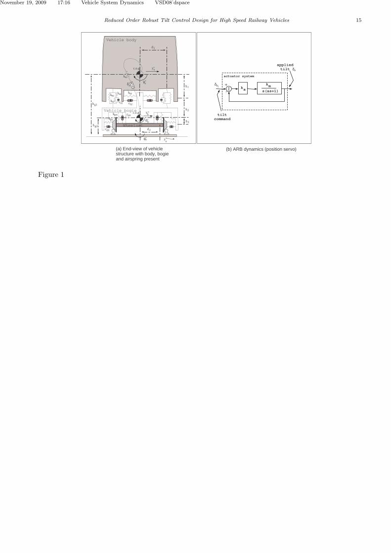
The modelling of the tilting railway vehicle is based upon a linearised end-view diagram (Figure 1),including both lateral and roll dynamics of both the body and the bogie plus the contribution of theairspring, the dynamics of the actuation system and the bogie lateral kinematics (resulting to a 13th ordermodel). The pair of linear airsprings represents the vertical suspensions, which only contribute to the rollmotion of the vehicle (vertical degrees of freedom are ignored). The model also contains the stiffness ofan anti-roll bar connected between the body and the bogie frame. Detailed wheelset dynamics were notincluded for simplicity, however the associated effects are incorporated in the model by using an appropriate2nd order LP filter (bogie lateral kinematics). The filter was characterised by a 5Hz cut-off frequency and20% damping.

Active tilt is provided via a rotational displacement actuator, in series with the roll stiffness (‘activeanti-roll bar (ARB)’ [6]), represented by a position servo in series with the ARB; the parameters werechosen to provide 3.5Hz bandwidth and 50% damping; in addition, the ARB is assumed to provide upto a maximum tilt angle of 10 degrees. The advantages of ARB result from their relative simplicity, i.e.small weight increase, low cost, easily fitted as an optional extra to build or as a retro-fit.

The mathematical models of increasing complexity,via the Newtonian approach, were developed to en-capsulate the lateral and roll dynamics of the tilting vehicle system. The equations of motion are givenbelow with all variables and parameter values provided in Appendix A. For the vehicle body (lateral androll):

mvyv = −2ksy(yv − h1θv − yb − h2θb) − 2csy(yv − h1θv − yb − h2θb) −mvv

2

R+ mvgθo − hg1mvθo (1)

ivrθv = −kvr(θv − θb − δa) + 2h1{ksy(yv − h1θv − yb − h2θb) + csy(yv − h1θv − yb − h2θb)}

+ mvg(yv − yb) + 2d1{−kaz(d1θv − d1θb) − ksz(d1θv − d1θr)} − ivrθo (2)

For the vehicle bogie (lateral and roll):

mbyb = 2ksy(yv − h1θv − yb − h2θb) + 2csy(yv − h1θv − yb − h2θb)

− 2kpy(yb − h3θb − yw) − 2cpy(yb − h3θb − yw) −mbv

2

R+ mbgθo − hg2mbθo (3)


Reduced Order Robust Tilt Control Design for High Speed Railway Vehicles 3

ibrθb = kvr(θv − θb − δa) + 2h2{ksy(yv − h1θv − yb − h2θb) + csy(yv − h1θv − yb − h2θb)}

− 2d1{−kaz(d1θv − d1θb) − ksz(d1θv − d1θr)} + 2d2(−d2kpzθb − d2cpzθb)

+ 2h3{kpy(yb − h3θb − yw) + cpy(yb − h3θb − yw)} − ibrθo (4)

for the (additional) airspring state:

θr = −(ksz + krz)

crzθr +

ksz

crzθv +

krz

crzθb + θb (5)

for the ARB actuation system:

δa = −22δa − 483.6δa + 483.6δai(6)

and for the bogie kinematics:

yw = −12.57yw − 987yw + 987yo (7)

These can be represented in the usual state-space form with the state vector x given by[yv θv yb θb yv θv yb θb θr δa δa yw yw], i.e. body lateral and roll position, bogie lateral and roll po-sition, body lateral and roll rate, bogie lateral and roll rate,airspring roll position, applied tilt and tiltrate, bogie kinematics position and rate, respectively (13 states).

It is worth noting that the system is excited by the track disturbance, including both deterministic (lowfrequency, intended features) and stochastic (higher frequency, track irregularities) elements, while thecontrol input is the ideal tilt command. In fact, for simulation purposes the state vector is augmented withfour disturbance states (i.e. track cant position and velocity, track curvature position and straight trackposition). More details on modelling exercise can be found in [7].

Substantial coupling exists between the lateral and roll motions which result in two sway modes combiningboth lateral and roll movement. The upper sway mode, its node appears above the body center of gravity,with predominantly roll movement; and the lower sway mode, the node located below the body center ofgravity, characterised mainly by lateral motion. The modal analysis of the vehicle is shown in Table 1.

3 Model and controller reduction concepts

Model reduction techniques attempt to approximate the dynamic model of the plant by a lower-ordersystem easier to control. In addition, reducing the complexity of the system can offer further advantages,such as elimination of system modes irrelevant to control, simplification of the design process and theaccompanying simulations, identification of crucial system characteristics, etc.

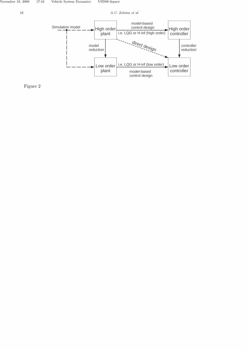
Two main approaches exist to the reduced-order controller design problem [3]: (i) direct designs, wherebythe low-order controller is designed via an optimization procedure model reduction problem, (ii) and twotypes of indirect designs. The first type, i.e. model reduction, attempts to approximate the input-outputcharacteristics of the plant by a lower order dynamic system, which automatically results in lower-ordercontrollers when modern-control methods are employed. Of course the approximation should be carriedout sensibly, so that the critical modes of the system are not highly affected. For this reason, most model-reduction techniques using this approach are normally accompanied by some form of robust control-designmethodology (LQG/LTR, H∞/µ) to ensure the additional uncertainty introduced by the approximation onsystem has minimal effects on system stability and performance. The second (indirect) type, i.e. controllerreduction, attempts to apply approximation techniques directly to the (high-order) controller. The designconcepts can be seen in Figure 2; (note that there are also cases whereby high-order plants and/or reduced-order equivalents can be directly identified from simulation models).

It is worth mentioning that direct low-order controller designs are not as straightforward as the indirectones, with no commercially available software packages for the design procedure (while a number of software



packages is available for indirect low-order controller design methods) [3]. The work in this paper has theindirect designs as a central concern.

3.1 Model reduction

A number of methods for model reduction are available, i.e. see [3], and the approach followed in thispaper is to decompose the system into slow and fast modes, whereby the former is retained and thelatter eliminated (effectively keeping a form of the physical interpretation from the original model). Themethod [8] is briefly described here. Let the original system be given in state-space form as

x(t) = Ax(t) + Bu(t), y(t) = Cx(t) + Du(t) (8)

with A stable. Introduce an orthogonal state-space transformation V so that V T AV is in real-Schur form.In this form, the structure of the transformed matrix is essentially upper triangular, with real eigenvaluesappearing on the main diagonal, while (simple) complex-conjugate eigenvalues correspond to 2× 2 blocksextending above and below the main diagonal. The eigenvalues (assumed stable) are ordered according totheir magnitude, so that the slow modes are located in the upper-diagonal block. Thus, if m representsthe number of slow modes that we wish to retain,

(

V T1

V T2

)

A(

V1 V2

)

=

(

As A12

0 Af

)

(9)

where As and Af denote the two blocks containing the slow and fast modes, respectively, and where V1

consists of the first m columns of V . Note that (simple) complex conjugate eigenvalues are not allowed tobe split. Next, let X be the solution of the Sylvester equation

AsX − XAf + A12 = 0 (10)

It is well-known that the solution to this equation exists and is unique, provided that λi(As)− λj(Af ) 6= 0,for all possible i and j; note that this is automatically satisfied if the eigenvalues are separated by a positivegap in magnitude as is assumed here. Introducing the additional transformation

(

I −X

0 I

)(

V T1

V T2

)

A(

V1 V2

)

(

I X

0 I

)

=

(

As 00 Af

)

(11)

which allows the separation of slow and fast modes via parallel decomposition; and the state vector, in thenew coordinate system, is related to the original state vector set x via the transformation

z(t) =

(

z1(t)z2(t)

)

=

(

V T1 − XV T

2

V T2

)

x(t) (12)

where z1(t) is the state-vector of the slow part of the realization. This allows us to retain the physicalsignificance of the new state variables zi, through their link with the original state-vector x. The (low-order) controller can be then designed on the reduced-order model. More details on the actual modelapproximation of the tilt system are included in the control design section.

3.2 Controller reduction

Controller reduction aims to preserve the properties of the closed loop in which the controller is requiredto operate. This is motivated by the fact that designers desire to have as much closeness as possible inthe behavior of the closed-loop of the original plant with the high-order controller and the closed-loop ofthe original plant with the low-order controller. In particular, controller order reduction may be viewed as



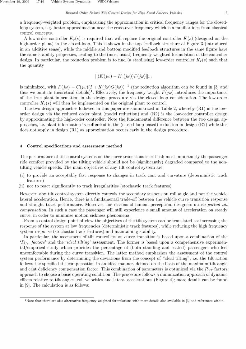
a frequency-weighted problem, emphasizing the approximation in critical frequency ranges for the closed-loop system, e.g. better approximation near the cross-over frequency which is a familiar idea from classicalcontrol concepts.

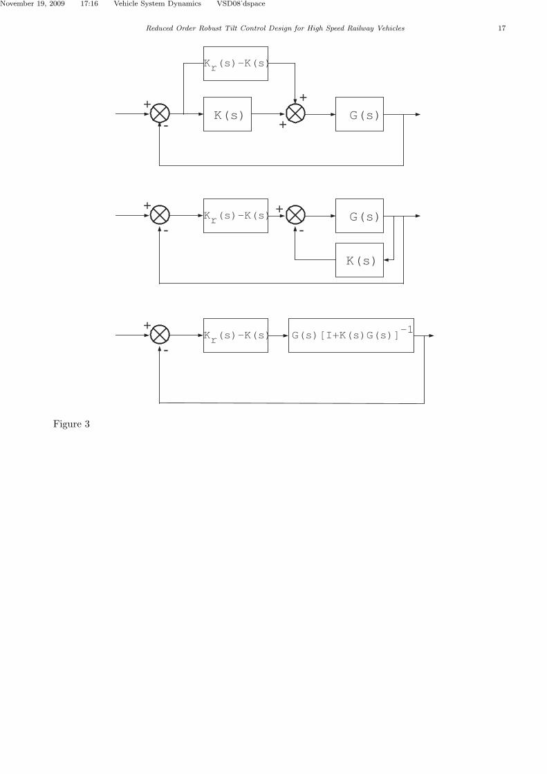
A low-order controller Kr(s) is required that will replace the original controller K(s) (designed on thehigh-order plant) in the closed-loop. This is shown in the top feedback structure of Figure 3 (introducedin an additive sense), while the middle and bottom modified feedback structures in the same figure havethe same stability properties, leading to the (most usual) frequency weighted formulation of the controllerdesign. In particular, the reduction problem is to find (a stabilising) low-order controller Kr(s) such thatthe quantity

||(K(jω) − Kr(jω))F (jω)||∞

is minimized, with F (jω) = G(jω)(I + K(jω)G(jω))−1 (the reduction algorithm can be found in [3] andthus we omit its theoretical details)1. Effectively, the frequency weight F (jω) introduces the importanceof the true plant information in the design procedure via the closed loop consideration. The low-ordercontroller Kr(s) will then be implemented on the original plant to control.

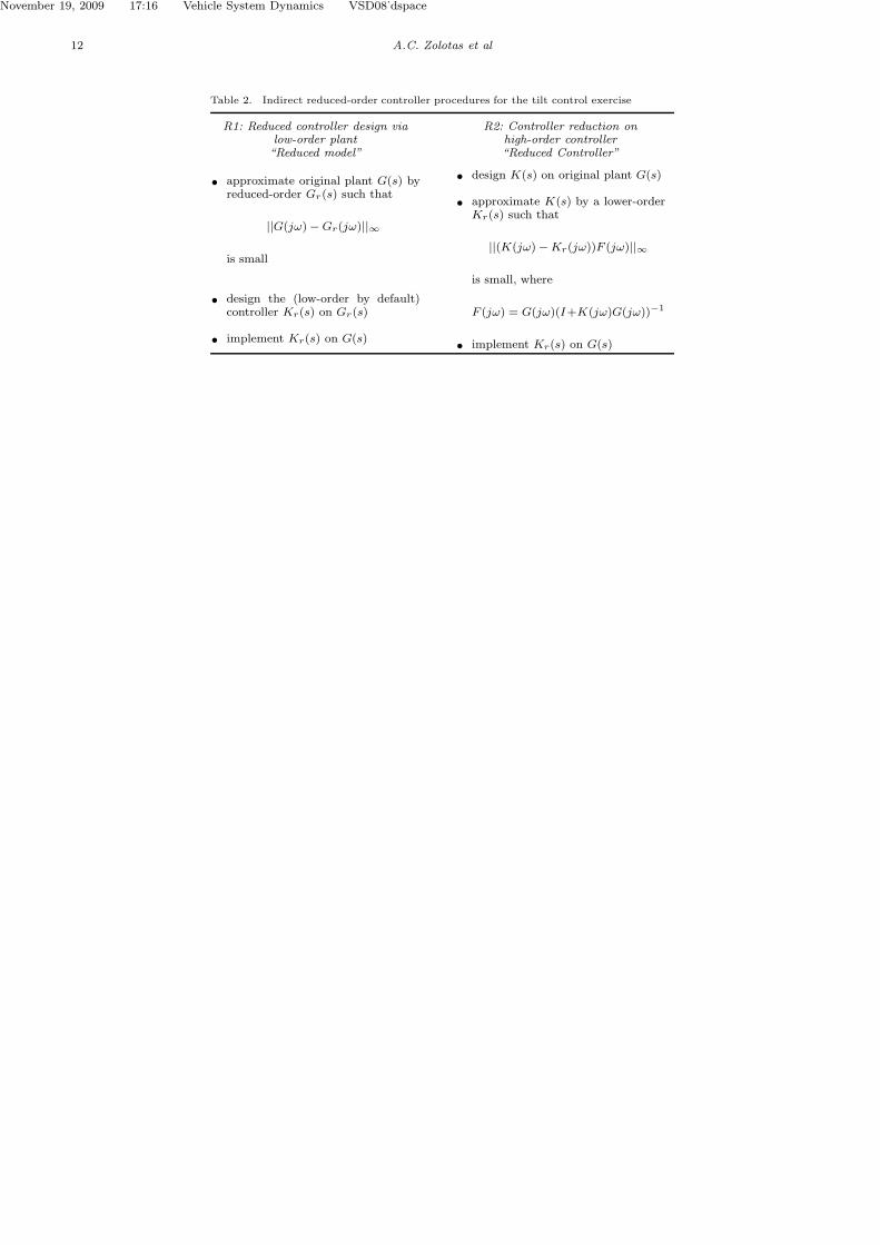
The two design approaches followed in this paper are summarized in Table 2, whereby (R1) is the low-order design via the reduced order plant (model reduction) and (R2) is the low-order controller designby approximating the high-order controller. Note the fundamental difference between the two design ap-proaches, i.e. plant information is reflected in the (closed-loop based) reduction in design (R2) while thisdoes not apply in design (R1) as approximation occurs early in the design procedure.

4 Control specifications and assessment method

The performance of tilt control systems on the curve transitions is critical; most importantly the passengerride comfort provided by the tilting vehicle should not be (significantly) degraded compared to the non-tilting vehicle speeds. The main objectives of any tilt control system are:

(i) to provide an acceptably fast response to changes in track cant and curvature (deterministic trackfeatures)

(ii) not to react significantly to track irregularities (stochastic track features)

However, any tilt control system directly controls the secondary suspension roll angle and not the vehiclelateral acceleration. Hence, there is a fundamental trade-off between the vehicle curve transition responseand straight track performance. Moreover, for reasons of human perception, designers utilise partial tiltcompensation. In such a case the passenger will still experience a small amount of acceleration on steadycurve, in order to minimise motion sickness phenomena.

From a control design point of view the objectives of the tilt system can be translated as: increasing theresponse of the system at low frequencies (deterministic track features), while reducing the high frequencysystem response (stochastic track features) and maintaining stability.

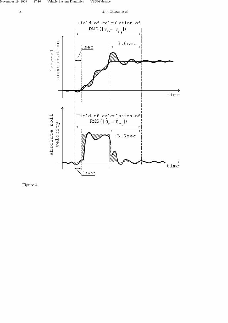
In particular, the assessment of tilt controllers on curve transition is based upon a combination of the‘PCT factors’ and the ‘ideal tilting ’ assessment. The former is based upon a comprehensive experimen-tal/empirical study which provides the percentage of (both standing and seated) passengers who feeluncomfortable during the curve transition. The latter method emphasizes the assessment of the controlsystem performance by determining the deviations from the concept of “ideal tilting”, i.e. the tilt actionfollows the specified tilt compensation in an ideal manner, defined on the basis of the maximum tilt angleand cant deficiency compensation factor. This combination of parameters is optimized via the PCT factorsapproach to choose a basic operating condition. The procedure follows a minimization approach of dynamiceffects relative to tilt angles, roll velocities and lateral accelerations (Figure 4); more details can be foundin [9]. The calculation is as follows:

1Note that there are also alternative frequency weighted formulations with more details also available in [3] and references within.



• |ym − ymi|, the deviation of the actual lateral acceleration ym from the ideal lateral acceleration ymi

,in the time interval between 1s before the start of the curve transition and 3.6s after the end of thetransition.

•∣

∣

∣θm − θmi

∣

∣

∣, the deviation of the actual absolute roll velocity θm from the ideal absolute roll velocity θmi

,

in the time interval between 1s before the start of the curve transition and 3.6s after the end of thetransition.

Regarding the straight track case the ‘rule-of-thumb’ currently followed by designers is to allow a lateralride quality degradation of the tilting train by no more than a specified margin of between 7.5% − 10%compared with the non-tilting vehicle.

5 Control design

The control design method adopted is the LQG with Loop Transfer Recovery (LQG/LTR) to emphasizerobustness of the overall LQG controller structure, as well as being an attractive (first) design approachin the framework of reduced-order control procedures.

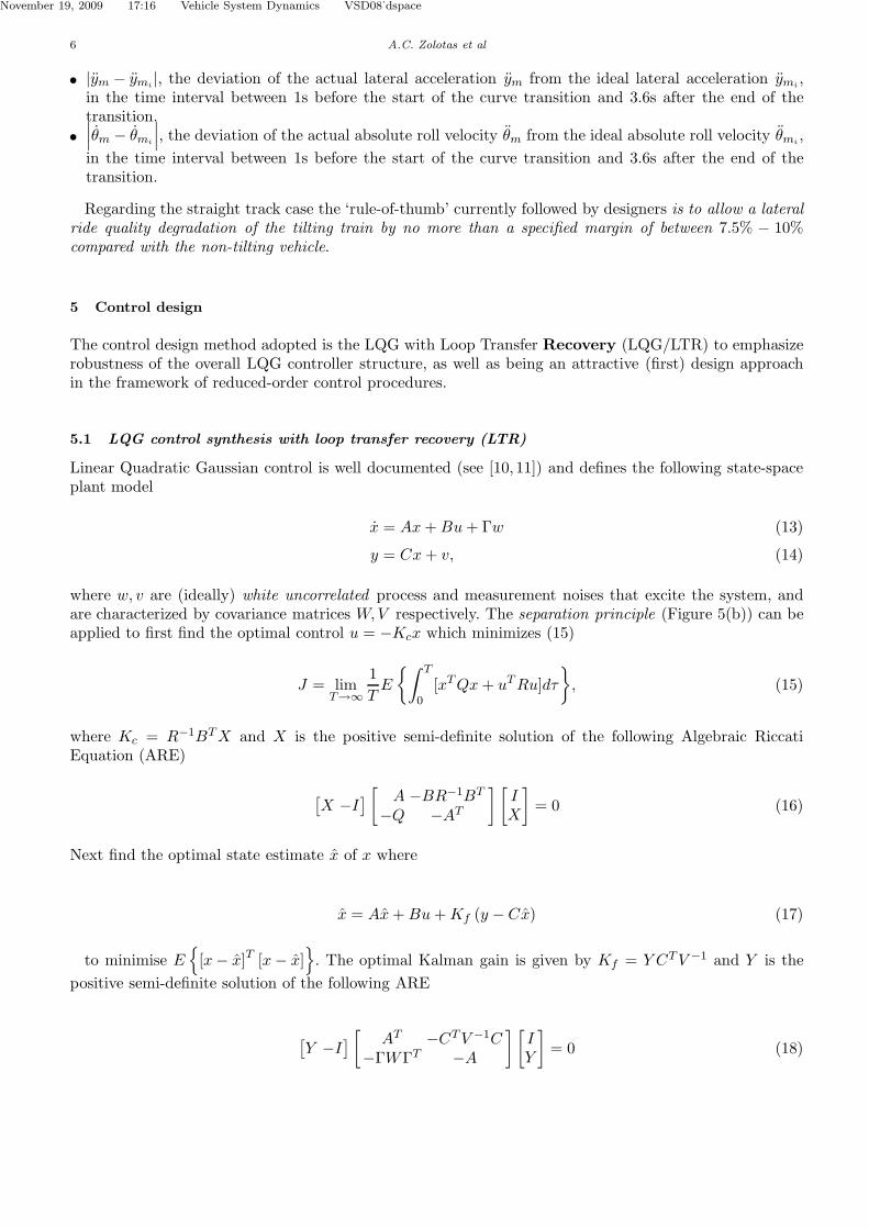
5.1 LQG control synthesis with loop transfer recovery (LTR)

Linear Quadratic Gaussian control is well documented (see [10, 11]) and defines the following state-spaceplant model

x = Ax + Bu + Γw (13)

y = Cx + v, (14)

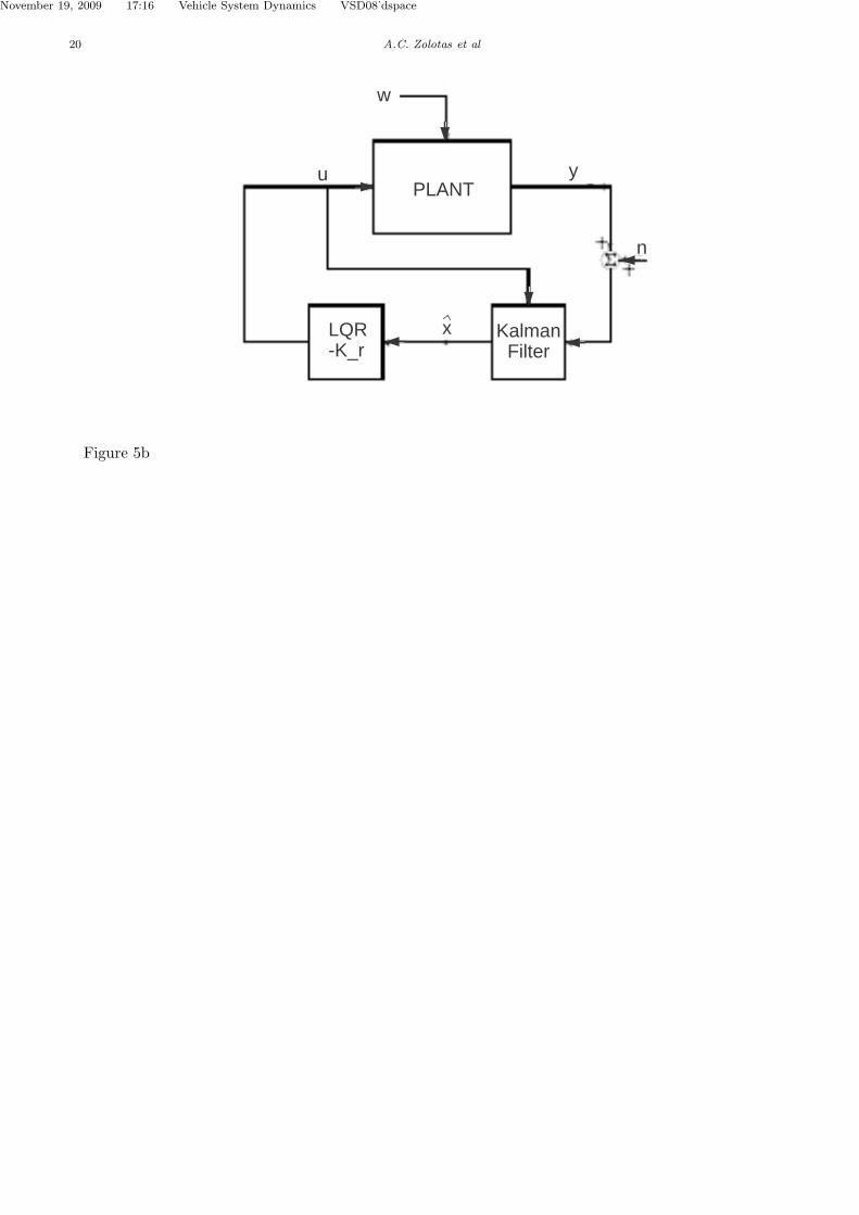
where w, v are (ideally) white uncorrelated process and measurement noises that excite the system, andare characterized by covariance matrices W,V respectively. The separation principle (Figure 5(b)) can beapplied to first find the optimal control u = −Kcx which minimizes (15)

J = limT→∞

1

TE

{∫ T

0[xT Qx + uT Ru]dτ

}

, (15)

where Kc = R−1BTX and X is the positive semi-definite solution of the following Algebraic RiccatiEquation (ARE)

[

X −I]

[

A −BR−1BT

−Q −AT

] [

I

X

]

= 0 (16)

Next find the optimal state estimate x of x where

x = Ax + Bu + Kf (y − Cx) (17)

to minimise E{

[x − x]T [x − x]}

. The optimal Kalman gain is given by Kf = Y CTV −1 and Y is the

positive semi-definite solution of the following ARE

[

Y −I]

[

AT −CTV −1C

−ΓWΓT −A

] [

I

Y

]

= 0 (18)



Weighting matrices Q (positive semidefinite), R (positive definite.) for control, and W (positive semidef-inite), V (positive definite) for estimation, can be tuned to provide the desired result. Note that it is alsopossible to follow the dual procedure, i.e. solve for the state estimate sub-problem and next for the optimalgain sub-problem.

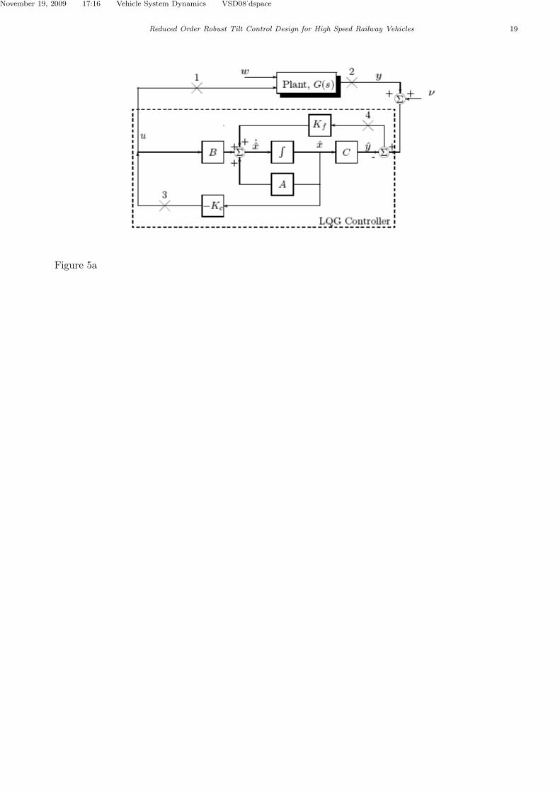
The synthesized LQG controller transfer function realization (Figure 5(a)) is given by

Klqg(s) = −Kc (sI − (A − BKc − KfC))−1 Kf (19)

Unfortunately the LQG compensators do not exhibit the good robustness properties of both the LQRand Kalman filter [10]. However, there is a way of either designing the Kalman filter such that the LQRrobustness properties are ‘recovered’ at the plant input; or designing the LQR such that the Kalmanfilter robustness properties are recovered at the plant output. The Loop Transfer Recovery procedure isextensively discussed in [10] and references within.

The main points of the procedure [10] are summarised below (with respect to Figure 5)

(i) Recovery at plant input. Design the Kalman filter gain Kf such that the loop TF K(s)G(s) (point1) approaches Kc(sI − A)−1B (point 3) . The plant must have at least as many outputs as inputs.In order for LTR to be applied, fictitious inputs must be included to make the system square andminimum phase. Recovery can be followed at plant input but not plant output. This is the approachundertaken in this paper.

(ii) Recovery at plant output. Design the LQR gain Kc such that the loop TF G(s)K(s) (point 2)approaches C(sI − A)−1Kf (point 4). In this case, artificial outputs must be included to make thesystem square and minimum phase. However, recovery can be applied only at plant output and notplant input.

In both cases the plant is assumed to be minimum phase for full recovery, however in the case ofnon-minimum phase systems, the same procedure can be used but only to partially recover the requiredrobustness properties for a specific range of frequencies (only partial recovery is achieved even in the caseof minimum phase systems in a practical implementation). More details on LTR for non-minimum phasesystems can be found in [10]. Note that LTR is a virtual design procedure (using fictitious noise inputs),thus extra care should be taken when recovering the required robustness properties. Also, care shouldbe taken for the required level of robustness to be achieved, due to the fact that full recovery wouldundoubtedly deteriorate the nominal performance of the true noise problem.

5.2 Remarks on the tilt control design

The control design is based on the SISO tilt model (actuator angle u = δaito effective cant deficiency

(combination of lateral acceleration and tilt angle) for 60% tilt compensation on steady curve θecd), withall disturbance signals set to zero. It is worth mentioning that, the simulation model (including trackdisturbance states) is 17th order while the design model for the process in the paper (without disturbancestates) is 13th order. Moreover, the LQG/LTR design on the SISO model can be seen as a simple extensionof the conventional (classical) nulling tilt problem in the optimal control framework.

The view adopted here is to synthesize the tilt controller via LQG theory with the weighting matricesQ,R for control and W,V for estimation purely considered as tuning parameters until an appropriatedesign is obtained (recovery at plant input as discussed above) [10]. More importantly,

• First the model is augmented using an extra state (integral of error of effective cant deficiency) forintegral action (thus providing zero sensitivity at zero frequencies and zero steady-state errors), i.e.

[

x

xi

]

=

[

A 0−Ci 0

] [

x

xi

]

+

[

B

0

]

u +

[

01

]

r (20)

y =[

Ci 0]

[

x

xi

]

, (21)



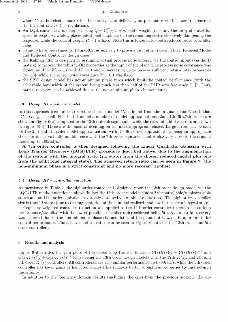
where Ci is the selector matrix for the effective cant deficiency output, and r will be a zero reference inthe tilt control case (i.e. regulation).

• An LQR control law is designed using Q = CTi q0Ci + qI state weight (selecting the integral state) for

speed of response, while q places additional emphasis on the remaining states effectively dampening theresponse, while the control weight R = 1 is fixed. Note this is followed for both reduced order controllercases.

• q0 and q have been tuned to 10 and 0.5 respectively to provide fast return ratios in both Reduced Modeland Reduced Controller design cases.

• the Kalman filter is designed by assuming virtual process noise entered via the control input (via the B

matrix) to recover the robust LQR properties at the input of the plant. The process noise covariance waschosen as W = W0 + wI with W0 = 1 and w increasing up to recover sufficient return ratio properties(w=50), while the sensor noise covariance V = 0.1 was fixed.

• the SISO design model has non-minimum phase zeros which limit the control performance (with theachievable bandwidth of the system being much less than half of the RHP zero frequency [11]). Thus,partial recovery can be achieved due to the non-minimum phase characteristics.

5.3 Design R1 - reduced model

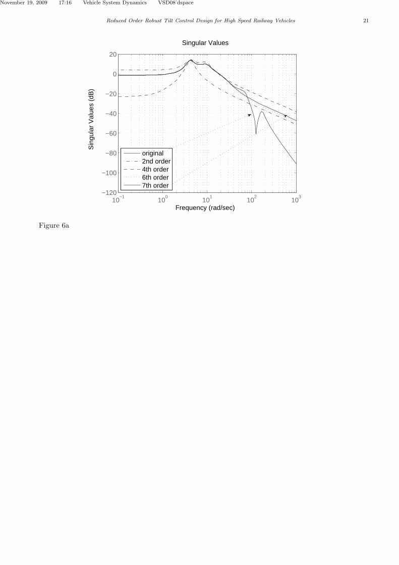
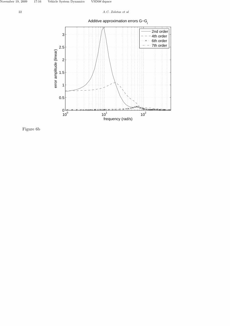
In this approach (see Table 2) a reduced order model Gr is found from the original plant G such that||G − Gr||∞ is small. For the tilt model a number of model approximations (2nd, 4th, 6th,7th order) areshown in Figure 6(a) compared to the 13th order design model, while the relevant additive errors are shownin Figure 6(b). These are the basis of deciding on the most appropriate choice. Large errors can be seenfor the 2nd and 4th order model approximation, with the 6th order approximation being an appropriatechoice as it has virtually no difference with the 7th order equivalent and is also very close to the originalmodel up to 100rad/s.

A 7th order controller is then designed following the Linear Quadratic Gaussian withLoop Transfer Recovery (LQG/LTR) procedure described above, due to the augmentationof the system with the integral state (six states from the chosen reduced model plus onefrom the additional integral state). The achieved return ratio can be seen in Figure 7 (thenon-minimum phase is a strict constraint and no more recovery applies).

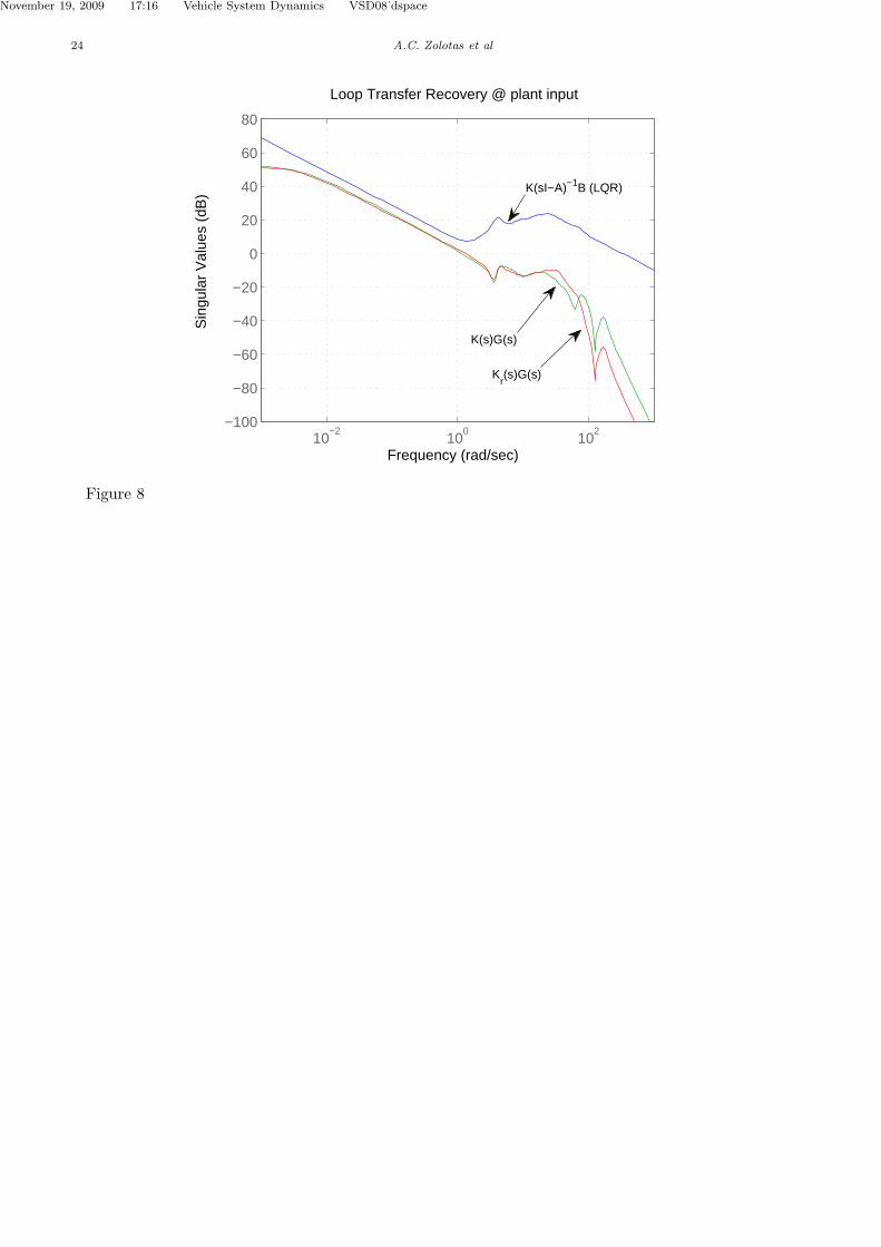
5.4 Design R2 - controller reduction

As mentioned in Table 2, the high-order controller is designed upon the 13th order design model via theLQG/LTR method mentioned above (in fact the 13th order model includes 2 uncontrollable/unobsvervablestates and an 11th order equivalent is directly obtained via minimal realization). The high-order controllersize is thus 12 states (due to the augmentation of the minimal realized model with the extra integral state).

Frequency weighted controller reduction was applied to the 12th order controller to retain closed loopperformance/stability, with the lowest possible controller order achieved being 5th. Again partial recoverywas achieved due to the non-minimum phase characteristics of the plant but it was still appropriate forcontrol performance. The achieved return ratios can be seen in Figure 8 both for the 12th order and 5thorder controllers.

6 Results and analysis

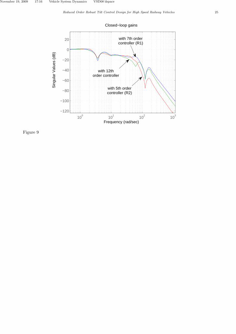
Figure 9 illustrates the gain plots of the closed loop transfer function G(s)K(s)(I + G(s)K(s))−1 andG(s)Kr(s)(I + G(s)Kr(s))

−1 (G(s) being the 13th order design model) with the 12th K(s), and 7th and5th order Kr(s) controllers. All controllers have very similar performance up to 60rad/s, while the 5th ordercontroller has lower gains at high frequencies (this suggests better robustness properties to unstructureduncertainty).

In addition to the frequency domain results (including the ones from the previous section), the de-



signed controllers were validated via simulation (on the 17th order simulation model with realistic trackdisturbance signals) using

(i) a curved (design) track of: 1000m curve radius, 155mm (6deg) track elevation and 145m transition ateach end of the curve;

(ii) a non-tilting speed of 45m/s and a tilting speed of 58m/s (30% increase);(iii) a stochastic (lateral) track irregularities profile chosen as a usual medium quality track with 0.33 ×

10−8m track roughness.

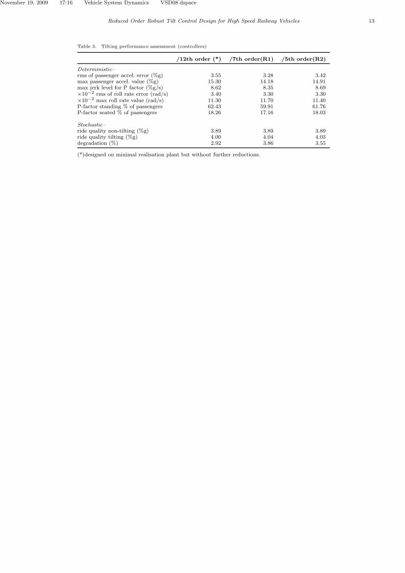
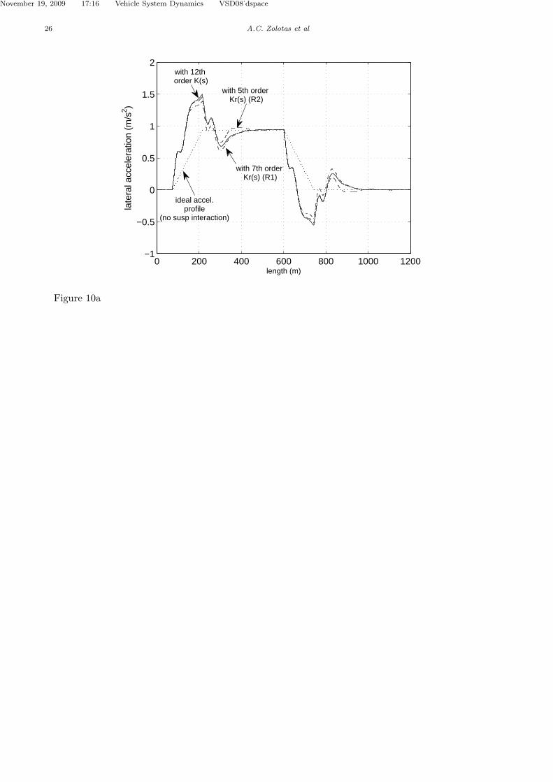
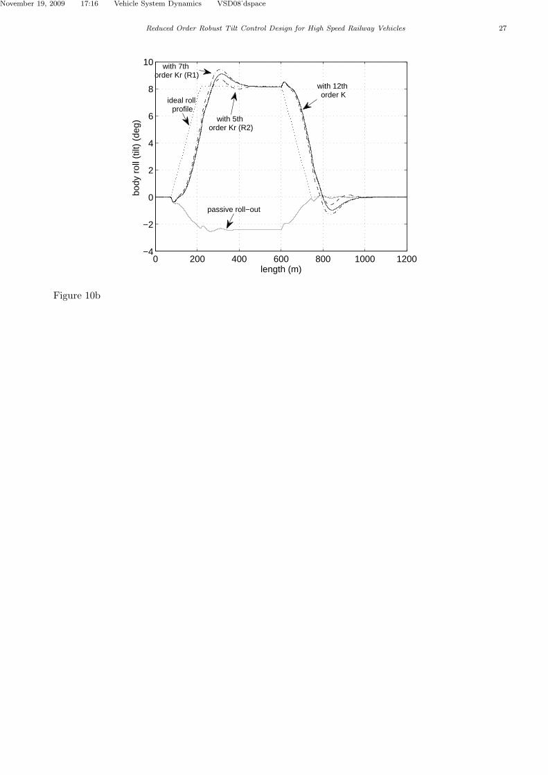
The time domain results for the passenger acceleration and body roll angle profile with all designedcontrollers validated can be seen in Figure 10, while the detailed performance assessment of the controllersis shown in Table 3. All controllers have similar performance (as expected from the frequency domainresults), with the 5th order controller an appropriate choice for implementation purposes due to being thesimplest solution. Note that the same weights were used in both design cases, thus some refinement willslightly improve the 12th and 5th order controller performance from controller reduction (the aim herewas to emphasise the design procedures rather than strictly the choice of weights). Moreover,

• the R1 design based controller performance deteriorates if reduced below 7th order in an open loop sense(especially the stochastic criterion of 7.5% degradation is violated);

• a further ‘closed-loop’ reduction process can be applied to the 7th order R1 design based controller toget a 5th order equivalent, but still cannot achieve the performance of the R2 design based 5th ordercontroller (esp. the stochastic performance);

• the R2 design based 5th order controller stochastic performance deteriorates if reduced to 4th order,and stability issues arise if reduced further;

• the R2 design approach is a better choice as it is based on closed loop properties, i.e. the true plant isrelevant in the design process in this case, while this does not apply in case R1.

7 Conclusions

The paper discussed on the design of reduced-order robust controllers for tilting railway vehicles. The de-sign is based on practical measurements using local vehicle information, i.e. with no ‘a priori’ informationon track profile. Two design approaches were presented, the first on reduced-order controller via modelapproximation which resulted to a 7th order controller and the second on controller reduction of the high-order controller which resulted to a 5th order controller. All controller structures provided appropriatetilt performance (although subject to non-minimum phase limitation), with the 5th order being the (sim-plest) choice to implement on the true plant. Shaping the principal gains of the return ratio of the systemwith the automatic LQG/LTR procedure, avoids manually designing networks of classical compensators.A careful selection and integrated application of different reduction methods can achieve appropriate sys-tem performance with low-order controllers, while controller reduction on high-order controllers to achieveappropriate closed loop properties is preferable. The presented approach can be also utilised for H-infinitycontrol methods; current work is based on this as well as robustness assessment via uncertainty represen-tations. The paper should be of considerable interest to control engineers who have to provide practicalsolutions but may be put off by the potential complexity of normal model-based control techniques.



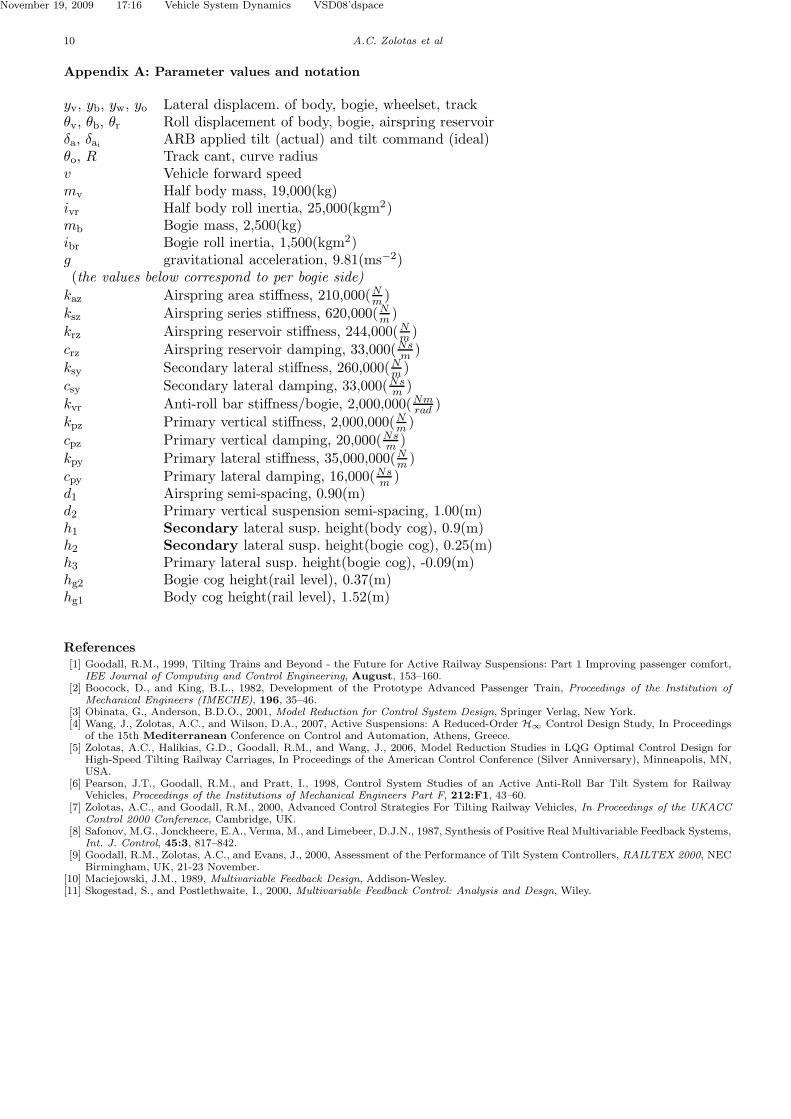
Appendix A: Parameter values and notation

yv, yb, yw, yo Lateral displacem. of body, bogie, wheelset, trackθv, θb, θr Roll displacement of body, bogie, airspring reservoirδa, δai

ARB applied tilt (actual) and tilt command (ideal)θo, R Track cant, curve radiusv Vehicle forward speedmv Half body mass, 19,000(kg)ivr Half body roll inertia, 25,000(kgm2)mb Bogie mass, 2,500(kg)ibr Bogie roll inertia, 1,500(kgm2)g gravitational acceleration, 9.81(ms−2)(the values below correspond to per bogie side)

kaz Airspring area stiffness, 210,000(Nm

)ksz Airspring series stiffness, 620,000(N

m)

krz Airspring reservoir stiffness, 244,000(Nm

)crz Airspring reservoir damping, 33,000(Ns

m)

ksy Secondary lateral stiffness, 260,000(Nm

)csy Secondary lateral damping, 33,000(Ns

m)

kvr Anti-roll bar stiffness/bogie, 2,000,000(Nmrad

)kpz Primary vertical stiffness, 2,000,000(N

m)

cpz Primary vertical damping, 20,000(Nsm

)

kpy Primary lateral stiffness, 35,000,000(Nm

)cpy Primary lateral damping, 16,000(Ns

m)

d1 Airspring semi-spacing, 0.90(m)d2 Primary vertical suspension semi-spacing, 1.00(m)h1 Secondary lateral susp. height(body cog), 0.9(m)h2 Secondary lateral susp. height(bogie cog), 0.25(m)h3 Primary lateral susp. height(bogie cog), -0.09(m)hg2 Bogie cog height(rail level), 0.37(m)hg1 Body cog height(rail level), 1.52(m)

References[1] Goodall, R.M., 1999, Tilting Trains and Beyond - the Future for Active Railway Suspensions: Part 1 Improving passenger comfort,

IEE Journal of Computing and Control Engineering, August, 153–160.[2] Boocock, D., and King, B.L., 1982, Development of the Prototype Advanced Passenger Train, Proceedings of the Institution of

Mechanical Engineers (IMECHE), 196, 35–46.[3] Obinata, G., Anderson, B.D.O., 2001, Model Reduction for Control System Design, Springer Verlag, New York.[4] Wang, J., Zolotas, A.C., and Wilson, D.A., 2007, Active Suspensions: A Reduced-Order H∞ Control Design Study, In Proceedings

of the 15th Mediterranean Conference on Control and Automation, Athens, Greece.[5] Zolotas, A.C., Halikias, G.D., Goodall, R.M., and Wang, J., 2006, Model Reduction Studies in LQG Optimal Control Design for

High-Speed Tilting Railway Carriages, In Proceedings of the American Control Conference (Silver Anniversary), Minneapolis, MN,USA.

[6] Pearson, J.T., Goodall, R.M., and Pratt, I., 1998, Control System Studies of an Active Anti-Roll Bar Tilt System for RailwayVehicles, Proceedings of the Institutions of Mechanical Engineers Part F, 212:F1, 43–60.

[7] Zolotas, A.C., and Goodall, R.M., 2000, Advanced Control Strategies For Tilting Railway Vehicles, In Proceedings of the UKACCControl 2000 Conference, Cambridge, UK.

[8] Safonov, M.G., Jonckheere, E.A., Verma, M., and Limebeer, D.J.N., 1987, Synthesis of Positive Real Multivariable Feedback Systems,Int. J. Control, 45:3, 817–842.

[9] Goodall, R.M., Zolotas, A.C., and Evans, J., 2000, Assessment of the Performance of Tilt System Controllers, RAILTEX 2000, NECBirmingham, UK, 21-23 November.

[10] Maciejowski, J.M., 1989, Multivariable Feedback Design, Addison-Wesley.[11] Skogestad, S., and Postlethwaite, I., 2000, Multivariable Feedback Control: Analysis and Desgn, Wiley.



Tables with captions

Table 1. 13th order ARB vehicle modal analysis(*)

Mode Damping (%) Frequency (Hz)

Body lower sway 16.5 0.67Body upper sway 27.2 1.50Bogie lateral 12.4 26.80Bogie roll 20.8 11.10Bogie kinematics 20.0 5.00Actuation system 50.0 3.50Airspring mode 100.0 3.70

(*)without disturbance states and before minimal realisa-tion.



Table 2. Indirect reduced-order controller procedures for the tilt control exercise

R1: Reduced controller design vialow-order plant

“Reduced model”

R2: Controller reduction onhigh-order controller“Reduced Controller”

• approximate original plant G(s) byreduced-order Gr(s) such that

||G(jω) − Gr(jω)||∞

is small

• design the (low-order by default)controller Kr(s) on Gr(s)

• implement Kr(s) on G(s)

• design K(s) on original plant G(s)

• approximate K(s) by a lower-orderKr(s) such that

||(K(jω) − Kr(jω))F (jω)||∞

is small, where

F (jω) = G(jω)(I+K(jω)G(jω))−1

• implement Kr(s) on G(s)



Table 3. Tilting performance assessment (controllers)

/12th order (*) /7th order(R1) /5th order(R2)

Deterministic–rms of passenger accel. error (%g) 3.55 3.28 3.42max passenger accel. value (%g) 15.30 14.18 14.91max jerk level for P factor (%g/s) 8.62 8.35 8.69×10−2 rms of roll rate error (rad/s) 3.40 3.30 3.30×10−2 max roll rate value (rad/s) 11.30 11.70 11.40P-factor standing % of passengers 62.43 59.91 61.76P-factor seated % of passengers 18.26 17.16 18.03

Stochastic–ride quality non-tilting (%g) 3.89 3.89 3.89ride quality tilting (%g) 4.00 4.04 4.03degradation (%) 2.92 3.86 3.55

(*)designed on minimal realisation plant but without further reductions.



Figure captions

Figure 1. Tilting vehicle end-view diagram with actuation system;

Figure 2. Reduced order controller design paths;

Figure 3. Reduced-order controller feedback formulation for stability criteria;

Figure 4. “Ideal Tilting”- Calculation of deviation of actual from ideal responses for acceleration androll velocity;

Figure 5. LQG control design: (a) LQG controller (b) separation principle ;

Figure 6. Model approximation: (a) magnitude of (SISO) approximation models (b) additive reductionerrors;

Figure 7. Loop transfer recovery at plant input for design R1;

Figure 8. Loop transfer recovery at plant input for design R2;

Figure 9. Closed loop gain comparisons of the different controller designs;

Figure 10. Time-domain results for design (curved) track (a) passenger acceleration (b) body rollangle (tilt).



Vehicle body

Vehicle bogie

Wheelset

c.o.g

c.o.g

kaz

yv

θv

hg1

hg2

krz crz

ksz

csy

ksy

d1

cpzkpz

kpy

kvr

h1

h2

h3θb

yb

δa

+

+

+

+

xxxxxxxxxxxxxxxxxxxxxxxxxxxx

xxxxxxxxxxxxxxxxxxxxxxxx

xxxxxxxxxxxxxxxxxxxxxxxxxxxx

xxxxxxxxxxxxxxxxxxxxxxxx

yo

θo+ +

d2cpy

s(as+1)

kmka+

-

tiltcommand

appliedtilt

Σ

actuator system

(a) End-view of vehiclestructure with body, bogieand airspring present

(b) ARB dynamics (position servo)

δai

δa

Figure 1



High orderplant

Low orderplant

High ordercontroller

Low ordercontroller

model-basedcontrol design

direct design

i.e. LQG or H-inf (high order)

model-basedcontrol design

i.e. LQG or H-inf (low order)

modelreduction

controllerreduction

Simulation model

Figure 2



-

K(s)

Kr(s)-K(s)++

G(s)-

- +

++G(s)K(s)

Kr(s)-K(s)

-Kr(s)-K(s)

+G(s)[I+K(s)G(s)]-1

Figure 3



Figure 4



Figure 5a



w

u y

n

LQR-K_r

KalmanFilter

PLANT

x

Figure 5b



10−1

100

101

102

103

−120

−100

−80

−60

−40

−20

0

20

Singular Values

Frequency (rad/sec)

Sin

gula

r V

alue

s (d

B)

original2nd order4th order6th order7th order

Figure 6a



100

101

102

0

0.5

1

1.5

2

2.5

3

frequency (rad/s)

erro

r am

plitu

de (

linea

r)

Additive approximation errors G−Gr

2nd order4th order6th order7th order

Figure 6b



10−2

10−1

100

101

102

103

−60

−40

−20

0

20

40

60

Loop Tranfer Recovery @ plant input

Frequency (rad/sec)

Sin

gula

r V

alue

s (d

B)

Kr(s)G(s)

Kr(sI−A)−1B

Figure 7



10−2

100

102

−100

−80

−60

−40

−20

0

20

40

60

80

Loop Transfer Recovery @ plant input

Frequency (rad/sec)

Sin

gula

r V

alue

s (d

B)

K(s)G(s)

Kr(s)G(s)

K(sI−A)−1B (LQR)

Figure 8



100

101

102

103

−120

−100

−80

−60

−40

−20

0

20

Closed−loop gains

Frequency (rad/sec)

Sin

gula

r V

alue

s (d

B)

with 12thorder controller

with 7th ordercontroller (R1)

with 5th ordercontroller (R2)

Figure 9



0 200 400 600 800 1000 1200−1

−0.5

0

0.5

1

1.5

2

length (m)

late

ral a

ccel

erat

ion

(m/s

2 )

with 5th order Kr(s) (R2)

with 7th order Kr(s) (R1)

with 12th order K(s)

ideal accel.profile

(no susp interaction)

Figure 10a



0 200 400 600 800 1000 1200−4

−2

0

2

4

6

8

10

length (m)

body

rol

l (til

t) (

deg)

passive roll−out

ideal roll profile

with 5th order Kr (R2)

with 12th order K

with 7th order Kr (R1)

Figure 10b

Reduced-order robust tilt control design for high-speed railway vehicles

Documents

Transcript of Reduced-order robust tilt control design for high-speed railway vehicles