Computer Aided Geometric Design 37 (2015) 69–84

Contents lists available at ScienceDirect

Computer Aided Geometric Design

www.elsevier.com/locate/cagd

Reduced curvature formulae for surfaces, offset surfaces, curves on a surface and surface intersections ✩

Spiros G. Papaioannou ∗, Marios M. Patrikoussakis

Department of Mechanical and Aerospace Engineering, University of Patras, Greece

a r t i c l e i n f o a b s t r a c t

Article history:Received 18 July 2014Received in revised form 26 May 2015Accepted 9 June 2015Available online 15 June 2015

Keywords:Reduced curvature formulaeGaussian mean and normal curvatureCurvature of curves on a surfaceCurvature of intersection curves of surfacesCurvature of intersection curves of offset (parallel) surfaces

We introduce the concept of reduced curvature formulae for 3-D space entities (surfaces, curves). A reduced formula entails only derivatives of the functions involved in the entity’s representation and admits no further algebraic simplifications. Although not always the most compact, reduced curvature formulae entail only basic arithmetic operators and are more efficient computationally compared to alternative unreduced formulae. Reduced formulae are presented for the normal, mean and Gaussian curvatures of a surface and the curvature of curves on a surface, where each surface or curve on a surface may be defined parametrically or implicitly. Reduced formulae are also presented for the curvature of surface intersection curves, where each of the intersecting surfaces may be a given surface or an offset of a given surface and each given surface may be defined parametrically or implicitly. Known formulae are cited, without derivation, to form a collection, in one place, of new and of known results scattered in the literature. Each curve curvature formula is presented together with a formula for the respective binormal vector, from which formulae for the Frenet frame and torsion of the curve can be derived.

© 2015 Published by Elsevier B.V.

1. Introduction

Formulae for computing various curvature measures are important in Geometric Modeling, CNC machining and other applications. Texts on classical differential geometry (Knoblauch, 1913; Struik, 1950; Lipschutz, 1969; Spivak, 1975;Do Carmo, 1976; Kreyszig, 1991) focus on the Gaussian and mean curvatures of surfaces, which determine local surface shape. They generally limit their discussion on the normal curvature to the classic formula expressing the normal curvature of a parametric surface as the ratio of the second to first fundamental forms of the surface, which is at the root of the classi-cal theory on surface curvature. Regarding the curvature of curves, they provide only a general formula for parametric space curves, on the tacit assumption that specific formulae for curves on a surface or surface intersection curves can somehow be derived. Both Ye and Maekawa (1999) and Goldman (2005) have noted the scarcity of English literature on the differen-tial geometry of intersection curves. A notable exception is Willmore (1959) who describes procedures (but gives no closed formulae) for computing the curvature, torsion and Frenet frame vectors of intersection curves of two implicit surfaces.

In recent years, interest in the differential geometry of curves on a surface and surface intersection curves has re-vived, motivated by research in Geometric Modeling (Faux and Pratt, 1981; Hartmann, 1996; Ye and Maekawa, 1999; Goldman, 2005) and the need for advanced CNC controls (Papaioannou and Patrikoussakis, 2011). The curvature of a plane

✩ This paper has been recommended for acceptance by Tamas Varady.

* Corresponding author.E-mail address: papaioan@mech.upatras.gr (S.G. Papaioannou).

http://dx.doi.org/10.1016/j.cagd.2015.06.0050167-8396/© 2015 Published by Elsevier B.V.

70 S.G. Papaioannou, M.M. Patrikoussakis / Computer Aided Geometric Design 37 (2015) 69–84

or space curve is a function of the first and second derivatives of the curve’s position vector. Similarly, the normal curvature of a surface and, by extension, its Gaussian and mean curvatures, are functions of the first and second partial derivatives of the surface’s position vector. These derivatives can, in turn, be expressed in terms of first and second derivatives, or partial derivatives of the functions involved in the actual curve or surface representation. We shall call a curvature formula entailing only representation function derivatives reduced, if it does not evidently admit further algebraic simplifications. We allow, however, the use of placeholders for reduced expressions in reduced curvature formulae, for the sake of compactness.

The task of generating a reduced formula for the curvature of the intersection curve of a parametric surface r(u, v) =[x(u, v) y(u, v) z(u, v)]T with an implicit surface f (x, y, z) = 0 will serve to illustrate the issues involved. An established fact in differential geometry is the dependence of the intersection curvature k of two surfaces Sa, Sb on their local normal curvatures kan , kbn , which reduces the task of computing k to computing kan , kbn and combining them, by means of an equation expressing this dependence, to produce k. The following expression of k2 in terms of kan , kbn is given in Lipschutz (1969)

k2 = k2an + k2

bn − 2kankbn cosϕ

sin2 ϕ(1)

where ϕ is the angle formed by the local normal vectors of Sa, Sb. Previous authors (Faux and Pratt, 1981; Ye and Maekawa, 1999) suggest substituting the values of kan , kbn , cosϕ , sinϕ into Equ. (1) to compute k. Efficiency gains can, however, be obtained by introducing known formulae for kan , kbn into Equ. (1), or an equivalent expression, to produce reduced formulae for k, by taking advantage of possible simplifications. This is a more systematic and efficient approach. It is also less complicated than trying to compute k, without regard to its dependence on kan , kbn .

Thus, to reduce Equ. (1) for the above case, we introduce into it the classic expression for the normal curvature krn of a parametric surface r(u, v) = [x(u, v) y(u, v) z(u, v)]T

krn = crn

|t|2|nr| , crn = L′a2 + 2M ′ab + N ′b2,

L′ = ruunr, M ′ = ruvnr, N ′ = rvvnr, t = aru + brv (2)

the expression for the normal curvature k f n of an implicit surface f (x, y, z) = 0

k f n = c f n

|t|2|nf| , c f n = −[t]THf[t]

c f n = −(fxxt2

x + f yyt2y + f zzt2

z + 2 fxytxt y + 2 fxztxtz + 2 f yzt ytz)

(3)

where Hf is the Hessian of f (x, y, z), and the following expressions for cosϕ and sinϕ

cosϕ = nr · nf

|nr||nf| , sinϕ = |nr × nf||nr||nf| = |t|

|nr||nf| (4)

where nr = ru × rv and nf = ∇ f are the normal vectors of the intersecting surfaces and t = nr × nf is the tangent vector of the intersection curve.

There have been, however, two missing links for this reduction process to succeed. Formula (3) for the normal curvature of an implicit surface has been provided only recently by Ye and Maekawa (1999), although implicit forms of this formula can be traced back to classical works (Spivak, 1975; Do Carmo, 1976). And unlike this formula, in which t is represented by its Cartesian coordinates, formula (2) for the normal curvature of a parametric surface entails the coordinates a, b of tin the basis ru , rv of the surface’s tangent plane. Reduced formulae for a, b when t is a tangent vector of the intersection curve of a parametric surface by another surface have not been known, but we provide this link in Section 3, Equ. (20b), which here assume the form

a = −rv · nf, b = ru · nf (5)

Introducing Equ. (2)–(4) into Equ. (1) and simplifying, we obtain

k = |crnnf − c f nnr||t|3 (6a)

where L′ , M ′ , N ′ , crn (Equ. (2)), c f n (Equ. (3)), a, b (Equ. (5)) and nr , nf , t are placeholders for reduced derivative expressions of the representation functions x(u, v), y(u, v), z(u, v), f (x, y, z) and formula (6a) is also reduced as evidenced by its explicit form

k = ((crn fx − c f nnrx)2 + (crn f y − c f nnry)

2 + (crn f z − c f nnrz)2)1/2

(t2 + t2 + t2)3/2(6b)

x y z

S.G. Papaioannou, M.M. Patrikoussakis / Computer Aided Geometric Design 37 (2015) 69–84 71

The formulae presented in this paper fall into three categories. Known formulae, which are cited without derivation. Derived reduced formulae for curvature measures for which alternative unreduced formulae or procedures have been pre-sented by other authors. Completely new formulae for the curvature of curves on implicit surfaces and the normal and intersection curvatures of offset surfaces.

The rest of the paper is organized as follows: Following a brief review of classical differential geometry (Section 2), we derive in Section 3 reduced formulae for the tangential coordinates a, b of the surface tangent vector t for use with Equ. (2)and in Section 4 reduced curvature formulae for curves on both parametric and implicit surfaces. In Section 5, from the Faux and Pratt (1981) expression of the kB vector, we derive reduced formulae for the curvature of intersection curves, for the remaining two representation modes (implicit/implicit and parametric/parametric) of the intersecting surfaces. In Section 6 we present reduced formulae for the normal and intersection curvatures of offset surfaces, a subject not treated in the English literature. The paper concludes with some final remarks (Section 7) and two appendices, the first of which compares the efficiency of proposed reduced to existing unreduced formulae and the second rederives curvature formulae presented earlier, by reformulating the problem as a surface intersection problem and applying proposed formulae for this problem.

A word on notation: We use capital bold letters to distinguish unit vectors from other vectors. The principal normal vector of a curve and the unit normal vector of a surface are denoted by NC and N, respectively. Otherwise, indexes indicate the representation of curves/surfaces and their differential quantities (r for parametric, f , g for implicit, h for explicit representations) and for partial derivatives of implicit functions ( f , g) of position vectors (r) and of their coordinates (x, y, z) the associated parameters. Dots signify derivatives w.r.t. arc length and primes derivatives w.r.t. any other variable.

2. Brief review of classical differential geometry

Classical differential geometry starts from the Frenet–Serret equations of a curve

T = kN

N = −kT + τ B

B = −τN (7)

and derives two basic curvature formulae. The first for the binormal curvature vector kB of a parametric space curve r(t) =[x(t) y(t) z(t)]T

kB = r′ × r′′

|r′|3 (8a)

from which follow expressions for the curvature k and the binormal vector B

k = |r′ × r′′||r′|3 , B = r′ × r′′

|r′ × r′′| (8b)

of the curve. In fact, all formulae for the curvature of curves derived in the sequel (curves on a surface and surface intersec-tion curves) originate at expressions of the kB vector and this close relationship between k and kB implies that for any such curvature formula of the form k = |v|/|t|3, where |v| is the norm of a vector expression and t is the curve’s tangent vector, there is a respective expression B = v/|v| of the binormal vector of the curve. The curve’s unit tangent vector T, principal normal vector NC and torsion τ can then be obtained from the formulae

T = r′

|r′| , NC = B × T, τ = r′′′ · B

|r′ × r′′| (9)

The second basic curvature formula

rC · Nr = krn = II

I= La2 + 2Mab + Nb2

Ea2 + 2Fab + Gb2, Nr = ru × rv

|ru × rv|E = ru · ru, F = ru · rv, G = rv · rv, L = ruu · Nr = −ru · Nru,

M = ruv · Nr = −ru · Nrv, N = rvv · Nr = −rv · Nrv (10)

gives the normal curvature krn of a parametric surface Sr at a point P, in terms of the first and second fundamental forms I = Ea2 + 2Fab + Gb2 and II = La2 + 2Mab + Nb2 of Sr at P. Both forms are associated with a tangent vector t = aru + brvof Sr. In particular, I is a surface metric allowing lengths, areas and angles on Sr to be expressed in terms of its first fundamental coefficients E , F , G . Thus, the norms of t and of the normal vector nr = ru × rv of Sr at P are

|t| = ((aru + brv)(aru + brv)

)1/2 = (Ea2 + 2Fab + Gb2)1/2

|nr| = |ru × rv| =(r2

ur2v sin2 γ

)1/2 = (r2

ur2v − r2

ur2v cos2 γ

)1/2 = (EG − F 2)1/2

(11)

72 S.G. Papaioannou, M.M. Patrikoussakis / Computer Aided Geometric Design 37 (2015) 69–84

The normal curvature krn is the curvature of the section curve of Sr by the normal plane spanned by t and Nr . It measures the curving of Sr in the tangent direction t and its variation as t rotates around Nr reveals the local surface geometry at P. This leads to an examination of the stationary values of krn , as the direction ratio a/b of t varies, with the following results: krn has either two real distinct stationary values (minimum krn1, maximum krn2, termed principal curvatures) or it is constant in all directions. In the latter case, the surface looks locally like a spherical cup and the point is an umbilic. Apart from umbilics, the principal curvatures are distinct and the associated principal directions are orthogonal. The local surface shape depends on the relative signs of krn1, krn2. This gives rise to two new curvature measures, the Gaussian curvature K = krn1krn2 and the mean curvature H = (krn1 + krn2)/2. Since krn1 ≤ krn ≤ krn2, K > 0 implies that krndoes not change sign and the local surface shape is cup-like. In particular, if H2 − K = 0, then krn1 = krn2 and the point is an umbilic. K < 0, on the other hand, implies a sign change of krn and the local surface shape is saddle-like.

The left part of formula (10) expresses the normal curvature krn of Sr at P as the projection on the surface unit normal vector Nr of the curvature vector rC = kNC of any curve C on Sr which passes through P and is tangent to t. Since Nr , NCare unit vectors, this part can also be written in the form

krn = kNC · Nr = k cos θ (12)

For reasons that will become apparent when we come to intersection curves, it is convenient to introduce into formula (10) the surface normal vector nr = ru × rv in place of the unit normal vector Nr = nr/|nr| of Sr and write

L = L′

|nr| , L′ = ruunr, M = M ′

|nr| , M ′ = ruvnr, N = N ′

|nr| , N ′ = rvvnr (13)

Formula (10) then reduces to formula (2).The classic formulae for the Gaussian and mean curvatures of a parametric surface are

Kr = crK

|nr|4 , crK = L′N ′ − M ′ 2,

Hr = crH

2|nr|3 , crH = E N ′ + GL′ − 2F M ′ (14)

Spivak (1975, vol. 3), Belyaev et al. (1998), Turkiyyah et al. (1997), Patrikalakis and Maekawa (2002) and Osher and Fedkiw(2003) provide the following formulae for the Gaussian and mean curvatures of a surface with explicit representation z = h(x, y) and implicit representation f (x, y, z) = 0

Kh = chK

|nh|4 , chK = hxxhyy − h2xy, |nh| = (

h2x + h2

y + 1)1/2

,

Hh = chH

2|nh|3 , chH = (1 + h2

x

)hyy − 2hxhyhxy + (

1 + h2y

)hxx (15)

K f = c f K

|nf|4 , |nf| =(

f 2x + f 2

y + f 2z

)1/2,

c f K = f 2x

(f yy f zz − f 2

yz

) + f 2y

(fxx f zz − f 2

xz

) + f 2z

(fxx f yy − f 2

xy

) + 2 fx f y( fxz f yz − fxy f zz)

+ 2 fx f z( fxy f yz − fxz f yy) + 2 f y f z( fxy fxz − f yz fxx)

H f = c f H

2|nf|3 , c f H = 2( fx f y fxy + fx f z fxz + f y f z f yz) − f 2x ( f yy + f zz) − f 2

y ( fxx + f zz) − f 2z ( fxx + f yy) (16)

It is important to note that we have cast the normal, Gaussian and mean curvatures of a surface in the generic forms

kin = cin

|t|2|ni| , Ki = ciK

|ni|4 , Hi = ciH

2|ni|3 , i ∈ (r,h, f , g) (17)

where index i indicates the surface representation. We shall call the numerator of each of these forms curvature factor of the respective curvature.

3. The classic normal curvature formula revisited

To apply formula (2) for the normal curvature of a parametric surface Sr in a tangent direction t, one must express t in the form

t = aru + brv (18a)

This task is trivially simple when t is defined as tangent to a curve C on Sr, represented by u = u(t), v = v(t). Then

t = r′ = ruu′ + rv v ′ (18b)

S.G. Papaioannou, M.M. Patrikoussakis / Computer Aided Geometric Design 37 (2015) 69–84 73

so that a = u′ , b = v ′ . When C is defined on Sr by an implicit equation f (u, v) = 0 then, by the implicit func-tion theorem, as long as fu �= 0, u is an explicit function u = u(v) of v and C can be represented parametrically as r(v) = [x(u(v), v) y(u(v), v) z(u(v), v)]T. Then v ′ = 1 and

f ′ = fuu′ + f v = 0 → u′ = − f v

fu

t = r′ = ruu′ + rv = − f v

furu + rv (18c)

so that a = − f v/ fu , b = 1 and formula (2) becomes

krn = crn

|t|2|nr| , crn = L′ f 2v − 2M ′ fu f v + N ′ f 2

u

|t|2 = E f 2v − 2F fu f v + G f 2

u (19)

regardless of which of the parameters u, v is a function of the other.Ye and Maekawa (1999) give the following general expressions for a, b, when t is an arbitrary tangent vector of Sr

a = G(t · ru) − F (t · rv)

EG − F 2, b = E(t · rv) − F (t · ru)

EG − F 2(20a)

which are obtained by taking the dot product of Equ. (18a), first with ru , then with rv and solving the resulting system for a, b. We shall reduce these expressions for the case when t is tangent to the curve of intersection of Sr by another surface with local normal vector n. Then t = (ru × rv) × n and using the vector identity (a × b) × c = (a · c)b − (b · c)a, we obtain

t = (ru · n)rv − (rv · n)ru

t · ru = (ru · n)F − (rv · n)E

t · rv = (ru · n)G − (rv · n)F (21)

Introduction of the last two expressions into Equ. (20a) yields

a = −(rv · n), b = ru · n (20b)

4. Curvature of curves on a surface

For a curve C on a parametric surface Sr, defined parametrically by u = u(t), v = v(t), the classic expression (8a) of the kB vector yields (Hartmann, 1996)

kB = (ruu′ + rv v ′) × (ruuu′ 2 + 2ruvu′v ′ + rvv v ′ 2) + ru × rv(u′v ′′ − u′′v ′)|ruu′ + rv v ′|3 (21a)

If C is defined implicitly by f (u, v) = 0, Equ. (21a) becomes

kB = (rv fu − ru f v) × a + β(ru × rv)

|rv fu − ru f v |3a = ruu f 2

v − 2ruv fu f v + rvv f 2u , β = fuu f 2

v + f v v f 2u − 2 fuv fu f v (21b)

Hartmann suggests computing the curvature of C as k = √|kB|2. The resulting formulae when Equ. (21a) or (21b) is intro-duced into this expression are far from been reduced.

We shall use the general expression for the curvature k of a space curve C (Equ. (8b)) as a starting point to generate reduced curvature formulae for curves on Sr, by substituting in it reduced expressions of the derivatives r′ , r′′ of the position vector of C, in terms of derivatives of the functions involved in the representation of C. Curves on a surface may be represented parametrically, explicitly or implicitly, as the surface itself. In all cases, the domain or range of the curve (depending on the type of variables involved in the curve’s definition) must be contained within the domain of definition of the surface, otherwise, numerical problems will arise. For parametric representations r(u, v) = [x(u, v) y(u, v) z(u, v)]T

of Sr and u = u(t), v = v(t) of C, r′ , r′′ are expressed in terms of representation function derivatives, using the chain rule

r′ =⎡⎣ x′

y′z′

⎤⎦ =

⎡⎣ xu xv

yu yv

zu zv

⎤⎦[

u′v ′

], r′′ =

⎡⎣ x′′

y′′z′′

⎤⎦ =

⎡⎣ xuu xuv xv v

yuu yuv yv v

zuu zuv zv v

⎤⎦

⎡⎣ u′ 2

2u′v ′v ′ 2

⎤⎦ +

⎡⎣ xu xv

yu yv

zu zv

⎤⎦[

u′′v ′′

](22a)

and formulae (8b) become

74 S.G. Papaioannou, M.M. Patrikoussakis / Computer Aided Geometric Design 37 (2015) 69–84

k = ((xp ypp − xpp yp)2 + (yp zpp − ypp zp)2 + (zpxpp − zpp xp)2)1/2

(x2p + y2

p + z2p)3/2

xp = xuu′ + xv v ′, yp = yuu′ + yv v ′, zp = zuu′ + zv v ′

xpp = xuuu′ 2 + 2xuv u′v ′ + xv v v ′ 2 + xuu′′ + xv v ′′,ypp = yuuu′ 2 + 2yuv u′v ′ + yv v v ′ 2 + yuu′′ + yv v ′′,zpp = zuuu′ 2 + 2zuv u′v ′ + zv v v ′ 2 + zuu′′ + zv v ′′

B = [(yp zpp − ypp zp)(zp xpp − zpp xp)(xp ypp − xpp yp)]T

((xp ypp − xpp yp)2 + (yp zpp − ypp zp)2 + (zpxpp − zpp xp)2)1/2(23)

When C is defined in the parametric plane of Sr by an implicit equation f (u, v) = 0, we distinguish two cases. If this equation can be solved in the form say u = u(v), C can be represented as a space curve r(v) =[x(u(v), v) y(u(v), v) z(u(v), v)]T and its curvature obtained by means of formula (8b). Otherwise, we need a special curvature formula entailing partial derivatives of f (u, v). Assuming fu �= 0, we can stipulate the existence of a function u = u(v) and of a representation of C as above. Then v ′ = 1, v ′′ = 0 and

f ′ = fuu′ + f v = 0 → u′ = − f v

fu

f ′u = fuuu′ + fuv = − fuu f v + fuv fu

fu, f ′

v = − fuv f v + f v v fu

fu

u′′ = f ′u f v − fu f ′

v

f 2u

= 2 fuv fu f v − fuu f 2v − f v v f 2

u

f 3u

(24)

so that Equ. (22a) are adapted as follows:

r′ =⎡⎣ x′

y′z′

⎤⎦ =

⎡⎣ xu xv

yu yv

zu zv

⎤⎦[ − f v/ fu

1

],

r′′ =⎡⎣ x′′

y′′z′′

⎤⎦ =

⎡⎣ xuu xuv xv v

yuu yuv yv v

zuu zuv zv v

⎤⎦

⎡⎣ f 2

v / f 2u−2 f v/ fu

1

⎤⎦ +

⎡⎣ xu xv

yu yv

zu zv

⎤⎦[

u′′0

](22b)

Further

x′ y′′ − x′′ y′ = [ xu xv ][ − f v/ fu

1

]⎛⎝[ yuu yuv yv v ]

⎡⎣ f 2

v / f 2u−2 f v/ fu

1

⎤⎦ + yuu′′

⎞⎠

− [ yu yv ][ − f v/ fu

1

]⎛⎝[ xuu xuv xv v ]

⎡⎣ f 2

v / f 2u−2 f v/ fu

1

⎤⎦ + xuu′′

⎞⎠

= (xuu f 2v − 2xuv fu f v + xv v f 2

u )(yu f v − yv fu)

f 3u

− (yuu f 2v − 2yuv fu f v + yv v f 2

u )(xu f v − xv fu)

f 3u

− (xu yv − xv yu)(2 fuv fu f v − fuu f 2v − f v v f 2

u )

f 3u

(25)

and deriving similar expressions for y′z′′ − y′′z′ , z′x′′ − z′′x′ , we finally obtain the formulae

k = ((cxy − c yx − nzupp)2 + (c yz − czy − nxupp)2 + (czx − cxz − nyupp)2)1/2

(c2xl + c2

yl + c2zl)

3/2

cxq = xuu f 2v − 2xuv fu f v + xv v f 2

u , c yl = yu f v − yv fu, cxy = cxqc yl

c yq = yuu f 2v − 2yuv fu f v + yv v f 2

u , cxl = xu f v − xv fu, c yx = c yqcxl

czq = zuu f 2v − 2zuv fu f v + zv v f 2

u , czl = zu f v − zv fu, c yz = c yqczl

czy = czqc yl, czx = czqcxl, cxz = cxqczl, upp = 2 fuv fu f v − fuu f 2v − f v v f 2

u

S.G. Papaioannou, M.M. Patrikoussakis / Computer Aided Geometric Design 37 (2015) 69–84 75

nx = yu zv − yv zu, ny = zuxv − zv xu, nz = xu yv − xv yu

B = [(c yz − czy − nxupp)(czx − cxz − nyupp)(cxy − c yx − nzupp)]T

((cxy − c yx − nzupp)2 + (c yz − czy − nxupp)2 + (czx − cxz − nyupp)2)1/2(26)

Example 1. Given a spherical surface Sr, represented as r = R[cos u cos v sin u cos v sin v]T, the curvature of the surfacecurve f = u − v = 0, −π/2 ≤ u, v ≤ π/2, is found by means of curvature formula (8b) to be

k = (3 cos2 v + 5)1/2

R(cos2 v + 1)3/2

Verify this expression using curvature formula (26).

Partial derivatives of f : fu = 1, f v = −1, fuu = fuv = f v v = 0, upp = 0.Partial derivatives of Sr: ru = R[−sin u cos v cos u cos v 0]T, rv = R[−cos u sin v −sin u sin v cos v]T, ruu =

R[−cos u cos v −sin u cos v 0]T, ruv = R[sin u sin v −cos u sin v 0]T, rvv = −R[cos u cos v sin u cos v sin v]T.

cxl, c yl, czl: cxl = R(sin u cos v + cos u sin v), c yl = R(− cos u cos v + sin u sin v), czl = −R cos v , (c2xl + c2

yl + c2zl)

3/2 =R3(cos2 v + 1)3/2.cxq, c yq, czq: cxq = 2R(sin u sin v − cos u cos v), c yq = −2R(sin u cos v + cos u sin v), czq = −R sin v .

cxy, c yx, cxz, czx, c yz, czy : cxy = cxqc yl = 2R2(sin u sin v − cos u cos v)2, c yx = c yqcxl = −2R2(sin u cos v + cos u sin v)2, cxz = cxqczl = −2R2 cos v(sin u sin v − cos u cos v), czx = czqcxl = −R2 sin v(sin u cos v + cos u sin v), c yz = c yqczl =2R2 cos v(sin u cos v + cos u sin v), czy = czqc yl = −R2 sin v(− cos u cos v + sin u sin v).

Curvature formula (26): (cxy − c yx)2 = 4R4, (c yz − czy)

2 = R4(sin u cos2 v + sin u + cos u sin v cos v)2, (czx − cxz)2 =

R4(sin u sin v cos v − cos u cos2 v − cos u)2

k = ((cxy − c yx)2 + (c yz − czy)

2 + (czx − cxz)2)1/2

(c2xl + c2

yl + c2zl)

3/2= (3 cos2 v + 5)1/2

R(cos2 v + 1)3/2

The task of developing curvature formulae for curves lying on an implicit surface Sf has been an open question, according to Goldman (2005). The rest of this section is our attempt to provide an answer. When Sf is represented as f (x, y, z) = 0, a parametric definition x = x(u), y = y(u), z = z(u) of C on Sf, involving all three coordinates cannot be distinguished from an ordinary parametric representation of C as a space curve, even though incidentally x = x(u), y = y(u), z = z(u) satisfy the surface equation f (x, y, z) = 0 identically. Also an implicit definition g(x, y, z) = 0 of C as a curve on Sf cannot be distinguished from its definition as an intersection curve of the surfaces f (x, y, z) = 0, g(x, y, z) = 0. In the first case, the curvature of C is provided by curvature formula (8b), while the second case is treated in Section 5.

Distinct definitions of C on Sf result by imposing on only two of the three coordinates of Sf, say on x, y, a parametric restriction x = x(u), y = y(u) or an implicit restriction g(x, y) = 0. In the first case, a value of u fixes x, y, but z can only be obtained from the implicit equation f (x, y, z) = 0 if f z �= 0. The curvature formula must somehow reflect this fact. The derivatives r′ , r′′ in the general curvature formula (8b) are then obtained for the x and y components from the given functions x = x(u), y = y(u), while for z′ , z′′ , the curve representation f (x(u), y(u), z) = 0 yields

f ′ = fxx′ + f y y′ + f zz′ = 0 → z′ = zp

fz, zp = −(

fxx′ + f y y′) (27)

and by differentiating z′

z′′ = − f z( f ′xx′ + f ′

y y′ + fxx′′ + f y y′′) − ( fxx′ + f y y′) f ′z

f 2z

(28a)

where, by the chain rule⎡⎣ f ′

xf ′

yf ′

z

⎤⎦ =

⎡⎣ fxx fxy fxz

fxy f yy f yz

fxz f yz f zz

⎤⎦

⎡⎣ x′

y′z′

⎤⎦ (29)

and by introducing Equ. (29) into Equ. (28a), the latter becomes

z′′ = zpp

f 3z

, zpp = −(f 2

z

(fxxx′ 2 + f yy y′ 2 + 2 fxyx′ y′ + fxx′′ + f y y′′) + 2 f z

(fxzx′ + f yz y′)zp + f zzz2

p

)(28b)

Then, introduction of the above expressions for z′ , z′′ into formulae (8b), yields

76 S.G. Papaioannou, M.M. Patrikoussakis / Computer Aided Geometric Design 37 (2015) 69–84

k = ( f 6z (x′ y′′ − x′′ y′)2 + (y′zpp − y′′ f 2

z zp)2 + ( f 2z zpx′′ − zpp x′)2)1/2

( f 2z (x′ 2 + y′ 2) + z2

p)3/2

B = [(y′zpp − y′′ f 2z zp)( f 2

z zpx′′ − zpp x′) f 3z (x′ y′′ − x′′ y′)]T

( f 6z (x′ y′′ − x′′ y′)2 + (y′zpp − y′′ f 2

z zp)2 + ( f 2z zpx′′ − zpp x′)2)1/2

(30)

These expressions are symmetric in x, y but non-robust since, when f z = 0 we have zp = zpp = 0 and k, B assume the indeterminate values 0/0, 0/0. This is expected since, as noted above, f (x, y, z) = 0 cannot be solved for z when this condition exists.

When both Sf and C are represented implicitly as f (x, y, z) = 0 and g(x, y) = 0, respectively, assuming g y �= 0, we can stipulate the existence of a function y = y(x) and represent again C on S parametrically by x = x, y = y(x), with parameter x this time. Then x′ = 1, x′′ = 0 and

g′ = gx + g y y′ = 0 → y′ = − gx

g y, y′′ = g′

y gx − g y g′x

g2y

f ′ = fx + f y y′ + f zz′ = 0 → z′ = zp

g y fz, zp = f y gx − fx g y

z′′ = ( f ′y gx + f y g′

x − f ′x g y − fx g′

y)g y fz − zp(g′y f z + g y f ′

z)

g2y f 2

z(31a)

Introducing the derivative expressions[

g′x

g′y

]=

[gxx gxy

gxy g yy

][1y′

]= 1

g y fz

[gxx gxy

gxy g yy

][g y fz

−gx fz

]⎡⎣ f ′

xf ′

yf ′

z

⎤⎦ =

⎡⎣ fxx fxy fxz

fxy f yy f yz

fxz f yz f zz

⎤⎦

⎡⎣ 1

y′z′

⎤⎦ = 1

g y fz

⎡⎣ fxx fxy fxz

fxy f yy f yz

fxz f yz f zz

⎤⎦

⎡⎣ g y fz

−gx fz

zp

⎤⎦ (32)

we obtain

y′′ = ypp

g3y

, ypp = 2gxy gx g y − gxx g2y − g yy g2

x , z′′ = zpp

g3y f 3

z

zpp = 2 fxy gx g2y f 2

z − 2 fxz g2y f zzp + 2 f yz gx g y fzzp − fxx g3

y f 2z − f yy g2

x g y f 2z

− f zz g y z2p − 2gxy gx g y f y f 2

z + gxx f y g2y f 2

z + g yy g2x f y f 2

z (31b)

y′z′′ − y′′z′ = c yz

g3y f 3

z

c yz = −2 fxy g2x g y f 2

z + 2 fxz gx g y fzzp − 2 f yz g2x f zzp + fxx gx g2

y f 2z

+ f yy g3x f 2

z + f zz gxz2p + 2gxy fx gx g y f 2

z − gxx fx g2y f 2

z − g yy fx g2x f 2

z (33)

With the above expressions of y′ , y′′ , z′ , z′′ and the values x′ = 1, x′′ = 0, formulae (8b) become

k = ((ypp f 3z )2 + (c yz)

2 + (zpp)2)1/2

((g2x + g2

y) f 2z + z2

p)3/2

B = [c yz − zpp ypp f 3z ]T

((ypp f 3z )2 + (c yz)2 + (zpp)2)1/2

(34)

Curvature formula (34) encompasses the known formula for the curvature of a plane implicit curve g(x, y) = 0

k = ypp

(g2x + g2

y)3/2

= 2gxy gx g y − gxx g2y − g yy g2

x

(g2x + g2

y)3/2

(35)

as a special case, when Sf is the x–y coordinate plane, defined by f (x, y, z) = z = 0. Then, f z = 1, zp = zpp = c yz = 0 and formula (34) reduces to formula (35).

The curvatures of special curves on a surface are also of interest. Geodesics have their principal normal vector NC aligned with the surface unit normal vector N. Consequently (Equ. (12)), their curvature k is equal to the local normal curvature kn

S.G. Papaioannou, M.M. Patrikoussakis / Computer Aided Geometric Design 37 (2015) 69–84 77

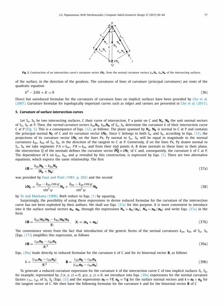
Fig. 1. Construction of an intersection curve’s curvature vector kNC , from the normal curvature vectors kanNa , kbnNb of the intersecting surfaces.

of the surface, in the direction of the geodesic. The curvatures of lines of curvature (principal curvatures) are roots of the quadratic equation

k2 − 2Hk + K = 0 (36)

Direct but unreduced formulae for the curvatures of curvature lines on implicit surfaces have been provided by Che et al.(2007). Curvature formulae for topologically important curves such as ridges and ravines are presented in Che et al. (2011).

5. Curvature of surface intersection curves

Let Sa, Sb be two intersecting surfaces, C their curve of intersection, P a point on C and Na , Nb the unit normal vectors of Sa, Sb at P. Then, the normal curvature vectors kanNa , kbnNb of Sa, Sb determine the curvature k of their intersection curve C at P (Fig. 1). This is a consequence of Equ. (12), as follows: The plane spanned by Na , Nb is normal to C at P and contains the principal normal NC of C and its curvature vector kNC . Since C belongs to both Sα and Sb, according to Equ. (12), the projections of its curvature vector kNC on the lines Px, Py normal to Sα , Sb will be equal in magnitude to the normal curvatures kan , kbn of Sa, Sb, in the direction of the tangent to C at P. Conversely, if on the lines Px, Py drawn normal to Sa, Sb we take segments P A = kan , P B = kbn and from their end points A, B draw normals to these lines in their plane, the intersection Q of the normals defines the curvature vector

−−→PQ = kNC of C and, consequently, the curvature k of C at P.

The dependence of k on kan , kbn and ϕ revealed by this construction, is expressed by Equ. (1). There are two alternative equations, which express the same relationship. The first

kB = kanNb − kbnNa

|Na × Nb| (37a)

was provided by Faux and Pratt (1981, p. 262) and the second

kNC = kan − kbn cosϕ

sin2 ϕNa + kbn − kan cosϕ

sin2 ϕNb (38)

by Ye and Maekawa (1999). Both reduce to Equ. (1) by squaring.Surprisingly, the possibility of using these expressions to derive reduced formulae for the curvature of the intersection

curve has not been exploited by their authors. We shall use Equ. (37a) for this purpose. It is more convenient to introduce into it the surface normal vectors na , nb , through the expressions Na = na/|na|, Nb = nb/|nb| and write Equ. (37a) in the form

kB = kan|na|nb − kbn|nb|na

|t| , |t| = |na × nb| (37b)

The convenience stems from the fact that introduction of the generic forms of the normal curvatures kan , kbn of Sα , Sb(Equ. (17)) simplifies this expression, as follows

kB = cannb − cbnna

|t|3 (39a)

Equ. (39a) leads directly to reduced formulae for the curvature k of C and for its binormal vector B, as follows

k = |cannb − cbnna||t|3 , B = cannb − cbnna

|cannb − cbnna| (39b)

To generate a reduced curvature expression for the curvature k of the intersection curve C of two implicit surfaces Sf, Sg, for example, represented by f (x, y, z) = 0, g(x, y, z) = 0, we introduce into Equ. (39a) expressions for the normal curvature factors c f n , cgn of Sf, Sg (Equ. (3)) and the expressions nf = ∇f, ng = ∇g for the surface normal vectors and t = nf × ng for the tangent vector of C. We then have the following formulae for the curvature k and for the binormal vector B of C

78 S.G. Papaioannou, M.M. Patrikoussakis / Computer Aided Geometric Design 37 (2015) 69–84

k = ((c f n gx − cgn fx)2 + (c f n g y − cgn f y)

2 + (c f n gz − cgn fz)2)1/2

(t2x + t2

y + t2z )

3/2

c f n = −(fxxt2

x + f yyt2y + f zzt2

z + 2 fxytxt y + 2 fxztxtz + 2 f yzt ytz)

cgn = −(gxxt2

x + g yyt2y + gzzt2

z + 2gxytxt y + 2gxztxtz + 2g yzt ytz)

B = [(c f n gx − cgn fx)(c f n g y − cgn f y)(c f n gz − cgn fz)]T

((c f n gx − cgn fx)2 + (c f n g y − cgn f y)2 + (c f n gz − cgn fz)2)1/2(39c)

For two parametric surfaces Sr1, Sr2, represented by r1(u, v) = [x1(u, v) y1(u, v) z1(u, v)]T, r2(p, q) =[x2(p, q) y2(p, q) z2(p, q)]T with normal vectors n1 = r1u × r1v , n2 = r2p × r2q , the tangent vector t = n1 × n2 of their intersection curve C has tangential coordinates in the basis r1u , r1v of the tangent plane of Sr1 a1 = −r1v · n2 , b1 = r1u · n2and in the basis r2p , r2q of the tangent plane of Sr2 a2 = −r2q · n1 , b2 = r2p · n1 (Equ. (20b)). Then, Equ. (39a) yields the formulae

k = ((cr1n2x − cr2n1x)2 + (cr1n2y − cr2n1y)

2 + (cr1n2z − cr2n1z)2)1/2

(t2x + t2

y + t2z )

3/2

cr1 = L′1a2

1 + 2M ′a1b1 + N ′1b2

1, L′1 = r1uun1, M ′

1 = r1uvn1, N ′1 = r1vvn1

cr2 = L′2a2

2 + 2M ′a2b2 + N ′2b2

2, L′2 = r2ppn2, M ′

2 = r2pqn2, N ′2 = r2qqn2

B = [(cr1n2x − cr2n1x)(cr1n2y − cr2n1y)(cr1n2z − cr2n1z)]T

((cr1n2x − cr2n1x)2 + (cr1n2y − cr2n1y)2 + (cr1n2z − cr2n1z)2)1/2(39d)

The curvature formula for the intersection curve of a parametric with an implicit surface was derived in Section 1 (Equ. (6b)), but it could have more readily been derived from Equ. (39a).

Interest in the differential geometry of surface intersection curves has recently expanded to include intersection curves in R4 and even higher dimensions (Goldman, 2005; Aléssio, 2006; 2012; Düldül, 2010).

6. Normal and intersection curvatures of offset surfaces

Intersection curves of surfaces which are offsets of (also known as parallel to) given surfaces do arise in modern appli-cations, justifying a revival of interest in their differential properties. For example, in the 3-axis CNC milling of free-form geometries, with a ball-end cutter of radius R , it is sometimes desirable to move the cutter with its ball-end being in si-multaneous contact with two given surfaces, both of which must be machined or one must be machined, while the other is used for guiding the tool. Then, the center point of the ball-end of the cutter, whose motion is programmed, moves along the intersection of two surfaces which are offsets of the given surfaces, at distance R .

6.1. Normal curvature

Let Sp be an offset surface of a given surface S, at distance d. Classical texts focus on the fact that at corresponding points P, Pp on S, Sp, that is points lying on a common normal line, the principal directions of the two surfaces are parallel and their principal curvatures kni , kpni , i = 1, 2, are related by

kni = kpni

1 + dkpni, kpni = kni

1 − dkni, i = 1,2 (40)

They don’t show, however, how the normal curvatures of S, Sp are related, in other directions. We shall investigate this matter, using Euler’s equation (Struik, 1950), which expresses the normal curvature kn at a surface point P, in a given tangent direction t, in terms of the principal curvatures kn1, kn2 of the surface at P and the angle ϕ of t with the direction of kn1, as follows:

kn = kn1 cos2 ϕ + kn2 sin2 ϕ = (kn1 − kn2) cos2 ϕ + kn2 (41a)

We apply Euler’s equation to Sp and substitute in it the principal curvatures kpn1, kpn2 of Sp by their expressions in terms of the principal curvatures of S (Equ. (40)), to obtain

kpn = (kpn1 − kpn2) cos2 ϕp + kpn2

=(

kn1 − kn2)

cos2 ϕp + kn2 (41b)

1 − dkn1 1 − dkn2 1 − dkn2

S.G. Papaioannou, M.M. Patrikoussakis / Computer Aided Geometric Design 37 (2015) 69–84 79

Since the principal directions on S, Sp are parallel, t makes equal angles with the directions of the principal curvatures kn1of S and kpn1 of Sp. Thus, by applying Euler’s equation to S, we express cos2 ϕp in terms of the principal curvatures of S

cos2 ϕp = kn − kn2

kn1 − kn2(42)

and Equ. (41b) becomes

kpn =(

kn1

1 − dkn1− kn2

1 − dkn2

)(kn − kn2

kn1 − kn2

)+ kn2

1 − dkn2

= kn − dkn1kn2

1 − d(kn1 + kn2) + d2kn1kn2

= kn − dK

1 − 2dH + d2 K(41c)

The last expression of the normal curvature kpn of Sp entails the normal curvature kn of the base surface S in the tangent direction t and the Gaussian and mean curvatures K , H of S. Reduced formulae for these curvatures have been given in Section 2 (Equ. (15)–(17)). Substituting kn , K , H by their generic expressions, we obtain

kipn =cin

|t|2|ni| − dciK|ni|4

1 − dciH|ni|3 + d2ciK

|ni|4= cipn

|t|2|ni| , cipn = |ni|(cin|ni|3 − dciK |t|2)|ni|4 − dciH |ni| + d2ciK

(43)

6.2. Curvature of intersection curves of offset surfaces

Expressions derived by instantiating the normal curvature expression (43) for a surface Srp offset of a given parametric surface Sr (i = r) and for a surface Sfp offset of a given implicit surface Sf (i = f ), can now be combined in all three modes (implicit/implicit, parametric/parametric and parametric/implicit) of the given surfaces Sr, Sf, with the aid of Equ. (39a), to yield curvature formulae for the intersection curves of offset surfaces. It may also be desirable to compute the curvature of the intersection of a given surface Sa with a surface Sbp offset of a given surface Sb. In all these cases, Equ. (39a), (43)can be used to produce intersection curvature formulae for offset surfaces, as it was done for given implicit and parametric surfaces in Section 5, provided proper expressions for the curvature factors crn , c f n , crK , c f K , crH , c f H of the given surfaces are utilized. For two surfaces Sfp, Sgp offset of given implicit surfaces Sf, Sg represented by f (x, y, z) = 0, g(x, y, z) = 0, for example, Equ. (39a) yields

k = ((c f pn gx − cgpn fx)2 + (c f pn g y − cgpn f y)

2 + (c f pn gz − cgpn fz)2)1/2

(t2x + t2

y + t2z )

3/2

c f pn = |nf|(c f n|nf|3 − dc f K |t|2)|nf|4 − dc f H |nf| + d2c f K

, cgpn = |ng|(cgn|ng|3 − dcg K |t|2)|ng|4 − dcg H |ng| + d2cg K

B = [(c f pn gx − cgpn fx)(c f pn g y − cgpn f y)(c f pn gz − cgpn fz)]T

((c f pn gx − cgpn fx)2 + (c f pn g y − cgpn f y)2 + (c f pn gz − cgpn fz)2)1/2(44)

with nf = ∇f, ng = ∇g, t = nf ×ng , where the expressions for the normal curvature factors c f n , cgn are derived from Equ. (3)and those for c f K , c f H , cg K , cg H from Equ. (16).

Example 2. Given a spherical surface Sf of radius R and a circular conical surface Sg with a 90◦ aperture and its apex at the center of the sphere, implicitly represented by

f = x2f + y2

f + z2f − R2 = 0, g = y2

g + z2g − x2

g = 0

and offsets Sfp, Sgp of these surfaces at distance d (Fig. 2): a) Express, by means of geometry, the curvature k of the largest of the two circles of intersection of Sfp, Sgp, in terms of R , d. b) Verify the curvature expression found in (a) by means of the general curvature formula (44).

(a) In the x–z plane, the generatrix line OP of Sgp has equation z = x + √2d. It meets the circle x2 + z2 = (R + d)2 at P,

whose coordinates are found by solving the system of these two equations to be

xP =√

2(√

R2 + 2dR − d), zP =

√2(

√R2 + 2dR + d)

2 2

80 S.G. Papaioannou, M.M. Patrikoussakis / Computer Aided Geometric Design 37 (2015) 69–84

Fig. 2. X–z plane view of the given surfaces Sf, Sg, their offsets Sfp, Sgp, their surface normal vectors nf , ng and the tangent vector t of the intersection circle of Sfp, Sgp.

Since zP equals the radius r of the intersection circle of Sfp, Sgp, the curvature of this circle is

k = 1

r=

√2

(√

R2 + 2dR + d)

(b) Partial derivatives of the given surfaces Sf, Sg:

fx = 2x f , f y = 2y f , f z = 2z f , fxx = f yy = f zz = 2, fxy = fxz = f yz = 0

gx = −2xg, g y = 2yg, gz = 2zg, gxx = −2, g yy = gzz = 2, gxy = gxz = g yz = 0

Surface normal vectors of Sf, Sg at Pf, Pg (y f = yg = 0):

nf = ∇f = [2x f 0 2z f ]T, ng = ∇g = [−2xg 0 2zg ]T,

|nf| = 2R, |ng| = 2(x2

g + z2g

)1/2 = 2(O P − d) = 2(√

2r − d) = 2√

R2 + 2dR

Tangent vector of the intersection circle of Sfp, Sgp at P:

tP = nf × ng = 4[

0 −(z f xg + x f zg) 0]T

To evaluate the norm of tP , we substitute the coordinates of Pf(x f , 0, z f ), Pg(xg, 0, zg) in terms of coordinates of P(xP , 0, zP ), using the defining relations of the offset surfaces:

rP = rf + dnf

|nf| = rg + dng

|ng||nf|x f + 2dx f = |nf|xP → x f = R

R + dxP , z f = R

R + dzP

|ng|xg − 2dxg = |ng|xP → xg = |ng|xP

|ng| − 2d, zg = |ng|zP

|ng| + 2d

Before applying curvature formula (44), it is convenient to express all quantities it entails in terms of R , d, |ng|, |tP|. Thus, we have

xP =√

2(|ng| − 2d)

4, r = zP =

√2(|ng| + 2d)

4

x f =√

2R(|ng| − 2d)

4(R + d), y f =

√2R(|ng| + 2d)

4(R + d)

xg = zg =√

2|ng|4

, |tP| = 4∣∣(z f xg + x f zg)

∣∣ = R|ng|2R + d

Curvature factors of Sfp, Sgp (Equ. (3), (17)):

S.G. Papaioannou, M.M. Patrikoussakis / Computer Aided Geometric Design 37 (2015) 69–84 81

c f n = −2t2P y = −2|tP|2, c f K = 16

(x2

f + z2f

) = 16R2, c f H = −16(x2

f + z2f

) = −16R2

c f pn = |nf|(c f n|nf|3 − dc f K |tP|2)|nf|4 − dc f H |nf| + d2c f K

= −2R|tP|2R + d

cgn = −2t2P y = −2|tP|2, cg K = 16

(x2

g − z2g

) = 0, cg H = −16x2g = −2|ng|2

cgpn = cgn|ng|3|ng|3 − dcg H

= −2|ng||tP|2|ng| + 2d

Curvature of the intersection circle of Sfp, Sgp (Equ. (44)):

k = ((c f pn gx − cgpn fx)2 + (c f pn gz − cgpn fz)

2)1/2

|tP|3

c f pn gx − cgpn fx = c f pn(−2xg) − cgpn(2x f ) = 2√

2R|ng|2|tP|2(R + d)(|ng| + 2d)

c f pn gz − cgpn fz = c f pn(2zg) − cgpn(2z f ) = 0

k = |c f pn gx − cgpn fx||tP|3 = 2

√2

|ng| + 2d=

√2

(√

R2 + 2dR + d)

7. Concluding remarks

The following properties of reduced curvature formulae can now be stated:

a) They are closed formulae, entailing only basic arithmetic operators (addition, subtraction, multiplication, division) and square root operators. They are thus suitable for casual users, whose skills do not extend beyond basic algebra and the extraction of function derivatives.

b) They are more efficient compared to alternative unreduced formulae (see Appendix A).

Although we have presented several reduced formulae, we have not exhausted all cases that may arise. We have not, for example, dealt with the curvature of curves defined by differential equations. Curves on offset surfaces may also arise in ways other than as intersections with other surfaces. An open problem is developing a curvature formula for the curve Cptraced by a point Pp on a surface Sp, offset of a given surface S, when its corresponding point P traces on S a given curve C. In this case, C and Cp do not have the same directions at corresponding points, so Euler’s formula (Equ. (41a)) cannot be used to relate the curvatures of C, Cp. The solution of this problem would be of practical interest in the isoparametric 3-D machining of a surface patch S, with a ball-end cutter.

Acknowledgement

The authors wish to thank the anonymous reviewers for their constructive comments and helpful suggestions.

Appendix A. Efficiency comparison of curvature formulae

We compare the cost of reduced curvature formulae to the cost of alternative unreduced formulae, in three cases, based on the following assumptions: The comparisons do not include the cost of computing function derivative values, which is the same for the compared formulae but case-dependent. These are assumed to be available. The cost of each formula is quantified by means of a multiplication count Cm, an addition count Ca and a square root count Csr. In forming these counts, divisions are assumed equivalent to multiplications, small integer powers equivalent to repeated multiplications and subtractions and multiplications by 2 equivalent to additions. The cost of standard vector operations then is: For a scalar product a · b, Cm = 3, Ca = 2, for a vector product a × b, Cm = 6, Ca = 3, for a double vector product a × b × c, Cm = 12, Ca = 6.

Case 1. Computation of the tangential coordinates a, b of t, when t is the tangent vector of the intersection curve of a parametric surface r = [x(u, v) y(u, v) z(u, v)]T by another surface with normal vector n. Table 1 compares the cost of using the unreduced formulae of Ye and Maekawa (1999) for a, b (Equ. (20a)) to the cost of using our reduced formulae (Equ. (20b)).

Case 2. Computation of the curvature k of the curve of intersection of a parametric surface r = [x(u, v) y(u, v) z(u, v)]T by an implicit surface f (x, y, z) = 0. Table 2 compares the cost of using the formulae of Ye and Maekawa (1999), Equ. (20a), for computing the coordinates a, b required by formula (2), and formulae (1)–(3) for computing k to the cost of computing a, b by our reduced formulae (Equ. (20b)) and our reduced formula (Equ. (6b)) for k.

82 S.G. Papaioannou, M.M. Patrikoussakis / Computer Aided Geometric Design 37 (2015) 69–84

Table 1Cost comparison of the unreduced and reduced formulae for a, b.

Ye and Maekawa (1999), Equ. (20a)

Cm Ca Our formulae, Equ. (20b)

Cm Ca

E , F , G 9 6 a, b 6 4EG − F 2 2 1t = (ru × rv) × n 12 6t · ru , t · rv 6 4a, b 6 2Total counts 35 19 6 4

Table 2Cost comparison of unreduced and reduced formulae for computing the intersection curvature of a parametric with an implicit surface.

Ye and Maekawa (1999), Equ. (20a), (1)–(3)

Cm Ca Csr Our reduced formulae, Equ. (20b), (6b)

Cm Ca Csr

A, b 35 19 0 a, b 6 4 0L′ , M ′ , N ′ 9 6 0 nrx , nry , nrz 6 3 0crn 6 3 0 L′ , M ′ , N ′ 9 6 0|nr|, |nf|, |t|, |t|3 11 6 3 crn 6 3 0c f n 9 8 0 tx , t y , tz 6 3 0cosϕ, sinϕ 7 2 0 |t|, |t|3 5 2 1k f n , krn 4 0 0 c f n 9 8 0k 5 3 1 k 10 5 1Total counts 86 47 4 Total counts 57 34 2

Case 3. We prove the equivalence of Goldman’s formula for the curvature of the intersection curve of two implicit surfaces f (x, y, z) = 0, g(x, y, z) = 0 (Goldman, 2005)

k = |((∇ f × ∇g) ∗ ∇(∇ f × ∇g)) × (∇ f × ∇g)||∇ f × ∇g|3 (A.1a)

with our reduced formula for this curvature (Equ. (39c)) and, in the process, we compare the efficiencies of the two formu-lae. Since the denominator in both formulae is |t|3, it suffices to prove the equivalence of the numerators.

In Equ. (A.1a), ∗ is the matrix multiplication operator, with operands the curve’s tangent vector t = ∇ f × ∇g and the matrix M = ∇t. This matrix is formed with columns the gradients of the components of t, that is M = [∇tx ∇t y ∇tz]. Thus, Equ. (A.1a) can be written

k = |[ tx t y tz ] ∗ [∇tx ∇t y ∇tz ] × [ tx t y tz ]|(t2

x + t2y + t2

z )3/2

(A.1b)

The columns of M are

∇tx = ∇( f y gz − f z g y) = ∇ f y gz + f y∇gz − ∇ f z g y − f z∇g y

∇t y = ∇( f z gx − fx gz) = ∇ f z gx + f z∇gx − ∇ fx gz − fx∇gz

∇tz = ∇( fx g y − f y gx) = ∇ fx g y + fx∇g y − ∇ f y gx − f y∇gx (A.2)

Let [X Y Z ] be the vector [tx, t y, tz] ∗ [∇tx ∇t y ∇tz]. Then, by matrix multiplication

X = ( fxy gz + f y gxz − fxz g y − f z gxy)tx + ( f yy gz + f y g yz − f yz g y − f z g yy)t y

+ ( f yz gz + f y gzz − f zz g y − f z g yz)tz

Y = ( fxz gx + f z gxx − fxx gz − fx gxz)tx + ( f yz gx + f z gxy − fxy gz − fx g yz)t y

+ ( f zz gx + f z gxz − fxz gz − fx gzz)tz

Z = ( fxx g y + fx gxy − fxy gx − f y gxx)tx + ( fxy g y + fx g yy − f yy gx − f y gxy)t y

+ ( fxz g y + fx g yz − f yz gx − f y gxz)tz (A.3)

and the first component of the vector [X Y Z ] × [tx, t y, tz] is

Y tz − Zt y = (f yyt2

y + f zzt2z + fxytxt y + fxztxtz + 2 f yzt ytz

)gx

− (g yyt2

y + gzzt2z + gxytxt y + gxztxtz + 2g yzt ytz

)fx − ( fxxtx + fxyt y + fxztz)(g yt y + gztz)

+ (gxxtx + gxyt y + gxztz)( f yt y + f ztz) (A.4a)

S.G. Papaioannou, M.M. Patrikoussakis / Computer Aided Geometric Design 37 (2015) 69–84 83

Table 3Cost comparison of the unreduced Goldman’s formula to our reduced formula for computing the intersection curvature of two implicit surfaces.

Goldman’s formula, Equ. (A.1b) Cm Ca Csr Our formula, Equ. (39c) Cm Ca Csr

tx , t y , tz 6 3 0 tx , t y , tz 6 3 0|t|, |t|3 5 2 1 |t|, |t|3 5 2 1Matrix ∇(∇t) = [∇tx ∇t y ∇tz] 30 27 0 c f n , cgn 18 16 0[X Y Z ] = [tx, t y, tz] ∗ [∇tx ∇t y ∇tz] 9 6 0 k 10 5 1[X Y Z ] × [tx, t y , tz] 6 3 0|[X Y Z ] × [tx, t y , tz]|, k 4 2 1Total counts 60 43 2 39 26 2

which, by means of the normality conditions f yt y + f ztz = − fxtx , g yt y + gztz = −gxtx , becomes

Y tz − Zt y = (fxxt2

x + f yyt2y + f zzt2

z + 2 fxytxt y + 2 fxztxtz + 2 f yzt ytz)

gx

− (gxxt2

x + g yyt2y + gzzt2

z + 2gxytxt y + 2gxztxtz + 2g yzt ytz)

fx

= −(c f n gx − cgn fx) (A.4b)

Similarly, it can be shown that the second and third components of the vector [X Y Z ] ×[tx, t y, tz] are Ztx − Xtz = −(c f n g y −cgn f y) and Xt y − Y tx = −(c f n gz − cgn fz). Thus, the numerator in Goldman’s formula (Equ. (A.1b)) is

∣∣[ tx t y tz ] ∗ [∇tx ∇t y ∇tz ] × [ tx t y tz ]∣∣= (

(c f n gx − cgn fx)2 + (c f n g y − cgn f y)

2 + (c f n gz − cgn fz)2)1/2

(A.5)

the same as in our formula (Equ. (39c)). Table 3 compares the cost of computing the intersection curvature of two implicit surfaces by Goldman’s formula, Equ. (A.1b), to the cost of computing the same curvature by our reduced formula (39c).

Appendix B. Alternative proof of formulae (30), (34)

The curvature formula for a curve C, defined by a pair of parametric equations x = x(u), y = y(u) on an implicit surface Sf represented by f (x, y, z) = 0, was derived in Section 4 (Equ. (30)) from the curve representation f (x(u), y(u), z) = 0. As a correctness test, we shall derive this formula by considering C as the curve of intersection of Sf with a generalized cylindrical surface Sr with position vector r = [x(u) y(u) v]T and using Equ. (6b) to obtain its curvature.

Normal vector of Sf : nf = [ fx f y f z]T. Parametric derivatives and normal vector of Sr: ru = [xu yu 0]T, rv = [0 0 1]T, ruu = [xuu yuu 0]T, ruv = rvv = [0 0 0]T, nr = ru × rv = [yu −xu 0]T. Tangent vector of C: t = nf × nr = [ f zxu fz yu −zp]T, |t| = ( f 2

z (x2u + y2

u) + z2p)1/2, zp = fxxu + f y yu .

Curvature factors of Sf, Sr (Equ. (2), (3)):

c f n = −(fxxt2

x + f yyt2y + f zzt2

z + 2 fxytxt y + 2 fxztxtz + 2 f yzt ytz) = zpp + f 2

z ( fxxuu + f y yuu)

zpp = −(f 2

z

(fxxx2

u + f yy y2u + 2 fxyxu yu + fxxuu + f y yuu

) + 2 f z( fxzxu + f yz yu)zp + f zzz2p

)L′ = ruunr = xuu yu − yuuxu, M ′ = ruvnr = 0, N ′ = rvvnr = 0, a = −rvnf = − f z, b = runf = zp,

crn = L′a2 + 2M ′ab + N ′b2 = f 2z (xuu yu − yuuxu).

Numerator terms of curvature formula (6b):

crn fx − c f nnrx = f 2z (xuu yu − yuuxu) fx − (

zpp + f 2z ( fxxuu + f y yuu)

)yu

= −(yu zpp − yuu f 2

z zp)

crn f y − c f nnry = f 2z (xuu yu − yuuxu) f y + (

zpp + f 2z ( fxxuu + f y yuu)

)xu

= −(f 2

z zpxuu − zppxu)

crn f z − c f nnrz = f 3z (xuu yu − yuuxu)

Formula (6b) for the intersection curvature of an implicit with a parametric surface:

k = ((crn fx − c f nnrx)2 + (crn f y − c f nnry)

2 + (crn f z − c f nnrz)2)1/2

(t2x + t2

y + t2z )

3/2

= ((yu zpp − yuu f 2z zp)2 + ( f 2

z zpxuu − zpp xu)2 + f 6z (xu yuu − xuu yu)2)1/2

( f 2(x2 + y2) + z2 )3/2

z u u p

84 S.G. Papaioannou, M.M. Patrikoussakis / Computer Aided Geometric Design 37 (2015) 69–84

which is formula (30) with the parametric derivatives x′ , x′′ , y′ , y′′ denoted here as xu , xuu , yu , yuu . Formula (34) for the curvature of a curve C defined implicitly as g(x, y) = 0 on an implicit surface f (x, y, z) = 0 can be proved in a similar man-ner, by considering C as the curve of intersection of two implicit surfaces f (x, y, z) = 0, g(x, y) = 0, the latter representing an implicitly defined generalized cylinder and using formula (39c).

References

Aléssio, O., 2006. Differential geometry of intersection curves in R4 of three implicit surfaces. Comput. Aided Geom. Des. 23, 455–471.Aléssio, O., 2012. Formulas for second curvature, third curvature, normal curvature, first geodesic curvature and first geodesic torsion of implicit curve in

n-dimensions. Comput. Aided Geom. Des. 29, 189–201.Belyaev, A., Pasko, A., Kunii, T., 1998. Ridges and ravines on implicit surfaces. In: Proceedings of Computer Graphics International ’98. Hanover, pp. 530–535.Che, W., Paul, J.C., Zhang, X., 2007. Lines of curvature and umbilical points for implicit surfaces. Comput. Aided Geom. Des. 24, 395–409.Che, W., Zhang, X., Zhang, Y.K., Paul, J.C., Xu, B., 2011. Ridge extraction of a smooth 2-manifold surface based on vector field. Comput. Aided Geom. Des. 28,

215–232.Do Carmo, P.M., 1976. Differential Geometry of Curves and Surfaces. Prentice-Hall, Englewood Cliffs, NJ.Düldül, M., 2010. On the intersection curve of three parametric hypersurfaces. Comput. Aided Geom. Des. 27, 118–127.Faux, I.D., Pratt, M.J., 1981. Computational Geometry for Design and Manufacture. Ellis Horwood, Chichester, England.Goldman, R., 2005. Curvature formulae for implicit curves and surfaces. Comput. Aided Geom. Des. 22, 632–658.Hartmann, E., 1996. G2 interpolation and blending on surfaces. Vis. Comput. 12, 181–192.Knoblauch, J., 1913. Grundlagen der Differentialgeometrie. Druck und Verlag von B.G. Teubner, Leipzig.Kreyszig, E., 1991. Differential Geometry. Dover Publications Inc., New York.Lipschutz, M., 1969. Differential Geometry. Schaum’s Outlines. Schaum Publishing Co., New York.Osher, S., Fedkiw, R., 2003. Level Set Methods and Dynamic Implicit Surfaces. Appl. Math. Sci., vol. 153. Springer-Verlag, New York.Papaioannou, S.G., Patrikoussakis, M.M., 2011. Curve interpolation based on the canonical arc length parametrization. Comput. Aided Des. 43, 21–30.Patrikalakis, N.M., Maekawa, T., 2002. Shape Interrogation for Computer Aided Design and Manufacturing. Springer-Verlag, New York.Spivak, M., 1975. A Comprehensive Introduction to Differential Geometry, vol. 3. Publish or Perish, Boston.Struik, D.J., 1950. Lectures on Classical Differential Geometry. Addison-Wesley, Reading, MA.Turkiyyah, G.M., Storti, D.W., Ganter, M., Chen, H., Vimawala, M., 1997. An accelerated triangulation method for computing the skeletons of free-form solid

models. Comput. Aided Des. 29, 5–19.Willmore, T.J., 1959. An Introduction to Differential Geometry. Clarendon Press, Oxford.Ye, X., Maekawa, T., 1999. Differential geometry of intersection curves of two surfaces. Comput. Aided Geom. Des. 16, 767–788.