J. Math. Anal. Appl. 345 (2008) 350–361

Contents lists available at ScienceDirect

J. Math. Anal. Appl.

www.elsevier.com/locate/jmaa

Recurrence relations for semilocal convergence of a Newton-like methodin Banach spaces ✩

P.K. Parida ∗, D.K. Gupta

Department of Mathematics, Indian Institute of Technology, Kharagpur 721302, India

a r t i c l e i n f o a b s t r a c t

Article history:Received 8 February 2007Available online 3 April 2008Submitted by Richard M. Aron

Keywords:Newton-like methodLipschitz continuousHölder continuousCubic convergenceRecurrence relations

The aim of this paper is to establish the semilocal convergence of a multipoint third orderNewton-like method for solving F (x) = 0 in Banach spaces by using recurrence relations.The convergence of this method is studied under the assumption that the second Fréchetderivative of F satisfies Hölder continuity condition. This continuity condition is milderthan the usual Lipschitz continuity condition. A new family of recurrence relations aredefined based on the two new constants which depend on the operator F . These recurrencerelations give a priori error bounds for the method. Two numerical examples are workedout to demonstrate the applicability of the method in cases where the Lipschitz continuitycondition over second derivative of F fails but Hölder continuity condition holds.

© 2008 Elsevier Inc. All rights reserved.

1. Introduction

Let F : Ω ⊆ X → Y be a nonlinear operator on an open convex subset Ω of a Banach space X with values in a Banachspace Y. Many researchers [1,2,4,5] have developed and studied the convergence of one point third order iterative methodssuch as Chebyshev’s method, Halley’s method and super-Halley’s method to solve nonlinear operator equations F (x) = 0.These methods are useful in solving stiff systems of equations [15], where a quick convergence is required. They haveestablished the convergence of these methods by considering the second Fréchet derivative of F to be Lipschitz continuous.One drawback of these methods is that they involve the second derivative of the operator F which at times is very difficultto compute. This restricts the use of these methods as their informational efficiency is less than or equal to unity.

Multipoint third order iterative methods [3,6,7,10–12,16] are also discussed to find the solutions of F (x) = 0 in Banachspaces. These methods require information at more than one point and are easy to use as they need only the operator Fand its first derivative F ′ . The convergence of one such iterative method studied by Wu and Zhao [11] is given as

yn = xn − F ′(xn)−1 F (xn),

xn+1 = xn −(

F ′(xn) + F ′(yn)

2

)−1

F (xn), n = 0,1, . . . .

⎫⎪⎬⎪⎭ (1)

They constructed a majorizing function to study the convergence of this method under the assumption that F ′′ satisfiesLipschitz continuity condition. Parida and Gupta [10] developed a semilocal convergence analysis of the above iterativemethod by using recurrence relations under the same assumptions on the operator F .

✩ This work is supported by financial grant, CSIR (No. 10-2(5)/2004(i)-EU II), India.

* Corresponding author. Fax: +91 3222 255303/282700.E-mail addresses: pradipparida@yahoo.com (P.K. Parida), dkg@maths.iitkgp.ernet.in (D.K. Gupta).

0022-247X/$ – see front matter © 2008 Elsevier Inc. All rights reserved.doi:10.1016/j.jmaa.2008.03.064

P.K. Parida, D.K. Gupta / J. Math. Anal. Appl. 345 (2008) 350–361 351

But there are certain problems for which the convergence analysis cannot be studied under the assumption that thesecond derivative of F be Lipschitz continuous.

Example. Let us consider the integral equation of Fredholm type [13]

F (x)(s) = x(s) − f (s) − λ

1∫0

s

s + tx(t)2+p dt, (2)

with s ∈ [0,1], x, f ∈ C[0,1], p ∈ (0,1] and λ is a real number. Now for instance when we choose sup norm, the corre-sponding second derivative of the operator F satisfies∥∥F ′′(x) − F ′′(y)

∥∥ � |λ|(1 + p)(2 + p) log 2‖x − y‖p, x, y ∈ Ω. (3)

Hence for p ∈ (0,1), F ′′ does not satisfy the Lipschitz continuity condition. For example, for p = 1/2, F ′′ satisfies the Höldercontinuity condition given by∥∥F ′′(x) − F ′′(y)

∥∥ � 15

4|λ| log 2‖x − y‖1/2, x, y ∈ Ω,

but not the Lipschitz continuity condition. For p = 1, the condition (3) reduces to Lipschitz continuity condition. Underthe assumption that F ′′ satisfies Hölder continuity condition, Hernández and Salanova [9] and Hernández [7] studied theconvergence of Chebyshev’s method and its second derivative free version by using recurrence relations. Also under similarconditions, by using the technique of recurrence relations, Ye and Li [12] studied the convergence of Euler–Halley method.

In this paper, we establish the semilocal convergence of the method (1) by using recurrence relations under the assump-tion that F ′′ satisfies Hölder continuity condition. In order to increase its R-order of convergence from 2 to (2 + p), we havealso given a reformulation of the method (1).

The paper is organized as follows: In Section 2, some preliminary results are given. The recurrence relations for themethod (1) are established in Section 3. An existence-uniqueness theorem is given in Section 4 to establish the R-order ofthe method to be 2 and a priori error bounds. In Section 4.1, the convergence of a modified version of the method (1) isgiven to establish that the R-order of the method can be increased. In Section 5, two numerical examples are worked outto show the efficacy of our convergence analysis. Finally, conclusions form Section 6.

2. Preliminary results

In this section, we shall discuss the convergence of the iterative method (1) for solving the nonlinear operator equation

F (x) = 0. (4)

Let F be twice Fréchet differentiable operator in Ω and BL(Y,X) be the set of bounded linear operators from Y into X.Let Γ0 = F ′(x0)

−1 ∈ BL(Y,X) exists at some point x0 ∈ Ω and assume that the following conditions hold on F :

1. ‖Γ0‖ � β,

2.∥∥Γ0 F (x0)

∥∥ � η,

3.∥∥F ′′(x)

∥∥ � M, ∀x ∈ Ω,

4.∥∥F ′′(x) − F ′′(y)

∥∥ � N‖x − y‖p, ∀x, y ∈ Ω, p ∈ (0,1].

⎫⎪⎪⎪⎪⎬⎪⎪⎪⎪⎭

(5)

If a0 = Mβη, b0 = Nβη1+p be two parameters, then for n ∈ Z+ , define two real sequences

an+1 = an f (an)2 g(an,bn) and bn+1 = bn f (an)2+p g(an,bn)1+p, (6)

where

f (x) = (2 − x)/(2 − 3x), (7)

g(x, y) =[

x(4 − x)(3 − x)

(2 − x)2+ (p + 4)y

2(p + 1)(p + 2)

]. (8)

Let r0 be the smallest positive zero of the polynomial h(x) = −x3 +16x2 −24x+4, then r0 = 0.1905960896 . . . . The followinglemmas will prove a number of properties of the sequences {an} and {bn}.

Lemma 2.1. Let f and g be the functions defined by (7) and (8) respectively, then for x ∈ (0, r0),

(i) f is increasing and f (x) > 1,(ii) g is increasing in both arguments for y > 0,

(iii) f (δx) < f (x) and g(δx, δp y) < δp g(x, y), for δ ∈ (0,1) and p ∈ (0,1].

352 P.K. Parida, D.K. Gupta / J. Math. Anal. Appl. 345 (2008) 350–361

Proof. The proof is simple and can be omitted. �Lemma 2.2. For fixed p ∈ (0,1], let f and g be the functions defined by (7) and (8), respectively. Let

Φp(x) = 2(p + 1)(p + 2)(−x3 + 16x2 − 24x + 4)

(p + 4)(2 − x)2. (9)

If 0 < a0 � r0 and 0 � b0 � Φp(a0), then

(i) f (an)2 g(an,bn) � 1,

(ii) {an}, {bn} are decreasing and an < 1, ∀n.

Proof. From definitions of f and g , one can easily conclude that

f (an)2 g(an,bn) � 1 iff bn � 2(p + 1)(p + 2)(−a3n + 16a2

n − 24an + 4)

(p + 4)(2 − an)2= Φp(an).

Induction will be used to prove this lemma. For 0 < a0 � r0 and 0 � b0 � Φp(a0), one can easily conclude from above thatf (a0)

2 g(a0,b0) � 1. Thus, from Eq. (6), we obtain

a1 = a0 f (a0)2 g(a0,b0) � a0 < 1,

and as f (x) > 1 in (0, r0], we get

b1 = b0 f (a0)2+p g(a0,b0)

1+p � b0 f (a0)2 g(a0,b0)

[f (a0)

2 g(a0,b0)]p � b0.

Let the statements hold for n = k. Then proceeding similarly, one can easily prove that ak+1 � ak < 1, and bk+1 � bk . Sincef and g are increasing functions, we get

f (ak+1)2 g(ak+1,bk+1) � f (ak)

2 g(ak,bk) � 1.

Thus, the above statements also hold for n = k + 1. Hence, it is true for all n. This proves Lemma 2.2. �Lemma 2.3. Let us suppose 0 < a0 < r0 and 0 < b0 < Φp(a0). Define γ = a1/a0 , then for n � 1, we have

(i) an � γ 2n−1an−1 � γ 2n−1a0 , strictly holds for n � 2,

(ii) bn < γ 2n−1bn−1 < γ 2n−1b0 ,

(iii) f (an)g(an,bn) < γ 2n/ f (a0).

Proof. We will prove (i) and (ii) by induction. Since a1 = γ a0 and a1 < a0 from Lemma 2.2(i), we get γ < 1. By Lem-mas 2.1(i) and 2.2(i), we get

b1 = b0 f (a0)2+p g(a0,b0)

1+p = b0(

f (a0)2 g(a0,b0)

)(f (a0)g(a0,b0)

)p

<(

f (a0)2 g(a0,b0)

)(f (a0)

2 g(a0,b0))p

b0 <(

f (a0)2 g(a0,b0)

)b0 = γ b0.

Also,

a2 = a1 f (a1)2 g(a1,b1) < γ a0 f (γ a0)

2 g(γ a0, γ b0) < γ a0 f (a0)2γ g(a0,b0) = γ 2a1.

Suppose (i) and (ii) hold for n = k, then

ak+1 = ak f (ak)2 g(ak,bk) < γ 2k−1

ak−1 f(γ 2k−1

ak−1)2

g(γ 2k−1

ak−1, γ2k−1

bk−1)

< γ 2k−1ak−1 f (ak−1)

2γ 2k−1g(ak−1,bk−1) = γ 2k

ak.

Also as f (x) > 1 in (0, r0], we get

bk+1 = bk f (ak)2+p g(ak,bk)

1+p = bk(

f (ak)2 g(ak,bk)

)(f (ak)g(ak,bk)

)p

< bk(

f (ak)2 g(ak,bk)

)(f (ak)

2 g(ak,bk))p

< bk

(ak+1

ak

)< γ 2k

bk.

Hence,

ak+1 < γ 2kak < γ 2k

γ 2k−1 · · ·γ 20a0 = γ 2k+1−1a0

and

bk+1 < γ 2kbk < γ 2k

γ 2k−1 · · ·γ 20b0 = γ 2k+1−1b0.

P.K. Parida, D.K. Gupta / J. Math. Anal. Appl. 345 (2008) 350–361 353

Thus (i) and (ii) hold for all n by induction. Condition (iii) follows from

f (an)g(an,bn) < f(γ 2n−1a0

)g(γ 2n−1a0, γ

2n−1b0)< γ 2n−1 f (a0)g(a0,b0) = γ 2n

/ f (a0)

as γ = a1/a0 = f (a0)2 g(a0,b0). �

3. Recurrence relations for the method

In this section, the recurrence relations are derived for the method given by (1) under the assumptions mentioned in theprevious section.

Since existence of Γ0 gives existence of y0, we get M‖Γ0‖‖y0 − x0‖ � Mβη = a0. Also,∥∥∥∥I − Γ0F ′(y0) + F ′(x0)

2

∥∥∥∥ =∥∥∥∥Γ0

F ′(x0) − F ′(y0)

2

∥∥∥∥ � 1

2M‖Γ0‖‖x0 − y0‖ � a0

2< 1.

Hence, (F ′(y0)+F ′(x0)

2 )−1 F ′(x0) exists by Banach theorem [14, p. 155], and

∥∥∥∥(

F ′(y0) + F ′(x0)

2

)−1

F ′(x0)

∥∥∥∥ � 1

1 − 12 M‖Γ0‖‖x0 − y0‖

� 2

2 − a0.

Thus, we have

‖x1 − x0‖ �∥∥∥∥(

F ′(y0) + F ′(x0)

2

)−1

F ′(x0)

∥∥∥∥∥∥F ′(x0)−1 F (x0)

∥∥ � 2

2 − a0‖y0 − x0‖ (10)

and

‖x1 − y0‖ � ‖x1 − x0‖ + ‖x0 − y0‖ � 4 − a0

2 − a0‖y0 − x0‖. (11)

Also,

N‖Γ0‖‖y0 − x0‖1+p � Nβη1+p = b0.

Based on these results, the following inequalities can be proved for n � 1,

(I) ‖Γn‖ = ∥∥F ′(xn)−1∥∥ � f (an−1)‖Γn−1‖,

(II) ‖yn − xn‖ = ∥∥Γn F (xn)∥∥ � f (an−1)g(an−1,bn−1)‖yn−1 − xn−1‖,

(III) M‖Γn‖‖yn − xn‖ � an,

(IV) ‖xn+1 − xn‖ � 2

2 − an‖yn − xn‖,

(V) ‖xn+1 − yn‖ � 4 − an

2 − an‖yn − xn‖,

(VI) N‖Γn‖‖yn − xn‖1+p � bn.

⎫⎪⎪⎪⎪⎪⎪⎪⎪⎪⎪⎪⎪⎪⎬⎪⎪⎪⎪⎪⎪⎪⎪⎪⎪⎪⎪⎪⎭

(12)

Now induction can be used to prove the conditions (I)–(VI). Assume that x1 ∈ Ω . We now have

∥∥I − Γ0 F ′(x1)∥∥ � M‖Γ0‖‖x0 − x1‖ � Mβ

2

2 − a0‖y0 − x0‖ � 2a0

2 − a0< 1.

Hence by Banach theorem, Γ1 = F ′(x1)−1 exists and

‖Γ1‖ � ‖Γ0‖1 − M‖Γ0‖‖x0 − x1‖ � 2 − a0

2 − 3a0‖Γ0‖ = f (a0)‖Γ0‖. (13)

Thus y1 exists. Now by applying Taylor’s method, one can easily obtain

F (xn+1) =1∫

0

F ′′(yn + t(xn+1 − yn))(1 − t)dt(xn+1 − yn)2 + 1

2

1∫0

F ′′(xn + t(yn − xn))

dt(yn − xn)(xn+1 − yn)

− 1

2

1∫0

F ′′(xn + t(yn − xn))

dt(yn − xn)2 +1∫

0

F ′′(xn + t(yn − xn))(1 − t)dt(yn − xn)2. (14)

354 P.K. Parida, D.K. Gupta / J. Math. Anal. Appl. 345 (2008) 350–361

It is to be noted that∥∥∥∥∥1∫

0

F ′′(x0 + t(y0 − x0))(1 − t)dt(y0 − x0)

2 − 1

2

1∫0

F ′′(x0 + t(y0 − x0))

dt(y0 − x0)2

∥∥∥∥∥�

∥∥∥∥∥1∫

0

F ′′(x0 + t(y0 − x0))(1 − t)dt(y0 − x0)

2 − 1

2F ′′(x0)(y0 − x0)

2

∥∥∥∥∥+

∥∥∥∥∥ 1

2

1∫0

F ′′(x0 + t(y0 − x0))

dt(y0 − x0)2 − 1

2F ′′(x0)(y0 − x0)

2

∥∥∥∥∥� (p + 4)N

2(p + 1)(p + 2)‖y0 − x0‖2+p .

Using this result in (14), we get∥∥Γ1 F (x1)∥∥ � ‖Γ1‖

∥∥F (x1)∥∥

� f (a0)‖Γ0‖[

M(4 − a0)(3 − a0)

(2 − a0)2‖y0 − x0‖2 + (p + 4)N

2(p + 1)(p + 2)‖y0 − x0‖2+p

]

� f (a0)

[a0(4 − a0)(3 − a0)

(2 − a0)2+ (p + 4)b0

2(p + 1)(p + 2)

]‖y0 − x0‖

= f (a0)g(a0,b0)‖y0 − x0‖. (15)

Also,

M‖Γ1‖‖y1 − x1‖ � M‖Γ0‖ f (a0)2 g(a0,b0)‖y0 − x0‖ � a0 f (a0)

2 g(a0,b0) = a1. (16)

Hence, for n = 1, the conditions (I)–(III) follow from Eqs. (13), (15) and (16), respectively. Proceeding as in (10) and (11), onecan easily prove (IV) and (V) for n = 1.

We also have

N‖Γ1‖‖y1 − x1‖1+p � N‖Γ0‖ f (a0) f (a0)1+p g(a0,b0)

1+p‖y0 − x0‖1+p � b1. (17)

Thus, condition (VI) follows from the above equation. Now by considering that the statements (I)–(VI) hold for n = k andxk ∈ Ω , one can easily prove that the conditions (I)–(VI) also hold for n = k + 1. Hence, by induction it holds for all n.

4. Convergence analysis

The following theorem will establish the convergence of the sequence {xn} and give a priori error bounds for it. Letus denote γ = a1/a0 and Δ = 1/ f (a0), R = 2/((2 − a0)(1 − γΔ)), B(x0, Rη) = {x ∈ X: ‖x − x0‖ < Rη} and B(x0, Rη) ={x ∈ X: ‖x − x0‖ � Rη}.

Theorem 4.1. Let r0 be the smallest positive zero of the polynomial h(x) = −x3 + 16x2 − 24x + 4. If Φp(x) be the function defined byEq. (9), then let us assume that 0 < a0 � r0 and 0 � b0 � Φp(a0) hold. Under the assumptions given in (5) on F and B(x0, Rη) ⊆ Ω ,the method (1) starting from x0 generates a sequence {xn} converging to the root x∗ of (4) with R-order at least 2. In this case xn, yn

and x∗ lie in B(x0, Rη) and the solution x∗ is unique in B(x0,2/(Mβ) − Rη) ∩ Ω . Furthermore, the error bounds on x∗ is given by

‖x∗ − xn‖ � 2γ 2n−1

(2 − γ 2n−1a0)

Δn

(1 − γ 2nΔ)

η. (18)

Proof. It is sufficient to show that {xn} is a Cauchy sequence in order to establish the convergence of {xn}.Now for a0 = r0, b0 = Φp(a0) = 0 and f (a0)

2 g(a0,b0) = 1. Hence from (6), an = an−1 = · · · = a0 and bn = bn−1 = · · · =b0 = 0.

Also from (12), we have

‖yn − xn‖ � f (an−1)g(an−1,bn−1)‖yn−1 − xn−1‖ = f (a0)g(a0,b0)‖yn−1 − xn−1‖� · · · � (

f (a0)g(a0,b0))n‖y0 − x0‖ = Δnη

and

‖xn+1 − xn‖ � 2

2 − a‖yn − xn‖ � 2

2 − aΔnη.

n 0

P.K. Parida, D.K. Gupta / J. Math. Anal. Appl. 345 (2008) 350–361 355

Thus,

‖xm+n − xm‖ � ‖xm+n − xm+n−1‖ + · · · + ‖xm+1 − xm‖ � 2

2 − a0

[Δm+n−1 + · · · + Δm]

η = 2Δm

2 − a0

(1 − Δn

1 − Δ

)η. (19)

Hence, if we take m = 0, xn ∈ B(x0, Rη). Similarly one can prove that yn ∈ B(x0, Rη). Also from the above equation, we canconclude that {xn} is a Cauchy sequence.

Let 0 < a0 < r0 and 0 < b0 < Φp(a0). Now from (12) and Lemma 2.3(iii), for n � 1, we have

‖yn − xn‖ � f (an−1)g(an−1,bn−1)‖yn−1 − xn−1‖ � · · · � ‖y0 − x0‖n−1∏j=0

f (a j)g(a j,b j) <

n−1∏j=0

(γ 2 j

Δ)η = γ 2n−1Δnη,

where γ = a1/a0 < 1 and Δ = 1/ f (a0) < 1. Hence,

‖xm+n − xm‖ � ‖xm+n − xm+n−1‖ + · · · + ‖xm+1 − xm‖� 2

2 − am+n−1‖ym+n−1 − xm+n−1‖ + · · · + 2

2 − am‖ym − xm‖

<2

2 − am+n−1γ 2m+n−1−1Δm+n−1η + · · · + 2

2 − amγ 2m−1Δmη

<2Δm

2 − am

[γ 2m+n−1−1Δn−1 + · · · + γ 2m−1]η

<2γ 2m−1Δm

2 − γ 2m−1a0

[γ 2m[2n−1−1]Δn−1 + · · · + γ 2m[2−1]Δ + 1

]η.

By Bernoulli’s inequality, for every real number x > −1 and every integer k � 0, we have (1 + x)k − 1 � kx. Thus,

‖xm+n − xm‖ <2γ 2m−1Δm

(2 − γ 2m−1a0)

1 − γ 2mnΔn

(1 − γ 2mΔ)

η. (20)

Thus, for m = 0, we get

‖xn − x0‖ <2

2 − a0

1 − γ nΔn

1 − γΔη < Rη. (21)

Hence, xn ∈ B(x0, Rη). Also, yn ∈ B(x0, Rη) results from

‖yn+1 − x0‖ � ‖yn+1 − xn+1‖ + ‖xn+1 − xn‖ + · · · + ‖x1 − x0‖� ‖yn+1 − xn+1‖ + 2

2 − an‖yn − xn‖ + · · · + 2

2 − a0‖y0 − x0‖

<2

2 − an+1‖yn+1 − xn+1‖ + 2

2 − an‖yn − xn‖ + · · · + 2

2 − a0‖y0 − x0‖

< · · · < 2

2 − a0

1 − γ n+2Δn+2

1 − γΔη < Rη.

On taking limit as n → ∞ in (19) or (21), we get x∗ ∈ B(x0, Rη). To show that x∗ is a solution of F (x) = 0, we see that‖F (xn)‖ � ‖F ′(xn)‖‖Γn F (xn)‖ and the sequence {‖F ′(xn)‖} is bounded as∥∥F ′(xn)

∥∥ �∥∥F ′(x0)

∥∥ + M‖xn − x0‖ <∥∥F ′(x0)

∥∥ + M Rη.

Since F is continuous, so by taking limit as n → ∞ we get F (x∗) = 0. To show the uniqueness of x∗ , let y∗ be the anotherroot of (4) in B(x0,2/(Mβ) − Rη) ∩ Ω . Then

0 = F (y∗) − F (x∗) =1∫

0

F ′(x∗ + t(y∗ − x∗))

dt(y∗ − x∗).

If we can show that∫ 1

0 F ′(x∗ + t(y∗ − x∗))dt is invertible, then y∗ = x∗ . From

‖Γ0‖∥∥∥∥∥

1∫0

[F ′(x∗ + t(y∗ − x∗)

) − F ′(x0)]

dt

∥∥∥∥∥ � Mβ

1∫0

∥∥x∗ + t(y∗ − x∗) − x0∥∥dt � Mβ

1∫0

((1 − t)‖x∗ − x0‖ + t‖y∗ − x0‖

)dt

<Mβ

2

(Rη + 2

Mβ− Rη

)= 1,

and the Banach theorem [14, p. 155], the operator∫ 1 F ′(x∗ + t(y∗ − x∗))dt is invertible. Hence, y∗ = x∗ . �

0

356 P.K. Parida, D.K. Gupta / J. Math. Anal. Appl. 345 (2008) 350–361

4.1. On the R-order of convergence (2 + p)

The R-order convergence of the method in Section 4 is found to be 2, where as the method is of order 3. In [8], it isestablished that the R-order of the Halley’s method can be increased from 2 to (2 + p). In order to increase the R-order ofour method from 2 to (2 + p), we rewrite the method (1) in the following way:

yn = xn − F ′(xn)−1 F (xn),

H(xn, yn) = F ′(xn)−1[F ′(yn) − F ′(xn)],

Q (xn, yn) = −1

2H(xn, yn)

[I + 1

2H(xn, yn)

]−1

,

xn+1 = yn + Q (xn, yn)(yn − xn), n = 0,1, . . . .

⎫⎪⎪⎪⎪⎪⎪⎬⎪⎪⎪⎪⎪⎪⎭

(22)

Now consider the sequences

an+1 = an f (an)2 g(an, bn) and bn+1 = bn f (an)2+p g(an, bn)1+p, (23)

where

f (x) = (2 − x)/(2 − 3x), (24)

g(x, y) =[

x2

(2 − x)2+ (p + 4)y

2(p + 1)(p + 2)

], (25)

a0 = Mβη and b0 = Nβη1+p are two parameters.As the expression for f is the same as the expression of f of the previous section, the properties of f are the same as

defined previously. If r0 be the smallest positive zero of the polynomial h(x) = 2x2 − 3x + 1, it is very easy to prove that forx ∈ (0, r0] and y > 0, g is increasing in both arguments, and g(δx, δp+1 y) < δp+1 g(x, y), for δ ∈ (0,1) and p ∈ (0,1].

Also it is very easy to prove properties similar to properties of Lemma 2.2 with new functions g and Φp(x) given by

Φp(x) = 8(p + 1)(p + 2)(2x2 − 3x + 1)

(p + 4)(2 − x)2. (26)

Proceeding similarly as in Lemma 2.3, one can easily prove the following lemma.

Lemma 4.1. Let us suppose a0 ∈ (0, r0) and 0 < b0 < Φp(a0). Define γ = a1/a0 , then for n � 1, we have

(i) an � γ (2+p)n−1an−1 � γ ((2+p)n−1)/(1+p)a0 , strictly holds for n � 2,

(ii) bn < (γ (2+p)n−1)1+pbn−1 < γ (2+p)n−1b0 ,

(iii) f (an)g(an, bn) < γ (2+p)n/ f (a0).

Depending upon the properties of the sequences {an} and {bn} we can easily have

(I) ‖Γn‖ = ‖F ′(xn)−1‖ � f (an−1)‖Γn−1‖,(II) ‖yn − xn‖ � f (an−1)g(an−1, bn−1)‖yn−1 − xn−1‖,

(III) M‖Γn‖‖yn − xn‖ � an,

(IV) ‖xn+1 − yn‖ � an/(2 − an)‖yn − xn‖,(V) ‖xn+1 − xn‖ � 2/(2 − an)‖yn − xn‖,

(VI) N‖Γn‖‖yn − xn‖1+p � bn.

⎫⎪⎪⎪⎪⎪⎪⎪⎪⎪⎬⎪⎪⎪⎪⎪⎪⎪⎪⎪⎭

(27)

Now we give below a theorem to establish the R-order convergence of the method to be (2 + p) and a priori error bounds.For this, let Δ = 1/ f (a0) and R = 2/((2 − a0)(1 − γ Δ)).

Theorem 4.2. Let 0 < a0 � r0 and 0 � b0 � Φp(a0) hold, where r0 is the smallest positive zero of the polynomial h(x) = 2x2 − 3x + 1and Φp(x) be the function defined by (26). Under the assumptions given in (5) on F and B(x0, Rη) ⊆ Ω , the method (22) starting fromx0 generates a sequence {xn} converging to the root x∗ of (4) with R-order at least (p + 2). In this case xn, yn and x∗ lie in B(x0, Rη)

and the solution x∗ is unique in B(x0,2/(Mβ) − Rη) ∩ Ω . Furthermore, the error bounds on x∗ are given by

‖x∗ − xn‖ � 2γ ((2+p)n−1)/(1+p)

(2 − γ ((2+p)n−1)/(1+p)a0)

Δn

(1 − γ (2+p)nΔ)

η. (28)

P.K. Parida, D.K. Gupta / J. Math. Anal. Appl. 345 (2008) 350–361 357

Proof. Here it is sufficient to prove the R-order convergence of the sequence {xn}. Let 0 < a0 < r0 and 0 < b0 < Φp(a0).Now from (27) and Lemma 4.1(iii), for n � 1, we obtain

‖xm+n − xm‖ � ‖xm+n − xm+n−1‖ + · · · + ‖xm+1 − xm‖

� 2

2 − am

[(m+n−2∏

j=0

f (a j)g(a j, b j)

)η + · · · +

(m−1∏j=0

f (a j)g(a j, b j)

)η

]

<2

2 − am

[γ ((2+p)m+n−1−1)/(1+p)Δm+n−1 + · · · + γ ((2+p)m−1)/(1+p)Δm]

η

= 2Δm

2 − am

[γ ((2+p)m+n−1−1)/(1+p)Δn−1 + · · · + γ ((2+p)m−1)/(1+p)

]η

<2γ ((2+p)m−1)/(1+p)Δm

2 − γ ((2+p)m−1)/(1+p)a0

[γ ((2+p)m[(2+p)n−1−1])/(1+p)Δn−1

+ γ ((2+p)m[(2+p)n−2−1])/(1+p)Δn−2 + · · · + γ ((2+p)m[(2+p)−1])/(1+p)Δ + 1]η.

Thus, by Bernoulli’s inequality, we get

‖xm+n − xm‖ <2γ ((2+p)m−1)/(1+p)Δm

(2 − γ ((2+p)m−1)/(1+p)a0)

1 − γ (2+p)mnΔn

(1 − γ (2+p)mΔ)

η. (29)

Rest of the things are the same as given in Theorem 4.1. �Remark 4.1. Note that, if p = 1, then Hölder continuity condition reduces to Lipschitz continuity condition. So the R-orderof convergence is at least 3 for this case.

5. Numerical examples

In this section, two numerical examples are given for demonstrating the efficacy of our convergence analysis describedin the previous section.

Example 5.1. Let X = C[a,b] be the space of continuous functions on [a,b] and consider the integral equation F (x) = 0,where

F (x)(s) = x(s) − f (s) − λ

b∫a

G(s, t)x(t)2+p dt, (30)

with s ∈ [a,b], x, f ∈ X, p ∈ (0,1] and λ be a real number. The kernel G is continuous and nonnegative in [a,b] × [a,b].

Sol. The given integral equations are Hammerstein integral equations of second kind [17]. Here, we have taken norm assup-norm and G(s, t) as the Green’s function

G(s, t) ={

(b − s)(t − a)/(b − a), t � s,

(s − a)(b − t)/(b − a), s � t.

Now it is easy to find the first and the second derivatives of F as

F ′(x)u(s) = u(s) − λ(2 + p)

b∫a

G(s, t)x(t)1+pu(t)dt, u ∈ Ω,

F ′′(x)(uv)(s) = −λ(1 + p)(2 + p)

b∫a

G(s, t)x(t)p(uv)(t)dt, u, v ∈ Ω.

Here F ′′ does not satisfy the Lipschitz continuity condition as, for p ∈ (0,1) and ∀x, y ∈ Ω , we have

∥∥F ′′(x) − F ′′(y)∥∥ =

∥∥∥∥∥λ(1 + p)(2 + p)

b∫a

G(s, t)[x(t)p − y(t)p]

dt

∥∥∥∥∥ � |λ|(1 + p)(2 + p) maxs∈[a,b]

∣∣∣∣∣b∫

a

G(s, t)dt

∣∣∣∣∣∥∥x(t)p − y(t)p∥∥

� |λ|(1 + p)(2 + p)‖l‖‖x − y‖p,

358 P.K. Parida, D.K. Gupta / J. Math. Anal. Appl. 345 (2008) 350–361

Fig. 1. Conditions on the parameter S .

where

‖l‖ = maxs∈[a,b]

∣∣∣∣∣b∫

a

G(s, t)dt

∣∣∣∣∣.But it satisfies the Hölder continuity condition as p ∈ (0,1). Hence, N = |λ|(1 + p)(2 + p)‖l‖. Note that it is easy to compute∥∥F (x0)

∥∥ � ‖x0 − f ‖ + |λ|‖l‖‖x0‖2+p

and ∥∥F ′′(x)∥∥ � |λ|(1 + p)(2 + p)‖l‖‖x‖p .

Hence, M = |λ|(1 + p)(2 + p)‖l‖‖x‖p = N‖x‖p . Also note that∥∥I − F ′(x0)∥∥ � |λ|(2 + p)‖l‖‖x0‖1+p

and if |λ|(2 + p)‖l‖‖x0‖1+p < 1, then by Banach theorem [14, p. 155], we obtain

‖Γ0‖ = ∥∥F ′(x0)−1

∥∥ � 1

1 − |λ|(2 + p)‖l‖‖x0‖1+p= β.

Hence,

∥∥Γ0 F (x0)∥∥ � ‖x0 − f ‖ + |λ|‖l‖‖x0‖2+p

1 − |λ|(2 + p)‖l‖‖x0‖1+p= η.

Now in the interval [a,b] = [0,1], we have

‖l‖ = maxs∈[0,1]

∣∣∣∣∣1∫

0

G(s, t)dt

∣∣∣∣∣ = 1/8.

Here for λ = 1/3, p = 1/2, f (s) = 1, and initial point x0 = x0(s) = 1 in the interval [a,b] = [0,1], we have ‖Γ0‖ � β =1.11628, ‖Γ0 F (x0)‖ � η = 0.0465116, N = 0.15625. Now we look for a domain in the form of Ω = B(x0, S) such that

Ω = B(x0, S) ⊆ C[0,1] = X.

So M = M(S) = 0.15625S p . Hence, a0 = a0(S) = M(S)βη = 0.00811249S p and b0 = Nβη1+p = 0.00174959. Now in orderto calculate S from the conditions of Theorem 4.1, it is necessary that B(x0, Rη) ⊆ Ω . For this it is sufficient to checkS − (R(S)η + 1) > 0 and Φp(a0(S)) − b0 > 0. Hence, it is necessary that S ∈ (1.04797,550.87) as is evident from Fig. 1.

Also, a0(S) < r0 = 0.1905960896 if and only if S < 551.9752734. Hence, if we choose S = 550 then we have Ω =B(1,550), M = 3.66439, a0 = 0.190255 and b0 = 0.00174959 < 0.00312851 = Φp(0.190255). Thus, the conditions of The-orem 4.1 are satisfied. Hence, a solution of Eq. (30) exists in B(1,0.243) ⊆ Ω and the solution is unique in the ballB(1,0.2459395) ∩ Ω .

It is to be noted that if we consider p = 1 in Eq. (30), we get the following problem to solve

F (x)(s) = x(s) − f (s) − λ

b∫a

G(s, t)x(t)3 dt, (31)

then it is easy to conclude that F ′′ is Lipschitz continuous as evident from the inequality∥∥F ′′(x) − F ′′(y)∥∥ � 6|λ|‖l‖‖x − y‖.

P.K. Parida, D.K. Gupta / J. Math. Anal. Appl. 345 (2008) 350–361 359

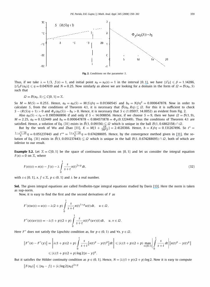
Fig. 2. Conditions on the parameter S .

Thus, if we take λ = 1/3, f (s) = 1, and initial point x0 = x0(s) = 1 in the interval [0,1], we have ‖Γ0‖ � β = 1.14286,‖Γ0 F (x0)‖ � η = 0.047619 and N = 0.25. Now similarly as above we are looking for a domain in the form of Ω = B(x0, S)

such that

Ω = B(x0, S) ⊆ C[0,1] = X.

So M = M(S) = 0.25S . Hence, a0 = a0(S) = M(S)βη = 0.0136054S and b0 = Nβη2 = 0.000647878. Now in order tocalculate S , from the conditions of Theorem 4.1, it is necessary that B(x0, Rη) ⊆ Ω . For this it is sufficient to checkS − (R(S)η + 1) > 0 and Φp(a0(S)) − b0 > 0. Hence, it is necessary that S ∈ (1.05017,14.0052) as evident from Fig. 2.

Also a0(S) < r0 = 0.1905960896 if and only if S < 14.008856. Hence, if we choose S = 9, then we have Ω = B(1,9),M = 2.25, a0 = 0.122449 and b0 = 0.000647878 < 0.884571878 = Φp(0.122449). Thus the conditions of Theorem 4.1 aresatisfied. Hence, a solution of Eq. (31) exists in B(1,0.09156) ⊆ Ω which is unique in the ball B(1,0.6862158) ∩ Ω .

But by the work of Wu and Zhao [11], K = M[1 + 5N3M2β

] = 2.4120366. Hence, h = Kβη = 0.131267496. So t∗ =1−√

1−2hh η = 0.051237443 and t∗∗ = 1+√

1−2hh η = 0.674288695. Hence, by the convergence method given in [11], the so-

lution of Eq. (31) exists in B(1,0.051237443) ⊆ Ω which is unique in the ball B(1,0.674288695) ∩ Ω , both of which areinferior to our result.

Example 5.2. Let X = C[0,1] be the space of continuous functions on [0,1] and let us consider the integral equationF (x) = 0 on X, where

F (x)(s) = x(s) − f (s) − λ

1∫0

s

s + tx(t)2+p dt, (32)

with s ∈ [0,1], x, f ∈ X, p ∈ (0,1] and λ be a real number.

Sol. The given integral equations are called Fredholm-type integral equations studied by Davis [13]. Here the norm is takenas sup-norm.

Now, it is easy to find the first and the second derivatives of F as

F ′(x)u(s) = u(s) − λ(2 + p)

1∫0

s

s + tx(t)1+pu(t)dt, u ∈ Ω,

F ′′(x)(uv)(s) = −λ(1 + p)(2 + p)

1∫0

s

s + tx(t)p(uv)(t)dt, u, v ∈ Ω.

Here F ′′ does not satisfy the Lipschitz condition as, for p ∈ (0,1) and ∀x, y ∈ Ω,

∥∥F ′′(x) − F ′′(y)∥∥ =

∥∥∥∥∥λ(1 + p)(2 + p)

1∫0

s

s + t

[x(t)p − y(t)p]

dt

∥∥∥∥∥ � |λ|(1 + p)(2 + p) maxs∈[0,1]

∣∣∣∣∣1∫

0

s

s + tdt

∣∣∣∣∣∥∥x(t)p − y(t)p∥∥

� |λ|(1 + p)(2 + p) log 2‖x − y‖p .

But it satisfies the Hölder continuity condition as p ∈ (0,1]. Hence, N = |λ|(1 + p)(2 + p) log 2. Now it is easy to compute∥∥F (x0)∥∥ � ‖x0 − f ‖ + |λ| log 2‖x0‖2+p

360 P.K. Parida, D.K. Gupta / J. Math. Anal. Appl. 345 (2008) 350–361

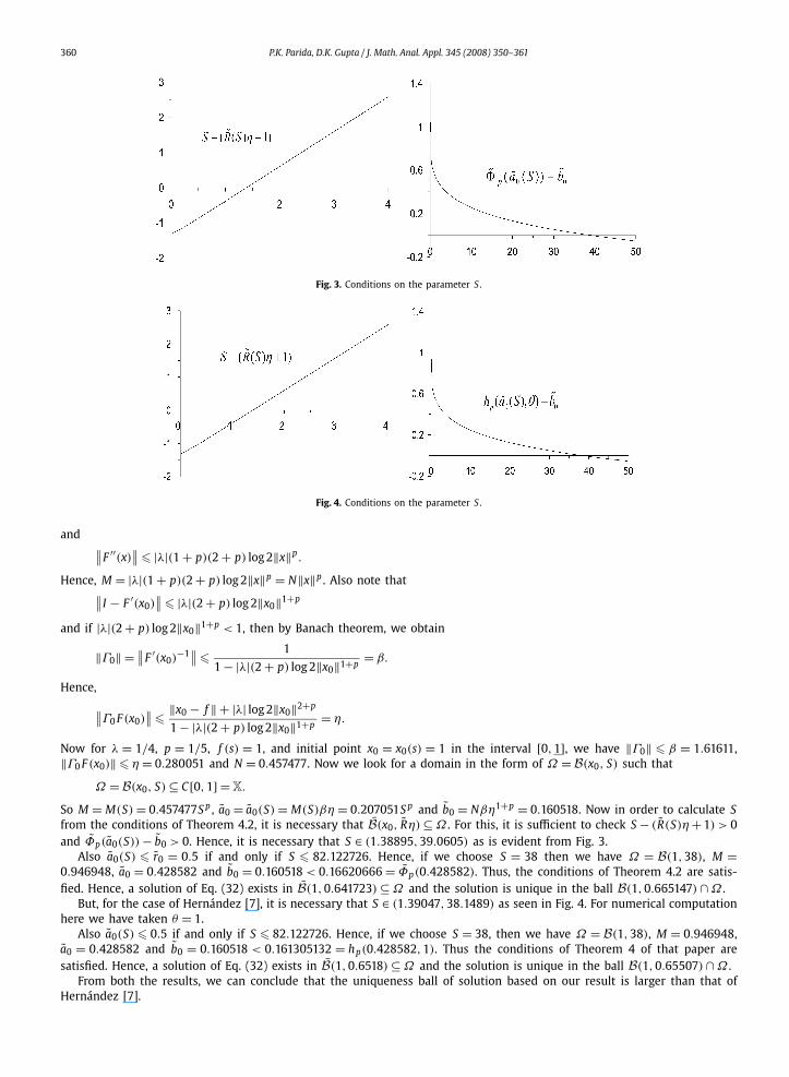
Fig. 3. Conditions on the parameter S .

Fig. 4. Conditions on the parameter S .

and ∥∥F ′′(x)∥∥ � |λ|(1 + p)(2 + p) log 2‖x‖p .

Hence, M = |λ|(1 + p)(2 + p) log 2‖x‖p = N‖x‖p . Also note that∥∥I − F ′(x0)∥∥ � |λ|(2 + p) log 2‖x0‖1+p

and if |λ|(2 + p) log 2‖x0‖1+p < 1, then by Banach theorem, we obtain

‖Γ0‖ = ∥∥F ′(x0)−1

∥∥ � 1

1 − |λ|(2 + p) log 2‖x0‖1+p= β.

Hence,

∥∥Γ0 F (x0)∥∥ � ‖x0 − f ‖ + |λ| log 2‖x0‖2+p

1 − |λ|(2 + p) log 2‖x0‖1+p= η.

Now for λ = 1/4, p = 1/5, f (s) = 1, and initial point x0 = x0(s) = 1 in the interval [0,1], we have ‖Γ0‖ � β = 1.61611,‖Γ0 F (x0)‖ � η = 0.280051 and N = 0.457477. Now we look for a domain in the form of Ω = B(x0, S) such that

Ω = B(x0, S) ⊆ C[0,1] = X.

So M = M(S) = 0.457477S p , a0 = a0(S) = M(S)βη = 0.207051S p and b0 = Nβη1+p = 0.160518. Now in order to calculate Sfrom the conditions of Theorem 4.2, it is necessary that B(x0, Rη) ⊆ Ω . For this, it is sufficient to check S − (R(S)η + 1) > 0and Φp(a0(S)) − b0 > 0. Hence, it is necessary that S ∈ (1.38895,39.0605) as is evident from Fig. 3.

Also a0(S) � r0 = 0.5 if and only if S � 82.122726. Hence, if we choose S = 38 then we have Ω = B(1,38), M =0.946948, a0 = 0.428582 and b0 = 0.160518 < 0.16620666 = Φp(0.428582). Thus, the conditions of Theorem 4.2 are satis-fied. Hence, a solution of Eq. (32) exists in B(1,0.641723) ⊆ Ω and the solution is unique in the ball B(1,0.665147) ∩ Ω .

But, for the case of Hernández [7], it is necessary that S ∈ (1.39047,38.1489) as seen in Fig. 4. For numerical computationhere we have taken θ = 1.

Also a0(S) � 0.5 if and only if S � 82.122726. Hence, if we choose S = 38, then we have Ω = B(1,38), M = 0.946948,a0 = 0.428582 and b0 = 0.160518 < 0.161305132 = hp(0.428582,1). Thus the conditions of Theorem 4 of that paper aresatisfied. Hence, a solution of Eq. (32) exists in B(1,0.6518) ⊆ Ω and the solution is unique in the ball B(1,0.65507) ∩ Ω .

From both the results, we can conclude that the uniqueness ball of solution based on our result is larger than that ofHernández [7].

P.K. Parida, D.K. Gupta / J. Math. Anal. Appl. 345 (2008) 350–361 361

6. Conclusions

In this paper, recurrence relations are developed for establishing the convergence of third order Newton-like methods forsolving F (x) = 0 in Banach spaces under the Hölder continuity condition over F ′′ . An existence-uniqueness theorem is givento establish the R-order of the method to be 2 and a priori error bounds. Also we give convergence analysis of anotherformulation of our method in order to increase the R-order of the method from 2 to (2 + p). One important contributionof our approach is that the convergence analysis of the method is established even when Lipschitz condition over F ′′ fails.

Acknowledgments

We would like to thank the referees for their careful reading of this paper. Their comments uncovered several weaknesses in the presentation of thepaper and helped us in clarifying them.

References

[1] V. Candela, A. Marquina, Recurrence relations for rational cubic methods I: The Halley method, Computing 44 (1990) 169–184.[2] V. Candela, A. Marquina, Recurrence relations for rational cubic methods II: The Chebyshev method, Computing 45 (1990) 355–367.[3] J.A. Ezquerro, M.A. Hernández, Avoiding the computation of the second Fréchet-derivative in the convex acceleration of Newton’s method, J. Comput.

Appl. Math. 96 (1998) 1–12.[4] J.M. Gutiérrez, M.A. Hernández, Recurrence relations for the super-Halley method, Comput. Math. Appl. 36 (1998) 1–8.[5] M.A. Hernández, Reduced recurrence relations for the Chebyshev method, J. Optim. Theory Appl. 98 (1998) 385–397.[6] M.A. Hernández, Second-derivative-free variant of the Chebyshev method for nonlinear equations, J. Optim. Theory Appl. 104 (2000) 501–515.[7] M.A. Hernández, Chebyshev’s approximation algorithms and applications, Comput. Math. Appl. 41 (2001) 433–445.[8] J.A. Ezquerro, M.A. Hernández, On the R-order of the Halley method, J. Math. Anal. Appl. 303 (2005) 591–601.[9] M.A. Hernández, M.A. Salanova, Modification of the Kantorovich assumptions for semilocal convergence of the Chebyshev method, J. Comput. Appl.

Math. 126 (2000) 131–143.[10] P.K. Parida, D.K. Gupta, Recurrence relations for a Newton-like method in Banach spaces, J. Comput. Appl. Math. 206 (2007) 873–887.[11] Q. Wu, Y. Zhao, Third-order convergence theorem by using majorizing function for a modified Newton method in Banach space, Appl. Math. Com-

put. 175 (2006) 1515–1524.[12] X. Ye, C. Li, Convergence of the family of the deformed Euler–Halley iterations under the Hölder condition of the second derivative, J. Comput. Appl.

Math. 194 (2006) 294–308.[13] H.T. Davis, Introduction to Nonlinear Differential and Integral Equations, Dover, New York, 1962.[14] L.V. Kantorovich, G.P. Akilov, Functional Analysis, Pergamon Press, Oxford, 1982.[15] J.D. Lambert, Computational Methods in Ordinary Differential Equations, Wiley, New York, 1979.[16] J.M. Ortega, W.C. Rheinboldt, Iterative Solution of Nonlinear Equations in Several Variables, Academic Press, 1970.[17] A.D. Polyanin, A.V. Manzhirov, Handbook of Integral Equations, CRC Press, Boca Ratón, FL, 1998.