Journal of Computational and Applied Mathematics 206 (2007) 873–887www.elsevier.com/locate/cam

Recurrence relations for a Newton-like method in Banach spaces�

P.K. Parida, D.K. Gupta∗

Department of Mathematics, Indian Institute of Technology, Kharagpur-721302, India

Received 15 June 2006; received in revised form 29 August 2006

Abstract

The convergence of iterative methods for solving nonlinear operator equations in Banach spaces is established from the convergenceof majorizing sequences. An alternative approach is developed to establish this convergence by using recurrence relations. Forexample, the recurrence relations are used in establishing the convergence of Newton’s method [L.B. Rall, Computational Solutionof Nonlinear Operator Equations, Robert E. Krieger, New York, 1979] and the third order methods such as Halley’s, Chebyshev’sand super Halley’s [V. Candela, A. Marquina, Recurrence relations for rational cubic methods I: the Halley method, Computing 44(1990) 169–184; V. Candela, A. Marquina, Recurrence relations for rational cubic methods II: the Halley method, Computing 45(1990) 355–367; J.A. Ezquerro, M.A. Hernández, Recurrence relations for Chebyshev-type methods, Appl. Math. Optim. 41 (2000)227–236; J.M. Gutiérrez, M.A. Hernández, Third-order iterative methods for operators with bounded second derivative, J. Comput.Appl. Math. 82 (1997) 171–183; J.M. Gutiérrez, M.A. Hernández, Recurrence relations for the Super–Halley method, Comput.Math. Appl. 7(36) (1998) 1–8; M.A. Hernández, Chebyshev’s approximation algorithms and applications, Comput. Math. Appl. 41(2001) 433–445 [10]].

In this paper, an attempt is made to use recurrence relations to establish the convergence of a third order Newton-like method usedfor solving a nonlinear operator equation F(x) = 0, where F : � ⊆ X → Y be a nonlinear operator on an open convex subset �of a Banach space X with values in a Banach space Y. Here, first we derive the recurrence relations based on two constants whichdepend on the operator F. Then, based on this recurrence relations a priori error bounds are obtained for the said iterative method.Finally, some numerical examples are worked out for demonstrating our approach.© 2006 Elsevier B.V. All rights reserved.

MSC: 47H10; 41A25; 65Q05

Keywords: Nonlinear operator equations; Newton-like method; Cubic convergence; Recurrence relations; A priori error bounds

1. Introduction

The well-known Newton’s method and it’s variants are used to solve nonlinear operator equations F(x) = 0. Thesemethods are of second order and their convergence established by Kantorovich theorem [11,13], provide sufficientconditions to ensure convergence through a system of error bounds for the distance to the solution from each iterate.The convergence of the sequences obtained by these methods in Banach spaces are derived from the convergence ofmajorizing sequences. In [14], a new approach is used for the convergence of these methods by recurrence relations to

� This work is supported by financial Grant, CSIR (No: 10-2(5)/2004(i)-EU II), India.∗ Corresponding author. Tel.: +91 3222 283652(O); fax: +91 3222 255303/282700.

E-mail addresses: pradipparida@yahoo.com (P.K. Parida), dkg@maths.iitkgp.ernet.in (D.K. Gupta).

0377-0427/$ - see front matter © 2006 Elsevier B.V. All rights reserved.doi:10.1016/j.cam.2006.08.027

874 P.K. Parida, D.K. Gupta / Journal of Computational and Applied Mathematics 206 (2007) 873–887

get a priori error bounds for them. This paper is concerned with convergence of third order methods for F(x) = 0 inBanach spaces. For many applications, third order methods are used inspite of high computational cost in evaluating theinvolved second order derivatives. They can also be used in stiff systems [12], where a quick convergence is required.Moreover, they are important from the theoretical standpoint as they provide results on existence and uniqueness ofsolutions that improve the results obtained from Newton’s method [1,7]. Some of the well-known third order methodsare Chebyshev’s method, Halley’s method and super Halley’s method. Candela and Marquina [2,3] proposed recurrencerelations to study the convergence of Halley’s method and Chebyshev’s method. Also Gutuérrez and Hernández [8,9]and Ezquerro and Hernández [4] used recurrence relations to study the convergence of Super Halley and Chebyshev-typemethods.

In this paper, we shall use recurrence relations to establish the convergence of a third order Newton-like method forsolving a nonlinear operator equation F(x) = 0, where F : � ⊆ X → Y be a nonlinear operator on an open convexsubset � of a Banach space X with values in a Banach space Y. The recurrence relations based on two constants whichdepend on the operator F are derived. Then, based on this recurrence relations a priori error bounds are obtained forthe said iterative method. Finally, some numerical examples are worked out for demonstrating our work.

The paper is organized as follows. Section 1 is the introduction. In Section 2, recurrence relations for a Newton-like third order method are derived. The convergence analysis based on recurrence relations of the method derived inSection 2 is given in Section 3. In Section 4, some numerical examples are worked out. Finally, conclusions form theSection 5.

2. Recurrence relations for a third order method

In this section, we shall discuss a third order Newton-like method for solving the nonlinear operator equation

F(x) = 0, (1)

where F : � ⊆ X → Y be a nonlinear operator on a open convex subset � of a Banach space X with values in aBanach space Y. Recently, Frontini and Sormani [6,5] developed a family of third order iterative methods for solving(1). This family involves only the vue of F and it’s first derivative F ′. One of the most well-known member of thisfamily is

yn = xn − F ′(xn)−1F(xn),

xn+1 = xn −(

F ′(xn) + F ′(yn)

2

)−1

F(xn).

⎫⎬⎭ (2)

Let F be a twice Fréchet differentiable operator in � and BL(Y, X) be the set of bounded linear operators from Y intoX. It is assumed that �0 = F ′(x0)

−1 ∈ BL(Y, X) exists at some point x0 ∈ � and let the following conditions holdon F:

1. ‖F ′(x0)−1‖��,

2. ‖F ′(x0)−1F(x0)‖��,

3. ‖F ′′(x)‖�M, x ∈ �,

4. ‖F ′′(x) − F ′′(y)‖�N‖x − y‖ ∀x, y ∈ �.

⎫⎪⎪⎪⎪⎬⎪⎪⎪⎪⎭

(3)

Now taking a = M�� and b = N��2, a0 = 1, b0 = 1, c0 = a/2, d0 = 2/(2 − a), we define for n = 0, 1, . . .

an+1 = an

1 − aandn

,

bn+1 = an+1d2n

[a

2(2c2

n − 7cn + 6) + 5b

12(1 − cn)

3dn

],

cn+1 = aan+1bn+1

2,

dn+1 = bn+1

1 − cn+1.

⎫⎪⎪⎪⎪⎪⎪⎪⎪⎪⎪⎪⎬⎪⎪⎪⎪⎪⎪⎪⎪⎪⎪⎪⎭

(4)

P.K. Parida, D.K. Gupta / Journal of Computational and Applied Mathematics 206 (2007) 873–887 875

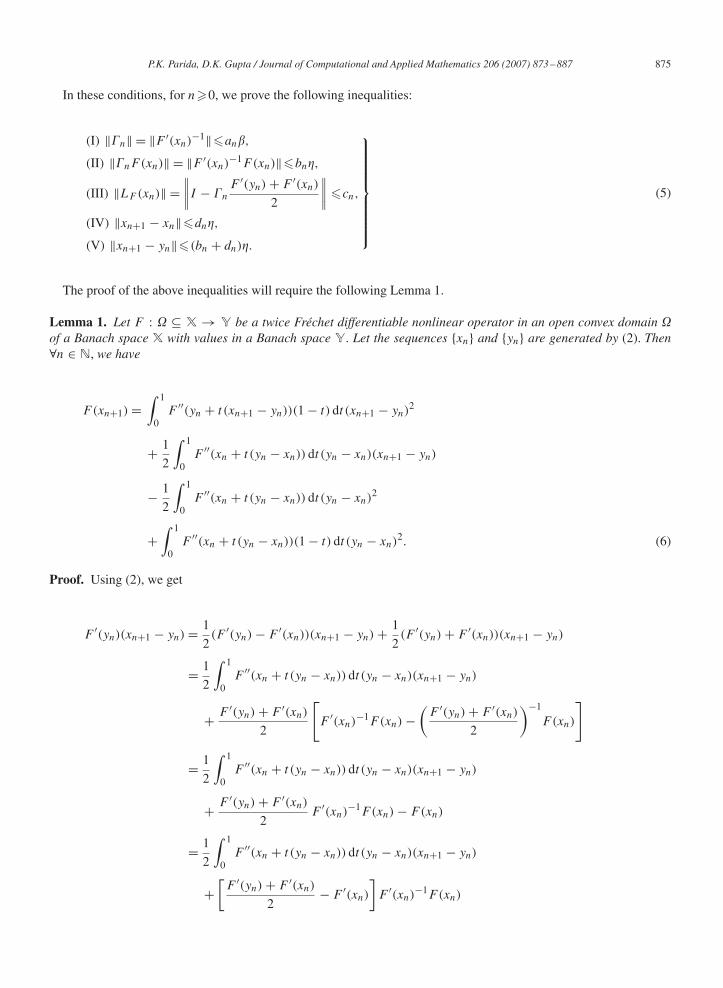
In these conditions, for n�0, we prove the following inequalities:

(I) ‖�n‖ = ‖F ′(xn)−1‖�an�,

(II) ‖�nF (xn)‖ = ‖F ′(xn)−1F(xn)‖�bn�,

(III) ‖LF (xn)‖ =∥∥∥∥I − �n

F ′(yn) + F ′(xn)

2

∥∥∥∥ �cn,

(IV) ‖xn+1 − xn‖�dn�,

(V) ‖xn+1 − yn‖�(bn + dn)�.

⎫⎪⎪⎪⎪⎪⎪⎪⎪⎬⎪⎪⎪⎪⎪⎪⎪⎪⎭

(5)

The proof of the above inequalities will require the following Lemma 1.

Lemma 1. Let F : � ⊆ X → Y be a twice Fréchet differentiable nonlinear operator in an open convex domain �of a Banach space X with values in a Banach space Y. Let the sequences {xn} and {yn} are generated by (2). Then∀n ∈ N, we have

F(xn+1) =∫ 1

0F ′′(yn + t (xn+1 − yn))(1 − t) dt (xn+1 − yn)

2

+ 1

2

∫ 1

0F ′′(xn + t (yn − xn)) dt (yn − xn)(xn+1 − yn)

− 1

2

∫ 1

0F ′′(xn + t (yn − xn)) dt (yn − xn)

2

+∫ 1

0F ′′(xn + t (yn − xn))(1 − t) dt (yn − xn)

2. (6)

Proof. Using (2), we get

F ′(yn)(xn+1 − yn) = 1

2(F ′(yn) − F ′(xn))(xn+1 − yn) + 1

2(F ′(yn) + F ′(xn))(xn+1 − yn)

= 1

2

∫ 1

0F ′′(xn + t (yn − xn)) dt (yn − xn)(xn+1 − yn)

+ F ′(yn) + F ′(xn)

2

[F ′(xn)

−1F(xn) −(

F ′(yn) + F ′(xn)

2

)−1

F(xn)

]

= 1

2

∫ 1

0F ′′(xn + t (yn − xn)) dt (yn − xn)(xn+1 − yn)

+ F ′(yn) + F ′(xn)

2F ′(xn)

−1F(xn) − F(xn)

= 1

2

∫ 1

0F ′′(xn + t (yn − xn)) dt (yn − xn)(xn+1 − yn)

+[F ′(yn) + F ′(xn)

2− F ′(xn)

]F ′(xn)

−1F(xn)

876 P.K. Parida, D.K. Gupta / Journal of Computational and Applied Mathematics 206 (2007) 873–887

=1

2

∫ 1

0F ′′(xn + t (yn − xn)) dt (yn − xn)(xn+1 − yn)

− F ′(yn) − F ′(xn)

2(yn − xn)

= 1

2

∫ 1

0F ′′(xn + t (yn − xn)) dt (yn − xn)(xn+1 − yn)

− 1

2

∫ 1

0F ′′(xn + t (yn − xn)) dt (yn − xn)

2.

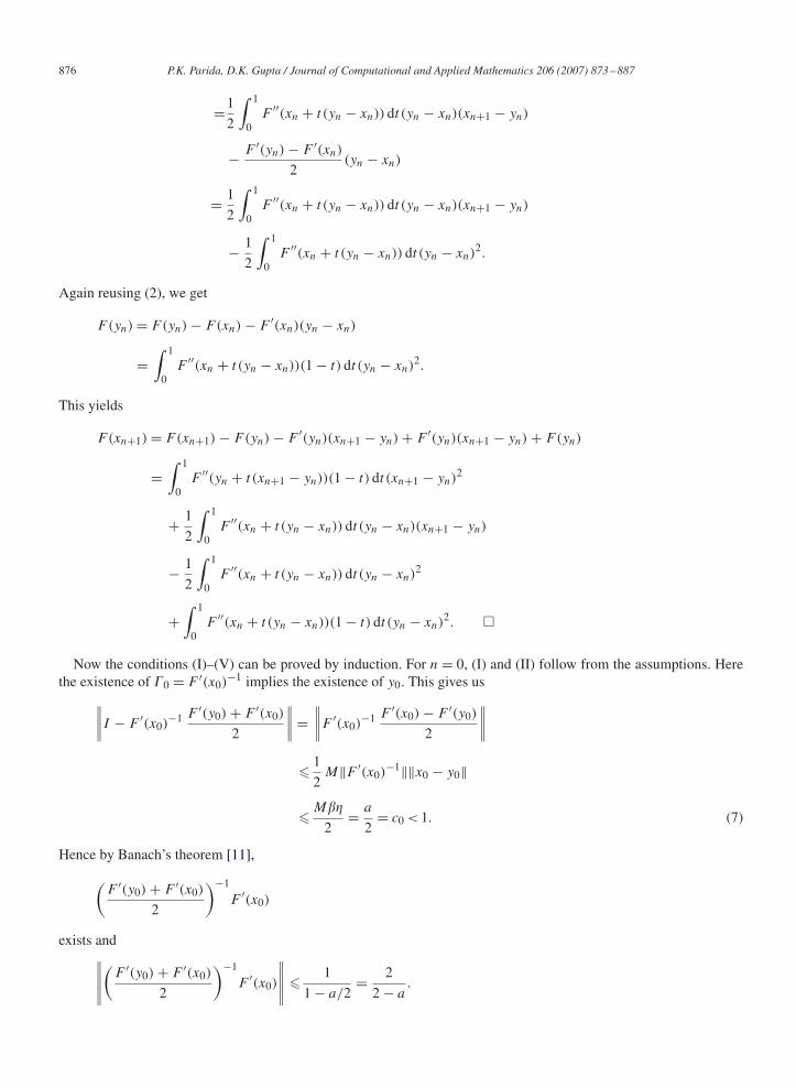
Again reusing (2), we get

F(yn) = F(yn) − F(xn) − F ′(xn)(yn − xn)

=∫ 1

0F ′′(xn + t (yn − xn))(1 − t) dt (yn − xn)

2.

This yields

F(xn+1) = F(xn+1) − F(yn) − F ′(yn)(xn+1 − yn) + F ′(yn)(xn+1 − yn) + F(yn)

=∫ 1

0F ′′(yn + t (xn+1 − yn))(1 − t) dt (xn+1 − yn)

2

+ 1

2

∫ 1

0F ′′(xn + t (yn − xn)) dt (yn − xn)(xn+1 − yn)

− 1

2

∫ 1

0F ′′(xn + t (yn − xn)) dt (yn − xn)

2

+∫ 1

0F ′′(xn + t (yn − xn))(1 − t) dt (yn − xn)

2. �

Now the conditions (I)–(V) can be proved by induction. For n = 0, (I) and (II) follow from the assumptions. Herethe existence of �0 = F ′(x0)

−1 implies the existence of y0. This gives us∥∥∥∥I − F ′(x0)−1 F ′(y0) + F ′(x0)

2

∥∥∥∥=∥∥∥∥F ′(x0)

−1 F ′(x0) − F ′(y0)

2

∥∥∥∥� 1

2M‖F ′(x0)

−1‖‖x0 − y0‖

� M��

2= a

2= c0 < 1. (7)

Hence by Banach’s theorem [11],

(F ′(y0) + F ′(x0)

2

)−1

F ′(x0)

exists and∥∥∥∥∥(

F ′(y0) + F ′(x0)

2

)−1

F ′(x0)

∥∥∥∥∥ � 1

1 − a/2= 2

2 − a.

P.K. Parida, D.K. Gupta / Journal of Computational and Applied Mathematics 206 (2007) 873–887 877

Now we have

‖x1 − x0‖ =∥∥∥∥∥(

F ′(y0) + F ′(x0)

2

)−1

F(x0)

∥∥∥∥∥�∥∥∥∥∥(

F ′(y0) + F ′(x0)

2

)−1

F ′(x0)

∥∥∥∥∥ ‖F ′(x0)−1F(x0)‖

� 2�

2 − a= d0� (8)

and

‖x1 − y0‖�‖x1 − x0‖ + ‖x0 − y0‖

� 2�

2 − a+ � = (b0 + d0)�. (9)

Thus, for n = 0, the existence of the conditions (III)–(V) follow from (7)–(9), respectively. Assume that the conditions(I)–(V) hold for n = 1, 2, . . . , k and consider xk ∈ �, ck+1 < 1 and aakdk < 1. We now have

‖I − �kF′(xk+1)‖ = ‖�k(F

′(xk) − F ′(xk+1))‖�M‖�k‖‖xk − xk+1‖�Mak�dk�

�aakdk < 1.

Hence by Banach’s theorem [11],

�k+1 = F ′(xk+1)−1

exists and

‖�k+1‖� ‖�k‖1 − ‖�k‖‖F ′(xk) − F ′(xk+1)‖

� ak�

1 − aakdk

= ak+1�. (10)

Also

∥∥∥∥∥∫ 1

0F ′′(xk + t (yk − xk))(1 − t) dt (yk − xk)

2 − 1

2

∫ 1

0F ′′(xk + t (yk − xk)) dt (yk − xk)

2

∥∥∥∥∥�∥∥∥∥∥∫ 1

0F ′′(xk + t (yk − xk))(1 − t) dt (yk − xk)

2 − 1

2F ′′(xk)(yk − xk)

2

∥∥∥∥∥+∥∥∥∥∥1

2

∫ 1

0F ′′(xk + t (yk − xk)) dt (yk − xk)

2 − 1

2F ′′(xk)(yk − xk)

2

∥∥∥∥∥

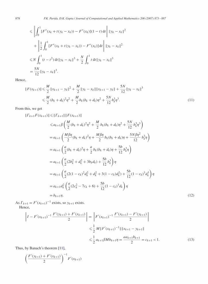
878 P.K. Parida, D.K. Gupta / Journal of Computational and Applied Mathematics 206 (2007) 873–887

�∥∥∥∥∥∫ 1

0[F ′′(xk + t (yk − xk)) − F ′′(xk)](1 − t) dt

∥∥∥∥∥ ‖yk − xk‖2

+∥∥∥∥∥1

2

∫ 1

0[F ′′(xk + t (yk − xk)) − F ′′(xk)] dt

∥∥∥∥∥ ‖yk − xk‖2

�N

∫ 1

0(t − t2) dt‖yk − xk‖3 + N

2

∫ 1

0t dt‖yk − xk‖3

= 5N

12‖yk − xk‖3.

Hence,

‖F(xk+1)‖� M

2‖xk+1 − yk‖2 + M

2‖yk − xk‖‖xk+1 − yk‖ + 5N

12‖yk − xk‖3

� M

2(bk + dk)

2�2 + M

2bk(bk + dk)�

2 + 5N

12b3k�

3. (11)

From this, we get

‖�k+1F(xk+1)‖�‖�k+1‖‖F(xk+1)‖

�ak+1�

(M

2(bk + dk)

2�2 + M

2bk(bk + dk)�

2 + 5N

12b3k�

3)

= ak+1

(M��

2(bk + dk)

2� + M��

2bk(bk + dk)� + 5N��2

12b3k�

)

= ak+1

(a

2(bk + dk)

2� + a

2bk(bk + dk)� + 5b

12b3k�

)

= ak+1

(a

2(2b2

k + d2k + 3bkdk) + 5b

12b3k

)�

= ak+1

(a

2(2(1 − ck)

2d2k + d2

k + 3(1 − ck)d2k ) + 5b

12(1 − ck)

3d3k

)�

= ak+1d2k

(a

2(2c2

k − 7ck + 6) + 5b

12(1 − ck)

3dk

)�

= bk+1�. (12)

As �k+1 = F ′(xk+1)−1 exists, so yk+1 exists.

Hence,∥∥∥∥I − F ′(xk+1)−1 F ′(yk+1) + F ′(xk+1)

2

∥∥∥∥=∥∥∥∥F ′(xk+1)

−1 F ′(xk+1) − F ′(yk+1)

2

∥∥∥∥� 1

2M‖F ′(xk+1)

−1‖‖xk+1 − yk+1‖

� 1

2ak+1�Mbk+1� = aak+1bk+1

2= ck+1 < 1. (13)

Thus, by Banach’s theorem [11],(F ′(yk+1) + F ′(xk+1)

2

)−1

F ′(xk+1)

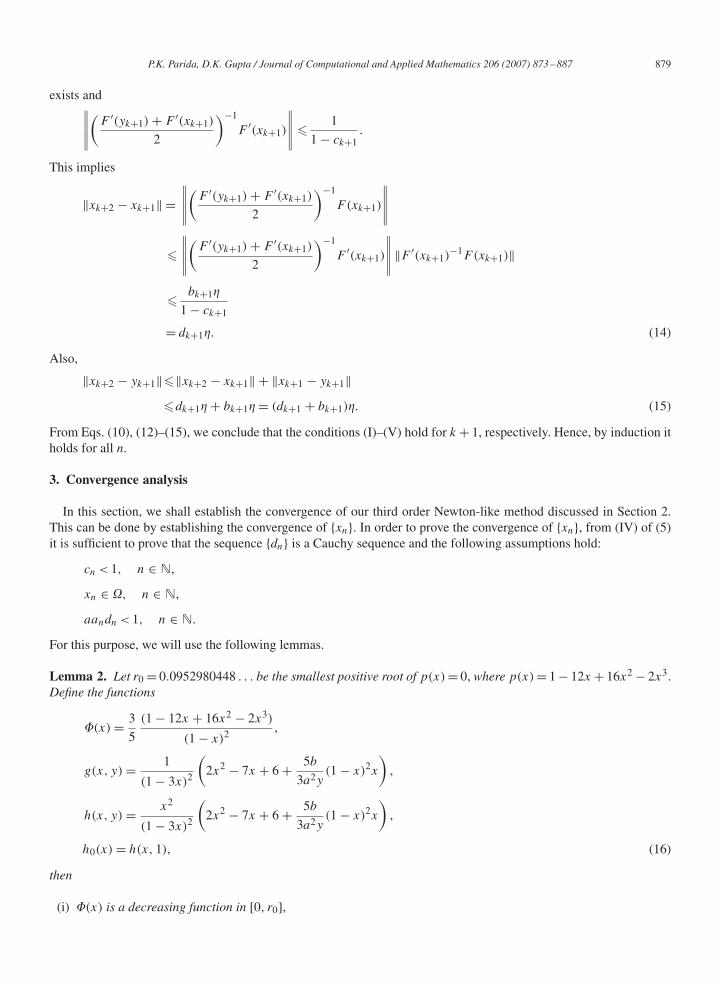
P.K. Parida, D.K. Gupta / Journal of Computational and Applied Mathematics 206 (2007) 873–887 879

exists and∥∥∥∥∥(

F ′(yk+1) + F ′(xk+1)

2

)−1

F ′(xk+1)

∥∥∥∥∥ � 1

1 − ck+1.

This implies

‖xk+2 − xk+1‖ =∥∥∥∥∥(

F ′(yk+1) + F ′(xk+1)

2

)−1

F(xk+1)

∥∥∥∥∥�∥∥∥∥∥(

F ′(yk+1) + F ′(xk+1)

2

)−1

F ′(xk+1)

∥∥∥∥∥ ‖F ′(xk+1)−1F(xk+1)‖

� bk+1�

1 − ck+1

= dk+1�. (14)

Also,

‖xk+2 − yk+1‖�‖xk+2 − xk+1‖ + ‖xk+1 − yk+1‖�dk+1� + bk+1� = (dk+1 + bk+1)�. (15)

From Eqs. (10), (12)–(15), we conclude that the conditions (I)–(V) hold for k + 1, respectively. Hence, by induction itholds for all n.

3. Convergence analysis

In this section, we shall establish the convergence of our third order Newton-like method discussed in Section 2.This can be done by establishing the convergence of {xn}. In order to prove the convergence of {xn}, from (IV) of (5)it is sufficient to prove that the sequence {dn} is a Cauchy sequence and the following assumptions hold:

cn < 1, n ∈ N,

xn ∈ �, n ∈ N,

aandn < 1, n ∈ N.

For this purpose, we will use the following lemmas.

Lemma 2. Let r0 = 0.0952980448 . . . be the smallest positive root of p(x) = 0, where p(x) = 1 − 12x + 16x2 − 2x3.Define the functions

�(x) = 3

5

(1 − 12x + 16x2 − 2x3)

(1 − x)2,

g(x, y) = 1

(1 − 3x)2

(2x2 − 7x + 6 + 5b

3a2y(1 − x)2x

),

h(x, y) = x2

(1 − 3x)2

(2x2 − 7x + 6 + 5b

3a2y(1 − x)2x

),

h0(x) = h(x, 1), (16)

then

(i) �(x) is a decreasing function in [0, r0],

880 P.K. Parida, D.K. Gupta / Journal of Computational and Applied Mathematics 206 (2007) 873–887

(ii) g(x, y) and h(x, y) are increasing functions of x in [0, r0], for y > 1,(iii) g(x, y) and h(x, y) are decreasing functions of y,(iv) h0(x) and h′

0(x) are increasing functions in [0, r0].

Proof. Since

�′(x) = 3

5

(−12 + 32x − 6x2

(1 − x)2+ 2(1 − 12x + 16x2 − 2x3)

(1 − x)3

)

�0, ∀x ∈ [0, r0]this implies �(x) is a decreasing function. The proof of others follow from similar reasonings as given for �(x). �

Lemma 3. The following recurrence relations hold for the sequences {an} and {cn}.

an+1 =n∏

k=0

(1 + 2ck

1 − 3ck

), (17)

cn+1 = c2n(2c2

n − 7cn + 6)

(1 − 3cn)2

(1 + 5b

3a2an

(1 − cn)2cn

(2c2n − 7cn + 6)

). (18)

Proof. As

cn = aanbn

2⇒ bn = 2cn

aan

.

We get

dn = bn

1 − cn

= 2cn

aan(1 − cn). (19)

As a0 = 1, this gives

an+1 = an

1 − aandn

= an

1 − 2cn

1−cn

= an(1 − cn)

1 − 3cn

= an

(1 + 2cn

1 − 3cn

)=

n∏k=0

(1 + 2ck

1 − 3ck

). (20)

Also

cn+1 = aan+1bn+1

2

= a

2a2n+1d

2n

(a

2(2c2

n − 7cn + 6) + 5b

12(1 − cn)

3dn

)

= a

2

(an(1 − cn)

1 − 3cn

)2( 2cn

aan(1 − cn)

)2 (a

2(2c2

n − 7cn + 6) + 5b

12(1 − cn)

3(

2cn

aan(1 − cn)

))

= 2

a

c2n

(1 − 3cn)2

(a

2(2c2

n − 7cn + 6) + 5b

6(1 − cn)

2 cn

aan

)

= c2n(2c2

n − 7cn + 6)

(1 − 3cn)2

(1 + 5b

3a2an

(1 − cn)2cn

(2c2n − 7cn + 6)

).

Hence the lemma is proved. �

P.K. Parida, D.K. Gupta / Journal of Computational and Applied Mathematics 206 (2007) 873–887 881

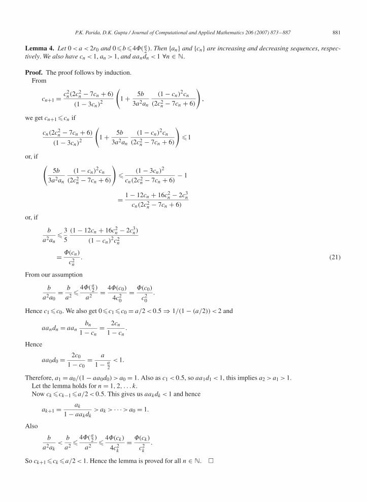
Lemma 4. Let 0 < a < 2r0 and 0�b�4�( a2 ). Then {an} and {cn} are increasing and decreasing sequences, respec-

tively. We also have cn < 1, an > 1, and aandn < 1 ∀n ∈ N.

Proof. The proof follows by induction.From

cn+1 = c2n(2c2

n − 7cn + 6)

(1 − 3cn)2

(1 + 5b

3a2an

(1 − cn)2cn

(2c2n − 7cn + 6)

),

we get cn+1 �cn if

cn(2c2n − 7cn + 6)

(1 − 3cn)2

(1 + 5b

3a2an

(1 − cn)2cn

(2c2n − 7cn + 6)

)�1

or, if (5b

3a2an

(1 − cn)2cn

(2c2n − 7cn + 6)

)� (1 − 3cn)

2

cn(2c2n − 7cn + 6)

− 1

= 1 − 12cn + 16c2n − 2c3

n

cn(2c2n − 7cn + 6)

or, if

b

a2an

� 3

5

(1 − 12cn + 16c2n − 2c3

n)

(1 − cn)2c2

n

= �(cn)

c2n

. (21)

From our assumption

b

a2a0= b

a2�

4�( a2 )

a2= 4�(c0)

4c20

= �(c0)

c20

.

Hence c1 �c0. We also get 0�c1 �c0 = a/2 < 0.5 ⇒ 1/(1 − (a/2)) < 2 and

aandn = aan

bn

1 − cn

= 2cn

1 − cn

.

Hence

aa0d0 = 2c0

1 − c0= a

1 − a2

< 1.

Therefore, a1 = a0/(1 − aa0d0) > a0 = 1. Also as c1 < 0.5, so aa1d1 < 1, this implies a2 > a1 > 1.Let the lemma holds for n = 1, 2, . . . k.Now ck �ck−1 �a/2 < 0.5. This gives us aakdk < 1 and hence

ak+1 = ak

1 − aakdk

> ak > · · · > a0 = 1.

Also

b

a2ak

<b

a2�

4�( a2 )

a2� 4�(ck)

4c2k

= �(ck)

c2k

.

So ck+1 �ck �a/2 < 1. Hence the lemma is proved for all n ∈ N. �

882 P.K. Parida, D.K. Gupta / Journal of Computational and Applied Mathematics 206 (2007) 873–887

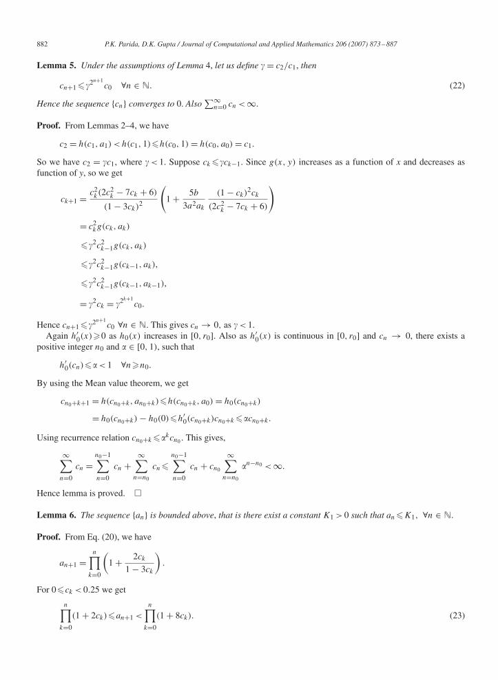
Lemma 5. Under the assumptions of Lemma 4, let us define � = c2/c1, then

cn+1 ��2n+1c0 ∀n ∈ N. (22)

Hence the sequence {cn} converges to 0. Also∑∞

n=0 cn < ∞.

Proof. From Lemmas 2–4, we have

c2 = h(c1, a1) < h(c1, 1)�h(c0, 1) = h(c0, a0) = c1.

So we have c2 = �c1, where � < 1. Suppose ck ��ck−1. Since g(x, y) increases as a function of x and decreases asfunction of y, so we get

ck+1 = c2k(2c2

k − 7ck + 6)

(1 − 3ck)2

(1 + 5b

3a2ak

(1 − ck)2ck

(2c2k − 7ck + 6)

)

= c2kg(ck, ak)

��2c2k−1g(ck, ak)

��2c2k−1g(ck−1, ak),

��2c2k−1g(ck−1, ak−1),

= �2ck = �2k+1c0.

Hence cn+1 ��2n+1c0 ∀n ∈ N. This gives cn → 0, as � < 1.

Again h′0(x)�0 as h0(x) increases in [0, r0]. Also as h′

0(x) is continuous in [0, r0] and cn → 0, there exists apositive integer n0 and � ∈ [0, 1), such that

h′0(cn)�� < 1 ∀n�n0.

By using the Mean value theorem, we get

cn0+k+1 = h(cn0+k, an0+k)�h(cn0+k, a0) = h0(cn0+k)

= h0(cn0+k) − h0(0)�h′0(cn0+k)cn0+k ��cn0+k .

Using recurrence relation cn0+k ��kcn0 . This gives,

∞∑n=0

cn =n0−1∑n=0

cn +∞∑

n=n0

cn �n0−1∑n=0

cn + cn0

∞∑n=n0

�n−n0 < ∞.

Hence lemma is proved. �

Lemma 6. The sequence {an} is bounded above, that is there exist a constant K1 > 0 such that an �K1, ∀n ∈ N.

Proof. From Eq. (20), we have

an+1 =n∏

k=0

(1 + 2ck

1 − 3ck

).

For 0�ck < 0.25 we get

n∏k=0

(1 + 2ck)�an+1 <

n∏k=0

(1 + 8ck). (23)

P.K. Parida, D.K. Gupta / Journal of Computational and Applied Mathematics 206 (2007) 873–887 883

Taking logarithm of (23), we get

lnn∏

k=0

(1 + 2ck)� ln(an+1) < lnn∏

k=0

(1 + 8ck)

This reduces ton∑

k=0

ln(1 + 2ck)� ln(an+1) <

n∑k=0

ln(1 + 8ck)�8n∑

k=0

ck < ∞. �

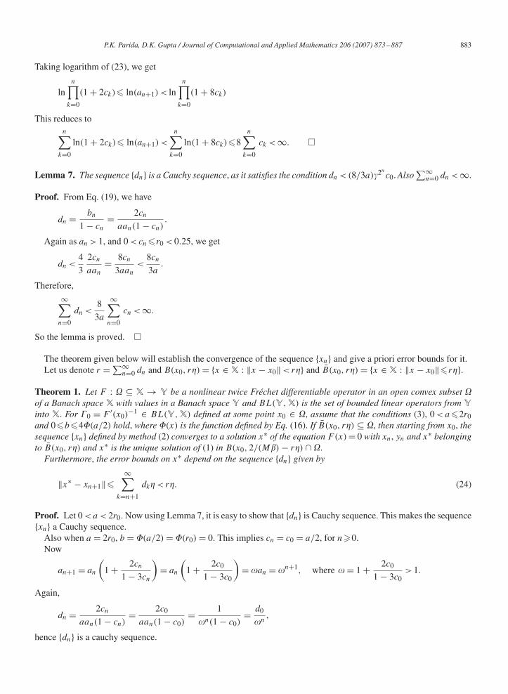
Lemma 7. The sequence {dn} is a Cauchy sequence, as it satisfies the condition dn < (8/3a)�2nc0. Also

∑∞n=0 dn < ∞.

Proof. From Eq. (19), we have

dn = bn

1 − cn

= 2cn

aan(1 − cn).

Again as an > 1, and 0 < cn �r0 < 0.25, we get

dn <4

3

2cn

aan

= 8cn

3aan

<8cn

3a.

Therefore,

∞∑n=0

dn <8

3a

∞∑n=0

cn < ∞.

So the lemma is proved. �

The theorem given below will establish the convergence of the sequence {xn} and give a priori error bounds for it.Let us denote r =∑∞

n=0 dn and B(x0, r�) = {x ∈ X : ‖x − x0‖ < r�} and B̄(x0, r�) = {x ∈ X : ‖x − x0‖�r�}.

Theorem 1. Let F : � ⊆ X → Y be a nonlinear twice Fréchet differentiable operator in an open convex subset �of a Banach space X with values in a Banach space Y and BL(Y, X) is the set of bounded linear operators from Y

into X. For �0 = F ′(x0)−1 ∈ BL(Y, X) defined at some point x0 ∈ �, assume that the conditions (3), 0 < a�2r0

and 0�b�4�(a/2) hold, where �(x) is the function defined by Eq. (16). If B̄(x0, r�) ⊆ �, then starting from x0, thesequence {xn} defined by method (2) converges to a solution x∗ of the equation F(x) = 0 with xn, yn and x∗ belongingto B̄(x0, r�) and x∗ is the unique solution of (1) in B(x0, 2/(M�) − r�) ∩ �.

Furthermore, the error bounds on x∗ depend on the sequence {dn} given by

‖x∗ − xn+1‖�∞∑

k=n+1

dk� < r�. (24)

Proof. Let 0 < a < 2r0. Now using Lemma 7, it is easy to show that {dn} is Cauchy sequence. This makes the sequence{xn} a Cauchy sequence.

Also when a = 2r0, b = �(a/2) = �(r0) = 0. This implies cn = c0 = a/2, for n�0.Now

an+1 = an

(1 + 2cn

1 − 3cn

)= an

(1 + 2c0

1 − 3c0

)= an = n+1, where = 1 + 2c0

1 − 3c0> 1.

Again,

dn = 2cn

aan(1 − cn)= 2c0

aan(1 − c0)= 1

n(1 − c0)= d0

n,

hence {dn} is a cauchy sequence.

884 P.K. Parida, D.K. Gupta / Journal of Computational and Applied Mathematics 206 (2007) 873–887

Also, aandn = ad0 = 2a/(2 − a) < 1. Hence all the conditions on the sequences {an}, {bn}, {cn} and {dn} hold true.Thus, in both cases {dn} is a Cauchy sequence, and hence the sequence {xn} is convergent.

Hence, there exists a x∗ such that, limn→∞ xn = x∗.Now from Eq. (11), we get

‖F(xn+1)‖� M

2(bn + dn)

2�2 + M

2bn(bn + dn)�

2 + 5N

12b3n�

3

= 1

�d2n

(a

2(2c2

n − 7cn + 6) + 5b

12(1 − cn)

3dn

)�.

Since the sequence {dn} converges to 0, {cn} is bounded and F is continuous, we get

‖F(x∗)‖ = limn→∞ � lim

n→∞

[1

�d2n

(a

2(2c2

n − 7cn + 6) + 5b

12(1 − cn)

3dn

)�

]= 0.

Also

‖xn+1 − x0‖�‖xn+1 − xn‖ + ‖xn − xn−1‖ + · · · + ‖x1 − x0‖

�n∑

k=0

dk��r�,

From this, we conclude that xn lies in B̄(x0, r�) and similarly one can easily prove that yn lies in B̄(x0, r�). Now takinglimit as n → ∞ we get x∗ ∈ B̄(x0, r�).

Again, for every m�n + 1,

‖xm − xn+1‖�‖xm − xm−1‖ + ‖xm−1 − xm−2‖ + · · · + ‖xn+2 − xn+1‖

�m−1∑

k=n+1

dk�

�∞∑

k=n+1

dk� < r�,

By taking m → ∞ we get

‖x∗ − xn+1‖�∞∑

k=n+1

dk� < r�,

Now for the uniqueness of x∗, let y∗ is another zero of Eq. (1). Then

0 = F(y∗) − F(x∗) =∫ 1

0F ′(x∗ + t (y∗ − x∗)) dt (y∗ − x∗).

To show y∗ = x∗, we have to show that∫ 1

0 F ′(x∗ + t (y∗ − x∗)) dt is invertible. Now for

‖�0‖∥∥∥∥∥∫ 1

0[F ′(x∗ + t (y∗ − x∗)) − F ′(x0)] dt

∥∥∥∥∥ �M�∫ 1

0‖x∗ + t (y∗ − x∗) − x0‖ dt

�M�∫ 1

0(1 − t)‖x∗ − x0‖ + t‖y∗ − x0‖ dt

<M�

2

(r� + 2

M�− r�

)= 1,

P.K. Parida, D.K. Gupta / Journal of Computational and Applied Mathematics 206 (2007) 873–887 885

it follows from Banach’s theorem [11], the operator∫ 1

0 F ′(x∗ + t (y∗ − x∗)) dt is invertible and hence y∗ = x∗. Hencethe theorem is proved. �

4. Numerical examples

In this section, numerical examples are given for demonstrating the convergence of our third order Newton-likemethod based on recurrence relations.

Example 1. Let X=C[0, 1] be the space of continuous functions on [0, 1] and consider the integral equation F(x)=0,where

F(x)(s) = −1 + x(s) + x(s)

∫ 1

0

s

s + tx(t) dt , (25)

with s ∈ [0, 1], x ∈ C[0, 1] and 0 < �2. Integral equations of this kind called Chandrasekhar equations arise inelasticity or neutron transport problems [12]. The norm is taken as sup-norm.

Now it is easy to find the first derivative of F as

F ′(x)u(s) = u(s) + u(s)

∫ 1

0

s

s + tx(t) dt + x(s)

∫ 1

0

s

s + tu(t) dt, u ∈ �

and the second derivative as

F ′′(x)(uv)(s) = u(s)

∫ 1

0

s

s + tv(t) dt + v(s)

∫ 1

0

s

s + tu(t) dt, v ∈ �.

The second derivative F ′′ satisfies the Lipschitz condition as,

‖[F ′′(x) − F ′′(y)](uv)‖ = 0‖x − y‖ ∀x, y ∈ �.

Now one can easily compute

‖F(x0)‖ =∥∥∥∥∥−1 + x0(s) + x0(s)

∫ 1

0

s

s + tx0(t) dt

∥∥∥∥∥�‖x0 − 1‖ + || max

0� s �1

∣∣∣∣∣∫ 1

0

s

s + tdt

∣∣∣∣∣ ‖x0‖2

�‖x0 − 1‖ + || log 2‖x0‖2

and

‖F ′′(x)‖�2|| max0� s �1

∣∣∣∣∣∫ 1

0

s

s + tdt

∣∣∣∣∣= 2|| log 2.

Also notice that

‖I − F ′(x0)‖ =∥∥∥∥∥∫ 1

0

s

s + tx0(t) dt + x0(s)

∫ 1

0

s

s + tdt

∥∥∥∥∥�2|| max

0� s �1

∣∣∣∣∣∫ 1

0

s

s + tdt

∣∣∣∣∣ ‖x0‖

�2|| log 2‖x0‖ (26)

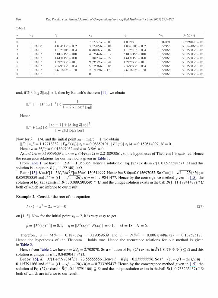
886 P.K. Parida, D.K. Gupta / Journal of Computational and Applied Mathematics 206 (2007) 873–887

Table 1

n an bn cn dn �dn (�dn) ∗ �

0 1 1 7.829572e − 003 1.007891 1.007891 8.929102e − 021 1.016036 4.804513e − 002 3.822051e − 004 4.806350e − 002 1.055955 9.354906e − 022 1.016813 1.102980e − 004 8.781060e − 007 1.102981e − 004 1.056065 9.355883e − 023 1.016815 5.811215e − 010 4.626441e − 012 5.811215e − 010 1.056065 9.355883e − 024 1.016815 1.613115e − 020 1.284237e − 022 1.613115e − 020 1.056065 9.355883e − 025 1.016815 1.242973e − 041 9.895592e − 044 1.242973e − 041 1.056065 9.355883e − 026 1.016815 7.379973e − 084 5.875364e − 086 7.379973e − 084 1.056065 9.355883e − 027 1.016815 2.601602e − 168 2.071194e − 170 2.601602e − 168 1.056065 9.355883e − 028 1.016815 0 0 0 1.056065 9.355883e − 02

and, if 2|| log 2‖x0‖ < 1, then by Banach’s theorem [11], we obtain

‖�0‖ = ‖F ′(x0)−1‖� 1

1 − 2|| log 2‖x0‖ .

Hence

‖�0F(x0)‖� ‖x0 − 1‖ + || log 2‖x0‖2

1 − 2|| log 2‖x0‖Now for = 1/4, and the initial point x0 = x0(s) = 1, we obtain

‖�0‖�� = 1.17718382, ‖�0F(x0)‖�� = 0.08859191, ‖F ′′(x)‖�M = 0.150514997, N = 0.Hence a = M�� = 0.015697052 and b = N��2 = 0.As a�2r0 = 0.19059609 and 0 = b�4�(a/2) = 2.210893861, so the hypotheses of Theorem 1 is satisfied. Hence

the recurrence relations for our method is given in Table 1.From Table 1, we have r = �dn = 1.056065. Hence a solution of Eq. (25) exists in B̄(1, 0.09355883) ⊆ � and this

solution is unique in B(1, 11.22148) ∩ �.But in [15], K=M[1+5N/3M2�]=M=0.150514997. Hence h=K��=0.015697052. So t∗=((1−√

1 − 2h)/h)�=0.089298359 and t∗∗ = ((1 + √

1 − 2h)/h)� = 11.19841477. Hence by the convergence method given in [15], thesolution of Eq. (25) exists in B̄(1, 0.089298359) ⊆ �, and the unique solution exists in the ball B(1, 11.19841477)∩�both of which are inferior to our result.

Example 2. Consider the root of the equation

F(x) = x3 − 2x − 5 = 0 (27)

on [1, 3]. Now for the initial point x0 = 2, it is very easy to get

� = ‖F ′(x0)−1‖ = 0.1, � = ‖F ′(x0)

−1F(x0)‖ = 0.1, M = 18, N = 6.

Therefore, a = M�� = 0.18 < 2r0 = 0.19059609 and b = N��2 = 0.006�4�(a/2) = 0.139525178.Hence the hypotheses of the Theorem 1 holds true. Hence the recurrence relations for our method is givenin Table 2.

Hence from Table 2 we have r = �dn = 2.702070. So a solution of Eq. (25) exists in B̄(1, 0.2702070) ⊆ � and thissolution is unique in B(1, 0.8409041) ∩ �.

But by [15], K =M[1+5N/3M2�]=23.55555556. Hence h=K��=0.235555556. So t∗ =((1−√1 − 2h)/h)�=

0.115791166 and t∗∗ = ((1 + √1 − 2h)/h)� = 0.733265437. Hence by the convergence method given in [15], the

solution of Eq. (27) exists in B̄(1, 0.115791166) ⊆ �, and the unique solution exists in the ball B(1, 0.733265437)∩�both of which are inferior to our result.

P.K. Parida, D.K. Gupta / Journal of Computational and Applied Mathematics 206 (2007) 873–887 887

Table 2

n an bn cn dn �dn (�dn) ∗ �

0 1 1 9.000000e − 002 1.098901 1.098901 1.098901e − 011 1.246575 7.328440e − 001 8.221907e − 002 7.984955e − 001 1.897397 1.897397e − 012 1.518675 4.753985e − 001 6.497783e − 002 5.084355e − 001 2.405832 2.405832e − 013 1.763823 2.283736e − 001 3.625295e − 002 2.369642e − 001 2.642796 2.642796e − 014 1.907317 5.546990e − 002 9.521882e − 003 5.600315e − 002 2.698800 2.698800e − 015 1.944708 3.257958e − 003 5.702198e − 004 3.259817e − 003 2.702059 2.702059e − 016 1.946929 1.116472e − 005 1.956323e − 006 1.116474e − 005 2.702070 2.702070e − 017 1.946937 1.310515e − 010 2.296342e − 011 1.310515e − 010 2.702070 2.702070e − 018 1.946937 1.805635e − 020 3.163911e − 021 1.805635e − 020 2.702070 2.702070e − 019 1.946937 3.427721e − 040 6.006201e − 041 3.427721e − 040 2.702070 2.702070e − 01

10 1.946937 1.235255e − 079 2.164467e − 080 1.235255e − 079 2.702070 2.702070e − 0111 1.946937 1.604201e − 158 2.810951e − 159 1.604201e − 158 2.702070 2.702070e − 0112 1.946937 2.705599e − 316 4.740867e − 317 2.705599e − 316 2.702070 2.702070e − 01

5. Conclusions

In this paper, recurrence relations are developed for establishing the convergence of a third order Newton-like methodfor solving F(x)=0 in Banach spaces. Based on this recurrence relations an existence-uniqueness theorem and a priorierror bounds are established for this method. This approach is simple and efficient in comparison with the usual approachused for this purpose. Numerical examples are worked out to demonstrate our approach.

Acknowledgements

The authors would like to thank the referees for their careful reading of this paper. Their comments uncovered severalweaknesses in the presentation of the paper and helped us to clarify it.

References

[1] I.K. Argyros, Quadratic equations and applications to Chandrasekhar’s and related equations, Bull. Austral. Math. Soc. 32 (1985) 275–292.[2] V. Candela, A. Marquina, Recurrence relations for rational cubic methods I: the Halley method, Computing 44 (1990) 169–184.[3] V. Candela, A. Marquina, Recurrence relations for rational cubic methods II: the Halley method, Computing 45 (1990) 355–367.[4] J.A. Ezquerro, M.A. Hernández, Recurrence relations for Chebyshev-type methods, Appl. Math. Optim. 41 (2000) 227–236.[5] M. Frontini, E. Sormani, Some variant of Newton’s method with third-order convergence, Appl. Math. Comput. 140 (2003) 419–426.[6] M. Frontini, E. Sormani, Third-order methods from quadrature formulae for solving systems of nonlinear equations, Appl. Math. Comput. 149

(2004) 771–782.[7] J.M. Gutiérrez, M.A. Hernández, M.A. Salanova, Quadratic equations in Banach spaces, Numer. Funct. Anal. Optim. 7 (l&2) (1996) 113–121.[8] J.M. Gutiérrez, M.A. Hernández, Third-order iterative methods for operators with bounded second derivative, J. Comput. Appl. Math. 82 (1997)

171–183.[9] J.M. Gutiérrez, M.A. Hernández, Recurrence relations for the Super–Halley method, Comput. Math. Appl. 7 (36) (1998) 1–8.

[10] M.A. Hernández, Chebyshev’s approximation algorithms and applications, Comput. Math. Appl. 41 (2001) 433–445.[11] L.V. Kantorovich, G.P. Akilov, Functional Analysis, Pergamon Press, Oxford, 1982.[12] J.D. Lambert, Computational Methods in Ordinary Differential Equations, Wiley, New York, 1979.[13] J.M. Ortega, W.C. Rheinboldt, Iterative solution of nonlinear equations in several variables, Academic Press, Reading, MA, 1970.[14] L.B. Rall, Computational Solution of Nonlinear Operator Equations, Robert E. Krieger, New York, 1979.[15] Q. Wu, Y. Zhao, Third-order convergence theorem by using majorizing function for a modified Newton method in Banach space, Appl. Math.

Comput. 175 (2006) 1515–1524.