Reconstruction of virtual photons from Au+Au collisions at ...

Reconstruction of virtualphotons from Au+Aucollisions at 1.23 GeV/uRekonstruktion virtueller Photonen aus Au+Au Stoßen bei 1,23 GeV/u

Rekonstrukcja wirtualnych fotonów w zderzeniach Au+Au przy energii 1,23 GeV/u

Approved thesis submitted under the agreement of international joint doctorate supervisionfor the degree of Doctor of Physics at the Jagiellonian University in Krakówand the degree of Dr. rer. nat. at the Technische Universität Darmstadtby M.Sc. Szymon Harabasz from KrakówDate of submission: 10.05.2017, Date of defense: 14.06.2017Darmstadt 2017 — D 17

1. Supervisor: Prof. Dr. phil. nat. Tetyana Galatyuk2. Supervisor: Prof. dr hab. Piotr Salabura1. Referee: Priv.-Doz. Dr. Anton Andronic2. Referee: Prof. Dr. Bengt Friman

Fachbereich PhysikInstitut für Kernphysik

Wydział Fizyki, Astronomiii Informatyki Stosowanej

Reconstruction of virtual photons from Au+Au collisions at 1.23 GeV/uRekonstruktion virtueller Photonen aus Au+Au Stoßen bei 1,23 GeV/uRekonstrukcja wirtualnych fotonów w zderzeniach Au+Au przy energii 1,23 GeV/u

Thesis by M.Sc. Szymon Harabasz from Kraków

1. Supervisor: Prof. Dr. phil. nat. Tetyana Galatyuk2. Supervisor: Prof. dr hab. Piotr Salabura1. Referee: Priv.-Doz. Dr. Anton Andronic2. Referee: Prof. Dr. Bengt Friman

Date of submission: 10.05.2017Date of defense: 14.06.2017

Darmstadt 2017 — D 17

Published under the terms of the following Creative Commons license:Attribution-NonCommercial-NoDerivs 4.0 Internationalhttp://creativecommons.org/licenses/by-nc-nd/4.0/

Erklärung zur Dissertation

Hiermit versichere ich, die vorliegende by ohne Hilfe Dritter nur mit den angegebenen Quellen undHilfsmitteln angefertigt zu haben. Alle Stellen, die aus Quellen entnommen wurden, sind als solchekenntlich gemacht. Diese Arbeit hat in gleicher oder ähnlicher Form noch keiner Prüfungsbehördevorgelegen.

Darmstadt, den 10.05.2017

(S. Harabasz)

Oswiadczenie

Ja, nizej podpisany Szymon Harabasz, doktorant Wydziału Fizyki, Astronomii i Informatyki StosowanejUniwersytetu Jagiellonskiego, oswiadczam, ze przedłozona przeze mnie rozprawa doktorska pt. „Recon-struction of virtual photons from Au+Au collisions at 1.23 GeV/u” jest oryginalna i przedstawia wynikibadan wykonanych przeze mnie osobiscie, pod kierunkiem prof. dra hab. Piotra Salabury i prof. dr phil.nat. Tetyany Galatyuk. Prace napisałem samodzielnie.Oswiadczam, ze moja rozprawa doktorska została opracowana zgodnie z Ustawa o prawie autorskim iprawach pokrewnych z dnia 4 lutego 1994 r. (Dziennik Ustaw 1994 nr 24 poz. 83 wraz z pózniejszymizmianami).Jestem swiadomy, ze niezgodnosc niniejszego oswiadczenia z prawda ujawniona w dowolnym czasie,niezaleznie od skutków prawnych wynikajacych z ww. ustawy, moze spowodowac uniewaznienie stopnianabytego na podstawie tej rozprawy.

Darmstadt, dnia 10.05.2017

(S. Harabasz)

Abstract

Electromagnetic radiation provides a valuable test to understand the macroscopic properties of stronglyinteracting matter under extreme conditions. Photons and dileptons themselves are not subject to thestrong force, hence their mean-free path is much longer than the size of the hot and dense fireball formedin heavy-ion collisions. This allows them to leave the medium without re-scatterings and be the directmessenger of the processes in which they were created.

As a consequence, photon and dilepton spectra contain contributions from all stages of the reaction:first-chance collisions in the pre-equilibrium phase, QGP and hot hadronic gas, and the meson decaysafter the freeze-out. Already basic properties of the carefully extracted medium component from thevirtual photons spectra give rise to non-trivial information. The yield in the low mass region (LMR,above the π0 and below the vector meson masses) is the proxy of the life-time of the fireball. The slopeof the invariant mass distribution is directly related to the medium’s temperature, after appropriateextrapolation to full phase space.

In this context, heavy-ion collisions at lowest beam kinetic energies around 1 GeV per nucleon arehighly important not only by completing the beam energy scan and providing a baseline for studies ofdeconfinement and chiral symmetry restoration. Reactions at these energies explore regions of the QCDphase diagram of highest possible baryon chemical potential and reach conditions, where the quarkcondensate drops significantly.

This thesis presents data analysis of dilepton excess radiation in Au+Au at Ebeam = 1.23A GeV exper-iment performed by HADES. This starts with an overview of QCD symmetries and its thermodynamicsproperties, that are essential in situating the current work in the broad context of big questions of con-temporary nuclear and particle physics: origin of hadron masses and quark confinement. It is followedby a discussion of details of experimental setup that are necessary to understand the data analysis.

The data analysis is described in the main part of the manuscript. This starts with tools and techniquesthat have been used. Special effort has been made to “demystify” the usage of a neural network forsingle lepton identification. An excellent performance in terms of lepton sample purity has been proven.The efficiency is not highest possible and a more sensitive algorithm of reconstructing Cherenkov signalhas do be adopted for improvement. The current analysis refrains from this and uses well tested legacyalgorithms, the same as in previously published data, in order to provide a clean baseline and cross-checkfor other independent Au+Au analyses.

It is not possible to divide all e+ and e− in a single event into correlated pairs and combinatorialbackground has to be estimated on a statistical way. The existing formalism which allows to do this withthe help of same-event like-sign spectra was slightly extended to introduce in a mathematically correctway a factor which takes into account asymmetry between average probability to reconstruct like-signand opposite-sign lepton pairs (here called k-factor). It is also argued, that this factor accounts notonly for pure geometrical acceptance, but also for track reconstruction efficiency, at least as long as thedefinitions of "acceptance" and "efficiency" commonly used in HADES are adopted.

Reconstructed signal has to be corrected for efficiency in order to be compared with other measure-ments and theory predictions. This is done for the first time in HADES by multiplying the signal afterbackground subtraction by a factor depending on the same pair kinematic variable as the signal spec-trum. It is argued that this is the best solution considering finite statistics of the April 2012 run. Theself-consistency of this correction and resulting systematic error are carefully studied. In the same wayextrapolation to full phase-space is performed and as the model used for this is dominated by two-bodykinematics, this should be valid at least for extracted medium radiation.

After all the analysis steps spectra are examined in order to make physical statements. The modelindependent ones come especially from comparison with other experiments. Despite the troubles withstatistics, the non-linear scaling with ⟨Apart⟩ of the excess yield above conventional hadronic cocktail orNN reference, deduced from previous HADES measurements, has been observed. The point at

�sNN =

2.41 GeV could be included in beam energy scan of Au+Au collisions. Almost exponential shape of the

2

dilepton invariant mass spectrum signals radiation from a thermalized source. Average temperature ofthe medium emitting dileptons was directly extracted from the fit to the invariant mass.

Comparison to model calculations of HSD and Rapp-Wambach spectral function showed their consis-tency with the data (in spite of small caveats) in various observables. This allowed to extend the setof physical conclusions with a few of model-dependent ones. In particular, lifetime of the fireball, aver-age baryochemical potential and radial flow of dilepton source could be estimated. In spite of differentmathematical descriptions, the general physical picture of virtual photon emissivity enhanced by cou-pling to baryonic resonances is rather clear. The resonance regeneration results then in stronger thanlinear ⟨Apart⟩ dependence.

3

Kurzfassung

Elektromagnetische Strahlung ermöglicht einen wertvollen Test für das Verständnis der makroskopis-chen Eigenschaften von stark wechselwirkender Materie unter extremen Bedingungen. Photonen undDileptonen sind der starken Kraft nicht unterworfen, sodass ihre mittlere freie Weglänge viel größer istals die Abmessungen des heißen und Dichten Feuerballs, der in Schwerionenkollisionen gebildet wird.Dies macht es ihnen möglich das Medium ohne weitere Wechselwirkungen zu verlassen und als direkteBoten für die Prozesse zu fungieren, in denen sie produziert wurden.

Daher setzten sich Photonen- und Dileptonenspektren aus Beiträgen zusammen, die aus allen Stadiender Reaktion stammen: Von ersten Nukleon-Nukleon Kollisionen aus der Phase bevor die Materie das(thermische) Gleichgewicht erreicht, aus dem Quark-Gluon-Plasma (QGP) und dem heißen Hadronen-gas, und von Zerfällen von Mesonen nach dem Ausfrieren. Grundlegende Eigenschaften der sorgfältigzu extrahierenden Medium-Komponente der Spektren virtueller Photonen liefern bereits nicht-trivialeInformationen. Die Menge an Dileptonen mit kleinen Massen oberhalb der π0-Masse und unterhalbder Masse der Vektormesonen (engl. Low Mass Range, LMR) dient zur Messung der Lebensdauer desMediums. Zudem besteht ein direkter Zusammenhang zwischen der Steigung des invarianten Massen-spektrums und der Temperatur des Mediums, nachdem eine geeignete Extrapolation der gemessenenVerteilung zum vollen Phasenraum vorgenommen wurde.

Schwerionenkollisionen bei niedrigsten kinetischen Energien von etwa 1 GeV pro Nukleon sind indiesem Kontext von außerordentlich großer Bedeutung. Zum einen wird der Strahlenergie-Scan ver-vollständigt, zum anderen wird eine Basislinie für weiteren Studien zur Wiederherstellung der chiralenSymmetrie und des Quark-Deconfinement etabliert. Reaktionen bei diesen Energien sondieren die Re-gion des QCD-Phasendiagramms mit dem höchsten möglichen baryochemischem Potential und erreichenBedingungen, unter denen das Quark-Kondensat bedeutend reduziert wird.

Diese Dissertation stellt die Datenanalyse von Dileptonen in Au+Au Kollisionen bei einer Strahlen-ergie von Ebeam = 1,23A GeV mit dem HADES Experiment vor, die zu Spektren der Dileptonen-Überschussstrahlung führt. Sie beginnt mit einem Überblick über die Symmetrien und die thermody-namischen Eigenschaften der QCD, die für die Platzierung dieser Arbeit in den Kontext großer Fragender aktuellen Kern- und Teilchenphysik, insbesondere der Herkunft der Hadronenmassen und des Quark-Confinement, notwendig sind. Darauf folgt eine Diskussion der Details des experimentellen Aufbaus, diefür das Verständnis der Datenanalyse benötigt werden.

Die Analyse der Daten wird im Hauptteil beschrieben und beginnt mit den verwendeten Hilfsmittelnund Techniken. Ein besonderes Augenmerk liegt hierbei auf der Entmystifizierung der Nutzung einesneuronalen Netzwerks (oftmals als „Black Box“ angesehen) für die Leptonenidentifikation. Dessenexzellente Leistung wird in Form der Reinheit der Leptonenauswahl nachgewiesen. Verglichen mitder Methode zur Identifikation von Leptonen, die bereits für frühere Publikationen benutzt wurdeund auch in dieser Arbeit zum Einsatz kommt, kann die Detektions-Effizienz für Elektronen mit Hilfeeines empfindlicheren Rekonstruktionsalgorithmus für Cherenkov-Licht weiter erhöht werden. In dieserAnalyse wird hierauf jedoch verzichtet, sodass die vorliegenden Resultate als Basislinie und Test fürandere unabhängige Au+Au Analysen dient.

Da es nicht möglich ist alle produzierten e+ und e- eines Ereignisses in korrelierte Paare aufzuteilen,muss der kombinatorische Untergrund auf statistischem Wege abgeschätzt werden. Der dazu bereitsexistierende Formalismus, in dessen Rahmen der kombinatorische Untergrund durch Paare mit gleicherLadung beschrieben wird, wurde hierzu um einen Faktor erweitert. Diese Korrektur berücksichtigt inmathematisch korrekter Form die Asymmetrie in der Rekonstruktionswahrscheinlichkeit für Paare gle-icher und unterschiedlicher Ladung (hier kurz k genannt). Es wird des Weiteren diskutiert, dass in diesenKorrekturfaktor nicht nur die reine geometrische Akzeptanz einfließt, sondern er auch die Rekonstruk-tionseffizienz der Teilchenspuren innerhalb des Detektors berücksichtigt.

Zum Vergleich mit anderen Messungen und theoretischen Vorhersagen muss das gewonnene Signalnoch um die Effizienz korrigiert werden. Dies wird zum ersten Mal in HADES durch die Multiplikation

4

des Signals, nach Subtraktion des Untergrunds, mit einem Faktor durchgeführt, der von der gleichenVariable wie das Signal abhängt. Es wird argumentiert, das dies die beste Lösung hinsichtlich der be-grenzten Statistik des April 2012 Runs darstellt. Die Konsistenz dieser Korrektur wird überprüft undder resultierende systematische Fehler sorgfältig abgeschätzt. Auf ähnliche Weise wird die Extrapolationzum vollen Phasen-Raum der Leptonen durchgeführt. Da das hierzu genutzte Modell von Zweikörper-Kinematik dominiert wird, sollte dieser Ansatz zumindest für die extrahierte Strahlung aus dem Mediumgültig sein.

Nach diesen Schritten in der Analyse werden die resultierende Spektren auf ihre physikalischen Aus-sagen untersucht. Modell-unabhängig sind dabei besonders die Vergleiche zu anderen Experimenten.Trotz der Schwierigkeiten mit der limitierten Statistik, kann die nicht-lineare ⟨Apart⟩ Skalierung derÜberschussstrahlung über dem konventionellen hadronischen Cocktail oder NN-Referenzspektren ausvorherigen HADES-Messungen bestätigt werden. Der Datenpunkt bei

�sNN = 2, 41 GeV fügt sich in

den Strahlenergie-Scan von Au+Au Kollisionen ein. Der nahezu exponentielle Verlauf des invariantenMassenspektrums von Dileptonen signalisiert darüber hinaus den thermischen Ursprung der Strahlung.Die mittlere Temperatur des Dileptonen emittierenden Mediums wird durch einen Fit an das invarianteMassenspektrum bestimmt.

Der Vergleich mit theoretischen Ergebnissen von HSD und der Rapp-Wambach Spektralfunktion zeigtderen Konsistenz mit den Daten in verschiedenen Variablen (mit kleinen Vorbehalten). Damit kannder Satz an physikalischen Schlussfolgerungen mit Modell-abhängigen Aussagen erweitert werden. Ins-besondere die Lebensdauer des Feuerballs, das mittlere baryochemische Potential und der radiale Flussder Dileptonenquelle kann abgeschätzt werden. Trotz unterschiedlicher mathematischer Ansätze liefernbeide Modelle ein gemeinsames physikalisches Bild: Die Emissivität virtueller Photonen wird durchWechselwirkungen mit baryonischen Resonanzen erhöht. Die Regeneration der Resonanzen resultiert ineiner stärker als linearen Abhängigkeit von ⟨Apart⟩.

5

Streszczenie

Jako ze fotony nie oddziałuja silnie, ich srednia droga swobodna w obszarze gestej i goracej materii (ang.fireball) formowanym w zderzeniach ciezkich jonów jest duzo wieksza niz jego rozmiar. Pozwala im toopuszczac ten osrodek bez oddziaływan rozpraszania i dostarczac bezposredniej informacji o proce-sach, w których powstały. W konsekwencji, widma dileptonów zawieraja wkłady z kazdego stadiumreakcji jadrowej: z wczesnych zderzen nukleonów przed osiagnieciem równowagi termodynamicznej, zplazmy kwarkowo-gluonowej lub goracego gazu hadronowego, z rozpadów mezonów po wymrozeniu(ang. freeze-out). Juz podstawowe własnosci widm wirtualnych fotonów pozwalaja na wyciagniecienietrywialnych wniosków. Całkowita liczba dileptonów w obszarze masy niezmienniczej powyzej π0

(0.14 GeV/c2) i ponizej mas mezonów wektorowych (~0.78 GeV/c2) zalezy od czasu zycia osrodka.Nachylenie rozkładu masy jest bezposrednio zwiazane z temperatura tegoz osrodka.

W tym kontekscie, zderzenia ciezkich jonów przy najnizszych energiach wynoszacych około 1 GeVna nukleon sa niezwykle waznie dla pełnego zrozumienia diagramu fazowego silnych oddziaływan orazprzywrócenia symetrii chiralnej, podstawowej symetrii QCD spontanicznie złamanej w prózni. W reakc-jach przy tak niskich energiach materia znajduje sie w obszarach wykresu fazowego chromodynamikikwantowej, gdzie potencjał chemiczny barionów jest najwyzszy i wartosc kondensatu kwarkowego,bedacego sygnatura złamania symetrii chiralnej, ulega znaczacej redukcji.

Niniejsza rozprawa przedstawia analize danych eksperymentalnych prowadzaca do utworzenia widmdileptonów w zderzeniach Au+Au przy Ebeam = 1.23A GeV, przeprowadzonych przez eksperymentHADES. We wstepie omówiono podstawowe symetrie i własnosci termodynamiczne chromodynamikikwantowej, które sa istotne dla umieszczenia biezacej pracy w szerokim kontekscie istotnych py-tan współczesnej fizyki jadrowej i czastek elementarnych: pochodzenia mas hadronów i uwiezieniakwarków. Po nim nastepuje opis szczegółów układu detekcyjnego, niezbednych do zrozumienia anal-izy danych.

Sama analiza jest opisana w głównej czesci manuskryptu. Opis ten rozpoczyna sie od uzytych narzedzi.Sporo miejsca poswiecono wyjasnieniu uzycia sieci neuronowej do identyfikacji leptonów. Wykazanezostało doskonałe działanie sieci neuronowej przy identyfikacji leptonów z wysoka wydajnoscia i czys-toscia uzyskanej próbki. W wyniku analizy wskazano na elementy algorytmu identyfikacji leptonóww detektorze RICH które wymagaja ulepszen. Zostało to przeprowadzone w alternatywnej analizie.W dalszej czesci pracy pozostano przy istniejacych, dobrze przetestowanych algorytmach, które byłyjuz uzyte w analizie poprzednio opublikowanych danych, aby dostarczyc punkt odniesienia dla innych,niezaleznych analiz eksperymentu Au+Au.

Podstawowym problem analizy par e+e− jest oszacowanie tła kombinatorycznego które nie jestmozliwe do rozróznienia od prawdziwego sygnału pochodzacego od emisji z jednego wierzchołkareakcji. Tło kombinatoryczne musi zostac oszacowane metodami statystycznymi. Istniejacy formalizmpozwalajacy dokonac tego oszacowania za pomoca par leptonów tego samego znaku został nieznacznierozszerzony, aby w sposób matematycznie poprawny wprowadzic czynnik (oznaczany k) uwzgledniajacyasymetrie miedzy prawdopodobienstwem rekonstrukcji par tego samego i róznego znaku w detektorze.Wykazano, ze czynnik ten odnosi sie nie tylko do geometrycznej akceptancji detektora, lecz równiez dowydajnosci rekonstrukcji sladów czastek w eksperymencie HADES.

Uzyskany sygnał powinien byc poprawiony na wydajnosc, aby mozliwe było porównanie z innymipomiarami i z przewidywaniami modeli teoretycznych. Po raz pierwszy w eksperymencie HADES, jestto osiagane poprzez przemnozenie rozkładów sygnału pozostałych po odjeciu tła kombinatorycznegoprzez czynnik korekcyjny zalezny od tej samej zmiennej kinematycznej co samo widmo sygnału. Dostar-czane sa argumenty, ze jest to najlepsze mozliwe rozwiazanie, biorac pod uwage ograniczona statystykeeksperymentu. Test samo-zgodnosci tej poprawki i oszacowany za jego pomoca bład systematycznyzostały starannie zbadane. W ten sam sposób przeprowadzona została ekstrapolacja do pełnego zakresukata bryłowego oraz pedów leptonów. Uzyta funkcja korekcji została oparta o model uwzgledniajacyspecyfike zródeł dielektronowych emitowanych w reakcji Au+Au.

6

Otrzymane w wyniku analizy rozkłady sa badane w celu wyciagniecia fizycznych wniosków. Tesposród nich, które sa niezalezne od modelu wynikaja głównie z porównania do innych eksperymentów.Pomimo trudnosci zwiazanych z ograniczona statystyka, mozliwe było potwierdzenie nieliniowej za-leznosci od ⟨Apart⟩ natezenia wirtualnych fotonów powyzej konwencjonalnego „koktajlu” hadronowegolub referencyjnego rozkładu NN , wynikajacego z wczesniejszych pomiarów na detektorze HADES. Punktodpowiadajacy

�sNN = 2.41 GeV został dołaczony do zaleznosci od energii wiazki w zderzeniach

Au+Au. Srednia temperatura osrodka emitujacego dileptony została uzyskana bezposrednio z dopa-sowania rozkładu Boltzmanna to widma masy niezmienniczej.

Porównanie przewidywan modelowych HSD oraz funkcji spektralnej mezonu ρ0 wg. modelu Rappai Wambacha do danych eksperymentalnych wykazało, ze sa one (z niewielkimi zastrzezeniami) zgodne.Uzyskana zgodnosc pozwoliła na wyznaczenie istotnych parametrów zderzenia takich jak czas zyciaosrodka, sredni potencjał chemiczny barionów i radialny pływ dileptonów. Pomimo róznic w opisiemodeli, uzyskano ogólny obraz emisji wirtualnych fotonów istotnie zwiekszonej wskutek sprzezeniado rezonansów barionowych. Regeneracja rezonansów skutkuje zaleznoscia od ⟨Apart⟩ silniejsza, nizliniowa.

7

Contents

1. Strongly interacting matter and its electromagnetic probes 23

1.1. Quantum chromodynamics primer . . . . . . . . . . . . . . . . . . . . . . . . . . . . . . . . . . . 251.2. Running coupling constant and asymptotic freedom of QCD . . . . . . . . . . . . . . . . . . . 271.3. Broken symmetries of QCD . . . . . . . . . . . . . . . . . . . . . . . . . . . . . . . . . . . . . . . 29

1.3.1. Center symmetry and deconfinement . . . . . . . . . . . . . . . . . . . . . . . . . . . . 291.3.2. Spontaneously broken chiral symmetry . . . . . . . . . . . . . . . . . . . . . . . . . . . 311.3.3. Chiral symmetry restoration . . . . . . . . . . . . . . . . . . . . . . . . . . . . . . . . . . 33

1.4. Medium effects and chiral symmetry restoration . . . . . . . . . . . . . . . . . . . . . . . . . . 331.5. Phase diagram of QCD . . . . . . . . . . . . . . . . . . . . . . . . . . . . . . . . . . . . . . . . . . 351.6. Evolution of a heavy-ion collision system . . . . . . . . . . . . . . . . . . . . . . . . . . . . . . . 361.7. Probing QCD matter with photons . . . . . . . . . . . . . . . . . . . . . . . . . . . . . . . . . . . 371.8. The aim of this work . . . . . . . . . . . . . . . . . . . . . . . . . . . . . . . . . . . . . . . . . . . 40

2. The HADES apparatus 51

2.1. Ring Imaging CHerenkov . . . . . . . . . . . . . . . . . . . . . . . . . . . . . . . . . . . . . . . . 532.1.1. Cherenkov radiation . . . . . . . . . . . . . . . . . . . . . . . . . . . . . . . . . . . . . . . 532.1.2. RICH detectors . . . . . . . . . . . . . . . . . . . . . . . . . . . . . . . . . . . . . . . . . . 542.1.3. HADES RICH . . . . . . . . . . . . . . . . . . . . . . . . . . . . . . . . . . . . . . . . . . . 55

2.2. Target . . . . . . . . . . . . . . . . . . . . . . . . . . . . . . . . . . . . . . . . . . . . . . . . . . . . 572.3. Tracking system . . . . . . . . . . . . . . . . . . . . . . . . . . . . . . . . . . . . . . . . . . . . . . 57

2.3.1. Magnet . . . . . . . . . . . . . . . . . . . . . . . . . . . . . . . . . . . . . . . . . . . . . . . 582.3.2. Multiwire Drift Chambers . . . . . . . . . . . . . . . . . . . . . . . . . . . . . . . . . . . 58

2.4. META detectors . . . . . . . . . . . . . . . . . . . . . . . . . . . . . . . . . . . . . . . . . . . . . . 622.4.1. TOF wall . . . . . . . . . . . . . . . . . . . . . . . . . . . . . . . . . . . . . . . . . . . . . . 622.4.2. RPC wall . . . . . . . . . . . . . . . . . . . . . . . . . . . . . . . . . . . . . . . . . . . . . . 622.4.3. Pre-Shower detector . . . . . . . . . . . . . . . . . . . . . . . . . . . . . . . . . . . . . . . 622.4.4. Beam detectors . . . . . . . . . . . . . . . . . . . . . . . . . . . . . . . . . . . . . . . . . . 652.4.5. Trigger and data acquisition . . . . . . . . . . . . . . . . . . . . . . . . . . . . . . . . . . 65

3. Data analysis tools and techniques 71

3.1. Particle reconstruction in HADES . . . . . . . . . . . . . . . . . . . . . . . . . . . . . . . . . . . 713.2. Event selection . . . . . . . . . . . . . . . . . . . . . . . . . . . . . . . . . . . . . . . . . . . . . . . 723.3. Centrality selection . . . . . . . . . . . . . . . . . . . . . . . . . . . . . . . . . . . . . . . . . . . . 733.4. Track pre-selection and sorting . . . . . . . . . . . . . . . . . . . . . . . . . . . . . . . . . . . . . 743.5. Single lepton identification with hard cuts . . . . . . . . . . . . . . . . . . . . . . . . . . . . . . 75

3.5.1. Cut on Pre-Shower observable . . . . . . . . . . . . . . . . . . . . . . . . . . . . . . . . . 763.5.2. Cut on effective mass . . . . . . . . . . . . . . . . . . . . . . . . . . . . . . . . . . . . . . 82

3.6. Multilayer perceptrons . . . . . . . . . . . . . . . . . . . . . . . . . . . . . . . . . . . . . . . . . . 843.7. Application of MLP for lepton identification . . . . . . . . . . . . . . . . . . . . . . . . . . . . . 86

3.7.1. Training sample . . . . . . . . . . . . . . . . . . . . . . . . . . . . . . . . . . . . . . . . . 863.7.2. Input variables . . . . . . . . . . . . . . . . . . . . . . . . . . . . . . . . . . . . . . . . . . 883.7.3. Training procedure . . . . . . . . . . . . . . . . . . . . . . . . . . . . . . . . . . . . . . . . 913.7.4. Condition on y(x) . . . . . . . . . . . . . . . . . . . . . . . . . . . . . . . . . . . . . . . . 91

9

3.7.5. Additional cut on dtrack-ring . . . . . . . . . . . . . . . . . . . . . . . . . . . . . . . . . . . 923.8. Cut on the angle to nearest neighbor track candidate αCP . . . . . . . . . . . . . . . . . . . . 933.9. Evaluation of the signal purity . . . . . . . . . . . . . . . . . . . . . . . . . . . . . . . . . . . . . 94

3.9.1. Rotated RICH technique . . . . . . . . . . . . . . . . . . . . . . . . . . . . . . . . . . . . 943.9.2. Comparison between hard cut and multivariate analyses . . . . . . . . . . . . . . . . 953.9.3. Comparison of pair spectra . . . . . . . . . . . . . . . . . . . . . . . . . . . . . . . . . . . 95

4. Efficiency corrections 99

4.1. Determination of single lepton efficiency . . . . . . . . . . . . . . . . . . . . . . . . . . . . . . . 1004.2. Efficiency drop in the course of the beam-time . . . . . . . . . . . . . . . . . . . . . . . . . . . 1034.3. Self-consistency check . . . . . . . . . . . . . . . . . . . . . . . . . . . . . . . . . . . . . . . . . . 1094.4. close pair effects . . . . . . . . . . . . . . . . . . . . . . . . . . . . . . . . . . . . . . . . . . . . . . 1104.5. One-dimensional efficiency correction for pairs . . . . . . . . . . . . . . . . . . . . . . . . . . . 112

4.5.1. Simulating the cocktail . . . . . . . . . . . . . . . . . . . . . . . . . . . . . . . . . . . . . 1134.5.2. Consistency check of the cocktail . . . . . . . . . . . . . . . . . . . . . . . . . . . . . . . 1154.5.3. Momentum smearing . . . . . . . . . . . . . . . . . . . . . . . . . . . . . . . . . . . . . . 1154.5.4. Model dependence of the correction factors . . . . . . . . . . . . . . . . . . . . . . . . 116

4.6. Relative acceptance correction for missing sectors . . . . . . . . . . . . . . . . . . . . . . . . . 1194.7. Validation of the efficiency correction methods . . . . . . . . . . . . . . . . . . . . . . . . . . . 122

5. Subtraction of the combinatorial background 125

5.1. Calculation of the combinatorial background . . . . . . . . . . . . . . . . . . . . . . . . . . . . 1255.1.1. Like-sign geometric background . . . . . . . . . . . . . . . . . . . . . . . . . . . . . . . . 125

5.2. Correction for pair reconstruction asymmetry . . . . . . . . . . . . . . . . . . . . . . . . . . . . 1295.2.1. Influence of the track reconstruction on the k-factor . . . . . . . . . . . . . . . . . . . 1295.2.2. k-factor applied in one or many dimensions . . . . . . . . . . . . . . . . . . . . . . . . 130

5.3. Mixed-event combinatorial background . . . . . . . . . . . . . . . . . . . . . . . . . . . . . . . 1325.4. Systematic uncertainty of the combinatorial background . . . . . . . . . . . . . . . . . . . . . 134

6. Summary of systematic uncertainties 137

7. Interpretation of dilepton spectra 139

7.1. Normalization to the number of π0 . . . . . . . . . . . . . . . . . . . . . . . . . . . . . . . . . . 1397.1.1. Charged pion analysis . . . . . . . . . . . . . . . . . . . . . . . . . . . . . . . . . . . . . . 139

7.2. Neutral meson reconstruction with γ conversion . . . . . . . . . . . . . . . . . . . . . . . . . . 1427.3. Invariant mass and excess radiation . . . . . . . . . . . . . . . . . . . . . . . . . . . . . . . . . . 1427.4. Centrality dependence of the integrated excess yield . . . . . . . . . . . . . . . . . . . . . . . 1447.5. Slopes of the spectra and what they tell us about the effective temperature of the source . 1467.6. Comparison to previous HADES measurements . . . . . . . . . . . . . . . . . . . . . . . . . . . 1507.7. Comparison to theoretical models . . . . . . . . . . . . . . . . . . . . . . . . . . . . . . . . . . . 1527.8. Conclusions and outlook . . . . . . . . . . . . . . . . . . . . . . . . . . . . . . . . . . . . . . . . . 158

Appendices 161

A. Tuning Pre-Shower parameters 163

A.1. Gain calibration . . . . . . . . . . . . . . . . . . . . . . . . . . . . . . . . . . . . . . . . . . . . . . 163A.2. Digitization parameters . . . . . . . . . . . . . . . . . . . . . . . . . . . . . . . . . . . . . . . . . 164

10 Contents

List of Figures

1.1. Elementary particles and their basic properties. Note that the mass evaluationsof certain particles are from 2008 and more recent can be found in [1]. Figurefrom https://commons.wikimedia.org/wiki/File:Standard_Model_of_Elementary_

Particles.svg (accessed December 20th, 2016). . . . . . . . . . . . . . . . . . . . . . . . . . 241.2. Compilation of the world data for the e+e− → hadrons scattering cross-section as the

function of center-of-mass energy�

s (left panel) and the ratio of this cross section to theσ(e+e− → μ+μ−) [1]. . . . . . . . . . . . . . . . . . . . . . . . . . . . . . . . . . . . . . . . . . . 26

1.3. Gluon interaction vertices of Quantum Chromodynamics. . . . . . . . . . . . . . . . . . . . . 271.4. Basic experimental checks of QCD. Left: summary of measurements of αs as a function of

energy scale Q [1]. Right: three-jet event recorded by the OPAL Collaboration. . . . . . . . 281.5. Left: renormalized Polyakov loop in the pure SU(3) gauge theory. Right: energy density

and specific heat of the full QCD. Plots are taken from [2]. . . . . . . . . . . . . . . . . . . . . 311.6. Vector and axial-vector spectral functions, their sum and difference, as measured in τ

decays by ALEPH [3, 4]. Shaded areas indicate exclusive decay channels and in case of“MC” in the labels, the shapes of the contributions are taken from Monte-Carlo simulation. 41

1.7. Quark (left) and gluon (right) condensates as functions of temperature and density, nor-malized to the vacuum values [5]. See also [6]. . . . . . . . . . . . . . . . . . . . . . . . . . . 42

1.8. Two scenarios for chiral restoration: dropping mass (left) and resonance melting (right).Plots taken from [7]. . . . . . . . . . . . . . . . . . . . . . . . . . . . . . . . . . . . . . . . . . . . 42

1.9. Feynman diagrams for ρ0 meson propagator in hot and dense medium. Left: excitation ofbaryon or meson resonances, right: formation of pion loops. . . . . . . . . . . . . . . . . . . 42

1.10.Imaginary parts of the ρ0 meson propagators for different conditions of the hot and densemedium, calculated in [8] (RW) and [9] (EK). . . . . . . . . . . . . . . . . . . . . . . . . . . . 43

1.11.Left: phase diagram of bcc 3He, calculated in [10], inset shows the result of slight variationof the parameters of Hamiltonian out of the optimal fit to high-temperature experiments.Right: entropy as a function of temperature for different values of the magnetic field. . . . 43

1.12.One of many expected QCD phase diagrams [11, 12]. Not that first-order transition linewith critical point can exist only in thermodynamic limit N → ∞. In addition, quitediverse predictions can be made about the order of the chiral phase transition, as μBincreases, including the possibility, that the first order region of the mu/d−ms plane shrinksin the direction of vanishing quark masses (it is already below physical masses for μB = 0and this is the reason for the cross-over nature of the transition here), see for example[13, 14]. . . . . . . . . . . . . . . . . . . . . . . . . . . . . . . . . . . . . . . . . . . . . . . . . . . 44

1.13.Schematic evolution of a heavy-ion collision for high-energy case, where intermediateevolution can be described by equations of hydrodynamics. . . . . . . . . . . . . . . . . . . . 45

1.14.Left: scaling of the elliptic flow measured at RHIC as a function of transverse mass withthe number of constituent quarks [15]. Right: chemical freeze-out points on the T − μBplane. Black squares and dark blue stars: [16], black solid symbols (squares, circles,triangles): [17], green square: [18], green solid circles: [19], lila diamond: [20]. Redtriangle is thermal fit to dilepton spectra from [21]. . . . . . . . . . . . . . . . . . . . . . . . . 46

1.15.Expected spectrum of dilepton invariant mass in ultrarelativistic heavy-ion collisions withparticular sources marked. Figure taken from [22]. . . . . . . . . . . . . . . . . . . . . . . . . 46

11

1.16.Inclusive e+e− invariant mass spectra from proton-nucleon and nucleon-nucleon colli-sions, measured by the CERES Collaboration[23]. Curves show contributions from dif-ferent hadron decays, expected based on proton-proton collisions. Thick line with theshaded area represents the sum and its systematic error. Higher transverse momentum(here denoted by p⊥) cut results in the decrease of the yield from π0-Dalitz decay in S+Au. 47

1.17.Left: invariant mass spectrum of dileptons measured in Pb+Au at 158A GeV beam kineticenergy by the CERES Collaboration [24], together with model calculations of the ρ0 spec-tral function. Right: invariant mass of excess dimuons measured at the same energy inIn+In by the NA60 Collaboration [21] compared to the model calculations of Ruppert etal. [25], van Hees and Rapp [26] and Dusling and Zahed [27]. . . . . . . . . . . . . . . . . . 47

1.18.Direct photons measured by the ALICE Collaboration in 40% most central Pb+Pb at2.76A GeV beam kinetic energy [28]. Left: transverse momentum spectrum, right: el-liptic flow coefficient v2 as a function of transverse momentum. . . . . . . . . . . . . . . . . 48

1.19.Dielectron excess as a function of beam energy, measured by STAR at RHIC [29]. . . . . . . 481.20.Left: dielectron production in C+C collisions measured at 1A GeV by HADES [30] and at

1.04A GeV by DLS [31]. Both data sets are within the DLS acceptance. Right: scaling ofthe excess e+e− yield with the beam kinetic energy. In this plot full triangles representHADES excess, open triangles - DLS, full squares - inclusive π0 yield in C+C, full circles -inclusive η, open circles - η-Dalitz contribution. Dotted and dashed lines are scaled-downlines from total π0 and η yield, respectively, for better comparison with the excess yield. . 49

1.21.Left: spectra of dilepton invariant mass, measured by HADES in C+C and Ar+KCl col-lisions, normalized to the respective numbers of produced pions and divided by averageyield in p+ p and n+ p collisions. Right: transverse mass distribution in different invari-ant mass bins, as measured by HADES in Ar+KCl reactions at 1.76A GeV. Scaling factorsadded for visibility and extracted inverse slope parameters are indicated. . . . . . . . . . . . 49

1.22.Invariant mass spectra obtained from microscopic transport approach with coarse-grainedmodifications of vector meson spectral functions compared to the measurement done byHADES. Left panel shows different cocktail components, right – the importance of inclu-sion baryonic effects in the spectral function self-energies. . . . . . . . . . . . . . . . . . . . . 50

1.23.Left: evolution of the central cell of Au+Au at 1.23A GeV and Ar+KCL at 1.76A GeVcollisions in the plane of temperature and baryochemical potential. each point is plottedafter a step of 2 fm/c, so their distances reflect the velocity of the evolution. In orange, thelines of constant ratio of the quark condensate to its vacuum value are indicated. Theyshow, that at high T and μB the chiral symmetry is fully restored, but the onset of therestoration should be observed already at SIS18 energies. Right: density as a function oftime for different reactions. . . . . . . . . . . . . . . . . . . . . . . . . . . . . . . . . . . . . . . . 50

2.1. A “fish-eye” view of HADES inside its cave. Photograph by A. Rost. . . . . . . . . . . . . . . . 512.2. A schematic view of a cross section through two opposite sectors of HADES. . . . . . . . . . 522.3. Propagation of the electromagnetic perturbation caused by a particle traversing a medium

with the velocity lower (left) and higher (right) than the speed of light in the medium.Figure taken from [33] . . . . . . . . . . . . . . . . . . . . . . . . . . . . . . . . . . . . . . . . . . 53

2.4. Refractive index of C4F10 measured [34] as a function of the wavelength with the help ofFabry-Perot interferometer. Lines are fits of the Sellmeier formula Eq. 2.2. . . . . . . . . . . 54

2.5. Schematic view of RICH detectors in CLEO III (left, figure taken from [35]) and LHCb(right). . . . . . . . . . . . . . . . . . . . . . . . . . . . . . . . . . . . . . . . . . . . . . . . . . . . 55

2.6. Left: schematic view of the HADES RICH and its photon detector plane. Electron trackis indicated in red, rays of Cherenkov light in blue. Right: Optical parameters of thecomponents of HADES RICH detector. [36] . . . . . . . . . . . . . . . . . . . . . . . . . . . . . 56

12 List of Figures

2.7. Lorentz factor γ dependence of the momentum of electrons muons and pions. Dashedlines indicate threshold values of γ for emission of Cherenkov light in the C4F10 used inHADES RICH, as well as in CO2 and N2, also often considered as radiator gases in RICHdetectors. . . . . . . . . . . . . . . . . . . . . . . . . . . . . . . . . . . . . . . . . . . . . . . . . . . 56

2.8. Gold target used in the April 2012 experiment. . . . . . . . . . . . . . . . . . . . . . . . . . . . 572.9. Left: side view of HADES magnet coils. Right: map of the magnetic field between the coils. 582.10.Left: a single cell of MDC showing the arrangement of different wires. The minimum

distance of a charge particle track (indicated as a blue arrow) to the sense wire is alsodefined. Right: orientation of wires in different layers of HADES MDCs. . . . . . . . . . . . 59

2.11.Finding a point passed by a charged particle in MDCs as a crossing of several fired wires. . 602.12.Momentum dependence of the specific energy loss dE/dx in HADES Multiwire Drift Cham-

bers. Colored solid lines indicate values expected for different particle species as calcu-lated using usual Bethe-Bloch formula. . . . . . . . . . . . . . . . . . . . . . . . . . . . . . . . . 61

2.13.TOF during installation on the HADES mechanical frame. In the central part two sectorsof Pre-Shower can be also seen. . . . . . . . . . . . . . . . . . . . . . . . . . . . . . . . . . . . . 63

2.14.Arrangement of cells in a one sector of the RPC wall. . . . . . . . . . . . . . . . . . . . . . . . 632.15.(a) Cross-section through a single RPC cell: 1-aluminum electrodes, 2-glass electrodes,

3-PVC pressure plate, 4-kapton insulation, 5-aluminum shielding. (b) Outside view of acell with shielding, end cap and HV cable. . . . . . . . . . . . . . . . . . . . . . . . . . . . . . . 64

2.16.Time resolution of the RPC determined separately for each day of the Au+Au run, showingperformance of the detector stable in time. . . . . . . . . . . . . . . . . . . . . . . . . . . . . . 67

2.17.The partition of read-out planes in modules of Pre-Shower detector into pads. . . . . . . . 682.18.A schematic view of the Pre-Shower hit reconstruction algorithm. In three modules charge

induced on 3 × 3 corresponding pads around the maximum in the first module is inte-grated. If an electromagnetic shower was formed, the charge in the second and thirdmodule should be larger, than in the first one. . . . . . . . . . . . . . . . . . . . . . . . . . . . 68

2.19.Photographs of the Start detector used in the Au+Au run. Left: metalization. Right:detector mounted in the PCB. . . . . . . . . . . . . . . . . . . . . . . . . . . . . . . . . . . . . . . 69

2.20.An overview of the HADES trigger system in the Au+Au experiment. . . . . . . . . . . . . . 692.21.Left: total amount of collected raw data in Au+Au and other HADES runs. Right: inter-

action rate in HADES compared to other existing and future experiments. . . . . . . . . . . 70

3.1. Distribution of reconstructed reaction vertices for all events with reconstructed Start hit.15 slices of segmented gold target are clearly visible. Logarithmic intensity axis was usedin order to indicate Au+C reactions on the diamond Start detector. . . . . . . . . . . . . . . 72

3.2. Number of charged pions (upper panel) and RICH rings (lower panel) reconstructed perevent in each sector of HADES, during a one day of the beam-time. Lines indicate 3σdeviations from corresponding mean values in the given sector. In particular runs, sectors(indicated in the legend) with the number of pions outside the window are marked asrecommended to be skipped for hadron analysis. For leptons both quantities have to betaken into account. Note, that the X axis is arranged in such a way, that 10000 unitscorrespond to one hour and 100 units correspond to one minute of the beam-time, so40% of every interval is empty by construction and this does not indicate any break inbeam delivery of break down of the detection system. . . . . . . . . . . . . . . . . . . . . . . . 77

3.3. Impact parameter (left panel) and number of participants (right panel) distributions inHADES corresponding to the selected centrality bins of constant width (10%). Note that inthe legends widths of the number of participant distributions are given and not systematicuncertainties of the mean. . . . . . . . . . . . . . . . . . . . . . . . . . . . . . . . . . . . . . . . . 78

List of Figures 13

3.4. Number of events after each subsequent event selection condition separated into the mul-tiplicity classes. mult bin 0 denotes an overflow bin, i.e. events with 140 or more particlecandidates. Multiplicity underflow contains events with less than 17 candidates. . . . . . . 78

3.5. Velocity of the particle vs. its momentum times charge for the two HADES sub-systemsseparately for pre-selected particles after the track sorting. System 0 denotes the particleswith time-of-flight measurement derived from the RPC detector, system 1 - from the TOFscintillator wall. . . . . . . . . . . . . . . . . . . . . . . . . . . . . . . . . . . . . . . . . . . . . . . 79

3.6. Matching between a track and a RICH ring in the θ angle vs. Pre-Shower ΔQPre-Showerobservable for a selected momentum bin and projections of Δθ in several narrow bins ofΔQ. In the projections, fits of polynomial + Gaussian distributions are indicated with redcurves. The shift of the maximum position from 0 is due to RICH misalignment for whicha correction was introduced later. . . . . . . . . . . . . . . . . . . . . . . . . . . . . . . . . . . . 80

3.7. Integrals of the whole distributions (black) and the Gaussian part (red) of the fits from Fig.3.6, plotted as a function of the Pre-Shower observable ΔQPre-Shower = QPost I +QPost II −QPre for a few momentum bins. Bottom right: the construction of the ΔQPre-Shower vs.momentum cut: In the momentum range denoted by (a) the cut value corresponding toremoval of 20% of the signal is marked. In the area (b), a constant value ΔQ = 100 istaken, in (c) it is a large negative value. To the resulting histogram the function ΔQ(p) =

ap+b + c is fitted. . . . . . . . . . . . . . . . . . . . . . . . . . . . . . . . . . . . . . . . . . . . . . . 81

3.8. ΔQPre-Shower as a function of particle’s momentum for two polarities separately. The cut onthe observable is indicated by the black curve. Entries above the curve are accepted, beloware rejected. For better visibility, distribution is made after applying cuts on dtrack-ring andm2

eff. . . . . . . . . . . . . . . . . . . . . . . . . . . . . . . . . . . . . . . . . . . . . . . . . . . . . . 81

3.9. Effective mass distributions of particles for a few selected momentum bins. Out of thepolynomial + two Gaussians function fitted to the distributions, both Gaussian parts areplotted. It should be noted, that for the momentum high enough, the two peaks overlapsand, consequently, there is no good separation anymore. For this region the constant valueof the cut is chosen, as shown in Fig. 3.10. . . . . . . . . . . . . . . . . . . . . . . . . . . . . . 82

3.10.Effective mass of the particle vs. its momentum times charge for the two systems sepa-rately. Momentum-dependent cut on the mass is indicated with the black curve. For bettervisibility, the distribution is plotted after applying cuts on dtrack-ring andΔQPre-Shower, as ex-plained before, but no cut on β . . . . . . . . . . . . . . . . . . . . . . . . . . . . . . . . . . . . . 83

3.11.Velocity of the particle vs. its momentum times charge for two systems separately forleptons identified with the hard cut method. . . . . . . . . . . . . . . . . . . . . . . . . . . . . 83

3.12.Momentum distributions of leptons candidates after each subsequent hard identificationcuts. . . . . . . . . . . . . . . . . . . . . . . . . . . . . . . . . . . . . . . . . . . . . . . . . . . . . . 84

3.13.An example scheme of multilayer perceptron. . . . . . . . . . . . . . . . . . . . . . . . . . . . . 85

3.14.The simplest non-trivial MLP. It has two input variables x1 and x2. Two top panels rep-resent two nodes in the single hidden layer. They calculate sigmoid of different linearcombinations of the input variables. Bottom left panel is the output node which adds thesigmoids up. Computing the activation function of the last sum is skipped and bottomright panel shows just the decision boundary for a particular value of the output variable. 86

3.15.PID plots of signal and background models for the MLP training, defined by the RICHmatching quality cut in real data, in two systems separately. . . . . . . . . . . . . . . . . . . . 87

14 List of Figures

3.16.Different sets of input variables and definitions of signal and background sample used inthe neural network training. Green color means that a variable is used in a particulartraining instance, red that it is not used. Blue in the column corresponding to the mo-mentum of particle indicates that this variable is used in the neural network input onlyin system 0. Thick outlines indicate the weights, that are chosen to be used in the pairanalysis. The most right column describes signal and background definitions for the train-ing. “EXP” means that the network was trained on the experimental data, “SIM” - onsimulation. “RICH QA” indicates the standard definitions based on the RICH matchingquality, “GEAND PID” means, that signal and background samples were selected based onthe particle’s type information transported from the GEANT analysis level. . . . . . . . . . . 89

3.17.Distributions of all input variables in system 0 for signal (blue histograms) and back-ground (red histograms). . . . . . . . . . . . . . . . . . . . . . . . . . . . . . . . . . . . . . . . . 90

3.18.Distributions of all input variables in system 1 for signal and background. . . . . . . . . . . 903.19.Architecture of the MLP used in system 0 (left) and system 1 (right). Thickness of each

line is proportional to the absolute value of the associated weight. Color corresponds tothe value with sign: red means large positive, blue large negative, green is close to 0. . . . 91

3.20.Distributions of the quantity y(x) as a function of particle’s momentum times charge (q isthe charge of the particle, so q/|q| is the sign of the charge that is charge). Entries withy(x) close to 1 correspond to signal, those close to 0 are background. . . . . . . . . . . . . . 91

3.21.Resulting distributions of particle’s velocity versus momentum times charge (PID plots)after applying the cut on y(x). . . . . . . . . . . . . . . . . . . . . . . . . . . . . . . . . . . . . . 92

3.22.Matching of the track to the ring as a function of particle’s momentum times charge afterapplying the cut on the MLP response. . . . . . . . . . . . . . . . . . . . . . . . . . . . . . . . . 93

3.23.PID plots after applying the cuts on y(x) and on dtrack-ring . . . . . . . . . . . . . . . . . . . . 933.24.Distributions of p× q/|q| for lepton candidates sample after pre-selection and subsequent

identification cuts. . . . . . . . . . . . . . . . . . . . . . . . . . . . . . . . . . . . . . . . . . . . . 943.25.The principle of the rotating RICH technique. The green distribution is one of the com-

ponents of the RICH matching quality (Eq. 3.1) for original data. The orange one is thedistribution from data with RICH rings moved to the neighboring sector. Dashed area isthe signal resulting from the difference of those two. In order to make the backgroundbetter visible in this plot, no lepton identification cuts were applied. . . . . . . . . . . . . . . 95

3.26.Integrated yield and average purity in the momentum range p ∈ (400 − 500) [MeV/c]obtained from multivariate analyses with different sets of input variables and definitionsof signal and background models as well as from hard cut analysis. Numbering of weightsis according to Fig. 3.16. . . . . . . . . . . . . . . . . . . . . . . . . . . . . . . . . . . . . . . . . . 96

3.27.From left to right: signal, signal-to-background ratio and significance Sgn = S�S+B

ob-tained for different cuts on dtrack-ring (denoted here as RICH QA) and y(x) (denoted MLP). 97

3.28.From left to right: signal, signal-to-background ratio and significance Sgn = S�S+B

ob-tained for different cuts on the angle to the nearest neighbor of lepton track. . . . . . . . . 97

3.29.Numbers of events with given electron and positron multiplicity after PID selection (left)and additionally after cuts removing close pairs (right). . . . . . . . . . . . . . . . . . . . . . 98

4.1. Two-dimensional representations of the efficiency of positron reconstruction and identifi-cation. The values are averaged over the variable which is not shown (φ in the left panel,momentum in the right one). . . . . . . . . . . . . . . . . . . . . . . . . . . . . . . . . . . . . . . 101

4.2. Two-dimensional representations of the efficiency of electron reconstruction and identifi-cation. The values are averaged over the variable which is not shown (φ in the left panel,momentum in the right one). . . . . . . . . . . . . . . . . . . . . . . . . . . . . . . . . . . . . . . 101

List of Figures 15

4.3. One-dimensional representations of the efficiency for electron (left panel) and positron(right panel) reconstruction and identification in different centrality bins, averaged overθ and φ. . . . . . . . . . . . . . . . . . . . . . . . . . . . . . . . . . . . . . . . . . . . . . . . . . . 102

4.4. One-dimensional representations of the efficiency for electron (left panel) and positron(right panel) obtained from embedding single leptons to real events (red curve) and toUrQMD (black curve), both for 0-40% centrality. . . . . . . . . . . . . . . . . . . . . . . . . . . 102

4.5. Efficiency correction as a function of dilepton invariant mass (left panel) and transversemass (for invariant mass 0.15Mee < 0.55 [GeV/c2], right panel) obtained from singlelepton efficiency matrices calculated with embedding leptons to UrQMD events (blackline) or to real data (red line). . . . . . . . . . . . . . . . . . . . . . . . . . . . . . . . . . . . . . 103

4.6. The truncated (in order to get rid of large fluctuations) average number of identifiedelectrons (upper panel) and positrons (lower panel) in a single event as a function of thetime during the data acquisition. For the sectors, for which it was possible to make a linearfit to the trend, it is shown as well. . . . . . . . . . . . . . . . . . . . . . . . . . . . . . . . . . . 105

4.7. The truncated average number of identified electrons (upper panel) and positrons (lowerpanel) per event as a function of the time during the data acquisition. The time-dependentfactor taking into account the degradation of efficiency has been applied. . . . . . . . . . . 106

4.8. Average number of leptons(left panel) and all tracks (right panel) reconstructed per sectorand per event. . . . . . . . . . . . . . . . . . . . . . . . . . . . . . . . . . . . . . . . . . . . . . . . 107

4.9. The truncated average number of reconstructed π0-Dalitz pairs in a single event as afunction of the time during the data acquisition. The upper plot shows the trends withoutapplying the time-dependent factor for reconstruction of single leptons and the lower plotshows them after applying such factor. . . . . . . . . . . . . . . . . . . . . . . . . . . . . . . . . 108

4.10.Ratio of the number of the reconstructed tracks corrected for efficiency to the number ofthe particles inside the HADES acceptance, calculated for the same data sample, as usedto generate the efficiency correction, separately for electron and positrons. . . . . . . . . . . 109

4.11.Ratio of the number of the reconstructed tracks corrected for efficiency to the number ofthe particles inside the HADES acceptance, calculated for positrons produced in η-Dalitzdecays, taking into account all decay events (left) and only those with lepton pair openingangle above 9◦ (right). . . . . . . . . . . . . . . . . . . . . . . . . . . . . . . . . . . . . . . . . . . 110

4.12.Left: ratio of the opening angle distributions of e+e− pairs from π0 and η Dalitz decaysfor tracks reconstructed and corrected for efficiency to the pairs in the HADES acceptance.Right: the same after applying the correction emerging from the ratio in the left panel. . . 111

4.13.Left: ratio of the invariant mass distributions of e+e− pairs from π0 and η Dalitz decaysfor tracks reconstructed and corrected for efficiency to particles in the HADES acceptance.Right: the same after applying the correction emerging from the ratio in the left panel ofFig. 4.12. . . . . . . . . . . . . . . . . . . . . . . . . . . . . . . . . . . . . . . . . . . . . . . . . . . 112

4.14.Left: invariant mass distribution of e+e− signal without efficiency correction and afterapplying the single-leg correction. Right: distributions of all e+e− combinations dividedby the exponential functions fitted separately to both of them. . . . . . . . . . . . . . . . . . 112

4.15.Invariant mass distributions of the simulated cocktail used for the pair efficiency correc-tion. Left: pairs filtered by single-leg acceptance matrices (lines) and pairs processedthrough GEANT and analyzed requiring the standard acceptance condition (points),Right: pairs filtered by single-leg acceptance matrices and weighted by single-leg effi-ciency matrices (lines) and pairs processed through full analysis chain (points). The fact,that values measured in experiment are different due to particle scattering and momentumresolution of the detector are addressed in Section 4.5.3. . . . . . . . . . . . . . . . . . . . . 114

4.16.Distributions of original vs. reconstructed momentum of electrons in two selected θ bins,based on a combined π0-Dalitz and η-Dalitz simulation. For comparison, π− from UrQMD(fulfilling track quality criteria as for leptons) are shown in one bin of polar angle. . . . . 115

16 List of Figures

4.17.Ratio of the invariant mass distributions of the full Pluto cocktail filtered by acceptanceand weighted by efficiency, before and after performing the momentum smearing proce-dure for calculation of the invariant mass. As discussed in text, efficiency values are inboth cases obtained for ideal values of momentum. . . . . . . . . . . . . . . . . . . . . . . . . 117

4.18.Efficiency (left) and acceptance corrections (right) as a function of pair invariant mass forvarious centrality bins. . . . . . . . . . . . . . . . . . . . . . . . . . . . . . . . . . . . . . . . . . . 117

4.19.Efficiency (left) and efficiency×acceptance corrections (right) as a function of pair invari-ant mass (top) and transverse mass (in the range 0.15 < Mee < 0.55 [MeV/c2], bottom)calculated with three different models. . . . . . . . . . . . . . . . . . . . . . . . . . . . . . . . . 118

4.20.Mean efficiency (left) and efficiency×acceptance corrections (right) as a function of pairinvariant mass (top) and transverse mass (in the range 0.15 < Mee < 0.55 [MeV/c2],bottom) calculated with three different models. Mean is represented by positions of thepoints and standard deviation by the error bars. . . . . . . . . . . . . . . . . . . . . . . . . . . 119

4.21.The correction acceptance losses due to one or two missing sectors. θee,avg is the averagepolar angle of two leptons and Θee is the opening angle of the pair. . . . . . . . . . . . . . . 120

4.22.Ratios of the correction factors like in Fig. 4.21 calculated from η-Dalitz decay pairs tothe ones obtained with lepton pairs homogeneous in p, θ and φ. . . . . . . . . . . . . . . . . 121

4.23.Distribution of the opening angle vs. average polar angle of the two particle in the pair,for all e+e− combinations reconstructed in the experimental data. . . . . . . . . . . . . . . . 122

4.24.Comparison of the cocktail used to calculate pair efficiency correction, filtered by accep-tance and weighted by single-lepton efficiency with data points, corrected only by therelative acceptance of missing sectors. In the left panel ideal values were used in the cock-tail. In the right panel momentum was smeared to calculate invariant mass and to cut onp > 100 MeV/c, analogous to what is done in experiment. . . . . . . . . . . . . . . . . . . . . 123

5.1. Schematic view of correlated background pairs in Dalitz decay of neutral mesons (left)and in decay to two photons with subsequent conversion. Background pairs are markedwith ellipses. . . . . . . . . . . . . . . . . . . . . . . . . . . . . . . . . . . . . . . . . . . . . . . . 126

5.2. Left: shape of the k-factor as a function of dilepton invariant mass. Right: Invariant massof all e+e− combinations (black), like-sign combinatorial background not multiplied (red)and multiplied (blue) by the detection asymmetry factor, and signal obtained after sub-traction of both background spectra from all e+e− pairs (orange and green respectively).No single-track efficiency corrections were applied to these spectra. . . . . . . . . . . . . . . 129

5.3. The k-factor as a function of dilepton invariant mass calculated with different approaches.Details are in the text. . . . . . . . . . . . . . . . . . . . . . . . . . . . . . . . . . . . . . . . . . . 130

5.4. Comparison of the invariant mass distributions (numbers of counts) of all e+e− combi-nations (black), like-sign combinatorial background without a correction for the k-factor(magenta) and with k-factor correction applied on the event-by-event basis in two ways(red and blue). In option 1, k-factor is a matrix in invariant mass, transverse momentumand rapidity of a lepton pair. In option 2 such matrices are calculated for four polar anglebins of both leptons (in total 16 matrices) separately. . . . . . . . . . . . . . . . . . . . . . . . 131

5.5. Invariant mass vs. transverse momentum distributions for lepton pairs of different signsobtained with event mixing. . . . . . . . . . . . . . . . . . . . . . . . . . . . . . . . . . . . . . . 132

5.6. Comparison of signal obtained after correcting background with k-factor in one or twodimensions. Left: one-dimensional mass-dependent correction and two-dimensional,dependent on mass and pt , with several values of minimal ratio r = min{N++,N−−}

max{N++,N−−} (de-noted as minratio), below which geometric mean is replaced by arithmetic one. Right:one-dimensional and two-dimensional, dependent on mass and opening angle, with twovalues of minimal r. . . . . . . . . . . . . . . . . . . . . . . . . . . . . . . . . . . . . . . . . . . . 133

List of Figures 17

5.7. Left: ratio of the same-event like-sign distribution to the mixed-event opposite-sign. Right:signal after subtracting combinatorial background calculated in three different ways. . . . 133

5.8. Left: cocktail of the dilepton combinatorial background contributions in UrQMD. Right:ratio of the true unlike-sign combinatorial background to its like-sign estimator. . . . . . . 135

6.1. Relative systematic, statistical and total uncertainty as a function of the dilepton invariantmass for the case of spectra, where all the sources of systematic uncertainty contributionsare present. The individual contributions to the systematic uncertainty are shown as well,the three of them which were estimated to be 10% each, independently of mass, areshown as one, after adding them in squares. . . . . . . . . . . . . . . . . . . . . . . . . . . . . 137

7.1. Particle identification of hadrons in RPC (left) and TOF (right). Dashed lines representkinematic β(p) for pions, kaons, protons and light nuclei, solid lines are 2σ cuts for pions. 140

7.2. Differential distributions of π− (left) and π+ (right), corrected for acceptance and effi-ciency. Lines represent fits with a sum of two Boltzmann components. . . . . . . . . . . . . 141

7.3. Total corrected yield of π− (left) and π+ (right) as a function of the rapidity. Full pointsare data, open points are data reflected about Y = 0 axis. Dashed lines represent extrap-olation with the Gauss fit, solid lines – extrapolation with UrQMD. . . . . . . . . . . . . . . 141

7.4. Invariant mass distribution of dilepton signal in Au+Au at Ebeam = 1.23A GeV in 40%most central collisions. It is corrected for the efficiency and normalized to the π0 multi-plicity. Error bars represent statistical error (Poisson), rectangles are the systematic. . . . 143

7.5. Left panel: invariant mass distributions from 40% most central Au+Au events atEbeam = 1.23A GeV together with the simulated cocktail of the freeze-out sources.Right: invariant mass distributions from Au+Au and average of p+p and n+p atEbeam = 1.25 GeV. In this case spectra were normalized to respective numbers of neutralpions and η contributions were subtracted. . . . . . . . . . . . . . . . . . . . . . . . . . . . . . 144

7.6. Integrated excess dileptons yield per pion, as a function of center-of-mass beam energy,measured by HADES (present work) and STAR [29]. Note that the HADES point has beenscaled up by factor 2 to account for different rapidity coverage of the two experiments. . 144

7.7. Dilepton excess yield in four centrality bins extracted by subtracting η contribution andNN reference and extrapolating to 4π by means of one-dimensional acceptance correc-tion. . . . . . . . . . . . . . . . . . . . . . . . . . . . . . . . . . . . . . . . . . . . . . . . . . . . . . 145

7.8. Left panel: integrals of the spectra in the mass range dominated by π0 after η but withoutthe reference subtraction. Right panel: Integral of the excess yield above the π0 mass afterη and the reference subtraction as a function of the centrality. All integrals are normalizedto respective numbers of π0 deduced from charged pion multiplicities. Ticks representstatistical uncertainties, rectangles systematic (both on the integral and on ⟨Apart⟩). Thenon-filled rectangle in the middle corresponds to 0-40% most central events. . . . . . . . . 146

7.9. Dilepton transverse mass spectra in four centrality bins for invariant mass 0.15 < Mee <0.55 GeV/c2, fitted with a sum of two exponential functions. . . . . . . . . . . . . . . . . . . 148

7.10.Left: inverse slope parameters of two exponential components fitted to the transversemass of dileptons in the invariant mass range of 0< Mee < 0.15 GeV/c2, compared to π−.Right: simulated spectra of transverse mass of π0 (magenta) and dileptons from its Dalitzdecay (green) together with two exponent fit to both spectra and extracted inverse slopeparameters. . . . . . . . . . . . . . . . . . . . . . . . . . . . . . . . . . . . . . . . . . . . . . . . . 149

7.11.Excess dilepton yield extracted by subtracting η contribution (left) and η as well as NNreference (right). . . . . . . . . . . . . . . . . . . . . . . . . . . . . . . . . . . . . . . . . . . . . . 149

7.12.Ratio of the invariant mass yield in Au+Au, Ar+KCl and C+C to the reference. Respectiveη contributions are subtracted from all spectra. . . . . . . . . . . . . . . . . . . . . . . . . . . 151

18 List of Figures

7.13.Left: energy dependence of inclusive multiplicity per participant for dilepton excess overη-Dalitz (extrapolated to 4π) as well as π0 and η. For the excess, full triangles are HADESmeasurements [30, 37, 38], open triangles – DLS [31]. π0 and ηwere measured with pho-ton calorimetry by TAPS collaboration in C+C (black) [39] and Ca+Ca (blue, equivalentto Ar+KCl) collisions [40]. Measurements of π0 in Au+Au collisions are from HADES[41], TAPS at 0.8 and 1A GeV and E895 2A GeV [42]. Right: participant number depen-dence of the same excess for four Au+Au centrality classes (squares) Ar+KCl (stars) andC+C at Ebeam = 2A GeV, properly scaled to Ebeam = 1.23A GeV/c2. Blue points areintegrated in 0.15 < Mee < 0.5 GeV, the red ones in 0.3 < Mee < 0.7 GeV/c2. The powerlaw fits to C+C, Ar+KCl and two peripheral Au+Au bins are shown and the exponentsare printed. . . . . . . . . . . . . . . . . . . . . . . . . . . . . . . . . . . . . . . . . . . . . . . . . 151

7.14.Left panel: invariant mass distributions from 40% most central Au+Au events atEbeam = 1.23A GeV and a cocktail comprising in-medium ρ0 from the coarse-grainingapproach and freeze-out contributions from π0, η and ω. Right panel: data points aftersubtracting the reference of elementary nucleon collisions (red) or main cocktail compo-nents π0 and η (green), compared to the in-medium ρ0 radiation only. . . . . . . . . . . . 152

7.15.Invariant mass distributions of 40% most central Au+Au events at Ebeam = 1.23A GeVcompared to the result of the HSD calculation without including medium effects on theρ0 (left panel) and with dropping mass and collisional broadening included (right panel). 153

7.16.Dilepton transverse mass spectra in four centrality bins for the invariant mass 0 < Mee <0.15 GeV/c2 compared to HSD transport model and a hadronic cocktail combined withcoarse-graining calculation. Models are normalized to the same value as data at 500MeV/c2. . . . . . . . . . . . . . . . . . . . . . . . . . . . . . . . . . . . . . . . . . . . . . . . . . . 155

7.17.Dilepton transverse mass spectra in four centrality bins for the invariant mass 150 <Mee < 550 MeV/c2 compared to HSD transport model and a hadronic cocktail combinedwith coarse-graining calculation. Models are normalized to the same value as data at 500MeV/c2. . . . . . . . . . . . . . . . . . . . . . . . . . . . . . . . . . . . . . . . . . . . . . . . . . . 156

7.18.Left: time evolution of thermodynamic properties of 7×7×7 central 1 fm3 cells of thefireball from the coarse graining. Right: time evolution of the cumulative dilepton yieldin the range of 0.3< Mee < 0.7 GeV/c2 and of the transverse velocity. . . . . . . . . . . . . 157

A.1. Distributions of QPre for hits centered at one single pad (left) and for all the hits in Pre-Shower detector (right) together with Landau’s fits. . . . . . . . . . . . . . . . . . . . . . . . 164



A.4. Efficiency of the Pre chamber as a function of detector pad. . . . . . . . . . . . . . . . . . . . 166A.5. Efficiency of the Post II chamber as a function of detector pad. . . . . . . . . . . . . . . . . . 167A.6. Left: xtrapolated charge vs. particle’s velocity for sector 0, module Pre. Right: global

efficiency as a function of velocity. . . . . . . . . . . . . . . . . . . . . . . . . . . . . . . . . . . 167A.7. Comparison ofΔQ vs. momentum distribution in experiment (left) and simulation (right)

for particles after track sorting. . . . . . . . . . . . . . . . . . . . . . . . . . . . . . . . . . . . . 168A.8. Cross-check of the efficiency of module 1 (Post I) as a function of β in simulation and

experiment. . . . . . . . . . . . . . . . . . . . . . . . . . . . . . . . . . . . . . . . . . . . . . . . . 168

List of Figures 19

List of Tables

1.1. Relative strength of the force between two protons in contact interacting by four funda-mental forces and lifetimes of hadrons decaying by them. [43, 44] . . . . . . . . . . . . . . . 23

3.1. HADES centrality classes defined by numbers of hits in TOF and RPC. . . . . . . . . . . . . . 74

7.1. Multiplicities and temperatures of charged pions and π0 calculated as their average. Sta-tistical error is negligible and systematic one was estimated to 10%. . . . . . . . . . . . . . 141

21

1 Strongly interacting matter and its

electromagnetic probes

According to the Standard Model of elementary particles and their interactions, there exist four types offundamental forces. Gravitation and electromagnetism are familiar from everyday observation. Micro-scopically, electromagnetism is described by a quantum field theory – Quantum Electrodynamics (QCD).It is now the most precisely tested theory in physics, among the results that it provides, Lamb shift andanomalous magnetic moment of electron belong to the most famous. Gravitation is described by Gen-eral Relativity by Einstein. As it can be seen from Table 1.1, it is much weaker than other interactions.Because of this and of the fact, that no satisfactory quantum gravity theory exists, this interaction is ofno relevance in microscopic physics and, strictly speaking, is not a part of the Standard Model. Besidesgravitation and electromagnetism there are also weak and strong interactions, which govern the phe-nomena observed not earlier than in the 20th century in laboratories of nuclear and particle physicists.The names of the last two are derived from their properties shown in Table 1.1.

Interaction Relative strength Lifetime [s]Strong 1 10−22 − 10−24

Electromagnetic 10−2 10−16 − 10−21

Weak 10−7 10−7 − 10−13

Gravity 10−39

Table 1.1.: Relative strength of the force between two protons in contact interacting by four fundamen-tal forces and lifetimes of hadrons decaying by them. [43, 44]

The weak interaction is responsible e.g. for the β radiation (p → n + e+ + νe and n → p + e− + νe,where νe is the electron neutrino, a very light particle undergoing only gravity and the weak interactionand νe is its antiparticle), decays of pions and muons (π+ → μ+ + νμ, μ+ → e+νe + νμ) or numerousphenomena involving “strange” K-mesons. The weak force is of no relevance to the current work andwill not be discussed any further.

The strong force governs the structure of atomic nuclei and their ingredients – hadrons (from Greekαδρoς, “thick, stout”, it is a common name for all particles sensitive to this force). It is describedby a quantum field theory called Quantum Chromodynamics (QCD). Basic features of this theory arepresented in the following sections.

The Standard Model introduces also classification of known elementary particles, shown in Fig. 1.1.Matter particles are quarks and leptons (λεπτoς – “thin, fine, small”). Quarks undergo all interactions,leptons do not the strong force, neutrinos are neutral with respect to electromagnetism. All these parti-cles are fermions (have spin s = ±1

2 and are subject to Fermi-Dirac quantum statistics) and are subdividedinto generations, of which three are currently known. Interactions are mediated by gauge bosons (theyare subject to Bose-Einstein quantum statistics): gluon for strong, photon for electromagnetic, W andZ bosons for weak. Higgs boson is a quantum of the field, coupling to which generates masses of allelementary particles. Its observation [45] is considered as a closure of experimental confirmations of theSM.

23

Figure 1.1.: Elementary particles and their basic properties. Note that the mass evaluations of cer-tain particles are from 2008 and more recent can be found in [1]. Figure from https://commons.wikimedia.org/wiki/File:Standard_Model_of_Elementary_Particles.svg

(accessed December 20th, 2016).

1.1 Quantum chromodynamics primer

It is on purpose, that the name of this theory makes an allusion to the Quantum Electrodynamics (QED).The latter emerges from the requirement, that quantum fields of matter particles are invariant underthe phase transformation, that is under the multiplication by eieΦ. Such transformations build up theU(1) group and the phase invariance is called U(1) symmetry. In the case, that the phase Φ is constantthroughout the whole spacetime, the condition is fulfilled automatically, as all the measurable quantitiesinvolve the product of the field and its complex conjugate and the transformation multiplies them bye−ieΦe+ieΦ. When one, however, allows Φ to vary in the spacetime, the only way to keep the theory invari-ant is to introduce a field A(x), which transforms as a four-vector under the Lorentz transformation andundergoes the gauge transformation Aμ(x)→ Aμ(x)− ∂μΦ(x) (μ here denotes a four-vector component)at the same time, when the matter field is multiplied by the phase factor with the phase Φ(x) (detailscan be found e.g. in [46]). Since this is the same as the gauge transformation, which is obeyed bythe electromagnetic potentials according to the Maxwell equations, it is natural to identify componentsof A with electric and magnetic potentials and to understand the interaction with matter, which mustbe inevitably added to the theory together with the above phase and gauge transformations 1, as theelectrodynamics. The constant e ≈ 1.602× 10−19 C, which was present in the phase factor, determinesnow the coupling of fields to each other and so the strength of their interaction. It is identified with theelectric charge of the particle of interest (electron, muon, etc.)

1 One has to redefine also a derivative to make it transform in the same way as the matter field. This must involve addinga new term, that is interpreted as the interaction.

24 1. Strongly interacting matter and its electromagnetic probes

10-8

10-7

10-6

10-5

10-4

10-3

10-2

1 10 102

σ[m

b]

ω

ρ

φ

ρ′

J/ψ

ψ(2S)Υ

Z

√s [GeV]

10-1

1

10

10 2

10 3

1 10 102

Rω

ρ

φ

ρ′

J/ψ ψ(2S)

Υ

Z

√s [GeV]

Figure 1.2.: Compilation of theworld data for the e+e− → hadrons scattering cross-section as the functionof center-of-mass energy

�s (left panel) and the ratio of this cross section to the σ(e+e− →

μ+μ−) [1].

In the same way, as electromagnetism is a necessity, when the spacetime-dependent (local) U(1) sym-metry is required, QCD comes from the requirement to have local SU(3) symmetry. Transformations ofthis group have the following form

g(x) = exp(ig8∑

a=1

TaΦa), (1.1)

where Ta = λa/2 (λ are Gell-Mann matrices) are eight generators of the group, Φa are eight correspond-ing parameters, and g is the gauge coupling parameter analogous to the electric charge in QED. Since thetransformation is a 3×3 matrix, there have to be 3 fields arranged in a column vector to be transformedby it. The 3 base vectors are labeled by “colors” (“red”, “green” and “blue”), that are charges associ-ated with the SU(3) symmetry. There are also anti-charges (“anti-red”, “anti-green” and “anti-blue”) inthe same way as there are two opposite charges in electromagnetism. This goes in line with the fact,that all observed hadrons are either bound states of three fields qqq, where each of them have differentcolor charge, bound states of three fields of antiparticles qqq with different anti-colors or bound state ofparticle and antiparticle qq, with corresponding colors (“red”-“anti-red”, “green”-“anti-green” or “blue”-“anti-blue”). One can shortly say, that all hadrons are “white”, i.e. color-neutral. In July 2015, the LHCbCollaboration reported a discovery of two pentaquark states consisting of uudcc [47]. Having the quarkcontent of a baryon and a meson it is still “white”’.

The elementary fields q are called quarks and they are fermions of spin 1/2. Until now, six types(flavors) of them have been established. They are listed in Fig. 1.1. It is noticeable, that u and d quarkshave very similar masses. The mass of s quark is also sufficiently close, that it is possible to define anotherSU(3) group describing symmetry between different quark flavors. This symmetry is only approximate,but it has allowed to describe quite precisely spectra of hadrons containing u, d and s. This symmetryis global, so there are no gauge field associated with it. The quark model is corroborated by the crosssection for e+e− → hadrons scattering, as shown in Fig. 1.2. The low energy range, up to about 1.5GeV/c2 is dominated by the resonant structures, which will be of interest later in this chapter. At higherenergies one can observe steps in the continuum under the narrow resonant peaks. This steps can beunderstood already in the “naive quark model”, that predicts

R=σ(e+e− → hadrons)σ(e+e− → μ+μ−) = Nc

∑q

e2q ,

where Nc is the number of colors, eq is the charge of the quark q in units of electron charge and sumranges over the quark flavors, that can be produced at a particular energy. Then the steps indicate thethresholds for the production of cc pair (the one above the ψ(2S) peak) and bb (above Υ ).

1.1. Quantum chromodynamics primer 25

Knowing all this, it is not surprising, that the Lagrangian density of QCD can be written in a verysimilar form as its QED counterpart:

�QCD = −12

trFμνFμν +∑

q=u,d,s

q�iγμDμ −mq

�q, with Dμ = ∂μ − i gAμ. (1.2)

The objects denoted by individual symbols have of course much more complicated structure. The gaugefield is now Aμ =

∑8a=1 TaAa

μ. There are then eight independent gluon vector fields Aaμ. When the matter

fields transform according to (1.1), the gauge transformation of the gluon field takes the form:

Aμ(x)→ g(x)�

Aμ(x) +ig∂μ

�g†(x). (1.3)

Main consequence of the matrix structure of the gauge field is the fact, that even though the field-strength tensor can be written as Fμν =

ig

�Dμ, Dν

(which is also possible in QED), it takes more explicitly

the form (for one color component):

F aμν = ∂μAa

ν − ∂νAaμ + g f a

bcAbμAcν, (1.4)

where f abc are structure constants of the SU(3) group (for completeness: [Tb, Tc] = f a

cbTa). This means,that in the Lagrangian density there are terms describing interactions between gluons and gluons carrycolor charge (precisely, they are combinations of color and anti-color). These interactions can be visual-ized by vertices shown in Fig. 1.3. This all is in contrast to photons in QED. They are not charged, donot interact with each other and vertices analogous to those of Fig. 1.3 are not present. As the reasonfor gluon interactions is the presence of non-commuting generators (matrices), QCD is an example ofnon-abelian gauge theory.

Figure 1.3.: Gluon interaction vertices of Quantum Chromodynamics.

1.2 Running coupling constant and asymptotic freedom of QCD

In any quantum field theory, the time-evolution operator, involved in calculations of probabilities/cross-sections of any physical process, can be expressed as (see Ref. [48]):

U(t, t0) = T

exp

�−i

∫t0

tdt ′HI(t′) �

,

where HI(t) = eiH0(t−t0)(Hint)e−iH0(t−t0) is the interaction Hamiltonian written in the interaction picture,where the full Hamiltonian can be split into parts describing free propagation of the fields and theirinteractions H = H0+Hint. The interaction part can be connected to the previously discussed Lagrangiandensity by the relation:

Hint =

∫d3 x int [φ(x)] = −

∫d3 x�int [φ(x)] .


Here� is again the part of the Lagrangian density responsible for the interaction. In the example of QEDit is an interaction of a charged particle with a photon and has the form −eψγμψAμ. [φ(x)] indicatesa functional dependence on fields present in the theory, denoted generically as φ. In the expressionfor U(t, t0) the symbol T means the time-ordering operation. The operator rearranges each term in theTaylor expansion such, that the factors with later time argument appear to the left of the factors withearlier time.

The exponential form of the time-evolution operator means that the full calculation of any physicalprocess has to take into account infinite number of Taylor series terms with increasing number of factorsrepresenting particles and their interaction points involved. Particles, that appear between vertices,are called virtual. Their masses differ from that of observed real particles (one says, they are off-shell)and they can be propagated only during the time for which the Heisenberg uncertainty principle allowsfor a violation of energy conservation that is caused by them. In the case of QED, when consideringinteractions of elementary particles or between electrons and low-Z atoms, higher-order terms includehigher powers of the fine-structure constant α = e2/4πε0ħhc ≈ 1/137 and will be small corrections tolower-order terms. This allows to develop perturbation theory, which restricts calculations only to theorder that is necessary to obtain results with required precision.

It turns out, that considering higher-order (in first approximation only second-order) corrections to theprocess of the photon propagation leads to the modification of the coupling constant. At small distanceit gets an effective value [48]:

αeff(q2) =

α

1− α3π log

� −q2

Am2

� , (QED)

where A = exp(5/3). One can set q = 1/r, where r is the distance to the charged particle. At veryshort distances (like rc ≡ ħh/mec) the coupling strongly rises. Putting aside the doubts, if virtual particlesare anything more than just mathematical entities appearing in computations, one can interpret therunning coupling constant in terms of charge screening. If a charged particle were inserted into a dielectricmedium, the medium would be polarized in such a way, that the molecules would be turned towardsthe particle with their side charged oppositely to the particle’s charge. If any other test particle wereput to the medium at a large distance to the first one, it would interact with the superposition of theCoulomb field from the first particle and polarized molecules, which would seem smaller, than the fieldfrom the original particle only. The test particle would therefore effectively interact with a particle ofsmaller electric charge. If, however, the distance between embedded particles were smaller than thetypical distances between molecules, the interaction would have the original, larger value.

According to the picture of virtual particles, pairs of electrons and positrons (and other chargedparticle-antiparticle pairs) are continuously created and annihilated around any charge. They get po-larized and screen the charge from other test particles. Hence the notion of vacuum polarization. Theelectric charge, that we measure at large distances is the effect of this screening. Only so close to themeasured charge, that one does not feel the effect of virtual pairs, the bare value of the charge can be ac-cessed, the one, which is parameter in the Lagrangian and is different from the physical value measuredin experiments (what is commonly referred to as renormalization).

Similar picture is valid in the case of QCD. The difference is that interactions between gluons lead tothe lowering of the coupling with decreasing distance (antiscreening). The values of running couplingconstant of QCD αs as a function of energy scale Q, based on different measurements, is shown in Fig.1.4 (left panel). The right panel of the same figure shows the three-jet event e+e− → Z0→ qqg – a directexperimental evidence of the existence of gluon.

The fact, that αs is small at high energy scale/small distance inspires the idea, that a new state ofstrongly interacting matter is formed, called quark-gluon plasma (QGP). At very high particle and energydensities first the volume available for each hadron will be of the order of hadron size and the hadronsstart to overlap and lose their identity, making quarks not confined anymore, but instead free to crawlthrough the whole medium. In addition, for high momentum transfers, which translates to high energy

1.2. Running coupling constant... 27

or particle densities, the coupling constant of QCD gets very small and this makes the gas nearly ideal.It is believed to have existed shortly after the Big Bang and be formed in the very high energy heavyion-collisions at particle accelerators. Study of QGP and especially the phase transition between it andordinary hadronic matter will give an insight into the reason, why in matter at normal conditions quarkhave to be confined in “white” hadrons and where do masses of hadrons, much larger than the massesof quarks that build them up, come from.

1.3 Broken symmetries of QCD

The existence of QCD, as discussed above, is one of most beautiful examples, that physics is all aboutsymmetries. The QCD has further symmetries, which determine the phase structure of strongly inter-acting matter. The most important, center and chiral symmetries are presented briefly in the following,based on [7, 2].

1.3.1 Center symmetry and deconfinement

Thermodynamic properties of a many-body system can be derived from the grand canonical partitionfunction:

Z = tr exp [− (H −μN)/T] , (1.5)

where H is the Hamiltonian, N - number of particles, μ - chemical potential, T - temperature (andkB = 1). The derivation of the grand canonical ensemble does not require the system to be large, onlyto be in contact with energy and particle reservoir much larger than the system itself. Similarly as thetransition amplitude or expectation values of observables, also the partition function can be representedin the path integral formulation:

Z∝∫

D�q, q, Aa

μ

�exp

�−∫ 1/T

0

d t

∫d3 x�� E

QCD

�q, q, Aa

μ

�− 13

iμq†q��

. (1.6)

The factor in front of the second term in exponent takes into account, that the “baryon number” ofquarks is 1

3 . The � EQCD denotes the Euclidean Lagrangian obtained from the ordinary one by change of

QCD αs(Mz) = 0.1185 ± 0.0006

Z pole fit

0.1

0.2

0.3

αs (Q)

1 10 100Q [GeV]

Heavy Quarkonia (NLO)e+e– jets & shapes (res. NNLO)

DIS jets (NLO)

Sept. 2013

Lattice QCD (NNLO)

(N3LO)

τ decays (N3LO)

1000

pp –> jets (NLO)(–)

Y

XZ

Figure 1.4.: Basic experimental checks of QCD. Left: summary of measurements of αs as a function ofenergy scale Q [1]. Right: three-jet event recorded by the OPAL Collaboration.


variables t = −ix0. This allows to exploit the formal similarity between e−iH t encountered in field theoryand e−E/T from statistical physics. This connection can be understood intuitively by noting that the timeevolution of a single spin σ = ±1 described by e−iH t has the same structure (series of randomly arranged+1’s and −1’s) as a linear chain of such spins with temperature T having the energy distribution e−E/T .

The integral over “imaginary time” extends then from 0 to 1/T . Because the partition function wasdefined as the trace in Eq. (1.5), i.e. the sum of diagonal matrix elements in any complete set of states,the “time evolution” described by the exponent must bring the system back to the “initial” state. Thisleads to the requirement, that the gluon field is periodic in time (and quarks are anti-periodic):

Aμ(t + 1/T, �x) = Aμ(t, �x), q(t + 1/T, �x) = −q(t, �x). (1.7)

One can observe, that the periodic boundary condition on the gluon field restricts the gauge (1.1) tobe periodic as well. Assuming in addition

g (t + 1/T, �x) = hg (t, �x)

with the twist matrix h ∈ SU(3), the gauge-transformed gluon field will have the property:

Atransfμ (t + 1/T, �x) = hAtransf

μ (t, �x)h†.

But it still needs to be strictly periodic according to (1.7). This means, that h must belong to the centerZ(3) of the SU(3), that is they must commute with all the elements of SU(3). In other words, they mustbe proportional to the unit matrix:

h= z�, z = exp(2πin/3)

and n ∈ {1, 2,3} for the case of SU(3). For quarks the twisted transformation gives:

qtransf (t + 1/T, �x) = g (t + 1/T, �x)q (t + 1/T, �x) = −zg (t, �x)q (t, �x) = −zqtransf (t, �x) .

The anti-periodicity condition is fulfilled only if z = 1 and the center symmetry disappears. Thus thecenter symmetry is not a symmetry of the full QCD, but only of the theory, where quarks are neglected(“pure Yang-Mills SU(3) theory”).

This is a problem only for “dynamical” quarks, which are variables in the Lagrangian. One can considerthe theory with static, i.e. infinitely heavy quarks, being nothing else than external sources of the colorcharge. To do this one defines a Polyakov loop:

L(x) = tr� exp

�ig

∫ 1/T

0

dtA0(t, �x)

�

(� enforces path ordering of the exponential and the term “loop” alludes to the integral along the lineof imaginary time, where the integrand is periodic). It can be shown, that it corresponds to the infinitelyheavy test quark in x . Namely, one can write the expectation value:

��L(x)L†(0)��= 1

Z

∫D�Aaμ

�L(x)L†(0)ex p

�−SEYM

�= exp

�−FQ(r, T )/T�≡ Γ (r, T ),

where SEYM is the action for gluons only (Yang-Mills theory) in Euclidean space (with imaginary time),

r is the distance between quarks. The second expression is a ratio of partition functions that describesystems of gluons with and without heavy quark-antiquark pair inserted and thus is connected to the freeenergy of the pair (third expression). The free energy at T = 0 can be parametrized by the Coulomb-like

1.3. Broken symmetries of QCD 29

plus linear potential FQ(r, T = 0) = σr − α/r. For T > 0, but below certain critical temperature Tc, itis expected to remain valid, but the parameters become functions of T . Especially, if the string tensionσ(Tc) = 0, then it would be a signal of the deconfinement. However, heavy charge sources will polarizegluonic medium in their immediate surroundings. This mean, that even with deconfinement (σ=0) andat large distances (r → ∞), FQ(r, T ) has to be non-zero, because the polarized medium with quarkspresent will differ from the one without them. This leads to the introduction of the polarization termQ(r, T ), that vanish for r → 0, because then the medium “sees” a color-neutral object. The free energy isthen written as:

FQ(r, T ) = σ(T )r − α(T )r+ 2Q(r, T ).

Combining all this together and defining Γ (T ) = limr→∞ Γ (r, T ) one can state, the the onset of decon-finement would be signalized by

Γ (T ) =�

0 for T ≤ Tcexp(−2Q(T )/T )> 0 for T > Tc.

The Polyakov loop plays then the role of the order parameter, quantity that vanishes in given thermody-namic conditions and is non-zero in other conditions, analogous to the total magnetization m(T ) of theIsing model (however this one is zero below the critical temperature). The presence of the order param-eter and change of its value is the evidence for a phase transition. This behavior is shown schematicallyin Fig. 1.5 (left panel).

Figure 1.5.: Left: renormalized Polyakov loop in the pure SU(3) gauge theory. Right: energy density andspecific heat of the full QCD. Plots are taken from [2].

As it was mentioned, the center symmetry is not a symmetry of the full QCD. Above a certain distanceit is more favorable to create from vacuum a real quark-antiquark pair that binds to the heavy quarksand forms a pair of heavy mesons, like DD or BB. Then the heavy quarks can be put apart without anyfurther energy cost. Thus FQ(r, T ) does not go anymore to infinity with r →∞ and Polyakov loop doesnot vanish.

The transition point can be defined naturally by considering the specific heat CV (T ) = (∂ ε/∂ T )V ,where ε is the energy density. Both these quantities are shown in the right panel of Fig. 1.5 as obtainedfrom the numeric calculation on a discrete space-time lattice for the case of two light and 1 heavy flavorand the ratio of masses mlight/mstrange = 0.05. The temperature of deconfinement obtained from thepeak position in the CV/4T 3 amounts to

Tc = 160± 15 MeV.

This is in remarkable agreement with the highest possible temperature, “a boiling point” of hadronicmatter, estimated by Rolf Hagedorn to be TH = 160± 10 MeV [49].


1.3.2 Spontaneously broken chiral symmetry

In the limit of vanishing quark masses, QCD has further symmetry – chiral symmetry (also this limit iscalled chiral). This is an invariance of the Lagrangian under vector and axial-vector transformations:

ψ→ exp

�−iαi

Vλi

2

�ψ, ψ→ exp

�−iαi

Aλi

2γ5

�ψ,

that conserve Noether currents:

jμV,i = ψγμλ

i

2ψ, jμA,i = ψγ

μγ5λi

2ψ

and conserved charges (3-space integrals of zeroth components of currents) commute with the Hamilto-nian of QCD. One can decompose quark fields into left- and right-handed parts by defining

ψL =12(1− γ5)ψ, ψR =

12(1+ γ5)ψ.

Then vector and axial-vector transformations get replaced by the following:

ψL → exp

�−iαi

Lλi

2

�ψL, ψR→ exp

�−iαi

Rλi

2

�ψR,

and related Noether currents are linear combinations of the vector and axial-vector ones: jμL,i =12

�jμV,i − jμA,i

�, jμR,i =

12

�jμV,i + jμA,i

�.

In the physical vacuum expectation values of quark condensate ⟨ψψ⟩= ⟨0|ψLψR+ ψRψR|0⟩ and gluoncondensate ⟨G2⟩ = − (β(gs)/2gs) ⟨Gμνa Ga

μν⟩ (β(gs) is the beta function from the renormalization group)do not vanish and the former one leads to the spontaneous breaking of the chiral symmetry. In general,one of consequences of spontaneous symmetry breaking is the existence of massless Goldstone bosons.For the chiral symmetry they would be pions for SU(2) and in addition kaons for SU(3). Their non-zeromass can be understood by taking into account, that in QCD chiral symmetry is only approximate, asup, down and strange quarks have very small, yet non-vanishing masses and they explicitly break thesymmetry. Interestingly, the consequences of only approximate symmetry are still realized, even if alsoonly approximately: masses of pions are clearly smaller than of all other hadrons (mπ ≈ 140 MeV/c2,mρ ≈ 770 MeV/c2, mp ≈ 938 MeV/c2).

For massless fermions, eigenstates of helicity are at the same time eigenstates of parity. For unbrokensymmetry there should then exist doublets of degenerate hadrons of opposite parity. That it is not thecase (e.g. ma1

≈ 1260 �= mρ, mf1(1260) �= mω ≈ 782 MeV/c2, mf1(1420) �= mφ ≈ 1020 MeV/c2), isanother consequence of chiral symmetry breaking.

The strength of the breaking can be quantified by several order parameters. One of them is the quarkcondensate, which can be directly related to the pion decay constant fπ = 93 MeV by Gell-Mann-Oakes-Renner (GOR) formula [50]:

m2π f 2π = −2mq⟨qq⟩.

Taking mq = 6 MeV/c2 this yields ⟨qq⟩= −(240 MeV)3/c2 = −1.8 fm−3ħh3c.The connection between the breaking of chiral symmetry and hadronic spectra can also be understood

in terms of Weinberg sum rules [51, 52]. They can be expressed in terms of the electromagnetic spectralfunction, defined as a Fourier transform of the retarded correlator of the electromagnetic current atdifferent space-time points:

Πμνem(q0, q) = −i

∫d4 x eiqx θ (x0) ⟨

�jμem(x), jνem(0)

⟩ (1.8)


0

0.5

1

1.5

2

2.5

3

0 0.5 1 1.5 2 2.5 3 3.5s (GeV2)

v 1(s)

ALEPH

Perturbative QCD (massless)

Parton model prediction

ππ0

π3π0,3ππ0,6π(MC)

ωπ,ηππ0,kk0(MC)

πkk-bar(MC)

0

0.2

0.4

0.6

0.8

1

1.2

0 0.5 1 1.5 2 2.5 3 3.5s (GeV2)

a 1(s)

ALEPH



π2π0,3π

π4π0,3π2π0,5π

πkk-bar(MC)

0

0.5

1

1.5

2

2.5

3

0 0.5 1 1.5 2 2.5 3 3.5s (GeV2)

(v1+

a 1)(s

)

ALEPH



-1

-0.5

0

0.5

1

1.5

2

2.5

3

0 0.5 1 1.5 2 2.5 3 3.5s (GeV2)

(v1-

a 1)(s

)ALEPH

Perturbative QCD/parton model

Figure 1.6.: Vector and axial-vector spectral functions, their sum and difference, as measured in τ decaysby ALEPH [3, 4]. Shaded areas indicate exclusive decay channels and in case of “MC” in thelabels, the shapes of the contributions are taken from Monte-Carlo simulation.

(angle bracket accounts is the quantum-mechanical expectation value). In vacuum the spectral functionis related to the measurable quantities via:

R= σ(e+e− → hadrons)/σ(e+e− → μ+μ−) = −12πs

ImΠvacem (s).

The sum rules connect order parameters of the chiral symmetry breaking with moments of the center-of-mass energy squared s, weighted by the difference between vector and axial-vector spectral function,namely:

fn = −∫ ∞

0

dsπ

sn (ImΠV (x)− ImΠA(x)) .

In particular f−2 = f 2π ⟨r2

π⟩/3 − FA (rπ is the pion charge radius and FA - coupling constant for π± →μ±νμγ), f−1 = f 2

π , f0 = 0. The vacuum vector and axial-vector spectral functions were measured byALEPH [3, 4] and OPAL [53] collaborations in decays of τ produced in e+e− collisions at Large Electron-Positron collider, decaying into vector (even number of pions/kaons) and axial-vector (odd number of


<qq>(T,n)/<qq>(0,0)

0.00

0.25

0.50

1.00

−

−

−

−

00.1

0.20.3

0.40.5

0.6n [fm^(−3)]

050

100150

200250

300

T [MeV]

<GG>(T,n)/<GG>(0,0)

0.70

0.80

0.90

1.00

−

−

−

−

00.1

0.20.3

0.40.5

0.6n [fm^(−3)]

050

100150

200250

300

T [MeV]

Figure 1.7.: Quark (left) and gluon (right) condensates as functions of temperature and density, normal-ized to the vacuum values [5]. See also [6].

pions/kaons) channels, see Fig. 1.6 which clearly displays the difference between spectral functions andthus the non-vanishing order parameter of chiral symmetry breaking.

1.3.3 Chiral symmetry restoration

Mass

Spec

tral

Fun

ctio

n

"a1"

"ρ"

pert. QCD

Dropping Masses ?

Mass

Spec

tral

Fun

ctio

n

"a1"

"ρ" pert. QCD

Melting Resonances ?

Figure 1.8.: Two scenarios for chiral restoration: dropping mass (left) and resonance melting (right). Plotstaken from [7].

One can calculate the change of the chiral condensate using the low-density approximation, thatassumes the thermal medium to be a gas of non-interacting hadrons: pions at finite T and small density,nucleons at finite ρN and small temperature. The result is (see [54]):

⟨⟨qq⟩⟩(T,μB)⟨qq⟩ ≈ 1− T 2

8 f 2π

− 13ρN

ρ0− . . . ,

where ρ0 ≈ 0.16 fm−3 is the normal nuclear matter density. According to this formula, already in normalnuclear matter the quark condensate drops by about 30% compared to its vacuum value.

Similar calculation can be done for the gluon condensate. Both condensates are plotted in Fig. 1.7.First suggestions about the connection between the quark condensate and spectral functions were madeby Pisarski [55]. Brown and Rho [56, 57] predicted that the masses of hadrons, excitations of the QCDvacuum, will decrease monotonically with the order parameters. This “Brown-Rho scaling” is an exampleof “dropping mass” scenario: when the chiral symmetry gets restored, masses of chiral partners approacheach other and at some point get degenerate. Certainly more sophisticated is the “resonance melting”


scenario, in which the degeneracy is realized by broadening of spectral functions of chiral partners andmaking them indistinguishable. This will be presented in more details in Sec. 1.4. Both scenarios aresketched schematically in Fig. 1.8.

1.4 Medium effects and chiral symmetry restoration

An alternative to the Brown-Rho-like (“dropping mass”) description of the chiral symmetry restorationare hadronic many-body approaches. An example is based on effective Massive Yang-Mills Lagrangian.Here the “matter” field is the unitary field describing pions [58]:

U = exp�i�

2φ/ fπ�

, φ = φaτa/�

2.

Hadrons are gauge fields in this approach. As usual, their coupling to matter fields is realized by intro-ducing covariant derivative, similar like when applying a “minimal coupling” to realize an interaction ofnon-relativistic quantum-mechanical particle with electromagnetic field:

DμU = ∂ μ − ig(AμLU − UAμR),

where AμL and AμR refer to the two circular polarizations of the gauge field. One can add kinetic and massterms for hadrons and additional terms going beyond the minimal coupling, that are needed to get aright phenomenological behavior in vacuum. The resulting Lagrangian has the form:

�MYM =14

f 2πTr�DμU DμU†

�− 12

Tr�(FμνL )

2 + (FμνR )2+m2

0Tr�(AμL)

2 + (AμR)2

− iξTr�DμU DνU

†(FμνL + FμνR )+σTr

�FμνL U FRμνU

†�

.

Remembering, how left- and right-handed currents are related to the vector and axial-vector one, it ispossible to define ρμ = Vμ = AμR+AμL and Aμ = AμR−AμL and write the Lagrangian in the form (axial-vectorfield is redefined to remove the term ∂ μ �πAμ, g2

ρππ =12 g2 and, by convention, Vμ = ρμaτa/

�2):

�MYM =12

m2ρ �ρ

2μ +

12

�m2ρ + g2 f 2

π

��a 2

1μ + g2 fπ �π× �ρμ · �a1μ

+ g2ρππ

��ρ 2μ �π

2 − �ρμ · �π �ρμ · �π�+ gρππ �ρμ · ( �π× ∂ μ �π) + . . . .

It is easy to spot the mass of a1 meson: m2a1= m2

ρ + g2 f 2π , and figure out that the splitting of ρ0 and

a1 masses is due to chiral symmetry breaking, as it involves the order parameter fπ. Electromagneticinteraction is introduced by the Vector Meson Dominance (VMD) model. In general this assumes, that theelectromagnetic radiation is dominated or even entirely mediated by an excitation of intermediate vectormeson. This is possible, because vector mesons have the same quantum numbers as photons (J PC = 1−−),and comes from the fact, that for masses of the virtual photon Mγ∗ � 1 GeV/c2 the spectrum is saturatedby three lowest vector meson resonances: two-pion (ρ(770)), three-pion (ω(782)) and kaon-antikanon(φ(1020)) channels. The current can be then written as:

jμem(Mγ∗ � 1 GeV/c2) =m2ρ

gρρμ +

m2ω

gωωμ +

m2φ

gφφμ.

In higher masses, the partonic description plays a dominant role:

jμem(1.5 GeV/c2 � Mγ∗ � 3 GeV/c2) =∑

q∈{u,d,s}eqqγμq.


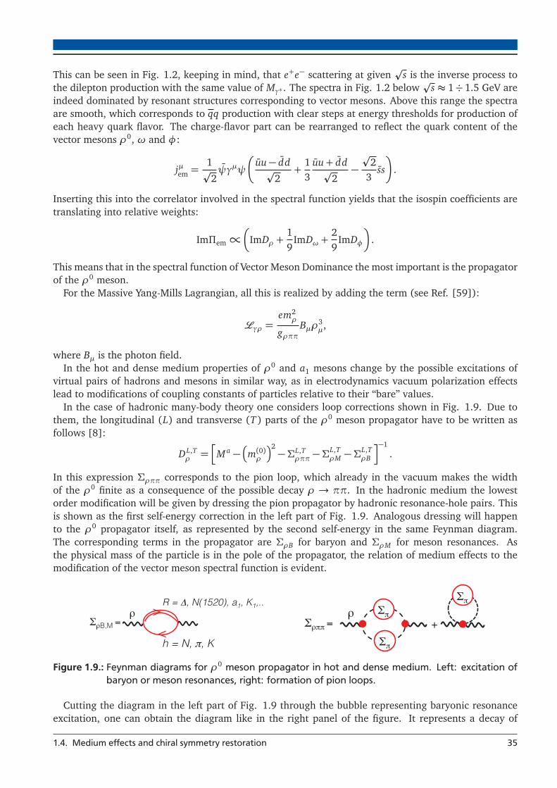
This can be seen in Fig. 1.2, keeping in mind, that e+e− scattering at given�

s is the inverse process tothe dilepton production with the same value of Mγ∗ . The spectra in Fig. 1.2 below

�s ≈ 1÷ 1.5 GeV are

indeed dominated by resonant structures corresponding to vector mesons. Above this range the spectraare smooth, which corresponds to qq production with clear steps at energy thresholds for production ofeach heavy quark flavor. The charge-flavor part can be rearranged to reflect the quark content of thevector mesons ρ0, ω and φ:

jμem =1�2ψγμψ

�uu− dd�

2+

13

uu+ dd�2−�

23

ss

�.

Inserting this into the correlator involved in the spectral function yields that the isospin coefficients aretranslating into relative weights:

ImΠem∝�

ImDρ +19

ImDω +29

ImDφ

�.

This means that in the spectral function of Vector Meson Dominance the most important is the propagatorof the ρ0 meson.

For the Massive Yang-Mills Lagrangian, all this is realized by adding the term (see Ref. [59]):

�γρ =em2

ρ

gρππBμρ

3μ,

where Bμ is the photon field.In the hot and dense medium properties of ρ0 and a1 mesons change by the possible excitations of

virtual pairs of hadrons and mesons in similar way, as in electrodynamics vacuum polarization effectslead to modifications of coupling constants of particles relative to their “bare” values.

In the case of hadronic many-body theory one considers loop corrections shown in Fig. 1.9. Due tothem, the longitudinal (L) and transverse (T) parts of the ρ0 meson propagator have to be written asfollows [8]:

DL,Tρ =

�M a − �m(0)ρ �2 −ΣL,T

ρππ −ΣL,TρM −ΣL,T

ρB

�−1.

In this expression Σρππ corresponds to the pion loop, which already in the vacuum makes the widthof the ρ0 finite as a consequence of the possible decay ρ → ππ. In the hadronic medium the lowestorder modification will be given by dressing the pion propagator by hadronic resonance-hole pairs. Thisis shown as the first self-energy correction in the left part of Fig. 1.9. Analogous dressing will happento the ρ0 propagator itself, as represented by the second self-energy in the same Feynman diagram.The corresponding terms in the propagator are ΣρB for baryon and ΣρM for meson resonances. Asthe physical mass of the particle is in the pole of the propagator, the relation of medium effects to themodification of the vector meson spectral function is evident.

ΣρB,M =>

>

R = Δ, N(1520), a1, K1,..ρ

h = N, π, K

Σρππ =

Σπ

ρ Σπ Σπ

+

Figure 1.9.: Feynman diagrams for ρ0 meson propagator in hot and dense medium. Left: excitation ofbaryon or meson resonances, right: formation of pion loops.

Cutting the diagram in the left part of Fig. 1.9 through the bubble representing baryonic resonanceexcitation, one can obtain the diagram like in the right panel of the figure. It represents a decay of

1.4. Medium effects and chiral symmetry restoration 35

the resonance with ρ0 excitation according to VMD. This has important consequences for low-energyheavy-ion collisions. In this regime the production of thermal pions is too small to excite many ππresonances. However, ρ0 can be excited in the pion cloud of baryons and its properties, modified bystrongly interacting medium, will give a contribution to the spectra of virtual photons. Moreover, thisbrings a possibility to constrain ρN couplings and their dependence on the density of cold nuclear matterby studying the production of the vector meson in πN and πA reactions [60].

Alternatively, one can adopt the scattering amplitude approach, like the one presented in [9]. Therethe amplitude f c.m.

ρa to scatter the ρ0 meson from a particle a is calculated as a sum over resonancesgiven by Breit-Wigner distributions and the term describing smooth underlying background. The spectralfunction can then be obtained as:

Πρa(E, p) = −4π

∫d3k(2π)3

na(ω)�

sω

f c.m.ρa ,

with E and p being the energy and momentum of the ρ0 meson, ω2 = m2a + k2 and na is the occupation

number from Bose-Einstein or Fermi-Dirac distribution, depending if a is boson or fermion.

0

2

4

6

8

10

0.2 0.4 0.6 0.8 1 1.2

-Im

Dρ (

GeV

-2)

M (GeV)

T=100 MeV, q=350 MeV

RW vacuumEK vacuumRW, ρN=ρ0/2EK, ρN=ρ0/2RW, ρN=ρ0EK, ρN=ρ0

0

2

4

6

8

10

0.2 0.4 0.6 0.8 1 1.2

-Im

Dρ (

GeV

-2)

M (GeV)

T=150 MeV, q=350 MeV

RW vacuumEK vacuumRW, ρN=ρ0/2EK, ρN=ρ0/2RW, ρN=ρ0EK, ρN=ρ0

Figure 1.10.: Imaginary parts of the ρ0 meson propagators for different conditions of the hot and densemedium, calculated in [8] (RW) and [9] (EK).

Fig. 1.10 shows the calculations of Dρ in hot and dense hadronic medium under different conditionsusing both approaches outlined above. Both predict “resonance melting”, which is stronger in the many-body theory. In addition, with a good will, one can observe a shift of the maximum towards smallermasses in the scattering amplitude approach. In the many-body theory the maximum moves rather tohigher masses.

The calculation of QCD and Weinberg sum rules at finite temperature, presented in [61] confirm thatthe melting of the ρ0 meson spectral function, observed in dilepton experiments (cf. Section 1.7), isindeed compatible with chiral symmetry restoration.

1.5 Phase diagram of QCD

The existence of order parameters that change with thermodynamic properties of strongly interactingmedium, modify the symmetry pattern of the theory, and even influence how important different degreesof freedom (hadrons, quarks) are, leads to an idea that strongly interacting matter can exist in differentphases.

Phase structure of matter can be more complex than expected at the first glimpse. This is the case evenfor the substance the most familiar from everyday observation: H2O. The number of different crystallineforms of ice is now referred to as “many” (but it is at least 18) and there are three amorphous phases[62].


Figure 1.11.: Left: phase diagram of bcc 3He, calculated in [10], inset shows the result of slight variationof the parameters of Hamiltonian out of the optimal fit to high-temperature experiments.Right: entropy as a function of temperature for different values of the magnetic field.

Also body-centered cubic (bcc) 3He has phases which differ by their magnetic behavior. Among theothers, two antiferromagnetic ones can be observed. In the normal antiferromagnetic (naf) state twosimple cubic sublattices of the bcc structure are magnetic. In the simple cubic antiferromagnetic (scaf)phase, simple cubic sublattices are themselves antiferromagnetic and spins of both of them are rotatedwith respect to each other by 90◦ around the �B field in order to minimize the energy. Left panel of Fig.1.11 shows the low-temperature region of 3He phase diagram, resulting from a mean-field calculationof the appropriate Hamiltonian with parameters listed also in the figure, obtained from fit to varioushigh-T experiments [10]. Right panel shows the entropy as a function of temperature for several valuesof the magnetic field. There is a first-order phase transition (indicated by solid line) between naf and scafphases and smooth cross-over (dashed-line) between low- and high-entropy regions of the naf phase. Itis worth noting, that slight adjustment of the Hamiltonian parameters outside the optimal fit causes theemergence of the first-order transition with a critical end-point (CP), as shown in the inset of the leftpanel of Fig. 1.11.

It is expected that the phase diagram of strongly interacting matter has also a very rich structure (seeFig. 1.12 for one example). Most often discussed are the hadronic matter and gas of faintly interactingquarks and gluons (quark-gluon plasma, QGP). The vital question is about the nature of the phase tran-sition between the hadronic and quark-gluon phase. In contrast to phase diagrams of water or bcc 3He,QCD phase boundaries have not been established experimentally and are yet subject to various theoreti-cal predictions providing quite different results on the existence and location of the critical point. Herethe first-order phase transition is expected up to a certain temperature and above it the phase boundaryis supposed to be a smooth cross-over. The location of the critical point (and even number of them) isbeing a topic of extensive theoretical and experimental studies.

Besides the possible deconfinement, the phase diagram has many more interesting features. Examplesare different kinds of color superconductor (CSC phases). This is the strong-force analogue of super-conducting metals described by the Bardeen-Cooper-Schrieffer (BCS) theory. Already within the coldhadronic matter, as density increases, the gas-like behavior should convert into liquid-like and this isexpected to happen through the first-order phase transition with a critical end-point. Low-energy heavy-ion collision experiments place the critical point at chemical potential of normal nuclear matter andtemperature of T = 15 − 20 MeV [63]. At finite chemical potential, hadronic phase can be separatedfrom QGP by states with inhomogenous spontaneous breaking of chiral symmetry or quarkyonic matter.The former arise from the idea, that quark condensate or similar quantity would be spatially modulated.

1.5. Phase diagram of QCD 37

Figure 1.12.: One of many expected QCD phase diagrams [11, 12]. Not that first-order transition linewith critical point can exist only in thermodynamic limit N →∞. In addition, quite diversepredictions can be made about the order of the chiral phase transition, as μB increases,including the possibility, that the first order region of the mu/d − ms plane shrinks in thedirection of vanishing quark masses (it is already below physical masses for μB = 0 and thisis the reason for the cross-over nature of the transition here), see for example [13, 14].

The latter is a confined phase with weakly interacting quarks deep below the Fermi surface and baryonsclose to it, within the shell of the thickness roughly ΛQC D. Thus the excitations are still hadrons, but bulkthermodynamic properties of the matter are governed by partonic degrees of freedom. It is not clear,how such predictions, valid for QCD with very large number of colors, hold in reality with Nc = 3.

There are only few possibilities, when extreme states of matter, occupying points of the phase diagramfar from the normal atomic nuclei, could exist. First of all, few microseconds after the Big Bang, thematter should have been extremely hot and without baryons, so the early Universe evolved down closeto the Y axis of the phase diagram. The cores of neutron stars are predicted to be extremely dense, butnot too hot, which are the conditions necessary to form color superconductors. In relativistic collisions ofheavy ions, nuclear matter can reach finite temperature and density and make a journey through differ-ent areas of the phase diagram, depending on sizes of the ions and their initial kinetic energies. Finally,in neutron star mergers temperatures as high as 100 MeV/kB may occur [64], in which case they wouldbe the systems with very high density and moderately high temperature, where the thermodynamic limitwould be undoubtedly applicable.

1.6 Evolution of a heavy-ion collision system

Before the collision, ions have normal nuclear matter properties. When they meet, the density increasesand the initial kinetic energy becomes the energy of chaotic thermal motion of nucleons, and then inthe end shards of the collision fly away, reaching finally zero temperature and density. Therefore, thecolliding system has to pass a trajectory through the phase diagram undergoing possibly several phasetransitions if the total energy of colliding ions is large enough.

More detailed picture is shown in terms of a cartoon scheme in Fig. 1.13. Initial stage is governedby nucleon-nucleon processes, like Bremsstrahlung or, at energies high enough, Drell-Yan processes (hard


Hadron Freezeout Hydrodynamic

Evolution Energy Stopping Hard Collisions

Initial state

Time ee

Figure 1.13.: Schematic evolution of a heavy-ion collision for high-energy case, where intermediate evolu-tion can be described by equations of hydrodynamics.

scattering, in which quark from one hadron annihilates with antiquark from another one into virtualphoton or weak Z boson, that then decays into a l+l− pair, l = e,μ). Then the system compresses andgets heated, possibly forming the QGP. The existence of a sizable collective flow of particles (see e.g.[65] for RHIC results) indicates a generally rapid thermalization of the medium: if it happens before theinitial spatial anisotropy of non-central collisions is smeared out, pressure gradients with different valuesin different directions are built up, and this makes the medium to expand stronger in these directions,where the gradients are larger.

Further evolution can be described by microscopic transport calculations like UrQMD (Ultra-relativisticQuantum Molecular Dynamics, [66]), GiBUU (Gießen Boltzmann-Uehling-Uhlenbeck, [67]) or HSD(Hadron-String Dynamics, [68]) and at low energies this accounts for the whole evolution of the fire-ball. At higher energies, the success of hydrodynamic description of particles collective flow parametersat high energies, at least at low transverse momenta, where there is no contribution from hard processes[69, 70], gave rise to the conjecture that the medium evolves as a, possibly slightly viscous, fluid. Thesetwo approaches are merged together in hybrid models (see e.g. [71, 72]), where the hydrodynamiccalculation describes intermediate stage of the system’s evolution, while the transport simulation is usedfor the early stage, before the system reaches thermal equilibrium (providing an initial condition for thehydrodynamics) and in the late one, when the particle picture is more appropriate.

Moreover, the scaling of the flow parameters with number of constituent quarks in hadrons (see leftpanel of Fig. 1.14), observed at RHIC, may be considered as one of the most prominent signatures of thequark-gluon plasma formation and hadron production through quark coalescence mechanism. However,deviations from such scaling have been later observed at LHC [73].

If thermodynamic conditions allowed to form the QGP, the system has to transit back to the hadronicphase. Then, as the cross sections for inelastic scattering are clearly smaller than for elastic ones, theformer cease earlier. The identities of hadrons do not change anymore and this moment is called chemicalfreeze-out. Using grand canonical partition functions with different empirical modifications (so calledStatistical Hadronization Model, [74, 75, 76]), one can extract from particle ratios T and μB of thesystem at this moment. For different

�sNN the points accumulate around a single curve on the phase

diagram, called the chemical freeze-out line, see right panel of Fig. 1.14.

At the end also elastic collisions cease and thermal spectra of the particles get fixed (giving a chance toextract temperature as an inverse slope of the Boltzmann distribution). This last stage of the evolutionof the system is called thermal freeze-out.

1.6. Evolution of a heavy-ion collision system 39

Hadron gas

LQCD

SIS18

SIS100/AGS

SIS300+

SPS/RHIC BES LHC RHIC

RHIC fixed target

SIS1

SIS

Quark-Gluon Plasma

Nuclei

NICA 100

RHIC

1

R

SIS

R

J-PARC

Figure 1.14.: Left: scaling of the elliptic flow measured at RHIC as a function of transverse mass with thenumber of constituent quarks [15]. Right: chemical freeze-out points on the T − μB plane.Black squares and dark blue stars: [16], black solid symbols (squares, circles, triangles): [17],green square: [18], green solid circles: [19], lila diamond: [20]. Red triangle is thermal fit todilepton spectra from [21].

1.7 Probing QCD matter with photons

Flow observables provide information about an early stage of heavy-ion collision and formation of equi-librium, hadrons distributions are settled only at the end of the system’s evolution. However, to probehot and dense state of QCD matter directly, photons, real γ and virtual γ∗, are needed. The latter decayinto lepton pairs l+l− practically immediately, so lepton pairs and virtual photons are often notionallyidentified and referred to as dileptons. They are not subject to the strong force and their electromagneticinteraction probability is suppressed by α2 (α ≈ 1/137 – fine structure constant) and is negligible onthe distance needed for such electromagnetic probes to leave the medium. This means, that they do notundergo practically any rescatterings and bring undistorted information about the process in which theywere created.

Furthermore, they are emitted in different processes during the whole nuclear collision. More specifi-cally, the sources of radiation can be summarized as in Fig. 1.15, for case of ultrarelativistic collisions. Itshows the conjectured distribution of dileptons’ invariant mass:

M =�(E1 + e2)2 − (�p1 + �p2)2 ≈ 2

�|�p1||�p2| sin Θ12

2.

The last approximation is valid for particles with masses much smaller than their momenta and involvesthe opening angle Θ12 between leptons. It is not needed technically, because one can always easilyperform full calculation, but it often facilitates an understanding of the kinematics.

It turns out, that different parts of the distribution are populated by processes dominating at differ-ent stages of the collision. Before the nuclei meet, electromagnetic radiation is emitted through theBremsstrahlung process. In the initial stage of the collision, before the nuclear matter gets equilibrated,dileptons from Drell-Yan annihilations can be radiated. This source requires very large collision energyand occupies correspondingly high mass region of the spectrum. If the energy is sufficient to reach tem-perature and density of deconfinement phase transition and if QGP has enough time to get equilibrated,thermal dilepton spectrum from perturbative quark-antiquark annihilation will be populated. It shouldbe best visible in the intermediate mass region (IMR) of 1.5 GeV/c2 � Mll � 3 GeV/c2, when subtractingthe background of semileptonic decays (decays of a hadron with producing only one lepton) of correlated


charmed baryon pairs DD. Then QGP cools down and expands, vector mesons are produced, eitherthrough resonant ππ or KK annihilations, dominant at high energies, or through off-shell pion annihi-lation at low energies. As the vector mesons couple directly to the l+l−, the dilepton spectroscopy inthe low mass region (LMR, Mll � 1.5 GeV/c2), reflects immediately the modifications of ρ0, ω and φspectral functions and gives an insight into the pattern of the chiral symmetry restoration. To extract thisinformation, one has to subtract contribution of sources radiating mainly after the freeze-out: decays ofhadronic resonances, and π0, η and ω in Dalitz (i.e. three-body) channels. The picture is closed withthe late decays of charmonia J/Ψ or Ψ ′. Their production is related to the deconfinement pattern andabsorption in nuclear matter.

Rates of the dileptons from decays of vector mesons are directly related to their spectral function,provided that the Vector Meson Dominance is still valid in the medium. The relation is as follows:

dNll

d4 xd4q= − α

2em

π3M2f B(q0, T )1

3 gμνImΠμνem (M , q;μB, T ) , (1.9)

which is correct only to the first order in αem on the side of the electromagnetic interaction, but exactin the strong interaction. In this expression f B is the thermal Boltzmann factor dependent on energycomponent of the four-momentum q0 and the temperature. To make a connection with the experiment,which typically measures dNll/dMll with Mll being the invariant mass of the l+l− pair, an appropri-ate integral over phase-space evolution has to be performed and this requests an input from modelsconstrained by the experiment.

The opportunity to directly access the properties of hot and dense strongly interacting matter withphotons and dileptons has been exploited since decades with different sizes of colliding systems and atenergies from around 1A GeV to several TeV. At relatively high energies, dilepton spectra were measuredby the CERES Collaboration at the Super Proton Synchrotron (SPS) in CERN. While e+e− productionin p+Be and p+Au collisions at 450A GeV could be described by a sum cocktail of simulated hadronice+e− sources (see left and middle panel of Fig. 1.16), in S+Au collisions at 200A GeV a clear enhance-ment over the cocktail has been observed (right panel of Fig. 1.16). In the measurement of Pb+Auat 158A GeV it was possible to subtract the hadronic cocktail and compare the resulting ρ0 spectrum

Figure 1.15.: Expected spectrum of dilepton invariant mass in ultrarelativistic heavy-ion collisions withparticular sources marked. Figure taken from [22].

1.7. Probing QCD matter with photons 41

10-9

10-8

10-7

10-6

10-5

10-4

0 0.5 1

10-9

10-8

10-7

10-6

10-5

10-4

0 0.5 1

mee (GeV/c2)

(d2 N

ee /d

ηdm

) / (

dNch

/dη

) (5

0MeV

/c2 )-1

p-Be 450 GeV/u2.1 < η < 2.65p

⊥ > 50 MeV/c

⟨dNch /dη⟩ = 3.8π →

eeγ

ρ,ω

→ e

e

φ →

ee

η → ee

γ

η , → eeγ

ω → eeπ o

charm

mee (GeV/c2)

p-Au 450 GeV/u2.1 < η < 2.65p

⊥ > 50 MeV/c

⟨dNch /dη⟩ = 7.0

π →

eeγ

ρ,ω

→ e

e

φ →

ee

η → ee

γ

η , → eeγ

ω → eeπ o

charm

mee (GeV

S-Au 200 GeV/u2.1 < η < 2.65p

⊥ > 200 MeV/c

⟨dNch /dη⟩ = 125

π →

eeγ

ρ/ω

→ e

e

φ →

ee

η → ee

γ

η , → eeγ

ω → eeπo

charm

10-9

10-8

10-7

10-6

10-5

10-4

0 0.5 1

Figure 1.16.: Inclusive e+e− invariant mass spectra from proton-nucleon and nucleon-nucleon collisions,measured by the CERES Collaboration[23]. Curves show contributions from different hadrondecays, expected based on proton-proton collisions. Thick line with the shaded area repre-sents the sum and its systematic error. Higher transverse momentum (here denoted by p⊥)cut results in the decrease of the yield from π0-Dalitz decay in S+Au.

with two in-medium scenarios [56, 77], discussed in Section 1.4. This comparison clearly favors the in-medium hadronic many-body effects. At the same accelerator the NA60 Collaboration measured μ+μ−

0 0.2 0.4 0.6 0.8 1 1.2 1.4 1.6

0.2

0.4

0.6

0.8

1

1.2

1.4

1.6

1.8-610×-1 )2

>(10

0 M

eV/c

ch>/

<Nee

/dm

ee<d

N

)2 (GeV/ceem

(a)

ρcocktail massρdropping

in-medium hadronic

0 0.5 1 1.5 2 2.5-1010

-910

-810

-710

-610

-1)

(20

MeV

)η

/dch

dM)/

(dN

η/d

μμ

N2(d

M (GeV)

In-In >30η/dchdN

excess dimuons

Renk/RuppertHees/RappDusling/Zahed

Figure 1.17.: Left: invariant mass spectrum of dileptons measured in Pb+Au at 158A GeV beam kineticenergy by the CERES Collaboration [24], together with model calculations of the ρ0 spectralfunction. Right: invariant mass of excess dimuons measured at the same energy in In+In bythe NA60 Collaboration [21] compared to the model calculations of Ruppert et al. [25], vanHees and Rapp [26] and Dusling and Zahed [27].

in In+In at 158A GeV energy [78, 21]. In the dimuon channel it was affordable to achieve an excellentdata quality thanks to the absence of the main uncorrelated background source in e+e− – the externalphoton conversion in detector material. In Fig. 1.17 (right panel), comparison of the excess dimuons


to theoretical models is displayed. Good agreement of the many-body calculation of [26] with datais clearly visible. It is also possible to fit the function dN/dM ∝ M3/2 exp(−M/T ) to the IMR of thespectrum after subtracting Drell-Yan and DD contributions. The advantage over fitting to the spectraof transverse momenta or related quantities is that invariant mass, by definition, is a Lorentz invari-ant and is insensitive to the motion of the source emitting the radiation. The inverse slope parameterT can then be interpreted as a true temperature, not shaded by the collective expansion. In case ofμ+μ− measurement by NA60, the value extracted from the fit in the range 1.2 < M < 2.0 GeV/c2 wasT = 205 ± 12 MeV [21]. The obtained value is an average over space-time evolution of the source ofthe dileptons in the fit range. Even though the source is supposed to be dominated by the quark-gluonplasma and this constraints the spread of temperature values around the average, this result still shows,that the temperatures reached in hot and dense stage of heavy-ion collisions are by far higher than thoseof chemical freeze-out in the same nuclear reactions.

Electromagnetic probes are also used at much higher energies available at Large Hadron Collider(LHC) in CERN. Here the result from direct real photons (photons not coming from decays of particles,but from thermal source) measured by the ALICE Collaboration in Pb+Pb at 2.76A GeV [28] are difficultto interpret. On the one hand, extremely high temperature extracted from the fit to the transversemomentum spectrum of photons, T = 304 ± 51 MeV/kB, see left panel of Fig. 1.18, indicates thatthey are radiated mostly in rather early stage of the collision. On the other hand, a sizable ellipticflow parameter v2, see right panel of the Fig. 1.18, comparable to the one of hadrons, speaks for lateremission, when the flow is already established. Similar measurements have been made by PHENIX at

(GeV/c)T

p0 2 4 6 8 10 12 14

)2 c-2

(G

eVdy

Tdp

TpN2 d

ev

. N

π21

-710

-610

-510

-410

-310

-210

-110

1

10

210

310

= 2.76 TeVNNs0-40% Pb-Pb,

Direct photons (scaled pp)

T = 0.5,1.0,2.0 pμDirect photon NLO for

51 MeV±/T), T = 304 T

exp(-p×Exponential fit: A

ALI−PREL−27968

Figure 1.18.: Direct photons measured by the ALICE Collaboration in 40% most central Pb+Pb at2.76A GeV beam kinetic energy [28]. Left: transverse momentum spectrum, right: ellip-tic flow coefficient v2 as a function of transverse momentum.

RHIC [79] with the slope T = 321±19(stat)±19(syst) MeV/kB for 0-20% most central Au+Au collisions.Even though it can be argued, that part of the high value inverse slope parameter can be explained bythe blue-shift of the expanding fireball, large yield of direct photons itself indicates early emission withhigh temperature and the precise statement of the so-called “direct photon puzzle” is that theoreticalmodels have difficulties in simultaneous of pT and v2 distributions [80]. For example, in refs. [81, 82]calculations that agree with ALICE and PHENIX data within systematic uncertainties were presented, butlater ref. [80] provided higher precision data, with which the calculations are no longer fully consistent.

The connection between high and low energy regime is brought by the Beam Energy Scan at Relativis-tic Heavy Ion Collider (RHIC) in Brookhaven National Laboratory (BNL) in Upton, NY, US. Initial resultson the size of the low-mass dielectron excess over hadronic sources, normalized to the number of pions,as a function of

�sNN is shown in Fig. 1.19.

1.7. Probing QCD matter with photons 43

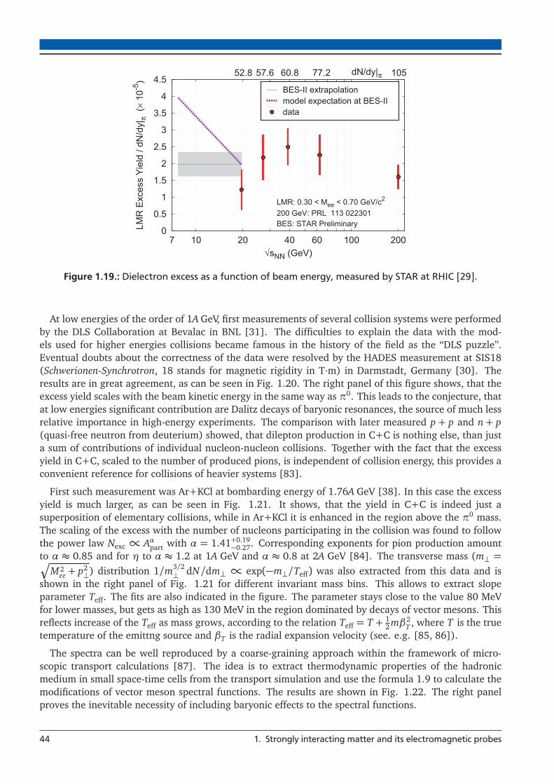
0

0.5

1

1.5

2

2.5

3

3.5

4

4.5

7 10 20 40 60 100 200

LMR

Exc

ess

Yiel

d / d

N/d

y|π

(× 1

0-5)

√sNN (GeV)

LMR: 0.30 < Mee < 0.70 GeV/c2

52.8 dN/dy|π

200 GeV: PRL 113 022301

57.6

BES: STAR Preliminary

60.8 77.2 105

BES-II extrapolationmodel expectation at BES-IIdata

Figure 1.19.: Dielectron excess as a function of beam energy, measured by STAR at RHIC [29].

At low energies of the order of 1A GeV, first measurements of several collision systems were performedby the DLS Collaboration at Bevalac in BNL [31]. The difficulties to explain the data with the mod-els used for higher energies collisions became famous in the history of the field as the “DLS puzzle”.Eventual doubts about the correctness of the data were resolved by the HADES measurement at SIS18(Schwerionen-Synchrotron, 18 stands for magnetic rigidity in T·m) in Darmstadt, Germany [30]. Theresults are in great agreement, as can be seen in Fig. 1.20. The right panel of this figure shows, that theexcess yield scales with the beam kinetic energy in the same way as π0. This leads to the conjecture, thatat low energies significant contribution are Dalitz decays of baryonic resonances, the source of much lessrelative importance in high-energy experiments. The comparison with later measured p + p and n+ p(quasi-free neutron from deuterium) showed, that dilepton production in C+C is nothing else, than justa sum of contributions of individual nucleon-nucleon collisions. Together with the fact that the excessyield in C+C, scaled to the number of produced pions, is independent of collision energy, this provides aconvenient reference for collisions of heavier systems [83].

First such measurement was Ar+KCl at bombarding energy of 1.76A GeV [38]. In this case the excessyield is much larger, as can be seen in Fig. 1.21. It shows, that the yield in C+C is indeed just asuperposition of elementary collisions, while in Ar+KCl it is enhanced in the region above the π0 mass.The scaling of the excess with the number of nucleons participating in the collision was found to followthe power law Nexc ∝ Aαpart with α = 1.41+0.19−0.27. Corresponding exponents for pion production amountto α ≈ 0.85 and for η to α ≈ 1.2 at 1A GeV and α ≈ 0.8 at 2A GeV [84]. The transverse mass (m⊥ =�

M2ee + p2⊥) distribution 1/m3/2

⊥ dN/dm⊥ ∝ exp(−m⊥/Teff) was also extracted from this data and isshown in the right panel of Fig. 1.21 for different invariant mass bins. This allows to extract slopeparameter Teff. The fits are also indicated in the figure. The parameter stays close to the value 80 MeVfor lower masses, but gets as high as 130 MeV in the region dominated by decays of vector mesons. Thisreflects increase of the Teff as mass grows, according to the relation Teff = T + 1

2 mβ2T , where T is the true

temperature of the emittng source and βT is the radial expansion velocity (see. e.g. [85, 86]).

The spectra can be well reproduced by a coarse-graining approach within the framework of micro-scopic transport calculations [87]. The idea is to extract thermodynamic properties of the hadronicmedium in small space-time cells from the transport simulation and use the formula 1.9 to calculate themodifications of vector meson spectral functions. The results are shown in Fig. 1.22. The right panelproves the inevitable necessity of including baryonic effects to the spectral functions.


]2 [GeV/ceeM

0 0.2 0.4 0.6 0.8

]2ba

rn/G

eV/c

μ

[ee

/dM

σd

-210

-110

1

10

210

3101 AGeV HADES1.04 AGeV DLS

[AGeV]bE0 1 2

exc

N

-710

-510

-310

-110

10C12C +12

0π

η

Dalitzη

Excess

Figure 1.20.: Left: dielectron production in C+C collisions measured at 1A GeV by HADES [30] and at1.04A GeV by DLS [31]. Both data sets are within the DLS acceptance. Right: scaling of theexcess e+e− yield with the beam kinetic energy. In this plot full triangles represent HADESexcess, open triangles - DLS, full squares - inclusive π0 yield in C+C, full circles - inclusive η,open circles - η-Dalitz contribution. Dotted and dashed lines are scaled-down lines fromtotal π0 and η yield, respectively, for better comparison with the excess yield.

1.8 The aim of this work

To push forward the understanding of the strongly interacting matter at relatively low temperaturesbut high densities, studies of heavy-ion collisions at low energies but large systems are necessary. This

]2 [MeV/ceeM0 0.2 0.4 0.6

)ee

/dM

NN

)/(d

Nee

/dM

AA

) (d

N0

πAA

/N0

πNN

(N 0

1

2

3

4

5

6

7

8

Ar+KCl 1.76A GeV

C+C 1A GeV

C+C 2A GeV

]2 [GeV/cm0 0.3 0.6 0.9 1.2 1.5

]-5

/2)2

[

(GeV

/c d

N/d

m-1

)3/

2 m 0

π(N

-1110

-910

-710

-510

-310

-110

1

Ar+KCl 1.76A GeV1±79

<130

3±80130-300

4±77 0.1)×300-450 (

6±960.01)×450-650 (

26±1310.001)×>650 (

Figure 1.21.: Left: spectra of dilepton invariant mass, measured by HADES in C+C and Ar+KCl collisions,normalized to the respective numbers of produced pions and divided by average yield inp+p and n+p collisions. Right: transverse mass distribution in different invariant mass bins,as measured by HADES in Ar+KCl reactions at 1.76A GeV. Scaling factors added for visibilityand extracted inverse slope parameters are indicated.

1.8. The aim of this work 45

]2M [GeV/c0 0.2 0.4 0.6 0.8 1

-1 ]2 d

N/d

M [

GeV

/c×)0 π

1/N

(

-910

-810

-710

-610

-510

-410

-310

-210UrQMD

πη

foωfoρφρMedium

ωMediumπMulti

Coarse-Graining < 1.1 GeV/ceHADES acceptance, 0.1 < p

Ar + KCl @ 1.76 AGeV

(a)

]2M [GeV/c0 0.2 0.4 0.6 0.8 1

-1 ]2 d

N/d

M [

GeV

/c×)0 π

1/N

(

-910

-810

-710

-610

-510

-410

-310

-210

ρMediumωMedium

(no baryons)ρ (no baryons)ω

SumSum (n. b.)

Influence of baryonic effectsAr + KCl @ 1.76 AGeV (a)

Figure 1.22.: Invariant mass spectra obtained from microscopic transport approach with coarse-grainedmodifications of vector meson spectral functions compared to the measurement done byHADES. Left panel shows different cocktail components, right – the importance of inclusionbaryonic effects in the spectral function self-energies.

was the inspiration of the heavy-ion program in HADES. It started with the mid-sized system Ar+KCl at1.76A GeV beam kinetic energy and continued with Au+Au at 1.23A GeV – the largest system possiblewith this energy at SIS18. Fig. 1.23 shows the evolution of the most central cell of the Au+Au collision asobtained in the coarse-graining approach, similar in spirit to the one discussed above [88, 89]. While atSPS energies the system reaches much higher densities than in the SIS18 and SIS100 regime, it remainsin this state only for a very short time. In contrast, at lower energies the lifetime of the hot and densefireball is much longer – up to 30 fm/c. It can be argued, that the contemporary phase diagram of

Figure 1.23.: Left: evolution of the central cell of Au+Au at 1.23AGeV and Ar+KCL at 1.76AGeV collisionsin the plane of temperature and baryochemical potential. each point is plotted after a stepof 2 fm/c, so their distances reflect the velocity of the evolution. In orange, the lines ofconstant ratio of the quark condensate to its vacuum value are indicated. They show, thatat high T and μB the chiral symmetry is fully restored, but the onset of the restorationshould be observed already at SIS18 energies.Right: density as a function of time for different reactions.


strongly interacting matter is often plotted very carefully without any scale on axes and it is hard to stateexactly where the central cell really travels in it and if the hadronic transport is still valid there. Onecan even doubt, if it is allowed at all to extract thermal properties of for systems at such low energy,but results on particle rates [90] and dilepton production [38, 87] in ArKCl show surprisingly gooddescription. Thus Au+Au reactions at low energies may explore the terra incognita of the diagram.Similar like in other systems and energies, dileptons are one of the most promising senses to be used inthis exploration. The aim of this work is thus to extract possibly the highest quality spectra from Au+Auat 1.23A GeV measured by HADES and hopefully to give the theory as a gift a new inspiring motivation!

1.8. The aim of this work 47

2 The HADES apparatus

Figure 2.1.: A “fish-eye” view of HADES inside its cave. Photograph by A. Rost.

The experimental system particularly suitable for measuring properties of virtual photons radi-ated from heavy-ion collisions at low beam energies is the High Acceptance Di-Electron Spectrometer(HADES) operating at SIS18 accelerator in GSI Helmholtzzentrum für Schwerionenforschung in Darm-stadt, Germany. The accelerator facility is able to provide a variety of beams ranging from protons toUranium ions, of the maximum kinetic energy per nucleon depending on accelerated species, i.e. ∼4.5GeV and ∼1.5 AGeV, respectively. Experiments using proton (on H2 and Nb targets), deuteron (on H2), C(on C), Ar (on KCl) and Au (on Au) have been performed by HADES. The opportunity to use a secondaryπ− beam was taken recently by HADES in the summer 2014 campaign.

The HADES is essentially a magnetic spectrometer. It consists of a tracking system composed of twopairs of Multiwire Drift Chambers (MDC), located in front of and behind the magnetic field. A hadron-blind Ring Imaging CHerenkov (RICH) detector, placed in the magnetic field free region, is supported byan electromagnetic Pre-Shower detector to serve lepton identification. Velocity of a particle is measuredby the time-of-flight wall detectors. The whole system is arranged in six identically designed parts(sectors), each of them covering 60◦ of the azimuth angle around the beam axis and 18-80◦ polar angle,cf. Figures 2.1 and 2.2 (left panel).

Precise measurements of dilepton spectra are fulfilled by the following features of the detector design:

1. A large geometrical acceptance allows to effectively register rare dielectron decays, i.e. about 40%of decay pairs with large opening angle (like ω → e+ + e−) can be measured and about 10% ofclose pairs (like from π0-Dalitz decay).

2. A high trigger rate of the order of 10-40 kHz sufficient for collection of statistics necessary to studyrare dielectron decays. With this respect, HADES is very competitive to all existing (and many ofplanned) heavy-ion experiments studying hadronic matter characterized by large baryon chemicalpotential.

3. Excellent invariant mass resolution (of the order of few %), necessary to study in-medium modifi-cations of vector mesons.

49

Figure 2.2: A schematic view of a cross sectionthrough two opposite sectors of HADES.

4. Low material budget (X/X0 ∼ 2 · 10−3 for tracking chambers [91]) to reduce background fromsecondary particles produced in detector material, especially from e+e− products of γ conversion,as well as multiple scattering of particles.

5. An excellent hadron discrimination makes it possible to obtain a clear e+/e− sample in the exper-imental conditions, where up to 200 charged particles in an event are crossing the acceptance ofthe spectrometer (for Au+Au at 1.23 AGeV), but the interesting dilepton signal is of the order of10−4.

The detector system is capable for the reconstruction of rare strangeness production like Ξ, Λ, φ andK+/K−, as well as global properties of nuclear reaction. The full description of the spectrometer is givenin [92]. The following sections provide an overview of the features most relevant for the physics analysisbeing the topic of the current work.

2.1 Ring Imaging CHerenkov

2.1.1 Cherenkov radiation

When a charged particle passes through a medium, its electric field causes a polarization of the mediumclose to particle’s trajectory [33]. Afterwards, the medium relaxes to its initial state, but the momentarypolarization produces a small electromagnetic perturbation propagating with the speed of light. Asshown on the left panel side of Fig. 2.3, if the velocity of the particle is smaller than the speed oflight in the medium v < c/n with n - refractive index of the medium, contributions from perturbationsat different points of the trajectory will cancel out at large distances. If, however, v > c/n, thesecontributions will add up coherently to form a conical wavefront. Its propagation can also be representedin terms of rays of light, one of them is also shown in the Fig. 2.3. From the geometry shown there, onecan immediately obtain the angle at which the rays are emitted:

ΘC = arccos�

cv · n�

, (2.1)

50 2. The HADES apparatus

Figure 2.3.: Propagation of the electromagnetic perturbation caused by a particle traversing a mediumwith the velocity lower (left) and higher (right) than the speed of light in the medium. Figuretaken from [33]

Figure 2.4: Refractive index of C4F10 mea-sured [34] as a function ofthe wavelength with the helpof Fabry-Perot interferometer.Lines are fits of the Sellmeierformula Eq. 2.2.

where c is the speed of light, v is particle’s velocity and n is the refractive index of the medium. Thewavelength dependence of the refractive index is governed by the empirical Sellmeier formula:

(n(λ)− 1) =10−6p1

p−22 −λ−2

, (2.2)

where λ is the wavelength and p1 and p2 are free parameters. The dependence, measured using Fabry-Perot interferometer [34], is shown in Fig. 2.4. From this one can see, that the condition v > c/n(λ)⇒n> β−1 imposes an upper limit on the wavelength. Together with the fact, that the spectrum in generalgrows monotonically with the energy [93] and that the sensitivity of the human eye is peaked at thegreen light, this allows to understand, why Cherenkov radiation is often observed as a blue light.

2.1.2 RICH detectors

From Eq. 2.1 the opening angle of Cherenkov cone depends directly on the momentum of a particleof a specific type. Measuring the angle can thus be used for particle identification with Ring Imaging

2.1. Ring Imaging CHerenkov 51

10

1 2 0 mrad

3 0 0 mrad

12

Gas CF 4

1 2 ( m )

θC

mirror

Beampipe

Track

Photodetectors 3 3 0 mrad

C F 4 10

Figure 2.5.: Schematic view of RICH detectors in CLEO III (left, figure taken from [35]) and LHCb (right).

Cherenkov (RICH) detectors. One of the simplest possible applications of this idea is the RICH detectorof the CLEO experiment [94], shown schematically in Fig. 2.5 (left panel). Cherenkov light is emitted,when a hadron goes through a thin LiF radiator. A small gap between it and the Multi-Wire ProportionalChamber (MWPC) serving as photon detector lets the cone open such, that photons emitted at specificopening angle hit those pads of the MWPC, which are located on the circle of a radius corresponding tothe opening angle.

A disadvantage of such a simple setup is a short path of the particle through the radiator and thus asmall number of Cherenkov photons. However, introducing thicker radiator while still letting the photonshit the photon detector directly would lead to appearance of a “donut” instead of a circle on the pad plane(sum of circles of different radii from different points of the path) and again make the determination ofthe cone opening angle impossible. Another problem is that installing the photon detector on the wayof charged particles will lead to a number of difficulties (e.g. many direct hits of particles, which bothmake fake signals and damage the detector), especially in heavy-ion collision experiments.

Both issues can be solved by introducing a spherical mirror reflecting Cherenkov light in such a way,that photons emitted along the whole path of a particle hit a single circle on the detection surface (inthis case located backwards), as shown in case of both RICH detectors of LHCb experiment [95], shownin Fig. 2.5 (right panel), and HADES RICH in Fig. 2.6.

2.1.3 HADES RICH

In case of HADES’ RICH detector, shown in Fig. 2.6 (left), opening angle of the Cherenkov cone is notmeasured. For the C4F10 radiator gas, the threshold value of the Lorentz factor γ =

�1

1−1/n2 is 18. Fig.2.7 shows, that in the momentum region available for particles emitted from Au+Au at 1.23 AGeV onlyelectrons and positrons can have γ high enough to radiate Cherenkov light. The respective momentumthreshold is 10 MeV/c, while for next heavier particles, muons and pions, it is roughly 1.9 and 2.4 GeV/c,respectively. The criterion for electron identification is then just the existence of the ring.

The photon detector is an MWPC with CsI photocathode segmented such, that ring diameter in termsof segments (pads) is almost constant over the whole detector (7-8 pads). This allows for application ofefficient ring finding algorithms. The counter gas of MWPC is CH4.

The two volumes of HADES RICH are separated by a CaF2 window to avoid mixing of gases. Thematerial of the window was chosen to obtain sufficient transmittance. The data on transmittances and


Figure 2.6.: Left: schematic view of the HADES RICH and its photon detector plane. Electron track isindicated in red, rays of Cherenkov light in blue. Right: Optical parameters of the componentsof HADES RICH detector. [36]

quantum efficiencies of materials used to build the HADES RICH detector are shown in Fig. 2.6 (right).One may note rather low quantum efficiency of the CsI, which might even have decrease due to theknown effect of aging. This led to an idea of replacing the MWPC by an array of Photo-Multiplier Tubes(PMTs), which will be performed in HADES from 2019 on.

2.1. Ring Imaging CHerenkov 53

γ

0 10 20 30 40 50 60 70 80 90 100

p [G

eV/c

]

1

2

3

4

5

6

7

+/-e

+/-μ

+/-π

10F4C 2CO 2N

γ

0 20 40 60

p [G

eV/c

]

0.01

0.02

0.03

0.04

+/-e

10F4C 2CO 2N

Figure 2.7.: Lorentz factor γ dependence of the momentum of electrons muons and pions. Dashed linesindicate threshold values of γ for emission of Cherenkov light in the C4F10 used in HADESRICH, as well as in CO2 and N2, also often considered as radiator gases in RICH detectors.

2.2 Target

In the April 2012 experiment the Au target consisting of 15 segments, shown in Fig. 2.8, was used. Thereason for taking the segmented target was to reduce photon conversion probability (by increasing thechance, that photon leaves the target region without interacting with other Au nucleus).

2.3 Tracking system

The main design guidelines for the tracking system were invariant mass resolution of 1-2% for electron-positron pairs from decays of vector mesons, e.g. ρ(770), ω(782), φ(1020) (corresponding to about2% momentum resolution of single leptons) and low material budget to reduce the probability of γconversion and multiple scattering of charged particles. It should also be able to handle large chargedparticle multiplicities with a high event rate, what is necessary to investigate electromagnetic decays ofvector mesons in Au+Au collisions.

To fulfill these requirements, the tracking system of HADES consists of a compact superconductingmagnet and four sets of multiwire drift chambers, two traversed by a charged particle before its trajectoryis bent by the magnetic field and two traversed after that.

2.3.1 Magnet

Six coils of the IronLess Superconducting Electron (ILSE) magnet are mounted around the circular sup-port structure. The coils generate field of a nearly toroidal shape and strength of 3.6 T inside the coilsand below 0.8 T between them, when operating with the highest current of 3500 A, see Fig. 2.9. Duringthe Au+Au run the current was set to 2500 A. The chosen shape of the field assures, that it vanishes inthe region, where MDCs and RICH are located. Coils of the magnet are cooled by a single phase liquidhelium at p = 2.8 bar and T = 4.7 K.


Figure 2.8.: Gold target used in the April 2012 experiment.

Figure 2.9.: Left: side view of HADES magnet coils. Right: map of the magnetic field between the coils.

2.3. Tracking system 55

2.3.2 Multiwire Drift Chambers

The smallest unit of the Multiwire Drift Chambers (or Mini Drift Chambers, in all cases abbreviated asMDC) of HADES is a cell consisting of a sense wire together with two potential wires located in the sameplane and with two surrounding planes of cathode wires, as shown in the left panel Fig. 2.10. Each of24 chambers (6 sectors×4 modules) contains 6 layers of such cells which are orientated as explained inthe right panel Fig. 2.10 in order to get high spatial resolution of the order of 60-100 μm in polar and120-200 μm in azimuth direction.

Particle’s trajectory and momentum has to be reconstructed from only two points before and two afterthe magnetic field, what is already challenging. First, fired cells in all layers of each single chamberare projected to a common plane to find a maximum representing a crossing point of fired wires, corre-sponding to a point traversed by a particle. This is illustrated in Fig. 2.11. Two such points in the innerand the outer pair of chambers define inner and outer track segments, which are then matched to obtaina track candidate.

Momentum is calculated with a Runge-Kutta algorithm, which is used to solve numerically the equationof motion of a particle in known magnetic field (defined by a 3-dimensional field map). It is appliediteratively and the quality of the trajectory reconstruction is quantified by the result of the χ2 test.

Moreover, the readout electronics of drift chambers is able to extract width of measured signal definedas time-over-threshold. This can be translated by a non-linear transformation into specific energy lossdE/d xM DC of a particle. As Fig. 2.12 shows, it is not really a quantity allowing to discriminate betweenelectrons and pions, but at least it can be used to reject of protons in a multi-parameter analysis.


Figure 2.10.: Left: a single cell of MDC showing the arrangement of different wires. The minimum dis-tance of a charge particle track (indicated as a blue arrow) to the sense wire is also defined.Right: orientation of wires in different layers of HADES MDCs.

Figure 2.11.: Finding a point passed by a charged particle in MDCs as a crossing of several fired wires.

2.3. Tracking system 57

Figure 2.12: Momentum dependence ofthe specific energy loss dE/dxin HADES Multiwire DriftChambers. Colored solid linesindicate values expected fordifferent particle species ascalculated using usual Bethe-Bloch formula.


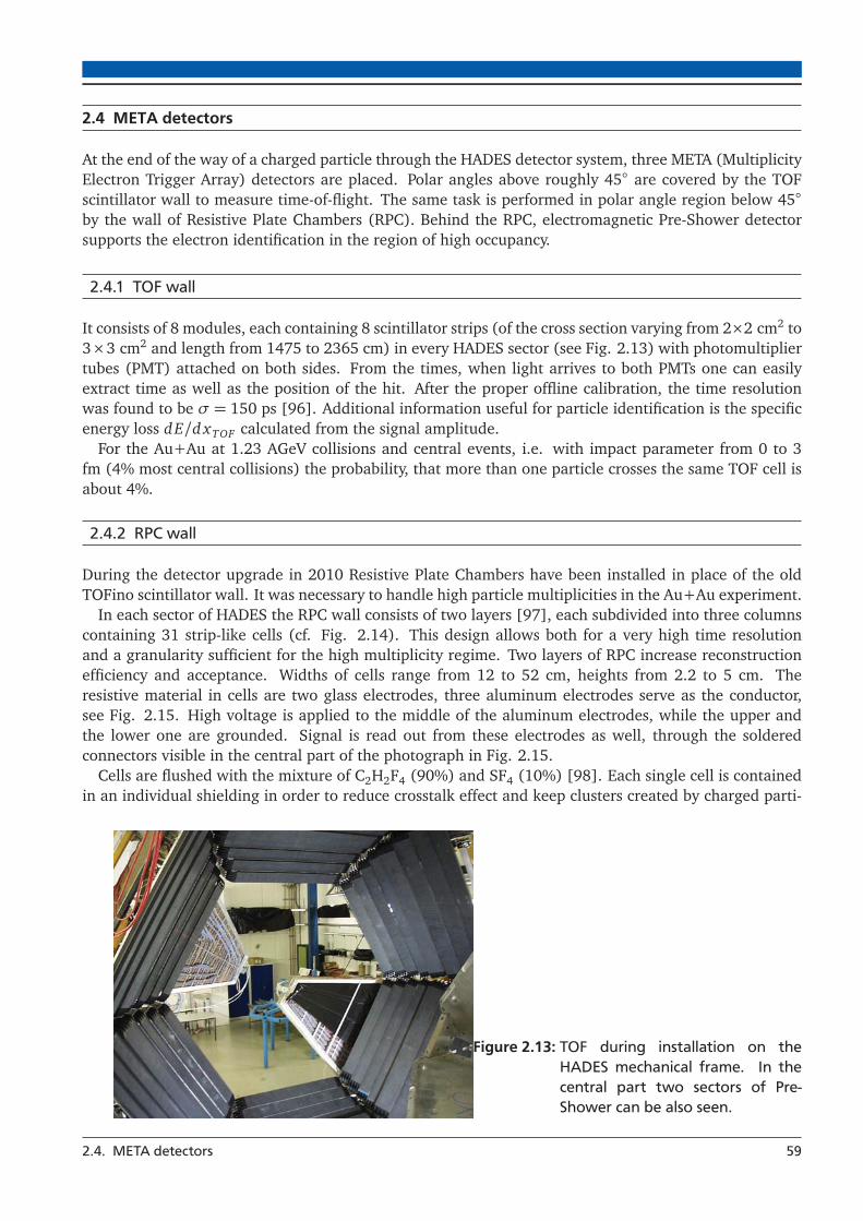
2.4 META detectors

At the end of the way of a charged particle through the HADES detector system, three META (MultiplicityElectron Trigger Array) detectors are placed. Polar angles above roughly 45◦ are covered by the TOFscintillator wall to measure time-of-flight. The same task is performed in polar angle region below 45◦by the wall of Resistive Plate Chambers (RPC). Behind the RPC, electromagnetic Pre-Shower detectorsupports the electron identification in the region of high occupancy.

2.4.1 TOF wall

It consists of 8 modules, each containing 8 scintillator strips (of the cross section varying from 2×2 cm2 to3×3 cm2 and length from 1475 to 2365 cm) in every HADES sector (see Fig. 2.13) with photomultipliertubes (PMT) attached on both sides. From the times, when light arrives to both PMTs one can easilyextract time as well as the position of the hit. After the proper offline calibration, the time resolutionwas found to be σ = 150 ps [96]. Additional information useful for particle identification is the specificenergy loss dE/d xTOF calculated from the signal amplitude.

For the Au+Au at 1.23 AGeV collisions and central events, i.e. with impact parameter from 0 to 3fm (4% most central collisions) the probability, that more than one particle crosses the same TOF cell isabout 4%.

2.4.2 RPC wall

During the detector upgrade in 2010 Resistive Plate Chambers have been installed in place of the oldTOFino scintillator wall. It was necessary to handle high particle multiplicities in the Au+Au experiment.

In each sector of HADES the RPC wall consists of two layers [97], each subdivided into three columnscontaining 31 strip-like cells (cf. Fig. 2.14). This design allows both for a very high time resolutionand a granularity sufficient for the high multiplicity regime. Two layers of RPC increase reconstructionefficiency and acceptance. Widths of cells range from 12 to 52 cm, heights from 2.2 to 5 cm. Theresistive material in cells are two glass electrodes, three aluminum electrodes serve as the conductor,see Fig. 2.15. High voltage is applied to the middle of the aluminum electrodes, while the upper andthe lower one are grounded. Signal is read out from these electrodes as well, through the solderedconnectors visible in the central part of the photograph in Fig. 2.15.

Cells are flushed with the mixture of C2H2F4 (90%) and SF4 (10%) [98]. Each single cell is containedin an individual shielding in order to reduce crosstalk effect and keep clusters created by charged parti-

Figure 2.13: TOF during installation on theHADES mechanical frame. In thecentral part two sectors of Pre-Shower can be also seen.

2.4. META detectors 59

Figure 2.14: Arrangement of cells in a one sec-tor of the RPC wall.

Figure 2.15.: (a) Cross-section through a single RPC cell: 1-aluminum electrodes, 2-glass electrodes, 3-PVCpressure plate, 4-kapton insulation, 5-aluminum shielding. (b) Outside view of a cell withshielding, end cap and HV cable.

cles small. Since mechanical uniformity may influence the time resolution, cells are compressed by threesprings applying a controlled force on a PVC plate, which in turn distributes it over the whole cell.

It has bean found [99], that during the Au+Au experiment the intrinsic efficiency of the HADES RPCwas about 95%, the intrinsic time resolution below σ = 70 ps (stable over the whole beam-time, asshown in Fig. 2.16) and the measured time resolution for electrons (including contributions from theStart detector and tracking) amounted to σ = 81 ps.

For the Au+Au at 1.23 AGeV collisions and central events the probability, that more than one particlecrosses the same RPC cell is about 5%.

2.4.3 Pre-Shower detector

When a fast, light particle passes through heavy material (like Pb) it gets decelerated and emits elec-tromagnetic radiation (bremsstrahlung). Radiated photons may convert in the same material into e+e−pairs, which in turn may emit further bremsstrahlung photons. This leads to development of a cascade(or shower) of charged particles. Because of much larger masses of other particles, like protons or pions,emission of bremsstrahlung is strongly suppressed. Therefore this phenomenon can be used for electronand positron identification.

The Pre-Shower detector consists of three gas chambers separated by two layers of lead. In eachchamber signal is read by a planar electrode divided in 32 rows of pads. Each row contains from 20 to32 pads, as shown in Fig. 2.17. If an electromagnetic cascade is induced, the number of charged particlestraversing some region of the third (Post II) chamber should be larger, then in the second one (Post I)and this should be larger than in the first one (Pre). For the given pad geometry, the signal integratedover 3×3 pads around the local maximum found in Pre chamber is in average larger in Post I and PostII than in Pre (see Fig. 2.18). This is not the case for hadrons which fly through the detector without


Figure 2.16.: Time resolution of the RPC determined separately for each day of the Au+Au run, showingperformance of the detector stable in time.

Figure 2.17: The partition of read-outplanes in modules of Pre-Shower detector into pads.

generating additional particles, except few percent cases when hadronic showers are generated, or evenget stopped in one of lead layers. This allows to define the quantity:

ΔQ =∑Post I

Q+∑

Post II

Q−∑Pre

Q (2.3)

as a quantity discriminating between electrons (or positrons) and hadrons. A careful calibration of thedetector, allows to remove inhomogenities in detector’s response due to different behavior of readoutelectronics and gas amplification and thus to cut on the above quantity in a consistent way for the wholedetector. It is described in the Appendix A.

2.4.4 Beam detectors

The beam detector Start, shown in the Fig. 2.19, is used to provide start time with a high resolution,crucial for time-of-flight measurements and also to monitor beam structure and focusing. It is a 70 μm


Figure 2.18.: A schematic view of the Pre-Shower hit reconstruction algorithm. In three modules chargeinduced on 3×3 corresponding pads around the maximum in the first module is integrated.If an electromagnetic shower was formed, the charge in the second and thirdmodule shouldbe larger, than in the first one.

Figure 2.19.: Photographs of the Start detector used in the Au+Au run. Left: metalization. Right: detec-tor mounted in the PCB.

thick single-crystal Chemical Vapour Deposition (scCVD) diamond detector [100, 101]. On both sides ofthe diamond there is a 50 nm Cr layer and 150 nm Au layer split in 16 strips of 200 μm width oriented inx and y direction and thus providing position information. Intrinsic time resolution of the Start detectorwas about 60 ps and efficiency was 90%.

During the Au+Au run also the VETO detector and Forward Wall hodoscope were installed in theHADES cave along the beam line behind the START counter. The former one was introduced to rejectcoincidences between signals in Start and TOF detectors, which were not caused by a nuclear reactionin the target. The latter one serves for reaction plane reconstruction. Information obtained from them isnot relevant for the current work and then they are not described here.


2.4.5 Trigger and data acquisition

Schematic view of the trigger generation in HADES during the Au+Au beam-time is shown in Fig. 2.20.Very precise digital signals from Start and time-of-flight detectors are sampled with 800 MHz clock,equivalent time span is 1.25 ns (yellow area in the figure). Then only the first signal is taken (redarea). Signal from Start is delayed by ~270 ns (purple area). Signals from time-of-flight detectors arestretched to have the length of 50 ns (light green rectangles) needed to collect signals from all particlesfrom an event and build the analog multiplicity signal which is used by the trigger (see below). Finally,the coincidence between signals is requested (dark blue rectangles), and after additional conditions oftechnical nature (data acquisition is not busy, there is no other trigger e.g. calibration, pulser etc.) anevent is triggered with the reference time being the result of operations described. The reference time issent to all TDC boards digitizing TOF detectors. PT2 and PT3 stand for Physical Trigger and correspondto conditions on minimal particle multiplicity. This is defined in terms of hit multiplicity in the TOFdetector (in fact the number of signals from photomultipliers being two times the requested number ofhits): 6 for PT2, 20 for PT3. Downscaling means, that only every eighth event of PT2 class is reallytriggered and stored. There is no second level trigger, defining an event with a lepton candidate, used inthe past experiments (see e.g. [30, 38]), because in high multiplicity events a lepton candidate is nowexpected to be found in practically every event.

Figure 2.20.: An overview of the HADES trigger system in the Au+Au experiment.

Data acquisition system, upgraded for the April 2012 experiment, is based on Trigger and Read-outBoards developed especially for HADES (TRB [102]) using versatile Field-Programmable Gate Arrays(FPGA) with dedicated add-on boards for different subsystems (containing ADC, TDC, hubs etc.) andoptical links for serial data transmission, using a special protocol called TRBnet. This provided a veryhigh performance allowing for 8 kHz trigger rate and 200 MB/s data rate. The total volume of collectedraw data in comparison to previous runs is shown in the left panel of Fig. 2.21. In the right panel,interaction rate in HADES is compared to other facilities. In HADES it is the highest out of the currentlyexisting experiments.


) [GeV]NNsCollision Energy (1 10

Inte

ract

ion

Rat

e [H

z]

1

10

210

310

410

510

610

710 CBM SIS100

HADESNICA/MPD

STAR F.t. STAR BES II

NA61/SHINE

BM@N II

Figure 2.21.: Left: total amount of collected raw data in Au+Au and other HADES runs. Right: interactionrate in HADES compared to other existing and future experiments.


3 Data analysis tools and techniques

3.1 Particle reconstruction in HADES

Data acquisition system writes Hades List Data (HLD) files. They contain raw data obtained from read-out electronics of various detectors: ADC or TDC values together with hardware addresses allowing toidentify single module of the corresponding detector. To get the data useful for physics analysis one has toproduce Data Summary Tape (DST) files containing, among the others, physical quantities characterizingreconstructed particles. This part of the analysis is standard and the same for all the physics cases(production of virtual and real photons, pions, strange hadrons etc.) and is performed once (althoughis repeated, when algorithms performing one of steps listed below are improved) and the resulting filesare used by each person interested in a particular physics question. This is possible, because most of thesoftware used in HADES is build over Hades sYstem for Data Reduction and Analysis (HYDRA) toolkit,based in turn on the ROOT Object-Oriented Data Analysis Framework.

The production of such data consist of the following steps:

1. Unpacking Every component of the read-out electronics is designed in such a way, that it sendsthe data in the form as compact as possible, especially encoding different pieces of information ina single data word (example for Pre-Shower: sector, module, row and column, where a single padelectrode is located and ADC value are encoded in a single 4-byte integer). This information hasto be decoded in order to be processed further.

2. Calibration Values obtained from electronics modules (like ADC values) have to be converted intophysical quantities (like charges), even when they are expressed in arbitrary units. This allows alsoto remove variations emerging from not perfectly identical modules of electronics or response ofdetector modules.

3. Hit reconstruction In this step calibrated read-outs are put together in order to reconstruct aresponse of charged particle trajectory with the given detector. This involves e.g. reconstructionof RICH rings, determination of crossing points in drift chambers, finding maxima and calculatingintegrated charges in Pre-Shower, calculating position and time-of-flight in TOF and RPC.

4. MDC track reconstruction From hits in drift chambers straight-line segments are combined sepa-rately in two chambers located “before” the magnetic field (inner segment) and in two chambers“after” the field (outer segment). One tries then to match inner and outer segments using a Runge-Kutta method. The measure of how well two particular segments fit together is quantified by theχ2, which takes into account reconstruction errors. Requiring it to be below a specific limit allowsto keep only well matched segments belonging with a high probability to the track of a single realparticle. An output of the computation is a vector of particle’s momentum.

5. Full track reconstruction To get the full information needed to identify a charged particle passingthrough the spectrometer, the track reconstructed in MDC has to be matched with a hit in one oftime-of-flight detectors and, in case of leptons, also with a RICH ring. From all the rings found inthe event the one is taken, for which the quantity 1:

dtrack-ring = �Δθtrack-ring

�2+�Δφtrack-ring · sinθtrack

�2. (3.1)

1 The multiplication (and not division) by factor sinθ may be not intuitive, but at least can be understood mathematicallyby inserting transformation to spherical coordinates into the infinitesimal path length: (ds)2 = (d x)2 + (d y)2 + (dz)2 =(dr)2 + r2(dθ )2 + r2(sinθ )2(dφ)2 and setting r = 1, dr = 0 for a sphere.

65

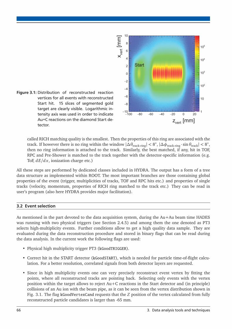
Figure 3.1: Distribution of reconstructed reactionvertices for all events with reconstructedStart hit. 15 slices of segmented goldtarget are clearly visible. Logarithmic in-tensity axis was used in order to indicateAu+C reactions on the diamond Start de-tector.

[mm]vertz100− 80− 60− 40− 20− 0 20

[mm

]ve

rtx

10−

8−

6−

4−

2−

0

2

4

6

8

10

1

10

210

310

410

510

Start

called RICH matching quality is the smallest. Then the properties of this ring are associated with thetrack. If however there is no ring within the window |Δθtrack-ring|< 8◦, |Δφtrack-ring · sinθtrack|< 8◦,then no ring information is attached to the track. Similarly, the best matched, if any, hit in TOF,RPC and Pre-Shower is matched to the track together with the detector-specific information (e.g.ToF, dE/d x , ionization charge etc.)

All these steps are performed by dedicated classes included in HYDRA. The output has a form of a treedata structure as implemented within ROOT. The most important branches are those containing globalproperties of the event (trigger, multiplicities of tracks, TOF and RPC hits etc.) and properties of singletracks (velocity, momentum, properties of RICH ring matched to the track etc.) They can be read inuser’s program (also here HYDRA provides major facilitation).

3.2 Event selection

As mentioned in the part devoted to the data acquisition system, during the Au+Au beam time HADESwas running with two physical triggers (see Section 2.4.5) and among them the one denoted as PT3selects high-multiplicity events. Further conditions allow to get a high quality data sample. They areevaluated during the data reconstruction procedure and stored in binary flags that can be read duringthe data analysis. In the current work the following flags are used:

• Physical high multiplicity trigger PT3 (kGoodTRIGGER).

• Correct hit in the START detector (kGoodSTART), which is needed for particle time-of-flight calcu-lation. For a better resolution, correlated signals from both detector layers are requested.

• Since in high multiplicity events one can very precisely reconstruct event vertex by fitting thepoints, where all reconstructed tracks are pointing back. Selecting only events with the vertexposition within the target allows to reject Au+C reactions in the Start detector and (in principle)collisions of an Au ion with the beam pipe, as it can be seen from the vertex distribution shown inFig. 3.1. The flag kGoodVertexCand requests that the Z position of the vertex calculated from fullyreconstructed particle candidates is larger than -65 mm.

66 3. Data analysis tools and techniques

It is possible, that particles from more than one nuclear reaction are registered within the time windowsettled for the data acquisition. Such overlapping or pile-up events have to be removed since they lead towrong estimation of reaction centrality and other event characteristics. The conditions to reject pile-upevents are [103]:

• Reconstructed START hit object exists and has no second cluster (kNoPileUpSTART).

• No VETO hit within ±15 ns from the START time (kNoVETO).

• Exclusion of events, where a later START hit was found within the range 15-350 ns, that has nocorrelated VETO hit in the window ±2 ns (kGoodSTARTVETO).

• Exclusion of events, where a later START hit was found within the range 80-350 ns, that is corre-lated to more than four META hits inside the time window of 7±5 ns. The offset of 7 ns correspondsto the fastest particles (kGoodSTARTMETA).

Fig. 3.4 shows the numbers of events after applying each selection condition.During the data acquisition it occurred from time to time, that one or more gas chambers (MDC

modules or RICH MWPC) suffered from trips. The affected detector gets then inefficient for a certaintime. Moreover, in the case of MDC this inefficiency depends on the type of the particle and its velocity:it will be larger for minimum ionizing particles and smaller for highly ionizing ones. The MDC sector 2(azimuth angle φ ∈ (240◦ −300◦)) remained inactive during the most of the beam-time. This issues canhardly be handled in the analysis, if problematic sectors are not removed from the data sample. Sincethe usual time needed to fully recover MDC’s from trips was of the order of few minutes, it was decidedto remove problematic sectors for each separate run (typically 2-3 minutes). In order to quantify loses,for each sector the number of reconstructed charged pions and RICH rings has been plotted as a functionof time-ordered runs. Then for runs, when any of the numbers is much away from its the average (3σ),the corresponding sector is marked as useless for hadron (number of pions) or lepton (number of rings)analysis. Examples of time trends of both quantities are given in Fig. 3.2. In the upper panel, showingthe number of pions, one can see attempts to maintain the high voltage of MDC sector 2 on. For detailssee [104].

Missing sectors change the geometrical acceptance of the spectrometer. This is a problem, when spec-tra are going to be compared with the model or reference from elementary reactions. Even apart fromthat, the spectra from Au+Au should be presented in a unified acceptance. This can be achieved eitherby analyzing only runs, in which five sectors were active (besides sector 2), or by taking into accountalso runs with smaller number of sectors and correcting them for the relative loss in the acceptance, asit will be discussed in Section 4.6. It is also discussed there, that it makes no sense to include in theanalysis runs with three or less active sectors. Hence in the Fig. 3.4 numbers of events with at least fourand at least five sectors are plotted. It can be inferred, that the events with less than four sectors usefulfor lepton analysis are roughly 10% of selected events, what corresponds on average to 3 days of thebeam-time. Events with less than five sectors are 42%, what corresponds to 13 days. Only in 8.5% ofselected events (2.5 days) all 6 sectors were available.

3.3 Centrality selection

In order to study system-size dependence of the results, centrality selection of the events, based on theGlauber Monte Carlo simulation is used in HADES (see B. Kardan [105]). The mean value of the num-ber of charged particles produced in a collision Nch is assumed to be directly proportional to number ofnucleons participating in the interaction Npart: Nmean

ch = μNpart with fluctuations given by the Gaussiandistribution of the width σ = k

�Nmean

ch . The minimization procedure is used to fit the generated distri-bution of Nch to the experimentally measured distribution of the number of tracks in MDC Ntrack or ofhits in TOF and RPC Nhits in order to extract values of the free parameters μ and k. This allows to relate

3.3. Centrality selection 67

Figure 3.2.: Number of charged pions (upper panel) and RICH rings (lower panel) reconstructed per eventin each sector of HADES, during a one day of the beam-time. Lines indicate 3σ deviationsfrom corresponding mean values in the given sector. In particular runs, sectors (indicated inthe legend) with the number of pions outside the window are marked as recommended tobe skipped for hadron analysis. For leptons both quantities have to be taken into account.Note, that the X axis is arranged in such a way, that 10000 units correspond to one hourand 100 units correspond to one minute of the beam-time, so 40% of every interval is emptyby construction and this does not indicate any break in beam delivery of break down of thedetection system.


impact parameter b [fm]0 2 4 6 8 10 12 14 16 18 20

/db

[fm]

σd

0

10

20

30

40

50

60

70

80 97 ±> = 92 part0-100% <N

33 ±> = 301 part 0-10 % <N

23 ±> = 212 part10-20 % <N

18 ±> = 148 part20-30 % <N

15 ±> = 102 part30-40 % <N

Figure 3.3.: Impact parameter (left panel) and number of participants (right panel) distributions inHADES corresponding to the selected centrality bins of constant width (10%). Note thatin the legends widths of the number of participant distributions are given and not systematicuncertainties of the mean.

Class ⟨Ndatapart ⟩ b [fm] NMETA,cut

low NMETA,cuthigh bin in Fig. 3.4

0-10% 301.1 ± 11.2 0.00-4.60 ≥ 160 < 250 mult bin 410-20% 211.8 ± 10.1 4.60-6.50 ≥ 121 < 160 mult bin 320-30% 148.5 ± 7.8 6.50-7.95 ≥ 88 < 121 mult bin 230-40% 101.7 ± 6.3 7.95-9.18 ≥ 60 < 88 mult bin 10-40% 190.9 ± 8.7 0.00-9.18 ≥ 60 < 250

Table 3.1.: HADES centrality classes defined by numbers of hits in TOF and RPC.

event classes defined in terms of Ntrack or Nhits to the corresponding average impact parameter ⟨b⟩ ornumber of participants ⟨Npart⟩ as shown in Fig. 3.3 and in Table 3.1.

In the experimental data, the definitions of the centrality classes are based on the total number ofMETA hits within t < 35 ns for TOF and t < 25 ns for RPC. Using number of META hits instead of MDCtracks to estimate the centrality is much more robust, as it is not influenced by transient inefficienciesof gas chambers. Simulated UrQMD events can be distributed into centrality classes defined directly bythe event impact parameter b. At the time of completing this part of work, the number of META hitsin simulation was by roughly 20% higher in simulation than in experiment. This was due to usage ofGHEISHA hadronic interaction model in GEANT, which is not optimized for low-energy experiments.Therefore, the centrality classes derived from the Glauber fit to experimental data were not applicableto the simulation and the selection based on the impact parameter was prefered in this case. Later,change to the GCALOR model resulted in an agreement better than few percent. The centrality classesare summarized in Table 3.1.

Here ⟨Ndatapart ⟩ denotes an average number of participants, ⟨b⟩ is the impact parameter, NMETA,cut

low and

NMETA,cuthigh are minimum and maximum numbers of META hits in a particular centrality class.

Numbers of events after each selection condition discussed above and within all centrality bins areshown in Fig. 3.4. The total number of selected events is around 2.9 · 109.

3.4. Track pre-selection and sorting 69

Figure 3.4.: Number of events after each subsequent event selection condition separated into the mul-tiplicity classes. mult bin 0 denotes an overflow bin, i.e. events with 140 or more particlecandidates. Multiplicity underflow contains events with less than 17 candidates.

3.4 Track pre-selection and sorting

In the output of the DST production many combinations of the same track segments and RICH andMETA hits are contained. In the analysis to each track maximum one RICH ring can be attached andup to 3 hits in each of META detectors. However, RICH rings and META hits can be shared between inprinciple unlimited number of tracks. Also joining inner and outer track segments produces a number ofcombinations and a particular segment is shared among many track candidates. This however increasescombinatorics which must be reduced. Ideally, only one pair of inner and outer segment, one clusterof hits in any of the time-of-flight detectors and possibly one RICH ring and one Pre-Shower hit shouldcorrespond to one electron. Moreover the ring and hits in META detectors should be used exclusivelyby this particle. Exceptions could be very close pairs of particles (two particles produced together in adecay with a very small opening angle), which may produce overlapping RICH rings and inner trackssegments, which cannot be resolved and only one segment/ring is reconstructed. Also, if two particleshit the same cell of one of time-of-flight detectors, only one hit will be detected and reconstructed (timeand position information will correspond to the faster particle). There is in fact no good way, to handlethis exceptional situations, however they are anyway very seldom compared to wrong combinations.And this main issue is solved by track sorting.

Track sorting is an algorithm, which loops over all track candidates in a given event. If it finds severaltracks sharing the same component (track segment, detector hit...) values of a parameter quantifyingtheir quality are compared among them. Possible quality parameters are the product of the χ2

RK of theRunge-Kutta fitting and the distance between the track extrapolated to the plane of a META detector and


q/|q| [MeV/c]×p-1000 -500 0 500 1000

β

0.85

0.9

0.95

1

1.05

1.1

1.15

1

10

210

310

410

510

Pre-selected, system 0

-π +

π

-e +e

q/|q| [MeV/c]×p-1000 -500 0 500 1000

β

0.85

0.9

0.95

1

1.05

1.1

1.15

1

10

210

310

410

Pre-selected, system 1

-e

-π

+π

+e

Figure 3.5.: Velocity of the particle vs. its momentum times charge for the two HADES sub-systems sep-arately for pre-selected particles after the track sorting. System 0 denotes the particles withtime-of-flight measurement derived from the RPC detector, system 1 - from the TOF scintilla-tor wall.

the reconstructed hit position (in mm): χ2RK × dtrack-META or just the χ2

RK. The analysis discussed in [106]shows, that there is no significant difference between final results obtained using either of the two andin the current analysis χ2

RK is used. Only the track candidate with the smallest χ2RK is then marked to be

used in the further analysis.In general, one expects, that electron tracks have worse quality parameter than protons or pions, be-

cause of their on average smaller momentum which induces more multiple scattering and are strongerbent in the magnetic field. If they share e.g. the same hit in one of META detectors, then the electronwill be removed from the data sample. To minimize the probability of such a situation, one may requestcertain preconditions before the track sorting. This means, that only those tracks, for which the condi-tions are fulfilled are considered by the sorter and only sharing track segments or detector hits betweenthem is taken into account. This leads to an idea of including in these preconditions loose identificationcuts and minimum quality requirements. The conditions used in the current analysis are as follows:

1. Quality requirements:

• Track is not marked as a fake by the track finding procedure.

• Track has been constructed from fitted track segments and the outer segment matches to a hitin any META detector, Runge-Kutta fit converged.

• χ2RK < 500.

• META hit is within the cell pointed by the track.

• The distance between the track and META hit in the direction along the META cell is smallerthan 3σ.

2. Loose identification cuts for electrons:

• Track has matched RICH ring (|Δθtrack-ring|< 8◦, |Δφtrack-ring · sinθtrack|< 8◦).• β > 0.9.

• p > 100 MeV/c and p < 1000 MeV/c.

There are two types of fake tracks [107]. One are those containing a track segment that shares firedwires (at least 4) with another segment. In this case the segment that has less shared wires, or smaller

3.4. Track pre-selection and sorting 71

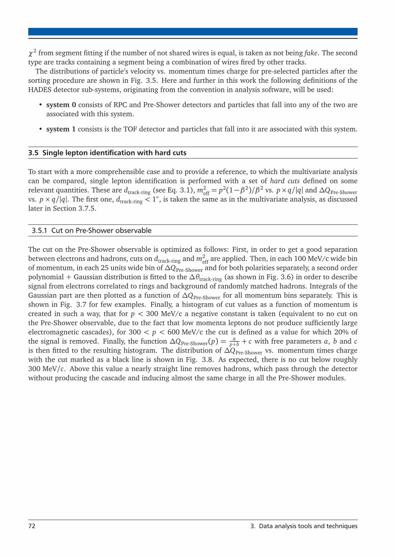
χ2 from segment fitting if the number of not shared wires is equal, is taken as not being fake. The secondtype are tracks containing a segment being a combination of wires fired by other tracks.

The distributions of particle’s velocity vs. momentum times charge for pre-selected particles after thesorting procedure are shown in Fig. 3.5. Here and further in this work the following definitions of theHADES detector sub-systems, originating from the convention in analysis software, will be used:

• system 0 consists of RPC and Pre-Shower detectors and particles that fall into any of the two areassociated with this system.

• system 1 consists is the TOF detector and particles that fall into it are associated with this system.

3.5 Single lepton identification with hard cuts

To start with a more comprehensible case and to provide a reference, to which the multivariate analysiscan be compared, single lepton identification is performed with a set of hard cuts defined on somerelevant quantities. These are dtrack-ring (see Eq. 3.1), m2

eff = p2(1−β2)/β2 vs. p×q/|q| and ΔQPre-Showervs. p× q/|q|. The first one, dtrack-ring < 1◦, is taken the same as in the multivariate analysis, as discussedlater in Section 3.7.5.

3.5.1 Cut on Pre-Shower observable

The cut on the Pre-Shower observable is optimized as follows: First, in order to get a good separationbetween electrons and hadrons, cuts on dtrack-ring and m2

eff are applied. Then, in each 100 MeV/c wide binof momentum, in each 25 units wide bin ofΔQPre-Shower and for both polarities separately, a second orderpolynomial + Gaussian distribution is fitted to the Δθtrack-ring (as shown in Fig. 3.6) in order to describesignal from electrons correlated to rings and background of randomly matched hadrons. Integrals of theGaussian part are then plotted as a function of ΔQPre-Shower for all momentum bins separately. This isshown in Fig. 3.7 for few examples. Finally, a histogram of cut values as a function of momentum iscreated in such a way, that for p < 300 MeV/c a negative constant is taken (equivalent to no cut onthe Pre-Shower observable, due to the fact that low momenta leptons do not produce sufficiently largeelectromagnetic cascades), for 300 < p < 600 MeV/c the cut is defined as a value for which 20% ofthe signal is removed. Finally, the function ΔQPre-Shower(p) =

ap+b + c with free parameters a, b and c

is then fitted to the resulting histogram. The distribution of ΔQPre-Shower vs. momentum times chargewith the cut marked as a black line is shown in Fig. 3.8. As expected, there is no cut below roughly300 MeV/c. Above this value a nearly straight line removes hadrons, which pass through the detectorwithout producing the cascade and inducing almost the same charge in all the Pre-Shower modules.


Figure 3.6.:Matching between a track and a RICH ring in the θ angle vs. Pre-ShowerΔQPre-Shower observ-able for a selected momentum bin and projections of Δθ in several narrow bins of ΔQ. Inthe projections, fits of polynomial + Gaussian distributions are indicated with red curves. Theshift of the maximum position from 0 is due to RICH misalignment for which a correction wasintroduced later.

3.5. Single lepton identification with hard cuts 73

Figure 3.7.: Integrals of the whole distributions (black) and the Gaussian part (red) of the fits from Fig.3.6, plotted as a function of the Pre-Shower observable ΔQPre-Shower = QPost I +QPost II −QPrefor a fewmomentum bins. Bottom right: the construction of theΔQPre-Shower vs. momentumcut: In the momentum range denoted by (a) the cut value corresponding to removal of 20%of the signal is marked. In the area (b), a constant valueΔQ = 100 is taken, in (c) it is a largenegative value. To the resulting histogram the functionΔQ(p) = a

p+b + c is fitted.

q/|q| [MeV/c]×p-1000 -500 0 500 1000

[a.u

.]P

re-S

how

erQ

Δ

-400

-200

0

200

400

600

800

1000

1

10

210

310

410

Figure 3.8:ΔQPre-Shower as a function ofparticle’s momentum for twopolarities separately. The cuton the observable is indicatedby the black curve. Entriesabove the curve are accepted,below are rejected. For bettervisibility, distribution is madeafter applying cuts on dtrack-ringand m2

eff.


3.5.2 Cut on effective mass

The final cut on m2eff is optimized in such a way, that in 100 MeV/c wide momentum bins a distribution

of two Gaussians (for electrons and pions peaks) + fourth order polynomial (for other componentsof underlying background) is fitted to the m2

eff. A few examples of the fit are shown in Fig. 3.9 (fornegatively charged particles). Then the cut is defined as melectron+4σelectron based on the mean melectron

Figure 3.9.: Effective mass distributions of particles for a few selected momentum bins. Out of the poly-nomial + two Gaussians function fitted to the distributions, both Gaussian parts are plotted.It should be noted, that for the momentum high enough, the two peaks overlaps and, con-sequently, there is no good separation anymore. For this region the constant value of the cutis chosen, as shown in Fig. 3.10.

and with the width σelectron of the Gaussian part fitted to the electrons’ peak or the cut value fixd tom2

eff = 10000 MeV2/c4 (meff = 100 MeV/c2) at higher momentum, where one cannot resolve betweenelectrons’ and pions’ peaks. The resulting cut is shown in Fig. 3.10. Final distributions of velocityvs. momentum for identified particles are shown in Fig. 3.11 and projections on the momentum afterapplying subsequent identification cuts in Fig. 3.12.

3.5. Single lepton identification with hard cuts 75

q/|q| [MeV/c]×p-1000 -500 0 500 1000

]4/c2

[MeV

2 eff

m

-20000

-10000

0

10000

20000

30000

40000

50000

1

10

210

310

410

510

system 0

+e-e

-π +

π

q/|q| [MeV/c]×p-1000 -500 0 500 1000

]4/c2

[MeV

2 eff

m

-20000

-10000

0

10000

20000

30000

40000

50000

1

10

210

310

410

510

system 1

+e-e

+π

-π

Figure 3.10.: Effective mass of the particle vs. its momentum times charge for the two systems separately.Momentum-dependent cut on the mass is indicated with the black curve. For better visibil-ity, the distribution is plotted after applying cuts on dtrack-ring andΔQPre-Shower, as explainedbefore, but no cut on β .

q/|q| [MeV/c]×p-1000 -500 0 500 1000

β

0.85

0.9

0.95

1

1.05

1.1

1.15

1

10

210

310

410

system 0

q/|q| [MeV/c]×p-1000 -500 0 500 1000

β

0.85

0.9

0.95

1

1.05

1.1

1.15

1

10

210

310

410

system 1

Figure 3.11.: Velocity of the particle vs. its momentum times charge for two systems separately for lep-tons identified with the hard cut method.


q/|q| [MeV/c]×p-1000 -500 0 500 1000

210

310

410

510

610

710

System 0 Pre-selected

cuttrack-ring

d

cutsShQΔ, track-ringd

cutseff2, m

ShQΔ,

track-ringd

q/|q| [MeV/c]×p-1000 -500 0 500 1000

210

310

410

510

610

710


cuttrack-ringd

cutseff2, mtrack-ringd

Figure 3.12.:Momentum distributions of leptons candidates after each subsequent hard identificationcuts.

3.6 Multilayer perceptrons

Feed-forward multilayer perceptron (MLP) is a type of an artificial neural network and an example oftechniques of multivariate analysis (MVA). It allows to make a single decision based on values of a num-ber of quantities. The key advantage is, that all the quantities and correlations between them are takeninto account at the same time, which allows for the most careful and the fairest possible discriminationof underlying events. For example, when considering all discriminating quantities separately, a partic-ular event can be rejected if one of quantities lies just below the threshold for it, even though all theother quantities are well above respective thresholds. Similarly, an event might be accepted, even whenit should be rejected when taking into account all the quantities at the same time.

Mathematically, MLP is nothing else than a function y : �n → [0,1]. Applying a conditiony(x1, ..., xn) = const defines an (n− 1)-dimensional surface in the n-dimensional space of input quanti-ties x1, ..., xn (one may compare it to a surface of total energy conservation E = const in a phase spaceof many bodies, however in the case of neural networks the surface usually will not be closed). Pointsin the space, simultaneous measurements of all the quantities for single events, will be located on an

Figure 3.13: An example scheme of multi-layer perceptron.

3.6. Multilayer perceptrons 77

either side of the surface and this will allow to discriminate them. The condition y(x1, ..., xn) = c, for cbetween 0 and 1, will then define the surface which divides the space into points to be accepted (withy(x1, ..., xn)> c) or rejected (with y(x1, ..., xn)< c).

Figure 3.14.: The simplest non-trivial MLP. It has two input variables x1 and x2. Two top panels representtwo nodes in the single hidden layer. They calculate sigmoid of different linear combinationsof the input variables. Bottom left panel is the output node which adds the sigmoids up.Computing the activation function of the last sum is skipped and bottom right panel showsjust the decision boundary for a particular value of the output variable.

The mathematical form of the function makes it possible to obtain a very flexible discriminating sur-face. It consists of layers containing nodes (see Fig. 3.13). The minimum number of layers is two: onecontains input quantities x1, ..., xn, the other one - calculated output. It is possible to define arbitrarynumber of additional “hidden” layers with arbitrary number of nodes, performing intermediate steps ofcalculation. Each node in every layer (besides the input one) is connected to all nodes in the precedinglayer and only to them. This means, that the value at a particular node is calculated based only on valuesat nodes, to which it is connected, according to the formula:

x (k)j = A

!w(k)0 j +

Mk−1∑i=1

w(k)i j · x (k−1)i

". (3.2)

Here, (k) or (k− 1) in the superscript denote the layer and j or i in the subscript denote the node in thelayer. Summation runs over all nodes in the preceding layer, w(k)i j are parameters (weights) to be fitted. Ais called activation function. The simplest choice would be a step function, but the sharp threshold can bealso smeared by using e.g. hyperbolic tangent function tanh or sigmoid function A(x) = 1

1+e−x (which is

a Fermi function flipped around the y axis: x →−x). The weights w(k)0 j corresponds to the so-called biasnode. As it can be read off the Eq. 3.2, this is an additional node of each layer, having always the value1 at the input. When the activation function A(x) is the step function, all the other weights define theshape of the hypersurface in the �Mk−1 space of the neuron’s inputs, above which the neuron responds.The weight associated with the bias node shifts the surface with respect to 0. This might be crucial for


the convergence of the neural network optimization procedure. Similar interpretation is valid in case ofa more complicated activation function, only the surface becomes a thicker o thinner skin.

Perceptron or feed-forward network is a neural network in which output from a one node is sent onlyto nodes in the following layer.

It is instructive to examine, how a complicated decision boundary is built up. Fig. 3.14 shows thesimplest non-trivial MLP with two input quantities and one hidden layer. Two top panels are sigmoidfunctions at two nodes of the hidden layer: 1/(1+ exp(−x1 + x2)) and 1/(1+ exp(−4x1 − x2)). Bottomleft panel shows a sum of the two, which would be calculated in the output node with both weightsequal 1. The step of calculating sigmoid of this sum is here skipped, thus the output value ranges from0 to 2 and not to 1. Then bottom right panel shows the decision boundary for the value y(x1, x2) = 1.2.

Finding optimal values of weights w(k)i j , often called training or learning, is a minimization problem.One prepares a sample of events, which certainly should be accepted and of those, which certainlyshould be rejected. Having in mind an application of the MLP in physics, one can call them signal andbackground samples. Then a loss function is defined, which describes a performance of the perceptronon the training data. Usually the cross-entropy function is taken:

L(w) =events∑

i

�y (i) ln

�y�x(i),w

��+�1− y (i)

�ln�1− y

�x(i),w

��,

where y�x(i),w

�is the response of the MLP to the training event x(i) with weights w, y (i) is 1 for signal

events and 0 for background. One can start with random weights and search for the minimum of the lossfunction iteratively by calculating gradients of it with respect to weights and tuning them to get lowervalue of L(w).

3.7 Application of MLP for lepton identification

In the present work MLP was used to identify single e+/e− tracks present in the large background ofhadrons. The implementation used was the one included in the Toolkit for Multivariate Data Analysis(TMVA [108]), which is currently fully integrated into the ROOT Object Oriented Data Analysis Frame-work - a base for almost all the software used in HADES data analysis. One argument for choosing thisimplementation was thus its availability and possibility to easily and clean merge it with all programsused. Another reason was the existing in the working group experience from using this implementationin previous experiments.

3.7.1 Training sample

In order to find optimal definitions of signal and background samples, the following possibilities werecompared:

1. Tracks from real data, selected based on dtrack-ring, Eq. 3.1,

2. Simulated tracks selected based on dtrack-ring,

3. Simulated tracks selected based on the identity information propagated from the event generator.

Potentially the purest way of defining signal and background sample for training of MLP would beusing a Monte Carlo simulation. There it can be checked, which tracks are leptons and which hadrons.However, this is not optimal for particle identification in the real data if all the characteristics of particletracks are not perfectly reproduced in simulation. Then the second best possibility is to select fromdata lepton sample as little as possible contaminated by hadrons and treat it as signal and possibly

3.7. Application of MLP for lepton identification 79

q/|q| [MeV/c]×p-1000 -500 0 500 1000

β

0.85

0.9

0.95

1

1.05

1.1

1.15

0

500

1000

1500

2000

2500

system 0, signal

q/|q| [MeV/c]×p-1000 -500 0 500 1000

β

0.85

0.9

0.95

1

1.05

1.1

1.15

0

200

400

600

800

1000

1200

1400

1600

1800

2000

2200

system 1, signal

q/|q| [MeV/c]×p-1000 -500 0 500 1000

β

0.85

0.9

0.95

1

1.05

1.1

1.15

0

200

400

600

800

1000

1200

1400

1600

system 0, background

q/|q| [MeV/c]×p-1000 -500 0 500 1000

β

0.85

0.9

0.95

1

1.05

1.1

1.15

0

200

400

600

800

1000

1200

1400

system 1, background

Figure 3.15.: PID plots of signal and backgroundmodels for theMLP training, defined by the RICHmatch-ing quality cut in real data, in two systems separately.

clean hadron sample as background. In HADES lepton analysis this selection can be done based on theRICH ring-track matching quality 3.1. Fig. 3.25 in Section 3.9.1 shows the difference of the azimuthangle Δφ between lepton candidate track and closest matched RICH ring. From the discussion there,it can be easily concluded, that applying a very tight condition on the angular correlation does noteliminate hadron contribution fully, but at least minimizes it. Conversely, requiring the angle differenceto be larger then a certain value, will eliminate almost fully true correlations and leave only chancecoincidences. Definition of signal and background sample is then as follows:

dtrack-ring < 0.5◦ for signal,

dtrack-ring > 7◦ for background.

Velocity vs. momentum distributions (PID plots) for signal and background sample defined in this wayare shown in Fig. 3.15.

Training on simulated tracks with signal and background defined based on dtrack-ring serves as anintermediate step for comparison with the two other possibilities.


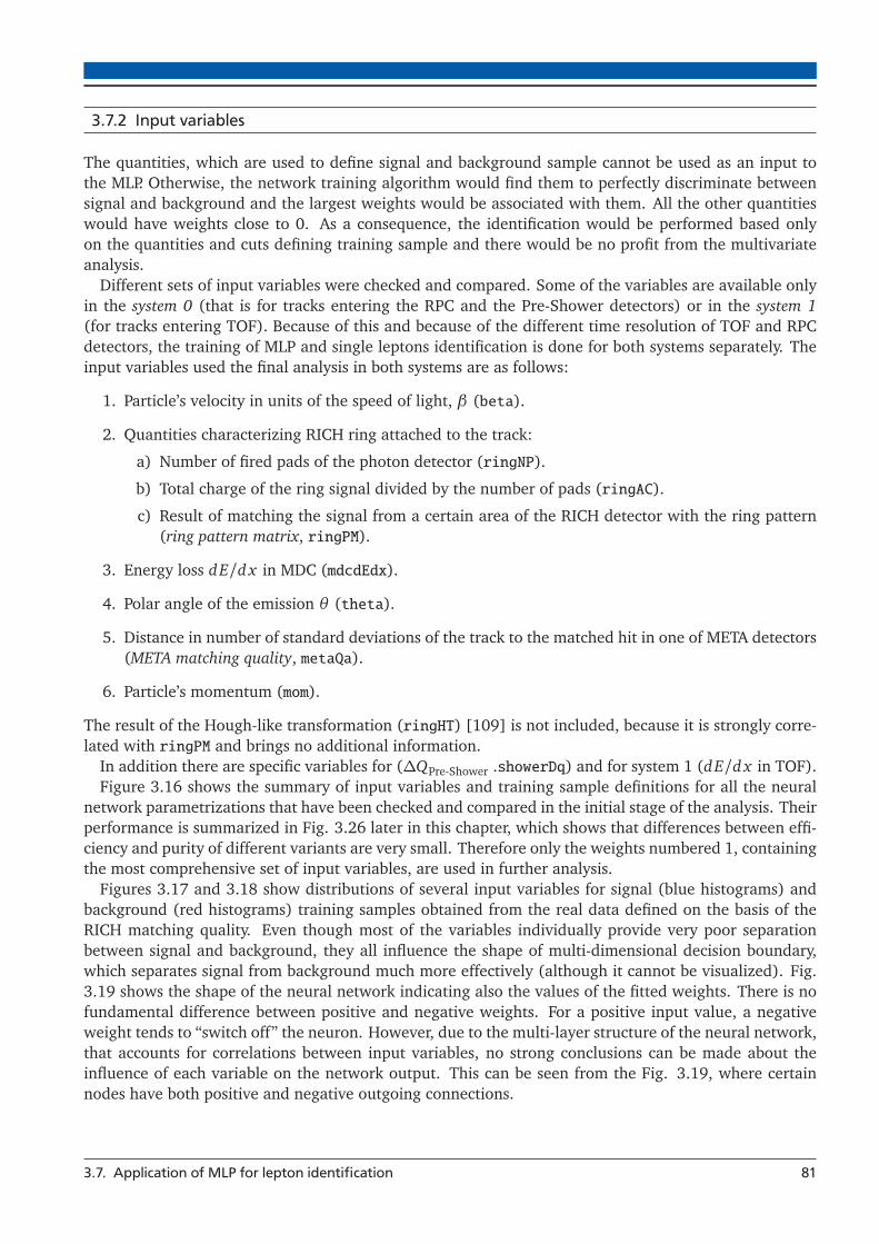
3.7.2 Input variables

The quantities, which are used to define signal and background sample cannot be used as an input tothe MLP. Otherwise, the network training algorithm would find them to perfectly discriminate betweensignal and background and the largest weights would be associated with them. All the other quantitieswould have weights close to 0. As a consequence, the identification would be performed based onlyon the quantities and cuts defining training sample and there would be no profit from the multivariateanalysis.

Different sets of input variables were checked and compared. Some of the variables are available onlyin the system 0 (that is for tracks entering the RPC and the Pre-Shower detectors) or in the system 1(for tracks entering TOF). Because of this and because of the different time resolution of TOF and RPCdetectors, the training of MLP and single leptons identification is done for both systems separately. Theinput variables used the final analysis in both systems are as follows:

1. Particle’s velocity in units of the speed of light, β (beta).

2. Quantities characterizing RICH ring attached to the track:

a) Number of fired pads of the photon detector (ringNP).

b) Total charge of the ring signal divided by the number of pads (ringAC).

c) Result of matching the signal from a certain area of the RICH detector with the ring pattern(ring pattern matrix, ringPM).

3. Energy loss dE/d x in MDC (mdcdEdx).

4. Polar angle of the emission θ (theta).

5. Distance in number of standard deviations of the track to the matched hit in one of META detectors(META matching quality, metaQa).

6. Particle’s momentum (mom).

The result of the Hough-like transformation (ringHT) [109] is not included, because it is strongly corre-lated with ringPM and brings no additional information.

In addition there are specific variables for (ΔQPre-Shower .showerDq) and for system 1 (dE/d x in TOF).Figure 3.16 shows the summary of input variables and training sample definitions for all the neural

network parametrizations that have been checked and compared in the initial stage of the analysis. Theirperformance is summarized in Fig. 3.26 later in this chapter, which shows that differences between effi-ciency and purity of different variants are very small. Therefore only the weights numbered 1, containingthe most comprehensive set of input variables, are used in further analysis.

Figures 3.17 and 3.18 show distributions of several input variables for signal (blue histograms) andbackground (red histograms) training samples obtained from the real data defined on the basis of theRICH matching quality. Even though most of the variables individually provide very poor separationbetween signal and background, they all influence the shape of multi-dimensional decision boundary,which separates signal from background much more effectively (although it cannot be visualized). Fig.3.19 shows the shape of the neural network indicating also the values of the fitted weights. There is nofundamental difference between positive and negative weights. For a positive input value, a negativeweight tends to “switch off” the neuron. However, due to the multi-layer structure of the neural network,that accounts for correlations between input variables, no strong conclusions can be made about theinfluence of each variable on the network output. This can be seen from the Fig. 3.19, where certainnodes have both positive and negative outgoing connections.


weights no. Input variables

trained on ringNP ringAC ringHT ringPM metaQa richQa beta theta mom mdcdEdx tofdEdx showerDq

0 EXP, RICH QA

1 EXP, RICH QA

2 EXP, RICH QA

3 EXP, RICH QA

4 EXP, RICH QA

5 EXP, RICH QA

6 EXP, RICH QA

7 EXP, RICH QA

8 EXP, RICH QA

9 EXP, RICH QA

10 SIM, GEANT PID

11 SIM, GEANT PID

12 SIM, RICH QA

Figure 3.16.: Different sets of input variables and definitions of signal and background sample used inthe neural network training. Green color means that a variable is used in a particular train-ing instance, red that it is not used. Blue in the column corresponding to the momentumof particle indicates that this variable is used in the neural network input only in system 0.Thick outlines indicate the weights, that are chosen to be used in the pair analysis. The mostright column describes signal and background definitions for the training. “EXP” means thatthe network was trained on the experimental data, “SIM” - on simulation. “RICH QA” in-dicates the standard definitions based on the RICH matching quality, “GEAND PID” means,that signal and background samples were selected based on the particle’s type informationtransported from the GEANT analysis level.


ringNP

5 10 15 20 25 30 35 40 45

1.2

/ (1

/N)

dN

0

0.05

0.1

0.15

0.2

0.25SignalBackground

U/O

-flo

w (

S,B

): (

0.0,

0.0

)% /

(0.0

, 0.0

)%

Input variable: ringNP

ringAC

100 200 300 400 500 600

15.2

/

(1/N

) dN

0

0.001

0.002

0.003

0.004

0.005

0.006

0.007

0.008

U/O

-flo

w (

S,B

): (

0.0,

0.0

)% /

(0.0

, 0.0

)%

Input variable: ringAC

metaQa

0.5 1 1.5 2 2.5 3 3.5 4

0.10

2 /

(1/N

) dN

0

0.1

0.2

0.3

0.4

0.5

0.6

0.7

U/O

-flo

w (

S,B

): (

0.0,

0.0

)% /

(0.0

, 0.0

)%

Input variable: metaQa

ringHT100 200 300 400 500 600 700 800

22.4

/

(1/N

) dN

0

0.005

0.01

0.015

0.02

0.025

0.03

0.035

0.04

U/O

-flo

w (

S,B

): (

0.0,

0.0

)% /

(0.1

, 0.0

)%

Input variable: ringHT

beta

0.9 0.92 0.94 0.96 0.98 1 1.02 1.04 1.06 1.08 1.1

0.00

512

/ (1

/N)

dN

0

5

10

15

20

25

30

U/O

-flo

w (

S,B

): (

0.0,

0.0

)% /

(0.0

, 0.0

)%

Input variable: beta

mdcdEdx

1 2 3 4 5 6 7 8 9 10

0.24

2 /

(1/N

) dN

0

0.1

0.2

0.3

0.4

0.5

0.6

0.7

U/O

-flo

w (

S,B

): (

0.0,

0.0

)% /

(0.0

, 0.0

)%

Input variable: mdcdEdx

theta

20 30 40 50 60 70

1.61

/

(1/N

) dN

0

0.01

0.02

0.03

0.04

0.05

U/O

-flo

w (

S,B

): (

0.0,

0.0

)% /

(0.0

, 0.0

)%

Input variable: theta

showerDq

-400 -200 0 200 400 600 800 1000 1200 1400

51.2

/

(1/N

) dN

0

0.001

0.002

0.003

0.004

0.005

0.006

0.007

U/O

-flo

w (

S,B

): (

0.0,

0.0

)% /

(0.0

, 0.0

)%

Input variable: showerDq

mom

100 200 300 400 500 600 700 800 900 1000

24.6

/

(1/N

) dN

0

0.0005

0.001

0.0015

0.002

0.0025

0.003

0.0035

0.004

U/O

-flo

w (

S,B

): (

0.0,

0.0

)% /

(0.0

, 0.0

)%

Input variable: mom

Figure 3.17.: Distributions of all input variables in system 0 for signal (blue histograms) and background(red histograms).

ringNP

5 10 15 20 25 30 35 40 45

1.2

/ (1

/N)

dN

0

0.05

0.1

0.15

0.2

0.25SignalBackground

U/O

-flo

w (

S,B

): (

0.0,

0.0

)% /

(0.0

, 0.0

)%

Input variable: ringNP

ringAC

100 200 300 400 500 600

15.2

/

(1/N

) dN

0

0.001

0.002

0.003

0.004

0.005

0.006

0.007

0.008

U/O

-flo

w (

S,B

): (

0.0,

0.0

)% /

(0.0

, 0.0

)%

Input variable: ringAC

metaQa

0.5 1 1.5 2 2.5 3 3.5 4

0.10

2 /

(1/N

) dN

0

0.1

0.2

0.3

0.4

0.5

0.6

0.7

U/O

-flo

w (

S,B

): (

0.0,

0.0

)% /

(0.0

, 0.0

)%

Input variable: metaQa

ringHT100 200 300 400 500 600 700 800

22.4

/

(1/N

) dN

0

0.005

0.01

0.015

0.02

0.025

0.03

0.035

0.04

U/O

-flo

w (

S,B

): (

0.0,

0.0

)% /

(0.1

, 0.0

)%

Input variable: ringHT

beta

0.9 0.92 0.94 0.96 0.98 1 1.02 1.04 1.06 1.08 1.1

0.00

512

/ (1

/N)

dN

0

5

10

15

20

25

30

U/O

-flo

w (

S,B

): (

0.0,

0.0

)% /

(0.0

, 0.0

)%

Input variable: beta

mdcdEdx

1 2 3 4 5 6 7 8 9 10

0.24

2 /

(1/N

) dN

0

0.1

0.2

0.3

0.4

0.5

0.6

0.7

U/O

-flo

w (

S,B

): (

0.0,

0.0

)% /

(0.0

, 0.0

)%

Input variable: mdcdEdx

theta

20 30 40 50 60 70 80

1.84

/

(1/N

) dN

0

0.005

0.01

0.015

0.02

0.025

0.03

0.035

0.04

U/O

-flo

w (

S,B

): (

0.0,

0.0

)% /

(0.0

, 0.0

)%

Input variable: theta

tofdEdx

1 2 3 4 5 6 7

0.18

2 /

(1/N

) dN

0

0.2

0.4

0.6

0.8

1

1.2

1.4

1.6

1.8

2

2.2

U/O

-flo

w (

S,B

): (

0.0,

0.0

)% /

(0.0

, 0.8

)%

Input variable: tofdEdx

Figure 3.18.: Distributions of all input variables in system 1 for signal and background.


3.7.3 Training procedure

It is a commonly accepted, that details of the neural network architecture do not have big influence onthe results, at least in nuclear and particle physics applications. Therefore, the choice here is to keep thedefault configuration of the TMVA’s MLP training: with 2 hidden layers and N + 1 and N nodes in them,where N is the number of input variables. The activation function is sigmoid, A(x) = 1

1+e−x . The defaultnumber of 500 training cycles was preserved, as a loss function cross-entropy was used, training wasdone with the standard back-propagation method, where updating of weights starts from the output andproceeds towards the input layer. There were roughly 106 training tracks both for signal and backgroundin both systems.

ringNP :

ringAC :

metaQa :

ringHT :

beta :

mdcdEdx :

theta :

showerDq :

mom :

Bias node :Layer 0 Layer 1 Layer 2 Output layer

ringNP :

ringAC :

metaQa :

ringHT :

beta :

mdcdEdx :

theta :

tofdEdx :

Bias node :

Layer 0 Layer 1 Layer 2 Output layer

Figure 3.19.: Architecture of the MLP used in system 0 (left) and system 1 (right). Thickness of each line isproportional to the absolute value of the associated weight. Color corresponds to the valuewith sign: red means large positive, blue large negative, green is close to 0.

3.7.4 Condition on y(x)

q/|q| [MeV/c]×p800− 600− 400− 200− 0 200 400 600 800

)xM

LP y

(

0

0.1

0.2

0.3

0.4

0.5

0.6

0.7

0.8

0.9

1

1

10

210

310

410

510

system 0

q/|q| [MeV/c]×p800− 600− 400− 200− 0 200 400 600 800

)xM

LP y

(

0

0.1

0.2

0.3

0.4

0.5

0.6

0.7

0.8

0.9

1

1

10

210

310

410

510

system 1

Figure 3.20.: Distributions of the quantity y(x) as a function of particle’s momentum times charge (q isthe charge of the particle, so q/|q| is the sign of the charge that is charge). Entries with y(x)close to 1 correspond to signal, those close to 0 are background.

Fig. 3.20 shows the output value y(x) of the MLP for system 0 and 1 for weights number 6, drawnversus momentum times charge of a particle. The separation between signal- and background-like tracksis clearly visible. The shape of the spectrum encourages to define the decision boundary momentum


dependent. One can see, that at low momentum the sample is strongly dominated by leptons and theirdistribution stretches towards the values of y(x) as low as 0.2. This is not the case at higher momentumvalues, where the number of pions and protons is larger and they become predominant at lower y(x). Tomake use of this property of the distribution and make the cut well defined, the sample was divided into100 MeV/c wide momentum bins (separately for both systems and for positive and negative particles).In each bin a high order polynomial was fitted to the y(x) distribution in order to make it easier tofind its minimum. In the analysis, the value of the cut on y(x) for a particular momentum is found asa linear interpolation between locations of minima in two nearest bins. The resulting lines of cuts arealso shown in Fig. 3.20 and of β vs. momentum×charge after this cut in Fig .3.21. The resulting β vs.momentum×charge distributions obtained after this cut are shown in Fig .3.21.

q/|q| [MeV/c]×p-1000 -500 0 500 1000

β

0.85

0.9

0.95

1

1.05

1.1

1.15

1

10

210

310

410

MLP cut, system 0

q/|q| [MeV/c]×p-1000 -500 0 500 1000

β

0.85

0.9

0.95

1

1.05

1.1

1.15

1

10

210

310

410

510

MLP cut, system 1

Figure 3.21.: Resulting distributions of particle’s velocity versus momentum times charge (PID plots) afterapplying the cut on y(x).

3.7.5 Additional cut on dtrack-ring

The quantity dtrack-ring (Eq. 3.1), used to define signal and background training samples for MLP cannotbe used as an input variable. Nothing prevents however from cutting on it additionally to the cut ony(x). The precise definition of the cut is again a matter of discussion. As can be seen from Fig. 3.25 inSec. 3.9.1, the signal, which would remain after subtracting background of randomly matched hadrons,at low momenta has broad tails under a narrow peak. There is a variety of phenomena, which contributeto this effect. One of them comes from e+e− pairs with relatively small opening angle. Because of thelow efficiency of the RICH detector, it is possible, that the ring created by a particular lepton will not befound and the nearest matched ring will be the one created by the partner lepton. Another possibilityare so called corona rings. It may happen, that the ring created by a lepton will not be found, but anotherring will be reconstructed from a few pads of the original one and some pad(s) fired nearby due to noiseor a direct hit of a particle or photon on the detector. Matching quality dtrack-ring for such a ring mightbe up to about 8 degree (twice the typical radius of a ring), but still might be a good signature, that thetrack of interest was lepton.

Both cases, together with the shape of the dtrack-ring vs. momentum distribution, shown in Fig. 3.22,suggest that the best decision would be a momentum-dependent graphical cut on dtrack-ring, wide at lowand strict at higher momenta. However, it turns out, that the narrow cut, independent of the momentum,works better with respect to the combinatorial background suppression. This is due to the fact, that theefficiency for lepton reconstruction and identification is rather low and clearly lower than 50%. Thismeans, that in most cases only one lepton from a particular pair will be identified. If there is a lepton


q/|q| [MeV/c]×p-1000 -500 0 500 1000

[deg

]tr

ack-

ring

d

0

1

2

3

4

5

6

7

8

9

10

1

10

210

310

410

system 0

q/|q| [MeV/c]×p-1000 -500 0 500 1000

[deg

]tr

ack-

ring

d

0

1

2

3

4

5

6

7

8

9

10

1

10

210

310

410

510

system 1

Figure 3.22.:Matching of the track to the ring as a function of particle’s momentum times charge afterapplying the cut on the MLP response.

q/|q| [MeV/c]×p-1000 -500 0 500 1000

β

0.85

0.9

0.95

1

1.05

1.1

1.15

1

10

210

310

410

cuts, system 0track-ringMLP and d

q/|q| [MeV/c]×p-1000 -500 0 500 1000

β

0.8

0.85

0.9

0.95

1

1.05

1.1

1.15

1.2

1

10

210

310

410

510 cut, system 1track-ringMLP and d

Figure 3.23.: PID plots after applying the cuts on y(x) and on dtrack-ring

found with low momentum and a high dtrack-ring value, its partner from a small opening angle pair ismost probably not reconstructed. The found lepton can be therefore safely rejected. The cut was chosento be dtrack-ring < 1◦ and this was validated by the study presented in Section 3.9.3 (Fig. 3.27).

Distributions of β versus p × q/|q| for the identified lepton sample after applying both cuts are pre-sented in Fig. 3.23 and momentum distributions after each subsequent cut in Fig. 3.24.

3.8 Cut on the angle to nearest neighbor track candidate αCP

Similar like in previous experiments, a cut to lepton’s nearest neighbor is applied also in this analysis. Thepurpose of this cut is to reduce combinatorial background rather than to improve lepton identification.However, this cut is made for every single lepton and also it enters the calculation of efficiency matricespresented in the next chapter. Therefore the cut is discussed here.

In previous experiments the analysis was based on quantities, which is also currently available in thedata set: angle to nearest segment fitted and angle to nearest segment non-fitted. The segments are the innersegments of MDC tracks, fitted means that the inner segment could be matched to an outer segment. In


q/|q| [MeV/c]×p-1000 -500 0 500 1000

210

310

410

510

610

710


MLP cut

cutstrack-ring

MLP and d

q/|q| [MeV/c]×p-1000 -500 0 500 1000

210

310

410

510

610

710


MLP cut

cutstrack-ring

MLP and d

Figure 3.24.: Distributions of p × q/|q| for lepton candidates sample after pre-selection and subsequentidentification cuts.

the Au+Au analysis, non-fitted segments are not relevant, because almost all segments can find a matchdue to large track multiplicity.

These two quantities try to assign a possible lepton identity to the found nearest segments. If thenearest neighbor is predicted not to be lepton, then the opening angle to the reference track is multipliedby -1 and the negative angle is stored in the data set for the primary track. However, the prediction isbased only on the matching to a RICH ring. If tight matching is requested for the reference lepton track,then the nearest neighbor segment will probably be matched to the same ring, given high track densityin Au+Au.

To improve the situation, in this analysis, the nearest neighbor is sought manually and the openingangle is multiplied by -1 if no ring was matched to the neighbor or it’s dE

d x (MDC)> 3. Then the referencetracks for which angle to the nearest neighbor lie between 0 and a certain cut value are removed. InSection 3.9.3 results of the two cut values are compared in terms of invariant mass signal, signal-to-background ratio and significance to provide an ultimate benchmark.

3.9 Evaluation of the signal purity

3.9.1 Rotated RICH technique

One of the factors that has to be taken into account when comparing different lepton identificationtechniques is the purity of the obtained sample. Misidentified particles of other types present in thesample after all identification cuts must be treated as a background which should be considered. Theirrelative contribution can be estimated based on the Monte Carlo simulation using the information aboutparticle’s true identity obtained from the event generator. The results yielded by this method are howeverfar from being realistic as long as particle distributions and detector responses are not in a very goodagreement with the data.

An alternative approach is fully based on experimental data and exploits the sixfold symmetry ofthe HADES acceptance with respect to rotations by azimuth angle φ. Since wrongly identified leptonsare those particles, which are only by chance matched to RICH rings, one can statistically reproducethe contribution of such mismatched tracks. This is done by adding 60◦ to azimuth positions of thereconstructed rings and then running the usual track-ring matching algorithm. In this way, rings arevirtually moved to the neighboring sector and it is impossible to match track and ring left in the detector

3.9. Evaluation of the signal purity 87

Figure 3.25: The principle of the rotating RICH tech-nique. The green distribution is one ofthe components of the RICH matchingquality (Eq. 3.1) for original data. Theorange one is the distribution from datawith RICH rings moved to the neighbor-ing sector. Dashed area is the signalresulting from the difference of thosetwo. In order to make the backgroundbetter visible in this plot, no lepton iden-tification cuts were applied.

by the same real lepton. Thus the procedure yields only accidental matches and the assumption is, thatthe number of them will be the same, as when the matching procedure is applied to the original data,without rotated RICH rings. The data prepared in such a way can then be analyzed in order to estimate,how many of mismatched tracks remain after identification cuts.

As it can be seen from Fig. 3.25, data with rotated RICH reproduces very well the background lyingunder the signal of lepton tracks correlated to RICH rings and this technique can be used to estimatedthe purity of the final lepton sample or at least to decide, which of the compared identification methodsprovides the best purity.

3.9.2 Comparison between hard cut and multivariate analyses

The most decisive criteria when comparing two ways of identifying particles is to evaluate efficiency andpurity. Efficiency is the ratio of particles of interest, which survive identification cuts, purity quantifiesthe contamination from misidentified particles: it is a ratio of those correctly identified to all identified.One can compare efficiency values relatively between two methods just by comparing two particle yields,while purity values can be calculated using RICH rotating technique.

Comparison of integrated yields and average purity values for all tested considered ways of neuralnetwork training and for hard cut analysis is shown in Fig. 3.26 for both systems separately. There isno big difference between all the types of the neural network. The hard cut analysis provides slightlylower yield (i.e. lower efficiency) together with the purity comparable to the one obtained with themultivariate analysis. For the further analysis, weights 1 were chosen.

3.9.3 Comparison of pair spectra

Fig. 3.27 shows dilepton pair signal (S), signal-to-background ratio (S/B) and significance (Sgn= S�S+B

)for different cuts on y(x) and on dtrack-ring. For the case when the cut on dtrack-ring was momentum-dependent (graphical cut), it was designed to keep the purity constant as a function of momentum. Twodifferent values of the cut on angle to nearest neighbor are tested in Fig. 3.28. They show that thebest combination concerning signal-to-background ratio and significance is momentum-dependent cuton y(x), dtrack-ring < 1◦ and αCP > 4◦ and it is used in the subsequent analysis. Details on the subtraction


Purity [%]98 98.5 99 99.5 100

Yie

ld

820

840

860

880

900

920

310×

Weights 0Weights 1Weights 2Weights 3Weights 4Weights 5Weights 6Weights 7Weights 8Weights 9Weights 10Weights 11Weights 12Hard cuts

System 0

Purity [%]99.2 99.4 99.6 99.8 100 100.2

Yie

ld

1500

1600

1700

1800

1900

310×

Weights 0Weights 1Weights 2Weights 3Weights 4Weights 5Weights 6Weights 7Weights 8Weights 9Weights 10Weights 11Weights 12Hard cuts

System 1

Figure 3.26.: Integrated yield and average purity in the momentum range p ∈ (400− 500) [MeV/c] ob-tained from multivariate analyses with different sets of input variables and definitions ofsignal and background models as well as from hard cut analysis. Numbering of weights isaccording to Fig. 3.16.

of the combinatorial background and signal extraction are given in Chapter 5.Numbers of events with given electrons and positrons multiplicities are shown in Fig. 3.29 for the case

of only particle identification applied (left panel) and after applying in addition close pair rejection cutsdiscussed above. In both cases only events with at least two leptons (i.e. the events which contribute tothe pair spectra) are plotted for better visibility. Plots of this type have to be carefully interpreted. Onecould for example argue, that if they are not symmetric about the diagonal, this indicates the presenceof hadron contamination (in fact in the present analysis the distributions are reasonably symmetric, es-pecially after close pair cuts). It has been however checked with the Monte Carlo simulation, that this isjust an effect of different acceptance and efficiency for e+ and e−, this is also confirmed by Fig. 5.5. Simi-larly, one could expect, that after close pair cuts the distribution would become more concentrated aboutthe diagonal (i.e. have higher correlation coefficient) as on average more background (represented bylike-sign pairs – off-diagonal) should be removed than the signal (represented by the opposite-sign pairs,close to diagonal). This is in fact not the case in the current analysis. This comes from the constructionof the close pair rejection procedure – it is the cut on the opening angle between two well reconstructedunlike-sign leptons, which are identified as converted photon. Removing them reduces number of eventsat the diagonal. The signal-to-background ratio averaged over the whole dilepton invariant mass range isindeed reduced because pairs of very small opening angle, where the signal-to-background ratio is veryhigh, are removed. Nevertheless, his brings a gain in the higher invariant mass range. Plots of the typeas in Fig. 3.29 do not contain this information.


]2 [GeV/ceeM0 0.1 0.2 0.3 0.4 0.5 0.6 0.7 0.8

]-1 )2

[(G

eV/c

ee d

N/d

M0

π1/

N

9−10

8−10

7−10

6−10

5−10

4−10

Signal

]2 [GeV/ceeM0 0.1 0.2 0.3 0.4 0.5 0.6 0.7 0.8

CB

/ N

Sig

N

2−10

1−10

1

10

Signal-to-background

]2 [GeV/ceeM0 0.1 0.2 0.3 0.4 0.5 0.6 0.7 0.8

CB

+ N

sig

N /

sig

N

1

10

210

310

Significance

]2 [GeV/ceeM0 0.1 0.2 0.3 0.4 0.5 0.6 0.7 0.8

CB

+ N

sig

N /

sig

N

1

10

210

310

Significance

MLP graph, RICH QA < 1

MLP graph, RICH QA < 1.5

MLP graph, RICH QA graph

MLP 0.6, RICH QA graph

Figure 3.27.: From left to right: signal, signal-to-background ratio and significance Sgn = S�S+B

obtainedfor different cuts on dtrack-ring (denoted here as RICH QA) and y(x) (denoted MLP).

]2 [GeV/ceeM0 0.1 0.2 0.3 0.4 0.5 0.6 0.7 0.8

]-1 )2

[(G

eV/c

ee d

N/d

M0

π1/

N

9−10

8−10

7−10

6−10

5−10

4−10

Signal

CP > 4

CP > 6

No CP cut

]2 [GeV/ceeM0 0.1 0.2 0.3 0.4 0.5 0.6 0.7 0.8

CB

/ N

Sig

N

2−10

1−10

1

10

Signal-to-background

CP > 4

CP > 6

No CP cut

]2 [GeV/ceeM0 0.1 0.2 0.3 0.4 0.5 0.6 0.7 0.8

CB

+ N

sig

N /

sig

N

1

10

210

310

Significance

CP > 4

CP > 6

No CP cut

Figure 3.28.: From left to right: signal, signal-to-background ratio and significance Sgn = S�S+B

obtainedfor different cuts on the angle to the nearest neighbor of lepton track.


1.3e+05 5.9e+02 4

3.7e+06 3.9e+04 2.8e+02 3

1.7e+05 4.3e+04 3.1e+03 40

8.8e+02 3.4e+02 42 1

2 2

+Number of e0 1 2 3 4

-N

umbe

r of e

0

1

2

3

4

1

10

210

310

410

510

610

After PID

6.9e+04 1.9e+02 1

2.3e+05 1.3e+03 7

7.8e+04 1.4e+03 11

2.8e+02 3

1 1

+Number of e0 1 2 3 4

-N

umbe

r of e

0

1

2

3

4

1

10

210

310

410

510

After PID and close pair cuts

Figure 3.29.: Numbers of events with given electron and positron multiplicity after PID selection (left)and additionally after cuts removing close pairs (right).


4 Efficiency corrections

All the processes, that lead to particle’s detection, whether it is ionization of atoms in a gas or excitation ofthem in a scintillator, ejection of an electron from a photocathode or production of an electron-hole pairin a semiconductor, have a stochastic character. As a consequence, the probability, that a charged particlewill produce a measurable signal is always different from the unity. Moreover, tracking and matchingalgorithms may fail to reconstruct a certain particle and it is more likely, when more of them are passingthrough a single piece of detection system, as it is often the case in heavy-ion experiments. In addition,distributions of measured quantities have finite widths, due to finite resolution of detectors. Whencuts on these distributions are used to select particles of requested type, those of them that populatetails of distributions will be almost inevitably removed from the sample. All such losses are describedwith a common name of inefficiencies. Physics spectra can only be compared to theory predictions andresults from other experiments, thus interpreted, if they are free from inefficiency effects or corrected forefficiency.

One possibility is to multiply the final spectra by a (usually non-constant) factor that heals the lossesdue to inefficiency. This method comes with the risk that the factor will be model-dependent, i.e. thatthe corrected spectra will not really show the features of real physical distributions, but rather those ofthe model used to calculate the correction. The source of this problem is following: Assume that theemission of an interesting particle depends on two kinematic variables, say transverse momentum ptand rapidity y , and one wishes to make a distribution of one of them, e.g. of rapidity. If in a selectedbin of rapidity, transverse momentum is distributed differently in reality and in the model (what is notknown a priori), and if the efficiency itself depends on pt , then the correction factor for this y bin will bedominated by the efficiency value in the range of pt that is strongly populated in the model and possiblydifferent from the value in the range populated in the real data. This will make the factor simply wrong.A solution would be to make a multi-differential distribution in all kinematic variables, on which particleemission may depend, calculate the correction factor in this multi-dimensional space, correct in each cellof the space separately and only then project on the axis that is of interest.

This solution is impractical for the dilepton analysis. In principle, the emission of the electron-positronpair and efficiency of its reconstruction depend on its full kinematics. The kinematics of two particlesis described by two four momenta, i.e. eight variables. Since the rest mass of e+/e− is fixed, 8 − 2 =6 independent variables remain. It is possible to find such that fully characterize the pair: besidesthose relevant for physics considerations (invariant mass, transverse momentum, helicity1), this couldbe azimuth and polar direction of the pair and its orientation. However, it would be very difficult tocalculate the correction factor in the space of all these variables with a reasonably fine cell sizes.

Another approach is to treat both particles that build up the pair separately. Their kinematics arethen described by three variables each, e.g. momentum value, and azimuth φ and polar θ angles ofthe emission. For a pair this gives again six degrees of freedom. The correction factor has then to becalculated only in three-dimensional cells and this is much easier. The main difference compared to themethod discussed previously is that the correction has to be applied event-by-event. The pair spectrahave to be filled with weights corresponding to the values of the correction factors for both particles thatbelong to the pair. This cannot be, however, regarded as a disadvantage of this method.

A typical way to calculate the correction factor is to use a Monte Carlo simulations, that describesrescattering processes of particles in the detectors and electronic signal generation. Such simulatedsignals can in principle be processed by the same algorithms that serve to track reconstruction and

1 Angle between the direction of the virtual photon in the rest frame of the mother particle and the direction of electron(or equivalently positron) in the rest frame of the virtual photon

93

particle identification in the analysis of measured data. An important assumption is that interactions ofparticles and generation of signals in the simulation reflect the reality to high precision. This requiresa thorough study of existing detectors. One of problems of calculating the correction factor in a highly-dimensional space is that it would require an enormous number of events to be simulated in order to fillall the cells with sufficient statistics.

In the current analysis the efficiency correction is calculated based on the Monte Carlo method. Inthe first step the correction factor is calculated for single simulated electrons and positrons as a functionof their total momentum p as well as θ and φ angles (Section 5.2.1). It turns out, that the number ofidentified leptons in a single event (and thus the efficiency) decreased in the course of the beam-time andthis has to be taken into account by an overall empirical factor (Section 4.2). In addition, the presenceof another nearby lepton (what is very likely, because e+/e− pair have mostly small opening angles)influences the reconstruction of the first one. This is regarded as a residual effect due to correlation inthe reconstruction with respect to the full efficiency description and therefore is represented by a factorthat depends only on the opening angle of the pair (Section 4.4). Finally to the efficiency correctioncontribute also the losses due to the fact, that no leptons could be reconstructed in specific parts ofthe spectrometer in certain periods of time. As there are no simply tracks that could be weighted by anycorrection factor, these losses are accounted for by a factor dependent on the pair kinematics, in a similarway, as discussed in the beginning of this chapter. It is done, however, only in two-dimensional space tominimize the problem of statistics and the variables are selected such to minimize model dependence.Since these are not the same variables, as one would like to plot from the point of view of physicsdiscussion, this correction cannot be applied on the final spectra, but event-by-event (Section 4.6).

4.1 Determination of single lepton efficiency

In the first step, the detector response on single electrons and positrons is to be computed. To do this,electrons and positrons with homogeneous spectra of momentum (from 0 to 1000 MeV/c), θ and φ aresimulated using the Pluto event generator [110]. They are then processed using the GEANT-3 DetectorDescription and Simulation Tool to simulate the particle interactions within the detector system andto generate secondary particles. This also gives an information, which detector volumes were crossedby the particle. Then appropriate digitizers contained in the HYDRA package can be used to simulateelectronic response of the individual detectors. The example of the Pre-Shower digitizer and tuning ofits parameters, performed by the author, is discussed in the Appendix A.

The output of the digitizers can already be subject to the usual hit/cluster finding, tracking and match-ing procedures, that are used for the experimental data. But to make sure, that the result will approxi-mately correspond to the effect of lepton reconstruction in the data, the background of all other particlesproduced in the reaction has to be introduced. This can be done by combining simulated e+/e− with fullevents, either measured in experiment (established expression: embedding to data) or simulated withsome model, like UrQMD (embedding to UrQMD) in our case. In both cases, one e+ (and separately onee−) per event is embedded in each sector of the HADES spectrometer. This allows to increase the numberof simulated leptons keeping the computing time and disk space approximately the same (as they aregoverned by much more abundant background particles). On the other hand, this should bring no biason the results, since the reconstruction in different sectors should be completely independent. In thecurrent analysis embedding to UrQMD is used to calculate efficiency matrices and embedding to data isused then to estimate systematic uncertainty.

Reconstructed events with embedded leptons are analyzed in the way, that closely follows the full anal-ysis of the real data. In parallel to the three-dimensional distributions of N(p,θ ,φ) for reconstructed andidentified e+ and e−, analogous distributions are filled for particles that crossed the HADES acceptance,based on the geometric information transported from the GEANT calculation. Both types of distribu-tions are build as functions of original (“ideal”) values of p, θ and φ, with which the particleswere simulated. The condition for the latter ones is that in each of the MDC modules at least four

94 4. Efficiency corrections

p [MeV/c]0 200 400 600 800 1000

[deg

]θ

0

10

20

30

40

50

60

70

80

90

0

0.05

0.1

0.15

0.2

0.25

0.3

0.35

0.4

0.45

0.5Positron

[deg]φ

0 50 100 150 200 250 300 350

[deg

]θ

0

10

20

30

40

50

60

70

80

90

0

0.05

0.1

0.15

0.2

0.25

0.3

0.35

0.4

0.45

0.5Positron

Figure 4.1.: Two-dimensional representations of the efficiency of positron reconstruction and identifica-tion. The values are averaged over the variable which is not shown (φ in the left panel,momentum in the right one).

p [MeV/c]0 200 400 600 800 1000

[deg

]θ

0

10

20

30

40

50

60

70

80

90

0

0.05

0.1

0.15

0.2

0.25

0.3

0.35

0.4

0.45

0.5Electron

[deg]φ

0 50 100 150 200 250 300 350

[deg

]θ

0

10

20

30

40

50

60

70

80

90

0

0.05

0.1

0.15

0.2

0.25

0.3

0.35

0.4

0.45

0.5Electron

Figure 4.2.: Two-dimensional representations of the efficiency of electron reconstruction and identifica-tion. The values are averaged over the variable which is not shown (φ in the left panel,momentum in the right one).

layers of wires should be crossed by the lepton’s trajectory. This provides a reasonably safe definitionof the particle, that fall into HADES acceptance and should be reconstructed if the efficiency would be100%. The iterations over reconstructed tracks and particles transported from the GEANT stage are doneindependently and corresponding distributions are also filled independently. However, in the iterationon the reconstructed tracks there is an explicit check, that the GEANT particle associated with the track,is the one, that has been embedded. Efficiency is defined as the ratio of the N(p,θ ,φ) distribution forthe reconstructed leptons to the one for leptons crossing the HADES acceptance:

Eff(p,θ ,φ) =Nreco(p,θ ,φ)Nacc(p,θ ,φ)

. (4.1)

4.1. Determination of single lepton efficiency 95

p [MeV/c]0 200 400 600 800 1000

Effi

cien

cy [%

]

0

5

10

15

20

25

30

35Electron

0-40% centrality

0-5% centrality

5-10% centrality

10-20% centrality

20-30% centrality

30-40% centrality

p [MeV/c]0 200 400 600 800 1000

Effi

cien

cy [%

]

0

5

10

15

20

25

30

35Positron

0-40% centrality

0-5% centrality

5-10% centrality

10-20% centrality

20-30% centrality

30-40% centrality

Figure 4.3.: One-dimensional representations of the efficiency for electron (left panel) and positron (rightpanel) reconstruction and identification in different centrality bins, averaged over θ and φ.

The calculation were done with 107 events for electrons and the same number for positrons in case ofembedding to UrQMD and 4.9·107 events for both lepton signs in case of embedding to the data. Besidesthe efficiency matrix calculated from all the available events together (that corresponds to PT3 in realdata), there are also ones calculated separately for different centrality classes as defined in Section 3.3.

p [MeV/c]0 200 400 600 800 1000

Effi

cien

cy [%

]

0

5

10

15

20

25

30

35Electron

Emb. to UrQMD

Emb. to data

p [MeV/c]0 200 400 600 800 1000

Effi

cien

cy [%

]

0

5

10

15

20

25

30

35Positron

Emb. to UrQMD

Emb. to data

Figure 4.4.: One-dimensional representations of the efficiency for electron (left panel) and positron (rightpanel) obtained from embedding single leptons to real events (red curve) and to UrQMD(black curve), both for 0-40% centrality.

Making a projection of a matrix, which is a ratio of two distributions, from three to two dimensionsrequires a special care and will never be accurate if the statistics is not constant in the dimension,that is integrated-out. Therefore, more understandable information is carried by the matrices that arecalculated from the beginning in two dimensions, just to present the main features of the real, three-dimensional ones. Such 2D representations are shown in Figs. 4.1 and 4.2.


Efficiencies in different centrality bins are plotted in one-dimensional representation in Fig. 4.3. Themain point is that the efficiency drops with increasing centrality because of higher occupancy of theinvolved detectors, that disturb the reconstruction of the embedded leptons.

Similar comparison, but for embedding to events measured experimentally and simulated with UrQMDis shown in Fig. 4.4. The latter is systematically higher by few percent. It comes from different descrip-tion of the background present in the event. This means that the background description provided byMonte Carlo is not fully accurate.

In the further analysis efficiency matrices calculated with embedding to UrQMD are used in orderto enable self-consistency checks with simulated dilepton sources, which at the moment are availableonly embedded to UrQMD. As a consequence, the deviation between the two descriptions of the eventbackground has to be taken into account as systematic uncertainty. To study this uncertainty in graterdetail, one-dimensional efficiency corrections as a function of pair observables have been calculatedusing the method desribed in Section 4.5 for embedding to real data and to UrQMD. Example results areshown in Fig. 4.5. The relative deviation is again of the order of few percent.

]2 [GeV/ceeM

0 0.2 0.4 0.6 0.8 1

Cor

rect

ion

fact

or

0

10

20

30

40

50

60Efficiency correction

Emb. to UrQMDEmb. to data

Efficiency correction

]2 [MeV/cm

200 300 400 500 600 700 800 900 1000

Cor

rect

ion

fact

or

0

10

20

30

40

50


Emb. to UrQMDEmb. to data


Figure 4.5.: Efficiency correction as a function of dilepton invariant mass (left panel) and transverse mass(for invariant mass 0.15Mee < 0.55 [GeV/c2], right panel) obtained from single lepton effi-ciency matrices calculated with embedding leptons to UrQMD events (black line) or to realdata (red line).

The contribution to systematic uncertainty, resulting from Fig. 4.5, is included in the presentation offinal results.

4.2 Efficiency drop in the course of the beam-time

Plotting the number of identified electrons or positrons per event as a function of time one can observeclear decreasing trend during the beam-time, see Fig. 4.6. There is no reason to expect decreasingradiation of leptons, so the trend has to be assigned to the degradation of the reconstruction efficiencyand has to be taken into account empirically, when the data is corrected for inefficiency. To accountfor this effect, the linear fit to the trend is done in the sectors 0, 1, 4 and 5. In sector 3 fluctuationsdo not allow to fit the linear function, but just the inspection suggest constant efficiency in this sector(sector 2 is ignored in the analysis). The factor obtained from evaluating the fit function at the time ofa particular event is then used as an additional weight when filling the spectra. The question emerges,

4.2. Efficiency drop in the course of the beam-time 97

Figure 4.6.: The truncated (in order to get rid of large fluctuations) average number of identified elec-trons (upper panel) and positrons (lower panel) in a single event as a function of the timeduring the data acquisition. For the sectors, for which it was possible to make a linear fit tothe trend, it is shown as well.

how the factor should be normalized, that is, at which time should it have the value of unity. To answerthis, one can compare the trend for average numbers of reconstructed tracks per sector and per eventwith the numbers of leptons, as shown in Fig. 4.8. The drop of efficiency is not visible for all tracks andit has to be addressed to the detector specific for lepton identification i.e. to RICH. The parameters ofthe RICH in simulation are tuned based on the measurements with single-photon UV lamp, performedseveral months after the experiment. Therefore if the fall of the efficiency is associated with the damageof the detector (or its readout), the simulation reflects the state at the end of the beam-time and at thismoment the time-dependent factor should be fixed to 1 [111, 112].

The effect of applying the factor can be seen in Fig. 4.7. As one would expect, the trends becomeconstant on average. The cross-check can be done, by plotting the number of reconstructed π0-Dalitzpairs2. With the linear drop of the single track efficiency, pair reconstruction should decrease non-linearly. Nevertheless, applying the time-dependent factor should make even pair trends constant. Thisis indeed true, as shown in Fig. 4.9.

2 Minv < 150 MeV/c2, Θee > 9 deg, dilepton pair reconstruction will be discussed in more detail in following chapters.


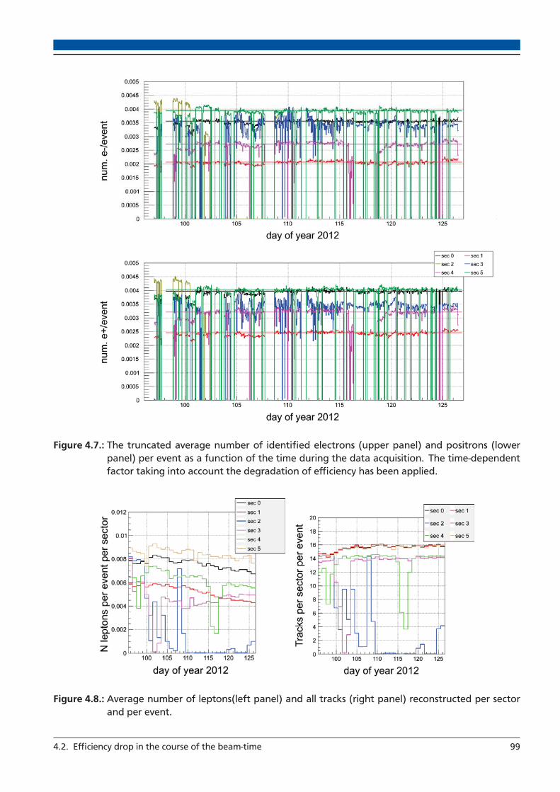
Figure 4.7.: The truncated average number of identified electrons (upper panel) and positrons (lowerpanel) per event as a function of the time during the data acquisition. The time-dependentfactor taking into account the degradation of efficiency has been applied.

Figure 4.8.: Average number of leptons(left panel) and all tracks (right panel) reconstructed per sectorand per event.

4.2. Efficiency drop in the course of the beam-time 99

Figure 4.9.: The truncated average number of reconstructedπ0-Dalitz pairs in a single event as a functionof the time during the data acquisition. The upper plot shows the trends without applyingthe time-dependent factor for reconstruction of single leptons and the lower plot shows themafter applying such factor.


4.3 Self-consistency check

p [MeV/c]100 200 300 400 500 600 700 800 900 1000

[deg

]θ

20

30

40

50

60

70

80

0.8

0.85

0.9

0.95

1

1.05

1.1Electron

p [MeV/c]100 200 300 400 500 600 700 800 900 1000

[deg

]θ

20

30

40

50

60

70

80

0.8

0.85

0.9

0.95

1

1.05

1.1Positron

Figure 4.10.: Ratio of the number of the reconstructed tracks corrected for efficiency to the number ofthe particles inside the HADES acceptance, calculated for the same data sample, as used togenerate the efficiency correction, separately for electron and positrons.

The minimum requirement on the consistency of the efficiency correction is that applying it for tracksreconstructed in simulation should allow to reproduce distributions of particles within the acceptance ofthe detector system. Preferably, this should be the case also if the code used to check this is maintainedseparately and follows a slightly different approach to the analysis, than the code used to generateefficiency correction matrices.

The method was based on the iteration over reconstructed tracks nested in the loop over simulatedparticles, transported from the GEANT level. Since the information about the simulated particle, usedto generate signals, from which the track has been reconstructed, is included in the track object, thematching of those two is possible in the nested loop.

In the first step, the check is done in the trivial case of the same input data, as used to generate thecorrection. The result, being effectively the ratio 3

∫fcorr(p,θ ,φ) · Nreco(p,θ ,φ)dφ

Nacc(p,θ )

of the distributions of reconstructed tracks corrected for efficiency to the distribution of particles insidethe HADES acceptance as a function of the polar emission angle and the momentum, is shown in Fig.4.10 for electrons and positrons. The values very close to unity indicate a very good agreement. Sincein the computation of the efficiency matrices and in the self-consistency check two alternative algo-rithms are used in looping over the data and matching a reconstructed track to a simulated particle, theagreement proves also, that the choice of the algorithm does not introduce any significant systematicerror.

The next step is to perform check using event generator with particle decays. This can be done bysimulating production and decays of dilepton sources in Pluto, embedding the daughter particles to dataor simulated events and perform the self-consistency test. Here, 107 events of each π0-Dalitz and η-Dalitz were simulated and embedded to UrQMD. Fig. 4.11 shows the result for positrons coming from3 fcorr(p,θ ,φ) = 1/Eff(p,θ ,φ), see Eq. 4.1.

4.3. Self-consistency check 101

p [MeV/c]100 200 300 400 500 600 700 800 900 1000

[deg

]θ

20

30

40

50

60

70

80

0.8

0.85

0.9

0.95

1

1.05

1.1γ + -e+e → η

p [MeV/c]100 200 300 400 500 600 700 800 900 1000

[deg

]θ

20

30

40

50

60

70

80

0.8

0.85

0.9

0.95

1

1.05

1.1 > 9 deg-e+open,eα

Figure 4.11.: Ratio of the number of the reconstructed tracks corrected for efficiency to the number ofthe particles inside the HADES acceptance, calculated for positrons produced in η-Dalitzdecays, taking into account all decay events (left) and only those with lepton pair openingangle above 9◦ (right).

the η-Dalitz decay. In the left panel the ratio for all reconstructed events is shown, the agreement israther poor. However, when selecting only events with e+e− pair opening angle larger than 9◦, the resultof comparison is satisfactory, taking into account limited statistics. This points towards correlation effectsin the reconstruction of lepton pairs when two tracks are close to each other. This cannot be taken intoaccount assuming pair efficiency as a product of the two single leg efficiencies calculated independentlyand is the matter of pair correction and will be discussed in the next section.

4.4 close pair effects

The influence of one lepton track on the reconstruction of another one is expected to be a residualeffect, small compared to the value of efficiency itself. Also the full dependence of efficiency on the pairkinematics has been already taken into account by the single track correction. Therefore, even if leptonclose pair effects have to be corrected on the pair level, it is not necessary to calculate the correctionin six-dimensional space, as it was discussed in the introduction to this chapter. One expects, that one-dimensional correction should be sufficient. The most obvious quantity, on which the correction factorshould depend, is the opening angle of the pair.

The procedure is then to use again simulated Dalitz decays of π0 and η embedded to UrQMD eventsand build the distributions of the dilepton opening angle for pairs inside the HADES acceptance and ofthe pairs of reconstructed tracks corrected for efficiency. The ratio can be used as an additional correctionfactor. It is shown in the left panel of Fig. 4.12. It has been checked, that the ratio is the same for bothπ0 and η, so both data sets were merged together to get more statistics.

The rise of the ratio towards very small opening angles means that efficiency correction calculated forsingle tracks overestimates the true one in this region. The reason is that even if one track could notproduce enough Cherenkov light in the RICH detector to be identified as a lepton, it can still be matchedto the ring produced by the second lepton if the opening angle is small enough. Furthermore, Cherenkovlight produced by both particles can contribute together to a ring of better quality. This is confirmedby the correspondence between the width of the rising peak in Fig. 4.12 and the cut on the dtrack-ringquantity. It can also be shown, that for wider cuts the width of the rising region gets larger as well.


[deg]Θ

0 5 10 15 20

Cor

rect

ed /

In a

ccep

tanc

e

0

1

2

3

4

5

6

Without pair correction

[deg]Θ

0 5 10 15 20

Cor

rect

ed /

In a

ccep

tanc

e

0

1

2

3

4

5

6With pair correction

Figure 4.12.: Left: ratio of the opening angle distributions of e+e− pairs from π0 and η Dalitz decaysfor tracks reconstructed and corrected for efficiency to the pairs in the HADES acceptance.Right: the same after applying the correction emerging from the ratio in the left panel.

In the range of about 1.5−6◦ the ratio drops dramatically. This is due to the sorting procedure, whichdoes not allow two reconstructed tracks to share common outer MDC segment or META hit. In such caseonly the one, that has best (lower) Runge-Kutta χ2 is used in the further analysis. In the first order thisallows to reject clone/ghost/fake tracks, but the secondary effect is the drop of efficiency of close leptonpairs.

The ratio from the left panel of Fig. 4.12 can be used as a correction applied on the pair level inthe event-by-event manner. The first test is to check the same ratio after applying this corrections. It isshown in the right panel of the Fig. 4.12. The ratio is now compatible with the unity within statisticaluncertainties and the differences from various PID methods became even smaller than before. Smalldiscrepancy from the unity is still present between 1.5◦ and 3◦. This is the remnant of the large drop inthe range 1.5− 6◦ in the left panel. The possible explanation is that due to a very low efficiency thereis insufficient number of reconstructed pairs that could be weighted by the correction factor and theagreement with the distribution of pairs within the geometric acceptance cannot be reached.

As the next step the effect of the correction on a distribution of a variable, that is of more physicalinterest has been checked. Fig. 4.13 shows the ratio of invariant mass distributions for the reconstructedpairs corrected by the product of single track efficiency values and for the pairs inside the HADES accep-tance. In the left panel it is shown without any additional correction and reflects similar features as thesame ratio drawn as a function of opening angle (since the invariant mass is a monotonic function of theopening angle). Their ratio in the right panel is made again after applying the correction factor from theleft panel of Fig. 4.12. In this case the ratio is also compatible with the unity within error bars and thesmall discrepancy visible in the opening angle representation is washed out in the invariant mass.

The right panel of Fig. 4.13 allows to estimate the systematic error introduced by the correction forinefficiency for pairs. It reflects namely the difference between the reconstructed distributions afterapplying all the corrections and the original spectra. Since the ratio deviates from 1 by 0.1 at maximum,a contribution of 10% to the systematic uncertainty is assumed.

4.4. close pair effects 103

]2 [GeV/ceeM0 0.1 0.2 0.3 0.4 0.5

Cor

rect

ed /

In a

ccep

tanc

e

0

0.5

1

1.5

2

2.5

3

3.5

4

4.5Without pair correction

]2 [GeV/ceeM0 0.1 0.2 0.3 0.4 0.5

Cor

rect

ed /

In a

ccep

tanc

e

0

0.2

0.4

0.6

0.8

1

1.2

1.4

1.6

1.8

2With pair correction

Figure 4.13.: Left: ratio of the invariant mass distributions of e+e− pairs from π0 and η Dalitz decaysfor tracks reconstructed and corrected for efficiency to particles in the HADES acceptance.Right: the same after applying the correction emerging from the ratio in the left panel ofFig. 4.12.

4.5 One-dimensional efficiency correction for pairs

In the previous sections the validity of the single-leg event-by-event approach to the efficiency correctionand the way to calculate such correction was discussed. In practice, applying this correction does notprovide satisfactory results. The issue is illustrated in the left panel of Fig. 4.14. It shows the invariant

]2 [GeV/ceeM0 0.2 0.4 0.6 0.8 1

]-1 )2

[(G

eV/c

ee d

N/d

M0

π1/

N

9−10

8−10

7−10

6−10

5−10

4−10

3−10

2−10Signal

Corrected

Raw

]2 [GeV/ceeM0 0.2 0.4 0.6 0.8 1

)ee

Mα

Yie

ld /

fit e

xp(-

0

0.2

0.4

0.6

0.8

1

1.2

1.4

1.6

1.8

2All e+e- combinations

= 102χRaw,

= 172χCorrected,

Figure 4.14.: Left: invariant mass distribution of e+e− signal without efficiency correction and after ap-plying the single-leg correction. Right: distributions of all e+e− combinations divided by theexponential functions fitted separately to both of them.

mass distributions of the signal pairs both without efficiency correction (blue circles) and after the single-


leg correction applied (red circles). It is evident that the corrected spectrum has larger point-to-pointfluctuations.

Point-to-point fluctuations appear not only in the signal spectrum, but they are present already in thedistribution of all e+e− as well as like-sign pairs. This cannot be easily seen, because all such distributionsdrop rapidly, exponentially in the first approximation, with increasing invariant mass. The difference invalue between two adjoining points coming from this trend is therefore larger than the fluctuation. Yetthe fluctuation can be observed when the function f (Mee) = a exp(bMee) is fitted to the distributionand then the distribution is divided by the fit result. This is shown in the right panel of Fig. 4.14,where the fluctuations are clearly visible. It can also be noticed, that they are enhanced after applyingefficiency correction. The origin of the latter effect is not yet fully understood. A possible interpretationinvolves not fully independent probabilities to detect two leptons of not necessarily small opening angle,when they fire the same MDC wire or hit the same time-of-flight module. Nevertheless, after subtractingcombinatorial background the fluctuations grow, while the dropping trend is reduced, because signal hasits mass dependence weaker than exponential.

Remarkable is also increase of the size of statistical error bars relative to the positions of the pointsafter correcting for efficiency. One does not expect the correction to enhance statistical uncertainty, itshould grow proportionally to the value of the points and in the plot made in logarithmic scale thelines should appear to have roughly the same length. The errors are correctly propagated in the his-tograms of all unlike-sign and like-sign combinations even if they are filled with weights representingcorrections for both legs. However, the formalism for combinatorial background estimation and sub-traction, discussed in the next chapter, operates essentially on numbers of reconstructed pairs and doesnot take into account correction weights. This may lead to incorrect subtraction which in turn may bereflected in overestimated statistical errors of the signal. This can also contribute to artificially enhancedpoint-to-point fluctuations discussed above.

To reduce these effects, efficiency is calculated as a function of dilepton pair properties, based onsingle-leg matrices computed in the first place, using simulated pairs from various sources. First, un-corrected signal is extracted and only then it is multiplied by the correction function. In order to avoidmodel dependence it would be desirable to represent the correction in multidimensional space, using asmany degrees of freedom as possible, preferably all six. Even though it would (in principle) be possibleto populate such a phase space in simulation by generating enough events, it is impossible with real data.In fact, measured events provide enough statistics only for one-dimensional distributions. Subtraction ofthe combinatorial background in the situation of empty bins in two-dimensional representations leads tomany difficulties and partially incorrect results, as it is elucidated in the next chapter. Therefore the onlyviable procedure is to subtract background and correct it for efficiency in one dimension using each timea factor calculated as a function of the same variable as the spectrum under study. When the correction isobtained from the pair cocktail not very far from reality, the introduced error due to model dependenceshould not be very large.

4.5.1 Simulating the cocktail

The correction functions are calculated based on a cocktail of dilepton sources simulated with Pluto[110]. The two leptons in each event are first filtered by the HADES acceptance. This is done using singleleg acceptance matrices, dependent on p, θ and φ. While filtering by the acceptance matrices, a randomnumber is generated from the flat distribution between 0 and 1. If the random number is smaller, thanthe respective value in the acceptance matrix, the particle is regarded as being accepted. If this is the casefor both particles in the pair, this pair is used to fill all the required distributions of pairs inside the HADESacceptance. In order to mimic the distributions of reconstructed pairs, efficiency values are read for bothleptons in accepted pairs from the respective single-particle matrices. Additional factor, which takes intoaccount correlation effects on pair reconstruction, is taken from the distribution shown in the left panelof Fig. 4.12. Then the second set of distributions is filled, this time with weights being products of the

4.5. One-dimensional efficiency correction for pairs 105

three factors. This is the main advantage of this method over the full simulation and reconstruction chain(besides highly reduced computing resources): the spectra that represent reconstructed pairs containthe same number of counts as the spectra of pairs in the acceptance (only the weights are different).Concerning the efficiency values shown later on, the spectra of pairs from full reconstruction chain ofsimulated data have roughly 30 times less counts than the spectra only weighted with reconstructionefficiency. This influences statistical errors and fluctuations of the simulated spectra.

As suggested by [87, 88, 89] and will be further discussed in Chapter 7, the dominant source ofdilepton pairs above Mee = 150 MeV/c2 is the decay ρ0 → e+e−, where the spectral function of ρ0 hasbeen calculated within the coarse-graining approach. This is also the second largest contribution below150 MeV/c2, the first one being the π0 Dalitz decay. Therefore these two contributions constitute acocktail sufficient for pair efficiency calculation, that should not introduce too large model bias. Theycan be also accompanied by ω → e+e− in order to populate masses above 700 MeV/c2, where the ρ0

contribution starts to die out. The η-Dalitz is included just for the sake of formality.The parameters of the sources are following: π0 is generated thermally with two temperature com-

ponents: 49 MeV/kB and 89 MeV/kB, the fraction of the former one being 98%, these parameters areobtained from the charged pion analysis, described in Section 7.1.1. η is generated from the thermalsource of the temperature 50 MeV/kB (the same as for pions, neglecting the second component) and ωwith the assumption of 60 MeV/kB. ρ0 is taken from [89]. Decays to respective channels are simulateddirectly in Pluto with branching ratio of unity. Roughly 107 pairs from each source were generated.

]2 [GeV/ceeM0 0.2 0.4 0.6 0.8 1

]2 [1

/GeV

/cee

dN

/dM

0π

1/N

9−10

8−10

7−10

6−10

5−10

4−10

3−10

2−10 0

π

η

ee→ωthermal 0

ρin-medium Total

In acceptance

]2 [GeV/ceeM0 0.2 0.4 0.6 0.8 1

]2 [1

/GeV

/cee

dN

/dM

0π

1/N

9−10

8−10

7−10

6−10

5−10

4−10

3−10

2−10

0π

η

ee→ωthermal 0

ρin-medium Total

Reconstructed / Filtered

Figure 4.15.: Invariant mass distributions of the simulated cocktail used for the pair efficiency correction.Left: pairs filtered by single-leg acceptance matrices (lines) and pairs processed throughGEANT and analyzed requiring the standard acceptance condition (points), Right: pairs fil-tered by single-leg acceptancematrices andweighted by single-leg efficiencymatrices (lines)and pairs processed through full analysis chain (points). The fact, that values measured inexperiment are different due to particle scattering and momentum resolution of the detec-tor are addressed in Section 4.5.3.

All the contributions are properly scaled in the same way as the measured spectra, as explained below.The latter are normalized to the number of analyzed events and to the average number of neutral pionsproduced in the reaction, also the cocktail components are scaled down to the number of simulated pairsand to the number of π0. The branching ratios to respective channels [1]: 1.174 · 10−2 for π0-Dalitz,6.9 · 10−3 for η-Dalitz, 7.28 · 10−5 for ω → ee are taken into account as well. The final multiplicativefactor is the production rate per event in 40% most central events, which is taken as 0.107 for η, based


on the direct reconstruction with the conversion method, as discussed in Ref. [41] and outlined inSection 7.2. and 0.003 forω as it comes from the Statistical Hadronization Model fit to the data. Specialcase with respect to the normalization is ρ0, where the multiplicity×branching ratio can be estimatedas 1.55 · 10−2 based on the coarse-graining calculation. The calculation was done, however, for impactparameter b = 0, so to make it consistent with other cocktail ingredients, a scaling like A1.4

part [38] isassumed.

4.5.2 Consistency check of the cocktail

In order to verify, that the used methods describes pair reconstruction efficiency, the cocktail filteredby acceptance and weighted down by efficiency is compared to the result of full analysis of the samesources. The signal sources are embedded to UrQMD events and processed through the GEANT and DSTprocedures in the same way, as single leptons used to compute efficiency matrices. The simulation dataare then analyzed in the same way as the experimental ones, with the only difference that in the formercase only true leptons coming from the appropriate source are taken into account, what is obviously notpossible with the measured data.

In Fig. 4.15 invariant mass distribution of cocktail components from the full chain analysis and fromthe filtering method are compared. Left panel shows the spectra in the HADES acceptance, right panelthe reconstructed spectra and corresponding ones filtered by acceptance and scaled down by efficiency.In both cases the agreement is of the order of 1 %.

4.5.3 Momentum smearing

All the plots concerning efficiency discussed until now involved “ideal” kinematics of the particles, i.e.with which they were generated. They are different from the reconstructed values. Examples of originalvs. reconstructed momentum distributions of e− in two selected polar angle ranges are shown in Fig.4.16. One effect that can be seen is the resolution of reconstructed momentum. It is expected to get

[MeV/c]ideal

p0 500 1000 1500 2000

[MeV

/c]

reco

p

0

200

400

600

800

1000

1200

1400

1600

1800

2000

1

10

210

310

410

(55 deg - 70 deg)∈ θElectrons,

[MeV/c]ideal

p0 500 1000 1500 2000

[MeV

/c]

reco

p

0

200

400

600

800

1000

1200

1400

1600

1800

2000

1

10

210

310

410

(0 deg - 35 deg)∈ θElectrons,

[MeV/c]ideal

p0 500 1000 1500 2000

[MeV

/c]

reco

p

0

200

400

600

800

1000

1200

1400

1600

1800

2000

1

10

210

310

(0 deg - 35 deg)∈ θNegative pions,

Figure 4.16.: Distributions of original vs. reconstructed momentum of electrons in two selected θ bins,based on a combined π0-Dalitz and η-Dalitz simulation. For comparison, π− from UrQMD(fulfilling track quality criteria as for leptons) are shown in one bin of polar angle.

worse towards larger values, because of smaller curvature of particle’s track in the magnetic field. Thiseffect is symmetric: it makes the reconstructed value of the momentum larger or smaller than the idealone with equal probability. Another effect is energy loss, most prominent at low momenta. This acts onlyin one direction, i.e. the reconstructed value is lower than the original one. It can be observed, that aparticle may lose its momentum almost entirely. This, together with the fact, that the effect is not visiblefor pions (also shown in Fig. 4.16) indicates, that the main energy loss mechanism is bremsstrahlungand it must happen mostly in the target, where heavy atomic nuclei are present.


It can be argued how these effects should be taken into account, when correcting measured datafor efficiency. The assessment of this issue is as follows. It is always easier to destroy an information,than to try to recover it afterwards. Both approaches involve a probabilistic factor. Given an idealvalue of momentum, only a probability distribution of reconstructed values is known. Conversly, givena reconstructed values, only a probability distribution of real values can be known. But recoveringideal momentum from the reconstructed one requires matrix inversion (deconvolution, unfolding, “de-smearing”), which is the source of uncertainty due to numeric issues but not only. This is where the shapeof the original momentum distribution of particles used to fill the smearing matrix plays a role. At a singlevalue of reconstructed momentum two different values of ideal momentum will contribute differentlydepending if the original distribution is flat or falls off exponentially. This influences the distribution ofideal momentum for a given reconstructed value, obtained after inverting the matrix. In contrast, thedistribution of reconstructed momentum for a given ideal value comes from direct, not inverted matrixand is independent of the distributions for other values and thus independent of the shape of the originaldistribution. This speaks for smearing the momentum in the simulation, which has been used tocalculate the efficiency correction, instead of attempting to de-smear experimentally measuredvalues.

In this analysis it was not possible to reach the level of self-consistency of efficiency correction asshown in Sections 4.3 and 4.4, when reconstructed values were used in the numerator of the single-leg matrices, Eq. 4.1. Therefore both numerator and denominator were filled with ideal values andthese values consequently used to read the efficiency and to calculate kinematic quantities (like pairinvariant mass) up to the level of all the distributions in Fig. 4.15. In this approach efficiency matricesstill contain energy loss effects, the fact if particle was reconstructed or not depends on its momentumafter rescattering. Original momentum is used only to do accounting in a consistent way. One cansay, that the probability of particle’s detection depends on the momentum, with which it was emitted,because it influences the momentum value after rescattering and this determines if the particle couldbe detected or not. From this point of view, ideal values can readily be used when reading from thematrix efficiency values in the filtering procedure. To build the filtered spectra compatible with thosemeasured in experiment, the smeared values should be used in calculating invariant mass and other pairobservables as well as in reproducing the cuts that are applied in experimental data, like p > 100 MeV/c.The factor that is introduced to the invariant mass distribution due to the smearing can be seen in Fig.4.17. In addition, Fig. 4.24 shows raw data points compared to the cocktail with and without thesmearing.

Fig. 4.18 shows efficiency and acceptance corrections as a function of invariant mass for differentcentrality bins. The centrality dependence is as expected: in most central events efficiency is lower dueto higher track density and thus the correction is larger. Acceptance correction was calculated togetherwith the efficiency as the ratio of the yield in the full solid angle to the yield in the acceptance. In this casesmall differences between centrality bins come from the fact, that also minimum single-leg efficiency of5% is required to consider a particle being accepted.

4.5.4 Model dependence of the correction factors

In order to estimate the systematics due to the theoretical model used in the calculation of efficiency andacceptance correction for pairs, alternative models have also been used to calculate the corrections andcompare them. It can be expected, that using for such a purpose a cocktail containing only freeze-outsources is not adequate. Such a cocktail ignores in-medium radiation, which should have a dominant rolein the mass range above π0. This would lead to overestimation of the systematic uncertainty. Further-more, with freeze-out sources only, it is practically impossible to populate the mass range between η andω masses with statistics large enought to compute the corrections. Therefore the followingalternativemodels have been used in the present analysis:

1. Hadron-String Dynamics [113]


]2 [GeV/ceeM0 0.2 0.4 0.6 0.8 1

(no

t sm

ear.

)ee

(sm

ear.

) / N

eeN

0

0.2

0.4

0.6

0.8

1

1.2

1.4

1.6Total cocktail

Figure 4.17: Ratio of the invariant mass distributionsof the full Pluto cocktail filtered by ac-ceptance and weighted by efficiency,before and after performing the mo-mentum smearing procedure for calcu-lation of the invariant mass. As dis-cussed in text, efficiency values are inboth cases obtained for ideal values ofmomentum.

]2 [GeV/ceeM0 0.2 0.4 0.6 0.8 1

Cor

rect

ion

fact

or

0

10

20

30

40

50

60

70


0-40% centrality0-5% centrality

5-10% centrality10-20% centrality20-30% centrality

30-40% centrality

]2 [GeV/ceeM

0 0.1 0.2 0.3 0.4 0.5 0.6 0.7 0.8 0.9 1

Cor

rect

ion

fact

or

0

1

2

3

4

5

6

7

8

9

10Acceptance correction

Figure 4.18.: Efficiency (left) and acceptance corrections (right) as a function of pair invariant mass forvarious centrality bins.

2. Cocktail as in Section 4.5.1, but with in-medium ρ0 contribution replaced with thermal ρ0 −→e+e−, with temperature of 55 MeV/kB, with factor 1/M3

ee coming from Vector Meson Dominanceand without the threshold of two pion mass.

The comparison of the efficiency and efficiency×acceptance correction factors from the three models isshown in Fig. 4.19 as an example for invariant mass and transverse mass in the region above π0 andbelow η mass.

To quantify the spread, mean and standard deviation of the three corrections has been calculated bin-by-bin. It is shown in Fig. 4.20. Positions of the points indicate the mean and error bars indicate thestandard deviation. It can be seen, that the relative spread is rather small. For this reason, the meancorrection has been used for all the final spectra.


]2 [GeV/ceeM

0 0.2 0.4 0.6 0.8 1

Cor

rect

ion

fact

or

0

10

20

30

40

50


0ρCocktail with thermal

Cocktail with coarse-grainingHSD


]2 [GeV/ceeM

0 0.2 0.4 0.6 0.8 1

Cor

rect

ion

fact

or

0

50

100

150

200

250

300

350

400

450

500Acc. correction×Eff.


Cocktail with coarse-graining

HSD

Acc. correction×Eff.

]2 [MeV/cm

200 300 400 500 600 700 800 900 1000

Cor

rect

ion

fact

or

0

10

20

30

40

50



Cocktail with coarse-grainingHSD


]2 [MeV/cm

200 300 400 500 600 700 800 900 1000

Cor

rect

ion

fact

or

0

50

100

150

200

250

300

350

400

450

500Acc. correction×Eff.


Cocktail with coarse-graining

HSD

Acc. correction×Eff.

Figure 4.19.: Efficiency (left) and efficiency×acceptance corrections (right) as a function of pair invari-ant mass (top) and transverse mass (in the range 0.15 < Mee < 0.55 [MeV/c2], bottom)calculated with three different models.

In the presentation of final results, the relative deviation (standard deviation divided by mean), as inFig. 4.20, is added to the total systematic uncertainty. For spectra corrected for efficiency, the relativedeviation of efficiency correction factors is taken. For spectra corrected for acceptance, it is the deviationof efficiency×acceptance correction factors. This takes into account possible cancellation of the deviationsof that come from the efficiency and acceptance corrections separately.


]2 [GeV/ceeM

0 0.2 0.4 0.6 0.8 1

Cor

rect

ion

fact

or

0

10

20

30

40

50


]2 [GeV/ceeM

0 0.2 0.4 0.6 0.8 1

Cor

rect

ion

fact

or

0

50

100

150

200

250

300

350

400

450

500Acc. correction×Eff. Acc. correction×Eff.

]2 [MeV/cm

200 300 400 500 600 700 800 900 1000

Cor

rect

ion

fact

or

0

5

10

15

20

25

30

35

40

45

50Efficiency correctionEfficiency correction

]2 [MeV/cm

200 300 400 500 600 700 800 900 1000

Cor

rect

ion

fact

or

0

50

100

150

200

250

300

350

400

450

500Acc. correction×Eff. Acc. correction×Eff.

Figure 4.20.:Mean efficiency (left) and efficiency×acceptance corrections (right) as a function of pair in-variant mass (top) and transverse mass (in the range 0.15< Mee < 0.55 [MeV/c2], bottom)calculated with three different models. Mean is represented by positions of the points andstandard deviation by the error bars.

4.6 Relative acceptance correction for missing sectors

As discussed in Section 3.2, in particular periods of the beam-time certain HADES sectors were notoperational and they are completely removed from the affected events to avoid difficulties related tocorrections for effects that triggered the partial operation of the particular sector. Thus HADES operatedin these events effectively with different acceptance. This prohibits to analyze the complete data setas a whole and to compare the results with previous experiments running where all six sectors wereoperational. Events with all 6 sectors operating in the Au+Au experiment are available only for onlysmall (2%) part of the total statistics. Therefore, corrections for the missing acceptance due to notoperational sectors with respect to configuration with six sectors have to be calculated. Fig. 3.4 shows,that the number of events with only four sectors is almost the same as with five, hence independentcorrections have to provided for these two cases. Acceptance correction in general depends on themodel but in this case it will be shown, that model dependence is large only in the phase-space regions,that are weakly populated by dileptons.

4.6. Relative acceptance correction for missing sectors 111

Figure 4.21.: The correction acceptance losses due to one or two missing sectors. θee,avg is the averagepolar angle of two leptons and Θee is the opening angle of the pair.

The correction can be calculated as a ratio of the distribution obtained with one or two sectors switchedoff to the one with all sectors present. This cannot be done on the single particle level, as a function ofquantities that characterize single particles, p, θ and φ. A sector removed from the analysis means, thatthere are no tracks in a certain range of the φ angle and there is nothing that could be weighted by acorrection factor. Various pair observables have been studied to reduce model dependency. Finally, it hasbeen found that a two-dimensional function of Θee − θee,avg, where Θee is the opening angle and θee,avgis the average polar angle of two leptons building up the pair is best suited for this purpose.

As an input, the sample of pairs, that are homogeneously distributed in invariant mass, rapidity andtransverse momentum is simulated in Pluto. This correction is purely geometric and to be applied underthe assumption, that all the tracks are already corrected for efficiency. Therefore in this calculation itis not necessary to do the GEANT analysis and track reconstruction. Instead, in the calculations bothleptons of the pair are filtered by a single particle acceptance matrix, introduced in Section 4.5.1, in


Figure 4.22.: Ratios of the correction factors like in Fig. 4.21 calculated from η-Dalitz decay pairs to theones obtained with lepton pairs homogeneous in p, θ and φ.

order to obtain the distribution of pairs inside the acceptance. On the top of it, sectors are removedby applying cuts on the φ angle. Because of the assumption, that the data are already corrected forefficiency, the data set is symmetric under six-fold rotation around the Z axis. Consequently, only thefollowing conditions are sufficient to account for loses present in the data:

• Remove φ ∈ (0◦ − 60◦) to cover all the cases, with one sector missing.

• Remove φ ∈ (0◦ − 120◦) to cover all cases with two adjacent sectors missing (d=0).

• Remove φ ∈ (0◦ − 60◦) ∪ (120◦ − 180◦) to cover all cases with two sectors missing, separated byone working sector (d=1).

• Remove φ ∈ (0◦ −60◦)∪ (180◦ −240◦) to cover all cases with two opposite sectors missing (d=2).

4.6. Relative acceptance correction for missing sectors 113

Figure 4.23: Distribution of the opening angle vs. av-erage polar angle of the two particle inthe pair, for all e+e− combinations re-constructed in the experimental data.

-

The shapes of the resulting corrections are shown in Fig. 4.21. The factors are quite sizable in certainregions, reaching the value of about 4. This strengthens the argument to skip events with three or lessworking sectors – in this case the correction would be even larger. The cut-off along the diagonal has itsorigin in the kinematics. Low average polar angle implies that both particles are close to each other andthis limits possible values of the opening angle. If average θ is large, the opening angle can take anyvalue, depending on the difference of the azimuth angles.

In order to validate the model dependence of the missing sector correction, it has been computed inthe same way, but for pairs with kinematics of π0 and η Dalitz decays. The ratios of the correctionfactors calculated with η-Dalitz pairs to those computed from homogeneous pairs are shown in Fig.4.22. The differences are of the order of 5-10%. Comparison with the distribution of opening angle vs.average polar angle, obtained from experimental data and shown in Fig. 4.23, confirms, that significantdeviations from the unity are present mainly in those regions of the phase space, which are not stronglypopulated in the data. This corroborates the validity of the correction.

In order to not underestimate systematic uncertainty contribution originating from this correction, itwas assumed to be of 10% i.e. the largest deviation from unity visible in Fig. 4.22 in regions, wherestatistics is non-zero according to Fig. 4.23.

4.7 Validation of the efficiency correction methods

Both the cocktail used in the calculation of the pair correction and experimental spectra are normalizedto the π0 multiplicity. The efficiency correction is the ratio of the cocktail filtered by acceptance to theone weighted additionally by single-lepton efficiencies. In order to validate the method used to correctspectra for efficiency, one can go other way around and compare raw data with the cocktail filtered andweighted with single track efficiency values. If the procedure is applied in a right way, distributionsshould agree in the π0 region, allowing for some tolerance due to in-medium ρ0 contribution to thecocktail. This can be seen in Fig. 4.24 for cases when ideal momentum values were used in the cocktailand when momentum smearing was done as described in Section 4.5.3. The data points are corrected formissing sectors, because this is the only correction, that has to be applied on the event-by-event basis, asdiscussed in Section 4.6. Momentum smearing brings the agreement to the very good level. Additionally,one can observe the effect of the smearing on the spectral shape of cocktail components, especially of ω.


]2 [GeV/ceeM0 0.2 0.4 0.6 0.8 1

]2 [1

/GeV

/cee

dN

/dM

0π

1/N

9−10

8−10

7−10

6−10

5−10

4−10 Pluto 0π

Pluto η

Pluto ee →ωthermal Pluto 0

ρin-medium PlutoTotal

Raw data

Reconstructed / Filtered

]2 [GeV/ceeM0 0.2 0.4 0.6 0.8 1

]2 [1

/GeV

/cee

dN

/dM

0π

1/N

9−10

8−10

7−10

6−10

5−10

4−10 Pluto 0π

Pluto η

Pluto ee →ωthermal Pluto 0

ρin-medium PlutoTotal

Raw data

+ smearedReconstructed / Filtered

Figure 4.24.: Comparison of the cocktail used to calculate pair efficiency correction, filtered by accep-tance and weighted by single-lepton efficiency with data points, corrected only by therelative acceptance of missing sectors. In the left panel ideal values were used in the cock-tail. In the right panel momentum was smeared to calculate invariant mass and to cut onp > 100 MeV/c, analogous to what is done in experiment.

4.7. Validation of the efficiency correction methods 115

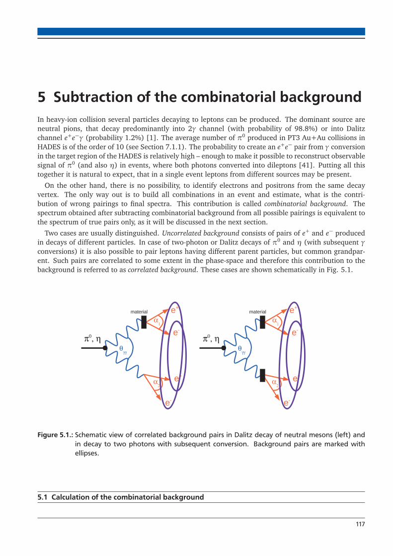
5 Subtraction of the combinatorial background

In heavy-ion collision several particles decaying to leptons can be produced. The dominant source areneutral pions, that decay predominantly into 2γ channel (with probability of 98.8%) or into Dalitzchannel e+e−γ (probability 1.2%) [1]. The average number of π0 produced in PT3 Au+Au collisions inHADES is of the order of 10 (see Section 7.1.1). The probability to create an e+e− pair from γ conversionin the target region of the HADES is relatively high – enough to make it possible to reconstruct observablesignal of π0 (and also η) in events, where both photons converted into dileptons [41]. Putting all thistogether it is natural to expect, that in a single event leptons from different sources may be present.

On the other hand, there is no possibility, to identify electrons and positrons from the same decayvertex. The only way out is to build all combinations in an event and estimate, what is the contri-bution of wrong pairings to final spectra. This contribution is called combinatorial background. Thespectrum obtained after subtracting combinatorial background from all possible pairings is equivalent tothe spectrum of true pairs only, as it will be discussed in the next section.

Two cases are usually distinguished. Uncorrelated background consists of pairs of e+ and e− producedin decays of different particles. In case of two-photon or Dalitz decays of π0 and η (with subsequent γconversions) it is also possible to pair leptons having different parent particles, but common grandpar-ent. Such pairs are correlated to some extent in the phase-space and therefore this contribution to thebackground is referred to as correlated background. These cases are shown schematically in Fig. 5.1.

θγγ

π0, η

α1

α2

θγγ

π0, η

α1

α2

Figure 5.1.: Schematic view of correlated background pairs in Dalitz decay of neutral mesons (left) andin decay to two photons with subsequent conversion. Background pairs are marked withellipses.

5.1 Calculation of the combinatorial background

117

5.1.1 Like-sign geometric background

It is rather intuitive, that combinatorial background can be estimated by spectra of lepton pairs of thesame sign: in the full phase-space (that is, leaving aside the acceptance and efficiency of the detectionsystem) there is no difference between electrons and positions and therefore the probability to builda combinatorial e+e− pair should be the same as to build e+e+ or e−e− pairs that are always of com-binatorial origin. This argument does not change in the case of correlated background. The intuitiondoes not give an answer if for combinatorial background estimation one should take e+e+, e−e−, somecombination of them and which type of combination. This was studied in [114, 115, 116], where theresult

⟨BG+−⟩= 2�⟨FG++⟩⟨FG−−⟩.

was obtained, where BG+− is the combinatorial background contribution in the yield of opposite-signpairs and FG++, FG−− are yields of like-sign pairs. The result was obtained for muons from charmedmesons decays in the intermediate mass region. In particular, the derivations of the above formulamake use of the assumptions that (a) the numbers N+/− of mesons have Poisson distributions, (b)cov(N+, N−) = 0. These assumptions are not applicable to dileptons from hadron decays populatinginvariant masses below 1 GeV/c2. Such dileptons are always produced in pairs (correlated). Moreover,statistical distributions of the multiplicity of their parent particles cannot be assumed.

The derivation that can be applied in the case, when signal pairs are correlated is given in [117]. Itassumes, that e+ and e− are always produced in pairs, due to charge conservation. Then it considersthe probability of registering np out of N initially produced pairs given by the binomial distributionB(np, N ,εp). Out of the not registered pairs, single tracks can be still detected and the probability isgiven by the multinomial distribution with three possible outcomes: no track, one e+ detected, one e−detected:

ω(n+, n−)def= M(n+, n−; N − np,ε+,ε−)

def=

(N − np)!

n+!n−!(N − np − n+ − n−)!ε

n++ ε

n−− (1− ε+ − ε−)N−np−n+−n− ,(5.1)

where ε+ and ε− are the probabilities to detect a single track (from a not fully reconstructed pair).Summing over values of n+ (or n−) up to the total number of not reconstructed pairs N −np one gets theprobability distributions for n− (or n+, respectively):

ω(n+)def=

N−np∑n−=1

M(n+, n−; N − np,ε+,ε−),

ω(n−)def=

N−np∑n+=1

M(n+, n−; N − np,ε+,ε−).(5.2)

Then the number of all unlike-sign combinations of reconstructed leptons is given by:

⟨n+−⟩= n2p + np

N−np∑n+=1

n+ω(n+) + np

N−np∑n−=1

n−ω(n−) +N−np∑n+=1

N−np∑n−=1

n+n−ω(n+, n−) (5.3)

For like-sign combinations it is:

⟨n++⟩=N−np∑n+=1

(np + n+)(np + n+ − 1)

2ω(n+) (5.4)

118 5. Subtraction of the combinatorial background

and similarly for ⟨n−−⟩. The expected number of reconstructed pairs for given N is obtained by averagingover np:

⟨N+−⟩=∑np

⟨n+−⟩B(np, N ,εp) = [εp + ε+(1− εp)][εp + ε−(1− εp)](N2 − N) + εpN ,

⟨N++⟩=∑np

⟨n++⟩B(np, N ,εp) =12[εp + ε+(1− εp)]

2(N2 − N),

⟨N−−⟩=∑np

⟨n−−⟩B(np, N ,εp) =12[εp + ε−(1− εp)]

2(N2 − N).

(5.5)

Then averaging over N yields the total number of "foreground" pairs (detailed explicit calculation makesuse of properties of binomial and multinomial distributions and is outlined in the reference [117]):

⟨FG+−⟩=∑

N

⟨N+−⟩P(N) = [εp+ε+(1−εp)][εp+ε−(1−εp)](⟨N2⟩−⟨N⟩)+εp⟨N⟩= ⟨BG+−⟩+⟨S⟩. (5.6)

Identifying εp⟨N⟩ with the signal leads to the conclusion that the unlike-sign foreground separates intosignal and background. In case of like-sign pairs only background is present:

⟨FG++⟩=∑

N

⟨N++⟩P(N) = 12[εp + ε+(1− εp)]

2(⟨N2⟩ − ⟨N⟩) = ⟨BG++⟩,

⟨FG−−⟩=∑

N

⟨N−−⟩P(N) = 12[εp + ε−(1− εp)]

2(⟨N2⟩ − ⟨N⟩) = ⟨BG−−⟩.(5.7)

Comparing the expressions for background of different signs allows to express the unlike-sign combina-torial background through yields of like-sign pairs:

⟨BG+−⟩= 2�⟨BG++⟩⟨BG−−⟩= 2

�⟨FG++⟩⟨FG−−⟩. (5.8)

The above calculations were done assuming silently, that the reconstruction probability does not de-pend on the sign of the pair: ε+− = ε++ = ε−− = εp. This assumption can be withdrawn in order togeneralize the approach of [117]. The result will be then:

⟨BG+−⟩= [ε+− + ε+(1− ε+−)][ε+− + ε−(1− ε+−)][ε++ + ε+(1− ε++)][ε−− + ε−(1− ε−−)]2�⟨FG++⟩⟨FG−−⟩. (5.9)

This expression is clearly different from the often quoted (see e.g. [116, 118]):

⟨BG+−⟩= ε+−�ε++ε−−

2�⟨FG++⟩⟨FG−−⟩

Nevertheless, the steps described below are valid also for the latter expression.The quotient in Eq. 5.9 could in principle be calculated directly using Monte Carlo methods. However,

all the systematic uncertainties from modeling of efficiency in simulation would be amplified. Moreover,the risk of biasing the data by the model dependence would appear. A possible way to avoid theseproblems is to generate a data sample without signal. For such a sample unlike-sign foreground is equalto background and the above equation can be written as (lower-case letters are used to distinguish fromthe original data sample):

⟨ f g+−⟩= [ε+− + ε+(1− ε+−)][ε+− + ε−(1− ε+−)][ε++ + ε+(1− ε++)][ε−− + ε−(1− ε−−)]2�⟨ f g++⟩⟨ f g−−⟩. (5.10)

5.1. Calculation of the combinatorial background 119

Together it gives:

⟨BG+−⟩= ⟨ f g+−⟩2$⟨ f g++⟩⟨ f g−−⟩

2�⟨FG++⟩⟨FG−−⟩ ≡ k2

�⟨FG++⟩⟨FG−−⟩. (5.11)

The signal-free data could be simulated, but the problems of systematic and model dependence wouldstill be present. Instead, particles from different measured events can be combined into pairs (eventmixing). Such pairs do not contain correlated signal by definition, all the efficiency values are true andsingle track distributions are identical as in data. Possible difficulty emerge in case of pairs with openingangle so small, that the presence of one particle influences the detection of another one. This effect playsa role only for same-event pairs and leads to a difference between pair efficiency in real data sample andin event mixing. Nevertheless, this is not a problem if a cut on minimal opening angle is applied, whatis the case in a typical dilepton analysis (see Fig. 4.12). In addition, small opening angles are weaklypopulated by background pairs in any case.

The probability P(N) in Eqs. 5.6 and 5.7 serves only for proper averaging of terms with N from Eq.5.5 and there is no assumption about the underlying probability distribution, in particular Poissondistribution, at this point. In other words, ⟨ f (N)⟩=∑N f (N)P(N), no matter how P(N) is distributed.In this context, the only distinctive property of the pair production according to the Poisson distributionis the fact, that background would then be equal to the product of average single electron and positronmultiplicities, as it is discussed in [117].

The formula to estimate combinatorial background as a geometric mean of yields of like-sign pairs isexact (provided that all used assumptions are justified). For quick checks it can be approximated byarithmetic mean, which can be calculated by simple additions and subtractions of histogram withouttaking care of calculating square roots of bin entries and correct error propagation. Assuming namely,that Np and Nn are both larger than their difference, one can write e.g. Nnn = Npp + ε and

�Npp · Nnn = Npp ·

√√1+

ε

Npp≈ Npp ·

�1+

12ε

Npp

�= Npp +

ε

2=

12(Npp + Nnn). (5.12)

It is a general fact, that arithmetic mean is always larger than geometric, because 12

�Npp + Nnn

� −$Npp · Nnn =

12

�$Npp −$Nnn

�2is always a positive number.

5.2 Correction for pair reconstruction asymmetry

The k-factor used in this analysis was calculated with mixed event for each centrality class separately.The event mixing procedure was the same as for determining the shape of the combinatorial backgroundat higher masses, as discussed in Section 5.3.

The shape of the k-factor as a function of dilepton invariant mass and its effect on the combinatorialbackground shape and on the signal obtained after background subtraction from all e+e− combinationsare shown in Fig. 5.2. When the asymmetry factor is ignored, an accumulation of the signal developsabove π0-Dalitz with the maximum around 0.15 GeV/c2. It corresponds precisely to the invariant massvalue, for which the k-factor reaches the maximum of around 1.05. This shows that the accumulationis an unphysical artifact due to the asymmetry between reconstruction of like- and unlike-sign pairs inHADES. Similar observations have been made also in PHENIX [117], STAR [119] and ALICE [120, 121]analyses.

Below 0.1 GeV/c2 the asymmetry factor deviates strongly from the unity and this is where it has thelargest influence on the background value. On the other hand, as it can be seen e.g. from the right panelof Fig. 5.2 or from Fig. 3.27, the background in this region is clearly lower than the signal and the latteris barely affected by the k-factor.


]2 [GeV/ceeM0 0.2 0.4 0.6 0.8 1

k-fa

ctor

0.75

0.8

0.85

0.9

0.95

1

1.05

1.1

1.15 hmassNP_w6w6_oa9degRecur

Entries 162976

Mean 0.1117

RMS 0.08991

]2 [GeV/ceeM0 0.1 0.2 0.3 0.4 0.5 0.6

]-1 )2

[(G

eV/c

ee d

N/d

M0

π1/

N

-910

-810

-710

-610

-510

-410

hmassNP_w6w6_oa9degRecur

Entries 162976

Mean 0.1117

RMS 0.08991

pairs-e+All e

Comb. bgr., no k-factor

Comb. bgr., with k-factor

Signal, no k-factor

Signal, with k-factor

Figure 5.2.: Left: shape of the k-factor as a function of dilepton invariant mass. Right: Invariant massof all e+e− combinations (black), like-sign combinatorial background not multiplied (red) andmultiplied (blue) by the detection asymmetry factor, and signal obtained after subtraction ofboth background spectra from all e+e− pairs (orange and green respectively). No single-trackefficiency corrections were applied to these spectra.

5.2.1 Influence of the track reconstruction on the k-factor

In order to better understand the origin of the asymmetry, which is corrected for with the k-factor, it hasbeen calculated with various approaches, as shown in Fig. 5.3. All were based on the event mixing. Inthe first one, experimental events were mixed and object used to build pairs were reconstructed tracks(black points in the figure). In the three other cases, UrQMD events were mixed. In one of these cases,pairs of reconstructed tracks were mixed in the full analogy to experimental data (red points). In anotherone, pairs were build from original simulated particles, after filtering them through the acceptance (bluepoints). The last case was identical with the exception, that the spectra were weighted by products ofsingle particle reconstruction efficiencies, described in Section (green points). The error bands representstatistical uncertainty of each analysis.

The figure shows that the k-factors calculated with reconstructed tracks in experimental data and insimulation are fully consistent. This is a manifestation of detector efficiency reproduced with excellentaccuracy in HADES Monte Carlo simulation. Filtering by the geometric acceptance only gives very dif-ferent results, while adding weights from single particle efficiencies makes the k-factor again close tothe one calculated with reconstructed tracks. This implies, that the effects corrected for by the k-factorcannot be fully explained by geometrical acceptance of the detector, but reconstruction efficiency playsan important role.

5.2.2 k-factor applied in one or many dimensions

Concerning the practical application of the detection asymmetry factor, it can be discussed, whether itshould be applied on the event-by-event basis, as an appropriate weight for each like-sign backgroundpair, or only the final background distribution should be multiplied by it. The former case would have theadvantage, that the factor could be calculated in many variables, on which pair kinematics may depend(invariant mass, transverse momentum, rapidity, polar angle of both leptons) and afterwards applieddirectly to other distributions, even of quantities, in which k-factor was not calculated explicitly (e.g.

5.2. Correction for pair reconstruction asymmetry 121

]2 [GeV/ceeM0 0.1 0.2 0.3 0.4 0.5

k-fa

ctor

0.75

0.8

0.85

0.9

0.95

1

1.05

1.1

Exp. data

Sim. reco.

Sim. FILTERED by ACC

EFF×Sim. FILTERED by ACC

Figure 5.3.: The k-factor as a function of dilepton invariant mass calculated with different approaches.Details are in the text.

opening angle or transverse mass). However, this is not the right approach. Assuming for simplicity, thatthe asymmetry factor was calculated only as a function of invariant mass and transverse momentum, theyield of like-sign pairs in a particular mass bin is equal to:

N k++(M) =

∑pt

N++(M , pt)k(M , pt),

N k−−(M) =∑pt

N−−(M , pt)k(M , pt).

Then calculating like-sign combinatorial background as the geometric mean gives the result:

NCB(M) = 2�

N k++(M) · N k

++(M) = 2

√√√√!∑pt

N++(M , pt)k(M , pt)

"·!∑

pt

N++(M , pt)k(M , pt)

"

�= k(M) · 2�N++(M) · N++(M),because the k-factor cannot be moved from under the square root sign. This point is illustrated in Fig.5.4. Correction for detection asymmetry on the event-by-event basis leads to strong overestimation ofthe combinatorial background so that it gets much higher than the amount of all e+e− combinations. Thesituation does not change significantly, when the set of variables, in which k-factor is calculated, varies.

Therefore only final background distribution can be multiplied by the detection asymmetry factor. Itmay be done in many dimensions in order to keep a possible multi-variable dependence. In the endthe background distribution is integrated over the variables other than the one that is of interest in aparticular moment. There is however a hazard of not populating certain bins with enough counts. Inthe case of rare probes detected with small efficiency, even the statistics that can be obtained with eventmixing is not completely unlimited, as it is often assumed. This is even bigger problem for same-eventspectra. If a particular bin of e+e+ or e−e− distribution is empty, then the geometric mean used tocalculate same-event like-sign background or the k-factor in event mixing gets zero and this leads torather unphysical situations of no background or infinite k-factor. Then the second-to-best solution is to


Figure 5.4: Comparison of the invariantmass distributions (numbers ofcounts) of all e+e− combinations(black), like-sign combinatorialbackground without a correctionfor the k-factor (magenta) andwith k-factor correction appliedon the event-by-event basis in twoways (red and blue). In option1, k-factor is a matrix in invariantmass, transverse momentum andrapidity of a lepton pair. In option2 such matrices are calculatedfor four polar angle bins of bothleptons (in total 16 matrices)separately.

replace the geometric average with arithmetic one, which in case of one component being zero meanstaking just the second one. But this leads to discontinuity between bins, where geometric and arithmeticmeans are used, because the arithmetic one is actually a good approximation of the geometric only if thedifference between two components is much smaller then each of them, see Eq. 5.12. It is just oppositeto the situation, when one component is zero.

Similar situation takes place at edges of acceptance and this case is better for the illustration of theproblem. Fig. 5.5 shows distributions of invariant mass vs. transverse momentum of pairs of varioussigns, obtained in event mixing. They are strongly suppressed at low M and pt but the value of thetransverse mass mt =

�M2 + p2

t where it happens is different for all signs1. This has a strong effect onthe distribution of average between e+e+ and e−e−. Very low values of mt are not populated by e+e+

and the yield of e−e−, rather large in this region, is used in place of geometric mean. For slightly highermt , e+e+ is populated only very weakly and geometric mean takes low values, that increase again withincreasing e+e+, as mt grows further.

]2 [GeV/ceeM0 0.1 0.2 0.3 0.4 0.5 0.6

[GeV

/c]

t,ee

p

0

0.1

0.2

0.3

0.4

0.5

0.6

0

2

4

6

8

10

12

14

+-

]2 [GeV/ceeM0 0.1 0.2 0.3 0.4 0.5 0.6

[GeV

/c]

t,ee

p

0

0.1

0.2

0.3

0.4

0.5

0.6

0

1

2

3

4

5

6

++

]2 [GeV/ceeM0 0.1 0.2 0.3 0.4 0.5 0.6

[GeV

/c]

t,ee

p

0

0.1

0.2

0.3

0.4

0.5

0.6

0

1

2

3

4

5

6

7

8--

Figure 5.5.: Invariant mass vs. transverse momentum distributions for lepton pairs of different signs ob-tained with event mixing.

A possible solution is to set a condition on minimal value of the ratio r = min{N++,N−−}max{N++,N−−} , below which

arithmetic mean is used instead of geometric one. As displayed in Fig. 5.6 (left panel), this makes

1 mt is the radial coordinate in the M − pt plane and the minimum radius at which non-zero yield appears depends on thesign of the pair.

5.2. Correction for pair reconstruction asymmetry 123

the distribution of the mean smoother. Nevertheless such a description of background or calculation ofthe k-factor are still mathematically incorrect. and better solution is to avoid empty bins, possibly bymultiplying background with k-factor only in one dimension. It is therefore necessary to check if theresults from different multi-dimensional calculations are consistent with the one-dimensional ones.

Fig. 5.6 (right panel) shows comparisons of signal obtained by subtracting background corrected withone-dimensional k-factor and different variants of two-dimensional ones. In the left panel it is done inthe M − pt plane, with several values of the ratio r = min{N++,N−−}

max{N++,N−−} . While without using this ratio signalis fully removed in the range 80-140 MeV/c2, increasing it makes two-dimensional approach consistentwith one-dimensional up to 0.4 GeV/c2. The right panel compares one-dimensional application of k-factor with two-dimensional, done in the mass vs. opening angle representation. Those two are fullyconsistent up to 0.4 GeV/c2, even without the ratio r. In both representations, the deviations above 0.4GeV/c2 come from statistics in same-event like-sign background, which is quite sparse in this region andhas many bins empty or with very few counts. The agreement between the case, when k-factor is appliedin one-dimensional representation M and the cases. when it is done in two-dimensional M− pt or M−θshows, that there is no need to consider a three-dimensional M − pt − θ .

hmassSigWithK_w6w6_oa9degRecur

Entries 12483

Mean 0.05994

RMS 0.04521

]2 [GeV/ceeM0 0.1 0.2 0.3 0.4 0.5 0.6

]-1 )2

[(G

eV/c

ee d

N/d

M0

π1/

N

-910

-810

-710

-610

-510

-410


Entries 12483

Mean 0.05994

RMS 0.04521

k-factor 1d

proj. M-pt

proj. M-pt, minratio 0.1




Entries 12483

Mean 0.05994

RMS 0.04521

]2 [GeV/ceeM0 0.1 0.2 0.3 0.4 0.5 0.6

]-1 )2

[(G

eV/c

ee d

N/d

M0

π1/

N

-910

-810

-710

-610

-510

-410


Entries 12483

Mean 0.05994

RMS 0.04521

k-factor 1d

-Mθproj.

-M, minratio 0.1θproj.

Figure 5.6.: Comparison of signal obtained after correcting background with k-factor in one or two di-mensions. Left: one-dimensional mass-dependent correction and two-dimensional, depen-dent on mass and pt , with several values of minimal ratio r = min{N++,N−−}

max{N++,N−−} (denoted as min-ratio), below which geometric mean is replaced by arithmetic one. Right: one-dimensionaland two-dimensional, dependent on mass and opening angle, with two values of minimal r.

This paragraph can be concluded by the statement, that one-dimensional application of k-factor agreeswith two-dimensional in the regions, where statistics is sufficient and deviations appear, when the two-dimensional suffers from empty bins. Therefore doing the correction in one dimension is the correctapproach.

5.3 Mixed-event combinatorial background

At sufficiently high values of invariant mass no significant contribution of correlated combinatorial back-ground is expected and this makes the mixed-event spectrum a good approximation of the combinatorialbackground. Thanks to this, the issue of small statistics in this mass region can be resolved at least par-tially. The statistics in event mixing is almost unlimited and only the spectrum of all e+e− combinations


contributes to statistical uncertainties and fluctuations. As a result, they get better by factor of about 2for signal.

]2 [GeV/ceeM0 0.2 0.4 0.6 0.8 1

Rat

io

0

100

200

300

400

500

600

700

800Like-sign same event / Event mixing

]2 [GeV/ceeM0 0.1 0.2 0.3 0.4 0.5 0.6 0.7 0.8

]-1 )2

[(G

eV/c

ee d

N/d

M0

π1/

N

9−10

8−10

7−10

6−10

5−10

4−10

Signal

no k factor

with k factor

and mix CB above 0.4 GeVwith k factor

Figure 5.7.: Left: ratio of the same-event like-sign distribution to the mixed-event opposite-sign. Right:signal after subtracting combinatorial background calculated in three different ways.

Various aspects of the event mixing procedure have been tested. In order to avoid combining leptonsfrom events of very different characteristics, events were divided into pools. These are 10% centralityclasses, 5 bins of z position of the event vertex and four bins of the reaction plane azimuthal angle (see[105]) – in total 80 event pools. In each pool an event buffer of length 80 was stored and leptons fromevery single event were combined with those coming from 80 previous events of the same class. Withthis event partition and buffer size it was possible to obtain the mixed-event background spectrum thatis in agreement with the same-event like-sign background and also to avoid the situation when events ofthe types that occur seldom or in which leptons are particularly rare, would be never mixed.

It is, however necessary to verify, that the slopes of same-event like-sign spectrum and mixed-evente+e− are the same. An example can be seen in the left panel of Fig. 5.7. It shows the ratio of thetwo mentioned distributions as a function of the invariant mass. The error bars are statistical and theyare governed by the uncertainty of same-event. All what can be said is that the ratio is consistent withconstant within errors above Mee = 0.4 GeV/c2. In the same way the slopes are consistent in this range.

Next question is the proper normalization of the mixed-event spectrum. It has of course much morecounts than same-event. On the other hand, if any type of weighting that takes into account the fre-quency of different event classes is used, then the bin contents in the histogram from event mixing aretypically very low. The simplest way to handle this is to scale the mixed-event distribution by the ratioof its integral to the integral of same-event like-sign, both computed in an appropriate range. In thisanalysis, the integrals are calculated in the same mass range in which mixed event is applied to describethe background. It is Mee > 0.4 GeV/c2.

In the right panel of Fig. 5.7 one can see the comparison of signal spectra obtained in different ap-proaches. Black circles show the same-event like-sign background, calculated without the k-factor (blackpoints), second with it (red points). One can see, that the k-factor reduces an unphysical enhancementof the signal just above the π0 mass. The third spectrum comes from using mixed event to describethe background above Mee = 0.4 GeV/c2 (blue points). This choice is based on the results from Fig.5.7. Right panel shows, that in this region both estimators of combinatorial background have expo-nential shape with the same slope. This is also confirmed by the left panel, where the ratio is aboveMee = 0.4 GeV/c2 consistent with the constant value. Extending the region, where mixed event is used,

5.3. Mixed-event combinatorial background 125

further below Mee = 0.4 GeV/c2 is not necessary, because same event like-sign backround has sufficientstatistics there. The normalization of mixed-event is as discussed above. This approach is consistent withthe second one, but reduces statistical error and fluctuations between points. This is therefore the finalapproach to calculate combinatorial background as a function of the mass.

5.4 Systematic uncertainty of the combinatorial background

Like-sign combinatorial background is well justified mathematically and the k-factor allows to accountfor difference in reconstruction probability of like- and unlike-sign pairs as a function of pair kinematicproperties. It has still to be checked that it describes combinatorial background accurately, that is ifthe like-sign spectrum is equal the spectrum of wrong unlike-sign pairings. Such check can be carriedout only in simulation. In this work, such attempt was made using 108 UrQMD events, generated forefficiency calculations in HADES. UrQMD produces, among other particles, π0, η and photons. Whenthe UrQMD output is processed through GEANT, the particles decay with known branching ratios andphotons have a chance to convert in detector materials. These generates a sample of dileptons. Thedecay and conversion is calculated independently, with different random number generator seed, everytime, when the GEANT simulation is performed separately for UrQMD events with particles of everyspecies embedded to them. 2 Even though the events are reused, so π0, η and γ have the same kine-matics, different of them will decay into Dalitz channel or convert in each run. The dileptons are thuswell randomized. For this reason, four data samples 3 were added together to get larger statistics ofUrQMD combinatorial background lepton pairs. It has been also checked, that the results of the presentconsiderations obtained with every of these data sets separately, vary in general by less than 10% withrespect to each other and that the variation is smaller than the statistical error. The combined samplecontains 4 · 108 events, the true combinatorial background cocktail from this sample is shown in theleft panel of Fig. 5.8. The background is dominated by uncorrelated pairs from different sources. Im-portant contribution comes also from correlated background. The third type of the background is due

]2 [GeV/ceeM0 0.1 0.2 0.3 0.4 0.5 0.6 0.7 0.8 0.9 1

Cou

nts

1

10

210

310

410

510

610CB uncorr CB corr. conv.

CB corr. Dalitz πe-

e-p μe-

CB true

]2 [GeV/ceeM0 0.1 0.2 0.3 0.4 0.5 0.6 0.7 0.8 0.9 1

Rat

io

0.8

0.85

0.9

0.95

1

1.05

1.1

1.15

1.2

CB true / CB like-sign

Figure 5.8.: Left: cocktail of the dilepton combinatorial background contributions in UrQMD. Right: ratioof the true unlike-sign combinatorial background to its like-sign estimator.

to misidentification of muons, pions or protons as electrons or positrons. The largest is electron-pion2 In the future, UrQMD events will be processed through GEANT only once and combined with GEANT output for different

embedded particles directly before the DST calculation. Then using combined data samples will not be appropriate.3 With deuteron and Λ embedded, as well as pure UrQMD simulations with two sets of GEANT material budget parameters

of RICH.


contribution, containing both e+π− and e−π+ pairs. Electron-muon pairs (e+μ− and e−μ+) follow. Thecontribution of e−p is negligible. This is expected, since pions are the main source of contaminationin electron sample: only small number of muons are produced and protons are better separated fromleptons already by kinematics. Within the statistics that has been analyzed, pairs of two misidentifiedparticles never appear, which confirms the very high purity of lepton PID.

The cocktail of true combinatorial background is compared with its estimation by like-sign pairs yieldin the right panel of Fig. 5.8 by making a ratio of the two. Like-sign background was multiplied by thek-factor obtained from event mixing of real data. The result is consistent with unity within statisticalerrors and consequently systematic uncertainty of the combinatorial background cannot be estimatedwith the precision higher, than the statistics of the simulation allows to.

Based on the difference from unity of the point values below 0.4 GeV/c2, where statistical error andfluctuations of the simulation are still reasonably small, the upper limit on the like-sign combinatorialbackground uncertainty can be estimated to be 2%. This translates to 0.02 · B/S (S - signal, B - back-ground) uncertainty on the signal and this is taken as a conservative evaluation for all invariant massvalues.

5.4. Systematic uncertainty of the combinatorial background 127

6 Summary of systematic uncertainties

Systematic uncertainties for each analysis step that may lead to the emergence of systematics weredescribed in the corresponding chapters. The comments about the uncertainty contributions are high-lighted with colored boxes in respective sections. To summarize, the following contributions are takeninto account (they are listed in the order in which they are discussed in text):

]2 [GeV/ceeM0 0.1 0.2 0.3 0.4 0.5 0.6 0.7 0.8

Rel

ativ

e un

ceta

inty

[%]

0

20

40

60

80

100

Contributions 2+4+6B/S×0.02

yieldη

Ref. subtractioneff. corr.×Model dep. of acc.

Model dep. of seff. corr.Emb. to data or to sim.Total systematicStatisticalTotal

Figure 6.1.: Relative systematic, statistical and total uncertainty as a function of the dilepton invariantmass for the case of spectra, where all the sources of systematic uncertainty contributionsare present. The individual contributions to the systematic uncertainty are shown as well, thethree of them which were estimated to be 10% each, independently of mass, are shown asone, after adding them in squares.

1. Calculating single lepton efficiency by embedding simulated electrons and positrons to UrQMDevents or to real data (Section 5.2.1). This contribution was estimated bin-by-bin in pair observ-ables and is smaller than 2%.

2. Self-consistency check of the efficiency correction allows to estimate the uncertainty of the correc-tion procedure to 10% (Section 4.4).

3. Using different models to calculate one-dimensional efficiency and acceptance corrections, as dis-cussed in Section 4.5.4. This contribution is calculated bin-by-bin in pair observables and brings

129

4% at maximum in the case of efficiency correction and 7% at maximum in the case of efficiencyand acceptance correction. In the spectra corrected for efficiency only the former contributionis included, in those corrected for efficiency and acceptance – only the latter. This allows toavoid double counting. In addition, as mentioned in Section 4.5.4, estimating the uncertaintyfor efficiency×acceptance correction takes into account possible cancellations of the uncertaintieswith respect to the case, when they are calculated for efficiency and acceptance separately andthen added together as independent.

4. Correction for the acceptance of missing sectors is estimated to introduce 10% contribution tosystematic uncertainty (Section 4.6).

5. Subtraction of the combinatorial background brings additional uncertainty of 0.02 · B/S (Section5.4). It is the largest contribution to systematic error.

6. Normalization to the number of π0 contributes with 10% uncertainty (Section 7.1.1). This can becorrelated with the error from efficiency correction if they are both driven by the track reconstruc-tion efficiency in the drift chambers and the time-of-flight measurement. However, it is difficultto calculate the correlation coefficient and the safe assumption is to treat them as independent.This uncertainty is included only in the spectra and integrated yields which are normalized to thenumber of pions.

7. Uncertainty of the η yield (Section 7.2). This contribution is calculated bin-by-bin and is 5% atmaximum. This uncertainty is included only in the spectra, where the η is actually subtracted.

8. Uncertainty of the reference spectra, see [83, 38]. This contribution is calculated bin-by-bin andis 20% in the π0 region and besides that has maximum of 10% at invariant mass of around0.5 GeV/c2, where the difference between the reference and the Au+Au spectra is the small-est. This uncertainty is included only in the spectra, where the reference is actually subtracted.

The origins of practically all the contributions are independent of each other. It is thus assumed thatthe uncertainties are independent and they are added is squares to obtain the total uncertainty. Notethat some of the contributions are taken into account only in the spectra, in which the reason to includethem is present (acceptance correction, η or reference subtraction). The contributions to the systematicuncertainty and the total one (including all of them), together with the relative statistical error are shownin Fig. 6.1. The statistical error and the one from subtraction of combinatorial background dominate.Possibilities to estimate the uncertainty of combinatorial background with higher precision have to befurther studied. The total systematic uncertainty is calculated as discussed above and represented in allplots of the next chapter as boxes.

130 6. Summary of systematic uncertainties

7 Interpretation of dilepton spectra

In this chapter results of the data analysis are presented. In order to draw any conclusions about theradiation of hot and dense medium, dilepton sources emitting after the freeze-out have to be knownin the first place. In the mass range accessible for present analysis these are π0 and η. Their spectralshape is obtained from simulation and multiplicity is estimated experimentally. In the case of π0 onepossibility is to take an average of charged pions multiplicities, making use of the isospin symmetry. Bothπ0 and η has been fully reconstructed from the conversion of their decay photons in detector material.Contribution of η is then subtracted from spectra for consistent comparison with previous HADES runs,although in Au+Au it is negligible. Typically, π0 is not subtracted, but spectra are normalized to itsmultiplicity, which allows to compare relative radiation strength beyond the “trivial” freeze-out. Sections7.1.1 and 7.2 give an overview of methods used to estimate the meson multiplicities and quote theresults.

The dilepton spectra will be compared to the measured reference of elementary NN collisions atthe same kinetic energy per nucleon. The reference spectrum has its respective η contribution sub-tracted as well. By virtue of this and of the proper normalization, it should be equivalent to incoherentsuperposition of collisions of single nucleons in Au nuclei.

The extracted excess radiation over reference (including subtraction of both NN and η) can be furtherstudied in terms of the dependence of its integrated yield on the number of participating nucleons⟨Apart⟩ between different centrality classes of Au+Au collisions and with previous HADES measurements.Shapes of invariant as well as of transverse mass (when expansion velocity is taken into account) carryinformation about temperature of the medium. Interpretation in context of the existing models resultsin even deeper physical insights. They are summarized in the conclusions part.

7.1 Normalization to the number of π0

Dilepton spectra from different reactions are normalized to the π0 multiplicity in respective events. Atlow energies normalization to the number of charged tracks Nch is inadequate, since the number is dom-inated by protons from projectile and target, in contrast to higher energies, where Nch is dominated bynewly produced particles. Neutral pion multiplicity can be obtained either from the direct reconstructionby means of the double γ conversion method or from multiplicities of charged pions. In the latter case,due to isospin symmetry, Nπ0 ≈ 1

2(Nπ+ + Nπ−) (this was also confirmed inspecting UrQMD simulation).

7.1.1 Charged pion analysis

The general features of event and track selection in the charged pion analysis are the same as for leptons[122]. Pion tracks are selected with:

1. Track is not marked as a fake by the track finding procedure.

2. Track has been constructed from fitted track segments and the outer segment was matched to a hitin any META detector, Runge-Kutta fit converged.

3. Runge-Kutta χ2 < 400.

4. META hit is within the cell pointed by the track.

131

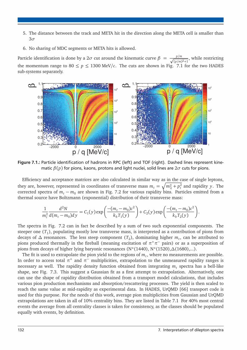
5. The distance between the track and META hit in the direction along the META cell is smaller than3σ

6. No sharing of MDC segments or META hits is allowed.

Particle identification is done by a 2σ cut around the kinematic curve β = p/m�(p/m)2+1

, while restricting

the momentum range to 80 ≤ p ≤ 1300 MeV/c. The cuts are shown in Fig. 7.1 for the two HADESsub-systems separately.

p / q [MeV/c]2000− 0 2000

β

0.2

0.3

0.4

0.5

0.6

0.7

0.8

0.9

1

1.1

1

10

210

310

410

510

p / q [MeV/c]2000− 0 2000

β

0.2

0.3

0.4

0.5

0.6

0.7

0.8

0.9

1

1.1

1

10

210

310

410

510

Figure 7.1.: Particle identification of hadrons in RPC (left) and TOF (right). Dashed lines represent kine-matic β(p) for pions, kaons, protons and light nuclei, solid lines are 2σ cuts for pions.

Efficiency and acceptance matrices are also calculated in similar way as in the case of single leptons,they are, however, represented in coordinates of transverse mass mt =

�m2π + p2

t and rapidity y . Thecorrected spectra of mt − m0 are shown in Fig. 7.2 for various rapidity bins. Particles emitted from athermal source have Boltzmann (exponential) distribution of their transverse mass:

1m2

t

d2Nd(mt −m0)d y

= C1(y)exp

�−(mt −m0)c2

kbT1(y)

�+ C2(y)exp

�−(mt −m0)c2

kbT2(y)

�.

The spectra in Fig. 7.2 can in fact be described by a sum of two such exponential components. Thesteeper one (T1), populating mostly low transverse mass, is interpreted as a contribution of pions fromdecays of Δ resonances. The less steep component (T2), dominating higher mt , can be attributed topions produced thermally in the fireball (meaning excitation of π+π− pairs) or as a superposition ofpions from decays of higher lying baryonic resonances (N*(1440), N*(1520),Δ(1680),...).

The fit is used to extrapolate the pion yield to the regions of mt , where no measurements are possible.In order to access total π+ and π− multiplicities, extrapolation to the unmeasured rapidity ranges isnecessary as well. The rapidity density function obtained from integrating mt spectra has a bell-likeshape, see Fig. 7.3. This suggest a Gaussian fit as a first attempt to extrapolation. Alternatively, onecan use the shape of rapidity distribution obtained from a transport model calculations, that includesvarious pion production mechanisms and absorption/rescattering processes. The yield is then scaled toreach the same value at mid-rapidity as experimental data. In HADES, UrQMD [66] transport code isused for this purpose. For the needs of this work, average pion multiplicities from Gaussian and UrQMDextrapolations are taken in all of 10% centrality bins. They are listed in Table 7.1 For 40% most centralevents the average from all centrality classes is taken for consistency, as the classes should be populatedequally with events, by definition.

132 7. Interpretation of dilepton spectra

]2 [MeV/c0-mtm0 200 400 600 800

]-3 )2

[(M

eV/c

dy 0-m t

dmN2 d

t2m1

6−10

4−10

2−10

1

210

410

610

810

1010

1210

1410

1610

]2 [MeV/c0-mtm0 200 400 600 800

]-3 )2

[(M

eV/c

dy 0-m t

dmN2 d

t2m1

4−10

2−10

1

210

410

610

810

1010

1210

1410

1610 0 0.19 *10≤ y ≤0.091 0.29 *10≤ y ≤0.192 0.39 *10≤ y ≤0.293 0.49 *10≤ y ≤0.394 0.59 *10≤ y ≤0.495 0.69 *10≤ y ≤0.596 0.79 *10≤ y ≤0.697 0.89 *10≤ y ≤0.798 0.99 *10≤ y ≤0.899 1.09 *10≤ y ≤0.9910 1.19 *10≤ y ≤1.0911 1.29 *10≤ y ≤1.1912 1.39 *10≤ y ≤1.2913 1.49 *10≤ y ≤1.39

Figure 7.2.: Differential distributions of π− (left) and π+ (right), corrected for acceptance and efficiency.Lines represent fits with a sum of two Boltzmann components.

cmy

1.5− 1− 0.5− 0 0.5 1 1.5

dN/d

y [1

/evt

]

0

2

4

6

8

10

120-10%10-20%20-30%30-40%

cmy

1.5− 1− 0.5− 0 0.5 1 1.5

dN/d

y [1

/evt

]

1

2

3

4

5

0-10%10-20%20-30%30-40%

Figure 7.3.: Total corrected yield of π− (left) and π+ (right) as a function of the rapidity. Full points aredata, open points are data reflected about Y = 0 axis. Dashed lines represent extrapolationwith the Gauss fit, solid lines – extrapolation with UrQMD.

The statistical uncertainty in the pion yield determination is negligible. The systematic one was es-timated to be of 10% and the main contribution is the extrapolation in rapidity. The same is thus theuncertainty of the 1/Nπ0 factor used to normalize dilepton spectra.

7.1. Normalization to the number of π0 133

Centrality ⟨Nπ−⟩ ⟨Nπ+⟩ ⟨Nπ0⟩ Tπ−

1 [MeV/kB] Tπ−

2 [MeV/kB] Tπ+

1 [MeV/kB] Tπ+

2 [MeV/kB]0-10% 17.05 9.75 13.40 49.4 ± 2.5 93.4 ± 4.7 61.4 ± 3.1 105.4 ± 5.3

10-20% 12.20 6.75 9.48 45.3 ± 2.3 87.7 ± 4.4 55.4 ± 2.8 97.2 ± 4.920-30% 8.85 4.80 6.83 43.2 ± 2.2 83.7 ± 4.1 52.0 ± 2.6 91.5 ± 4.630-40% 6.35 3.45 4.90 41.6 ± 2.1 80.5 ± 4.0 49.4 ± 2.5 87.0 ± 4.40-40% 11.10 6.20 8.65

Table 7.1.:Multiplicities and temperatures of charged pions and π0 calculated as their average. Statisticalerror is negligible and systematic one was estimated to 10%.

7.2 Neutral meson reconstruction with γ conversion

It is also possible to fully reconstruct neutral mesons π0 and η. This requires detection of real photons.At the time of the Au+Au experiment, HADES did not contain any detector for photon measurementusing e.g. calorimetry. Still, it is possible to detect e+e− pairs created in external γ conversions. Inthis type of analysis [41] leptons are identified based on a β vs. momentum cut only – besides the lowefficiency of the RICH detector, many conversions occur in its mirror and such cases would be lost whenrequiring a presence of a RICH ring.

Identified particles are combined into e+e−e+e− multiplets and their invariant mass is investigated.Properly selected topological cuts on opening angles between e+ and e− and between dilepton pairsreduce the background – both from wrong combinations and from hadron contamination due to veryconservative particle identification. The background is then fairly well described by event mixing, in thiscase mixed objects are whole e+e− pairs.

With this method π0 multiplicity in 40% most central events was estimated to be9.7 ± 0.27(stat) ± 1.8(syst) ± 1.3(extra) per event, where the first uncertainty takes into account allthe systematics besides the one, that comes from extrapolation to full phase space. This one is givenseparately as the second uncertainty. The result is consistent with the one from charged pion multiplic-ities, but in the case of conversion method the uncertainty is larger. In fact, the low multiplicity withoverwhelming background contribution makes the analysis very difficult and its result highly apprecia-ble. The η multiplicity in the 40% most central events is estimated to be0.107 ± 0.005(stat) ± 0.028(syst) ± 0.007(extra) per event. The uncertainty is quite large but, as itwill be shown later in this chapter, since η does not play any important role in the dilepton spectra fromAu+Au collisions, also its uncertainty has little impact on excess e+e− yield.

7.3 Invariant mass and excess radiation

Invariant mass spectrum of dilepton signal, corrected for efficiency is shown in Fig. 7.4 with statistic andsystematic uncertainty (the latter are shown as boxes around the symbols). Substantial yield is visible inthe mass range above π0, what allows to interpret the origin of the virtual photon radiation.

The first step is to compare with the reference measurement of p+p and n+p 1 at Ebeam = 1.25 GeV[83]. The difference should reveal medium radiation, not present in collisions of elementary hadrons. Ifthere were no such a radiation, heavy-ion collisions would look like a (properly scaled) sum of individualinteractions of their nucleons. In Au+Au there would be roughly the same probability for n+p collisionsas for p+p and n+n together and the radiation from p+p is assumed to be the same as from n+n. As aconsequence, an appropriate reference spectrum is an average of n+p and p+p.

For comparison, the sources, that radiate mainly after the freeze-out, have to be properly accountedfor. The comparison of the measured invariant mass spectrum to the freeze-out cocktail is shown in

1 It was measured in d+p reactions, with events selected, where neutron in deuteron was quasi-free


]2 [GeV/ceeM0 0.1 0.2 0.3 0.4 0.5 0.6 0.7 0.8

]-1 )2

[(G

eV/c

ee d

N/d

M0

π1/

N

9−10

8−10

7−10

6−10

5−10

4−10

3−10

2−100-40% centrality

0-40% centrality

Figure 7.4.: Invariant mass distribution of dilepton signal in Au+Au at Ebeam = 1.23A GeV in 40% mostcentral collisions. It is corrected for the efficiency and normalized to the π0 multiplicity. Errorbars represent statistical error (Poisson), rectangles are the systematic.

the left panel of Fig. 7.5. The ingredients are the same as described in Section 4.5.1 with the onlydifference that now ω→ π0e+e− channel is included (branching ratio 7.7 · 10−4). The radiation beyondthe freeze-out, is clearly visible.

In order to compare to reference, the spectrum has to be normalized to the number of pions produced,i.e. number of events analyzed times the π0 multiplicity per event. As the latter is approximately pro-portional to the system size [38] (i.e. number of π0 is constant as a function of ⟨Apart⟩), this assumes aproper scaling for NN reactions and gives an insight into effects, that are beyond simple superpositionof single colliding nucleons. From the scaled spectra, properly normalized η-Dalitz, calculated in sim-ulation, is subtracted. Nevertheless, in Au+Au reactions this contribution is smaller than 10% and it isnegligible, as it can be seen in the left panel of Fig. 7.5 and also by comparing with the right panel of thesame figure, where this yield is subtracted. The comparison of Au+Au spectrum to reference is shownin Fig. 7.5 (right panel) as overlay of the two distributions. A substantial excess can be seen, which isroughly of the factor 4.

7.3. Invariant mass and excess radiation 135

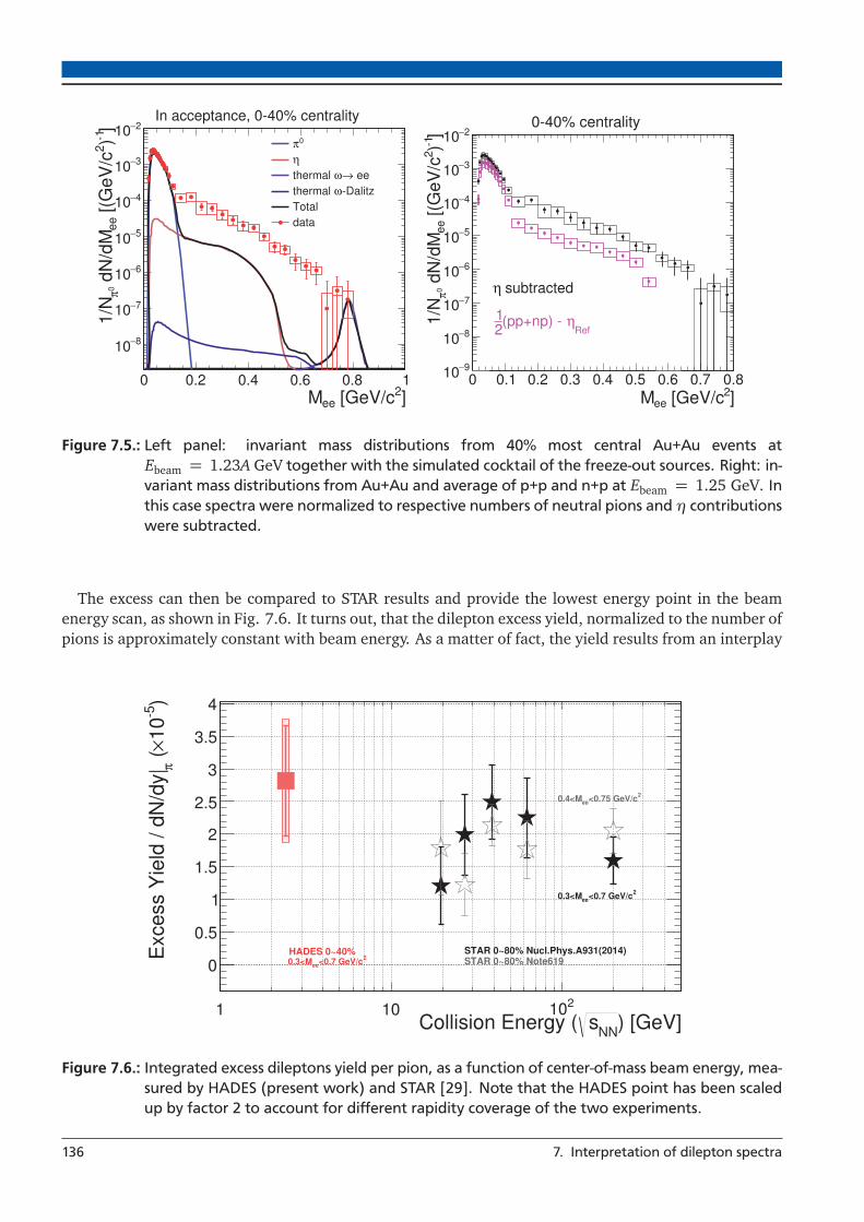
]2 [GeV/ceeM0 0.2 0.4 0.6 0.8 1

]-1 )2

[(G

eV/c

ee d

N/d

M0

π1/

N

8−10

7−10

6−10

5−10

4−10

3−10

2−100

π

η

ee→ωthermal -Dalitzωthermal

Totaldata

In acceptance, 0-40% centrality

]2 [GeV/ceeM0 0.1 0.2 0.3 0.4 0.5 0.6 0.7 0.8

]-1 )2

[(G

eV/c

ee d

N/d

M0

π1/

N

9−10

8−10

7−10

6−10

5−10

4−10

3−10

2−100-40% centrality

subtractedη

Refη(pp+np) -

21

Figure 7.5.: Left panel: invariant mass distributions from 40% most central Au+Au events atEbeam = 1.23A GeV together with the simulated cocktail of the freeze-out sources. Right: in-variant mass distributions from Au+Au and average of p+p and n+p at Ebeam = 1.25 GeV. Inthis case spectra were normalized to respective numbers of neutral pions and η contributionswere subtracted.

The excess can then be compared to STAR results and provide the lowest energy point in the beamenergy scan, as shown in Fig. 7.6. It turns out, that the dilepton excess yield, normalized to the number ofpions is approximately constant with beam energy. As a matter of fact, the yield results from an interplay

) [GeV]NNsCollision Energy (1 10 210

)-5

10× (

πE

xces

s Y

ield

/ dN

/dy|

0

0.5

1

1.5

2

2.5

3

3.5

4

HADES 0~40% STAR 0~80% Nucl.Phys.A931(2014)STAR 0~80% Note6192<0.7 GeV/cee0.3<M

2<0.7 GeV/cee0.3<M

2<0.75 GeV/cee0.4<M

Figure 7.6.: Integrated excess dileptons yield per pion, as a function of center-of-mass beam energy, mea-sured by HADES (present work) and STAR [29]. Note that the HADES point has been scaledup by factor 2 to account for different rapidity coverage of the two experiments.


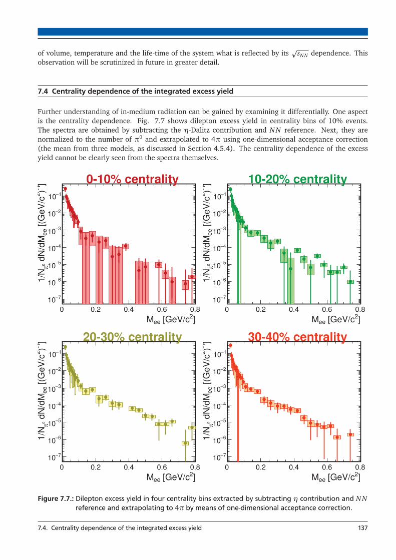
of volume, temperature and the life-time of the system what is reflected by its�

sNN dependence. Thisobservation will be scrutinized in future in greater detail.

7.4 Centrality dependence of the integrated excess yield

Further understanding of in-medium radiation can be gained by examining it differentially. One aspectis the centrality dependence. Fig. 7.7 shows dilepton excess yield in centrality bins of 10% events.The spectra are obtained by subtracting the η-Dalitz contribution and NN reference. Next, they arenormalized to the number of π0 and extrapolated to 4π using one-dimensional acceptance correction(the mean from three models, as discussed in Section 4.5.4). The centrality dependence of the excessyield cannot be clearly seen from the spectra themselves.

]2 [GeV/ceeM0 0.2 0.4 0.6 0.8

]-1 )2

[(G

eV/c

ee d

N/d

M0

π1/

N

7−10

6−10

5−10

4−10

3−10

2−10

1−10

0-10% centrality

]2 [GeV/ceeM0 0.2 0.4 0.6 0.8

]-1 )2

[(G

eV/c

ee d

N/d

M0

π1/

N

7−10

6−10

5−10

4−10

3−10

2−10

1−10

10-20% centrality

]2 [GeV/ceeM0 0.2 0.4 0.6 0.8

]-1 )2

[(G

eV/c

ee d

N/d

M0

π1/

N

7−10

6−10

5−10

4−10

3−10

2−10

1−10

20-30% centrality

]2 [GeV/ceeM0 0.2 0.4 0.6 0.8

]-1 )2

[(G

eV/c

ee d

N/d

M0

π1/

N

7−10

6−10

5−10

4−10

3−10

2−10

1−10

30-40% centrality

Figure 7.7.: Dilepton excess yield in four centrality bins extracted by subtracting η contribution and NNreference and extrapolating to 4π by means of one-dimensional acceptance correction.

7.4. Centrality dependence of the integrated excess yield 137

To make a qualitative assertion spectra are integrated in the range 0.3 < Mee < 0.7 MeV/c2. Thischoice has been made in view of possible relation of the dilepton yield to the lifetime of the fireballand a comparison to available STAR BES results. The integrals are shown in the left panel of Fig. 7.8as a function of the average number of participants. Here the increasing trend is present in two moreperipheral bins, which breaks down in central bins. The latter is not a physics effect but comes frominsufficient data quality as can be observed in Fig. 7.7. This is due to the small efficiency and signal-to-background ratio in the analysis using RICH ring finder (the two effects are related: loosing a lepton dueto inefficiency destroys the signal, but background remains almost unaffected). The problem is resolvedin the backtracking (BT) analysis, where the increasing trend is visible in all centrality bins [104] and theyields in the two peripheral bins are indeed consistent with the ones from the analysis discussed here.

⟩part

A⟨100 150 200 250 300

0π

/ N

eeN

0

0.001

0.002

0.003

0.004

0.005

0.006 0.3± = 0.2 α fit with part

αA

]2 < 100 [MeV/cee20 < M

subtractedNo reference

⟩part

A⟨100 150 200 250 300

0π

/ N

eeN

0

0.02

0.04

0.06

0.08

0.1

0.12

0.14

0.16

0.18

0.23−10× ]2 < 520 [MeV/cee120 < M

Figure 7.8.: Left panel: integrals of the spectra in the mass range dominated by π0 after η but withoutthe reference subtraction. Right panel: Integral of the excess yield above the π0 mass afterη and the reference subtraction as a function of the centrality. All integrals are normalizedto respective numbers of π0 deduced from charged pion multiplicities. Ticks represent statis-tical uncertainties, rectangles systematic (both on the integral and on ⟨Apart⟩). The non-filledrectangle in the middle corresponds to 0-40% most central events.

To verify this statement and exclude other issues like e.g. wrong normalization, one can considerintegrals in the invariant mass region dominated by π0-Dalitz decays (without subtracting the reference).In this case signal to background ratio is high in all centrality classes and the abundance of neutral pionsmakes the efficiency problem less important. The result is shown in the left panel of Fig. 7.8. Since thespectra are normalized to the number of π0 deduced from charge pion multiplicities, one would expectthe integrals to be constant as a function of ⟨Apart⟩. However, even in the considered mass range, thereis a contribution from medium radiation of about 10-20% of the total yield, cf. Figs. 7.14 and 7.15.Therefore, what is actually expected is a slight increase and it is indeed the case, as shown in Fig. 7.8(left panel).

7.5 Slopes of the spectra and what they tell us about the effective temperature of the source

Like in the case of charged pions, transverse mass spectra of dileptons are expected to have exponentialshape, from which an inverse slope parameter can be extracted, event though caution is needed wheninterpreting this parameter as the temperature of emitting source.


For the π0-Dalitz region the fits are shown in Fig. 7.9. Similar like in the case of charged pions,two-component fit consist of: (i) the steep slope up to ~400 MeV/c2 dominated by Δ→ Nπ0, (ii) theflat one, in wchich π0 from decays of various baryonic resonances are superimposed. Slope parametersextracted from the fit are summarized in the left panel of Fig. 7.10 and compared to the one obtainedfrom π− analysis. The values are lower than for charged pions. The reason is, that the spectra in Fig. 7.9are not for fully reconstructed π0, but for dileptons from its Dalitz decays and they are a convolution ofthe neutral pion distributions with the decay kinematics. It is illustrated in the right panel of Fig. 7.10. Asimple simulation has been performed, in which a sample of π0 with two thermal components, decayingsolely to the e+e−γ channel, was generated. Then transverse mass spectra of dileptons (sum of e+ ande− four-vectors) and of π0 (sum of four-vectors of e+, e− and γ) were plotted and fitted with a sum oftwo exponential components. Extracted inverse slope parameter for both components turned out to beby about 12 MeV/kB lower for the dilepton than for the π0. When taking into account the correction, theresults coincide with the ones from charged pions. Please note, that the effective temperature Teff fromthe fit to transverse mass/momentum is subject to the blue shift. In order to extract the temperature atkinetic freeze-out Tkin, the averaged radial expansion velocity ⟨βT⟩ has to be taken into account:

Tkin = Teff −m · ⟨βT⟩2. (7.1)

This gives for pions with Teff = 82.8 MeV/kB and ⟨βT⟩= 0.36 the value Teff = 64.6 MeV/kB.

It is often argued, that exponential (without any structure) shape of the invariant mass of the excesscan be a signature of chiral restoration. The HADES spectrum is shown in Fig. 7.11 for 40% most centralevents. Two variants are presented: (i) η contribution is subtracted, (ii) η and NN reference (minus re-spective η contribution) are removed. Single exponential function was fitted to both distributions in therange 0.2-0.8 GeV/c2. The inverse slope parameter from fit to the invariant mass has the advantage overthe one from fit to transverse mass or momentum, that it is not affected by the fireball expansion velocity(i.e. it is free from the blue shift and correspondingly lower, than the Teff extracted from a Boltzmannfit to transverse mass or momentum spectra). It can be therefore interpreted as the true temperatureof the source. The values extracted from the two variants are consistent, subtracting the reference hasno influence on them beyond the uncertainties. Taking into account that the spectra are integrated overspace-time evolution of the fireball, the result is in agreement with coarse-grained UrQMD simulation,as shown in Fig. 1.23, from which the (model-dependent) values of μB and of quark condensate, whichgets significantly depleted, can be read-off. Substantial depletion of the ⟨qq⟩ in the HADES range of Tand μB can be seen and this fact is reflected in the dilepton spectra.

7.5. Slopes of the spectra and what they tell us about the effective temperature of the source 139

]-5

/2)2

[(M

eV/c

dN

/dm

-1 )3/

2m 0

π(N 11−10

10−10

9−10

8−10

7−10

6−10

5−10 0-10% centrality

two Boltzmann

]-5

/2)2

[(M

eV/c

dN

/dm

-1 )3/

2m 0

π(N 11−10

10−10

9−10

8−10

7−10

6−10


two Boltzmann

]-5

/2)2

[(M

eV/c

dN

/dm

-1 )3/

2m 0

π(N 11−10

10−10

9−10

8−10

7−10

6−10


two Boltzmann

]-5

/2)2

[(M

eV/c

dN

/dm

-1 )3/

2m 0

π(N 11−10

10−10

9−10

8−10

7−10

6−10


two Boltzmann

]2 [MeV/cm0 200 400 600 800 1000

Rat

io to

fit

0

1

2/ndf = 2.05/82χ

]2 [MeV/cm0 200 400 600 800 1000

Rat

io to

fit

0

1

2/ndf = 1.15/82χ

]2 [MeV/cm0 200 400 600 800 1000

Rat

io to

fit

0

1

2/ndf = 3.99/82χ

]2 [MeV/cm0 200 400 600 800 1000

Rat

io to

fit

0

1

2/ndf = 2.11/82χ

Figure 7.9.: Dilepton transverse mass spectra in four centrality bins for invariant mass 0.15 < Mee <0.55 GeV/c2, fitted with a sum of two exponential functions.


⟩part

A⟨100 150 200 250 300

slop

eT

0

20

40

60

80

100

120-Dalitz)0

π(2T -Dalitz)0π(1T

)-π(2T )-π(1T

2 < 150 MeV/ceeFit to data for 0 < M

Figure 7.10.: Left: inverse slope parameters of two exponential components fitted to the transverse massof dileptons in the invariant mass range of 0 < Mee < 0.15 GeV/c2, compared to π−. Right:simulated spectra of transverse mass of π0 (magenta) and dileptons from its Dalitz decay(green) together with two exponent fit to both spectra and extracted inverse slope param-eters.

]-5

/2)2

[(G

eV/c

ee d

N/d

M-1 )

3/2

eeM 0

π(N

7−10

6−10

5−10

4−10

3−10

2−10

1−10

1

10

0-40% centrality

subtractedη

B3.50 MeV/k± = 70.73slopeT

single Boltzmann

0-40% centrality

]2 [GeV/ceeM0 0.2 0.4 0.6 0.8

Rat

io to

fit

0

1

2/ndf = 3.02/132χ

]-5

/2)2

[(G

eV/c

ee d

N/d

M-1 )

3/2

eeM 0

π(N

7−10

6−10

5−10

4−10

3−10

2−10

1−10

1

10

0-40% centrality

subtractedref

η(pp+np)-21 subtractedη

B4.61 MeV/k± = 71.73slopeT

single Boltzmann

0-40% centrality

]2 [GeV/ceeM0 0.2 0.4 0.6 0.8

Rat

io to

fit

0

1

2/ndf = 3.54/132χ

Figure 7.11.: Excess dilepton yield extracted by subtracting η contribution (left) and η as well as NNreference (right).

7.5. Slopes of the spectra and what they tell us about the effective temperature of the source 141

7.6 Comparison to previous HADES measurements

It is possible to interpret data in model-independent way by putting them in broader context of systemsize and collision energy dependence. The first of the two can be investigated thanks to data samplescollected by HADES over years in different runs. In Fig. 7.12 ratios of dilepton yields obtained indifferent experiments to the NN reference are shown. All samples have their respective η contributionssubtracted and they are normalized to the π0 multiplicities. Compared in this way, C+C spectra at twobeam kinetic energies [30, 37] are equivalent to the reference within errors. This means, that thereare no “medium effects” that would enhance virtual photon radiation compared to the the sources atfreeze-out. This also means that normalization to pions removes energy dependence – at least as long astheir multiplicity is also not affected by the medium.

Situation changes in case of Ar+KCl at Ebeam = 1.76A GeV. Here strong enhancement over thereference, of around factor 3, is visible above the π0 mass. The enhancement is even stronger in Au+Aucollisions (though only at very low invariant mass values), which can be interpreted as a confirmationof the previously observed “resonance-clock” of the fireball, i.e. the possibility to extract the lifetime ofthe fireball from the strength of the in-medium ρ0 radiation. It is also noticeable from the figure, thatthe radiation in Au+Au is stronger than in other experiments in the region below the π0 mass. This canbe compared to Figs. 7.14 and 7.15, where the radiation due to coupling with baryons has a significantcontribution in the π0-Dalitz region. In fact, the V-like shape of the Au+Au-to-reference ratio in thisregion is also consistent with theoretical picture developed above, since the “baryonic” contributionrelative to π0 is smallest at mass around 0.06 GeV/c2.

The Au+Au measurement can also contribute to the systematic study of the collision energy depen-dence of the excess yield. The left panel of Fig. 7.13 shows the excess over η yield, integrated in therange of 0.15− 0.5 GeV/c2, as well as yields of π0 and η. They are normalized to the average numberof participants Apart in order to cancel different centrality selection in different experiments and of trivialsystem size dependence. The same energy dependence of the excess was observed in C+C (black) andAr+KCl/Ca+Ca (blue, the two systems are considered as equivalent from the point of view of size andisospin), measured by HADES (full triangles [30, 37, 38]) and DLS (open triangles [31]). It is also nearlythe same as energy dependence of π0 production, which justifies normalization of dilepton spectra topion multiplicity. Solid lines through the π0 and η points are second-order polynomial fits. When theyare scaled down to go through baryonic radiation points, they indicate non-linear scaling of the latterwith ⟨Apart⟩ (the lines do not overlap). When it is taken into account, Au+Au may follow the energydependence established by lighter systems, but this would need to be confirmed by another Au+Aumeasurement in similar energy range (1− 2A GeV).

The extensive study of system size dependence is shown in the right panelof Fig. 7.13. The integral of the excess yield is shown for two integration ranges: 0.15 < Mee <0.5 GeV/c2 (blue) and 0.13 < Mee < 0.7 GeV/c2 (red). Squares are four centrality bins of Au+Au, starsare Ar+KCl at Ebeam = 1.76A GeV and triangles are C+C at Ebeam = 2A GeV. The latter two werescaled to Ebeam = 1.23A GeV using energy dependence of π0 production for the lower integration rangeand of η for the higher range, as in the left panel of the figure. This means, that in the lower range theAr+KCl yield was multiplied by 0.62 and C+C by 0.53. In the higher range the corresponding factorswere 0.46 and 0.38, respectively. This choice was driven by the observation, that the lower part of theintegration range brings a dominant contribution to the integrated yield, due to the exponential shape ofthe spectra, see Fig. 7.11. Secondly, the energy dependence of the dilepton production at given invariantmass was expected to be similar to meson production at this mass. The two spectra were corrected foracceptance in analogous way as it was discussed for Au+Au, using the cocktail consisting of π0, η andω with acceptance matrices for single leptons from corresponding experiments.2

2 The same as made public for theory: https://hades-wiki.gsi.de/foswiki/bin/view/Public/

HadesDataFilterAADileptons (accessed December 14th, 2016)


]2 [GeV/ceeM0 0.2 0.4 0.6

)ee

/dM

NN

)/(dN

ee/d

MAA

) (dN

0 πAA/N

0 πNN

(N 0

2

4

6

8

10

12Ar+KCl 1.76A GeVC+C 1A GeVC+C 2A GeVAu+Au 1.23A GeV

Figure 7.12: Ratio of the invariant mass yield inAu+Au, Ar+KCl and C+C to the refer-ence. Respective η contributions aresubtracted from all spectra.

[A GeV]beamE0 1 2

⟩pa

rtA⟨/π4

M

7−10

6−10

5−10

4−10

3−10

2−10

1−10

1 Au+Au,Ar+KClC+C,0π

η

rad.-e+ebaryonic

⟩part

A⟨10 210

π4 exce

ssN

6−10

5−10

4−10

3−10 0.13±=1.23α with part

αScaling as A

0.12±=1.23α with part

αScaling as A

Figure 7.13.: Left: energy dependence of inclusive multiplicity per participant for dilepton excess overη-Dalitz (extrapolated to 4π) as well as π0 and η. For the excess, full triangles are HADESmeasurements [30, 37, 38], open triangles – DLS [31]. π0 and ηwere measured with photoncalorimetry by TAPS collaboration in C+C (black) [39] and Ca+Ca (blue, equivalent to Ar+KCl)collisions [40]. Measurements of π0 in Au+Au collisions are from HADES [41], TAPS at 0.8and 1A GeV and E895 2A GeV [42]. Right: participant number dependence of the sameexcess for four Au+Au centrality classes (squares) Ar+KCl (stars) and C+C at Ebeam = 2A GeV,properly scaled to Ebeam = 1.23A GeV/c2. Blue points are integrated in 0.15 < Mee <0.5 GeV, the red ones in 0.3 < Mee < 0.7 GeV/c2. The power law fits to C+C, Ar+KCl andtwo peripheral Au+Au bins are shown and the exponents are printed.

The two central event classes of Au+Au are not reliable in the current analysis due to low efficiencyof the RICH. The two remaining confirm the power law scaling of the excess yield, as in [38], shrinkingat the same time the fit error. The result is N4π

excess∝ Aαpart with α= 1.23 for both integration ranges.

7.6. Comparison to previous HADES measurements 143

7.7 Comparison to theoretical models

Further understanding of the excess yield may come from the comparison to model calculations. One isthe thermal emission based on the ρ0 spectral function, with thermal parameters obtained from coarse-grained space-time cells of fireball simulated with UrQMD [89]. Freeze-out components discussed aboveare also added. As it can be seen in Fig. 7.14 (left panel) such a cocktail describes mass spectrum very

]-1 )2

[(G

eV/c

ee d

N/d

M0

π1/

N

8−10

7−10

6−10

5−10

4−10

3−10

2−100

π

η

ee→ωthermal

-Dalitzωthermal 0

ρCoarse-Graining

Total

data


]2 [GeV/ceeM0 0.2 0.4 0.6 0.8 1R

atio

to c

ockt

ail

0

1

2

]-1 )2

[(G

eV/c

ee d

N/d

M0

π1/

N

8−10

7−10

6−10

5−10

4−10

3−10

2−10

0ρCoarse-Graining

0π - ηdata -

- ref.ηdata -


]2 [GeV/ceeM0 0.2 0.4 0.6 0.8 1R

atio

to c

ockt

ail

0

1

2

Figure 7.14.: Left panel: invariant mass distributions from 40% most central Au+Au events atEbeam = 1.23A GeV and a cocktail comprising in-medium ρ0 from the coarse-grainingapproach and freeze-out contributions from π0, η and ω. Right panel: data points aftersubtracting the reference of elementary nucleon collisions (red) or main cocktail compo-nents π0 and η (green), compared to the in-medium ρ0 radiation only.

well in the invariant mass range above 0.4 GeV/c2 and there is some discrepancy for lower masses.One can also attempt to extract medium radiation by subtracting the reference from the experimentalspectrum (both properly normalized and after removing η contribution, as discussed above) and bycomparing it with the thermal ρ0 radiation only. This is shown in the right panel of Fig. 7.14. They stillagree within experimental uncertainties, at least above 0.2 GeV/c2. However, there is a systematic shiftwith respect to the left panel of the figure. A possible interpretation of this fact will be addressed lateron.

Before that, one may take a look at another calculation, Hadron String Dynamics (HSD) transportmodel [113]. The results of the calculation are compared with the data points in Fig. 7.15. Compared tothe cocktail including coarse-grained calculation of the spectral function, HSD describes data somewhatbetter below 0.4 GeV/c2 invariant mass, while above there is a clear discrepancy, which gets reduced afterinclusion of the ρ0 dropping mass and broadening effects. Note, that the HSD spectra are normalizedto the average number of π0 per event obtained in the simulation, i.e. 11.2, while the experimentallymeasured spectra are normalized to 8.65 resulting from charged pion analysis. Note also an important


]2 [1

/GeV

/cee

dN

/dM

0π

1/N

8−10

7−10

6−10

5−10

4−10

3−10

2−10-Dalitz0

π -Dalitzη

-Dalitzω -Dalitz+

Δ-e+e→ω

-e+e→ρ

p-n bremss. -N bremss.π

+brems.Δ+ρ Sumdata

HSD without medium effects

]2 [GeV/ceeM0 0.2 0.4 0.6 0.8 1

Rat

io to

mod

el

0

1

2

]2 [1

/GeV

/cee

dN

/dM

0π

1/N

8−10

7−10

6−10

5−10

4−10

3−10

2−10-Dalitz0

π -Dalitzη

-Dalitzω -Dalitz+

Δ-e+e→ω

-e+e→ρ

p-n bremss. -N bremss.π

+brems.Δ+ρ Sumdata

drop.+broaden.0ρHSD with

]2 [GeV/ceeM0 0.2 0.4 0.6 0.8 1

Rat

io to

mod

el

0

1

2

Figure 7.15.: Invariant mass distributions of 40% most central Au+Au events at Ebeam = 1.23A GeV com-pared to the result of the HSD calculation without including medium effects on the ρ0 (leftpanel) and with dropping mass and collisional broadening included (right panel).

role of the Δ regeneration in course of the heavy-ion collision in HSD [113], where up to 8 generationsof Δ are needed to saturate the dilepton yield. No higher lying resonances are included, although thework of [123] implies strong ρ0 coupling to such resonances.

Considering the two types of calculations together, one can notice, that in HSD both bremsstrahlungcontributions andΔ+-Dalitz have at low masses the spectral shape not very different from the in-mediumradiation from the coarse-graining approach. In contrast, even medium-modified ρ0 in HSD does notcontribute significantly to the low mass range. However, the vector meson spectral function in the coarse-graining is calculated within the strict Vector Meson Dominance model. This assumes, that actually alldileptons are mediated through vector mesons which are interpolating fields between hadrons and virtualphotons having the same quantum numbers and non-vanishing mass (due to virtuality). Therefore theρ0 spectrum in the coarse-graining approach saturates the dileptons radiation from the medium (theremight be also contributions from other vector mesons, ω and φ, treated in the same way) and sums allsources coherently.

The spectral function contains not only the dilepton radiation from the medium, but also Δ andbremsstrahlung contribution, which is present to some extent in the reference spectra. Therefore onecould question comparing experimentally extracted excess just with the medium ρ0 spectrum, as in theright panel of Fig. 7.14. The ratio of the data to model after subtracting the η contribution and thereference minus its respective η (red points in the right panel of Fig. 7.14) deviates from unity strongerthan the ratio after subtracting only the η from Au+Au data (green points) and also stronger than theratio of the full experimental spectrum to the full cocktail (left panel). Desirable would be to calculatethe spectral function in vacuum and check, whether it can be subtracted from the result of in-mediumcalculation. On the other hand, the in-medium radiation is emitted after fireball cells are thermalized

7.7. Comparison to theoretical models 145

and its largest contribution comes from about 10-20 fm/c (see Fig. 7.18), thus first-chance collisionsshould not be included in it.

At the same time, substantial deviation is present already before any subtraction (left panel) andremains after subtraction only η from Au+Au. This suggests, that the thermodynamic parameters ex-tracted from UrQMD differ from the real ones or that the in-medium radiation is overestimated in thecoarse-grained calculation of spectral function itself and it could be further scrutinized.

In Fig. 7.16 transverse mass distributions for the invariant mass 0 < Mee < 150 MeV/c2 are shownin four centrality bins, compared to HSD calculations and a hadronic freeze-out cocktail together within-medium radiation according to ρ0 spectral function calculated in the coarse-graining approach whenavailable. The agreement between data and models is fairly good.

Similar comparisons can be done in higher invariant mass range 0.15< Mee < 0.55 GeV/c2, as seen inFig. 7.17. There is in fact a very good agreement between shapes of the spectra from the two models andconsequently they both describe the data as far as it can be judged from the limited statistics. Exponentialfunction cannot be fitted to the spectra – their spectra are modified in a way typical for the radial flow,i.e. they get concave (compare e.g. to Fig. 7 in [86]). Still, good agreement between data and themodel based on the coarse graining allows to infer thermal properties of the radiating source from themodel. Fig. 7.18 shows a few of them. It turns out that the highest dilepton emission rate occurs in timerange of 10-20 fm/c. During this period transverse velocity βT, which is the measure of the radial fireballexpansion, accelerates from about 5 to 30% of the speed of light. This is also when highest temperatures(above 70 MeV/kB) and densities (as large as triple normal nuclear matter density) are reached. If thisis the case, dilepton spectra should be sensitive to drop of the quark condensate and partial restorationof the chiral symmetry.


]-5

/2)2

[(M

eV/c

dN

/dm

-1 )3/

2m 0

π(N 11−10

10−10

9−10

8−10

7−10

6−10

5−10 0-10% centrality med.withHSD,

CG + cocktail

]-5

/2)2

[(M

eV/c

dN

/dm

-1 )3/

2m 0

π(N 11−10

10−10

9−10

8−10

7−10

6−10


med.withHSD,

]-5

/2)2

[(M

eV/c

dN

/dm

-1 )3/

2m 0

π(N 11−10

10−10

9−10

8−10

7−10

6−10


med.withHSD,

]-5

/2)2

[(M

eV/c

dN

/dm

-1 )3/

2m 0

π(N 11−10

10−10

9−10

8−10

7−10

6−10


CG + cocktail

]2 [MeV/cm0 200 400 600 800 1000R

atio

to m

odel

0

1

2 to HSDto CG

]2 [MeV/cm0 200 400 600 800 1000R

atio

to m

odel

0

1

2

]2 [MeV/cm0 200 400 600 800 1000R

atio

to m

odel

0

1

2

]2 [MeV/cm0 200 400 600 800 1000R

atio

to m

odel

0

1

2 to HSDto CG

Figure 7.16.: Dilepton transverse mass spectra in four centrality bins for the invariant mass 0 < Mee <0.15 GeV/c2 compared to HSD transport model and a hadronic cocktail combined withcoarse-graining calculation. Models are normalized to the same value as data at 500MeV/c2.


]-5

/2)2

[(M

eV/c

dN

/dm

-1 )3/

2m 0

π(N

12−10

11−10

10−10

9−10

8−10


CG + cocktail

]-5

/2)2

[(M

eV/c

dN

/dm

-1 )3/

2m 0

π(N

12−10

11−10

10−10

9−10

8−10


med.withHSD,

]-5

/2)2

[(M

eV/c

dN

/dm

-1 )3/

2m 0

π(N

12−10

11−10

10−10

9−10

8−10


med.withHSD,

]-5

/2)2

[(M

eV/c

dN

/dm

-1 )3/

2m 0

π(N

12−10

11−10

10−10

9−10

8−10


CG + cocktail

]2 [MeV/cm0 200 400 600 800 1000R

atio

to m

odel

0

1

2

3 to HSDto CG

]2 [MeV/cm0 200 400 600 800 1000R

atio

to m

odel

0

1

2

3

]2 [MeV/cm0 200 400 600 800 1000R

atio

to m

odel

0

1

2

3

]2 [MeV/cm0 200 400 600 800 1000R

atio

to m

odel

0

1

2

3 to HSDto CG

Figure 7.17.: Dilepton transverse mass spectra in four centrality bins for the invariant mass 150 < Mee <550 MeV/c2 compared to HSD transport model and a hadronic cocktail combined withcoarse-graining calculation. Models are normalized to the same value as data at 500MeV/c2.


Figure 7.18.: Left: time evolution of thermodynamic properties of 7×7×7 central 1 fm3 cells of the fireballfrom the coarse graining. Right: time evolution of the cumulative dilepton yield in the rangeof 0.3< Mee < 0.7 GeV/c2 and of the transverse velocity.


7.8 Conclusions and outlook

The goal of this work was to reconstruct dilepton spectra in Au+Au collisions at Ebeam = 1.23A GeV bymeans of the data analysis based entirely on RICH ring reconstruction algorithms inherited from previousHADES runs. In the course of the analysis the mathematical formalism behind combinatorial backgroundsubtraction has been understood in great detail and this has lead to the introduction of the k-factorcalculated with the event mixing technique. The analysis faced large difficulties due to low efficiency ofthe ring reconstruction algorithms, that decreased the signal-to-background ratio. Despite that, it waspossible to extract thermal dilepton radiation from hot and dense fireball. It was compared to modelcalculations and relatively good agreement allowed to draw certain model-dependent conclusions aboutthe properties of nuclear matter under the conditions achieved in the energy regime under study. Thequantitative results of the models can now be regarded as reflecting the reality – at least approximately.Model-independent Boltzmann fits, especially to the invariant mass spectrum, allow to extract the truetemperature of the dilepton emitting source.

Even if the formalism of the two considered models, HSD and CG, is different, the qualitative physicalpicture that emerges to an experimenter is consistent. HSD is the transport calculation that predictsemission of dileptons in medium from Dalitz decay of Δ (regenerated appropriate number of times)and nucleon-nucleon and pion-nucleon bremsstrahlung together with the decays of thermally producedρ0 and adds them incoherently, on the level of probabilities. Coarse-grained calculation of the spectralfunction assumes strict vector meson dominance i.e. all virtual photons are mediated by ρ0 and itsspectra are modified by self-energy terms, that account essentially for the same elementary processes.Their contributions are added coherently, on the level of amplitudes. The difference between the twomodels is smaller than the statistical and systematic uncertainty of experimental data, this does notallow to discriminate between them, but further studies are ongoing. Also, while HSD tends to increaseappropriately the abundance of Δ and CG takes higher lying resonances into account, experimentaldata seem to be not sensitive to which resonant state is really excited. The fact, that the spectrum hasexponential shape signals thermal system. In the end, dilepton emission is enhanced due to various typesof interactions between hadrons, that occur more often due to high density. The density in turn translatesto change in the order parameter of chiral symmetry breaking. If it results in distinctive phase propertiesof the matter, it has to (and will) be further studied using observables that are yet to be proposed.

On the dilepton side, there is a number of topics that can be studied in the future. It would probablybe appreciable, that this is done using the novel backtracking algorithm (BT), which provides higherreconstruction efficiency and thus signal-to-background ratio. Of course, the analysis with ring findercan also be carried out in parallel in order to validate, that higher precision BT analysis has also at leastthe same accuracy as ring finder. Possible future analysis could involve

1. Angular distributions, especially dilepton polar anisotropy in the center-of-mass frame and possiblyalso in the helicity frame. This could be a further test for theoretical models and may provideadditional information on the nature of the emitting source.

2. Radial flow based on experimental data. In the current analysis it was only possible to compare theshape of transverse mass, modified by the expansion velocity, in a broad invariant mass range andafter verifying the agreement, to extract the ⟨βT⟩ from the model. With higher statistics it shouldalso be possible to plot mt spectra in narrow invariant mass bins. The inverse slope should thenbehave like according to Eq. 7.1. By fitting to the Mee dependence of the slope it should be possibleto extract ⟨βT⟩ and confront it with models.

3. Dilepton elliptic flow coefficient v2. It develops in the early stage of the collision and dileptons areideal probes as they leave the fireball without reinteractions.

4. Systematic uncertainty of the combinatorial background, calculated by comparing the true back-ground (wrong opposite-sign pairs) with its like-sign estimation, has now precision limited by the


statistics of the simulation used in the calculation. It would be impractical to simulate on presentcomputing facilities significantly more than 108 UrQMD events which are currently available (diskspace, computing time). One can consider using an event generator to simulate events containingonly a certain number of dileptons, but it is not clear, how realistic such a model would be.

5. A more extensive study of the dependence of the transverse mass/momentum slope of dileptonsfrom Dalitz decays on the thermal distribution of the mother particle would be interesting. Thiscan be done by simulating Dalitz decays of π0 or other particles decaying into Dalitz channel withdifferent source temperatures or by finding an analytic expression.

6. Last but not least: Estimation of the upper limit for u boson/dark photon needs to be finalized. Forthis, finely binned invariant mass distribution of dileptons serves as an input.

Further experiments are planned in HADES, in which investigation of thermal dilepton radiation andphase structure of strongly interacting matter will play a major role. The spectrometer will be upgradedby replacing Pre-Shower with an lead glass electromagnetic calorimeter (ECAL). It will not only allowto directly detect real photons but also should have electron to pion separation power as good as itwas designed for Pre-Shower. In April 2012 Au+Au beam it was hardly possible (due to aging) tomaintain Pre-Shower at high voltage values at which it operates in the streamer mode needed for leptonidentification. Therefore installation of the ECAL will in fact be an improvement. The other significantupgrade will be of the RICH detector. Photon detection plane based on the MWPC will be replaced by anarray of photomultipliers. This is expected to increase lepton identification efficiency.

After that, Ag+Ag at Ebeam = 1.65A GeV is going to be measured still at SIS18 accelerator (FAIRphase 0). As it can be presumed interpolating between coarse-graining calculations for Au+Au andAr+KCl runs, the density should not be much lower than in the former and the temperature not muchlower than in the latter. This means the most extreme combination of the two thermodynamic param-eters studied up to now with HADES. The aim here is to reconstruct ω and φ peaks and to accessintermediate-mass dileptons. Furthermore, ρ0 and a1 spectral functions will be measured in pion- andproton-induced reactions to address their behavior in cold nuclear matter. At future SIS100 acceleratorAg+Ag at Ebeam = 3.5A GeV experiment is planned and it may be able to thoroughly explore the mostinteresting region of the phase diagram with new exotic phases. The currently developed CBM (Com-pressed Baryonic Matter) experiment at FAIR will then study possible first-order phase transition(s) withhigh-precision data from Au+Au collisionns and may have a chance to hit the critical point, if it exists.

Yet many interesting phenomena are still to be explored with HADES and still at SIS18 and even stillwith already existing data!

7.8. Conclusions and outlook 151

Appendices

153

A Tuning Pre-Shower parameters

In this appendix procedures of calibrating gain of the Pre-Shower detector in HADES and of tuning itsdigitization parameters are described. The calibration is needed to optimize lepton identification, Thecorrect digitization is necessary for accurate efficiency correction based on Monte Carlo simulation.

A.1 Gain calibration

Calibration of Pre-Shower consists of two parts. One is calibration of the front-end electronics responseto charge induced on pads of planar read-out electrode. This part is done by registering ADC response ofeach read-out channel when a well defined charge is injected into it, and when there is no input charge,only noise. This is done many times for every channel (in practice the charge is injected alternatelyinto odd and even columns) in order to collect statistics sufficient for fitting a straight response line.Parameters of the line (slope and offset) are stored in the database for every channel. This allows to cutout the noise and equalize the response of different front-end modules. The procedure can be performedbefore, after and during breaks in data taking. It was done during all previous beam-times. Part of mymaster thesis [124] project was to adapt the software that calculates these calibration parameters to thenew version of HYDRA framework, developed for the Au+Au beam.

Already the charge induced when a particle with specific properties passes through the detector candepend on the location in the chamber due to different gas or geometry conditions. This has to be takeninto account if unitary particle identification condition is going to be used for the whole detector area. Aplaceholder for an additional, multiplicative calibration parameter that would level out such details wasforeseen in the database from the very beginning. It has, however, never been used in the experimentsbefore Au+Au, because resulting smearing of ΔQ (see Eq. 2.3), averaged over the whole detector, wasnot a crucial problem in lepton identification.

As described in Section 2.4.3, a Pre-Shower hit object contains information about charges integratedover corresponding 3×3 pads areas in the three chambers, while in the Pre chamber maximum charge islocated in the central pad. In order to calculated the gain parameter, histograms of charge integrals QPre,QPost I, QPost II are made for every pad from hits centered at this pad and in addition global histogramsare made for the whole detector. They are fitted with Landau’s distribution. Examples are shown in Fig.A.1.

Figure A.1.: Distributions ofQPre for hits centered at one single pad (left) and for all the hits in Pre-Showerdetector (right) together with Landau’s fits.

155

The gain factor is then a ratio of the Most Probable Values (MPV) from fit to the global histogram tothe one from a single pad:

gain(pad) =M PV (global)M PV (pad)

.

Figs. A.2 and A.3 show the effect of using the additional calibration parameter. Left panels of both



figures present data with gain = 1, right panels with values calculated as above. Fig. A.2 shows QPredistributions for all the pads in one sector, grupped by rows (gaps are between rows with less than 32pads). Fig. A.3 shows average QPre for every pad arranged in the way as in the real detector chamber.The calibrated gain levels out charges from different pads and makes the average distribution narrower,which results in better possibility to optimize the hard cut on ΔQ(p) (Section 3.5) as well as in betterperformance of the neural network with ΔQ as one of input observables.

The same gain calibration was performed (under my supervision) by A.Snoch, participant of HGS-HIReSummer Student Program at GSI 2015 for the pion beam campaign of June-August 2014 [125]. Theopportunity to revisit the procedure and its principles revealed the potential for its further optimization.It might be, that the trend of uncalibrated charge as a function of column within a single row originatesmainly from the incident angle of a particle on the detector plane, which is close to right angle in themiddle and smaller on the sides of each sector, due to geometry. This would be the result of longerpath of particles (the primary one and secondary conversion electrons) through gas chambers and largerionization. In this case Eq. 2.3 would need to be modified to take the angle into account and thegain parameter would involve only pure detector effects. In addition, the incident angle on the META

156 A. Tuning Pre-Shower parameters

wall would allow to improve the track-hit matching, especially for timing detectors, but it is not yetimplemented in DST.

A.2 Digitization parameters

An important step in Monte Carlo simulation of a detector system is digitization, generation of possiblyrealistic detector responses for given simulated particles. They corresponds to values measured in realexperiment and to detection probability of a real detector. If models used to generate such responsesare not sufficiently accurate, the statements based on Monte Carlo, especially spectra and quantitiescorrected for efficiency, cannot be considered as physically meaningful. In the case of Pre-Shower, digiti-zation is based on efficiency values and charge distributions measured in experiment. More specifically,QPre, QPost I and QPost I vs. particle’s velocity β distributions are stored, following the assumption, thatthis dependence is the strongest one. Similarly, the detection efficiency is assumed to depend on thevelocity. It also changes from pad to pad of the detector. It is not possible. Even the statistics from thewhole experimental run is too small to calculate the efficiency as a function of velocity for each individualpad. Therefore an average distribution of Eff(β) for the whole detector was computed and also for allthe pads average values, independent of velocity or any other particle’s property. They were comparedwith the overall value for the whole detector in order to obtain a pad-dependent scaling factor, by whichEff(β) is to be multiplied.

col0 5 10 15 20 25 30

row

0

5

10

15

20

25

30

0.7

0.75

0.8

0.85

0.9

0.95

1

efficiency, s0, m0

col0 5 10 15 20 25 30

row

0

5

10

15

20

25

30

0.7

0.75

0.8

0.85

0.9

0.95

1

efficiency, s1, m0

col0 5 10 15 20 25 30

row

0

5

10

15

20

25

30

0.7

0.75

0.8

0.85

0.9

0.95

1

efficiency, s2, m0

col0 5 10 15 20 25 30

row

0

5

10

15

20

25

30

0.7

0.75

0.8

0.85

0.9

0.95

1

efficiency, s3, m0

col0 5 10 15 20 25 30

row

0

5

10

15

20

25

30

0.7

0.75

0.8

0.85

0.9

0.95

1

efficiency, s4, m0

col0 5 10 15 20 25 30

row

0

5

10

15

20

25

30

0.7

0.75

0.8

0.85

0.9

0.95

1

efficiency, s5, m0

Figure A.4.: Efficiency of the Pre chamber as a function of detector pad.

Efficiency was calculated in the simplest possible way. For the Post I module, as reference detectorsserved Pre and Post II chambers. Therefore efficiency is the ratio:

Eff(Post I) =N(QPre > 0∧QPost I > 0∧QPost II > 0)

N(QPre > 0∧QPost II > 0).

A.2. Digitization parameters 157

col0 5 10 15 20 25 30

row

0

5

10

15

20

25

30

0.7

0.75

0.8

0.85

0.9

0.95

1

efficiency, s0, m1

col0 5 10 15 20 25 30

row

0

5

10

15

20

25

30

0.7

0.75

0.8

0.85

0.9

0.95

1

efficiency, s1, m1

col0 5 10 15 20 25 30

row

0

5

10

15

20

25

30

0.7

0.75

0.8

0.85

0.9

0.95

1

efficiency, s2, m1

col0 5 10 15 20 25 30

row

0

5

10

15

20

25

30

0.7

0.75

0.8

0.85

0.9

0.95

1

efficiency, s3, m1

col0 5 10 15 20 25 30

row

0

5

10

15

20

25

30

0.7

0.75

0.8

0.85

0.9

0.95

1

efficiency, s4, m1

col0 5 10 15 20 25 30

row

0

5

10

15

20

25

30

0.7

0.75

0.8

0.85

0.9

0.95

1

efficiency, s5, m1

Figure A.5.: Efficiency of the Post II chamber as a function of detector pad.

There is no other detector behind the Post II chamber that could be used as a reference, so the bestwhat could be assumed was that its efficiency is identical as the one of Post I. For Pre the whole trackingsystem can serve as a reference detector, second one being the Post I chamber. The efficiency can beexpressed as follows:

Eff(Pre) =N(Track exists∧QPre > 0∧QPost I > 0)

N(Track exists∧QPost I > 0).

The efficiency values as a function of detector pad of the Pre and Post I chambers are shown in Figs. A.4and A.5 for the situation that corresponds to parameters stored in the database.

Pre-Shower is only used to support lepton identification and as lepton candidates only the tracks areconsidered with β > 0.9. Therefore it is only crucial, that charge and efficiency values for high velocitytracks come directly from measurement. Below a specified value one can interpolate. It is not possible, touse measured values for all velocities, since at some point statistics becomes too low. In the final versionstored in the database the global efficiency for β < 0.6 was taken the same as for β = 0.6. The chargedistributions above roughly β = 0.85 were fitted with Laundau’s distributions. The fit parameters wereextrapolated up to β = 0 using an exponential fit to histograms of parameters as a function of velocity.Based on the Landau’s distributions with extrapolated parameters, charge vs. velocity histogram wasgenerated in the extrapolation region. An example of extrapolated charge vs. β distribution and globalefficiency as a function of β are shown in Fig. A.6.

The test of charge digitization is ΔQ vs. momentum distribution, shown in Fig. A.7 for experimentaldata (left) and Monte Carlo (right), for all particles after track sorting. This choice allows to select samplewith significant leptons contribution and especially of particles with β > 0.9. On the other hand, it doesnot bring the bias on the distribution due to usage of ΔQ and p in particle identification. The centralpart of the two plots, where well reconstructed electrons are dominating, shows very similar trend in


β

0 0.2 0.4 0.6 0.8 1

char

ge

0

50

100

150

200

250

300

350

0

0.02

0.04

0.06

0.08

0.1

0.12

0.14

0.16

0.18

0.2

, s0, m0βgeneric charge vs.

β

0 0.1 0.2 0.3 0.4 0.5 0.6 0.7 0.8 0.9 1

Effi

cien

cy

0.9

0.92

0.94

0.96

0.98

1

1.02

1.04

efficiency generic

Figure A.6.: Left: xtrapolated charge vs. particle’s velocity for sector 0, module Pre. Right: global effi-ciency as a function of velocity.

both cases. In other parts distributions are rather different. This is not due to wrong performance ofdigitizer, but rather due to larger amount of hadron-like background tracks in experiment.

Test of the digitizer efficiency as a function of β is shown in Fig. A.8 where it is compared betweensimulation and experiment for particle safter track sorting. The agreement on the level of few percent issatisfactory. As Shower observable is not the strongest particle identification criterion, it does not bringsignificant contribution to the overall systematic uncertainty.


q [MeV/c]×p1000− 500− 0 500 1000

QΔ

Sho

wer

400−

200−

0

200

400

600

800

1000

1200

1400

1

10

210

310

q [MeV/c]×p1000− 500− 0 500 1000

QΔ

Sho

wer

400−

200−

0

200

400

600

800

1000

1200

1400

1

10

210

310

Figure A.7.: Comparison ofΔQ vs. momentum distribution in experiment (left) and simulation (right) forparticles after track sorting.

Figure A.8: Cross-check of the efficiency of module 1(Post I) as a function of β in simulationand experiment.

β

0.9 0.92 0.94 0.96 0.98 1

Effi

cien

cy

0.5

0.6

0.7

0.8

0.9

1

1.1

ExperimentSimulation

Module 1


Acknowledgments

In the first place I owe my deepest gratitude to my Doktorvater for providing me a possibility to jointhe HADES group in Kraków already during my Master studies and in the beginning of PhD and myDoktormutter Tetyana Galatyuk for allowing me to continue the PhD in the group at TU Darmstadtunder the joint supervision agreement. Their guidance and discussions with them, sometimes quitelively but always deep and fruitful, enabled me to gain an understanding of what I am actually doingand, more importantly, why I am doing this. I am also very thankful for helping me to sort out all theformal and other issues that appeared during my studies.

I am indebted to “my post-doc”, Gosia Gumberidze for helping me in tedious every-day details of mywork. I would not go far without her continuously pointing out, that I must have a problem in someplace of my analysis (also helping to solve the problems), that my plots are wrong (different ranges onthe Y axis!) or that I have a typo in some PowerPoint slide. Of course my end would be even moremiserable without lending me several household items and car trips to a supermarket. Also results oncharged pion analysis, a crucially important input to my work, are coming from Gosia.

My deepest appreciation goes to HADES software coordinator Jochen Markert for taking care that weall can work smoothly and produce reliable results and for helping to solve the most difficult problemsrelated to programming. To him and to other memebers of data reconstruction team, especially Vladimirand Olga Pechenov and Georgy Kornakov, special thanks go for providing all us excellent quality data,with which we could play.

I am very grateful to those who were involved in the discussions about data analysis, in particular toJoachim Stroth, Romain Holzmann, Wolfgang Koenig and Patrick Sellheim.

I also thank to the teams of HSD and coarse-graining. Their results are highly important in under-standing and interpreting the experimental spectra, that I have plotted.

I would like to offer my special thanks to my colleagues from the TU Darmstadt group: Federico,Florian, Adrian and Frederic for awesome scientific discussions during our group meetings, for creatinga unique team atmosphere and for the fact, that what happens in the Ratskeller stays in Ratskeller (or atleast I hope so).

One should not forget all the colleagues from neighbor HADES groups in GSI and Frankfurt, whocreated a very friendly working environment: Christoph, Ilse, Jurek, Christian M., Manuel, ChristianW., Christina, Erwin, Claudia (also for telling the η multiplicity), Heidi, Timo, Erik, Behruz (also fordetermining centrality selection) and all the others.

I want to thank also Witek and Jacek from Kraków for assisting me with bits of paper work, that Icame across.

I am also very thankful to the whole HADES Collaboration for building the spectrometer and runningthe experiment, data from which I had a great pleasure to analyse. It is necessary to mention fantasticatmosphere of the Collaboration Meetings.

I thank the HGS-HIRe team for valuable support and organization of very interesting Lecture Weeks,Power Weeks and Soft-skill Courses as part of the Graduate Program. I spent a great time and havelearned a lot. I thank also prof. dr. Bengt Friman for the time devoted to our PhD Committee meetings.

I want also to express my gratitude to the proofreaders of the thesis: Piotr, Tetyana, Gosia and Florian(who corrected the German version of the abstract) – you did a huge amount of work! If the manuscripthas still some flaws, then it is only my fault.

I would like to thank my all my family, my parents and brothers for strong support and believing inme, especially my Mom for accepting the fact that her little baby decided to move abroad.


Bibliography

[1] Particle Data Group Collaboration, K. A. Olive et al., “Review of Particle Physics,” Chin. Phys.C38 (2014) 090001.

[2] H. Satz, Extreme States of Matter in Strong Interaction Physics. Springer-Verlag Berlin Heidelberg,2012.

[3] R. Barate et al., “Measurement of the axial-vector τ spectral functions and determination ofαs(M2

τ) from hadronic τ decays,” The European Physical Journal C - Particles and Fields 4 no. 3,(1998) 409–431. http://dx.doi.org/10.1007/s100529800895.

[4] M. Davier, A. Höcker, B. Malaescu, C.-Z. Yuan, and Z. Zhang, “Update of the ALEPH non-strangespectral functions from hadronic τ decays,” Eur. Phys. J. C74 no. 3, (2014) 2803,arXiv:1312.1501 [hep-ex].

[5] S. Zschocke, B. Kampfer, O. Pavlenko, and G. Wolf, “Evaluation of QCD sum rules for HADES,”2002.

[6] W. Peters, M. Post, H. Lenske, S. Leupold, and U. Mosel, “The Spectral function of the rho mesonin nuclear matter,” Nucl. Phys. A632 (1998) 109–127, arXiv:nucl-th/9708004 [nucl-th].

[7] B. Friman, C. Hohne, J. Knoll, S. Leupold, J. Randrup, R. Rapp, and P. S. (Eds.), The CBM PhysicsBook. Springer-Verlag Berlin Heidelberg, 2011.

[8] R. Rapp and J. Wambach, “Low-mass dileptons at the CERN-SpS: evidence for chiralrestoration?,” Eur. Phys. J. A 6 no. 4, (1999) 415–420.http://dx.doi.org/10.1007/s100500050364.

[9] V. L. Eletsky, M. Belkacem, P. J. Ellis, and J. I. Kapusta, “Properties of ρ and ω mesons at finitetemperature and density as inferred from experiment,” Phys. Rev. C 64 (Jul, 2001) 035202.http://link.aps.org/doi/10.1103/PhysRevC.64.035202.

[10] J. H. Hetherington and F. D. C. Willard, “Two-, Three-, and Four-Atom Exchange Effects in bcc3He,” Phys. Rev. Lett. 35 (Nov, 1975) 1442–1444.http://link.aps.org/doi/10.1103/PhysRevLett.35.1442.

[11] K. Fukushima and T. Hatsuda, “The phase diagram of dense QCD,” Rept.Prog.Phys. 74 (2011)014001, arXiv:1005.4814 [hep-ph].

[12] K. Fukushima and C. Sasaki, “The phase diagram of nuclear and quark matter at high baryondensity,” Prog. Part. Nucl. Phys. 72 (2013) 99–154, arXiv:1301.6377 [hep-ph].

[13] P. de Forcrand and O. Philipsen, “The curvature of the critical surface (m(u,d),m(s))**crit(mu):A Progress report,” PoS LATTICE2008 (2008) 208, arXiv:0811.3858 [hep-lat].

[14] O. Philipsen and C. Pinke, “The Nf = 2 QCD chiral phase transition with Wilson fermions at zeroand imaginary chemical potential,” Phys. Rev. D93 no. 11, (2016) 114507, arXiv:1602.06129[hep-lat].

[15] STAR Collaboration, M. M. Aggarwal et al., “An Experimental Exploration of the QCD PhaseDiagram: The Search for the Critical Point and the Onset of De-confinement,” 2010.

163

[16] A. Andronic, P. Braun-Munzinger, and J. Stachel, “Thermal hadron production in relativisticnuclear collisions: The Hadron mass spectrum, the horn, and the QCD phase transition,” Phys.Lett. B673 (2009) 142–145, arXiv:0812.1186 [nucl-th]. [Erratum: Phys.Lett.B678,516(2009)].

[17] J. Cleymans, H. Oeschler, K. Redlich, and S. Wheaton, “Comparison of chemical freeze-outcriteria in heavy-ion collisions,” Phys. Rev. C 73 (Mar, 2006) 034905.http://link.aps.org/doi/10.1103/PhysRevC.73.034905.

[18] J. Stachel, A. Andronic, P. Braun-Munzinger, and K. Redlich, “Confronting LHC data with thestatistical hadronization model,” Journal of Physics: Conference Series 509 no. 1, (2014) 012019.http://stacks.iop.org/1742-6596/509/i=1/a=012019.

[19] HADES Collaboration, G. Agakishiev et al., “Statistical model analysis of hadron yields inproton-nucleus and heavy-ion collisions at SIS 18 energiesStatistical hadronization modelanalysis of hadron yields in p + Nb and Ar + KCl at SIS18 energies,” Eur. Phys. J. A52 no. 6,(2016) 178, arXiv:1512.07070 [nucl-ex].

[20] FOPI Collaboration Collaboration, X. Lopez et al., “Subthreshold production of Σ(1385)baryons in Al+Al collisions at 1.9A GeV,” Phys. Rev. C 76 (Nov, 2007) 052203.http://link.aps.org/doi/10.1103/PhysRevC.76.052203.

[21] NA60 Collaboration, H. J. Specht, “Thermal Dileptons from Hot and Dense Strongly InteractingMatter,” AIP Conf. Proc. 1322 (2010) 1–10, arXiv:1011.0615 [nucl-ex].

[22] CBM Collaboration, S. Chattopadhyay et al., “Challenges in QCD matter physics - TheCompressed Baryonic Matter experiment at FAIR,” arXiv:1607.01487 [nucl-ex].

[23] CERES Collaboration Collaboration, G. Agakichiev et al., “Enhanced Production of Low-MassElectron Pairs in 200 GeV/Nucleon S-Au Collisions at the CERN Super Proton Synchrotron,”Phys. Rev. Lett. 75 (Aug, 1995) 1272–1275.http://link.aps.org/doi/10.1103/PhysRevLett.75.1272.

[24] CERES Collaboration, A. Marin et al., “Dilepton measurements with CERES,” PoS CPOD07(2007) 034, arXiv:0802.2679 [nucl-ex].

[25] J. Ruppert et al., “Low Mass Dimuons Produced in Relativistic Nuclear Collisions,” Phys. Rev. Lett.100 (Apr, 2008) 162301. http://link.aps.org/doi/10.1103/PhysRevLett.100.162301.

[26] H. van Hees and R. Rapp, “Dilepton radiation at the CERN super-proton synchrotron,” NuclearPhysics A 806 no. 1–4, (2008) 339 – 387.http://www.sciencedirect.com/science/article/pii/S0375947408004144.

[27] K. Dusling and I. Zahed, “Transverse momentum spectra of dileptons measured by the NA60Collaboration in In+In collisions at 158 GeV/nucleon,” Phys. Rev. C80 (2009) 014902,arXiv:hep-ph/0701253 [HEP-PH].

[28] ALICE Collaboration, D. Lohner, “Measurement of Direct-Photon Elliptic Flow in Pb-Pb Collisionsat�

sNN = 2.76 TeV,” J.Phys.Conf.Ser. 446 (2013) 012028, arXiv:1212.3995 [hep-ex].

[29] STAR Collaboration, P. Huck, “Beam Energy Dependence of Dielectron Production in Au + AuCollisions from STAR at RHIC,” Nucl. Phys. A931 (2014) 659–664, arXiv:1409.5675[nucl-ex].

[30] HADES Collaboration, G. Agakishiev et al., “Study of dielectron production in C+C collisions at1-A-GeV,” Phys. Lett. B663 (2008) 43–48, arXiv:0711.4281 [nucl-ex].

164 Bibliography

[31] DLS Collaboration, R. J. Porter et al., “Dielectron cross-section measurements in nucleus-nucleusreactions at 1-A/GeV,” Phys. Rev. Lett. 79 (1997) 1229–1232, arXiv:nucl-ex/9703001[nucl-ex].

[32] CBM Collaboration, S. Chattopadhyay et al., “Challenges in QCD matter physics - TheCompressed Baryonic Matter experiment at FAIR,” arXiv:1607.01487 [nucl-ex].

[33] S. Tavernier, Experimental Techniques in Nuclear and Particle Physics. Springer-Verlag, BerlinHeidelberg, 2010.

[34] T. Filippas et al., “Precision measurements of gas refractivity by means of a Fabry–Perotinterferometer illustrated by the monitoring of radiator refractivity in the DELPHI RICHdetectors,” Nuclear Instruments and Methods in Physics Research Section B: Beam Interactions withMaterials and Atoms 196 no. 3–4, (2002) 340 – 348.http://www.sciencedirect.com/science/article/pii/S0168583X02012910.

[35] “Rich Detector Principles.” http://physics.syr.edu/hep/rich.html. Accessed: 2014-12-24.

[36] L. Fabbietti et al., “Photon detection efficiency in the CsI based HADES RICH,” NuclearInstruments and Methods in Physics Research Section A: Accelerators, Spectrometers, Detectors andAssociated Equipment 502 no. 1, (2003) 256 – 260.http://www.sciencedirect.com/science/article/pii/S0168900203002845. ExperimentalTechniques of Cherenkov Light Imaging. Proceedings of the Fourth International Workshop onRing Imaging Cherenkov Detectors.

[37] HADES Collaboration Collaboration, G. Agakichiev et al., “Dielectron Production in 12C+12 CCollisions at 2A GeV with the HADES Spectrometer,” Phys. Rev. Lett. 98 (2007) 052302.

[38] HADES Collaboration, G. Agakishiev et al., “Dielectron production in Ar+KCl collisions at 1.76AGeV,” Phys. Rev. C84 (2011) 014902, arXiv:1103.0876 [nucl-ex].

[39] TAPS Collaboration Collaboration, R. Averbeck et al., “Production of π0 and η mesons incarbon-induced relativistic heavy-ion collisions,” Zeitschrift für Physik A Hadrons and Nuclei 359no. 1, (1997) 65–73.

[40] TAPS Collaboration Collaboration, R. Holzmann et al., “Contribution of π0 and η Dalitz decaysto the dilepton invariant-mass spectrum in 1A GeV heavy-ion collisions,” Phys. Rev. C 56 (1997)R2920–R2923.

[41] C. Behnke, Reconstruction of π0 and η Mesons via Conversion in Au+Au at 1.23 Gev/u with theHADES Spectrometer. PhD thesis, Goethe Universität Frankfurt, 2017.

[42] E895 Collaboration Collaboration, J. L. Klay et al., “Charged pion production in 2A to 8A GeVcentral Au+Au Collisions,” Phys. Rev. C 68 (2003) 054905.

[43] D. H. Perkins, Introduction to high energy physics, 4th ed. Press Syndicate of the University ofCambridge, 2000.

[44] B. Martin and G. Shaw, Particle Physics, 2nd ed. John Wiley & Sons, 1997.

[45] ATLAS Collaboration, G. Aad et al., “Observation of a new particle in the search for the StandardModel Higgs boson with the ATLAS detector at the LHC,” Phys. Lett. B716 (2012) 1–29,arXiv:1207.7214 [hep-ex].

[46] M. Maggiore, A Modern Introduction to Quantum Field Theory. Oxford University Press, 2005.

Bibliography 165

[47] LHCb Collaboration Collaboration, R. Aaij et al., “Observation of J/ψp Resonances Consistentwith Pentaquark States in Λ0

b→ J/ψK−p Decays,” Phys. Rev. Lett. 115 (Aug, 2015) 072001.

[48] M. E. Peskin and D. V. Schroeder, An Introduction to Quantum Field Theory. Westview Press, 1995.

[49] R. Hagedorn, “On the hadronic mass spectrum,” Nuovo Cim. A52 no. 4, (1967) 1336–1340.[,223(2016)].

[50] M. Gell-Mann, R. J. Oakes, and B. Renner, “Behavior of current divergences under SU(3) xSU(3),” Phys. Rev. 175 (1968) 2195–2199.

[51] S. Weinberg, “Precise Relations between the Spectra of Vector and Axial-Vector Mesons,” Phys.Rev. Lett. 18 (Mar, 1967) 507–509. http://link.aps.org/doi/10.1103/PhysRevLett.18.507.

[52] T. Das, V. S. Mathur, and S. Okubo, “Low-Energy Theorem in the Radiative Decays of ChargedPions,” Phys. Rev. Lett. 19 (Oct, 1967) 859–861.http://link.aps.org/doi/10.1103/PhysRevLett.19.859.

[53] OPAL Collaboration, K. Ackerstaff et al., “Measurement of the strong coupling constant α(s) andthe vector and axial vector spectral functions in hadronic τ decays,” Eur.Phys.J. C7 (1999)571–593, arXiv:hep-ex/9808019 [hep-ex].

[54] R. Rapp, J. Wambach, and H. van Hees, “The Chiral Restoration Transition of QCD and Low MassDileptons,” Landolt-Bornstein 23 (2010) 134, arXiv:0901.3289 [hep-ph].

[55] R. D. Pisarski, “Phenomenology of the Chiral Phase Transition,” Phys. Lett. B110 (1982)155–158.

[56] G. E. Brown and M. Rho, “Scaling effective Lagrangians in a dense medium,” Phys. Rev. Lett. 66(May, 1991) 2720–2723. http://link.aps.org/doi/10.1103/PhysRevLett.66.2720.

[57] G. Brown and M. Rho, “Chiral restoration in hot and/or dense matter,” Physics Reports 269 no. 6,(1996) 333 – 380.http://www.sciencedirect.com/science/article/pii/0370157395000674.

[58] C. Song, “Properties of vector mesons at finite temperature: Effective Lagrangian approach,”Phys. Rev. D 53 (Apr, 1996) 3962–3966.http://link.aps.org/doi/10.1103/PhysRevD.53.3962.

[59] H. Gomm, O. Kaymakcalan, and J. Schechter, “Anomalous spin-1-meson decays from the gaugedWess-Zumino term,” Phys. Rev. D 30 (Dec, 1984) 2345–2355.http://link.aps.org/doi/10.1103/PhysRevD.30.2345.

[60] HADES Collaboration, P. Salabura, J. Stroth, and L. Fabbietti, “The HADES Pion Beam Facility,”Nucl. Phys. News 25 no. 2, (2015) 22.

[61] P. M. Hohler and R. Rapp, “Is ρ-Meson Melting Compatible with Chiral Restoration?,” Phys. Lett.B731 (2014) 103–109, arXiv:1311.2921 [hep-ph].

[62] F.-L. V. et al., “Crystalline and amorphous ices,” in Proceedings of the International School ofPhysics “Enrico Fermi” Course 187 “Water: Fundamentals as the Basis for Understanding theEnvironment and Promoting Technology”, P. G. Debenedetti, M. A. Ricci, and F. Bruni, eds. IOS,Amsterdam, SIF, Bologna, 2015.

[63] P. Chomaz, “The Nuclear liquid gas phase transition and phase coexistence: A Review,” 2004.

166 Bibliography

[64] A. Kurkela and A. Vuorinen, “Cool quark matter,” Phys. Rev. Lett. 117 no. 4, (2016) 042501,arXiv:1603.00750 [hep-ph].

[65] STAR Collaboration Collaboration, L. Adamczyk et al., “Inclusive charged hadron elliptic flow inAu + Au collisions at

�sNN = 7.7–39 GeV,” Phys. Rev. C 86 (Nov, 2012) 054908.

http://link.aps.org/doi/10.1103/PhysRevC.86.054908.

[66] M. Bleicher et al., “Relativistic hadron hadron collisions in the ultrarelativistic quantummolecular dynamics model,” J.Phys. G25 (1999) 1859–1896, arXiv:hep-ph/9909407 [hep-ph].

[67] O. Buss et al., “Transport-theoretical Description of Nuclear Reactions,” Phys.Rept. 512 (2012)1–124, arXiv:1106.1344 [hep-ph].

[68] W. Ehehalt and W. Cassing, “Relativistic transport approach for nucleus-nucleus collisions fromSIS to SPS energies,” Nuclear Physics A 602 no. 3–4, (1996) 449 – 486.http://www.sciencedirect.com/science/article/pii/0375947496000978.

[69] P. Romatschke and U. Romatschke, “Viscosity Information from Relativistic Nuclear Collisions:How Perfect is the Fluid Observed at RHIC?,” Phys. Rev. Lett. 99 (Oct, 2007) 172301.http://link.aps.org/doi/10.1103/PhysRevLett.99.172301.

[70] C. Nonaka and S. A. Bass, “Space-time evolution of bulk QCD matter,” Phys. Rev. C 75 (Jan,2007) 014902. http://link.aps.org/doi/10.1103/PhysRevC.75.014902.

[71] J. Auvinen and H. Petersen, “Evolution of elliptic and triangular flow as a function of�

sNN in ahybrid model,” Phys. Rev. C88 no. 6, (2013) 064908, arXiv:1310.1764 [nucl-th].

[72] M. Bleicher, S. Endres, J. Steinheimer, and H. van Hees, “Recent results from the UrQMD hybridmodel for heavy ion collisions,” in International Workshop on Collectivity in Relativistic Heavy IonCollisions (IWoC 2014) Kolymbari, Crete, Greece, September 14-20, 2014. 2015.arXiv:1503.07371 [nucl-th].http://inspirehep.net/record/1355583/files/arXiv:1503.07371.pdf.

[73] ALICE Collaboration, B. B. Abelev et al., “Elliptic flow of identified hadrons in Pb-Pb collisions at�sNN = 2.76 TeV,” JHEP 06 (2015) 190, arXiv:1405.4632 [nucl-ex].

[74] J. Cleymans, H. Oeschler, and K. Redlich, “Influence of impact parameter on thermal descriptionof relativistic heavy ion collisions at (1-2) A-GeV,” Phys.Rev. C59 (1999) 1663,arXiv:nucl-th/9809027 [nucl-th].

[75] F. Becattini, J. Manninen, and M. Gazdzicki, “Energy and system size dependence of chemicalfreeze-out in relativistic nuclear collisions,” Phys.Rev. C73 (2006) 044905,arXiv:hep-ph/0511092 [hep-ph].

[76] A. Andronic, P. Braun-Munzinger, and J. Stachel, “Thermal hadron production in relativisticnuclear collisions: The Hadron mass spectrum, the horn, and the QCD phase transition,”Phys.Lett. B673 (2009) 142–145, arXiv:0812.1186 [nucl-th].

[77] R. Rapp and J. Wambach, “Chiral symmetry restoration and dileptons in relativistic heavy ioncollisions,” Adv. Nucl. Phys. 25 (2000) 1, arXiv:hep-ph/9909229 [hep-ph].

[78] NA60 Collaboration, R. Arnaldi et al., “First measurement of the rho spectral function inhigh-energy nuclear collisions,” Phys. Rev. Lett. 96 (2006) 162302, arXiv:nucl-ex/0605007[nucl-ex].

Bibliography 167

[79] PHENIX Collaboration, A. Adare et al., “Enhanced production of direct photons in Au+Aucollisions at

�sNN = 200 GeV and implications for the initial temperature,” Phys. Rev. Lett. 104

(2010) 132301, arXiv:0804.4168 [nucl-ex].

[80] PHENIX Collaboration, A. Adare et al., “Azimuthally anisotropic emission of low-momentumdirect photons in Au+Au collisions at

$s

NN= 200 GeV,” Phys. Rev. C94 no. 6, (2016) 064901,

arXiv:1509.07758 [nucl-ex].

[81] H. van Hees, C. Gale, and R. Rapp, “Thermal photons and collective flow at energies available atthe BNL Relativistic Heavy-Ion Collider,” Phys. Rev. C 84 (Nov, 2011) 054906.http://link.aps.org/doi/10.1103/PhysRevC.84.054906.

[82] H. van Hees, M. He, and R. Rapp, “Pseudo-critical enhancement of thermal photons in relativisticheavy-ion collisions?,” Nucl. Phys. A933 (2015) 256–271, arXiv:1404.2846 [nucl-th].

[83] HADES Collaboration, G. Agakishiev et al., “Origin of the low-mass electron pair excess in lightnucleus-nucleus collisions,” Phys. Lett. B690 (2010) 118–122, arXiv:0910.5875 [nucl-ex].

[84] R. Averbeck, R. Holzmann, V. Metag, and R. S. Simon, “Neutral pions and η mesons as probes ofthe hadronic fireball in nucleus-nucleus collisions around 1A GeV,” Phys. Rev. C 67 (Feb, 2003)024903. http://link.aps.org/doi/10.1103/PhysRevC.67.024903.

[85] R. Scheibl and U. W. Heinz, “Coalescence and flow in ultrarelativistic heavy ion collisions,” Phys.Rev. C59 (1999) 1585–1602, arXiv:nucl-th/9809092 [nucl-th].

[86] U. W. Heinz, “Concepts of heavy ion physics,” in 2002 European School of high-energy physics,Pylos, Greece, 25 Aug-7 Sep 2002: Proceedings, pp. 165–238. 2004. arXiv:hep-ph/0407360[hep-ph]. http://doc.cern.ch/yellowrep/CERN-2004-001.

[87] S. Endres, H. van Hees, J. Weil, and M. Bleicher, “Dilepton production and reaction dynamics inheavy-ion collisions at SIS energies from coarse-grained transport simulations,” Phys. Rev. C 92(Jul, 2015) 014911.

[88] F. Seck, “Towards realistic event generator for in-medium signals,” Master’s thesis, TechnischeUniversität Darmstadt, 2015.

[89] T. Galatyuk, P. M. Hohler, R. Rapp, F. Seck, and J. Stroth, “Thermal Dileptons fromCoarse-Grained Transport as Fireball Probes at SIS Energies,” Eur. Phys. J. A52 no. 5, (2016)131, arXiv:1512.08688 [nucl-th].

[90] G. Agakishiev et al., “Statistical hadronization model analysis of hadron yields in p + Nb and Ar+ KCl at SIS18 energies,” The European Physical Journal A 52 no. 6, (2016) 178.http://dx.doi.org/10.1140/epja/i2016-16178-x.

[91] HADES Collaboration, Proposal for a High-Acceptance Di-Electron Spectrometer. GSI, 1994.

[92] G. Agakichiev et al., “The high-acceptance dielectron spectrometer HADES,” The EuropeanPhysical Journal A 41 no. 2, (2009) 243–277.http://dx.doi.org/10.1140/epja/i2009-10807-5.

[93] J. D. Jackson, Classical Electrodynamics 3rd ed. John Wiley & Sons Inc., New York, 1999.

[94] M. Artuso et al., “The CLEO RICH detector,” Nuclear Instruments and Methods in Physics ResearchSection A: Accelerators, Spectrometers, Detectors and Associated Equipment 554 no. 1–3, (2005)147 – 194. http://www.sciencedirect.com/science/article/pii/S016890020501524X.

168 Bibliography

[95] C. Matteuzzi, “The LHCb RICH system: Detector performance,” Nuclear Instruments and Methodsin Physics Research Section A: Accelerators, Spectrometers, Detectors and Associated Equipment 766no. 0, (2014) 245 – 249.http://www.sciencedirect.com/science/article/pii/S0168900214004896. RICH2013Proceedings of the Eighth International Workshop on Ring Imaging Cherenkov DetectorsShonan, Kanagawa, Japan, December 2-6, 2013.

[96] G. Kornakov, “Time of Flight calibration and reaction time determination,” 2014. Talk in theHADES Collaboration Meeting XXVIII, Bratislava, Slovakia.

[97] D. Belver et al., “The HADES RPC inner TOF wall,” Nuclear Instruments and Methods in PhysicsResearch Section A: Accelerators, Spectrometers, Detectors and Associated Equipment 602 no. 3,(2009) 687 – 690.http://www.sciencedirect.com/science/article/pii/S0168900208019633. Proceedings ofthe 9th International Workshop on Resistive Plate Chambers and Related Detectors RPC08.

[98] A. Blanco et al., “{RPC HADES-TOF} wall cosmic ray test performance,” Nuclear Instruments andMethods in Physics Research Section A: Accelerators, Spectrometers, Detectors and AssociatedEquipment 661, Supplement 1 (2012) S114 – S117. X. Workshop on Resistive Plate Chambersand Related Detectors (RPC 2010).

[99] G. Kornakov et al., “Time of flight measurement in heavy-ion collisions with the HADES RPC TOFwall,” Journal of Instrumentation 9 no. 11, (2014) C11015.http://stacks.iop.org/1748-0221/9/i=11/a=C11015.

[100] W. Koenig and J. Pietraszko, “Beam detectors in Au+Au run,” 2012. Talk in the HADESCollaboration Meeting XXIV, Cracow, Poland.

[101] J. Pietraszko et al., “Radiation damage in single crystal CVD diamond material investigated witha high current relativistic 197Au beam,” Nuclear Instruments and Methods in Physics ResearchSection A: Accelerators, Spectrometers, Detectors and Associated Equipment 763 no. 0, (2014) 1 –5. http://www.sciencedirect.com/science/article/pii/S0168900214007013.

[102] J. Michel et al., “The HADES DAQ System: Trigger and Readout Board Network,” Nuclear Science,IEEE Transactions on 58 no. 4, (2011) 1745–1750.

[103] J. Markert, “Software and DST status,” 10, 2015. Talk on the XXX Hades Collaboration Meeting,Estoril, Portugal.

[104] P. Sellheim, Reconstruction of the low-mass dielectron signal in 1.23A GeV Au+Au collisions. PhDthesis, Goethe Universität Frankfurt, 2017.

[105] B. Kardan, Centrality Determination at 1.23A GeV Gold-Gold Collisions and Readout-Electronics forthe HADES Electromagnetic Calorimeter. PhD thesis, Goethe Universität Frankfurt, 2015.

[106] C. Ungethüm, “Searching for the Dark Photon,” Master’s thesis, Technische UniversitätDarmstadt, 2015.

[107] O. Pechenov and V. Pechenov, “News from Tracking in Low and High Multiplicities,” 10, 2014.Talk on the XXVIII Hades Collaboration Meeting, Bratislava, Slovakia.

[108] A. Hoecker et al., “TMVA: Toolkit for Multivariate Data Analysis,” PoS ACAT (2007) 040,arXiv:physics/0703039.

[109] L. Fabietti, Study of the e+e− pair acceptance in the dilepton spectrometer HADES. PhD thesis,Technische Universität München, 2003.

Bibliography 169

[110] I. Frohlich et al., “Pluto: A Monte Carlo Simulation Tool for Hadronic Physics,” PoS ACAT2007(2007) 076, arXiv:0708.2382 [nucl-ex].

[111] T. Kunz, “Photon Signal Response of the RICH Detector,” 2014. Talk in the HADES CollaborationMeeting XXVII, Munich, Germany.

[112] P. Huck, “Suche nach einem seltenen Zerfall des η-Mesons in pp-Reaktionen bei Ekin = 3.5 GeV,”Master’s thesis, Technische Universität München, 2009.

[113] E. L. Bratkovskaya et al., “System size and energy dependence of dilepton production inheavy-ion collisions at 1-2 GeV/nucleon energies,” Phys. Rev. C87 (2013) 064907.

[114] S. Constantinescu, S. Dita, and D. Jouan, “Study of the estimation of the combinatorial muonpair background,” 1996. Report PNO–DER–96–01.

[115] M. Gazdzicki and M. I. Gorenstein, “Background subtraction from the dilepton spectra in nuclearcollisions,” arXiv:hep-ph/0003319 [hep-ph].

[116] M. Abreu et al., “Dimuon and charm production in nucleus-nucleus collisions at the CERN-SPS,”The European Physical Journal C - Particles and Fields 14 no. 3, (2000) 443–455.http://dx.doi.org/10.1007/s100520000373.

[117] PHENIX Collaboration Collaboration, A. Adare et al., “Detailed measurement of the e+e− paircontinuum in p+ p and Au+Au collisions at

�sNN = 200 GeV and implications for direct photon

production,” Phys. Rev. C 81 (Mar, 2010) 034911.http://link.aps.org/doi/10.1103/PhysRevC.81.034911.

[118] A. Toia, Performance of the HADES Spectrometer for Dilepton Identification in the Reaction C+C at1-2 AGeV. PhD thesis, Justus-Liebig-Universität Giessen, 2004.

[119] STAR Collaboration, L. Adamczyk et al., “Measurements of Dielectron Production in Au+AuCollisions at

�sNN = 200 GeV from the STAR Experiment,” Phys. Rev. C92 no. 2, (2015) 024912,

arXiv:1504.01317 [hep-ex].

[120] ALICE Collaboration, M. K. Köhler, “Dielectron measurements in pp, p-Pb and Pb-Pb collisionswith ALICE at the LHC,” Nucl. Phys. A931 (2014) 665–669, arXiv:1407.7809 [nucl-ex].

[121] M. K. Köhler, Dielectron production in proton-proton collisions with ALICE. PhD thesis, TechnischeUniversität Darmstadt, 2014.

[122] H. Schuldes, Charged Kaon and φ Reconstruction in Au+Au Collisions at 1.23 AGeV. PhD thesis,Goethe Universität Frankfurt, 2016.

[123] A. V. Anisovich, R. Beck, E. Klempt, V. A. Nikonov, A. V. Sarantsev, and U. Thoma, “Properties ofbaryon resonances from a multichannel partial wave analysis,” Eur. Phys. J. A48 (2012) 15,arXiv:1112.4937 [hep-ph].

[124] S. Harabasz, “Procedury kalibracji i wizualizacji danych detektora kaskady elektromagnetycznejw zderzeniach ciezkich jonow,” Master’s thesis, Jagiellonian University, Cracow, 2011.

[125] A. Snoch, “Calibration of Pre-Shower detector gain for HADES,” 2015. HGS-HIRe SummerStudent Program at GSI – Book of Reports.

170 Bibliography

Curriculum vitae

Szymon Harabasze-mail: [email protected]

Education

2011 - 2017

Doctoral studies in Physics under a joint supervision agreement between Jagiellonian University in Cra-cow and Technische Universität Darmstadt

2011

Master of Science in PhysicsJagiellonian University in Cracow

2005

Maturity examI Liceum Ogólnokształcace im. Bartłomieja Nowodworskiego w Krakowie

Additional experience

July - August 2009

Participation in the GSI Summer Student Programm in Darmstadt, Germany

July 2012

HGS-HIRe soft-skills course I Making an Impact as an Effective Researcher

June 2013

HGS-HIRe soft-skills course II Leading Teams in a Research Environment

April 2013 - July 2015

Participation in tutoring the Physics Lab Course for the Advanced in the Institute of Nuclear Physics ofthe Technical University Darmstadt

Major international scientific conference contributions

September 2013

Fairness 2013 Workshop for young scientists with research interests focused on physics at FAIR, Berlin,GermanyTalk title: Electron identification in Au+Au collisions at 1.23 GeV/u using multivariate analysis

May 2014

Quarm Matter 2014, Darmstadt, GermanyPoster title: Di-electron reconstruction in [email protected] GeV/u

171

June 2016

Critical Point and Onset of Deconfinement 2016, Wrocław, PolandTalk title: Measurement of virtual photons radiated from Au+Au collisions at Ebeam = 1.23A GeV withHADES

Awards

October 2016

Giersch Excellence Award

Personal interests

• Computing, programming languages and technologies

• Culture tourism

• Poland’s and world history

172 Curriculum vitae

Reconstruction of virtual photons from Au+Au collisions at ...

Documents

Transcript of Reconstruction of virtual photons from Au+Au collisions at ...