Western University Western University

Scholarship@Western Scholarship@Western

Electronic Thesis and Dissertation Repository

9-12-2014 12:00 AM

Reconstructing the Spatial and Temporal Patterns of Daily Life in Reconstructing the Spatial and Temporal Patterns of Daily Life in

the 19th Century City: A Historical GIS Approach the 19th Century City: A Historical GIS Approach

Donald Lafreniere, The University of Western Ontario

Supervisor: Dr. Jason Gilliland, The University of Western Ontario

A thesis submitted in partial fulfillment of the requirements for the Doctor of Philosophy degree

in Geography

© Donald Lafreniere 2014

Follow this and additional works at: https://ir.lib.uwo.ca/etd

Part of the Human Geography Commons

Recommended Citation Recommended Citation Lafreniere, Donald, "Reconstructing the Spatial and Temporal Patterns of Daily Life in the 19th Century City: A Historical GIS Approach" (2014). Electronic Thesis and Dissertation Repository. 2433. https://ir.lib.uwo.ca/etd/2433

This Dissertation/Thesis is brought to you for free and open access by Scholarship@Western. It has been accepted for inclusion in Electronic Thesis and Dissertation Repository by an authorized administrator of Scholarship@Western. For more information, please contact wlswadmin@uwo.ca.

RECONSTRUCTING THE SPATIAL AND TEMPORAL PATTERNS OF

DAILY LIFE IN THE 19TH CENTURY CITY: A HISTORICAL GIS APPROACH

(Thesis Format: Integrated Article)

by

Donald Joseph Lafreniere

Graduate Program in Geography

A thesis submitted in partial fulfillment of the requirements for the degree of

Doctor of Philosophy

The School of Graduate and Postdoctoral Studies The University of Western Ontario

London, Ontario, Canada

© Donald Joseph Lafreniere 2014

ii

ABSTRACT

In recent years, historians and historical geographers have become interested in

the use of GIS to study historical patterns, populations, and phenomena. The result has

been the emergence of a new discipline, historical GIS. Despite the growing use of GIS

across geography and history, the use of GIS in historical research has been limited

largely to visualization of historical records, database management, and simple pattern

analysis. This is, in part, due to a lack of accessible research on methodologies and

spatial frameworks that outline the integration of both quantitative and qualitative

historical sources for use in a GIS environment. The first objective of this dissertation is

to develop a comprehensive geospatial research framework for the study of past

populations and their environments.

The second objective of this dissertation is to apply this framework to the study of

daily life in the nineteenth-century city, an important area of scholarship for historical

geographers and social historians. Other daily life studies have focused on various

experiences of daily life, from domestic duties and child rearing to social norms and the

experience of work in early factories. An area that has received little attention in recent

years is the daily mobility of individuals as they moved about the ‘walking city’. This

dissertation advances our understanding of the diurnal patterns of daily life by recreating

the journey to work for thousands of individuals in the city of London, Ontario, and its

suburbs in the late nineteenth century. Methodologies are created to capture past

populations, their workplaces, and their relationship to the environments they called

home. Empirical results outline the relationship between social class, gender, and the

journey to work, as well as how social mobility was reflected through the quality of

iii

individuals’ residential and neighbourhood environments. The results provide a new

perspective on daily mobility, social mobility, and environment in the late nineteenth-

century city. Results suggest that individuals who were able to be upwardly socially

mobile did so at the expense of substantial increases in their journey to work.

Keywords: Historical GIS, Journey to Work, Time-Space, Daily Life, Qualitative GIS,

Social Mobility

iv

CO-AUTHORSHIP STATEMENT

The following dissertation contains a manuscript which has been published in a

peer-reviewed journal. Donald Lafreniere was the principal and corresponding author for

the manuscripts. Dr. Jason Gilliland was the co-author providing important guidance,

supervision, and review of the manuscripts. The following citations are provided to

indicate the destinations of the manuscripts:

Chapter Three: Lafreniere, D., and Gilliland, J. 2014. All the World’s a Stage: A GIS

Framework for Recreating Personal Time-Space from Qualitative and Quantitative

Sources. Transactions in GIS, doi: 10.1111/tgis.12089

Chapter Four: Lafreniere, D. and Gilliland, J. (in preparation) Revisiting the Walking

City: A Geospatial Examination of the Journey to Work.

Chapter Five: Lafreniere, D. and Gilliland, J. (in preparation) Following the butcher, the

baker, and the candlestick-maker: Urban Environments, Social Mobility, and the Journey

to Work in the Nineteenth-Century City.

v

ACKNOWLEDGEMENTS

My deepest appreciation goes to my supervisor, Dr. Jason Gilliland for his

passionate support and mentorship throughout my PhD research.

I would like to thank my thesis examiners Dr. Jeff Hopkins, Dr. Michelle

Hamilton, Dr. Godwin Arku, and Dr. John Bonnett.

I also thank Morris O. Thomas and Dr. Chris Mayda for their early

encouragement that set me down my path towards a PhD and for initiating my love for

historical geography.

I am grateful for the financial support that made this research possible including

the Vanier Canada Graduate Scholarship, SSHRC Master’s Canada Graduate

Scholarship, Ontario Graduate Scholarship, and the Western Graduate Research

Scholarships.

I am thankful for the intellectual and collegial support of an amazing community

of scholars at Western and abroad. Among them: Doug Rivet, Dr. Richard Sadler, Tor

Oiamo, Dr. Pat Dunae, Dr. John Lutz, Dr. Sherry Olson, Martin Healy, John Osborne,

Sandra Kulon, Nick Van Allen, Chris Hewitt, Dr. Mathew Novak, and Dr. Janet Loebach.

I also wish to acknowledge the assistance of archivists from Western Archives

and Libraries, including Barry Arnott, John Lutman, Theresa Regnier, and Cheryl Woods

as well as my students, Jen Sguigna and Michael Carfagnini.

Finally, a heartfelt thank you goes to my wife Erin and son Peter who have always

supported my dreams and continually pushing me to strive for new heights.

vi

TABLE OF CONTENTS

ABSTRACT ........................................................................................................................ ii

CO-AUTHORSHIP STATEMENT .................................................................................. iv

ACKNOWLEDGEMENTS .................................................................................................v

TABLE OF CONTENTS ................................................................................................... vi

LIST OF TABLES ...............................................................................................................x

LIST OF FIGURES .......................................................................................................... xii

LIST OF APPENDICES .................................................................................................. xvi

CHAPTER ONE ..................................................................................................... 1

INTRODUCTION .............................................................................................................. 1

1.1 RESEARCH BACKGROUND ........................................................................ 1

1.2 GEOGRAPHIC CONTEXT ............................................................................. 6

1.3 STRUCTURE OF THE DISSERTATION ..................................................... 10

1.4 REFERENCES ............................................................................................... 11

CHAPTER TWO .................................................................................................. 15

BROAD LITERATURE THEMES ................................................................................. 15

2.1 DISCIPLINARY CONTEXT ............................................................. 15

2.1.1 Historical Trends .............................................................................. 16

2.1.2 An Emerging Discipline: Historical GIS ......................................... 19

2.1.3 Historical GIS- Epistemology and Methodological Debates ........... 21

2.1.4 Finding a Home within the Debates................................................. 24

2.2 THE CHALLENGE OF HISTORICAL SOURCES ...................................... 25

2.3 UNDERSTANDING COMMUNITY AND NEIGHBOURHOOD .............. 29

2.3.1 Conceptualizing Neighbourhood in the Nineteenth Century City ... 36

2.4 REFERENCES ............................................................................................... 37

vii

CHAPTER THREE.............................................................................................. 50

ALL THE WORLD’S A STAGE: A GIS FRAMEWORK FOR RECREATING

PERSONAL TIME-SPACE FROM QUALITATIVE AND QUANTITATIVE

SOURCES ........................................................................................................................ 50

3.1 ABSTRACT .................................................................................................... 51

3.2 INTRODUCTION .......................................................................................... 52

3.3 RELATED WORK ......................................................................................... 55

3.4 BUILDING GEOSPATIAL STAGES ........................................................... 57

3.4.1 The Built Environment Stage........................................................... 58

3.4.2 The Social Environment Stage......................................................... 61

3.5 INTEGRATING AND CONTEXTUALIZING NARRATIVES ................... 69

3.5.1 Digitalization and Text Parsing ....................................................... 70

3.5.2 Creating Events from Texts ............................................................. 71

3.6 GEOREFERENCING QUALITATIVE SOURCES ...................................... 73

3.7 TOWARDS SPATIAL STORIES- THE CASE OF

RICHARD MATTHEWS ......................................................................... 78

3.8 CONCLUSION ............................................................................................... 81

3.9 REFERENCES ............................................................................................... 83

CHAPTER FOUR ................................................................................................ 93

REVISITING THE WALKING CITY:

A GEOSPATIAL EXAMINATION OF THE JOURNEY TO WORK .......................... 93

4.1 ABSTRACT .................................................................................................... 94

4.2 INTRODUCTION .......................................................................................... 95

4.3 RELATED WORK ......................................................................................... 96

4.4 IDENTIFYING METHODOLOGICAL CHALLENGES ............................. 98

4.5 CASE STUDY: LONDON, CANADA ........................................................ 102

4.6 OVERCOMING LIMITATIONS ................................................................. 104

4.6.1 Larger Samples and Absolute Workplaces .................................... 104

4.6.2 Calculating the Journey to Work ................................................... 118

4.6.3 Comparing Euclidean and Network Methods ................................ 123

4.6.4 Comparing to Assumed Workplaces Method ................................ 130

viii

4.7 THE WALKING CITY OBSERVED .......................................................... 136

4.7.1 Differing Commutes by Occupational Class ................................. 138

4.7.2 Coincident Home-Work Locations ................................................ 143

4.7.3 Women’s Experiences ................................................................... 150

4.8 CONCLUSION ............................................................................................. 154

4.9 REFERENCES ............................................................................................. 156

CHAPTER FIVE ................................................................................................ 174

FOLLOWING THE BUTCHER, THE BAKER, AND THE CANDLESTICK-MAKER:

URBAN ENVIRONMENTS, SOCIAL MOBILITY, AND THE JOURNEY TO WORK

IN THE NINETEENTH-CENTURY CITY.................................................................. 174

5.1 ABSTRACT .................................................................................................. 175

5.2 INTRODUCTION ........................................................................................ 176

5.3 ESTABLISHING LONGITUDINAL LINKS .............................................. 178

5.3.1 Preparing Data for Record Linkage ............................................... 182

5.3.2 Record Linkage Results ................................................................. 184

5.4 RESIDENTIAL, OCCUPATIONAL, AND WORKPLACE .............................

MOBILITIES .......................................................................................... 187

5.4.1 Residential Mobility....................................................................... 188

5.4.2 Occupational Mobility and Job Tenure.......................................... 196

5.4.3 Changing Home-Work Relationships ............................................ 202

5.5 CAPTURING HISTORIC ENVIRONMENTS ............................................ 207

5.5.1 Residential Environment Quality Indicators .................................. 210

5.4.2 Neighbourhood Environment Quality Indicators........................... 211

5.6 THE COMPLEXITIES OF URBAN LIFE: ENVRIONMENTS,

SOCIAL MOBILITY, AND THE JOURNEY TO WORK ................... 221

5.6.1 Residential Environments, Social Mobility and the ............................

Journey to Work .......................................................................... 225

5.6.2 Neighbourhood Environments, Social Mobility and the ....................

Journey to Work ......................................................................... 230

5.7 CONCLUSION ............................................................................................. 237

ix

5.8 REFERENCES ............................................................................................. 239

CHAPTER SIX ................................................................................................... 247

CONCLUSION............................................................................................................... 247

6.1 SUMMARY .................................................................................................. 247

6.2 FUTURE DIRECTIONS .............................................................................. 252

6.3 REFERENCES ............................................................................................. 254

APPENDICES .................................................................................................................255

CURRICULUM VITAE ..................................................................................................273

x

LIST OF TABLES Table 1.1 Chombart de Lauwe’s Hierarchy of Social Spaces........................................................4 Table 1.2 Distribution of Population by Ethnic Origin: London City and Suburbs, 1881 Census

of Canada .......................................................................................................................8 Table 2.1 Criticism of quantitative history and GIS ....................................................................22 Table 3.1 Number of Actors and Events Mapped by Geocoding Procedure ...............................76 Table 4.2 Geocoded Census Population Compared to the Total Census Population: London City and Suburbs, 1881 ................................................................................106 Table 4.3 Match Weights Used to Record Link Census/City Directory Database to Business Directory .................................................................................................110 Table 4.4 Comparison of Geocoded City Directory Sample to Journey to Work Sample, 1881..............................................................................................................114 Table 4.5 Modified Darroch and Orenstein Occupational Class Scheme ..................................115 Table 4.6 Comparing Spatial Distribution, by Census Geography, of the Workforce Sample to the Geocoded Total Population Dataset Distributed Across Occupational Classes .................................................................................................118 Table 4.7 Working at Closest Workplace vs. Actual Workplace: Brewery and Cigar Factory Workers.........................................................................................................133 Table 4.8 Cumulative Percentage at Specified Distances from Workplace (in km)..................140 Table 4.9 Percentage of Workers with Coincident Home-Work Locations for Select Occupations: London, Philadelphia, and Milwaukee, 1880-81 .................................145

xi

Table 5.1 Match Weights Used to Record Link 1881 Worker Sample to 1891 Worker Sample ..........................................................................................................184 Table 5.2 Percentage of Occupational Mobility 1881-1891 by Direction and Occupational Class.....................................................................................................197 Table 5.3 Occupational Mobility by Occupational Class, 1881-1891, by Residential Mobility, Percentage of Individuals ...........................................................................198 Table 5.4 Changing Home-Work Relationships ........................................................................201 Table 5.5 Linked Worker Sample Journey to Work 1881-1891 by Occupational Class ...........203 Table 5.6 Residential and Neighbourhood Environment Indicators ..........................................220 Table 5.7 Determining Social Mobility by Residential Environmental Indicators ....................224 Table 5.8 Determining Social Mobility by Neighbourhood Environmental Indicators ............225 Table 5.9 Changes in Residential Environment, by Indicators ..................................................227 Table 5.10 Relationship Between Changes in Residential Environments and the Daily Journey to Work .........................................................................................................229 Table 5,11 Changes in Neighbourhood Environment, by Indicators ...........................................231 Table 5.12 Relationship between changes in Neighbourhood Environments and the Daily Journey to Work ...............................................................................................................234

xii

LIST OF FIGURES Figure 1.1 Location of Study Site: London, Ontario, Canada .........................................................8 Figure 2.1 The Steevian Scheme of Community ..........................................................................31 Figure 3.1 1915 Fire Insurance Plan of London ............................................................................59 Figure 3.2 Built Environment Stage workflow .............................................................................60 Figure 3.3 Social Environment Stage workflow ...........................................................................63 Figure 3.4 Example of variables included in the 1891 social environment stage geodatabase .........................................................................................................66 Figure 3.5 Built and Social Environment Stages used together to explore children’s potential exposure to noxious environments on their journey to school .....................68 Figure 3.6 Distances travelled within an industrial area by children on their daily journey to school ..........................................................................................................69 Figure 3.7 Workflow to integrate and contextualize qualitative sources in a GIS ........................72 Figure 3.8 Georeferencing workflow for narrative sources ..........................................................75 Figure 3.9 Built and Social Environments used to spatialize Actors in Richard Matthews diary 77 Figure 3.10 ArcScene 10 provides the ability to model the built and social environments of the city in three-dimensions. The Stages are used in concert to recreate this time-space path of a postal clerk’s morning journey to work ..............................81

xiii

Figure 4.1 Excerpt of the London Classified Business Directory, 1881 .....................................109 Figure 4.2 Network Derived Journey to Work Scheme ..............................................................121 Figure 4.3 Distribution of Distances Traveled to Work ..............................................................122 Figure 4.4 Daily Traffic Patterns in London and Suburbs, 1881 ................................................123 Figure 4.5 Differences between Euclidean and Network Distance Methods ..............................124 Figure 4.6 Percentage of Network Distance that is Underrepresented when the Euclidean Method is used – by Number of Journeys ................................................126 Figure 4.7 Percentage of Network Distance that is Underrepresented when the Euclidean Method is used as related to Network--Derived Distance ........................127 Figure 4.8 Earnest Smith’s Journey to Work Using Euclidean and Network Methods ..............129 Figure 4.9 Closer look at Earnest Smith’s Journey to Work in the Dense Urban Core ..............130 Figure 4.10 Brewery Workers: Differences between Closest and Actual Employer ....................135 Figure 4.11 Cigar Factory Workers: Differences between Closest and Actual Employer ...........136 Figure 4.12 Used to Determine Work at Home vs Work Outside of the Home Status ..............................................................................................................138 Figure 4.13 Relationship between Labourers and their Workplaces .............................................142 Figure 4.14 Lawyer’s Residences and Law Offices in London, 1881 ..........................................147

xiv

Figure 4.15 Doctor’s Residences and Doctor’s Offices in London, 1881 ....................................148 Figure 4.16 Distance to Work for Women, Select Occupations, in Metres ..................................152 Figure 5.1 Record Linkage Procedure .........................................................................................187 Figure 5.2 Distance of Residential Moves from 1881 to 1891 ...................................................189 Figure 5.3 Distance of Residential Moves from 1881 to 1891 by Age of Household Head ........................................................................................................189

Figure 5.4 Distance of Residential Moves from 1881 to 1891 by Household Size .........................................................................................................191 Figure 5.5 Distance of Residential Moves from 1881 to 1891 by 1881 Occupational Class ..........................................................................................................................192

Figure 5.6 Linear Mean Direction and Distance of Moves by 1881 Occupational Class ..........................................................................................................................194

Figure 5.7 Woodfield Heritage Conservation District 2008 ......................................................195 Figure 5.8 Old East Village Heritage Conservation District 2008 .............................................195 Figure 5.9 The Changing Journey to Work and Residence- Ira Collins ....................................205 Figure 5.10 The Changing Journey to Work and Residence- Amelia Miller ...............................206 Figure 5.11 Multi-Scaled Environmental Indicators Used to Determine Quality of Residential and Neighbourhood Environments .........................................................209

xv

Figure 5.12 Model for Population-Based Viewshed Buffer ..........................................................215 Figure 5.13 Examples of Population-Based Buffers at Diffferent Population Thresholds for the Same Residence in 1881 and 1891 ................................................................216 Figure 5.14 The Complex Web of Social Neighbourhoods in London.........................................217 Figure 5.15 Industrial Environment and Workers Residence, 1881 .............................................219 Figure 5.16 Upwardly Mobile Workers Move Out of Industrial Environments into Suburban Neighbourhoods.........................................................................................232 Figure 6.1 Melding of Disciplines Represented in this Dissertation ...........................................252

xvi

LIST OF APPENDICES Appendix A Modified Darroch and Ornstein Occupational Class Scheme. ..................................255

1

CHAPTER ONE

Introduction

1.1 RESEARCH BACKGROUND

What was the experience of living in the nineteenth-century industrial city? To

what extent did people segregate themselves along ethnic lines, religious affiliation, and

social status? What was the daily life like outside of the home domain—in the

workplace, schools, churches, and social clubs? A diverse literature exists on the

residential patterning in the rapidly industrializing cities of nineteenth-century North

America. Sam Bass Warner Jr.’s classic work on Philadelphia (1968) and Peter

Goheen’s sophisticated empirical study of the spatial organization of population in

Toronto (1970) are among the early influential works. Olivier Zunz’s (1982) work on

heavily-segregated industrial Detroit extended population studies beyond residential

patterns to divisions within employment, religion, education, and access to services.

Studies like these have mainly been constructed using aggregated samples of census

records and tax rolls to examine the nature and patterns of ethnic and socioeconomic

concentration, as well as other social indicators such as rate of homeownership, family

organization, and demographic behaviour. Their results are often summarized in indices,

tables, and graphs which highlight concentrations and fluctuations of various populations

over time and space. But what was life like outside of the home? While these early

empirical studies highlight the nocturnal spatial patterns and allow inferences of the

social processes behind segregation and home ownership in selected cities, they do not

tend to reveal very much about how these patterns and processes influenced the diurnal

2

experiences of ordinary people. The practices of daily life outside of the home are

typically absent in historical geographic studies.

Ever since the emergence of La Nouvelle Histoire (Le Goff, Chartier and Revel

1978), nineteenth-century daily life studies have become an important area of scholarship

for many social historians (Alexander 2007, Bradbury 1996, Lacelle 1987, Mitchell 2009,

Picard 2005). Daily life in this scholarship has been framed in the narrative tradition of

history: rich textual explorations of the most intimate details of life, from the

practicalities of refuse collection to proper dress for an outing to the music hall. In most

cases, this scholarship is derived from an examination of the literary accounts of city life,

including daily newspapers, letters, and personal diaries (McCulloch 2004). This

scholarship is an important layer in our understanding of the day-to-day experiences of

ordinary people; however, it is not the only approach found within the historiography of

nineteenth-century urban life.

Inspired by the techniques and writings that emerged during the quantitative

revolution of geography in the 1960s, urban historical geographers began to revisit the

numerical evidence available in census records, tax rolls, and city directories to construct

their interpretations of the patterns of daily life (Dennis 1977, Greenberg 1981, Lees

1969, C. Pooley 1984). Coupling this quantitative approach with the qualitative,

narrative approach familiar to social historians provides a well-diversified historiography

on the daily life of Victorian citizens. However, Richard Dennis (2000), in a critical

review of the state of urban historical geography, argues that modern urban historical

geographers should be “eclectic in the sources they use and the approaches they adopt”

3

(p. 242). Dennis calls for a ‘triangulation’ of different kinds of sources that inform one

another. Literary accounts of city life should be cross-examined by the statistical record,

while quantitative sources require the contextualization of the narratives (Dennis 2000).

The empirical aim of this dissertation is to advance our understanding of the

social spaces and interactions in the industrial city by ‘triangulating’ a host of sources to

reconstruct the daily movements of people within the nineteenth-century city. I take a

theoretical lead from Robert Park’s (1925) assertion that social relations are inevitably

correlated with spatial relations, that physical distances are the indexes of social

distances. Richard Dennis (1977), in his examination of marriage patterns in Victorian

Huddersfield, England, tested Park’s theory and found that physical distance operated

independently of social distance. Dennis concluded, however, by saying that this

relationship needs to be reassessed at multiple scales of analysis, with information on

forms of interaction other than marriage, and with more precise measurements of distance

than were afforded by the district-to-district calculations he computed. This study tests

Park’s concept empirically by taking Dennis’ (1977, 2000) suggestions and

reconstructing the daily movements of individuals using a ‘triangulation’ of archival

sources rich with spatial and temporal data, such as censuses, city directories, personal

diaries, school attendance registers, and cartographic sources. I examine daily social

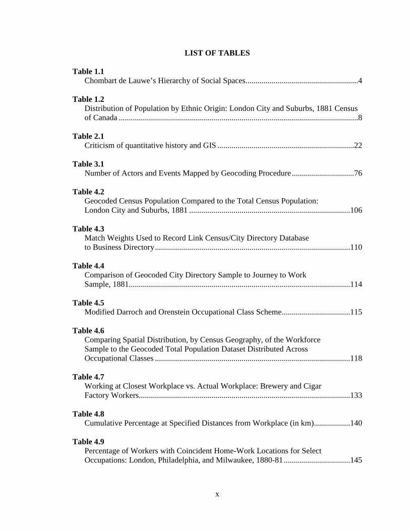
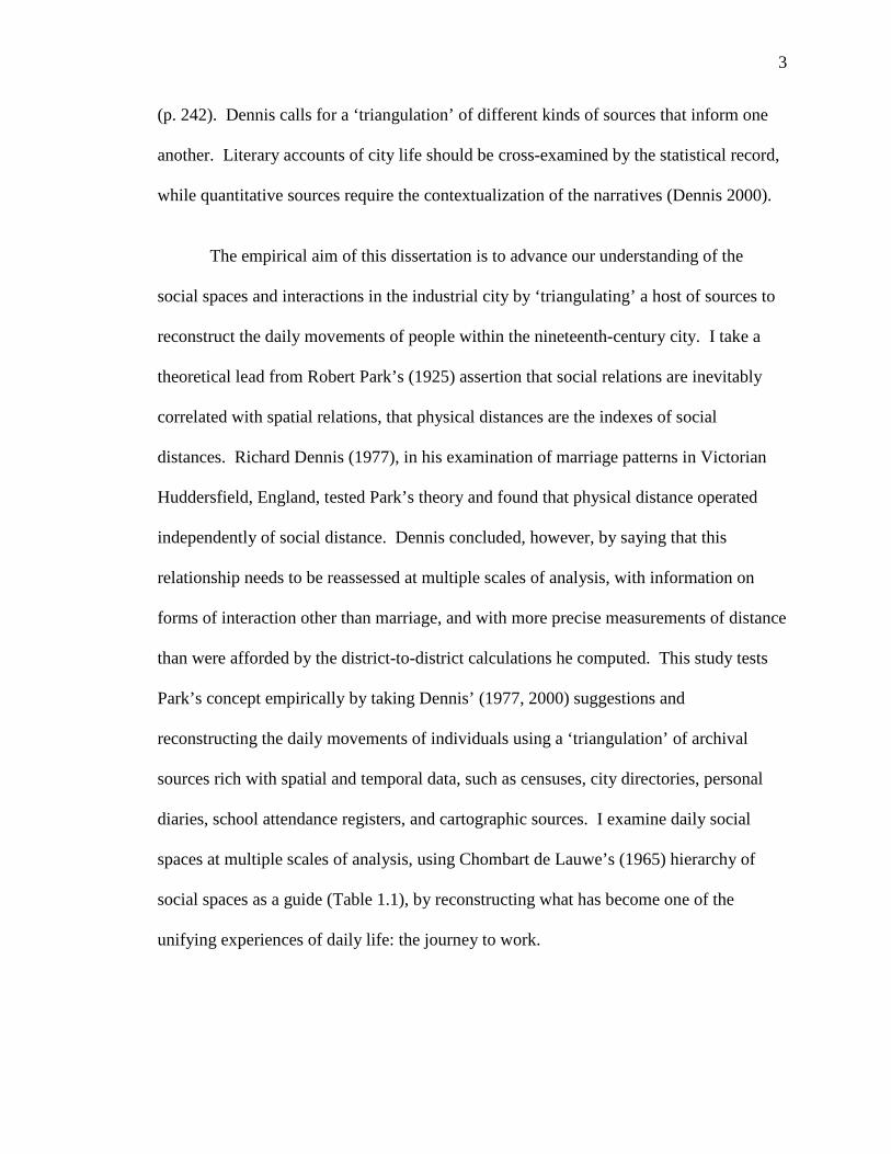
spaces at multiple scales of analysis, using Chombart de Lauwe’s (1965) hierarchy of

social spaces as a guide (Table 1.1), by reconstructing what has become one of the

unifying experiences of daily life: the journey to work.

4

Table 1.1 – Chombart de Lauwe’s Hierarchy of Social Spaces

This dissertation also has a broader aim: to set forth a comprehensive geospatial

research framework for the study of past populations and their environments. To do so,

this work will utilize a tool that in recent years has been applied by scholars for historical

geographic research, a Historical GIS (HGIS). The use of GIS for historical research was

championed by a small cohort of historical geographers in the early 2000s. Arguably, the

first substantial collection of work utilizing HGIS was featured in a special issue of

Social Science History, edited by American historical geographer and vocal cheerleader

of HGIS Anne Kelly Knowles (2000). It was followed quickly by a special edition of

History and Computing, edited by British historical geographers Paul Ell and Ian

Gregory, that outlined the rapid progress and future directions of the emerging discipline

(Ell & Gregory, 2001; Gregory, Kemp, & Mostern, 2001). In Canada, Jason Gilliland

and Sherry Olson established a uniquely Canadian approach applying GIS capabilities to

the study of 19th century Montreal (Gilliland & Olson, 2003). Several books quickly

followed (Gregory, 2003; Knowles A. , 2002; 2008) which have captured the attention of

non-geographers, specifically historians, and prompted them to explore using GIS for

Space Type Types of Use Frequency of Use

Familial Space Household Daily Neighbourhood Space Household, Social Activities

Daily

Economic Space Work, School, Low Order Retailing

Daily, Weekly

Urban Regional Space Financial, High Order

Monthly, Yearly

The World Varies Occasional Forays

5

historical inquiries. In Canada, HGIS has particularly caught attention of historians with

interests in past environments (Bonnell & Fortin, 2014). Very recently HGIS scholarship

has inspired humanists to also embrace a geospatial approach to their craft, resulting in

three edited collections (Bodenhamer, Corrigan, & Harris, 2010; Dear, Ketchum, Luria,

& Richardson, 2011; Gregory & Geddes, 2014). HGIS (or, as it is increasingly being

coined, spatial history) as a discipline is now in its adolescence. Increasing numbers of

researchers and students are utilizing the database management and visualization

capabilities that are readily accessible to novice GIS users. With very few exceptions,

scholars have not taken advantage of the spatial analytical capability that GIS has been

developed for.

Researchers have been limited from harnessing the full capabilities of GIS in

historical research for many reasons. These include a limited access to dedicated HGIS

training, few detailed methodologies that are broadly accessible and relevant for novice

users, and very few historical datasets ready for use in GIS. Only a handful of

institutions worldwide are offering graduate courses in HGIS and only the History

Department of Idaho State University is offering a degree program in HGIS (MA in

Historical Resources Management with a GIS track). Instead, formal HGIS training has

been offered in the form of short workshops, which may provide a solid introduction but

generally do not allow new users to fully develop skill-sets needed to move beyond

visualization or database management. Despite the rich library of guidebooks, manuals,

methodological academic articles, and websites on GIS and other geospatial technologies,

there is a dearth of resources available for researchers who are new to using GIS in

historical research. The only notable exception is a book by Gregory and Ell (2007) that

6

treats the issue with some authority. However, the historical data needed is rarely

digitalized, most often sitting in archival collections dispersed across research

institutions, government depositories, and in local community libraries or museums.

Historical data is never complete and requires the historian’s craft of juxtaposing sources

against each other to check for representativeness and accuracy. Additionally, rarely

does historical data include spatial references, and those that do are referencing archaic

locations for which there are no geolocators and reference tables available. Some of

these hurdles have been overcome by other HGIS scholars; however, rarely are the details

of these critical decisions made known to the rest of the research community. Significant

research and methodological expertise is needed before many historical sources can be

used for spatial or statistical analysis in a GIS. This dissertation researches these issues

and outlines a methodological framework that can be applied to a wide range of HGIS

projects.

1.2 GEOGRAPHIC CONTEXT

This research is broadly applicable to any geographic area for which there exists a

good repository of data on individuals and their habitations. The applicability is more

fully discussed within each individual manuscript. Generally, this work will be found as

most relevant to scholars of North American and European cities from the late 18th to

early 20th centuries, though the research framework has also been applied to study a rural

setting as well (Van Allen & Lafreniere, in review).

The study site is the mid-sized city of London, Ontario, Canada in the late

nineteenth century. London is located halfway between Toronto and Detroit on the plains

7

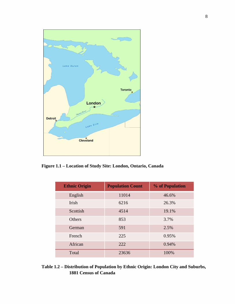
of the lower Great Lakes basin (Figure 1.1). During this period, London was evolving

from a regional commercial centre to a bipolar city with commercial functions in the

downtown core and an expanding industrial district on the eastern edge of the city and in

the Village of London East. This period of rapid industrialization marks a shift in

production from home-based artisans to factory-based wage labour (Pred, 1966; Vance,

1967). Additionally, this is a period of early suburbanization, with residential

neighbourhoods being established at the fringe of the city. Nineteenth-century London

was a quintessential British town on Canadian soil. Both the established citizenry and the

waves of recent immigrants were predominantly from the British Isles, and Protestant

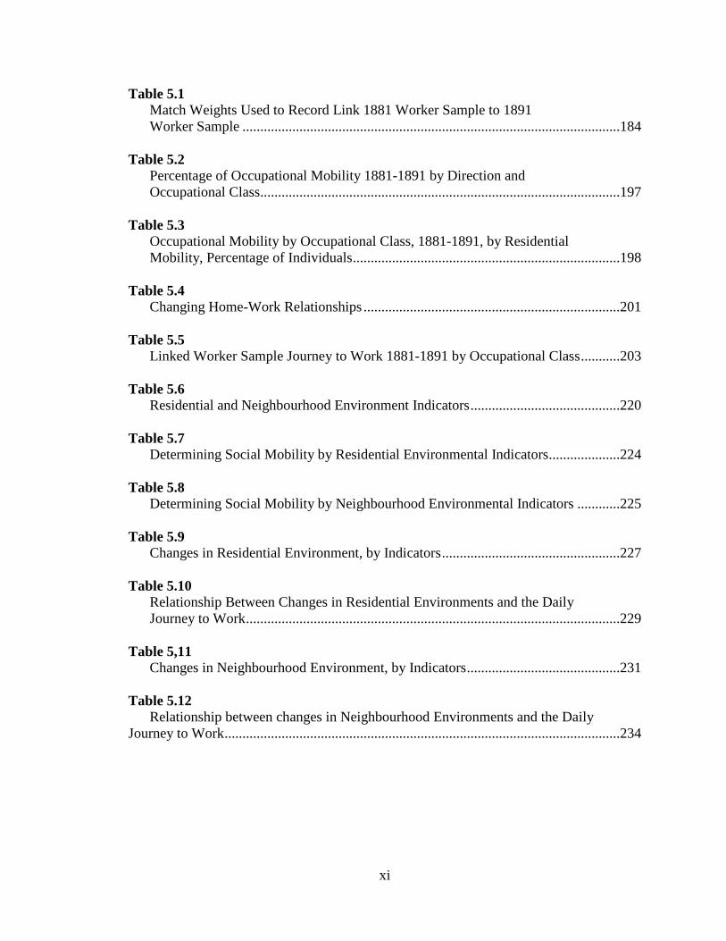
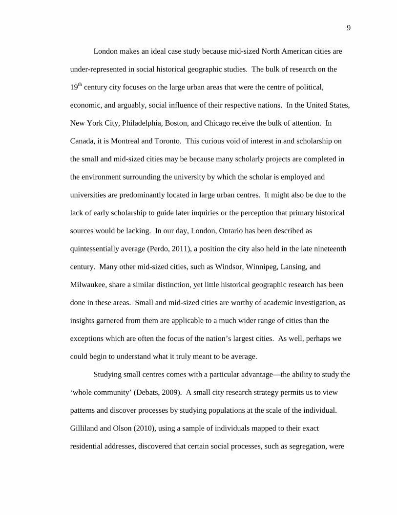
faiths dominated the religious composition of the growing city (Table 1.2). More than

just the town’s namesake, London, England contributed the inspiration for many features

in the urban landscape. The Thames River meandered through the city, Victoria Park

dominated the urban core, and British toponyms were found throughout the city’s streets,

with Piccadilly, Wellington, and Oxford among them. With a population of 19,746 at the

time of the 1881 Census of Canada, London ranked 8th among Canadian cities and 86th in

North America, making it comparable to cities such as St. John, NB, Lancaster, PA, and

Des Moines, IA. For this study, I also included the three major suburbs of London:

Petersville (aka London West), the Village of London East, and the urban section of

Westminster Township (aka London South). Together these suburbs totaled 3,890

residents. It was critical to include these suburbs as they contributed significantly to the

available employers and the diverse workforce found about the city. Additionally,

suburban populations and industries are often overlooked in other studies, mostly because

the census separates them from the urban core when disseminating their enumerations.

8

Figure 1.1 – Location of Study Site: London, Ontario, Canada

Ethnic Origin Population Count % of Population

English 11014 46.6% Irish 6216 26.3%

Scottish 4514 19.1%

Others 853 3.7%

German 591 2.5%

French 225 0.95%

African 222 0.94%

Total 23636 100%

Table 1.2 – Distribution of Population by Ethnic Origin: London City and Suburbs, 1881 Census of Canada

9

London makes an ideal case study because mid-sized North American cities are

under-represented in social historical geographic studies. The bulk of research on the

19th century city focuses on the large urban areas that were the centre of political,

economic, and arguably, social influence of their respective nations. In the United States,

New York City, Philadelphia, Boston, and Chicago receive the bulk of attention. In

Canada, it is Montreal and Toronto. This curious void of interest in and scholarship on

the small and mid-sized cities may be because many scholarly projects are completed in

the environment surrounding the university by which the scholar is employed and

universities are predominantly located in large urban centres. It might also be due to the

lack of early scholarship to guide later inquiries or the perception that primary historical

sources would be lacking. In our day, London, Ontario has been described as

quintessentially average (Perdo, 2011), a position the city also held in the late nineteenth

century. Many other mid-sized cities, such as Windsor, Winnipeg, Lansing, and

Milwaukee, share a similar distinction, yet little historical geographic research has been

done in these areas. Small and mid-sized cities are worthy of academic investigation, as

insights garnered from them are applicable to a much wider range of cities than the

exceptions which are often the focus of the nation’s largest cities. As well, perhaps we

could begin to understand what it truly meant to be average.

Studying small centres comes with a particular advantage—the ability to study the

‘whole community’ (Debats, 2009). A small city research strategy permits us to view

patterns and discover processes by studying populations at the scale of the individual.

Gilliland and Olson (2010), using a sample of individuals mapped to their exact

residential addresses, discovered that certain social processes, such as segregation, were

10

only visible at the smallest of spatial scales, such as the street level or block face. Their

impressive HGIS of Montreal captured a sample of 17,000 individuals, representing only

10% of the city’s population. The sheer size of Montreal, at 175,000 people, coupled

with few sources that captured the entire metro area, restricted their ability to capture the

entire population. By embracing the study of smaller urban centres, we are better able to

capture the entire city, allowing for analysis at a limitless range of spatial scales and for

the re-aggregation of data at the most appropriate interval for a given statistical method.

This dissertation outlines a full-count population-based approach to the creation of a

historical spatial infrastructure that is flexible and adaptive to future research questions,

new sources, and analytical tools. This tool can be applied to a large range of topics from

social mobility, segregation, educational opportunities, religious patterns, rural-urban

migration, diffusion of technology, and retail and industrial development, as well as

issues that relate to present city life such as historical preservation, archeology, cultural

heritage, land use and transportation planning, urban green space preservation, and

brownfield redevelopment. In this dissertation, I will examine the daily journey to work

and its relationship to social mobility.

1.3 STRUCTURE OF THE DISSERTATION

This dissertation is in an integrated article format. Following this introductory

chapter is a short chapter that outlines a broad review of the literature and themes that

guide and support the subsequent research. Chapters 3-5 are written in a manuscript

format for publication in academic journals. Chapter 6 concludes the dissertation with a

discussion and suggestions for future research.

11

The first manuscript (Chapter 3), published in Transactions in GIS, investigates

and presents a methodological model for incorporating both qualitative and quantitative

historical sources in a GIS. The manuscript outlines the initial spatial data infrastructure

needed to complete the studies in chapters 4 and 5.

Chapter 4 outlines a new methodological framework for recreating the journey to

work in the nineteenth century city. Case studies are analyzed and the results compared

to previous studies.

Chapter 5 outlines a methodological framework for studying the same population

longitudinally through time. Two environmental indices are created to examine the

relationship between social mobility and the changing journey to work from 1881-1891.

1.4 REFERENCES

Alexander, J. (2007). Daily Life in Immigrant America. Westport, CT: Greenwood Press.

Bodenhamer, D., Corrigan, J., & Harris, T. (Eds.). (2010). The Spatial Humanities: GIS

and the Future of Humanities Scholarship. Bloomington, IN: Indiana University

Press.

Bradbury, B. (1996). Working Families: Age, Gender, and Daily Survival in

Industrializing Montreal. Toronto: Oxford University Press.

Chombart de Lauwe, P. H. (1965). Des hommes et des villes. Paris: Payot.

Dear, M., Ketchum, J., Luria, S., & Richardson, D. (Eds.). (2011). GeoHumanities: Art,

History, Text at the Edge of Place. London: Routledge.

12

Debats, D. (2009). Using GIS and Individual-Level Data for Whole Communities: A Path

Toward the Reconciliation of Political and Social History. Social Science

Computer Review, 27(3), 313-330.

Dennis, R. (1977). Distance and social interaction in a Victorian city. Journal of

Historical Geography, 3(3), 237-250.

Dennis, R. (2000). Historical Geographies of Urbanism. In B. Graham, & C. Nash (Eds.),

Modern Historical Geographies (pp. 218-247). London: Prentice Hall.

Ell, P., & Gregory, I. (2001). Adding a New Dimension to Historical Research with GIS.

History & Computing, 13(1), 1-6.

Gilliland, J., & Olson, S. (2003, January-February). Montreal, l'avenir du passe.

GEOinfo, 5-7.

Gilliland, J., & Olson, S. (2010). Residential Segregation in the Industrializing City: A

Closer Look. Urban Geography, 31(1), 29-58.

Goheen, P. (1970). Victorian Toronto 1850-1900. Chicago: Department of Geography,

University of Chicago.

Greenberg, S. (1981). Industrial Location and Ethnic Residential Patters in an

Industrializing City: Philadelphia, 1880. In T. Hershberg, Philadelphia: Work,

Space, Family and Group Experience in the Nineteenth Century (pp. 204-229).

New York: Oxford University Press.

Gregory, I. (2003). A Place in History: A Guide to Using GIS in Historical Research.

Oxford: Oxbow.

Gregory, I., & Ell, P. (2007). Historical GIS: Technologies, Methodologies and

Scholarship. Cambridge: Cambridge University Press.

13

Gregory, I., & Geddes, A. (Eds.). (2014). Towards Spatial Humanties: Historical GIS

and Spatial History. Bloomington: Indiana University Press.

Gregory, I., Kemp, K., & Mostern, R. (2001). Geographical Information and Historical

Research: current progress and future directions. History and Computing, 13(1),

7-22.

Knowles, A. (2000). Introduction to Special Issue: Historical GIS, the Spatial Turn in

Social Science History. Social Science History, 24(3), 451-470.

Knowles, A. (Ed.). (2002). Past Time, Past Place: GIS for History. Redlands, CA: ESRI

Press.

Knowles, A. (Ed.). (2008). Placing History: How GIS is Changing Historical

Scholarship. Redlands, CA: ESRI Press.

Lacelle, C. (1987). Urban Domestic Servants in 19th-Century Canada. (J. Brathwaite,

Trans.) Ottawa: National Historic Parks and Sites.

Le Goff, J., Chartier, R., & Revel, J. (1978). La Nouvelle Histoire. Paris: Retz.

Lees, L. (1969). Patterns of Lower-Class Life: Irish Slum Communities in Nineteenth-

Century London. In Y. C.-C. City, S. Thernstrom, & R. Sennett (Eds.),

Nineteenth-Century Cities: Essays in the New Urban History (pp. 359-385). New

Haven: Yale University Press.

McCulloch, G. (2004). Documentary Research in Education, History and the Social

Sciences. London: RoutledgeFalmer.

Mitchell, S. (2009). Daily Life in Victorian England (2nd ed.). Westport, CT: Greenwood

Press.

14

Park, R. (1925). The Urban Community as a Spatial Pattern and a Moral Order. In E.

Burgess, The Urban Community: selected papers from the proceedings of the

American Sociological Society (pp. 3-18). New York: Greenwood Press.

Perdo, K. (2011, November 7). Picture perfect(ly) average. The London Free Press.

Picard, L. (2005). Victorian London: The Life of a City 1840-1870. London: Weidenfeld

& Nicolson.

Pooley, C. (1984). Residential differentiation in Victorian cities: a reassessment.

Transactions of the Institute of British Geographers, New Series 9, 131-144.

Pred, A. (1966). The American Mercantile City: 1800-1840, Manufacturing, Growth and

Structure. In A. Pred, The Spatial Dynamics of U.S Urban-Industrial Growth,

1800-1914 (pp. 143-215). Cambridge: M.I.T Press.

Van Allen, N., & Lafreniere, D. (in review). Signed, Sealed, and Delivered: Late-19th

Century Post Office Petitions, Spaces, and Postal Communities. Rural History.

Vance, J. (1967). Housing the Worker: Determinative and Contingent Ties in Nineteenth

Century Birmingham. Economic Geography, 43(2), 95-127.

Warner, S. B. (1968). The Private City: Philadelphia in three periods of its growth.

Philadelphia: University of Philadelphia Press.

Zunz, O. (1982). The Changing Face in Inequality: Urbanization, industrialization and

immigrants in Detroit, 1880-1920. Chicago: University of Chicago Press.

15

CHAPTER TWO

Broad Literature Themes

A comprehensive literature review covering the scholarship relevant is included

within each separate study in this dissertation. This chapter reviews literature that does

not belong to any one of the studies herein but must be addressed to help contextualize

some of the larger approaches and themes found throughout the dissertation.

2.1 DISCIPLINARY CONTEXT

This dissertation contains three studies that contribute broadly to the sub-

discipline of historical geography. Though if you were to read through the pages of the

disciplines two premier journals, Historical Geography or Journal of Historical

Geography you would be hard-pressed to find studies that take an approach to past

geographical patterns in the same way as I do here. While identified as historical

geography by geographers, these studies borrow techniques and approaches familiar to

many social historians, demographers, and computer scientists. This interdisciplinary

perspective, known at Historical GIS, owes its inspiration to, and benefits from, over half

a decade of epistemological change within the broader discipline of historical geography.

This next section reviews the literature, illustrating the morphology of historical

geography and outlines the debates that have driven the progress and emergence of the

new discipline of Historical GIS.

16

2.1.1 Historical Trends

The sub-discipline of historical geography has served as a foundation for the

larger discipline of geography since the eighteenth century. The earliest academic studies

in geography, c. 1700-1850, were historical in nature, focusing on scriptural and biblical

geographies and on geographies of changing boundaries and territories (Butlin, 1993).

Using these three centuries of philosophical thought as a guide, Modern North American

historical geography has been through three phases of epistemological and

methodological exploration from the 1950s to the present. The earliest phase treated

regional settlement history as the major concern of study and was anchored by

geographers such as Don Meinig, Alan Baker, John Clarke and Cole Harris (Holdsworth,

2002). They were influenced by Carl Sauer’s Berkeley School where the study of

human-environment relationships (cultural landscapes), the reconstruction of past

geographies, and their change over time were central ways of knowing (Clayton, 2000;

Sauer, 1925). The re-creation of place, culture and identity were central to their work in

regional studies (Holdsworth, 2002). Prince (1971), writing on the methodological

approaches prevalent in this phase, suggests that historical geographers studied “real

worlds”, past geographies and their processes of change, through a narrative-based

empirical approach. Modernisation theory, which posits an evolutionary change from a

‘traditional’ to a ‘modern’ society, grounded this first phase of historical geography

(Baker, 2003).

The catalyst for the second phase of epistemological and methodological

exploration was the quantitative revolution in geography in the 1960s. It pushed

historical geography to the margins of the discipline, as narrative-based, empirical

17

scholarship was not as valued as the new epistemology of spatial science (Clayton, 2000).

The epistemological shift away from description and towards interpretation was central to

this phase. Some historical geographers (Goheen, 1970); (Haggett, 1965); (Peach, 1975);

(Pitts, 1965) embraced the new spatial analytic methodologies in spatial science, such as

network models, gravity models, segregation indices and simulation models. While

others such as (Clark, 1968); (Meinig, 1968); (Smith, 1966) continued writing as they had

for years with a strong commitment to the historical study of landscapes and occasional

ventures into the reconstructions of regional geographies of the past. Historical

geography was ‘saved’ from the margins of the discipline by the development of

humanistic geography in the 1970s and 80s. The period saw a sub-disciplinary shift

away from source-bound empiricism, which had dominated historical geographical study

to that time, to explorations of different methods of explanation. These humanistic

historical geographers sought to integrate social theory into their studies and thus

embraced the philosophies of Marxism, humanism, idealism, and structuralism (Butlin,

1993).

The third epistemological and methodological phase (1980s to present) is

described by Clayton (2000) as ‘eclectic’; he suggests that no single orthodoxy is likely

to emerge from it. As Holdsworth (2002, p. 676) observes, a trend in this phase is that

“modern historical geographies are more likely to simultaneously embrace the local and

the global, rather than dwell at the regional scale.” Williams (1994) highlights how

historical geographers have returned to their ‘stock-in-trade’ interest in human-

environment relationships in response to recent public concern over environmental

issues. Informed by the perspectives of postmodernism, some recent work in historical

18

geography starts from the premise that “geographers create and communicate meaning

from partial vantage points” rather than simply recreating a prior and separate

geographical reality (Clayton, 2000, p. 338). For example, Cosgrove (1984) argues that

landscape becomes a ‘way of seeing’ the spatiality and temporality of social life and

human identity. As Graham and Nash (2000) suggest, the cultural turn in geography has

influenced historical geographical approaches by extending the concern with class to

other axes of domination and identity such as race and gender. Mitchell (2002) says that

this has caused historical geography to become deeply theoretical without sacrificing, but

instead relying on, its traditional empirical richness.

Despite many historical geographers finding a comfortable place within this

marriage of theory and empiricism, it is the eclecticism of the sub-discipline which has

once again pushed historical geography to the margins of the discipline. An “anything

goes” attitude has emerged, resulting in no unifying theory or epistemology for the sub-

discipline. Historical geographers are becoming increasingly interdisciplinary in their

collaborations, often looking first to the closest cognate discipline than within geography

itself (Holdsworth D. , 2002). Williams (2002) worries this may lead to the sub-

discipline being swallowed by cultural geography and environmental history. Writing in

self-reflection, a historical geographer (Kay, 1990) describes his sub-discipline as

“antiquarian in its purpose”. Such an identity crisis, coupled with the pressures to

compete for resources with other geographies that appear to be more contemporarily

relevant, has resulted in fewer students being trained in the sub-discipline and even fewer

hired upon the retirement of their mentors (Meinig, 1989). However, despite this

apparent impending mortality, it is the same eclecticism of the 1980s and 90s that has

19

allowed some aspiring historical geographers to forge a new epistemology, one that is

moving to completely reshape the discipline.

2.1.2 An Emerging Discipline: Historical GIS

Aided by the computational advancements in geographic information systems

(GIS) and the “spatial turn” in history (Withers, 2009), the next generation of historical

geographers has developed a new methodology and epistemology: historical GIS.

Historical GIS, or HGIS, is the creation and use of a relational database of historical

geographical data in a GIS. Anne Knowles, one of the earliest supporters and most

prolific writers on the methodology, suggests that “almost every historical document

contains some kind of geographical information” (Knowles, 2008, p. 2) and thus can be

incorporated into an HGIS. Examples of historical data commonly used include

censuses, city directories, historical maps and social surveys. HGIS allows one to

visualise the geographic patterns embedded in historical evidence, examine evidence at

different scales, aggregate data on-the-fly into various units, and integrate a nearly

limitless range of material from the narrative to nominal. As Knowles (2000, p. 453)

points out, “Historical GIS computerizes much that is basic to historical geography”. It

may be this inherent familiarity that has encouraged even the most senior of historical

geographers to say that “historical GIS is an exciting and challenging development”

(Baker, 2003, p. 44) and to encourage their peers “to be open to the dazzling array of new

ways of seeing, and imaging, the past” (Holdsworth D. , 2003, p. 491). Knowles’s

equally prolific colleague, Ian Gregory has gone so far to claim that “in less than a

decade, historical GIS has emerged to become an accepted and evolving part of both the

20

quantitative and qualitative spheres of historical geography” (Gregory & Healey, 2007, p.

649).

From the literature, there appears to be quite a fervour surrounding HGIS.

Knowles, in the opening line of her introduction to an influential special issue of Social

Science History devoted to HGIS, proclaimed that “people love new tools that enable

them to do what they have dreamed of doing” (Knowles, 2000, p. 451). Is HGIS truly an

epistemological advance of historical geography, or is it just an analytical tool? Gregory

and Healey (2007) argue that HGIS can aid in the advancement of historical geographical

scholarship in three ways: First, by providing revisionist studies that challenge existing

orthodoxies. Examples of such work include investigations of patterns of social change,

such as racial and ethnic segregation in North American cities (Gilliland & Olson, 2010);

(Hillier, 2003). Secondly, by tackling questions that have not been resolved to date, such

as the origins and patterns of the American Dust Bowl in the 1930s (Cunfer, 2008).

Thirdly, Gregory and Healey argue that HGIS provides a new way of knowing the past,

which enables historical geographers to ask completely new questions.

One of the earliest and still most utilized strengths of HGIS is its ability to easily

visually represent historical data through the creation of maps. Orford (2005) argues that

maps help researchers synthesise spatial patterns and relationships that may not be

obvious or intuitive. Maps represent an inductive epistemology that is important in the

formation of geographic theories and the generation of hypotheses. Krygier (1997) calls

this way of knowing a scientific “visual epistemology”. Siebert (2000) also argues for

this inductive approach; however, she stresses the need for a progression from a visual

epistemology to the interpretation of findings and the creation of knowledge. While not

21

historical geographers, Knigge & Cope (2006) and Steinberg & Steinberg (2005) suggest

that the intuitive model that ‘grounded visualization’ affords can ground the multiple

interpretations and partial vantage points that the HGIS based approach to historical

geographical scholarship offers.

This current dialogue echoes the discussions of the 1960s that pitted description

against interpretation; however, it is just one of the debates found within the young sub-

disciplinary approach of historical GIS.

2.1.3 Historical GIS- Epistemological and Methodological Debates

HGIS has seen a host of debates emerge since its founding in the late 1990s.

Siebert’s stress on the interpretation of findings is one of these debates. Gregory and

Healey (2007, p. 650) acknowledge Siebert’s concern but also attempt to moderate it:

“historical GIS studies...are better at identifying and describing patterns that they are at

explaining them. Nevertheless, the ability to be able to recognize patterns will clearly

lead to more robust explanations.” Baker (2003) reminds us that spatial analysis will

provide the answer to ‘where?’ a particular historical event or process took place but it

will not tell us ‘why there?’ Baker goes on to also support this type of inductive work,

suggesting that it is the mapping of historical processes that itself raises new questions.

Rose-Redwood (2009) suggests that this insistence on moving beyond the descriptive

demonstrates the growing influence of critical GIS on the development of a post-

positivist historical GIS.

Although Gregory and Ell (2007, p. 161) postulate that “the quantitative nature of

spatial data does not mean that spatial analysis is necessarily positivist”, others, including

22

Anne Knowles, a staunch supporter of historical GIS, have concerns that this new

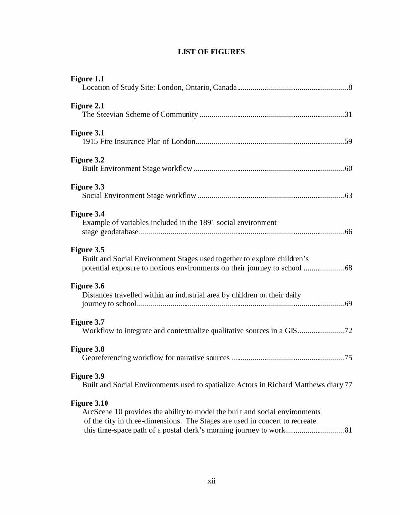
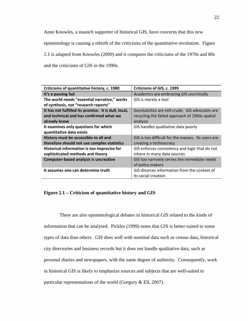
epistemology is causing a rebirth of the criticisms of the quantitative revolution. Figure

2.1 is adapted from Knowles (2000) and it compares the criticisms of the 1970s and 80s

and the criticisms of GIS in the 1990s.

Criticisms of quantitative history, c. 1980 Criticisms of GIS, c. 1995 It’s a passing fad Academics are embracing GIS uncritically The world needs “essential narrative,” works of synthesis, not “research reports”

GIS is merely a tool

It has not fulfilled its promise. It is dull, local, and technical and has confirmed what we already know

Geostatistics are still crude. GIS advocates are recycling the failed approach of 1960s spatial analysis

It examines only questions for which quantitative data exists

GIS handles qualitative data poorly

History must be accessible to all and therefore should not use complex statistics

GIS is too difficult for the masses. Its users are creating a technocracy

Historical information is too imprecise for sophisticated methods and theory

GIS enforces consistency and logic that do not inhere in many data sources

Computer-based analysis is uncreative GIS too narrowly serves the immediate needs of policy makers

It assumes one can determine truth GIS divorces information from the context of its social creation

Figure 2.1 – Criticism of quantitative history and GIS

There are also epistemological debates in historical GIS related to the kinds of

information that can be analysed. Pickles (1999) notes that GIS is better-suited to some

types of data than others. GIS does well with nominal data such as census data, historical

city directories and business records but it does not handle qualitative data, such as

personal diaries and newspapers, with the same degree of authority. Consequently, work

in historical GIS is likely to emphasize sources and subjects that are well-suited to

particular representations of the world (Gregory & Ell, 2007).

23

The lack of temporal functionality in GIS is often criticised by historical

geographers who have not embraced GIS (O'Sullivan, 2005). Progress has been slow in

implementing temporal functions into the software as GIS software vendors do not see

this as a particularly important development priority for their primary market—municipal

governments and industry. However, historical GIS users have adopted a number of ad-

hoc solutions such as time-stamping, which involves the inclusion of a database of

temporal references related to a particular point in space. Bodenhamer (2008) points out

that such a solution can be cumbersome to build. Time references are not always an issue

in GIS, however, particularly when a researcher is building a database of stand-alone

features, such tenants of a building. The building is static, so the attributes of time can be

easily assigned to the building.

Debates also surround the use of inherently incomplete historical sources in an

environment that demands a high level of certainty in the data inputted. Incomplete,

inaccurate and ambiguous sources are a common problem for historians, but history has

embraced this ontological issue by making it an epistemological challenge (Evans, 1997).

For historical GIS, the issue is more methodological: how to take such ambiguous

sources and bring them into a strict coordinate system. Gregory and Healey (2007) offer

three approaches: mathematical, representational and documentary. The mathematical

approach uses fuzzy logic, which assigns a coordinate based on a mathematical

calculation of the most likely expected location of a given attribute. The representational

approach involves the researcher aggregating the data into a raster which is projected

using blurred lines and colours to represent areas of uncertainty. The documentary

approach is adopted from traditional narrative historians, who through the use of

24

footnotes systematically address each ambiguity found in their research. Historical GIS

accomplishes this through the use of metadata, data that describes data. Contemporary

geographic information science scholars such as Yao and Jiang (2005) are also tackling

these issues and their findings are providing important guidance to the qualitative GIS

community.

2.1.4 Finding a Home within the Debates

The studies that make up this dissertation do not claim to resolve all of these

complex debates, but they do offer some progress. In particular, are the debates

suggesting that HGIS is a return to the decontextualized histories and quantitative

traditions of the 1980s. At its origin, GIS is a numerical tool, driven by coordinates of

latitude and longitude, capable of very complex mathematical computations. This

numerical basis however does not predetermine the output of research that results from

its use. If careful concerns for the origins and contexts of the source material are

maintained, a GIS approach to history can add important contextual cues to historical

records that would otherwise be cost prohibitive or impossible to accomplish otherwise.

Positioning the traditional quantitative historical sources, such as censuses, against

qualitative sources such as diaries and newspapers (as outlined in chapter 3), allows

researchers to conceptualise and criticise their quantitative findings and provide the

context need to create a spatial narrative, rather than a purely quantitative assessment of

the patterns and processes observed.

These studies also address the debates by Pickles and others that methodologies

are needed over limitations GIS has for integrating qualitative sources. In addition to the

traditional sources that have been widely used in historical GIS databases for other cities,

25

these studies illustrate methodologies and case studies for using qualitative archival

sources in a GIS. Diaries and school records are used to conceptualise, criticise and

illustrate quantitative findings. This use of qualitative sources requires a subjective

approach to analysis, helping to suppress criticisms that HGIS research is purely

positivist in nature. The textual analysis of qualitative sources is in itself an interpretive

exercise which would certainly please Siebert and others who call for more interpretation

in historical GIS.

These studies embrace Knigge & Cope’s (2006) ‘grounded visualization’ as an

analytic base for studying the nineteenth century city. This answers the debates in

historical GIS that calls for an interpretive epistemology. Though not challenged

explicitly, attempts are made in these studies to illustrate ways to overcome some of the

temporal limitations of GIS. Though much more work and emphasis is needed by

scholars in the area of temporal GIS, the studies here illustrate that the temporal

limitations of the software are not slowing the field from advancing and producing

knowledge.

2.2 THE CHALLENGE OF HISTORICAL SOURCES

A historical geographer’s object of study is rooted in the past. Thus to commence

any investigation he must turn to the historical record and rely upon the documents that

have survived in the world’s archives, libraries, museums and personal collections.

However, there are methodological difficulties that a scholar must address when working

with historical sources. First, the scholar must evaluate the source critically as well as

place the source within its historical context. Perhaps the most critical methodological

26

challenge is the issue of authenticity (Black, 2010). Scholars must determine if the

source is original, or, if a duplicate, how has it been modified from the original.

Secondly, it is necessary to critically evaluate how the original purpose for the

creation of a historical source has influenced the information contained within it. For

example, any source that is collected by a third party, such as the census, municipal tax

rolls and city directories, has an inherent bias in who is and who is not captured in the

register. Censuses have received the most attention of the three sources noted above;

however, the scholarship on the reliability of the census is somewhat limited given the

wide use of the census. Steckel (1991) notes that there are three types of errors that affect

the reliability of census data: underenumeration, overenumeration and misreporting.

Underenumeration has been noted by Miller (1922) for African Americans in the US

South and Curtis (2001) for Lower Canada in the 1851-71 censuses. The

underenumeration of aboriginal populations has been discussed in Baskerville and Sager

(1990), Curtis (2001), Hamilton (2007) and Hamilton and Inwood (2011). Davenport

(1985), Dunae (1998), and Galois & Harris (1994) have discussed underenumeration in

remote or secluded areas, while Dunae (2009), Dunae et al. (2013), Knights (1969), Katz

(1975) and Olson & Thornton (2011) have hinted at underenumeration in urban areas.

Overenumeration has been tackled by Curtis (2001) in discussing double-counting in the

1861 census and by Curtis (1995), Dunae (1998) and Furstenberg et al. (1979) in their

reviews of municipal check censuses in Montreal, Victoria and Philadelphia.

Misreporting or misrepresentation has also been identified as an issue with

censuses. This includes how occupations are represented, as examined by Baskerville

(1993), Baskerville and Sager (1998), Bradbury (2007), Curtis (2001), and Dunae (2009).

27

Inwood & Reid (2001) review both gender and occupation. Darroch (2000) reviews the

issues with the representation of family previous to the ‘relation to household head’

question in 1901. How ethnicity and language are identified have been critical to the

studies of Dillon (2002), Gaffield (2007), Hamilton & Inwood (2011), and Lutz (2008).

Beyond sources that are enumerated, scholars also use textual and oral sources,

which are created by (in)direct testimony of witnesses to historical events. Sources such

as diaries and letters can help overcome the problem of aggregation and the recording of

the ‘official’ rather than personal view of the world (Black, 2010). They provide an

intimate, personal view of the past. McCulloch (2004) warns that they can be very biased

and subjective, although he notes that if a record is written immediately after an event, it

can be especially reliable, and can be very telling if used in concert with other sources

(Black, 2010); (Hoffman & Taylor, 1996). Oral histories can be used to gain insight into

the nature of past personal relationships and the significance of past events to the

participants, as well as for the re-creation of life courses. However, the degradation of

time has a strong effect on the accuracy and reliability of memories and perceptions

(Hareven, 1982).

Despite the lengthy list of concerns in using historical sources, Baker reminds us

that “no study in historical geography can be better than the sources on which it is

founded” and that the best studies rely upon a wide range of sources that reinforce each

other or perhaps even speak to each other (Baker, 1997, p. 234). As Dennis (2000)

argues, the ‘triangulation’ of sources can create a deep and fluid re-creation of a past

reality.

28

Although the benefit of studying the past with a broad range of historical sources

is evident, historical geographers have been slow to embrace the use of GIS. For those

who have begun to use GIS, the census has been the most widely used historical source

because of its familiarity, comprehensiveness, and ease of access. Many models of using

the census in a GIS exist in the form of national historical GIS’s. Among the earliest

projects was the Great Britain HGIS, started by Southall and later joined by Gregory et

al. (2002). There are also national projects in the US (Fitch & Ruggles, 2003), China

(Bol & Ge, 2005), Russia (Merzlyakova, 2005), and South Korea (Kim, 2005). Other

uses of census data are at the local urban scale. Among the earliest urban projects was

Montreal, spearheaded by Gilliland and Olson (2003). Others include Philadelphia

(Hillier, 2002), Tokyo (Siebert, 2000), Hartford (Schlichting, Tuckel, & Maisel, 2006),

Victoria (Dunae, Lutz, Lafreniere, & Gilliland, 2011), and Alexandria, Virginia and

Newport, Kentucky (Debats, 2008)

Lastly, there have been a number of scholars who have attempted to use other

historical sources in a GIS, such as Fyfe et al. (2009) with their use of hotel registers,

Lafreniere and Rivet (2010) with disparate cartographic sources, Gilliland and Novak

(2006) with fire insurance plans, Debats (2009) with voting records, Travis (2010) with

literary novels, Gregory and Cooper (2009) with travel diaries, and Gregory and Hardie

(2011) with newspapers. Many of these uses of non-tabular data are in their infancy and

have inspired the need to create the detailed methodology outlined in chapter three for

qualitative sources.

29

2.3 UNDERSTANDING COMMUNITY AND NEIGHBOURHOOD

George Hillery sent us a cautionary reminder that community is indeed an area of

little agreement. In a broad review of the early literature on both rural and urban

definitions of community he found ninety-four different definitions, bounded within

sixteen different concepts. His summary concluded that most scholars in the first half of

the twentieth century had the basic agreement that community consisted of “persons in

social interaction within a geographic area and having one or more additional common

ties” (Hillery, 1955, p. 111). Although geographic and sociological thought on

community has progressed since Hillery’s writing, many of the themes he identified, such

as common life, consciousness of kind, possession of common norms, and a collection of

institutions still emerge in more contemporary scholarship on community.

At the risk of not being chronologically consistent, we need to step back before

we can march forward in this review. Much of Hillery’s appraisal included the work of

Robert Park and the rest of the Chicago School of Urban Sociology. Park’s work

includes the now well-known concept of human ecology, the idea that the urban

experiences of humans are divided along the lines of community and society (Park, 1925)

(Park, 1952). Community was theorized by Park as being a ‘natural’ process that occurs

through the interplay of market competition for rents, human adaption to these forces and

spatial interaction. His concept of ‘natural communities’ inspired his colleague Ernest

Burgess to develop the concentric ring model of urban development. It illustrates how

communities (or what we may think of now as neighbourhoods of socially segregated

peoples) emerged in cities but were generally stable and homogenous, although

susceptible to invasion and succession by new groups over time.

30

This early work by the Chicago School sociologists, which influenced the later

work reviewed by Hillery, was based on Park’s notion that community is built because

“social relations are so frequently and so inevitably correlated with spacial [sic] relations”

(Park, 1925, p. 18). Despite the many issues identified with the Chicago School

conception, such as the issues surrounding the use of behavioural and mental disorders to

delineate natural communities within the city, many geographers of the latter half of the

twentieth century accepted this notion that propinquity equaled or led to community and

neighbourhood.

Geographers such as John Clarke embraced models that were developed with

obvious roots in Burgess’ concentric ring model. Clarke, embracing the Steevian Scheme

of structured social spaces, conceptualizes ‘community’ as “the proximity of individuals

one to another in absolute and social space, together with those bonds which are forged

between individuals living beside one another, bonds of inter-marriage and of kinship, of

common ancestry and common experience and of friendship and co-operation…”

(Clarke, 1991, p. 390). Richard Dennis (1984) also embraces this conceptualization of

community by arguing that social interaction is critical to community, and given that his

studies were preoccupied with the ‘walking city’ of the middle nineteenth century,

propinquity was necessary. Dennis argues that any type of community, whether

delineated along class lines, ethnicity or common interest, is more likely to exist “where

families have lived and worked in the same area for a long time, and where neighbours

are also kin.” (Dennis, 1984, p. 250) And much like others who follow the propinquity-

equals-community conceptualization, Dennis argues that one can measure and map

community through an examination of the density of kin or residential tenure.

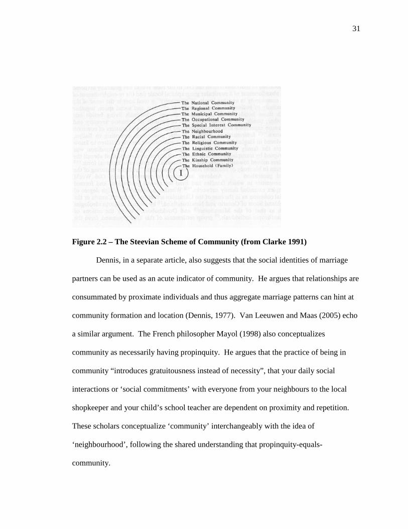
31

Figure 2.2 – The Steevian Scheme of Community (from Clarke 1991)

Dennis, in a separate article, also suggests that the social identities of marriage

partners can be used as an acute indicator of community. He argues that relationships are

consummated by proximate individuals and thus aggregate marriage patterns can hint at

community formation and location (Dennis, 1977). Van Leeuwen and Maas (2005) echo

a similar argument. The French philosopher Mayol (1998) also conceptualizes

community as necessarily having propinquity. He argues that the practice of being in

community “introduces gratuitousness instead of necessity”, that your daily social

interactions or ‘social commitments’ with everyone from your neighbours to the local

shopkeeper and your child’s school teacher are dependent on proximity and repetition.

These scholars conceptualize ‘community’ interchangeably with the idea of

‘neighbourhood’, following the shared understanding that propinquity-equals-

community.

32

Following the Chicago School’s teachings on the importance of proximity to

community building came Melvin Webber’s countering assertion that there can be

‘community without propinquity’ (Webber, 1963). Webber saw how the advancements

in communications and transportation diminished the importance of space in community

building. He demonstrated how friendships could be maintained from a distance and how

community can be created based on professional or other relational groupings, as well as

neighbourhoods. Although not specifically theorizing on the conceptualization of

community, Torsten Hägerstrand’s (1970) lessons on the importance of considering

individuals with widely varying space-time paths follows much of Webber’s inferences

because communities can be created beyond the sphere of one’s residence. Scholarship

that Hägerstrand inspired, such as the early work of Goodchild & Janelle (1984) and later

Mei-Po Kwan (1999), have further elaborated on these ideas.

A shared identity is among the most influential factors in the production of a

community without propinquity. Any shared activity or affiliation can create a sense of

community. It may be membership in a fraternal society or club association such a

writers guild, Shriners or Scouting. It may be through a professional organization such as

the CAG or AAG, a term coined by Wenger (1998) as a ‘community of practice’. A

shared identity within a specific genre of occupation often produces a community. For

example, Perkins & Metz (1988) found that sixty-seven percent of volunteer firefighters

found their membership and affiliation with the fire department was more important to

them than their church community. Sports team affiliation can also manifest itself as

community (Jacobson, 2003). Religious affiliation is often linked with a strong

community, as noted by Tom Bulten (2002) in his study of community among Christian

33

Reformed church members. Butlen found that propinquity had little influence on the

ability of congregations to experience a sense of community. Ethnic or racial identity can

also produce communities without a residential base. Examples are often seen in large

urban centres where an ethnic group may have a wide residential distribution across the

urban area. The Chinese community of the Greater Toronto Area is an example of this.

Although there is some residential propinquity around Spadina Avenue and Dundas

Street in what many refer to as Chinatown, there is a larger ethnic community of Chinese

that includes those that live in the greater metropolitan area. Ethnic communities can

also been seen to be completely non-geographic, in which having an ethnic identity, thus

a shared identity, allows one to claim oneself as a member of a potentially world-wide

community.

Experiential communities exist among those who share an event or history. The

experience of serving for the armed forces, the experience of deployment during a time of

war, the loss of a loved one due to a specific disease or misfortune (such as drunk

driving), or participation in a notable event (whether tragic or positive) can create strong

non-place-based communities. Common stages in the life course can also create

community, such as the common bonds felt by senior citizens or by parents who reach

broadly to create communities with others who also have children with special needs,

have adopted children, or are home schooling their children.

Many of these communities without propinquity have been created or exist only

with the aid of modern communication technologies, most notably the internet. Kitchin

(1998) coined the term ‘virtual communities’ to describe the new forms of social

relations being created by these new technologies. Technologies like the internet allow

34

for close interaction between people with similar interests, concerns or experiences,

overcoming the barriers of distance. The internet (or its early variations in landline

modem-based bulletin boards) was not the first iteration of virtual communities.

Amateur radio operators, using radio frequencies that permit worldwide communications,

had created a vibrant virtual community as early as the 1930s. Haring (2006) describes

how hundreds of thousands of predominantly middle to upper class men formed an

identity and community through their shared recreational interest in electronics and radio

communication. However, it was the internet that sparked the interest of more scholars in

the production of virtual communities. Among the types of virtual communities that can

be found on the internet are support groups (like many listed above), task-related groups

(petitions or political action groups), interest groups (e.g. sports fans) and in dynamic

environments where a diverse array of relationships and communities can interact in

tandem (eg. Facebook and Twitter). The importance of virtual communities to their

participants can be seen by the proliferation of smartphones and the applications

embedded within them to maintain close and near-immediate contact with other members

of their community through commercial environments like Facebook and Twitter. Some

scholars have argued that these virtual communities are simply extensions of ‘real’

geographically-bounded communities (Parks, 2011) while others (primarily those writing

about the early years of the internet) question the idea of virtual communities altogether.

The conceptualization of community is also a concern of urban planners, as they

see a proliferation of propinquity without community. Work such as that of Jane Jacobs

and Andres Duany professes that there is a need for well-functioning neighbourhoods in

order to re-establish a sense of community and ultimately strengthen urban places.

35

Community activists have attempted to artificially create community by naming

neighbourhoods. In Indianapolis, neighbourhood residents were encouraged to develop

names for their neighbourhoods in the hopes that it would create a shared identity and

foster community attachment (Levitz, 2012). Historic preservationists see this pattern as

well and claim that the creation of heritage districts can create a shared neighbourhood

and community identity (Tyler, Ligibel, & Tyler, 2009).

Yet a fourth conceptualization of community exists which has been theorized by

Benedict Anderson. He argued that a nation was an imagined political community whose

members “will never know their fellow-members, meet them, or even hear of them, yet in

the minds of each they carry the image of their communion” (Anderson, 1983, p. 15).

This imagined community can be seen through the perceived close bond that citizens

have with each other when travelling abroad. For example, Canadians often sew small

flags on their backpacks when travelling in Europe; other Canadians who notice these

flags will extend a friendly acknowledgement or a kind gesture to their perceived

community member. Imagined communities can also be seen in international sporting

competitions such as the Olympics when national pride and community engagement

overcomes other social barriers such as class or ethnicity. Gillian Rose (1990) extended

Anderson’s understanding of imagined communities and theorized that they can exist on

more than just a national scale. She argued that imagined communities are “a group of

people bound together by some kind of belief stemming from particular historical and

geographical circumstance in their own solidarity” (p.426). Her work focused on the

neighbourhood of Poplar in London, England, where she used oral histories to capture

two contrasting politicized views of community. Rose’s work inspired other geographers

36

to think about imagined communities, such as Gill Valentine, who examined the

geographies of sexuality (Valentine, 1995).

2.3.1 Conceptualizing Neighbourhood in the Nineteenth Century City

This section has outlined how the conceptualization of community and

neighbourhood is complex and can be interpreted in a myriad of ways. The studies in

this dissertation conceptualize ‘community’ interchangeably with the idea of

‘neighbourhood’, following the propinquity-equals-community model. This

conceptualization is driven by the historical nature of the studies. The subject of these

studies, the Victorian city, was primarily a walking city and thus propinquity was critical

to the production of community. The transportation and communication networks needed

to create and sustain communities without propinquity did not yet exist. I take notice of

Robert Park’s assertions that social relations are correlated with spatial relations because

of who he was studying and the time in which he was theorizing his understanding of

communities. Park was a student of Georg Simmel, who was even more concerned with

geometric distances than Park. Simmel tells us that society is made up of the interaction

between individuals. He observed the smallest of social interactions to see how larger

scale institutions, such as schools and churches, emerged from them (Farganis, 1996).

Although, Simmel did not theorize community directly many of the ‘institutions’ he saw

created through interactions are familiar to those hallmarks of community and

neighbourhood building described earlier in this section. I see Simmel’s (and later

Park’s) assertions as, in some ways, as a historical source. Simmel was observing social

interactions and their impacts during the same time period that is the focus of this

dissertation. Although it may be seen as an antiquated perspective on community and

37

neighbourhood, it is tantalizing to have a perspective that was developed through

observations of temporally similar populations and by a scholar with a firsthand

understanding of live in the nineteenth century.

2.4 REFERENCES

Anderson, B. (1983). Imagined Communities: reflections on the orgin and spread of

nationalism. London: Verso.

Baker, A. (1991). The Limits of Inference in Historical Geography. In D. B. Green (Ed.),

Historical Geography: A methodological protrayal (pp. 219-230). Savage, MD:

Rowman & Littlefield Publishers.

Baker, A. (1997). "The Dead Don't Answer Questionnaires": researching and writing

historical geography. Journal of Geography in Higher Education, 21(2), 231-243.

Baker, A. (2003). Geography and History: Bridging the Divide. Cambridge: Cambridge

University Press.

Baskerville, P. (1993). She Has Already Hinted at Board: Enterprising Urban Women in

British Columbia, 1863-1896. Histoire sociale / Social History, 26(52), 205-283.

Baskerville, P., & Sager, E. (1990). The 1881 Canadian Census: Vancouver Island.

Victoria: Public History Group.

Baskerville, P., & Sager, E. (1998). Unwilling Idlers: The urban unemployed and their

families in late Victorian Canada. Toronto: University of Toronto Press.

Black, I. (2010). Analysing Historical and Archival Sources. In N. Clifford, S. French, &

G. Valentine (Eds.), Key Methods in Geography (pp. 466-484). London: Sage

Publishing.

38

Bodenhamer, D. (2008). History and GIS: Implication for the Discipline. In A. Knowles

(Ed.), Placing History: how maps, spatial data, and GIS are changing historical

scholarship (pp. 221-233). Redlands, CA: ESRI Press.

Bol, P., & Ge, J. (2005). China Historical GIS. Historical Geography, 33(1), 150-52.

Bradbury, B. (2007). Working Families: Age, Gender, and Daily Survival in

Industrializing Montreal. Toronto: University of Toronto Press.

Butlin, R. (1993). Historical Geography: through the gates of space and time. London:

Edward Arnold.

Butlin, T. (2002). Community and Propinquity of Church Members. Christian Scholar's

Review, 31(4), 359-375.

Clark, A. H. (1968). Acadia: The Geography of Early Nova Scotia to 1760. Madison:

University of Wisconsin Press.

Clarke, J. (1991). Social integration on the Upper Canadian frontier: elements of

community in Essex County 1790-1850. Journal of Historical Geography, 17(4),

390-412.

Clayton, D. (2000). Historical Geography. In R. Johnston, D. Gregory, G. Pratt, & M.

Watts (Eds.), The Dictionary of Human Geography (4th ed.). Malden, MA:

Blackwell Publishing.

Cosgrove, D. (1984). Social formation and symbolic landscape. London: Croom Helm

Cunfer, G. (2008). Scaling the Dust Bowl. In Placing History: How Maps, Spatial Data,

and GIS are Changing Historical Scholarship (pp. 95-122). Redlands, CA: ESRI

Press.

39

Curtis, B. (1995). Expert Knowledge and the Social Imaginary: The Case of the Montreal

Check Census. Histoire Sociale / Social History, 28(56), 313-346.

Curtis, B. (2001). The Politics of Population: State Formation, Statistics, and the Census

of Canada, 1840-1875. Toronto: University of Toronto Press.

Darroch, G. (2000). Constructing Census Families and Classifying Households:

Relationship to Head of Family or Household in the 1901 Census of Canada.

Historical Methods, 33(4), 206-210.

Davenport, D. (1985). Duration of residence in the 1855 census of New York State.

Historical Methods, 18(1), 5-12.

Debats, D. (2008). A Tale of Two Cities: Using Tax Records to Develop GIS Files for

Mapping and Understanding Nineteenth-Century U.S Cities. Historical Methods,

41(1), 17-38.

Debats, D. (2009). Using GIS and Individual-Level Data for Whole Communities: A Path

Toward the Reconciliation of Political and Social History. Social Science

Computer Review, 27(3), 313-330.

Dennis, R. (1977). Distance and social interaction in a Victorian city. Journal of

Historical Geography, 3(3), 237-250.

Dennis, R. (1984). English Industrial Cities of the Nineteenth Century. Cambridge:

Cambridge University Press.

Dennis, R. (2000). Historical Geographies of Urbanism. In B. Graham, & C. Nash (Eds.),

Modern Historical Geographies (pp. 218-247). London: Prentice Hall.

Dillon, L. (2002). Challenges and Opportunities for Census Record Linkage in the French

and English Canadian Context. History and Computing, 14(1-2), 185-212.

40

Dunae, P. (1998). Making the 1891 Census of British Columbia. Histoire sociale / Social

History, 31(62), 223-239.

Dunae, P. (2009). Sex, Charades, and Census Records: Locating Female Sex Trade

Workers in a Victorian City. Histoire sociale / Social History, 42(84), 267-297.

Dunae, P., Lafreniere, D., Gilliland, J., & Lutz, J. (2013). Dwelling Places, Social Spaces:

Revealing the Environments of Urban Workers in Victoria using Historical GIS.

Labour/Le Travail, 72, 37-73.

Dunae, P., Lutz, J., Lafreniere, D., & Gilliland, J. (2011). Making the Inscrutable,

Scrutable: Race and Space in Victoria's Chinatown, 1891. B.C Studies, 169, 51-

80.

Evans, R. (1997). In defence of history. London: Granta Books.

Farganis, J. (1996). Georg Simmel: Dialectic of Individual and Society. In Readings in

Social Theory: The Classic Tradition to Post-Modernism (pp. 146-157). New

York: McGraw-Hill.

Fitch, C., & Ruggles, S. (2003). Building the National Historical Geographic Information

System. Historical Methods, 36(1), 41-51.

Furstenberg, F., Strong, D., & Crawford, A. (1979). What happened when the census was

redone: An analysis of the recount of 1870 in Philadelphia. Sociology and Social

Research, 63(3), 475-505.

Fyfe, D., Holdsworth, D., & Weaver, C. (2009). Historical GIS and Visualization:

Insights From Three Hotel Guest Registers in Central Pennsylvania, 1888-1897.

Social Science Computer Review, 27(3), 348-362.

41

Gaffield, C. (2007). Language, Ancestry, and teh Competing Constructions of Identity in

Turn-of-the-Century Canada. In E. Sager, & P. Baskerville (Eds.), Household

Counts: Canadian Households and Families in 1901 (pp. 423-440). Toronto:

University of Toronto Press.

Galois, R., & Harris, C. (1994). Recalibrating Society: The Population Geography of

British Columbia in 1881. Canadian Geographer, 38(1), 37-53.

Gieryn, T. (2000). A Space for Place in Sociology. Annual Review in Sociology, 26, 463-

496.

Gilliland, J., & Novak, M. (2006). Positioning the past with the present: on integrating

fire insurance plans and GIS for urban environmental history. Environmental

History, 11(1), 136-139.

Gilliland, J., & Olson, S. (2003). Montreal, l'avenir du passe. GEOinfo, January-

February, 5-7.

Gilliland, J., & Olson, S. (2010). Residential Segregation in the Industrializing City: A

Closer Look. Urban Geography, 31(1), 29-58.

Goheen, P. (1970). Victorian Toronto 1850-1900. Chicago: Department of Geography,

University of Chicago.

Goodchild, M., & Janelle, D. (1984). The City Around the Clock: Space-Time Patterns of

Urban Ecological Structure. Environment and Planning A, 16, 807-820.

Graham, B., & Nash, C. (2000). Modern Historical Geographies. London: Prentice Hall.

Grannis, R. (1998). The Importance of Trivial Streets: Residential Streets and Residential

Segregation. American Journal of Sociology, 103(6), 4530-1564.

42

Gregory , I., Bennett, C., Gilham, V., & Southall, H. (2002). The Great Britain Historical

GIS Project: from maps to changing human geography. Cartographic Journal,

39(1), 37-49.

Gregory, I. (2008). "A Map is Just a Bad Graph": why spatial statistics are important in

historical GIS. In A. Knowles (Ed.), Placing History: how maps, spatial data, and

GIS are changing historical scholarship (pp. 124-149). Redlands, CA: ESRI

Press.

Gregory, I., & Cooper, D. (2009). Thomas Gray, Samuel Taylor Coleridge and

Geographical Information Systems: A Literary GIS of Two Lake District Tours.

International Journal of Humanities and Arts Computing, 3(1-2), 61-84.

Gregory, I., & Ell, P. (2007). Historical GIS: Technologies, Methodologies and

Scholarship. Cambridge: Cambridge University Press.

Gregory, I., & Hardie, A. (2011). Visual GISting: bring together corpus linguistics and

geographical information systems. Literary and Linquistic Computing, 26(3),

297-314.

Gregory, I., & Healey, R. (2007). Historical GIS: stucturing, mapping and analyzing

geographies of the past. Progress in Human Geography, 31, 638-653.

Hagerstrand, T. (1970). What about People in Regional Science? Papers of the Regional

Science Association, 24, 7-21.

Haggett, P. (1965). Locational Analysis in Human Geography. London: Edward Arnold.

Hamilton, M. (2007). "Anyone Not on the List Might As Well Be Dead": Aboriginal

Peoples and the Censuses of Canada, 1851-1916. Journal of the Canadian

Historical Association, 18(1), 57-79.

43

Hamilton, M., & Inwood, K. (2011). The Aboriginal Population and the 1891 Census of

Canada. In P. Axelsson, & P. Skold (Eds.), Indigenous Peoples and Demography:

The complex relation between identity and statistics (pp. 95-115). New York:

Berghahn.

Hareven, T. (1982). The subjective reconstruction of past lives. In T. Hareven, Family

time and Industrial time: The relationship between the family and work in a New

England industrial community. Cambridge: Cambridge University Press.

Harin, K. (2006). Ham Radio's Technical Culture. Cambridge: MIT Press.

Hillery, G. (1955). Definitions of Community: Areas of Agreement. Rural Sociological

Society, 20(2), 111-123.

Hillier, A. (2002). Redlining in Philadelphia. In A. Knowles (Ed.), Past Time, Past

Place: GIS for History. Redlands: ESRI Press.

Hillier, A. (2003). Spatial Analysis of historical redlining: a methodological exploration.

Journal of Housing Research, 14, 137-67.

Hoffman, F., & Taylor, R. (1996). Much to be Done: Private Life in Ontario from

Victorian Diaries. Toronto: Natural Heritage / Natural History.

Holdsworth, D. (2002). Historical Geography: the ancients and the moderns -

generational vitality. Progress in Human Geography, 26(5), 671-678.

Holdsworth, D. (2003). Historical Geography: new ways of imaging and seeing the past.

Progress in Human Geography, 27(4), 486-493.

Inwood, K., & Reid, R. (2001). Gender and Occupational Identity in a Canadian Census.

Historical Methods, 34(2), 57-70.

44

Jacobson, B. (2003). The Social Psychology of the Creation of a Sports Fan Identity: A

Theoretical Review of the Literature. Athletic Insight: The Online Journal of

Sport Psychology, 5(2), 1-14.

Katz, M. (1975). The People of Hamilton, Canada West: Family and Class in a Mid-

Nineteenth-Century City. Cambridge: Harvard University Press.

Kay, J. (1990). The Future of Historical Geography in the United States. Annals of the

Association of American Geographers, 80(4), 618-623.

Kim, J. (2005). HGIS project of South Korea. Historical Geography, 33, 152-154.

Kitchin, R. (1998). Cyberspace: The World in the Wires. New York: John Wiley.

Knigge, L., & Cope, M. (2006). Grounded Visualization: Integrating the anaylsis of

qualitative and quantitative data through grounded theory and visualization.

Environment and Planning A, 38, 2021-2037.

Knights, P. (1969). A method for estimating census underenumeration. Historical

Methods Newsletter, 3, 5-8.

Knowles, A. (2000). Introduction to Special Issue: Historical GIS, the Spatial Turn in

Social Science History. Social Science History, 24(3), 451-470.

Knowles, A. (2008). GIS and History. In A. Knowles (Ed.), Placing History: how maps,

spatial data and GIS are changing historical scholarship (pp. 2-25). Redlands,

CA: ESRI Press.

Krygier, J. (1997). Envisioning the American West: Maps, the representational barrage of

nineteenth-century expedition report, and the production of scientific knowledge.

Cartography and Geographic Information Systems, 24(1), 27-50.

45

Kwan, M.-P. (1999). Gender, the Home-Work Link, and Space-Time Patterns of

Nonemployment Activities. Economic Geography, 75(4), 370-394.

Lafreniere, D., & Rivet, D. (2010). Rescaling the Past through Mosaic Historical

Cartography. Journal of Maps, v2010, 417-422.

Levitz, D. (2012, January 03). The Awkward Art of Neighbourhood Naming. The

Atlantic Cities.

Logan, J., Jindrick, J., Shin, H., & Zhang, W. (2011). Mapping America in 1880: The

Urban Transition Historical GIS Project. Historical Methods, 44(1), 49-60.

Lutz, J. (2008). Makuk: a new history of Aboriginal-white relations. Vancouver: UBC

Press.

Mayol, P. (1998). The Neighborhood. In M. de Certeau, L. Giard, & P. Mayol (Eds.), The

Practice of Everyday Life: Volume 2: Living and Cooking (T. Tomasik, Trans.,

pp. 7-14). Minneapolis, MN: University of Minnesota Press.

McCulloch, G. (2004). Life and Times. In Documentary Research in Education, History

and the Social Sciences (pp. 101-127). London: RoutledgeFalmer.

Meinig, D. W. (1968). The Great Columbian Plain: a historical geography. Washington

D.C: University of Washington Press.

Meinig, D. W. (1989). The Historical Geography Imperative. Annals of the Association of

American Geographers, 79(1), 79-87.

Merzlyakova, I. (2005). Historical GIS initiative in Russia. Historical Geography, 33,

147-189.

Miller, K. (1922). Enumeration errors in Negro population. Scientific Monthly, 14, 168-

177.

46

Mitchell, D. (2002). On Cole Harris. Historical Geography, 30, 93-97.

Novak, M., & Gilliland, J. (2011). Trading Places: A Historical Geography of Retailing

in London, Canada. Social Science History, 35(4), 543-570.

Olson, S., & Thornton, P. (2011). Peopling the North American City: Montreal 1840-

1900. Montreal: McGill-Queens University Press.

Orford, S. (2005). Cartography and Visualization. In N. Castree, A. Rogers, & D.

Sherman (Eds.), Questioning Geography: Fundamental Debates (pp. 189-205).

Oxford: Blackwell.

O'Sullivan, D. (2005). Geographical Information Science: time changes everything.

Progress in Human Geography, 29, 749-756.

Park, R. (1925). The Urban Community as a Spatial Pattern and a Moral Order. In E.

Burgess, The Urban Community: selected papers from the proceedings of the

American Sociological Society (pp. 3-18). New York: Greenwood Press.

Park, R. (1952). Human Communities: The City and Human Ecology. New York: Free

Press.

Parks, M. (2011). Social Network Sites as Virtual Communities. In Z. Papacharissi (Ed.),

A Networked Self: Identity, Community, and Culture on Social Network Sites.

New York: Routledge.

Peach, C. (Ed.). (1975). Urban Social Segregation. London: Longman.

Perkins, K., & Metz, C. (1988). Note on Commitment and Community among Volunteer

Firefighters. Sociological Inquiry, 58(1), 117-121.

Pickles, J. (1999). Arguments, Debates, and Dialogues: the GIS-social theory debate and

the concern for alternatives. In P. Longley, M. Goodchild, D. Maguire, & D.

47

Rhind (Eds.), Geographical Information Systems: Principles, Techniques,

Managment and Applications (2nd ed., pp. 49-60). Hoboken, NJ: John Wiley &

Sons.

Pitts, F. (1965). A graph theoretic approach to historical geography. Professional

Geographer, 17, 15-20.

Prince, H. (1971). Real, imagined and abstract worlds of the past. In C. Board (Ed.),

Progress in Geography (Vol. 3, pp. 1-86). London: Edward Arnold.

Raudenbush, S., & Sampson, R. (1999). Ecometrics: Toward a science of assessing

ecological settings, with application to the systematic social observation of

neighborhoods. Sociological Methodology, 29, 1-41.

Rose, G. (1990). Imagining Poplar in the 1920s: contested concepts of community.

Journal of Historical Geography, 16(4), 425-437.

Rose-Redwood, R. (2009). Book Review: Anne K. Knowles (Ed), Placing History: how

maps, spatial data, and GIS are changing historical scholarship. Journal of

Historical Geography, 35, 394-397.

Schlichting, K., Tuckel, P., & Maisel, R. (2006). Residental Segregation and the

Beginning of the Great Migration of African Americans to Hartford, Connecticut:

A GIS-Based Analysis. Historical Methods, 39(3), 132-143.

Siebert, L. (2000). Using GIS to Document, Visualize, and Interpret Tokyo's Spatial

History. Social Science History, 24(3), 537-574.

Smith, G. (1966). The Historical Geography of the Holy Land. London: Collins.

Steckel, R. (1991). The Quality of Census Data for Historical Inquiry: A Research

Agenda. Social Science History, 15(4), 579-599.

48

Steinberg, S., & Steinberg, S. (2005). Qualitative Research Methods and GIS. In S.

Steinberg, & S. Steinberg, Geographic Information Systems for the Social

Sciences: Investigating Space and Place. London: Sage Publications.

Travis, C. (2010). Abstract Machine: Geographical Information Systems for Literary and

Cultural Studies: 'Mapping Kavanagh'. International Journal of Humanities and

Arts Computing, 4(1-2), 17-37.

Tyler, N., Ligibel, T., & Tyler, I. (2009). Historic preservation: an introduction to its

history, principles, and practice. (2nd, Ed.) New York: W.W Norton.

Valentine, G. (1995). Out and About: Geographies of Lesbian Landscapes. International

Journal of Urban and Regional Research, 19(1), 96-111.

van Leeuwen, M., & Maas, I. (2005). Endogamy and Social Class in History: An

Overview. International Instituut voor Sociale Geschiedenis, 1-23.

Webber, M. (1963). Order in Diversity: Community without Propinquity. In L. Wirigo

(Ed.), Cities and Space. Baltimore: Johns Hopkins University Press.

Wenger, E. (1998). Communities of Practice: Learning, Meaning and Identity.

Cambridge: University of Cambridge Press.

Williams, M. (1994). The relations of environmental history and historical geography.

Journal of Historical Geography, 20, 3-21.

Williams, M. (2002). Epilogue: critique and evaluation. In H. C. Darby, The relations of

history and geography: studies in England, France and the United States (pp.

203-211). Exeter: University of Exeter Press.

Withers, C. (2009). Place and the "Spatial Turn" in Geography and History. Journal of

the History of Ideas, 70(4), 637-658.

49

Wood, C. (2002). Why postal code level data is better. The Canadian Appraiser, 46(2),

34-36.

Yao, X., & Jiang, B. (2005). Visualization of Qualitative Locations in Geographic

Information Systems. Cartography and Geographic Information Science, 32(4),

219-229.

50

CHAPTER THREE

All the World’s a Stage: A GIS Framework for Recreating Personal Time-Space from Qualitative and Quantitative Sources

Don Lafreniere and Jason Gilliland

In Press in Transactions in GIS, 2014

doi: 10.111/tgis.12089

51

3.1 ABSTRACT

This article presents a methodological model for the study of the space-time patterns of

everyday life. The framework utilizes a wide range of qualitative and quantitative sources

to create two environmental stages, social and built, which place and contextualize the

daily mobilities of individuals as they traverse urban environments. Additionally, this

study outlines a procedure to fully integrate narrative sources in a GIS. By placing

qualitative sources, such as narratives, within a stage-based GIS, researchers can begin to

tell rich spatial stories about the lived experiences of segregation, social interaction, and

environmental exposure. The article concludes with a case study utilizing the diary of a

postal clerk to outline the wide applicability of this model for space-time GIS research.

Keywords: Qualitative GIS, Narrative, Space-Time, Historical GIS, Contextualizing Data

52

3.2 INTRODUCTION

Set design is an important consideration for any play, movie, or theatrical

endeavor. Visual imagery is critical to capturing the audience’s attention and placing

them within the scene created for them. A well-designed set allows an audience to

apprehend important contextual clues about the world view being presented. If a film

maker were telling the story of the First World War’s Battle of Polygon Wood, the

backdrop would include a vivid recreation of the fallen woodlot with its miles of trenches

and mud, not the modern four-lane A19 motorway that traverses much of the former

Ypres Salient.

As geographers, we find it important to tell not only where an event occurs, but

how the space in which a geographical phenomenon operates can influence outcomes.

We need an understanding of the environment in which an activity, event, or

phenomenon occurs. In geographical research, the environment may be social, physical,

or ecological, and often is a combination of these.

Human geographers find it fundamental to have an understanding of the social

environment — be it sociological, economic, or political. We often begin by creating a

profile of the demographic characteristics and composition of the population we are

studying. The demographic profile typically includes a combination of variables

extracted from a census sample or similar survey that represents the nocturnal population.

To adhere to the demands of research ethics, these samples are traditionally aggregated to

arbitrary geographies such as census tracts.

However, neither environments nor actors are static. Environments are created

and continually modified, both physically and socially, by the actors who use them.

53

Actors are mobile, not only residentially mobile, but continuously mobile as they move

through their daily lives. These daily time-space patterns have provided countless lines

of enquiry for geographers over the past half-century, with topics ranging from racial and

ethnic segregation to labour markets, and from health outcomes to community cohesion.

Kwan (2013) has recently argued that we need to expand our analytical focus

from the static residential spaces captured in census-based studies to other places and

times in people’s daily lives. She suggests that a deeper understanding of a population’s

spatio-temporal experiences could be established if we study ‘where and when people

work, eat, play, shop, and socialize’ (Kwan, 2013, p. 6). Congruent with her theoretical

framework, this paper will outline a methodological framework to study the space-time

patterns of everyday life using a wide range of qualitative and quantitative sources.

We argue in this paper that when studying the spatio-temporal patterns of

individuals, a stage must first be set in which to place and contextualize the space-time

paths and social interactions. This means going beyond merely putting one layer of

space-time data atop another, or placing the paths against a backdrop such as Google

Earth, as these common approaches decontextualize the data. Instead, we argue that

space-time data should be contextualized on a set of rich environmental stages

constructed using a wide-range of qualitative and quantitative sources such as

temporally-representative maps, social surveys, photographs, and local property data.

We advocate for the creation of a GIS where sources are fully integrated with the

contextualizing stage, going beyond the simple recognition that they share the same

geographic and temporal space.

54

This paper provides a detailed framework for the creation of two environmental

stages, built and social. A built environment stage comprises of data sources that allow

for the modelling of the human-made spaces in cities, including the structures, land uses,

transportation systems and parks. These are the physical spaces in which people live,

work, play, and the domain that researchers of individual space-time patterns have largely

been concerned. A social environment stage comprises a dataset of all residents of the

city, at the scale of the individual, complete with their full socio-demographic

characteristics. It includes their familial, workplace, school, and religious affiliations and

networks. This allows for the modelling of the social structures and social relations that

shape the everyday lives of individuals. The social environment is also their community,

the racial ghetto, the effects of living ‘on the wrong side of the tracks’, or their ‘hood. It

allows for the uncovering of the socially-constructed places in the city such as ‘eastside’,

‘westside’, or ‘uptown’. It also encompasses micro-scale social environments such as

families, co-workers, classmates, and congregations.

In addition to laying out the framework for a stage-based GIS, this paper makes

an attempt to integrate narrative sources in a GIS. By utilizing data-rich environmental

stages, we have created a methodology that allows narrative sources to be used in a GIS

in concert with, and contextualized by, traditional quantitative data. This framework

affords researchers the ability to not only georeference non-tabular sources, such as

narratives, within a GIS but also to maintain and even add important contextual clues.

Additionally, by integrating this approach with the environmental stages, a deeper

understanding of the spaces recorded in the narrative can be achieved than by examining

the text alone. We can interrogate both the physical and social spaces occupied by not

55

only the writer, but also each and every person he mentions within his daily account of

life in the city. We can map not only the physical spaces occupied by diary writer and his

relations, but also the social networks of friendship, family, and business. This new

framework for a space-time GIS allows for the creation of rich spatial stories and a more

robust and accurate interpretation of the space-time patterns of past populations, the

places they created, and the larger social environments present in urban areas.

3.3 RELATED WORK

In recent years, an interdisciplinary mass of scholars has turned its attention to the

use and potential of GIS as a research tool to dissect and analyze qualitative sources

(Kwan & Ding, 2008; Jung, 2009; Jung & Elwood, 2010; Cooper & Gregory, 2011). This

attention can be attributed to both the increasing data-handling abilities of a desktop GIS

and the potential for spatially statistically rich mixed-methods insight that can be

acquired through the use of a GIS. To date, the use of qualitative sources in a GIS has

centred primarily in participatory GIS (PPGIS), where the prime concern has been to

enfranchise local knowledge (Corbett & Rambaldi, 2009; Cowan, McGarry, Moran,

McCarthy, & King, 2012; Craig, Harris, & Weiner, 2002; Loebach & Gilliland, 2010;

Rambaldi, Kwaku Kyem, McCall, & Weiner, 2006) or as an epistemology for capturing

non-cartographic forms of spatial information (Elwood, 2009a; Dennis, Gaulocher,

Carpiano, & Brown, 2009; Koti, 2010; Kwan, 2007). The potential of qualitative GIS

has begun to catch the interest of a range of scholars who have embraced the ‘spatial

turn’ in the social sciences and humanities (Bodenhamer, Corrigan, & Harris, 2010; Dear,

Ketchum, Luria, & Richardson, 2011).

56

This newest crop of spatial thinkers has been inspired by the possibilities

promoted by those who have adopted GIS for historical research. Early work in the

blossoming discipline of Historical GIS (HGIS) was focused largely on the creation of

national HGIS datasets that spatialized aggregated collections of tabular government

sources such as censuses (Gregory , Bennett, Gilham, & Southall, 2002; McMaster &

Noble, 2005; St-Hilaire, Moldofsky, Richard, & Beaudry, 2007), administrative

boundaries (Bol, 2008; De Moor & Wiedemann, 2001; Kunz & Boehler, 2005) and

toponyms (Berman, 2004; Mostern & Johnson, 2008; Southall, Mostern, & Berman,

2011). Other projects utilized individual-level nominal sources such as city directories,

censuses, and tax rolls to create datasets at the local scale (Debats, 2008; 2009; Dunae,

Lutz, Lafreniere, & Gilliland, 2011; Gilliland & Olson, 2003; 2010). Only recently have

HGIS scholars attempted to incorporate written texts, such as travel diaries or

recollections of an event in a newspaper, into a geospatial environment. Most notable is

the work by Ian Gregory and his colleagues, who have begun to extract spatial and

temporal cues from corpuses of newspapers and travel accounts (Cooper & Gregory,

2011; Gregory & Cooper, 2009; Gregory & Hardie, 2011). These early efforts show that

the incorporation of written texts into a GIS is of interest to humanities researchers;

however, they involve little more than mapping place names with the aid of a gazetteer.

It has been noted that there is a “challenge of including local knowledge in GIS-

based data structures and GIS-based analysis, because it is often represented in forms

such as texts…” (Jung, 2009, p. 118). We suggest that a deeper understanding of space-

and place-making can be captured from a corpus of written texts. It requires an

integration of the spatial cues found within a text with a deep understanding of the local

57

environment to which the text refers. A further challenge is georeferencing textual data

that is expressed solely using situational relationships, such as the “new mill near where

the river bends” or “the vacant lot on First Street by the abandoned factory”. Yao and

Jiang (2005), Yao and Thill (2006), and Jung and Elwood (2010) have pioneered

techniques for such ‘qualitative locations’, allowing for the visualization of textual

sources that do not have absolute Euclidean geometries. These important methodological

contributions will aid researchers in using GIS to visualize, quantify, and interrogate

constructions of place and time.

What is missing from current qualitative GIS research, and is of interest to

researchers both within and outside of traditional GIS circles, is the maintenance of the

contextual cues that lie within many textual sources. What we present here is a

framework for using a GIS for the contextualization of qualitative sources, particularly

texts, beyond just locating their point or extent on a map. We see this integration of texts

as allowing researchers to not only fully utilize the data-handling and analytical

capabilities of a GIS for qualitative sources, but to recreate the space-time paths, or

spatial stories, of a large number of individuals with relative ease.

3.4 BUILDING GEOSPATIAL STAGES

This paper outlines the GIS framework and data structures created during the

nearly decade-long creation of the Imag(in)ing London Historical GIS Project. Our

HGIS, spanning 1871-2013, has been built to be robust and flexible in both the

sophistication of the spatial analysis techniques that can be employed as well as the range

58

of sources that can be incorporated. This allows for a deep contextualization of both the

quantitative and qualitative sources that are brought into the system.

Our HGIS is comprised of two stages, a built environment stage and a social

environment stage. Each stage is designed and built to be independent from the other,

both spatially and temporally, but are used in concert to perform queries and analysis.

Each is built using the spatial references from a specific temporal period recorded in an

archival cartographic source. Further, each stage is comprised of many ‘scenes’, or

temporal periods represented. We have built environment ‘scenes’ that represent the

entire city of London, Ontario and its suburbs for 1855, 1881, 1888, 1907, 1915, 1926,

1958, and 2008-2013.

3.4.1 The Built Environment Stage

The foundation of a built environment scene could be any historical source or

combination of sources that captures a comprehensive representation of the past

landscape, such as a topographic map, geodetic survey, or fire insurance plan (FIP). Our

first built environment scene began with the 1881 FIP of London created by the Charles

E. Goad Company. Goad produced FIPs for most major cities in Canada and Great

Britain from 1878-1970 (Goad, 1984). Similar to those produced by the American

Sanborn Map Company, the plans were created to aid fire insurance companies in

assessing risk. FIPs have long been recognised for their accuracy and immense detail on

the built environment of the city (Bloomfield G. T., 1982; Krafft, 1993; Oswald, 1997).

Each building’s use, number of floors, construction material, and position within the lot

are documented with a cartographic precision of 1:6000. The height of larger buildings is

often recorded, along with the use of individual rooms and the location of fire hazards

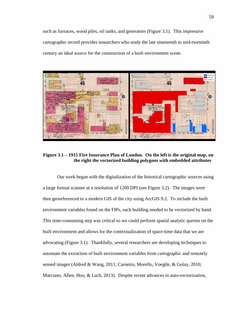
59

such as furnaces, wood piles, oil tanks, and generators (Figure 3.1). This impressive

cartographic record provides researchers who study the late nineteenth to mid-twentieth

century an ideal source for the construction of a built environment scene.

Figure 3.1 – 1915 Fire Insurance Plan of London. On the left is the original map, on the right the vectorized building polygons with embedded attributes

Our work began with the digitalization of the historical cartographic sources using

a large format scanner at a resolution of 1200 DPI (see Figure 3.2). The images were

then georeferenced to a modern GIS of the city using ArcGIS 9.2. To include the built

environment variables found on the FIPs, each building needed to be vectorized by hand.

This time-consuming step was critical so we could perform spatial analytic queries on the

built environment and allows for the contextualization of space-time data that we are

advocating (Figure 3.1). Thankfully, several researchers are developing techniques to

automate the extraction of built environment variables from cartographic and remotely

sensed images (Aldred & Wang, 2011; Carneiro, Morello, Voegtle, & Golay, 2010;

Marciano, Allen, Hou, & Lach, 2013). Despite recent advances in auto-vectorization,

60

there is still the need to assign the environmental attributes noted on the FIPs to each

feature in the geodatabase. To facilitate comparison across multiple temporal periods, the

variables needed to be normalized using common categories. Once loaded into the

geodatabase, the temporal scene was complete and ready to be added to other scenes in

the built environment stage of the HGIS.

Figure 3.2 – Built Environment Stage workflow

Of equal importance to the creation of a contextually rich stage-based historical

GIS is the civic addressing that is found within the FIPs. Each property is noted with a

precise civic address that can be used as a common spatial identifier, facilitating an easy

integration of a wide range of sources into the GIS. Of particular interest to Canadian

scholars is how this addressing can be used to facilitate the geocoding of the decennial

census of Canada prior to 1901, when no addresses are listed in the manuscript records.

This would also be of interest to other scholars who have access to individual-level data

that is devoid of a fine-grained spatial identifier.

61

3.4.2 The Social Environment Stage

A social environment stage can be created using any combination of sources that,

when record linked, provide a rich dataset outlining the many social indicators found in

the geographic area of interest. Annual city directories and the decennial census of

Canada are the cornerstones of our social environment stage. We elected to use the

decennial census as it provides the most reliable record of nineteenth and early twentieth

century urban populations (Curtis, 2001; Olson & Thornton, 2011; Sager & Baskerville,

2007).

We desired to have as rich a social environment stage as possible. The

combination of decennial censuses and annual city directories provides not only the

name, age, occupation, birthplace, ethnicity, and marital status of each individual, but

also the relationships found within each family unit or domicile, the tenancy of each

residential unit, and the place of work for those employed both within and outside the

home. We have benefited from the valiant efforts of the Canadian Century Research

Infrastructure Project (Gaffield, 2007), the 1881 Canadian Census Project (Dillon, 2000)

and the Historical Data Unit at the University of Guelph who have each assisted in the

creation of a complete count of the entire population of the city of London from 1871-

1901. This has allowed us to map every individual to their exact residential unit,

including children, a population that is rarely captured in geo-demographic studies. The

city directories, geocoded on an annual basis, allow us to understand the social

environment between the census years, including residential mobility, changing social

mobility, and property ownership. We can even follow as domestic scenes change, such

as when teenagers leave their parents’ homes to start their own households.

62

A historical city directory typically consists of four sections. There is an

alphabetical listing of each resident in the city which includes their full name, residential

address, housing tenure, occupation, and workplace. A business directory lists all

commercial and industrial operations in the city. It is sorted by the primary service

provided or good produced, and includes the name, full address, and in some cases the

owner and/or partners of the business. A street directory provides a detailed geographical

record of each street. Every address in the city is recorded along with the head of

household or business located at that address. Each address is placed in order as if you

were walking down the street and notations of proximity to cross streets and vacant land

are included. Finally, the miscellaneous directory lists the churches, schools, post

offices, and other similar public buildings located throughout the city.

The creation of the social environment stage began with the semi-automated

transcription of the city directories (Figure 3.3). All four sections of the directory, for

every year between 1871 and 1901, were run through an optical character recognition

(OCR) procedure in Adobe Acrobat. The OCR is imperfect, so each record was reviewed

by a researcher who made corrections or manual transcriptions where needed. The file

was then text parsed and imported into a MS Access database. Using the temporally-

corresponding built environment stage, we created an address point locator and geocoded

the directories. This overcame most issues that are associated with geocoding historical

records, such as street name changes or additions, and changes in residential buildings

and lots. 71% of the city directory entries across all years were geocoded through the

automated functions within ArcGIS. A combination of factors prevented the remainder

from being completed with the point locator. In 1871-1883, some addresses were

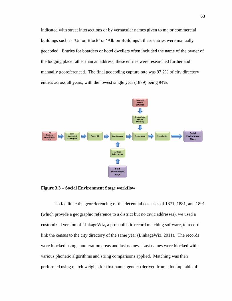
63

indicated with street intersections or by vernacular names given to major commercial

buildings such as ‘Union Block’ or ‘Albion Buildings’; these entries were manually

geocoded. Entries for boarders or hotel dwellers often included the name of the owner of

the lodging place rather than an address; these entries were researched further and

manually georeferenced. The final geocoding capture rate was 97.2% of city directory

entries across all years, with the lowest single year (1879) being 94%.

Figure 3.3 – Social Environment Stage workflow

To facilitate the georeferencing of the decennial censuses of 1871, 1881, and 1891

(which provide a geographic reference to a district but no civic addresses), we used a

customized version of LinkageWiz, a probabilistic record matching software, to record

link the census to the city directory of the same year (LinkageWiz, 2011). The records

were blocked using enumeration areas and last names. Last names were blocked with

various phonetic algorithms and string comparisons applied. Matching was then

performed using match weights for first name, gender (derived from a lookup table of

64

first names), and occupation. Occupation also included a lookup table of similar

occupational titles derived from the Historical International Standard Classification of

Occupations (HISCO) (van Leeuwen, Maas, & Miles, 2002; 2004). Only the most

probable matches (90% threshold) were automatically matched; the remainder were

manually reviewed by the researchers before inclusion in the geodatabase.

Historical demographers are acutely aware of the issues that have resulted from

the change in the census questions from enumeration to enumeration. The final step in

the creation of the social environment stage included our attempts to normalize the

census and directory variables for easier comparisons year over year (see Figure 3.4 for

the variables found within the social environment stage geodatabase). We have largely

followed the lead of the researchers involved in the North Atlantic Population Project

(NAPP) (Ruggles, 2002; Roberts, et al., 2003). Relevant variables such as the number of

rooms and state of construction found within the 1891 census were extracted and

included in the built environment stage.

The result is a robust geodatabase, or social stage, that affords us a completely

new way of looking at a city and its population. For the better part of the twentieth

century, researchers have followed the model of the Chicago School of Sociology,

studying urban populations by placing them within the arbitrary boundaries and hard

edges of the census tracts. Much like the pioneers Charles Booth (1889) and Herbert

Ames (1897), we can now map and analyze social patterns at the scale of a single block.

We can see that a new Irish Catholic immigrant, his wife, and eight children live in the

back lot behind an English Protestant industrial capitalist who employs three servants. At

65

an even finer scale, we can see the merchants’ wives who may share a friendly salutation

from porch to porch and the young single factory worker who rents a room above the

living quarters of a bourgeois insurance agent. A myriad of possible research topics may

be interrogated in a social environment stage built at this micro-scale. Rich individual-

level data allows a researcher to ask questions and discern patterns that are lost in

aggregated census data.

Researchers also benefit from the flexibility and adaptability of having a GIS built

upon a set of two or more spatially-linked, multi-temporal stages. The system can

combine any range of data included within the stages’ geodatabases, and additional

‘bricks’ may be added to the foundation of the GIS as new research questions arise. We

found ourselves doing so as we moved from projects focused on urban morphology to

those more demographic in nature.

We can combine the spatial accuracy of civic addresses with the cartographic

record of businesses, buildings and lots found on the FIP to map nearly any archival

source with the most subtle reference to an individual, business, event, or street corner.

This allows the unique opportunity to incorporate into the HGIS seemingly aspatial

archival sources such as payroll records, newspapers, or police digests, with all people

and events placed in their exact historic spatial locations. Researchers thereby have a

novel perspective on the past, allowing us to pose new questions and guiding us toward

more robust answers. This also allows for a deeper contextualization of sources, as each

source can be viewed within its appropriate temporal scene as well as in its spatial

relation to other actors or events.

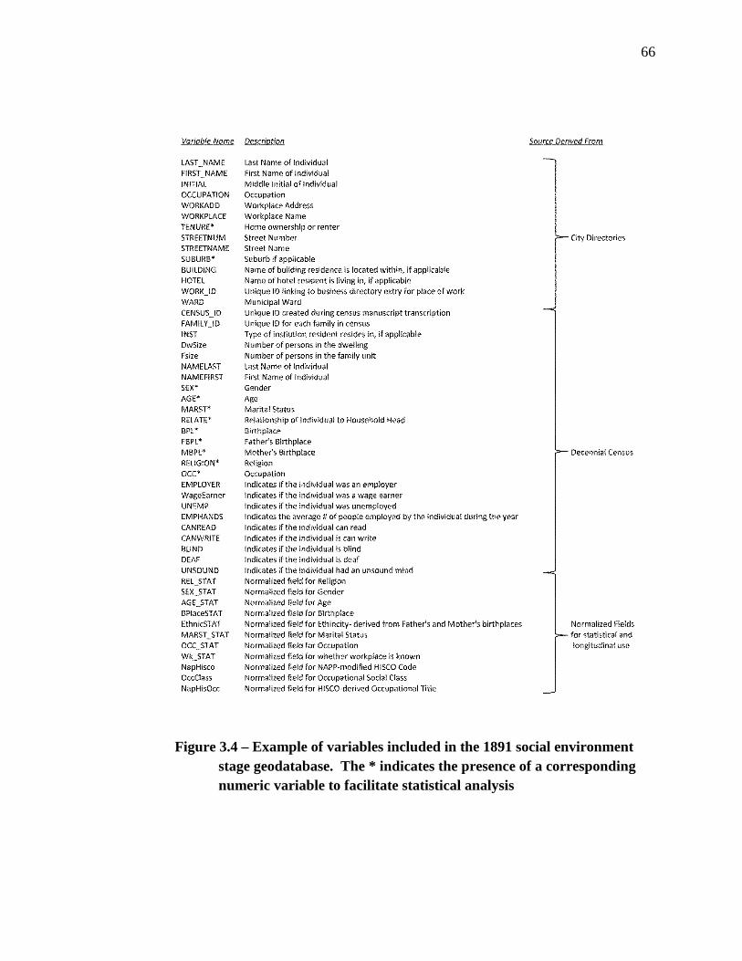
66

Figure 3.4 – Example of variables included in the 1891 social environment stage geodatabase. The * indicates the presence of a corresponding numeric variable to facilitate statistical analysis

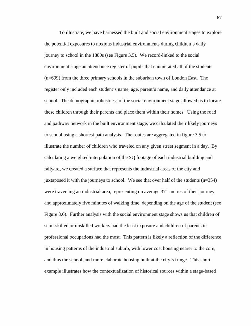
67

To illustrate, we have harnessed the built and social environment stages to explore

the potential exposures to noxious industrial environments during children’s daily

journey to school in the 1880s (see Figure 3.5). We record-linked to the social

environment stage an attendance register of pupils that enumerated all of the students

(n=699) from the three primary schools in the suburban town of London East. The

register only included each student’s name, age, parent’s name, and daily attendance at

school. The demographic robustness of the social environment stage allowed us to locate

these children through their parents and place them within their homes. Using the road

and pathway network in the built environment stage, we calculated their likely journeys

to school using a shortest path analysis. The routes are aggregated in figure 3.5 to

illustrate the number of children who traveled on any given street segment in a day. By

calculating a weighted interpolation of the SQ footage of each industrial building and

railyard, we created a surface that represents the industrial areas of the city and

juxtaposed it with the journeys to school. We see that over half of the students (n=354)

were traversing an industrial area, representing on average 371 metres of their journey

and approximately five minutes of walking time, depending on the age of the student (see

Figure 3.6). Further analysis with the social environment stage shows us that children of

semi-skilled or unskilled workers had the least exposure and children of parents in

professional occupations had the most. This pattern is likely a reflection of the difference

in housing patterns of the industrial suburb, with lower cost housing nearer to the core,

and thus the school, and more elaborate housing built at the city’s fringe. This short

example illustrates how the contextualization of historical sources within a stage-based

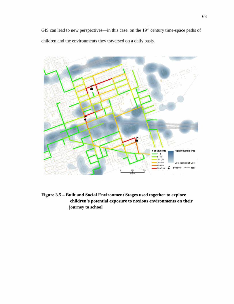
68

GIS can lead to new perspectives—in this case, on the 19th century time-space paths of

children and the environments they traversed on a daily basis.

Figure 3.5 – Built and Social Environment Stages used together to explore children’s potential exposure to noxious environments on their journey to school

69

Figure 3.6 – Distances travelled within an industrial area by children on their daily journey to school

3.5 INTEGRATING AND CONTEXTUALIZING NARRATIVES

Our interest in spatializing narratives stems from a larger research program that is

exploring the social structures of nineteenth century cities through the lens of spatial

mobilities. We wish to understand the true impact of segregation on the creation of

community by looking at the extent of social interaction through the re-creation of

individual space-time paths, what we call the spatial stories of urban life. We quickly

determined that the best sources of such fine resolution data on social interaction are

personal diaries. Nineteenth-century personal diaries vary widely in the type of

information that was recorded in them. Culley outlines that most diaries served not only

as a method of private personal record keeping (i.e. personal finances, illness, and

appointments) but also as semi-public records of life (Culley, 1989, pp. 15-17). Culley,

as well as Adams and Gossage (1998), argue that men wrote about their public activities

70

and women about family and community events. Our experience with urban diaries

confirms this.

3.5.1 Digitalization and Text Parsing

To date, we have incorporated twelve diaries that have overlapping spatial and

temporal extents. The diaries were located in a regional archive and first had to be

digitalized in preparation for inclusion in the GIS. The diaries were scanned page by

page and transcribed manually. Attempts were then made to parse the text using a

number of automated text mining methods including natural language processing

(Piotrowski, 2012), named entity recognition (Nissim, Matheson, & Reid, 2004), and

feature selection algorithms. We had limited success; even with the use of

disambiguation techniques, we found that less than 40% of the text was able to be

identified satisfactorily. A host of reasons influenced this low capture rate, such as the

wide use of shorthand, nicknames and archaic terms. Foremost was the heavy use of

vernacular terms used for locations or events. For example, “went to 7’oclock (sic)

prayer meeting at the sabbath school” or “met at the gallery building before heading to

tea at Old J Weston’s”.

Automated text segmentation and event generation is an area of significant

interest to computational linguists who are intrigued by the challenge as well as the

research possibilities available if we could harness the vast archive of data stored in texts,

especially the limitless textual archive of the internet. Interest in historical texts has been

limited until very recently. Notable efforts are underway by Michael Piotrowski (2012)

to tackle the challenges of applying current natural language processing techniques to

historical corpora. Further work has begun by Ian Gregory and others as part of a larger

71

project in the spatial humanities (Gregory, 2013). Despite these recent efforts, no

universally applicable technique for parsing and identifying historical texts is currently

available. Piotrowski argues that most successful natural language processing projects

for historical texts have taken place with tools built specifically for a historical corpora

representing a specific time and place (Piotrowski, 2012, p. 100). We did not have the

resources to create a tool specific to our corpora and thus found it more effective to parse

the text manually.

3.5.2 Creating Events from Texts

A primary concern among qualitative social scientists is how to maintain the

important contextual clues about the people, places, and events that are embedded within

a written narrative. The benefit of a manual approach to text parsing when combined

with a stage-based GIS is the ability to tease out not only subtle or incomplete references

to people, places, and events, but also to be able to extrapolate time, relationships, and

spatial mobilities.

We started by first parsing out unique socio-spatial events (Figure 3.7). An event

can take two forms. First, it can be a temporally specific mention of someone who was

spatially mobile. This can be obvious, such as “left for work at 7am”, or more subtle,

such as “We had dinner & supper at 438” (438 is the address of the diarist’s in-laws, thus

we can infer movement). The second type of event is one that involves a social

interaction, even if we are unsure of the extent of the spatial mobility present. For

example, “last evening Dick was with us for tea”. We do not necessarily know where tea

took place but we are still able to parse out this interaction.

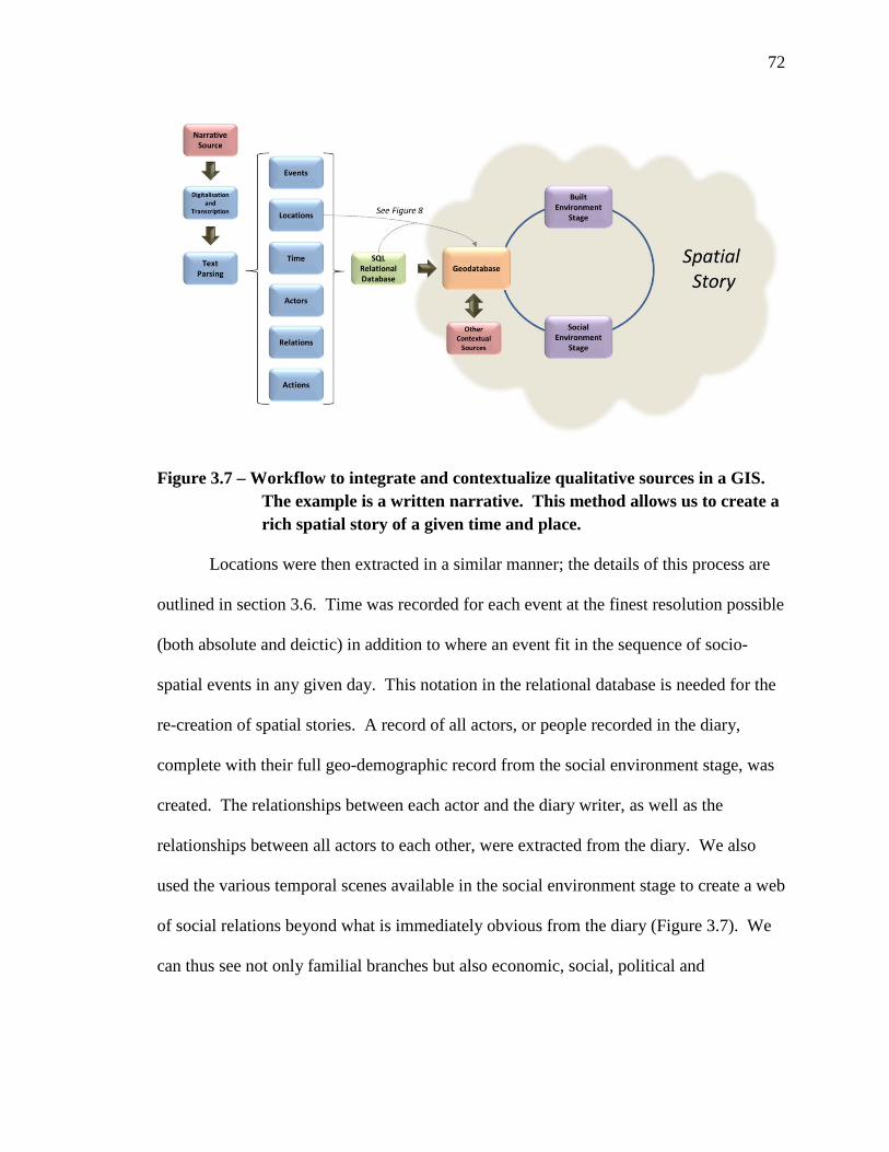
72

Figure 3.7 – Workflow to integrate and contextualize qualitative sources in a GIS. The example is a written narrative. This method allows us to create a rich spatial story of a given time and place.

Locations were then extracted in a similar manner; the details of this process are

outlined in section 3.6. Time was recorded for each event at the finest resolution possible

(both absolute and deictic) in addition to where an event fit in the sequence of socio-

spatial events in any given day. This notation in the relational database is needed for the

re-creation of spatial stories. A record of all actors, or people recorded in the diary,

complete with their full geo-demographic record from the social environment stage, was

created. The relationships between each actor and the diary writer, as well as the

relationships between all actors to each other, were extracted from the diary. We also

used the various temporal scenes available in the social environment stage to create a web

of social relations beyond what is immediately obvious from the diary (Figure 3.7). We

can thus see not only familial branches but also economic, social, political and

73

employment-based relations. In essence, we have captured a comprehensive social

network of the entire city, centred on individual diary writers.

Actions were the final element of our relational database to be parsed out of the

narrative. Actions include a number of elements such as the direction of travel, origins,

destinations, and waypoints, or stops along the way. Each event was codified using an

index of ‘why’ codes to indicate whether it was work-related, social, educational,

religious, for commerce, or otherwise; multiple reasons could be indicated. Finally, the

complete passage from the digitalized narrative was included so researchers can view the

original event in context.

3.6 GEOREFERENCING QUALITATIVE SOURCES

The spatialization of historical sources is still in relative infancy. Most projects

georeference historical sources using modern spatial datasets and address locators, as the

time and resources needed to create temporally-specific geolocators is enormous.

Notable exceptions include the pioneering project Montréal l’avenir du passé (Gilliland

& Olson, 2003). Others include the recent efforts of the Urban Transition Historical GIS

Project (Logan, Jindrick, Shin, & Zhang, 2011), which has successfully geocoded the

1880 US census to a resolution as fine as the street segment, and the historical GISes of

Alexandria, Virginia and Newport, Kentucky created by Debats (2009). Another

approach advocated by Southall et al (2011) has been to utilize databases of historical

place names and digital gazetteers. Their methods have made the geocoding of locations

somewhat less taxing; however, they do not serve to map qualitative spatial relations at

the scale of everyday life, such as the location of the “coloured barber near the market”.

Our interest in qualitative sources, including their incomplete spatial references,

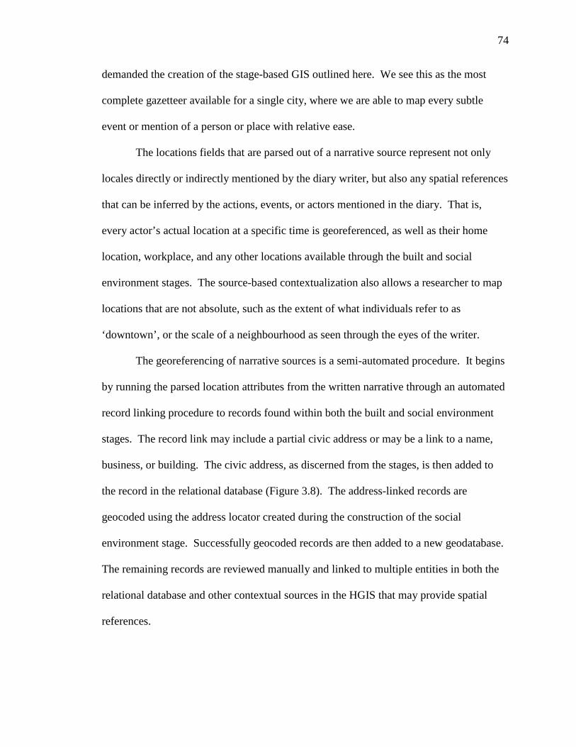
74

demanded the creation of the stage-based GIS outlined here. We see this as the most

complete gazetteer available for a single city, where we are able to map every subtle

event or mention of a person or place with relative ease.

The locations fields that are parsed out of a narrative source represent not only

locales directly or indirectly mentioned by the diary writer, but also any spatial references

that can be inferred by the actions, events, or actors mentioned in the diary. That is,

every actor’s actual location at a specific time is georeferenced, as well as their home

location, workplace, and any other locations available through the built and social

environment stages. The source-based contextualization also allows a researcher to map

locations that are not absolute, such as the extent of what individuals refer to as

‘downtown’, or the scale of a neighbourhood as seen through the eyes of the writer.

The georeferencing of narrative sources is a semi-automated procedure. It begins

by running the parsed location attributes from the written narrative through an automated

record linking procedure to records found within both the built and social environment

stages. The record link may include a partial civic address or may be a link to a name,

business, or building. The civic address, as discerned from the stages, is then added to

the record in the relational database (Figure 3.8). The address-linked records are

geocoded using the address locator created during the construction of the social

environment stage. Successfully geocoded records are then added to a new geodatabase.

The remaining records are reviewed manually and linked to multiple entities in both the

relational database and other contextual sources in the HGIS that may provide spatial

references.

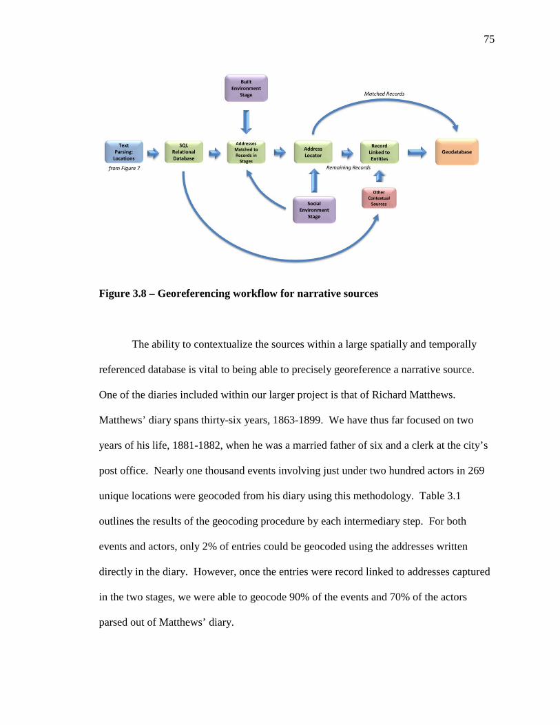
75

Figure 3.8 – Georeferencing workflow for narrative sources

The ability to contextualize the sources within a large spatially and temporally

referenced database is vital to being able to precisely georeference a narrative source.

One of the diaries included within our larger project is that of Richard Matthews.

Matthews’ diary spans thirty-six years, 1863-1899. We have thus far focused on two

years of his life, 1881-1882, when he was a married father of six and a clerk at the city’s

post office. Nearly one thousand events involving just under two hundred actors in 269

unique locations were geocoded from his diary using this methodology. Table 3.1

outlines the results of the geocoding procedure by each intermediary step. For both

events and actors, only 2% of entries could be geocoded using the addresses written

directly in the diary. However, once the entries were record linked to addresses captured

in the two stages, we were able to geocode 90% of the events and 70% of the actors

parsed out of Matthews’ diary.

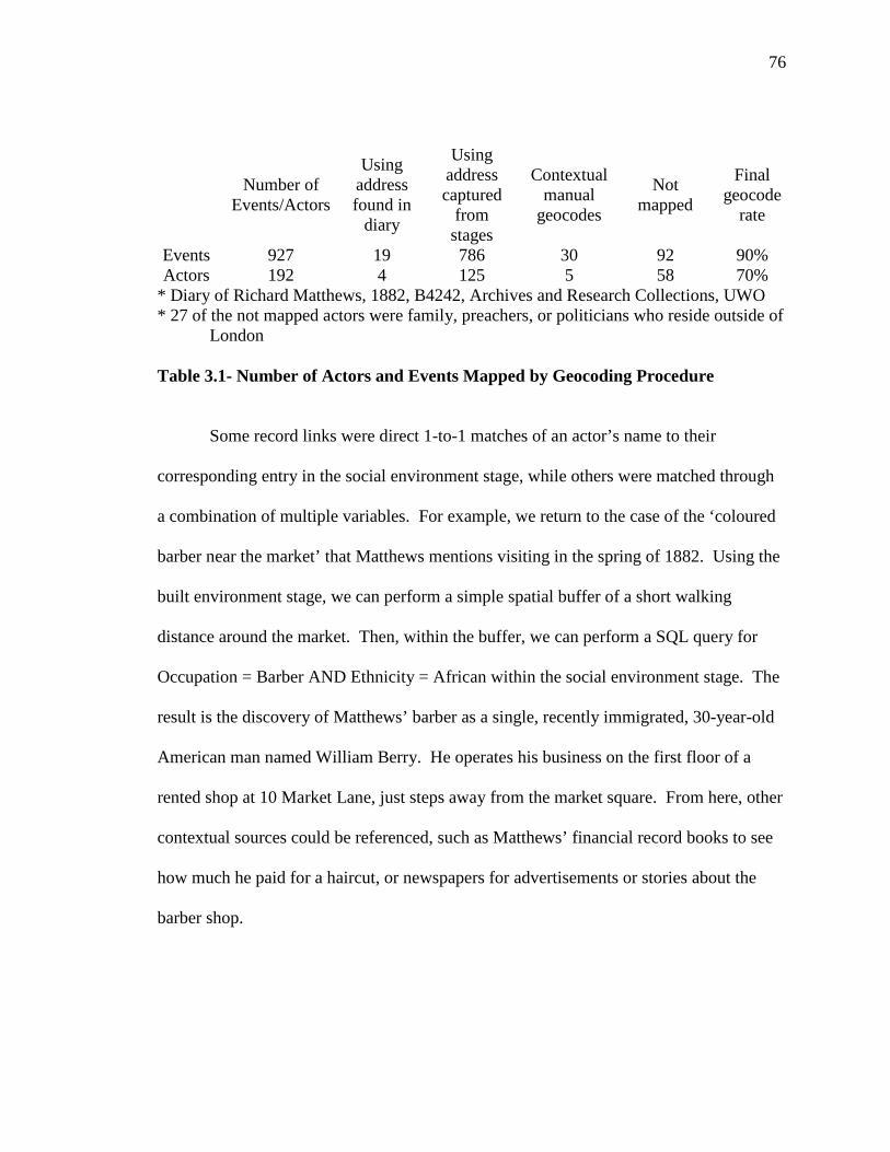
76

Number of Events/Actors

Using address found in

diary

Using address captured

from stages

Contextual manual

geocodes

Not mapped

Final geocode

rate

Events 927 19 786 30 92 90% Actors 192 4 125 5 58 70%

* Diary of Richard Matthews, 1882, B4242, Archives and Research Collections, UWO * 27 of the not mapped actors were family, preachers, or politicians who reside outside of London Table 3.1- Number of Actors and Events Mapped by Geocoding Procedure

Some record links were direct 1-to-1 matches of an actor’s name to their

corresponding entry in the social environment stage, while others were matched through

a combination of multiple variables. For example, we return to the case of the ‘coloured

barber near the market’ that Matthews mentions visiting in the spring of 1882. Using the

built environment stage, we can perform a simple spatial buffer of a short walking

distance around the market. Then, within the buffer, we can perform a SQL query for

Occupation = Barber AND Ethnicity = African within the social environment stage. The

result is the discovery of Matthews’ barber as a single, recently immigrated, 30-year-old

American man named William Berry. He operates his business on the first floor of a

rented shop at 10 Market Lane, just steps away from the market square. From here, other

contextual sources could be referenced, such as Matthews’ financial record books to see

how much he paid for a haircut, or newspapers for advertisements or stories about the

barber shop.

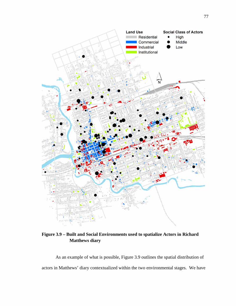
77

Figure 3.9 – Built and Social Environments used to spatialize Actors in Richard Matthews diary

As an example of what is possible, Figure 3.9 outlines the spatial distribution of

actors in Matthews’ diary contextualized within the two environmental stages. We have

78

included land use characteristics from the built environment stage as it provides a clear

image of the delineated spaces in the city. Using a simplified version of the Darroch and

Ornstein (1980) occupational class scheme we aggregated the actors in Matthews diary

into one of three social classes. The result is a spatial view of the diversity of individuals

Matthews interacts with throughout his daily life. No one social class dominates and we

see that actors live in a range of residential situations from single unit detached homes in

the suburbs, to small bungalows and residential hotels in the industrial areas of the city.

We see relations in both in the wealthy ‘Woodfield’ district north-east of downtown and

in the working class ‘London East’ neighbourhood. These are patterns that would not be

possible to discern without the ability to place the narrative within the context of the rich

built and social environment stages.

3.7 TOWARDS SPATIAL STORIES- THE CASE OF RICHARD MATTHEWS

Utilizing a stage-based GIS provides not just the ability to georeference

qualitative locations but also the ability to recreate the space-time paths and the ensuing

social interactions that are otherwise hidden within qualitative sources. A simple

comment about getting a haircut deepens our understanding of activity spaces and the

distances urban residents would travel in the walking city to complete their personal and

household chores. It provides us a taste of how racial differences were experienced

during the day when residents left their segregated neighbourhoods. It may be a

launching point for enquiries into the economic opportunities and experiences of new

immigrants. We recognize that no single case will lead a researcher to in-depth

79

conclusions, but this simple example, grouped with thousands of others, provides the

script for the creation of a rich spatial story.

Our current research interests are focused on developing a better understanding of

the impact of diurnal segregation (or integration) on the everyday lives of individuals,

both past and present. Who Matthews does and does not visit on his weekly Sunday

stroll provides only a limited view of the social structures impacting his life. Utilizing

the two environmental stages and the twelve diaries, we have recreated the time-space

paths of Matthews, as well as hundreds of other urban residents, for various time periods

between 1881 and 1901. These spatial stories shed light on the true social distances that

influenced the lived experiences of residents as they traversed the city to work, school,

church, and play.

Time geography and time space modelling has a deep scholarship. Inspired by

the pioneering work of Hägerstrand (1970) on space-time paths and prisms, scholars

continue to work towards effective geovisualization techniques that overcome the

interpretive difficulties of three dimensional geographic data (Kwan & Lee, 2004;

Nakaya, 2013; Yu & Shaw, 2011). While others are developing new models that can be

used to interrogate spatio-temporal mobility data (Chen, Shaw, Yu, Lu, Chai, & Jia,

2011; Shaw & Yu, 2009; Stewart, Fan, & White, 2013; Yu, 2006). However, with only

one notable exception (Mennis, Mason, & Cao, 2013), the space-time patterns observed

are not placed within a rich, multi-variant environmental framework like what we present

here.

Our approach to the geovisualization and analysis of spatial stories is to immerse

the narrative source within a three-dimensional model of the city created using the two

80

stages described above. Using the 3D capabilities of ESRI’s ArcScene 10, we have

created a ‘Google Street View-like’ representation of the city. Figure 3.10 represents a

recreation of the morning journey to work for Richard Matthews on April 12, 1882 as he

described it in his diary. His time-space pattern is highlighted by the brown arrow that

shows his departure at 8:15am and his arrival 10 minutes later at Fred Wheeler’s home to

borrow a copy of David Copperfield. He continues on to work, arriving at 8:50am. This

rather routine journey to work becomes a spatial story when we not only contextualize

the interaction between the actors in time-space, but set the route within the larger

environment that influences how the space is used and experienced. Here we have

utilized the social environment stage to symbolize each building polygon from the built

environment stage by ethnicity of the head of household. Labelled atop each polygon is

the value of each property in dollars per square metre as derived from the total building

value found in the municipal tax roll. Vegetation, telegraph poles, and gas street lamps

are included; their locations were identified using period photographs and a later geodetic

survey which mapped individual trees. Photographs of buildings are available through

hyperlinks embedded within the built environment stage. Thumbnails are provided

below the scene and change as you modify the extent of the map. Many other built and

social environment variables are available to be viewed and analyzed by the researcher

but the limitations of a paper map restrict us from illustrating them here. Through this

3D representation, we have an enlightening view of the physical and social landscapes

actors experienced and interacted with in their daily space-time rhythms.

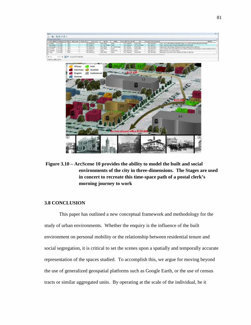
81

Figure 3.10 – ArcScene 10 provides the ability to model the built and social environments of the city in three-dimensions. The Stages are used in concert to recreate this time-space path of a postal clerk’s morning journey to work 3.8 CONCLUSION

This paper has outlined a new conceptual framework and methodology for the

study of urban environments. Whether the enquiry is the influence of the built

environment on personal mobility or the relationship between residential tenure and

social segregation, it is critical to set the scenes upon a spatially and temporally accurate

representation of the spaces studied. To accomplish this, we argue for moving beyond

the use of generalized geospatial platforms such as Google Earth, or the use of census

tracts or similar aggregated units. By operating at the scale of the individual, be it

82

buildings or actors, we can not only overcome the modifiable areal unit problem, but we

can perform multi-scaled analysis and aggregation that cannot otherwise be done. This

approach makes possible, for the first time, the realization of the promise that draws

many scholars to GIS—that by “assigning a geographic reference to data…it then

becomes possible to compare that characteristic, event, phenomenon etc. with others that

exist in the same geographic space. What were previously seemingly unrelated facts

become integrated and correlated.” (Kemp, 2010, p. 32)

This paper has also provided a methodology for the recreation of individual

space-time paths using narrative sources within a stage-based GIS. Core to this approach

is the ability to parse narrative sources into six parts, each reflecting either a spatial,

temporal, or social relationship found within the narrative. Then using temporally-

specific attributes from the built and social environment stages we georeference the

narrative to the exact locations noted within the urban fabric. Although we preserve

access to the original narrative via a hyperlink in the attribute table we recognize that by

segmenting the narrative in this way much of the qualitative-nature of the source is lost.

We see this as a small price to pay for the new perspectives that can be seen when you

integrate a narrative within the stage-based GIS. By harnessing the spatial precision,

analytical capabilities, and contextual cues available through the stage-based GIS,

researchers can now better understand the role that environmental interactions play on the

quantity and nature of human daily mobility. This is approach is congruous with Kwan’s

(2013) call for a temporally-integrated approach to the study of social geographies.

Further, this paper has outlined the need to place both the source data and the

space-time patterns observed within their larger environmental contexts. We advocate

83

for the creation of a ‘full city view’ or ‘real world’ within a geospatial environment

however has Black (2010, p. 478) reminds us “the past can never be recovered as a solid

whole, as history is always fragmented”. We must acknowledge that when working with

any historical sources there are inherent inaccuracies, biases, and omissions thus limiting

the assumptions and potentially the analysis one can perform. Additionally, we face

many of the challenges outlined by Elwood (2009b) such as how to manipulate and

represent such complex data and how to overcome the heterogeneity that is intrinsic to

such representations. We also recognize some of the limitations that Sheppard (1995;

2005) outlines when attempting to represent qualitative information in the Boolean logic

and map algebra of the raster and vector GIS.

Although our case study uses historical sources, we see these approaches as being

applicable to a wide range of contemporary lines of enquiry. Scholarship ranging from

impact of the built environment on individual health to how complex social structures

influence the settlement patterns of new immigrants can benefit from this approach.

Although a significant investment of time and resources is needed to build a stage-based

GIS, we see the rewards to be great. The diversity of enquiries that are possible is only

limited by the imagination of the researcher.

3.9 REFERENCES

Adams, A., & Gossage, P. (1998). Chez Fadette: girlhood, family, and private space in

late-nineteenth century Saint-Hyacinthe. Urban History Review, 26(2), 56-68.

84

Aldred, D., & Wang, J. (2011). A method for obtaining and applying classification

parameters in object-based urban rooftop extration from VHR multispectral

images. International Journal of Remote Sensing, 32(10), 2811-2823.

Ames, H. (1897). The city below the hill: a sociological study of a portion of the city of

Montreal, Canada. Montreal: The Bishop Engraving and Printing Co.

Berman, M. L. (2004). Key Issues in Compiling a Digital Gazetteer for China's Historical

Religious Sites. ECAI Congress on Cultural Atlases. Berkeley: ECAI Congress on

Cultural Atlases.

Black, I. (2010). Analysing Historical and Archival Sources. In N. Clifford, S. French, &

G. Valentine (Eds.), Key Methods in Geography (2nd Edition ed., pp. 466-484).

London: Sage Publishing.

Bloomfield, G. T. (1982). Canadian Fire Insurance Plans and Industrial Archeology. IA,

The Journal of the Society for Industrial Archeology, 8, 67-80.

Bodenhamer, D., Corrigan, J., & Harris, T. (Eds.). (2010). The Spatial Humanities: GIS

and the Future of Humanities Scholarship. Bloomington, IN: Indiana University

Press.

Bol, P. (2008). Creating a GIS for the History of China. In A. K. Knowles (Ed.), Placing

History: How Maps, Spatial Data, and GIS are Changing Historical Scholarship

(pp. 27-59). Redlands, CA: ESRI Press.

Booth, C. (1889). Life and Labour of the People. London: Macmillan.

Carneiro, C., Morello, E., Voegtle, T., & Golay, F. (2010). Digital Urban Morphometrics:

Automatic Extraction and Assessment of Morphological Properties of Buildings.

Transactions in GIS, 14(4), 497-531.

85

Chen, J., Shaw, S.-L., Yu, H., Lu, F., Chai, Y., & Jia, Q. (2011). Exploratory data

analysis of activity diary data: a space-time GIS approach. Journal of Transport

Geography, 19(3), 394-404.

Cooper, D., & Gregory, I. (2011). Mapping the English Lake District: a literary GIS.

Transactions of the Institute of British Geographers, 36(1), 89-108.

Corbett, J., & Rambaldi, G. (2009). Geographic Information Technologies, Local

Knowledge, and Change. In M. Cope, & S. Elwood (Eds.), Qualitative GIS: A

Mixed Methods Approach (pp. 75-91). London: Sage.

Cowan, D., McGarry, F., Moran, H., McCarthy, D., & King, C. (2012). Dreamcatcher: IT

to Support Indigenous People. IT Professional, 14(4), 39-47.

Craig, W., Harris, T., & Weiner, D. (Eds.). (2002). Community Participation and

Geographic Information Systems. New York: Taylor & Francis.

Culley, M. (1989). "I look at Me": Self as Subject in the Diaries of American Women.

Women's Studies Quarterly, 17(3/4), 15-22.

Curtis, B. (2001). The Politics of Population: State Formation, Statistics, and the Census

of Canada, 1840-1875. Toronto: University of Toronto Press.

Darroch, G., & Ornstein, M. (1980). Ethnicity and Occupational Structure in Canada in

1871: The Vertical Mosaic in Historical Perspective. Canadian Historical Review,

61(3), 305-333.

De Moor, M., & Wiedemann, T. (2001). Reconstructing Territorial Units and

Hierarchies: A Belgian Example. International Journal of Humanities and Arts

Computing, 13(1), 71-98.

86

Dear, M., Ketchum, J., Luria, S., & Richardson, D. (Eds.). (2011). GeoHumanities: Art,

History, Text at the Edge of Place. London: Routledge.

Debats, D. (2008). A Tale of Two Cities: Using Tax Records to Develop GIS Files for

Mapping and Understanding Nineteenth-Century U.S Cities. Historical Methods,

41(1), 17-38.

Debats, D. (2009). Using GIS and Individual-Level Data for Whole Communities: A Path

Toward the Reconciliation of Political and Social History. Social Science

Computer Review, 27(3), 313-330.

Dennis, S., Gaulocher, S., Carpiano, R., & Brown, D. (2009). Participatory photo

mapping (PPM): Exploring an integrated method for health and place research

with young people. Health and Place, 15(2), 466-473.

Dillon, L. (2000). International Partners, Local Volunteers, and Lots of Data: The 1881

Canadian Census Project. International Journal of Humanities and Arts

Computing, 12(2), 163-176.

Dunae, P., Lutz, J., Lafreniere, D., & Gilliland, J. (2011). Making the Inscrutable,

Scrutable: Race and Space in Victoria's Chinatown, 1891. B.C Studies, 169, 51-

80.

Elwood, S. (2009a). Multiple Representations, Significations, and Epistemologies in

Community-Based GIS. In M. Cope, & S. Elwood (Eds.), Qualitative GIS: A

Mixed Methods Approach (pp. 57-74). London: Sage.

Elwood, S. (2009b). Geographic Information Science: new geovisualization technologies

-- emerging questions and linkages with GIScience research. Progress in Human

Geography, 33(2), 256-263.

87

Gaffield, C. (2007). Conceptualizing and Constructing the Canadian Century Research

Infrastructure. Historical Methods, 40(2), 54-64.

Gilliland, J., & Olson, S. (2003, January-February). Montreal, l'avenir du passe.

GEOinfo, 5-7.

Gilliland, J., & Olson, S. (2010). Residential Segregation in the Industrializing City: A

Closer Look. Urban Geography, 31(1), 29-58.

Goad, C. (1984). A Catalogue of Fire Insurance Plans Published by Charles E. Goad

1878-1970. London: C.E. Goad.

Gregory , I., Bennett, C., Gilham, V., & Southall, H. (2002). The Great Britain Historical

GIS Project: from maps to changing human geography. Cartographic Journal,

39(1), 37-49.

Gregory, I. (2013). Spatial Humanties: Texts, Geographic Information Systems and

Places. Retrieved 07 15, 2013, from

http://www.lancaster.ac.uk/spatialhum/index.html

Gregory, I., & Cooper, D. (2009). Thomas Gray, Samuel Taylor Coleridge and

Geographical Information Systems: A Literary GIS of Two Lake District Tours.

International Journal of Humanities and Arts Computing, 3(1-2), 61-84.

Gregory, I., & Hardie, A. (2011). Visual GISting: bring together corpus linguistics and

geographical information systems. Literary and Linquistic Computing, 26(3),

297-314.

Hagerstrand, T. (1970). What about People in Regional Science? Papers of the Regional

Science Association, 24, 7-21.

88

Jung, J.-K. (2009). Computer-Aided Qualitative GIS: A Software-level Integration of

Qualitative Research and GIS. In M. Cope, & S. Elwood (Eds.), Qualitative GIS:

A Mixed Methods Approach (pp. 115-135). London: Sage.

Jung, J.-K., & Elwood, S. (2010). Extending the Qualitative Capabilities of GIS:

Computer-Aided Qualitative GIS. Transactions in GIS, 14(1), 63-87.

Kemp, K. (2010). Geographic Information Science and Spatial Analysis for the

Humanities. In D. Bodenhamer, J. Corrigan, & T. Harris (Eds.), The Spatial

Humanities: GIS and the Future of Humanities Scholarship (pp. 31-57).

Bloomington, Indiana: Indiana University Press.

Koti, F. (2010). Confronting Sociospatial Exclusion on the Fringe of Africa's Cities

Using Participatory GIS: Lessions from Athi River Town, Kenya. Africa Today,

56(3), 62-82.

Krafft, T. (1993). Reconstructing the North American Urban Landscape: Fire Insurance

Maps- An Indispensable Source. Erdkunde- Archive for Scientific Geography,

47(3), 196-211.

Kunz, A., & Boehler, W. (2005). HGIS Germany: An Information System on German

States and Territories from 1820 to 1914. Historical Geography, 33, 145-147.

Kwan, M.-P. (2007). Affecting Geospatial Technologies: Toward a Feminist Politics of

Emotion. The Professional Geographer, 59(1), 22-34.

Kwan, M.-P. (2013). Beyond Space (As We Knew It): Towards Temporally Integrated

Geographies of Segregation, Health, and Accessibility. Annals of the Assocation

of American Geographers, 103(5), 1078-1086.

89

Kwan, M.-P., & Ding, G. (2008). Geo-Narrative: Extending Geographic Information

Systems for Narrative Analysis in Qualitative and Mixed-Method Research. The

Professional Geographer, 60(4), 443-465.

Kwan, M.-P., & Lee, J. (2004). Geovisualization of Human Activity Patterns Using 3D

GIS. In M. Goodchild, & D. Janelle (Eds.), Spatially Integrated Social Science

(pp. 48-66). New York: Oxford University Press.

LinkageWiz. (2011). LinkageWiz Data Matching Software. Retrieved from

www.linkagewiz.net

Loebach, J., & Gilliland, J. (2010). Child-Led Tours to Uncover Children's Perceptions

and Use of Neighborhood Environments. Children, Youth and Environments,

20(1), 52-90.

Logan, J., Jindrick, J., Shin, H., & Zhang, W. (2011). Mapping America in 1880: The

Urban Transition Historical GIS Project. Historical Methods, 44(1), 49-60.

Lutz, J., Dunae, P., Gilliland, J., Lafreniere, D., & Harvey, M. (2013). Turning Space

Inside Out: Spatial History and Race in Victorian Victoria. In J. Bonnell, & M.

Fortin (Eds.), Historical GIS Research in Canada. Calgary: University of Calgary

Press.

Marciano, R., Allen, R., Hou, C.-Y., & Lach, P. (2013). "Big Historical Data" Feature

Extraction. Journal of Map and Geography Libraries, 9, 69-80.

McMaster, R., & Noble, P. (2005). The U.S National Historical Geographic Information

System. Historical Geography, 33, 134-136.

90

Mennis, J., Mason, M., & Cao, Y. (2013). Qualitative GIS and the visualization of

narrative activity space data. International Journal of Geographical Information

Science, 27(2), 267-291.

Mostern, R., & Johnson, I. (2008). From named place to naming event: creating

gazetteers for history. International Journal of Geographical Information Science,

22(10), 1091-1108.

Nakaya, T. (2013). Analytical Data Transformations in Space-Time Region: Three

Stories of Space-Time Cube. Annals of the Association of American Geographers,

103(5), 1100-1106.

Nissim, M., Matheson, C., & Reid, J. (2004). Recognising Geographical Entities in

Scottish Historical Documents. Workshop on Geographic Information Retrieval,

SIGIR 2004. Sheffield.

Novak, M., & Gilliland, J. (2011). Trading Places: A Historical Geography of Retailing

in London, Canada. Social Science History, 35(4), 543-570.

Olson, S., & Thornton, P. (2011). Peopling the North American City: Montreal 1840-

1900. Montreal: McGill-Queens University Press.

Oswald, D. (1997). Fire Insurance Maps: Their History and Applications. College

Station, Texas: Lacewing Press.

Piotrowski, M. (2012). Natural Language Processing for Historical Texts: Synthesis

lectures on human language technologies. San Rafael, CA: Morgan & Claypool.

Rambaldi, G., Kwaku Kyem, P., McCall, M., & Weiner, D. (2006). Participatory Spatial

Information Management and Communication in Developing Countries. The

Electronic Journal of Information Systems in Developing Countries, 25, 1-9.

91

Roberts, E., Ruggles, S., Dillon, L., Gardarsdottir, O., Oldervoll, J., Thorvaldsen, G., et

al. (2003). The North Atlantic Population Project. Historical Methods, 36(2), 80-

88.

Ruggles, S. (2002). Linking Historical Censuses: A New Approach. History and

Computing, 14(1-2), 213-224.

Sager, E., & Baskerville, P. (Eds.). (2007). Household Counts: Canadian Households

and Families in 1901. Toronto: University of Toronto Press.

Shaw, S.-L., & Yu, H. (2009). A GIS-Based time-geographic approach of studying

individual activities and interactions in a hybrid physical-virtual space. Journal of

Transport Geography, 17(2), 141-149.

Sheppard, E. (1995). GIS and society: towards a research agenda. Cartography and

Geographic Information Systems, 22(1), 5-16.

Sheppard, E. (2005). Knowledge production through critical GIS: geneology and

prospects. Cartographica, 40(4), 5-21.

Southall, H., Mostern, R., & Berman, M. L. (2011). On historical gazetteers.

International Journal of Humanities and Arts Computing, 5(2), 127-145.

Stewart, K., Fan, J., & White, E. (2013). Thinking about Space-Time Connections:

Spatiotemporal Scheduling of Individual Activities. Transactions in GIS.

St-Hilaire, M., Moldofsky, B., Richard, L., & Beaudry, M. (2007). Geocoding and

Mapping Historical Census Data: The Geographical Component of the Canadian

Century Research Infrastructure. Historical Methods, 40(2), 76-91.

92

van Leeuwen, M., Maas, I., & Miles, A. (2002). HISCO: Historical International

Standard Classification of Occupations. Leuven, Belgium: Leuven University

Press.

van Leeuwen, M., Maas, I., & Miles, A. (2004). Creating a Historical International

Standard Classification of Occupations: An Exercise in Multinational

Interdisciplinary Cooperation. Historical Methods, 37(4), 186-197.

Yao, X., & Jiang, B. (2005). Visualization of Qualitative Locations in Geographic

Information Systems. Cartography and Geographic Information Science, 32(4),

219-229.

Yao, X., & Thill, J.-C. (2006). Spatial Queries with Qualitative Locations in Spatial

Information Systems. Computers Environment and Urban Systems, 30(4), 485-

502.

Yu, H. (2006). Spatio-temporal GIS design for Exploring Interactions of Human

Activities. Cartography and Geographic Information Science, 33(1), 3-19.

Yu, H., & Shaw, S.-L. (2011). GIS Designs for Studying Human Activities in a Space-

Time Context. In T. Nyerges, H. Couclelis, & R. McMaster (Eds.), The SAGE

Handbook of GIS and Society (pp. 251-268). London: SAGE Publishing.

93

CHAPTER FOUR

Revisiting the Walking City: A Geospatial Examination of the Journey to Work

Don Lafreniere and Jason Gilliland

94

4.1 ABSTRACT

The daily commute to work and its related social histories have long been of

interest to historical geographers and urban historians. This article revisits the existing

scholarship on the nineteenth-century journey to work and outlines a new methodological

framework that uses a historical GIS to overcome many of the challenges identified in

previous studies. These challenges include a reliance on small, atypical samples of

workers, approximations of the spatial relationship between home and work, and

unrealistic interpretations of journeys travelled by employing only Euclidean paths.

Combining city directories and decennial censuses through the use of probabilistic record

linkage techniques uncovers the relationship between work and home for over 5,000

workers in London, Ontario in 1881. A GIS network-derived journey to work model

recreates more realistic journeys that considers the many natural and built environment

barriers that influenced the paths and distances workers travelled on a daily basis.

Empirical results of the journey to work along lines of occupational class, coincident

home-work location, and gender are presented and contextualized to studies in other

cities. The results highlight that experiences of commuting differ widely along lines of

social class and gender.

Keywords: Journey to Work, Space-Time, Historical GIS, Census, Mobility

95

4.2 INTRODUCTION

The rapid industrialization and urbanization experienced in the late nineteenth

century affected many aspects of daily life. For adults, one aspect that bridged all socio-

demographic and economic groups was the journey to work. This unifying experience of

daily life was a result of the growing spatial separation between home and the workplace

due to changes in the nature of work, from primarily home-based artisanal work to wage

labour. The journey to work also reflected larger evolving urban processes, such as

suburbanization and segregation. In the second half of the nineteenth century, mid-sized

Canadian cities were still largely dominated by commuters who travelled to work by foot,

either on the streets, alongside the horse-drawn carts used for heavy or bulky loads, or on

the rapidly-emerging network of sidewalks. Commuters were closely connected to the

physical and built environments they traversed, enjoying the pleasant fragrance of

flowers wafting from the gardens of well-built homes or subjected to the foul odours that

emanated from the breweries and cigar factories. They had to cope with the elements that

the glass and steel of our modern automobiles shelter us from, such as July’s intense sun

and January’s blowing snow and sleet. The daily commute provided individuals an

intimate scale by which to experience the social environments present in the city. In the

walking city, everyone else on the street was within earshot as well as within an easy

visual distance, making the journey to work one of the periods with the highest potential

for social interaction during an individual’s daily time-space rhythm.

This paper revisits the late nineteenth-century journey to work in the

industrializing city, an area of research that has had little attention since the 1990s. Using

the mid-sized Canadian city of London, Ontario as a case study, this paper extends the

96

existing literature by exploring the spatial and temporal pattern of work at a scope and

scale unprecedented in earlier studies. Through the use of a full count of the city’s

population in 1881 and 1891, which includes the workplace of nearly every male (and

many female) workers, we can, for the first time, establish the relationship between home

and work for an entire urban population. The dataset is interrogated using the spatial

analytic capabilities of a GIS to recreate the daily time-space patterns of individuals from

every socio-demographic and economic group in the city.

This study of the journey to work was undertaken for an important

methodological purpose – to recreate the spatial relationships between work and home.

By having a sound methodology with which to recreate these relationships, other scholars

can then re-examine the roles played by transportation, residential segregation, land use

policies, and restrictive covenants on access to employment and its impact on

demography, social mobility, and housing choice. This study looks to create a

methodology that overcomes the many limitations noted in the literature of previous

journey to work studies.

4.3 RELATED WORK

The study of Canadian work history saw a resurgence in the late 1960s thanks to

British historian E.P. Thompson’s call to recover the lives and experiences of working-

class people “from the enormous condescension of posterity” (Thompson, 1980 [1963],

p. 12). This call was answered by the likes of Kealey (1980) and Bradbury (1996), who

both described the changes in working life during periods of industrialization in large

Canadian cities (Toronto and Montreal, respectively). Several edited collections have

97

been compiled, with chapters on the working lives of everyone from shantymen and

railway workers to boys in mining camps and girls in textile shops (Craven, 1995; Cross,

1974; Opp & Walsh, 2006). This scholarship provides a rich and invaluable narrative,

used by students of Canadian labour history across the country. However, the spatial

relationships between work and home are less known.

While there is little empirical evidence, especially for Canada, setting out details

of the journey to work before 1900, the importance of the geography of the home-work

relationship has been considered for several non-Canadian cities. The greatest attention

has come from scholars who studied the dominant industrial cities of Britain, especially

London (Green, 1988; Lees, 1969; Pooley & Turnbull, 1997; 1999; 2000), as well as

Birmingham (Vance, 1967), Huddersfield (Dennis R. , 1984), Liverpool (Pooley C. ,

1984), and Newcastle (Barke, 1991). In North America, work has been concentrated in

large metropolitan areas such as Philadelphia; the journey to work was one of the areas of

interest of the twelve year (1969-1981) Philadelphia Social History Project led by

Theodore Hershberg (Greenberg, 1980; Hershberg T. , 1976; Hershberg, Light, Cox, &

Greenfield, 1981). For Canada, Montreal has been the most productive laboratory,

though we find the concerns of the relationship between work and home to be secondary

to wages (Hoskins, 1989), the process of industrial suburbanization (Gilliland, 2004;

Lewis, 2000), segregation (Gilliland & Olson, 2010; Gilliland, Olson, & Gauvreau, 2011;

Olson & Thornton, 2011), and the nature of the work itself (Bradbury B. , 1996). An

important exception to the gulf of empirical research on the journey to work in Canada

prior to 1900 is Peter Goheen’s study of Toronto (1970). Goheen uses the daily commute

98

to illustrate the extent of residential segregation among differing social classes in

Victorian Toronto.

There has been more interest in the Canadian experience of the journey to work

after the turn of the 20th century. Richard Harris and Victoria Bloomfield took on the

topic while exploring the processes of decentralization of workplaces and the broader

suburbanization of cities (Harris & Bloomfield, 1997; Bloomfield & Harris, 1997). Their

landmark paper (Bloomfield & Harris, 1997) outlined a methodology that has served as

the inspiration for much of this paper.

4.4 IDENTIFYING METHODOLOGICAL CHALLENGES

Despite what may appear at first blush to be a wealth of previous research, the

study of the daily commute to work has not received significant attention. Geographer

Richard Dennis suggests that one of the reasons may be that “data for studying journeys

to work are exceedingly scarce, particularly for quantitative research in which a single

source records both place of residence and place of work” (Dennis R. , 1984, p. 132). As

a result, previous research on the nineteenth-century city has utilized sources (data) that

either represent a small, non-random, possibly atypical sample of workers or only allow

for the inference of home and work, rather than absolute spatial links (Dennis R. , 1984,

p. 132). For example, Green (1988) uses only a wage book for a single employer, as did

Hoskins (1989) for his study of railworkers in Montreal. Barke (1991) used city

directories to capture a set of nearly two thousand workers over four time slices.

However, his sample only included middle-class business owners because he did not

have the workplaces of non-owners, so it only represented 4% of the middle-class

99

population of Newcastle. Dennis (1984), though recognizing the limitations of his

methodology and calling for alternatives, elected to use the census returns for only one

industry, silk manufacturing. Industry-specific studies have also been completed by Pred

(1966) for five industries in New York City. The Philadelphia Social History Project also

used five industries, derived from the Census of Manufacturing, though this sample was

still robust with over 3700 workers represented. Bloomfield and Harris (1997) concerned

themselves with a similarly small sample of employers.

Methodological decisions surrounding how to best recreate the needed home-

work links have typically been constrained by limitations in the sources or lack of

resources necessary for compiling and analyzing a more comprehensive database of

employees and employers. These limitations have led authors of most previous studies to

use methods of approximation. Vance (1967) saw the need to combine the census along

with a comprehensive source of workplaces—the business directory. However, the 1851

British census he utilized did not include workplaces for those enumerated, so he was

unable to match individuals to their specific places of work. Vance instead created

labour sheds, or areas where workers reside, and employment fields, areas of workplaces,

and compared the distances between them. Dennis (1984), using the same sources as

Vance, was likewise restricted to only inferring home-work links in his study of

Huddersfield’s silk industry. The Philadelphia Social History Project (Greenberg, 1980;

Hershberg, Light, Cox, & Greenfield, 1981) also inferred the workplaces of its city’s

workers by creating arbitrary labour shed boundaries for each industry and then matching

an individual’s occupational title to the product manufactured within individual

businesses. Pooley, in his study of the journey to work in late-nineteenth century

100

Liverpool, used a ten percent census sample and calculated distances from an individual’s

residence to the nearest potential workplace. He explains that ‘for dock workers this is

defined as the nearest operational dock; all office workers are assumed to work in the

C.B.D. [central business district]” (Pooley C. , 1984, p. 134).

The impact of a lack of quality sources has resulted in other difficulties for

scholars of the nineteenth-century journey to work. Many authors are interested in

evaluating the differences in how the journey to work was experienced by members of

various ethnic or racial groups. Mayer (1977), in his study of Milwaukee, used

individuals’ surnames, as recorded in the city directory, to infer their ethnic affiliation.

Mayer acknowledges the difficulties of this approach, suggesting that even in the best of

cases only seventy-percent accuracy can be expected (Mayer, 1977, p. 54). Deskins

(1972) used directories in a similar manner to examine the racial differences in the

journey to work in Detroit in the late 19th century. He derived race by a “colored”

notation within the alphabetical directory rather than utilizing the more authoritative and

complete decennial federal census. His decision not to use the census was not explained,

nor did he compare the aggregate population totals by racial affiliation between the two

sources to gauge the reliability of the “colored” notation in the directory. From these

assumptions, significant historical generalizations of race-based behaviour were

generated. These criticisms were noted by his colleagues and resulted in a heated debate

within the pages of the Professional Geographer (Deskins, 1975; Gale & Katzman,

1975).

Deskins’ work has other methodological limitations, ones shared with nearly all

previous journey to work studies – poor spatial accuracy in locating home and workplace

101

as well as the methodology used to calculate the actual journey to work. Deskins’ work,

separate from his controversial derivation of race, suffered the greatest shortcomings. He

was unable to link individuals to their workplaces, nor did he have the resources needed

to map individuals to their specific residences. To compensate, he elected to approximate

the location of work and home by using the mean centre of residences and the mean

centre of workplaces while controlling for the extremes by calculating the standard

distance around each mean. The resulting ‘worktrip vector’ is nothing more than a

measure between the residential areas of Detroit and the non-residential areas. Other

studies suffer from similar limitations, though not as severe. Green (1988) attempted to

map each worker in Henry Poole’s bespoke tailor shop to their exact residence, but found

that addresses in London (UK) during the later decades of the nineteenth century were

haphazard. His efforts were limited by a combination of address changes, street name

changes, and sources that did not coincide temporally. His solution was to estimate each

street’s addressing by assigning civic address #1 at one terminus of the street and

assigning numbers at equal intervals moving down the street (Green, 1988, p. 186). Both

Goheen and the Philadelphia Social History Project elected to use arbitrary grids to map

residences and workplaces. The Philadelphia Social History Project created 660 x 775

foot grids and measured from centroid to centroid to calculate the length of the daily

journey (Hershberg, Light, Cox, & Greenfield, 1981, p. 131). Additionally, as discussed

earlier in this section, several studies have assumed that workers were employed at the

closest workplace for which they were qualified. This assumption skews the results to

indicate shorter daily commutes than may have been realized.

102

Due to the lack of computational power and robust data sets, all previous

nineteenth-century journey to work studies elected to use Euclidean, or straight-line,

distances in their calculations, rather than taking into account the actual distances that

would have been traveled on the existing roadways. Even the most contemporary of

studies, those that are beyond the scope of my current research, rarely utilize existing

geospatial technologies to recreate more realistic paths (Corcoran, Chhetri, & Stimson,

2009; Sultana & Weber, 2007), and one of the only exceptions uses hypothetical journeys

(Bousssauw, Neutens, & Witlox, 2011).

This paper first overcomes the limitations outlined above that have influenced the

results of previous journey to work studies. Secondly, it extends the existing journey to

work methodologies by utilizing the spatial analytical capabilities of GIS and computer-

based probabilistic record matching algorithms. Lastly, this paper will outline some of

the journey to work experiences along lines of socio-economic class, gender, and age.

4.5 CASE STUDY: LONDON, CANADA

Previous journey to work studies have been primarily concerned with large urban

centres, rarely concerning themselves with the more common medium-sized nineteenth

century towns. Debats (2009) outlines how studying large urban centres is not practical

when the scale of analysis is the individual. We heed his advice in this study and apply

the same ‘small city research strategy’ he extols. This case study is the mid-sized

Canadian city of London, Ontario, Canada. London provides a classic example of a city

that was changing from a commercial to an industrial town. London is located half-way

between Toronto and Detroit, an advantageous position that was quickly recognized by

103

many investors and industrialists. Several major companies began to employ Londoners

in the last two decades of the nineteenth century. The Grand Trunk Railway built its train

car factory in London East in 1887, which added over a hundred jobs to its already large

operation in the city. Imperial Oil commenced refining in London East in 1880.

Established companies such as the brewers Labatt and Carling, the confectioner

McCormick, and McClary’s foundry increased their workforce during this era as the

demands for their goods grew faster than the efficiencies of mechanization. Despite these

increases, London continued to be a diverse commercial city with most of its workers

employed at small or medium sized firms in a wide range of industries. In 1881, there

were an average of 2.5 workers per business; by 1891 it had risen to nearly 4 workers per

firm.

The London of 1881 was a quintessential British town on Canadian soil. Both the

established citizenry and the waves of recent immigrants were predominantly from the

British Isles, and Protestant faiths dominated the religious composition of the growing

city. With a population of 19,746 at the time of the 1881 Census of Canada, London

ranked 8th among Canadian cities and 86th in North America, making it comparable to

cities such as St. John, NB, Lancaster, PA, and Des Moines, IA. For this study, I also

included the three major suburbs of London: Petersville (aka London West), the Village

of London East, and the urban section of Westminster Township (aka London South).

Together these suburbs totaled 3,890 residents. It is critical to include these suburbs as

they contributed significantly to the available employers and the diverse workforce found

about the city. Additionally, suburban populations and industries are often overlooked in

104

other studies, mostly because the census separates them from the urban core when

disseminating their enumerations.

4.6 OVERCOMING LIMITATIONS

4.6.1 Larger Samples and Absolute Workplaces

To overcome the limitations of small sample sizes and the lack of

representativeness found in previous studies, this paper utilizes the robust built and social

environment stages outlined in paper 1 of this thesis. Specifically, this study harnesses

the geocoded decennial census that was captured through the creation of the social

environment stage. As outlined by Figure 3.3, the census was record-linked to the city

directory, which facilitated the geocoding of nearly all individuals to their residential

location. This dataset locates nearly 90% of the population in London and suburbs in

1881 and provides the needed variables to determine the home residence for each worker

in the city.

No other journey to work study has captured what is arguably the whole of the

workforce in an urban location. Various methods of sampling have been utilized and

rarely, with the exception to a certain extent of Deskins and Mayer, have researchers

compared the distribution of their samples to the total enumerated population. It is

generally accepted by historical geographers and historians alike that the federal census

represents the gold standard record of a past population, though there are critics (Curtis,

2001). Table 4.2 compares the geocoded population used in this study to the full census

enumeration collected in London for the year 1881. To illustrate how representative the

90% sample is, the population has been disaggregated using key demographic variables.

It is observed that along lines of religion, gender, and marital status, the variances are no

105

more than 1%. For ethnic origin, we see an equally representative sample, with only a

2.55% overrepresentation of those of Irish decent and a 1.44% underrepresentation of

Scottish in the geocoded sample versus the total population. Birthplace is also

representative, with only a 1.92% underrepresentation of those born in Ontario. The

representativeness of the sample population is without question. There are no concerns

of an ecological fallacy, as the sample is not only representative, but is also disaggregated

to the level of the individual.

Religion 1881

Geocoded Population

Census Population Variance

n = 21246 n =23636 Protestant 83.46% 84.74% -1.28% Catholic 14.37% 13.33% 1.04% Other 1.77% 1.45% 0.32% Unknown 0.40% 0.48% -0.08%

Gender 1881 Geocoded Population Census Population Variance n = 21246 n =23636 Female 50.46% 50.45% 0.01% Male 49.54% 49.55% -0.01%

Marital Status 1881

Geocoded Population Census Population Variance

n = 21246 n =23636 Married 32.88% 33.49% -0.61% Single 62.68% 62.07% 0.61% Widowed 4.44% 4.44% 0.00%

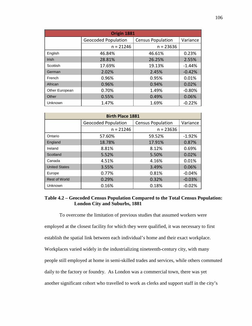
106

Origin 1881 Geocoded Population Census Population Variance n = 21246 n = 23636 English 46.84% 46.61% 0.23% Irish 28.81% 26.25% 2.55% Scottish 17.69% 19.13% -1.44% German 2.02% 2.45% -0.42% French 0.96% 0.95% 0.01% African 0.96% 0.94% 0.02% Other European 0.70% 1.49% -0.80% Other 0.55% 0.49% 0.06% Unknown 1.47% 1.69% -0.22%

Birth Place 1881 Geocoded Population Census Population Variance n = 21246 n = 23636 Ontario 57.60% 59.52% -1.92% England 18.78% 17.91% 0.87% Ireland 8.81% 8.12% 0.69% Scotland 5.52% 5.50% 0.02% Canada 4.51% 4.16% 0.01% United States 3.55% 3.49% 0.06% Europe 0.77% 0.81% -0.04% Rest of World 0.29% 0.32% -0.03% Unknown 0.16% 0.18% -0.02%

Table 4.2 – Geocoded Census Population Compared to the Total Census Population: London City and Suburbs, 1881

To overcome the limitation of previous studies that assumed workers were

employed at the closest facility for which they were qualified, it was necessary to first

establish the spatial link between each individual’s home and their exact workplace.

Workplaces varied widely in the industrializing nineteenth-century city, with many

people still employed at home in semi-skilled trades and services, while others commuted

daily to the factory or foundry. As London was a commercial town, there was yet

another significant cohort who travelled to work as clerks and support staff in the city’s

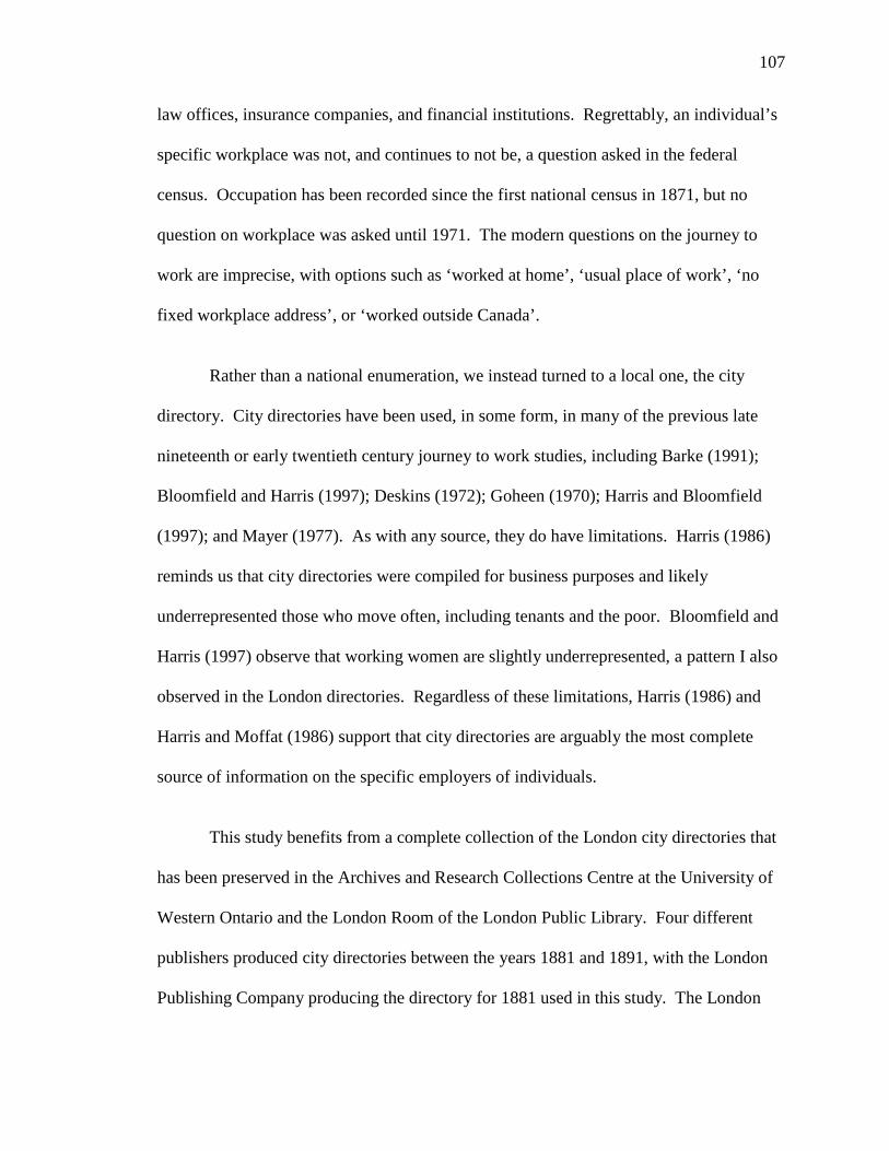
107

law offices, insurance companies, and financial institutions. Regrettably, an individual’s

specific workplace was not, and continues to not be, a question asked in the federal

census. Occupation has been recorded since the first national census in 1871, but no

question on workplace was asked until 1971. The modern questions on the journey to

work are imprecise, with options such as ‘worked at home’, ‘usual place of work’, ‘no

fixed workplace address’, or ‘worked outside Canada’.

Rather than a national enumeration, we instead turned to a local one, the city

directory. City directories have been used, in some form, in many of the previous late

nineteenth or early twentieth century journey to work studies, including Barke (1991);

Bloomfield and Harris (1997); Deskins (1972); Goheen (1970); Harris and Bloomfield

(1997); and Mayer (1977). As with any source, they do have limitations. Harris (1986)

reminds us that city directories were compiled for business purposes and likely

underrepresented those who move often, including tenants and the poor. Bloomfield and

Harris (1997) observe that working women are slightly underrepresented, a pattern I also

observed in the London directories. Regardless of these limitations, Harris (1986) and

Harris and Moffat (1986) support that city directories are arguably the most complete

source of information on the specific employers of individuals.

This study benefits from a complete collection of the London city directories that

has been preserved in the Archives and Research Collections Centre at the University of

Western Ontario and the London Room of the London Public Library. Four different

publishers produced city directories between the years 1881 and 1891, with the London

Publishing Company producing the directory for 1881 used in this study. The London

108

alphabetical directories include the name, residential address, tenure, occupation, and

employer for each private citizen and business firm in the city. For widowed women, the

name of their late husband is also noted. Those workers who did not work outside of

their homes were also enumerated; the directory lists only a residential address or in some

instances denotes this relationship between home and work with the word ‘same’. These

variables are captured from the social environment stage and used to establish the needed

home-work link in this study.

The geocoded business directory was utilized to determine the specific worksite

of each employed person in the city (these details are outlined in chapter 3). The

business directory lists both major and minor employers, as well as sole proprietors,

classified by their predominant industry or service (see Figure 4.1). The name of the

business and/or proprietor, along with a business address or the name of a significant

commercial building is included in each listing. For those companies who paid an

additional fee, a larger advertisement was included with some details of the services or

wares for sale.

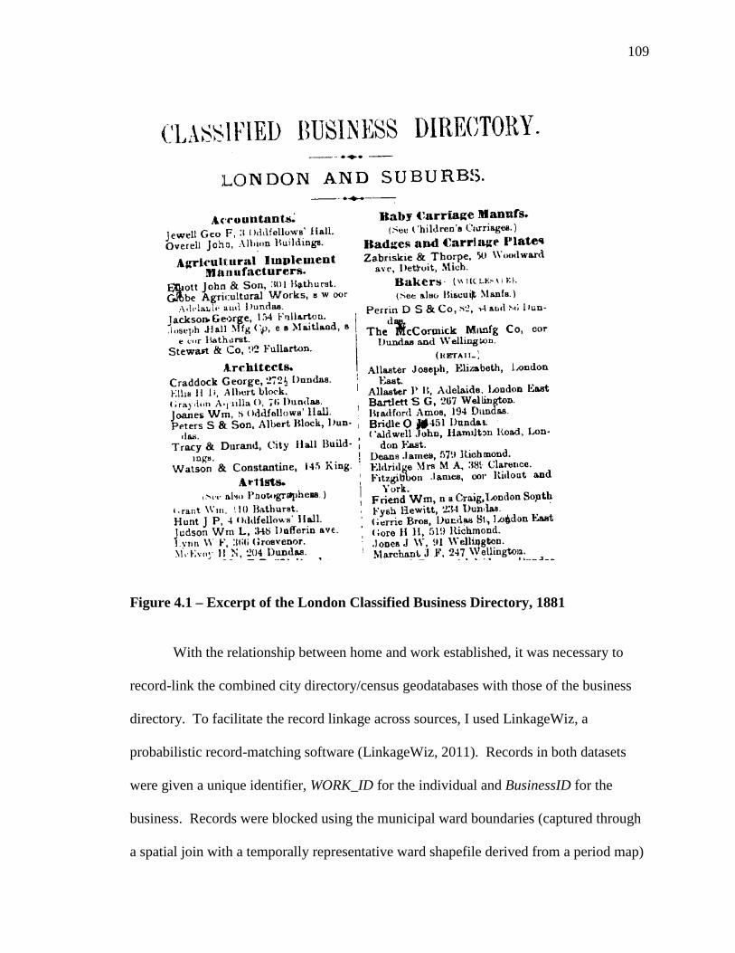
109

Figure 4.1 – Excerpt of the London Classified Business Directory, 1881

With the relationship between home and work established, it was necessary to

record-link the combined city directory/census geodatabases with those of the business

directory. To facilitate the record linkage across sources, I used LinkageWiz, a

probabilistic record-matching software (LinkageWiz, 2011). Records in both datasets

were given a unique identifier, WORK_ID for the individual and BusinessID for the

business. Records were blocked using the municipal ward boundaries (captured through

a spatial join with a temporally representative ward shapefile derived from a period map)

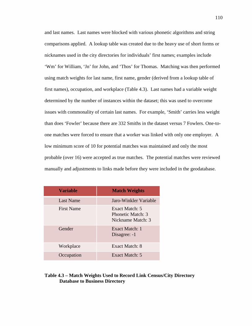
110

and last names. Last names were blocked with various phonetic algorithms and string

comparisons applied. A lookup table was created due to the heavy use of short forms or

nicknames used in the city directories for individuals’ first names; examples include

‘Wm’ for William, ‘Jn’ for John, and ‘Thos’ for Thomas. Matching was then performed

using match weights for last name, first name, gender (derived from a lookup table of

first names), occupation, and workplace (Table 4.3). Last names had a variable weight

determined by the number of instances within the dataset; this was used to overcome

issues with commonality of certain last names. For example, ‘Smith’ carries less weight

than does ‘Fowler’ because there are 332 Smiths in the dataset versus 7 Fowlers. One-to-

one matches were forced to ensure that a worker was linked with only one employer. A

low minimum score of 10 for potential matches was maintained and only the most

probable (over 16) were accepted as true matches. The potential matches were reviewed

manually and adjustments to links made before they were included in the geodatabase.

Table 4.3 – Match Weights Used to Record Link Census/City Directory Database to Business Directory

Variable Match Weights

Last Name Jaro-Winkler Variable First Name Exact Match: 5

Phonetic Match: 3 Nickname Match: 3 Gender Exact Match: 1 Disagree: -1

Workplace Exact Match: 8

Occupation Exact Match: 5

111

For workers who were employed by a large company with multiple worksites,

such as the railway workers of the Great Western Railway, I used the occupation to

estimate the most appropriate worksite. For example, engine builders were assumed to

work in the engine house and wood and coal workers to work in the wood and coal yards.

For complete unknowns, the main office was used, as it was assumed they would traverse

there regularly for instructions and supplies or to retrieve wages. Each of these entries

received a new record in the business directory geodatabase. For those who worked for

an individual, such as gardeners or domestic servants, a new record was created in the

business directory geodatabase for the home residence of the employer as listed in the

city directory. To facilitate analysis, the field WkPlaceID was created to differentiate the

worksites from the businesses.

The result is a robust sample of 5081 workers matched to their specific workplace

out of the 2295 workplaces in the city. In previous studies, the largest sample of workers

reported was 800, all from a single workplace (Harris & Bloomfield, 1997). There were

14,707 adults between the ages of 17 and 63 in the city of London and its suburbs who

were considered available for work. Age 63 was used as the upper limit as the number of

individuals listed as ‘gentlemen’ was observed to increase significantly after this

threshold. The reverse was observed for teenagers, with the rise in employment coming

between their 16th and 17th year. It must be considered that 7,504 of the available

workforce were women and this study is during a period where wage employment for

women outside the home was still very low. I estimate that 12% of working-aged women

were engaged in wage labour or as proprietors in a home-based cottage industry.

Frances, Kealey, and Sangster (1996) found 11% of women were engaged in wage labour

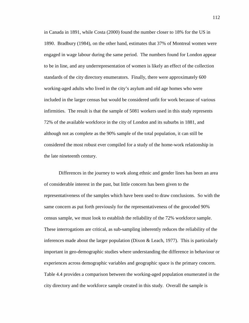
112

in Canada in 1891, while Costa (2000) found the number closer to 18% for the US in

1890. Bradbury (1984), on the other hand, estimates that 37% of Montreal women were

engaged in wage labour during the same period. The numbers found for London appear

to be in line, and any underrepresentation of women is likely an effect of the collection

standards of the city directory enumerators. Finally, there were approximately 600

working-aged adults who lived in the city’s asylum and old age homes who were

included in the larger census but would be considered unfit for work because of various

infirmities. The result is that the sample of 5081 workers used in this study represents

72% of the available workforce in the city of London and its suburbs in 1881, and

although not as complete as the 90% sample of the total population, it can still be

considered the most robust ever compiled for a study of the home-work relationship in

the late nineteenth century.

Differences in the journey to work along ethnic and gender lines has been an area

of considerable interest in the past, but little concern has been given to the

representativeness of the samples which have been used to draw conclusions. So with the

same concern as put forth previously for the representativeness of the geocoded 90%

census sample, we must look to establish the reliability of the 72% workforce sample.

These interrogations are critical, as sub-sampling inherently reduces the reliability of the

inferences made about the larger population (Dixon & Leach, 1977). This is particularly

important in geo-demographic studies where understanding the difference in behaviour or

experiences across demographic variables and geographic space is the primary concern.

Table 4.4 provides a comparison between the working-aged population enumerated in the

city directory and the workforce sample created in this study. Overall the sample is

113

representative, with significant variances being found in a select number of variables.

For example, Ontario-born workers are overrepresented while those born in England are

underrepresented. Single workers are overrepresented while those who are widowed are

underrepresented.

A brief explanation is in order for the occupational class variable outlined in

Table 4.4. To facilitate the comparisons of the journey to work across the large number

of occupations found in the sample, I elected to use a modification of the occupational

class scheme developed by Darroch and Ornstein (1980) for their study of the

occupational structure in Canada in 1871. The scheme was modified by Lisa Dillon

(2008) for use with the 1881 census and was provided to me for use in this study. The

occupational class scheme is used as a proxy for socio-economic status since no wage

information is available at the scale of the individual until the 1901 federal census (Table

4.5). A copy of the full conversion chart from the North American Population Project’s

modified Historical International Standard Classification of Occupations (NAPP-HISCO)

to the Darroch and Ornstein occupational class scheme is located in Appendix A of this

dissertation.

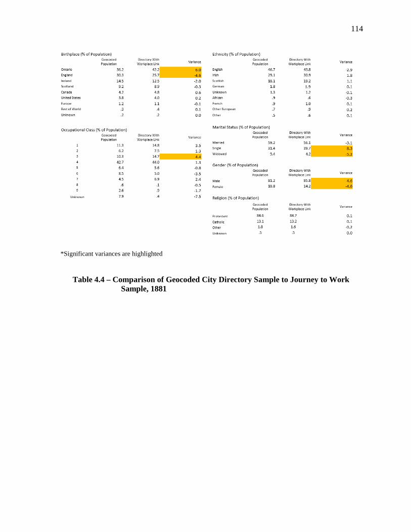
114

*Significant variances are highlighted

Table 4.4 – Comparison of Geocoded City Directory Sample to Journey to Work Sample, 1881

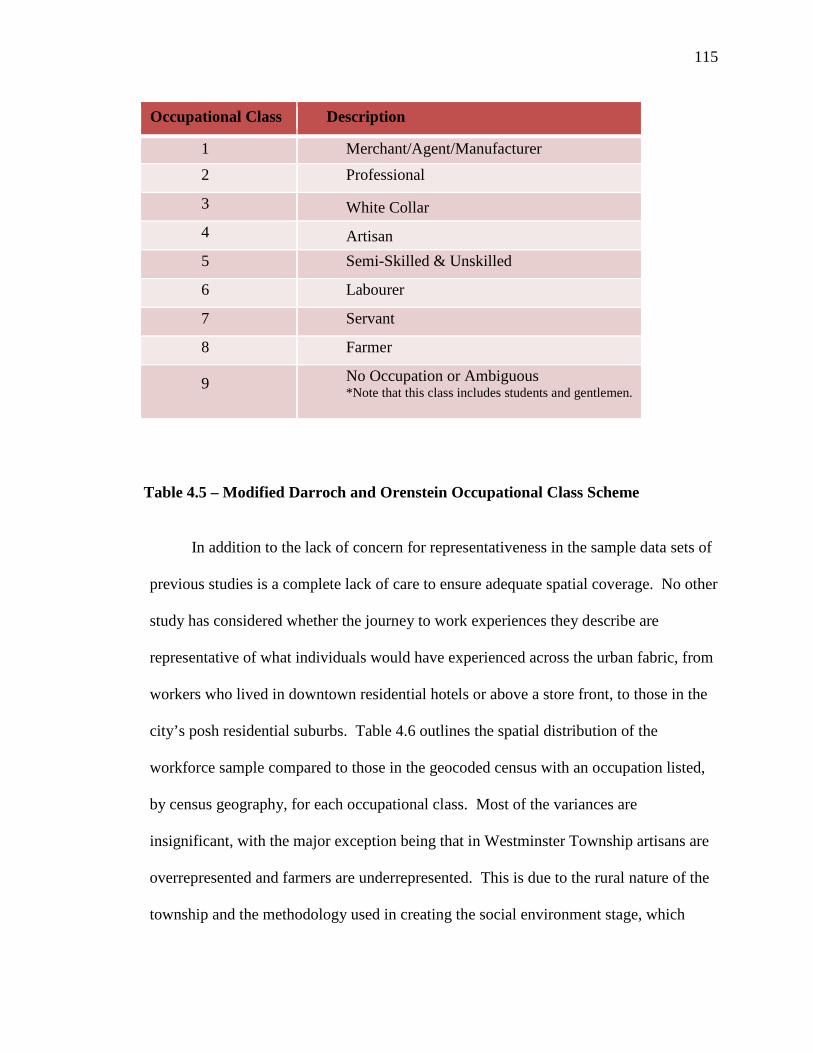
115

Table 4.5 – Modified Darroch and Orenstein Occupational Class Scheme

In addition to the lack of concern for representativeness in the sample data sets of

previous studies is a complete lack of care to ensure adequate spatial coverage. No other

study has considered whether the journey to work experiences they describe are

representative of what individuals would have experienced across the urban fabric, from

workers who lived in downtown residential hotels or above a store front, to those in the

city’s posh residential suburbs. Table 4.6 outlines the spatial distribution of the

workforce sample compared to those in the geocoded census with an occupation listed,

by census geography, for each occupational class. Most of the variances are

insignificant, with the major exception being that in Westminster Township artisans are

overrepresented and farmers are underrepresented. This is due to the rural nature of the

township and the methodology used in creating the social environment stage, which

Occupational Class Description

1 Merchant/Agent/Manufacturer 2 Professional

3 White Collar 4 Artisan 5 Semi-Skilled & Unskilled

6 Labourer 7 Servant 8 Farmer

9 No Occupation or Ambiguous *Note that this class includes students and gentlemen.

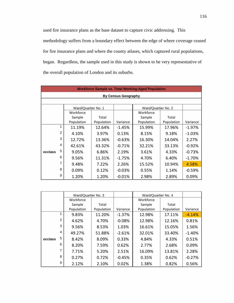
116

used fire insurance plans as the base dataset to capture civic addressing. This

methodology suffers from a boundary effect between the edge of where coverage ceased

for fire insurance plans and where the county atlases, which captured rural populations,

began. Regardless, the sample used in this study is shown to be very representative of

the overall population of London and its suburbs.

Workforce Sample vs. Total Working-Aged Population

By Census Geography

Ward/Quartier No. 1 Ward/Quartier No. 2 Workforce

Sample Population

Total Population Variance

Workforce Sample

Population Total

Population Variance

occlass

1 11.19% 12.64% -1.45% 15.99% 17.96% -1.97% 2 4.10% 3.97% 0.13% 8.15% 9.18% -1.03% 3 12.72% 13.36% -0.63% 16.30% 14.04% 2.27% 4 42.61% 43.32% -0.71% 32.21% 33.13% -0.92% 5 9.05% 6.86% 2.19% 3.61% 4.33% -0.73% 6 9.56% 11.31% -1.75% 4.70% 6.40% -1.70% 7 9.48% 7.22% 2.26% 15.52% 10.94% 4.58% 8 0.09% 0.12% -0.03% 0.55% 1.14% -0.59% 9 1.20% 1.20% -0.01% 2.98% 2.89% 0.09%

Ward/Quartier No. 3 Ward/Quartier No. 4 Workforce

Sample Population

Total Population Variance

Workforce Sample

Population Total

Population Variance

occlass

1 9.83% 11.20% -1.37% 12.98% 17.11% -4.14% 2 4.62% 4.70% -0.08% 12.98% 12.16% 0.81% 3 9.56% 8.53% 1.03% 16.61% 15.05% 1.56% 4 49.27% 51.88% -2.61% 32.01% 33.40% -1.40% 5 8.42% 8.09% 0.33% 4.84% 4.33% 0.51% 6 8.20% 7.59% 0.62% 2.77% 2.68% 0.09% 7 7.71% 5.20% 2.51% 16.09% 13.81% 2.28% 8 0.27% 0.72% -0.45% 0.35% 0.62% -0.27% 9 2.12% 2.10% 0.02% 1.38% 0.82% 0.56%

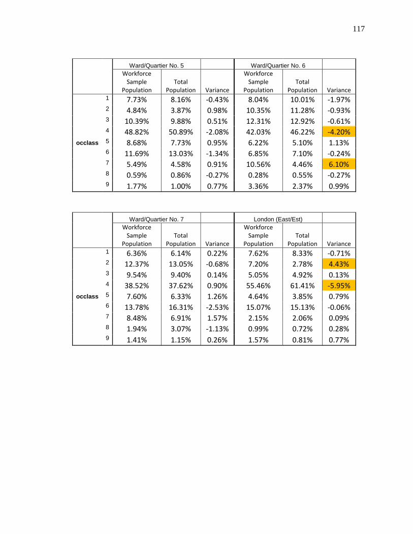
117

Ward/Quartier No. 5 Ward/Quartier No. 6 Workforce

Sample Population

Total Population Variance

Workforce Sample

Population Total

Population Variance

occlass

1 7.73% 8.16% -0.43% 8.04% 10.01% -1.97% 2 4.84% 3.87% 0.98% 10.35% 11.28% -0.93% 3 10.39% 9.88% 0.51% 12.31% 12.92% -0.61% 4 48.82% 50.89% -2.08% 42.03% 46.22% -4.20% 5 8.68% 7.73% 0.95% 6.22% 5.10% 1.13% 6 11.69% 13.03% -1.34% 6.85% 7.10% -0.24% 7 5.49% 4.58% 0.91% 10.56% 4.46% 6.10% 8 0.59% 0.86% -0.27% 0.28% 0.55% -0.27% 9 1.77% 1.00% 0.77% 3.36% 2.37% 0.99%

Ward/Quartier No. 7 London (East/Est) Workforce

Sample Population

Total Population Variance

Workforce Sample

Population Total

Population Variance

occlass

1 6.36% 6.14% 0.22% 7.62% 8.33% -0.71% 2 12.37% 13.05% -0.68% 7.20% 2.78% 4.43% 3 9.54% 9.40% 0.14% 5.05% 4.92% 0.13% 4 38.52% 37.62% 0.90% 55.46% 61.41% -5.95% 5 7.60% 6.33% 1.26% 4.64% 3.85% 0.79% 6 13.78% 16.31% -2.53% 15.07% 15.13% -0.06% 7 8.48% 6.91% 1.57% 2.15% 2.06% 0.09% 8 1.94% 3.07% -1.13% 0.99% 0.72% 0.28% 9 1.41% 1.15% 0.26% 1.57% 0.81% 0.77%

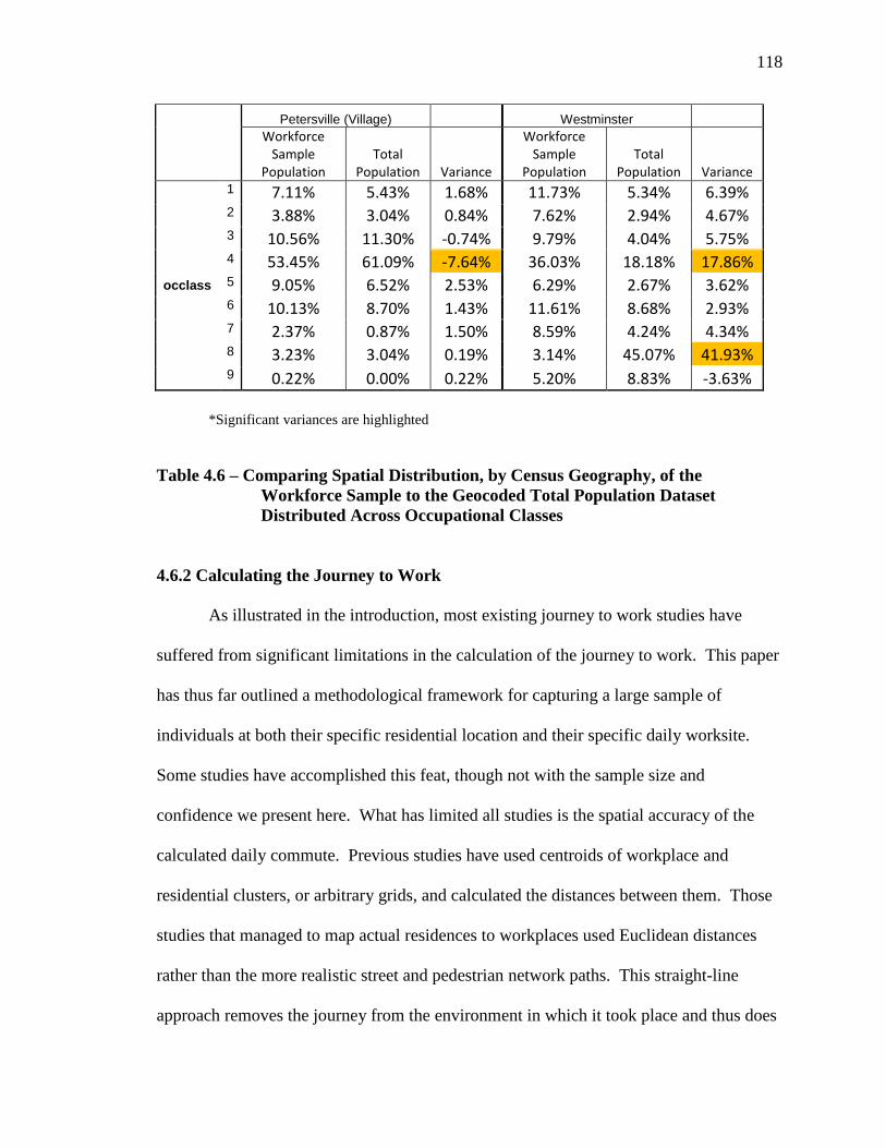
118

Petersville (Village) Westminster Workforce

Sample Population

Total Population Variance

Workforce Sample

Population Total

Population Variance

occlass

1 7.11% 5.43% 1.68% 11.73% 5.34% 6.39% 2 3.88% 3.04% 0.84% 7.62% 2.94% 4.67% 3 10.56% 11.30% -0.74% 9.79% 4.04% 5.75% 4 53.45% 61.09% -7.64% 36.03% 18.18% 17.86% 5 9.05% 6.52% 2.53% 6.29% 2.67% 3.62% 6 10.13% 8.70% 1.43% 11.61% 8.68% 2.93% 7 2.37% 0.87% 1.50% 8.59% 4.24% 4.34% 8 3.23% 3.04% 0.19% 3.14% 45.07% 41.93% 9 0.22% 0.00% 0.22% 5.20% 8.83% -3.63%

*Significant variances are highlighted

Table 4.6 – Comparing Spatial Distribution, by Census Geography, of the Workforce Sample to the Geocoded Total Population Dataset Distributed Across Occupational Classes 4.6.2 Calculating the Journey to Work

As illustrated in the introduction, most existing journey to work studies have

suffered from significant limitations in the calculation of the journey to work. This paper

has thus far outlined a methodological framework for capturing a large sample of

individuals at both their specific residential location and their specific daily worksite.

Some studies have accomplished this feat, though not with the sample size and

confidence we present here. What has limited all studies is the spatial accuracy of the

calculated daily commute. Previous studies have used centroids of workplace and

residential clusters, or arbitrary grids, and calculated the distances between them. Those

studies that managed to map actual residences to workplaces used Euclidean distances

rather than the more realistic street and pedestrian network paths. This straight-line

approach removes the journey from the environment in which it took place and thus does

119

not consider factors that may have influenced the commute. We know that the built form

(building density, size, fencing), transportation networks (rail lines, roads and pedestrian

pathways), and natural barriers (rivers/lakes, elevation changes) influence the routes that

individuals elect to take as they traverse the city (Ewing & Cervero, 2010; Hanson, 2004;

Larsen K. , et al., 2009; Larsen, Gilliland, & Hess, 2012). This study considers these

environmental influences, providing a more reliable image of the daily commute to work

in the late nineteenth century.

To begin, I harnessed the built environment stage to extract the 1881 road

network for use in ArcGIS’s Network Analyst. Possible pedestrian paths were added to

the road network geodatabase by creating segments across obvious open space as denoted

in the fire insurance plans. Two types of networks can be created for use in ArcGIS: a

network dataset and a geometric network. I elected to create a network dataset because it

is optimized for undirected flow, whereas the geometric network is best used for directed

systems such as rivers or utility lines. Default connectivity options were used and global

turns were enabled as pedestrians are expected to be able to walk where they want and

not have to follow restrictions typically imposed on vehicle traffic such as one-way

streets (although there were no one-way streets in London in the nineteenth century).

Length, expressed in meters, was the only cost calculated in the network; estimates of

travel times were not added as they were is too unpredictable to estimate for the 1880s

because of poor roads and differences in personal behaviour.

To calculate the path and distance to work, I used the shortest path route tools

within the Network Analyst extension of ArcGIS 9.3 (and later version 10). The first

step was to use the Calculate Locations tool within Network Analyst to calculate and

120

create a network location field for each business in the business directory shapefile

extracted from the social environment stage. This is similar to snapping or linking the

business to the road network, thus allowing the shortest path tool to more quickly and

accurately locate the workplaces as stops. The distance from the centre of the businesses

building polygon to the network was captured (an average of 24 metres) to be added to

the final calculated journey to work distance. The network dataset was used as the input

analysis network. The search tolerance was set to 200 meters in order to capture the few

businesses that are far from the road network, such as the Great Western Railway and the

Imperial Oil refining facility.

Numerous barriers to pedestrian travel were added before routes were calculated.

These included dense multi-track rail yards and the two branches of the Thames River.

Tolls existed on the many routes that emanated in and out from London’s city limits,

especially on bridges such as Clarke’s Bridge on present-day Wellington Road. Diaries

of the period suggest that these costs influenced travel paths for some of the lower

income residents of the city and suburbs. While they may have had an impact on

journeys, I elected not to include these tolls as barriers because of the difficulty in

determining a toll’s influence on a given individual.

The workforce sample geodatabase and the business directory (with the newly

created network location fields) were joined and a new route started in Network Analyst.

The workers were loaded as stops using the default geometry search options. The

businesses were then loaded as stops using the network location fields. The routes were

solved, resulting in 4,945 routes calculated, and the distance to the network was added

back to produce a final journey to work distance (Figure 4.2). These routes represent the

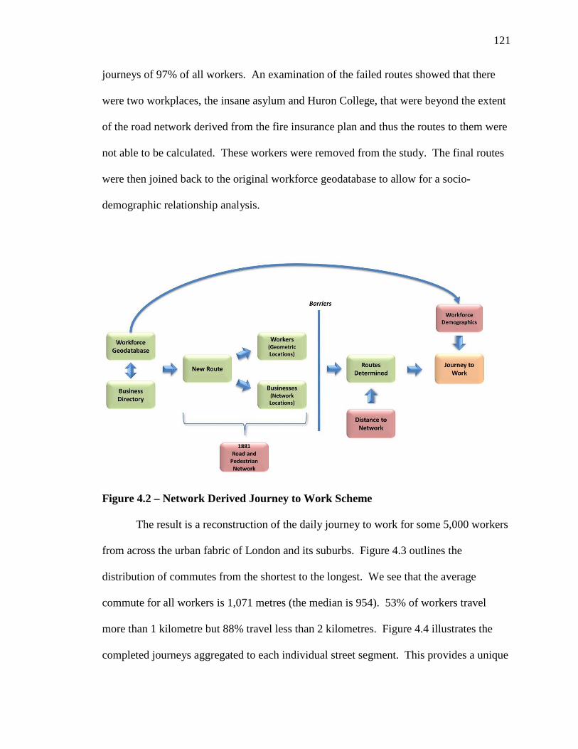
121

journeys of 97% of all workers. An examination of the failed routes showed that there

were two workplaces, the insane asylum and Huron College, that were beyond the extent

of the road network derived from the fire insurance plan and thus the routes to them were

not able to be calculated. These workers were removed from the study. The final routes

were then joined back to the original workforce geodatabase to allow for a socio-

demographic relationship analysis.

Figure 4.2 – Network Derived Journey to Work Scheme

The result is a reconstruction of the daily journey to work for some 5,000 workers

from across the urban fabric of London and its suburbs. Figure 4.3 outlines the

distribution of commutes from the shortest to the longest. We see that the average

commute for all workers is 1,071 metres (the median is 954). 53% of workers travel

more than 1 kilometre but 88% travel less than 2 kilometres. Figure 4.4 illustrates the

completed journeys aggregated to each individual street segment. This provides a unique

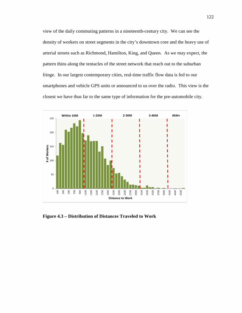
122

view of the daily commuting patterns in a nineteenth-century city. We can see the

density of workers on street segments in the city’s downtown core and the heavy use of

arterial streets such as Richmond, Hamilton, King, and Queen. As we may expect, the

pattern thins along the tentacles of the street network that reach out to the suburban

fringe. In our largest contemporary cities, real-time traffic flow data is fed to our

smartphones and vehicle GPS units or announced to us over the radio. This view is the

closest we have thus far to the same type of information for the pre-automobile city.

Figure 4.3 – Distribution of Distances Traveled to Work

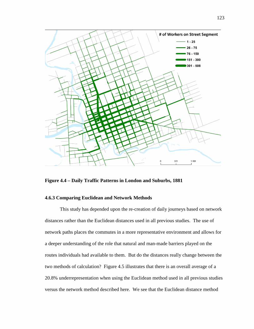
123

Figure 4.4 – Daily Traffic Patterns in London and Suburbs, 1881

4.6.3 Comparing Euclidean and Network Methods

This study has depended upon the re-creation of daily journeys based on network

distances rather than the Euclidean distances used in all previous studies. The use of

network paths places the commutes in a more representative environment and allows for

a deeper understanding of the role that natural and man-made barriers played on the

routes individuals had available to them. But do the distances really change between the

two methods of calculation? Figure 4.5 illustrates that there is an overall average of a

20.8% underrepresentation when using the Euclidean method used in all previous studies

versus the network method described here. We see that the Euclidean distance method

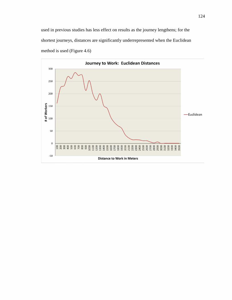
124

used in previous studies has less effect on results as the journey lengthens; for the

shortest journeys, distances are significantly underrepresented when the Euclidean

method is used (Figure 4.6)

125

* Euclidean mean is 848m, Network 1071m

Figure 4.5 – Differences between Euclidean and Network Distance Methods

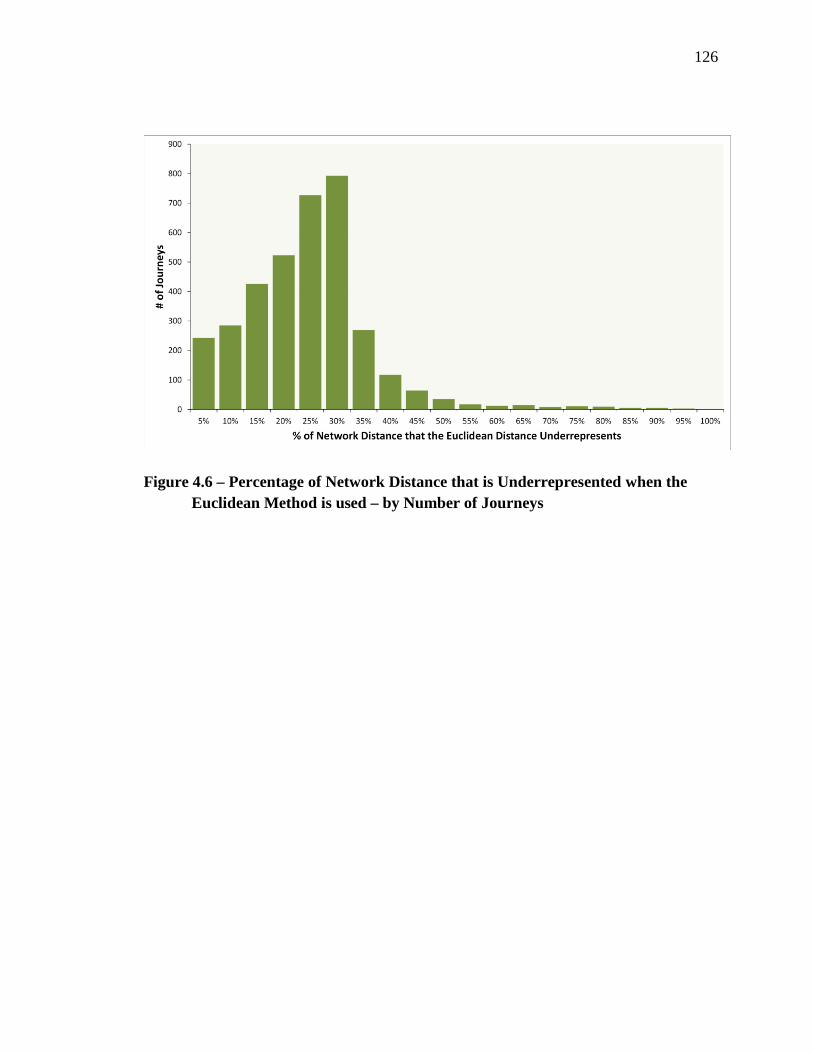
126

Figure 4.6 – Percentage of Network Distance that is Underrepresented when the Euclidean Method is used – by Number of Journeys

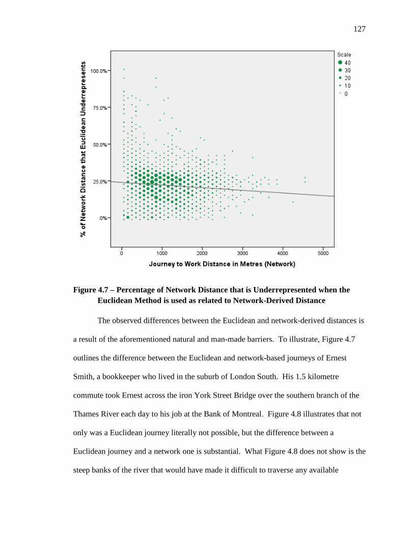
127

Figure 4.7 – Percentage of Network Distance that is Underrepresented when the Euclidean Method is used as related to Network-Derived Distance

The observed differences between the Euclidean and network-derived distances is

a result of the aforementioned natural and man-made barriers. To illustrate, Figure 4.7

outlines the difference between the Euclidean and network-based journeys of Ernest

Smith, a bookkeeper who lived in the suburb of London South. His 1.5 kilometre

commute took Ernest across the iron York Street Bridge over the southern branch of the

Thames River each day to his job at the Bank of Montreal. Figure 4.8 illustrates that not

only was a Euclidean journey literally not possible, but the difference between a

Euclidean journey and a network one is substantial. What Figure 4.8 does not show is the

steep banks of the river that would have made it difficult to traverse any available

128

shortcuts or alternative river crossings. If we look closer (Figure 4.8), we see the

inability to continue with a more straight-line journey after crossing the river, as the

density of the urban core of London restricted travel to the established roadways. These

barriers resulted in a commute that was over 25% longer than the Euclidean distance,

resulting in an extra 5-15 minutes’ walk, depending on the weather and other factors.

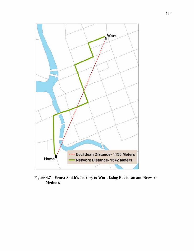
129

Figure 4.7 – Ernest Smith’s Journey to Work Using Euclidean and Network Methods

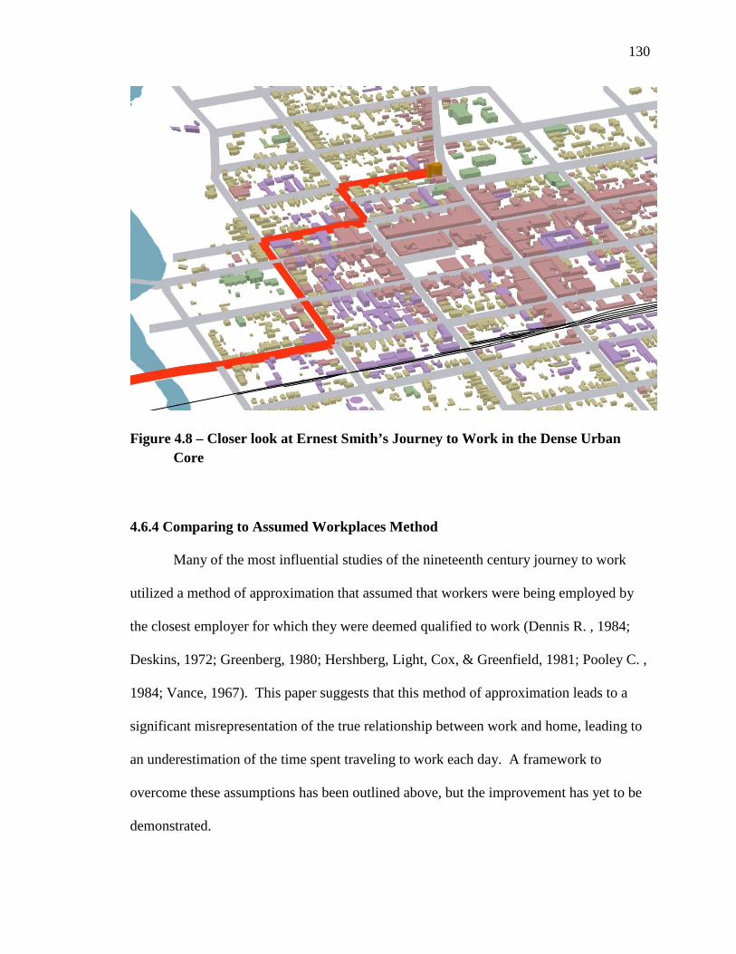
130

Figure 4.8 – Closer look at Ernest Smith’s Journey to Work in the Dense Urban Core

4.6.4 Comparing to Assumed Workplaces Method

Many of the most influential studies of the nineteenth century journey to work

utilized a method of approximation that assumed that workers were being employed by

the closest employer for which they were deemed qualified to work (Dennis R. , 1984;

Deskins, 1972; Greenberg, 1980; Hershberg, Light, Cox, & Greenfield, 1981; Pooley C. ,

1984; Vance, 1967). This paper suggests that this method of approximation leads to a

significant misrepresentation of the true relationship between work and home, leading to

an underestimation of the time spent traveling to work each day. A framework to

overcome these assumptions has been outlined above, but the improvement has yet to be

demonstrated.

131

To perform a comparative analysis between the two methods, I needed to find the

closest workplace to each worker’s home that would employ a worker with a related

occupation, then compare that distance to the actual distance the worker was travelling to

work each day. To estimate what would be the closest workplace for which a given

worker was qualified, I first needed to link each worker with his/her industry of

employment. However, due to the large number of industries (158) and workplaces

(2295) — each of which would require a separate analysis — I elected to use a sample. I

chose two types of workplaces representing two different industries, breweries and cigar

factories. They were chosen because they represent workplaces that were not listed in

multiple industry categories in the business directory, and thus provide a more direct

relationship between home and a potential closest employer. Additionally, while they are

both medium-sized industries in which workers commuted from a wide geographic area,

they have differing levels of skilled labour and industrialization. Breweries employed 95

workers, a mix of skilled and semi-skilled labour, in a heavily mechanized environment.

Maltsters, brewmasters, and coopers made up the skilled class, while semi-skilled

workers included bottlers, packers, warehouse clerks, and teamsters. Some unskilled

positions were also found in the city’s breweries, such as those whose tasks were to

shovel grain, load wagons, or clear rodents out of vats and barrels (Phillips, 2000). Cigar

manufacturing, a rapidly growing industry in 1881, was a modest operation with products

made by hand by individual workers using a limited number of simple tools such as a

rolling board, knife, and wrapping leafs. A total of 118 workers in our database were

working in cigar factories. The 1889 Royal Commission on Labour and Capital includes

testimonies from Londoners that suggest that many more individuals were employed in

132

cigar making. They were primarily young women and children, recent immigrants who

were ‘secured by indenture’ and paid the lowest of wages to complete the simple task of

rolling tobacco leaves into cigars (Canada, Royal Commission on the Relations of Labor

and Capital, 1889). We do not capture many of these indentured workers in this study.

Those we do capture, however, represent a sample similar to that discussed in the Royal

Commission reports, comprised of unskilled cigar makers, packers, and wood planers,

including many who are women and teenagers.

To find the closest potential workplace on the road and pedestrian path network, I

utilized the Closest Facility Analysis tools in Network Analyst. Workplaces were loaded

as facility locations using the network location fields created for the journey to work

analysis. The workers were loaded as incident locations, again using the default

geometry location functions. Routes were calculated between each worker’s residence

and the closest workplace within their industry. The exported result has a name field that

indicates both IDs from the facilities (workplaces) and incidents (workers) separated by a

hyphen (eg. 125 – 50). These IDs needed to be separated so the distance calculations to

the closest facility could be joined to the dataset with the worker’s actual distance to

work. To facilitate, a new field was created and the following VBScript run in the field

calculator: Left( [Name] , ((InStr ( 1, [Name] ,"‐",1) ‐2))). The difference between the

actual and potential distances was calculated with a 0 difference denoting that the worker

was working at the closest employer and any positive number reflecting the difference in

metres. Table 4.7 charts the results, while Figures 4.9 and 4.10 provide graphic

representations of the differences between closest and actual employer for brewery

workers and cigar makers, respectively.

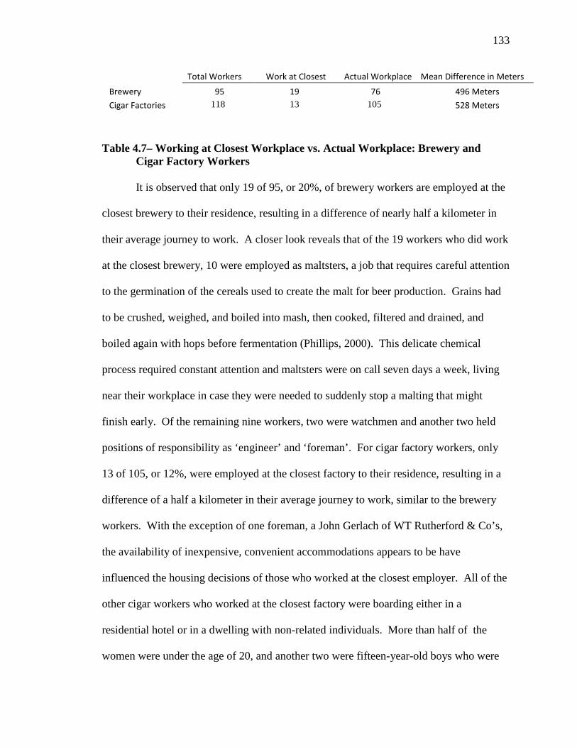
133

Total Workers Work at Closest Actual Workplace Mean Difference in Meters Brewery 95 19 76 496 Meters Cigar Factories 118 13 105 528 Meters

Table 4.7– Working at Closest Workplace vs. Actual Workplace: Brewery and Cigar Factory Workers

It is observed that only 19 of 95, or 20%, of brewery workers are employed at the

closest brewery to their residence, resulting in a difference of nearly half a kilometer in

their average journey to work. A closer look reveals that of the 19 workers who did work

at the closest brewery, 10 were employed as maltsters, a job that requires careful attention

to the germination of the cereals used to create the malt for beer production. Grains had

to be crushed, weighed, and boiled into mash, then cooked, filtered and drained, and

boiled again with hops before fermentation (Phillips, 2000). This delicate chemical

process required constant attention and maltsters were on call seven days a week, living

near their workplace in case they were needed to suddenly stop a malting that might

finish early. Of the remaining nine workers, two were watchmen and another two held

positions of responsibility as ‘engineer’ and ‘foreman’. For cigar factory workers, only

13 of 105, or 12%, were employed at the closest factory to their residence, resulting in a

difference of a half a kilometer in their average journey to work, similar to the brewery

workers. With the exception of one foreman, a John Gerlach of WT Rutherford & Co’s,

the availability of inexpensive, convenient accommodations appears to be have

influenced the housing decisions of those who worked at the closest employer. All of the

other cigar workers who worked at the closest factory were boarding either in a

residential hotel or in a dwelling with non-related individuals. More than half of the

women were under the age of 20, and another two were fifteen-year-old boys who were

134

neighbours and worked together at William Kelly and Sons cigar factory, suggesting that

we are picking up a few of the underrepresented workers in the city directory. Most of

the city’s cigar factories were located in the downtown core among other medium-sized

factories that used paper and wood products, such as furniture manufacturers, carriage

factories, and paper bag makers. Rents were low in this district of the city with most

residential offers being in hotels or above storefronts, thus allowing an opportunity for

the lowest paid cigar factory workers to find accommodations close to work, reducing

their commutes to help compensate for the long work shifts that were demanded of them.

It is recognized that many factors go into residential and workplace choice; however,

these two examples, each with their peculiarities in occupational demands or residential

needs, help illustrate that there are significant errors and omissions if one assumes that

people work for the closest employer for which they are qualified. By establishing true

home-work links, we can not only better understand what was a more realistic daily

journey to work, but can also begin to provide some insight into residential choices made

by workers in the nineteenth-century walking city.

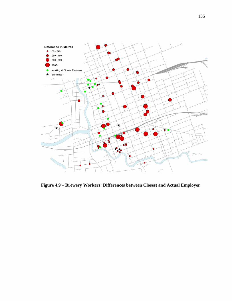
135

Figure 4.9 – Brewery Workers: Differences between Closest and Actual Employer

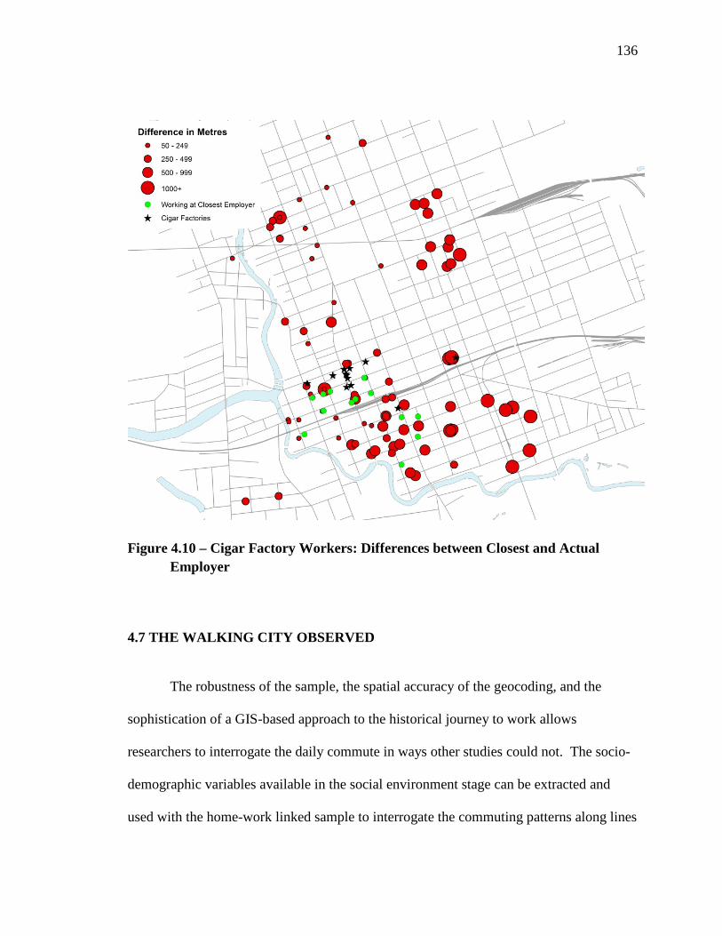
136

Figure 4.10 – Cigar Factory Workers: Differences between Closest and Actual Employer

4.7 THE WALKING CITY OBSERVED

The robustness of the sample, the spatial accuracy of the geocoding, and the

sophistication of a GIS-based approach to the historical journey to work allows

researchers to interrogate the daily commute in ways other studies could not. The socio-

demographic variables available in the social environment stage can be extracted and

used with the home-work linked sample to interrogate the commuting patterns along lines

137

of ethnicity, age, gender, occupational class, or any combination of these that may be of

interest. This section illustrates the possibilities by interrogating the journeys by

occupational class, workplace location, and gender.

Before completing the socio-demographic analysis, it was necessary to first

separate out those workers who were working at home and those who had a commute.

Those who lacked a commute to work were as important to the social geography of the

industrial city as those who had a daily journey. Although many records in the city

directory directly indicated that work was taking place in the home, there were numerous

individuals for whom the information was either vague or missing. The expectation

would be that the geocoding of home and work would then intersect; however, due to

occasional imprecisions in digitization or geocoding, some people who were indeed

working at home were shown to have short commutes of anywhere from a fraction of a

metre to twenty or thirty metres. A decision was made to consider anyone working less

than 50 meters from home to be working at home. This threshold was selected based on

the trend seen in the chart in Figure 4.12 and also because 50m covers the maximum

distance seen in the city lots from the front yard to a rear tenement, the residential

experience for some of London’s domestic servants.

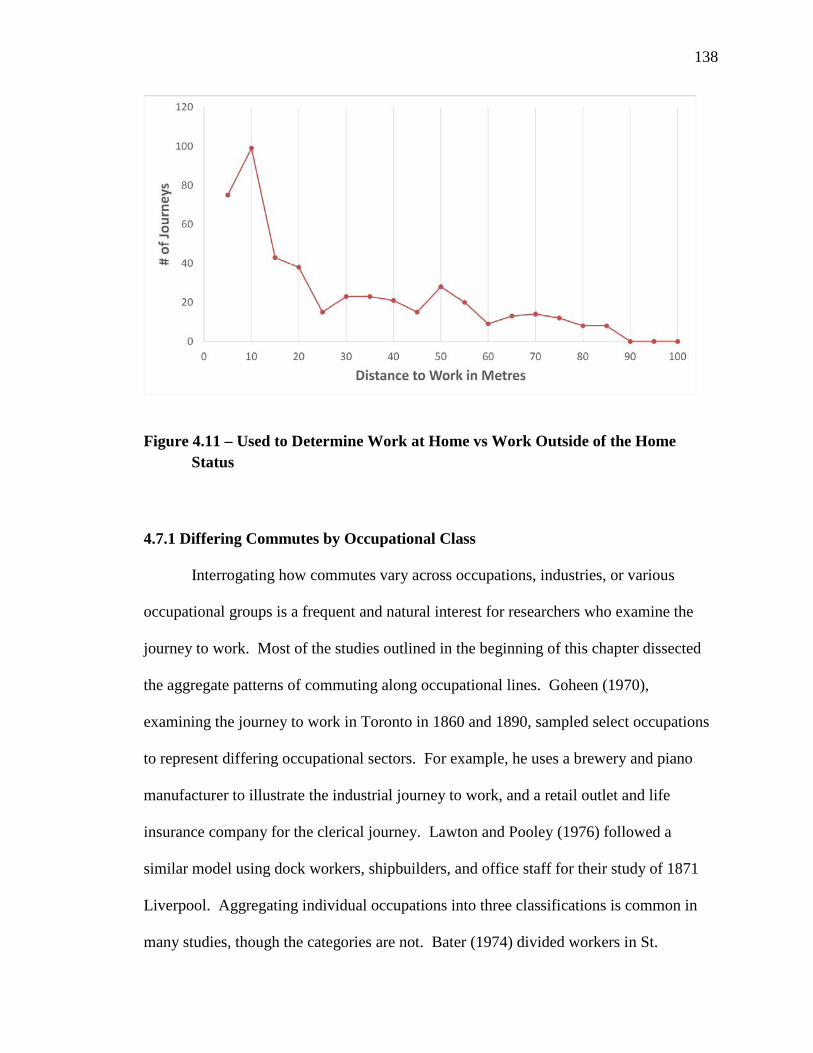
138

Figure 4.11 – Used to Determine Work at Home vs Work Outside of the Home Status

4.7.1 Differing Commutes by Occupational Class

Interrogating how commutes vary across occupations, industries, or various

occupational groups is a frequent and natural interest for researchers who examine the

journey to work. Most of the studies outlined in the beginning of this chapter dissected

the aggregate patterns of commuting along occupational lines. Goheen (1970),

examining the journey to work in Toronto in 1860 and 1890, sampled select occupations

to represent differing occupational sectors. For example, he uses a brewery and piano

manufacturer to illustrate the industrial journey to work, and a retail outlet and life

insurance company for the clerical journey. Lawton and Pooley (1976) followed a

similar model using dock workers, shipbuilders, and office staff for their study of 1871

Liverpool. Aggregating individual occupations into three classifications is common in

many studies, though the categories are not. Bater (1974) divided workers in St.

139

Petersburg, Russia into managerial and professional, workshop owners and artisans, and

factory workers. Barke (1991) divided his sample for Newcastle upon Tyne into the

categories of professional, which included occupations such as accountants, lawyers and

architects, producer-retailer, which included blacksmiths, watchmakers, and bakers, and

finally retailers, which included pawnbrokers as well as those who sold fish, glass, or

poultry. Taking a different approach, Hershberg et al. (1981) used industries to select

their sample, starting first with ship building, sugar refining, iron rolling, banking, and

morocco leather finishing. They were selected for their spatial coverage across

Philadelphia, the ethnic composition of their workforces, and their respective longevity as

industries in the city. To supplement their sample, they also used seven occupations to

represent the swath of social classes, with physicians and lawyers representing the

professional class, confectioners and bookbinders the small proprietors, and blacksmiths,

cabinetmakers, and carpenters the artisanal proprietors. Mayer (1977) categorised all

occupations into one of eight occupational classifications using a scheme developed for

the 1940 U.S. census by Edwards (1940) and later modified by Thernstrom (1973) and

Conzen (1976). To evaluate the differing journey to work across occupations in London,

I follow Mayer’s lead and utilize an occupational class scheme, though unlike Mayer, I

employed one developed for the census that was used to build the dataset (see Table 4.5).

This method allows us to easily examine all occupations across the entire spatial extent of

the city rather than employing a sampling strategy, as done in the other studies.

As all other studies have utilized Euclidean rather than network distances, it is

impossible to accurately compare distances travelled across various cities. Additionally,

the absolute distance travelled is largely influenced not only by residential and workplace

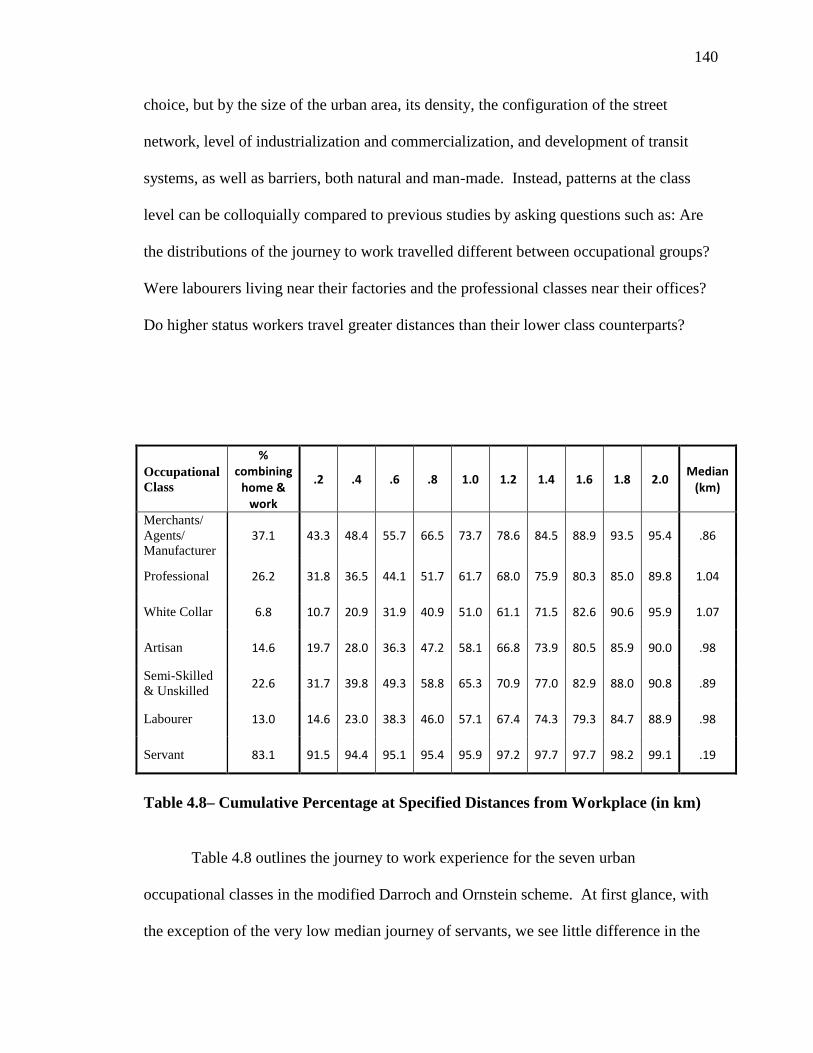
140

choice, but by the size of the urban area, its density, the configuration of the street

network, level of industrialization and commercialization, and development of transit

systems, as well as barriers, both natural and man-made. Instead, patterns at the class

level can be colloquially compared to previous studies by asking questions such as: Are

the distributions of the journey to work travelled different between occupational groups?

Were labourers living near their factories and the professional classes near their offices?

Do higher status workers travel greater distances than their lower class counterparts?

Occupational Class

% combining

home & work

.2 .4 .6 .8 1.0 1.2 1.4 1.6 1.8 2.0 Median (km)

Merchants/ Agents/ Manufacturer

37.1 43.3 48.4 55.7 66.5 73.7 78.6 84.5 88.9 93.5 95.4 .86

Professional 26.2 31.8 36.5 44.1 51.7 61.7 68.0 75.9 80.3 85.0 89.8 1.04

White Collar 6.8 10.7 20.9 31.9 40.9 51.0 61.1 71.5 82.6 90.6 95.9 1.07

Artisan 14.6 19.7 28.0 36.3 47.2 58.1 66.8 73.9 80.5 85.9 90.0 .98

Semi-Skilled & Unskilled 22.6 31.7 39.8 49.3 58.8 65.3 70.9 77.0 82.9 88.0 90.8 .89

Labourer 13.0 14.6 23.0 38.3 46.0 57.1 67.4 74.3 79.3 84.7 88.9 .98

Servant 83.1 91.5 94.4 95.1 95.4 95.9 97.2 97.7 97.7 98.2 99.1 .19

Table 4.8– Cumulative Percentage at Specified Distances from Workplace (in km)

Table 4.8 outlines the journey to work experience for the seven urban

occupational classes in the modified Darroch and Ornstein scheme. At first glance, with

the exception of the very low median journey of servants, we see little difference in the

141

median journey to work between the classes, with a difference of only 210 metres

between the longest and shortest median distances travelled by those who were not in

service. As is observed in all other studies with a predominantly British population, most

servants lived in their masters’ domiciles, and those who did not lived very nearby,

usually in boarding houses with other servants. However, if we examine the journeys

closer by looking at the cumulative percentages at distance bands from 200 metres to 2

kilometres, we reveal a more complex pattern. Excluding servants for the time being,

those in the highest occupational class of merchants, agents, and manufacturers, lived

overwhelmingly closer to their workplaces than workers in any other group. Nearly 50%

lived less than 400 metres from work and three-quarters lived within a kilometer. They

have the highest cumulative percentage of workers living close to work across every

distance band but the very longest. Surprisingly, this pattern is not shared with the

studies outlined above, where they found that factory owners and merchants, if they did

not live at their businesses, lived a considerable distance away compared to other

occupational groups. This difference may be a function of the very dense urban core of

London that permitted a very short distance from the commercial and most of the

industrial firms to the desirable neighbourhood on Talbot Street overlooking the Thames

River and to the Woodfield neighbourhood adjacent to the city’s only public park. The

exception would be those industrialists involved in the growing rail and barrel works in

the suburb of London East, as they lived in the same neighbourhood as their colleagues,

but their businesses were significantly further away.

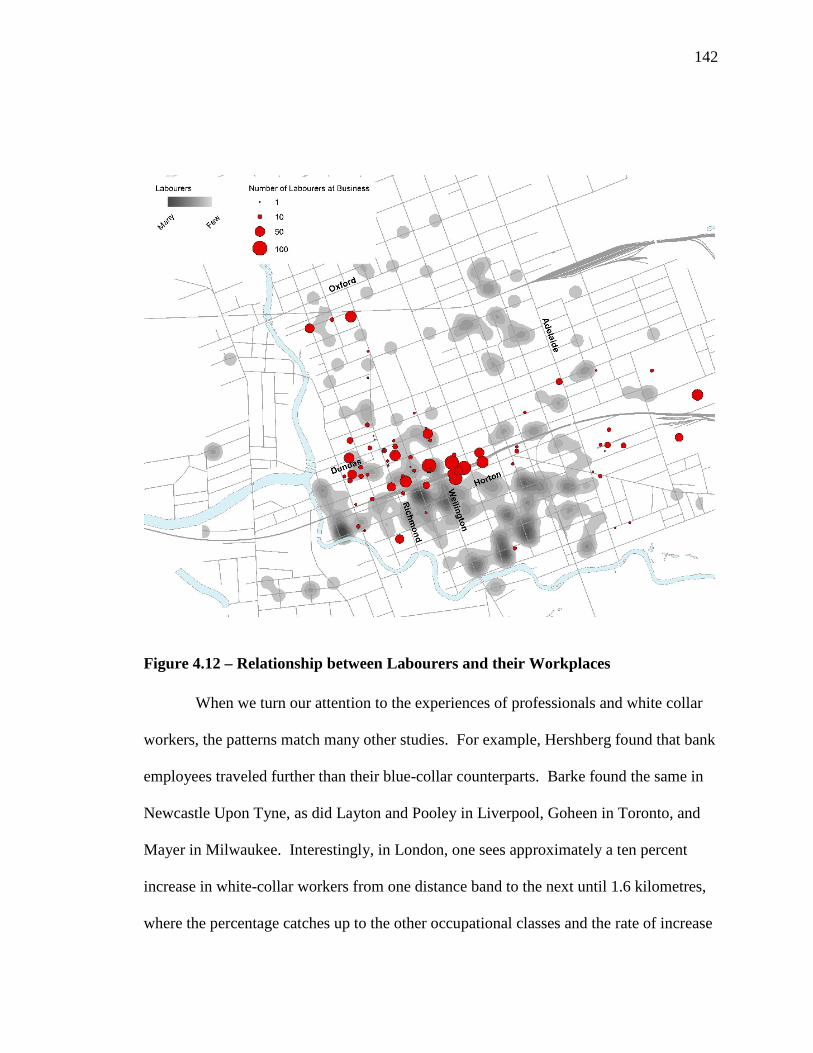
142

Figure 4.12 – Relationship between Labourers and their Workplaces

When we turn our attention to the experiences of professionals and white collar

workers, the patterns match many other studies. For example, Hershberg found that bank

employees traveled further than their blue-collar counterparts. Barke found the same in

Newcastle Upon Tyne, as did Layton and Pooley in Liverpool, Goheen in Toronto, and

Mayer in Milwaukee. Interestingly, in London, one sees approximately a ten percent

increase in white-collar workers from one distance band to the next until 1.6 kilometres,

where the percentage catches up to the other occupational classes and the rate of increase

143

slows. What is less pronounced in London is the number of labourers living close to their

workplaces. This pattern was observed in Liverpool, Milwaukee, and somewhat in St.

Petersburg. In London, however, labourers lag behind the other lower class group, semi-

skilled and unskilled workers, until they meet at a 1.2 kilometre journey. This may be

explained by the high demand and limited inventory of housing in the core and nearby

neighbourhoods. Instead we see labourers travelling from modest homes north-east of

downtown as well as from the neighbourhood along the north shore of the south branch

of the Thames to jobs along the rail lines in the centre of the city as well as the new

industries in London East (Figure 4.13)

4.7.2 Coincident Home-Work Locations

Studying the home-work relationship has primarily been the domain of feminist

scholars who have been interested in the extent of unpaid domestic work by women and

girls or the important role that piecework and cottage crafts played in supplementing the

household income (Bradbury B. , 1984; Bradbury B. , 1996; Bullen, 1986). However,

significant numbers of men still combined work and home. In the aggregate, we find that

in 1881, 26% of London workers were combining home and work. 61% of the women

worked at home whereas only 16% of men did. Women represent just over half (53%) of

the work-at-home population in London in 1881.

The methodology used to determine who worked at home versus outside the home

was not clearly outlined in the few other studies that have directly investigated this

relationship. The most comparable studies to this one are the work done by Hershberg et

al. (1981) and Mayer (1977) who interrogated the frequency of coincident home-work

locations in 1880 in Philadelphia and Milwaukee respectively. Similar to this study, they

144

relied heavily on the workplace information provided within the annual city directory;

however, neither study outlines how they deemed a worker to be working at home. Table

4.9 compares the frequency of workers who combined home and work, by occupation,

for London to the case studies of Philadelphia and Milwaukee. All occupations listed in

the comparable studies are included as well as select additional occupations for London.

With the robustness of the London sample, we have the possibility to report every

occupation, but have elected to only report some of the most notable here. Considering

that each city has its own local industries that dominate the economy and the comparison

cities have significantly larger populations than London (Philadelphia 850,000 and

Milwaukee 115,000 in 1880), sample sizes for specific occupations are surprisingly

similar across the cases.

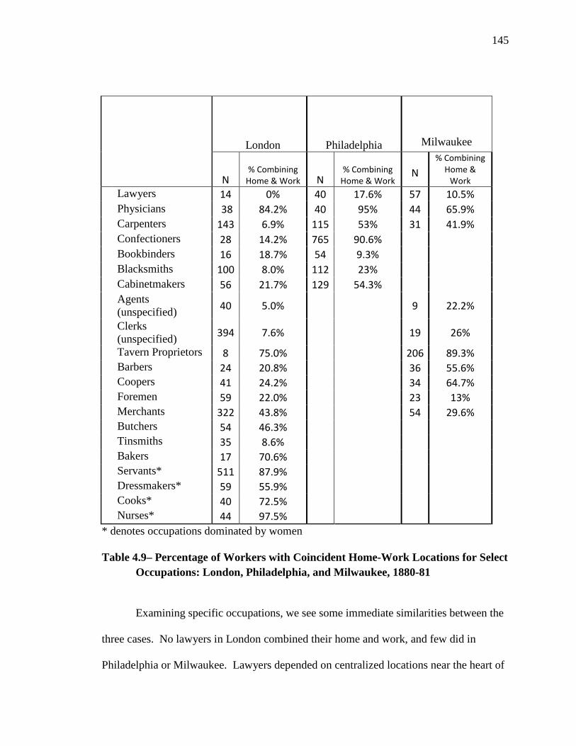
145

London

Philadelphia

Milwaukee

N % Combining

Home & Work N % Combining

Home & Work

N

% Combining Home &

Work

Lawyers 14 0% 40 17.6% 57 10.5% Physicians 38 84.2% 40 95% 44 65.9% Carpenters 143 6.9% 115 53% 31 41.9% Confectioners 28 14.2% 765 90.6% Bookbinders 16 18.7% 54 9.3% Blacksmiths 100 8.0% 112 23% Cabinetmakers 56 21.7% 129 54.3% Agents (unspecified) 40 5.0% 9 22.2%

Clerks (unspecified) 394 7.6% 19 26%

Tavern Proprietors 8 75.0% 206 89.3% Barbers 24 20.8% 36 55.6% Coopers 41 24.2% 34 64.7% Foremen 59 22.0% 23 13% Merchants 322 43.8% 54 29.6% Butchers 54 46.3% Tinsmiths 35 8.6% Bakers 17 70.6% Servants* 511 87.9% Dressmakers* 59 55.9% Cooks* 40 72.5% Nurses* 44 97.5%

* denotes occupations dominated by women Table 4.9– Percentage of Workers with Coincident Home-Work Locations for Select Occupations: London, Philadelphia, and Milwaukee, 1880-81

Examining specific occupations, we see some immediate similarities between the

three cases. No lawyers in London combined their home and work, and few did in

Philadelphia or Milwaukee. Lawyers depended on centralized locations near the heart of

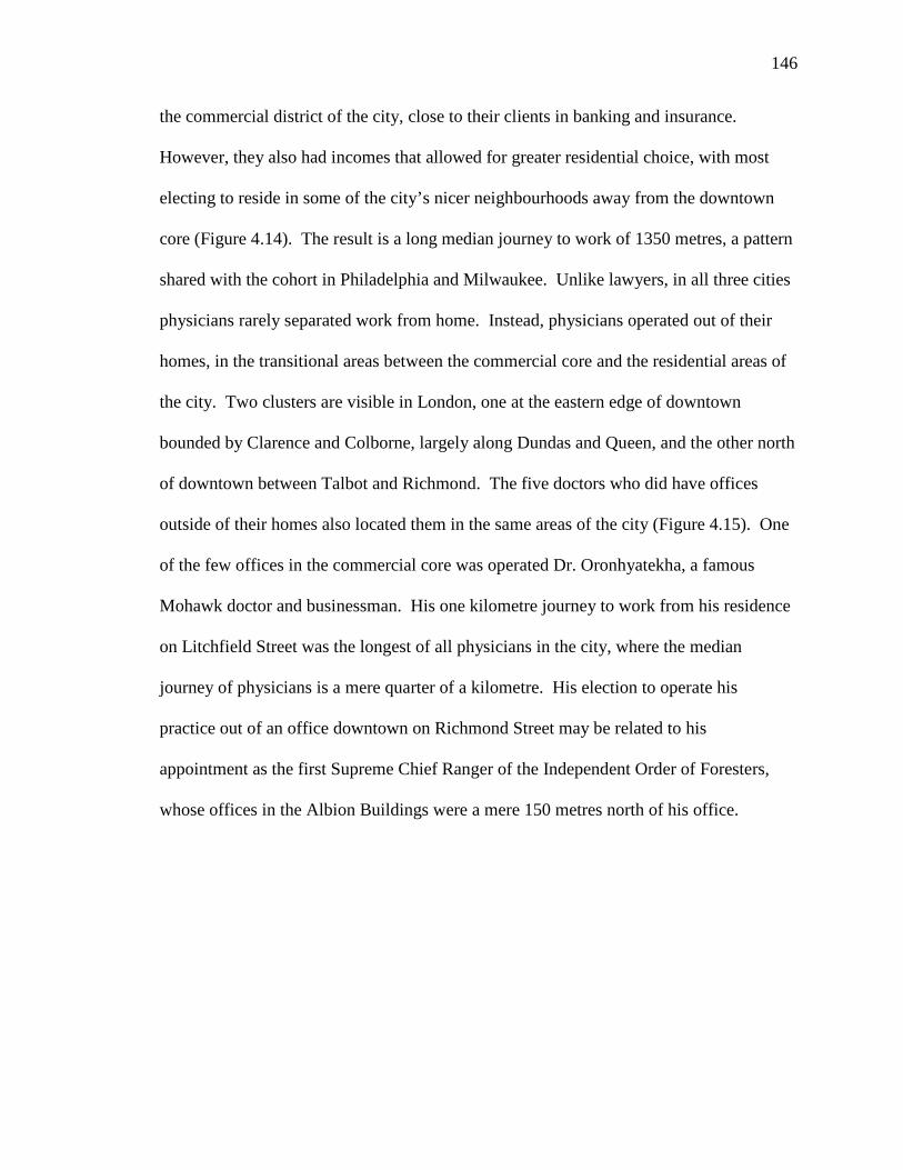
146

the commercial district of the city, close to their clients in banking and insurance.

However, they also had incomes that allowed for greater residential choice, with most

electing to reside in some of the city’s nicer neighbourhoods away from the downtown

core (Figure 4.14). The result is a long median journey to work of 1350 metres, a pattern

shared with the cohort in Philadelphia and Milwaukee. Unlike lawyers, in all three cities

physicians rarely separated work from home. Instead, physicians operated out of their

homes, in the transitional areas between the commercial core and the residential areas of

the city. Two clusters are visible in London, one at the eastern edge of downtown

bounded by Clarence and Colborne, largely along Dundas and Queen, and the other north

of downtown between Talbot and Richmond. The five doctors who did have offices

outside of their homes also located them in the same areas of the city (Figure 4.15). One

of the few offices in the commercial core was operated Dr. Oronhyatekha, a famous

Mohawk doctor and businessman. His one kilometre journey to work from his residence

on Litchfield Street was the longest of all physicians in the city, where the median

journey of physicians is a mere quarter of a kilometre. His election to operate his

practice out of an office downtown on Richmond Street may be related to his

appointment as the first Supreme Chief Ranger of the Independent Order of Foresters,

whose offices in the Albion Buildings were a mere 150 metres north of his office.

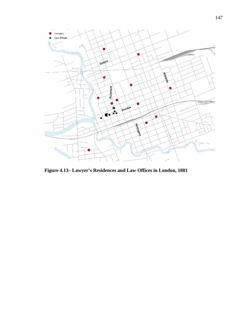
147

Figure 4.13– Lawyer’s Residences and Law Offices in London, 1881

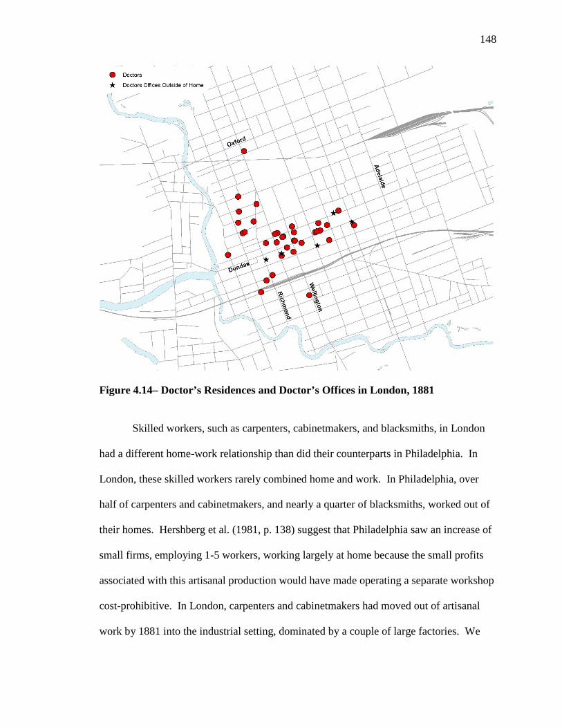
148

Figure 4.14– Doctor’s Residences and Doctor’s Offices in London, 1881

Skilled workers, such as carpenters, cabinetmakers, and blacksmiths, in London

had a different home-work relationship than did their counterparts in Philadelphia. In

London, these skilled workers rarely combined home and work. In Philadelphia, over

half of carpenters and cabinetmakers, and nearly a quarter of blacksmiths, worked out of

their homes. Hershberg et al. (1981, p. 138) suggest that Philadelphia saw an increase of

small firms, employing 1-5 workers, working largely at home because the small profits

associated with this artisanal production would have made operating a separate workshop

cost-prohibitive. In London, carpenters and cabinetmakers had moved out of artisanal

work by 1881 into the industrial setting, dominated by a couple of large factories. We

149

find 45 (32%) of the carpenters were working at the Ontario Car Works in London East,

building parlour train cars for the Great Western Railway. Another 26 (18%) were

employed at Thomas Green’s planing shop and sawmill. The remainder worked as

carpenters in factories such as John Elliott’s Phoenix foundry, where they made

agricultural implements such as plows and shovels. Cabinetmakers follow much the

same pattern, with over 80% being employed by three firms, the London Furniture

Company, John Ferguson’s coffin and cabinet factory, or the Bennett Brothers office

furniture factory. London’s blacksmiths were not found in a select few dominant

factories, but rather spread across the industrial fabric of the city. The 100 blacksmiths in

London were employed across 38 different factories, differing in form and function.

Though not centralized, blacksmithing in London was still different from the more

artisanal nature of blacksmithing reported for Philadelphia. The few blacksmiths who did

combine home and work in London were all found in small homes with shops in the rear,

located exclusively in largely industrialized areas of the city, presumably to reduce the

possibility of irritating their neighbours.

Confectioners and coopers followed the same pattern, where few in London

combined work and home compared to their counterparts in Philadelphia and Milwaukee.

Most stark is the difference between London and Philadelphia for confectioners. A

surprising 90.6% of confectioners in Philadelphia worked in their homes, versus a modest

14.2% in London. The only explanation provided for Philadelphia is that because they

‘served a neighborhood market… they had little reason to separate their work and

residence’ (Hershberg, Light, Cox, & Greenfield, 1981, p. 137). In London, all but 7 of

the confectioners were employed by one of two firms, either McCormick’s

150

Manufacturing or Daniel Perrin’s Biscuit Co. Both firms were substantial in size,

employing over a hundred men, and had a large distribution of their confections across

Canada. Coopers in London followed a similar pattern, with the majority working for

either Seale and Child’s Cooperage or that of William Hawkins. Both firms supplied

Labatt and Carling the barrels needed for their beer and ale. In contrast, Milwaukee’s

coopers worked in a more artisanal setting, with one or two coopers working out of a

home, utilizing the ready access to cheap lumber from Wisconsin’s growing timber trade

to supply barrels to one of Milwaukee’s forty or so breweries.

Turning our attention from industrial labour to commercial work, we see an

expected home-work relationship pattern in London. Tavern proprietors, like their

counterparts in Milwaukee, primarily lived above or behind their pubs. Agents and

clerks largely worked outside of the home, as they served the needs of either a specific

organization or the public at large. Curiously, this does not correlate with the experience

in Milwaukee, where a surprisingly high percentage of agents and clerks worked at their

residences. Unfortunately, Mayer does not specifically address why this was observed,

an omission that raises the curiosity of this researcher.

4.7.3 Women’s Experiences

Women’s relationship between work and home is not explicitly treated by

Hershberg et al. or by Mayer, so comparisons are not possible. A glance at Table 4.9

provides some insight into the experiences of women in London. Women’s paid labour

was dominated by occupations that extended from their duties at home. Few married

women had steady employment outside of the home and thus most did not report an

occupation to a census enumerator. Bradbury (1984) outlines that women worked for

151

wages occasionally, taking in washing, ironing, sewing, or performing other domestic

duties for neighbours, relatives, or friends. Dressmaking and tailoring in particular were

popular part-time occupations for women; most women were sewing at home for their

families and the more entrepreneurial also made items for sale to supplement the family

income. Few of these part-time dressmakers are captured in the city directories;

however, we are able to examine 59 dressmakers who appear to work on a more full-time

basis producing dresses for the ladies of London. Interestingly, only 56% of them work

from home, with the remainder working primarily as one of many women at a

dressmaking shop, such as those owned by Lydia Crone and by Mrs. Montague. These

dressmakers had the longest commute of any women working outside the home, with a

median journey of nearly a mile (1.6km) (Figure 4.15). The daily newspaper, the London

Advertiser, had a steady increase in the number of notices in the female help wanted

section for dressmakers and sewing girls through the 1870s. This increased demand for

‘outsourced’ dresses was partially a response to the School Act of 1871 which made

schooling compulsory for all children, including the young girls who would have helped

with the sewing (Ross, 1896). This loss of domestic labour, combined with the increases

in real wages throughout the period, meant that women began to purchase dresses rather

than make them themselves. The advertisements for dressmakers in the newspaper do

not list a wage, though the frequency and voracity of the want ads suggest that the wages

may have been higher than women would have made sewing at home, finding

employment in the cigar factories, or working as cleaners in the one of the many hotels.

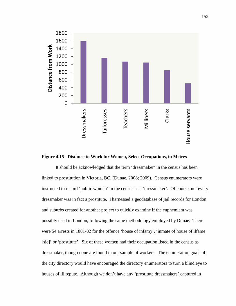
152

Figure 4.15– Distance to Work for Women, Select Occupations, in Metres

It should be acknowledged that the term ‘dressmaker’ in the census has been

linked to prostitution in Victoria, BC. (Dunae, 2008; 2009). Census enumerators were

instructed to record ‘public women’ in the census as a ‘dressmaker’. Of course, not every

dressmaker was in fact a prostitute. I harnessed a geodatabase of jail records for London

and suburbs created for another project to quickly examine if the euphemism was

possibly used in London, following the same methodology employed by Dunae. There

were 54 arrests in 1881-82 for the offence ‘house of infamy’, ‘inmate of house of ilfame

[sic]’ or ‘prostitute’. Six of these women had their occupation listed in the census as

dressmaker, though none are found in our sample of workers. The enumeration goals of

the city directory would have encouraged the directory enumerators to turn a blind eye to

houses of ill repute. Although we don’t have any ‘prostitute dressmakers’ captured in

0200400600800

10001200140016001800

Dres

smak

ers

Tailo

ress

es

Teac

hers

Mill

iner

s

Cler

ks

Hous

e se

rvan

ts

Dist

ance

from

Wor

k

153

this study, the evidence suggests that it was possible that the environment found by

Dunae in Victoria may also have existed in London.

The transition of girls to school and increasing household income resulted in more

than just the need to purchase dresses from a dedicated dressmaker, it also helped support

an increase in employment of domestic servants in Canadian middle-class homes. We

found over 500 female domestic servants in our journey to work sample; this was the

largest single occupation of women in the city. Nearly all (88%) lived in their masters’

homes. The domestic servant was usually a single, young woman (median age in London

was 23), and was primarily of English, Irish, or Scottish descent. Being ‘in service’,

however, came with a stigma. Some scholars suggest that those women who had a

choice preferred to work in factories, offices, or shops regardless of a difference in pay

(Barber, 1991, p. 8), while others argue that working-class parents preferred their

daughters to work in private homes rather than being exposed to the dangers of the

factory or receiving the low wages of the shops (Fahmi, 1997, p. 73). I found the

frequent advertisements for reliable servants to be increasingly dominant in the help

wanted section of the newspaper from 1879-1891. The advertisements also served as a

public notice that a household was capable of paying for domestic help, as the live-in

servant was an important status symbol in Victorian Canada.

Cooks and nurses represent another group of women who lived at work rather

than working from home. London’s cooks worked overwhelmingly in the city’s hotels,

working for both a wage and for room and board. They were older than domestic

servants, with a median age over 30. The few that did not live at the hotel had a very

short commute, averaging only a few hundred metres. All but a select few nurses lived at

154

work, either caring for children in the Protestant Orphans’ Home or for the infirm at the

insane asylum.

This section has illustrated the importance of interrogating the relationship

between home and work, particularly for revealing the situation of a large portion of

women. Women had long work days in the domestic sphere, and so did men in the

factory. This was a period of industrialization when, in the aggregate, production shifted

from being home-based and artisanal to factory-based. However, the decision to work

outside or inside the home is still not always clear to historians and historical

geographers. We need to continue to seek to understand the complexities of the

geography of work in the nineteenth century.

4.8 CONCLUSION

This paper has outlined a new methodological framework for recreating the

spatial relationships between work and home. The methodologies herein overcome many

of the limitations of previous studies, helping to invigorate an area of research that has

had little attention since the early 1990s. Although much of the data is the same as used

by other researchers, by harnessing a complete digital record of the city’s population and

businesses, we can begin to understand the journey to work for not just a subset of the

city’s population, but for nearly every single individual, occupational group, workplace,

or neighbourhood in the city. With a robust record linkage procedure, I have been able to

make absolute links between workers and their workplaces and calculate their daily

journeys on a model of the street and pedestrian paths of the city. This method

155

overcomes the concerns that Dennis (1984) postulated about quantitative research on the

journey to work due to a lack of data that directly links work and home.

It must be acknowledged that the methodologies used herein are not perfect. Like

any interrogation of the past, we are limited by the quality of the data recorded. In this

case, we must remember that city directories were compiled for an explicit financial

purpose, to sell advertising and subscriptions to businesses and citizens alike (H.H.B.,

1913). It was very much like a paid version of the telephone book that was commonly

distributed a few years ago before the creation of internet searches. The census was not

perfect either, as Curtis (2001), Hamilton (2007), Steckel (1991) and many others have

thoroughly outlined. Census enumerations were and continue to be wrought with

imprecise methods and procedures resulting in marginalized individuals being

undercounted, misrepresented, or omitted completely. For this study of the journey to

work, the effects include a skew towards full-time wageworkers, rather than those who

worked part-time, did piecework, or were chronically unemployed. Married women who

did not work outside the home, as well as teenagers who worked after school and on

weekends are also missed. These issues affect this study and must be considered when

findings are analyzed.

The algorithms used may also skew results. The study utilizes shortest path

techniques provided by the software company ESRI. Although the mathematical models

used have been scrutinized and accepted by the larger GIS community, the assumption

that individuals are most efficient in their commutes is still not confirmed. In the walking

city, it would be expected that some individuals trip-chained or took differing routes to

meet with a friend or relative or to patronize a preferred vendor or service provider.

156

As well, this study provides a methodology to study the journey to work at one

point in time. We know that populations are not static and residential moves were

frequent; less so were changes in employer or the specific worksite in which one carried

out one’s daily tasks. We know that residential mobility happens for many reasons,

among them the attempt to better not only the daily commute, but also the size and

quality of one’s accommodation (Gilliland & Olson, 1998). A natural next step is to

attempt to follow workers longitudinally across time. Other journey to work studies have

looked at how patterns change over time, but no other has examined the same individuals

over time. By looking at how the daily commute changed for individuals, combined with

how their residential environments changed, we can begin to untangle how individuals

made choices to balance the daily commute and the desire to improve the environment

they and their children lived in. This will be the focus of the next chapter of this

dissertation.

4.9 REFERENCES

Adams, A., & Gossage, P. (1998). Chez Fadette: girlhood, family, and private space in

late-nineteenth century Saint-Hyacinthe. Urban History Review, 26(2), 56-68.

Aldred, D., & Wang, J. (2011). A method for obtaining and applying classification

parameters in object-based urban rooftop extration from VHR multispectral

images. International Journal of Remote Sensing, 32(10), 2811-2823.

Alexander, J. (2007). Daily Life in Immigrant America. Westport, CT: Greenwood Press.

Ames, H. (1897). The city below the hill: a sociological study of a portion of the city of

Montreal, Canada. Montreal: The Bishop Engraving and Printing Co.

157

Barber, M. (1991). Immigrant Domestic Servants in Canada. Ottawa: Canadian

Historical Association.

Barke, M. (1991). The middle-class journey to work in Newcastle upon Tyne, 1850-

1913. Journal of Transport History, 12(2), 107-134.

Bater, J. (1974). The Journey to Work in St. Petersburg 1860-1912. Journal of Transport

History, 2(4), 214-233.

Berman, M. L. (2004). Key Issues in Compiling a Digital Gazetteer for China's Historical

Religious Sites. ECAI Congress on Cultural Atlases. Berkeley: ECAI Congress on

Cultural Atlases.

Black, I. (2010). Analysing Historical and Archival Sources. In N. Clifford, S. French, &

G. Valentine (Eds.), Key Methods in Geography (2nd Edition ed., pp. 466-484).

London: Sage Publishing.

Bloomfield, A. V., & Harris, R. (1997). The journey to work; a historical methodology.

Historical Methods, 30 .n2, 97-110.

Bloomfield, G. T. (1982). Canadian Fire Insurance Plans and Industrial Archeology. IA,

The Journal of the Society for Industrial Archeology, 8, 67-80.

Bodenhamer, D., Corrigan, J., & Harris, T. (Eds.). (2010). The Spatial Humanities: GIS

and the Future of Humanities Scholarship. Bloomington, IN: Indiana University

Press.

Bol, P. (2008). Creating a GIS for the History of China. In A. K. Knowles (Ed.), Placing

History: How Maps, Spatial Data, and GIS are Changing Historical Scholarship

(pp. 27-59). Redlands, CA: ESRI Press.

Booth, C. (1889). Life and Labour of the People. London: Macmillan.

158

Bousssauw, K., Neutens, T., & Witlox, F. (2011). Minimum commuting distance as a

spatial characteristic in a non-monocentric urban system: The case of Flanders.

Papers in Regional Science, 90(1), 47-65.

Bradbury, B. (1984). Women and Wage Labour in a Period of Transition: Montreal,

1861-1881. Histoire sociale - Social History, 17(33), 115-131.

Bradbury, B. (1996). Working Families: Age, Gender, and Daily Survival in

Industrializing Montreal. Toronto: Oxford University Press.

Bullen, J. (1986). Hidden Workers: Child Labour and the Family Economy in Late

Nineteenth-Century Urban Ontario. Labour/Le Travail, 18, 163-187.

Canada, Royal Commission on the Relations of Labor and Capital. (1889). Report of the

Royal Commission on the Relations of Labor and Capital in Canada. Ottawa: A.

Senecal.

Carneiro, C., Morello, E., Voegtle, T., & Golay, F. (2010). Digital Urban Morphometrics:

Automatic Extraction and Assessment of Morphological Properties of Buildings.

Transactions in GIS, 14(4), 497-531.

Chen, J., Shaw, S.-L., Yu, H., Lu, F., Chai, Y., & Jia, Q. (2011). Exploratory data

analysis of activity diary data: a space-time GIS approach. Journal of Transport

Geography, 19(3), 394-404.

Chombart de Lauwe, P. H. (1965). Des hommes et des villes. Paris: Payot.

Conzen, K. (1976). Immigrant Milwaukee 1836-1860: accomodation and community in a

frontier city. Cambridge: Harvard University Press.

Cooper, D., & Gregory, I. (2011). Mapping the English Lake District: a literary GIS.

Transactions of the Institute of British Geographers, 36(1), 89-108.

159

Corbett, J., & Rambaldi, G. (2009). Geographic Information Technologies, Local

Knowledge, and Change. In M. Cope, & S. Elwood (Eds.), Qualitative GIS: A

Mixed Methods Approach (pp. 75-91). London: Sage.

Corcoran, J., Chhetri, P., & Stimson, R. (2009). Using circular statistics to explore the

geography of the journey to work. Papers in Regional Science, 88(1), 119-132.

Costa, D. (2000). From Mill Town to Board Room: The Rise of Women's Paid Labor.

The Journal of Economic Perspectives, 14(4), 101-122.

Cowan, D., McGarry, F., Moran, H., McCarthy, D., & King, C. (2012). Dreamcatcher: IT

to Support Indigenous People. IT Professional, 14(4), 39-47.

Craig, W., Harris, T., & Weiner, D. (Eds.). (2002). Community Participation and

Geographic Information Systems. New York: Taylor & Francis.

Craven, P. (Ed.). (1995). Labouring Lives: Work & Workers in Nineteenth-Century

Ontario. Toronto: University of Toronto Press.

Cross, M. (Ed.). (1974). The Workingman in the Nineteenth Century. Toronto: Oxford

University Press.

Culley, M. (1989). "I look at Me": Self as Subject in the Diaries of American Women.

Women's Studies Quarterly, 17(3/4), 15-22.

Curtis, B. (2001). The Politics of Population: State Formation, Statistics, and the Census

of Canada, 1840-1875. Toronto: University of Toronto Press.

Darroch, G., & Ornstein, M. (1980). Ethnicity and Occupational Structure in Canada in

1871: The Vertical Mosaic in Historical Perspective. Canadian Historical Review,

61(3), 305-333.

160

De Moor, M., & Wiedemann, T. (2001). Reconstructing Territorial Units and

Hierarchies: A Belgian Example. International Journal of Humanities and Arts

Computing, 13(1), 71-98.

Dear, M., Ketchum, J., Luria, S., & Richardson, D. (Eds.). (2011). GeoHumanities: Art,

History, Text at the Edge of Place. London: Routledge.

Debats, D. (2008). A Tale of Two Cities: Using Tax Records to Develop GIS Files for

Mapping and Understanding Nineteenth-Century U.S Cities. Historical Methods,

41(1), 17-38.

Debats, D. (2009). Using GIS and Individual-Level Data for Whole Communities: A Path

Toward the Reconciliation of Political and Social History. Social Science

Computer Review, 27(3), 313-330.

Dennis, R. (1977). Distance and social interaction in a Victorian city. Journal of

Historical Geography, 3(3), 237-250.

Dennis, R. (1984). English Industrial Cities of the Nineteenth Century. Cambridge:

Cambridge University Press.

Dennis, R. (2000). Historical Geographies of Urbanism. In B. Graham, & C. Nash (Eds.),

Modern Historical Geographies (pp. 218-247). London: Prentice Hall.

Dennis, S., Gaulocher, S., Carpiano, R., & Brown, D. (2009). Participatory photo

mapping (PPM): Exploring an integrated method for health and place research

with young people. Health and Place, 15(2), 466-473.

Deskins, D. (1972). Race, Residence, and Workplace in Detroit, 1880-1965. Economic

Geography, 48(1), 79-94.

161

Deskins, D. (1975). A Rejoinder to Gale and Katzman's Comments on "Race, Residence,

and Workplace in Detroit, 1880-1965". The Professional Geographer, 27(3), 356-

361.

Dillon, L. (2000). International Partners, Local Volunteers, and Lots of Data: The 1881

Canadian Census Project. International Journal of Humanities and Arts

Computing, 12(2), 163-176.

Dillon, L. (2008). 1881 Canadian Census Project, North Atlantic Population Project, and

Minnesota Population Center. National Sample of the 1881 Census of Canada.

Montreal, QC: Département de Démographie, Université de Montréal.

Dixon, C., & Leach, B. (1977). Sampling Methods for Geographical Research (Concepts

and Techniques in Modern Geography ed., Vol. 17). Norwich: Geo Books.

Dunae, P. (2008). Geographies of Sexual Commerice and the Production of Prostitutional

Space: Victoria, British Columbia, 1860-1914. Journal of the Canadian

Historical Association, 19(1), 115-142.

Dunae, P. (2009). Sex, Charades, and Census Records: Locating Female Sex Trade

Workers in a Victorian City. Histoire sociale / Social History, 42(84), 267-297.

Dunae, P., Lutz, J., Lafreniere, D., & Gilliland, J. (2011). Making the Inscrutable,

Scrutable: Race and Space in Victoria's Chinatown, 1891. B.C Studies, 169, 51-

80.

Edwards, A. (1940). Alphabetical Index of Occupations and Industries. Bureau of the

Census, U.S Department of Commerce. Washington D.C: Government Printing

Office.

162

Ell, P., & Gregory, I. (2001). Adding a New Dimension to Historical Research with GIS.

History & Computing, 13(1), 1-6.

Elwood, S. (2009a). Multiple Representations, Significations, and Epistemologies in

Community-Based GIS. In M. Cope, & S. Elwood (Eds.), Qualitative GIS: A

Mixed Methods Approach (pp. 57-74). London: Sage.

Elwood, S. (2009b). Geographic Information Science: new geovisualization technologies

-- emerging questions and linkages with GIScience research. Progress in Human

Geography, 33(2), 256-263.

Ewing, R., & Cervero, R. (2010). Travel and the Built Environment. Journal of the

American Planning Association, 76(3), 265-294.

Fahmi, M. (1997). 'Ruffled' Mistresses and 'Discontented' Maids: Respectability and the

Case of Domestic Service, 1880-1914. Labour/Le Travail, 39, 69-97.

Frances, R., Kealey, L., & Sangster, J. (1996). Women and Wage Labour in Australia and

Canada, 1880-1980. Labour/Le Travail, 38, 54-89.

Gaffield, C. (2007). Conceptualizing and Constructing the Canadian Century Research

Infrastructure. Historical Methods, 40(2), 54-64.

Gale, S., & Katzman, D. (1975). Comments on Race, Residence, and Workplace in

Detroit, 1880-1965. The Professional Geographer, 27(3), 353-356.

Gilliland, J. (2004). Muddy shore to modern port: redimensioning the Montreal

waterfront time-space. Canadian Geographer, 48(4), 448-472.

Gilliland, J., & Olson, S. (1998). Claims on housing space in nineteenth-century

Montreal. Urban History Review / Revue d’histoire urbaine, 26(2), 3-16.

163

Gilliland, J., & Olson, S. (2003, January-February). Montreal, l'avenir du passe.

GEOinfo, 5-7.

Gilliland, J., & Olson, S. (2010). Residential Segregation in the Industrializing City: A

Closer Look. Urban Geography, 31(1), 29-58.

Gilliland, J., Olson, S., & Gauvreau, D. (2011). Did Segregation Increase as the City

Expanded? The Case of Montreal, 1881-1901. Social Science History, 35(4), 465-

503.

Goad, C. (1984). A Catalogue of Fire Insurance Plans Published by Charles E. Goad

1878-1970. London: C.E. Goad.

Goheen, P. (1970). Victorian Toronto 1850-1900. Chicago: Department of Geography,

University of Chicago.

Green, D. R. (1988). Distance to work in Victorian London: A case study of Henry Poole,

bespoke tailors. Business History, 30(2), 179-194.

Greenberg, S. (1980). The relationship between work and residence in an industrialsing

city. In W. W. Cutler, & H. Gillette (Eds.), The divided metropolis: Social and

spatial dimensions of Philadelphia, 1800-1975. Westport, Conn: Greenwood

Press.

Greenberg, S. (1981). Industrial Location and Ethnic Residential Patters in an

Industrializing City: Philadelphia, 1880. In T. Hershberg, Philadelphia: Work,

Space, Family and Group Experience in the Nineteenth Century (pp. 204-229).

New York: Oxford University Press.

164

Gregory , I., Bennett, C., Gilham, V., & Southall, H. (2002). The Great Britain Historical

GIS Project: from maps to changing human geography. Cartographic Journal,

39(1), 37-49.

Gregory, I. (2003). A Place in History: A Guide to Using GIS in Historical Research.

Oxford: Oxbow.

Gregory, I. (2013). Spatial Humanties: Texts, Geographic Information Systems and

Places. Retrieved 07 15, 2013, from

http://www.lancaster.ac.uk/spatialhum/index.html

Gregory, I., & Cooper, D. (2009). Thomas Gray, Samuel Taylor Coleridge and

Geographical Information Systems: A Literary GIS of Two Lake District Tours.

International Journal of Humanities and Arts Computing, 3(1-2), 61-84.

Gregory, I., & Ell, P. (2007). Historical GIS: Technologies, Methodologies and

Scholarship. Cambridge: Cambridge University Press.

Gregory, I., & Geddes, A. (Eds.). (2014). Towards Spatial Humanties: Historical GIS

and Spatial History. Bloomington: Indiana University Press.

Gregory, I., & Hardie, A. (2011). Visual GISting: bring together corpus linguistics and

geographical information systems. Literary and Linquistic Computing, 26(3),

297-314.

Gregory, I., Kemp, K., & Mostern, R. (2001). Geographical Information and Historical

Research: current progress and future directions. History and Computing, 13(1),

7-22.

H.H.B. (1913, September 27). Making Toronto's Directory: A Prodigious Undertaking.

The Toronto Star Weekly.

165

Hagerstrand, T. (1970). What about People in Regional Science? Papers of the Regional

Science Association, 24, 7-21.

Hamilton, M. (2007). "Anyone Not on the List Might As Well Be Dead": 7 Aboriginal

Peoples and the Censuses of Canada, 1851-1916. Journal of the Canadian

Historical Association, 18(1), 57-79.

Hanson, S. (2004). The Context of Urban Travel: Concepts and Recent Trends. In S.

Hanson, & G. Giuliano (Eds.), The Geography of Urban Transportation (pp. 3-

29). New York: Guilford Press.

Harris, R. (1986). Housing in Canadian Cities: An Agenda and Review of Sources.

Urban History Review, 14(3), 258-266.

Harris, R. (1993). Industry and Residence: The decentralization of New York City, 1900-

1940. Journal of Historical Geography, 19(2), 169-190.

Harris, R., & Bloomfield, A. V. (1997). The impact of industrial decentralization on the

gendered journey to work, 1900-1940. Economic Geography, 73(1), 94-117.

Harris, R., & Moffat, B. (1986). How Reliable is the Modern City Directory. The

Canadian Geographer, 30(2), 154-158.

Hershberg, T. (1976). The Philadelphia Social History Project: An Introduction.

Historical Methods Newsletter, 9(2-3), 43-58.

Hershberg, T., Light, D., Cox, H., & Greenfield, R. (1981). The "journey to work". An

empirical investigation of work, residence and transportation, Philadelphia, 1850

and 1880. In T. Hershberg (Ed.), Philadelphia: Work, space, family and group

experience in the nineteenth century. New York: Oxford University Press.

166

Hoskins, R. (1989). An Analysis of the Payrolls of the Point St.Charles Shops of the

Grand Trunk Railway. Cahiers de géographie du Québec, 33(90), 323-344.

Jung, J.-K. (2009). Computer-Aided Qualitative GIS: A Software-level Integration of

Qualitative Research and GIS. In M. Cope, & S. Elwood (Eds.), Qualitative GIS:

A Mixed Methods Approach (pp. 115-135). London: Sage.

Jung, J.-K., & Elwood, S. (2010). Extending the Qualitative Capabilities of GIS:

Computer-Aided Qualitative GIS. Transactions in GIS, 14(1), 63-87.

Kealey, G. (1980). Toronto Workers Respond to Industrial Capitalism 1867-1892.

Toronto: University of Toronto Press.

Kemp, K. (2010). Geographic Information Science and Spatial Analysis for the

Humanities. In D. Bodenhamer, J. Corrigan, & T. Harris (Eds.), The Spatial

Humanities: GIS and the Future of Humanities Scholarship (pp. 31-57).

Bloomington, Indiana: Indiana University Press.

Knowles, A. (2000). Introduction to Special Issue: Historical GIS, the Spatial Turn in

Social Science History. Social Science History, 24(3), 451-470.

Knowles, A. (Ed.). (2002). Past Time, Past Place: GIS for History. Redlands, CA: ESRI

Press.

Knowles, A. (Ed.). (2008). Placing History: How GIS is Changing Historical

Scholarship. Redlands, CA: ESRI Press.

Koti, F. (2010). Confronting Sociospatial Exclusion on the Fringe of Africa's Cities

Using Participatory GIS: Lessions from Athi River Town, Kenya. Africa Today,

56(3), 62-82.

167

Krafft, T. (1993). Reconstructing the North American Urban Landscape: Fire Insurance

Maps- An Indispensable Source. Erdkunde- Archive for Scientific Geography,

47(3), 196-211.

Kunz, A., & Boehler, W. (2005). HGIS Germany: An Information System on German

States and Territories from 1820 to 1914. Historical Geography, 33, 145-147.

Kwan, M.-P. (2007). Affecting Geospatial Technologies: Toward a Feminist Politics of

Emotion. The Professional Geographer, 59(1), 22-34.

Kwan, M.-P. (2013). Beyond Space (As We Knew It): Towards Temporally Integrated

Geographies of Segregation, Health, and Accessibility. Annals of the Assocation

of American Geographers, 103(5), 1078-1086.

Kwan, M.-P., & Ding, G. (2008). Geo-Narrative: Extending Geographic Information

Systems for Narrative Analysis in Qualitative and Mixed-Method Research. The

Professional Geographer, 60(4), 443-465.

Kwan, M.-P., & Lee, J. (2004). Geovisualization of Human Activity Patterns Using 3D

GIS. In M. Goodchild, & D. Janelle (Eds.), Spatially Integrated Social Science

(pp. 48-66). New York: Oxford University Press.

Lacelle, C. (1987). Urban Domestic Servants in 19th-Century Canada. (J. Brathwaite,

Trans.) Ottawa: National Historic Parks and Sites.

Larsen, K., Gilliland, J., & Hess, P. (2012). Route based analysis to capture the

environmental influences on a child's mode of travel between home and school.

Annals of the Association of American Geographers, 102(6), 1348-1365.

Larsen, K., Gilliland, J., Hess, P., Tucker, P., Irwin, J., & He, M. (2009). Identifying

influences of physical environments and socio-demographic characteristics on a

168

child's mode of travel to and from school. American Journal of Public Health,

99(3), 520-526.

Lawton, R., & Pooley, C. (1976). The social geography of Merseyside in the nineteenth

century. Final Report to SSRC, Liverpool.

Le Goff, J., Chartier, R., & Revel, J. (1978). La Nouvelle Histoire. Paris: Retz.

Lees, L. (1969). Patterns of Lower-Class Life: Irish Slum Communities in Nineteenth-

Century London. In Y. C.-C. City, S. Thernstrom, & R. Sennett (Eds.),

Nineteenth-Century Cities: Essays in the New Urban History (pp. 359-385). New

Haven: Yale University Press.

Lewis, R. (2000). Manufacturing Montreal: The Making of an Industrial Landscape.

Baltimore: Johns Hopkins University Press.

LinkageWiz. (2011). LinkageWiz Data Matching Software. Retrieved from

www.linkagewiz.net

Loebach, J., & Gilliland, J. (2010). Child-Led Tours to Uncover Children's Perceptions

and Use of Neighborhood Environments. Children, Youth and Environments,

20(1), 52-90.

Logan, J., Jindrick, J., Shin, H., & Zhang, W. (2011). Mapping America in 1880: The

Urban Transition Historical GIS Project. Historical Methods, 44(1), 49-60.

Lutz, J., Dunae, P., Gilliland, J., Lafreniere, D., & Harvey, M. (2013). Turning Space

Inside Out: Spatial History and Race in Victorian Victoria. In J. Bonnell, & M.

Fortin (Eds.), Historical GIS Research in Canada. Calgary: University of Calgary

Press.

169

Marciano, R., Allen, R., Hou, C.-Y., & Lach, P. (2013). "Big Historical Data" Feature

Extraction. Journal of Map and Geography Libraries, 9, 69-80.

Mayer, J. (1977). The Journey to Work, Ethnicity and Occupation in Milwaukee, 1860-

1900. PhD Thesis, University of Michigan, Ann Arbor.

McCulloch, G. (2004). Documentary Research in Education, History and the Social

Sciences. London: RoutledgeFalmer.

McMaster, R., & Noble, P. (2005). The U.S National Historical Geographic Information

System. Historical Geography, 33, 134-136.

Mennis, J., Mason, M., & Cao, Y. (2013). Qualitative GIS and the visualization of

narrative activity space data. International Journal of Geographical Information

Science, 27(2), 267-291.

Miller, R. (1982). Household Activity Patterns in Nineteenth-Century Suburbs: A Time-

Geographic Exploration. Annals of the Association of American Geographers, 72,

355-371.

Mitchell, S. (2009). Daily Life in Victorian England (2nd ed.). Westport, CT: Greenwood

Press.

Mostern, R., & Johnson, I. (2008). From named place to naming event: creating

gazetteers for history. International Journal of Geographical Information Science,

22(10), 1091-1108.

Nakaya, T. (2013). Analytical Data Transformations in Space-Time Region: Three

Stories of Space-Time Cube. Annals of the Association of American Geographers,

103(5), 1100-1106.

170

Nissim, M., Matheson, C., & Reid, J. (2004). Recognising Geographical Entities in

Scottish Historical Documents. Workshop on Geographic Information Retrieval,

SIGIR 2004. Sheffield.

Novak, M., & Gilliland, J. (2011). Trading Places: A Historical Geography of Retailing

in London, Canada. Social Science History, 35(4), 543-570.

Olson, S., & Thornton, P. (2011). Peopling the North American City: Montreal 1840-

1900. Montreal: McGill-Queens University Press.

Opp, J., & Walsh, J. (Eds.). (2006). Home, Work, and Play: Situating Canadian Social

History, 1840-1980. Toronto: Oxford University Press.

Oswald, D. (1997). Fire Insurance Maps: Their History and Applications. College

Station, Texas: Lacewing Press.

Park, R. (1925). The Urban Community as a Spatial Pattern and a Moral Order. In E.

Burgess, The Urban Community: selected papers from the proceedings of the

American Sociological Society (pp. 3-18). New York: Greenwood Press.

Phillips, G. (2000). The Odyssey of Beer and Brewing in Victorian London-Middlesex.

Sarnia: Cheshire Cat Press.

Picard, L. (2005). Victorian London: The Life of a City 1840-1870. London: Weidenfeld

& Nicolson.

Piotrowski, M. (2012). Natural Language Processing for Historical Texts: Synthesis

lectures on human language technologies. San Rafael, CA: Morgan & Claypool.

Pooley, C. (1984). Residential differentiation in Victorian cities: a reassessment.

Transactions of the Institute of British Geographers, New Series 9, 131-144.

171

Pooley, C. G., & Turnbull, J. (1997). Changing home and workplace in Victorian

London: the life of Henry Jaques, shirtmaker. Urban History, 24(2), 148-178.

Pooley, C., & Turnbull, J. (1999). The Journey to Work: A Century of Change. Area,

31(3), 281-292.

Pooley, C., & Turnbull, J. (2000). Modal choice and modal change: the journey to work

in Britain since 1890. Journal of Transport Geography, 8, 11-24.

Pred, A. (1966). The American Mercantile City: 1800-1840. Annals of the Association of

American Geographers, 56(2), 307-338.

Pred, A. (1966). The American Mercantile City: 1800-1840, Manufacturing, Growth and

Structure. In A. Pred, The Spatial Dynamics of U.S Urban-Industrial Growth,

1800-1914 (pp. 143-215). Cambridge: M.I.T Press.

Rambaldi, G., Kwaku Kyem, P., McCall, M., & Weiner, D. (2006). Participatory Spatial

Information Management and Communication in Developing Countries. The

Electronic Journal of Information Systems in Developing Countries, 25, 1-9.

Roberts, E., Ruggles, S., Dillon, L., Gardarsdottir, O., Oldervoll, J., Thorvaldsen, G., &

Woollard, M. (2003). The North Atlantic Population Project. Historical Methods,

36(2), 80-88.

Ross, G. (1896). The School System of Ontario Canada: Its History and Distinctive

Features. New York: D. Appleton and Co.

Ruggles, S. (2002). Linking Historical Censuses: A New Approach. History and

Computing, 14(1-2), 213-224.

Sager, E., & Baskerville, P. (Eds.). (2007). Household Counts: Canadian Households

and Families in 1901. Toronto: University of Toronto Press.

172

Shaw, S.-L., & Yu, H. (2009). A GIS-Based time-geographic approach of studying

individual activities and interactions in a hybrid physical-virtual space. Journal of

Transport Geography, 17(2), 141-149.

Sheppard, E. (1995). GIS and society: towards a research agenda. Cartography and

Geographic Information Systems, 22(1), 5-16.

Sheppard, E. (2005). Knowledge production through critical GIS: geneology and

prospects. Cartographica, 40(4), 5-21.

Southall, H., Mostern, R., & Berman, M. L. (2011). On historical gazetteers.

International Journal of Humanities and Arts Computing, 5(2), 127-145.

Steckel, R. (1991). The Quality of Census Data for Historical Inquiry: A Research

Agenda. Social Science History, 15(4), 579-599.

Stewart, K., Fan, J., & White, E. (2013). Thinking about Space-Time Connections:

Spatiotemporal Scheduling of Individual Activities. Transactions in GIS.

doi:10.1111/tgis.12028

St-Hilaire, M., Moldofsky, B., Richard, L., & Beaudry, M. (2007). Geocoding and

Mapping Historical Census Data: The Geographical Component of the Canadian

Century Research Infrastructure. Historical Methods, 40(2), 76-91.

Sultana, S., & Weber, J. (2007). Journey to Work Patterns in the Age of Sprawl:

Evidence from Two Midsize Southern Metropolitan Areas. The Professional

Geographer, 59(2), 193-208.

Thernstrom, S. (1973). The Other Bostonians: Poverty and Progress in the American

Metropolis. Cambridge: Harvard University Press.

173

Thompson, E. P. (1980 [1963]). The Making of the English Working Class. London:

Penguin Books.

Van Allen, N., & Lafreniere, D. (in review). Signed, Sealed, and Delivered: Late-19th

Century Post Office Petitions, Spaces, and Postal Communities. Rural History.

van Leeuwen, M., Maas, I., & Miles, A. (2002). HISCO: Historical International

Standard Classification of Occupations. Leuven, Belgium: Leuven University

Press.

van Leeuwen, M., Maas, I., & Miles, A. (2004). Creating a Historical International

Standard Classification of Occupations: An Exercise in Multinational

Interdisciplinary Cooperation. Historical Methods, 37(4), 186-197.

Vance, J. (1967). Housing the Worker: Determinative and Contingent Ties in Nineteenth

Century Birmingham. Economic Geography, 43(2), 95-127.

Warner, S. B. (1968). The Private City: Philadelphia in three periods of its growth.

Philadelphia: University of Philadelphia Press.

Warnes, A. M. (1970). Early separation of homes from workplaces and the urban

structure of Chorley, 1780-1850. Transactions: Historical Society of Lancashire

and Cheshire, 122, 105-135.

174

CHAPTER FIVE

Following the Butcher, the Baker, and the Candlestick-Maker: Urban Environments, Social Mobility, and the Journey to Work in the

Nineteenth-Century City

Don Lafreniere and Jason Gilliland

175

5.1 ABSTRACT

A shared experience among most adults is the exhilarating but stressful

experiences of moving and changing employment. The decision or need to move afford

individuals an opportunity to choose an environment that best meets their needs, desires,

and hopefully improves their overall quality of life. In this article we follow a sample of

workers in London, Ontario from 1881 to 1891 and evaluate how changes in their home-

work relationship results in a changes in their daily journey to work. Further, we harness

a robust historical GIS that models the built environment of the city to evaluate the

changes in the workers residential and neighbourhood environments as a result of their

moves and job changes. Six environmental indicators are measured and used as a proxy

for measuring individual social mobility. Empirical results highlight the complexities of

the relationship between residential needs, neighbourhood environments, and the journey

to work. Findings outline that workers in the nineteenth century who were able to be

upwardly socially mobile and improve their overall environment did so at the expense of

substantial increases in their journey to work.

Keywords: Social Mobility, Journey to Work, Space-Time, Historical GIS, Residential

Mobility, Urban Environments

176

5.2 INTRODUCTION

When taking a new job, either across town or across the country, individuals and

families face the difficult task of balancing their residential needs while minimizing their

commute to work. We know that the decision where to live is based largely on where

one is in their lifecourse (Mulder and Hooimeijer 1999). Moves are triggered primarily

by changes in family composition (Clark and Huang 2003, Mok 2007, Mulder 2007), job

changes (Brown 1975, Dieleman 2001), economic hardship (Clark and Onaka 1983,

Crowley 2003), the desire to reduce the daily journey to work (Prillwitz, Harms and

Lanzendorf 2007, Zax and Kain 1991), or, often, a combination of these factors (Feijten,

Hooimeijer and Mulder 2008, Gilliland and Olson 1998, Kronenberg and Carree 2012,

Olson and Thornton 2011). The decision or need to move affords individuals an

opportunity to choose an environment that best meets their needs or desires. It may be

living in a dense, walkable urban community, on an expanse of land in a rural setting,

near specific amenities, or within easy access to the school of choice for their children.

With voluntary moves, individuals attempt to improve their overall quality of life through

increases in earned income, job satisfaction, social/familial ties, or improvements in their

dwelling or neighbourhood quality. These decisions are weighed against the cost of

housing and the distance or travel time to work.

This desire to improve one’s lot in life and the careful balancing act that ensues

existed for the citizens of Canadian cities during the nineteenth century, as it does for

people today. Indeed, the decision may have been more acute in the past, especially in

the desire to improve the quality of one’s residential environment. Urban residents did

not benefit from the protections of modern land use planning. Residential

177

neighbourhoods of the late nineteenth century were not sheltered from the widespread

presence of foul odours, pollutants, and noise that accompanied early urban

industrialization. Municipal regulation of urban development was limited primarily to

public health (specifically sanitation) and what bylaws were in place only applied to

individual buildings, not land uses (Hulchanski 1982). Gilliland and Olson (1998)

outline how the citizens of nineteenth-century Montreal continually adapted to the

environment (often annually through a rigid system of annual leases that expire May 1),

seeking improved housing conditions through larger dwellings, less crowding, and lower

population densities. Among Anglo-Canadians during this period, the rigid British social

class structure still influenced daily life and the social customs of individuals, and

arguably, with the exception of only dress, residential condition served as a primary sign

of social status (Bradbury and Myers 2005, Choko and Harris 1990, Harris, Levine and

Osborne 1981).

Despite these understandings, little work has been done to examine how an

individual’s residential conditions changed over time. A wealth of research exists on the

changes in home ownership, and a notable literature has reviewed changes in the

residence itself, but few have concerned themselves with the greater neighbourhood

environment. Even less work has been done evaluating how residential mobility was

associated with changes to the daily journey to work, despite the commute being

recognized as an important factor in residential choice. This paper presents a historical

GIS approach to uncovering changes in individuals’ and families’ residences and

workplaces, and their corresponding effects on the daily journey to work over the decade

from 1881-1891. By harnessing the built and social environment stages created during

178

the construction of the Imag(in)ing London HGIS (Lafreniere and Gilliland 2014), we

follow the same individuals, over time, and evaluate the changes in both the quality of

their dwelling, or residential environment, as well as their broader neighbourhood

environment. We use the changes in the environment as a measure of social mobility and

critique the impact these residential moves have on the daily journey to work. This

unique geospatial view of the interplay between residential, workplace, and social

mobility provides a new perspective on daily life in Canada’s early industrializing cities.

The paper begins with the methods used to establish the longitudinal links needed

to create the longitudinal study of the journey to work. It continues by evaluating the

extent of residential, occupational, and workplace mobilities of the workers of London

from 1881 to 1891. The succeeding section outlines an approach to capturing historic

residential and neighbourhood environments as a proxy for social mobility. The paper

concludes with a discussion of the relationship between the journey to work, residential

moves, and social mobility.

5.3 ESTABLISHING LONGITUDINAL LINKS

To facilitate an analysis of the changing journey to work and residential and

social mobility, we first need to establish longitudinal links across datasets to identify the

same individuals over time. For several decades geographers, historians, and

demographers have been laboring on projects that aim to link large samples of

individuals from individual cities, regions or countries across decennial censuses and

other nominal datasets such as annual city directories and tax registers. First the domain

of the quantitative scholars of the ‘new urban history’ of the early 1970s, today historical

179

demographers push the level of sophistication and rigor in matching individuals across

time. Some early examples include the parallel social history projects in Hamilton led by

Katz (1975) and in Philadelphia led by Hershberg (1981). These early models used a

combination of manual and automated record linkage procedures to link censuses over

time and other enumerated sources, such as city directories, to the census. Steve Ruggles,

the director of the Minnesota Population Center (MPC), one of the world’s leading

developers of linked demographic datasets, notes that these early studies generally lost

between 60 and 80 percent of the population each decade due to linkage failures (Ruggles

2002). With the availability of national scale datasets in the last few decades and the

capabilities of computer-aided linkages, significant progress has been made to improve

techniques, though there are still many issues to overcome.

Important issues must be considered when attempting to record link the census.

When working with national datasets, Ruggles (2002) outlines the need to control for

migration, emigration, and immigration to achieve the best results and Hautaniemi,

Anderton, and Swedlund (2000) argue that you must first determine deaths before

controlling for various types of migrations. Steckel (1991) and later Dillon (2002)

identify that infants, children, young adults, low-income individuals, manual labourers,

black Americans, and single men are difficult to link. There are also issues of errors in

enumeration (Curtis 2001, Dunae 1998, Hamilton and Inwood 2011), name changes

(Dillon 2002), and transcription errors and bias (Antonie, et al. 2010). Early attempts at

record linkage were done exclusively by hand, but as computing became mainstream, so

did procedures to automate record linkages. All semi-automated or fully automated

linking procedures attempt to use as many variables as possible to establish a true link

180

between data sets; combinations of name, age, birthplace, gender and occupation are

common. However, with each variable included in the automation attempt, the

processing time is increased. Antonie et al. (2010) observed in their attempts to link the

3.5 million records of the 1871 census to the over 4 million records in 1881 that it would

take nearly two years to complete an automated analysis of all of the possible matches.

A number of models and procedures have been developed to overcome these

issues while maintaining as high a match rate as possible. The first, addressing the issues

identified by Antonie et al., is known as blocking. Blocking reduces the number of

possible pairs by assigning an absolute clause to the match algorithm. For example,

Antonie et al. used the first letter of the last name as well as birthplace. So thus, only

someone with the same birthplace and first initial would be included in the subsequent

analysis that looks for potential matches. There is no accepted standard for blocking, as

the determination of good blocking is the careful balance between a high match rate and

the accuracy of the matches, and this varies with the data sources being matched. For

example, Ruggles (2002) used state of birth, race, and gender, while his colleagues from

the Minnesota Population Center used only race and gender in their study (Goeken, et al.

2011). In this study we are record linking a sample of workers created in the previous

chapter, derived from a combination of the 1881 census of Canada and local city

directories, to their corresponding records in the 1891 census and directory. Since we are

interested in the changing journey to work and residential environments of workers, we

blocked first on geography, limiting our matched sample only to those who persisted in

London over the decade.

181

The most researched procedure in historical census linking is related to name

matching. It is recognized that names are not unique; however, they are the most unique

of any individual characteristic in the census. Some researchers, such as Dillon (2002),

have struggled with the linguistic differences found in Canada’s early censuses by

separating French and English surnames into two groups prior to attempting to link

across censuses. To facilitate name matching researchers have adopted the use of a range

of phonetic algorithms such as Soundex, NYSIIS, and Double Metaphone. Each one uses

a different set of rules to convert names into an alpha-numeric code based on the phonetic

composition of the name (see Elmagarmid, Ipeirotis and Verykios (2007) for a review).

This indexing of names allows for quicker processing and potentially greater matches

across datasets. Most early attempts at automated record linkage used one of these

phonetic algorithms to help with issues related to misspellings and poor transcription,

which are an unfortunate reality of working with historical censuses. Later projects,

including those of the MPC and Antonie et al. (2010) at the University of Guelph, have

begun using Jaro-Winkler distance algorithms to improve name and birthplace matching.

Rather than convert a string into a pre-set alpha-numeric code as phonetic algorithms do,

Jaro-Winkler measures the similarity between two strings (number of like characters) as

well as measuring the distance between characters in each potential link set.

Additionally, rather than having a binary result of ‘yes’ or ‘no’ to a potential name match,

Jaro-Winkler creates a probability score ranging from 1, a direct match, to 0, or highly

unlikely.

Similar to the probability metrics used in Jaro-Winkler, the most sophisticated

researchers have started using probabilistic record linkage rather than the deterministic

182

methods used in the field’s infancy. Unlike deterministic methods, where a set of rules

are created to allow for a positive match, probabilistic methods use weights as well as

support vector machines (algorithms that analyze data and recognize patterns) to teach

the software what positive matches typically look like between the two datasets (Goeken,

et al. 2011). This allows for the creation of ‘fuzzy’ matches that can then be interpreted

by the knowledgeable scholar for validity. To our knowledge, no literature exists to

support which algorithm (deterministic or probabilistic) is best suited to particular

historical sources. For our case study of the journey to work in London, we employ a

probabilistic record linkage approach and complete several passes across the dataset,

adjusting weights each time after manually reviewing possible linked pairs.

5.3.1 Preparing Data for Record Linkage

To overcome some of the issues outlined above while maintaining as high a

match rate as possible, it is necessary to first prepare data for use in a probabilistic record

linkage software. Although it has not always been outlined in explicit detail in other

studies, this procedure is critical when working with historical data, as it helps overcome

both transcription error and short-hand notations that were widely used in non-digital

census enumerations (Winchester 2002 is a notable exception). As our interest in this

study is the relationship between the journey to work and environmental change, we need

to first isolate only those individuals for whom we have positive links between home and

work in both 1881 and 1891. The procedure of creating these links is outlined in

Lafreniere and Gilliland (Forthcoming), known as chapter four in this dissertation. As

previously reported for 1881, this resulted in a sample of 5081 workers; when the same

183

procedures were run for 1891, the result was a sample of 7956 individual workers. These

two samples, when record linked will represent our worker sample used in this study.

As is necessary with most large projects, transcription and digitalization of data

was performed by different groups of researchers. The worker sample was extracted

from the 1881 100% count of the census provided by the 1881 Canadian Census Project,

led by Lisa Dillon (U Montreal) with researchers from the Church of Jesus Christ of

Latter-day Saints and the Institute of Canadian Studies at the University of Ottawa

(Dillon 2000). The 1891 worker sample was extracted from a 100% sample compiled by

the Historical Data Research Unit at the University of Guelph with assistance from the

Minnesota Population Center. City directories for London were transcribed and coded

primarily by student researchers in the Human Environments Analysis Lab in the

Department of Geography at Western University, numbering several dozen over the

course of nearly ten years. With such diversity comes the need to clean and standardize

data for record linkage. Simple transformations, such as spelling, punctuation, and the

treatment of initials, need to be considered but are relatively easy to standardize.

Nicknames or short forms for first names are more problematic, as is age (revisit section

4.6.1 for details on overcoming issues with first names).

It is generally agreed that ages recorded in early censuses are unreliable with

rounding to the nearest 0 or 5 common (Knights 1971, Mason and Cope 1987, Steckel

1991), yet there is no agreed-upon standard approach to dealing with the age variable.

Hershberg, Burnstein and Dockhorn (1976) were the most generous in assigning weights,

giving credit to links where individuals’ reported age increased anywhere between 2 and

18 years between decennial censuses. Katz (1975) was similarly generous, with a

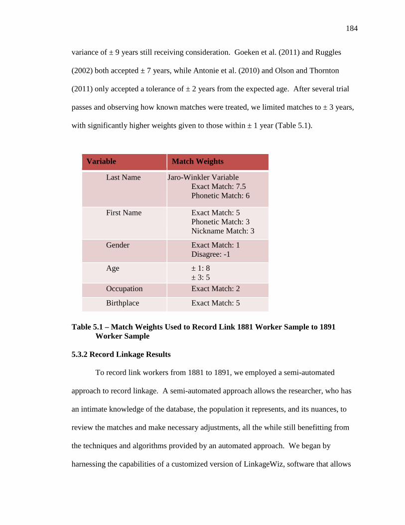
184

variance of ± 9 years still receiving consideration. Goeken et al. (2011) and Ruggles

(2002) both accepted ± 7 years, while Antonie et al. (2010) and Olson and Thornton

(2011) only accepted a tolerance of ± 2 years from the expected age. After several trial

passes and observing how known matches were treated, we limited matches to ± 3 years,

with significantly higher weights given to those within ± 1 year (Table 5.1).

Table 5.1 – Match Weights Used to Record Link 1881 Worker Sample to 1891 Worker Sample 5.3.2 Record Linkage Results

To record link workers from 1881 to 1891, we employed a semi-automated

approach to record linkage. A semi-automated approach allows the researcher, who has

an intimate knowledge of the database, the population it represents, and its nuances, to

review the matches and make necessary adjustments, all the while still benefitting from

the techniques and algorithms provided by an automated approach. We began by

harnessing the capabilities of a customized version of LinkageWiz, software that allows

Variable Match Weights

Last Name Jaro-Winkler Variable Exact Match: 7.5 Phonetic Match: 6

First Name Exact Match: 5 Phonetic Match: 3 Nickname Match: 3 Gender Exact Match: 1 Disagree: -1

Age ± 1: 8 ± 3: 5

Occupation Exact Match: 2

Birthplace Exact Match: 5

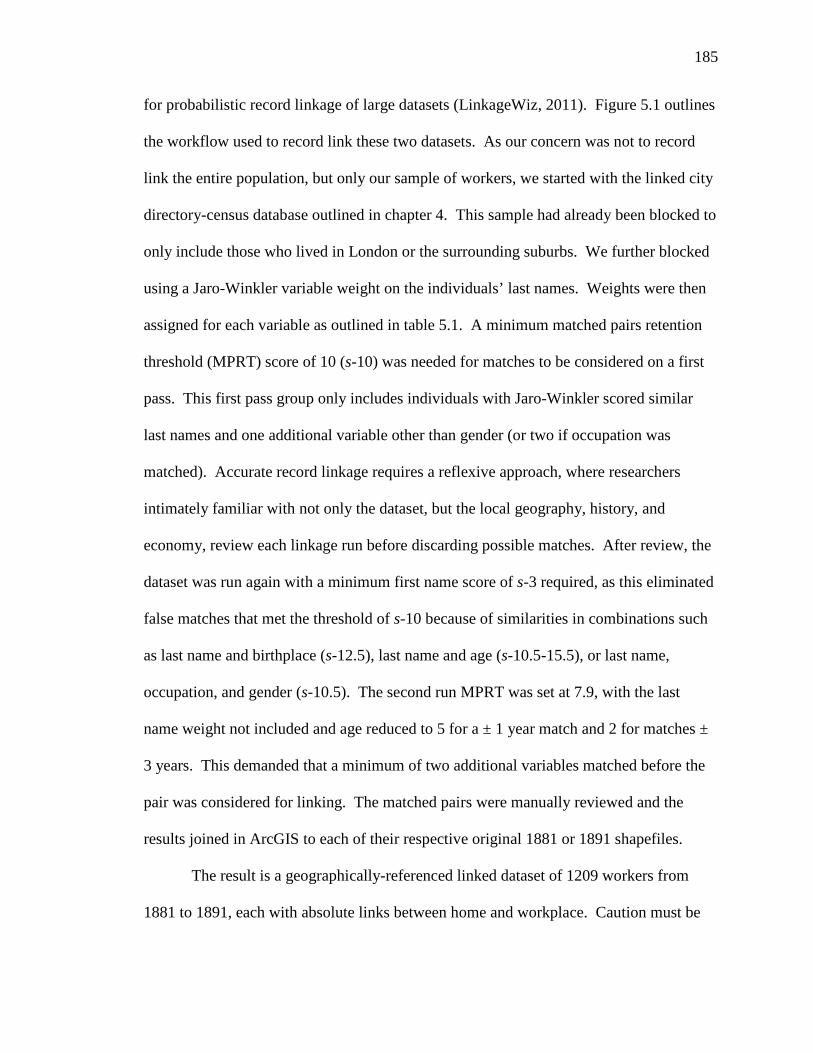
185

for probabilistic record linkage of large datasets (LinkageWiz, 2011). Figure 5.1 outlines

the workflow used to record link these two datasets. As our concern was not to record

link the entire population, but only our sample of workers, we started with the linked city

directory-census database outlined in chapter 4. This sample had already been blocked to

only include those who lived in London or the surrounding suburbs. We further blocked

using a Jaro-Winkler variable weight on the individuals’ last names. Weights were then

assigned for each variable as outlined in table 5.1. A minimum matched pairs retention

threshold (MPRT) score of 10 (s-10) was needed for matches to be considered on a first

pass. This first pass group only includes individuals with Jaro-Winkler scored similar

last names and one additional variable other than gender (or two if occupation was

matched). Accurate record linkage requires a reflexive approach, where researchers

intimately familiar with not only the dataset, but the local geography, history, and

economy, review each linkage run before discarding possible matches. After review, the

dataset was run again with a minimum first name score of s-3 required, as this eliminated

false matches that met the threshold of s-10 because of similarities in combinations such

as last name and birthplace (s-12.5), last name and age (s-10.5-15.5), or last name,

occupation, and gender (s-10.5). The second run MPRT was set at 7.9, with the last

name weight not included and age reduced to 5 for a ± 1 year match and 2 for matches ±

3 years. This demanded that a minimum of two additional variables matched before the

pair was considered for linking. The matched pairs were manually reviewed and the

results joined in ArcGIS to each of their respective original 1881 or 1891 shapefiles.

The result is a geographically-referenced linked dataset of 1209 workers from

1881 to 1891, each with absolute links between home and workplace. Caution must be

186

taken when comparing match rates between studies, as each utilizes different source

material and sampling strategies—or a ‘different universe’ (Dillon 2002, Ruggles 2002).

There is a need to examine differing record linkage methods with like data samples—an

aim outside of the scope of this research, but an area we hope to contribute to in the near

future. For consideration, the match rate we captured is higher than that reported by

Antonie et al. (2010), similar to that reported by Hershberg, Burnstein and Dockhorn

(1976), but lower than the 39% rates captured by Darroch (2002). This is largely due to

differing universes; ours is restricted by geography and work status, a rather restrictive

universe, whereas Darroch was working with a sample across a much larger region.

Although robust, our 24% link rate of the 1881 population does suffer from omissions.

First, Ruggles (2002, 217) reminds us that forward-linked samples, such has our desire

here, are more challenging than backwards-linked ones because of the effects of mortality

and emigration. Our sample here suffers from these challenges, as well as losing

individuals who left paid employment. We also miss young adults, who were under

working age in 1881. For women, name changes due to marriage limit our ability to

match across decades. Despite these omissions, this linked dataset will permit us to

complete the first (to our knowledge) historical journey to work study that views the

same population over time.

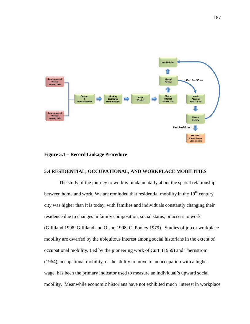
187

Figure 5.1 – Record Linkage Procedure

5.4 RESIDENTIAL, OCCUPATIONAL, AND WORKPLACE MOBILITIES

The study of the journey to work is fundamentally about the spatial relationship

between home and work. We are reminded that residential mobility in the 19th century

city was higher than it is today, with families and individuals constantly changing their

residence due to changes in family composition, social status, or access to work

(Gilliland 1998, Gilliland and Olson 1998, C. Pooley 1979). Studies of job or workplace

mobility are dwarfed by the ubiquitous interest among social historians in the extent of

occupational mobility. Led by the pioneering work of Curti (1959) and Thernstrom

(1964), occupational mobility, or the ability to move to an occupation with a higher

wage, has been the primary indicator used to measure an individual’s upward social

mobility. Meanwhile economic historians have not exhibited much interest in workplace

188

mobility, but instead have focused on the duration and drivers of individual job tenure,

noting that industrial jobs during the late nineteenth-century were brief, citing that high

labour mobility was an indicator of the ‘tenuousness of the employment relationship and

fluidity of the labour market’ (Jacoby 1985, 36-37, Jacoby and Sharma 1992) These

separate but complementary areas of scholarship all agree that individuals were mobile,

constantly changing the relationship between home and work. Despite this agreement,

the study of the changing relationship over time has received little attention, other than

anecdotal cases about individuals (Pooley and Turnbull 1997, Ulrich 1990) or studies

limited to employees from one workplace (Green 1988, Hoskins 1989).

5.4.1 Residential Mobility

To understand the changing relationship between home and work, we must first

examine the rate and intensity of residential mobility. In London, we observe high

residential mobility, similar to that reported for other Canadian cities during the same

period. Of our sample, 74.4% (n=900) of workers were living in a different residence ten

years later. The moves varied in intensity or spatial separation, from moves as close as

across the street, to substantial moves of over four kilometres (Figure 5.2). Similar to the

pattern found by Gilliland (1998) for Montreal, most moves were short, with a median

Euclidean distance of 741m. The distances moved over the decade vary by the size of the

household. We see a strong effect of the age of the household head on the distances of

residential moves, with the distances decreasing as age increases (Figure 5.3). An

increase in median distance moved is noted during the traditional years of retirement,

likely indicating moves into residences of kin or to secure a residential environment more

suitable to an individual with more limited personal mobility.

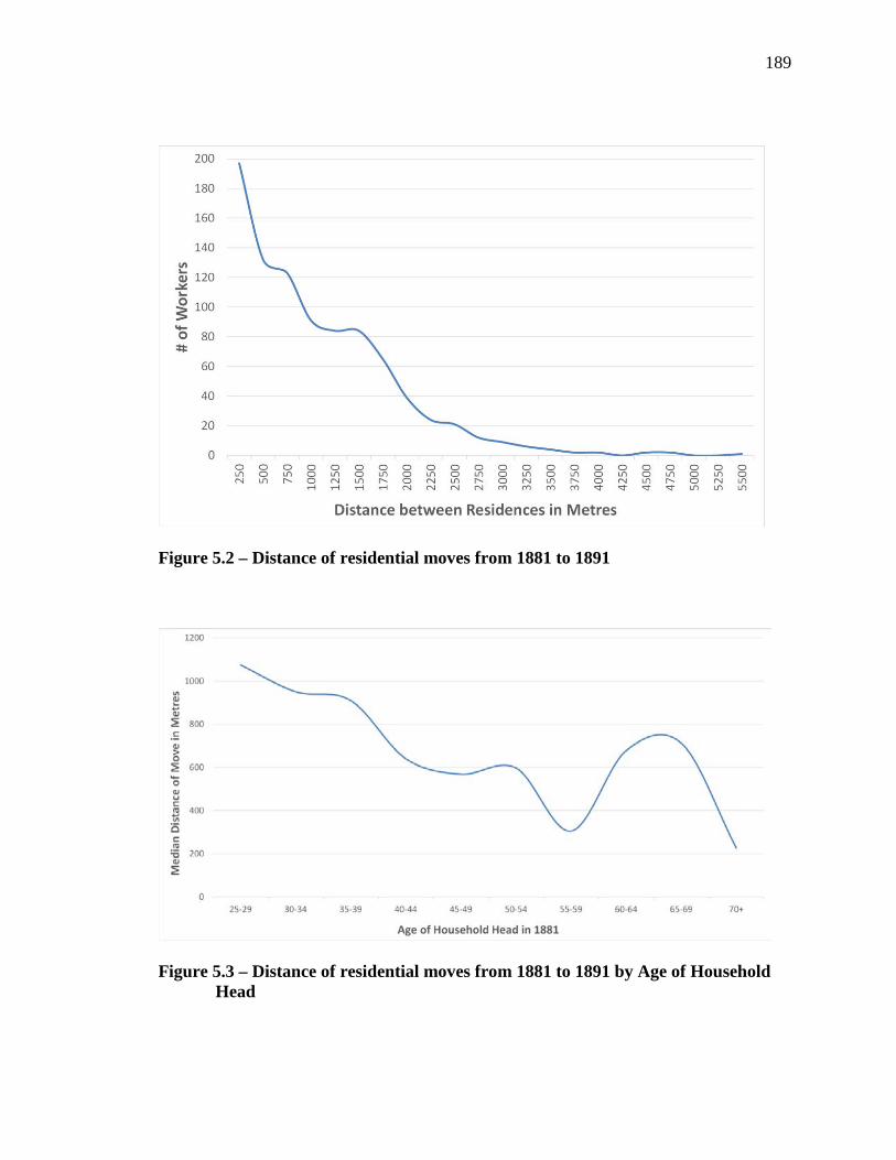
189

Figure 5.2 – Distance of residential moves from 1881 to 1891

Figure 5.3 – Distance of residential moves from 1881 to 1891 by Age of Household Head

190

The effect of household size is less pronounced than the age-effect, but is still

visible. The smallest and largest households moved greater distances as a response to

socio-demographic changes (Figure 5.4). Small households were comprised primarily of

young workers or widowed individuals who lived on their own. Over the course of a

decade, both transitioned into midsized households, the younger adding children and the

widows often taking residence with younger kin. These mid- to large-sized homes were

located largely in the city’s emerging neighbourhoods, further from the established

neighbourhoods from which the families moved. Those in the largest households were

generally young as well, living in boarding houses or residential hotels in the city’s core.

They were largely employed by the very hotels they lived in, as housekeepers, cooks, and

barbers. The hotelkeepers themselves are found in this group, as well as individuals who

worked at downtown factories such as Perrin’s biscuit company or McClary’s foundry.

Ten years later, many of these individuals were living in small dwellings with families or

had moved to smaller boarding houses in London East to take employment in one of the

factories there. This pattern is consistent with that observed by Dunae et al. (2013) for a

similar population of residential hotel dwellers in Victoria.

191

Figure 5.4 – Distance of residential moves from 1881 to 1891 by Household Size

Of particular interest to this larger study, we observe that moves vary based on

occupational class. Significant differences are found between higher and lower class

workers (Figure 5.5). Higher class occupations such as merchants, manufacturers, and

professionals had the shortest distance moves on average (median). A sharp increase is

noted for the middle classes. Labourers moved shorter distances than their middle-class

counterparts, whereas servants had the longest moves, with a median distance of over

1100m.

192

Figure 5.5 – Distance of Residential Moves from 1881 to 1891 by 1881 Occupational Class

The directionality of the moves presents a clearer picture. Figure 5.6 outlines the

linear directional mean of the moves by occupational class. The linear directional mean

is calculated by first obtaining the average distance of moves, by measuring the

Euclidean distance between origin and destination for each individual. The directional

mean of the lines is then calculated by statistical comparison of X and Y coordinates of

the origin and destination points and the trend presented on a street map. The length of

the line represents the mean distance between origin and destination. From inspection of

the map, we discover that many of the upper-class workers (merchants and

manufacturers, professionals, and white collar) moved into the wealthy near north

neighbourhood of Woodfield. Woodfield sits north-east of downtown and abuts Victoria

Park, at the time the city’s largest public space. Today, Woodfield is designated as two

193

heritage conservation districts (West and East Woodfield) to help preserve the eclectic

mix of Victorian architectures that adorn the neighbourhood (Figure 5.7). Many of the

homes in what has been dubbed the ‘Greatest Neighbourhood in Canada’ were built by

the individuals we are examining in this study (Canadian Institute of Planners 2012).

We also see that servants, the lowest occupational class from Figure 5.6, followed their

employers. They took residence in small, scattered cottages at the edge of the city’s

northern development, north of the present day CP Rail line on streets such as Pall Mall,

Maitland, and Miles. The middle classes of artisans, semi-skilled, and labourers moved

further eastward into the rapidly growing suburb of London East (which was

amalgamated into the city in 1885). Carpenters, blacksmiths, painters, and rail-workers

moved into the village to work at the oil refineries, rail yards, and car shops that were

built in the southern portion of the community. They occupied modest, well-appointed

homes, mostly Ontario cottages or homes built in the Queen Anne style, on streets north

of Dundas, such as Dufferin, Lorne, and Princess. Known today as Old East Village, this

thriving neighbourhood of past and present wage-workers has also been designated a

heritage conservation district (Figure 5.8)

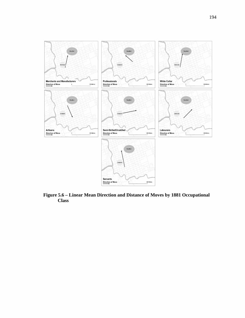
194

Figure 5.6 – Linear Mean Direction and Distance of Moves by 1881 Occupational Class

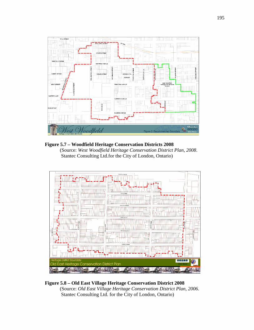
195

Figure 5.7 – Woodfield Heritage Conservation Districts 2008 (Source: West Woodfield Heritage Conservation District Plan, 2008.

Stantec Consulting Ltd.for the City of London, Ontario)

Figure 5.8 – Old East Village Heritage Conservation District 2008 (Source: Old East Village Heritage Conservation District Plan, 2006.

Stantec Consulting Ltd. for the City of London, Ontario)

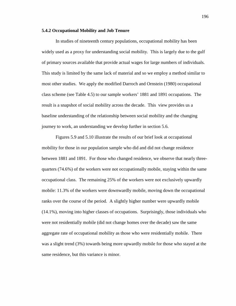
196

5.4.2 Occupational Mobility and Job Tenure

In studies of nineteenth century populations, occupational mobility has been

widely used as a proxy for understanding social mobility. This is largely due to the gulf

of primary sources available that provide actual wages for large numbers of individuals.

This study is limited by the same lack of material and so we employ a method similar to

most other studies. We apply the modified Darroch and Ornstein (1980) occupational

class scheme (see Table 4.5) to our sample workers’ 1881 and 1891 occupations. The

result is a snapshot of social mobility across the decade. This view provides us a

baseline understanding of the relationship between social mobility and the changing

journey to work, an understanding we develop further in section 5.6.

Figures 5.9 and 5.10 illustrate the results of our brief look at occupational

mobility for those in our population sample who did and did not change residence

between 1881 and 1891. For those who changed residence, we observe that nearly three-

quarters (74.6%) of the workers were not occupationally mobile, staying within the same

occupational class. The remaining 25% of the workers were not exclusively upwardly

mobile: 11.3% of the workers were downwardly mobile, moving down the occupational

ranks over the course of the period. A slightly higher number were upwardly mobile

(14.1%), moving into higher classes of occupations. Surprisingly, those individuals who

were not residentially mobile (did not change homes over the decade) saw the same

aggregate rate of occupational mobility as those who were residentially mobile. There

was a slight trend (3%) towards being more upwardly mobile for those who stayed at the

same residence, but this variance is minor.

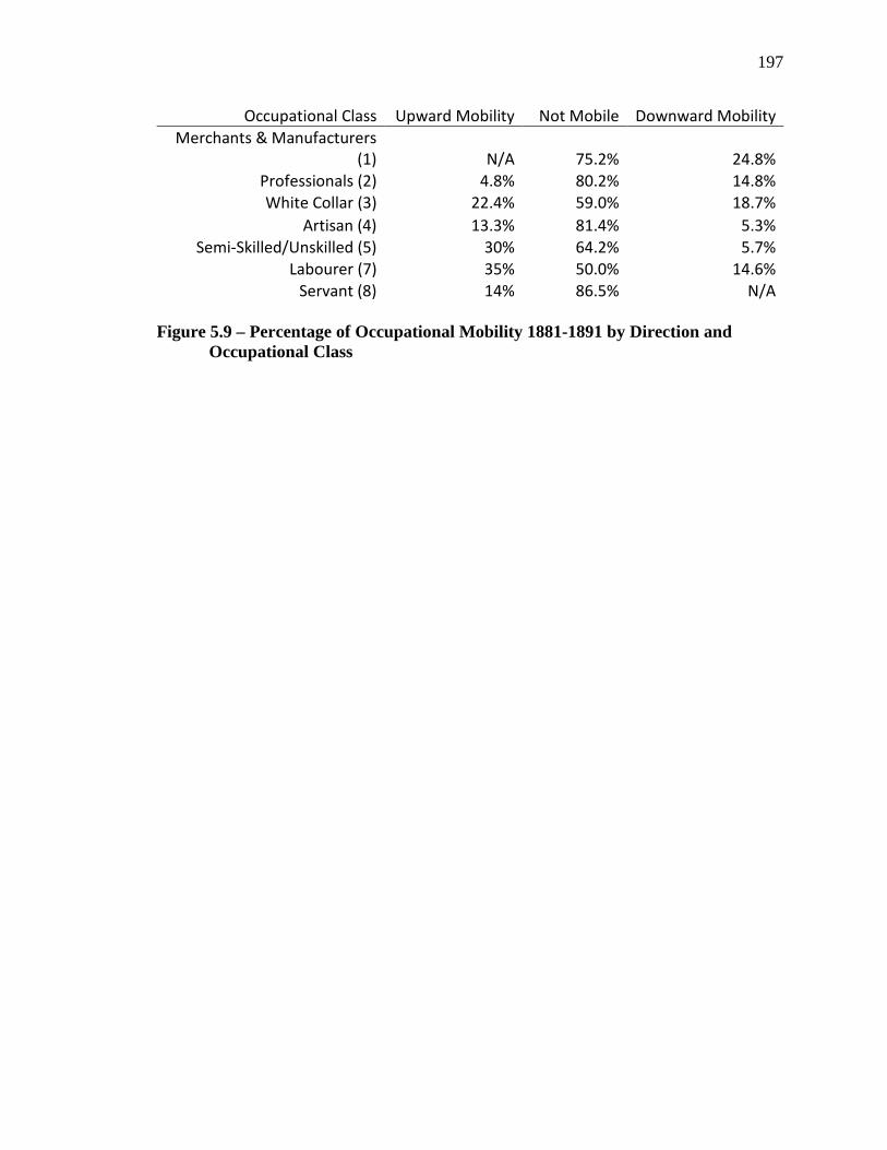
197

Occupational Class Upward Mobility Not Mobile Downward Mobility Merchants & Manufacturers

(1) N/A 75.2% 24.8% Professionals (2) 4.8% 80.2% 14.8% White Collar (3) 22.4% 59.0% 18.7%

Artisan (4) 13.3% 81.4% 5.3% Semi-Skilled/Unskilled (5) 30% 64.2% 5.7%

Labourer (7) 35% 50.0% 14.6% Servant (8) 14% 86.5% N/A

Figure 5.9 – Percentage of Occupational Mobility 1881-1891 by Direction and Occupational Class

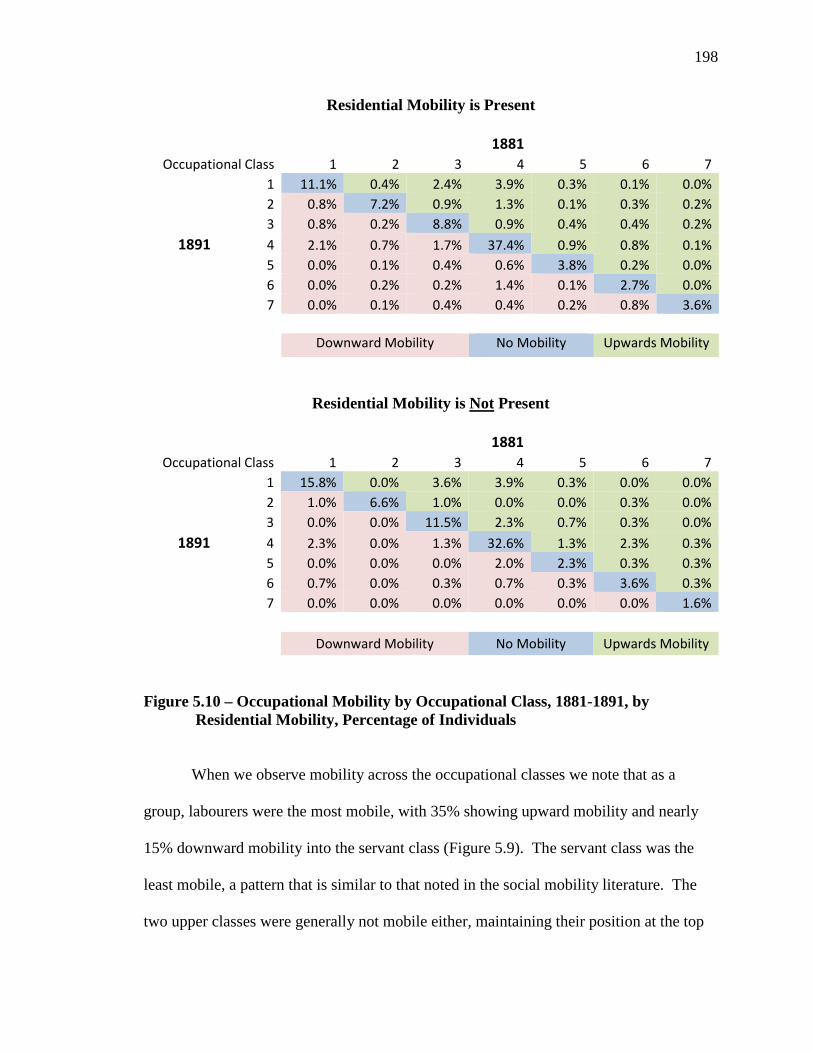
198

Residential Mobility is Present

1881

Occupational Class 1 2 3 4 5 6 7 1 11.1% 0.4% 2.4% 3.9% 0.3% 0.1% 0.0% 2 0.8% 7.2% 0.9% 1.3% 0.1% 0.3% 0.2% 3 0.8% 0.2% 8.8% 0.9% 0.4% 0.4% 0.2%

1891 4 2.1% 0.7% 1.7% 37.4% 0.9% 0.8% 0.1% 5 0.0% 0.1% 0.4% 0.6% 3.8% 0.2% 0.0% 6 0.0% 0.2% 0.2% 1.4% 0.1% 2.7% 0.0% 7 0.0% 0.1% 0.4% 0.4% 0.2% 0.8% 3.6%

Downward Mobility No Mobility Upwards Mobility

Residential Mobility is Not Present

1881

Occupational Class 1 2 3 4 5 6 7 1 15.8% 0.0% 3.6% 3.9% 0.3% 0.0% 0.0% 2 1.0% 6.6% 1.0% 0.0% 0.0% 0.3% 0.0% 3 0.0% 0.0% 11.5% 2.3% 0.7% 0.3% 0.0%

1891 4 2.3% 0.0% 1.3% 32.6% 1.3% 2.3% 0.3% 5 0.0% 0.0% 0.0% 2.0% 2.3% 0.3% 0.3% 6 0.7% 0.0% 0.3% 0.7% 0.3% 3.6% 0.3% 7 0.0% 0.0% 0.0% 0.0% 0.0% 0.0% 1.6%

Downward Mobility No Mobility Upwards Mobility

Figure 5.10 – Occupational Mobility by Occupational Class, 1881-1891, by Residential Mobility, Percentage of Individuals

When we observe mobility across the occupational classes we note that as a

group, labourers were the most mobile, with 35% showing upward mobility and nearly

15% downward mobility into the servant class (Figure 5.9). The servant class was the

least mobile, a pattern that is similar to that noted in the social mobility literature. The

two upper classes were generally not mobile either, maintaining their position at the top

199

of the social hierarchy. It is interesting to note, however, that the amount of mobility

between the merchant class and the artisan class is rather high, with 13.3% of artisans

moving upwards into the top class and nearly a quarter of merchants and manufacturers

moving downwards. Upon further examination, we see that most of the individuals who

moved down the occupational class scheme were owners of small- to mid-sized

businesses who later went to work for one of the larger industrial operations in the city.

For example, John Fleming, owner of an axe factory in 1881, was found ten years later

widowed and working as an engine man for the large Forest City Machine Works.

Another, John Murphy, a grocer in 1881, became a box maker at Fleischmann’s paper

company. We see the reverse experience in the group of workers who were upwardly

mobile into the merchant class. Workers left industrial employment to start small shops

within the same industry in which they were previously working, often in partnership

with other artisans. We must remind readers that observing occupational mobility

through the use of coded occupational titles (such as the North American Population

Project HISCO codes used in this study) does present challenges, as the ability to

calculate changes relies on the proper coding of occupation titles into the appropriate

groups. The meaning and nature of work associated with any given occupational title

changes over time, and some of the mobility we uncover may be an effect of these

changes.

Job tenure in London was remarkably high. We estimate that 34.8% of workers

who were employed outside of the home were employed by the same firm ten years later.

This is higher than the estimates of 26.9% reported by Carter and Savoca (1990) for San

Francisco. Whether someone had changed employers is not a simple determination. As

200

the primary concern of this study is the changing relationship between home and work,

we briefly examine job tenure along lines of residential and workplace mobility. We

view job tenure as whether a worker is travelling to the same worksite in 1891 as they

were 10 years earlier in 1881. We employ this approach to overcome the issues of

changing employers’ names, which was common during this period. Many companies

changed from surname-based monikers to less personalized descriptions; for example,

John Elliott & Son’s Foundry became Phoenix Foundry and E. Leonard and Sons became

London Engine and Boiler Works. We are uncertain if these name changes were in

everyday use or if city directory enumerators began to formalize the titles of the firms

they recorded. To determine if an individual was working at the same worksite, we

compared the latitude and longitude in both time periods, providing a modest buffer of

50m for geocoding differences in the two datasets. For a study of job tenure, this is

imperfect, as it does not account for individuals who stayed with the same employer but

either the employer changed location or they took up a position at a different worksite

operated by their employer. For a study of the changing journey to work, however, it is

essential. Reviewing our sample of job tenure, we observe an expected pattern: the

sample of workers who did not move had a higher percentage of decennial job tenure

than did those who did move over the period (Table 5.2). What is of interest is that the

differences were not great, 32.8% for those who were residentially mobile versus 40.8%

for those who were not. Home-based job tenure was expectedly higher for the non-

residentially mobile group versus the residentially mobile group.

201

Same Residence n= 309

n= Percentage

Same Workplace

Home-Based 42 13.6% Outside Home 126 40.8% Total 168 54.4%

Different Workplace

Outside Home 107 34.6%

Home-Based to Outside Home 20 6.5%

Outside Home to Home-Based 14 4.5%

Total 141 45.6%

Different Residence n= 900

n= Percentage

Same Workplace

Home-Based 69 7.7% Outside Home 295 32.8% Total 364 40.4%

Different Workplace

Outside Home 394 43.8%

Home-Based to Outside Home 90 10%

Outside Home to Home-Based 52 5.8%

Total 536 59.6% Table 5.2 – Changing Home-Work Relationships

202

5.4.3 Changing Home-Work Relationships

We have established how workers in London were residentially and

occupationally mobile and considered the lengths of their job tenure. What we have yet

to review is the extent of workplace mobility that was present over the period.

Workplace mobility is the critical missing link to completing our understanding of the

changing relationship between home and residence and its corresponding effect on the

daily journey to work, an area that, to our knowledge, has never been studied before

using the same population over time. Table 5.2 outlines the changing relationship

between work and home for our sample of 1209 workers in London. We observe that for

those that were residentially mobile, nearly three out of five (60%) changed their

workplace. More than two out of five (43.8%) worked outside of the home in both

periods, where another 15% of workers had shifted their employment either into or out of

their homes. For the remaining 40% of residentially mobile workers, the vast majority

(82%) continued employment outside the home and a small cohort moved residences and

maintained home-based employment. As we might expect, this cohort of home-based

workers is smaller than the cohort of home-based workers who were not residentially

mobile. We see a 14% difference in workplace persistence between the residentially

mobile and non-mobile groups. These patterns reinforce our notion that relationships

between home and work are complex and appear in various configurations.

In the aggregate, the average commute for all workers in the city in 1891 was

1305 metres (the median was 1216m). This is 22% longer than the average commute a

decade before. The change can be largely attributed to the continued suburbanization of

the city, especially to the north and east. The continued establishment of new factories in

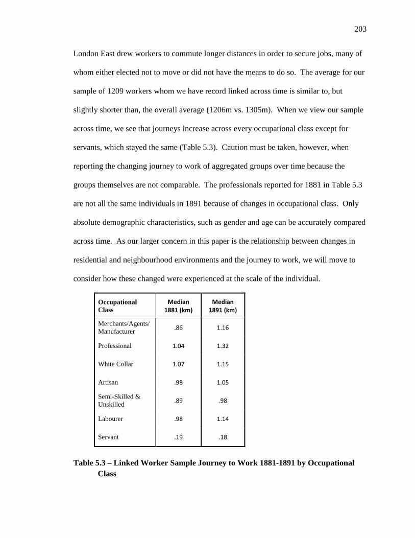
203

London East drew workers to commute longer distances in order to secure jobs, many of

whom either elected not to move or did not have the means to do so. The average for our

sample of 1209 workers whom we have record linked across time is similar to, but

slightly shorter than, the overall average (1206m vs. 1305m). When we view our sample

across time, we see that journeys increase across every occupational class except for

servants, which stayed the same (Table 5.3). Caution must be taken, however, when

reporting the changing journey to work of aggregated groups over time because the

groups themselves are not comparable. The professionals reported for 1881 in Table 5.3

are not all the same individuals in 1891 because of changes in occupational class. Only

absolute demographic characteristics, such as gender and age can be accurately compared

across time. As our larger concern in this paper is the relationship between changes in

residential and neighbourhood environments and the journey to work, we will move to

consider how these changed were experienced at the scale of the individual.

Occupational Class

Median 1881 (km)

Median 1891 (km)

Merchants/Agents/ Manufacturer .86 1.16

Professional 1.04 1.32

White Collar 1.07 1.15

Artisan .98 1.05

Semi-Skilled & Unskilled .89 .98

Labourer .98 1.14

Servant .19 .18

Table 5.3 – Linked Worker Sample Journey to Work 1881-1891 by Occupational Class

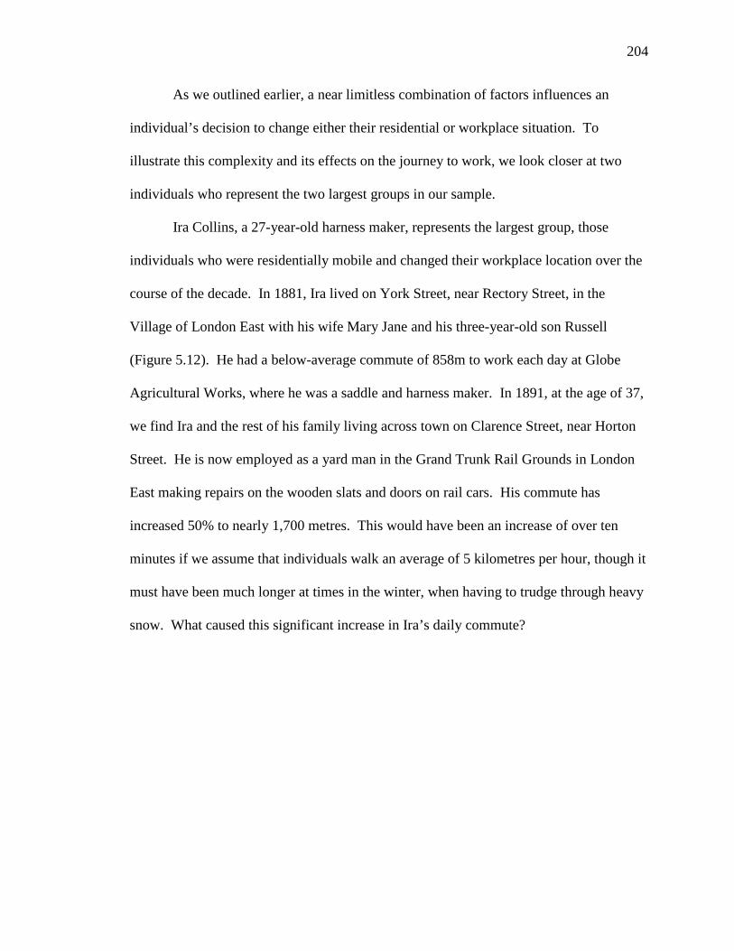
204

As we outlined earlier, a near limitless combination of factors influences an

individual’s decision to change either their residential or workplace situation. To

illustrate this complexity and its effects on the journey to work, we look closer at two

individuals who represent the two largest groups in our sample.

Ira Collins, a 27-year-old harness maker, represents the largest group, those

individuals who were residentially mobile and changed their workplace location over the

course of the decade. In 1881, Ira lived on York Street, near Rectory Street, in the

Village of London East with his wife Mary Jane and his three-year-old son Russell

(Figure 5.12). He had a below-average commute of 858m to work each day at Globe

Agricultural Works, where he was a saddle and harness maker. In 1891, at the age of 37,

we find Ira and the rest of his family living across town on Clarence Street, near Horton

Street. He is now employed as a yard man in the Grand Trunk Rail Grounds in London

East making repairs on the wooden slats and doors on rail cars. His commute has

increased 50% to nearly 1,700 metres. This would have been an increase of over ten

minutes if we assume that individuals walk an average of 5 kilometres per hour, though it

must have been much longer at times in the winter, when having to trudge through heavy

snow. What caused this significant increase in Ira’s daily commute?

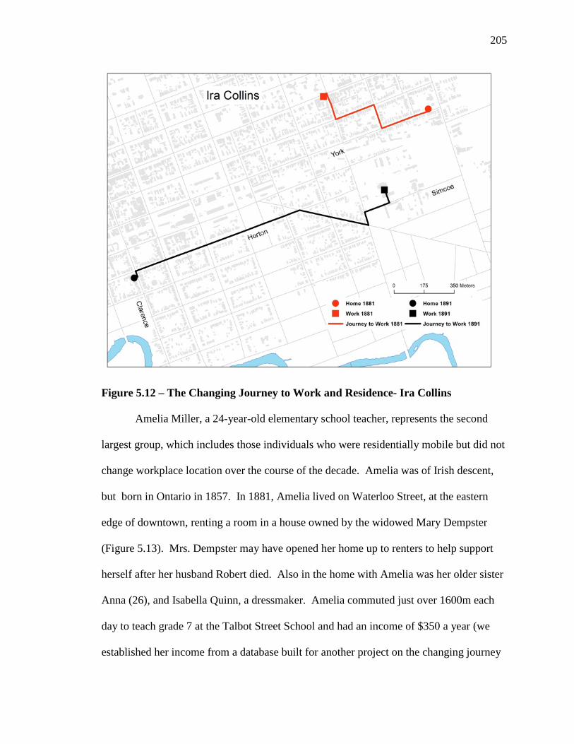
205

Figure 5.12 – The Changing Journey to Work and Residence- Ira Collins

Amelia Miller, a 24-year-old elementary school teacher, represents the second

largest group, which includes those individuals who were residentially mobile but did not

change workplace location over the course of the decade. Amelia was of Irish descent,

but born in Ontario in 1857. In 1881, Amelia lived on Waterloo Street, at the eastern

edge of downtown, renting a room in a house owned by the widowed Mary Dempster

(Figure 5.13). Mrs. Dempster may have opened her home up to renters to help support

herself after her husband Robert died. Also in the home with Amelia was her older sister

Anna (26), and Isabella Quinn, a dressmaker. Amelia commuted just over 1600m each

day to teach grade 7 at the Talbot Street School and had an income of $350 a year (we

established her income from a database built for another project on the changing journey

206

to school [Board of Education for the City of London, 1891]). In 1891, at the age of 34,

we find Amelia still teaching grade 7 at the same school. However, instead of a long

commute, we find Amelia living 71% closer to work, residing in a boarding house on

Kent Street only 463 metres from the school. Her income is now $450 a year, but she is

living with seven other individuals rather than the four she did a decade before. The

boarding house is run by Grace Heron, the oldest of the four Heron siblings who live

together in the home. Her brothers George (41, a travelling salesman) and James (34,

cabinetmaker), as well as her sister Maggie (35, no occupation listed—she likely helped

run the house) share the living space with 26-year-old Mary Austin, a housekeeper at the

Grigg House, young William Geary (22, an assistant druggist), and Amelia.

Figure 5.13 – The Changing Journey to Work and Residence- Amelia Miller

207

It appears that Amelia may have moved to shorten her long journey to work.

However, it is also possible that she wished to secure accommodations with similarly-

aged people, that the relationship with Mary Dempster went sour, or perhaps she sought a

living situation that included both men and women. After moving, however, she shared a

house with more people; was the consequence less living space, and greater crowding?

What about the environment outside the front door? Was the Kent Street location a more

appealing residential environment than Waterloo Street? Did it better represent her social

status as a white collar worker? Did it suggest that she was of an even higher class? As

for Ira, did he choose to move to a different neighbourhood? Or was he forced to leave

his home in London East because of fire or financial difficulties? Did he lose his job at

Globe Agricultural Works, or did he seek a new job with the G.T.R.? Was he seeking a

better physical or social environment for his family? Some of these questions we cannot

answer without detailed personal or business records. We can, however, harness the built

environment stage in the HGIS to examine Ira and Amelia’s residential and

neighbourhood environments over time to glean a different perspective on why

individuals may have changed their residential and workplace environments.

5.5 CAPTURING HISTORIC ENVIRONMENTS

When a family moves, a number of factors go into the decision of where to live.

A family must tread a careful balance between finding a home that meets their space

requirements, and is in a neighbourhood that is desirable to their lifestyle, all while

keeping within their budget. When a life event requires a family or individual to move or

change workplaces, it is also an opportunity to try to better their residential and/or

208

neighbourhood environment. If the family has had a stable residence for many years, a

move opens an opportunity to update the environment to better reflect the needs of the

family at its present stage in their lifecourse. Furthermore, moving into an environment

of greater quality is a public reflection of upward social mobility.

To begin to understand how families and individuals in the nineteenth-century

city attempted to improve their residential situations, we must look at two of the

environments that closely influenced the quality of daily life for the individual: the

residence and the neighbourhood. Figure 5.14 illustrates the environmental indicators

used to determine the quality of residential and neighbourhood environments. The home

or residential environment is determined by the characteristics within, and of, the

residential dwelling. It is the finest scale of spatial resolution at which we can study the

built environment of the city. It includes the socio-demographic environment within the

home, which for families is generally homogeneous with the household head, but for

individuals living in boarding houses, residential hotels, and institutions, we use the

individuals’ occupational class ranks. Living space per person provides us an indication

of crowding in the home, which is generally seen as a negative environmental factor.

High levels of crowding in nineteenth-century cities have been correlated with increases

in conflagrations, disease, crime, and in extreme cases, higher mortality. Building

material is typically used as a proxy for property condition or solidity. In London, most

of the homes were made from either wood or brick, with brick being considered superior,

especially during the late nineteenth century.

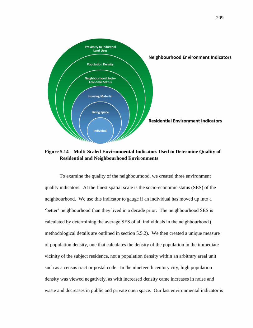
209

Figure 5.14 – Multi-Scaled Environmental Indicators Used to Determine Quality of Residential and Neighbourhood Environments

To examine the quality of the neighbourhood, we created three environment

quality indicators. At the finest spatial scale is the socio-economic status (SES) of the

neighbourhood. We use this indicator to gauge if an individual has moved up into a

‘better’ neighbourhood than they lived in a decade prior. The neighbourhood SES is

calculated by determining the average SES of all individuals in the neighbourhood (

methodological details are outlined in section 5.5.2). We then created a unique measure

of population density, one that calculates the density of the population in the immediate

vicinity of the subject residence, not a population density within an arbitrary areal unit

such as a census tract or postal code. In the nineteenth century city, high population

density was viewed negatively, as with increased density came increases in noise and

waste and decreases in public and private open space. Our last environmental indicator is

210

proximity to industrial uses. We calculate how close each individual was to the foul

smells, noise, and pollution that emanated from the smelters, factories, and coal-powered

locomotives that dominated the urban landscape in the nineteenth century. The farther

from these industrial environments a residence was located, the better the neighbourhood,

in general. To create these environmental indicators we returned to the environmental

variables embedded within the built and social environment stages of the Imag(in)ing

London HGIS (as discussed in Chapter three). The result is a recreation of historic

environments at a resolution, scale, and precision never seen before in urban historical

geographical research.

5.5.1 Residential Environment Quality Indicators

We created three measures that allow us to measure the quality of the residential

environment, household socio-economic status (SES), crowding, and change in dwelling

construction. Household SES is covered extensively in section 5.2, where we outline the

changes in occupational class ranking from 1881 to 1891. To establish our crowding

measure, we needed to determine the number of individuals in each residence as well as

the size of each dwelling. The number of individuals per building was captured by both

the 1881 and 1891 census enumerators and provided to us as a variable by the 1881

Canadian Census Project and the Historical Data Unit, respectively. Thankfully, the

enumerators were instructed in the same manner for both years, allowing for ease of

comparison. Enumerators were to record all individuals per building rather than

recording them by family unit. To establish the size of each dwelling, we turned to the

building polygons embedded in the built environment stage. Each building polygon was

created by digitizing the building footprints, as depicted on the fire insurance plans. Any

211

information about a building was recorded as attributes for analysis, such as the number

of stories, the building material, and building usage. The footprints were then run through

ArcGIS’s geometry tool to calculate the gross square footage (GSF) of floor space (also

known in property valuation as the Gross External Area). We did not deduct for the

thickness of exterior or interior walls, or the presence of unusable living space such as

chimneys and circulation areas (e.g., stairs, corridors, or entrance halls), as we were

concerned with relative changes rather than absolute usable space, for which estimates

would be less accurate. The square footage calculated was then multiplied by the number

of stories, and the crowding measure calculated by dividing total square footage by the

number of individuals in the building.

The final indicator of the residential environment is the building material of each

residence. This information was recorded in the building polygons embedded in the built

environment stage. Of the 3886 residential buildings in the city, 2443 were constructed

from wood, 1399 were made with brick, 34 were brick veneer over wood, and 10

buildings were built out of concrete. For ease of comparison, we designated the brick

veneer as brick and the ten concrete buildings as wood. This limits our comparison over

time to four scenarios: brick-to-brick and wood-to-wood, denoting no change in building

quality, wood-to-brick being considered an improvement, and brick-to-wood the

opposite.

5.5.2 Neighborhood Environmental Quality Indicators

Moving outward from the fine spatial scale of the individual residence, we created

three measures that allow for the measurement of the quality of the neighbourhood

environment. First is neighbourhood socio-economic status (N-SES). We created the N-

212

SES in order to determine if an individual moved into a ‘better’ neighbourhood, or a

community with a higher SES than they lived in a decade prior. We know that

individuals seek neighbourhoods that reflect their desired residential community, with

residents who share common socioeconomic characteristics and property values (Clapp

and Wang 2006). Positive social interaction with neighbours is deemed one of the top

neighbourhood features that lead to a high quality of life in contemporary cities (Sirgy

and Cornwell 2002), and in the walking city, where kinship and neighbourly support was

perhaps more valued and necessary (Olson and Thornton 2011), we expect that the same

held true. Individuals who were upwardly mobile would have sought neighbours who

would reflect their increased social status. To determine an upward move, we calculated

the N-SES similarly to the individual-level SES, just computed for the entire

neighbourhood rather than the head of household or the individual in a group living

situation. However, how do we determine someone’s neighbourhood?

There is little agreement in urban social geography about how to delimit a

neighbourhood. Many scholars conceptualize ‘community’ interchangeably with the idea

of ‘neighbourhood’. George Hillery provided a cautionary reminder that ‘community’ is

indeed an area of little agreement. In a broad review of the early literature on both rural

and urban definitions of community, he found ninety-four different definitions, bounded

within sixteen different concepts. His summary concluded that most scholars in the first

half of the twentieth century agreed that community consisted of “persons in social

interaction within a geographic area and having one or more additional common ties”

(Hillery 1955, 111). To Porteous, an individual’s neighbourhood is the ‘geographic

space in which one feels at home’ (1977, 68). More contemporary ideas or proxies for

213

neighbourhood acknowledge that neighbourhoods exist at multiple scales. A child may

perceive her neighbourhood as the area immediately adjacent to her home where she is

permitted to play; older children may include the streets traversed during the walk to and

from school (Loebach and Gilliland 2010). For adults, ‘neighbourhood’ may be used to

describe a former settlement that has been amalgamated into a larger urban system.

Neighbourhoods are also often considered to be delimited by administrative boundaries

such as school attendance districts, residential subdivisions, heritage districts, or police

precincts. Postal codes and census tracts have been commonly used as proxies for

neighbourhoods in contemporary research, though it is acknowledged that these

boundaries are arbitrary and are not available to students of the nineteenth-century city

(Wood 2002). To Mayol, the neighbourhood is the domain ‘in which the space-time

relationship is the most favourable for a dweller who moves from place to place on foot,

starting from his home.” (1998, 11) However, other scholars have highlighted that

neighbourhood is socially constructed by individuals within propinquity. Porteous

(1977) reports that residents perceive their immediate social neighbourhood to be as few

as nine to twelve houses. Borchert (1981) outlines the importance of frequent face-to-

face interaction as critical to creating a sense of neighbourhood belonging and

community.

We could delimit a walking-based conception of neighbourhood such as Mayol

has suggested by creating radial or street network buffers using an arbitrary buffer

distance as a proxy for ‘walkable’ distance. Instead, we combined Mayol’s conception of

neighbourhood with that of Porteous and Borchert and created a conception of

neighbourhood centered on the individual. We delimited neighbourhood for each

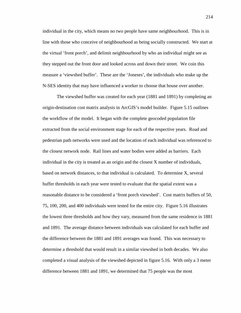
214

individual in the city, which means no two people have same neighbourhood. This is in

line with those who conceive of neighbourhood as being socially constructed. We start at

the virtual ‘front porch’, and delimit neighbourhood by who an individual might see as

they stepped out the front door and looked across and down their street. We coin this

measure a ‘viewshed buffer’. These are the ‘Joneses’, the individuals who make up the

N-SES identity that may have influenced a worker to choose that house over another.

The viewshed buffer was created for each year (1881 and 1891) by completing an

origin-destination cost matrix analysis in ArcGIS’s model builder. Figure 5.15 outlines

the workflow of the model. It began with the complete geocoded population file

extracted from the social environment stage for each of the respective years. Road and

pedestrian path networks were used and the location of each individual was referenced to

the closest network node. Rail lines and water bodies were added as barriers. Each

individual in the city is treated as an origin and the closest X number of individuals,

based on network distances, to that individual is calculated. To determine X, several

buffer thresholds in each year were tested to evaluate that the spatial extent was a

reasonable distance to be considered a ‘front porch viewshed’. Cost matrix buffers of 50,

75, 100, 200, and 400 individuals were tested for the entire city. Figure 5.16 illustrates

the lowest three thresholds and how they vary, measured from the same residence in 1881

and 1891. The average distance between individuals was calculated for each buffer and

the difference between the 1881 and 1891 averages was found. This was necessary to

determine a threshold that would result in a similar viewshed in both decades. We also

completed a visual analysis of the viewshed depicted in figure 5.16. With only a 3 meter

difference between 1881 and 1891, we determined that 75 people was the most

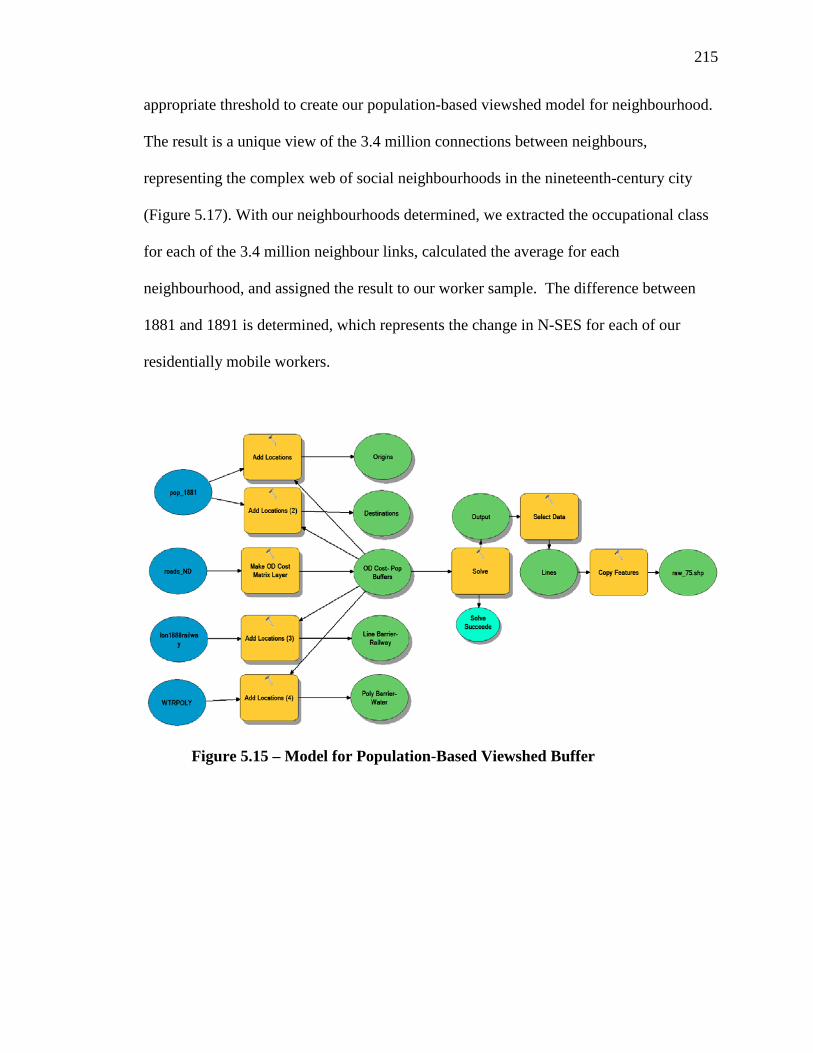
215

appropriate threshold to create our population-based viewshed model for neighbourhood.

The result is a unique view of the 3.4 million connections between neighbours,

representing the complex web of social neighbourhoods in the nineteenth-century city

(Figure 5.17). With our neighbourhoods determined, we extracted the occupational class

for each of the 3.4 million neighbour links, calculated the average for each

neighbourhood, and assigned the result to our worker sample. The difference between

1881 and 1891 is determined, which represents the change in N-SES for each of our

residentially mobile workers.

Figure 5.15 – Model for Population-Based Viewshed Buffer

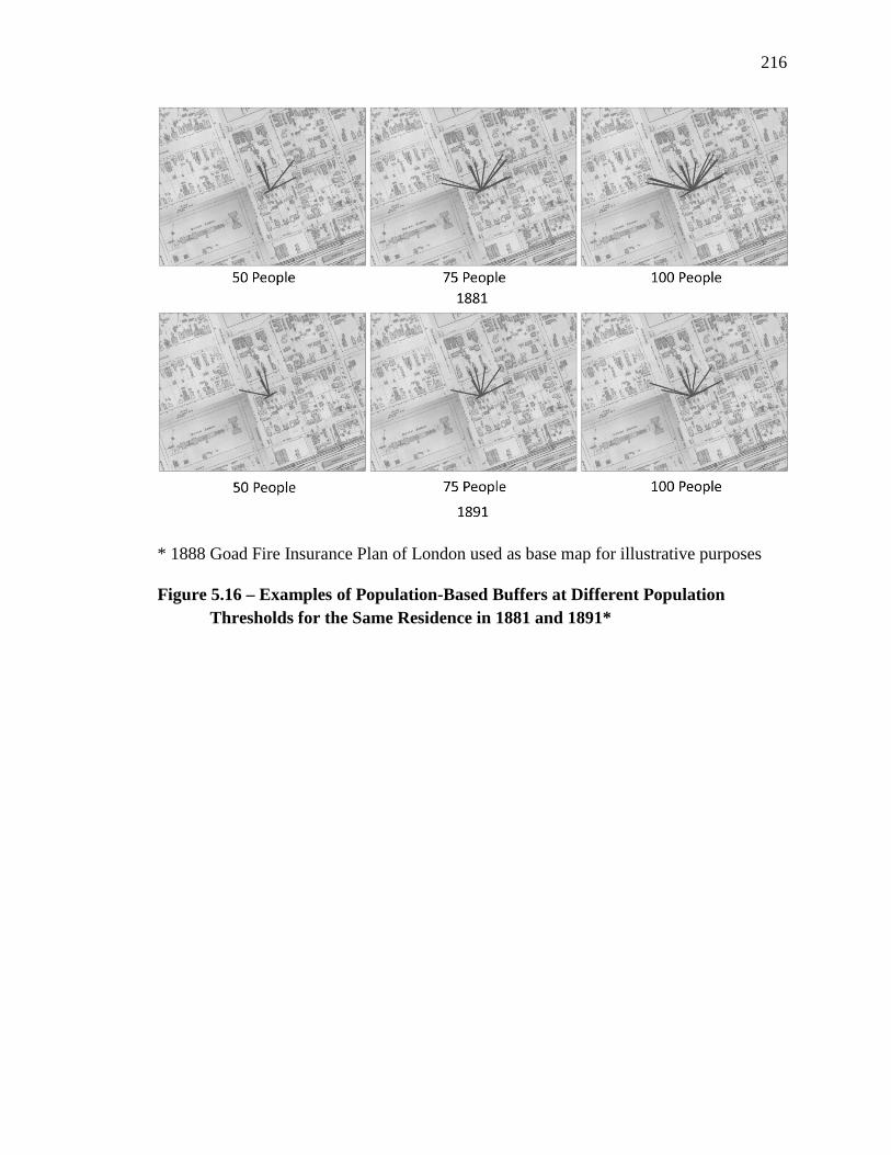
216

* 1888 Goad Fire Insurance Plan of London used as base map for illustrative purposes

Figure 5.16 – Examples of Population-Based Buffers at Different Population Thresholds for the Same Residence in 1881 and 1891*

217

Figure 5.17 – The Complex Web of Social Neighbourhoods in London*

* 1888 Goad Fire Insurance Plan of London used as base map for illustrative purposes. Not all buildings have connections because they are either not residential buildings or are not inhabited The second neighbourhood environment quality indicator is population density.

Population density is typically reported as the total population divided by total land area;

however, this technique does not work well when comparing small geographic areas. We

instead harnessed the viewshed neighbourhood buffers to calculate the effective

population density as experienced by each individual in the city. We captured the

geographic distance between neighbours that was calculated during the origin-destination

cost matrix analysis and determined the average distance between an individual and his

neighbours. The lower the average distance, the higher the population density would

218

have appeared to the person of interest. We then compared an individual’s experienced

population density in 1881 and 1891 to determine if they moved to a more or less dense

neighbourhood.

The final neighbourhood environment quality indicator is proximity to industrial

uses. Industrial areas of the nineteenth century city were noxious environments. They

were darker, smellier, and noisier than other areas of the city. Pollutants wafted from the

smoke stacks, chemicals were piled in the yards, and waste was disposed of in any

available open space or waterway. They were environments that most working people

tried to avoid living in, but this was difficult during the late nineteenth century, when

municipalities rarely limited land uses for fear of slowing industrial development. To

determine the proximity of a worker’s home to industrial uses, we first had to estimate

the effect of industrial land uses on the adjacent residential parcels. We do not have

information on the type of industrial activity in each factory, so estimating the amount of

noise, smell, and pollution produced by each individual factory is not possible. Instead,

we created a raster model of industrial impact by calculating a weighted interpolation of

the square footage of each industrial building in the city (Figure 5.18). Railyards were

also included, using a weight of 2 sq. feet for each rail line depicted on the fire insurance

plans. The result is an estimate of how far the activities of factories may have influenced

the neighbourhood environment of our sample of workers.

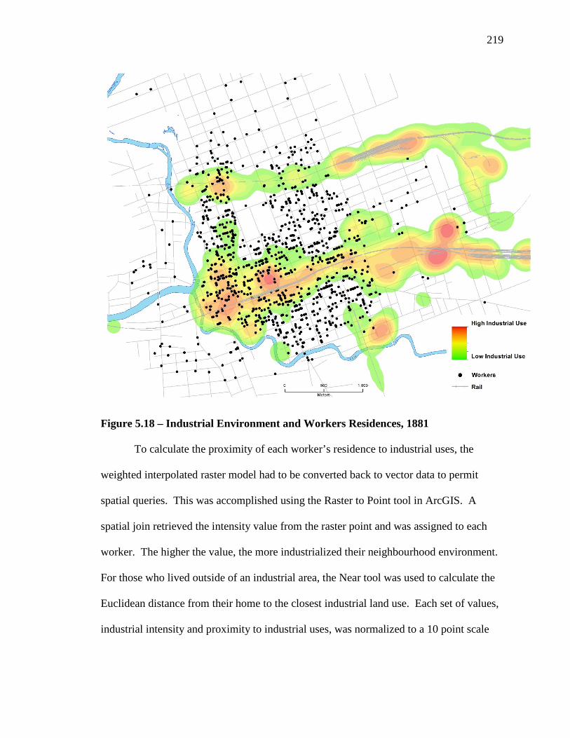
219

Figure 5.18 – Industrial Environment and Workers Residences, 1881

To calculate the proximity of each worker’s residence to industrial uses, the

weighted interpolated raster model had to be converted back to vector data to permit

spatial queries. This was accomplished using the Raster to Point tool in ArcGIS. A

spatial join retrieved the intensity value from the raster point and was assigned to each

worker. The higher the value, the more industrialized their neighbourhood environment.

For those who lived outside of an industrial area, the Near tool was used to calculate the

Euclidean distance from their home to the closest industrial land use. Each set of values,

industrial intensity and proximity to industrial uses, was normalized to a 10 point scale

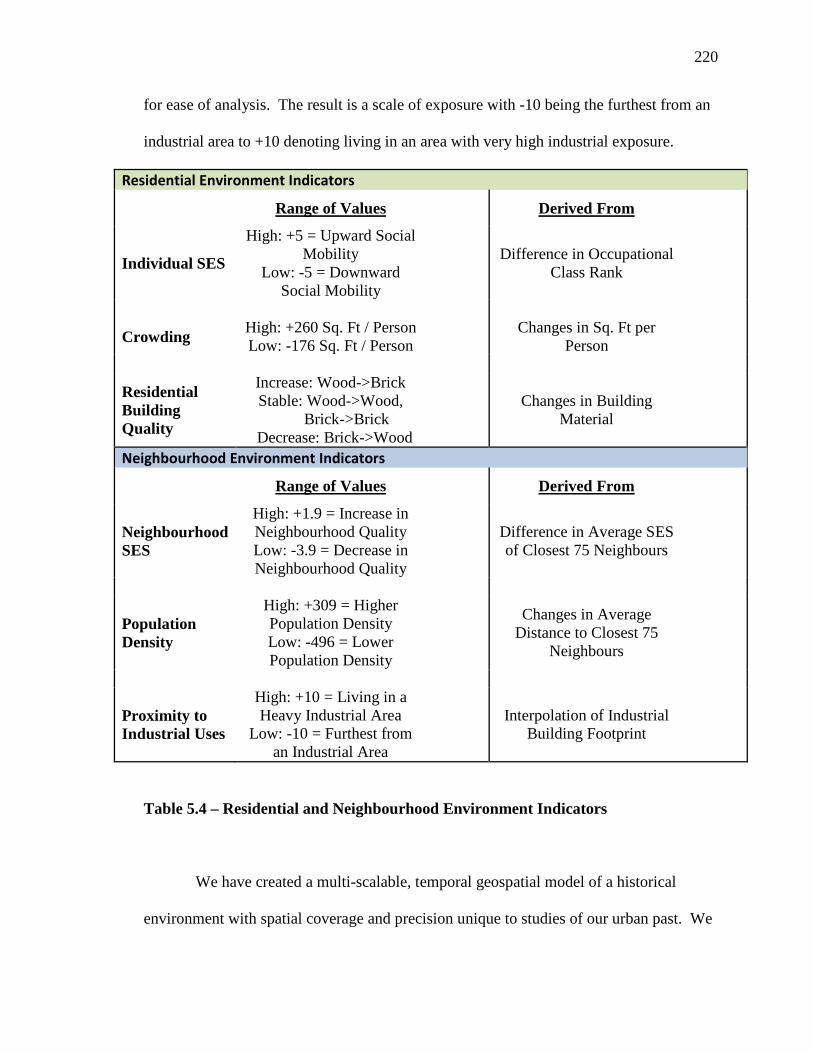
220

for ease of analysis. The result is a scale of exposure with -10 being the furthest from an

industrial area to +10 denoting living in an area with very high industrial exposure.

Residential Environment Indicators Range of Values Derived From

Individual SES

High: +5 = Upward Social Mobility

Low: -5 = Downward Social Mobility

Difference in Occupational Class Rank

Crowding High: +260 Sq. Ft / Person Low: -176 Sq. Ft / Person

Changes in Sq. Ft per Person

Residential Building Quality

Increase: Wood->Brick Stable: Wood->Wood,

Brick->Brick Decrease: Brick->Wood

Changes in Building Material

Neighbourhood Environment Indicators Range of Values Derived From

Neighbourhood SES

High: +1.9 = Increase in Neighbourhood Quality Low: -3.9 = Decrease in Neighbourhood Quality

Difference in Average SES of Closest 75 Neighbours

Population Density

High: +309 = Higher Population Density Low: -496 = Lower Population Density

Changes in Average Distance to Closest 75

Neighbours

Proximity to Industrial Uses

High: +10 = Living in a Heavy Industrial Area

Low: -10 = Furthest from an Industrial Area

Interpolation of Industrial Building Footprint

Table 5.4 – Residential and Neighbourhood Environment Indicators

We have created a multi-scalable, temporal geospatial model of a historical

environment with spatial coverage and precision unique to studies of our urban past. We

221

began at a fine spatial resolution by uncovering the socio-economic status of the

individual and how it changed over time. We moved outwards to the dwelling and

viewed the extent of crowding and the quality of the residential unit. Then we continued

onto the street to uncover an individualized perspective of the social and built

environment that influenced daily life. The model was applied to each and every

individual in the city, in two time periods, affording us a view of the city during the peak

of industrialization. With this unique perspective on the city, we return to our interest in

the changing journey to work and social mobility. Were the workers whom we can

follow over socially mobile, as measured through improvements in their residential and

neighbourhood environments? Did the desire to improve their environments result in a

lengthened journey to work? Or were some able to secure a residential situation that both

shortened their commute and improved the environments of their everyday lives?

5.6 THE COMPLEXITIES OF URBAN LIFE: ENVIRONMENT, SOCIAL

MOBILITY, AND THE JOURNEY TO WORK

In this paper we have followed a sample of workers across the decade between

1881 and 1891. We have established that they experienced high levels of residential and

workplace mobility. We expect that some of these mobility decisions were to acquire

better wages, more stable work, or better working conditions, while some mobility was in

response to changes in household composition such as needing to find larger

accommodations for growing families or the need to move in with one’s extended family

in the later years of life. These moves provided individuals an opportunity to try to

improve their quality of life, by increasing the quality or amount of living space in their

222

home, moving to a more well-to-do neighbourhood, or simply to an environment farther

away from the pollution, noise, and smells of industrialization.

We begin our review of workers’ residential environments in the aggregate,

focusing on our sample of the 900 workers who were residentially mobile. At finest scale

of the individual, we revisit our findings from section 5.4.2 and observe that 14.1% of

workers were upwardly mobile and 11.3% went down the social mobility scale, leaving

the vast majority (74.6%) as having no change in social status over time. For measures of

crowding, we observe that a near equal number of workers increased their living space

per person as decreased their living space per person (15% each). To our surprise, we see

a large number of workers with no discernable change (less than 2 sq.ft/person) in their

living space per household member. If we look closer at the family composition of this

group, we see considerable changes in household size over the period, with 44%

increasing the size of their household, 41% decreasing in size, and only 15% maintaining

the same size. With near uniform consistency, those who increased their household size

also increased the size of their dwelling, and similar decreases in dwelling size occurred

for the group whose households decreased in members. In the aggregate, this pattern

seems to suggest that many households were likely able to react to changes in household

size with an astonishing degree of accuracy.

For our examination of the quality of the workers’ residences, we see a more

uniform distribution. Just over half (52.8%) of workers stayed in a similarly-constructed

building over the decade: 58% of that group moved from a wood-framed house into

another wood-framed house, while the remaining 42% moved from a brick home to

another brick home. For those that did move to a dwelling with different construction

223

materials from their previous dwelling, a nearly equal number improved the quality of

their home, moving from a wood-frame to a brick home as did those who appear to have

decreased the quality, moving from a brick building to a wood one.

To review the three neighbourhood environment indicators in the aggregate, we

start at the finest spatial scale of the change in neighbourhood SES. We observe that

90% of workers changed their neighbourhood quality over the decade, with 54% moving

into a neighbourhood with a lower SES score than they were living in a decade

previously, while the other 36% increased the quality of their neighbourhood. A small

group of 90 (10%) saw no discernable change, which we determined to be any SES

change of less than +/-.1 over the decade.

Moving further into the neighbourhood, the change in population density is

relatively evenly distributed: 39% of workers moved to a neighbourhood with a lower

population density, while 34% saw an increase in density. We determine that the

remaining 27% had no change, with a change in population density indicator value of +/-

10 metres, recalling that we measure population density by the average distance between

the worker of interest and their closest 75 neighbours.

The last neighbourhood environment indicator is the proximity to industrial

environments. As we expected, the vast majority of workers (82%) in 1881 were living

in an environment we classified as industrial. By 1891, this number had dropped to 70%,

but still represents the majority of workers. Further, 81 of the 164 workers (49%) who

were not living in an industrial area in 1881 had moved into one by 1891, while 186 of

the 736 workers (25%) who were living in an industrial area in 1881 were able to move

out by 1891. Those who did not live in an industrial area, however, were still very close

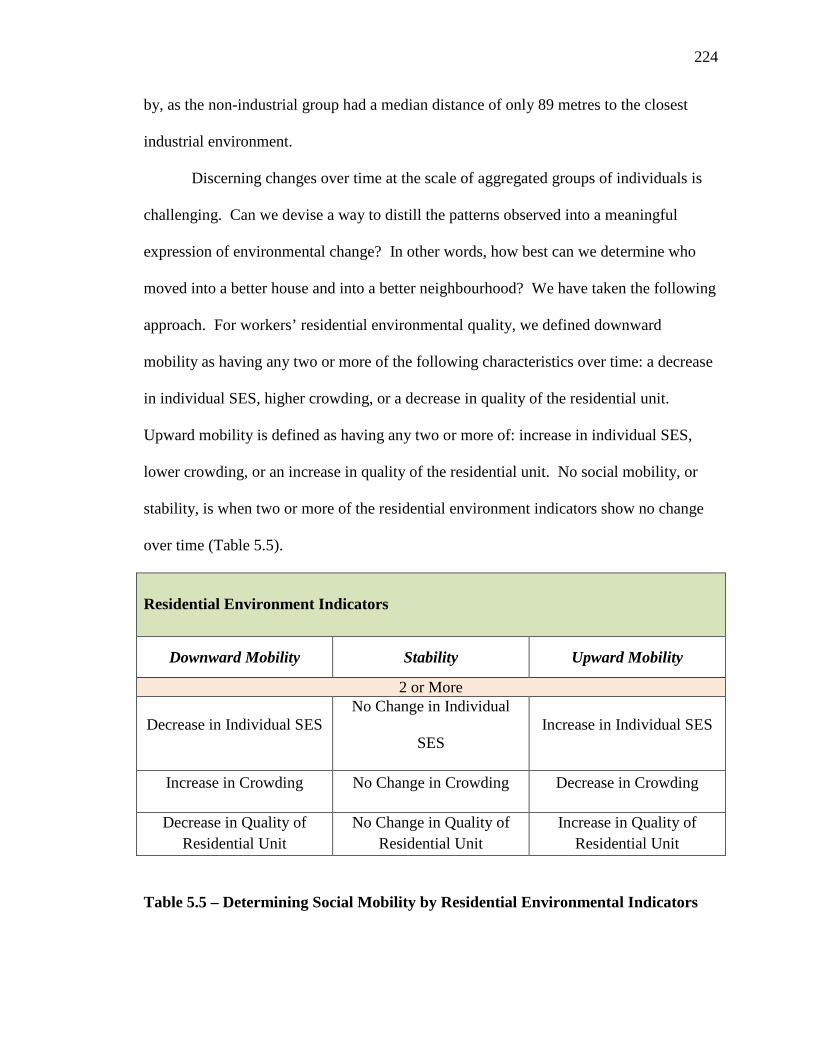
224

by, as the non-industrial group had a median distance of only 89 metres to the closest

industrial environment.

Discerning changes over time at the scale of aggregated groups of individuals is

challenging. Can we devise a way to distill the patterns observed into a meaningful

expression of environmental change? In other words, how best can we determine who

moved into a better house and into a better neighbourhood? We have taken the following

approach. For workers’ residential environmental quality, we defined downward

mobility as having any two or more of the following characteristics over time: a decrease

in individual SES, higher crowding, or a decrease in quality of the residential unit.

Upward mobility is defined as having any two or more of: increase in individual SES,

lower crowding, or an increase in quality of the residential unit. No social mobility, or

stability, is when two or more of the residential environment indicators show no change

over time (Table 5.5).

Residential Environment Indicators

Downward Mobility Stability Upward Mobility

2 or More

Decrease in Individual SES No Change in Individual

SES Increase in Individual SES

Increase in Crowding No Change in Crowding Decrease in Crowding

Decrease in Quality of Residential Unit

No Change in Quality of Residential Unit

Increase in Quality of Residential Unit

Table 5.5 – Determining Social Mobility by Residential Environmental Indicators

225

We apply a similar approach to determining whether a worker moved into a better

neighbourhood over time. Movement into a better neighbourhood is used as a proxy for

upward social mobility, and vice versa for decreases in neighbourhood quality. We see

downward mobility as having two or more of the following characteristics over time: a

decrease in neighbourhood SES, an increase in population density, or an increase in

proximity to or intensity of industrial environments. Upward mobility is the opposite,

having two or more positive characteristics: an increase in neighbourhood SES, a

decrease in population density, or a decrease in industrial exposure. Like residential

indicators, stability is when two or more of the indicators show no change over time

(Table 5.6).

Neighbourhood Environment Indicators

Downward Mobility Stability Upward Mobility

2 or More Decrease in Neighbourhood

SES No Change in

Neighbourhood SES Increase in Neighbourhood

SES Increase in Population

Density No Change in Population

Density Decrease in Population

Density Increase in Proximity to or

Intensity of Industrial Environments

No Change in Proximity to or Intensity of Industrial

Environments

Decrease in Proximity to or Intensity of Industrial

Environments Table 5.6 – Determining Social Mobility by Neighbourhood Environmental Indicators 5.6.1 Residential Environments, Social Mobility, and the Journey to Work

Did workers move to better their residential environments over the course of the

1880s? Our results, summarized in Table 5.7, indicate overwhelmingly that workers saw

226

stability in the quality of their residential environments: 74% of workers had stable

environments, with 26.5% of all workers showing stability across all three residential

environment indicators. We expected to see stability at the higher occupational classes,

but the stability at the lower classes is surprising. This perhaps reflects a housing market

that segregated lower class workers, restricting them to similar housing qualities and

sizes, or perhaps was due to lack of housing choice because of low inventory or inflated

costs.

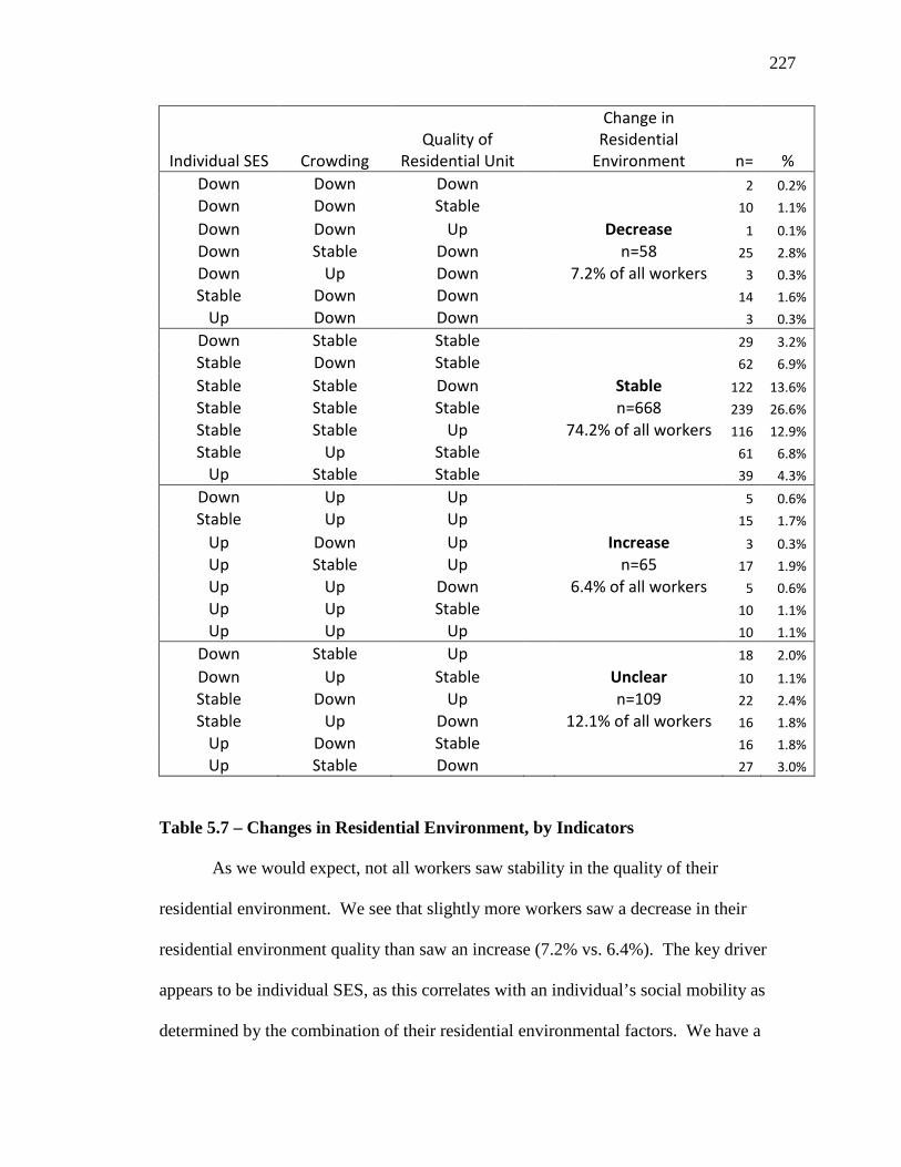
227

Individual SES Crowding Quality of

Residential Unit

Change in Residential

Environment n= % Down Down Down

2 0.2%

Down Down Stable

10 1.1% Down Down Up

Decrease 1 0.1%

Down Stable Down

n=58 25 2.8% Down Up Down

7.2% of all workers 3 0.3%

Stable Down Down

14 1.6% Up Down Down

3 0.3%

Down Stable Stable 29 3.2% Stable Down Stable

62 6.9%

Stable Stable Down

Stable 122 13.6% Stable Stable Stable

n=668 239 26.6%

Stable Stable Up

74.2% of all workers 116 12.9% Stable Up Stable

61 6.8%

Up Stable Stable

39 4.3% Down Up Up 5 0.6% Stable Up Up

15 1.7%

Up Down Up

Increase 3 0.3% Up Stable Up

n=65 17 1.9%

Up Up Down

6.4% of all workers 5 0.6% Up Up Stable

10 1.1%

Up Up Up

10 1.1% Down Stable Up 18 2.0% Down Up Stable

Unclear 10 1.1%

Stable Down Up

n=109 22 2.4% Stable Up Down

12.1% of all workers 16 1.8%

Up Down Stable

16 1.8% Up Stable Down 27 3.0%

Table 5.7 – Changes in Residential Environment, by Indicators

As we would expect, not all workers saw stability in the quality of their

residential environment. We see that slightly more workers saw a decrease in their

residential environment quality than saw an increase (7.2% vs. 6.4%). The key driver

appears to be individual SES, as this correlates with an individual’s social mobility as

determined by the combination of their residential environmental factors. We have a

228

modest-sized cohort of workers for whom the direction of social mobility as related to

changes in their residential environment is unclear. More than a third show an increase in

individual SES, yet did not move to increase another attribute of their residential

environment.

Although we do not see a major change in most workers’ residential environments

over time, a necessary repercussion of residential mobility is a change in the journey to

work. Did the desire to be socially mobile, as measured through our proxies of

residential environment indicators, result in lengthened daily commutes? Did those who

decreased the quality of their environment do so to overcome a long journey to work?

Table 5.8 outlines the relationship between social mobility and the journey to work. We

uncovered that a majority of those workers who were upwardly socially mobile also

increased their journey to work over time. More noteworthy is the percentage of distance

by which the journeys increased; this group of workers increased their daily commute, on

average, 188% over their 1881 distances. Lengthening journeys to work also appear to

have been a repercussion for many of the workers who remained socially stable.

Considerably more of these workers had longer commutes in 1891 than they did in 1881,

and the increase in the distance travelled was not modest, at nearly 50%. Consider that

another 9% of workers shifted their employment from home-based to outside-the-home,

resulting in an average journey of over 800 metres. The desire to maintain financial

stability may have pushed these workers to look for wage employment.

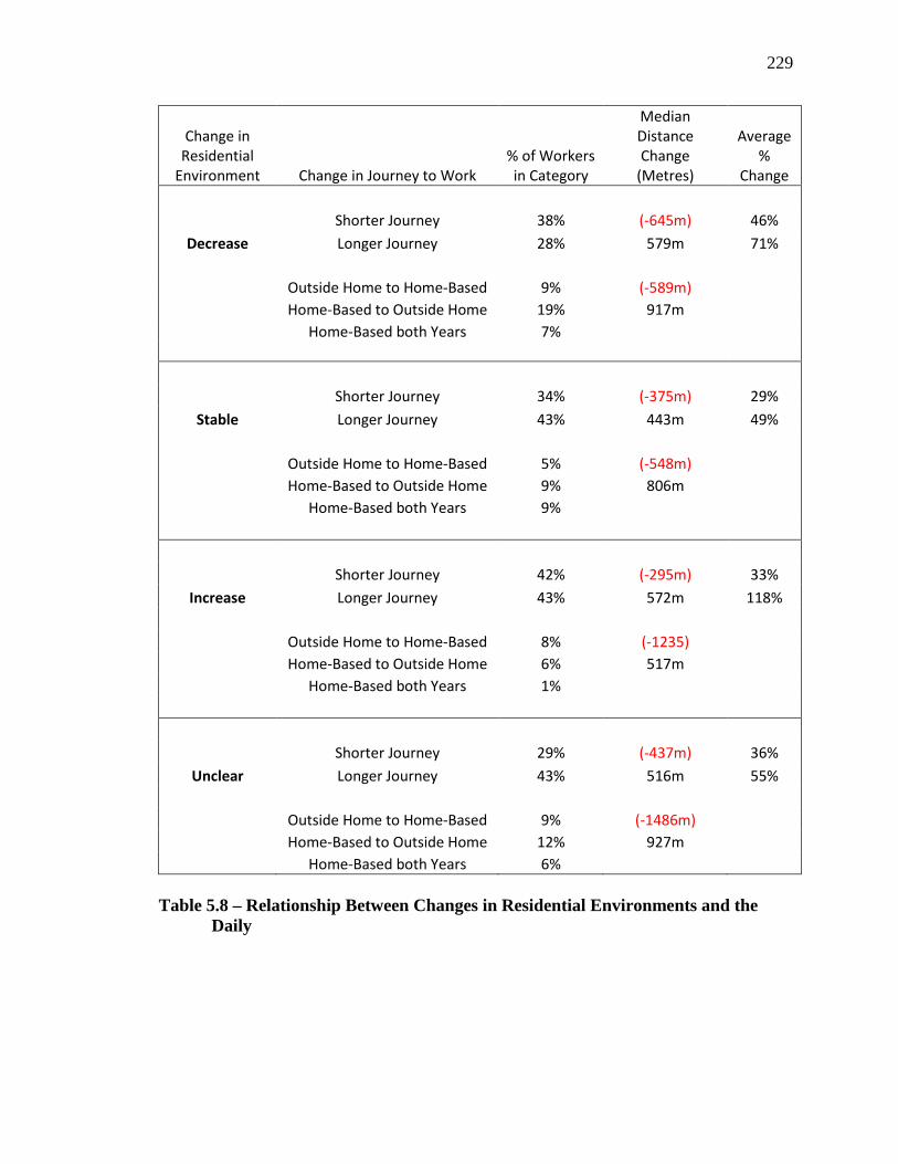
229

Change in Residential

Environment Change in Journey to Work % of Workers in Category

Median Distance Change

(Metres)

Average %

Change

Shorter Journey 38% (-645m) 46% Decrease Longer Journey 28% 579m 71%

Outside Home to Home-Based 9% (-589m) Home-Based to Outside Home 19% 917m Home-Based both Years 7%

Shorter Journey 34% (-375m) 29%

Stable Longer Journey 43% 443m 49%

Outside Home to Home-Based 5% (-548m) Home-Based to Outside Home 9% 806m Home-Based both Years 9%

Shorter Journey 42% (-295m) 33%

Increase Longer Journey 43% 572m 118%

Outside Home to Home-Based 8% (-1235) Home-Based to Outside Home 6% 517m Home-Based both Years 1%

Shorter Journey 29% (-437m) 36% Unclear Longer Journey 43% 516m 55%

Outside Home to Home-Based 9% (-1486m) Home-Based to Outside Home 12% 927m

Home-Based both Years 6% Table 5.8 – Relationship Between Changes in Residential Environments and the Daily

230

5.6.2 Neighbourhood Environments, Social Mobility, and the Journey to Work

Workers in late nineteenth-century London overwhelmingly maintained similar

residential environments over the decade between 1881 and 1891. Although we see little

change in their residences, did they manage to improve their neighbourhood

environments? Our results, summarized in Table 5.9, indicate that workers had quite a

variety of experiences. Rather than a large group that saw stability, we find nearly equal

numbers of those who increased and decreased their neighbourhood environmental

quality. For decreases in neighbourhood-experienced social mobility, it appears that

population density is the key driver. This falls in line with literature that outlines how

increases in density are generally associated with lower property values, leading to

inhabitation by lower social classes and encouraging development by factory owners and

small merchants. Interestingly, the largest contributors to the cohort of workers who

experienced increases in neighbourhood quality are those workers who saw an

improvement in population density and distance from industrial environments, yet a

decrease in neighbourhood SES. A view of their spatial distribution (Figure 5.19)

suggests that most moved from areas with an intensity of industrial use, mostly in the

downtown core, out to suburban retreats. A large number of this group moved to the

western suburb of Petersville, a neighbourhood of small homes occupied primarily by the

working classes. Petersville (aka London West) suffered a devastating flood in 1883

which displaced approximately fifty households, especially from the southern portion of

the community where we see many of this cohort moving to by 1891 (Novak & Gilliland,

2009). These workers made a choice to improve their environments, escaping the filth of

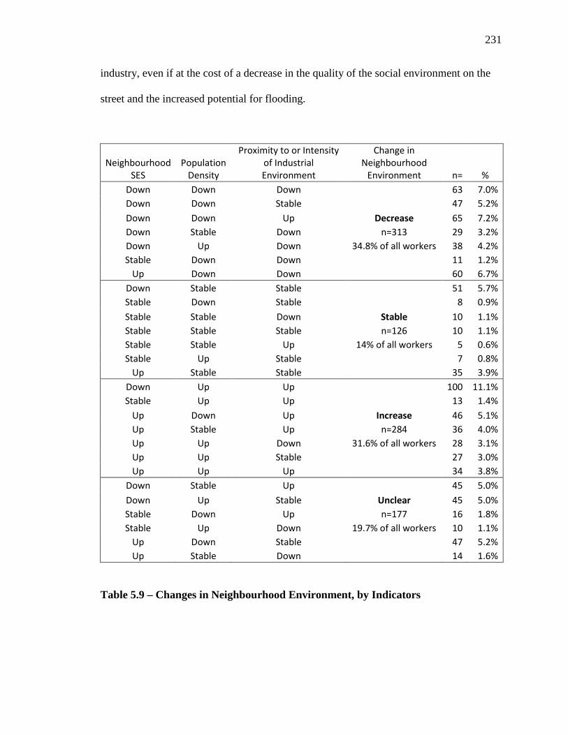
231

industry, even if at the cost of a decrease in the quality of the social environment on the

street and the increased potential for flooding.

Neighbourhood SES

Population Density

Proximity to or Intensity of Industrial Environment

Change in Neighbourhood

Environment n= % Down Down Down

63 7.0%

Down Down Stable

47 5.2% Down Down Up Decrease 65 7.2% Down Stable Down n=313 29 3.2% Down Up Down 34.8% of all workers 38 4.2% Stable Down Down

11 1.2%

Up Down Down

60 6.7% Down Stable Stable 51 5.7% Stable Down Stable

8 0.9%

Stable Stable Down Stable 10 1.1% Stable Stable Stable n=126 10 1.1% Stable Stable Up 14% of all workers 5 0.6% Stable Up Stable

7 0.8%

Up Stable Stable

35 3.9% Down Up Up 100 11.1% Stable Up Up

13 1.4%

Up Down Up Increase 46 5.1% Up Stable Up n=284 36 4.0% Up Up Down 31.6% of all workers 28 3.1% Up Up Stable

27 3.0%

Up Up Up

34 3.8% Down Stable Up 45 5.0% Down Up Stable Unclear 45 5.0% Stable Down Up n=177 16 1.8% Stable Up Down 19.7% of all workers 10 1.1%

Up Down Stable

47 5.2% Up Stable Down 14 1.6%

Table 5.9 – Changes in Neighbourhood Environment, by Indicators

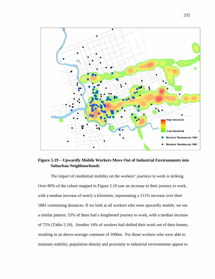
232

Figure 5.19 – Upwardly Mobile Workers Move Out of Industrial Environments into Suburban Neighbourhoods

The impact of residential mobility on the workers’ journeys to work is striking.

Over 80% of the cohort mapped in Figure 5.19 saw an increase in their journey to work,

with a median increase of nearly a kilometre, representing a 111% increase over their

1881 commuting distances. If we look at all workers who were upwardly mobile, we see

a similar pattern: 53% of them had a lengthened journey to work, with a median increase

of 72% (Table 5.10). Another 14% of workers had shifted their work out of their homes,

resulting in an above-average commute of 1006m. For those workers who were able to

maintain stability, population density and proximity to industrial environments appear to

233

trump neighbourhood SES, and their journey to work response supports this pattern. We

see very little change in the journey to work in this group, with equal distributions of

workers having an increase and decrease in their commutes over time. The rate of

change is low as well, with increases limited to 25% and decreases of only 12%. This

suggests that there was a level of contentment with the neighbourhood environment by

this group of workers.

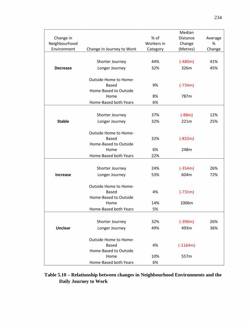
234

Change in Neighbourhood

Environment Change in Journey to Work

% of Workers in Category

Median Distance Change

(Metres)

Average %

Change

Shorter Journey 44% (-480m) 41% Decrease Longer Journey 32% 326m 45%

Outside Home to Home-

Based 9% (-734m)

Home-Based to Outside

Home 8% 787m Home-Based both Years 6%

Shorter Journey 37% (-88m) 12%

Stable Longer Journey 32% 221m 25%

Outside Home to Home-

Based 32% (-832m)

Home-Based to Outside

Home 6% 248m Home-Based both Years 22%

Shorter Journey 24% (-354m) 26%

Increase Longer Journey 53% 604m 72%

Outside Home to Home-

Based 4% (-731m)

Home-Based to Outside

Home 14% 1006m Home-Based both Years 5%

Shorter Journey 32% (-390m) 26%

Unclear Longer Journey 49% 493m 36%

Outside Home to Home-

Based 4% (-1164m)

Home-Based to Outside

Home 10% 557m Home-Based both Years 6%

Table 5.10 – Relationship between changes in Neighbourhood Environments and the Daily Journey to Work

235

Looking broadly at both the changes in residential and neighbourhood

environments of our sample of workers, it is clear that individuals were increasing their

daily journey to work in order to attempt to increase their social mobility. What about Ira

Collins and Amelia Miller? Did they manage to improve their environments? We saw

that Ira had a substantial increase in the distance of his journey to work of over 50%,

moving from London East to a neighbourhood south-east of downtown which is today

called SoHo (short for South of Horton). We see that he maintained stability in his

residential environment, with stability in individual SES and measures of crowding. He

did have a decrease in the quality of the construction of his home, moving from a brick

home in London East to a similar-sized wood frame house on Clarence. Overall, we see

a decrease in his neighbourhood environment, with a lower neighbourhood SES score

and higher population densities than when he was living in London East. However, his

proximity to industrial uses improved significantly considerably shifting 2.5 values in the

normalized proximity to industry scale. Looking closer, Ira moved from being less than

300 metres from Canada Chemical Manufacturing and less than 200 from Bennett’s large

furniture factory to over 350m to the closest industrial use. Instead, across the street was

one of the city’s new elementary schools Was the proximity to the school for his young

son Russell an impetus for his move? Were Ira and his wife Mary Jane seeking a

healthier built environment overall for the family to live in? Or was the move initiated

for other personal reasons, such as a job loss, eviction, or desire to live closer to

relatives? We know that Ira changed jobs and occupations, moving from his work as a

saddle maker at Globe Agricultural Works to a yard man with the Grand Trunk Railroad,

236

but without more information it is impossible to decipher the underlying motivation for

Ira’s moves.

Amelia Miller, the grade 7 teacher, did not change her workplace over the decade

between 1881 and 1891, but she did make a substantial change in her residential

situation. This change, however, did not impact her residential environment as much as

we might expect. We see stability in her environmental indicators, with no change in

individual SES (though we do know her wages increased over the period) or the quality

of the residential building material. Where we do see an important decrease in is the

crowding measure. Looking at her situation more closely, we see that although the

number in the people in the household doubled from four to eight, the size of the

dwelling increased substantially from a one-story 688 sq. foot bungalow to a very large

3200 sq. foot two-story house. The effective increase is a doubling of living space per

person, which certainly would have improved her quality of life at home. Amelia’s

change in neighbourhood environment shows a significant increase in neighbourhood

SES, confirming our earlier suggestion that she may have sought a neighbourhood that

better represented her social class as a white-collar worker. We do see a decrease in the

neighbourhood population density and proximity to industrial uses, as Amelia’s new

residence is located near John Carling’s large brewing operations, she would have

smelled the foul odors and heard the noise of horse carts that emanated from the brewery

on a daily basis.

Ira’s and Amelia’s experiences highlight the complexities involved in balancing

residential needs, neighbourhood environments, and the journey to work. Ira improved

the quality of his neighbourhood built environment at the expense of a significant

237

increase in his daily journey to work. Amelia was able to improve the quality of her

social neighbourhood and her personal living space while drastically decreasing her

journey to work, but to do so she had to move to a more noxious industrial environment.

Although complex, our re-creation of historical environments has allowed us to examine

the extent of individuals’ social mobility in a unique way, moving beyond just the

abstract differences of changes in occupation. This environmental approach to social

mobility provides a more nuanced understanding of how social mobility, reflected by

one’s environment, shaped the experience of daily life in the nineteenth-century city.

5.7 CONCLUSION

This paper has taken on an ambitious task, to complete a longitudinal study of a

population, their workplaces, and environments. First, we extended the historical record

linkage literature by developing a protocol that record-links geocoded samples of workers

with high precision across time using public databases of decennial census records.

These record linkages allowed us to follow the same workers as they changed residences

and workplaces, permitting us to complete the first known study of the journey to work

over an extended period of time with the same population. We established the extent of

residential, occupational, and workplace mobilities for over 1200 workers with a high

degree of spatial precision. We continued by creating a methodology for examining

historical environments at multiple spatial scales, from the individual’s home residential

environment, to the larger social and built environment characteristics of their

surrounding neighbourhood. This methodology moves beyond the arbitrary areal unit to

include a personalized approach to conceptualizing neighbourhoods. Recognizing that

238

‘neighbourhood’ is unique to each individual, we devised a way to create a

neighbourhood for each person in the city. Each person was placed as the centroid in his

or her own neighborhood, which emanated out like the view they would have seen as

they looked up and down the street from their front porch. Finally, we combined these

approaches to create a new conception of social mobility in the nineteenth-century city,

one based not only on changes in an individual’s occupation, but also on the quality of

the environments in which they spend their everyday lives.

It must be acknowledged that there are limitations to the methodologies and

assumptions we present here. Baker reminds us that all inferences made in historical

geography ‘whether drawn directly from empirical evidence or indirectly from theory, are

probabilistic statements’, a warning that surely applies to the work we present here (1991,

226). Our study is fundamentally based on two time slices that follow the decennial

census, 1881 and 1891. We know that many individuals would have changed their

residence and/or workplace, and thus their environments, more than once during the

course of this decade. With the methodologies and environmental stages in place, we

hope to revisit this study in the future to see it is possible to follow individuals every

calendar year. This would provide a more fine-grained understanding of life histories and

the frequency of change. For our treatment of environmental reflections of social

mobility, we were limited by the source material for determining the quality of the

residential environment. Ideally, information on the cost or rents of residential units

would have provided an additional factor to contribute to a more comprehensive view of

changes in residential quality.

239

Regardless of these opportunities for further development, what we have shown in

this study is that the relationship between home and work is complex. Individuals were

frequently changing their residential situations, trying to improve their residential and

neighbourhood environments while reducing or limiting the increase of their daily

commute. In 1880s London, Ontario, we find that many individuals did significantly

improve their residential and neighbourhood environments, but did so at the expense of a

longer commute each day. It was a fine balancing act, not different from that which

many of us face today. Although we often think of the past as a simpler time, we know

that life was not so simple, at least for the decisions on where our ancestors lived and

worked.

5.8 REFERENCES

Antonie, L., Baskerville, P., Inwood, K., & Ross, A. (2010). An Automated Record

Linkage System: Linking 1871 Canadian Census to 1881 Canadian Census. Paper

Presented at Longitudinal Analysis, Historical Sources, and Generational Change

Conference, Historical Data Research Unit, University of Guelph.

Baker, A. (1991). The Limits of Inference in Historical Geography. In D. B. Green (Ed.),

Historical Geography: A methodological protrayal (pp. 219-230). Savage, MD:

Rowman & Littlefield Publishers.

Board of Education for the City of London, 1891. Annual Report for the London Board of

Education. (M315-316). Western Archives and Research Collections Centre,

London, Ontario

240

Borchert, J. (1981). Urban Neighborhood and Community: Informal Group Life, 1850-

1970. Journal of Interdisciplinary History, 11(4), 607-631.

Bradbury, B., & Myers, T. (2005). Introduction. In B. Bradbury, & T. Myers (Eds.),

Negotiating Identities in Nineteenth- and Twentieth-Century Montreal (pp. 1-24).

Vancouver: UBC Press.

Brown, H. (1975). Changes in Workplace and Residential Location. Journal of the

American Institute of Planners, 41(1), 32-39.

Canadian Institute of Planners. (2012). Great Places in Canada. Retrieved 07 30, 2014,

from http://greatplacesincanada.ca

Carter, S., & Savoca, E. (1990). Labor Mobility and Lengthy Jobs in Nineteenth-Century

America. Journal of Economic History, 50(1), 1-16.

Choko, M., & Harris, R. (1990). The Local Culture of Property: A Comparative History

of Housing Tenure in Montreal and Toronto. Annals of the Association of

American Geographers, 80(1), 73-95.

Clapp, J., & Wang, Y. (2006). Defining neigborhood boundaries: Are census tracts

obsolete? Journal of Urban Economics, 59, 259-284.

Clark, W., & Huang, Y. (2003). The life course and residential mobility in British

housing markets. Environment and Planning A, 35(2), 323-339.

Clark, W., & Onaka, J. (1983). Life Cycle and Housing Adjustment as Explanations of

Residential Mobility. Urban Studies, 20, 47-57.

Crowley, S. (2003). The Affordable Housing Crisis: Residential Mobility of Poor

Families. The Journal of Negro Education, 72(1), 22-38.

241

Curti, M. (1959). The Making of an American Community: A Case Study of Democracy

in a Frontier County. Redwood City: Stanford University Press.

Curtis, B. (2001). The Politics of Population: State Formation, Statistics, and the Census

of Canada, 1840-1875. Toronto: University of Toronto Press.

Darroch, G. (2002). Semi-Automated Record Linkage with Suname Samples: A regional

study of 'case law' linkage, Ontario 1861-1871. History and Computing, 14(1 &

2), 153-183.

Darroch, G., & Ornstein, M. (1980). Ethnicity and Occupational Structure in Canada in

1871: The Vertical Mosaic in Historical Perspective. Canadian Historical Review,

61(3), 305-333.

Dieleman, F. (2001). Modelling Residential Mobility: a Review of Recent Trends in

Research. Journal of Housing and the Built Environment, 16, 249-265.

Dillon, L. (2000). International Partners, Local Volunteers, and Lots of Data: The 1881

Canadian Census Project. International Journal of Humanities and Arts

Computing, 12(2), 163-176.

Dillon, L. (2002). Challenges and Opportunities for Census Record Linkage in the French

and English Canadian Context. History and Computing, 14(1-2), 185-212.

Dunae, P. (1998). Making the 1891 Census of British Columbia. Histoire sociale / Social

History, 31(62), 223-239.

Dunae, P., Lafreniere, D., Gilliland, J., & Lutz, J. (2013). Dwelling Places, Social Spaces:

Revealing the Environments of Urban Workers in Victoria using Historical GIS.

Labour/Le Travail, 72, 37-73.

242

Elmagarmid, A., Ipeirotis, P., & Verykios, V. (2007). Duplicate Record Detection: A

Survey. IEEE Transactions on Knowledge and Data Engineering, 19(1), 1-16.

Feijten, P., Hooimeijer, P., & Mulder, C. (2008). Residential Experience and Residential

Environment Choice over the Life-course. Urban Studies, 45(1), 141-162.

Gilliland, J. (1998). Modeling Residential Mobility in Montreal, 1860-1900. Historical

Methods, 31(1), 27-42.

Gilliland, J., & Olson, S. (1998). Claims on housing space in nineteenth-century

Montreal. Urban History Review / Revue d’histoire urbaine, 26(2), 3-16.

Goeken, R., Huynh, L., Lynch, T. A., & Vick, R. (2011). New Methods of Census

Record Linking. Historical Methods, 44(1), 7-14.

Green, D. R. (1988). Distance to work in Victorian London: A case study of Henry Poole,

bespoke tailors. Business History, 30(2), 179-194.

Hamilton, M., & Inwood, K. (2011). The Aboriginal Population and the 1891 Census of

Canada. In P. Axelsson, & P. Skold (Eds.), Indigenous Peoples and Demography:

The complex relation between identity and statistics (pp. 95-115). New York:

Berghahn.

Harris, R., Levine, G., & Osborne, B. (1981). Housing Tenure and Social Classes in

Kingston Ontario 1881-1901. Journal of Historical Geography, 7(3), 271-289.

Hautaniemi, S., Anderton, D., & Swedlund, A. (2000). Methods and Validity of a Panel

Study Using Record Linkage. Historical Methods, 33(1), 16-29.

Hershberg, T. (Ed.). (1981). Philadelphia: Work, space, family and group experience in

the nineteenth century. New York: Oxford University Press.

243

Hershberg, T., Burnstein, A., & Dockhorn, R. (1976). Record Linkage. Historical

Methods Newsletter, 9(2 & 3), 137-163.

Hillery, G. (1955). Definitions of Community: Areas of Agreement. Rural Sociological

Society, 20(2), 111-123.

Hoskins, R. (1989). An Analysis of the Payrolls of the Point St.Charles Shops of the

Grand Trunk Railway. Cahiers de géographie du Québec, 33(90), 323-344.

Hulchanski, J. D. (1982). The Evolution of Ontario's Early Urban Land Use Planning

Regulations, 1900-1920. Research Paper no. 136. Canadian-American

Comparative Urban History Conference (pp. 1-37). Guelph: Centre for Urban &

Community Studies, University of Toronto.

Jacoby, S. (1985). Employing Bureaucracy: Managers, Unions, and the Transformation

of Work in American Industry. New York: Columbia University Press.

Jacoby, S., & Sharma, S. (1992). Employment Duration and Industrial Labor Mobility in

the United States 1880-1980. Journal of Economic History, 52(1), 161-179.

Katz, M. (1975). The People of Hamilton, Canada West: Family and Class in a Mid-

Nineteenth-Century City. Cambridge: Harvard University Press.

Knights, P. (1971). Accuracy of Age Reporting In The Manuscript Federal Censuses of

1850 and 1860. Historical Methods Newsletter, 4(3), 79-83.

Kronenberg, K., & Carree, M. (2012). On the Move: Determinants of Job and Residential

Mobility in Different Sectors. Urban Studies, 49(16), 3679-3698.

Lafreniere, D., & Gilliland, J. (2014). “All the World’s a Stage”: A GIS Framework for

Recreating Personal Time-Space from Qualitative and Quantitative Sources.

Transactions in GIS. doi:10.1111/tgis.12089

244

Lafreniere, D., & Gilliland, J. (Forthcoming). Revisiting the Walking City: A Geospatial

Examination of the Journey to Work. The Canadian Geographer.

LinkageWiz. (2011). LinkageWiz Data Matching Software. Retrieved from

www.linkagewiz.net

Loebach, J., & Gilliland, J. (2010). Child-Led Tours to Uncover Children's Perceptions

and Use of Neighborhood Environments. Children, Youth and Environments,

20(1), 52-90.

Mason, K., & Cope, L. (1987). Sources of Age and Date-of-Birth Misreporting in the

1900 U.S. Census. Demography, 24(4), 563-573.

Mayol, P. (1998). The Neighborhood. In M. de Certeau, L. Giard, & P. Mayol (Eds.), The

Practice of Everyday Life: Volume 2: Living and Cooking (T. Tomasik, Trans.,

pp. 7-14). Minneapolis, MN: University of Minnesota Press.

Mok, D. (2007). Do Two-earner Households Base Their Choice of Residential Location

on Both Incomes? Urban Studies, 44(4), 723-750.

Mulder, C. (2007). The family context and residential choice: A challenge for new

research. Population, Space and Place, 13(4), 265-278.

Mulder, C., & Hooimeijer, P. (1999). Residential Relcations in the Life Course. In L. van

Wissen, & P. Dykstra (Eds.). New York: Kluwer Academic.

Novak, M., & Gilliland, J. (2009) ’Buried Beneath the Waves’: Using GIS to Examine

the Physical and Social Impact of a Historical Flood.” Digital Studies, 1(2).

Olson, S., & Thornton, P. (2011). Peopling the North American City: Montreal 1840-

1900. Montreal: McGill-Queens University Press.

245

Pooley, C. (1979). Residential Mobility in the Victorian City. Transactions of the

Institute of British Geographers, 4(2), 258-277.

Pooley, C. G., & Turnbull, J. (1997). Changing home and workplace in Victorian

London: the life of Henry Jaques, shirtmaker. Urban History, 24(2), 148-178.

Porteous, J. D. (1977). Environment & Behavior: Planning and Everyday Urban Life.

Reading, MA: Addison-Wesley Publishing.

Prillwitz, J., Harms, S., & Lanzendorf, M. (2007). Interactions Between Residential

Relocations, Life Course Events, and Daily Commute Distances. Transportation

Research Record: Journal of the Transportation Research Board(2021), 64-69.

Ruggles, S. (2002). Linking Historical Censuses: A New Approach. History and

Computing, 14(1-2), 213-224.

Sirgy, M., & Cornwell, T. (2002). How Neighborhood Features Affect Quality of Life.

Social Indicators Research, 59, 79-114.

Steckel, R. (1991). The Quality of Census Data for Historical Inquiry: A Research

Agenda. Social Science History, 15(4), 579-599.

Thernstrom, S. (1964). Poverty and Progress: Social Mobility in a Nineteenth Century

City. Cambridge: Harvard University Press.

Ulrich, L. (1990). A Midwife's Tale: The Life of Martha Ballard, Based on Her Diary,

1785-1812. New York: Knopf.

Winchester, I. (1992). What Every Historian Needs to Know About Record Linkage for

the Microcomputer Era. Historical Methods, 25(4), 149-165.

Wood, C. (2002). Why postal code level data is better. The Canadian Appraiser, 46(2),

34-36.

246

Zax, J., & Kain, J. (1991). Commutes, quits and moves. Journal of Urban Economics, 29,

153-165.

247

CHAPTER SIX

Conclusion

6.1 SUMMARY

Lowenthal (1985) reminds us that ‘the past is a foreign country’. This dissertation

has set forth to serve as the introductory chapter preamble for its travel guide. When I

started down the long path of research that is a doctoral dissertation, I was inspired by

several writers and thinkers of the early discipline of historical GIS. Among them, Anne

Kelly Knowles asserted that ‘people love new tools that enable them to do what they

have dreamed of doing” (Knowles 2000, 451). What was lacking, however, was a

guidebook by which the student of this emerging discipline could use to learn these new

tools and apply them broadly to interests in our urban past. Thus emerged the broad aim

of this dissertation: to establish a comprehensive geospatial research framework for the

study of past populations and their environments. The framework and its complementary

techniques were used to fulfill this dissertation’s empirical aim: to advance our

understanding of the social spaces in both the diurnal and nocturnal nineteenth-century

city by reconstructing the daily movements of individuals to and from work or school.

These two aims merge and are addressed in this integrated format dissertation as three

independent studies.

The first study, presented here as chapter three, outlined the creation of the

foundational layers of the historical GIS and presented a methodological framework for

the study of the daily-space time patterns of individuals in our past cities. This study also

outlined an approach to integrating qualitative sources into a GIS, an area of research that

has only recently begun to find its way into historical studies. The foundational layers,

248

referred to as environmental stages, provide not only the means to rapidly place

seemingly aspatial historical sources in a geospatial environment, but they also provide

the important contextual information about the world in which the people represented in

the sources were living. To illustrate, this study uses the attendance records of three

elementary schools to recreate the likely journey to school for 699 students in 1881. The

integration of the attendance registers with the built and social environment stages

permitted an interrogation of relationship between social class and industrial exposure

during the daily walk to school. The integration and contextualization of qualitative

sources, such as the personal diary of Richard Matthews used in this study, highlights

how this stage-based approach to historical GIS allows scholars to do more than place

historical data on a map, but to move toward the creation of complex spatial stories of

everyday life. The culmination is the 3D representation of Matthews’ daily journey to

work, highlighting the varied social and built environments he would have experienced

and interacted with on a daily basis. This study will be of particular interest to

historically-minded scholars who are just beginning to integrate GIS into their research

programs and to humanities scholars who are looking to interrogate the spatial qualities

of their qualitative sources.

The second study, presented here as chapter four, outlined a new methodological

framework for recreating the historical spatial relationships between work and home.

This methodology was applied to a sample of over 5000 individuals to empirically review

their daily journey to work. This study revisited the existing scholarship on the

nineteenth-century journey to work and outlined how the stage-based geospatial research

framework discussed in chapter three can be used to overcome a number of the

249

methodological challenges that plagued previous studies. These challenges include a

reliance on small, atypical samples of workers, approximations of the spatial relationship

between home and work, and unrealistic interpretations of journeys travelled by

employing only Euclidean paths. Probabilistic record matching techniques were outlined

to illustrate how to create larger, more demographically and spatially representative

samples of the working age population, as well as to establish absolute spatial links

between their homes and their workplaces. A network-derived journey to work model

was developed that recreated more realistic journeys that consider the many natural and

built environment barriers that influenced the paths and distances travelled. Case studies

of brewery and cigar factory workers illustrate the improvements the models offer to

previous journey to work methodologies. The study concludes by presenting empirical

results of the journey to work in London in 1881 along lines of occupational class,

coincident home-work location, and gender. The results indicate that the highest

occupational classes lived closer to their workplaces than any other group and labourers

lived the furthest, which departs from the findings in other studies. Coincident home-

work locations of workers in London were compared to studies in Philadelphia and

Milwaukee, with results highlighting that differences in the size and location of industries

influenced which occupations were performed from home and which were carried out as

wage labour. Finally, women’s experience of work was reviewed and the dominance of

domestic labour that fills the pages of other studies also held true in London. A cohort of

dressmakers who worked outside of the home remind us of the importance of women’s

wages to the total household income.

250

The third study, presented here as chapter five, combines the methodologies and

results from the previous two chapters to present an approach to studying the relationship

between residence, workplace, and environment. The study begins by outlining and

applying a methodology for record linking populations longitudinally across decennial

censuses and city directories and is used to create a sample of workers that we can follow

across time. The result is the first journey to work study that evaluates the same

population over an extended period of time. This worker sample is followed across the

decade to evaluate the changes in the quality of both their residential and neighbourhood

environments. The change in environments is used as a measure of social mobility and is

compared to their change in journey to work. To facilitate analysis, six environmental

indicators were created to evaluate changes in the characteristics of workers’ residential

and neighbourhood environments. Empirical results highlight that the relationship

between residential needs, neighbourhood environments, and the journey to work is

complex. What is clear is that individuals who were able to be upwardly socially mobile

and improve their overall environment did so at the expense of substantial increases in

their journey to work.

The approaches and case studies found within these three studies represent a

melding of four distinct disciplines from across the social sciences (Figure 6.1). At the

surface, this work would be identified as scholarship in the discipline of historical

geography, though it is far from representative of recent or traditional historical

geographical scholarship. This dissertation instead treats the study of historical

populations and environments through a truly interdisciplinary lens. Methodological,

theoretical, and empirical contributions are made to urban and time-space geographies,

251

such as the treatment and consideration of built environments and their influence on

pedestrian paths and the influence of industrial landscapes on residential mobility.

Contributions are made to social history by presenting, arguably for the first time, the

whole of a past population in their individual residences and neighbourhoods, allowing us

to see patterns and processes in a new way. Some social historians will appreciate the

methods and case studies for utilizing archival sources already familiar to them, such as

diaries and school records, to reveal social interactions between large numbers of

individuals. Historical demography and the emerging discipline of spatial demography

benefit from advances in record linkage techniques, especially utilizing the spatial

characteristics that have been difficult to fully appreciate until now. Demographers will

also benefit from methodologies that outline how to spatialize the Canadian census,

providing opportunities to revisit their classic interests in household structure, fertility,

mortality, marriage, and kinship through a spatial lens. Finally, but most significantly, is

the contribution these studies have made to the field of GIS, specifically historical GIS.

Contributions are made to qualitative GIS, highlighting not only a technique for

geocoding, but how to integrate and contextualize qualitative sources with traditional

quantitative ones. Various methods and models are contributed to historical GIS, such as

3D GIS modelling of historical landscapes and a person-based viewshed buffer for

modelling historic conceptions of neighbourhood. Finally, these studies have illustrated

that historical GIS can move beyond the ‘point on the map’ or visualization of history

that is still so common in historical GIS studies. Instead, they encourage scholars to

more fully utilize the analytical capabilities that make GIS such a promising tool. I hope

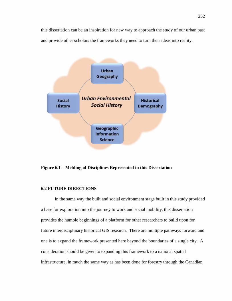
252

this dissertation can be an inspiration for new way to approach the study of our urban past

and provide other scholars the frameworks they need to turn their ideas into reality.

Figure 6.1 – Melding of Disciplines Represented in this Dissertation

6.2 FUTURE DIRECTIONS

In the same way the built and social environment stage built in this study provided

a base for exploration into the journey to work and social mobility, this dissertation

provides the humble beginnings of a platform for other researchers to build upon for

future interdisciplinary historical GIS research. There are multiple pathways forward and

one is to expand the framework presented here beyond the boundaries of a single city. A

consideration should be given to expanding this framework to a national spatial

infrastructure, in much the same way as has been done for forestry through the Canadian

253

National Forest Information System or water management with RésEau, the Canadian

Water Information Network. This may start by digitizing and geo-enabling the

comprehensive Historical Atlas of Canada, or partnering with the Canadian Century

Research Infrastructure by georeferencing the 100% sample of the census for 1871 and

1881. An expanded framework would allow researchers not only to study the cities of

their research domain, but to study geographic, social, demographic, economic and

political patterns across cities and across time.

Additionally, there are opportunities to advance and automate techniques for

integrating qualitative sources. Establishing techniques for non-textual sources such as

photographs, art, or oral histories would benefit researchers as well as provide an outlet

for collaborations with public partners in heritage preservation, genealogy, libraries, and

museums. Similar collaborations could arise from expanding the humble attempts at 3D

historical landscape modelling outlined here to more immersive presentations, such as

virtual or augmented reality platforms.

For studies of the journey to work, further directions include comparing the

aggregated patterns reported here with those of similar mid-sized Canadian cities such as

Windsor, Kingston, and Quebec City. Following individuals at a finer temporal scale,

such as every year, or, if appropriate records can be located, across every change in

workplace, would provide further insight into the relationship between home and work.

Additionally, we know very little about those individuals who have transient worksites,

such as travelling salesmen, letter carriers, and livery drivers. Furthermore, much more

can be done to understand how the urban and physical environments, such as the impact

254

of snow storms, muddy streets, major construction, and rail traffic, influenced the time-

space patterns of individuals, including the journey to work.

For studies of social mobility as reflected through one’s environment, we have

opportunities to dig deeper into residences and consider the age and cost of the dwelling,

or to determine changes made to a structure over time that may increase its value. A

consideration for neighbourhood amenities such as schools, churches, recreation halls,

and parks would provide further insight into the quality of the neighbourhood. So would

consideration of the amount of crime, fires, and accidents.

This dissertation advocated for the re-creation of the ‘real world’ within a

geospatial environment, a lofty goal that has not been fully realized. We have been told

that the past “can never be recovered as a solid whole, as history is always fragmented”

(Black 2010, 478). This may be true, but we can continue to strive to make the past a

little less foreign.

6.3 REFERENCES

Black, I. (2010). Analysing Historical and Archival Sources. In N. Clifford, S. French, &

G. Valentine (Eds.), Key Methods in Geography (pp. 466-484). London: Sage

Publishing.

Knowles, A. (2000) Introduction to Special Issue: Historical GIS, the Spatial Turn in

Social Science History. Social Science History, 24(3), 451-470.

Lowenthal, D. (1985) The Past is a Foreign Country. Cambridge: Cambridge University

Press.

255

Appendices

Appendix A: Modified Darroch and Ornstein Occupational Class Scheme *NAPP HISCO Code (North American Population Project modified Historical International Standard Classification of Occupations) Occupation Title Occupational Class NAPP HISCO Code Accountants 2 11010 Accountants nec 2 11090 Actors and related workers 2 17300 Advertising salesmen 1 44200 Agents nfs 1 43010 Agronomists and related scientists 2 5300 Alkali and soda makers 4 74430 Ambiguous responses 9 99500 Animal stuffers, taxidermists and shell workers 4 94920 Appraisers 1 44330 Architects 2 2100 Artificial flower makers 4 79940 Artistic Painters 2 16130 Artists nfs and art teachers 4 16110 Assistants nfs 5 99420 Athletes, sportsmen and related workers 9 18000 Auctioneers 1 44320 Auditors 2 11020 Authors 2 15100 Baker and confectioner 4 77610 Bakers 4 77620 Bank clerks 3 33140 Bank tellers (US) 3 33142 Barbers 5 57030 Barristers 2 12120 Bartender 5 53230 Basket makers 4 94220 Bath attendants 5 57040 Bicycle makers 4 84300 Biologists, botanists, zoologists and related scientists 2 5100 Blacksmiths 4 83120 Bleachers, dyer or textile product finisher 4 75600 Block, mast and tackle makers 4 87550 Boarding and lodging house keepers and managers 1 51040 Boatmen and canalmen 5 98130

256

Occupation Title Occupational Class NAPP HISCO Code Boilermaker 4 87350 Bookbinders and related workers 4 92600 Bookkeepers and bookkeeping clerks 3 33120 Bookkeepers nfs 3 33110 Bookkeeping, account and cash handling workers nec 3 33190 Bookmakers (sport) 5 59920 Boot and shoe makers and repairers 4 80100 Bottlers 4 77880 Box makers nec 4 81790 Box makers nfs 4 81710 Braziers 4 87230 Brewers 4 77820 Brick and tile makers 4 89300 Bricklayers 4 95120 Bristle and straw workers nec 4 94290 Brokers 1 43040 Broom makers 4 94240 Brush makers 4 94230 Builders 1 21230 Bus, tram or streetcar conductors 3 36040 Butchers 4 77310 Butlers 7 52050 Butter, cheese and dairy product makers 4 77500 Buyers 1 42000 Cabinet makers 4 81120 Candy makers 4 77640 Cannery workers and other food preservers 5 77400 Canvassers 1 49050 Capitalists 1 21330 Caretakers and janitors 5 55100 Carpenter and joiner 4 95410 Carpenters 4 95420 Carpet planners 5 95930 Carter (agricultural) 5 98562 Cartoonists 2 16140 Cash desk cashier 3 33160 Cashiers, bank or office 3 33130 Cattle workers, except specified dairy 6 62420 Caulker 4 87560 Cement makers 4 89620 Cement masons and finishers 4 95200 Chain makers 4 83840

257

Occupation Title Occupational Class NAPP HISCO Code Chair makers 4 81130 Chambermaids and room attendants 7 54060 Charcoal burners 4 74320 Charworkers 5 55200 Chemical engineering technicals 2 3250 Chemical engineers 2 2500 Chemical workers, product nfs 4 74000 Chemists 2 1100 Chimney sweeps 5 55240 Chiropractors 2 7930 Chocolate makers 4 77650 Cigar makers 4 78200 Cigarette makers 4 78300 Civil engineering technicians 2 3220 Civil engineers 2 2200 Civil servants, title unknown 3 31010 Clay-based products makers 4 89700 Clerk, nfs 3 39000 Clerks in shops and stores 3 45130 Clerks of court and other court clerks 3 31060 Clog makers 4 81600 Coach, carriage and wagon makers 4 81300 Coal gas makers 4 74330 Collector (cash or account) 3 33180 Commercial travellers 1 43020 Common labourers or general labourers 6 99130 Companions 7 54050 Compositors 4 92120 Conductors, nfs 3 36010 Confectioners and pastry makers 4 77630 Construction contractors 1 21220 Construction workers nec 4 95910 Contractors nfs 1 21210 Cook (Domestic) [UK only] 7 53101 Cook (Not domestic) [UK only] 4 53102 Cooks 4 53100 Coopers, hoop makers and benders 4 81500 Coppersmith or copperware maker 4 87330 Correspondence clerks 3 39320 Cottar and Fisherman 8 61330 Crane and hoist operators 5 97300 Croupiers 5 59930

258

Occupation Title Occupational Class NAPP HISCO Code Customs officers 3 31040 Cutler (knives, forks, spoon) 4 83550 Cutlers and cutting instrument makers 4 83540 Dairy farmers 8 61270 Dancers and dancing teachers 2 17200 Day labourers (e.g journalier) 6 99140 Dealer, merchant etc. (Wholesale and retail trade) 1 41010 Dealers and salesworkers nec 1 49090 Decorators 4 93200 Delivery men and drivers of goods 5 98550 Demolition workers 5 95950 Dentists 2 6200 Designers 2 16200 Distillers 4 77860 Draughtsmen 3 3100 Dressmakers 4 79130 Drivers (general haulage) 5 98560 Drivers (personal, for hire) 5 98530 Drivers (private) 5 98520 Drivers (public) 5 98540 Drivers, nec 5 98510 Drug workers 4 74100 Dye makers 4 74630 Economists 2 9000 Editors 2 15220 Electrical engineering technicians 2 3230 Electrical engineers 2 2300 Electrical fitters and electrical equipment assemblers 4 85100 Electrical products inspector or tester 2 85920 Electricians and wiremen 4 85500 Electricity generators 4 96100 Embroiderers 4 79540 Engine and locomotive builders 4 84140 Engineering technicians nec 2 3290 Engineers (US) nfs 4 96220 Engravers 4 16400 Engravers and etchers (artistic) 2 16150 Errand boys and errand girls 5 59950 Executive officer finance company 1 21182 Executive officer of other transport and communications 1 21162 Executive officer of public utilities 1 21172

259

Occupation Title Occupational Class NAPP HISCO Code Executive officers of extractive industry 1 21142 Executive officers of manufacturing concerns nfs 1 21122 Executive officers of railway concerns 1 21152 Executive officers of specified manufacturing concerns 1 21132 Factory labourers (unspecified) 6 99200 Farm labourers: orchard and fruit farm workers 6 62300 Farm machinery operators 5 62800 Farm managers, formen and supervisors nfs 8 61400 Farm workers (dairy) 6 62500 Farm workers (field crop and vegetables) 6 62200 Farm workers (poultry) 6 62600 Farm workers, specialisation unknown 6 62110 Farmer and Fisherman 8 61320 Farmer's sons and other male relatives 8 62113 Farriers or horseshoers 4 83150 Fashion models 3 45140 Fellmongers 4 76120 Fertilizer and manure makers 4 74920 Fibre preparers 4 75100 Field crop farmers 8 61220 Firefighters 4 58100 Fish butchers 4 77360 Fish farm workers 5 64920 Fishermen 5 64100 Foregemen 4 83140 Foremen and supervisors nfs 2 23110 Foremen and supervisors, commerce 2 23180 Foremen and supervisors, construction, except railway construction 2 23170 Foremen and supervisors, manufacturing 2 23120 Foremen and supervisors, mining 2 23130 Foremen and supervisors, nec 2 23190 Foremen and supervisors, other transport and communications 2 23150 Foremen and supervisors, public utilities 2 23160 Foremen and supervisors, railways 2 23140 Forest fire-fighters 5 63250 Foresters and wood wardens 5 63220 Forestry workers 5 63230 Fur and pelt dressers 4 76200 Fur-bearing animal workers 6 62450 Furriers and fur workers 4 79200

260

Occupation Title Occupational Class NAPP HISCO Code Gardener (Domestic) 7 62711 Gardener (Not domestic) 5 62713 Gardeners nfs 5 62710 Gate keepers 5 98730 General farmers and farmers nfs 8 61110 Gilders 4 93400 Glass bottle makers 4 89130 Glass engravers, etchers and finishers 4 89400 Glass makers 4 89120 Glaziers 4 95700 Glove makers and related workers 4 79400 Glue, size and gelatin[e] makers 4 74740 Goldsmith 4 88030 Governesses 3 13920 Government administrators 2 20200 Government functionaries, nec 3 31090 Grooms and horse keepers (Domestic) 7 62461 Grooms and horse keepers (Not domestic) 6 62463 Groundskeepers, etc. 6 62940 Guides 5 59100 Gunpowder and explosive makers 4 74200 Gunsmiths 4 83600 Habitant 8 61119 Hairdressers 5 57020 Hammersmiths 4 83130 Hat makers 4 79330 Healers and therapists nec 2 7600 Heating, ventilation and refrigeration engineers 2 2460 Helpers nfs 5 99430 Helpers of relative or helping at home 5 99440 Hirers out 1 41020 Horse breaker 1 62470 Horse workers 6 62460 Hotel clerk or other receptionist 3 39400 Hotel keepers and managers 1 51020 House servants nfs and maids 7 54020 Housekeeper 7 52020 Husbandmen or cottars 8 61115 Hydrographic surveyors 2 3040 Industrial engineers 2 2800 Industrial machinery or tools engineers 2 2420 Ink, blacking, colouring, etc., makers 4 74640

261

Occupation Title Occupational Class NAPP HISCO Code Inspectors [of manufactories, companies], etc. 2 24100 Insurance clerks 3 39350 Insurance salesmen and agents 1 44120 Insurance, real estate and securities salesmen nec 1 44190 Insurance, real state or securities salesmen, nfs 1 44110 Interpreters, translators and philologists 2 19500 Investors nec 1 21390 Japanners 4 93330 Jewellers 4 88020 Joiners 4 95430 Journalists, reporters and correspondents 3 15230 Judge 2 12200 Jurists (except Lawyer, Judge or Solicitor) 2 12900 Knitters 4 75500 Labourers nfs 6 99120 Lacquerers and enamellers 4 93320 Land surveyors 2 3020 Landscape gardeners 5 62740 Lawyers 2 12100 Leather curriers and finishers 4 76140 Legal clerks 3 39340 Legislative officials and heads of government 2 20100 Librarians, archivists and curators 3 19100 Library and filing clerks 3 39500 Life sciences technicians 2 5400 Lime burners 4 89630 Linesmen: telephone, telegraph and electric 4 85700 Linoleum makers and floor cloth makers 4 94930 Lithographers 4 92400 Lithographic printers 4 92200 Livestock farmers 8 61260 Livestock workers, general or nfs 6 62410 Livestock workers, nec 6 62490 Lock and gate keepers 5 98700 Lock keepers 5 98720 Locksmiths 4 83700 Lumbermen, loggers and kindred workers 5 63120 Machine makers, builders and fitters 4 84130 Machinists 4 83400 Mail carriers [aka Postmen (UK)] 3 37030 Mail sorters 3 37050 Makers of soft drinks 4 77870

262

Occupation Title Occupational Class NAPP HISCO Code Maltsters 4 77830 Manufacturer's and sales agents 1 43030 Manufacturers nfs 1 21120 Manufacturers or proprietors of specified manufacturing concerns 1 21130 Marble mason 4 95160 Marblers 4 95960 Marine engineers 2 2440 Marine superintendents (deck) 2 4270 Market garden labourers 6 62720 Market gardeners 8 61240 Mason nfs or combined 4 95110 Material handling equipment operators nec 5 97900 Mathematicians and actuaries, etc. 2 8000 Matrons 7 52040 Mattress makers 4 79640 Meat cannery workers and other meat preservers (not sausages) 5 77380 Mechanical engineer (motors and engines, except marine) 2 2430 Mechanical engineering technicians 2 3240 Mechanical engineers, general or nfs 2 2410 Mechanics 4 84110 Medical and related assistants 2 6500 Medical doctors and physicians (UK: Medical doctors only) 2 6110 Medical doctors, nec 2 6190 Medical nurses, untrained or level of training unknown 2 7220 Medical scientists 2 5200 Members of religious orders 2 14140 Merchants, specified large-scale wholesaleing 1 41015 Messengers 3 37040 Metal annealers, temperers and hardeners 4 72600 Metal casters and workers in metal casting plants 4 72400 Metal drawers and workers in metal drawing 4 72700 Metal grinders and sharpeners 4 83530 Metal melters and reheaters, and workers in metal melting mills 4 72300 Metal moulders and coremakers 4 72500 Metal platers and coaters 4 72800 Metal polishers and finishers 4 83520 Metal rollers 4 72200 Metal smelter and furnacemen 4 72100

263

Occupation Title Occupational Class NAPP HISCO Code Metal Turners 4 83320 Metal workers, specialisation unknown 4 72000 Metallurgical technicians 2 3260 Metallurgists and assayers 4 2600 Metalworking machine operators 4 83310 Midwives 2 7320 Military officers 2 58420 Military, rank unknown 5 58410 Millers and related workers 5 77100 Milliners 4 79320 Millwrights 4 84120 Mine surveyors 2 3030 Mineral or stone treaters 5 71200 Miners 5 71120 Mining engineers 2 2700 Mining technicians 2 3270 Ministers of religion 2 14120 Missionaries 2 14130 Money collector 3 33150 Monthly nurses 2 7330 Music teachers 2 17130 Musical instrument maker nfs 4 94110 Musical performers and musicians nfs 2 17110 Nailer and nail makers 4 83850 Navvy, excavator and diggers, nfs 6 97410 Net maker 4 75920 Newsvendors 1 49040 Non-metallic mineral product makers 4 94300 Notary 2 12300 Nursemaids 7 54040 Nursery labourers 6 62730 Nurserymen and florists 8 61250 Nurses nfs 2 7200 Nursing aids and attendents 2 59940 Occupational title unclassifiable 9 99300 Oculist 2 6170 Office clerks, specialisation unknown 3 39310 Office machine operators 4 34000 Oil mill workers 4 74500 Oil Producer 1 21141 Optical instrument makers and workers (not opticians) 4 84230 Opticians and optometrists 2 7500

264

Occupation Title Occupational Class NAPP HISCO Code Orchardists and fruit farmers 8 61230 Organ builder 4 94140 Osteopaths 2 7920 Other (specialised) metal workers 4 72900 Other animal workers [e.g., dogs, elephants] 6 62920 Other baked goods makers 4 77690 Other barbers, hairdressers and related workers 5 57090 Other blacksmiths, hammermen and forgeing-press operators 4 83190 Other charworkers, cleaners and related workers 5 55290 Other cloth and related product manufacturing workers 4 79990 Other coal product makers [e.g., coke] 4 74390 Other compositors and typesetters 4 92190 Other correspondence and reporting clerks 3 39390 Other crew of boats, ships, etc. 5 98190 Other drinks makers and workers 4 77890 Other electrical fitters and related electrical workers 4 85990 Other fishermen, hunters and related workers 5 64990 Other food and beverage processors 4 77990 Other food and drink service workers 5 53290 Other forestry workers 5 63290 Other freight handlers 5 97190 Other furniture makers 4 81190 Other garment makers 4 79190 Other hat makers 4 79390 Other hospitality and entertainment keepers and managers 1 51090 Other housekeeping service supervisors 7 52090 Other jewellery and precious metal workers 4 88090 Other law enforcement officers 2 58290 Other leather goods makers 4 80390 Other machinery fitters and machine assemblers 4 84190 Other makers of wooden products 4 81990 Other mechanical engineers 2 2490 Other Medical, Dental, Veterinary and Related Workers 2 7990 Other members of the armed forces 5 58430 Other metal grinders, polishers and tool sharpeners nec 4 83590 Other metal workers nec 4 83890 Other metal working machine operators 4 83390 Other ministers of religion 2 14190

265

Occupation Title Occupational Class NAPP HISCO Code Other musical instrument makers and tuner 4 94190 Other nursery workers and gardeners 5 62790 Other owners of large scale productive enterprises 1 21190 Other paper product makers 4 91090 Other plant workers [e.g., gathers of herbs etc.] 6 62930 Other printers and related workers 4 92900 Other production or related worker, specialisation unknown 4 94910 Other professional, technical and related workers nec 2 19990 Other protective service workers 5 58900 Other road, railway and related construction labourers 6 97490 Other roofers 4 95390 Other sales personnel men, shop assistants and demonstrators 1 45190 Other Service Workers nec 5 59990 Other sheet metal workers 4 87390 Other ship builders 4 87590 Other ships' deck officers and pilots 2 4290 Other specialised farmers 8 61290 Other specialised painters nec 4 93190 Other specialised textile workers nec 4 75990 Other specialized agents 1 43090 Other specialized instrument makers (not musical instrument makers) 4 84290 Other specific glass makers 4 89190 Other specified clerks 3 39900 Other specified contractors 1 21290 Other specified creative artists 2 16190 Other specified leather curers 4 76190 Other specified servants 7 54090 Other stationary engine and related equipment operators 4 96900 Other street traders [for coffee and food?] 1 45290 Other structural metal preparers and erectors 4 87490 Other surveyors 2 3090 Other teaching personnel 2 13990 Other telephone/telegraph operators 3 38090 Other tobacco product makers 4 78400 Other tool makers and metal markers 4 83290 Other transport equipment operators 5 98900 Other welders, braziers, solderers 4 87290 Other wooden construction workers 4 95490 Other woodworking machine operators 4 81290

266

Occupation Title Occupational Class NAPP HISCO Code Other workers in meat preparation 5 77390 Others drivers 5 98690 Others hand sewers 4 79590 Others in agricultural or husbandry 6 62990 Others in building construction 4 95990 Others in construction 4 95190 Others in logging and wood cutting 5 63190 Others in machinery 4 84900 Others in music 2 17190 Others skilled railway workers 5 98490 Others working in mines and quarries 5 71190 Others working in upholstery jobs 4 79690 Others writers 3 15900 Oyster farm workers 5 64930 Packers 5 97150 Paint and varnish makers 4 74620 Painters, construction 4 93120 Painters, nfs 4 93110 Painters, ship 4 93130 Paper and paperboard products makers, except boxes 4 91020 Paper box makers 4 81730 Paperhangers 5 95920 Papermill machine operators and paper makers 4 73300 Patent Agents 1 19920 Pattern makers nfs and nec 4 83230 Paviours 4 95150 Pawnbrokers 1 49020 Performing artists nec 2 17900 Personal servants and valets 7 54030 Pharmacists 2 6400 Photo-engravers 4 92500 Photographers 3 16300 Physical science assistants and technicians 2 1400 Physical scientists nec 2 1300 Physicians (UK only) 2 6120 Physicists 2 1200 Piano maker 4 94120 Piano tuner 4 94130 Pig workers 6 62440 Pipe coverers and Insulators 4 95600 Pipe fitters 4 87130 Plasterers 4 95140

267

Occupation Title Occupational Class NAPP HISCO Code Plumbers 4 87120 Policemen and detectives, employer unknown 2 58210 Policemen and detectives, private service 2 58230 Policemen and detectives, public service 2 58220 Pork butchers 4 77320 Porters 5 97140 Post office, mail, and message workers nec 3 37090 Postal, mail and telegraph clerks 3 37010 Postmasters or postmistresses 3 31050 Postmen 3 37020 Pottery and porcelain makers and workers 4 89200 Pottery and porcelain painters 4 89500 Poultry farmers 8 61280 Printers nec 4 92000 Printers nfs 4 92110 Prison keepers and guards 5 58500 Producers, performing arts 2 17400 Production and related workers nec 4 94990 Professional engineers nec 2 2900 Professional engineers, specialisation unknown 2 2000 Proprietor nfs 1 21110 Proprietor, finance 1 21180 Proprietor, mining, quarrying, oil and natural gas extraction 1 21140 Proprietor, other transport and communications 1 21160 Proprietor, public utilities (i.e., water, gas, etc.) 1 21170 Proprietor, railway company 1 21150 Prostitutes 5 59300 Pub, saloon, tavern and coffee house keepers 1 51050 Public health physicians 2 6160 Publisher 1 21192 Quarrymen 5 71130 Railroad, railway clerk 3 39600 Railway breakmen 4 98420 Railway builders, workers and labourers 6 97430 Railway clerk (UK) or railway agent (CAN/US) 3 33200 Railway freight handlers 5 97130 Railway guards (UK) and Railroad Conductors (US/CAN) 3 36020 Railway signallers 5 98430 Railway switchmen and shunters 5 98440 Railway/railroad engineers and enginemen 4 98320 Railway/railroad firemen and stokers 4 98330

268

Occupation Title Occupational Class NAPP HISCO Code Real estate agents 1 44130 Refuse collectors and removers 5 55250 Restaurant keepers and managers 1 51030 Riggers nec or nfs 5 97210 River drivers 5 63130 Rivetters nec 4 87430 Road builders, workers and labourers 6 97420 Roofer, specialisation unknown 4 95310 Rope makers 4 75700 Rubber product makers 4 90100 Saddlers and harness makers 4 80320 Sail, tent and awning makers 4 79920 Salespeople, wholesale or retail trade 1 45120 Salt makers 4 74420 Sanitarians 2 7940 Sausage makers 4 77350 Saw makers 4 83820 Saw, spade, shovel and half wood/half metal agricultural instrument type things 4 83830 Sawyers and other titled wood/sawmill operatives 4 73200 Sawyers, woodworking 4 81220 Scaffolders 4 95440 School administrators and principals 2 13300 Scrap and junk dealers, scavengers 1 49030 Sculptors 2 16120 Seal hunters 5 64960 Seamen 5 98120 Seamstresses 4 79520 Servants nfs 7 54010 Sewers and sewing machine operators 4 79530 Sewing machine makers and builders 4 84150 Sheep workers 6 62430 Sheet metal worker, general 4 87320 Sheriffs and their deputies 2 58240 Ship and boat builders 4 87520 Ship and boat pilots 4 4260 Ship boat loaders and dock workers 5 97120 Ship construction engineers 2 2450 Ship riggers 5 97220 Ship’s carpenters 4 87540 Ship's cooks [UK only] 4 53103 Ship's engine men 5 98200

269

Occupation Title Occupational Class NAPP HISCO Code Ships' engineers 2 4300 Ship's masters and captains (inland waterways) 2 4240 Ship's masters and captains (sea or inland waterways) 2 4230 Ship's masters and captains (sea) 2 4220 Ship's navigating officers and ship's mates 2 4250 Ships' officers nfs 2 4210 Ship's pursers 2 51060 Shipwrights and ship joiners 4 87530 Silversmith 4 88040 Ski makers 4 81930 Slate and tile roofers 4 95320 Slaughterer, meat cutters or meat packer 4 77340 Sleeping- or pullman-car attendants 3 36030 Soap and perfume makers 4 74730 Social scientists and historians 2 19200 Social workers 3 19300 Solicitors 2 12130 Specialised makers of forged metal products 4 83160 Specialised occupations in the boot and shoe making industry 4 80200 Specialised physicians 2 6140 Specialised surgeons 2 6150 Specified chemical workers nec 4 74990 Speculators 1 21340 Spinners, doublers, twisters and winders 4 75200 Starch makers 4 74930 Stationary engineers and engine men 4 96230 Stationary firemen and firemen nfs 4 96240 Stereotypers and electrotypers 4 92300 Stewards 7 52030 Stock, weight and shipping clerks 3 39100 Stockbrokers 1 44140 Stone carvers or cutters and stone yard workers 4 82000 Stone masons 4 95130 Straw hat makers 4 79340 Street traders 1 45220 Structural metal workers 4 87420 Sugar refiners 4 77200 Superintendents and managers nfs 2 22110 Superintendents and managers, commerce 2 22180 Superintendents and managers, construction, except railway construction 2 22170

270

Occupation Title Occupational Class NAPP HISCO Code Superintendents and managers, manufacturing 2 22120 Superintendents and managers, mining, quarrying, etc. 2 22130 Superintendents and managers, nec 2 22190 Superintendents and managers, other transport and communications 2 22150 Superintendents and managers, public utilities 2 22160 Superintendents and managers, railways 2 22140 Surgeons 2 6130 Surveyors, general and nfs 2 3010 Tailors and tailoresses 4 79120 Tallow chandlers, candle makers and grease makers 4 74720 Tanners 4 76130 Tanners or fellmongers, specialisation unknown 4 76110 Tar makers 4 74340 Tax assessors 3 31030 Tax collectors 3 31020 Tea, coffee and cocoa preparers 4 77700 Teachers (of the disabled) 2 13250 Teachers (pre-primary) 2 13240 Teachers (primary) 2 13230 Teachers (secondary) 2 13220 Teachers (unspecified) 2 13210 Teachers in higher education 2 13100 Teamsters (inc. mine driver, etc.) 5 98670 Technicians 2 3210 Tel. operator 3 38010 Telegraph operator 3 38030 Telephone and telegraph installers 4 85600 Telephone operator 3 38020 Textile printers 4 92800 Textile workers, specialisation unknown 5 75000 Thatchers 4 95330 Timber cruisers 5 63240 Timekeepers, factory 3 39730 Timekeepers, railway 3 39720 Timekeepers, undefined and nec 3 39790 Tinsmith, tinner or tinker 4 87340 Tire makers and vulcanisers 4 90200 Tobacco preparers and tobacco factory workers 4 78100 Toll collectors 3 33170 Tool and die makers 4 83220 Tool makers nfs 4 83210

271

Occupation Title Occupational Class NAPP HISCO Code Toy and doll makers 4 94940 Trained nurses 2 7110 Transport conductors, nec 3 36090 Trappers or hunters 5 64970 Trunk or bag maker 4 80330 Turpentine makers 4 74940 Typists, stenographers and secretaries 3 32000 Umbrella makers 4 79930 Undertakers and embalmers 1 59200 Underwriters 1 19930 Upholsterers (except vehicle) 4 79620 Vehicle trimmers and upholsterers 4 79630 Veterinarians 2 6300 Vinegar makers and workers 4 77850 Waiter or waitress 5 53220 Washing and laundry services 5 56000 Watch and clock makers 4 84220 Watchmen and guards 5 58300 Waterway and harbour builders, workers and labourers 6 97440 Wax and polish makers 4 74750 Weavers 4 75400 Weaving and knitting-machine setters and pattern-card preparers 4 75300 Welders 4 87220 Well drillers, borers and related workers 5 71300 Whale hunters 5 64940 Whale or seal hunters 5 64950 Wheelwrights [and cartwrights] 4 81400 Whitewashers 5 95940 Wicker furniture makers 4 81140 Window cleaners 5 55230 Wine workers 4 77840 Wire makers 4 83860 Wood carvers 4 81250 Wood cutters and choppers 5 63140 Wood planers 4 81240 Wood treaters 4 73100 Wood turners and handle makers 4 81230 Wooden box makers 4 81720 Wooden tool makers 4 81920 Woodsmen and workers in the woods, nfs 5 63110

272

Occupation Title Occupational Class NAPP HISCO Code Woodworkers 4 81210 Worker nfs 6 99150 Workers in religion nec 2 14900 Working with gems and stones 4 88050

273

Curriculum Vitae

Name: Donald Joseph Lafreniere

Post-secondary Education and Degrees:

Eastern Michigan University Ypsilanti, Michigan, USA 2006-2009 B.Sc., Geography w/highest honours B.Sc., History The University of Western Ontario London, Ontario, Canada 2009-2014, Ph.D., Geography

Select Honours and Awards:

Vanier Canada Graduate Scholar – 2011-2014 Fellowship, National Endowment for the Humanities – 2012 Pass with Distinction, PhD Comprehensive Examination – 2012 Carville Earle Award, AAG – 2011 ESRI Canada Ltd. Graduate Student Award – 2011 Ontario Graduate Scholarship – 2010 Best Paper Award, Journal of Maps – 2009 SSHRC Canada Graduate Scholarship- Master’s – 2009

Select Publications: Lafreniere, D., and Gilliland, J. 2014. All the World’s a Stage: A GIS Framework for

Recreating Personal Time-Space from Qualitative and Quantitative Sources. Transactions in GIS. doi: 10.1111/tgis.12089

Dunae, P., Lafreniere, D., Gilliland, J., and Lutz, J. 2013 Dwelling Places, Social

Spaces: Revealing the Environments of Urban Workers in Victoria using Historical GIS. Labour/Le Travail 72, 37-73.

Ridge, M., Lafreniere, D., and Nesbit, S. 2013. Creating Deep Maps and Spatial

Narratives through Design. International Journal of Humanities and Arts Computing 7, 176-189.

Dunae, P. Lutz, J, Lafreniere, D., and Gilliland, J. 2011. Making the Inscrutable,

Scrutable: Race and Space in Victoria’s Chinatown, 1891. B.C. Studies 169, 51-80.

Lafreniere, D., and Rivet, D. 2010. Rescaling the Past through Mosaic Historical

Cartography. Journal of Maps 6(1), 417-422.