
Recommended guideline for allocation simulation - USN ...
149
www.usn.no Faculty of Technology, Natural Sciences and Maritime Sciences Campus Porsgrunn FMH606 Master's Thesis 2021 EET Recommended guideline for allocation simulation Madelen Smedsli Field B? Field B? Field A? Field C? Field C? Field A? Field A Platform Vest Field B Field C Produced Oil Produced Gas
-
Upload
khangminh22 -
Category
Documents
-
view
0 -
download
0
Transcript of Recommended guideline for allocation simulation - USN ...

www.usn.no
Faculty of Technology, Natural Sciences and Maritime Sciences Campus Porsgrunn
FMH606 Master's Thesis 2021
EET
Recommended guideline for allocation simulation
Madelen Smedsli
Field B?
Field B?
Field A?
Field C?
Field C?
Field A?
Field A
Platform VestField B
Field C
Produced Oil
Produced Gas
www.usn.no
The University of South-Eastern Norway takes no responsibility for the results and
conclusions in this student report.
Course: FMH606 Master's Thesis, 2021
Title: Recommended guideline for allocation simulation
Number of pages: 93 + Appendices
Keywords: Allocation, UniSim, ProMax, PVTsim
Student: Madelen Smedsli
Supervisor: Britt M. E. Moldestad
External partner: Equinor ASA, Trine Amundsen Madsen
Availability: Open
Summary:
A platform often has oil and gas production from more than one field. The determination of how much oil
and gas originates from the different fields is called allocation. The platform studied in this report is called
Platform Vest, located in the North Sea, with production from field A, field B (high GOR) and field C
(low GOR). The current allocation method for Platform Vest is based on oil recovery factors (ORF) for
each component. Other allocation methods evaluated are allocation by difference, process simulation and
pro-rata allocation.
The main objective for the report is to recommend the most fair and prudent allocation for Platform Vest
and allocation in general.
The objective is studied using different process simulations created in UniSim and ProMax, with varying
fluid characterisations (obtained from PVTsim) and different process input parameters and utilities.
When comparing the different allocation methods, the current established ORF method was the method
that gave the fairest allocation of gas and oil to the different fields, especially when considering the
different GOR values of the fields.
Inclusion of aromatics in the fluid characterisation and the case using the ProMax model gave the highest
deviation from the initial case when comparing the estimated ORFs. Both cases should be investigated
further to determine the impact this can have on the allocation.
In conclusion, the newest fluid characterisation and up-to-date process input (a process simulation will never
be more accurate than the accuracy of the input parameters) should always be used when possible. The C20+
lumping and the allocation utility method can be safely used with the ORF estimation with approximately
the same result as the initial case. The C10+ lumping scheme can be considered for ORF estimation
without too large deviations from the initial case.

Preface
3
Preface This Master’s thesis is written as the result for the FMH606 course at the University of South-
Eastern Norway, Faculty of Technology, Natural Sciences and Maritime Sciences (TNM) at
campus Porsgrunn. The thesis is written in collaboration with Equinor ASA as an external
partner, and Trine Amundsen Madsen as an external supervisor representing the company.
I would like to thank Trine Amundsen Madsen at Equinor for the opportunity to write my thesis
in collaboration with them, and for the great supervision and guidance she has given throughout
the thesis work.
I would also like to thank Britt M. E. Moldestad for great supervision and help during the thesis
work.
The scope of work for this thesis is given in Appendix A – Scope of work.
Porsgrunn, 19.05.21
Madelen Smedsli

Contents
4
Contents
Preface ................................................................................................................... 3
Contents ................................................................................................................. 4
Table of figures ..................................................................................................... 7
Nomenclature ...................................................................................................... 10
1 Introduction ..................................................................................................... 12
2 Platform Vest ................................................................................................... 14
2.1 The fields ............................................................................................................................... 14 2.1.1 Field A ............................................................................................................................ 14 2.1.2 Field B ............................................................................................................................ 14 2.1.3 Field C ............................................................................................................................ 15
2.2 Process description.............................................................................................................. 15
3 Allocation ......................................................................................................... 20
3.1 Allocation methods ............................................................................................................... 20 3.1.1 Equity-based allocation ................................................................................................ 20 3.1.2 Allocation by difference ............................................................................................... 20 3.1.3 Pro-rata allocation ......................................................................................................... 21 3.1.4 Uncertainty-based allocation ....................................................................................... 21 3.1.5 Simulation-based allocation ........................................................................................ 21
3.2 Current allocation method for Platform Vest ..................................................................... 22 3.2.1 Input and production streams ..................................................................................... 22 3.2.2 Oil export allocation ...................................................................................................... 22 3.2.3 Gas export allocation .................................................................................................... 23
4 Fluid characterisation ..................................................................................... 24
4.1 Equation of state ................................................................................................................... 24 4.2 Fluid characterisation using PVTsim.................................................................................. 25
4.2.1 Lumping method ........................................................................................................... 25 4.2.2 Comparison old and new well composition ............................................................... 26 4.2.3 Comparison old and new PVTsim characterisation .................................................. 28
4.3 Phase envelope ..................................................................................................................... 30 4.3.1 Phase envelope for the new characterisation ............................................................ 30
4.4 Value adjustment .................................................................................................................. 32
5 UniSim .............................................................................................................. 34
5.1 Allocating components ........................................................................................................ 34 5.2 EOS......................................................................................................................................... 34 5.3 The simulation model ........................................................................................................... 34 5.4 Allocated production streams ............................................................................................. 35
6 ProMax ............................................................................................................. 36
6.1 Allocating components ........................................................................................................ 36 6.2 EOS......................................................................................................................................... 36 6.3 The simulation model ........................................................................................................... 36 6.4 Allocated production streams ............................................................................................. 37
7 Results and discussion .................................................................................. 38

Contents
5
7.1 Simulation with new characterisation vs. old characterisation ....................................... 38 7.1.1 Phase envelope comparison ........................................................................................ 38 7.1.2 UniSim simulation results for new vs. old characterisation ..................................... 42
7.2 Hypothetical components vs. UniSim allocation utility .................................................... 46 7.3 Benzene in the fluid setup ................................................................................................... 49
7.3.1 Phase envelope with incorporated benzene to the fluid setup ................................ 49 7.3.2 UniSim simulation result with added benzene ........................................................... 51
7.4 Pressure and temperature adjustment in the first stage separator ................................ 54 7.5 C20+ lumping for the fluid characterisation and input ..................................................... 57
7.5.1 Phase envelope for the C20+ characterisation .......................................................... 58 7.5.2 UniSim results for the C20+ characterisation ............................................................ 60
7.6 C10+ lumping for the fluid characterisation and input ..................................................... 63 7.6.1 Phase envelope for the C10+ characterisation .......................................................... 63 7.6.2 UniSim results for the C10+ characterisation ............................................................ 65
7.7 Future allocation in UniSim ................................................................................................. 68 7.7.1 Future allocation with tuning on the oil ...................................................................... 69 7.7.2 Year 8 with GOR tuning ................................................................................................ 74 7.7.3 Year 8 with gas tuning .................................................................................................. 77
7.8 ProMax vs. UniSim for Platform Vest reallocation ............................................................ 79 7.8.1 Phase envelope prediction ........................................................................................... 79 7.8.2 Oil and gas prediction .................................................................................................. 81
7.9 Different allocation methods ............................................................................................... 85 7.9.1 The ORF method (the current allocation agreement) ................................................ 85 7.9.2 Allocation by difference ............................................................................................... 85 7.9.3 Pro-rata allocation ......................................................................................................... 85 7.9.4 Allocation by process simulation ................................................................................ 86 7.9.5 Allocation method results ............................................................................................ 86
7.10 Recommended guideline for allocation simulation ................................................... 88
8 Conclusion ...................................................................................................... 90
References ........................................................................................................... 91
Appendices .......................................................................................................... 93
Appendix A – Scope of work .............................................................................. 94
Appendix B – PVTsim procedure ....................................................................... 96
Appendix C – Old fluid characterisation ......................................................... 100
Appendix D – New fluid characterisation ........................................................ 102
Appendix E – UniSim model ............................................................................. 104
Appendix F – Process equipment input .......................................................... 114
Appendix G – Inflow data for reallocation ....................................................... 115
Appendix H – ProMax model ............................................................................ 116
Appendix I – Building the UniSim model ........................................................ 125
Appendix J – Utility method in UniSim ............................................................ 131
Appendix K – C20+ fluid characterisation....................................................... 133
Appendix L – C10+ fluid characterisation ....................................................... 135
Appendix M – Future allocation profiles ......................................................... 137

Contents
6
Appendix N – Future allocation ORF result for year 10 and 12 ..................... 138
Appendix O – UniSim GOR model ................................................................... 142
Appendix P – Building the ProMax model ...................................................... 144
Appendix Q – Allocation methods calculation ............................................... 147

Contents
7
Table of figures Figure 1.1: Simple overview of Platform Vest ........................................................................ 12
Figure 2.1: Illustration of the first separation stage ................................................................. 16
Figure 2.2: Illustration of the second and third separation stage ............................................. 16
Figure 2.3: Illustration of the condensate export ..................................................................... 17
Figure 2.4: Illustration of the first and second recompression stage ....................................... 17
Figure 2.5: Illustration of the third recompression stage ......................................................... 18
Figure 2.6: Illustration of the low-pressure compression ........................................................ 18
Figure 2.7: Illustration of the gas export .................................................................................. 19
Figure 2.8: Illustration of the total process on Platform Vest .................................................. 19
Figure 4.1: Critical parameters for field A, new vs. old characterisation ................................ 29
Figure 4.2: Critical parameters for field B, new vs. old characterisation ................................ 29
Figure 4.3: Critical parameters for field C, new vs. old characterisation ................................ 30
Figure 4.4: Phase envelope, new characterisation, PVTsim, Field A ...................................... 31
Figure 4.5: Phase envelope, new characterisation, PVTsim, Field B ...................................... 31
Figure 4.6: Phase envelope, new characterisation, PVTsim, Field C ...................................... 32
Figure 5.1: Complete UniSim model ....................................................................................... 35
Figure 6.1: Complete ProMax model....................................................................................... 37
Figure 7.1: Phase envelope, new characterisation, UniSim vs. PVTsim, Field A ................... 39
Figure 7.2: Phase envelope, new characterisation, UniSim vs. PVTsim, Field B ................... 39
Figure 7.3: Phase envelope, new characterisation, UniSim vs. PVTsim, Field C ................... 40
Figure 7.4: Phase envelope, new vs. old characterisation, UniSim, Field A ........................... 41
Figure 7.5: Phase envelope, new vs. old characterisation, UniSim, Field B ........................... 41
Figure 7.6: Phase envelope, new vs. old characterisation, UniSim, Field C ........................... 42
Figure 7.7: Field A ORFs, new vs. old characterisation .......................................................... 44
Figure 7.8: Field B ORFs, new vs. old characterisation .......................................................... 45
Figure 7.9: Field C ORFs, new vs. old characterisation .......................................................... 46
Figure 7.10: Field A ORFs, Hypo-method vs. Allocation utility ............................................ 47
Figure 7.11: Field B ORFs, Hypo-method vs. Allocation utility............................................. 48
Figure 7.12: Field C ORFs, Hypo-method vs. Allocation utility............................................. 49
Figure 7.13: Phase envelope, Initial vs. benzene, UniSim, Field A ........................................ 50
Figure 7.14: Phase envelope, Initial vs. benzene, UniSim, Field B ......................................... 50

Contents
8
Figure 7.15: Phase envelope, Initial vs. benzene, UniSim, Field C ......................................... 51
Figure 7.16: Field A ORFs, Initial vs. benzene ....................................................................... 52
Figure 7.17: Field B ORFs, Initial vs. benzene........................................................................ 53
Figure 7.18: Field C ORFs, Initial vs. benzene........................................................................ 53
Figure 7.19: Total oil production, all T and P adjustments ..................................................... 55
Figure 7.20: Field A ORFs, all T and P adjustments ............................................................... 56
Figure 7.21: Field B ORFs, all T and P adjustments ............................................................... 56
Figure 7.22: Field C ORFs, all T and P adjustments ............................................................... 57
Figure 7.23: Phase envelope, Initial vs. C20+, UniSim and PVTsim, Field A ....................... 58
Figure 7.24: Phase envelope, Initial vs. C20+, UniSim and PVTsim, Field B ........................ 59
Figure 7.25: Phase envelope, Initial vs. C20+, UniSim and PVTsim, Field C ........................ 59
Figure 7.26: Field A ORFs, C20+ lumping vs. initial case ..................................................... 61
Figure 7.27: Field B ORFs, C20+ lumping vs. initial case ...................................................... 62
Figure 7.28: Field C ORFs, C20+ lumping vs. initial case ...................................................... 63
Figure 7.29: Phase envelope, Initial vs. C10+, UniSim and PVTsim, Field A ....................... 64
Figure 7.30: Phase envelope, Initial vs. C10+, UniSim and PVTsim, Field B ........................ 64
Figure 7.31: Phase envelope, Initial vs. C10+, UniSim and PVTsim, Field C ........................ 65
Figure 7.32: Field A ORFs, C10+ lumping vs. initial case ..................................................... 67
Figure 7.33: Field B ORFs, C10+ lumping vs. initial case ...................................................... 67
Figure 7.34: Field C ORFs, C10+ lumping vs. initial case ...................................................... 68
Figure 7.35: Field A, Oil production, standalone, A with B and all-in ................................... 69
Figure 7.36: Field B, Oil production, standalone, A with B and all-in .................................... 70
Figure 7.37: Field C, Oil production, standalone, A with B and all-in .................................... 71
Figure 7.38: Field A ORFs, standalone, A with B and all-in................................................... 72
Figure 7.39: Field B ORFs, standalone, A with B and all-in ................................................... 73
Figure 7.40: Field C ORFs, standalone and all-in ................................................................... 74
Figure 7.41: Field A, standalone ORFs, oil tuned vs. GOR tuned .......................................... 75
Figure 7.42: Field B, standalone ORFs, oil tuned vs. GOR tuned ........................................... 76
Figure 7.43: Field C, standalone ORFs, oil tuned vs. GOR tuned ........................................... 77
Figure 7.44: Field A, standalone ORFs, oil tuned vs. gas tuned.............................................. 78
Figure 7.45: Field B, standalone ORFs, oil tuned vs. gas tuned .............................................. 78
Figure 7.46: Field C, standalone ORFs, oil tuned vs. gas tuned .............................................. 79
Figure 7.47: Phase envelope, UniSim vs. ProMax, Field A .................................................... 80

Contents
9
Figure 7.48: Phase envelope, UniSim vs. ProMax, Field B .................................................... 80
Figure 7.49: Phase envelope, UniSim vs. ProMax, Field C .................................................... 81
Figure 7.50: Field A ORFs, ProMax vs. UniSim ..................................................................... 83
Figure 7.51: Field B ORFs, ProMax vs. UniSim ..................................................................... 83
Figure 7.52: Field C ORFs, ProMax vs. UniSim ..................................................................... 84
Figure 7.53: Field A, Allocation methods, Gas and oil production ......................................... 86
Figure 7.54: Field B, Allocation methods, Gas and oil production ......................................... 87
Figure 7.55: Field C, Allocation methods, Gas and oil production ......................................... 87

Nomenclature
10
Nomenclature
Symbol Description
Bn Estimated quantity to user n [ton/h]
c Volume correction [m3/mol]
EOS Equation of state
GL Gas lift
GOR Gas-oil-ratio
mAG, i Allocated gas for component i [ton/h]
mAO, i Allocated oil for component i [ton/h]
mGB, i Gas basis for component i [ton/h]
mHC, i Hydrocarbon inflow of component i [ton/h]
mIBG Gas imbalance [ton/h]
mIBO Oil imbalance [ton/h]
mOB,i Oil basis for component i [ton/h]
moil,i Oil flow of component i in the export [ton/h]
mTG Total gas export, dry basis [ton/h]
mTO Total oil export, dry basis [ton/h]
n Moles [mol]
ORF Oil recovery factor [%]
P Pressure [Pa]
Pc Critical Pressure [Bar]
PNA Paraffin, naphthene and aromatic
PVT Pressure, volume and temperature
Q Total quantity to be allocated [ton/h]
Q1 Quantity allocated to user 1 [ton/h]
Q2 Quantity allocated to user 2 [ton/h]
Qn Quantity allocated to user n [ton/h]

Nomenclature
11
R Gas constant [J/°K*mol]
T Temperature [°C]
Tc Critical Temperature [°C]
Tr Reduced temperature [°K]
UBA Uncertainty based allocation
V Volume [m3]
�̂� Molar volume [m3/mol]
�̂�𝒕 Translated molar volume [m3/mol]
VF Vapour fraction [-]
ZRA Rackett compressibility factor [-]
ω Acentric factor [-]

1 Introduction
12
1 Introduction Offshore oil and gas platforms are costly installations with a long-life expectancy, typically
20 to 30 years [1, p.12]. It is, therefore, expected that one platform has oil and gas production
from more than one field. If fields are coproducing over one platform, it is essential to
understand the commingling effects and how this will affect the total production from the
different fields. The determination of how much oil and gas originates from the different
fields is called allocation. [2]
Different methods can be used to allocate the oil and gas products, including process
simulation, allocation by difference and pro-rata allocation. The most important aspect is that
the allocation is fair and prudent for all the different producers and owners on the platform.
The platform used for the cases in this report is called Platform Vest. This platform, located
in the North Sea, has production from three fields, all having different owners.
Figure 1.1 shows a simple overview of Platform Vest. The platform produces oil and gas
from fields called field A, field B and field C. The outflow streams from the platform are fuel
gas, flare gas, export gas, export oil and produced water. The gas lift to field B and field C is
provided from Platform Øst. The fuel and flare gas are set to zero in this scope for
simplifications, meaning that the total produced gas is the gas export stream.
Figure 1.1: Simple overview of Platform Vest
The main objective of this report is to investigate and recommend the most fair and prudent
allocation for Platform Vest and allocation in general. The fluid characterisations for the
different fields are studied using PVTsim, and phase envelopes are generated. Different
simulation models are built using the simulation software UniSim, to investigate the effect
variations in the fluid characterisation and setup will have on the simulated results. A simple
simulation model is also built with the simulation software ProMax and compared to a simple
case in UniSim, to study differences between the software.
The current allocation agreement for Platform Vest is based on ORFs (oil recovery factors)
obtained from standalone simulations for each field. The ORFs obtained from the different

1 Introduction
13
cases is thus essential parameters to study and compare. Other allocation methods are also
evaluated and compared to the current allocation agreement for Platform Vest.
This report contains 8 chapters. The first chapter is the introduction.
Chapter 2 gives a description of Platform Vest, the different fields, and the process
description.
Chapter 3 includes theory on allocation in general, different allocation methods and a
description of the current allocation agreement for Platform Vest.
Chapter 4 includes the fluid characterisation for the different fields, a description of the
selected equation of state, the phase envelopes, and an introduction to the software PVTsim.
Chapter 5 includes theory on the simulation software UniSim, and how it is used for
allocation.
Chapter 6 includes theory on the simulation software ProMax, and how it is used for
allocation.
Chapter 7 includes the results for the different cases and discussion around them. A
recommended guideline based on the results from the different cases is also included in the
last chapter.
Chapter 8 includes the conclusion of the report.
2 Platform Vest
14
2 Platform Vest Platform Vest is a platform located in the North Sea with gas and condensate production from
three different fields. These fields are called A, B and C. After arriving on the platform, the
three fields are commingled together and separated into gas and condensate for export out of
Platform Vest. A platform with condensate production needs to be able to handle gas,
condensate, and water. The difference between condensate and oil is that condensate is
technically gas that has gone from the vapour phase to the liquid phase due to cooling. This
condensation process happens when the fluid enters the platform. The downside related to
condensate is that it is a much more unstable fluid than oil; therefore, it is essential to
stabilise the condensate as much as possible before it is exported from the platform. [3]
To be able to produce from a field, the pressure in the reservoir needs to be adequate to lift
the fluid from the reservoir to the platform. As a reservoir is producing, the reservoir pressure
will decrease due to the reduction of the total fluid amount in the reservoir. If the production
flow should be kept at a sufficient level, there is a need for artificial driving forces to the
production. Two efficient methods used for oil recovery are water injection and gas injection.
[4] With water injection, water is inserted into the reservoir to increase the reservoir pressure.
Gas injection uses the same principle only with inserting gas instead of water. [5]
2.1 The fields
Platform Vest has production from three different fields. These fields are further described in
the sections below.
2.1.1 Field A
The A field was the initially intended producer on Platform Vest and is the oldest field to
produce on the platform of the three fields. The field is produced by pressure depletion,
meaning that the pressure in the reservoir is the driving force to get the fluid from the
reservoir and up to the platform. [3] The reservoir is a high-pressure and high-temperature
reservoir and is at a depth of 4600 metres. The A field’s production is in the tail phase,
meaning that the recovery from the fields is declining each year. The field is a gas and
condensate field, but the condensate is sold as oil. The typical GOR (gas-oil ratio) value for
field A is 2500 Sm3/Sm3. Equinor is the owner of 55% of the field, while Company A,
Company B and Company C own 20%, 19% and 6%, respectively. [6]
2.1.2 Field B
The B field was the second field to produce on Platform Vest together with Field A. The B
field produces by pressure depletion and gas cap expansion, meaning that the gas above the
oil in the reservoir will expand and put pressure on the oil. The field has previously produced
with water and gas injection. Field B is also equipped with a gas lift (provided from Platform
Øst), a process where compressed gas is injected into the production stream from the
reservoir to lift the oil up to the surface. [7] The reservoir is at a depth of 3500 metres. The
field is a gas, condensate, and oil field with high GOR (typically 5000 Sm3/Sm3). Equinor is

2 Platform Vest
15
the owner of 59% of the field, while Company C and Company B own 23% and 18%,
respectively. [6]
2.1.3 Field C
The C field is the latest field to join the production on Platform Vest. The C field produces by
water injection and is also equipped with a gas lift (provided from Platform Øst). The
reservoir is at a depth of 3800 metres. The field is a gas and oil field with low GOR (typically
120-130 Sm3/Sm3). In this field, Equinor is not an owner. Field C is owned by Company D,
Company A and Company E with 50%, 30% and 20% shares, respectively. [6]
2.2 Process description
The products from field A, B and C are arriving at Platform Vest from the different
reservoirs. The fluid from field B and C are combined at the inlet manifold, while the field A
fluid are routed to the test manifold. Initially, the platform had only production from field A,
and later field A and field B together; the platform has thus not the capacity to route all the
field streams to the same separator. Field A is permanently routed through the test separator,
so that field B and C can be combined in the inlet separator. Field B is a high GOR field, and
field C is a low GOR field; the commingled stream will try to adjust these differences. This
can result in field C getting less of the products out in the oil export when producing together
with field B. Field B can, on the other hand, get more of the products out in the oil phase
when producing with field C.
The naming of the process equipment is based on the NORSOK standard [8]. The prefix 20
means that the purpose of the equipment is to separate and stabilise the fluid, prefix 21 means
crude handling, prefix 23 is gas recompression and scrubbing, 24 means gas treatment, and
27 is gas pipeline compression. The item function codes used are VA for separators, VE for
columns, VG for scrubbers, HA for shell and tube heat exchangers, HB for plate heat
exchangers, HJ for printed circuit heat exchangers, KA for centrifugal compressors and PA
for centrifugal pumps.
Achieving good separation between the liquid and gas phase is accomplished with the use of
multiple separation stages. The different stages in the separation process will have decreasing
pressure to ensure high stability of the gas and liquid leaving the last separator. Three-stage
separation is most common for the separation of fields with medium to high GOR and
moderate inlet pressure. The three-stage separation process is also seen as the most optimum
for instalment cost. The gas streams out of the second and third stage separators need to be
recompressed to meet the pressure of the first stage separation. [9, p. 197-198] A more
thorough process description is described in the sections below.
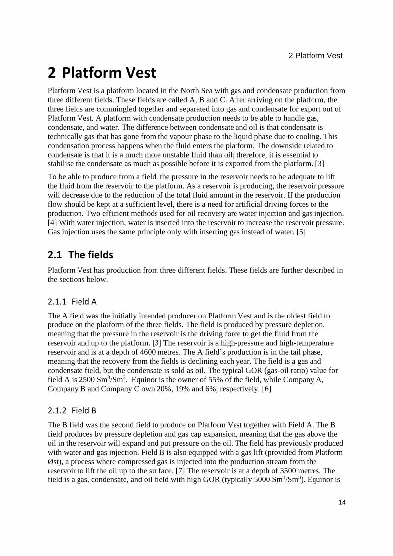
The first separation stage is shown in Figure 2.1 [10]. The inlet separator (20VA001) and the
test separator (20VA004) are both 3-phase-separators which separates the gas at the top, the
condensate in the middle, and the water out at the bottom. The condensate downstream of the
inlet separator is heated to the desired temperature in a heat exchanger (20HA101). This is to
separate water and gas from the oil in a more efficient way. The heated commingled stream is
then mixed with the test separator's condensate in the mixer (MIX-107). [3]
2 Platform Vest
16
Figure 2.1: Illustration of the first separation stage
The second and third stage separation process is illustrated in Figure 2.2 [10]. The mixed
stream with both condensate streams is then routed to the second stage separator (20VA002).
The second stage separator is a two-phase separator that separates the gas at the top and the
liquid out at the bottom. The second stage separator operates at a lower pressure than the inlet
and the test separators. The second stage liquid outlet is then routed to the third stage
separator (20VA003), a three-phase separator operating at an even lower pressure than the
second stage separator. This separator separates the remaining water at the bottom, the gas
out in the top and the condensate out in the middle. [3]
Figure 2.2: Illustration of the second and third separation stage
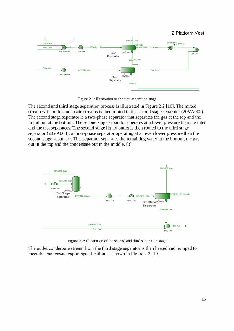
The outlet condensate stream from the third stage separator is then heated and pumped to
meet the condensate export specification, as shown in Figure 2.3 [10].
2 Platform Vest
17
Figure 2.3: Illustration of the condensate export
The first and second stage recompression is illustrated in Figure 2.4 [10]. The gas out of the
third stage separator is cooled (23HB001) and routed through a scrubber (23VG001) that
separates the liquid from the vapour. The liquid out of the first scrubber is pumped (23PA
001) and mixed into the inlet stream to the third stage separator. The vapour out of the first
scrubber is compressed (23KA001) and cooled (23HB002) right after to remove the heat of
compression from the fluid. This is called the first stage of recompression. The fluid is then
routed through a second scrubber (23VG002) to remove even more liquid from the vapour.
The liquid out of the second scrubber is mixed into the inlet stream to the third stage
separator. The vapour out of the scrubber is compressed (23KA002) to meet the outlet vapour
pressure of the second-stage separator. This is the second stage of recompression. The vapour
from the second stage separator is mixed (MIX-110) with the second stage recompression
vapour. [3]
Figure 2.4: Illustration of the first and second recompression stage
The third stage of recompression is illustrated in Figure 2.5 [10]. The combined stream,
including the second recompression stage vapour and the second stage separator vapour, is
cooled (23HJ001) and routed through a third scrubber (23VG003) to remove even more of
the liquid from the vapour. The liquid from the third scrubber is pumped (23PA002) and
mixed into the inlet stream to the second stage separator. The vapour out of the third scrubber
is compressed (23KA003). [3]

2 Platform Vest
18
Figure 2.5: Illustration of the third recompression stage
The low-pressure recompression is illustrated in Figure 2.6 [10]. The vapour out of the inlet
separator and the test separator are combined, and the mixed stream is cooled (23HJ600) and
routed through a scrubber (23VG600) to remove the liquid from the vapour. The liquid out of
the scrubber is mixed into the inlet stream to the second stage separator. The vapour out of
the scrubber is compressed (23KA600) to meet the third stage recompression vapour. This is
called low-pressure compression. The vapour out of the low-pressure compression and the
third stage recompression are mixed (MIX-112) and then cooled (24HJ001) before being
routed through another scrubber (24VG001) for additional liquid removal from the vapour.
The liquid stream from this scrubber is mixed into the inlet stream to the inlet separator. [3]
Figure 2.6: Illustration of the low-pressure compression
The final step in the process is illustrated in Figure 2.7 [10]. The vapour stream is cooled
(24HA001) and dried from the remaining water. Gas drying methods could include
adsorption or absorption with, for instance, glycol. [3] The dried gas is then cooled
(27HJ001) before it is sent to the last scrubber (27VG001), where the last bit of liquid is
separated out. The liquid outlet from this last scrubber is mixed into the inlet of the second
2 Platform Vest
19
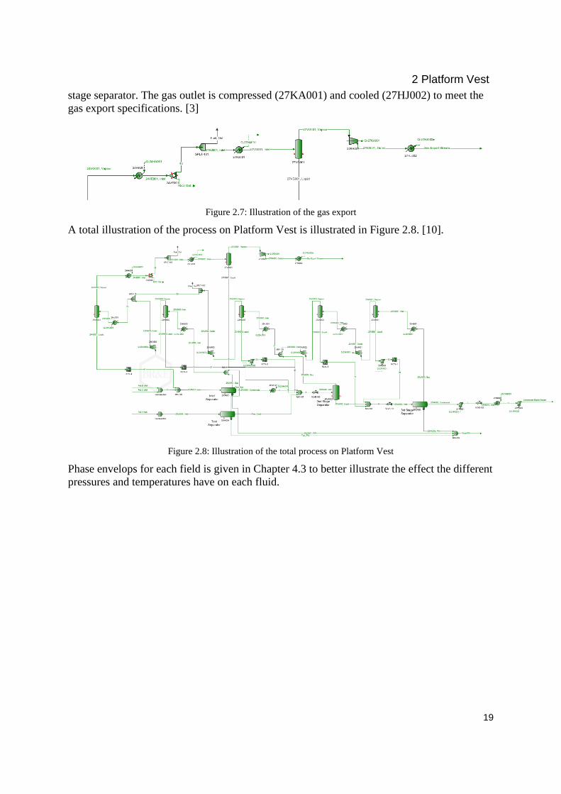
stage separator. The gas outlet is compressed (27KA001) and cooled (27HJ002) to meet the
gas export specifications. [3]
Figure 2.7: Illustration of the gas export
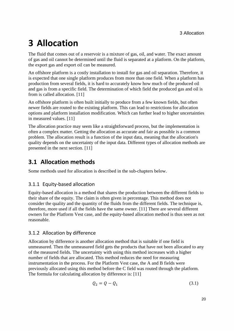
A total illustration of the process on Platform Vest is illustrated in Figure 2.8. [10].
Figure 2.8: Illustration of the total process on Platform Vest
Phase envelops for each field is given in Chapter 4.3 to better illustrate the effect the different
pressures and temperatures have on each fluid.
3 Allocation
20
3 Allocation The fluid that comes out of a reservoir is a mixture of gas, oil, and water. The exact amount
of gas and oil cannot be determined until the fluid is separated at a platform. On the platform,
the export gas and export oil can be measured.
An offshore platform is a costly installation to install for gas and oil separation. Therefore, it
is expected that one single platform produces from more than one field. When a platform has
production from several fields, it is hard to accurately know how much of the produced oil
and gas is from a specific field. The determination of which field the produced gas and oil is
from is called allocation. [11]
An offshore platform is often built initially to produce from a few known fields, but often
newer fields are routed to the existing platform. This can lead to restrictions for allocation
options and platform installation modification. Which can further lead to higher uncertainties
in measured values. [11]
The allocation practice may seem like a straightforward process, but the implementation is
often a complex matter. Getting the allocation as accurate and fair as possible is a common
problem. The allocation result is a function of the input data, meaning that the allocation's
quality depends on the uncertainty of the input data. Different types of allocation methods are
presented in the next section. [11]
3.1 Allocation methods
Some methods used for allocation is described in the sub-chapters below.
3.1.1 Equity-based allocation
Equity-based allocation is a method that shares the production between the different fields to
their share of the equity. The claim is often given in percentage. This method does not
consider the quality and the quantity of the fluids from the different fields. The technique is,
therefore, more used if all the fields have the same owner. [11] There are several different
owners for the Platform Vest case, and the equity-based allocation method is thus seen as not
reasonable.
3.1.2 Allocation by difference
Allocation by difference is another allocation method that is suitable if one field is
unmeasured. Then the unmeasured field gets the products that have not been allocated to any
of the measured fields. The uncertainty with using this method increases with a higher
number of fields that are allocated. This method reduces the need for measuring
instrumentation in the process. For the Platform Vest case, the A and B fields were
previously allocated using this method before the C field was routed through the platform.
The formula for calculating allocation by difference is: [11]
𝑄2 = 𝑄 − 𝑄1 (3.1)
3 Allocation
21
Where Q2 is the unknow quantity allocated to user 2, Q is the total quantity to be allocated
and Q1 is the known quantity for user 1.
3.1.3 Pro-rata allocation
Pro-rata allocation (or Proportional allocation) is allocation based on measured or estimated
field quantities. This means that each field gets the amount of production proportional to the
estimated quantity of the specific field. This method is less affected by biases since the
uncertainties are evenly distributed between the fields. The formula for calculating allocation
pro-rata is: [11]
𝑄𝑛 = 𝑄 ∗𝐵𝑛
∑ 𝐵𝑛𝑛
(3.2)
Where Qn is the quantity allocated to user n and Bn is the measured/estimated quantity to user
n.
3.1.4 Uncertainty-based allocation
Uncertainty-based allocation (UBA) uses the accuracy of the input to give a fairer allocation.
The input data with the lowest uncertainty is emphasised more than data with higher
uncertainty. This method requires that the uncertainties in the system are highly evaluated.
[11]
3.1.5 Simulation-based allocation
Allocation can also be done by making a model in a process simulation software, such as
UniSim or ProMax. A simulation model needs sufficient input data for the simulation to be
solvable. The input data is often pressure and temperature specifications for the different
process equipment, field compositions and stream flows. A process simulation can provide
information on the hydrocarbons after being separated and experiencing thermodynamic
changes in the process. Normally, the simulation model is built from a process flow diagram
from the real platform process. However, it is better for just allocation purposes to construct a
model that favours stability and solvability, assuming that the process specification is
achieved. The uncertainty of the simulation model is dependent on the uncertainty of the
input data and the quality of the model. [11]
A process simulation software has basic hydrocarbons defined in the component library. If
the library components are used for a simulation with more than one fields, it is
impossible/challenging to measure how much of the hydrocarbons in the export belonging to
which field. One way of solving this problem is to define hypothetical components for each
field. In this way, the user can track the hydrocarbons from different fields throughout the
process and know which field the product is originated from.
Simulation-based allocation is always used for new fields to get an understanding of the
commingling effect, limitations or if there is a need for modifications.

3 Allocation
22
3.2 Current allocation method for Platform Vest
This chapter describes the current allocation method used for Platform Vest.
3.2.1 Input and production streams
The hydrocarbon mass flow to Platform Vest from the A field is not directly measured but
determined by other measurements and calculations. Field A is routed through the test
separator alone, making measurements from the test separator useful to decide flow from the
field. The field’s hydrocarbon flow is determined using updated well performance curves and
densities from sample analysis and validated with measurements from the test separator. The
uncertainty for this method can be set to ± 5%. [12]
The hydrocarbon flow from field B and field C are measured separately with topside
multiphase flow metres. The uncertainty with this type of meter is set to ± 5%. [13] Backup
flow determination for field B and C is subsea multiphase flow metres or well performance
curves. [14]
The production streams are measured with fiscal metres on a mass basis. The parameter to be
measured on the gas export is the accumulated monthly mass. The parameters measured for
the oil export are the daily mass and the accumulated monthly mass. [14]
3.2.2 Oil export allocation
The oil export allocation is based on standalone ORFs. The ORF (oil recovery factor)
determines how much of a specific component is recovered in the oil production. ORFs need
to be calculated for each component in every field. The ORFs also need to be free of any gas
lift, only pure component from the specific field. The formula for the calculation is: [14]
𝑂𝑅𝐹𝑖,𝐹𝑖𝑒𝑙𝑑 𝑥 =𝑚𝑂𝑖𝑙𝑖,𝐹𝑖𝑒𝑙𝑑 𝑥
𝑚𝐻𝐶𝑖,𝐹𝑖𝑒𝑙𝑑 𝑥
(3.3)
ORF is calculated for the following components (i = N2, CO2, C1, C2, C3, iC4, nC4, iC5,
nC5, C6, C7, C8, C9 and C10+), where mOil is the oil in the liquid product for the specific
component (i) and mHC is the total hydrocarbon feed of that specific component. Platform
Vest has production from three fields, meaning that the specific ORFs needs to be calculated
for each field, resulting in 14 ORFs for each field and a total of 42 ORFs for each Platform
Vest case. The ORFs is based on a standalone simulation for the fields. A standalone
simulation is a simulation where only the production from one field is simulated, resulting in
three different simulation models. This gives a non-commingled result for the simulation. The
input to the simulations is given from the fluid characterisation of the fields and typical
process input. The ORFs are kept and used for the allocation until a new fluid
characterisation or other changes requires for a new simulation. This is often done once every
year. [14]
The formula for calculating the basis for the oil production for each field is:
3 Allocation
23
𝑚𝑂𝐵𝑖,𝐹𝑖𝑒𝑙𝑑 𝑥= 𝑚𝐻𝐶𝑖,𝐹𝑖𝑒𝑙𝑑 𝑥
∗ 𝑂𝑅𝐹𝑖,𝐹𝑖𝑒𝑙𝑑 𝑥 (3.4)
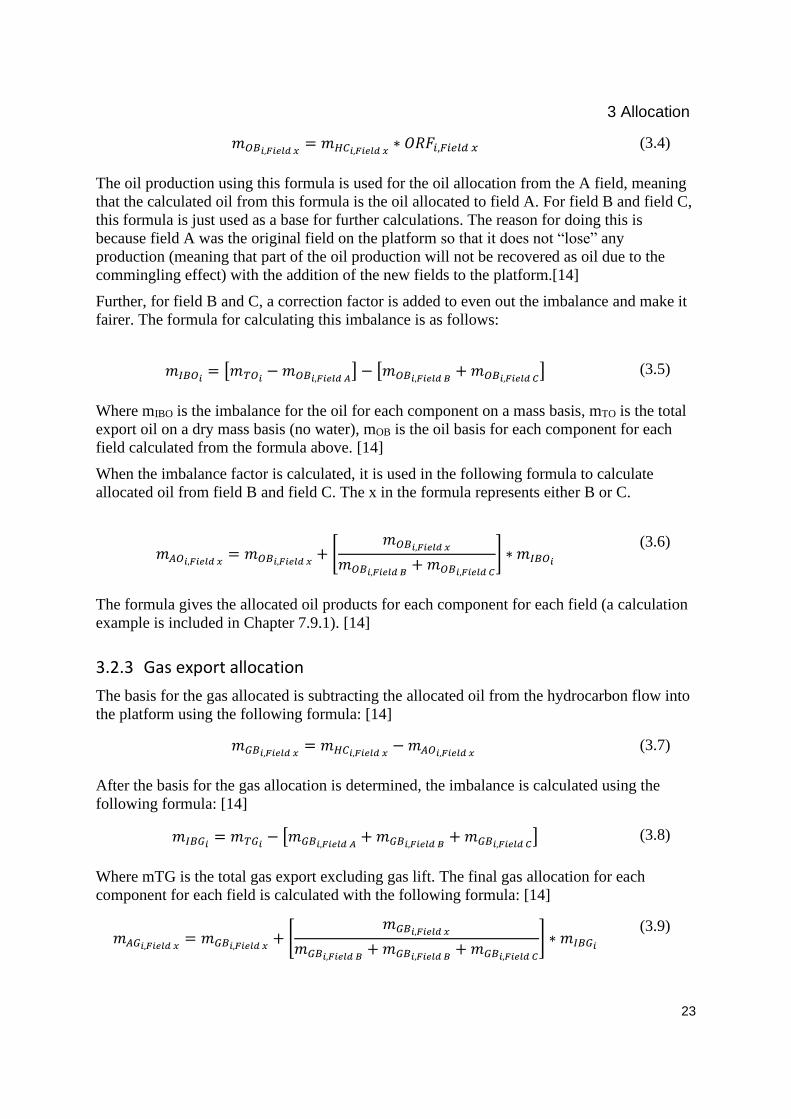
The oil production using this formula is used for the oil allocation from the A field, meaning
that the calculated oil from this formula is the oil allocated to field A. For field B and field C,
this formula is just used as a base for further calculations. The reason for doing this is
because field A was the original field on the platform so that it does not “lose” any
production (meaning that part of the oil production will not be recovered as oil due to the
commingling effect) with the addition of the new fields to the platform.[14]
Further, for field B and C, a correction factor is added to even out the imbalance and make it
fairer. The formula for calculating this imbalance is as follows:
𝑚𝐼𝐵𝑂𝑖= [𝑚𝑇𝑂𝑖
− 𝑚𝑂𝐵𝑖,𝐹𝑖𝑒𝑙𝑑 𝐴] − [𝑚𝑂𝐵𝑖,𝐹𝑖𝑒𝑙𝑑 𝐵
+ 𝑚𝑂𝐵𝑖,𝐹𝑖𝑒𝑙𝑑 𝐶] (3.5)
Where mIBO is the imbalance for the oil for each component on a mass basis, mTO is the total
export oil on a dry mass basis (no water), mOB is the oil basis for each component for each
field calculated from the formula above. [14]
When the imbalance factor is calculated, it is used in the following formula to calculate
allocated oil from field B and field C. The x in the formula represents either B or C.
𝑚𝐴𝑂𝑖,𝐹𝑖𝑒𝑙𝑑 𝑥= 𝑚𝑂𝐵𝑖,𝐹𝑖𝑒𝑙𝑑 𝑥
+ [𝑚𝑂𝐵𝑖,𝐹𝑖𝑒𝑙𝑑 𝑥
𝑚𝑂𝐵𝑖,𝐹𝑖𝑒𝑙𝑑 𝐵+ 𝑚𝑂𝐵𝑖,𝐹𝑖𝑒𝑙𝑑 𝐶
] ∗ 𝑚𝐼𝐵𝑂𝑖
(3.6)
The formula gives the allocated oil products for each component for each field (a calculation
example is included in Chapter 7.9.1). [14]
3.2.3 Gas export allocation
The basis for the gas allocated is subtracting the allocated oil from the hydrocarbon flow into
the platform using the following formula: [14]
𝑚𝐺𝐵𝑖,𝐹𝑖𝑒𝑙𝑑 𝑥= 𝑚𝐻𝐶𝑖,𝐹𝑖𝑒𝑙𝑑 𝑥
− 𝑚𝐴𝑂𝑖,𝐹𝑖𝑒𝑙𝑑 𝑥 (3.7)
After the basis for the gas allocation is determined, the imbalance is calculated using the
following formula: [14]
𝑚𝐼𝐵𝐺𝑖= 𝑚𝑇𝐺𝑖
− [𝑚𝐺𝐵𝑖,𝐹𝑖𝑒𝑙𝑑 𝐴+ 𝑚𝐺𝐵𝑖,𝐹𝑖𝑒𝑙𝑑 𝐵
+ 𝑚𝐺𝐵𝑖,𝐹𝑖𝑒𝑙𝑑 𝐶] (3.8)
Where mTG is the total gas export excluding gas lift. The final gas allocation for each
component for each field is calculated with the following formula: [14]
𝑚𝐴𝐺𝑖,𝐹𝑖𝑒𝑙𝑑 𝑥= 𝑚𝐺𝐵𝑖,𝐹𝑖𝑒𝑙𝑑 𝑥
+ [𝑚𝐺𝐵𝑖,𝐹𝑖𝑒𝑙𝑑 𝑥
𝑚𝐺𝐵𝑖,𝐹𝑖𝑒𝑙𝑑 𝐵+ 𝑚𝐺𝐵𝑖,𝐹𝑖𝑒𝑙𝑑 𝐵
+ 𝑚𝐺𝐵𝑖,𝐹𝑖𝑒𝑙𝑑 𝐶
] ∗ 𝑚𝐼𝐵𝐺𝑖
(3.9)

4 Fluid characterisation
24
4 Fluid characterisation Fluid characterisation defines how a fluid will behave in correlation to other fluids and how it
will be affected by different PVT changes. The fluid characterisation and the process model
for Platform Vest are based on the equation of state called SRK (Soave-Redlich-Kwong).
4.1 Equation of state
An equation of state is an equation describing the relation between the pressure, the
temperature, and the volume of a gas. The most used EOS for simple gases is the ideal gas
law (PV = nRT); this equation is adequate for calculations at low pressures. If the gas is at
high pressure or low temperature, the gas will deviate from the ideal behaviour, making the
ideal gas law insufficient. A more complex equation such as the Soave-Redlich-Kwong
(SRK) equation is needed for the PVT calculations in this case. [15, p. 191]
The SRK equation of state is a cubic equation of state because it can be written as a third-
order equation for the specific volume. [15, p. 203] This EOS is dependent on the critical
temperature and the critical pressure of the fluid. The critical temperature is the highest
temperature at which the fluid is in both the vapour phase and the liquid phase, while the
critical pressure is the highest pressure at which the fluid is in both phases. [15, p. 200]. The
equation is as follows: [15, p. 203]
𝑃 =𝑅𝑇
�̂� − 𝑏−
𝛼𝑎
�̂�(�̂� + 𝑏)
(4.1)
Where:
𝑎 = 0.42747(𝑅𝑇𝑐)2
𝑃𝑐
(4.2)
𝑏 = 0.08644𝑅𝑇𝑐
𝑃𝑐
(4.3)
𝛼 = [1 + 𝑚(1 − √𝑇𝑟 )]2 (4.4)
𝑇𝑟 =𝑇
𝑇𝑐
(4.5)
𝑚 = 0.48508 + 1.55171𝜔 − 0.1561𝜔2 (4.6)
The saturated-liquid volumes predicted by the SRK EOS will have an average deviation of
16%. This can be improved by incorporating the Peneloux volume translation. This method
used the knowledge that the predicted volumes by SRK is too large and will be improved by
being reduced the predicted volume by a value c (the volume correction). The formula for
this is: [16]

4 Fluid characterisation
25
�̂�𝑡 = �̂� − 𝑐 (4.7)
This incorporated into the SRK EOS gives the following formulas:
𝑃 =𝑅𝑇
�̂� − 𝑏−
𝛼𝑎
(�̂� + 𝑐)(�̂� + 𝑏 + 2𝑐)
(4.8)
𝑏 = 0.08644𝑅𝑇𝑐
𝑃𝑐− 𝑐
(4.9)
𝑐 =𝑅𝑇𝑐
𝑃𝑐(0.1156 − 0.4077 ∗ 𝑍𝑅𝐴)
(4.10)
Where ZRA is the Rackett compressibility factor. [16]
The EOS used for simulation with simulation software in Equinor is the SRK and the SRK
Peneloux for fluid characterisation.
4.2 Fluid characterisation using PVTsim
The fluid characterisation for a mixture can be found and calculated from different methods.
The method used for the scope in this report is a calculation using software called PVTsim.
The input values to PVTsim are the mol% (or weight%), the density and the molar weight of a
fluid mixture. PVTsim includes a variety of EOS to choose from, and the equation used for this
scope is the SRK. The output from PVTsim is multiple state values, including critical pressure,
critical temperature, and critical volume for all the components in the fluid mixture. See
Appendix B – PVTsim procedure for an elaborated procedure for the different fields in
PVTsim.
For a new fluid characterisation in PVTsim, the input values to PVTsim are given from an
analysis of fluid samples from the test separator. It is essential that these samples are taken
when production is under normal operating conditions to get a sample that best represents the
reality. The separator samples are sent to a non-associated company responsible for doing the
tests needed for the sample. This company uses gas chromatography to determine the
composition, a densitometer to determine the density and a cryoscopy to determine the
molecular weight. The results are given back to Equinor in a report, and the results can be used
as the input values to PVTsim to characterise the fluid. [17]
For the scope of this report, there was a given fluid characterisation that has been used for a
few years. This characterisation is defined from PVT analysis taken from separator samples a
few years ago. Part of the results will compare this old fluid characterisation and a new fluid
characterisation based on new separator samples.
4.2.1 Lumping method
PVTsim has an option for lumping hydrocarbons together to form a hypothetical hydrocarbon
with the average fluid characterisation for all the hydrocarbons set to be in that hydrocarbon
4 Fluid characterisation
26
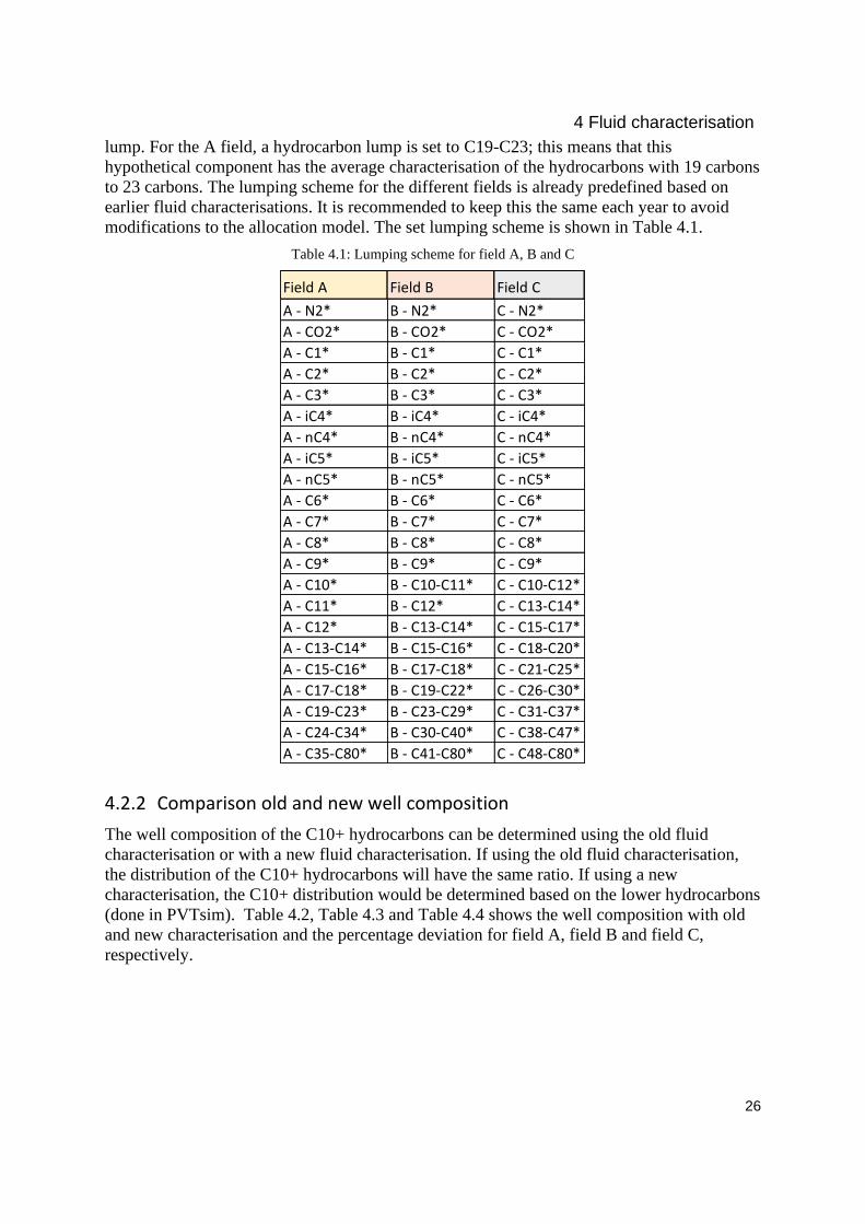
lump. For the A field, a hydrocarbon lump is set to C19-C23; this means that this
hypothetical component has the average characterisation of the hydrocarbons with 19 carbons
to 23 carbons. The lumping scheme for the different fields is already predefined based on
earlier fluid characterisations. It is recommended to keep this the same each year to avoid
modifications to the allocation model. The set lumping scheme is shown in Table 4.1.
Table 4.1: Lumping scheme for field A, B and C
4.2.2 Comparison old and new well composition
The well composition of the C10+ hydrocarbons can be determined using the old fluid
characterisation or with a new fluid characterisation. If using the old fluid characterisation,
the distribution of the C10+ hydrocarbons will have the same ratio. If using a new
characterisation, the C10+ distribution would be determined based on the lower hydrocarbons
(done in PVTsim). Table 4.2, Table 4.3 and Table 4.4 shows the well composition with old
and new characterisation and the percentage deviation for field A, field B and field C,
respectively.
Field A Field B Field C
A - N2* B - N2* C - N2*
A - CO2* B - CO2* C - CO2*
A - C1* B - C1* C - C1*
A - C2* B - C2* C - C2*
A - C3* B - C3* C - C3*
A - iC4* B - iC4* C - iC4*
A - nC4* B - nC4* C - nC4*
A - iC5* B - iC5* C - iC5*
A - nC5* B - nC5* C - nC5*
A - C6* B - C6* C - C6*
A - C7* B - C7* C - C7*
A - C8* B - C8* C - C8*
A - C9* B - C9* C - C9*
A - C10* B - C10-C11* C - C10-C12*
A - C11* B - C12* C - C13-C14*
A - C12* B - C13-C14* C - C15-C17*
A - C13-C14* B - C15-C16* C - C18-C20*
A - C15-C16* B - C17-C18* C - C21-C25*
A - C17-C18* B - C19-C22* C - C26-C30*
A - C19-C23* B - C23-C29* C - C31-C37*
A - C24-C34* B - C30-C40* C - C38-C47*
A - C35-C80* B - C41-C80* C - C48-C80*

4 Fluid characterisation
27
Table 4.2: Field A well composition new vs. old characterisation
Table 4.3: Field B well composition new vs. old characterisation
Field A New Old Deviation (%)
A - N2* 0.00449 0.00449 0.00 %
A - CO2* 0.03994 0.03994 0.00 %
A - C1* 0.72172 0.72172 0.00 %
A - C2* 0.08927 0.08927 0.00 %
A - C3* 0.04346 0.04346 0.00 %
A - iC4* 0.00898 0.00898 0.00 %
A - nC4* 0.0164 0.0164 0.00 %
A - iC5* 0.00688 0.00688 0.00 %
A - nC5* 0.00792 0.00792 0.00 %
A - C6* 0.00947 0.00947 0.00 %
A - C7* 0.01332 0.01332 0.00 %
A - C8* 0.01237 0.01237 0.00 %
A - C9* 0.00707 0.00707 0.00 %
A - C10* 0.00449 0.00418 -6.85 %
A - C11* 0.00297 0.00281 -5.51 %
A - C12* 0.00205 0.00201 -2.41 %
A - C13-C14* 0.00315 0.00310 -1.49 %
A - C15-C16* 0.00188 0.00196 4.24 %
A - C17-C18* 0.00120 0.00124 3.97 %
A - C19-C23* 0.00157 0.00159 0.86 %
A - C24-C34* 0.00109 0.00110 0.25 %
A - C35-C80* 0.00031 0.00071 126.72 %
Field B New Old Deviation (%)
B - N2* 0.00691 0.00691 0.00 %
B - CO2* 0.02402 0.02402 0.00 %
B - C1* 0.81959 0.81959 0.00 %
B - C2* 0.05805 0.05805 0.00 %
B - C3* 0.03273 0.03273 0.00 %
B - iC4* 0.00487 0.00487 0.00 %
B - nC4* 0.01047 0.01047 0.00 %
B - iC5* 0.00333 0.00333 0.00 %
B - nC5* 0.00445 0.00445 0.00 %
B - C6* 0.00475 0.00475 0.00 %
B - C7* 0.00685 0.00685 0.00 %
B - C8* 0.00588 0.00588 0.00 %
B - C9* 0.00344 0.00344 0.00 %
B - C10-C11* 0.00332 0.00439 32.06 %
B - C12* 0.00137 0.00148 7.88 %
B - C13-C14* 0.00226 0.00241 6.55 %
B - C15-C16* 0.00175 0.00165 -5.67 %
B - C17-C18* 0.00135 0.00111 -17.88 %
B - C19-C22* 0.00185 0.00128 -31.04 %
B - C23-C29* 0.00163 0.00103 -36.87 %
B - C30-C40* 0.00085 0.00081 -4.08 %
B - C41-C80* 0.00027 0.00050 85.15 %

4 Fluid characterisation
28
Table 4.4: Field C well composition new vs. old characterisation
The deviation between the different predicted well compositions is considerable. This verifies
that it would be interesting to see how the different compositions influence the predicted
results when incorporated into a process simulation.
4.2.3 Comparison old and new PVTsim characterisation
The two parameters compared in this section are the predicted critical pressure and the
predicted critical temperature for the new and old characterisation. These parameters are
essential for the fluid behaviour of the components. Figure 4.1, Figure 4.2 and Figure 4.3
show a comparison between the critical pressure with new and old characterisation and a
comparison for the critical temperature for field A, field B and field C, respectively. The x-
axis illustrates the molecular weight of the hydrocarbon. Critical pressure and critical
temperature
Field C New Old Deviation (%)
C - N2* 0.00247 0.00247 0.00 %
C - CO2* 0.02336 0.02336 0.00 %
C - C1* 0.26983 0.26983 0.00 %
C - C2* 0.0696 0.0696 0.00 %
C - C3* 0.0861 0.0861 0.00 %
C - iC4* 0.01607 0.01607 0.00 %
C - nC4* 0.05074 0.05074 0.00 %
C - iC5* 0.0181 0.0181 0.00 %
C - nC5* 0.02853 0.02853 0.00 %
C - C6* 0.03307 0.03307 0.00 %
C - C7* 0.05277 0.05277 0.00 %
C - C8* 0.05056 0.05056 0.00 %
C - C9* 0.03487 0.03487 0.00 %
C - C10-C12* 0.06561 0.07001 6.71 %
C - C13-C14* 0.03442 0.03498 1.64 %
C - C15-C17* 0.04077 0.03981 -2.37 %
C - C18-C20* 0.03065 0.02884 -5.91 %
C - C21-C25* 0.03512 0.02960 -15.72 %
C - C26-C30* 0.02183 0.01992 -8.74 %
C - C31-C37* 0.01742 0.01739 -0.20 %
C - C38-C47* 0.01130 0.01346 19.07 %
C - C48-C80* 0.00680 0.00992 45.81 %

4 Fluid characterisation
29
Figure 4.1: Critical parameters for field A, new vs. old characterisation
Figure 4.2: Critical parameters for field B, new vs. old characterisation

4 Fluid characterisation
30
Figure 4.3: Critical parameters for field C, new vs. old characterisation
These figures show that there is a deviation between the old and new characterisation for the
hydrocarbons. Based on this finding, a more detailed simulation analysis (chapter 7.1) shows
the effect of the deviations and what this will mean for the simulation results.
The total fluid characterisation for all fields with old and new characterisation is given in
Appendix C – Old fluid characterisation and Appendix D – New fluid characterisation.
4.3 Phase envelope
The phase envelope is the pressure and temperature prediction of the phase diagram for a
fluid consisting of multiple components. The phase envelope predicted for a fluid is
determined for a fixed fluid composition. The area inside the phase envelope is identified as
the two-phase area where both liquid and gas are present. [9, p.43] The phase envelopes
predicted for the results in this report are solely included to confirm that the phase diagram is
predicted the same in the characterisation and simulation and determine if the phase diagram
is the same between the different cases in the result. According to [18], the predicted phase
envelope will change if PNA (paraffin, naphthene and aromatic) is included in the fluid.
According to [19, p.86], the phase envelopes will be broader and higher with extended fluid
characterisation, and narrower and downscaled with a lower degree of fluid characterisation
(for instance, with C20+ or C10+ characterisation).
4.3.1 Phase envelope for the new characterisation
The phase envelopes for the different fields are obtained from the PVTsim results and shown
in Figure 4.4, Figure 4.5 and Figure 4.6 for field A, field B, and field C, respectively.

4 Fluid characterisation
31
Figure 4.4: Phase envelope, new characterisation, PVTsim, Field A
Figure 4.5: Phase envelope, new characterisation, PVTsim, Field B

4 Fluid characterisation
32
Figure 4.6: Phase envelope, new characterisation, PVTsim, Field C
These phase envelopes will be compared to the simulation models to determine if the fluid
characterisation is incorporated successfully into the simulation model. The different phase
envelops also show that the fields are very different when looking at the properties.
4.4 Value adjustment
The oil produced from an offshore platform consists of different qualities. These qualities can
be defined from the normal boiling point of the hydrocarbon obtained from the fluid
characterisation. The cut description for the normal boiling points is described in Table 4.5.
together with the value for the product. The prices and dollar exchange rate are retrieved 3rd
of March 2021. The exchange rate used for the calculation is 8.49 NOK/USD [20].
Table 4.5: Oil products NBP range and value
Oil product NBP range Value
°C USD/ton
Naphtha 20 - 165 °C 588.2 [21]
Jet kerosene 165 - 250 °C 455.4 [22]
Gasoil 250 - 375 °C 537.9 [23]
Atmospheric residue 375+ °C 264.1 [24]
The products with NBP (normal boiling point) lower than 20 °C is cut as gas and will not be
included in the value estimation. The value of the gas export will also not be included for
value estimation. This is to limit the number of results to be discussed for this scope. A value
adjustment for the oil products mentioned will indicate value for the profit to each field.

4 Fluid characterisation
33
The oil production cuts will be the same for both new and old characterisation. The cuts are
given in Table 4.6, based on NBPs given in Appendix C – Old fluid characterisation and
Appendix D – New fluid characterisation.
Table 4.6: Oil product cuts for the different fields
Component Cut Component Cut Component Cut
A - iC5* Naphtha B - iC5* Naphtha C - iC5* Naphtha
A - nC5* B - nC5* C - nC5*
A - C6* B - C6* C - C6*
A - C7* B - C7* C - C7*
A - C8* B - C8* C - C8*
A - C9* B - C9* C - C9*
A - C10* Kerosene B - C10-C11* Kerosene C - C10-C12* Kerosene
A - C11* B - C12* C - C13-C14*
A - C12* B - C13-C14* C - C15-C17* Gasoil
A - C13-C14* B - C15-C16* Gasoil C - C18-C20*
A - C15-C16* Gasoil B - C17-C18* C - C21-C25*
A - C17-C18* B - C19-C22* C - C26-C30* Residue
A - C19-C23* B - C23-C29* Residue C - C31-C37*
A - C24-C34* Residue B - C30-C40* C - C38-C47*
A - C35-C80* B - C41-C80* C - C48-C80*
Field A Field B Field C
5 UniSim
34
5 UniSim UniSim is a process simulation software developed by Honeywell International Inc. The
UniSim Design version used for the results in this report is R460.2.
5.1 Allocating components
To allocate different hydrocarbons in a process simulation using UniSim, the software
recommends using hypothetical components for the different fields. This means that there is
separate methane for each field with supposedly the same fluid characterisation. These
components are defined in the environmental design for the simulation. The fluid
characterisation for these components is described in Appendix C – Old fluid characterisation
and Appendix D – New fluid characterisation. UniSim needs the value for normal boiling
point, molecular weight, liquid density, critical temperature, critical pressure, critical volume,
and the acentric factor to define a hypothetical component.
5.2 EOS
The standard EOS used for process simulations in Equinor is the SRK equation of state. For
UniSim simulations, the company standard is to use SRK with Peneloux volume correction.
The SRK-Peneloux is thus chosen as the EOS for the simulations for this report.
5.3 The simulation model
The simulation model is built according to the process described in the Process description
chapter. The only difference is the addition of heat exchangers before the inlet and test
separators. These are added to ensure that the equipment has the same thermodynamic
properties according to the given process parameters. A figure of the model is given in Figure
5.1 [25].
A closer illustration of the model is given in Appendix E – UniSim model.

5 UniSim
35
Figure 5.1: Complete UniSim model
The process input (temperature and pressure) for given process equipment are given in
Appendix F – Process equipment input and the profiles are given in Appendix G – Inflow
data for reallocation. The input composition is given in Appendix C – Old fluid
characterisation and Appendix D – New fluid characterisation.
5.4 Allocated production streams
To easier know which field the product is allocated from, the export streams are divided into
products from field A, field B, field C and the GL. This is done by using dividers in UniSim,
which allows the user to divide all the components into different product streams. These
dividers are marked with an X in Figure 5.1.

6 ProMax
36
6 ProMax ProMax is a process simulation software developed by Bryan Research & Engineering, LLC.
The ProMax version used for the results in this report is 5.0.
6.1 Allocating components
ProMax offers an allocation method called mixed species or allocation by full account. This
gives the opportunity to use library components (not defining hypotheticals) for different
hydrocarbons in the simulation and still know which field they are coming from. Giving the
opportunity to just have one methane in the simulation instead of three hypothetical methane
like in UniSim. ProMax claims that this gives a more thermodynamically correct
commingling compared to just using hypothetical components.
For the Platform Vest case, the fluid characterisation for the lightest hydrocarbons (C1 to C6)
was the same for the different fields. These hydrocarbons were thus only added as library
components. The hydrocarbons from C7 and heavier were defined as hypothetical. ProMax
uses single oils to represent the hypothetical components, where the only needed fluid
characterisation input is the molecular weight and the specific gravity. The fluid
characterisation for the single oils is described in Appendix C – Old fluid characterisation and
Appendix D – New fluid characterisation.
6.2 EOS
The EOS used for Promax is SRK.
6.3 The simulation model
The simulation model is built according to the process described in the Process description
chapter, with added heat exchangers as the UniSim model. A figure of the model is given in
Figure 6.1 [10].
A closer illustration of the ProMax model is given in Appendix H – ProMax model.

6 ProMax
37
Figure 6.1: Complete ProMax model
The process input (temperature and pressure) for given unit operators are given in Appendix
F – Process equipment input and the profiles are given in Appendix G – Inflow data for
reallocation. The input composition is given in Appendix C – Old fluid characterisation and
Appendix D – New fluid characterisation. Same as the UniSim model.
6.4 Allocated production streams
Due to the mixed-species option in ProMax, there is no need to split the product streams into
different fields. Instead, there is an option for mixed species analysis that can be incorporated
into the stream. This analysis gives the opportunity to see what and how much product is
coming from which field.

7 Results and discussion
38
7 Results and discussion The results in this report are divided into; a fluid characterisation part where simulations with
new and old characterisation are compared, a reallocation part to specifically look at how the
ORFs change with different changes in the UniSim model and the characterisation, an
UniSim future allocation part with tuning on oil, gas and GOR, and a simple ProMax model
comparison. Different allocation methods are also compared to the current allocation
agreement for Platform Vest. The last section in this chapter includes a recommended
guideline for allocation simulation based on the results from the different cases in the results.
7.1 Simulation with new characterisation vs. old characterisation
For this comparison part, two different UniSim simulation models are developed. Where one
model has the new characterisation, and one model has the old characterisation. The lumping
scheme, EOS, and the model in total were kept the same, with the only changes being the
fluid properties for the hypothetical components and the well composition. A detailed
description of how the model is made is given in Appendix I – Building the UniSim model.
7.1.1 Phase envelope comparison
The phase envelops from PVTsim are compared to the phase envelops in UniSim to see if the
estimated curves match. This is a necessary quality assurance for proper setup in UniSim, to
ensure that the fluid will behave the same as the estimated fluid in PVTsim. The VF (vapour
fraction) is 1.0 for field A and field C and 0.99 for field B. The inlet conditions for the
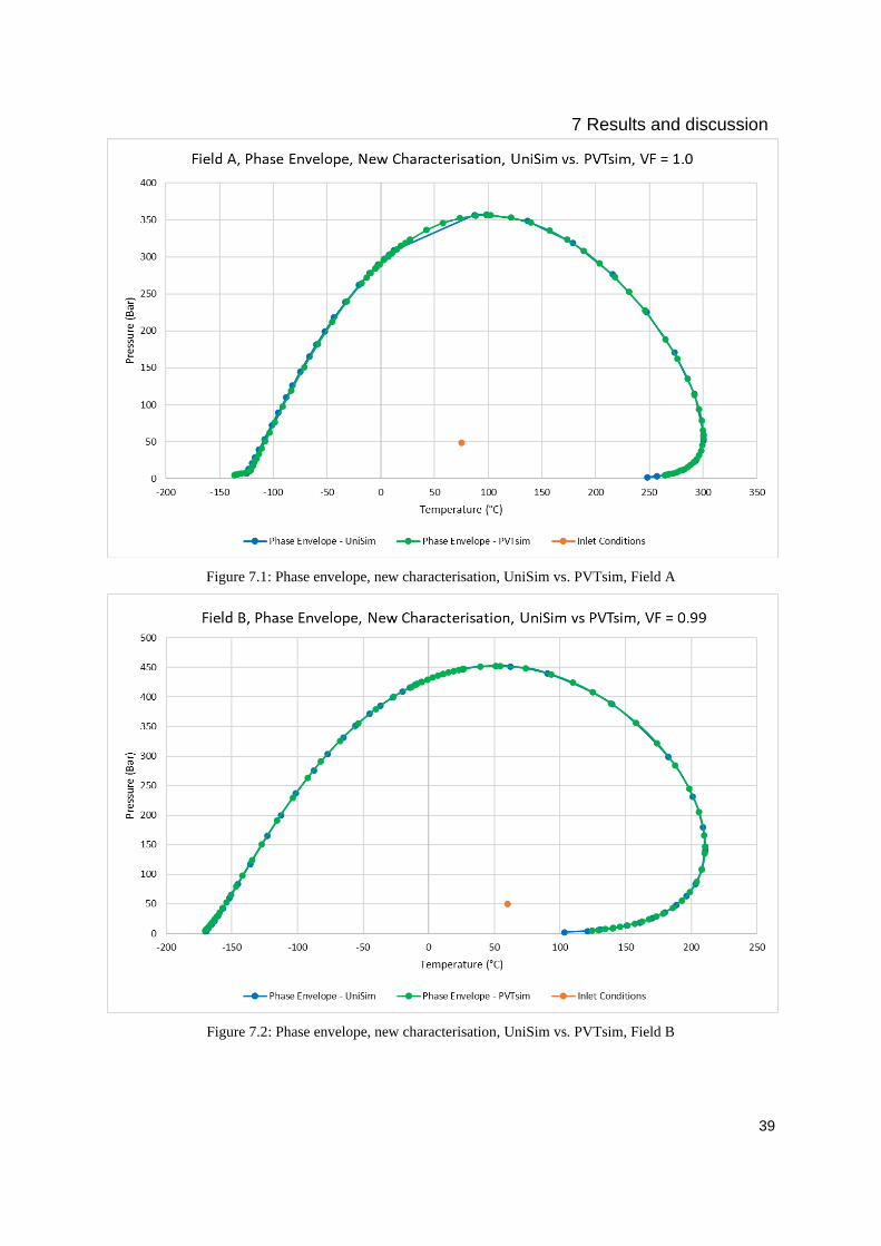
different fields are also included on the phase envelopes. Figure 7.1, Figure 7.2 and Figure
7.3 show the phase envelope comparison for field A, field B and field C, respectively.
7 Results and discussion
39
Figure 7.1: Phase envelope, new characterisation, UniSim vs. PVTsim, Field A
Figure 7.2: Phase envelope, new characterisation, UniSim vs. PVTsim, Field B

7 Results and discussion
40
Figure 7.3: Phase envelope, new characterisation, UniSim vs. PVTsim, Field C
The curves show that the phase envelope determined from PVTsim matches the phase
envelope determined from UniSim. This indicates that the new fluid characterisation is
incorporated correctly into the simulation model. The inlet conditions are inside the two-
phase area for all the fields.
For the old fluid characterisation, the component properties and the fluid composition are
different from the new characterisation. The phase envelopes for the old and new
characterisation are thus expected to deviate for the different fields. For the old
characterisation, a PVTsim analysis is not included. The phase envelopes are thus predicted
by UniSim. The phase envelopes from the UniSim model with the old characterisation is
compared to the predicted UniSim phase envelopes with new characterisation. The VF is 0.99
for all the fields specified in both the new and old model to get a comparable result. Inlet
conditions are also included in the figures. Figure 7.4, Figure 7.5 and Figure 7.6 show the
phase envelopes for the new and old characterisation for field A, field B and field C,
respectively.

7 Results and discussion
41
Figure 7.4: Phase envelope, new vs. old characterisation, UniSim, Field A
Figure 7.5: Phase envelope, new vs. old characterisation, UniSim, Field B

7 Results and discussion
42
Figure 7.6: Phase envelope, new vs. old characterisation, UniSim, Field C
The phase envelopes from the new and old characterisation deviate significantly from each
other. This indicates that the fluids from the new characterisation will not behave the same
way as the fluids with the old characterisation. This indicates that the results from the
different simulation models will deviate.
7.1.2 UniSim simulation results for new vs. old characterisation
The simulation is performed with the old and new fluid characterisation to evaluate the
predicted results and study the deviations. The results predicted by the UniSim models are the
oil and gas production (both total and for each field) and the estimated value for the oil
products from each field, and the total value. The result values are taken both from an all-in
simulation, meaning that all the fields are producing to the platform simultaneously, and from
standalone cases where one field is routed through the platform alone. Both standalone cases
and all-in are included to observe the commingling effect between the fields and see the
difference when the field is producing alone. This is done for both the new fluid
characterisation case and the old fluid characterisation case. The simulation results from the
standalone cases are shown in Table 7.1, and the simulation results with the all-in case are
shown in Table 7.2.

7 Results and discussion
43
Table 7.1: Standalone simulation results for all fields with new and old characterisation
Table 7.2: All-in simulation results for all fields with new and old characterisation
The oil production is given in Sm3/d, the gas production is given in MSm3/d, and the value is
given in MNOK/year. The new and old fluid characterisation predicts approximately the
same gas production (with the chosen unit) for all the fields and in total for both the
standalone cases and the all-in case.
For the oil production, field A and field C are getting less oil production with the new
characterisation compared to the old, while field B is getting more oil production with the
new characterisation than the old characterisation. For the value adjustment, field A is
predicted less value with the new characterisation, while field B and field C is gaining more
value with the new characterisation. These trends are current for both all-in simulation and
standalone cases.
Field B is gaining oil production when producing in an all-in simulation compared to
standalone. This means that the fluids from A and C are helping the fluids from B to go out in
the oil phase instead of the gas phase. For the C field and the A field, this is reversed with
more oil production on a standalone basis than all-in.
Standalone simulation Field A Field B Field C
Oil production, Sm3/d:
New characterisation 1148 2991 2747
Old characterisation 1163 2979 2749
Approximate deviation -15 11 -2
Gas production, MSm3/d:
New characterisation 2.1 9.6 0.3
Old characterisation 2.1 9.7 0.3
Approximate deviation 0.0 0.0 0.0
Value adjustment, MNOK/yr:
New characterisation 1301 3457 3067
Old characterisation 1310 3415 3020
Approximate deviation -9 42 47
All-in simulation Field A Field B Field C Total
Oil production, Sm3/d:
New characterisation 1130 3147 2557 6834
Old characterisation 1148 3121 2570 6839
Approximate deviation -18 26 -13 -6
Gas production, MSm3/d:
New characterisation 2.1 9.6 0.3 12.0
Old characterisation 2.1 9.7 0.3 12.1
Approximate deviation 0.0 -0.1 0.0 0.0
Value adjustment, MNOK/yr:
New characterisation 1297 3564 2959 7821
Old characterisation 1309 3509 2923 7741
Approximate deviation -11 55 36 80
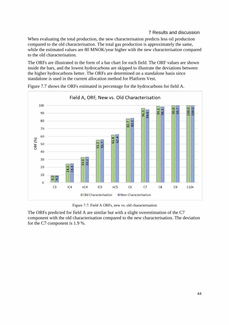
7 Results and discussion
44
When evaluating the total production, the new characterisation predicts less oil production
compared to the old characterisation. The total gas production is approximately the same,
while the estimated values are 80 MNOK/year higher with the new characterisation compared
to the old characterisation.
The ORFs are illustrated in the form of a bar chart for each field. The ORF values are shown
inside the bars, and the lowest hydrocarbons are skipped to illustrate the deviations between
the higher hydrocarbons better. The ORFs are determined on a standalone basis since
standalone is used in the current allocation method for Platform Vest.
Figure 7.7 shows the ORFs estimated in percentage for the hydrocarbons for field A.
Figure 7.7: Field A ORFs, new vs. old characterisation
The ORFs predicted for field A are similar but with a slight overestimation of the C7
component with the old characterisation compared to the new characterisation. The deviation
for the C7 component is 1.9 %.

7 Results and discussion
45
Figure 7.8 shows the ORFs estimated for field B.
Figure 7.8: Field B ORFs, new vs. old characterisation
The ORFs predicted for field B are similar but with an overestimation for the C7+
hydrocarbons with the old characterisation compared to the new. The highest deviation is
3.1% overestimation with the old characterisation compared to the new characterisation for
the C7 component.

7 Results and discussion
46
Figure 7.9 shows the ORFs estimated for field C.
Figure 7.9: Field C ORFs, new vs. old characterisation
The ORFs estimated for field C is the most similar when comparing the new and old
characterisation, with the highest deviation of 0.8 % for the iC5 component.
The consequence of keeping the old characterisation instead of switching to the new is 11
MNOK/year favouring field A, 55 MNOK/year less to field B and 36 MNOK/year less to
field C when looking at the all-in simulation case. The most crucial allocation principle is that
the allocation between the producers should always be as fair and prudent as possible. The
ORFs are also important parameters used for the current allocation agreement. Therefore, it is
important that this parameter is up to date and representative of the current fluids in
production. The new characterisation is based on newer test samples and is therefore seen as
the more up-to-date characterisation. Keeping the old characterisation will give different
values compared to the new characterisation; it is recommended to switch to the new
characterisation. The new characterisation will be used as a reference for correct allocation
results for Platform Vest for the following cases. The new characterisation simulation results
will be referred to as the initial/original results when compared to other cases.
7.2 Hypothetical components vs. UniSim allocation utility
UniSim offers a utility that gives the user the possibility to track a component from one input
stream to one outlet stream. This gives the possibility to use library components for the
lighter hydrocarbons where the fluid characterisation is estimated equally. The higher (C6+)
hydrocarbons often have varying characterisation depending on the field and will be defined
as hypothetical components like the initial case.
The results gained from an allocation utility in UniSim is the flow in either mass, mol or

7 Results and discussion
47
volume (no option to get the std volume flow). This reduces the opportunity to compare the
predicted results to the results from the initial case. The standalone ORFs are the only result
obtained from the UniSim simulation using the allocation utility method. The Appendix J –
Utility method in UniSim shows how the utility allocation is used and set up in the UniSim
model.
Figure 7.10, Figure 7.11 and Figure 7.12 show the ORFs estimated for field A, field B and
field C, respectively.
Figure 7.10: Field A ORFs, Hypo-method vs. Allocation utility
The ORFs predicted for field A are estimated slightly higher for the library components in the
utility allocation compared to the hypo-method. The highest deviation is 1.2% for the iC5
component. The higher hydrocarbons (C6+) are estimated approximately the same when
comparing the values from the two methods.
.

7 Results and discussion
48
Figure 7.11: Field B ORFs, Hypo-method vs. Allocation utility
The estimated ORFs for field B follow the same trend as the field A results, with slightly
higher predictions with the utility allocation compared to the hypo-method for the lower
hydrocarbons. The highest deviation is 1.0% for the iC5 component.

7 Results and discussion
49
Figure 7.12: Field C ORFs, Hypo-method vs. Allocation utility
The field C ORFs are estimated approximately the same for the two methods, with a slightly
higher value estimation for the allocation utility compared to the hypo-method. The highest
deviation is 0.6% for the iC5 component.
Comparing the results shows that field A is the field that has the highest deviation between
the allocation utility and the hypo-method. Overall, the results are very similar, with the
highest deviation being 1.2% for iC5 in field A. The negative with using the allocation utility
method is the limitation of the possible results. If ORFs are the only needed result for a
simulation, the utility method is a good enough method. The utility method is also timesaving
since the lower hydrocarbons can be added as library components.
7.3 Benzene in the fluid setup
This part of the result illustrates how the ORFs change when an aromatic is incorporated into
the well composition. The PVT analysis reports that approximately 1 wt.% of the well fluid is
aromatics, and this section will investigate how this will affect the results from the
simulations. Benzene is used as an aromatic for this case, and 1 wt.% of the total flow from
each field is the basis for the benzene flow. Benzene is added as a library component to the
fluid setup, and all other parameters are kept the same as in the initial simulation case.
7.3.1 Phase envelope with incorporated benzene to the fluid setup
Figure 7.13, Figure 7.14 and Figure 7.15 show the phase envelope for the initial case
compared to the phase envelope where benzene is added to the fluid setup for field A, field B
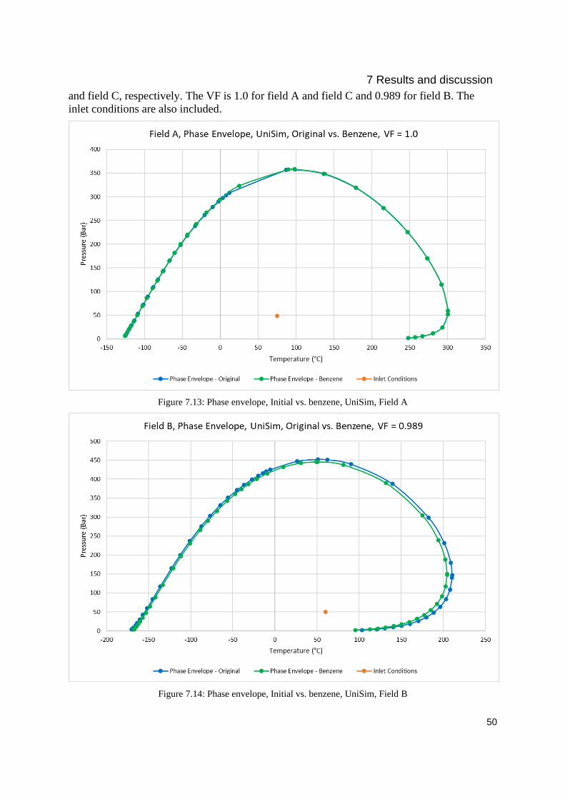
7 Results and discussion
50
and field C, respectively. The VF is 1.0 for field A and field C and 0.989 for field B. The
inlet conditions are also included.
Figure 7.13: Phase envelope, Initial vs. benzene, UniSim, Field A
Figure 7.14: Phase envelope, Initial vs. benzene, UniSim, Field B

7 Results and discussion
51
Figure 7.15: Phase envelope, Initial vs. benzene, UniSim, Field C
These results show similar phase envelop curves when comparing the initial case and the case
with benzene for field A and field C. The phase envelopes predicted for field B is slightly
deviation, indicating that the fluids in the different simulation models will behave slightly
deviating from each other.
7.3.2 UniSim simulation result with added benzene
The simulation results are based on standalone for the different fields to be able to get the
correct ORF values and be able to track the benzene to the different fields. Table 7.3 shows
the total estimated results for oil and gas production on a standalone basis.
Table 7.3: Standalone simulation results for all fields with the initial case and the benzene case
The gas production is estimated approximately the same for the two cases (with the given
unit MSm3/d), but the oil production with benzene is much higher than in the initial case.
This suggests that the benzene influences how much of the inlet fluid is going out in the oil
Standalone simulation Field A Field B Field C
Oil production, Sm3/d:
Initial case 1148 2991 2747
Benzene case 1182 3104 2776
Approximate deviation -34 -114 -28
Gas production, MSm3/d:
Initial case 2.1 9.6 0.3
Benzene case 2.1 9.6 0.3
Approximate deviation 0.0 0.0 0.0

7 Results and discussion
52
instead of the gas. Note that for this case, only 1 wt.% of benzene was added to the inlet
streams and gives high deviations in the resulting when comparing to the initial simulation
case. Field B has the highest deviation with 114 Sm3/d more oil production with benzene
added compared to the initial case.
Figure 7.16, Figure 7.17 and Figure 7.18 show the ORFs estimated for field A, field B and
field C, respectively.
Figure 7.16: Field A ORFs, Initial vs. benzene
The estimated ORFs for field A for the benzene case is noticeably higher than the initial case.
The highest deviation is 1.9 % higher ORF estimation for the C6 component.

7 Results and discussion
53
Figure 7.17: Field B ORFs, Initial vs. benzene
The estimated ORFs for field B with benzene is higher than the initial case. The most
significant deviation is 5.8 % for the C6 component.
Figure 7.18: Field C ORFs, Initial vs. benzene
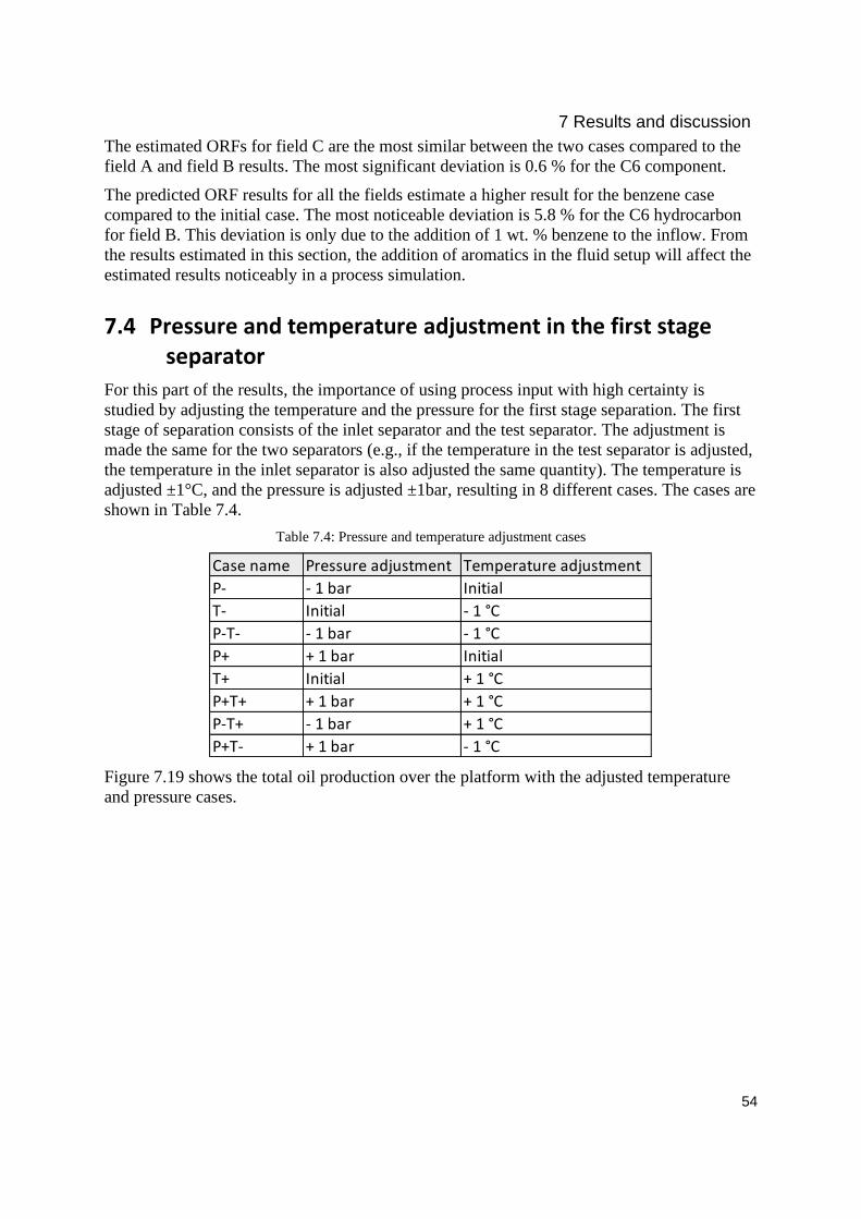
7 Results and discussion
54
The estimated ORFs for field C are the most similar between the two cases compared to the
field A and field B results. The most significant deviation is 0.6 % for the C6 component.
The predicted ORF results for all the fields estimate a higher result for the benzene case
compared to the initial case. The most noticeable deviation is 5.8 % for the C6 hydrocarbon
for field B. This deviation is only due to the addition of 1 wt. % benzene to the inflow. From
the results estimated in this section, the addition of aromatics in the fluid setup will affect the
estimated results noticeably in a process simulation.
7.4 Pressure and temperature adjustment in the first stage separator
For this part of the results, the importance of using process input with high certainty is
studied by adjusting the temperature and the pressure for the first stage separation. The first
stage of separation consists of the inlet separator and the test separator. The adjustment is
made the same for the two separators (e.g., if the temperature in the test separator is adjusted,
the temperature in the inlet separator is also adjusted the same quantity). The temperature is
adjusted ±1°C, and the pressure is adjusted ±1bar, resulting in 8 different cases. The cases are
shown in Table 7.4.
Table 7.4: Pressure and temperature adjustment cases
Figure 7.19 shows the total oil production over the platform with the adjusted temperature
and pressure cases.
Case name Pressure adjustment Temperature adjustment
P- - 1 bar Initial
T- Initial - 1 °C
P-T- - 1 bar - 1 °C
P+ + 1 bar Initial
T+ Initial + 1 °C
P+T+ + 1 bar + 1 °C
P-T+ - 1 bar + 1 °C
P+T- + 1 bar - 1 °C

7 Results and discussion
55
Figure 7.19: Total oil production, all T and P adjustments
The results show that the oil production is similar, but the P+T- case and the P-T+ case gives
the highest deviation with 17 Sm3/d. The result for gas production is not included due to
approximately the same predictions for all the cases.
Figure 7.20, Figure 7.21 and Figure 7.22 show some selected ORF estimations for field A,
field B and field C, respectively. These ORFs are selected due to having the highest deviation
compared to the ORFs for the other components.

7 Results and discussion
56
Figure 7.20: Field A ORFs, all T and P adjustments
The results show that the ORFs estimated for field A is similar, but the P+T- case deviates
the highest with 1.0 % for the nC4 and iC5 component compared to the initial case.
Figure 7.21: Field B ORFs, all T and P adjustments
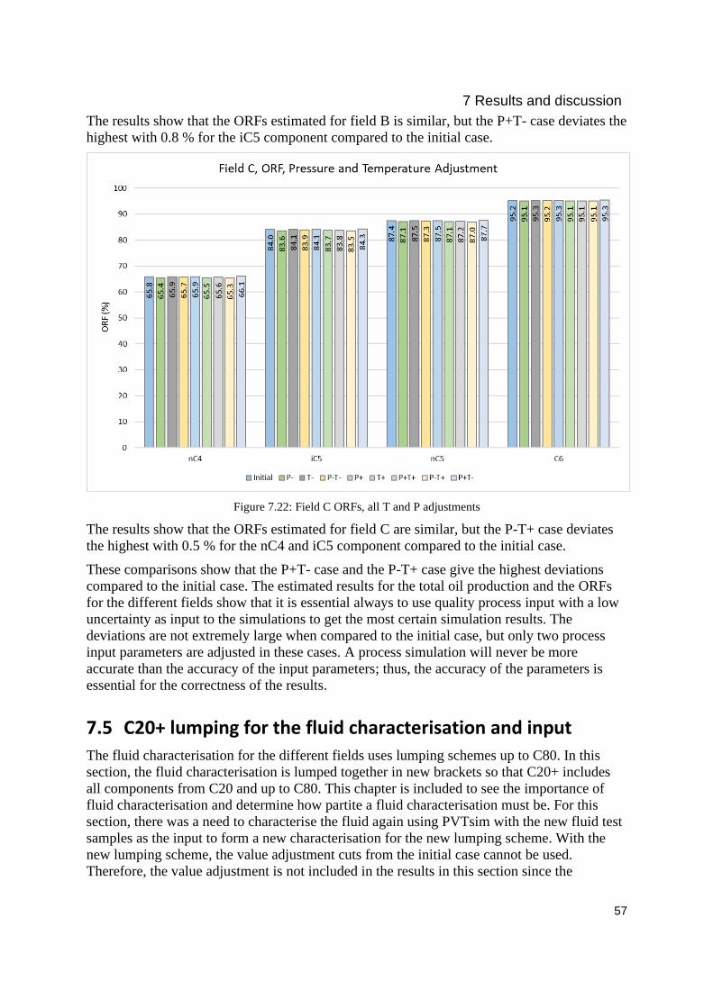
7 Results and discussion
57
The results show that the ORFs estimated for field B is similar, but the P+T- case deviates the
highest with 0.8 % for the iC5 component compared to the initial case.
Figure 7.22: Field C ORFs, all T and P adjustments
The results show that the ORFs estimated for field C are similar, but the P-T+ case deviates
the highest with 0.5 % for the nC4 and iC5 component compared to the initial case.
These comparisons show that the P+T- case and the P-T+ case give the highest deviations
compared to the initial case. The estimated results for the total oil production and the ORFs
for the different fields show that it is essential always to use quality process input with a low
uncertainty as input to the simulations to get the most certain simulation results. The
deviations are not extremely large when compared to the initial case, but only two process
input parameters are adjusted in these cases. A process simulation will never be more
accurate than the accuracy of the input parameters; thus, the accuracy of the parameters is
essential for the correctness of the results.
7.5 C20+ lumping for the fluid characterisation and input
The fluid characterisation for the different fields uses lumping schemes up to C80. In this
section, the fluid characterisation is lumped together in new brackets so that C20+ includes
all components from C20 and up to C80. This chapter is included to see the importance of
fluid characterisation and determine how partite a fluid characterisation must be. For this
section, there was a need to characterise the fluid again using PVTsim with the new fluid test
samples as the input to form a new characterisation for the new lumping scheme. With the
new lumping scheme, the value adjustment cuts from the initial case cannot be used.
Therefore, the value adjustment is not included in the results in this section since the

7 Results and discussion
58
comparison would not be legitimate. A detailed description of the C20+ characterisation is
given in Appendix K – C20+ fluid characterisation.
7.5.1 Phase envelope for the C20+ characterisation
The phase envelope from PVTsim is compared to the phase envelope from UniSim to assure
the quality of the proper UniSim setup for the C20+ simulation. The phase envelope for the
initial case is also included to see how it deviates from the phase envelope predicted for the
C20+ case. Figure 7.23, Figure 7.24 and Figure 7.25 show the phase envelops for field A,
field B and field C, respectively. The VF is 1.0 for field A and field C and 0.96 for field B.
The inlet conditions are also included in the figures.
Figure 7.23: Phase envelope, Initial vs. C20+, UniSim and PVTsim, Field A

7 Results and discussion
59
Figure 7.24: Phase envelope, Initial vs. C20+, UniSim and PVTsim, Field B
Figure 7.25: Phase envelope, Initial vs. C20+, UniSim and PVTsim, Field C
The curves show that the phase envelope determined from PVTsim for the C20+ lumping
scheme matches the phase envelope determined from the UniSim model with C20+ lumping.

7 Results and discussion
60
This indicates that the C20+ fluid characterisation is incorporated correctly into the C20+
simulation model. The inlet conditions are inside the two-phase area for all the fields.
The phase envelopes from the initial case and the C20+ case deviate significantly from each
other. This indicates that the fluids from the C20+ characterisation will not behave the same
way as the fluids in the initial case, resulting in possible deviations between the simulation
results.
7.5.2 UniSim results for the C20+ characterisation
The results given from the UniSim models are the oil and gas production, both total and for
each field. The results are estimated both from an all-in simulation and from the standalone
cases. The standalone cases and the all-in case are included to observe the commingling
effect between the fields and see the difference when the field is producing alone. This is
done for the C20+ case, which is compared to the initial case. The simulation result with the
standalone cases is shown in Table 7.5, and the simulation result with the all-in case is shown
in Table 7.6.
Table 7.5: Standalone simulation results for all fields with the initial case and the C20+ case
Table 7.6: All-in simulation results for all fields with the initial case and the C20+ case
The initial case and the C20+ case predict approximately the same gas production for all the
fields and in total with the standalone cases and the all-in case. For field A the estimated oil
production is approximately the same for both cases and simulations. Field B and field C
have a slightly lower oil prediction in the initial case compared to the C20+ case, with 2
Sm3/h and 7 Sm3/d difference, respectively. When evaluating the total production, the initial
case predicts less oil production compared to the C20+ case.
Standalone simulation Field A Field B Field C
Oil production, Sm3/d:
Initial case 1148 2991 2747
C20+ case 1148 2993 2754
Approximate deviation 0 -3 -6
Gas production, MSm3/d:
Initial case 2.1 9.6 0.3
C20+ case 2.1 9.6 0.3
Approximate deviation 0.0 0.0 0.0
All-in simulation Field A Field B Field C Total
Oil production, Sm3/d:
Initial case 1130 3147 2557 6834
C20+ case 1130 3148 2565 6843
Approximate deviation 0 -2 -7 -9
Gas production, MSm3/d:
Initial case 2.1 9.6 0.3 12.0
C20+ case 2.1 9.6 0.3 12.0
Approximate deviation 0.0 0.0 0.0 0.0

7 Results and discussion
61
The commingling effect for the C20+ case follows the same prediction as the initial case,
with higher oil prediction for field B with all-in, and higher predictions for field A and field C
with standalone simulation.
The simulation results show that the difference with using C20+ lumping instead of the initial
lumping does not give high deviations.
The ORFs are determined on a standalone basis and compared to the predicted ORF values in
the initial case.
Figure 7.26, Figure 7.27 and Figure 7.28 show the ORFs estimated for field A, field B and
field C, respectively.
Figure 7.26: Field A ORFs, C20+ lumping vs. initial case
The ORF estimates for field A predicts approximately the same values when comparing the
C20+ case with the initial case.

7 Results and discussion
62
Figure 7.27: Field B ORFs, C20+ lumping vs. initial case
The ORF estimates for field B predicts approximately the same values when comparing the
C20+ case with the initial case.
.

7 Results and discussion
63
Figure 7.28: Field C ORFs, C20+ lumping vs. initial case
The ORF estimates for field C predict similar values when comparing the C20+ case with the
initial case, but slightly more deviating than the deviations for field A and field B. The
highest deviation is 0.7 % for the iC4 component.
The results from the C20+ case shows that the estimates from the simulations and the ORFs
are very similar to the initial case, despite the phase envelopes dissimilarities.
7.6 C10+ lumping for the fluid characterisation and input
In this section, the fluid characterisation is lumped together in even fewer brackets so that
C10+ includes all components C10 and higher up to C80. This case is investigated since the
result with C20+ lumping showed very similar results to the initial case. This case is also
interesting since the C10+ characterisation is often a more easily obtained analysis than an in-
depth laboratory analysis for the total composition (which often is expensive). For this
section, there was also a need to characterise the fluid again using PVTsim with the new fluid
test samples as the input. A detailed description of the C10+ characterisation is given in
Appendix L – C10+ fluid characterisation.
7.6.1 Phase envelope for the C10+ characterisation
The phase envelope from PVTsim is compared to the phase envelope from UniSim to assure
the quality of the proper UniSim setup for the C10+ simulation. The phase envelope for the
initial case is also included to see how it deviates from the phase envelope predicted for the
C10+ case. Figure 7.29, Figure 7.30 and Figure 7.31 show the phase envelops for field A,
field B and field C, respectively. The VF is 1.0 for field A and field C and 0.88 for field B.

7 Results and discussion
64
The inlet conditions are also included for field A and field C but excluded from field B since
the inlet conditions are outside the phase envelope with the set vapour fraction.
Figure 7.29: Phase envelope, Initial vs. C10+, UniSim and PVTsim, Field A
Figure 7.30: Phase envelope, Initial vs. C10+, UniSim and PVTsim, Field B

7 Results and discussion
65
Figure 7.31: Phase envelope, Initial vs. C10+, UniSim and PVTsim, Field C
The curves show that the phase envelope determined from PVTsim for the C10+ lumping
scheme matches the phase envelope determined from the UniSim model with C10+ lumping.
This indicates that the C10+ fluid characterisation is incorporated correctly into the C10+
simulation model.
The phase envelopes from the initial case and the C10+ case deviate significantly from each
other. This indicates that the fluids from the C10+ characterisation will not behave the same
way as the fluids in the initial case, resulting in possible deviations between the simulation
results.
7.6.2 UniSim results for the C10+ characterisation
The results given from the UniSim models are the oil and gas production, both total and for
each field. The results are estimated both from an all-in simulation and from standalone
cases. Standalone cases and an all-in case are both included to observe the commingling
effect between the fields and see the difference when the field is producing alone. This is
done for the C10+ case, which is compared to the initial case. The simulation result with the
standalone cases is shown in Table 7.7, and the simulation result with the all-in case is shown
in Table 7.8.

7 Results and discussion
66
Table 7.7: Standalone simulation results for all fields with the initial case and the C10+ case
Table 7.8: All-in simulation results for all fields with the initial case and the C10+ case
The initial case and the C10+ case predict approximately the same gas production for all the
fields and in total with the standalone cases and the all-in case. For field A and field B, the
estimated oil production is slightly higher for the initial case compared to the C10+ case, with
3 Sm3/h and 12 Sm3/d difference, respectively. Field C has a slightly lower oil production
prediction for the standalone case when comparing the C10+ case to the initial case. In the
all-in simulation, the predicted oil production for field C is approximately the same, with 2
Sm3/h higher in the C10+ case.
The commingling effect for the C10+ case follows the same prediction as the initial case,
with higher oil prediction for field B with all-in and higher for field A and field C with
standalone.
The simulation results show that using C10+ lumping instead of the initial lumping the
deviations is not excessively high.
The ORFs are determined on a standalone basis and compared to the predicted ORF values in
the initial case.
Figure 7.32, Figure 7.33 and Figure 7.34 show the ORFs estimated for field A, field B and
field C, respectively.
Standalone simulation Field A Field B Field C
Oil production, Sm3/d:
Initial case 1148 2991 2747
C10+ case 1145 2980 2749
Approximate deviation 3 10 -2
Gas production, MSm3/d:
Initial case 2.1 9.6 0.3
C10+ case 2.1 9.6 0.3
Approximate deviation 0.0 0.0 0.0
All-in simulation Field A Field B Field C Total
Oil production, Sm3/d:
Initial case 1130 3147 2557 6834
C10+ case 1127 3134 2557 6819
Approximate deviation 3 12 0 15
Gas production, MSm3/d:
Initial case 2.1 9.6 0.3 12.0
C10+ case 2.1 9.6 0.3 12.0
Approximate deviation 0.0 0.0 0.0 0.0
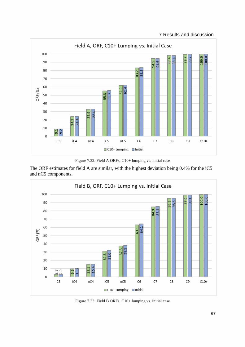
7 Results and discussion
67
Figure 7.32: Field A ORFs, C10+ lumping vs. initial case
The ORF estimates for field A are similar, with the highest deviation being 0.4% for the iC5
and nC5 components.
Figure 7.33: Field B ORFs, C10+ lumping vs. initial case

7 Results and discussion
68
The ORF estimates for the field B results are slightly more deviating than the A field ORF
result, with the most significant deviation for the C6 hydrocarbon at 1.1 %.
Figure 7.34: Field C ORFs, C10+ lumping vs. initial case
The ORF estimates for the C field are more deviating than the A and B field ORF result, with
the most significant deviation for the iC4 hydrocarbon with 2.1 %.
The results from the C10+ lumping case shows that the estimates are not too far from the
initial case but more divergent than the C20+ case results. The current allocation method for
Platform Vest is based on ORFs, meaning that the ORF estimate should be accurate.
On the other hand, a detailed laboratory analysis with a total lumping scheme is expensive;
thus, maybe an ORF estimation with C10+ lumping is sufficient for some allocations.
7.7 Future allocation in UniSim
Future allocation is the practice of allocating the predicted production to the different fields
over a period, often a few years or even longer, with commonly an allocation for each year in
the set period. It is necessary to perform future allocation as a foundation for the allocation
agreement that should be fair for all users. The future allocation is also important to estimate
the production and allocation in the future and better understand the commingling between
the different fields. The years allocated in the future allocation for this case are year 8, 10 and
12, and the profiles are given in Appendix M – Future allocation profiles. Estimates for gas,
oil, and water production, predicted GOR, inlet pressure and gas lift are given in the profile
for the selected years.
A few different methods can be used to match the simulation model to these predicted
estimates. For this scope, the predicted results for standalone simulation, all-in simulation and

7 Results and discussion
69
field A with field B will be evaluated for all three years. These are selected to evaluate how
the results change with different commingling and different approaches. The A with B field is
studied since the C field is the newest field on the platform; to estimate how the production
would be if field C were not routed through the platform.
For future allocation, the new characterisation with the initial lumping scheme is used.
7.7.1 Future allocation with tuning on the oil
One way to do the future allocation is to tune the inflow from each field to match the
predicted oil production from that specific field. This tuning is done on a standalone basis,
meaning that the tuning is done with no commingling between the different fields. This
tuning method is a chosen approach based on the assumption that the predicted profiles are
on a standalone basis. The tuned inflow for each field on a standalone basis is kept when
inserted into the all-in simulation case and the field A with field B simulation case. The
tuning is done on the oil instead of the gas; since the allocation method is ORF-based, it is
essential to have the estimated oil production as authentic to the actual case as possible.
Appendix M – Future allocation profiles give the profiles, and Appendix N – Future
allocation ORF result for year 10 and 12 gives complementary results that are not included in
the sections below.
Figure 7.35 shows the oil production for field A with the different simulation cases for the
three years.
Figure 7.35: Field A, Oil production, standalone, A with B and all-in
The results for field A show slightly lower oil production when field A is producing together
with the B field, and even lower when all fields are producing together. The oil production

7 Results and discussion
70
from field A is negatively impacted when producing with the B field and all-in. From the
decline in the oil production over the years from field A, it is noticeable that the production
from the A field is in the tail phase.
Figure 7.36 shows the oil production for field B with the different simulation cases for the
three years.
Figure 7.36: Field B, Oil production, standalone, A with B and all-in
The results for field B show slightly higher oil production when field A is producing together
with the B field, and even higher when all fields are producing together. The oil production
from field B is positively impacted when producing with the A field and all-in. From the
decline in the oil production from field B it is noticeable that the production from the B field
is declining, but the amount is over three times higher than the oil production from field A.

7 Results and discussion
71
Figure 7.37 shows the oil production for field C with the different simulation cases for the
three years.
Figure 7.37: Field C, Oil production, standalone, A with B and all-in
Field C shows higher oil production when field C is producing alone on the platform
compared to all-in. The oil production from field C is negatively impacted when producing
with all-in simulation. The oil production from field C increases from year 8 to year 12,
indicating a steady production.
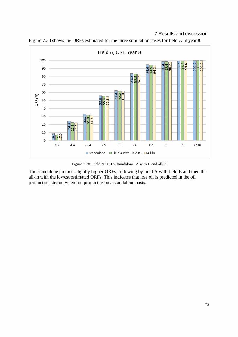
7 Results and discussion
72
Figure 7.38 shows the ORFs estimated for the three simulation cases for field A in year 8.
Figure 7.38: Field A ORFs, standalone, A with B and all-in
The standalone predicts slightly higher ORFs, following by field A with field B and then the
all-in with the lowest estimated ORFs. This indicates that less oil is predicted in the oil
production stream when not producing on a standalone basis.

7 Results and discussion
73
Figure 7.39 shows the ORFs estimated for the three simulation cases for field B in year 8.
Figure 7.39: Field B ORFs, standalone, A with B and all-in
The standalone predicts the lowest ORFs, following by field A with field B and then the all-
in case with the highest estimated ORFs. This indicates that more oil is predicted in the oil
production stream when producing with the other fields, compared to standalone.

7 Results and discussion
74
Figure 7.40 show the ORFs estimated for the two simulation cases for field C in year 8.
Figure 7.40: Field C ORFs, standalone and all-in
The standalone predicts a shockingly high ORF estimate compared to the all-in case for field
C. This indicates that a lot more oil is predicted in the oil production stream when producing
standalone than all-in with the other fields.
Field C is a low GOR field, indicating that the field contains a higher oil to gas ratio
compared to the other fields. When a low GOR field coproduces with a high GOR field, the
high amount of gas will prevent oil products from the low GOR field to go out in the oil
production stream.
Field A (medium GOR) and Field C (low GOR) are the two fields negatively impacted fields
when producing all-in compared to standalone for the oil production. Field B (high GOR) is
the only field with a better oil production estimate with all-in simulation compared to
standalone simulation. This is due to the oil components from field A and field C attracting
the oil from field B, making more of it go out in the oil production stream.
The ORF results show the same trend for all three years. ORFs for year 8 are presented
below, while ORFs for year 10 and 12 can be seen in Appendix N – Future allocation ORF
result for year 10 and 12.
7.7.2 Year 8 with GOR tuning
The GOR (Gas-oil-ratio) is another parameter that can be tuned to match the predicted GOR
for the different years. In this method the inlet flow and composition are adjusted for each
field to match the GOR prediction for the production. A new UniSim model is built to predict

7 Results and discussion
75
this new composition and inflow. A detailed description of how the model is built and how it
works can be found in Appendix O – UniSim GOR model.
The estimated ORFs are predicted for year 8 for the standalone approach for the three fields.
These ORFs are compared to the ORFs estimated with the standalone oil tuning method done
in Chapter 7.7.1.
Figure 7.41 shows the field A standalone ORFs estimated for two methods in year 8
Figure 7.41: Field A, standalone ORFs, oil tuned vs. GOR tuned
The oil tuning method predicts higher ORFs compared to the GOR tuning method for field A.

7 Results and discussion
76
Figure 7.42 shows the field B standalone ORFs estimated for the two methods in year 8.
Figure 7.42: Field B, standalone ORFs, oil tuned vs. GOR tuned
The ORFs show similar values for the oil tuning compared to the GOR tuning for field B.

7 Results and discussion
77
Figure 7.43 shows the field C standalone ORFs estimated for two methods for year 8.
Figure 7.43: Field C, standalone ORFs, oil tuned vs. GOR tuned
The oil tuning method predicts higher ORFs compared to the GOR tuning method for field C.
The low and mediate GOR fields A and C predict a lower ORF estimate with the GOR tuning
method compared to the oil tuning method. The high GOR field B estimates similar ORFs
when comparing the two tuning methods.
GOR tuning is a method that can be used when the composition is uncertain, estimated from
old samples, or if the predicted GOR value is more valid than other tuning parameters.
7.7.3 Year 8 with gas tuning
Instead of tuning the model to the oil production, it can be tuned to match the predicted gas
production. This tuning is done the same way as the oil tuning method, on a standalone basis.
The ORFs are predicted and compared to the estimated ORFs from the oil tuning method.
Figure 7.44, Figure 7.45 and Figure 7.46 show the standalone ORFs estimated for the two
methods in year 8 for field A, field B and field C, respectively.

7 Results and discussion
78
Figure 7.44: Field A, standalone ORFs, oil tuned vs. gas tuned
Figure 7.45: Field B, standalone ORFs, oil tuned vs. gas tuned

7 Results and discussion
79
Figure 7.46: Field C, standalone ORFs, oil tuned vs. gas tuned
Field A and field B have similar ORF predictions when comparing the results from the two
tuning methods. For field C gas tuning method estimates slightly higher ORFs compared to
the oil tuning method. The highest deviation is 1.9 % for the iC4 and nC4 components.
The differences between the oil tuning method and gas tuning methods are because the
simulations are only tuned to match one of the phases. In the oil tuning method, the predicted
gas is not matched, and for the gas tuning method, the predicted oil is not matched. Since
ORF values are essential for the current allocation agreement, the tuning on the predicted oil
is deemed more correct than tuning on the predicted gas.
7.8 ProMax vs. UniSim for Platform Vest reallocation
For this comparison part, a ProMax model was developed with the new fluid characterisation
as input. The result from the ProMax simulation case is compared to the UniSim simulation
case with the new characterisation, also called the initial case. A detailed description of how
the model is made is given in Appendix P – Building the ProMax model.
7.8.1 Phase envelope prediction
Figure 7.47, Figure 7.48 and Figure 7.49 show the phase envelope estimated by UniSim and
Promax for field A, field B and field C, respectively. The VF is set to 1.0 for field A and field
C and 0.97 for field B. The inlet conditions are also included in the figures.

7 Results and discussion
80
Figure 7.47: Phase envelope, UniSim vs. ProMax, Field A
Figure 7.48: Phase envelope, UniSim vs. ProMax, Field B

7 Results and discussion
81
Figure 7.49: Phase envelope, UniSim vs. ProMax, Field C
The phase envelopes for ProMax are predicted differently than the phase envelopes from
UniSim. The phase envelopes deviate significantly from each other, indicating that the fluids
in the ProMax model will not behave the same way as the fluids in the UniSim model,
resulting in possible deviations between the simulation results.
7.8.2 Oil and gas prediction
The oil and gas production (both total and for each field), the estimated value for the oil
products from each field and total, and the ORFs for each field are compared. The results are
predicted from an all-in simulation, meaning that all the fields are producing to the platform
simultaneously. The ORFs are estimated from standalone simulations. The all-in simulation
results are shown in Table 7.9.
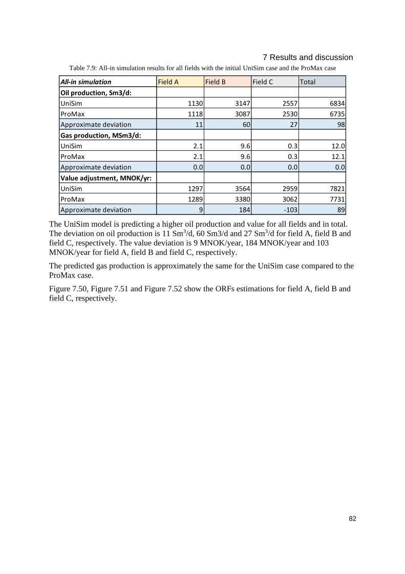
7 Results and discussion
82
Table 7.9: All-in simulation results for all fields with the initial UniSim case and the ProMax case
The UniSim model is predicting a higher oil production and value for all fields and in total.
The deviation on oil production is 11 Sm3/d, 60 Sm3/d and 27 Sm3/d for field A, field B and
field C, respectively. The value deviation is 9 MNOK/year, 184 MNOK/year and 103
MNOK/year for field A, field B and field C, respectively.
The predicted gas production is approximately the same for the UniSim case compared to the
ProMax case.
Figure 7.50, Figure 7.51 and Figure 7.52 show the ORFs estimations for field A, field B and
field C, respectively.
All-in simulation Field A Field B Field C Total
Oil production, Sm3/d:
UniSim 1130 3147 2557 6834
ProMax 1118 3087 2530 6735
Approximate deviation 11 60 27 98
Gas production, MSm3/d:
UniSim 2.1 9.6 0.3 12.0
ProMax 2.1 9.6 0.3 12.1
Approximate deviation 0.0 0.0 0.0 0.0
Value adjustment, MNOK/yr:
UniSim 1297 3564 2959 7821
ProMax 1289 3380 3062 7731
Approximate deviation 9 184 -103 89

7 Results and discussion
83
Figure 7.50: Field A ORFs, ProMax vs. UniSim
The ORFs predicted for field A in ProMax are slightly higher than the UniSim ORFs. With
the highest deviation being 3.2 % for the C7 component.
Figure 7.51: Field B ORFs, ProMax vs. UniSim

7 Results and discussion
84
The ORFs predicted for field B in the ProMax model is estimated higher than the ORFs for
the UniSim model. With the highest deviation being 8.2 % for the C7 component.
Figure 7.52: Field C ORFs, ProMax vs. UniSim
The ORFs predicted for field C in the ProMax model is estimated higher than the ORFs for
the UniSim model. With the highest deviation being 2.5 % for the C3 component.
The comparison results between the two simulation models show differences, especially
when looking at the estimated value and oil production. The ORFs are also important
parameters used in the current allocation agreement, and it is essential that these parameters
are representative.
The discussion on which of the simulation tools gives the most correct estimations is not
clear. The ProMax creators claim that the thermodynamic is more correct when creating a
mixed-species instead of using hypothetical components. The result clearly shows that there
are differences when using the two models, even when the input is supposed to be the same.
The procedure for definition hypothetical components (single oils) in ProMax is to use the
molecular weight and the specific gravity as input and let the software calculate the other
properties based on that. The set procedure for defining hypothetical components in UniSim
is to trust the total fluid characterisation given from the PVTsim analysis and use these
parameters as input. The question then is if the properties calculated from ProMax are more
correct than the properties from PVTsim. To get a clear conclusion on the topic on which
simulation tool is the most correct, there is a need for further analyses.

7 Results and discussion
85
7.9 Different allocation methods
Year 8 from future allocation is used as a base for the comparison of the different allocation
methods. The equity-based allocation is not included since the total number of different
companies with ownership in the different fields is high. The uncertainty-based allocation is
also not studied since the accuracy of the parameters is not measured or given. The methods
looked more into in this section are the allocation by difference and the pro-rata allocation.
The measurement values for the allocation are given in Table 7.10.
Table 7.10: Results from the year 8 simulations on a mass basis
7.9.1 The ORF method (the current allocation agreement)
The calculation for the ORF method is done following the formulas (3.3) to (3.9). The results
are given in Table 7.11.
Table 7.11: Allocated quantity with ORF method
7.9.2 Allocation by difference
For the Platform Vest case, the C field was the last field to produce from the Platform. This
field is therefore chosen as the field to be allocated by difference. Field A and field B will be
allocated first, and then the rest is assumed to be from field C. The formula used for the
allocation is (3.1). The result from the by difference allocation is given in Table 7.12.
Table 7.12: Allocated quantity with by difference method
7.9.3 Pro-rata allocation
The pro-rata allocation is calculated using (3.2). The result from this allocation method is
given in Table 7.13.
Table 7.13: Allocated quantity with pro-rata allocation method
Field A (Standalone) Field B (Standalone) Field C (Standalone) Commingled (All-in)
Dry feed rate, (ton/d): 2307.5 12045.5 1233.6 15586.6
Typical produced gas, (ton/d): 1586.4 9271.9 127.7 11012.0
Typical produced oil, (ton/d): 721.2 2773.7 1106.6 4575.3
Field A Field B Field C
Typical produced gas, (ton/d): 1586.4 9291.1 134.5
Typical produced oil, (ton/d): 721.2 2755.0 1099.2
Field A Field B Field C
Typical produced gas, (ton/d): 1586.4 9271.9 153.8
Typical produced oil, (ton/d): 721.2 2773.7 1080.4
Field A Field B Field C
Typical produced gas, (ton/d): 1590.1 9293.9 128.0
Typical produced oil, (ton/d): 717.1 2757.9 1100.3

7 Results and discussion
86
7.9.4 Allocation by process simulation
The simulation model used is all-in year 8 in UniSim. The result from this allocation method
is given in Table 7.14.
Table 7.14: Allocated quantity with all-in simulation allocation method
7.9.5 Allocation method results
Illustrations of the result with the different allocation methods are given in the figures below.
Figure 7.53, Figure 7.54 and Figure 7.55 show the allocated oil and gas production for field
A, B and C, respectively. The y-axis for all the figures has the same range of 120 ton/d for oil
production and 100 ton/day for gas production. The green column illustrates the input values
used for the allocation obtained from standalone simulations.
Figure 7.53: Field A, Allocation methods, Gas and oil production
For field A, the different allocation methods predict similar values for both gas production
and oil production. The highest allocated value for the oil production is 721 ton/day (by
difference and ORF method) and the lowest is 713 ton/day (all-in simulation), resulting in a
deviation of 7 ton/day when comparing the methods. For the gas production allocation, the
highest value is 1595 ton/day (all-in simulation) and the lowest is 1586 ton/day (by difference
and ORF method), resulting in a deviation of 9 ton/day when comparing the methods. For
field A, the allocation method that gives the highest prediction, and the prediction equal to
the input values, are the by difference allocation and ORF method.
Field A Field B Field C
Typical produced gas, (ton/d): 1594.9 9213.5 203.7
Typical produced oil, (ton/d): 712.7 2832.3 1030.4

7 Results and discussion
87
Figure 7.54: Field B, Allocation methods, Gas and oil production
For field B, the different allocation methods predict deviating values for both gas production
and oil production. The highest allocated value for the oil production is 2832 ton/day (all-in
simulation) and the lowest is 2755 ton/day (ORF method), resulting in a deviation of 77 ton/d
when comparing the methods. For the gas production allocation, the highest value is 9294
ton/day (pro-rata allocation) and the lowest is 9213 ton/day (all-in simulation), resulting in a
deviation of 81 ton/day when comparing the methods. For field B, the allocation method that
gives predictions like the input values is the by difference allocation followed by the ORF
method and the pro-rata allocation.
Figure 7.55: Field C, Allocation methods, Gas and oil production
For field C, the different allocation methods predict deviating values for both gas production
and oil production. The highest allocated value for the oil production is 1100 ton/day (pro-
rata allocation) and the lowest is 1030 ton/d (all-in simulation), resulting in a deviation of 70
ton/day when comparing the methods. For the gas production allocation, the highest value is
204 ton/day (all-in simulation) and the lowest is 128 ton/day (pro-rata allocation), resulting in
a deviation of 76 ton/day when comparing the methods. For field C, the allocation method
that gives predictions closest the input values are the pro-rata allocation followed by the ORF
method.
The results from the comparison between the different allocation methods show that there are
significant differences depending on which method that is used. The results from field A give
similar allocation values for the different methods, while the results from field B and field C
deviate considerably.

7 Results and discussion
88
The GOR values for the different fields are also essential to consider when selecting an
allocation method for the platform. The all-in simulation method gives a much higher oil
production to field B than any other methods and much lower oil production to field C than
the other methods. For the gas production, this trend is reversed with a much lower prediction
with the all-in simulation for field B and higher with the all-in simulation for field C. The all-
in simulation method for allocation is thus not a suitable allocation method for Platform Vest.
The by difference allocation predicts similar values to the input values for field A and field C
but deviates considerably for field C. The allocation by difference is thus not optimal for
Platform Vest. Then the ORF method and the pro-rata allocation method remains.
The input values are obtained from standalone simulations for the fields, making it not
reasonable that these input values are accurately representative when all the fields are
producing together. For field C, the pro-rata allocation predicts the same values as the input
values for gas production. When considering that field C is a low GOR field, the realistic gas
production would be a little higher than the standalone prediction. For gas production, the
ORF method and the pro-rata allocation predicts approximately the same oil allocation. This
results in the ORF method being the fairest for field C.
For field B, the pro-rata allocation and the ORF method are approximately equally deviation
compared to the input values, making both methods applicable for allocation for the field.
Based on the evaluation of the different allocation methods, the current ORF method is the
most fair and prudent allocation on Platform Vest when considering all the fields.
The evaluation is only based on and concluded for the result for year 8. When selecting an
allocation method, a complete conclusion cannot be made until predictions are calculated for
more years to study the future and historically production trends.
The calculations for the results are given in Appendix Q – Allocation methods calculation.
7.10 Recommended guideline for allocation simulation
The recommended guideline for allocation simulation based on the results in this report can
be summarised in the following points.
• Always use the newest fluid characterisation to assure a fair and prudent allocation.
• The allocation utility in UniSim is good enough if the only needed output is the ORFs.
• Aromatics in the fluid setup can impact the allocation, but this needs to be
investigated further to see the full effect.
• C20+ lumping scheme gives insignificant deviation compared to the original lumping
scheme. This new lumping scheme can be used instead of the original without
noticeable deviations.
• The PVT analysis for a C10+ lumping is much cheaper compared to a finer lumping
scheme analysis. When only comparing the estimated ORFs, the deviation between
the C10+ case and the initial case is not too large. In comparison, the results between
the new and old characterisation gave a much higher deviation. This indicates that it is
better to use C10+ lumping than to keep an old fluid characterisation.

7 Results and discussion
89
• Future allocation can be done with different tuning methods.
The GOR tuning method is preferred if the fluid composition is uncertain or the GOR
value is the most valid estimated value for the different fields.
Tuning to match the estimated oil production is preferred if the allocation is
dependent on accurate oil simulation. This is the case for Platform Vest, where ORF
is the current allocation agreement.
Tuning to match the estimated gas production is preferred if the allocation is
dependent on accurate gas simulation. This is not the case for Platform Vest.
• Allocation simulation using ProMax compared to UniSim gave noticeable deviations.
The decision on which simulation software is the most correct needs to be researched
more thoroughly before a conclusion regarding the different simulation software can
be made.
• When looking at the different allocation methods, the most significant deviation
between the methods occurred for the high GOR field B and the low GOR field C.
For field A the allocation methods were not too deviating.
• Based on evaluations of the different allocation methods, the current ORF method is
the most fair and prudent allocation on Platform Vest for all fields.
8 Conclusion
90
8 Conclusion Allocation simulation is a complex and complicated process, where the most crucial aspect is
to get the allocation as fair and prudent as possible. The possible allocation methods depend
on the different fields, the production platform and the owners and users. Many different parties
shall be satisfied with the established allocation method.
Platform Vest is a platform with production from three fields, where each field has different
owners. Field A is the original field on the platform, and it is important that this field is not
negatively impacted by allowing production from other fields through the same platform.
However, the allocation cannot be biased towards the A field either. The allocation method
needs to be unbiased towards all involving parties but also fair and prudent.
When comparing the different allocation methods, the current established ORF method was the
method that gave the fairest allocation of gas and oil to the different fields, especially when
considering the different GOR values of the fields. If any of the other methods were to be used,
at least one field would get an unfair allocation with either too low predictions or too high
predictions.
For future allocation, the tuning method recommended when the allocation method is ORF
based is to tune to match the predicted oil production.
Predicting the ORFs for the allocation should be as close to the initial case as possible. The
result from this report ranks the ORF deviation from highest to lowest, with the highest
occurred when incorporating benzene to the fluid inflow (5.8 %), followed by using the old
characterisation (3.1 %), using the C10+ lumping (2.1 %), allocation utility method (1.2 %),
adjusting the process input for the first stage separation (1.0 %) and lastly using the C20+
lumping (0.7 %).
The deviation between the predicted ORF in ProMax and UniSim was 8.2 %, but the conclusion
on which software is the most correct needs to be further analysed to obtain a fair decision.
The addition of benzene to the inflow gave the most significant deviation if the ProMax
comparison is disregarded. PNA in the fluid characterisation should thus be further investigated
to determine the impact this can have on the allocation.
To summarise, the newest fluid characterisation should always be used when possible. The
C20+ lumping and the allocation utility method can safely be used with approximately the
same result as the initial case if only the ORFs are the required result. The process input should
always be representative of the actual case to get the most up-to-date simulation for the
allocation. The C10+ lumping scheme can be considered without too large deviations for the
ORFs when a complete fluid analysis is not created and acquired.
In conclusion, for Platform Vest the most fair and prudent allocation method for all fields is
the current allocation method using standalone ORFs achieved from process simulations.

References
91
References [1] S. Chakrabarti, Handbook of Offshore Engineering, Illinois: Elsevier Science &
Technology, 2005.
[2] S. Kanshiro, “A review of hydrocarbon allocation methods in the upstream oil and gas
industry,” Journal of Petroleum Science and Engineering, volume 184, January 2020.
[Online]. Available: doi: 10.1016/j.petrol.2019.106590
[3] J. H. Johnsen. “Gass- og kondensatbehandling.” ndla.
https://ndla.no/nb/subject:6/topic:1:182061/topic:1:151959/resource:1:157189/346?filters=ur
n:filter:01c27030-e8f8-4a7c-a5b3-489fdb8fea30 (accessed Mar. 3, 2021).
[4] A. Aabø. “Drivmekanismer i reservoaret.” ndla.
https://ndla.no/subject:6/topic:1:182061/topic:1:155237/resource:1:153039?filters=urn:filter:
01c27030-e8f8-4a7c-a5b3-489fdb8fea30 (accessed Mar. 5, 2021).
[5] J. Lavis. “What’s the difference between gas lift and gas injection.” Drillers.
https://drillers.com/whats-difference-gas-lift-gas-injection/ (accessed Mar. 5, 2021).
[6] Equinor, Field information for A, B and C, Jan. 2021.
[7] L. V. Lidal. “Gassløft og kjemikalieinjeksjon.” ndla.
https://ndla.no/subject:6/topic:1:182061/topic:1:151959/resource:1:181801?filters=urn:filter:
01c27030-e8f8-4a7c-a5b3-489fdb8fea30 (accessed Mar. 5, 2021).
[8] NORSOK STANDARD, Design principles: coding system, Jan. 1995.
[9] S. Mokhatab, W. A. Poe and J. Y. Mak, Handbook of Natural Gas Transmission and
Processing: Principles and Practices, 4th ed. Oxford: Elsevier Science & Technology, 2018.
[Online]. Available:https://ezproxy1.usn.no:2452/lib/ucsn-
ebooks/reader.action?docID=5560017
[10] Bryan Research & Engineering, ProMax, version 5.
[11] The Energy Institute (EI), "Guidelines for the allocation of fluid streams in oil and gas
production," London, England, 1st ed. 2012
[12] Equinor, Mail correspondence with uncertainties, Mar. 2021.
[13] E. Åbro et al. “Experience with the multiphase meter system used for allocation of
Visund South tie-in to Gullfaks C.” [Online]. Available: https://nfogm.no/wp-
content/uploads/2019/02/2015-25-Experiences-with-the-multiphase-meter-system-
%C3%85bro-Statoil.pdf (accessed April. 7, 2021).
[14] Equinor, Provided current allocation method for Platform Vest, Jan. 2021.
[15] R.M. Felder and R. W. Rousseau, Elementary principle of chemical processes, 3rd ed.
New Jersey; Wiley, 2005.
[16] J.N. Jaubert, R. Privat, Y.L. Guennec and L. Coniglio, “Note on the properties altered by
application of a Peneloux-type volume translation to an equation of state”, Fluid Phase
Equilibria, vol. 419, pp. 88-95, 2016. [Online]. Available: doi: 10.1016/j.fluid.2016.03.012
[17] Equinor. Provided fluid analysis reports for field A, B and C. Jan. 2021.

References
92
[18] E. Skouras, “Thermodynamics in Gas Processing – Phase Envelope Predictions and
Process Design,” presented at 1st Trondheim Gas Technology Conference, Trondheim,
Norway, 21-22 October 2009. [Online]. Available:
https://www.sintef.no/globalassets/upload/energi/arrangementer/tgtc09/a4_1_skouras.pdf
[19] J. M. Campbell, Gas conditioning and processing: volume 1: The basic principles, 7th ed.
Oklahoma: Campbell Petroleum Series, 1992.
[20] Norges bank. “Exchange rates.” https://www.norges-
bank.no/en/topics/Statistics/exchange_rates/?tab=currency&id=USD (accessed Mar. 3, 2021)
[21] Markets insider. “Naphthapreis (European).”
https://markets.businessinsider.com/commodities/naphthapreis (accessed Mar. 3, 2021)
[22] Commodity3. “Jet Fuel Kerosene in US$/mt.”
https://www.commodity3.com/swaps/7/jet-fuel-kerosene-in-us$-mt (accessed Mar. 3, 2021)
[23] Kurzycz. “Gas oil.” https://eng.kurzy.cz/commodities/gas-oil-price-development-chart/
(accessed Mar. 3, 2021)
[24] Equinor, Provided calculation example, Jan. 2021.
[25] Honeywell International Inc., UniSim, Version R460.2.

Appendices
93
Appendices
Appendix A – Scope of work
Appendix B – PVTsim procedure
Appendix C – Old fluid characterisation
Appendix D – New fluid characterisation
Appendix E – UniSim model
Appendix F – Process equipment input
Appendix G – Inflow data for reallocation
Appendix H – ProMax model
Appendix I – Building the UniSim model
Appendix J – Utility method in UniSim
Appendix K – C20+ fluid characterisation
Appendix L – C10+ fluid characterisation
Appendix M – Future allocation profiles
Appendix N – Future allocation ORF result for year 10 and 12
Appendix O – UniSim GOR model
Appendix P – Building the ProMax model
Appendix Q – Allocation methods calculation

Appendices
94
Appendix A – Scope of work
Faculty of Technology, Natural Sciences and Maritime Sciences, Campus Porsgrunn
FMH606 Master's Thesis
Title: Recommended guideline for allocation simulation USN supervisor: Britt M. E. Moldestad External partner: Equinor ASA, Trine Amundsen Madsen Task background: Oil and gas fields are typically owned by different companies. To determine the quantity and quality of the feed and product stream belonging to each user/partner, the oil and gas product are allocated between the partners. Allocation simulations are performed to allocate the values between partners for ongoing production, and for evaluating commingling effects for new tie-ins fields to define the allocation method fair and prudent for all producers. Allocation simulation are important for all oil and gas companies, and Equinor allocate for 50 billion NOK every month. Task description:
A recommended guideline for allocation includes evaluation from fluid sampling, fluid characterization, process simulation and evaluation. The following scope are recommended: 1. What is allocation and what are the basic allocation principles?
2. Evaluate PVT description of different wells. How are PVT samples taken and measured?
3. Evaluate the fluid characterization and the EOS model prediction for component properties, and the transfer from PVTsim to the process simulation tool.
4. Evaluate the overall uncertainties in allocation simulation. Compare UniSim process simulation tool to ProMax process simulation tool for allocation simulations for different fields. Data from fields will be provided and case study to be performed. Evaluate the different allocation methods.
5. Summarize the findings in a report and recommend a guideline for allocation simulation.
Student category: EET, Madelen Smedsli The task is suitable for online students (not present at the campus): No

Appendices
95
Practical arrangements:
The Covid-19 pandemic effects the location of workplace. There is unfortunately no capacity at the local Equinor office due to regulations. The work will be carried out at the University or home office with close collaboration with supervisor via Teams.
Software’s to be used depend on the availability for the student. Unisim/Aspen Hysys and ProMax (to checked) will be used during this study. If access to PVTsim, this tool will also be used to evaluate fluid characterization. If no access, the evaluation will be carried out in collaboration with supervisor.
Supervision:
As a general rule, the student is entitled to 15-20 hours of supervision. This includes necessary time for the supervisor to prepare for supervision meetings (reading material to be discussed, etc).
Signatures:
17.02.21
Britt M. E. Moldestad, USN Supervisor, date
18.02.21
Trine A. Madsen, External Supervisor, date
17.02.21
Madelen Smedsli, Student, date

Appendices
96
Appendix B – PVTsim procedure The PVTsim procedure is described as follows:
1) When opening PVTsim, the software opens as the following figure.
2) When defining the EOS as SRK Peneloux, click on new plus fluid and the following
page will open:

Appendices
97
3) The input to the figure above is found from the analysis reports (not added as an
appendix due to confidentiality). The input is mol % or weight % (from N2 to C36+
for field A, and from N2 to C10+ for field B and C), the mol weight (from N2 to C10)
and the density (C6 to C10). The Cn is extended to 36 as shown above (for all field).
4) The lumping scheme is defined in the lumping fane as illustrated in the figure below
(for field A):

Appendices
98
5) Click the OK button, and the following output is given:

Appendices
99
6) The figure above is the new fluid characterisation for field A.
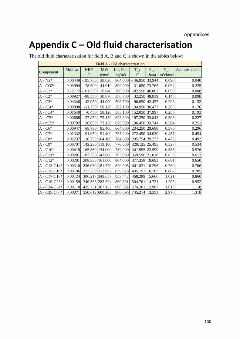
Appendices
100
Appendix C – Old fluid characterisation The old fluid characterisation for field A, B and C is shown in the tables below:
Molfrac NBP MW Liq Den T_c P_c V_c Acentric factor
- C g/mol kg/m3 C bara m3/kmol -
A - N2* 0.00449 -195.750 28.020 804.000 -146.950 33.944 0.090 0.040
A - CO2* 0.03994 -78.500 44.010 809.000 31.050 73.765 0.094 0.225
A - C1* 0.72172 -161.550 16.040 300.000 -82.550 46.002 0.099 0.008
A - C2* 0.08927 -88.550 30.070 356.700 32.250 48.839 0.148 0.098
A - C3* 0.04346 -42.050 44.090 506.700 96.650 42.455 0.203 0.152
A - iC4* 0.00898 -11.750 58.120 562.100 134.950 36.477 0.263 0.176
A - nC4* 0.01640 -0.450 58.120 583.100 152.050 37.997 0.255 0.193
A - iC5* 0.00688 27.850 72.150 623.300 187.250 33.843 0.306 0.227
A - nC5* 0.00792 36.050 72.150 629.900 196.450 33.741 0.304 0.251
A - C6* 0.00947 68.750 85.400 664.800 234.250 29.688 0.370 0.296
A - C7* 0.01332 91.950 91.400 737.200 272.490 34.020 0.457 0.454
A - C8* 0.01237 116.750 104.100 764.600 295.754 29.233 0.476 0.492
A - C9* 0.00707 142.250 119.100 776.000 320.125 25.495 0.527 0.534
A - C10* 0.00418 165.850 134.000 782.000 341.955 22.599 0.585 0.576
A - C11* 0.00281 187.250 147.000 793.000 359.596 21.018 0.630 0.612
A - C12* 0.00201 208.350 161.000 804.000 377.358 19.693 0.681 0.650
A - C13-C14* 0.00310 236.050 181.570 820.005 401.831 18.296 0.760 0.706
A - C15-C16* 0.00196 273.239 212.662 839.028 435.191 16.763 0.887 0.785
A - C17-C18* 0.00124 306.217 243.657 853.442 468.289 15.666 1.021 0.860
A - C19-C23* 0.00159 346.355 283.294 869.391 504.761 14.721 1.205 0.952
A - C24-C34* 0.00110 425.731 367.157 898.302 574.201 12.967 1.613 1.118
A - C35-C80* 0.00071 550.612 600.203 986.695 745.214 13.353 2.970 1.318
Component
Field A - Old characterisation

Appendices
101
Molfrac NBP MW Liq Den T_c P_c V_c Acentric factor
- C g/mol kg/m3 C bara m3/kmol -
B - N2* 0.00691 -195.750 28.020 804.000 -146.950 33.944 0.090 0.040
B - CO2* 0.02402 -78.500 44.010 809.000 31.050 73.765 0.094 0.225
B - C1* 0.81959 -161.550 16.040 300.000 -82.550 46.002 0.099 0.008
B - C2* 0.05805 -88.550 30.070 356.700 32.250 48.839 0.148 0.098
B - C3* 0.03273 -42.050 44.090 506.700 96.650 42.455 0.203 0.152
B - iC4* 0.00487 -11.750 58.120 562.100 134.950 36.477 0.263 0.176
B - nC4* 0.01047 -0.450 58.120 583.100 152.050 37.997 0.255 0.193
B - iC5* 0.00333 27.850 72.150 623.300 187.250 33.843 0.306 0.227
B - nC5* 0.00445 36.050 72.150 629.900 196.450 33.741 0.304 0.251
B - C6* 0.00475 68.750 84.700 667.600 234.250 29.688 0.370 0.296
B - C7* 0.00685 91.950 91.000 738.900 265.226 34.364 0.453 0.453
B - C8* 0.00588 116.750 104.800 762.000 290.199 30.027 0.482 0.494
B - C9* 0.00344 142.250 121.000 768.200 314.967 25.520 0.544 0.540
B - C10-C11* 0.00439 175.504 139.568 786.924 341.455 22.588 0.605 0.593
B - C12* 0.00148 208.350 161.000 804.000 368.325 20.181 0.681 0.650
B - C13-C14* 0.00241 236.371 181.819 820.189 392.675 18.611 0.761 0.706
B - C15-C16* 0.00165 273.401 212.813 839.095 425.270 16.925 0.888 0.785
B - C17-C18* 0.00111 306.254 243.696 853.456 454.795 15.729 1.021 0.860
B - C19-C22* 0.00128 341.698 279.107 867.522 486.545 14.792 1.184 0.942
B - C23-C29* 0.00103 404.299 343.077 890.808 539.121 13.880 1.489 1.074
B - C30-C40* 0.00081 485.030 463.927 925.426 584.513 12.468 2.119 1.258
B - C41-C80* 0.00050 586.846 687.185 1008.297 727.629 13.459 3.434 1.312
Field B - Old characterisation
Component
Molfrac NBP MW Liq Den T_c P_c V_c Acentric factor
- C g/mol kg/m3 C bara m3/kmol -
C - N2* 0.00247 -195.750 28.020 804.000 -146.950 33.944 0.090 0.040
C - CO2* 0.02336 -78.500 44.010 809.000 31.050 73.765 0.094 0.225
C - C1* 0.26983 -161.550 16.040 300.000 -82.550 46.002 0.099 0.008
C - C2* 0.06960 -88.550 30.070 356.700 32.250 48.839 0.148 0.098
C - C3* 0.08610 -42.050 44.090 506.700 96.650 42.455 0.203 0.152
C - iC4* 0.01607 -11.750 58.120 562.100 134.950 36.477 0.263 0.176
C - nC4* 0.05074 -0.450 58.120 583.100 152.050 37.997 0.255 0.193
C - iC5* 0.01810 27.850 72.150 623.300 187.250 33.843 0.306 0.227
C - nC5* 0.02853 36.050 72.150 629.900 196.450 33.741 0.304 0.251
C - C6* 0.03307 68.750 84.900 666.800 234.250 29.688 0.370 0.296
C - C7* 0.05277 91.950 91.100 738.800 274.051 34.306 0.454 0.454
C - C8* 0.05056 116.750 105.100 760.600 299.624 30.166 0.485 0.494
C - C9* 0.03487 142.250 120.200 771.400 324.194 26.329 0.537 0.538
C - C10-C12* 0.07001 185.638 145.555 792.116 361.074 22.444 0.629 0.610
C - C13-C14* 0.03498 236.230 181.709 820.108 404.908 19.410 0.761 0.706
C - C15-C17* 0.03981 281.814 219.983 842.837 446.039 17.528 0.920 0.804
C - C18-C20* 0.02884 324.247 261.749 860.608 485.673 16.166 1.103 0.902
C - C21-C25* 0.02960 372.657 310.352 879.558 528.193 15.246 1.329 1.008
C - C26-C30* 0.01992 427.130 369.879 898.535 575.505 14.554 1.613 1.121
C - C31-C37* 0.01739 476.979 443.996 918.904 631.448 14.095 1.996 1.235
C - C38-C47* 0.01346 534.466 581.660 967.975 773.306 14.726 2.724 1.354
C - C48-C80* 0.00992 632.335 798.965 1053.372 919.284 16.849 4.104 1.237
Field C - Old characterisation
Component

Appendices
102
Appendix D – New fluid characterisation The new fluid characterisation for field A, B and C is shown in the tables below:
Molfrac NBP MW Liq Den T_c P_c V_c Acentric factor
- C g/mol kg/m3 C bara m3/kmol -
A - N2* 0.00449 -195.750 28.014 804.000 -146.950 33.944 0.090 0.040
A - CO2* 0.03994 -78.500 44.010 809.000 31.050 73.765 0.094 0.225
A - C1* 0.72172 -161.550 16.043 300.000 -82.550 46.002 0.099 0.008
A - C2* 0.08927 -88.550 30.070 356.700 32.250 48.839 0.148 0.098
A - C3* 0.04346 -42.050 44.097 506.700 96.650 42.455 0.203 0.152
A - iC4* 0.00898 -11.750 58.124 562.100 134.950 36.477 0.263 0.176
A - nC4* 0.01640 -0.450 58.124 583.100 152.050 37.997 0.255 0.193
A - iC5* 0.00688 27.850 72.151 623.300 187.250 33.843 0.306 0.227
A - nC5* 0.00792 36.050 72.151 629.900 196.450 33.741 0.304 0.251
A - C6* 0.00947 68.750 85.400 664.700 234.250 29.688 0.370 0.296
A - C7* 0.01332 91.950 91.400 738.800 255.105 34.156 0.455 0.454
A - C8* 0.01237 116.750 104.000 765.200 278.491 30.856 0.475 0.491
A - C9* 0.00707 142.250 119.200 776.200 300.934 26.823 0.527 0.535
A - C10* 0.00449 165.850 133.704 789.718 321.034 24.312 0.575 0.576
A - C11* 0.00297 187.250 146.704 801.947 337.909 22.673 0.619 0.612
A - C12* 0.00205 208.350 160.704 813.112 354.775 21.246 0.671 0.650
A - C13-C14* 0.00315 235.802 181.082 827.590 377.793 19.676 0.751 0.704
A - C15-C16* 0.00188 273.146 212.279 845.276 409.423 17.949 0.880 0.784
A - C17-C18* 0.00120 306.236 243.380 861.389 438.404 16.835 1.015 0.860
A - C19-C23* 0.00157 346.726 284.841 882.807 475.256 15.970 1.207 0.955
A - C24-C34* 0.00109 426.411 383.196 921.044 553.238 14.890 1.700 1.146
A - C35-C80* 0.00031 492.630 499.174 953.945 630.397 14.402 2.271 1.299
Component
Field A - New characterisation

Appendices
103
Molfrac NBP MW Liq Den T_c P_c V_c Acentric factor
- C g/mol kg/m3 C bara m3/kmol -
B - N2* 0.00691 -195.750 28.014 804.000 -146.950 33.944 0.090 0.040
B - CO2* 0.02402 -78.500 44.010 809.000 31.050 73.765 0.094 0.225
B - C1* 0.81959 -161.550 16.043 300.000 -82.550 46.002 0.099 0.008
B - C2* 0.05805 -88.550 30.070 356.700 32.250 48.839 0.148 0.098
B - C3* 0.03273 -42.050 44.097 506.700 96.650 42.455 0.203 0.152
B - iC4* 0.00487 -11.750 58.124 562.100 134.950 36.477 0.263 0.176
B - nC4* 0.01047 -0.450 58.124 583.100 152.050 37.997 0.255 0.193
B - iC5* 0.00333 27.850 72.151 623.300 187.250 33.843 0.306 0.227
B - nC5* 0.00445 36.050 72.151 629.900 196.450 33.741 0.304 0.251
B - C6* 0.00475 68.750 84.800 667.400 234.250 29.688 0.370 0.296
B - C7* 0.00685 91.950 91.000 741.400 254.887 34.580 0.450 0.453
B - C8* 0.00588 116.750 104.600 762.900 278.975 30.456 0.480 0.493
B - C9* 0.00344 142.250 120.200 772.400 301.598 26.308 0.536 0.538
B - C10-C11* 0.00332 176.357 140.082 792.265 329.102 23.254 0.602 0.594
B - C12* 0.00137 208.350 161.000 810.051 354.584 21.046 0.675 0.650
B - C13-C14* 0.00226 236.627 182.018 825.236 378.315 19.469 0.758 0.707
B - C15-C16* 0.00175 274.121 213.486 843.345 410.175 17.781 0.887 0.787
B - C17-C18* 0.00135 306.118 243.550 859.228 438.191 16.736 1.017 0.860
B - C19-C22* 0.00185 342.853 281.231 879.258 471.652 15.957 1.189 0.947
B - C23-C29* 0.00163 403.512 352.417 908.951 528.901 15.072 1.534 1.091
B - C30-C40* 0.00085 477.672 468.563 945.787 612.035 14.474 2.131 1.265
B - C41-C80* 0.00027 577.277 668.668 992.620 743.902 14.384 3.279 1.329
Field B - New characterisation
Component
Molfrac NBP MW Liq Den T_c P_c V_c Acentric factor
- C g/mol kg/m3 C bara m3/kmol -
C - N2* 0.00247 -195.750 28.014 804.000 -146.950 33.944 0.090 0.040
C - CO2* 0.02336 -78.500 44.010 809.000 31.050 73.765 0.094 0.225
C - C1* 0.26983 -161.550 16.043 300.000 -82.550 46.002 0.099 0.008
C - C2* 0.06960 -88.550 30.070 356.700 32.250 48.839 0.148 0.098
C - C3* 0.08610 -42.050 44.097 506.700 96.650 42.455 0.203 0.152
C - iC4* 0.01607 -11.750 58.124 562.100 134.950 36.477 0.263 0.176
C - nC4* 0.05074 -0.450 58.124 583.100 152.050 37.997 0.255 0.193
C - iC5* 0.01810 27.850 72.151 623.300 187.250 33.843 0.306 0.227
C - nC5* 0.02853 36.050 72.151 629.900 196.450 33.741 0.304 0.251
C - C6* 0.03307 68.750 84.900 666.800 234.250 29.688 0.370 0.296
C - C7* 0.05277 91.950 91.000 741.400 254.887 34.580 0.450 0.453
C - C8* 0.05056 116.750 105.000 761.600 279.334 30.211 0.484 0.494
C - C9* 0.03487 142.250 120.300 772.400 301.726 26.282 0.536 0.538
C - C10-C12* 0.06561 187.102 146.479 798.544 337.724 22.533 0.626 0.613
C - C13-C14* 0.03442 236.788 182.144 826.117 378.580 19.500 0.757 0.707
C - C15-C17* 0.04077 282.567 220.685 848.476 417.553 17.547 0.919 0.806
C - C18-C20* 0.03065 324.771 262.240 871.283 455.294 16.378 1.099 0.904
C - C21-C25* 0.03512 373.036 315.460 896.119 500.021 15.518 1.350 1.019
C - C26-C30* 0.02183 426.742 385.107 922.419 552.753 14.900 1.690 1.148
C - C31-C37* 0.01742 475.895 466.712 947.672 610.041 14.564 2.110 1.263
C - C38-C47* 0.01130 533.725 580.175 976.416 684.064 14.434 2.722 1.354
C - C48-C80* 0.00680 626.160 787.354 1017.399 813.772 14.638 3.954 1.254
Field C - New characterisation
Component

Appendices
104
Appendix E – UniSim model The figures below illustrate the UniSim model.

Appendices
105

Appendices
106

Appendices
107

Appendices
108

Appendices
109

Appendices
110

Appendices
111

Appendices
112

Appendices
113

Appendices
114
Appendix F – Process equipment input
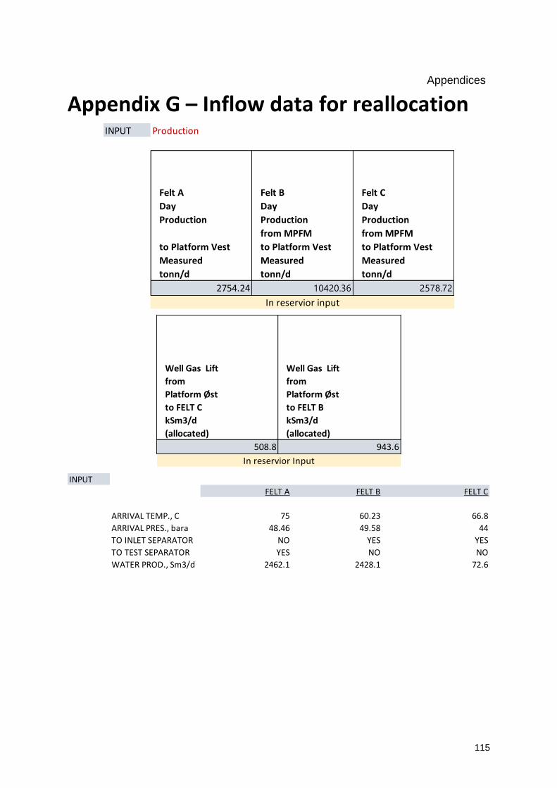
Appendices
115
Appendix G – Inflow data for reallocation
INPUT Production
Felt A
Day
Production
to Platform Vest
Measured
tonn/d
Felt B
Day
Production
from MPFM
to Platform Vest
Measured
tonn/d
Felt C
Day
Production
from MPFM
to Platform Vest
Measured
tonn/d
2754.24 10420.36 2578.72
In reservior input
Well Gas Lift
from
Platform Øst
to FELT C
kSm3/d
(allocated)
Well Gas Lift
from
Platform Øst
to FELT B
kSm3/d
(allocated)
508.8 943.6
In reservior Input
INPUT
FELT A FELT B FELT C
ARRIVAL TEMP., C 75 60.23 66.8
ARRIVAL PRES., bara 48.46 49.58 44
TO INLET SEPARATOR NO YES YES
TO TEST SEPARATOR YES NO NO
WATER PROD., Sm3/d 2462.1 2428.1 72.6
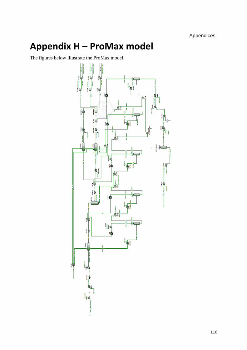
Appendices
116
Appendix H – ProMax model The figures below illustrate the ProMax model.

Appendices
117

Appendices
118

Appendices
119

Appendices
120

Appendices
121

Appendices
122

Appendices
123

Appendices
124

Appendices
125
Appendix I – Building the UniSim model The procedure for building the UniSim model is as follows:
1) The EOS is set to SRK as shown in the figure below:
2) The component list is added and named Platform Vest as shown in the figure below:

Appendices
126
3) Hypothetical components for each field is defined as follows, with the fluid
characterisation as the input.
4) The library component of H2O is added to the component list as shown in the figure
below:

Appendices
127
5) When the environment is defined the model can be build by using the equipment
shown in the figure below:
6) The final UniSim model is illustrated in Appendix E – UniSim model.
7) The following spreadsheets are created when the UniSim model is finish built.
8) The process input sheet is as follows, where the values are incorporated directly into
the stream.

Appendices
128
9) The reservoir input sheet is as follows, where the values are incorporated directly into
the stream.

Appendices
129
10) The quality control sheet is as follows, where the simulated values are compared to
the measured values. As well as a mass balance over the total process.
11) The ORF sheet is as follows, where the ORFs are calculated directly into the sheet.
(Only A and B in the figure to save space)
12) The value adjustment sheet is as follows, where the value in NOK/year is calculated
directly into the sheet. (only C included in the figure to save space).

Appendices
130

Appendices
131
Appendix J – Utility method in UniSim The utility method is as follows:
1) Add a utility called allocation utility to either the condensate export stream or the gas
export stream.
2) In the utility the feed stream is selected as follows:
3) In the figure above the A field well is selected as the feed stream.
4) In the result tab the product stream is selected, as follows:

Appendices
132
5) The utility will track the components from the selected feed stream to the selected
product stream. The results is available in molar, mass or volume flow.
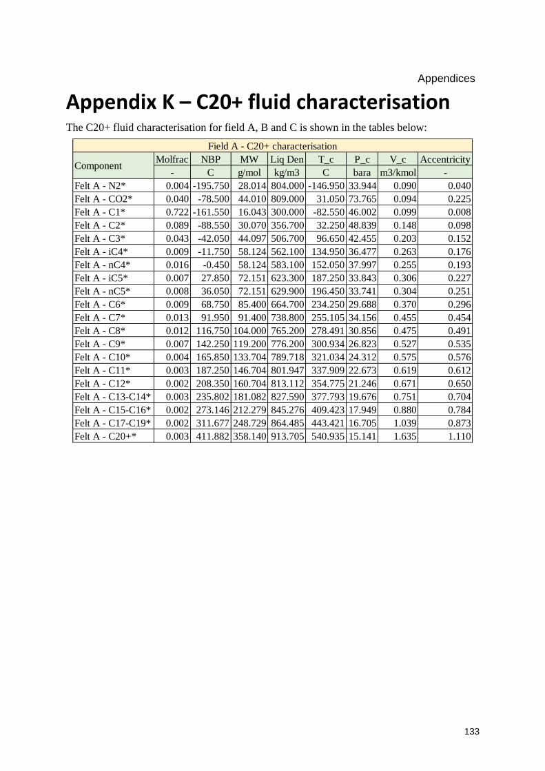
Appendices
133
Appendix K – C20+ fluid characterisation The C20+ fluid characterisation for field A, B and C is shown in the tables below:
Molfrac NBP MW Liq Den T_c P_c V_c Accentricity
- C g/mol kg/m3 C bara m3/kmol -
Felt A - N2* 0.004 -195.750 28.014 804.000 -146.950 33.944 0.090 0.040
Felt A - CO2* 0.040 -78.500 44.010 809.000 31.050 73.765 0.094 0.225
Felt A - C1* 0.722 -161.550 16.043 300.000 -82.550 46.002 0.099 0.008
Felt A - C2* 0.089 -88.550 30.070 356.700 32.250 48.839 0.148 0.098
Felt A - C3* 0.043 -42.050 44.097 506.700 96.650 42.455 0.203 0.152
Felt A - iC4* 0.009 -11.750 58.124 562.100 134.950 36.477 0.263 0.176
Felt A - nC4* 0.016 -0.450 58.124 583.100 152.050 37.997 0.255 0.193
Felt A - iC5* 0.007 27.850 72.151 623.300 187.250 33.843 0.306 0.227
Felt A - nC5* 0.008 36.050 72.151 629.900 196.450 33.741 0.304 0.251
Felt A - C6* 0.009 68.750 85.400 664.700 234.250 29.688 0.370 0.296
Felt A - C7* 0.013 91.950 91.400 738.800 255.105 34.156 0.455 0.454
Felt A - C8* 0.012 116.750 104.000 765.200 278.491 30.856 0.475 0.491
Felt A - C9* 0.007 142.250 119.200 776.200 300.934 26.823 0.527 0.535
Felt A - C10* 0.004 165.850 133.704 789.718 321.034 24.312 0.575 0.576
Felt A - C11* 0.003 187.250 146.704 801.947 337.909 22.673 0.619 0.612
Felt A - C12* 0.002 208.350 160.704 813.112 354.775 21.246 0.671 0.650
Felt A - C13-C14* 0.003 235.802 181.082 827.590 377.793 19.676 0.751 0.704
Felt A - C15-C16* 0.002 273.146 212.279 845.276 409.423 17.949 0.880 0.784
Felt A - C17-C19* 0.002 311.677 248.729 864.485 443.421 16.705 1.039 0.873
Felt A - C20+* 0.003 411.882 358.140 913.705 540.935 15.141 1.635 1.110
Component
Field A - C20+ characterisation

Appendices
134
Molfrac NBP MW Liq Den T_c P_c V_c Accentricity
- C g/mol kg/m3 C bara m3/kmol -
Felt B - N2* 0.007 -195.750 28.014 804.000 -146.950 33.944 0.090 0.040
Felt B - CO2* 0.024 -78.500 44.010 809.000 31.050 73.765 0.094 0.225
Felt B - C1* 0.820 -161.550 16.043 300.000 -82.550 46.002 0.099 0.008
Felt B - C2* 0.058 -88.550 30.070 356.700 32.250 48.839 0.148 0.098
Felt B - C3* 0.033 -42.050 44.097 506.700 96.650 42.455 0.203 0.152
Felt B - iC4* 0.005 -11.750 58.124 562.100 134.950 36.477 0.263 0.176
Felt B - nC4* 0.010 -0.450 58.124 583.100 152.050 37.997 0.255 0.193
Felt B - iC5* 0.003 27.850 72.151 623.300 187.250 33.843 0.306 0.227
Felt B - nC5* 0.004 36.050 72.151 629.900 196.450 33.741 0.304 0.251
Felt B - C6* 0.005 68.750 84.800 667.400 234.250 29.688 0.370 0.296
Felt B - C7* 0.007 91.950 91.000 741.400 254.887 34.580 0.450 0.453
Felt B - C8* 0.006 116.750 104.600 762.900 278.975 30.456 0.480 0.493
Felt B - C9* 0.003 142.250 120.200 772.400 301.598 26.308 0.536 0.538
Felt B - C10* 0.002 165.850 134.000 786.189 320.808 24.039 0.580 0.576
Felt B - C11* 0.002 187.250 147.000 798.664 337.702 22.440 0.624 0.612
Felt B - C12* 0.001 208.350 161.000 810.051 354.585 21.046 0.675 0.650
Felt B - C13-C14* 0.002 236.627 182.018 825.236 378.315 19.469 0.758 0.707
Felt B - C15-C16* 0.002 274.121 213.486 843.345 410.175 17.781 0.887 0.787
Felt B - C17-C19* 0.002 311.880 249.219 862.572 443.513 16.602 1.043 0.874
Felt B - C20+* 0.004 430.133 377.497 920.750 563.383 15.019 1.819 1.133
Field B - C20+ characterisation
Component
Molfrac NBP MW Liq Den T_c P_c V_c Accentricity
- C g/mol kg/m3 C bara m3/kmol -
Felt C - N2* 0.002 -195.750 28.014 804.000 -146.950 33.944 0.090 0.040
Felt C - CO2* 0.023 -78.500 44.010 809.000 31.050 73.765 0.094 0.225
Felt C - C1* 0.270 -161.550 16.043 300.000 -82.550 46.002 0.099 0.008
Felt C - C2* 0.070 -88.550 30.070 356.700 32.250 48.839 0.148 0.098
Felt C - C3* 0.086 -42.050 44.097 506.700 96.650 42.455 0.203 0.152
Felt C - iC4* 0.016 -11.750 58.124 562.100 134.950 36.477 0.263 0.176
Felt C - nC4* 0.051 -0.450 58.124 583.100 152.050 37.997 0.255 0.193
Felt C - iC5* 0.018 27.850 72.151 623.300 187.250 33.843 0.306 0.227
Felt C - nC5* 0.029 36.050 72.151 629.900 196.450 33.741 0.304 0.251
Felt C - C6* 0.033 68.750 84.900 666.800 234.250 29.688 0.370 0.296
Felt C - C7* 0.053 91.950 91.000 741.400 254.887 34.580 0.450 0.453
Felt C - C8* 0.051 116.750 105.000 761.600 279.334 30.211 0.484 0.494
Felt C - C9* 0.035 142.250 120.300 772.400 301.726 26.282 0.536 0.538
Felt C - C10* 0.024 165.850 134.000 786.398 320.842 24.051 0.580 0.576
Felt C - C11* 0.022 187.250 147.000 799.061 337.766 22.462 0.624 0.612
Felt C - C12* 0.020 208.350 161.000 810.621 354.677 21.076 0.675 0.650
Felt C - C13-C14* 0.034 236.788 182.144 826.117 378.580 19.500 0.757 0.707
Felt C - C15-C16* 0.028 274.264 213.620 844.490 410.479 17.823 0.887 0.787
Felt C - C17-C19* 0.034 312.159 249.509 864.100 443.997 16.652 1.043 0.874
Felt C - C20+* 0.102 458.772 413.577 936.366 598.386 14.968 2.098 1.169
Field C - C20+ characterisation
Component

Appendices
135
Appendix L – C10+ fluid characterisation The C10+ fluid characterisation for field A, B and C is shown in the tables below:
Molfrac NBP MW Liq Den T_c P_c V_c Accentricity
- C g/mol kg/m3 C bara m3/kmol -
Felt A -N2* 0.004 -195.750 28.014 804.000 -146.950 33.944 0.090 0.040
Felt A - CO2* 0.040 -78.500 44.010 809.000 31.050 73.765 0.094 0.225
Felt A - C1* 0.722 -161.550 16.043 300.000 -82.550 46.002 0.099 0.008
Felt A - C2* 0.089 -88.550 30.070 356.700 32.250 48.839 0.148 0.098
Felt A - C3* 0.043 -42.050 44.097 506.700 96.650 42.455 0.203 0.152
Felt A - iC4* 0.009 -11.750 58.124 562.100 134.950 36.477 0.263 0.176
Felt A - nC4* 0.016 -0.450 58.124 583.100 152.050 37.997 0.255 0.193
Felt A - iC5* 0.007 27.850 72.151 623.300 187.250 33.843 0.306 0.227
Felt A - nC5* 0.008 36.050 72.151 629.900 196.450 33.741 0.304 0.251
Felt A - C6* 0.009 68.750 85.400 664.700 234.250 29.688 0.370 0.296
Felt A - C7* 0.013 91.950 91.400 738.800 255.105 34.156 0.455 0.454
Felt A - C8* 0.012 116.750 104.000 765.200 278.491 30.856 0.475 0.491
Felt A - C9* 0.007 142.250 119.200 776.200 300.934 26.823 0.527 0.535
Felt A - C10+* 0.019 272.242 195.000 842.000 412.857 19.292 0.964 0.795
Component
Field A - C10+ characterisation
Molfrac NBP MW Liq Den T_c P_c V_c Accentricity
- C g/mol kg/m3 C bara m3/kmol -
Felt B - N2* 0.007 -195.750 28.014 804.000 -146.950 33.944 0.090 0.040
Felt B - CO2* 0.024 -78.500 44.010 809.000 31.050 73.765 0.094 0.225
Felt B - C1* 0.820 -161.550 16.043 300.000 -82.550 46.002 0.099 0.008
Felt B - C2* 0.058 -88.550 30.070 356.700 32.250 48.839 0.148 0.098
Felt B - C3* 0.033 -42.050 44.097 506.700 96.650 42.455 0.203 0.152
Felt B - iC4* 0.005 -11.750 58.124 562.100 134.950 36.477 0.263 0.176
Felt B - nC4* 0.010 -0.450 58.124 583.100 152.050 37.997 0.255 0.193
Felt B - iC5* 0.003 27.850 72.151 623.300 187.250 33.843 0.306 0.227
Felt B - nC5* 0.004 36.050 72.151 629.900 196.450 33.741 0.304 0.251
Felt B - C6* 0.005 68.750 84.800 667.400 234.250 29.688 0.370 0.296
Felt B - C7* 0.007 91.950 91.000 741.400 254.887 34.580 0.450 0.453
Felt B - C8* 0.006 116.750 104.600 762.900 278.975 30.456 0.480 0.493
Felt B - C9* 0.003 142.250 120.200 772.400 301.598 26.308 0.536 0.538
Felt B - C10+* 0.015 326.161 237.000 866.000 463.929 17.547 1.251 0.907
Component
Field B - C10+ characterisation

Appendices
136
Molfrac NBP MW Liq Den T_c P_c V_c Accentricity
- C g/mol kg/m3 C bara m3/kmol -
Felt C - N2* 0.002 -195.750 28.014 804.000 -146.950 33.944 0.090 0.040
Felt C - CO2* 0.023 -78.500 44.010 809.000 31.050 73.765 0.094 0.225
Felt C - C1* 0.270 -161.550 16.043 300.000 -82.550 46.002 0.099 0.008
Felt C - C2* 0.070 -88.550 30.070 356.700 32.250 48.839 0.148 0.098
Felt C - C3* 0.086 -42.050 44.097 506.700 96.650 42.455 0.203 0.152
Felt C - iC4* 0.016 -11.750 58.124 562.100 134.950 36.477 0.263 0.176
Felt C - nC4* 0.050 -0.450 58.124 583.100 152.050 37.997 0.255 0.193
Felt C - iC5* 0.019 27.850 72.151 623.300 187.250 33.843 0.306 0.227
Felt C - nC5* 0.029 36.050 72.151 629.900 196.450 33.741 0.304 0.251
Felt C - C6* 0.033 68.750 84.900 666.800 234.250 29.688 0.370 0.296
Felt C - C7* 0.053 91.950 91.000 741.400 254.887 34.580 0.450 0.453
Felt C - C8* 0.051 116.750 105.000 761.600 279.334 30.211 0.484 0.494
Felt C - C9* 0.035 142.250 120.300 772.400 301.726 26.282 0.536 0.538
Felt C - C10+* 0.264 371.024 274.490 889.000 511.099 16.799 1.563 0.989
Component
Field C - C10+ characterisation

Appendices
137
Appendix M – Future allocation profiles The future allocation profiles for field A, B and C for year 8, 10 and 12 are shown in the
tables below:

Appendices
138
Appendix N – Future allocation ORF result for year 10 and 12
The following tables shown the ORFs for field A, B and C for the future allocation for year
10 and 12.

Appendices
139

Appendices
140

Appendices
141

Appendices
142
Appendix O – UniSim GOR model The model for the GOR tuning is developed as follows:
1) A simplified model of the process is created upstream the different fields well inflow.
As shown in the figure below:
2) A separate sheet is added to tune on the GOR value. This sheet is shown in the figure
below:

Appendices
143
3) The C5 and C10 fields include the simulated gas and condensate production over the
total process (not the simplified case). These values are compared to the measured
values and the difference is calculated.
In D21 the GOR for the total process is calculated.
For the simplified case, the gas and condensate are shown in C14 and C16. The GOR
for the simplified model is calculated using these values and are shown in C21.
The adjuster (ADJ-4-4) on the stream mixed into the gas stream for the simplified
case, adjust its flow to match the GOR on the total process to the measured GOR.
The gas and condensate on the simplified case are mixed, and the composition in this
stream is exported to the Field A Well stream.
The mass flow into the simplified process is guessed in B23. An upscaling factor is
calculated using D5/C14. The upscaled feed rate is calculated in B27, and this value is
exported as the Felt A Well mass flow.

Appendices
144
Appendix P – Building the ProMax model The procedure for building the ProMax model is as follows:
1) The EOS is set to SRK as shown in the figure below:
2) The hypothetical components (the C6+ components) are added as single oils as shown
in the figure below:

Appendices
145
3) The component list is created with library components for components lower than C6,
as shown in the figure below:
4) The model is built with process equipment using ProMax shapes as shown in the
figure below:

Appendices
146
5) The finished model is shown in Appendix H – ProMax model.
6) ProMax comes with a excel interface, but due to time limitation spreadsheets where
not made for the ProMax model. Instead, the results were read directly from the
different product streams.

Appendices
147
Appendix Q – Allocation methods calculation
1) By Difference
2) Pro-Rata
Inputs Quantites (ton/d):
Measured export gas (tonne/d) 11012.02
Field B estimate - gas 9271.90
Field A estimate - gas 1586.36
Measured export oil (tonne/d) 4575.28
Field B estimate - oil 2773.69
Field A estimate - oil 721.20
Calculations
Q - Produced gas 11012.02
Q1 - Produced gas allocated to Field C 153.76
Q - Produced oil 4575.28
Q1 - Produced oil allocated to Field C 1080.38
By difference
Inputs Quantites (ton/d):
Measured export gas (tonne/d) 11012.02
Field A estimate - gas 1586.36
Field B estimate - gas 9271.90
Field C estimate - gas 127.70
Gas estimation 10985.96
Measured export oil (tonne/d) 4575.28
Field A estimate - oil 721.20
Field B estimate - oil 2773.69
Field C estimate - oil 1106.62
Oil estimation 4601.51
Calculations
Field A calculated - gas 1590.12
Field B calculated - gas 9293.89
Field C calculated - gas 128.01
Field A calculated - oil 717.09
Field B calculated - oil 2757.87
Field C calculated - oil 1100.31
Pro rata

Appendices
148
3) ORF method
Standalone ORF Field A Field B Field C
N2 0.0 0.0 0.0
CO2 0.3 0.1 0.9
C1 0.0 0.0 0.1
C2 1.2 0.3 4.1
C3 9.2 3.0 33.2
iC4 24.4 10.7 69.0
nC4 33.2 16.1 79.7
iC5 55.8 33.1 92.7
nC5 62.4 39.5 94.6
C6 83.5 65.6 98.3
C7 94.6 86.1 99.5
C8 98.4 95.8 99.9
C9 99.7 99.1 100.0
C10+ 100.0 100.0 100.0
Year 8
Inflow, tonn/d Field A Field B Field C
N2 10.2 94.9 0.8
CO2 142.8 518.3 11.7
C1 940.3 6446.7 49.4
C2 218.0 855.8 23.9
C3 155.6 707.6 43.3
iC4 42.4 138.8 10.7
nC4 77.4 298.4 33.6
iC5 40.3 117.8 14.9
nC5 46.4 157.4 23.5
C6 65.7 197.5 32.0
C7 98.9 305.6 54.8
C8 104.5 301.6 60.6
C9 68.4 202.7 47.9
C10+ 296.6 1702.3 826.6
SUM 2307.5 12045.5 1233.6
Year 8
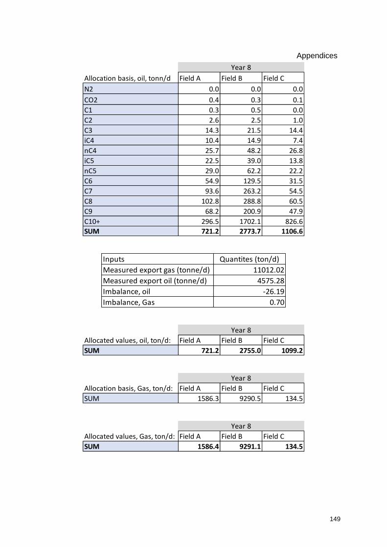
Appendices
149
Allocation basis, oil, tonn/d Field A Field B Field C
N2 0.0 0.0 0.0
CO2 0.4 0.3 0.1
C1 0.3 0.5 0.0
C2 2.6 2.5 1.0
C3 14.3 21.5 14.4
iC4 10.4 14.9 7.4
nC4 25.7 48.2 26.8
iC5 22.5 39.0 13.8
nC5 29.0 62.2 22.2
C6 54.9 129.5 31.5
C7 93.6 263.2 54.5
C8 102.8 288.8 60.5
C9 68.2 200.9 47.9
C10+ 296.5 1702.1 826.6
SUM 721.2 2773.7 1106.6
Year 8
Inputs Quantites (ton/d)
Measured export gas (tonne/d) 11012.02
Measured export oil (tonne/d) 4575.28
Imbalance, oil -26.19
Imbalance, Gas 0.70
Allocated values, oil, ton/d: Field A Field B Field C
SUM 721.2 2755.0 1099.2
Year 8
Allocation basis, Gas, ton/d: Field A Field B Field C
SUM 1586.3 9290.5 134.5
Year 8
Allocated values, Gas, ton/d: Field A Field B Field C
SUM 1586.4 9291.1 134.5
Year 8