Recognizing people by their gait: the shape of motion

Article 1

Recognizing Peopleby Their Gait:The Shape of Motion

James J. LittleJeffrey E. Boyd

Videre: Journal of Computer Vision Research

Quarterly Journal

Winter 1998, Volume 1, Number 2

The MIT Press

Videre: Journal of Computer Vision Research (ISSN 1089-2788) is aquarterly journal published electronically on the Internet by The MITPress, Cambridge, Massachusetts, 02142. Subscriptions and addresschanges should be addressed to MIT Press Journals, Five CambridgeCenter, Cambridge, MA 02142; phone: (617) 253-2889; fax: (617)577-1545; e-mail: [email protected]. Subscription rates are:Individuals $30.00, Institutions $125.00. Canadians add additional7% GST. Prices subject to change without notice.

Subscribers are licensed to use journal articles in a variety of ways,limited only as required to insure fair attribution to authors and theJournal, and to prohibit use in a competing commercial product. Seethe Journals World Wide Web site for further details. Address inquiriesto the Subsidiary Rights Manager, MIT Press Journals, Five CambridgeCenter, Cambridge, MA 02142; phone: (617) 253-2864; fax: (617)258-5028; e-mail: [email protected].

© 1998 by the Massachusetts Institute of Technology

The image flow of a moving figurevaries both spatially and tempo-rally. We develop a model-freedescription of instantaneous mo-tion, the shape of motion, thatvaries with the type of moving fig-ure and the type of motion. We usethat description to recognize indi-viduals by their gait, discriminatingthem by periodic variation in theshape of their motion. For each im-age in a sequence, we derive denseoptical flow, (u(x, y), v(x, y)).Scale-independent scalar featuresof each flow, based on momentsof the moving point weighted by|u|, |v|, or |(u, v)|, characterize thespatial distribution of the flow.

We then analyze the periodicstructure of these sequences ofscalars. The scalar sequences foran image sequence have the samefundamental period but differ inphase, which is a phase feature foreach signal. Some phase featuresare consistent for one personand show significant statisticalvariation among persons. Weuse the phase feature vectors torecognize individuals by the shapeof their motion. As few as threefeatures out of the full set of twelvelead to excellent discrimination.

Keywords: action recognition,gait recognition, motion features,optic flow, motion energy, spatialfrequency, analysis

Recognizing People by Their Gait:The Shape of Motion

James J. Little,1 Jeffrey E. Boyd2

1 IntroductionOur goal is to develop a model-free description of image motion, andthen to demonstrate its usefulness by describing the motion of a walkinghuman figure and recognizing individuals by variation in the character-istics of the motion description. Such a description is useful in videosurveillance where it contributes to the recognition of individuals andcan indicate aspects of an individual’s behavior. Model-free descriptionsof motion could also prove useful in vision-based user interfaces by help-ing to recognize individuals, what they are doing, and nuances of theirbehavior.

The pattern of motion in the human gait has been studied in kinesi-ology using data acquired from moving light displays. Using such data,kinesiologists describe the forward propulsion of the torso by the legs,the ballistic motion of swinging arms and legs, and the relationshipsamong these motions [23, 30]. Similarly, in computer vision, model-based approaches to gait analysis recover the three-dimensional struc-ture of a person in a model and then interpret the model. The literatureon moving light displays provides an introduction to modeling and mov-ing figures [11]. Unuma, Anjyo, and Takeuchi [42] show the value of astructural model in describing variations in gaits. They use Fourier analy-sis of joint angles in a model to synthesize images of different types ofgaits, e.g., a happy walk versus a tired walk.

Alternatives to the model-based approach emphasize determiningfeatures of the motion fields, acquired from a sequence of images, with-out structural reconstruction. Recent theoretical work demonstrates therecoverability of affine motion characteristics from image sequences[38]. It is therefore reasonable to suggest that variations in gaits arerecoverable from variations in images sequences and that a model-freeapproach to gait analysis is viable. Moreover, during periodic motionthe varying spatial distribution of motion is apparent. Capturing thisvariation and analyzing its temporal variation should lead to a usefulcharacterization of periodic motion.

Hogg [16] was among the first to study the motion of a walking figureusing an articulated model. There have recently been several attempts torecover characteristics of gait from image sequences, without the aid ofannotation via lights [35, 5, 27, 28, 31, 32, 3, 4]. Niyogi and Adelson[27, 28] emphasize segmentation over a long sequence of frames. Theirtechnique relies on recovering the boundaries of moving figures in thext domain [27] and recently [28] xyt spatiotemporal solids, followed byfitting deformable splines to the contours. These splines are the elementsof the articulated nonrigid model whose features aid recognition.

Polana and Nelson [31, 32] characterize the temporal texture of amoving figure by “summing the energy of the highest amplitude fre-quency and its multiples.” They use Fourier analysis. The results are

1. Department of Computer Science, Uni-versity of British Columbia, Vancouver, B.C.,Canada V6T 1Z4. [email protected]

2. Department of Electrical and Computer En-gineering, University of California, La Jolla,CA 92093-0407. [email protected]

Copyright © 1998Massachusetts Institute of Technologymitpress.mit.edu/videre.html

VIDERE 1:2 The Shape of Motion 2

normalized with respect to total energy so that the measure is 1 for pe-riodic events and 0 for a flat spectrum. Their input is a sequence of 128frames, each 128 × 128 pixels. Their analysis consists of determiningthe normal flow, thresholding the magnitude of the flow, determiningthe centroid of all “moving” points, and computing the mean velocity ofthe centroid. The motion in xyt of the centroid determines a linear tra-jectory. They use as motion signals reference curves that are “lines in thetemporal solid parallel to the linear trajectory.”

Polana and Nelson’s more recent work [32, 33] emphasizes the spatialdistribution of energies around the moving figure. They compute spatialstatistics in a coarse mesh and derive a vector describing the relativemagnitudes and periodicity of activity in the regions over time. Theirexperiments demonstrate that the values so derived can be used todiscriminate among differing activities.

Shavit and Jepson [39, 40] use the centroid and moments of a bi-narized motion figure to represent the distribution of its motion. Themovement of the centroid characterizes the external forces on an object,while the deformation of the object is computed from the dispersion (theeigenvalues of the covariance matrix) or ratio of lengths of the momentellipse.

Bobick and Davis [6] introduced the Motion Energy Image (MEI), asmoothed description of the cumulative spatial distribution of motionenergy in a motion sequence. They match this description of motionagainst stored models of known actions. Bobick and Davis [7] enhancedthe MEI to form a motion-history image (MHI), where pixel intensityis a function, over time, of the energy in the current motion energy(binarized) and recent activity, which they extend in later work [14].We will discuss these two representations further in Section 2.2.

Baumberg and Hogg [3] present a method of representing the shapeof a moving body at an instance in time. Their method produces adescription composed of a set of principal spline components and adirection of motion. In later work, Baumberg and Hogg [4] add temporalvariation by modeling the changing shape as a vibrating plate. Theycreate a vibration model for a “generic” pedestrian and then are ableto measure the quality of fit of the generic data to another pedestrian.

Liu and Picard [22] detect and segment areas of periodic motion inimages by detecting spectral harmonic peaks. The method is not modelbased and identifies regions in the images that exhibit periodic motion.

Recently more elaborate models, often including kinematics and dy-namics of the human figure, are used to track humans in sequences [36,9, 19, 18, 43].

Our work, in the spirit of Polana and Nelson, and Baumberg andHogg, is a model-free approach making no attempt to recover a struc-tural model of a human subject. Instead we describe the shape of themotion with a set of features derived from moments of a dense flow dis-tribution [20]. Our goal is not to fingerprint people, but to determinewhat content of motion aids recognition. We wish to recognize gaits,both types of gaits as well as individual gaits. The features are invariantto scale and do not require synchronization of the gait or identificationof reference points on the moving figure.

The following sections describe the creation of motion features andan experiment that determines the variation of the features over a set ofwalking subjects. Results of the experiment show that features acquiredby our process exhibit significant variation due to different subjects andare suitable for recognition of people by subtle differences in their gaits,


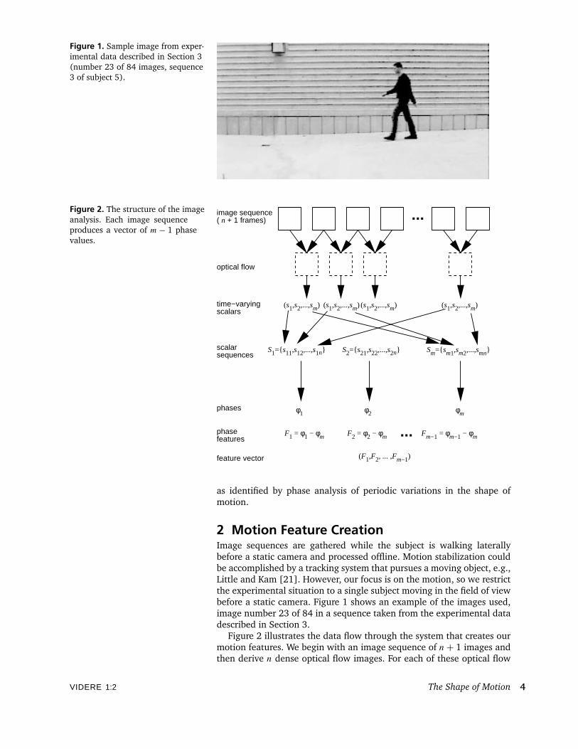
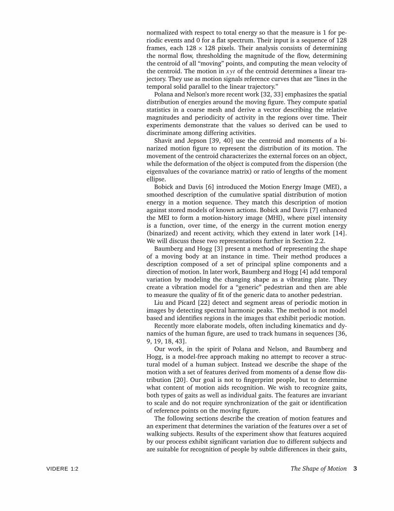
Figure 1. Sample image from exper-imental data described in Section 3(number 23 of 84 images, sequence3 of subject 5).

Figure 2. The structure of the imageanalysis. Each image sequenceproduces a vector of m − 1 phasevalues.

image sequence( n + 1 frames)

optical flow

time−varyingscalars

scalar sequences

phases

phase features

feature vector

...

(s1,s2,...,sm) (s1,s2,...,sm) (s1,s2,...,sm) (s1,s2,...,sm)

S1={s11,s12,...,s1n} S2={s21,s22,...,s2n} Sm={sm1,sm2,...,smn}

φ1 φ2 φm

F1 = φ1 − φm F2 = φ2 − φm Fm−1 = φm−1 − φm...(F1,F2, ... ,Fm−1)

as identified by phase analysis of periodic variations in the shape ofmotion.

2 Motion Feature CreationImage sequences are gathered while the subject is walking laterallybefore a static camera and processed offline. Motion stabilization couldbe accomplished by a tracking system that pursues a moving object, e.g.,Little and Kam [21]. However, our focus is on the motion, so we restrictthe experimental situation to a single subject moving in the field of viewbefore a static camera. Figure 1 shows an example of the images used,image number 23 of 84 in a sequence taken from the experimental datadescribed in Section 3.

Figure 2 illustrates the data flow through the system that creates ourmotion features. We begin with an image sequence of n+ 1 images andthen derive n dense optical flow images. For each of these optical flow


images we compute m characteristics that describe the shape of the mo-tion (i.e., the spatial distribution of the flow), for example, the centroidof the moving points, and various moments of the flow distribution.Some of these are locations in the image, but we treat all as time-varyingscalar values. We arrange the values to form a time series for each scalar.A walking person undergoes periodic motion, returning to a standardposition after a certain time period that depends on the frequency of thegait. Thus we analyze the periodic structure of these time series, anddetermine the fundamental frequency of the variation of each scalar.The set of time series for an image sequence share the same frequency,or simple multiples of the fundamental, but their phases vary. To makethe data from different sequences comparable, we subtract a referencephase, φm, derived from one of the scalars. We characterize each imagesequence by a vector, F = (F1, . . . , Fm−1), of m− 1 relative phase fea-tures. The phase feature vectors are then used to recognize individuals.

2.1 Tracking and Optical FlowThe motion of the object is a path in three dimensions; we view its pro-jection. Instead of determining motion of three-dimensional elements ofa figure, we look for characteristics of the periodic variation of the two-dimensional optical flow.

The raw optical flow identifies temporal changes in brightness; how-ever, illumination changes such as reflections, shadows, moving clouds,and inter-reflections between the moving figure and the background, aswell as reflections of the moving figure in specular surfaces in the back-ground, pollute the motion signal. To isolate the moving figure, we man-ually compute the average displacement of the person through the imagesequence and then use only the flow within a moving window travelingwith the average motion. Within the window there remain many islandsof small local variation, so we compute the connected components ofeach Fj and eliminate all points not in sufficiently large connected re-gions. The remaining large components form a mask within which wecan analyze the flow. This reduces the sensitivity of the moment compu-tations to outlying points.

Figure 3 shows six subimages from the sequence corresponding toFigure 1. We will refer to the subimages as images from here on andwill display our results in subimages, for compactness. All processing iscarried out in the coordinates of the original frames.

Unlike other methods, we use dense optical flow fields, generated byminimizing the sum of absolute differences between image patches [10].The algorithm is sensitive to brightness change caused by reflections,shadows, and changes of illumination, so we first process the imagesby computing the logarithm of brightness, transforming the multiplica-tive effect of illumination change into an additive one. Filtering by aLaplacian of Gaussian (effectively a bandpass filter) removes the addi-tive effects.

The optical flow algorithm, for each pixel, searches among a limitedset of discrete displacements for the displacement (u(x, y), v(x, y)) thatminimizes the sum of absolute differences between a patch in one imageand the corresponding displaced patch in the other image. The algorithmfinds a best-matching patch in the second image for each patch in thefirst. The algorithm is run a second time, switching the roles of the twoimages. For a correct match, the results will likely agree. In order toremove invalid matches, we compare the results at each point in the


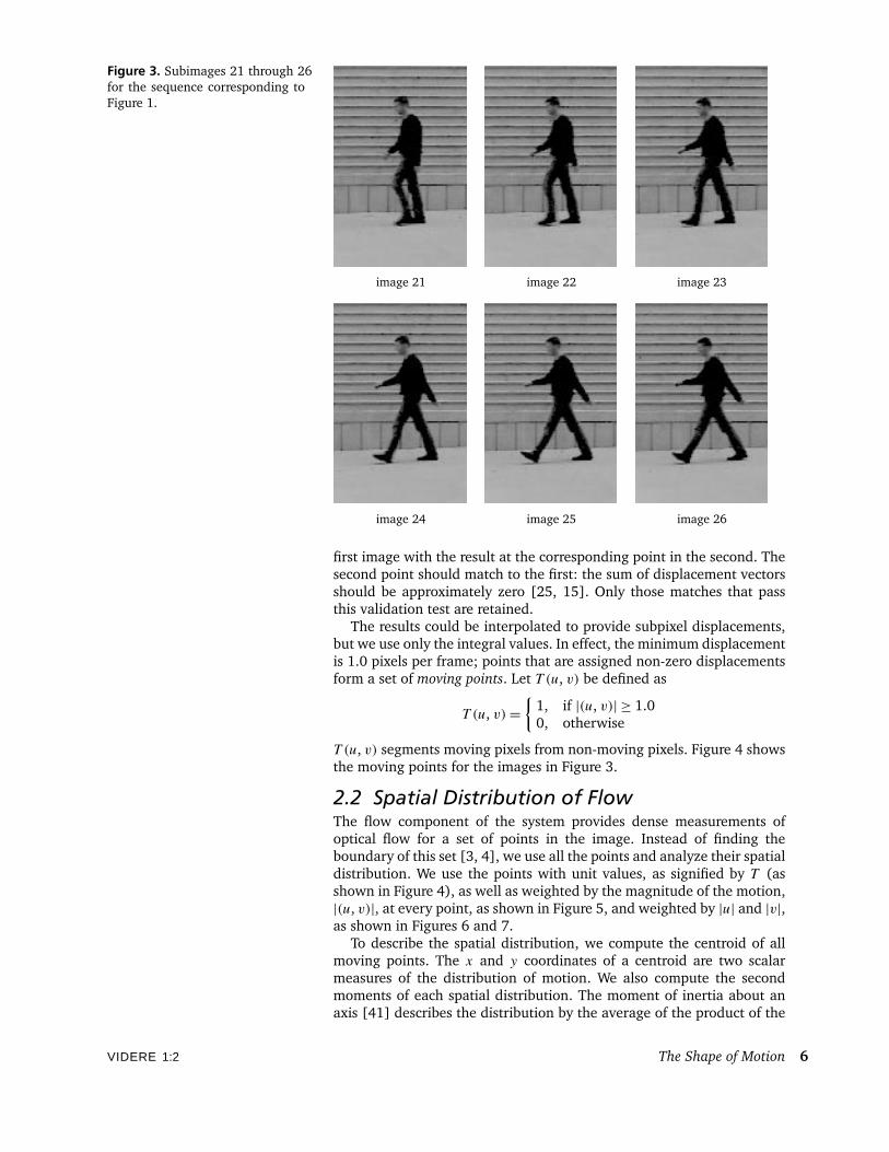
Figure 3. Subimages 21 through 26for the sequence corresponding toFigure 1.

image 21 image 22 image 23


first image with the result at the corresponding point in the second. Thesecond point should match to the first: the sum of displacement vectorsshould be approximately zero [25, 15]. Only those matches that passthis validation test are retained.

The results could be interpolated to provide subpixel displacements,but we use only the integral values. In effect, the minimum displacementis 1.0 pixels per frame; points that are assigned non-zero displacementsform a set of moving points. Let T (u, v) be defined as

T (u, v)={

1, if |(u, v)| ≥ 1.00, otherwise

T (u, v) segments moving pixels from non-moving pixels. Figure 4 showsthe moving points for the images in Figure 3.

2.2 Spatial Distribution of FlowThe flow component of the system provides dense measurements ofoptical flow for a set of points in the image. Instead of finding theboundary of this set [3, 4], we use all the points and analyze their spatialdistribution. We use the points with unit values, as signified by T (asshown in Figure 4), as well as weighted by the magnitude of the motion,|(u, v)|, at every point, as shown in Figure 5, and weighted by |u| and |v|,as shown in Figures 6 and 7.

To describe the spatial distribution, we compute the centroid of allmoving points. The x and y coordinates of a centroid are two scalarmeasures of the distribution of motion. We also compute the secondmoments of each spatial distribution. The moment of inertia about anaxis [41] describes the distribution by the average of the product of the


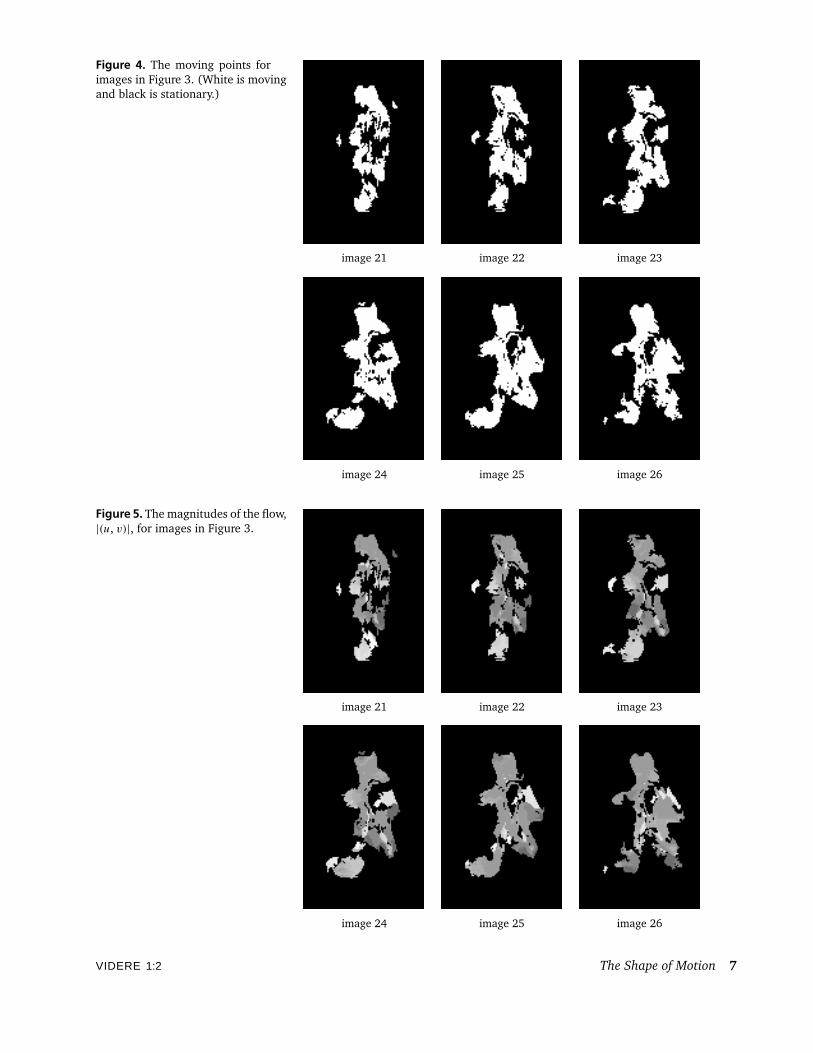
Figure 4. The moving points forimages in Figure 3. (White is movingand black is stationary.)



Figure 5. The magnitudes of the flow,|(u, v)|, for images in Figure 3.




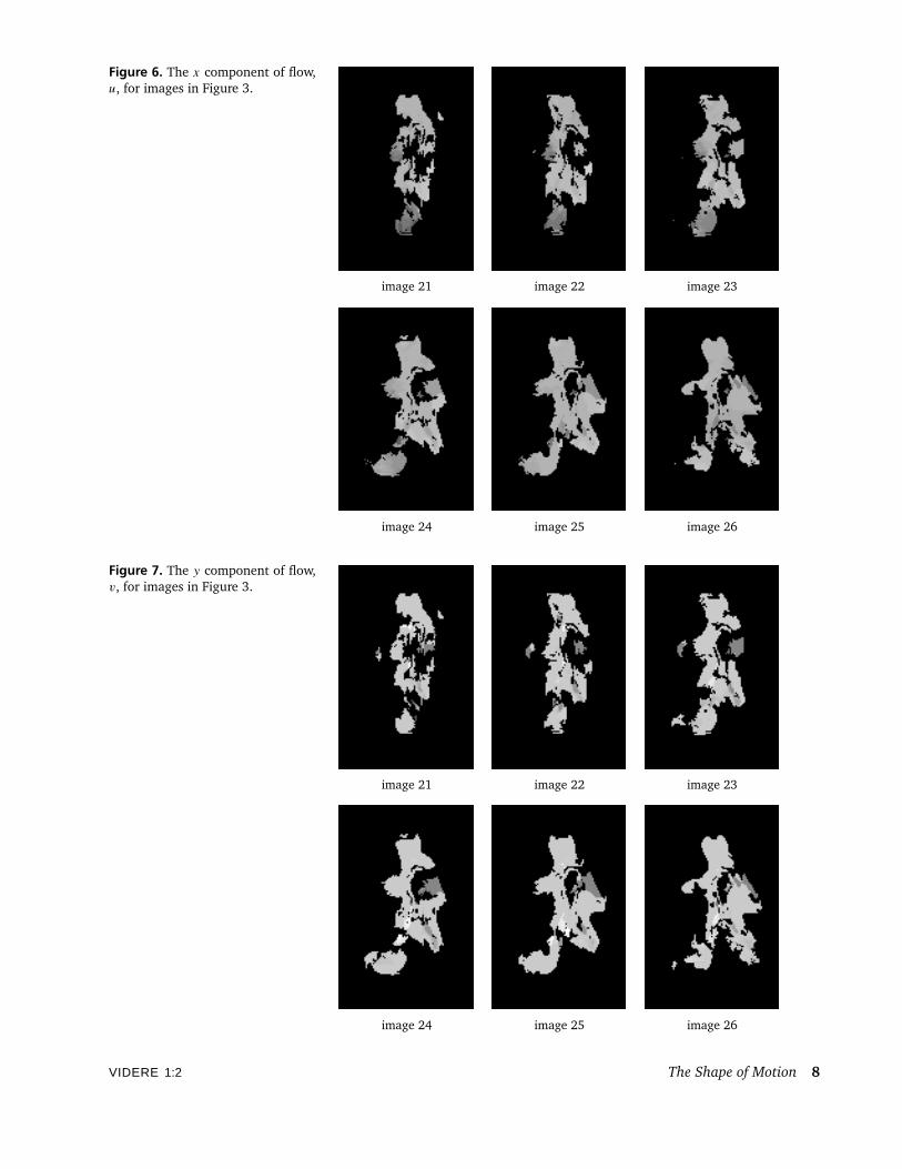
Figure 6. The x component of flow,u, for images in Figure 3.



Figure 7. The y component of flow,v, for images in Figure 3.




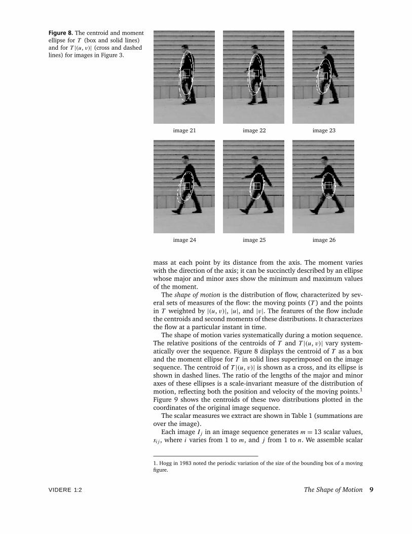
Figure 8. The centroid and momentellipse for T (box and solid lines)and for T |(u, v)| (cross and dashedlines) for images in Figure 3.



mass at each point by its distance from the axis. The moment varieswith the direction of the axis; it can be succinctly described by an ellipsewhose major and minor axes show the minimum and maximum valuesof the moment.

The shape of motion is the distribution of flow, characterized by sev-eral sets of measures of the flow: the moving points (T ) and the pointsin T weighted by |(u, v)|, |u|, and |v|. The features of the flow includethe centroids and second moments of these distributions. It characterizesthe flow at a particular instant in time.

The shape of motion varies systematically during a motion sequence.The relative positions of the centroids of T and T |(u, v)| vary system-atically over the sequence. Figure 8 displays the centroid of T as a boxand the moment ellipse for T in solid lines superimposed on the imagesequence. The centroid of T |(u, v)| is shown as a cross, and its ellipse isshown in dashed lines. The ratio of the lengths of the major and minoraxes of these ellipses is a scale-invariant measure of the distribution ofmotion, reflecting both the position and velocity of the moving points.1

Figure 9 shows the centroids of these two distributions plotted in thecoordinates of the original image sequence.

The scalar measures we extract are shown in Table 1 (summations areover the image).

Each image Ij in an image sequence generates m= 13 scalar values,sij , where i varies from 1 to m, and j from 1 to n. We assemble scalar

1. Hogg in 1983 noted the periodic variation of the size of the bounding box of a movingfigure.


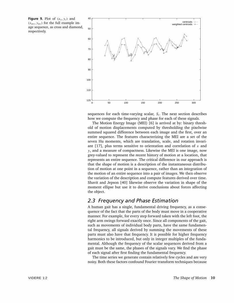
Figure 9. Plot of (xc, yc) and(xwc, ywc) for the full example im-age sequence, as cross and diamond,respectively.

40

50

60

70

80

90

100

110

1200 50 100 150 200 250 300

centroidsweighted centroids

sequences for each time-varying scalar, Si. The next section describeshow we compute the frequency and phase for each of these signals.

The Motion Energy Image (MEI) [6] is arrived at by: binary thresh-old of motion displacements computed by thresholding the pixelwisesummed squared difference between each image and the first, over anentire sequence. The features characterizing the MEI are a set of theseven Hu moments, which are translation, scale, and rotation invari-ant [17], plus terms sensitive to orientation and correlation of x andy, and a measure of compactness. Likewise the MEI is one image, nowgrey-valued to represent the recent history of motion at a location, thatrepresents an entire sequence. The critical difference in our approach isthat the shape of motion is a description of the instantaneous distribu-tion of motion at one point in a sequence, rather than an integration ofthe motion of an entire sequence into a pair of images. We then observethe variation of the description and compute features derived over time.Shavit and Jepson [40] likewise observe the variation in shape of themoment ellipse but use it to derive conclusions about forces affectingthe object.

2.3 Frequency and Phase EstimationA human gait has a single, fundamental driving frequency, as a conse-quence of the fact that the parts of the body must move in a cooperativemanner. For example, for every step forward taken with the left foot, theright arm swings forward exactly once. Since all components of the gait,such as movements of individual body parts, have the same fundamen-tal frequency, all signals derived by summing the movements of theseparts must also have that frequency. It is possible for higher frequencyharmonics to be introduced, but only in integer multiples of the funda-mental. Although the frequency of the scalar sequences derived from agait must be the same, the phases of the signals vary. We find the phaseof each signal after first finding the fundamental frequency.

The time series we generate contain relatively few cycles and are verynoisy. Both these factors confound Fourier transform techniques because


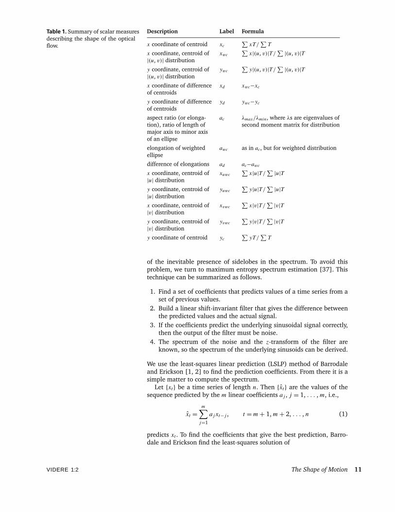
Table 1. Summary of scalar measuresdescribing the shape of the opticalflow.

Description Label Formula

x coordinate of centroid xc∑xT /

∑T

x coordinate, centroid of xwc∑x|(u, v)|T/∑ |(u, v)|T

|(u, v)| distribution

y coordinate, centroid of ywc∑y|(u, v)|T/∑ |(u, v)|T

|(u, v)| distribution

x coordinate of difference xd xwc−xcof centroids

y coordinate of difference yd ywc−ycof centroids

aspect ratio (or elonga- ac λmax/λmin, where λs are eigenvalues oftion), ratio of length of second moment matrix for distributionmajor axis to minor axisof an ellipse

elongation of weighted awc as in ac, but for weighted distributionellipse

difference of elongations ad ac−awcx coordinate, centroid of xuwc

∑x|u|T/∑ |u|T

|u| distribution

y coordinate, centroid of yuwc∑y|u|T/∑ |u|T

|u| distribution

x coordinate, centroid of xvwc∑x|v|T/∑ |v|T

|v| distribution

y coordinate, centroid of yvwc∑y|v|T/∑ |v|T

|v| distribution

y coordinate of centroid yc∑yT /

∑T

of the inevitable presence of sidelobes in the spectrum. To avoid thisproblem, we turn to maximum entropy spectrum estimation [37]. Thistechnique can be summarized as follows.

1. Find a set of coefficients that predicts values of a time series from aset of previous values.

2. Build a linear shift-invariant filter that gives the difference betweenthe predicted values and the actual signal.

3. If the coefficients predict the underlying sinusoidal signal correctly,then the output of the filter must be noise.

4. The spectrum of the noise and the z-transform of the filter areknown, so the spectrum of the underlying sinusoids can be derived.

We use the least-squares linear prediction (LSLP) method of Barrodaleand Erickson [1, 2] to find the prediction coefficients. From there it is asimple matter to compute the spectrum.

Let {xt} be a time series of length n. Then {xt} are the values of thesequence predicted by the m linear coefficients aj , j = 1, . . . ,m, i.e.,

xt =m∑j=1

ajxt−j , t =m+ 1,m+ 2, . . . , n (1)

predicts xt . To find the coefficients that give the best prediction, Barro-dale and Erickson find the least-squares solution of


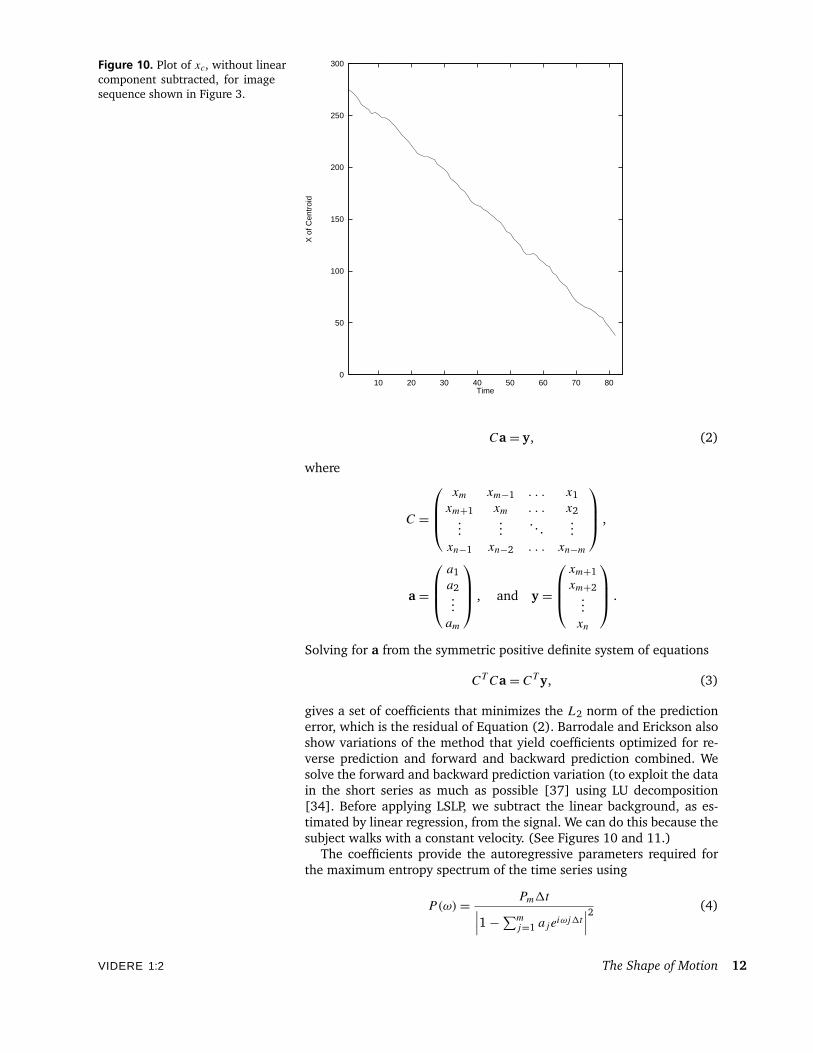
Figure 10. Plot of xc, without linearcomponent subtracted, for imagesequence shown in Figure 3.

0

50

100

150

200

250

300

10 20 30 40 50 60 70 80

X o

f Cen

troi

d

Time

Ca = y, (2)

where

C =

xm xm−1 . . . x1xm+1 xm . . . x2

......

. . ....

xn−1 xn−2 . . . xn−m

,

a =

a1a2...am

, and y =

xm+1xm+2

...xn

.

Solving for a from the symmetric positive definite system of equations

CTCa = CT y, (3)

gives a set of coefficients that minimizes the L2 norm of the predictionerror, which is the residual of Equation (2). Barrodale and Erickson alsoshow variations of the method that yield coefficients optimized for re-verse prediction and forward and backward prediction combined. Wesolve the forward and backward prediction variation (to exploit the datain the short series as much as possible [37] using LU decomposition[34]. Before applying LSLP, we subtract the linear background, as es-timated by linear regression, from the signal. We can do this because thesubject walks with a constant velocity. (See Figures 10 and 11.)

The coefficients provide the autoregressive parameters required forthe maximum entropy spectrum of the time series using

P(ω)= Pm1t∣∣∣1−∑mj=1 aje

iωj1t

∣∣∣2 (4)


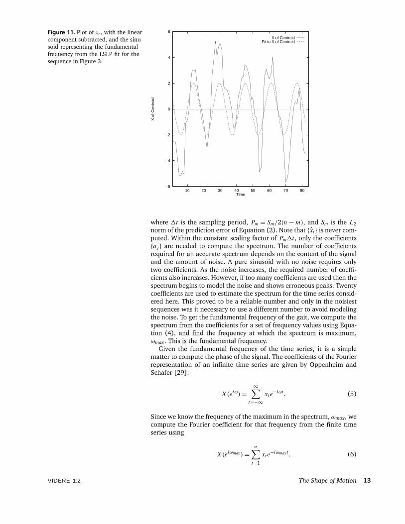
Figure 11. Plot of xc, with the linearcomponent subtracted, and the sinu-soid representing the fundamentalfrequency from the LSLP fit for thesequence in Figure 3.

-6

-4

-2

0

2

4

6

10 20 30 40 50 60 70 80

X o

f Cen

troi

d

Time

X of CentroidFit to X of Centroid

where 1t is the sampling period, Pm = Sm/2(n − m), and Sm is the L2norm of the prediction error of Equation (2). Note that {xt} is never com-puted. Within the constant scaling factor of Pm1t , only the coefficients{aj} are needed to compute the spectrum. The number of coefficientsrequired for an accurate spectrum depends on the content of the signaland the amount of noise. A pure sinusoid with no noise requires onlytwo coefficients. As the noise increases, the required number of coeffi-cients also increases. However, if too many coefficients are used then thespectrum begins to model the noise and shows erroneous peaks. Twentycoefficients are used to estimate the spectrum for the time series consid-ered here. This proved to be a reliable number and only in the noisiestsequences was it necessary to use a different number to avoid modelingthe noise. To get the fundamental frequency of the gait, we compute thespectrum from the coefficients for a set of frequency values using Equa-tion (4), and find the frequency at which the spectrum is maximum,ωmax. This is the fundamental frequency.

Given the fundamental frequency of the time series, it is a simplematter to compute the phase of the signal. The coefficients of the Fourierrepresentation of an infinite time series are given by Oppenheim andSchafer [29]:

X(eiω)=∞∑

t=−∞xte−iωt . (5)

Since we know the frequency of the maximum in the spectrum, ωmax, wecompute the Fourier coefficient for that frequency from the finite timeseries using

X(eiωmax)=n∑t=1

xte−iωmaxt . (6)


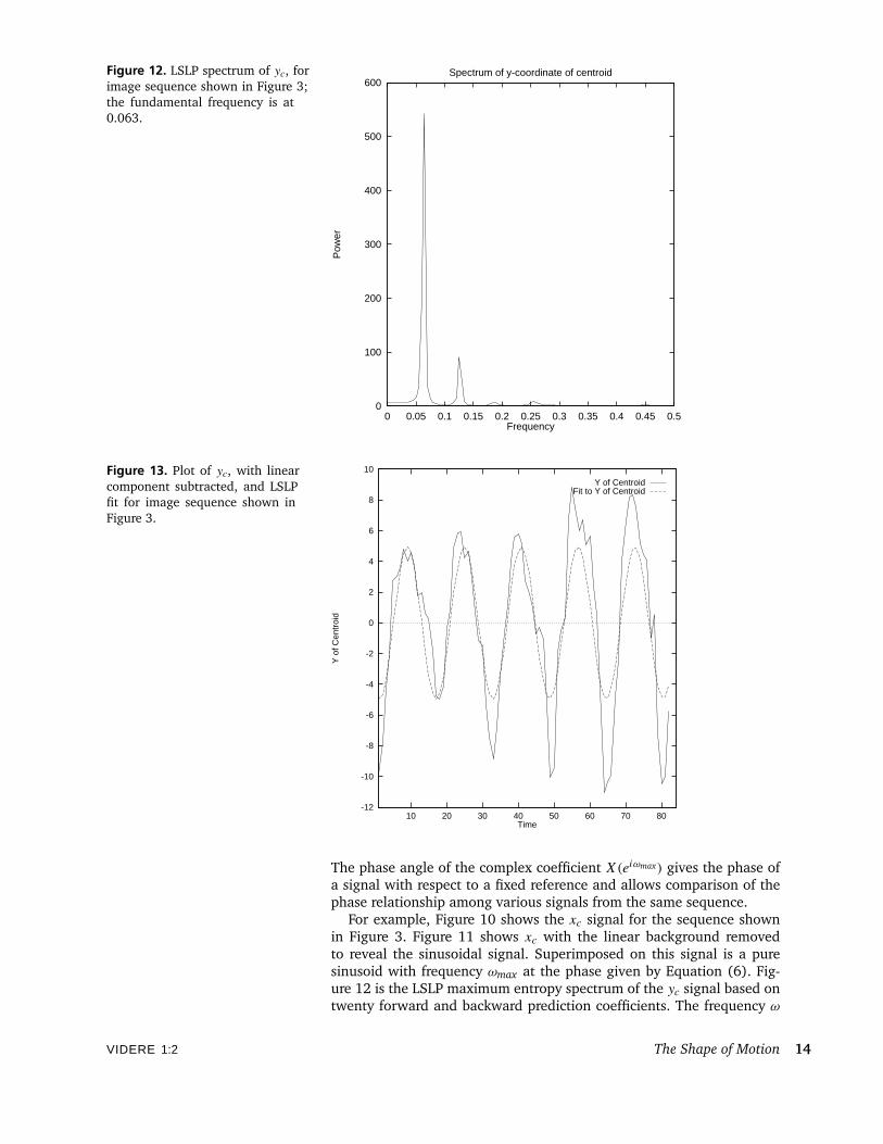
Figure 12. LSLP spectrum of yc, forimage sequence shown in Figure 3;the fundamental frequency is at0.063.

0

100

200

300

400

500

600

0 0.05 0.1 0.15 0.2 0.25 0.3 0.35 0.4 0.45 0.5

Pow

er

Frequency

Spectrum of y-coordinate of centroid

Figure 13. Plot of yc, with linearcomponent subtracted, and LSLPfit for image sequence shown inFigure 3.

-12

-10

-8

-6

-4

-2

0

2

4

6

8

10

10 20 30 40 50 60 70 80

Y o

f Cen

troi

d

Time

Y of CentroidFit to Y of Centroid

The phase angle of the complex coefficient X(eiωmax) gives the phase ofa signal with respect to a fixed reference and allows comparison of thephase relationship among various signals from the same sequence.

For example, Figure 10 shows the xc signal for the sequence shownin Figure 3. Figure 11 shows xc with the linear background removedto reveal the sinusoidal signal. Superimposed on this signal is a puresinusoid with frequency ωmax at the phase given by Equation (6). Fig-ure 12 is the LSLP maximum entropy spectrum of the yc signal based ontwenty forward and backward prediction coefficients. The frequency ω


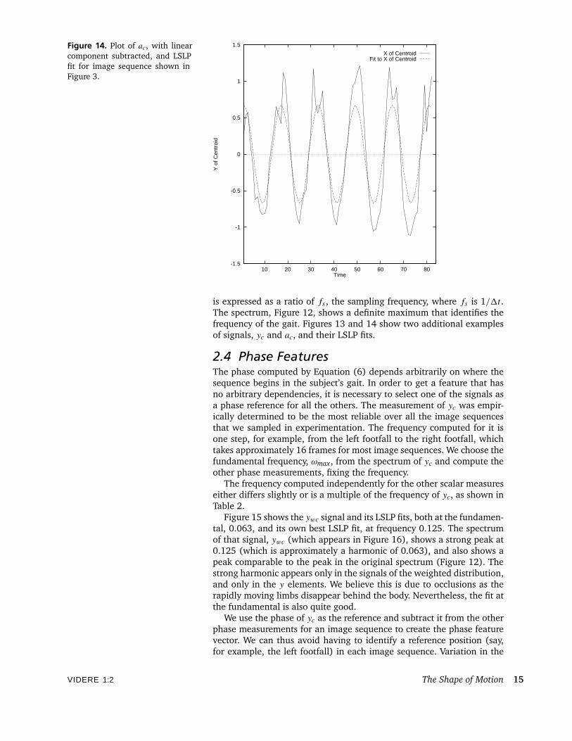
Figure 14. Plot of ac, with linearcomponent subtracted, and LSLPfit for image sequence shown inFigure 3.

-1.5

-1

-0.5

0

0.5

1

1.5

10 20 30 40 50 60 70 80

Y o

f Cen

troi

d

Time

X of CentroidFit to X of Centroid

is expressed as a ratio of fs, the sampling frequency, where fs is 1/1t .The spectrum, Figure 12, shows a definite maximum that identifies thefrequency of the gait. Figures 13 and 14 show two additional examplesof signals, yc and ac, and their LSLP fits.

2.4 Phase FeaturesThe phase computed by Equation (6) depends arbitrarily on where thesequence begins in the subject’s gait. In order to get a feature that hasno arbitrary dependencies, it is necessary to select one of the signals asa phase reference for all the others. The measurement of yc was empir-ically determined to be the most reliable over all the image sequencesthat we sampled in experimentation. The frequency computed for it isone step, for example, from the left footfall to the right footfall, whichtakes approximately 16 frames for most image sequences. We choose thefundamental frequency, ωmax, from the spectrum of yc and compute theother phase measurements, fixing the frequency.

The frequency computed independently for the other scalar measureseither differs slightly or is a multiple of the frequency of yc, as shown inTable 2.

Figure 15 shows the ywc signal and its LSLP fits, both at the fundamen-tal, 0.063, and its own best LSLP fit, at frequency 0.125. The spectrumof that signal, ywc (which appears in Figure 16), shows a strong peak at0.125 (which is approximately a harmonic of 0.063), and also shows apeak comparable to the peak in the original spectrum (Figure 12). Thestrong harmonic appears only in the signals of the weighted distribution,and only in the y elements. We believe this is due to occlusions as therapidly moving limbs disappear behind the body. Nevertheless, the fit atthe fundamental is also quite good.

We use the phase of yc as the reference and subtract it from the otherphase measurements for an image sequence to create the phase featurevector. We can thus avoid having to identify a reference position (say,for example, the left footfall) in each image sequence. Variation in the


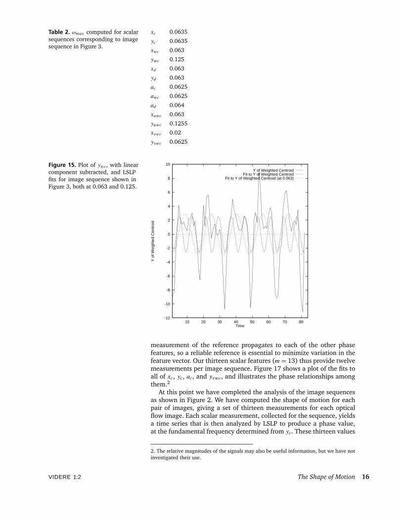
Table 2. ωmax computed for scalarsequences corresponding to imagesequence in Figure 3.

xc 0.0635

yc 0.0635

xwc 0.063

ywc 0.125

xd 0.063

yd 0.063

ac 0.0625

awc 0.0625

ad 0.064

xuwc 0.063

yuwc 0.1255

xvwc 0.02

yvwc 0.0625

Figure 15. Plot of ywc, with linearcomponent subtracted, and LSLPfits for image sequence shown inFigure 3, both at 0.063 and 0.125.

-12

-10

-8

-6

-4

-2

0

2

4

6

8

10

10 20 30 40 50 60 70 80

Y o

f Wei

ghte

d C

entr

oid

Time

Y of Weighted CentroidFit to Y of Weighted Centroid

Fit to Y of Weighted Centroid (at 0.063)

measurement of the reference propagates to each of the other phasefeatures, so a reliable reference is essential to minimize variation in thefeature vector. Our thirteen scalar features (m= 13) thus provide twelvemeasurements per image sequence. Figure 17 shows a plot of the fits toall of xc, yc, ac, and yvwc, and illustrates the phase relationships amongthem.2

At this point we have completed the analysis of the image sequencesas shown in Figure 2. We have computed the shape of motion for eachpair of images, giving a set of thirteen measurements for each opticalflow image. Each scalar measurement, collected for the sequence, yieldsa time series that is then analyzed by LSLP to produce a phase value,at the fundamental frequency determined from yc. These thirteen values

2. The relative magnitudes of the signals may also be useful information, but we have notinvestigated their use.


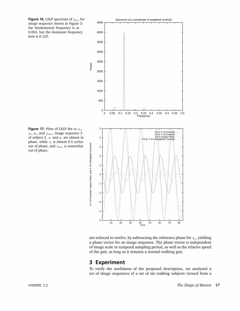
Figure 16. LSLP spectrum of ywc, forimage sequence shown in Figure 3;the fundamental frequency is at0.063, but the dominant frequencyhere is 0.125.

0

500

1000

1500

2000

2500

3000

3500

4000

4500

0 0.05 0.1 0.15 0.2 0.25 0.3 0.35 0.4 0.45 0.5

Pow

er

Frequency

Spectrum of y-coordinate of weighted centroid

Figure 17. Plots of LSLP fits to xc,yc, ac, and yvwc, image sequence 3of subject 5. xc and ac are almost inphase, while yc is almost 0.5 cyclesout of phase, and yvwc is somewhatout of phase.

-5

-4

-3

-2

-1

0

1

2

3

4

5

10 20 30 40 50 60 70 80

X,Y

of C

entr

oid,

Asp

ect R

atio

, and

Y o

f v-W

eigh

ted

Cen

troi

d

Time

Fit to X of CentroidFit to Y of CentroidFit to Aspect Ratio

Fit to Y of v-Weighted Centroid

are reduced to twelve, by subtracting the reference phase for yc, yieldinga phase vector for an image sequence. The phase vector is independentof image scale or temporal sampling period, as well as the relative speedof the gait, as long as it remains a normal walking gait.

3 ExperimentTo verify the usefulness of the proposed description, we analyzed aset of image sequences of a set of six walking subjects viewed from a


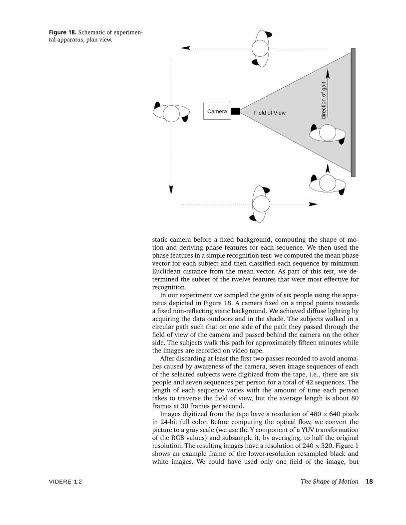
Figure 18. Schematic of experimen-tal apparatus, plan view.

Camera Field of View

dire

ctio

n of

gai

t

static camera before a fixed background, computing the shape of mo-tion and deriving phase features for each sequence. We then used thephase features in a simple recognition test: we computed the mean phasevector for each subject and then classified each sequence by minimumEuclidean distance from the mean vector. As part of this test, we de-termined the subset of the twelve features that were most effective forrecognition.

In our experiment we sampled the gaits of six people using the appa-ratus depicted in Figure 18. A camera fixed on a tripod points towardsa fixed non-reflecting static background. We achieved diffuse lighting byacquiring the data outdoors and in the shade. The subjects walked in acircular path such that on one side of the path they passed through thefield of view of the camera and passed behind the camera on the otherside. The subjects walk this path for approximately fifteen minutes whilethe images are recorded on video tape.

After discarding at least the first two passes recorded to avoid anoma-lies caused by awareness of the camera, seven image sequences of eachof the selected subjects were digitized from the tape, i.e., there are sixpeople and seven sequences per person for a total of 42 sequences. Thelength of each sequence varies with the amount of time each persontakes to traverse the field of view, but the average length is about 80frames at 30 frames per second.

Images digitized from the tape have a resolution of 480× 640 pixelsin 24-bit full color. Before computing the optical flow, we convert thepicture to a gray scale (we use the Y component of a YUV transformationof the RGB values) and subsample it, by averaging, to half the originalresolution. The resulting images have a resolution of 240× 320. Figure 1shows an example frame of the lower-resolution resampled black andwhite images. We could have used only one field of the image, but


the gain of vertical resolution using a full frame offsets the temporalsmoothing produced by using both fields. We use only the lower 160pixels, cutting off the top (which contains only sky). If the camera werecloser we would have had a better view of the moving figures, at thecost of shorter sequences. We opted to get long sequences to improvefrequency and phase estimation. Since the step is approximately 10-20frames, we need at least that, preferably at lease two steps to includethe full cycle. We have used at least 60 frames in all our experiments buthave not experimented with shorter sequences.

4 ResultsWe analyze the phase features in two ways. First, analysis of varianceallows us to determine whether or not there is any significant variationin the phase features among the subjects. Second, we test the matchesbetween each sequence and the remaining sequences to show successfulrecognition. The following two sections describe the results based onthese analyses.

4.1 Analysis of VarianceAnalysis of variance (ANOVA) is a statistical method used to indicate thepresence of a significant variation in a variable related to some factor.Here the variables are the phase features and the factor in which we areinterested is the person walking in front of the camera. Our analysis usesa single-factor ANOVA as described by Winer [45]. The method analyzesonly a single variable and must be repeated for each phase feature.We used the commercial statistical software package StatView 4.5 toperform the analysis.

Care is necessary because most statistical software expects a contin-uous random variable to exist on a line, but phase features exist on acircle, i.e., the phase wraps around causing problems for conventionalcomputations. For example, suppose we have two phase measurementsof +175◦ and −175◦. The mean of these numbers computed in the con-ventional way is 0◦, but because the phase wraps around, the correctmean is 180◦ (or −180◦). The incorrect mean of 0◦ leads to erroneousvariances and confounds ANOVA. We were able to use the commercialsoftware by transforming any feature with a distribution crossing 180◦by rotating the reference for that feature by 180◦, performing the analy-sis, and then rotating the result back. To perform the rotation we usedthe following formula:

θnew ={θ − 180◦ if θ ≥ 0θ + 180◦ if θ < 0

.

This approach proved to be simple and effective while allowing us tocapitalize on the reliability of commercial software.

We now show the analysis for the single phase feature, xc, summa-rized in Table 3. The numbers given indicate the phase as a fraction of acircle’s circumference. Therefore, all phases are in the range [−0.5, 0.5].ANOVA computes the F statistic (the ratio of the between-person vari-ance to the within-person variance) for each feature, and an associatedprobability. The probability indicates the likelihood that the null hypoth-esis is true. In this case, the null hypothesis is that the mean featurevalues for all the people are the same, namely

H0 : µ1 = µ2 = µ3 = µ4 = µ5 = µ6,


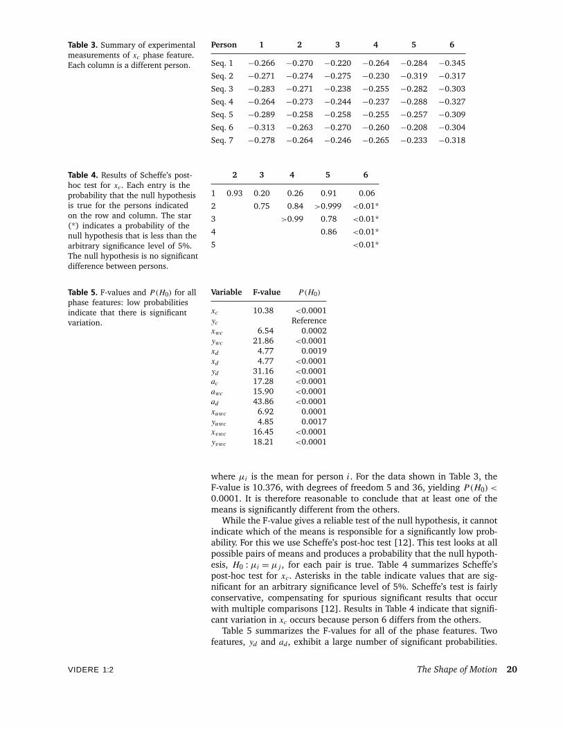
Table 3. Summary of experimentalmeasurements of xc phase feature.Each column is a different person.

Person 1 2 3 4 5 6

Seq. 1 −0.266 −0.270 −0.220 −0.264 −0.284 −0.345

Seq. 2 −0.271 −0.274 −0.275 −0.230 −0.319 −0.317

Seq. 3 −0.283 −0.271 −0.238 −0.255 −0.282 −0.303

Seq. 4 −0.264 −0.273 −0.244 −0.237 −0.288 −0.327

Seq. 5 −0.289 −0.258 −0.258 −0.255 −0.257 −0.309

Seq. 6 −0.313 −0.263 −0.270 −0.260 −0.208 −0.304

Seq. 7 −0.278 −0.264 −0.246 −0.265 −0.233 −0.318

Table 4. Results of Scheffe’s post-hoc test for xc. Each entry is theprobability that the null hypothesisis true for the persons indicatedon the row and column. The star(*) indicates a probability of thenull hypothesis that is less than thearbitrary significance level of 5%.The null hypothesis is no significantdifference between persons.

2 3 4 5 6

1 0.93 0.20 0.26 0.91 0.06

2 0.75 0.84 >0.999 <0.01*

3 >0.99 0.78 <0.01*

4 0.86 <0.01*

5 <0.01*

Table 5. F-values and P(H0) for allphase features: low probabilitiesindicate that there is significantvariation.

Variable F-value P(H0)

xc 10.38 <0.0001yc Referencexwc 6.54 0.0002ywc 21.86 <0.0001xd 4.77 0.0019xd 4.77 <0.0001yd 31.16 <0.0001ac 17.28 <0.0001awc 15.90 <0.0001ad 43.86 <0.0001xuwc 6.92 0.0001yuwc 4.85 0.0017xvwc 16.45 <0.0001yvwc 18.21 <0.0001

where µi is the mean for person i. For the data shown in Table 3, theF-value is 10.376, with degrees of freedom 5 and 36, yielding P(H0) <

0.0001. It is therefore reasonable to conclude that at least one of themeans is significantly different from the others.

While the F-value gives a reliable test of the null hypothesis, it cannotindicate which of the means is responsible for a significantly low prob-ability. For this we use Scheffe’s post-hoc test [12]. This test looks at allpossible pairs of means and produces a probability that the null hypoth-esis, H0 : µi = µj , for each pair is true. Table 4 summarizes Scheffe’spost-hoc test for xc. Asterisks in the table indicate values that are sig-nificant for an arbitrary significance level of 5%. Scheffe’s test is fairlyconservative, compensating for spurious significant results that occurwith multiple comparisons [12]. Results in Table 4 indicate that signifi-cant variation in xc occurs because person 6 differs from the others.

Table 5 summarizes the F-values for all of the phase features. Twofeatures, yd and ad, exhibit a large number of significant probabilities.


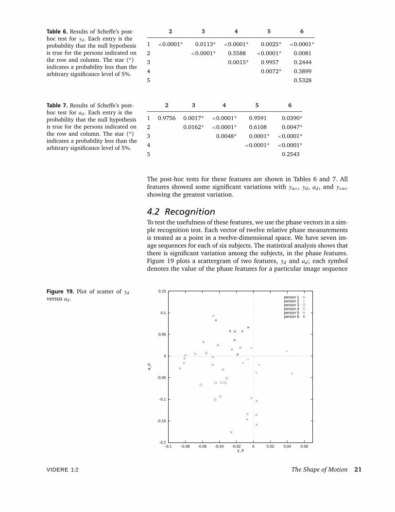
Table 6. Results of Scheffe’s post-hoc test for yd . Each entry is theprobability that the null hypothesisis true for the persons indicated onthe row and column. The star (*)indicates a probability less than thearbitrary significance level of 5%.

2 3 4 5 6

1 <0.0001* 0.0113* <0.0001* 0.0025* <0.0001*

2 <0.0001* 0.5588 <0.0001* 0.0081

3 0.0015* 0.9957 0.2444

4 0.0072* 0.3899

5 0.5328

Table 7. Results of Scheffe’s post-hoc test for ad . Each entry is theprobability that the null hypothesisis true for the persons indicated onthe row and column. The star (*)indicates a probability less than thearbitrary significance level of 5%.

2 3 4 5 6

1 0.9756 0.0017* <0.0001* 0.9591 0.0390*

2 0.0162* <0.0001* 0.6108 0.0047*

3 0.0048* 0.0001* <0.0001*

4 <0.0001* <0.0001*

5 0.2543

The post-hoc tests for these features are shown in Tables 6 and 7. Allfeatures showed some significant variations with ywc, yd, ad, and yvwcshowing the greatest variation.

4.2 RecognitionTo test the usefulness of these features, we use the phase vectors in a sim-ple recognition test. Each vector of twelve relative phase measurementsis treated as a point in a twelve-dimensional space. We have seven im-age sequences for each of six subjects. The statistical analysis shows thatthere is significant variation among the subjects, in the phase features.Figure 19 plots a scattergram of two features, yd and ad; each symboldenotes the value of the phase features for a particular image sequence

Figure 19. Plot of scatter of ydversus ad .

-0.2

-0.15

-0.1

-0.05

0

0.05

0.1

0.15

-0.1 -0.08 -0.06 -0.04 -0.02 0 0.02 0.04 0.06

a_d

y_d

person 1person 2person 3person 4person 5person 6


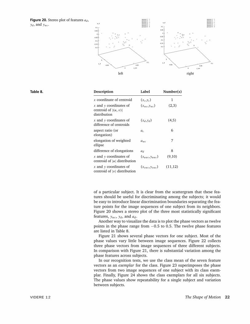
Figure 20. Stereo plot of features ad ,yd , and ywc.

person 1

0

0.05

0.1

-0.05

0

-0.2

-0.15

-0.1

-0.05

0

0.05

0.1

y_wc

y_d

a_d

person 2person 3person 4person 5person 6

person 1

0

0.05

0.1-0.05

0

-0.2

-0.15

-0.1

-0.05

0

0.05

0.1

y_wc

y_d

a_dperson 2person 3person 4person 5person 6

left right

Table 8. Description Label Number(s)

x coordinate of centroid (xc,yc) 1

x and y coordinates of (xwc,ywc) (2,3)centroid of |(u, v)|distribution

x and y coordinates of (xd ,yd) (4,5)difference of centroids

aspect ratio (or ac 6elongation)

elongation of weighted awc 7ellipse

difference of elongations ad 8

x and y coordinates of (xuwc,yuwc) (9,10)centroid of |u| distribution

x and y coordinates of (xvwc,yvwc) (11,12)centroid of |v| distribution

of a particular subject. It is clear from the scattergram that these fea-tures should be useful for discriminating among the subjects; it wouldbe easy to introduce linear discrimination boundaries separating the fea-ture points for the image sequences of one subject from its neighbors.Figure 20 shows a stereo plot of the three most statistically significantfeatures, ywc, yd, and ad.

Another way to visualize the data is to plot the phase vectors as twelvepoints in the phase range from −0.5 to 0.5. The twelve phase featuresare listed in Table 8.

Figure 21 shows several phase vectors for one subject. Most of thephase values vary little between image sequences. Figure 22 collectsthree phase vectors from image sequences of three different subjects.In comparison with Figure 21, there is substantial variation among thephase features across subjects.

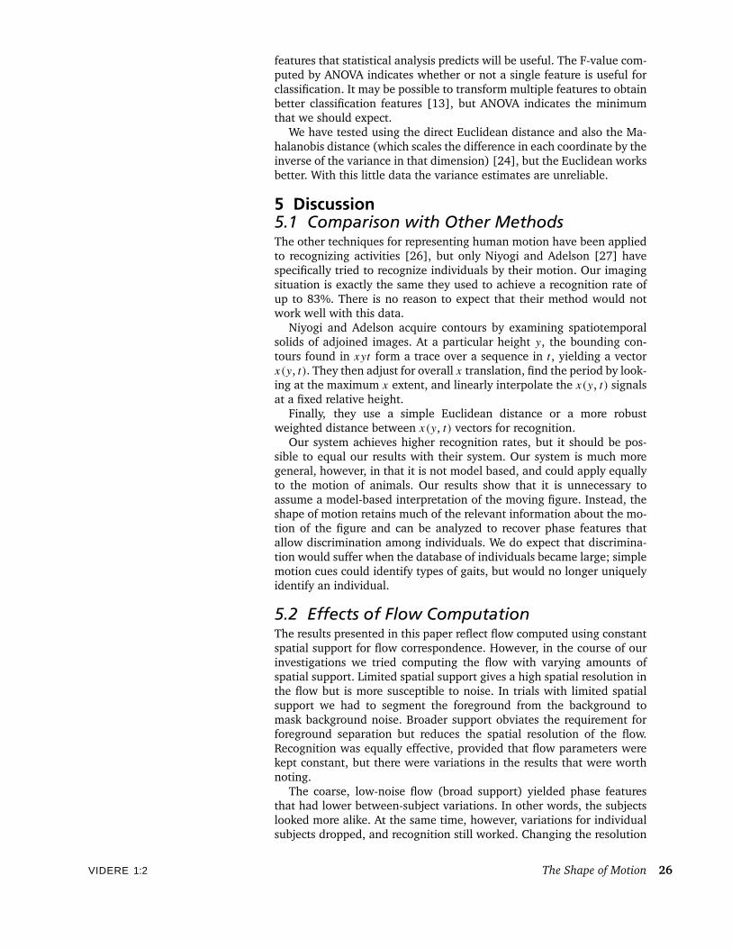
In our recognition tests, we use the class mean of the seven featurevectors as an exemplar for the class. Figure 23 superimposes the phasevectors from two image sequences of one subject with its class exem-plar. Finally, Figure 24 shows the class exemplars for all six subjects.The phase values show repeatability for a single subject and variationbetween subjects.


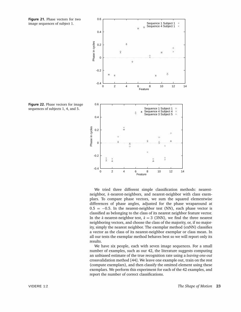
Figure 21. Phase vectors for twoimage sequences of subject 1.

-0.4

-0.2

0

0.2

0.4

0.6

0 2 4 6 8 10 12 14

Pha

se in

cyc

les

Feature

Sequence 1 Subject 1Sequence 4 Subject 1

Figure 22. Phase vectors for imagesequences of subjects 1, 4, and 5.

-0.4

-0.2

0

0.2

0.4

0.6

0 2 4 6 8 10 12 14

Pha

se in

cyc

les

Feature

Sequence 1 Subject 1Sequence 4 Subject 4Sequence 3 Subject 5

We tried three different simple classification methods: nearest-neighbor, k-nearest-neighbors, and nearest-neighbor with class exem-plars. To compare phase vectors, we sum the squared elementwisedifferences of phase angles, adjusted for the phase wraparound at0.5 = −0.5. In the nearest-neighbor test (NN), each phase vector isclassified as belonging to the class of its nearest neighbor feature vector.In the k-nearest-neighbor test, k = 3 (3NN), we find the three nearestneighboring vectors, and choose the class of the majority, or, if no major-ity, simply the nearest neighbor. The exemplar method (exNN) classifiesa vector as the class of its nearest-neighbor exemplar or class mean. Inall our tests the exemplar method behaves best so we will report only itsresults.

We have six people, each with seven image sequences. For a smallnumber of examples, such as our 42, the literature suggests computingan unbiased estimate of the true recognition rate using a leaving-one-outcrossvalidation method [44]. We leave one example out, train on the rest(compute exemplars), and then classify the omitted element using theseexemplars. We perform this experiment for each of the 42 examples, andreport the number of correct classifications.


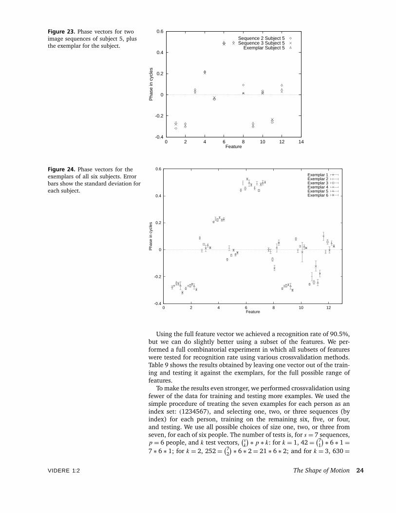
Figure 23. Phase vectors for twoimage sequences of subject 5, plusthe exemplar for the subject.

-0.4

-0.2

0

0.2

0.4

0.6

0 2 4 6 8 10 12 14

Pha

se in

cyc

les

Feature

Sequence 2 Subject 5Sequence 3 Subject 5

Exemplar Subject 5

Figure 24. Phase vectors for theexemplars of all six subjects. Errorbars show the standard deviation foreach subject.

-0.4

-0.2

0

0.2

0.4

0.6

0 2 4 6 8 10 12

Pha

se in

cyc

les

Feature

Exemplar 1Exemplar 2Exemplar 3Exemplar 4Exemplar 5Exemplar 6

Using the full feature vector we achieved a recognition rate of 90.5%,but we can do slightly better using a subset of the features. We per-formed a full combinatorial experiment in which all subsets of featureswere tested for recognition rate using various crossvalidation methods.Table 9 shows the results obtained by leaving one vector out of the train-ing and testing it against the exemplars, for the full possible range offeatures.

To make the results even stronger, we performed crossvalidation usingfewer of the data for training and testing more examples. We used thesimple procedure of treating the seven examples for each person as anindex set: (1234567), and selecting one, two, or three sequences (byindex) for each person, training on the remaining six, five, or four,and testing. We use all possible choices of size one, two, or three fromseven, for each of six people. The number of tests is, for s = 7 sequences,p = 6 people, and k test vectors,

(sk

) ∗ p ∗ k: for k = 1, 42= (71) ∗ 6 ∗ 1=7 ∗ 6 ∗ 1; for k = 2, 252= (72) ∗ 6 ∗ 2= 21 ∗ 6 ∗ 2; and for k = 3, 630=


Table 9. Results of recognition, usingleave-one-out crossvalidation, withthe number of features used andpercentage correct.

Number Features Percent correct

1 ad 66.7

2 ad , yvwc 85.7

3 ywc, ad , yvwc 90.5

4 yd , ac, ad , yvwc 92.9

5 xd , yd , awc, ad , yvwc 95.2

6 xd , yd , awc, ad , xuwc, yvwc 95.2

Table 10. Subsets of size k = 1: re-sults of recognition, with the numberof features used and percentage cor-rect.


1 ad 66.7

2 ywc, ad 85.7


4 yd , awc, ad , yvwc 95.2

5 yd , awc, ad , xuwc, yvwc 95.2



1 ad 61.9

2 ad , yvwc 85.3



5 xc, yd , ac, ad , yvwc 93.7

(73

) ∗ 6 ∗ 3= 35 ∗ 6 ∗ 3. Again we perform full combinatorial experimentsand find the best features. Table 10 shows the results for k = 1, Table 11for k = 2, and Table 12 for k = 3.

Even when almost half of the data are omitted, the recognition ratesremain over 90% when five features are used out of twelve. Only threefeatures are needed for excellent success rates.

The analysis of variance predicts that the features will have the fol-lowing approximate significance:

ad > yd > ywc > yvwc > ac > xvwc >

awc > xc > xuwc > xwc > yuwc > xd.

The scattergram of yd and ad indicates why these features are actuallyuseful in recognition (Figure 19); the separation of subjects using thesefeatures is quite good. When we consider triples of features, using exNN,the subsets of features that showed best recognition rates were (ywc, ad,yvwc), (yd, ad, yvwc), and (ywc, yd, ad). These correspond well with the



1 ad 60.5

2 ad , yvwc 84.6



5 xc, yd , ac, ad , yvwc 92.2


features that statistical analysis predicts will be useful. The F-value com-puted by ANOVA indicates whether or not a single feature is useful forclassification. It may be possible to transform multiple features to obtainbetter classification features [13], but ANOVA indicates the minimumthat we should expect.

We have tested using the direct Euclidean distance and also the Ma-halanobis distance (which scales the difference in each coordinate by theinverse of the variance in that dimension) [24], but the Euclidean worksbetter. With this little data the variance estimates are unreliable.

5 Discussion5.1 Comparison with Other MethodsThe other techniques for representing human motion have been appliedto recognizing activities [26], but only Niyogi and Adelson [27] havespecifically tried to recognize individuals by their motion. Our imagingsituation is exactly the same they used to achieve a recognition rate ofup to 83%. There is no reason to expect that their method would notwork well with this data.

Niyogi and Adelson acquire contours by examining spatiotemporalsolids of adjoined images. At a particular height y, the bounding con-tours found in xyt form a trace over a sequence in t , yielding a vectorx(y, t). They then adjust for overall x translation, find the period by look-ing at the maximum x extent, and linearly interpolate the x(y, t) signalsat a fixed relative height.

Finally, they use a simple Euclidean distance or a more robustweighted distance between x(y, t) vectors for recognition.

Our system achieves higher recognition rates, but it should be pos-sible to equal our results with their system. Our system is much moregeneral, however, in that it is not model based, and could apply equallyto the motion of animals. Our results show that it is unnecessary toassume a model-based interpretation of the moving figure. Instead, theshape of motion retains much of the relevant information about the mo-tion of the figure and can be analyzed to recover phase features thatallow discrimination among individuals. We do expect that discrimina-tion would suffer when the database of individuals became large; simplemotion cues could identify types of gaits, but would no longer uniquelyidentify an individual.

5.2 Effects of Flow ComputationThe results presented in this paper reflect flow computed using constantspatial support for flow correspondence. However, in the course of ourinvestigations we tried computing the flow with varying amounts ofspatial support. Limited spatial support gives a high spatial resolution inthe flow but is more susceptible to noise. In trials with limited spatialsupport we had to segment the foreground from the background tomask background noise. Broader support obviates the requirement forforeground separation but reduces the spatial resolution of the flow.Recognition was equally effective, provided that flow parameters werekept constant, but there were variations in the results that were worthnoting.

The coarse, low-noise flow (broad support) yielded phase featuresthat had lower between-subject variations. In other words, the subjectslooked more alike. At the same time, however, variations for individualsubjects dropped, and recognition still worked. Changing the resolution


of the flow changed the set of features showing the most-significantvariation. Features that were useful for fine flow were not necessarilyviable for coarse flow, and vice versa. The key factor is that whatevercombination of flow algorithm and parameters is used, that combinationmust be held constant for recognition to work.

The figures appearing in this paper are for flow with relatively highspatial resolution. Elements of a figure such as moving arms or legs havehigh velocities, and change their spatial orientation during movement,unlike the trunk. Thus, flow values of the center of the body are less sub-ject to noise. With better spatiotemporal resolution, the limbs are betterdetected in the flow. This suggests that the features of flow that dependon the spatial distribution of velocities would be more important. This isexactly what we found. In these tests, the phase features that were mosteffective in recognition included ad, yd, ywc, and yvwc.

5.3 Intuitive Understanding of Phase FeaturesAfter statistical analysis and testing of classification methods, we mustconsider why these phase features allow recognition. At present we haveno provable explanation, but we offer the following speculation basedon our experimental results and intuition.

The phase features we compute are scale independent. They shouldnot vary with the distance between the camera and the subject. Noscaling of the data is required. The phase of the scalar signals remainsunchanged if the subject is small or large in the camera field of view.

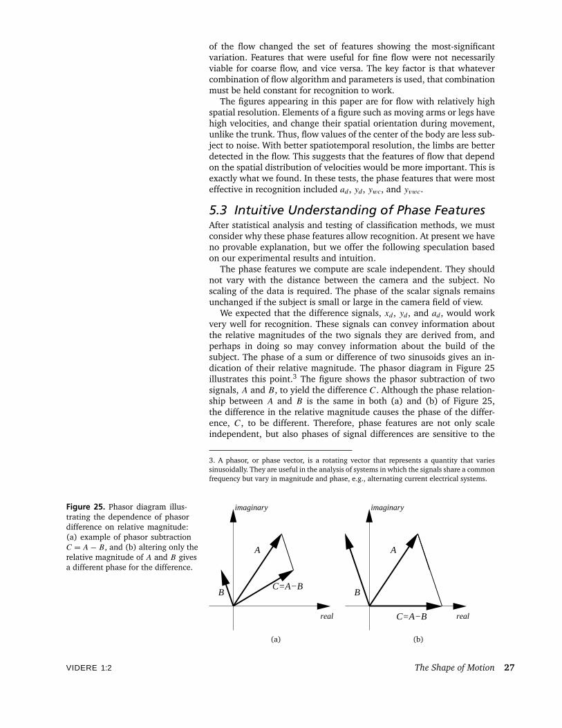
We expected that the difference signals, xd, yd, and ad, would workvery well for recognition. These signals can convey information aboutthe relative magnitudes of the two signals they are derived from, andperhaps in doing so may convey information about the build of thesubject. The phase of a sum or difference of two sinusoids gives an in-dication of their relative magnitude. The phasor diagram in Figure 25illustrates this point.3 The figure shows the phasor subtraction of twosignals, A and B, to yield the difference C. Although the phase relation-ship between A and B is the same in both (a) and (b) of Figure 25,the difference in the relative magnitude causes the phase of the differ-ence, C, to be different. Therefore, phase features are not only scaleindependent, but also phases of signal differences are sensitive to the

3. A phasor, or phase vector, is a rotating vector that represents a quantity that variessinusoidally. They are useful in the analysis of systems in which the signals share a commonfrequency but vary in magnitude and phase, e.g., alternating current electrical systems.

Figure 25. Phasor diagram illus-trating the dependence of phasordifference on relative magnitude:(a) example of phasor subtractionC = A− B, and (b) altering only therelative magnitude of A and B givesa different phase for the difference.

real

imaginary

A

BC=A−B

real

imaginary

A

B

C=A−B

(a) (b)


relative magnitudes of the scalar signals. This means that people of dif-fering builds but with similar rhythms might still be distinguished by ouranalysis.

Our expectations were largely realized in our results: ad and yd wereexcellent for recognition where high spatiotemporal resolution was used,but xd was poor. Our results suggest that, while our notions about theusefulness of the difference signals may be valid, we still need to under-stand better the effects of flow calculations on the features.

5.4 Limitations of ResultsAlthough the analysis of our results is valid, we are limited in our abilityto extrapolate them. Our sample size was small (only six subjects) sowe cannot conclude much about gaits in the entire human population.In addition to the small sample size, no steps were taken to ensure arandom sample. However, the excellent recognition results and strongstatistical evidence of variation between subjects attest to the value ofshape-of-motion features.

As mentioned in Sections 5.1 and 5.2, the parameters used in thecomputation of optical flow can affect the values of the phase features.Although we believe that varying parameters and methods for comput-ing optical flow will produce features useful for recognition, we do notyet understand enough to predict which features will be the best.

It is entirely possible, even likely, that there are correlations amongthe various features. We have not analyzed the data extensively to iden-tify these correlations.

In an effort to control the conditions of the experiment, we consideredonly pedestrians walking across the camera field of view. There is noreason to expect that shape-of-motion features are invariant to viewingangle, so we expect recognition—using the features we have acquired—to fail if the view is not approximately perpendicular to the directionof the gait. Some of our preliminary results suggest that recognition ispossible for pedestrians walking towards and away from the camera. Ourexperiments included only three sequences each for two subjects; wewere able to classify five out of six for a sequence in which the subjectwalks across the field of view, but with some motion towards the camera.For sequences walking towards and away from the camera, we correctlyclassified all six sequences.

However, the exemplars are not similar in the two cases. When mo-tion is perpendicular to the viewing direction, self-occlusion is maximal,but the figure’s relative motion is largest. Motion along the viewingdirection eliminates self-occlusion, but the relative motion is less. Insurveillance applications where multiple cameras are employed, this isnot likely to be a problem. One simply selects the images from the cam-era with the best viewing angle for recognition. Moreover, it is possibleto identify which direction an individual is walking and use that infor-mation to select the appropriate set of exemplars tuned to the directionof movement.

The controlled experimental situation eliminates other considera-tions, such as moving backgrounds, tracking cameras, and occlusions.

5.5 Future WorkThe experiment described here attempts to eliminate confounding fac-tors from the experiment by acquiring all image sequences under iden-tical circumstances. There remains the task of determining what effect


other factors may have, such as viewing angle, clothing of subjects, andtime.

For practical application of shape-of-motion features, we need toknow the useful range of camera views over which the recognition willwork for a single set of exemplars. A useful experiment would be todetermine the sensitivity of the features to viewing angle. The resultswould enable a multicamera surveillance system to select an optimalview for recognition.

People have ways of subjectively describing the way a person walks.A person may have a bouncy walk or perhaps a shuffle. One may in-fer that a person is excited or lethargic based on such observations. Afuture experiment may determine if the phase features of walking canbe correlated to subjective descriptions of the way a person walks. Theresult would be a feature space that is segmented based on subjectivedescriptions. Some human-figure animation work in computer graphicsby Unuma et al suggest that this may be possible [42]. They model ahuman gait using a set of periodic joint-angle functions for several sub-jectively different gaits. They then interpolate Fourier decompositionsof these signals to generate a variety of gait types. Based on this idea,our proposed model-free recognition method may be able not only torecognize, but describe too.

Model-free recognition may be applied to the domain of image data-bases. The method could search a large database of image sequences forgaits of various types. For example, one could search a database for se-quences that contain periodic motion. Then, if the moving region hasall the correct phase relationships, one may conclude that the sequencecontains a person walking. Further analysis may allow one to search forpeople who walk like a given person, or exhibit certain characteristics intheir gait.

Moving light displays (MLDs) have seen extensive use in gait analysis,and experiments with them have shown that recognition by humans ispossible using the MLD images alone. The focus of computer analysis ofMLDs has been on the construction of a kinematic model of the subject.Our results suggest that this may not be necessary for recognition. Opti-cal flow computed from MLD images may be viewed as a point samplingof the full flow field. If the sampling is sufficient to estimate the scalarsused in our recognition system, then model-free recognition is possible.In related work [8], we have examined the relationships between theMLD flow and full flow images and found that the phase features havevalues, when derived from the MLD images, that are similar to the val-ues using full gray-value images. This suggests that there is no need todetermine an articulated model to interpret MLD images.

6 SummaryThe spatial distribution of optical flow, the shape of motion, yieldsmodel-free features whose variation over time is periodic. The essen-tial difference among these features is the relative phase between theperiodic signals. Our experiments and analysis demonstrate that thesephase measurements are repeatable for particular subjects and vary sig-nificantly between subjects. The variation makes the features effectivefor recognizing individuals by characteristics of their gait, and the recog-nition is relatively insensitive to the means for computing optical flow.The phase analysis applies directly to periodic motion events, but theflow description, the shape of motion, applies to other motions.


7 AcknowledgmentsWe wish to thank the graduate students at the UCSD Visual Com-puting Laboratory for their participation as subjects in our experi-ments. Also, Dr. J. Edwin Boyd provided valuable advice on the useof ANOVA. Thanks also to Don Murray for valuable suggestions aboutthe manuscript.

References[1] Barrodale, I. and Erickson, R. E. Algorithms for least-squares linear

prediction and maximum entropy spectral analysis—part I: Theory.Geophysics, 45(3):420–432, 1980.

[2] Barrodale, I. and Erickson, R. E. Algorithms for least-squareslinear prediction and maximum entropy spectral analysis—part II:FORTRAN program. Geophysics, 45(3):433–446, 1980.

[3] Baumberg, A. M. and Hogg, D. C. Learning flexible models fromimage sequences. Technical Report 93.36, University of LeedsSchool of Computer Studies, 1993.

[4] Baumberg, A. M. and Hogg, D. C. Learning spatiotemporal modelsfrom training examples. Technical Report 95.9, University of LeedsSchool of Computer Studies, 1995.

[5] Bharatkumar, A. G., Daigle, K. E., Pandy, M. G., Cai, Q., andAggarwal, J. K. Lower limb kinematics of human walking with themedial axis transformation. In IEEE Workshop on Nonrigid Motion,pages 70–76, 1994.

[6] Bobick, A. F. and Davis, J. W. An appearance-based representation ofaction. In Proc. 13th International Conference on Pattern Recognition,1996.

[7] Bobick, A. F. and Davis, J. W. Real-time recognition of activity usingtemporal templates. In Workshop on Applications of Computer Vision,1996.

[8] Boyd, J. E. and Little, J. Global vs. segmented interpretation ofmotion: Multiple light displays. In IEEE Nonrigid and ArticulatedMotion Workshop, pages 18–25, 1997.

[9] Bregler, C. Learning and recognizing human dynamics in videosequences. In Proc. IEEE Conf. Computer Vision and PatternRecognition, 1997, pages 568–574, 1997.

[10] Bulthoff, H., Little, J. J., and Poggio, T. A parallel algorithm forreal-time computation of optical flow. Nature, 337:549–553, 1989.

[11] Cedras, C. and Shah, M. A survey of motion analysis from movinglight displays. In Proc. IEEE Conf. Computer Vision and PatternRecognition, 1994, pages 214–221, 1994.

[12] Cohen, P. R. Empirical Methods for Artificial Intelligence. The MITPress, Cambridge, MA, 1995.

[13] Cui, Y., Swets, D., and Weng, J. Learning-based hand signrecognition using shoslif-m. In Proc. 5th International Conference onComputer Vision, pages 631–636, 1995.

[14] Davis, J. W. and Bobick, A. F. The representation and recognitionof human movement using temporal templates. In Proc. IEEEConf. Computer Vision and Pattern Recognition, 1997, pages 928–934, 1997.

[15] Fua, P. A parallel stereo algorithm that produces dense depth mapsand preserves image features. Technical Report 1369, INRIA, 1991.


[16] Hogg, D. C. A program to see a walking person. Image and VisionComputing, 1(1):5–20, 1983.

[17] Hu, M. Visual pattern recognition by moment invariants. IRE Trans.Information Theory, IT-8(2), 1962.

[18] Hunter, E. A., Kelly, P. H., and Jain, R. C. Estimation of articulatedmotion using kinematics of constrained mixture densities. In IEEENonrigid and Articulated Motion Workshop, pages 10–17, 1997.

[19] Ju, S. X., Black, M. J., and Yacoob, Y. Cardboard people: Aparameterized model of articulated motion. In 2nd Int. Conf. onAutomatic Face- and Gesture-Recognition, pages 38–44, Killington,Vermont, 1996.

[20] Little, J. J. and Boyd, J. E. Describing motion for recognition. InIEEE Symposium on Computer Vision, pages 235–240, 1995.

[21] Little, J. J. and Kam, J. A smart buffer for tracking using motiondata. In Proc. Workshop on Computer Architectures for MachinePerception, pages 257–266, 1993.

[22] Liu, F. and Picard, R. W. Detecting and segmenting periodic motion.Technical Report 400, MIT Media Lab Perceptual ComputingSection, 1996.

[23] Luttgens, K. and Wells, K. F. Kinesiology: Scientific Basis of HumanMotion. Saunders College Publishing, Philadelphia, 1982.

[24] Mahalanobis, P. On the generalized distance in statistics. Proc. Natl.Inst. Science, 12:49–55, 1936.

[25] Marr, D. and Poggio, T. Cooperative computation of stereo disparity.Science, 194(4262):283–287, 1976.

[26] Nelson, R. C. and Polana, R. Qualitative recognition of motionfrom temporal texture. Journal of Visual Communication and ImageRepresentation, 5:172–180, 1994.

[27] Niyogi, S. A. and Adelson, E. H. Analyzing and recognizing walkingfigures in XYT. In Proc. IEEE Conf. Computer Vision and PatternRecognition, 1994, pages 469–474, 1994.

[28] Niyogi, S. A. and Adelson, E. H. Analyzing gait with spatiotemporalsurfaces. In IEEE Workshop on Nonrigid Motion, pages 64–69, 1994.

[29] Oppenheim, A. V. and Schafer, R. W. Discrete-Time Signal Processing.Prentice-Hall, Englewood Cliffs, NJ, 1989.

[30] Piscopo, J. and Baley, J. A. Kinesiology, the science of movement.John Wiley and Sons, New York, 1981.

[31] Polana, R. and Nelson, R. Detecting activities. In Proc. IEEEConf. Computer Vision and Pattern Recognition, 1993, pages 2–7,1993.

[32] Polana, R. and Nelson, R. Recognition of nonrigid motion. InProc. 1994 DARPA Image Understanding Workshop, pages 1219–1224, 1994.

[33] Polana, R. and Nelson, R. Nonparametric recognition of nonrigidmotion. Technical Report TR575, University of Rochester, 1995.

[34] Press, W. H., Teukolsky, S. A., Vetterling, W. T., and Flannery, B. P.Numerical Recipes in C (2nd Edition). Cambridge University Press,1992.

[35] Rohr, K. Towards model-based recognition of human movements inimage sequences. Computer Vision, Graphics, and Image Processing,59(1):94–115, 1994.


[36] Rowley, H. A. and Rehg, J. M. Analyzing articulated motion usingexpectation maximization. In Proc. IEEE Conf. Computer Vision andPattern Recognition, 1997, pages 935–941, 1997.

[37] S. Lawrence Marple, J. Digital Spectral Analysis with Applications.Prentice-Hall, Englewood Cliffs, NJ, 1987.

[38] Seitz, S. M. and Dyer, C. R. Affine invariant detection of periodicmotion. In Proc. IEEE Conf. Computer Vision and Pattern Recognition,1994, pages 970–975, 1994.

[39] Shavit, E. and Jepson, A. Motion understanding using phaseportraits. In IJCAI Workshop: Looking at People, 1993.

[40] Shavit, E. and Jepson, A. Qualitative motion from visual dynamics.In IEEE Workshop on Qualitative Vision, pages 82–88, 1993.

[41] Teh, C. H. and Chin, R. T. On image analysis by the methodsof moments. IEEE Transactions on Pattern Analysis and MachineIntelligence, 10:496–513, 1988.

[42] Unuma, M., Anjyo, K., and Takeuchi, R. Fourier principles foremotion-based human figure animation. In Proceedings of SIGRAPH95, pages 91–96, 1995.

[43] Wachter, S. and Nagel, H.-H. Tracking of persons in monocularimage sequences. In IEEE Nonrigid and Articulated Motion Workshop,pages 1–9, 1997.

[44] Weiss, S. M. and Kulikowski, C. A. Computer Systems That Learn.Morgan Kaufmann, 1991.

[45] Winer, B. J. Statistical Principles in Experimental Design. McGraw-Hill, New York, 1971.


Editors in Chief

Christopher Brown, University of RochesterGiulio Sandini, Universita di Genova, Italy

Editorial Board

Yiannis Aloimonos, University of MarylandNicholas Ayache, INRIA, FranceRuzena Bajcsy, University of PennsylvaniaDana H. Ballard, University of RochesterAndrew Blake, University of Oxford, United KingdomJan-Olof Eklundh, The Royal Institute of Technology (KTH), SwedenOlivier Faugeras, INRIA Sophia-Antipolis, FranceAvi Kak, Purdue UniversityTakeo Kanade, Carnegie Mellon UniversityJoe Mundy, General Electric Research LabsTomaso Poggio, Massachusetts Institute of TechnologySteven A. Shafer, Microsoft CorporationDemetri Terzopoulos, University of Toronto, CanadaSaburo Tsuji, Osaka University, JapanAndrew Zisserman, University of Oxford, United Kingdom

Action Editors

Minoru Asada, Osaka University, JapanTerry Caelli, Ohio State UniversityAdrian F. Clark, University of Essex, United KingdomPatrick Courtney, Z.I.R.S.T., FranceJames L. Crowley, LIFIA—IMAG, INPG, FranceDaniel P. Huttenlocher, Cornell UniversityYasuo Kuniyoshi, Electrotechnical Laboratory, JapanShree K. Nayar, Columbia UniversityAlex P. Pentland, Massachusetts Institute of TechnologyEhud Rivlin, Technion—Israel Institute of TechnologyLawrence B. Wolff, Johns Hopkins UniversityZhengyou Zhang, Microsoft Research, Microsoft CorporationSteven W. Zucker, Yale University

Recognizing people by their gait: the shape of motion

Documents

Transcript of Recognizing people by their gait: the shape of motion