Ravulakollu, Kiran Kumar (2012) Sensory Integration Model ...
164
Ravulakollu, Kiran Kumar (2012) Sensory Integration Model Inspired by the Superior Colliculus For Multimodal Stimuli Localization. Doctoral thesis, University of Sunderland. Downloaded from: http://sure.sunderland.ac.uk/id/eprint/3759/ Usage guidelines Please refer to the usage guidelines at http://sure.sunderland.ac.uk/policies.html or alternatively contact [email protected].
-
Upload
khangminh22 -
Category
Documents
-
view
1 -
download
0
Transcript of Ravulakollu, Kiran Kumar (2012) Sensory Integration Model ...

Ravulakollu, Kiran Kumar (2012) Sensory Integration Model Inspired by the Superior Colliculus For Multimodal Stimuli Localization. Doctoral thesis, University of Sunderland.
Downloaded from: http://sure.sunderland.ac.uk/id/eprint/3759/
Usage guidelines
Please refer to the usage guidelines at http://sure.sunderland.ac.uk/policies.html or alternatively contact [email protected].

Ravulakollu, Kiran Kumar (2012) Sensory Integration Model Inspired by the Superior Colliculus For Multimodal Stimuli Localization. Doctoral thesis, University of Sunderland.
Downloaded from: http://sure.sunderland.ac.uk/3759/
Usage guidelines
Please refer to the usage guidelines at http://sure.sunderland.ac.uk/policies.html or alternatively contact [email protected].

Sensory Integration Model Inspired by the Superior Colliculus For Multimodal Stimuli Localization
Kiran Kumar Ravulakollu
A thesis submitted in partial fulfillment of the requirements of the University of Sunderland for the degree of
Doctor of Philosophy
October 2012
Faculty of Applied Sciences
Department of Computing, Engineering and Technology University of Sunderland
Sunderland United Kingdom

ii
Acknowledgements I would like to acknowledge a number of people, who provided me moral and
physical motivation along with support in successful completion of the thesis.
First, I would like to thank my primary director of studies Prof. Stefan Wermter who
has provided a constant guidance and support during the research and
development of this project. Stefan is very helpful in shaping the idea into a
research area and constantly monitored the progress through-out the process. His
initiation for publications assisted to realize their importance for a bright start.
My supervisor late Dr. Harry Erwin had been an immense treasure for biological
inspiration in this project. His clarifications and discussions had given an insight in
the area which later helped in modeling the project. I would like to convey my deep
regards for his support during the research and development of the project.
I would like to thank my director of studies Dr. Kevin Burn for giving me the
opportunity to continue under his supervision during the writing-up state. His
motivation and constant encouragement has extended my confidence in
successful completion of this research project.
I would also like to thank a number of fellow researchers in the group in particular
Dr. Jindong Liu, Dr. Michael Knowles, Mr. Simon Farrand and Dr. Chi-Yung Yan
who has shared their experience on several areas that let me able to find insights
at conceptual level and execute the motivation behind the approach.
I would like to thank my brother Dr. Ravi Shankar Ravulakollu for his moral and
financial support and also for believing in me without which I wouldn’t have fulfilled
my dream. I also take the opportunity to thank my family, for their undivided
patience and understanding. I feel deeply sorry to them since my research has
always proceeded over their requirements. Hereafter, my contributions to family
will be equal to my career.

iii
Finally, I would like to acknowledge the continued support of my friends. In
particular, I thank Dhinesh Gollapudi, Kiran Kumar Vangara and Bharath Kumar
Musunuru who have believed in me and gave necessary motivation along with
constant support during the times necessary. Their sponsorship at times needed
for my publication is much appreciated. I also thank all my near and dear friends
who supported me directly or indirectly for everything during the research and
development.

i
Abstract Sensory information processing is an important feature of robotic agents that must
interact with humans or the environment. For example, numerous attempts have
been made to develop robots that have the capability of performing interactive
communication. In most cases, individual sensory information is processed and
based on this, an output action is performed. In many robotic applications, visual
and audio sensors are used to emulate human-like communication. The Superior
Colliculus, located in the mid-brain region of the nervous system, carries out
similar functionality of audio and visual stimuli integration in both humans and
animals.
In recent years numerous researchers have attempted integration of sensory
information using biological inspiration. A common focus lies in generating a single
output state (i.e. a multimodal output) that can localize the source of the audio and
visual stimuli. This research addresses the problem and attempts to find an
effective solution by investigating various computational and biological
mechanisms involved in the generation of multimodal output. A primary goal is to
develop a biologically inspired computational architecture using artificial neural
networks. The advantage of this approach is that it mimics the behaviour of the
Superior Colliculus, which has the potential of enabling more effective human-like
communication with robotic agents.
The thesis describes the design and development of the architecture, which is
constructed from artificial neural networks using radial basis functions. The
primary inspiration for the architecture came from emulating the function top and
deep layers of the Superior Colliculus, due to their visual and audio stimuli
localization mechanisms, respectively. The integration experimental results have
successfully demonstrated the key issues, including low-level multimodal stimuli
localization, dimensionality reduction of audio and visual input-space without
affecting stimuli strength, and stimuli localization with enhancement and
depression phenomena. Comparisons have been made between computational
and neural network based methods, and unimodal verses multimodal integrated
outputs in order to determine the effectiveness of the approach.

iv
List of Contents
Abstract…………………………….…………………………………………………….i Acknowledgement……………….…………………………………………………….ii Contents………………………….……………………………………………………..iv Glossary……………………………………………………………………………….viii List of Figures………………………………………………………………………….ix List of Tables…………………….…………………………………………………….xii List of Equations……………….…………………………………………………….xiii
Chapter 1: Introduction………………………….……………..……………………1-5
1.1. Overview…………………………………………………………………………..1 1.2. Motivation…………………………………………………………………………1 1.3. Research Question ……………………………………………………………..2 1.4. Aim and Objectives……………………………………………………...……...3 1.5. Research Contribution…………………………………………………………3 1.6. Thesis Structure…………………………………………………………………3
Chapter 2: Literature Review……………………………………….6-32
2.1 Introduction…………………………………………………………….………...6 2.2 Biological Overview of the Superior Colliculus……………………………6
2.2.1. The Biological Motivation………………………………………………...6
2.2.2. Neuroscience aspects of the Superior Colliculus……………………..8
2.3 Multimodal Behaviour of the Superior Colliculus………………………..12 2.4 Literature on Multisensory Integration…………………………………….15 2.5 Literature Review on Integration of Audio and Visual Data……………16
2.5.1. Probabilistic Approach………………………………………………….17
2.5.2. Neural Network Approach……………………………………………...20
2.5.3. Application-driven Approach…………………………………………...26
2.5.4. Conceptual Approach…………………………………………………..28
2.6 Summary and Discussion……………………………………………………31

List of Contents
v
Chapter 3: Methodology and Design Architecture of the Integration Model…………………………………………………….33-57
3.1 Introduction…………………………………………………………………….33 3.2 Literature on Design and Architecture…………………………………….33
3.2.1. Audio Angle Determination…………………………………………….35
3.2.2. Cross-Correlation……………………………………………………….36
3.2.3. Visual Angle Determination……………………………………………37
3.2.4. Difference Image………………………………………………………..37
3.3 Architecture…………………………………………………………………….39 3.3.1. Experimental Platform………………………………………………….40
3.4 Computational Design (Stage-I).……………………………………………43 3.4.1. Audio Processing……………………………………………………….44
3.4.2. Visual Processing……………………………………………………….45
3.5 Unimodal Stimuli Experiments………………………………………………47 3.5.1. Audio Input……………………………………………………………….47
3.5.2. Visual Input………………………………………………………………51
3.6 Computational Design (Stage-II).……………………………………………55
3.6.1. Integration Phenomena…………………………………………………55
3.6.2. Design Criteria…………………………………………………………..56
3.7 Summary and Discussion……………………………………………………56
Chapter 4: Neural Network Modelling of Multimodal Stimuli Integration………………………………………………………58-93
4.1 Introduction…………………………………………………………………….58
4.2 Multimodal Stimuli Determination………………………………………….58
4.3 Integration Model Design and Processing………………………………..61
4.4 Computational-based Integration Model………………………………….62
4.4.1. Integration Criteria………………………………………………………63
4.4.2. Integrated Outcome…………………………………………………….64
4.3.3. Error Determination…………………………………………………….65
4.5 Neural Network-based Integration Model…………………………………67
4.5.1. Why Neural Networks……………………………………………….....67

List of Contents
vi
4.5.2. RBF Motivation…………………………………………………………..69
4.5.3. Dimensionality………….………………………………………………..73
4.5.4. Learning Criteria…………………………………………………………77
4.5.5. Neural Network Training………………………………………………..79
4.6 Integration Model………………………………………………………………80
4.6.1. Experimental Outcome…………………………………………………81
4.7 Integration Model Evaluation……………….……………………………….89 4.7.1. Computational Verses Neural Network Model……………………….90
4.8 Summary………………..……………………………………………………….92
Chapter 5: Experimental Analysis…………………………….94-128
5.1. Introduction……………………………………………………………….……94 5.2. Preparation of Training and Test Data……………………………….……94
5.3. Unimodal Experimental Analysis for Localization……………….……..95 5.3.1. Unimodal Audio Localization analysis……………………………….96
5.3.2. Unimodal Visual Localization analysis………………………..……108
5.4. Integrated Experimental data analysis…………………………….…….113 5.5. Unimodal Verses Multimodal Performance……………………….…….118 5.6. Computational versus Neural Network Outcome……………….……..120 5.7. Enhancement and Depression Phenomena Evaluation……….……..125 5.8. Summary & Discussion…………………………………………….………127
Chapter 6: Conclusions and Recommendations…………129-136
6.1 Introduction……………………………………………………………………129 6.2 Conclusions…………………………………………………………………...129
6.2.1. Summary of the Project……………………………………………….129
6.2.2. Objectives Evaluation………………………………………………….130
6.2.3. Summary of Contribution……………………………………………...133
6.3 Recommendations for Future Work………………………………………134
References………………………………………………………….137-145
Appendices

List of Contents
vii
Appendix A: Importance of audio and visual sensors
for interaction……………………………………..…... A1
Appendix B: List of Publications………………………………B1-B3

viii
Glossary
AANN : Auto Associative Neural Network AI : Artificial Intelligence ANN : Artificial Neural Network BN : Bayesian Network CANN : Compounded Artificial Neural Network DImg : Difference Image DSP : Digital Signal Processing EA : Evolutionary Algorithms GCC : Generalized Cross Correlation HSFr : Horizontal Scale Frame IC : Inferior Colliculus ILD : Interaural Level Difference ITD : Interaural Time Difference LED : Light Emitting Diode SC : Superior Colliculus RGB : Red-Green-Blue TDNN : Time Delay Neural Network TDOA : Time Difference On Arrival TOA : Time Of Arrival

ix
List of Tables
Table 3.1 Audio localization output table………………………………………. 49
Table 3.2 Audio localization error chart………………………………………… 50
Table 3.3 Visual localization output table……………………………………… 53
Table 3.4 Visual localization error chart………………………………………… 53
Table 4.1 Computational multimodal integration output table ………………. 64
Table 5.1 Audio localization error chart for sample - 1…....………………….. 97
Table 5.2 Audio localization error chart for sample - 2…..…..……………….. 99
Table 5.3 Audio localization error table for sample - 3……….………………. 101
Table 5.4 Audio localization error table for sample - 4……………………….. 103
Table 5.5 Audio localization error table for sample - 5…………….…………. 105
Table 5.6 Visual localization error chart for sample - 1……………………….. 109
Table 5.7 Visual localization error chart for sample - 2………………… 111
Table 5.8 Multimodal localization error chart for sample-1(multimodal input) 114
Table 5.9 Multimodal localization error chart for sample-2(multimodal input) 116
Table 5.10 Comparison table of multimodal output……………….……………. 122
Table 5.11 Error comparison table of multimodal output……………….……… 123
x
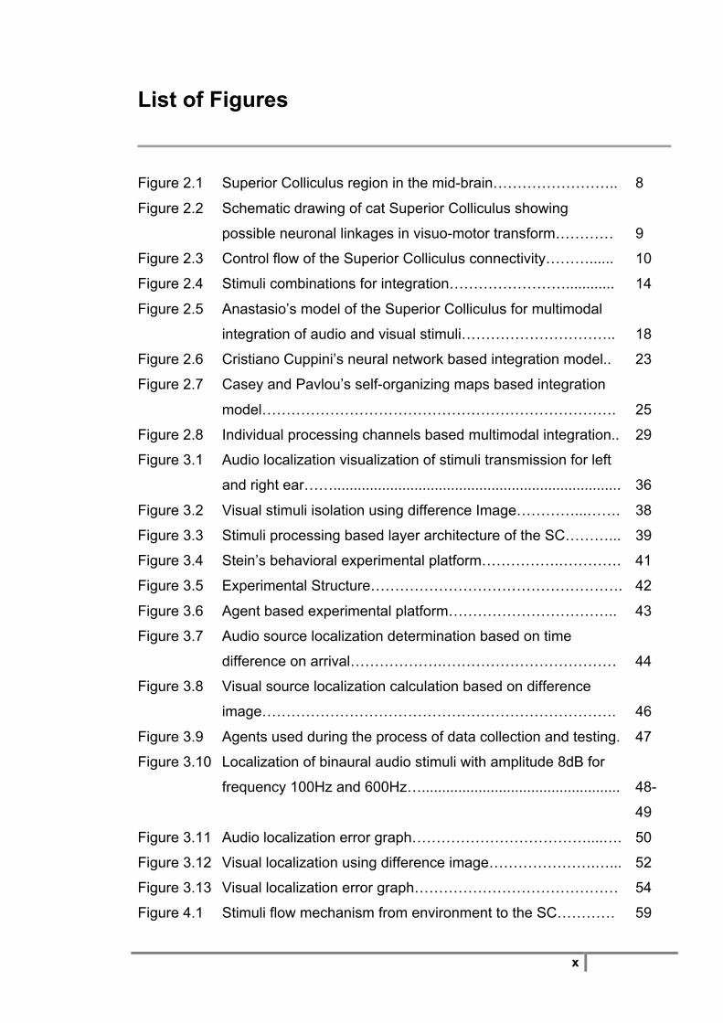
List of Figures
Figure 2.1 Superior Colliculus region in the mid-brain…………………….. 8
Figure 2.2 Schematic drawing of cat Superior Colliculus showing
possible neuronal linkages in visuo-motor transform…………
9
Figure 2.3 Control flow of the Superior Colliculus connectivity………...... 10
Figure 2.4 Stimuli combinations for integration……………………............ 14
Figure 2.5 Anastasio’s model of the Superior Colliculus for multimodal
integration of audio and visual stimuli…………………………..
18
Figure 2.6 Cristiano Cuppini’s neural network based integration model.. 23
Figure 2.7 Casey and Pavlou’s self-organizing maps based integration
model……………………………………………………………….
25
Figure 2.8 Individual processing channels based multimodal integration.. 29
Figure 3.1 Audio localization visualization of stimuli transmission for left
and right ear…….......................................................................
36
Figure 3.2 Visual stimuli isolation using difference Image…………...……. 38
Figure 3.3 Stimuli processing based layer architecture of the SC………... 39
Figure 3.4 Stein’s behavioral experimental platform…………….…………. 41
Figure 3.5 Experimental Structure……………………………………………. 42
Figure 3.6 Agent based experimental platform…………………………….. 43
Figure 3.7 Audio source localization determination based on time
difference on arrival……………….………………………………
44
Figure 3.8 Visual source localization calculation based on difference
image……………………………………………………………….
46
Figure 3.9 Agents used during the process of data collection and testing. 47
Figure 3.10 Localization of binaural audio stimuli with amplitude 8dB for
frequency 100Hz and 600Hz….................................................
48-
49
Figure 3.11 Audio localization error graph………………………………....…. 50
Figure 3.12 Visual localization using difference image………………….…... 52
Figure 3.13 Visual localization error graph…………………………………… 54
Figure 4.1 Stimuli flow mechanism from environment to the SC………… 59

xi
Figure 4.2 Detailed transformation mechanism from unimodal stimuli to
multimodal output…………………………………………………
62
Figure 4.3 Error representation of computational model output…………. 66
Figure 4.4 Biological neuron of human brain………………………………. 68
Figure 4.5 Radial Basis Neural Network model using matlab……………. 70
Figure 4.6 RBF based multisensory integration neural network model…. 72
Figure 4.7 Dimensionality variation in visual stimuli……………………….. 74
Figure 4.8 Audio analysis using limited stimuli to identify localization…… 76
Figure 4.9 Learning performance states -1 during multimodal training….. 78
Figure 4.10 Learning performance states -2 reaching threshold…………… 79
Figure 4.11 Error graph of neural network model training states…………... 80
Figure 4.12 Response of multiple visual input stimuli localization -1………. 82
Figure 4.13 Response of multiple visual input stimuli localization -2………. 83
Figure 4.14 Response of low audio and strong visual stimuli localization… 84
Figure 4.15 Response of strong audio and low visual stimuli localization… 85
Figure 4.16 Response of strong visual and strong audio stimuli
localization………………………………………………………….
86
Figure 4.17 Response of low visual and low audio stimuli localization
(Enhancement phenomena)………………………………………
88
Figure 4.18 Response of low visual and low audio stimuli localization
(Depression phenomena)…………………………………………
89
Figure 4.19 Computational model mean error chart…………………………. 90
Figure 4.20 Neural network model mean error chart……………………….. 91
Figure 4.21 Accuracy graph between neural and computational
integration model……………………………………………….…
92
Figure 5.1 Response of unimodal audio localization error for sample – 1. 98
Figure 5.2 Response of unimodal audio localization error for sample – 2. 100
Figure 5.3 Response of unimodal audio localization error for sample – 3. 102
Figure 5.4 Response of unimodal audio localization error for sample – 4. 104
Figure 5.5 Response of unimodal audio localization error for sample – 5. 106
Figure 5.6 Mean error graph for a given sample…………………………… 107
Figure 5.7 Response of unimodal visual localization error for sample – 1. 110
Figure 5.8 Response of unimodal visual localization error for sample – 2. 112

xii
Figure 5.9 Response of multimodal neural network integration model
error for sample-1…………………………………………………
115
Figure 5.10 Response of multimodal neural network integration model
error for sample-2………………………………………………….
117
Figure 5.11 Error performance chart between unimodal and multimodal
integration…………………………………………………………..
119
Figure 5.12 Error comparison between neural and computational modal
outputs for selected input…………………………………………
124
Figure 5.13 Intensity graph between unimodal and multimodal output……. 126

xiii
List of Equations
Equation 3.1 Time difference on arrival (TDOA) for audio stimuli...………... 44
Equation 3.2 Distance between agent and source (Distance)……………… 44
Equation 3.3 Auditory Localization of stimuli direction (Ɵ)………………….. 45
Equation 3.4 Angle of audio source based on direction (Angle)……………. 45
Equation 3.5 Difference Image determination (DImg)………………...……... 45
Equation 3.6 Visual localization of stimuli source (Ɵ)………………………... 46
Equation 4.1 Computational Integrated Output (Integrated Output)……….. 63
Equation 4.2 Activation function for RBF Z(x)………………………………… 71
Equation 4.3 Modified Gaussian activation function Z(x)………………........ 71

Chapter1: Introduction Audio & Visual Stimuli Integration Model
1
Chapter 1
Introduction
_________________________________________________________________
1.1. Overview
The human brain performs numerous stimuli-based information-processing
operations in order to enable a person to interact with the environment. Of these,
sensory information processing is a significant task. Each part of the brain has its
own vital activities such as sensing or response, or both in certain cases. As a
result many researchers are involved in decoding brain processing states, which
controls and co-ordinates human interaction with the environment.
This research attempts to develop an understanding of the co-ordination involved
in sensing the visual and audio stimuli that provide a mutual and controlled motor
response to those stimuli. In particular, the Superior Colliculus, located in the mid-
brain of the human nervous system, is one such location which performs
multimodal information processing. This thesis aims to develop an integration
model inspired by the Superior Colliculus, so that audio and visual stimuli can be
integrated to provide an efficient and controlled motor response.
1.2. Motivation
Humans and animals can effectively localize any visual or audio stimuli generated
within range. This is a key feature for interaction, either with the environment, or
with other humans or animals as stated in Appendix-A. There are several potential
applications of intelligent robotics involving human-robot interaction where it would
be desirable to have this feature. For example, in situations where a robot must
respond to human instructions (such as “ASIMO” in a ‘tour guide’ robotic

Chapter1: Introduction Audio & Visual Stimuli Integration Model
2
application (Koide, 2004)), the simultaneous, rather than sequential, arrival of
stimuli for both audio and visual information often takes place where significant
noise is present (the so-called ‘cocktail party’ effect (Elhilali, 2006)).
The equivalent human or animal response in such scenarios is effective and
spontaneous. If a robotic agent is able to provide a similar response by attending
to an individual requesting attention, it has the potential of making the interaction
more human-like. One way of providing such efficiency would be by mimicking the
biological processes carried out for integration. The Superior Colliculus (SC)
region of the brain is responsible for providing audio-visual integration, as well as
response generation. Hence, a computational architecture inspired by the SC has
the potential to provide an effective platform for generating similar behaviour.
In terms of development, the use of ‘sensor fusion’ methods such as the Kalman
filter will provide an effective engineering-based integrated output according to the
given inputs. However, an engineering or computational approach will provide the
solution only for the defined platform. When it comes to using such engineering-
based agents, any irregularities in the defined input data set will not be addressed.
To eliminate this, a platform independent approach is proposed. The aim is to
develop an effective multisensory integration model inspired by the SC using a
neural network platform, so that the simultaneous arrival of audio and visual stimuli
will result in the effective localization of the source.
1.3. Research Question
Is it possible to create a computational architecture inspired by the Superior
Colliculus of the mid-brain, using artificial neural networks, which enables the
efficient integration of audio and visual stimuli arriving simultaneously at an agent,
in order to localize the source of the stimuli?

Chapter1: Introduction Audio & Visual Stimuli Integration Model
3
1.4. Aim and Objectives
The project aim is to design and develop an architecture for multisensory
integration that is inspired by the functionalities of the SC when processing audio
and visual information.
The specific objectives are:
1. To understand the biological way of multimodal functionalities of the SC.
2. To review the literature on modelling the SC.
3. To review different approaches to audio and visual extraction and
integration.
4. To examine neural network approaches to integration.
5. To develop and design an architecture suitable for multimodal integration
for a robotic platform.
6. To test and evaluate the performance of the architecture.
1.5. Research Contribution
The main contribution lies in the reduction of dimensional space (audio and visual)
to an integrated single space by using neural networks for processing stimuli
integration mechanisms. The novelty lies in the form of the architecture and its
ability to handle low intensity stimuli and generate an efficient and accurate
integrated output, even in the presence of low audio and visual signals.
1.6. Thesis Structure
The remainder of this thesis is organized as follows:
Chapter 2 is an overview of the SC and multimodality. Following a brief
introduction to the SC from a biological perspective, stimulus processing in the SC
is studied. How the SC exhibits multimodal behaviour is detailed in relation to
stimuli processing and motor response. A review of existing literature in

Chapter1: Introduction Audio & Visual Stimuli Integration Model
4
understanding multimodal behaviour in different contexts is provided. Along with a
theoretical analysis, computational implementation aspects of the SC are also
discussed in order to identify the feasibility of considering multimodal behaviour.
Chapter 3 details the methodology of the research carried out. It describes two
different types of stimuli processing: unimodal and multimodal for audio and visual
stimuli, along with a design strategy towards implementation. Starting with a
briefing on existing literature concerning available design aspects of multimodal
integration mechanisms, the architecture is proposed in order to generate a unique
model that can perform integration of audio and visual stimuli. The architecture is
based on a defined design strategy, which identifies the stimuli localization
aspects. The importance of the learning mechanism and its use in the integration
model is also discussed.
Chapter 4 deals with the implementation of the model. Starting with the reasons
behind developing a neural network platform, various issues that are significant
when building a neural network with learning criteria and its implementation,
including the advantages, are discussed. Along with theoretical aspects of the
audio and visual integration model, the practical and implementation constraints,
along with the biological inspiration for the model are also discussed.
Chapter 5 describes experimental work carried out with the model. It starts with
the motivation behind the experimental setup and environment along with data
collection of both unimodal and multimodal sensory audio and visual stimuli. This
includes data set analysis, preparation of data sets and stability of the integrated
outcome. Later the data sets are used to train the integration network, followed by
verification with the test data.
Chapter 6 presents a detailed analysis of the experimental results. It includes a
critical analysis of training and testing, and unimodal and integration results are
compared. A detailed performance evaluation is also undertaken.

Chapter1: Introduction Audio & Visual Stimuli Integration Model
5
Chapter 7 details the main conclusions resulting from the work, in the context of
the research hypothesis and initial objectives. There is also a discussion of
suggested future work.

Chapter2: Literature Audio & Visual Stimuli Integration Model
6
Chapter 2
Literature Review
_________________________________________________________________ 2.1. Introduction Throughout the history of technology, there has been a constant transformation of
biological inspirations to sustain modern requirements. This research of sensory
stimuli processing, concerned with audio and visual information, has been inspired
by information processing within the human nervous system, including the brain.
When it comes to receiving visual and audio stimuli, the eyes and ears are the
most widely used primary sensory organs. In this chapter, research into
understanding the biological way of processing visual and audio stimuli in the
human brain is described in the form of a detailed literature review on existing
work of various researchers active in this area. The emphasis is on the region of
the brain called the Superior Colliculus (SC). Also discussed is the feasibility of a
conceptual transformation of the SC into a computational method.
2.2. Biological Overview of the Superior Colliculus In this section, a motivation was provided detailing the need for biological
inspiration. During the process, the purpose for the SC was identified by
answering several questions raised during the research. Later an investigation into
the SC based on neuro-science aspects is detailed.
2.2.1. The Biological Motivation:
An early motivation behind the research was to investigate ways to integrate
sensory stimuli such that the outcome or resultant could be in the form of a
combined response. Questions that arose include:

Chapter2: Literature Audio & Visual Stimuli Integration Model
7
• What is the need to have a combined response for sensory stimuli?
• How is the combined response different from the individual responses?
• How can this combined response be more useful than the individual
responses?
During research into autonomous intelligent robotics and industrial robots, there is
always a requirement for sensors to acquire data from the environment as the
robot performs its task. Every sensor is designed for its own specific purpose of
information receiving and transmitting to a designated receiver. Later, using this
response, the agent will perform the desired operation like movement etc.
However in certain cases, the final action from the agent may not only depend on
the response of a single sensor, but on the response of a group of sensors. For
example, the control of an autonomous-guided robotic vehicle may require:
• visual information from both the front and side views;
• balancing the vehicle at the desired speed;
• noise from a rear or side vehicle to be recognized and localized;
In the above-mentioned scenario, use of a visual sensor and audio sensor, and
balancing with gyro information, will be necessary to handle the acceleration and
braking of the vehicle effectively. In such a case rather than a centralized network,
a distributed network with individual processing units for dedicated functionalities
will reduce overload of the network. During such circumstances sensory stimuli
integration prior to the intended action is always an advantage when it comes to
performance and accuracy of the system. Hence there is an advantage of
integrating the sensory stimuli to reduce the processing time and time of response.
Since the research is concerned with audio and visual stimuli, a small region of the
human brain that performs a similar mechanism is of direct interest and relevance.
When it comes to audio and visual information, there are two different kinds of
response that are observed while studying the stimuli response mechanisms.
Study of these mechanisms is essential as they represent the efficiency of the
integration. They are:

Chapter2: Literature Audio & Visual Stimuli Integration Model
8
• Voluntary response.
• Involuntary response.
In the human brain, involuntary responses are sudden and unplanned, and are
frequently observed during action-response mechanisms. However the Superior
Colliculus is one region of the human brain that is responsible for generating
voluntary responses in terms of eye movements called saccades as an extension
to head movements. In order to have a clear understanding of saccades, it is
important to have a detailed and clear knowledge of the SC and its working
mechanism.
2.2.2. Neuroscience aspects of the Superior Colliculus
The SC forms the rostral bumps located on either side of the dorsal aspects of the
mid brain of the human as shown in figure 2.1. This forms a part of the roof of the
midbrain. Unlike the Inferior Colliculus, which is audio centred, the SC is vision
centred, with a reflexive mechanism as its central functionality.

Chapter2: Literature Audio & Visual Stimuli Integration Model
9
Figure 2.1 Superior Colliculus region in the mid-brain: Superior Colliculus located in the mid-
brain region of the human brain. Image Courtesy of Medical Neurosciences 731
The SC is a layered structure containing I-VII layers that can gather information
from visual organs and extend to other layers, which can generate responses to
perform centre activities such as saccade (section 2.3, page 10) generation (Juan,
2008) is shown in figure 2.2.
Figure 2.2: Schematic drawing of cat superior colliculus showing possible neuronal
linkages in visuomotor transform: Thick arrows, major path; boxes outline representative slices
of terminal fields from optic (retinal) tract and corticotectal tracts from areas 17, 18, 19, 21, C-B,
and 7; shaded areas, major foci of degeneration after lesions to these areas. MBSC, medial
brachium of superior colliculus; LBSC, lateral brachium of superior colliculus; NIC, interstitial
nucleus of Cajal and adjacent reticular formation; C-B, Clare-Bishop area; D, nucleus of

Chapter2: Literature Audio & Visual Stimuli Integration Model
10
Darkshevitch; OC, oculomotor nuclei; PAG, periaquiductal gray matter. Roman numerals represent
the seven-collicular laminae (layers) of the Superior Colliculus signifying the arrangement inside
the superior colliculus. (Source: From Ingle and Sprague 123.) The neuro-science interpretation of the SC is that the top, or superficial, layers are
in direct contact with the optical tract, as shown in figure 2.3. Through this tract
visual information is transmitted into the SC from the eyes. This visual information
is received through the retina and visual cortex regions of the human eye. Due to
this direct contact, the SC is the primary receiver of visual stimuli. This means that
the SC is involved in the generation of involuntary or reflexive responses that are
caused by visual stimuli. However, since the deep layers are in contact with the
Inferior Colliculus (IC) (audio processing unit) and Somatosensory system (sense
of touch), the SC responds to visual, audio and somatosensory stimuli.
Figure 2.3 Control flow of the Superior Colliculus connectivity: Control flow diagram
representing an internal connectivity of superior colliculus towards receiving visual stimuli directly

Chapter2: Literature Audio & Visual Stimuli Integration Model
11
from optic tract along with an extension towards spinal cord for motor action. Image Courtesy by
Medical Neurosciences 731
Therefore, the SC cannot be considered as a vision-only centred processing unit.
This is due to its intermediate and deep layers, which are in contact with many
other stimuli processors and sensory modalities, together with motor response
units. For this reason the SC can receive sensory stimuli from various regions of
the brain and can also receive and transmit motor responses. Hence it is sensitive
to audio, visual and somatosensory (touch) stimuli. If the strategic alignment of
layers and their influence on the stimuli is considered, it is understood that the
deep layers play a major role in the motor response generated by the SC.
However this influence is not completely exclusive. The SC extends towards the
spinal cord through tectospinal tracts. Due to this extension, the SC is able to co-
ordinate reflexive movements such as eye and head movements.
A neuroscience study of the SC reveals that the localization of audio and visual
stimuli is carried out in the mid-brain region of the nervous system. As established
earlier, the SC actions can be both voluntary and involuntary. However, voluntary
actions are usually influenced by other regions of the brain such as the cerebellum
and amygdale. Information from all these regions is used at SC to perform a
voluntary saccade. However, involuntary saccades corresponding to audio and
visual stimuli are mainly based on SC localization.
Usually the auditory cortex region encodes auditory cues such as the time
difference and level difference. These operations are performed in the Medial
Superior Olive (MSO) region. However, higher order regions such as the SC,
Inferior Colliculus (IC), and Planum Temporale (PT) are also capable of encoding
such cues. The SC is the primary region of the human brain that responds to
auditory and visual stimuli by generating a motor response to perform saccadic
movement or subsequent head movement. On average, when it comes to
efficiency of auditory localization, mammals can achieve an accuracy of ±10 in the
horizontal axis and ±4-50 in the vertical axis (Hawkins, 1996).

Chapter2: Literature Audio & Visual Stimuli Integration Model
12
2.3. Multimodal Behaviour of the Superior Colliculus
It is evident that the SC has the capability to receive audio, visual and
somatosensory stimuli from various regions of the human brain. Neural activation
experiments conducted by Stein and Meredith confirmed that the SC can generate
responses for both audio and visual stimuli (King, 2004). The responses for such
stimuli can be observed in terms of eye or head movements due to their
connectivity with the spinal cord. Multimodal behaviour allows both animals and
humans to perform effectively under noisy or multiple stimuli conditions.
This behaviour need not always be associated with multi-modal stimuli.
Sometimes stimuli arriving from different sources can also be handled by the SC.
The visual stimuli transmitted through magnocellular and parvocellular retinal
ganglion cells unite at various levels of the SC. These signals have the feature of
multiple and parallel streams of information preservation. With such a capability,
these signals are analyzed for various aspects of the visual environment
individually (Waxman, 2009). Similarly the optic tract axons terminate in a highly
synaptic space that can help in generating a map-like environment. The axons of
ganglion cells along with optic tract extend to the SC, forming a retinotopic map.
Due to an extension of the SC through the spinal cord via tectospinal tracts, the
retinotopic map is used for stimuli localization with the help of eye, neck and head
movements. These movements represent both involuntary and voluntary
movements generated by the SC.
Rapid movements of the eyes on a horizontal axis are often termed ‘saccadic
movements’. Though their purpose is to rapidly fix the vision on a target, the type
of fixation can be of various types. Saccadic movements can be commanded
(general), fixation (on a target) and reflexive (involuntary). Reflexive movements
are usually observed following the appearance of an object in the visual field of the
eye, or any disturbance in the audio field of the ear. However, rather than the SC
acting alone, the cerebellum also plays a vital role in the generation of fixation
saccades. In either of these cases stimuli are localized using the above criteria by
moving the eyes or head towards the direction of the source. Since saccades are
Chapter2: Literature Audio & Visual Stimuli Integration Model
13
pursuit in their behaviour, they can stabilize the foveae of the eye continuously and
clearly even on a moving object.
From the above observations, it is evident that the SC performs sensory stimuli
integration for generating saccadic movements. Stimuli can refer to a single
stimulus of audio or visual, multiple visual stimuli, multiple audio stimuli and audio
and visual stimuli together. The need for integration occurs when there is a
simultaneous arrival of more than one audio and visual stimulus at the SC.
Unimodal stimuli integration then takes place in the SC to identify an effective
response. However when it comes to the simultaneous arrival of audio stimuli, due
to interference effects, stimuli with similar audio properties will be interpreted as
noise unless at least one of the stimuli has a unique property such as frequency or
amplitude.
Many techniques are designed to handle the so-called ‘cocktail party effect’.
However when it comes to a classroom situation, for example, where students use
low voice levels when generating audio stimuli, integration is a difficult task due to
the recognition problem. This is not only with audio but also visual stimuli. Hence
the strength of stimuli is one such property that can affect the SC response.
There is an argument that the SC considers the priority of visual stimuli due to its
direct contact with the eyes through the optic tract, but this is only when stimuli of
different strengths arrive at different time intervals. If a human subject is seated on
a swivel chair and rotated for some time, when the chair comes to a halt a visual
stimulus received is overridden by any audio stimulus that arrives at the ear. In this
particular case, initially the visual stimulus was overridden by the audio one. A
later audio stimulus is also not effective when it comes to the integration process,
due to the unstable state of receiving stations (eyes and ears). This signifies that
for SC both the stimuli are equally prioritized when it comes to integration.
In the following figure 2.4, integration process can be classified based on the input

Chapter2: Literature Audio & Visual Stimuli Integration Model
14
Figure 2.4 Stimuli combinations for integration: Diagrammatic representation of various
combinations formed with the weak and strong stimulus of audio and visual stimuli that are possible
when integrating them.
stimuli strength. The time of stimuli arrival, along with the strength of the stimuli,
are the two major factors that influence the integration process. In figure 2.4, ‘W’
represents the weak stimuli and ‘S’ represents the strong stimuli of corresponding
visual and audio stimuli. The representation shown illustrates the possible stimulus
combinations that can emerge during the process of integration.
When it comes to the outcome of these combinations, a weak combination need
not always have to produce a weak response; similarly with a strong combination.
Following the neural response experiments conducted on the SC of cats by Stein
and Meredith (Meredith, 1986a), two different phenomena are proposed in
understanding the integration process with stimuli strength:
• Enhancement
• Depression
These two phenomena can be observed in most of the combinations of the weak
and strong stimuli. However, from the stimuli classification obtained from figure 2.4,
Audio Stimuli Visual Stimuli
Strong Audio +
Strong Visual
Weak Audio +
Weak Visual
Weak Audio +
Strong Visual
Strong Audio +
Weak Visual
SS SS WW WW

Chapter2: Literature Audio & Visual Stimuli Integration Model
15
the occurrence of these phenomena can be understood. The phenomena of
depression and enhancement are mainly based on the distance between stimuli
along with their strength, irrespective of the type of stimulus. In the case of a weak
and strong combination, a winner-takes-all criterion usually applies. This can be
categorised under enhancement. During the combination of two strong and
relatively close stimuli, there will be an enhancement of the integrated output
rather than either of the individual ones. Similarly during the combination of two
weak stimuli relatively closer in terms of stimuli intensity, there will be an
enhancement in the integrated output rather than either or both of them.
On the other hand, depression is the phenomenon where the system is left in a
state of confusion in determining the angle for localization. During the combination
of two strong stimuli, which are far away from one another, the integrated output
generated will be more depressed, than either stimulus. Hence the outcome will be
in the same state as before, which is empty. Similarly during the combination of
two weak stimuli relatively far from one another, although the inputs are detected,
the integrated output will be strongly depressed. This results in no output being
generated.
2.4. Literature on Multisensory Integration This section reviews neuroscience research based on a similar criterion of
exploring the multisensory behaviour of the SC. It is carried out in the context of
this thesis and how useful it is to support the research hypothesis, and hence the
design and development of the computational model.
Stanford evaluates the neuroscience view of the computations carried out by
neurons of the SC for multimodal integration of sensor stimuli (Stanford, 2005).
Neuron responses are not considered as “high” or “low”, but are ‘super additive’,
‘additive’ and ‘sub additive’. These responses can be used to explain the maximum
responses that the SC can produce in modality-specific cases. Modality-specific
study provides an opportunity to observe the computations that take place in cases
of low response and high response. This research provides a platform for

Chapter2: Literature Audio & Visual Stimuli Integration Model
16
explaining the enhancement of integrated output for audio and visual integration in
the SC.
According to Beauchamp, biological evidence exists for multimodal integration that
takes place for audio and visual information in the deep layers of the human brain
system (Beauchamp, 2004). The author describes the integration with a focus on
behavioural tasks and their influence in different aspects that are encountered
during the process. However, it is not clearly stated that how the decision is made
in determining the final outcome of the integration in terms of audio and visual input
information.
Gilbert demonstrates how spatial information about the source of a stimulus is
available at the receptor surface for visual and audio sensory systems (Gilbert,
2008). To support this, a pit viper example is considered where integration takes
place between visual information and mechanoreceptor information.
Mechanoreceptors (available both on skin and hair) are the sensory detectors that
can determine the change in air pressure or vibration. They are also sensitive
towards odours. For instance, pit vipers use infrared information from pit organs
along with visual information, which then travel together for summation of inputs in
two modalities. Since the odour detected by the mechanoreceptors is not sufficient
to determine the direction of the source, visual cues are used in the integration
process to localize pray. Variation in the integration also occurs when the angular
velocity of the prey is recognised along with the change in the intensity of smell in
the air of the source. At this point, when the source is recognised, a high body
saccade is noticed. The visual field of the animal, with the source viewed in same
field, has a strong influence in the body saccades.
2.5. Literature Review on Integration of Audio and Visual Data
This section reviews literature describing various modelling techniques for
performing audio and visual integration. In the following all such literature is
provided with a classification based on the implementation technique used.
Different researchers implement the concept of multimodal integration on various

Chapter2: Literature Audio & Visual Stimuli Integration Model
17
platforms based on their requirements. Through this literature review these
techniques are analysed so that the observations can be used during the design
and development of the integration network.
2.5.1. Probabilistic Approach
Anastasio proposed an integration model based on the assumption that “SC
neurons that show inverse effectiveness, compute the probability of the target
present for moving the saccades” (Anastasio, 2000). The principle of inverse
effectiveness is stated as an increase in the strength of multisensory integration in
response to the decrease of individual sensory stimuli (Holmes, 2009). The
proposed model for multisensory integration provides an explanation for the
inverse effectiveness phenomenon. When it comes to spontaneous bimodal
probabilities, the model has produced non-conclusive evidence for inverse
effectiveness. The authors try to show that SC neurons use probabilities for the
localization of stimuli sources. Figure 2.5 is a diagrammatic representation of the
integration model discussed. In the figure, probability ‘p’ is the chances of occurring
audio and visual given both the stimuli arrive at the Superior Colliculus. When
designing a multimodal integration model of the SC, Bayes’ probability concepts
may be useful when working on the enhancement of output stimuli, but the authors
have not given a reason for the behaviour, or why only inverse effectiveness is
considered when determining the enhancement, which may be due to the
contradictory effect shown in a small number of neurons.

Chapter2: Literature Audio & Visual Stimuli Integration Model
18
Figure 2.5 Anastasio’s model of the SC for multimodal integration of audio and visual
stimuli: Pictorial Representation of Anastasio’s Model of superior colliculus for multimodal
integration of audio and visual stimuli. This image depicts the transmission of both audio and visual
stimuli through their sensory aid to the SC. Here Anastasio’s probabilistic model will perform
integration.
The tracking model developed by Wilhelm et al., uses vision and sonar-based
components on account of their low cost for mass production (Wilhelm, 2004). A
Gaussian distribution is used to model the skin colour for making it easy to identify
the face in the visual sequence. For the detection of colour, automated colour
calibration and a white balancing algorithm are used. Sonar sensors that cover 360
degrees in dual levels with a pre-processed mechanism are used for eliminating
noise. Thus obtained sonar data is used in locating the face in the visual data.
Hence, the sensor fusion described in this report of Wilhelm uses a stochastic
motion model with a Gaussian distribution. This system is able to track the
localized face (image) even if there are people moving in the environment. Though
the system is able to track the image, it is only based on its location. If the object is
moving during localization then the proposed tracking is not suitable, as it keeps
changing from frame to frame. However, it is well suited for a fixed source.
Xiaotao Zou and Bir Bhanu have described two different approaches for
multimodal integration using audio and visual data. First, a Time Delay Neural
Network (TDNN) extracts audio and video data at feature level separately and then
fuses both data forms. Second, a Bayesian Network (BN) jointly models audio and
video signals and tracks humans by Bayes inference. According to Stork, detection

Chapter2: Literature Audio & Visual Stimuli Integration Model
19
of motion that handles sequential data during multimodal function is possible with
the fusion of audio and visual data at feature level (Stork, 1992). Normalized cross-
correlation for feature selection in the TDNN architecture is considered as being
efficient for identifying the difference between successive images. A sound
spectrogram is used to break down the sound into steps for audio inputs to the
network (Zou, 2005).
Bayesian networks may be useful when processing graphical representations with
probability models. This model can be enhanced to handle time series data using a
Dynamic Bayesian Network. A statistical model, a Transformed Mixture of
Gaussians, is used to model the frames. Assuming all the probabilities are
Gaussian, audio data is generated using the time of arrival to the microphones. A
static Bayesian Network (BN) is used to link the sequential audio and visual data
involving the covariance matrix and parameter estimation with an expectation
maximization algorithm based on the standard Bayes’ rule. High accuracy and less
training time are achieved in detecting the object in the BN (Zou, 2005).
Using a probabilistic approach Bennewitz has determined on which person
attention is focused by the agent in multiple people conversations (Bennewitz,
2005). For that decision, this approach uses visual and speech input. In getting the
information of a person in the visual path, the technique (feature extraction using
the dark parts of the eyes and cheeks etc) is effective for images of considerable
brightness. As the number of persons in the conversation increases, it becomes
more difficult to detect the correct person. The speech information is processed
with automata and state machines using lexical analysis, limited to only a few
words or phrases. As the number of words or phrases increases, the slower the
automaton machine becomes. This is due to the gaze direction technique, which
helps to find the traces from the remaining input in the case of multiple stimuli.
Hence this approach is potentially a good technique for multimodal scenarios. This
paper is a good demonstration of human-robot interaction, especially in scenarios
involving conversations, meetings and discussions in small groups.

Chapter2: Literature Audio & Visual Stimuli Integration Model
20
For the development of a multimodal robot interaction system, a model for speech
communication in human-robot interaction has been developed with the use of
simple linguistics, irrespective of grammar, along with gestures and contextual
scene knowledge (Huwel et al., 2006). A Hidden Markov Model is used for parsing
the speech and a semantic parsing algorithm used for determining its meaning.
The model focuses more on speech analysis and generating the action, depending
on the semantic parsing. A system called “Control” is designed in such a way that
the multimodal processing is done at this stage for all types of communications.
The BIRON robotic system is used to verify the above-mentioned concepts in an
experimental environment. It is not clearly explained how the multimodal
understanding of speech and the contextual scene are combined. Also, this model
shows that human robot understanding can be improved when speech is combined
with contextual space and gestures.
2.5.2. Neural Network Approach
The model proposed by Trappenberg (1998) is mainly focused on a competitive
neural network with spiking neurons of short range (excitatory) and long range
(inhibitory) firing rates. Due to the lack of consideration of 4 types of neurons
responsible for saccade generation in SC, the acquired results from the simulation
are not close enough compared to the results that are observed from animal
testing. This is due to consideration of only fixation and burst neurons. An average
firing neuron network is more sensitive to further updates and modifications
compared to a spiking neural network. If the same spiking network is trained using
winner-takes-all (competitive) learning, its performance is improved, which further
generates outputs that will have more chance of producing similar results to animal
experiments done by Stein and Meredith (1993). A spiking neural network with all
four neurons (fixation, burst, build up and excitatory) can form a more apt and
realistic full functional model (Trappenberg, 1998) and (Kyriakos and Jurgen, 2007).
Quaia et al., (1999) provides a model for a saccadic system where the functionality
of the SC is minimal compared to cerebellum circuitry (Quaia, 1999). According to

Chapter2: Literature Audio & Visual Stimuli Integration Model
21
the authors, the role of the SC is only to provide the directional drive towards the
target for the eyes. However it is up to the cerebellum to determine the
appropriateness and accuracy of the directional drive. The burst, build up and
fixation neurons available in the deep layers of the SC are used to determine the
direction. The processing from the cerebellum is used to improve the directional
drive, track the target, and end the saccade.
Two contrasting models for multimodality, with and without integration of human
information processing, are evaluated in experiments conducted by Dominic W
Massaro (2004). The paper shows that the Fuzzy Logic Model of Perception
(FLMP) predictions are quite supportive for many experimental cases on BALDI, an
embodied conversational agent. The Single Channel Model (SCM), which is a non-
integration model, processes the stimuli in single channels only. A particular time
scale is considered and information is processed through either visual or audio
processing channels, but not both. The fusion of visual and audio information in
FLMP does not follow any sort of pattern, which means it can be synchronous or
asynchronous with the time frame. The fusion may be early or late. In either case
integration will have an influential effect on the outcome. Another model is fusion at
the feature-level or decision-level. The influence of these fusion models can have
improvement on Embodied Conversational Agents (ECAs) than human machine
interactions.
According to Wolf and Bugmann, Natural Language Processing is a slow process
compared with Image Processing when considering long sentences, rather than
just action words (Wolf and Bugmann, 2006). Hence the use of time scale for
semantics determination is a suggestive idea when developing a multimodal
system that can process the above inputs. The proposed constraint algorithm for
multimodal input processing is effective for applications where the knowledge set is
constrained, but the platform for implementation is not. When including time
semantics, a network that can be sensitive towards minor changes in the input,
along with quick processing and response generation, is required. Hence a
platform like a neural network is effective as far as semantic mapping and timing is
concerned. In the proposed future algorithm, the scope of the network can also be

Chapter2: Literature Audio & Visual Stimuli Integration Model
22
extended to unconstrained environments, as linguistic processing is time
consuming with the growth in sentences. This will contradict the time and mapping
semantics of the algorithm.
Jolly et.al., propose a Compounded Artificial Neural Network (CANN) for making
quick and more effective decisions in a dynamic environment like robot soccer
(Jolly et al., 2006). The learning of the Artificial Neural Network (ANN) is carried out
with an Evolutionary Algorithm (EA) with crossover and mutation, as well as back
propagation techniques. However as the population grows, the performance of the
EA decreases due to the increase in the decision space. ANN logical decisions are
made according to the rule base. As the network grows, accuracy in prediction
decreases. To eliminate it, the primary level (before the input layer) is added to
generate the inputs from trained ANNs of nC2 combinations, where n is the number
of robots in the team. This determines that for the successful generation of output
at least 2 inputs are necessary. With this CANN model, however, the problem of
space verses accuracy is not resolved, but comparatively high accuracy in
decision-making with increase in population size is achieved. As the number of
robots increases in a team, for example 10-11 players for soccer, the primary level
is so huge that the inputs have to reach the main network with some delay, in
which the final decision, though accurate, may not be appropriate due to the delay
in processing. So in this case, expanding the team is limited.
Cuppini has provided a mathematics-based neural network model of multimodal
integration in the SC along with an insight into possible mechanisms that underpin
it, as shown in the figure 2.6. This model details the enhancement and depression
phenomena, along with cross modality, similar modality and inverse effectiveness.
Unimodal neuron activity characterized by non-linear phenomena is easy to study
by considering quantitative mathematical tools such as probability. Gaussian
functions are used for the spatial representation of neuronal and synapse activity.
Using a Mexican hat function the strength of the activity is assigned to the
corresponding activity function so that the activity of the final multimodal output can
be determined. The disposition of the hat from unimodal to multimodal explains the
enhancement and depression phenomena either in between the modalities or

Chapter2: Literature Audio & Visual Stimuli Integration Model
23
within a modality. It is considered that the stimuli are always sigmoidal and non-
linear (Cuppini et.al., 2007).
Figure 2.6 Crisiano Cuppini’s neural network based integration model: Recurrent neural
network with feed forward mechanism from unimodal to integrated output and vice versa
The model of Cutsuridis mainly identifies issues of how the saccades are
generated once the motor command is activated, especially for targeted and
voluntary saccades. Irrespective of its complexity, Cutsuridis has used the concept
of an anti-saccade task in developing a decision-making model of the SC
(Cutsuridis et.al., 2007). Anti-saccade is the time taken for the eye to actually
deviate in the opposite direction from the source. This model identifies that there
are other cells that take part in saccade generation just before their actual firing.
These cells can be studied with this anti-saccade task. By using this information,
decision-making in the SC is explained.
This concept is quite convincing at a theoretical level, but may not be effective in
implementation since all the inputs are considered to be linear. No biological
evidence is available for supporting this inference. The model is expected to
perform well only when the synaptic currents (neuron activity) is high. It is a new
concept, but for a decision making task in the SC a huge complex network model is
Chapter2: Literature Audio & Visual Stimuli Integration Model
24
suggested. Furthermore, the anti-saccade concept might be used to support some
intermediate layers of the SC in decision-making, as those are the places where
the integration (final decision) is expected to emerge.
In another article the author demonstrates the functionality of the SC, focusing
mainly on real-time audio source localization (Trifa et.al., 2007). Audio localization
is calculated using Interaural Time Difference (ITD) and Interaural Level Difference
(ILD), with a cross-correlation function on a spiking neural network for biological
resemblance in functionality. This model pre-processes signals before they arrive
at the actual network for noise reduction purposes and then localizes using
Generalized Cross Correlation (GCC) with phase transformation. Finally, an
integrated distributed control framework is developed. The network can use the
visual data for carrying other modalities, such as recognition, identification and
tracking. The paper describes a sensitive model for audio localization in noisy
environments. However the concept of multimodality is not utilized as far as source
localization is concerned. The focus is mainly on noisy audio inputs and their
localization. The result is also compared with ITD, ILD and GCC models, but not
with the integrated models. As in the former case, accuracy and precision is high.
According to Armingol use of AI techniques such as Genetic Algorithms and
Search Algorithms in a driving application for visual processing with colour
enhancements is effective (Armingol et.al., 2007). It covers many possible
situations such as pedestrians crossing, speeding and traffic signalling that helps a
driver to make decisions. However, the camera covers only the straight road ahead
of the vehicle - it does not cover the back or side views. In the case of the mirror
image, either a back camera with audio support, or an existing camera, should be
adjusted to an angle so that a mirror image comes into view which can be used to
identify the vehicles at the back. However the extraction may not be efficient as
the back mirrored image appears very small and is not enough to run the extraction
algorithm for identifying fast moving vehicles. Hence audio is used along with a
rear camera to integrate with visual processing, which will be useful in heavy traffic
situations, changing lanes and overtaking, contributing to a Driver Assistance
System.

Chapter2: Literature Audio & Visual Stimuli Integration Model
25
In a paper by Casey and Pavlou, a neural network model is designed to simulate
the behaviour of the SC (Casey and Pavlou, 2008) as shown in the figure 2.7. It
involves processing audio and visual stimuli that are non real-world discrete inputs,
since the authors are testing the integrated results as spatial representations and
comparing them with biological data. Rate-coded algorithms are used for
representing sensory topographical Self Organising Maps (SOMs). According to
Figure 2.7 Casey and Pavlou’s self organizing maps based integration model: SOM neural
networks for topographical representation of multimodal stimuli where the input layers are
connected with hebbian linkage that helps to learn the audio and visual stimuli.
the authors, alignment of sensory maps can be successful even with multimodal
representations due to the mapping feature of SOM network.
Concatenating the individual modalities provides the comparison of multiple
modalities. Though SOMs can provide a first approximation to the neuroscience
view (Kohonen, 1982), a rate-coded algorithm has its limitations and hence the
model is more static in its range of processing the inputs. The range of inputs
covered is 35% - 46% towards the integration from the whole input data collected
(Casey, 2009). If the model is trained on real-world inputs then this can be further

Chapter2: Literature Audio & Visual Stimuli Integration Model
26
decreased due to additive integration technique. If the inputs taken are very few
then limited accuracy can be achieved. This model can support suppression and
enhancement of integrated output, as a first high-level approach towards
multimodal integration (Stein, 1993). The applicability of the model is limited at this
stage due to the narrow input stimuli range.
2.5.3. Application-driven Approach
In a paper by Stiefelhagen, the audio and video features are integrated separately
such that the individual contributions of microphones and cameras will not affect
the final decision of the tracking system (Stiefelhagen, 2002). Particle filters for
audio and visual data are used for localizing the speaker. This paper is focused on
audio and visual perception in a smart lecture room. In a specific example like this,
where performance of the integration model is a critical issue, individual tracking of
audio and visual data provides a more specific localization. Consider the case
where a lecturer is in focus and a student stands and speaks simultaneously. In
this case the multimodal system will help to track the person. This is a good
example of where the applicability of a multimodal system can provide accurate
and efficient results in making the decision with limited complexity (Stiefelhagen et.
al, 2006). In another case, such as a group discussion, a multimodal system can
direct the cameras to decide which person to focus on.
In their research on wearable devices Hanheide provide a novel idea for human
computer interaction by integrating visual and inertial data processing (Hanheide
et.al., 2005). Integration with head gestures can provide rich vocabularies
necessary for communication. In a way the multimodal integration of visual and
head gestures with inertial data can provide better communication between human
and robot with the help of wearable sensory and computing devices. This system
uses the head (holding a camera) for movements to generate commands by
interacting with the environment. In case the user wants to change the selection of
his choice, the way for navigating to the choice is not available. In this proposed
paradigm items visible in the environment have to be assigned semantics so that

Chapter2: Literature Audio & Visual Stimuli Integration Model
27
they can trigger the commands. However, as the environment grows, the
semantics set increases. In the case of the appearance of a new item that is not
known, it is not clear what the action is.
The work of Cucchiara proposes a different type of Multimedia Surveillance
System using biometric technology for visual feature extraction for person
identification in a closed circuit television application (Cucchiara, 2005).
Contradicting issues like safety, privacy and ethics are well grounded with various
practical examples that are currently in operation across the world. The
multimodality (multi input dimensions) is used in a way to extract the best features
from the various cameras including thermal, fixed, distributed and omni-directional.
The omni-directional camera can be integrated with audio such that it can project
the trajectory. The multimodality concept can be used for identification and tracking
the person as an integrated mechanism in the surveillance system.
Designing a multi agent system for an intelligent multisensor surveillance system is
in principle not a difficult task. However, according to Pavon, when it comes to the
efficiency achieved by agents in co-operating and co-ordinating all the sensors,
integrating the information is slow (Pavon et.al., 2007). In the case of centralizing
all the systems, the limitations of the centralization architecture come to focus. The
author has proposed a combination of centralized and distributed systems.
However in this case, as the system grows, the more complex the design becomes.
This reduces the performance of the system with time. Since it is a surveillance
system, reaction times should be high.
In such cases, grouping similar sensors and considering them as an agent with a
distributed network and then centralizing all the agents will improve speed and
productivity. When it comes to the size of the group, scalability is an issue that
needs to be dealt with for a distributed network at the sensor level. When it comes
to designing such a system, there is a requirement for a high level language that
can establish co-operation and co-ordination among the agents without
compromising performance, scalability and efficiency. For the structure proposed

Chapter2: Literature Audio & Visual Stimuli Integration Model
28
by the author for managing the agents, a huge network is required for processing
and maintaining control.
When designing an integration model for security purposes, it is important to have
certain features that can determine authentication of the input. Palavinel and
Yagnanarayana have provided an approach using different inputs such as speech,
images of the face, and both for authentication of an individual (Palanivel, 2008).
The model discussed in this paper is an Auto Associative Neural Network (AANN)
that receives inputs such as visual, acoustic and visual-speech (both audio and
visual stimuli from the same source simultaneously). The focus is on authentication
of the target for maximum security. For visual data images, feature extraction and
detection is carried out on various facial features such as the eyes, the centre of
the mouth and skin colour. Normalized vector data is used for both acoustic and
visual-speech extraction with segmental levels. The AANN uses both the visual-
speech and visual data for the total authentication. The results are more accurate
for multimodal authentication than with a single input. However, more run time
memory is required and the time of execution is greater. This is because it is
necessary to carry out feature extraction from different features of the face
individually and then provide them to the network for the integration.
Feature extraction is carried out directly on the input images, which are distorted
after the process. Since the input is not replicated, every extraction needs a re-
consideration of the input. When demanding high sophisticated security, memory is
not an issue. However with speed comes efficiency, which cannot be effectively
achieved due to the time-consuming extraction process. Hence it contradicts the
model.
2.5.4. Conceptual Approach
The Integration methodology proposed by Coen proposes that perceptual stimuli
processing is more viable than unimodal processing during multimodal integration
(Coen, 2001). This may be right when the modalities are limited and there is some
correspondence in their processing levels, including time. But when it comes to a

Chapter2: Literature Audio & Visual Stimuli Integration Model
29
live environment, as the modalities increase, the complexity increases in finding
the similarities between the processing levels, and sometimes there may not be
similar levels. In such instances similarities are determined using Individual
Processing Channels. In the proposed multimodal system shown in figure 2.8, it
was said that the input might appear at any level. This signifies that the received
input is considered as its own irrespective of the source of input. By doing so the
criteria of differentiating between signal and noise of each and every modality for
which the model was developed is not met.
Figure 2.8 Individual processing channels based multimodal integration: Post-perceptual
Integration system. Input information received from various stations across the network is
individually processed at the specific station that transmitted for the integration of stimuli.
Building such a vast, complex system for limited modalities and a limited
environment is possible, but it is doubtful when the modalities increase or the
environment grows. The “assumptions described by Piaget (1954) about
multimodality in the real human world”, are the only supportive evidence for the
main concept in the paper. Apart from the Piaget assumptions, no other support is
provided for explaining how “the stimulus is processed as perceptual processing

Chapter2: Literature Audio & Visual Stimuli Integration Model
30
levels, not as individual processing levels in the human or animal brain system”
(Coen, 2001).
A paper by Schauer is based on early fusion of audio and visual information for
providing an integrated output (Schauer, 2004). The authors are inspired by the
audio information pathway of the Inferior Colliculus along with the visual and
multimodal pathways that are processed at the SC of the mid brain. Evidence
shows that the sound stimulus is processed in the Inferior Colliculus. However the
visual processing is carried out in superficial layers along with deep layers of the
SC, and intermediate layers are responsible for multimodality. This shows that
stimuli are processed to some extent in the corresponding units, and after
integration (King, 2004) and (Stein and Meredith, 1993). For this early integration
a novel network is proposed that can generate individual spatial maps of visual
fields and audio stimuli. These maps are further integrated and a final multimodal
map is generated. This multimodal map generation is based on a parameter
optimization technique, which is an effective computational methodology to achieve
the behaviour.
Yavuz provides solutions to various design issues and proves that optimizing the
multimodal components at a computational level for integration in intelligent agents
is effective (Yavuz, 2007). The focus is on efficient decision making at various
levels to increase the efficiency at all possible levels including data acquisition,
sensor information, further processing, dealing with various algorithms, and finally
performance. The design proposed is huge as all possible performance levels and
possible constraints are included.
Hardware considerations represent one main issue when optimizing the design.
This paper considers mobility, navigation and autonomy of hardware. Along with
hardware, various possible and alternative software that are compatible and
optimal without compromising on performance are also adapted. Various systems
are integrated to a single intelligent autonomous robot. They include electronic and
mechanical interconnections of the various equipment. This conceptual system is
complex when it comes to building it. The author recommends fuzzy logic based

Chapter2: Literature Audio & Visual Stimuli Integration Model
31
behaviour integration where efficiency is expected to be more than any other
system.
In a paper by Paleari, the author demonstrates human-computer interaction
compared to human-human communication, including all the features and gestures
usually followed (Paleari, 2006). A framework is described for multimodal emotion
recognition. Fusion can be performed at feature level and at decision level. The
extracted features are extrapolated with audio and visual data. However in the
case of emotion, a gesture is added as in Scherer’s theory to the extraction. This
whole fusion can be provided from a multimodal fusion of the above-required
modalities.
2.6. Summary and Discussion
This chapter provides an introduction at a conceptual level to the Superior
Colliculus, stimuli localization, and the integration process carried out in the SC. A
literature review has been undertaken on work carried out in understanding the SC
integration, along with various attempts to perform a process for audio and visual
data integration. Through this review three different implementation techniques are
studied. Pros and cons of these techniques are examined and are used in
subsequent further chapters of stimuli integration system development.
The biological importance of the SC is also described due to its presence in the
mammalian brain system. This introduction describes the flow of stimuli
information from the environment to the SC through sensory stimuli receivers such
as the eyes and ears. It also reveals how the stimuli are transmitted into the SC
along with the various changes the stimuli undergo during the generation of motor
responses transmitted from the SC towards generating saccades and head
movements. During this literature review interesting facts have been identified.
These include biological evidence that suggest multimodal integration of sensory
stimuli in the SC.

Chapter2: Literature Audio & Visual Stimuli Integration Model
32
The chapter also provides a brief description of the motor response generated by
the SC, its importance, and its role in the development of the multimodal
integration system. In the next chapter a brief literature analysis of this area is
provided so that a methodology can be derived, which is useful in identifying the
effectiveness of the model.
The literature review is classified into four different types based on the type of
methodology followed in implementing the multimodal concept. From each
author’s work, conclusions are drawn, which are later used in design and
development of the integration model in this project. From the literature research,
the probabilistic approach is considered unsuitable for this project due to the
aspects of uncertainty intrinsic within it. This is because of a lack of biological
influence or motivation on the model in both processing and development. Hence,
considering into account the biological similarities extracted from the functionality
of the Superior Colliculus detailed in chapter-2, a biological influenced model is
proposed. The architecture of the model is derived from the Superior Colliculus
neural findings described in chapter-3 section 3.2. This literature has laid the
neural network platform for the architecture. The design and development aspects
defined in chapter-4 justify the usage of neural network methods in particular RBF
network. Similar is the state with experimentation and evaluation methodology.
Observation and inferences that are made in this chapter are significantly used
during the course of project.

Chapter3: Methodology Audio & Visual Stimuli Integration Model
33
Chapter 3
Methodology and Design Architecture of the Integration Model _______________________________________________________________
3.1 Introduction
This chapter describes the transformation of the biological functionality of the
Superior Colliculus (SC) into a computational model. The approach aims mainly at
generating an integrated response for audio and visual stimuli. In this context,
artificial neural networks (ANNs) are particularly attractive for this modelling
because of their biological nature, learning and simultaneous processing. The
focus lies in the design of the architecture of the integration model. This
methodology considers the core problem and supports the solution with a feasible
design of the architecture. Through this architecture the goal of the project can be
achieved and validated.
The process of sensory information integration is an important task due to the
complexity involved in transforming the biological model into a computational
model. In this case, with audio and visual sensory information, the methodology
plays a critical role in understanding how the research question is being analysed
and evaluated. In this process both qualitative and quantitative approaches are
followed, which helps in the transformation and design of the model.
3.2 Literature on Design and Architecture
The literature classifies different types of methodologies and approaches used for
integrating audio and visual data as follows:
• Conceptual.
• Artificial Neural network.

Chapter3: Methodology Audio & Visual Stimuli Integration Model
34
• Probabilistic.
These approaches are unique in their own circumstances and are capable of
providing feasible output. However, for this research a combination of these
approaches is used at various levels, in order to satisfy the research question.
According to the conceptual approach, it is important that the design and
architecture is based on the central motivation of the research, which in this case
is concerned with the SC. Hence, the methodology follows the audio and visual
stimuli flow pattern of the SC, from the point of stimuli arrival, to the generation of
motor control. Due to the relative similarity of neuron processing in the human
brain, neural networks are considered to be a suitable architecture. This is
because they enable parallel processing of audio and visual stimuli, together with
control signal generation following integration of those stimuli.
In contrast, the above implementation could also be carried out based on a simple
computational approach. Here a computational model could be constructed that
can process the stimuli and generate a control command, which can integrate the
audio and visual stimuli in both static and dynamic conditions. However, a
computational approach can provide a solution to the problem only in static
conditions.
In contrast, a neural network approach provides an ongoing solution where the
problem changes dynamically with the environment (Stergiou, 2007). A neural
network approach will have the advantage of an adapting learning mechanism, so
that as the network is trained the output generated is also improved due to the
error control criteria in the network processing. This is because the network is
suitable for dynamic environments where learning can be adapted at any point
during the training.
Hence, a neural network is considered as a base architecture for processing and
integrating audio and visual stimuli, in order to generate motor control. In principle
the architecture should contain three individual processing platforms, where audio,
visual and integration mechanisms are carried out. Audio and visual units are
connected to the integration layer, so that the stimuli flow towards audio and
visual layers can be transmitted to the integration layer.

Chapter3: Methodology Audio & Visual Stimuli Integration Model
35
Hearing is a widely used means of localizing targets within the environment in the
animal world (Chan, 2009). Due to the location of an ear on either side of the head,
each with a capability to receive audio stimuli generated within a 1800 range, the
resulting 3600 range gives the modality an advantage in terms of scope. This
helps in detecting the target over a large field. The approach proposed is different
from existing acoustic-based robotic applications. Many existing applications use
computational Digital Signal Processing (DSP) techniques with the help of a large
number of microphones in analyzing and capturing the sound stimuli. In contrast,
the mechanism proposed here is based on a biological motivation using the
mammalian acoustic system, which utilizes the audio data from the regions such
as the IC, along with audio cortex principles, in receiving and analysing stimuli
from the environment.
3.2.1 Audio Angle Determination
When it comes to localization of sound stimuli, azimuth is the primary factor that
needs to be determined. In this context, azimuth is the angle at which the target
stimuli are generated relative to a fixed frame of reference such as the centre of
the eyes. This centre is always considered as 00, dividing the left ear side and
right ear side as negative and positive directions of azimuth, as shown in Figure
3.1. In the figure Ɵ is the angle of incidence of audio stimuli at the centre of agent.
The direction of the audio source, either to the left or right side of the frame of
reference, can be calculated using the Time Difference Of Arrival (TDOA) of the
sound waves at the left and right ends of the receiving terminal. However, this
computational TDOA is equivalent to the biological ITD of audio localization in the
cortex of the brain system (McAlpine, 2003). When it comes to calculating TDOA it
is important to identify two identical points in the left and right audio waveform in
order to ensure accuracy. This similarity identification process is initially carried on
the first sound waveform that is received at the same side of the stimuli source

Chapter3: Methodology Audio & Visual Stimuli Integration Model
36
Figure 3.1 Audio localization visualization of stimuli transmission for left and right ear: The
angle (Ɵ) of received sound stimulus is determined from a fixed frame of reference located at the
centre of both ears perpendicular to the base. A generated sound stimulus is received at the left
(L) and right (R) side of the frame of reference. ITD is calculated based on the time gap available
between the L and R locations for a particular stimulus at an instant of time.
(ipsilateral) and later to the waveform of the opposite side of the source (contra-
lateral) through the process of cross-correlation.
3.2.2 Cross-correlation
Cross-correlation is the process of identifying the location/region at which the
signals exhibit similarity. However, in order to localize audio stimuli, the signals
received at the left and right ear should be computed for the point of maximum
similarity, or maximum correlation, when the stimuli are super-imposed. Hence,
using the technique of cross-correlation, the point of maximum similarity of the left
and right sound signals is calculated. Using this correlation value, the length of the
vector stimuli is determined for both left and right ears.
On obtaining the vector length of the left and right stimuli the distance of the
sound source from the centre of the ears is determined. TDOA is calculated using
the variation of a signal from the point of maximum similarity. By doing so, the time

Chapter3: Methodology Audio & Visual Stimuli Integration Model
37
lapsed for the signal to reach the receiver beyond the point of similarity is
determined. Having thus obtained TDOA, since the speed of sound is known, the
distance between the audio source and the centre (i.e. the intersection point of the
reference frame and the centre of the ears) is obtained.
Since the distance between the left and right ear of the agent is known, the angle
at which the audio source is located from the centre is determined. A detailed
explanation of how the angle is obtained based on geometrical triangulation is
shown in section 3.4.
3.2.3 Visual Angle Determination
In common with the audio aspect, visual localization plays a crucial role. With the
biological structure provided in chapter 2, when it comes to visual stimuli
localization, or delivering attention, the scope is limited to the visual range of the
human eye. Similarly, with a robotic agent, the scope is limited to the horizontal
visual range of the camera in terms of saccade generation, along with agent head
movements. Considering the fact that localization in the SC is instantaneous (for
involuntary saccade generation), without intervention of the cortex directly, a most
convenient method of visual angle determination is adapted. To emulate the quick
and spontaneous response to stimuli in the SC, difference identification, using a
frame delay technique called ‘difference image’, is used.
3.2.4 Difference Image
This process is based on the concept that changes in the visual environment are
often identified from consecutive visual frames. Performing a brightness
separation technique using difference images can always separate intensity or
brightness variations. Using a criterion based on the factor of brightness, all
possible variations in the visual field can be isolated as a difference image. This
difference image, containing various intensities, can be transformed into Red-
Green-Blue (RGB) components of brightness, through which the highest intensity
at a particular instant of time can be identified and isolated.

Chapter3: Methodology Audio & Visual Stimuli Integration Model
38
Later this difference image is transformed into a weight vector and is interpolated
to the visual frame such that the frame of reference can coincide with the centre of
the visual vector. Figure 3.2 shows how these difference images are generated
based on two successive frames, where the first frame is a null image with no
activation, and the second frame has activation at two different locations. The third
image is the difference image generated from the first two frames. Hence, with the
help of geometrical correlation, the angle at which the highest visual variance is
located can be calculated from the centre with respect to the frame of reference.
Figure 3.2 Visual stimuli isolation using difference image: The image of visual environment
containing a set of LEDs separated by 100 followed by speakers are provided in (a), (b) while (c) is
a difference image. (a) The visual image obtained at t0 from the camera of agent without visual
stimuli (b) The visual image obtained at t1 from the camera of agent with visual activation at LEDs
located. (c) The difference image significantly providing the variation of stimuli at t0 and t1 at 00 and
200.
The methodology described above concerns the processing details of audio and
visual stimuli localization. Using this methodology an architecture is developed
that can process stimuli and localize the source in terms of angle. The following
section describes how the above methodology can be transformed into an
architectural design based upon the SC.

Chapter3: Methodology Audio & Visual Stimuli Integration Model
39
Localization that is carried in the previous section, has considered speed of stimuli
in air medium as constant. When it comes to real time application, situations arise
causing a medium between source and destination. In such cases, speed factor is
variable and depending on the type of stimuli it influences TDOA as well. This is
another research prospect that can be considered for future work as, influence of
variable mediums on multimodal behaviour of audio and visual data.
3.3 Architecture
The SC of the human brain provides the motivation for the multimodal
computational architecture developed during this work. The form of the
instantaneous output delivered by the SC for the primary stimuli in the multimodal
environment laid the foundations for the computational model. This approach
transforms the biological model into a computational model. This model is different
from earlier integration models in terms of processing levels, architecture and
minimal error for maximum network performance. Hence, a dual layered
architecture was considered, where one layer receives input from different audio
and visual stimuli available in the environment, while the other performs the
integration of these stimuli based upon a synchronized time (with an estimated
delay of 3.2 seconds to align the agent to the frame of reference) cycle for
generating motor responses, as shown in figure 3.3.

Chapter3: Methodology Audio & Visual Stimuli Integration Model
40
Figure 3.3 Stimuli processing based layer architecture of the SC: A layered network structure
capable of processing inputs from both audio and visual input layers which are later transmitted to
the integration layer, using vector transformation, where integration is carried out.
The Concept behind the architecture can be summarised as follows:
For audio input processing, the TDOA is calculated and projected onto the audio
layer. The audio input is provided to the model in the form of audible sound
signals within the range of the microphones. Similarly for visual input processing,
a Difference Image (DImg) is calculated from the current and previous visual
frames and is projected onto the visual layer. The network receives both visual
and audio input as real-time input stimuli. These inputs are used to determine the
source of the visual or audio stimuli. The audio and visual layers are then
associated for the generation of the integrated output. Even in case of the
absence of one of the two inputs, the final outcome on the angle of displacement
for the generation of eye or head movement is made based upon the available
input stimuli. An asynchronous timer at the integration layer verifies this
phenomenon of multiple stimuli arrival. In the case of simultaneous arrival of
different sensory inputs, the model integrates both inputs and generates a
common enhanced or depressed output, depending on the signal strength of the
inputs. The particular focus here is on studying the appropriate depression and
enhancement of the integrated output.
3.3.1 Experimental Platform
In order to investigate this methodology, a series of datasets had to be collected
for both unimodal and multimodal stimuli. In order to support the rationale behind
the approach from a biological viewpoint, the experimental framework of Stein and
Meredith was considered (Stein, 1993), as shown in figure 3.4. Stein used this
platform to observe and study the behaviour of a trained cat during multimodal
circumstances. In this platform, when audio and visual stimuli are activated with
the help of speaker and light, the cat’s behaviour is monitored.

Chapter3: Methodology Audio & Visual Stimuli Integration Model
41
Figure 3.4 Stein’s behavioural experimental platform: Behavioural experimental-platform setup,
for testing a cat’s multimodal behaviour during audio and visual input stimuli along with response
monitoring using food trays. Image courtesy: “The Merging of The Senses” by Stein and Meredith
of 1993.
Based on the single neuron behaviour paradigms for examining unimodal and
multimodal sensory stimuli orientation (Stein et. al., 1988, 1989) on cats’
behaviour for motor responses generation, a semi circular environment was
designed. This could generate the stimuli for audio and visual signals that a
trained animal (a cat in Stein’s experiments) could respond to. The set-up involved
the animal at the centre of a circle, where a series of speakers and Light Emitting
Diodes (LEDs) were located in pairs, along with food trays spaced at 300 intervals
in a semi-circular manner. Although the intention of the experiment was to
demonstrate multimodal behaviour, it is useful to examine the responses observed
by Stein in understanding the SC behaviour. Given audio stimuli through the
speaker, along with visual stimuli from the LED, the animal was expected to reach
the food tray below the speaker or LED depending on the multimodal output.
The behavioural platform was used to perform a series of trials with different
mammals based on spatial coincidence, disparity and resolution trials. This study
demonstrated the behaviour of the SC in various cases, along with the types of
stimuli. Data collected from electrophysiological and behavioural experiments was
compared and many similarities were observed. Hence, based on the size of the
population, it was observed that spacial trials could be classified under
coincidence as enhancement, and disparity as depression.

Chapter3: Methodology Audio & Visual Stimuli Integration Model
42
Their behavioural experimental platform provides a good starting point for carrying
out a series of experiments for this research as projected in figure 3.5.
Figure 3.5 Experimental structure: Using the experimental platform defined in figure 3.4,
describes the types of networks that are tested on the platform and also the output generated from
the corresponding network. The ‘section’ part notified in each block is the part of thesis that
corresponds to the work.
The environment created for this work includes a series of audio sources
(speakers) and visual sources (LEDs) arranged in a semi-circular environment, so
that each source is the same distance from the centre, within audio and visual
range of the agent. Replacing the cat with a robot head, as shown in Figure 3.6,
modified Stein’s behavioural set up. The robot was equipped with a set of
cameras that served as eyes and a set of microphones that served as ears,
located in a similar position to the eyes and ears of a human. The robot has the
agility to move the head in both left and right directions.
Using cameras and microphones as sensory information receiving devices, stimuli
from the environment could be collected and fed to the integration network. As a
result of visual or audio input, the aim is to orient robot’s head towards the
direction of the source as feedback to the stimuli. This platform could be used for
both unimodal and multimodal input stimuli generation and receiving. One
important aspect of using this behavioural platform is that environmental noise
could be taken into account while detecting and tracking stimuli for the
enhancement and depression phenomena. However these phenomena are
always sensitive to noisy stimuli, which was critical for this research. This platform

Chapter3: Methodology Audio & Visual Stimuli Integration Model
43
is best suited to studies related to saccadic movements (horizontal) of both the
eyes and the head.
Figure 3.6 Agent based experimental platform: Experimental setup and robot platform for
testing the multimodal integration model for an agent based on visual and audio stimuli. An agent is
dispensed at the centre of a series of speakers and LEDs’ within the audio and visual range. Upon
activation of audio stimuli from the indicated speaker, the agent aligns at an angle signifying the
direction of stimuli source.
In the above scenario, agent is surrounded by a series of mics’ and LEDs at -300, -
200, -100, 00, +100, +200, +300 respectively from left to right, while the mics are
also located upto -900 and +900. The given graphical representation in figure 3.6 is
the experimental demonstration of agent-based localization for multimodal
behaviour of steins behavioural platform. The experimental results obtained form
this environment is projected in the later sections of this chapter.
3.4 Computational Design (Stage-I)
In this section, the methodology described above for unimodal stimuli processing
is transformed into a computational (non-neural network) design. A feasible
strategy is adapted such that the computational design for the agent is efficient
and is also capable of generating input data sets.
Activated Audio Stimuli

Chapter3: Methodology Audio & Visual Stimuli Integration Model
44
3.4.1 Audio Processing
The first set of experiments is based on collecting the audio data from a tracking
system within the experimental platform setup. Audio sound source localisation is
determined by using the inter-aural time difference for two microphones (Murray et.
al., 2005) and the TDOA, which is used for calculating the distance from the sound
source to the agent. The signal overlap of the left and right stimuli enables the
time difference to be determined using equation 3.1.
( )( ) ( )( ) rSRLxcorrRLxcorrlengthTDOA ×⎭⎬⎫
⎩⎨⎧ −
+= ,max
21,
….... (3.1)
In equation (3.1) ‘xcorr ()’ is the function that determines the cross-correlation of
the left ‘L’ and right ‘R’ channels of a sound signal. Use of the ‘max(xcorr)’ function
determines the highest correlation region in the signal. Sr is the sample time of the
sound card used by the agent. Once the TDOA is determined, the distance of the
sound source from the agent is calculated using equation (3.2).
encySoundFrequTDOA×=Distance ..................... (3.2)
The result is a distance vector of a sensory map for further processing to generate
the multimodal integrated output. This is shown in the Figure 3.7.
c
D
dO RL
MN
0º
+90º-90º
Sη
α
λ βɣ
Ɵ
Figure 3.7 Audio source localization determination based on time difference on arrival:
Determination of sound source directions using TDOA where c is the distance of the source and θ
is the angle to be determined based on TDOA and the speed of sound. The distance d between
two microphones (ears), L and R, is known.

Chapter3: Methodology Audio & Visual Stimuli Integration Model
45
However, for unimodal input data sets, we can determine the direction of the
sound source in an isolated state using geometry along with the data available,
including speed of sound, distance between the ‘ears’ of the agent, and the
distance of the sound source from the centre of agent (the centre of the ears).
Assume the sound source is far away from the agent, i.e. c>>d, then α=β=λ≈900
and the sound source direction can be calculated using triangulation as follows:
⎟⎠
⎞⎜⎝
⎛ ×=⎟
⎠
⎞⎜⎝
⎛== −−
dVsTDOA
dML 11 sinsinγθ ………..... (3.3)
Where Vs is the sound speed in air
By using the distance of the sound source (D) and the distance between the ears
(d), the direction (θ) of the sound source is determined as follows:
⎟⎠
⎞⎜⎝
⎛= −
dDSinAngle 1)(θ
……….... (3.4)
From the above methodology the unimodal data for the audio input is collected
and the audio stimuli can be made available for the integration model.
3.4.2 Visual Processing
We now consider visual data processing, where a set of small active LEDs serve
as the location of the visual stimuli in the environment. A change in the
environment is determined based on the difference between subsequent images.
By using a difference function, the difference between two successive frames is
calculated.
1DImg −−= ii imageimage ................. (3.5)
Where DImg is the difference image and image (i) where i=1 to n and so on are
consecutive images received at the eye (camera).

Chapter3: Methodology Audio & Visual Stimuli Integration Model
46
A continuous traversing of the environment eventually identifies the activation.
Based on the brightness intensity in the difference image, the activation is
considered. Once the difference images are obtained containing only the
variations of the light intensity, they are transformed into a vector. Once the
vectors are extracted they can be used as direct inputs to the integrated neural
model. However, in the case of unimodal data, difference images are processed
directly to identify the area of interest as shown in figure 3.8.
Figure: 3.8 Visual source localization calculation based on difference image: Difference
Image (DImg) used for scaling and to determine the location of the highlighted area of the image in
which the dash line represents the length of the visual range and distance between the two
cameras eye1 and eye2.
The intensity of the light is also considered to identity activation with higher
brightness. Breaking down the activation into RGB components enables this
process to be carried out. Using this method a series of images is collected. From
this vector the maximum colour intensity location (maxindex) is identified and
extracted. With the help of this information and the distance between the centres
of the eyes to the visual source, it is easy to determine the direction of the visual
intensity changes in the environment using the formula given in equation 3.6.
( )⎭⎬⎫
⎩⎨⎧ ×−
= −
o_sourcef_sensor_tdistance_oth x visual_widgevisual_ranl_widthhalf_visuamaxindextan 1θ
……. Eq. (3.6)
This computational design provides a means to carry out unimodal stimuli
experiments based on the methodology discussed earlier.

Chapter3: Methodology Audio & Visual Stimuli Integration Model
47
3.5 Unimodal Stimuli Experiments
Initially, the computational model was experimentally verified using the
behavioural platform for unimodal input data collection of audio and visual stimuli.
The agent in this case was a PeopleBot robot with a set of two microphones for
audio input and a camera for visual input (MobileRobots Inc, 2006) as shown in
figure 3.9.
Figure 3.9 Agents used during the process of data collection and testing: Robotic platform (a)
is used for audio and visual stimuli collection for unimodal data collection and processing. Agent
(b) is used for multimodal data acquisition and has capability to deliver output in terms of head
movement (similar movement of saccades).
3.5.1 Audio Input
The agent used for audio data collection has two microphones attached on either
side of the head resembling the position of the ears. The speakers are stimulated
using an external amplifier to generate sound signals of strength within human
audible limits, closer to the lower limit. For these experiments signals with smaller
frequencies and variable amplitude were considered, since with these lower
frequencies the multimodal behaviour can be identified and also the behaviour of
stimuli can be studied with greater efficiency. Hence frequencies with a range of
100 Hz – 2kHz are used.

Chapter3: Methodology Audio & Visual Stimuli Integration Model
48
Sound stimuli were generated randomly from any of the different speakers on the
behavioural platform, and by implementing the TDOA method, the direction of the
stimulus was determined. On the arrival of audio stimuli at the deep processing
levels of the SC, stimuli received from left and right channels are analysed using
cross-correlation and the location of the source was determined.
This localization was based on the frame of reference described in the design
section. The graphical representation in figure 3.10 shows sample results using a
single audio stimulus with amplitude 8dB, at frequencies of 100Hz (minimum) and
600Hz (maximum) used during the experimentation. It was observed that audio
localization seems effective at these frequencies and amplitudes. The stimuli were
projected using an audio analyzer, which details the stimuli arrival on time (x-axis)
to amplitude (y-axis) axis. Similarly, the localization was projected on -900 to +900
single axis plot, signifying the horizontal (saccadic path) space. Regarding the
graphs shown in figure 3.10:
The sound stimuli presented in left and right channels were represented on a
graph with the time on the x-axis and amplitude on the y-axis, for the stimuli initial
and end points of both 100Hz and 600Hz. The left and right channels are provided
on the time axis signifying the time of stimuli arrival which in this case is a
Similarly, the sound localization graph is location identification with respect to the
directional stimuli and angle stretching across -900 to 900 horizontal.
(a) Localization with Amplitude 8 & Frequency 100Hz across the horizontal saccadic frame (-900 to 900)
0.122 0.123 0.124 0.125 0.126 0.127 0.128 0.129 0.13 0.131 -0.2 0
0.2 Left Channel
0.122 0.123 0.124 0.125 0.126 0.127 0.128 0.129 0.13 0.131 -0.2 0
0.2 Right Channel
-80 -60 -40 -20 0 20 40 60 80 0 0.5
1 Sound Source Localization

Chapter3: Methodology Audio & Visual Stimuli Integration Model
49
(b) Localization with Amplitude 8 & Frequency 600Hz across the horizontal saccadic frame (-900 to 900)
Figure 3.10 Localization of binaural audio stimuli with amplitude 8dB for frequency 100Hz
and 600Hz: Graphical representation of audio localization. When there is an audio stimulus
available from the environment, it is interpreted according to the received times at the two ears of
the agent. The signals received at the left and right ear are plotted on a graph of time on the x-axis
and amplitude on the y-axis. Once the TDOA is calculated and the direction of the audio source is
located it can be shown in the range from -900 to 900, which in this case is identified as (a) 180 and
(b) -100.
By running the above experiment for lower frequency ranges of 100 to 600 Hz with
the amplitude level at 8dB, initial experiments were carried out and the results are
presented below. For each frequency, the sound stimuli are activated at angles
varying from -900 to 900. Table 3.1 presents the angles given by the tracking
system for initial amplitude of 8dB, which are discussed in the above section.
These angles are obtained by the audio processing unit for the principal
frequencies indicated in rows to the designated direction in the columns.
Audio Localization Output Table
Frequency (Hz)
Vs
Angle (degree)
-900 -600 -45 -30 -20 -10 0 10 20 30 45 60 90
100 Hz -81.07 -61.39 -6.29 -31.44 -21.41 -8.4 0 10.52 21.41 33.97 41.07 63.39 50.04
200 Hz -71.07 -63.39 -42.11 -33.97 -25.97 -14.8 0 10.52 21.41 35.59 42.11 63.69 80.2
300 Hz -76.88 -63.39 -41.07 -29.97 -25.97 -14.8 -2.09 12.4 21.41 31.44 38.95 63.39 80.00
400 Hz -73.19 -63.39 -41.07 -75.6 -33.41 -10.52 -2.09 10.42 16.98 36.59 41.07 63.39 73.41
500 Hz -43.9 -63.4 -17 -22.14 -17 -10.5 0 10.52 21.41 29.29 48.4 63.39 53.41
600 Hz -76.9 -61.38 -42.09 -31.40 -21.41 -10.2 0 10.52 21.41 31.44 41.01 62.01 80.02
Table 3.1 Audio localization output table: Accuracy of the projected angles in degrees to
various frequencies from 100Hz to 600Hz at amplitude 8db.
0.122 0.123 0.124 0.125 0.126 0.127 0.128 0.129 0.13 0.131 -0.2 0
0.2 Left Channel
0.122 0.123 0.124 0.125 0.126 0.127 0.128 0.129 0.13 0.131 -0.2 0
0.2 Right Channel
-80 -60 -40 -20 0 20 40 60 80 0 0.5
1 Sound Source Localization

Chapter3: Methodology Audio & Visual Stimuli Integration Model
50
Table 3.1 shows a sample set of audio data for which the experimentally obtained
localization was relatively close to the target values. The errors obtained were
presented in the following Table 3.2.
Audio Localization Error Chart
Amplitude : 8 dB Noise Levels : 0.4 – 4dB Frequency
Vs Angle
100Hz 200Hz 300Hz 400Hz 500Hz 600Hz Mean Error
-900 8.93 18.93 13.12 16.81 46.01 -13.1 15.12 -600 1.39 3.39 3.39 3.39 3.04 -1.38 2.20 -450 1.05 2.89 3.93 3.93 2.91 -2.91 1.97 -300 1.44 3.97 0.03 2.80 0 -1.40 1.14 -200 1.41 5.97 5.97 3.21 3.0 -1.41 3.03 -100 1.60 4.80 4.80 0.52 0.50 0.52 2.12 00 0 0 2.09 2.09 0 0 0.70
100 0.52 0.52 2.40 0.42 0.52 1.41 0.97 200 1.41 1.41 1.41 3.02 1.41 1.01 1.61 300 3.97 5.59 1.41 6.59 0.71 1.44 3.29 450 3.93 2.89 6.05 3.93 3.40 1.01 3.54 600 3.39 3.69 3.39 3.39 3.39 2.01 3.21 900 39.04 9.98 10.0 16.59 36.59 9.98 20.36
Mean Error 5.24 4.93 4.46 5.13 7.81 2.89 5.08
Table 3.2 Audio localization error chart: The error obtained in localizing the audio stimuli for
each of stimuli generated from table 3.1.
A graphical representation of the localization error is shown in Figure 3.11

Chapter3: Methodology Audio & Visual Stimuli Integration Model
51
Figure 3.11 Audio localization error graph: Graphical representation of audio localization error,
featuring relative similarity of each frequency to the target localization.
This shows the model works effectively for localization of lower frequencies, where
the absolute mean error level is less than 100. The experimental outcome signifies
the effectiveness of the approach along with the appropriateness of stimuli
selection. However, in order to verify the success of the methodology a set of data
samples were collected by varying the amplitude from 8db to 22db in intervals of 2
decibels. Similar experiments were carried out on the same frequency range with
a change in amplitude in both laboratory and open (noisy) conditions. This resulted
in an audio input dataset of 168 samples. These are presented in the next chapter.
3.5.2. Visual Input
The camera was able to cover 600, from -300 to 300. The series of frames collected
as input from the camera are processed and the output should determine which of
the LEDs is active. The frames are used to generate difference images, which
contain only the changes that have occurred in the visual environment of the agent.
They are calculated by measuring the RGB intensity variations from pixel to pixel
in the two successive images. This series of difference images is used to identify
any kind of change in the environment. The difference images are plotted on a
plane covering -900 to 900 on the horizontal axis and signal strength (intensity) on
the vertical axis. Figure 3.12 represents one such plot of the difference image
signal intensity.
It is clear that visual coverage is 600 (-300 to +300) and auditory coverage is 3600.
When it comes to generalizing the axis, a scale of -90 to +90 is used for
localization so that both audio and visual stimuli can be represented. However, the
demonstration of the stimuli is carried out on much larger scale only for
visualization of the stimuli. This criterion is adapted for all the stimuli
representation in the thesis for both unimodal and multimodal presented in
chapter-3 and chapter-4.
Using the plot shown in figure 3.12, the direction of the source from the centre of
the agent is determined. The difference images are mapped onto a standard

Chapter3: Methodology Audio & Visual Stimuli Integration Model
52
Horizontal Scale Frame (HSFr), to determine the location of the activation as a
data format to input the system. The HSFr is a scale that divides the 1800 frame
into 50 increments. Thus the generated final HSFr image varies according to the
intensity projections of difference images.
Figure 3.12 Visual localization using difference image: (a) The difference image (DImg) is
shown scaled to a unique size for all the images, to standardize it as a vector for the map
alignment in the multimodal phase. (b) Horizontal Scale Frame image (HSFr) is a frame, which is
scaled to -900 to 900.
In this HSFr the horizontal axis was divided into 100 intervals. Hence, all the visual
information that arrived at the camera was transformed into difference image
intensity plot and finally plotted on an HSFr to locate the source in the visual
environment. Within this data collection process, different inputs were gathered
and later used as a test set for the integration model that could generate a
multimodal integrated output.
0 50 100 150 200 250 300 350 0 100 200 300
-80 -60 -40 -20 0 20 40 60 80 0
0.5
1 Visual Source Localization
Intensity Projection of DImg (a)
Visual Source Localization (b)

Chapter3: Methodology Audio & Visual Stimuli Integration Model
53
By running the above experiment on the behavioural platform with given
conditions, the results obtained are recorded as shown in the Table 3.3.
Visual Localization Output Table
Noise level: Lights On (Day) Intensity: 0 – 0.5
Visual Intensity Vs
Angle (degree) -300 -200 -100 00 100 200 300
Set 1 -30.15 -18.98 -10.89 1.01 9.46 19.45 30.01
Set 2 -29.12 -17.63 -10.08 0.46 10.03 18.98 29.98
Set 3 -30.01 -19.01 -10.00 0.98 10.98 18.01 30.45
Set 4 -29.98 -19.89 -9.98 -0.11 10.00 19.08 29.46
Set 5 -30.72 -18.53 -10.76 1.46 10.01 20.75 30.54
Set 6 -29.12 -20.14 -9.98 0.15 10.05 19.96 30.01
Table 3.3 Visual localization output table: Accuracy of the projected angles in degrees to
various visual stimuli from different set of .
For each of the stimuli transmitted, a visual aid (LED) is activated (turned on) at
angles varying between -300 to 300. This range complies with visual range of the
agent. Based on the unimodal output obtained, the following Table 3.4 shows the
error obtained during the localization.
Visual Localization Error Chart
Noise level: Lights Off (Day) Intensity: 0 – 0.5
Light Intensity* Vs
Angle (degree) Set 1 Set 2 Set 3 Set 4 Set 5 Set 6 Mean Error
-300 0.15 -0.88 0.01 -0.02 0.72 -0.88 0.44
-200 -1.02 -2.37 -0.99 -0.11 -1.47 0.14 1.02
-100 0.89 0.08 0.0 -0.02 0.76 -0.02 0.30
00 1.01 0.46 0.98 -0.11 1.46 0.15 0.70
100 -0.54 0.03 0.98 0.0 0.01 0.05 0.27
200 -0.55 -1.02 -1.99 -0.92 0.75 -0.04 0.88
300 0.01 -0.02 0.45 -0.54 0.54 0.01 0.26
Mean Error 0.60 0.69 0.77 0.25 0.82 0.18 0.55
Table 3.4 Visual localization error chart: The error obtained in localizing the visual stimuli for
each of stimuli provided.
After running this experiment based on a six different sets, a number of difference
images were collected. By transforming the image onto a horizontal map at 100

Chapter3: Methodology Audio & Visual Stimuli Integration Model
54
intervals, the angle of the source was identified. The error obtained during the
localization from Table 3.4 is transformed onto a graph as shown in figure 3.13.
Figure 3.13 Visual localization error graph: Graphical representation of visual localization error,
featuring relative similarity of each stimuli to the target localization.
From the above graph drawn between visual localization error and localization, the
errors lie in the range of (-2.50, 1.50). On the other hand, the mean error is less
than one degree. Though the error appears to be out of range (-20, 20), it was
significant when it comes to demonstrating the effective output. From a series of
visual experiments conducted with variable light and laboratory conditions, an
input data set of 162 samples was generated.
Finally from the above unimodal data collection and analysis, it is observed that a
satisfactory similarity was obtained from both audio and visual experiments
compared to the target. With the audio experimental data, considering the level of
accuracy within ±50, 80% of observations were similar to the expected targets.
Similarly with the visual input data, considering the level of accuracy within ±20,
90% of observations generated were similar to target results.

Chapter3: Methodology Audio & Visual Stimuli Integration Model
55
3.6 Computational Design (Stage-II) In this phase, a methodology for audio and visual stimuli integration is proposed in
order to investigate the integration criteria along with enhancement and
depression phenomena associated with it. As discussed in Chapter 2, multimodal
integration is a widely researched concept whose efficiency is determined based
on the requirements and targets.
3.6.1 Integration Phenomena
During integration, the signal strength was also included in the network for
generating the output. Stein and Meredith have previously identified two
phenomena, depression and enhancement, as crucial for multimodal integration.
In the approach here, the visual constraints from consecutive frames for
confirming whether or not a signal of low strength was noise, have also been
considered. By reducing the frequency to 100Hz for a weak audio signal and by
also varying the LED intensity in the behavioural environment, it was possible to
generate a weak stimulus to study the integration phenomena response.
A synchronous timer was used to verify and confirm whether the visual and audio
stimuli are synchronized in terms of Time Of Arrival (TOA). If the arrival of the
stimuli is asynchronous then an integration of the inputs is not necessary, as the
location of the source can be determined depending on the unimodal processing.
In cases of multiple signals with a synchronous TOA, the signal strength is
considered for both signals. Once the strongest signal is identified then preference
is given first to this signal and only later an additional preference may be
associated with the other signal. This case occurs mainly with unimodal data, such
as a visual environment with two different visual stimuli, or an audio field with two
different audio stimuli.

Chapter3: Methodology Audio & Visual Stimuli Integration Model
56
3.6.2 Design Criteria
Initially computational approach was adapted to verify the mechanism of
integrating audio and visual stimuli based on stimuli strength and time of arrival.
Although the outcome is multimodal, when it comes to applying the model to
applications where the agent has to receive live feeds of input data, the required
level of accuracy is not achieved. This is because of noise levels that are included
in the input data, along with the level of prediction states. Hence, to increase
accuracy, the introduction of a filter would have been appropriate.
One possible solution might have been a Kalman filter, due to its inclusive
‘predictor-corrector’ nature. The Kalman filter is an efficient and widely used
mechanism in stimuli processing applications to reduce noise levels. However, the
computational model is a static mechanism towards generation of multimodal
output (Funk, N, 2003). A static modelling integration model cannot produce an
efficient output, since the error from input to input remains unchanged. Hence to
ensure error reduction, a learning mechanism is introduced using a neural network
concept. In the next chapter, integration is studied in detail along with the
feasibility study and applicability.
3.7 Summary and Discussion
This chapter provides an introduction to the methodology adopted to fulfil the
research question. The methodology provides a sensitive and systematic
combination of qualitative and quantitative aspects such that it can be executed at
all possible states of its development. This methodology describes the process of
research implementation at conceptual, design and computational levels to project
a clear view of design and development.
Initial sections of this chapter describe inputs that are needed and outputs that can
be obtained by using multimodal integration. Due to the non-availability of input
data sets, the methodology proposes input data-set generation and collection.
Hence an experimental platform is considered that is helpful for both input data set
generation, experimentation of multimodal integration and testing.

Chapter3: Methodology Audio & Visual Stimuli Integration Model
57
This chapter also describes the cross-correlation and difference image
mechanisms that are adapted for audio localization and visual attention.
Computational design aspects of how stimuli localization is carried out in both
audio and visual stimuli cases, based on mathematical formulations, are also
discussed. These formulations suit the requirements by considering possible
factors that affect localization and multimodal integration.
Finally, the design is carried out in two different stages, where Stage-I deals with
unimodal stimuli processing and generation along with multimodal stimuli
generation. Stage-II deals with multimodal stimuli processing along with integration
model generation and development. In the next chapter, a detailed study is carried
out on integration mechanisms in terms of methodology, design, computational
design and experimentation. Architectural aspects of the integration model are
also described.

Chapter4: Neural Modelling Audio & Visual Stimuli Integration Model
58
Chapter 4
Neural Network Modelling of Multimodal Stimuli Integration
4.1. Introduction
As a continuation of the methodology, in this chapter the design and development
of the integration model is discussed in detail. The methodology includes audio
and visual stimuli determination, integration design formulation, and model
development. During the development process, a computational approach towards
integration was first attempted, where it is evaluated to determine its effectiveness.
This helps in identifying problems that must be overcome when developing the
new architecture.
The proposed neural network approach is adopted to overcome the difficulties of
the computational approach with the help of the learning concept and training of
the network for an effective multimodal outcome. The chapter details the design
and development of the neural network, along with implementation and testing.
The network was later subjected to learning and during the process, the role of
dimensionality reduction towards training and testing was also discussed. The
multimodal outcome for the neural network approach is verified against the
projected outcome and the success of the model including accuracy was
determined.
4.2. Multimodal Stimuli Determination
In this section, the integration of audio and visual information based on the SC is
described. The received audio and visual inputs are preprocessed considering the

Chapter4: Neural Modelling Audio & Visual Stimuli Integration Model
59
functionality of the optic chiasm (indicated in figure 2.2) and the information flow in
the optic tract, along with information from the audio processing region of brain, IC.
This preprocessing generates the DImg from the captured visual input along with
the TDOA for the audio stimulus, as shown in Chapter 3. The preprocessed
information enters the SC network, which performs multimodal integration of the
available stimulus, and the corresponding motor output is generated. The flow of
information is shown in figure 4.1.
Figure 4.1 Stimuli flow mechanism from environment to the SC: Schematic representation of
stimuli flow from the external environment to the superior colliculus model
The network model is mainly focused on stimuli processing in the form of spacial
maps to resemble the actual integration in the deep layers of the SC. Hence, the
model is considered to have two types of inputs towards integration:
• the TDOA audio map
• the DImg visual stimulus map
The input audio stimuli arriving at the integration network will be in the form of a
vector, which is the transformed version of the input TDOA-based stimuli. Similarly
the visual input to the network is the vector-transformed version DImg of the
original stimuli. These resemble the various transformations that audio and visual

Chapter4: Neural Modelling Audio & Visual Stimuli Integration Model
60
stimuli undergo during their transmission from the eyes and ears to the SC. In
order to consider the effectiveness, especially for multimodal stimuli cases, the
vectors are also equipped with stimuli intensities, as established in Chapter 3. The
vector outcomes of audio and visual stimuli are not of the same magnitude due to
stimuli intensity variations.
Since the integration model is focusing on horizontal saccades, only the variations
on a horizontal scale are considered at this point, although this can be extended to
vertical saccades by using a two-dimensional feature map representation. To
identify the maximum intensity cases of multiple stimuli, a Bayesian probability-
based approach is used to determine the signal that is input to the network. A
synchronous timer is used for counting the time lapse between the arrivals of the
various stimuli of the corresponding senses. Hence, the occurrence of multiple
unimodal stimuli is detailed.
In order to integrate the stimuli it is necessary that the vectors should be equi-
dimensional so that a common platform can be used for integration. Hence, the
unimodal vectors can be interpolated on to a single reference frame (containing
localization and intensity data only) in the form of vectors such that stimuli data
can be optimized without loss of information. Alternatively, the dimensionality of
the vectors can be altered. The visual stimulus obtained from the input in the
range (-300, 300) is processed to generate DImg. Since the visual stimuli obtained
from this experiment have lower range of coverage, scaling of the vector is
adapted. The vector transformation of DImg is scaled to 1800 HSFr. The final
obtained visual vector will be on 1800 reference. However, if the received stimuli
had greater range of coverage similar to auditory, then scaling factor can be
avoided. Similarly, the audio stimulus was initially collected over a range of 1800
(based on the location of the stimuli source). Later the generated TDOA is used
for localization and is projected onto 1800 scale. This also corresponds to the
localization of the unimodal instance. When it comes to determining localization
for multimodal instances, due to the presence of various stimuli vector reference,
the stimuli vector data is interpolated to a common reference such as HSFr.

Chapter4: Neural Modelling Audio & Visual Stimuli Integration Model
61
When both the vectors are available within the required dimensional space, the
process of integration is carried out. As established in section 2.3 of chapter 2,
stimuli integration takes place only on the simultaneous arrival of audio and visual
inputs. It is clear that integration arises only when the stimuli arrival is
synchronous. In such a case, a stimuli intensity factor is considered to identify the
next gaze point for the agent. Hence, for each and every stimuli vector generated,
the weight is also calculated.
In the case of audio data, a weight vector represents the strength of the sound
stimulus, and the intensity of the stimulus peak generated. However in the case of
a visual stimulus, the weight vector is an encoded Red-Green-Blue (RGB)
representation that determines its intensity.
4.3. Integration Model Design and Processing
Based upon the audio and visual vectors described above, an integration model is
designed in order to perform audio and visual integration. From the literature
review (Chapter 2), based upon the two stimuli arriving simultaneously, a dual
layered integration model is proposed. This model depicts the processing of the
SC in stimuli arrival and transmission across the network. Figure 4.2 shows the
basic functionality of how the processing is to be carried out.

Chapter4: Neural Modelling Audio & Visual Stimuli Integration Model
62
Figure 4.2 Detailed transformation mechanism from unimodal stimuli to multimodal output:
Integration Model depicting the transformation of stimuli into vector form, outlining the step-by-step
changes towards integrated output generation
In figure 4.2 the process of stimuli transmission from unimodal to multimodal
states with the help of integration is described. However, when it comes to the
computations that are used to process the integration, they vary depending upon
the approach. Based on the literature review it is observed that various
computational approaches can be used to perform the integration. In this thesis
the integration model development is initiated with a computational approach. The
approach is modified accordingly based on the requirements and performance.
4.4. Computational-based Integration Model
This approach is also called a computational approach, which uses conventional
computational methods to perform the integration of audio and visual stimuli. The
outcome of the integration model is an average that is located within or around the
audio and visual stimuli vectors.
For example traditional averaging of stimuli will provide a region of concentration
that is in between them. Since the integrated output can be localized to either of
the input stimuli, a weight factor is considered that defines the strength of the

Chapter4: Neural Modelling Audio & Visual Stimuli Integration Model
63
stimulus. Using this factor the output is a region of concentration that is higher in
weight for one of the stimuli, depending on their relative strength.
4.4.1 Integration Criteria
The processing of the integrated output is as follows:
{ })(
)()(Output Integrated 11
Av
Av
WWAWVW
+×+×
= ……………. Eq. (4.1)
Where, each factor of the equation depends on the input stimuli obtained.
Wv = Visual Vector Weight is the absolute value of the vector transformed visual
stimuli containing the weights of the activation in the given range of stimuli.
WA = Audio Vector Weight is the absolute value of the vector transformed audio
stimuli containing the weights of the audio spikes in the given range of the stimuli.
V1 = normalized Visual Intensity is the summation of red, green and blue values of
the intensities obtained in the difference image to the column ratio of the pixels
from the camera used.
A1 = normalized Audio Intensity is the highest peak recorded in the audio stimuli
analysis, which is used during cross-correlation for stimuli localization.
This equation 4.1 determines the weighted vector outcome in terms of the
directional vector of the integrated source location. This signifies that the outcome
concentration is biased to the area of higher strength. Finally, since that
integration output concentration cannot always correspond to the source of origin,
the stimulus closer to localization is considered as source of stimulus origin. This
signifies the integrated mean always lies between the two variables, and the
chances of integrated output exceeding either of the localization are less.

Chapter4: Neural Modelling Audio & Visual Stimuli Integration Model
64
4.4.2 Integrated Outcome
The integrated output generated from a range of inputs using the computational
approach is shown in table 4.1. The table contains the individual localization
obtained at the end of the pre-processing state along with stimuli intensity. The
integrated output is determined based on eq. 4.1, and source directional
information is expressed as an angle (degrees) from the center of agent, while the
corresponding intensities are normalized and expressed within the range (0, 1).
The difference between the experimental integrated output and the expected
output is determined as an error and is provided in Table 4.1.
Input Visual_Source Angle Vis_Intensity Audio_Source
Angle Aud_intensity Expected_Output Angle (E)
Integrated_Output Angle (I)
Error_Obtained (I-‐E)
1 -‐16.5 0.41 -‐17.34 0.08 -‐16.5 -‐16.632 0.132
2 17.35 0.62 -‐8.57 0.32 17.35 8.468 8.882
3 17.35 0.62 10.73 0.30 17.35 15.205 2.145
4 -‐30.7 1.00 21.87 0.06 -‐30.7 -‐27.912 -‐2.788
5 -‐16.53 0.35 33.97 0.09 -‐16.53 -‐5.992 -‐10.538
6 17.35 0.47 -‐17.34 0.08 17.35 12.219 5.131
7 17.35 0.42 31.97 0.45 31.97 24.841 7.129
8 -‐30.86 1.00 6.42 0.36 -‐30.86 -‐20.931 -‐9.929
9 17.35 0.51 17.34 0.11 17.34 17.348 0.002
10 17.35 0.51 31.44 0.18 17.35 20.930 -‐3.580
11 17.35 0.53 -‐17.34 0.15 17.35 9.727 7.623
12 17.35 0.53 -‐6.42 0.95 -‐6.42 2.063 -‐8.483
13 17.35 0.52 10.73 0.92 10.73 13.127 -‐2.397
14 -‐30.86 1.00 21.87 0.13 30.86 -‐24.835 -‐6.025
15 17.35 0.42 -‐4.27 0.28 17.35 8.753 8.597
16 17.35 0.42 -‐19.59 0.68 -‐19.59 -‐5.511 -‐14.079
17 17.35 0.43 -‐8.57 1.00 -‐8.57 -‐0.758 -‐7.812
18 17.35 0.44 6.41 1.00 6.41 9.728 -‐3.318
19 17.35 0.43 24.19 0.78 24.19 21.750 2.440
20 -‐30.7 1.00 -‐15.12 0.38 -‐30.7 -‐26.410 -‐4.290
21 17.35 0.47 -‐15.12 0.81 -‐15.12 -‐3.232 -‐11.888
22 17.35 0.47 -‐8.57 1.00 -‐8.57 -‐0.229 -‐8.341
23 -‐16.5 0.31 8.57 1.00 8.57 2.640 5.930
24 -‐30.87 1.00 31.44 0.54 -‐30.87 -‐9.126 -‐21.744
25 -‐30.37 1.00 17.34 1.00 17.34 -‐6.468 23.808
26 -‐30.37 1.00 -‐26.55 1.00 -‐-‐-‐-‐ -‐28.460 -‐-‐-‐

Chapter4: Neural Modelling Audio & Visual Stimuli Integration Model
65
27 -‐16.5 0.25 -‐8.57 1.00 -‐8.57 -‐10.181 1.611
28 17.35 0.44 -‐8.57 1.00 -‐8.57 -‐0.709 -‐7.861
29 17.35 0.29 19.59 0.27 17.35 18.428 -‐1.078
30 -‐30.87 1.00 26.55 0.70 -‐30.87 -‐7.286 -‐23.584
Table 4.1 Computational multimodal integration output table: Table containing the output
generated from the computational model, from the input stimuli localization data and their
intensities normalized between 0-1.
In the Table the highlighted row-30 signifies the following:
Column 1 is the visual source angle (-30.870) reached from the multimodal stimuli
with stimuli intensity (1.00) in column 2. Column 3 is the audio source angle
(26.550) reached from the multimodal stimuli with intensity (0.70) given in column
4. Column 5 determines the output generated by the integration model which in
this case is -7.2860. However the labeled data signifies the target output as -
30.870 based on the intensity of stimuli. The final column of the table presents the
angle error that the model has generated during the process.
4.4.3 Error Determination
From the results obtained using the experimental platform, a sample set is
provided to determine the typical deviation or error obtained through the
computational approach to multimodal integration. Figure 4.3 shows the error
between the expected and obtained integrated output.

Chapter4: Neural Modelling Audio & Visual Stimuli Integration Model
66
Figure 4.3 Error representation of computational model output: Error analysis graph from the
above random selection of multimodal outputs. This plot is the representation of error in the
available input space signifying the maximum error obtained.
Figure 4.3 indicates the distribution of error, from the available inputs. The
obtained error lies in the range (-250, 250), which is over the estimated ±50 of
variance. Hence, an alternative approach to multimodal integration is justified on
performance.
It is observed that the error is significant. However, using non-linear interpolation
(Park, 1997) based on von Mises angular distribution, parameters governing the
integration function can be used instead of a least mean square function to reduce
the error obtained (Harremoes, 2010). This leads to a minimal error along with a
smooth localized output for the integrated data.
An alternative computational approach could involve the use of a filter such as the
non-linear Kalman filter (Landis, 2005). However, since the principal aim of this
project was to develop a biologically inspired architecture, the approach was not

Chapter4: Neural Modelling Audio & Visual Stimuli Integration Model
67
pursued further, and an alternative approach using artificial neural networks is
considered.
4.5. Neural Network-based Integration Model
In this section, the methodology concludes with a neural network based
integration model. This is developed using the computational approach in
conjuction with a neural network platform in order to overcome computational
difficulties, such as error determination and reduction, without affecting the
computational speed. It also reduces difficulties associated with on-going data
processing and transmission, such as vector transmission and dynamic data
processing.
4.5.1. Why neural networks
Neural networks represent a widely used data processing method whose
computational patterns are close to biological behaviour patterns. Neural networks
are known for their computational efficiency through parallel processing, even in
the presence of noisy data. Since the concept of neural networks is developed
from the computational patterns between the neurons of brain system as shown in
figure 4.4, they are classified as simple inter-connected message transfer
multiprocessing states/stations that can perform computations at a higher level
(Smith, 2003).

Chapter4: Neural Modelling Audio & Visual Stimuli Integration Model
68
Figure 4.4 Biological neuron of human brain: Neural activity in human brain. The image
signifies the inner structure of brain neurons and their neuron transmission across dendrites.
Image courtesy by Software Creation Mystery
Neural networks are used mainly in applications dealing with deriving patterns
from imprecise data. When it comes to computations, a neural network adapts to
the input data and uses a parallel computation methodology in deriving a solution.
Unlike traditional computing methods, it is not always necessary to feed the
network with conventional algorithmic methods. However, a feasible combination
of neural networks and conventional algorithmic methods will often render an
efficient outcome (Stergiou, 2007).
In this project a dynamic combination of audio and visual stimuli are fed to the
network. Hence, the chances of noise in the form of distortion of the stimuli, or
external noise, are significant. To improve the efficiency of the network it is very
important that the model adapts to the input stimuli and generates an effective
audio-visual integrated output. Alternatively, implementing learning criteria will
help improve the performance of the network along with an adaptation towards
new input data. Finally, the neuron computations performed in the SC of the brain
can be modelled using a biologically inspired network to perform the audio-visual
integration. This is the rationale behind the use of neural networks as a platform
for the development of the audio-visual integration modal inspired by the Superior
Colliculus.

Chapter4: Neural Modelling Audio & Visual Stimuli Integration Model
69
4.5.2. RBF Motivation
Considering the aspects discussed in the literature review, it was considered
important for the model to be biologically inspired to enable instantaneous
transformation of multimodal stimuli into accurate motor commands. Due to the
need to process both audio and visual layers, the model was required to perform
multi-tasking. The input data that is delivered to the network model may not be
linear data. Hence the model should perform effectively even with non-linear data.
Based on the above processing requirements, a Self Organizing Map (SOM)
network is a potentially effective choice due to the mapping feature that simulates
the localization properties in the input space of the brain system. A SOM network
is based on determining the density of input concentration over a deterministic
dimensional space. Compared to other neural network techniques, the SOM is
considered more effective for classification modelling than prediction (Khan, 2009).
The SOM network has previously been used for localization problems (Casey and
Pavlou, 2008), however, any missing or incomplete data sets will result in a
completely deviated or out-of-range output. This causes ineffective localization,
resulting in poor performance, and due to the clustering nature of the network, the
SOM even tries to cluster the noise present in the data, causing a deviation in the
localization (Pang, 2003).
The Radial Basis Function (RBF) network has similar properties, such as
biological plausibility, for implementing neural phenomena. RBF networks are
effective in complex localization problems even with non-linear data (Bors, 2001)
involving data features of multi-dimensional space (Powell, 1987). When it comes
to data transformations and interpolation of input feature data, RBF networks can
effectively perform the weight adjustments such that criteria for the integration can
be satisfied (Broomhead, 1988). Similarly, the RBF can effectively optimize the
model output with the available training set and improves efficiency as the training
set increases (Moody, 1989). When it comes to training, on-line training features
adapted by the RBF fit the changing data sets (Bors, 1996). A Matlab model of the

Chapter4: Neural Modelling Audio & Visual Stimuli Integration Model
70
RBF network is shown in figure 4.5 detailing the functional working and data
transmission.
Figure 4.5 Radial Basis Function neural network model using Matlab: A typical RBF network
containing input, hidden and output layer detailing the data processing and transmission.
In the above network:
I – Input Layer L1 – Hidden Layer operating on highest activation L2 – Output Layer operates on linear function b1, b2 – bias or threshold at layer 1 and 2 IW1,1 – Represents the weight allocated with respect to input layer LW2,1 – Represents the weight obtained from L1 allocated to output layer ||dist|| – Distance function s1, s2,R – Represents the matrix order so that the computations are applicable
The network is a typical radial basis neural network with input, hidden and output
layer, as shown in figure 4.5. The input to the network was transmitted from the
input layer to the hidden layer, where the radial basis function is applied. In the
hidden layer, with the allocation of random weights to the hidden neurons, with
highest activation were identified. Using input weights on the radial basis function
against a given threshold, the output generated was transmitted to the output layer
through L1. In the output layer, the received activation, the linear weights of the
neurons and the thresholds were accumulated and the summation was
transmitted as output to L2. At L2, a linear deterministic value is generated as
output of the network.

Chapter4: Neural Modelling Audio & Visual Stimuli Integration Model
71
An RBF network was chosen to design the integration model. During the design
process, initially the radial basis function has to determine the weights of the
network for generating the required output. However, a distance function is
considered as an activation function as shown in eq. (4.2) along with larger scope
for inputs (radius for the function in input space). To generate an activation
function that can entertain a varied range of inputs along with deterministic output,
a generalized function is required. A generalized activation function requires a
greater number of neurons for its generation.
( ) ( )uxOxZ i −= ……………………. Eq. (4.2)
Where x and u are the initial and center of the input vectors that have initiated the
RBF network in the integrated output function.
The activation function should be able to classify the patterns from the input
entries. Due to the lack of generalization, a Gaussian distribution function is used
instead of a discrete function. Gaussian functions are known for their consistency
for the output irrespective of the number of hidden units.
The Gaussian activation function is defined by equation 4.3:
∑=
−=
n
i
uxi
ieWxZ1
2
)()()( β
……..………. Eq. (4.3)
Where Wi, β are the current weight of neurons between the input and hidden
layers, respectively. The weight parameters in the function have considerable
influence on the entity that can change the final output of the network.
Training algorithm:
1. Initialize the system states
2. At hidden layer:
§ Using the distance function determine the weight of each input vector (IWi,i)
§ Compute output at the hidden layer (L1) using RBF function Z(x) § Determine the highest activation using b1

Chapter4: Neural Modelling Audio & Visual Stimuli Integration Model
72
§ Transmit the output to hidden layer (L1)
3. At output layer:
§ The weights (LWj,i) at the hidden layer are fixed based on the successful generation of output
§ Thus obtained weights are used to determine output using summation function along with bias (b2)
§ The gradients at this level for the obtained activations with respect to weights should be zero, signifying the target
§ Using linear separability, the final output of the network is obtained
To construct a RBF network it is important to determine the network features.
Hence the following features are considered for the design of the radial basis
function network. Figure 4.6 is the network design and implementation carried out
using Matlab.
Figure 4.6 RBF based multisensory integration neural network model: Multisensory
Integration model. Radial basis neural network model used for generating multimodal output for
both unimodal and multimodal stimuli inputs.
The network is a 3-layer structure with input, hidden and output layers. The hidden
layer is supplied with neurons during the process of network development based
Chapter4: Neural Modelling Audio & Visual Stimuli Integration Model
73
on the modification of the radial basis function towards the goal. The network is
provided with variables such as input vectors, target vectors (expected output),
error or goal along with a limit on the number of neurons. The radial basis function
spread, which defines the radius of the activation function across the hyper
dimensional space of the hidden layer, is initially large. A larger spread has to be
used to make the approximation smoother, without increasing the number of
neurons for generalization.
Considering the input layer, it is capable of receiving information from the
environment in the form of visual or audio vectors. This vector information is thus
passed on to the hidden layer that uses a Gaussian activation function to
determine the absolute distance between the hidden dimensional space and the
input vectors. Later, with dimensionality reduction of the data-sets and with the
help of a summation function, the output is delivered to the output layer.
4.5.3. Dimensionality
In this section, the details of how dimensionality is varied during the course of
integration and how the transformations are carried out are discussed.
Dimensionality usually arises when there is feature selection involved in larger
data sets. During classification, various parameters or dimensions are used to
enable the isolation of required features from the input space. During the process,
according to Bellman, as the input space grows larger, many parameters or
dimensions are required to perform feature isolation (Bellman, 1957). This
eventually gives rise to the dimensionality problem i.e., “input space and
dimensionality are linear in nature”, generating sparse data sets for information
classification and organization problems.
While feeding the input patterns to the neural network, in the case of huge
datasets, if no pre-processing is carried out then the number of computations
required to process the network increases. In the case of radial basis networks, an
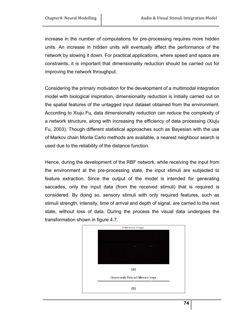
Chapter4: Neural Modelling Audio & Visual Stimuli Integration Model
74
increase in the number of computations for pre-processing requires more hidden
units. An increase in hidden units will eventually affect the performance of the
network by slowing it down. For practical applications, where speed and space are
constraints, it is important that dimensionality reduction should be carried out for
improving the network throughput.
Considering the primary motivation for the development of a multimodal integration
model with biological inspiration, dimensionality reduction is initially carried out on
the spatial features of the untagged input dataset obtained from the environment.
According to Xiuju Fu, data dimensionality reduction can reduce the complexity of
a network structure, along with increasing the efficiency of data processing (Xiuju
Fu, 2003). Though different statistical approaches such as Bayesian with the use
of Markov chain Monte Carlo methods are available, a nearest neighbour search is
used due to the reliability of the distance function.
Hence, during the development of the RBF network, while receiving the input from
the environment at the pre-processing state, the input stimuli are subjected to
feature extraction. Since the output of the model is intended for generating
saccades, only the input data (from the received stimuli) that is required is
considered. By doing so, sensory stimuli with only required features, such as
stimuli strength, intensity, time of arrival and depth of signal, are carried to the next
state, without loss of data. During the process the visual data undergoes the
transformation shown in figure 4.7.
(a)
(b)

Chapter4: Neural Modelling Audio & Visual Stimuli Integration Model
75
(c)
Figure 4.7 Dimensionality variation in visual stimuli: (a) is the difference image that is
collected from the environment, while (b) is the feature extraction segment of figure (a). Figure (b)
is considered as dimensionally reduced due to the elimination of the vertical axis. Hence variables
such as horizontal axis, intensity and depth are transmitted to the network. (c) Represents the light
intensity of the reduced difference image, signifying null loss of data.
When it comes to data from the received audio signal, it is important to determine
the maximum similarity point between the left and right ears for an accurate
identification. Hence, from the received stimuli the integration model, extracts the
similar features using the TDOA along with signal strength over a smaller range of
signal that has maximum similarity, as shown in figure 4.8. By doing so, the
amount of signal that is inspected for the current state is minimized prior to the
multimodal integration.

Chapter4: Neural Modelling Audio & Visual Stimuli Integration Model
76
Figure 4.8 Audio Analysis using limited stimuli to identify localization: Audio analysis
description using the binaural separation and stimuli localization using cross-correlation based on
stimuli arrival.
Once the pre-processed data is available at the integration model, in order to
increase the computational efficiency, only factors that influence the multimodal
stimuli for localization are considered. Similar to the common platform that is used
for referencing the unimodal localization of audio and visual stimuli, a common
Spatial Reference (SRf) platform is used to analyze the stimuli. However, strength
and intensity of the stimuli are two primary factors that are prioritized during the
process.
With the above-mentioned series of modifications concerning computational time,
network design and development, the integration network model was developed to
perform the integration of audio-visual stimuli that arrive simultaneously at the
agent.
4.5.4. Learning Criteria
Learning was an important aspect of neural network design that involves the
process of training the network with the available data, so that after the process
the network was able to provide the desired outcome (Cheshire Engineering
Corporation, 2003). It was carried based on the weight adjustment of the neurons
such that least possible error will be generated while delivering the output. The
processes of learning in this multimodal integration RBF network was carried in
three steps related to centre, weight and width of the network.
On obtaining the outcome from the integration network, in order to determine the
output from the training pattern, the k-nearest search algorithm was used in which
the distance between the individual outputs within ‘k’ distance ranges was

Chapter4: Neural Modelling Audio & Visual Stimuli Integration Model
77
considered. Also the computational time that was required to perform the distance
function was useful for quick response generation. The following algorithm was
used to determine the nearest output from the training set.
K-nearest neighbour algorithm:
1. Compute Euclidean distance between the target and available training
space
2. Determine the sample space that fall within the range of acceptable
localization
3. Using root mean square error, determine the nearest neighbour optimally
using training space
4. Determine the weighted average of the nearest source location as the
output of the integration model and transmit the error back to the model.
Since the inverse of distance is proportional to the weighted average, the k-
nearest neighbour should always be better than the predicted.
Initially, a function (radial basis function) is derived, such that the weights of the
neurons can be generated. This function is the core (center) of the network. Later,
the derived function should be approximated (generalized) to an extent to perform
the required task for the network. This function is responsible for generating the
neuron weights in the network. Finally, the width or network training rate, which
performs the training, was based on the initial weight and time steps that are used
during network initiation.
The radial basis neural network model is trained over associative learning such
that the association of the stimuli strength can be calculated at the maximum
location of integrated intensity. The network is trained over 900 epochs and the
performance graphs are as shown in figure 4.9.

Chapter4: Neural Modelling Audio & Visual Stimuli Integration Model
78
(i) at 100 Epochs
(ii) at 500 Epochs
(iii) at 800 Epochs
(iv) at 900 Epochs
Figure 4.9 Learning performance states-1 during multimodal training: Learning performance
states-1. Performance of learning for the integration model during the training process that is drawn
between network performance and different number of epochs are provided.
Learning is initiated with a random selection of goal. However, the target is to set
goal=0. During the process of training, as the number of epochs is increased, a
gradual reduction in the goal is identified signifying the decline in the graph from
figure 4.9. From 800 epochs onwards, the performance graph is constant and
parallel to the x-axis. This indicates the stable or threshold state of the training
which can seen from figure 4.10
(i) at 850 Epochs
(ii) at 900 Epochs
Figure 4.10 Learning performance states-2 reaching threshold: Performance of learning for
the integration model during the training process that is drawn between network performance
during the final epoch just before and after threshold is provided.

Chapter4: Neural Modelling Audio & Visual Stimuli Integration Model
79
At 850 epochs, the learning state of the model is considered as optimal due to the
steady decrease in the network error. At this state, though the goal is constant,
performance of the integration model decreases. Hence the obtained state of the
neural network is used to perform audio-visual stimuli integration.
Considering learning of the model at various epochs states, the consistency of the
model is also verified with the test samples. The graph thus represents the
learning performance of the integration model. Though the learning process is
smooth, the final given goal or target is not achieved. However, considering the
extent of output at the minimal error state, the network output is effective. The
accuracy achieved by the network was provided below.
4.5.5 Neural Network Training
During the process of neural network training, the error obtained after every 100
inputs states of the network was considered. At each input step, the mean error
generated at all the source locations was considered. Figure 4.11 is a graph
showing the training errors after every 100 inputs.

Chapter4: Neural Modelling Audio & Visual Stimuli Integration Model
80
Figure 4.11 Error graph of neural network model training states: Error graph of neural network
model featuring the range of error that was encountered during network training at given input
source locations.
Figure 4.11 shows the gradual decrease in the error, with the increased number of
inputs. This indicates the effectiveness of the neural network model in obtaining a
more efficient output. This also complies with the accuracy factor, demonstrating
the neural network integration model was more accurate (less error) in generating
integrated output. In this section, the performance of the integration model was
visualized based on both learning and training criteria.
4.6. Integration Model
Considering the features described above, a neural network model was developed
using radial basis network function. The network receives audio and visual stimuli
information in the form of vector data containing localization and intensity
information. This information is transmitted to the integration model to generate
corresponding motor output for saccade generation. The developed network is
mounted on a PeopleBot agent and is subjected to the behavioral experimental
environment. This time the agent is exposed to the simultaneous transmission of
audio and visual information. A synchronous counter identifies the delay present
between the received multimodal stimuli and determines whether to consider the
unimodal or integration model. During the experimental verification, multimodal
stimuli that are synchronous are used.
Before discussing the experimental work, it is noted that multimodal instances can
also appear with visual stimuli. However, when it comes to audio stimuli, which is
supplied through IC to the SC, multimodal instances are bypassed and the final
audio outcome is transferred to the SC. Hence the multimodal audio case does not
belong to stimuli integration aspect of SC. In the case of visual stimuli, since the
optic tract is directly connected to the SC the chances of receiving simultaneous
stimuli were greater. This connection signifies the availability of stimuli at the SC,

Chapter4: Neural Modelling Audio & Visual Stimuli Integration Model
81
which are presented in the next section using the HSFr and subjected to
localization based on the stimuli intensity. 4.6.1. Experimental Outcome
The neural network model contained within the agent is tested using the
behavioral platform with experiments involving the simultaneous bombardment of
visual and audio stimuli. During the experimentation, the following integration
output cases are identified. Integration Case Studies:
(a) Multiple visual input stimuli: In the case of more than one visual input in
the environment, the difference image vector is generated, identifying the
areas of visual interference from the environment, as shown in figure
4.12(a). From the difference image vector the intensity of the signal is
identified in terms of RGB values, as shown in figure 4.12(b). Examining
the variations in the spikes generated, the intensities of both red and green
are considered. The first and last peak show that the green spike is lower in
intensity compared to the second peak. Considering the second, the green
and red spikes are high in intensity when compared to the rest. However,
the plot of the maximum values of the available RGB intensities determines
the position of the source. By plotting the position onto a [-90, 90] scale the
location of the source is determined, which in this case is -300.
(a)

Chapter4: Neural Modelling Audio & Visual Stimuli Integration Model
82
(b)
Figure 4.12 Response of multiple visual input stimuli localization 1: Example of multiple
visual input stimuli received by the agent and how the visual localization is determined using the
difference image and intensity information. The maximum intensity is identified in the second peak
where all RGB values are highest when compared with the rest of the peaks.
Even in circumstances of simultaneously available, multiple visual stimuli, the
integration model perform a similar intensity determination methodology by
projecting the one with the highest. An example is shown in figure 4.13(a), where
there are five stimuli. Later the highest intensity stimulus is projected on to HSFr to
perform the localization. During the highest peak determination, the use of RGB
components determines the effectiveness of the Gaussian method for identifying
the difference between the stimuli and eliminating them as shown in figure 4.13(b).
The criteria of multimodal integration appear when both the audio and visual
stimuli are available at the integration model simultaneously. During the course of
integration, depending on the stimuli intensity and their output behaviour, the
following cases are classified. During the classification, the output state of the
integrated signal is used to determine the enhancement and depression
phenomena.
(a)
0 50 100 150 200 250 300 350 0 100 200 300
-80 -60 -40 0 20 40 60 80 0
0.5
1 Visual Source Localization

Chapter4: Neural Modelling Audio & Visual Stimuli Integration Model
83
(b)
Figure 4.13 Response of multiple visual input stimuli localization 2: (a) depicts multiple visual
stimuli and the response generated when multiple inputs arrived at the integration model. (b)
Shows the maximum intensity peak location and how the destination stimulus localization is
determined.
(b) Weak audio and strong visual stimuli: If a low intensity audio signal and a
visual signal with a strong intensity are received at the same time by the
multimodal integration system, after verifying the time frame to confirm the arrival
of the signals, both inputs are considered by the integration system. After
preprocessing the signals, the localization maps are generated on the HSFr. In the
graphs we can observe that the stimulus in the audio plot has a very low intensity
and the source is determined accordingly, which is 150, as shown in figure 4.14(a).
For the visual stimulus, the single spikes in red and green are considered for the
maximum signal value, which is 50, as shown in figure 4.14(b). When plotted on
the standard space scale, the sources are identified as being at two different
locations, but the overall integrated location is identified as being close to the
stronger visual stimulus. This is at 60 as shown in figure 4.14(c). In this case the
integration mechanism considers the strength of the visual signal compared to the
audio signal.
0 50 100 150 200 250 300 350 0 100 200 300
-80 -60 -40 -20 0 20 40 60 80 0
0.5
1 Visual Source Localization

Chapter4: Neural Modelling Audio & Visual Stimuli Integration Model
84
(a)
(b)
-80 -60 -40 -20 0 20 40 60 800
0.5
1Integrated source localization
(c)
Figure 4.14 Response of low audio and strong visual stimuli localization: Audio and visual
input with strong visual stimulus determining the main preference for the localization. The output
signifies the orientation of output towards the strong stimuli.
(c) Strong Audio and Weak Visual Stimuli: In this case the intensity of the audio
stimulus is stronger than the intensity of the visual stimulus. TDOA has localized
the audio stimulus around -90, as shown in figure 4.15(a). When it comes to the
visual stimulus, the highest RGB component is green (representing a depletion in
intensity), and there are two activation stimuli. Here there is a consistency in the
0.122 0.124 0.126 0.128 0.13 0.132 -0.2 0
0.2 Left Channel
0.122 0.124 0.126 0.128 0.13 0.132 -0.2 0
0.2 Right Channel
-80 -60 -40 -20 0 20 40 60 80 0 0.5
1 Sound Source Localization
0 50 100 150 200 250 300 350 0 100 200 300
-80 -60 -40 -20 0 20 40 60 80 0
0.5
1 Visual Source Localization

Chapter4: Neural Modelling Audio & Visual Stimuli Integration Model
85
green spike, while the red spikes vary, as shown in figure 4.15(b). The location of
the two inputs is on different sides of the centre. Hence, during the process of
integration, the audio stimulus plays a vital role in generating the multimodal
output. When the multimodal output is generated, the location of the integrated
output is closer to the audio stimulus as shown in figure 4.15(c).
0.122 0.123 0.124 0.125 0.126 0.127 0.128 0.129 0.13 0.131-0.2
0
0.2Left Channel
0.122 0.123 0.124 0.125 0.126 0.127 0.128 0.129 0.13 0.131-0.2
0
0.2Right Channel
-80 -60 -40 -20 0 20 40 60 800
0.5
1Sound Source Localization
(a)
0 50 100 150 200 250 300 3500
50
100
150
200
-80 -60 -40 -20 0 20 40 60 800
0.5
1Visual Source Localization
(b)
-80 -60 -40 -20 0 20 40 60 800
0.5
1Integrated Source Localization
(c)
Figure 4.15 Response of strong audio and low visual stimuli localization: Multimodal input
case with strong audio stimulus. The integrated output is biased by the intensity of the stronger
stimulus, which in this case is audio.
The above two representative cases are observed during multimodal integration,
with one of the signals being relatively strong in its intensity. The integration model

Chapter4: Neural Modelling Audio & Visual Stimuli Integration Model
86
focuses on the stimulus with the highest intensity, which therefore influences the
integrated decision.
(d) Strong visual and strong audio stimuli: In this scenario, when the sensors
receive the signals, their modalities are plotted on an intensity graph to determine
the signal intensity. In the intensity graphs shown in figure 4.16, the sources are
located on either side of the centre and the activations are of high intensity. When
the output is computed, the source is located close to the visually detected peak.
0 50 100 150 200 250 300 3500
100
200
300
-80 -60 -40 -20 0 20 40 60 800
0.5
1Visual Source Localization
(a)
0.122 0.123 0.124 0.125 0.126 0.127 0.128 0.129 0.13 0.131-0.2
0
0.2Left Channel
0.122 0.123 0.124 0.125 0.126 0.127 0.128 0.129 0.13 0.131-0.2
0
0.2Right Channel
-80 -60 -40 -20 0 20 40 60 800
0.5
1Sound Source Localization
(b)
-80 -60 -40 -20 0 20 40 60 800
0.5
1Integrated Source Localization
(c)

Chapter4: Neural Modelling Audio & Visual Stimuli Integration Model
87
Figure 4.16 Response of strong visual and strong audio stimuli localization: Example of
multimodal enhancement response. The integrated output is generated based on a distance
function between the audio and visual intensity.
In this case it is not clear whether the SC will prioritize in every case of integration.
However in the case of multiple strong intensity stimuli the visual stimulus will
have the higher priority, while the strong audio stimulus will have some influence
on the multimodal integrated output. Hence the integrated output localization is
closer to the strong stimulus, which is shown in figure 4.16(c). This signifies the
partial prioritization towards visually strong stimuli.
(e) Weak visual and weak audio stimuli: In circumstances where both visual
and audio signals are of low intensities, the behaviour of the SC is often difficult to
predict. In this case, the SC can be thought of as a kind of search engine that
keeps traversing the environment to locate any variations within it. When both
audio and visual signals are of low intensity, the SC suppresses the audio signal.
Though the visual signal is low in its intensity, as far as the SC is concerned, it is
the only sensory data available. Therefore, the source is identified much closer to
the visual stimulus, as shown in figure 4.17.
0 50 100 150 200 250 300 3500
50
100
150
200
-80 -60 -40 -20 0 20 40 60 800
0.5
1Visual Source Localization
(a)

Chapter4: Neural Modelling Audio & Visual Stimuli Integration Model
88
0.122 0.123 0.124 0.125 0.126 0.127 0.128 0.129 0.13 0.131-0.2
0
0.2Left Channel
0.122 0.123 0.124 0.125 0.126 0.127 0.128 0.129 0.13 0.131-0.2
0
0.2Right Channel
-80 -60 -40 -20 0 20 40 60 800
0.5
1Sound Source Localization
(b)
-80 -60 -40 -20 0 20 40 60 800
0.5
1Integrated source localization
(c)
Figure 4.17 Response of low visual and low audio stimuli localization (Enhancement
phenomena): Example of multimodal enhancement response. The integrated output is generated
based on a distance function between the audio and visual intensity where the audio signal is
suppressed due to its low intensity and the visual stimulus is the only input available. Hence the
distance function is biased towards the visual stimulus enhancing the final output.
In some cases, depression may occur if the visual stimulus is out of range or the
audio stimulus is becoming less intense. This can also happen if the audio
stimulus is out of range and the visual stimulus is weak. This case signifies two
factors. One is with the availability of stimuli, while the other is associated with
strength or intensity. In the figure 4.18:
(a) represents the non availability of the stimuli causing no localization.
(b) represents the availability of audio stimuli with weak intensity. This shows the
model exhibiting depression behaviour.
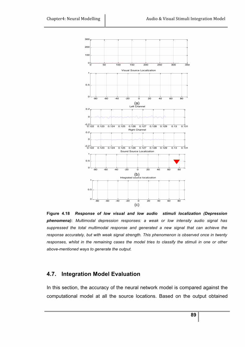
Chapter4: Neural Modelling Audio & Visual Stimuli Integration Model
89
0 50 100 150 200 250 300 3500
100
200
300
-80 -60 -40 -20 0 20 40 60 800
0.5
1Visual Source Localization
(a)
0.122 0.123 0.124 0.125 0.126 0.127 0.128 0.129 0.13 0.131-0.2
0
0.2Left Channel
0.122 0.123 0.124 0.125 0.126 0.127 0.128 0.129 0.13 0.131-0.2
0
0.2Right Channel
-80 -60 -40 -20 0 20 40 60 800
0.5
1Sound Source Localization
(b)
-80 -60 -40 -20 0 20 40 60 800
0.5
1Integrated source localization
(c)
Figure 4.18 Response of low visual and low audio stimuli localization (Depression
phenomena): Multimodal depression responses: a weak or low intensity audio signal has
suppressed the total multimodal response and generated a new signal that can achieve the
response accurately, but with weak signal strength. This phenomenon is observed once in twenty
responses, whilst in the remaining cases the model tries to classify the stimuli in one or other
above-mentioned ways to generate the output.
4.7. Integration Model Evaluation
In this section, the accuracy of the neural network model is compared against the
computational model at all the source locations. Based on the output obtained

Chapter4: Neural Modelling Audio & Visual Stimuli Integration Model
90
from a test set, error states that are generated at every source location are
considered.
4.7.1. Computational Verses Neural Network Model
Using the computational integration model provided earlier in this chapter, the
mean error obtained across the source locations from -300 to +300 is represented
in figure 4.19.
Figure 4.19 Computational Model Mean Error Chart: Error graph of computational model
featuring the range of error that is encountered during integration output generation for the test set.
From the graph it is apparent that the mean error ranges from approximately 50 to
180. This graph demonstrates the error obtained at all stations that are used for
localizing the stimuli source. Since the error rises above ±50, the use of saccade
degree of variance does not influence integration output.
Similarly, a neural network mean error chart is shown in figure 4.20 to identify the
range of error generated.

Chapter4: Neural Modelling Audio & Visual Stimuli Integration Model
91
Figure 4.20 Neural network model mean error chart: Error graph at stimuli localization stations
featuring the contribution of multimodal error that is encountered during integration output
generation for test set.
Figure 4.20 shows that the range of error lies between approximately 0.20 to 20.
This error range excludes the saccade degree of variance. Based on the error
generated, the neural network model output is approximately 20 times more
accurate than the computational model output. Including the degree of freedom to
± 50, for both computational and neural network error graphs, the neural network
output is three times more effective than the computational output.
In figure 4.21 a comparison between the error states of the neural network model
and the computational model is shown, to highlight the relative accuracy achieved
by both approaches.

Chapter4: Neural Modelling Audio & Visual Stimuli Integration Model
92
Figure 4.21 Accuracy graph between neural and computational integration model: Accuracy
graph featuring error states of neural network integration model and computational model for given
stimuli locations .
4.8. Summary
This chapter is a continuation of the methodology from Chapter-3 detailing the
integration process and implementation details. Initially it describes the integration
formulation containing audio and visual data processing. A schematic
representation of the integration process is shows, how it is carried out, along with
the requirements for avoiding difficulties involving computations.
Later, design aspects of the integration model are proposed irrespective of the
development platform, using intermediate processing stages and critical features
that are necessary for the model development. This design is based on the
biological stimuli processing analysis generated from the SC mentioned in Chapter
2. During this stage, the possible developmental platforms are discussed.
Based on the literature review, computational-based integration model
development is adapted to ensure the computational aspect of the model is

Chapter4: Neural Modelling Audio & Visual Stimuli Integration Model
93
feasible. This section details the development and working aspects of the model,
along with the results that are achieved during the process. However, the level of
error achieved during the process is of greater concern. The error reduction
discussion in the computational approach eventually supports a neural network
platform, suggesting reduction in the computational time and a minimal error when
the model is given stimuli from a live environment.
In the next section the feasibility of a radial basis function neural network approach
is discussed along with the network development, including the network structure
and working platform to implement integration criteria. During the process, the
dimensionality aspect that involves the size of input data is also discussed, where
stimuli pre-processing is adapted at the development stage to enhance the
network efficiency. Dimensionality issues with the input feature set are discussed
in the next chapter, which describes how effectively the data set is used in making
the network effective.
Finally, the developed neural network is subjected to the behavioral experimental
platform and the output is generated. Samples of outputs were projected where
enhancement and depression phenomena are identified. An important research
goal of the project is achieved as the integration model is capable of generating
enhancement and depression phenomena in multimodal output generation. The
model is successful in generating the multimodal output for the given inputs. As far
as the initial tests are concerned, the output is adequate. However, when it comes
to efficiency, the model has to be tested and evaluated for determining
performance in terms of accuracy. In the next chapter a detailed experimental
analysis and evaluation were described.

Chapter 5: Experimental Analysis Audio & Visual Stimuli Integration Model
94
Chapter 5 Experimental Analysis _________________________________________________________________
5.1. Introduction
In this chapter, the results of the experiments described in the previous chapter
are analysed to verify the success of the model. During this process, unimodal
experiments are initially considered and the performance is analyzed. Similarly,
integration experiments are considered with both unimodal and multimodal data
under varied circumstances for enhancement and depression. Later, the input
space is classified for training and testing. Based on the learning criteria, the
integration model is subjected to learning over the training data set and tested.
The obtained test results are used to compare the computational integration model
with the neural network integration model.
The next section, discusses how the stimuli space was used to perform the
training and testing of the model, along with classification of the sub-space for the
training set and test set.
5.2. Preparation of Training and Test Data During the experimentation, data was collected in two different phases. Initially
unimodal audio and visual data was obtained. Multimodal data was collected using
the same experimental platform with the simultaneous arrival of audio and visual
data.
From the obtained datasets, samples from each category were initially used to
verify the success of the unimodal experimental phase. Both audio and visual

Chapter 5: Experimental Analysis Audio & Visual Stimuli Integration Model
95
unimodal localization experiments were performed using the static data samples.
These datasets were re-used to test the performance of the multimodal system
with unimodal data. During this data collection phase, multimodal data samples
were also collected from the experimental platform with labelled inputs under
similar conditions.
In the multimodal experimental phase, the integration model was tested using
audio and visual multimodal data. In the following sections, a series of tables are
provided which show the error in the multimodal output. Although the output of the
integration model was accurate to approximately 2 – 30, a higher degree of
accuracy was desirable. Hence the neural network was subjected to supervised
learning, so that the error could be reduced and the output accuracy could be
increased. In order to train the network effectively, it is important that the learning
criteria and the dataset partition for training and test sets are also effective.
Initially the integration model was trained using only the multimodal data input. In
the multimodal data, a random selection of each sample from each category is
formed into test data. The remaining sub-space is used as training data for the
neural network. Apart from the above dataset, the integration model is also tested
on another dataset that is generated from the simultaneous transmission of both
unimodal audio and unimodal visual data, effectively generating a multimodal
input. Though the transmission conditions are similar to that of multimodal input,
the outputs vary due to their different intensity levels. Hence, this variation leads to
generation of different outputs. However, they serve as a test and validation set for
determining the success and performance of the integration model.
5.3. Unimodal Experimental Analysis for Localization
The unimodal experimental setup with audio and visual stimuli is used to
investigate accuracy of localization. Further investigations involved multimodal
inputs in the sub-space. However in this section, the unimodal input stimuli that
are collected are used to determine the success under variable conditions.

Chapter 5: Experimental Analysis Audio & Visual Stimuli Integration Model
96
5.3.1 Unimodal Audio Localization Analysis
Different audio stimuli collected from the behavioural platform are used to test
localization accuracy. Based on the results generated, the error is processed and
analyzed to determine the performance of the unimodal audio localization. The
collected audio input space is classified into eight different types based on the
source amplitude levels. The following results are from the computational model.
Out of the available input space, samples are selected in the range 8 - 22dB as
follows: 10, 12, 16, 20 and 22dB. The selection of stimuli frequency and amplitude
was made based on the audible-limit of hardware equipment used by the agent.
Localization attempts are carried out with 8dB signals, but these were found to be
insufficient for stimuli localization. The background noise in the laboratory ranged
from 0.4 to 4dB. During testing, unimodal inputs with frequencies ranging from
100Hz to 600Hz are localized. The results obtained are shown in Tables 5.1 to 5.5.
From the output states, the localization error is used to determine the
effectiveness of the model.
The localization error is determined by measuring the difference between the
actual and predicted source location. All these output and error states are
recorded in Tables 5.1 to 5.5. Each table also shows the mean and standard
deviation of errors for each audio frequency and each source location.

Chapter 5: Experimental Analysis Audio & Visual Stimuli Integration Model
97
Audio Sample 1:
Source amplitude = 10dB
The error obtained during the localization is tabulated as follows in Table 5.1
Audio Localization Error Chart for Sample 1
Frequency
Vs
Angle 100Hz 200Hz 300Hz 400Hz 500Hz 600Hz Mean St Dev
-900 8.93 3.93 3.12 6.81 6.06 0.06 4.82 3.12
-600 1.39 3.39 3.39 3.39 3.04 -1.38 2.66 1.92
-450 1.29 2.89 1.07 1.07 0.17 2.09 1.43 0.94
-300 3.45 1.97 -0.03 2.6 1.86 0.40 1.72 1.32
-200 2.66 2.03 1.97 0.41 0.02 -1.41 1.42 1.54
-100 1.43 2.8 0.78 0.52 0.56 0.24 1.06 0.94
00 1 -0.5 2.09 2.09 0 0 0.95 1.13
100 0.73 0.32 2.4 0.42 0.52 0.52 0.82 0.79
200 1.87 1.01 1.41 0.02 1.41 1.41 1.19 0.63
300 3.97 2.59 1.44 2.59 -0.71 1.44 2.12 1.58
450 1.33 0.89 2.05 0.93 1.41 0.01 1.10 0.68
600 2.89 3.69 3.39 3.39 3.39 2.01 3.13 0.60
900 11.98 6.98 6.0 5.59 4.59 1.98 6.19 3.31
Mean 3.30 2.54 2.24 2.29 1.83 1.00 2.20 0.76
St Dev 3.38 1.91 1.52 2.09 2.02 1.18 2.02 0.75
Table 5.1 The localization error in degrees for the input data sample 1 using amplitude of 10dB.
The mean provided in column and row indicate the mean with corresponding
source location and input frequency respectively. Similarly with standard deviation,

Chapter 5: Experimental Analysis Audio & Visual Stimuli Integration Model
98
represents the extent of deviation that can cause at each mean from the
respective row and column. The errors shown in Table 5.1 are represented
graphically in figure 5.1
Figure 5.1 Response of unimodal audio localization error for sample 1: Graphical
representation of audio localization error shown in table 5.1. In this graph the range of error lies
between (-2, 12) degrees
Figure 5.1 shows the error variation across the audio range (-900, 900). It is
observed that the error significantly increases for angles in the range (±600, ±900).
However in the range of (-600, +600), the error lies within (-20, +40). Also, as the
frequency of the stimuli increases, the error significantly reduces. This signifies
that the integration model is more effective for higher frequencies. The strength of
the stimuli decreases gradually starting from the centre. This signifies that the
model is influenced mainly by the strength of stimuli, rather than frequency.

Chapter 5: Experimental Analysis Audio & Visual Stimuli Integration Model
99
Audio Sample 2:
Source amplitude = 12dB
The error obtained during the localization is tabulated in Table 5.2
Audio Localization Error Chart for Sample 2 Frequency
Vs
Angle
100Hz 200Hz 300Hz 400Hz 500Hz 600Hz Mean St Dev
-900 6.73 2.83 3.02 4.61 2.09 0.96 3.37 2.03
-600 1.19 2.12 0.39 0.01 0.16 0.98 0.81 0.79
-450 0.02 0.91 1.03 2.03 0.57 1.69 1.04 0.73
-300 -1.41 0.17 -0.03 0.96 0.46 1.98 0.84 1.12
-200 -1.02 -0.46 0.17 0.98 -1.42 1.54 0.93 1.15
-100 0.88 1.38 0.98 0.92 1.36 0.17 0.95 0.44
00 0 -0.5 1.0 1.05 0 0.5 0.51 0.62
100 1.23 0.88 0.40 0.02 0.83 0.34 0.62 0.44
200 1.04 0.36 0.04 0.77 0.21 0.01 0.41 0.42
300 -0.02 -0.41 0.12 1.02 -0.02 2.14 0.62 0.95
450 -0.79 0.16 -1.02 -0.02 0.01 0.97 0.50 0.71
600 1.07 0.24 1.98 0.36 1.29 2.17 1.19 0.80
900 -2.64 -7.08 -4.0 -0.66 -9.33 0.02 3.96 3.66
Mean 1.39 1.35 1.09 1.03 1.83 1.00 1.28 0.32
St Dev 2.21 2.36 1.64 1.30 2.85 0.80 1.86 0.75
Table 5.2 The localization error in degrees for the input data sample 2 given the source amplitude
is 12dB.

Chapter 5: Experimental Analysis Audio & Visual Stimuli Integration Model
100
A graphical representation of the error shown in Table 5.2 is presented in figure
5.2
Figure 5.2 Response of unimodal audio localization error for sample 2: Graphical
representation of audio localization error shown in table 5.2. In this graph the range of error lies
between (-10, 8) degrees.
It can be seen in figure 5.2 that, most of the errors lie in the range (-20, 20) for
sources in the range of (-600, 600). However, for the range (±600, ±900) it varies
between (-100, 80), which is a significant deviation from the mean error. However,
compared to audio sample1, a reduction is obtained in the mean error, particularly
in the range (-600, +600). Here, the maximum error magnitude is reduced by over
two degree. This is attributed to the increase in stimuli intensity resulting from the
increased amplitude. There is little change in the ranges (-600, -900) and (+600,
+900).

Chapter 5: Experimental Analysis Audio & Visual Stimuli Integration Model
101
Audio Sample 3:
Source amplitude = 16dB.
Based on the output generated with input sample 3, error obtained during the
localization is presented in Table 5.3
Audio Localization Error Chart for Sample 3
Frequency
Vs
Angle
100Hz 200Hz 300Hz 400Hz 500Hz 600Hz Mean St Dev
-900 2.1 0.80 1.98 3.41 0.83 0.23 1.56 1.16
-600 0.98 1.17 0.98 0.17 -0.66 -0.14 0.68 0.74
-450 -0.88 0.17 -0.44 -1.02 0.17 1.01 0.62 0.76
-300 -0.83 0.17 -0.03 0.0 -0.46 0.98 0.41 0.61
-200 -0.83 -0.46 0.0 0.98 -1.02 0.56 0.64 0.79
-100 -0.88 1.38 0.98 0.92 1.01 0 0.86 0.84
00 0 0.5 -1 0.0 0.0 0.5 0.33 0.55
100 0.5 -0.88 0.40 -0.46 -0.83 0.0 0.51 0.60
200 0.09 0.36 -0.04 0.0 0.21 0.01 0.12 0.15
300 0.0 -0.41 0.12 1.02 -0.02 0.86 0.41 0.56
450 -0.79 0.16 -1.02 -0.02 1.01 0.97 0.66 0.85
600 1.07 0.24 1.98 0.36 1.29 2.17 1.19 0.80
900 -2.64 0.0 -2.02 -0.66 -3.63 0.02 1.50 1.51
Mean 0.89 0.52 0.85 0.69 0.86 0.57 0.73 0.16
St Dev 1.19 0.63 1.15 1.10 1.28 0.65 1.00 0.29
Table 5.3 The localization error in degrees for the input data sample 3, given the source amplitude
is 16dB.
Graphical representations of errors obtained in Table 5.3 are presented in figure
5.3.

Chapter 5: Experimental Analysis Audio & Visual Stimuli Integration Model
102
Figure 5.3 Response of unimodal audio localization error for sample 3: Graphical
representation of audio localization error shown in table 5.3. In this graph the range of error lies
between (-4, 4) degrees
Figure 5.3 shows that errors have been reduced to a range of (-40, 40). If the
boundary errors are excluded, the mean error lies in the range (-10, 20). This error
reduction indicates that the relative accuracy is increased as the amplitude of the
stimuli increases. Similarly, as the stimuli frequency decreases, the error also
decreases. This contradicts the findings of the first experiment (audio sample 1).
This signifies that although frequency plays an effective role in localizing the
source, it is the strength of the stimuli, which is the amplitude in this case, which
plays a critical role in determining the localization performance. This behaviour can
be observed in all the cases shown.
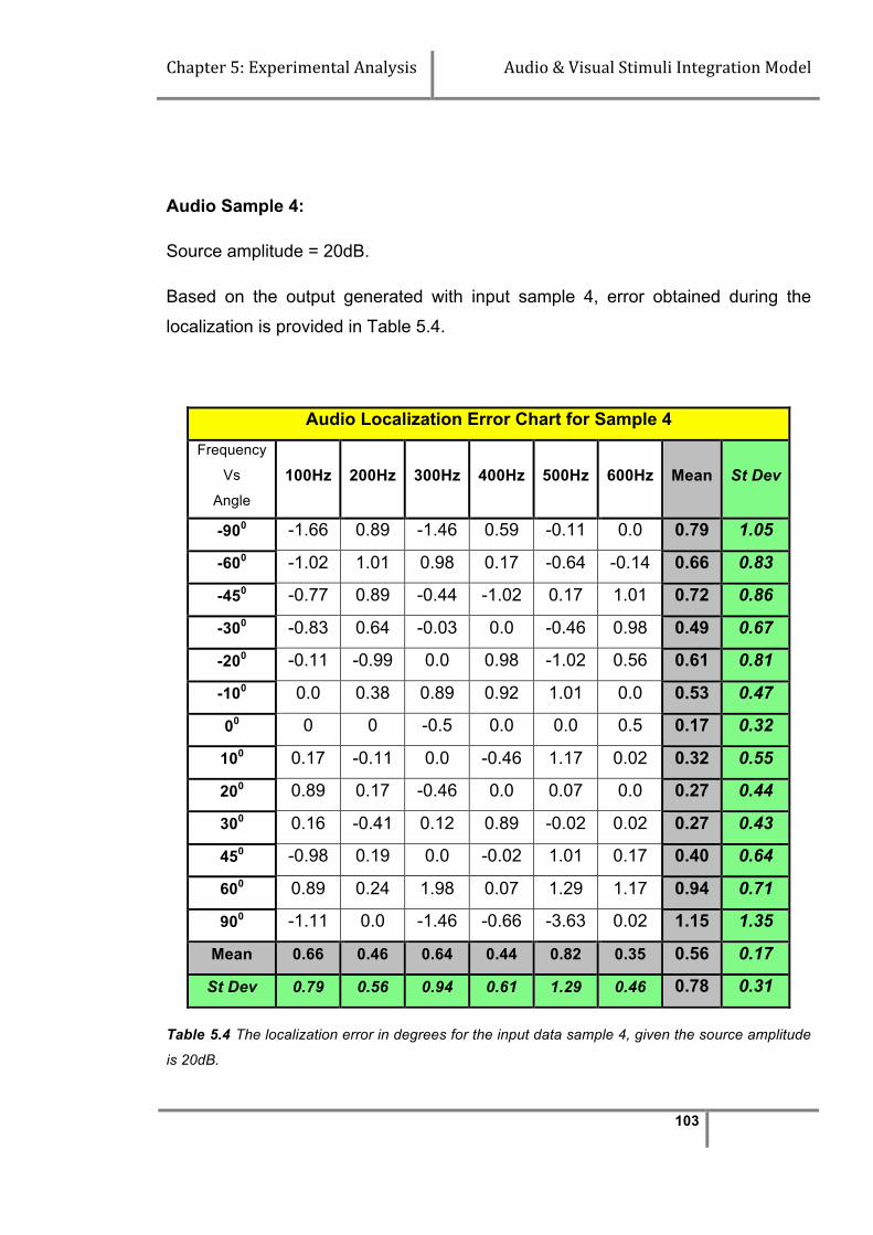
Chapter 5: Experimental Analysis Audio & Visual Stimuli Integration Model
103
Audio Sample 4:
Source amplitude = 20dB.
Based on the output generated with input sample 4, error obtained during the
localization is provided in Table 5.4.
Audio Localization Error Chart for Sample 4 Frequency
Vs
Angle
100Hz 200Hz 300Hz 400Hz 500Hz 600Hz Mean St Dev
-900 -1.66 0.89 -1.46 0.59 -0.11 0.0 0.79 1.05
-600 -1.02 1.01 0.98 0.17 -0.64 -0.14 0.66 0.83
-450 -0.77 0.89 -0.44 -1.02 0.17 1.01 0.72 0.86
-300 -0.83 0.64 -0.03 0.0 -0.46 0.98 0.49 0.67
-200 -0.11 -0.99 0.0 0.98 -1.02 0.56 0.61 0.81
-100 0.0 0.38 0.89 0.92 1.01 0.0 0.53 0.47
00 0 0 -0.5 0.0 0.0 0.5 0.17 0.32
100 0.17 -0.11 0.0 -0.46 1.17 0.02 0.32 0.55
200 0.89 0.17 -0.46 0.0 0.07 0.0 0.27 0.44
300 0.16 -0.41 0.12 0.89 -0.02 0.02 0.27 0.43
450 -0.98 0.19 0.0 -0.02 1.01 0.17 0.40 0.64
600 0.89 0.24 1.98 0.07 1.29 1.17 0.94 0.71
900 -1.11 0.0 -1.46 -0.66 -3.63 0.02 1.15 1.35
Mean 0.66 0.46 0.64 0.44 0.82 0.35 0.56 0.17
St Dev 0.79 0.56 0.94 0.61 1.29 0.46 0.78 0.31
Table 5.4 The localization error in degrees for the input data sample 4, given the source amplitude
is 20dB.

Chapter 5: Experimental Analysis Audio & Visual Stimuli Integration Model
104
A graphical representation of error obtained in Table 5.4 is presented in figure 5.4.
Figure 5.4 Response of unimodal audio localization error for sample 4: Graphical
representation of audio localization error from table 5.4, featuring relative similarity of each
frequency to the target localization. In this graph the range of error lies between (-4, 2) degrees.
In this sample, the localization error lies between (-40, 20), which is reduced
compared with the previous sample set. Also, the mean error lies in the range of (-
10, 10), which is less than the previous sample. This again signifies the
effectiveness of the integration model with the increase in stimuli strength.

Chapter 5: Experimental Analysis Audio & Visual Stimuli Integration Model
105
Audio Sample 5:
Source amplitude = 22dB
Based on the output generated using input sample 5, error obtained during the
localization is provided in Table 5.5.
Audio Localization Error Chart for Sample 5
Frequency
Vs
Angle
100Hz 200Hz 300Hz 400Hz 500Hz 600Hz Mean St Dev
-900 -0.88 0.17 -0.11 0.59 -1.44 0.0 0.53 0.74 -600 -0.44 0.86 0.12 0.0 -0.88 -0.66 0.49 0.63 -450 -0.83 0.0 -0.44 1.56 0.17 0.98 0.66 0.89 -300 -0.14 0.64 1.02 0.0 -0.88 0.0 0.45 0.66 -200 -0.68 0.64 1.02 0.0 -0.64 0.51 0.58 0.70 -100 0.0 0.38 0.98 0.92 1.01 0.0 0.55 0.48 00 0.0 0.0 0.0 0.0 0.0 0.0 0.00 0.00
100 0.17 -0.11 0.0 -0.46 0.76 0.02 0.25 0.40 200 0.89 0.17 -0.46 -0.14 0.07 0.0 0.29 0.45 300 -0.16 -0.41 0.12 0.89 -0.02 0.02 0.27 0.44 450 -0.98 0.16 0.0 -0.02 1.01 0.17 0.39 0.64 600 0.89 0.24 1.98 0.07 1.29 1.17 0.94 0.71 900 -0.11 0.0 -0.46 -0.83 0.37 0.02 0.30 0.42
Mean 0.47 0.29 0.52 0.42 0.66 0.27 0.44 0.15 St Dev 0.60 0.35 0.74 0.63 0.84 0.47 0.61 0.18
Table 5.5 The localization error in degrees for the input data sample 5, given the source amplitude
is 22dB.
A graphical representation of error tabulated in Table 5.5 is presented in figure 5.5

Chapter 5: Experimental Analysis Audio & Visual Stimuli Integration Model
106
Figure 5.5 Response of unimodal audio localization error for sample 5: Graphical
representation of audio localization error from table 5.5, featuring relative similarity of each
frequency to the target localization. In this graph the range of error lies between (-1.5, 2) degrees.
In figure 5.5 the localization error range is (-1.50, 20) and the mean error does not
exceed 10. This again demonstrates that, localization is improved with increased
stimuli strength.
The above graphs show errors obtained during localization of low frequency audio
stimuli across variable amplitudes. From the graphs it can be seen that as the
amplitude (strength of stimuli) increases, the magnitude of errors between the
predicted and actual source location gradually decreases. Considering the entire
input space, the error lies within a range of ±100, which gradually decreases with
increased stimuli intensity.

Chapter 5: Experimental Analysis Audio & Visual Stimuli Integration Model
107
The mean and standard deviation of error are now considered based on a sample
set for a group of stimuli source stations. In the following three particular source
stations (00, 450, 900) are considered, and the mean errors obtained for
frequencies 100Hz to 600Hz. Figure 5.6 shows the mean errors obtained during
the source location across the amplitude range.
Figure 5.6 Mean error graph for a given sample: Representation of audio localization mean
error of a source stations (00, 450, 900) for a frequency range (100, 600)Hz.
In the figure 5.6 the trend line passing through the given series represents the flow
of error within the range of amplitudes 8 - 22dB. For 00 and 450, the mean error is
less than 20 including the possible deviations. However for 900, it is significantly
higher; and shows that, with a decrease in amplitude the error increases. Similarly

Chapter 5: Experimental Analysis Audio & Visual Stimuli Integration Model
108
as the amplitude increases, the mean error decreases which implies that
localization is effective for higher order amplitudes.
5.3.2 Unimodal Visual Localization Analysis
In this section different visual stimuli transmitted from the behavioral platform
under varied light conditions are used to determine localization performance. The
error is processed and analyzed to determine the performance of unimodal visual
localization. The collected visual input space is classified into three different types
based on the visibility for day and night lighting conditions in the laboratory.
Due to interference (noise) caused by other nearby visual stimuli, the LEDs that
emit light from the visual source are affected. Since this interference causes
variations in the stimuli strengths that are received at the agent, the quality of the
signal is also affected. The quality of the stimuli is quantified based on intensity,
which is normalized in the range of 0 to 1.
In the following results, the visual stimuli can be categorized as follows:
Sample 1: Day time conditions (laboratory lights on)
Sample 2: Night time conditions (laboratory lights off)

Chapter 5: Experimental Analysis Audio & Visual Stimuli Integration Model
109
Visual Sample 1:
Time = Day
Condition = lights on
The error obtained during localization of visual sample 1 is provided in Table 5.6,
and the graphical representation of the error is presented in figure 5.7.
Visual Localization Error Chart for Sample 1 Light Intensity*
Vs Angle (degree)
Set 1 Set 2 Set 3 Set 4 Set 5 Set 6 Mean St Dev
-300 0.85 0.37 0.03 0.54 0.04 -0.64 0.41 0.52
-200 -3.26 -3.67 -2.24 -2.44 -3.44 -3.88 3.16 0.67
-100 1.01 0.53 0.0 0.62 1.59 -0.98 0.79 0.88
00 2.01 2.46 2.46 2.24 1.46 1.57 2.03 0.44
100 0.86 -0.68 0.98 0.0 0.98 2.14 0.94 0.96
200 -3.05 -2.44 -2.44 -1.44 -1.02 -3.05 2.24 0.84
300 -0.44 -0.30 -0.20 0.02 -0.13 0.07 0.19 0.19
Mean 1.64 1.49 1.19 1.04 1.24 1.76 1.39 0.28
St Dev 2.08 2.02 1.72 1.51 1.75 2.22 1.88 0.27
Table 5.6 The error obtained in localizing the visual stimuli for each of input generated from
sample 1. The table also provides the mean and standard deviation for each of the source location
and for each of the visual stimuli category.
The overall pattern of error appeaers similar, irrespective of the type of stimuli. The
error range is (20, -40) and the variation of error for all the stimuli indicates that the
output of localization is within the acceptable range (variance of 50).

Chapter 5: Experimental Analysis Audio & Visual Stimuli Integration Model
110
Figure 5.7 Response of unimodal visual localization error for sample-1: Graphical
representation of visual localization error from Table 5.6, featuring relative similarity of each
stimulus to the target localization. In this graph the range of error lies between (-40, 30).

Chapter 5: Experimental Analysis Audio & Visual Stimuli Integration Model
111
Visual Sample 2:
Time = Night
Condition = Lights off
The error determined during localization of visual sample 2 is provided in the Table
5.7, and the graphical representation of the error determined is presented in figure
5.8.
Visual Localization Error Chart for Sample 2
Light
Intensity*
Vs
Angle
(degree)
Set 1
Set 2
Set 3
Set 4
Set 5
Set 6
Mean St
Dev
-300 0.85 0.37 0.03 0.54 0.04 -0.44 0.38 0.45
-200 -0.16 -0.66 0.98 0.0 0.07 -0.41 0.38 0.56
-100 0.21 0.31 0.0 0.20 1.02 0.0 0.29 0.38
00 1.10 0.5 0.0 0.0 0.0 0.02 0.27 0.45
100 0.42 0.12 0.02 0.0 0.46 0.0 0.17 0.21
200 -1.05 0.02 -0.26 0.04 0.0 0.07 0.24 0.43
300 0.36 0.05 -0.20 0.02 -0.13 -0.64 0.23 0.33
Mean 0.59 0.29 0.21 0.11 0.25 0.23 0.28 0.16
St Dev 0.71 0.38 0.41 0.20 0.40 0.29 0.40 0.17
Table 5.7 Visual localization error chart with lights-off condition: The error obtained in
localizing the visual stimuli for each of input generated from sample 2. A graphical representation of
this table is provided in figure 5.8 depicting the range of error obtained.
Figure 5.8 indicates an improvement of the mean error, when compared to the
previous sample shown in figure 5.7. The random spikes in the graph are due to

Chapter 5: Experimental Analysis Audio & Visual Stimuli Integration Model
112
the random selection of data from the input space. However, the mean error lies
below one degree. This indicates the improvisation of accuracy in the visual stimuli
aspect of localization model.
Figure 5.8 Response of unimodal visual localization stimuli for sample-2: Graphical
representation of audio localization error from table 5.7, featuring relative similarity of each stimulus
to the target localization. In this graph the range of error lies between (-1.5, 1.5) degrees.
The results obtained above are two different samples that are used in obtaining
the unimodal visual input data for the experimental investigation. From the above
figures 5.7 and 5.8 it is shown that, with an increase in stimuli intensity an
improvement in the localization performance is obtained. Hence the graphs signify
that the quality of the stimuli influences the accuracy of localization by reducing the
error.

Chapter 5: Experimental Analysis Audio & Visual Stimuli Integration Model
113
5.4 Integrated Experimental Data Analysis
In this section, the multimodal integration model is subjected to testing with the
help of a behavioral experimental platform to localize simultaneously generated
audio and visual stimuli. The level of performance achieved was determined along
with further verification using other inputs in the sub-space. In this section, the
multimodal input stimuli collected are used to verify the success by determining
the error involved from expected and target output states.
Integrated experimental analysis examines various input states involved in
generating the multimodal output, similar to the unimodal analysis. Since a
research goal is to verify the enhancement and depression phenomena associated
with the integrated output, various cases are demonstrated.

Chapter 5: Experimental Analysis Audio & Visual Stimuli Integration Model
114
Integration Sample 1
In Table 5.8, a set of multimodal stimuli samples (expressed in degrees) are
collected in the order of decreasing intensities of frequencies. As input for this
sample, five different multimodal sets of data were created, where:
Set 1 = 500Hz, Set 2 = 400Hz, Set 3 = 300Hz, Set 4 = 200Hz and Set 5 = 100Hz
along with visual stimuli in the range of (0.5, 1).
The error in the multimodal localization for sample 1 is given in table 5.8.
Multimodal Localization Error Chart for Sample 1 Audio Sample (degree)
Vs
Visual Sample (degree)
Set 1 Set 2 Set 3 Set 4 Set 5 Mean St Dev
-30 0.07 -0.5 0.0 0.0 0.07 0.13 0.24
-20 1.41 0.04 -0.9 0.0 0.33 0.54 0.83
-10 1.01 1.07 0.97 0.0 -0.05 0.62 0.57
0 -- -1.3 -0.04 -1.11 0.04 0.50 0.70
10 -0.56 -- -0.06 -0.07 0.0 0.14 0.26
20 -1.02 -0.56 0.04 0.0 0.01 0.33 0.47
30 0.08 0.89 0.01 0.0 -0.06 0.21 0.40
Mean 0.59 0.62 0.29 0.17 0.08 0.35 0.24
St Dev 0.92 0.91 0.54 0.42 0.13 0.58 0.34
Table 5.8 Multimodal localization error chart for sample 1 (multimodal input): Multimodal
localization error determined from the sample 1 with respect to corresponding audio and visual
stimuli data.
Figure 5.9 is a graphical representation of the error table 5.8.

Chapter 5: Experimental Analysis Audio & Visual Stimuli Integration Model
115
Figure 5.9 Response of multimodal neural network integration model error for sample 1:
Graphical representation of audio localization error from table 5.8, featuring error obtained during
the multimodal localization out of above instances. In this graph the error obtained at the random
selected state is plotted.
In Table 5.8 cells that are empty signify that no output is detected. This results
from lack of deterministic states of output stimuli, which can be considered as
depression, and will be discussed further in section 5.5. Figure 5.9 is a random
selection of inputs selected from the multimodal input space, where audio and
visual input is simultaneously transmitted to the integration model. On the graph
are plotted the errors that are obtained for inputs which are localized within the
range (-300, 300). From the graph the error of these inputs is in the range (-1.50,
1.50), while the mean error is less than one degree.
The graph also indicates that as the frequency decreases, the localization
improves with error less than ±10. This signifies that the increase in intensity that
influences the multimodal localization is effectively adapted in the neural network
integration model.

Chapter 5: Experimental Analysis Audio & Visual Stimuli Integration Model
116
Integration Sample 2 The network was tested by presenting to it both audio and visual data. These
samples are a selection of five sets of inputs with frequency ranging from 500 to
100Hz, and fixed visual inputs from a day time (lights on), where the intensity is in
the range of (0.5, 1). The multimodal outcomes given in Table 5.9 signify a
relatively close localization (error < 20) from the input supplied.
Multimodal Error Localization (-300)
Input Visual Stimuli
Audio Stimuli
Multimodal Output Error
Set 1 -30.85 -26.55 -30.35 0.35 Set 2 -30.37 -28.57 -30.00 0.0 Set 3 -30.03 -29.17 -30.00 0.0 Set 4 -30.54 -29.17 -30.02 0.02 Set 5 -30.04 -29.86 -30.00 0.0
(i)
Multimodal Error Localization (300)
Input Visual Stimuli
Audio Stimuli
Multimodal Output Error
Set 1 29.36 33.97 30.85 0.85
Set 2 29.70 29.59 30.00 0.0 Set 3 29.30 30.00 30.00 0.0 Set 4 30.02 29.84 30.00 0.0 Set 5 29.87 29.84 30.00 0.0
(vii)
Multimodal Error Localization (-200)
Input Visual Stimuli
Audio Stimuli
Multimodal Output Error
Set 1 -16.74 -17.34 -17.04 -2.96 Set 2 -16.33 -18.98 -19.00 -1.0 Set 3 -17.76 -19.17 -19.00 -1.0 Set 4 -17.56 -19.89 -20.00 0.0 Set 5 -16.56 -19.32 -19.87 -0.13
(ii)
Multimodal Error Localization (200)
Input Visual Stimuli
Audio Stimuli
Multimodal Output Error
Set 1 16.95 21.87 20.05 0.05 Set 2 17.56 21.04 20.98 0.98 Set 3 17.56 20.09 20.00 0.0 Set 4 18.56 20.89 20.04 0.04 Set 5 18.98 20.89 20.04 0.04
(vi)
Multimodal Error Localization (-100)
Input Visual Stimuli
Audio Stimuli
Multimodal Output Error
Set 1 11.01 -8.57 10.26 0.26 Set 2 -10.53 -9.12 10.05 0.05 Set 3 -10.00 -9.12 10.00 0.0 Set 4 -10.62 10.00 10.00 0.0 Set 5 -11.59 10.00 -12.00 2.0
(iii)
Multimodal Error Localization (100)
Input Visual Stimuli
Audio Stimuli
Multimodal Output Error
Set 1 10.86 10.73 10.00 0.0 Set 2 9.32 11.23 10.56 0.56 Set 3 10.98 10.50 10.00 0.0 Set 4 10.00 10.17 10.00 0.0 Set 5 10.98 10.17 10.00 0.0
(v)
Multimodal Error Localization (00)
Input Visual Stimuli
Audio Stimuli
Multimodal Output Error
Set 1 2.01 1 0 0.0
Set 2 2.46 0 0 0.0 Set 3 2.46 0 0 0.0 Set 4 2.24 0 0 0.0 Set 5 1.46 0 0.56 0.56
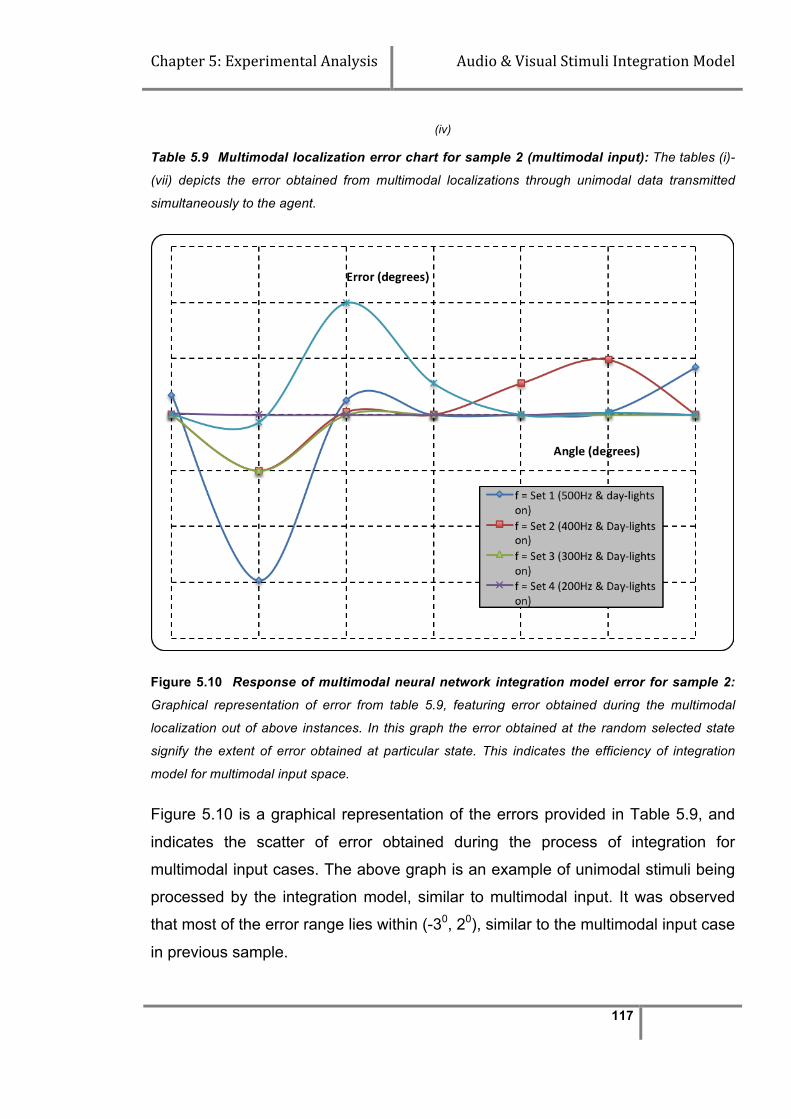
Chapter 5: Experimental Analysis Audio & Visual Stimuli Integration Model
117
(iv)
Table 5.9 Multimodal localization error chart for sample 2 (multimodal input): The tables (i)-
(vii) depicts the error obtained from multimodal localizations through unimodal data transmitted
simultaneously to the agent.
Figure 5.10 Response of multimodal neural network integration model error for sample 2:
Graphical representation of error from table 5.9, featuring error obtained during the multimodal
localization out of above instances. In this graph the error obtained at the random selected state
signify the extent of error obtained at particular state. This indicates the efficiency of integration
model for multimodal input space.
Figure 5.10 is a graphical representation of the errors provided in Table 5.9, and
indicates the scatter of error obtained during the process of integration for
multimodal input cases. The above graph is an example of unimodal stimuli being
processed by the integration model, similar to multimodal input. It was observed
that most of the error range lies within (-30, 20), similar to the multimodal input case
in previous sample.
Chapter 5: Experimental Analysis Audio & Visual Stimuli Integration Model
118
Finally, from the integration sample 1 and 2 it was observed that in both samples
the maximum error obtained was in the range of (-1.50, 1.50). Also the
concentration of the error was close to the x-axis. This signifies that the integration
model is effective with an error less than ±20 for both unimodal and multimodal
data samples.
In the next section, the neural network model was subjected to performance tests,
based on the output obtained using unimodal and multimodal data. Also, the
preliminary experimental analyses that were carried out in the previous chapter
are critically evaluated.
5.5 Unimodal Verses Multimodal Performance
From the unimodal experiments for localizing audio and visual stimuli, error levels
are obtained for respective cases. During unimodal stimuli analysis it was
observed that for auditory experimental data an overall accuracy of 80% is
achieved. Similarly, with visual stimuli an accuracy of 90% is achieved, including
the variance.
However, the integration model is expected to reach a higher level of accuracy
with audio and visual stimuli combined. During the multimodal experimental phase,
an estimate of ±50 of variance is considered. This is to comply with the motor
commands that are used to generate saccades. During the initial state, though
multimodal output is achieved, significant level of error is also generated as shown
in figure 5.11.
The data used in the generation of the unimodal verses multimodal performance
graph are as follows:
For Audio:
Set 1 = 100Hz, Set 2 = 200Hz, Set 3 = 300Hz, Set 4 = 400Hz, Set 5 = 500Hz
For Visual:

Chapter 5: Experimental Analysis Audio & Visual Stimuli Integration Model
119
Set 1 = Lights on (Day-Lab), Set 2 = Lights off (Day-Lab), Set 3 = Lights on (Night-
Lab), Set 4 = Lights off (Night-Lab), Set 5 = Lights off (Day-Studio)
For Multimodal:
Each set in the multimodal data is the combination of corresponding sets from
unimodal audio and visual data, to facilitate a more direct comparison.
Figure 5.11 Error performance chart between unimodal and multimodal integration: Error
graph of unimodal audio and visual data compared against multimodal integration error.
The graph represents mean error of unimodal audio and visual data over five
different set of inputs against multimodal output generated from the neural network
integration model. The selection of input sets is based on increasing order of
stimuli strength. From the graph it was evident that the error generated by the
multimodal data is significantly less than that of unimodal data. Also there was a
gradual decrease in the error, demonstrating the effectiveness of multimodal data.
The graph also indicates that multimodal output was more efficient than the
unimodal cases with respect to increase in stimuli strength.

Chapter 5: Experimental Analysis Audio & Visual Stimuli Integration Model
120
In another aspect, the error state observed in figure 5.11 among audio and visual
states are varied to greater extent. The audio data set error is significantly greater,
compared to visual data sets. This variation could be due to the wide locus (3600)
of audio sensors located at the agent. Due to which the range of stimuli received
and localized will entertain intermediate noise causing interference. On the other
hand due to narrow visual locus, the chances of interference are comparatively
less. But for multimodal case, the overall error is minimized due to the integration
aspect that reduces the individual effect, due to the learning aspect induced.
However, it was also observed that all the multimodal output is not completely
effective in terms of successful localization of stimuli source, due to the
enhancement and depression phenomena. This is demonstrated in the next
section.
5.6 Computational versus Neural Network Outcome
In this section, the output generated by both the computational and neural network
approaches is discussed. This analysis is carried out in two different ways. Initially,
two different samples of the same input are used to generate multimodal output.
Later a sample set for a fixed source location such as -300 (since variations were
observed at this location) was used to generate multimodal results.
In the first instance, a comparison is made between the multimodal outcome of the
computational model and the neural network model, described in the previous
sections. After careful observation of the output and error generated in the Chapter
4 and Chapter 5, the findings can be summarized as follows:
§ Output: For a given multimodal input, the output is generated for all cases,
irrespective of the strength of the stimuli. This is true of both the
computational and neural network models.

Chapter 5: Experimental Analysis Audio & Visual Stimuli Integration Model
121
§ Error: For a random selection of inputs, error states are also tabulated in
section. In the computational output Table 4.1, it is observed that a
maximum error of 230 is obtained from the input sample space, which is
high. Considering the degree of saccade freedom for object localization
(50), this error is considered too high. This influences the accuracy of the
model.
On the other hand, for neural network samples the maximum error obtained
is -2.960. This error is considerably lower when compared with the previous
case. Considering the degree of saccade freedom for object localization
(50), this error is not significant since the ANN integration model error is less
than the error degree of saccade freedom for human eye. The model is also
much more accurate.
§ Accuracy: This refers to the correctness of output generated for a given
multimodal input. In other words, when there is less than ±20 error obtained
from a multimodal output, then it is considered as accurate when compared
with computational model. In this context, using the computational model
there are few accurate cases. However, with the neural network model,
more than half than 75% of the sample set has generated accurate results.
§ Depression and Enhancement: From the sample space, stimuli exhibiting
depression and enhancement phenomena were now considered. With the
computational model, out of the accurate outcomes considered from this
case, the instances of exhibiting the enhancement phenomena are barely
noticeable (the highlighted rows of Table 4.1 and 5.10). This is because the
computational algorithm used for integration (weighted arithmetic mean)
signifies that the output always lies within the bounds of the given input as
discussed in section 4.4.1. However, the chances of depression occurring
are high. A case of depression is identified from the Table 4.1 row 25. Even
with the presence of maximum intensity levels for either of the stimuli, the

Chapter 5: Experimental Analysis Audio & Visual Stimuli Integration Model
122
output generated can also be inaccurate if the stimuli are on far apart from
one another. This signifies that the output is depressed.
Unlike the computational model, the neural network output has no
limitations on the output generated. Hence, the occurrence of enhancement
and depression phenomena is due to the stimuli strength. The sample
highlighted in red in table 5.17 indicates that the output of that particular
state is higher than either of the input stimuli and is correctly identifies the
source location. This signifies enhancement in the multimodal output.
However, this cannot be completely true, because enhancement and
depression phenomena can only be confirmed by measuring the intensity of
both input and output stimuli. Based on the increase and decrease of the
stimuli intensity, the phenomena can be classified, which is demonstrated in
the next chapter.
In another instance, from the available multimodal input space, a fixed set of data
was used and is subjected to integration using both the computational and neural
network model. Thus, the obtained output was compared, along with error,
accuracy, and enhancement and depression phenomena. Table 5.10 shows the
input and output for the multimodal test case.
Comparison Table of Multimodal Output Visual Stimuli
Visual Intensity
Audio Stimuli
Audio Intensity
Expected Output
Computational Output
Neural Network Output
-30.03 0.90 31.97 0.46 -30 -9.06 -30.00
-16.33 0.82 -19.34 0.44 -20 -17.38 -16.33 -9.45 0.32 10.05 0.41 -10 1.50 1.05 2.46 0.81 6.42 0.41 0 3.79 2.40
10.56 0.14 9.82 0.38 10 10.02 10.00 17.56 0.85 18.96 0.36 20 17.98 19.98 29.7 0.84 30.44 0.35 30 29.92 29.92
Table 5.10 Multimodal input & output table used for test case: The selected multimodal input
stimuli that are used as a unit-test set for verifying performance of the integration model. The
output obtained for both computational and neural network models are provided.

Chapter 5: Experimental Analysis Audio & Visual Stimuli Integration Model
123
The highlighted orange and blue instances in table 5.10 represent the depression
and enhancement in the output, respectively. The error obtained is shown in the
table 5.11.
Error Comparison Table of Multimodal Output
Computational Error
Neural Network Error
Computational Error (%)
Neural Network Error (%) Variation
-20.94 0.0 69.8% 0% 69.8
-2.62 3.67 13.1% 18.35% -5.34
11.5 11.05 >100% >100% --
3.79 2.40 37.9% 24% 13.9
0.02 0.0 2% 0% 2
2.02 0.02 10.1% 0.1% 10
0.08 0.08 0.2% 0.2% 0
Mean = 5.86 Mean = 2.46
Table 5.11 Error percentage comparison table of multimodal outputs for the test case: The
error percentage generated using the computational and neural network integration models is
detailed signifying the variation.
From the above test case based on the output exhibited in table 5.10 and 5.11 the
following observations were made.
§ Output: Output is generated irrespective of intensity of stimuli. This
signifies that the integration models are responsive to at least most of the
stimuli.
§ Error: From the output obtained from both cases, the error present in the
output is shown graphically in figure 5.11.

Chapter 5: Experimental Analysis Audio & Visual Stimuli Integration Model
124
Figure 5.12 Error comparison between neural and computational modal outputs for
selected input: Graph obtained from projecting the error obtained from integration output
of both computational and neural network models
In both cases, a significant error variation occurred at certain source
locations. However, the error with the computational model is particularly
pronounced at -300. On the other hand, many of the errors appear to be
close to x-axis.
§ Accuracy: Accuracy in this case was measured, taking into account the
degree of saccade freedom (±50) for object localization. From the selected
input category, the computational model has successfully achieved 50%
accuracy, while the neural network model has achieved 86% accuracy in
the generation of output. However, since performance cannot be measured
based on limited input space, in the next section a performance analysis is
carried out considering the entire stimuli space.
§ Depression and Enhancement: From the resultant output obtained, in
either of the cases the phenomena are observed. As discussed previously,
only depression in the output can be observed in the computational model.

Chapter 5: Experimental Analysis Audio & Visual Stimuli Integration Model
125
The highlighted instance in table 5.20 is an example of stimuli depression.
However, due to the huge variation in intensity, it can also be classed as an
error unless intensity values are examined. However the next highlighted
instance signifies a huge change in the output, irrespective of relative
similar intensities. This case is also identified in the neural network model.
This instance is a demonstration of depression phenomena.
In the neural network model output, the grey highlighted instance signifies
enhancement of the stimuli. The output generated is accurate and also
higher then either of the stimuli. This indicates the success of the model in
both training and accuracy. However, a later examination of intensity
determines the accuracy of the enhancement and depression phenomena.
5.7 Enhancement and Depression Phenomena Evaluation During the course of the research, variations while integrating audio and visual
stimuli were identified and classified accordingly. In this section, a discussion is
provided on the enhancement and depression phenomena and their behaviour
with respect to the stimuli intensities.
In Chapter 4, the integrated output provided demonstrates the circumstance that
lead to enhancement and depression phenomena. In particular, it was observed
that the enhancement of the output is obtained in the following case:
• Strong audio and strong visual stimulus (Figure 4.15)
Similarly depression of the output is obtained in the following case:
• Weak audio and weak visual stimulus (Figure 4.16 and 4.17)
In Chapter 5, experimental analysis provided by the integration sample 2
significantly demonstrates the increase in the output (accurate to the required
level) resulting from enhancement phenomena. In the output provided in table 5.9,

Chapter 5: Experimental Analysis Audio & Visual Stimuli Integration Model
126
in most of the cases an enhancement in the output stimuli is observed. However,
the highlighted region in the table shows more accurate output due to strong
enhancement.
In the computational and neural network model comparison provided in Chapter 5,
table 5.10 highlight the enhancement and depression phenomena observed in
both the cases. In this example, depression phenomena was demonstrated clearly
where the multimodal output was significantly less compared to either of the
inputs. However when it comes to accuracy, the above mentioned case was not
accurate because the model is expected to generate a null output. Hence the
integration model accuracy was reduced (by less than 20) in such instances.
In figure 5.12 the phenomena are demonstrated graphically.
Figure 5.13 Intensity graph between unimodal and multimodal output: Intensity graphs of
audio, visual and multimodal output demonstrating intensity verses output.
In terms of intensity, the graph has generated a mixed pattern for audio and visual
cases. In comparison with visual, audio has recorded significant intensity levels.
While the visual intensity is concerned it is considerably low. The amount of signal
that is taken into account for analyzing the visual stimuli is very sharp and small in
many cases (in order to capture the immediate change in visual environment). On

Chapter 5: Experimental Analysis Audio & Visual Stimuli Integration Model
127
the other hand, multimodal stimuli intensity contains priority-based factors of each
of the stimuli and their intensity levels along with localization.
With reference to figure 5.12, in sets 1 and 2, the multimodal intensity is greater
than either of the input intensities, signifying the stimuli are from the same
direction. However, for the next three sets, there is a gradual drop in the
multimodal intensity, even though high unimodal stimuli are recorded. This is due
to the stimuli sources being on either side of the reference frame. Set 5
demonstrates depression, where no significant multimodal output is obtained.
Finally, it is concluded that stimuli direction and intensity are the critical factors
responsible for the generation of enhancement and depression phenomena.
Though the integration output appears to be visually biased, it is actually intensity
biased. However, when it comes to action generation, such as saccade
generation, priority is given to visual stimuli.
5.8 Summary & Discussion
This chapter describes results that are generated from the audio and visual stimuli
integration models developed in chapter 4. In this chapter, both unimodal and
multimodal designs are tested using data collected during the initial phase of the
project development. This is followed by an analysis detailing the accuracy that
was achieved under different conditions, thus quantifying the performance.
Initially unimodal experimental analysis is carried out for both audio and visual
data sets. For audio localization, a series of input samples from five different
states are fed to the network. Each of these states is verified against the target
output and the amount of error generated by each stimulus is tabulated. Generally
it is observed that as the frequency of the stimuli increases, the accuracy of
localization increases. Similarly with the visual data, where samples of two states
(lights-on and lights-off) are provided, it is observed that a visual stimuli increase,
multimodal error gets reduced. However, it is observed that as noise in the form of

Chapter 5: Experimental Analysis Audio & Visual Stimuli Integration Model
128
other interfering light decreases, the localization improves. This is demonstrated
with the help of the above-mentioned sample states.
In the next section, multimodal data sets are analyzed in order to determine the
success of the neural network integration model. Based on two example instances
provided, which obtained from both the unimodal dataset and the multimodal
dataset, the output is analyzed for accuracy. Considering the error obtained in
both cases, the range lies between (-1.50, 1.50). This indicates the accuracy of the
neural network model in the successful generation of output for both unimodal and
multimodal input instances. However, in the next chapter accuracy is
demonstrated based on the entire input space to identify the performance of the
model.
There was a comparison between the computational model and the neural
network model output. Factors such as error, output, accuracy and enhancement
and depression phenomena were discussed. Finally it was shown that the neural
network model is successful in generating the maximum successful output with
greater accuracy and minimal error.

Chapter6: Conclusion Audio & Visual Stimuli Integration Model
129
Chapter 6
Conclusions and Recommendations
_________________________________________________________________
6.1. Introduction
This chapter provides an overall review of this research project. Conclusions
drawn from experimental analysis carried out in previous chapters are used to
summarize the research aspects such as research question, project objectives,
contribution followed by future recommendations.
This chapter is organized as follows. Section 6.2.1 describes the summary of the
project based on the research question. Section 6.2.2 describes the project
objectives and how they are achieved during the course of this thesis. Section
6.2.3 describes the contribution and how it is successfully acquired. Later, the
chapter is concluded by presenting possible recommendations for enhancing this
research into an application.
6.2. Conclusions
6.2.1. Summary of the Project
This section summarizes the main achievements of the research, in terms of the
research question and objectives.
The original research question can be re-stated as follows: Is it possible to create
a computational architecture inspired by the Superior Colliculus of the mid-brain,
using an artificial neural network, which enables the efficient integration of audio
and visual stimuli arriving simultaneously at an agent, in order to localize the
source of the stimuli? A series of experiments has successfully demonstrated that

Chapter6: Conclusion Audio & Visual Stimuli Integration Model
130
the architecture is effective in accurately localizing multimodal stimuli, including
those arriving simultaneously at the robot.
In order to achieve this, the research was carried out beyond the original research
question, in that the architecture has been shown to be effective at localizing a
wide range of input stimuli under different conditions. They include unimodal audio
or visual stimuli, with a range of frequencies and intensities. For both the unimodal
and the multimodal cases, it has been shown to outperform the purely
computational approach tested during the project for comparative purposes.
Along with the research question, the following objectives were defined against
which the success of the project can be quantified:
§ To understand the biological way of multimodal functionalities of the SC.
§ To review the literature on modelling the SC.
§ To review different approaches to audio and visual extraction and
integration.
§ To examine neural network approaches to integration.
§ To develop and design an architecture suitable for multimodal integration
for a robotic platform.
§ To test and evaluate the performance of the architecture.
During the course of the research, all objectives have been successfully achieved.
This is explored in detail in the following section.
6.2.2 Objectives Evaluation Objective:
§ To understand the biological way of multimodal functionalities of the SC.

Chapter6: Conclusion Audio & Visual Stimuli Integration Model
131
At the beginning of the research, motivated by biological considerations,
multisensory integration of audio and visual stimuli within the mammalian nervous
system and the brain were investigated within the context of the research
question. In particular, the region of the brain called the Superior Colliculus was
identified as being responsible for audio and visual stimuli integration. This was
explored in detail in order to develop critical and in-depth understanding of the
integration process. Chapter 2 of the thesis fulfils this objective. Three distinct
areas were investigated, namely biological motivation, neuroscience aspects of
the SC, and multimodal behaviour of the SC.
This work established the desirability of stimuli integration, along with the
advantages that can be achieved in the context of autonomous intelligent agents
that require a source localization capability. A link between the input stimuli and
the output motor command, in the form of saccades, was identified that justified
the motivation of studying the SC in this project. Neuroscience aspects of the SC
described the stimuli flow and structural architecture, which correspond to stimuli
transmission and saccade generation.
With regard to multimodal behaviour of the SC, stimuli processing in different
regions and the mechanism of integration are discussed. Also, the stimuli
combinations explored in this context had provided an insight into the motor
commands used for saccade generation. It also provided an understanding of the
motor output that is expected from the SC. In addition, stimuli integration was
classified and the phenomena of enhancement and depression identified.
Objectives:
§ To review the literature on modelling the SC.
§ To review different approaches to audio and visual extraction and
integration.
§ To examine neural network approaches to integration.

Chapter6: Conclusion Audio & Visual Stimuli Integration Model
132
The following outcomes were also achieved based upon the literature review:
• A literature review on modelling the multisensory integration based on the
SC in the second part of Chapter 2 describes the attempts made in this
context. This review helps in identifying the integration process with respect
to the required criterion, which is integration for low intensity stimuli.
• In Chapter 2 various approaches that correspond to integration of audio and
visual stimuli are reviewed. This review helps in narrowing the approach
that is used for the development of the integration model.
• In literature review section of Chapter 2, various computational,
probabilistic, neural and applicative approaches are studied to develop a
feasible and suitable integration model that can answer the research
question. In Chapter 3 a methodology is developed based on the review
that can perform audio and visual stimuli integration.
Objectives:
§ To develop and design an architecture suitable for multimodal integration
for a robotic platform.
§ To test and evaluate the performance of the architecture.
The project outcomes that are delivered after the successful development of the
integration model are:
• Chapters 3 and 4 describe the design and development of both unimodal
and multimodal integration models. During this process, based on the
findings of the review chapter, the integration process is designed as a
computational model and later developed into a neural network for
improved performance. The neural network is trained on a large stimuli
space, such that the integration model can be optimized and made more
effective with respect to the generation of output i.e., saccade generation.
• Evaluation is critical for the success of any model. However, in this project,
a self evaluation criterion was adopted. This criterion evaluates the
integration model in two phases. Initially, it is tested with unimodal data and

Chapter6: Conclusion Audio & Visual Stimuli Integration Model
133
multimodal data and the output is evaluated. Secondly, it is compared to the
computational model using multimodal data. The experimental findings
published in Chapters 4 and 5 explicitly signify the success of the
integration model in the respective states and confirm the success of the
architecture as a multimodal integration model.
6.2.3. Summary of Contribution
The main novelty is the architecture and its ability to handle low intensity audio
and visual stimuli and generate efficient and accurate integrated output. During the
process, the model also contributes to research into successful reduction of audio
and visual dimensional space into an integrated single space.
• The Superior Colliculus inspired dual layered architecture has been
developed, where each layer has preprocessed localization data that
arrives from corresponding layers to the integration layer simultaneously.
This architecture is implemented using a RBF based neural network
platform. The model is trained to integrate audio and visual stimuli and
generate an integrated output based on the intensity levels of the stimuli.
The integration model experimental outcome described in Chapter 4
signifies the success of the proposed architecture. Similarly, the
experimental analysis provided in Chapter 5 has demonstrated the
performance of the integration model with respect to variable stimuli
intensity. This signifies that the novelty of the architecture for successful
adaptation towards low-level stimuli is achieved.
• This research is an attempt to investigate multimodal stimuli integration
behaviour. During the process, apart from achieving the project objectives,
the research has successfully integrated audio and visual stimuli into a
single command that is used to generate saccades. On the other hand, this
research can also be referred as solution for a dimensionality reduction
problem in multimodal context. Transformation of two-dimensional stimuli
into a single dimension control signal is accurately achieved using the
neural network training process. Therefore this research has contributed to

Chapter6: Conclusion Audio & Visual Stimuli Integration Model
134
the successful reduction of audio and visual dimensional space into an
integrated single space.
6.3. Recommendations for future work
There are a number of recommendations made as a follow-up to this research.
Possible directions are given below:
§ It would be useful to extend the scope of the integrated output. This project
is intended for generation of horizontal saccade only. However, the
introduction of a vertical dimension (level difference) would help in the
simultaneous detection of more than one stimulus out of the horizontal
plane. This could be used to localize in a two dimensional space. However,
the addition of a vertical direction would add complexity and would require
different hardware and software solutions. For example audio localization
with the current set up only configured in one dimension.
§ Another extension of the project could be in the variation of distance
between the source and agent. Initially this aspect is overcome by the
approximation function used for localization. This function is estimated
based on the distance as a variable. However, for future enhancement the
function can be extended to operate for any kind of distances. But for such
cases, a different kind of experimental setup has to be designed to satisfy
the variable distance between source and agent mechanism.
§ An important enhancement would be to extend the scope of the integration
mechanism by adapting it to all types of input stimuli. One major objective
of the project is to investigate the behaviour of the integration stimuli i.e.
enhancement and depression phenomena. However, when it comes to a
more realistic application:

Chapter6: Conclusion Audio & Visual Stimuli Integration Model
135
• Visual stimuli localization becomes more complex, if object
identification along with color detection is used, then the chances of
recognizing the object increases.
• In the case of audio, rather than simple activation detection, if the
sound is distinguished based on strength of the stimuli, along with
their time of arrival, then the chances of a more significant audio role
in the integration process can be increased. This would improve the
overall localization performance.
• The above suggestions can be adapted either before or after
integration, depending on the requirements. However if they are
adapted before integration, there could be an increase in the time
delay between stimuli generation and integration. Hence post-
integration is suggested. By doing so, the final integrated output
generated can be recognized and the corresponding action can be
taken.
§ A practical recommendation could be to transform the model into an
application that can be used to alert the driver of a vehicle to approaching
traffic. When it comes to development of a commercial application such as
a driver assistance system, it is necessary that it should be both adaptive
as well as effective. For such applications it is critical to have highest
possible accuracy. Since the application involves risk to the user, it is
suggested that training of the network should be made more efficient by
using a bigger training set.
§ Another potential application is a self-driven camera (equipped with a mic)
that can be used to localize any stimuli within its focus, and later can track
the stimuli in the case of a moving source. This concept could also be used
in social robot scenario, where a robot interacts with people in public in
places such as museums, and hospitals and schools.

Chapter6: Conclusion Audio & Visual Stimuli Integration Model
136
Overall, this research project is considered a success in answering the research
question and the objectives have been achieved. The research is still in its
development state, as far as a reliable application in a real scenario is concerned.
However, many of the ideas explored can provide a firm foundation for ongoing
and future research in this area.

Reference Audio & Visual Stimuli Integration Model
137
References
A
Anastasio, T. J., Patton, P. E., Belkacem-Baussaid, K. (2000) “Using Bayes’
Rule to Model Multisensory Enhancement in the Superior Colliculus”.
Neural Computation, 12, pp. 1165 – 1187.
Armingol, J. M., Escalera, A., Hilario, C., Collado, J. M., Carrasco, J. P., Flores, M. J., Postor, J. M. and Rodriguez, F. J. (2007) “IVVI: Intelligent
vehicle based on visual information”. Robotics and Autonomous Systems,
55, pp. 904 – 916.
Asif Ullah Khan., Bandopadhyaya T, K., and Sharma, S. (2009) “Classification
of Stocks Using Self Organization Map”. International Journal of Soft
Computing Applications, 4, ISSN: 1453-2277, pp. 19 – 24.
B
Beauchamp, M. S., Lee, K. E., Argall, B. D. and Martin, A. (2004) “Integration of
Auditory and Visual Information about Objects in Superior Temporal
Sulcus”. Neuron (Cell Press), 41, pp. 809 – 823.
Bellman, R. E. and Rand Corporation. (1957) “Dynamic Programming”.
Princeton University Press. ISBN: 069107951X.
Bennewitz, M., Faber, F., Joho, D., Schreiber, M. and Behnke, S. (2005) “Integrating Vision and Speech for Conversations with Multiple Persons”.
Proceedings of International Conference on Intelligent Robots and System
(IROS).
Benediktsson, J. A., Swain, P. H. and Ersoy, O. K. (1990) “Neural Network
Approaches Versus Statistical Methods in Classification of Multisource

Reference Audio & Visual Stimuli Integration Model
138
Remote Sensing Data”. IEEE Transactions on Geoscience and Remote
Sensing, 28(4), pp. 540 – 552.
Bors, A. G. (2001) “Introduction to the Radial Basis Function (RBF) Networks”.
Online Symposium for Electronics Engineers, DSP Algorithms: Multimedia,
1(1), pp. 1-7.
Bors, A. G. and Pitas I. (1996) “Median radial basis functions neural network”.
IEEE transactions on Neural Networks, 7(6), pp. 1351 – 1364.
Broomhead, D.S. and Lowe D. (1988) “Multivariable functional interpolation and
adaptive networks”. Complex Systems, 2, pp. 321 – 355.
C
Calvert, G. A. and Thesen, T. (2004) “Multisensory integration: methodological
approaches and emerging principles in the human brain”. Journal of
Physiology Paris, 98, Pp. 191 – 205.
Casey, M. C., and Pavlou, A. (2008) “A Behavioural Model of Sensory Alignment
in the Superficial and Deep Layers of the Superior Colliculus”. Proceeding
of International Joint Conference on Neural Networks (IJCNN’08), pp. 2750
– 2755.
Casey, M. C. (2009) “Modelling the Sensory Hierarchy: From Gaze Shifts to
Emotions”. Artificial Intelligence and Natural Computation Seminars,
Birmingham.
Chan, V. (2009) “Audio-visual sensor fusion for object localization”. Institute of
Neuromorphic Engineer, Article in ine-web, Doi:10.2417/1200906.1640.
(Cited on 24/08/2010).
Cheshire Engineering Corporation. (2003) “Neural Network Technology”.
Neuralyst, User’s guide, Chapter-3.

Reference Audio & Visual Stimuli Integration Model
139
Chinmaya Mission. (1983) “Symbolism in Hinduism” Chinmaya Mission
Publications, Mumbai, INDIA, ISBN: 9788175971493. Pages 338 and 339.
Coen, M. H. (2001) “Multimodal Integration – A Biological View”. Proceedings of
the 15th International Joint Conference on Artificial Intelligence (IJCAI’01),
pp. 1414 – 1424.
Cucchiara, R. (2005), “Multimedia Surveillance Systems”. 3rd International
Workshop on Video Surveillance and Sensor Networks (VSSN’05),
Singapore, pp. 3 – 10, ISBN: 1-59593-242-92.
Cuppini, C., Magosso, E., Serino A., Pellegrino, G. D. and Ursino, M. (2007) “A Neural Network for the Analysis of Multisensory Integration in the
Superior Colliculus”. Proceedings of Artificial Neural Networks - ICANN
2007, Part 11, 4669, pp. 9 – 11.
Cutsuridis, V., Smyrnis, N., Evdokimidis, I. and Perantonis, S. (2007) “A
Neural Model of Ddecision-making by the Superior Colliculus in an Anti-
saccade task”. Neural Networks, 20, pp.690 – 704.
E
Elhilali, M. and Shamma, S. (2006) “A biologically-Inspired Approach to the
Cocktail Party Problem”. IEEE International Conference on Acoustics,
Speech and Signal Processing, 5, pp. 637 – 640.
F
Funk, N. (2003) “A Study of the Kalman Filter applied to Visual Tracking”.
Edmonton, 7 December.
G

Reference Audio & Visual Stimuli Integration Model
140
Gilbert, C. and Kuenen, L. P. S. (2008) “Multimodal Integration: Visual Cues
Help Odour-Seeking Fruit Flies”. Current Biology, 18, pp. 295 – 297.
H
Hanheide, M., Bauckhage, C. and Sagerer, G. (2005) “Combining
Environmental Cues & Head Gestures to Interact with Wearable Devices“.
Proceedings of 7th International Conference on Multimodal Interfaces, pp.
25 – 31.
Harremoes, P. (2010) “Information Theory for angular data”. IEEE Information
Theory Workshop, ITW2010, pp. 1 – 5.
Hawkins, H. L., McMullen, T. A., Popper, A. N. and Fay, R. R. (1996) “Auditory
Computation”. Springer Handbook of Auditory Research, pp. 334 – 336.
Holmes, N. P. (2009) “The Principle of Inverse Effectiveness in Multisensory
Integration: Some Statistical Considerations”. Brain Topography, 21(3 – 4),
pp. 168 – 176.
Huwel, S., Wrede, B. and Sagerer, G. (2006) “Robust Speech Understanding for
Multi-Modal Human-Robot Communication”. 15th IEEE International
Symposium on Robot and Human Interactive Communication (RO-MAN 06),
UK, pp. 45 – 50.
J
Jolly, K.G., Ravindran, K.P., Vijayakumar, R. and Sreerama, R. K. (2006) “Intelligent decision making in multi-agent robot soccer system through
compounded artificial neural networks”. Robotics and Autonomous Systems,
55, pp. 589 – 596.

Reference Audio & Visual Stimuli Integration Model
141
Juan, C.H,, Muggleton, N.G., Tzeng, O.J.L., Hung, D.L., Cowey, A. and Walsh, V. (2008) “Segregation of CIsual Selection and Saccades in Human”.
Cerebral Cortex, 18(10), pp. 2410 – 2415.
K
King, A.J. (2004). “The Superior Colliculus”. Current Biology, 14(9), pp. R335 –
R338.
Kohonen, T. (1982) “Self-Organized formation of Topographical correct feature
Maps”. Biological Cybernetics, 43, pp. 59 – 69.
Koide, Y., Kanda. T., Sumi, Y., Kogure, K. and Ishiguro, H. (2004) “An
approach to Integrating an interactive guide robot with ubiquitous sensors”.
Intelligent Robots and System, IROS’04 Proceedings, 3, pp. 2500 – 2505.
Kyriakos, V. and Jurgen, A. (2007), “A Biologically inspired spiking neural
network for sound source lateralization”. IEEE transactions on Neural
Networks, 18(6), pp. 1785 – 1799.
L
Landis, M. F., Crassidis, J. L. and Cheng, Y. (2005) “Nonlinear Attitude Filtering
Methods”. Systems Engineering, Publisher: Citeseer, 30(August), pp. 12 –
28.
Londhe, S. (2008) “Symbolism in Hinduism”. A Tribute to Hinduism, Pragun
Publications, INDIA, ISBN: 8189920669.
M

Reference Audio & Visual Stimuli Integration Model
142
Massaro, D. W. (2004) “A Framework for Evaluating Multimodal integration by
Humans and A Role for Embodied Conversational Agents”. In Proceedings
of the 6th International Conference on Mulitmodal Interfaces (ICMI’04), pp.
24 – 31.
McAlpine, D. and Grothe, B. (2003) “Sound localization and delay lines – do
mammals fit the model?”. Trends in Neuroscience, 26(7), pp. 347 – 350.
Meredith, M. A. and Stein, B. E. (1986a) “Visual, auditory and somatosensory
convergence on cells in superior colliculus results in multisensory
integration”. J. Neurophysiol. 56, pp. 640 – 662.
MobileRobots Inc. (2006) “Performance PeopleBot Operations Manual”.
MobileRobots Exclusive Advanced Robot Control & Operations Software,
Version 3.
Moody J. (1989) “Fast learning in networks of locally-tuned processing units”.
Neural Computation, 1, pp. 281 – 294.
Murray, J., Erwin, H., Wermter, S. (2005) “A Hybrid Architecture using Cross-
Correlation and Recurrent Neural Networks for Acoustic Tracking in
Robots”. Biomimetic Neural Learning for Intelligent Robots, pp. 55-73.
P
Palanivel, S. and Yegnanarayana, B. (2008) “Multimodal person authentication
using speech, face and visual speech”. Computer Vision and Image
Understanding (IEEE), 109, pp. 44-55.
Paleari, M. and Lisetti, C. L. (2006) “Toward Multimodal Fusion of Affective
Cues”. Proceedings of International Conference on Human Computer
Multimodality HCM’06, pp. 99 – 108.
Pang, K. (2003) “Self Organizing Maps”. Neural Networks, [Online] (Cited:
21/10/2011).

Reference Audio & Visual Stimuli Integration Model
143
Park, F. C. and Bahram, R. (1997) “Smooth Invariant Interpolation of Rotations”.
ACM Transactions on Graphics, 16(3), pp. 277 – 295.
Pavon, J., Gomez-Sanz, J., Fernandez-Caballero, A. and Valencia-Jimenez, J. J. (2007) “Development of intelligent multisensor surveillance systems with
agents”. Robotics and Autonomous Systems, 55, Pp. 892 – 903.
Powell, M. J. D. (1987) “Radial basis functions for multivariable interpolation: a
review”. Algorithms for approximation, Clarendon Press, New York, ISBN:
0-19-853612-7.
Q
Quaia, C., Lefevre, P. and Optican, L. M. (1999) “Model of the Control of
Saccades by Superior Colliculus and Cerebellum”. Journal of
Neurophysiology, 82(2), pp. 999 – 1018.
S
Schauer, C. and Gross, H. M. (2004) “Design and Optimization of Amari Neural
Fields for Early Auditory – Visual Integration“. Proc. Int. Joint Conference
on Neural Networks (IJCNN), Budapest, pp.2523 – 2528.
Smith, L. (2003) “An Introduction to Neural Networks”. Centre for Cognitive and
Computational Neursocience, University of Stirling, (Cited: 20/10/2011).
Srinivas, C. (1993) “Visual disorders in ancient Indian science (interpretative
study)”. Bull Indian Inst Hist Med Hyderabad, 23(2), pp. 101-111.
Stanford, T. R., Stein, B. E. and Quessy, S. (2005) “Evaluating the Operations
Underlying Multisensory Integration in the Cat Superior Colliculus”. The
Journal of Neuroscience, 25(28), pp. 6499 – 6508.

Reference Audio & Visual Stimuli Integration Model
144
Stein, B. E., Huneycutt, W. S. and Meredith, M. A. (1988) “Neurons and
behaviour: the same rules of multisensory integration apply”, Brain
Research, 488, pp. 355 – 358.
Stein, B. E., Meredith, M. A., Huneycutt, W. S. and McDade, L. (1989) “Behavioral indices of multisensory integration: orientation to visual cues is
affected by auditory stimuli”, Cognitive Neuroscience, 1, pp. 12 – 24.
Stein, B. E. and Meredith, M. A. (1993) “The Merging of the Senses”, Cognitive
Neuroscience Series. MIT Press, Cambridge.
Stergiou, C. and Siganos, D. (2007) “Neural Networks”. A report on introduction
to Artificial Neural Networks. Vol. 4 [Online]. (Cited: 10 August 2010).
Stiefelhagen, R. (2002) “Tracking focus of attention in meetings”, International
conference on Multimodal Interfaces (IEEE), Pittsburgh, PA. pp. 273 – 280.
Stork, D. G., Wolff, G. and Levine, E. (1992) “Neural Network lip reading system
for improved speech recognition”. Proceedings of International Joint
Conference on Neural Networks (IJCNN’92), 2, pp. 289 – 295.
T
Trappenberg, T. (1998) “A Model of the Superior Colliculus with Competing and
Spiking Neurons”. BSIS Technical Report, No. 98-3.
Trifa, V. M., Koene, A., Moren, J. and Cheng, G. (2007) “Real-time acoustic
source localization in noisy environments for human-robot multimodal
interaction”. Proceedings of RO-MAN 2007 (IEEE International Symposium
on Robot & Human Interactive Communication), Korea, pp. 393 – 398.
W

Reference Audio & Visual Stimuli Integration Model
145
Waxman, S. G. (2009) Clinical Neuroanatomy 26th Edition. McGraw-Hill Medical
Publisher, ISBN: 00771603999.
Wilhelm, T., Bohme, H. J. And Gross, H. M. (2004) “A multi-modal system for
tracking and analyzing faces on a mobile robot”. Robotics and Autonomous
Systems, 48(1), pp. 31 – 40.
Wolf, J. C. and Bugmann, G. (2006) “Linking Speech and Gesture in Multimodal
Instruction Systems”. The 15th IEEE International Symposium on Robot and
Human Interactive Communication (RO-MAN 06), UK.
X
Xiuju Fu and Lipo Wang. (2003) “Data Dimensionality Reduction With
Application to Simplifying RBF Neural Structure and Improving
Classification Performance”, IEEE Transactions on Systems, Man and
Cybernetics – Part B: Cybernetics, 33(3), pp. 399 – 409.
Y
Yavuz, H. (2007) “An integrated approach to the conceptual design and
development of an intelligent autonomous mobile robot”. Robotics and
Autonomous Systems, 55, pp. 498 – 512.
Z
Zou, X. and Bhanu, B. (2005) “Tracking humans using Multi-modal Fusion”. IEEE
Conference on Computer Vision and Pattern Recognition (CVPR‘05), pp. 4
– 4.

A-‐1
Appendix – A
Importance of audio and visual sensors for interaction
Sensory organs in human beings play a vital role when it comes to interaction. Out
of them, eyes and ears responsible for audio and visual stimuli processing are
considered critical for this research. In the context of vision a Sanskrit (ancient
Indian language) saying goes like “*Sarvendriyanam Nayanam Pradhanam”.
According to Ayurveda (ancient Indian medical practice) ‘the eyes are the first
among different organs of the body when it comes to interacting with the external
world’ (Srinivas, 1993). In the context of eternal sound which describes the
importance of audio stimuli over living beings a Sanskrit saying goes as
“*Sisurvethi Pasurvethi…Vethi gaana rasam Phanihi”. Means music (sound) can
be felt and enjoyed by kids, animals and even snakes alike. In other words, an
audible sound stimulus was always felt effective in grabbing attention when it
comes to interaction with kids, animals (mammals) and even animals without ears.
According to Sanskrit the mystic sound of ‘AUM’ was the first generated audio
stimuli that echoed the universe in the form of primal energy, which later
developed various sounds. (Londhe, 2008) In the book of Symbolism in Hinduism
by Chinmaya Mission, page 338 and 339 describes in details about the importance
of audio stimuli in both music and life when it comes to interaction (Chinmaya
Mission, 1983).
This thesis is the advanced research work carried out to investigate the sound and
visual stimuli and their integration based on biological inspiration of the Superior
Colliculus and to develop a model that can perform integration mechanism
effectively.
‘*’--- are the English version of Sanskrit quotes that are explained with the literal and ethical meaning in a philosophical way which signifies the importance of visual and audio sensors for interaction with environment.

B
Appendix – B
List of Publications
Three papers have been published for presenting the initial experimental results
and the research concepts developed during the project.
Ravulakollu, K., Knowles, M., Liu, J. and Wermter, S. (2009) “Towards
Computational Modelling of Neural Multimodal Integration Based on the
Superior Colliculus Concept”. Innovations in Neural Information Paradigms
and Applications, Pp. 269~291, ISBN: 978-3-642-04002-3.
Ravulakollu, K., Erwin, H. and Burn, K. (2011) “Improving Robot-Human
Communication by Integrating Visual Attention and Auditory Localization
Using a Biologically Inspired Model of Superior Colliculus”. Journal of
Advanced Material Research, 403 – 408, Pp. 4711 – 4717.
Ravulakollu, K., Liu, J. and Burn, K. (2012) “Stimuli Localization: An Integration
Methodology Inspired by the Superior Colliculus for Audio and Visual
Attention”. Journal of Procedia Computer Science, 13, Pp. 31 – 42.

Appendix -‐ B Publication: Book Chapter with Springer-‐Verlag
B-‐1
Towards Computational Modelling of Neural Multimodal Integration based on the Superior Colliculus Concept
Kiran Ravulakollu, Michael Knowles, Jindong Liu and Stefan Wermter University of Sunderland
Centre for Hybrid Intelligent Systems Department of Computing, FAS
St Peters Way, Sunderland, SR6 0DD, UK www.his.sunderland.ac.uk
Abstract Information processing and responding to sensory input with appropriate actions are among the most important capabilities of the brain and the brain has specific areas that deal with auditory or visual processing. The auditory information is sent first to the cochlea, then to the inferior colliculus area and then later to the auditory cortex where it is further processed so that then eyes, head or both can be turned towards an object or location in response. The visual information is processed in the retina, various subsequent nuclei and then the visual cortex before again actions can be performed. However, how is this information integrated and what is the effect of auditory and visual stimuli arriving at the same time or at different times? Which information is processed when and what are the responses for multimodal stimuli? Multimodal integration is first performed in the Superior Colliculus, located in a subcortical part of the midbrain. In this chapter we will focus on this first level of multimodal integration, outline various approaches of modelling the superior colliculus, and suggest a model of multimodal integration of visual and auditory information. 1. Introduction and Motivation The Superior Colliculus (SC) is a small part of the human brain that is responsible for the multimodal integration of sensory information. In the deep layers of the SC integration takes place among auditory, visual and somatosensory stimuli. Very few types of neurons, such as burst, build up and fixation neurons are responsible for this behaviour [4, 10]. By studying these neurons and their firing rates, integration can be successfully explored. The integration that takes place in the SC is an important phenomenon to study because it deals with different strengths of different stimuli arriving at different times and how the actions based on them are generated. There is evidence that when two different stimuli are received at the same time, the stronger signal influences the response accordingly based on Enhancement and Depression Criteria [3]. A better understanding of multimodal integration in the SC not only helps in exploring the properties of the brain, but also provides indications for building novel bio-inspired computational or robotics models. Multimodal integration allows humans and animals to perform under difficult, potentially noisy auditory or visual stimulus conditions. In the human brain, the Superior Colliculus is the first region that provides this multimodal integration [23]. The deep layers of the Superior Colliculus integrate multisensory inputs and generate directional information that can be used to identify the source of the input information [20]. The SC uses visual and auditory information for directing the eyes using saccades, that is horizontal eye movements which direct the eyes to the location of the object which generated the stimulus. Before integrating the different modalities the individual stimuli are preprocessed in separate auditory and visual pathways. Preprocessed visual and auditory stimuli can then be used to integrate the stimuli in the deep layers of the SC and eventually generate responses based on the multimodal input. The types of saccades can be classified in different ways [39] as shown in Figure 1. Most saccades are reflexive and try to identify the point of interest in the visual field which has moved due to the previous visual frame changing to the current one [20]. If no point of interest is found in the visual field, auditory information can be used to identify a source. Saccades are primary actions which in some cases are autonomous and are carried out without conscious processing in the brain. When there is insufficient information to determine the source based on a single modality, the SC uses multimodal integration to determine the output. Saccades are the first actions taken as a result of receiving enough visual and auditory stimuli.