Ratcheted molecular-dynamics simulations identify efficiently the transition state of

protein folding

Guido Tiana1, a) and Carlo Camilloni2, b)

1)Department of Physics, University of Milano, and INFN, via Celoria 16,

20133 Milan, Italy

2)Department of Chemistry, University of Cambridge, Lensfield Road, Cambridge,

CB2 1EW, United Kingdom

(Dated: 6 July 2012)

The atomistic characterization of the transition state is a fundamental step to im-

prove the understanding of the folding mechanism and the function of proteins. From

a computational point of view, the identification of the conformations that build out

the transition state is particularly cumbersome, mainly because of the large compu-

tational cost of generating a statistically–sound set of folding trajectories. Here we

show that a biasing algorithm, based on the physics of the ratchet–and–pawl, can be

used to identify efficiently the transition state. The basic idea is that the algorith-

mic ratchet exerts a force on the protein when it is climbing the free–energy barrier,

while it is inactive when it is descending. The transition state can be identified as

the point of the trajectory where the ratchet changes regime. Besides discussing this

strategy in general terms, we test it within a protein model whose transition state

can be studied independently by plain molecular dynamics simulations. Finally, we

show its power in explicit–solvent simulations, obtaining and characterizing a set of

transition–state conformations for ACBP and CI2.

Keywords: biased molecular dynamics, transition state, protein folding simulations

a)Electronic mail: tiana@mi.infn.itb)Electronic mail: cc536@cam.ac.uk

1

arX

iv:1

207.

1288

v1 [

q-bi

o.B

M]

5 J

ul 2

012

I. INTRODUCTION

The transition state of biomolecular processes is particularly important because is the

main determinant of the associated rate. Unfortunately, being the most unstable state of

the process, its characterization is difficult. In the case of protein folding, a perturbative

technique where one measures the effect of amino-acid mutations on folding/unfolding rates,

has been successful in providing a structural characterization of this evanescent state1. Al-

though this procedure is experimentally rather demanding, we have now information about

the structure of the transition state of tens of proteins.

With the improvement of the force fields2,3 that describes the interaction in proteins, it

becomes more and more interesting the attempt to characterize the folding transition state

without employing experimental information4–7. Within this context, the determination

of the transition state implies two challenging problems, namely the generation of folding

trajectories and the identification of the transition state along each of them. Concerning

the former, the most straightforward way is simply to perform molecular–dynamics (MD)

simulations solving the equation of motion of the system. In the case of proteins of realistic

size and using realistic force fields in explicit solvent, generating a statistically–sound number

of folding trajectories is not trivial even if one can use the fastest computers available8,9.

Smarter techniques, comprising transition path sampling10, milestoning11 and dominant

reaction pathways12,13, exploit the fact that only a small subset of all possible trajectories

is statistically relevant, but these methods are computationally efficient when the total

number of atoms is not large (typically in implicit–solvent models). Even if one can generate

efficiently folding trajectories, the problem of identifying the transition state is still hard.

The transition state between two (meta)stable states is built out of the set of conformations

for which the probability of falling down to each of them is 1/2. Consequently, the most

direct way to identify the transition state is to start several MD simulations from each

of the conformations selected from a folding trajectory, and to count the fraction of such

trajectories which meet the native state before meeting the denatured state (or vice versa),

until this fraction is exactly 1/214. This procedure is very time consuming, but is the only

safe way to identify the transition state15.

Some years ago, Marchi and Ballone introduced the idea of biasing MD simulations to

generate efficiently trajectories between conformations of a system, using an algorithm based

2

of the physics of the ratchet–and–pawl16. It consists in defining a ratcheting coordinate y and

dumping the thermal fluctuations along the direction of y opposite to the wished target. The

algorithm was later used to enhance the thermal unfolding of proteins interacting with an

implicit-solvent force field17,18. Recently, ratcheted MD simulations were used to repeatedly

simulate the folding of single–domain proteins in explicit solvent19. Using a simplified protein

model, a Beccara et al.20 employed a Onsager–Machlup functional and showed that the

ratcheted MD algorithm produces trajectories that are overall statistically relevant, thus

validating the approach of ref.19.

In what follows, we will investigate whether it is possible to use ratcheted MD simulations

to obtain directly and efficiently a good approximation of the conformations which build out

the transition state of protein folding. The basic idea is that while climbing the main free–

energy barrier which separates the denatured from the folded state, the ratchet exerts work,

while descending on the other side it is essentially off. The transition between the two

regimes marks the transition state.

Although the whole goal of this work is to develop a method that can be used for realistic

systems in explicit solvent, we first validate it using a model whose folding trajectories can

be generated by plain MD and whose transition state can be obtained exactly using the

committors method of ref.14.

II. THE MODEL AND THE SIMULATIONS

A model which is suitable for developing a computational strategy and validating it

against transition state obtained with the exact method is a modified all–atom Go model,

where a non–specific interaction between hydrophobic atoms is added on the top of the

native–structure. The Go model assures that folding can be simulated repeatedly also with-

out the ratcheting algorithm, in order to be able to obtain reference trajectories, while the

hydrophobic interaction makes the energy landscape more roughed, and thus more realistic.

The Go implementation is that of ref.21, in which pairs of atoms building native contacts

interact with a Lennard–Jones potential whose minimum lies at ε0 = −0.62 (in arbitrary

units). The hydrophobic potential has also the Lennard–Jones form and acts between side

chain carbons of ALA, VAL, LEU, ILE, PHE and TRP. The minimum of the potential lies

at a distance of 0.35 nm, where the depth is εhy = −0.3. This value of εhy has been chosen

3

because it is the lowest which guarantees the folding of the proteins studied within an RMSD

of 0.3 nm from the experimental native conformation.

The simulations were carried out with a modified22,23 version of Gromacs24, using the

topologies generated with the SMOG web server25. The time step used is 0.002 ps (time

units are merely nominal).

The specific heat, calculated with parallel–tempering simulations26, is displayed in Fig.

1 and compared with that for a plain Go model. As expected, the two–states character of

the denaturation transition diminished. However, the stability of the native state increased,

suggesting that the hydrophobic interaction introduced in the model favors the native con-

formation, where hydrophobic packing is optimized, more than the denatured state. On the

basis of this specific–heat plot, we used the trajectory obtained at T = 1 to generate 10 un-

correlated unfolded conformations to be used as initial states of the folding simulations. The

folding simulations were carried out at T = 0.91, which is regarded as room temperature.

From each of the 10 unfolded conformations we carried out 10 simulations at T = 0.91

for 6 ns each. The average folding time, defined as the time needed to reach a RMSD of 0.4

nm, is τf = 1505 ps.

Similar simulations were carried out using the ratcheting algorithm. The ratchet is im-

plemented as in ref.19, that is adding to the molecular potential a ratcheting term

Vrat(ρ(t)) =

k2

(ρ(t)− ρm(t))2 , ρ(t) > ρm(t)

0, ρ(t) ≤ ρm(t),(1)

where

ρ(t) = (y(t)− ytarget)2 (2)

and

ρm(t) = min0≤τ≤t

ρ(τ). (3)

The ratcheting coordinates y(t) used in the present work are either the distance dCM of the

contact map of a given protein conformation from the native contact map, or the RMSD (in

both cases ytarget = 0). The distance dCM , introduced by Bonomi et al.27, is defined as

dCM = ‖C − C‖ =

(N∑

j>i+2

(Cij − Cij)2

)1/2

, (4)

4

were Cij is the i,j element of a NxN matrix defined as

Cij(rij) =

1−

(rijr0

)p1−

(rijr0

)q , rij ≤ rcut

0, rij > rcut,

(5)

rij is the distance between atom i and j and C is the defined on the native state. The

parameters used in these simulations are p = 6, q = 10, r0 = 0.75 nm and rcut = 1.23 nm.

Both in the case of plain–MD and ratcheted simulations, the sequence of events along

the folding trajectories under each set of conditions were studied calculating the matrix

Mij = θ (t(i, k)− t(j, k)), where t(i, k) is the time at which the ith contact is stably formed in

the kth simulation and θ is the Heaviside’s step function. This matrix satisfies Mij+Mji = 1

and each element Mij assumes the value 1 if the formation of the ith contact precedes the

formation of the jth, 0 if it follows it, and 1/2 if the two are uncorrelated. The average

matrix

Mij =1

ns

ns∑k=1

Mij, (6)

where ns = 100 is the number of trajectories, is interpreted as the probability that the

formation of the ith contact precedes the formation of the jth. A quantity related to Mij

is the probability Aj =∑

i 6=jMij/(ns − 1) that the jth contact is formed after any other

contact.

The order of contact formation in two trajectories was compared using the distance

d(M,M ′) ≡ 1

n2s

∑ij

[1− δ(Mij,M′ij)], (7)

between the associated matrices, where δ is the Kronecker symbol.

III. RATCHETED TRAJECTORIES

A necessary condition for the ratcheting algorithm to identify the correct transition state

of folding is to generate statistically–relevant trajectories. Failure of this condition would

lead to the identification of free–energy saddle points not corresponding to the main tran-

sition state of the folding process. Ratchet–generated trajectories are not expected to be

associated – as they are – to a large statistical weight, because the corresponding folding

time lies in the low–probability initial region of the folding–time distribution. However, as

5

suggested in ref.19 and validated in this Section in the case of two model proteins, ratcheted

MD simulations can provide the most probable sequence of contact formation if carried out

in appropriate conditions. In this respect, ratcheted trajectories can be regarded as a coarse

graining over time of the actual trajectories, in which the time–scale information is lost.

As a reference we generated 100 trajectories with plain MD simulations. The average

folding time was 1505 ps and all trajectories reached the native conformations in the 10000

ps made available for each of them. The mean distance d between each pair of matrix

Mij (cf. Eq. (7)) is 0.37, indicating that the sequence of events along the different folding

trajectories are rather homogeneous (cf. ref.19). Briefly, this sequence implies first the

formation of most contacts in the two terminal helices, than in the central helices and then

the tertiary contacts.

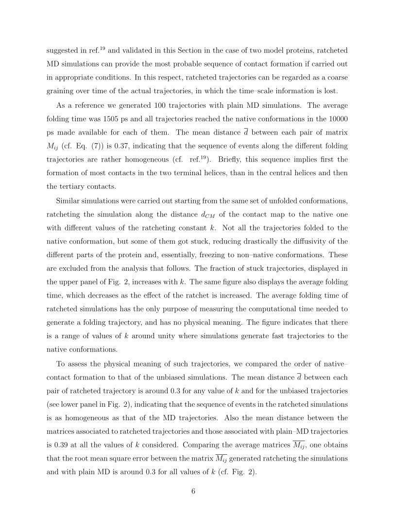
Similar simulations were carried out starting from the same set of unfolded conformations,

ratcheting the simulation along the distance dCM of the contact map to the native one

with different values of the ratcheting constant k. Not all the trajectories folded to the

native conformation, but some of them got stuck, reducing drastically the diffusivity of the

different parts of the protein and, essentially, freezing to non–native conformations. These

are excluded from the analysis that follows. The fraction of stuck trajectories, displayed in

the upper panel of Fig. 2, increases with k. The same figure also displays the average folding

time, which decreases as the effect of the ratchet is increased. The average folding time of

ratcheted simulations has the only purpose of measuring the computational time needed to

generate a folding trajectory, and has no physical meaning. The figure indicates that there

is a range of values of k around unity where simulations generate fast trajectories to the

native conformations.

To assess the physical meaning of such trajectories, we compared the order of native–

contact formation to that of the unbiased simulations. The mean distance d between each

pair of ratcheted trajectory is around 0.3 for any value of k and for the unbiased trajectories

(see lower panel in Fig. 2), indicating that the sequence of events in the ratcheted simulations

is as homogeneous as that of the MD trajectories. Also the mean distance between the

matrices associated to ratcheted trajectories and those associated with plain–MD trajectories

is 0.39 at all the values of k considered. Comparing the average matrices Mij, one obtains

that the root mean square error between the matrix Mij generated ratcheting the simulations

and with plain MD is around 0.3 for all values of k (cf. Fig. 2).

6

Summing up, the difference between ratcheted and plain–MD trajectories is comparable

with the (small) differences between pairs of plain–MD trajectories. Even when the ratchet is

strong, although the fraction of folding trajectories drops drastically, the sequence of events

in the few folding trajectories results correct.

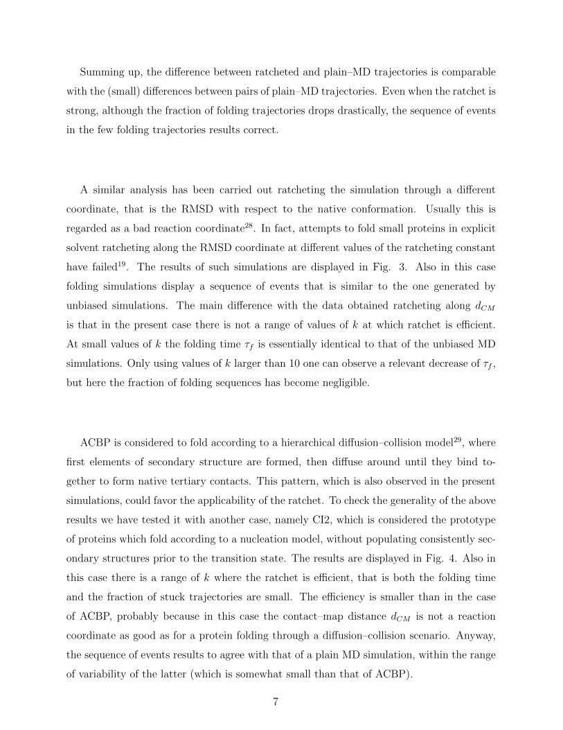
A similar analysis has been carried out ratcheting the simulation through a different

coordinate, that is the RMSD with respect to the native conformation. Usually this is

regarded as a bad reaction coordinate28. In fact, attempts to fold small proteins in explicit

solvent ratcheting along the RMSD coordinate at different values of the ratcheting constant

have failed19. The results of such simulations are displayed in Fig. 3. Also in this case

folding simulations display a sequence of events that is similar to the one generated by

unbiased simulations. The main difference with the data obtained ratcheting along dCM

is that in the present case there is not a range of values of k at which ratchet is efficient.

At small values of k the folding time τf is essentially identical to that of the unbiased MD

simulations. Only using values of k larger than 10 one can observe a relevant decrease of τf ,

but here the fraction of folding sequences has become negligible.

ACBP is considered to fold according to a hierarchical diffusion–collision model29, where

first elements of secondary structure are formed, then diffuse around until they bind to-

gether to form native tertiary contacts. This pattern, which is also observed in the present

simulations, could favor the applicability of the ratchet. To check the generality of the above

results we have tested it with another case, namely CI2, which is considered the prototype

of proteins which fold according to a nucleation model, without populating consistently sec-

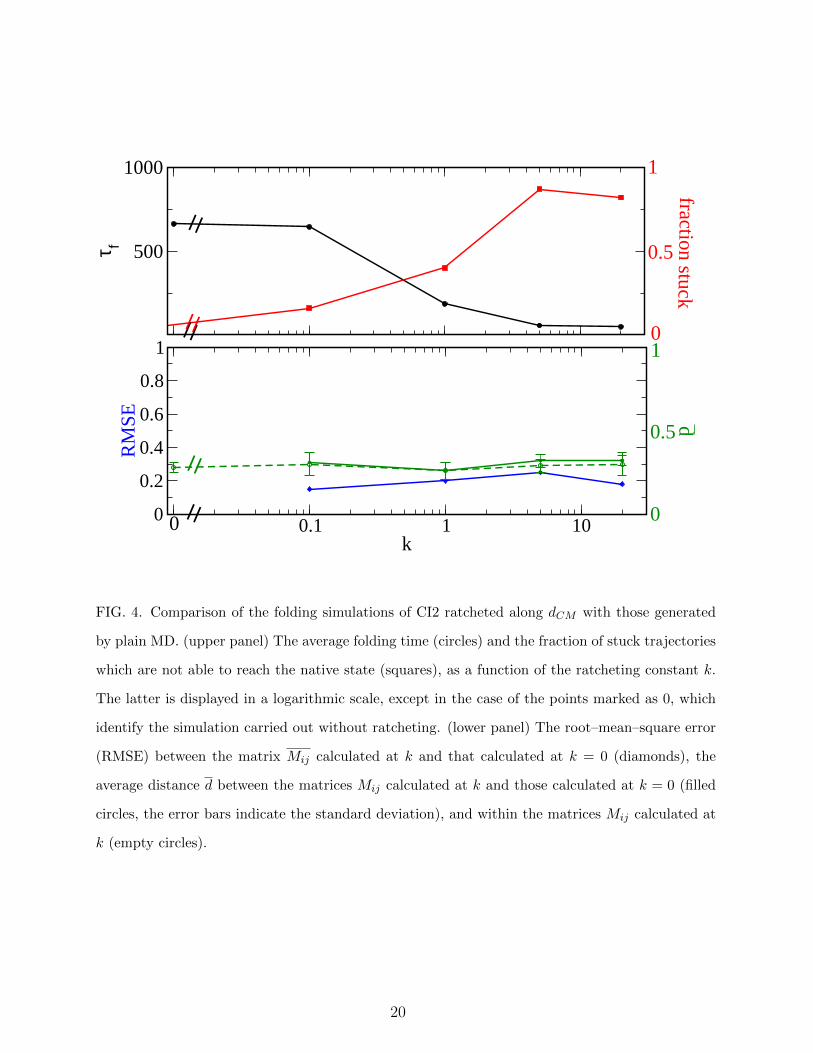
ondary structures prior to the transition state. The results are displayed in Fig. 4. Also in

this case there is a range of k where the ratchet is efficient, that is both the folding time

and the fraction of stuck trajectories are small. The efficiency is smaller than in the case

of ACBP, probably because in this case the contact–map distance dCM is not a reaction

coordinate as good as for a protein folding through a diffusion–collision scenario. Anyway,

the sequence of events results to agree with that of a plain MD simulation, within the range

of variability of the latter (which is somewhat small than that of ACBP).

7

IV. IDENTIFICATION OF THE TRANSITION STATE: THE STRATEGY

The analysis of the time–dependence of the degrees of freedom associated with the ratchet

can provide some information to localize the transition state of the system. The basic idea

is that, as the system climbs the free energy barrier whose top is the transition state, the

ratchet is very active and thus Vrat is well above zero. When the system crosses the transition

state and descends the free–energy barrier, the ratchet is essentially inactive and Vrat small.

The point of the trajectory where Vrat drops is hypothesized to be the transitions state.

Before verifying this hypothesis, we attempt to formalize the above idea, in a simple

scenario where the molecular force can be approximated in an elementary form. Assuming

that the dynamics of the degrees of freedom ~x of the system can be described by an over–

damped dynamics

d~x

dt=

1

γ

[~f(~x)− k∆ρ · ~uρ + ~η

], (8)

where γ is the friction coefficient; η is the thermal noise satisfying < ~η(t) · ~η(t′) >=

(2NTγ)δ(t − t′); ~uρ the versor that defines the direction of the ratcheting coordinate ρ;

∆ρ(t) ≡ ρ − ρm is the difference between the value of the ratcheting coordinate and its

minimum; and Boltzman’s constant is set to 1. Let’s assume that ρ is a good reaction

coordinate, that is it moves according to the slowest time scale of the system30, and that

the associated diffusion constant is approximately equal to that of the microscopic degrees

of freedom. Then, the dynamics of ρ can be written as

dρ

dt=

1

γ[fρ − k∆ρ+ η] , (9)

where fρ is the effective force which moves the one–dimensional degree of freedom ρ (i.e.,

minus the gradient of the free energy). By virtue of its definition, ρm follows the dynamics

dρmdt

=dρ

dtδ(∆ρ)θ(−dρ/dt), (10)

where θ is a step function that is 1 if its argument is positive and 0 otherwise. Consequently

the quantity ∆ρ which measures the activity of the ratchet follows

d(∆ρ)

dt=

1γ

[fρ − k∆ρ+ η] if ∆ρ > 0 or dρ/dt > 0

0 if ∆ρ = 0 and dρ/dt < 0.(11)

8

If the molecular force ~f pushes the system downhill towards its target state and it is over-

whelming with respect to the typical diffusive force (i.e., fρ � −(2Tγ/∆t)1/2), then ∆ρ is

approximately zero along the associated part of trajectory.

A more common scenario is that where the system is running downhill, the diffusive term

is not negligible, but the molecular force is overwhelming with respect to the ratchet (i.e.,

fρ � −k∆ρ), so that we can neglect the term proportional to k in Eq. (11). To make things

simple, let’s focus on a fraction of the trajectory that is short enough that the force fρ can

be approximated as constant. In this case ∆ρ experiences a diffusion biased by a constant

force, and by a trap at 0. In fact, when ∆ρ = 0 the system can move away only if dρ/dt > 0

(cf. the condition controlling the first line of Eq. (11)); thus the exit rate wexit from the trap

is proportional to the probability that η > |fρ| (∆t/2Tγ)1/2. This case is analogous to that

of a massive particle diffusing on a slope with a trap at the bottom. Since the stochastic

noise η is normally distributed, wexit is proportional to erfc(|fρ| (∆t/2Tγ)1/2). We can assign

to the trap an effective energy Utrap, so that wexit is equal to Kramers escape rate, that is

exp

[UtrapT

]=

1

2erfc

[|fρ|

(∆t

2Tγ

)1/2]. (12)

In the neighborhood of 0, ∆ρ will soon populate a distribution given by

p(∆ρ) =

2Z

erfc

[|fρ|

(∆t

2Tγ

)1/2]−1

if 0 < ∆ρ < ε

1Z

exp[− |fρ|∆ρ

T

]if ∆ρ > ε,

(13)

where ε is the (small) length which defines the trap and

Z = 2 · erfc

[|fρ|

(∆t

2Tγ

)1/2]−1

+T

|fρ|ε. (14)

The average value of ∆ρ expected in this regime is then

< ∆ρ >=T 2

εf 2ρ erfc[|fρ|(∆t)/2Tγ)1/2]−1 + |fρ|T

ε→0−−→ T

|fρ|. (15)

On the other hand, if the system is climbing the free–energy barrier (i.e. fρ �

(2Tγ/∆t)1/2), the conditions ∆ρ = 0 and dρ/dt < 0 in Eq. (11) are never satisfied si-

multaneously. Consequently,

p(∆ρ) =1

Zexp

[−

k2∆ρ2 − fρ∆ρ

T

](16)

9

where

Z =

(πT

2k

)1/2

exp

[f 2ρ

2kT

](1 + erf

[fρ

(2kT )1/2

]), (17)

giving the average

< ∆ρ >= 2(2/π)1/2Tk exp

[− f2ρ

2kT

]+ fρ(Tk)1/2

(1 + erf

[fρ

(2kT )1/2

])(k3T )1/2

(1 + erf

[fρ

(2kT )1/2

]) f2ρ�2kT−−−−−→ 2fρ

k. (18)

The transition state is the intermediate scenario where fρ vanishes. Assuming |fρ| �

2Tγ/∆t)1/2, one can neglect the molecular force in Eq. (11), obtaining

p(∆ρ) =

2/Z if 0 < ∆ρ < ε

1Z

exp[−k∆ρ2

2T

]if ∆ρ > ε,

(19)

where Z = 2 + (πk/2T )1/2/ε. This is an ideal distribution, because it is unlikely that the

system spends enough time at the transition state to populate it. However, it can be useful

to obtain the average ∆ρ which separates the rising from the descending regime. In fact, we

get

< ∆ρ >=2T

4kε+ (2πkT )1/2

ε→0−−→(

2T

πk

)1/2

. (20)

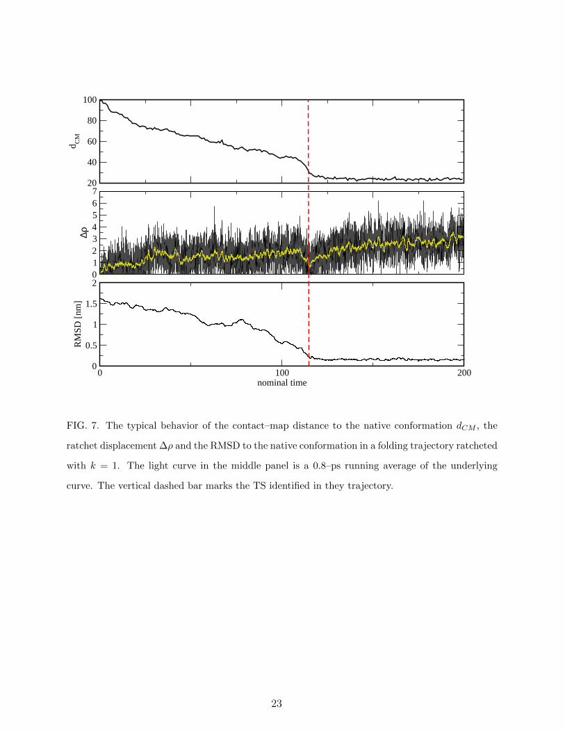
The behavior of ∆ρ in a typical ratcheted simulation is displayed in the middle panel of

Fig. 7. Although it is difficult to distinguish a priori where the system is climbing and where

it is descending the folding free–energy barrier, it is reasonable to argue that in part of the

trajectory in the range 30 < t < 125 the system is climbing, while in the range 110 < t < 125

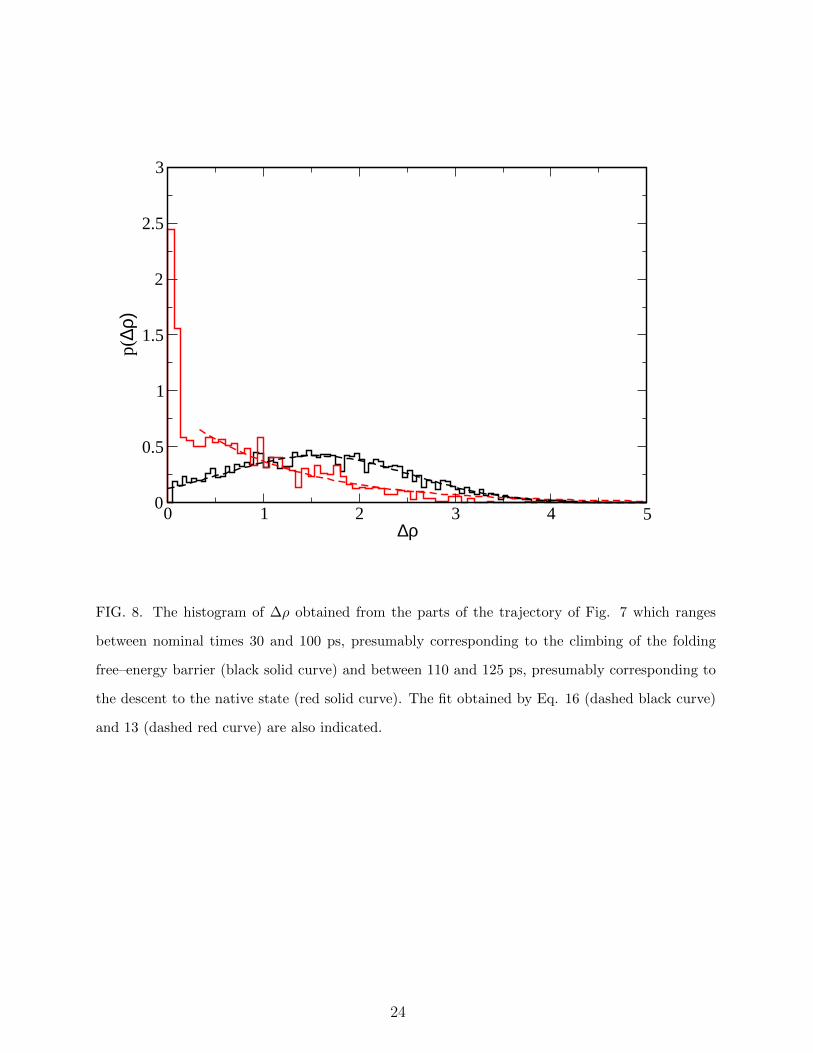
it is descending. The distribution p(∆ρ) associated with these two parts of the trajectory

are displayed in Fig. 8 with solid black and red curves, respectively. The black curve is fitted

by Eq. (16), the correlation coefficient being 0.958. The red curve displays a sharp peak at

low values of ∆ρ as predicted by the first line of Eq. (13), allowing to obtain ε = 0.3, while

the remaining part is fitted by the second line of f Eq. (13), with a correlation coefficient of

0.965. This means that, although the molecular force fρ certainly depends on the specific

point of the trajectory, the system crosses the free-energy barrier experiencing an effective

force of fρ = 0.75 and descend it pushed by an effective force fρ = −1.45.

The value of < ∆ρ > obtained in Eq. (20) can be used to estimate the order of magnitude

of the threshold to distinguish the regime where the system is climbing the free-energy

barrier from that in which it is descending, that is the transition state. For example, in the

simulation we performed with T = 0.91 and k = 1, we obtain < ∆ρ >= 0.76 (cf. Fig. 7).

10

V. IDENTIFICATION OF THE TRANSITION STATE: RESULTS

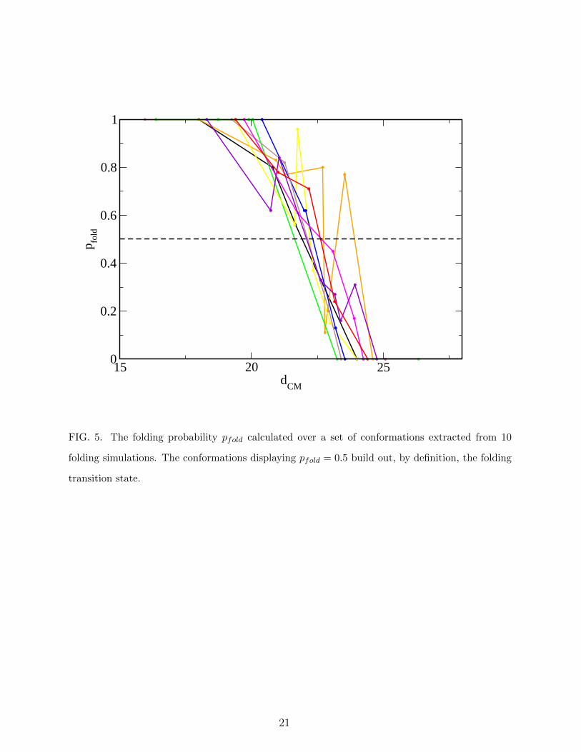
Before applying the strategy discussed above, the actual TS was identified through a

commitment analysis14 on 10 plain–MD folding trajectories of ACBP. From each of them

we extracted a variable number (from 5 to 10) of conformations chosen in the region where

the value of dCM displays a rapid decrease to low values. From each of them we started

100 plain-MD simulations, calculating the probability pfold that the simulation reaches the

native basin (operatively defined from dCM < 19) before reaching the denatured basin

(operatively defined from dCM > 25). The conformations displaying 0.4 < pfold < 0.6 are

defined as TS conformations. The behavior of pfold with respect to the value of dCM of the

associated conformation is displayed in Fig. 5. The associated conformations are displayed

in Fig. 6(A). They are remarkably native–like, displaying an average RMSD to the native

conformation of 0.68± 0.17 nm, and fairly homogeneous, their mutual average RMSD being

0.85± 0.17 nm.

For each trajectory generated with the ratcheting algorithm, we have looked for the TS

in the region where the RMSD to the native conformation was in the range between 0.2

nm and 1 nm. The putative TS is the conformation such that the average value of ∆ρ in

the preceding 8 ps is larger than that predicted by Eq. (20) and in the following 0.8 ps is

smaller. In this way, we could identify a conformation in 64% of trajectories at k = 0.1, in

the 86% of the trajectories at k = 1 and in the 49% of trajectories at k = 20. In no cases

more than one conformation is identified.

The structural properties of the conformations identified by the above criteria are sum-

marized in Fig. 9. The average contact–map distance is comparable to that of the actual TS

at all values of k. The structural homogeneity of the TS conformations is slightly decreasing

with the increasing of k, the mutual average RMSD going from 0.85 nm at k = 0 to 0.61

nm at k = 20. The average similarity of the TS conformations obtained from ratcheted

simulations to the actual TS conformations is within the error bars σ associated with the

intrinsic variability of the TS conformations (the difference between the two averages being

≈ 0.2σ; black error bars in the figure). Also the RMSD to the native conformation displays

a slight decrease from 0.68 nm at k = 0 to 0.46 nm at k = 20. Summing up, at all values of

k analyzed, ratcheted MD simulations can identify TS conformations which are structurally

similar to the actual TS conformations, becoming slightly more native–like at increasing k.

11

A representation of the protein in the TS obtained at k = 1 is displayed in Fig. 6B.

The main differences between the actual TS and that obtained by ratcheted conformation

at k = 1 involves the terminals of the protein. The actual TS displays large fluctuation

in the C-terminal part of the chain and, to a smaller extent, in the N–terminal and in the

loop region. The ratcheted TS overestimates the fluctuations in the C-terminal region, while

it slightly underestimates those involving the loop. Anyway, the two sets are remarkably

similar.

VI. AN EXPLICIT–SOLVENT CASE: THE TRANSITION STATE OF

ACBP AND CI2 SIMULATED WITH THE AMBER FORCE FIELD

The very goal of the strategy discussed above is not the identification of the transition

state with simplified protein descriptions, but in realistic explicit–solvent models. In order

to test the algorithm we analyzed the folding and unfolding trajectories generated using the

ratcheting algorithm in ref.19. Using the Amber03 force field31, we simulated 10 folding and

10 unfolding trajectories of ACBP and CI2 in a dodecahedron box of 261 nm3 solvated with

∼ 104 TIP3P water molecules, ratcheting along dCM with a ratcheting constant k = 1kJ/mol

for 50 ns at T = 300K. All trajectories folded within 0.25 nm from the native conformation.

The transition state is identified with the same strategy used in the Go–model simulations,

requiring that the average of ∆ρ in the preceding 8 ps is larger than 1 and in the following 8 ps

is smaller than 2 (this is a somewhat looser condition than for the Go model, but guarantees

the identification of a unique TS for each trajectory), while the RMSD to the native state

should range between 0.3 and 1 nm. The conformation thus obtained are displayed in Fig.

10. They are less homogeneous than those obtained by means of the Go model, the average

mutual RMSD being 0.82± 0.19 nm in the case of ACBP and 0.76± 0.14 nm in the case of

CI2. Their RMSD to the native state is 0.68± 0.19 nm in the case of ACBP and 0.70± 0.17

nm in the case of CI2.

In order to validate the TS without carrying out a commitment analysis which is ex-

tremely time–consuming in explicit solvent32, we have compared the TS conformations ob-

tained from the folding trajectories to the TS conformations obtained by unfolding trajec-

tories under the same conditions. According to the principle of detailed–balance, under the

same conditions the two TS must be identical33. The TS conformations obtained in this case

12

are slightly more native–like, displaying a RMSD to the native conformation of 0.43± 0.13

nm for ACBP and 0.62± 0.07 nm for CI2. In order to compare the set of TS conformations

obtained from folding and from unfolding trajectories, we have calculated the average pair-

wise RMSD of conformations across the two sets, which is 0.81 ± 0.10 nm for ACBP and

0.76± 0.13 nm for CI2.

The average similarity between the folding and the unfolding TS is compatible, within

the error bars, to the intrinsic heterogeneity of each set (their difference is 0.05σ in the case

of ACBP and 0 in the case of CI2), and so guarantees that the two TS can be regarded as

approximatively identical.

VII. CONCLUSIONS

The complexity of the characterisation of biomolecular processes is driving a continuos

improvement of the experimental and the computational techniques34. In particular, in the

field of computer simulations, in the last few years we have assisted in a leap in the accessible

time scale of plain MD simulations. Nonetheless even these major improvements are not

able to address the complexity of folding problem for realistic proteins32. This points to

the necessity of carrying on with the development of both simplified model and advanced

sampling methods. The present work further validates the use of the ratcheting algorithm

in the study of protein folding and extends its use to the approximate identification, at an

atomic level, of the transition state ensemble of a protein in explicit solvent.

VIII. ACKNOWLEDGMENTS

CC was supported by a Marie Curie Intra-European fellowship. We acknowledge the use

of computing facilities provided by CamGrid.

REFERENCES

1A. R. Fersht, Structure and mechanism in protein science (W. H. Freeman and Co., 2002).

2K. A. Beauchamp, Y.-S. Lin, R. Das, and V. S. Pande, “Are Protein Force Fields Get-

ting Better? A Systematic Benchmark on 524 Diverse NMR Measurements,” Journal of

Chemical Theory and Computation, 8, 1409 (2012).

13

3K. Lindorff-Larsen, P. Maragakis, S. Piana, M. P. Eastwood, R. O. Dror, and D. E. Shaw,

“Systematic Validation of Protein Force Fields against Experimental Data,” PLoS ONE,

7, e32131 (2012).

4N. Calosci, C. N. Chi, B. Richter, C. Camilloni, A. Engstrom, L. Eklund, C. Travaglini-

Allocatelli, S. Gianni, M. Vendruscolo, and P. Jemth, “Comparison of successive transition

states for folding reveals alternative early folding pathways of two homologous proteins.”

Proceedings of the National Academy of Sciences of the United States of America, 105,

19241 (2008).

5C. D. Geierhaas, X. Salvatella, J. Clarke, and M. Vendruscolo, “Characterisation of tran-

sition state structures for protein folding using ’high’, ’medium’ and ’low’ Phi-values,”

Protein engineering, design & selection, 21, 215 (2008).

6E. Paci, M. Vendruscolo, C. M. Dobson, and M. Karplus, “Determination of a transition

state at atomic resolution from protein engineering data,” Journal of Molecular Biology,

324, 151 (2002).

7M. Vendruscolo, E. Paci, and C. M. Dobson, “Three key residues form a critical contact

network in a protein folding transition state,” Nature, 409, 641 (2001).

8K. Lindorff-Larsen, S. Piana, R. O. Dror, and D. E. Shaw, “How fast-folding proteins

fold,” Science (New York, NY), 334, 517 (2011).

9R. Best, “Atomistic molecular simulations of protein folding,” Current Opinion in Struc-

tural Biology, 22, 52 (2012).

10P. G. Bolhuis, D. Chandler, C. Dellago, and P. L. Geissler, “Transition path sampling

throwing ropes over rough mountain passes, in the dark,” Annual Reviews Physical Chem-

istry, 53, 291 (2002).

11A. K. Faradjian and R. Elber, “Computing time scales from reaction coordinates by mile-

stoning.” J. Chem. Phys., 120, 10880 (2004).

12P. Faccioli, M. Sega, F. Pederiva, and H. Orland, “Dominant pathways in protein folding,”

Physical Review Letters, 97, 108101 (2006).

13P. Faccioli, “Characterization of protein folding by dominant reaction pathways,” The

Journal of Physical Chemistry B, 112, 13756 (2008).

14P. Geissler, C. Dellago, and D. Chandler, “Kinetic pathways of ion pair dissociation in

water,” Journal of Physical Chemistry B, 103, 3706 (1999).

14

15V. Pande, A. Grosberg, T. Tanaka, and E. Shakhnovich, “On the transition coordinate

for protein folding,” J. Chem. Phys., 108, 334 (1998).

16M. Marchi and P. Ballone, “Adiabatic bias molecular dynamics: A method to navigate the

conformational space of complex molecular systems,” J. Chem. Phys., 110, 3697 (1999).

17E. Paci and M. Karplus, “Forced unfolding of fibronectin type 3 modules: an analysis by

biased molecular dynamics simulations,” Journal of Molecular Biology, 288, 441 (1999).

18E. Paci and M. Karplus, “Unfolding proteins by external forces and temperature: the

importance of topology and energetics,” Proceedings of the National Academy of Sciences

of the United States of America, 97, 6521 (2000).

19C. Camilloni, R. A. Broglia, and G. Tiana, “Hierarchy of folding and unfolding events

of protein G, CI2, and ACBP from explicit-solvent simulations.” Journal Of Chemical

Physics, 134, 045105 (2011).

20S. A Beccara, T. Skrbic, R. Covino, and P. Faccioli, “Dominant folding pathways of a

WW domain.” Proceedings of the National Academy of Sciences of the United States of

America, 109, 2330 (2012).

21P. C. Whitford, J. K. Noel, S. Gosavi, A. Schug, K. Y. Sanbonmatsu, and J. N. Onuchic,

“An all-atom structure-based potential for proteins: bridging minimal models with all-

atom empirical forcefields,” Proteins, 75, 430 (2009).

22C. Camilloni, D. Provasi, G. Tiana, and R. A. Broglia, “Exploring the protein G helix

free-energy surface by solute tempering metadynamics,” Proteins, 71, 1647 (2008).

23M. Bonomi, D. Branduardi, G. Bussi, C. Camilloni, D. Provasi, P. Raiteri, D. Donadio,

F. Marinelli, F. Pietrucci, and R. A. Broglia, “PLUMED: a portable plugin for free-

energy calculations with molecular dynamics,” Computer Physics Communications, 180,

1961 (2009).

24B. Hess, C. Kutzner, D. van der Spoel, and E. Lindahl, “GROMACS 4: Algorithms for

highly efficient, load-balanced, and scalable molecular simulation,” Journal of Chemical

Theory and Computation, 4, 435 (2008).

25J. K. Noel, P. C. Whitford, K. Y. Sanbonmatsu, and J. N. Onuchic, “SMOG@ctbp:

simplified deployment of structure-based models in GROMACS.” Nucleic Acids Research,

38, W657 (2010).

26U. Hansmann, “Parallel tempering algorithm for conformational studies of biological

molecules,” Chemical Physics Letters, 281, 140 (1997).

15

27M. Bonomi, F. L. Gervasio, G. Tiana, D. Provasi, R. A. Broglia, and M. Parrinello,

“Insight into the folding inhibition of the HIV-1 protease by a small peptide,” Biophysical

journal, 93, 2813 (2007).

28R. Best and G. Hummer, “Coordinate-dependent diffusion in protein folding.” Proceedings

of the National Academy of Sciences of the United States of America, 107, 1088 (2010).

29B. B. Kragelund, P. Osmark, T. B. Neergaard, J. Schiødt, K. Kristiansen, J. Knudsen,

and F. M. Poulsen, “The formation of a native-like structure containing eight conserved

hydrophobic residues is rate limiting in two-state protein folding of ACBP,” Nature struc-

tural biology, 6, 594 (1999).

30H. Risken, The Fokker-Planck Equation (Springer, 1996).

31Y. Duan, C. Wu, S. Chowdhury, M. C. Lee, G. Xiong, W. Zhang, R. Yang, P. Cieplak,

R. Luo, T. Lee, J. Caldwell, J. Wang, and P. Kollman, “A point-charge force field for

molecular mechanics simulations of proteins based on condensed-phase quantum mechan-

ical calculations,” Journal of Computational Chemistry, 24, 1999 (2003).

32D. E. Shaw, P. Maragakis, K. Lindorff-Larsen, S. Piana, R. O. Dror, M. P. Eastwood, J. A.

Bank, J. K. Salmon, and W. Wriggers, “Atomic-Level Characterization of the Structural

Dynamics of Proteins,” Science (New York, NY), 330, 341 (2010).

33A. V. Finkelstein, “Can protein unfolding simulate protein folding?” Protein Engineering,

10, 843 (1997).

34A. Bartlett and S. E. Radford, “An expanding arsenal of experimental methods yields

an explosion of insights into protein folding mechanisms,” Nature Structural & Molecular

Biology, 16, 582 (2009).

16

0.8 1 1.2 1.4T

0

0.5

1

1.5Cv

FIG. 1. The specific heat of ACBP (whose structure is displayed in the inset) as a function of

temperature for the model interacting through the modified Go model (solid curve) and through

a standard Go model (dashed curve). The temperature is expressed in energy units.

17

500

1000

1500

2000

τ f

0.1 1 10k

0

0.2

0.4

0.6

0.8

1

RM

SE

0

1

0.5

fraction stuck

=

d

0

0.5

1===

0 =

FIG. 2. Comparison of the folding simulations of ACBP ratcheted along dCM with those generated

by plain MD. (upper panel) The average folding time (circles) and the fraction of stuck trajectories

which are not able to reach the native state (squares), as a function of the ratcheting constant k.

The latter is displayed in a logarithmic scale, except in the case of the points marked as 0, which

identify the simulation carried out without ratcheting. (lower panel) The root–mean–square error

(RMSE) between the matrix Mij calculated at k and that calculated at k = 0 (diamonds), the

average distance d between the matrices Mij calculated at k and those calculated at k = 0 (filled

circles, the error bars indicate the standard deviation), and within the matrices Mij calculated at

k (empty circles).

18

500

1000

1500

2000

τ f

0.1 1 10k

0

0.2

0.4

0.6

0.8

1

RM

SE

0

1

0.5

fraction stuck

=

d

0

0.5

1===

0 =

FIG. 3. Comparison of the folding simulations of ACBP ratcheted along the RMSD with those

generated by plain MD. (upper panel) The average folding time (circles) and the fraction of stuck

trajectories which are not able to reach the native state (squares), as a function of the ratchet-

ing constant k. The latter is displayed in a logarithmic scale, except in the case of the points

marked as 0, which identify the simulation carried out without ratcheting. (lower panel) The root–

mean–square error (RMSE) between the matrix Mij calculated at k and that calculated at k = 0

(diamonds), the average distance d between the matrices Mij calculated at k and those calculated

at k = 0 (filled circles, the error bars indicate the standard deviation), and within the matrices

Mij calculated at k (empty circles). Here, the values of k are given in energy units divided by nm.

19

500

1000

τ f

0.1 1 10k

0

0.2

0.4

0.6

0.8

1

RM

SE

0

1

0.5

fraction stuck

=

d

0

0.5

1===

0 =

FIG. 4. Comparison of the folding simulations of CI2 ratcheted along dCM with those generated

by plain MD. (upper panel) The average folding time (circles) and the fraction of stuck trajectories

which are not able to reach the native state (squares), as a function of the ratcheting constant k.

The latter is displayed in a logarithmic scale, except in the case of the points marked as 0, which

identify the simulation carried out without ratcheting. (lower panel) The root–mean–square error

(RMSE) between the matrix Mij calculated at k and that calculated at k = 0 (diamonds), the

average distance d between the matrices Mij calculated at k and those calculated at k = 0 (filled

circles, the error bars indicate the standard deviation), and within the matrices Mij calculated at

k (empty circles).

20

15 20 25dCM

0

0.2

0.4

0.6

0.8

1

p fold

FIG. 5. The folding probability pfold calculated over a set of conformations extracted from 10

folding simulations. The conformations displaying pfold = 0.5 build out, by definition, the folding

transition state.

21

FIG. 6. Comparison between the Go–model transition–state conformations for ACBP obtained

by plain–MD simulations through the commitment analysis (A) and those obtained by ratcheted

simulations as explained in the text (B). The width and the color of the average conformations

denote the RMS fluctuations.

22

20

40

60

80

100

d CM

01234567

∆ρ

0 100 200nominal time

0

0.5

1

1.5

2

RM

SD [n

m]

FIG. 7. The typical behavior of the contact–map distance to the native conformation dCM , the

ratchet displacement ∆ρ and the RMSD to the native conformation in a folding trajectory ratcheted

with k = 1. The light curve in the middle panel is a 0.8–ps running average of the underlying

curve. The vertical dashed bar marks the TS identified in they trajectory.

23

0 1 2 3 4 5∆ρ

0

0.5

1

1.5

2

2.5

3

p(∆ρ

)

FIG. 8. The histogram of ∆ρ obtained from the parts of the trajectory of Fig. 7 which ranges

between nominal times 30 and 100 ps, presumably corresponding to the climbing of the folding

free–energy barrier (black solid curve) and between 110 and 125 ps, presumably corresponding to

the descent to the native state (red solid curve). The fit obtained by Eq. 16 (dashed black curve)

and 13 (dashed red curve) are also indicated.

24

0

20

40

60

80

100

d CM

0.1 1 10k

02468

101214

RM

SD [A

]

0

FIG. 9. Structural properties of transition–state conformations obtained at various values of k and

obtained from plain MD simulations (k = 0). (upper panel) The average distance between the

contact map of TS conformations and that of the native state. (lower panel) The average RMSD

between pairs of TS conformations at each value of k (black squares), the average RMSD between

TS conformations obtained at different values of k and those obtained by plain MD simulations (red

diamonds) and average RMSD to the native conformation (blue circles). The error bars indicate

the standard deviation.

25

(a) (b)

FIG. 10. The conformations corresponding to the transition state of ACBP (a) and CI2 (b) from

the explicit–solvent ratcheted simulations. The thickness of the surface indicates the standard

deviation associated to the average structure.

26