Rapid qualitative and quantitative detection of beef fillets spoilage based on Fourier transform...
36
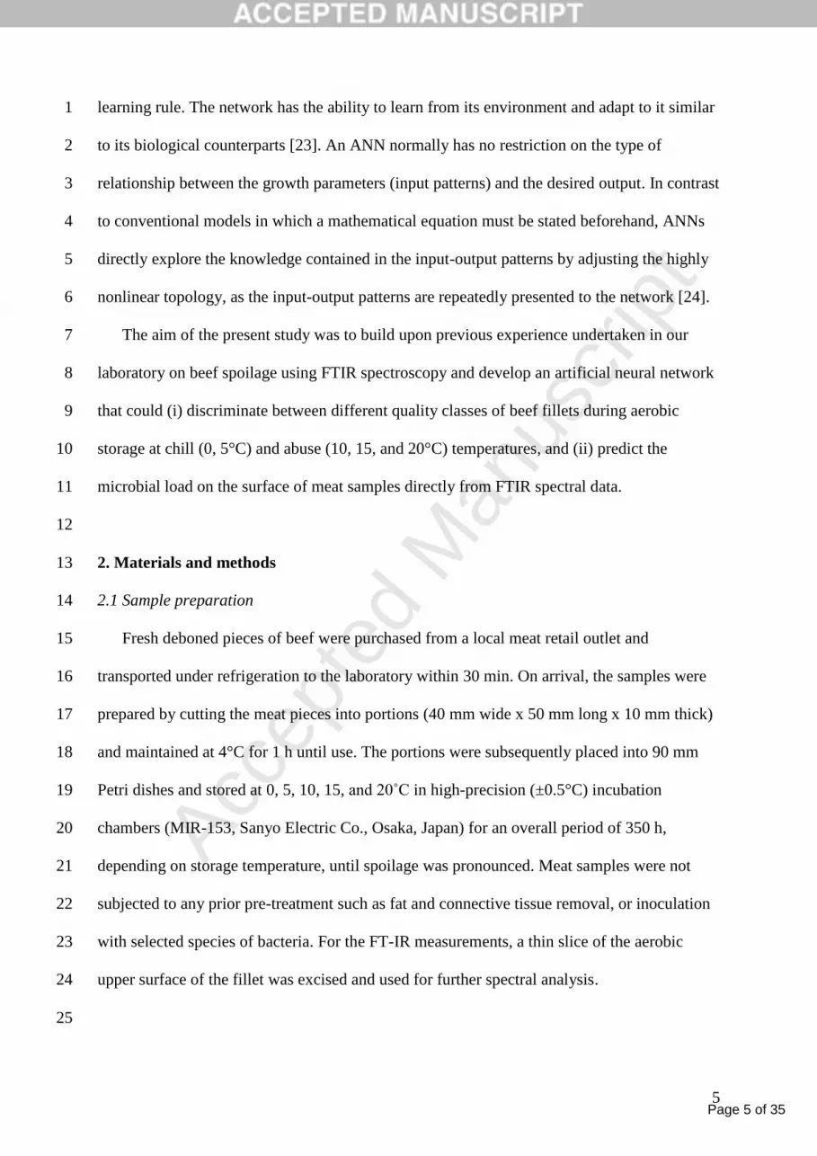
Accepted Manuscript Title: Rapid qualitative and quantitative detection of beef fillets spoilage based on Fourier transform infrared spectroscopy data and artificial neural networks Authors: A.A. Argyri, E.Z. Panagou, P.A. Tarantilis, M. Polysiou, G.-J.E. Nychas PII: S0925-4005(09)00917-4 DOI: doi:10.1016/j.snb.2009.11.052 Reference: SNB 11942 To appear in: Sensors and Actuators B Received date: 27-7-2009 Revised date: 3-11-2009 Accepted date: 22-11-2009 Please cite this article as: A.A. Argyri, E.Z. Panagou, P.A. Tarantilis, M. Polysiou, G.- J.E. Nychas, Rapid qualitative and quantitative detection of beef fillets spoilage based on Fourier transform infrared spectroscopy data and artificial neural networks, Sensors and Actuators B: Chemical (2008), doi:10.1016/j.snb.2009.11.052 This is a PDF file of an unedited manuscript that has been accepted for publication. As a service to our customers we are providing this early version of the manuscript. The manuscript will undergo copyediting, typesetting, and review of the resulting proof before it is published in its final form. Please note that during the production process errors may be discovered which could affect the content, and all legal disclaimers that apply to the journal pertain.
-
Upload
agriculturalathensu -
Category
Documents
-
view
1 -
download
0
Transcript of Rapid qualitative and quantitative detection of beef fillets spoilage based on Fourier transform...

Accepted Manuscript
Title: Rapid qualitative and quantitative detection of beeffillets spoilage based on Fourier transform infraredspectroscopy data and artificial neural networks
Authors: A.A. Argyri, E.Z. Panagou, P.A. Tarantilis, M.Polysiou, G.-J.E. Nychas
PII: S0925-4005(09)00917-4DOI: doi:10.1016/j.snb.2009.11.052Reference: SNB 11942
To appear in: Sensors and Actuators B
Received date: 27-7-2009Revised date: 3-11-2009Accepted date: 22-11-2009
Please cite this article as: A.A. Argyri, E.Z. Panagou, P.A. Tarantilis, M. Polysiou, G.-J.E. Nychas, Rapid qualitative and quantitative detection of beef fillets spoilage basedon Fourier transform infrared spectroscopy data and artificial neural networks, Sensorsand Actuators B: Chemical (2008), doi:10.1016/j.snb.2009.11.052
This is a PDF file of an unedited manuscript that has been accepted for publication.As a service to our customers we are providing this early version of the manuscript.The manuscript will undergo copyediting, typesetting, and review of the resulting proofbefore it is published in its final form. Please note that during the production processerrors may be discovered which could affect the content, and all legal disclaimers thatapply to the journal pertain.
e101281
TextBox
Sensors and Actuators B: Chemical, Volume 145, Issue 1, 4 March 2010, Pages 146-154

Page 1 of 35
Accep
ted
Man
uscr
ipt
1
1
Rapid qualitative and quantitative detection of beef fillets spoilage based on 2
Fourier transform infrared spectroscopy data and artificial neural 3
networks 4
5
A.A. Argyria,b
, E.Z. Panagoua,*
, P.A. Tarantilisc, M. Polysiou
c, G.-J.E. Nychas
a 6
7
a Laboratory of Microbiology and Biotechnology of Foods, Department of Food Science and 8
Technology, Agricultural University of Athens, Iera Odos 75, 118 55 Athens, Greece 9
b Applied Mycology Group, Cranfield Health, Cranfield University, College Road, Cranfield, 10
Bedfordshire MK43 0AL, United Kingdom 11
c Laboratory of Chemistry, Agricultural University of Athens, Iera Odos 75, 118 55 Athens, Greece 12
13
14
15
16
17
18
19
20
21
22
23
24
25
26
Corresponding author. Tel/Fax: +30 210 529 4693. E-mail address: [email protected] 27
28
Running title: Monitoring meat spoilage with FTIR and neural networks 29
30
Manuscript

Page 2 of 35
Accep
ted
Man
uscr
ipt
2
Abstract 1
A machine learning strategy in the form of a multilayer perceptron (MLP) neural network 2
was employed to correlate Fourier transform infrared (FTIR) spectral data with beef spoilage 3
during aerobic storage at chill and abuse temperatures. Fresh beef fillets were packaged under 4
aerobic conditions and left to spoil at 0, 5, 10, 15, and 20°C for up to 350 hours. FTIR spectra 5
were collected directly from the surface of meat samples, whereas total viable counts of 6
bacteria were obtained with standard plating methods. Sensory evaluation was performed 7
during storage and samples were attributed into three quality classes namely fresh, semi-fresh, 8
and spoiled. A neural network was designed to classify beef samples to one of the three 9
quality classes based on the biochemical profile provided by the FTIR spectra, and in parallel 10
to predict the microbial load (as total viable counts) on meat surface. The results obtained 11
demonstrated that the developed neural network was able to classify with high accuracy the 12
beef samples in the corresponding quality class using their FTIR spectra. The network was 13
able to classify correctly 22 out of 24 fresh samples (91.7%), 32 out of 34 spoiled samples 14
(94.1%), and 13 out of 16 semi-fresh samples (81.2%). No fresh sample was misclassified as 15
spoiled and vice versa. The performance of the network in the prediction of microbial counts 16
was based on graphical plots and statistical indices (bias and accuracy factors, standard error 17
of prediction, mean relative and mean absolute percentage residuals). Results demonstrated 18
good correlation of microbial load on beef surface with spectral data. The results of this work 19
indicated that the biochemical fingerprints during beef spoilage obtained by FTIR 20
spectroscopy in combination with the appropriate machine learning strategy have significant 21
potential for rapid assessment of meat spoilage. 22
23
24
25
Keywords: Artificial neural networks, Aerobic storage, Beef fillets, FTIR, Machine learning, 26
Meat spoilage.27

Page 3 of 35
Accep
ted
Man
uscr
ipt
3
1. Introduction 1
In most developed countries meat consumption is very high mainly due to its high 2
nutritional value in the human diet. The great variability in raw meat in terms of chemical 3
composition, technological and chemical attributes results in highly variable end products 4
which are marketed without a desired and controlled level of quality [1]. In order to maintain 5
quality standards, control procedures must be carried out on meat comprising chemical 6
analyses, instrumental methods, organoleptic evaluation, and molecular screening methods. 7
More than fifty methods have been used for the detection of microbiologically spoiled or 8
contaminated meat (e.g. organoleptic, microbiological, and physico-chemical), all of which 9
are well documented [2]. However, these techniques are invasive, time consuming, labour 10
intensive, demand highly trained personnel, and thus they are unsuitable for online application 11
and routine analysis [3-7]. The lack of general agreement on the early signs of incipient 12
spoilage for meat makes more difficult the task to evaluate it objectively, mainly due to 13
changes in the technology of meat preservation (e.g. vacuum, modified atmospheres, etc.). 14
The use of microbial metabolites as a consequence of microbial activity in meat has been 15
continuously recognized as a potential means for assessing meat quality [4, 6, 8]. The 16
attempts that have been made over the last two decades to associate given metabolites with 17
microbial spoilage of meat have not been very much appreciated, due to low understanding of 18
the underlying phenomena [6]. 19
Recently, some interesting analytical approaches using mathematical equations have been 20
applied to describe the kinetics of ephemeral/specific spoilage organisms (E(S)SO) with the 21
purpose to predict spoilage of various foods [7, 9]. Other approaches are based on the use of 22
biosensors (enzymatic reactor systems), electronic noses (array of sensors), and vibrational 23
spectroscopy methods (e.g. FTIR, Raman spectroscopy) [10-12] for the same purpose. In 24
contrast to conventional methods, Fourier transform infrared (FTIR) spectroscopy is rapid, 25

Page 4 of 35
Accep
ted
Man
uscr
ipt
4
non-invasive, requires no specific consumable or reagent permitting users to collect full 1
spectra in a few seconds allowing simultaneous assessment of numerous meat properties [4-5, 2
13]. The basic concept underlying this method stipulates that as bacteria grow on meat, they 3
utilize nutrients and produce by-products that cause spoilage. The quantification of these 4
metabolites represents a fingerprint characteristic of any biochemical substance, providing 5
thus information about the type and the rate of spoilage [2, 13]. The integration of the FTIR 6
Attenuated Total Reflectance biosensors or other biosensors in tandem with an information 7
platform would result in the development of an “expert system” that would be able to 8
qualitatively and/or quantitatively discriminate between meat samples based on extracted pre-9
processing features. 10
The application of advanced statistical methods (e.g. discriminant function analysis, 11
clustering analysis, partial least square regression, chemometrics) and intelligent 12
methodologies (neural networks, fuzzy logic, evolutionary algorithms, genetic programming) 13
can be used as qualitative indices rather quantitative since their primary target is to distinguish 14
objects or groups or populations [14-15]. Nowadays, machine learning strategies are based on 15
supervised learning algorithms [16]. The last mentioned approach together with the 16
development of artificial neural networks (ANN) could be used effectively in the evaluation 17
of meat spoilage. Interest in using artificial neural networks in food science is increasing in 18
the last years, as they have shown promising results in several applications such as sensory 19
analysis, pattern recognition, classification, microbial predictions, and food process 20
optimization [17-21]. Essentially, ANNs are computing algorithms that attempt to imitate the 21
computational capabilities of large, highly connected networks of relatively simple elements 22
such as neurons in the human brain [22]. They contain a series of mathematical equations that 23
are used to simulate biological processes such as learning and memory. Their development 24
first involves a learning process that adaptively responds to the input variables according to a 25
Page 5 of 35
Accep
ted
Man
uscr
ipt
5
learning rule. The network has the ability to learn from its environment and adapt to it similar 1
to its biological counterparts [23]. An ANN normally has no restriction on the type of 2
relationship between the growth parameters (input patterns) and the desired output. In contrast 3
to conventional models in which a mathematical equation must be stated beforehand, ANNs 4
directly explore the knowledge contained in the input-output patterns by adjusting the highly 5
nonlinear topology, as the input-output patterns are repeatedly presented to the network [24]. 6
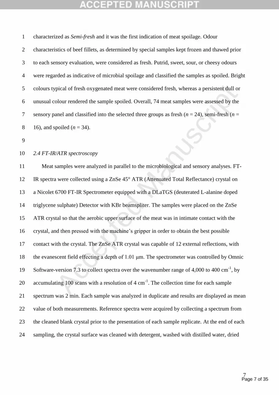
The aim of the present study was to build upon previous experience undertaken in our 7
laboratory on beef spoilage using FTIR spectroscopy and develop an artificial neural network 8
that could (i) discriminate between different quality classes of beef fillets during aerobic 9
storage at chill (0, 5°C) and abuse (10, 15, and 20°C) temperatures, and (ii) predict the 10
microbial load on the surface of meat samples directly from FTIR spectral data. 11
12
2. Materials and methods 13
2.1 Sample preparation 14
Fresh deboned pieces of beef were purchased from a local meat retail outlet and 15
transported under refrigeration to the laboratory within 30 min. On arrival, the samples were 16
prepared by cutting the meat pieces into portions (40 mm wide x 50 mm long x 10 mm thick) 17
and maintained at 4°C for 1 h until use. The portions were subsequently placed into 90 mm 18
Petri dishes and stored at 0, 5, 10, 15, and 20˚C in high-precision (±0.5°C) incubation 19
chambers (MIR-153, Sanyo Electric Co., Osaka, Japan) for an overall period of 350 h, 20
depending on storage temperature, until spoilage was pronounced. Meat samples were not 21
subjected to any prior pre-treatment such as fat and connective tissue removal, or inoculation 22
with selected species of bacteria. For the FT-IR measurements, a thin slice of the aerobic 23
upper surface of the fillet was excised and used for further spectral analysis. 24
25

Page 6 of 35
Accep
ted
Man
uscr
ipt
6
2.2 Microbiological analyses 1
For microbiological analysis a portion (40 mm wide x 50 mm long x 10 mm thick) was 2
added to 150 ml sterile quarter strength Ringer‟s solution, and homogenized in a stomacher 3
(Lab Blender 400, Seward Medical, London, UK) for 60 s at room temperature (ca. 20°C). 4
Further decimal dilutions were prepared with the same diluent, and duplicate 0.1 ml samples 5
of three appropriate dilutions were spread in triplicate on plate count agar (PCA 4021452; 6
Biolife, Italy) for counts of total viable bacteria (TVC), which was incubated at 30ºC for 48 h. 7
Duplicate samples from each storage temperature were analyzed at appropriate time intervals 8
to allow for efficient kinetic analysis of total viable counts. Specifically, meat samples stored 9
at 0 and 5°C were analyzed every 24 h, whereas samples stored at 10, 15, and 20°C were 10
analyzed every 8, 6, and 4 h, respectively. Growth data from plate counts were log 11
transformed and fitted to the primary model of Baranyi and Roberts [25] using the in-house 12
program DMFit (Institute of Food Research, Norwich, UK) to determine the kinetic 13
parameters of microbial growth (maximum specific growth rate and lag phase duration). 14
15
2.3 Sensory analysis 16
Sensory evaluation of meat samples was performed during storage according to Gill and 17
Jeremiah [26] by a sensory panel composed of five members (staff from the laboratory) at the 18
same time intervals as for microbiological analyses. The same trained persons were used in 19
each evaluation, and all were blinded to the sample tested. The sensory evaluation was carried 20
out in artificial light and the temperature of all samples was close to ambient. The descriptors 21
selected were based on the perception of colour, smell, and taste. The first two descriptors 22
were assessed before and after cooking for 20 min at 180˚C in a preheated oven, while the last 23
descriptor was evaluated only after cooking. Each sensory attribute was scored on a three-24
point hedonic scale corresponding to: 1=Fresh; 2=Marginal; and 3=Spoiled. Score of 1.5 was 25
Page 7 of 35
Accep
ted
Man
uscr
ipt
7
characterized as Semi-fresh and it was the first indication of meat spoilage. Odour 1
characteristics of beef fillets, as determined by special samples kept frozen and thawed prior 2
to each sensory evaluation, were considered as fresh. Putrid, sweet, sour, or cheesy odours 3
were regarded as indicative of microbial spoilage and classified the samples as spoiled. Bright 4
colours typical of fresh oxygenated meat were considered fresh, whereas a persistent dull or 5
unusual colour rendered the sample spoiled. Overall, 74 meat samples were assessed by the 6
sensory panel and classified into the selected three groups as fresh (n = 24), semi-fresh (n = 7
16), and spoiled (n = 34). 8
9
2.4 FT-IR/ATR spectroscopy 10
Meat samples were analyzed in parallel to the microbiological and sensory analyses. FT-11
IR spectra were collected using a ZnSe 45° ATR (Attenuated Total Reflectance) crystal on 12
a Nicolet 6700 FT-IR Spectrometer equipped with a DLaTGS (deuterated L-alanine doped 13
triglycene sulphate) Detector with KBr beamspliter. The samples were placed on the ZnSe 14
ATR crystal so that the aerobic upper surface of the meat was in intimate contact with the 15
crystal, and then pressed with the machine‟s gripper in order to obtain the best possible 16
contact with the crystal. The ZnSe ATR crystal was capable of 12 external reflections, with 17
the evanescent field effecting a depth of 1.01 μm. The spectrometer was controlled by Omnic 18
Software-version 7.3 to collect spectra over the wavenumber range of 4,000 to 400 cm-1
, by 19
accumulating 100 scans with a resolution of 4 cm-1
. The collection time for each sample 20
spectrum was 2 min. Each sample was analyzed in duplicate and results are displayed as mean 21
value of both measurements. Reference spectra were acquired by collecting a spectrum from 22
the cleaned blank crystal prior to the presentation of each sample replicate. At the end of each 23
sampling, the crystal surface was cleaned with detergent, washed with distilled water, dried 24
Page 8 of 35
Accep
ted
Man
uscr
ipt
8
with lint-free tissue, cleaned with ethanol and finally dried with lint-free tissue at the end of 1
each sampling interval. 2
3
2.5 Pre-treatment of the data and neural network development 4
The FT-IR spectra collected between 1800 and 1000 cm-1
were initially submitted to 5
smoothing based on the Savitzky-Golay algorithm. Subsequently, mean-centred and 6
standardized spectral data were subjected to principal components analysis (PCA). The PCA 7
is an unsupervised method that transforms a large number of potentially correlated factors 8
into a small number of orthogonal (uncorrelated) factors (i.e. principal components), reducing 9
thus the size of the initial dataset and optimizing the feature vector [27]. Since the raw 10
spectral data could not be used because of the strong correlation among the variables 11
(wavenumbers), the uncorrelated principal components from PCA analysis were employed for 12
this purpose. The variables (wavenumbers), for which the communality values of the first 13
three PCs were higher or equal to 0.6 were considered as significantly explaining the variance 14
of the spectral data, and hence they were considered as potential wavenumbers associated 15
with the biochemical changes during meat spoilage. The wavenumbers that were selected 16
from the first PCA to be significant in this data set ranged from 1718 to 1203 cm-1
and 1020 17
to 1001 cm-1
and were selected for further analyses. A second PCA with the selected variables 18
(wavenumbers) revealed the Principal Components (PCs) that significantly contributed to the 19
variance of the data set. In our case, the total variance (100%) of the data set could be 20
explained by 37 principal components (PCs) from which the first five were extracted and used 21
as input to the developed neural network, accounting for 98.08% of cumulative variance 22
observed in the experiment (data not shown). 23
A multilayer perceptron (MLP) network based on backpropagation was developed to 24
determine the applicability of neural networks as a meat quality classifier. The network 25

Page 9 of 35
Accep
ted
Man
uscr
ipt
9
consisted of an input layer with seven input nodes for storage temperature, sampling time, and 1
the five principal components (Fig. 1). The output layer consisted of two nodes, one for the 2
quality class (Fresh, Semi-fresh, Spoiled), and another for the predicted total viable counts of 3
the meat sample. The class membership of a single sample pattern was coded in a numerical 4
format by assigning 1 for “Fresh” samples, 2 for “Semi-fresh”, and 3 for “Spoiled” samples 5
with a cut-off value of 0.5. In order to keep the neural network as simple as possible one 6
hidden layer was selected with a varying number of neurons. The network configuration was 7
approached empirically by testing different possibilities (i.e. neurons in the hidden layer, 8
learning rate, and momentum) and selecting the one that provided the best classification 9
accuracy. In a fully interconnected network, all neurons in the hidden layer are connected to 10
all neurons in the input and output layers, but no connections are allowed between neurons in 11
one layer or from one neuron to itself, or directly between input and output layer neurons. The 12
hidden neurons are in fact the elements in a neural network that provide high degree of 13
nonlinearity (24). In these networks each node receives signals through connections with 14
other nodes or the outside world in the case of the input layer. The net input to node j has the 15
form: 16
n
i
jiijj xwI1
(1) 17
where xi are the inputs, wij are connection weights associated with each input/node and θj is 18
the bias associated with node j. The output from each node is used as an input in a nonlinear 19
transfer function: 20
Oj = f (Ij ) (2) 21
22
The most commonly used transfer functions are sigmoidal, hyperbolic tangent and linear 23
function. In our work the sigmoidal and hyperbolic tangent were selected as transfer functions 24
in both hidden and output layers. All inputs were normalized in the range from 0.1 to 0.9 and 25

Page 10 of 35
Accep
ted
Man
uscr
ipt
10
-1 to +1 for sigmoidal and hyperbolic tangent functions, respectively, to avoid saturation 1
problems in their performance due to different value ranges of the inputs. 2
The standard backpropagation algorithm for network training is based on the steepest-descent 3
gradient approach applied to the minimization of the error function defined as: 4
5 (3)
6
where dq represents the desired network output for the qth
input pattern in the s network layer 7
and yout is the network output. The generalized delta rule was applied for adjusting the weights 8
of the feedforward networks in order to minimize equation 3. The rule for adjusting weights 9
was given by the following equation: 10
1s s s s s
ij ij j j ijw t w t y w t (4) 11
where η is the learning rate parameter, α the momentum term, and δ the negative derivative of 12
the total square error with respect to the neuron‟s output. 13
The entire database consisted of 74 meat spectral patterns corresponding to different 14
storage temperatures and sampling times. As the number of observations was small, 15
separation of the dataset into training and testing subsets (hold-out method) would further 16
reduce the number of data and would result in insufficient training of the network. Therefore, 17
in order to improve the robustness of classification, the leave-1-out cross validation technique 18
was employed to evaluate the performance of the developed network. The classification 19
accuracy of the MLP network was determined by the number of correctly classified samples 20
in each sensory class divided by the total number of samples in the class. The performance of 21
the neural network in the prediction of total viable counts for each meat sample analyzed was 22
determined by the bias (Bf) and accuracy (Af) factors [28], the mean relative percentage 23
residual (MRPE) and the mean absolute percentage residual (MAPR) [29], and finally by the 24
root mean squared error (RMSE) and the standard error of prediction (SEP) [30]. The MLP 25
32
,
1
1
2qs out s
s
E d y

Page 11 of 35
Accep
ted
Man
uscr
ipt
11
network was developed in MATLAB version 7.0 code (Mathworks, Inc., Massachusetts, 1
USA). 2
3
3. Results 4
The population dynamics of total viable counts (TVC) during beef fillet storage at different 5
temperatures is presented in Figure 2, whereas the estimated kinetic parameters after fitting 6
with the primary model of Baranyi and Roberts are shown in Table 1. Lag phase was 7
observed only at 0 and 5°C, while a progressive increase of maximum specific growth rate 8
(μmax) values with storage temperature was evident. The aerobic plate counts of meat samples 9
indicated that the total microflora ranged from 2.9-3.3 log10 cfu cm-2
at the onset of storage 10
(fresh samples) to 8.7-9.4 log10 cfu cm-2
for samples characterised as spoiled. 11
Typical FTIR spectral data in the range of 1800 to 1000 cm-1
collected from fresh and spoiled 12
beef fillet samples stored at 5°C for 10 days are shown in Figure 3. These spectra can be 13
employed to obtain metabolic snapshots (fingerprints) of beef fillets during storage at 14
different temperatures in an attempt to monitor meat spoilage. The temperature of 5°C was 15
chosen as a typical chill storage temperature for meat. The comparison of FTIR spectra could 16
provide information on certain biochemical changes occurring during meat spoilage. Hence, 17
based on Figure 2, a major peak at 1640 cm-1
due to the presence of moisture (O-H stretch) 18
with an underlying contribution from amide I in the meat sample was apparent, whereas a 19
second peak at 1550 cm-1
appeared due to the absorbance of amide II (N-H bend, C–N 20
stretch). A second amide vibration was shown at 1400 cm−1
(C–N stretch), followed by amide 21
III peaks at 1315 and at 1240 (C-N stretch, N-H bend, C-O stretch, O=C-N bend). The peaks 22
at 1460, 1240 and 1175 cm-1
can be attributed to fat (C=O ester). Finally, the peaks arising 23
from 1025 to 1140 could be absorbance due to amines (C-N stretch) [4-5, 13, 31, 32]. 24

Page 12 of 35
Accep
ted
Man
uscr
ipt
12
An MLP neural network based on back propagation was used to classify beef fillet 1
samples into three sensorial categories (fresh, semi-fresh, spoiled) from the metabolic 2
fingerprints of FTIR spectral data after dimensionality reduction with principal components 3
analysis. The classification performance of the MLP network with variable number of 4
neurons in the hidden layer and different transfer functions (logistic sigmoid and hyperbolic 5
tangent) is presented in Fig. 4. The learning rate (n = 0.10) and momentum (α = 0.20) 6
parameters were selected to ensure that the convergence of the learning process was achieved. 7
Generally, the classification performance of the network obtained for the meat samples stored 8
at different temperatures and cross validated with leave-1-out method was lower when the 9
selected transfer function was hyperbolic tangent despite the fact that the algorithm converged 10
faster. The highest overall correct classification with hyperbolic tangent transfer function 11
(86.5%) was obtained with 20 neurons in the hidden layer (Fig. 4b), however within the 12
individual classes performance was low, especially for semi-fresh meat samples (62.5%). The 13
best performance of the classifier was obtained with 10 neurons in the hidden layer and a 14
logistic sigmoid transfer function (Fig. 4a) providing a 90.5% overall correct classification, 15
which within the selected classes corresponded to 91.7%, 94.1%, and 81.3% for fresh, 16
spoiled, and semi-fresh meat samples, respectively. The classification accuracies obtained 17
from this network, designated as 7-10-2, are presented in the form of a confusion matrix in 18
Table 2. The sensitivities (i.e. how good the network is at correctly identifying the positive 19
samples) for fresh and spoiled meat samples were 91.7% and 94.1%, respectively, 20
representing 2 misclassifications out of 24 fresh meat samples, and also 2 misclassifications 21
out of 34 spoiled samples. In the case of semi-fresh samples the respective figure was 22
somehow lower (81.2%). In this case 3 samples out of 16 were misclassified, 1 as fresh and 2 23
as spoiled. The specificity index (i.e. how good the network is at correctly identifying the 24

Page 13 of 35
Accep
ted
Man
uscr
ipt
13
negative samples) was also high especially in fresh and spoiled samples, indicating 1
satisfactory discrimination between these two classes (Table 2). 2
The plot of predicted versus observed total viable counts (Fig. 5) showed reasonably good 3
distribution around the line of equity (y = x), with the majority of data (ca. 78%) included 4
within the ± 1 log unit area, although some over-prediction was evident in the case of fresh 5
meat samples, especially with low observed initial counts. The performance of the MLP 6
network is also presented in Figure 6 where the % relative error of prediction is depicted 7
against the observed microbial population. Based on this plot, data were almost equally 8
distributed above and below 0, with approximately 88% of predicted microbial counts 9
included within the ± 20% RE zone. It needs to be emphasized though that the network over-10
estimated the bacterial population for certain fresh samples, especially at lower observed 11
microbial counts, corresponding to low temperature (0°C) and short storage time. The 12
performance of the MLP network to predict total viable counts in meat samples in terms of 13
statistical indices is presented in Table 3. Based on the calculated values of the bias factor (Bf) 14
it can be inferred that the network under-estimated total viable counts in semi-fresh and 15
spoiled samples (Bf < 1), whereas for fresh samples over-estimation of microbial population 16
was evident (Bf > 1). In addition, the values of the accuracy factor (Af) indicated that the 17
predicted total viable counts were 18.1%, 12.2%, and 8.4% different (either above or below) 18
from the observed values for fresh, semi-fresh, and spoiled meat samples, respectively. The 19
mean relative percentage residual index (MRPR) also confirmed the under-prediction for 20
semi-fresh and spoiled samples (MRPR > 0) and over-prediction for fresh samples (MRPR < 21
0), whereas the values of mean absolute percentage residual (MAPR), representing the 22
average deviation between observed and predicted counts, verified the information provided 23
by the accuracy factor. The standard error of prediction (SEP) index is a relative typical 24
deviation of the mean prediction values and expresses the expected average error associated 25

Page 14 of 35
Accep
ted
Man
uscr
ipt
14
with future predictions. The lower the value of this index is, the better the capability of the 1
network to predict microbial counts in new meat samples. The value of the index was less 2
than 10% in spoiled samples indicating good performance of the network for microbial count 3
predictions in this class (Table 3). Comparable results were observed for semi-fresh samples 4
(SEP 13.6%), but for fresh samples the index gave higher values as the network over-5
estimated microbial counts for some fresh samples, particularly those stored at 0°C and for 6
short storage time (Fig. 5). 7
8
4. Discussion 9
A major challenge facing the meat industry today is to obtain reliable information on meat 10
quality throughout the production, distribution, and storage chains, and turn this information 11
into decision support systems which would ultimately provide a guaranteed quality of meat 12
products for consumers [1]. The metabolomic concept in food microbiology which has been 13
introduced recently [14] improved the concept of using single biochemical indicators as 14
proposed in late 80s and 90s [3, 33-36]. Chemometrics (e.g. principal components analysis-15
PCA, hierarchical cluster analysis-HCA, discriminant function analysis-DFA, partial least 16
square regression-PLSR), in parallel with machine learning approaches based on soft 17
computing (e.g. artificial neural networks-ANN, genetic algorithms, support vector machines-18
SVM) have been applied as data mining techniques in bioprocess data [16, 37]. These 19
approaches could rapidly provide information related to the contribution of the ephemeral 20
spoilage organisms (ESO) in meat or to the categorization of meat with regard to (i) type of 21
meat and (ii) spoilage [3, 15, 38, 39]. Ellis and co-workers [4, 5] have been the pioneers 22
stipulating that FTIR spectroscopy can be used directly on the surface of food to produce 23
biochemical interpretable „„fingerprints” (metabolic snapshots), enabling thus early detection 24
of microbial spoilage of chicken breast and beef rump steaks. 25

Page 15 of 35
Accep
ted
Man
uscr
ipt
15
In this work, FTIR spectroscopy was employed to obtain metabolic fingerprints of beef 1
fillets during storage in aerobic conditions at five different storage temperatures (0, 5, 10, 15, 2
and 20°C). A machine learning approach was then followed to develop a pattern recogniser 3
based on a simple multi-layer perceptron (MLP) neural network, in an attempt to classify 4
meat samples in three quality classes (Fresh, Semi-fresh, Spoiled) as judged previously by a 5
taste panel. The classification performance of the MLP network was very good for fresh and 6
spoiled samples with correct classification rates exceeding 91% (Table 2) after leave-1-out 7
cross validation of the dataset. It is characteristic that no fresh samples was misclassified as 8
spoiled and vice versa, indicating that the biochemical fingerprints provided by FTIR spectral 9
data could discriminate these two classes quite accurately. Lower percentages were obtained 10
for semi-fresh samples (ca. 81%) with erroneous classifications in the other two classes. It 11
must be emphasized however that the number of examined samples within each class was not 12
equally distributed, due to the different spoilage rate of beef samples at the different 13
temperatures assayed (Table 2). This may have affected the learning process of the neural 14
network, which is basically a data driven approach [40], and thus could account for the lower 15
classification accuracies observed for this class. It is also worth noting that the logistic 16
sigmoid transfer function employed in the neurons of the hidden layer gave higher 17
classification accuracies compared with the hyperbolic tangent transfer function (Fig. 4), 18
despite the fact that the latter results in faster convergence of the training algorithm [24]. It is 19
worth-noting that initially two independent neural networks were developed for the prediction 20
of either quality class or TVC counts, with lower prediction accuracies each (data not shown). 21
Moreover, as both output parameters are not independent, in the sense that quality class is 22
related to microbiological counts and vice versa, a network that would combine both outputs 23
would be more efficient. The relatively lower accuracies obtained in the semi-fresh class 24
could also be attributed to the performance of the sensory evaluation process, as the difference 25

Page 16 of 35
Accep
ted
Man
uscr
ipt
16
between “fresh” and “semi-fresh” class is sometimes not very clear. So further improvement 1
on prediction could be based on better training of sensory evaluation panels in combination 2
with the development of an improved/standardised protocol for meat assessment. 3
The application of machine learning to correlate FTIR spectral data with meat spoilage is 4
not new and it has been tackled in the past [2, 4, 5]. However, in these works, the focus was 5
given on the rapid detection of bacterial spoilage, in terms of microbiological analyses, 6
whereas no attempt was made to correlate spectral data with quality classes defined by 7
sensory assessment of the samples. In addition, spoilage was monitored in only one storage 8
temperature (room temperature), whereas in our work five different storage temperatures have 9
been assayed (0, 5, 10, 15 and 20°C). In this way spoilage has been monitored not only at 10
abuse temperatures but also at chill temperatures. Concerning TVC counts indicating beef 11
spoilage it was found by sensory evaluation that the respective values ranged from 7.0-8.2 12
log10 cfu cm-2
, depending on storage temperature. In a previous work undertaken in our lab 13
[13], FTIR snapshots were taken into account for the characterization of minced beef samples 14
into the same quality classes using linear discriminant function analysis (DFA) analysis. 15
Results showed that the classification accuracies of the MLP classifier were better compared 16
with DFA in the characterization of meat samples, indicating the advantage of ANN approach 17
in tackling complex, non-linear problems as meat spoilage. 18
Another challenge from the microbiological perspective would be the implementation of 19
machine learning approaches to correlate FTIR spectral data to bacterial counts on meat 20
samples. As reported in previous works [5], spectra collected from the surface of beef 21
contained biochemical information that could be correlated with the spoilage status of the 22
samples. In this way, expensive and time-consuming microbiological analysis could be 23
replaced in the long term by an on-line system based on spectroscopic data, providing rapid, 24
non-invasive, and low cost microbiological analyses [4, 7]. To investigate this issue, the MLP 25
Page 17 of 35
Accep
ted
Man
uscr
ipt
17
classifier was designed with two nodes in the output layer, one corresponding to the sensorial 1
class of beef fillets, and another one for the prediction of microbial counts for each sampling 2
time and storage temperature, based on TVC measurements. The comparison of observed and 3
predicted bacterial counts, based on calculated statistical induces and plots (Figs. 5-6, Table 4
3), presented reasonably good agreement, showing that the developed neural network 5
approach could be used effectively to assess the spoilage condition of beef fillets. The plots of 6
the estimates versus observed bacterial counts were within ca. 1 log10 cfu cm-2
from the line 7
of equity, which is comparable with a value of ca. 0.5 log10 cfu cm-2
for beef steaks reported 8
previously [5]. These results were also confirmed by the percent relative error index (%RE) 9
between observed and predicted values (Fig. 6) with the exception of three samples 10
corresponding to fresh beef fillets with low initial counts. The calculated validation indices 11
showed acceptable performance of the developed neural network in predicting total viable 12
counts of beef samples directly from FTIR spectral data. The values of the bias factor (Bf) 13
were close to unity indicating good agreement between predictions and observations when the 14
three quality classes were taken together (Table 3). However, within classes, underestimation 15
was evident for spoiled and semi-fresh samples, while TVC for fresh samples were 16
overestimated. However, the calculated values Bf are within the range of 0.9 to 1.0 or 1.0 to 17
1.05 which are considered adequate [41], whereas other authors have accepted Bf values of 18
between 0.75 and 1.25 as being acceptable for spoilage microorganisms [42]. Generally, the 19
highest prediction accuracy of the neural network was observed in the case of spoiled samples 20
as this class presented the lowest values of indices compared to the other two classes. 21
Concerning the values of the accuracy factor (Af) it has been reported [43] that an increase of 22
0.15 (15%) would be acceptable for each independent variable included in model 23
development. Therefore, in our study, with only one independent variable (temperature) we 24
would expect Af up to 1.15, which is in good agreement with the calculated values for the 25

Page 18 of 35
Accep
ted
Man
uscr
ipt
18
three classes and the overall model as well (Table 3). The mean relative percentage residual 1
and the mean absolute percentage residual are statistics similar to the bias and accuracy 2
factors [44] which provided similar information as the other two indices about the 3
performance of the neural network. 4
5
4. Conclusion 6
In conclusion, these data demonstrate the utility of the analytical approach based on FTIR 7
spectroscopy which in combination with an appropriate machine learning strategy (artificial 8
neural networks) could become an effective tool for monitoring beef fillets spoilage during 9
aerobic storage at chill and abuse temperatures. The collected spectra could be considered as 10
biochemical fingerprints containing valuable information for the discrimination of meat 11
samples in quality classes corresponding to different spoilage levels, and also could be used to 12
predict satisfactorily the microbial load directly from the sample surface. 13
14
Acknowledgements 15
The authors acknowledge the Symbiosis-EU (www.symbiosis-eu.net) project (no 211638) 16
financed by the European Commission under the 7th
Framework Programme for RTD. The 17
information in this document reflects only the authors‟ views and the Community is not liable 18
for any use that may be made of the information contained therein. 19
20
21
22

Page 19 of 35
Accep
ted
Man
uscr
ipt
19
References 1
[1] J.L. Damez, S. Clerjon, Meat quality assessment using biophysical methods related to 2
meat structure, Meat Sci. 80 (2008) 132-149. 3
[2] D.I. Ellis, R. Goodacre, Rapid and quantitative detection of the microbial spoilage of 4
muscle foods: current status and future trends, Trends Food Sci. Technol. 12 (2001) 5
414-424. 6
[3] R.H. Dainty, Chemical/biochemical detection of spoilage, Int. J. Food Microbiol. 33 7
(1996) 19-34. 8
[4] D.I. Ellis, D. Broadhurst, D.B. Kell, J.J. Rowland, R. Goodacre, Rapid and 9
quantitative detection of the microbial spoilage of meat by Fourier transform infrared 10
spectroscopy and machine learning, Appl. Environ. Microbiol. 68 (2002) 2822-2828. 11
[5] D.I. Ellis, D. Broadhurst, R. Goodacre, Rapid and quantitative detection of the 12
microbial spoilage of beef by Fourier transform infrared spectroscopy and machine 13
learning, Anal. Chim. Acta 514 (2004) 193-201. 14
[6] G.-J.E. Nychas, E.H. Drosinos, R.G. Board, Chemical changes in stored meat, in R.G. 15
Board, A.R. Davies (Eds.), The Microbiology of Meat and Poultry, Blackie Academic 16
and Professional, London, 1998, pp. 288-326. 17
[7] G.-J.E. Nychas, P.N. Skandamis, C.C. Tassou, K.P. Koutsoumanis, Meat spoilage 18
during distribution, Meat Sci. 78 (2008) 77-89. 19
[8] J. Sutherland, Modelling food spoilage, in P. Zeuthen, L. Bogh-Sorensen (Eds.), Food 20
Preservation Techniques, CRC Woodhead Publishing, Cambridge, 2003, pp. 452-474. 21
[9] T.A. McMeekin, J. Baranyi, J. Bowman, P. Dalgaard, M. Kirk, T. Ross, S. Schmid, 22
M.H. Zwietering, Information systems in food safety management, Int. J. Food 23
Microbiol. 112 (2006) 181-194. 24

Page 20 of 35
Accep
ted
Man
uscr
ipt
20
[10] D.I. Ellis, D. Broadhurst, S.J. Clarke, R. Goodacre, Rapid identification of closely 1
related muscle foods by vibrational spectroscopy and machine learning, Analyst 130 2
(2005) 1648-1654. 3
[11] A.M. Herrero, Raman spectroscopy a promising technique for quality assessment of 4
meat and fish: a review, Food Chem. 107 (2008) 1642-1651. 5
[12] T. Rajamäki, H.L. Alakomi, T. Ritvanen, E. Skyttä, M. Smolander, R. Ahvenainen, 6
Application of an electronic nose for quality assessment of modified atmosphere 7
packaged poultry meat, Food Control 17 (2006) 5-13. 8
[13] M.S. Ammor, A. Argyri, G.-J.E. Nychas, Rapid monitoring of the spoilage of minced 9
beef stored under conventionally and active packaging conditions using Fourier 10
transform infrared spectroscopy in tandem with chemometrics, Meat Sci. 81 (2009) 11
507-514. 12
[14] R. Goodacre, S. Vaidyanathan, W.B. Dunn, G.G. Harrigan, D.B. Kell, Metabolomics 13
by numbers: acquiring and understanding global metabolite data, Trends Biotechnol. 14
22 (2004) 245-252. 15
[15] M.P.H. Verouden, J.A. Westerhius, M.J.V. Werf, A.K. Smilde, Exploring the analysis 16
of structured metabolomics data, Chemometr. Intell. Lab. 98 (2009) 88-96. 17
[16] R. Goodacre, Applications of artificial neural networks to the analysis of multivariate 18
data, in H.M. Cartwright (Ed.), Intelligent data analysis in science: a handbook, 19
Oxford University Press, Oxford, 2000, pp. 123-152. 20
[17] A.H. Geeraerd, C.H. Herremans, C. Cenens, J.G. Van Impe, Application of artificial 21
neural networks as a non-linear modular modelling technique to describe bacterial 22
growth in chilled food products, Int. J. Food Microbiol. 44 (1998) 49-68. 23
[18] D. Guyer, X. Yang, Use of genetic artificial neural networks and spectral imaging for 24
defect detection in cherries, Comp. Electron. Agric. 29 (2000) 179-194. 25

Page 21 of 35
Accep
ted
Man
uscr
ipt
21
[19] R. Krishnamurthy, A.K. Srivastava, J.E. Paton, G.A. Bell, D.C. Levy, Prediction of 1
consumer liking from trained sensory panel information: Evaluation of neural 2
networks, Food Qual. Pref. 18 (2007) 275-285. 3
[20] E.Z. Panagou, V. S. Kodogiannis, Application of neural networks as a non-linear 4
modelling approach in food mycology, Expert Syst. Appl. 36 (2009) 121-131. 5
[21] P. Poirazi, F. Leroy, M.D. Georgalaki, A. Aktypis, L. Vuyst, E. Tsakalidou, Use of 6
artificial neural networks and a gamma-concept-based approach to model growth of 7
and bacteriocin production by Streptococcus macedonicus ACA-DC 198 under 8
simulated conditions of kasseri cheese production, Appl. Environ. Microbiol. 73 9
(2007) 768-776. 10
[22] J.S. Almeida, Predictive non-linear modelling of complex data by artificial neural 11
networks, Curr. Opin. Biotechnol. 13 (2002) 72-76. 12
[23] F.M. Ham, I. Kostanic, Fundamental neurocomputing concepts, in F.M. Ham, I. 13
Kostanic (Eds.), Principles of neurocomputing for science and engineering, Arnold 14
Publishers, London, 2001, pp. 24-91. 15
[24] C.M. Bishop, Neural networks for pattern recognition, Oxford University Press, 16
Oxford, 2004. 17
[25] J. Baranyi, T.A. Roberts, A dynamic approach to predicting bacterial growth in food. 18
Int. J. Food Microbiol. 23 (1994) 277-294. 19
[26] C.O. Gill, L.E. Jeremiah, The storage life of non-muscle offals packaged under 20
vacuum or carbon dioxide, Food Microbiol. 8 (1991) 339-353. 21
[27] B.S. Everitt, G. Dunn, Principal components analysis, in B.S. Everitt, G. Gunn (Eds.), 22
Applied multivariate data analysis, Arnold Publishers, London, 2001, pp. 48-71. 23
[28] T. Ross, Indices for performance evaluation of predictive model in food microbiology, 24
J. Appl. Microbiol. 81 (1996) 501-508. 25

Page 22 of 35
Accep
ted
Man
uscr
ipt
22
[29] A. Palanichamy, D.S. Jayas, R.A. Holley, Predicting survival of Escherichia coli 1
O157:H7 in dry fermented sausage using artificial neural networks, J. Food Prot. 71 2
(2008) 6-12. 3
[30] R.M. García-Gimeno, C. Hervás-Martínez, R. Rodríguez-Pérez, G. Zurera-Cosano, 4
Modelling the growth of Leuconostoc mesenteroides by artificial neural networks, Int. 5
J. Food Microbiol. 105 (2005) 317-332. 6
[31] G. Socrates, Infrared and Raman Characteristic Group Frequencies: Tables and 7
Charts, 3rd edition, John Wiley and Sons, West Sussex, 2001. 8
[32] M. Chen, J. Irudayaraj, D.J. McMahon, Examination of full fat and reduced fat 9
cheddar cheese during ripening by Fourier Transform Infrared Spectroscopy, J. Dairy 10
Sci. 81 (1998) 2791–2797. 11
[33] C.O. Gill, The control of microbial spoilage in fresh meats, in A.M. Pearson, T.R. 12
Dutson (Eds.), Advances in meat research: Meat poultry microbiology, AVI 13
Publishing Co., Westport, 1986, pp 49–88. 14
[34] A. Kakouri, G.-J.E. Nychas, Storage of poultry meat under modified atmospheres or 15
vacuum packs; possible role of microbial metabolites as indicator of spoilage, J. Appl. 16
Bacteriol. 76 (1994) 163-172. 17
[35] T.A. McMeekin, Microbial spoilage of meats, in R. Davies (Ed.), Developments in 18
food microbiology, Applied Science Publishers, London, 1982, pp. 1–40. 19
[36] G.-J.E. Nychas, D.M. Dillon, R.G. Board, Glucose: a key substrate in microbial 20
spoilage of meat and meat products, Biotechnol. Appl. Biochem. 10 (1988) 203-231. 21
[37] S. Charaniya, W.S. Hu, G. Karypis, Mining bioprocess data: opportunities and 22
challenges, Trends Biotechnol. 26 (2008) 690-699. 23

Page 23 of 35
Accep
ted
Man
uscr
ipt
23
[38] M. Mataragas, P. Skandamis, G.-J.E. Nychas, E.H. Drosinos, Modelling and 1
predicting spoilage of cooked, cured meat products by multivariate analysis, Meat Sci. 2
77 (2007) 348-356. 3
[39] S. Panigrahi, S. Balasubramanian, H. Gu, C. Logue, M. Marchello, Neural-network-4
integrated electronic nose system for identification of spoiled beef, Lebensm.-Wiss. 5
Technol. 39 (2006) 135-145. 6
[40] I.A. Basheer, M. Hajmeer, Artificial neutal networks: fundamentals, computing, 7
design, and application. J. Microbiol. Methods 43 (2000) 3-31. 8
[41] T. Ross, Predictive microbiology for the meat industry, Meat and Livestock Australia, 9
North Sydney, 1999. 10
[42] P. Dalgaard, Fresh and lightly preserved seafood, in C.M.D. Man, A.A. Jones (Eds.), 11
Shelf-life evaluation of foods, Aspen Publishing Inc., Maryland, 2000, pp. 110-139. 12
[43] T. Ross, P. Dalgaard, S. Tienungoon, Predictive modeling of the growth and survival 13
of Listeria in fishery products, Int. J. Food. Microbiol. 62 (2000) 231-245. 14
[44] S. Jeyamkondan, D.S. Jayas, R.A. Holley, Microbial modelling with artificial neural 15
networks, Int. J. Food Microbiol. 64 (2001) 343-354. 16
17
18
19

Page 24 of 35
Accep
ted
Man
uscr
ipt
24
Biographies 1
2
Anthoula Argyri is a PhD candidate within the Applied Mycology Group at Cranfield 3
University. Her PhD research is focused on the application of rapid instrumental techniques 4
(FTIR, Raman spectroscopy, e-nose, HPLC, GC) for spoilage detection of meat. 5
6
Efstathios Panagou is a Lecturer of quantitative food microbiology at the Agricultural 7
University of Athens. His PhD degree was focused on fermentation processes and microbial 8
ecology of naturally fermented table olives. His current research interests include table olive 9
fermentation, predictive microbiology and rapid methods for the determination of food 10
spoilage and quality. 11
12
Petros Tarantilis is Assistant Professor of instrumental analysis of plants at the Agricultural 13
University of Athens. His research interests involve the isolation, purification and structure 14
determination of natural products using spectroscopic techniques, the instrumental analysis of 15
food as well as the development of new techniques for the separation, evaluation and analysis 16
of main compounds of natural products. 17
18
Moschos Polysiou is Professor of instrumental analysis - organic chemistry at the 19
Agricultural University of Athens, Director of the Chemistry Laboratory and Vice-Rector for 20
Academic Affairs and Personnel. His research interests involve isolation, identification and 21
study of the main components of natural products by spectroscopic and analytical methods, 22
study of synthetic and natural products as anticancer agents, study of the stereochemistry of 23
biologically active compounds by molecular modeling and development of new techniques 24
for the classification-identification of pollen and microorganisms by FTIR spectroscopy. 25

Page 25 of 35
Accep
ted
Man
uscr
ipt
25
1
George-John Nychas is Professor at the Food Science and Technology Department of the 2
Agricultural University of Athens, and also Director of the Laboratory of Microbiology and 3
Biotechnology of Foods. In the last 20 years he has coordinated and/or participated in 30 EU 4
projects, in the area of food safety, food microbial ecology, microbial physiology of 5
pathogenic and spoilage bacteria, natural antimicrobial systems, metabolomics, mathematical 6
(predictive) modeling and risk analysis. 7
8
Page 26 of 35
Accep
ted
Man
uscr
ipt
26
Figure Legends 1
2
Fig. 1. Schematic structure of the developed neural network. The input layer contains the 3
incoming signals of the network corresponding to storage temperature, time, and the values of 4
the five principal components. The output layer contains two nodes, one for the predicted 5
quality class (Fresh, Semi-fresh, Spoiled) of meat samples and one for total viable counts. 6
ijw : synaptic weights with i being the index of the input signal neuron and j being the output 7
signal neuron; b: bias term. 8
9
Fig. 2. Changes of total viable counts (TVC) obtained from beef fillets stored under aerobic 10
conditions at 0°C (), 5°C (), 10°C (), 15°C (), and 20°C (). Data points are values 11
from duplicate meat samples after incubation at 30°C for 48 h. Lines represent growth curves 12
fitted with the Baranyi primary model. 13
14
Fig. 3. Typical FTIR spectra in the range of 1800 to 1000 cm-1
collected from fresh (black 15
line) and spoiled (red line) beef fillets stored at 5°C for 10 days. 16
17
Fig. 4. Classification performance of neural networks with variable number of neurons in the 18
hidden layer according to logistic sigmoid (a) and hyperbolic tangent activation transfer 19
functions. 20
21
Fig. 5. Comparison of total viable counts (TVC) of beef fillets generated by the ANN model 22
against experimentally observed values during storage at aerobic conditions (F: fresh; SF: 23
semi-fresh; S: spoiled meat samples). 24
25
Fig. 6. Percent relative errors between observed and predicted by the neural network total 26
viable counts (TVC) during storage of beef fillets at aerobic conditions (F: fresh; SF: semi-27
fresh; S: spoiled meat samples). 28
29

Page 27 of 35
Accep
ted
Man
uscr
ipt
27
1 2
3
4
Fig. 1. 5
6
7
8
9
10
11
12
13
14

Page 28 of 35
Accep
ted
Man
uscr
ipt
28
1
2
3
4
5
6
7
8
9
10
11
12
13
14
15
16
17
18
19
20
21
22
23
24
25
26
27
Fig. 2. 28
29
2
3
4
5
6
7
8
9
10
0 50 100 150 200 250 300 350
Storage time (hours)
log
cfu
cm
-2

Page 29 of 35
Accep
ted
Man
uscr
ipt
29
1
2
3
4
5
6
7
8
9
10
11
12
13
14
15
16
17
18
19
20
Fig. 3. 21
22
0.0
0.1
0.2
0.3
0.4
0.5
0.6
0.7
0.8
0.9
1.0
1.1
1.2
1.3
1.4
1.5
1.6
Ab
sorb
an
ce
1000 1100 1200 1300 1400 1500 1600 1700 1800
Wavenumbers (cm-1)

Page 30 of 35
Accep
ted
Man
uscr
ipt
30
1
2
3
4
5
6
7
8
9
10
11
12
13
14
15
16
17
18
19
20
21
22
23
24
25
26
27
28
29
30
31
32
33
34
35
36
37
38
39
40
41
42
43
44
45
46
47
48
Fig. 4. 49
50
Number of neurons
Co
rrec
t cl
assi
fica
tio
n (
%)
40
50
60
70
80
90
100
5 10 15 20 25
Fresh Semi-fresh Spoiled Overall
40
50
60
70
80
90
100
5 10 15 20 25
Fresh Semi-fresh Spoiled Overall
(b)
(a)

Page 31 of 35
Accep
ted
Man
uscr
ipt
31
1
2
3
4
5
6
7
8
9
10
11
12
13
14
15
16
17
18
19
20
21
22
23
24
25
26
Fig. 5. 27
28
Observed N (log10 cfu cm-2
)
Pre
dic
ted N
(lo
g1
0 c
fu c
m-2
)
2
4
6
8
10
2 4 6 8 10
F
SF
S

Page 32 of 35
Accep
ted
Man
uscr
ipt
32
1
2
3
4
5
6
7
8
9
10
11
12
13
14
15
16
17
18
19
20
21
22
23
24
25
Fig. 6. 26
-80
-60
-40
-20
0
20
40
60
80
2 4 6 8 10
F
SF
S
Rel
ativ
e E
rror
(%)
Observed N (log10 cfu cm-2
)

Page 33 of 35
Accep
ted
Man
uscr
ipt
33
Table 1
Estimated kinetic parameters of total viable counts (TVC) by the Baranyi model as a function of storage temperature (initial counts 3.10 ± 0.30
log10 cfu cm-2
).
Temperature (°C) μmax (h-1
)a
Lag phase (h) y0 (log10 cfu cm-2
)b
yend (log10 cfu cm-2
)c
Standard error of fit R2
Observed Predicted
0 0.057 125.2 3.03 8.71f
-e
0.445 0.953
5 0.091 42.5 3.26 9.44 9.47 0.384 0.974
10 0.111 -d
3.26 8.77 8.78 0.522 0.924
15 0.194 - 2.87 9.15 9.07 0.338 0.975
20 0.312 - 3.17 9.42 9.18 0.278 0.982
a maximum specific growth rate
b, c initial and final total viable counts estimated by the Baranyi model
d not observed
e not computed as fitted curve presented no upper asymptote
f mean value from two independent experiments

Page 34 of 35
Accep
ted
Man
uscr
ipt
34
Table 2
Confusion matrix of the 7-10-2 MLP classifier performing the task of discrimination of meat
samples based on the leave-1-out cross validation method.
True class Predicted class
Row Total (ni.) Sensitivity (%)
Fresh Semi-fresh Spoiled
Fresh (n=24) 22 2 0 24 91.7
Semi-fresh (n=16) 1 13 2 16 81.2
Spoiled (n=34) 0 2 32 34 94.1
Column Total (n.j) 23 17 34 74
Specificity (%)
95.6 76.5 94.1
Overall correct classification (accuracy): 90.5%.

Page 35 of 35
Accep
ted
Man
uscr
ipt
35
Table 3
Performance of the 7-10-2 MLP classifier for the prediction of total viable counts in meat samples (fresh, semi-fresh, spoiled, overall) analyzed
by FTIR.
Statistical index Mathematical expression Fresh Semi-fresh Spoiled Overall
Bias factor (Bf) 10log( / )/P O n
1.031 0.951 0.982 0.991
Accuracy factor (Af) 10log( / ) /P O n
1.181 1.122 1.084 1.123
Mean Relative Percentage Residual (MRPR %) 1001 O P
n O
-5.572 3.971 1.082 -0.451
Mean Absolute Percentage Residual (MAPR %) 1001 O P
n O
17.564 11.078 7.869 11.708
Root Mean Squared Error (RMSE) 2( )O P
n
0.872 0.846 0.835 0.850
Standard Error of Prediction (SEP %) 2100 ( )O P
nO
20.861 13.622 9.917 12.937