Range based localisation using RF and theapplication to mining safety

Gerold Kloos, Jose E. Guivant and Eduardo M. NebotARC Centre of Excellence for Autonomous Systems (CAS)

School of Aerospace, Mechanical and Mechatronic EngineeringUniversity of Sydney NSW 2006 Australia{g.kloos, jguivant, nebot}@acfr.usyd.edu.au

Favio MassonInstituto de Investigaciones en Ingenierıa Electrica

Universidad Nacional del SurAv. Alem 1253, 8000, Bahıa Blanca, Argentina

fmasson@uns.edu.ar

Abstract— This paper describes the derivation and experi-mental validation of a novel sensor model for radio frequencysensors to be used for localisation purposes. A comprehensivedescription of the modelling aspects is presented. Outdoor rangeonly tracking results using the newly derived model are fullydescribed with a comparison to the free space model commonlyused for radio frequency applications.

Although this approach is applicable for generic localisationpurposes in indoor and outdoor environments, it is of funda-mental importance when applied to proximity detection involvinglarge machines. In particular in environments such as mining,stevedoring and construction there is a need to detect the presenceof personnel in close proximity to machines. A close proximitysystem that makes use of the newly derived model is presentedworking with a 100 tons mining haul truck.

I. INTRODUCTION

There is a wide variety of applications for systems that cantrack the position of agents, like persons, vehicles or goods ina reliable and predictable manner. Most indoor applicationsfocus on improving the interaction of mobile robots withpeople therefore requiring good knowledge of a person’slocation. Outdoor applications of position tracking are morecommon in the areas of asset tracking, safety or surveillance.The application we target is in the mining area.

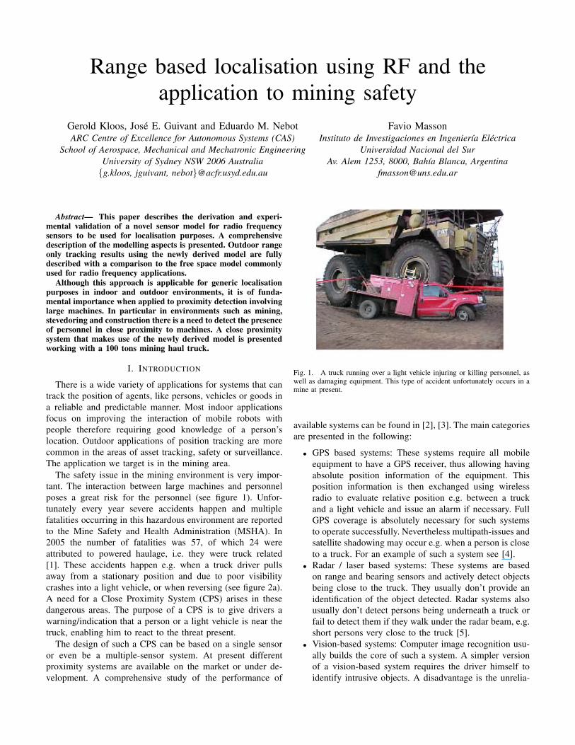
The safety issue in the mining environment is very impor-tant. The interaction between large machines and personnelposes a great risk for the personnel (see figure 1). Unfor-tunately every year severe accidents happen and multiplefatalities occurring in this hazardous environment are reportedto the Mine Safety and Health Administration (MSHA). In2005 the number of fatalities was 57, of which 24 wereattributed to powered haulage, i.e. they were truck related[1]. These accidents happen e.g. when a truck driver pullsaway from a stationary position and due to poor visibilitycrashes into a light vehicle, or when reversing (see figure 2a).A need for a Close Proximity System (CPS) arises in thesedangerous areas. The purpose of a CPS is to give drivers awarning/indication that a person or a light vehicle is near thetruck, enabling him to react to the threat present.

The design of such a CPS can be based on a single sensoror even be a multiple-sensor system. At present differentproximity systems are available on the market or under de-velopment. A comprehensive study of the performance of

Fig. 1. A truck running over a light vehicle injuring or killing personnel, aswell as damaging equipment. This type of accident unfortunately occurs in amine at present.

available systems can be found in [2], [3]. The main categoriesare presented in the following:

• GPS based systems: These systems require all mobileequipment to have a GPS receiver, thus allowing havingabsolute position information of the equipment. Thisposition information is then exchanged using wirelessradio to evaluate relative position e.g. between a truckand a light vehicle and issue an alarm if necessary. FullGPS coverage is absolutely necessary for such systemsto operate successfully. Nevertheless multipath-issues andsatellite shadowing may occur e.g. when a person is closeto a truck. For an example of such a system see [4].

• Radar / laser based systems: These systems are basedon range and bearing sensors and actively detect objectsbeing close to the truck. They usually don’t provide anidentification of the object detected. Radar systems alsousually don’t detect persons being underneath a truck orfail to detect them if they walk under the radar beam, e.g.short persons very close to the truck [5].

• Vision-based systems: Computer image recognition usu-ally builds the core of such a system. A simpler versionof a vision-based system requires the driver himself toidentify intrusive objects. A disadvantage is the unrelia-

Cab PillarCab Pillar

Door PillarMirror, Door Pillar

730 E

Driverscabin

Blind spots when sitting in drivers cabin

50m radius

(a)

Legend

Truck

Pedestrian with RFID tag

RFID tag reader

RFID connection

(b) (c)

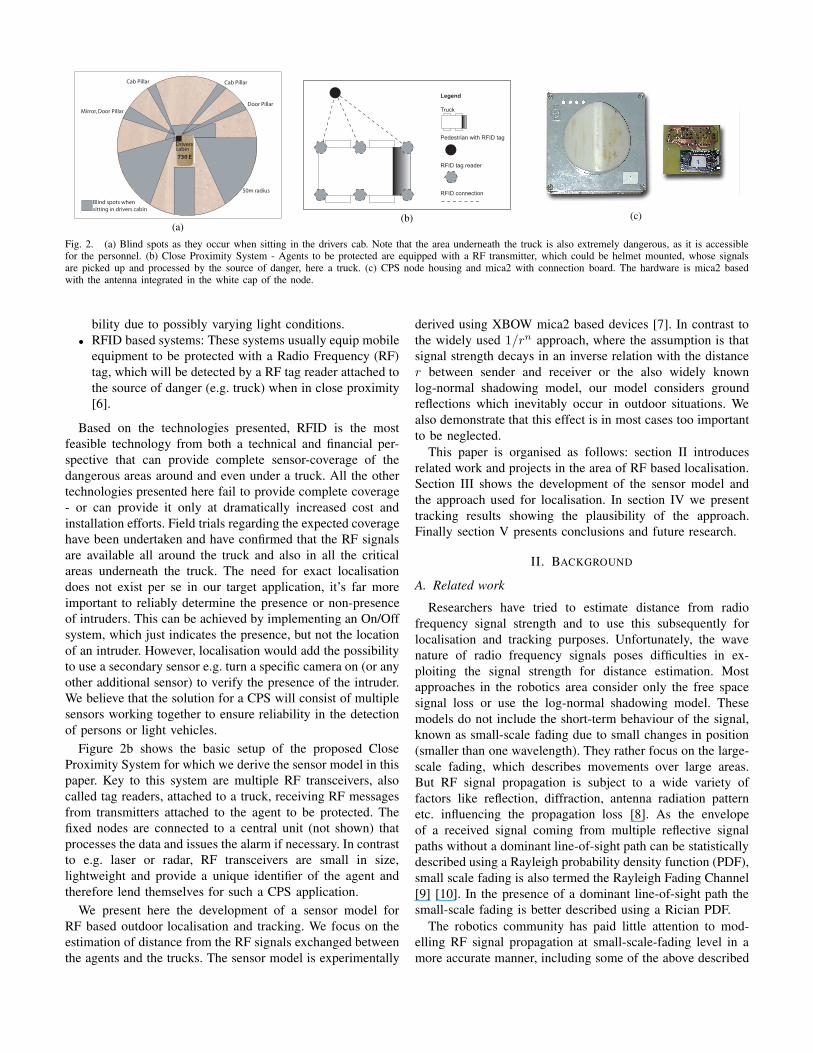
Fig. 2. (a) Blind spots as they occur when sitting in the drivers cab. Note that the area underneath the truck is also extremely dangerous, as it is accessiblefor the personnel. (b) Close Proximity System - Agents to be protected are equipped with a RF transmitter, which could be helmet mounted, whose signalsare picked up and processed by the source of danger, here a truck. (c) CPS node housing and mica2 with connection board. The hardware is mica2 basedwith the antenna integrated in the white cap of the node.

bility due to possibly varying light conditions.• RFID based systems: These systems usually equip mobile

equipment to be protected with a Radio Frequency (RF)tag, which will be detected by a RF tag reader attached tothe source of danger (e.g. truck) when in close proximity[6].

Based on the technologies presented, RFID is the mostfeasible technology from both a technical and financial per-spective that can provide complete sensor-coverage of thedangerous areas around and even under a truck. All the othertechnologies presented here fail to provide complete coverage- or can provide it only at dramatically increased cost andinstallation efforts. Field trials regarding the expected coveragehave been undertaken and have confirmed that the RF signalsare available all around the truck and also in all the criticalareas underneath the truck. The need for exact localisationdoes not exist per se in our target application, it’s far moreimportant to reliably determine the presence or non-presenceof intruders. This can be achieved by implementing an On/Offsystem, which just indicates the presence, but not the locationof an intruder. However, localisation would add the possibilityto use a secondary sensor e.g. turn a specific camera on (or anyother additional sensor) to verify the presence of the intruder.We believe that the solution for a CPS will consist of multiplesensors working together to ensure reliability in the detectionof persons or light vehicles.

Figure 2b shows the basic setup of the proposed CloseProximity System for which we derive the sensor model in thispaper. Key to this system are multiple RF transceivers, alsocalled tag readers, attached to a truck, receiving RF messagesfrom transmitters attached to the agent to be protected. Thefixed nodes are connected to a central unit (not shown) thatprocesses the data and issues the alarm if necessary. In contrastto e.g. laser or radar, RF transceivers are small in size,lightweight and provide a unique identifier of the agent andtherefore lend themselves for such a CPS application.

We present here the development of a sensor model forRF based outdoor localisation and tracking. We focus on theestimation of distance from the RF signals exchanged betweenthe agents and the trucks. The sensor model is experimentally

derived using XBOW mica2 based devices [7]. In contrast tothe widely used 1/rn approach, where the assumption is thatsignal strength decays in an inverse relation with the distancer between sender and receiver or the also widely knownlog-normal shadowing model, our model considers groundreflections which inevitably occur in outdoor situations. Wealso demonstrate that this effect is in most cases too importantto be neglected.

This paper is organised as follows: section II introducesrelated work and projects in the area of RF based localisation.Section III shows the development of the sensor model andthe approach used for localisation. In section IV we presenttracking results showing the plausibility of the approach.Finally section V presents conclusions and future research.

II. BACKGROUND

A. Related work

Researchers have tried to estimate distance from radiofrequency signal strength and to use this subsequently forlocalisation and tracking purposes. Unfortunately, the wavenature of radio frequency signals poses difficulties in ex-ploiting the signal strength for distance estimation. Mostapproaches in the robotics area consider only the free spacesignal loss or use the log-normal shadowing model. Thesemodels do not include the short-term behaviour of the signal,known as small-scale fading due to small changes in position(smaller than one wavelength). They rather focus on the large-scale fading, which describes movements over large areas.But RF signal propagation is subject to a wide variety offactors like reflection, diffraction, antenna radiation patternetc. influencing the propagation loss [8]. As the envelopeof a received signal coming from multiple reflective signalpaths without a dominant line-of-sight path can be statisticallydescribed using a Rayleigh probability density function (PDF),small scale fading is also termed the Rayleigh Fading Channel[9] [10]. In the presence of a dominant line-of-sight path thesmall-scale fading is better described using a Rician PDF.

The robotics community has paid little attention to mod-elling RF signal propagation at small-scale-fading level in amore accurate manner, including some of the above described

Transmitter

ReceiverDirect ray

Ground-reflected ray

Fig. 3. RF signal reflection - the two-ray model. The receiver sees the sumof both signal rays from the transmitter, the direct line-of-sight ray and theground reflected ray.

effects. This is probably due to the fact that most of theresearch is done for indoor environments, where small-scalefading would be harder to model as the environment ismuch more complex compared to an outdoor environmentas encountered e.g. in mining. Independent of the type ofenvironment, more accurate modelling of the RF propagationis the key to achieve higher accuracy for localisation andtracking purposes, as will be shown in subsection II-B.

A large number of papers are concerned with localisationusing RF signals. We showcase just some of the approachespresented. A sensor model for RFID can be found in [11]used in an indoor application. The authors show a simplifiedprobabilistic (discrete) sensor model for antennas receivingsignals from RFID tags. Using RFID tags distributed inan indoor environment at known locations, they localise amobile robot. To overcome the simplifications in their sensormodel, the number of distributed RFID tags is large. Anotherprobabilistic model for sensor localisation is shown in [12]. Itis based on the log-normal-shadowing model and also assumesa log-normal distribution of the possible distances for packetsreceived with a certain signal strength. The influences of themultipath fading here are included in an increased signalvariance. A map based approach for indoor localisation usingparticle filters and a wireless map is presented in [13]. Nosensor model is presented, instead a signal strength map ofthe environment is built. This is time consuming and requiresa new map to be built when the environment changes. Acomparison between a map based approach and the log-normalmodel can be found in [14]. Finally, a time of flight (TOF)localisation approach using RF signals is shown in [15]. Thistechnique has increased accuracy, but poses a higher demandon the hardware as it needs a high accuracy clock, thus makingit more expensive than e.g. Received Signal Strength Indicator(RSSI) based solutions.

B. Signal propagation

In any real application RF signals will be subjected to reflec-tions, at least one reflection from the ground will inevitablyoccur. This situation is shown in figure 3. The paths fromthe transmitter to the receiver will have different lengths, andtherefore the signals will arrive at the receiver with a differentphase. As the receiver sees the sum of all existing signal paths,the path or phase difference will lead to a so-called path gain,which will be different from 1. The gain can be greater than

1 if the rays interfere in a constructive manner, or smallerif they interfere in a destructive manner with each other. Inthis scenario the received power Pr can be calculated usingequation 1. This equation includes the free space loss, but alsothe components due to reflection. The path lengths are also afunction of the antenna installation heights.

Pr(d) = Pt

(λ

4πd

)2∣∣∣∣∣

N∑i=1

Γi(αi)ri

exp(−jkri)

∣∣∣∣∣2

(1)

Here λ is the wave-length of the RF-signal centre frequency,d denotes the horizontal distance between transmitter andreceiver, Γi is the reflection coefficient of the i-th ray as givenby equation 2, αi is the angle of incidence of the i-th rayon the reflecting surface and ri is the path length of the i-thray. k = 2πf

c with f being the frequency of the signal and cthe constant for speed of light. For the line-of-sight ray thereflection coefficient is taken to be 1. The reflection coefficientΓ is given by

Γ(θ) =cos θ − a

√εr − sin2 θ

cos θ + a√

εr − sin2 θ(2)

where θ = 90 − α and a = 1/ε for vertical polarization or 1for horizontal polarization. εr is the relative dielectric constant,e.g. for dry soil approx. 2.5. This constant is different for eachtype of surface and will therefore influence the propagationbehaviour of the RF signals. The evaluation of the RF signalbehaviour for different surfaces has still to be done.

Figure 4 shows the theoretical path gain for the two-raymodel. One can see that the signal oscillates at high spatialfrequency for small distances and that the spatial oscillationfrequency decreases with increasing distance. Most of theRF sensor models like e.g. the log-normal shadowing modelneglect these oscillations. Including information about the

0 5 10 15 20 2510

−14

10−12

10−10

10−8

10−6

10−4

10−2

100

Total path gain

Distance [m]

Tot

al p

ath

gain

in fr

ee s

pace

Fig. 4. Theoretical RF signal path gain for one ground reflection considered.The path gain is the product of free space attenuation and the relative gaindue to reflection. Transmitter height is 2.5m, receiver height is 1.75m andtransmission frequency is 900 MHz.

Fig. 5. Test setup. The three receivers were mounted at three different heightson a pole. The transmitter (a mica2 mote, not shown here) was also mountedon a pole, which was moved in a continuous (radial) path. Its position waslogged using RTK-GPS for reference purposes.

RF signal oscillations into a sensor model can theoreticallyimprove the performance of localisation algorithms.

III. RF SENSOR MODELLING

Correct sensor modelling forms the core for accurate local-isation. We show here how we model the signal distributionfor a fixed angle between transmitter and receiver. The signalis often also a function of the angle between transmitterand receiver, when the antennas exhibit a non-omnidirectionalradiation pattern. For the hardware used this has already beenverified by the authors and is subject to further work to modelthis behaviour. The radio (antenna pattern) irregularities forthe XBOW mica2 are described in more detail in [16].

A. Real data recording - the test setup

For our experiments we used hardware based on XBOWmica2. The rough mining environment makes it necessary toenclose the hardware in a tough housing as shown in figure 2c.To record data for the sensor model the setup was as shownin figure 5: Three receiving nodes were installed on a pole atdifferent heights (2.0m, 2.5m and 3.0m). A sending node wasinstalled on top of another pole at a fixed height of 1.75m (notshown in the figure). The sender was moved and its positionlogged using RTK-GPS. The sender was sending messages,which were picked up by the three receivers. The RSSI ofthese messages was logged for each receiving sensor nodeindividually and could be correlated to the GPS position of thesender and thus to the distance between sender and receiver.

B. Evaluation of the RSSI signal mean vs. distance

To evaluate the RSSI signal mean vs. distance between thenodes, the transmitter was moved at a constant angle in aradial path away from the receivers at slow speed (figure 12a).A large number of RSSI values, about 1 value every 1cmof distance travelled, were thus logged. An example of theresulting plot for sensor #1 can be seen in figure 6 (top). Aspreviously shown the signal depends also on the height of the

2 4 6 8 10 12 14 16 18 20−100

−80

−60

Original datapoints

2 4 6 8 10 12 14 16 18 20−100

−50Exponential component

Rec

eive

d S

igna

l Str

engt

h [d

Bm

]

2 4 6 8 10 12 14 16 18 20

−10

0

10

Sinusoidal component

Distance [m]

Fig. 6. Signal components - Top shows the original data-points received- Middle shows the exponential approximation to the original data-points -Bottom shows the difference between the original data-points (top) and theexponential approximation (middle), which will be modelled using Fourierseries

sensors, therefore it was expected to have a different curve foreach of the three sensors. This was also verified and can beseen later on.

As previously described, in any real occurring situation,the signal at a receiver will at the very least consist of thefree space component due to the direct ray and additionalcomponents from reflections. As shown in section II-B thedirect signal path can be modelled as a free space approx-imation, while the reflection component will involve sineterms. Therefore we chose to model the signal as the sum ofan exponential approximation (see equation 3), depicting thefree space loss, and a Fourier series (see equation 4) for thereflective component. The free space component (see figure6 (middle) for an example for sensor #1) is mathematicallydescribed by:

fexp(x) = aebx + cedx (3)

Here a, b, c and d are parameters, while x is the horizontaldistance between sender and receiver, corresponding to thehorizontal distance d from equation 1. These parameters werefound using the least squares method. We chose this formas it can approximate the free space loss sufficiently throughappropriate choice of the parameters. At the same time it offersthe flexibility to better approximate the real occuring signalbehaviour, which does not adhere to the strict free space lossformula. The reflective component (see figure 6 (bottom) foran example for sensor #1) can be approximated by:

frefl(x) =∞∑

k=−∞ckejkωx (4)

The ck are the complex Fourier coefficients, while ω is theangular frequency 2πf , f being the fixed spatial samplingfrequency at which the data-points were recorded. The quantityx is again the horizontal distance between transmitter andreceiver. It is not necessary to use all of the computed coeffi-cients as no benefit is gained in terms of increased localisation

−90 −80 −70 −600

500

1000

1500

Received Signal Strength [dBm]

Cou

nt

Signal variance at 0.5 m:μ = −65.93 dBm σ = 0.47 dBm

−90 −80 −70 −600

500

1000

1500

Received Signal Strength [dBm]

Cou

nt

Signal variance at 2.1 m:μ = −72.10 dBm σ = 0.55 dBm

−90 −80 −70 −600

500

1000

1500

Received Signal Strength [dBm]

Cou

nt

Signal variance at 3.9 m:μ = −76.74 dBm σ = 0.76 dBm

−90 −80 −70 −600

500

1000

1500

Received Signal Strength [dBm]

Cou

nt

Signal variance at 6.3 m:μ = −82.00 dBm σ = 0.94 dBm

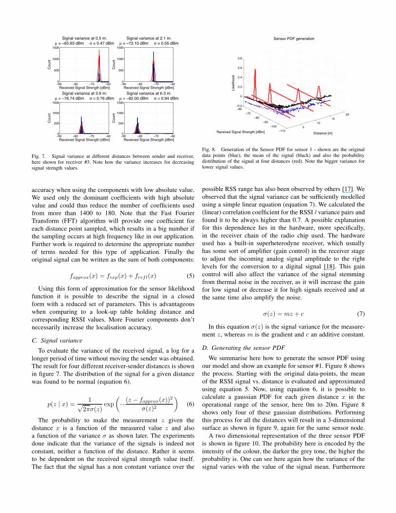
Fig. 7. Signal variance at different distances between sender and receiver,here shown for receiver #3. Note how the variance increases for decreasingsignal strength values.

accuracy when using the components with low absolute value.We used only the dominant coefficients with high absolutevalue and could thus reduce the number of coefficients usedfrom more than 1400 to 180. Note that the Fast FourierTransform (FFT) algorithm will provide one coefficient foreach distance point sampled, which results in a big number ifthe sampling occurs at high frequency like in our application.Further work is required to determine the appropriate numberof terms needed for this type of application. Finally theoriginal signal can be written as the sum of both components:

fapprox(x) = fexp(x) + frefl(x) (5)

Using this form of approximation for the sensor likelihoodfunction it is possible to describe the signal in a closedform with a reduced set of parameters. This is advantageouswhen comparing to a look-up table holding distance andcorresponding RSSI values. More Fourier components don’tnecessarily increase the localisation accuracy.

C. Signal variance

To evaluate the variance of the received signal, a log for alonger period of time without moving the sender was obtained.The result for four different receiver-sender distances is shownin figure 7. The distribution of the signal for a given distancewas found to be normal (equation 6).

p(z | x) =1√

2πσ(z)exp

(− (z − fapprox(x))2

σ(z)2

)(6)

The probability to make the measurement z given thedistance x is a function of the measured value z and alsoa function of the variance σ as shown later. The experimentsdone indicate that the variance of the signals is indeed notconstant, neither a function of the distance. Rather it seemsto be dependent on the received signal strength value itself.The fact that the signal has a non constant variance over the

5

10

15

20

−110

−100

−90

−80

−70

−60−0.2

0

0.2

0.4

0.6

0.8

Distance [m]

Sensor PDF generation

Received Signal Strength [dBm]

Like

lihoo

d

Fig. 8. Generation of the Sensor PDF for sensor 1 - shown are the originaldata points (blue), the mean of the signal (black) and also the probabilitydistribution of the signal at four distances (red). Note the bigger variance forlower signal values.

possible RSS range has also been observed by others [17]. Weobserved that the signal variance can be sufficiently modelledusing a simple linear equation (equation 7). We calculated the(linear) correlation coefficient for the RSSI / variance pairs andfound it to be always higher than 0.7. A possible explanationfor this dependence lies in the hardware, more specifically,in the receiver chain of the radio chip used. The hardwareused has a built-in superheterodyne receiver, which usuallyhas some sort of amplifier (gain control) in the receiver stageto adjust the incoming analog signal amplitude to the rightlevels for the conversion to a digital signal [18]. This gaincontrol will also affect the variance of the signal stemmingfrom thermal noise in the receiver, as it will increase the gainfor low signal or decrease it for high signals received and atthe same time also amplify the noise.

σ(z) = mz + c (7)

In this equation σ(z) is the signal variance for the measure-ment z, whereas m is the gradient and c an additive constant.

D. Generating the sensor PDF

We summarise here how to generate the sensor PDF usingour model and show an example for sensor #1. Figure 8 showsthe process. Starting with the original data-points, the meanof the RSSI signal vs. distance is evaluated and approximatedusing equation 5. Now, using equation 6, it is possible tocalculate a gaussian PDF for each given distance x in theoperational range of the sensor, here 0m to 20m. Figure 8shows only four of these gaussian distributions. Performingthis process for all the distances will result in a 3-dimensionalsurface as shown in figure 9, again for the same sensor node.

A two dimensional representation of the three sensor PDFis shown in figure 10. The probability here is encoded by theintensity of the colour, the darker the grey tone, the higher theprobability is. One can see here again how the variance of thesignal varies with the value of the signal mean. Furthermore

Distance [m]

RS

S [d

Bm

]Sensor 1 PDF

0 5 10 15 20−100

−95

−90

−85

−80

−75

−70

−65

−60

−55

−50

0.1 0.2 0.3 0.4 0.5 0.6 0.7 0.8 0.9

(a)

Distance [m]

RS

S [d

Bm

]

Sensor 2 PDF

0 5 10 15 20−100

−95

−90

−85

−80

−75

−70

−65

−60

−55

−50

0.1 0.2 0.3 0.4 0.5 0.6 0.7 0.8 0.9

(b)

Distance [m]

RS

S [d

Bm

]

Sensor 3 PDF

0 5 10 15 20−100

−95

−90

−85

−80

−75

−70

−65

−60

−55

−50

0.1 0.2 0.3 0.4 0.5 0.6 0.7 0.8 0.9

(c)

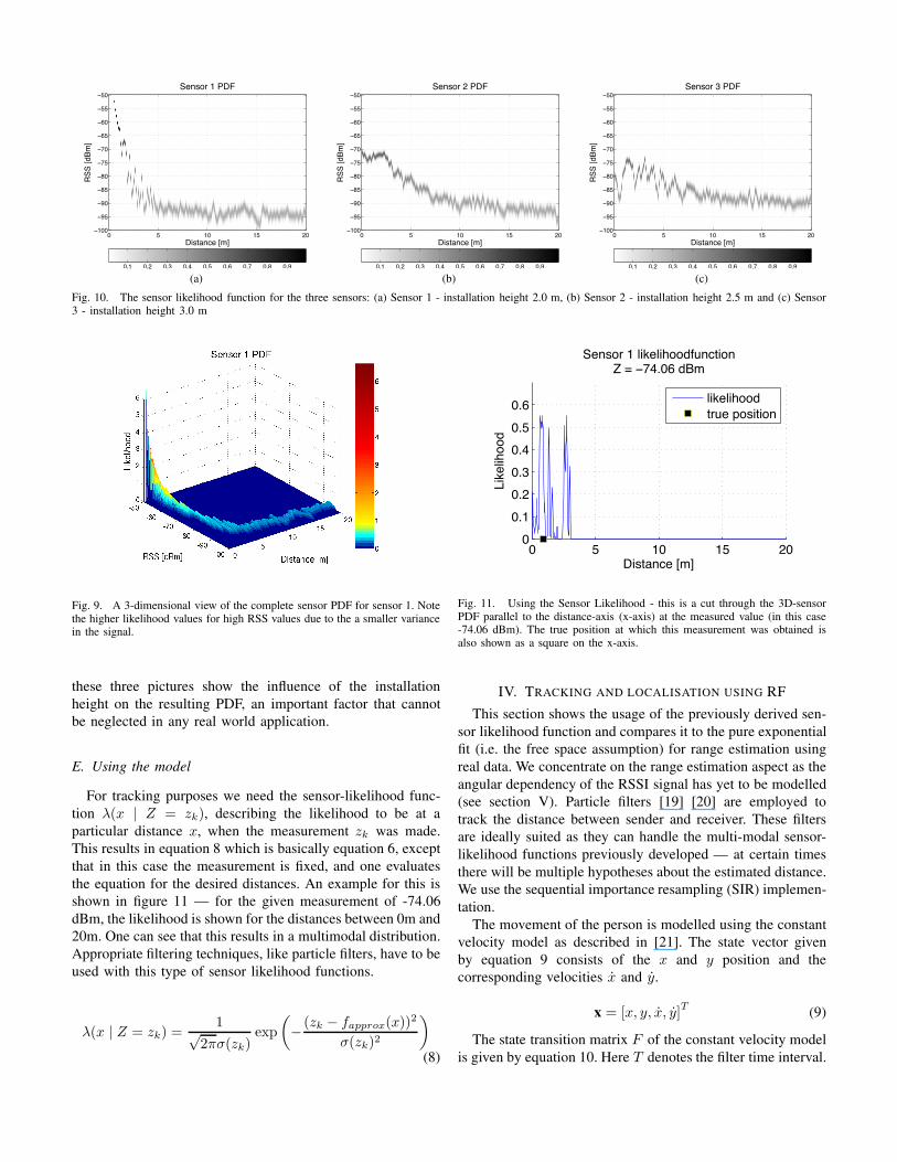
Fig. 10. The sensor likelihood function for the three sensors: (a) Sensor 1 - installation height 2.0 m, (b) Sensor 2 - installation height 2.5 m and (c) Sensor3 - installation height 3.0 m

Fig. 9. A 3-dimensional view of the complete sensor PDF for sensor 1. Notethe higher likelihood values for high RSS values due to the a smaller variancein the signal.

these three pictures show the influence of the installationheight on the resulting PDF, an important factor that cannotbe neglected in any real world application.

E. Using the model

For tracking purposes we need the sensor-likelihood func-tion λ(x | Z = zk), describing the likelihood to be at aparticular distance x, when the measurement zk was made.This results in equation 8 which is basically equation 6, exceptthat in this case the measurement is fixed, and one evaluatesthe equation for the desired distances. An example for this isshown in figure 11 — for the given measurement of -74.06dBm, the likelihood is shown for the distances between 0m and20m. One can see that this results in a multimodal distribution.Appropriate filtering techniques, like particle filters, have to beused with this type of sensor likelihood functions.

λ(x | Z = zk) =1√

2πσ(zk)exp

(− (zk − fapprox(x))2

σ(zk)2

)

(8)

0 5 10 15 200

0.1

0.2

0.3

0.4

0.5

0.6

Distance [m]

Like

lihoo

d

Sensor 1 likelihoodfunctionZ = −74.06 dBm

likelihoodtrue position

Fig. 11. Using the Sensor Likelihood - this is a cut through the 3D-sensorPDF parallel to the distance-axis (x-axis) at the measured value (in this case-74.06 dBm). The true position at which this measurement was obtained isalso shown as a square on the x-axis.

IV. TRACKING AND LOCALISATION USING RF

This section shows the usage of the previously derived sen-sor likelihood function and compares it to the pure exponentialfit (i.e. the free space assumption) for range estimation usingreal data. We concentrate on the range estimation aspect as theangular dependency of the RSSI signal has yet to be modelled(see section V). Particle filters [19] [20] are employed totrack the distance between sender and receiver. These filtersare ideally suited as they can handle the multi-modal sensor-likelihood functions previously developed — at certain timesthere will be multiple hypotheses about the estimated distance.We use the sequential importance resampling (SIR) implemen-tation.

The movement of the person is modelled using the constantvelocity model as described in [21]. The state vector givenby equation 9 consists of the x and y position and thecorresponding velocities x and y.

x = [x, y, x, y]T (9)

The state transition matrix F of the constant velocity modelis given by equation 10. Here T denotes the filter time interval.

F =

⎡⎢⎢⎣

1 0 T 00 1 0 T0 0 1 00 0 0 1

⎤⎥⎥⎦ (10)

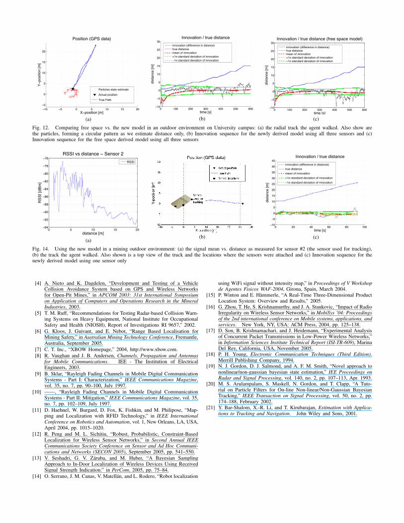
The observation Z consists of the RSSI measurement fromthe fixed nodes. Figure 12a shows the almost radial track themobile node took in the University environment. To evaluatethe performance of the model, we define an innovation ν tobe the difference of the true distance dtrue between receiverand transmitter and the estimated distance dest between them.

ν = dtrue − dest (11)

A. University campus - open environment

Figure 12b and 12c show the above defined innovation forthe new model and the free space model respectively. Alsoshown is the one σ bound for the innovation along with themean of the innovation. For both models the one sigma boundis about 2 meters. Two observations were made regarding thebehaviour of the free space model.

First, one thing that can be seen is that the free space modelexhibits an increase in the deviation at around 400 seconds.Between 400 and 550 seconds the innovation is biased — theinnovation stays consistently below zero, as can also be seenby the mean of the innovation moving away from zero.

Second, when the agent is stationary, as for example be-tween 130 and 170 seconds or between 220 and 260 seconds,the free space model will converge to one range solution asthis sensor model is unimodal. This results in a constant valuefor the estimated range, which can be the wrong estimateddistance, as can be seen for these two time spans. In bothcases the estimated value is about 2 meters off the real valueand stays constantly. Both points can be attributed to the freespace sensor model being not accurate enough.

B. Field trials

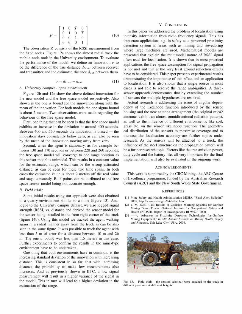
Some initial results using our approach were also obtainedin a quarry environment similar to a mine (figure 13). Ana-logue to the University campus dataset, we also logged signalstrength (RSSI) vs. distance and derived the sensor model forthe sensor being installed in the front right corner of the truck(figure 14b). Using this model we tracked the agent walkingagain in a radial manner away from the truck as can be alsoseen in the same figure. It was possible to track the agent withless than 5 m of error for a distance between 10 m and 26m. The one σ bound was less than 1.5 meters in this case.Further experiments to confirm the results in the mine-typeenvironment have to be undertaken.

One thing that both environments have in common, is theincreasing standard deviation of the innovation with increasingdistance. This is consistent in so far, that with increasingdistance the probability to make low measurements alsoincreases. And as previously shown in III-C, a low signalmeasurement will result in a higher variance of the signal inthe model. This in turn will lead to a higher deviation in theestimation of the range.

V. CONCLUSION

In this paper we addressed the problem of localisation usingintensity information from radio frequency signals. This hasimportant applications e.g. in safety as a personnel proximitydetection system in areas such as mining and stevedoringwhere large machines are used. Mathematical models arepresented that explain the multimodal nature of RSSI signaloften used for localisation. It is shown that in most practicalapplications the free space assumption for signal propagationis not met and that at the very least ground reflection effectshave to be considered. This paper presents experimental resultsdemonstrating the importance of this effect and an applicationto localisation. It is also shown that a single source in mostcases is not able to resolve the range ambiguities. A three-sensor approach demonstrates that by extending the numberof sensors the multiple hypotheses are resolved.

Actual research is addressing the issue of angular depen-dency of the likelihood function introduced by the sensorhousing and the new antenna arrangement (the original mica2antennas exhibit an almost omnidirectional radiation pattern),as well as the influence of different environments, like soil,grass etc. on the sensor likelihood function. The geometri-cal distribution of the sensors to maximise coverage and toincrease the localisation accuracy are further topics underresearch. As the sensors will be attached to a truck, theinfluence of the steel structure on the propagation pattern willbe a further research topic. Factors like the transmission power,duty cycle and the battery life, all very important for the finalimplementation, will also be evaluated in the ongoing work.

ACKNOWLEDGMENTS

This work is supported by the CRC Mining, the ARC Centreof Excellence programme, funded by the Australian ResearchCouncil (ARC) and the New South Wales State Government.

REFERENCES

[1] Mine Safety and Health Administration MSHA, “Fatal Alert Bulletin,”2005, http://www.msha.gov/fatals/fab.htm.

[2] T. M. Ruff, “Test Results of Collision Warning Systems for SurfaceMining Dump Trucks, National Institute for Occupational Safety andHealth (NIOSH), Report of Investigations RI 9652,” 2000.

[3] ——, “Advances in Proximity Detection Technologies for SurfaceMining Equipment,” in 34th Annual Institute on Mining Health, Safetyand Research, Salt Lake City, USA, 2004.

Fig. 13. Field trials - the sensors (circled) were attached to the truck indifferent positions at different heights.

Position (GPS data)

X−position [m]

Y−

posi

tion

[m]

−10 −5 0 5 10 15 20

−5

0

5

10

15

20

Particles state estimate

Actual position

True Path

(a)

Innovation / true distance

time [s]

dist

ance

[m]

0 100 200 300 400 500 600−10

−5

0

5

10

15

20

25

30innovation (difference in dstance)true distancemean of innovation+1σ standard deviation of innovation−1σ standard deviation of innovation

(b)

Innovation / true distance (free space model)

time [s]

dist

ance

[m]

0 100 200 300 400 500 600−10

−5

0

5

10

15

20

25

30

innovation (difference in distance)true distancemean of innovation+1σ standard deviation of innovation−1σ standard deviation of innovation

(c)

Fig. 12. Comparing free space vs. the new model in an outdoor environment on University campus: (a) the radial track the agent walked. Also show arethe particles, forming a circular pattern as we estimate distance only, (b) Innovation sequence for the newly derived model using all three sensors and (c)Innovation sequence for the free space derived model using all three sensors

0 5 10 15 20−94

−92

−90

−88

−86

−84

−82

−80

−78

−76

distance [m]

RS

SI [

dBm

]

RSSI vs distance − Sensor 2

RSSI

(a)(b)

Innovation / true distance

time [s]

dist

ance

[m]

0 20 40 60 80 100−10

−5

0

5

10

15

20

25

30

35

40

45innovation (difference in distance)

true distance

mean of innovation

+1σ standard deviation of innovation

−1σ standard deviation of innovation

(c)

Fig. 14. Using the new model in a mining outdoor environment: (a) the signal mean vs. distance as measured for sensor #2 (the sensor used for tracking),(b) the track the agent walked. Also shown is a top view of the truck and the locations where the sensors were attached and (c) Innovation sequence for thenewly derived model using one sensor only

[4] A. Nieto and K. Dagdelen, “Development and Testing of a VehicleCollision Avoidance System based on GPS and Wireless Networksfor Open-Pit Mines,” in APCOM 2003: 31st International Symposiumon Application of Computers and Operations Research in the MineralIndustries, 2003.

[5] T. M. Ruff, “Recommendations for Testing Radar-based Collision Warn-ing Systems on Heavy Equipment, National Institute for OccupationalSafety and Health (NIOSH), Report of Investigations RI 9657,” 2002.

[6] G. Kloos, J. Guivant, and E. Nebot, “Range Based Localisation forMining Safety,” in Australian Mining Technology Conference, Fremantle,Australia, September 2005.

[7] C. T. Inc., “XBOW Homepage,” 2004, http://www.xbow.com.[8] R. Vaughan and J. B. Andersen, Channels, Propagation and Antennas

for Mobile Communications. IEE - The Institution of ElectricalEngineers, 2003.

[9] B. Sklar, “Rayleigh Fading Channels in Mobile Digital CommunicationSystems - Part I: Characterization,” IEEE Communications Magazine,vol. 35, no. 7, pp. 90–100, July 1997.

[10] ——, “Rayleigh Fading Channels in Mobile Digital CommunicationSystems - Part II: Mitigation,” IEEE Communications Magazine, vol. 35,no. 7, pp. 102–109, July 1997.

[11] D. Haehnel, W. Burgard, D. Fox, K. Fishkin, and M. Philipose, “Map-ping and Localization with RFID Technology,” in IEEE InternationalConference on Robotics and Automation, vol. 1, New Orleans, LA, USA,April 2004, pp. 1015–1020.

[12] R. Peng and M. L. Sichitiu, “Robust, Probabilistic, Constraint-BasedLocalization for Wireless Sensor Networks,” in Second Annual IEEECommunications Society Conference on Sensor and Ad Hoc Communi-cations and Networks (SECON 2005), September 2005, pp. 541–550.

[13] V. Seshadri, G. V. Zaruba, and M. Huber, “A Bayesian SamplingApproach to In-Door Localization of Wireless Devices Using ReceivedSignal Strength Indication.” in PerCom, 2005, pp. 75–84.

[14] O. Serrano, J. M. Canas, V. Matellan, and L. Rodero, “Robot localization

using WiFi signal without intensity map,” in Proceedings of V Workshopde Agentes Fisicos WAF-2004, Girona, Spain, March 2004.

[15] P. Winton and E. Hammerle, “A Real-Time Three-Dimensional ProductLocation System: Overview and Results,” 2005.

[16] G. Zhou, T. He, S. Krishnamurthy, and J. A. Stankovic, “Impact of RadioIrregularity on Wireless Sensor Networks,” in MobiSys ’04: Proceedingsof the 2nd international conference on Mobile systems, applications, andservices. New York, NY, USA: ACM Press, 2004, pp. 125–138.

[17] D. Son, B. Krishnamachari, and J. Heidemann, “Experimental Analysisof Concurrent Packet Transmissions in Low-Power Wireless Networks,”in Information Sciences Institute Technical Report (ISI-TR-609), MarinaDel Rey, California, USA, November 2005.

[18] P. H. Young, Electronic Communication Techniques (Third Edition).Merrill Publishing Company, 1994.

[19] N. J. Gordon, D. J. Salmond, and A. F. M. Smith, “Novel approach tononlinear/non-gaussian bayesian state estimation,” IEE Proceedings onRadar and Signal Processing, vol. 140, no. 2, pp. 107–113, Apr. 1993.

[20] M. S. Arulampalam, S. Maskell, N. Gordon, and T. Clapp, “A Tuto-rial on Particle Filters for On-line Non-linear/Non-Gaussian BayesianTracking,” IEEE Transaction on Signal Processing, vol. 50, no. 2, pp.174–188, February 2002.

[21] Y. Bar-Shalom, X.-R. Li, and T. Kirubarajan, Estimation with Applica-tions to Tracking and Navigation. John Wiley and Sons, 2001.