Journal of Hydrology 501 (2013) 133–145

Contents lists available at ScienceDirect

Journal of Hydrology

journal homepage: www.elsevier .com/ locate / jhydrol

Rainwater lens dynamics and mixing between infiltrating rainwaterand upward saline groundwater seepage beneath a tile-drainedagricultural field

0022-1694/$ - see front matter � 2013 Elsevier B.V. All rights reserved.http://dx.doi.org/10.1016/j.jhydrol.2013.07.026

⇑ Corresponding author. Tel.: +31 (0)6 30548000; fax: +31 (0)88 335 7856.E-mail address: Perry.deLouw@deltares.nl (P.G.B. de Louw).

P.G.B. de Louw a,⇑, S. Eeman b, G.H.P. Oude Essink a, E. Vermue b, V.E.A. Post c

a Deltares, Dept. of Soil and Groundwater, P.O. Box 85467, 3508 AL Utrecht, The Netherlandsb Wageningen University, Environmental Sciences Group, Soil Physics, Ecohydrology and Groundwater Management, P.O. Box 47, 6700 AA Wageningen, The Netherlandsc School of the Environment, National Centre for Groundwater Research and Training, Flinders University, GPO Box 2100, Adelaide SA 5001, Australia

a r t i c l e i n f o

Article history:Received 26 March 2013Received in revised form 12 July 2013Accepted 17 July 2013Available online 24 July 2013This manuscript was handled by CorradoCorradini, Editor-in-Chief, with theassistance of Juan V. Giraldez, AssociateEditor

Keywords:Rainwater lensSaline seepageSalinizationLens dynamicsMixingMonitoring

s u m m a r y

Thin rainwater lenses (RW-lenses) near the land surface are often the only source of freshwater in agri-cultural areas with regionally-extensive brackish to saline groundwater. The seasonal and inter-annualdynamics of these lenses are poorly known. Here this knowledge gap is addressed by investigating thetransient flow and mixing processes in RW-lenses beneath two tile-drained agricultural fields in theNetherlands. Evidence of RW-lens dynamics was systematically collected by monthly ground- and soilwater sampling, in combination with daily observations of water table elevation, drain tile dischargeand drain water salinity. Based on these data, and numerical modeling of the key lens characteristics,a conceptual model of seasonal lens dynamics is presented. It is found that variations in the positionof the mixing zone and mixing zone salinities are small and vary on a seasonal timescale, which is attrib-uted to the slow transient oscillatory flow regime in the deepest part of the lens. The flow and mixingprocesses are faster near the water table, which responds to recharge and evapotranspiration at a time-scale less than a day. Variations of drain tile discharge and drain water salinity are also very dynamic asthey respond to individual rain events. Salinities of soil water can become significantly higher than in thegroundwater. This is attributed to the combined effect of capillary rise of saline groundwater during dryperiods and incomplete flushing by infiltrating freshwater due to preferential flow through cracks in thesoil. The results of this study are the key to understanding the potential impact of future climate changeand to designing effective mitigating measures such as adapting tile-drainage systems to ensure thefuture availability of freshwater for agriculture.

� 2013 Elsevier B.V. All rights reserved.

1. Introduction

In many coastal areas worldwide, groundwater is brackish tosaline because of the combined effects of seawater intrusion andmarine transgressions (e.g. Post and Abarca, 2010; Werner et al.,2013). In such areas, freshwater lenses recharged by rainwaterare often the only water resource available for agriculture anddrinking water. The best-known type of freshwater lens is the Ba-don Ghijben–Herzberg (BGH) lens (Drabbe and Badon Ghijben,1889; Herzberg, 1901), which develops in areas with salinegroundwater where recharge creates an elevated water table inareas like dune belts along the coast (e.g. Stuyfzand, 1993;Vandenbohede et al., 2008), below islands (e.g. Chidley and Lloyd,1977; Underwood et al., 1992), and even in inland desert areas (e.g.Kwarteng et al., 2000).

Another type of a rainwater-fed lens forms in areas wheresaline groundwater migrates to the surface by upward groundwa-ter flow (referred to here as seepage), such as the coastal area ofthe Netherlands (De Louw et al., 2011; Velstra et al., 2011) andBelgium (Vandenbohede et al., 2010) and the Po-delta, Italy(Antonellini et al., 2008). They differ from BGH-lenses in that theupward moving saline groundwater limits the penetration depthof rainwater, and thus the volume of the freshwater lens (De Louwet al., 2011; Eeman et al., 2011). Field measurements by De Louwet al. (2011) in the south-western delta of the Netherlands showedthat the transition zone between infiltrated rainwater and upwardseeping saline groundwater occurs within 2 m below ground level(BGL) and that nearly all mapped lenses lacked truly fresh ground-water (chloride concentration <0.3 g L�1). These lenses are theobject of the current study, and are referred to as RW-lenses. Forthe purpose of this study, the vertical extent of the RW-lens isbounded by the water table and the depth below which no rainwa-ter penetrates (Bmix, which is the depth at which the salinity equals

134 P.G.B. de Louw et al. / Journal of Hydrology 501 (2013) 133–145

the salinity of regional groundwater, Fig. 1). With this definition,the RW-lens is not purely a freshwater lens, and salinities withinthe RW-lens vary both in space and in time.

The dynamic behavior of salinities within RW-lenses and thesoil moisture in the unsaturated zone above them is of greatimportance from an agricultural perspective. It is expected thatlens thickness and mixing zone properties are not steady stateand will respond to temporal recharge variations at intra- and in-ter-annual timescales, as well as to seepage variations on a longertimescale. Due to their limited size and vicinity to the land surface,RW-lenses are vulnerable to changing precipitation and evapo-transpiration (which control recharge) patterns. During dry peri-ods, saline groundwater can reach the root zone via capillaryrise, affecting crop growth (Katerji et al., 2003; Rozema and Flow-ers, 2008). Besides recharge and seepage, another important factorthat controls the size of the RW-lens is tile drainage (De Louwet al., 2011; Velstra et al., 2011). Adapting drainage systems hasbeen proposed as an effective water management strategy to mit-igate the predicted adverse consequences of increased drought andsea level rise (e.g. Poulter et al., 2008). The latter may enhance up-ward seepage rates (Maas, 2007; De Louw et al., 2011; Eeman et al.,2011, 2012), thus negatively impacting the freshwater volumestored in RW-lenses.

Successful implementation of any measure to make the RW-lenses more resilient to future climate change requires knowledgeof their dynamic behavior. So far, research into lens dynamics hasmainly been focused on BGH-freshwater lenses (e.g. Drabbe andBadon Ghijben, 1889; Herzberg, 1901; Meinardi, 1983; Underwoodet al., 1992; Collins and Easley, 1999; Bakker, 2000; Stoeckl andHouben, 2012). Stoeckl and Houben (2012) examined the develop-ment and flow dynamics of freshwater lenses by physical experi-ments on laboratory scale. Underwood et al. (1992) examinedthe dynamic behavior of the mixing zone of a BGH-lens of a gener-alized atoll groundwater system and found that mixing is con-trolled by oscillating vertical flow due to tidal fluctuation, whilerecharge determines lens thickness. On Jeju Island (Korea), mea-surements showed small tidally-induced variations, but no long-term seasonal variation of the fresh–salt water interface (Kimet al., 2006). In BGH-lenses the response to recharge variations isin the order of decades (e.g. Vaeret et al., 2011; Oude Essink,1996). Rotzoll et al. (2010) observed thinning rates of 0.5 to1.0 m y�1 in thick freshwater lenses in Hawaii due to long termgroundwater withdrawal and reduced recharge.

In the absence of long-term field data for RW-lenses, their re-sponse at intra-annual and inter-annual timescales remains poorly

Fig. 1. (a) Schematic cross-section visualizing the conceptual model of a RW-lens in an aconductivity (EC) of groundwater at an arbitrary point in the RW-lens. The vertical extentThe depth of the center of the mixing zone (Dmix) is at the point where the EC is 50% of

characterized and understood. De Louw et al. (2011) reported that,since temporal variations were not measured, they could not con-clusively determine if the noted absence of fresh groundwater wasa transient or a permanent feature of the RW lens. Velstra et al.(2011) used DC resistivity measurements to delineate RW-lensesin the northern coastal area of the Netherlands and found seasonalvariations in lens-thickness. However, the use of geophysics tomonitor temporal variations of shallow subsurface resistivities isdifficult due to the limited resolution, impact of unsaturated zoneconditions and non-unique interpretation of the measurementdata (Goes et al., 2009). Recently, Eeman et al. (2012) developeda theoretical relation between lens thickness variations and sinu-soidal recharge variations. Their study showed how temporalthickness variations of a RW-lens increased with increasing re-charge amplitude and with decreasing recharge frequency includ-ing damping and delay in the response of the lens, but the modelwas not corroborated with measured data. To understand the com-plex RW-lens field behavior, direct measurements of groundwaterand soil water salinities are much needed.

The intent of the present study was to address the knowledgegap that exists on the temporal dynamics of RW-lenses. To thisend, a comprehensive set of data was collected at two tile-drainedagricultural fields in the Netherlands. The data consisted ofgroundwater and soil water salinities, groundwater levels, draintile discharge and drain water salinity, precipitation andevapotranspiration. The main objectives were (i) to obtain direct,field-based evidence of RW-lens dynamics, and (ii) to quantifythe temporal variations of the flow and mixing processes withinthe RW-lens. The main focus was on the control of recharge andtile drainage. A numerical flow and transport model was used tocomplement the collected field data and to support the develop-ment of a conceptual model of RW-lens dynamics.

2. Study area

Two of the 27 agricultural sites examined by De Louw et al.(2011) were selected to monitor the RW-lens dynamics and mixingbehavior between March 2009 and January 2011. These sites werereferred to as sites 11 and 26 in De Louw et al. (2011) but here assite A and B, respectively. These sites were selected primarily be-cause of their representative hydrogeological conditions and rain-water lens characteristics, which are typical for the saline seepageareas of the south-western part of the Netherlands (De Louw et al.,2011). Practical considerations, such as accessibility of the sitesand a nearby electricity supply, also played a role. Monitoring sites

rea with upward seepage of saline groundwater. (b) Vertical profile of the electricalof the RW-lens at any point is from the base of mixing zone (Bmix) to the water table.the seepage water salinity (ECs).

P.G.B. de Louw et al. / Journal of Hydrology 501 (2013) 133–145 135

A (latitude 51�4200400N, longitude 03�5102600E) and B (latitude51�4304400N, longitude 03�4705700E) are both situated on theSchouwen-Duivenland island in the south-western part of theNetherlands (Fig. 2a). The mean annual precipitation and potentialMakkink (1957) evapotranspiration for the period 1980–2010 are815 mm and 613 mm, respectively (data from the RoyalNetherlands Meteorological Institute KNMI). Groundwater ispredominantly saline, and originates from Holocene transgressionsduring the periods 7500 BP to 5000 BP and 350 AD to 1000 AD (Vosand Zeiler, 2008; Post et al., 2003). Upward seepage of salinegroundwater occurs where the land surface lies below mean sealevel (MSL).

Site A is a 300 m long agricultural field located at the transitionfrom a former salt marsh to a tidal creek paleo-channel (Fig. 2c).Due to differential subsidence by sediment compaction, the landsurface elevation of the paleo-channel (�0.2 m MSL) is presentlyabove that of the salt marsh sediments (�0.7 m MSL). The field isbordered by ditches with a surface water level which is maintainedat an depth of 1.3 m BGL, and the field is tile-drained at a depth of1.0 m BGL with a horizontal drain separation of 10 m. Fine-grainedto medium coarse-grained sand is found between 2.5 m and 30 mBGL, which belongs to a regionally-extensive aquifer. The aquifer isconfined by 2.5 m of heterogeneous low-permeability sedimentscomprised of peat, clay and sandy clay at the former salt marshand sandy clay to clayey sand at the creek ridge (Fig. 2c). Asfreshwater head gradients between 1.5 m and 4 m depth were con-siderably larger than the relative density difference that accounts

Fig. 2. (a) Map showing the location of study sites, (b) schematic diagram showing thmeasurement point. The minimum and maximum distances between installed piezomesection at site A showing the geology, water table, vertical flow direction, the base of the Rvertical lines), and (d) plan view of site B showing the location of the measurement pointfigure legend, the reader is referred to the web version of this article.)

for the buoyancy effect, the vertical flow direction (but not themagnitude) can be inferred directly from the head measurements(Post et al., 2007). At the former salt marsh, the measured headswere permanently higher in the sandy aquifer at 4 m depth thanat 1.5 m depth in the aquitard, resulting in a continuous upwardgroundwater flow (De Louw et al., 2011, Fig. 2c). At the creek ridge,the freshwater head was lower at 4 m depth than at 1.5 m depth,indicating downward flow. Due to these different vertical flow pat-terns, the RW lenses below the former salt marsh are thin(1.5 < Bmix < 3 m) compared to the creek ridge (4 < Bmix < 10 m)(De Louw et al., 2011). Only the data collected in the former saltmarsh zone with permanent upward seepage is presented in thispaper.

Site B is located in a former salt marsh at an elevation of �2.0 mMSL and is bordered by a ditch with a surface water level main-tained at 1.1 m BGL (Fig. 2d). Drain tiles with a length of �80 mare located at a depth of 0.70 m BGL with a horizontal separationof 10 m. The upper 2.5 m of the subsoil consists of silty clay anda 0.10–0.15 cm thick peat layer at about 0.5 m depth. Between3.0 m and 4.5 m BGL a sequence of clayey fine sand and sandy clayoccurs. These low-permeability sediments form a semi-confiningunit, below which the same regionally-extensive sandy aquifer asat site A is found. Head gradients indicate that permanent upwardseepage occurs everywhere below the agricultural field, and theRW-lenses have a thickness between 1.5 and 2 m (de Louw et al.,2011). Shrinkage cracks in the clayey top soil were observed duringthe driest months of the year (May–October).

e depths below ground surface of the rhizons and piezometers installed at eachters and rhizons of a measurement point are respectively 0.5 and 2.5 m, (c) crossW-lens (Bmix, De Louw et al., 2011) and the locations of the measurement points (reds, the ditch and the drain tiles. (For interpretation of the references to colour in this

Fig. 3. (a) Schematic representation of the setup of the SEAWAT-model of the RW-lens between two drain tiles at site B. (b) The specific yield (S)-depth relation isderived from measured water table fluctuations and precipitation data using Eq. (1).

136 P.G.B. de Louw et al. / Journal of Hydrology 501 (2013) 133–145

3. Methods

3.1. Monitoring network

The monitoring networks of site A and B consisted of measure-ment points at various distances from the northwestern (site A)and western (site B) ditch, at which time-series data of groundwa-ter salinity, soil water salinity, water table elevation andhydraulic head were collected at different depths (Fig. 2c and d).The measurement points were located between two subsurfacedrain tiles, except for MP4 and MP5 of site B, which werepositioned within 0.2 m of a drain tile to assess the effect of tiledrainage (Fig. 2d).

At each measurement point a cluster of piezometers was in-stalled (Fig. 2b). Each cluster consisted of 6 or 7 piezometers with0.16 m long screens at depths (bottom of screen) of 0.8 m, 1.0 m,1.3 m, 1.6 m, 2.0 m, 3.0 m and 4.0 m BGL. Piezometers withpre-fabricated bentonite plugs of the same diameter as the augerborehole were used to avoid preferential flow. The electricalconductivity (EC) of groundwater samples was measured in thefield every month for a period of 22 months (March 2009–Decem-ber 2010). Before taking groundwater samples for measurement,all the standing water was extracted from the piezometers. Thepiezometers were then allowed to re-fill with groundwater, whichcould take up to several hours due to the low permeability of thesediments. Errors in the order of 1–5% were associated with theEC measurements due to calibration difficulties in the field.

At each measurement point a cluster of soil moisture samplers(rhizons from Rhizosphere�) were installed to obtain soil watersamples (Fig. 2b). The porous section of the rhizons had a diameterof 2.5 mm, a length of 100 mm and an average pore size of 2.5 lm.Each cluster contained 5 rhizons at depths (measured from thebottom of the porous section) of 0.15 m, 0.30 m, 0.45 m, 0.60 mand 0.75 m BGL. Suction was applied for at least 4 h, after whichthe soil water was collected and the EC was measured in the field.When the amount of collected water was insufficient for an ECmeasurement, demineralized water was added and the measuredEC was corrected for dilution. Soil water was sampled monthlyon the same days as the groundwater was sampled, for a periodof 17 months (July 2009–December 2010).

At all measurement points, the hydraulic head at 4 m depth wasrecorded between March 2009 and January 2011 with a 1-h fre-quency using data-logging pressure transducers (SchlumbergerWater Service Divers�). Measured heads were converted to equiv-alent freshwater heads using the equations presented in Post et al.(2007). The water table elevation was inferred by measuring thewater level in a piezometer with a 1.0 m long screen installed ata depth between 0.5 m and 1.5 m BGL.

At site B the drain tile discharge (Qdrain) and salinity (ECdrain)were measured from February 2010 to January 2011. The ends of2 drain tiles (Fig. 2d) were connected and the discharge waterwas collected in a container (1 m � 0.6 m � 0.6 m). A known vol-ume of water was pumped from the container automatically witha water-level-controlled-pump, and the number of pumpingevents per hour was recorded automatically. These recordingswere multiplied by the pumping volume to obtain Qdrain. Water le-vel fluctuations in the container were measured with a pressuretransducer to verify the pumped volumes and the inferred Qdrain.The EC of the collected drain water was measured hourly in a smallcompartment installed in the pipe connecting the 2 drain tilesusing a CTD-diver from Schlumberger Water Service�.

Precipitation (P) was measured at both sites with a tippingbucket rain gauge which reported rainfall at 1-h intervals. Dailysums of the potential Makkink (1957) evapotranspiration (ETp)were obtained from the nearest meteorological station of the KNMI

(Wilhelminadorp, at 23 and 19 km from site A and B respectively).The obtained ETp data is assumed to be representative for both fieldsites since the data of KNMI show that evapotranspiration patternsin the Netherlands are rather uniform (Sluijter et al., 2011). Theretention characteristics of the soil were determined based onsamples taken from 0.2 and 0.4 m BGL following the method de-scribed in Stolte (1997).

3.2. Numerical modeling

3.2.1. Spatial and temporal discretizationA RW-lens between two drain tiles under the field conditions of

site B was simulated using the variable-density flow and transportcode SEAWAT version 4 (Langevin et al., 2008). The setup of themodel is shown in Fig. 3a. A cross-section perpendicular to thedrain tiles was modeled, which had a length of 10 m and a thick-ness of 4.5 m, i.e., the thickness of the aquitard at site B. Drain tileswere implemented at the left and right boundaries at 0.7 m BGL(Fig. 3) through the MODFLOW drain package (Harbaugh et al.,2000). The side boundaries were no-flow and no-solute fluxboundaries. All inflows, i.e. recharge and vertical upward seepage,were applied at the top and bottom model boundaries, respec-tively. Water could leave the system by tile drainage and evapo-transpiration. The mesh consisted of 40 columns of 0.25 m, 1 rowof 0.25 m, and 45 layers of 0.1 m.

Simulation time spanned a period of 20 years. The same se-quence of daily varying recharge, calculated using the meteorolog-ical data of 2009 and 2010 as detailed below, was repeated 10times. After some initial simulations it was found that subdividingeach stress period of 1 day into 20 flow time steps provided ade-quate simulation of the water table fluctuations. The flow timesteps were automatically subdivided into a number of transporttime steps according to the Courant number which was not al-lowed to be greater than 1 (Langevin et al., 2008).

3.2.2. Hydraulic parametersThe hydraulic parameters varied with depth based on the litho-

logical strata that were encountered in the auger holes (Fig. 3a).The Dutch Geohydrological Information System (REGIS II, 2005)contains an extensive database of hydraulic conductivity measure-ments of soil materials in the south-western part of the Nether-lands, and provides a range of horizontal (Kh) and vertical

P.G.B. de Louw et al. / Journal of Hydrology 501 (2013) 133–145 137

hydraulic conductivity (Kv) for each material type. The values of Kh

and Kv that were adopted after calibration lie within the range ofvalues in REGIS II. The hydraulic conductivity anisotropy factor(Kh/Kv) was set to 5 for the entire model (REGIS II, 2005; De Louwet al., 2011).

The moving water table was simulated through MODFLOW’scell wetting and drying option. With this option, model cells aremade inactive when the head falls below the bottom of the cell.The cell becomes active again (that is, it rewets) once the head inthe underlying cell rises above the cell’s bottom (Harbaugh et al.,2000). For the highest active cells a specific yield (S) was used toaccount for storage changes due to a fluctuating water table,whereas a confined storage coefficient was used for all fully-saturated cells below. The use of a specific yield parameter tosimulate water table fluctuations is a gross simplification of theconditions in the field, as it does not take into account the dynamicconditions in the unsaturated zone, which vary continuously as aresult of rainfall, evapotranspiration and tile drainage. Differentstrategies have been proposed in the literature to account for this(e.g. Acharya et al., 2012), but here the following approach wasused in this study to determine S. For selected periods throughoutthe year, S was quantified based on measured water table fluctua-tions and rainfall amounts using:

S ¼Pn

t¼1PðtÞðhðnÞ � hð1ÞÞ ð1Þ

where h is the water table depth (m BGL), P is the daily rainfall(m d�1), and n represents the number of days considered for the cal-culation. 12 periods of continuous increasing water levels rangingin length between 2 and 5 days were selected. A relation was foundbetween S calculated according to Eq. (1) and the water table depth,which was implemented in the model by letting the specific yieldvary with depth (Fig. 3b). A constant value of S of 0.12 was appliedat a depth below 0.7 m BGL. Above this depth, S decreases to 0.05for the upper 0.3 m. The values of S were not adjusted duringcalibration.

3.2.3. SeepageThe vertical seepage flux from the aquifer into the aquitard was

estimated based on measured data of site B for a period of 343 days(6 February 2010–13 January 2011), based on a salt mass balancefor the tile drains:

Xn

t¼1

qsðtÞ ¼Pn

t¼1ðQ drainðtÞ � ECdrainðtÞÞECs � A

ð2Þ

where n = 343, qs is the vertical seepage flux (m d�1), Qdrain is themeasured drain tile discharge (m3 d�1), A is the surface area thatcontributes to Qdrain (m2), and ECdrain and ECs (mS cm�1) denotethe drain and seepage water salinity, respectively. This assumesthat all dissolved salt that is discharged by the drain tiles originatesfrom seepage and that no storage of salt occurs during the consid-ered period. With these assumptions, the vertical seepage flux cal-culated according to Eq. (2) was qs = 0.29 mm d�1.

3.2.4. RechargeTo calculate the recharge, daily values of the actual evapotrans-

piration (ETa) are required, which, in principle, could be based onreported values of the potential Makkink (1957) evapotranspira-tion ETp for the KNMI meteorological station in Wilhelminadorpmultiplied by a crop factor f. The value of f is unknown, and itwas found that the model outcomes had a high sensitivity to thisparameter. Therefore, the daily values of ETa were determinedbased on water balance considerations instead. Using the samedata as for the estimation of qs, the total ETa between day 1 andday 343 was first calculated according to:

Xn

t¼1

PðtÞ �Xn

t¼1

ETaðtÞ þXn

t¼1

qsðtÞ ¼Xn

t¼1

QdrainðtÞA

ð3Þ

Eq. (3) was solved forPn

t¼1ETaðtÞ using measured values of Pand Qdrain, and values of qs based on Eq. (2). Subsequently, a surro-gate crop factor fs for the considered period was calculated by:

fs ¼Pn

t¼1ETaPnt¼1ETp

ð4Þ

The calculated value of fs was 0.69, and accounts for all pro-cesses that reduce ETp, such as crop type, growth stage and plantstress due to limited soil moisture availability and the presenceof salt in the root zone. Daily values of ETa were then obtainedby the multiplication of fs with the daily values of ETp. Finally, dailyrecharge fluxes for the model were obtained by subtracting thedaily values of ETa from P. Daily recharge could be either positiveor negative with this approach, and was applied to the highest ac-tive model cells.

3.2.5. Salt transportChloride (Cl�) was used to represent salinity in the model and a

linear relation between density (q) and Cl� concentration was as-sumed. To compare the model-calculated concentrations with thefield measurements, modeled Cl� concentrations (g L�1) were con-verted into ECs (mS cm�1) using the linear relation derived frommeasured Cl�–EC pairs of 79 groundwater samples taken at siteA and B (De Louw et al., 2011): EC = 2.78Cl� + 0.45. Water enteringacross the bottom model boundary was assigned a Cl� concentra-tion of 12 g L�1 based on measured data. The same Cl� concentra-tion was used as the initial Cl� concentration in all model cells,allowing a RW-lens to develop in the saline groundwater body.

The negative recharge that was applied in the model whenETa > P constitutes a sink for both water and solutes. Conceptually,negative recharge is considered to represent water loss from thesaturated zone by capillary rise. In the field, depending on thesalinity of groundwater at the water table, variable amounts of sol-utes are thereby moved into the unsaturated zone and temporarilystored. During recharge events, the solutes residing in the unsatu-rated zone are flushed. To replicate this behavior in the model, aCl� concentration of 1.25 g L�1 was assigned to the water enteringthe system as recharge. This value was chosen such that the totalsalt mass leaving the model by capillary rise equaled the total saltmass entering the model by recharge.

Preliminary model runs showed that in order to reproduce thewidth of the mixing zone, longitudinal and transversal dispersivityvalues of 0.1 m and 0.01 m, respectively, were adequate. These val-ues are commensurate with values adopted in numerous casestudies in comparable settings (e.g. Stuyfzand, 1993; Lebbe,1999; Van Meir, 2001; Oude Essink, 2001; Vandenbohede andLebbe, 2007). The molecular diffusion coefficient for Cl� in porousmedia was assumed to be 8.6 � 10�5 m2 d�1.

3.2.6. Model calibrationThe model was calibrated manually by optimizing the fit be-

tween the simulated and measured (i) salinity-depth profiles atand between the two drain tiles, (ii) daily observations of Qdrain,(iii) ECdrain, and (iv) water table elevation. The Nash–Sutcliffe coef-ficient (NSC, Nash and Sutcliffe, 1970) was used to quantitativelyevaluate the dynamic model performance:

NSC ¼ 1�Pn

t¼1ðot � stÞ2Pnt¼1ðot � oÞ2

ð5Þ

in which ot represents the observed and st the simulated value forday t, and o the mean of the observed values. The model output

138 P.G.B. de Louw et al. / Journal of Hydrology 501 (2013) 133–145

for the 20th year (corresponding to the year 2010) was used to com-pare to the field data.

The outcomes of the calibrated model were used to analyze ver-tical flow velocities, transient path lines and travel times towardsthe drain tiles. The path lines and travel times were calculatedby forward-tracking particles placed at the center of every modelcell, using the post-processing package MODPATH version 3 (Pol-lock, 1994).

4. Field observations

4.1. Groundwater salinity and RW-lens thickness

Fig. 4 shows the salinity of the water in the saturated and unsat-urated zone as a function of depth for all monitoring locations. Thedata show the existence of a 1–1.50 m wide mixing zone at a depthDmix (= center of mixing zone with a salinity half that of seepagewater) of around 1.5 m BGL, and Bmix of around 2.2 m BGL. Onlylocation MP2-A had a wider mixing zone (about 2 m), with Bmix

at about 3.3 m BGL. Below the mixing zone the salinity stayed con-stant with depth until a depth of at least 25 m BGL (De Louw et al.,2011). The salinity below Bmix is therefore considered to be repre-sentative of the salinity of the groundwater (ECs) that constitutesthe vertical seepage. At site A the average ECs for MP1-A andMP2-A was 44 mS cm�1 (r2 = 0.88) while at site B the averageECs for all five locations was 34 mS cm�1 (r2 = 1.12). The ECs forMP3-A was lower (about 37 mS cm�1) than for the other two loca-tions at site A. This is probably due to the presence of the nearbythick freshwater lens that laterally mixes with the upward flowingsaline groundwater in the aquifer (Fig. 2c).

Fig. 4. Depth profiles of soil water salinity (in red) and groundwater salinity (in black)December 2010. The individual measurements are indicated by dots and median valuesmonitoring period and the depth of Bmix is indicated for each measurement point. (For inthe web version of this article.)

The scatter of the data points in Fig. 4 shows that the temporalsalinity variations are significantly larger around Dmix than aroundand below Bmix. The variations below Bmix were smaller than theaccuracy of the EC-readings. A seasonal trend of groundwatersalinity was found for some of the shallow screens: groundwatersalinities decreased when the water table rose and vice-versa forsampling depths of 1.3 m and 1.6 m at MP1-A and MP2-A, 0.8 m,1.0 m and 1.3 m at MP3-B and 1.0 m at MP4-B (Fig. 5d–f). Althoughsalinity variations were less pronounced for larger depths, the datasuggest that at sampling depths of 2 m and 3 m at MP1-A and MP2-A, 1.6 m and 2 m at MP3-B, and 1.3 m and 1.6 m at MP4-B, salini-ties show the opposite trend, i.e., they increased with increasingwater level, and decreased with decreasing water level (Fig. 5g–i).

Despite the observed temporal salinity variations at each sam-pling depth, the mixing zone location and width remained almostunchanged (Fig. 4). The maximum displacement of Dmix of all salin-ity profiles was between 0.05 m and 0.25 m and Bmix stayed virtu-ally at a fixed position throughout the entire 22-monthmeasurement period (Fig. 4). Water table fluctuations, on the otherhand, were highly dynamic, and changed in response to individualrainfall events as well as on a seasonal timescale (Fig. 6). As a re-sult, the RW-lens thickness was highly dynamic as well, and variedby up to 1.2 m per year.

4.2. Soil water salinity

In general, soil water salinities increased with depth at bothsites, but soil water salinities are notably higher at site B than atsite A (Fig. 4). At site A, salinities within the root zone (samplingdepths 0.15 m, 0.25 m, and 0.4 m) were always below 1.7 mS cm�1,

for sites A and B, based on monthly measurements during the period March 2009–are connected by a full line. The amplitude of the displacement of Dmix during the

terpretation of the references to colour in this figure legend, the reader is referred to

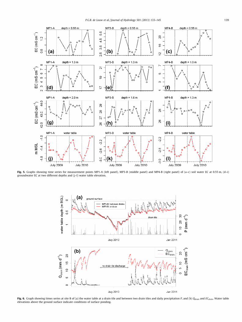
Fig. 5. Graphs showing time series for measurement points MP1-A (left panel), MP3-B (middle panel) and MP4-B (right panel) of (a–c) soil water EC at 0.55 m, (d–i)groundwater EC at two different depths and (j–l) water table elevation.

Fig. 6. Graph showing times series at site B of (a) the water table at a drain tile and between two drain tiles and daily precipitation P, and (b) Qdrain and ECdrain. Water tableelevations above the ground surface indicate conditions of surface ponding.

P.G.B. de Louw et al. / Journal of Hydrology 501 (2013) 133–145 139

140 P.G.B. de Louw et al. / Journal of Hydrology 501 (2013) 133–145

while they reached up to 15 mS cm�1 at site B. It should be notedthough that extracting soil water was more difficult at site A andtherefore data of dryer periods could not be obtained, except forsampling depth 0.55 m of MP1-A. Another conspicuous differenceis that for three locations at site B soil water salinities were muchhigher than in the saturated zone (Fig. 4), which was not the case atsite A.

For the sampling depths where sufficient samples could be col-lected throughout the year a clear seasonal trend in soil watersalinity was observed. Selected examples of this seasonal behaviorare shown in Fig. 5a–c. Higher soil water salinities occurred duringperiods with low water tables (Fig. 5j-l), low P and high ETa.

4.3. Drain tile discharge and drain water salinity

Fig. 6 shows the observed Qdrain and ECdrain, as well as the watertable at a drain tile and between two drain tiles. The data cover aperiod of almost 1 year. Drain tiles carried discharge when thewater table was above the drain tile level, and the discharge in-creased when the water table rose due to precipitation. ECdrain var-ied with Qdrain, where an increase of Qdrain caused a rapid andpronounced decline in ECdrain, followed by an increase of ECdrain

when the discharge decreased. Fig. 7b shows that ECdrain was line-arly correlated with water table depth, with ECdrain decreasingwhen the water table was rising. ECdrain never exceeded25 mS cm�1 or fell below 2 mS cm�1. The largest salt loads

Fig. 7. Scatter diagrams showing measurements at site B of (a) the water table elevationECdrain versus log(Qdrain) and (d) log(Clload) versus log(Qdrain). The salt load Clload is expres

(discharge times salt concentration) occurred during peak dis-charge events (Fig. 7d) when drain water salinities were low.

4.4. Model outcomes

Because the model started with initial Cl� concentrations of12 g L�1 a spin-up time was required during which the RW-lensdeveloped. It was found that after 8 years the total solute massin the model between consecutive 2-year recharge cycles changed<0.1%, indicating that there was no long-term change in the lensvolume. Fig. 8 shows the comparison between the observed andmodel-simulated dynamics of Qdrain, ECdrain, and the water tableelevation between the drain tiles during the measurement period.Also shown are the time-averaged observed and simulated salin-ity-depth profiles at and between the drain tiles. The simulateddynamics of Qdrain correspond well to the observed dynamics(NSC = 0.65) (Fig. 8a). In order to achieve this fit, high values ofKh (2.5 m d�1) needed to be assigned to the upper 0.4 m of the sub-soil. Cracks were observed at the surface, in particular during sum-mer, and these are believed to be the cause for the relatively-highKh value for this soil type. The adopted values of S (0.05–0.12) wereadequate to reproduce the observed response of the water tableelevation and Qdrain to recharge.

During calibration it was found that with a constant fs = 0.69,the simulated water table fell too deep in the summer. Simulationswith fs = 0.60 for the summer half of the year (15 April–14 October)

at MP5-B versus log(Qdrain), (b) the water table elevation at MP5-B versus ECdrain, (c)sed in g Cl� discharged per m drain tile.

Fig. 8. Graphs showing the comparison between observed and calculated (a) Qdrain, (b) ECdrain, (c) water table between the two drain tiles, and (d) salinity-depth profiles atand between the two drain tiles. The observed and calculated variation of Dmix is indicated as well.

P.G.B. de Louw et al. / Journal of Hydrology 501 (2013) 133–145 141

and fs = 1.0 for the winter half of the year (15 October–14 April), re-sulted in a much better fit with the observations whilst leaving thetotal ETa for the period unchanged. The justification on physicalgrounds for this approach is the reduction of ETa in summer dueto limited soil moisture availability and salt stress. In an analogousway, qs was set to 0.16 mm d�1 for the winter half of the year andto 0.42 mm d�1 for the summer half of the year, which is commen-

Fig. 9. Graphs showing model results between the drain tiles: (a) time series of the wate(2009–2010), (b) temporal variations of groundwater salinity at different depths. No recalculated water table and hence inactive.

surate with the observed change in the difference between thehead at 4 m depth and the water table. With these adjustments,the observed water table could be satisfactory simulated(NSC = 0.81) (Fig. 8c).

The measured depth and width of the mixing zone at and be-tween the drain tiles were well simulated by the model (Fig. 8d).Both the field data and the model results show a thicker RW-lens

r table, Dmix, Bmix and the vertical flow stagnation point (FLSP) for a period of 2 yearssults are shown for depths of 1.0 m and 0.8 m when model cells were above the

142 P.G.B. de Louw et al. / Journal of Hydrology 501 (2013) 133–145

between the drain tiles than at the drain tile. The small verticalseasonal displacements of Dmix and virtually steady position of Bmix

were also reproduced by the numerical model (Figs. 8d and 9a).The observed dynamics of ECdrain could only be partially repro-

duced by the model (NSC = 0.01 for the entire period of availabledata; 0.42 for the period after 15 September 2010). The largest dis-crepancies between simulated and observed values occurred di-rectly after the summer period when drain tiles start dischargingagain and simulated values of ECdrain are lower than observed(Fig. 8b). This is believed to be attributable to the fact the salinityof the recharge water after a period of drought is higher in the fieldthan the constant Cl� concentration of 1.25 g L�1 used in the mod-el. Attempts to increase the simulated ECdrain after periods ofdrought and ECdrain dynamics throughout the year, such as byadopting higher Kh and lower S-values for the upper soil, differentsalinities of recharge for summer and winter, smaller cells aroundthe drain tile and lower dispersivity values, resulted in littleimprovement, or a significant worsening of the fit for the othermetrics.

5. Discussion

5.1. Groundwater dynamics

The time-series data showed that Dmix did not vary more than0.25 m during the measurement period. The temporal depth varia-tion of Dmix showed a seasonal trend rather than a response to indi-vidual rain events, with a deeper Dmix during the winter half of theyear when the water table was high (Fig. 9a). The small vertical dis-placement of the mixing zone explains the observed seasonal salin-ity variations in the RW-lens, which are illustrated in the nextexample. The salinity gradient around Dmix is about 4 mS cm�1

and 3 mS cm�1 per 0.1 m depth interval for sites A and B, respec-tively (Fig. 4). From this it can be inferred that a vertical displace-ment of Dmix of only 0.05–0.25 m results in seasonal salinityvariations of 2–10 mS cm�1 for site A and 1.5–7.5 mS cm�1 for siteB, which is in accordance with the observations (Fig. 5) and modelresults (Fig. 9b). The upward and downward movement of Dmix andseasonal salinity variations suggest that there exists a seasonallyoscillating flow regime.

The effect of the transience of the flow on the dynamics of thesalinity distribution was analyzed by using the calibrated modelto determine, for every point in the cross-section, the percentageof time during which the flow has a vertical upward component.Fig. 10 shows that between 2.5 and 5 m from the drain tile, theflow around Dmix was upward half of the time, and downward half

Fig. 10. Contour plot that shows for every model cell the percentage of time duringwhich groundwater flow has an upward flow component (determined for a periodof 2 years, 2009–2010). The average positions of Dmix and Bmix for the modeledperiod 2009–2010 are indicated as dashed lines.

of the time. Average absolute vertical and horizontal flow velocitiesaround Dmix were in the order of 1–2 mm d�1 and 5–10 mm d�1,respectively. These small velocities and the fact that the flow alter-nates in vertical flow direction result in little vertical displacement,which explains why the seasonal variation of Dmix is only small.The numerical experiments of Eeman et al. (2012) showed muchlarger seasonal displacements of Dmix (0.5–1.0 m per year). This isprobably due to the fact that they considered a different hydrogeo-logical setting, i.e., a sandy aquifer without the presence of a low-permeability aquitard on top, allowing for much larger verticalflow velocities than in cases RW-lenses develop within an aquitard.

Beyond this, the calibrated model was used to determine thetemporal dynamics of the vertical flow stagnation point (FLSP),which is the point below which the flow switches from having avertical downward to a vertical upward component (De Louwet al., 2011). The FLSP at the point between the drain tiles showsa clear correlation with the elevation of the water table (Fig. 9a),whereby a rising water table resulted in a deeper FLSP. The FLSP re-sponds rapidly to water table fluctuations. Flow is downward for alarge part of the RW-lens when the water table is high, but whenthe water table falls below the drain tile all flow in the RW-lensis upward (Fig. 9a).

The oscillatory flow regime is further believed to be a driver forthe mixing of infiltrated rainwater and saline groundwater in aRW-lens (De Louw et al., 2011). This is illustrated by the transientpath lines within the RW-lens (Fig. 11a). Path lines started fromdifferent locations within the RW-lens show that certain regionsof the subsurface sometimes receive inflow from (i) rechargeacross the water table, (ii) saline groundwater from seepage, or(iii) a mixture of the two. Path lines originating in the fresh- andsaltwater zone cross each other over time, indicating mixing. The

Fig. 11. Cross sections showing (a) transient path lines started at 1 January 2009, atdifferent locations in the cross section, (b) travel time to the drain tile (in years). Thered dotted line delineates the bottom of the zone around the drain tile thatcontributed to a rainfall-driven drainage event with duration of 7 days (11–17November 2010). The average positions of Dmix and Bmix for the modeled period2009–2010 are indicated as dashed lines. (For interpretation of the references tocolour in this figure legend, the reader is referred to the web version of this article.)

P.G.B. de Louw et al. / Journal of Hydrology 501 (2013) 133–145 143

bends of the path lines indicate seasonal changes of periods withdifferent recharge; path lines are predominantly horizontally ori-ented during winter when there is a significant flow towards thedrain tile, and nearly vertical flow occurs during summer whenthe water table dropped below drain tile elevation. The oscillatoryregime is most dynamic for the zone 2.5–5 m from the drain tile(Fig. 10). Closer to the drain tile, flow between Bmix and Dmix is up-ward for most of the time (Fig. 10). Nonetheless, both observationsand simulations highlight the presence of a mixing zone below thedrain tile. The calculated path lines show that this mixing zonegroundwater results from mixing of rainwater with seepage at lar-ger distance from the drain tile subsequently flowing towards thedrain tile. Fig. 11b shows that within the RW-lens (i.e., above Bmix)the maximum travel time towards the drain tiles is 3.5 years.

5.2. Soil water dynamics

Important mixing processes occur in the zone where the watertable fluctuates and conditions alternate between saturated tounsaturated. For both sites A and B this zone extends from groundsurface to 1.3 m BGL. When the water table falls, water with vari-able dissolved salt concentrations is retained as soil water, whichwill mix and become diluted with infiltrated rainwater when thesoil saturates again. The temporary storage of salt in soil waterhas an important damping effect on groundwater salinity varia-tions when the RW-lens grows by the recharge by rainwater. Forexample, the average fillable porosity (Acharya et al., 2012) ofthe top soils of site B is �0.07 (S in Fig. 3), while the average totalporosity (i.e. the volumetric soil moisture content at saturation) is�0.49. Consequently, infiltration of 1 mm of rainfall leads to thesaturation of �14 mm of soil. Assuming instantaneous mixingwhen the soil gets saturated, the salinity of this saturated part willthen equate to 0.07/0.49 = 1/7 times the salinity of the infiltratedwater plus 0.42/0.49 = 6/7 times the salinity of resident soil water.The salinity of the mixture will thus be close to that of the soilwater before saturation since the resident soil water is diluted byonly a small amount of infiltrated water. This clearly shows thatthe salinity of groundwater recharge is controlled by mixing pro-cesses in the unsaturated zone, which is believed to be the expla-nation for the observed absence of truly fresh groundwater at siteA and B (Figs. 4 and 5) and most other locations measured by DeLouw et al. (2011).

The average salinity of soil water increases gradually withdepth from low values near the land surface to the groundwatersalinity at the water table, except at the monitoring points MP1-B, MP2-B and MP4-B at site B. At these locations the soil water at0.55 and 0.70 m BGL were found to have higher salinities thanthe groundwater at 0.80 and 1.0 m BGL (Fig. 4). This is attributedto the co-existence of macro-pores (e.g. cracks) and small poresin the top soil, and the following mechanisms are thought to oper-ate. Infiltration of rainwater occurs preferentially through themacro-pores, whereas capillary rise of water is strongest in thesmallest pores. The smallest pores also can retain soil water againstincreasingly negative soil water potentials during summer. Whenthe water table lowers, the concurrent loss of soil moisture dueto drainage and evapotranspiration is, at least partially, compen-sated by capillary rise. At the same time, the salinity of the ground-water just below the water table becomes more saline as the watertable fall ‘decapitates’ the lens and the vertical separation betweenthe water table and the base of the RW-lens becomes smaller. Thesalinity of the soil water in the small pores thereby increases withtime during summer, as the water that rises by capillary effects be-comes ever more saline. This effect is much smaller or even absentin the macro-pores. The high salinities in the small pores can per-sist during the infiltration events, as infiltration of rainwater occurspreferentially via the macro-pores, by-passing the soil aggregates

in which the smaller pores reside. Pulses of relatively freshwatercan recharge the RW-lens in this way, while high salinities persistin the unsaturated zone.

5.3. Drainage dynamics

Under no conditions during the measurement period did thedrain water consist solely of saline seepage water, which can be in-ferred from the fact that ECdrain never reached the EC of the seepagewater of about 35 mS cm�1 for site B (Fig. 6). This can be explainedby the presence of a mixing zone below the drain tile (Fig. 4; MP4-B and MP5-B) and the path lines in the RW-lens (Fig. 11a) whichindicate that groundwater flowing towards the drain tiles is mixedgroundwater.

The seasonal timescale of variation of groundwater and soilwater salinity contrasts starkly with the high-frequency dynamicsof ECdrain, which responds almost instantaneously to individual rainevents (Fig. 6). Cracks are thought to play an important role in thisdynamic behavior, facilitating the rapid infiltration of rainwaterand responses of drain tile discharge and salinity to rainfall. Velstraet al. (2011) found similar fast responses and also allotted this tothe existence of cracks in the clayey top soils. The dynamics ofECdrain (Fig. 6) indicate a fast mixing of infiltrated rain water andmixing zone groundwater. Particle tracking analysis shows thatpath lines originating from different depths converge and mix inthe drain tile (Fig. 11a). This is further illustrated in Fig. 11b inwhich the red dotted line the region delineates (based on particletracking) that contributes to a rainfall-driven drainage event withduration of 7 days (11–17 November 2010). For this event about80% of the discharged water came from above the drain tile levelwith a low salinity close to that of rainwater, and about 20% camefrom below the drain tile level with salinities representative of themixing zone. The linear relation between the water table and drainwater salinity (Fig. 7b) implies that a higher water table leads to alarger fraction of infiltrated rainwater and a smaller fraction ofmixing zone groundwater in drain water. However, the measure-ments also showed that despite the lower fraction of salinegroundwater in drain water, the absolute amount of saline ground-water drained increases with water table elevation (Fig. 7d). Fromthis it is inferred that during a water table rise, an increase of theflow of saline groundwater from the mixing zone towards the draintile is triggered, which is confirmed by the model results (notshown). Drain water will therefore never consist of solely rainwa-ter which explains why ECdrain never fell below 2 mS cm�1 (Fig. 6).

6. Conclusions

In this study, the temporal dynamics of thin RW-lenses and themixing between rainwater and saline seepage were investigatedusing field measurements at two tile-drained agricultural fieldsin the south-western part of the Netherlands and numerical simu-lations for one of the sites. Upward saline seepage limits the size ofthe RW-lens and the freshwater availability for agriculture pur-poses. The base and the center of the mixing zone were found ata depth of 1.8–3.3 m BGL and 0.8–1.8 m BGL, respectively. Forthe first time, field-based evidence of RW-lens dynamics was sys-tematically collected by monthly ground- and soil water sampling,in combination with daily observations of water table elevation,drain tile discharge and drain water salinity. These observationswere reproduced by the numerical model. Based on the field dataand numerical modeling of the key lens characteristics, aconceptual model of RW-lens dynamics and mixing behavior waspresented of which the most important characteristics are summa-rized below.

144 P.G.B. de Louw et al. / Journal of Hydrology 501 (2013) 133–145

The thickness of the RW-lens varied up to 1.2 m due to watertable fluctuations in response to individual recharge events. Theposition of the center of the mixing zone Dmix showed a muchsmaller change (< 0.25 m), and fluctuated at a much longer, sea-sonal time scale. The base of the RW-lens stayed virtually at thesame position. The small variations in the position of the mixingzone can be explained by the slow transient oscillatory flow regimein the deepest part of the RW-lens. This oscillatory flow regimealso controls the mixing between infiltrated rainwater and seepagewater in a RW-lens.

The flow and mixing processes are much faster near the watertable, which fluctuates on a daily basis in response to rechargeand evapotranspiration, and conditions alternate between satu-rated to unsaturated. When the water table falls, most of the waterwith variable dissolved salt concentrations is retained as soilwater, which will mix and become diluted with only a smallamount of infiltrated rainwater when the soil saturates again.The salinity of the mixture will thus be close to that of the soilwater before saturation, which explains the observed absence ofvery fresh groundwater. Although the mixing processes are fast,the temporary storage of salt in soil water has an important damp-ing effect on groundwater salinity variations when the RW-lensgrows due to the recharge by rainwater.

Salt migrates upwards into the root zone by capillary rise of thegroundwater at the water table. As the water table falls during thesummer, the water rising through the capillaries originates fromdeeper parts of the RW-lens and is therefore more saline. Salinitiesof soil water can become significantly higher than in the ground-water due to the unsynchronized effects of capillary rise of salinewater during dry periods and the flow of infiltrated rainwater dur-ing wet periods being restricted to cracks in the soil.

Preferential flow through cracks is thought to play an importantrole in the rapid response of the drain tile discharge to individualrain events. Groundwater of variable salinity, originating from dif-ferent parts of the RW-lens, as well as infiltrated rainwater, con-tributes to the drain tile discharge in proportions that vary on atimescale of hours to days, and this causes the dynamic behaviorof drain water salinity.

The small dimensions and dynamic behavior of the RW-lenses,especially the rapid removal of recharge through drain tiles and theloss of freshwater by evapotranspiration, make them vulnerableto climate change. RW-lenses may be expected to shrink due toevapotranspiration during drier summers, which are expected tobecome more frequent under future climate change (Van den Hurket al., 2006), but the projected increase in winter precipitation maynot compensate for the lens shrinkage because the tile-drainagesystem efficiently discharges the recharge. Alternative tile-drain-age configurations that promote prolonged retention and storageof infiltrated freshwater in RW-lenses could be a way to mitigatethe potential adverse effects of future climate change. The optimaldesign of such configurations will be the subject of future research.

Acknowledgements

This research was carried out in collaboration with the provinceof Zeeland, the Scheldestromen Water Board, Dienst LandelijkGebied and the Zuidelijke Land en Tuinbouw Organisation. Wethank the farmers Rien van den Hoek and Jan van der Velde forthe availability of their agricultural field for monitoring. We thankthe following persons for helping collect the field data: Mike vander Werf, Tommasso Letterio, Julia Claas, Bram de Vries and AndreCinjé. This work was funded in part by the National Centre forGroundwater Research and Training, a collaborative initiative ofthe Australian Research Council and the National Water Commis-sion. We thank Pieter Pauw (Deltares, Wageningen University)

and the anonymous reviewers for their valuable comments onthe paper.

References

Acharya, S., Jawitz, J.W., Mylavarapu, R.S., 2012. Analytical expressions for drainableand fillable porosity of phreatic aquifers under vertical fluxes fromevapotranspiration and recharge. Water Resour. Res. 48, W11526. http://dx.doi.org/10.1029/2012WR012043.

Antonellini, M., Mollema, P., Giambastiani, B., Bishop, K., Caruso, L., Minchio, A.,Pellegrini, L., Sabia, M., Ulazzi, E., Gabbianelli, G., 2008. Salt water intrusion inthe coastal aquifer of the southern Po Plain, Italy. Hydrogeol. J. 16, 1541–1556.

Bakker, M., 2000. The size of the freshwater zone below an elongated island withinfiltration. Water Resour. Res. 36 (1), 109–117.

Chidley, T.R.E., Lloyd, J.W., 1977. A mathematical model study of freshwater lenses.Groundwater 15 (3), 215–222.

Collins, W.H., Easley, D.H., 1999. Freshwater lens formation in an unconfined barrierisland aquifer. J. Am. Water Resour. Ass. 35, 1–22.

De Louw, P.G.B., Eeman, S., Siemon, B., Voortman, B.R., Gunnink, J., Van Baaren, S.E.,Oude Essink, G.H.P., 2011. Shallow rainwater lenses in deltaic areas with salineseepage. Hydrol. Earth Syst. Sci. 15, 3659–3678.

Drabbe, J., Badon Ghijben, W., 1889. Nota in verband met de voorgenomenputboring nabij Amsterdam. Tijdschr. Van Konink. Inst. Van Ing. 5, 8–22 (inDutch).

Eeman, S., Leijnse, A., Raats, P.A.C., Van der Zee, S.E.A.T.M., 2011. Analysis of thethickness of a freshwater lens and of the transition zone between this lens andupwelling saline water. Adv. Water Resour. 34 (2), 191–302.

Eeman, S., Van der Zee, S.E.A.T.M., Leijnse, A., De Louw, P.G.B., Maas, C., 2012.Response to recharge variation of thin rainwater lenses and their mixing zonewith underlying saline groundwater. Hydrol. Earth Syst. Sci. 16, 3535–3549.

Goes, B.J.M., Oude Essink, G.H.P., Vernes, R.W., Sergi, F., 2009. Estimating the depthof fresh and brackish groundwater in a predominantly saline region usinggeophysical and hydrological methods, Zeeland, the Netherlands. Near SurfaceGeophys. 7, 401–412.

Harbaugh, A.W., Banta, E.R., Hill, M.C., and McDonald, M.G., 2000, MODFLOW-2000,the U.S. Geological Survey modular ground-water model – User guide tomodularization concepts and the ground-water flow process: U.S. GeologicalSurvey Open-File Report 00-92, 121 p.

Herzberg, A., 1901. Die Wasserversorgung einiger Nordseebäder. J. Gasbeleucht.Wasserversorgung 44, 815–819 (in German).

Katerji, N., Van Hoorn, J.W., Hamdy, A., Mastrorilli, M., 2003. Salinity effect on cropdevelopment and yield, analysis of salt tolerance according to severalclassification methods. Agric. Water Manag. 62 (1), 37–66.

Kim, K.Y., Seong, H., Kim, T., Park, K.H., Woo, N.C., Park, Y.S., Koh, G.W., Park, W.B.,2006. Tidal effects on variations of fresh–saltwater interface and groundwaterflow in a multilayered coastal aquifer on a volcanic island (Jeju Island, Korea). J.Hydrol. 330, 525–542.

Kwarteng, A.Y., Viswanathan, M.N., Al-Senafy, M.N., Rashid, T., 2000. Formation offresh ground-water lenses in northern Kuwait. J. Arid Environ. 46, 137–155.

Langevin, C.D., Thorne, D.T., Dausman, A.M., Sukop, M.C., Guo, W., 2008. SEAWATVersion 4: a computer program for simulation of multi-species solute and heattransport: U.S. Geological Survey Techniques and Methods. Book 6, 39pp(Chapter A22).

Lebbe, L., 1999. Parameter identification in fresh–saltwater flow based on boreholeresistivities and freshwater head data. Adv. Water Resour. 22 (8), 791–806.

Maas, K., 2007. Influence of climate change and sea level rise on a Ghyben Herzberglens. J. Hydrol. 347 (2), 223–228.

Makkink, G.F., 1957. Testing the Penman formula by means of lysimeters. J. Inst.Water Eng. 11, 277–288.

Meinardi, C.R., 1983. Fresh and brackish groundwater under coastal areas andislands. GeoJournal 7 (5), 413–425.

Nash, J.E., Sutcliffe, J.V., 1970. River flow forecasting through conceptual models.Part I: a discussion of principles. J. Hydrol. 10, 282–290.

Oude Essink, G.H.P., 1996. Impact of sea level rise on groundwater flow regimes. Asensitivity analysis for the Netherlands. Ph.D. thesis, Delft University ofTechnology, 428pp.

Oude Essink, G.H.P., 2001. Saltwater intrusion in 3D large-scale aquifers: a Dutchcase. Phys. Chem. Earth 26 (4), 337–344.

Pollock, D.W., 1994. User’s Guide for MODPATH/MODPATH-PLOT, Version 3: aparticle tracking post-processing package for MODFLOW, the U.S. GeologicalSurvey finite-difference groundwater flow model: U.S. Geological Survey Open-File Report 94–464, 234pp.

Post, V.E.A., Van der Plicht, H., Meijer, H.A.J., 2003. The origin of brackish and salinegroundwater in the coastal area of the Netherlands. Geol. Mijnbouw/Netherlands J. Geosci. 82 (2), 133–147.

Post, V.E.A., Kooi, H., Simmons, C.T., 2007. Using hydraulic head measurements invariable-density ground water flow analyses. Ground Water 45 (6), 664–671.

Post, V.E.A., Abarca, E., 2010. Saltwater and freshwater interactions in coastalaquifers. Hydrogeol. J. 18 (1), 1–4.

Poulter, B., Goodall, J.L., Halpin, P.N., 2008. Applications of network analysis foradaptive management of artificial drainage systems in landscapes vulnerable tosea level rise. J. Hydrol. 357 (3–4), 207–217.

REGIS II, 2005. Hydrogeological model of the Netherlands. Report: Vernes RW, VanDoorn, THM. From Guide layer to Hydrogeological Unit, Explanation of the

P.G.B. de Louw et al. / Journal of Hydrology 501 (2013) 133–145 145

construction of the data set. TNO report NITG 05-038-B, Utrecht, theNetherlands (in Dutch).

Rotzoll, K., Oki, D.S., El-Kadi, A.I., 2010. Changes of freshwater-lens thickness inbasaltic island aquifers overlain by thick coastal sediments. Hydrogeol. J. 18,1425–1436.

Rozema, J., Flowers, T., 2008. Crops for a salinized world. Science 322, 1578–1582.Sluijter, R., Leenaers, H., Camarasa, M., 2011. Atlas of Dutch Climate. Royal

Netherlands Meteorological Institute KNMI, Noordhoff Uitgevers, Groningen(in Dutch).

Stolte, J., 1997. Manual for soil physical measurements, version 3. Wageningen, DLOWinand Staring Centre for Integrated Land, Soil and Water Research, TechnicalDocument 37, 77p.

Stoeckl, L., Houben, G., 2012. Flow dynamics and age stratification of freshwaterlenses: experiments and modeling. J. Hydrol. 458–459, 9–15.

Stuyfzand, P.J., 1993. Hydrochemistry and Hydrology of the Coastal Dune Area ofthe Western Netherlands. Ph.D. Thesis. Free University Amsterdam, ISBN 90-74741-01-0, 366 pp.

Underwood, M.R., Peterson, F.L., Voss, C.I., 1992. Groundwater lens dynamics of atollislands. Water Resour. Res. 28 (11), 2889–2902.

Vaeret, L., Leijnse, A., Cuamba, F., Haldorsen, S., 2011. Holocene dynamics of thesalt–fresh groundwater interface under a sand island, Inhaca, Mozambique.Quater. Int. 257, 74–82.

Van Meir, N., 2001: Density-dependent groundwater flow: design of a parameteridentification test and 3D-simulation of sea-level rise. PhD thesis Thesis, GhentUniversity, Ghent, Belgium, 319 pp.

Vandenbohede, A., Lebbe, L., 2007. Effects of tides on a sloping shore: groundwaterdynamics and propagation of the tidal wave. Hydrogeol. J. 15 (4), 645–658.http://dx.doi.org/10.1007/s10040-006-0128-y.

Vandenbohede, A., Luyten, K., Lebbe, L., 2008. Impacts of global change onheterogeneous coastal aquifers: case study in Belgium. J. Coast. Res. 24 (2B),160–170.

Vandenbohede, A., Courtens, C., Lebbe, L., De Breuck, W., 2010. Fresh–salt waterdistribution in the central Belgian coastal plain: an update. Geol. Belg. 11 (3),163–172.

Van den Hurk, B., Klein Tank, A., Lenderink, G., Ulden, A. van, Oldenborgh, G.J. van,Katsman, C, Brink, H. van den, Keller, F., Bessembinder, J., Burgers, G., Komen, G.,Hazeleger, W. & Drijfhout, S., 2006. KNMI Climate Change Scenarios 2006 forthe Netherlands. KNMI, De Bilt, Scientific Report WR 2006-01.

Velstra, J., Groen, J., De Jong, K., 2011. Observations of salinity patterns in shallowgroundwater and drainage water from agricultural land in the Northern part ofthe Netherlands. Irrig. Drain 60, 51–58.

Vos, P., Zeiler, F., 2008. Holocene transgressions of southwestern Netherlands,interaction between natural and antrophogenic processes. Grondboor & Hamer3–4 (in Dutch).

Werner, A.D., Bakker, M., Post, V.E.A., Vandenbohede, A., Lu, C., Ataie-Ashtiani, B.,Simmons, C.T., Barry, D.A., 2013. Seawater intrusion processes, investigationand management: recent advances and future challenges. Adv. Water Resour.51, 3–26.