Radiometric Dating: A New Technique
163
The University of Maine The University of Maine DigitalCommons@UMaine DigitalCommons@UMaine Electronic Theses and Dissertations Fogler Library Spring 5-8-2020 Radiometric Dating: A New Technique Radiometric Dating: A New Technique Amber Emily Hathaway University of Maine, [email protected] Follow this and additional works at: https://digitalcommons.library.umaine.edu/etd Recommended Citation Recommended Citation Hathaway, Amber Emily, "Radiometric Dating: A New Technique" (2020). Electronic Theses and Dissertations. 3214. https://digitalcommons.library.umaine.edu/etd/3214 This Open-Access Thesis is brought to you for free and open access by DigitalCommons@UMaine. It has been accepted for inclusion in Electronic Theses and Dissertations by an authorized administrator of DigitalCommons@UMaine. For more information, please contact [email protected].
-
Upload
khangminh22 -
Category
Documents
-
view
5 -
download
0
Transcript of Radiometric Dating: A New Technique

The University of Maine The University of Maine
DigitalCommons@UMaine DigitalCommons@UMaine
Electronic Theses and Dissertations Fogler Library
Spring 5-8-2020
Radiometric Dating: A New Technique Radiometric Dating: A New Technique
Amber Emily Hathaway University of Maine, [email protected]
Follow this and additional works at: https://digitalcommons.library.umaine.edu/etd
Recommended Citation Recommended Citation Hathaway, Amber Emily, "Radiometric Dating: A New Technique" (2020). Electronic Theses and Dissertations. 3214. https://digitalcommons.library.umaine.edu/etd/3214
This Open-Access Thesis is brought to you for free and open access by DigitalCommons@UMaine. It has been accepted for inclusion in Electronic Theses and Dissertations by an authorized administrator of DigitalCommons@UMaine. For more information, please contact [email protected].
RADIOMETRIC DATING: A NEW TECHNIQUE
By
Amber Emily Hathaway
M.A., University of Maine, 2014
B.A., University of Maine, 2012
A DISSERTATION
Submitted in Partial Ful�llment of the
Requirements for the Degree of
Doctorate of Philosophy
(in Physics)
The Graduate School
The University of Maine
May 2020
Advisory Committee:
C. T. Hess, Ph.D., Professor of Physics, Advisor
Thomas E. Stone, Ph.D., Associate Professor of Mathematics and Physics,
Husson University, Adjunct Graduate Faculty, University of Maine
Saima Farooq, Ph.D., Physics Lecturer, University of Maine
Andre Khalil, Ph.D., Associate Professor of Chemical and Biomedical
Engineering, University of Maine
George Bernhardt, Ph.D., Research Scientist and Physics Lecturer, University of Maine

RADIOMETRIC DATING: A NEW TECHNIQUE
By Amber Emily Hathaway
Dissertation Advisor: Dr. C. T. Hess
An Abstract of the Dissertation Presentedin Partial Ful�llment of the Requirements for the
Degree of Doctorate of Philosophy(in Physics)May 2020
Radiometric dating is a common technique used to estimate the age of sediment and ice
core samples. Lead-210 is widely used for dating sediment samples less than 150 years old.
The two most commonly used lead-210 dating techniques rely on the assumption that the
amount of lead-210 that is deposited in lake beds and other waterways remains constant
over time. However, this assumption may not always be physically realistic, and if the rate
is not constant, then age estimates derived using the constant rate assumption may not be
accurate.
A new dating technique allowing for non-constant lead-210 supply rates (the NCRS
model) was developed. It was implemented on 34 di�erent sediment samples. Of these
samples, 10 exhibited apparent sinusoidal �uctuations. Discrepancies in age estimates
between models were most pronounced for the upper sediment layers. For the data sets
which varied sinusoidally, the period was also computed and analyzed.

PREFACE
If my physics journey were a mathematical function, it would be the cosine. My foray into
this discipline began auspiciously enough, with a course in calculus-based Advanced
Placement (AP) Physics at Bangor High School, taught by Dr. Simon Wesley. The subject
matter was challenging; I remember scoring in the 50s on my �rst try at a kinematics test.
However, my instructor's enthusiasm for the subject was contagious. Through his lectures,
I saw something beautiful hidden behind the complexity, something exciting, and I
grabbled through the material, taking in what �eeting glances I could garner of that
elegance. By the end of the spring semester, I was determined to major in the discipline
when I started college the following fall.
I ended up earning my Bachelor's in Mathematics and Women's Studies1 instead, with
a minor in Physics, as well as one in Ethics and Social and Political Philosophy. There are
many factors that in�uenced my departure from the physics major, some unique and
personal, while others perhaps more common among those who leave physics. After
earning my Master's in Mathematics, I returned to physics to pursue my Ph.D. My
primary reason for choosing physics was that I wanted to remain close to home and the
University of Maine did not o�er a Ph.D. in any of the other disciplines I had studied. My
retention is thus a �uke in many ways, the con�uence of an atypical set of circumstances.
The journey to my Ph.D. involved countless tears, hours of listening to Kesha's
�Praying� on repeat, and many tough decisions. However, I am immensely grateful that I
was a�orded this opportunity to advance science and human knowledge, and also to better
understand myself. I am a small person, physically weak, and grapple with chronic anxiety
which can be incredibly limiting, physically as well as mentally. However, I was blessed
1The precursor to the Women's, Gender, and Sexuality Studies program.
ii

with my father's work ethic, and this journey has shown me that I am stronger and more
determined that I had thought possible.
While I persisted, many others, particularly students from marginalized backgrounds,
have not. I want to speak brie�y on this subject, as it is dear to my heart. We, and here I
mean society as a whole, as well as members of the physics community, like to view physics
as objective and free of bias. However, what we study in physics, what we choose to
consider physics, and who counts as a physicist are decisions made by humans who are
inherently subjective. It matters who is doing physics.
Astrophysicist Jocelyn Bell Burnell credits her di�erence both in terms of her gender as
well as the geographical location she grew up in as a contributing factor in her discovery of
pulsars. Coming from outside the mainstream physics tradition, she was willing to
investigate anomalies in radio telescope data which other scientists may have neglected.
Making physics an inclusive space is not merely a nice thing to do; it will make for better
science.
Di�erence made this document possible, although the ways in which it shaped my
dissertation are subtle, if not indistinguishable. The most obvious di�erence that comes
into play here is my mathematical training; the required math which was o� putting to
previous graduate students is what drew me in. Di�erences in disciplinary background may
seem untethered to identity facets like gender or social class, but I have always experienced
the sciences as a woman from a working class background, and my appreciation for math is
inevitably intertwined with my experiences as a woman studying math. I have often felt �at
home� in math, whereas in physics it took years of metaphorical couch sur�ng before I
managed to build a place of my own. While not solely due to gender, I think my gender
had its hand in making one discipline seem inviting and the other foreboding.
I want to acknowledge that most of the individuals I have met along my physics journey
have been kind, many supportive, and there are but few examples I can point to as
instances which have actively thwarted my interest in physics. I am also slower to
iii

comprehend physics than I am math, and my comparative underperformance in physics
has not been kind to a self which is already full of doubt. However, there is something
about physics as a discipline, what I can describe best as a cultural di�erence, this feeling
of je ne sais quoi, which permeates seemingly every facet. Each time I breathe in, it is
there, not enough to su�ocate, but its prevalence irritates my lungs. These days it is but a
minor nuisance, but there have been times when it was all I could feel.
I am not the only person who has struggled to �nd a place in physics. Women, black
and indigenous students, and working class students, among others, are vastly
underrepresented in this discipline. In my discipline. The percentages of individuals from
marginalized backgrounds receiving physics degrees has remained stagnant for years, even
as the shares in other STEM �elds like mathematics and chemistry have grown.
The question of how to make physics more inclusive is one that I regularly grapple
with. I don't have all the answers, but I do know that ignoring this question because it is
challenging will not make the situation better. We owe it to our students and to our �eld
to foster a learning environment in which individuals from a multiplicity of backgrounds
feel welcome.
My primary aim in writing this preface is to provide a sense of who the author of this
document is.2 However, in re�ecting on my trajectory, I see all of the places along my
path where I left or nearly left physics, and think of the others who have stood at that
same juncture and found it too much, and my heart breaks. While a minority in physics
due to my gender and, to a lesser extent, my socioeconomic status growing up, I still
bene�t from many privileges which have made my success possible, privileges that not
everyone studying physics has. I felt like this document would be incomplete without some
acknowledgment of the fact that not everyone is able to experience physics in the same
way. Although I struggled to reach this point, my struggles likely pale in comparison to
2If your takeaway is that I am an anxious mess of a woman with low self esteem, you are not wrong.
iv
what other marginalized students have had to overcome. Anything we can do to make
physics more accessible will give us a step in the right direction.
I doubt this preface will be read by more than a handful of individuals,3 but if you
happen to be someone who is struggling in physics, I want you to know that you are
enough. The �eld may feel rigid and con�ning at times, but it can grow and expand to �t
you. You don't have to stick with physics; I don't want to force you to stay somewhere
you're not happy. But if you're feeling insecure, know that my insecure self has just earned
a Ph.D. in physics. Your insecure self can do incredible things too.
Amber Hathaway
April 28, 2020
3Hi committee!
v

DEDICATION
To my partner, Brian Toner, for his unwavering support and con�dence in my abilities.
Also, to those of you who are interested in physics, but have been led to believe that you
do not belong here. Not only do you belong, you are needed. Diverse perspectives lead to
better science.
vi
ACKNOWLEDGEMENTS
First and foremost, I would like to thank my dissertation advisor, Dr. C. T. Hess for his
support and mentorship throughout this process. You have believed in my abilities even
when I haven't been sure of them myself, and for that I am grateful. I would also like to
thank my committee members Dr. Tom Stone, Dr. Saima Farooq, Dr. Andre Khalil, and
Dr. George Bernhardt for their feedback and guidance. I would like to thank my external
reader, Dr. James Kaste, for his feedback on this document. I would like to thank my
colleague, James Deaton, for teaching me the experimental side of things.
Thank you to my counselor, Michaele Potvin, who has helped me through some di�cult
times, and also the sta� and faculty members who have supported me when I've been
overwhelmed by my anxiety. I don't think I would have been able to make it this far into
my program without your help.
I would like to thank my high school physics teacher, Dr. Simon Wesley, for inspiring
my interest in physics and for supporting me from afar years after I have graduated. I
would also like to thank Pat Byard for her assistance over the years and for generally being
a positive and supportive force for the graduate students. I don't know how the physics
department would keep going without you.
Lastly, I would like to thank my partner Brian Toner. He has been my support system
throughout this whole process, encouraging me when I felt overwhelmed and sharing in my
triumphs. Without his continual support, this journey would have been signi�cantly more
di�cult.
vii
TABLE OF CONTENTS
PREFACE .. . . . . . . . . . . . . . . . . . . . . . . . . . . . . . . . . . . . . . . . . . . . . . . . . . . . . . . . . . . . . . . . . . . . . . . . . . . . . . . . . . . ii
DEDICATION .. . . . . . . . . . . . . . . . . . . . . . . . . . . . . . . . . . . . . . . . . . . . . . . . . . . . . . . . . . . . . . . . . . . . . . . . . . . . . . . vi
ACKNOWLEDGEMENTS . . . . . . . . . . . . . . . . . . . . . . . . . . . . . . . . . . . . . . . . . . . . . . . . . . . . . . . . . . . . . . . . . . vii
LIST OF TABLES . . . . . . . . . . . . . . . . . . . . . . . . . . . . . . . . . . . . . . . . . . . . . . . . . . . . . . . . . . . . . . . . . . . . . . . . . . . xi
LIST OF FIGURES . . . . . . . . . . . . . . . . . . . . . . . . . . . . . . . . . . . . . . . . . . . . . . . . . . . . . . . . . . . . . . . . . . . . . . . . . . xiv
Chapter
1. A BRIEF HISTORY OF RADIOMETRIC DATING .. . . . . . . . . . . . . . . . . . . . . . . . . . . . . . . . 1
1.1 The Discovery of Radiation . . . . . . . . . . . . . . . . . . . . . . . . . . . . . . . . . . . . . . . . . . . . . . . . . . . . . . . . . 1
1.2 Radiometric Dating and the Age of the Earth . . . . . . . . . . . . . . . . . . . . . . . . . . . . . . . . . . . . 9
1.3 Radiometric Dating on Shorter Timescales . . . . . . . . . . . . . . . . . . . . . . . . . . . . . . . . . . . . . . . . 15
2. A DEEPER LOOK AT LEAD-210 DATING .. . . . . . . . . . . . . . . . . . . . . . . . . . . . . . . . . . . . . . . . . 19
2.1 The Lead-210 Decay Process. . . . . . . . . . . . . . . . . . . . . . . . . . . . . . . . . . . . . . . . . . . . . . . . . . . . . . . . 19
2.2 Obtaining and Counting a Lead-210 Sample . . . . . . . . . . . . . . . . . . . . . . . . . . . . . . . . . . . . . . 20
2.3 The Constant Rate of Supply Model . . . . . . . . . . . . . . . . . . . . . . . . . . . . . . . . . . . . . . . . . . . . . . . 30
2.4 Problems with Current Dating Techniques . . . . . . . . . . . . . . . . . . . . . . . . . . . . . . . . . . . . . . . . 32
3. A NEW TECHNIQUE FOR RADIOMETRIC DATING .. . . . . . . . . . . . . . . . . . . . . . . . . . . . 37
3.1 Deriving the Non-Constant Rate of Supply Model . . . . . . . . . . . . . . . . . . . . . . . . . . . . . . . . 37
3.2 The NCRS Model with Sinusoidal and Linear Terms . . . . . . . . . . . . . . . . . . . . . . . . . . . . . 39
viii

3.3 Modeling a Pulse . . . . . . . . . . . . . . . . . . . . . . . . . . . . . . . . . . . . . . . . . . . . . . . . . . . . . . . . . . . . . . . . . . . . 40
3.4 Restating the NCRS Model . . . . . . . . . . . . . . . . . . . . . . . . . . . . . . . . . . . . . . . . . . . . . . . . . . . . . . . . . 42
3.5 Testing the NCRS Model with Simulated Data . . . . . . . . . . . . . . . . . . . . . . . . . . . . . . . . . . . 43
3.6 Assessing the Linearity Assumption . . . . . . . . . . . . . . . . . . . . . . . . . . . . . . . . . . . . . . . . . . . . . . . . 49
4. IMPLEMENTING THE NCRS MODEL . . . . . . . . . . . . . . . . . . . . . . . . . . . . . . . . . . . . . . . . . . . . . . 53
4.1 Testing the CRS Model on the Cochnewagon Lake Data . . . . . . . . . . . . . . . . . . . . . . . . . 53
4.2 Implementing the NCRS Model with Sinusoidal Terms on the
Cochnewagon Lake Data . . . . . . . . . . . . . . . . . . . . . . . . . . . . . . . . . . . . . . . . . . . . . . . . . . . . . . . . . . . . 54
4.3 Implementing the NCRS Model with Sinusoidal and Linear Fluctuations. . . . . . . 57
4.4 Modeling SS15 in Greenland: The Physically Unrealistic Linear Term . . . . . . . . . . 60
4.5 Modeling Gardner Pond . . . . . . . . . . . . . . . . . . . . . . . . . . . . . . . . . . . . . . . . . . . . . . . . . . . . . . . . . . . . . 67
4.6 Modeling Golden Lake . . . . . . . . . . . . . . . . . . . . . . . . . . . . . . . . . . . . . . . . . . . . . . . . . . . . . . . . . . . . . . 70
4.7 The NCRS Model: A Discussion . . . . . . . . . . . . . . . . . . . . . . . . . . . . . . . . . . . . . . . . . . . . . . . . . . . 74
5. FURTHER INVESTIGATIONS OF THE NCRS MODEL . . . . . . . . . . . . . . . . . . . . . . . . . . . 77
5.1 Testing the NCRSFitModelSoftware on More Lead-210 Data . . . . . . . . . . . . . . . . . . . . 77
5.1.1 Highland Lake . . . . . . . . . . . . . . . . . . . . . . . . . . . . . . . . . . . . . . . . . . . . . . . . . . . . . . . . . . . . . . . 79
5.1.2 Salmon Pond . . . . . . . . . . . . . . . . . . . . . . . . . . . . . . . . . . . . . . . . . . . . . . . . . . . . . . . . . . . . . . . . . 80
5.1.3 Lake Purrumbete . . . . . . . . . . . . . . . . . . . . . . . . . . . . . . . . . . . . . . . . . . . . . . . . . . . . . . . . . . . . 81
5.1.4 Warner Lake . . . . . . . . . . . . . . . . . . . . . . . . . . . . . . . . . . . . . . . . . . . . . . . . . . . . . . . . . . . . . . . . . 84
5.1.5 Bracey Lake . . . . . . . . . . . . . . . . . . . . . . . . . . . . . . . . . . . . . . . . . . . . . . . . . . . . . . . . . . . . . . . . . . 86
5.1.6 Barsjon Lake . . . . . . . . . . . . . . . . . . . . . . . . . . . . . . . . . . . . . . . . . . . . . . . . . . . . . . . . . . . . . . . . . 87
5.1.7 Laguna Negra: Failure in Modeling CRS Fit . . . . . . . . . . . . . . . . . . . . . . . . . . . . . . 89
ix

5.1.8 Long Lake: Failure to Produce the NCRS Fit . . . . . . . . . . . . . . . . . . . . . . . . . . . . . 92
5.1.9 Bullen Merri: A Questionable Fit . . . . . . . . . . . . . . . . . . . . . . . . . . . . . . . . . . . . . . . . . . 93
5.1.10 Other Questionable Fits . . . . . . . . . . . . . . . . . . . . . . . . . . . . . . . . . . . . . . . . . . . . . . . . . . . . 95
5.2 Examining the Period of Oscillations. . . . . . . . . . . . . . . . . . . . . . . . . . . . . . . . . . . . . . . . . . . . . . . 98
5.2.1 Estimating the Error in the Period of Oscillations . . . . . . . . . . . . . . . . . . . . . . . . 100
5.2.2 Results . . . . . . . . . . . . . . . . . . . . . . . . . . . . . . . . . . . . . . . . . . . . . . . . . . . . . . . . . . . . . . . . . . . . . . . 105
5.3 Oceanic Oscillations . . . . . . . . . . . . . . . . . . . . . . . . . . . . . . . . . . . . . . . . . . . . . . . . . . . . . . . . . . . . . . . . . 106
6. CONCLUSIONS AND FUTURE RESEARCH .. . . . . . . . . . . . . . . . . . . . . . . . . . . . . . . . . . . . . . . 108
6.1 Summary and Conclusions . . . . . . . . . . . . . . . . . . . . . . . . . . . . . . . . . . . . . . . . . . . . . . . . . . . . . . . . . . 108
6.2 Improvements and Further Work . . . . . . . . . . . . . . . . . . . . . . . . . . . . . . . . . . . . . . . . . . . . . . . . . . . 111
6.3 Cesium Dating and Other Fallout Radionuclides . . . . . . . . . . . . . . . . . . . . . . . . . . . . . . . . . . 113
6.4 Conclusion. . . . . . . . . . . . . . . . . . . . . . . . . . . . . . . . . . . . . . . . . . . . . . . . . . . . . . . . . . . . . . . . . . . . . . . . . . . . 115
REFERENCES . . . . . . . . . . . . . . . . . . . . . . . . . . . . . . . . . . . . . . . . . . . . . . . . . . . . . . . . . . . . . . . . . . . . . . . . . . . . . . . 119
APPENDIX A � LAKE DATA .. . . . . . . . . . . . . . . . . . . . . . . . . . . . . . . . . . . . . . . . . . . . . . . . . . . . . . . . . . . . . 120
APPENDIX B � PERIOD OF OSCILLATIONS ERROR SIMULATIONS . . . . . . . . . . . . . 126
APPENDIX C � SAMPLE R CODE .. . . . . . . . . . . . . . . . . . . . . . . . . . . . . . . . . . . . . . . . . . . . . . . . . . . . . . 139
APPENDIX D � NCRSFITMODELSOFTWARE CODE .. . . . . . . . . . . . . . . . . . . . . . . . . . . . . . . . 141
BIOGRAPHY OF THE AUTHOR .. . . . . . . . . . . . . . . . . . . . . . . . . . . . . . . . . . . . . . . . . . . . . . . . . . . . . . . . 144
x
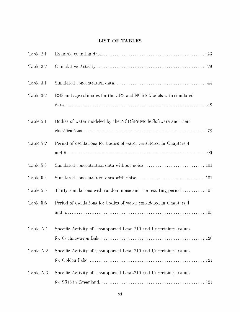
LIST OF TABLES
Table 2.1 Example counting data. . . . . . . . . . . . . . . . . . . . . . . . . . . . . . . . . . . . . . . . . . . . . . . . . . . . . . . . . 23
Table 2.2 Cumulative Activity. . . . . . . . . . . . . . . . . . . . . . . . . . . . . . . . . . . . . . . . . . . . . . . . . . . . . . . . . . . . 29
Table 3.1 Simulated concentration data. . . . . . . . . . . . . . . . . . . . . . . . . . . . . . . . . . . . . . . . . . . . . . . . . . 44
Table 3.2 RSS and age estimates for the CRS and NCRS Models with simulated
data. . . . . . . . . . . . . . . . . . . . . . . . . . . . . . . . . . . . . . . . . . . . . . . . . . . . . . . . . . . . . . . . . . . . . . . . . . . . . . 48
Table 5.1 Bodies of water modeled by the NCRSFitModelSoftware and their
classi�cations. . . . . . . . . . . . . . . . . . . . . . . . . . . . . . . . . . . . . . . . . . . . . . . . . . . . . . . . . . . . . . . . . . . . 78
Table 5.2 Period of oscillations for bodies of water considered in Chapters 4
and 5. . . . . . . . . . . . . . . . . . . . . . . . . . . . . . . . . . . . . . . . . . . . . . . . . . . . . . . . . . . . . . . . . . . . . . . . . . . . . 99
Table 5.3 Simulated concentration data without noise . . . . . . . . . . . . . . . . . . . . . . . . . . . . . . . . . . 101
Table 5.4 Simulated concentration data with noise. . . . . . . . . . . . . . . . . . . . . . . . . . . . . . . . . . . . . . 101
Table 5.5 Thirty simulations with random noise and the resulting period. . . . . . . . . . . . . 104
Table 5.6 Period of oscillations for bodies of water considered in Chapters 4
and 5. . . . . . . . . . . . . . . . . . . . . . . . . . . . . . . . . . . . . . . . . . . . . . . . . . . . . . . . . . . . . . . . . . . . . . . . . . . . . 105
Table A.1 Speci�c Activity of Unsupported Lead-210 and Uncertainty Values
for Cochnewagon Lake. . . . . . . . . . . . . . . . . . . . . . . . . . . . . . . . . . . . . . . . . . . . . . . . . . . . . . . . . . 120
Table A.2 Speci�c Activity of Unsupported Lead-210 and Uncertainty Values
for Golden Lake. . . . . . . . . . . . . . . . . . . . . . . . . . . . . . . . . . . . . . . . . . . . . . . . . . . . . . . . . . . . . . . . . 121
Table A.3 Speci�c Activity of Unsupported Lead-210 and Uncertainty Values
for SS15 in Greenland. . . . . . . . . . . . . . . . . . . . . . . . . . . . . . . . . . . . . . . . . . . . . . . . . . . . . . . . . . 121
xi

Table A.4 Speci�c Activity of Unsupported Lead-210 and Uncertainty Values
for Gardner Pond. . . . . . . . . . . . . . . . . . . . . . . . . . . . . . . . . . . . . . . . . . . . . . . . . . . . . . . . . . . . . . . 122
Table A.5 Speci�c Activity of Unsupported Lead-210 and Uncertainty Values
for Highland Lake. . . . . . . . . . . . . . . . . . . . . . . . . . . . . . . . . . . . . . . . . . . . . . . . . . . . . . . . . . . . . . . 122
Table A.6 Speci�c Activity of Unsupported Lead-210 and Uncertainty Values
for Salmon Pond. . . . . . . . . . . . . . . . . . . . . . . . . . . . . . . . . . . . . . . . . . . . . . . . . . . . . . . . . . . . . . . . 123
Table A.7 Speci�c Activity of Unsupported Lead-210 and Uncertainty Values
for Warner Lake. . . . . . . . . . . . . . . . . . . . . . . . . . . . . . . . . . . . . . . . . . . . . . . . . . . . . . . . . . . . . . . . . 123
Table A.8 Speci�c Activity of Unsupported Lead-210 and for Bracey Lake. . . . . . . . . . . . 124
Table A.9 Speci�c Activity of Unsupported Lead-210 and Uncertainty Values
for Barsjon. . . . . . . . . . . . . . . . . . . . . . . . . . . . . . . . . . . . . . . . . . . . . . . . . . . . . . . . . . . . . . . . . . . . . . 125
Table B.1 Thirty simulations with random noise and the resulting period for
Cochnewagon Lake . . . . . . . . . . . . . . . . . . . . . . . . . . . . . . . . . . . . . . . . . . . . . . . . . . . . . . . . . . . . . 129
Table B.2 Thirty simulations with random noise and the resulting period for
SS15 . . . . . . . . . . . . . . . . . . . . . . . . . . . . . . . . . . . . . . . . . . . . . . . . . . . . . . . . . . . . . . . . . . . . . . . . . . . . . 130
Table B.3 Thirty simulations with random noise and the resulting period for
Gardner Pond . . . . . . . . . . . . . . . . . . . . . . . . . . . . . . . . . . . . . . . . . . . . . . . . . . . . . . . . . . . . . . . . . . . 131
Table B.4 Thirty simulations with random noise and the resulting period for
Golden Lake. . . . . . . . . . . . . . . . . . . . . . . . . . . . . . . . . . . . . . . . . . . . . . . . . . . . . . . . . . . . . . . . . . . . . 132
Table B.5 Four simulations with random noise and the resulting period for
Highland Lake . . . . . . . . . . . . . . . . . . . . . . . . . . . . . . . . . . . . . . . . . . . . . . . . . . . . . . . . . . . . . . . . . . 133
Table B.6 Thirty simulations with random noise and the resulting period for
Salmon Pond . . . . . . . . . . . . . . . . . . . . . . . . . . . . . . . . . . . . . . . . . . . . . . . . . . . . . . . . . . . . . . . . . . . . 134
xii
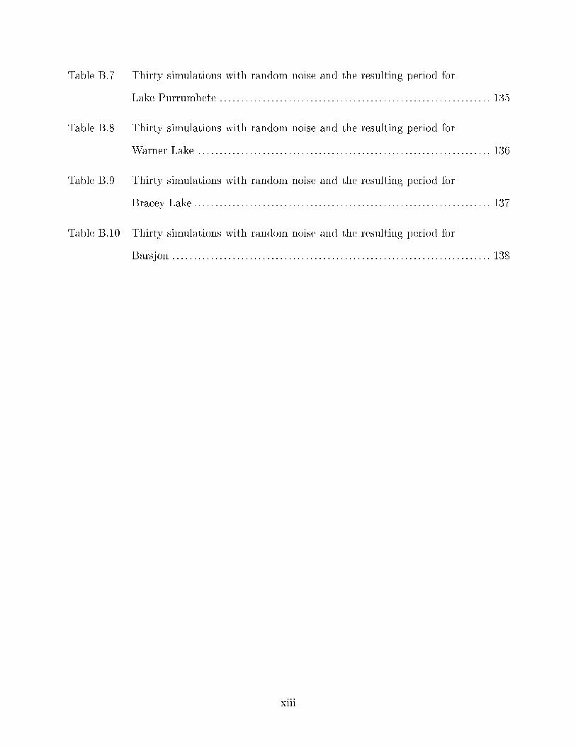
Table B.7 Thirty simulations with random noise and the resulting period for
Lake Purrumbete . . . . . . . . . . . . . . . . . . . . . . . . . . . . . . . . . . . . . . . . . . . . . . . . . . . . . . . . . . . . . . . 135
Table B.8 Thirty simulations with random noise and the resulting period for
Warner Lake . . . . . . . . . . . . . . . . . . . . . . . . . . . . . . . . . . . . . . . . . . . . . . . . . . . . . . . . . . . . . . . . . . . . 136
Table B.9 Thirty simulations with random noise and the resulting period for
Bracey Lake . . . . . . . . . . . . . . . . . . . . . . . . . . . . . . . . . . . . . . . . . . . . . . . . . . . . . . . . . . . . . . . . . . . . . 137
Table B.10 Thirty simulations with random noise and the resulting period for
Barsjon . . . . . . . . . . . . . . . . . . . . . . . . . . . . . . . . . . . . . . . . . . . . . . . . . . . . . . . . . . . . . . . . . . . . . . . . . . 138
xiii

LIST OF FIGURES
Figure 1.1 X-ray image of Anna Bertha Röntgen's hand and ring. . . . . . . . . . . . . . . . . . . . . . 3
Figure 2.1 The uranium-238 decay series. . . . . . . . . . . . . . . . . . . . . . . . . . . . . . . . . . . . . . . . . . . . . . . . . . 20
Figure 2.2 An example spectrum produced by MAESTRO. . . . . . . . . . . . . . . . . . . . . . . . . . . . . . 22
Figure 2.3 A graphical representation of the sample counts. . . . . . . . . . . . . . . . . . . . . . . . . . . . . 25
Figure 2.4 Data presented in Douglas Cahl's master's thesis of unsupported
lead-210 vs. depth. . . . . . . . . . . . . . . . . . . . . . . . . . . . . . . . . . . . . . . . . . . . . . . . . . . . . . . . . . . . . . 33
Figure 3.1 Plot of the simulated data with CRS and NCRS �ts.. . . . . . . . . . . . . . . . . . . . . . . . 46
Figure 3.2 Age estimates of the simulated data with CRS and NCRS �ts. . . . . . . . . . . . . . 47
Figure 3.3 A graph showing the all time precipitation accumulation in Augusta,
Maine from January 1, 1950 to July 17, 2017.. . . . . . . . . . . . . . . . . . . . . . . . . . . . . . . . 50
Figure 4.1 Natural logarithm of unsupported lead-210 vs. depth. . . . . . . . . . . . . . . . . . . . . . . 54
Figure 4.2 A comparison of CRS and NCRS model with no linear term.. . . . . . . . . . . . . . . 55
Figure 4.3 A comparison of CRS and NCRS model results with no linear term. . . . . . . 56
Figure 4.4 Data from Douglas Cahl's thesis with CRS and NCRS �t lines. . . . . . . . . . . . . 58
Figure 4.5 A comparison of CRS and NCRS age estimates. . . . . . . . . . . . . . . . . . . . . . . . . . . . . . 60
Figure 4.6 A comparison of CRS and NCRS �ts for the lake SS15 in Greenland
lead-210 data. . . . . . . . . . . . . . . . . . . . . . . . . . . . . . . . . . . . . . . . . . . . . . . . . . . . . . . . . . . . . . . . . . . . 61
Figure 4.7 A comparison of CRS and NCRS age estimates for the lake SS15 in
Greenland lead-210 data including a linear term in the NCRS model. . . . . . 64
xiv
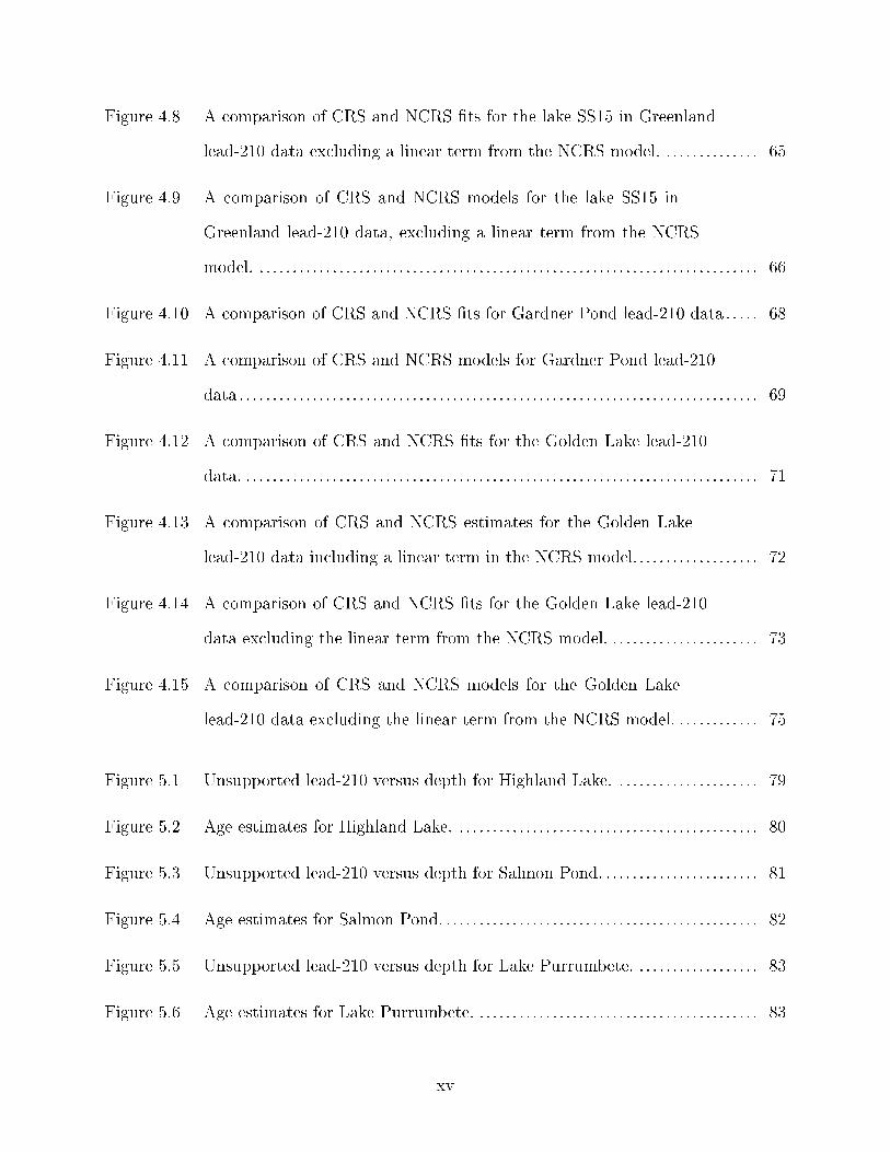
Figure 4.8 A comparison of CRS and NCRS �ts for the lake SS15 in Greenland
lead-210 data excluding a linear term from the NCRS model. . . . . . . . . . . . . . . 65
Figure 4.9 A comparison of CRS and NCRS models for the lake SS15 in
Greenland lead-210 data, excluding a linear term from the NCRS
model. . . . . . . . . . . . . . . . . . . . . . . . . . . . . . . . . . . . . . . . . . . . . . . . . . . . . . . . . . . . . . . . . . . . . . . . . . . . 66
Figure 4.10 A comparison of CRS and NCRS �ts for Gardner Pond lead-210 data . . . . . 68
Figure 4.11 A comparison of CRS and NCRS models for Gardner Pond lead-210
data . . . . . . . . . . . . . . . . . . . . . . . . . . . . . . . . . . . . . . . . . . . . . . . . . . . . . . . . . . . . . . . . . . . . . . . . . . . . . . 69
Figure 4.12 A comparison of CRS and NCRS �ts for the Golden Lake lead-210
data. . . . . . . . . . . . . . . . . . . . . . . . . . . . . . . . . . . . . . . . . . . . . . . . . . . . . . . . . . . . . . . . . . . . . . . . . . . . . . 71
Figure 4.13 A comparison of CRS and NCRS estimates for the Golden Lake
lead-210 data including a linear term in the NCRS model. . . . . . . . . . . . . . . . . . . 72
Figure 4.14 A comparison of CRS and NCRS �ts for the Golden Lake lead-210
data excluding the linear term from the NCRS model. . . . . . . . . . . . . . . . . . . . . . . 73
Figure 4.15 A comparison of CRS and NCRS models for the Golden Lake
lead-210 data excluding the linear term from the NCRS model. . . . . . . . . . . . . 75
Figure 5.1 Unsupported lead-210 versus depth for Highland Lake. . . . . . . . . . . . . . . . . . . . . . 79
Figure 5.2 Age estimates for Highland Lake. . . . . . . . . . . . . . . . . . . . . . . . . . . . . . . . . . . . . . . . . . . . . . 80
Figure 5.3 Unsupported lead-210 versus depth for Salmon Pond. . . . . . . . . . . . . . . . . . . . . . . . 81
Figure 5.4 Age estimates for Salmon Pond. . . . . . . . . . . . . . . . . . . . . . . . . . . . . . . . . . . . . . . . . . . . . . . . 82
Figure 5.5 Unsupported lead-210 versus depth for Lake Purrumbete. . . . . . . . . . . . . . . . . . . 83
Figure 5.6 Age estimates for Lake Purrumbete. . . . . . . . . . . . . . . . . . . . . . . . . . . . . . . . . . . . . . . . . . . 83
xv

Figure 5.7 Unsupported lead-210 versus depth for Warner Lake in Peru. . . . . . . . . . . . . . . 84
Figure 5.8 Age estimates for Warner Lake in Peru. . . . . . . . . . . . . . . . . . . . . . . . . . . . . . . . . . . . . . . 85
Figure 5.9 Unsupported lead-210 versus depth for Bracey Lake. . . . . . . . . . . . . . . . . . . . . . . . . 86
Figure 5.10 CRS and NCRS Age estimates for Bracey Lake. . . . . . . . . . . . . . . . . . . . . . . . . . . . . . 87
Figure 5.11 Unsupported lead-210 versus depth for Barsjon Lake. . . . . . . . . . . . . . . . . . . . . . . . 88
Figure 5.12 CRS and NCRS Age estimates for Barsjon Lake. . . . . . . . . . . . . . . . . . . . . . . . . . . . . 89
Figure 5.13 Unsupported lead-210 versus depth for Laguna Negra in Argentina. . . . . . . . 90
Figure 5.14 Error message received when modeling Laguna Negra data. . . . . . . . . . . . . . . . . 91
Figure 5.15 Unsupported lead-210 versus depth for Long Lake. . . . . . . . . . . . . . . . . . . . . . . . . . . 92
Figure 5.16 Error message received when modeling Long Lake data. . . . . . . . . . . . . . . . . . . . . 93
Figure 5.17 Unsupported lead-210 versus depth for Lake Bullen Merri in Australia. . . . . . 94
Figure 5.18 CRS and NCRS Age estimates for Lake Bullen Merri in Australia. . . . . . . . . 95
Figure 5.19 Unsupported lead-210 versus depth for the Damariscotta River Core
1. . . . . . . . . . . . . . . . . . . . . . . . . . . . . . . . . . . . . . . . . . . . . . . . . . . . . . . . . . . . . . . . . . . . . . . . . . . . . . . . . . 96
Figure 5.20 Unsupported lead-210 versus depth for the Damariscotta River Core
2. . . . . . . . . . . . . . . . . . . . . . . . . . . . . . . . . . . . . . . . . . . . . . . . . . . . . . . . . . . . . . . . . . . . . . . . . . . . . . . . . . 97
Figure 5.21 Unsupported lead-210 versus depth for a body of water in Greenland. . . . . . 98
Figure 5.22 Unsupported lead-210 versus depth the Hidden BT data set. . . . . . . . . . . . . . . . 99
Figure 5.23 The �t function for the simulated concentration data without noise. . . . . . . . 102
Figure 5.24 The �t function for the simulated concentration data with noise. . . . . . . . . . . 103
xvi

Figure 6.1 Unsupported and supported lead-210 and cesium-137 activity in
Golden Lake. . . . . . . . . . . . . . . . . . . . . . . . . . . . . . . . . . . . . . . . . . . . . . . . . . . . . . . . . . . . . . . . . . . . . 114
xvii
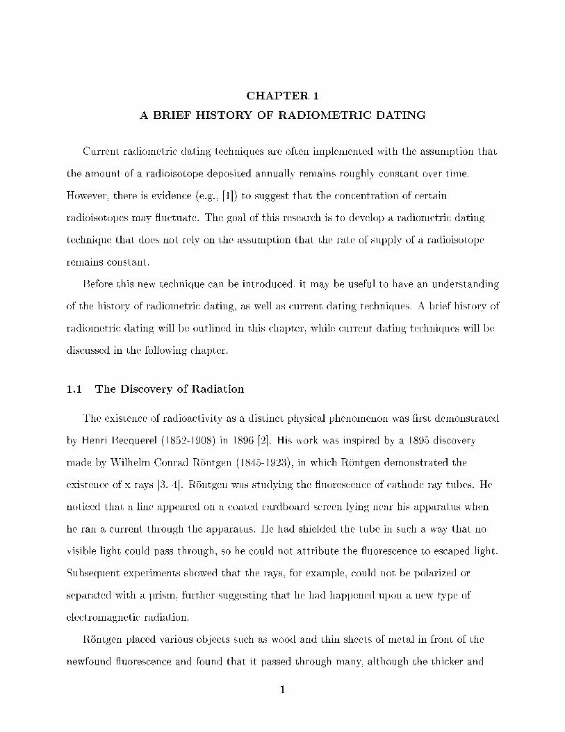
CHAPTER 1
A BRIEF HISTORY OF RADIOMETRIC DATING
Current radiometric dating techniques are often implemented with the assumption that
the amount of a radioisotope deposited annually remains roughly constant over time.
However, there is evidence (e.g., [1]) to suggest that the concentration of certain
radioisotopes may �uctuate. The goal of this research is to develop a radiometric dating
technique that does not rely on the assumption that the rate of supply of a radioisotope
remains constant.
Before this new technique can be introduced, it may be useful to have an understanding
of the history of radiometric dating, as well as current dating techniques. A brief history of
radiometric dating will be outlined in this chapter, while current dating techniques will be
discussed in the following chapter.
1.1 The Discovery of Radiation
The existence of radioactivity as a distinct physical phenomenon was �rst demonstrated
by Henri Becquerel (1852-1908) in 1896 [2]. His work was inspired by a 1895 discovery
made by Wilhelm Conrad Röntgen (1845-1923), in which Röntgen demonstrated the
existence of x rays [3, 4]. Röntgen was studying the �uorescence of cathode ray tubes. He
noticed that a line appeared on a coated cardboard screen lying near his apparatus when
he ran a current through the apparatus. He had shielded the tube in such a way that no
visible light could pass through, so he could not attribute the �uorescence to escaped light.
Subsequent experiments showed that the rays, for example, could not be polarized or
separated with a prism, further suggesting that he had happened upon a new type of
electromagnetic radiation.
Röntgen placed various objects such as wood and thin sheets of metal in front of the
newfound �uorescence and found that it passed through many, although the thicker and
1
denser an object was, the harder it was for the radiation to pass through. Lead, he found,
was almost impenetrable, and thus made a good shield against these new rays. Röntgen
chose the name �x ray� for his discovery because the odd behavior of these rays was unlike
anything else known to science at the time.
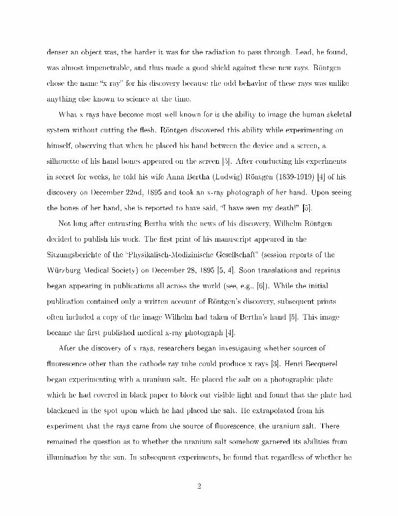
What x rays have become most well known for is the ability to image the human skeletal
system without cutting the �esh. Röntgen discovered this ability while experimenting on
himself, observing that when he placed his hand between the device and a screen, a
silhouette of his hand bones appeared on the screen [5]. After conducting his experiments
in secret for weeks, he told his wife Anna Bertha (Ludwig) Röntgen (1839-1919) [4] of his
discovery on December 22nd, 1895 and took an x-ray photograph of her hand. Upon seeing
the bones of her hand, she is reported to have said, �I have seen my death!� [5].
Not long after entrusting Bertha with the news of his discovery, Wilhelm Röntgen
decided to publish his work. The �rst print of his manuscript appeared in the
Sitzungsberichte of the �Physikalisch-Medizinische Gesellschaft� (session reports of the
Würzburg Medical Society) on December 28, 1895 [5, 4]. Soon translations and reprints
began appearing in publications all across the world (see, e.g., [6]). While the initial
publication contained only a written account of Röntgen's discovery, subsequent prints
often included a copy of the image Wilhelm had taken of Bertha's hand [5]. This image
became the �rst published medical x-ray photograph [4].
After the discovery of x rays, researchers began investigating whether sources of
�uorescence other than the cathode ray tube could produce x rays [3]. Henri Becquerel
began experimenting with a uranium salt. He placed the salt on a photographic plate
which he had covered in black paper to block out visible light and found that the plate had
blackened in the spot upon which he had placed the salt. He extrapolated from his
experiment that the rays came from the source of �uorescence, the uranium salt. There
remained the question as to whether the uranium salt somehow garnered its abilities from
illumination by the sun. In subsequent experiments, he found that regardless of whether he
2

Figure 1.1. X-ray image of Anna Bertha Röntgen's hand and ring.Photoprint from radiograph by W. K. Röntgen, 1895. Credit: Wellcome Collection. CC
BY
3

had exposed the salt to sunlight, the salt still blackened the photographic plate, suggesting
that the salt itself was creating the rays.
Marie Skªodowska Curie (1867-1934), who would end up coining the term
�radioactivity,� took interest in Becquerel's discovery and chose it as the subject of her
doctoral work [3]. She wanted to test all known elements and compounds, some of which
were rare and hard to obtain, to see which ones gave o� this mysterious radiation. Röntgen
and Becquerel had both shown that the rays they observed caused the air to become
electrically conducive. Curie used an electrometer with a piezoelectric crystal that her
husband Pierre had built and modi�ed to suit her work to determine which elements
exhibited this property and found that in addition to uranium, thorium also emitted
radiation.
Marie Curie also observed that when testing pitchblende, an ore from which the
uranium had been removed, it gave o� more radiation than uranium itself. Similarly, she
found that calcite was more active than pure thorium [7]. Thus, she hypothesized that
there was some yet unknown element in the uranium ore that was also emitting radiation.
She also discovered that radiation was a property of an element itself, as the radioactivity
remained unchanged when a sample was, for example, heated or exposed to light. She wrote
up her �ndings, using the name radioactivity for the phenomenon she had investigated.
Her results were presented on her behalf at the Academy of Sciences in April of 1898.
It was at this point that Pierre joined her in her studies, and together they worked to
discover the properties of the unknown element. The Curies chemically separated
pitchblende and by 1898 had found evidence of a metal which they believed to be similar to
bismuth. They called it polonium, after Marie's homeland, Poland. However,
demonstrating its existence proved di�cult, as traditional spectral analysis techniques
failed to show anything new, since there was too little polonium in the samples to be
observed through this technique. Later that year they found evidence of a radioactive
substance di�erent from polonium, which they called radium. A chemist colleague,
4

Eugène-Anatole Demarçay (1852-1903), was able to demonstrate a unique spectral line for
radium [7]. While this evidence was enough to convince many physicists that radium was
in fact a distinct element, chemists required a measurable quantity of the substance.
Marie thus set out to isolate radium [7]. She proposed using slag, minerals residual
after extracting the uranium from pitchblende in the production of uranium. It was from
this slag that, over the course of several years, she was �nally able to extract su�cient
quantities of radium to demonstrate its existence as a distinct radioactive element.
The nature of radioactivity remained elusive, although Marie had a theory regarding its
nature. In a manuscript published in Revue Scienti�que, she put forth the idea that
radiation came from the separation of atoms [8]. She stated,
La matière radioactive serait donc de la matière où règne un état de
mouvement intèrieur violent, de la matière en train de se disloquer. S'il en est
ainsi, le radium doit perdre constamment de son poids. Mais la petitesse des
particules est telle que bien que la charge électrique envoyée dans l'espace soit
facile à constater, la masse correspondante doit être absolument insigni�ante ;
on trouve par le calcul qu'il faudrait des millions d'années pour que le radium
perde un équivalent en milligrammes de son poids. La véri�cation est
impossible à faire.
La théorie matérialiste de la radioactivité est très séduisante. Elle explique
bien les phénomènes delà radioactivité. Cependant, en adoptant cette théorie, il
faut nous résoudre à admettre que la matière radioactive n'est pas à un état
chimique ordinaire; les atomes n'y sont pas constitués à l'état stable, puisque
des particules plus petites que l'atome sont rayonnées. L'atome, indivisible au
point de vue chimique, est divisible ici, et les sous-atomes sont en mouvement.
La matière radioactive éprouve donc une transformation chimique qui est la
source de l'énergie rayonnée ; mais ce n'est point une transformation chimique
ordinaire, car les transformations chimiques ordinaires laissent l'atome
5

invariable. Dans la matière radioactive, s'il y a quelque chose qui se modi�e,
c'est forcément l'atome, puisque c'est à l'atome qu'est attachée la radioactivité
(Curie, 70).
Her statement loosely translates as:
The radioactive material is therefore matter in which there is a state of
violent internal movement, of material being dislocated. If this is so, radium
must constantly lose its weight. But the smallness of the particles is such that
although the electric charge sent into space is easy to notice, the corresponding
mass must be absolutely insigni�cant; it is calculated that it would take
millions of years for radium to lose an equivalent in milligrams of its weight.
Veri�cation is impossible to do.
The materialistic theory of radioactivity is very seductive. It explains the
phenomena of radioactivity well. However, by adopting this theory, we must
resolve to admit that the radioactive material is not in an ordinary chemical
state; the atoms are not constituted in the stable state, since particles smaller
than the atom are radiated. The atom, indivisible from the chemical point of
view, is divisible here, and the sub-atoms are in motion. The radioactive
material thus experiences a chemical transformation which is the source of the
radiated energy; but it is not an ordinary chemical transformation, for ordinary
chemical transformations leave the atom invariable. In the radioactive material,
if there is something that changes, it is necessarily the atom, since it is to the
atom that the radioactivity is attached.
It is unclear whether Marie fully ascribed to this belief at the time. Pierre was greatly
opposed to this view, and a paper the couple jointly a�xed their names to published two
years later would caution against the hasty adoption of such an assertion [7, 9].
Nevertheless, Marie's suggestion that radiation was caused by the splitting of atoms would
be validated a couple of years later.
6

Marie had noted in her article that there seemed to be at least two distinct types of
radiation, x-ray radiation, known today also as γ radiation, and what she referred to as
cathode rays, known today as β radiation. The two behaved di�erently; while the cathode
rays were de�ected by a magnetic �eld, the x rays were not [8].
The Curies were not the only researchers to notice distinctions between types of
radiation. In 1899, about a year before Mare Curie published the manuscript in which she
laid out her theory of radiation, Ernest Rutherford (1852-1908) had commented upon two
types of radiation he had observed in his laboratory, which he referred to as α radiation
and β radiation [3]. The α radiation, he observed, was readily absorbed, while the β
radiation could travel deeper into an object. Paul Villard (1860-1934) discovered a third
type of radiation coming from radium which behaved like Röntgen's x rays. This radiation
he termed as γ radiation, following Rutherford's naming convention.
The nature of β particles was determined by Becquerel in 1900, when he demonstrated
that they had the same charge to mass ratio as an electron [3]. However, α particles
remained elusive. It was shown that they, like β particles, were de�ected by a magnetic
�eld, but in a di�erent direction and to a lesser extend, suggesting that α particles had
opposite charges and were heavier than electrons. Although speculation that α particles
were related to helium was published as early as 1903 [10], it was not until 1908 when
Rutherford and Thomas Royds (1884-1955) showed de�nitively that α particles were
helium ions [11].
The Curies, Rutherford, Becquerel, and others observed that radioactive elements
seemed to emit radioactive particles distinct from the original element [3]. The progeny of
radium and thorium, which would come to be known during that era as radon, thoron, and
actinon,1 were radioactive, but not nearly as radioactive as the elements they had
originated from. While the radioactivity of radium and thorium remained roughly
unchanged over the duration of an experiment, scientists began noticing that activities of
1thoron and actinon are now known to be isotopes of radon
7

radon, thoron, and actinon decreased with time. This decrease seemed to follow an
exponential trend, �rst decaying rapidly and then tapering o� as the quantities of radon,
thoron, and actinon were reduced.
In 1902, Rutherford and his assistant Frederick Soddy (1877-1956) formalized this
decrease in the number of particles over time in the nuclear decay equation, [12]:
N(t) = N(0)e−λt, (1.1)
where t is time, λ is the decay constant, N(t) is the number of atoms of a given
radioisotope2 at time t, and N(0) is the initial concentration.3 The decay constant was
found to be unique to a given radioisotope and governed how fast a sample of that
radioisotope would decay. This paper has largely been credited as the publication that
established the �disintegration of the elements� (known today as nuclear decay). Certainly,
Rutherford and Soddy make a strong case for it in their paper. However, it is worth noting
that a rough concept of nuclear decay existed prior to the 1902 publication, such as
articulated by Marie Curie [8].
Although they did not use the term secular equilibrium in their paper, Rutherford and
Soddy noticed that if thorium and one of its progeny, which they termed thorium X,4 were
kept together, the activity of thorium X would remain roughly constant after some time
had elapsed. This observation supplied an important insight, namely that more atoms of a
given isotope could be introduced into a sample through radioactive decay. For example, if
thorium-234 was decaying in the presence of other radioisotopes including uranium-238,
the creation of new thorium-234 particles through uranium-238 decay would have to be
accounted for.
2The term radioisotope had not yet been coined at the time of Rutherford and Soddy's publication, andthus is not utilized in their manuscript.
3Rutherford and Soddy stated the equation in a slightly di�erent format in their paper: ItT0
= e−λt,where I0 and It are the initial activity and the activity after time t, respectively [12].
4Thorium X is known today as radium-224.
8

1.2 Radiometric Dating and the Age of the Earth
Rutherford is credited with �rst suggesting that radioactivity could be used to estimate
the ages of minerals [2]. Prior to the discovery of radioactivity, William Thompson
(1824-1907), perhaps better known as Lord Kelvin, had estimated the age of the earth
based upon the premise that the earth's temperature was due to its molten origins [13].
Over time, the earth had cooled, and he estimated how long it would take for the earth to
cool from its presumed original state to the surface temperature he experienced. In 1862
Thompson estimated that the earth had formed between 20 and 400 million years prior [13].
Pierre Curie and his student, Albert Laborde (1878-1968), discovered in 1903 that
radium generates heat [13]. Rutherford, along with Howard T. Barnes (1873-1950),
determined that the generation of heat was a direct consequence of the decay process [14].
Rutherford recognized that Thompson had not accounted for the generation of heat
through radioactive decay in his calculations of the age of the earth and started looking for
alternative avenues to estimate the age of the earth. Using a sample containing uranium
that he had on hand, Rutherford estimated the age of the sample to be on the order of 500
million years [2], older than Thompson's estimate. Rutherford presented his �ndings in a
lecture in 1904 [2, 15].
Although the exact nature of α particles was not yet understood, Rutherford speculated
that they were related to helium. Sir William Ramsay (1852-1916) and Soddy had recently
provided an estimate as to how fast radium, a product in the uranium decay series,
produced alpha particles [10]. Since helium does not decay, as long as no helium leaves the
sample through natural processes, Rutherford speculated that the amount of helium in a
uranium sample could be used to estimate the age of the sample. This is how he made his
1904 estimate [2].
Rutherford was not the only scientist to attempt to date samples using their helium
concentrations. Robert Strutt (1842-1919) conducted numerous dating experiments
between 1908 and 1910 using this method [16]. A problem with this dating method soon
9
became apparent, however, as Strutt's estimates did not align with the accepted geological
ages of his samples. It became apparent that helium was somehow escaping from the
samples.
Another element used in these early dating attempts was lead. Rutherford had
suggested to American radiochemist Bertram Boltwood (1870-1927) that lead was the end
product of uranium decay and thus might be used to estimate the age of a sample
[2, 13, 16]. Although Boltwood began investigating this idea in 1905, his �rst published
results did not appear until 1907, as his initial age estimates proved to be inaccurate [13].
One issue with Boltwood's initial dating attempts was that the radioactive decay constants
had not been accurately determined yet. Estimates of the half-life of radium in particular
changed several times between 1905 and 1907, and each updated value altered Boltwood's
predictions.
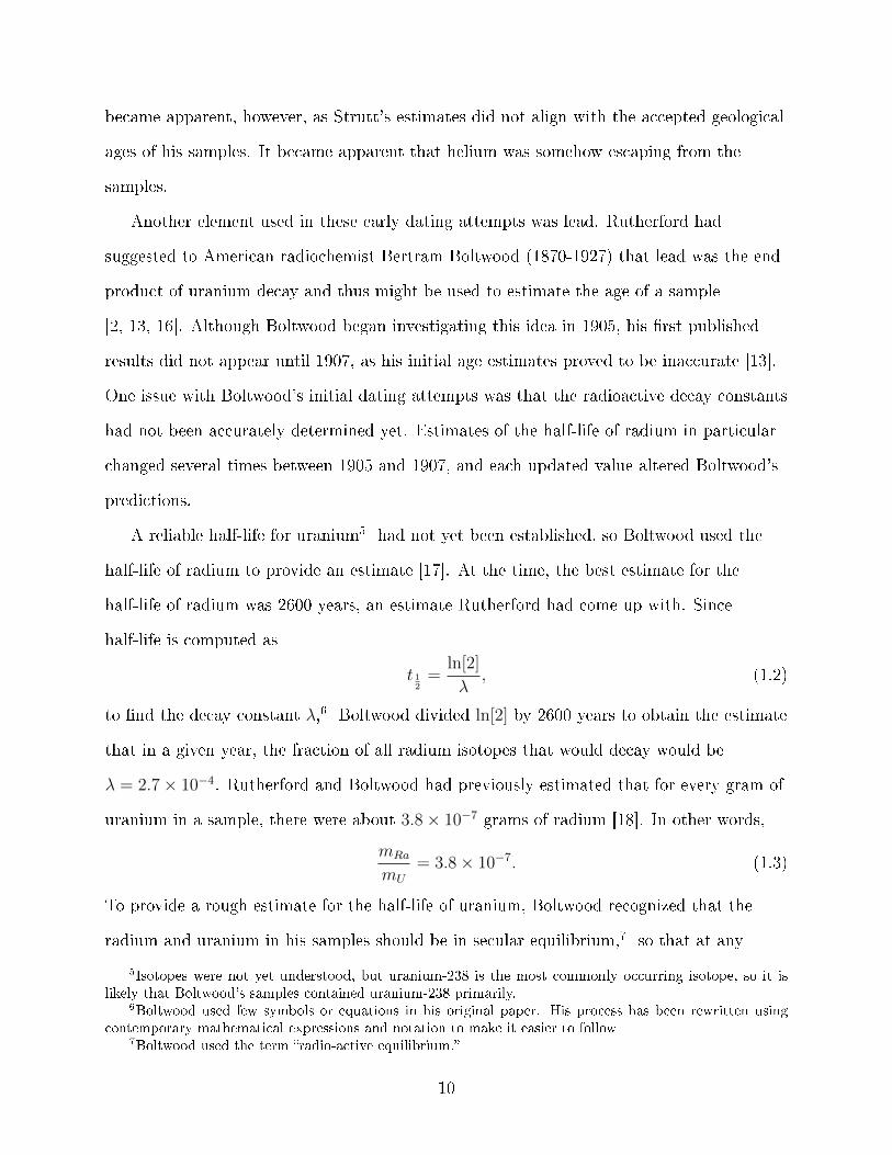
A reliable half-life for uranium5 had not yet been established, so Boltwood used the
half-life of radium to provide an estimate [17]. At the time, the best estimate for the
half-life of radium was 2600 years, an estimate Rutherford had come up with. Since
half-life is computed as
t 12
=ln[2]
λ, (1.2)
to �nd the decay constant λ,6 Boltwood divided ln[2] by 2600 years to obtain the estimate
that in a given year, the fraction of all radium isotopes that would decay would be
λ = 2.7× 10⁻⁴. Rutherford and Boltwood had previously estimated that for every gram of
uranium in a sample, there were about 3.8× 10⁻⁷ grams of radium [18]. In other words,
mRa
mU
= 3.8× 10⁻⁷. (1.3)
To provide a rough estimate for the half-life of uranium, Boltwood recognized that the
radium and uranium in his samples should be in secular equilibrium,7 so that at any
5Isotopes were not yet understood, but uranium-238 is the most commonly occurring isotope, so it islikely that Boltwood's samples contained uranium-238 primarily.
6Boltwood used few symbols or equations in his original paper. His process has been rewritten usingcontemporary mathematical expressions and notation to make it easier to follow
7Boltwood used the term �radio-active equilibrium.�
10

moment in time, equal amounts of uranium and radium atoms should be decaying. That is,
λUNU = λRaNRa. (1.4)
Instead of using the atomic masses of radium and uranium to extrapolate the number of
particles of each type, he assumed that the masses were the same. If the atomic masses
were the same, then the ratio he and Rutherford had computed of radium to uranium in a
sample would be the same as the ratio between the number of particles in each. In other
words,
mRa
mU
≈ NRa
NU
(1.5)
and thus
λU = λRaNRa
Nu
≈ λRamRa
mU
. (1.6)
Multiplying λRa by mRa
mU, he arrived at the conclusion that the decay constant for uranium
was on the order of 10−10 decays per year [17]. This implied that the half-life of uranium
was on the order of 1010 years.
To estimate the age of the minerals in his sample, he took the ratio of lead to uranium
in each sample and multiplied it by 1010. Boltwood did not explain why this should yield
the age of the sample. His approach was perhaps more heuristic than what follows, but the
same equation can easily be derived mathematically using appropriate approximations.
From the nuclear decay equation,
NU(t) = NU(0)e−λU t ≈ (NU(t) +NPb(t))e−λU t, (1.7)
where NPb is the number of lead atoms in the sample. The latter part of the equation relies
on the assumption that all of the uranium in the sample that has decayed has decayed to a
stable isotope of lead that has remained in the sample, and that there is no lead in the
sample from other sources. Rearranging,
NU(1− e−λU t) = NPbe−λU t (1.8)
11

and thus
NPb
NU
= eλU t − 1. (1.9)
Using a Taylor series expansion,
NPb
NU
≈ (1 + λU t)− 1 = λU t. (1.10)
Ignoring the atomic mass di�erences between lead and uranium,
mPb
mU
≈ λU t. (1.11)
By his estimates, his samples ranged in age from 410 million to 2.2 billion years. This
implied that the earth had to be at least 2.2 billion years old, signi�cantly older than
previous radiometric dating e�orts had suggested.
There were several problems with Boltwood's approach. The biggest issue was that
many of his samples contained thorium as well as uranium. Thorium also decays to lead,
but Boltwood assumed that it did not [17]. His �awed assumption was premised on the
fact that, while he found roughly constant uranium to lead ratios in his mineral samples
from a given location, the thorium to lead ratios varied substantially from one sample to
another. By assuming that all of the lead in his samples came from uranium, his results for
samples with high thorium to uranium ratios were necessarily skewed. Furthermore, the
samples likely contained various isotopes of both lead and uranium. While this could not
have been accounted for at the time, as isotopes had not yet been identi�ed, it may have
skewed his results, as di�erent isotopes have di�erent half-lives and come from di�erent
decay chains. Boltwood also made many simpli�cations, such as ignoring mass di�erences
between uranium and radium, which denied the method the rigor that would be needed for
accurate age estimates. Nonetheless, Boltwood had provided the framework that would
lead to modern lead-uranium dating.
While Boltwood and Rutherford occasionally toyed with the question of the age of the
earth, neither one published extensively on the subject following Boltwood's 1907 paper.
12
Arthur Holmes (1890-1965), one of Strutt's students, was inspired by Boltwood's work and
set out to improve upon Boltwood's techniques. His �rst publication, in 1911, utilized
Boltwood's basic technique, using equation [1.11] to compute the age of his sample, but
with a newly calculated half-life of uranium of 8.2 billion years [19]. While this value does
not match the currently accepted value, Holmes's half-life calculation was closer than
Boltwood's 10 billion year estimate. Two years later, Holmes published a book examining
the di�erent methods that were being used at the time to estimate the age of the earth
[20]. Using a further re�ned half-life of uranium of 5.4 billion years, he estimated that one
of his samples was 1.6 billion years old.
Discoveries during the 1910s led to complications in the radiometric dating technique
established by Boltwood and re�ned by Holmes [13]. One issue was that it was discovered
that lead was a decay product of thorium, thus adding challenge to dating samples
containing both uranium and thorium. In 1913, Soddy introduced the concept of the
isotope, showing that there existed atoms with the same proton number but di�erent
neutron numbers. The term isotope was suggested to Soddy by the physician Dr. Margaret
Todd8 (1859-1918), from the Greek iso topos, which means �same place� [22]. The term
was �tting because isotopes of an element occupy the same place on the periodic table. It
was found also that isotopes of the same radioactive element had di�erent half-lives.
Recognizing that there were di�erent isotopes of both uranium and lead, and that di�erent
isotopes of uranium decayed into di�erent isotopes of lead meant that Boltwood's method
could no longer be expected to provide a reliable age estimate. Although Holmes was forced
8Todd is an intriguing �gure in the history of medicine. She did not show much of a passion for medicine,but rather seemed to pursue it because medical school was one of the highest educational attainmentsavailable to women [21], becoming one of the �rst students at the Edinburgh School of Medicine for Women.There she met the woman who would become her life partner, Dr. Sophia Jex-Blake, a physician and oneof the founders of the school. While attending medical school, Todd wrote and published the novel Mona
Maclean, Medical Student under a male pseudonym. The novel was signi�cant in part because it receivedmuch praise as well as support for the movement to integrate women into the medical profession. Althoughshe did practice medicine at times, it was her writing that seemed to compel her, as she went on to publishseveral more books and stories. She died by suicide in 1918, three months after her �nal book, a biographyof Dr. Jex-Blake, had been published.
13

to leave academia for years at a time due to low wages o�ered to him as a student and later
as an instructor [15], he continued to pursue a reliable technique for lead-uranium dating.
It was not until the late 1930s when American physicist Alfred Nier (1911-1994)
provided the insight which would make accurate radiometric dating possible. Previously,
due to the observed unchanging atomic weight of lead in various samples, it was assumed
that lead isotopes existed in roughly the same ratios in all samples. Nier examined the
abundance of lead isotopes in various samples and found that the lead composition was not
uniform [23, 24]. Since di�erent lead isotopes have distinct half-lives, the assumption of
uniform abundance led to incorrect notions regarding the age of samples. Nier's work
provided the insight to account for variations in lead isotopes between samples. Arthur
Holmes used the ideas put forth by Nier to estimate the age of the Earth. He concluded
that the Earth was about 3 billion years old [25], much closer to the currently accepted 4.5
billion years than any previous calculations. At about the same time, German physicist
Fritz Houtermans (1903-1966) independently produced a similar estimate of the age of the
Earth based upon Nier's work [2, 26].
The current estimate for the age of the Earth was determined by American geochemist
Clair Patterson (1922-1995) in 1956 not by dating terrestrial samples, but rather by dating
meteorites [27, 13]. Patterson analyzed the lead compositions of �ve di�erent meteorites,
two iron meteorites and three stone meteorites. Iron meteorites do not contain uranium, so
the lead composition should theoretically remain unchanged over time. The two iron
meteorites in Patterson's study had almost identical compositions. Using the idea that all
three stone meteorites had started with the same lead composition, he estimated the age
for each of the stone meteorites and found the age estimates ranged from 4.5 billion to 4.6
billion years [27].
14

1.3 Radiometric Dating on Shorter Timescales
While early radiometric dating e�orts focused on objects which had existed for
hundreds of millennia, interest soon turned to using radioactivity to determine the age of
more recent samples. Carbon-14, which was �rst proposed as a radioactive dating tool in
the late 1940s by American nuclear chemist Willard Libby (1908-1980) [28, 29], has a
half-life of 5730 years, much shorter than the half-lives of uranium-238, uranium-235, and
thorium-232. This shorter half-life makes it useful for dating objects which have existed for
a few millennia, such as archaeological artifacts and glaciers.
Carbon-14 is produced when cosmic rays collide with nitrogen [30]. It, along with stable
carbon-12, is taken in and released by organisms during their lifetime, for example by
inhalation and exhalation. Thus, living organisms typically have the same ratio of
carbon-14 to carbon-12 as the atmosphere. When an organism dies, it no longer takes in
new carbon-14 and the carbon-14 present in its system slowly decays. Carbon-12, which is
not radioactive, will also be present in the organism's system and the carbon-12 levels will
remain the same as time elapses. Thus, the ratio of carbon-14 to carbon-12 will decrease
over time. By examining the ratio of carbon-14 to carbon-12, an estimate of the age of the
organism or artifact can be made. Mathematically, this works as follows. From the decay
equation,
NC14(t) = NC14(0)e−λC14t, (1.12)
where λC14 = 1.21× 10⁻⁴ decays per year. The amount of carbon-14 remaining at the
present time, NC14 can be measured directly from the sample. To determine the initial
amount of carbon-14, the atmospheric ratio of carbon-14 to carbon-12 at the time of the
organism's death must be known. Multiplying the atmospheric ratio by the amount of
carbon-12 in the sample can provide an estimate of how much carbon-14 was present in the
organism's system at the time of its death, NC14(0). Once that �nal quantity has been
determined, equation [1.12] can be solved for time.
15

While carbon-14 has many uses, its half-life is still long enough that it may be di�cult
to date very recent phenomena due to the fact that very little carbon-14 will have decayed.
Other radioisotopes with still shorter half-lives can be useful for this purpose. One of the
most widely used of these radioisotopes is lead-210.
Lead-210 is a naturally occurring isotope of lead which is a product of the uranium-238
decay series [31], with a half-life of about 22.3 years [32]. Lead-210 was �rst used in
radiometric dating in 1963 by E. D. Goldberg, who used it to estimate the age of glacier ice
[33]. Almost a decade later, it was used by Krishnaswamy et al. to date lake sediment
samples [34]. Dating lake sediment samples remains one of its most common uses in
radiometric dating.
The method of dating lake cores or ice cores di�ers from artifact dating in a signi�cant
way. It is generally assumed that the entirety of an artifact was constructed at a particular
instance in time, so the date that is estimated from the analysis of a sample of the object
can often be understood to stand for the age of the artifact as a whole. With core samples,
however, layers of sediment or ice build up over time. Thus, the sediment at the bottom of
a lake core sample would be expected to be older than the sediment at the top of the
sample. To estimate the age, certain assumptions must be made regarding the manner in
which the sediment was deposited.
To utilize Krishnaswamy et al.'s model, it must be assumed that the rate of supply of
lead-210, that is, the �ux of lead 210 reaching the surface of the sediment, and the
sedimentation rate remain constant in time [34, 35]. While these assumptions work
reasonably well for many samples, they may be too restrictive to be used to analyze others.
A new technique for lead-210 dating, known as the constant rate of supply (CRS) model,
was introduced in 1978 by Appleby and Old�eld [36]. This model required only that the
rate of supply remain constant. The CRS model will be discussed in detail in a subsequent
chapter.
16

Krishnaswamy et al. also investigated the possibility of using several other
radioisotopes for dating, namely cesium-137 and iron-55 [34]. Many dating techniques such
as those used in carbon-14 and lead-210 dating rely on the assumption that deposits of the
radioisotope have remained roughly constant over time, but this assumption must often be
eschewed when using cesium-137 for radiometric dating. Cesium-137 is a product of
nuclear �ssion [2] and has a half-life of about 30.2 years [32], indicating that cesium-137
could be used on timescales similar to the ones lead-210 is used for. Since cesium-137 is
part of the fallout from nuclear testing, it would be expected that in regions where nuclear
testing has occurred, increases in the cesium-137 content of the soil can be mapped to the
time period in which the testing occurred. However, in practice, cesium-137 dating has
proven inconsistent [37]. Davis et al. examined the cesium-137 pro�les of lakes in northern
New England and Scandinavia. Lead-210 dating was performed on 14 of the 16 New
England lakes and the chronostratigraphic pollen markers of the New England lakes were
analyzed as well. Cesium-137 was observed at depths corresponding to dates that the
lead-210 and pollen markers estimated were prior to the fallout. These results suggest that
cesium-137 may be more mobile than lead-210, moving through the sediment layers instead
of remaining stationary, which could make it di�cult to extrapolate accurate ages from the
cesium-137 pro�le of a sample.
Another fallout radionuclide used in radiometric dating is strontium-90 [38]. As with
cesium-137, prior to the testing of nuclear weapons, very little strontium-90 would be
expected to be found in the soil. Strontium-90 was deposited in the Great Lakes region
from 1953 through 1964 through fallout from weapons testing and precipitation. After
1964, major above ground nuclear weapons testing was discontinued, thus diminishing the
amount of Sr-90 deposited in the region annually. Some Sr-90 could still be expected to be
observed in post-1964 samples, as radioactive remnants of nuclear weapons testing would
be delivered via precipitation, but the amount of Sr-90 being added would show a
signi�cant decrease compared to the nuclear testing years.
17

Lerman examined the Sr-90 concentration in the Great Lakes between 1954 and 1969
[38]. Because the Great Lakes are interconnected, the Sr-90 concentration could be
decreased by out�ow as well as radioactive decay and increased by in�ow from multiple
sources, requiring a more complicated mathematical relation than is used to describe
isolated lakes. Lerman proposed a system of di�erential equations describing the
concentration of Sr-90 in the Great Lakes as a function of time. The di�erential equations
took into account the various sources of in�ow and out�ow for each lake, as well as loss due
to radioactive decay. Lerman's model did not �t the collected concentration completely. He
was able to obtain a better �t for three of the Great Lakes by increasing the input for the
years 1962-1964 by a small amount and increasing the out�ow by 6− 8%. The need to
increase the out�ow suggested that there were additional mechanisms by which Sr-90 was
removed, although what those mechanisms would be was not immediately clear.
18

CHAPTER 2
A DEEPER LOOK AT LEAD-210 DATING
2.1 The Lead-210 Decay Process
Lead-210 is part of the uranium-238 decay series [31], as shown in Figure 2.1. It has a
half-life of about 22.26 years [32], and can decay to bismuth-210 through electron emission
or to mercury-206 through α emission. Compared to many other naturally occurring
radioisotopes, lead-210 has a relatively long half-life, which makes it useful for dating
sediment samples that are no more than 100-150 years old.
Since lead-210 is part of the uranium-238 decay chain, if uranium-238 or one of its
progeny, such as radon-222, are present in a sample, new lead-210 atoms will be continually
introduced into the sample through radioactive decay. If the system is in secular
equilibrium, the amount of lead-210 in the sample will remain nearly unchanged as time
passes. Since the amount of lead-210 stays constant, it is not useful for radiometric dating.
This type of lead is referred to as supported lead-210 because there is a source that
replenishes it.
If, however, lead-210 is separated from its source, then over time, the lead that is
present in the sample will decay. There are multiple mechanisms by which this separation
occurs in nature. It may, for example, be swept away by wind or be deposited in
precipitation. Some lead-210 particles separated in such a manner may reach the bed of a
lake. Over time, sediment will accumulate atop this lead-210, sealing it into the lake bed.
This lead is referred to as unsupported lead-210 and it is this lead which is used to date
samples.
19

Figure 2.1. The uranium-238 decay series.For isotopes that have two possible decays, the most common decays are shown with solidarrows, while less frequently occurring decays are represented with dashed arrows. Some
infrequent decays have been omitted from the chart for readability.
2.2 Obtaining and Counting a Lead-210 Sample
To begin the dating process,1 a core sample must be taken. The site for the core
sample may be chosen for a variety of reasons. However, there are several features that
1Although this chapter refers primarily to the lead-210 dating process, because all radioisotopes decaysimilarly, many steps of the process of radiometric dating are the same, regardless of the isotope used fordating. Variations may exist in, for example, what type of detector is used to count the particles. However,the general process of collecting a core sample, counting the decays of radioisotope, and modeling the age ofthe sample follows similarly.
20
may make for a more ideal sample site [39]. Relatively undisturbed bodies of water2 are
preferable because if there is too much mixing of the upper sediment layers, the lead that
exists in these sediments may migrate between layers, making it di�cult to estimate the
surface concentration accurately. In a naturally formed lake, cores are often taken from the
center of the lake to minimize disturbances caused by shoreline activity. Choosing bodies of
water with other geological or temporal markers that can corroborate age estimates can
also be useful.
In reservoirs, it is advisable to take core samples that reach the layers of sediment that
existed prior to the creation of the reservoir. Since the reservoir was created in a speci�c
time frame, the creation of the reservoir can serve as a check on age estimates provided by
radiometric dating. Samples with higher sedimentation rates are desirable because a higher
sedimentation rate decreases the amount of mixing of the sediment after it has been
deposited [40] and also minimizes the adverse e�ects of diagenesis on the sample [41].
Nonetheless, bodies of water with less desirable attributes may be of interest to scienti�c
study, and with the appropriate mathematical tools, it may be possible to analyze these
samples as well.
The core samples analyzed by the Environmental Radiation Lab (ERL) at the
University of Maine are sometimes provided by external agents, while at other times are
collected by students. The coring tools used vary depending on the department or
institution that is collecting the core sample. For a brief discussion of which coring tools
are desirable for what types of bodies of water, see [39].
When a lake core sample is taken, it is cut into thin slices, often half an inch in
thickness. The slices are weighed once when wet to �nd the wet weight and again when
dried to �nd the dry weight, M [1]. The individual slices are then ground and placed inside
tubes to be analyzed for their lead-210 content.
2Most ideal are lakes containing varved sediment, that is, a collection of thin sediment layers thatalternate in color. In such bodies of water, there is so little mixing of the sediment that each strati�cationcorresponds to the summer or winter of a given year. Thus, the age of the sediment can be determined bycounting the layers.
21
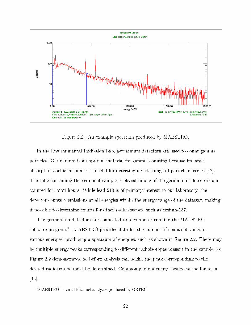
Figure 2.2. An example spectrum produced by MAESTRO.
In the Environmental Radiation Lab, germanium detectors are used to count gamma
particles. Germanium is an optimal material for gamma counting because its large
absorption coe�cient makes it useful for detecting a wide range of particle energies [42].
The tube containing the sediment sample is placed in one of the germanium detectors and
counted for 12-24 hours. While lead-210 is of primary interest to our laboratory, the
detector counts γ emissions at all energies within the energy range of the detector, making
it possible to determine counts for other radioisotopes, such as cesium-137.
The germanium detectors are connected to a computer running the MAESTRO
software program.3 MAESTRO provides data for the number of counts obtained at
various energies, producing a spectrum of energies, such as shown in Figure 2.2. There may
be multiple energy peaks corresponding to di�erent radioisotopes present in the sample, as
Figure 2.2 demonstrates, so before analysis can begin, the peak corresponding to the
desired radioisotope must be determined. Common gamma energy peaks can be found in
[43].
3MAESTRO is a multichannel analyzer produced by ORTEC
22

Table 2.1. Example counting data.Energy (keV ) Counts)
505 26506 25507 30508 27509 85510 177511 234512 110513 34514 25515 19516 20
Once the appropriate energy peak has been identi�ed, the peak area must be computed.
For example, suppose the �ctional data presented in Table 2.1 were the counts collected for
energies around 510 keV (Note that lead-210 has a peak around 47 keV and thus this
�ctional data is not meant to be representative of lead-210).
This data is represented graphically in Figure 2.3. As the histogram shows, while there
is a clear peak at 511 keV , the counts at 510 keV and 512 keV are also higher than the
background radiation counts. To calculate the value of the peak, the �rst step is to
compute the gross area corresponding to the energies from 510 keV to 512 keV . This is
done by adding the individual counts, i.e.,
G =512∑i=510
ci = 177 + 234 + 110 = 521, (2.1)
where G denotes the gross area and ci denotes the count at the ith energy. In general, for a
peak starting at some energy L and ending at some energy R, where L and R stand for left
and right, respectively, the gross area is given by [42]
G =R∑i=L
ci. (2.2)
However, the gross count G is not the value of the peak, as the background radiation has
not been taken into account. We will assume that the background radiation does not have
23

a peak at the location of the peak of interest and thus is approximately constant
throughout the peak, a reasonable assumption in many situations. (For instances in which
there is signi�cant overlap between the peaks of the sample and background radiation, see
e.g., [42].)
To determine the background count, m channels immediately to the left and m
channels immediately to the right will be selected. For the purposes of this example, we
will choose m = 4. In general, as long as the background counts are close to uniform,
choosing three to �ve channels on either side of the peak should generally be su�cient to
estimate the background counts [42]. To �nd the background count under the peak, the
background counts are averaged and then multiplied by n, the number of channels under
the peak. In this case, n = 3. In general, the background counts are given by [42]
B =n
2m[L−1∑
i=L−m
ci +R+m∑i=R+1
ci]. (2.3)
Note that 2m, the averaging factor, has been moved to the front of the equation for ease of
notation. The background counts in this example are then given by
B =3
2 · 4[
510−1∑i=510−4
ci +512+4∑i=512+1
ci] =3
8[
509∑i=506
ci +516∑i=513
ci] = 77.25 ≈ 77. (2.4)
To then �nd the area of the peak, the background must be subtracted from the gross peak.
In other words, the area N , which represents the total number of counts, is given by [42]
N = G−B =R∑i=L
ci −n
2m[L−1∑
i=L−m
ci +R+m∑i=R+1
ci]. (2.5)
In this particular example, N = 521− 77 = 444.
Once the number of counts in the peak has been determined, the uncertainty of the peak
must be computed. Since each peak tends to form a distribution that is close to a Poisson
distribution, a rough estimate for the uncertainty would be ∆N =√N [1]. However,
because there is also some uncertainty in the estimation of the background counts, that
uncertainty must be accounted for as well. For this reason, the uncertainty is given by [1]
∆N =
√N +
B
m. (2.6)
24
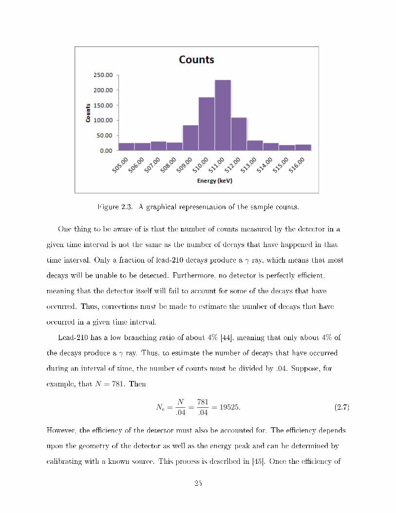
Figure 2.3. A graphical representation of the sample counts.
One thing to be aware of is that the number of counts measured by the detector in a
given time interval is not the same as the number of decays that have happened in that
time interval. Only a fraction of lead-210 decays produce a γ ray, which means that most
decays will be unable to be detected. Furthermore, no detector is perfectly e�cient,
meaning that the detector itself will fail to account for some of the decays that have
occurred. Thus, corrections must be made to estimate the number of decays that have
occurred in a given time interval.
Lead-210 has a low branching ratio of about 4% [44], meaning that only about 4% of
the decays produce a γ ray. Thus, to estimate the number of decays that have occurred
during an interval of time, the number of counts must be divided by .04. Suppose, for
example, that N = 781. Then
Ne =N
.04=
781
.04= 19525. (2.7)
However, the e�ciency of the detector must also be accounted for. The e�ciency depends
upon the geometry of the detector as well as the energy peak and can be determined by
calibrating with a known source. This process is described in [45]. Once the e�ciency of
25

the detector has been determined for the given energy peak, the total number of decays can
be determined by dividing the modi�ed number of counts Ne by the e�ciency γe,
Nt =Ne
γe. (2.8)
For the example above, assuming a detector with e�ciency γe = .25, the total number of
decays in the given time interval would be
Nt =19525
.25= 78100. (2.9)
Thus, for our hypothetical example, while the detector measured only N = 781 counts,
about Nt = 78100 lead-210 decays occurred during time interval in which the data was
collected.
For radiometric dating, it is not the actual activity at each depth that is essential, but
rather a proportional representation of how many counts there are at each depth. In other
words, it does not matter so much whether we use the 50 and 25 count estimate without
the e�ciency at two depths or the 200 and 100 counts that would be expected once
e�ciency is taken into account; the ratio between the two depths is the same. As long as
all measurements are taken using the same detector, all measurements will be reduced by
the same e�ciency factor γe. For this reason, the e�ciency of the detector is sometimes
omitted from the activity calculations. That is, Ne is used in place of Nt in activity
calculations. Making this change will not a�ect age estimates, but the calculated �activity"
will not be a true activity, and thus could not be used for comparing against activity
calculations from other detectors.
From the number of total decays Nt, the activity can be determined. The activity is
de�ned as the number of decays per unit time [45],
A =dN
dt=
d
dtN(t) = −λN0e
−λt = −λN(t). (2.10)
In practice, activity is generally obtained by taking the number of decays Nt and dividing it
by the time that elapsed as the detector counted. For example, if it took 12 hours (or 43200
26

s) for the detector to complete its counting, then, continuing with the example above,
A =Nt
t=
78100
43200= 1.8079. (2.11)
Thus the activity would be 1.81 Bq.
The speci�c activity is what is used for radiometric dating. The speci�c activity is the
activity per unit mass of a sample [45], or
C =A
M, (2.12)
where M is the dry mass of the sample, as mentioned previously.
Beyond a certain depth, the concentration of lead-210 will remain roughly unchanged.
The speci�c depth at which this occurs varies from one body of water to the next, and can
be approximated by looking for a point in the data beyond which the �uctuations in
lead-210 are small. The tail of the data is averaged to determine an estimate of the
supported lead-210 in the sample.4 Once the speci�c activities have been computed, an
estimate of the speci�c activity of supported lead-210 is determined by averaging the
speci�c activities for depths deeper than the chosen cut o� depth. This activity estimate is
then subtracted from the speci�c activities to obtain an estimate of the unsupported
lead-210 present in each layer of the sample. A plot of concentration of unsupported
lead-210 versus depth can then be constructed.
Although the rationale may not become clear until the CRS model has been described,
a modi�ed activity Am in units of Bqcm2 must also be computed. This value is obtained by
multiplying the speci�c activities by what is called the dry mass, Md, which itself a mass
but rather has units of gcm2 . The process of obtaining the dry mass is described below.5
4To use this technique, it is worth noting that the deviation between di�erent data points in the tail ofthe curve should be fairly small. If the standard deviation is greater than about 10 %, then another techniquemay be needed. Dr. James Kaste recommends calculating the radium-226 content in each sediment layerand using that to determine a unique supported lead-210 value for each data point.
5The following technique is the one which was outlined to me. Dr. Kaste suggests a more straightforwardapproach. His recommendation is to use the thickness of the layer and the radius of the core tube to determinethe volume of the core slice. Dividing the dry mass by the volume will then yield the bulk density.
27

The loss on ignition must also be computed to determine how much of the sample is
composed of organic versus inorganic matter. The samples are sent to the Sawyer
Environmental Chemistry Laboratory at the University of Maine, where the are heated to
500◦C [1]. The organic sediment in the sample will burn o�, while the inorganic matter will
remain. Since the organic and inorganic constituents of the samples have di�erent densities,
the percentages of each will be needed to determine the dry mass densities of the samples.
It is assumed that the organic matter has a density of 1.6 gcm3 and that the inorganic
sediment has a density of 2.5 gcm3 [1]. The solid density S is the sum of the organic and
inorganic densities by their respective percentages, given mathematically as [1]
S = 1.6O + 2.5I, (2.13)
where O and I denote the percentages of organic and inorganic matter in the sample,
respectively.
The presence of water in the sediment sample must be accounted for. To begin with,
the percent sediment by weight is computed. If the dry weight is denoted by d and the wet
weight by w, then the percent sediment by weight, sw, will be the ratio of the two
multiplied by 100%, i.e.
sw =d
w· 100%. (2.14)
Likewise, since the sample is made up of sediment and water, the percent water by weight
is given by
fw = 100%− sw. (2.15)
From here, the percentages of sediment and water by volume must be computed so that
the mass density and ultimately the dry mass can then be determined. The percent water
by volume fv is given by [1]
fv =fw
fw + swS
. (2.16)
The percent sediment by volume sv is thus
sv = 100%− fv. (2.17)
28

Table 2.2. Cumulative Activity.Depth (cm) Modi�ed Activity ( Bq
cm2 ) Cumulative Activity ( Bqcm2 ))
1 .48 1.293 .37 .815 .21 .447 .16 .239 .07 .07
The mass density ρM is given by [1]
ρM = S · sv. (2.18)
Once the mass density has been calculated, the dry mass Md can be determined. The dry
mass is the solid density of the sample in gcm3 multiplied by the depth of the interval, D, in
cm. From [1],
Md = S ·D. (2.19)
Observe that the units of Md are gcm2 .
Now that Md has been determined, the desired conversion can be made. The speci�c
activities S are multiplied by Md to obtain a modi�ed activity in units of Bqcm2 ,
A = S ·Md. (2.20)
Note that although Am had been previously used in this paper to distinguish the activities
from the modi�ed activities, the subscript is omitted from the above equation as well as
throughout the remainder of this document to remain consistent with conventional
notation.
One �nal calculation remains to be computed, namely the cumulative activities. To
obtain cumulative activities, the modi�ed activities of a layer are summed with all of the
modi�ed activities of lower depths. As an example, consider the �ctionalized activity data
given in Table 2.2. The lowest depth is 9 cm, with a corresponding modi�ed activity of .07
Bqcm2 . Since there are no sediment layers beneath this layer, the cumulative activity is the
same as the modi�ed activity. The 7 cm sediment layer has one layer beneath it, so the
29

cumulative activity is the sum of the modi�ed activities of the 7 cm and 9 cm layers, or
Ac = .07 + .16 = .23 Bqcm2 . Similarly, the cumulative activity of the 5 cm layer is the sum of
the modi�ed activities of the 5, 7, and 9 layers, the cumulative activity of the 3 cm layer is
the sum of the modi�ed activities of the 3, 5, 7, and 9 cm layers, and the cumulative
activity of the 1 cm layer is the sum of all of the modi�ed activities. The sum of all
modi�ed activities is generally used as the initial condition A(0) when estimating the age
of a sample. More detail on the typical dating technique used will be presented in the
following section.
As mentioned in the introductory chapter, there are two commonly used methods for
dating samples based on their lead-210 content. The Constant Flux, Constant
Sedimentation (CFCS) model was introduced by Goldberg [33] and re�ned by
Krishnaswamy [34]. As the name suggests, this model assumes that, for a given sample, the
�ux and the sedimentation rate are constant. A second model, the Constant Rate of
Supply (CRS) model, proposed by Appleby and Old�eld, assumes that the lead-210 �ux is
constant. This assumption means that the dry mass sedimentation �ux multiplied by the
activity per gram is constant. Derivations of the CFCS model can be found in many
sources (e.g., [34, 35, 1]), but since it is more restrictive than the CRS model, it will not be
analyzed in detail here. A derivation of the CRS model will be provided in the following
section.
2.3 The Constant Rate of Supply Model
In 1978, Appleby and Old�eld introduced a mathematical model for dating sediment
samples assuming a constant supply rate of lead-210, which they termed the Constant Rate
Supply (CRS) Model [36]. Their derivation is as follows: Suppose that the initial
concentration of unsupported lead-210 C0 in Bqg
satis�es the equation
C0(t)r(t) = ζ, (2.21)
30

where ζ is constant and r(t) gcm2yr
is the dry mass sedimentation rate at time t. If x is the
depth of the sediment of age t, then the concentration of lead-210 at depth x, in
accordance with the nuclear decay equation, is given by
C(x) = C0(t)e−kt, (2.22)
where
k =ln 2
22.26= .03114 (2.23)
is the radioactive decay constant of lead-210 in inverse years. Then, rearranging the
concentration equation,
C0(t) = C(x)ekt. (2.24)
If the sediment is laid down during a small period of time δt, then the thickness of this
layer is given by
δx =r(t)
ρ(x)δt, (2.25)
where ρ(x) is the dry mass per unit wet volume of the sediment at depth x in gcm3 . Then
the rate of change of depth is
x =r
ρ. (2.26)
Solving for r,
r(t) = ρ(x)x. (2.27)
Substituting (2.24) and (2.27) into (2.21),
C(x)ektρ(x)x = ζ, (2.28)
or
C(x)ρ(x)x = ζe−kt. (2.29)
Consider the function
A(x) =
∫ ∞x
ρ(x)C(x)dx, (2.30)
31

where A is the total residual unsupported lead-210 beneath sediments of depth x. By the
Fundamental Theorem of Calculus,
A =d
dt(
∫ ∞x
ρ(s)C(s)ds) = [ρ(s)C(s)]s=∞ − ρ(x)C(x)x. (2.31)
Since the unsupported lead-210 concentration decreases with depth, [ρ(s)C(s)]s=∞ = 0,
and thus
A = −ρ(x)C(x)x = −ζe−kt. (2.32)
Hence,
A = −∫ t
−∞ρ(x)C(x)xds = −
∫ t
−∞ζe−ksds. (2.33)
Using the negative sign to �ip the limits of integration,
A = −∫ t
−∞ζe−ksds =
∫ ∞t
ζe−ksds (2.34)
and thus
A(x) =ζ
ke−kt. (2.35)
Given the initial condition A(0),
A(x) = A(0)e−kt. (2.36)
Solving (2.36) for t,
t =1
klnA(0)
A(x), (2.37)
where t is the age in years of the layer of depth x. For a given sample, the age can thus be
estimated from A(x), assuming that the �ux of unsupported lead-210 is nearly constant.
2.4 Problems with Current Dating Techniques
Both the CFCS and CRS models work relatively well in certain situations, but neither
one applies universally to all sediment samples. Consider the following data, used by
Douglas Cahl in his master's thesis [1] and presented in Figure 2.4. Under the CRS model,
the relationship between activity and depth should follow an exponential decay curve, but
32

Figure 2.4. Data presented in Douglas Cahl's master's thesis of unsupported lead-210 vs.depth.
there appear to be sinusoidal �uctuations as well. Neither the CRS model nor the CFCS
model account for periodic �uctuations in activity such as the one observed here.
While this project was initiated with lead-210 in mind, since all radioisotopes decay in
accordance with the nuclear decay equation, with slight modi�cations it could be applied
to many other radioisotopes. Of particular interest is cesium-137, which exists in the
environment primarily as fallout from nuclear weapons testing. Cesium-137, which has a
half-life of about 30.2 years [32], theoretically should be usable for estimating the age of
samples on similar timescales to those dated using lead-210. However, it has proven an
unreliable dating source due in part to an ability to permeate the soil layers in a manner
that other radioisotopes generally do not demonstrate [37].
The behavior of cesium-137 varies considerably from one lake to another, depending on
the biological, chemical, and geological properties of the lake [46]. For example, the type of
water in a lake has been shown to in�uence the mobility of cesium-137 [47]. In a study of
Lake St. Clair in Michigan, it was found that sorbed cesium-137 was more mobile in anoxic
soft water, that is, soft water with depleted levels of dissolved oxygen, and less mobile in
33
oxic, or oxygen rich, soft water [47]. Hard water was found to fall between oxic and anoxic
soft waters in terms of cesium-137 mobility, although there was little di�erence between
oxic and anoxic hard water. Other factors such as the composition of the lake bed may also
in�uence the mobility of cesium-137, as it is readily absorbed by some minerals such as clay
and mica [47, 48].
Although cesium-137 may sometimes provide unreliable age estimates under the CRS
and CFCS models, it can play a crucial role in radiometric dating. Due to losses from the
top of a core sample that may occur in coring, lead-210 age estimates may fail if not
calibrated against another radioisotope such as cesium-137 [49]. Additionally, in regions in
which the watershed and lake bed have undergone disturbances, using lead-210 alone can
provide inaccurate age estimates [50], so an additional radioisotope such as cesium-137 may
be needed to con�rm the estimates. While a piecewise approach employing CRS techniques
and comparing against chronostratigraphic markers has been been applied to a sampling of
cesium-137 samples with some success [49], a model that handles all cesium-137 samples
remains elusive. If the mobility of cesium-137 could be modeled mathematically, then a
more comprehensive model for cesium-137 dating which does not require a constant rate of
supply of cesium-137 could perhaps be devised.
Additional radioisotopes of interest could include beryllium-7 and strontium-90.
Beryllium-7 deposits have been shown to vary seasonally [51]. With a half-life of about
53.3 days [32], it might not be as useful for dating lake core samples, but it could provide
information for short timescale analyses. Like cesium-137, strontium-90 is a radionuclide
introduced into the environment primarily as fallout from nuclear weapons testing [38].
With a half-life of 28.8 years [32], it can be used for aging samples of similar timescales to
those aged using lead-210. In particular, changes in concentration of strontium-90 in the
Great Lakes over time have been studied in some detail by Lerman [38]. While Lerman
devised a model speci�c to the Great Lakes, a more general model that could encompass
strontium-90 dating might be useful.
34

Devising a general model that can be used for cesium-137 and strontium-90 is a
pressing matter in North America. Very little cesium-137 and strontium-90 present in lake
sediment samples is naturally occurring. Nuclear weapons testing in the United States
introduced large quantities of these radioisotopes into the environment beginning in 1952
and continuing through the mid-1960s [50]. In the years since above ground nuclear
weapons testing ended, little new cesium-137 and strontium-90 has been introduced into
North American lake beds. Since these two radioisotopes have half-lives on the order of 30
years, much of the cesium-137 and strontium-90 introduced into the environment through
weapons testing has decayed. These diminishing levels have added an additional layer of
di�culty to cesium-137 dating [52]. Thus, it is imperative to develop techniques to
accurately age sediment samples using these radioisotopes while the levels of these isotopes
are still detectable in North American sediment samples.
In addition, for lead-210 samples exhibiting sinusoidal �uctuations, the period of the
oscillations will be calculated and analyzed. It is hypothesized that the oscillations are
caused by changes in wind and rainfall due to climate cycles, such as perhaps the North
Atlantic Oscillation, which has been speculated to create periodic �uctuations in
atmospheric lead-210 in parts of Europe [53]. However, further study would be needed to
assess the nature of the sinusoidal behavior.
The aim of the following chapters is to devise a mathematical model for radiometric
dating that does not require a constant rate of supply of a given radioisotope. The hope is
that in doing so, more samples will be able to analyzed and with better accuracy than
current models provide. Additionally, for samples that show sinusoidal oscillations, I aim to
examine the period of oscillations and investigate the physical signi�cance of the period.
Chapter 3 will provide a derivation of this new model, called the Non-Constant Rate of
Supply (NCRS) model. The CRS and NCRS models will be implemented on a �ctitious
data set to demonstrate the utility of the NCRS model. In Chapter 4, the NCRS model
will be applied to four existing data sets and compared against the CRS model. Chapter 5
35

will examine 30 additional sediment samples. For the samples with sinusoidal oscillations,
the period will be computed. Climate cycles will be considered as a potential cause of the
oscillations. In Chapter 6, I will draw some conclusions and o�er recommendations for
future work.
36
CHAPTER 3
A NEW TECHNIQUE FOR RADIOMETRIC DATING
3.1 Deriving the Non-Constant Rate of Supply Model
I developed a Non-Constant Rate of Supply (NCRS) model in an e�ort to expand the
scope of samples that can be analyzed using radiometric dating. The method closely
follows the techniques used by Appleby and Old�eld in the development of their CRS
model [36]. The main di�erence between the two approaches is the initial assumption.
Instead of assuming that the rate of supply of lead-210 is constant, I assumed that it was
allowed to �uctuate.
Suppose that instead of a constant supply rate, the lead-210 rate varies by some known
functions of time. In other words,
C0(t)r(t) = ζ + f1(t) + f2(t) + · · ·+ fn(t), (3.1)
where ζ in Bqcm2yr
is constant, C0 in Bqg
is the initial concentration of unsupported lead-210
in the sediment, r(t) in gcm2yr
is the dry mass sedimentation rate at time t, and
f1(t), f2(t) · · · fn(t) in Bqcm2yr
are arbitrary functions of time. If x is the depth of the
sediment of age t, then the concentration of lead-210 at depth x is given by
C(x) = C0(t)e−kt, (3.2)
where k = .03114 is the radioactive decay constant of lead-210 in inverse years. Then,
rearranging the concentration equation,
C0(t) = C(x)ekt. (3.3)
For the same reason as outlined in Chapter 2 in the derivation of the CRS model, the rate
of change of depth is given by
x =r(t)
ρ(x), (3.4)
37

where ρ(x) is again the dry mass per unit wet volume of the sediment at depth x in gcm3 .
Solving for r(t),
r(t) = ρ(x)x. (3.5)
Substituting (3.3) and (3.5) into (3.1),
C(x)ektρ(x)x = ζ + f1(t) + f2(t) + · · ·+ fn(t) (3.6)
or, rearranging,
C(x)ρ(x)x = e−kt(ζ + f1(t) + f2(t) + · · ·+ fn(t)). (3.7)
Let
A(x) =
∫ ∞x
ρ(s)C(s)ds, (3.8)
where A in Bqcm2 is the total residual unsupported lead-210 beneath sediment layers of depth
x. Observe that, by the Fundamental Theorem of Calculus,
A =d
dt(
∫ ∞x
ρ(s)C(s)ds) = [ρ(s)C(s)]s=∞ − ρ(x)C(x)x. (3.9)
The unsupported lead-210 concentration decreases with depth, meaning that
[ρ(s)C(s)]s=∞ = 0, and hence
A = −ρ(x)C(x)x = −e−kt(ζ + f1(t) + f2(t) + · · ·+ fn(t)). (3.10)
Thus,
−∫ t
−∞ρ(x)C(x)xds = −
∫ t
−∞e−ks(ζ + f1(s) + f2(s) + · · ·+ fn(s))ds. (3.11)
Absorbing the negative sign into the limits of integration,
−∫ t
−∞e−ks(ζ + f1(s) + f2(s) + · · ·+ fn(s))ds
=
∫ ∞t
e−ks(ζ + f1(s) + f2(s) + · · ·+ fn(s))ds (3.12)
38

and thus
A(x) = ζ
∫ ∞t
e−ksds+
∫ ∞t
f1(s)e−ksds+
∫ ∞t
f2(s)e−ksds+ · · ·+
∫ ∞t
fn(s)e−ksds
= −ζ[−1
ke−ks]∞t +
∫ ∞t
f1(s)e−ksds+
∫ ∞t
f2(s)e−ksds+ · · ·+
∫ ∞t
fn(s)e−ksds. (3.13)
In general,
A(x) =ζ
ke−kt +
∫ ∞t
f1(s)e−ksds+
∫ ∞t
f2(s)e−ksds+ · · ·+
∫ ∞t
fn(s)e−ksds, (3.14)
where t is the age in years of the sediment layer of depth x.1 Given an initial condition
A(0) and functions f1, f2, · · · fn, this equation can be written explicitly, as demonstrated in
the following sections. For a given sample, the age can be estimated from A(x), although if
the rate of supply is non-constant, that is, fi 6= 0 for any i, numerical techniques may be
required to determine t.
3.2 The NCRS Model with Sinusoidal and Linear Terms
If the rate of supply of a radioisotope is assumed to be non-constant, the natural
question would be what sort of functions may describe it. Some data, such as shown in
Figure ??, suggest that the rate of supply may �uctuate sinusoidally. The potential causes
of these sinusiodal �uctuations are not fully understood, but will be discussed in later
chapters. Another possible non-constant change would be a linear change. Such a change
may occur, for example, if there is in�ow or out�ow to the body of water from which the
core sample was collected, or if the radioisotope is able to migrate through the layers of soil.
Suppose that a plot of concentration versus depth for a given sample suggests that in
addition to exponential decay, the concentration rate shows both sinusoidal and linear
�uctuations. In other words,
C0(t)r(t) = ζ + a sin (bt+ c) + gt, (3.15)
1Note that A(x) is used here to be consistent with Appleby and Old�eld's notation, since their notationwas used for the CRS derivation. However, A(t) might make more sense. While the accumulation of lead-210does vary with depth, that variation is a direct consequence of the nuclear decay process, which progresseswith time.
39

where a, b, c, g, and ζ are constant. Then
C0(t)r(t) = C(x)ρ(x)xekt = ζ + a sin (bt+ c) + gt (3.16)
and therefore
C(x)ρ(x)x = e−kt(ζ + a sin (bt+ c) + gt). (3.17)
Then
A(x) =
∫ ∞t
C(x)ρ(x)xds =
∫ ∞t
e−ks(ζ + a sin (bs+ c) + gs)ds. (3.18)
Thus,
A(x) = ζ
∫ ∞t
e−ksds+ a
∫ ∞t
sin (bs+ c)e−ksds+ g
∫ ∞t
se−ksds
=ζ
ke−kt + a
∫ ∞t
sin (bs+ c)e−ksds+ g
∫ ∞t
se−ksds. (3.19)
Integrating,
A(x) =ζ
ke−kt +
a
k2 + b2(k sin (bt+ c) + b cos (bt+ c))e−kt + g(
t
k+
1
k2)e−kt
= e−kt(ζ
k+
g
k2+gt
k+
a
k2 + b2(k sin (bt+ c) + b cos (bt+ c)). (3.20)
If a sample has only sinusoidal variance in the rate of supply of the radionuclide, then
g = 0 in [3.20]. If it displays only linear variance, then a = 0 in [3.20]. While sinusoidal and
linear changes to the concentration are some of the more common changes that might be
observed, this method will work for many mathematical functions.
3.3 Modeling a Pulse
Another possible occurrence that could a�ect the rate of supply would be if a large
quantity of a radioisotope was introduced into a lake in a short amount of time. This may
be found, for example, in a body of water into which nuclear reactor e�uent is released,
such as was shown in [54]. Mathematically, such an in�ux might be modeled with a delta
function.
40

Suppose that a pulse is released at some time t0. Assume that
C0(t)r(t) = ζ + hδ(t− t0), (3.21)
where h in Bqcm2yr
is constant. Then
C0(t)r(t) = C(x)ρ(x)xe−kt = ζ + hδ(t− t0), (3.22)
and thus
C(x)ρ(x)x = e−kt(ζ + hδ(t− t0)). (3.23)
Therefore
A(x) =
∫ ∞t
C(x)ρ(x)xdt =
∫ ∞t
e−ks(ζ + hδ(s− t0)ds). (3.24)
Integrating,
A(x) =ζ
ke−kt + h
∫ ∞t
e−ksδ(s− t0)ds. (3.25)
The results of integration depend on whether the depth (or, correspondingly, the time) at
which the pulse was released is included in the limits of integration. For older sediment,
which accumulated before the pulse was released, there will be no contribution from the
pulse term, as is consistent with the mathematical de�nition of an integral over a delta
function. For newer sediment which has accumulated after the pulse, however, recalling
that ∫ ∞−∞
f(s)δ(s− t0) = f(t0), (3.26)
then
h
∫ ∞t
e−ksδ(s− t0)ds = he−kt0 . (3.27)
Therefore,
A =
ζke−kt t > t0
ζke−kt + he−kt0 t < t0.
(3.28)
Recall that A(x) is de�ned as the accumulation of all sediment layers below the depth x.
The pulse contributes excess radionuclides only to the sediment layer corresponding to the
41
time t0, but because A is cumulative, the introduction of the pulse of radioisotopes will be
re�ected in the A values for the upper sediment layers.
3.4 Restating the NCRS Model
Before an attempt is made at modeling the data, it is important to demonstrate the
equivalency between the approach outlined in previous sections and the one that will be
utilized in the following sections. Observe that
C0(t)r(t) = ζ + a sin (bt+ c) + gt = ζ(1 +a
ζsin (bt+ c) +
g
ζt). (3.29)
Note that aζand g
ζare constant, so they could be renamed in some fashion such as this:
C0(t)r(t) = ζ(1 + a1 sin (bt+ c) + g1t). (3.30)
By equations (3.3) and (3.5),
C(x)ρ(x)x = ζe−kt(1 + a1 sin (bt+ c) + g1t). (3.31)
Next, suppose that
C0(t)r(t) = ζ. (3.32)
Suppose also that
C(x) = (C0 + a sin (bt+ c) + gt)e−kt = C0e−kt(1 +
a
C0
sin (bt+ c) +g
C0
). (3.33)
Once again, since aC0
and gC0
are constants, the equation can be rewritten thusly:
C(x) = C0(t)e−kt(1 + a1 sin (bt+ c) + g1t). (3.34)
This is an equivalent way of stating that the rate of supply is not constant, as can be seen
by substituting (3.34) and (3.5) into (3.32),
C(x)ρ(x)x = ζe−kt(1 + a1 sin (bt+ c) + g1t). (3.35)
42

The equation for A(x) will then have a slightly modi�ed form,
A(x) = ζe−kt(1
k+g1k2
+g1t
k+
a1k2 + b2
(k sin (bt+ c) + b cos (bt+ c)). (3.36)
One further clari�cation must be made before the modeling can begin. The data that was
measured directly was lead-210 concentration versus depth, as you see in Figure 2.4. To be
able to use the NCRS model, the depth data must be related to time. It will be assumed
that there is a linear relation between the two. The rationale behind this assumption will
be discussed in Section 3.6.
3.5 Testing the NCRS Model with Simulated Data
Before the NCRS model is applied to experimental data, it may be useful to see how it
performs on a simulated data set. To generate this data set, it will be assumed that the
concentration of lead-210 in a sample is given by the equation
c(x) = .5e.4x(1 + .1 sin (x) + .8x) (3.37)
Note that equation [3.37] has no physical signi�cance and is merely used for illustrative
purposes.
R was used to generate the simulated data. R is a statistical software package that is
frequently used in the �elds of mathematics and statistics. I chose it for much of the
research I have done in this paper primarily because of its nonlinear modeling capabilities,
which I will demonstrate in this section. While R does have some downsides in areas such
as memory management, none of its weaknesses have seemed to adversely a�ect its
performance regarding the �tting and generation that I have needed to do for this paper.
Depths 1 cm through 11 cm were chosen in .5 cm increments and substituted into
equation [3.37] to obtain concentration values, given in Table 3.1. R gave concentration
values to eight signi�cant digits. However, to introduce some variability into the data so
that the equation �tted by R would not be a perfect �t, only one or two signi�cant digits
were used in the simulated data, which are given in Table 3.1. The data are shown in
43

Table 3.1. Simulated concentration data.Depth (cm) Concentration from R ( Bq
cm2 ) Rounded Concentration ( Bqcm2 )
1.0 .63149078 .631.5 .63106464 .632.0 .60455634 .602.5 .56282744 .563.0 .51415539 .513.5 .46420913 .464.0 .41634290 .424.5 .37210821 .375.0 .33184939 .335.5 .29525972 .306.0 .26181466 .266.5 .23104698 .237.0 .20267078 .207.5 .17678975 .188.0 .15283658 .158.5 .13148816 .139.0 .11259029 .119.5 .09611026 .1010.0 .08192217 .0810.5 .06981963 .0711.0 .05954510 .06
Figure 3.1 in red. After simulating the data, the curve �tting principles behind the CRS
and NCRS models were used to �t the data. First, to �nd the CRS model �t, an
exponential curve of the form
C(x) = ae−bx (3.38)
was �tted to the data using the nonlinear �t function in R (see Appendix C for sample R
code), with initial parameters a = .63 and b = .4. The resulting curve was given as
C(x) = .8746e−.2050x, (3.39)
shown in Figure 3.1 in green.
To estimate the error, the residual sum of squares (RSS) will be used. Mathematically,
the RSS is de�ned as
RSS =n∑i=1
(yi − f(x))2, (3.40)
44

where yi is the measured value and f(xi) is the value that would be predicted by the
equation [55]. The RSS works well to compare between models on the same data set. The
smaller the RSS value, the lower the deviation from the model. However, it cannot
necessarily be used to compare models across data sets because the number of data points
greatly in�uences the RSS value. The more non-zero terms there are, the larger the
resulting RSS value. Thus, if the RSS values are larger for one set of data than for another,
it does not necessarily mean that the model is a better �t in one case than in the other.
However, throughout this paper, the goal will be to test the performance of the NCRS
model against the CRS model on a given data set. Since the models are being compared on
the same data set, the RSS will work �ne for this purpose.
The qprC package was installed in R. This allowed for utilization of the RSS function.
For the CRS model, the RSS value was found to be RSS = .01895.
For the NCRS model �t, a curve of the form
C(x) = ae−bx(1 + d sin (x) + fx) (3.41)
was �tted to the data using the initial parameters a = .5, b = .4, d = .1, and f = .8. The
resulting �t was
C(x) = .5137e−.3978x(1 + .0822 sin (x) + .7585x), (3.42)
shown in Figure 3.1 in blue. Observe that the coe�cients in this equation are close to the
coe�cients in equation [3.37], as would be expected. The RSS value given was
RSS = .0001246. Since the RSS value for the NCRS model was much lower than the RSS
value for the CRS model, this suggests that the NCRS model is a better �t for the data.
To obtain the CRS solution, the cumulative activity must �rst be determined. To do so,
all of the activities in Table 3.1 must be summed, which yields A(0) = 6.38 Bqcm2 . (For the
purposes of this exercise, it was assumed that Md = 1 gcm2 for each data point, so the
activities and modi�ed activities are interchangeable, save for units.) Substituting this
45

Figure 3.1. Plot of the simulated data with CRS and NCRS �ts.
initial condition into equation [2.36],
A(t) = 6.38e−.03114t, (3.43)
which is shown in Figure 3.2 in green.
To estimate the age using the NCRS model, a conversion between x and t must be
made. Equation [3.42] can be rewritten as
C(x) = e−.6661−.3978x(1 + .0822 sin (x) + .7585x). (3.44)
Assuming that x and t are linearly related,
−.6661− .3978x = −.03114t+ ct. (3.45)
To convert between depth and time, we need an initial condition. Since the top layer of
sediment corresponds to the accumulation of sediment during a small window of time that
dates to approximately the time at which the core sample was taken, this layer of sediment
is considered to correspond to t = 0. There is some ambiguity as to what the corresponding
depth should be, since each sediment layer has some thickness to it. Generally the
46

Figure 3.2. Age estimates of the simulated data with CRS and NCRS �ts.
midpoint of the slice is used for the depth, as the researcher is looking for the average age
of the sample. For example, if a slice is .5 cm thick, it would be considered to have a depth
of .25 cm. Using the x = 1 cm depth as the depth at t = 0,
−.6661− .3978(1) = −.03114(0) + ct, (3.46)
and hence
ct = −1.064. (3.47)
Furthermore,
x =1
−.3978(−.03114t− 1.064 + .6661) = .07828t+ 1 (3.48)
Thus,
C(x) = e−1.064−.03114t(1 + .0822 sin (.07828t+ 1) + .7585(.07828t+ 1)) (3.49)
= e−1.064−.03114t(1.759 + .0822 sin (.07828t+ 1) + .05938t)
= C0e−.03114t(1 + .0467 sin (.07828t+ 1) + .03376t),
where
C0 =1
1.759e−1.064. (3.50)
47
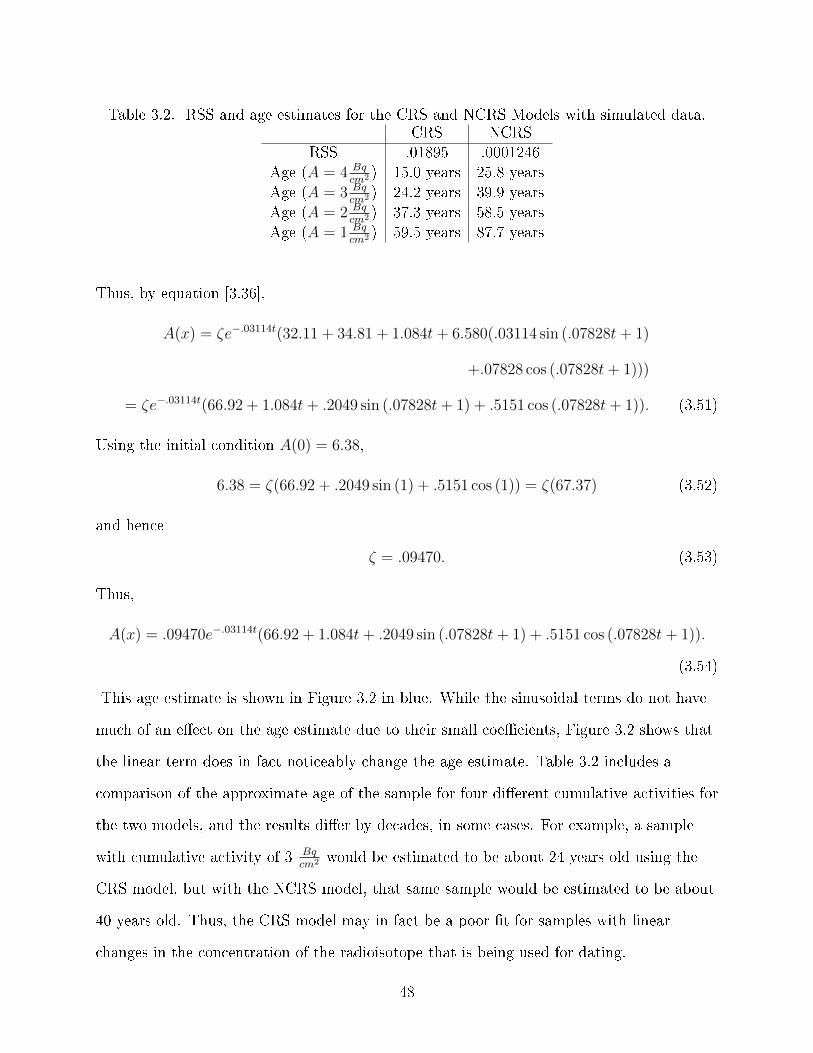
Table 3.2. RSS and age estimates for the CRS and NCRS Models with simulated data.CRS NCRS
RSS .01895 .0001246
Age (A = 4 Bqcm2 ) 15.0 years 25.8 years
Age (A = 3 Bqcm2 ) 24.2 years 39.9 years
Age (A = 2 Bqcm2 ) 37.3 years 58.5 years
Age (A = 1 Bqcm2 ) 59.5 years 87.7 years
Thus, by equation [3.36],
A(x) = ζe−.03114t(32.11 + 34.81 + 1.084t+ 6.580(.03114 sin (.07828t+ 1)
+.07828 cos (.07828t+ 1)))
= ζe−.03114t(66.92 + 1.084t+ .2049 sin (.07828t+ 1) + .5151 cos (.07828t+ 1)). (3.51)
Using the initial condition A(0) = 6.38,
6.38 = ζ(66.92 + .2049 sin (1) + .5151 cos (1)) = ζ(67.37) (3.52)
and hence
ζ = .09470. (3.53)
Thus,
A(x) = .09470e−.03114t(66.92 + 1.084t+ .2049 sin (.07828t+ 1) + .5151 cos (.07828t+ 1)).
(3.54)
This age estimate is shown in Figure 3.2 in blue. While the sinusoidal terms do not have
much of an e�ect on the age estimate due to their small coe�cients, Figure 3.2 shows that
the linear term does in fact noticeably change the age estimate. Table 3.2 includes a
comparison of the approximate age of the sample for four di�erent cumulative activities for
the two models, and the results di�er by decades, in some cases. For example, a sample
with cumulative activity of 3 Bqcm2 would be estimated to be about 24 years old using the
CRS model, but with the NCRS model, that same sample would be estimated to be about
40 years old. Thus, the CRS model may in fact be a poor �t for samples with linear
changes in the concentration of the radioisotope that is being used for dating.
48

3.6 Assessing the Linearity Assumption
Before delving into the linearity assumption, it is worth noting that the linearity
assumption is implicitly built into the CRS and CFCS models. Recall that the
concentration data is obtained as a function of depth, and that C(x) is plotted versus x,
not t. Thus, the equation for C(x) could be written as
C(x) = C′
0e−αx+β, (3.55)
where α and β are constant. By invoking
C(x) = C0e−kt, (3.56)
this necessarily means that x and t are related through some linear transformation, as each
one appears in the exponent of the exponential and C0 is constant.
As was mentioned in a previous section, it is assumed that x and t are linearly related.
However, it is reasonable to wonder whether this assumption is necessarily true. The linear
assumption is perhaps the most natural starting assumption, as it seems probable that in
many environments, the amount of sediment deposited during each time step should
remain constant. Each .5 cm thick slice of a core sample includes the sediment
accumulation over a period of several years. For this reason, what matters to the linearity
assumption is whether the volume of sediment deposits in a sample region remain constant
from one year to the next.
Precipitation is one source of sediment deposits. Although precipitation may vary
widely on short timescales such as from day to day, on larger timescales it often remains
relatively constant. One step which may be useful to assess whether the linearity
assumption is reasonable is to look up precipitation accumulations for a region over a
period of several years. To access precipitation data, we will use the NOWData feature
provided by the National Oceanic and Atmospheric Administration (NOAA), accessed via
the site https://w2.weather.gov/climate/xmacis.php?wfo=gyx. The graph shown in Figure
3.3 is the precipitation data for Augusta, Maine.
49

Figure 3.3. A graph showing the all time precipitation accumulation in Augusta, Mainefrom January 1, 1950 to July 17, 2017.
Graph obtained from NOAA's NOWData feature, available athttps://w2.weather.gov/climate/xmacis.php?wfo=gyx
Figure 3.3 shows the all time accumulation of precipitation in Augusta, Maine.
Although one line is partially obscured, there are two lines on the graph, one in brown and
one in green. The green line shows the actual accumulation while the brown line shows the
expected accumulation. While the green line does deviate slightly in places, as would be
expected since weather does not behave in a perfectly predictable fashion, it very nearly
�ts the linear brown line. While this data does not go back for the 100-150 year period
that might be represented in a lake core sample, it does provide evidence that the average
50

precipitation remains roughly constant over time. Thus it seems reasonable for lakes in the
Augusta area to assume that the precipitation is not signi�cantly altering the amount of
sediment that is being deposited in a given time step.
Augusta, Maine was chosen for this demonstration because of its proximity to
Monmouth, Maine, the location of Cochnewagon Lake. It is worth noting that the
NOWData feature does not di�erentiate between types of precipitation. Since di�erent
forms of precipitation carry sediment di�erently, it is reasonable to ask whether rainfall
and snowfall individually remain constant over time. This may be especially important
since the changing climate is a�ecting the forms of precipitation in some geographical
locations. Although perhaps not as easily accessible, data di�erentiating between rain and
snow accumulations does exist for many locations and can likely be acquired by contacting
a local National Weather Services branch o�ce. However, unless there have been
noticeable shifts in the types of precipitation in a location, it may be reasonable to assume
that the annual occurrences of rain and snow remain roughly constant if the annual
precipitation remains constant.
In�ow and out�ow to a body of water may also carry in and remove sediment. If a
barrier is created that restricts the in�ow or out�ow, or if there are changes to the climate
that could signi�cantly a�ect the �ow of the waterways, such as rapid melting of glaciers,
then it may be worth examining whether the change has a�ected the rate of sediment
deposit. However, in relatively stable environments, in�ow and out�ow should not a�ect
the rate at which sediment accumulates.
While wind is harder to quantify than precipitation, it is again reasonable to assume
that over a su�ciently long period of time, wind will deposit the same amount of sediment
into the body of water each time step. What tends to occur with wind is that it changes
direction. Since di�erent soils are made up of di�erent types of organic and inorganic
matter, changes in wind direction may change the type of matter that is being deposited,
but it may not change the overall amount of matter that is being deposited. It may, for
51

example, increase or decrease the amount of lead-210 being introduced into the lake bed
without a�ecting the overall sediment depositions. Since several years are represented in a
.5 cm thick core sample, as long as there are not sustained, large scale changes in the wind
patterns, the wind likely will not change the sediment deposition rate.
Generally, a linear assumption is likely warranted. However, in cases in which there are
changes that would a�ect the rate at which sediment is being deposited, the question
remains whether the NCRS model could still be implemented. As long as the change could
be mathematically modeled, the NCRS model will still work. For example, assume that a
dam is constructed that reduces the amount of sediment that is being deposited annually.
The relationship between depth and time will likely still be linear in the years after the
dam is constructed, although the coe�cients will be di�erent. To take into account the
e�ect of the dam, two distinct calculations would have to be made, one for the years prior
to the introduction of the dam and one for the years following the dam's completion. Even
in instances in which the linearity assumption would not hold, the NCRS model could still
be used, just with a di�erent assumption.
52

CHAPTER 4
IMPLEMENTING THE NCRS MODEL
4.1 Testing the CRS Model on the Cochnewagon Lake Data
Consider the data presented in Figure 2.4 of the concentration of unsupported lead-210
as a function of depth, taken from Cochnewagon Lake. Cochnewagon Lake, also known as
Cochnewagon Pond, is a body of water located in Monmouth Township, Maine.
The CRS model assumes that the concentration of lead-210 decays exponentially, so to
�nd an equation for the data, the natural logarithm of concentration can be plotted against
depth and a best �t line can be determined. The resulting plot is shown in Figure 4.1.
Mathematica was used to generate the best �t line,1
log(C) = −.513− .244x. (4.1)
Exponentiating,
C(x) = e−.513−.244x. (4.2)
This equation is shown in Figure 4.4 in green. R was used to calculate the RSS value to
determine the �tness of the CRS model for the Cochnewagon Lake data. It was found that
RSS = .01263.
Assuming that depth and time have a linear dependence,
−.513− .244x = −.03114t+ ct, (4.3)
where ct is constant. Using the assumption that the �rst data point is the concentration at
t = 0,
−.513− .244(.25) = −.03114(0) + ct, (4.4)
1Note that all coe�cients in the following sections have been rounded to three signi�cant digits. Theactual equations produced by Mathematica and R included more digits, which were retained until the endof the calculations, at which point the coe�cients were rounded.
53

and thus
ct = −.574. (4.5)
Hence,
−.513− .244x = −.03114t− .574. (4.6)
Substituting equation [4.6] into equation (4.2),
C(x) = e−.574−.03114t = .563e−.03114t = C0e−.03114t. (4.7)
From equation (3.14), using the initial condition that A(0) = .1501 in Bqcm2 ,
A(x) = .150e−.03114t. (4.8)
4.2 Implementing the NCRS Model with Sinusoidal Terms on the
Cochnewagon Lake Data
R was used to �nd the best �t curve including sinusoidal �uctuations. The curve was
given by the equation
C(x) = .519e−.197x(1 + .150 sin(1.79x+ 3.13)). (4.9)
Figure 4.1. Natural logarithm of unsupported lead-210 vs. depth.
54

Figure 4.2. A comparison of CRS and NCRS model with no linear term.
Equation (4.9) is shown in Figure 4.2 in blue. The RSS value was found using R to be
RSS = .006966.
C(x) can be rewritten as
C(x) = .519e−.197x−.655(1 + .150 sin (1.793x+ 3.13)). (4.10)
Using the same technique as outlined in the previous sections, it was found that
−.197x− .655 = −.03114t+ ct, (4.11)
and thus,
ct = −.704. (4.12)
Thus,
x = .158t+ .25 (4.13)
and hence,
C(x) = .519e−.03114t−.0493(1 + .150 sin (.283t+ .448)) (4.14)
= C0e−.03114t−.0493(1 + .150 sin (.283t+ .448)).
55
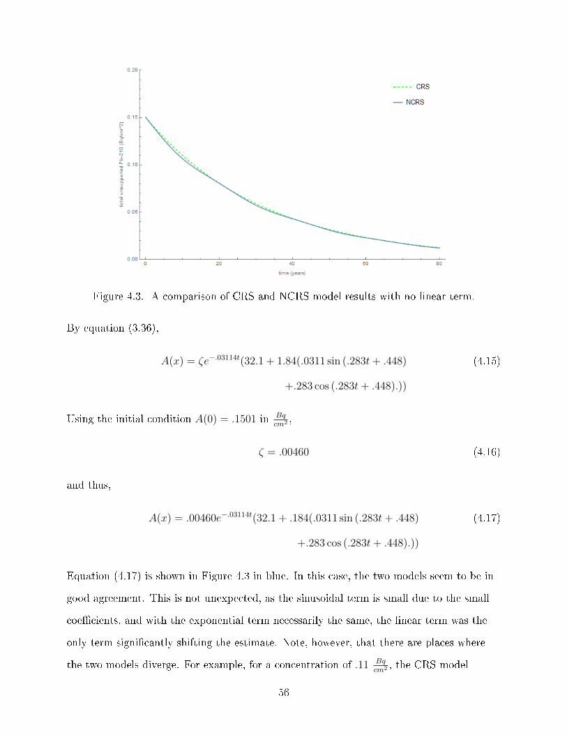
Figure 4.3. A comparison of CRS and NCRS model results with no linear term.
By equation (3.36),
A(x) = ζe−.03114t(32.1 + 1.84(.0311 sin (.283t+ .448) (4.15)
+.283 cos (.283t+ .448).))
Using the initial condition A(0) = .1501 in Bqcm2 ,
ζ = .00460 (4.16)
and thus,
A(x) = .00460e−.03114t(32.1 + .184(.0311 sin (.283t+ .448) (4.17)
+.283 cos (.283t+ .448).))
Equation (4.17) is shown in Figure 4.3 in blue. In this case, the two models seem to be in
good agreement. This is not unexpected, as the sinusoidal term is small due to the small
coe�cients, and with the exponential term necessarily the same, the linear term was the
only term signi�cantly shifting the estimate. Note, however, that there are places where
the two models diverge. For example, for a concentration of .11 Bqcm2 , the CRS model
56

estimates the age to be 9.98 years, while the NCRS model estimates the age to be 9.43
years, a di�erence of about half a year. The sine term is particularly muted in this lake,
however. In subsequent examples, more pronounced sinusoidal e�ects will be seen.
Observe also that the NCRS model shows some small, periodic oscillations that the
CRS model does not account for. This too will merit further study in subsequent sections.
4.3 Implementing the NCRS Model with Sinusoidal and Linear Fluctuations
Several small streams, including Wilson Stream, �ow into or out of Cochnewagon Lake
[56]. Since there is in�ow and out�ow, it is possible that the lead-210 deposits could be
�uctuating linearly. It is also possible that there is some other mechanism in the lake that
is causing a linear change. For this reason, the NCRS model was redone including both
sinusoidal and linear terms.
The nonlinear regression feature in R was used to �nd best �t curve for the
unsupported lead-210 data using the following model equation:
C(x) = C0ek1x(1 + a1 sin (bx+ c) + g1x). (4.18)
The given best �t curve was
C(x) = .348e−.401x(1 + .269 sin (2.16x+ 1.39) + .694x). (4.19)
Equation (4.19) is shown in Figure 4.4 in blue. The RSS value was found using R to be
RSS = .002180, which is less than a �fth of the size of the RSS value found using the CRS
model, suggesting that the NCRS model is a better �t.
Equation [4.19] can be rewritten in the following form:
C(x) = e−.401x−1.05(1 + .269 sin (2.16x+ 1.39) + .694x). (4.20)
Assuming again that depth and time are linearly related,
−.401x− 1.05 = −.03114t+ ct, (4.21)
57

Figure 4.4. Data from Douglas Cahl's thesis with CRS and NCRS �t lines.
where ct is an arbitrary constant distinct from the constant determined in the previous
section. Using the same assumption as previously that when t = 0, x = .25,
−.401(.25)− 1.05 = ct, (4.22)
and hence
ct = −1.16. (4.23)
Solving for x,
x = .0778t+ .25. (4.24)
58

Thus,
C(x) = e−.401x−1.05(1 + .269 sin (2.16x+ 1.39) + .694x) (4.25)
= e−.401(.0778t+.25)−1.05(1 + .269 sin (2.16(.0778t+ .25) + 1.39)
+.694(.0778t+ .25))
= e−.03114t−.955(1.17 + .269 sin (.168t+ 1.92) + .0540t)
= .385e−.03114t(1.17 + .269 sin (.168t+ 1.92) + .0540t)
= .452e−.03114t(1 + .230 sin (.168t+ 1.92) + .0460t)
= C0e−.03114t(1 + .230 sin (.168t+ 1.92) + .0460t)
By equation (3.36),
A(x) = ζe−.03114t(1
.03114+
.0460
.031142+.0460t
.03114(4.26)
+.230
.031142 + .1682(.03114 sin (.168t+ 1.92)
+.168 cos (.168t+ 1.92)))
= ζe−.03114t(32.1 + 47.4 + 1.48t+ 7.87(.03114 sin (.168t+ 1.92)
+.168 cos (.169t+ 1.92)))
= ζe−.03114t(79.5 + 1.48t+ 7.87(.03114 sin (.168t+ 1.92)
+.168 cos (.168t+ 1.92))).
Given the initial condition A(0) = .1501 Bqcm2 ,
.150 = ζ(79.5 + 7.87(.03114 sin (1.92) + .168 cos (1.92))). (4.27)
Thus,
ζ = .00189. (4.28)
59

Figure 4.5. A comparison of CRS and NCRS age estimates.
Therefore,
A(x) = .00189e−.03114t(79.5 + 1.48t (4.29)
+7.87(.03114 sin (.168t+ 1.92)
+.168 cos (.168t+ 1.92))).
Equation (4.29) is shown in Figure 4.5 in blue, compared to the CRS solution, which is
shown in green. This model deviates quite a bit from the CRS solution. Since a mechanism
that would cause linear changes in the rate of supply of lead-210 has not yet been
established for Cochnewagon Lake (although in�ow and out�ow are potential contenders),
the results presented in this section should not necessarily be taken as a better estimate for
the age of Cochnewagon Lake data. However, should such a mechanism be con�rmed, then
the NCRS model should be considered seriously as a potential better �t.
4.4 Modeling SS15 in Greenland: The Physically Unrealistic Linear Term
The next body of water we will analyze is lake SS15 in Greenland. I obtained the data
for this lake from the ERL computer amongst a collection of lake data that had been
60
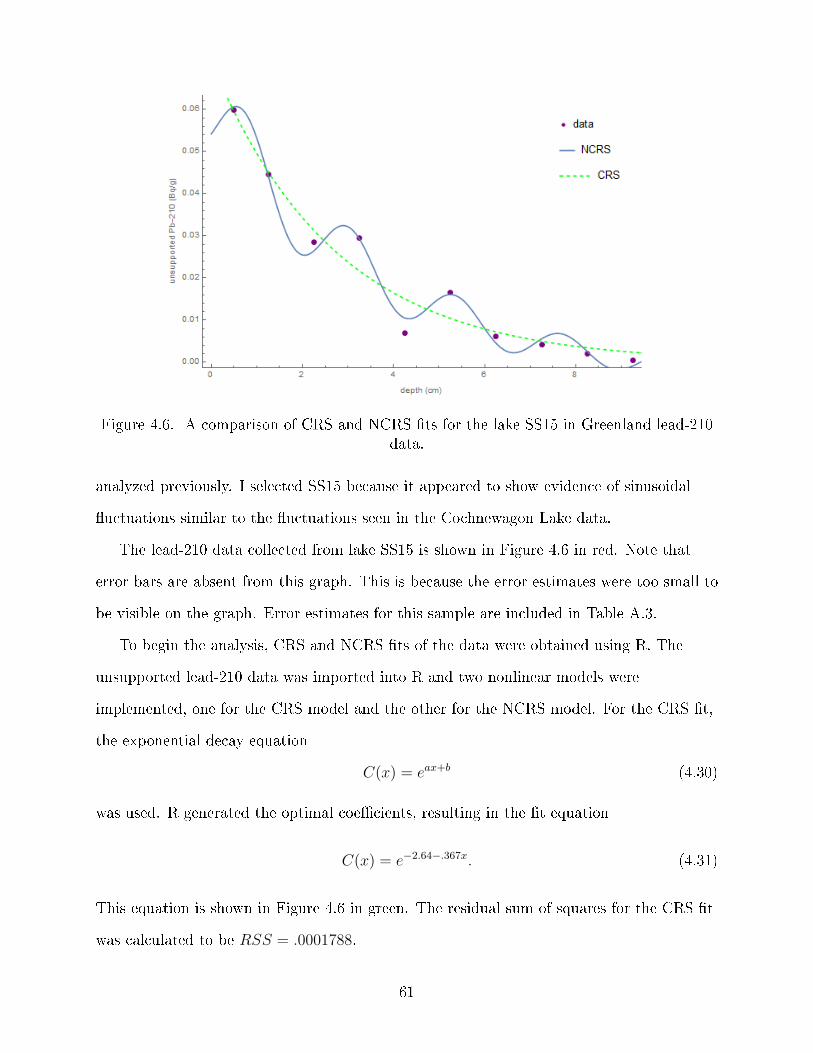
Figure 4.6. A comparison of CRS and NCRS �ts for the lake SS15 in Greenland lead-210data.
analyzed previously. I selected SS15 because it appeared to show evidence of sinusoidal
�uctuations similar to the �uctuations seen in the Cochnewagon Lake data.
The lead-210 data collected from lake SS15 is shown in Figure 4.6 in red. Note that
error bars are absent from this graph. This is because the error estimates were too small to
be visible on the graph. Error estimates for this sample are included in Table A.3.
To begin the analysis, CRS and NCRS �ts of the data were obtained using R. The
unsupported lead-210 data was imported into R and two nonlinear models were
implemented, one for the CRS model and the other for the NCRS model. For the CRS �t,
the exponential decay equation
C(x) = eax+b (4.30)
was used. R generated the optimal coe�cients, resulting in the �t equation
C(x) = e−2.64−.367x. (4.31)
This equation is shown in Figure 4.6 in green. The residual sum of squares for the CRS �t
was calculated to be RSS = .0001788.
61

For the NCRS model, equation [4.18] was inputted into the nonlinear �t function in R.
R outputted the optimal coe�cients, resulting in the equation
C(x) = .0595e−.165x(1 + .202 sin(2.71x− .459)− .104x). (4.32)
This equation is shown in Figure 4.6 in blue. The residual sum of squares was found to be
RSS = 2.431× 10⁻⁵. Comparing the ratios of the two RSS values, the NCRS model's error
estimate is more than 7 times smaller than the CRS model's error estimate, suggesting
that the NCRS model is a better �t for the data.
To obtain the CRS solution, the cumulative activity at the surface layer must be
known. For the data presented in this chapter, the cumulative accumulations were
provided in the spreadsheet from which the concentration data was obtained. The
cumulative activity was given to be A(0) = .1372 Bqcm2 . The CRS solution is thus obtained
by substituting this initial condition into the exponential decay equation
A(x) = A(0)e−.03114t. (4.33)
Thus, age estimates for the CRS model can be obtained from the equation
A(x) = .137e−.03114t. (4.34)
This CRS age estimate is shown in Figure 4.7 in green.
Before the NCRS solution can be obtained, Equation [4.32] must be rewritten so that a
conversion between depth and time can be made. Note that
C(x) = .0595e−.165x(1 + .202 sin(2.71x− .459)− .104x) (4.35)
= e−2.81−.165x(1 + .202 sin(2.71x− .459)− .104x),
and thus to switch from x to t,
−2.82− .165x = −.03114t+ ct. (4.36)
Using the initial depth x = .5 as the depth estimate for t = 0,
−2.82− .165(.5) = −.03114(0) + ct, (4.37)
62
and hence
ct = −.290. (4.38)
Solving equation [4.37] for x,
x = .5 + .188t. (4.39)
Rewriting equation [4.35] in terms of time,
C(x) = e−.2.90−.03114t(1 + .202 sin(2.71(.5 + .188t)− .459) (4.40)
−.104(.5 + .188t))
= e−2.91−.03114t(.948 + .202 sin(.496t+ .894)− .0195t)
= .948e−2.90−.03114t(1 + .213 sin(.496t+ .894)− .0206t).
Thus,
C(x) = C0e−.03114t(1 + .213 sin(.496t+ .894)− .0206t). (4.41)
Now that equation [4.41] is in the correct form, the coe�cients can be substituted into
equation [3.36]. This results in the model equation,
A(x) = ζe−.03114t(1
−.03114+−.0206
.031142+−.0206t
.03114(4.42)
+.213
.031142 + .4962(.03114 sin(.496t+ .894) + .496 cos(.496t+ .894)).
Simplifying,
A(x) = ζe−.03114t(10.9− .662t+ .864[.03114 sin(.496t+ .894) (4.43)
+.496 cos(.496t+ .894)]).
The constant ζ remains to be determined. Using the initial condition A(0) = 0.1372 Bqcm2 ,
0.137 = ζ(10.9 + .864(.03114 sin(.894) + .496 cos(.894))) = 11.3. (4.44)
Then
ζ =.137
11.3= .0121. (4.45)
63

Therefore equation [4.32] becomes
A(x) = .0121e−.03114t(10.9− .661670t+ .864[.03114 sin(.496t+ .894) (4.46)
+.496 cos(.496t+ .894)]).
Equation [4.46] is shown in Figure 4.7 in blue. Due to the decreasing linear term, the
initial NCRS �t would seem to suggest that the entire sample is less than 20 years old,
which is not consistent with the generally accepted age estimates for lake sediment samples
of a similar depth. For this reason, the NCRS model was recomputed without the linear
term.
Using R, the coe�cients for the best �t curve were recalculated excluding the linear
term. The resulting equation was
C(x) = .0608e−.316x(1 + .278 sin(2.78x− .669)). (4.47)
Figure 4.7. A comparison of CRS and NCRS age estimates for the lake SS15 in Greenlandlead-210 data including a linear term in the NCRS model.
64

The RSS value was calculated to be RSS = 6.77× 10⁻⁵. While not as close a �t as the
original NCRS model, this modi�ed model is still a better �t than the purely exponential
CRS �t. Equation [4.47] is shown in Figure 4.8 in blue.
Equation [4.47] can be rewritten as
C(x) = e−2.80−.316x(1 + .278 sin(2.78x− .669)). (4.48)
Assuming that x and t are linearly related,
−2.80− .316x = −.03114t+ ct. (4.49)
Using the condition that x = .5 cm when t = 0 s, ct = −2.96. Therefore,
x = .5 + .0985t, (4.50)
and thus
C(x) = e−.03114t−2.96(1 + .278 sin(2.78(.5 + .0985t)− .669)) (4.51)
= e−.03114t−2.96(1 + .278 sin(.274t+ .721))
Figure 4.8. A comparison of CRS and NCRS �ts for the lake SS15 in Greenland lead-210data excluding a linear term from the NCRS model.
65

Therefore,
C(x) = C0e−.03114t(1 + .278 sin(.274t+ .721)). (4.52)
Substituting the coe�cients of equation [4.52] into equation [3.36],
A(x) = ζe−.03114t(32.1 + .278(.03114 sin(.274t+ .721) (4.53)
+.274 cos(.274t+ .721))).
Solving for ζ in the same manner as before, using the initial condition A(0) = .1372
Bqcm2 , ζ = .00416, and hence
A(x) = .004164e−.03114t(32.1 + .278(.03114 sin(.274t+ .721) (4.54)
+.274 cos(.274t+ .721))).
Equation [4.54] is shown in Figure 4.9 in blue, compared to the CRS �t, shown in green.
While the sinusoidal �uctuations are relatively small, the age estimates di�er by about a
year in places. For example, for a concentration of .095 Bqcm2 , the NCRS model estimates the
age to be about 10.9 years, while the CRS model estimates the age to be about 11.8 years.
A di�erence of a year on a time scale of about 10 years is not insigni�cant.
Figure 4.9. A comparison of CRS and NCRS models for the lake SS15 in Greenlandlead-210 data, excluding a linear term from the NCRS model.
66

Further, as mentioned previously, the NCRS model does provide information that the
CRS model does not. The period of the oscillations can easily be obtained from the NCRS
model, the signi�cance of which will be discussed in Section 5.2.
4.5 Modeling Gardner Pond
The next body of water I selected for modeling was Gardner Pond in Gardner, Maine.
This sample's data was included in a set of lake sample data contained on the computer in
the ERL. I selected it because it appeared to have some data points that did not lie along
an exponential decay curve. The data for this pond is shown in Figure 4.10 in red.
R was used to obtain the CRS and NCRS �ts. For the CRS �t, an exponential model
was used. The coe�cients of the best �t exponential were generated in R, resulting in the
equation
C(x) = e.671−.625x. (4.55)
Equation [4.55] is shown in Figure 4.10 in green. The RSS value was found to be
RSS = .0196. Using the initial condition A(0) = .408 Bqcm2 , the CRS solution is
A(x) = .408e−.03114t. (4.56)
Equation [4.56] is shown in Figure 4.11 in green.
For the NCRS model, an initial �t including both a sinusoidal and a linear term was
implemented in R. The coe�cients generated in R corresponded to the equation
C(x) = 1.39e−.451x(1 + .244 sin(1.64x+ .0959)− .0257x). (4.57)
This model was a much better �t than the initial model, with an RSS value RSS = .00214.
A secondary NCRS �t without the linear term was also considered. The coe�cients for
this equation were generated in R, producing the equation
C(x) = 1.37e−.474x(1 + .263 sin(1.66x+ .0202)). (4.58)
67

Figure 4.10. A comparison of CRS and NCRS �ts for Gardner Pond lead-210 data
This equation was about as good a �t as the model including the linear term, with
RSS = .00215. Since the linear term did not seem to improve the �t of the model any, it
was omitted, and equation [4.58] was used. Equation [4.58] is shown in Figure 4.10 in blue.
Equation [4.58] can be rewritten as
C(x) = e−.315−.474x(1 + .263 sin(1.66x+ .0202)). (4.59)
A conversion between depth and time can then be made, using
.315− .474x = .03114t+ ct. (4.60)
Since the depth x = 1 cm corresponds to t = 0, ct = −.158. Therefore,
x = .0658t+ 1. (4.61)
Equation [4.10] can thus be rewritten as
C(x) = e−.159−.03114t(1 + .263 sin(1.66(.0658t+ 1) + .0202)), (4.62)
which reduces to
C(x) = C0e−.03114t(1 + .263 sin(.109t+ 1.68)). (4.63)
68
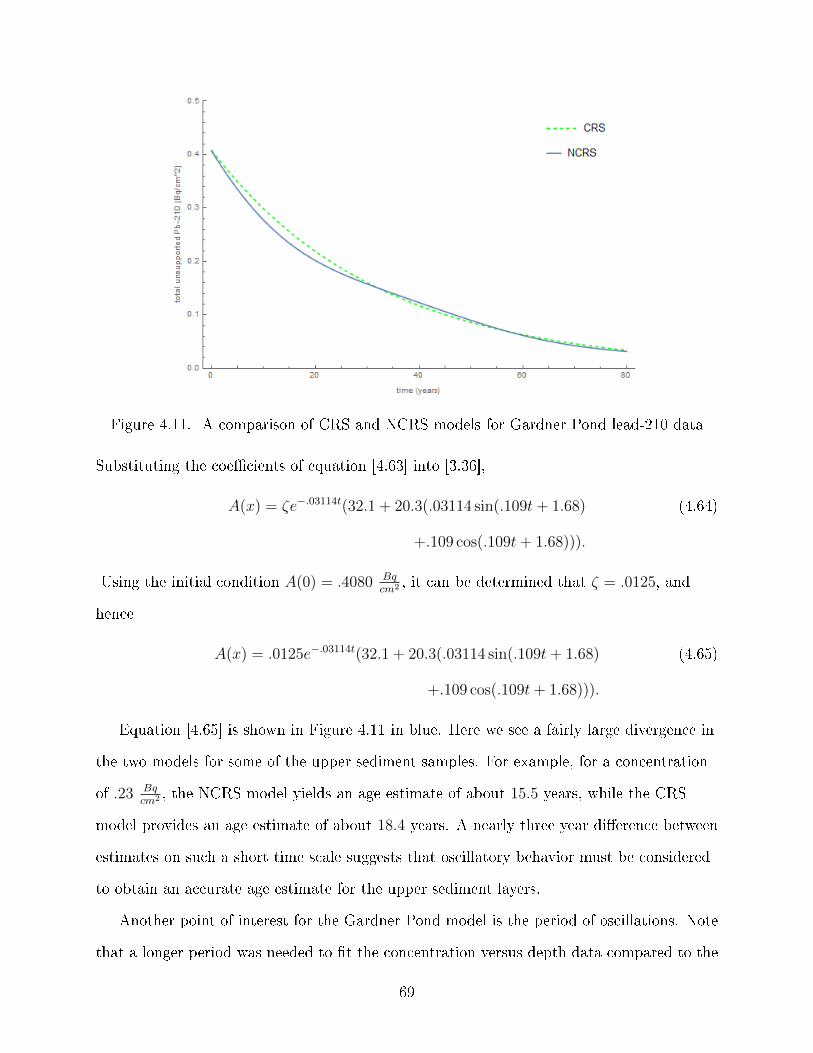
Figure 4.11. A comparison of CRS and NCRS models for Gardner Pond lead-210 data
Substituting the coe�cients of equation [4.63] into [3.36],
A(x) = ζe−.03114t(32.1 + 20.3(.03114 sin(.109t+ 1.68) (4.64)
+.109 cos(.109t+ 1.68))).
Using the initial condition A(0) = .4080 Bqcm2 , it can be determined that ζ = .0125, and
hence
A(x) = .0125e−.03114t(32.1 + 20.3(.03114 sin(.109t+ 1.68) (4.65)
+.109 cos(.109t+ 1.68))).
Equation [4.65] is shown in Figure 4.11 in blue. Here we see a fairly large divergence in
the two models for some of the upper sediment samples. For example, for a concentration
of .23 Bqcm2 , the NCRS model yields an age estimate of about 15.5 years, while the CRS
model provides an age estimate of about 18.4 years. A nearly three year di�erence between
estimates on such a short time scale suggests that oscillatory behavior must be considered
to obtain an accurate age estimate for the upper sediment layers.
Another point of interest for the Gardner Pond model is the period of oscillations. Note
that a longer period was needed to �t the concentration versus depth data compared to the
69

two previously discussed models, and correspondingly, the oscillations in the time estimate
have a longer period. The potential signi�cance of this will be discussed in Section 5.2.
4.6 Modeling Golden Lake
The next body of water we will analyze is Golden Lake. This was another data set from
the ERL computer that appeared to show �uctuations in the data points. The lead-210
data collected from Golden Lake is shown in Figure 4.12 in red. No error bars are present
because the measurement uncertainty was too small to be represented on this graph.
After initial �tting attempts were made for the Golden Lake data using both the CRS
and NCRS models, it became clear that the �rst data point deviated from the trend
followed by the remaining points in the series. The �rst data point corresponds to the
lead-210 in the surface layer of sediment. There are many issues that could potentially lead
to inaccurate measures in the surface layer of sediment, since this is the sediment that
comes into direct contact with plants and animals in the lake, as well as moving water
currents. Since this data point was so di�erent from the remaining points, it was omitted
from the later �tting attempts.
The lead-210 speci�c activities were imported into R and two nonlinear �t models were
implemented. The �rst was an exponential �t,
C(x) = eax+b, (4.66)
which was used for the CRS �t. R outputted the optimal coe�cients for a and b, yielding
C(x) = e−.303x−2.83. (4.67)
This curve is shown in Figure 4.12 in green. The RSS value for this curve was computed as
RSS = 5.579× 10⁻⁵. For the NCRS �t, equation [4.18] was used. R outputted the optimal
coe�cients, which yielded the equation
C(x) = .0510e−.142x(1 + .0950 sin(2.37x− 1.79)− .0899x). (4.68)
70

Figure 4.12. A comparison of CRS and NCRS �ts for the Golden Lake lead-210 data.
This curve is shown in Figure 4.12 in blue. The RSS value was RSS = 1.465× 10⁻⁵. Note
that the NCRS �t is almost four times better a �t by the RSS metric. Note also that the
NCRS model seems to match the periodicity of the data well, something that the CRS
model cannot account for.
Once the CRS and NCRS �ts were obtained, the age estimates could be computed. For
the CRS model, equation [2.36] will be utilized. For the initial condition A(0) = 0.289 Bqcm2 ,
A(x) = .289e−.03114t. (4.69)
Equation [4.69] is shown in Figure 4.13 in green.
To estimate the age using the NCRS model, �rst a conversion between depth and time
must be made. Rewriting equation [4.68],
C(x) = e−2.98−.142x(1 + .0950 sin(2.37x− 1.79)− .0899x). (4.70)
Employing the linearity assumption,
−2.98− .142x = −.03114t+ ct. (4.71)
71

Figure 4.13. A comparison of CRS and NCRS estimates for the Golden Lake lead-210 dataincluding a linear term in the NCRS model.
Since the depth x = .5 cm corresponds to t = 0,
−2.98− .142(.5) = −.03114(0) + ct, (4.72)
and thus
ct = −3.05. (4.73)
Substituting equation [4.73] into equation [4.71] and solving for x,
x = .220t+ .5. (4.74)
Now equation [4.70] can be rewritten in terms of time:
C(x) = e−2.98−.142x(1 + .0950 sin(2.37x− 1.79)− .0899t) (4.75)
= e−2.98−.142(.220t+.5)(1 + .0950 sin(2.37(.220t+ .5)− 1.79)
−.0899(.220t+ .5))
= e−.03114t−3.05(.955 + .0950 sin(.520t− .611)− .0198t)
= .955e−.03114t−3.05(1 + .0995 sin(.520t− .611)− .0198t)
= C0e−.03114t(1 + .0995 sin(.520t− .611)− .0198t).
72

Figure 4.14. A comparison of CRS and NCRS �ts for the Golden Lake lead-210 dataexcluding the linear term from the NCRS model.
Now that equation [4.75] is in the correct form, the coe�cients can be substituted into
equation [3.36], yielding
A(x) = ζe−.03114t(1
.03114− .0198
(.03114)2− .0198t
.03114(4.76)
+.0995
(.03114)2 + (.520)2(.03114 sin(.520t− .611) + .520 cos(.520t− .611)))
= ζe−.03114t(11.7− .635t+ .366(.03114 sin(.520t− .611)
+.520 cos(.520t− .611))).
Using the initial condition A(0) = 0.2892 Bqcm2 , it was determined that ζ = .0244, and thus
A(x) = .0244e−.03114t(11.7− .635t+ .366(.03114 sin(.520t− .611) (4.77)
+.520 cos(.520t− .611))).
Equation [4.77] is shown in Figure 4.13 in blue.
Since the linear term seems to yield an unrealistic age estimate, the NCRS model was
recomputed in R without the linear term. R generated coe�cients, resulting in the equation
C(x) = .0551e−.287x(1 + .126 sin(2.47x− 2.21)). (4.78)
73

The RSS value was found to be RSS = 3.19× 10⁻⁵, which is better than the CRS �t,
although not as close as the original NCRS �t. Equation [4.78] is shown in Figure 4.14 in
blue.
Using the same process as outlined in the previous examples, it was found that the
linearity condition is given by
x = .109t+ .5, (4.79)
and thus
C(x) = e−2.04−.03114t(1 + .126 sin(.262t− 1.01)). (4.80)
Therefore,
C(x) = C0e−.03114t(1 + .126 sin(.262t− 1.01)). (4.81)
Substituting the coe�cients from [4.81] into [3.36],
A(x) = ζe−.03114t(32.1 + 1.81(.03114 sin(.262t− 1.01) (4.82)
+.262 cos(.262t− 1.01))).
Using the initial condition A(0) = .2892 Bqcm2 , ζ = .00895, and hence
A(x) = .00895e−.03114t(32.1 + 1.81(.03114 sin(.262t− 1.01) (4.83)
+.262 cos(.262t− 1.01))).
Equation [4.83] is shown in Figure 4.15 in blue.
4.7 The NCRS Model: A Discussion
In this chapter, the NCRS model was tested against the CRS model on four di�erent
lake sediment samples. Upon analyzing these four lake samples, several distinctions become
apparent. The �rst is that when a linear term is introduced into the NCRS model, the age
estimates of the CRS and NCRS models can diverge by as much as several decades. This
may suggest that the linear term is not generally useful for estimating the age of sediment
74

Figure 4.15. A comparison of CRS and NCRS models for the Golden Lake lead-210 dataexcluding the linear term from the NCRS model.
samples. However, it is worth noting that many age estimates made using the CRS model
are not veri�ed by alternative means, such as pollen markers. Thus, it remains to be
determined whether the CRS models are indeed accurate age models for the given bodies of
water. Potential validation techniques will be discussed in Chapter 6.
It may be that linear increases or decreases are more gradual than would be predicted
by a curve �tting function, and more information about the body of water in question
would be needed to determine an accurate coe�cient for the linear term. Because the
linear term has the ability to change the age estimates so drastically, it would be worth
pursuing whether its inclusion is in fact warranted.
When the linear term is omitted from the NCRS model, the CRS and NCRS age
estimates align more closely. However, for the upper sediment layers, the two models can
yield age estimates that di�er by several years. Since the upper sediment layers are
relatively new, such a discrepancy is nontrivial and suggests that for bodies of water which
seem to exhibit oscillatory behavior, such behavior needs to be incorporated into the
models to yield accurate age estimates.
75

Further, the NCRS model provides some information that the CRS model cannot. The
sinusoidal �uctuations in the NCRS model could be used to estimate the period of
oscillations for each body of water. If the periods are similar, this may suggest a common
physical phenomenon is responsible for creating the oscillations.
In the following chapter, data from additional samples will be �tted using the NCRS
model without the linear term. While su�cient details will be provided such that the
equations can be checked, intermediary steps will be omitted in the interest of readability.
Once a critical number of bodies of water have been analyzed, the periods of each, as well
as of the lakes considered in this chapter, will be estimated and analyzed.
76
CHAPTER 5
FURTHER INVESTIGATIONS OF THE NCRS MODEL
5.1 Testing the NCRSFitModelSoftware on More Lead-210 Data
An algorithm, NCRSFitModelSoftware, was developed to compute approximate
coe�cients for the NCRS model. The algorithm was developed by Dr. Brian Toner, in
conjunction with the author. The code is included in Appendix
Although NCRSFitModelSoftware was developed such that a linear term could be
included, it was not utilized in these models. The rationale was that because the linear
term can drastically alter the age estimates, it should only be included when there is clear
physical evidence that it is needed.
NCRSFitModelSoftware was run on the data for the four lakes investigated in Chapter
4 and produced similar results to those presented previously. The results were not
identical, and varied slightly for di�erent runs of the algorithm on the same data set. This
is due to the inherent di�culty associated with nonlinear �tting, where the initial
parameters in�uence the �t that is chosen. There may be many locally good �ts, but
�nding a universal best �t can be challenging. Thus a good �t that agreed closely with, but
perhaps not identically to, the model produced by the �tting mechanisms devised in
Chapter 4 was what was sought.
The data used in this section was core data that had been obtained by members of the
Environmental Research Lab (ERL) previously. Di�erent samples may have been acquired
and processed by di�erent individuals. While the ERL has data for many of the lake cores
analyzed in the lab over the years, not all data sets proved useful for this analysis. Some of
the lake core data appeared to follow a pure exponential decay curve, while others
demonstrated erratic behavior that did not appear to be sinusoidal in nature. However, the
NCRSFitModelSoftware was run on most samples (33 in total), regardless of the perceived
77
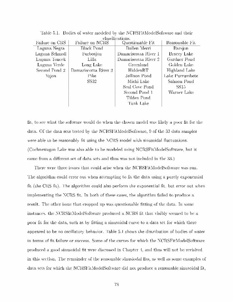
Table 5.1. Bodies of water modeled by the NCRSFitModelSoftware and theirclassi�cations.
Failure on CRS Failure on NCRS Questionable Fit Reasonable FitLaguna Negra Black Pond Bullen Merri BarsjonLaguna Schmoll Furbosjon Damariscotta River 1 Bracey LakeLaguna Toncek Lilla Damariscotta River 2 Gardner PondLaguna Verde Long Lake Greenland Golden LakeSecond Pond 2 Damariscotta River 3 HiddenBT Highland Lake
Ysjon Pike Jellison Pond Lake PurrumbeteSS32 Michi Lake Salmon Pond
Seal Cove Pond SS15Second Pond 1 Warner LakeTilden PondTunk Lake
�t, to see what the software would do when the chosen model was likely a poor �t for the
data. Of the data sets tested by the NCRSFitModelSoftware, 9 of the 33 data samples
were able to be reasonably �t using the NCRS model with sinusoidal �uctuations.
(Cochnewagon Lake was also able to be modeled using NCRSFitModelSoftware, but it
came from a di�erent set of data sets and thus was not included in the 33.)
There were three issues that could arise when the NCRSFitModelSoftware was run.
The algorithm could error out when attempting to �t the data using a purely exponential
�t (the CRS �t). The algorithm could also perform the exponential �t, but error out when
implementing the NCRS �t. In both of these cases, the algorithm failed to produce a
result. The other issue that cropped up was questionable �tting of the data. In some
instances, the NCRS�tModelSoftware produced a NCRS �t that visibly seemed to be a
poor �t for the data, such as by �tting a sinusoidal curve to a data set for which there
appeared to be no oscillatory behavior. Table 5.1 shows the distribution of bodies of water
in terms of �t failure or success. Some of the curves for which the NCRSFitModelSoftware
produced a good sinusoidal �t were discussed in Chapter 4, and thus will not be revisited
in this section. The remainder of the reasonable sinusiodal �ts, as well as some examples of
data sets for which the NCRSFitModelSoftware did not produce a reasonable sinusoidal �t,
78

will be considered in the subsequent subsections. While for each of the samples considered
below the NCRS model appeared to be a better �t than the CRS model based on the RSS
value, in some cases neither appears to be a particularly good �t, suggesting that a
di�erent set of curves may be needed.
5.1.1 Highland Lake
The Highland Lake data appeared to show some �uctuations, although it did not have
the clear sinusoidal trend that the lake samples considered in Chapter 4 showed.
Nonetheless, NCRSFitModelSoftware was run on the data. The CRS model equation was
found to be
C(x) = e−0.216x+2.17, (5.1)
shown in Figure 5.1 in black, while the NCRS �t was
C(x) = exp−0.275x+ 2.40(1− 0.335 sin(1.93x+ 0.231)), (5.2)
shown in Figure 5.1 in blue. The RSS value for the CRS model computed by the
NCRSFitModelSoftware was RSS = 16.70, while for the NCRS model it was RSS = 8.009.
Figure 5.1. Unsupported lead-210 versus depth for Highland Lake.
79
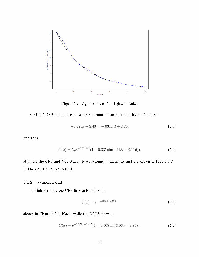
Figure 5.2. Age estimates for Highland Lake.
For the NCRS model, the linear transformation between depth and time was
−0.275x+ 2.40 = −.03114t+ 2.26, (5.3)
and thus
C(x) = C0e−0.03114t(1− 0.335 sin(0.218t+ 0.116)). (5.4)
A(x) for the CRS and NCRS models were found numerically and are shown in Figure 5.2
in black and blue, respectively.
5.1.2 Salmon Pond
For Salmon lake, the CRS �t was found to be
C(x) = e−0.284x+0.0960, (5.5)
shown in Figure 5.3 in black, while the NCRS �t was
C(x) = e−0.379x+0.415(1 + 0.408 sin(2.96x− 3.84)), (5.6)
80

Figure 5.3. Unsupported lead-210 versus depth for Salmon Pond.
shown in Figure 5.3 in blue. The RSS values were computed to be RSS = 0.1707 for the
CRS model and RSS = 0.001978 for the NCRS model.
The conversion between depth and time was given as
−0.379x+ 0.415 = −.03114t+ 0.130, (5.7)
leading to
C(x) = e−0.03114t(1 + 0.408 sin(0.243t− 2.88)). (5.8)
A(x) plots for the CRS and NCRS estimates are shown in Figure 5.8 in black and blue,
respectively.
5.1.3 Lake Purrumbete
For Lake Purrumbete, for the CRS model,
C(x) = e−0.427x−0.465, (5.9)
shown in Figure 5.5 in black, and for the NCRS model,
C(x) = e−0.533x−0.172(1 + 0.514 sin(4.08x+ 0.992)), (5.10)
81

Figure 5.4. Age estimates for Salmon Pond.
shown in Figure 5.5 in blue. The RSS values were RSS = 0.0137 for the CRS model and
RSS = 0.00267 for the NCRS model.
For the NCRS model, it was determined that
−0.533x− 0.172 = −.03114t− 0.838, (5.11)
and thus,
C(x) = C0e−0.03114t(1 + 0.514 sin(0.239t+ 1.24)). (5.12)
The A(x) curves are shown in Figure 5.6, with the CRS �t in black and the NCRS �t in
blue.
82

Figure 5.5. Unsupported lead-210 versus depth for Lake Purrumbete.
Figure 5.6. Age estimates for Lake Purrumbete.
83
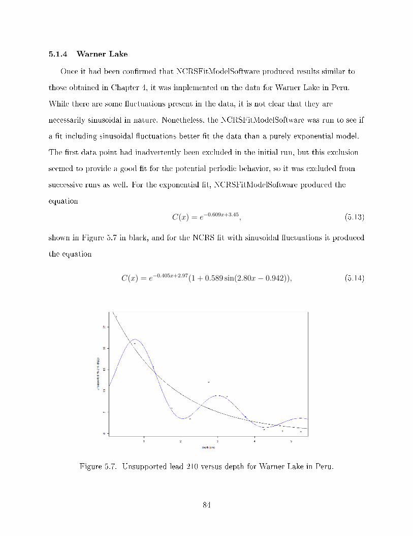
5.1.4 Warner Lake
Once it had been con�rmed that NCRSFitModelSoftware produced results similar to
those obtained in Chapter 4, it was implemented on the data for Warner Lake in Peru.
While there are some �uctuations present in the data, it is not clear that they are
necessarily sinusoidal in nature. Nonetheless, the NCRSFitModelSoftware was run to see if
a �t including sinusoidal �uctuations better �t the data than a purely exponential model.
The �rst data point had inadvertently been excluded in the initial run, but this exclusion
seemed to provide a good �t for the potential periodic behavior, so it was excluded from
successive runs as well. For the exponential �t, NCRSFitModelSoftware produced the
equation
C(x) = e−0.609x+3.45, (5.13)
shown in Figure 5.7 in black, and for the NCRS �t with sinusoidal �uctuations it produced
the equation
C(x) = e−0.405x+2.97(1 + 0.589 sin(2.80x− 0.942)), (5.14)
Figure 5.7. Unsupported lead-210 versus depth for Warner Lake in Peru.
84

Figure 5.8. Age estimates for Warner Lake in Peru.
shown in Figure 5.7 in blue. For the relationship between x and t, it determined that
−0.405x+ 2.97 = −.03114t+ 2.77, (5.15)
resulting in the equation
C(x) = C0e−0.03114t(1 + 0.589 sin(0.215t− 0.471)) (5.16)
A(x) was determined numerically for the CRS and NCRS �ts. The results are shown in
Figure 5.8, with the CRS �t in black and the NCRS �t in blue. Note that because
NCRSFitModelSoftware was developed using R, the �gures are produced in R rather than
Mathematica, which is why the images appear di�erent than in previous sections.
85

5.1.5 Bracey Lake
The NCRSFitModelSoftware was then implemented on the Bracey Lake lead-210 data.
The CRS �t was found to be
C(x) = e−0.239x−0.0722, (5.17)
shown in Figure 5.9 in black, while the NCRS �t was found to be
c(x) = e−0.245x−0.0418(1 + 0.113 sin(1.86x+ 1.50)), (5.18)
shown in Figure 5.9 in blue. The linearity condition was found to be
−0.245x− 0.0418 = −.03114t− 0.226, (5.19)
and thus
C(x) = C0e−0.03114∗t(1 + 0.589 sin(0.215t− 0.236)). (5.20)
A(x) was determined numerically. The CRS and NCRS results are shown in Figure 5.10 in
black and blue, respectively.
Figure 5.9. Unsupported lead-210 versus depth for Bracey Lake.
86

Figure 5.10. CRS and NCRS Age estimates for Bracey Lake.
5.1.6 Barsjon Lake
Barsjon Lake in Sweden also seemed to be modeled reasonably well using the
NCRSFitModelSoftware. The algorithm produced the CRS �t
C(x) = e−0.179x−2.74, (5.21)
shown in Figure 5.11 in black, and the NCRS �t
C(x) = e−0.211x− 2.58(1 + 0.239 sin(2.82x+ 2.51)), (5.22)
87

Figure 5.11. Unsupported lead-210 versus depth for Barsjon Lake.
shown in Figure 5.11 in blue. The RSS values were computed to be RSS = 0.0001681
and RSS = 7.372× 10⁻⁵ for the CRS and NCRS �ts, respectively.
The linearity condition was found to be
−0.211x− 2.58 = −.03114t− 2.68, (5.23)
yielding the equation
C(x) = e−0.03114t(1 + 0.239 sin(0.417t+ 1.25)). (5.24)
The CRS and NCRS age curves were computed numerically and are shown in Figure 5.12
in black and blue, respectively.
88

Figure 5.12. CRS and NCRS Age estimates for Barsjon Lake.
5.1.7 Laguna Negra: Failure in Modeling CRS Fit
While the NCRSFitModelSoftware produced an output for many of the data sets, in
some instances it failed to produce a result. The �rst place where it could run into trouble
was in modeling the exponential �t, which would be used for the CRS model. One such
example of this is the sample from Laguna Negra in Argentina. As shown in Figure 5.13,
the data appears to follow an exponential curve reasonably well, although the tail of the
curve skews upward a little.
When NCRSModelFitSoftware was run on the data, an error message appeared, shown
in Figure 5.14. The message stated, �Missing value or an in�nity produced when evaluating
the model." The x and y data values were checked and no missing data points were found,
so presumably the algorithm ran into issues with an in�nite value somehow.
The data was able to be �tted with an exponential curve using the nls function in R,
the solution of which is shown plotted against the data points in Figure 5.13. Since the
data does not seem to exhibit any clear oscillatory behavior, no attempt was made to
manually �t it using the NCRS model with sinusoidal �uctuations.
89

Figure 5.13. Unsupported lead-210 versus depth for Laguna Negra in Argentina.
90

Figure 5.14. Error message received when modeling Laguna Negra data.
91

5.1.8 Long Lake: Failure to Produce the NCRS Fit
Another possible outcome was that the NCRSModelFitSoftware would produce a result
for the exponential �t, but not for the NCRS �t. An example of this can be seen in the
modeling of Long Lake. The Long Lake data is shown in Figure 5.15.
When the NCRSFitModelSoftware was run on the Long Lake data, an exponential
solution was produced. However, when the algorithm searched for an NCRS �t, an error
was produced, as shown in Figure 5.16. The following message was given, �number of
iterations exceeded maximum of 50." This issue can arise when the set of initial conditions
chosen for the nls function are not well suited to the data, and sometimes can be remedied
by a di�erent choice of initial conditions. However, it can also arise when the function is
not well suited to the data. Note that one data point deviates quite a bit from the others,
which likely made it di�cult for the software to �t the data with a curve. Aside from one
errant initial data point, the Long Lake data appears fairly close to exponential decay, so a
manual �t using the nls function was not attempted at this time.
Figure 5.15. Unsupported lead-210 versus depth for Long Lake.
92
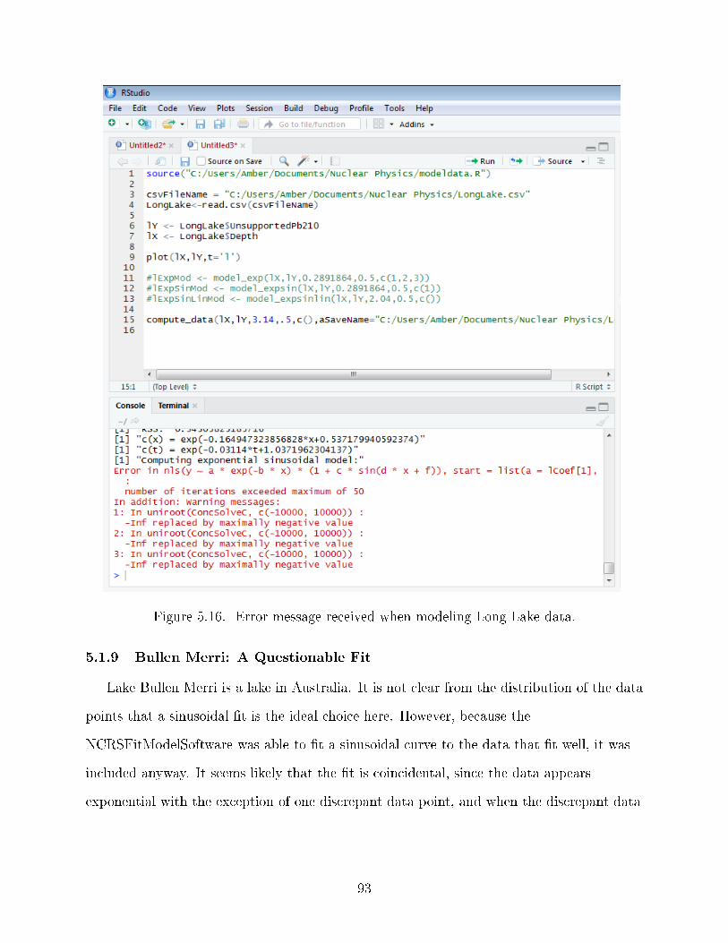
Figure 5.16. Error message received when modeling Long Lake data.
5.1.9 Bullen Merri: A Questionable Fit
Lake Bullen Merri is a lake in Australia. It is not clear from the distribution of the data
points that a sinusoidal �t is the ideal choice here. However, because the
NCRSFitModelSoftware was able to �t a sinusoidal curve to the data that �t well, it was
included anyway. It seems likely that the �t is coincidental, since the data appears
exponential with the exception of one discrepant data point, and when the discrepant data
93
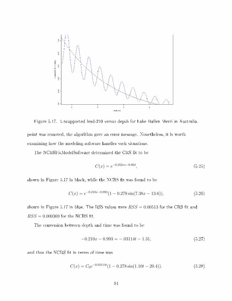
Figure 5.17. Unsupported lead-210 versus depth for Lake Bullen Merri in Australia.
point was removed, the algorithm gave an error message. Nonetheless, it is worth
examining how the modeling software handles such situations.
The NCRSFitModelSoftware determined the CRS �t to be
C(x) = e−0.252∗x−0.864, (5.25)
shown in Figure 5.17 in black, while the NCRS �t was found to be
C(x) = e−0.210x−0.993(1− 0.278 sin(7.38x− 13.6)), (5.26)
shown in Figure 5.17 in blue. The RSS values were RSS = 0.00513 for the CRS �t and
RSS = 0.000369 for the NCRS �t.
The conversion between depth and time was found to be
−0.210x− 0.993 = −.03114t− 1.31, (5.27)
and thus the NCRS �t in terms of time was
C(x) = C0e−0.03114t(1− 0.278 sin(1.10t− 20.4)). (5.28)
94

Figure 5.18. CRS and NCRS Age estimates for Lake Bullen Merri in Australia.
The A(x) curves were computed numerically and plotted in Figure 5.17, with the CRS
curve in black and the NCRS curve in blue.
While a �t curve and age estimate were able to be produced using the
NCRSFitModelSoftware, the �t here does not appear to be a particularly good �t. Thus,
discretion must be used when implementing the NCRSFitModelSoftware. If a �t does not
look reasonable, it is worth questioning whether it is useful for the data set in question.
5.1.10 Other Questionable Fits
While Lake Bullen Merri provides a good example of a �t provided by the
NCRSFitModelSoftware that upon closer inspection does not seem to �t the data well, I
thought it might be useful to provide a few more examples. Some of these data sets may in
fact have some periodic behavior, but due to some discrepancies in the data, the algorithm
was not able to correctly deduce the periodic nature. These data sets may bene�t from a
manual �tting. Others, like Lake Bullen Merri seem to exhibit no clear periodic trend at
all. The Damariscotta River core 1 data sample (Figure 5.19) appears to follow an
exponential curve fairly well. There is one data point at x = 7.5cm that does deviate from
95
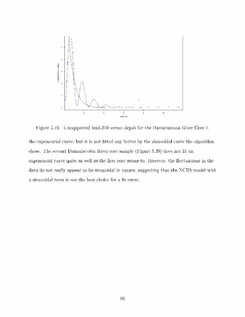
Figure 5.19. Unsupported lead-210 versus depth for the Damariscotta River Core 1.
the exponential curve, but it is not �tted any better by the sinusoidal curve the algorithm
chose. The second Damariscotta River core sample (Figure 5.20) does not �t an
exponential curve quite as well as the �rst core seems to. However, the �uctuations in the
data do not really appear to be sinusoidal in nature, suggesting that the NCRS model with
a sinusoidal term is not the best choice for a �t curve.
96

Figure 5.20. Unsupported lead-210 versus depth for the Damariscotta River Core 2.
The next sample (Figure 5.21) was labeled only with the country of origin, Greenland,
so it is not clear which body of water it came from. For this sample, while it appears that
there may be some periodic behavior, the peaks of the data do not match with the peaks of
the selected function, and the period of the �t function seems shorter than the one
exhibited by the data. This may be an instance in which manual �tting could potentially
provide a more informative result.
97
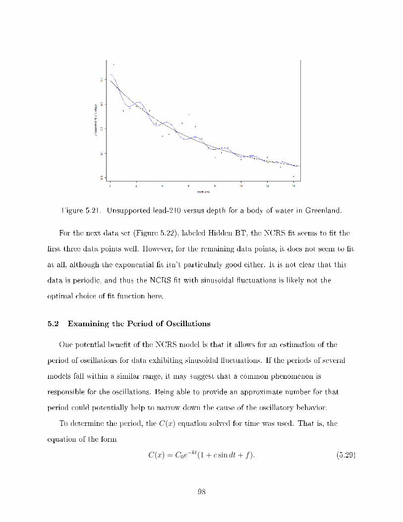
Figure 5.21. Unsupported lead-210 versus depth for a body of water in Greenland.
For the next data set (Figure 5.22), labeled Hidden BT, the NCRS �t seems to �t the
�rst three data points well. However, for the remaining data points, it does not seem to �t
at all, although the exponential �t isn't particularly good either. It is not clear that this
data is periodic, and thus the NCRS �t with sinusoidal �uctuations is likely not the
optimal choice of �t function here.
5.2 Examining the Period of Oscillations
One potential bene�t of the NCRS model is that it allows for an estimation of the
period of oscillations for data exhibiting sinusoidal �uctuations. If the periods of several
models fall within a similar range, it may suggest that a common phenomenon is
responsible for the oscillations. Being able to provide an approximate number for that
period could potentially help to narrow down the cause of the oscillatory behavior.
To determine the period, the C(x) equation solved for time was used. That is, the
equation of the form
C(x) = C0e−kt(1 + c sin dt+ f). (5.29)
98

Figure 5.22. Unsupported lead-210 versus depth the Hidden BT data set.
The period was computed by dividing 2π by the coe�cient of the time term inside the sin
function. Using the notation above, this could be described mathematically as
T =2π
d. (5.30)
For the bodies of water considered in Chapter 5, the period was computed using
NCRSFitModelSoftware.
Table 5.2. Period of oscillations for bodies of water considered in Chapters 4 and 5.Body of Water Period (years) Equation
Cochnewagon Lake 22 4.14SS15 23 4.52
Gardner Pond 57 4.63Golden Lake 24 4.81Highland Lake 29 5.4Salmon Pond 26 5.8
Lake Purrumbete 26 5.12Warner Lake 29 5.16Bracey Lake 27 5.20Barsjon Lake 15 5.24
99

The period of oscillations for each of the bodies of water described in Chapters 4 and 5
which had a reasonable NCRS �t was computed and compiled in Table 5.2. All but two of
the bodies of water, Barsjon Lake and Gardner Pond, have periods between 20 and 30
years. Before we examine the potential implications of the computed periods, however, it is
worthwhile to consider the uncertainty in the period calculations.
5.2.1 Estimating the Error in the Period of Oscillations
While there historically have been trends in weather data, there also is some variance,
some noise. Thus obtaining a precise equation for the deposition of lead-210 in a lake core
sample is infeasible. Thus there is no �true" value to which the generated equations can be
compared. However, an estimate of the error could be obtained through simulations using
noisy data.
To estimate the error properly, the experimental error for each data point must be
known. This could be obtained by taking multiple cores from the same body of water,
analyzing the slices, and determining the mean and standard deviation of the lead-210
content at each depth. However, none of these ten bodies of water had multiple cores taken,
so the experimental error could not be determined. An alternate approach was needed.
To estimate the error, I chose a generating equation to create a set of �true" data
points. The equation I chose was
C(x) = .5e−.2x(1 + .15 sin (1.8x+ 3)). (5.31)
You may notice that this model equation is close to the generated concentration equation
for Cochnewagon Lake. I wanted to use an equation with physically realistic parameters, so
I opted to use Cochnewagon Lake's concentration equation as my starting point and then
round the coe�cients a little.
I generated eleven data points by substituting eleven depth values into the model
equation and rounding the output to two signi�cant digits. The values are shown in Table
5.3.
100
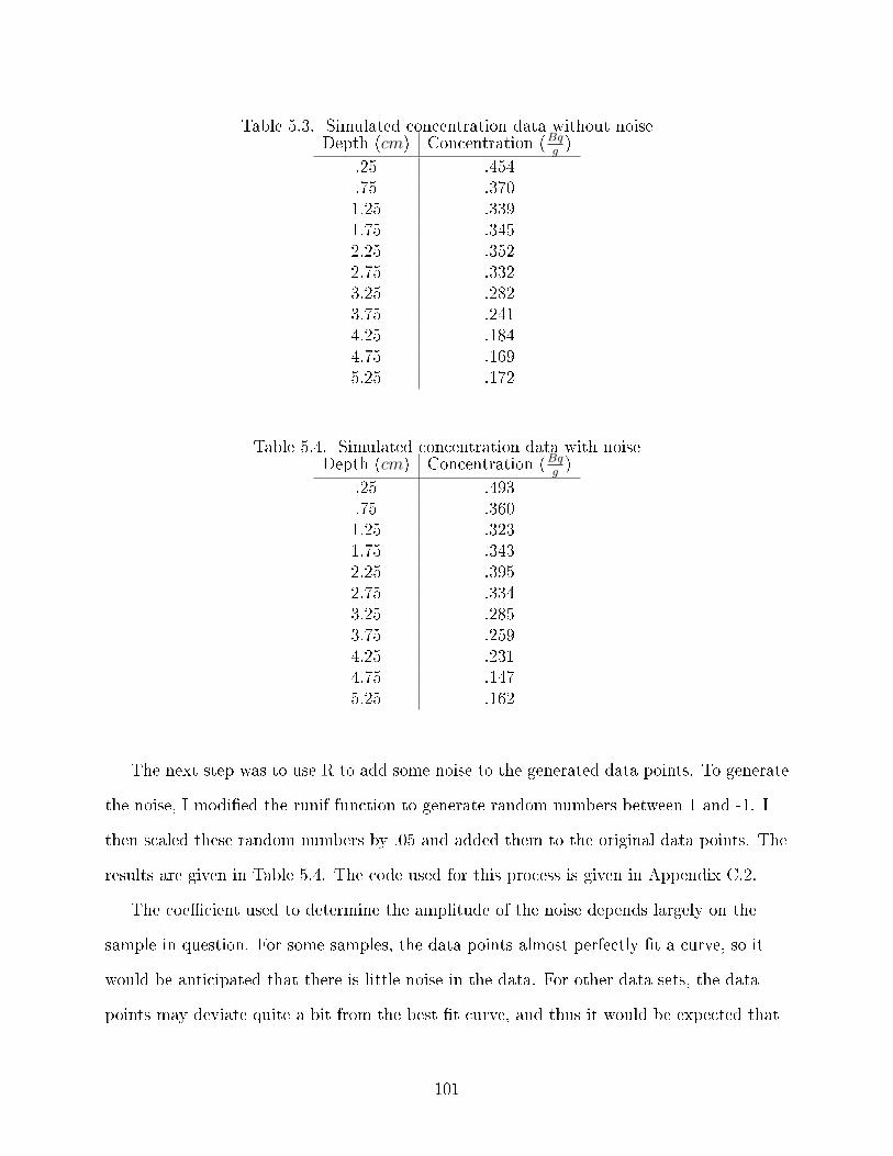
Table 5.3. Simulated concentration data without noiseDepth (cm) Concentration (Bq
g)
.25 .454
.75 .3701.25 .3391.75 .3452.25 .3522.75 .3323.25 .2823.75 .2414.25 .1844.75 .1695.25 .172
Table 5.4. Simulated concentration data with noiseDepth (cm) Concentration (Bq
g)
.25 .493
.75 .3601.25 .3231.75 .3432.25 .3952.75 .3343.25 .2853.75 .2594.25 .2314.75 .1475.25 .162
The next step was to use R to add some noise to the generated data points. To generate
the noise, I modi�ed the runif function to generate random numbers between 1 and -1. I
then scaled these random numbers by .05 and added them to the original data points. The
results are given in Table 5.4. The code used for this process is given in Appendix C.2.
The coe�cient used to determine the amplitude of the noise depends largely on the
sample in question. For some samples, the data points almost perfectly �t a curve, so it
would be anticipated that there is little noise in the data. For other data sets, the data
points may deviate quite a bit from the best �t curve, and thus it would be expected that
101

Figure 5.23. The �t function for the simulated concentration data without noise.
the data is noisier. To estimate the coe�cient, then, one method would be to determine
the mean error for all of the data points in a sample and multiply that number by 2. The
error is doubled because, taking the magnitude of the random numbers generated, the
mean of these random numbers would be on average about .5. Thus by doubling the
random numbers, the mean error of the simulated data points should be comparable to the
mean error of the original data points. I did not use this process for the purposes of this
example. Rather, I chose a coe�cient, .05, that visually looked like it produced an
appropriately large error. However, for the error estimates for the ten bodies of water
considered in this section, I took the more rigorous approach.
Once I had obtained the two sets of data, one without noise and one with, I ran the
NCRSFitModelSoftware on both data sets. Plots of the �t functions for the simulated
concentration data without and with noise are shown in Figures 5.23 and 5.24, respectively.
The software produced the equation for the concentration as a function of time for the
simulated data without noise:
C(t) = e−0.03114t(1 + 0.147 sin(0.280t+ 0.752)). (5.32)
102

Figure 5.24. The �t function for the simulated concentration data with noise.
For the data with noise, the equation was given as
C(t) = e−0.03114t(1− 0.187 sin(0.260t− 0.0509)). (5.33)
The periods for these two data sets were thus TWO = 22.4 years and TW = 24.1. Thus the
two period values di�ered by a little less than two years.
It is possible that a singular trial may produce larger or smaller deviations from the
original data than would be expected on average. For this reason, I ran twenty-nine more
simulations of data with noise and computed the period. The values of all thirty trials are
given in Table 5.5. It is worth noting that I ran more than 30 trials to accrue this data.
There were a couple of instances in which NCRSFitModelSoftware produced an error
message and did not provide a period estimate. There were also a few instances in which
the graph produced looked like a questionable �t, with a lot of small oscillations between
data points that did not appear warranted. These �ts were not included in the listed
simulations.
I used R to compute the mean and standard deviation of these 30 simulations. The
mean was µ = 21.7 years, while the standard deviation was 3.51 years. Since the mean
103

Table 5.5. Thirty simulations with random noise and the resulting periodData run Period (Y ears)Original 22.4
Simulation 1 24.1Simulation 2 16.7Simulation 3 26.4Simulation 4 27.4Simulation 5 19.9Simulation 6 28.7Simulation 7 27.8Simulation 8 15.9Simulation 9 18.7Simulation 10 18.8Simulation 11 17.0Simulation 12 23.4Simulation 13 19.3Simulation 14 22.4Simulation 15 22.4Simulation 16 25.5Simulation 17 16.7Simulation 18 26.2Simulation 19 23.0Simulation 20 18.9Simulation 21 22.0Simulation 22 21.1Simulation 23 23.3Simulation 24 19.0Simulation 25 24.6Simulation 26 19.6Simulation 27 21.4Simulation 28 20.0Simulation 29 20.6Simulation 30 19.8
was generated from simulated data, it is not a better estimate of the period, and is useful
primarily as a check to make sure the simulation process is running correctly. For 30
simulations, we would expect to see that the mean is similar to the �original" period (the
period determined from the NCRSModelFitSoftware), but because of the small sample size,
we would not expect them to be close to identical. Since the original period was 22.4
104

Table 5.6. Period of oscillations for bodies of water considered in Chapters 4 and 5.Body of Water Period (years)
Cochnewagon Lake 22.4± 6.7SS15 22.9± 3.1
Gardner Pond N/A±N/AGolden Lake 24.0± 4.1Highland Lake 28.9± 11Salmon Pond 25.9± 1.5
Lake Purrumbete N/A±N/AWarner Lake 29.2± 8.5Bracey Lake 26.6± 5.4Barsjon Lake 15.1± 6.3
years, the mean of the simulated period data 21.7 years seems reasonably close, given that
for a 95% con�dence interval around the simulation mean, the original value falls within
that range.
There are many techniques that can be used to estimate the error of a sample. I opted
to use twice the standard deviation as my error estimation technique. My preference is to
overestimate the error rather than potentially underestimate it, which this technique
should accomplish. Thus for this example, the error would be about 7.0 years, meaning
that the period for this �ctional data set would be 22.4± 7.0 years.
5.2.2 Results
I ran 30 simulations for each of the 10 bodies of water considered in this section. The
results of these simulations are shown in Appendix B. I used these simulations to compute
the error in the same manner outlined for this example, by computing the standard
deviation and doubling it. The results of these computations are shown in Table 5.6. For
two of the bodies of water, Gardner Pond and Lake Purrumbete, the means of the
simulations were di�erent enough (using a 95% con�dence interval) from the period values
obtained from the actual data that the two means could not be said to be the same. For
both of these bodies of water, a handful of the trials yielded periods on the order of 50− 60
105
years that visually appeared to �t the data well. Interestingly, even though the Gardner
Pond simulated data was generated using a curve that should have produced a 57 year
period, once the noise was introduced, the majority of the trials yielded periods on the
order of 20− 30 years. Because the noisy simulations were so di�erent from the periods
generated from the data, I decided that we do not have enough information to say what
the period of oscillations is for these two lakes.
For the remaining eight bodies of water, the period generated from the data did fall
within a 95% con�dence interval around the mean of the simulated noisy data. The
uncertainty, which was computed by doubling the standard deviation, varied widely from
one lake to the next. This is unsurprising, given that some lake data appeared to be noisier
than the other lakes. Once uncertainty was accounted for, seven of the bodies of water had
periods that overlapped with one another. The one exception was Barsjon, which had a
period that overlapped with some, but not all, of the lakes.
One thing to be aware of is that these results are only as good as the original �t curves.
Because of the conversion between depth and time, it is not only the sinusoidal piece but
also the exponential piece that have to be �t well to get an accurate estimate for the
period. Improved curve �tting techniques could yield better period estimates.
5.3 Oceanic Oscillations
For the bodies of water considered in the previous section, almost all had a period
between 20− 30 years. This raises the question as to what could be causing such
oscillations in lead-210 sediment content.
One possibility is that such �uctuations could be caused by climate cycles. Climate
cycles are periodic changes in things such as atmospheric temperature, air pressure, winds,
ocean surface temperature, and precipitation amounts. In particular, since the majority of
the bodies of water considered are in proximity to the Atlantic Ocean, for such bodies of
water, it is possible that one or more of the oceanic climate cycles is in�uencing lead-210
106

deposits. Despite extensive research, oceanic oscillations are still not fully understood.
Recently, e�orts have been made to estimate the period of oceanic oscillations (e.g.,
[57, 58]). Rather than exhibiting a single distinct period, it has been shown that the
processes behind such oscillations may have several distinct periods.
Of particular interest to this research are the North Atlantic Oscillation (NAO), the
Atlantic meridional overturning oscillation (AMOC), and the Atlantic mutidecadal
oscillation (AMO), which will be collectively referred to as the North Atlantic Oscillations
(NAOs). Each of these oscillations operates in the North Atlantic Ocean.
Seip et al. [57] found cycles for the NAOs with lengths of 7, 13, 20, 26, and 34 years.
Observe that, after accounting for uncertainty, almost all of the bodies of water considered
in the previous section had a period of 20 or 26 years, the one exception being Barsjon,
which could be said to have a period of 13 or 20 years. It is possible, then, that one
particular mechanism behind the oscillations with a period of 20− 26 years governs the
lead-210 deposits. It is also possible that all of the mechanisms a�ect lead-210 deposits to
some degree, some perhaps more so than others, and that if multiple sinusoidal functions
were used in the NCRS model instead of a single one, that a better �t could be found.
Such a process would require more sophisticated modeling software than the default
nonlinear �t function in R, but could be a good avenue for future research.
107
CHAPTER 6
CONCLUSIONS AND FUTURE RESEARCH
In this paper, I have derived a new model for radiometric dating, the non-constant rate
of supply (NCRS) model. It is a generalized model such that the commonly used constant
rate of supply (CRS) model could be viewed as a special case of the NCRS model when the
rate of supply of a given radionuclide is constant. It can be utilized whenever the
concentration data for a radioisotope in a given sample can be modeled by a combination
of mathematical functions (e.g., the concentration data may be modeled as an exponential
decay curve with sinusoidal �uctuations).
6.1 Summary and Conclusions
I applied the NCRS model to lead-210 data for 34 bodies of water. For four of these
bodies of water, I performed the NCRS analysis by hand (see Chapter 4). Initially I
included both sinusoidal and linear �uctuations in my concentration modelings. While the
inclusion of the linear term provided a better �t than sinusoidal and exponential terms
alone, it soon became apparent that the linear term signi�cantly shifted the age estimates,
in some cases by decades. While it would be expected that the linear term should a�ect
the age estimates some, in a couple of cases the age estimates it provided appeared to be
physically unrealistic. Thus, for future applications of the NCRS model, I removed the
linear term. Even though the linear term proved troublesome in certain cases, it did raise
some important questions for radiometric dating. If there is downward migration of
lead-210 in the soil, then conventional dating techniques may not accurately estimate the
age of the sediment. The linear term may still be useful in some instances, particularly in
bodies of water in which there is signi�cant migration of lead-210, but more information
about the body of water would be needed so that an accurate linear term could be
appended to the concentration equation.
108

To model the other bodies of water, Dr. Brian Toner and I developed the
NCRSModelFitSoftware, which automated the NCRS modeling process. Although the
software has the capability to include a linear term, I included only sinusoidal �uctuations
in addition to exponential decay. I pulled 33 bodies of water (including three that I had
modeled by hand previously) from a collection of processed data contained on the ERL
computer. While not all bodies of water exhibited sinusoidal �uctuations, for nine of the
samples, the NCRSModelFitSoftware was able to produce a �t curve with sinusoidal
�uctuations that appeared to �t the data reasonably well. Cochnewagon Lake was also
able to be �t by the software, but it came from a separate collection of data. In total, this
left 10 bodies of water with sinusoidal �uctuations to be further analyzed.
The sinusoidal oscillations did shift the age estimates, in some instances by a matter of
years. This e�ect was most pronounced for the upper layers of sediment, as the exponential
decay dampened out much of the sinusoidal term's e�ect in deeper sediment. On such a
short timescale, a di�erence of a few years matters when it comes to estimating the age of
the sediment. If there truly are sinusoidal �uctuations, which the data seems to support in
at least some bodies of water, it is imperative that these are considered in dating models.
An important future step will be to validate the model using samples of known age.
Often validation is done using a secondary radioisotope such as cesium-137 or hallmark
features of the sediment, such as pollen markers. While the cesium-137 content for each
sample is collected in the ERL, for many if not most of the bodies of water considered in
this paper, the lead-210 and cesium-137 dates do not align when the CRS model is used.
This issue was explored in [37], and was part of the inspiration for this paper, to reconcile
the two estimates by accounting for the potential downward migration of cesium-137. The
di�culties with direct application of the NCRS model to cesium-137 will be discussed later
in this chapter, but if those di�culties can be accounted for, this may be a fruitful avenue
for future research.
109

Since the CRS and NCRS models produce similar estimates for the deeper sediment
layers when considering only sinusoidal �uctuations, however, using a fallout radionuclide
as a calibration tool may not be a �ne grained enough technique to see di�erences between
the two models. Physical markers, such as pollen markers, could potentially be useful here,
if they could be located in the upper sediment layers. However, this would likely require
the introduction of a new plant species to a geographic region within the past 15-20 years
in order to see di�erences between the age estimates of the two models. This requirement
limits the number of available bodies of water from which the data could be extracted, but
if such bodies of water can be found, then they may prove useful for testing the utility of
the NCRS model.
Perhaps the best physical validation tool would be a varved lake. In such bodies of
water, there is so little sediment mixing that the season in which a sediment layer was
formed can be distinguished based on the color of the sediment. Thus, the age can be
determined by counting the stripes of color in the sediment. Obtaining varved lake data is
di�cult, as few such lakes exist. To retain the sediment strati�cation, there must be
virtually no plant or animal activity in the lake. However, if varved lake data could be
obtained, it could provide a robust validation tool, assuming the sediment had nonconstant
trends in the lead-210 data which would require the use of the NCRS model.
Another key factor I investigated was the period of oscillations. I computed the period
for all 10 samples with sinusoidal �uctuations. Eight of the 10 had period values on the
order of 20− 30 years. Of the remaining two bodies of water, Barsjon had a period of
about 15 years, while Gardner Pond had a period of about 57 years. Two of the bodies of
water, one of which was Gardner Pond, ended up being removed from the sample because
the uncertainty was too high for the age estimate to be considered meaningful. Of the
remaining eight bodies of water, all but Barsjon overlapped with the periods of one another.
Barsjon's period overlapped with some, but not all, of the bodies of water in the sample.
110

Since the majority of the bodies of water in the sample seemed to share a common
period, the natural question was, what could cause such a phenomenon? Since the
introduction of lead-210 into sediment is conducted through factors such as precipitation
and wind, climate cycles, which are cyclic in nature, seemed to be a probable contender. In
particular, since most of the bodies of water in the sample are close to the Atlantic Ocean,
I looked up the period of oscillations for the North Atlantic Oscillations (NAOs). Instead
of having one period, each of these oscillations has several distinct periods. Recent research
[57] suggests that the periods have lengths of about lengths of 7, 13, 20, 26, and 34 years.
With uncertainty, all of the bodies of water except Barsjon have periods of about 20 or 26
years, while Barsjon has a period of about 13 or 20 years. While this does not de�nitively
prove that climate cycles are responsible for the sinusoidal �uctuations in sediment
samples, it does suggest that climate cycles could be a potential cause.
6.2 Improvements and Further Work
To build upon this work, one of the best avenues for future research would be the
inclusion of more sediment samples. While it is encouraging to see that the bodies of water
in this study had periods that were roughly the same, it is possible that the observed
phenomenon is merely a �uke. More samples could provide further evidence that there is
indeed a phenomenon leading to oscillatory behavior in some sediment deposits.
The �t of the concentration versus depth data is crucial to the success of the NCRS
model. Both the exponential and sinusoidal pieces of the model must be �t well in order to
determine an accurate estimate of the period of oscillations. However, the nonlinear �t
function in R, which was what I used for the �ts, did not always produce sensible �ts (see
Sections 5.1.7-5.1.10). While in some cases, this was due to either the data being purely
exponential or too noisy, in other instances it was likely due to an issue with the function
itself.
111

The function is relying on mathematical optimization alone. There may be only a small
di�erence between two di�erent �t curves, but the function always picks the one that has
the smallest deviation from the data points, even if that �t makes less physical sense. I ran
into an issue several times, of which Damariscotta River Core 2 is a good example (see
Figure 5.20), where, to obtain the best possible �t, the software would produce a sinusoidal
function with a very short period and thus lots of oscillations. In the case of the
Damariscotta River Core 2, the data appears to be exponential, with one data point that
deviates from the exponential shape. Since it is expected that there will be some amount of
noise in the data, a human researcher would likely determine that a sinusoidal function was
not needed and that a pure exponential function would produce the most physically
realistic �t. The software, however, produced a curve that hits the outlier and comes close
to hitting the other points, but which does not seem like a good �t for the general trend of
the data. With enough oscillations, a function can reach nearly every data point, but the
necessity of so many oscillations is often not re�ected in the general shape of the data.
At present, there is no objective system for determining which �ts are reasonable and
which ones are not. It si up to the researcher to visually inspect the �ts and discard any
that seem unreasonable. In Sections 5.1.9 and 5.1.10 I have provided you with examples of
the types of �ts that I thought were unreasonable, but it would be better if unrealistic �ts
were ruled out by the �t function itself. If a better �t function could be devised, perhaps
one with noise reduction, then it could make the �tting process easier and reduce chances
of erroneously discarding a valid �t.
The cause of the sinusoidal oscillations could also prove to be a fruitful avenue for
research. While it seems probable that climate cycles could be the cause of such
�uctuations, the particular climate cycles and mechanisms that could be responsible remain
an open question. Since the bodies of water considered here come from various geographic
regions, investigations of individual lakes and their climates could help to better understand
112

the phenomenon. It is also possible that another cause aside from climate cycles is
responsible for the oscillations. Alternate explanations may be worth consideration.
6.3 Cesium Dating and Other Fallout Radionuclides
One of the goals at the outset of this project was to use the NCRS model to estimate
the age of samples using cesium-137. However, due to the unique shape of cesium curves,
the model must be adapted to �t cesium-137, which proved to be more di�cult than
initially anticipated. Consider the activity data for Golden Lake, shown in 6.1, for lead-210
and cesium-137, obtained from one of the old data sheets in the ERL. (Note that total
lead-210 activity, rather than unsupported lead-210 activity, is shown. Note also that
activity, rather than speci�c activity, is on the y axis, allowing lead-210 and cesium-137 to
be plotted on the same graph.) Unlike lead-210, which primarily exhibits exponential
decay, the cesium-137 data has almost a bell shape, although what happens in the very
middle of the graph is unclear. Unlike lead-210, which is constantly being produced,
cesium-137 was introduced into the environment during the above ground nuclear weapons
testing in the 1950s and 1960s. The presence of cesium-137 in pre-nuclear testing sediment
suggests that the cesium has been able to migrate through the layers of sediment. After the
weapons testing ended, cesium-137 continued to be deposited into waterways through wind
and precipitation, but at decreasing rates. The cesium-137 data must therefore be modeled
piecewise for the time prior to above ground nuclear weapons testing, the years of testing,
and the years post-testing. Let's suppose that the start of testing corresponds to depth x1
and the ending of testing corresponds to depth x2. For the years preceding the testing, we
will have approximately a decay curve, with starting amplitude S1, as well as potentially a
sinusoidal function to account for the oscillations visible in the data. For the years
post-testing, we have what looks like an increasing exponential function, going from a
relatively small value to maximum value S2. To model this, what we could do would be �ip
the data horizontally so that it looks like an exponential decay curve (meaning that we can
113

Figure 6.1. Unsupported and supported lead-210 and cesium-137 activity in Golden Lake.
have a starting value of S2 at depth x2). Then the depth data will correspond to rising
through the layers of sediment rather than descending. Because this data is ��ipped," it
would have to be treated separately from the weapons testing and pre-testing years,
because the information that would come from it would be in a sense reversed. The depths
and times generated from this curve would be measuring from the depth at concentration
S2, so calculations would have to be performed to transform the axis back to the origin.
When considering the testing years, however, we run into some di�culties. Since
cesium-137 was introduced into the atmosphere in large quantities over relatively short
intervals of time, one way to model the process by which it was introduced would be
through a series of pulse functions. However, since the sediment sample slices correspond
to several year intervals, even if the precise dates of the pulses were known, the data isn't
�ne grained enough to determine information about the individual pulses. Rather, what we
see is an accumulation of the e�ects of multiple pulses and their corresponding decays, the
shape of which we cannot precisely model with our limited information.
My initial thought was that perhaps we could ignore what was happening during the
testing years, since we know the dates of nuclear testing. However, because cesium-137 is
able to migrate through the soil, the sharp peaks that we see in the data may not
correspond exactly to the years of nuclear testing. We should be able to estimate the age of
sediment on the left side of the graph from the post-testing information, but the right half
114

we cannot determine an accurate age from without the information for the testing years.
We could make an estimate based on when nuclear testing began, but that estimate could
be o� by several years, introducing a large amount of uncertainty into our age estimates.
There are likely many more optimal approaches which could be taken, and it should be an
interesting question to be considered in future research.
Since other fallout radionuclides like strontium-190 were introduced into the
environment in the same fashion as cesium-137, similar models would be used. However,
for fallout radionuclides that have less ability to migrate through the soil layers, there may
not be as much di�culty in modeling as there is with cesium-137. There may not even be a
right half to the graph if the radioisotopes are nearly stationary, since these isotopes are
not naturally occurring. While cesium-137 is likely the most commonly collected and
utilized of the fallout radionuclides for radiometric dating, it would be interesting to apply
the NCRS model to other radioisotopes as well.
6.4 Conclusion
The research presented here provides much promise for future research endeavors. It is
intriguing to see that of the small sample of bodies of water considered, many exhibited
sinusoidal oscillations. Of the bodies of water with sinusoidal oscillations, almost all had
the same period, once uncertainty was accounted for. It is also notable that this period
seems to line up with the period of some of the processes behind the NAOs, suggesting
that perhaps climate cycles could be behind the periodic behavior.
There are many possibilities for improvement, particularly in regards to the �tting
process, which could yield better results. There are also many avenues to explore, such as
the cause of the oscillations and adapting the NCRS model for fallout radioisotopes.
Hopefully this work will be but the start of new research in radiometric dating and will
help us to better understand the world around us.
115

REFERENCES
[1] D. L. Cahl, �Di�usion coe�cients calculated using Cs 137 pro�les applied to Pb 210dating in lake core samples,� Master's thesis, University of Maine, 2012.
[2] H. R. von Gunten, �Radioactivity: A tool to explore the past,� Radiochimica Acta 71(1995) 305�316.
[3] B. Lindell, Pandora's Box: The History of radiation, radioactivity, and radiologicalprotection. Nordic Society for Radiation Protection, Sweden, 1st ed., 1996. Translatedfrom Swedish by Helen Johnson.
[4] G. Rosenbusch and A. Knect-van Eekelen, Wilhelm Conrad Röntgen: The Birth ofRadiology. Springer, Switzerland, 1st ed., 2019.
[5] T. J. Jorgensen, Strange Glow: The Story of Radiation. Princeton University Press,Princeton, N.J., 1st ed., 2016.
[6] W. C. Röntgen, �On a new kind of rays,� Science 3 no. 59, (1896) 227�231. Translatedfrom German by Arthur Stanton.
[7] B. Goldsmith, Obsessive genius: The inner world of Marie Curie. WW Norton &Company, 2005.
[8] M. S. Curie, �Les nouvelles substances radioactives,� Revue Scienti�que 37 no. 2,(1900) 65�71.
[9] M. Malley, �The discovery of atomic transmutation: Scienti�c styles and philosophiesin france and britain,� Isis 70 no. 2, (1979) 213�223.
[10] W. Ramsay and F. Soddy, �Experiments in radio-activity, and the production ofhelium from radium,� Nature (1903) 354�355.
[11] E. Rutherford and T. Royds, �Spectrum of the radiun emanation,� PhilosophicalMagazine 16 no. 2, (1908) 313�317.
[12] E. Rutherford and F. Soddy, �The cause and nature of radioactivity - Part I,� TheLondon, Edinburgh, and Dublin Philosophical Magazine and Journal of Science 21no. 4, (1902) 370�396.
[13] L. Badash, �The age-of-the-Earth debate,� Scienti�c American 261 no. 2, (1989)90�97.
[14] E. Rutherford and H. T. Barnes, �Heating e�ect of the radium emanation,� Nature 68no. 1774, (1903) 622.
[15] D. R. Prothero, The Story of the Earth in 25 Rocks: Tales of Important GeologicalPuzzles and the People who Solved Them. Columbia University Press, Columbia, N.Y.,1st ed., 2018.
116

[16] J. L. Powell, Four Revolutions in the Earth Sciences: from Hersey to Truth. ColumbiaUniversity Press, Columbia, N.Y., 1st ed., 2015.
[17] B. B. Boltwood, �On the ultimate disintegration products of the radioactive elements:Part II. the disintegration products of uranium,� American Journal of Science 23no. 134, (1907) 77�88.
[18] E. Rutherford and B. B. Boltwood, �The relative proportion of radium and uranium inradio-active minerals,� American Journal of Science 22 no. 127, (1906) 1.
[19] A. Holmes, �The association of lead with uranium in rock-minerals, and its applicationto the measurement of geological time,� Proceedings of the Royal Society of London.Series A, Containing Papers of a Mathematical and Physical Character 85 no. 578,(1911) 248�256.
[20] Arthur Holmes, The Age of the Earth. Harper & Brothers, 1913.
[21] K. Swenson, Medical women and Victorian �ction. University of Missouri Press, 2005.
[22] M. C. Nagel, �Frederick Soddy: From alchemy to isotopes,� The Journal of ChemicalEducation no. 9, (1982) 739�740.
[23] A. O. Nier, �Variations in the relative abundances of the isotopes of common lead fromvarious sources,� Journal of the American Chemical Society 60 (1938) 1571�1576.
[24] A. O. Nier, R. W. Thompson, and B. F. Murphey, �The isotopic composition of leadand the measurement of geological time, iii,� Physical Review 60 no. 2, (1941) 112�116.
[25] A. Holmes, �An estimate of the age of the earth,� Nature 157 (1946) 680�684.
[26] F. G. Houtermans, �Die Isotopen-Häu�gkeiten im natürlichen Blei un das Alter desUrans,� Naturwissenchaften 33 (1946) 185�186.
[27] C. Patterson, �Age of meteorites and the earth,� Geochimica et Cosmochimica Acta 10no. 4, (1956) 230�237.
[28] W. F. Libby, �Atmospheric helium three and radiocarbon from cosmic radiation,�Physical Review 69 (1946) 671�672.
[29] W. F. Libby, Radiocarbon Dating. University of Chicago Press, 1952.
[30] M. Hedman, The Age of Everything: How Science Explores the Past. University ofChicago Press, 2007.
[31] B. R. R. Persson and E. Holm, �Poloniun-210 and lead-210 in the terrestrialenvironment: a historical review,� Journal of Enviromental Radioactivity 102 (2011)420�429.
[32] K. S. Krane, Introductory Nuclear Physics. John Wiley & Sons, New York, 1st ed.,1988.
117

[33] E. D. Goldberg, �Geochronology with Pb-210 in radioactive dating,� in InternationalAtomic Energy Agency Symposium Proceedings, pp. 121�131. 1963.
[34] S. Krishnaswamy, D. Lal, J. M. Martin, and M. Meybeck, �Geochronology of lakesediments,� Earth and Planetary Science Letters 11 (1971) 407�414.
[35] J.A. Sanchez-Cabeza and A.C. Ruiz-Fernández, �210pb sediment radiochronology: anintegrated formulation and classi�cation of dating models,� Geochimica etCosmochimica Acta 82 (2012) 183�200.
[36] P. G. Appleby and F. Old�eld, �The calculation of lead-210 dates assuming a constantrate of supply of unsupported Pb-210 to the sediment,� Catena 5 (1978) 1�8.
[37] R. B. Davis, C. T. Hess, S. A. Norton, D. W. Hanson, K. D. Hoagland, and D. S.Anderson, �Cs-137 and Pb-210 dating of sediments from soft-water lakes in NewEngland (U.S.A.) and Scandinavia, a failure of Cs-137 dating,� Chemical Geology 44(1984) 151�185.
[38] A. Lerman, �Strontium-90 in the Great Lakes: Concentration-time model,� Journal ofGeophysical Research 77 no. 18, (1972) 3256�3264.
[39] P. Van Metre, J. T. Wilson, C. C. Fuller, E. Callender, and B. J. Mahler, �Collection,analysis, and age-dating of sediment cores from 56 us lakes and reservoirs sampled bythe us geological survey, 1992-2001,� tech. rep., US Geological Survey, 2004.
[40] J. A. Robbins, �A model for particle-selective transport of tracers in sediments withconveyor belt deposit feeders,� Journal of Geophysical Research: Oceans 91 no. C7,(1986) 8542�8558.
[41] E. Callender, �Geochemical e�ects of rapid sedimentation in aquatic systems: minimaldiagenesis and the preservation of historical metal signatures,� Journal ofPaleolimnology 23 no. 3, (2000) 243�260.
[42] G. Gilmore and J. D. Hemingway, Practical gamma-ray spectroscopy. John Wiley &Sons, 1st ed., 1995.
[43] R. B. Firestone, C. M. Baglin, and S. Y. F. Chu, Table of Isotopes: 1999 update. JohnWiley & Sons, 8th ed., 1999.
[44] P. A. Tanner, S. M. Pan, S. Y. Mao, and K. N. Yu, �γ-ray spectrometric andα-counting method comparison for the determination of pb-210 in estuarinesediments,� Applied Spectroscopy 54 no. 10, (2000) 1443�1446.
[45] G. F. Knoll, Radiation Detection and Measurement. John Wiley & Sons, Inc., 3rd ed.,2000.
[46] V. Putyrskaya, E. Klemt, and S. Röllin, �Migration of Cs-137 in tributaries, lake waterand sediment of Lago Maggiore (Italy, Switzerland) - analysis and comparison withLago di Lugano and other lakes,� Journal of Environmental Radioactivity 100 (2009)35�48.
118

[47] J. Wang, M. Baskaran, and J. Niedermiller, �Mobility of Cs-137 in freshwater lakes: Amass balance and di�usion study of Lake St. Clair, Southeast Michigan, USA,�Geochimica et Cosmochimica Acta 218 (2017) 323�342.
[48] J. M. Zachara, S. C. Smith, C. Liu, J. P. McKinley, R. J. Serne, and P. L. Gassman,�Sorption of Cs+ to micaceous subsurface sediments from the Hanford site, USA,�Geochimica et Cosmochimica Acta 66 (2002) 193�211.
[49] P. G. Appleby, �Three decades of dating recent sediments by fallout radionuclides: areview,� Holocene 18 no. 1, (2008) 83�94.
[50] M. Baskaran, J. Nix, C. Kuyper, and N. Karunakara, �Problems with the dating otsediment core using excess (210)Pb in a freshwater system impacted by large scalewatershed changes,� Journal of Environmental Radioactivity 138 (2014) 355�363.
[51] M. Yoshimori, �Production and behavior of beryllium 7 radionuclide in the upperatmosphere,� Advances in Space Research 36 (2005) 922�926.
[52] J. Z. Drexler, C.C. Fuller, and S. Arch�eld, �The approaching obsolescence of Cs-137dating of wetland soils in North America,� Quaternary Science Review 199 (2108)83�96.
[53] J. Paatero, B. Veleva, and J. Hatakka, �Long-term trends of lead-210 concentrations inground-level air in Finland and Bulgaria,� in Global Environmental Change: Challengesto Science and Society in Southeastern Europe: Selected Papers presented in theInternational Conference held 19-21 May 2008 in So�a Bulgaria, V. Alexandrov,M. F. Gajdusek, C. G. Knight, and A. Yotova, eds., pp. 229�234. Springer, 2010.
[54] C. T. Hess and C. W. Smith, �A mathematical model of the accumulation ofradionuclides by oysters (C. virginia) aquacultured in the e�uent of a nuclear powerreactor to include major biological parameters,� Health Physics 33 (1977) 121�130.
[55] C. Frankfort-Nachmias and A. Leon-Guerrero, Social Statistics for a Diverse Society.Sage Publications, 4th ed., 2006.
[56] Maine Department of Inland Fisheries and Wildlife, �Cochnewagon Pond, MonmouthTwp., Kennebec Co. U.S.G.S. Monmouth, Me.� https://www.maine.gov/ifw/docs/lake-survey-maps/kennebec/cochnewagon_pond.pdf,2006.
[57] Knut Lehre Seip, Øyvind Grøn, and Hui Wang, �The North Atlantic Oscillations:Cycle times for the NAO, the AMO and the AMOC,� Climate 7 no. 3, (2019) 43.
[58] Knut L Seip and Øyvind Grøn, �Atmospheric and ocean dynamics may explain cyclesin oceanic oscillations,� Climate 7 no. 6, (2019) 77.
119

APPENDIX A
LAKE DATA
This appendix contains the data used for the bodies of water analyzed in this paper.
Generally the data had already been processed, so the author did not need to manually
compute the speci�c activities, but rather needed only to check that the calculations
performed by previous researchers appeared to be correct, and then subtract the supported
lead-210 to obtain the unsupported lead-210 values. Below are the speci�c activities for
various lakes. Values omitted from �ts are denoted with a star.
A.1 Cochnewagon Lake
Table A.1. Speci�c Activity of Unsupported Lead-210 and Uncertainty Values forCochnewagon Lake.
Depth (cm) Speci�c Activity (Bqg) Uncertainty (Bq
g))
.25 .4487 .02221.25 .3520 .02082.25 .3587 .02333.25 .3222 .02064.25 .2246 .01915.25 .2185 .01926.25 .1869 .01937.25 .1015 .01528.25 .0662 .01419.25 .0636 .014110.25 .0372 .0126
120

A.2 Golden Lake
Table A.2. Speci�c Activity of Unsupported Lead-210 and Uncertainty Values for GoldenLake.
Depth (cm) Speci�c Activity (Bqg) Uncertainty (Bq
g))
.5* .0567 .00015701 .0424 .00013381.5 .0390 .00013062 .0329 .00011992.5 .0239 .00011363.5 .0234 .00010804.5 .0193 .00010115.5 .0095 .00009056.5 .0081 .00008517.5 .0041 .00008298.5 .0034 .00008159.5 .0028 .000076410.5 .0008 .000085611.5* -.0007 .000075912.5* .0001 .000071013.5* .0003 .000077814.5* .0003 .0000847
A.3 SS15 Greenland
Table A.3. Speci�c Activity of Unsupported Lead-210 and Uncertainty Values for SS15 inGreenland.
Depth (cm) Speci�c Activity (Bqg) Uncertainty (Bq
g))
.5 .0599005 .00006941.25 .0445720 .00005982.25 .0284988 .00003633.25 .0294943 .00009004.25 .0070382 .00000885.25 .0166277 .00003236.25 .0062154 .00001037.25 .0042522 .00000808.25 .0020304 .00000509.25 .0005493 .0000006
121
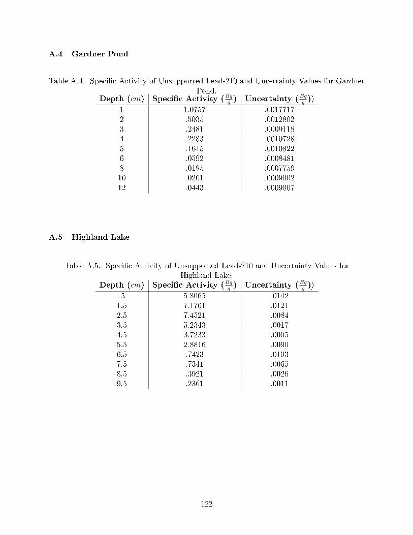
A.4 Gardner Pond
Table A.4. Speci�c Activity of Unsupported Lead-210 and Uncertainty Values for GardnerPond.
Depth (cm) Speci�c Activity (Bqg) Uncertainty (Bq
g))
1 1.0757 .00177172 .5035 .00128023 .2481 .00091184 .2283 .00107285 .1615 .00108226 .0592 .00084818 .0195 .000775910 .0261 .000900212 .0443 .0009007
A.5 Highland Lake
Table A.5. Speci�c Activity of Unsupported Lead-210 and Uncertainty Values forHighland Lake.
Depth (cm) Speci�c Activity (Bqg) Uncertainty (Bq
g))
.5 5.8065 .01421.5 7.1761 .01212.5 7.4521 .00843.5 5.2343 .00174.5 3.7233 .00055.5 2.8816 .00906.5 .7423 .01037.5 .7341 .00658.5 .3921 .00269.5 .2361 .0011
122

A.6 Salmon Pond
Table A.6. Speci�c Activity of Unsupported Lead-210 and Uncertainty Values for SalmonPond.
Depth (cm) Speci�c Activity (Bqg) Uncertainty (Bq
g))
.75 .6756 .00101.5 1.0611 .00212.5 .4839 .00103.5 .4120 .00104.5 .2825 .00075.5 .1906 .00056.5 .1357 .00047.5 .0945 .0003
A.7 Warner Lake
Table A.7. Speci�c Activity of Unsupported Lead-210 and Uncertainty Values for WarnerLake.
Depth (cm) Speci�c Activity (Bqg) Uncertainty (Bq
g))
.25* 27.5130 .0142.75 21.1710 .01211.25 15.6664 .00841.75 5.9330 .00172.25 3.4262 .00052.75 12.0525 .00903.25 8.7116 .01033.75 3.8524 .00654.25 .9480 .00264.75 .5300 .00115.25 .4179 .0015
123

A.8 Bracey Lake
Note that uncertainty values were not given for Bracey Lake.
Table A.8. Speci�c Activity of Unsupported Lead-210 and for Bracey Lake.Depth (cm) Speci�c Activity (Bq
g)
.75 .871.0 .711.5 .552.0 .542.5 .533.0 .473.5 .424.0 .364.5 .305.0 .285.5 .276.0 .246.5 .227.0 .217.5 .198.0 .148.5 .089.0 .089.5 .0710.0 .07
124

A.9 Barsjon
Table A.9. Speci�c Activity of Unsupported Lead-210 and Uncertainty Values for Barsjon.Depth (cm) Speci�c Activity (Bq
g) Uncertainty (Bq
g))
.50 .055342 .00026352.5 .047629 .00020904.5 .029374 .00017005.5 .021024 .00016106.0 .023316 .00015736.5 .023037 .00014717.0 .014992 .00016167.5 .012472 .00014158.5 .02062 .000126810.5 .007136 .000139112.5 .003237 .0001245
125
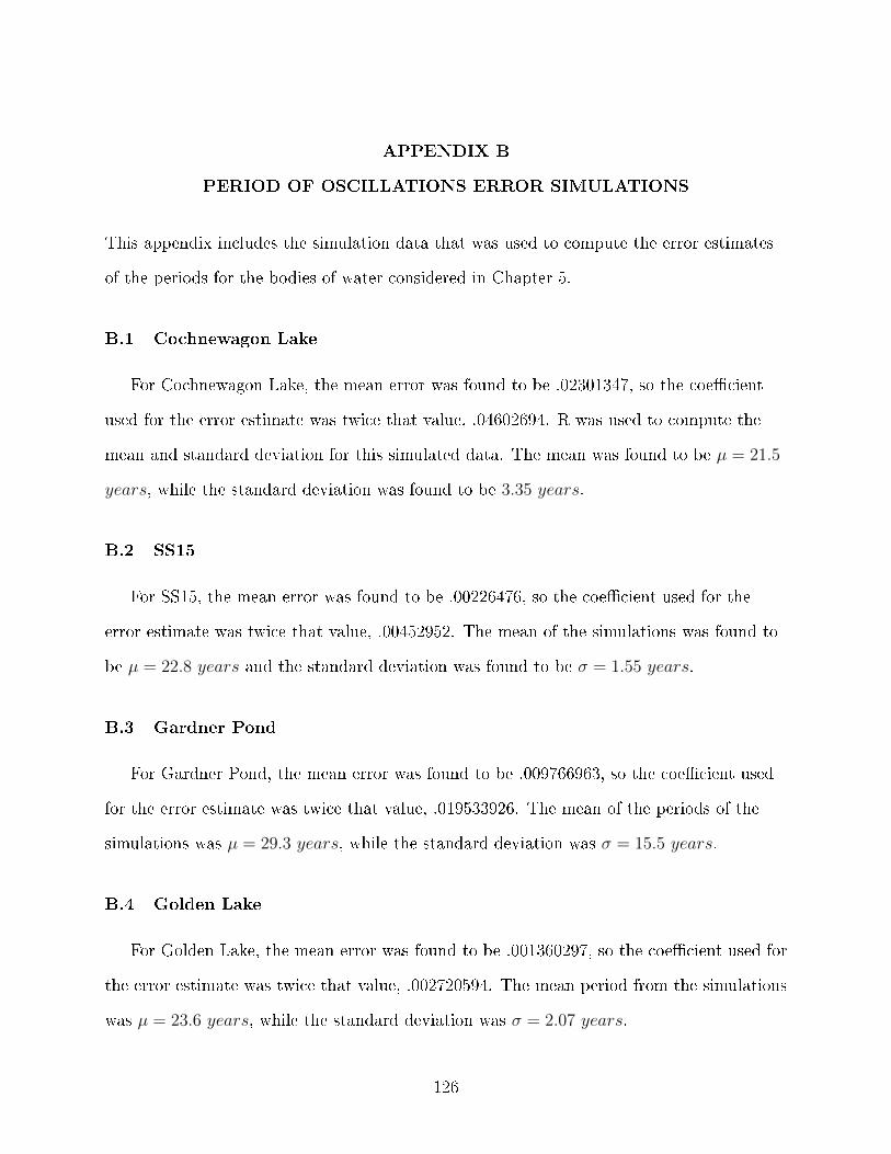
APPENDIX B
PERIOD OF OSCILLATIONS ERROR SIMULATIONS
This appendix includes the simulation data that was used to compute the error estimates
of the periods for the bodies of water considered in Chapter 5.
B.1 Cochnewagon Lake
For Cochnewagon Lake, the mean error was found to be .02301347, so the coe�cient
used for the error estimate was twice that value, .04602694. R was used to compute the
mean and standard deviation for this simulated data. The mean was found to be µ = 21.5
years, while the standard deviation was found to be 3.35 years.
B.2 SS15
For SS15, the mean error was found to be .00226476, so the coe�cient used for the
error estimate was twice that value, .00452952. The mean of the simulations was found to
be µ = 22.8 years and the standard deviation was found to be σ = 1.55 years.
B.3 Gardner Pond
For Gardner Pond, the mean error was found to be .009766963, so the coe�cient used
for the error estimate was twice that value, .019533926. The mean of the periods of the
simulations was µ = 29.3 years, while the standard deviation was σ = 15.5 years.
B.4 Golden Lake
For Golden Lake, the mean error was found to be .001360297, so the coe�cient used for
the error estimate was twice that value, .002720594. The mean period from the simulations
was µ = 23.6 years, while the standard deviation was σ = 2.07 years.
126

B.5 Highland Lake
For Highland Lake, the mean error was found to be .7209563, so the coe�cient used for
the error estimate was twice that value, 1.4419126. The mean of the simulation periods
was µ = 26.5 years, while the standard deviation was σ = 5.48 years.
B.6 Salmon Pond
For Salmon Pond, the mean error was found to be .01311514, so the coe�cient used for
the error estimate was twice that value, .02623028. The mean of the periods of the
simulations was 25.9 years, while the standard deviation was σ = .74 years.
B.7 Lake Purrumbete
For Lake Purrumbete, the mean error was found to be .006491262, so the coe�cient
used for the error estimate was twice that value, .012982524. The mean of the simulations
was µ = 33.5 years and the standard deviation was σ = 13.3 years.
B.8 Warner Lake
For Warner Lake, the mean error was found to be .006491262, so the coe�cient used for
the error estimate was twice that value, .012982524. The mean of the simulations was
found to be µ = 28.6 years, while the standard deviation was σ = 4.26 years.
B.9 Bracey Lake
For Bracey Lake, the mean error was found to be .006491262, so the coe�cient used for
the error estimate was twice that value, .012982524. The mean of the simulations was
µ = 26.4 years, while the standard deviation was σ = 2.72 years.
127

B.10 Barsjon
For Barsjon, the mean error was found to be .002155469, so the coe�cient used for the
error estimate was twice that value, .004310938. The mean of the simulations was µ = 14.4
years, while the standard deviation was σ = 3.13 years.
128

Table B.1. Thirty simulations with random noise and the resulting period forCochnewagon Lake
Data run Period (Y ears)Original 22.4
Simulation 1 18.9Simulation 2 19.3Simulation 3 18.9Simulation 4 16.0Simulation 5 23.1Simulation 6 20.5Simulation 7 16.2Simulation 8 25.5Simulation 9 22.0Simulation 10 24.2Simulation 11 21.8Simulation 12 16.6Simulation 13 24.4Simulation 14 17.1Simulation 15 20.0Simulation 16 27.4Simulation 17 24.9Simulation 18 23.8Simulation 19 22.0Simulation 20 21.6Simulation 21 23.2Simulation 22 16.7Simulation 23 20.2Simulation 24 22.8Simulation 25 26.4Simulation 26 15.7Simulation 27 24.1Simulation 28 23.9Simulation 29 25.5Simulation 30 22.1
129
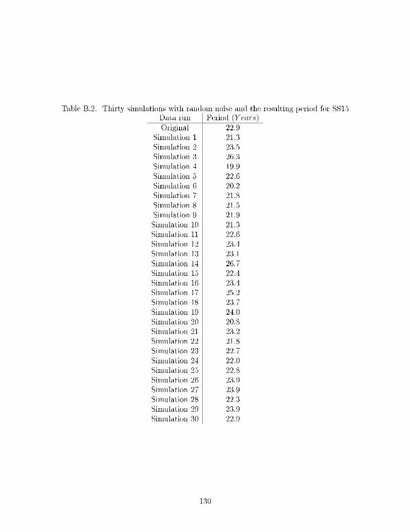
Table B.2. Thirty simulations with random noise and the resulting period for SS15Data run Period (Y ears)Original 22.9
Simulation 1 21.3Simulation 2 23.5Simulation 3 26.3Simulation 4 19.9Simulation 5 22.6Simulation 6 20.2Simulation 7 21.8Simulation 8 21.5Simulation 9 21.9Simulation 10 21.3Simulation 11 22.6Simulation 12 23.4Simulation 13 23.1Simulation 14 26.7Simulation 15 22.4Simulation 16 23.4Simulation 17 25.2Simulation 18 23.7Simulation 19 24.0Simulation 20 20.8Simulation 21 23.2Simulation 22 21.8Simulation 23 22.7Simulation 24 22.0Simulation 25 22.8Simulation 26 23.9Simulation 27 23.9Simulation 28 22.3Simulation 29 23.9Simulation 30 22.9
130

Table B.3. Thirty simulations with random noise and the resulting period for GardnerPond
Data run Period (Y ears)Original 57.4
Simulation 1 21.4Simulation 2 21.2Simulation 3 57.6Simulation 4 21.3Simulation 5 20.9Simulation 6 20.6Simulation 7 22.5Simulation 8 21.0Simulation 9 21.2Simulation 10 59.7Simulation 11 19.8Simulation 12 19.6Simulation 13 53.4Simulation 14 21.6Simulation 15 59.8Simulation 16 20.2Simulation 17 22.0Simulation 18 21.2Simulation 19 53.7Simulation 20 20.9Simulation 21 22.2Simulation 22 60.3Simulation 23 20.8Simulation 24 19.4Simulation 25 20.8Simulation 26 20.1Simulation 27 53.3Simulation 28 21.5Simulation 29 20.2Simulation 30 21.9
131

Table B.4. Thirty simulations with random noise and the resulting period for Golden LakeData run Period (Y ears)Original 24.0
Simulation 1 23.6Simulation 2 21.7Simulation 3 23.7Simulation 4 24.2Simulation 5 21.1Simulation 6 24.1Simulation 7 23.0Simulation 8 22.0Simulation 9 25.2Simulation 10 21.3Simulation 11 24.0Simulation 12 23.4Simulation 13 26.8Simulation 14 24.4Simulation 15 24.0Simulation 16 22.9Simulation 17 27.0Simulation 18 20.5Simulation 19 22.2Simulation 20 22.2Simulation 21 22.6Simulation 22 26.8Simulation 23 22.8Simulation 24 30.2Simulation 25 24.7Simulation 26 21.2Simulation 27 23.7Simulation 28 22.9Simulation 29 21.7Simulation 30 23.1
132

Table B.5. Four simulations with random noise and the resulting period for Highland LakeData run Period (Y ears)Original 28.8
Simulation 1 22.2Simulation 2 21.7Simulation 3 17.9Simulation 4 22.9Simulation 5 38.4Simulation 6 14.5Simulation 7 19.7Simulation 8 19.2Simulation 9 30.3Simulation 10 22.7Simulation 11 23.7Simulation 12 25.6Simulation 13 27.0Simulation 14 29.2Simulation 15 30.1Simulation 16 34.8Simulation 17 27.0Simulation 18 33.2Simulation 19 28.0Simulation 20 25.0Simulation 21 30.7Simulation 22 26.3Simulation 23 37.3Simulation 24 24.3Simulation 25 30.0Simulation 26 22.5Simulation 27 26.7Simulation 28 27.2Simulation 29 29.9Simulation 30 27.2
133

Table B.6. Thirty simulations with random noise and the resulting period for Salmon PondData run Period (Y ears)Original 25.9
Simulation 1 24.4Simulation 2 26.7Simulation 3 25.7Simulation 4 24.4Simulation 5 26.3Simulation 6 25.9Simulation 7 26.5Simulation 8 24.8Simulation 9 25.2Simulation 10 26.8Simulation 11 26.6Simulation 12 25.9Simulation 13 25.9Simulation 14 25.3Simulation 15 25.8Simulation 16 24.7Simulation 17 26.2Simulation 18 26.5Simulation 19 27.4Simulation 20 25.4Simulation 21 26.2Simulation 22 25.5Simulation 23 26.4Simulation 24 25.6Simulation 25 26.5Simulation 26 26.5Simulation 27 26.5Simulation 28 26.0Simulation 29 25.1Simulation 30 26.1
134

Table B.7. Thirty simulations with random noise and the resulting period for LakePurrumbete
Data run Period (Y ears)Original 26.3
Simulation 1 26.4Simulation 2 52.4Simulation 3 28.6Simulation 4 23.9Simulation 5 31.1Simulation 6 25.0Simulation 7 48.4Simulation 8 26.6Simulation 9 55.4Simulation 10 26.9Simulation 11 48.4Simulation 12 58.0Simulation 13 27.5Simulation 14 55.1Simulation 15 21.5Simulation 16 22.2Simulation 17 20.4Simulation 18 56.3Simulation 19 26.8Simulation 20 48.5Simulation 21 24.7Simulation 22 20.9Simulation 23 24.3Simulation 24 28.8Simulation 25 27.1Simulation 26 22.8Simulation 27 25.8Simulation 28 26.2Simulation 29 55.1Simulation 30 20.9
135

Table B.8. Thirty simulations with random noise and the resulting period for Warner LakeData run Period (Y ears)Original 29.2
Simulation 1 29.3Simulation 2 24.3Simulation 3 25.0Simulation 4 28.0Simulation 5 32.4Simulation 6 25.9Simulation 7 38.1Simulation 8 20.7Simulation 9 28.9Simulation 10 31.6Simulation 11 30.2Simulation 12 29.4Simulation 13 23.5Simulation 14 22.0Simulation 15 25.2Simulation 16 26.2Simulation 17 37.2Simulation 18 25.8Simulation 19 37.4Simulation 20 31.5Simulation 21 29.3Simulation 22 28.5Simulation 23 29.6Simulation 24 26.7Simulation 25 26.3Simulation 26 26.4Simulation 27 26.0Simulation 28 30.1Simulation 29 27.2Simulation 30 33.8
136

Table B.9. Thirty simulations with random noise and the resulting period for Bracey LakeData run Period (Y ears)Original 26.6
Simulation 1 21.7Simulation 2 22.4Simulation 3 25.7Simulation 4 26.1Simulation 5 29.7Simulation 6 27.6Simulation 7 24.1Simulation 8 23.6Simulation 9 24.6Simulation 10 25.6Simulation 11 25.0Simulation 12 26.4Simulation 13 27.9Simulation 14 26.3Simulation 15 20.2Simulation 16 29.9Simulation 17 32.3Simulation 18 28.0Simulation 19 24.2Simulation 20 30.9Simulation 21 29.5Simulation 22 26.5Simulation 23 25.5Simulation 24 27.5Simulation 25 28.8Simulation 26 27.8Simulation 27 27.8Simulation 28 26.3Simulation 29 23.7Simulation 30 26.6
137

Table B.10. Thirty simulations with random noise and the resulting period for BarsjonData run Period (Y ears)Original 15.1
Simulation 1 17.0Simulation 2 8.9Simulation 3 14.6Simulation 4 16.4Simulation 5 12.1Simulation 6 18.6Simulation 7 16.4Simulation 8 8.4Simulation 9 11.7Simulation 10 15.0Simulation 11 11.5Simulation 12 15.3Simulation 13 14.2Simulation 14 18.3Simulation 15 15.8Simulation 16 17.2Simulation 17 15.2Simulation 18 9.5Simulation 19 12.9Simulation 20 18.8Simulation 21 14.7Simulation 22 13.5Simulation 23 14.5Simulation 24 13.4Simulation 25 9.2Simulation 26 16.7Simulation 27 18.1Simulation 28 19.3Simulation 29 10.2Simulation 30 15.8
138

APPENDIX C
SAMPLE R CODE
C.1 Nonlinear Fitting
csvFileName = "C: /Users/Amber/Documents/Nuclear Phys ics/
SampleDataforCheckingRFit . csv "
csvFileName
SampleData <− read . csv ( csvFileName )
SampleData
plot ( SampleData )
y = SampleData$ concent ra t i on
x = SampleData$depth
non l in_mod=n l s ( y~a∗exp(−b∗x ) , start=l i s t ( a=0.63 ,b=0.4))
summary( non l in_mod)
l ibrary (qpcR)
RSS( non l in_mod)
non l in_mod
139
plot (x , y )
l ines (x , predict ( non l in_mod) , col="red" )
non l in_mod=n l s ( y~a∗exp(−b∗x )∗(1+c∗sin ( x)+d∗x ) ,
start=l i s t ( a=0.5 ,b=.4 ,c=.1 ,d=.8))
summary( non l in_mod)
RSS( non l in_mod)
non l in_mod
C.2 Simulating Data with Noise
csvFileName = "C:/ Users /Amber/Documents/Nuclear Phys ics /
SimulatedDataCochnewagonLake . csv "
SimulatedDataCochnewagonLake<−read . csv ( csvFileName )
y <− SimulatedDataCochnewagonLake$UnsupportedPb210
x <− SimulatedDataCochnewagonLake$Depth
yrnd <− y+0.05∗( r un i f (11)∗2−1)
yrnd
p lo t (x , yrnd )
140
APPENDIX D
NCRSFITMODELSOFTWARE CODE
#Example f o r Aoft_simp , uncomment to run example a f t e r sourc ing
#p l o t ( Aoft_simp (0 .5194 ,0 .1970 , f unc t i on ( x )(1+0.1496∗ s in (1.7930∗x
+3 .1259 ) ) , 0 . 1501 , . 2 5 ) , t=' l ' )
#Uses the c o e f f i c e n t s to compute the a c t i v i t y over time/depth
# @param a − a exponen t i a l c o e f f i c i e n t
# @param b − b e xponen t i a l c o e f f i c i e n t
# @param fn − The func t i on in the form of (1+ f ( x ) ) ( e . g .
(1+c∗sin (d∗x+f )+gx ) ) , we are computing A( t ) for
# @param A0 − A_0 the i n i t i a l concen t ra t i on
# @param x0 − x_0 the i n i t i a l cond i t i on o f x
# @param k − The decay c o e f f i c i e n t
# @param aYears − The number o f years to i n t e g r a t e over
# @param aStep − The time s t ep to i n t e g r a t e over
Aoft_simp <− function ( a , b , fn , A0 , x0=1, k=0.03114 ,
aYears = 100 , aStep = 0 .01 ){
#Bui ld a func t i on f o r a∗e^(−b∗x )
expfn <− function ( x ) ( a∗exp(−b∗x ) )
#Solve f o r c t
ConcSolve <− function (x , t , c ) ( expfn (x)−exp(−k∗t+c ) )
141
#a∗e^(−b∗x)−e^(−k∗ t+c )
ConcSolveC <− function (c ) ( ConcSolve ( x0 , 0 , c ) )
#a∗e^(−b∗x)−e^(c )
ct <− uniroot ( ConcSolveC , c (−10000 ,10000) )$ root
#Solve f o r c
#Bui ld a l i n e a r func t i on f o r x o f t
xo f t <− function ( t ) ( (−k∗t+ct−log ( a ) )/(−b) )
#x ( t ) = (−k∗ t+c−l n ( a ) )/(−b ) , t h i s i s a l i n e a r func t i on
#We have to e x t r a c t C0 l i n e a r p i e ce
#We do t h i s by f i n d i n g the i n t e r c e p t o f our (1+c∗ s in ( x∗d+f )+g∗x )
lFnPoints <− fn ( xo f t ( 0 : 1 0 0 ) )
lLM <− lm( lFnPoints~c ( 0 : 1 00 ) )
lC0Lin <− lLM$coef f ic ients [ 1 ]
#y−i n t e r c e p t o f fn , C_0
#So lve f o r z e t a
Coft <− function ( t ) (exp(−k∗t )∗ fn ( xo f t ( t ) )/ lC0Lin )
#C( t ) = e^(−k∗ t )∗(1+c∗ s in ( x ( t )∗d+f )+g∗x ( t ) )/C_0
lCInt <− i n t e g r a t e ( Coft , 0 , I n f )$value
#in t e g r a t e C( t ) d t from 0 to i n f i n i t y
lZe ta = A0/ lCInt
= A_0/SC( t )dt
#In t e g r a t e C(T) to ge t A(T) we b u i l d an array o f t_i and
use that to compute A( i )
142
#where t_i in T
lADataX <− seq (0 , aYears , aStep )
#Set o f T va l u e s
lADataY <− NULL
for ( i in lADataX){
lAo f t = lZeta∗ i n t e g r a t e ( Coft , i , I n f )$value
#A( t_i ) = lZe t a in t e g ra lC ( t ) d t from i to i n f i n i t y
lADataY <− c ( lADataY , lAo f t )
}
lAData <− cbind ( " year s " = lADataX , "A( t ) " = lADataY)
#Return the A(T) data
return ( lAData )
}
143

BIOGRAPHY OF THE AUTHOR
Amber Hathaway was born in Bangor, Maine and grew up in Veazie, Maine. She
graduated from Bangor High School in 2008. She completed her undergraduate studies at
The University of Maine, graduating summa cum laude with a Bachelor's of Arts in
Mathematics, a second major in Women's Studies, and minors in Physics and Ethics and
Social and Political Philosophy. During her tenure there, she was inducted into the
following honors societies: Phi Beta Kappa, Phi Kappa Phi, Pi Mu Epsilon, and Phi Sigma
Tau. She earned her Master's of Arts in Mathematics from the University of Maine in May
of 2014 with a dissertation entitled, �Emmy Noether's Theorem on Integral Invariants in
the Context of the Calculus of Variations." She has worked as a physics instructor at the
University of Maine's Upward Bound Program, as a calculus teaching assistant, and as a
physics teaching assistant. Amber Emily Hathaway is a candidate for the Doctorate of
Philosophy degree in Physics from the University of Maine in May 2020.
144