arX

iv:g

r-qc

/971

0106

v2 2

4 O

ct 1

997

preprint - UTF 406

Quantum Correction to the Entropy of the (2+1)-Dimensional

Black Hole

Andrei A. Bytsenko ∗

Departamento de Fisica, Universidade Estadual de Londrina, Caixa Postal 6001,

Londrina-Parana, Brazil

Luciano Vanzo † and Sergio Zerbini ‡

Dipartimento di Fisica, Universita di Trento

and Istituto Nazionale di Fisica Nucleare,

Gruppo Collegato di Trento, Italia

Abstract: The thermodinamic properties of the (2+1)-dimensional non-rotating black holeof Banados, Teitelboim and Zanelli are discussed. The first quantum correction to theBekenstein-Hawking entropy is evaluated within the on-shell Euclidean formalism, makinguse of the related Chern-Simons representation of the 3-dimensional gravity. Horizon andultraviolet divergences in the quantum correction are dealt with a renormalization of theNewton constant. It is argued that the quantum correction due to the gravitational fieldshrinks the effective radius of a hole and becomes more and more important as soon as theevaporation process goes on, while the area law is not violated.

PACS numbers: 04.60.Kz, 04.70.Dy, 97.60.Lf

1 Introduction

It is well known that we do not have yet at disposal a consistent and complete 4-dimensionalquantum gravity, but nevertheless a large number of interesting issues have been investigated,mainly within the semiclassical approximation. One of the most important issue is related to theblack hole physics and deals with the origin of the entropy, its quantum corrections, the infor-mation loss paradox, the validity of the area law (see, for example Ref. [1]). However, it is wellknown that in (3+1)-dimensions, the black hole quantum physics needs several approximations.

Recently 3-dimensional gravity has been studied in detail. Despite the simplicity of the 3-dimensional case (no propagating gravitons), it is a common believe that it deserves attentionas useful laboratory. In fact with surprise a black hole solution has been found by Banados,Teitelboim and Zanelli [2], the so called BTZ black hole. In particular, a simple geometricalstructure of a black hole allows exact computations since its Euclidean counterpart is locallyisomorphic to the constant curvature 3-dimensional hyperbolic space H3.

∗email: abyts@fisica.uel.br On leave from St. Petersburg State Technical University, Russia†e-mail: vanzo@science.unitn.it‡e-mail: zerbini@science.unitn.it

1

In this paper we shall compute the first quantum correction to the semiclassical Bekenstein-Hawking entropy for the BTZ black hole due to the one-loop gravitational fluctuations, in anattempt to elucidate the statistical origin of the black hole entropy [3, 4, 5, 6] and to explore thepossible relevance of the quantum fluctuations during the late stage of the black hole evaporationprocess.

With regard to this issues, we recall that a lot of papers have been appeared where thequantum entropy of matter fields, propagating in a black hole background, has been evaluatedby means of several different techniques (see, for example, Refs. [7, 9, 10, 8, 11, 12, 13, 14, 15,16, 17] and reference therein). We would like to stress here that we shall compute the one-loopcontribution due to the quantization of the gravitational field itself. The tree level approximationto the partition function as been discussed at length in [18], using the Brown and York approachto quasi-local thermodynamic for asymptotically anti-de Sitter black holes. It is found that in(2 + 1) dimensions, there is a thermodynamically stable black hole solution, and no negativeheat capacity instantons. Thus one expects that first quantum corrections be well defined.

As far as the computation of these corrections is concerned, some work has been done in[19, 20] and a motivation of our paper is to present a detailed and possibly complete discussionon this point.

The first quantum correction of the BTZ black hole will be evaluated making use of therelated Chern-Simons representation of the 3-dimensional gravity [21, 22]. It should be stressedthat within this approach a preliminary statistical mechanics explanation of the Bekenstein-Hawking entropy, counting boundary states at the horizon, has been given in Ref. [23].

The contents of the paper are the following. In Sect. 2 we briefly review a geometry ofthe Eclidean BTZ black hole. In Sect. 3 we present a derivation of the Selberg trace formula,starting from an elementary derivation of the heat- kernel trace related to the Laplace operator,necessary for our regularization. In Sect. 4 a computation of the first quantum correction to theentropy is outlined. The paper ends with some concluding remarks in Sect. 5. In the Appendixsome explicit computations are included.

2 The Euclidean BTZ Black Hole

Following [19] we summarize here geometrical aspects of the non-rotating BTZ black hole [2]which are relevant for our discussion. In the coordinates (t, r, φ), the static Lorentzian metricreads (8G=1 is assumed for the moment, thus the mass is dimensionless)

ds2L = −

(

r2

σ2− M

)

dt2 +

(

r2

σ2− M

)−1

dr2 + r2dφ2 , (2.1)

where M is the standard ADM mass and σ is a dimensional constant. A direct calculation showsthat the above metric is a solution of the 3-dimensional vacuum Einstein equation with negativecosmological constant, i.e.

Rµν = 2Λgµν , R = 6Λ = − 6

σ2. (2.2)

Thus, the sectional curvature k is constant and negative, namely k = Λ = −1/σ2. The metric(2.1) has an horizon radius given by

r+ =√

Mσ , (2.3)

and it describes a space-time locally isometric to the anti-de Sitter space.

2

The Euclidean section is obtained by the Wick rotation t → iτ and reads

ds2 =

(

r2

σ2− M

)

dτ2 +

(

r2

σ2− M

)−1

dr2 + r2dφ2 . (2.4)

Changing the coordinates (τ, r, φ) → (y, x1, x2) by means of

y =r+

re

r+

σ φ ,

x1 + ix2 =1

r

√

r2 − r2+ exp

(

i r+

σ2 τ + r+

σ φ)

, (2.5)

the metric becomes the one of upper-half space representation of H3, i.e.

ds2 =σ2

y2

(

d2y + dx21 + dx2

2

)

. (2.6)

As a consequence, the metric Eq. (2.4) describes a manifold homeomorphic to the hyperbolicspace H3.

It is known that the group of isometries of H3 is SL(2, IC). We shall consider a discretesubgroup Γ ⊂ PSL(2, IC) ≡ SL(2, IC)/{±Id} (Id is the identity element), which acts discon-tinuously at the point z belonging to the extended complex plane IC

⋃{∞}. We recall that atransformation γ 6= Id, γ ∈ Γ, with

γz =az + b

cz + d, ad − bc = 1 , a, b, c, d ∈ IC, (2.7)

is called elliptic if (Tr γ)2 = (a + d)2 satisfies 0 ≤ (Tr γ)2 < 4, hyperbolic if (Tr γ)2 > 4,parabolic if (Tr γ)2 = 4 and loxodromic if (Tr γ)2 ∈ IC\ [0, 4]. The element γ ∈ SL(2, IC) actson z = (y,w) ∈ H3, w = x1 + ix2 by means of the following linear-fractional transformation:

γz =

(

y

|cw + d|2 + |c|2y2,(aw + b)(cw + d) + acy2

|cw + d|2 + |c|2y2

)

. (2.8)

The periodicity of the angular coordinate φ allows to describe the BTZ black hole manifold asthe quotient H3 ≡ H3/Γ, Γ being a discrete group of isometry possessing a primitive elementγh ∈ Γ defined by the identification

γh(y,w) = (e2πr+

σ y, e2πr+

σ w) ∼ (y,w) . (2.9)

According to the Eq. (2.8) this corresponds to the matrix

γh =

er+

σ 0

0 e−r+

σ

, (2.10)

namely to an hyperbolic element (tr γh > 2) consisting in a pure dilatation. Furthermore, sincein the Euclidean coordinates τ becomes an angular type variable with period β, one is leads alsoto the identification

γe(y,w) = (y, eiβr+

σ2 w) ∼ (y,w) . (2.11)

This identification is generated by an elliptic element in the group Γ

γe =

eiβr+

σ2 0

0 e−iβr+

σ2

, (2.12)

3

as soon as tr γe < 2, and a conical singularity will be present. If

βr+

σ2= 2π , (2.13)

then γe = Id and the conical singularity is absent. As a result the period is determined to be

βH = 2πσ2

r+, (2.14)

and this is interpreted as the inverse of the Hawking temperature [5]. Therefore the on-shellBTZ black hole can be regarded as a strictly hyperbolic non-compact manifold H3. The massas a function of the black hole temperature T = β−1

H reads

M = 4π2σ2T 2, (2.15)

which shows the stability condition ∂M/∂T > 0 is fulfilled. The tree-level Bekenstein-Hawkingentropy SH may be simply obtained making use of the relation

βH =∂SH

∂M. (2.16)

Thus one has

SH = 4πr+ = 2A , (2.17)

which is the well known ”area law” for the black hole entropy. Note that A = 2πr+ is theperimeter of the horizon. If we choose G = 1 instead of 8G = 1, the entropy becomes A/4, as itis more familiar to a black hole physicists.

Another important thermodynamics input is the off-shell Euclidean action of a black hole,namely the action evaluated at β 6= βH (c. f. [18] for the quasi-local formalism of thermody-namics)

I = − 1

2π

∫

M(R− 2Λ)

√g d3x − 1

π

∫

∂MK√

h d2x. (2.18)

The boundary ∂M = S1 ⊗ S1 (a torus) is identified with period β (the first circle) at somefixed radius r = R (the second circle), which will be taken to infinity at the end, and K isthe trace of the extrinsic curvature of the boundary. The Euclidean action (2.18) is a divergentfunction of the boundary location, and therefore it is necessary to subtract the action of a chosenbackground [24] from it. This will be the zero mass solution, i.e. the M = 0 line element

ds20 =

r2

σ2dτ2 +

σ2

r2dr2 + r2dφ2, (2.19)

which corresponds also to the zero temperature state; all quantities referring to this referencebackground have a subscript ”0”. As mentioned above, at β 6= βH there will be a conicalsingularity whose contribution to the action, as is well known, is given by the Gauss-Bonnettheorem for a disk [25], and is

1

2π

∫

MR√

g d3x =2A

βH(βH − β). (2.20)

Contribution related to a background is vanishes, since A0 = 0. The difference of the actions canbe computed by matching the coordinate of the boundary location in the background, r = R0,to the coordinate of the boundary location in the black hole metric, r = R, so that the two

4

metrics asymptotically agree. Finally, the surface contribution is seen to vanish. Therefore, theoff-shell Euclidean action becomes

I = −2A

βH(βH − β) − r2

+β

σ2= Mβ − 2A, (2.21)

where (M,β) are now independent thermodynamics variables and r+ = σ√

M . On-shell we haveβ = βH and I = −2πr+. If one identifies I with − ln Z [5], the partition function of the blackhole, then the mean energy in the canonical ensemble will be

< E >= −∂β ln Z = M, (2.22)

as it was to be expected, and the entropy will be again S = 2A = 4πr+ = 4πσ√

M . BecauseS ∼

√M , the partition function as a ”sum over states” in semiclassical quantum 2 + 1-gravity

will converge, and the canonical ensemble for a black hole in equilibrium with thermal radiationwill lead to a stable thermodynamics.

We conclude this section with a comment on the global geometry of the ground state. Lookingat Eq. (2.19), it is clear that τ can be identified to any period β (in particular β = ∞), and thatφ has the period 2π. Changing the coordinates as r = σ2/y, τ = x1 and φ = x2/σ, one gets themetric of hyperbolic space

ds20 = σ2 dx2

1 + dx22 + dy2

y2, (2.23)

and the identification γp(w, y) = (w + β + i2πσ y) ≃ (w, y). This identification is generated byelements of Γ of the form

γp1=

(

1 β0 1

)

, γp2=

(

1 2πiσ0 1

)

, (2.24)

which are parabolic. Thus, our reference manifold can be regarded as the quotient H0 = H3/Γ0,where a subgroup Γ0 has primitive parabolic elements γp1

and γp2.

We note that for negative mass, one gets solutions with naked conical singularity [26] unlessone arrives at M = −1, namely H3, the Euclidean counterpart of the 3-dimensional anti-deSitter space-time. This solution is a permissible solution and can regarded as a ”bound state”[2].

3 Trace Formula and the Spectral Zeta Function

In this section we investigate the spectral properties associated with the Laplace type operatoracting in a non-compact hyperbolic manifold H3. To go further, it is convenient to introducespherical hyperbolic coordinates

y = cos θ , w = x1 + ix2 = ρ sin θeiϕ . (3.1)

It is easy to show that the fundamental domain of H3 is non-compact and it can be given asfollows [19]

F = {1 ≤ ρ ≤ N, 0 ≤ θ < π/2, 0 < ϕ < 2π} , (3.2)

where ln N = 2πr+/σ. Note that z′ = γhz = Nz and the corresponding transformation law for ascalar field Φ reads Φ(γz) = χΦ(z), γ ∈ Γ, where χ is a finite-dimensional unitary representation(a character) of Γ.

5

Let us consider an arbitrary integral operator which is given by a kernel k(z, z′). The operatoris invariant (i.e. the operator commutes with all operators of the quasi-regular representation ofthe group PSL(2, IC) in the space C∞

0 (H3)) if its kernel satisfy the condition k(γz, γz′) = k(z, z′)for any z, z′ ∈ H3. Thus, the kernel of the invariant operator, for example the Laplace operator,is a function of the geodesic distance between z and z′, namely

d(z, z′) = cosh−1

[

1 +(y − y′)2 + (x1 − x′

1)2 + (x2 − x′

2)2

2yy′

]

. (3.3)

Then the geodesic length between the point z and z′ = γhz is

l0 = inf d(z, γhz) = ln N = 2πr+

σ. (3.4)

It is convenient to replace such a distance with the fundamental invariant of a pair of points

u(z, z′) =1

2

(

cosh d(z, z′) − 1)

, u(z, z) = 0 , (3.5)

and therefore k(z, z′) = k(u(z, z′)). Finally for the sake of simplicity we put σ = 1 thus|k| = 1/σ2 = 1 and all the quantities are dimensionless (the physical dimensions can be restoredby dimensional analysis at the end of the calculations).

3.1 The Heat Kernel Trace Formula

Let us start with the heat kernel of the Laplace operator acting in H3. We shall use the methodof images. The heat-kernel reads (see, for example, [27, 28])

KH3

t (z, z′) =exp

(

−t − d2(z,z′)4t

)

(4πt)32

d(z, z′)

sinh d(z, z′). (3.6)

With regard to the heat kernel on H3, the method of images gives

Kt(z, z′) =∑

n

χnKH3

t (z, γnhz′) = KH3

t (z, z′) +∑

n 6=0

χnKH3

t (z, γnh z′)χn , (3.7)

where the separation between the identity and the non-trivial periodic geodesic contributionhas been done. In our case, the volume V (F3) of the fundamendal domain F3 is divergent andwe must introduce a regularization. The simplest one is to limit the integration in variable θbetween 0 < θ < π/2 − ε, with ε suitable. Thus we have

Vε(F ) =

∫ N

1

dρ

ρ

∫ 2π

0dϕ

∫ π/2−ε

0

sin θ

(cos θ)3dθ = 2π2r+(cot ε)2 = 2π2r+

(

1

ε2− 2

3+ O(ε)

)

. (3.8)

We may determine ε choosing

1

ε2=

R2

r2+

− 1

3. (3.9)

Thus

VR(F ) = 2π2 R2

r+− 2π2r+ =

∫ βH

0dτ

∫ 2π

0dφ

∫ R

r+

rdr , (3.10)

6

where the cuttof parameter R has been introduced (see Sect. 2 for notation). The integrationover the regularized (fundamental) domain of the diagonal part leads to

Tre−t∆0(R) ≡ TrKt(R) = VR(F )e−t

(4πt)32

+ 2πl0e−t∑

n 6=0

χn

(4πt)32

∫ π/2

0

(sin θ)d(z, γnhz)

(cos θ)3 sinh[d(z, γnhz)]

e−d2(z,γn

hz)

4t dθ , (3.11)

where ∆0 is a scalar Laplacian, d(z, γnhz) = cosh−1(1 + b2

n cos−2 θ). The integral over θ can beperformed by means of change of the integration variable θ → u given by 2

√ut = cosh−1(1 +

b2n cos−2 θ). As a consequence, the resulting integral becomes elementary, i.e.

Tr Kt(R) = VR(F )e−t

(4πt)32

+ 4πl0

∞∑

n=1

χne−t

b2n(4πt)

32

∫ ∞

n2l20

4t

e−tudu , (3.12)

since cosh−1(1 + b2n) = nl0. As a result one obtains

Tr Kt(R) = VR(F )e−t

(4πt)32

+l02

∞∑

n=1

χn

(sinh nl02 )2

e−t−l20n2

4t

(4πt)12

. (3.13)

Recently, the above heat-kernel trace has also been computed in [29].

3.2 The Explicit Form of the Zeta Function

In the previous subsection we have derived the heat kernel trace formula. For our purpose it isimportant that Eq. (3.13) looks (formally) as the Selberg trace formula associated with Laplaceoperator acting in a compact space H3 (a group Γ is co-compact). This statement is formalenough, nevertheless let us verify it withstanding a common style of presentation.

First of all we may consider a given (regularized) compact Riemannian manifold as confor-mally equivalent to one of constant scalar curvature. This is known as the Yamabe problem[30]. This problem has been solved for the case of non-positive scalar curvature in Ref. [31].Furthermore, let {λj}∞j=0 denote the non-zero isolated eigenvalues (appearing the same numberof times as its multiplicity) of positive self-adjoint Laplace operator. Let us introduce a suitableanalytic function h(r), where r2

j = λj − 1. It can be shown that h(r) is related to the quantityk(u(z, γz)) by means of the Selberg transform (see for example [32, 28] and references therein).Let h(p) being the Fourier transform of h(r),

h(p) =1

2π

∫ ∞

−∞e−irph(r)dr . (3.14)

For the derivation of the Selberg trace formula, one has to consider the contributions comingfrom the identity element in Γ and all γ-type conjugacy classes (the metod of images), namely

Tr h(∆0) =∑

j

h(λj) = C(I) + C(H) = V (F3)k(0) +∑

{γ}

χ(γ)

∫

F3

k(u(z, γz))dµ3 . (3.15)

The first term in the r.h.s. of Eq. (3.15) C(I) is the contribution of the identity element, whileV (F3) is the (finite) volume of the fundamental domain with respect to the Riemannian measuredµ3 = dx1dx2dyy−3. Formally for the non-compact manifold H3, whose fundamental domain isgiven by Eq. (3.2), one may put V (F3) ∼ VR(F ), where VR(F ) is given by Eq. (3.10).

7

Let us consider now the hyperbolic (a topologically non-trivial) contribution and show thatit is finite. First it reduces to

C(H) =∑

{γ}

χ(γ)

∫

F3

k(u(z, γz))dµ3 =∑

n 6=0

χn∫

F3

k(u(z, γnh z))dµ3 . (3.16)

Noting that χn = χ−n and

u(z, γnhz) =

1

2(cosh d(z, γn

h z) − 1) = b2n(1 + tan2 θ) , (3.17)

with b2n = sinh2(nl0

2 ), one has

C(H) = 4πl0

∞∑

n=1

χn∫ π/2

0

sin θ

(cos θ)3k(

b2n(1 + tan2 θ)

)

dθ = 2∞∑

n=1

χn

b2n

∫ ∞

b2n

k(x)dx . (3.18)

Recalling the Selberg transform in the 3-dimensional case [32, 28] one gets

k(0) =

∫ ∞

0

r2

2π2h(r) dr ,

∫ ∞

b2n

k(x)dx =1

4πh(n2r+) . (3.19)

Thus the final trace formula reads

Tr h(∆0)(R) = VR(F )

∫ ∞

0

r2

2π2h(r) dr + l0

∞∑

n=1

χn h(n2r+)

(sinh nl02 )2

. (3.20)

The trace formula (3.20) is valid for a large class of h(r) function. In particular, choosingh(r) = e−t(r2+1) in Eq. (3.20), one obtains the result of Eq. (3.13).

Finally the related zeta function can be calculated by means of the Mellin transform

ζ(s|∆0)(R) =1

Γ(s)

∫ ∞

0ts−1 Tr Kt(R)dt , (3.21)

valid for Re s > 3/2. A direct computation gives the analytic continuation of the zeta functionin neighborhood of point s = 0, i.e.

ζ(s|∆0)(R) = VR(F )Γ(s − 3

2)

(4π)32 Γ(s)

+l0

Γ(s)Γ(1 − s)

∫ ∞

0

(

2t + t2)−s

Ψ(2 + t)dt , (3.22)

where the function

Ψ(s) =∞∑

n=1

χn

(sinh nl02 )2

e−(s−1)l0n , (3.23)

has been introduced.For transverse 1-forms, there exists a similar trace formula, (see for example, [34]) and

we quote here only the results: there is no gap in the spectrum of Laplace operator ∆⊥1 ; the

Plancherel measure is (r2 + 1)/(2π2) and the heat-kernel trace formula reads

Tr e−t∆⊥1 (R) = Q(t)

VR(F ) + +2l0(4πt)

∞∑

n=1

χn e−n2l2

0

4t

(sinh nl02 )2

, (3.24)

with

Q(t) =1

4(πt)32

+1

2π32 t

12

. (3.25)

8

4 The First Quantum Correction to the Entropy of the BTZ

Black Hole

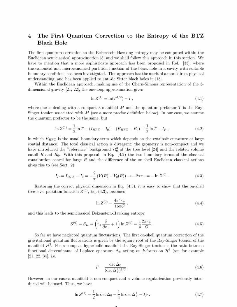
The first quantum correction to the Bekenstein-Hawking entropy may be computed within theEuclidean semiclassical approximation [5] and we shall follow this approach in this section. Wehave to mention that a more sophisticate approach has been proposed in Ref. [33], wherethe canonical and microcanonical partition function of the black hole in a cavity with suitableboundary conditions has been investigated. This approach has the merit of a more direct physicalunderstanding, and has been applied to anti-de Sitter black holes in [18].

Within the Euclidean approach, making use of the Chern-Simons representation of the 3-dimensional gravity [21, 22], the one-loop approximation gives

ln Z(1) = ln(T 1/2) − I , (4.1)

where one is dealing with a compact 3-manifold M and the quantum prefactor T is the Ray-Singer torsion associated with M (see a more precise definition below). In our case, we assumethe quantum prefactor to be the same, but

ln Z(1) =1

2ln T − (IBTZ − I0) − (BBTZ − B0) ≡

1

2ln T − IP , (4.2)

in which BBTZ is the usual boundary term which depends on the extrinsic curvature at largespatial distance. The total classical action is divergent; the geometry is non-compact and wehave introduced the ”reference” background H3

0 at the tree level [24] and the related volumecutoff R and R0. With this proposal, in Eq. (4.2) the two boundary terms of the classicalcontribution cancel for large R and the difference of the on-shell Euclidean classical actionsgives rise to (see Sect. 2),

IP = IBTZ − I0 = − 2

π(V (R) − V0(R)) → −2πr+ = − lnZ(0) . (4.3)

Restoring the correct physical dimension in Eq. (4.3), it is easy to show that the on-shelltree-level partition function Z(0), Eq. (4.3), becomes

lnZ(0) =4π2r+

16πG, (4.4)

and this leads to the semiclassical Bekenstein-Hawking entropy

S(0) = SH =

(

r+∂

∂r++ 1

)

lnZ(0) =1

4

2πr+

G. (4.5)

So far we have neglected quantum fluctuations. The first on-shell quantum correction of thegravitational quantum fluctuations is given by the square root of the Ray-Singer torsion of themanifold H3. For a compact hyperbolic manifold the Ray-Singer torsion is the ratio betweenfunctional determinants of Laplace operators ∆k acting on k-forms on H3 (see for example[21, 22, 34], i.e.

T =det ∆0

(det ∆⊥1 )1/2

. (4.6)

However, in our case a manifold is non-compact and a volume regularization previously intro-duced will be used. Thus, we have

ln Z(1) =1

2ln det ∆0 −

1

4ln det ∆⊥

1 − IP . (4.7)

9

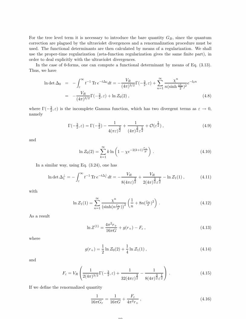
For the tree level term it is necessary to introduce the bare quantity GB , since the quantumcorrection are plagued by the ultraviolet divergences and a renormalization procedure must beused. The functional determinants are then calculated by means of a regularization. We shalluse the proper-time regularization (zeta-function regularization gives the same finite part), inorder to deal explicitly with the ultraviolet divergences.

In the case of 0-forms, one can compute a functional determinant by means of Eq. (3.13).Thus, we have

ln det∆0 = −∫ ∞

εt−1 Tr e−t∆0dt = − VR

(4π)3/2Γ(−3

2 , ε) +∞∑

n=1

χn

n(sinh nl02 )2

e−l0n

= − VR

(4π)3/2Γ(−3

2 , ε) + lnZ0(2) , (4.8)

where Γ(−32 , ε) is the incomplete Gamma function, which has two divergent terms as ε → 0,

namely

Γ(−32 , ε) = Γ(−3

2 ) − 1

4(πε)32

+1

(4π)32 ε

12

+ O(ε12 ) , (4.9)

and

lnZ0(2) =∞∑

k=1

k ln

(

1 − χe−2(k+1)r+

σ

)

. (4.10)

In a similar way, using Eq. (3.24), one has

ln det∆⊥1 = −

∫ ∞

εt−1 Tr e−t∆⊥

1 dt = − VR

8(4πε)32

+VR

2(4π)32 ε

12

− lnZ1(1) , (4.11)

with

lnZ1(1) =∞∑

n=1

χn

(

sinh(n r+

σ ))2

(

1

n+ 8n( r+

σ )2)

. (4.12)

As a result

ln Z(1) =4π2r+

16πG+ g(r+) − Fε , (4.13)

where

g(r+) =1

2lnZ0(2) +

1

4lnZ1(1) , (4.14)

and

Fε = VR

1

2(4π)3/2Γ(−3

2 , ε) +1

32(4πε)32

− 1

8(4π)32 ε

12

. (4.15)

If we define the renormalized quantity

1

16πGr=

1

16πG+

Fε

4π2r+, (4.16)

10

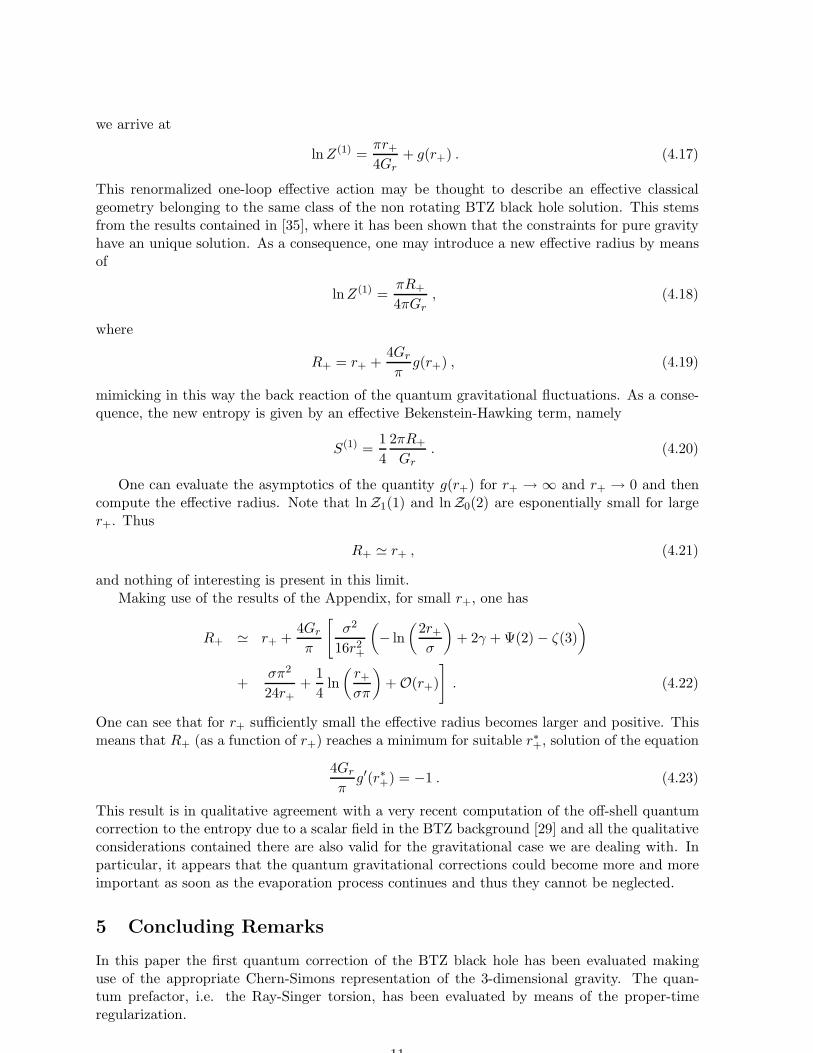
we arrive at

ln Z(1) =πr+

4Gr+ g(r+) . (4.17)

This renormalized one-loop effective action may be thought to describe an effective classicalgeometry belonging to the same class of the non rotating BTZ black hole solution. This stemsfrom the results contained in [35], where it has been shown that the constraints for pure gravityhave an unique solution. As a consequence, one may introduce a new effective radius by meansof

lnZ(1) =πR+

4πGr, (4.18)

where

R+ = r+ +4Gr

πg(r+) , (4.19)

mimicking in this way the back reaction of the quantum gravitational fluctuations. As a conse-quence, the new entropy is given by an effective Bekenstein-Hawking term, namely

S(1) =1

4

2πR+

Gr. (4.20)

One can evaluate the asymptotics of the quantity g(r+) for r+ → ∞ and r+ → 0 and thencompute the effective radius. Note that lnZ1(1) and lnZ0(2) are esponentially small for larger+. Thus

R+ ≃ r+ , (4.21)

and nothing of interesting is present in this limit.Making use of the results of the Appendix, for small r+, one has

R+ ≃ r+ +4Gr

π

[

σ2

16r2+

(

− ln

(

2r+

σ

)

+ 2γ + Ψ(2) − ζ(3)

)

+σπ2

24r++

1

4ln

(

r+

σπ

)

+ O(r+)

]

. (4.22)

One can see that for r+ sufficiently small the effective radius becomes larger and positive. Thismeans that R+ (as a function of r+) reaches a minimum for suitable r∗+, solution of the equation

4Gr

πg′(r∗+) = −1 . (4.23)

This result is in qualitative agreement with a very recent computation of the off-shell quantumcorrection to the entropy due to a scalar field in the BTZ background [29] and all the qualitativeconsiderations contained there are also valid for the gravitational case we are dealing with. Inparticular, it appears that the quantum gravitational corrections could become more and moreimportant as soon as the evaporation process continues and thus they cannot be neglected.

5 Concluding Remarks

In this paper the first quantum correction of the BTZ black hole has been evaluated makinguse of the appropriate Chern-Simons representation of the 3-dimensional gravity. The quan-tum prefactor, i.e. the Ray-Singer torsion, has been evaluated by means of the proper-timeregularization.

11

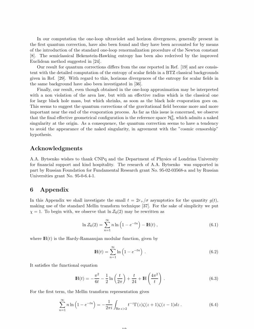
In our computation the one-loop ultraviolet and horizon divergences, generally present inthe first quantum correction, have also been found and they have been accounted for by meansof the introduction of the standard one-loop renormalization procedure of the Newton constant[8]. The semiclassical Bekenstein-Hawking entropy has been also rederived by the improvedEuclidean method suggested in [24].

Our result for quantum corrections differs from the one reported in Ref. [19] and are consis-tent with the detailed computation of the entropy of scalar fields in a BTZ classical backgroundsgiven in Ref. [29]. With regard to this, horizons divergences of the entropy for scalar fields inthe same background have also been investigated in [36].

Finally, our result, even though obtained in the one-loop approximation may be interpretedwith a non violation of the area law, but with an effective radius which is the classical onefor large black hole mass, but which shrinks, as soon as the black hole evaporation goes on.This seems to suggest the quantum corrections of the gravitational field become more and moreimportant near the end of the evaporation process. As far as this issue is concerned, we observethat the final effective geometrical configuration is the reference space H3

0, which admits a nakedsingularity at the origin. As a consequence, the quantum correction seems to have a tendencyto avoid the appearance of the naked singularity, in agreement with the ”cosmic censorship”hypothesis.

Acknowledgments

A.A. Bytsenko wishes to thank CNPq and the Department of Physics of Londrina Universityfor financial support and kind hospitality. The research of A.A. Bytsenko was supported inpart by Russian Foundation for Fundamental Research grant No. 95-02-03568-a and by RussianUniversities grant No. 95-0-6.4-1.

6 Appendix

In this Appendix we shall investigate the small t = 2r+/σ asymptotics for the quantity g(t),making use of the standard Mellin transform technique [37]. For the sake of simplicity we putχ = 1. To begin with, we observe that lnZ0(2) may be rewritten as

lnZ0(2) =∞∑

n=1

n ln(

1 − e−tn)

− IH(t) , (6.1)

where IH(t) is the Hardy-Ramanujan modular function, given by

IH(t) =∞∑

n=1

ln(

1 − e−tn)

. (6.2)

It satisfies the functional equation

IH(t) = −π2

6t− 1

2ln

(

t

2π

)

+t

24+ IH

(

4π2

t

)

. (6.3)

For the first term, the Mellin transform representation gives

∞∑

n=1

n ln(

1 − e−tn)

= − 1

2πi

∫

Re z>2t−zΓ(z)ζ(z + 1)ζ(z − 1)dz . (6.4)

12

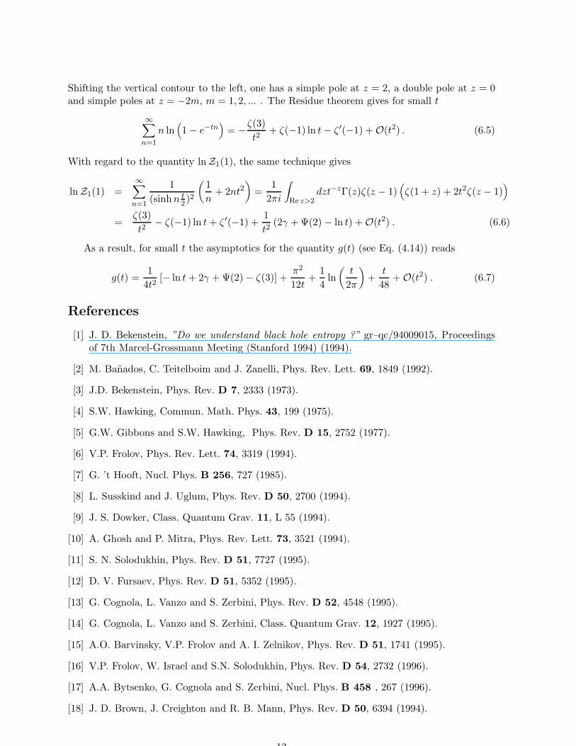
Shifting the vertical contour to the left, one has a simple pole at z = 2, a double pole at z = 0and simple poles at z = −2m, m = 1, 2, ... . The Residue theorem gives for small t

∞∑

n=1

n ln(

1 − e−tn)

= −ζ(3)

t2+ ζ(−1) ln t − ζ ′(−1) + O(t2) . (6.5)

With regard to the quantity lnZ1(1), the same technique gives

lnZ1(1) =∞∑

n=1

1

(sinh n t2)2

(

1

n+ 2nt2

)

=1

2πi

∫

Re z>2dzt−zΓ(z)ζ(z − 1)

(

ζ(1 + z) + 2t2ζ(z − 1))

=ζ(3)

t2− ζ(−1) ln t + ζ ′(−1) +

1

t2(2γ + Ψ(2) − ln t) + O(t2) . (6.6)

As a result, for small t the asymptotics for the quantity g(t) (see Eq. (4.14)) reads

g(t) =1

4t2[− ln t + 2γ + Ψ(2) − ζ(3)] +

π2

12t+

1

4ln

(

t

2π

)

+t

48+ O(t2) . (6.7)

References

[1] J. D. Bekenstein, ”Do we understand black hole entropy ?” gr–qc/94009015, Proceedingsof 7th Marcel-Grossmann Meeting (Stanford 1994) (1994).

[2] M. Banados, C. Teitelboim and J. Zanelli, Phys. Rev. Lett. 69, 1849 (1992).

[3] J.D. Bekenstein, Phys. Rev. D 7, 2333 (1973).

[4] S.W. Hawking, Commun. Math. Phys. 43, 199 (1975).

[5] G.W. Gibbons and S.W. Hawking, Phys. Rev. D 15, 2752 (1977).

[6] V.P. Frolov, Phys. Rev. Lett. 74, 3319 (1994).

[7] G. ’t Hooft, Nucl. Phys. B 256, 727 (1985).

[8] L. Susskind and J. Uglum, Phys. Rev. D 50, 2700 (1994).

[9] J. S. Dowker, Class. Quantum Grav. 11, L 55 (1994).

[10] A. Ghosh and P. Mitra, Phys. Rev. Lett. 73, 3521 (1994).

[11] S. N. Solodukhin, Phys. Rev. D 51, 7727 (1995).

[12] D. V. Fursaev, Phys. Rev. D 51, 5352 (1995).

[13] G. Cognola, L. Vanzo and S. Zerbini, Phys. Rev. D 52, 4548 (1995).

[14] G. Cognola, L. Vanzo and S. Zerbini, Class. Quantum Grav. 12, 1927 (1995).

[15] A.O. Barvinsky, V.P. Frolov and A. I. Zelnikov, Phys. Rev. D 51, 1741 (1995).

[16] V.P. Frolov, W. Israel and S.N. Solodukhin, Phys. Rev. D 54, 2732 (1996).

[17] A.A. Bytsenko, G. Cognola and S. Zerbini, Nucl. Phys. B 458 , 267 (1996).

[18] J. D. Brown, J. Creighton and R. B. Mann, Phys. Rev. D 50, 6394 (1994).

13

[19] S. Carlip and C. Teitelboim, Phys. Rev. D 51, 622 (1995).

[20] A. Ghosh and P. Mitra, Phys. Rev. D 56, 3568 (1997).

[21] E. Witten, Nucl. Phys. B 311, 46 (1988).

[22] S. Carlip, Class. quantum Grav. 10, 207 (1993)

[23] S. Carlip, Phys. Rev. D 51, 632 (1995).

[24] S.W. Hawking and G.T. Horowitz, Class. Quantum Grav. 13, 1487 (1996).

[25] C. Teitelboim, Phys. Rev. D 51, 4315 (1995).

[26] S. Deser,R. Jackiw and G. ’t Hooft, Ann. Phys. (N.Y.). 152, 220 (1984).

[27] R. Camporesi, Phys. Reports. 196, 1 (1990).

[28] A.A. Bytsenko, G. Cognola, L. Vanzo and S. Zerbini, Phys. Reports. 266, 1 (1996).

[29] R.B. Mann and S. N. Solodukhin, Phys. Rev. D 55, 3622 (1997).

[30] H. Yamabe. Osaka Math. J. 12, 21 (1960),

[31] N. Trudinger, Ann. Scuola Norm. Sup. Pisa Cl. Sci. 3, 265 (1968).

[32] E. Elizalde, S. D. Odintsov, A. Romeo, A.A. Bytsenko and S. Zerbini. ”Zeta RegularizationTechniques with Applications”. World Scientific, Singapore, (1994).

[33] J.D. Brown and J. W. York, Phys. Rev. D 47, 1420 (1993).

[34] A. A. Bytsenko, L. Vanzo and S. Zerbini,. Nucl. Phys. B 505, 641, (1997).

[35] M. Banados, M. Heanneaux, C. Teitelboim and J. Zanelli, Phys. Rev. D 48, 1506 (1993).

[36] I. Ichinose and Y. Satoh, Nucl. Phys. B447, 340 (1995).

[37] E. Elizalde, K. Kirsten and S. Zerbini, J. Phys. A: Math. Gen. 28, 617 (1995).

14