Quantitative Methods in Economics(Multiple Criteria Decision Making XVIII)

Proceedings of the International Scientific Conference25th May - 27th May 2016

Vrátna, Slovakia

Qua

ntita

tive

Met

hods

in E

cono

mic

s (M

ultip

le C

rite

ria

Dec

isio

n M

akin

g X

VII

I)

ISBN 978-80-972328-0-1

The Slovak Society for Operations Research Department of Operations Research and Econometrics

Faculty of Economic Informatics, University of Economics in Bratislava

Proceedings of the International Scientific Conference QUANTITATIVE METHODS IN ECONOMICS

Multiple Criteria Decision Making XVIII

25th May - 27th May 2016 Vrátna, Slovakia

Programme Committee: Pekár Juraj, University of Economics, Bratislava, ChairBrezina Ivan, University of Economics, Bratislava Fendek Michal, University of Economics, Bratislava Ferreira Manuel A. M., University Institute of Lisbon Fiala Petr, University of Economics, Prague Groshek Gerald, University of Redlands Jablonský Josef, University of Economics, Prague

Luká�ik Martin, University of Economics, Bratislava Mlynarovi� Vladimír, Comenius University, Bratislava Palúch Stanislav, University of Žilina Plevný Miroslav, University of West Bohemia Turnovec František, Charles University, Prague Vidovi� Milorad, University of Belgrade

Organizing Committee: Blaško Michaela Furková Andrea Gežík Pavel

Luká�iková Adriana Reiff Marian Surmanová Kvetoslava

Referees: Bartová Lubica, Slovak University of Agriculture, Nitra Benkovi� Martin, University of Economics, Bratislava Borovi�ka Adam, University of Economics, Prague Brezina Ivan, University of Economics, Bratislava �i�ková Zuzana, University of Economics, Bratislava Dlouhý Martin, University of Economics, Prague Domonkos Tomáš, University of Economics, Bratislava Fábry Ján, University of Economics, Prague Fendek Michal, University of Economics, Bratislava Fiala Petr, University of Economics, Prague Furková Andrea, University of Economics, Bratislava Gežík Pavel, University of Economics, Bratislava Goga Marián, University of Economics, Bratislava Han�lová Jana, VŠB-Technical University, Ostrava Horáková Galina, University of Economics, Bratislava Chocholatá Michaela, University of Economics, Bratislava Ivani�ová Zlatica, University of Economics, Bratislava Jablonský Josef, University of Economics, Prague Janá�ek Jaroslav, University of Žilina, Žilina

Jánošíková �udmila, University of Žilina, Žilina König Brian, University of Economics, Bratislava Ku�era Petr, Czech University of Life Sciences, Prague Kuncová Martina, University of Economics, Prague Kupkovi� Patrik, University of Economics, Bratislava Lichner Ivan, Institute of Economic Research SAS Luká�ik Martin, University of Economics, Bratislava Luká�iková Adriana, University of Economics, Bratislava Mitková Veronika, Comenius University in Bratislava Mlynarovi� Vladimír, Comenius University in Bratislava Palúch Stanislav, University of Žilina, Žilina Pekár Juraj, University of Economics, Bratislava Peško Štefan, University of Žilina, Žilina Radvanský Marek, Institute of Economic Research SAS Reiff Marian, University of Economics, Bratislava Rublíková Eva, University of Economics, Bratislava Surmanová Kveta, University of Economics, Bratislava Szomolányi Karol, University of Economics, Bratislava

25th May - 27th May 2016 Vrátna, Slovakia Technical Editor: Marian Reiff, Pavel Gežík, University of Economics, Bratislava Web Editor: Martin Luká�ik, University of Economics, Bratislava Web: http://www.fhi.sk/en/katedry-fakulty/kove/ssov/papers// Publisher: Letra Interactive, s. r. o. ISBN 978-80-972328-0-1 Number of copies: 90

CONTENT

Adam P. Balcerzak, Micha� Bernard Pietrzak

QUALITY OF HUMAN CAPITAL IN THE EUROPEAN UNION IN THE YEARS 2004-2013. APPLICATION OF STRUCTURAL EQUATION MODELLING

7

Jan Bartoška, Petr Ku�era, Tomáš Šubrt

MODIFICATION OF THE EVA BY WORK CONTOUR 13

Lubica Bartova, Jaroslava Hurnakova

ESTIMATION OF FARM INVESTMENT SUPPORT EFFECTS: A COUNTERFACTUAL APPROACH

19

Blanka Bazsová PROPOSAL AND EVALUATION OF THE COMPETENCY MODEL OF THE ACADEMIC EMPLOYEE

25

Jelena Birovljev, Aleksandra Marciki�, Nenad Vunjak, Otilija Sedlak, Zoran �iri�

THE APPLICATION OF QUEUEING THEORY FOR MODELING HUMAN RESOURCES IN AMBULANCE SERVICE

33

Adam Borovi�ka SELECTION OF THE OPEN UNIT TRUSTS FOR INVESTMENT VIA FUZZY MULTICRITERIA EVALUATION METHOD

39

�ula Borozan, Dubravka Pekanov Star�evi�

USING EXPERT OPINIONS TO QUANTIFY NET NON-MEASURABLE EXTERNAL BENEFIT OF CHP PLANTS

45

Ondej �ížek ESTIMATING THE REACTION FUNCTION OF THE ECB 52

Tomáš Domonkos, Brian König, Filip Ostriho

MIDDLE CLASS IN THE POST COMMUNIST COUNTRIES – CASE OF THE SLOVAK REPUBLIC

59

Michal Dorda, Dušan Teichmann

SIMULATION APPROACH TO FREIGHT TRAIN CLASSIFICATION MODELLING USING QUEUEING SYSTEM SUBJECT TO TWO TYPES OF FAILURES

67

Juraj Dubovec, Lucia Pan�íková

OPTIMIZATION OF TRANSPORT OUTPUTS FOR THE SAKE OF PUBLIC INTEREST

72

Jan Fábry OPTIMIZATION IN A MAINTENANCE OF TRAM SWITCHES 79

Michal Fendek OPTIMALITY CONDITIONS OF THE CONSUMERS FOR THE NETWORK INDUSTRIES MARKET

83

Manuel Alberto M. Ferreira, José António Filipe, Manuel Coelho

UNEMPLOYMENT PERIOD QUANTITATIVE APPROACH THROUGH INFINITE SERVERS QUEUE SYSTEMS

89

Petr Fiala MULTI-CRITERIA DYNAMIC PROJECT PORTFOLIO 95

Ludvík Friebel, Jana Friebelová

MODELLING OF MIGRATION BASED ON SOCIOECONOMIC FACTORS

101

Andrea Furková THE INNOVATIVE CLUSTERS IN THE EU: THE SENSITIVITY ANALYSIS OF THE SPATIAL WEIGHT MATRIX CONSTRUCTION

106

Pavel Gežík, Tomáš Domonkos, Andrej Babej

MUTUAL DEBT COMPENSATION AS A MINIMIZATION PROBLEM

114

Vojt�ch Graf, Dušan Teichmann, Michal Dorda

MATHEMATICAL MODEL FOR CREATION OF FLIGHT TIMETABLE WITH SEVERAL TIME SLOTS IN CONDITIONS OF CHARTER AIRLINE

119

Eva Grmanová, Peter Hošták

COMPARISON OF SELECTED APPROACHES FOR ASSESSING THE EFFICIENCY OF INSURANCE COMPANIES

128

Monika Hada�-Dyduch MODEL - SPATIAL APPROACH TO PREDICTION OF MINIMUM WAGE

134

Jana Han�lová DYNAMIC STEAM OF EUROPEAN CARBON, ENERGY AND STEEL MARKETS COINTEGRATION

139

Pavel Hole�ek, Jana Talašová, Jan Stoklasa

FUZZY SYSTEM FOR THE PERFORMANCE EVALUATION OF ACADEMIC STAFF MEMBERS AT UNIVERSITIES – THE CURRENT STATE

146

Milan Hornia�ek AN ALGORITHM FOR GENERAL INFINITE HORIZON LOT SIZING WITH DETERMINISTIC DEMAND

153

Jakub Chalmovianský MEASURING THE NAIRU FOR CZECH AND SLOVAK LABOUR MARKETS: BAYESIAN APPROACH

158

Michaela Chocholatá INTERRELATIONSHIPS BETWEEN GERMAN AND BALTIC STOCK MARKETS

165

Mariola Chrzanowska, Nina Drejerska

STATISTICAL COMPARATIVE ANALYSIS OF SOCIO-ECONOMIC DEVELOPMENT LEVEL OF POLISH BORDER REGIONS (NUTS 3)

170

Josef Jablonský RANKING OF DECISION MAKING UNITS IN DEA MODELS WITH NON-CONSTANT RETURNS TO SCALE

177

Jaroslav Janá�ek, Marek Kvet

FAIRNESS EVALUATION OF THE EMERGENCY SERVICE SYSTEM DESIGN

183

Marta Janá�ková, Alžbeta Szendreyová

AN IMPACT OF THE FREQUENT TRAFFIC ACCIDENTS ON THE LOCATION OF THE EMERGENCY MEDICAL SERVICES STATIONS

191

�udmila Jánošíková, Michal Haviar

IMPERIALIST COMPETITIVE ALGORITHM IN COMBINATORIAL OPTIMIZATION

196

Sokhibmalik Khomidov INDUSTRY AND ECONOMIC GROWTH: STRUCTURAL CHANGES IN INDUSTRY OF UZBEKISTAN

202

Martina Kuncová, Veronika Hedija, Roman Fiala

A COMPARISON OF SPECIALISED AGRICULTURAL COMPANIES PERFORMANCE

209

Martina Kuncová ANALYSIS OF THE IMPACT OF THE ELECTRICITY TARIFF RATE CHANGE ON THE CUSTOMERS ANNUAL COST AND OPTIMIZATION MODEL APPLICATION

216

Marek Kvet, Jaroslav Janá�ek

ACCELERATION OF THE OGRYCZAK’S APPROACH TO LEXICOGRAPHICAL MIN-MAX EMERGENCY SYSTEM DESIGN

224

Ivan Lichner FIRST PILLAR OF SLOVAK PENSION SYSTEM 230

Renata Majovská, Petr Fiala

MODELLING OF DYNAMIC NETWORK SYSTEMS 236

Petra Daníšek Matušková THE IMPACT OF INPUT PARAMETERS ON THE CAPITAL REQUIREMENTS FOR EQUITY PORTFOLIO IN INSURANCE

241

Veronika Mi ková LIGHTING THE BLACK BOX OF THE COMPUTABLE GENERAL EQUILIBRIUM MODEL DATABASE

247

Vladimír Mlynarovi� LEGISLATIVE CHANGES EFFECTS ON SLOVAK PENSION FUNDS EFFICIENCY

253

Daniel N�mec, Michal Pavlík

PREDICTING INSOLVENCY RISK OF THE CZECH COMPANIES 258

Ivana Olivková METHODOLOGY OF MULTI-CRITERIA EVALUATION OF VARIANTS OF CHECK-IN SYSTEMS IN PUBLIC TRANSPORT

264

Filip Ostriho POSSIBLE COMPLICATIONS WHEN APPLYING SPATIAL SYNTHETIC INSTRUMENTS: CASE OF SLOVAK REGIONS

271

Stanislav Palúch, Štefan Peško, Tomáš Majer

AN EXACT SOLUTION OF THE MINIMUM FLEET SIZE PROBLEM WITH FLEXIBLE BUS TRIPS

278

Adam Pápai LABOR MARKET RIGIDITIES AND MONETARY SWITCH IN A DSGE MODEL: APPLICATION TO THE SLOVAK ECONOMY

283

Juraj Pekár, Ivan Brezina, Zuzana �i�ková

LOCATION OF ELECTRIC VEHICLE CHARGING STATION IN 2-PHASES

289

Jan Pelikán VEHICLE ROUTING PROBLEM WITH PRIVATE AND COMMON CARRIER

294

Štefan Peško, Stanislav Palúch, Tomáš Majer

A GROUP MATCHING MODEL FOR A VEHICLE SCHEDULING PROBLEM

298

Micha� Bernard Pietrzak, Adam P. Balcerzak

A SPATIAL SAR MODEL IN EVALUATING INFLUENCE OF ENTREPRENEURSHIP AND INVESTMENTS ON UNEMPLOYMENT IN POLAND

303

Miroslav Plevný, Lenka Gladavská

ARGUMENTATION-BASED MULTIPLE CRITERIA DECISION PROBLEM WITH QUALITATIVE SCALES AS AN ALTERNATIVE TO QUANTITATIVE MULTIPLE CRITERIA DECISION PROBLEM

309

Marek Radvanský, Tomáš Miklošovi�, Ivan Lichner

MODELING EX-ANTE EFFECTS OF ALTERNATIVE REGIONAL COHESION POLICY IN 2014-2020 PERIOD ON NATIONAL LEVEL – CASE OF SLOVAKIA

316

Marian Reiff, Kvetoslava Surmanová

CLUSTER ANALYSIS OF EU AGRICULTURE 322

Vlastimil Reichel HOUSE PRICES AND BUSINESS CYCLE IN CZECH ECONOMY: A CROSSCORRELATION APPROACH

327

Eva Rubliková, Zlatica Ivani�ová

UNEMPLOYMENT FLOWS AND VACANCIES IN SLOVAKIA 332

Veronika Sko�dopolová THE ADVANTAGES OF USING GOAL PROGRAMMING FOR TIMETABLING

338

Radek Stolín A BONUS-MALUS SYSTEM BASED ON DEDUCTIBLES 343

Michal Struk, Markéta Matulová,

THE APPLICATION OF TWO-STAGE DATA ENVELOPMENT ANALYSIS ON MUNICIPAL SOLID WASTE MANAGEMENT IN THE CZECH REPUBLIC

349

Karolína Súkupová, Osvald Vaší�ek

MULTIPLE CONSTRAINTS APPLIED INTO THE DSGE MODEL: THE CASE OF UNCONVENTIONAL MONETARY EASING IN THE CZECH ECONOMY

356

Milan Svoboda, Pavla �íhová

STOCHASTIC MODEL OF SHORT-TIME PRICE DEVELOPMENT OF SHARES AND ITS PROFITABILITY IN ALGORITHMIC TRADING

362

Karol Szomolányi, Martin Luká�ik, Adriana Luká�iková

THE EFFECT OF TERMS-OF-TRADE ON SLOVAK BUSINESS CYCLES: A THEORETICAL APPROACH

369

�ubica Šimková, Milan Hornia�ek

INNOVATION VERSUS PARASITIC SECURITY 376

Michal Švarc PROPENSITY SCORE MATCHING AND ALTERNATIVE APPROACH TO INDIVIDUALS MATCHING FOR COUNTERFACTUAL EVALUATION PURPOSES

381

Dušan Teichmann, Michal Dorda

ABOUT AN UNCONVENTIONAL APPLICATION OF ASSIGNMENT PROBLEM

388

Michaela Tichá MULTICRITERIA COALITIONAL GAMES AND BARGAINING THEORY

393

Nenad Vunjak, Dragan Stoji�, Jelena Birovljev, Jovana Ivan�evi�, Jelena Vitomir

METHODOLOGY FOR DETERMINING INTEREST RATES - AN INTERNATIONAL TREND

398

Jana Závacká CAN CONSUMERS' CONFIDENCE CONTRIBUTE TO CYCLIC MOVEMENT OF THE ECONOMIC ACTIVITY?

404

Petr Zim�ík TAX QUOTA VS. WORLD TAX INDEX: PANEL DATA COMPARISON

411

Marek Zinecker, Adam P. Balcerzak, Tomáš Meluzín, Micha� Bernard Pietrzak

APPLICATION OF DCC-GARCH MODEL FOR ANALYSIS OF INTERRELATIONS AMONG CAPITAL MARKETS OF POLAND, CZECH REPUBLIC AND GERMANY

416

QUALITY OF HUMAN CAPITAL IN THE EUROPEAN UNION IN THEYEARS 2004-2013. APPLICATION OF STRUCTURAL EQUATION

MODELING

Adam P. Balcerzak, Nicolaus Copernicus University, Michał Bernard Pietrzak, Nicolaus Copernicus University

Abstract EU policy guidelines point out that improvement of quality of human capital (QHC) should be treated as an important factor supporting convergence process. Thus, the aim of the research is the identification of the variables that determine changes in QHC. It is assumed that QHC should be considered as a latent variable, which can be measured with application of Structural Equation Modeling (SEM). SEM includes confirmatory factor analysis and path analysis used in econometrics. In the research, the hypothetic SEM model was proposed for the years 2004-2013. Four subsets of observable variables were used: a) macroeconomic and labour market effectiveness, b) quality of education, c) national innovation system, d) health and social cohesion. The research confirmed significant influence of the proposed variables on the level of QHC and positive tendencies in changes of QHS in the EU countries.

Keywords: Structural Equation Model (SEM), quality of human capital, European Union

JEL Classification: C30, C38 AMS Classification: 62P20

1 INTRODUCTION Quality of human capital (QHC) is currently considered as one of the most important development factors in the case of highly developed countries that compete in the reality of global knowledge-based economy. The fundamental role of this factor was pointed out in many European Union policy guidelines, such as Lisbon Strategy or Europe 2020 plan (see: Balcerzak, 2015; Baležentis et al., 2011; European Commission, 2010). Thus, the aim of the research is the identification of variables that determine changes in QHC at macroeconomic level. Structural Equation Modeling (SEM) methodology was applied here. The research was conducted for the European Union countries in the year 2004-2013. QHC is analyzed as an economic factor that is crucial for utilizing the potential of global knowledge-based economy (Balcerzak, 2009). This perspective was a prerequisite to the selection of potential diagnostic variables for the model.

2 SEM METHODOLOGY Quality of human capital should be considered as a multivariate phenomenon (Balcerzak, 2016; Balcerzak and Pietrzak, 2016a, 2016c; Pietrzak and Balcerzak, 2016a) that can be also considered as a latent variable. Thus, it can be measured with application of SEM methodology. This analytical approach includes confirmatory factor analysis and path analysis used in econometrics. SEM models are more elastic than regression models, as they enable to analyse the interrelations between latent variables that are the result of influence of many factors (Loehlin, 1987; Bollen, 1989; Kaplan, 2000; Pearl, 2000; Brown, 2006; Byrne, 2010).

Quantitative Methods in Economics | 7

The SEM model consists of an external model and an internal model. The external model, which is also called a measurement model, is given as:

,εηCy y �� (1) ,δξCx x �� (2)

where: 1�py - the vector of observed endogenous variables, 1�qx - the vector of observed exogenous variables, xy CC , - matrices of factor loadings, 11, �� qp δε - vectors of measurement errors. The internal model, which is called a structural model, can be described as:

,ζBξAηη ��� (3) where: 1�mη - vector of endogenous latent variables, 1�kξ - vector of exogenous latent variables, mm�A - matrix of regression coefficients at endogenous variables, km�B - matrix of coefficients at exogenous variables, 1�mζ - vector of disturbances.

3 THE MEASUREMENT OF QUALITY OF HUMAN CAPITAL WITH APPLICATION OF SEM MODEL Quality of human capital is analysed at the macroeconomic level from the perspective of its influence on the abilities of countries to compete in the reality of global knowledge-based economy. The research is conducted for 24 EU economies in the years 2004-2013 basing on Eurostat data.

Table 1. The factors influencing quality of human capital

Aspect 1 (A1) - Macroeconomic and labour market effectiveness

�� – Employment rate (20 to 65)

�� – Labour productivity (percentage of EU28 total based on PPS per employed person)

�� – Unemployment rate (total - annual average, %)Aspect 2 (A2) - Quality of education�� – Lifelong learning - participation rate in education and training (last 4 weeks) (% of population 25 to 64) �� – Science and technology graduates (tertiary graduates in science and technology per 1 000 inhabitants aged 20-29 years)Aspect 3 (A3) - National innovation system

�� – Exports of high technology products as a share of total exports� – Total intramural R&D expenditure (GERD) Percentage of gross domestic product (GDP)Aspekt 4 (A4) Health and social cohesion

� – People at risk of poverty or social exclusion (Percentage of total population)�� – Life expectancy at birth ��� – Material deprivation rateSource: own work based on: Balcerzak and Pietrzak (2016b); Jantoń-Drozdowska and Majewska (2015); Madrak-Grochowska (2015); Pietrzak and Balcerzak (2016b); Rószkiewicz (2014); Zielenkiewicz (2014).

8 | Multiple Criteria Decision Making XVIII

It is assumed that QHC is a latent variable. In order to measure and describe QHC, an external model was built basing on SEM methodology. It is assumed that an internal model does not occur. It means that only the confirmatory factor analysis, which enables to measure the latent variable in the form of QHC, was conducted here. The analysis was conducted basing on the observed variables presented in Table 1. The variables belong to four socio-economic aspects related to QHC: a) macroeconomic and labour market effectiveness, b) quality of education, c) national innovation system, d) health and social cohesion. Basing on the literature review of previous research, it can be said that these aspects influence the abilities of countries to compete in the reality of knowledge-based economy.The assumed that the hypothetic SEM model was estimated in AMOS v. 16 packet with application of maximum likelihood method. The results are presented in Table 2. All the parameters of external model are statistically significant, which confirms that all the observable variables for QHC were properly identified. The standardized evaluations of parameters given in Table 2 can be used to evaluate the strengths of the influence of the given variable for QHC. The variables with the strongest influence can be ordered as follow: X(total intramural R&D expenditure, GERD), X�� (material deprivation rate), X (people at risk of poverty or social exclusion) and X� (lifelong learning - participation rate in education and training). The variables with average influence: X� (employment rate), X� (labour productivity) i X� (life expectancy at birth). Finally, the variables with the weakest influence: X� (exports of high technology products as a share of total exports), X� (unemployment rate) i X� (science and technology graduates)1. The results do not allow to point the dominant aspect in the context of evaluation of QHC at macroeconomic level.

Table 2. The estimations of parameters of SEM model based on the confirmatory factor analysis

Variable Parameter Estimate Standardized p-valuex1 α1 1 0,753 -x2 α2 4,494 0,702 ~0,00x3 α3 0,543 0,468 ~0,00x4 α4 1,507 0,818 ~0,00x5 α5 0,234 0,219 ~0,00x6 α6 0,701 0,470 ~0,00x7 α7 0,188 0,878 ~0,00x8 α8 0,276 0,864 ~0,00x9 α9 0,488 0,649 ~0,00x10 α10 3,156 0,870 ~0,00

Source: own estimation based on Eurostat data.

In order to asses an adjustment of the model to the input data, the Incremental Fit Index (IFI) and Root Mean Square Error of Approximation (RMSEA) coefficients were used. The value of the IFI coefficient for the estimated SEM model equals 0,722, and the value of the RMSEA coefficient equals 0,2339. These values are higher than the suggested values of 0,9 for IFI and 0,1 for RMSEA. However, due to the macro-economic data used in the research, the value of these indices can be assessed as acceptable. It means that the adjustment of the model to the input data is proper.

1 The strengths of impact of variables and their classification to the three subsets was done arbitrarily by the authors.

Quantitative Methods in Economics | 9

The level of QHC in the years 2004 and 2013 was assessed basing on the sum of product of values of Factor Score Weights and the values of given variables. The countries were ordered starting with the highest value of the obtained indicator for QHC to the ones with its lowest value. This enabled to propose two ratings of countries for the years 2004 and 2013. Then, the comparison of the values of indicator for QHC in the first and last year of analysis enabled to assed the percentage changes of the values of the indicator for the analyzed countries. The results are presented in Table 3.

Table 3. The level of quality of human capital in EU countries and its changes in the years 2004-2013

2004 2013 2004-2013Country QHC Rating Country QHC Rating Country % Change RatingSweden 27,44 1 Sweden 30,89 1 Poland 19,98% 1

Denmark 26,99 2 Finland 28,03 2 Slovak Rep 16,63% 2Finland 26,71 3 Denmark 27,33 3 Estonia 16,61% 3

Netherlands 25,70 4 Netherlands 26,36 4 Czech Rep. 15,90% 4Austria 24,30 5 Austria 25,62 5 Sweden 12,57% 5United

Kingdom 24,26 6 France 24,74 6 Bulgaria 9,47% 6Germany 23,40 7 Germany 24,49 7 Lithuania 9,27% 7France 22,92 8 Czech Rep. 23,46 8 Latvia 9,06% 8Ireland 22,32 9 Belgium 22,95 9 France 7,93% 9

Slovenia 22,13 10 Slovenia 22,72 10 Romania 6,68% 10

Belgium 22,12 11 United Kingdom 22,52 11 Austria 5,40% 11

Czech Rep. 20,24 12 Estonia 21,56 12 Finland 4,94% 12Spain 20,12 13 Ireland 20,82 13 Germany 4,65% 13Italy 19,74 14 Spain 20,07 14 Belgium 3,78% 14

Portugal 18,90 15 Portugal 19,53 15 Portugal 3,36% 15Estonia 18,49 16 Italy 19,28 16 Slovenia 2,67% 16Greece 17,69 17 Slovak Rep 19,26 17 Netherlands 2,58% 17

Hungary 17,41 18 Poland 18,48 18 Hungary 2,42% 18Lithuania 16,68 19 Lithuania 18,22 19 Denmark 1,27% 19

Slovak Rep 16,51 20 Hungary 17,83 20 Spain -0,24% 20Latvia 15,91 21 Latvia 17,35 21 Italy -2,31% 21Poland 15,41 22 Greece 16,65 22 Greece -5,85% 22

Romania 15,16 23 Romania 16,17 23 Ireland -6,73% 23

Bulgaria 14,30 24 Bulgaria 15,66 24 United Kingdom -7,17% 24

Source: own estimation based on Eurostat data.

4 CONCLUSIONS The conducted research concentrated on the problem of measurement of QHC at the macroeconomic level in the context of knowledge-based economy requirements. It was assumed that the QHC should be considered as a latent variable, thus SEM methodology was applied in the analysis. The aim of the research was the identification of variables that determine changes in QHC. The hypothetic SEM model confirmed a significant influence of the proposed ten variables on the level of QHC. The analysis shows significant differences in the sphere of QHC between

10 | Multiple Criteria Decision Making XVIII

“old” and “new” members of European Union. However, in the years 2004-2013 the new member states made significant progress, which could be seen especially in the case of Poland, the Slovak Republic, Estonia and the Czech Republic.

References [1] Balcerzak, A. P. (2009). Effectiveness of the Institutional System Related to the

Potential of the Knowledge Based Economy. Ekonomista, 6, p. 711-739. [2] Balcerzak. A. P. (2015). Europe 2020 Strategy and Structural Diversity between Old

and New Member States. Application of zero unitarization method for dynamic analysis in the years 2004-2013. Economics & Sociology 8(2), p. 190-210.

[3] Balcerzak, A. P. (2016). Multiple-criteria Evaluation of Quality of Human Capital in the European Union Countries. Economics & Sociology 9(2), p. 11-26.

[4] Balcerzak, A. P. and Pietrzak, M. B. (2016). Structural Equation Modeling in Evaluation of Technological Potential of European Union Countries in the years 2008-2012. In: Proceedings of the 10th Professor Aleksander Zelias International Conference on Modelling and Forecasting of Socio-Economic Phenomena (Papież, M., and & Śmiech, S., eds.). Foundation of the Cracow University of Economics, Cracow.

[5] Balcerzak, A. P. and Pietrzak, M. B. (2016). Human Development and Quality of Life in Highly Developed Countries. In: Financial Environment and Business Development.Proceedings of the 16th Eurasia Business and Economics Society (Bilgin, M. H., Danis, H., Demir, E., and Can, U., eds.). Springer, Heidelberg.

[6] Balcerzak, A. P. and Pietrzak, M. B. (2016). Application of TOPSIS Method for Analysis of Sustainable Development in European Union Countries. In: The 10th International Days of Statistics and Economics. Conference Proceedings (Loster, T.,and Pavelka, T., eds.). Prague.

[7] Baležentis, A., Baležentis, T. and Brauers, W. K. M. (2011). Implementation of theStrategy Europe 2020 by the Multi-objective Evaluation Method Multimoora. E&M Ekonomie a Management 2, p. 6-21.

[8] Bollen, K. A. (1989). Structural Equations with Latent Variables. Wiley.[9] Brown, T. A. (2006). Confirmatory Factor Analysis for Applied Research. Guilford

Press.[10] Byrne, B. M. (2010). Structural equation modeling with AMOS: Basic concepts,

applications, and programming. Routledge/Taylor & Francis, New York.[11] European Commission (2010). Europe 2020 A strategy for smart, sustainable and

inclusive growth, Communication from the commission, Brussels, 3.3.2010 COM(2010) 2020.

[12] Jantoń-Drozdowska, J. and Majewska, M. (2015). Social Capital as a Key Driver of Productivity Growth of the Economy: Across-countries Comparison. Equilibrium. Quarterly Journal of Economics and Economic Policy 10(4), p. 61-83.

[13] Kaplan, D. (2000). Structural Equation Modeling: Foundations and Extensions, Sage Publications.

[14] Loehlin, J. C. (1987). Latent variable models: An introduction to factor, path and structural analysis. Erlbaum.

[15] Pearl, J. (2000). Causality. Models, reasoning and inference, Cambrige.[16] Pietrzak, M. B. and Balcerzak, A. P. (2016). Assessment of Socio-Economic

Sustainable Development in New European Union Members States in the years 2004-2012. In: Proceedings of the 10th Professor Aleksander Zelias International Conference on Modelling and Forecasting of Socio-Economic Phenomena (Papież, M., and & Śmiech, S., eds.). Foundation of the Cracow University of Economics, Cracow.

Quantitative Methods in Economics | 11

[17] Pietrzak, M. B. and Balcerzak, A. P. (2016). Quality of Human Capital and Total Factor Productivity in New European Union Member States. In: The 10th International Days of Statistics and Economics. Conference Proceedings (Loster, T., and Pavelka, T., eds.).Prague.

[18] Rószkiewicz, M. M. (2014). On the Influence of Science Funding Policies on Business Sector R&D Activity 2014. Equilibrium. Quarterly Journal of Economics and Economic Policy 9(3), p. 9-26.

[19] Madrak-Grochowska, M. (2015). The Knowledge-based Economy as a Stage in the Development of the Economy. Oeconomia Copernicana 6(2), p. 7-21.

[20] Zielenkiewicz, M. (2014). Institutional Environment in the Context of Development of Sustainable Society in the European Union Countries. Equilibrium. Quarterly Journal of Economics and Economic Policy 9(1), p. 21-37.

Author’s addressAdam P. Balcerzak, PhD. Nicolaus Copernicus University, Department of Economics, Faculty of Economic Sciences and Management, Ul. Gagarina 13a 87-100 ToruńPoland email: adam.balcerzak@umk.pl

Michał Bernad Pietrzak, PhD.Nicolaus Copernicus University, Department of Econometrics and Statistics, Faculty of Economic Sciences and Management, Ul. Gagarina 13a 87-100 ToruńPoland email: michal.pietrzak@umk.pl

12 | Multiple Criteria Decision Making XVIII

MODIFICATION OF THE EVA BY WORK CONTOUR

Jan Bartoška, Petr Kučera, Tomáš Šubrt, Czech University of Life Sciences in Prague

Abstract The paper deals with EVA (Earned Value Analysis) modification by Work contour in context of the Project Human Resource Management (including Student Syndrome phenomenon).Successful duration of project activities is measured by the EVA tools, where the Budgeted Cost of Work Scheduled (BCWS) is a key parameter. The BCWS is created by work effort in a project activity. Therefore, work effort has a hidden influence on EVA. Consequently, in the real world of human resources, the BCWS is not usually linear in time. To express the BCWS parameters, nonlinear mathematical models are used in this paper, describing the course of different work contours incorporating the Student Syndrome phenomenon. The paper presents a proposal of the application of mathematical models for different courses of work contours during project planning. As well, the paper contains a case study.

Keywords: Project management, Earned Value Analysis, Mathematical model, Work contour, Work effort.

JEL Classification: C61 AMS Classification: 90B99

1 INTRODUCTION Earned Value Analysis (Vandevoorde and Vanhoucke, 2005; Project Management Institute, 2013; Kim and Kim, 2014) is based on comparing the Baseline and Actual Plan of the project realization. Baseline and Actual Plan is determined by the partial work of single resources in the particular project activities. Baseline is always based on expected resource work contours. The impact of human agent is usually not included here. The impact of human agent is usually expected only in the actual course of the project. The versatility of the human agent in projects can be described also by the first “Parkinson’s law” (Parkinson, 1991). It is natural for people to distribute work effort irregularly to the whole time sequence which was determined by the deadline of the task termination. The questions of “Parkinson’s first law” in project management are further dealt with in e.g. (Gutierrez and Kouvelis, 1991).

Work effort of an allocated resource has very often been researched in projects from the area of informational technologies and software development, as these projects contain a high level of indefiniteness, and even common and routine tasks are unique. At the same time, it concerns the area where it is possible to find a great number of approaches to estimate how laborious the project will be or how long the tasks will take, and also case studies. The proposal for mathematical apparatus for planning the course of tasks within a case study is dealt with for instance in (Özdamar Alanya, 2001), or Barry et al. (2002). The work effort can be described also using system dynamic models as presented e.g. in a study from project management teaching by Svirakova (2014). The others who research the project complexity and work effort are for instance Clift and Vandenbosh (1999), who point out a connection between the length of life cycle and project management structure where a key factor is again a human agent.

The aim of the paper is to propose an application of a non-linear modification of the BCWS parameter within EVA for the observation of the planned project duration according to the

Quantitative Methods in Economics | 13

actual work effort of the resource taking into account the human resource impact. The paper builds on the previous authors’ works (Bartoška, Kučera and Šubrt, 2015; Kučera, Bartoška and Šubrt, 2014).

2 MATERIALS AND METHODS 2.1 “Student Syndrome” phenomenon If there is a deadline determined for the completion of a task and a resource is a human agent, the resource makes its effort during the activity realization unevenly and with a variable intensity. Delay during activity realization with human resource participation leads to stress or to tension aimed at the resource or the tension of the resource him/herself. The development and growth of the tension evokes the increase in the work effort of the human agent allocated as a resource. For more details see (Bartoška, Kučera and Šubrt, 2015).

2.2 Mathematical model of the “Student Syndrome”Kučera, Bartoška and Šubrt (2014) propose a mathematical expression of the “Student Syndrome”. Its brief description follows: First, a function expressing the proper “Student Syndrome” denoted by p1 is introduced. It has three minima p1(t) = 0 in t = 0, t = 0.5, and t =1; and two maxima: former one close to the begin and latter one close to the end of the task realization. Beside this, functions denoted by p2 expressing the resource allocation according to single standard work contours of flat, back loaded, front loaded, double peak, bell and turtle are proposed. All these functions are in the form of 4th degree polynomial. For more details see (Kučera, Bartoška and Šubrt, 2014).

The expression of the “Student Syndrome” during the realization of a task can be variously strong. Therefore, the rate r of the “Student Syndrome” which acquires values between 0 and 1 is introduced. The case of r = 0 will represent a situation when the “Student Syndrome” does not occur at all and the resource keep the work contour exactly. As a result, the resource work effort p during a real task realization can be modeled in the following way:

p = rp1+(1–r)p2 (1)

Let us remark, as the rate of resources utilization in the allocation of resources during the implementation of project tasks cannot exceed 100%, all the functions are constructed so that

1)()()(1

0

1

02

1

01 ��� ��� dttpdttpdttp (2)

2.3 Earned Value Analysis (EVA) Within Earned Value Analysis (EVA) the budgeted cost for work performed (BCWP(Budgeted Cost for Work Performed) or EV (Earned Value)), actual cost for work performed (ACWP or AC (Actual cost)), and budgeted cost for work scheduled (BCWS or PV (Planned Value)) are measured and calculated (Project Management Institute, 2013):

� BCWS is defined as the permissible budgeted cost for accomplish project plan workload at some stage during project implementation. It mainly reflected the regulation workload of plan, not the regulation cost. The calculation formula is:

BCWS = Plan Workload . Quota Budget Price (3)

14 | Multiple Criteria Decision Making XVIII

� BCWP is defined as the cost calculating the accomplishment of work and quota budget price, which could be also called EV (Earned Value). It quantifies the accomplishment of the project. The calculation formula is:

BCWS = Accomplishment Workload . Quota Budget Price (4)

� ACWP is defined as actual cost at some stage during project implementation. ACWP is mainly used to reflect the values of actual consumption.

BCWS, BCWP and ACWP parameters are used to calculate other parameters (Vandevoorde and Vanhoucke, 2005; Project Management Institute, 2013), in particular Schedule Variance (SV), Cost Variance (CV), Cost Performance Index (CPI), Schedule Performance Index (SPI).

2.4 Modification of the BCWS by Work Effort The EVA extension in the form of BCWS parameter modification for different work contours (turtle, bell, double peak, back loaded, front loaded, etc.) which is described below and applied in a case study is based on previous work of the authors of this paper (Bartoška, Kučera and Šubrt, 2015; Kučera, Bartoška and Šubrt, 2014).

This approach can be applied when computing the BCWS of an activity in the project. It is computed in the classical way of using the formula:

BCWS = Percentage according to the calendar . BAC (5)

where BAC is Budget at Completion of the project. Let us denote by the part of the task duration for which we want to express the BCWS (e.g. for determining the BCWS for the first quarter of the task duration, a = 0.25 is used). The share of the whole work effort which this part of the task duration requires can be calculated for a single resource as:

1)(0

��a

dttp (6)

Let there are n resources, indexed by 1, 2, …, n, allocated at the task. Let rk, p1k, p2k denotes r,p1, p2 for k-th resource. Then the BCWS for a can be computed:

BACdttprtprBCWSn

k

a

kkkk ���

���

��� ��

�1 021 ))()1()(( (7)

The resource work effort affects the growth of BCWS. BCWS may grow unevenly up to highly variably in real environment. It is not possible to expect uniform increase of BCWS always and in case of all project tasks. In case of changing BCWS, EVA may provide with fundamentally different results for the assessment of the state and development of the project.

3 RESULTS AND DISCUSSIONThe “Student Syndrome” phenomenon impact manifests in resources work effort, changes the work contour shape and transfers itself into the whole project and EVA parameters. The work contours of the resources and the “Student Syndrome” impact may have a significant effect on both the actual and planned course of the project. As far as computations in EVA are based on unrealistically expected BCWS, EVA may be unsuccessful.

Quantitative Methods in Economics | 15

3.1 Case Study The illustrative case is described in Table 1. It is an IT project of a small extent. Planned tasks are differentiated by the type of work contour and by the human factor impact (Student Syndrome rate). IT projects distinguish by a higher degree of procrastination, in particular in the last part of the project duration. Analytical work at the beginning is usually realized with the active participation of the customer side of the project.

Student Syndrome Rate Work Contour Start Man-dayBusiness Requirements 0.3 Front Loaded 0 5End-User Requirements 0.3 Front Loaded 0 7Conceptual Design 0.3 Front Loaded 7 5Architectural Design 0.3 Front Loaded 7 8Database Components 0.5 Back Loaded 13 10Code/Logic Components 0.5 Back Loaded 13 17GUI Interface Components 0.5 Back Loaded 13 15User Acceptance Test 0.5 Back Loaded 30 5Performance Test 0.5 Back Loaded 32 6Product Release 0.5 Back Loaded 35 5

Total Scope 83Table 1 Case Study – The Project Plan

The project is planned for 40 working days. The total scope of the planned work is 83 man-days. As well, the project plan (see Figure 1) can be subjected to time analysis of the project (Critical Path Method, etc.), however, this paper does not further address these considerations.

Figure 1 Case Study – Gantt Chart

In case of the first 4 tasks we can expect the work especially at the beginning and a lower “Student Syndrome” phenomenon impact; therefore these tasks have the work contour type of front loaded (see Figure 2) and the Student Syndrome rate value r = 0.3 (see Table 1). In case of the remaining 6 tasks, it is possible to expect the work at the end of single tasks with a higher impact of procrastination; therefore these tasks have the work contour type of back loaded (see Figure 3) and the value r = 0.5 (see Table 1). The reason may be more technologically demanding nature of these tasks (programming and expert work).

0 5 10 15 20 25 30 35 40 45

Business RequirementsEnd-User Requirements

Conceptual DesignArchitectural Design

Database ComponentsCode/Logic Components

GUI Interface ComponentsUser Acceptance Test

Performance TestProduct Release

0

0,5

1

1,5

2

1 2 3 4 5 6 7 8

Architectural Design

0

0,5

1

1,5

2

1 2 3 4 5 6 7 8 9 10 11 12 13 14 15

GUI Interface Components

16 | Multiple Criteria Decision Making XVIII

Figure 2 Case Study – Front Loaded (r=0,3) Figure 3 Case Study – Back Loaded (r=0,5)

The application of the work contour of front loaded at the project beginning leads to a higher work effort rate of resources than planned. The application of the work contour of back loaded and a higher human factor impact causes a significantly lower work effort rate of resources than planned. The resulting difference may be a reason of EVA failures.

3.2 Linear and Non-Linear BCWS The BCWS curves (formula (7) and Figure 4) bring two parts of information: 1) the area below the curve expresses the expended work effort by the resource; 2) the function value determines the fulfilled project extent (e.g. on 40th day it is 83 man-days). The whole planned work effort course is higher than the identified course comprising the task nature and human resource impact. Form Figure 4 it can be evidently seen that since 13th day the work is carried out with a lower resource work effort. The overall difference between the linear BCWS and the non-linear BCWS is –39.283 man-days (the difference between the areas below the curves). The reason is the nature of the tasks (back loaded and front loaded) and the expected human factor impact (“Student Syndrome” phenomenon). Although the extent of the project (83 man-days) is satisfied to 40th day of the duration, the allocated resources do not pay the expected work effort to the project during its realization.

Figure 4 Case Study – Linear and Non-Linear BCWS

4 CONCLUSION The article discusses an application of a newly proposed BCWS calculation for monitoring the project duration within EVA. As the case study shows, as far as the task nature (work contour) and the human resource impact (“Student Syndrome” phenomenon) is comprised, the planned course of work effort (non-linear BCWS) may significantly differ from the commonly expected one (linear BCWS). A possible decline or increase of resources work effort, which is not evident in case of the uniform work plan with uniform work effort, may manifest itself in an irregular increase or decrease of the Earned Value. This may result in malfunctioning of EVA and in project failure.

References [1] Barry, E. J., Mukhopadhyay, T. and Slaughter, S. A. (2002). Software project duration

and effort: An empirical study. Information Technology and Management, 3(1-2), pp. 113–136.

-20

0

20

40

60

80

100

1 2 3 4 5 6 7 8 9 10 11 12 13 14 15 16 17 18 19 20 21 22 23 24 25 26 27 28 29 30 31 32 33 34 35 36 37 38 39 40

Linear BCWS

Non-Linear BCWS

Difference

Quantitative Methods in Economics | 17

[2] Bartoška, J., Kučera, P. and Šubrt, T. (2015). Modification of the BCWS by Work Effort. In: Proceedings of the 33rd International Conference Mathematical Methods in Economics MME 2015. Plzen: University of West Bohemia, 2015, pp. 19-24.

[3] Clift, B.T. and Vandenbosh, M. B. (1999). Project complexity and efforts to reduce product development cycle time. Journal of Business Research, 45(2), pp. 187–198.

[4] Gutierrez, G. J. and Kouvelis, P. (1991). Parkinson's law and its implications for project management. Management Science, 37(8), pp. 990-1001.

[5] Kim, B., C. and Kim, H., J. (2014). Sensitivity of earned value schedule forecasting to S-curve patterns. Journal of Construction Engineering and Management, 140(7), pp. 14-23.

[6] Kučera, P., Bartoška, J. and Šubrt, T. (2014). Mathematical models of the work contour in project management. In: Proceedings of the 32nd International conference on Mathematical Methods in Economics. Olomouc: Palacký University, pp. 518-523.

[7] Özdamar, L. and Alanya, E. (2001). Uncertainty modelling in software development projects (with case study). Annals of Operations Research, 102(1), pp. 157–178.

[8] Parkinson, C. N. (1991). Parkinson’s Law and Other Selected Writings On Management. Singapure: Federal Publications (S) Pte Ltd.

[9] Project Management Institute. (2013). A Guide to the Project Management Body of Knowledge (PMBOK® Guide). 5th ed. Newtown Square: Project Management Institute Inc.

[10] Svirakova, E. (2014). System dynamics methodology: application in project management education. In: Proceedings of the 11th International Conference on Efficiency and Responsibility in Education. Prague: Czech University of Life Sciences, pp. 813-822.

[11] Vandevoorde, S. and Vanhoucke, M. (2015). A comparison of different project duration forecasting methods using earned value metrics. International Journal of Project Management, 24(4), pp. 289–302.

Authors’ addresses (address is the same for all authors) Ing. Jan Bartoška, Ph.D., email: bartoska@pef.czu.czRNDr. Petr Kučera, Ph.D., email: kucera@pef.czu.czDoc. Ing. Tomáš Šubrt, Ph.D., email: subrt@pef.czu.cz Czech University of Life Sciences in Prague, Faculty of Economics and Management, Department of Systems Engineering, Kamýcká 29, 165 21 Praha 6 – Suchdol, Czech Republic

18 | Multiple Criteria Decision Making XVIII

ESTIMATION OF FARM INVESTMENT SUPPORT EFFECTS: A COUNTERFACTUAL APPROACH

Lubica Bartova, Jaroslava Hurnakova Dept. of Statistics and Operations Research, Faculty of Economics and

Management, Slovak University of Agriculture in NitraAbstract In the paper we employ the difference-in-differences and propensity score matching (DID-PSM) approach to estimate the net effect (average treatment effect on the treated ATT) of the investment support provided under the Rural Development Programme (RDP) in the Slovak Republic, on beneficiary farms. Propensity scores were estimated using logit model. DID-PSM allows us to address the selection bias, simultaneity bias and the functional form misspecification. We used balanced panel of farm level data. We found a positive net effect of the RDP 2007-2013 investment support on large beneficiary farms performance.Keywords: conditional difference in differences, matching, farm investment support, Slovakia

JEL Classification: C14, C49, D04, Q18 AMS Classification: 62G05, 62P20

1 INTRODUCTION Farm investment support is a policy measure of the IInd pillar of the EU Common Agricultural Policy (CAP), oriented on support of growth of agricultural production efficiency and enhancement of agricultural farm competitiveness. This support has been provided under the national Rural Development Programmes (RDP) of the EU Member States (EU MS). The main objective of this policy measure is a support of investment to new technologies aiming at improving the farm performance. In the paper we attempt to estimate the net effect of investment support provided under the RDP over 2007-2013 on the Slovak farm beneficiary performance using the counterfactual approach.

2 ESTIMATION OF INVESTMENT SUPPORT POLICY IMPACT There is growing number of empirical studies on estimation of policies impact. Commonly used methods in policy impact estimation are based on a comparison of before and post treatment effects or on comparison of units with and without treatment (beneficiaries vs. non-beneficiaries of the support). The shortcoming of such an approach is in the assessment of total instead of net effect of the treatment. It should be noted that farm investment support is not automatically granted to all farms, but it is a subject to a project approval. Only farms which submit a project and are selected according the criteria are granted this support. In the empirical analysis thus we can build a counterfactual of non-beneficiaries of the support. All types of the bias that can emerge in the RDP policy impact estimation are discussed by e.g. Michalek, (2012), Ortner, (2012), Ciaianet al. (2015). Since farms self-select themselves to apply or not for the investment support a selection bias may emerge. In addition, selection procedure of beneficiaries may favour particular type of agricultural enterprises. Thus another important issue is a simultaneity bias since the investment support is not assigned randomly for farms, but is endogenous, it depends e.g. on farm productivity level and region. The econometric literature has suggested approaches to reduce that kind of bias e.g. matching as a bias-reduction technique and use of conditional Difference in Difference (CDID) estimator (Heckman et al., 1997; Heckman and al., 1998; Smith and Todd, 2005)

Quantitative Methods in Economics | 19

Initial studies on evaluations of EU RDP applying the counterfactual approach represent Schmitt et al. (2004); Pufahl and Weiss (2009), Michalek (2009). Many studies, recently conducted, focus on the second order induced effects such as on productivity, profitability, income, employment and financial indicators and find mixed evidence. Some find positive impact of investment support on added value, farm profitability, productivity and income level (Kirchweger and Kantelhardt, 2014; Salvioni and Sciulli, 2011; Medonos et al., 2012; Spicka and Krause, 2013), but no impact on labour employment and return on assets and equity (Salvioni and Sciulli, 2011). Significant deadweight losses of farm investment support in Germany found Michalek et al. (2013). Net effects of different RDP measures in Austria investigated Kirchweger and Kantelhardt (2014), Kirchweger et al. (2015), in the Czech Republic - Ratinger et al. (2014), in Slovakia - Michalek (2009, 2012) and Božik et al. (2013).With regard to deficiencies of applied methods and availability of data, the main objective of the paper is to investigate effects of the investment support provided under the Rural Development Program (RDP) on the Slovak farm performance over 2007-2013.

3 METHODS AND DATA We constructed fully balanced panel of farm yearly data (IL MOARD SR 2014) of 946 farms; out of them 211 were beneficiaries of the investment support for at least 3 consecutive years, and 753 farms were non-beneficiaries of this support, for the period 2007 - 2013. The IL MOARD SR consisted data of 1975 agricultural enterprises, many of them had to be excluded due to missing data and outliers. To assess net effects of investment support on farms beneficiaries performance we employ a modified conditional difference in differences approach (CDID), which combine non-parametric propensity score matching (PSM) estimator proposed by Rosenbaum and Rubin (1983) and further expanded by Heckman et al. (1997, 1998) and Difference-in-Differences method (DID) to estimate the Average Treatment Effect on the Treated (ATT). The treatment variable takes only two values – beneficiary (treated group) and non-beneficiary of the investment support (control group). We are not able to compare the beneficiary outcomes with the outcomes of the same farms non-beneficiaries. Since only one state of each farm can be observed, the outcomes of beneficiaries had they not been non-beneficiaries is an unobserved counterfactual. The causal effect of investment support � is a difference between the potential outcome with treatment Y1 and the potential outcome without treatment Y0 (not directly observed). We estimate the causal effect of the investment support on the following farm outcomes (covariates) gross value added (GVA), value of production, annual work units (AWU), assets, utilised agricultural area (UAA), labour productivity (GVA/AWU) and land productivity (GVA/UAA). To address the selection bias, we define average treatment effect of investment support on beneficiaries (treated group) (ATT) (Eq.1): ���(�) = �(�� − ��|� = �, �(�) = �, � = 1) (1) where: X is a set of covariates of farm; Z is a subset of X representing a set of observable covariates; P is a probability distribution of observed covariates; D is a discrete variable, 1 participation in a program (beneficiary), 0 non-participation in a program (non-beneficiary). Estimation of ATT is difficult due to the dimensionality problem. Rosenbaum and Rubin (1983) reduced dimensionality of the conditioning problem by introduction a balancing scores b(Z). As the balancing score we used Propensity score ��(� = 1|�), which is the probability of participating in a programme given observed characteristics Z. The value of propensity score we derived from logit model where participation in investment support serves as an endogenous variable. The Propensity score matching (PSM) estimator for ATT (Caliendo and Kopeining, 2005) can be written in general as (Eq. 2):

20 | Multiple Criteria Decision Making XVIII

��� = ��(�)|���{�(�� |� = 1, �(�)) − �(��|� = 0, �(�)} (2) which is the mean difference in outcomes over the common support, appropriately weighted by the propensity score distribution of programme participants. The estimated propensity score is then used to create the groups. We applied propensity score matching algorithm (Dehejia and Wahba, 1999, 2002, Caliendo and Kopeinig, 2008),particularly the Nearest Neighbour Matching 1 to 1. All farms with very different characteristics are excluded from the sample. A sample of 211 pairs of beneficiaries and non-beneficiaries was identified by matching method. The non-beneficiary with the value of Pjthat is closest to beneficiary Pi is selected as the match (Eq.3):

�!�"# = min"

$�� − �"$ (3)

where P is a propensity score. Propensity score matching is applied to control for selection bias on observables at the beginning of the programme, a combination of PSM with DID methods - conditional DID (CDID) (Smith and Todd, 2005) is applied in case of the outcome data is available from both before (t’) and after periods (t). The PSM-DID can be described as Eq. 4: �%& − �'� = {∑(��+|(� = 1) − ��+|(� = 0)) − ∑(��+-|(� = 1) − ��+-|(� = 0))}/. (4) where (��+|(� = 1) − ��+|(� = 0)) is the difference in mean outcomes between the i participants and the i matched comparison units after the access to the investment support and (��+-|(� = 1) − ��+-|(� = 0)) is the difference in mean outcomes between the i participants and i matched comparison units at date 0 (prior to the investment support). Conditional difference-in-difference compares the conditional before-after outcomes of program participants with those of non-participants. Calculation of DID-ATT between the both beneficiary and non-beneficiary groups allows to estimate deadweight losses (DW) as relative change of particular indicator of beneficiaries DID to relative change of non-beneficiaries. DW effect occurs if a beneficiary would undertake a similar investment also without an investment support. Changes of outcomes observed in the situation of beneficiaries following the public intervention or would have occurred, even without the intervention. We used software R using the MatchIt package (Ho et al., 2011).

4 RESULTS AND DISCUSSIONFarm performance over the observed period had been affected by global crisis and agricultural prices instability. In 2013 farms in our panel, disregard of investment support, became unprofitable on average, while the average production and assets per farm increased compare to 2007. The average annual work units (AWU) and average acreage per farm (UAA) declined and productivity of these resources increased. Large farms prevail in our panel, with 30 AWU per farm and 1200 ha per farm on average in 2013. We found significant differences (t-test) in farm performance, average acreage, assets and AWU of beneficiaries and non-beneficiaries, in favour of beneficiary farms, before matching (2007). Significant differences remained also after matching in 2013. This could indicate that large well performing farms were more successful or were favoured in gaining the investment support. In 2013 farm beneficiaries of the investment support reached significantly higher capital endowment per ha of UAA than non-beneficiaries. Although non-beneficiaries gained significantly higher labour productivity than beneficiaries. A simple comparison of indicators of two farm groups above could provide us however biased results of the investment support effects on farm performance, therefore we applied PSM-DID approach to estimate the average treatment effect on treated. The propensity score was derived by logit regression and further the nearest neighbour matching was applied to get

Quantitative Methods in Economics | 21

a common support, which then consists of 211 of farm pairs. Positive value of DID-ATT reflects positive effect of the investment support on particular farm outcome. The investment support effect we found to be negative (DID-ATT) on average value of production, gross value added, farm acreage and labour productivity (Tab. 1). Investment support only slightly negatively affected farm beneficiary employment. We found positive effect of investment support on average value of assets and GVA per ha of UAA.

Deadweight losses of above 100% shows that reaching the level of particular outcome in 2013 would not occurred without the investment support (production, GVA per AWU). Investment support softened GVA decline in farms beneficiaries. On the other side land productivity (GVA per ha) fall in farms beneficiaries strongly behind of those non-beneficiaries. Although beneficiaries of investment support had already a stronger capital endowment than non-beneficiaries, further pronounced growth of assets was enabled due to support. Investment support contributed to a decline of number of employees, which could indicate asubstitution of labour by capital. Reduction of both, the average AWU per farm and the average farm size (UAA) were only slightly affected by the investment support, since they would occurred even without it.

Tab. 1 DID–ATT estimates for the selected outcome variables Output Assets GVA UAA AWU GVA per

AWUGVA per

ha2007Before matching D(1-0) 852046 836438 166969 556 19 2141 147After matching ATT 146783 -60796 13546 23 1 -85 1082013Before matching D(1-0) 912555 1385125 147596 527 17 2415 177After matching ATT -49414 -6917 -16933 -27 0 -704 178

DID-ATT -196197 53879 -30478 -50 -1 -619 70DWL (%) 212 93 6 38 93 245 -252

Notes: D(1-0) – difference of indicator B vs NB; ATT – average treatment effect on treated (B), DID – difference-in-differences, DWL – deadweight loss, UAA – Utilised agricultural area, GVA – Gross value added, AWU – annual work unit

5 CONCLUSIONS The objective of the paper was to demonstrate an application of advanced econometric semiparametric methodology for estimation of a policy direct effects. Effects of the Slovak farm investment support on beneficiary farms we estimated using the Average Treatment on Treated (ATT) obtained by a combination of propensity score matching (PSM) and Difference in differences (DID) methods. Farms in Slovakia over period 2007-2013 were highly affected by global crisis and agricultural prices instability. Beneficiaries of the investment support were large farms with a solid capital endowment. We found a positive net effect of investment support on beneficiary farm production and labour productivity. It seems that farm average acreage and number of employees will continue to fall. Our results show that findings of Michalek (2012), Božik et al. (2013) for Slovakia or Ratinger et al. (2014) for the Czech Republic, based on different previous periods, have been still valid. The investment support should be more targeted to small farms with low capital endowment and to support investment to new technologies. Combination of PSM and DID helps us to reduce bias in estimation of policy effect and to improve representativeness of the control group. This approach allows more precise effect estimation, yet more reliable results, compare to the traditional approaches e.g. before-after.

22 | Multiple Criteria Decision Making XVIII

Application of such an approach however requires sufficient extent and quality of observations.

Acknowledgments: Authors acknowledge financial support of the Slovak Scientific Grant Agency VEGA 1/0833/14.

References [1] Božik, M., Uhrinčaťová, E., Bordová, M. and Štulrajter, Z. (2013). Predikcia dosahov

agrárnych politík v odvetví poľnohospodárstva a na jeho regionálnej úrovni. Bratislava: VÚEPP.

[2] Caliendo, M., and Kopeinig, S. (2005). Some practical guidance for the implementation of propensity score matching. [online] IZA discussion paper no. 1588. Bonn. Available at: http://ftp.iza.org/dp1588.pdf [Accessed 12 April. 2016].

[3] Caliendo, M., Kopeinig, S. (2008). Some practical explanation for the implementation of propensity score matching. Journal of Economic Surveys, 22(1), pp. 31-72.

[4] Ciaian, P., Kancs, d'A. and Michalek, J. (2015). Investment Crowding-Out: Firm-Level Evidence from Germany. [online] LICOS discussion paper 370/2015. Available at: http://dx.doi.org/10.2139/ssrn.2634922 [Accessed 12 April. 2016].

[5] Dehejia, R. H., Wahba, S. (2002). Propensity Score-Matching Methods for Non-experimental Causal Studies. The Review of Economics and Statistics, 84(1), pp. 151-161.

[6] Dehejia, R.H. and Wahba, S. (1999). Causal effects in non-experimental studies: re-evaluation the evaluation of training programs. Journal of the American Statistical Association, 94(448), pp. 1053-1062.

[7] Heckman, J. J., Ichimura, H. and Todd, P. (1997). Matching as an Econometric Evaluation Estimator: Evidence from Evaluating a Job Training Program. Review of Economic Studies, 64(4), 605-654.

[8] Heckman, J. J., Ichimura, H. and Todd, P. (1998). Matching as an Econometric Evaluation Estimator. Review of Economic Studies, 65(2), pp. 261-294.

[9] Ho, D. E., Imai, K., King, G. and Stuart, E. A. (2011). Matchlt: Nonparametric preprocessing for parametric causal inference. Journal of Statistical Software, 42(8), pp. 1-28.

[10]Ministry of Agriculture and Rural Development of the Slovak Republic (2014). Information Letters. Database. Available at: http://www.mpsr.sk/en/ [Accessed 12 April. 2016].

[11]Kirchweger, S. and Kantelhardt, J. (2014). Structural Change and Farm Investment Support in Austria. In: Contributed Paper prepared for presentation at the 88th Annual Conference of the Agricultural Economics Society. [online] Paris: AgroParisTech. Available at: http://ageconsearch.umn.edu/handle/170545 [Accessed 12 April. 2016].

[12]Kirchweger, S., Kantelhardt, J. and Leisch, F. (2015). Impacts of the government-supported investments on the economic farm performance in Austria. Agricultural Economics – Czech, 61(8), pp. 343-355.

[13]Medonos, T., Ratinger, T., Hruska, M. and Spicka, J. (2012). The Assessment of the Effects of Investment Support Measures of the Rural Development Programmes: The Case of the Czech Republic. AGRIS Papers in Economics and Informatics, 4(4) pp. 35-48.

[14]Michalek, J. (2012). Counterfactual impact evaluation of EU rural development programmes – Propensity Score Matching methodology applied to selected EU Member States. Vol. 1: A micro-level approach. [online] Joint Research Centre, Institute for Prospective Technological Studies, European Commission, Luxembourg. Available at: http://ipts.jrc.ec.europa.eu/publications/pub.cfm?id=5360 [Accessed 12 April. 2016].

Quantitative Methods in Economics | 23

[15]Michalek, J. (2009). Application of the Rural Development Index and the generalized propensity score matching to the evaluation of the impact of the SAPARD programme in Poland and Slovakia. ADVANCED-EVAL working paper WP3-3, University of Kiel.

[16]Michalek, J., Ciaian, P. and Kancs, d´A. (2013). Firm-Level Evidence of Deadweight Loss of Investment Support Polices: A Case Study of Dairy Farms in Schleswig-Holstein. In: IATRC 2013 Symposium: "Productivity and Its Impacts on Global Trade" [online] Seville, pp. 1-31. Available at: https://ideas.repec.org/p/ags/iatr13/152258.html [Accessed 12 April. 2016].

[17]Ortner, K. M. (2012). Evaluation of investment support in rural development programmes: results for selected measures. European Rural Development Network. Studies rural areas and development no. 9.

[18]Pufahl, A., Weiss, Ch. R. (2009). Evaluating the Effects of Farm Programmes: Results from Propensity Score Matching. European Review of Agricultural Economics, 36(1), pp. 79-101.

[19]Ratinger, T., Medonos, T. and Hruska, M. (2014). The Assessment of the effects of the investment support scheme in the Czech Republic. Poster paper prepared for presentation at the EAAE 2014 Congress Agri-Food and Rural Innovations for Healthier Societies. [online] Available at: file:///C:/Users/EU/Downloads/Medonos%20(2).pdf [Accessed 12 April. 2016].

[20]Rosenbaum, P. and Rubin, D. (1983). The central role of the propensity score in observational studies for causal effects. Biometrica, 70(1), pp. 41-55.

[21]Schmitt, B., Lofredi, P., Berriet-Solliec, M. and Lepicier, D. (2003). Impact evaluation of the EU program for rural development in Burgundy: Correction for selection bias.CESAER working paper no. 2003/6. Dijon: CEASAER.

[22]Smith, J. A. and Todd. P. E. (2005). Does Matching Overcome Lalonde's Critique of Nonexperimental Estimators? Journal of Econometrics, 125(1-2), pp. 305-353.

[23]Spicka J. and Krause J. (2013). Selected Socioeconomic Impacts of Public Support for Agricultural Biogas Plants: The Case of the Czech Republic. Bulgarian Journal of Agricultural Science, 19(5), pp. 929-938.

Author’s addressDoc. Ing. Ľubica Bartová, CSc. Dept. of Statistics and Operations Research, Faculty of Economics and Management Slovak University of Agriculture in Nitra, Tr. A. Hlinku 2, 949 76 Nitra Slovak Republic e-mail: Lubica.Bartova@uniag.sk

24 | Multiple Criteria Decision Making XVIII

PROPOSAL AND EVALUATION OF THE COMPETENCY MODEL OF THE ACADEMIC EMPLOYEE

Blanka, Bazsová, VSB-Technical University of Ostrava, Faculty of Economics

Abstract Modern trends in human resources management progressively press for more and more complex assessment of employees based on the networking performance model with the competency model. The goal of this paper is to create a competency model of academic employees at the department by using multi-criteria decision making method – Analytic hierarchy process - to determine the weight of individual competencies represented in this model. The competency model can play an important role in evaluating the work of employees and significantly contribute to the objectification of rewarding system and human resources management at the department.

Keywords: AHP, competency model, human resources, Saaty´s matrix

JEL Classification: C44 AMS Classification: 90-02

1 INTRODUCTION Competency expresses the ability to perform a specific job. Competence expresses suitability for a particular performance. This is an assumption that an employee is qualified for a particular performance. (Hroník, 2006). Many authors tend to define competence as a set of knowledge, skills, abilities, motivation for a given position. Competency model is important for creating the preconditions for the company competitiveness. Koubek (2007) pointed out that competency model of each work position is important for the assessment of employees and their comparison. It is based on permanent monitoring of capabilities, experience and skills of employees. This can be the starting point for creating a system of education in the organization. It is a part of the comprehensive evaluation of the employee performance. It is also a part of the performance management (Wagnerová, 2008). Řeháček (2015) argues that competency models are a means to implement the strategy and its continuous verification. In order to enable the employees to realize the performance, they must have such prerequisites (Řeháček, 2015). The assessment by using competency model is a new approach to the organization effectiveness (Armstrong, 2009). Competency models and assessment based on competency models are used in all spheres of business activity. They cannot avoid also the area of education. For universities and schools, it is very important to have a professional team of experts who, in the process of learning and exchange of information, ideas and data, apply not only their knowledge, but can also apply their acquired skills, experience and use both traditional and non-traditional and modern approaches that facilitate perception and understanding of the taught material. The methodology for creating competency models is becoming increasingly important especially now, when (as emphasized by Majovská 2015) cognitive approaches and use of information technology come into the spotlight. Countries which perceive the importance of knowledge and sharing as their important potential for further development are called knowledge-based society. The development of cognitive technologies influences all society transformations from the industrial or the information society to the knowledge based society. There is no uniform classification of competencies in the literature. Breakdown of competencies should always suit the conditions of the organization in which competencies are grouped into competency models. Competency

Quantitative Methods in Economics | 25

models can have as simple, the so called single-stage structure, so as complex, i.e. multistage structure. It always depends on the needs and requirements of the organization.

2 METHODOLOGY Analytical Hierarchy Process (AHP) is a method of multi-criteria evaluation. It is based on a definition of each group of criteria and sub-criteria and an assessment of their importance - global significance for the criteria and local significance for the sub-criteria. The hierarchical structure represents the system and its elements, which are grouped and each element influences other elements (Ramík and Perzina, 2008).

2� 2� 2� 232� 1 4�� 4�� 4�32� 1 4⁄ �� 1 4�� 4�3 2� 1 4⁄ �� 1 4⁄ �� 1 4�323 1 4⁄ �3 1 4⁄ �3 1 4⁄ �3 1

where S = {sij}, where i, j = 1, 2, …, n.

4�" ≈ 6768

, (2)

This method is often used in the field of strategic management. The importance is determined by mutual comparing the criteria within one group and between the groups. Local significance represents the importance of each sub-criteria in relation to the parent criterion. The sum of local significances is equal to 1 (100%). The sum of global significances must also be equal to 1 (100%). When calculating significances, Saaty´s matrix of mutual comparison of all criteria to each other is used (Saaty, 1980). The resulting significance is equal to the geometric mean of the product of the individual paired comparisons. Saaty uses the 9-escalate scale of the criteria evaluation (Saaty, 1980) (see Table 1).

Value Criteria Evaluation1 equal importance among elements i and j

3 moderate importance of i element before j element

5 strong importance of i element before j element

7 very strong importance of i element before j element

9 the extreme importance element i before jTable 1 Saaty´s criteria evaluation

The Saaty´s matrix has 2 main attributes – reciprocity and consistency. The condition of reciprocity is considered as

4�" = �987

(3)

Consistency is evaluated by ratio of consistency (CR). The value of the consistency must be CR ≤ 0.1, where

�: = ;<><

(4) where RI is the random index.

(1)

26 | Multiple Criteria Decision Making XVIII

when

�' = ?@ABC33C�

≈ 6768

, (5)

where DEFG is the own number and n is number of criteria.

We determine the weight of each criterion according to the geometric mean

H� = I∏ 978

K8LM N

M/K

∑ !978#M/KK8LM

(6)

The final rating is then expressed in the following relationship O� = ∑ P�" × H"

Q"��

Where Ui represents the overall significance of the variant I with respect to the objective of the decision-making process, uij expressed the significances of the variants for the individual criteria and wj expresses the significance j of that criterion (Bazsová, 2015).

3 RESEARCH DESIGN The research aim is to create a competency model of a university academic employee. Using a method based on expert evaluation, groups of competencies that will serve as evaluation criteria are determined. Also, their importance (preference) using multi-criteria decision, namely the AHP (Analytic hierarchy process) method will be determined. This method is based on the paired evaluation of the individual criteria. It is therefore the appropriate tool for objectification of decisions in different areas of life. The created competency model will be evaluated for four academic employee of the department, who create a set of possible solutions. To be able to create a competency model of the academic employee, we have, as well as in other areas of business, to base on a philosophy based on the processes and strategies of the organization as such. The main processes in the university are education spheres and research activities. Educational or teaching activities relate to the purpose for which the university was established, namely providing education to all sections of the population at various levels and degrees - bachelor's, master's and doctoral. The aim of the research activities is to support the educational process and application of the latest scientific knowledge. Results of the research activities serve as a support tool for the learning process. In connection with this, we can hypothesize that the created competency model of the academic employee should take into account the needs of students. Success of students and the effectiveness of the perception of knowledge in the fields offered by the university and presented by the academic employees depend on their level of competence. If we apply the draft competencies by Hroník (2006), general and specific competences would be the centre of our attention. With regard to the implementation of the above main processes, this idea was extended and groups of competencies - language, general, computer, managerial and those of professional growth - were defined. These groups are further divided into sub-competencies shown in Figure 1.

(7)

Quantitative Methods in Economics | 27

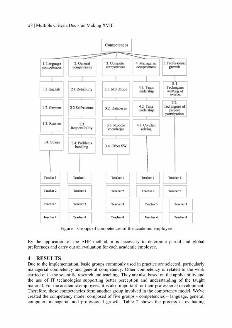
Figure 1 Groups of competences of the academic employee

By the application of the AHP method, it is necessary to determine partial and global preferences and carry out an evaluation for each academic employee.

4 RESULTS Due to the implementation, basic groups commonly used in practice are selected, particularly managerial competency and general competency. Other competency is related to the work carried out - the scientific research and teaching. They are also based on the applicability and the use of IT technologies supporting better perception and understanding of the taught material. For the academic employees, it is also important for their professional development. Therefore, these competencies form another group involved in the competency model. We've created the competency model composed of five groups - competencies – language, general, computer, managerial and professional growth. Table 2 shows the process at evaluating

28 | Multiple Criteria Decision Making XVIII

language competences. There were calculated criteria’s weights equal to 1.00 according to Saaty´s matrix, which is the part of AHP method.

1. Language competences 1.1 1.2 1.3 1.4 Geomean Weight

1.1 1 3 5 9 3.408658099 0.58111.2 1/3 1 3 5 1.495348781 0.25491.3 1/5 1/3 1 3 0.668740305 0.11401.4 1/9 1/5 1/3 1 0.293370579 0.0500

Table 2 Criteria evaluation - language competences – by using Saaty´s matrix

Figure 2 Evaluating of Groups of competences by using AHP Method

Groups and individual competencies relevant to the work of the academic employee were identified (see fig. 2). Using the AHP method, weights of the preferences between different competencies were determined, as well as global weights of individual competencies (see tab. 3).

Local weight Global weight0 100% AHP1 41% 41%

Quantitative Methods in Economics | 29

1.1 58.11% 23.83%1.2 25.49% 10.45%1.3 11.40% 4.67%1.4 5.00% 2.05%2. 17.29% 17.29%2.1 53.61% 9.27%2.2 4.23% 0.73%2.3 30.95% 5.35%2.4 11.20% 1.94%3 10.95% 10.95%3.1 29.43% 3.22%3.2 10.49% 1.15%3.3 9.48% 1.04%3.4 50.60% 5.54%4 5.67% 5.67%4.1 10.47% 0.59%4.2 25.83% 1.46%4.3 63.70% 3.61%5 25.09% 25.09%5.1 25.00% 6.27 %5.2 75.00% 18.82%

Table 3 Criteria evaluation – local and global weights

As we can see, the big significance has been calculated at language competences and professional growth competences (see Table 3). Individual local weights of the criteria were calculated as the product of the global weight of the criterion and the partial weight of the individual sub-criterion (in accordance with the AHP method). Calculation of the globalweight can be demonstrated on the assessment of the criteria 1.1 (English competency) in the most important group – language competences. The weight of the main criteria is 0.41. Thelocal weight was converted into the global weight determined by the relation:

0.41 × 0.5811 = 0.2383 = 23.83%

Subsequently, the assessment of four academic employees at the department was made and the achieved results were evaluated (see Table 4). The evaluation of four employees at the department using five criteria was performed by the department head.

Criteria Employee 1 Employee 2 Employee 3 Employee 4 MAX1 12.3010 36.9031 24.6021 24.6021 36.90312 8.6453 6.9162 10.3743 8.6453 10.37433 8.7630 5.4769 7.6676 7.6676 8.76304 4.5329 2.2665 5.0996 2.8331 5.09965 10.0344 12.5430 22.5774 17.5602 22.5774

Total 44.2767 64.1057 70.3210 61.3083 83.7174Percentage 52.89 76.56 84.00 73.23

4. 2. 1. 3.Table 4 Total assessment

(8)

30 | Multiple Criteria Decision Making XVIII

The department full-time employees were assessed. No doctoral students and part-time employees were evaluated. Calculation in Table 4 shows that the assessment is converted to a dimensionless value and the total usability is calculated using the weight of the individual criteria. The assessment was calculated as the product of the global weight of the criterion and the usability. The maximum usability is calculated. Values of the calculated total usability are compared and used to determine the order according to the highest usability of the individual employees. The results show that the highest usability was determined for the employee No. 3 (84%). Based on the obtained results, it is possible to determine the order of the employees by evaluated competencies. Evaluation based on the use of this method can serve as a basis for remuneration of the academic employees in the organization. Standardly, the assessment should be carried out once per year. Along with the assessment of the performance achieved (in the field of science and in the field of pedagogy), the assessment by competencies should also be taken into account. Mutual assessment of the employees would seem to be optimal, which raises the possibility of applying comparative analysis, but such an assessment is not used in practice nor can it be used.

5 CONCLUSION The results of evaluation of the different groups showed, that when using the AHP method, the highest weight had the language competencies and professional growth (see Figure 2 and Table 3). General competences are at the third position. Furthermore, the research revealed that the best performance, when measured by competencies, was showed by the academic employee no. 3 (see Table 4). Based on the performed assessment, the remuneration phase should subsequently occur. AHP methodology is a useful tool for evaluation of competencies as criteria. The criteria can be expressed qualitatively and quantitatively (Fiala, Jablonský and Maňas, 1994). AHP methodology was implemented in the human resources branch. Competency model of the academic employee and its assessment demonstrated the possibility to use the AHP method as a potential tool for evaluation of the university staff.

Acknowledgements: This work was supported within Operational Programme Education for Competitiveness – Project No. CZ.1.07/2.3.00/20.0296.

References [1] Armstrong, M. (2009). Odměňování pracovníků. Praha: Grada Publishing. [2] Bazsová, B. (2015). Use of Saaty´s Matrix by Performance Employee Measuring at the

University Department. In: Proceedings of the 11th International Conference on Strategic Management and its Support by Information Systems ´2015 SMSIS 2015). Uherské Hradiště: Němec, R., Zapletal, F., eds. VŠB-Technical University of Ostrava, pp. 25-35.

[3] Fiala, P., Jablonský, J. and Maňas, M. (1994). Vícekriteriální rozhodování. Praha: VŠE v Praze

[4] Koubek, J. (2007). Personální práce v malých a středních firmách. Praha: Grada Publishing

[5] Ramík, J. and Perzina, R. (2008). Moderní metody hodnocení a rozhodování. Karviná: Slezská univerzita v Opavě

[6] Majovská, R. (2014). Open Source Programmes as the Support in Mathematical Education. In: Proceedings of the 12th International Conference on Efficiency and Responsibility in Education ERIE 2014. Praha: Krejčí, I., Flégl, M., Houška, M. eds.Czech Univesity of Life Sciences Prague, pp. 341-347.

[7] Saaty, T. L. (1980). The analytic hierarchy process: planning, priority setting, resource allocation. London: Mc Graw-Hill International Book Co.

Quantitative Methods in Economics | 31

[8] Wagnerová, I. (2008). Hodnocení a řízení výkonnosti. New Jersey: Pearson publishing.

Author’s addressIng. Blanka Bazsová, PhD.VŠB-Technical University of Ostrava, Faculty of Economics, Department of Systems Engineering 17. listopadu 15/2172, 708 33 Ostrava Czech Republic email: blanka.bazsova@vsb.cz

32 | Multiple Criteria Decision Making XVIII

THE APPLICATION OF QUEUEING THEORY FOR MODELING HUMAN RESOURCES IN AMBULANCE SERVICE

Jelena Birovljev, University of Novi Sad, Faculty of Economics in Subotica, Aleksandra Marcikić, University of Novi Sad, Faculty of Economics in Subotica,

Nenad Vunjak, University of Novi Sad, Faculty of Economics in Subotica, Otilija Sedlak, University of Novi Sad, Faculty of Economics in Subotica,

Zoran Ćirić, University of Novi Sad, Faculty of Economics in Subotica

Abstract Nowadays, most of developed countries are facing an extreme challenge to establish efficient and effective health system despite of globalization and continuous changes in economic, political and social environment all over the world. Therefore, a systematic analysis and evaluation for effective resource allocation in a system is essential to provide competitive advantages for future survival and actions for the goal achievement. In the last decades, special focus has been given to practical implementation of operations research techniques in health care sector, in order to improve overall organization and quality. It seems that application of quantitative models in practice is widely used in developed countries and unfortunately in our local context awareness and usage of operation research models in health care systems is extremely rare. The main goal of this paper is to present how application of queueing models can aid decision making in health care sector, especially addressing workforce allocation. Based on the Erlang B model, simple staffing methods will be applied in order to obtain optimal number of ambulance crews in ambulance stations in Serbia.

Keywords: queueing models, healthcare management, staffing, Erlang B model

JEL Classification: C44 AMS Classification: 90C15

1 INTRODUCTION Organization and management of healthcare system are very complex tasks in every society, due to the unique nature of healthcare services. In life-threatening situations, where every second is important, an effective response of ambulance service can make a difference between life and death. Thus, managing operations of ambulance services and other healthcare organizations is a question of extraordinary social relevance. Nowadays, various quantitative methods are widely used to aid decision making process and improve overall efficiency. Optimal allocation of material, financial and human resources is extremely important in this sector and operations research models can be applied for different kinds of organizational issues in ambulance services, such as (Goldberg 2004):

� the location of fixed position and possibly variable position ambulance bases; � the dispatching of vehicles; � the number of vehicles of different types, staffing and equipment being carried � how and when to re-deploy resources under different system states.

All of the above mentioned topics are extensive and complex. The main goal of this paper is to present how application of queueing models can aid decision making in healthcare sector, especially addressing human resources allocation and staffing at ambulance stations in Serbia. Unfortunately, in our local environment, practical applications of quantitative models are

Quantitative Methods in Economics | 33

extremely rare, especially in healthcare organizations. Reasons for this situation are diverse and compound. Some of the possible reasons, which are also present in the other countries, include (Teow 2009):

� Low levels of managerial/mathematical background in the health care sector � Scientific papers are often written for operations research professionals, focusing on

specialised and technical topics, and not reaching healthcare professionals � Lack of process-related data for modeling � Lack of in-house operations research expertise � High cost of engaging external operations research consultants.

Thus, one of the goals of this paper is also to promote practical implementations of operations research methods, by presenting the benefits that healthcare organizations might achieve. The main idea of this paper is to embed observed regularities in demand for emergency medical services into human resources allocation proces, by determing the optimal staffing level for different periods of time. In that way, the balance between demand and supply of emergency medical services can be achieved, which consequently leads to the improvement of quality of medical services and increased satisfaction for both, patients and medical staff. The usual organizational problem of ambulance stations in Serbia is that the number of available ambulance crews has been determined ad hoc, regardless of the demand and system load, which might negatively influence the efficiency of the whole service. This survey has been conducted in order to improve management and organization of the only ambulance service station in the city of Subotica (Serbia), with population of 100,000 citizens. In order to obtain the optimal number of ambulance crews in various intervals of time queueing models have be applied. By knowing the internal organization and business conditions, these models can be easily applicable to other organizations with stohastics characteristics of the demand.

2 THE APPLICATION OF QUEUEING THEORY IN HEALTHCARE ORGANIZATIONS Queueing theory is a branch of operations research, which covers the mathematical analysis of waiting lines. Its results are often used to support decision making process about optimal allocation of resources needed to provide a service. Waiting is a part of everyday activities in all segments of life, but people are even more sensitive when waiting for medical services to resolve their health problems. Here, the application of queueing theory in healthcare organizations might improve patients' and employees' satisfaction by reducing the time spent in waiting lines (Bekker/De Bruin 2010, Yankovic/Green 2011, Brahma 2012). It is important to state that waiting to scheduled medical treatments is not a subject of queueing theory. Mathematical analysis of waiting lines is dealing with queues that occur when patients arrive without an appointment, which is the case of emergency and radiology departments in hospitals, ambulance service, etc. In a long period of time, most of healthcare organizations have sufficient capacities to serve even larger number of patients than the real demand, but the queues occur due to the unequal distribution of arrivals over time. Therefore, waiting lines are short term phenomena. The increase of a number of service providers (i.e. servers) leads to the greater quality and satisfaction, but also consequently to the higher costs. Those quantitative models are very applicative and suitable for determination of the most efficient way of the mass services system functioning (Ernst et al 2004). The overwhelming system capacity might cause the unnecessary costs, but on the other hand, insufficient number of servers could lead to the longer waiting times or other negative consequences, sometimes even with the fatal outcome. Queueing theory models ensure the achievement of balance between the available resources and quality of services at the one side and financial boundaries at the other side.

34 | Multiple Criteria Decision Making XVIII

3 MODIFICATION OF ERLANG B MODEL FOR NONSTATIONARY PROCCESSES Emergency medical services are provided 24 hours every day, but demand for these services varies over time. By detailed quantitative analysis it is possible to identify daily pattern to show which hours of the day are more frequent than the others. Consequently, the number of available ambulance crews should be adjusted to the demand fluctuations. This can be obtained by application of Erlang B model, which is especially suitable for modelling medical services (Restepo et al 2009, de Bruin et al 2010, Zuidhof 2010). Literature from this field show significant reasons to assume that the demand for emergency medical services follows anon-homogeneous Poisson process (Vasanawala/Desser 2005, Channouf et al. 2007). There is only one ambulance station in Subotica where all emergency calls arrive. The calls are immediately forwarded to the available ambulance crews. If there is no available ambulance crew at the moment, the call is lost in the system, which is described by the Erlang B model, M/G/c/c. In this model the ambulance requests arrive according to a Poisson process with a constant rate, the occupancy times (travel times) are independent and identically distributed with some general distribution G, and c ambulances are available (Zuidhof 2010). Namely, in a very urgent case, the closest crew interrupts the current, less urgent intervention, and responds to the new, more urgent call. If the case is not so urgent, patients are referred to the hospital’s emergency department or other healthcare institutions, due to the current occupation of all ambulance crews. It is important to accent that there is no waiting in thiscase, due to the urgent nature of those healthcare services. Therefore the queueing theory is used to model blocking probability. Blocking probability is the probability that the call will be lost in a system (forwarded to the other institutions), due to the occupancy of all ambulance crews. If the quality of emergency medical services is known upfront, in a form of the maximal level of blocking probability, application of Erlang B model allow us to determine the optimal staffing level.

Stationary is one of the basic assumptions for application of queueing models. Stationary process is a stochastic process whose joint probability distribution does not change over time.Consequently, parameters such as the mean and variance also do not change over time and do not follow any trends. But in our research, the rate of arrival calls depends on time t. In this case we apply Mt/G/c/c waiting model, where number of ambulance requests follows a Poisson distribution with the time-dependent mean �t. Since the stochastic process that represents the demand for ambulance services is nonstationary, the SIPP (stationary independent period-by-period) approach has been applied to modify input data for the Erlang B model. The SIPP approach provides the satisfactory solutions when there are no significant fluctuations of a demand within the certain time intervals (Green et al. 2007, Yom-Tov/Mandelbaum 2010). According to this, it is necessary to split a time period into the shorter intervals, which correspond to the constraints of a concrete staffing problem and within which the significant variations of a number of ambulance requests do not exist. Then, the mean arrival rate is determined for every interval and the value is used in Erlang B model. Occupancy times also depend on time t, thus the same approach will be applied. Therefore, the offered load � should be separately determined for every time interval t according to:

�t = �t�t (1)

where �t is an average number of ambulance requests and �t an average occupancy time in the current time interval t. In this case, blocking probability can be calculated for the separate time intervals:

Quantitative Methods in Economics | 35

(2)

where �t presents the offered load in time interval t and s the number of servers (ambulance crews). If � is a predefined maximum level of blocking probability, the optimal staffing level s* (number of ambulance crews) can be determined by

. (3)

Therefore, for a known value of �t and fixed�, minimal staffing level can be determined by varying the number of available ambulance crews.

In order to choose the most suitable staffing level it is also important to analyse the relation between performance and cost of various staffing levels. Performance of the staffing level is determined by the value of blocking probability and it is the indicator of schedule inadequacy. Thus, the goal is to minimize the value of performance. Performance of the staffing level is also determined by the expected number of ambulance requests �t, because the occurrence of all ambulances being occupied is more unfavourable on busy hours. (Zuidhof 2010)

(4)

It is also important to determine the costs of analysed staffing levels. The costs are defined as the sum of a number of available ambulance crews in every hour of an average week. (Zuidhof 2010)

(5)

4 NUMERICAL RESULTS In this paper demand for healthcare services is presented by the daily number of ambulance calls at the Ambulance Service in Subotica, Serbia. The data set which we use provides us information about the daily number of ambulance calls and occupancy times for three years period, from March 15th 2011 until March 15th 2014. In order to obtain the optimal staffing level, which is characterized by the lowest possible performance and costs, it is necessary to analyse the number and the occupancy time of ambulance requests on an average week. Values of the blocking probability (2), performance (4) and costs (5) based on the existing staffing level are presented in the next table.

Table 1: Indicators of the existing staffing level

Indicators

Blocking Probability Performance Total

Performance Costsmin max min max

0.0351 0.2317 0.0185 0.2534 24.76 372

In order to achieve equable quality of ambulance services over whole period of time, it is important to reduce the oscillations of the performance values, as well as its total value. This has been obtained by varying the staffing levels in a way that blocking probability stays below the predefined maximal value, with the minimal costs. At the existing staffing level high values of blocking probability are mainly present in the busy hours, which consequently lead to the higher values of performance. In the whole data set, extremely high values of

36 | Multiple Criteria Decision Making XVIII

performance can be noticed on Tuesday and Wednesday at 19h and during the morning hours on Saturday and Sunday. Generally speaking, morning hours are very busy during the whole week. The lowest values of performance are obtained during the night, due to the lower number of ambulance requests. When determining the optimal staffing level it was necessary to find the best ratio between the values of costs and performance, with the respect of themaximal blocking probability. Different staffing levels were considered which resulted in finding the optimal staffing level. Reducing the oscillations of the performance value led to the significant decrease of the total value of performance, but also to the costs increase.

Table 2: Performance and costs of an average week staffing levelExisting Staffing Level Optimal Staffing LevelTotal

Performance Costs Total Performance Costs

24.76 372 16.75 404

Figure 1: Blocking probability and performance of the optimal staffing level

5 DISCUSSION AND CONCLUSION In this paper the analysis of staffing level has been performed in order to improve allocation of human resources in ambulance service in Subotica. Currently, in this ambulance station there are two available crews every day, except the Friday, Saturday and Sunday when the additional crew is also available. Frequently, the number of ambulance requests is higher than the number of available ambulance crews, but there are also situations when there are no calls and all the crews at the station are free. The main idea of this paper was to apply the Erlang B model in order to rationalize and improve the allocation of human resources in this organization. The optimal staffing level for different time intervals (depending on the level of demand) has been determined by reducing the variations of performance with the respect to a predefined maximal value of blocking probability. But the lower value of performance consequently leads to higher costs, represented by the available number of ambulance crews. Therefore, the results of performed quantitative analysis point out the necessity of hiring an additional crew in frequent periods of day, in order to maintain the consistent quality of services over time. The additional crew can be provided by reorganization of the existing employees or with a new hiring. It is also important to consider the modification of working

Quantitative Methods in Economics | 37

hours in order to avoid a change of shifts in the most frequent time interval of the day (7am and 7pm). Thus, the results of applied staffing model provide the reliable basis for creation of an optimal scheduling model, which is one of the guidelines for future research in this area.

References [1] Bekker R. and De Bruin A. M. (2010). Time-dependent analysis for refused admissions in

clinical wards. Annals of Operations Research, 178(1), pp. 45–65. [2] Brahma P.K. (2012). Application of queueing theory in hospital manpower planning.

Saarbrucken: Lambert Academic Publishing.[3] Channouf, N., L’Ecuyer, P., Ingolfsson, A. and Avramidis, N. (2007). The application of

forecasting techniques to modeling emergency medical system calls in Calgary, Alberta. Health Care Management Science, 10(1), pp. 25–45.

[4] De Bruin, A.M., Bekker, R., van Zanten, L. and Koole, G.M. (2010). Dimensioning hospital wards using the Erlang loss model. Annals of Operations Research, 178(1), pp.23–43.

[5] Ernst A.T., Jiang H., Krishnamoorthy M. and Sier D. (2004). Staff scheduling and rostering: A review of applications, methods and models. European Journal of Operational Research, 153(1), pp. 3–27.

[6] Goldberg J.B. (2004). Operations research models for the deployment of emergency services vehicles. EMS Management Journal, 1(1), pp. 20–39.

[7] Green, L.V., Kolesar, P.J. and Whitt, W. (2007): Coping with time-varying demand when setting staffing requirements for a service system. Production and Operations Management, 16(1), pp. 13–39.

[8] Restrepo, M., Henderson, S. G. and Topaloglu, H. (2009). Erlang loss models for the static deployment of ambulances. Health Care Management Science, 12(1), pp. 67–79.

[9] Teow, K.L (2009). Practical operations research applications for healthcare managers.Annals Academy of Medicine Singapore, 38(6), pp. 564–566.

[10]Yankovic, N. and Green, V.L.: Indentifying good nursing levels: a queuing approach. Operations Research, 59(4), pp. 942–955.

[11]Yom-Tov, G. and Mandelbaum, A. (2010). The Erlang R Queue: Time-Varying QED Queues with Reetrant Customers in Support of Healthcare Staffing. MSOM Conference,Israel.

[12]Vasanawala, S.S. and Desser, T.S. (2005): Accommodation of requests for emergency US and CT: Applications of queueing theory to scheduling of urgent studies. Radiology,235(1), pp. 244–249.

[13]Zuidhof, G.M. (2010). Capacity Planning for Ambulance Services: Statistical Analysis, Forecasting and Staffing. Master thesis. Vrije Universiteit Amsterdam, Centrum Wiskunde en Informatica Amsterdam.

Author’s addressOtilija Sedlak, PhD, Full ProfessorUniversity of Novi Sad, Faculty of Economics Subotica, Department of Business Informatics and Quantitative Methods Segedinski put 9-11, 24000 Subotica Serbia e-mail: otilijas@ef.uns.ac.rs

38 | Multiple Criteria Decision Making XVIII

SELECTION OF THE OPEN UNIT TRUSTS FOR INVESTMENT VIA FUZZY MULTICRITERIA EVALUATION METHOD

Adam Borovička, University of Economics, Prague

Abstract The main aim of this article is to select the suitable open unit trusts for investment. A selection of the investment instruments is made on the basis of several criteria (characteristics). The main are return, risk and cost. In real cases, a value of return is not stable. This vague (imprecise) element is expressed by means of a triangular fuzzy number. The risk and cost are in the precise form. In order to select the open unit trusts for investment, a fuzzy multicriteria evaluation method is proposed. This method is inspired by algorithms of ELECTRE I and III methods. Their proposed modifications enable an imprecise expression of some input data. Moreover, the threshold values have not to be uneasily determined by a decision maker. The selection of the open unit trusts is described for two investment strategies – risk-averse and risk-seeking investor. The results are compared.

Keywords: multicriteria evaluation, open unit trust, triangular fuzzy number

JEL Classification: C44, G11 AMS Classification: 90-08

1 INTRODUCTION It is usual that a human being has some free financial resources which should be valorized. Several ways how to do it are available. On the one hand, we have a few banking products –bank deposit, saving account, building savings or pension savings. On the other hand, the investment instruments can be used – stocks, bonds, investment certificates, commodities etc. This article is focused on the open unit trusts. In recent years, the market of the open unit trusts also develops in the Czech Republic. An investment in the open unit trusts becomes more and more popular. The offer of the open unit trusts is wide in the Czech Republic. As a long-standing client of Česká spořitelna, I focused on the open unit trusts managed and then offered by the Česká spořitelna investment company. The main aim of the article is to select one or more suitableopen unit trusts for investment according to the stated investment policy. For this purpose, a fuzzy multicriteria evaluation method is proposed. This method offers some advantages for investment decision making. Firstly, this method can evaluate the investment alternatives according to more criteria (characteristics) at a time (e.g. return, risk or cost). The evaluation of alternatives can be made on the basis of quantitative and also qualitative input information. Secondly, the method enables to express input data in the imprecise form as a triangular fuzzy number. Lastly, the method divides the alternatives to the effective and ineffective. A decision maker can make an image about “good” and “bad” alternatives. The proposed method is based on the algorithms of the ELECTRE I and III methods. But some modifications and improvements are proposed for the purpose of a better applicability in the real situations. As mentioned above, the proposed fuzzy multicriteria evaluation method is applied in order to select the suitable open unit trust(s) for investment. The potential investor wants to valorize the open unit trusts by the main criteria (return, risk and cost) together. The investor finds out,which alternatives are “bad” and which would be suitable for a final investment portfolio. But a portfolio making is not a subject of this paper. In practical application, two investment

Quantitative Methods in Economics | 39

strategies are specified – risk-averse and risk-seeking investor. The investment policy of both types of investor is specified. The results are analyzed and compared. The structure of the article is as follows. After the introduction (Section 1), Section 2 describes an algorithm of the fuzzy multicriteria evaluation method. A brief research of the current methods is made. The advantages of the proposed concept are emphasized. In a Section 3, a real decision making situation is described in detail. In the last part (Section 4), the whole paper is summarized and some subjects for the future research are specified.

2 FUZZY MULTICRITERIA EVALUATION METHOD Nowadays, we know number of the fuzzy multicriteria evaluation methods. These methods usually accept the input information in the imprecise form. Then criteria values or weights are expressed as fuzzy numbers. We have fuzzy WSA, AHP (Bector, et al., 2002, Gu and Zhu, 2006), fuzzy conjunctive and disjunctive method (Hwang and Youn, 1981), fuzzy modifications of TOPSIS method (e. g. Wang and Elhag, 2006), and method based on the (fuzzy) preference relation scoring AGREPREF (Lagrèze, 1975), ELECTRE I (Roy, 1968) or ELECTRE III (Roy, 1978).

In spite of an existence of many methods, some practical situation can require a unique approach. Then the current approaches must be modified, or a new concept is proposed. The proposed method accepts an input data in strict and also imprecise form. The most methods do not enable this combination. Any additional information (threshold values or specification of utility function) from a decision maker is not required because it could be very problematic for him. The algorithm takes into account the differences in criteria values compared to other methods (e.g. ELECTRE III, conjunctive or disjunctive method). The proposed method is user-friendly, the algorithm is comprehensible. The algorithm of developed method can be briefly described in the following steps: Step 1: Formulate the criteria matrix ( )ijy�Y , where ijy ( 1,2,..., ; 1,2,..., )i n j k� � is an evaluation of the i-th alternative by the j-th criterion. The criteria values can be in strict form or in imprecise (vague) form as a triangular fuzzy number. An importance of the j-th criterion is specified in the strict form as ( 1,2,..., )jv j k� .

Step 2: Strict and fuzzy criteria values are compared. The comparison (or ranking) of triangular fuzzy numbers is made by mechanism of a fuzzy modification of TOPSIS (Chen, 2000). As in ELECTRE III, the following sets of criteria indices are specified, where set maxI ,or minI contains the indices of maximizing, or minimizing criteria

� �� �

max min

max min

| , ; , , 1, 2,..., ;| , ; , , 1, 2,..., ;

iPj ir jr is js

jPi jr ir js is

I r s y y y y r I s I i j n i jI r s y y y y r I s I i j n i j

� � � � � � � �

� � � � � � � �. (1)

Step 3: The matrices S and R are determined. Their elements express the grades of preference. The matrix S is defined as in the ELECTRE III technique. The concept of matrix R is derived from ELECTRE I method. However, it takes into account the criteria importance and works with the standardized criteria values. The element of the matrix R is formulated for each couple of alternatives i and j ( , 1,2,..., )i j n� in the following form

� �' '

' '

1

| |, , 0 else

| |

iPj

h ih jhh I

ij iPj ij ijk

h ih jhh

v y yr I r i j r

v y y

�

�

�

� � � � � � ��

�

�, (2)

40 | Multiple Criteria Decision Making XVIII

where 'ihy , or '

jhy ( , 1,2,..., ; 1,2,..., )i j n h k� � is the standardized criteria value. The difference (distance) between standardized fuzzy criteria values is measured by vertex method proposed in (Chen, 2000). Step 4: The aggregate preference of the i-th alternative in face of the j-th alternative is set by a proposed rule

ij ji ij jis s r r� � � . (3) The rule is modification of the ELECTRE III technique. The thresholds are eliminated. The effective alternative is such an alternative that embodies the highest discrepancy between number of alternatives in face of which is preferred and number of alternatives that are preferred in face of it. The concept combines the approach ELECTRE I and III approach to eliminate the ELECTRE I drawback, when the effective alternative must not exist.

3 SELECTION OF THE OPEN UNIT TRUSTS Imagine the following real decision making situation. A human being has some free financial resources which should be valorized for future use (e.g in pension age, or for short-term or medium-term consumption). As a long-term client of Česká spořitelna goes to the bank for advice. This client has just some banking products (building savings or saving account). Another way how to valorize the money is investment. The client is redirected to the investment counsel.They start to create the client’s investment policy together. The investment counsel requires some important information from a side of the client (potential investor). He specifies 3 main criteria – return, risk and cost of the investment. The potential investor should specify hispreferences about an importance of these criteria. It generally based on purpose of the investment, duration of the investment, attitude towards risk of the investment, mood or conditions in the capital market etc. Now we will distinguish two types of investors – risk-averse and risk-seeking investor. A risk-averse investor wants more likely long-term investment. The spared money should serve for (at least partly) financial protection of pension age. Then this type of investor fears a loss of the investment. Therefore a risk-averse investor is able to sacrifices some part of return for a lower risk of the investment. A criterion risk is more important than a criterion return for a risk-averse investor. Cost does not play fundamental role in a decision making process. A risk-seeking investor is more active in the capital market. His investment is rather short-term. It can be repeated. Return is the most important criterion. He is able to undergo greater risk for greater return of the investment. Then the cost connected with investment is a little bit more important for risk-seeking investor than for risk-averse.Also on the basis of the stated investment policy, the investment counsel offers an investment in the open unit trusts. In this way people can invest vicariously in bonds, stocks or properties in a small volume unlike a direct investment on a stock exchange. The Česká spořitelna investment company manages quite a number of the open unit trusts. The investment counsel offers bond and stock open unit trusts. The aim is to select the suitable fund(s) for investment for both types of investors.

3.1 Input information As mentioned above, 3 main criteria (characteristics) of the open unit trusts are stated. Return is measured monthly in a period from 2010 to 2015. Return is variable value in time. Therefore it is expressed in the imprecise form as a triangular fuzzy number. Its middle parameter is determined as average monthly return. Lower, or upper parameter is computed as an average monthly return reduced, or topped by three standard deviation of monthly returns (Borovička, 2015). This operation is based on a presumption of the normally distributed

Quantitative Methods in Economics | 41

returns. Risk is measured by the average absolute negative deviation proposed in (Borovička, 2015). This concept takes into account only values less than average return. Costs include all fees connected with investment in the open unit trusts, namely entry, supervisor, manager or license fees (as a percentage of the stake). All open unit trusts (5 bond and 3 stock funds) and appropriate data are in the following table (Tab. 1). Tab. 1 Return, risk and cost of the open unit trusts

Fund Return [%] Risk [%] Cost [%]High Yield dluhopisový ( 7.55, 0.35, 8.25)� 2,19 2,49Korporátní dluhopisový ( 4.28, 0.26, 4.81)� 1,23 2,75Sporobond ( 2.51, 0.40, 3.32)� 0,69 2,20Sporoinvest ( 0.39, 0.06, 0.51)� 0,18 1,05Trendbond ( 4.38, 0.27, 4.91)� 1,37 2,77Global Stocks ( 8.88, 0.90,10.67)� 2,21 6,33Sporotrend ( 21.46, 0.70, 20.07)� � 5,36 5,43Top Stocks ( 7.55,0.35,8.25)� 3,93 5,82

The weights of criteria are calculated by points method (Fiala, 2013). The investor assigns the points from the interval 0,10 to each criterion according to his preferences (mentioned above). The result of this procedure is in the following table (Tab. 2). Tab. 2 Weights of criteria for both investors

Risk-averse investor Risk-seeking investorCriterion Points Weight Points WeightReturn 7 0.368 10 0.526Risk 10 0.526 6 0.316Cost 2 0.105 3 0.158

3.2 Assumptions and results Now a selection of the open unit trusts is made by the proposed fuzzy multicriteria evaluation method for both investors. We can make some assumptions about the results. Generally, the bond funds usually have lower return and also lower risk than stock funds. This fact partly shows Tab. 2. Then we can expect on the basis of the preferences of the investors specified above that effective alternative(s) will be bond fund(s) for a risk-averse investor and stock fund(s) for a risk-seeking investor. The proposed method compares the triangular fuzzy numbers describing return of the funds. The ranking of funds from the greatest return is as follows: Global Stocks, Top Stocks, High Yield, Sporobond, Trendbond, Korporátní dluhopisový, Sporoinvest, Sporotrend. Now, the non-dominance test can be made. It is obvious that a rational investor will not invest in the dominated funds according to 3 selected criteria. The dominated alternatives are Korporátní dluhopisový, Trendbond and Sporotrend. These open unit trusts are eliminated from the following analysis. To select a suitable fund(s) for investment, the fuzzy multicriteria evaluation method is applied. The bond open unit trust Sporoinvest (effective alternative) is selected for a risk-averse investor. This result is not a surprise. Sporoinvest has unambiguously the lowest level of risk. Even if this fund has the lowest return, a considerable weight of a criterion risk is decisive (weight is greater than 0.5). A selection of this fund is also supported by the lowest level of cost. For risk-seeking investor, the stock open unit trust Global Stocks (effectivealternative) is chosen. This choice can be also expectable. This fund has the greatest return

42 | Multiple Criteria Decision Making XVIII

that is the most important for risk-seeking investor. Moreover, a level of the second most important criterion risk is significantly lower compared to other stock funds. Its level of risk rather gets near some bond funds. These aspects are superior to the greatest level of cost connected with an investment in Global Stocks. As we can see, the assumptions about the results are confirmed. For each investor, one open unit trust is selected. In case of need, a ranking of alternatives should be made via some additional procedure (e.g. Borovička, 2015). Then a portfolio can be made from the selected funds by ranking. But is not a purpose of this article.

4 CONCLUSION The article deals with a selection of the open unit trusts. In practical part, the investment decision making procedure is briefly described. The fuzzy multicriteria evaluation method is applied that is proposed in the theoretical part. The results are analyzed. In real situation, more (qualitative) criteria could be explicitly reflected (e.g. mood in the capital market, fund manager skills etc.). In the proposed method, another type of fuzzy number could be studied or fuzzy (imprecise) weights could be included. Then the techniques of a comparison of the fuzzy numbers could be further more studied and developed.

Acknowledgements: This work was supported by Grant No. IGA F4/54/2015 of the Internal Grant Agency, Faculty of Informatics and Statistics, University of Economics, Prague.

References

[1] Bector, C. R., Appadoo, S. S. and Chandra, S. (2002). Weighted factors scoring model under fuzzy data. In: Proceeding of the Annual Conference of the Administrative Sciences Association of Canada Management Science Division. Manitoba, Winipeg, pp. 95–105.

[2] Borovička, A. (2015). Vytváření investičního portfolia podílových fondů pomocí fuzzy metod vícekriteriálního rozhodování. Ph.D. University of Economics in Prague.

[3] Chen, C. H. (2000). Extensions of the TOPSIS for group decision-making under fuzzy environment. Fuzzy Sets and Systems, 114 (1), pp. 1–9.

[4] Fiala, P. (2013). Modely a metody rozhodování. Prague: Oeconomica.[5] Gu, X. and Zhu, Q. (2006). Fuzzy multi-attribute decision making method based on

eigenvector of fuzzy attribute evaluation space. Decision Support Systems, 41(2), pp. 400–410.

[6] Hwang, C. L. and Yoon, K. (1981). Multiple Attribute Decision Making – Methods and Applications, a State-of-the-Art Survey. New York: Springer-Verlag.

[7] Lagrѐze, E. J. (1975). La modélisation des préférences: Préordres, quasiordres et relations floues. Ph.D. Université de Paris V.

[8] Roy, B. (1968). Classement et choix en présence de points de vue multiples (la méthode ELECTRE). La Revue d'Informatique et de Recherche Opérationelle (RIRO), 2(8), pp. 57–75.

[9] Roy, B. (1978). ELECTRE III: algorithme de classement basé sur une représentation floue des préférences en présence des critères multiples. Cahiers du CERO, 20(1), pp. 3–24.

[10]Wang, Y. M. and Elhag, T. M. S. (2006). Fuzzy TOPSIS method based on alpha level sets within an application to bridge risk assessment. Expert Systems with Applications,31(2), pp. 309–319.

Quantitative Methods in Economics | 43

Author’s addressIng. Adam Borovička, PhD. University of Economics in Prague, Faculty of Informatics and Statistics, Department of Econometrics W. Churchill Sq. 4, 130 67 Prague 3 Czech Republic E-mail: adam.borovicka@vse.cz

44 | Multiple Criteria Decision Making XVIII

Using expert opinions to quantify net non-measurable external benefit of CHP plants

ĐulaBorozan, J.J. Strossmayer University of OsijekDubravkaPekanovStarčević, J.J. Strossmayer University of Osijek

AbstractEvaluating the socio-economic justification of the construction of large infrastructure facilities is often difficult primarily due to the existence of numerous non-measurable external costs and benefits. The aim of this paper is to demonstrate their quantification using an expert opinion approach in the case of a combined cycle heat and power (CHP) plant in Croatia. The analysis of expert opinions reveals that the construction and the operation of the 500 MW CHP plant will generate more non-measurable external benefits than costs, both during its construction and regular operation phase. Namely, the net benefit score has a positive value in both cases.

Keywords: non-measurable benefits and costs, CHP plant, expert opinion approach

JEL Classification: C83, D61, H43 AMS Classification: 90B50, 90B90

1 INTRODUCTION It is relatively easy to deal with measurableexternal costs (benefits) which refer to alleffects of the projectthat decrease (increase) the socio-economicpotentialof the local area, regionorentire country and are not included in market prices. This does not hold for non-measurable external costsandbenefits since they can be neither directly measured nor expressedin monetary terms. Though difficult to measure, they are important in project evaluation and therefore need to be properly considered. Moreover, Boardmanet al. (2006) stress that it is necessary tocarry outnot onlya quantitativebut also aqualitative assessment of non-measurable benefitsandcosts in order to understand them better and then involve them in the social justification of the project more properly. Other scholars also stress the importance of quantification of these costs and benefits in the overall project evaluation (e.g., Phillips and Phillips, 2006; Fahlen and Ahlgren, 2012; Sovacool, 2014; Florio and Sirtori, 2015). This paper aims at demonstrating how to quantify data obtained in expert opinion elicitation on non-measurable external costs and benefits that may appear during the construction and operation of a CHP plant named the Combined Cycle Heat and Power Plant “KKE Osijek 500” (hereinafter referred to as ‘the 500 MW CHP plant’) in Croatia and then use them to conduct a cost-benefit analysis. This power plant will be used to generate electricity, primarily for Eastern Croatia, process steam and district heating for the city of Osijek. Its energy source will be natural gas. The construction is planned to start in 2016. The details on this plant may be obtained from the IGH Institute (2014). The expert opinion approach is particularly used when there is insufficient knowledge due to the lack of historical data, when such data is not easily measurable and when multiple disciplines need to be involved in data collection and analysis.The remainder of the paper is organized as follows. Section 2 specifies briefly the main non-measurable benefits and costs related to the construction and operation of the 500 MW CHP plant, while Section 3 describes the methodology used to carry out the present study. Sections 4 and 5 provide the results of the expert opinion analysis and the main conclusions, respectively.

Quantitative Methods in Economics | 45

2 NON-MEASURABLE EXTERNAL BENEFITS AND COSTS Tierman and Peppard (2004) state that non-measurable benefits and costs have always been a thorny issue in project evaluation as they must be quantified to get real societal justification of the project. Ignoring these benefits and costs related to the construction and operation of CHP plants could lead to an unwarranted bias in the decision-making process. We specified the following main favorable impacts as non-measurable external benefits: strengthening the regional/local economic development, generating the socialandhealth benefits, increasing the security and stabilityin the heat and electricity supply, reducing theadverse impactson naturalenvironmentthroughemissions due to advanced technology, and finally, improving theCroatiangeo-strategic and energy position. Certainly, the construction and operation of the 500 MW CHP plant will cause the adverse impacts on public health, economy and environment. Hence, non-measurable external costs arise from the adverse impacts on human and environmental health, transport and local economy. They are described in detail and quantified in monetary terms inBorozanandPekanovStarčević(2014).The following is characteristic of both the benefits and costs: theyare mutually connected,they influence eachother, have asynergistic effect, and are manifestedlocally, regionally and globally. The assessment of intensity of their impactwas carried out by the experts during the process explained in the next section.

3 METHODOLOGY Fraumeni (2001) stated that measuring intangibles is an old-economy problem. There are many measurement techniques for measurable costs and benefits. However, they are not applicable to measurement of non-measurable costs and benefits. Though, to that end, the expert opinion approach may be used. The approach is widely used in many large investment projects characterized by complexity and uncertainty particularly related to health and environmental impacts due to numerous advantages such as cost- or time-savings or acquisition of a great deal of detailed knowledge of experts (e.g., Pauditšova, 1995; Shu et al., 2010; Krueger et al., 2012; Zubaryeva et al., 2012). It often takes the form of a survey via a questionnaire, as in the case of the present paper. The research process includes various successive steps, whereby the following ones are particularly important in quantification of non-measurable benefits and costs and then calculation of the net benefit score: questionnaire design, selection of experts and data collection and analysis.

Questionnaire design.Developing the survey questions on non-measurable costs and benefits of the 500 MW CHP plant involved a multi-step process. First, we developed a list of non-measurable costs and benefits which were then discussed with the experts directly involved in the 500 MW CHP plant project in Osijek. The result was a refined short questionnaire. It consists of two parts. The introductory part contains explanations of the aims of the survey, the basic assumption for evaluation and how results are to be used. It also lists the expertise field of all people who decided in advance to participate in the survey. The second part, the core part, includes two questions: the first onerelates tothegeneralassessment ofthe impactthe 500 MW CHP will generate on human health, the ecosystem, local economy andsociety as a wholeduringitsconstruction and operation; the second one relates to theassessment of the intensity of the impacts theconstruction and operation of the 500 MW CHP plant will generate on the specified non-measurable externalcosts and benefits listed in Section 2.

Selection of experts.A total of twenty experts were contacted in October 2013 by phone or face to face to be questioned and all agreed to participate after the introductory explanation of

46 | Multiple Criteria Decision Making XVIII

the project and their role therein.This short conversation was the preliminary phase in expert elicitation. Experts cover the following particular fields, i.e., four experts deal directly with power engineering (either as teachers or are professionally engaged in energy issues), two experts are representativesof entrepreneurs, four experts deal withenvironmental issues(one of them comes from theAssociationforNature and Environmental Protection - Green Osijek, two are professionallyinvolved in environmental protection and oneexpert teaches the course Environmental Protection), four experts deal with human healthprotection(twoaredoctorsand two are professionally engaged insafety at work issues), two experts are representatives ofthehighest level of thecity government, two experts are representatives of the investor -Hrvatskaelektroprivreda (HEP), and the last two have expertise in construction (one teaches several courses related thereto, and one is engaged in construction business). By covering different but important fields, and also by choosing experts who have not been involved in project evaluation and revision, we wanted to reduce the likelihood of bias and also to facilitate the public discussion on the external costs and benefits of such important project.

Data collection and analysis.Preliminary expert elicitationisused to collecttheopinionsofexpertsindividually and therefore toavoidbiasesstemmingfromgroupdynamics. Under the assumptionthat alllegislation related toenvironmentandits protection will be fullyrespected during theconstruction and operation ofthe 500 MW CHP plant, the task oftheexpertswas to assess: (i) thedominant influence(with either a “positive” or a “negative” answer) it will have on human health, the ecosystem, the economyandsociety as a whole, and (ii) the intensity of the impact it will have on the specified non-measurable benefits and costs on a ten-point Likert scale (1 “no impact” to 10 “extremely strong impact”). After collecting the completed questionnaires, the median wascalculated for each specified non-measurable external benefit and cost. The following criterion was developed for the purpose of determining the intensity of the impact importance:if the medianfor each individual itemrangesfrom 0 to 2, the impactis perceived as very weak;the impact is perceived as weak if the median ranges from 2 to 4, moderate if it ranges from 4to 6, strong and very strong if it ranges from 6 to 8 and 8to 10, respectively. To calculate the

net benefit score, each median of the item (i) is transformed by using the formula

i 1/ 2M�

,where i = 1,…, M. Thereby, M denotes the total number of non-measurable costs and benefits to be evaluated. The finalvalues for non-measurable external benefits and costs obtainedby this transformation are added, and the differencebetweenthe total value ofnon-measurable external benefitsandcosts is thevalue of a net benefit (B-C) score. This procedure was explained in Rajković (2011). For its application see, e.g., Ratknić and Braunović (2013).

4 RESULTS The experts evaluated positively the impact of the construction and operation of the 500 MW CHP plant on the economy and society in general. Namely, each of them considered that positive impacts will prevail. As for the impactonhuman health and ecosystem, expert responses were almostdividedbetween positive and negative effects, although at the end, negative impacts prevailed. One ofthe experts explained this in relation to himself in the following way: “Gas-fired cogeneration plants generallyhavea detrimentalimpact on global warming, and a substantiallylower impact on environment, human health and society. Namely, because of thehighefficiency and the useof gasinstead of oilorcoal, there are relativelymuch loweremissionsof CO2 equivalentsandother harmfulby-productshazardous to peopleand the ecosystem, typically about 450g/kWh ofelectricitycompared to conventionalcoal-fired thermal power plants(about 1000 g/kWh), but stillsignificantly

Quantitative Methods in Economics | 47

higherthanduring the production of energy from renewable power plants(typically a few tens ofg/kWhincludingindirect emissionsduring the construction anddecommissioning).” Although this explanation reflects his opinion, it seems to be characteristic of the sample. The experts also evaluated the specified non-measurable external benefits and costs that will result from the construction and operation of the 500 MW CHP plant. Table 1 shows the median and the categorized intensity of the impact on the items of interest.

Table 1: Experts’ opinion about the impact intensity of the 500 MW CHP plant COST / BENE-FIT

CATEGORYCONSTRUCTION OPERATION Impact median

Intensity of impact

Impact median

Intensity of impact

CO

STS

Impact on human health due to human activities 3.00 weak 1.00 very weak

Impact on human health due to plant operation 3.50 weak 2.00 weak

Impact on transport 2.00 very weak 1.00 very weakImpact on local economy 1.00 very weak 0.50 very weakImpact on environmental health 2.50 weak 2.00 weak

BEN

EFITS

Local economic growth 8.00 strong 8.00 strongImpulse to others 8.00 strong 4.50 moderateSocial benefits 6.00 moderate 7.00 strongSecurity of energy supply 0.50 very weak 9.00 very strongImprovement of geo-position 0.00 very weak 9.00 very strong

The external non-measurable coststhat will beproduced during the construction ofthe 500 MW CHP as adverse consequences of its impacts on human and environmental health and local economy will be slightly greaterthan the costs produced during its operation. More precisely, the intensity of impact may be classified in both cases as either very weak or weak. Second, unfavorable impacts onhuman healthcaused byhuman activities(e.g., injury at workand intraffic accidents with mildtodisastrous consequences) and regular operation ofthe power plant(noise, air pollution, etc.) are perceived generally to be higher, although weak, during the construction ofthe 500 MW CHP plant than thosethat would be generated duringitsregular operation. Third, considering localeconomic growth, both in terms ofnew capital investmentsandintensificationof otheractivities, external benefits that will be generated during the construction ofthe 500 MW CHP plant will be highercompared tothe same that will be generatedduring itsoperation. Fourth, benefitsin the form ofinsuranceof security and stabilityin energy supply forcitizensand businessesand theimprovement of theCroatiangeo-strategic and energy position due to increased energy productionand decreased importdependencyon electricity may be very strong, andthis, certainly, according to expert opinions, only during the operation of the power plant. Finally, perceived benefits that may be generated bythe constructionand operation of the 500 MW CHP plantwill begreaterthan perceived coststhat may be generated by the same power plant.

The net non-measurable external benefit score, i.e., the B-C score, are shownin Table 2.

48 | Multiple Criteria Decision Making XVIII

Table 2: The B-C score calculation

Phase Category Trans-formation

Total external costs / benefits

Net external benefit

Construction

Costs

Impact on human health due to human activities 0.25

0.95

1.05

Impact on human health due to plant operation 0.3

Impact on transport 0.15Impact on local economy 0.05Impact on environmental health 0.2

Benefits

Local economic growth 0.75

2.00Impulse to others 0.75Social benefits 0.55Security of energy supply 0Improvement of geo-position -0.05

Operation

Costs

Impact on human health due to human activity 0.05

0.40

3.10

Impact on human health due to plant operation 0.15

Impact on transport 0.05Impact on local economy 0Impact on environmental health 0.15

Benefits

Local economic growth 0.75

3.50Impulse to others 0.4Social benefits 0.65Security of energy supply 0.85Improvement of geo-position 0.85

According to expert opinions, the 500 MWh CHP plant will generatemore benefitsthancosts, both during the constructionand the operation phase. The B-C score ispositive(1.05 and 3.10 in the case of the constructionand operation, respectively) in both cases. In addition, it is interesting to note that the experts believethat the regular operation of the 500 MWh CHP plant will realize almost thrice as much net non-measurable external benefit during the regular operation phase as during the construction phase.

5 CONCLUSION The paper demonstrated the quantification of non-measurable external costs and benefits using the expert opinion approach in the case of the CHP plant and its usage to perform a cost-benefit analysis. The results show that electricity generation in CHP plants, particularly in higher efficiency combined steam and gas turbine heat and power plants using natural gas, may generate more non-measurable external benefits than costs. The simplicity of the procedure described makes it potentially suitable for policy makers, investors, local government, the public and analytic work on the cost and benefit evaluation in a wide range of investment projects. However, a final decision on the socio-economic justification of the construction of a large infrastructure facility such as the CHP plant should not be based only on the results obtained by this procedure. Certainly, the results may be a valuable input for both the integrated cost-benefit analysis that will include measurable and

Quantitative Methods in Economics | 49

non-measurable costs and benefits including the external ones, and policy makers at all levels who want to have a relatively quick insight into expert opinion. One direction for future research should be an application of the expert elicitation method in order to elicit quantitative data directly from experts, i.e., to ask them to make and express their opinion on the uncertainty related to human and environmental health impacts generated by such large and complex investment project.

Acknowledgements: This work was supported by the Croatian Science Foundation under Grant number IP-2013-11-2203.

References[1] Boardman, A., Greenberg, D., Vining, A. and Weimer, D. (2006). Cost-Benefit Analysis:

Concepts and Practice. Prentice Hall. [2] Borozan, Đ. and Pekanov Starčević, D. (2014). Cost-benefit analiza (analiza troškova

ikoristi) zaizradnjuplinske kombi kogeneracijskeelektrane KKE Osijek 500. Osijek: Faculty of Economics in Osijek.

[3] Fahlen, E. and Ahlgren, E.O. (2012). Accounting for external environmental costs in a study of a Swedish district-heating system – an assessment of simplified approaches. Journal of Cleaner Production, 27, pp. 165-176.

[4] Florio, M., Sirtori, E. (2016, in press). Social benefits and costs of large scale research infrastructures. Technological Forecasting and Social Change

[5] Fraumeni, B.M. (2001). E-Commerce: Measurement and measurement issues. The American Economic Review, 91, pp. 318-322.

[6] Institute IGH d.d. (2014). Environmental impact study for combined cycle heat and power plant “KKE Osijek 500”. Zagreb.

[7] Krueger, T., Page, T., Hubacek, K., Smith, L. and Hiscock, K. (2012). The role of expert opinion in environmental modelling. Environmental Modelling and Software, 36, pp. 4-18.

[8] Oliver, A., Barrick, J. and Janicki, T. N. (2009). Difficulties in quantifying IT projects with intangible benefits: A survey of local IT professionals. Proc CONISAR.

[9] Phillips, J. and Phillips, P. (2006). Return on investment measures success. Industrial Management, 48, pp. 18-23.

[10]Pauditšova, E. (1995). The expert evaluation method in the evaluation of suburban recreation projects – case study. Acta Environmentalica Universitat is Comeniane, 4(5), pp. 223-228.

[11]Rajković, D. (2011). Cost-benefit analiza u procjeni utjecaja na okoliš. Zagreb: Geology and Petroleum Engineering, Faculty of Mining.

[12]Ratknić, M. and Braunović, S. (2013). Cost-benefit analysis of establishment of Scots pine, Austrian pine and spruce forest plantations. Economics of Agriculture, 3, pp. 609-622.

[13]Shu, H., Duanmu, L., Zhang, C. and Zhu, Y. (2010). Study on the decision-making of district cooling and heating systems by means of value engineering. Renewable Energy,35, pp. 1929-1939.

[14]Sovacool, B.K. (2014). Cornucopia or curse? Reviewing the costs and benefits of shale gas hydraulic fracturing (fracking). Renewable and Sustainable Energy Reviews, 37, pp. 240-264.

[15]Tierman, C. and Peppard, J. (2004). Information technology: Of value or a vulture? European Management Journa, 22, pp. 609-623.

50 | Multiple Criteria Decision Making XVIII

[16]Zubaryeva, A., Thiel, C., Barbone, E. and Mercier, A. (2012). Assessing factors for the identification of potential lead markets for electrified vehicles in Europe: expert opinion elicitation. Technological Forecasting and Social Change,79, pp. 1622-1637.

Author’s addressProf. Đula Borozan, PhD. Josip JurajStrossmayer University of Osijek, Faculty of Economics in Osijek Gajevtrg 7, HR-31000 Osijek, Republic of Croatia e-mail: borozan@efos.hr

Asst. Prof. DubravkaPekanovStarčević, PhD.Josip JurajStrossmayer University of Osijek, Faculty of Economics in Osijek Gajevtrg 7, HR-31000 Osijek, Republic of Croatia e-mail: dpekan@efos.hr

Quantitative Methods in Economics | 51

ESTIMATING THE REACTION FUNCTION OF THE ECB

Ondřej ČížekUniversity of Economics, Prague

Abstract The reaction function of the European Central Bank (ECB) in the form of the forecast-based time-varying Taylor rule is estimated. The Survey of Professional Forecasters (SPF) database is used to estimate the rule. Markov switching methodology is applied in order to describe changes in monetary policy regime, which are anticipated due to the current economic crisis. The results of econometric estimation confirm the shift in regime in the beginning of the crisis. The important finding is that the coefficient before inflation is at odds with the Taylor principle.

Keywords:Taylor rule, European Central Bank, Survey of Professional Forecasters, Markov switching model

JEL Classification:E31, E32, E58AMS Classification: 91B84

1 INTRODUCTION The aim of this paper is to describe the monetary policy of the European Central Bank (ECB) with the Taylor rule (TR). This rule was applied to model the ECB monetary policy since the very existence of the Eurozone (Peersman, Smets[4]). The Taylor rule applicability for a situation of the current economic crisis is supported by Aastrup, Jensen [1] and Gerlach[2]. Nonetheless, certain modifications of the rule will be necessary in order to describe the reaction function of the ECB during the current crisis.

Central banks’ monetary policy are forward-looking due to the lags in transition mechanisms. For this reason, the ECB uses forecasts when conducting its monetary policy. The important goal of this paper is to analyze the Survey of Professional Forecasters database (SPF), which is used directly by the ECB when conducting its policy.

2 TAYLOR RULE The standard form of the Taylor rule is as follows:

tttt byar �� ����� ˆˆˆ , (1)

where rrr tt � ˆ is a deviation of the short-term real interest rate tr from an equilibrium value r , which is supposed to be invariant in time, ˆty represents output gap,

ˆt� is a deviation of the inflation rate from a central bank’s goal,

t� is i.i.d. random error, a , 0b � .

52 | Multiple Criteria Decision Making XVIII

The current economic crisis complicates the problem of modelling monetary policy of the ECB. For this reason, the Taylor rule has to be modified. Firstly, there have been important changes in regime in monetary policy. For this reason, Markov switching methodology will be used in this paper.

Secondly, the output gap is unobservable and must be estimated in order to apply the Taylor rule. The estimation of the gap is, however, extremely difficult during the times of the current economic crisis. For this reason, the unemployment rate is used instead of the output gap in this paper. The advantage of the unemployment rate is that it does not contain an increasing trend component. Therefore, the unemployment rate does not need to be detrended.

Thirdly, an equilibrium value of the real interest rate r is unobservable as well. Therefore, the short-term real interest rate tr will be used instead of the variable tr . Similarly, the inflation rate will not be used in the deviation form as well.

Finally, central banks are forward-looking and use forecasts when conducting monetary policy. For this reason, the explanatory variables of the Taylor rule will be forecasts rather than current values of the variables.

Taking into account these arguments, the Taylor rule is modified as follows:

� � � � tttttttt ScuSbar �� ������ �� |4|4 , (2)

where ttu |4� ( tt |4�� ) represents a forecast of the unemployment rate u (inflation rate � )made

in time t for a time period 4�t . The coefficients � �tb S , � �tc S are functions of the

unobservable state variable tS as the Taylor rule is assumed to change the coefficients according to the state of the economy

� �!"#

��

�,2,,1,

2

1

t

tt Sprob

SprobSb

� �!"#

��

�.2,,1,

2

1

t

tt Sproc

SprocSc

The regime-switching Taylor rule describes different regimes of the monetary policy depending on whether the economy is in the crisis or not. The state 1�tS denotes the crisis

regime, while state 2�tS is normal regime.The dynamics of the random variable tS is driven by Markov chain with the following matrix of transition probabilities

11 11

22 22

11

p pP

p p�$ %

� & '�( ),

where � �1Pr |ij t tp S j S i�� � � .

Quantitative Methods in Economics | 53

3 DATA The aggregated data for the 19 countries of the Eurozone is used in this paper.1 The data isobtained from an on-line database of the European Central Bank, has quarterly frequency and spans the time period 1999 Q1 - 2015 Q3.

Short-term nominal interest rate ( ti ) is represented by a 3-months Euribor, which is expressed in percentages, per annum and as an average over a given period. These data is available on the following address: http://sdw.ecb.europa.eu/quickview.do?SERIES_KEY=143.FM.M.U2.EUR.RT.MM.EURIBOR3MD_.HSTA

Forecasts of the unemployment and inflation rate2are obtained from the Survey of Professional Forecasters database. This database can be accessed online at the following address:

http://www.ecb.europa.eu/stats/prices/indic/forecast/html/index.en.html

Survey of Professional Forecasters ascertains forecasts for three different prediction periods:a) Forecasts for the whole year. In the first and second quarter of the year, expectations for

the given year and one year ahead are collected. In the third and fourth quarter of the year, forecasts two years ahead are collected as well.

b) Predictions for a given month. Within this category, forecasts are ascertained for a monthfollowingone and two years after the month, in which last data was published for a given variable.

c) Long-term predictions five years ahead.

The following types of forecasts are constructed in this paper:

� The forecastsof the inflation rate3utilizing predictions for the whole yearare obtained as follows:

1. quarter: 10|4 25,075,0 ��� ����� tt , (3)

2. quarter: 10|4 50,050,0 ��� ����� tt , (4)

3. quarter: 10|4 75,025,0 ��� ����� tt , (5)

4. quarter: 10|4 00,100,0 ��� ����� tt , (6)

where 0� ( 1� ) represents a forecast for a given (next) year.

� Predictions for a given month immediately give us one-year-ahead as well as two-years-ahead forecasts.

1 The Eurozone consists of Belgium, Finland, France, Ireland, Italy, Luxembourg, Germany, Netherlands, Portugal, Austria, Spain, Greece, Slovenia, Cyprus, Malta, Slovakia, Estonia, Latvia, Lithuania. 2 The inflation rate is measured by Harmonized Index of Consumer Prices (HICP). 3 The predictions for the unemployment rate were obtained similarly.

54 | Multiple Criteria Decision Making XVIII

These three types of forecasts will be denoted SPF1, SPF2 and SPF3.

4 ECONOMETRIC ESTIMATION The Taylor rule is econometrically estimated using three different types of forecasts to assure robustness of the results:

� � � � tspf

tttspf

tttspf

t ScuSbar �� ������ ��1|4

1|4

1 , (7) or

� � � � tspf

tttspf

tttspf

t ScuSbar �� ������ ��2|4

2|4

2 , (8)

where 1|4

spfttu � ( 2

|4spf

ttu � ) represents a forecast of the unemployment rate one year ahead, which was constructed by the method SPF1 (SPF2),

1|4

1 spfttt

spft ir ��� � ( 2

|42 spf

tttspf

t ir ��� � ) is the real interest rate calculated using the inflation forecasted by the method SPF1 (SPF2).

The Taylor rule is estimated using forecasts of the inflation rate two years ahead as well because of the lags in the monetary transmission mechanisms

� � � � tspf

tttspf

tttspf

t ScuSbar �� ������ ��3|8

2|4

2 . (9)

The Taylor rule in the form of (9)is more suitable from a viewpoint of lags in the transition mechanisms. On the other hand, longer prediction periods means higher uncertainty associated with the prediction.

Econometric estimation was performed using the software Eviews 8, estimation method „switching regression“ (swiftreg). The first-order autocorrelation of the random error t� was detected in all the estimated regressions. The random error is therefore modelled in the following way:

1t t t� � � *�� � � , (10)

where � �0,1� � is the autocorrelation coefficient and t* isi.i.d. random error.

The interest rate Euribor practically attained a zero lower bound in 2012. For this reason, the estimation was performed using data ending in 2012 Q4. The results of the estimation are summarized in the following table. Standard errors are in parenthesis below the estimated value of the coefficients.

Quantitative Methods in Economics | 55

coefficient

regression equation

a b c � 11p 22p log-likelihood

1tS �(7)

2tS �7,94

(1,04)

0,69(0,10)

0,75(0,10)

-1,17(0,25)

-0,25(0,16)

0,90(0,03)

0,94 0,97 5,37

1tS �(8)

2tS �7,42

(1,15)

0,60(0,09)

0,71(0,10)

-1,45(0,35)

-0,11(0,24)

0,91(0,03)

0,94 0,97 3,85

1tS �(9)

2tS �7,494(1,44)

0,54(0,10)

0,74(0,11)

-1,70(0,56)

-0,09(0,44)

0,91(0,04)

0,94 0,97 1,34

Table 1: The results from the estimation of the Taylor rule (7)– (11).

The estimated value of the parameter b turns out to be positive, which is in line with economic theory. Furthermore, this coefficient is statistically significantly different from a zero value.

The results for the coefficient c is however surprising as its estimated value is negative,which is at odds with the so called Taylor principle.

The estimation of the smoothed regime probabilities is practically the same for all the estimated regression equations (7) – (9) and is depicted at the following graph.

Graph 1: Smoothed regime probabilities � �1Pr �tS

56 | Multiple Criteria Decision Making XVIII

The graph shows that there was a systematic change in the regime of monetary policy of the European Central Bank in 2008. The probability 1�tS was practically zero from 2000 to 2008. The situation dramatically changed, however, and this probability was equal to one from 2009. The probability 1�tS was also equal to one at the beginning of the dataset in 1999, which is probably due to the initial anchoring of the monetary policy.

The systematic change of the monetary policy in 2008 is in line with a priory expectations. It is however surprising that there is not a significant change in the value of the parameter b .There was, definitely, a systematic change in the value of the coefficient c . Nonetheless, this parameter is still at odds with the Taylor principle in both regimes.

These results are robust to various specifications (7) - (9) and are supported by other empirical studies as well (Aastrup, Jensen[1], Pinkwart[5], Rabanal[6]).

5 CONCLUSION The presented paper describes the reaction function of the ECB by time-varying forecast-based Taylor rule.The estimation confirmed that there was a systematic change in monetary policy at the beginning of the economic crisis in 2008. The important result is that the estimated rule is at odds with the Taylor principle. There are studies documenting that not compliance with the Taylor rule leads to the higher inflation (Taylor [7], Lubik, Schorfheide[3]). The final significant result is that the unemployment rate turned out to be an important factor influencing the behavior of the ECB not only during the period of economic crisis, but also before this period.

Acknowledgements: This work was supported by IGS F4/63/2016, University of Economics, Prague and was processed with contribution of long term institutional support of research activities by Faculty of Informatics and Statistics, University of Economics, Prague.

References [1] Aastrup, M. and Jensen, H. (2010). What Drives the European Central Bank’s Interest-

Rate Changes? Centre for Economic Policy Research, CEPR Discussion Paper no. 9160. London

[2] Gerlach, S. (2011). ECB Repo Rate Setting During the Financial Crisis. Economics Letters, 112, pp. 186-188.

[3] Lubik, T. and Schorfheide, F. (2004). Testing for Indeterminacy: An Application to US Monetary Policy. American Economic Review, 94(1), pp. 190-217.

[4] Peersman, G. and Smets, F. (1999). The Taylor Rule: A Useful Monetary Policy Benchmark for the Euro Area? International Finance, 2(1), pp. 85-116.

[5] Pinkwart, N. (2011). Quantifying the ECB’s Interest Rate Smoothing Behavior. IWE Working Paper No. 01-2011.

[6] Rabanal, P. (2008). Should the ECB Target Employment?,“la Caixa”. Economic Paper No. 6.

[7] Taylor, J. B. (1999). A Historical Analysis of Monetary Policy Rules. In: Monetary Policy Rules. Chicago: University of Chicago Press, J. B. Taylor, ed., pp. 319–341.

Quantitative Methods in Economics | 57

Author’s addressIng. Ondřej Čížek, Ph.D.University of Economics inPrague, Faculty of Informatics and Statistics, Department ofEconometrics W. Churchill Sq. 4, 130 67 Prague 3Czech Republicemail: cizeko@vse.cz

58 | Multiple Criteria Decision Making XVIII

MIDDLE CLASS IN THE POST COMMUNIST COUNTRIES –CASEOFTHE SLOVAK REPUBLIC

Tomáš Domonkos, Institute of Economic Research SAS / University of Economics Bratislava, Brian König, University of Economics Bratislava

/Institute of Economic ResearchSAS,Filip Ostrihoň,Institute of Economic ResearchSAS

Abstract This research aims to discuss the trends in the size of the middle class, focusing mainly on transitive and post-transitive economies. Furthermore, we propose various definitions of the middle class in post-communists countries. The results for Slovakia regardless of the definition of middle class applied showed that during the last decade no substantial changes occurred in terms of size or income received. Moreover, the poor gained lower stake from the economic growth and the higher a person’s position in income ranking is the higher his gain from the shared economic growth. Keywords:middle class, poverty, PEGR

JEL Classification: I31, P36AMS Classification: 91B82

1 INTRODUCTION The role and contribution of the middle class to achieve economic growth has been subject to discussion for several decades if not centuries. One might say that it is not purely an academic research question as it also deserves the attention of broad proportion of the society. According to our knowledge for the moment there is no consensus among researchers how to define the middle class. This might be caused by the assumptions of which part of a particular society belongs to a certain strata labelled as middle class. The definitions of middle class are in literature mostly based on qualitative or quantitative parameters. According to Kharas (2010) most of the authors define middle class in terms of their income or values. Other used criterion is daily consumption per head. Average daily consumption is used as a criterion by e.g. Banerjee and Duflo (2008) or Ravallion (2009). Income is used for example by Kharas (2010) or Elwell (2014). Ravallion (2009) provides a useful overview how is the middle class defined in developed countries and developing countries. He distinguishes between relative and absolute definitions. The formerspecify the middle class as particular strata of society e.g. the population from the 20th percentile till the 80th percentile. The second one defines the middle class using preselected thresholds expressed in absolute values. Former definition should be looked at in terms of income or expenditures belonging to the analysed group. The second approach provides useful information about the size and income or expenditure of the middle class. Ravallion (2009) for example defines the middle class in developing countries as households with daily expenditures ranging from 2 till 13 dollars per day. It is absolutely reasonable to distinguish between the middle class in developing and developed countries. Anew question is raised when it comes to the post-communist countries in Central Eastern Europe. One of the specific features is a half century long “fight of classes” promoted by the communist ideology. The communists aimed to build a society without classes. We believe that this period left his footprint on the income distribution of the post-communist countries. Thus, the approaches proposed for developing and developed countries may not be appropriate when evaluating the middle class in these regions. We propose a definition of

Quantitative Methods in Economics | 59

middle class in post-communist countries and provide comparison of this approach with other used methods. Using such definition, the aim of the paper is to provide a broad overview of the development of middle class in Slovakia, as well to evaluate, whether the recent period of economic growth had contributed to the expansion of middle class.

The paper is hence structured as follows. Next section provides methodology for computing various shares and indices, as well as the different thresholds, which served to define the middle class. Third section compares the results for various definitions of middle class. The section also expands on the forth definition of middle class, by computing the poverty equivalent growth measure for all of the strata of society, to determine the income groups which were and were not favoured by the economic growth. Summary of the paper and concluding remarks are provided in the final section of the paper.

2 DATA AND METHODOLOGY The distribution of income in Slovakia was described using shares of population in particular income group and by the share of total income that particular group attained. Furthermore, the methodology of Kakwani and Son (2008) of computing poverty equivalent growth rate (PEGR) was employed. As more groups of society than the poor are considered, the focus on the poor is no longer pivotal for the application of this methodology. Nevertheless, for the description of the methodology the term “poor” is still used as the methodology was developed in regard to examination of poverty and pro-poor growth.

The poverty equivalent growth rate as a concept is based on the pro-poor growth index ϕ,which is in detail described by Kakwani and Pernia (2000). Assuming growth of mean income γ, the PEGR denoted as γ*, can be computed using following formula:

+,, �* (1) Based on the methodology of Kakwani and Son (2008) the economic growth is considered poverty reducing if:

0* �, (2) This condition is further also referred to as “Group expanding Growth” for other income groups than the poor. Furthermore, the economic growth is deemed relatively pro-poor (more in favour of the poor, than other strata in relative sense), if the following condition holds:

,, �* (3) The condition is referred to as “Growth relatively in favourof group examined”. Additionally, the economic growth is considered absolutely pro-poor (more in favour of the poor, than other strata in absolute sense), if the economic growth meets the following condition:

� �- .** 1 ++,, ��� (4) Where ϕ* is the absolute pro-poor growth index. Analogously also this condition is for different groups referred to as “Growth absolutely in favour of particular group”. Procedure for estimating γ, γ*, ϕ, and ϕ* were provided by Kakwani and Son (2008).

For the empirical analysis, microdata from European Union Statistics on Income and Living conditions (EU SILC) published by Eurostat were used. Survey data for Slovakia were available for years 2005-2014 of which each year contained from 14858 to 16546 individual observations at personal level. The changes in income distribution were analysed using equalised disposable income of households1 adjusted for inflation2, which was matched with

1 EU SILC variable equalized disposable income HX090 was used. 2 Harmonized CPI with the base year of 2005 available from Eurostat database was used for the adjustment.

60 | Multiple Criteria Decision Making XVIII

the corresponding members of the household. Negative values of disposable income were disregarded during the computation of presented measures. Furthermore, personal cross-sectional weights3 were employed.

Four particular definitions of middle class are taken in consideration, which are as follows: - Income stratification based on the minimal wage and EU average income; - Income stratification based on the 75% and 125% of median income explained in

Ravallion (2009); - Income stratification based on the median income, mean income and 90th percentile of

income; - Income stratification based on the poverty threshold, mean income and 90th percentile of

income.

The first method defines the middle class as those persons, whose income lies in the range from the minimum wage till the EU average wage. The minimum wage in Slovakia is quite close to the poverty threshold applied by the European commission. People earning more than the minimum wage are not poor. All of the converging countries desire to achieve wage convergence, thus we take the assumption that the EU average wage might be a reasonable upper threshold. The second approach is often used in the literature. It assumes middle class person somebody whose income is from the range of 75% and 125% of the median income. The last two approaches set an upper middle class and a lower middle class. The upper middle class is defined in both cases from the mean income till the 90th percentile. High income class is the upper 10% of the population. Lower middle class is defined in one case from the range of median income and average income and then from the poverty threshold up to the average income.

3 RESULTS AND DISCUSSIONFor the purpose of our analysis we compare fourdifferent approachesfor definingmiddle class. At the beginning we will suppose that the lower limit of middle class is defined by the minimal wage and the upper limit is expressed by the EU28 average income.

Table 1: Income stratification based on the minimal wage and EU average income

Year

Poverty threshold(minimal

wage)

Higher class threshold

(EUaverage)Unit

Poor(0-minimal

wage)

Middle Class(minimal wage-EU average)

Higher Class(EU average-

more)

2005 2013 14521 Population 21% 79% 0%Income 10% 88% 2%

2006 2096 14100 Population 16% 84% 1%Income 7% 87% 6%

2007 2493 14964 Population 15% 84% 0%Income 7% 91% 2%

2008 2621 15352 Population 11% 89% 0%Income 5% 93% 2%

2009 3182 15278 Population 11% 88% 1%Income 4% 92% 3%

2010 3291 15295 Population 12% 87% 1%Income 5% 91% 4%

3 Authors’ own variant of variable RB050a, computed according to the methodology of Eurostat, was used as a proxy for the cross-sectional weights originally used by the Eurostat <http://ec.europa.eu/eurostat/statistics-explained/index.php/EU_statistics_on_income_and_living_conditions_(EU-SILC)_methodology_%E2%80%93_concepts_and_contents>.

Quantitative Methods in Economics | 61

2011 3257 14843 Population 13% 86% 1%Income 5% 90% 5%

2012 3239 14673 Population 12% 87% 2%Income 4% 91% 4%

2013 3297 14455 Population 13% 86% 1%Income 5% 91% 4%

2014 3439 14793 Population 14% 85% 2%Income 5% 89% 6%

Source: Authors' calculations based on EU-SILC data.

Based on the results shown in the Table 1 we can see that this definition covers very broad group of population, while according to this separation around 90% of Slovak population belongs to the middle class which earns approximately 85% of total real disposal incomes. In the context of this stratification, higher class nearly ceases to exist in SR. Considering low-income households we can observe that there was decreasing tendency in the share of low income population in pre-crisis period (2005-2009), followed by slow increasing since crisis broke out. Change in the share of the low-income group was mirrored in the movement of middle class share. Higher class was relatively stable over observed period.

Table 2: Income stratification based on the 75% and 125% of median income

Year

Poverty threshold

(75% median)

Higher class threshold(125%

median)Unit

Poor(0-75% ofmedian)

Middle Class(75%-

125% of median)

Higher Class

(125% of median

and more)

2005 2124 3539 Population 24% 47% 29%Income 12% 42% 46%

2006 2383 3972 Population 23% 49% 28%Income 11% 42% 46%

2007 2804 4674 Population 22% 50% 28%Income 12% 44% 44%

2008 3255 5426 Population 23% 50% 28%Income 12% 45% 43%

2009 3817 6362 Population 21% 50% 29%Income 11% 44% 46%

2010 4089 6815 Population 24% 46% 30%Income 12% 41% 48%

2011 4050 6749 Population 23% 47% 30%Income 11% 41% 47%

2012 4288 7147 Population 26% 44% 31%Income 13% 39% 48%

2013 4110 6851 Population 23% 47% 30%Income 12% 43% 46%

2014 4162 6937 Population 23% 49% 28%Income 11% 43% 45%

Source: Authors' calculations based on EU-SILC data.

Different point of view on income groups can be seen if we suppose that the lower limit of middle class is defined by the 75 % of the median income and the upper limit by the 125 % of the median income. In this case low-income group (Poor) and higher class represent relatively higher share on total population in average (23%, 29%) compared to the previous case (14%, 1%). This fact is at the expense of lower middle class population share (48%) which seems to be more representative in condition of SR.

62 | Multiple Criteria Decision Making XVIII

Table 3: Income stratification based on the median, mean and 90th percentile of income

Year Median Mean Income

90th

percentile of income

UnitPoor(0-

median)

Lower Middle Class

(median-mean)

UpperMiddle Class

(mean-90th percentile)

Higher Class(90th

percentile-more)

2005 2830 3124 4795 Population 50% 10% 30% 10%Income 33% 10% 36% 21%

2006 3178 3649 5417 Population 50% 15% 25% 10%Income 32% 14% 30% 24%

2007 3739 4125 6244 Population 50% 9% 31% 10%Income 34% 9% 36% 21%

2008 4340 4696 7130 Population 50% 8% 32% 10%Income 34% 8% 38% 20%

2009 5089 5651 8936 Population 50% 10% 30% 10%Income 33% 10% 37% 21%

2010 5451 6049 9551 Population 50% 10% 30% 10%Income 32% 9% 37% 21%

2011 5399 5976 9357 Population 50% 9% 31% 10%Income 33% 9% 37% 21%

2012 5717 6240 9921 Population 50% 7% 33% 10%Income 33% 7% 40% 20%

2013 5480 5911 9159 Population 50% 7% 33% 10%Income 33% 7% 40% 19%

2014 5545 6106 9421 Population 50% 9% 31% 10%Income 32% 9% 37% 21%

Source: Authors' calculations based on EU-SILC data.

Another possible way of income stratification is to divide middle class into two subgroups, whereas particular thresholds are constructing as follows: median income, mean income and 90th percentile of income. Results presented in the Table 3 do not point out on significant changes in population or income shares of individual middle classes (Lower and Upper). Lower middle class represented 10% share on total population in average and upper middle class made up approximately 30% share of population. Meaningful change can be seen in 2006 where 5% of upper middle class moved towards lower middle class. Low-income households (Poor) took from 32% to 34% of total households incomes, whereas higher class consisting of 10% on total population received more than 20% of all households’ incomes.

Table 4: Income stratification based on the median, mean and 90th percentile of income

Year Poverty threshold

Mean Income

90th percentile Unit Poor

Lower Middle Class

UpperMiddle Class

Higher Class

2005 1698 3124 4795 Population 13% 47% 30% 10%Income 5% 37% 36% 21%

2006 1907 3649 5417 Population 12% 53% 25% 10%Income 5% 41% 30% 24%

2007 2243 4125 6244 Population 10% 49% 31% 10%Income 4% 38% 36% 21%

2008 2604 4696 7130 Population 11% 48% 32% 10%Income 4% 38% 38% 20%

2009 3054 5651 8936 Population 11% 49% 30% 10%Income 4% 38% 37% 21%

2010 3271 6049 9551 Population 12% 48% 30% 10%Income 5% 37% 37% 21%

Quantitative Methods in Economics | 63

2011 3240 5976 9357 Population 13% 46% 31% 10%Income 5% 37% 37% 21%

2012 3430 6240 9921 Population 13% 44% 33% 10%Income 5% 34% 40% 20%

2013 3288 5911 9159 Population 13% 44% 33% 10%Income 5% 35% 40% 19%

2014 3327 6106 9421 Population 12% 47% 31% 10%Income 5% 37% 37% 21%

Source: Authors' calculations based on EU-SILC data.

The fourth approach proposed in this paper divides the population in terms of income in four particular sub-groups. The poor make up in average (from 2005 till 2014) 12% of the population and earn 5% of all the income received by households. The lower middle class represents in average 48% of the total population and sharing 37% of the total income. The upper middle class with income over the average annual equalized disposable income and lower than the 90th percentile shares similarly to the lower middle class 37 % of the income and make up 30 % of the total population. Finally the upper 10 percentile shares in average 21 % of the income.In terms of population share or income share, none of the four groups showssystematic increasing or decreasingdynamics.Therefore, it seems that neitherthe EU accession in 2004 nor the crises in 2009 had conspicuous impact on the size of all the four groups in terms of population or income.

Results for PEGR The concept of Poverty equivalent growth rate (PEGR) was applied to all income groups using the fourth definition of middle class i.e. the poverty line as an upper threshold for the poor and as a lower threshold for the lower middle class, distribution mean as an upper threshold for the lower middle class and as a lower threshold for the higher middle class, and ninetieth percentile as an upper threshold for the higher middle class and as a lower threshold for the rich. This variant of thresholds was selected, due to the fact that it is less dependent on quantiles, which inherently produce smaller variation in the size of groups, possibly causing complication during the computation of PEGR. The thresholds were average between two years to obtain a mean threshold for a sub-period, which remained fixed during the computation. The results are presented in table 5:

Table 5:Effect of economic growth on the strata of Slovak Republic 2005-06 2006-07 2007-08 2008-09 2009-10 2010-11 2011-12 2012-13 2013-14

The PoorGrowth relatively in favour No Yes Yes No No No No Yes NoGrowth absolutely in favour No No No No No No No Yes No

Poverty reducing Growth Yes Yes Yes Yes Yes No Yes No Yes

Lower Middle Class

Growth relatively in favour No Yes Yes No Yes Yes Yes No NoGrowth absolutely in favour No Yes Yes Yes Yes Yes Yes No NoGroup expanding Growth Yes Yes Yes Yes Yes Yes Yes No Yes

Higher Middle class

Growth relatively in favour No Yes Yes No Yes Yes Yes Yes NoGrowth absolutely in favour No Yes No No No Yes Yes Yes NoGroup expanding Growth Yes Yes Yes Yes Yes Yes Yes No No

The RichGrowth relatively in favour Yes Yes Yes Yes Yes Yes Yes Yes YesGrowth absolutely in favou Yes Yes Yes Yes Yes Yes Yes Yes YesGroup expanding Growth Yes Yes Yes Yes Yes Yes Yes Yes Yes

Source: Authors' calculations based on EU-SILC data. Note: Economic growth denotes the period of growth of real equalised disposable income per member of household. Not all of the examined periods were periods of income growth. The periods of economic decline (fall of the mean income in 2010-11 and 2012-12) were highlighted using light grey.

64 | Multiple Criteria Decision Making XVIII

After having an overview ofthe results presented in Table 5, it is possible to notice that the income distribution is generally expanding, which can be interpreted as natural result of the economic growth. This is evident as during the growth periods all of income groups expanded, with the exception of higher middle class in 2013-2014.

Regarding the redistribution of income, it is possible to see that most of this income growth was allocated into the group of rich and least to the income group of poor. The relations between the concepts of relatively and absolutely in favour are reversed in case of these two groups, as income growth which is absolutely in favour of poor is always relatively in their favour, while due to high initial levels of income of rich if they experience relatively favourable income growth than it has to be also favourable in the absolute sense.

Neither of these trivial dominances seems to hold for the middle class where interesting situations occur, such as favourable growth in absolute sense but not in relative for lower middle class in 2008-2009, and favourable growth in relative sense but not in absolute for higher middle class in sub-periods 2007-2008 and 2009-2010. Nevertheless, there are more unambiguously favourable growth episodes for both lower and higher middle class then there are unambiguously unfavourable growth episodes for these income groups.

4 CONCLUSIONS This research intended to discuss the definition of middle class in post-communist European countries. Four particular approaches for defining middle class were used. The case of Slovakia was investigatedas an empirical example. According to the results achieved for Slovakia regardless of the definition of middle class applied we can conclude, that during the last decadeno substantial changes can be seen. Taking a look on how and which strata of the society gained from economic growth provide a slightly different view. The poor gained the lover stake from the economic growth. The results further indicate that the higher is a person’s position in income ranking the higher gain will be likely shared in terms of economic growth. However, this resultis ratherpreliminary and should be confirmed with additional research.

Acknowledgements: This paper was supported by Grant Agency of Slovak Republic under the project VEGA 2/0181/15 “Analyzing the Impact of European Legislation in the Field of Taxes and Pensions on Slovak Economy with the Emphasis on the Sustainability of Public Finance”.

References [1] Banerjee, A.V. and Duflo, E. (2008). What is middle class about the middle classes

around the world? Journal of Economic Perspectives, 22, pp. 3–28.Easterly, W. (2001). The Middle Class Consensus and Economic Development. World Bank, [online] Available at: https://williameasterly.files.wordpress.com/2010/08/34_easterly_middleclassconsensus_prp.pdf

[2] Elwell, C.K. (2014). The Distribution of Household Income and the Middle Class. CRS Report, [online] Available at: https://fas.org/sgp/crs/misc/RS20811.pdf.

[3] Ravallion, M. (2009). The Developing World’s Bulging (but Vulnerable) “Middle Class”.[Online]. The World Bank Policy Research Working Paper series no. 4816. Available at: https://openknowledge.worldbank.org/bitstream/handle/10986/4013/WPS4816.pdf

Quantitative Methods in Economics | 65

[4] Kharas, H. (2010). The Emerging Middle Class in Developing Countries. [Online].OECD Development Center Working Paper series no. 285. Available at: http://www.oecd.org/dev/44457738.pdf

[5] Kakwani, N., and Son, H.H. (2008). Poverty Equivalent Growth Rate. Review of Income and Wealth, 54, pp. 643 – 655.

[6] Kakwani, N., and Pernia, E. (2000). What is Pro-Poor Growth? Asian Development Review, 16, pp. 1–22.

Authors’ addressIng. Tomáš Domonkos, PhD.Institute of Economic Research, SASDepartment of Empirical ResearchŠancová 56, 811 05 Bratislava, SRemail: tomas.domonkos@savba.sk

University of Economics in BratislavaDepartment of Operations Research and EconometricsDolnozemská cesta 1, 852 35 Bratislava, SRemail: tdomonkos@euba.sk

Ing. Brian König, PhD.University of Economics in BratislavaDepartment of Operations Research and EconometricsDolnozemská cesta 1, 852 35 Bratislava, SRemail: konigbrian@euba.sk

Institute of Economic Research, SASDepartment of Empirical ResearchŠancová 56, 811 05 Bratislava, SRemail: brian.konig@savba.sk

Ing. Filip Ostrihoň, PhD.Institute of Economic Research, SAS Department of Empirical Research Šancová 56, 811 05 BratislavaSlovak Republic email: filip.ostrihon@savba.sk

66 | Multiple Criteria Decision Making XVIII

SIMULATION APPROACH TO FREIGHT TRAIN CLASSIFICATION MODELLING USING QUEUEING SYSTEM SUBJECT TO TWO

TYPES OF FAILURES

Michal Dorda, Dušan TeichmannVŠB – Technical University of Ostrava

Abstract The paper deals with modelling the freight train classification process that is carried out inmarshalling yards. The process is modelled with a finite single-server queue with a server subject to two classes of failures – non-preemptive failures and so-called catastrophes. The non-preemptive failures correspond to secondary shunting and we consider that they do not interrupt the service process (primary shunting of inbound freight trains); we consider that it is possible to finish the classification process of the inbound freight train before we begin secondary shunting. The catastrophes represent failures of the infrastructure of the marshalling yard that is necessary to carry out both primary and secondary shunting. Therefore we assume that the catastrophes interrupt both primary and secondary shunting and all the trains found in the system are flushed out. Moreover, no trains enter the system when the catastrophic failure is under repair. The paper describes a simulation model of the queueing system, the model is based on a coloured Petri net.

Keywords: marshalling yard, hump, queueing system, simulation, coloured Petri net, CPN Tools

JEL Classification: C63 AMS Classification: 90B22

1 INTRODUCTION Marshalling yards belong to important places of rail networks in freight transport. Each inbound freight train, that has to be classified in the marshalling yard, stops on a selected arrival track in so-called reception sidings. Tracks of the reception sidings correspond to a buffer where the inbound freight trains are prepared before their classification. The freight trains that has already been prepared for their classification also wait here if another freight trains is being classified. If the freight train is ready to be classified then a shunting locomotive is pulling the train towards a so-called hump where the individual wagons (or their groups if several wagons have the same destination) start moving by gravity through a so-called ladder – the ladder is a group of switches enabling to sort the wagons on individual tracks of sorting sidings. The tracks of sorting sidings represent buffers for assembling the wagons from which new outbound freight trains are formed.

It is also often necessary to classify trains of wagons that have entered the marshalling yard from industrial sidings that lead to the marshalling yard. Such train of wagons has to be shunted on a selected track in the reception sidings and then the train of wagons is also pulled towards the hump. That means the infrastructure we need to classify the inbound freight trains is occupied when the trains of wagons coming from the industrial sidings are being classified.

Let us call classification of the inbound freight trains primary shunting and classification of the trains of wagons from the industrial sidings secondary shunting. Moreover, malfunctions of the infrastructure which is used for both primary and secondary shunting can be taken into

Quantitative Methods in Economics | 67

account as discussed in the following section of the article. The presented article continues in article [4]; in the article the mathematical model of the problem is presented. In this article we demonstrate a different approach to solving the problem; the approach is based on a coloured Petri net model.

2 ASSUMPTIONS AND NOTATION The inbound freight trains correspond to customers entering a queueing system. The trains can wait in a queue which is represented by the arrival tracks of the reception sidings. Let mbe the number of the arrival tracks. Because during both primary and secondary shunting an arrival track is occupied, the capacity of the queue is equal to m-1. The hump, the shunting locomotive and other parts of the infrastructure necessary for train classification represent a server of the queueing system. Requests for secondary shunting can be considered to be failures of the server. The failures we denote as first class failures and they are non-preemptive. That means if a new request for secondary shunting has been made when an inbound freight train is being classified, the primary shunting process has to be finished before we start with secondary shunting.

In addition, in practice it may happen that an element (or elements) of the infrastructure we need to carry out both primary and secondary shunting is broken down. In such cases it is obvious that shunting (both primary and secondary) must be immediately interrupted and we are not able to classify the trains until the failure of the hump is repaired. Moreover, because it is required to keep rail freight transport as smooth as possible, freight trains has to be classified in a different way. Therefore we assume that the queueing system empties – all the trains found in the system leave the system in order to be classified in a different way. Moreover no trains (even trains of wagons from the industrial sidings) enter the system until the failure is repaired (that means the system is empty until the hump is ready to classify the trains again). Such category of server failures that cause emptying the system are often called disasters in queueing theory – see for example [1], [2], [5], [7], [8] or [9].

Table 1: The summary of the random variables

The random variables Practical meaningThe probability

distributions used in the model

The parameters

of thedistributions

Costumer inter-arrival timesPrimary shunting

Exponentially distributed λ > 0

Customer service times Erlang distributed n ≥ 1,nμ > 0

Times between failures – first class failures Secondary shunting

Exponentially distributed η1 > 0

Times to repair – first class failures Exponentially distributed ζ1 > 0

Times between failures – second class failures Failures of the

infrastructure needed for classification

Exponentially distributed η2 > 0

Times to repair – second class failures

Exponentially distributed ζ2 > 0

As regards random variables used in the model, a summary of them is provided in Table 1. Most assumptions are based on surveys carried out in the marshalling yard “Ostrava pravé nádraží”. Please remind that the modelled system does not accept any requests for primary or

68 | Multiple Criteria Decision Making XVIII

secondary shunting when the second class failure is under repair; so we can say that parameters λ and η1 are equal to 0 when the hump is down.

3 SIMULATION MODEL The simulation model was created using the software tool CPN Tools. Each Petri net created in CPN Tools consists of two parts – a graph of the coloured Petri net (places, transitions and arcs) and inscriptions (for example arc inscriptions or place inscriptions). More detailed information about coloured Petri nets can be found for example in [6].

The simulation model is depicted in Figure 1. Two colour sets were defined – a colour set “A” containing token colours “c1”, “c2”, “f” and “ff” and a colour set “B” with a token colour “p”. Tokens “c1” model the requests for primary shunting and tokens “c2” requests for secondary shunting. Tokens “f” and “ff” model the disastrous failures of the infrastructure, the tokens “f” model the failures which interrupt primary shunting whilst tokens “ff” the failures interrupting secondary shunting. Tokens “p” are auxiliary and model for example free places in the queue and so on.

Figure 1: The simulation model created in CPN Tools

Colour set “A” is defined as timed in order to model time duration of individual processes (customer inter-arrival times, service times, times between failures, times to repair). To generate values from the probability distributions used in the model, a function had to be declared: “fun ET(k, mi) = round(erlang(k, mi/1.0));”. The function generates values from the Erlang distribution of probability which is defined by a shape parameter denoted k and a scale parameter mi in the declaration of the function. Please note that for k=1 the function generates values from the exponential distribution.

Quantitative Methods in Economics | 69

To estimate performance measures of the system some monitoring functions were defined. The functions are:

� “ES_and_EF_1” – estimates the sum of the mean number of the customers in the service ES (the utilization of the hump by primary shunting) and the mean number of the broken servers due to the first class failures EF1 (the utilization of the hump by secondary shunting). � “EL” – estimates the mean number of the customers waiting in the queue EL.� “EK” – enables to estimate the mean number of the customers found in the system EK. � “EF_2” – estimates the mean number of the broken servers due to the disastrous failures EF2.

The auxiliary text “CPN'Replications.nreplications 30” was added into the model. After evaluating the text 30 independent replications are run in order to get confidence intervals for the observed performance measures. To stop each replication after reaching a predefined value of simulation time a breakpoint function has to be defined. The function stops each simulation run after reaching the simulation time equal to 31 536 000 minutes; that is about 60 years – this is enough to estimate the steady state performance measures.

4 RESULTS OF THE EXPERIMENT In the section results of the simulation experiment are presented. Data were taken from paper [3] – the values of the parameters m, λ, n, nμ, η1 and ζ1 were reused. The values are based on surveys done in the marshalling yard “Ostrava pravé nádraží”. The values of parameters η2and ζ2 are fictional because of a data deficiency. The applied value of η2 corresponds to the mean time between disastrous failures which is approximately equal to 1 month and the value of ζ2 to the mean time to repair 2 days. The summary of all the values used for the experiment is provided in Table 2.

Table 2: The values of the parameters used for the experimentThe parameters The values of the parameters used for the experimentSystem capacity m = 5

Costumer inter-arrival times λ = 0.01520 min-1

Customer service times n = 10, nμ = 0.63622 min-1

Times between non-preemptive failures η1 = 0.01037 min-1

Times to repair – non-preemptive failures ζ1 = 0.02464 min-1

Times between disastrous failures η2 = 0.000023 min-1

Times to repair – disastrous failures ζ2 = 0.00035 min-1

Table 3: The results of the experimentThe performance

measuresThe mathematical

modelThe simulation model

The lower bound The upper boundES + EF1 0.49395 0.49361 0.49499

EL 0.30001 0.30300 0.30434EK 0.52174 0.52450 0.52635EF2 0.06166 0.06010 0.06255

Table 3 summarizes the results of the experiment. In the table you can see the results got by solving the mathematical model published in paper [4] and the simulation results got by the

70 | Multiple Criteria Decision Making XVIII

coloured Petri net model. The simulation results are shown as two-sided 95% confidence intervals – in the table you can see the lower and the upper bound of each confidence interval. As can be seen in Table 3, the results got by both approaches are comparable.

5 CONCLUSIONS The presented article describes the coloured Petri net simulation model of the freight train classification process that is modelled as the queueing model subject to two types of the failures. The simulation approach was applied in order to verify the mathematical model which was published by the authors last year – see reference [4].

The experiment showed that both models give comparable results. However, the simulation model has an important advantage over the mathematical model. The advantage is that the simulation model can be easily adapted to changes in the assumptions about the random variables used in the model. For example in the mathematical model we assumed that the times to repair are exponentially distributed. If the assumption was not satisfied then it would be necessary to create a new mathematical model. But in the simulation model we just change the function which generates pseudorandom numbers and the simulation model is adapted.

References [1] Atencia, I.,and Moreno, P. (2004). The discrete-time Geo/Geo/1 queue with negative

customers and disasters. Computers & Operations Research, 31(9), pp. 1537-1548. [2] Chakravarthy, S. R. (2009). A disaster queue with Markovian arrivals and impatient

customers. Applied Mathematics and Computation, 214(1), pp. 48-59. [3] Dorda, M. and Teichmann, D. (2013). Modelling of freight trains classification using

queueing system subject to breakdowns. Mathematical Problems in Engineering, 2013, pp. 1-11.

[4] Dorda, M. and Teichmann, D. (2015). M/En/1/m queueing system subject to two types of failures. In: Proceedings of 33rd International Conference Mathematical Methods in Economics MME 2015. Plzeň: University of West Bohemia, pp.139-144.

[5] Dudin, A. N. and Karolik, A. V. (2001). BMAP/SM/1 queue with Markovian input of disasters and non-instantaneous recovery. Performance Evaluation, 45(1), pp. 19-32.

[6] Jensen, K., Kristensen, L. M. and Wells, L. (2007). Coloured Petri Nets and CPN Tools for modelling and validation of concurrent systems. International Journal on Software Tools for Technology Transfer, 9(3-4), pp. 213-254.

[7] Lee, D. H., Yang, W. S. and Park, H. M. (2011). Geo/G/1 queues with disasters and general repair times. Applied Mathematical Modelling, 35(4), pp. 1561-1570.

[8] Yechiali, U. (2007). Queues with system disasters and impatient customers when system is down. Queueing Systems, 56(3-4), pp. 195-202.

[9] Wang, J., Liu, B. and Li, J. (2008). Transient analysis of an M/G/1 retrial queue subject to disasters and server failures. European Journal of Operational Research, 189(3), pp. 1118-1132.

Author’s addressIng. Michal Dorda, Ph.D., doc. Ing. Dušan Teichmann, Ph.D.VŠB – Technical University of Ostrava, Faculty of Mechanical Engineering, Institute of Transport 17. listopadu 15/2172, 708 33 Ostrava-Poruba Czech Republic email: michal.dorda@vsb.cz

Quantitative Methods in Economics | 71

OPTIMIZATION OF TRANSPORT OUTPUTS FOR THE SAKE OF PUBLIC INTEREST

Juraj Dubovec, Lucia Pančíková

Abstract Optimization of transport outputs in public sector comes out from the general goal of transport politics of the state which is as follows: to synchronize the supply of transport services and transport demands of the citizens; in the existing structure of public transport services on the base of space-functional integration. It is all being done regarding the following goal: to increase the quality of transport demands satisfaction of the company and to pay attention to principles of persistent sustainability of personal public transport services. Standards of the transport services of the selected territory are the main part of the public transport, clearly reasoned by the objectives of the population mobility. The result of the optimization is to set the necessary volume of transport performances in order to ensure the transport operations, which are the base elements for working up the contract in public interest and are used as a groundwork for the public procurement.

Keywords: optimization, transport, public interest, mobility

JEL Classification: D120, D420 AMS Classification: 90B10

1 INTRODUCTIONThe conception of bus and railway transport has been processed on base of the act of the government. The basic principle of the conception is to continue in transferring the part of state responsibility for transport queuing to particular regions; including questions of financing this conception. One of the results of this action is more effective expenditure of public finance dedicated for personal public transport. The basic goal of the conception of personal bus and railway public transport is to create conditions for ensuring the effectiveness of public services, which are financed from public sources. In order to ensure this, it should be done by setting the optimal range and effective using of public sources. This goal is needed to be ensure by following procedure:

� By passing-over of selected competences in the area of regional railway transport onto higher territorial unit (VUC), � Optimization of the extent of ordering actions in public interest, � By regulated competition as a tool for effective using of public sources.

Ministry of Transport, Posts and Telecommunication (MDPT SR) suggested consecutive transfer of regional railway transport into the level of higher territorial units as transferred action of Civil service; since 2008 it is their independent action of VUCs.The final goal is to transfer the whole personal railway transport into VUC. Using this, better conditions for harmonization suburb personal bus and regional (suburb) personal railway transport will be created. The decision about choosing a variant will be the result of analysis of financial consequences on budgets of VUCs. This decision will also be the result of ensuring regional railway transport exceeding more than one budget of VUC. The next step is to optimize the range of required actions in public interest. In this area, it is necessary to synchronize transport needs of population with transport supply in persistently-maintainable state. The final product of optimization is to set necessary volume of transport

72 | Multiple Criteria Decision Making XVIII

outputs for ensuring transport queuing, which will be the base step in working out an agreement for the sake of public interest (later, for public procurement).

The regulated competition comes out from foreign experiences, which show that financing personal public transport from public sources (and by implementing public competition) creates conditions of sustainable pressure for lowering costs of transporters in personal public transport. It also creates the pressure for increasing quality of transport an creates conditions for harmonization transport and for removing side-runs of bus and railway connections. The support of personal public transport in the Slovak Republic and applications of basic approach of EU in personal public transport area are based on the following principles:

� Financing of personal public transport from public sources on the level of state, region and borough, � Transfer a part of responsibility for transport queuing onto regional and municipal level, � Transfer of actions in the area of personal public transport regulation onto regional and municipal level, including also tariffs politics, � Freedom of the personal public transport market, freedom of support of competitiveness and freedom of applying the principle of regulated competition in using forms of public procurement.

The necessary condition for successful realization of the suggested conception is active participation of VUC, mainly in area of objectivization of parameters of transport queuing of regions and in area of applying actions of public procurement for the sake of public interest. By transferring competences of tariffs onto VUC and municipality, i.e. the order party of actions for the sake of public interest, clean subsidiary and institutional assumption of harmony of three basic parameters:

� The range of performances for the sake of public interest, � Price, � Compensation of loss.

In practice, it means that a municipality decides whether within ordering performances it focuses on the tariff level or on range of ordered services. In spite of big regional difference of profit proportions from bargained transport of pupils, students, retirees and other bargained groups, the goal is as follows: transporters are supposed to ensure regular bus transport in such a range which would be according to social needs. Therefore VUCs should implement system of regulations of prices and tariff conditions of people travelling in municipal transport and implement more economical management and more effective controlling. In the railway transport, performances for the sake of public interests are applied since 1994 according to the law of National Parliament of the Slovak Republic no. 258/1993 collection of laws about railways of the Slovak Republic. For railway transport, every year the agreement about performances for the sake of public interest between the state, ŽSR (Railways of the Slovak Republic, including national and regional routes) and the Railway Company Slovakia (ŽSSK) is concluded. In this agreement quantification of the range of prices and performances for the sake of public interest for a regular year is included.

2 PLAN OF TRANSPORT QUEUING According to current laws, the factotum of performances has to make a plan of transport queuing in personal railway as well as in personal road transport. In personal railway transport the law no. 514/2009 coll. of laws about transport on lines determines this necessity. According to this, the plan of transport queuing has to include:

� Definition of territory of transport queuing and demand for adequate range of transport services,

Quantitative Methods in Economics | 73

� The way how to solve side-run transport and how to ensure the sequence to transport services which are provided by other types of transport, mainly by bus public transport, � The way how to pay for losses, which have been made the railway company due to ensuring transport queuing. This could be done by paying for losses from public budget or by possible changes in tariffs or by granting exclusive right for transport services, � Goals and intentions for solving disproportion of demand and supply in some territory, including needs for investments into infrastructure, � Actions for ensuring coordination with other types of transport in the area, mainly coordination with bus public transport.

In personal road transport the plan for transport queuing is defined according to the law no. 56/2012 coll. of laws about road transport. According to this law, the plan has to include:

� List of bus lines or their parts, on which regular transport for the sake of public interest has to be realized, � Demands for adequate range of transport services, � The way how to solve side-run transport, actions how to ensure coordination and sequence on railway or municipal railway transport, � The way of calculation and schedule of proving contributions from public budget, � Possibilities of modifications of tariff of regular transport or modification of assigning exclusive right for transport services on particular bus line or at specific bus stops, � Goals and intentions of solving disproportions of demand and supply in some territory, this should also include needs of investments into Vehicle Park, into technical base or into organization and route of bus lines.

Despite the fact that coordination of transport queuing with other types of transport is the main content of both the plans, in practice, plans for personal railway and personal bus transport are created separately. On base of the condition for processing the plan of transport queuing the following steps are necessary:

� The plan for transport queuing for the whole regional queuing personal transport should be processed by only one factotum (for bus and railway transport), � On base of identified goals of the plan of transport queuing the extent of transport queuing system by bus as well as by railway transport should be set up. The priority should be coordination of travel plans between different types of transport, � Agreements about services with bus or railway Transport Company should be set up either by direct or public ordering of that agreement.

3 THE SUGGESTION OF MODEL FOR OUTPUTS IN RAILWAY TRANSPORT FOR THE SAKE OF PUBLIC INTEREST

�� Suburb trains and personal regional trains ensure basic operation on lines in suburb agglomerations or in cities, i.e. where interval transport is very dense. On the other hand it is necessary to reduce this type of transport if the location is not densely populated. Trains will be part of integrated transport systems created by regional governments. � Fast regional trains ensure relationships between bigger centres in regions. They can also ensure tangecial relations between two regions, if transport flows are not very high. Their financing should be realized by regions even in case of remote and regional transport, i.e. mainly on lines with low flows, bad infrastructure etc.

74 | Multiple Criteria Decision Making XVIII

�� Long-distance trains, i.e. express trains and fast trains ensure connection between agglomerations (regional centres) in the Slovak republic and their interconnection between regional centres and neighbouring states. These trains should be financed via state budget, however certain support will possible, mainly due to insufficient infrastructure.

These models can be further defined in three variants: � Railway transport up to 50 kilometres or up to 1 hour of travelling, � Railway transport up to 100 kilometres, � The whole railway transport operated by personal trains.

By comparing it can be seen that there are 50 per cent of transport volume of personal trains which is created by connections up to 50 km. Moreover, over 92 per cent of the whole volume is created by connections up to 100 kilometres. Resulting from this, connections of personal trains satisfy regional transport capacities. To realize regional transport as a part of integrated transport system, where all the types of transport will be cooperate, seems to be effective solution. Creation of such integrated transport system will be realized by regional government (on base of mutual agreement of multiple regions and transporters.

4 BASIC TRANSPORT QUEUING In order to set the number of connection of basic transport queuing, the location and time factor plays an important role. The necessity of travelling in certain time period into various institutions creates possibility for merging connection in order to ensure transport queuing. This transport queuing comes out from working time analysis, classes analysis, surgery hours and office hours. The assignment of the basic transport queuing has to respect the size of municipality, the structure of its citizens, location and distance of the municipality to the nearest tributary municipality, civic amenities, number of working possibilities and number of transported people. [2]The calculation of standards of basic transport queuing for bus transport assumes that allocation of lines is optimal on the given route. Next, it is necessary to know division of transported work between individual and public transport. Every line always connects more than one municipality with their tributary municipality which is the centre of economic, educational, social, administrative and other activities. On the selected line the sum of data of involved municipalities is used.

5 OPTIMIZATION OF THE VOLUME OF ORDERING OUTPUTS FOR THE SAKE OF PUBLIC INTEREST Optimization of outputs for the sake of public interest comes out from the general goal of transport politics of the state, which is as follows: to harmonize transport services supply with transport needs of population in existing structure of public transport services on base of space-functional integration with increasing quality of satisfaction of transport needs. Moreover, it is important to pay attention on principles of persistent sustainability of personal public transport. Such defined goal is in harmony with transport politics of EU, where transport-political principles are oriented mainly on support of public mass transport of citizens. [1]The final product of optimization is to set the needed volume of transport outputs in order to ensure transport queuing which is the base for working out the agreement for the sake of public interest (later for public procurement). Standards of transport queuing of the location are basic element for defining the range of public transport. This range is justified by intentions of population mobility. In real,

Quantitative Methods in Economics | 75

requirements on public transport in regions can vary due to local conditions. In ensuring effective organization of transport queuing based on optimal division of transport systems these requirement have to be met.

Optimal division of transport work of transport system is the effective way how to ensure transport queuing of location. From the view of organ responsible for transport queuing, this can be done only by implementing coordinate action in ensuring it. In addition, according to foreign experiences, the actions should be as follows:

�� Realization of transport-socio survey in the selected region, � Creation of a plan of transport queuing of a region, � Qualified optimization of transport queuing of a location.

The goal of transport-sociologic survey is to set direction of population mobility together with tributary centres of commutation in the region (except for boroughs, significant municipalities can also be such centres). In determining the range of demands for creating and operating of transport connections basic characteristics of particular municipalities located on the route of particular transport connection have to be met. These are as follows:

� Size of population of the municipality, social position of citizens, expected wage incomes, � Structure of population (age structure – pupils, student, university students, economic active persons, unemployed people, retirees), � Possibilities of be employed in the municipality, � Facilities of the municipality (medical facilities, school facilities, etc.), � Number of personal vehicles in municipality.

All of the stated facts have to be met and have to be included into the plan of transport queuing of the region based on principles of multimodality, effectivity and ecological expedience of personal public transport with guarantee of ensuring basic transport queuing for citizens of the region. By optimizing following actions should be set up:

� Definite way how to ensure transport queuing in a region where the defining criteria is the network of transport infrastructure in given location (rail lines of the 1st

and 2nd category), � Regional railway lines and ground communication of the 1st, 2nd and 3rd

category, � List of parallel regional trains and bus lines including possible assignation of time position during the day (connections which all have stops on parallel route in mutual distance lower than 1.5 kilometres, moreover the time difference between them is lower than 30 minutes and the difference of travel speed of the connections is lower than 10 kilometres per hour), � Range of standards of transport queuing (in number of pair connections). Financing of these standards will be guaranteed from the regional level for terminal municipalities.

Other (such as sequencing of urban mass transportation regarding following factors: employment force of companies, schools location, location of sports facilities in the city, lines of suburban bus and railway transport, frequency and time schedule of connection regardless the type of public transport, time for waiting for changing to another connection, interconnection between two municipalities at periphery, etc.)

76 | Multiple Criteria Decision Making XVIII

6 CONCLUSION By optimizing transport queuing of location the effective ratio between systems of personal public transport participating at ensuring transport queuing of selected region is supposed to be achieved. In practice, it is necessary to create software support which enables:

� Minimization of costs of public transport in regions, � Adequacy of range of public transport regarding the real demand, formulated in

demands of the given office for transport (demands will meet results of realized survey as well as characteristics of particular centres in regions operated by public transport.

The result of optimization will be: � Tracing of transport connection of particular municipalities regarding population

mobility based on realized survey, � List of profitable and loss individual transport connections, � Assignment of needed volume of transport outputs to ensure their transport queuing in

dividing to train kilometres and bus kilometres.

7 NOTE TO GOVERNMENTAL PRICE REGULATION Since 17th of November, 2014, National Railway Company Železničná spoločnosť Slovenskoimplemented free transport for pupils, students and retirees. [6] This free-of-charge transport is not valid for all types of trains nor for all transport operators. It is valid only for trains ran operated for the sake of public interest. Trains of all categories ran by the ZSSK company belong to this group. Free-of-charge travelling is applied to all types of trains – regular trains (Os), express trains (Ex), regional trains (Rex), fast trains (R) as well as EuroCity trains (EC). In case of international train (train coming from / heading for other country such as the Czech Republic or Hungary) there is a possibility to travel for free only at Slovak part of the journey (within Slovak territory). Travelling with free-of-charge trains is also valid for Regiojet trains operating between Bratislava and Komarno. Free-of-charge tickets are not valid for InterCity (IC) trains operating between Bratislava and Košice. Also, it is not valid for trains between Košice and Prague as these trains are not seen as trains for the sake of public interest. Free-of-charge tickets are also not valid for the transport operator Leo Express which has been operating one pair of night trains between Košice and Prague since 14th of December. This extreme form of price regulation (free-of-charge travelling) has influence on market customers. It deforms calculation which is the main idea as money provide us neural mutual measure of all incomparable needs of different customers.

Acknowledgements: This work was supported by the research grant APVV-14-0658 “Optimisation of urban and regional public personal transport”.

References [1] Eoropean commission. (2014). Politics of European Union, Transport. ISBN 978-92-79-

42793-0. [online] Available at: http://europa.eu/pol/pdf/flipbook/sk/transport_sk.pdf[Accessed April 2016].

[2] Surovec, P., Dudáček, J., Gogola, M., Košťálová, A., Kováč, B., Kuzmová, M. andStacho, M. The economic model of sustainable mobility in the urban agglomeration.Grant project VEGA MŠ SR and SAV č.1/2623/05, working paper. University of Žilina, FPEDAS, 2005 - 2007.

Quantitative Methods in Economics | 77

[3] Slovakrail. (2016). Bezplatna-preprava [online] Available at: http://www.slovakrail.sk/sk/preprava-osob/slovensko/produkty-a-zlavy/bezplatna- preprava-vo-vlakoch-zssk/bezplatna-preprava-v-kocke.html [Accessed April. 2016].

Author’s addressIng. Juraj Dubovec, PhD. University of Žilina, Faculty of Management Science and Informatics, Department of Management Theories Univerzitná 8215/1, 010 26 ŽilinaSlovak Republic email: juraj.dubovec@fri.uniza.sk

Ing. Lucia Pančíková, PhD. University of Žilina, Faculty of Management Science and Informatics, Department of Macro and Microeconomics Univerzitná 8215/1, 010 26 ŽilinaSlovak Republic email: lucia.pancikova@fri.uniza.sk

78 | Multiple Criteria Decision Making XVIII

OPTIMIZATION IN A MAINTENANCE OF TRAM SWITCHES

Jan Fábry, University of Economics, Prague

Abstract The paper is aimed at the optimization of routes for service team maintaining tram switches. The problem is formulated as the multiple travelling salesman problem with one depot. The obtained solution differs from the existing maintenance plan in terms of setting uniform route time durations for individual service workers. The proposed solution eliminates large fluctuations of route times. A route plan for the reduced number of servicemen was proposed with the acceptable change in working hours.

Keywords: multiple travelling salesman problem, traffic line maintenance, tram switch

JEL Classification: C44 AMS Classification: 90C15

1 INTRODUCTION The paper is aimed at the optimization of routes for maintenance of tram switches in Prague. The main issue is to verify whether the existing maintenance plan is effective or whether it is possible to improve it. In the paper, we concentrate on selected section of a network of all tram lines. Each morning all servicemen start their tours at common depot and finish them there in the afternoon. At each intersection, a worker performs the regular maintenance of all tram switches. Workers use trams for travelling between intersections on their routes.

Because of the layout of tram lines, the total length of routes in terms of distance, as well as the total time that all workers spend on routes, can be hardly shortened. However, the schedule of routes can be improved as to all servicemen spend comparable time in work. Therefore, the uniform distribution of routes time durations is proposed. In addition, there is a possibility to decrease a number of workers necessary for the maintenance, while the working time is still within a reasonable range. To solve the instance, it can be formulated as the multiple travelling salesman problem with one depot. In the following section, the optimization approach is described.

2 MULTIPLE TRAVELLING SALESMAN PROBLEM The problem is a typical instance of multiple travelling salesman problem with one depot [1].Svestka and Huckfeldt [6] report an application for deposit carrying between different branch banks. Lenstra and Rinnooy Kan [3] describe the application which consists in finding the routes of a technical crew that has to visit telephone boxes in North Holland. Another example is the overnight security service problem, investigated by Calvo and Cordone in [2].In Bektas [1] the following model can be used for the problem with multiple vehicles available in one depot:

min,1 1

/��� �

n

i

n

jijijxc (2.1)

,,...,3,2,11

nixn

jij ���

�(2.2)

Quantitative Methods in Economics | 79

,,...,3,2,11

njxn

iij ���

�(2.3)

,2

1 mxn

jj ��

�(2.4)

,2

1 mxn

jj ��

�(2.5)

,,,...,3,2,,...,2,1,1 jinjnippxuu ijji ����0�� (2.6)

,,...,2,1,0 nixii �� (2.7)

� � ,,...,2,1,,1,0 njixij �� (2.8)

,,...,2,1,0 niRui �� � (2.9)

where m is a number of vehicles, n is a number of locations (incl. depot denoted by index 1) and ijc corresponds to travel time between locations i and j. Binary variable ijx is equal to 1if a vehicle goes directly from i to j, 0 otherwise. The objective (2.1) is to minimize total time travelled by all vehicles. Equations (2.2) and (2.3) assure that each location is visited exactly once, constraints (2.4) and (2.5) determine that exactly m routes are generated. Equations (2.7) eliminate loops at each location. The set of inequalities (2.6) with non-negative variables

iu eliminate partial cycles, constant p determines maximal number of locations that can be visited on a route [5].

The model is formulated to minimize total time for all routes. Another approach, used further in the problem of maintenance of tram switches, is to minimize the longest route in terms of time. Let us denote T as the variable for its evaluation. For this purpose, it is necessary to introduce value is representing time that a vehicle spends at location i. Then, variable iu is replaced by variable it corresponding time a vehicle arrives to location i. Instead of constraints (2.6) the following inequalities must be used (M is a high constant):

.,,...,3,2,,...,2,1,)1( jinjnitxMcst jijijii ���0���� (2.10)

Starting time for all vehicles is set to 0: .01 �t (2.11)

In addition, the following inequalities are defined due to individual routes duration: ,,...,3,2,111 niTxcxst iiiii �0�� (2.12)

and the objective (2.1) is replaced by .min/T (2.13)

3 MAINTENANCE OF TRAM SWITCHES The subject of research is the everyday maintenance of tram switches by the technical department of the transport entertainment in Prague [4]. Tram lines network is divided into several sections that are to be investigated separately. Selected section contains 311 tram

80 | Multiple Criteria Decision Making XVIII

switches in 36 intersections (3 tram depots are included). Each morning six workers are available at the depot to be distributed to six routes. The maintenance of a switch takes, on the average, 5 minutes. Workers use trams for travelling between intersections; given travelling times include waiting time for a tram.

In Table 1, real time durations (in minutes) of routes together with numbers of maintained switches are presented. Values indicate non-uniform distribution of routes both in times and numbers of assigned switches.

Route number

Real schedule Optimal schedule

Duration Number of switches Duration Number of

switches1 312 51 344 532 331 50 358 533 353 56 361 464 299 42 365 575 380 59 364 466 373 53 365 56

Table 1: Schedule for 6 workers

Using the optimization approach described above, we obtained the solution with uniform schedule of routes (see optimal schedule in Table 1). While in existing schedule the minimal and maximal route durations are 299 and 380 minutes, in the optimal schedule there are 344 and 365 minutes. The optimization model was used to decrease a number of workers. Unfortunately, the optimum solution could not be found because of the computational complexity of the problem. The proposed schedule was obtained after 24 hours of run with the gap of 24.5 % (see Table 2).

Route number

Proposed schedule

Duration Number of switches

1 418 692 407 643 389 634 395 535 410 62

Table 2: Schedule for 5 workers

Because the maximal time duration of the route (418 minutes) satisfies the working hours (including the lunch break), proposed solution is recommended as the most advantageous uniform schedule minimizing labor cost.

Acknowledgements: This paper was processed with contribution of long term institutional support of research activities by Faculty of Informatics and Statistics, University of Economics, Prague.

References [1] Bektas, T. (2006). The multiple traveling salesman problem: an overview of formulations

and solution procedures. Omega, 34(3), pp. 209-219. [2] Calvo, R. W. and Cordone, R. (2003). A heuristic approach to the overnight security

service problem. Computers and Operations Research, 30(9), pp. 1269–1287.

Quantitative Methods in Economics | 81

[3] Lenstra, J. K. and Rinnooy Kan, A. H. G. (1976). On General Routing Problems. Networks, 6(3), pp. 273–280.

[4] Marková, P. (2016). Optimization in maintenance service of tram switches. Bachelor thesis (in Czech), University of Economics, Prague.

[5] Miller, C. E., Tucker, A. W., and Zemlin, R. A. (1960). Integer Programming Formulations and Traveling Salesman Problems. Journal of the ACM, 7(4), pp. 326–329.

[6] Svestka, J. A. and Huckfeldt, V. E. (1973). Computational Experience with an m-Salesman Traveling Salesman Algorithm. Management Science 19(7), pp. 790–799.

Author’s addressdoc. Ing. Jan Fábry, Ph.D.University of Economics, Prague, Faculty of Informatics and Statistics, Department of Econometrics W. Churchill sq. 4, 130 67 Prague Czech Republic email: fabry@vse.cz

82 | Multiple Criteria Decision Making XVIII

OPTIMALITY CONDITIONS OF THE CONSUMERS FOR THE NETWORK INDUSTRIES MARKET

Michal Fendek, Department of Operations Research and Econometrics, University of Economics Bratislava

Abstract Equilibrium on the network industries market, as well as on any market, is being created based on the level of demand and supply on relevant market. Currently a significant attention in scholarly discussions on various levels is being paid to the subject of network industries. It is understandable as network industries in fact ensure the production and distribution of energy sources which play a key role in an effective operation of the developed economies. We will point out certain features of network industries market where the consumer usually is not able to substitute a product of network industry with other product of appropriate characteristics in a short time period, thus considering the product being exclusive. This exclusivity can be formally represented in the utility function and other related analytical tasks. In this paper we analyze the behavior optimization model of consumers in the network industry markets as well as the question of effectiveness of this specific market.

Keywords: microeconomic optimization model, network industries market, utility maximization model, optimality conditions

JEL Classification: D42, D43, C61 AMS Classification: 49M37

1 INTRODUCTION Currently a significant attention in scholarly discussions on various levels is being paid to the subject of network industries. It is understandable as network industries in fact ensure the production and distribution of energy sources which play a key role in an effective operation of the developed economies. The discussions are usually focused on the question of a reasonable profit of the network industries companies and on the other hand on the question of prices which are determined by the reasonable and generally acceptable costs of their production.

Naturally, equilibrium on the network industries market, as well as on any market, is beingcreated based on the level of demand and supply on said market. In this paper we will discuss the analysis of microeconomic optimization models of consumers and producers behavior on the network industries market, i.e. the analysis of demand and supply phenomena on this specific market, as well as the general questions of network industries sector effectivity.

2 OPTIMALITY CONDITIONS OF THE CONSUMERS FOR THE NETWORK INDUSTRIES MARKET For the network industries market equilibrium models a certain segregation of the market is characteristic, resulting in the network industries production usually not being substitutable (Fendek, M. and Fendeková, E, 2009). Therefore a satisfaction gained from their consumption can be uniquely quantified. In principle, it is such a representation of utility function where a network industry product is considered to be a good with its own and exactly formulated utility function and the other goods are considered as a consumption of one calculated aggregated good with standardized unit price.

Quantitative Methods in Economics | 83

Surplus of a consumer or a producer as the standard categories of microeconomic analysis can be very effectively used to describe the behavior of the consumers and producers on the market of goods and services, as they allow us to competently explain an intuitive tendencies of, mostly, consumers in creating their consumer strategy regarding the changing marketplace parameters, in this case mostly prices.

In this article we point out a specific interpretation of “consumer surplus” in case of network industries production demand analysis. Its specifics result from the fact that a consumer is usually not able to substitute network industries production, e.g. gas, for other goods with adequate performance, thus seeing it as exclusive and this exclusivity can be then formally interpreted in the construction of the utility function and other resulting analytical problems.

Suppose there is m consumers Si for i = 1, 2, ..., m on the relevant network industry market.The network industry good or service of a homogenous character, let it be electricity distribution, is provided by n subjects, suppliers Dj for j = 1, 2, …, n. We examine market of the homogenous good where a consumption of the good in the volume of xi is a consumption of the homogenous good of the i-th consumer Si and a consumption of all the other goods in a market basket of this consumer is represented by calculated aggregate variable x0i. If a utility of consuming the network industry product for a consumer Si is given by ui(xi), which represents utility in monetary units, and the price of the calculated good is standardized to “1” then total utility of consumer Si in monetary units is represented by the function vi(xi, x0i) as follows

� � � � iiiiii xxuxxv 00, ��where

� �� � RRxu

RRxxv

ii

iii

/

/

::, 2

0

This perception of the utility function allows us to interpret it as a total utility in “monetary units” of a consumer buying xi units of the network industry product and concurrently buying x0i units of aggregate other goods of consumer basket which are priced by standardized price of one monetary unit.

Notice, that in result of utility function vi(xi,x0i) being linear to variable x0i – demand for the aggregated goods, marginal degree of substitution does not depend either on consumption of this aggregated good nor on its utility as

� � � �

� �� �

� �� �

� �� �� �� � � �

� � � �iiiii

i

i

ii

i

iiii

iii

i

iii

i

iii

i

i

ii

iiii

i

iii

xmuxudxdx

xxu

xxxux

xxu

xxxu

xxxu

dxdx

dxx

xxvdxx

xxv

�1��

22

�2

�2�2

�2

�

2�2

2�2

��

�2

2�

22

0

0

0

0

0

0

0

00

00

1

0,,

where

� � � � RRxmuxu iiii /�1 :

84 | Multiple Criteria Decision Making XVIII

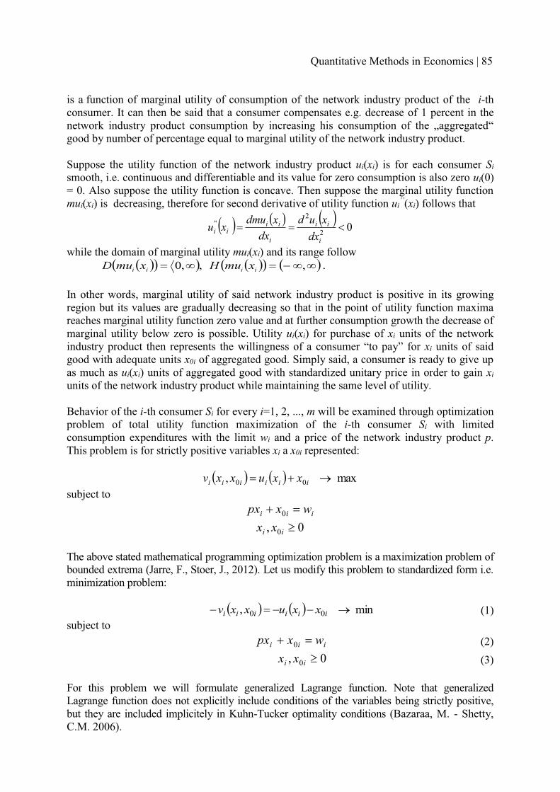
is a function of marginal utility of consumption of the network industry product of the i-th consumer. It can then be said that a consumer compensates e.g. decrease of 1 percent in the network industry product consumption by increasing his consumption of the „aggregated“ good by number of percentage equal to marginal utility of the network industry product.

Suppose the utility function of the network industry product ui(xi) is for each consumer Sismooth, i.e. continuous and differentiable and its value for zero consumption is also zero ui(0) = 0. Also suppose the utility function is concave. Then suppose the marginal utility function mui(xi) is decreasing, therefore for second derivative of utility function ui

’’(xi) follows that

� � � � � � 02

2'' ���

i

ii

i

iiii dx

xuddx

xdmuxu

while the domain of marginal utility mui(xi) and its range follow � �� � � � �� � �� .,,,0 33��3� iiii xmuHxmuD

In other words, marginal utility of said network industry product is positive in its growing region but its values are gradually decreasing so that in the point of utility function maxima reaches marginal utility function zero value and at further consumption growth the decrease of marginal utility below zero is possible. Utility ui(xi) for purchase of xi units of the network industry product then represents the willingness of a consumer “to pay” for xi units of said good with adequate units x0i of aggregated good. Simply said, a consumer is ready to give up as much as ui(xi) units of aggregated good with standardized unitary price in order to gain xiunits of the network industry product while maintaining the same level of utility.

Behavior of the i-th consumer Si for every i=1, 2, ..., m will be examined through optimization problem of total utility function maximization of the i-th consumer Si with limited consumption expenditures with the limit wi and a price of the network industry product p.This problem is for strictly positive variables xi a x0i represented:

� � � � max, 00 /�� iiiiii xxuxxvsubject to

iii wxpx �� 0

0, 0 4ii xx

The above stated mathematical programming optimization problem is a maximization problem of bounded extrema (Jarre, F., Stoer, J., 2012). Let us modify this problem to standardized form i.e. minimization problem:

� � � � min, 00 /���� iiiiii xxuxxv (1) subject to

iii wxpx �� 0 (2) 0, 0 4ii xx (3)

For this problem we will formulate generalized Lagrange function. Note that generalized Lagrange function does not explicitly include conditions of the variables being strictly positive, but they are included implicitely in Kuhn-Tucker optimality conditions (Bazaraa, M. - Shetty, C.M. 2006).

Quantitative Methods in Economics | 85

The generalized Lagrange function of the mathematical programming problem (1), ..., (3) is:

� � � � � �� � � �iiiiiii

iiiiiiiiiii

wxpxxxuwxpxxxvxxL

�����������

00

000 ,,,�

�� (4)

We formulate the Kuhn-Tucker optimality conditions for the Lagrange function (4) for the i-th consumer Si as follows

� � � � � �

� � � �

0 0 0

0

0 00

0

0

, , , , , ,0 0 0

, , , ,0 0 (5)

0 0

i i i i i i i i i i i i

i i i

i i i i i i i ii i

i i

i i

L x x L x x L x xx x

L x x L x xx x

x xx x

� � ��

� �

2 2 24 4 �

2 2 2

2 2� �

2 24 4

The Kuhn-Tucker optimality conditions (5) after using the analytical form of the Lagrange (4) and other updates we get:

� �� �� � � �

0

0

0

0 (a) 1 0 (d) (g)

0 (b) 1 0 (e) (6)

0 (c) 0 (f )

i i i i i i i

i i i i i i

i i

p mu x px x w

x p mu x x

x x

� �

� �

� 4 � 4 � �

� � � �

4 4

In other words if a consumer is willing to identify the optimal consumer strategy (xi*, x0i

*), that means that the consumption of xi

* units of the network industry product with a price p and the consumption of x0i

* units of remaining aggregated goods with price 1 maximize his total utility v(xi

*, x0i*), multiplier λi

* must exist, for which the Kuhn-Tucker optimality conditions (6) hold (Bazaraa, M. - Shetty, C.M., 2006), thus variables vector ( xi

*, x0i* , λi

*) is a solution to (a), (b), ..., (g).

We now point out certain interesting economically interpretable consequences of the Kuhn-Tucker optimality conditions in the context of consumer behavior analysis on the network industries market (Fendek, M. and Fendeková, E., 2012):

1. Condition (g) implies that optimum market basket of the i-th consumer ( xi*, x0i

*) at a price p of the network industry product and the price of aggregated good being 1can be purchased for customers budget wi.

2. Condition (e) implies that for positive optimum consumption of the aggregated good x0i*

the optimum value of the Lagrange multiplier is 1, i.e. λi* =1.

3. Condition (b) then implies that at positive consumption of the aggregated good x0i* and at

positive consumption of the network industry product xi* which maximizes utility

necessarily holds that in the point of maximum utility of the good its marginal utility equals its price, since Lagrange multiplier equals one λi

* =1 and holds

� � � � pdx

xduxmuii xxi

iii �'

)

%&(

$�

� *

* (7)

4. Consequence (3) also confirms another important theoretical postulate, namely that a consumer increases his consumption, of the network industry product in this case, until the marginal utility reaches the level of good’s market price.

86 | Multiple Criteria Decision Making XVIII

3 CONCLUSION

In this paper we examined the optimality conditions for the partial models of the consumer’sbehavior on the network industry market as well as the optimality conditions for the model of the product effective allocation on this market. We showed how the findings resulting from the Kuhn-Tucker optimality conditions analysis formulated for the relevant problems of mathematical programming can be effectively used to interpret the factual relations, principles and strategic decisions in consumer’s behavior on the network industry market.

Breaking of the equilibrium conditions can of course not be eliminated, the everyday economic life even expects some development and instability on every market and thus also the relative momentariness of the conditions validity, which in fact is not an unsolvable problem. It is however important to identify the situation competently and evaluate the possible reactions to the changed parameters of the system.

Therefore we showed that the use of the model approach and the optimization theory at the network industries market supply and demand equilibrium conditions analysis allows us to effectively study the equality conditions as well as the consequences of the market parameters change which results in reassessment of equilibrium attributes.

Acknowledgements: This article was published with a support of Scientific Grant Agency of the Ministry of Education of the Slovak Republic and of Slovak Academy of Sciences as a part of a project „Optimization Models and Methods as a Tool of an Effective Regulation in the Modern Theory of Network Industries Organization“, 2015 – 2017.

References [1] Blum, U., Müller, S. and Weiske von Gabler, A. (2006). Angewandte Industrieökonomik.

Theorien - Modelle – An-wendungen. Berlin: Verlag Gabler. [2] Bazaraa, M. and Shetty, C.M. (2006). Nonlinear Programming: Theory and Algorithms.

New York: Wiley-Interscience. [3] Carlton, D.W. and Perloff, J. M. (2005). Modern Industrial Organization. Boston:

Addison Wesley. [4] Fendek, M. and Fendeková, E. (2008). Mikroekonomická analýza. Bratislava: IURA

Edition. [5] Fendek, M. and Fendeková, E. (2010). Modely cenovej regulácie sieťových odvetví.

Ekonomický časopis, 58(10), pp. 1039–1055.[6] Fendek, M. and Fendeková, E. (2012). Podmienky optimálnosti Kuhna-Tuckera v

modeloch rovnováhy trhu sieťových odvetví. Politická ekonomie, 60(6), pp. 801–821.[7] Fendek, M. and Fendeková, E. (2009). Models of regulation of network industries in

Slovakia. International journal of economics and business research, 1(4), pp. 479–495.[8] Fendek, M. (2008). Natural monopoly cost-oriented price regulation. In: Quantitative

methods in economics (Multiple criteria decision making XIV). Bratislava: IURA EDITION, pp. 45–53.

[9] Jarre, F. and Stoer, J. (2004). Optimierung. Berlin: Springer Verlag. [10]Martin, S. (2012). Industrial Organization: A European Perspective. Oxford: Oxford

University Press. [11]Shy, Oz. (2001). The Economics of Network Industries. Cambridge: Cambridge

University Press.

Quantitative Methods in Economics | 87

Author’s addressMichal Fendek Department of Operations Research and Econometrics, University of Economics Bratislava Dolnozemska cesta 1/b 852 35 Bratislava Slovakia e-mail: fendek@dec.euba.sk

88 | Multiple Criteria Decision Making XVIII

UNEMPLOYMENT PERIOD QUANTITATIVE APPROACH THROUGH INFINITE SERVERS QUEUE SYSTEMS

Manuel Alberto M. Ferreira1, José António Filipe1, Manuel Coelho2

1Instituto Universitário de Lisboa (ISCTE-IUL), BRU-IUL, ISTAR-IUL, Portugal

2 Universidade de Lisboa (UL), SOCIUS/ISEG, SIRIUS/ISEG, Portugal

Abstract This paper stands over the (Ferreira, Filipe and Coelho, 2014) work. There using results on the infinite servers queue systems with Poisson arrivals - M|G|∞ queues - busy period, it ispresented an application of those queue systems in the unemployment periods time lengthparameters and distribution function study. It is now completed with an economic analysis aiming the evaluation of the assistance costs due. These queue systems are adequate to the study of many population processes, and this quality is brought in here. The results presented are mainly on unemployment periods length and their number in a certain time interval. Also, some questions regarding the practical applications of the outlined formulas are discussed.

Keywords: Infinite servers queues, busy period, unemployment. JEL Classification: C18 AMS Classification: 60G99

1 RISING THE MODEL In the queue systems used thoroughgoing this work

- The customers arrive according to a Poisson process at rate � ,

- Receive a service which time length is a positive random variable with distribution function � �.G and mean � ,

- Upon they arrive, each one finds immediately an available server1,

- Each customer service is independent from the other customers’ services and from the arrivals process,

- The traffic intensity is � ��� .

That is: they are | |M G 3 queues. It is easy to understand how these queues can be applied to the unemployment study. Then:

- � is the rate at which occur the firings, supposed to happen according to a Poisson process

- The service time, paradoxically, is the time between the worker firing and the moment he/she finds a new job.

1Or there is no distinction between the customer and its server, as it happens in the application to be considered in this work.

Quantitative Methods in Economics | 89

In any queue system, a busy period is a period that begins when a costumer arrives at the system finding it empty, ends when a costumer abandons the system letting it empty and in it there is always at least one customer present. So in a queuing system there is a sequence of idle and busy periods, during its operation time.

In the | |M G 3queue system, as in any queue system with Poisson arrivals, the idle periods have an exponentially distributed length with mean 1�� .

But the busy period’s distribution is much more complicated, being in general given by infinite sums which parcels are convolutions (Ferreira and Andrade, 2009). In spite of it, it is possible to present some results as it will be seen.

For what interests in this work

- A busy period is a period of unemployment

- An idle period is a period of full employment.

The results to be presented are on unemployment periods length and their number in a certain time interval.

A study in following also this approach, over a public health situation, can be seen in Ferreira (2014).

2 UNEMPLOYMENT PERIOD TIME LENGTH DISTRIBUTION Designate D the random variable unemployment period length. According to the results known for the | |M G 3 queue busy period length distribution, see (Ferreira and Andrade, 2009),

- - . 1 (2.1)eE D�

��

�

whichever is the worker unemployment time length distribution, see Takács (1962)

- As for - .Var D , it depends on the whole unemployment time length distribution probabilistic structure. But Sathe (1985) demonstrated that

(2.2)

where s, the unemployment time length coefficient of variation

- If a worker unemployment time length distribution function is

� � � �, 0, (2.3)

1 t

eG t te e e

�

� � �

�

� � �� 4

� �

the D distribution function is

90 | Multiple Criteria Decision Making XVIII

� � � � � �1 1 , 0 2.4 ,e tD t e e t�� ��� �� � � 4

see Ferreira (1991)

- If the unemployment time length of a worker is such that

� �1

11 , 0 (2.5)1

te

G t te e �

��� �� �

� �

� � 4� �

the D distribution function is

� � � � � �1

11 , 0 2.6 ,e tD t e t� �

�� �

� � 4

see (Ferreira, 1995)

- For � and � great enough (very intense unemployment conditions) since � �.G is

such that for � great enough � � 0, 0G t t5 4 ,

� � � �1 , 0 2.7 ,e tD t e t�� ��5 � 4

see (Ramalhoto and Ferreira, 1994).

Note:

- As for this last result, begin noting that many probability distributions fulfill the condition � � 0, 0G t t5 4 for � great enough. The exponential distribution is an example.

- As for the meaning of � and � great enough, computations presented in (Ramalhoto and Ferreira, 1994) show that for 1� � , after 10� � it is reasonable to admit (2.7) for many service time distributions.

Calling the mean number of unemployed people in the unemployment period, if � �.G is exponential

.

For any other � �.G probability distribution

see (Ferreira and Filipe, 2010). Of course, multiplying (2.8) or (2.9), as appropriate, by the mean cost of each unemployment subsidy it is possible to estimate the assistance costs caused by the unemployment period.

Quantitative Methods in Economics | 91

Be the probability that everybody is working at time t, being the time origin the unemployment period beginning. Being , where is the probability density

function associated to � �.G , the service time hazard rate function2,

,

see Proposition 3.1 in (Ferreira and Andrade, 2009). And calling the mean number of unemployed people at time t, being the time origin the unemployment period beginning instant

,

see Proposition 5.1 in (Ferreira and Andrade, 2009).

3 UNEMPLOYMENT PERIODS IN A TIME INTERVAL MEAN NUMBER After the renewal processes theory, see Çinlar (1975), calling ( )R t the mean number of unemployment periods that begin in - .0, t , being 0t � the beginning instant of an unemployment period, it is possible to obtain, see Ferreira (1995),

� �� � � �

0 0

1 1

0

(3.1)

t utG v dv G v dv

R t e e du� �

�� � � �$ % $ %( ) ( )� �

� � �

and, consequently,

� � � �1 1 (3.2),e t R t t� � �� � 0 0 �

see Ferreira (2004).

Also,

A) � � � �, 0

1 t

eG t te e e

�

� � �

�

� � �� 4

� �

� � 1 (3.3)R t e t�� �� �

B) � �1

11 , 0 1

te

G t te e �

��� �� �

� �

� � 4� �

� � � � � � � �211 1 3.4

teR t e e e t e e e ��

� � � � �� ��� � � � � �� � � � � �

C) � �0, 1,

tG t

t��

�#� " 4!

2That is: the rate at which unemployed people finds a new job.

92 | Multiple Criteria Decision Making XVIII

� � � �1,

1 , t

R te t t�

�� � ��

�#� " � � 4!

(3.5)

D) If the unemployment time length is exponentially distributed

� �1 1

(3.6)

t t

e e

e e t R t e t� �� �

�� �

� � � � � �� � � �� � � ��� � 0� 0 �

4 CONCLUSIONS So that this model can be applied it is necessary that the firings occur according to a Poisson process at constant rate. It is a hypothesis that must be tested. Thus remain outside of thisstudy, periods of unemployment caused by mass firings.Among the results presented, (2.1), (2.2), (2.7) and (3.2) are remarkable for its simplicity and also for requiring only the knowledge of the firings rate� , the mean unemployment time� ,and the unemployment time variance.

The other results are little more complex and demand the goodness of fit test for the distributions indicated to the unemployment times.

References [1] Çinlar, E. (1975). Introduction to Stochastic Processes. Englewood Cliffs, NJ: Prentice

Hall.[2] Ferreira, M. A. M.(1991). Um sistema M|G|3 com período de ocupação exponencial.

Actas das XV Jornadas Luso-Espanholas de Matemática (C. Braumann, ed.), Vol. IV, Universidade de Évora, Évora, 1991, D63-D66.

[3] Ferreira, M. A. M. (1995). Comportamento transeunte e período de ocupação de sistemas de filas de espera sem espera. PhD. Instituto Universitário de Lisboa (ISCTE – IUL).

[4] Ferreira, M. A. M. (2004). | |M G 3 queue busy cycle renewal function for some particular service time distributions. In: Proceedings of the International Conference Quantitative Methods in Economics (Multiple Criteria Decision Making XII). Bratislava: IURA EDITION, pp. 42-47.

[5] Ferreira, M. A. M. and Andrade, M. (2009). The Ties between the | |M G 3Queue System Transient Behaviour and the Busy Period. International Journal of Academic Research, 1(1), pp. 84-92.

[6] Ferreira, M. A. M. and Filipe, J. A. (2010). Economic Crisis: Using | |M G 3Queue Systems Busy Period to solve Logistics Problems in an Organization. China-USA Business Review, 9(9), pp. 59-63.

[7] Ferreira, M. A. M., Filipe, J. A. and Coelho, M. (2014). Unemployment Modelled Through M|G|∞ Systems. International Journal of Latest Trends in Finance and Economic Sciences, 4 (1), pp. 677-679.

[8] Ferreira, M. A. M. (2014). The pandemic period length modelled through queue systems.In: Proceedings of the International Conference Quantitative Methods in Economics (Multiple Criteria Decision Making XVII). Bratislava: Ekonóm, pp. 43-47.

[9] Ramalhoto, M. F. and Ferreira, M. A. M. (1996). Some further properties of the busy period of a | |M G 3queue. Central European Journal for Operations Research and Economics, 4 (4), pp. 251-278.

[10] Sathe, Y. S. (1985). Improved bounds for the variance of the busy period of the | |M G 3 queue. Advances in Applied Probability, 17(4), pp. 913-914.

Quantitative Methods in Economics | 93

[11] Takács L. (1962). An introduction to queueing theory. Oxford: Oxford University Press.

Authors’ addressesProfessor Catedrático Manuel Alberto M. Ferreira Instituto Universitário de Lisboa (ISCTE-IUL), Escola de Tecnologias e Arquitectura (ISTA), Departamento de Matemática, BRU-IUL, ISTAR-IUL Av. das Forças Armadas, 1649-026 Lisboa, Portugal Email: manuel.ferreira@iscte.pt

Professor Auxiliar com Agregação José António Filipe Instituto Universitário de Lisboa (ISCTE-IUL), Escola de Tecnologias e Arquitectura (ISTA), Departamento de Matemática, BRU-IUL, ISTAR-IUL Av. das Forças Armadas, 1649-026 Lisboa, Portugal Email: josé.filipe@iscte.pt

Professor Auxiliar com Agregação Manuel Coelho Universidade de Lisboa (UL), Lisbon School of Economics and Management, Departamento de Economia, SOCIUS/ISEG, SIRIUS/ISEG Rua Miguel Lupi, 20, 1249-078, Lisboa, Portugal Email: coelho@iseg.ulisboa.pt

94 | Multiple Criteria Decision Making XVIII

MULTI-CRITERIA DYNAMIC PROJECT PORTFOLIO

Petr Fiala, University of Economics, Prague

Abstract Project management is the discipline of planning, organizing, securing and managing resources to bring about the successful completion of specific project objectives. Project opportunities come in time and it is necessary to decide which will be accepted for creating a dynamic portfolio of projects and which will be rejected. Using of standard methods or trying to design and apply sophisticated methods based on quantitative analysis is possible for portfolio management. Selection of project portfolio is a dynamic multi-criteria decision-making problem under risk. The paper presents an approach for dynamic project portfolio management based on the Analytic Network Process (ANP) model. The ANP model consists of four basic clusters (projects, resources, criteria, time) with their elements and influences. An important factor of the proposed ANP model is time. Hybrid procedure for dynamics of the project portfolio management is proposed.

Keywords: projects, project portfolio, ANP, resources, criteria, dynamics

JEL Classification: C44 AMS Classification: 90B10

1 INTRODUCTION Projects are in accelerating world rhythm the right option of solving problems of lot of organizations. Project management is the discipline of planning, organizing, securing and managing resources to bring about the successful completion of specific project objectives. In an accelerating economic world, projects become tools for promoting the objectives of the organization. There is a very extensive literature on the management of individual projects and project portfolios. We start from a publication (Larson, Gray, 2011) that describes very clearly project management as a managerial process. Nothing is permanent, everything is temporary, and that makes pressure on companies to finish new products or services faster, cheaper and definitely not to fail. Risk is a very important factor in project management. Most project organizations exist in a multi-project environment. This environment creates the problems of project interdependency and the need to share resources. Ensuring alignment requires a selection process that is systematic, open, consistent, and balanced. All of the projects selected become part of a project portfolio that balances the total risk for the organization. Management of the project portfolio ensures that only the most valuable projects are approved and managed. The key to success in project portfolio management is to select the right projects at the right time (Levine, 2005). The project selection process is considered a major component of project portfolio management. This should be accompanied by periodically repeated inspections of project portfolio, which would identify projects that should be terminated. Effective portfolio management helps to achieve outperformance, making strategy real through organizational change. Strategic project portfolio management enables present a framework for organization to complete significant strategic projects. Portfolio management is a process. This process must improve over time. Building feedback into every stage of the process is critical for the improvement. To select a portfolio of projects are basically two approaches, one is based on standard methods used in practice, the second approach is based on searching and applying new sophisticated methods based on quantitative analysis. The paper focuses on the of project portfolio selection problem solved by applying sophisticated models. The aim is to develop a

Quantitative Methods in Economics | 95

general model, which would be completed for the specific needs of problems. This is not about managing individual projects, but their networks where relationships exist among projects. This paper aims to verify the ability to model and solve the problem of dynamic project portfolio using the Analytic Network Process (ANP) model.

2 PROJECT PORTFOLIO SELECTION PROBLEM The network economy is a term for today’s global relationship among economic subjects characterized by massive connectivity. The central act of the new era is to connect everything to everything in deep web networks at many levels of mutually interdependent relations, where resources and activities are shared, markets are enlarged and costs and risk are reduced. Network systems contain both positive and negative feedbacks. A variety of feedback processes create complex system behaviour (Fiala, 2006). The portfolio management domain encompasses project management oversight at the organization level through the project level. Full insight of all components of the organization is crucial for aligning internal business resources with the requirements of the changing environment. Project portfolios are frequently managed by a project office that serves as a bridge between senior management and project managers and project teams. Project opportunities come in time and it is necessary to decide which will be accepted for creating a dynamic portfolio of projects and which will be rejected (see Fig. 1).

Time Fig. 1: Dynamic flow of projects

The portfolio management domain encompasses project management oversight at the organization level through the project level. Full insight of all components of the organization is crucial for aligning internal business resources with the requirements of the changing environment. Project portfolios are frequently managed by a project office that serves as a bridge between senior management and project managers and project teams. Project opportunities come in time and it is necessary to decide which will be accepted for creating a dynamic portfolio of projects and which will be rejected (see Fig. 1) Project portfolio is set all projects that are implemented in the organization at that time. It is generally expected that the portfolio should be designed in such a way as to maximize the possibility of achieving the strategic goals of the company. This is consistent with the notion that portfolio selection problem is a multi-criteria decision making. The main goal of each project is to increase the value of the organization, so most managers prefer financial criteria for project evaluation. The most commonly used indicators include net present value, internal rate of return, payback period, rate of return. In addition to these financial indicators, however, in selecting a portfolio of projects should be taken into account other characteristics.

Lot of professionals tried to find sophisticated way to improve techniques for project management in different ways. The paper presents an approach for dynamic project portfolio management based on the ANP model.

P6 P5 P3 P1

P2 P4 P7

96 | Multiple Criteria Decision Making XVIII

3 ANALYTIC NETWORK PROCESS The Analytic Hierarchy Process (AHP) is the method for setting priorities. A priority scale based on reference is the AHP way to standardize non-unique scales in order to combine multiple performance measures. The Analytic Network Process (ANP) is the method (Saaty, 2001) that makes it possible to deal systematically with all kinds of dependence and feedback in the performance system. The well-known AHP theory is a special case of the Analytic Network Process. The ANP approach seems to be very appropriate instrument for project portfolio management. Another issue is the appropriate selection of clusters, which would be the basis of the basic model and their fulfillment by system elements. Another specific problem is the creation of sub - networks in the ANP model characterizing the specific important circumstances of the model. The current economic environment is characterized by significant changes. An important problem of the model will be to capture the dynamics that would represent appropriate change The ANP method is suitable for the determination of priorities in network systems where there are different types of dependencies between the elements of the system. Time dependent priorities play an increasingly important role in a rapidly changing environment of network systems. Long-term priorities can be based on time dependent comparisons of system elements. Short-term predictions can be based on using of compositional data exponential smoothing. A hybrid procedure that combines the advantages of both approaches is proposed. The structure of the ANP model for dynamic project portfolio (DPP) is described by clusters of elements connected by their dependence on one another. A cluster groups elements (projects, resources, criteria, time) that share a set of attributes. At least one element in each of these clusters is connected to some element in another cluster. These connections indicate the flow of influence between the elements (see Fig. 2). The ANP model consists of four basic clusters with their elements and influences:

Projects This cluster consists of potential alternatives of projects of which will be selected a dynamic portfolio. There are priorities among projects for inclusion in the portfolio. The cluster has connections to all other clusters. Resources Resources are necessary for the implementation of projects. Main resources are human resources between which are relations important for creating project teams. The cluster has connections to all other clusters. Criteria Projects are evaluated according to criteria which include benefits, opportunities, costs, and risks (BOCR). The cluster has connections to all other clusters. Time Time is measured in discrete units. Elements of other clusters vary in time and theirs values depend on the values in previous time periods.

Quantitative Methods in Economics | 97

Resources Criteria

Projects

Time

Fig. 2: Flows of influence between the elements

Sub-networks The basic ANP model is completed by specific sub-networks. The sub-networks are used to model important features of the DPP problem. The most important features in our ANP-based framework for DPP management are captured in sub-networks:

� dynamic flow of projects, � time dependent resources.

Dynamic flow of projects Project opportunities come in time and it is necessary to decide which will be accepted for creating a dynamic portfolio of projects and which will be rejected. The sub-network connects clusters: time and projects. Time dependent resources A specific sub-network is devoted to model time dependent amounts of resources. The time dependent amount of resources is given by. The sub-network connects clusters: time, resources and projects.

4 DYNAMICS OF ANP METHODAn important characteristic of project portfolio management is dynamics. Time dependent priorities in the ANP model can be expressed by forecasting using pairwise comparison functions (Saaty, 2007) or by predictions based on using of compositional data exponential smoothing (Raharjo, et al., 2009). Time-dependent comparisonsDynamic extensions of ANP method can work with time-dependent priorities in a networked system. There are two approaches for time-dependent pairwise comparisons:

� structural, by including scenarios � functional by explicitly involving time in the judgment process.

For the functional dynamics there are analytic or numerical solutions. The basic idea with the numerical approach is to obtain the time dependent principal eigenvector by simulation (Saaty, 2007). Judgment matrix in dynamic form

�(Z) = [

\��(Z) \��(Z) … \�Q(Z)\��(Z) \��(Z) … \�Q(Z)

⋮ ⋮ ⋮\Q�(Z) \Q�(Z) … \QQ(Z)

^.

Forecasting using pairwise comparison functions brings a problem with keeping the consistency of paired comparisons. A procedure based on exponential smoothing was designed, which is suitable for short-term predictions (Raharjo, et al., 2009).

98 | Multiple Criteria Decision Making XVIII

Compositional Data AnalysisThe compositional data are everywhere, where we need to work with data containing only relative information, which is useful for working with weights. The following operations are defined on the simplex space

%Q = _` = (��, ��, … , �Q), �� > 0, b = 1,2, … , c, ∑ ��Q��� = 1d.

Closure operator C(x): For any vector ` = (ef, eg, … , eh) ∈ klh

o(`) = p ef∑ eq

hqLf

, eg∑ eq

hqLf

, … , eh∑ eq

hqLf

r.

Perturbation: For any two vectors from simplex space X, Y ∈ sh

` ⊕ u = o(efvf, egvg, … , ehvh).Power transformation: For any vector from simplex space X ∈ sh and w ∈ kl

w ⊗ ` = o(efw, eg

w, … , ehw)

Difference: ` ⊖ u = ` ⊕ (−f ⊗ u)

Exponential smoothing with compositional data can be used for predicting weights in a short time: z+ = (H+�, H+�, … , H+Q), H+� > 0, b = 1,2, … , c, ∑ H+�

Q��� = 1,

Simple exponential smoothing Vector of observations at time t

`+ = (�+�, �+�, … , �+Q), �+� > 0, b = 1,2, … , c, ∑ �+�Q��� = 1,

elements of simplex space. Vector of predictions at time t

u+ = (~+�, ~+�, … , ~+Q), ~+� > 0, b = 1,2, … , c, ∑ ~+�Q��� = 1,

elements of simplex space. The formula for simple exponential smoothing of compositional data:

u+ = � ⊗ `+C� ⊕ (1 − �) ⊗ u+C�.Double exponential smoothing We introduce for trend modeling a vector of trend values �+, a vector of slopes �+, a smoothing constant 0 ≤ α ≤ 1, a trend constant 0 ≤ β ≤ 1.Formulas for double exponential smoothing of compositional data:

�+ = � ⊗ `+ ⊕ (1 − �) ⊗ (�+C� ⊕ �+C�),�+ = � ⊗ (�+ ⊖ �+C�) ⊕ (1 − � ) ⊗ �+C�,

u+ = �+C� ⊕ �+C�.Hybrid procedure For the prediction of time-dependent priorities ANP method we propose a hybrid procedure that combines the benefits of long-term forecasting of pairwise comparison functions and short-term weight predictions using exponential smoothing compositional data. This procedure also mutually enriches both procedures obtaining more accurate data. Both procedures were presented in the previous sections and here we limit ourselves to a brief summary of the hybrid procedure steps. Step 1: Formulation of pairwise comparison functions. Step 2: Testing and improving consistency of pairwise comparisons. Step 3: Collection of historical data by ANP priorities over time. Step 4: Using of compositional exponential smoothing. Step 5: Selection of the best coefficient α, β with lowest value of error. Step 6: Forecasting of priorities for next time periods. Step 7: Re-formulation of pairwise comparison functions based on short-run model. Go to Step 2.

Quantitative Methods in Economics | 99

5 CONCLUSIONS The paper presents a proposed methodology for dynamic project portfolio management. The basic ANP model with clusters (projects, resources, criteria and time) was created. The proposed ANP model captures the relationships between the clusters and their elements. An important factor of the ANP model is time. The paper proposes a hybrid procedure for time-dependent priority setting. The procedure is based on a combination of pairwise comparison functions and exponential smoothing. The methodology is verified on the projects of an engineering company. The experimental results will affect the specification, completing and extending the model.

Acknowledgements The research project was supported by Grant No. IGA F4/54/2015, Faculty of Informatics and Statistics, University of Economics, Prague.

References [1] Fiala, P. (2006). An ANP/DNP analysis of economic elements in today's world network

economy. Journal of Systems Science and Systems Engineering, 15(2), pp. 131-140. [2] Larson, E. W. and Gray, C. F. (2011). Project Management: The Managerial Process. 5th

ed. New York: McGraw-Hill. [3] Levine, H. A. (2005). Project Portfolio Management: A Practical Guide to Selecting

Projects, Managing Portfolios, and Maximizing Benefits. San Francisco: Jossey-Bas. [4] Raharjo, H., Xie, M. and Brombacher, A. C. (2009). On modeling dynamic priorities in

the analytic hierarchy process using compositional data analysis. European Journal of Operational Research, 194(3), pp. 834-846.

[5] Saaty, T. L. (1996). Decision making with Dependence and Feedback: The Analytic Network Process. Pittsburgh: RWS Publications.

[6] Saaty, T. L. (2007). Time dependent decision making; dynamic priorities in the AHP/ANP: Generalizing from points to functions and from real to complex variables. Mathematical and Computer Modeling, 46(7), pp. 860-891.

Author’s addressProf. RNDr. Ing. Petr Fiala, CSc., MBA University of Economics, Prague, Department of Econometrics W. Churchill Sq. 4, 130 67 Prague 3 Czech Republic email: pfiala@vse.cz

100 | Multiple Criteria Decision Making XVIII

MODELLING OF MIGRATION BASED ON SOCIOECONOMIC FACTORS

Ludvík Friebel, University of South Bohemia, Faculty of Economics Jana Friebelová, University of South Bohemia, Faculty of Economics

Abstract In our contribution we focused our attention on modelling the relationship between the migration in the given districts on the one side and the socioeconomic variables as explanatory variables on the other side. More concretely, our model considered severalsocioeconomic variables: average salary, unemployment, criminality, average length of incapacity to work, proportion of economically active inhabitants, registered entities, dwelling price and specific pollution in conjunction with transport accessibility of particular districts.The used data set was combined from different public sources. During the modelling process we respected the spatial character of the observed data in terms with the driving time.

Keywords: dwelling, economic activity, unemployment, average salary, specific pollution, multicriteria decision making, regression. JEL Classification: C51, C38AMS Classification: 62H11, 62P10, 93E24

1 INTRODUCTION The evaluation of regions has been recently analysed by many authors. The economic situation and life quality at the level of administrative districts (LAU1) of South Moravia is investigated, for example, by Živělová and Jánský [6]. In their work, life quality is assessed on the base of analysis of the population and unemployment increase. Moreover, the authors involve indicators of medical care and transport and technical infrastructure.

The same authors, in another work [7], investigate the development in regions (NUTS 3) primarily from the social aspects’ point of view. The quality of life in given regions is assessed in terms of the unemployment rate, the number of job applicants per one vacancy, the number of physicians per 1000 inhabitants, the number of completed flats and the length of road network. The data envelopment analysis model as a tool for the assessment of districts is used in work [1].

The assessment of the regions resp. regional disparities is considered by the Ministry of Regional Development of the Czech Republic within the scope of the WD-05-07-3 –Regional disparities Program in the availability and affordability of housing, their socioeconomic consequences and tools directed to decrease regional disparities, for more details see [3].

The above mentioned works focus on the comparison of the regions, with respect to particular aspects. In the scope of multicriteria regional evaluation, the output of the MasterCard Czech Centres of Development Project (http://www.centrarozvoje.cz) are considered to be important. The quality of life and economic potential of towns were assessed in this project using 11 selected indicators (Master CARD WordlWIDE, 2010), whose weights were determined empirically, see [4].

Quantitative Methods in Economics | 101

Furthermore, Kuprová and Kamenický [2] in their work deal with evaluation of life quality in the NUTS 3 regions. The evaluation is based on 47 particular indicators.

In our contribution, we focused our attention to modelling of a relationship between the migration in the given districts on one side and socioeconomic variables as explanatory variables on the other side. More concretely, our regression model considered several socioeconomic variables, resp. indexes in conjunction with price of dwelling, quality of transport services and environment.

In different multicriteria decision makings in the above mentioned works is used as a level of life quality a theoretical integral assessing criterion. In our work, we tried to substitute amigration instead of life quality. There is questionable how much migration reflects an attractiveness of a region and how can be explained with predictive variables. We use multinomial regression analysis method to study just this dependency.

The migration is dependent on many factors. These objective parameters are the secondary considering differences among regions. Let’s consider multiple differences between migration between regions surrounding Prague and Ústí nad Labem. Thus the importance of the location and implied socio-economic factors is permanently rising. As the elementary unit of localization of dwelling we have chosen the districts (LAU1).

2 MATHERIALS AND METHODSWe have evaluated the efficiency and development of 76 districts (NUTS-4, resp. LAU-1) in the Czech Republic, according to the selected criteria by the DEA method. We had to exclude the city of Prague from the model because of its exceptionality originating in the capital status and in the subsidy policy of the EU. In our contribution we considered three consequent years 2011, 2012 and 2013.

The first and the largest data set was obtained from the Czech Statistical Office. The data about air quality was obtained from Czech Hydrometeorological Institute. Average salary was estimated based on Statistics on Income and Living Conditions. The next dataset was obtained from a real estate agency server, where a comparison of dwelling prices in all districts of the Czech Republic is periodically published. The information about transport services we obtained from digital vector database of the Czech Republic ArcČR 500.

The unemployment (UN) is represented by percentage of unemployed people. This rate is derived as the ratio of the available job applicants registered at the Labour Office aged 15–64 to the whole population aged 15-64.

The criminality had to be related to population of particular district in order to eliminate influence of different number of inhabitants. In our contribution criminality (CR) represents the number of crimes per 10 thousand inhabitants. The source for this statistics is the Police Headquarters of the Czech Republic. For economically efficient regions, this indicator is often higher than the others.

The average length of incapacity to work (IW) is represented by the number of calendar days of incapacity to work per one registered event. The information about incapacity to work was provided by the Czech Social Security Administration.

The registered entities (RE) was related to population of particular district in order to eliminate influence of different number of inhabitants. For building a regression model we used number of registered entities per one thousand inhabitants.

The last index is the proportion of economically active inhabitants (EA). This indicator represents the proportion of economically active inhabitants, defined as a ratio of inhabitants aged from 15 to 64 to the whole population.

102 | Multiple Criteria Decision Making XVIII

The source data are available at http://www.czso.cz.

Environment is in our contribution represented with the sum of specific emissions of main pollutants (SE) involving solids, sulphur dioxide, nitrogen oxides, carbon monoxide (tone per km2). The source data are available at http://www.chmi.cz.

Average salary (AS) was estimated based on “Household incomes, expenditures and debts” which is periodicaly published by Czech Statistical Office within survey “Statistics on Income and Living Conditions”. This survey involves 8866 households in 2011, 8773 household in 2012 and 8275 household in 2013.

The quality of transport services is represented by two variables: the driving time from centre of district to the capital (TC) and driving time from centre of district and to the centre of region (TR). Both variables we obtained from the geographical information system and the above mentioned database ArcČR. This database is free downloadable at https://www.arcdata.cz/produkty/geograficka-data/arccr-500.

The last index representing dwelling is constructed as the average price of the flats sold in given district within considered years (PD). This entry was obtained from http://www.realitymorava.cz, where the comparison of dwelling prices in all districts of the Czech Republic is periodically published. Dataset consists from 238210 flats sold in year 2011, 201118 flats sold in year 2012 and 94779 flats sold in year 2013.

As mentioned earlier we tried to explain migration with the set of explanatory variables. Migration was obtained from the Czech Statistical office as net migration ratio which is the difference between immigrants and emigrants of a district in a period related to population.

We have considered a lot of predictive variables – indices. At first, we use classical linear regression methodology to construct a model in order to predict a net migration in the districts of the Czech Republic depending on the socio-economic variables as the explanatory variables. For dependent variable Y we can write following model formula:

~ = \ + ���� + ���� + ⋯ + �3�3 + �, (1)

where ξ is a sum of impact of the all explanatory variables that are not included in the model which follows N(0, σ). The regression coefficients were estimated with the ordinary least square method (OLS).

3 RESULTS At first we propose multiple regression model for complete set of explanatory variables. Only two variables were considered in the model as statistically significant – driving time to the capital (TC) and price of dwelling (PD) see Table 1. It is clear that with decreasing distances and driving time migration increases. Districts closer to the center of the republic are higher net migration than the others. Districts surrounding the capital are exceptional, because their migration is in years 2011 and 2012 higher than 20%. The average net migration in the whole Středočeský Region is 6.04 %.

2011 2012 2013β p-value Β p-value β p-value

TC -0.405050 0.000227 -0.318020 0.006736 -0.307458 0.007057PD 0.739390 0.000000 0.598789 0.000052 0.366019 0.005700

Table 1 Results of OLS regression

Quantitative Methods in Economics | 103

Dependence of net migration on price of dwelling is not surprising, because both variables interact. With increasing migration grows demand for flats and affects their price.

The above model suggests that the net migration depends only on those two variables and that it is not affected by the other. This result was a bit surprising. Therefore we have look also at the model of dwelling price.

2011 2012 2013β p-value β p-value β p-value

TC 0.291521 0.002382 0.296375 0.002981 0.246119 0.020331AS 0.324067 0.000881 0.291404 0.004457 0.223003 0.041780EA -0.237209 0.024512 -0.216857 0.048323 -0.204620 0.071151UN -0.258368 0.015235 -0.292813 0.008881 -0.292353 0.010778RE 0.444316 0.002612 0.409285 0.012678 0.248371 0.194400IW -0.171979 0.029799 -0.169850 0.044869 -0.185971 0.045799

Table 2 Results of OLS regression for price of dwelling

Considering price of dwelling as explained variable we found for all assessed years at requested significance level the four explanatory variables (see Table 2): driving time to capital (DC), average salary (AS), unemployment (UN) and average incapacity for work (IW). Influence of remaining two variables (proportion of economically active inhabitants (EA) and number of registered entities(RE)) are significant in first two assessed years, but in last years were from OLS model excluded.

4 CONCLUSIONS The above mentioned two regression models suggest us that the migration depends on several variables, but most of them are truly reflected in the dwelling price. For this reason, we can assume that the migration is ruled by the hierarchical model shown in Figure 1.

Figure 1: Hierarchical OLS for Explaining net migration

At the first level of the proposed hierarchical model, the dependency on driving time is as important as on price of dwelling which is not surprising. The level of importance is similar in all assessed years, see Table 1.

Looking at the lower level of the model in Table 2, we can divide the remaining explanatory variables into two separate groups. The first group consists of unemployment and incapacity to work. Both mentioned factors keep their significance in the set of explanatory variables. The second group is represented with explanatory variables with changing importance or significance. The influence of salaries on migration is decreasing; it suggests changes in

Migration

PD TC

AS EA UN RE IW TC

104 | Multiple Criteria Decision Making XVIII

preferences of population. But this index is included in all years. The importance of the share or economic active people is decreasing as well as the number of the registered entities. In the last year, those explanatory variables lost the requested significance level.

It is questionable if low prices of flats can stimulate immigration. The regression at the first level of hierarchical model shows the opposite. In many districts, where there are low prices of dwelling there is also low migration. The results show that the dwelling price is a consequence rather than a cause of migration. For this reason, we tried, in the second level of the model, to disaggregate further the price of dwelling in the variables that represent economic situation in particular districts.

References [1] Friebelová, J. and Friebel, L. (2011). Life quality evaluation in regions of the Czech

Republic according to selected criteria using the DEA method. Acta Universitatis Agriculturae et Silviculturae Mendelianae Brunensis, 59(4), pp. 87-96.

[2] Kuprová, L. and Kamenický, J. (2016). Multikriteriální hodnocení postavení krajů v rámci ČR v letech 2000 až 2004. Statistika, 43(4), pp. 303–315.

[3] Lux, M. and Sunega, P. (2007). Vliv podmínek bydlení na zamýšlenou migraci české populace za prací. Czech Sociological Review, 43(2), pp. 305–332.

[4] Master CARD WordlWIDE (2010). Česká centra rozvoje 2010. [online] Available at:http://www.centrarozvoje.cz/dokument/kompletni_vysledky_projektu_CCoC_2010.pdf [Accessed 18 October. 2010].

[5] Živělová, I. and Jánský, J. (2008). Analysis of life quality development in the administrative districts of South Moravia. Agricultural Economics, 54(9), pp. 431–439.

[6] Živělová, I. and Jánský, J. (2008). Analýza kvality života z pohledu sociálních a kulturních zdrojů v krajích České republiky. [online] Available at: http://www.mmr-vyzkum.cz/infobanka/DownloadFile/38628.aspx [Accessed 10 September. 2010].

Author’s addressIng. Ludvík Friebel, PhD. University of South Bohemia, Faculty of Economics, Department of Applied Mathematics and Informatics Studentská 13, České BudějoviceCzech Republic email: friebel@ef.jcu.cz

Quantitative Methods in Economics | 105

THE INNOVATIVE CLUSTERS IN THE EU: THE SENSITIVITY ANALYSIS OF THE SPATIAL WEIGHT MATRIX CONSTRUCTION

Andrea Furková University of Economics

Abstract The paper deals with spatial clustering of innovative activity across 245 NUTS2 European Union regions in 2010 and 2012. The patent applications were chosen as a proxy for innovative activity at the European Patent Office. Local Getis-Ord statistic was used to answer the main question whether the innovative activity performed in one region may be associated with the innovative activity in neighbouring regions. Based on this statistic so called “hot spots” and “cold spots” have been identified. The robustness of the results was checked by means of employing different forms of spatial weight matrices.

Keywords: Getis-Ord statistic, spatial analysis, research and development, patents

JEL Classification: O3, C1 AMS Classification: 91G20

1 INTRODUCTION In strategic document of the European Union (EU) - Europe 2020 [2] research and development (R&D) was denoted as a significant part of the EU's growth strategy. Nowadays, the innovation and the knowledge are regarded as essential forces for starting and fuelling the engine of growth. Moreover, most growth theories highlighted the importance of knowledge spillovers in process of economic progress within and across countries (see e.g. [11], [13]). The knowledge accumulation and the knowledge diffusion are often strongly localized into clusters of innovative firms, sometimes in close cooperation with public institutions such as research centres and universities. These clusters can be identified within and also across countries or regions. Thus, the study of flow of knowledge between geographic regions became more eminent and popular.

The spatial concentration of innovative activity originates from the essential nature of the innovation process. This statement was developed by Feldman [3] who pointed out to the following five facts about the innovation process: the uncertainty of the innovation process, the reliance on advances in scientific knowledge, the complexity of the innovation process, the importance of learning-by-doing and learning-by-using, and the cumulativeness of innovative activity. Evidently, the main aim of the R&D policy is an enhancement of the innovation output. However, what can be considered as innovation output is not so straightforward and it can be represented in various ways. The most common proxies of innovation output are used scientific publications and citations, patents or new products and processes. From the studies dealing with innovation clusters and knowledge spillovers can be mentioned e.g. [9], [6] or [7].

The aim of this paper is to evaluate spatial dependence process, i.e. evaluate the fact that innovative activity performed in one region may be associated with the innovative activity in neighbouring regions and to examine the existence of spatial innovative clusters in the EU.

106 | Multiple Criteria Decision Making XVIII

Our proxy for innovative activity refers to patent application at the EPO (European Patent Office) in 2010 and 2012. The existence of the potential clusters will be verified throughout the sensitivity analysis of the spatial weight matrix selection.

The rest of the paper is organized as follows: section 2 deals with methodological issues, section 3 presents empirical results based on local Getis-Ord statistics. The paper closes with concluding remarks.

2 METHODOLOGY In general, spatial association corresponds to the situation where observations or spatial units are non-independent over the space that means that nearby spatial units are associated in some way. Usually two common facts are declared as a potential reasons for why we would expect spatial dependence.

The first is that the administrative boundaries for collecting information do not accurately reflect the nature of the underlying process generating the data set. The second important reason is that the spatial dimension of socio-demographic, economic or regional activity may actually be an important aspect of a modelling problem. Spatial dependence is also called spatial autocorrelation. Spatial autocorrelation can be identified in a number of ways: Global and Local indicators of spatial association such as Moran’s I, Geary’s C (for more details see e.g. [8]) or Getis-Ord statistic. Getis-Ord statistic will be the main tool for our analysis and it will be presented in more details in subsection 2.2.

The starting point of any spatial analysis is the construction of the spatial weight matrix W.Let us denote N as the number of regions in the data set, then W is a square symmetric matrixNxN dimension and each element ijw of the matrix reflects the „spatial influence“ of unit j on unit i. For the construction of the matrix W, can be used a binary matrix or some geographic or economic proximity measure such as contiguity, physical distance or transportation costs between units. Thus, the relationship can be binary (1 is present, 0 if not) or variable. Diagonal elements of the matrix W are set to zero in order to exclude “self-influence”. The problem of spatial weight matrices will be discussed in subsection 2.1.

2.1 Spatial weight matrices The construction of the matrix W can be based either on the distance or the boundaries of the spatial units. In literature we can also find combined distance-boundary weights. Next, we will introduce only the spatial weight matrices used in our empirical part ([12], [4]):

� Weights Based on Distance This family of weight matrices is appropriate if distance itself is an important criterion of spatial influence. These matrices are based on the centroid distances ijd , between each pair of spatial units i and j. The most common weights based on distance are k-Nearest Neighbour Weights, Radial Distance Weights, Power Distance Weights or Exponential Distance Weights. From this group of weights, in our empirical part we exploit only Radial Distance Weights and therefore we present it in more details and it can be defined as follows:

If d denotes a threshold distance (or bandwidth) beyond which there is no direct spatial influence between spatial units, then the corresponding radial distance weight matrix W has spatial weights of the form:

Quantitative Methods in Economics | 107

1, 0

0, ij

ijij

d dw

d d0 0#6� " �6!

(1)

� Weights Based on Boundaries In many cases the boundaries shared between spatial units play an important role in determining degree of “spatial influence”. Most common weights based on boundaries are Spatial Contiguity Weights or Shared-Boundary Weights. From this group of weights we exploit in our empirical part only Spatial Contiguity Weights and therefore we present it in more details and it can be describe as follows:

These weights simply indicate whether spatial units share a boundary or not. If the set of boundary points of unit i is denoted by bnd(i) then the so-called queen contiguity weights are defined by

� � � �� � � �

1,

0, ij

bnd i bnd jw

bnd i bnd j

7 ��#6� "7 ��6!

(2)

Two units are neighbours in this sense if they share any part of a common border. Other forms of spatial contiguity weights could be e.g. rook or bishop contiguity.

2.2 Indicators of Spatial Autocorrelation Statistics mentioned before such as Moran’s I and Geary’s cannot distinguish so called hot spots and cold spots, they only indicate spatial clustering. Getis and Ord (see [5], [10])introduced a family of statistics G, that can distinguish spatial clusters. Global versions of this family of statistics are Getis-Ord General � �G d and � �*G d statistic (for more details see [5]

and [10]. The local versions of this family of statistics, � �G d and � �*G d , enable to detect pockets of spatial association that may not be evident when using global statistics. The statistic is calculated for each areal unit in the data. Each unit has an associated test statistic and we can also map which of the polygons has a statistically significant relationship with its neighbours, and show type of relationship. In [5], the statistic � �iG d is defined as follows:

� �� �

1

1

,

N

ij jj

i N

jj

w d xG d j i

x

�

�

� ��

�(3)

where � �� �ijw d is a symmetric binary spatial weight matrix with ones for all links defined as being within distance d of a given i and all other links are zero including the link of point i to itself. This statistic measures the degree of association that results from the concentration of weighted points (or area represented by a weighted point) and all other weighted points included within a radius of distance d from the original weighted point. � �*

iG d statistic

includes the value ix itself as well as “neighbourhood” values. Getis and Ord focused upon physical distances, but “distance” may be interpreted as travel time, conceptual distance, or any other measure that makes possible the N points to be located in a space of one or more dimensions. In [10], the statistics � �iG d , � �*

iG d and � �G d , � �*G d are extended to include variables that do not have a natural origin and non-binary weights are allowed.

108 | Multiple Criteria Decision Making XVIII

3 EMPIRICAL RESULTS The spatial analysis of innovative activities was performed for 245 NUTS 2 (Nomenclature of Units for Territorial Statistics) EU regions1 in 2010 and 2012. The data and corresponding shp file were retrieved from the Eurostat web page and the whole analysis was carried out in the software GeoDa. As a proxy for innovative activity we have chosen a patent applications (per million of inhabitants) at the EPO classified by inventor’s region in the EU. The main aim of this paper was to evaluate spatial dependence process, i.e. evaluate the fact that innovative activity (represented by patent applications) performed in one region may be associated with the innovative activity in neighbouring regions and to confirm the existence of spatial clusters of patent applications. The existence of the potential innovative clusters will be verified throughout the sensitivity analysis of the spatial weight matrix selection. The main tool for the analysis was local version of Getis-Ord statistic based on the equation (3).

Our calculations started with the contiguity queen´s case weight matrix (2) under the consideration. Gradually, the first, the second and finally the third order version of this matrix were used. Local � �iG d statistic was calculated for each region and the results are presented

by means of � �iG d cluster maps (see Figures 1 - 3).

These maps provide information which of the regions has a statistically significant relationship with its neighbours, and shows the type of this relationship. The calculations were done for two years – 2012 and 2010 in order to identify possible time trend changes. Our results indicate the existence of spatial innovative clusters in the EU. In 2012, high values of patent applications tend to cluster especially in the regions of Germany, Austria, Denmark and Luxembourg (first order queen case matrix). On the other hand, cold spots are significant in most of regions of post-communist countries and in the regions of Spain, Portugal, Greece and Italy. We can notice that using higher orders of the matrix have led to the increase number of hot spots and colds spots. The exploitation of different orders of queen’ case matrix allowed answering the question if the innovative activity carried out in one region spills over only to the physical neighbouring regions or also to the regions sharing a border with these first-order, second-order or third-order regions. Following our results this hypothesis can be supposed to be confirmed. The results for year 2010 have indicated relatively similar spatial pattern. Total number of hot and cold spots in 2012 was always greater that in 2010. Surprisingly, the difference between years 2010 and 2012 is that more North Europe regions are identified as hot spots in 2010.

1 We considered NUTS 2 regions of the EU corresponding to actual state in 2012. Due to the possible problems with isolated regions we excluded 20 island regions of Cyprus, Malta, France, Finland, Spain, Greece, Portugal and Italy. Another reduction of the data set had to be done due to missing data; we excluded 7 regions of Bulgaria, Germany and Greece.

Quantitative Methods in Economics | 109

(a) (b)

Figure 1: � �iG d Cluster Maps for the patent applications (per million of inhabitants) - Contiguity queen’s case weight matrix (the first order) – (a) year 2012 and (b) year 2010

(a) (b)

Figure 2: � �iG d Cluster Maps for the patent applications (per million of inhabitants) - Contiguity queen’s case weight matrix (the second order) – (a) year 2012 and (b) year 2010

(a) (b)

Figure 3: � �iG d Cluster Maps for the patent applications (per million of inhabitants) - Contiguity queen’s case weight matrix (the third order) – (a) year 2012 and (b) year 2010

110 | Multiple Criteria Decision Making XVIII

Analogous sensitivity analysis was made based on the distance weight matrix. We opted a distance weight matrix defined in (1) based on the Euclidian distance and Arc distance with threshold distance 420 km (420 km was the minimum value for which there will be no isolated observations). From the Figure 4 and Figure 5 we can see very similar spatial pattern for the Euclidian distance and Arc distance weight matrix. Also both years showed no significant changes in spatial innovative clusters in the EU regions. On the contrary, we found an apparent change in results in comparison with queen case matrix results, i.e. the number of hot and cold spots significantly increased in the case of the distance weight matrices.

(a) (b)

Figure 4: � �iG d Cluster Maps for the patent applications (per million of inhabitants) - Euclidian distance weight matrix – (a) year 2012 and (b) year 2010

(a) (b)

Figure 5: � �iG d Cluster Maps for the patent applications (per million of inhabitants) - Arc distance weight matrix (threshold distance 420 km) – (a) year 2012 and (b) year 2010

4 CONCLUSION In this paper we provided an empirical evidence of innovative spatial clusters in the EU. We tried to answer the question whether regional geographical proximity matters in explaining innovation activity. Following the results of local Getis-Ord statistics for patent applications we detected hot spots and cold spots. The sensitivity analysis of the results was based on the different orders of queen case contiguity weight matrices and two types of distance weight

Quantitative Methods in Economics | 111

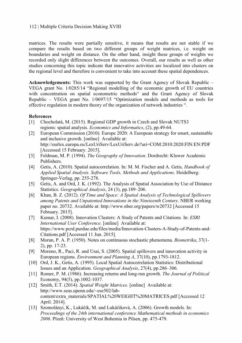
matrices. The results were partially sensitive, it means that results are not stable if we compare the results based on two different groups of weight matrices, i.e. weight on boundaries and weight on distance. On the other hand, insight these groups of weights we recorded only slight differences between the outcomes. Overall, our results as well as other studies concerning this topic indicate that innovative activities are localized into clusters on the regional level and therefore is convenient to take into account these spatial dependences.

Acknowledgements: This work was supported by the Grant Agency of Slovak Republic –VEGA grant No. 1/0285/14 “Regional modelling of the economic growth of EU countries with concentration on spatial econometric methods“ and the Grant Agency of Slovak Republic – VEGA grant No. 1/0697/15 “Optimization models and methods as tools for effective regulation in modern theory of the organization of network industries “.

References [1] Chocholatá, M. (2015). Regional GDP growth in Czech and Slovak NUTS3

regions: spatial analysis. Economics and Informatics, (2), pp.49-64. [2] European Commission (2010). Europe 2020: A European strategy for smart, sustainable

and inclusive growth. [online] Available at: http://eurlex.europa.eu/LexUriServ/LexUriServ.do?uri=COM:2010:2020:FIN:EN:PDF [Accessed 15 February. 2015].

[3] Feldman, M. P. (1994). The Geography of Innovation. Dordrecht: Kluwer Academic Publishers.

[4] Getis, A. (2010). Spatial autocorrelation. In: M. M. Fischer and A. Getis, Handbook of Applied Spatial Analysis. Software Tools, Methods and Applications. Heidelberg: Springer-Verlag, pp. 255-278.

[5] Getis, A. and Ord, J. K. (1992). The Analysis of Spatial Association by Use of Distance Statistics. Geographical Analysis, 24 (3), pp.189–206.

[6] Khan, B. Z. (2012). Of Time and Space: A Spatial Analysis of Technological Spillovers among Patents and Unpatented Innovations in the Nineteenth Century. NBER working paper no. 20732. Available at: http://www.nber.org/papers/w20732 [Accessed 15 February. 2015].

[7] Kumar, I. (2008). Innovation Clusters: A Study of Patents and Citations. In: ESRI International User Conference. [online] Available at: https://www.pcrd.purdue.edu/files/media/Innovation-Clusters-A-Study-of-Patents-and-Citations.pdf [Accessed 11 Jun. 2015].

[8] Moran, P. A. P. (1950). Notes on continuous stochastic phenomena. Biometrika, 37(1-2), pp. 17-23.

[9] Moreno, R., Paci, R. and Usai, S. (2005). Spatial spillovers and innovation activity in European regions. Environment and Planning A, 37(10), pp.1793-1812.

[10] Ord, J. K., Getis, A. (1995). Local Spatial Autocorrelation Statistics: Distributional Issues and an Application. Geographical Analysis, 27(4), pp.286–306.

[11] Romer, P. M. (1986). Increasing returns and long-run growth. The Journal of Political Economy, 94(5), pp.1002-1037.

[12] Smith, E.T. (2014). Spatial Weight Matrices. [online] Available at: http://www.seas.upenn.edu/~ese502/lab-content/extra_materials/SPATIAL%20WEIGHT%20MATRICES.pdf [Accessed 12 April. 2014].

[13] Szomolányi, K., Lukáčik, M. and Lukáčiková, A. (2006). Growth models. In:Proceedings of the 24th international conference Mathematical methods in economics 2006. Plzeň: University of West Bohemia in Pilsen, pp. 475-479.

112 | Multiple Criteria Decision Making XVIII

Author’s addressIng. Andrea Furková PhD.University of Economics in Bratislava, Faculty of Economic Informatics, Department of Operations research and Econometrics Dolnozemská 1/b, 852 35 BratislavaSlovak Republic Email: andrea.furkova@euba.sk

Quantitative Methods in Economics | 113

MUTUAL DEBT COMPENSATION AS A MINIMIZATION PROBLEM

Pavel Gežík, University of Economics in Bratislava,Tomáš Domonkos, University of Economics in Bratislava,

Andrej Babej, University of Economics in Bratislava

Abstract The mutual debt compensation problem allows a particular group of agents (persons, households, companies, regions or states) to clear off their debts directly or indirectly. This research presents a novel approach based on linear programming, which aims to minimize the debt remaining in the system. This method seems more straightforward than the usually applied one which aims to maximize the total debt cleared off. Furthermore, we assume a mandatory bi-directional relationship between agents, which generates a broader set of potential solutions compared to unidirectional systems. The efficiency of the approach is tested on a randomly generated sample of ten cases. The results show, that the proposed approach is able to reduce the indebtedness of the tested systems in average by 78%.

Keywords: mutual debt problem, linear programming, GAMS

JEL Classification: C61, C63 AMS Classification: 90B99

1 INTRODUCTION The mutual debt compensation problem has been subject to discussion in the Czech Republic and Slovak Republic since the beginning of the nineteen-nineties. It allows a particular group of agents (persons, households, companies, regions or states) to clear off their debts directly or indirectly. In the literature two mainstream approaches have been discussed. The first one is based on linear programing and aims to maximize the compensated debt in the system (Fecenko, 1994; Gazda 2001, 2015). The second group of approaches were based on graph theory, relying on the cycle cancelation method in a digraph (Domonkos, 2005; Gazda, 2015). The approach presented here relies on the assumption, that new credit-debt relationships may be generated. We term this as flexible credit-debt structure. System with new credit-debt structures was previously discussed by Gazda (Gazda 2000). This approach leads to broader set of solutions, thus the amount of debt cleared off can be higher compared to the systems assuming rigid credit relationships.

Furthermore, instead of maximizing the debt cleared of, we aim to minimize the remaining debt in the system. This approach is more straightforward and easy to understand. Furthermore, it may save computational resources. We test the efficiency of the results on ten hundred randomly generated cases.

2 MODEL The mutual debt compensation with flexible credit structure assumes existence of a weighted digraph D=(V,E,d) and �: � → :��. The weights ��," assigned to each particular edge represents the debt of agent i towards agent j.1 The considered system is fair, therefore, the credit-debt ratio should remain unchanged after the optimization procedure compared to the original balance for all the agents as well as the system (Gazda et al., 2015).

1 If there is no debt relationship between two agents, then ��," = 0.

114 | Multiple Criteria Decision Making XVIII

The assumption of new debt structure requires an adjusted weighted complete digraph G=(V,E,c) and 2: � → :�� by adding an artificial number & ≫ �\��,"∈���," to each particular weighted edge.

2�" = ���," + & ∀ b ≠ �

0 ∀ b = �

Then the fairness in terms of G requires holding unchanged the condition∑ ��," − ∑ �",�

3"

3"�� = ∑ 2�," − ∑ 2",�

3"��

3"�� throughout the entire optimization procedure for all

particular agents. The total debt after compensation remaining in the system can be then defined as �(�) = ∑ ∑ 2�,"��,"

3"��

3��� , where ��," ∈ ⟨0,1⟩ and denotes the share on total debt

after compensation in percentage terms. The result of the mutual debt compensation is then (1 − ��,")2�," and the original balance of the agent should remain constant∑ 2�,"!1 − ��,"# = ∑ 2",�(1 − �",�)3

"��3"�� for ∀ b = 1,2, … , .. The graph G can be represented

by matrix � = !2�,"# which we in fact use in the calculations. The minimization problem of the remaining debt can be formulated as follows:

min → �(�) = � � ~�,"

3

"��

3

���~�," = 2�,"��,"

� 2�,"!1 − ��,"# − � 2",�!1 − �",�#3

"��

= 03

"��

; b = 1,2, … , .

��," ∈ ⟨0,1⟩

3 RESULTS AND DISCUSSIONThe model’s performance is tested on ten randomly generated cases. We consider systems with ten agents. The debts are generated according to six different random distributions.

Table 1 Distribution used to generate mutual debt structures Position in sequence Distribution

1. Exponential with D = 22. Normal(4;1)3. Normal(7;1,5)4. Normal(9;2,5)5. Normal(15;4)6. Normal(25;5)

The procedure consists of two steps. In the first one the decision, which particular distribution from the six above mentioned is applied to generate the debt between two particular agents is taken in compliance with an exponential distribution with parameter D = 1,5. We round up the values generated from one till five and the numbers higher than five are modified to six.Then this number is used to select a particular distribution according to Table 1 which then generates the particular weight. This procedure allows the generation of structures with low number of extreme cases and frequent occurrence of zeros. This is one particular assumption we set on the structure, but we aim to test in future work a wider range of systems with different assumptions.

Quantitative Methods in Economics | 115

The program code from GAMS for one particular tested example: Sets i index uzla /1*10/ Alias(i,j) Sets offdiag1(i,j); offdiag1(i,j)=yes; offdiag1(i,i)=no; Table c(i,j) 1 2 3 4 5 6 7 8 9 10 1 0 22 20 21 20 25 20 21 20 21 2 21 0 20 21 23 25 20 21 25 21 3 21 20 0 20 20 26 25 20 25 20 4 21 21 20 0 20 20 20 26 21 21 5 21 24 25 21 0 25 21 23 24 24 6 21 20 25 25 27 0 22 20 27 24 7 20 24 21 20 22 20 0 24 24 20 8 24 20 20 24 21 27 24 0 25 21 9 25 21 20 25 21 21 24 20 0 25 10 20 20 24 20 21 27 20 22 27 0; Scalar n; n=card(i); Variables f,x,y; x.lo(i,j)=0; x.up(i,j)=1; positive variable y; Equations ohr1(i,j) ohr2(i) ucel; ucel.. f=e=sum((i,j),y(i,j)); ohr1(i,j)..y(i,j)=e=c(i,j)*x(i,j); ohr2(i)..sum(j,c(i,j)*(1-x(i,j))$offdiag1(i,j))-sum(j,c(j,i)*(1-x(j,i))$offdiag1(j,i))=e=0; Model VZD/all/; Solve VZD using lp minimizing f; Display x.l; Display y.l;

Results from GAMS after the optimization procedure in percentage terms.

LP status(1): optimal Optimal solution found. Objective : 33.000000 VARIABLE x.L 1 4 6 7 9 2 0.095 0.120 3 0.038 0.040 5 0.542 8 0.167 0.208 10 0.148 VARIABLE y.L 1 4 6 7 9 2 2.000 3.000 3 1.000 1.000 5 13.000 8 4.000 5.000 10 4.000

116 | Multiple Criteria Decision Making XVIII

The solution from GAMS may be expressed in its reduced form ~�,". The initial indebtedness of the system before compensation was 197 and after the optimization procedure with new debt structures the remaining debt is 33.

Table 2 Results after the compensation with new debt relationshipsAgent a1 a2 a3 a4 a5 a6 a7 a8 a9 a10

a1 0 0 0 0 0 0 0 0 0 0a2 0 0 0 2 0 0 0 0 3 0a3 0 0 0 0 0 1 1 0 0 0a4 0 0 0 0 0 0 0 0 0 0a5 0 0 0 0 0 0 0 0 13 0a6 0 0 0 0 0 0 0 0 0 0a7 0 0 0 0 0 0 0 0 0 0a8 4 0 0 5 0 0 0 0 0 0a9 0 0 0 0 0 0 0 0 0 0a10 0 0 0 0 0 4 0 0 0 0

Source: Author’s own calculations.

The results of the optimization after applying the model on ten simulated systems showed significant reduction of debt for all particular debt structures. The average reduction was almost 79%, whilst the results vary from the range of 70% till 84%. It is important to bear in mind, that different systems might have higher or lower reduction rates. However, if we assume, that there are no administrative and legislative boundaries then an economic sector’s indebtedness may be reduced substantially. Thus, the impact of such measure on the business environment can be considered rather positive.

Table 3 Results from the ten randomly simulated structures Matrix Amount of Debt Reduction of Debt Final Debt % of ReductionM1 197 164 33 83,25%M2 240 189 51 78,75%M3 219 175 44 79,91%M4 254 210 44 82,68%M5 252 202 50 80,16%M6 212 148 64 69,81%M7 275 207 68 75,27%M8 240 178 62 74,17%M9 231 182 49 78,79%M10 215 180 35 83,72%Average 78,65%

Source: Author’s own calculations.

4 CONCLUSION The mutual debt compensation problem has great potential of solving indebtedness ofinterconnected agents. The recent crises period (economic, financial and banking, etc.) opened the door for new innovative approaches of mitigating their impact. This research focuses on problems which assume flexible debt structures, therefore higher level of elimination can be achieved in terms of debt remaining in a particular system.

Quantitative Methods in Economics | 117

Furthermore, if a system has no cycles, the standard approaches cannot eliminate any debt, but the flexible approach can overcome this issue and reduce the total indebtedness of the system. We do believe that the methods proposed until now has not achieved the higher efficiency as the approach presented in this paper in terms of remaining debt. We aim to test the results in greater detail in our next research.

References [1] Domonkos, T. (2006). O riešení problému druhotnej platobnej neschopnosti metódou

započítavania pohľadávok a záväzkov, ŠVOČ. University of Economics, Bratislava,.[2] Fecenko, J. (1994). K optimalizácii operácií zápočtov pohľadávok a záväzkov po lehote

splatnosti. Journal of Economics 42(5)., p. 360–374.[3] Gazda, V., Horváth, D. and Rešovský, M. (2015). An Application of Graph Theory in the

Process of Mutual Debt Compensation. Acta Polytechnica Hungarica 12(3), p. 7–24.[4] Gazda, V. (2001). Mutual Debts Compensation as Graph Theory Problem. Trends in

Mathematics, Mathematical Finance, p. 162–167.[5] Gazda, V. (2000). Mutual debts compensation as graph theory application. Callenges for

business administrators in the new millennium. Gökçeada - Çanakkale, Turkey, SilesianUniversity, p. 521–526. [online] Available at:http://www.opf.slu.cz/vvr/akce/turecko/pdf/SLGazda.pdf. [Accessed 8th April 2016]

Author’s address

Ing. Pavel Gežík, PhD. University of Economics in Bratislava, Faculty of Economic Informatics, Department of Operations Research and Econometrics Dolnozemská 1/b, 852 35 BratislavaSlovak Republic email: pavel.gezik@euba.sk

Ing. Tomáš Domonkos, PhD. University of Economics in Bratislava, Faculty of Economic Informatics, Department of Operations Research and Econometrics Dolnozemská 1/b, 852 35 BratislavaSlovak Republic email: tomas.domonkos@euba.sk

Ing. Andrej Babej University of Economics in Bratislava, Faculty of Economic Informatics, Department of Operations Research and Econometrics Dolnozemská 1/b, 852 35 BratislavaSlovak Republic email: andrej.babej@euba.sk

118 | Multiple Criteria Decision Making XVIII

MATHEMATICAL MODEL FOR CREATION OF FLIGHTTIMETABLE WITH SEVERAL TIME SLOTS IN CONDITIONS OF

CHARTER AIRLINE

Vojtěch Graf, VŠB - Technical University of Ostrava, Dušan Teichmann, VŠB - Technical University of Ostrava,

Michal Dorda, VŠB - Technical University of Ostrava

Abstract In transport, mathematical modelling methods are often applied to optimize transport processes. Optimization goals can differ; they depend on the task we want to optimize. However, we can often meet with the problem that a mathematical model cannot be solved exactly. This fact often happens when the mathematical model is formed by many variables and constraints – these two elements determine how the mathematical model is large. The most sensitive models are the models containing integer or bivalent variables. The article is focused on an estimation of solvability limits for which the linear programming model of optimal aircraft scheduling for a charter airline is still solvable.

Keywords: Mathematical modelling, linear programming, aircraft scheduling

JEL Classification: C61 AMS Classification: 90C08

1 INTRODUCTION The article is focused on an experimental research into solvability of an optimization model which is intended for planning aircraft scheduling in situations when two mutually disjunctive time intervals are given for each flight. It holds that each flight has to depart in one of the time intervals. The research is important because the mathematical model mainly contains bivalent variables. Adding binary variables in a mathematical model usually increases a computational time that is necessary to solve the model. It may happen that such model is not able to give an optimal solution within a given time limit.

2 STATE OF THE ART In order to solve many practical problems, especially problems relating to planning or coordination in transport, different optimization methods based on mathematical modelling can be employed. The presented problem belongs to the group of vehicle scheduling problems. Most often, such models are applied in bus transport [1], [2] or [3]. In railway transport we can mention for example paper [4]. In air transport, optimization methods are often used to plan flight scheduling, crew scheduling or maintenance [5]. In literature, we can often meet with various combinations of the task mentioned earlier in the article. The authors of article [6] combine flight scheduling problem with crew scheduling problem. We can also meet with a combination of flight scheduling problem with maintenance scheduling [7].

To solve all the above mentioned problems linear programming methods, dynamic programming methods or various heuristics are used [8].

The article follows in previously published articles [9], [10] and [11]. In article [9]a modification of the mathematical model is presented; in the model it is assumed that for each flight only single time interval for its departure is given.

Quantitative Methods in Economics | 119

The time interval is defined so that the flight is dispatched during a requested day. In article [10] changes in calculation times are tested depending on the number of the flights that should be dispatched. Article [11] is devoted to a modification of the model in which it is assumed that each flight can be dispatched in mutually disjunctive time intervals (or slots); the modification presented in the article works with two possible time slots for each flight departure. In all the articles linear programming methods are employed to solve the problem. The total number of the aircraft assigned to the planned flights represents an optimization criterion in the articles.

3 MATHEMATICAL MODEL Let us formulate the task to be solved. Let a set of flights I be given, the set I consists of all the flights that have to be dispatched. For each flight a set of time slots J is given, each flight has to depart in one of the given time slots. Set J is assumed to have two elements (that means each flight can depart in one of two mutually disjunctive time slots). For each flight

Ii� value jid , is defined – the value represents a lower bound of time slot j=1,2 – and value

jih , is given – it defines an upper bound of time slot j=1,2.

For each flight its flight time iT and a time i8 that is necessary for preparation the aircraft for a consecutive flight (the minimum time the aircraft must spend at the airport after serving a flight) are known. Our task is to decide about departure times of the individual flights and to find out their order in which the individual flights should be served by the aircraft so that the number of the aircraft assigned to the flights is as minimal as possible.

To model such decisions we must define variables in the mathematical model. It was necessary to define three groups of variables. The first group of the variables – variables jix ,

– models decisions about relationships between flights � �09� Ii and Ij � .If 1,0 �jx then a new aircraft is assigned to flight Ij � . If 1, �jix for Iji �, and ji � ,then the aircraft serves flight j after serving flight i (that means flights i and j are served by the same aircraft in order i→j). The second group of variables – variables it – models the departure times of the individual flights to final destinations. The last group of variables –variables iz – give information which time slot is chosen for each flight. If 1�iz , then slot time 1 is chosen for flight Ii� (that means the flight departs in time interval 1,1, ; ii hd );

if 0�iz , then slot time 2 is chosen for flight Ii� (that means the flight is dispatched in time slot 2,2, ; ii hd ). Symbol T which is used in the model represents a so-called prohibitive constant. The mathematical model has the following form:

��

�Ij

joxzxtf ,),,(min (1)

subject to:

� ��9�

�0

, 1Ii

jix Ij� (2)

1, 0��Ij

jix Ii� (3)

)1()( , ��4��� jiiiij xTTtt 8 IjIi �� , (4)

120 | Multiple Criteria Decision Making XVIII

iiiii tzdzd 0���� )1(2,1, JjIi �� , (5)

iiiii tzhzh 4���� )1(2,1, JjIi �� , (6)0, �iix Ii� (7)� �1,0, �jix � � IjIi �9� ,0 (8)

04it Ii� (9)� �1,0�iz Ii� (10)

Optimization criterion (1) quantifies the number of the aircraft we need to serve all the planned flights. The group of constraints (2) models that each planned flight has to be dispatched. The group of constraints (3) ensures that only single task is assigned to the aircraft after serving the flight. That means the aircraft can be assigned to another consecutive flight (if it is admissible in terms of time) or the aircraft is idle (put out of operation). The group of constraints (4) ensures that assigning the aircraft to the consecutive flight is admissible in terms of time. The groups of constraints (5) and (6) secure that each flight departs only in the pre-defined time slots. The group of constraints (7) ensures that the same flight is not assigned to the same aircraft two times. The groups of constraints (8), (9) and (10) represent domains of definition of all the variables used in the model. The number of the variables is equal to

mm 32 � (including mm 22 � binary variables) and the number of the constraints in the model equals to mm 102 2 � , where m is the number of the flights (the number of the elements of set I).

4 EXPERIMENTAL PART Computational experiments were carried out using a model example. The computational experiments were run on a student (demo) version of optimization software Xpress-IVE [12]. To conduct the experiments we employed a personal computer with the following parameters: AMD-8300 Eight-Core 3.3 GHz processor and RAM 8GB.

In the article results of two experiments are presented. The first experiment was aimed at finding out how the calculation times depend on the number of the planned flights. A similar problem was also studied in article [10], but the experiments differ in the modification of the model (in article [10] the model without variables zi was used). The second experiment was devoted to an investigation how the calculation times depend on a width of the individual time slots.

Table 1 summarizes input data regarding the individual planned flights – the flight times and the times for flight preparation.

Flight i 1 2 3 4 5 6 7 8 9 10 11 12 13 14 15 16Ti 100 150 180 120 110 130 100 140 165 135 120 115 155 125 145 120τi 45 70 80 60 50 60 40 60 70 60 55 60 65 60 65 55

Table 1: Input data - the flight times and the times for flight preparation

Quantitative Methods in Economics | 121

Table 2 summarizes input data regarding the time slots (the lower and upper bounds) for the first experiment.

Flight i di,1 hi,1 di,2 hi,21 0 1140 420 14402 300 120 540 13203 360 900 540 12004 540 1260 720 13505 480 1320 960 14406 150 720 300 11407 240 1140 450 13208 360 720 720 13209 180 900 360 1020

10 420 1200 660 138011 60 1260 250 138012 960 1080 1080 120013 300 420 420 54014 120 1080 660 132015 480 1260 540 132016 500 1000 600 1200

Table 2: Input data – the time slots for the first experiment

It is presumed that all the flights have to depart during a day (24 hours), therefore values jid , and jih , can take values only from interval 1440,0 . The values of all the variables are

expressed in minutes.

4.1 Results of the first experiment The calculation times were tested on examples with selected numbers of the flights. The first experiment consists of 12 examples – see its results in Table 3. The experiment started with 5 planned flights because we did not expect any calculation difficulties for lower number of the flights.

5 6 7 8 9 10 11 12 13 14 15 16

ct [s] 0.1 0.1 0.1 0.2 3.3 9.4 285.2 166.4 78.0 327.7 33937.2 -

Table 3: The calculation times

As you can see in Table 3, for 16 flights we did not obtain an optimal solution after 86 400 seconds, therefore the experiment was stopped. The calculation times can be depicted in a graph – see Figure 1. Please note that the y-axis has a logarithmical scale in order to be able to present all the results in the same graph. We can say that the calculation times increase exponentially with the increasing number of the planned flights. However due to the logarithmical scale of the graph the exponential dependence is not so visible in Figure 1.

122 | Multiple Criteria Decision Making XVIII

0,1

1

10

100

1000

10000

100000

5 6 7 8 9 10 11 12 13 14 15

The

calc

ulat

ion

time

The number of the fl ights

Figure 1: The dependence of the calculation time on the number of the flights

Another piece of information we got by the first experiment is the number of the aircraft we need to serve all the planned flights. If the number of the flights is 5 up to 8, only single aircraft is needed to serve all the flights. If we must serve 9 and more flights, we need two aircraft to be able to serve the flights – see Table 4.

5 6 7 8 9 10 11 12 13 14 15 16Aircraft needed 1 1 1 1 2 2 2 2 2 2 2 -Table 4: The number of the aircraft needed to serve the flights

Tables 5 up to 8 present the results of the optimization calculations we got for 5, 9, 12 and 15 flights. We present only these selected results because of page limitations of the article. Please note that the flight denoted with 0 represents beginning of the aircraft operation or its ending (putting the aircraft out of operation). In the tables you can see the order in which the planned flights should be served. For example the order for 5 flights (Table 5) is 0→5→2→3→4→1→0; all the flights can be served by the single aircraft.

Flight Time slots ti zii j 1. 2.0 5 - - - -5 2 480-960 1320-1440 620 12 3 300-540 120-1320 780 03 4 360-540 900-1200 1000 04 1 540-720 1260-1350 1260 01 0 0-420 1140-1440 1440 0

Table 5: The results for 5 planned flights

Flight Time slots ti zii j 1. 2.0 3 - -3 4 360-540 900-1200 360 14 9 540-720 1260-1350 620 19 1 180-360 900-1020 940 01 2 0-420 1140-1440 1175 02 0 300-540 120-1320 1320 00 5 - - - -5 8 480-960 1320-1440 480 18 6 360-720 720-1320 720 06 7 150-300 720-1140 920 07 0 240-450 1140-1320 1320 0

Table 6: The results for 9 planned flights

Quantitative Methods in Economics | 123

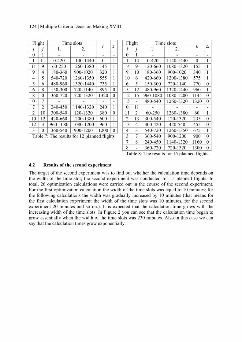
Flight Time slots ti zii j 1. 2.0 1 - - - -1 11 0-420 1140-1440 0 111 9 60-250 1260-1380 145 19 4 180-360 900-1020 320 14 5 540-720 1260-1350 555 15 6 480-960 1320-1440 735 16 8 150-300 720-1140 895 08 0 360-720 720-1320 1320 00 7 - - - -7 2 240-450 1140-1320 240 12 10 300-540 120-1320 380 010 12 420-660 1200-1380 600 112 3 960-1080 1080-1200 960 13 0 360-540 900-1200 1200 0Table 7: The results for 12 planned flights

Flight Time slots ti zii j 1. 2.0 1 - - - -1 14 0-420 1140-1440 0 114 9 120-660 1080-1320 155 19 10 180-360 900-1020 340 110 6 420-660 1200-1380 575 16 5 150-300 720-1140 770 05 12 480-960 1320-1440 960 112 15 960-1080 1080-1200 1145 015 - 480-540 1260-1320 1320 00 11 - - - -11 2 60-250 1260-1380 60 12 13 300-540 120-1320 235 013 4 300-420 420-540 455 04 3 540-720 1260-1350 675 13 7 360-540 900-1200 900 07 8 240-450 1140-1320 1160 08 - 360-720 720-1320 1300 0Table 8: The results for 15 planned flights

4.2 Results of the second experiment The target of the second experiment was to find out whether the calculation time depends on the width of the time slot; the second experiment was conducted for 15 planned flights. In total, 26 optimization calculations were carried out in the course of the second experiment. For the first optimization calculation the width of the time slots was equal to 10 minutes; for the following calculations the width was gradually increased by 10 minutes (that means for the first calculation experiment the width of the time slots was 10 minutes, for the second experiment 20 minutes and so on.). It is expected that the calculation time grows with the increasing width of the time slots. In Figure 2 you can see that the calculation time began to grow essentially when the width of the time slots was 230 minutes. Also in this case we can say that the calculation times grow exponentially.

124 | Multiple Criteria Decision Making XVIII

0100020003000400050006000700080009000

1000011000120001300014000

0 20 40 60 80 100 120 140 160 180 200 220 240 260

Calcu

latio

n tim

e

Width of the time slots

Figure 2: The dependence of the calculation time on the width of the time slots

The second experiment also revealed that the width of the time slots has an effect on the number of the aircraft we need to serve all the planned flights. If the width of the time slots was from 10 up to 70 minutes, then 3 aircraft were needed to serve the flights. If the width of the time slots was at least 80 minutes, then only 2 aircraft are necessary to serve 15 planned flights.

5 CONSLUSIONS The article is aimed at the creation of the flight timetable using mathematical modelling methods. In order to plan how the given set of the flights should be served, the mathematical model has been formed; in the model it is assumed that flights can depart only during pre-defined time slots – for each flight two time slots were defined. The mathematical model consists of the binary variables therefore the calculation time grows essentially with the increasing number of the planned flights. That is the reason why we decided to carry out the experiments presented in the article; both experiments were aimed at the investigation how the calculation time depends on some parameters of the model. All the optimization calculations were conducted using optimization software Xpress-IVE. The mathematical model is intended for flight timetable planning within a period of a day. It is also assumed that each aircraft has its capacity enough to serve the individual flights.

The first experiment revealed that in the case of the mathematical model presented in the article 15 flights is the limit. The calculation time for 15 flights was 33937.2 seconds. For 16 flights we found out that we were not able to get an optimal solution in the given time limit. On the basis of the results of all the experiments we can say that the calculation time grows exponentially with the number of the flights. We carried out 12 optimization calculations in total.

Quantitative Methods in Economics | 125

The second experiment was devoted to the investigation how the calculation time depends on the width of the time slots. In total, 26 optimization calculations were carried out with the width of the time slots from 10 up to 280 minutes (the step was 10 minutes); the calculations were done for 15 planned flights. The experiment revealed that the calculation time grows exponentially in this case. Moreover, we found out that the width of the time slots also affects the number of the aircraft needed to serve all the planned flights.

In the future we would like to add other constraints into the model in order to model real operation more precisely (for example crew scheduling or aircraft maintenance and so on). We think that we also should deal with the fact that the model is able to find out an optimal solution only for few flights (currently up to 15).

References [1] Černý, J. and Kluvánek, P. (1990). Základy matematickej teorie dopravy. ALFA. [2] Černý, J. (2001). Optimalizační modely a metody pro oběhové rozvrhy v regionální

dopravě. Proceedings of the intenational conference Věda o dopravě, Praha 6.11.2001. – 7.11.2001, Praha: Fakulta dopravní, ČVUT Praha, p. 54-59.

[3] Černá, A. and Černý, J. (2004). Teorie řízení a rozhodování v dopravních systémech.Pardubice, Institut Jana Pernera.

[4] Teichmann, D., Dorda, M., Golc, K. and Bínová, H. (2015). Locomotive assignment problem with heterogeneous vehicle fleet and hiring external locomotives.Mathematical Problems in Engineering.

[5] Bína, L., Bínová, H., Ploch, J. and Žihla, Z. (2014). Provozování letecké dopravy a logistiky. CERN.

[6] Mercier, A. and Soumis, F. (2007). An integrated aircraft routing, crew scheduling and flight retiming model. Computers & Operations Research, 34, p. 2251 – 2265.

[7] Sriram, Ch. and Haghani, A. (2003). An optimization model for aircraft maintenance scheduling and re-assignment. Transportation Research Part A, 37, p. 29 – 48.

[8] El Moudani, W. and Mora – Camino, F. (2000). A dynamic approach for aircraft assignment and maintenance scheduling by airlines. Journal of Air Transport Managament, 6, p. 233 – 237.

[9] Graf, V. and Teichmann, D. (2015). Timetable Optimalization for Charter Air Transport Company, Proceeding of Intenational Confrence of Strategic Management and its Support by Information Systems, VŠB – TU Ostrava, Uherské Hradiště, p. 200-207.

[10] Graf, V., Teichmann, D. and Dorda, M. (2015). An Experimental Study on Dependence of Time Intervals for Connections on Optimization Computations for Task of Aircraft Scheduling. Communications – Scientific Letters of the University of Zilina, 17(2), p. 35-41.

[11] Graf, V., Teichmann, D. and Dorda, M. (2016). Mathematical Model of Charter Flight Scheduling With Predefined Time Slots, Proceeding of Conference on Applied Mathematics, Institute of Mathematics and Physics and SjF STU in Bratislava, Bratislava, p. 417-423.

[12] FAIR ISAAC CORPORATIN (2014). [online]. Available at:http://www.fico.com/en/products/fico-xpress-optimization-suite/ [Accessed 20 Feb. 2016].

126 | Multiple Criteria Decision Making XVIII

Author’s addressIng. Vojtěch GrafVŠB - Technical University of Ostrava, Faculty of Mechanical Engineering, Institute of Transport 17. listopadu 15/2172, Ostrava – Poruba, 708 33 Czech Republic email: vojtech.graf@vsb.cz

doc. Ing. Dušan Teichmann, PhD. VŠB - Technical University of Ostrava, Faculty of Mechanical Engineering, Institute of Transport 17. listopadu 15/2172, Ostrava – Poruba, 708 33 Czech Republic email: dusan.teichmann@vsb.cz

Ing. Michal Dorda, PhD. VŠB - Technical University of Ostrava, Faculty of Mechanical Engineering, Institute of Transport 17. listopadu 15/2172, Ostrava – Poruba, 708 33 Czech Republic email: michal.dorda@vsb.cz

Quantitative Methods in Economics | 127

COMPARISON OF SELECTED APPROACHES FOR ASSESSING THE EFFICIENCY OF INSURANCE COMPANIES

Eva Grmanová, Alexander Dubcek University of Trencin,Peter Hošták, Alexander Dubcek University of Trencin

Abstract This paper considers the comparison of selected approaches for assessing the efficiency of commercial insurance companies. The approaches are based on Data Envelopment Analysis (DEA) models and paper focuses on their specific features and applications. The first approach-"traditional+PCA" is based on the combined use of traditional models and statistical methods that employ multidimensional exploratory techniques, particularly methods of Principal Component Analysis (PCA). The second approach - "Network" is based on the utilization of network DEA models. A special attention is paid to the simple serial network DEA model - a two-stage model. Paper provides a comparison of the strengths and weaknesses of analyzed approaches and applies them in evaluating the efficiency of commercial insurance companies.

Keywords: Efficiency, DEA models, PCA, network structure, Two-stage model

JEL Classification: C01, C67, G22AMS Classification: 90C05

1 INTRODUCTION The insurance market as one of the components of the financial system contributes significantly to the performance of the national economy and influences the economic growth of the state. Positive developments in the insurance market are determined primarily by insurance companies, which are among the most important subjects of the insurance market. Insurance companies operate in a highly competitive environment. They must continually monitor their own results and compare them with the results of competitors. Then opt for various strategies in order to operate in the market as efficiently as possible. Contemporaneous domestic as well as foreign scientific literature characterizes a variety of approaches for assessing the efficiency of insurance companies. Numerous body of scientific papers describe the specific approach and present analysis of its application to selected insurance companies, respectively their branches. The output of such studies is often a comparison of insurance companies on the basis of achieved level of efficiency. Each of the approaches has advantages and disadvantages. Selecting the right approach based on defined objectives and optimization of the process of assessing the effectiveness can improve the management of the insurance company and may benefit its performance.

2 LITERATURE REVIEW Several authors studied application of DEA models in combination with PCA. Zhu [10] has published study of economic performance of Chinese cities by using DEA models and PCA. Cinca et al. [1] describe the procedure under which efficiencies are calculated for all possible DEA model specifications and the results are analyzed using PCA. The authors in the comparative analysis assert that, in contrast to the classical approach, their approach has advantage that the model equivalence or dissimilarity can be easily assessed using this approach. The reasons why particular DMUs achieve a certain level of efficiency with a given model specification become clear.

128 | Multiple Criteria Decision Making XVIII

Scientific papers dealing with the efficiency of the insurance companies that employ network DEA models tend to primarily analyze two-stage models. Kao [6] provides an overview of the various applications of network DEA. In section on assessment of the efficiency of commercial insurance companies he mentions application of a two-stage structure by Yang [9] in comparison of the production and inventory efficiencies of 72 life and health insurance companies in Canada; authors Kao et al. [5] in assessment of the efficiency of 24 non-life insurance companies in Taiwan; as well as authors Tsai et al. [8] in assessment of the operational and profitability efficiencies of 11 life insurance companies in Taiwan.

3 RESEARCH GOAL AND METHODOLOGY The goal of this paper is a comparison of two selected approaches for assessing the efficiency of insurance companies based on DEA models emphasizing their specifics and their application in assessing the efficiency of commercial insurance companies in Slovakia. The subject of the analysis is the efficiency of 16 commercial insurance companies based in Slovakia in 2014. NOVIS poisťovňa, a.s. is excluded from the analysis because it operates on the Slovak insurance market since 2013 and its results in 2014 were affected by short-term nature of its activities in the market. Table 1 shows a list of insurance companies analyzed. The values of the analyzed indicators are drawn from the annual reports of insurance companies in 2014 [3]. Efficiency scores are expressed assuming constant returns to scale. The first approach - "traditional + PCA" is based on a combination of the use of traditional models, such as the CCR models and BCC models and statistical techniques - multivariate exploratory techniques, particularly methods of PCA and factor analysis, which are used to reduce data dimensions. The combination of these methods may vary. We will focus on the approach proposed by Cinca et al. [1]. Based on their approach, we create models that combine inputs and outputs. Each model has at least one input and at least one output. PCA method is applied to the efficiency measure expressed in all models with various combinations of inputs and outputs. This approach allows to specify DMU, which only had a good performance with respect to the ratios that measure the input utilization by the specific indicator. The assessment is based on a comparison of the efficiency scores from various models. For example, if i-th DMU has small values of the efficiency score in models that do not include the first entry, but its efficiency is high in other models, one can conclude that the i-th DMU only had a good performance with respect to the ratios that measure the input utilization by the first input. Use of multidimensional exploratory techniques in models of efficiency scores allows us to determine the focus of the strategy of individual insurance companies. The second approach - "network" is based on the use of network DEA models. As stated in Kao [6] network DEA concerns using the DEA technique to measure the relative efficiency of a system, taking into account its internal structure. The results are more meaningful than those obtained from the black-box approach, where the operations of the component processes are ignored. According to Kao [6] the black-box model only considers the inputs Xi consumed by and the outputs Yr produced from the system. In contrast to the black-box model, a network model takes the operations of the component processes into account in measuring efficiency. Network systems have various types of structure. They are by classified as series, parallel, mixed, hierarchical, and dynamic. Simple two-stage models are among the models with a series structure. Their first application was published by Färe et al. [2], followed by Seiford et al. [7]. These models are the most commonly applied network models in the insurance industry. They allow to assess the efficiency of two partial processes that make up the whole process. The outputs of the first sub-process are used as inputs for the expression of efficiency score in the second sub-process. The advantage of two-stage models is that they asses the efficiency of the whole process with respect to the partial processes.

Quantitative Methods in Economics | 129

4 KEY RESEARCH FINDINGS Efficiency scores below are expressed in the nine input-oriented CCR models. The models are identified on the basis of used inputs: cost of claims incurred: A/, operating costs: B/, and outputs: insurance premium: 1/, revenues from financial investments: 2/. Thus, in the model AB12 there are two inputs and two outputs. Efficiency score is expressed in accordance with Jablonský et al. [4, p. 82].

Tab. 1: Efficiency scores in % (traditional model +PCA)Insurance company AB12 A12 B12 AB1 AB2 A1 A2 B1 B2

Allianz - Slovenská poisťovňa, a.s. 95.40 58.77 40.43 95.17 21.37 54.92 21.37 40.43 12.50ČSOB Poisťovňa, a.s. 94.23 47.05 47.13 94.23 16.01 44.88 16.01 47.13 13.36

Generali poisťovňa, a.s. 77.53 47.14 33.21 77.34 17.22 43.97 17.22 33.21 10.33NN Životná poisťovňa, a.s. 100 100 100 90.13 100 39.40 100 49.60 100

KOMUNÁLNA poisťovňa, a.s. Vienna Insurance Group 96.05 31.23 91.06 96.05 12.94 31.23 5.58 91.06 12.94

KOOPERATIVA poisťovňa, a.s. Vienna Insurance Group 99.54 37.30 70.01 99.54 16.76 36.92 11.12 70.01 16.76

MetLife Amslico poisťovňa, a.s. 79.59 51.02 49.32 77.46 32.70 35.65 32.70 40.16 29.26Poisťovňa Cardif Slovakia, a.s. 92.43 83.54 31.22 92.43 3.26 83.54 3.26 31.22 0.97

Poštová poisťovňa, a. s. 88.75 88.08 29.04 88.75 16.45 88.08 16.45 29.04 4.31Poisťovňa Slovenskej sporiteľne,

a.s. Vienna Insurance Group 100 35.46 100 100 35.63 31.93 14.32 100 35.63

Rapid life životná poisťovňa, a.s. 29.46 14.33 24.11 28.90 13.04 10.63 8.46 20.63 13.04Union poisťovňa, a.s. 81.48 52.85 32.88 81.40 17.71 50.66 17.71 32.88 9.13

UNIQA poisťovňa, a.s. 51.31 32.68 21.43 51.12 12.44 30.06 12.44 21.43 7.05Wüstenrot poisťovňa, a.s. 85.03 47.34 37.94 85.03 15.16 45.97 15.16 37.94 9.94

ERGO Poisťovňa, a.s. 41.07 41.07 13.61 38.27 19.34 34.62 19.34 12.92 5.74AEGON Životná poisťovňa, a.s. 100 100 32.65 100 28.62 100 28.62 32.65 7.42

Source: authors´ workings using EMS

The efficiency scores from models that express various combinations of inputs and outputs (whereas each model has at least one input and at least one output) are in Table 1. Acomparison of the efficiency scores from nine models suggests that three insurance companies that are efficient in the model AB12 are not efficient in all nine models. Only NN Životná poisťovňa, a.s. is efficient in most models. This insurance company has low efficiency score in models A1 and B1, i.e. in models that do not include an indicator of income from financial investments. It is efficient in all other models, with the exception of AB1 model. From this we can conclude that NN Životná poisťovňa, a.s. only had a good performance with respect to the ratios that measure the input utilization by the second outputs. Revenue from financial investments is the strength of this insurance company. The efficiency score values show weaknesses of some insurance companies. Insurance company Cardif Slovakia, a.s. achieved very low efficiency scores in models A2 and B2. Similarly, Poštová poisťovňa, a.s. reached a very low efficiency score in the model B2. A comparison of efficiency scores in models with one input and one output shows that the highest average level of efficiency is expressed in the model with cost of claims incurred and insurance premium, whereas the lowest average level of efficiency is expressed in the model with operating cost and revenues from financial investments. We have applied factor analysis to express the efficiency score. The method of PCA was used for extraction. Varimax rotational technique was employed. Table 2 shows the values of the factor loadings. Table 3 shows the values of the factor scores for all insurance companies. Each factor is a linear combination of the original values. The factors are independent of each other. Own value of the first, second and third factor was greater than one. Two factors explain 74.71% of the variability. Three factors explain 98.12% of the

130 | Multiple Criteria Decision Making XVIII

variability. The first factor explains 47.85% of total variability, the second factor explains 26.86% of total variability, the third factor explains 23.40% of total variability. Tab. 2: Factor loadings

Model 1. factor 2. factor 3. factorAB12 0.134220 0.524989 0.781952

A12 0.407873 0.910459 -0.014165B12 0.474861 -0.163528 0.855504AB1 0.025687 0.523982 0.790646AB2 0.978893 0.078046 0.160974A1 -0.179604 0.982368 -0.013186A2 0.979531 0.165698 -0.011894B1 0.039905 -0.206076 0.969431B2 0.955525 -0.085100 0.261753

Source: authors´ workings using Statistica software

The specifications that achieve the first component loading are A2, AB2 and B2. These are models assessing the second output - revenues from financial investments. The specifications that achieve the second component loading are A1 and A12. These are models assessing the first output versus the first input. The specifications that achieves the third component loading are B1, B12, AB1 and AB12. They are models assessing the first output versus the second input. NN Životná poisťovňa, a.s. obtained the highest value of the factor score for the first factor. The value of the factor score differs significantly from the factor score for the first factor of other insurance companies. This insurance company has particularly strong revenues from financial investments. AEGON Životná poisťovňa, a.s. obtained the highest value of the factor score for the second factor. This insurance company has a particularly strong ratio between insurance premium and cost of claims incurred. The strategy of this insurance company mainly focuses on the optimization of this ratio. Similar conclusions holds for Poštová poisťovňa, a.s. and Poisťovňa Cardif Slovakia, a.s..Poisťovňa Slovenskej sporiteľne, a.s., VIG obtained the highest value of the factor score for the third factor. This insurance company has a particularly strong ratio between insurance premium and operating cost. Similar insight holds for insurance company KOMUNÁLNA poisťovňa, a.s., VIG..

Tab. 3: Factor scoresInsurance company 1. factor 2. factor 3. factor

Allianz - Slovenská poisťovňa, a.s. -0.156650 0.23886 0.08002ČSOB Poisťovňa, a.s. -0.311688 -0.21609 0.32045

Generali poisťovňa, a.s. -0.218959 -0.23010 -0.37892NN Životná poisťovňa, a.s. 3.568402 0.33165 0.22868

KOMUNÁLNA poisťovňa, a.s. Vienna Insurance Group -0.656849 -0.71093 1.79908

KOOPERATIVA poisťovňa, a.s. Vienna Insurance Group -0.416097 -0.54672 1.15002

MetLife Amslico poisťovňa, a.s. 0.528070 -0.42159 -0.18429Poisťovňa Cardif Slovakia, a.s. -0.869648 1.49780 -0.07999

Poštová poisťovňa, a. s. -0.426960 1.67098 -0.31767Poisťovňa Slovenskej sporiteľne, a.s.

Vienna Insurance Group 0.056664 -0.66237 2.03872

Rapid life životná poisťovňa, a.s. -0.143637 -1.61953 -1.39085Union poisťovňa, a.s. -0.244826 0.04332 -0.33042

UNIQA poisťovňa, a.s. -0.271141 -0.81786 -1.10142Wüstenrot poisťovňa, a.s. -0.330575 -0.17554 -0.09604

ERGO Poisťovňa, a.s. -0.016742 -0.54063 -1.59770AEGON Životná poisťovňa, a.s. -0.089366 2.15875 -0.13965

Source: authors´ workings using Statistica software

Quantitative Methods in Economics | 131

Tab. 4: Efficiency scores (two-stage model) in %

Source: authors´ workings

In the next step, we express the efficiency score of insurance companies in the two-stage DEA model by Zhu [11, p. 314]. The efficiency score is in Table 4. We express the efficiency scores by using Microsoft Excel Solver. All the efficiency scores in the two-stage model are smaller than the efficiency scores in the traditional model with two inputs and two outputs. None of the insurance companies is efficient. NN Životná poisťovňa, a.s. achieved the highest value of the efficiency score. Poisťovňa Cardif Slovakia, a.s. achieved the lowest value of the efficiency score. The efficiency score of 92.4% of the Poisťovňa Cardif Slovakia, a.s. in the CCR model with two inputs and two outputs does not reveal its hidden reserves. The use of a two-stage model respectively combinations of a DEA + PCA allows to reveal reserves of this insurance company.

5 CONCLUSIONS Use of two methods in assessment of the efficiency generates information about the efficiency of insurance companies with respect to other insurance companies as well as information on the focus of their strategies. The traditional CCR model has enabled us to compare the efficiency of the entire insurance process across all insurers. The efficiency score expresses by what percentage it is necessary to reduce both analyzed inputs in order to achieve full efficiency. The combination of CCR model and of the multidimensional exploratory techniques provides information on insurance companies that only had a good performance with respect to the ratios that measure the input utilization by the specific indicator. At the same time we were able to identify the strategic focus of individual insurance companies. The use of a two-stage DEA model enabled us to compare the efficiency of the insurance process in terms of the two partial processes. This approach allows to reveal otherwise hidden reserves of insurance companies. Our research, however, has certain limitations. Efficiency assessment is carried out in the DEA models assuming constant returns to scale. The models are affected by the choice of indicators used in the analysis. In the analysis, we use a simple network model. Use of complex network models might produce additional interesting results.

Acknowledgements: This article is part of a research project funded by the Scientific Grant Agency of the Ministry of Education, Science, Research and Sport of the Slovak republic and the Slovak Academy of Science VEGA 1/0208/14.

Insurance company Efficiency scoreAllianz - Slovenská poisťovňa, a.s. 14.59

ČSOB Poisťovňa, a.s. 13.25Generali poisťovňa, a.s. 11.93

NN Životná poisťovňa, a.s. 90.09KOMUNÁLNA poisťovňa, a.s. Vienna Insurance Group 6.77

KOOPERATIVA poisťovňa, a.s. Vienna Insurance Group 11.82MetLife Amslico poisťovňa, a.s. 27.99Poisťovňa Cardif Slovakia, a.s. 1.42

Poštová poisťovňa, a. s. 6.53Poisťovňa Slovenskej sporiteľne, a.s. Vienna Insurance Group 17.67

Rapid life životná poisťovňa, a.s. 9.06Union poisťovňa, a.s. 11.22

UNIQA poisťovňa, a.s. 8.33Wüstenrot poisťovňa, a.s. 11.05

ERGO Poisťovňa, a.s. 8.42AEGON Životná poisťovňa, a.s. 11.28

132 | Multiple Criteria Decision Making XVIII

References [1] Cinca, C.S. and Molinero, C.M. (2004). Selecting DEA Specifications and Ranking Units

via PCA. Discussion Papers in Management. University of Southampton.[2] Färe, R. and Grosskopf, S. (1996). Productivity and Intermediate Products: A Frontier

Approach. Economics Letters 50, p. 65-70. [3] Insurance. (2014). Annual Reports. [4] Jablonský, J. and Dlouhý, M. (2004). Models of Evaluating the Efficiency of Production

Units. Professional Publishing. [5] Kao, Ch. and Hwang, S-N. (2008). Efficiency Decomposition in Two-stage Data

Envelopment Analysis: an Application to Non-life Insurance Companies in Taiwan.European Journal of Operational Research 185, p. 418-429.

[6] Kao, Ch. (2014). Network Data Envelopment Analysis: A review. European Journal of Operational Research 239, p. 1-16.

[7] Seiford, L., M. and Zhu, J. (1999). Profitability and Marketability of the Top 55 U.S. Commercial Banks. Management Science 9(45), p. 1270-1288.

[8] Tsai, H. Y. and Wang, A. S. (2010). The Efficiency Analysis of Life Insurance Company in Taiwan: Two-stage Data Envelopment Analysis. Journal of Testing and Evaluation38, p. 283-290.

[9] Yang, Z.A. (2006). Two-stage DEA Model to Evaluate the Overall Performance of Canadian Life and Health Insurance Companies. Mathematical and Computer Modelling43, p. 910-919.

[10]Zhu, J. (1998). Data Envelopment Analysis vs. Principal Component Analysis: an Illustration Study of Economic Performance of Chinese Cities. European Journal of Operational Research, 111(1), p. 50-61.

[11]Zhu, J. (2009). Quantitative Models for Performance Evaluation and Benchmarking: Data Envelopment Analysis with Spreadsheets. Worcester, Springer.

Author´s address doc. RNDr. Eva Grmanová, PhD.Alexander Dubcek University of Trencin. Faculty of Social and Economic Relations, Department of Economy and Economics, Študentská 2, 911 50 Trenčín, Slovak Republice mail: eva.grmanova@tnuni.sk

MBA Peter Hošták, PhD.Alexander Dubcek University of Trencin. Faculty of Social and Economic Relations, Department of Public Administration Študentská 2, 911 50 Trenčín, Slovak Republice mail: peter.hostak@tnuni.sk

Quantitative Methods in Economics | 133

MODEL - SPATIAL APPROACH TO PREDICTION OF MINIMUM WAGE

Monika Hadaś-Dyduch, University of Economics in Katowice

Abstract The aim of the article is to present the author's model for prediction of the minimum wage. The model is based on wavelet analysis and methods of adaptation. Use of multiresolution analysis for prediction of the minimum wage in combination with the method to compensate the exponential gave good results in terms of minimizing the error.Research the minimum wage is very important. It should be noted that, in 2014, the level of gross minimum wages across the EU Member States varied from 33 % to just over 50 % of average gross monthly earnings for those persons working in industry, construction or services.

Keywords: wavelets, prediction, salary, minimum wage.

JEL Classification: C5, F3 AMS Classification: 90C05

1 INTRODUCTON In January 2016, 22 out of the 28 EU Member States (Denmark, Italy, Cyprus, Austria, Finland and Sweden were the exceptions) had a national minimum wage. As of 1 January 2016, monthly minimum wages varied widely, from EUR 215 in Bulgaria to EUR 1 923 in Luxembourg. There was also a national minimum wage in the following candidate countries of the EU: Albania, Montenegro, the former Yugoslav Republic of Macedonia, Serbia and Turkey. It should be noted that for those EU Member States outside of the euro area that have minimum wages (Bulgaria, the Czech Republic, Croatia, Hungary, Poland, Romania and the United Kingdom), as well as for Albania, the former Yugoslav Republic of Macedonia, Serbia, Turkey and the United States, the levels and ranking of minimum wages expressed in euro terms are affected by exchange rates. (see more in: Eurostat).

Research the minimum wage is very important. It should be noted that, in 2014, the level of gross minimum wages across the EU Member States varied from 33 % to just over 50 % of average gross monthly earnings for those persons working in industry, construction or services (activities of households as employers and extra-territorial organisations and bodies are excluded). The level of minimum wages in relation to the mean value of average gross monthly earnings was highest in Slovenia (51.3 %), Greece (50.1 %, 2011) and Turkey (50.0 %, 2010). At the lower end of the ranking, the United States (2013 data), the Czech Republic and Spain each reported that the level of their minimum wage was less than 35 % of average gross monthly earnings. (see: Eurostat).

The article discusses the problem of prediction work a minimum. It proposed an original model to predict the short-term, based on multiresolution analysis and econometric methods. To research and predicting time series can be use a variety methods (Biernacki 2009).Research shows (Hadaś-Dyduch 2015a, 2015b, 2015c, 2016; Vidakovic, Mueller 1994) thatwavelet analysis can be used on a variety of academic levels, among other things: to study the properties of economic processes, smoothing ranks, removing noise, study the relationship between processes of different time scales and so on.

134 | Multiple Criteria Decision Making XVIII

2 MULTIRESOLUTION ANALYSIS A multiresolution analysis (MRA) or multiscale approximation (MSA) is the design method of most of the practically relevant discrete wavelet transforms (DWT) and the justification for the algorithm of the fast wavelet transform (FWT). It was introduced in this context in 1988/89 by Stephane Mallat and Yves Meyer and has predecessors in the microlocal analysis in the theory of differential equations (the ironing method) and the pyramid methods of image processing as introduced in 1981/83 by Peter J. Burt, Edward H. Adelson and James Crowley.

„Wavelets are functions that satisfy certain requirements. The very name wavelet comes from the requirement that they should integrate to zero, „waving“ above and below the x-axis. The diminutive connotation of wavelet suggest the function has to be well localized. Other requirements are technical and needed mostly to insure quick and easy calculation of the direct and inverse wavelet transform. There are many kinds of wavelets. One can choose between smooth wavelets, compactly supported wavelets, wavelets with simple mathematical expressions, wavelets with simple associated filters, etc.“ (Vidakovic, Mueller 1994). The most simple wavelet is the Haar wavelet. The Haar as a special case of the Daubechies wavelet, the Haar wavelet is also known as Db1. "In contrast to Haar’s simple-step wavelets, which exhibit jump discontiniues, Daubechies wavelets are continuous. As a consequence of their continuity, Daubechies wavelets approximate continuous signal more accurately with fewer wavelets than do Harr’s wavelets, but at the cost of intricate algorithms based upon a sophisticated theory. The Daubechies wavelets, are a family of orthogonal wavelets and characterized by a maximal number of vanishing moments for some given support. With each wavelet type of this class, there is a scaling function which generates an orthogonal multiresolution analysis. Furthermore, each Daubechies wavelet is compactly supported. The Daubechies wavelets are neither symmetric nor antisymmetric around any axis, except for db1, which is in fact the Haar wavelet. Satisfying symmetry conditions cannot go together with all other properties of the Daubechies wavelets.” (Daubechies, 1992).

3 MODEL The proposed algorithm for the prediction can be described as follows. In the first place,determined by the corresponding coefficients ka , according to the following relationship::

� ���

��

��3

0

k

krrk pkra + , � �12,,2,1,0 �� nk � . (1)

where: + is a scaling function of Daubechies wavelet.

Followed by an application function approximating, the form (assuming that the initial number of the form:

122210 ,,,,�� nn pppp � ):

- .� �12

)2()1()()1()2()(~

12

21012

����

���������

�

��

nrararararararf

n +

+++++

�(2)

where: + is a scaling function of Daubechies wavelet (Fig. 1).

The Daubechies wavelets, based on the work of Ingrid Daubechies, are a family of orthogonal wavelets defining a discrete wavelet transform and characterized by a maximal number of vanishing moments for some given support. With each wavelet type of this class, there is a scaling function (called the father wavelet) which generates an orthogonal multiresolution analysis.

Quantitative Methods in Economics | 135

Figure 1: Daubechies wavelet. Source: Own elaboration.

Using Daubechies wavelet functions

� �nxx MpD

Mp

MD n�� 22)( 2

, ++ , � �nxx mpD

mp

mnD �� 22)( 2, ::

and given certain conditions (see: Hasiewcz, Śliwiński 2005), we get the following models decomposed wavelet (see also: Hasiewcz, Śliwiński 2005):

� � � � � �- .

- .

- .

- .� � �

���

�

� ��

����x

pxn

K

Mm

x

pxn

mpD

gpmnD

MpD

gpMnD

pD

M

M

M

M

nxnxKxg2

122

1 2

2

,,

,, 2ˆ2ˆ,ˆ :;+�

� � � � � �- .

- .

- .

- .� � �

���

�

� ��

����x

pxn

K

Mm

x

pxn

mpD

fpmnD

MpD

fpMnD

pD

M

M

M

M

nxnxKxf2

122

1 2

2

,,

,, 2ˆ2ˆ,ˆ :;+�

where:� �

- .� ��

��

�12,0:

.,,,

,

2ˆpuk

kMnpDk

MgpMnD

kMn

uy +� , � �- .� ��

��

�12,0:

.,,,

,

2ˆpuk

kMnpD

MfpMnD

kMn

u+�

� �- .� ��

��

�ppuk

kmnpDk

mgpMnD

kmn

uy,1:

.,,,

,

2ˆ :; , nxu km

kmn �� 2, , � �- .� ��

��

�ppuk

kmnpD

mgpMnD

kmn

u,1:

.,,,

,

2ˆ :;

+ - is a scaling function of Daubechies wavelet, ��3

3�

� 1)( dxx+ ,

: - is a Daubechies wavelet, ��3

3�

� 0)( dxx:

Featuring a smoothed time series, which aim to simplify, written as: nyyyy ˆ,,ˆ,ˆ,ˆ 321 � ,undertakes to solution a simple task:

Min � �� �� �6<

6=>

6!

6"#

�����

�

n

tttt yyy

n 1

211ˆ1 �� , 1,0�� (3)

The forecast for one period forward is determined by the formula: � � ttPt yyy ������ �� 1ˆˆ

1 .Wherein ty value smoothed by the trend creepy-wavelet, and parameter - .1,0�� - called thesmoothing constant, finessed so as to minimize errors ex-post prediction.

136 | Multiple Criteria Decision Making XVIII

4 RESULT Application copyright model for the production of short-term done for monthly minimum wages - bi-annual data, based on Eurostat data. Data on gross monthly earnings, which is based on the study, cover remuneration in cash paid before any tax deductions and social security contributions payable by wage earners and retained by the employer, and restricted to gross earnings which are paid in each pay period. (see: Eurostat). The model described inchapter 3, were applied to the monthly minimum wages - bi-annual data. The model was applied to countries: Belgium, Bulgaria, Czech Republic, Estonia, Ireland, Greece.

Based on the described algorithm determined wages forecast for randomly selected countries, namely: Belgium, Bulgaria, Czech Republic, Estonia, Ireland, Greece. The values obtained do not cover one hundred percent of real value, they are burdened with some errors. For alpha minimizing an error forecasts expired, prediction one period forward has the following errors:

� For Belgium: APE – 0,35%.� For Bulgaria: APE – 0,33%.� For the Czech Republic: APE – 0,39%.� For Estonia: APE – 0,44%.� For Ireland: APE – 0,39%.� For Greece: APE – 0,42%.

The results of prediction are acceptable. Errors forecasts wages selected countries obtained from a copyright prediction model are low compared with other prediction methods in the same category.

5 CONCLUSION Research the minimum wage is an important issue for a substantial part of the population. The proportion of workers whose earnings are equal to the minimum wage is very different depending on the country. Studies show that, I n 2014, the level of gross minimum wages across the EU Member States varied from 33 % to just over 50 % of average gross monthly earnings for those persons working in industry, construction or services (activities of households as employers and extra-territorial organisations and bodies are excluded) as covered by NACE Rev. 2 Sections B–S (NACE - The Statistical classification of economic activities in the European Community, abbreviated as NACE, is the classification of economic activities in the European Union (EU); the term NACE is derived from the French Nomenclature statistique des activités économiques dans la Communauté européenne. Various NACE versions have been developed since 1970. NACE is a four-digit classification providing the framework for collecting and presenting a large range of statistical data according to economic activity in the fields of economic statistics (e.g. production, employment and national accounts) and in other statistical domains developed within the European statistical system (ESS). NACE Rev. 2, a revised classification, was adopted at the end of 2006 and, in 2007, its implementation began. The first reference year for NACE Rev. 2 compatible statistics is 2008, after which NACE Rev. 2 will be consistently applied to all relevant statistical domains (Eurostat)). The minimum wage is related to investments and savings. It is worth in this context, to analyze the position of [Hadaś-Dyduch, 2014].

Research the minimum wage, conducted for the application model prediction. The test can be conducted from a different perspective, a more spatial, in a manner clearly different, eg. aspresented in research (Balcerzak, Pietrzak 2015a, 2015b, 2016a, 2016b).

Quantitative Methods in Economics | 137

References [1] Biernacki, A. (2009). Numerical Evaluation of the Random Walk Search Algorithm.

Man-Machine Interactions, Springer Berlin Heidelberg.[2] Balcerzak, A. P. and Pietrzak, M. B. (2015). Application of TOPSIS Method for Analysis

of Sustainable Development in European Union Countries. The 10th International Days of Statistics and Economics. Conference Proceedings (Loster, T., and Pavelka, T., eds.).Prague, Czech Republic.

[3] Balcerzak, A. P. and Pietrzak, M. B. (2015). Human Development and quality of life in highly developed countries. Business Challenges in the Changing Economic Landscape - Vol. 1. (Bilgin, M.H., Danis, H., Demir, E., and Can, U., eds.). Springer.

[4] Balcerzak, A. P. and Pietrzak, M. B. (2016). Assessment of Socio-Economic Sustainable Development in New European Union Members States in the years 2004-2012.Proceedings of the 10th Professor Aleksander Zelias International Conference on Modelling and Forecasting of Socio-Economic Phenomena (Papież, M., and Śmiech, S., eds.). Foundation of the Cracow University of Economics, Cracow.

[5] Balcerzak, A. P. and Pietrzak, M. B. (2016). Structural Equation Model in Evaluation of Technological Potential of European Union Countries in the years 2008-2012. Proceedings of the 10th Professor Aleksander Zelias International Conference on Modelling and Forecasting of Socio-Economic Phenomena (Papież, M., and Śmiech, S., eds.). Foundation of the Cracow University of Economics.

[6] Daubechies, I. (1992). Ten lectures on wavelets. CBMS-NSF Lecture Notes 61, SIAM. [7] Hadaś-Dyduch, M. (2014). The market for structured products in the context of inflation.

Proceedings of the 8th Professor Aleksander Zelias International Conference on Modelling and Forecasting of Socio-Economic Phenomena (Papież, M., and Śmiech, S., eds.). Foundation of the Cracow University of Economics.

[8] Hadaś-Dyduch, M. (2015). Prediction of wavelets analysis. Financial management of Firms and Financial Institutions, Proceedings (Part I.) 10th International Scientific Conference, VSB-Technical University of Ostrava, Czech Republic.

[9] Hadaś-Dyduch, M. (2015). Polish macroeconomic indicators correlated-prediction withindicators of selected countries. Proceedings of the 9th Professor Aleksander Zelias International Conference on Modelling and Forecasting of Socio-Economic Phenomena(Papież, M. and Śmiech, S., eds.). Foundation of the Cracow University of Economics.

[10]Hadaś-Dyduch, M. (2015). Wavelets in prediction. Theory, Method, Simulation.Scholar’s Press. Saarbrucken, Germany.

[11]Hadaś-Dyduch, M. (2016). Wygładzenie falkowe jako kluczowy instrument w predykcji krótkookresowej. Alignment wavelets as main instrument in the short-time prediction.Hradecké ekonomické dny. (Jedlička, P., ed.). University of Hradec Králové.

[12]Hasiewicz, Z. and Śliwiński, P. (2005). Falki ortogonalne o zwartym nośniku,Akademicka Oficyna Wydawnicza EXIT.

[13]Vidakovic, B. and Mueller, P. (1994). Wavelets for kids. Instituto de Estadística, Universidad de Duke.

Author’s addressIng. Monika Hadaś-Dyduch, PhD. University of Economics in Katowice, Faculties of Economy, Department of Statistical and Mathematical Methods in Economics ul. Bogucicka 14, 40-287 Katowice Poland email: monika.dyduch@ue.katowice.pl

138 | Multiple Criteria Decision Making XVIII

DYNAMIC STEAM OF EUROPEAN CARBON, ENERGY AND STEEL MARKETS COINTEGRATION

Jana Hanclova, VSB-Technical University of Ostrava

Abstract Two aims are set for this paper. The first is to estimate a long-run equilibrium (cointegrating process) of the carbon, energy and steel prices on the European markets and the second one is to investigate the role of steel exchange prices in these markets in the light of changes in the structure of supply and demand. The analysis is based on spot carbon prices (on EU ETS and over-the-counter), energy prices of crude oil and natural gas and steel billet prices. We use the daily data from the period between February 2, 2013 and December 28, 2015 (i.e. 710 observations). The empirical evidence confirms the hypothesis that the five variables form one long-run equilibrium (cointegrating) relationship where the steel prices play the crucial role. Meanwhile, in the short-run effects on prices of crude oil and carbon allowances have been identified.

Keywords: cointegration, spot prices, CO2 emission allowances, steel prices, energy prices, EU ETS, CER

JEL Classification: C32, F18, Q37 AMS Classification: 62P20

1 INTRODUCTION - REVIEW OF LITERATURE Since January 1, 2005, each ton of CO2 (carbon) emitted by energy intensive plants in Europe has been priced. The European Union Emissions Trading Scheme (EU ETS) aims at helping Member States to achieve a compliance with their commitments under the Kyoto Protocol. Its main objective consists in giving incentives to industrials to reduce emissions and to contribute to the promotion of low carbon technologies and energy efficiency among CO2 emitting plants. The most important combustion entities manage the compliance between their allocation and annual verified emissions by buying or selling European Union Allowances (EUA’s) which allow them to emit a ton of CO2. The EU ETS is split into several phases (Zapletal and Moravcova, 2013): Phase I (2005-2007), Phase II (2008-2012) and Phase III (2013-2020). After the beginning of the Phase III, the number of international emissions trading schemes has increased dramatically and we now count 17 emission trading systems already in force (Mazza and Petitjean, 2015). Nowadays, the world’s biggest and leading infrastructure in terms of trading volume is the EU ETS covering almost 45% of the total CO2 emissions of the EU countries. The EU ETS also allows the trading of two assets related to the flexibility mechanism - the Emission Reduction Units (ERUs) emitted by joint Implementation projects and the Certified Emission Reductions (CERs) issued by the Clean Development Mechanism (CDM). These mechanisms intend to lower the overall costs of achieving the emission targets. They take into account the fact that it could be cheaper for a company to meet the Kyoto protocol’s requirements in terms of emission reduction by investing abroad. Integration dynamics for different asset classes or markets have been highlighted in the literature recently. The paper of Mizrach (2012) investigates the integration of the global carbon market. That paper suggests that the spot market is fully cointegrated in the EU ETS and the EUA futures are also cointegrated in phase I and Phase II. It further outlines Granger causality between the European and US markets. Even if that study focuses on the first two phase his sample ends in April 2010.

Quantitative Methods in Economics | 139

Medina et al. (2014) also indicate that both carbon market liquidity and trading activity have been improving from Phase I to Phase II. Mazza and Petitjean (2015) look at three stock exchanges representing the total volume traded within the European carbon market (the International-European Climate Exchange (ICE-ECX), the NASDAQ OMX and the European Energy Exchange (EEX)), use both daily prices (2010-2013) and intraday quotes (2012-2013) and apply the cointegrated model. They concluded that the ECX and EEX platforms exhibit a reasonable level of integration. The futures prices (for three month contract maturities) did not occur at the daily level but rather at the hourly frequency. Tang et al. (2013) provided the unit root test and the cointegration test for the EUA futures market during the period of 2009-2011. Their results show that the logarithm of spot and futures prices in EU ETS carbon futures market are non-stationary and the long-term equilibrium relationship may exist between them. This article contributes to the literature in two main aspects. Firstly, the analysis of the cointegration takes into consideration not only carbon and energy prices but also steel prices during the starting period of phase III (2013-2015). Secondly, our study takes into account the role of particular steel prices in the cointegration process. We use Granger causality tests and cointegration modelling to test for a long-run equilibrium and short-run links among carbon emissions prices, energy prices and steel prices during the 2013 – 2015 period. The paper is organized as follows: Section 2 briefly presents an empirical methodology that allows for the cointegration procedure and testing weak exogeneity. Section 3 describes the data and estimates the relationship among carbon, energy and also steel markets. The paper ends with discussion and the conclusions.

2 METHODOLOGY

2.1 Cointegration Vector error correction model (VECM) is the vector autoregressive (VAR) model with all variables imposed cointegration constraints (Juriová, 2012). The model VAR(p) can be written as:

1 1 ,− −= ⋅ + + ⋅ + ⋅ + ⋅ +�t t p t p t t ty A y A y B x D d εεεε (1)

where ( )'1 , ,= �t t mty y y is m-dimensional non-stationary series, tx is s-dimensional

exogenous series, td is d-dimensional deterministic variable, ( )'1 , ,= �t t mtε ε εε ε εε ε εε ε ε is innovation

vector, 1, ,� pA A are the coefficient matrices ( )m m⋅ for endogenous variables with lag p, B is the coefficient matrices ( )m s⋅ for exogenous variables. According to the Granger’s representation theorem (Johansen, 1991), if p time series are cointegrated, it can be expressed by an error correction model (ECM) (with intercept and no trend) as:

1

0 11

,−

− −=

= + + +�p

t t i t i ti

y d y y uΔ Π Γ ΔΔ Π Γ ΔΔ Π Γ ΔΔ Π Γ Δ (2)

where ( )1= + + −� p mA A IΠΠΠΠ and ( )1+= − + +�i i pA AΓΓΓΓ for 1, , 1.i p= −� iΓΓΓΓ and ΠΠΠΠ are

the coefficient matrices, tu is a vector of error terms. ΠΠΠΠ is a reduced rank r p< and determines the number of cointegrated vectors. ΠΠΠΠ can be decomposed as ´α βα βα βα β , where matricesαααα and ββββ have the same dimension ( ).m r⋅ Matrixαααα contains the short-term adjustment coefficients and matrix ββββ includes coefficients for r cointegration vectors. Johansen (1988, 1991) provides the test statistics for rank .ΠΠΠΠ

140 | Multiple Criteria Decision Making XVIII

The Johansen trace and max-eigenvalue statistics tests include the following hypotheses

( )0 :H h r=ΠΠΠΠ versus ( )_ :A traceH h r>ΠΠΠΠ or ( )_ max : 1,AH h r= +ΠΠΠΠ (4)

where ( ) ( ) ( ) ( )max 11

ln 1 , , 1 ln 1m

trace i ri r

r T r r Tλ λ λ λ += +

= − − + = − −� and iλ are eigenvalues.

A sequential testing procedure is used to determine the number of cointegration vectors. During the first step, the hypothesis of 0 : 0H r = against the alternative of : 0AH r > is tested. If the null hypothesis is rejected, it is concluded that there is at most one cointegration vector. During the second step 0 : 1H r = versus : 1AH r > is tested, and this sequential procedure is repeated until the null hypothesis is not rejected).

2.2 Weak exogeneity test The decomposition of matrix ´=Π α βΠ α βΠ α βΠ α β allows for further interpretations of long-term relations. The expression t -1b´y captures stationary deviations from the long-term cointegration relationship, and the matrix αααα contains the speed of adjustment coefficients. Large values of those coefficients indicate a strong response to the deviation from the previous period. Hypotheses about the common driving forces in the system are associated with tests on matrix

.αααα If an element ijα of matrix αααα is zero, then the i-th element of ty does not adjust to the j-thdisequilibrium in the cointegration relation. When there is a zero row in ,αααα it means that this particular endogenous variable does not react to any disequilibrium in this long-term relationship and thus, it can be treated as a price setter (in that case prices are considered as endogenous variables). In this case the price is defined as weakly exogenous for long-term parameters .ββββ Testing for a weak exogeneity of the i-th price requires a test of hypothesis

0 : 1ijH α = for j=1,…, r. In order to conduct this test, the row restrictions on matrix αααα are placed and a new model is estimated. Then, a likelihood ratio test compares restricted and unrestricted models to ascertain whether the restrictions are valid.

3 DATA AND EMPIRICAL RESULTS 3.1 Data The analysis of cointegration is conducted using daily data from the period between February 2, 2013 and December 28, 2015 (i.e. 710 observations). This analysis is based on carbon spot prices, energy spot prices and steel billet prices aggregated from www.quandl.com/data/. The EUA carbon allowances price is determined on several markets, i.e. over-the counter (OTC) and on spot and futures markets. The most liquid market is the OTC market. Transactions on this OTC market are usually operated by industrial brokers. We use daily EUA spot prices - CO2_EUA (in EUR/ton of CO2. The crude oil price - CR_OIL (Europe Brent Spot Price FOB – dollars per barrel, code DOE/RBRTE), the natural gas – NGAS (in EUR/MWh, code FRED/DHHNGSP1) are used to represent the energy markets. Steel prices are presented using cash and settlement price of steel billet prices from London metal exchange – LME (in USD/metric ton, code LME/PR-FM). To ensure that all price series are traded with the same currency, the USD price series is converted to euro using daily exchange rate provided by the European Central bank. The lower need for carbon permits partly resulted from the crisis in 2008 and the weak recovery of industrial companies. As well as in

1 This is the daily Henry-Hub price from the database Federal Reserve Economic data.

Quantitative Methods in Economics | 141

the first two phases, carbon prices have been following a similar path in the Phase III (2013-2020). In April 2013, the European Commission hesitated to implement a back-loading plan in order to strengthen the prices on the market. Consequently, EUA prices have dropped down again. In July 2013, this back loading plan has been ratified and carbon prices still remained unstable and low. In order to deal with excessive price fluctuations, the European Commission and the European Council have agreed on a Market Stability Reserve instrument whose objective is to address imbalances in supply and demand in the EU ETS. The measure should improve the resilience of the European carbon market by adjusting volumes for auctions, rather than focusing on allowances prices. Figure 1 shows the trends for the logarithm of prices. The analysis of cointegration among variables requires their non-stationary I(1). In order to establish stochastic properties of time series, first, we implement conventional unit root tests – the Augmented Dickey-Fuller test (ADF) and Elliot-Rothenberg-Stock (DF-GLS) test. These test statistics indicate that all series are I(1).

0.8

1.0

1.2

1.4

1.6

1.8

2.0

2.2

I II III IV I II III IV I II III IV2013 2014 2015

LNCO2_EUA

-5

-4

-3

-2

-1

0

I II III IV I II III IV I II III IV2013 2014 2015

LNCO2_CER

0.5

1.0

1.5

2.0

2.5

I II III IV I II III IV I II III IV2013 2014 2015

LN_NGAS

3.6

4.0

4.4

4.8

5.2

I II III IV I II III IV I II III IV2013 2014 2015

LNCR_OIL

4.8

5.2

5.6

6.0

6.4

6.8

I II III IV I II III IV I II III IV2013 2014 2015

LN_LME

Figure 1 Daily logarithm prices

ADF test DF_GLS test Level First difference Level First difference

LNCO2_EUA intercept + trend -4.797 (0.0005)

none -23.996 (0.000)

intercept + trend -2.471 [-2.890]

intercept -4.368 [-1.941]

LNCO2_CER none

-1.419 (0.1453) none

-31.601(0.000) intercept

-1.838 [-1.941] intercept

-1.488 [-1.941]

LN_NGAS intercept + trend -4.797 (0.3684)

none -24.089 (0.000)

intercept + trend -1.343 [-2.890]

intercept -23.864 [-1.941]

LNCR_OIL intercept + trend -1.139 (0.9200)

intercept -24.234 (0.000)

intercept -2.457 [-1.941]

intercept -5.106 [-1.941]

LN_LME none

-0.449 (0.5200) none

-33.718 (0.000) intercept

-1.081 [-1.941] intercept

-26.705 [-1.941]

Table 1 Unit root tests. ( ) MacKinnon one-sided p-value, [ ] critical value at 5% level.

142 | Multiple Criteria Decision Making XVIII

3.2 Empirical results and discussion Since Table 2 depicts that the time series above are first-order integration, VECM model is suitable for them. Before establishing the VAR(p) model, we should find out the most appropriate lag order. Consequently, the lag order of the VAR model can be defined as 3. The cointegration relationship can be written as:

*** ***1 1 1 1

*** ***1

2_ 0.227 2_ 0.804 _

1.120 _ 0.381 _ 3.876.t t t t

t

CE LNCO EUA LNCO CER LN NGASLNCR OIL LN LME

− − − −

−

= − − +

+ − − (5)

From the results of (5) we can see that the cointegrating coefficients vector ββββ includes all statistically significant coefficients at 1% (indicated by ***), which reveals the presence of a long-term relationship among daily log prices on these three carbon, energy and steel markets, which is presented in figure 2. Consequently, the prices of our assets seem to be informationally connected, with arbitrage being the mechanism by which this connection is realized.

-.8

-.6

-.4

-.2

.0

.2

.4

.6

.8

I II III IV I II III IV I II III IV

2013 2014 2015Figure 2 Cointegrating vector with intercept and no trend.

Regarding the adjustment coefficients in the vector ( )*** * ***´ 0.1058 0.0136 0.0124 ´= −αααα ������� �������������� �������������� �������������� ������� . (6)

we notice that two estimated coefficients are statistically significant at 1%, which implies that there is substantial price adjustment in maintaining the long-run equilibrium from day to another on investigated markets using carbon prices EUA and crude oil prices. We also identify the carbon price CO2_CER, the price of natural gas and the steel price as weakly exogenous for long-term parameters .ββββ Our finding also confirm Granger causality (Chocholata, 2010) running from steel price (LN_LME) to the crude oil prices (LNCR_OIL) with p-value 0.033 and to the carbon prices (LNCO2_EUA) with p-value 0.046 in 2χ test.

4 CONLUSIONS We examine the cointegration relationship among the prices of the European carbon allowances (EUA and CER), the crude oil prices, the natural gas prices and also the steel billet prices using daily data from the period between February 2, 2013 and December 28, 2015.

Quantitative Methods in Economics | 143

The empirical evidence confirms the hypothesis that the five variables form one long-run equilibrium (cointegrating) relationship, where the steel prices play the important role and as well on a short-run basis effects on prices of crude oil and carbon allowances. When the arrival of news perturbs the long-run cross-price relationship, the adjustment process required to restore equilibrium is done by the carbon prices EUA. Besides that the crude oil prices also play an important role in the adjustment process. The absolute values of the adjustment speed coefficients are not relatively high. This fact implies a rather lazy response to any long-run disequilibrium. In conclusion, we find that the European carbon prices, the energy prices and the steel prices exhibit a reasonable level of cointegration at the daily frequency. This market still needs to be closely monitored by the regulatory authorities because of the high level of volatility and the fragile level of liquidity.

Acknowledgements: This article was supported by the Czech Science Foundation (16-01298S), European Social Fund within the project CZ.1.07/2.3.00/20.0296 and also through the Student Grant Competition project (SP2016/116) of Faculty of Economics, VŠB-Technical University of Ostrava.

References [1] Chocholata, M. (2010). Testovanie Grangerovej kauzality medzi výmennými kurzami a

burzovými indexmi. Ekonomika a informatika 8 (2010), p. 49-60. [2] Johansen, S. and Juselius, K. (1990). Maximum likelihood estimation and inference on

cointegration – with applications to the demand for money. Oxford Bulletin of Economics and Statistics 52, p. 169-210.

[3] Johansen, S. (1991). Estimation and hypothesis testing of cointegration vectors in Gaussian vector autoregressive models. Econometrica 59, p. 1551-1580.

[4] Johansen, S. (1988). Statistical analysis of cointegration vectors. Journal of Economic Dynamics and Control 12, p. 231-254.

[5] Juriová, J. (2012). Influence of cyclical development of the most significant foreign-trade partners on small open economy (VAR approach). Proceedings of 30th International Conference Mathematical Methods in Economics. Silesian University in Opava, Karviná, p. 390-395.

[6] Medina, V., Pardo, A. and Pascula, R. (2014). The timeline of trading frictions in the European carbon market. Energy Econonomics, 42, p. 378-394.

[7] Mizrach, B. (2012). Integration of the global carbon markets. Energy Economics 34, p. 335-349.

[8] Papiez, M., and Smiech S. (2015). Dynamic steam coal market integration: Evidence from rolling cointegration analysis. Energy Economics 51, p. 510-520.

[9] Tang, B., Shen, Ch. and Gao, CH. (2013). The efficiency analysis of the European CO2

futures market. Applied Energy 112, p. 1544-1547. [10] Zapletal. F. and Moravcova, E. (2013). Analysis of current conditions within the ETS

and its impacts on firms in the Czech Republic. Proceedings of the 10th International Conference on Strategic Management and its Support by Information Systems 2013. VŠB-Technical University of Ostrava, Ostrava, p. 236-256.

144 | Multiple Criteria Decision Making XVIII

Author’s address Doc. Ing. Jana Han�lová, Csc. VSB-Technical University of Ostrava, Faculty of Economics, Department of Systems Engineering Sokolska tr. 33, 701 21 Ostrava Czech Republic email: jana.hanclova@vsb.cz

Quantitative Methods in Economics | 145

FUZZY SYSTEM FOR THE PERFORMANCE EVALUATION OF ACADEMIC STAFF MEMBERS AT UNIVERSITIES – THE CURRENT

STATE

Pavel Holeček, Palacký University Olomouc, Faculty of Science,Jana Talašová, Palacký University Olomouc, Faculty of Science,

Jan Stoklasa, Palacký University Olomouc, Faculty of Arts

AbstractThe topic of the paper is the fuzzy evaluation model used in the Information System for Academic Staff Members’ Performance Evaluation. In this system, the academic staff members are evaluated according to their performance in main two areas – pedagogical activities and the research and development. The evaluations in both areas are determined using a special model, which takes into consideration the position of the academic staff member and the performance standard that was set for this given position. A fuzzy rule base is then used to obtain the overall evaluation. An important feature of the described system is the use of the linguistic fuzzy modeling – the evaluations are presented in a verbal and also in a graphical form. Moreover, the evaluation results are provided on different levels of aggregation – from a brief overview to the detailed list of all activities performed by the particular academic staff member. The supervisors (e.g. heads of the department, or dean) are therefore given a powerful tool, which gives them the required information on their subordinates’ performances in a comprehendible way, thus enabling them to make qualified decisions. After a brief summary of the used mathematical model, the paper focuses on the presented information system, its possibilities and the benefits for the university management.

Keywords: academic staff, evaluation, fuzzy expert system

JEL Classification: C44AMS Classification: 90B50

1 INTRODUCTIONThere are many diverse ways how universities can evaluate their academic staff members. The paper will deal with the model developed at the Palacký University Olomouc [2, 3, 5, 6].In the first part, the basic characteristics of the model will be outlined. The main second part of the paper is devoted to the introduction of the information system called IS HAP, which is a software implementation of the described model that has been developed also at the Palacký University in Olomouc.

2 THE USED MATHEMATICAL MODELEach year, the academic staff members fill in an evaluation forms where their activities performed during the evaluation period are summarized. Two main areas of activities are taken into account – a) pedagogical activities, and b) research and development.

Each activity in the evaluation form has been assigned a certain number of points. The points for the pedagogical activities are derived from the time complexity of the activity. The points of activities from the area of the research and development are related to the points used by the official model for evaluation of research outcomes in the Czech Republic (RIV). Thisway, the number of points in the area of pedagogical activities and the number of points for

146 | Multiple Criteria Decision Making XVIII

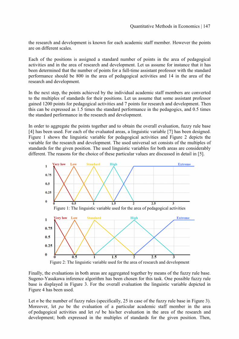
the research and development is known for each academic staff member. However the points are on different scales.

Each of the positions is assigned a standard number of points in the area of pedagogical activities and in the area of research and development. Let us assume for instance that it has been determined that the number of points for a full-time assistant professor with the standard performance should be 800 in the area of pedagogical activities and 14 in the area of the research and development.

In the next step, the points achieved by the individual academic staff members are converted to the multiples of standards for their positions. Let us assume that some assistant professor gained 1200 points for pedagogical activities and 7 points for research and development. Thenthis can be expressed as 1.5 times the standard performance in the pedagogics, and 0.5 times the standard performance in the research and development.

In order to aggregate the points together and to obtain the overall evaluation, fuzzy rule base [4] has been used. For each of the evaluated areas, a linguistic variable [7] has been designed. Figure 1 shows the linguistic variable for pedagogical activities and Figure 2 depicts the variable for the research and development. The used universal set consists of the multiples of standards for the given position. The used linguistic variables for both areas are considerably different. The reasons for the choice of these particular values are discussed in detail in [5].

Figure 1: The linguistic variable used for the area of pedagogical activities

Figure 2: The linguistic variable used for the area of research and development

Finally, the evaluations in both areas are aggregated together by means of the fuzzy rule base. Sugeno-Yasukawa inference algorithm has been chosen for this task. One possible fuzzy rule base is displayed in Figure 3. For the overall evaluation the linguistic variable depicted in Figure 4 has been used.

Let n be the number of fuzzy rules (specifically, 25 in case of the fuzzy rule base in Figure 3). Moreover, let pa be the evaluation of a particular academic staff member in the area of pedagogical activities and let rd be his/her evaluation in the area of the research and development; both expressed in the multiples of standards for the given position. Then,

Quantitative Methods in Economics | 147

the overall evaluation for the particular academic staff member is then calculated by the formula:

,)()(

)()(),(

21 1

21 1

rdApaA

evrdApaArdpaeval

in

i i

iin

i i

�

�����

�

�

where for i=1,... , n:� Ai1 is the fuzzy number that represents the meaning of the linguistic term describing

the evaluation of pedagogical activities in the i-th rule.� Ai2 is the fuzzy number that represents the meaning of the linguistic term describing

the evaluation of the research and development in the i-th rule.� evi is the real number representing the most typical value of the linguistic term

describing the overall evaluation in the i-th rule (i.e. 0, 0.5, 1, 1.5, or 2, respectively).

Because of the limited space, the reader is kindly asked to refer to the papers [3, 5, 6]for more detailed information on the used model. The aim of this section was not to provide complete information on the model, but to present the reader only its brief characteristic that will be necessary in the further text. In the next chapter, the IS HAP information system that implements the model will be introduced.

Figure 3: The used fuzzy rule base

Figure 4: The linguistic variable for the overall evaluation

3 SOFTWARE IMPLEMENTATION OF THE MODELThe described evaluation model has been implemented into the information system called IS HAP. The system is a web application and therefore it is accessible from any computer with the connection to the internet.

The academic staff members fill in their activities performed since the last evaluation into a form, which is shown in Figure 5. The IS HAP is able to gather certain data automatically. For example, it can cooperate with the STAG information system [1] and download the available data on pedagogical activities from it.

148 | Multiple Criteria Decision Making XVIII

Figure 5: The evaluation form in the IS HAP

The evaluation results can be seen in Figure 6. For each evaluation area, the evaluation is described verbally. For example, the evaluation “High (38 %), Extreme (62 %)” means that the performance of the particular academic staff member is between high and extreme and it is closer to the latter value. The IS HAP uses also a graphical representation, which is even easier to interpret. The individual performance classes has been assigned colors (the class names and the corresponding colors can be seen in Figures 1, 2, and 4), e.g. a blue color represents an excellent performance, while a dark red color represents very low performance.

Figure 6: Presentation of the evaluation results for a particular academic staff member

Quantitative Methods in Economics | 149

The heads of the departments can the browse the evaluation results for their department. Thedean has access to the evaluations on all departments. Such an evaluation results for some department are depicted in Figure 7. Each row represents an academic staff member. In the columns, there are the individual evaluation areas. The supervisor has therefore all necessary information presented clearly on a single page on various levels of aggregation:

1. A brief look at the colors in various columns can give a quick answer to the questions how well performed the academic staff members on the department in the individual areas (e.g. in the research and development).

2. If the supervisor needs more detailed information on some area (pedagogics or research and development), the percentage of points for subareas is displayed. For example, the supervisor can see, how many points for the pedagogical activities did the academic staff member earned for lecturing, how many for supervising students, and, finally, how many for the development of the fields of study. The supervisor can therefore gain better knowledge about which type of activities did the academic staff member focused on.

3. If the supervisor requires even more detailed information, he/she can click on any of the evaluation areas (or subareas) to obtain a detailed list of activities performed by the academic staff member.

Figure 7: Summary of the evaluation results on a particular department

The IS HAP makes it possible for the supervisor to have complete information on the activities performed by the academic staff members. Its use reduces tedious paperwork and searching for the required information as the data are available directly in the information system. Moreover, it allows gathering the data on the performed activities in a user-friendly way (some of them can be obtained automatically) and it ensures that the evaluation results are presented in an easily comprehendible way.

4 FUTURE DEVELOPMENTThe practical experiences with the IS HAP originated some ideas for the future development of both the IS HAP software and the model.

150 | Multiple Criteria Decision Making XVIII

From the practical point of view, the importance of the connection to the other information systems has been revealed. Loading the data from various data sources (such as STAG) is important not only because it saves the work of the academic staff members, but even more importantly it reduces the chance of errors in the data they provide. In the future, an effort should be made to extend the list of the information systems that can be used as a data source for the IS HAP.

The usage of a fuzzy rule in the IS HAP turned out to be a great advantage during its practical application on various universities. The main benefit is that the fuzzy rule base can be easily designed or modified according to the requirements of the university management. The behavior of the evaluation model can be thus changed by swapping the fuzzy rule base without modification of the software itself. This makes the IS HAP to be a very versatile tool. In the future, other fuzzy rule bases suitable for different situations should be identified.

From the theoretical point of view, the IS HAP system could be extended by new evaluation models in the future. Some of such models have been sketched for example in [2]. For instance, one of the models considered in the paper would propose the suitable position for the particular academic staff member (an assistant professor, associate professor, or professor) according to his/her performance and the composition of his/her activities. This could allow the university management to identify promising academic staff members aspiring on a higher-level.

5 CONCLUSIONThe paper focused on a mathematical model for academic staff performance evaluation developed at the Palacký University in Olomouc, especially from the practical point of view –the software implementation of the model has been introduced (the IS HAP information system). The IS HAP makes it possible to gather the necessary information on the activities of the academic staff members’ performed during the year and to provide the processed information to the supervisors in an aggregated and comprehendible way. The possible future development and extensions of the software have been also outlined in the paper.

Acknowledgements: The research has been supported by the grant GA14-02424S Methods of operations research for decision support under uncertainty of the Grant Agency of the Czech Republic.

References [1] IS/STAG, (2016). IS/STAG - Information system of the study agenda (in Czech). [online]

Available at: http://stag.zcu.cz/ [Accessed 16 Mar. 2016].[2] Holeček, P., Stoklasa, J. and Talašová, J. (2016). Human Resources Management at

Universities - a Fuzzy Classification Approach. [online] Available at: http://www.inderscience.com/info/ingeneral/forthcoming.php?jcode=ijmor [Accessed 16 Mar. 2016].

[3] Stoklasa, J., Talašová, J. and Holeček, P. (2011). Academic staff performance evaluation - variants of models. Acta Polytechnica Hungarica, 8(3), pp. 91-111.

[4] Sugeno, M. and Yasukawa, T. (1993). A fuzzy-logic-based approach to qualitative modeling. IEEE Transactions on Fuzzy Systems, 1(1), pp. 7-31.

[5] Talašová, J. and Stoklasa, J. (2010). Fuzzy approach to academic staff performance evaluation. In: 28th International Conference on Mathematical Methods in Economics

Quantitative Methods in Economics | 151

2010. České Budějovice: University of South Bohemia in České Budějovice, Faculty of Economics, pp. 621-626.

[6] Talašová, J., Stoklasa, J. and Holeček, P. (2014). HR management through linguistic fuzzy rule bases - a versatile and safe tool? In: 32nd International conference on Mathematical Methods in Economics MME 2014. Olomouc: Palacký University, pp. 1027-1032.

[7] Zadeh, L. A. (1975). The concept of linguistic variable and its application to approximate reasoning. Information Sciences 8, pp. 199-249.

Author’s addressMgr. Pavel Holeček, Ph.D.Palacký University Olomouc, Faculty of Science, Dept. of Mathematical Analysis and Applications of Mathematics17. listopadu 1192/12, 771 46 OlomoucCzech Republicemail: pavel.holecek@upol.cz

doc. RNDr. Jana Talašová, CSc.Palacký University Olomouc, Faculty of Science, Dept. of Mathematical Analysis and Applications of Mathematics17. listopadu 1192/12, 771 46 OlomoucCzech Republicemail: jana.talasova@upol.cz

Mgr. et Mgr. Jan Stoklasa, D.Sc (Tech.)Palacký University Olomouc, Faculty of Arts, Department of Applied EconomicsKřížkovského 12, 771 80, OlomoucCzech Republicemail: jan.stoklasa@upol.cz

152 | Multiple Criteria Decision Making XVIII

AN ALGORITHM FOR GENERAL INFINITE HORIZON LOT SIZING WITH DETERMINISTIC DEMAND

Milan Horniaček, Comenius University in Bratislava, Faculty of Social and Economic Sciences

AbstractWe present an algorithm for solving an infinite horizon discrete time lot sizing problem with deterministic non-stationary demand and discounting of future cost. Besides non-negativity and finite supremum over infinite horizon, no restrictions are placed on single period demands. (In particular, they need not follow any cyclical pattern.) Variable procurement cost, fixed ordering cost, and holding cost can be different in different periods. The algorithm uses forward induction and its essence lies in the use of critical periods. Period j following t is the critical period of t if satisfying demands in any set of periods between t and j, including jand excluding t, from an order in t is not more expensive than satisfying it from an order in aa later period and j is the last period with this property. When deciding whether to place an order in period t, all demands from t to its critical period are taken into account.

Keywords: inventory, lot sizing, non-cyclical deterministic demand, discounting of future coss, forward induction, critical period.

JEL Classification: C61AMS Classification: 90B05

1 INTRODUCTIONFirms’ activities are dynamic in their nature and conditions for them can change. Therefore, dynamic models for optimization of inventories are needed. This requirement is satisfied (among others) by dynamic discrete time lot sizing models with deterministic non-stationary demand. (See [5], Chapter 4, for their description.) Nevertheless, these models have finite horizon. This is usually justified by life-cycle of the good that is purchased ([5], p. 92). Firms, however, usually do not have an upper bound on their life time. Thus, infinite horizon discrete time models are more appropriate for analysis and optimization of their activities, including inventory management. Moreover, a repetition of an optimal inventory strategy computed from a finite horizon program can lead to suboptimal behavior in models with infinite horizon. (See [1], subsection 2.1 for an example.) Therefore, the use of finite horizon discrete time models of dynamic lot sizing with deterministic non-stationary demand should be supplemented by the use of infinite horizon discrete time models of dynamic lot sizing with deterministic non-stationary demand, keeping the usual assumptions of the former, namely periodic review of inventory (at the beginning of a period), zero lead time, impossibility ofbackorders.

In the present paper we develop an algorithm for computing optimal inventory strategy for such model. We work with discounting of future cost (which is a common approach in microeconomics) rather than with the limit of average cost as the length of the time horizon approaches infinity. (See [5], Chapter 10, for characterization of the latter approach.) Besides non-negativity and finite supremum over infinite horizon, no restrictions are placed on single period demands. (In particular, they need not follow any cyclical pattern. Therefore, the algorithm developed in [1] cannot be used here.) Variable procurement cost, fixed ordering cost, and holding cost can be different in different periods.

Quantitative Methods in Economics | 153

The algorithm uses forward induction and its essence lies in the use of critical periods. Aperiod j following period t is the critical period of t if (a) satisfying demand in any subset of the set of periods � �j,...,1t � from an order in t (provided that an order is made in period t inorder to satisfy demand in period t) is not more expensive than satisfying it from an order in aperiod � �j,...,1tk � (from which it can be satisfied) and (b) j is the last period with this property. If such period j does not exist, then the critical period of t is t. (If the critical period is the same for period t and several consecutive periods following it, then an order is placed only in period t.) When deciding whether to place an order in period t, all demands from t to its critical period are taken into account. Thus, for each period t, we determine the last period in which demand is served from an order in t, not, as in [9], the period in which an order satisfying demand in t is placed. This speeds up computation of an optimal inventory strategy. (A backward induction, as in [8], cannot be used in our infinite horizon model.) When we get to the first period following the critical period of t, in which an order is made, we can be sure that the following computations will not change quantity ordered in the critical period of t and preceding periods. Thus, we can compute optimal ordered quantities for any finite number of consecutive periods without computing them for the rest of the time horizon of the model.

Throughout the paper, we endow each finite dimensional real vector space with the Euclidean topology and each infinite dimensional Cartesian product of finite dimensional real vector spaces with the product topology.

2 INVENTORY OPTIMIZATION PROBLEMThe time horizon of the model is (i.e., the set of positive integers). A firm wants to minimize sum of discounted total cost of satisfying demands for a single input. It uses the same discount factor � �1,0 in each period. (It does not discount the first period.) Durability of the input is T periods (i.e., an input purchased in period t can be used in periods t, t+1, …, t+T-1). For each t , 0�td is deterministic demand for the input in period t, 0�tC is unit purchasing cost of the input in period t, 0�th is the unit holding cost in period t (i.e., cost of storing one unit of the input between periods t and t+1), and 0�tK is the fixed ordering cost in period t (a firm incurs it if and only if it makes an order in period t).We assume that

�� tt dsup , �� tt Csup , �� tt hsup , and �� tt Ksup . (1)

Denote by tx the stock of the input at the beginning of period t, before an order is made. We assume that, using its stock of the input to satisfy demand, a firm proceeds from its oldest to its newest part. We also assume that ��� �

�1T1j j1 dx0 and its composition with respect of

vintages of the input is such that it can be fully used in periods 1,…,T-1. Let 0qt � be an order in period t and let � �1,0t � satisfy 1t �� if an order is made in period t. Then a firm solves the minimization program

min � �ttttt1t

t1:t1t

tt t1t dqxhKqC

t�������

��

�

�� (2)

subject to

ttt dqx �� ,t � (3)

154 | Multiple Criteria Decision Making XVIII

� �,xdq0 t1Tt

tj jtt ���� ���� ,t � (4)

,dqxx ttt1t ���� ,t � (5)

� �.1,0t � .t � (6)

The objective function (3) is the sum of discounted purchasing cost, discounted fixed ordering cost, and discounted cost of holding inventory. (Taking into account (1) , it is well-definedand continuous.) We cannot omit purchasing cost from the objective function because cost is discounted and unit purchasing cost of the input can be different in different periods. Constraint (3) ensures that demand is satisfied in each period. Constraint (4) ensures that ordered quantities are non-negative and (together with the assumption on the order of using parts of a stock and the assumption on 1x ) that in each period a firm purchases only an amount of the input that can be used before its durability expires. It also ensures that an order is made in period t only if 1t �� . (Clearly, in each optimal solution of program (2)-(6) an order is made in period t if 1t �� .) Constraint (5) describes dynamics of stock of the input.

A strategy is a sequence � � � � ttt }q,{s . It is feasible if it satisfies constraints (3)-(6). It is optimal if it solves program (2)-(6).

Clearly, the set of feasible strategies is non-empty. (It is enough to set }0,xdmax{q ttt �� and 1t �� if and only if 0qt � for each t .) It is closed because (3)

and (4) are expressed by weak inequalities and (5) by equality between terms continuous in components of a strategy. It is also compact because it is a subset of space � � � �� ��� tNt dsupT,01,0 that is compact by Tychonoff theorem. Thus, as the objective

function is continuous, program (2)-(6) has an optimal solution. In the following section we propose an algorithm for its solution. We apologize to a reader that, due to space limitations, we cannot explain here in more detail (beyond obvious interpretation of inequalities (10) and (11) in the following section) why the algorithm gives an optimal solution of program (2)-(6) and give an example of its application.

3 ALGORITHMFor each t let

� � � �� �jjjtj1j

tk ktk

jjtt dCKhddC1Tt,...,1tjW �������� ���

� , (7)

� � � �� � � �

,ij,...,1n,1j,...,1ti

,dCKdhCWjV

niik kii

tiniik k

1itk k

tktt

t��

���

��

���

�����

�������

��

���

��

� (8)

tt Vmaxr � if !tV and trt � if .Vt � (9)

We call tr the critical period of period t. Symbol tm stands for the first period following t in which an order is made. (In the algorithm, in order to shorten its description, we formally allow for the case tmt � .) In the description of the algorithm below, values without asterisk

Quantitative Methods in Economics | 155

are preliminary (they can be changed by later computations and decisions) and values with asterisk are final. Arrow (") stands for assignment command (e.g., ba" means that a isassigned to symbol b); we use it when the equality sign ( � ) is false from the mathematical point of view or it could lead to a confusion.

Description of the algorithm

Step 1. Let 1t � . Go to step 2.

Step 2. If tt xd � , then ,0*t �� 0q*

t � , t1t "� , and return to step 2. Otherwise, go to step 3.

Step 3. Let 1*t �� . Compute tW . If !tW , compute tr . If �tW or !tW but trt � ,

then t*t dq � , t1t "� , and go to step 2. Otherwise, let tt dq � , 1t ��� , tmt � and go to

step 4.

Step 4. Compute �W . If !�W , compute �r . If ��W or !�W buttmrr �� , then

0*j �� , 0q*

j � , tt qdq "� � , �� "�1 , and return to step 4. Otherwise, go to step 5.

Step 5. If tmr�� and 1rt ��� , go to step 6. Otherwise, go to step 7.

Step 6. If

� � � � � �� ������

���������

������

��

��

��

����

��

�

�

�� �����

�

r1rk k1r1r

t1rrmk km

tm

1mk k

1mtk k

tkt

r1ri ik

rk

tkrk k

t

tmtmtmtmtm

ttt

tt

tmtm

dCKdC

dhCdhdCK

, (10)

(where we omit the fourth sum if tmt � ) then 0*mt�� and 0q*

mt� unless tmt � ,

�� ��1tk kt dq � , �� �

���

rk kdq , tm"� , and go to step 9. Otherwise, 0* ��� and 0q* �� unless

1rt ��� , �� "�1 , and go to step 4.

Step 7. If tmr�� , then 0*

1rt��� and 0q*

1rt�� unless 1rt ��� , 1*

mt�� ,

tt m*m qq � , t

*t qq � ,

t1rtm "� , and go to step 3. Otherwise, go to step 8.

Step 8. If

� � � � � �� �

� � � ���������

���

���������

�������

����

��

�����

��

���

����

��

�

�

��

�

�

�����

r1rk k1r1r

t1r11rk k

rmk k

tkrmk km

tm

11rk k1r1r

t1r

rmk k

1mtk k

tkt

r1ri ik

rk

tkrk k

t

tmtmtmtm

tt

ttm

ttt

tttt

tt

ttm

tm

dCKdhdC

dCK

dhCdhdCK

, (11)

then 0*mt�� and 0q*

mt� , ��� �

tt

rmk kt

*t dqq , t1rt "� , 1*

t �� , �� ��1tk kt dq � , 1��� ,

�� ����

rk kdq , ��tm , �� "�1 , and go to step 4. Otherwise, 0* ��� , 0q* �� , �� "�1 ,

and go to step 4.

Step 9. If 1rt ��� , then t*t qq � , t"� , 1*

t �� , tt dq � , tmt � , 1t ��� , and go to step 4.

Otherwise, 1��� , �� ����

rk kdq , tm"� , �� "�1 , and go to step 4.

156 | Multiple Criteria Decision Making XVIII

4 CONCLUSIONSFirms usually work with open-ended planning horizon. They make decisions in certain discrete points of time. Thus, infinite horizon discrete time models are appropriate for analysis of decision making in firms. This holds also for inventory decisions. This area is crucial for reducing cost of achieving specified output goals. This holds not only for firms producing material goods but also for financial firms. Thus, models for optimization of inventory management can be used also as sub-models of models of financial activities (developed, e.g., in [2], [3], [4]). They can enhance also analysis of strategic interaction between firms on both sides of a market (carried out in [6] and [7]). Thus, further refinement of our work can be useful also for research in above mentioned directions.

Acknowledgements: This work was supported by grant APVV-14-0020 from the Association for Support of Research and Development of the Slovak Republic.

References [1] Horniaček, M. (2014). An algorithm for infinite horizon lot sizing with deterministic

demand. Applied Mathematics, 5(2), pp. 217-225.[2] Hozlár, E. (2014). Factoring credit risk and its security modeling. In: Quantitative

Methods in Economics: Multiple Criteria Decision Making XVII. Bratislava: Ekonóm, pp.79-81.

[3] Mlynarovič, V. (2014). The analytical system for portfolio performance and risk distribution. In: Quantitative methods in economics: Multiple criteria decision making XVII. Bratislava: Ekonóm, pp. 182-187.

[4] Mlynarovič, V. (2013). Dekompozícia výnosov a rizika portfólia. In: Využitie kvantitatívnych metód vo vedecko-výskumnej činnosti a v praxi X. Bratislava: Ekonóm, pp. 122-128. Available at: http://www.fhi.sk/files/katedry/kove/ssov/Cingov/Cingov-2013.pdf [Accessed 8 May. 2016]

[5] Muckstadt, J.A. and Sapra, A. (2010). Principles of inventory management. Berlin: Springer-Verlag.

[6] Šimková, Ľ. (2014). An example of renegotiation-proof equilibrium with product innovation. In: Quantitative Methods in Economics: Multiple Criteria Decision Making XVII. Bratislava: Ekonóm, pp. 276-279.

[7] Šimková, Ľ. (2014). Impact of cooperation of firms on both sides of the market on innovation. In: Mathematical Methods in Economics (MME 2014). Olomouc: Palacký university, pp. 885-889.

[8] Wagelmans, A., Hoesel, S.V. and Kolen, A. (1992). Economic lot sizing: An O(n log n) algorithm that runs in linear time in Wagner-Whitin case. Operations Research, 40(1), pp.145-156.

[9] Wagner, H.M. and Whitin, T.M. (1958). Dynamic version of the economic lot size model.Management Science, 5(1), pp. 89-96.

Author’s addressdoc. Ing. Milan Horniaček, CSc.Comenius University in Bratislava, Faculty of Social and Economic Sciences, Institute of EconomicsMlynské luhy 4, 821 05 BratislavaSlovak Republicemail: milan.horniacek@fses.uniba.sk

Quantitative Methods in Economics | 157

MEASURING THE NAIRU FOR CZECH AND SLOVAK LABOUR MARKETS: BAYESIAN APPROACH

Jakub Chalmovianský, Masaryk University, Brno

AbstractThe purpose of this contribution is to present and compare estimates of non-accelerating inflation rate of unemployment and corresponding unemployment gap in the Czech Republic and the Slovak Republic. The estimates of these indicators are based on a bivariate Phillips curve model, as an unobserved components model, where use is made of Bayesian estimationand diffuse Kalman filtering techniques. Since the data on unemployment rate for the Slovak economy shows some evidence of structural changes, the model for this country has to be modified to allow for such behaviour. Eventually, results for both economies are compared mostly on the basis of their statistical properties.

Keywords: Bayesian estimation, Gibbs sampler, Kalman filter, Non-accelerating inflation rate of unemployment, Unobserved components model

JEL Classification: C11, C32, E24AMS Classification: 62P20

1 INTRODUCTIONUnemployment rate is one of the well-known macroeconomic indicators not only for economists but also for general public. The reason for that lies in the indirect link betweenunemployment and proper functioning of households. This relationship can be, with a bit of perspective, described by a saying: “No bees no honey, no work no money.” Higher unemployment rate therefore indicates greater social problems for households. However, from an economic point of view there is much more to it. Besides the actual value of unemployment rate, one might also be interested in its “natural level”, i.e. level of unemployment such that theobserved unemployment rate fluctuates around it. The non-accelerating inflation rate of unemployment (NAIRU) is one of the concepts for such unobservable measure. It refers to a level of unemployment that is consistent with constant price inflation, given current economic conditions, OECD [6].The aim of this contribution is to estimate the NAIRU for Czech and Slovak labour marketsand to compare some of the properties of these estimates. Trajectories of NAIRU will be obtained using Bayesian estimation and diffuse Kalman filtering techniques applied to bivariate unobserved components model, which stems from an approach introduced in Planas, Rossi and Fiorentini [7]. The model presented in their work is suited to estimate potential output and output gap. Therefore in this contribution some modifications need to be introduced to account for different dynamics in unemployment rate in comparison with output. The model, as well as the data used, will be the discussed in the next section.

2 MODEL AND DATA FOR ESTIMATING THE NAIRU The model for estimating the NAIRU is composed of two blocks. The first one, shown in equations (2.1) to (2.3), describes decomposition of unemployment rate (��) into its trend (��)and cyclical component (��): �� = �� + �� (2.1)∆�� = �� + �� (2.2)�(�)�� = �� (2.3)

158 | Multiple Criteria Decision Making XVIII

Where evolution of trend component is represented by the means of random walk with trend, �� , and dynamics of cyclical one follows autoregressive process of the second order, i.e. �(�) = (1 − � � + �� ��) with � as lag operator. In line with the original model proposedby Planas, Rossi and Fiorentini [7] this AR(2) is reparameterized in terms of polar coordinates as stated in equation (2.4).�(�) = �1 − 2� cos ���� � � + �� ��� (2.4)The newly incorporated parameters of the AR(2) process has the following meaning: � = amplitude of the cyclical movements, � = period of the cyclical component. It is worth noting that symbol � refers to the Ludolph’s constant. Finally, terms denoted as �� and �� are mutually independent Gaussian white noises with variances �� and �� , respectively. Components �� and �� are then naturally interpretable as the NAIRU and the unemployment gap, i.e. difference between actual unemployment rate and the NAIRU.The proposed model is complemented by the second block, namely equation (2.5), that relates change in inflation, ∆�� to unemployment rate (in second difference, ∆���) and lagged unemployment gap (��� ), making use of another AR(2) polynomial:(1 − � � + �� ��)∆�� = �� + ���� + �∆��� + ���� + �� (2.5)Here �� is Gaussian white noise with variance �� that is orthogonal to cyclical innovations of unemployment gap, ��. Furthermore, the innovations from equations (2.2) and (2.5) (�� for NAIRU and �� for inflation) are assumed to be independent.

2.1 Prior distribution of parameters In order to make it possible to estimate this model within a Bayesian framework, prior distribution for all parameters in the model has to be defined. Let � = (��, �, �, � , ��, ��)be the vector of all parameters from the equation (2.5) and assume the block independence structure of the model. Then the joint distribution of all parameters can be rewritten as the following product, where the distribution of each of the factors can be defined:���, �, ��, �, ��, ��, ��� = �(�) �(�) �(��) �(�, ��) ����, ��� (2.6)For the purpose of our model, we will assume the following distributions:�(�) = ��!(", #")

� $ � − �%�& − �%' = ��!(�, #�)�(��) = *-(.�/, 0�/) (2.7)�(�, ��) = 3*-��/, 45� , .�/, 0�/�*5����, ��� = 3*-���/, 4�/� , .�/, 0�/�

where ��!(. , . ) denotes the Beta distribution, �&, �% are the upper and lower bounds of �’ssupport (in our model �% = 2 as the minimal possible period, �& = 69 which is equal to the number of observations), *-(. , . ) is the inverted Gamma-2 distribution and analogically 3*-(. , . ) stands for Normal-inverted Gamma-2 distribution (for more information about therespective distributions and their properties, see Bauwens, Lubrano, Richard [1]). Finally, *5serves as an index set for imposing constraint of non-negativity on the parameters �, �, ��. All the hyperparameters of the above mentioned distributions are assumed to be given and for the computational convenience the prior distributions for most of the parameters, besides �, �, are assumed as naturally conjugate. For simplicity, let the set of all model parameters be denoted as 8 = ��, �, ��, �, ��, ��, ���.

2.2 Estimation techniques Within the Bayesian framework we now need to characterize the joint posterior distribution of the unobservables, trend and cyclical component, conditionally on the data,

Quantitative Methods in Economics | 159

i.e. �(�:, �:, 8|;:). Here ;: ≡ {�:, ∆�:}, where the notation means all observations till time > inclusive, e.g. �: ≡ {� , … , �:}. However, given our model, no closed form solution for this distribution exists. Yet, we can get draws from the distribution of interest using the Gibbs sampler. Within this context, we will make use of the following equality:�(�:, �:, 8|;:) = �(�:, �:|8, ;:)�(8|�:, �:, ;:) (2.8)First of all, we have to simulate the state variables (��, ��) given model parameters. This can be done by rewriting the model (2.1) – (2.3) and (2.5) into a state-space format and then applying the Forward Filtering Backward Sampling algorithm of Carter, Kohn [2] with diffuse Kalman filter, as is stated in de Jong [3]. In order to specify the second full conditional distribution we follow the approach put forward in Planas, Rossi, Fiorentini [7]. Thanks to the assumption of prior block independence in (2.6), it consists of three independent blocks of parameters according to the model structure:�(8|�:, �:, ;:) = ����, ��?�:��(�, �, ��|�:)���, ��?�:, �:, ∆�:, �, �, ��, ��, ��� (2.9)Obtaining samples from the first block of parameters is simple. Since we assume naturally conjugate 3*- prior, we can derive the conditional distribution analytically (see for instance Bauwens, Lubrano, Richard [1], p.58, or Planas, Rossi, Fiorentini [7], p. 21). For the second conditional this is not the case. However, we can still split it into three full conditionals: �(�|�, ��, �:), �(�|�, ��, �:) and finally �(��|�, �, �:), where the first two verify:�(�|�, ��, �:) ∝ �(� , ��|�, �, ��) ∏ �(��|��� , �, �, ��)�(�):�BC (2.10)�(�|�, ��, �:) ∝ �(� , ��|�, �, ��) ∏ �(��|��� , �, �, ��)�(�):�BC (2.11)The log-concavity of these distributions cannot be ensured, hence a use of the adaptive rejection Metropolis scheme proposed by Gilks et al. [4], [5] is recommended. On the other hand, the third full conditional, �(��|�, �, �:), can be expressed analytically, thanks to the conjugate *-distribution (see Bauwens, Lubrano, Richard [1], p.304 or Planas, Rossi, Fiorentini [7], p. 21).At this point, it remains to sample from the third full conditional distribution, which is proportional to the following expression:���, ��?�:, �:, ∆�:, �, �, ��, ��, ��� ∝∝ �(Δ� , Δ�� |�:, �:, 8) ∏ �(Δ�� |Δ��� , 8)�(�, ��)EFBC (2.12)Given conjugate 3*- prior allows us to sample using the standard results as stated in Bauwens, Lubrano, Richard [1] and adding one additional step in the form of Metropolis-Hastings algorithm. The acceptance probability for each candidate (�,G ��G ) is given by:

min H1, ��∆� , ∆��?�,G ��G , �:, �:, �, �, ��, ��, �����∆� , ∆��?�, ��, �:, �:, �, �, ��, ��, ���I (2.13)

This closes the whole circle of simulations from the full conditional distributions, which is repeated for J-times, with first J/ burn-in repetitions, in order to ensure convergence to the joint posterior distribution �(�:, �:, 8|;:).

2.3 Data To estimate the Czech and Slovak NAIRU only data on unemployment rate and inflation rate are needed. For this purpose following variables from the OECD database were used:� ��: Seasonally adjusted harmonised unemployment rate� ��: Inflation rate on the basis of consumer price index (CPI), measured as the percentage

change on the same period of the previous year.

160 | Multiple Criteria Decision Making XVIII

Figure 1: Unemployment rates in the Czech Republic and the Slovak Republic

For both countries the sample is made up of 69 quarterly observations, starting from 1998Q3 to 2015Q3. Figure 1 shows the trajectories of unemployment rate for the economies under investigation, in this figure we can observe similar behaviour of unemployment rate for both of them, at least in terms of timing of peaks and troughs. The biggest difference lies in the level of unemployment, which is considerably higher in Slovakia. It also has to be noted that we have detected possible structural break in the mean of the Slovak unemployment rate starting in 2006Q1, which can be the consequence of tax and labour market reforms introduced in theSlovak Republic, mostly during the 2004 - 2006 period. In order to account for this break we have decided to split the dataset at this point, to evaluate medians of both parts and then subtract the difference between them from the first part of the sample. Afterwards, we estimate the model for this modified variable and eventually we add this difference back to the first period of the NAIRU estimate.

3 COMPARISON OF CZECH AND SLOVAK ESTIMATESAfter presenting the crucial assumptions and elements of the investigated model, we can finally focus on the actual estimates of the NAIRU for Czech and Slovak labour markets in detail. Results presented in the following paragraphs are based on J = 8000 repetitions, with a burn-in phase of the first 4000 samples.We set the prior information for the model parameters to be rather noninformative and as similar as it is possible for both countries (the only differences are for the prior values of parameters �� and �� from equation (2.5)). This approach has been chosen to keep the starting point for both countries more or less the same and let the data speak instead. Standard deviation of trend component was set as 1/3, and for the cyclical component as 2/3,of the sample standard deviation of actual unemployment. Hence, prior signal-to-noise ratio for both countries was set to �� ��⁄ = 0.25.Tables 1 and 2 report prior and posterior means and their standard deviations, the numerical standard error (NSE) associated with the sample mean, Geweke’s convergence diagnostic (Geweke CD) and 95% highest posterior density interval (HPDI) for the posterior mean of most parameters for Czech and Slovak NAIRU, respectively. From the values of NSE we see that the chosen number of replications is sufficient. All the values for Geweke CD fall into the 95% confidence interval of standardized normal distribution. Therefore convergence of all parameters at the significance level P = 0.05 is satisfied.

Quantitative Methods in Economics | 161

Table 1: Prior and posterior characteristics of model parameters for the Czech RepublicParameter Prior (s. d.) Posterior (s. d.) NSE Geweke CD 95% HPDI

� 0.8 0.623 0.0025 0.0180 (0.301; 0.896)(0.1614) (0.1590)

� 20 27.128 0.1711 -0.6122 (8.640; 49.338)(1.9351) (10.8208)

�� 0.2 0.110 0.0003 -1.1121 (0.076; 0.140)(0.20) (0.0192)

� 0.2 0.157 0.0004 0.6767 (0.115; 0.187)(0.20) (0.0246)

� 0.2 0.197 0.0003 1.0483 (0.158; 0.239)(0.20) (0.0203)

� 0 -0.000 0.0003 -0.7062 (-0.041; 0.042)(0.20) (0.0206)

�� 0 -0.000 0.0003 1.5103 (-0.041; 0.042)(0.20) (0.0202)

�� 0.1 0.086 0.0003 0.1575 (0.045; 0.127)(0.20) (0.0217)

�� 0.001 -0.0161 0.0004 -0.0130 (-0.070; 0.033)(0.406) (0.0261)

Table 2: Prior and posterior characteristics of model parameters for Slovak RepublicParameter Prior (s. d.) Posterior (s. d.) NSE Geweke CD 95% HPDI

A 0.8 0.623 0.0025 -0.7979 (0.298; 0.899)(0.1614) (0.1608)

τ 20 27.404 0.1719 -0.6857 (8.721; 49.484)(1.9351) (10.8696)

μS 0 0.021 0.0004 1.0034 (-0.016; 0.073)(0.20) (0.0269)

β 0.2 0.117 0.0005 -0.3197 (0.021; 0.089)(0.20) (0.0327)

λ 0.2 0.178 0.0003 -0.4935 (0.126; 0.233)(0.20) (0.0220)

ϕS 0 -0.001 0.0004 1.3288 (-0.056; 0.057)(0.20) (0.0222)

ϕS� 0 -0.002 0.0011 1.2408 (-0.177; 0.180)(0.20) (0.0708)

κS 0.25 0.186 0.0004 -0.5215 (0.088; 0.181)(0.20) (0.0250)

μX 0.001 0.045 0.0007 0.1893 (-0.048; 0.086)(0.564) (0.0416)

As we have discussed earlier, prior signal-to-noise ratio was set to the value of 0.25 for both countries. Nevertheless, posterior signal-to-noise ratio for these countries differs significantly. In the Czech model, its value is close to the prior setting: �� ��⁄ = 0.2494, but the Slovak model sets the variation of cyclical component greater relatively to the trend component, since the ratio reduced to: �� ��⁄ = 0.1748. This may partly explain the difference in smoothing of the unemployment rate trajectories that can be seen in Figure 2. Another common feature is the fall of unemployment rate deep below the NAIRU level, which started in 2007Q1 and continued until the onset of the global financial crisis at the end of 2008. However, unemployment rate remained below its potential until 2009Q2 for Czech and 2009Q3 for the Slovak economy. Similar pattern of behaviour of unemployment rate and NAIRU for both countries is evident also in subsequent periods. Unemployment rate grew above the level of NAIRU and identically

162 | Multiple Criteria Decision Making XVIII

peaked in the first quarter of 2010, thereafter the unemployment rate fluctuates more or less around the NAIRU with repeated decrease in the last quarters, starting sooner and being more significant for the Slovak labour market.

Figure 2: NAIRU estimates for the Czech Republic and the Slovak Republic

Table 3: Descriptive statistics of unemployment rates and NAIRU estimates

StatisticCzech Republic Slovak Republic

Unemp. rate NAIRU Unemp. Rate[before / after break]

NAIRU[before / after break ]

Max (quarter) 9.2 (2000Q1) 8.3 (2000Q1) 19.5 (2001Q2) 18.7 (2001Q4)Min (quarter) 4.2 (2008Q3) 5.8 (2008Q2) 8.9 (2008Q4) 12.0 (2008Q2)

Mean 7.07 6.97 14.92[17.59 / 12.74]

15.26[17.71 / 13.26]

Median 7.20 6.64 14.30[18.00 / 13.45]

14.06[18.04 / 13.66]

Std. Deviation 1.22 0.79 2.96[1.63 / 1.77]

2.38[0.99 / 0.76]

Table 3 shows descriptive statistics of unemployment rate and corresponding NAIRU estimates and concludes their comparison. Statistics for each country show only small changes in maximal and minimal values and their timing. More significant differences are noticeable in the case of the Czech Republic median, which decreases from 7.20 to 6.64, and naturally for both standard deviations. They fall by 35% for Czech and by almost 20% for the Slovak Republic. It is worth noting that standard deviation for Slovak unemployment rate does not significantly change after the break, but this does not apply to the central tendency measures. This supports the existence of structural break in the mean. Lastly, we need to focus on the characteristics of NAIRU between the two countries. Again, we can see completely different levels of minimum, maximum and all of the measures of central tendency, but these facts are already apparent from Figure 2. The standard deviation, as a measure of variability is almost 4-times greater for Slovakia. However, this is mostly caused by the structural break. On the other hand, standard deviation for the post-break period is very close to that of the Czech Republic standard deviation in the whole sample.

Quantitative Methods in Economics | 163

4 CONCLUSIONIn the presented contribution estimation of NAIRU trajectories for the Czech Republic and theSlovak Republic by means of bivariate unobserved components model within the Bayesian framework has been presented. Labour markets in these countries have been divided for more than 20 years, but both countries still have much in common from an economic point of view and face the same external influences. Hence it is not surprising that the estimated NAIRU trajectories exhibit the same dynamics. However, it seems that the Slovak labour market showed a tendency to catch up with its Czech neighbour during the past ten years. Although this finding still needs to be tested, as it may be partially caused by the method selected to allow for the structural break in the mean. The method is simple yet may not be the best possible. For the future research it is therefore worth considering a different method. It will also be of great importance in future research to investigate the robustness of the estimates with respect to their revisions over time.

Acknowledgements: This work was supported by funding of specific research at Faculty of Economics and Administration, project MUNI/A/1040/2015. This support is gratefully acknowledged.

References [1] Bauwens, L., Lubrano, M. and Richard, J. F. (1999). Bayesian inference in dynamic

econometric models. Oxford: Oxford University Press.

[2] Carter, C. and Kohn, R. (1994). On Gibbs sampling for state space models. Biometrika,81(3), pp. 541–553.

[3] De Jong, P. (1991). The diffuse Kalman filter. The Annals of Statistics, 19(2), pp. 1073-1083.

[4] Gilks, W. R., Best, N.G. and Tan, K.K.C. (1995). Adaptive Rejection Metropolis Sampling within Gibbs Sampling. Journal of the Royal Statistical Society. Series C (Applied Statistics), 44(4), pp. 455-472.

[5] Gilks, W. R., Neal, R.M., Best, N.G. and Tan, K.K.C. (1997). Corrigendum: Adaptive Rejection Metropolis Sampling. Journal of the Royal Statistical Society. Series C (Applied Statistics), 46(4), pp. 541-542.

[6] Organisation for Economic Co-operation and Development, (2016). OECD glossary of statistical terms. [online] Available at: https://stats.oecd.org/glossary [Accessed 12 Mar.2016].

[7] Planas, C., Rossi, A. and Fiorentini, G. (2008). Bayesian analysis of the output gap. Journal of Business & Economic Statistics, 26(1), pp. 18-32.

Author’s addressMgr. Jakub ChalmovianskýMasaryk University, Faculty of Economics and Administration,Lipová 41a, 602 00 BrnoCzech RepublicE-mail: 380234@mail.muni.cz

164 | Multiple Criteria Decision Making XVIII

INTERRELATIONSHIPS BETWEEN GERMAN AND BALTIC STOCK MARKETS

Michaela Chocholatá, University of Economics in Bratislava

Abstract The paper deals with the analysis of relationships of the three Baltic stock markets, i.e. Estonian (OMX Tallinn), Latvian (OMX Riga) and Lithuanian (OMX Vilnius), with the German market (DAX) during the period January 7, 2000 – March 11, 2016 based on cross-market correlation coefficients and DCC model. The results showed that the interrelationships are relatively low and therefore there exist an opportunity of gains from the international diversification.

Keywords: Baltic stock markets, cross-market correlation coefficients, DCC model

JEL Classification: G15, C58 AMS Classification: 91B84, 62P20 1 INTRODUCTION It is commonly known that the financial markets are intertwined, so it seems to be useful to analyse not only a single market, but to deal also with the mutual relationships between them in order to assess the potential capital diversification benefits. The stronger the interconnec-tions are, the lower is the possible gain from international diversification and vice versa. Especially attractive is to investigate the linkages between mature and emerging markets, to assess the impact of various crisis and the issue of contagion (for more information see e.g., Forbes and Rigobon, 2002). Concerning the methods of analysis, the recent studies concentrate besides cross-correlations analysis, cointegration approaches (for more information see e.g., Luká�ik et al., 2006) or spatial econometric approaches (for more information see e.g., Furková, 2013) also on the more sophisticated methods based on autoregressive conditional heteroskedasticity (ARCH) models and their multivariate extensions enabling to capture also the development of covariances over time. Different types of multivariate ARCH-class models can be found in the literature (for a survey see e.g., Bauwens et al., 2006), very popular in recent years has become especially the dynamic conditional correlation (DCC) model of Engle (2002). Many studies have been published dealing with the integration of Central and Eastern European emerging markets with the mature markets (for a survey see e.g., Syllignakis and Kouretas, 2011; Chocholatá, 2013). Another attractive group of emerging markets in Europe build the Baltic markets (Estonia, Latvia and Lithuania) and their linkages with, e.g. the US market (Kuusk et al., 2011), the various groups of major international stock markets (Maneschiöld, 2006; Deltuvaite, 2015), the Russian and Polish market (Asaturov et al., 2015) and the Nordic markets (Nielsson, 2007). The main aim of this paper is to analyse the relationships of the three Baltic stock markets, i.e. Estonian (OMX Tallinn), Latvian (OMX Riga) and Lithuanian (OMX Vilnius), with the German market, i.e. DAX, during the period January 7, 2000 – March 11, 2016 based on cross-market correlation coefficients as well as on the multivariate DCC model. The paper is structured as follows: section 2 deals with data and methodology, section 3 presents empirical results and section 4 concludes.

Quantitative Methods in Economics | 165

2 DATA AND METHODOLOGY Our data includes the weekly prices of the three Baltic indices – OMX Tallinn (OMXT), OMX Riga (OMXR) and OMX Vilnius (OMXV) as well as the German stock index DAX. All the data were retrieved from the web-page http://stooq.com for the period January 7, 2000 – March 11, 2016 (845 observations). The analysed stock indices together with the corresponding logarithmic stock returns (in %) are graphically depicted on Figure 1. Based on descriptive statistics (available from the author upon request) the mean values of all the logarithmic stock returns oscillated around the 0, the most volatile was the German market (3.34 %) followed by the Latvian (3.17 %), Estonian (2.83 %) and Lithuanian market (2.65 %). All the analysed return series were negatively skewed with higher kurtosis than the normal distribution. One of the very simple approaches in order to analyse the relationship between the stock returns is to calculate the cross-market correlation coefficients (Baumöhl et al., 2011), i.e. the pair-wise unconditional correlations 1,1, ?�yx� :

yxyx

yx@@

� ),cov(, � (1)

where the symbol ),cov( yx denotes covariance between stock returns’ series tx and ty , x@ and y@ represent standard deviations of analysed stock returns. The unconditional correlations between pairs of analysed logarithmic returns are summarized in Table 1.

2,000

4,000

6,000

8,000

10,000

12,000

14,000

-30

-20

-10

0

10

20

00 02 04 06 08 10 12 14

DAX DLDAX

0

200

400

600

800

-30-20-100102030

00 02 04 06 08 10 12 14

OMXR DLOMXR

0200400600800

1,0001,200

-20

-10

0

10

20

00 02 04 06 08 10 12 14

OMXT DLOMXT

0100200300400500600

-30-20-100102030

00 02 04 06 08 10 12 14

OMXV DLOMXV Source: Own calculation in econometric software EViews.

Figure 1 Stock market indices and logarithmic returns

166 | Multiple Criteria Decision Making XVIII

Since the correlation of the German market with the Latvian one is very low, the relationships of the German market with the Estonian and Lithuanian ones are of middle size (Baumöhl et al., 2011). Concerning the relationships between the individual Baltic markets, the strongest interconnections were observed for the pair Estonia – Lithuania, while the remaining two correlation coefficients varied only around 0.3. The conditional means of individual stock return series were modelled based on Box-Jenkins ARMA models. Since the presence of the ARCH effect was detected, the univariate ARCH-class models (e.g. GARCH – generalized ARCH and EGARCH – exponential GARCH) were used to capture the conditional volatility. In order to capture not only the volatility linkages between the analysed pairs of stock markets, but also time-varying correlations, the DCC models are to be estimated.

Table 1 Pair-wise unconditional correlation coefficients DLDAX DLOMXR DLOMXT DLOMXV

DLDAX 1.000000 0.152984 0.401599 0.317681 DLOMXR 0.152984 1.000000 0.308335 0.351828 DLOMXT 0.401599 0.308335 1.000000 0.601970 DLOMXV 0.317681 0.351828 0.601970 1.000000

Source: Own calculation in econometric software EViews. The estimation of the DCC model (Engle, 2002) can be summarized as follows: in the first step the conditional variances obtained from the estimated univariate ARCH-class models are used to model the conditional variance-covariance matrix tH of the form:

tttt DRDH � (2) where A Biithdiag�tD is a 2x2 diagonal matrix with the time-varying standard deviations from univariate ARCH-class models on the diagonal. � �ijt��tR is the time-varying correlation matrix of conditional correlation coefficients:

2121 )()( ??� tttt QQQR diagdiag (3)

where � �tijq ,�tQ is the variance-covariance matrix of standardized residuals and takes the following form:

1t

T1t1tt Q��QQ ??? CC??� baba qqqq )1( (4)

Symbol A BT

tt��Q E� denotes the unconditional variance-covariance matrix of standardized residuals. The conditional correlation matrix is also estimated in the second step. The whole estimation is based on use of the maximum likelihood method. 3 EMPIRICAL RESULTS Using the software EViews, in the first step the following ARMA-ARCH models were estimated (complete results are available from the author upon request): DLDAX: AR(3) – EGARCH(1,1,1); DLOMXR: AR(1,2,4,7,8) – GARCH(1,1); DLOMXT: ARMA((1,4);(1,4)) – GARCH(1,1) and DLOMXV: MA(1,2,3) – GARCH(1,1).

Quantitative Methods in Economics | 167

The standardized residuals from these models were thereafter used for estimation of conditional correlations in the second step. Programs for estimation of DCC models were written with the help of advice provided on the web-page of EViews User Forum. Graphically are the dynamic conditional correlations (DCCs) presented on the Figure 2.

-.1

.0

.1

.2

.3

.4

00 02 04 06 08 10 12 14

DCC_OMXR_DAX

.0

.2

.4

.6

.8

00 02 04 06 08 10 12 14

DCC_OMXT_DAX

-.2

.0

.2

.4

.6

.8

00 02 04 06 08 10 12 14

DCC_OMXV_DAX

Source: Own calculation in econometric software EViews.

Figure 2 Dynamic conditional correlations between the German stock returns and individual Baltic markets stock returns

Since the DCCs for the pairs DLOMXT_DLDAX and DLOMXV_DLDAX were during the analysed period oscillating around 0.36 and 0.24, respectively, the development of DCC for DLOMXR_DLDAX was during the analysed period non-stationary with an upward tendency from the values slightly below the 0 in 2002 to the value of almost 0.35 in October 2014 followed by a quite sharp decline in the next periods. 4 CONCLUSION The paper examined the interrelationships between the German and Baltic stock markets (Estonian, Latvian and Lithuanian) based on calculation of the cross-market correlation coefficients as well as on the DCC models. The cross-market correlation coefficient of the German market with the Latvian one of 0.15 indicated very low level of co-movement of these two markets. Although the cross-market correlation coefficients for the pair Germany-Lithuania and Germany-Estonia were higher (0.32 and 0.4, respectively), based on these values can be concluded that there are not very strong interrelationships between the individual Baltic markets and the German market. In comparison to the cross-market correlation coefficients are the mean values of DCCs for the pairs Germany-Lithuania and Germany-Estonia slightly lower (0.24 and 0.36). More turbulent was the development of DCC for the pair Germany-Latvia with the highest value of almost 0.35 in October 2014.

168 | Multiple Criteria Decision Making XVIII

Taking the German market as a bench market for the Western Europe, concerning the presented results, it can be concluded that the interrelationships are relatively low and therefore there exist an opportunity of gains from the international diversification. Acknowledgements: This work was supported by the Grant Agency of Slovak Republic - VEGA grant No. 1/0285/14 “Regional modelling of the economic growth of EU countries with concentration on spatial econometric methods“. References [1] Asaturov, K., Teplova, T. and Hartwell, C.A. (2015). Volatility Spillovers and Contagion

in Emerging Europe. Journal of Applied Economic Sciences, X(6), pp. 929-945. [2] Baumöhl, E., Lyócsa, Š. and Výrost, T. (2011). Fundamentálna analýza akciových trhov.

Košice: ELFA. [3] Bauwens, L., Laurent, S. and Rombouts, J.V.K. (2006). GARCH Models: A Survey.

Journal of Applied Econometrics, 21(1), pp. 79-109. [4] Chocholatá, M. (2013). Analysis of stock market linkages: evidence from the selected

CEE markets. Journal of theoretical and applied computer science, 7(4), pp. 56-69. [5] Deltuvaite, V. (2015). An empirical investigation of the Baltic stock markets global

Integration. Procedia - Social and Behavioral Sciences, [online] 213, pp. 430-435. Available at: http://www.sciencedirect.com/science/article/pii/S1877042815059170 [Accessed 10 Mar. 2016].

[6] Forbes, K. J. and Rigobon, R. (2002). No Contagion, Only Interdependence: Measuring Stock Market Comovements. Journal of Finance, 57(5), pp. 2223-2262.

[7] Engle, R. F. (2002). Dynamic conditional correlation: A simple class of multivariate generalized autoregressive conditional heteroskedasticity models. Journal of Business and Economic Statistics, 20(3), pp. 339-350.

[8] Furková, A. (2013). Spatial dependence econometrics models. Ekonomika a informatika, 11(2), pp. 41-52.

[9] Kuusk, A., Paas, T. and Viikmaa, K. (2011). Financial contagion of the 2008 crisis: is there any evidence of financial contagion from the US to the Baltic states. EasternJournal of European Studies, 2(2), pp. 61-76.

[10]Luká�ik, M., Luká�iková, A. and Szomolányi, K. (2006). The long-run determinants of money demand in Slovakia. In: Quantitative Methods in Economics (Multiple criteria decision making XIII). Bratislava: IURA Edition, pp. 92-100.

[11]Maneschiöld, P.-O. (2006). Integration Between the Baltic and International Stock Markets. Emerging Markets Finance and Trade, 42(6), pp. 25-45.

[12]Nielsson, U. (2007). Interdependence of Nordic and Baltic Stock Markets. Baltic Journal of Economics, 6(2), pp. 9-27.

[13]Syllignakis, M. N. and Kouretas, G. P. (2011). Dynamic correlation analysis of financial contagion: Evidence from the Central and Eastern European markets. International Review of Economics and Finance, 20(4), pp. 717-732.

[14]Stooq, (2016). Stooq. [online] Available at: http://stooq.com [Accessed 15 Mar. 2016] [15]EViews.com, (2014). EViews User Forum. [online] Available at:

http://forums.eviews.com/ [Accessed 10 Oct. 2014]. Author’s address doc. Ing. Michaela Chocholatá, PhD. University of Economics in Bratislava, Faculty of Economic Informatics, Department of Operations Research and Econometrics Dolnozemská 1/b, 852 35 Bratislava Slovak Republic email: michaela.chocholata@euba.sk

Quantitative Methods in Economics | 169

STATISTICAL COMPARATIVE ANALYSIS OF SOCIO-ECONOMIC DEVELOPMENT LEVEL OF POLISH BORDER REGIONS (NUTS 3)

Mariola Chrzanowska, Warsaw University of Life Sciences, Nina Drejerska Warsaw University of Life Sciences

AbstractAlthough some new chances for cross-border cooperation occur both for open boundaries of the European Union and the Schengen zone as well as for external EU borders, some significant differences can be seen in the economic performance of these territories. The aim of the paper is to compare development level of Polish regions situated near the EU external and internal borders with use of the k-means method and the Ward's method. Clusters of regions distinguished in the research process are justified by the geographical location of the regions as well as some characteristics independent from that factor.

Keywords: border region, k-means method, Ward's method, socio-economic development

JEL Classification: R15, C38AMS Classification: 62H30

INTRODUCTIONSocio-economic development is determinated to a significant extent by localization and macro-economic conditions. There are different circumstances of when we compare regions near internal EU borders with those located near external EU borders. Those first can benefit from all facilities of the Single European Market even if the free movement of goods, services, capital, and people hasn’t always operated smoothly. Moreover, they can be supported by special instruments for cross-border cooperation programs and projects. As a result numerous economic indicators in border regions of Austria, Slovakia, the Czech Republic, Poland and Hungary have improved since 2004, (Poreisz, 2015). However, there are some indications that the European space has not achieved coherency. The hierarchical decision-making structures in the nation-state have created gaps between regions at the borders of nations which are atypical (Eskelinen and Snickars, 1995). It can displays in various ways. For example in Poland, the absolute values of investment outlays in trade were significantly higher in the border regions located along the western and southern border than north-eastern border (Powęska, 2015).

Figure 1. EU external and internal borders across Poland

Source: Więckowski M., 2010: Turystyka na obszarach przygranicznych Polski. PAN, IGPiZ Warszawa, p. 97.

170 | Multiple Criteria Decision Making XVIII

A regional development level depends on the size of the financial investment and the potential of property, labour, environment and land, and the use of these elements in space. Various measures can be used to illustrate it (e.g. the EU Regional Human Development Index). This can be also done using statistical tools as for example – the k-means method and the Ward's method. The main aim of the study is to compare development level of Polish regions situated near the EU external and internal borders (fig. 1).

MATERIAL AND METHODSThe study includes all Polish border regions (NUTS 3), covers years 2004 and 2014 (the Polish accession to the EU and the most recent accessible data). Values of GDP per capitawere applied as references (fig. 2) to grouping of border regions with use of the k-means method and the Ward's method. It is reasonable as many economists try to explain the crucial issue of whether different regions are similar to each with use of this indicator (Dudek, Koszela and Krawiec, 2013). There were used data from the Local Data Bank of the Central Statistical Office of Poland.The following variables were applied as those determining clusters: X1 – municipal (gmina) and county (powiat) hard surface roads in km per 10 thousand of population, X2 - children in preschool education establishments, per 1 thousand children aged 3-5 years, X3 - foundations, associations and social organizations per 1000 population, X4 - entered entities per 1000 population in working age, X5 - gas supply network - distribution network per 100 km2, X6 -sewage network - distribution network per 100 km2, X7 - water supply network - distribution network per 100 km2, X8 – proportion of employment in the third (service) sector, X9 -employed persons per 1000 population.

Figure 2. GDP per capita in Polish regions (NUTS 3) in 2013 in PLN

Source: own elaboration based on the data of the STRATEG system (http://strateg.stat.gov.pl).

Apart from data accessibility, there exist some reasons for taking up such characteristics. A regional development level depends undoubtedly on competitiveness of respective territories (Drejerska and Braja, 2014). Economic activeness of companies was investigated in the caseof the evaluation of economic competitiveness of the Lithuanian and Polish border region cities (Bruneckienė and Sinkienė, 2015). Some further similar aspects were taken into account in research on border regions: infrastructural factors (Lewczuk and Ustinovichius, 2015), social capital aspects (Chrzanowska, Drejerska and Pomianek, 2013) or labour market indicators (Domonkos and Radvanský, 2010).In order to analyze regions, two alternative methods were applied: the Ward’s method and the k-means method. The first one belongs to the group of hierarchical clustering methods. In this procedures each object initially represents a cluster of its own. Then clusters are consequently

Quantitative Methods in Economics | 171

merged until the cluster configuration is obtained. Each cluster consists of objects that are similar between themselves and dissimilar to objects of other groups. All hierarchical procedures can be described using one general algorithm – a central clustering procedure. This method uses distance measures to determine the similarity or dissimilarity between any pair of objects. A type of distance between clusters is the main difference between agglomeration methods. In central clustering procedure, the starting point is D matrix of distances between the objects P1, P2,…,Pn being classified. Thus, there are given n clusters G1, …,Gn.

1. Having given the matrix of distances between clusters G1, …,Gn: ][ ijd�D (i,j = 1,2,…,n), (1)

the smallest element of matrix D is chosen. }{min

,ij

jipq dd � (i,j = 1,2,…,n), p<q. (2)

2. Clusters Gp and Gq are connecting into one new cluster. A new cluster has number p: qpp GGG #�: . (3)

3. In next step the q-th row and q-th column are removed from matrix D. As a consequence, dimension of matrix D is reduced by one (n:=n-1.)

4. Distances pjd (j=1, 2,…, n) between the Gp cluster and all other clusters are calculated in compliance to the chosen method. Then, pjd values substitute the row with number p inD matrix (p-th column is replaced by jpd elements).

5. Steps 1 – 4 are repeated until all objects create one cluster (e.g. when n=1).A general formula for calculating distances while combining the clusters Gp and Gq into a new cluster in hierarchical clustering is given by:

qjpjpqqjqpjppj ddcbddadad ����� (4)

or:222222qjpjpqqjqpjppj ddcbddadad ����� (5)

Value of parameters ap, aq, b, c are specific for different clustering methods. In the Ward’s method, they are calculated using (6) and (7).In the Ward’s method, the distance between clusters is the difference between sums of squares of deviations for separate units from the centroids of groups where those points belong to (Ostasiewicz 1999). Formula (5) is calculated as following equation:

pqqpi

iqj

qpi

qipj

qpi

pipj d

nnnnd

nnnnn

dnnn

nnd

���

��

��

��

�� (6)

Another method applied in the research is the k-means method. Basically this is an iterative process that divides a given data set into k disjoint groups in order to minimize within-cluster variance. The method is based on the following function:

� ����� �

�K

k Ci

m

jkjij

k

vz1 1

2 , (7)

where: ijz - normalized value of i-th object of j-th variable,

kjv - j-th component of vector of position measures calculated for objects belonging to the k-thclass,

kCi means that the i-th object belongs to the k-th class.Function (7) is the sum of squares of distances between objects and vectors of position measures of classes those objects belong to. Distances between objects belonging to particular classes as well as distances of objects from vectors of position measures of classes the objects

172 | Multiple Criteria Decision Making XVIII

belong to, should be minimal which result in a situation that classes contain the most similar objects. Thus in order to obtain optimal classification, minimum of function (7) should be found. Components of vector of position measures of k-th class (k=1, 2, …, K), providing optimal classification are described by the following formula:

�

�kCi

ijk

kj zn

v 1, (8)

where nk – number of objects belonging to the k-th class.Actually, the k-means method is applied in compliance with the following steps. Firstly, number of classes and initial partition into K classes are set (randomly or according to the researcher’s intuition). If there are no premises, a preliminary hierarchical analysis of a sample obtained in a result of drawing from a large set can be done. The analysis may be run a few times on a few samples in order to assess the stability of solution. After setting the number of clusters, the researcher can calculate averages for all classifying variables for all clusters. The procedure is to be repeated until the classifications obtained in two iterations are the same (Dziechciarz, 2002). More information on clustering can be found in works of other authors (Hartigan 1975; Hartigan and Wong, 1979; Spath 1980; Kolatch 2001).

RESEARCH RESULTSAt the beginning, the Ward’s method for 2004 and 2014 was used in order to set a number of clusters. Numerous simulations confirm that within all agglomerative methods, this is the method recognizing the group structure in the best way (Grabiński and Sokołowski 1980). Results were illustrated as a dendrogram showing clusters of compounds according to how strongly correlated the compounds are (fig. 3). Figure 3. Clusters of NUTS 3 regions according to the Ward’s method (Euclidean distance) in2004 and 2014

0 5 10 15 20 25TRÓJMIEJSKIM. SZCZECIN

SŁUPSKIKOSZALIŃSKIWAŁBRZYSKI

JELENIOGÓRSKIZIELONOGÓRSKI

GORZOWSKIOLSZTYŃSKI

BIAŁOSTOCKIRYBNICKI

NYSKIBIELSKI

SZCZECIŃSKISZCZECINECKO-PYRZYCK

GDAŃSKINOWOTARSKI

ŁOMŻYŃSKISUWALSKI

CHEŁMSKO-ZAMOJSKIBIALSKI

EŁCKIELBLĄSKI

PRZEMYSKIKROŚNIEŃSKI

NOWOSĄDECKI

0 5 10 15 20 25

TRÓJMIEJSKIM. SZCZECIN

NYSKIGDAŃSKI

WAŁBRZYSKISZCZECIŃSKIOLSZTYŃSKI

SŁUPSKIJELENIOGÓRSKI

KOSZALIŃSKIZIELONOGÓRSKI

GORZOWSKIBIAŁOSTOCKI

RYBNICKIBIELSKI

SUWALSKIŁOMŻYŃSKI

CHEŁMSKO-ZAMOJSKIBIALSKI

EŁCKIELBLĄSKI

SZCZECINECKO-PYRZYCKPRZEMYSKI

KROŚNIEŃSKINOWOTARSKI

NOWOSĄDECKI

2004 2014

Source: own calculation.

Figure 4. Clusters of NUTS 3 regions according to the Ward’s method in 2004 and 2014

2004 2014

Quantitative Methods in Economics | 173

Source: own calculation.

In the second step of research, in a result of the k-means method application, there were obtained 6 groups of objects, respectively for data describing selected variables in 2004 and 2014 (fig. 5).

Figure. 6. Clusters of NUTS 3 regions according to the k-means method in 2004 and 2014

2004 2014 Source: own calculations.Next, mean values of separate characteristics in separate groups were compared with the use of the univariate analysis of variance (tab. 1). According to ANOVA test all variables are statistically significant. It means that all characteristics included in the study discriminated groups well - for all characteristics one should reject the hypothesis that the mean level of characteristic was the same in all groups.

Table 1. Results of variance analysis testing differences of means in groupsVariable Intergroup variance df Intragroup variance df F-statistic p-value

X1 19,52 5 5,48 20 14,23 0,00X2 19,83 5 5,17 20 15,34 0,00X3 18,24 5 6,76 20 10,78 0,00X4 19,38 5 5,62 20 13,80 0,00X5 19,83 5 5,17 20 15,36 0,00X6 23,86 5 1,14 20 84,09 0,00X7 23,09 5 1,91 20 48,44 0,00X8 20,29 5 4,71 20 17,25 0,00X9 20,85 5 4,15 20 20,09 0,00

Source: own calculations.

Application of both methods distinguishes groups of east border regions (majority of them are also boundaries of the European Union and the Schengen zone) (fig. 5 and 6 vs. fig. 1). The relatively low level of economic development of neighbouring countries and their location on the external border of the European Union hamper the development of entrepreneurship in these areas (Jabłonska, 2015). Moreover, this situation is to a large extent determined by the political relations with neighbouring countries. Polish-Russian border cooperation has been largely conditioned by the state of political relations at the interstate (Żukowski andChełminiak, 2015). What is more, clustering of the Polish east border regions according to the k-means method (both for 2004 and 2014) covers to a large extent a group of the Polish regions of the lowest GDP per capita (fig. 2).

174 | Multiple Criteria Decision Making XVIII

The Polish–German border can be also and an example of a border region with a difficult history and EU integration as a turning point. Owing to lively cross–border cooperation, EU financial support, and a new approach to regional politics, intensification of this regions’development became possible (Malkowski, 2015). This different situation of the Polish west border regions is proved by grouping them into a separate cluster (fig. 5. and 6.)Each method of regions clustering indicates regions M. Szczecin and Trójmiejski as separate. According to the statistical approach, they form individual NUTS 3 regions but all their characteristics of the socio-economic development level are better than in the case of other investigated regions because of their functions as cities.

CONCLUSIONS Review of the state of the art and results of different research suggest that situation of border (peripheral) regions differs as far as economic and social development level is considered. Results of the authors’ analysis with use of the k-means method and the Ward's method proves that there exist differences in the development level across investigated border regions in Poland. Each method of clustering indicates regions M. Szczecin and Trójmiejski as separate which is justified by their urban character. Different situation of the Polish west and east border regions is proved by grouping them into separate clusters. Distinguished clusters of regions can be explained by the geographical location of the regions as well as some aspects independent from that factor.

REFERENCES[1] Bruneckienė, J. and Sinkienė, J. (2015). The Economic Competitiveness of Lithuanian-

Polish Border Region’s Cities: the Specific of Urban Shrinkage. Equilibrium. Quarterly Journal of Economics and Economic Policy, 10(4), pp. 133-149.

[2] Chrzanowska, M., Drejerska, N. and Pomianek, I. (2013). An attempt to determine the functional area of Warsaw with the use of the measure of relative development level and Hellwig’s measure. Acta Scientiarum Polonorum. Oeconomia, 12(1), pp. 5-15.

[3] Domonkos, T. and Radvanský, M. (2010). Regional Modeling at the Slovak Academy of Sciences. In: Quantitative Methods in Economics (Multiple Criteria Decision Making XV). Bratislava: IURA Edition, pp. 15-22.

[4] Drejerska, N. and Braja, M. (2014). Local self-governments as actors in local development - a perspective of inhabitants of the Warsaw suburban area. In: Agrarian perspectives XXIII: the community-led rural development. Prague: Czech University of Life Sciences Prague, pp. 271-277.

[5] Dudek, H., Koszela, G. and Krawiec, M. (2013). Changes in households expenditures structures in the European Union - is there convergence? Roczniki Naukowe Ekonomii Rolnictwa i Rozwoju Obszarów Wiejskich, 100(4), pp. 43-50.

[6] Dziechciarz, J. (2002). Econometrics. Wroclaw: Wrocław Economic University Pub.[7] Eskelinen, H. and Snickars, F. (1995). Competitive European Peripheries? An

Introduction. In: Eskelinen, H. and Snickars F., eds., Competitive European Peripheries, 1 st ed. Berlin Heidelberg: Springer Verlag, pp. 1-14.

[8] Grabiński, T. and Sokołowski, A. (1980). The effectiveness of some single identification procedures. In: M. Kunt and F. De Coulon, eds., Signal Processing: theories and applications, 1st ed. Amsterdam: North Holland Publishing Co., pp. 617-623.

[9] Hartigan, J. (1975). Clustering analysis. New York: John Wiley&Sons.[10] Hartigan, J. and Wong, M. (1979). Algoritm AS136, A k-means algorithm. Applied

statistics, 28(1), pp. 100-108.

Quantitative Methods in Economics | 175

[11] Jabłońska, M. (2015). The Need to Support Regional Entrepreneurship. The Evidence from Poland’s Eastern Border Regions and the Region of Łódź. Entrepreneurship and Management, XVI(2), pp. 13-29.

[12] Kolatch, E. (2001). Clustering Algorithms for Spatial Databases: A Survey. [online] Available at: http://citeseerx.ist.psu.edu/viewdoc/download?doi=10.1.1.28.1145&rep=rep1&type=pdf [Accessed 10 Mar. 2016].

[13] Lewczuk, J. and Ustinovichius, L. (2015). The Concept of Multi-Functional Development of Cross-Border Regions: Poland Case. Procedia Engineering, 122, pp. 65-70.

[14] Malkowski, A. (2015). Competitive Border Region Theory and Practice.Entrepreneurship and Management, XVI(5), pp. 183-190.

[15] Ostasiewicz, W. (1999). Statistical methods of data analysis. Wroclaw: Wrocław Economic University Pub.

[16] Poreisz, V. (2015). Development Differences Between Central and Eastern European Regions by Country Borders. Journal of Economics & Management, 19(1), pp. 123-136.

[17] Powęska, H. (2015). Inwestycje w handlu w regionach przygranicznych Polski.Research Papers of Wrocław University of Economics no. 402, Wrocław: Wydawnictwo Uniwersytetu Ekonomicznego we Wrocławiu.

[18] Spath, H. (1980). Cluster Analysis Algorithms. New York : Halsted Press.[19] Więckowski, M. (2010). Turystyka na obszarach przygranicznych Polski. [online]

Available at: http://rcin.org.pl/Content/2752/WA51_13636_r2010-nr224_Prace-Geogr.pdf [Accessed 10 Mar. 2016].

[20] Żukowski, A. and Chełminiak, M. (2015). Polish-Russian Cross -border Cooperation from the Perspective of Polish Foreign Policy. General View. Regional Formation & Development Studies, 17(3), pp. 181-188.

Author’s addressMariola Chrzanowska, PhD, Faculty of Applied Informatics and Mathematics, Warsaw University of Life Sciences, 159 Nowoursynowska Street, 02-776 Warsaw, Poland,mariola_chrzanowska@sggw.plNina Drejerska, PhD, Faculty of Economic Sciences, Warsaw University of Life Sciences, 166 Nowoursynowska Street, 02-787 Warsaw, Poland, nina_drejerska@sggw.pl

176 | Multiple Criteria Decision Making XVIII

RANKING OF DECISION MAKING UNITS IN DEA MODELS WITH NON-CONSTANT RETURNS TO SCALE

Josef JablonskýUniversity of Economics, Prague

AbstractThe paper deals with the problem of ranking of decision making units (DMUs) in radial data envelopment analysis (DEA) models under the assumption of non-constant returns to scale. The conventional DEA models split the DMUs into two classes – inefficient and efficient. The inefficient DMUs can be easily ranked according to their efficiency score given by the model. The efficient ones have identical efficiency scores and cannot be ranked directly according to their values. Many approaches have been proposed in the past in order to solve this problem. First of them is Andersen and Petersen model but in case of non-constant returns to scale this model need not lead always to feasible solution. The main aim of this paper is to compare various approaches with the special attention to cross efficiency evaluation models that can help to overcome this shortcoming.

Keywords: data envelopment analysis, super-efficiency, cross-efficiency, ranking

JEL Classification: C44AMS Classification: 90C15

1 INTRODUCTIONData envelopment analysis (DEA) is a tool for evaluation the efficiency and performance of theset of decision making units (DMUs). Efficiency score which is one of the main information given by DEA models reflects efficiency of transformation of multiple inputs into multiple outputs. In typical case, higher inputs influence the efficiency score in negative way and in the contrary higher outputs in positive way. There have been proposed DEA models of different nature in the past. The most important group of DEA models are radial models. They split the DMUs into two groups – efficient and inefficient. The efficient units are those lying on the efficient frontier which is estimated by the model. Each DMU receives its efficiency score –efficient units 100% and inefficient units (depending on the model used) lower that 100%. The inefficient units can be easily ranked according to their efficiency score. The efficient units cannot be ranked in standard DEA models as their efficiency score is equal to 100%. That iswhy many models have been formulated in order to allow ranking of efficient units in DEA models. This stream in DEA research is widely developed since 1993 when Andersen and Petersen (1993) published their super-efficiency model (AP model). Super-efficiency models are based on measuring the distance of the DMU under evaluation from a new efficient frontier given by the removal of this unit from the set of units. Except the AP model several other super-efficiency models have been formulated up to the present. Tone’s model (Tone, 2002) is one of the most popular. (Adler et al., 2002) gives an extensive review of ranking methods in DEA model. A newer discussion and presentation of new results in ranking of efficient DMUs can be found in Jablonsky (2012).Unfortunately, AP model is applicable under the assumption of constant returns to scale only. Freeing this assumption may lead to infeasibility of the model. The main aim of this paper is to discuss the problem of ranking of DMUs in radial DEA models under the assumption of non-constant returns to scale. The paper is organized as follows. The next section contains basic definitions and formulations of radial DEA models. Section 3 presents the approach for ranking

Quantitative Methods in Economics | 177

of DMUs in radial DEA models in case of non-constant returns to scale. This approach is illustrated and verified on a numerical example in Section 4. The last Section of the paper summarizes the results and identifies main directions for future research.

2 METHODOLOGYLet us suppose that the set of DMUs contains n elements. The DMUs are evaluated by m inputs and r outputs with inputs and outputs values xij, i = 1, 2, …, m, j = 1, 2, …, n and ykj, k =1, 2, …, r, j = 1, 2, …, n, respectively. The efficiency of the DMUq can be expressed as the weighted sum of outputs divided by the weighted sum of outputs with weights reflecting the importance of single inputs/outputs vi, i = 1, 2, …, m and uk, k = 1, 2, …, r as follows:

.

1

1

�

�

�

�� m

iiqi

r

kkqk

q

xv

yu$ (1)

Standard CCR input oriented DEA model formulated by Charnes, Cooper and Rhodes in 1978 consists in maximization of efficiency score (1) of the DMUq subject to constraints that efficiency scores of all other DMUs are lower or equal than 1. The linearized form of this model is as follows:

maximize ��

�r

kkqkq yu

1$

subject to ,11

���

m

iiqixv (2)

.,...,2,1,,...,2,1,,

,,...,2,1,011

mirkvu

njxvyu

ik

m

iiji

r

kkjk

���

�������

%If the optimal value of model (2) $*

q = 1 then the DMUq is CCR efficient and it is lying on the CCR efficient frontier. $*

q < 1 shows that the DMUq is not CCR efficient and lower value indicates lower efficiency. Model (2) is often referenced as primal CCR input oriented modelunder the assumption of constant returns to scale. Its dual form formulated below is more efficient from computational points of view:

minimize &&'

())*

+�� ��

�

�

�

�r

kk

m

iiq ss

11%$

subject to ,1

iqq

n

jijij xsx $, ���

�

� i = 1,2,...,m, (3)

,1

kq

n

jkjkj ysy ���

�

�, k = 1,2,...,r,

,j ≥ 0, j = 1,2,…,n,where ,j, j = 1, 2, …, n are weights of DMUs, s�i, i = 1, 2, …, m, and s+

k, k = 1, 2, …, r are slack (surplus) variables and $q is the efficiency score of the DMUq which expresses rate of improvement of outputs in order this unit reaches the efficient frontier. The unit DMUq is efficient when $*

q = 1 and all slack (surplus) variables are zero, otherwise this unit is inefficient.Model (3) can be easily modified for the assumption of variable returns to scale by adding the convexity constraint (this model is often denoted as BCC model):

178 | Multiple Criteria Decision Making XVIII

.11��

�n

jj, (4)

The first important contribution to ranking of efficient units in DEA models is the AP modelintroduced in (Andersen and Petersen, 1993). Its input oriented formulation is identical to model (3) that is extended by the constraint ensuring zero weights for the unit under evaluation, i.e. ,q = 0. It causes that the DMUq is removed from the set of units and the efficient frontier changes its shape after this removal. Super-efficiency score AP

q$ measures the distance of the evaluated DMUq from the new efficient frontier. AP model has always solution under the assumption of constant returns to scale. Any other assumption about returns to scale may lead to the infeasibility of the model. This causes that this model is inapplicable in this case.

3 MODELS FOR RANKING OF EFFICIENT DMUsThe AP model presented in previous section cannot be used for ranking of efficient DMUs under the assumption of non-constant returns to scale. If the decision maker requires ranking of DMUs and the applied DEA model assumes variable (or in general non-constant) returns to scale it is at first necessary to determine inefficient units that can be ranked according to their efficiency scores. For discrimination among efficient units various concepts can be applied but they usually do not take into account non-constant returns to scale. They are based on different principles – the most often used category of models is SBM super-efficiency, see e.g. Tone (2002). His super-efficiency model as well as other SBM models can be applied for discrimination purposes for efficient units identified by radial models in case of variable returns to scale. Another possibility is to apply the concept of cross efficiency that is quite simple and is applicable for non-constant returns to scale. The basic idea of cross efficiency is evaluation of each DMU using optimal weights of inputs and outputs given by conventional DEA models. Let us denote ukj, k = 1, 2, …, r, j = 1, 2, …, noptimal weight of the k-th output given by model (2) in evaluation of the unit DMUj, vij,i = 1, 2, …, m, j = 1, 2, …, n optimal weight of the i-th input given by the same model. In case of variable returns to scale model (2) must be extended by additional free variable - which is in fact dual variable belonging to the constraint (4). Let us denote this variable for the unit DMUj as -j. Cross efficiency of the unit DMUq by using optimal weights given by evaluation of the unit DMUj under the assumption of variable returns to scale is defined as follows:

.,...2,1,,...,2,1, njnqxv

yuE m

i iqij

rk jkqkj

qj ���

��� -

(5)

It is clear that Eqq = $q, i.e. by using optimal weights of the unit DMUq its cross efficiency is equal to the efficiency score given by the model (3) with additional constraint (4). It can be easily proved that Eqj � 1 for DEA input oriented models. Average cross efficiency .q is defined as follows:

n

En

jqj

q

��� 1. , (6)

For average cross efficiencies hold .q (0,1> and it is clear that the upper bound can appear in very special cases only. That is why the values .q can be used for complete ranking of efficient DMUs. More information about cross efficiency models can be found in (Sexton et al., 1986) and (Green et al., 1996).

Table 1 Data set – 2012.

Quantitative Methods in Economics | 179

Faculty Acadstaff

Labour costs

# of stud

# of grad

RIVpoints

ScoreCRS

ScoreVRS

FSV UK 137 57831 4105 821 3632 1.689 xxxEkF JCU 69 26842 1764 522 578 0.671 0.799FSE UJEP 67 26246 2200 559 122 0.768 0.827ESF MU 93 49739 4453 738 1064 1.042 1.053OPF SU 108 44908 4385 882 853 0.933 0.954FE ZCU 61 20063 2312 519 367 0.953 1.083HF TUL 83 32510 2081 600 988 0.735 0.819FES UP 78 35977 2639 556 33 0.806 0.839FP VUT 81 30280 2758 821 538 0.845 0.897EkF VSB 175 71448 6539 1701 1684 0.871 1.110FME Zlín 84 28277 3419 970 889 1.347 1.367FFU VSE 82 42899 3176 805 946 0.879 0.937FMV VSE 172 71074 4713 1301 902 0.634 0.664FPH VSE 106 47113 3778 1022 422 0.805 0.817FIS VSE 100 43880 3332 686 1274 0.822 0.824NH VSE 65 28621 2572 462 1064 0.995 1.059FM VSE 39 16542 1437 321 277 0.844 1.583PEF CZU 186 121546 9462 2822 1648 1.315 xxxPEF MZLU 114 49361 3658 958 1151 0.772 0.782

4 NUMERICAL ILLUSTRATIONThe cross efficiency concept is illustrated in this section on the real data set of 19 public economic faculties in the Czech Republic. The data set contains 2 inputs (number of employees and labor costs) and 3 outputs measuring teasing and research performance of the faculty (number of students, number of graduated, and total number of RIV points which is the measure of research performance used in the Czech Republic). The data set for year 2012 is presented in Table 1. The last two columns of this table contain efficiency scores given by radial model under the assumption of constant and variable returns to scale (CRS/VRS) respectively. The values lower than 1 indicate inefficiency, the values greater than 1 are super-efficiency measures given by AP model. CRS model identifies 4 faculties as efficient – the highest rank (according to AP model) has FSV UK and, in the contrary, the worse unit is FM VSE. Another situation occurs in case of VRS model. Under this assumption 8 units are efficient and the AP model cannot find feasible solution in two cases (denoted “xxx”).

Table 2 Cross-efficiency evaluation.Faculty FSV ESF FE EkF FME NH FM PEFFSV UK 1.0000 0.6656 0.6749 0.4561 0.6749 0.9469 1.0000 0.4253ESF MU 0.6304 1.0000 0.8887 0.7427 0.8847 0.9046 1.0000 0.9847FE ZCU 0.4717 0.5766 1.0000 0.5189 0.8670 0.7375 1.0000 0.4018EkF VSB 1.0000 0.9589 0.6533 1.0000 1.0000 0.7908 0.2282 1.0000FME Zlín 0.5203 0.6812 0.8766 0.7394 1.0000 0.7302 1.0000 1.0000NH VSE 0.8759 1.0000 0.8600 0.7482 0.8990 1.0000 1.0000 0.9352FM VSE 0.2813 0.4162 0.6316 0.2202 0.4603 0.5921 1.0000 0.2081PEF MZLU 0.4954 0.6803 0.8220 0.6826 0.9150 0.7192 1.0000 1.0000Cross eff score 0.6594 0.7474 0.8009 0.6385 0.8376 0.8027 0.9035 0.7444

180 | Multiple Criteria Decision Making XVIII

Except the results given by conventional cross efficiency model we propose to use the set of weights as the simple average of optimal weights ukj, k = 1, 2, …, r, j = 1, 2, …, n, and vij,i = 1, 2, …, m, j = 1, 2, …, n, over all DMUs. Let us denote

./and,/,/1

avg

11nnvvnuu

n

jj

n

jij

avgi

n

jkj

avgk ���

���

��� -- (7)

Using the average weights (7) in calculation of efficiency scores the average cross efficiency score is defined. It is presented, together with the results given by conventional cross efficiency score with CRS and VRS presented in Table 3.

Table 3 Results

FacultyCrosseff

VRSRank Crosseff

CRS Rank Avg

VRSRank Avg

CRSRank

FSV UK 0.6594 7 0.8329 5 0.5741 7 0.8051 7ESF MU 0.7474 5 0.8718 3 0.6852 5 0.8980 2FE ZCU 0.8009 4 0.8200 6 0.8017 2 0.8647 5EkF VSB 0.6385 8 0.8188 7 0.5584 8 0.8283 6FME Zlín 0.8376 2 0.9701 1 0.7784 3 0.9863 1NH VSE 0.8027 3 0.8586 4 0.7729 4 0.8742 4FM VSE 0.9035 1 0.7518 8 0.9564 1 0.7756 8PEF MZLU 0.7444 6 0.9360 2 0.6175 6 0.8861 3

The first double columns contain conventional cross efficiency scores and ranking of the BCC/CCR efficient units under the assumption of VRS and CRS. The next two pairs of columns present the average efficiency scores using the set of average weights (7). The results show that the assumption about returns to scale in DEA models is extremely important. FM VSE is classified as the best unit under the assumption of VRS (by the way it is not expected result for those familiar in Czech higher education) and the worse or even not efficient in case of CRS (see Table 1). The other results are more or less in harmony.

5 CONCLUSIONSApplication of cross efficiency evaluation is one of the possibilities how to rank efficient units in DEA models and can be applied in case of VRS. Advantage of this approach consists in its simplicity. Disadvantage is given by problems with numerical explanation of results – the given numbers are just a values for ranking the DMUs but without any clear meaning. The paper does not contain a more detailed analysis of differences in rankings given by different models. It is an interesting task which can be taken as a starting point for future research. It can be concentrated on comparison of ranking models with randomly generated data sets of different size and under assumption of different returns to scales.

Acknowledgements: The research is supported by the Czech Science Foundation, project no. 16-01821S.

References [1] Adler, N., Friedman, L. and Sinuany-Stern, Z. (2002). Review of ranking methods in data

envelopment analysis. European Journal of Operational Research, 140(2), pp. 249-265.[2] Andersen, P. and Petersen, N.C. (1993). A procedure for ranking efficient units in data

envelopment analysis. Management Science, 39 (10), pp. 1261-1264.[3] Cooper, W.W., Seiford, L.M. and Tone, K. (2006). Data Envelopment Analysis: A

Comprehensive Text with Models, Applications, References and DEA-Solver Software.Berlin: Springer.

Quantitative Methods in Economics | 181

[4] Green, R.H., Doyle, J.R. and Cook, W.D. (1996). Preference voting and project ranking using DEA and cross-efficiency evaluation. European Journal of Operational Research,90 (3), pp. 461-472.

[5] Jablonsky, J. (2012). Multicriteria approaches for ranking of efficient units in DEA models. Central European Journal of Operations Research, 20(3), pp. 435-449.

[6] Sexton, T.R., Silkman, R.H. and Hogan, A.J. (1986). Data envelopment analysis: Critique and extensions. In: R.H. Silkman, ed., Measuring efficiency: An assessment of data envelopment analysis, 1 st ed. CA: Jossey-Bass, pp. 73-105.

[7] Tone, K. (2001). A slack-based measure of efficiency in data envelopment analysis. European Journal of Operational Research, 130(3), pp. 498-509.

[8] Tone, K. (2002). A slack-based measure of super-efficiency in data envelopment analysis. European Journal of Operational Research, 143(1), pp. 32–41.

Author’s addressProf. Ing. Josef Jablonský, CSc.University of Economics, Prague, Faculty of Informatics and Statistics, Department of EconometricsW. Churchill Sq. 4, 13067 Praha 3Czech Republice-mail: jablon@vse.cz

182 | Multiple Criteria Decision Making XVIII

FAIRNESS EVALUATION OF THE EMERGENCY SERVICE SYSTEM DESIGN

Jaroslav Janáček University of Žilina, Faculty of Management Science and Informatics

Marek Kvet University of Žilina, University Science Park

Abstract This contribution deals with the emergency service system design, in which the request of equal accessibility is taken into account to some extent. Within this paper, we introduce a gauge of system design fairness to evaluate the gain of the serviced community from the point of the worst situated users. The gauge of the system design fairness represents the opposite parameter to the well-known price of fairness, which measures relative loss of min-sum objective function value, when requests of equal accessibility are imposed on the system design. To compare the both ways of emergency system design evaluation we solved several problems, where the radial formulation was used as a concept of solving technique due to previously observed excellent performance. The technique is applied on such emergency service system design, where the generalized disutility is considered instead of simple one.

Keywords: emergency system design, price of fairness, loss of fairness, generalized disutility

JEL Classification: C61 AMS Classification: 90C27

1 INTRODUCTION A standard quality criterion applied to the evaluation of the emergency service system design, which comprises limited number of service center deployment at positions from a given finite set of possible locations, is represented by the sum of disutility amounts perceived by individual system users. For example, If the perceived user disutility corresponds to the distance from the user’s location to the nearest located service center, then the associated system design can be tackled as an instance of the weighted p-median problem using some of the plethora developed exact and approximate methods [1], [4], [5], [6].

Usage of the weighted p-median problem for the service center deployment optimizes service accessibility of an average user, but it may lead to such situation, where some minority of users are caught in locations, which are inadmissibly distant from any service center. Such design obtained by so-called min-sum optimization is considered to be unfair, even if it is optimal from the point of the average user. The fair designing or scheduling emerge whenever limited resources are to be fairly distributed among participants. The fairness has been broadly studied in [2], [10], [11] and many schemes of fairness were suggested. The lexicographic min-max criterion was denoted as the strongest one. Various approaches to the total or partial lexicographic minimization were developed [3], [5], [8], [12]. To be able to compare loss and gain from the point of the average users’ disutility and the point of fair criterion, the price of fairness [2] was introduced. Nevertheless, a gauge of fairness contribution caused by application of some measure in the process of center deployment is still missing even if there were developed come measures of equity as Gini coefficient, these parameters does not refer to fairness well. To be able to evaluate the gain of the serviced

Quantitative Methods in Economics | 183

community from the point of fairness, we suggest a gauge of the fairness and compare used fairness measures in the deployment process from the points of all above mentioned objectives. The remainder of the paper is organized as follows. Section 2 is devoted to explanation of the price of fairness, Gini coefficient and gauge of the fairness. The radial approach to the semi-fair service center deployment is concisely described in Section 3 and the associated numerical experiments and the deployment comparison are performed in Section 4. The results and findings are summarized in Section 5.

2 DESIGN FAIRNESS EVALUATION 2.1 Price of fairness The optimal deployment of the service centers is defined as a problem to locate at most p service centers at positions from the given finite set I so that a given objective function

modelling disutility perceived by users’ is minimal. To model the decisions on the particular

center locations, we introduce binary variables yi{0,1} for each possible center location

from I. Then vector y of the components yi describes the concrete service system design,

which generates disutility for each users’ location. Let set J be a set of users’ locations and bj denotes the number of users sharing the location j. The disutility perceived by users sharing

location j to the possible service center location i will be denoted as Dj(y). The general

optimal service center deployment problem can be formulated by the model (1), where m

corresponds to the cardinality of I. },}1,0{:)(min{ �

�Ii

im pyf yy (1)

The min-sum problem can be described by substituting function (2) for f in (1). The problem corresponds to the well-known weighted p-median problem.

)()( yy jJj

js Dbf �

� (2)

The min-max fair deployment can be modelled by the usage of the function (3) in model (1). }:)(max{)( JjDf jm � yy (3)

If the lexicographical min-max fair problem is solved, then the disutility of the worst situated user is minimized first, and then the disutility the second worst situated users is minimized unless the minimal reached disutility from the previously processed users gets worsened. This process is repeated until no user’s disutility can be reduced. If a fair solution is accepted, then the min-sum objective function value computed accordinglyto (2) is worsened in comparison to the min-sum optimal solution. To express the relative degradation of the solution caused by application of fairness criterion, the parameter called the price of fairness (POF) was introduced [2]. The parameter is stated as follows. Let ymin-sum

and yf denote the min-sum and fair optimal solutions respectively, then the relation between the system and fair optimum called the price of fairness can be calculated according to (4).

)(

)()(min

min

sums

sums

fs

fffPOF �

���

yyy

(4)

2.2 Gini coefficient The Gini coefficient is commonly used to evaluate equity or inequity of some estatedistribution among population. In this case we can use it to evaluate distribution of disutility among individual system users in a given distribution system determined by deployment y. For consistency of studied criteria, we assume that the values of disutility perceived by individual users in a min-sum optimal system design vary from the value Gw+1 to G0. Let us

184 | Multiple Criteria Decision Making XVIII

consider that the range is partitioned into w+1 zones by other w values Gt for t=1, …, wwhere Gw+1 < Gw < , …, < G2 < G1 < G0. Let us define the total population B of users and the total perceived distribution D(y) by (5).

jJj

jJj

j bDDbB ��

�� )()(; yy (5)

Cumulated relative volume CRBi of users taken from the less to the most affected ones can be calculated for value Gw+1-i for i=1, …, w+1 according to (6).

BbbCRB

iwjwjw GDGJj

j

DGJj

ji /

111 )()(&&&

'

(

)))

*

+�� ��

���� ��

�

yy

(6)

The associated cumulated relative disutility CRDi can be calculated for value Gw+1-i for i=1, …, w+1 according to (7).

)(/)()(

111 )()(

yyyyy

DbDbDCRD

iwjwjw GDGJj

jj

DGJj

jji&&&

'

(

)))

*

+�� ��

���� ��

�

(7)

The pairs (CRBi, CRDi) for i= 1, …., w+1 together with pair (CRB0, CRDo) =(0, 0) determine a piecewise linear curve of dependence of cumulated relative disutility on cumulated relative volume CRBi of users. The area A under this curve over range [0, 1] is given by (8).

��

��� ���

1

111 2/))((

w

iiiii CRDCRDCRBCRBA (8)

Then the Gini coefficient equals to the value 1-2A. The coefficient equals to zero, if each of the users perceives the same disutility. Maximal inequality corresponds with the value of one.

2.3 Gain of fairness To express the quality of a solution of the service center deployment problem from the point of lexicographical fairness, the situation is a bit more complicated in comparison to the min-sum criterion. Given service center deployment y induces differences in users’ access to provided service. The deployment y can be characterized by the distribution vector [B0(y),B1(y) … Bw(y)], where the t-th component of the vector is defined according to (9).

wtforbB

tjt GDGJj

jt ...,,0)()(1

�� ���

� y

y(9)

The lexicographic min-max problem according to [12] consists in lexicographic minimization of the vector [B0(y), B1(y) … Bw(y)] subject to y{0, 1}m and the condition that vector ycontains at most p ones. The lexicographic ordering of the distribution vectors enables to decide on which of two different deployments is better from the point of fairness, but it does not enable to quantify the difference between them. That is why we introduce the following gauge of the min-max lexicographic fairness. First, we extend the distribution vector by the component w+1, which gives the number of users, whose distance from the nearest service center equals to Gw+1.After these preliminaries, the sum of the distribution vector components is equal to the number B. The suggested gauge E(B(y)) of the extended distribution vector B(y)= [B0(y),B1(y), …, Bw(y), Bw+1(y)] is defined by (10).

Quantitative Methods in Economics | 185

&&&

'

(

)))

*

+&'

()*

+/�

��

�

���2

11

0

1)()(log))((ww

t

twtB BBE yyB (10)

The value E(B(y)) decreases, when distribution vector B(y) gets lexicographically smaller. The coefficient called gain of fairness (GOF) gives relative decrease of the gauge comparing the min-sum optimal solution ymin_sum to solution yf obtained under fairness conditions. The gain of fairness (GOF) can be expressed using (11).

))((

))(())((min

min

sum

fsum

EEEGOF �

� ��

yByByB

(11)

3 RADIAL APPROACH TO SEMI-FAIR EMERGENCY SYSTEMDESIGN

The suggested semi-fair deployment algorithm of fairness level L [7], [9] can be described by two phases, where the first one performs the lexicographic minimization of the distribution vector B(y) restricted to the given number of the L first components. The second phase minimizes the objective function (2) subject to additional condition that the L first components of the associated distribution vector cannot get worsened. The suggested algorithm is based on the concept of homogenous radial formulation of the service center deployment problem with generalized disutility, which was broadly studied in [7], [9] both for the fair and system optimal deployment design. To formulate the public service system design problem with the generalized disutility, we use above mentioned denotation J of the set of users’ locations and a set I of possible service center locations. At most p locations from I must be chosen so that the sum of users’ disutility contributions is minimal, when min-sum objective is applied. The generalized disutility Dj(y)for any user located at j is modeled by a sum of weighted disutility contributions from the rnearest centers. The weight coefficients qk for k = 1 ... r are positive real values, which meet the inequalities q1 ≥ q2 ≥ … ≥ qr [13]. The disutility contribution dij from center location i to a user at j is considered to be proportional to the integer network distance between location iand location j. The decisions, which determine the designed system, can be modeled by above introduced location variables yi.

The approximate radial formulation starts with the range 0, v+1 of all possible integer distance values (disutility contributions) from a user to a possible center location. To describe the problem, auxiliary binary variables xjsk for s = 0 … v and k=1 … r are introduced. The variable xjsk takes the value of 1 if the k-th smallest distance from the user at jJ to the located center is greater than s and it takes the value of 0 otherwise. Then the expression xj0k + xj1k +xj2k + xj3k +…+ xjvk constitutes the k-th smallest disutility contribution dk

j* for the user at j. To complete the associated radial model, we introduce a zero-one constant aij

s for each triple i, j, s where iI, jJ and s= 0 … v. The constant aij

s is equal to 1 if and only if the disutility contribution dij of a user at the location j from the possible center location i is less than or equal to s, otherwise aij

s is equal to 0. Then the model can be formulated as follows:

jskJj

v

s

r

kkj xqbMinimize � ��

�� 01(12)

186 | Multiple Criteria Decision Making XVIII

vsJjforryaxtoSubjectIi

isij

r

kjsk ..0,

1��� ��

�(13)

�

�Ii

i py (14)

rkvsJjforx jsk ..1,,..0,}1,0{ �� (15)

Iiforyi }1,0{ (16)

The constraints (13) ensure that the sum of variables xjsk over k expresses the number of service centers in the radius ds from the user location j, which remains to the number r. The constraint (14) puts a limit p on the number of located facilities. Even though the constraints do not ensure the above declared meaning of the individual variables xjsk, the objective function (12) gives the sum of disutility values. The generalized disutility for a user at the location j can be described by (17).

����

�v

sjsk

r

kkj xqD

01)(x (17)

The lexicographic min-max problem according to [12] consists in lexicographic minimizing of the vector [B0(y), B1(y), …, Bw(y)] subject to (13) –(16). The nonlinearity in the (9) can be excluded by introducing a series of slack non-negative variables htj for given stage t and for jJ. The variables htj must be connected to the system of original variables by link-upconstraints (18) and obligatory constraints (19).

JjtuforGxqhr

ku

v

sjskkuj ���� �

��

�

,,...,01

10

(18)

Jjtuforhuj �� ,,....,00 (19)

The constraints (20), where B*u denotes the optimal objective function value for u=0, …,t-1, ensure that optimization at the stage t does not spoil the objective function value achieved at the previous stages.

1,....,0* ����

tuforBhb uJj

ujj (20)

An optimal solution of the semi-fair emergency system design problem can be obtained by step-by-step solving series of L the following problems, where the t-th problem is formulated as follows.

�Jj

tjj hbMinimize (21)

Subject to (13)-(16) and (18)-(20).

4 COMPUTATIONAL STUDY To compare service center deployments obtained by semi-fair optimization process for various fairness levels L of system with failing centers, we performed the series of numerical experiments. To solve the problems described in the previous sections, the optimization software FICO Xpress 7.7 (64-bit, release 2014) was used and the experiments were run on a

Quantitative Methods in Economics | 187

PC equipped with the Intel® Core™ i7 2630 QM processor with the parameters: 2.0 GHz and 8 GB RAM. The used benchmarks were derived from the real emergency health care system, which was originally implemented in two regions of Slovak Republic, i.e. Trenčín and Trnava. These service systems cover demands of all communities - towns and villages spread over the particular regions by a given number of ambulance vehicles. In the benchmarks, the set of communities represents both the set J of users’ locations and also the set I of possible center locations. The cardinalities of these sets are 276 and 249 respectively. The number p of located centers was derived from the original design and it takes the value of 28 and 25. The computational study was performed for r = 3 and the reduction coefficients q1 = 1, q2 = 0.2 and q3 = 0.1. The values Gt for t=0, …, v+1 introduced in the Section 2.2 were obtained according to (22).

��

���r

kkt qtvG

1*)1( (22)

Both following tables are organized in the same way and contain results obtained by semi-fair optimization process. The experiments with one region were performed for various levels L of semi-fairness. The other labels used for column denotation have the following meaning: CT is the total computational time of the semi-fair process given in seconds.

ObjF denotes the min-sum objective function of the resulting emergency system design. The min-sum objective function was computed as the sum of perceived disutility values of all system users. In this case, a user’s disutility consists of r disutility contributions coming from the r nearest centers, where each contribution is weighted by the reduction coefficients. In this study, the disutility contribution is proportional to the distance between the user and the relevant service center. The value of min-sum objective function is proportional to an average user disutility. POF denotes price of fairness computed according to (4). The price of fairness was developed to evaluate the loss of the min-sum objective function value caused by adopting the fair approach to the more affected users. GOF represents the gain of fairness computed according to (11). GINI denotes well-known Gini coefficient and in this case it was computed according to the expression 1-2A, where the value of A is defined by (8). MaxDisut denoted the disutility perceived by the worst situated users in the resulting emergency system design.

Table 1 Results of numerical experiments for the region of Trenčín (276 possible center locations and p = 28)

L CT [s] ObjF POF GOF GINI MaxDisut4 20.5 34145.7 0.000 0.000 0.889 42.36 29.1 34145.7 0.000 0.000 0.889 42.38 37.5 34145.7 0.000 0.000 0.889 42.3

10 46.9 34145.7 0.000 0.000 0.889 42.312 55.1 34463.0 0.009 0.107 0.889 39.014 65.6 34571.4 0.013 0.140 0.889 37.616 77.4 34662.4 0.015 0.301 0.889 31.118 87.5 34662.4 0.015 0.301 0.889 31.120 100.7 34719.5 0.017 0.328 0.890 29.522 119.6 35063.8 0.027 0.380 0.890 27.2

188 | Multiple Criteria Decision Making XVIII

Table 2 Results of numerical experiments for the region of Trnava (249 possible center locations and p = 25)

L CT [s] ObjF POF GOF GINI MaxDisut4 17.1 40148.1 0.000 0.000 0.921 35.66 24.0 40148.1 0.000 0.000 0.921 35.68 29.6 40148.1 0.000 0.000 0.921 35.6

10 36.5 40148.1 0.000 0.000 0.921 35.612 44.0 40148.1 0.000 0.000 0.921 35.614 55.1 40514.6 0.009 0.077 0.922 33.816 65.1 41046.8 0.022 0.271 0.922 26.118 78.1 41046.8 0.022 0.271 0.922 26.120 97.8 41140.6 0.025 0.400 0.925 21.522 112.2 41140.6 0.025 0.400 0.925 21.5

5 CONCLUSIONS We introduced a gauge of system design fairness to evaluate the gain of the serviced community from the point of the worst situated users and we compared it with other characteristics of the fair system design as the price of fairness and the Gini coefficient. The comparison was performed using a pool of emergency service system designs obtained by semi-fair optimization process for various fairness levels. The process was applied on such emergency service system design, where the generalized disutility was considered. We have found that the introduced gauge called gain of fairness is consistent with the price of fairness in the sense that it grows monotonically with increasing level of fairness. In contrast to this result, the studied Gini coefficient, which is generally used as a measure of equity, failed as a measure of fairness. The future research will be focused on exploiting of the gain of fairness as a fitness value in metaheuristics designed for fair emergency system construction.

Acknowledgements: This work was supported by the research grants VEGA 1/0518/15 “Resilient rescue systems with uncertain accessibility of service”. This work was also supported by the project University Science Park of the University of Žilina (ITMS: 26220220184) supported by the Research & Development Operational Program funded by the European Regional Development Fund. We would like to thank to „Centre of excellence for systems and services of intelligent transport“ (ITMS 26220120050) for built up the infra-structure, which was used.

References [1] Avella, P., Sassano, A. and Vasil'ev, I. (2007). Computational study of large scale p-

Median problems. Mathematical Programming, 109(1), pp. 89-114. [2] Bertsimas, D., Farias, V. and Trichakis, N. (2011). The Price of Fairness. Operations

Research, 59(1), pp. 17-31. [3] Buzna, Ľ., Koháni, M. and Janáček, J. (2014). An Approximation Algorithm for the

Facility Location Problem with Lexicographic Minimax Objective. Journal of Applied Mathematics, Special Issue (2014), Article ID 562373.

Quantitative Methods in Economics | 189

[4] García, S., Labbé, M. and Marín, A. (2011). Solving Large p-Median Problems with a Radius Formulation. INFORMS Journal on Computing, 23(4), pp. 546-556.

[5] Janáček, J. and Kvet, M. (2014). Lexicographic Optimal Public Service System Design.In: Proceedings of 32nd International Conference Mathematical Methods in Economics,[online] Olomouc: Palacký University, Czech Republic, pp. 366-371. Available at: http://mme2014.upol.cz/downloads/MME_2014_Proceedings.pdf [Accessed 7 Jan. 2016].

[6] Janáček, J. and Kvet, M. (2014). Relevant Network Distances for Approximate Approach to the p-Median Problem. In: Selected Papers of the International Conference of the German operations research society (GOR), Hannover: Springer, pp. 123-128.

[7] Janáček, J. and Kvet, M. (2015). Emergency System Design with Temporarily Failing Centers. In: Proceedings of the 13th International Symposium on Operational Research,[online] Bled: Slovenian Society INFORMATIKA Section for Operational Research, Slovenia, pp. 490-495. Available at: http://www.fgg.uni-lj.si/~/sdrobne/sor/SOR'15%20-%20Proceedings.pdf [Accessed 7 Jan. 2016]

[8] Kvet, M. and Janáček, J. (2015). Min-max Optimal Public Service System Design.Croatian Operational Research Review, 6(1), pp. 17-27.

[9] Kvet, M. and Janáček, J. (2015). Semi-fair Deployment of the Service Centers in a Transportation Network. In: Proceedings of the 13th International Symposium on Operational Research, [online] Bled: Slovenian Society INFORMATIKA Section for Operational Research, Slovenia, pp. 458-463. Available at: http://www.fgg.uni-lj.si/~/sdrobne/sor/SOR'15%20-%20Proceedings.pdf [Accessed 7 Jan. 2016]

[10]Marsh, M. and Schilling, D. (1994). Equity Measurement in Facility Location Analysis. European Journal of Operational Research, 74, pp. 1-17.

[11]Nash, J. (1950). The Bargaining Problem. Econometrica, 18(2), pp. 155-162. [12]Ogryczak, W. and Slivinski, T. (2006). On Direct Methods for Lexicographic Min-Max

Optimization. In: M. Gavrilova, ed., ICCSA 2006, LNCS 3982. Berlin Heidelberg: Springer, pp. 802-811.

[13]Snyder, L. and Daskin, M. (2005). Reliability Models for Facility Location: The Expected Failure Cost Case. Transport Science, 39(3), pp. 400-416.

Authors’ addressesProf. RNDr. Jaroslav Janáček, CSc.University of Žilina - Faculty of Management Science and Informatics Univerzitná 8215/1, 010 26 Žilina, SlovakiaEmail: jaroslav.janacek@fri.uniza.sk

Ing. Marek Kvet, PhD. University of Žilina - University Science Park Univerzitná 8215/1, 010 26 Žilina, SlovakiaEmail: marek.kvet@uvp.uniza.sk

190 | Multiple Criteria Decision Making XVIII

AN IMPACT OF THE FREQUENT TRAFFIC ACCIDENTS ON THE LOCATION OF THE EMERGENCY MEDICAL SERVICES STATIONS

Marta Janáčková, University of Žilina,Alžbeta Szendreyová, University of Žilina

Abstract The paper deals with the location of a certain number of centers of the Emergency medical services (EMS). We solve the task as a p-median problem, where the optimization criterion is to maximize the system utility of the customers. In terms of life-saving, the provision of such services is considered useful only within a certain time. This characteristic is provided by the utility criterion. We also take into account the places with the frequent occurrence of traffic accidents. We compare the obtained optimal solution of the problem with the current situation.

Keywords: p-median, center, utility, network, public systems

JEL Classification: C61 AMS Classification: 90B06, 90B80

1 INTRODUCTION In this paper we deal with the public service system design. Specifically, we deal with the placement of the Emergency medical services (EMS) centers. The provision of the EMS to the customer is limited by the time. It is not enough to minimize only the total time of the provided service. In urgent cases, the EMS care must be provided within a few minutes. If the waiting time exceeds a certain time limit, then the assistance becomes ineffective. In Slovak Republic, it is given by law, that the intervention of the crew must be realized within 15 minutes from the report acceptance of the urgent case.

A location of the EMS centers is influenced by a number of parameters. Examples include the population density of the area, respectively, the number of inhabitants in villages, the distances between villages, the character and the condition of a road network and the intensity of customers’ calls. Some parameters are known. Other ones are accidental and we can’t influence them. We can monitor the repetition of the occurrences of the emergency services. The statistically significant ones are taken into account in design of the public service system.

In this paper we deal with the design of the EMS centers location in the p-median format. When calculating the weight of individual municipalities, we take into account not only the number of inhabitants of the dwelling places but also the increased risk that is caused by the road sections with frequent traffic accidents. We compare the optimal solution with the current location of EMS centers.

2 P-MEDIAN PROBLEM The p-median problem is a well-known problem. It is used to decide how to place p centers so as to obtain the optimal value of the objective function. We solve the problem in this paper in the following form: Let I is a set of the candidates for center locations and let J is a set of the customers. The customers are located in the nodes of the network. Segments between nodes iand j are evaluated by distance coefficients dij for each possible location iI and for each dwelling place jJ. The utility function is denoted by coefficient uij and it depends on the

Quantitative Methods in Economics | 191

distance dij. This dependence is not linear. Our task is to place the given number p of service centers to some nodes from the set I and from them to serve each customers from the set J so that the value of the utility reaches the maximum. The decision on placing or not placing a service center at a possible center location iI is modeled by a variable yi. The variable yi

takes the value of 1, if the center is located at place iI and it takes the value of 0 otherwise. The decision on assigning of the customer from node j to the center at the place i is modeled by a variable zij. It takes the value of 1 if the customer j is served from the center i and takes the value of 0 otherwise. The model then will be in the following form:

4Z[\[]� ^ ^ #__∈ab∈d�b_]b_ (1)

J�#e�� !f ^ ]b_b∈d= 1 gfh e ∈ j (2)

]b_ ≤ lb gfh [ ∈ *, e ∈ j (3)

^ lbb∈d≤ � (4)

lb ∈ {0,1} gfh [ ∈ * (5)]b_ ∈ {0,1} gfh [ ∈ *, e ∈ j (6)

The coefficients in the model have the following meanings: I … set of possible center locations, J … set of customers (dwelling places), uij … evaluation of the utility of the service providing between nodes i and j, bj … weighted requirement of the customers in nodes j, p … required number of the location of the service centers.

The coefficient uij is the function of distances among the nodes (in kilometers). The weight bjtakes into account the population of the node j and the coefficient of the probability of the EMS intervention.

3 FUNCTION OF THE UTILITY The provision of the urgent medical care depends on the speed of its provision. According to the regulations in Slovak Republic, the medical services have to be provided within 15 minutes from the time the requirement was accepted. The provision can be useless after exceeding this time limit. That is why we use maximization of the utility instead of minimization the distance (in kilometers or in minutes) when we design the placement of the EMS centers. To express the utility function, we need a function, which has a decreasing and “jumping” character. If we want easily compare the utility of the service for the customer, it is suitable to use a “normalized” form of the function, which causes that its maximum reaches always the same value. In our experiments, we use the function in the following form:

�(p) = qrtuvwxyz qrutuvwxyz (7)

The variable d represents a distance between the EMS center and the customer (kilometric distance or time distance). The parameter dcrit represents the value, at which it occurs the jump in the function. The utility value is fundamentally changing when overstep the value of dcrit.The utility becomes negligible. The parameter T is the forming coefficient of the function. It affects the "steepness" of its course in a neighborhood of dcrit. The course of the function becomes shallower with increasing T. The significance of the jump softens and the course of

192 | Multiple Criteria Decision Making XVIII

the function gradually nears to linear character. For all values of parameters T and dcrit, the function u(d) takes its maximum for u(0) = 1.

4 EXPERIMENTS We dealt the location of the EMS on the territory of the Žilina region. According to the evaluation status at December 31, 2013, there are 36 locations of the EMS centers in this region and they are located in 29 dwelling places. To come closer to the reality, we kept the number of the centers in the same value as the number of dwelling places, in which the EMS stations are actually located. There are more EMS centers in some dwelling places. Our model does not take into account this situation that is why we located less centers than they are actually located. It is possible to decide interactively to locate up to 36 centers.

In our experiments with the p-median problem, we determined the weight of the dwelling place as follows: 100 inhabitants of the dwelling places were considered as one customer (it is rounded to the integer). Statistics from 2013 show that the average intensity of calling to accident is 8.6 per year and per customer (per 100 inhabitants). We assigned a coefficient of the accident to each dwelling place. This coefficient was calculated from the number of accidents, which had been statistically obtained for the cadaster of the dwelling place. It was also calculated per one customer. We obtained the coefficient of the need for intervention as a sum of the intensity of calls and the accident rate per customer. The weight of the dwelling place was expressed as the product of the number of its customers and the coefficient of the need for intervention. If the dwelling place did not exist in the statistics with the increased number of the accidents, its coefficient of the intervention was equal to the intensity of the calls per customer. We took over the statistics from the information that is available on the website of the Regional Directorate of Police in Žilina, Slovak Republic.

Each dwelling place of the region was the candidate for the placement in our experiment. The objective function was the function of the utility, described in part 3. We solved all tasks for the critical value dcrit = 20 (kilometers). The forming coefficient T took on gradually the values of 1, 4 and 7. According to available data, the region of Žilina has about 691100 inhabitants (6911 customers). They live in 315 villages.

5 EVALUATION OF THE RESULTS We placed p centers in our design such that to maximize the value of the utility. In addition to the utility we monitored the total number of travelled kilometers among the centers and customers assigned to them. The next monitored parameter was the maximum distance between the customer and the center, which was assigned to him by the optimal solution. The results of the design are shown in the table 1. In the columns we find these data: the value of the forming parameter T, the total utility of the optimal solution, the relative utility per customer (number of inhabitants divided by 100), the total distance among centers and assigned customers, the relative distance and maximum distance (the distance between the worst placed customer and the center assigned to him).

Quantitative Methods in Economics | 193

Table 1 Evaluation of the EMS centers design for the Žilina region with accident sectionsNumber of candidates = 315, p = 29, dcrit = 20, weighted requirements = 594766

T Total utility Relative utility

Total distance centers-

customers

Relative distance per

customerMax distance

1 594,73 1 30123 4,36 174 583,44 0,98 23363 3,38 267 568,82 0,96 22995 3,33 26

10 563,28 0,95 22995 3,33 2613 562,59 0,95 22876 3,31 2616 563,71 0,95 22876 3,31 26

For comparison, the table 2 shows the values of the actual situation of Žilina region. Data in the table correspond to the system solution from the table 1 and they are calculated in the same way as data in table 1.

Table 2 Evaluation of the utility of the actual locations of the EMS centers for the ŽilinaNumber of candidates = 315, p = 29, dcrit = 20, weighted requirements = 594766

T Total utility Relative utility

Total distance centers-

customers

Relative distance per

customerMax distance

1 594,15 1,00 25610 3,71 244 579,82 0,97 25610 3,71 247 563,90 0,95 25610 3,71 24

10 558,49 0,94 25610 3,71 2413 558,11 0,94 25610 3,71 2416 559,59 0,94 25610 3,71 24

Table 3 contains the numbers of differences between the optimal solutions for each used Tand the actual situation. The differences were calculated for the locations of the EMS centers in Žilina region.

Table 3 Numbers of differences between the optimal location of the EMS stations and actual situation in the Žilina region

T 1 4 7 10 13 171 17 13 11 11 10 10

5 CONCLUSIONS There were registered 1912 road accidents in the Žilina region in 2014 and 1976 road accidents were registered a year earlier. The statistics show that there were only 24 road sections with repeating road accidents over the years 2011 and 2015. For example, for some of them, there were registered 48 road accidents from the total number of 1912 in 2014. Similarly, it was in other years. This number does not significantly affect the weight of the requirements to call for the EMS intervention.

194 | Multiple Criteria Decision Making XVIII

The tables show, that the best results for the client we obtained for T = 1, when the maximum distance is 17 kilometers. An improving the maximum distance is compensated by total distance. The total distance is better than the total distance in real situation when the coefficient T is higher and equal than 4. The value of the utility reaches more than 94% in all cases and it is slightly better in system solution than in real situation.

Acknowledgements: This work was supported by the research grant VEGA 1/0518/15 “Resilient rescue systems with uncertain accessibility of service”. We would also like to thank to “Centre of excellence for systems and services of intelligent transport” (ITMS 26220120050) for built up the infrastructure, which was used.

References [1] Janáček, J. (2013). Emergency Public Service System Design Using IP-Solver. In:

Proceedings of the 1st WSEAS International Conference on Optimization Techniques in Engineering (OTENG’13), [online] Antalya: WSEAS Press, pp. 97-101. Available at: www.wseas.us/e-library/conferences/2013/Antalya/OTEMA/OTEMA-12.pdf [Accessed 21 Mar. 2016].

[2] Janáčková, M., and Szendreyová, A. (2014). Properties of the cost matrix and the p-median problem. International Journal of Applied Mathematics and Informatics, [online] Volume 8, pp. 34-41. Available at: http://www.naun.org/main/UPress/ami/2014/a102013-120.pdf [Accessed 21 Mar. 2016].

[3] Xpress-MP Manual (2005). Getting Started. Blisworth: Dash Associates.

Author’s address RNDr. Marta Janáčková, CSc. University of Žilina in Žilina, Faculty of Mechanical Engineering, Department of Applied MathematicsUniverzitná 1, 010 26 ŽilinaSlovak Republic Email: marta.janackova@fstroj.uniza.sk

RNDr. Alžbeta Szendreyová, PhD.University of Žilina in Žilina, Faculty of Operation and Economics of Transport and Communications, Department of Mathematical Methods and Operations ResearchUniverzitná 1, 010 26 ŽilinaSlovak Republic Email: alzbeta.szendreyova@fri.uniza.sk

Quantitative Methods in Economics | 195

IMPERIALIST COMPETITIVE ALGORITHM IN COMBINATORIAL OPTIMIZATION

Ľudmila Jánošíková, Michal Haviar University of Žilina, Faculty of Management Science and Informatics

Abstract The paper suggests an adaptation of the imperialist competitive algorithm for solving hard combinatorial optimization problems. The imperialist competitive algorithm belongs to the group of evolutionary algorithms. Originally it was proposed for continuous optimization. It is inspired by imperialistic competition, where dominating countries tend to gain control over colonies and spread their empires. In optimization, countries correspond to particular solutions to the problem. Good solutions represent imperialist countries, worse solutions theircolonies. The colonies have to adapt to the dominating countries, which means that they acquire some of the imperialist’s traits. This process may result in a possibly better characteristics of the country, i.e. a better solution to the problem. The algorithm is applied to the capacitated p-median problem and tested using benchmark instances.

Keywords: capacitated p-median problem, evolutionary algorithm, imperialist competitive algorithm

JEL Classification: C61 AMS Classification: 90C11, 90C59

1 IMPERIALIST COMPETITIVE ALGORITHM Originally proposed for continuous optimization, the imperialist competitive algorithm (ICA) is a population-based algorithm [1]. It is inspired by imperialistic competition, where dominating countries tend to gain control over colonies and spread their empires. In optimization, countries correspond to particular solutions to the problem. Good solutions represent imperialist countries, worse solutions their colonies. The colonies have to adapt to the dominating countries, which means that they acquire some of the imperialist’s traits. This process may result in a possibly better characteristics of the country, i.e. a better solution tothe problem.

Let us describe the algorithm in more details. The algorithm starts with generating an initial population of Npop solutions. From the initial population, Nimp best solutions are selected to be imperialists and the rest Npop - Nimp solutions form colonies that are controlled by imperialists. The colonies are assigned to imperialists in a random fashion to create Nimp empires. The number of colonies assigned to an imperialist depends on the normalized power of the imperialist. In a minimization problem, the imperialist’s power is inversely proportional to the objective function of the solution corresponding to that imperialist. We define the normalized power npi of the i-th imperialist as a ratio of the inverse cost ci of the corresponding solution and the sum of inverse costs of all imperialists:

��

�

�

�impN

jj

ii

c

cnp

1

1

1

(1)

196 | Multiple Criteria Decision Making XVIII

The normalized power of the imperialist represents its share in the total power of all imperialists. The number of colonies that are assigned to a given imperialist is then defined as a product of its normalized power and the total number of colonies: npi � Npop.

After initial empires have been created, imperialist countries start to improve their colonies. This process is modelled by moving all colonies toward their imperialists. In combinatorial optimization problems, this assimilation is implemented so that a part of the combinatorial structure representing the imperialist is copied to the structure corresponding to the colony. If the problem can be formulated as an integer programming problem with only binary variables, i.e. the solution is a binary vector, then the assimilation of a colony results in a new solution which Hamming distance from the imperialist is less than the distance of the original colony. To reach different points around the imperialist, a random deviation to the direction of the movement is introduced. This deviation resembles a mutation operation in a genetic algorithm, however in the context of colonization it models a revolution in the country.

While moving toward the imperialist, a colony with a lower cost may be generated. In such a case, this colony becomes a new imperialist of the empire and the present imperialist becomes a colony.

After assimilation has finished, the imperialistic competition begins among all the empires. Every imperialist tries to take possession of colonies of other empires and control them. To model this competition, the weakest colony of the weakest empire is removed from this empire and assigned randomly to another imperialist. An imperialist acquires the colony with the probability that is proportional to its power. If only the imperialist is left in the weakest empire, then the empire ceases to exist and the imperialist becomes a colony of the winning imperialist. After one round of competition the empires go again through assimilation.

Assimilation together with imperialistic competition converge to a state where just one empire exists. However the development does not stop then; revolutions in colonies continue and might improve the imperialist. The stopping criterion is similar to other metaheuristics, e.g. total computation time, the number of iterations performed from the last improvement of the best solution, etc.

The ICA is presented more formally in Fig. 1.

Figure 1 Imperialist competitive algorithm

The original version of the ICA operates on real variables. Among the few applications in discrete optimization that have been published so far we can refer to the paper [4] reporting

1) Initialize the empires. 2) For all empires repeat:

For all colonies of the empire repeat: a) Move the colony toward its imperialist (Assimilation). b) Randomly change the position of the colony (Revolution). c) If the colony has lower cost than the imperialist, exchange the

position of that colony and the imperialist. 3) Pick the weakest colony of the weakest empire and give it to another

empire (Imperialistic competition). 4) If the stopping criterion is met, stop. Otherwise, go to step 2.

Quantitative Methods in Economics | 197

the application to the quadratic assignment problem. We implemented the ICA for another hard combinatorial problem – the capacitated p-median problem.

2 CAPACITATED P-MEDIAN PROBLEM In this section, a mathematical programming model of the capacitated p-median problem isintroduced and implementation details of the ICA for this combinatorial problem are described.

We are given a set I of candidate locations, where exactly p facilities are to be placed. These facilities serve customers from the set J. Each customer j has an associated demand bj and must be assigned to exactly one facility. Each facility has a given capacity Q which must not be exceeded by the total demand of customers located in its service area. Further the distance dij between location i and customer j is given. The objective is to find location of p facilities and the assignment of customers to them so that the total distance between facilities and their relevant customers could be as small as possible. In the context of graph theory we face a capacitated p-median problem.

The decision on opening a facility must be done for each candidate location i I. To model this decision we need a binary variable yi, which takes the value 1 if a facility is located in node i, otherwise it takes the value 0. The assignment of customer j to the facility located in node i is modelled by binary variable xij. Variable xij takes value 1, if customer j will be served by a facility located in node i, otherwise xij = 0.

After these preliminaries, the model of the capacitated p-median problem can be written as follows: minimize ��

Ii Jjijij xd (2)

subject to 1��Ii

ijx for j J (3)

iij yx � for i I, j J (4)

QxbJj

ijj ��

for i I (5)

pyIi

i ��

(6)

� �1,0, iij yx for i I, j J (7)

The objective function (2) minimizes the total distance between facilities and their relevant customers. Constraints (3) ensure that every customer j will be assigned to exactly one facility i. Constraints (4) ensure that if a customer j is assigned to a node i, then a facility will be open in the node i. Constraints (5) limit the total demand of customers assigned to each facility.Constraint (6) limits the total number of facilities. The remaining obligatory constraints (7)specify the definition domains of the variables.

Now we describe the implementation details of the ICA related to the aforementioned problem.

A solution of the capacitated p-median problem is recorded in the form of a p-dimensional vector. A vector element represents the index of a candidate location selected as a median. There are no duplicated indices and there is no ordering among the indices. The initial population of Npop countries is created by consecutive selecting p-tuples from a randomly

198 | Multiple Criteria Decision Making XVIII

generated permutation of candidate locations. The movement of a colony toward its relevant imperialist is performed in such a way that a predefined number of medians in the solution representing the colony are replaced by medians from the solution representing the imperialist. The number of replaced medians depends on the parameter p. For instance, let the colony and the imperialist be the vectors [1, 2, 3, 4, 5] and [2, 5, 9, 10, 12], respectively. Let the scope of assimilation be 1. Then a randomly selected colony’s median that is not in the imperialist, i.e. one of the set {1, 3, 4} is replaced by a randomly selected median from the imperialist’s set {9, 10, 12}. Thus a new colony may be [10, 2, 3, 4, 5]. After assimilation the country goes through revolution with a pre-set probability. Revolution means that a randomly selected median is replaced by another median that is not present in this solution. If the colony is identical with the imperialist, assimilation is superfluous and revolution takes place with probability 1. The process finishes after a pre-defined number of cycles (repetitions of steps 2, 3, and 4) has executed or a pre-defined amount of computation time has elapsed. In our experiments this time was always long enough so that the development could reach the state where the only empire exists. In such a case the only remaining imperialist is the best solution. To evaluate the power of a country, the cost corresponding to the objective function (2) has to be calculated, it means customers must be assigned to medians. The assignment is determined by a heuristic described in [2]. The last parameter of the ICA is the method for calculation of the empire’s power that is needed in step 3. The simplest way is to set the power of an empire equal to the power of the imperialist. We experimented also with a more complicated method suggested in [1], however the final results did not outperform the results obtained with the simplest method.

3 COMPUTATIONAL EXPERIMENTS We tested the ICA on a set of benchmark instances proposed by Lorena and Senne. The instances are available at site http://www.lac.inpe.br/~lorena/instancias.html. The set contains five instances named p3038_600 to p3038_1000. The size of the instances is 3038 nodes. Thenumber of medians ranges from 600 to 1000. The sets of candidate locations and customers are identical in all instances, i.e. every node can be a median. Optimal solutions of these instances have not been published so far, so our results are compared to lower bounds obtained using a column generation method [3] and published in [5].

We compared the ICA with an efficient implementation of the genetic algorithm (GA) [2]. The standard one-point crossover is applied in every generation to create two new individuals from a pair of selected individuals. To ensure a diversity of population, the offspring goes through mutation with a pre-set probability. The population is renewed in a steady-stated method: the offspring is included in the population if it has better fitness value than the worst individual in the old population. The parameters of the GA were set as follows: population size – 100 individuals, mutation rate – 0.2. We experimented a lot with the parameters of the ICA. Finally the population size and revolution rate were set in a similar way as in the GA (Npop = 100 countries, revolution rate – 0.2). The best results were achieved with the number of imperialists Nimp = Npop/10 and the assimilation range set to 10% of p. The stopping criterion in both algorithms was the computation time (3600 seconds).

Table 1 compares the GA with the ICA. The best solution out of 10 runs and standard deviation of the solutions are presented for every problem instance.

Quantitative Methods in Economics | 199

Table 1 Comparison of the GA and ICA

InstanceLower bound

GA ICABest sol. St. dev. Best sol. St. dev.

p3038_600 122020.66 135259.45 560.25 131482.56 461.36

p3038_700 108685.59 121969.41 608.22 119036.20 304.60

p3038_800 98530.99 113750.82 398.08 109934.64 433.26

p3038_900 90239.65 105632.22 427.36 102406.89 396.38

p3038_1000 83231.58 98309.16 507.40 94537.56 484.76

As can be seen, the ICA outperforms the GA. Average gap between the best solution and the lower bound is 12.81% for the GA and 9.32% for the ICA. The ICA is also more stable, as the average standard deviation is 416.07 versus 500.26 of the GA.

The computational experiments were performed on a personal computer equipped with the Intel Core i7 processor with 1.60 GHz and 8 GB RAM. The applications were implemented in Java language.

4 CONCLUSIONS In the paper, the adaptation of the Imperialist Competitive Algorithm for combinatorial optimization is presented. The capacitated p-median problem is chosen for demonstration of its implementation and comparison with the genetic algorithm which is a well-known population-based metaheuristics. The computational tests were performed using benchmark instances. The comparison reveals that the ICA can be successfully adapted to discrete optimization problems and should be taken into account as a promissing solution method.Like other metaheuristics it has a lot of parameters that must be fine-tuned to produce near-optimal solutions. It can be combined with other techniques, e.g. mathematical programming solvers. Results of such a hybrid algorithm will be presented at the conference.

Acknowledgements: This research was supported by the research grants VEGA 1/0518/15 “Resilient rescue systems with uncertain accessibility of service” and APVV-0760-11 “Designing of Fair Service Systems on Transportation Networks”.

References [1] Atashpaz-Gargari, E. and Lucas, C. (2007). Imperialist Competitive Algorithm: An

Algorithm for Optimization Inspired by Imperialistic Competition. In: IEEE Congress on Evolutionary Computation, pp. 4661-4667.

[2] Correa, E., Steiner, M., Freitas, A. and Carnieri, C. (2004). A Genetic Algorithm for Solving a Capacitated p-Median Problem. Numerical Algorithms, 35(2), pp. 373-388.

[3] Lorena, L. and Senne, E. (2004). A column generation approach to capacitated p-median problems. Computers and Operations Research, 31(6), pp. 863-876.

[4] Mamaghani, A. and Meybodi, M. (2011). An Application of Imperialist Competitive Algorithm to Solve the Quadratic Assignment Problem. In: Proceedings of the 6th

International Conference on Internet Technology and Secured Transactions, [online] Abu Dhabi, United Arab Emirates, pp. 562-565. Available at: http://ceit.aut.ac.ir/~meybodi/paper/safari-IEEE-2011.pdf

[5] Stefanello, F., Araújo, O. and Müller, F. (2015). Matheuristics for the capacitated p-median problem. International Transactions in Operational Research, 22(1),pp. 149-167.

200 | Multiple Criteria Decision Making XVIII

Author’s addressprof. Ing. Ľudmila Jánošíková, PhD.University of Žilina, Faculty of Management Science and Informatics, Department of Mathematical Methods and Operations Research Univerzitná 1, 010 26 ŽilinaSlovak Republic e-mail: Ludmila.Janosikova@fri.uniza.sk

Ing. Michal Haviar University of Žilina, Faculty of Management Science and Informatics, Department of Mathematical Methods and Operations Research Univerzitná 1, 010 26 ŽilinaSlovak Republic

Quantitative Methods in Economics | 201

1

INDUSTRY AND ECONOMIC GROWTH: STRUCTURAL CHANGES ININDUSTRY OF UZBEKISTAN

Sokhibmalik Khomidov,Tashkent state university of economics, Tashkent, Uzbekistan

Abstract The role of industry in general and mainly мanufacturing industry in maintaining economic growth is placed under the thorough point of view in represented paper. Brief formulation of concerned literature is performed as well. Trigonometric function has been applied in industrial sector structural changes measuring. Practical unit of the article deals with structural changes estimating of the Republic of Uzbekistan industry sector structure.Econometric analysis of industry output influence on gross domestic product has been conducted and final conclusions have been worked out in the research.

Keywords: Industry, мanufacturing industry, value added, structural changes, economic growth.

JEL classification: C01, C02AMS classification: 91G70

1. INTRODUCTION

The industry and structural changes of its components obtain significant importance in maintaining the stable economic growth. The practice of developing and new industrial states primarily indicates the economic succeeding of the country to be performed in deep structural changes of industry and especially manufacturing industry.

[1] - [5] in general researches determine мanufacturing industry as the main driving force of the economic growth. Researches having examined the issue such kind of relationship in occurrence of the higher labor productivity in мanufacturing industry and as aresult the stable growth of output has been defined.

The author considers мanufacturing industry as the means of effectively solving such problems as providing required market equilibrium, improving economic competitivenes, employment and rising population income. Manufacturing industry has the specific importance in creating job places. As experts say, creating of one workplace in мanufacturing industry results in creating of two or three workplaces other branches [4].

Nevertheless, complicated global economic processes taking place in the world economy for the last years has been causing serious structural changes in the countries’ industry sector. This matter in turn, aroused the necessity of investigating the case of stabile industry development and structural changes of its components.

Hereby, the latest studies of the industry sector development and the structural changes in industry of the republic of Uzbekistan, referred as the country providing high growth rate of gross domestic product by means of implementing wide system changes in economy, particularly in industry have been highlighted.

202 | Multiple Criteria Decision Making XVIII

2

2. RELATED LITERATURE

The notion “structure” refers to the core meaning of the structural change. In main sources the “structure” (lat. structura - structura, system, location, order) is defined as stable correlation of system elements and its interior and inside composition system.

Main issues of the studies that are available have been under point of view of the most researcher, and Nobel prize-holders Leontief (1951), Kuznets (1966) and Solow (1964) as well. In particular Solow investigated the influence rate of changes in share of production factors in industrial structure on economic growth development by empirical way of assessment [6].

Such kinds of researches [7] - [11] have been deeply conducted in scientific sources. In represented works the quantity analysis of мanufacturing industry influence on economic growth carried out in the experiences with several countries (Latin America, China).

Kaldor’s scientific researches in 1960s on the issue have been found significantly attractive of all studies and most of above mentioned works are based upon his scientific conclusions. Exactly the causes of high level labour productivity and its influence on economic growth have been reasoned confidently in Kaldor’s researches.

Primarily indicated characteristics of most works the studies upon have examined, is considered as directly evaluating structural changes, in particular мanufacturing industry with occurring structural changes influence on economic growth. But perhaps the issues of structural change measuring in industry are not considered as the object of clearly investigating.

The researches in scientific sources serve as fundamental for the exact targeted aim [12]-[17]. In his researches Moore (1978) investigated structural changes in Yugoslavian industry and Vikström (2001) made the same analysis of structural changes in Sweden industry and economy.

Our researches that are available have come to a different profile of issue, studying the structural changes measuring in common industry and setting marginal terms to structural changes index.

3. THE ANGLE MEASURE OF STRUCTURAL CHANGE

Measuring structural changes represented in researches of Moore (1978) and Vikström (2001) “cosine- coefficient” method are applied. The method is based on calculating of angle cosine between vectors. Method referred is interpreted in following two vectors.

For instance � �AA ssA ,2,1 ,� and � �BB ssB ,2,1 ,� integral vector is given. In this case cosine between angles is equal to following

BABA

.,

)cos( �D , where �D 000 (1)

If inserting to (1) appropriate coordinates of structural vectors are more detailed formulated, we’ll receive the following formula:

� � � �� � � � � � � � � � � �2,2

2,1

2,2

2,1

,2,2,1,1

,2,1,2,1

,2,1,2,1

,.,

,,,.,

)cos(BBAA

BABA

BBAA

BBAA

ssss

ssssssssssss

BABA

���

������D (2)

Now, we’ll examine the issue of angle cosine calculating between vectors in n - space. For instance between time � �21;tt volume structure vector consisting of � �1111 ,...,, 21

tn

ttt xxxX �

Quantitative Methods in Economics | 203

3

coordinates after definite period has changed into volume structure vector consisting of � �2222 ,...,, 21

tn

ttt xxxX � coordinates. In this case curve angle cosine between vectors is equal to following denotation:

� �� � � � � � � �2

122

22

121

222

21

2211

1

2

1

2

1

)( . . .)()()( . . .)()(

. . .,)cos(222111

212121

21

21

21

21

tn

tttn

tt

tn

tn

tttt

n

i

ti

n

i

ti

ti

n

i

ti

tt

tt

xxxxxx

xxxxxx

XX

XX

XXXX

�����

���

�

��

��

��

�

��

�� (3)

Referred amount identifies the strength of structural change. Here )cos(� denoting curve angle cosine of structural vectors, are defined as � �21

21 , tt XX and 11tX scalar multiplication

of vectors, ni ,1� .

Here, 111

21 ����

��n

i

ti

n

i

ti XX and � � 10 21 00 t

iti XX satisfy the terms.

And also 1)cos(0 00 � being placed in interval, as its amount is closer to 1, so higher the level of structural changes is considered and vice versa.

4. DYNAMICS OF STRUCTURAL CHANGES IN INDUSTRIAL SECTOR:EMPIRICAL RESULTS

Average annual growth rate of the country’s industry production and the structural changes indices are performed in Table 1. According to table within 2006 - 2010 average annual growth rate of industry (10.6 percent) has been indicated.

For several years serious changes have occurred in the industrial sector system. Notably, in 2014 mechanical engineering and metal manufacturing sector (19.2 percent), food industry sector (15.1percent) and light industry sector (14.1 percent) of the structure were recorded as dominants.

Table 1. Growth rates and structural change in the Uzbekistan

Period Average annual growth rate of industrial production

(percent)

Index of structural change

(coefficient)

1996-2000 4.4 0.972001-2005 7.7 0.952006-2010 10.6 0.962011-2014 8.1 0.97

Source: Author’s calculations.

As it is emphasized, specific branches share changes in the industry sector structurecannot provide distinct conclusions on holistic structural changes in the sector. Therefore, inbelow table the dynamics of the indices generalizing structural changes in whole is displayed. Structural changes indicator calculated applying formula (3) has revealed highest indices almost for all years (Figure 1).

204 | Multiple Criteria Decision Making XVIII

4

Source: Author’s calculations.

Figure 1. Dynamics of structural changes in industrial sector, (1996-2014)In accordance with the results available, within 1996-2014 average index of structural

changes in industry indicates 0.994 in figures.

5. FACTORS OF STRUCTURAL CHANGES IN INDUSTRIAL SECTOR ANDECONOMIC GROWTH

Positive changes in the country’s industrial sector structure and stable growth rate of production are identified in the following primary factors:

� State Programs adopted on industry stable development;� macroeconomic stability and favourable investment environment created in the coutry;� free economic and special economic zones in the states regions;� creating modern, vital and highly technological industrial objects and their production

capacity development; � enlarging production localization scope;� financial support of local production enterprises.

As analysis reveal, the indices of generalized structural changes in industrial sector performing changes in structure results, however, don’t serve for making firm conclusions on their development dynamics.

Particularly, the average annual growth rate of industrial production and correlation coefficient between its structural changes index being equal to amount of 0.34, consequently linking strength of both the given parameters are observed considerably low.

But the positive correlation between industrial production and GDP is obvious. In accordance with this correlation the growth of industrial production results in the rising of GDP (Figure 2).

0.97

0.975

0.98

0.985

0.99

0.995

1

1996 1997 1998 1999 2000 2001 2002 2003 2004 2005 2006 2007 2008 2009 2010 2011 2012 2013 2014

Inde

x of

Stru

ctur

al C

hang

e

Year

Quantitative Methods in Economics | 205

5

Source: Author’s calculations.

Figure 2. Correlation between industrial production and GDP,(2000-2014 years, R2 - determination coefficient )

In received by econometrical analysis regression equation consisting of 4.36989369.1 �� IndGDP function, GDP and Ind determine respectively state gross

domestic and industrial production output within 2000 - 2014.According to represented in the graph regression coefficient angle tangent equal to tgα

(tgα=ΔGDP/ΔInd) industrial production output index raising to 1 point results in rise in GDPindex to1.9369 or approximately to 2 points.

The determination coefficient being equal to 0.996 indicates 99.6 percent of GDP total changeability which is equal to industrial production output share in regression equation.

6. CONCLUSIONS

Researches have examined and the results of analysis revealed the considerable effect of state industry upon dynamics of GDP. However, firmly confident conclusions on industrial development are not delivered by index of structural changes in industrial sector. It is only regarded as quantity generalizing of comparable positive or negative changes occurred in industrial structure grades. Therefore, there is no exact correlation between presented index and production available.

Nevertheless, direct vital influence on production growth of absolute changes determining transference of the low technology production, into medium technology production, medium size technology production into the higher technology production and low labor productivity branches shifting towards higher labour productivity sector inindustrial structure have been obviously revealed.

As all the absolute changes of industrial output in the structure having been identified, the weight of available evidence of considerably strong correlation between represented indicator and economic growth (correlation coefficient 0.998) have been recognized.

206 | Multiple Criteria Decision Making XVIII

6

References

[1] Bonino, N. and Willebald, H. (2013). Structural Change and Long-Term Patterns. A Methodological Proposal For Uruguay In The Very Long Run. IV Jornadas Académicas-XV Jornadas de Coyuntura Facultad de Ciencias Económicas y de Administración.

[2] Cortuk, O. and Singh, N. (2013). Analyzing the Structural Change and Growth Relationship in India: State-level Evidence. [online] Available at:http://economics.ucsc.edu/research/downloads/structural_change_growth_state_2013a.pdf [Accessed 30 Mar. 2016].

[3] Dietrich, А. (2009). Does growth cause structural change, or is it the other way round? A Dynamic Panel Data Analyses for Seven OECD Countries. [online] Available at: http://www.wiwi.uni-jena.de/Papers/jerp2009/wp_2009_034.pdf[Accessed 30 Mar. 2016].

[4] Estola, M. (2011). Measuring the growth and the structural change of a multi-sector economy. Presentation for Econophysics, New Economy & Complexity, International Conference at 26-28 May. [online] Available at: http://www.enec.ro/proceedings-archive-1/enec-2011?download=242:ENEC%202011 [Accessed 30 Mar. 2016].

[5] Guo, D. (2007). The leading role of manufacture in regional economic growth in China: A spatial econometric view of Kaldor’s law. Workshop on Agglomeration and growth in knowledge-based societies Kiel, Germany, April 20-21.

[6] Lall, S. (2000). Technological Change and Industrialization in the Asian Newly Industrializing Economies: Achievements and Challenges. In: L. Kim and R.R. Nelson, eds., Technology, Learning and Innovation: Experiences of Newly Industrializing Economies, 1st ed. Cambridge: Cambridge University Press.

[7] Lavopa, A. and Szirmai, A. (2012), Industrialization, Employment and Poverty, UNU-MERIT Working Paper Series 2012-081. Maastricht, The Netherlands: United Nations University, Maastricht Economic and Social Research Institute on Innovation and Technology.

[8] Libanio, G. and Moro, S. (2015). Manufacturing Industry and Economic Growth in Latin America, A Kaldorian approach. [online] Available at:https://www.researchgate.net/publication/255652796_MANUFACTURING_INDUSTRY_AND_ECONOMIC_GROWTH_IN_LATIN_AMERICA_A_KALDORIAN_APPROACH [Accessed 30 Mar. 2016].

[9] Lin Ch.Ch. and Lu Sh. Sh. (2014). Structural Change, Drivers and Growth. Version: February 10. 2014.

[10] McMillan, M. and Rodrik, D. (2011). Globalization, Structural Change and Productivity Growth. In M. Bacchetta and M. Jansen, eds., Making Globalization Socially Sustainable, 1st ed. Geneva: International Labour Office and World Trade Organization.

[11] Moore, J. H. (1978). A Measure of Structural Change in Output. Review of Income and Wealth 24 (1).

[12] Pasinetti, L. (1981). Structural Change and Economic Growth - A Theoretical Essay on the Dynamics of the Wealth of the Nations. Cambridge University Press. Cambridge, UK.

[13] Solow, R. M. (1964). Capital, Labor, and Income in Manufacturing. Conference on Research in Income and Wealth. Princeton University Press.

[14] Szirmai, A., Naudé, W. and Alcorta, L. (2013). Introduction and Overview: The Past, Present and Future of Industrialization. In A. Szirmai, W. Naudé and L. Alcorta, eds.,

Quantitative Methods in Economics | 207

7

Pathways to Industrialization in the Twenty-First Century: New Challenges and Emerging Paradigms, Oxford, UK: Oxford University Press.

[15] Szirmai, A. and Verspagen, B. (2011). Manufacturing and Economic Growth in Developing Countries, 1950-2005. UNU-MERIT Working Paper Series 2011-069.Maastricht, The Netherlands: United Nations University, Maastricht Economic and Social Research Institute on Innovation and Technology.

[16] Targetti, F. (2005). Kaldor’s Contribution to Development Economics. Economic Development and Change. [online] Available at:http://www.ferdinandotargetti.it/articoli/art/1_4.htm [Accessed 30 Mar. 2016].

[17] Vikström, P. (2001). Long term patterns in Swedish growth and structural change: 1870-1990, Research Memorandum GD-48, Groningen Growth and Development Centre.

Author’s address

Sokhibmalik Khomidov.Tashkent state university of economics, chair of “Macroeconomics”, 49, Uzbekistanstreet, Tashkent, 100003, Republic of Uzbekistan.email: soxibmalik1981@mail.ru

208 | Multiple Criteria Decision Making XVIII

A COMPARISON OF SPECIALISED AGRICULTURAL COMPANIES PERFORMANCE

Martina Kuncov , Dpt. of Economic Studies, College of Polytechnics Jihlava Veronika Hedija, Dpt. of Economic Studies, College of Polytechnics Jihlava,

Roman Fiala, Dpt. of Economic Studies, College of Polytechnics Jihlava,

Abstract Agricultural sector belongs to the primary sectors depending mainly on the natural resources. As the problem of the subsidizing of agricultural companies is still important not only in the Czech Republic and the question of the self-sufficiency in the raising of swine is discussed, the comparison of this kind of farming companies could better describe the situation on the Czech market. The aim of the paper is to compare the economic performance of all companies included in the sector raising of swine (according to CZ-NACE classification) in the Czech Republic. The performance is assessed using selected coefficients of the profitability ratios, labour productivity and cost efficiency. The study uses data collected from the database Albertina CZ Gold Edition for the year 2013. For assessment of the economic performance of the firms, the multiple-criteria evaluation of alternatives methods are chosen.

Keywords: companies’ comparison, profitability ratios, labour productivity, cost efficiency, multi-criteria evaluation

JEL Classification: C44, Q12 AMS Classification: 90B50

1 INTRODUCTION The sector of rising of swine belongs to the traditional and very important sector of agricultural animal production in the Czech Republic. According to the Czech Statistical Office data, the production of swine meat in the carcass weight was 235,991 t in 2014 which represented more than 50 percent of total meat production. The consumption of swine meat is equally important. It was 40.7 kg per capita which represented more than 50 percent of total consumption of meat in 2014 in the Czech Republic [2]. According to Eurostat [4] the typical herd size is higher than 400 of pigs in the Czech Republic and the large breeders predominate. The main problems that faced this sector were: the dramatic decline in domestic production (from 5 million pigs in 1989 to 1.4 million in 2012) and no national program for subsidizing pig meat production As the problems of economic efficiency of this sector is still discussed we decided to compare all the companies belonging to sector raising of swine (according to CZ-NACE classification) in the Czech Republic in the year 2013 from the economic performance point of view. To evaluate the economic performance of the firms we use the multiple-criteria evaluation of alternatives methods, specifically TOPSIS (Technique for Order Preference by Similarity to Ideal Solution) and PRIAM (Programme utilisatnt l´Intelligence Artificiele en Multicritere). The performance is assessed using selected ratio indicators: return on assets, return on equity, return on sales, labour productivity and cost efficiency.

2 FIRM PERFORMANCE EVALUATION The performance of the firm and their measurement belong to very important and discussed issues not only in academic sphere but also at the level of corporate top management and owners. There are many studies dealing with this issue, we can mention for instance [8] or

Quantitative Methods in Economics | 209

[15]. There are three types of performance in [8]: financial performance, operational performance and overall effectiveness. Financial performance contains overall profitability: return on equity (ROE), return on assets (ROA), return on investment (ROI), return on sales (ROS), profit margin, earnings per share, stock price, sales growth of foreign sales, Tobin’s Q. Operational performance includes product-market outcomes (e.g. market share, efficiency, innovation) and internal process outcomes (e.g. productivity, employee retention and satisfaction). Overall effectiveness contains reputation, survival, perceived overall performance, achievement of aims and perceived overall performance. Some scholars have criticized subjective indicators of effectiveness [6]. That is one of the reasons, why we decided to work only with financial and operational performance measures.

There are many technics which are used to evaluate firm performance. Yang et al. made a summary of research techniques for performance measurement, including [17]: graphical tools (spider and radar diagrams, Z chart), integrated performance indices (for instance analytic hierarchy process - AHP or principal components analysis - PCA), statistical methods (for instance regression analysis), data envelopment analysis (DEA). Some authors use for measurement of organizational effectiveness multiple-criteria evaluation of alternatives methods as TOPSIS and PRIAM. From the previous studies, which applied TOPSIS method, we can mention for instance [16] and [19]. In [16] the authors focused on the evaluation of the financial performance of manufacturing firms in Turkey with the help of TOPSIS and VIKOR (VlseKriterijumska Optimizacija I Kompromisno. Resenje) methods comparatively. Companies in the Taiwan Stock Market were evaluated with the help of four financial ratios: the inventory turnover, net income ratio, earnings per share and current ratio using TOPSIS method [19].

3 DATA AND METHODS As it was mentioned before we compared the economic performance of the companies belonging to the sector CZ-NACE 01.460 – Raising of swine [3] in the year 2013. According to the database Albertina [1] 45 companies had this type of activity in 2013. Because of the fact that some data for 3 companies were missing we excluded them from the analysis. The final dataset covers the data of 42 companies.

To evaluate the economic performance of companies we use multiple criteria evaluation of alternatives. These methods are usually used in the situations where it is necessary to compare a lot of different alternatives according to the selected criteria in order to find the best alternative, to separate the alternatives into acceptable and non-acceptable or to create the order of alternatives [19]. Firstly the aim of the decision-making process must be specified and then the criteria, alternatives and the preferences of the decision maker must be defined. The preferences can be described by aspiration levels (or requirements), criteria order or by the weight of the criteria [8].

The model of multi-criteria evaluation of alternatives contains a list of alternatives { }paaaA ,,, 21 �= , a list of criteria { }kfffF ,,, 21 �= and an evaluation of the alternatives

by each criterion in the criteria matrix with information about the evaluation of each alternative by each criterion [6]. The theory of multi-criteria evaluation of alternatives offers many different methods for this kind of problems. For the analysis we have used two methods in which the minimization from the ideal alternative principle is included: TOPSIS [12] and PRIAM with additional calculation of the relative distance [6].

210 | Multiple Criteria Decision Making XVIII

TOPSIS (Technique for Order Preference by Similarity to Ideal Solution) method is also able to rank the alternatives using the relative index of distance of the alternatives from the ideal and basal alternative. Higher relative index of distance means better alternative. The user must supply only the information about the weights of criteria [12].

PRIAM (Programme utilisatnt l´Intelligence Artificiele en Multicritere) belongs to the group of methods that need information about aspiration levels for each criterion that should be matched. The alternatives that meet the requirements (aspiration levels) are taken as the acceptable ones. The decision-maker can change the requirements to obtain different solution (different set of good alternatives) [13]. If there is no acceptable alternative it is possible to calculate the distance of each alternative from the vector of aspiration levels [6]. In our study we suppose the aspiration level to be the best value of each criterion. Then we calculate the distance for each criterion according to formula:

�=

−=

n

j j

ijji a

yad

1

, (1)

where di is the relative index for the distance of alternative i, aj is the aspiration level for the criterion j and yij is the real value for the alternative i and criterion j (i=1,2,…,m, j=1,2,…, n). As the best alternative has the lowest index, for better comparison with the previous methods we use the final value for each alternative as (1-di).

As we stated above the important part in application of multi-criteria evaluation model is the defining the criteria for evaluation. When setting the criteria, we use data from database Albertina [1]. This database consists of only quantitative data from financial statements and there is no information about intangible assets which are the important factor of economic performance of the firms [16]. To evaluate the economic performance of companies we use three groups of financial ratios:

• Profitability ratio. This group consists of thee ratio indicators: return on assets (ROA), return on equity (ROE) and return on sales (ROS). To calculate these indicators, we use earnings before interest and taxes (EBIT) as the profit.1 For calculation of ROS, the amount of sales is computed as the sum of revenues from sale of goods and revenues from sales of own products and services. • Labour productivity. The labour productivity is calculated as the ratio of value added and labour costs. Labour productivity is usually calculated using data on the number employees. However, the exact number of employees is not available in our database, so we use this alternative form of indicator. • Cost efficiency. The cost efficiency is calculated as a ratio of operating costs and sales where the sales are computed as the sum of revenues from sale of goods and revenues from sales of own products and services.

Indicators of profitability ratio are used as the measurement of financial performance. Labour productivity and cost efficiency are a measure of operational performance.

Using multi-criteria evaluation methods, we set the same weight for all tree groups of indicators (0.333 for each group and 0.111 for every indicator of profitability ratio). Simultaneously, we maximize the value of profitability ratio (the profit per 1 Czech crown of assets, equity or sales) and labour productivity (value added per 1 Czech crown of labour costs) and minimalize the value of cost efficiency indicator (operating costs per 1 Czech crown of sales). During the analysis of the firm data, we identify two firms having negative

1 We used also earnings before interest, taxes depreciation and amortization (EBITDA). The final results were very similar in comparison with EBIT.

Quantitative Methods in Economics | 211

equity. These firms report also the lost (negative profit) in examined year. The value of ROE was positive despite the lost. To eliminate the distortion caused by negative equity, we assign to these two firms the worst rating in this criterion.

4 RESULTS AND DISCUSSION Firstly, we present the value of all criterions which are used in multi-criteria evaluation models. Table 1 shows the median, average value, best and the worst values for all three profitability ratios and also for labour productivity and cost efficiency.

As regards the profitability ratios, the average value of ROA is 5.82 percent and 54.8 percent of all firms reach the value above average. 11 from 42 examined firms reached negative ROA and ROS which was caused by negative EBIT. As regards ROE, the negative value of ROE reported 16 firms. However, the negative earnings after taxes (EAT) was observed in 18 firms. Two firms report negative equity and negative EAT and ROE was positive in this case.

Table 1 – Descriptive statistics for selected criterions of firm performance Profitability ratios Labour

Productivity Cost

Efficiency ROA ROE ROS Best value 0.3713 0.7283 1.0024 3.7458 0.4684 Worst value -0.1366 -2991 / -4.6204 2 -0.6673 -2.6723 7.6816 Average (St.deviation)

0.0582 (0.0954)

-71.3 / -0.10 (455.98 / 0.804)

0.0827 (0.2147)

1.2469 (1.0553)

1.2307 (1.0684)

Median 0.0613 0.0254 0.0576 1.1428 1.0257 Number (%) of comp. with negative value

11 (26.2%)

16 (38.1%)

11 (26.2%)

3 (7.1%)

0 (0%)

Number (%) of comp. with values above average

23 (54.8%)

41 / 32 (97.6 / 76.2)

16 (38.1%)

17 (40.5%)

36 (87.7%)

As the next step we used two methods (PRIAM and TOPSIS) to find companies with the best and the worst performance in the industry according to selected criteria. The aim is to minimize the distance from the ideal solution. In our case the best values (see Table 1) are taken as the ideal hypothetical company. Before we applied the formula (1) for the calculation of distance as a result of PRIAM method it was necessary to normalize all data, i.e. to change the scale into 0 (worst values) to 1 (best values). For the normalization the formulas usually connected with WSA (Weighted sum approach) method were used [6]. According to the non-dominance testing only 8 of the 42 companies were non-dominated. It means that 34 companies cannot be on the first place in the final order because for each of them there is another company that has better values for all criteria (or the same and at least one better). 4 of the non-dominated companies are at the top (Table 2, in bold) but there is also 1 non-dominated company (Velkovýkrmny Zákupy a.s.) that occupy the last position. It was caused by the fact that this company had the highest value for ROS (no other is better) but also the worst values for the labour productivity, cost efficiency and also the negative equity and profit.

The results for both methods are similar (first 6 places are the same, then there are small differences in the order) although TOPSIS method calculates the relative distance from the best and worst values and PRIAM uses only the ideal ones. The winner company has the minimal distance to ideal solution because of the best ROA (37 percent) and very good values in other criteria. The return on equity is more than 42 percent and return on sales amounts 48

2 ROE for 1 company was extremely different (-2991) and so we have calculated first with this value and the second numbers are without this outlier as it influences the average and standard deviation.

212 | Multiple Criteria Decision Making XVIII

percent. This firm produces almost 3 Czech crown added value per 1 Czech crown labour cost and operating costs amounts for 85 percent of sales. In Table 2 the values called “distance” describe the closeness to the ideal solution that is why the higher value is the better. The best and worst companies according to our comparison with the criteria values are in Table 3.

Table 2 – Results Company PRIAM

Rank distance TOPSIS

Rank rel.distanceAgro Vyšeho�ovice zem�d�lská a obchodní, a.s. 1 0.9071 1 0.8696Granero Vlasatice, s.r.o. 2 0.8779 2 0.7859AG - Horní Rybníky, s.r.o. 3 0.8559 3 0.7717Farma Staré M�sto, s.r.o. 4 0.8162 4 0.7607Animo Žatec, a.s. 5 0.8156 5 0.7581Lité, a.s. 38 0.5895 40 0.4990Rchp Benátky, s.r.o. 39 0.5552 34 0.5542Zem�d�lsko obchodní spole�nost Brodek u Prost�jova, a.s. 40 0.4948 41 0.4443MBH-Agramm, s.r.o. 41 0.4880 38 0.5054Velkovýkrmny Zákupy, a.s. 42 0.1459 42 0.2707

Table 3 – Criteria values for the best and worst companies ROA ROE ROS Labour

Productivity Cost

EfficiencyAgro Vyšeho�ovice zem�d�lská a obchodní, a.s.

0.3713 0.4243 0.4824 2.960 0.8525

Granero Vlasatice, s.r.o. 0.1015 0.0895 0.1701 3.6504 0.5259 AG - Horní Rybníky, s.r.o. 0.0955 0.0606 0.0749 3.7458 0.9449 Zem.obch. spole�nost Brodek u Prost�jova, a.s. -0.1366 -0.1904 -0.6673 0.3652 2.7927 MBH-Agramm, s.r.o. -0.0997 -2991 -0.0537 0.7049 1.9744 Velkovýkrmny Zákupy, a.s. 0.0222 -2991 1.0024 -2.6723 7.6816

5 CONCLUSIONS The sector of raising of swine in the Czech Republic faces various problems connected partly with the different conditions for the subsidizing from EU and national sources. Our analysis aimed at 42 companies from this sector and the year 2013. The aim of the paper was to compare the economic and operational performances of all of them using the multi-criteria evaluation methods. As the measurement of economic performance we used selected indicators of profitability, productivity and cost effectiveness. We found out that there were big differences among examined firms. Except of ROS and labour productivity in other three criteria more than 50% of companies had the ratios above the sector average (for the cost efficiency below the average as lower values are preferred). On the other hand more than a quarter of firms had negative profitability ratios. We used methods TOPSIS and PRIAM to evaluate the performance of firms breeding pigs. Both methods provided us very similar results and both seem to be good for this type of comparison because of the numerical type of all criteria – it is necessary to normalize data not to have the negative values. As regards the economic performance, the best company was Agro Vyšeho�ovice zem�d�lská a obchodní, a.s. It reported the best value of ROA (37 percent) and also very good results in other criteria. The worst company was Velkovýkrmny Zákupy, a.s. that reported the worst value of labour productivity, cost efficiency and ROE and on the other hand the best value of ROS. It confirms the fact that ratings firms using only one criterion may be highly misleading. The proposed evaluation can be used in the situation of having all numerical data for the selected indicators. The results are dependent on the criteria selection and the criteria weights might be to a certain extent subjective. It is possible to add other ones if necessary and as far as we are

Quantitative Methods in Economics | 213

able to define the criteria type (min/max) and the weights. The final evaluation provides complete overview of the whole sector and in case of more years evaluation is available the changes inside the sector can be observed and analyzed with respect to the given criteria and their weights.

Acknowledgements: This work was supported by the contribution of long term institutional support of research activities by the College of Polytechnics Jihlava.

References [1] Albertina: The Database of the Companies. Bisnode CR a.s. 2016 [2] Czech Statistical Office: Statistická ro�enka �eské republiky 2015, [online], available at:

https://www.czso.cz/csu/czso/statisticka-rocenka-ceske-republiky-2015, [Accessed 2016-3-10].

[3] Czech Statistical Office: The Classification of the Economic Activities CZ-NACE [online], available at: https://www.czso.cz/csu/czso/klasifikace_ekonomickych_cinnosti_cz_nace [Accessed 2016-03-10]

[4] Eurostat: Pig Farming Sector – Statistical Portrait 2014. [online], available at: http://ec.europa.eu/eurostat/statistics-explained/index.php/Pig_farming_sector_-_statistical_portrait_2014 [Accessed 2016-03-10]

[5] Evans, G.W. (1984). An Overwiev of Techniques for Solving Multiobjective Mathematical Programs. Management Science. 30/11 (1984), pp. 1268–1282.

[6] Fey, C. F. and Denison, D. R. (2003). Organizational Culture and Effectiveness: Can American Theory Be Applied in Russia? Organization Science 14 (2003), pp. 686–706.

[7] Fiala, P. (2008). Modely a metody rozhodov n . Oeconomica, Praha. [8] Hult, G. T. M. et al. (2008). An assessment of the measurement of performance in

international business research. Journal of International Business Studies 39 (2008), pp. 1064 –1080.

[9] Hwang, C. L. and Yoon, K. (1981). Multiple Attribute Decision Making: Methods and Applications, Springer-Verlag, New York.

[10]Jablonský, J. (2006). SANNA - A Spreadsheet Based System for Multicriteria Decision. Book of Abstracts. Chania.

[11]Kuncová, M. and Doucek, P. (2011). Comparison of the Cluster Analysis and the Methods of the Multi-criteria Evaluation of Alternatives Used to Create a Groups of Countries Similar in the Take up of the Internet Services. In: Proceedings of the 31th Conference Mathematical Methods in Economics 2011, Janská Dolina, PROFESSIONAL PUBLISHING, pp. 419–424.

[12]Lai, Y. J. and Liu, T. Y. (1994). TOPSIS for MODM. European Journal of Operation Research 76/3 (1994), pp. 486–500.

[13]Levine, P. and Pomerol, J.-Ch. (1986). PRIAM, an interactive program for choosing among multiple attribute alternatives. European Journal of Operational Research 25 (1986), pp. 272–280.

[14]Ley, C. (2012). Czech pig industry poised for growth. [online], available at: http://www.wattagnet.com/articles/13517-czech-pig-industry-poised-for-growth [Accessed 2016-03-12]

[15]Richard, P. J., Devinney, T. M., Yip, G. S. and Johnson, G. (2009). Measuring Organizational Performance: Towards Methodological Best Practice. Journal of Management 35 (2009), pp. 718–804.

[16]Šiška, L. (2013). Intangible Factors of Company´s Performance. In: 21st Interdisciplinary Information Management Talks (IDIMT). Prague, pp. 335–342.

214 | Multiple Criteria Decision Making XVIII

[17]Yalcin, N., Bayrakdaroglu, A. and Kahraman C. (2012). Application of fuzzy multi-criteria decision making methods for financial performance evaluation of Turkish manufacturing industries. Expert Systems with Applications 39 (2012), 350–364.

[18]Yang, H., Yeung, J. F. Y., Chan, A. P. C., Chiang, Y. H. and Chan D. W. M. (2010). A critical review of performance measurement in construction. Journal of Facilities Management 8 (2010), pp. 269–284.

[19]Yoon, K. and Hwang, C. L. (1995). Multiple Attribute Decision Making: An Introduction. Sage, Thousand Oaks, California. Wang, T-C. and Hsu, J.C. (2004). Evaluation of the Business Operation Performance of the Listing Companies by Applying TOPSIS Method. In: Proceedings of the IEEE International Conference on Systems, Man & Cybernetics: IEEE, The Hague, 2004, pp. 1286–1291.

Author’s address Ing. Martina Kuncová, Ph.D. College of Polytechnics Jihlava, Department of Economic Studies Tolstého 16, 586 01 Jihlava Czech Republic email: martina.kuncova@vspj.cz

Ing. Veronika Hedija, Ph.D. College of Polytechnics Jihlava, Department of Economic Studies Tolstého 16, 586 01 Jihlava Czech Republic email: veronika.hedija@vspj.cz

Ing. Roman Fiala, Ph.D. College of Polytechnics Jihlava, Department of Economic Studies Tolstého 16, 586 01 Jihlava Czech Republic email: roman.fiala@vspj.cz

Quantitative Methods in Economics | 215

ANALYSIS OF THE IMPACT OF THE ELECTRICITY TARIFF RATE CHANGE ON THE CUSTOMERS ANNUAL COST AND

OPTIMIZATION MODEL APPLICATION

Martina Kuncová, Dpt. of Econometrics, University of Economics, Prague

Abstract The electricity market in the Czech Republic has been changing since the deregulation in 2006. The whole country is divided into three distribution areas and the consumers can choose its electricity supplier. Every year the number of suppliers, their products and prices for the electricity consumption change. The formula for the final annual electricity cost calculation includes more factors such as consumption, fixed fees or taxes. The price of the electricity consumption differ not only for the suppliers but also for the tariff rates that are dependent on the type of the consumption (for the heating or accumulative heating and hot water heating) that is connected with the type of the circuit breaker. In this article the tariff rate change and its impact on the annual cost is analyzed using the optimization model. The aim is to find out the amount of the consumption and the circuit breaker type when the tariff rate D25d is cheaper than D02d and vice-versa. Data from the years 2015 and 2016 are used.

Keywords: electricity consumption, tariff rates, Czech electricity market, optimization model

JEL Classification: C44 AMS Classification: 90C15

1 INTRODUCTION The liberalization of the electricity markets in Europe started around the year 1990 in the United Kingdom where the government restructured and privatized the British electricity supply industry [11]. The second period – since 2003 till 2009 - of the liberalization process was connected with the liberalization for small customers. The main principles of nondiscrimination and a stepwise opening of the market to competition were given by European Commission but the detailed rules was implemented in each EU member state individually. The target electricity model of efficient allocation of transmission capacity with cross-border regulations is what the member states try to implement. The model region where the integration is most advanced in Europe is the Nordic region (Finland, Sweden, Norway, Denmark). Also in the Czech Republic the process of deregulation started in 2002 for companies and since 2006 the households can choose the electricity supplier on the retail market as well. Since 2007 the liberalization of the retail market in EU should be finished and the households can choose the electricity supplier or switch to another one. Unfortunately in many countries the switching rate is low [2] but in some countries the trend is rising [1] – see Figure 1. It can be seen that the ability of consumers to choose the best supplier is limited even in a transparent markets [12] but o the other hand the switching can be lower in the countries where the market is more stabilized and consumers are satisfied with their suppliers (like in Austria or Germany). In many countries the liberalization of the market led to the increasing number of suppliers and their products. Table 1 describes selected EU countries and the number of offers and suppliers available to household consumers in capital cities in 2013 [1].

216 | Multiple Criteria Decision Making XVIII

Figure 1 – Switchig rates for electricity households consumers in EU [1]

Table 1 – Number of electricity suppliers and their offers in capital cities of selected countriesCountry AT CZ DK FI FR DE UK HU PL SK NONumber of offers (suppliers)

40(25)

61(32)

124(23)

204(43)

29(11)

376(146)

59(22)

4(4)

77(21)

19(19)

100(35)

In this paper the optimization approach is used, in contrast to simulation approach presented in [7] and [8] or multicriteria decision making approach published in [3] and [8]. The optimization consists in the search for the electricity consumption ranges for each product just to minimize the annual electricity consumption cost. The electricity consumption of one household is analyzed to compare the final prices for all suppliers and their products in all three distribution regions in 2015 and 2016 when the tariff rate D25d and D02d can be used.

2 CZECH ELECTRICITY MARKET The electricity market in the Czech Republic is composed of various subjects: consumers, producers, distributors, suppliers and except of them the Energy Regulatory Office (ERU) and the Operator of the market (OTE). The Czech Republic is divided into three regions operated by three distributors (PRE, CEZ, E.ON.) and in each distributor’s area a lot of suppliers is working [4]. Each household has its tariff rate according to the supplier’s conditions. The complete list of suppliers and their offered products and prices is changing every year. The selection of the suppliers depends on the contract conditions but mainly on the prices. As the final costs of the electricity consumption are influenced not only by the electricity take-off amount and the customers region but also by the suppliers prices connected with the tariffs and circuit breaker type it is hard to choose the appropriate product for each consumer. Generally the price for the electricity consumption (for all tariff rates) can be divided into two components. The first one is the controlled charge for services related to electricity transport from the generator to the final customer. This charge is annually given by Energy Regulatory Office (ERU) [5]. It covers: • monthly lease for the circuit breaker, • price per megawatt hour (MWh) in high tariff (HT), • price per megawatt hour in low tariff (LT), • price per system services, • price for the support of the renewable energy purchase, • charges for the electricity market operator,

Quantitative Methods in Economics | 217

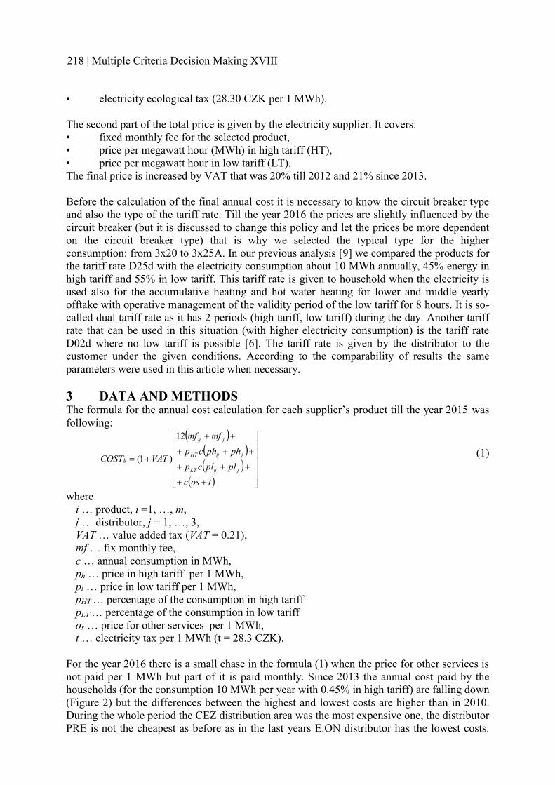
• electricity ecological tax (28.30 CZK per 1 MWh).

The second part of the total price is given by the electricity supplier. It covers: • fixed monthly fee for the selected product, • price per megawatt hour (MWh) in high tariff (HT), • price per megawatt hour in low tariff (LT), The final price is increased by VAT that was 20% till 2012 and 21% since 2013.

Before the calculation of the final annual cost it is necessary to know the circuit breaker type and also the type of the tariff rate. Till the year 2016 the prices are slightly influenced by the circuit breaker (but it is discussed to change this policy and let the prices be more dependent on the circuit breaker type) that is why we selected the typical type for the higher consumption: from 3x20 to 3x25A. In our previous analysis [9] we compared the products for the tariff rate D25d with the electricity consumption about 10 MWh annually, 45% energy in high tariff and 55% in low tariff. This tariff rate is given to household when the electricity is used also for the accumulative heating and hot water heating for lower and middle yearly offtake with operative management of the validity period of the low tariff for 8 hours. It is so-called dual tariff rate as it has 2 periods (high tariff, low tariff) during the day. Another tariff rate that can be used in this situation (with higher electricity consumption) is the tariff rate D02d where no low tariff is possible [6]. The tariff rate is given by the distributor to the customer under the given conditions. According to the comparability of results the same parameters were used in this article when necessary.

3 DATA AND METHODS The formula for the annual cost calculation for each supplier’s product till the year 2015 wasfollowing:

� �� �� �

� � '''''

)

%

&&&&&

(

$

��

���

���

��

��

toscplplcpphphcp

mfmf

VATCOSTjijLT

jijHT

jij

ij

12

)1( (1)

where i … product, i =1, …, m, j … distributor, j = 1, …, 3,VAT … value added tax (VAT = 0.21), mf … fix monthly fee, c … annual consumption in MWh,ph … price in high tariff per 1 MWh,pl … price in low tariff per 1 MWh,pHT … percentage of the consumption in high tariffpLT … percentage of the consumption in low tariffos … price for other services per 1 MWh,t … electricity tax per 1 MWh (t = 28.3 CZK).

For the year 2016 there is a small chase in the formula (1) when the price for other services is not paid per 1 MWh but part of it is paid monthly. Since 2013 the annual cost paid by the households (for the consumption 10 MWh per year with 0.45% in high tariff) are falling down (Figure 2) but the differences between the highest and lowest costs are higher than in 2010. During the whole period the CEZ distribution area was the most expensive one, the distributor PRE is not the cheapest as before as in the last years E.ON distributor has the lowest costs.

218 | Multiple Criteria Decision Making XVIII

The number of products offered by suppliers circulates around 60 (in 2015 60 products for D25d and 61 for D02d offered by 32 companies, in 2016 30 companies offered 57 resp. 58 products).

Figure 2 - Trends for the annual costs for the tariff rate D25d and the annual consumption 10 MWH

To minimize the annual cost the linear programming model can be created [8]. The aim is to find the ranges (minimal and maximal) for the annual consumption for each product (if possible) that guarantee the cost lower than for the other products. First it is good to compare all the products pairwise to find the dominated ones. For non-dominated product we are able (based on (1)) to calculate the values of energy consumption c that ensure winning of the given supplier/product k. The mathematical model of this problem for each product i,k = 1, …, m and distributor j = 1, 2, 3 can be written as following [10]:

min(max) z = csubject to: COSTij ≤ COSTkj (2)

When there exists no optimal solution for the product k then the minimal (in the mathematic sense) annual costs can never be achieved for any consumption level when choosing this product. The same model was used for the comparison of the two different tariff rates (here D25d and D02d) when only non-dominated products were selected for both tariff rates and each of the distributors’ area. The model (2) was enlarged by the constraints COSTsj≤COSTkj,where s = 1,…,n represents the product of the tariff D02d whereas k represents the product of the tariff rate D25d. This model found the ranges of the consumption for the non-dominated D25d products. Afterwards the right hand sides were changed into the COSTsj to find the ranges for the consumption with the lowest annual costs for the D02d products.

4 RESULTS AND DISCUSSIONThe analysis was made for the year 2015 and 2016 and for the tariff rates D25d and D02d and for the situation than if possible, the low tariff can be used for 55% of the total consumption. Table 2 summarizes basic data – from all products there was only 7-13% non-dominated ones.

Quantitative Methods in Economics | 219

Table 2 – Number of products, companies and non-dominated productsYear Tariff rate Number of

productsNumber of companies

Number of non-dominated productsE.ON / PRE / CEZ

2015 D25d 60 32 8 / 8 / 9D02d 61 32 6 / 7 / 7

2016 D25d 57 31 8 / 8 / 8D02d 58 31 5 / 4 / 4

The optimization models for the year 2015 and D25d showed that there are only 3 products with lowest annual costs (the fourth product of Fosfa company has lowest costs only for 0 consumption) – Table 3. In 2016 there are only 2 products with the lowest costs (and 2 others – Fosfa FEE Smart and Fonergy Premium – with the lowest costs for 0 consumption) – Table 4. In both years the cheapest distributor region is E.ON, CEZ is the most expensive one. For the consumption of 10 MWh per year the best supplier stays the same (but it is diferent from the previous years – see [10]).

Table 3 – Cheapest products of D25d tariff rate for different consumption ranges for 2015

2015

Ranges for consumption in MWh per year

0 – 5.009E.ON, PRE:

5.009 – 14.039CEZ: 5.009 – 16.856

E.ON, PRE: >14,039CEZ: >16.856

Best product Fonergy Premium

ST Energy Standard

CARBOUNION KOMODITY

Table 4 – Cheapest products of D25d tariff rate for different consumption ranges for 2016

2016

Ranges for consumption in MWh per year 0 – 3.42857 >3.42857

Best product Fosfa FEE e-Tarif

ST Energy Standard

Ranges for prices E.ON 1505.62-11138.72 >11138.72Ranges for prices PRE 1736.30-11241.65 >11241.65Ranges for prices CEZ 1852.46-11682.21 >11682.21

Situation for the D02d tariff rate is different as in 2015 there was more companies with the lowest costs (5 for E.ON and 6 for PRE and CEZ) - Table 5 - but in 2016 they were only 2 (with 2 others with the lowest costs for 0 consumption) – Table 6. In the situation of the consumption of 10 MWh per year the supplier is different and also the prices are higher than for D25d.

Table 5 – Cheapest products of D02d tariff rate for different consumption ranges for 2015

2015

Ranges for consumption in MWh per year

0-1.971 1.971-7.263

7.263-27(E.ON, PRE)

7.263-12(CEZ)

>27 (E.ON)27-116(PRE)

12-60 (CEZ)

>60(CEZ)>116(PRE)

Best productFosfa FEE St.,

Fonergy Premium

EEE Duo24 EEE Comp.

EP Energy Trading Klasik

Bohemia Energy

Home St.

220 | Multiple Criteria Decision Making XVIII

Table 6 – Cheapest products of D02d tariff rate for different consumption ranges for 2016

2016

Ranges for consumption in MWh per year

0 – 2.5899 (E.ON, CEZ)

0 – 3.410 (PRE)

>2.5899 (E.ON, CEZ)

>3.410 (PRE)

Best product Fosfa FEE e-Tarif

Central Energy D Standard

Ranges for prices E.ON 1242.6-11168.3 >11168.3Ranges for prices PRE 1387.8-14457.8 >14457.8Ranges for prices CEZ 1387.8-11512.7 >11512.7

Table 7 – Ranges for the annual consumption and the cheapest products (with 55% of low tariff)Year Tariff rate D02d D25d

2015

Ranges for consumption in MWh per year

0-0.394 (E.ON)0-0.379 (PRE)0-0.481 (CEZ)

0.394-5.009(E.ON)

0.379-5.009 (PRE)0.481-5.009 (CEZ)

5.009-14.039(E.ON, PRE)5.009-16.856

(CEZ)

>14.039 (E.ON, PRE)

>16.856 (CEZ)

Best productFosfa FEE St.,

Fonergy Premium

Fonergy Premium ST Energy Standard

CARBOUNION COMMODITY

2016

Tariff rate D02d D25dRanges for consumption in MWh per year

0-0.345 (E.ON)0-0.329 (PRE)0-0,419 (CEZ)

0.345-3.429(E.ON)

0.329-3.429 (PRE)0.419-3.429 (CEZ)

>3.429

Best product Fosfa FEE e-Tarif Fosfa FEE e-tarif ST Energy Standard

The next model used both tariff rates prices and the task was to find the ranges for which there was a product with the lowest annual cost. Table 7 shows the results. It is clear that in the situation when nearly for the half of the consumption the low tariff prices can be used (in D25d) it is better to have this tariff rate (when fulfill the conditions of water heating) and the D02d is cheaper only for small consumption. But when it is supposed to be able to use high tariff only in both tariff rates, the results are different (Table 8). While in 2015 in E.ON and PRE distribution regions it was better to have D25d rate for the higher consumption, in the CEZ region the D02d was suitable for any consumption. The same situation was for the 2016 data.

Table 8 – Ranges for the annual consumption and the cheapest products (with 100% of high tariff)Year Tariff rate D02d D25d

2015

Ranges for consumption in MWh per year (E.ON, PRE)

0-1.971 1.971-5.880 >5.880

Best product Fosfa FEE St., Fonergy Premium

EEE Duo 24 Nano Energies Trade

Tariff rate D02dRanges for consumption in MWh per year (CEZ)

0-1.971 1.971-7.263 7.263-12 12-60 >60

Best product Fosfa FEE St., Fonergy Premium

EEE Duo 24

EEEComp.

EP Energy Trading Klasik

Bohemia Energy Home

St.

Quantitative Methods in Economics | 221

2016

Tariff rate D02dRanges for consumption in MWh per year

0-2.5899 (E.ON)0-3.410 (PRE)

0-2.1687

>2.5899 (E.ON)>3.410 (PRE)

>2.1687 (CEZ)

Best productFosfa FEE e-tarifFosfa FEE smart

(CEZ)Central Energy D Standard

5 CONCLUSIONS The situation on the electricity market in the Czech Republic after the deregulation gives the households the possibility to select the appropriate supplier. As the formula consists of different prices it is not easy to decide for the cheapest product. The analyses compared two different tariff rates. The results showed that when the conditions for the tariff rate D25d are fulfilled then it is better to have it especially for the higher consumption. Once it is necessary to use only high tariff prices for both tariff rates then the D02d is cheaper. In both cases only few of the products can be selected as the cheapest ones.

Acknowledgements: This work was supported by the grant No. F4/54/2015 of the Faculty of Informatics and Statistics, University of Economics, Prague.

References [1] ACER/CEER: Annual Report on the Results of Monitoring the Internal Electricity and

Natural Gas Markets in 2013 [online], available at: http://www.europarl.europa.eu/meetdocs/2014_2019/documents/itre/dv/acer_market_monitoring_report_2014_/acer_market_monitoring_report_2014_en.pdf [Accessed 2016-02-20].

[2] Boltz, W. (2013). The Challenges of Electricity Market Regulation in the European Union. Evolution of Global Electricity Markets. Elsevier Inc. 2013, pp. 199–224.

[3] Diakoulaki, D. and Karangelis, F. (2007). Multi-criteria decision analysis and cost–benefit analysis of alternative scenarios for the power generation sector in Greece. Renewable and Sustainable Energy Reviews, 11(4) (2007), pp. 716–727.

[4] ERU: Distribution regions in the Czech Republic. ERU, 2015. [online], available: http://www.a-tender.cz/distribuce_elektriny_a_plynu_v_cr.html [Accessed 2015-10-02].

[5] ERU: Energy Regulatory Office - Price calculator, ERU 2015, [online], available: http://kalkulator.eru.cz/VstupniUdaje.aspx [Accessed 2016-02-28].

[6] ERU: Věstník 9/2015 ERU, 2015, [online], available: https://www.eru.cz/documents/10540/1174016/ERV_9_2015.pdf/2892b192-e693-40cb-835f-be04715df391 [Accessed 2016-02-28].

[7] Hegazy, Y.G., Salama, M.M.A. and Chickhani, A.Y. (2003). Adequacy assessment of distributed generation systems using Monte Carlo Simulation. Power Systems - IEEE Transactions 18(1) (2003), pp. 48–52.

[8] Kuncová, M. (2015). Methods for the Electricity Supplier Selection – Case Study of theCzech Republic. International Journal of Mathematical Models and Methods in Applied Sciences 9 (2015), pp. 714–720.

[9] Kuncová, M. and Sekničková, J. (2014). Analysis of the efficiency of the electricity supplier selection depending upon the price changes. In: Proceedings of the 34th

Mathematical Methods in Economics Conference. Palacký University in Olomouc, 2014, pp. 542–547.

222 | Multiple Criteria Decision Making XVIII

[10]Kuncová, M. and Sekničková, J. (2015). Optimization Models Used for the Electricity Supplier Selection. In: Proceedings of the 33rd Mathematical Methods in Economics 2015 Conference. West-Bohemia University, Cheb, 2015, pp. 443–448.

[11]Newbery, D. (2013). Evolution of the British Electricity Market and the Role of Policy for the Low-Carbon Future. Evolution of Global Electricity Markets. Elsevier Inc. 2013, pp. 3–30.

[12]Wilson, Ch. M. and Waddams Price C. (2010). Do consumers switch to the best supplier? Oxford Economic Papers 62(4) (2010), pp. 647–668.

Author’s addressIng. Martina Kuncová, Ph.D. University of Economics in Prague, Dpt. of Econometrics W.Churchill Sq. 4, 13067 Prague 3 Czech Republic email: martina.kuncova@vse.cz

Quantitative Methods in Economics | 223

ACCELERATION OF THE OGRYCZAK’S APPROACH TOLEXICOGRAPHICAL MIN-MAX EMERGENCY SYSTEM DESIGN

Marek Kvet University of Žilina, University Science Park

Jaroslav JanáčekUniversity of Žilina, Faculty of Management Science and Informatics

Abstract This paper focuses on the emergency service system design, in which the request of equal accessibility is considered to some extent. The cases of failing and reliable service centers are taken into account, when the problem is formulated. The concept of solving technique is based on the radial formulation due to previously observed excellent performance and flexibility of the approach. To assure some level of service accessibility for the worst situated users, several steps of the lexicographical min-max optimization are used according to the Ogryczak’s iterative approach. This approach proved to be very slow when problems with failing centers were solved. This paper deals with possible ways of the Ogryczak’s approach acceleration making use of the radial formulation.

Keywords: emergency system design, failing centers, computational process acceleration

JEL Classification: C61 AMS Classification: 90C27

1 INTRODUCTION This paper is focused on some computational aspects of solving technique for the fair emergency system design, where unreliability of located centers is taken into account. The system design problem with unreliable – temporary inaccessible service centers was usually modeled for the objective to minimize disutility perceived by so called average user [1], [4], [7]. These min-sum models were formulated in two modes, either in the form of location-allocation model [1], [7] or in so called radial form [4], where the latter mode approved to be better in accelerating the solving process based on branch-and-bound technique. With rise of requests for fairness in service system designing, attempts at emergency system design with min-max and lexicographic min-max objectives appeared [6]. Nevertheless, it was found that the iterative approaches, which verifies step-by-step existence of a solution with objective function value less than given threshold, often fail due to enormous computational time demanded by the individual steps. The computational time becomes inacceptable especially, when disutility of the worth situated user exceeds the threshold connected with the given step. This phenomenon makes the Ogryczak’s approach almost inapplicable even for partial lexicographical optimization. The goal of this contribution is to suggest an algorithm, which effectively specifies the range of thresholds, for which time of associate sub-problem solving is acceptable. This range can enable to apply the Ogryczak’s approach in semi-fair emergency system design, where extents of disutility perceived by the worst situated users are minimized in several initial steps, and then min-sum objective is applied under condition that the achieved disutility limits are not exceeded. The remainder of the paper is organized as follows. Section 2 is devoted to explanation of the Ogryczak’s approach. The radial approach to the semi-fair service center deployment is concisely described in Section 3 together with the suggested algorithm for effectivespecification of the range of thresholds. The associated numerical experiments and the

224 | Multiple Criteria Decision Making XVIII

deployment comparison are performed in Section 4. The results and findings are summarized in Section 5.

2 OGRYCZAK’S APPROACHThe optimal deployment of the service centers is defined as a problem to locate at most p

service centers at positions from the given finite set I so that a given objective function

modelling disutility perceived by users’ is minimal. We introduce binary variables yi�{0,1}

for each possible center location from I, to model the decisions on the particular center

locations. Let vector y of the components yi describe the concrete service center deployment,

which generates disutility for each users’ location. Let a set J be the set of users’ locations and

bj denote the number of users sharing the location j. The disutility perceived by users sharing

location j to the possible service center location i will be denoted as Dj(y). The min-sum

optimal service center deployment problem can be formulated by model (1), where m

corresponds to the cardinality of I. },}1,0{:)(min{ ��

��

��Ii

im

Jjjj pyDb yy (1)

If the lexicographical min-max fair problem is solved, then the disutility of the worst situated user is minimized first, and then the disutility the second worst situated users is minimized unless the minimal reached disutility from the previously processed users gets worsened. This process is repeated until no user’s disutility can be reduced. To express the quality of a solution of the service center deployment problem from the point of lexicographical fairness, the situation is a bit more complicated in comparison to the min-sum criterion. A service center deployment y induces different extents of disutility of users sharing different users’ locations. The extents of disutility can be characterized by the distribution vector [B0(y), B1(y) … Bw(y)], where the t-th component of the vector is defined according to (2), where G0> G1> …> Gw> Gw+1 are the abovementioned thresholds.

wtforbB

tjt GDGJj

jt ...,,0)()(1

�� �0�

�� y

y(2)

The lexicographic min-max problem according to [6] consists in lexicographic minimization of the vector [B0(y), B1(y) … Bw(y)] subject to y��{0, 1}m and the condition that vector ycontains at most p components, which equal to one. It follows from [6] that lexicographical minimization of adjusted vector [B0(y), B1(y) … Bw(y)] can be performed instead of the lexicographic minimization of the original distribution vector [B0(y), B1(y) … Bw(y)]. The t-th component of the adjusted vector is defined according to (3).

wtforbB

jt DGJj

jt ...,,0)()(1

�� ���

� y

y (3)

3 RADIAL APPROACH AND LEXICOGRAPHICAL OPTIMIZATION The suggested semi-fair deployment algorithm [5] can be described by two phases, where the first one performs the lexicographic minimization of the distribution vector B(y) restricted to the given number of the L first components. The second phase solves problem (1) subject to additional condition that the L first components of the adjusted distribution vector cannot get worsened.

The generalized disutility Dj(y) for any user located at j is modeled by a sum of weighted disutility contributions from the r nearest centers. The weight coefficients qk for k = 1 ... r are positive real values, which meet the inequalities q1 ≥ q2 ≥ … ≥ qr [7] and these coefficients can be proportional to the probability that the k-th nearest center is the first center which does

Quantitative Methods in Economics | 225

not fail. The disutility contribution dij from center location i to a user at j is considered to be proportional to the integer network distance between location i and location j.The following radial model of the problem solved at each of the first L steps is based on the concept of homogenous system of radii, which was broadly studied in [2], [3]. The radial formulation assumes the range 0, v+1 of all possible integer disutility contribution values. To describe the problem, auxiliary binary variables xjsk for s = 0 … v and k=1 … r are introduced, where variable xjsk takes the value of 1 if the k-th smallest disutility contribution for a user at j�J coming from the located centers is greater than s and the variable takes the value of 0 otherwise. Then the expression xj0k + xj1k + xj2k + xj3k +…+ xjvk constitutes the k-th smallest disutility contribution dk

j* for the user at j. In addition, we introduce a zero-one constant aij

s for each triple i, j, s where i�I, j�J and s= 0 … v. The constant aijs equals to 1 if

and only if the disutility contribution dij of a user at the location j from the possible center location i is less than or equal to s, otherwise aij

s is equal to 0. Then the problem solved at the t-th step can be formulated as follows:

��Jj

tjj hbMinimize (4)

vsJjforryaxtoSubjectIi

isij

r

kjsk ..0,

1��4� ��

��(5)

��

0Ii

i py (6)

JjtuforGxqh u

r

k

v

sjskkuj ���4 �

� �� � ,...,,01

1 0(7)

1,....,0* ��0��

tuforBhb uJj

ujj (8)

rkvsJjforx jsk ..1,,..0,}1,0{ ���� (9)

Iiforyi �� }1,0{ (10)

Jjtuforhuj ��4 ,,...,00 (11)

The constraints (5) ensure that the sum of variables xjsk over k expresses the number of service centers in the radius ds from the user location j, which remains to the number r. The constraint (6) sets a limit p on the number of located facilities. The nonlinearity in the (3) can be excluded by introducing a series of slack non-negative variables htj for given stage t and for j�J. The variables htj must be connected to the system of original variables by link-up constraints (7) and obligatory constraints (11). The constraints (8), where B*u denotes the optimal objective function value for u=0, …,t-1, ensure that optimization at the stage t does not spoil the objective function value achieved at the previous stages. The generalized disutility for a user at the location j is described by (12) in the above model.

����

�v

sjsk

r

kkj xqD

01)(x (12)

As mentioned in the Introduction, this iterative approach often fails due to enormous computational time demanded by the step, when disutility of the worth situated user exceeds the associated threshold Gt+1. We suggest the following algorithm, which effectively specifies the range of thresholds, for which time of associate sub-problem solving is acceptable.

226 | Multiple Criteria Decision Making XVIII

Step 0. Solve the problem (13), (5), (6), (14), (9), (10), (15) for t=0. Denote the associated computational time by Tc. Set the time limit Tl of solving process of the problem (13), (5), (6), (14), (9), (10), (15) to the value �Tc, where � > 1 is a parameter of the algorithm. Set the maximal and minimal values of the explored subscripts to tmn=0, tmx=v respectively.

Step 1. Set t=tmn+(tmx-tmn) div 2. Solve the problem (13), (5), (6), (14), (9), (10), (15) for given t. If the computational time is less than the time limit Tl, then check the objective function value (13). In the case, when the objective function value equals 0, set tmn=t, in the opposite case set tmx=t. Otherwise (the computational time exceeds Tl), set tmx=t. Step 2. If tmn=tmx-1, terminate and return the value tmn as a resulting subscript value, otherwise go to Step 1.

This algorithm specifies the resulting threshold Gtmn+1 in the sense that all the problems with thresholds Gtmn+1, Gtmn, …, G1 are easy to solve. |This way, the range for semi-fair designs is specified.

For the purpose of the algorithm description the constraints (4), (7), (11) were reformulated to the following form of constraints (13), (14), (15) respectively and the resulting problemwas solved in the above algorithm for given t.

��Jj

jjhbMinimize (13)

JjforGxqh t

r

k

v

sjskkj ��4 �

� �� � 1

1 0(14)

Jjforhj �40 (15)

4 COMPUTATIONAL STUDY To compare the original approach, which consists of step-by step solving of the problem (4) –(11) for the t=0, 1, …, t*, where t* was the first step, when the objective function value was greater than 0, with the new suggested approach described by the above algorithm, we performed the series of numerical experiments. To solve the problems described in the previous sections, the optimization software FICO Xpress 7.7 (64-bit, release 2014) was used and the experiments were run on a PC equipped with the Intel® Core™ i7 2630 QM processor with the parameters: 2.0 GHz and 8 GB RAM. The used benchmarks were derived from the real emergency health care system, which was originally implemented in seven regions of Slovak Republic, i.e. Banská Bystrica (BB), Košice (KE), Nitra (NR), Prešov (PO),Trenčín (TN), Trnava (TT) and Žilina (ZA). These sub-systems cover demands of all communities - towns and villages spread over the particular regions by a given number of ambulance vehicles. In the benchmarks, the set of communities represents both the set J ofusers’ locations and also the set I of possible center locations. The cardinalities of these sets vary from 249 to 664 according to the considered region. The number p of located centers was derived from the original design and it varies from 25 to 67. The computational study was performed for r = 3 and the reduction coefficients q1 = 1, q2 = 0.2 and q3 = 0.1. Thefollowing table contains results obtained by both approaches.

Quantitative Methods in Economics | 227

The label “BASIC APPROACH” denotes results obtained by the original version of the algorithm mentioned above, while the label “BISECTION” denotes results of the suggested algorithm. Each row of the table corresponds to one of the mentioned self-governing regions of Slovakia. The labels used for column denotation have the following meaning:

|I| is the number of possible service center locations.

p denotes the number of centers to be located.

CT [s] is the total computational time given in seconds.

Iter denotes the number of iterations performed by the associated process.

Gtmn+1 represents the resulting threshold. Table 1 Results of numerical experiments with 7 self-governing regions of Slovakia

Region |I| pBASIC APPROACH BISECTION

CT [s] Iter Gtmn+1 CT [s] Iter Gtmn+1

BB 515 52 434.4 15 22.1 124.3 6 23.4KE 460 46 775.0 29 19.5 357.1 6 20.8NR 350 35 1065.3 29 19.5 223.4 7 22.1PO 664 67 1250.5 28 19.5 711.3 6 19.5TN 276 28 649.3 29 19.5 156.2 6 20.8TT 249 25 573.7 26 19.5 104.4 7 20.8ZA 315 32 666. 7 26 22.1 202.8 7 23.4

5 CONCLUSIONS We have suggested an algorithm for effective specification of the range of thresholds, which can be used with Ogryczak’s approach to semi-fair emergency service system design. The suggested algorithm was compared to the original one and it was found that the new algorithm can save approximately three quarters of the computational time regarding the original approach. The future research in this area will be focused on exploiting exposing structures for mastering the semi-fair emergency system construction also for the semi-fair levels, where the threshold is out of the range obtained by the studied algorithms.

Acknowledgements: This work was supported by the research grants VEGA 1/0518/15 “Resilient rescue systems with uncertain accessibility of service”. This work was also supported by the project University Science Park of the University of Žilina (ITMS: 26220220184) supported by the Research & Development Operational Program funded by the European Regional Development Fund. We would like to thank to „Centre of excellence for systems and services of intelligent transport“ (ITMS 26220120050) for built up the infra-structure, which was used.

References [1] Drezner, T. and Drezner, Z. (2007). The gravity p-median model. European Journal of

Operational Research 179 (2007), pp. 1239-1251.

228 | Multiple Criteria Decision Making XVIII

[2] García, S., Labbé, M. and Marín, A. (2011). Solving large p-median problems with a radius formulation. INFORMS Journal on Computing 23(4) (2011), pp. 546-556.

[3] Janáček, J. and Kvet, M. (2014). Relevant Network Distances for Approximate Approach to the p-median Problem. In: Selected Papers of the International Conference of the German operations research society (GOR), Hannover: Springer, pp. 123-128.

[4] Janáček, J. and Kvet, M. (2015). Emergency system design with temporarily failing centers In: Proceedings of the 13th International Symposium on Operational Research,Bled, Slovenia, pp. 490-495.

[5] Kvet, M. and Janáček, J. (2015). Semi-fair deployment of the service centers in a transportation network In: Proceedings of the 13th International Symposium on Operational Research, Bled, Slovenia, pp. 458-463.

[6] Ogryczak, W. and Slivinski, T. (2006). On Direct Methods for Lexicographic Min-Max Optimization. In: Gavrilova, M. (Eds.): ICCSA 2006, LNCS 3982, Berlin: Heidelberg: Springer, pp. 802-811.

[7] Snyder, L. V. and Daskin, M. S. (2005). Reliability Models for Facility Location; The Expected Failure Cost Case. Transport Science 39(3) (2005), pp. 400-416.

Authors’ addressesIng. Marek Kvet, PhD. University of Žilina - University Science Park Univerzitná 8215/1, 010 26 Žilina, SlovakiaEmail: marek.kvet@uvp.uniza.sk

Prof. RNDr. Jaroslav Janáček, CSc.University of Žilina - Faculty of Management Science and Informatics Univerzitná 8215/1, 010 26 Žilina, SlovakiaEmail: jaroslav.janacek@fri.uniza.sk

Quantitative Methods in Economics | 229

FIRST PILLAR OF SLOVAK PENSION SYSTEM

Ivan Lichner, Institute of Economic Research SAS

Abstract Population ageing imposes growing pressure on the pension systems of many European countries. In this paper results of simulation of first pillar of Slovak pension system are presented to provide additional information on the possible development and discuss available possibilities to mitigate the expected negative development.

Keywords: simulation, pension system, modelling, forecast

JEL Classification: C53, H55 AMS Classification: 37M05

1 INTRODUCTION According to latest demographic forecast1 speed of population ageing in Slovakia will be one of the highest in the European Union over the coming decades. Between years 2015 and 2060 population over 65 will grow faster only in Luxembourg, Cyprus, Norway and Iceland. Over next 15 years number of inhabitants over 65 years will increase by more than 50 % in Slovakia. This development will bring with it several socio-economic challenges, among most prominent will be increase in need of long-term care and health care services, and also increased pressures on pension system. In this paper we will focus on the impact of ageing and other relevant factors that will be having an impact on the first pillar of Slovak pension system and its balance. Goal of this paper is to estimate possible development of first pillar of Slovak pension system balance. This will be achieved by utilization of simulation model with respect to the current legislative conditions under expected different wages and price development. Pension system in Slovakia is according to changes that took place with legislative changes2 effective from year 2005 composed of three pillars:

- PAYG pillar (compulsory); - Capitalization pillar (voluntary with option to enter up to 35 years of age); - Private pension’s savings (voluntary).

Figure 1: Growth of population over 65 years compared to 2015 level 1 EUROPOP 2013 main scenario.2 Act 43/2004 about pension savings

0%

20%

40%

60%

80%

100%

120%

2020 2030 2040 2050 2060

Slovakia

Poland

Austria

Hungary

Czech Republic

230 | Multiple Criteria Decision Making XVIII

In this paper we will focus only on development of the first PAYG pillar of pension system as only this has possible impact on public finances in case if the contributions do not fully cover the expenditures of this part of pension system. Currently are deficits of this pillar of pension system cover by surpluses of other Social insurance company funds and from state budget. In the paper of Sivák et al. (2011) authors were examining the possible impacts of parametric changes on PAYG and results of their simulations suggested that those changes would not outweigh the burden of growing number of pensioners. Kvetan and Radvanský in their paper from 2008 analyzed impact of two pillar system on the sustainability of the pension system. According to their results introduction of two pillar pension system (semi-compulsory) will lead to lower deficits of pension system as whole. Similar conclusion was drawn by Domonkos et al. (2014), who also pointed out on higher immediate and medium term deficits when using two-pillar pension system compared to single-pillar. These result from higher contributions to the second pillar which could have been otherwise used for covering present expenditures of pension system.

Analysis that is conducted in this paper focuses on the forecast of possible development of PAYG pillar of pension system balance under the current legislative framework up to 2060. Results of the simulations would provide information on the scope and probability of the PAYG balance and replacement ratio of the average pension to average wage.

2 METHODOLOGY To estimate possible development of first pillar of pension system simulation model needed to be build. Applied model approach represents extension of static model that was developed in Lichner (2013). Extended simulation model should be divided in two parts: Income and Expenditures of PAYG system parts.

Income part of model estimated possible development of the PAYG system according to the level of effective contribution rate, employment and average wage. Effective contribution rate (�2�) was set at its level from last available year 2014 – 15.4% of gross wage. Employment (�����,") with respect to age3 (i) and sex (j) was estimated according to static expectations of participation rate from year of last available data - 2014. In case of participation of age groups 60-64 and 65-69 in which participation would increase with future increases of retirement age we expected its convergence to level of employment rate of age group 55-59 years in 2014. In simulations values of average wage (\H�,") growth rates were randomly chosen for each age group and sex with normal distribution. Mean and standard deviation of random process selecting the value of annual growth rate of wages were set at the level of past 15 annual growth rates with omission of 5 periods with highest increases that mostly occurred in periods of economic conjecture and are relatively unlikely to occur again. To calculate contribution of each age and sex group to pension fund of Social insurance Company following formula was applied:

2�.Z�b��,",+ = 12 ∗ �����," ∗ �2� ∗ \H�," (1)

Total contribution income for given year (��'+) was then represented by the sum of PAYG system contributions of selected sub-groups:

��'+ = ∑ 2�.Z�b��,",+�," (2)

3 In the simulation model age was defined as 5 years age groups from 15-59 years and age group of over 60 years.

Quantitative Methods in Economics | 231

Expenditure side of the model composed of equations combining the relations between number of retired, average pension and pensioner’s price index (PePI) to define the future needs of resources to be paid from PAYG system. Number of retired (:�Zb,Z) was estimated according to past development and future expected changes in the retirement age.

Figure 2: Number of retired

Pensioner’s price index was defined by random process with normal distribution that has mean and standard deviation based on past development and forecast of PePI by IFP (2016). Due to data availability average pensions (\�b,Z) were estimated only according to age and were valorized by PePI for age groups over 654. In case of retirees in age group of retirement entry average pension was calculated according to level of average wage of given group and constant replacement rate from 2014. Amount of resources needed for the pensions from PAYG system for given age group (��.4b,Z) was calculated on the basis of following equation:

��.4b,Z = :�Zb,Z ∗ \�b,Z (3)

Total expenditures on pensions from PAYG system was then calculated as sum of age groups pensions expenditures:

��+ = ∑ ��.4�,+� (4)

By combination of total contributions and total expenditures balance of PAYG pension system was calculated:

�\�Z = ��'Z − ��Z (5)

System of those equations (1) – (5) was used to estimate future development of PAYG part of the pension system at its current parametric setup. In each run of the model new values of wage annual growth rates and pensioner´s price index were set for each year during period 2015-2060. This allowed us to analyze impact of wage and price changes on the first pillar of pension system balance.

3 RESULTS In this section results obtained after 10 000 runs of above defined simulation model are presented. According to the results of simulation average deficit of PAYG system would

4 After year 2040 over 70 due to increase of retirement age over 65 years of age.

800 000

900 000

1 000 000

1 100 000

1 200 000

1 300 000

1 400 000

1 500 000

232 | Multiple Criteria Decision Making XVIII

remain slightly below 1 bill. EUR until the 2040. Expected growth in number of retired will be offset by possible growth of average wage and relatively lower growth of PePI during this period. After 2040 average deficit would start to increase more rapidly. In the horizon of 10 years PAYG system would possibly achieve surplus, even though probability of this event is marginal. At the horizon of forecasted period in case of negative development maximal deficitwould achieve more than 25 bill. EUR.

Figure 3: First pillar of pension system balance, mill. EUR

Over next 10 years balance of PAYG system would remain in range of 0 to -2.5 bill. EUR and from 2030 slight increase in probability of deficit over 2.5 bill. EUR will occur. After 2040 the deficit most probably will be in range between 2.5 and 5 bill. EUR. After year 2050 without substantial change in calculation method of initial pensions deficit of PAYG system would be over 5 bill. EUR, with growing trend.

Table 1: Level of first pillar of pension system deficit distribution, % 2015 2020 2025 2030 2035 2040 2045 2050 2055 2060 more than 0 bill.EUR 0.0 0.0 0.0 0.2 1.1 2.3 0.3 0.1 0.2 0.6 -2.5 to 0 bill.EUR 100.0 100.0 100.0 97.0 88.7 72.6 22.7 8.2 4.7 5.3 -5 to -2.5 bill.EUR 0.0 0.0 0.0 2.8 10.2 24.8 57.6 37.4 21.9 18.2 -10 to -5 bill.EUR 0.0 0.0 0.0 0.0 0.0 0.0 6.0 30.0 45.6 42.8 more than -10 bill.EUR 0.0 0.0 0.0 0.0 0.0 0.0 0.0 0.9 6.0 12.5

Expected static replacement rate at the age of retirement would not be sufficient to keep overall replacement rate at socially acceptable level close to 40 % of average wage. Results of the simulations suggest that already in 2020 with probability of 25 % replacement ratio will be in range between 30-35 %. In next ten years replacement rate will be in this range with probability of 90 %. Between years 2035 and 2050 replacement rate would be most probably between 25 and 30 % of average wage. After year 2050 replacement rate would be highly probably below 25 % of average wage. To increase the replacement rate changes in valorization of the pensions from PAYG system would be implemented, but those would lead to increases in the deficits. Thus without contribution rates changes replacement rate would not stay at its current levels without risks of higher deficits and growing social tensions.

-30 000

-25 000

-20 000

-15 000

-10 000

-5 000

0

5 000

10 000

2015 2020 2025 2030 2035 2040 2045 2050 2055 2060

minimal

average

maximal

Quantitative Methods in Economics | 233

Table 2: Pension to average wage replacement rate distribution 2015 2020 2025 2030 2035 2040 2045 2050 2055 2060 less than 20 % 0.0% 0.0% 0.0% 0.0% 0.0% 0.0% 0.1% 0.9% 4.2% 12.8% 20-25 % 0.0% 0.0% 0.0% 0.1% 3.2% 15.6% 21.4% 34.7% 48.6% 57.4% 25-30 % 0.0% 0.0% 3.6% 43.0% 72.1% 72.4% 64.1% 54.2% 41.2% 26.9% 30-35 % 0.0% 25.9% 90.1% 56.0% 24.5% 12.0% 14.2% 9.8% 5.7% 2.7% more than 35 % 100.0% 74.1% 6.3% 0.9% 0.2% 0.1% 0.3% 0.4% 0.3% 0.1%

4 CONCLUSIONS Aging of population in Slovakia will over coming decades translate in continuous growth of number of pensioners. Peak in the number of pensioners would be achieved between 2055 and 2060. Over next 25 years PAYG pillar of pension system would generate deficit around 750 mil. EUR annually. In this period expected growth in number of pensioners will be offset by expected growth of average wage and relatively lower growth of pensioners´ prices(according to current development and its forecasts). After year 2040 average level of deficit would start to increase more rapidly and after year 2050 without substantial changes in calculation method of initial pension deficit of PAYG system would be over 5 bill. EUR.

On the other hand, expected static replacement rate at the age of retirement (ratio between initial pension and average wage of 60+ age group) would not be sufficient to keep overall replacement rate at socially acceptable level close to 40 % of average wage. Results of the simulations suggest that already in 2020 with probability of 25 % replacement ratio will be in range between 30-35 %. Between years 2035 and 2050 replacement rate would be most probably between 25 and 30 % of average wage. After year 2050 replacement rate would be highly probably below 25 % of average wage.

To increase the replacement rate, changes in valorization of the pensions from PAYG system would be implemented, but those would lead to increases in the deficits. Thus without contribution rates increase replacement rate would not stay at its current levels without risks of higher deficits and growing social tensions. It is important to stress that pensions from the second pillar of pension system would contribute to more socially acceptable level of replacement rate. Thus it is important to encourage labour market entrants to enter this pillar of pension system as replacement rate of pensions from first pillar will drop significantly in future.

Acknowledgements: This work was supported by the Slovak Research and Development Agency under the contract No. by APVV-14-0787.

References [1] Cameron, A. C. and Trivedi, P. K. (2010). Microeconometrics Using Stata, Rev. ed.

College Station, Texas: Stata Pres. [2] Domonkos, T., Domonkos, Š., Jánošová, M. and Ostrihoň, F. (2014). A Long-run

Macroeconomic Model of Slovakia (Long-term sustainability of the pension system). In: EcoMod2014 international conference on economic modeling, Bank of Indonesia, Denperas Bali.

[3] Eurostat, (2016). Database – Eurostat. [online] Available at: http://ec.europa.eu/eurostat[Accessed 25 Mar. 2016].

[4] Šrámková, L., Žúdel, B. and Habrman, M. (2016). Automobilky budú hrať opäť prvé husle. Komentár 1 (2016), Ministerstvo financií SR, Bratislava.

234 | Multiple Criteria Decision Making XVIII

[5] Lichner, I. (2013). How to reduce pension system deficits of PAYG pension system in Slovakia? In: Impacts of ageing on public finances and labour markets in EU regions. Theoretical models and empirical analyses. Institute of economic research SAS and OECD, Bratislava, 2013, pp. 262-276.

[6] Kvetan, V. and Radvanský, M. (2008). Modelovanie udržateľnosti financovania penzijného systému na Slovensku. In: Forum Statisticum Slovacum 2 (2008), pp. 31-42.

[7] Sivák, R., Ochotnický, P. and Čaplánová, A. (2011). Fiškálna udržateľnosť penzijných systémov. In: Politická ekonomie. 6 (2011), pp. 723 – 742.

Author’s addressIng. Ivan Lichner, PhD. Institute of Economic Research, Slovak Academy of Sciences Šancová 56, 811 05 Bratislava Slovak Republic email: ivan.lichner@savba.sk

Quantitative Methods in Economics | 235

MODELLING OF DYNAMIC NETWORK SYSTEMS

Renata Majovská, Technical University of Ostrava Petr Fiala, University of Economics, Prague

Abstract Business is more and more affected by network and dynamic environment. Coordination and cooperation can significantly improve the efficiency of network systems. There are some approaches to model and analyse dynamics of these systems. Important features of this environment are established in the proposed approach. The approach is based on utilisation of STELLA software. The combination of network structure modelling and simulation of dynamic behaviour of units in network systems can be a powerful instrument for coordination in dynamic supply networks.

Keywords: network systems, dynamics, STELLA software

JEL Classification: C44 AMS Classification: 90B10

1 INTRODUCTION The globalization and technology improvement has changed the business environment. It became more complex and dynamics, one consequence is that organizations are making efforts to deal with the increasing challenges and to keep competitive. Production will need to find a new role in an extended form with supply and distribution networks. It is necessary to redefine the boundaries of manufacturing and production management. Supply chain management is a philosophy that provides the tools and techniques enabling organizations to develop strategic focus and achieve sustainable competitive advantage. It presents management with a new focus and way of thinking about how their organization exists and operates within the wider business environment.

2 DYNAMIC SUPPLY NETWORKSSupply chain management has generated a substantial amount of interest both by managers and by researchers. Supply chain management is now seen as a governing element in strategy and as an effective way of creating value for customers. There are many concepts and strategies applied in designing and managing supply chains (see [7]). The expanding importance of supply chain integration presents a challenge to research to focus more attention on supply chain modelling (see [9]). Supply chain management is more and more affected by network and dynamic business environment. The overall business environment is becoming increasingly dynamic. Supply chains operate in network environment as supply networks. Supply networks are dynamic multilevel systems with sets of suppliers, manufacturers, distributors, retailers and customers. The multiple decision-makers are interconnected with dynamic structures and dynamic linkages by material, financial, information flows and decision flows. Most supply networks are composed of independent units with individual preferences. Each unit will attempt to optimize his own preference. Behaviour that is locally efficient can be inefficient from a global point of view. In supply network behaviour are inefficiencies. An increasing number of companies in the world subscribe to the idea that developing long-term coordination and cooperation can significantly improve the efficiency of supply networks and provide a way to ensure competitive advantage. Once traditionally

236 | Multiple Criteria Decision Making XVIII

driven by pure competition, the supply network for many successful firms has matured from an adversarial relationship to one of supply network partnership (see [5], [10]).

3 SYSTEM DYNAMICSSystem dynamics is concerned with problem solving in living systems (see [3]). It links together hard control theory with soft system theory. System dynamics needs relevant tools from both ends of the systems spectrum. If the possible causal factors are identified and their respective contribution to the overall dynamics are quantitatively measured and benchmarked, then it would be conducive to performance improvement by eliminating or reducing the relevant dynamics. Systems of information feedback control are fundamental to all systems. Feedback theory explains how decisions, delays and predictions can produce either good control or dramatically unstable operation. The supply network dynamics (see [1], [8]) lead to the increase in the cost of the units and the whole network. A feedback control system causes a decision, which in turn affects the original environment. In supply networks, orders and inventory levels lead to manufacturing decisions that fill orders and correct inventories. As a consequence of using system dynamics in supply network redesign, we are able to generate added insight into system dynamic behaviour and particularly into underlying causal relationships.

4 BULLWHIP EFFECTThe so-called bullwhip effect (see [4]), describing growing variation upstream in a supply chain, is probably the most famous demonstration of system dynamics in supply chains. The basic phenomenon is not new and has been recognized by Forrester. There are some known causes of the bullwhip effect: information asymmetry, demand forecasting, lead-times, batch ordering, supply shortages and price variations. Information sharing of customer demand has a very important impact on the bullwhip effect (see [2]).The analyses of causes and suggestions for reducing the bullwhip effect in supply chains are challenges to modelling techniques. We consider a k-stages supply chain. The customer demands are independent and identically distributed random variables. The last stage observes customer demand D and places an order q to previous stage. All stages place orders to the previous stage in the chain. The orders are received with lead-times Li between stages i and i+1. The stages use the moving average forecast model with p observations. To quantify increase in variability, it is necessary to determine the variance of orders qk relative to the variance of demands D. In the case of decentralized information the variance increase is multiplicative at each stage of the supply chain

2

21

2 2(1 )k k

i i

i

L LVar(q )Var(D) p p�

� � �0 .

In the case of centralized information, i.e. the last stage provides every stage with complete information on customer demand, the variance increase is additive:

2

2

11)(2)(2

1p

L

p

L

Var(D))Var(q i

k

ii

k

ik ��

�� ���

The centralized solution can be used as a benchmark, but the bullwhip effect is not completely eliminated.

Quantitative Methods in Economics | 237

5 STELLA SOFTWARE The STELLA software is one of several computer applications created to implement concepts of system dynamics (see [6]). It combines together the strengths of an iconographic programming style and the speed and versatility of computers. The instrument is very appropriate to proposed modelling framework for dynamic multilevel supply network. The approach enables to solve a broad class of dynamic problems. Differential equation can be used for modelling of system dynamics. STELLA software offers the numerical techniques (Eller’s method, Runge-Kutta-2 and Runge-Kutta-4 methods) to solve the model equations.STELLA software contains many built-in functions that can facilitate dynamic modelling of supply networks. There are some examples of instruments for proposed modelling approach:

AND/OR to modelling of AND/OR network environment, DELAY to modelling of led-times, DT time step, FORCST forecasts demand in stages of supply network, RANDOM generates random customer demand.

6 PROPOSED APPROACH FOR MODELLING The structure of supply networks and relations among units can be modelled by different types of networks. AND/OR networks can be applied for modelling flexible and dynamic supply networks (see [11]). The approach follows an activity on arc representation where each arc corresponds to a particular supply network activity. Each activity has multiple performance criteria. Nodes represent completion of activities and establish precedent constraints among activities. The initial suppliers without predecessors and end customers without successors are represented by nodes displayed as circles. Two types of nodes are defined to specifying prior activities. AND nodes (displayed as triangles �) are nodes for which all the activities must be accomplished before the outgoing activities can begin. OR nodes (triangles �) require at least one of the incoming activities must be finished before the outgoing activities can begin. As an example of dynamic problem, a stochastic inventory problem can be analysed with the finite time horizon. AND/OR supply network consists of a structure of suppliers, different production modes, an assembly of components and production of an end product to a customer. FIG. 1: AND/OR supply network

Source: Authors

Supplier 1

Supplier 2

Supplier 3

Production Mode 1

Production Mode 2

Subcontractor

Assembly

Transportation

Customer

238 | Multiple Criteria Decision Making XVIII

Fig. 1 illustrates a AND/OR supply network consists of a structure of suppliers, different production modes, an assembly of components and production of an end product to a customer. A stochastic inventory problem with the finite time horizon can be analysed as an example of dynamic problem. We can describe the behaviour of the network decision-makers and propose a dynamic system that captures the adjustments of the commodity shipments and the prices over space and time. We illustrate using of STELLA software on a simple supply network model. The AND/OR network from Fig. 1 can be modelled by STELLA software (see Fig.2).

FIG. 2: Supply network by STELLA software

Source: Authors

Fig. 3 demonstrates the bullwhip effect by comparison of random customer demand (Demand) and orders in different stages of the supply network (A order, Sub order and P order) by decentralized information. Centralized information of customer demand can reduce the bullwhip effect.

FIG. 3: Bullwhip effect

Source: Authors

Supplier1

Supplier2

Supplier3

Subsupply Supply Production Assembly

Subcontract

Customer

S shipment 1

S shipment 2

S shipment 3

S shipment

P mode 2

P mode 1P shipment Transport

Sub shipment

DemandP order

Sub order

A order

23:22 28. kvď 2003

Untitled

Page 1

0.00 3.00 6.00 9.00 12.00

Time

1:

1:

1:

2:

2:

2:

3:

3:

3:

4:

4:

4:

0

15

30

1: Demand 2: A order 3: Sub order 4: P order

1

11 1

2

2

2

23

3

3

3

4

44

4

Quantitative Methods in Economics | 239

7 CONCLUSIONS Coordination of decisions in supply networks is a key issue. The combination of network structure modelling and simulation of dynamic behaviour of units in supply network can be a powerful instrument of coordination in dynamic supply networks. Dynamic supply networks are modelled by AND/OR networks. Simulation approach by STELLA software is an appropriate tool for coordination and prediction of real supply network situation.

Acknowledgements This paper was written with the support of the Czech Science Foundation project No. P402/12/G097 DYME - Dynamic Models in Economics.

References [1] De Souza, R., Song, Z. and Chaoyang, L. (2000). Supply chain dynamics and

optimization. Integrated Manufacturing Systems, 11(5), pp. 348-364. [2] Fiala, P. (2005). Information sharing in supply chains. OMEGA: The International

Journal of Management Science, 33(5), pp. 419-423. [3] Forrester, J. W. (1961). Industrial Dynamics. Cambridge: MIT Press.[4] Lee, H. L., Padmanabhan, P. and Whang, S. (1997). Information Distortion in a Supply

Chain: The Bullwhip Effect. Management Science, 43(4), pp 546-558. [5] Macbeth, D.K. and Ferguson, N. (1994). Partnership Sourcing: An Integrated Supply

Chain Management Approach. London: Pitman Publishing. [6] Ruth, M. and Hannon, B. Modeling dynamic economic systems. (1997). New York:

Springer. [7] Simchi-Levi, D., Kaminsky, P. and Simchi-Levi, E. (1999). Designing and Managing

the Supply Chain: Concepts, Strategies and Case studies. Boston: Irwin/ Mc Graw-Hill.

[8] Swaminathan, J., Smith, S. and Sadeh, N. (1998). Modeling Supply Chain Dynamics: A Multiagent Approach. Decision Sciences 29(3), pp. 607-632.

[9] Tayur, S., Ganeshan, R. and Magazine, M. (1999). Quantitative models for supply chain management. Boston: Kluwer.

[10] Thomas, D. J. and Griffin, P.M. (1996). Coordinated Supply Chain Management. European Journal of Operational Research, 94(1), pp 1-15.

[11] Zeng, D. (2001). Managing flexibility for inter-organizational electronic commerce. Electronic Commerce Research, 1(1), pp 33-51.

Author’s addressPaedDr. Renata Majovská, PhD.Vysoká škola báňská - TU, Ostrava, Ekonomická fakultaSokolská třída 33, 701 21 Ostrava 1 Czech Republic email: renata.majovska@vsb.cz

Prof. RNDr. Ing. Petr Fiala, CSc., MBA University of Economics, Prague, Department of Econometrics W. Churchill Sq. 4, 130 67 Prague 3 Czech Republic email: pfiala@vse.cz

240 | Multiple Criteria Decision Making XVIII

THE IMPACT OF INPUT PARAMETERS ON THE CAPITAL REQUIREMENTS FOR EQUITY PORTFOLIO IN INSURANCE

Petra Daníšek Matušková, VŠB-TU Ostrava

Abstract Insurance sector represents one of the most complex sectors of financial services which aim is to eliminate negative impact of unpredictable events. The capital adequacy presents a very significant tool of regulation in the functioning of financial institutions and the important role of management is to determine the optimal amount of regulatory capital. In the current years, the financial market development led to the increased regulations and to stricter requirements on capital in all the financial institutions. New regulatory directive named Solvency II, which should regulate insurance sector at the level of the European Union, should be fully implemented in the year 2016. It should change the current approach in the risk management, capital adequacy and transparency in the insurance sector. Main aim of this paper is to estimate capital requirements for equity portfolio, denominated in various currencies according to Solvency II by using Value at Risk and Expected Shortfall. And then is to analyse impact of input parameters on capital requirements.

Keywords: insurance, market risk, solvency II,

JEL Classification: G17, G22, C3 AMS Classification: 65C05, 60J65

1 INTRODUCTION Financial market development in the current years led to the increased regulations and to stricter requirements on capital in the financial sector. There are two reasons why insurers hold amount of capital. The first reason is the internal reason. Without sufficient capital for coverage risk, the manager managers cannot provide future profits. This capital is called economic capital. The second reason is the external reason, when the supervisors require a minimum capital requirement for the client’s protection, credibility, transparency and stability of the economics system. It is a regulatory capital. The determination of adequate amount of capital that the insurance must hold presents a significant task for the risk management. Because low level of capital entails the risk of violating the liabilities due. On the contrary its inadequate high level can lead to inefficient capital allocation. The insurance market has been continuously harmonized by the implementation of three generation of directives since the 70s of last century. Next insurance sector was regulated by directive Solvency I. This legal solvency regime and the regulation are insufficient and it does not enable to detect all risks and it also does not require that the insurer takes into consideration the environment of low interest rates. Therefore, it has been substituted in 2009 by legally amended Solvency II which is based on the regulation of risk management, balance approach and it implements more fundamental and more complex evaluation of a total financial situation of the insurer. Full implementation of Solvency II is assumed in 2016, see EIOPA [3].Main aim of this paper is to estimate capital requirements for equity portfolio, denominated in various currencies according to Solvency II by using Value at Risk and Expected Shortfall. And then is to analyse impact of input parameters on capital requirements.

Quantitative Methods in Economics | 241

2 VALUE AT RISK AND EXPECTED SHORTFALL Value at Risk (VaR) is probably most used method for measuring and managing risks in practice because it is relatively simple and understandable conception. VaR represents the risk value, which with given probability α will not be exceeded during certain time period N, see Hull [6]. Mathematically VaR can be expressed as one sided quantile of distribution of profits and losses for certain time of holding, and it is determined based on certain historical period. It is a function which consists of two parameters: time horizon (N) and the significance level (α).

�=-VaR) X~Pr( �1 , (1) when the X~1 is joint probability distribution of increment value of the portfolio. Alexander [1] shows, that there are three basic methods used to calculate VaR in practice: Variance and covariance method, which is used for estimation of potential portfolio’s losses volatility and correlation, which are acquired from historical data, Historical simulation, where the potential future loss is estimated based on losses which happened in the past, Monte Carlo simulation, which works with large number of simulations of portfolio’s value development and which will be further described in detail. Expected Shortfall (ES) is second method, which is recommended by directive Solvency II. This method represents a coherent risk measure and captures extreme losses that are occurred with low probability, which is typical for insurance sector. ES can be defined as the averageof expected losses that exceeding the Value at Risk on the confidence level α. The Expected Shortfall of X at confidence level α ∈ (0, 1) is defined as:

)( �� VARXXEES �� (2) where ES is expected extreme loss, X is random variable with E(|X|) < ∞, VaR represent Value at Risk on confidence level α.Indisputable advantage of ES method is that it detects damages which are above the VaR level. This attribute is very important especially in the insurance where it is probable that with a small probability there will be extreme damages. In comparison with general VaR method the ES supports diversification.

3 MONTE CARLO SIMULATIONMonte Carlo simulation (MC) is a flexible tool modelling stochastic processes and is used to determine the value of non-linear instruments or can be used where mathematical methods fail, see Alexander [1]. Method is deriving from the law of big numbers; where the large numbers of randomly generated risk factors with selected characteristics come close to theoretical assumption, see Tichý [10]. Because the method is based on generating a large number of random scenarios, there is created estimation’s error than corresponds to standard deviation of result. In 1997 Boyle et al. [2], introduced techniques, which are trying to lower estimation error (dispersion of result) and by this increasing simulation’s Monte Carlo effectiveness. At the same time, it comes to reducing the number of generated scenarios and decreasing the time requirement of Monte Carlo simulation. Among these procedures of MC belong: Antithetic Sampling Monte Carlo, Stratified Sampling Monte Carlo, Control variants Monte Carlo, Moment matching Monte Carlo and others. When applying Primitive Monte Carlo simulation (PMC) random elements are generated so that they correspond to characteristics of selected probability distribution. It is necessary to estimate also correlation structure. Development of yield of assets is simulated with selected model specifying behaviour of individual portfolio instruments e.g. Brownian motion, Levy’s model etc. This technique is relatively quick, but the estimation will be sufficiently accurate only for large number of random scenarios

242 | Multiple Criteria Decision Making XVIII

Antithetic Sampling Monte Carlo (ASMC) is for its simplicity and comprehensibility used very often in finance. The method is based on negative correlation among vectors of random elements, meaning 1),( ��XX2 , see Tichý [10]. Supposing X random elements z~ from normalized normal distribution then remaining components iz~ are obtained as opposites with respect to its mean value m, according to the relation:

� izm ~2 symmetric distribution, (3)We can achieve double the amount of random elements, which better fulfil characteristics of selected distribution. The method’s limitations lie in the fact that it can be used only when generating random elements from symmetric probability distributions. Latin hypercube sampling (LHS) was first introduced by McKay et al. in 1979 and it is based on stratified sampling. The entire scope of the input random variable is covered by uniformly with respect to the distribution function a real value is a priori excluded. The method principle lies in dividing domain of the cumulative distribution function F(x) (which is corresponded to the probability density function f(x)) into N disjunctive intervals (stratas). Individual stratas have a same probabilities of 1/N. From each strata is selected one value, which represents the entire interval and is to be used only once in the simulation. By using inverse transformation of the distribution function is obtained the representative value of random variable. One of the methods for the selection samples from individual stratas is:

� �&'(

)*+ ��

� �

NknFx iki

11, (5)

when Fi-1 is the inverse distribution function of random variable Xi, k is the kth strata of the ith

random variable Xi, n is a randomly generated number from the interval (0;1) and N is the number of intervals. After generating representative samples for all random variables taken into consideration samples for individual simulations are selected in the form of random permutations of whole numbers 1, 2, … N. Usually, among the individual variables, it comes to the correlations which influence the accuracy of results and therefore this method is widened of recording also mutual relations among the elements (LHSD). More methods of selecting representative values for correlated random vectors exist. Most often the correlation is solved by simple change in ranking of representative samples in individual variables without changing their values.

4 ESTIMATION OF CAPITAL REQUIREMENTS Data base are daily closing prices of three stock indexes, which are denominated in three different currencies, were used as input data: Down Jones Industrial Average (DJI) denominated in USD, Deutsche Aktien IndeX (DAX) denominated in EUR and FTSE 100 (FTSE) denominated in GBP. Prices of individual indexes were inquired on daily basis in the period of January 1st, 2003 to January 1st, 2015. For the same period exchange rates of foreign currencies to CZK were also inquired. In case that some stock markets did not trade, the missing data were substituted by the value from previous business day. We have available time line of 3110 daily logarithmic yields of stock markets and exchange rates. Further, we suppose portfolio with minimum risk (M), which was determined, based on conditions of Markowitz model and its composition is shown in Table 1.

DJI (%) DAX (%) FTSE (%) E(Rp)* (%) σ(Rp)* (%) S KM 0.2827 0.3053 0.4120 0.198 15.728 0.1274 9.9446

Table 1: Portfolio composition, * annual values

Quantitative Methods in Economics | 243

From the aforementioned table it is evident that the portfolio does not have normal distribution. The mean value is approximately 0.2 % and standard deviation is 16 % for portfolio with minimum risk. The data are more or less symmetrically distributed around mean value; there is identified low positive skewness (S) and higher kurtosis (K) compared to normal distribution. Higher kurtosis or so-called Leptokurtic distribution is typical for financial assets. Between indexes there is dependence, the most correlation is between DJI/DAX about 0.51. Correlation between next indexes is slight. The first, have been estimated degrees of freedom (n) for multivariate Student distribution by methods of moments. And then has been performed the analysis of sensitivity of degrees of freedom to kurtosis. This analysis confirmed the well-known rule, when degrees of freedom increase, the kurtosis decreases and vice versa. When n closing to infinity the Student probability distribution to near Normal distribution. From the above assumptions and assumption, that behaviour of individual portfolio’s instrument follows Brownian motion, the multivariate normal distribution and multivariate Student distribution for portfolio with minimum risk by PMC, ASMC and LHSD methods were simulated. The descriptive characteristics are shown in Table 2.

PMC ASMC LHSD

E(Rp) %* σ(Rp) %* E(Rp) %* σ(Rp) %* E(Rp) %* σ(Rp) %*

N (μ. σ) 0.2388 15.751 0.1980 15.639 0.2388 15.751

t (μ. σ. n) 0.2436 20.515 0.1992 21.609 0.2436 20.515

S K S K S K

N (μ. σ) 0.0069 3.0115 -0.000 3.0010 0.0069 3.0115

t (μ. σ. n) -0.120 9.2776 0.0000 8.4565 -0.120 9.2776 Table 2: Descriptive characteristics for probability distribution

From the above table it can be seen that individual estimations of mean and standard deviation based on multivariate normal distribution is almost equal to the empirical mean and empirical standard deviation. But does not correspond with empirical kurtosis, which is very low. This estimation is very close to standard normal distribution, which is characterized by zero mean and standard deviation of one. Simulation of multivariate Student distribution provides a better estimate of the kurtosis, but the standard deviation increase about 0.3 pp and also increase of the mean value. In this case, the multivariate Student distribution is appropriate for estimation of capital requirements, due to better capture the heavy tails and high kurtosis, which is characteristic for financial assets. A comparison of different methods shows that we cannot state which method is the best. The best estimation of mean value is acquired by ASMC method for both probability distributions. Results obtained by simulation ASMC for multivariate Student distribution are most closely empirical statistical characteristics. This method is also very simple and the least time-consuming. Its limitations lie in the possibility to utilize it only for symmetric distribution of probability. PMC and LHSD provides better estimate of standard deviation and kurtosis for both probability distributions. PMC and LHSD method in our case lead to the same results. It can be stated, that we can assume sufficient number of scenarios, the basic methods provide asimilar results as other more sophisticated approaches.Based on simulated probability distributions and input information VaR and ES have been calculated at 99.5 % and 85 % confidence level for a yearlong time horizon, which correspond to solvency capital requirement (SCR) and minimal capital requirement (MCR) according to Solvency II. SCR and MCR for market risk are composed of several components. In this case, the capital requirements consist of equity (E) and currency risk (C). Results are summarized in Table 3.

244 | Multiple Criteria Decision Making XVIII

VALUE AT RISK

Multivariate normal distribution Multivariate normal distribution

PMC ASMC LHSD PMC ASMC LHSDSCR MCR SCR MCR SCR MCR SCR MCR SCR MCR SCR MCR

35.64 11.34 36.12 12.06 35.64 11.34 59.27 13.22 64.24 14.90 59.27 13.22

E 30.41 8.07 30.87 8.72 30.41 8.07 53.72 10.24 56.54 10.62 53.72 10.24

C 5.23 3.27 5.25 3.34 5.23 3.27 5.55 2.98 4.8 3.5 5.55 2.98

EXPECTED SHORTFALL

Multivariate normal distribution Multivariate Student distribution

PMC ASMC LHSD PMC ASMC LHSDSCR MCR SCR MCR SCR MCR SCR MCR SCR MCR SCR MCR

40.68 19.47 41.16 20.17 40.68 19.47 79.40 26.13 86.86 28.70 79.40 26.13

E 34.98 15.53 35.42 16.16 34.98 15.53 73.60 22.46 75.91 23.14 73.60 22.45

C 5.7 3.94 5.74 4.01 5.7 3.94 5.8 3.67 7.13 4.2 5.8 3.66 Table 3: Capital requirements for portfolio with minimum risk in %

From Table 3 it is evident that capital requirements calculated by VaR for multivariate normal distribution the SCR is oscillating at approx. 36 % and MCR at approx. 11 % for all used methods. SCR and MCR obtained by ES increased and oscillating at approx. 41 % and 19 %. With the multivariate student distribution the values of SCR increased approx. about 24 pp and value MCR approx. about 2 pp for VaR method and 40 pp and 7 pp for ES method. We can see, that the estimation of capital requirements reflected the conclusions of the evaluation of simulation methods of probability distributions. Capital requirements obtained by LHSD corresponding capital requirements obtained by PMC, which is simpler. The results confirm the aforementioned fact that capital requirements will be higher in the case of using the EC method and multivariate Student distribution. The major part from total capital requirements is equity risk. The SCR for equity risk partake in total SCR almost 85 % and currency risk only 15 % for multivariate normal distribution and for VaR method. The value of MCR for equity risk is 8 % and for currency risk it is 3.3 %. For multivariate Student distribution and VaR method, it can be seen that, SCR for equity risk has increased by 23 pp, but the SCR for currency risk has increased only by 0.3 pp. For same distribution and method, the MCR for equity risk has slightly increased by 2 pp and contribution of currency risk has decreased. As well as in previous case, the equity risk contributes 86 % to total SCR and for ES method and normal distribution. The total MCR to be composed of 16 % equity risk and 4 % currency risk. SCR for equity risk for multivariate Student distribution increase again to 74 % and for currency risk increase to 6 %. Value of MCR for equity risk is 22.5 % and for currency risk it has increased to 4 %.

5 CONCLUSION The current time of political and economic instability and also the development of European market lead to the fact that the emphasis is placed on credibility, transparency and the stability of financial institutions. Proper and adequate risk management represents an essential pillar inthe management of companies. The insurance sector offers one of the most comprehensive services for residents and prepares to implement the new solvency regime Solvency II, which is protected their clients and ensure the stability of the sector. The new directive brings many changes. One of them is new rules for determining capital requirements.

Quantitative Methods in Economics | 245

Input parameters as probability distribution or simulation method play a key role in estimating capital requirements. Large number of simulations led to minor differences between the various methods of Monte Carlo simulation, but otherwise the result may contain significant differences. Significant impact on the results has a choice of the right probability distribution of individual assets. Financial assets are not normally distributed. Although it may be maintained symmetry of distribution, the data has high kurtosis and heavy ends. This means that low changes of assets value occur with high frequency, and major abnormality occurs rarely. Therefore, the simulation should be chosen just such a probability distribution that can capture this fact. Therefore, must be chosen probability distribution, which can capture this behaviour of assets. The method of estimate capital requirements also play role. The capital requirements were higher for Expected Shortfall method, which capture average losses exceeded VaR. The capital requirements for market risk are composed of several components.In our case the mainly part is equity capital requirements, which represent 85 % total capital requirement for market risk.

Acknowledgements: This work was supported by the Czech Science Foundation through project No. 13-13142S, and within Operational Programme Education for Competitiveness –Project No. CZ.1.07/2.3.00/20.0296. The support is greatly acknowledged. References [1] Alexander, C. (2008). Market Risk Analysis Volume IV: Value at Risk Models.

Chichester: John Wiley & Sons. [2] Boyle, P., Broadie, M. and Glasserman, P. (1997). Monte Carlo Methods for Security

Pricing. Journal of Economic Dynamics and Control, 21, pp. 1267-1321. [3] Česká národní banka – ČNB, (2016). [online] Available at: http://www.cnb.cz

[Accessed 1 Mar. 2016] [4] European Insurance and Occupational Pension Authority – EIOPA, (2016). [online]

Available at: https://eiopa.europa.eu/ [Accessed 2 Mar. 2016] [5] Glasserman, P. (2003). Monte Carlo Methods in Financial Engineering. Berlin:

Springer. [6] Hull, J. (2007). Risk Management and Financial Institutions. Prentice Hall: Pearson. [7] Jäckel, P. (2002). Monte Carlo Methods in Finance. Chichester: John Wiley & Sons. [8] Sandstrӧm, A. (2011). Handbook of Solvency for Actuaries and Risk Managers Theory

and Practice. CRC Press.[9] Stein, M. (1987). Large Sample Properties of Simulations Using Latin Hypercube

Sampling. Technometrics, 29(2), pp. 143-151. [10] Tichý, T. (2010). Simulace Monte Carlo ve financích: Aplikace při ocenění

jednoduchých opcí. Ostrava: VŠB-TU Ostrava. [11] Zmeškal, Z. a kol. (2013). Finanční modely. Praha: Ekopress.

Author’s addressIng. Petra Daníšek MatuškováVSB-TU Ostrava, Faculty of Economics, Department of Finance Sokolská 33, 701 21 Ostrava 1 Czech Republicemail: petra.matuskova@vsb.cz

246 | Multiple Criteria Decision Making XVIII

LIGHTING THE BLACK BOX OF THE COMPUTABLE GENERAL EQUILIBRIUM MODEL DATABASE

Veronika Mitková, Comenius University in Bratislava, Faculty of Social and Economic Sciences, Institute of Economics

Abstract The aim of the paper is to create a database for the computable general equilibrium model of the Slovak Republic. The parameters of the model will be estimated by econometric methods. This implies that there is a need for the time series data in consistent form. The sources and methods used to complete the time series data of variables used in the model are described in this paper.Keywords: CGE model, econometric estimation, CGE model database

JEL Classification: C68AMS Classification: 62P20

1 THE MODEL The model consists of 19 equations, mostly linear in parameters, 6 of them are identities. There are 16 parameters to estimate. The model was inspired by the work of Hans Löfgren [1] and modified such that correspond to the economy of Slovak republic. The estimation methods set may be a calibration, an econometric approach, a maximum entropy approach orthe Bayesian cross entropy approach (for a more complex view see i.e. [3]).Let us consider two production factors, capital (CAP) and labor (LAB), two sectors of production, public sector (PS) and the aggregated sector of all remaining sectors (NS). The public sector includes sectors according to NACE Rev. 2 (Statistical Classification of Economic Activities in the European Community) O, P and Q: Public administration, defense, education, human health and social work activities. The households are divided according to NUTS2 regions to the Bratislava region (BA) and the aggregated region of West, Middle and East Slovakia (SK). The model equations are grouped in three sectors as follows.

Production and Commodity Block Production function

PSLABPSCAPPSLABPSCAPPSPS QFQFdQ ,,

,,��� ��� (1)

NSLABNSCAPNSLABNSCAPNSNS QFQFdQ ,,

,,��� ��� (2)

Factor demand

&&'

())*

+ ���

���

NSCAP

NSNSNSCAP

PSCAP

PSPSPSCAPCAP QF

QPQF

QPWF

,,

,, �� (3)

&&'

())*

+ ���

���

NSLAB

NSNSNSLAB

PSLAB

PSPSPSLABLAB QF

QPQF

QPWF

,,

,, �� (4)

Institution Block Factor income

� �NSCAPPSCAPCAPCAPBACAPBA QFQFWFshryYH ,,,, ���� (5) � �NSLABPSLABLABLABBALABBA QFQFWFshryYH ,,,, ���� (6)

Quantitative Methods in Economics | 247

� �NSCAPPSCAPCAPCAPSKCAPSK QFQFWFshryYH ,,,, ���� (7) � �NSLABPSLABLABLABSKLABSK QFQFWFshryYH ,,,, ���� (8)

Household income LABBACAPBABA YHYHYH ,, �� (9)

LABSKCAPSKSK YHYHYH ,, �� (10) Household demand

PS

BABAPSBAPS P

YHQH �� ,, 3 (11)

PS

SKSKPSSKPS P

YHQH �� ,, 3 (12)

NS

BABANSBANS P

YHQH �� ,, 3 (13)

NS

SKSKNSSKNS P

YHQH �� ,, 3 (14)

System Constraint Block Factor market equilibrium

CAPNSCAPPSCAP qfsQFQF �� ,, (15)

LABNSLABPSLAB qfsQFQF �� ,, (16) Output market equilibrium

SKPSBAPSPS QHQHQ ,, �� (17)

SKNSBANSNS QHQHQ ,, �� (18) Price normalization equation

cpiPcwtsPcwts NSNSPSPS ���� (19) where parameters are:

��d production function efficiency parameter in activity � �NSPSa , , cpi consumer price index,

ccwts commodity � �NSPSc , weight in CPI,

hfshry share of the income from factor � �LABCAPf , in household � �SKBAh , ,

fqfs supply of factor � �LABCAPf , ,

�� f value-added share for factor � �LABCAPf , in activity � �NSPSa , ,

ch3 share of commodity � �NSPSc , in the consumption of household � �SKBAh , , and variables are:

Pc commodity � �NSPSc , price, Qc output level in commodity � �NSPSc , ,QFfα quantity demanded of factor � �LABCAPf , by activity � �NSPSa , , QHch quantity of consumption of commodity � �NSPSc , by household � �SKBAh , , WFf average wage of factor � �LABCAPf , , YHhf transfer of income to household � �RUh , from factor � �LABCAPf , , YHh household � �SKBAh , income.

248 | Multiple Criteria Decision Making XVIII

2 THE DATABASE The data from 1995q1 till 2014q4 were collected. The databases of Eurostat (Statistical Agency of the European Union), Slovstat (Statistical Office of the Slovak Republic) and the Macroeconomic database of the National Bank of Slovakia were used.

2.1 The gross national product The value of the gross national product was collected from the database of the Eurostat. The aggregated value can be found as Gross domestic product at market prices B1GQ. The production approach sums the Output and the Intermediate consumption, together as Value added, gross B1G plus Taxes less subsidies on products D21X31 plus Statistical discrepancy YA1.

The expenditure approach sums the final consumption expenditure of households, NPISHs and government, together as Final consumption expenditure P3 plus Gross capital formation P5G plus External balance of goods and services B11 plus Statistical discrepancy YA0.

The income approach sums the Compensation of employees D1, Operating surplus and mixed income B2A3G plus Taxes on production and imports D2 minus Subsidies D3 plus Statistical discrepancy YA2.

2.2 The output QaFor the volume of the output was used the aggregate B1GQ and it was further disaggregated to the public sector output and other sectors according to the shares of these sectors on the gross value added. On the Eurostat database in the Economy and finance section following the National accounts, Quarterly national accounts, Basic breakdowns of main GDP aggregates and employment, Gross value added and income A10 industry breakdowns, geo: SK, NACE-R2: Total, O, P, Q, NA-item: B1G, not seasonally adjusted and unit: currentprices, mil € was chosen. The shares of the public sector and non-public sectors were calculated and used for the disaggregation of the output.

2.3 The factor demand QFfaThe demand for factors is firstly disaggregated according to activities to public sector and other sectors and later on to capital and labor. The first part of the disaggregation follows the procedure described in part 2.2, the shares of labor in each time by the Eurostat database in National accounts, Quarterly national accounts, Basic breakdowns of main GDP aggregates and employment, Employment A10 industry breakdowns, geo: SK, NACE-R2: O, P, Q, NA-item: EMP_DC (total employment domestic concept), not seasonally adjusted, unit: percentage of total (based on persons).

2.4 The commodity consumption QHchThe final demand is in the first step disaggregated to the public sector commodities demand and other sectors demand, in the second step according to the household affiliation (Bratislava region vs. other regions). In the Slovstat database in the section of Macroeconomic statistics, Quarterly data, Final consumption of households by COICOP were chosen categories Total, Education and Health, millions of euro in current prices. The second step of disaggregation was made by Eurostat data: Demography and migration, Regional data, Population on 1 January by broad age group, sex and NUTS2 region. The share parameters were calculated as Bratislava’s share on total and the East, West and Middle Slovakia’s sum of shares on total. The data are yearly so the quarterly data were simply four identical values. The eight share parameters were used to disaggregate the consumption time series data.

Quantitative Methods in Economics | 249

2.5 The household’s income YHhfThe household should be disaggregated according to household type to Bratislava region and rest of the Slovakia and factor type to capital and labor. The eight share parameters were used as for the factor demand and consumption of commodity as described in former articles.

2.6 The commodity price Pc, and the consumer price index cpiThe data comes from the Slovstat database, in the section of Macroeconomic statistics, Prices, Historical data, the Indices of consumer prices and average consumer prices of selected commodities were chosen. The price of the public sector commodity is represented by the Education and Health categories; the price of rest of the commodities belongs to the remaining categories. The category “total” than represents the consumer price index. The indices of consumer prices by COICOP are published monthly in two timelines with different base years: from 1997m1 till 2001m12 with base December 1995 and from 2002m1 till 2014m12 with base December 2000. The period of 2002 – 2014 was recalculated such that the base year is December 1995. The time series values were than aggregated to quarterly data and divided by 100. Finally the forecast was made back to 1995q1 as simple time trend with seasonal dummies:

ttc udqdqdqtP ������ 44332210, 33333

tudqdqdqtcpi ������ 44332210 33333(20)(21)

2.7 The factor prices WFfThe price of labor comes from the Eurostat, Economy and finance, National accounts (ESA2010), Quarterly national accounts, Auxiliary indicators, Labor productivity and unit labor costs data source. The NA-item Nominal unit labor cost based on hours worked, not seasonally adjusted, published as index with the base of 2010. The data available are from 1997q1. As a price of capital the interest rate was considered. Since there is a lack of the data for such a long period from 1995, the only appropriate time series can be found in the National Bank of Slovakia Macroeconomic database, in the section of Financial market, Interest rates, Rates on households deposits, Q level, where quarterly data from 1997q1.The data for previous periods were predicted back to 1995q1 as a simple time trend with season dummy variables.

ttCAP udqdqdqtWF ������ 44332210, 33333

ttLAB udqdqdqtWF ������ 44332210, 33333(22)(23)

3 THE CONCLUSION The data collected in such manner may be considered as complete and consistent. It contains eighty quarterly observations of 21 variables, in the time period from 1995q1 till 2014q4. The first sight on the time series implies a high correlation of variables with exception of the price of the capital (see Fig. 1). The future research is primarily concerned to the econometric estimation of the parameters of the computable general equilibrium model presented in this paper. The first part was already made, the production function parameter estimates can be found in [2] where the values obtained by the procedure of calibration and by the econometric approach are quite different for the public sector. It may be explained by the sensitivity of the CGE model to the initial set of labor – capital shares in the production function, which was the same for both sectors. In the econometric estimation these shares are different for the public sector and the rest of the sectors.

250 | Multiple Criteria Decision Making XVIII

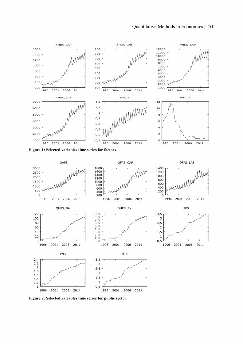
200

400

600

800

1000

1200

1400

1600

1996 2001 2006 2011

YHBA_CAP

100

200

300

400

500

600

700

800

900

1996 2001 2006 2011

YHBA_LAB

1000 2000 3000 4000 5000 6000 7000 8000 9000

10000 11000 12000

1996 2001 2006 2011

YHSK_CAP

1000

2000

3000

4000

5000

6000

7000

1996 2001 2006 2011

YHSK_LAB

0,5

0,6

0,7

0,8

0,9

1

1,1

1,2

1996 2001 2006 2011

WFLAB

0

2

4

6

8

10

12

1996 2001 2006 2011

WFCAP

Figure 1: Selected variables time series for factors

0 500

1000 1500 2000 2500 3000

1996 2001 2006 2011

QAPS

200 400 600 800

1000 1200 1400 1600 1800

1996 2001 2006 2011

QFPS_CAP

0 200 400 600 800

1000 1200 1400

1996 2001 2006 2011

QFPS_LAB

0 20 40 60 80

100 120

1996 2001 2006 2011

QHPS_BA

0 100 200 300 400 500 600 700 800 900

1996 2001 2006 2011

QHPS_SK

0,5 1

1,5 2

2,5 3

3,5

1996 2001 2006 2011

PPS

1 1,2 1,4 1,6 1,8

2 2,2 2,4

1996 2001 2006 2011

PNS

0,5 1

1,5 2

2,5 3

3,5

1996 2001 2006 2011

PAPS

Figure 2: Selected variables time series for public sector

Quantitative Methods in Economics | 251

Acknowledgements: This paper research was supported by the Slovak Research and Development Agency, project No. APVV-14-0020: Pareto Optimal Interactions Modeling in the Financial and Business Adaptive Processes.

References [1] Löfgren, H. (2003). Exercises in General Equilibrium Modeling Using GAMS. [online]

Microcomputers in Policy Research 4a. International Food Policy Research Institute.Available at: http://www.rri.wvu.edu/CGECourse/GAMSExer.pdf[Accessed 8 Mar. 2016].

[2] Miťková, V. (2015). Computable equilibrium model parameters calibration vs. estimation. In: Proceedings of 33rd international conference Mathematical Methods in Economics. [online] Plzeň: University of West Bohemia, pp. 555-559. Available at: http://mme2015.zcu.cz/downloads/MME_2015_proceedings.pdf [Accessed 8 Mar. 2016]

[3] Miťková, V. (2016). The CGE Model Parameters Estimations Techniques. In: Ekonomické rozhľady, 45(1), pp. 9-18.

Author’s addressIng. Veronika Miťková, PhD. Comenius University in Bratislava, Faculty of Social and Economic Sciences, Institute of Economics Mlynské luhy 4, 821 05 BratislavaSlovak Republic veronika.mitkova@fses.uniba.sk

252 | Multiple Criteria Decision Making XVIII

LEGISLATIVE CHANGES EFFECTS ON SLOVAK PENSION FUNDS EFFICIENCY

Vladimír Mlynarovič, Institute of Economics, Faculty of Social and Economic Sciences, Comenius University in Bratislava

Abstract The paper compares historical returns of selected Slovak pension funds in the three periods specified according to significant legislative changes in pension system. The methodology of Black – Litterman optimization is used to construct historical efficient frontiers for conservative and growth pension funds. As results the paper shows significant shifts of efficient frontiers for both types of funds as a reaction of investment companies on legislative changes.

Keywords: pension funds, efficient frontiers, Black – Litterman model

JEL Classification: G11 AMS Classification: 91B28

1 INTRODUCTION Saving for old-age pensions is inevitably a long-term undertaking; this is especially true on the national scale. In the past, the state pension contributions of economically active Slovaks were used to fund the pensions of those who had already retired. But this approach is no longer able to generate sufficient funds to meet the needs of future liabilities, due to Slovakia’s unfavorable demographic developments. To address this issue Slovakia extended its pay-as-you-go scheme, now known as the first pillar, by adding two further saving pillars, in which people can save for their retirement. From the beginning of 2005 Slovaks were given the option to start saving for their pensions through newly established pension fund administration companies known as the second – or capitalization – pillar. During an initial 18-months period (1 January 2005 – 30 June 2006), persons registered for pension insurance (1st pillar) had to decide whether to join or not the new scheme. More than 1.5 million citizens (i.e. around 60% of the economically active population) joined and redirect part of their pension contributions (to their newly created personal pension accounts. Six management companies: Aegon DSS, Allianz - Slovenská DSS, AXA DSS, Poštová DSS, ING DSS, and VÚB Generali DSS, currently operate their pension funds. However after 2006 the extensive changes to the second pillar were initiated, e.g.:� the second pillar became voluntary and young people entering the labor market could

choose to save for their pensions in the second pillar but were not required to do so;� government changed the fee structure for private pension fund management companies;� the pension contribution rate has been lowered form 9% of the gross wage to 4%; � the scheme had been temporarily opened three times to enable participants to opt out; I But in the paper we concentrate on the analysis of such type of legislative changes that in our opinion can directly and significantly influence building of the investment strategies or portfolio structures of pension funds and positions of the efficient frontiers on the Slovak pension funds market. Among such type of legislative changes we have: � Beginning July 1, 2009 DSS companies had to launch a guarantee fund for each of their

pension investment funds. All yields from the pension funds will flow to it. After six

Quantitative Methods in Economics | 253

months, the DSS companies compared the yields in their pension funds with a benchmark and only then they were able to take a portion of it in fees.

� Beginning April 1, 2012 pension management companies are obliged to administer two types of funds, a guaranteed bond fund and an unguaranteed equity fund. They can also run other types of guaranteed or unguaranteed funds (e.g. mixed). Until 31 December 2012, pension management companies administered four types of statutory funds (bond, mixed, equity, and index funds), while before 1 April 2012 there had been three funds (conservative, balanced, growth).

2 METHODOLOGY Although modeling efficient frontier in mean variance space is still very popular (e.g.[4,5]), inthe past there were several risk measures proposed, different from the variance, including semi-standard deviation, semi-absolute deviation and below target risk(e.g. [3]). There are also models explicitly examining skewness of return distribution. Relatively new measure of lower partial risk comprises also Value at Risk, which is widely used for market risk measurement. This risk measure is very popular in conservative environment as probability of huge loss, larger than let’s say VaR0.99, is very low, provided that the portfolio’s returns have normal distribution. However, considering the existing methodologies of non-linear programming it is impossible to find out a portfolio with the lowest VaR. For this reason the CVaR (conditional value at risk or expected loss) becomes more and more attractive risk measure, namely with regard to its theoretical and computing features.

The second limitation of the mean – variance approach is that its recommended asset allocations are highly sensitive to small changes in inputs and, therefore, to estimation error. In its impact on the results of a mean – variance approach to asset allocation, estimation error in expected returns has been estimated to be roughly 10 times as important as estimation error in variances and 20 times as important as estimation error in covariances. Thus the most important inputs in mean - variance optimization are the expected returns.

Fisher Black and Robert Litterman in [1] developed quantitative approach to dealing with the problem of estimation error. The goal of this model is to create stable, mean –variance efficient portfolios, which overcome the problem of input sensitivity. The Black - Litterman model uses “equilibrium” returns as a neutral starting point. Equilibrium returns are calculated using either CAPM or reverse optimization method in which the vector of implied expected equilibrium returns P is extracted from known information, where

CwP � and w is in this case the vector of market capitalization weights, C is the covariance matrix, n� n, where n is the number of assets, and δ is risk - aversion coefficient, which represents the market average risk tolerance. In general, the Black – Litterman approach consists of the following steps:

1. Define equilibrium market weights and covariance matrix for all asset classes. 2. Calculate the expected return implied from the market equilibrium portfolio. 3. Express market views and confidence for each view. 4. Calculate the view adjusted market equilibrium returns. 5. Run mean – variance optimization.

In our application we use this approach without market views expressions to describe efficient frontier of the Slovak pension funds market in the following way. Let vector wcdescribe the capitalization on the market of the funds and Ec is the corresponding return of the

254 | Multiple Criteria Decision Making XVIII

weighted market competition for the current period. The risk adjusted return can be written in the form c

TccE Cww �

and we assume that this return is for the weighted market competition zero. So we have

c

Tc

cc

ECww

�

and finally the vector ccc CwP �is used as the vector of expected returns in mean – variance optimization.

3 RESULTS AND CONCLUSIONS The analysis was done on the base weekly date on the fund performance from April 2005 to August 2015. The modeling period was divided into three parts: period 0 (from April 29, 2005 to July 3, 2009), period 1 (from July 3, 2009 to April 5, 2012), and period 3 (from July 3, 2009 to April 5, 2012) as it follows from the indicted terms of legislative changes. Efficient frontiers were modeling in Excel environment (e.g. [2]) on the base of 4 weeks return moving averages for two type of funds, conservative and growth. Together wit six DSS companies there are two fictive companies, market competition (MC) computed on the base of weighted average (wa) and simple average (sa) returns, are included into analysis.

The results for conservative and growth funds are presented in the Tables 1 and 2 and on the Pictures 1 and 2. We can conclude that the introduction of guarantees has caused the pension fund management companies to stop investing in equity shares, meaning that both analyzed funds generate in the period 1 similar yields. This is because pensions saving companies have to report and compare the value of the assets in their funds on a six-month basis and as a result are investing in a very conservative way and not risking any losses. But this safe investment strategy brings lower yields. On the Pictures 1 and 2 we can see significant shifts of efficient frontiers in a direction of lower returns and higher risks. It also reflects the high volatility on global financial markets. On the other hand, in the period 2 we can see shifts of the frontier in expected directions.

Table 1: Conservative Funds Period 0_Aegon 0_Allianz 0_Postova 0_NN 0_VUB 0_AXA 0_MC_wa 0_MC_sa

0

R1 1.29% 0.78% 0.64% 0.88% 0.96% 0.91% 0.75% 0.71%R2 4.19% 3.12% 1.43% 2.60% 3.75% 3.30% 3.24% 3.06%R3 10.54% 35.17% 5.99% 8.92% 18.84% 20.54%R4 -0.42% -0.03% -0.07% -0.14% -0.13% -0.12% -0.01% 0.01%R5 3.2425 4.0172 2.2574 2.9687 3.8880 3.6150 4.2980 4.2882

1_Aegon 1_Allianz 1_Postova 1_NN 1_VUB 1_AXA 1_MC_wa 1_MC_sa

1

R1 0.48% 0.29% 0.26% 0.30% 3.07% 0.39% 1.38% 0.57%R2 0.24% 0.17% 0.12% 0.12% 5.58% 0.25% 1.24% 1.06%R3 10.50% 25.87% 6.84% 6.45% 19.66% 30.68%R4 -0.03% -0.01% -0.01% -0.01% -1.66% -0.01% -0.32% 0.01%R5 0.50 0.57 0.47 0.40 1.82 0.65 0.90 1.87

2_Aegon 2_Allianz 2_Postova 2_NN 2_VUB 2_AXA 2_MC_wa 2_MC_sa

2

R1 0.70% 0.86% 1.79% 0.52% 0.84% 1.14% 0.87% 0.91%R2 1.33% 1.71% 3.46% 0.92% 1.62% 2.33% 1.82% 1.89%R3 9.87% 33.37% 5.12% 10.16% 16.16% 25.31%R4 0.01% 0.00% -0.32% 0.02% 0.00% -0.06% 0.00% -0.01%R5 1.91 2.00 1.94 1.77 1.93 2.04 2.08 2.07

Quantitative Methods in Economics | 255

Table 2: Growth Funds Period 0_Aegon 0_Allianz 0_Postova 0_NN 0_VUB 0_AXA 0_MC_wa 0_MC_sa

0

R1 4.99% 3.39% 3.63% 3.26% 3.41% 3.36% 3.46% 3.57%

R2 1.18% 0.84% 0.87% 0.78% 0.84% 0.82% 0.87% 0.89%

R3 10.97% 30.24% 5.59% 11.18% 12.46% 29.56%

R4 -0.05% 0.00% -0.01% 0.00% 0.00% 0.00% 0.00% 0.00%

R5 0.24 0.25 0.24 0.24 0.25 0.24 0.25 0.25

1_Aegon 1_Allianz 1_Postova 1_NN 1_VUB 1_AXA 1_MC_wa 1_MC_sa

1

R1 0.49% 0.29% 0.55% 0.29% 0.65% 0.53% 0.33% 0.35%

R2 1.34% 0.79% 2.03% 0.60% 2.40% 1.94% 1.42% 1.51%

R3 10.98% 31.88% 5.39% 11.21% 12.28% 28.25%

R4 -0.14% -0.02% -0.15% -0.04% -0.24% -0.14% 0.00% -0.01%

R5 2.73 2.77 3.71 2.05 3.70 3.65 4.26 4.27

2_Aegon 2_Allianz 2_Postova 2_NN 2_VUB 2_AXA 2_MC_wa 2_MC_sa

2

R1 4.08% 8.32% 5.89% 5.16% 6.09% 3.65% 5.65% 5.29%

R2 3.50% 7.89% 5.35% 4.22% 5.72% 3.34% 5.48% 4.99%

R3 7.96% 36.85% 6.94% 11.98% 9.45% 26.82%

R4 0.06% -0.27% -0.03% -0.01% -0.03% 0.09% 0.02% 0.03%

R5 0.86 0.95 0.91 0.82 0.94 0.92 0.97 0.94

Black - Litterman Eficiernt frontiers on the base of 4-weeks moving averages Conservative FundsPeriod 0: April 29, 2005 : July 3, 2009Period 1: July 3, 2009 : April 5, 2012Period 2: April 5, 2012 : August 28, 2015

0_postova

0_aegon

0_MC_sa

0_MC_wa

0_vub

0_allianz

0_axa

0_nn

1_postova

1_aegon

1_MC_wa

1_vub

1_allianz1_nn

1_MC_sa

1_axa

2_nn

2_aegon

2_vub2_allianz

2_MC_wa

2_MC_sa

2_axa

2_Postova

0.00%

1.00%

2.00%

3.00%

4.00%

5.00%

6.00%

0.00% 0.50% 1.00% 1.50% 2.00% 2.50% 3.00% 3.50%Risk, p.a. (by standard deviations)

Expe

cted E

quilli

brium

Retu

rn, p.

a

Period 0

Period 1Period 2

Figure 1: Conservative Funds Efficient Frontiers

256 | Multiple Criteria Decision Making XVIII

Black - Litterman Eficiernt frontiers on the base of 4-weeks moving averagesGrowth FundsPeriod 0: April 29, 2005 : July 3, 2009Period 1: July 3, 2009 : April 5, 2012Period 2: April 5, 2012 : August 28, 2015

0_nn0_axa

0_allianz0_vub

0_mc_wa

0_mc_sa

0_aegon

0_postova

1_axa

1_mc_sa

1_nn1_allianz

1_vub

1_mc_wa

1_aegon

1_postova

2_axa2_aegon

2_nn

2_MC_sa

2_postova

2_allianz

2_vub

2_MC_wa

0.00%

1.00%

2.00%

3.00%

4.00%

5.00%

6.00%

7.00%

8.00%

0.00% 1.00% 2.00% 3.00% 4.00% 5.00% 6.00% 7.00% 8.00% 9.00%

Risk, p.a. (by standard deviations)

Expec

ted Eq

uillibri

um Re

turn, p.

a Period 0Period 1Period 2

Figure 2: Growth Funds Efficient Frontiers

Legend: R1 - Risk, p.a., R2 - Equilibrium return, p.a., R3 - Market weights, R4 - Risk adjusted return, R5 - Equilibrium return / Risk

Acknowledgements: This paper research was supported by the Slovak Research and Development Agency, project No. APVV-14-0020: Pareto Optimal Interactions Modeling in the Financial and Business Adaptive Processes.

References [1] Black, F. and Litterman, R. (1990). Global Portfolio Optimization. Financial Analysts

Journal, 48(5), pp. 28-43. [2] Jackson, M. and Staunton, M. (2001). Advanced Modeling in Finance using Excel and

VBA. New York: John Wiley and Sons. [3] Konno, H., Waki, H. and Yuuki, A. (2002). Portfolio Optimization under Lower Partial

Risk Measures. Asia/Pacific Financial Markets, 9(2), pp.127-140. [4] Markowitz, H. (1959). Portfolio Selection: Efficient Diversification of Investments. New

York: John Wiley and Sons. [5] Mlynarovič, V. (2001). Finančné investovanie. Teória a aplikácie. Bratislava: IURA

Edition.

Author’s addressdoc. Ing. Vladimír Mlynarovič, CSc.Univerzita Komenského v Bratislave, Fakulta sociálnych a ekonomických viedÚstav ekonómieMlynské luhy 4 1/b, 852 35 Bratislava email: mlynarovic@fses.uniba.sk

Quantitative Methods in Economics | 257

PREDICTING INSOLVENCY RISK OF THE CZECH COMPANIES

Daniel Němec, Masaryk University, Michal Pavlík, KPMG Slovakia

Abstract The goal of this paper is to create and evaluate the models for predicting insolvency risk of the Czech companies. This contribution aims to reveal the most important factors which affect the bankruptcy in the Czech Republic including the characteristics of the local business environment. Using the public data from the accounting statements (from 2005 to 2013) we have built model with one-year forecast horizon. The model is treated as the standard logit models and estimated using the maximum likelihood approach. Comparing the results with the traditional bankruptcy models proves that our model has overall better predictive power and can be thus used for reliable evaluations of the future financial stability of the Czech companies.

Keywords: bankruptcy prediction, logistic regression, bankruptcy model, Czech Republic

JEL Classification: G33, C35, C52 AMS Classification: 91B30, 62P20

1 INTRODUCTION Bankruptcy or insolvency of the companies have important impacts on the economy. Although these processes may be treated as those helping to clear the markets, they may influence outcomes of healthy companies as well. Predictability of bankruptcy is thus a key element in risk management that help to protect the business activities of the companies. Table 1 depicts the development of insolvency in the Czech Republic. The number of insolvency cases (considering the bankruptcy of companies) is highly correlated with the overall economic activity. But, there are many individual factors which could lower or increase the probability of bankruptcy. The main goal of this contribution is to evaluate the ability of openly available data from balance sheets and profit and loss accounts to predict the bankruptcy of Czech companies for one year ahead. We will be doing that task by building and estimating prediction model of bankruptcy for the Czech companies that published their balance sheet data publicly. We try to reveal the most important factors for predicting bankruptcy and we compare our results with other bankruptcy models from the literature. This comparison should stress the importance of updating the model parameters especially with regard to the analyzed economy.

Table 1: Insolvency motions in the Czech Republic 2008 2009 2010 2011 2012 2013 2014

Companies 3 418 5 255 5 559 6 753 8 398 6 021 3 563Consumers 1 936 4 237 10 559 17 600 23 830 30 888 31 577

Total 5 354 9 492 16 118 24 353 32 228 36 909 35 104Source: Creditreform (2014): Development of insolvencies in the Czech Republic in 2014. Available at http://www.creditreform.cz/novinky-downloads/vyvoj-insolvenci-v-cr.html

Our model approach is based on standard logit model using the data from balance sheets and profit and loss accounts of the Czech companies from 2005 to 2013. The structure of our contribution is as follows. In the second section, the methodology and data are described including a short review of other available methods for predicting bankruptcy. The third section presents our estimated prediction model and evaluates its discrimination power in comparison with the results based on alternative bankruptcy models. Last section concludes.

258 | Multiple Criteria Decision Making XVIII

2 METHODOLOGY AND DATA Our approach for building and estimating the prediction model of bankruptcy is based on a standard logit modelling methodology. As Aziz and Daz [2] pointed out, the multivariate logit models (on average) are able to outperform the prediction abilities (measured as the ratio of correctly classified cases of healthy and insolvent companies) of multivariate discriminant analysis methods, decision trees methods or univariate analysis methods. To be more specific, they analyzed 3 studies of univariate analysis methods with 81.09% correctly classified cases (standard deviation was 3.09), 25 studies using multivariate discriminant analysis methods (85.13% correctly predicted cases with standard deviation 0.34), 19 studies based on logit model approach (86.66% correctly predicted cases with standard deviation 0.46), 5 studies with decision trees methods (86.37% correctly predicted cases with standard deviation 2.29), and 7 studies of neural networks approach (87.39% correctly predicted cases with standard deviation 1.6). The studies based on other methods were less successful or they had considerably higher standard deviation of their success rate. Similar results are presented by Bellovery et al. [4].

Table 2: List of variables ID Variable Effect References (examples)

LiquidityR1 financial assets / short-term liabilities - H, Kl, ZR2 financial assets + short-term receivables / current liabilities - H, Kl, ZR3 current assets / short-term liabilities - B, H, IN, Kl, Z, ZmR4 working capital / inventory - HR5 working capital / revenue - HR6 working capital / assets - A, B, JT, OR7 current assets / liabilities (external resources) - T

IndebtednessR8 equity / assets +/- H, Kl, ZR9 assets / equity +/- Z

R10 EBIT / interest expense - H, IN, JT, Kl, ZR11 liabilities / receivables + ZR12 equity / long-lived assets - ZR13 retained earnings / assets - AR14 liabilities (external resources) / assets + B, H, Kl, O, Z, ZmR15 assets / liabilities (external resources) - INR16 short-term liabilities (external resources) / assets + TR17 CF (EBITDA) / liabilities (external resources) - B, OR18 liabilities (external resources) / equity - JTR19 equity / liabilities (external resources) - AR20 long-term liabilities (external resource) / equity - JT

RentabilityR21 EBIT / assets - A, B, H, IN, Kl, O, Z, ZmR22 EAT / sales - JT, ZR23 EBT / long-term liabilities - Kl, T, ZR24 EAT / return - Z

ActivityR25 sales / assets - A, H, IN, T, ZR26 sales / inventory - H, JT, Kl, ZR27 receivables*365 / sales + H, Kl, ZR28 liabilities*365 / sales + H, Kl, ZR29 financial assets*365 / sales + HR30 sales / long-lived assets - Kl

Source: A = Altman [1]; B = Beaver [3]; H = Holečková [5]; IN = Index IN05 [8]; JT = Jakubík, Teplý [6]; Kl = Kalouda [7]; O = Ohlson [9]; T = Taffler [10]; Z = Zalai [12]; Zm = Zmijewskij [13];

Quantitative Methods in Economics | 259

There are many variables which might be related to the risk of bankruptcy. We are focusing on the variables that may be obtained from the balance sheets and profit and losses accounts. Table 2 presents all variables (financial ratios) that were used in our analysis, the expected effect on probability to bankruptcy and references to other similar studies using particular variables or to other theoretical books (mostly Czech) that are describing the relevance of these variables to the solvency of companies. The variables may be divided into four groups of indicators: liquidity, indebtedness, profitability and overall economic activity of the companies.

All financial indicators were computed using the data from balance sheets and profit and loss accounts provided by the Albertina database (see www.albertina.cz). This database covers the data from business register of the Czech companies. We have used the data set covering the period from 2005 to 2013. The original data set consisted of 1 175 955 balance sheets from 241 380 companies. As a first step, all balance sheets for the period longer or shorter than 12 months were omitted. On average, 4.8 balance sheets for one company remained. As the next step, all the remaining data were filtered using the following criterion: � Total assets equal total liabilities and equity (to eliminate possible errors in published

account statements). � Total assets are higher than 200 000 CZK. This sum of assets was defined as the value

of minimal legal capital valid till 1. 1. 2014. Using this condition, the small companies and problematic companies where assets do not reach the minimum required seed money).

� Excluding financial companies (based on the economic activity classification CZ-NACE) due to fact that these companies have different structure of capital).

� Excluding companies with missing values of financial indicators (after considering and excluding the variables with most missing observation and low prediction power estimated using univariate logit models).

Table 3: Sample properties (distribution by time) Full sample Model sample

Year Total Insolvent Healthy Insolvent Total2005 11 210 8% 37 4% 36 37 732006 10 984 8% 32 3% 30 32 622007 12 672 9% 51 5% 60 51 1012008 14 799 11% 121 12% 118 121 2392009 16 646 12% 196 19% 195 196 3912010 18 353 13% 187 18% 182 187 3692011 20 684 15% 217 21% 216 217 4332012 21 536 15% 145 14% 144 145 2892013 12 802 9% 53 5% 51 53 104Total 139 686 100% 1 039 100% 1 022 1 039 2061

Source: own calculations based on Albertina database.

The restricted sample consists of 810 026 observations of 175 556 companies. The logit model requires the dependent variables as a dummy variable. This requirement supposes aproper definition of the bankruptcy (i.e. the company was gone bankrupt in particular year or was not). These companies were defined using the indicator that the company was declared bankrupt or it was adjudicated bankrupt by the court and its equity was negative. The last condition to include the company and corresponding observations to our analysis was the availability of the balance sheets in two consecutive years. The statistical properties of your final data set are presented in the Table 3 and Table 4.

260 | Multiple Criteria Decision Making XVIII

Table 4: Sample properties (distribution by economic activity classification)

Full sample Model sample

CZ-NACE Description Total Insolvent Healthy Insolvent Total

A Agriculture, forestry and fishing 4 128 26 0.63% 26 26 52

B Mining and quarrying 203 3 1.48% 0 3 3

C Manufacturing 20 003 285 1.42% 285 285 570

D Electricity, gas, steam and air conditioning supply 1 189 3 0.25% 3 3 6

E Water supply, sewerage, waste management and remediation activities 1 213 6 0.49% 3 6 9

F Construction 13 995 167 1.19% 167 167 334

G Wholesale and retail trade, repair of motor vehicles and motorcycles 38 410 247 0.64% 247 247 494

H Transportation and storage 4 254 80 1.88% 78 80 158

I Accommodation and food service activities 5 206 44 0.85% 42 44 86

J Information and communication 5 002 21 0.42% 21 21 42

L Real estate activities 19 700 49 0.25% 49 49 98

M Professional, scientific and technical activities 17 279 64 0.37% 64 64 128

N Administrative and support service activities 3 661 16 0.44% 16 16 32

P Education 1 393 3 0.22% 3 3 6

Q Human health and social work activities 2 708 8 0.30% 6 8 14

R Arts, entertainment and recreation 1 379 10 0.73% 7 10 17

S Other service activities 992 7 0.71% 5 7 12

Total 140 725 1 039 0.74% 1 022 1 039 2 061

Source: own calculations based on Albertina database.

To prevent the incorrectly predicted bankruptcy cases, we have created the model sample that consists of almost equally distributed healthy and insolvent companies (equally distributed by year and economic activity classification CZ-NACE). The healthy companies were selected as random sample (clustered by the year and CZ-NACE classification) with the condition that the resulting sample meets the properties of original (full sample) and model sample defined by the averages of explanatory variables. This property was tested using the individual t-tests. All tests of equal means did not reject the null hypothesis using the 1% level of significance. Finally, model sample was divided into two groups: the training group (consisting of 1 456 observations) and the validating group (consisting of 605 observations). The ratio 70:30 was selected to meet the property of enough observations to validate the prediction performance of our model. Surprisingly, Aziz and Dar [2] pointed out, that 46% of analyzed studies (and models) based the prediction outcomes of the models on original data set (i.e. the data set that was used for calibrating the model).

Quantitative Methods in Economics | 261

3 BANKRUPTCY MODEL OF THE CZECH COMPANIES Before estimating the final multivariate logit model, we have performed univariate estimations to reveal the most important factors for predicting bankruptcy and using the correlation matrix to omit all highly correlated factors. The estimated final model (using the maximum likelihood method) is presented in Table 5.

Table 5: Prediction model of bankruptcy (one year ahead predictions) Variable Description Parameter Standard error p-value

- Intercept 0.0068 0.321 0,983R3 current assets / short-term liabilities -0.5160 0.142 0.000R9 assets / equity -0.0559 0.008 0.000

R14 liabilities (external resources) / assets 0.6346 0.234 0.007R17 CF (EBITDA) / liabilities (external resources) -2.8307 0.440 0.000R19 equity / liabilities (external resources) -1.1347 0.305 0.000R29 financial assets*365 / sales -0.0016 0.001 0.006

Test statisticsLR test 1074.4 (0.000) Pseudo R2 0.5219Wald test 370.1 (0.000) Hosmer-Lemeshow test (p-value) 0.2948Source: own calculations.

In comparison to other similar studies (see Table 7), we have identified one factor (R29 –financial assets to average one-day sales) that was not identified by these studies. On the other hand, our one-year prediction model does not contain the financial indicators ROA (return over assets – R21) or ROS (return over sales – R22). Table 6 describes the discriminating power of our model. The model is able to predict correctly almost 84% of cases. This relatively high value of correctly classified companies is acceptable.

Table 6: Classification table (validation sample) Predicted TotalHealthy Insolvent

Actual Healthy 245 56 301Insolvent 41 263 304

Total 286 319 605Source: own calculations.

Table 7 compares our results with the models from other similar studies (some of them were calibrated using the data for Czech companies). The comparison is based on the same validation sample. It could be seen, that the traditional models and their modifications for the Czech data (Altman [1], Taffler [10], Zmijewski [13], Ohlson [9], and IN05 [8]) have worse prediction outcomes. On the other hand, the model proposed by Valecký, Slivková [13], who used similar methodology but more financial indicators for the Czech companies, shows good prediction ability too.

Table 7: Models comparison (one year ahead predictions) Correctly classified Type I error Type II error

Our model 83.97% 0.176 0.143Altman [1] 75.89% 0.268 0.192Taffler [10] 53.35% 0.392 0.479IN05 [8] 72.71% 0.301 0.196Ohlson [9] 76.36% 0.284 0.159Zmijewski [13] 64.96% 0.398 0.209Valecký, Slivková [11] 80.17% 0.253 0.112Source: own calculations.

262 | Multiple Criteria Decision Making XVIII

4 CONCLUSION Our results based on logit model approach proved that the balance sheet data are able to predict bankruptcy one-year ahead very well. Approximately 86.5% of insolvent companies were correctly classified. Comparing our results with the models from other studies shows the necessity to build at least country specific models.

Acknowledgements: This work was supported by funding of specific research at Faculty of Economics and Administration, project MUNI/A/1040/2015. This support is gratefully acknowledged.

References [1] Altman, I. E. (1986). Financial ratios, discriminant analysis and the prediction of

corporate bankruptcy. The Journal of Finance, 23(4), pp. 589–609.[2] Aziz, M., and Dar, H. A. (2006). Predicting Corporate Bankruptcy: Where We Stand?

Corporate Governance, 6(1), pp. 18-33. [3] Beaver, W. (1966). Financial ratios as predictors of failure. Journal of Accounting

Research, 4, pp. 71–111. [4] Bellovary, J., Giacomino, D., and Akers, M. (2007). A Review of Bankruptcy Prediction

Studies: 1930-Present. Journal of Financial Education, 33, pp. 1-42. [5] Holečková, J. (2008). Finanční analýza firmy. Praha: ASPI. [6] Jakubík, P. and Teplý, P. (2008). The Prediction of Corporate Bankruptcy and Czech

Economy’s Financial Stability through Logit Analysis. IES FSV working paper 19/2008. Prague: Charles University.

[7] Kalouda, F. and Vaníček, R. (2013). Alternatitní bankrotní modely – první výsledky. In: European Financial Systems. Proceedings of the 10th International Scientific Conference(Deev, O., Kajurová, V., and Krajíček, J.). Brno: Masaryk University.

[8] Neumaierová, I. and Neumaier, I. (2005). Index IN05. In: Evropské finanční systémy: Sborník příspěvků z mezinárodní vědecké konference. Brno: Masarykova univerzita, pp. 143–146.

[9] Ohlson, J. A. (1980). Financial ratios and the probabilistic prediction of bankruptcy. Journal of Accounting Research, 18(1), pp. 109–131.

[10]Taffler, R., and Tishaw, H. (1977). Going, going, gone – four factors which predict. Accountancy, 3, pp. 50–54.

[11] Valecký, J. and Slivková, E. (2012). Mikroekonomický scoringový model úpadku českých podniků. Ekonomická revue, 15, pp. 15–26.

[12] Zalai, K. (1997). Finančno-ekonomická analýza podniku. Bratislava: Sprint. [13] Zmijewski, M. (1984). Methodological issues related to the estimation of financial

distress prediction models. Journal of Accounting Research, 22, pp. 59–82.

Author’s addressIng. Daniel Němec, PhD.Masaryk University, Faculty of Economics and Administration, Department of Economics Lipová 41a, 602 00 BrnoCzech Republic email: nemecd@econ.muni.cz

Ing. Michal PavlíkKPMG Slovakia, Dvořákovo nábrežie 10, 811 02 BratislavaSlovak Republic email: mich.pavlik@gmail.com

Quantitative Methods in Economics | 263

METHODOLOGY OF MULTI-CRITERIA EVALUATION OF VARIANTS OF CHECK-IN SYSTEMS IN PUBLIC TRANSPORT

Ivana OlivkováVŠB – Technical University of Ostrava

Abstract Check-in system is a key interface between the carrier and the passenger. In the transition to a new system or upgrading an existing check-in it is necessary to take into account several important facts affecting the quality of transport process, and the associated satisfaction of passengers. The paper wants to contribute to the development of theories that could promote further progress in the evaluation of new technologies in the field of public transport. The proposed methodology allows the evaluation of multiple criteria with respecting their relative importance and thus its possible use in the evaluation of variants of check- in systems.

Keywords: multi-criteria evaluation, check- in system, public transport

JEL Classification: C44 AMS Classification: 90C15

1 INTRODUCTION The development of electronic check-in systems records currently considerable progress in many types of payments, including the application in transport. Use of new technologies in public transport contributes both to higher customer satisfaction [5] and smoother movement of passengers and also increases the efficiency of collection of fare compared to the current payment method [4]. Currently are various market pressures to improve check-in system based on paper ticket, whether in the form of a draft of new system or in potential measures to improve the current situation. For this reason, the article focuses on the possibilities of modern check in technologies that are used for public transport, their subsequent comparison and evaluation.

2 DETERMINATION OF THE OBJECTIVES In the theory of decision-making there are several methods of multi-criteria evaluation of variants [1]. Their use depends on the type, completeness and on level of detail of available information. In practice there are often cases when it is necessary to decide on the variants of fundamental importance the earliest opportunity but the availability, quantity and quality of information for decision usually does not correspond to their real needs. For solving such type of the task are usually employed methods based on qualitative estimates: scoring method [3] or the method of determining the ranking of the variants [3]. In the case that there are the needed information in the detailed structure and the evaluation are carried out by experts, can be objectified their evaluation. For solving such type of the task can be employed methods for the evaluation of variants such as WSA method (Weighted Sum Approach) [2] and TOPSIS method (Technique for Order Preference by Similarity to Ideal Solution) [2]. From the above, there are the following objectives:

� Propose methodology of multi-criteria evaluation of variants of check-in systems in public transport

264 | Multiple Criteria Decision Making XVIII

� Experimental verification of the proposed method, making multi-criteria evaluation of variants of check-in systems in public transport based on processing traffic survey selected group of experts.

These objectives are further processed together and divided into three consecutive steps: � Choice of variants � Defining evaluation criteria � Multi-criteria evaluation of the variants.

2.1 Choice of variants Variants (alternatives) are defined as specific decision options that are available for choice.The possibilities of modern technology in the check-in systems are discussed for example in publications [6], and [7]. Based on the completed questionnaires there were identified five variants of check-in systems:

1. Check- In2. Check -In / Check- Out 3. Be- In / Be- Out 4. SMS 5. NFC.

2.2 Definition of evaluation criteria The criteria are defined as aspects based on which the variants are evaluated. After analysis and consultation with experts I have selected five criteria for the evaluation of variants. These criteria describe the most important qualities that must have check-in system in public transport:

1. Ease of checking - it is mainly the issue of uniform tariffs and conditions of carriage for passengers understandable

2. Speed of checking - support for fast transactions at check-in not to cause delay for travellers to exchange/get in the public transport vehicle

3. Multifunctionality - an extension of the use of check-in system to other areas than just transport

4. Operation reliability - the general ability of the check-in system to perform the required function for a specified period of time, taking into account the effects of operational and other conditions

5. Operation costs - a crucial factor for effective management and maintenance of the system, together with a draft tariff system operates on an early return of investment.

3 METHODOLOGY Traffic survey was designed for a selected group of evaluators (experts on traffic issues). We addressed 45 evaluators in November 2015. The evaluators were informed about the variants of check-in systems and based on their expertise these variants were evaluated through criteria. Evaluators answered questions through a pre-prepared questionnaire.

3.1 Multi-criteria evaluation of the variants The mathematical definition is given [2]:

� by a list of variants A = {a1, a2 , ... , am}, � by a list of criteria F = {f1, f2 , ... , fn}, � by evaluating variants according to various criteria in the form of a matrix Y:

Quantitative Methods in Economics | 265

g … g�; = ⋮�

� l ⋯ l �⋮ ⋱ ⋮l� ⋯ l��� (1)

The aim is to find a variant that achieves the best evaluation of all criteria, eventually these variants appropriately arrange. Table 1 shows the scores of individual variants check-in systems according to selected criteria. Rating scale is in the range from 1 to 10 b. The higher the number was, the higher the evaluator preferred the variant. Table 1: Entry matrix Y

Ease ofchecking

Speed ofchecking

Multifunctio-nality

Operation reliability

Operation costs

Check-in 6,8 7,6 6,9 7,2 6,4Check-in/Check-out 6,2 5,1 6,5 6,3 5,6

Be-in/Be-out 8,9 9,6 5,1 4,1 5,2SMS 7,2 4,3 4,8 4,6 7,5NFC 7,8 8,1 8,7 6,1 6,7

The second step is to determine the weight of each evaluation criteria. Weights of evaluation criteria reflect their importance numerically; the importance from the point of view of the evaluators [3]. For the determination of weight the following equation is applied (2): v = (0 , 0�, … , 0�), ∑ 0_ = 1,�_B 0_ ≥ 0 (2)

0 , 0�, … , 0� …weight of criteria [-] The weights were calculated on the basis of scoring method that evaluators determined through a questionnaire. Rating scale is in the range from 1 to 10. Due to the requirements of comparability weights to the criteria established by different methods these weights should be normalized (the sum of the standardized set of criteria weights is equal to one). The standardization of criteria weights is done according to (3): 0_ = ��∑ ������ (3)

0_ ... weight of jth criteria, #_ ... score of jth criteria In the table 2 there are the average scores and average values of the weights of individual criteria calculated from all the evaluators’ values.

Table 2: Average scores and average values of the weights Ease of

checkingSpeed ofchecking

Multifunctio-nality

Operation reliability

Operation costs

Score 5,5 7,6 6,5 8,3 9,1Weight 0,15 0,20 0,18 0,22 0,25

The problem is solved in two ways: � WSA method (Weighted Sum Approach) � TOPSIS method (Technique for Order Preference by Similarity to Ideal Solution)

WSA method WSA method - the principle is to maximize the weighted sum. The process of calculating by the method of WSA is divided into three consecutive steps. Step 1: Determining the ideal variant H and basal variant D of matrix Y

266 | Multiple Criteria Decision Making XVIII

The ideal variant is a variant H (hypothetical) that achieves the best value in all criteria. Basal variant D is a variant that achieves the worst values in all criteria.

Table 3: Ideal and basal variant of entry matrix YEase of

checkingSpeed ofchecking

Multifunctio-nality

Operation reliability

Operation costs

Ideal variant 8,9 9,6 8,7 7,2 7,5Basal variant 6,2 4,3 4,8 4,1 5,2

Step 2: Transformation of matrix Y on normalized matrix R according to the formula: hb_ = �x��������� (4)

hb_ ... normalized element in the ith row and jth column of the matrix R�_ ... basal variant of jth element �_ ... ideal variant of jth element

Table 4: Transformed normalized matrix REase of

checkingSpeed ofchecking

Multifunctio-nality

Operation reliability

Operation costs

Check-in 0,22 0,62 0,54 1,00 0,52Check-in/Check-out 0,00 0,15 0,44 0,71 0,17

Be-in/Be-out 1,00 1,00 0,08 0,00 0,00SMS 0,37 0,00 0,00 0,16 1,00NFC 0,59 0,72 1,00 0,65 0,65

Step 3: Calculation of weighted utility of variant ai according to the formula: �(b) = ∑ 0_∙hb_�_B (5) �(b) ...utility of variant in the ith row 0_ ... weight of criteria in the jth row hb_ ... normalized element in the ith row and jth column of the matrix RTable 5: Utility of variants

Check-in 0,61Check-in/Check-out 0,31

Be-in/Be-out 0,36SMS 0,34NFC 0,72

The variant that achieves the highest value of utility u(ai) is assessed as the best.

TOPSIS methodTOPSIS method (Technique for Order Preference by Similarity to Ideal Solution) -principle is the selection of variant that is closest to the ideal variant and furthest from baseline variant.Step 1: Calculation of normalized matrix R according to the formula:hb_ = �x�

¡^ �¢£¤�¥¦x��

(6)

hb_ ... normalized element in the ith row and jth column of the matrix Ry¨© ... element in the ith row and jth column of the matrix Y

Quantitative Methods in Economics | 267

Table 6: Normalized matrix REase of

checkingSpeed ofchecking

Multifunctio-nality

Operation reliability

Operation costs

Check-in 0,43 0,49 0,44 0,46 0,41Check-in/Check-out 0,47 0,38 0,49 0,47 0,42

Be-in/Be-out 0,57 0,62 0,33 0,26 0,33SMS 0,55 0,33 0,37 0,35 0,57NFC 0,46 0,48 0,52 0,36 0,40

After this transformation, the columns in the matrix R are vectors units length.Step 2: Calculation of weighted matrix W according to the formula:«b_ = hb_ ∙ 0_ (7)«b_ ... weighted element of the matrix Whb_ ... normalized element in the ith row and jth column of the matrix R0_ ...weight of criteria in the jth row

Table 7: Weighted matrix WEase of

checkingSpeed ofchecking

Multifunctio-nality

Operation reliability

Operation costs

Check-in 0,07 0,10 0,08 0,10 0,10Check-in/Check-out 0,07 0,08 0,09 0,10 0,11

Be-in/Be-out 0,09 0,12 0,06 0,06 0,08SMS 0,08 0,07 0,07 0,08 0,14NFC 0,07 0,10 0,09 0,08 0,10

Step 3: Determining the ideal variant H and basal variant D in view to the values in the weighted matrix WTable 8: Ideal and basal variant of weighted matrix W

Ease ofchecking

Speed ofchecking

Multifunctio-nality

Operation reliability

Operation costs

Ideal variant 0,09 0,12 0,09 0,10 0,14Basal variant 0,07 0,07 0,06 0,06 0,08

Step 4: Calculation of distance of variants from the ideal di+ and from basal di

- variantaccording to the formulas:

pbq = ¬∑ �«b_ − �_���_B (8)

pb� = ¬∑ �«b_ − �_��_B �(9) pbq ... distance from the ideal variantdi- ... distance from the basal variantwij ... weighted element of the matrix WDj ... basal variant of jth elementHj ... ideal variant of jth element

In both cases is used the Euclidean measure of distance.Step 5: Calculation of the relative indicator of distance of variants from basal variant �b = °xt°x±q°xt (10)ci ... relative indicator of distance of variantsdi+ ... distance from ideal variantdi- ... distance from basal variant

268 | Multiple Criteria Decision Making XVIII

Table 9: Relative indicators of distance of variants from basal variantCheck-in 0,52

Check-in/Check-out 0,48Be-in/Be-out 0,50

SMS 0,49NFC 0,67

The variant that achieves the highest value of indicators of distance ci is assessed as the best.

3.2 Achieved resultsThe results that were achieved by individual methods are summarized in Table 10. Best variation (ideal) would be one that would have a value equal to one in the final evaluation. This variant would have the best value on an evaluation scale in all criteria, ie. value of 10. Influence on the result of the calculation have mainly values of entry matrix and vector weights of individual criteria.

Table 10: The results of methods WSA method TOPSIS method

Check-in 0,61 0,52Check-in/Check-out 0,31 0,48

Be-in/Be-out 0,36 0,50SMS 0,34 0,49NFC 0,72 0,67

Table 10 shows that results acquired using the multi-criteria decision-making methods (WSA, TOPSIS) agree on the order of individual variants.

4 CONCLUSIONS The methods of multi-criteria evaluation of variants were used to evaluate the check-in systems. As the most suitable variant of the check-in system in public transport was evaluated NFC technology. This variant has in comparison with other variants higherevaluation particularly in multifunctionality, i.e. in an extension of the use of check-in system to other areas than just transport. The resulting values which were determined using TOPSIS method are not significantly different in comparison Check-In technology with Be- In / Be- Out technology. Be- In / Be- Out has the highest evaluation in the criteria of ease and speed of check-in. The least suitable SMS and Check -In / Check- Out technologies are evaluated. For SMS technology this is mainly caused by the low evaluation of the criteria of speed of check in and multifunctionality. Check-In / Check-Out has a low evaluation of criterion of ease of check in. To conclude the proposed methodology of multi-criteria evaluation of variants are important results of the experiment, which show that the used methods are suitable as a tool for selecting appropriate check-in system in public transport. From the two of applied methods achieves method TOPSIS more accurate evaluation, mainly due to its computational complexity and a higher sensitivity to a change of input parameters. Greater differentiation between the variations of check-in systems can be achieved thanks to significant differences between the values in the entry matrix and also between the weights of individual criteria. The questionnaire survey would have to be answered by more respondents who are also very well aware of the operational characteristics of the above mentioned check-in technologies.

Quantitative Methods in Economics | 269

Acknowledgements: This paper was supported with the internal research project SP2016/87 “Mathematical modelling and simulation of processes and systems in transport and logistics”.

References [1] Fiala, P. (2003). Modely a metody rozhodování. Praha : Oeconomica.[2] Fiala, P., Jablonský, J. and Maňas M. (1994). Vícekriteriální rozhodování. Praha: VŠE

Praha.[3] Fotr, J., Švecová, L. et al. (2010). Manažerské rozhodování : postupy, metody a nástroje.

Praha: Ekopress.[4] Křivda, V., Olivková, I., Paĺo, J. and Richtář, M. (2009). Dopravní telematika. Žilina: ŽU

Žilina.[5] Olivková, I. (2015). Model for Measuring Passenger Satisfaction and Assessing Mass

Transit Quality. Journal of Public Transportation, 18(3), pp. 52-70. [6] Olivková, I. (2012). Metodika výběru elektronického platebního systému pro platbu ve

veřejné dopravě. Certified methodology. [7] Olivková, I. (2012). Metodika pro výběr nejvhodnější moderní telematické technologie.

Certified methodology.

Author’s addressdoc. Ing. Ivana Olivková, Ph.D.VŠB – Technical University of Ostrava, Faculty of Mechanical Engineering, Instituteof Transport, 17. listopadu 15/2172, 708 33 Ostrava-Poruba, The Czech Republic email: ivana.olivkova@vsb.cz

270 | Multiple Criteria Decision Making XVIII

POSSIBLE COMPLICATIONS WHEN APPLYING SPATIAL SYNTHETIC INSTRUMENTS: CASE OF SLOVAK REGIONS

Filip Ostrihoň, IER SAS

Abstract Presented paper addresses a possible issue connected with the application of pre-programmed Le Gallo and Páez (2013) procedure for generating synthetic instrumental variables in case of Slovak regional data at NUTS 3 level. The paper further suggests a slight modification to the procedure to overcome the observed complication when creating synthetic instruments for NUTS 3 regional data of Slovakia. Properties of instrumental variable created this way are demonstrated by the estimation of Keynesian consumption function for Slovak regions. Sargan test confirmed the validity of used synthetic instrument, however, the Hausman test did not rejected the exogeneity of regional income. Based on the obtained results the marginal propensity to consumption of Slovak regions is rather low.

Keywords: instrumental variable, synthetic variables, spatial series, panel data, consumption, Slovakia

JEL Classification: C23, C26, E21 AMS Classification: 62P20, 91B82

1 INTRODUCTION In case of endogeneity problems, miss-specification, measurement errors, lagged endogenous variables, or heterogeneity, the application of instrumental variable (IV) estimation methods becomes a valid option for obtaining consistent estimates. A relatively recent method for generating synthetic instruments was proposed by Le Gallo and Páez (2013). This method exploits latent map patterns of spatial series for constructing synthetic instruments, which are further in text also referred to as spatial synthetic instruments. The authors also provide rather straightforward five-step procedure for generating these synthetic instruments. Although the approach is sufficiently general to be applicable to arbitrary spatial series or regional data, a complication may arise for the regional data of Slovakia at NUTS 3 level if the procedure is translated one-to-one into a software program code, as can be seen further in the paper. The paper is hence structured as follows. Subsequent section provides the description of pre-requisites as well as of the procedure for generating spatial synthetic instruments. Third section addresses the issue of a possible complication in construction of the instrument for regional data of Slovakia and proposes a slight modification to the IV generating procedure as a fail-safe mechanism. Fourth section presents a practical example of using the synthetic instruments to estimate Keynesian consumption function of Slovak regions, as well as suggests the areas of possible future application of the spatial synthetic instruments in Slovak conditions. Final section summarizes the paper with several concluding remarks.

2 LE GALLO - PÁEZ SYNTHETIC INSTRUMENTAL VARIABLE GENERATION PROCEDURE The approach of Le Gallo and Páez (2013) is based on the existence of spatial weights matrix W, which in the simplest case may be defined as a contiguity matrix (obtaining value 1 if spatial units are contiguous and 0 otherwise). The authors subsequently propose transformation of the weight matrix into a projection matrix M.

Quantitative Methods in Economics | 271

��

���

����

���

���

nn

TT ιιIWιιIM (1)

In equation (1), I is n×n identity matrix, ι is n×1 vector of ones, and n is the number of analyzed spatial units. This matrix captures the pattern of contiguities, without a reference to any variable. The authors further suggest performing an eigenvector analysis on matrix M, which yields a set of n vectors Ei of size n. According to Le Gallo and Páez (2013) each of these eigenvectors can be used to produce a map pattern. The idea is to construct a spatial filter S,as a linear combination of obtained eigenvectors. This spatial filter will replicate the pattern of residual autocorrelation of desired variable Y, serving as a synthetic counterpart which can be used as instrumental variable for Y, provided that a matrix of eigenvectors E exists. Transcript of the procedure for generating this instrumental variable proposed by Le Gallo and Páez (2013) is outlined below: Step 1. The spatial filter is empty S = [ ] and set of explanatory variables consists of a constant X+ = ι (vector of ones), the index value is set i = 1. Step 2. The eigenvector Ei is considered for the set of explanatory variables. Hence a model Y = f([X+, Ei], [β, θ]) + ε is estimated using ordinary least squares (OLS), where Y is a single period observation of the filtered variable (variable in need of IV), β is a vector of estimatedcoefficients of X+, θ is the estimated coefficient of Ei and ε is a vector of error terms. Step 3. The estimated parameter θ is inserted into the spatial filter S: S = S + θEi, if parameter θ is statistically significant at predetermined level, otherwise omit step 4.Step 4. The set of explanatory variables is augmented X+ = [X+, S], and the model Y = f(X+, β) + ε is estimated.Step 5. Unless i = n, set i = i + 1 and start next iteration from step 2. Obtained vector S is the spatial filter, possibly applicable as an instrumental variable.

3 POSSIBLE COMPLICATION FOR SOME SPATIAL SERIES Although the procedure proposed by Le Gallo and Páez (2013) is rather general, a complication may arise for some spatial series when the procedure is programmed into arbitrary econometric software. Such case occurred for Slovak regions at NUTS 3 level.

3.1 Observed complication for Slovak regional data Based on the spatial structure of Slovakia, the contiguity matrix of Slovak regions at NUTS 3 level is presented in the relation (2).

�����������

�����������

�

�

0110000010110000110111000110010000100110001110100000110100000010

W (2)

In the contiguity matrix of Slovak regions W, the first row/column stands for Bratislava region, second for Trnava region, third for Trenčín region, fourth for Nitra region, fifth for Žilina region, sixth for Banský Bystrica region, seventh for Prešov region, and fifth for Košice region. After transformation of W for Slovakia to a projection matrix according to

272 | Multiple Criteria Decision Making XVIII

equation (1), and subsequent eigenvector analysis, the matrix of eigenvectors E obtained approximate values:

�����������

�����������

�

��������

������

������������������

�

37.035.048.035.028.044.034.008.046.020.010.035.063.006.039.025.028.025.020.035.035.038.038.053.025.026.064.035.000.000.055.015.030.033.046.035.028.044.036.027.021.047.012.035.028.044.037.044.052.015.002.035.035.038.005.056.034.060.029.035.035.038.006.022.0

E (3)

It is possible to see from relation (3) that the fifth eigenvector E5 is constant. Automatizing the procedure of Le Gallo and Páez (2013) into a program would render the algorithm malfunctioning for Slovak regional data, as fifth eigenvector is a linear combination of the constant used as part of the X+ set, which yields error in econometric software due to perfect multicollinearity.

3.2 Suggested steps for the modification of instrumental variable generation procedure For the purposes of automatization of the procedure of Le Gallo and Páez (2013) in econometric software, a slight modification to the algorithm was proposed. As part of the Step 2, the eigenvector Ei was first tested if it is not a linear combination of a constant. This can be achieved e.g. by regressing the eigenvector Ei on a constant using OLS. If there is no standard deviation of the dependent variable, then model Y = f([X+, Ei], [β, θ]) + ε is estimated without a constant. Otherwise, the procedure remains unchanged compared to the one presented in section 2.

4 PRACTICAL APPLICATION OF SYNTHETIC INSTRUMENTS ON REGIONAL DATA OF SLOVAKIA For a practical illustration of the spatial synthetic instruments generated according to Le Galloand Páez (2013), with the modification which allowed the automatization in econometric software for Slovak data, a Keynesian model of consumption function as presented in Gujarati and Porter (2009) was estimated.

4.1 Keynesian consumption function The theoretical model of consumption function according to the Keynesian framework has the form:

ttt uYC ��� 10 ;; (4)

In equation (4), the C is consumption expenditure, Y is income, t is time, u is the error term, β0and β1 are estimated parameters. According to Gujarati and Porter (2009) the parameter β1 is known as marginal propensity to consumption (MPC), i.e. the amount of extra consumption driven by additional unit of income. The MPC is expected to be between 0 and 1. However, according to Gujarati and Porter (2009) the Keynesian model can be expanded to incorporate the income determination via the national income identity:

)( tttt SICY ��� (5)

In equation (5) I is the investment (which is assumed to be exogenous) and S represent the savings. Based on the equation (5), total income is equal to total consumption expenditure plus total investment expenditure, which is equal to total savings. Given the assumptions of

Quantitative Methods in Economics | 273

equation (5), Gujarati and Porter (2009) showed that income will be correlated with the error term of equation (4), and consequently the OLS estimator will be inconsistent. Although, the presented model is constructed for the aggregate data on national level, for the purposes of this exercise it is assumed that equation (4) also holds on regional level and can be estimated using panel data methods. As the equations (4) and (5) show, the Keynesian framework assumes closed economy, which is impossible to satisfy on regional level, but similar relations may still hold to a certain degree. The regional income was modeled as regional GDP, which should have a close relationship with regional income and regional consumption.

4.2 Used panel data, instrumental variables, and statistical tests Available data from regional database (RegDat) and database DATAcube of Statistical office of Slovak Republic were used for the estimation. The dependent variable was computed as a product of regional average consumption of a household member and the size of population in each region. The explanatory variable was the nominal GDP. As for the instrument, regional gross fixed capital formation (henceforth denoted as investment) was considered, which may be considered exogenous in regard to the equation (4) according to the example of Gujarati and Porter (2009). Presented indicators were available for period 2001-2013. However, the correlation between investment and consumption was rather high (see table 1). Therefore, avariable of regional gross expenditures on research and development (GERD) was considered, which exhibited lower correlation with consumption and only slightly lower correlation with the instrumented variable of GDP than the investment. This variable was available from 2001-2012, subsequently reducing the size of the sample when it was used. In the last step the synthetic spatial instrument of regional GDP was created, using the procedure detailed in section 2 with the modification described in section 3 and significance level of α = 0.2.1 The comparison of the instruments is presented in table 1.

Table 1: Correlation among the variables C Y I GERD SI

C 1.00 0.63 0.52 0.38 0.55 Y 0.63 1.00 0.95 0.92 0.91 I 0.52 0.95 1.00 0.93 0.84

GERD 0.38 0.92 0.93 1.00 0.80 SI 0.55 0.91 0.84 0.80 1.00

Source: Author’s own calculation.Notes: The C denotes the indicator of regional consumption, Y the indicator of regional GDP, I the indicator of regional investment, GERD the indicator of regional gross expenditures on research and development, and SI the synthetic instrument for regional GDP. Correlation coefficients rounded to two decimal places are presented in the table.

The validity of instruments was also tested using heteroscedasticity robust version of Sargan test. Similarly, the endogeneity of regional GDP was verified using heteroscedasticity robust Hausman test. Furthermore, additional statistical tests were employed, to ensure validity of obtained estimates. The Bhargava, Franizini, and Narendranathan (1982) dP statistic was computed to test for the period serial correlation of order one, as well as the test statistics proposed by Wooldridge (2002, 2012), which can be used for testing arbitrary serial correlation for different panel data estimators. Robust modification of White and Breusch-Pagan test was used for testing the presence of period heteroscedasticity, standard Breusch-Pagan test for contemporaneous serial correlation, and Greene test for cross-sectional 1 A more conservative significance levels, such as α = 0.05, yielded spatial instruments with higher correlation with the explained variable.

274 | Multiple Criteria Decision Making XVIII

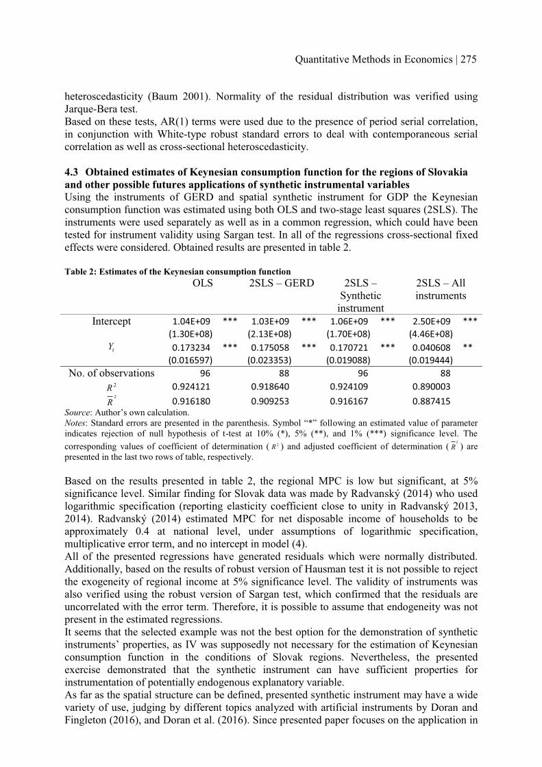
heteroscedasticity (Baum 2001). Normality of the residual distribution was verified using Jarque-Bera test. Based on these tests, AR(1) terms were used due to the presence of period serial correlation, in conjunction with White-type robust standard errors to deal with contemporaneous serial correlation as well as cross-sectional heteroscedasticity.

4.3 Obtained estimates of Keynesian consumption function for the regions of Slovakia and other possible futures applications of synthetic instrumental variables Using the instruments of GERD and spatial synthetic instrument for GDP the Keynesian consumption function was estimated using both OLS and two-stage least squares (2SLS). The instruments were used separately as well as in a common regression, which could have been tested for instrument validity using Sargan test. In all of the regressions cross-sectional fixed effects were considered. Obtained results are presented in table 2.

Table 2: Estimates of the Keynesian consumption function OLS 2SLS – GERD 2SLS –

Syntheticinstrument

2SLS – Allinstruments

Intercept 1.04E+09 *** 1.03E+09 *** 1.06E+09 *** 2.50E+09 *** (1.30E+08) (2.13E+08) (1.70E+08) (4.46E+08)

tY 0.173234 *** 0.175058 *** 0.170721 *** 0.040608 ** (0.016597) (0.023353) (0.019088) (0.019444)

No. of observations 96 88 96 88 2R 0.924121 0.918640 0.924109 0.890003 2

R 0.916180 0.909253 0.916167 0.887415 Source: Author’s own calculation.Notes: Standard errors are presented in the parenthesis. Symbol “*” following an estimated value of parameter indicates rejection of null hypothesis of t-test at 10% (*), 5% (**), and 1% (***) significance level. The corresponding values of coefficient of determination ( 2R ) and adjusted coefficient of determination ( 2

R ) are presented in the last two rows of table, respectively.

Based on the results presented in table 2, the regional MPC is low but significant, at 5% significance level. Similar finding for Slovak data was made by Radvanský (2014) who used logarithmic specification (reporting elasticity coefficient close to unity in Radvanský 2013, 2014). Radvanský (2014) estimated MPC for net disposable income of households to be approximately 0.4 at national level, under assumptions of logarithmic specification, multiplicative error term, and no intercept in model (4).All of the presented regressions have generated residuals which were normally distributed. Additionally, based on the results of robust version of Hausman test it is not possible to reject the exogeneity of regional income at 5% significance level. The validity of instruments was also verified using the robust version of Sargan test, which confirmed that the residuals are uncorrelated with the error term. Therefore, it is possible to assume that endogeneity was not present in the estimated regressions. It seems that the selected example was not the best option for the demonstration of synthetic instruments’ properties, as IV was supposedly not necessary for the estimation of Keynesian consumption function in the conditions of Slovak regions. Nevertheless, the presented exercise demonstrated that the synthetic instrument can have sufficient properties for instrumentation of potentially endogenous explanatory variable. As far as the spatial structure can be defined, presented synthetic instrument may have a wide variety of use, judging by different topics analyzed with artificial instruments by Doran and Fingleton (2016), and Doran et al. (2016). Since presented paper focuses on the application in

Quantitative Methods in Economics | 275

conditions of Slovakia, several areas of their potential use can be pointed out. Similarly to the presented analysis, the synthetic instruments can be utilized in conditions of Slovakia for regional analysis of consumption smoothing, such as the one conducted by Ivaničová and Ostrihoň (2014), regional analysis of elementary school enrolment rate on county level similar to the one of Lichner and Štefánik (2015), or regional competitiveness analysis, as was performed across V4 countries by Furková and Surmanová (2011). With the implementation of additional techniques to the examination of national and regional convergence (as presented by Workie Tiruneh 2013 or Furková and Chocholatá 2016), it is possible to expect that synthetic instruments might be useful for this application as well, provided that latent spatial paths are not correlated with the error term of growth variable.

5 CONCLUSIONS The paper addresses a complication which may arise when generating synthetic IV according to the approach of Le Gallo and Páez (2013) for regional analysis of Slovakia at NUTS 3 level. As had been shown, in such case there exist an eigenvector of the projection matrix which is constant and subsequently perfectly collinear with the intercept used in the subsequent steps of the Le Gallo and Páez (2013) procedure. Therefore, the paper suggests aslight modification, which should allow the application of the procedure automatized via program code also to the regional data of Slovakia. It is not clear whether this event of constant eigenvector occurs only for the regional data of Slovakia or it can be also experienced during regional analyses of other countries. Future research can also verify whether this complication arises when different variants of spatial weight matrix for Slovak NUTS 3 regions are used. Nevertheless, proposed modification may serve as a fail-safe mechanism for pre-programmed Le Gallo and Páez (2013) approach, which may allow its wider applicability to a broader range of cases. Regarding the practical example of regional Keynesian consumption function, which was intended to demonstrate the use of synthetic IV for Slovak regional data, it seems that the regional income is rather uncorrelated with the error term. Additionally, the marginal propensity to consumption seems to be of a smaller magnitude for the case of Slovak regions. This result may also contribute to previous findings of Ivaničová and Ostrihoň (2014), who reported high degree of consumption smoothing for Slovak regions. Interestingly, when multiple instruments were jointly applied as present in table 2, the marginal propensity to consumption was even lower, possibly supporting the notion of weak relation between regional consumption and income across Slovak regions.

Acknowledgements: This paper was supported by Grant Agency of Slovak Republic under the project VEGA 2/0181/15 “Analyzing the Impact of European Legislation in the Field of Taxes and Pensions on Slovak Economy with the Emphasis on the Sustainability of Public Finance”.

References [1] Baum, C. F. (2001). Residual diagnostics for cross-section time series regression

models. In: The Stata Journal 1 (2001), pp. 101–104.[2] Bhargava, A., Franzini, L. and Narendranathan, W. (1982). Serial Correlation and the

Fixed Effects Model. In: The Review of Economic Studies 49 (1982), pp. 533-549. [3] Doran, J. and Fingleton, B. (2016). Employment Resilience in Europe and the 2008

Economic Crisis: Insights from Micro-Level Data. In: Regional Studies 50 (2016), pp. 644-656.

276 | Multiple Criteria Decision Making XVIII

[4] Doran, J., McCarthy, N. and O’Connor, M. (2016). Entrepreneurship and employment growth across European regions. In: Regional Studies, Regional Science 3 (2016), pp. 121-128

[5] Furková, A. and Chocholatá, M. (2016). Spatial Econometric Modelling of Regional Club Convergence in the EU. In: Ekonomický časopis 64 (2016), [accepted paper].

[6] Furková, A. and Surmanová, K. (2011). Stochastic Frontier Analysis of regional competitiveness. In: Quantitative methods in economics 12 (2011), pp. 67-76.

[7] Gujarati, D.N. and Porter, D.C. (2009). Basic Econometrics. McGraw-Hill Education.,New York.

[8] Ivaničová Z. and Ostrihoň F. (2014). Consumption smoothing and risk sharing across the regions (fiscal effects panel data approach). In: Proceedings of the Quantitative methods in economics: multiple criteria decision making XVII (Reiff, M., Gežík, P., and Lukáčik, M. eds.). Vydavateľstvo EKONÓM, Bratislava, pp. 88-96.

[9] Le Gallo, J. and Páez, A. (2013). Using synthetic variables in instrumental variable estimation of spatial series models. In: Environment and Planning A 45 (2013), pp. 2227 – 2242.

[10] Lichner, I. and Štefánik, M. (2015). Prognóza počtu žiakov základných škôl do roku 2025. In: Forum Statisticum Slovacum 11 (2015), pp. 65-70.

[11] Radvanský, M. (2013). Application of modified Klein regional model to cohesion policy analysis. In: EcoMod2013: international conference on economic modeling.University of life sciences, Prague, pp. 1-30.

[12] Radvanský, M. (2014). Možnosti analyzovania vplyvu kohéznej politiky na regióny a trh práce SR: ekonometrický prístup. Ekonomický ústav SAV, Bratislava.

[13] Workie Tiruneh, M. (2013). Does Labour Force Education Accelerate the Speed of Convergence? Empirical Evidence from Selected EU Countries. In: Ekonomický časopis 61 (2013), pp. 344-357.

[14] Wooldridge, J. M. (2002). Econometric Analysis of Cross Section and Panel Data. The MIT Press, Cambridge.

[15] Wooldridge, J. M. (2012). Introductory Econometrics: A Modern Approach. South-Western, Mason.

Author’s addressIng. Filip Ostrihoň, PhD. Institute of Economic Research, Slovak Academy of Sciences Department of Empirical Research Šancová 56, 811 05 BratislavaSlovak Republic email: filip.ostrihon@savba.sk

Quantitative Methods in Economics | 277

AN EXACT SOLUTION OF THE MINIMUM FLEET SIZE PROBLEM WITH FLEXIBLE BUS TRIPS

Stanislav Palúch, Štefan Peško, Tomáš MajerFaculty of Management Science and Informatics,

University of Žilina, Žilina, Slovakia

Abstract

A bus trip is a quadruple of data defining departure time, departure place, arrival time and arrival place. Two trips are linkable if one bus can provide both of them. A running board is a sequence of trips performable by one bus. The original minimum fleet size problem is to arrange the given set of trips into minimum number of running boards provided that departure and arrival times are fixed. If departure and arrival times of trips are allowed to be shifted in time a further decrease of the number of running boards can be achieved. This paper introduces an exact model of the minimum fleet size problem with trips which are allowed to be shifted in time. Computer experiments with Gurobi solver for corresponding MILP model show that proposed approach is applicable for real word instances. Keywords: vehicle scheduling, mixed linear programming, flexible trip

JEL Classification: C61 AMS Classification: 90C27, 90C10

1 TITLE OF THE SECTION A municipal or regional personal bus transport is performed on a transportation network. A transportation network is defined by an edge weighted graph – i.e. by a set of vertices and a set of edges. Two edge weights – time length and geographic length – are associated with every edge. These edge weights allow us to calculate time distance matrix >(�, h) and geographic distance matrix – the last mentioned is not important for us. The value >(�, h)expresses how long it takes for a bus to move from the place � to place h.A bus timetable is composed of bus trips. Full specification of a trip comprises data of corresponding route, bus stops and related departure and arrival times. However, it suffices to define a bus trip [ by four essential data (p!b, p�b, !b, �b) – departure time, departure place, arrival time and arrival place for scheduling purposes. The trip e is linkable after the trip [ ifp!_ ≥ !b + >��b, p�_�i.e. if a bus after finishing the trip [ can pull into departure place of the trip e.A running board of a bus is a sequence of trips [ , [�, … , [�such that for every 1 ≤ ² < \ the trip [´q is linkable after the trip ².Every running board is, in fact, a sequence of trips performable by one bus – it represents the daily schedule of jobs assigned to this bus. The minimum fleet size problem – MFSP – is defined as follows: Suppose we are given a set ¶ containing · trips. The goal is to arrange all trips from ¶ into minimum number of running boards. MFSP can be formulated as an assignment problem: Let us define constants �b_ and decision variables Zb_ for every [ = 1,2, … , ·, e = 1,2, … , ·

� �b_ = ¸1 if p!_ ≥ !b + >��b, p�_� 0 otherwise

278 | Multiple Criteria Decision Making XVIII

� Zb_ = »1 if the trip e is linked immediatly after trip [0 otherwise �b_ = 1 if and only if the trip e can be linked after trip e, otherwise �b_ = 0.

Maximize ^ ^ Zb_�

_B �

bB (1)

subject to: ^ Zb_�

bB ≤ 1 for e = 1,2, … , · (2)

^ Zb_�

_B ≤ 1 for [ = 1,2, … , · (3)

Zb_ ≤ �b_ for [ = 1,2, … , ·, e = 1,2, … , · (4)

Zb_ ≥ 0 for [ = 1,2, … , ·, e = 1,2, … , · (5)

Just formulated problem has an integer solution, Zb_ ∈ {0,1}.

If departure and arrival times of trips are allowed to be shifted in time a further decrease of the number of running boards can be achieved. Let us introduce · additional integer variables lb that indicate that the trip departs (resp. arrives) in time p!b + lb (resp. !b + lb) instead of p!b (resp. !b).Let us define Ãb_ = p!_ − !b − >��b, p�_�Shifted trip e can be linked immediately after shifted trip [ ifp!_ + l_ ≥ !b + lb + >��b, p�_�i.e. if 0 ≤ Ãb_ + l_ − lbIn order to adapt mathematical model (1) – (5) for flexible trips we have to make several changes. First of all we are to introduce new integer variables lb and to limit them from below and from above. This can be done without loss of generality by two types of constraints lb ≤ . and 0≤lb ,where . is the maximum allowed shift of trips. It is not guaranteed that new model will give integer values of Zb_ therefore it is necessary to require that Zb_ ∈ {0,1}.

Condition (4) should be replaced by

Zb_ ≤ ¸1 if 0 ≤ Ãb_ + l_ − lb0 otherwise what is equivalent with Zb_ ≤ maxÄ0, �1 + Ãb_ + l_ − lb�ÅNo one from two last constraints is a linear constraint. This obstacle can be avoided by introducing a large constant 4 and a new binary decision variable ]b_. We want to secure that ]b_ = 1 if and only if Ãb_ + l_ − lb ≥ 0.

Quantitative Methods in Economics | 279

Ãb_ + l_ − lb + 1 ≤ 4. ]b_ (6)4�]b_ − 1� ≤ Ãb_ + l_ − lb (7)

If Ãb_ + l_ − lb ≥ 0 then Ãb_ + l_ − lb + 1 > 0 and condition (7) holds for both ]b_ = 0 and ]b_ = 1. It follows from (6) in this case that ]b_ = 1.If Ãb_ + l_ − lb < 0 then Ãb_ + l_ − lb + 1 ≤ 0 (due to integrity of Ãb_, l_, lb) and condition (6) holds for both ]b_ = 0 and ]b_ = 1. It follows from (7) in this case that ]b_ = 1.

Maximize ^ ^ Zb_�

_B �

bB (8)

subject to: ^ Zb_�

bB ≤ 1 for e = 1,2, … , · (9)

^ Zb_�

_B ≤ 1 for [ = 1,2, … , · (10)

Ãb_ + l_ − lb + 1 ≤ 4. ]b_ for [ = 1,2, … , ·, for e = 1,2, … , · (11) 4�]b_ − 1� ≤ Ãb_ + l_ − lb for [ = 1,2, … , ·, for e = 1,2, … , · (12) lb ≤ � for [ = 1,2, … , · (13) ]b_ ∈ {0,1} for [ = 1,2, … , ·, for e = 1,2, … , · (14) Zb_ ∈ {0,1} for [ = 1,2, … , ·, for e = 1,2, … , · (15) lb ≥ 0, integer, for [ = 1,2, … , · (16)

2 COMPUTATIONAL RESULTS Mathematical model (8) – (16) was solved for instances (obtained by random generator) containing 200, 400, 600 and 800 trips. Our experiments were conducted on HP XW6600 Workstation (8-core Xeon 3GHz, RAM 16GB) with OS Linux (Debian/jessie). We also used the Python interface to commercial mathematical programming solver Gurobi .

3 CONCLUSION Computational results of instances mentioned above are contained table 1. Computational experiments show, that the number of used vehicles decreases with increasing allowed shift �.Computational time rises with increasing number of trips but it is almost independent on allowed shift �. Most pleasant fact is that in spite of the fact that computational time is growing with the number of trips, this method is still applicable for practical real world instances.

280 | Multiple Criteria Decision Making XVIII

Table 1. Computational time and number of buses – dependence on the number of trips and allowed shift � .

200 trips 400 trips 600 trips 800 trips

allowed shift δ

number of buses time [s] number

of buses time [s] number of buses time [s] number

of buses time [s]

0 19 11,70 31 47,60 53 150,43 36 229,501 19 11,67 31 48,01 53 152,11 36 214,982 18 11,83 30 48,32 52 135,60 35 201,953 18 11,77 30 67,43 52 107,46 34 202,964 18 11,94 30 68,38 52 107,89 34 204,745 18 11,83 30 62,16 52 111,74 34 249,226 18 11,82 30 49,47 52 108,82 34 246,627 18 16,13 30 47,87 52 108,17 34 221,838 18 15,34 30 48,21 52 107,92 34 293,739 18 15,27 30 48,73 52 108,25 33 295,3410 18 16,34 29 48,53 52 107,84 33 219,30

Acknowledgements: This work was supported by the research grant APVV-14-0658 ”Optimization of urban and regional public personal transport”.

References [1] A. Ceder. (2011). Public-transit vehicle schedules using a minimum crew-cost approach.

Total Logistic Managment, 4, pp. 21-42. [2] Gurobi Optimization Inc. (2015). Gurobi Optimizer Reference Manual. [online] Available

at: http://www.gurobi.com [Accessed 20 Dec. 2015]. [3] Palúch, S. and Černý, J. (1995). Bus Scheduling with Flexible Journeys. Ricerca

Operativa, 24(71). [4] Palúch, S. (2003) Bus scheduling as a graph coloring problem. Communications -

scientific letters of the University of Žilina, 4, pp. 16-20. [5] Palúch, S. (2008). Two approaches to vehicle and crew scheduling in urban and regional

bus transport. In: Quantitative Methods in Economics (Multiple Criteria Decision Making XIV): Proceedings of the International Scientific Conference. Bratislava: Iura Edition, pp. 212-218.

[6] Palúch, S. (2013). Vehicle and crew scheduling problem in regular personal bus transport - the state of art in Slovakia. In: 16th international conference on transport science - ICTS 2013. Portorož, Slovenija, pp. 297-304.

[7] Peško, Š. (2008). Flexible bus scheduling with overlapping trips. In: Quantitative Methods in Economics (Multiple Criteria Decision Making XIV): Proceedings of the International Scientific Conference. Bratislava: Iura Edition, pp. 225-230.

[8] Peško, Š. (2001). The minimum fleet size problem for flexible bus scheduling. In: Studies of the Faculty of management science and informatics University of Žilina, 9, pp. 75-81.

[9] Wren, A. and Rousseau, J. (1995). Bus driver scheduling - an overview. In: Daduna, J.,Branco, I. and Pinto Paixao, J., Computer-Aided Transit Scheduling. Berlin: Springer Verlag, pp. 173-187.

[10] Wren, A. (1996). Scheduling, timetabling and rostering - a special relationship. In: Burke, E. K. and Ross, P., Practice and Theory of Automated Timetabling. Berlin: Springer Verlag, pp. 46-75.

Quantitative Methods in Economics | 281

Author’s addressDoc. RNDr. Štefan Peško, CSc.University of Žilina, Faculty of Management Science and Informatics,Department of Mathematical Methods and Operational Analysis Univerzitná 8215/1, 01026 Žilinae-mail: stefan.pesko@fri.uniza.sk

Doc. RNDr. Stanislav Palúch, CSc.University of Žilina, Faculty of Management Science and Informatics,Department of Mathematical Methods and Operational Analysis Univerzitná 8215/1, 01026 Žilinae-mail: stanislav.paluch@fri.uniza.sk

Ing Tomáš Majer, PhD..University of Žilina, Faculty of Management Science and Informatics,Department of Mathematical Methods and Operational Analysis Univerzitná 8215/1, 01026 Žilinae-mail: tomas.majer@fri.uniza.sk

282 | Multiple Criteria Decision Making XVIII

LABOR MARKET RIGIDITIES AND MONETARY SWITCH IN A DSGE MODEL: APPLICATION TO THE SLOVAK ECONOMY

Adam Pápai, Masaryk University, Brno

Abstract This paper investigates the structural and dynamical characteristics of the Slovak economy during the last 13 years. The focus lies mainly in the examination of the Slovak labor market. To achieve our goal, we use a dynamic stochastic general equilibrium model for small open economies. The selected model contains several labor market rigidities, like search and matching processes, wage adjustment costs and hiring costs to improve our results of estimation. Furthermore, we augment the model with switching mechanism to capture the entry of Slovak Republic into the Eurozone, therefore abandoning its autonomous monetary policy. Our results suggest that there are significant rigidities in the Slovak labor market. Also, the Slovak Republic is greatly influenced by foreign economic forces.

Keywords: DSGE model, labor market, frictions, Slovak economy, switch

JEL Classification: E32, J60 AMS Classification: 91B40

1 INTRODUCTION Labor market represents a crucial part of each economy. It is a place, where job seekers look for vacant job positions and firms hire workers while negotiating working hours and paid wages. A well-functioning labor market is a key component of a healthy economy. Therefore, it is desirable to examine it to an extent that gives us better understanding of the forces that influence it greatly. Hence, the aim of this paper is to examine the structural properties and dynamical characteristics of the Slovak labor market.

At present, dynamic stochastic general equilibrium (DSGE) models are widely used macro-econometric tools of the policy makers, like central banks, as well as the private sector. They are used because of their great modifiability, vast variability of estimation results and easy interpretation. There are several articles investigating the behavior of the Slovak economy using DSGE models. Múčka and Horváth [2] studied different fiscal policy scenarios. They were interested in various methods to lower the public debt. Their findings were, among other things, that decreasing the public debt is the least harmful by cuts in government wage bill. On the other hand, increase in income taxes is the most harmful. Senaj et al. [5] estimated amodel with a monetary regime switch with the use of Bayesian techniques. They compared impulse responses of several shocks under autonomous and common monetary policy. The results for responses to monetary policy shock showed considerable differences between these two monetary regimes. Similarly, Pisca and Vašíček [4] examined the impacts of accession of Slovakia to the Eurozone. They found higher elasticity of substitution between domestic and foreign goods after the entry implying lower transaction costs and weaker barriers of trade. Their estimation also captured the effects of expansionary and restrictive fiscal policy on the GDP. However, only few articles, like Němec [3], investigated the Slovak labor market using DSGE approach. He aimed to examine the extent of flexibility of Slovak and Czech labor markets and reveal structural differences between them. He concluded that in both countries there is a flexible wage environment, however firms face increasing vacancy posting costs

Quantitative Methods in Economics | 283

which slow down the vacancy creation. For other interesting papers about DSGE models for the Slovak Republic, see Tvrz and Vašíček [6] and Zeman and Senaj [7].

1.1 History of economic situation As figure 1 shows, the Slovak economy experienced a relatively stable growth during the last two decades with only few significant setbacks. The first was the currency crisis in the late 90s, when output decreased. This led to a rapid increase of the unemployment rate from 13 to 19 percent. Despite the persistent growth of GDP, the unemployment rate remained near its observed maximum value for considerably long time. Only after joining the European Union did the unemployment rate begin to decline. This decrease continued until the second significant drop in output when Slovakia was affected by the financial crisis of 2007-2008. At this time, the unemployment rate reached its lowest value around 9 percent. After the Great recession, the Slovak Republic experienced one of the fastest economic recoveries and growths in the European Union. This was partially achieved by a well-timed admission into the Eurozone in 2009, while the exchange rate between the Slovak koruna and euro was fixed earlier in 2008. The rise of unemployment rate caused by the recession stopped in 2010 at 15 percent. It was then followed by a four year period of high unemployment until 2014, when the unemployment rate finally begun to decline.

Figure 1: Real GDP and unemployment rate of Slovakia. Data source: http://www.nbs.sk/

2 MODEL A medium sized small open economy DSGE model developed by Albertini et al. [1] is selected for the estimation. The model is quite complex, so only the key components will be presented here.1 The labor market is the most crucial part of the model. Here, the job searchers meet the firms who look for workers. A Cobb-Douglas search and matching function is implemented to ensure a non-Walrasian labor market. It ‘creates’ seeker-vacancy pairs which then become a productive combination of worker and filled job position. Wages and hours worked are the result of a bilateral Nash bargaining process, where the firms and employees divide the surplus of the production based on their negotiating powers. There is also an exogenous job separation rate. Furthermore, the model contains several rigidities: the matching function makes it impossible to pair each worker with a vacancy; there is a real

1 For a detailed overview of the model see Albertini et al. [1].

284 | Multiple Criteria Decision Making XVIII

vacancy creation cost which increases the expenses of producers; the Rotemberg-style wage and price frictions also increase the costs if the firms want to adjust them. The model consists of three agents and a foreign sector modelled as AR(1) processes. Households decide between consumption of goods and leisure. There are three types of firms. The intermediate good producers are the only firms that hire workers and create vacancies. They sell their goods to the retailers who produce and sell the final good for private consumption. The last type is represented by the importers, who sell foreign goods on the domestic market for domestic currency facing exchange rate fluctuation risks. The monetary authority is represented by a Taylor-type rule for the autonomous monetary policy period. The current interest rate depends on its previous value, inflation, output and exchange rates. For the time period after the admission to Eurozone, the domestic interest rate is equal to the interest rate of the foreign sector. Finally, there is no capital nor government present in the model.

3 DATA AND CALIBRATION Quarterly time series of 11 observations were acquired from the web site of the National bank of Slovakia.2 Our data set covers the period between 2002Q1 and 2015Q3. The first observation is given by the availability of vacancy’s time series. Following Albertini et al. [1], we use 8 variables for the domestic economy and 3 represent the foreign sector given by the Eurozone. Output per capita (yt) is defined as real GDP divided by the economically active population. Interest rate (it) is represented by 3-month BRIBOR until 2008 and EURIBOR afterward. Inflation (πt) is calculated as a change in the consumer price index. Exchange rate (qt) is represented by the real effective exchange rate between the Slovak Republic and the Eurozone. Vacancy rate (vt) is acquired as number of vacancies normalized by the economically active population. The unemployment rate (ut) is from the Labor Force Survey of the Statistical Office of the Slovak Republic. Total hours are divided by number of employees to get the hours worked (ht) suitable for the model. Quarterly wages (wt) deflated by CPI are the last observed variable for the domestic economy. The foreign sector, represented by the Eurozone is defined using output, interest rate and inflation (y*

t, i*t, and π*

t,). The time series were seasonally adjusted and stationarized to represent percentage differences from the steady states. The interest rates and the inflations were demeaned, while the rest of the variables were detrended using Hodrick-Prescott filter with the usual smoothing parameter λ = 1600. We divided the observed time series into two separate periods to investigate the possible changes in the structure of the Slovak economy: the period from 2002Q1 to 2008Q4 represents the autonomous monetary policy (28 periods) and the period between 2009Q1 and 2015Q3 represents the common monetary policy (27 periods).

We calibrated the model parameters to determine the non-stochastic steady state. Several parameters were set according to the literature. The discount factor (β) was set to 0.9966 and the Frisch elasticity of labor supply (ϕ) to 3.8, as in Múčka and Horváth [2]. Also the prior value of the deep-habit parameter (ϑ = 0.7) was taken from the mentioned article. We set the labor share in production (ζ) to a widely used value of 2/3. The values of other parameters were calculated from the data. The import share on GDP was set to 0.427 for the period before the admission and to 0.453 after. The steady state value of unemployment, calculated as the mean of the unemployment rate was set to 0.149 and 0.133 respectively.

For both time periods two chains of Metropolis-Hastings algorithms with 600 000 draws were generated with acceptance ratio around 0.3. Matlab and its Dynare toolbox were used for the computations. Bayesian techniques, like the Kalman filter or Random Walk Metropolis-

2 http://www.nbs.sk/en/monetary-policy/macroeconomic-database/macroeconomic-database-chart

Quantitative Methods in Economics | 285

Hastings algorithm, were used for the estimation of the model. This allows us, among other things to investigate the behavior of unobserved variables.

4 ESTIMATION RESULTS It is important to note that, the recession in 2008 began only one quarter before Slovakiajoined the monetary union. Therefore, we cannot distinguish between the effects of these two events in the obtained results.

First, we look at the historical shock decomposition of output shown in figure 2. For greater clarity, we arranged the shocks into groups. Foreign shocks include shocks to foreign output, inflation and interest rate. The labor market shocks consists of bargaining, matching and vacancy shocks. Other shocks cover all the other shocks, like preference, cost-push shocks or uncovered interest rate parity and monetary shocks for the period before. As expected, our estimation shows that the output depends mainly on the shocks to productivity. The extensive boom of the Slovak economy between 2006 and 2009 was also due to the positive influence from the Eurozone. Also, figure 2 suggests that the Great recession was not caused by external shocks, rather it came from other, domestic sources. Finally, we can observe a strong positive influence of labor market shocks at the fourth quarter of the observed time period that pushed the output upwards.

Figure 2: Historical shock decomposition of output. Source: author’s estimations

Now we look at the estimated parameters found in table 1. We can see the high and stable value of the habit persistence. The monetary regime change did not change the preferences of the households. Higher bargaining power of firms suggests lower trade union participation.

ParameterPrior

distributionPrior mean and

standard deviationPost. mean

BeforePost. mean

AfterHabit persistence beta 0.7, 0.15 0.710 0.705Inverse of Frisch el. gamma 3.8, 0.75 3.914 3.845El. of subst. (dom. & for.) gamma 1, 0.2 0.881 0.832Firm’s bargaining power beta 0.5, 0.2 0.645 0.619El. of matching beta 0.5, 0.2 0.866 0.850

286 | Multiple Criteria Decision Making XVIII

El. of vacancy creation gamma 1, 0.5 6.164 5.217Price and wage setting parametersBackward price (d. good) beta 0.75, 0.1 0.799 0.795Backward price (f. good) beta 0.75, 0.1 0.786 0.774Backward looking wage beta 0.75, 0.1 0.743 0.736Price adj. cost (d. good) gamma 50, 15 58.798 54.259Price adj. cost (f. good) gamma 50, 15 63.627 52.789Wage adjustment cost gamma 50, 15 60.445 61.429Monetary policy parametersInterest rate smooth. beta 0.5, 0.15 0.488 -Inflation gamma 1.5, 0.5 2.804 -Output gap normal 0.25, 0.1 0.257 -Output difference normal 0.25, 0.1 0.278 -Exchange rate normal 0.25, 0.1 0.342 -

Table 1: Structural parameter estimations. Source: author’s estimationsThere are significant frictions in the economy. The elasticity of vacancy creation shows increasing vacancy creation costs. All three price adjustment parameters are close together. This shows, that all types of firms face similar conditions in the Slovak Republic.

5 CONCLUSION In this paper we investigated the dynamical and structural properties of the Slovak economy before and after the admission to the Eurozone. We focused mainly on the examination of the labor market. For this purpose, we estimated a small open economy DSGE model using Bayesian techniques. We found significant frictions present in the Slovak labor market. Also, the structural parameters did not show a great change after the admission.

Acknowledgements: This work is supported by funding of specific research at Faculty of Economics and Administration, project MUNI/A/1040/2015.

References [1] Albertini, J., Kamber, G. and Kirker, M. (2012). Estimated small open economy model

with frictional unemployment. Pacific Economic Review, 17 (2), pp. 326–353. [2] Múčka, Z. and Horváth, M. (2015). Fiscal Policy Matters: A New DSGE Model for

Slovakia. Council for Budget Responsibility discussion paper No. 1/2015. Bratislava. [3] Němec, D. (2013). Investigating Differences Between the Czech and Slovak Labour

Market Using a Small DSGE Model with Search and Matching Frictions. Czech Economic Review, 7, pp. 21–41.

[4] Pisca, V. and Vašíček, O. (2014). Behavior of Slovak economy integrated into EMU: DSGE model with a government sector and inflation targeting. In: International Scientific Conference Quantitative Methods in Economics (Multiple Criteria Decision Making XVII). Bratislava: EKONÓM, pp. 213–219.

[5] Senaj, M., Výškrabka, M. and Zeman, J. (2010). MUSE: Monetary Union and Slovak Economy model. National Bank of Slovakia working paper no. 1/2010. Bratislava.

[6] Tvrz, S., and Vašíček, O. (2014) Nonlinear DSGE model of the Slovak economy with time-varying parameters. In: International Scientific Conference Quantitative Methods in Economics (Multiple Criteria Decision Making XVII). Bratislava: EKONÓM, pp. 292–297.

[7] Zeman, J. and Senaj, M. (2009). DSGE model – Slovakia. National Bank of Slovakia working paper no. 3/2009. Bratislava.

Quantitative Methods in Economics | 287

Author’s addressIng. Adam Pápai Masaryk University, Faculty of Economics and Administration, Department of Economics Lipová 507/41a, 602 00 BrnoCzech Republic email: papai@mail.muni.cz

288 | Multiple Criteria Decision Making XVIII

LOCATION OF ELECTRIC VEHICLE CHARGING STATION IN 2-PHASES

Juraj Pekár, Ivan Brezina, Zuzana �i�ková University of Economics in Bratislava

AbstractThe advent of electro mobility depends on the provision of adequate conditions. One of the necessary conditions for the expansion of electro mobility is to ensure appropriate network of charging stations. In the paper the authors proposing a method for constructing a network of charging stations to ensure two main objectives, namely the availability of rapid charging stations for the highest possible number of citizens, and accessibility for population from the entire analyzed area. Using appropriate location models seems to be suitable tool while the process is divided into two stages. Practical application considers the coverage of the Slovak Republic.

Keywords: Location models, Electro mobility JEL Classification: C61, C90, L91 AMS Classification: 90C08, 90C90

1 INTRODUCTIONThe use of electric vehicles brings a significant reduction in noise and emissions from transport with positive impacts on the quality of life. Electro mobility is a general term for the development of electric-powered vehicles away from the use of fossil fuels. For the development of electro mobility in Slovakia it is necessary to ensure adequate infrastructure - charging stations for electric vehicles as well as the subsequent government measures that help increasing the market share of electric vehicles in the car market. Essential precondition for the development of electro mobility is suitable charging infrastructure. Types of charging stations are based on standards: slow charging (AC power up to 3.7 kW), rapid charging (power from 3.7 kW up to 22 kW), and fast charging (power over 22 kW), last two standards presuppose publicly available charging stations of AC or DC. The paper deals with the construction of public charging stations network, where fast and rapid charging stations are considered. Model approach is based on the consideration that location of more powerful (fast) charging stations is realized at first in order to cover the largest possible number of inhabitants within a specified distance. Next it is provided coverage of all residents using less expensive charging stations. The paper is aimed on locating of charging stations under predetermined conditions using some optimization models. The core part of this paper is oriented on approach composed of two phases, when the first phase is aimed at location of limited number of fast charging stations which are supplemented by rapid charging stations provided coverage of all residents. The presented approach is demonstrated on Slovak Republic coverage. 2 LOCATION MODELS Different works aimed at various location problems can be found, e.g. (Brezina at al. 2009), (Brezina at al. 2011), (Drezner, Z. at al. 2004), (Jánošíková, �., Žarnay, M. 2014), (Pekár, J. 2010), (Eiselt, H. A., Sandblom, C. L. 2004). As mentioned above, the network structure of charging stations is realized for the two types of charging stations. The primary objective is

Quantitative Methods in Economics | 289

faster deployment of charging stations; this objective can be achieved using the maximal covering location model when determining the number of charging stations as well as maximal distance. Another model is used to solve the problem of location of such a minimal number of charging stations at the maximal distance determined by the driving range of electric vehicles in order to achieve feasibility of using electric vehicles to travel across selected points. 2.1 Maximal covering location problemMaximal covering problem when determining the number of charging stations and the maximal distance can be represented by model that allows determining the points (towns and villages), where charging stations need to be located while determining the specified number of charging stations and the maximal distance to station. The goal is to deploy charging stations to ensure that a maximal number of points are covered. Further on following notation is used. Let n, K and p represent respectively the number of points, maximal distance from charging station and number of charging stations. Also suppose the known minimal distances within all points are represented by parameters ijd ,

, 1, 2,...i j n� . Let , 1, 2,...jb j n� represent number of inhabitants in the j-th point. Moreover

two kinds of binary variables are used. Variables � �0,1 , 1, 2,...ix i n� � , with the following notation: 1ix � if the charging station is established in i-th point and 0ix � otherwise and variables � �0,1 , 1, 2,...jy j n� � where 1jy � if the charging station within the distance K is available from the j-th point and 0jy � otherwise. The model can be stated as follows:

A B A B

A B

A B

A B� � A B

1

1

1

, max 1

0 , 1, 2,... 2

3

1, 4

, 0,1 5

n

i iin

ij j ij

n

jj

j k

j j

f b y

a x y i n

x p

x j N

x y

�

�

�

� /

? 4 �

�

� �

�

�

�

�

x y

0,

1,ij

ijij

d Ka

d K�#6� " 06!

i, j = 1, 2,... n (6)

The objective function (1) ensures establishment of maximal covered number of inhabitants. Equations (2) enable setting of variables , 1, 2,...jy j n� based on distance of j-th point from the charging station. Coefficients ija , , 1, 2,...i j n� represent accessibility between i-th and j-th point calculated according to (6). Equation (3) limits number of charging stations. Let Nk be the set of nodes in which the charging stations must to be placed, than equations (4) enable setting of predetermined location of charging station, e.g. depending on point’s importance. 2.2 Minimal charging stations location problem This section is aimed on determining the minimal number of charging stations at the maximal distance that enables to locate charging stations within the required availability (distance K) from all cities. Model (7) – (10) enables reflecting the population and importance of each point (necessary existence of the charging station in the regional capitals) as well as the today's existence of charging stations at some point.

290 | Multiple Criteria Decision Making XVIII

Let B represents the total population size (at all points along). Thus coefficients

1 , 1,2,...jj

bc j n

B� ? � represent the potential number of requests at the j-th point. Using

before mentioned notation the model can be stated as follows:

A B

A B

A B� � A B

1

1

( ) min 7

1, 1,2,..., 8

1, 9

0,1 , 1,2,..., 10

n

j jj

n

ij jj

j k

j

f c x

a x i n

x j N

x j n

�

�

� /

4 �

� �

� �

�

�

x

The objective (7) enables minimizing number of charging station while taking into account population size. Equations (8) ensure accessibility of i-th point from at least one of the charging stations within the distance K. 3 TWO-PHASES DECISION PROCESS WHEN PLACING CHARGING STATIONS In this part is presented two-stage process of placing two different types of charging stations (rapid and fast charging). Previous section is devoted to models which address only one type of object placement, but in real life it is usually necessary to place multiple types of facilities that cater to various types of demand. Whereas at present there exist a variety of charging stations with different performance having different purchase prices and in economic terms is meaningless to cover the territory with only one type, but rather with more types of charging stations with different performance. Consider two types of charging stations depending on their performance. Location of two types of charging stations can be divided into two stages: 1. stage: Solving maximal covering location problem when determining the number of

charging stations and the maximal distance enables to determine location of predetermined number of fast charging stations that cover the widest possible population. Calculated values of variables are designated as A B* 1 ,jx j N� .

2. stage: Using of model (7)-(10) enables 100 % coverage of population by adding a second type of charging stations (rapid charging stations). It is ensured by replacement of equations (9) by following: A B* 1 ,j jx x j N4 � , where values A B* 1 ,jx j N� are calculated in 1. stage. Thus we build charging stations only in places where there is no fast charging station.

Presented two-stage process charging station location enables covering as many inhabitants as possible by fast charging stations while ensuring 100% population coverage of the population leastwise by rapid charging stations. 4 LOCATION OF CHARGING STATION IN SLOVAKIA In following section the construction of network of charging station in Slovakia (2916 municipalities) according to abovementioned approach will be presented. Suppose the possibility of building twenty fast charging stations while in each regional capital such station must be placed. The second phase is designed to complement the network with rapid charging stations, so that from any point (site in Slovakia) must be possible to reach at least one charging station while taking into consideration prelocated charging station from the first phase. Proposed problems were implemented in GAMS and solved by Cplex 12.2.0.0. Input data:

Quantitative Methods in Economics | 291

n = 2916– number of points; p = 20– number of fast charging stations (used in the first phase); K = 30 km– maximal possible distance to charging station (suppose identical distance in both of phases in our case); B = 5 378 511– number of inhabitants in Slovakia; bj, j = 1, 2,... 2916 – number of inhabitants in corresponding point, dij, i, j = 1, 2,... 2916 –minimal distances between all the pairs of points1; Maximal coverage (according to (1) – (6)) is provided by placing the charging stations in those cities: Bratislava – Ružinov, Trnava, Topo�níky, Kúty, Podkylava, Pribeta, Nitra, Tren�ín, Nová Baa, Horné Vestenice, Visolaje, Banská Bystrica, Ož�any, Spišský Štvrtok, Prešov, Košice – Západ, Ve�ké Raškovce, Topo�ovka, Žilina, Ivachnová. Thus, it realized the availability of charging stations within 30 km for 4,272,375 inhabitants of Slovakia. Charging network is complemented by location of rapid charging stations in the following municipalities: Malacky, Gab�íkovo, Kolárovo, Žiar nad Hronom, Detva, Torna�a, Gemerská Poloma, Vranov nad Top�ou, Krá�ovský Chlmec, Nižná, Rudno, Mužla, Murá, Slovenská Ves, Moldava nad Bodvou, Sobrance, Demandice, Ve�ký Krtíš, Fi�akovo, Nižný Slavkov, Bardejov, Žalobín, Topo�a, Krpe�any, Senec, Senica, Nová Ves nad Žitavou, Krupina, Brezno, Spišská Nová Ves, Stará �ubova, Trebišov, Mestisko, �adca, Pieš any, Rybany, Rimavské Brezovo, Gelnica, Svetlice, Námestovo, Východná. Thus full territorial coverage is achieved by building up 20 fast charging stations and 41 rapid charging stations. 5 CONCLUSION Electro mobility is one of the areas starting to implement green technology. The use of electric vehicles represents a significant reduction in noise and emissions from transport with positive impacts on the quality of life. Although using the internal combustion engine will certainly continue in the near future, it is necessary to create appropriate conditions to start a gradual transition from internal combustion engines to new and more efficient technologies. In this paper the authors proposes a procedure for the construction of a network of charging stations, which could increase interest in using of electric vehicles, while pursuing two basic objectives: the availability of rapid charging stations for the highest possible number of citizens, as well as to motivating citizens for its use in any territory by covering the whole population with network of charging stations. The case-study was realized throughout Slovakia. Acknowledgements: This paper is supported by the Grant Agency of Slovak Republic – VEGA, grant no. 1/0245/15 „Transportation planning focused on greenhouse gases emission reduction“.

References[1] Brezina, I., Pekár, J. and �i�ková, Z. (2009). Model of the collection centres in

communes of Slovak Republic. In: 27th International Conference on Mathematical methods in economics 2009. Prague: Czech University of Life Sciences Prague, pp. 29-32.

[2] Brezina, I., Dupa�, A. and Pekár, J. (2011). Zelená a reverzná logistika ako nástroj zefektívnenia spa�ovania odpadu v Slovenskej republike. Ekonomický �asopis, 59(2), pp. 132-147.

1 The input data are available on request

292 | Multiple Criteria Decision Making XVIII

[3] Drezner, Z. at al. (2004). Facility location. Applications and theory. Berlin: Springer-Verlag.

[4] Jánošíková, �. and Žarnay, M. (2014). Location of Emergency Stations as the Capacitated p-median Problem. In: Proceedings of the International Scientific Conference Quantitative Methods in Economics – Multiple Criteria Decision Making XVII, Virt: Ekonóm, pp. 116-122.

[5] Pekár, J., Brezina, I. and �i�ková, Z. (2010). Model Support for Construction of Regional Models. In: International Conference on Regional Disparities in Central and Eastern Europe Location. Smolenice: IURA EDITION, pp. 191-195.

[6] Eiselt, H. A. and Sandblom, C. L. (2004). Decision analysis, location models and scheduling problems. Berlin: Springer – Verlag.

[7] Slovenská asociácia pre elektromobilitu – SEVA, (2016). [online] Available at: http://www.seva.sk/sk/ [Accessed 20 Feb. 2016].

Author’s address doc. Mgr. Juraj Pekár, PhD., prof. Ing. Ivan Brezina, CSc., doc. Ing. Zuzana �i�ková, PhD. University of Economics in Bratislava, Faculty of business informatics, Department of Operations research and Econometrics, Dolnozemská 1/b, 852 35 Bratislava, Slovak Republic email: pekar@euba.sk, brezina@euba.sk, cickova@euba.sk

Quantitative Methods in Economics | 293

VEHICLE ROUTING PROBLEM WITH PRIVATE AND COMMON CARRIER

Jan Pelikán, University of Economics Prague

Abstract The goal of the paper is vehicle routing problem with split demand of customers and two type of delivers. First deliver is private deliver owning a fleet of vehicles and second one is common carrier. Demand of customers and their distance matrix are given. Demand can besplit, a part is delivered by main deliver and a part by common carrier. Total costs which are minimized are the sum of private carrier costs depending on distance of routes of private vehicles and costs of common carrier depending only on amount of transported goods. The mathematical model of the problem is included in the paper, a modified insert method proposed and numerical experiments are presented.

Keywords: vehicle routing problem, insert heuristic, common carriers

JEL Classification: C44 AMS Classification: 90C15

1 INTRODUCTION Vehicle routing problem lies in delivering of goods from depot to customers. Transport is provided by a fleet of vehicles with a given capacity and distances between customers. Demand has to be covered by vehicles of the fleet and can be split. The costs are sum of distances of all vehicles’ routes. The vehicle routing problem studied in the paper is characterized by following points:

� There are two carriers assuring transport to customers: the private carrier with their fleet of heterogeneous vehicles with given capacity.

� Common carrier with unlimited capacity. � Demand of customers can be split into parts which are transported or by private carrier

vehicles or by common carrier. � Costs of private carrier transport depend on distance of vehicle route and price of one

km of particular vehicle. � Costs of common carrier depends only on amount of transported goods and price of

transported unit. � Total costs are sum of private and common carrier are minimized.

Tabu search heuristic for vehicle routing problem with private and common carriers with non-split demand is published in [2]. Fleet of vehicles of the private carrier is homogenous (with the same capacity of vehicles). A modification of the Clarke and Wright’s savings algorithm is used in [1] to solve so called the truckload and less-than-truckload problem, where private carrier uses less-than-truckload vehicles while an outside carrier trucks. A heuristic proposed in [3] selects customers according the distance from depot, customers which are closer to depot are assigned to private carrier, the others to common carrier.

2 MATHEMATICAL MODEL Let G= {V,E} is undirected complete graph, V= {1,2,…,n}, depot is vertex 1, vertexes 2,3,…,n are customers. A number of vehicles of the private carrier is S.Parameters of the model are:

• d(i,j) distance between vertex i and vertex j,

294 | Multiple Criteria Decision Making XVIII

• qi demand of vertex i,• ws capacity of s-th vehicle, s = 1,2,…,S,• ps cost per km of the s-th vehicle, • cc, cost of the transport a unit of goods by common carrier.

Variables of the model are: • xs

ij binary, equals 1 if vehicle s travels from vertex i to vertex j,• yi

s an amount of goods (a part of demand of vertex i), which is transported by private carrier,

• zi an amount of goods (a part of demand of vertex i), which is transported by common carrier (outside carrier),

• uis variables in anti-cyclic constraints.

Mathematical model of the vehicle routing problem with private and common carrier:

)8(,,0,0,

)7(,2,)1(1

)6(1

)5(,1

)4(1)(

)3(

)2(,

)1(min),(

1

1

1,,

sjizybinaryx

sjiuxnu

sx

siyxq

iqyiz

swy

jsxx

zcxpjid

isi

sij

sj

sij

si

j

sj

si

j

siji

is

si

is

si

i

sji

i

sij

iic

jis

sijs

E44

E4E0���

E0

�E4

�E��

E0

EE�

/�

�

�

�

�

��

��

�

�

In this formulation the objective function (1) minimizes the sum of travel costs of vehicles of private carrier and common carrier costs. Constraint (2) states that the same vehicle must enter and leave a vertex. Inequality (3) assures that capacity of s-th vehicle is not exceeded. Equation (4) means that the demand each vertex will be satisfied. Constraint (5) prevents supply of vertex by the vehicle s if this vehicle does not enter the vertex. At most one departure the depot is possible for each vehicle states (6). Anti-cyclic conditions are in (7).

3 MODIFIED INSERT HEURISTIC The following notation is used for the modified insert heuristic: the route of s-th vehicle

�� ,1,,...,2,1),,...,,( )(1)(21 ���� ssh

sssh

sss vvSsvvvV and delivery to node i by vehicle s isdenoted as ysi..

Heuristic algorithm. Step 1. {choice of vehicle s and its initial route}

Quantitative Methods in Economics | 295

Vehicle s and node k are selected in order to maximize the value ))1,(),1((),,( kdkdpycyks s

skc

sk ���@ , where ys

k is maximum uncovered demand of node k which does not exceed available capacity of the vehicle s, ie. 0≤ ys

k≤qk and ysk≤ws . Value

�(s,k) has to be positive. If no vehicle with initial route is selected then stop, otherwise put skss

skkk

sss ywwyqqshvkvv �������� :,:;3:)(,1:,:,1: :321 and go to Step 2. Step 2. {insertion}Repeatedly select a node k, a quantity ys

k and the edge (vsj ,vs

j+1) to maximize the value )),(),(),((),,,( 11

sj

sj

sj

sjs

skc

sk vvdvkdkvdpycyjks �� ����F , where ys

k is maximal uncovered demand of node k which does not exceed available capacity of the vehicle s, ie.

sskk

sk wyqy 00� ,0 , value s

ky has to be positive. If no node k is selected, then go to step 1 otherwise put s

kkk yqq ��: , skss yww ��:: and delete edge ),( 1

sj

sj vv � and add edges

),(),,( 1sj

sj vkkv � in route Vs .

Step3. {common carriers transport}The remaining demand qk is assigned to transport by common carrier.

4 NUMERICAL EXPERIMENTS The experiments have been performed on benchmarks from dataset of testing instances available at http://www.uv.es/~belengue/carp.html. Parameters of the instance egl-e3 are: #vertexes=77, #vehicles=7, Σqi=521, Σwi=420, #binary variables=41503, #constraints=42142. Value of object function obtained by heuristic and by solving model is placed in Table 1 and Table 2. Two version of heuristic is used, the sequential version creates routes gradually, parallel version forms routes for vehicles all at once, simultaneously. Both versions of heuristic is written in VBA language. Finally, the model is solved using CPLEX 12.0, the time limit was half an hour on PC (Intel®Core™2Quad, 2,83GHz). The best value of object function is shown. If the result is not optimal, value of object function, the gap of object function are placed under the value of N in parenthesis (in % of lower bound). Value N1 are costs of private carries, N2 are costs of common carrier, total costs are N. The amount of goods transported is place under value N1, resp. N2 in parenthesis.

Table 1. Results of instance egl-e3

cc seq. par. model

N1 N2 N N1 N2 N N1 N2 N

10 0 5210 5210 0 5210 5210 0 5210 5210

50050270 150500

20077050270 150500

20077089620 80500

170120(220) (301) (220) (301) (360) (161)

1000117050 101000

219050118630 101000

21963089620 161000

250620(420) (101) (420) (101) (360) (161)

2000122090 202000

324090118090 202000

32039586900 322000

428285(420) (101) (420) (101) (360) (161)

296 | Multiple Criteria Decision Making XVIII

Parameters of the instance S1-B are: #vertexes=140, #vehicles=10, Σqi=965, Σwi=810, #binary variables=196000, #constraints=197572 .

cc seq. par. ModelN1 N2 N N1 N2 N N1 N2 N

10 0 9650 9650 0 9650 9650 0 9650 9650 opt.

50079340 327500

40684079340 327500

4068400 482500 482500

(79%)(310) (655) (310) (655) 0 (965)

1000252090 155000

407090252090 155000

407090360 756000 956360

(81%)(810) (155) (810) (155) (200) (765)

2000247440 310000

557440249335 310000

559335360 1912000 1912360

(82%)(810) (155) (810) (155) (9) (956)

Table 2. Results of instance S1-B

Conclusion The paper presents an interesting modification for distribution problem. Mathematical model of the problem is presented and the new heuristic method is proposed.

Acknowledgement: This work was supported by the grant No. 16-00408S of the Czech Science Foundation.

References [1] Chu, Ch-W. (2005). A heuristic algorithm for the truckload and less-than-truckload

problem. European Journal of Operational Research, 165(3), pp. 657-667. [2] Coté, J-F. and Potvin, J-Y. (2009). A tabu seach heuristic for the vehicle routing problem

with private fleet and common carrier. European Journal of Operational Research,198(2), pp. 464-469.

[3] Plevný, M. (2013). Vehicle routing problem with a private fleet and common carriers –the variety with a possibility of sharing the satisfaction of demand. In: 31st International Conference on Mathematical Methods in Economics 2013. Jihlava: College of Polytechnics, pp. 730-736.

Author’s addressProf. RNDr. Jan Pelikán, CSc.University of Economics Prague W. Churchill sq. 4, 130 67 Prague 3 Czech Republic email: pelikan@vse.cz

Quantitative Methods in Economics | 297

A GROUP MATCHING MODEL FOR A VEHICLE SCHEDULING PROBLEM

Štefan Peško, Stanislav Palúch, Tomáš MajerFaculty of Management Science and Informatics,

University of Žilina, Žilina, Slovakia

Abstract

A bus trip is a quadruple of data defining departure time, departure place, arrival time and arrival place. Two trips are linkable if one bus can provide both of them. A running board is a sequence of trips performable by one bus. The original minimum fleet size problem is to arrange the given set of trips into minimum number of running boards. This paper solves a generalized problem in which we have a subset of trips instead of a single trip and a collection of subsets of trips instead of a given set of trips. The goal is to choose exactly one trip from every subset and to arrange chosen trips into minimum number of running boards. A maximum group matching formulation of this problem is proposed and computer experiments with Gurobi solver for corresponding MILP model are discussed. Keywords: vehicle scheduling, mixed linear programming, group matching, flexible trip

JEL Classification: C61 AMS Classification: 90C27, 90C10

1 ORIGINAL MINIMUM FLEET SIZE PROBLEM A bus trip is a quadruple (�Q, \Q, PQ,  Q) where �Q is departure time, \Q is arival time, PQ is departure bus stop and  Q is arival bus stop of the trip c. Vehicles travel on a transportation network modeled by an edge weighted graph or digraph. A time distance matrix ¡ = {�(P,  )} determining the travel time �(P,  ) from bus stop P to bus stop   can be calculated using a graph model of transportation network. Trip � can be carried immediately after trip b by the same bus if

�" ≥ \� + �! �, P"# (1)

i.e. if a bus after arriving to the arrival bus stop  � of trip b can pull to the departure bus stop P" of the trip � sufficiently early in order to carry trip �. In this case we will say, that the trip �can be linked after trip b and we will write b ≺ �. A running board of a bus is a sequence of trips b�, b�, . . . , b¤ such that for very c, 1 ≤ c < � it holds: bQ ≺ bQl�. By other words, a running board is a sequence of trips which can be carried by the same bus in one day. It represents a day schedule of work for one bus.

The goal of bus scheduling with minimum number of buses is the following: Given the set %of trips to arrange all trips from % into minimum running boards. Resulting set of running boards is called a bus schedule. Relation ≺ on the set S can be modeled by a directed graph § = (%, �) where � = {(b, �) | b ∈ %, � ∈ %, b ≺ � }. Remember that ≺ is a precedence relation on %, i.e. – it is antireflexive and transitive relation on %.

Suppose that % = {1, 2, . . . , .}.

Denote by ��" a decision binary variable with the following meaning

��" = ¨1 if the trip j is linked immediately after trip i in a running board 0 otherwise

(2)

298 | Multiple Criteria Decision Making XVIII

Imagine that we have a bus schedule with . = |%| buses – every bus makes only one trip. This situation corresponds to ��" = 0 for all (b, �) ∈ �. When we realized one linkage for (b, �) ∈ � (what is indicated by setting ��" = 1) we have saved one bus. Therefore the more decision variables ��" are equal to 1 the less vehicles are used in corresponding bus schedule. In order to obtain a feasible bus schedule, at most one trip � can be linked after arbitrary trip band at most one trip b can be linked before arbitrary trip �. Just mentioned facts lead to the following mathematical model.

Maximize � ��"(�,")∈�

(3)

subject to: � ��"

3

���

≤ 1 for � = 1,2, … , . (4)

� ��"

3

"��

≤ 1 for b = 1,2, … , . (5)

��" ∈ {0,1} for b = 1,2, … , ., � = 1,2, … , . (6)

Mathematical model (3) – (6) is an instance of assignment problem, therefore condition (6) can be replaced by

��" ≥ 0 for b = 1,2, … , ., � = 1,2, … , . (7)

and linear program (3) – (5), (7) has still an integer solution.

2 MINIMUM FLEET SIZE PROBLEM WITH SHIFTED TRIPS The number of used vehicles could be made even lower if some time shifts of trips are allowed. Let maximum allowed shift is ¿. Assign by (b, D) for b ∈ % and D ∈ {0, 1, . . . , ¿} trip originated from trip b by shifting both departure and arrival time of b by D minutes later. Thus we have for every trip b ∈ % the set of shifted instances of trip b

&� = {(b, 0), (b, 1), … , (b, ¿)} (8)

Our goal is to choose exactly one shifted trip from every set &�, b ∈ % and to arrange chosen shifted trips into minimum number of running boards.

Let us define a digraph � = (À, �) where À = Á &� = % × {0,1, … , ¿}

�∈�and

� = _ !(b, �), (�, �) # | �" + � ≥ \� + � + �! �, P"# d

In other words, À is the set of all possible shifted trips and the ordered pair !(b, �), (�, �) # is an arc of � if a bus can catch the departure of shifted trip (�, �) after finishing the shifted trip(b, �).

It is convenient to enumerate À asÀ = {1,2, … , Â = .. (¿ + 1)},

Quantitative Methods in Economics | 299

where shifted trips (1,0), (1,1), … , (1, ¿) are enumerated as 1,2, … , ¿ + 1, shifted trips (2,0), (2,1), … , (2, ¿) are enumerated (¿ + 2), (¿ + 3), … ,2(¿ + 1), e.t.c. shifted trips (b, 0), (b, 1), … , (b, ¿) are enumerated as

(¿ + 1)(b − 1) + 1, (¿ + 1)(b − 1) + 2, … , (¿ + 1). bLet us introduce following binary variables ��" , Ã� for all b ∈ À , � ∈ À :

��" = ¨1 if the trip � is linked immediately after trip b in a running board 0 otherwise

(9)

Ã� = ¨0 if the trip b is chosen into a running board 0 otherwise

(10)

Each set &Q, c ∈ % is the set of all shifted instances of the original trip k by 0,1, … , ¿minutes therefore &Q has ¿ + 1 elements.

Since the number of unused elements of each &Q should be equal to ¿ + 1 it must hold: � Ã�

�∈�Ä

= ¿ for all c ∈ % (11)

If the shifted trip b was not used then variables ��" have to be equal to zero for all � ∈ À.

This is ensured by the constraint Ã� + � ��" ≤

";(�,")∈Å

1 for all b ∈ À(12)

Similarly if shifted trip � is not used in any running board then zero values of all ��" for all

b ∈ À are guaranteed byÃ" + � ��" ≤

�;(�,")∈Å

1 for all � ∈ À(13)

On the other hand, if trip b ∈ À is used what is indicated by Ã� = 0 then the constraint (12) guarantees that at most for one � ∈ À is ��" = 1. Similarly, if trip � ∈ À is used what is indicated by Ã" = 0 then the constraint (13) guarantees that at most for one b ∈ À is ��" = 1.

Hence the mathematical model for the minimum fleet size problem with shifted trips is as follows:

Maximize � ��"(�,")∈Å

(14)

subject to: Ã� + � ��" ≤";

(�,")∈Å

1 for all b ∈ À (15)

Ã" + � ��" ≤�;

(�,")∈Å

1 for all � ∈ À(16)

300 | Multiple Criteria Decision Making XVIII

� Ã��∈�Ä

= ¿ for all c ∈ % (17)

��" ∈ {0,1} for b = 1,2, … , Â, � = 1,2, … ,  (18)

Ã� ∈ {0,1} for b = 1,2, … ,  (19)

3 COMPUTATIONAL RESULTS Mathematical model (14) – (19) was solved for instances (obtained by random generator) containing 200, 400, 600 and 800 trips. Our experiments were conducted on HP XW6600 Workstation (8-core Xeon 3GHz, RAM 16GB) with OS Linux (Debian/jessie). We also used the Python interface to commercial mathematical programming solver Gurobi . Corresponding computational results are contained in the following table:

Table 1. Computational time and number of buses – dependence on the number of trips and allowed shift ¿ .

200 trips 400 trips 600 trips 800 trips

allowed shift δ

number of buses time [s] number

of buses time [s] number of buses time [s] number

of buses time [s]

0 28 0,46 36 2,13 82 5,08 98 10,871 28 1,06 36 6,06 82 14,89 98 31,692 28 2,12 36 11,27 82 29,61 98 59,083 28 3,27 36 15,72 82 61,34 98 116,214 28 4,74 35 25,57 81 110,23 98 224,345 28 5,57 35 51,76 81 171,64 97 295,336 28 7,00 35 75,28 81 214,21 97 391,747 27 8,09 35 113,14 81 174,73 97 443,768 27 9,65 33 113,32 81 343,14 97 612,029 26 12,83 33 153,37 81 454,33 97 410,7410 26 13,78 33 192,15 81 473,54 97 454,87

4 CONCLUSION Computational experiments show, that the number of used vehicles decreases with increasing allowed shift ¿. Computational time rises almost nearly always with increasing allowed shift but there are some exceptions. Most pleasant fact is that in spite of the fact, that computational time is growing with the number of trips, this method is still applicable for practical real world instances.

Acknowledgements: This work was supported by the research grant APVV-14-0658 ”Optimization of urban and regional public personal transport”.

References [1] A. Ceder (2011). Public-transit vehicle schedules using a minimum crew-cost approach.

Total Logistic Managment, 2011(4), pp. 21-42. [2] Gurobi Optimization Inc., (2015). Gurobi Optimizer Reference Manual. [online]

Available at: http://www.gurobi.com [Accessed 20 Dec. 2015].

Quantitative Methods in Economics | 301

[3] Palúch, S. and Černý, J. (1995). Bus Scheduling with Flexible Journeys. Ricerca Operativa, 24(71).

[4] Palúch, S. (2003). Bus scheduling as a graph coloring problem. Communications - scientific letters of the University of Žilina, 4, pp. 16-20.

[5] Palúch, S. (2008). Two approaches to vehicle and crew scheduling in urban and regional bus transport. In: Quantitative Methods in Economics (Multiple Criteria Decision Making XIV). Bratislava: Iura Edition, pp. 212-218.

[6] Palúch, S. (2013). Vehicle and crew scheduling problem in regular personal bus transport - the state of art in Slovakia. In: 16th international conference on transport science - ICTS 2013. Portorož: Faculty of Maritime Studies and Transport, pp. 297-304.

[7] Peško, Š. (2008). Flexible bus scheduling with overlapping trips. In: Quantitative Methods in Economics (Multiple Criteria Decision Making XIV). Bratislava: Iura Edition, pp. 225-230.

[8] Peško, Š. (2001): The minimum fleet size problem for flexible bus scheduling. In: Studies of the Faculty of management science and informatics, University of Žilina. Žilina: Žilinská univerzita, pp. 75-81.

[9] Wren, A. and Rousseau, J.M. (1995). Bus driver scheduling - an overview. In: Daduna, J, Branco, I and Pinto Paixao, J, ed., Computer-Aided Transit Scheduling, Berlin: Springer Verlag, pp. 173-187.

[10] Wren, A. (1996). Scheduling, timetabling and rostering - a special relationship. In: Burke, E., K., Ross, P. ed., Practice and Theory of Automated Timetabling, Berlin: Springer Verlag, pp. 46-75.

Author’s addressDoc. RNDr. Štefan Peško, CSc.University of Žilina, Faculty of Management Science and Informatics,Department of Mathematical Methods and Operational Analysis Univerzitná 8215/1, 01026 Žilinae-mail: stefan.pesko@fri.uniza.sk

Doc. RNDr. Stanislav Palúch, CSc.University of Žilina, Faculty of Management Science and Informatics,Department of Mathematical Methods and Operational Analysis Univerzitná 8215/1, 01026 Žilinae-mail: stanislav.paluch@fri.uniza.sk

Ing Tomáš Majer, PhD..University of Žilina, Faculty of Management Science and Informatics, Department of Mathematical Methods and Operational Analysis Univerzitná 8215/1, 01026 Žilinae-mail: tomas.majer@fri.uniza.sk

302 | Multiple Criteria Decision Making XVIII

A SPATIAL SAR MODEL IN EVALUATING INFLUENCE OF ENTREPRENEURSHIP AND INVESTMENTS ON UNEMPLOYMENT

IN POLAND

Michał Bernard Pietrzak, Nicolaus Copernicus University Adam P. Balcerzak, Nicolaus Copernicus University

Abstract The research objective of the article is to analyse the impact of changes in the level of entrepreneurship and business investments on unemployment in Poland with the application of spatial econometrics methodology. A spatial SAR model was used to model unemployment, since this phenomenon exhibits the presence of positive spatial dependence. The research was done for 66 regions at NUTS 3 level for the year 2015. In order to provide interpretations of the results measures of average impact such as average direct impact, average indirect impact and average induced impact were applied. The obtained results indicate a positive impact of entrepreneurship and investment on decline in unemployment rate and improvement of Poland’s socio-economic situation.

Keywords: spatial econometrics, SAR model, spatial dependence, unemployment, entrepreneurship, investments

JEL Classification: C21, E24 AMS Classification: 62P20

1 INTRODUCTION Economic spatial analysis is currently an important direction of development of spatial econometrics (Cliff and Ord, 1981; Klaassen et al. 1979; Anselin, 1988; Griffith 1988;Haining, 2005). This is mainly due to its application value, as it can be the basis for effective spatial policy planning at municipal level. Therefore, research effort in this field concentrates on a wide range of phenomena, such as unemployment, quality of human capital,effectiveness of institutions, migration, trade, economic growth and innovation (Müller-Frączek and Pietrzak, 2011, Biczkowski et al., 2014; Pietrzak et al., 2014; Wilk et al., 2013; Pietrzak, 2014a; 2014b; 2014c, Hadaś-Dyduch, 2015; Pietrzak and Łapińska 2015, Balcerzak and Rogalska, 2016; Balcerzak et al., 2016; Balcerzak, 2009, 2015, 2016; Hadaś-Dyduch,2016).The aim of the article is a spatial analysis of the impact of entrepreneurship and investment onthe unemployment rate. The research was done for the Polish sub-regions (NUTS 3). In the analysis, a hypothesis on the impact of growth in the level of entrepreneurship and growth in the level of investment on the decline in unemployment rate at the regional level was proposed. The estimation of parameters of a Spatial Autoregressive Model (SAR) model enabled to confirm the direction of impact of assumed unemployment determinants and to measure their strengths.

2 SPATIAL SAR MODEL AND INTERPRETATIONS OF ITS PARAMETERS SAR model given with equation from (1) to (4) is a model of linear regression that is additionally enriched by the properties of spatial autoregression (Bivand et al. 2008). The spatial autoregression is added to the model by inclusion of spatial lags of dependent process into the model, which describe the average impact of the process from neighbouring regions

Quantitative Methods in Economics | 303

on the values of the process in an analysed region. Spatial SAR model can be described as follows:

εXWYY ��� ��

r

k

rr

032 (1)

,)(0

εXYWI ��� ��

r

k

rr32 εWIXWIY 1

0

1 )()( �

�

� ���� � 232 r

k

rr (2)

εWVXWVY )()(0

�� ��

r

k

rr3 , 1)()( ��� WIWV 2 (3)

εWVXWSY )()(0

�� ��

r

k

rr , rr 3)()( WVWS � , (4)

where Y is a vector of dependent process, Xr is a vector of r-explanatory process, k- is a number of explanatory variables 2 is the parameter of the spatial autoregression, W is the spatial weight matrix, I is the matrix of ones, 3 is r-structural parameter, and % represents the spatial white noise with a multivariate normal distribution. In order to interpret the values of parameters of spatial models, three measures of average

impact can be used: Average Direct Impact �� ; Average Indirect Impact IA ; Average Induced Impact RA (LeSage and Pace 2009, Pietrzak, 2013). Average Direct Impact �� expresses an average value of the change in the dependent process in any location influenced by the explanatory process rX of the same location. The measure is calculated as an average of all values ijr )(WS when ji � and may be expressed by equation (5):

))((1 WSrD trnA �� , (5) where the tr symbol represents the trace of the matrix, n makes a number of observations.

Average Indirect Impact IA expresses an average change in the dependent process in a freely selected location caused by a change in the explanatory process rX under the condition that the change in the process rX occurred in the first-order neighbouring localization (the two locations have common border). The measure can be given with

equation ))((1 TrI trnA WSW/� � . (6)

Average Induced Impact RA expresses an average change in the dependent process in a freely selected location caused by a change in the dependent process rX , provided that the change in the dependent process rX occurred in a higher than the first-order neighbouring localization. The locations are neighbours in the sense of the neighbourhood of k-th order, when they are separated by k-borders. The measure can be written with equation (7).

))((1 TrR trnA WSG/� �

, BWI1F ��� (7) where 1 is the matrix of ones, I is the matrix of ones, BW is the first-order neighbourhood binary matrix, G s the matrix F having row sums normalized.

3 SPATIAL ANALYSIS OF UNEMPLOYMENT IN POLAND According to the main objective of the article, the spatial SAR model (equation 9) was applied to analyse the determinants of unemployment rate in Poland in the year 2015. The research was conducted for 66 sub-regions (NUTS 3 classification). The number of entities of the economy per capita in 2015 (X1) and the average level of investment per capita in the

304 | Multiple Criteria Decision Making XVIII

years 2012-2015 (X2) were taken as explanatory processes. Standard neighbourhood matrix, where the neighbourhood is defined basing on the criterion of the common border, is used. In the research, a hypothesis on the positive influence of entrepreneurship and investments on the unemployment rate at the regional level was proposed.

%3332 ����� 22110 XXWYY . (9)

Table 1. The results of the estimation of the SAR for unemployment rate in PolandParameters Estimates p-value2 0,639 ~0,00

03 0,102 ~0,00

13 -0,671 ~0,00

23 -0,832 ~0,00

Properties of the mdpseudo-R2 Moran I statistics p-value

0,672 0,023 0,210Source: own estimation.

The results of estimation of parameters of the model are presented in Table 1. The autoregression parameter 2 is statistically significant. A positive value of the parameter reaching 0,639 indicates the existence of a strong spatial dependency in the case of unemployment. This means that the change in the situation on the labour market in a given region has a significant impact on the labour markets in other neighbouring regions. This influence is the strongest in the case of first-order neighbouring regions, and it decreases with the increase in the degree of neighbourhood. Also, the parameters β1 and β2 are statistically significant, which means that both the changes in the level of entrepreneurship and investment determine the unemployment rate. Negative values of estimations of the parameters β1 and β2allow to verify the hypothesis about the positive influence of these determinants on the decline in the unemployment rate at the regional level. The value of pseudo-R2 indicates high goodness of fit of the model to empirical data. The value of Moran I statistic indicates that the null hypothesis on absence of spatial autocorrelation of residuals cannot be rejected. This indicates correct properties of random component.The discussed measures of the average impact can be used as a tool for measuring the impact of explanatory processes on the unemployment rate in the selected regions. The three measures were calculated basing on the estimated values of parameters of the SAR model and the matrix W. The results are presented in Table 2. The influence of X1 process on the unemployment can be interpreted as follows: an increase of 100 businesses entities per 10,000 inhabitants in any given region will result in an average decrease in the unemployment rate of 0.785% in the same region, the decline in the unemployment rate by an average of 0.143% in the first-order neighbouring regions, and a decline in the unemployment rate by an average of 0.001% in other regions. The impact of the process X2 can be interpreted by analogy.

Table 2. The values of measures of average impact for SAR model

Process/Measure Measure DA Measure IA Measure RAProcess 1X -0,785 -0,143 -0,001Process 2X -0,927 -0,214 -0,002

Source: own estimation.

Quantitative Methods in Economics | 305

The measure of the average impact can be used to assess changes in the labour markets in any selected regions. This can help in forming the guidelines for effective regional policy. The application of the proposed measures to interpret the impact of the explanatory processes will be presented on the example of a hypothetical scenario. In the scenario, any three neighbouring regions will be considered. The change in the case of explanatory process is assumed only in region 1. An increase of 100 businesses entities per 10,000 inhabitants and an increase in investments of 1,000 PLN per capita is assumed. These changes will not only influence the unemployment rate in region 1, but will also have impact on the neighbouring region 2 and the neighbouring region 3. The average change in the unemployment rate in region 1, which is the result of change of explanatory process in the same region, can be determined by measure DA . The growth of entrepreneurship in region 1 will result in the fall in the unemployment rate of 0.785%, and as a result of investment growth the unemployment will decrease by 0.927%, which gives a total decline in the unemployment rate of 1,712% in region 1. On the other hand, the average change of the unemployment rate in region 2 and 3, which is the result of change of the explanatory process in the first-order neighboring region (region 1), can be measured with AI . In the case of the region 2 and the region 3, there will be a total decrease in the unemployment rate of 0.357%, despite the fact that in these regions there has been no change in the level of explanatory processes. The results for scenario are presented in Table 3.

Table 3. The average impact of explanatory variables for a hypothetical scenario

RegionsAverage impact based on the measures

Total effect Entrepreneurship Investments

Region 1 -1,712 -0,785(DA ) -0,927(

DA )

Region 2 -0,357 -0,143(IA ) -0,214(

IA )

Region 3 -0,357 -0,143(IA ) -0,214(

IA )

Source: own estimation.

4 CONCLUSIONS Not taking spatial interrelations into consideration in the case of many economic phenomena should be considered as an important cognitive error. In the case of research on unemployment, it is very difficult to accept the fact that a change in determinants of the unemployment rate in the selected region will not affect the situation in the neighbouring regions. Such an assumption is made in the case of linear regression model. Only the application of models with spatial autoregression, including SAR models, can allow to take into consideration the existing spatial interdependencies. However, the researcher using the spatial model faces the problem of appropriate interpretation of model parameters. The correct interpretation of the impact of explanatory processes can be made after the application of measures of average impact. In the case of presented research, the estimation of parameters of SAR model confirmed the existence of strong positive spatial interrelations of unemployment rate. The results confirmed the positive influence of entrepreneurship and investments on the unemployment rate at the regional level.

References [1] Anselin, L. (1988). Spatial Econometrics: Method and Models. Boston: Kluwer

Academic Publishers. [2] Balcerzak, A. P. (2009). Effectiveness of the Institutional System Related to the

Potential of the Knowledge Based Economy. Ekonomista 2009(6), pp. 711-739.

306 | Multiple Criteria Decision Making XVIII

[3] Balcerzak, A. P. (2015). Europe 2020 Strategy and Structural Diversity Between Old and New Member States. Application of Zero-unitarizatin Method for Dynamic Analysis in the Years 2004-2013. Economics and Sociology 8(2), pp. 190-210.

[4] Balcerzak, A. P. (2016). Multiple-criteria Evaluation of Quality of Human Capital in the European Union Countries. Economics and Sociology, 9(2), pp. 11-26.

[5] Balcerzak, A. P. and Rogalska, E. (2016). Non-Keynesian Effects of Fiscal Consolidations in Central Europe in the Years 2000-2013. In: Entrepreneurship, Business and Economics - Vol. 2. Proceedings of the 15th Eurasia Business and Economics Society. Heidelberg: Springer, pp. 271-282.

[6] Balcerzak A., Pietrzak, M. B., and Rogalska E. (2016). Fiscal Contractions in Eurozone in the years 1995-2012: Can non-Keynesian effects be helpful in future deleverage process? In: Business Challenges in the Changing Economic Landscape - Vol. 1. Proceedings of the 14th Eurasia Business and Economics Society Conference.Heidelberg: Springer, pp. 483-496.

[7] Biczkowski, M., Muszyńska, M., Müller-Frączek, I., Pietrzak, M. B. and Wilk J.(2014). The delimitation of bipolar metropolitan area within the kujawsko-pomorskie region. Oeconomia Copernicana 5(2), pp. 101-122.

[8] Bivand R. S., Pebesma E. J. and Gómez-Rubio V. (2008). Applied Spatial Data Analyses with R. New York: Springer.

[9] Cliff A. D. and Ord J. K. (1981). Spatial Processes: Models and Applications. London:Pion.

[10] Griffith, D. A. (1988). Advanced Spatial Statistics. Dordrecht: Kluwer Academic Publisher.

[11] Hadaś-Dyduch, M. (2015). Polish macroeconomic indicators correlated-prediction with indicators of selected countries. In: Proceedings of the 9th Professor Aleksander Zelias International Conference on Modelling and Forecasting of Socio-Economic Phenomena. Cracow: Foundation of the Cracow University of Economics, pp. 68-76.

[12] Hadaś-Dyduch, M. (2016). Econometric-wavelet prediction in the aspect of space-time. In: Proceedings of the 10th Professor Aleksander Zelias International Conference on Modelling and Forecasting of Socio-Economic Phenomena. Cracow: Foundation of the Cracow University of Economics.

[13] Haining, R. P. (2005). Spatial Data Analysis. Theory and Practice, Cambridge: Cambridge University Press.

[14] Klaassen, L. H., Paelinck, H. P. and Wagenaar S. (1979) Spatial Systems: a general introduction. Farnborough: Saxon House.

[15] LeSage, J. P, and Pace, R. K. (2009). Introduction to Spatial Econometrics. Boca Raton: CRC Press.

[16] Müller-Frączek, I. and Pietrzak, M. B. (2011). Przestrzenna analiza stopy bezrobocia w Polsce w latach 2004-2008. In: Hradecké ekonomické dny 2011. Ekonomický rozvoj a management regionů. Hradec Králové: Gaudeamus, pp. 205-209.

[17] Pietrzak, M. B. (2013). Interpretation of Structural Parameters for Models with Spatial Autoregression. Equilibrium. Quarterly Journal of Economics and Economic Policy,8(2), pp. 129-155.

[18] Pietrzak, M. B. (2014a). The Modifiable Areal Unit Problem - Analysis of Correlation and Regression. Equilibrium. Quarterly Journal of Economics and Economic Policy,9(4), pp. 113-131.

[19] Pietrzak, M. B. (2014b). Redefining the Modifiable Areal Unit Problem Within Spatial Econometrics, the Case of the Aggregation Problem. Equilibrium. Quarterly Journal of Economics and Economic Policy, 9(3), pp. 131-151.

Quantitative Methods in Economics | 307

[20] Pietrzak, M. B. (2014c). Redefining the Modifiable Areal Unit Problem Within Spatial Econometrics – the Case of the Scale Problem. Equilibrium. Quarterly Journal of Economics and Economic Policy, 9(2), pp. 111-132.

[21] Pietrzak, M. B., Wilk, J., Kossowski, T. and Bivand, R. (2014). The identification of spatial dependence in the analysis of regional economic development - join-count test application. In: Proceedings of the 8th Professor Aleksander Zelias International Conference on Modelling and Forecasting of Socio-Economic Phenomena. Cracow:Foundation of the Cracow University of Economics, pp. 135-144.

[22] Pietrzak, M. B., and Łapińska, J. (2015). Determinants European Union’s trade –evidence from a panel estimation of the gravity model, E & M Ekonomie a Management18(1), pp. 18-27.

[23] Wilk J., Pietrzak M. B. and Siekaniec M. (2013). The impact of metropolitan areas on internal migrations in Poland. The case of southern regions. In: Proceedings of the 8th Professor Aleksander Zelias International Conference on Modelling and Forecasting of Socio-Economic Phenomena. Cracow: Foundation of the Cracow University of Economics, pp. 124-132.

Author’s addressMichał Bernad Pietrzak, PhD.Nicolaus Copernicus University, Department of Econometrics and Statistics Ul. Gagarina 13a 87-100 ToruńPoland email: michal.pietrzak@umk.plAdam P. Balcerzak, PhD. Nicolaus Copernicus University, Department of Economics Ul. Gagarina 13a 87-100 ToruńPoland email: adam.balcerzak@umk.pl

308 | Multiple Criteria Decision Making XVIII

ARGUMENTATION-BASED MULTIPLE CRITERIA DECISION PROBLEM WITH QUALITATIVE SCALES AS AN ALTERNATIVE

TO QUANTITATIVE MULTIPLE CRITERIA DECISION PROBLEM

Miroslav Plevný, University of West Bohemia, Faculty of Economics, Lenka Gladavská, University of West Bohemia, Faculty of Economics

AbstractBasic models of multiple criteria decision problem deal with quantitative data, weight of criteria and aggregation function. However humans use rather arguments for supporting theirdecisions and can explain their choices using arguments of various strengths in favor or against these choices. The aim of the contribution is to show the argumentation-based multiple-criteria decision problem with qualitative scales. We use a bipolar scale for the criteria which enable us to distinguish between positive values in favor of the choice and negative values against the choice. With this approach we can use both qualitative criteria and numerical criteria which we change to qualitative. In the paper this approach is shown as an alternative to the quantitative multiple-criteria decision problem on a realistic example from practice.

Keywords: multiple-criteria decision, argumentation, qualitative scales.

JEL Classification: C61AMS Classification: 90C29, 68T27

1 INTRODUCTION In this paper, we use the argumentation-based approach proposed by Leila Amgoud et al. [1] on a multiple criteria decision problem from practice. This approach presents an alternative to aggregation function that put together the utility functions of individual criteria and the weights representing the importance of criteria. Instead of the aggregation function, we construct the arguments in favor of the decision and arguments against the decision for each possible decision. The decision is then made on the basis of the arguments using different principles. The arguments have various forces depending on the certainty level of the argument, importance degree of the criterion, and satisfaction or dissatisfaction degree of the criterion. In contradistinction to aggregation approach we are able to provide a reason underlying the decision we made.

Why use the argumentation-based decision in multiple criteria decision problems? One reason is that we can use both quantitative and qualitative criteria. The second is that supporting arguments present the explanation of the decision. The third is that we develop models close to the way people do the decision.

2 LITERATURE REVIEW Argumentation is a new domain of the actual research in Artificial Intelligence with application in agent-based negotiation, legal reasoning or decision explanation support [4]. Argumentation is a form of reasoning in which the participants present their arguments to defend or attack certain propositions. The aim of argumentation is to persuade. Often the conclusions are not definitive and can change given new information.

Quantitative Methods in Economics | 309

The argumentation was introduced by Dung [6]. He proposed the argumentation framework with the relation “attacks” between arguments and the properties of the sets of arguments (conflict-free, admissible) and he defined credulous and skeptical semantics also. Other papers introduce different extensions of argumentation framework. In [2] a preference relation between arguments is proposed in which attack (A, B) only succeeds if argument B is not preferred to argument A. In [7] the assumption based argumentation is proposed. In extended argumentation framework of Dung also attacks against attacks are allowed [9]. Dunne et al. [8] introduce weighted argumentation system in which attacks are associated with a weight.

We can have arguments in favor of other arguments (the support relation) and also arguments against other arguments (the defeat relation). These bipolar relations between arguments may be used in order to define the strengths of arguments. This is called an abstract bipolar argumentation framework and was introduced in [3].

3 ARGUMENT-BASED DECISION Models of multiple criteria decision use usually the quantitative aggregation approach. Given the result set and the utility functions for each criterion we attach weight to each criterion and construct new aggregated function. We choose different approach, qualitative approach using arguments. The advantage of this approach is that we have an explanation why we prefer some decision as shown in [1]. The basic idea proposed in this paper is to construct the arguments in favor of or against each possible decision. Next, we evaluate the strength of each argument. Finally, we compare decisions on the basis of the arguments.

Different principles for comparing decisions were proposed in [1] for comparing the decisions on the base of arguments. The “Counting arguments pros” (CAP) principle prefers the decision which has more supporting arguments. The “Counting arguments cons” (CAC) principle prefers the decision which has less arguments against the decision. But the CAP and CAC principles do not count with the strengths of the arguments. To take into account the strengths of arguments two other principles called “Promotion focus” (PROM) and “Prevention focus” (PREV) were proposed in [1]. Using PROM principle we prefer a decision which has at least one supporting argument stronger than any supporting argument of the other decision. Using PREV principle a decision will be preferred when all arguments against the decision are weaker than at least one argument against the other decision. Formally, let D = {d1, d2} be a set of all possible decisions, ArgP(di) the sets of arguments in favor of the decision di and ArgC(di) the sets of arguments against the decision di. A > B means that argument A is “stronger” than argument B. Then we define a partial pre-ordering on the set of potential decisions D:

PROM: d1 >PROM d2 iff ∃ � ∈ �hÉÊ(p ) .��ℎ !ℎ! ∀ � ∈ �hÉÊ(p�); � > �, (1) PREV: d1 >PREV d2 iff ∃ � ∈ �hÉÎ(p�) .��ℎ !ℎ! ∀ � ∈ �hÉÎ(p ); � > �. (2)

The combination of PROM and PREV principles is possible. The psychological validity of these principles was studied in [5]. Various principles can lead to different decisions.

Humans see the criteria often as qualitative. For example we say that acquisition price is low, average or high. The argumentation-based approach uses for criteria valuation qualitative bipolar scale {-2, -1, 0, 1, 2} with neutral point 0. This corresponds with the distinctions often made by humans: strongly negative, weakly negative, neutral, weakly positive and strongly positive. Then we need the evaluation vectors for the decisions. The i-th component of evaluation vector corresponds to the value of the i-th criterion.

310 | Multiple Criteria Decision Making XVIII

Both criteria and arguments have various forces. In the argumentation-based approach the set C of criteria should be partitioned and stratified into subsets C1,..., Cn.. All criteria in Ci should have the same importance level, and for i >j the criteria in Ci should be more important than the criteria in Cj. The force of an argument depends on: 1) certainty level of the argument; 2) importance degree of the criterion; and 3) satisfaction or dissatisfaction degree of the criterion. Let the force of an argument A be a triple:

Force(A) = 4α, β, λ5 (3)

where α corresponds to certainty level of the argument, β the importance degree of the criterion and λ the (dis)satisfaction degree of the criterion.

Now, we need to define some preference relation between two arguments to be able to balance the relative importance of the criteria with the satisfaction or dissatisfaction degree. Let A, B be two arguments where according (3): Force(A) = 4α, β, λ5, Force(B) = 4α', β', λ'5.Some possible combinations can be defined as follows:� conjunctive combination: A > B iff: min(α, β, λ) > min(α', β', λ');� semi-conjunctive combination: A >B iff: α ≥ α' AND min(β, λ) > min(β', λ'); � strict combination: A>B iff: α>α' OR (α=α' AND β>β') OR (α=α' AND β=β' AND λ>λ').

4 A PRACTICAL EXAMPLE We used the above described argumentation-based decision making for a problem of the real company. The company deals with the folding, collating and enveloping systems (Letter shop, Print shop) and performs complex mailing campaigns and catalogue projects. Because of the increasing failure rate of the machines of the enveloping systems the company decided to replace some of the machines by new ones. The company owns six machines for enveloping system. Three of them Buhrs ITM with low failure rate were bought in 2006. The remaining three machines Bell+Howell (XP-6) were bought in 2001 and have high failure rate. The task is to choose optimal replacement of two of the older machines Bell+Howell.

4.1 Criteria setting and importance of criteria Under the agreement with the company the following four criteria were chosen for the selection process of new machines: c1 acquisition price of machine [CZK], c2 machine output per shift [number of pieces per shift], c3 machine operators [number of employees], c4 maintenance costs [CZK]. Acquisition price, number of machine operators and maintenance costs (c1, c3, c4) should be minimized. The machine output per shift (c2) should be maximized. The management of the company was asked to evaluate selected criteria according to marking method (see Table 1). The scale for the importance of criteria was set from 0 to 10. The higher value means the higher importance of the criterion.

Table 1 Marking method evaluation c1 c2 c3 c48 6 5 2

Then the management was asked to evaluate the criteria according to comparative method using Fuller triangle.

Quantitative Methods in Economics | 311

Table 2 Comparative method evaluation c1 c2 c3 c43/7 2/7 2/7 0

On the basis of the management evaluation we decided to divide set of criteria C as follows:C = C3 ∪ C2 ∪ C1 where C3 = {c1} (most important); C2 = {c2, c3}; C1 = {c4} (less important).

4.2 Machines offer The company received the offer of machines from four companies. See the details in the following table.

Table 3 Machines offer Supplier Bell+Howell Sitma Xertec W+DType Docutec Arisma Pitney-Bowes W+DMachine output per shift 48 000 96 000 60 000 60 000Machine operators 1 2 2 2Acquisition price in CZK 2 498 000 4 934 000 5 494 000 4 425 000

The company decided to replace two older machines on the basis of the amount available at the moment. The management prefers both new machines from the same supplier.

4.3 Set of potential decisions and evaluation vectors for decisions Let D = {d1, d2, d3, d4} be a set of potential decisions. Decision d1 represents a purchase of two machines from Bell+Howell, d2 a purchase of two machines from Sitma, d3 a purchase of two machines from Xertec and d4 a purchase of two machines from W+D. Now, we need the evaluation vectors for the decisions. The i-th component of evaluation vector corresponds to the value of the i-th criterion. First, we evaluate the c1 criterion (the acquisition price). The price of the Bell+Howell machine is the lowest and differs significantly from the prices of other machines. As the acquisition price should be minimized we evaluate the price of Bell+Howell machine as strongly positive. Thus e(d1, c1) = 2. Similarly we evaluate the acquisition prices of the machines from Sitma, Xertec and W+D. Overall, we proposed following evaluation:

e(d1, c1) = 2; e(d2, c1) = -1; e(d3, c1) = -2; e(d4, c1) = 0.

We consider the price of W+D machine as average, neutral, the price of Sitma machine weakly negative, and the price of Xertec as the most expensive machine like strongly negative. For the criterion c2 (machine output per shift) according the Table 3 the number of pieces 60 000 of the Xertec and W+D machines is near the average, so we evaluate both like neutral. The output 96 000 of the Sitma machine is the best and differ significantly from the average. The machine output per shift should be maximized so this output is evaluated as strongly positive. The output of the Bell+Howell machine is the lowest and we evaluated it asweakly negative. Thus the evaluation of the c2 criterion will be as follows:

e(d1, c2) = -1; e(d2, c2) = 2; e(d3, c2) = 0; e(d4, c2) = 0.

According the criterion c3 (number of machine operators), the Bell+Howell requires one person, the other machines two persons. We proposed following evaluation of the c3 criterion:

e(d1, c3) = 1; e(d2, c3) = -1; e(d3, c3) = -1; e(d4, c3) = -1

The information about the maintenance costs, the c4 criterion, is not available. Thus e(d1, c4) = 0; e(d2, c4) = 0; e(d3, c4) = 0; e(d4, c4) = 0.

312 | Multiple Criteria Decision Making XVIII

On the basis of the above criteria evaluation, the evaluation vectors for the decisions are as follows (i-th component of evaluation vector corresponds to the value of the i-th criterion):

e(d1) = (2, -1, 1, 0); e(d2) = (-1, 2, -1, 0); e(d3) = (-2, 0, -1, 0); e(d4) = (0, 0, -1, 0).

4.4 Arguments definition and sets of arguments pros and cons Now, we have to define the arguments pros and cons for each decision. The supporting arguments will take the form of an explanation. Formally, the argument was defined as a 4-tuple A = 4S, d, g, c5 where S is the support of the argument, d the decision, c the criterion which is evaluated for decision d, and g represents the way the criterion is satisfied. Let us define the arguments less formally. Instead of the definition by tuples we just describe the arguments. For example, the argument A1 represents verbally “The acquisition price of the Bell+Howell machines is strongly positive.” This way 16 arguments may be formulated: A1 is related to decision d1 and the criterion c1 based on the fact that evaluation e(d1, c1) = 2; A2 is related to decision d1 and the criterion c2 based on the fact that evaluation e(d1, c2) = -1; A3 is related to decision d1 and the criterion c3 based on the fact that evaluation e(d1, c3) = 1; A4 is related to decision d1 and the criterion c4 based on the fact that evaluation e(d1, c4) = 0; A5 is related to decision d2 and the criterion c1 based on the fact that evaluation e(d2, c1) = -1; A6 is related to decision d2 and the criterion c2 based on the fact that evaluation e(d2, c2) = 2; A7 is related to decision d2 and the criterion c3 based on the fact that evaluation e(d2, c3) = -1; A8 is related to decision d2 and the criterion c4 based on the fact that evaluation e(d2, c4) = 0; A9 is related to decision d3 and the criterion c1 based on the fact that evaluation e(d3, c1) = -2; A10 is related to decision d3 and the criterion c2 based on the fact that evaluation e(d3, c2) = 0; A11 is related to decision d3 and the criterion c3 based on the fact that evaluation e(d3, c3) = -1; A12 is related to decision d3 and the criterion c4 based on the fact that evaluation e(d3, c4) = 0; A13 is related to decision d4 and the criterion c1 based on the fact that evaluation e(d4, c1) = 0; A14 is related to decision d4 and the criterion c2 based on the fact that evaluation e(d4, c2) = 0; A15 is related to decision d4 and the criterion c3 based on the fact that evaluation e(d4, c3) = -1; A16 is related to decision d4 and the criterion c4 based on the fact that evaluation e(d4, c4) = 0.

Now, we construct the sets of arguments in favor of each decision ArgP(di), and sets of arguments against the decision ArgC(di). Intuitively, the argument is in favor of a decision if this decision satisfies positively a criterion, and the argument is against a decision if the criterion is insufficiently satisfied by this decision. Evaluation 0 represents the neutral point of the bipolar scale.

ArgP(d1)={A1, A3}; ArgP(d2)={A6}; ArgP(d3)={ }; ArgP(d4)={ }; ArgC(d1)={A2}; ArgC(d2)={A5, A7}; ArgC(d3)={A9, A11}; ArgC(d4)={A15}.

4.5 Force of arguments We assume that all information is fully certain. Thus α=2 for each argument in our knowledge base. We divided the criteria according to their importance to the three sets Ci. Weset β=i for the criterion c in Ci so β=3 for the c1 criterion, β=2 for the c2 and c3 criteria, and β=1 for the c4 criterion. Finally λ is the satisfaction degree of an argument Ai if Ai belongs to the subset ArgP(di), and dissatisfaction degree if A belongs to the subset ArgC(di). The satisfaction degree λ depends on the evaluation using the bipolar scale {-2, -1, 0, 1, 2}. Overall, the forces of all formulated arguments can be set as follows: Force(A1) = (2, 3, 2); Force(A2) = (2, 2, -1); Force(A3) = (2, 2, 1); Force(A4) = (2, 1, 0);Force(A5) = (2, 3, -1); Force(A6) = (2, 2, 2); Force(A7) = (2, 2, -1); Force(A8) = (2, 1, 0); Force(A9) = (2, 3, -2); Force(A10) = (2, 2, 0); Force(A11) = (2, 2, -1); Force(A12) = (2, 1, 0); Force(A13) = (2, 3, 0); Force(A14) = (2, 2, 0); Force(A15) = (2, 2, -1); Force(A16) = (2, 1, 0).

Quantitative Methods in Economics | 313

4.6 Preference relation and decision making Now let's use a conjunctive combination together with the PROM principle to compare decisions we described in the previous subchapters. In that case only supporting arguments (pros) are considered. We prefer a decision which has at least one argument pros stronger than any argument pros of the other decision.

ArgP(d1) = {A1, A3}; ArgP(d2) = {A6}; ArgP(d3) = { }; ArgP(d4) = { }.

According to conjunctive combination A1 > A3 but there is no preference relation between A1and A6. If we use a strict combination together with a PROM principle then A1 > A6, sodecision d1 is preferred to decision d2, and we have the explanation – the main reason is that the acquisition price is strongly positive (argument A1), and, moreover, the number ofmachine operators is positive (argument A3). Decisions d1 and d2 are also preferred to d3 and d4 as there are no supporting arguments for d3 and d4.

Now let's use a conjunctive combination together with the PREV principle for comparing decisions. In that case only arguments against the decision (cons) are considered. A decision will be preferred with all arguments against weaker than at least one argument against the other decision.

ArgC(d1) = {A2}; ArgC(d2) = {A5, A7}; ArgC(d3) = {A9, A11}; ArgC(d4) = {A15}.

According to conjunctive combination there is no preference relation between A2, A5, A7, A11, A15. Only the argument A9 is weaker than other arguments cons. Using a strict combinationtogether with a PREV principle we can conclude:

� A5 > A2 so decision d1 is preferred to decision d2;� A9 > A2 so decision d1 is preferred to decision d3;� A5 > A9, A5 > A11 so decision d3 is preferred to decision d2;� A5 > A15 so decision d4 is preferred to decision d2;� A9 > A15 so decision d4 is preferred to decision d3.

As the arguments A2 against the decision d1 and A15 against the decision d4 have the same force the conclusion is that according to prevention focus (PREV) principles decisions d1 and d4 are preferred.

Finally, we combine promotion and prevention focus principles in PROM/PREV principle and using the strict combination the conclusion is that the decision d1 is preferred. The company should buy two new machines from Bell+Howell. The main reason underlying the decision d1 is that the acquisition price is strongly positive (argument A1). In addition the number of machine operators is positive (argument A3).

5 CONCLUSION In the paper we present an argument-based approach to multiple criteria decision problem. The argumentation based decision enables to compare the decisions according the different principles. We demonstrated this approach on the practical example where we showed how to find the most suitable decision. At the same time we are able to justify the preferred decision using the arguments supporting the preferred decision. A sticking point when applying these principles is that the application of various principles mentioned above (such as CAC, CAC, PROM, PREV) can lead to different decisions. According to our knowledge none of theauthors in the previously published and to us known literature addressed these contradictions in more detail. Currently, this topic is the subject of our future research.

314 | Multiple Criteria Decision Making XVIII

References [1] Amgoud, L., Bonnefon, J.F. and Prade, H. (2005). An argumentation-based approach to

multiple criteria decision. In: Proceedings of the 8rd ECSQARU. Berlin: Springer Verlag, pp. 269–280.

[2] Amgoud, L., and Cayrol, C. (1998). On the acceptability of arguments in preference-based argumentation. In: Proceedings of the Fourteenth conference on Uncertainty in artificial intelligence. San Francisco: Morgan Kaufmann, pp. 1–7.

[3] Amgoud, L., Cayrol, C., Lagasquie-Schiex, M.C. and Livet, P. (2008). On bipolarity in argumentation frameworks. International Journal of Intelligent Systems 23(10), pp. 1062–1093.

[4] Bench-Capon, T.J., and Dunne, P.E. (2007). Argumentation in artificial intelligence. Artificial Intelligence 171(10-15), pp. 619–641.

[5] Bonnefon, J.F., Glasspool, D., McCloy, R. and Yule, P. (2005). Qualitative decision making: Competing methods for the aggregation of arguments. Technical report.

[6] Dung, P.M. (1995). On the acceptability of arguments and its fundamental role in nonmonotonic reasoning, logic programming and n-person games. Artificial Intelligence 77(2), pp. 321–357.

[7] Dung, P.M., Kowalski, R.A. and Toni, F. (2006). Dialectic proof procedures for assumption-based, admissible argumentation. Artificial Intelligence 170(2), pp. 114–159.

[8] Dunne, P.E., Hunter, A., McBurney, P., Parsons, S. and Wooldridge, M. (2011). Weighted argument systems: Basic definitions, algorithms, and complexity results. Artificial Intelligence, 175(2), pp. 457–486.

[9] Hanh, D.D., Dung, P.M., Hung, N.D. and Thang, P.M. (2012). Inductive Defense for Sceptical Semantics of Extended Argumentation. Journal of Logic and Computation21(2), pp. 307–349.

Author’s addressesdoc. Dr. Ing. Miroslav Plevný, Mgr. Lenka Gladavská, D.E.A. University of West Bohemia in Pilsen, Faculty of Economics Univerzitní 8, 306 14 PlzeňCzech Republic email: plevny@kem.zcu.cz, gladavsk@kem.zcu.cz

Quantitative Methods in Economics | 315

MODELING EX-ANTE EFFECTS OF ALTERNATIVE REGIONAL COHESION POLICY IN 2014-2020 PERIOD ON NATIONAL LEVEL –

CASE OF SLOVAKIA

Marek Radvanský, Institute of Economic Research SAS, ���������������� Institute of Economic Research SAS,

Ivan Lichner, Institute of Economic Research SAS

AbstractThis paper provides results of ex-ante assessment of European Structural and Investment funds (ESIF) impact on Slovak economy during the current programming period 2014-2020 by regional HERMIN model at NUTS-3 level. Alternative policy scenarios are taking into consideration timeliness of implementation as well as different regional allocation. Results suggest positive impacts of ESIF on economic development and different effects of policy goal selection on regional convergence.

Keywords: HERMIN, regional impact assesment model, convergence, programming period2014-2020

JEL Classification: C44, C54, E24, R58 AMS Classification: 62P20

1 INTRODUCTIONProgramming period 2014-2020 is only the second full programming period since Slovak EU accession. Both previous ex-ante impact assessments [12], [3] ware estimated by HERMIN methodology [1], [4]. Despite that it was implemented only at national level, the results comparison of these applications can provide additional information about process and changes in implementation within selected period.

Regionalization of HERMIN model was developed by Wroclaw Regional Development Agency (WARR) [5] on NUTS-2 level in Poland [13], with each particular region is being treated as a separate satellite model linked to national data. Therefore, Slovakia is the first country with model application on NUTS-3 level for ex-post evaluation [11] of the Cohesion policy impacts (CPI) as well as ex-ante evaluation presented in this paper.

One of the main reasons for utilizing HERMIN methodology for impact modelling is that itwas approved by European Commission for CPI assessment and was designed to be applied for small open economies with limited availability of data (also on regional level). Thus it is relatively easily applicable also to Slovak conditions. On the other hand, there are several methodological limitations that must be taken into consideration. Applied HERMIN model is not capable of incorporating the so-called spill-over effects among regions. However, this is the price to be paid for its simple structure and applicability in Slovakia on regional level.

2 APPLIED METHODOLOGYMajority of functional regional models in Europe use the NUTS-2 regional breakdown. Following the decentralization of governmental powers in Slovakia in 1996, the functional regions are those classified as NUTS-3, i.e., self-governing regions. For this reason, presentedex-ante evaluation is carried out at the level of NUTS-3 regions and at the national level.

316 | Multiple Criteria Decision Making XVIII

One of the basic features of the general HERMIN model is the modelling of a small open economy [1]. At the same time, its basic theoretical framework takes into account the structure of Cohesion policy instruments. Structure of this model must comply with following basic requirements:

� The economy must be disaggregated into a small number of sectors that make it possible to identify the key structural shifts in the economy over the assessed period.

� The model must specify a mechanism through which an economy is connected to the external world and which should be able to capture the international trade of goods and services, inflation transmission, labour migration and foreign direct investment. The external (or world) economy is a very important direct and indirect factor influencing the economic growth and convergence of the lagging EU economies.

� Production in individual sectors incorporated in the model is described by production functions using a specific form – Constant Elasticity of Substitution (CES) and Cobb-Douglas (C-D) [6].

The most common way to comply with these requirements is to use a theoretical model structure of the general HERMIN model which consists of five sectors: the manufacturing sector (mainly internationally traded sectors), the market services sector (mainly internationally non-traded sectors which predominantly constitute domestic supply); the agriculture sector; the construction sector; and the public sector (also known as non-market services sector).

In terms of production, the model is composed of three blocks: a supply block, an absorption (demand) block and an income distribution block. It is designed as an integrated system of equations, with interrelationships between all their sub-components and sectors, and is based on the Keynesian assumptions and mechanisms which form the core of the model. In justified cases it also incorporates the features of the neoclassical economic theory, in particular as regards to the supply block.

2 DEFINING ALTERNATIVE POLICY SCENARIOS According to limited data availability, baseline scenario for the implementation of the available financial resources from ESIF was based on the assumption that it will be similar in the time, regional and thematic structure to the previous programming period [11]. This assumption was supported also by the fact that implementation from current budget is already even more delayed as it was in the past programming period. This delay in implementation is result of massive implementation of resources from previous programing period in the past two years (2014 and 2015). Effects of delayed CPI were discussed in [8].

Within the current programming period 15.3 bill. EUR are available from ESIF for years2014-2020 for Slovakia. Paper treats only the effects of the financial resources for goals of growth and employment, and European territorial cooperation (13.7 bill. EUR). According to the report of Central coordination authority (CKO) up to end of 2015, only 4.2% of available funds were contracted and only operational program (OP) from which real transfers occurred was OP of Rural development [2] which in facts is not taken into consideration.

Quantitative Methods in Economics | 317

Table 1: Structure of implemenation, billions of EUR, Delayed scenario2014 2015 2016 2017 2018 2019 2020 2021 2022 Total

Physical infrastructure 0 0.0 346.3 745.5 839.1 893.3 1219.5 955.3 2684.8 7683.8

Human capital 0 15.4 43.2 93.4 146.9 199.5 267.7 343.8 759.2 1868.9

Direct aid to the productive sector 0 15.4 144.2 379.1 417.0 554.8 479.9 566.0 1659.1 4215.5

- from which to manufaturing 0 1.0 35.7 264.6 306.6 404.4 306.2 368.1 1115.0 2801.6

- from which to services 0 14.4 108.4 114.4 110.4 150.5 173.7 197.9 544.1 1413.9

Total 0 30.8 533.6 1218.0 1403.0 1647.6 1967.1 1865.1 5103.0 13768.3

To estimate expected level and structure of ESIF implementation in the current programming period it was assumed that structure and time of implementation will be similar to the OPs with similar main goal in programming period 2007-2013. By the matching of OPs´ main goal similarities coupling of OPs for structure transition was defined (Table 2).

Table 2: Coupling of past and current OP for transition of time, region and thematic structure

Current OP

Research and

innovations

Integrated infrastracture

Human resources

Quality of environment

Integrated regional

OP

Effective general

governemnt

Technical assistance

Past OPResearch

and development

Transport Education Environment Regional OP

Technical assistance

Technical assistance

Based on this procedure implementation over time, regions and its thematic structure was defined for model purposes. More than 55% of total ESIF resources would be used on investments into physical infrastructure, approximatelly 14% would be used for human capital enhancements and remaining would serve for direct aid to productive sector. To this baseline expected pace and structure of implementation alternative policy scenarios with respect to the time allocation and regional allocation were defined. To compare effects of alternative allocation scheme over time, scenario with more balanced time allocation was also created (Table 3). Effects of delayed CPI on previous programming period were discussed in [8].

Table 3: Distribution of total allocation in time as % of total2014 2015 2016 2017 2018 2019 2020 2021 2022

Delayed 0.0% 0.2% 3.9% 8.8% 10.2% 12.0% 14.3% 13.5% 37.1%

Balanced 0.0% 0.2% 5.0% 10.0% 15.0% 20.0% 20.0% 16.5% 13.3%

Effects of different types of regional and cohesion policies on Slovak regions was treated in several cases [7], [9] and [10]. We will follow [10] to propose two alternative scenarios, which will reallocate the part of ESIF according to relationship ESIFÊ = (1-���ESIFÊ +wÊ���ESIF, whereas i represents i-th region, � represents size of reallocation (arbitrary set to 0.5) and wÊ is (time) vector of weight matrix W based on modified distance function. Cohesion scenario is based on increased support based on the square distance from the strongest/weakest region (support to strongest/weakest region will be halved) and vice versa. Thus Cohesion scenario will be based on weight calculated by equation wÊ,Ë =

!ÌÍ,ÎCÏÊÐÍ ÌÍ,Î#Ñ

Ò !ÌÍ,ÎCÏÊÐÍ ÌÍ,Î#ÑÍ

and Growth scenario by wÊ,Ë = ÓÏÔÕÍ ÌÍ,ÎCÌÍ,ÎÒ ÓÏÔÕÍ ÌÍ,ÎCÌÍ,ÎÍ

, where is obvious that

Ò wÊ,ËÊ = 1. Q represents the nominal regional GDP per inhabitant in baseline scenario.

318 | Multiple Criteria Decision Making XVIII

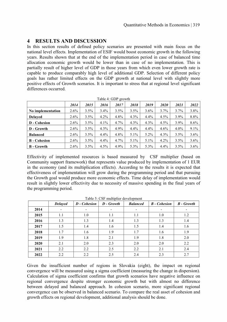
4 RESULTS AND DISCUSSION In this section results of defined policy scenarios are presented with main focus on the national level effects. Implementation of ESIF would boost economic growth in the following years. Results shown that at the end of the implementation period in case of balanced time allocation economic growth would be lower than in case of no implementation. This is partially result of higher level of GDP in those years from which even lower growth rate is capable to produce comparably high level of additional GDP. Selection of different policy goals has rather limited effects on the GDP growth at national level with slightly more positive effects of Growth scenarios. It is important to stress that at regional level significantdifferences occurred.

Table 4: GDP growth2014 2015 2016 2017 2018 2019 2020 2021 2022

No implementation 2.6% 3.5% 3.4% 3.5% 3.5% 3.6% 3.7% 3.7% 3.8%Delayed 2.6% 3.5% 4.2% 4.8% 4.3% 4.4% 4.5% 3.9% 8.8%D - Cohesion 2.6% 3.5% 4.1% 4.7% 4.3% 4.3% 4.5% 3.9% 8.6%D - Growth 2.6% 3.5% 4.3% 4.9% 4.4% 4.4% 4.6% 4.0% 9.1%Balanced 2.6% 3.5% 4.4% 4.8% 5.1% 5.2% 4.3% 3.5% 3.6%B - Cohesion 2.6% 3.5% 4.4% 4.7% 5.1% 5.1% 4.2% 3.5% 3.6%B - Growth 2.6% 3.5% 4.5% 4.9% 5.3% 5.3% 4.4% 3.5% 3.6%

Effectivity of implemented resources is based measured by CSF multiplier (based on Community support framework) that represents value produced by implementation of 1 EUR in the economy (and its multiplication effects). According to the results it is expected that effectiveness of implementation will grow during the programming period and that pursuing the Growth goal would produce more economic effects. Time delay of implementation would result in slightly lower effectivity due to necessity of massive spending in the final years of the programming period.

Table 5: CSF multiplier developmentDelayed D - Cohesion D - Growth Balanced B - Cohesion B - Growth

2014 - - - - - -2015 1.1 1.0 1.1 1.1 1.0 1.22016 1.3 1.3 1.4 1.3 1.3 1.42017 1.5 1.4 1.6 1.5 1.4 1.62018 1.7 1.6 1.9 1.7 1.6 1.92019 1.9 1.8 2.1 1.9 1.8 2.02020 2.1 2.0 2.3 2.0 2.0 2.22021 2.2 2.2 2.5 2.2 2.1 2.42022 2.2 2.2 2.5 2.4 2.3 2.7

Given the insufficient number of regions in Slovakia (eight), the impact on regional convergence will be measured using a sigma coefficient (measuring the change in dispersion).Calculation of sigma coefficient confirms that growth scenarios have negative influence on regional convergence despite stronger economic growth but with almost no difference between delayed and balanced approach. In cohesion scenario, more significant regional convergence can be observed in balanced scenario. To compare the real asset of cohesion and growth effects on regional development, additional analysis should be done.

Quantitative Methods in Economics | 319

Figure 1: Regional convergence measured by sigma coefficient

Implementation of ESIF resources would also create new job opportunities and this effect will start to be significant from year 2016. In the first two years impact of ESIF funds availability on employment was only marginal. Most significant impact would occur in last year of Delayed scenario, but sustainability of those jobs would be much lower compared to those created in Balanced scenario. Results of alternative policy scenarios are not presented due to only marginal changes on national level.

Figure 2: Employment generated by implementation

5 CONCLUSIONS This paper presents first application of regional HERMIN methodology for ex-ante assessment of EU funds implementations in Slovakia in 2014-20 period, thus results should be taken with vigilance. Implementation of ESIF resources has potential to generate additional GDP and jobs. During the process of data preparation it was revealed that regional allocations were significantly uneven. This was most evitable in case of Trnava region that had more significant share of resources available in both policy scenarios and was significantly underfunded in previous programing period. In the strongest regions, the low differences between cohesion and growth scenario suggest that they are operating far below regional absorption capacity of ESIF. In case of more balanced implementation over the programming period sustainability of created jobs would be higher as well as effectiveness of the used resources. This was confirmed by the development of the CSF multiplier at the end of the programming period. Alternative policy scenarios provided additional information on the impacts of different policy goals selection. According to the obtained results pursuing the Growth goal would lead to faster economic growth but on the other hand would lead to deepening of regional differences. During the crisis, regional model suggested to prefer cohesion scenario over growth one [10], but presented results indicates, that this is not the case in current conditions.

2,20%

2,30%

2,40%

2,50%

2,60%

2,70%

2,80%

2014 2015 2016 2017 2018 2019 2020 2021 2022

Delayed

D - Cohesion

D - Growth

Balanced

B - Cohesion

B - Growth

-

50,0

100,0

150,0

200,0

250,0

2016 2017 2018 2019 2020 2021 2022

Delayed

Balanced

320 | Multiple Criteria Decision Making XVIII

Additional research should be carried out in this field of research to fine tune certain characteristics of the model that currently seem not clear. Also, exploration of results on individual regions can reveal other growth and cohesion factors.

Acknowledgements: This work was supported by the Slovák Research and Development Agency under the contract No. APVV-14-0324.

References [1] Bradley, J., Herce, J. A. and Modesto, L. (1995). Modelling in the EU periphery – The

HERMIN project. Economic Modelling, 12(3), pp. 219–220. [2] CKO. (2014). Správa o stave implementácie európskych štrukturálnych a �����������!#

fondov [pdf] Bratislava: Úrad vlády Slovenskej republiky, Available at: https://lt.justice.gov.sk/Attachment/Vlastn%C3%BD%20materi%C3%A1l%20na%20MPK%20-%2010_9.pdf?instEID=-1&attEID=70265&docEID=389050&matEID=7651&langEID=1&tStamp=20140911110257310 [Accessed 2 Apr. 2016].

[3] �����, R., Baláž, V., Páleník, M., Páleník, V.,  ¡��¢£¢¤¡�, T., Hasprová, M., Rehák, Š., �¥¦§�§�¢, T., Borovský, P. and Velická, A. (2014). Ex ante hodnotenie. Partnerská dohoda Slovenskej republiky na roky 2014-$<$<@# \^��`���^# !|~�|�����# ��`^��� [pdf] Bratislava: Slovenská akadémia vied, p. 45 Available at: http://www.nsrr.sk/download.php?FNAME=1412071335.upl&ANAME=ExAnte+PD+SR+Zaverecna+sprava.docx [Accessed 3 Apr. 2016].

[4] Kvetan, V., Mlýnek, M. and Radvanský, M. (2006). Model HERMIN (The HERMIN model). Ekonomický ���|���, 54(10), pp. 994–1008.

[5] Mogila, Z. (2010). Effects of cohesion policy on social and economic disparities between Poland and Slovakia. In: Regional disparities in central and Eastern Europe. Bratislava: Institute of economic research SAS, pp. 98–115.

[6] ¨©ª¦¡«¢¬­ ¯° and �¤±§¡�¢¤�¬­ ²° (2015). Production (Non) Homogeneity across Slovak Regions. Politická ekonomie, (63) pp. 641–657.

[7] MVaRR SR. (2008). Národná stratégia regionálneho rozvoja. Bratislava.[8] Radvanský, M. and Frank, K. (2010). Modelling the Impact of Postponed Implementation

of EU Structural Funds - The Case of Slovakia. In: EcoMod2010. Istanbul Bilgi University. pp. 1-11.

[9] Radvanský, M. and Domonkos, T. (2010). Regional disparities under different types of cohesion policy case of Slovakia. In: EcoMod2010. Istanbul Bilgi University.

[10]Radvanský, M. (2014). Possibilities of Analysing the Impact of Cohesion Policy on Slovak Regions and Labour Market: Econometric Approach. Bratislava: Institute of Economic Research of the Slovak Academy of Sciences.

[11]Radvanský M., Frank, K., Lichner, I. and  ¡��¢£¢¤¡�¬­ ³° (2016). Impact of Cohesion Policy on Regional Development of Slovakia, Ex-post Assessment of NSRF 2007-13.Bratislava: Institute of Economic Research of the Slovak Academy of Sciences.

[12]Šikula, M. et al. (2006). Ex-����# !|~�|�����# �^`|~��!|# ��`��������!|# `���`�����!|#rámca SR°­²�¤¥¦¥�§�­©µ¦�¤±°­Bratislava: Ekonomický ústav SAV.

[13]Zaleski, J. (2009). Regionalization of HERMIN macro-economic modelling framework in Poland. Wroclaw Regional Development Agency Working paper. Wroclaw.

Author’s addressIng. Marek Radvanský, PhD.,  ¶¦°­³¢·�£­ ¡��¢£¢¤¡�¬­¸«¹°, Ing. Ivan Lichner, PhD. Institute of Economic Research, Slovak Academy of SciencesŠancová 56, 811 05 Bratislava Slovak Republic email: marek.radvansky@savba.sk, tomas.miklosovic@savba.sk, ivan.lichner@savba.sk

Quantitative Methods in Economics | 321

CLUSTER ANALYSIS OF EU AGRICULTURE

Marian Reiff, University of Economics, BratislavaKvetoslava Surmanová, University of Economics, Bratislava

Abstract The objective of this paper is to investigate the differences of agriculture performance across the EU countries in period 2010 to 2013. Ward clustering method is used to classify European agriculture based on variables Agricultural raw materials exports, Agricultural raw materials imports, Crop production index, Food production index, Livestock production index, Cereal yield, Agriculture value added and Agriculture value added per worker. Significant difference was revealed on characteristic Agriculture value added per worker.

Keywords: Cluster analysis, Economic performance, Agriculture

JEL Classification: C38, O13,AMS Classification: 91C20

1 INTRODUCTION The common agriculture policy is common policy for all European Union (EU) member states. It is run by EU and is also financed from its budget. For the last five decades it is the EU most important policy. It went through several reforms and together with liberalization of agriculture trade, the agricultural sector has been moved to market orientation and less protection [1]. Aim of this paper is comparison of economic results of agricultural sector of EU states in in period 2010 to 2013.

2 CLUSTER ANALYSIS

Cluster analysis is multivariate statistical technique that entails division of large group of observations into smaller and more homogeneous groups. In analysis of European Union agriculture we apply to cluster analysis to classify European Union member states according to different performance measured by variables as agricultural raw materials exports, agricultural raw materials imports, crop production index, food production index, livestock production index, cereal yield, agriculture value added and agriculture value added per worker. Source of the data is World data bank [4]. The data were averaged across a five year reference period (2010–2013) to mitigate specific effect in particular years, caused by fluctuations either in production due to for example bad weather conditions or in input, output prices on world markets. Summary statistics for five year reference period and twenty-eight European Union countries are listed in Table 1.

Our aim is to identify group of countries that are similar to each other but different from other groups of countries based on studied characteristics. We have selected minimizing variance criterion for determining which clusters are merged at successive steps. Minimizing variance inside of each cluster emphasizing inner homogeneity, which implies preference of Ward’s method. The method uses approach of analysis of variance to evaluate by squared Euclidean distances between clusters.

322 | Multiple Criteria Decision Making XVIII

Cluster membership is assigned based on calculation of the total sum of squared deviations from the mean of cluster. Two clusters are merged if it results smallest increase in overall sum of squared within-cluster distances. In order to determine the number of clusters, relatively large merging distances are considered. The process of Ward's method is an iterative process that is repeated until a desired number of clusters are achieved, or until each of all the clusters is formed into a single massive cluster.

The results of hierarchical clustering can be viewed through development tree or dendrogram. The root of the dendrogram represents the whole data set. The nodes within dendogram describe the extent to which the object relates. The results of the cluster analysis are adendrogram obtained by cross-section at different levels. More about Ward's method interested reader can find in [2], [3].

Cluster analysis was performed in Matlab by applying Ward’s method. Results of Ward’smethod are depicted by dendrogram on Fifure 1. Results are also described in detail and depicted on Table 2 and Figure 2.

Table 1: Summary statistics of selected variables for period 2010-2013 summarizing information from 28 EU states

Variables Mean Median Minimum MaximumStandard Deviation

Coefficient of Variation

Agricultural raw materials exports (% of merchandise

exports) 2,3154287 1,7453354 0,1057926 10,135018 2,0717155 0,8947438Agricultural raw materials imports (% of merchandise

imports) 1,5364174 1,4379083 0,3611562 3,0351713 0,5860896 0,3814651

Crop production index (2004-2006 = 100) 98,473929 96,3475 68,225 138,6475 15,045874 0,1527904

Food production index (2004-2006 = 100) 99,777143 100,22 83,7175 125,0025 10,38543 0,1040863

Livestock production index (2004-2006 = 100) 98,832768 98,55875 81,5725 115,9925 8,4859169 0,0858614Cereal yield (kg per

hectare) 5055,6359 4917,8609 1783,5415 9058,975 1745,7506 0,3453078Agriculture, value added

(annual % growth) 0,1919555 0,0723989 -6,4259817 7,9941255 3,7620404 19,598503

Agriculture, value added (% of GDP) 2,5875196 2,2775148 0,3149151 6,277538 1,4493857 0,5601448

Agriculture value added per worker (constant 2005 US$) 32232,272 25915,635 3158,2919 135039,16 28585,623 0,8868634

Quantitative Methods in Economics | 323

Figure 1: Dendrogram 2010-2013

Netherlands

Sw

eden

Cyprus

ItalyBelgiumD

enmark

Luxembourg

FinlandSloveniaFrance

SpainM

altaE

stoniaBulgariaG

reeceSlovak R

epublicLithuaniaR

omania

Germ

anyAustriaC

roatiaU

nited Kingdom

IrelandC

zech Republic

Latvia

Portugal

Hungary

Poland

Table 2 Description of Dendrogram 2010-2013 Analysis of clustering in the period 2010-2013 – Ward’s method Clusters Creation of the clusters from European Union countries Distance

form clusters

numberof countries

Z1 [:{[(Netherland, Sweden)+Cyprus]+Italy}+[(Belgium, Denmark)+Luxembourg]:]

0,05 7

Z2 {(Finland, Slovenia)+[(France, Spain)+Malta]} 0,08 5Cluster1 Z1 + Z2 0,15 12Z3 {(Estonia, Bulgaria)+[(Greece, Slovak Republic) +(Lithuania,

Romania)]}0,08 6

Z4 [(Germany, Austria)+(Croatia, United Kingdom)] 0,02 4Cluster 2 Z3 + Z4 0,19 10Cluster3 Z1 + Z2 + Z3 + Z4 0,52 22Z5 {[(Portugal, Hungary)+Latvia]+(Ireland, Czech Republic)} 0,28 5Z6 Poland 1Cluster4 Z5 + Z6 0,67 6Final Cluster Cluster 3 + Cluster 4 1,28 28

324 | Multiple Criteria Decision Making XVIII

Figure 2: Depiction of Cluster 1, Cluster 2 and cluster 4 on map of Europe.

To verify difference between clusters of evidence is appropriate to use methods that reveal these differences. To identify indicators that are of significantly different level in one cluster compared to another, Wilcoxon rank sum test procedure was used. Wilcoxon rank sum test was performed on Cluster tree and Cluster four. Cluster numbers are assigned in Table 2. From this analysis indicates that significant differences between clusters tree and four are caused by Agriculture value added per worker. The conclusions are based on p-values listed in Table 3, which were compared with the level of significance (α = 0.05).

Table 3: Results of Wilcoxon Rank Sum Test, Evidence of significant differences between cluster 3 and cluster 4 at level of significance α=0.05

Variables p-valueAgricultural raw materials exports (% of merchandise

exports) 0,6143294Agricultural raw materials imports (% of merchandise

imports) 0,6542153Crop production index

(2004-2006 = 100) 0,9108405Food production index

(2004-2006 = 100) 0,9553504Livestock production index

(2004-2006 = 100) 0,5379726Cereal yield (kg per

hectare) 0,4666991Agriculture, value added

(annual % growth) 0,4666991Agriculture, value added

(% of GDP) 0,4331284

Agriculture value added per worker ( 2005 US$) 0,0007812

Quantitative Methods in Economics | 325

Table 4: Summary statistics for variable "Agriculture value added per worker (constant 2005 US$)"

Mean MedianStandard Deviation Minimum Maximum

Cluster 3 38748,29 32844,19 28984,85 10259,49 135039,2Cluster 4 8340,201 8235,971 3495,445 3158,292 12976,06

Summery statistic for significantly different variable between clusters tree and four “Agriculture value added per worker” are listed in Table 4.

CONCLUSION Empirical cross country analysis of agriculture performance in European Union indicate significant difference exist within 28 EU countries in Agriculture value added per worker at the level of significance 0.05.

Acknowledgements: This work was supported by the Grant Agency of Slovak Republic -VEGA grant No. 1/0285/14 “Regional modelling of the economic growth of EU countries with concentration on spatial econometric methods“.

References [1] Giannakis, E. and Bruggeman, A. (2015). The highly variable economic performance of

European agriculture. Land Use Policy, 45(5), pp. 26 – 35. [2] Ivaničová, Z. and Kalužák, L. (2015). Dynamika vývoja krajín Eurozóny na základe

vybraných ukazovateľov. Ekonomické rozhľady, 44(4), pp. 476 – 492. [3] Ward, J. H. (1963). Hierarchical grouping to optimize an objective function. Journal of

American Statistical Association, 58(301), pp. 236 – 244. [4] World Bank, (2016). World Development Indicators. [online] Available at:

http://databank.worldbank.org/data/reports.aspx?source=world-development-indicators [Accessed 9 January, 2016].

Author’s addressIng. Marian Reiff, PhD. Ing. Kvetoslava Surmanová, PhD.University of Economics in Bratislava, Faculty of business informatics, Department of Operations research and Econometrics Dolnozemská 1/b, 852 35 BratislavaSlovak Republic email: marian.reiff@euba.sk, kvetoslava.surmanova@euba.sk

326 | Multiple Criteria Decision Making XVIII

HOUSE PRICES AND BUSINESS CYCLE IN CZECH ECONOMY: A CROSSCORRELATION APPROACH

Vlastimil Reichel, Masaryk University

Abstract This paper investigates a relationship between house prices and business cycles in the Czech economy. The aim is to find the leading indicator for monitoring business cycles. The methodology of leading indicator applied by the OECD is used to determine, whether the house prices are crucial in the business cycles. Moreover, the cross correlation approach identifies the relationship between quarterly house prices and the following individual variables: GDP, consumption, mortgage interest rate, employment, wages and number of newly started or finished buildings. The data set covers a period between 2004:Q1 and 2015:Q3. The results of the paper will help for later research and modelling of the housing sector in the Czech economy.

Keywords: house prices, business cycles, cross correlation approach

JEL Classification: E32 AMS Classification: 62P20

1 INTRODUCTION The housing sector is still a major topic of macroeconomic modelling. Recently, the housing sector has begun to play a significant role in the functioning of the Czech economy. The last decade has shown how uncontrolled price growth in the real estate market can lead to overheating of the economy with consequence of serious economic fluctuations which appear not only in one state, but also across countries and continents. A typical example is the American mortgage crisis. However, not only overseas countries struggled with growing house price. Increase was noticed in almost all economies of the former Eastern European block, where the mortgage market was just starting to develop. Some studies prove, thatcountries with developed housing sector are less prone to unexpected shocks then the less developed ones (see Cesa-Bianchi 2012 or Cesa-Bianchi, Cespedes and Rebuci 2015).However, not even a developed market has assurance of stable prices. Specific attention has been devoted to the behavior between housing sector variables and the variables of the rest of the economy. The example of the relationship between house market and real economy can be captured by the relationship between house price and consumption. Guerrieri and Iacoviello(2015) found an asymmetric link between house price and economic activity in USA data during housing boom and the subsequent recession. To determine the complicated relationships between variables they are divided into “lagging” and “leading” indicators. Alagging indicator is one that follows an event. In our cases the lagging indicators are those whose behavior of time series is observed after the similar behavior of house price time series. Leading indicators signal future events. In our cases the leading indicators are those whosebehavior of time series is observed before the similar behavior of house price time series. This paper is focused on finding the relationship between house prices and variables which describe the housing sector and the real economy.

Firstly, a maximum and minimum (first relevant global minimum after maximum) of housing price time series is identified and after that this peak is compared with a maximum and minimum (first relevant global minimum after maximum) of other time series. The peaks

Quantitative Methods in Economics | 327

analysis allows us to notice time shifts in the observed time series. Secondly, a more comprehensive analysis of the above relationships is demonstrated by the cross correlation approach. This study will be used as a basis for further investigation of the real estate market of the Czech economy.

2 DATA AND METHODOLOGY This research partly follows the OECD (2004) methodology of composite leading indicator for monitoring and predicting business cycles. The methodology can be written in several steps:

� data collection and their preparation; � the peak analyses; � a cross-correlation calculating.

2.1 Data The following variables were used in the research of housing sector influence on the business cycle: house price Ö�, output �, consumption �, mortgage interest rate :E, employment and wages (divided to three groups: total (�Ø, ÙØ), construction (�Ú, ÙÚ), real estate (�¤, Ù¤)) and number of newly started Û3 or finished buildings ÛÜ. The data were obtained from the Czech Statistical Office and the Czech National Bank and they cover the period from 2004:Q1 to 2015:Q3. The seasonally adjusted quarterly time series were all in logarithms, except for mortgage interest rate. Hodrick Prescott filter (with lambda=1600, see Hodrick and Prescott1981) is used to obtain the cyclical component of the variables.

2.2 The peak analysis The peak analysis is based on identifying the location of maximum and minimum value in each time series and their comparison relative to the selected variable. The following section presents (i) the house price maximum, (ii) first minimum of time series after this maximum and (iii) length of time period between maximum and minimum. Next, lagging or leading of maximum (and minimum) of other series relative to house price is mentioned and the length of difference between maximum and minimum peaks of each series is discussed.

2.3 The cross correlation approach The cross correlation approach is a method of estimating the degree to which two series are correlated. The theory and algorithm was adopted from Paul Bourke (1996). Consider two series �� and ~� where b = 0,1,2. . .  − 1. In our case �� is the vector of all variablesmentioned above and ~� is house price. The cross correlation �(�) at delay � is defined as

�(�) = ∑ [(G7CG7 )∗(ß7àáCßâ)]Ó∑ (G7CG7 )Ñ∗Ó∑ (ß7àáCßâ7 )Ñ,

where � and ~â are the sample means of the corresponding series. If the above is computed for all delays � = 0,1,2, . . . Â − 1 then it results in a cross correlation series of twice the length of the original series.

The range of delays � and thus the length of the cross correlation series can be less than N, for example the aim may be to test correlation at short delays only. The denominator in the expression above serves to normalise the correlation coefficients such that −1 ≤ �(�) ≤ 1,where the bounds indicate maximum correlation and 0 indicates no correlation. A high negative correlation indicates a high correlation but of the inverse of one of the series.

328 | Multiple Criteria Decision Making XVIII

3 RESULTS As it is mentioned above, the first analysis will deal with the comparing of the time series peaks. Table 1 compares the summary statistics for the time series data set. The columns &\�and &b. describe time when the time series show maximal and minimal peak, the äåæe and äçèé show lags of maximal peaks of other variables in comparison with house price,∆ëæeCëqì shows the delay between maximal and minimal values of each series.

Table 1: Time series description Var. Max äåæe Min äçèé ∆ëæeCëqì Var. Max äåæe Min äçèé ∆ëæeCëqì

Ö� 08:Q4 - 11:Q4 - 12 �Ø 08:Q4 0 11:Q4 0 12

� 08:Q2 -2 09:Q4 -8 6 �Ú 10:Q4 8 13:Q2 6 10

� 09:Q1 1 12:Q4 4 15 �¤í 09:Q1 1 10:Q1 -3 8

:E 09:Q4 4 11:Q4 0 8 HØ 07:Q4 -4 09:Q1 -11 5

Û3 08:Q2 -2 09:Q4 -8 6 HÚ 07:Q4 -4 08:Q4 -12 4

ÛÜ 07:Q4 -4 10:Q4 -4 12 H¤í 08:Q1 -3 10:Q2 -2 13

Source: Authors calculations

Table 1 presents leading variables �, :E, �Ú and �¤í as well as lagging variables �, Û3, ÛÜ,HØ, HÚ, H¤í. It can be observed that wages were already behind their upper limit and decreased at the time when real estate price reached maximum. In contrast, for example mortgage interest rate and number of employees in construction have been just waiting for reaching its peak. Similarly, the differences in the minimum peak can be commented too. It is also interesting that in the maximums of times series there is no large delay or overrunning like in minimums.

Another informative characteristic is a time difference between maximum and minimum (in quarters). The differences between maximum and minimum ∆ëæeCëqì are quite long in employment and short in wages (except real estate wages). This can be considered as anevidence of rigidities in the labour market. The firms cannot reduce the number of employeesin short time, but they can decrease their wages. The next interesting results are for variables Û3 and ÛÜ. Initiation of new houses reacts very fast, on the contrary the reaction of completion of new houses is relatively slow. Interpretation can be as follows: If the interest in new housing falls because of a crisis, then the construction companies, which cannot decrease the number of employees, transfer these employees to existing contracts. For this reason the decline of Û3 can be faster than the decline of ÛÜ. In the Table 1 it is possible toobserve a very long time reaction for consumption indicator. In the short run, households are unwilling to substantially decrease their consumption, therefore the adjustment is slow. The calculations demonstrate that it takes almost four years (15 quarters) for the households to reduce their consumption from maximum to minimum.

Table 2 shows the cross correlation values of house price with the gaps of the examined time series. The statistically significant values are shown in bold and the highest correlation values are underlined. The results, as shown in Table 2, indicate positive correlation between house price and all the other variables in time t, but only finished houses variable has the significant and highest value in this time. The remaining variables show the highest (or lowest)

Quantitative Methods in Economics | 329

correlation as delayed or leading. Interestingly, each of highest correlation is positive. For this reason, it can be argued that each time series is cyclical with the house price. The result shows that variables after year 2004 behave pro-cyclically.

Table 2: Cross correlation between house price and the other variable Variable t-5 t-4 t-3 t-2 t-1 t t+1 t+2 t+3 t+4 t+5

� 0,59 0,63 0,66 0,68 0,64 0,53 0,40 0,31 0,25 0,22 0,16� 0,22 0,30 0,40 0,50 0,60 0,67 0,70 0,74 0,78 0,80 0,75

:E 0,03 0,25 0,45 0,61 0,74 0,83 0,88 0,90 0,87 0,80 0,70�Ø 0,61 0,69 0,77 0,86 0,90 0,87 0,78 0,66 0,50 0,32 0,12�Ú -0,25 -0,25 -0,20 -0,13 0,02 0,21 0,37 0,52 0,65 0,77 0,85�¤í 0,42 0,42 0,44 0,51 0,55 0,53 0,52 0,54 0,57 0,55 0,53HØ 0,62 0,67 0,69 0,68 0,59 0,40 0,18 -0,04 -0,26 -0,41 -0,48HÚ 0,59 0,67 0,72 0,76 0,72 0,58 0,42 0,29 0,19 0,12 0,04H¤í 0,16 0,27 0,38 0,46 0,46 0,44 0,43 0,43 0,44 0,39 0,31Û3 0,63 0,70 0,73 0,72 0,71 0,68 0,63 0,58 0,46 0,32 0,20ÛÜ 0,31 0,46 0,58 0,67 0,72 0,73 0,70 0,64 0,56 0,50 0,43

Source: Authors calculations

Looking at some of the values of cross correlation coefficients, it is clear that findings presented in this paper are similar to the results of the other authors. For example, there exists a pro-cyclical relation between real estate price and mortgage interest rate as shown inIacoviello (2000) or Tsatsaronis and Zhu (2004); or between house price and consumption as shown in Hloušek (2012). In comparison with Brůha and Polanský (2014), who tested cross correlation on Czech economy time series covering the period 2001Q1-2012Q4, slightly different results can be observed. For example, they show correlation between flat prices and consumption as negative and negligible. The results of the correlational analysis obtained from research presented in this place show positive and statistically significant value. It can be seen as an evidence of a relatively strong comovement after year 2005. While focusing onshifts between time series it can be observed that the shifts are similar to shifts presented in Table 1. For this reason information about the lagging and leading indicators are verified.

4 CONCLUSION This paper analyses the housing sector and its influence on business cycles in the Czech economy. According to the previous researches and available data, the methodology for finding leading and lagging indicators is chosen. The results show that the maximum value of each series is close in leads (or lags) compared to the maximum of house price series. On the other hand, the minimum of each series is far in leads (or lags) compared to the minimum of house price series. This result confirms the idea of pro-cyclical relationship in the boom. The cross correlation coefficients calculated in this paper confirmed a pro-cyclical behaviour in Czech economy after year 2005. This paper also identifies which of the variables are lagging and leading indicators. The results can be used as preliminary for the next research and modelling of the housing sector in the Czech economy.

Acknowledgements: This paper was created as a part of the specific research project no. MUNI/A/1049/2015 at Masaryk University.

330 | Multiple Criteria Decision Making XVIII

References [1] Bourke, P. (1996). Cross Correlation. [online] Available at:

http://paulbourke.net/miscellaneous/correlate/ [Accessed 15 Jan. 2016]. [2] Brůha, J. and Polanský, J. (2014). The housing sector over business cycles: Empirical

analysis and DSGE modelling. Czech National Bank, Research Department. Working paper.

[3] Cesa-Bianchi, A. (2012). Housing cycles and macroeconomic fluctuations: a global perspective. Inter-American Development Bank, Research department publications 4810.

[4] Cesa-Bianchi, A., Cespedes, F. and Rebussi, A. (2015). Global liquidity, house prices and the macroeconomy: evidence from advanced and emerging economies. Journal of Money, Credit and Banking, 47(S1), pp. 301-335

[5] Guerrieri, L. and Iacoviello, M. (2015). Collateral constraints and macroeconomic asymmetries. Available at SSRN 2648869

[6] Hloušek, M. (2012). DSGE model with collateral constraint: estimation on Czech data. In: Proceedings of 30th International Conference Mathematical Methods in Economics.(Ramík, J. and Stavárek, D.) Karviná: Silesian University: School of Business Administration.

[7] Hodrick, R. and Prescott, E. (1997). Post-war U.S. business cycles: an empirical investigation. Journal of Money, credit, and Banking, pp. 1-16.

[8] Iacoviello, M. (2002). House price and the business cycle in Europe: a VAR analysis. Boston College Working Papers in Economics, 540, pp. 1-43.

[9] OECD (2004). The OECD–JRC Handbook on Practices for Developing Composite Indicators. Paris: OECD Committee on Statistics.

[10]Tsatsaronis, K. and Zhu, H. (2004). What drives housing price dynamics: cross-country evidence. BIS Quarterly Review, March.

Author’s addressIng. Mgr. Vlastimil Reichel Masaryk University Lipová 507/41a602 00, Brno Czech Republic email: reichel.v@mail.muni.cz

Quantitative Methods in Economics | 331

UNEMPLOYMENT FLOWS AND VACANCIES IN SLOVAKIA

Eva Rublíková, University of Economics, BratislavaZlatica Ivaničová, University of Economics, Bratislava

Abstract

In this paper we present analysis of unemployment problem in Slovakia. We will analyse the unemployment flows and the relationship between registered unemployment and vacancies in monthly data, staring in January 2001 to December 2015. The aim is to look for regression model of outflow rates (as a proxy of the probability of leaving unemployment pool) and vacancy ratio. In addition we will discuss time series method of short-term forecasting for outflow rates and vacancy ratios.

Keywords: Unemployment, Vacancies, Inflow, Outflow, Regression model, ARIMA model

JEL Classification: C22 J64

1. INTRODUCTION

The labor market is very dynamic system within economically active and non – active persons who flows from one state to the other one. We are intersting in the monthly aggregate flows of registered unemployed workers to the employment (the outflows from employment into unemployement), and the monthly aggregate flows of employed to unemployment (the inflows from employment into unemployment) in Slovakia during the years 2001 to 2015.Both these flows influence the monthly aggregate unemployment which depend also on the monthly registered job vacancies offered by the firms. The relationship between unemployment and job vacancies is known as the Beveridge Curve which provides an indication of how effectively unemployed workers are matched with opportunities for employment. Beveridge curve is some form of the efficiency of the labour market. There are many interesting works how to explain the Beveridge curve in Spain (Antolin, P. 2005), in Australia (Fahrer, J., Pease, A. 1993), in Czech Republic (Galuscak, K., Munich, D. 2007), in Slovakia (Burda, M. C., Lubyova, M. 1995) which are much comprehensive as we think to present now. Our submission is based on ideas of mentioned authors and on the book of Lyard, R,. Nickell, S., Jackman, R., 1992) which are simplified to the time series analysis of looking for some dynamic regression model which could explain the basic relationship between unemployment rate and vacancy ratio, given outflow rates and inflow rates. In addition we are looking for short–term forecasts of outflow rate and vacancy rate by menas of SARIMA model.

2. DATA ANALYSIS

The data used in the analysis are taken from the database of Slovak Ministry of Social Affairs and family of Slovak Republic. They are monthly data about registered unemployment given as the number of job applicants registered in the offices of labor (U), vacancies (V), outflows from unemployment to employment (O) and inflow from employment to unemployment (I).

332 | Multiple Criteria Decision Making XVIII

We are working with percentage data rather than absolute data. The rates are defined as: Unemployment rate = Unemployment /Labor Force = U/LF = UR; Inflow rate = Inflow/LF= I/LF = IR), Outflow rate = Outflow/Unemployment = O/U = OR. On the assumption of the steady state in economy i tis possible to calculate the “average duration of unemployment” as the ratio (U/Inflow = average duration = AD in months) which explains expected „average time“ for which those who enter unemployment remain there. Our data are monthly time series data starting on January 2001 to December 2015 with seasonality, but we are working with seasonnly adjusted data.

Figure 1 shows the development of unemployment rate and vacancy rate seasonally adjusted over the period 1/2001-12/2015. It provides a closer look at the labor market in which the business cycle is reflected.

Figure 1 Unemployment, Vacancies in Slovakia, 1/2001-12/2015

t

VariablesUR (%)VR (%)

0 30 60 90 120 150 1808

11

14

17

20

23

0

2

4

6

8

10

12

Note: Seasonally adjusted data on unemployment rate and vacancy rate Left axis: Unemployment rate (%), Right axis: Vacancy Rate (%)

Analysing data we can say, that the rate of unemploymnet reach the value about 8 % in 2008 and from this year its values were increasing gradually due to the economic crisis to 15,4 % in the year 2013. From the year 2013 the rate of unemployment is decreasing and the vacancy rate is increasing. Especially during the year 2015 firms proposed more job vacancies (nearly three times more) than in the previous year. Closer look to the development of flows rates in registered unemployment during the analysed pariod is given on Figure 2.

Figure 2 Unemployment flows in Slovakia, 1/2001-12/2015

t

VariablesOutflow raInflow rate

0 30 60 90 120 150 1804,7

6,7

8,7

10,7

12,7

0,5

0,8

1,1

1,4

1,7

2

Note: Seasonally adjusted data on outflow rate and inflow rate Left axis: Outflow rate (%), Right axis: Inflow rate (%)

Quantitative Methods in Economics | 333

A popular way to ilustrate changes in the economy using the labor market data is the Beveridge curve describing the relationship between the unemployment rate and the rate of vacancy. From the Beveridge curve we can find out, that during the periods of increasing demand and increasing vacancies the unemployment is decrreasing, but during the recession the opposite is true. On the other hand simultaneous increases in the rates of unemployment and vacancy are due to rising mismach in the labor market. The Slovak Beveridge curve is depicted on Figure 3.

Figure 3 The Slovak Beveridge Curve, 1/2001-12/2015

Unemployment rate (%)

Vaca

ncy r

ate (%

)

8 11 14 17 20 230

2

4

6

8

10

12

Note: Seasonally adjusted monthly data Source: Ministry of Labor Social Affairs and Family SR

During 2008, the Slovak economy was hiting by a recession that lasted until 2013. In the last two years firms used to offer more job vacancies and the rate of unemployment started to decrease. This situation could be explain by an effort of gowerment to decrease the rate of unemployment by various legislative intents.

2. REGRESSION MODEL OF OUTFLOW and INFLOW RATE In our presentation we are looking for simplified dynamic regression model to describe how unemployment changes over time and how much it is due to changes in flows and how much to duration. In Slovakia these changes are depicted on Figure 4.

Figure 4 Inflow rates and duration of unemployment in Slovakia, 1/2001-12/2015

t

VariablesAvDur.Infl.R

0 30 60 90 120 150 1800

5

10

15

20

25

5

8

11

14

17

20(X 0,001)

Note: Seasonally adjusted data on average duration of unemployment and inflow rate Left axis: Average Duration (months), Right axis: Inflow rate (%)

334 | Multiple Criteria Decision Making XVIII

The „average duration“ of unemployment started to increas from the year 2008, mostly because of high long-term unmeployment. In the year 2008 the rate of long-term unemployed persons (which are unemployed more than two years) to the stock of the uenmployed, was about 48.68 % . From that year till 2015 the rates varies from 40 % to 51 %. Although we know about this problem we start to estimate the dynamic regression model of outflow rate relationship to the vacancy rate given by the simple hiring function mentioned in {3}, without calculating variable of „average effictiveness“ of unemployed, because we assume its very law value.

To see the development of both variables over the period 1/2001-12/2015 we have used the seasonally adjusted data which are depicted on Figure 5. Both variables are nonstationary so instead of taking the first differences of variables, we add the time variable to the model of the form 0 1 3log( ) (log( )t t tOR VR t; ; ; �� � � � (1) The long-run relationship (1) is estimated by the least squared method with dummy variable for April 2009. Parameter of vacancy ratio is statistically significant at 10 %.

1286719.000532.0)log(0433476.0349859.0)log( DtVROR tt ����Coefficient of determination is 60 % and residuals are autocorrelated with coefficinet of autocorrelation 76.0)ˆ(1 ��tr � close to one, so residuals are nonstationary following random walk. The long-run elasticity with respect to vacancy ratio is very law, but we have an important additional explanation of the fall in outflow rate coming from the growth of long-term unemployment.

Figure 5 Outflow rate and Vacancy rate in Slovakia, 1/2001-12/2015

t

VariablesOutfl.RVac.R

0 30 60 90 120 150 1800,6

0,8

1

1,2

1,4

1,6

1,8

0

2

4

6

8

10

12

Note: Seasonally adjusted data on outflow rate and vacancy rate Left axis: Outflow rate (%), Right axis: Vacancy rate (%)

We tried to find out some dynamics in the model for outflow rate and we have been successfull to add vacancy ratio and unemployment rate with lag 1 in the form 0 1 1 2 1 3log( ) log( ) log( )t t t tOR VR UR t; ; ; ; �� �� � � � � (2) Estimation of the model (2)

1 1log( ) 0.5105 0.018489log( ) 0.000464log( ) 0.00201t t tOR VR UR t� �� � � � �All parameters of the estimated model (2) are statistically significant at any level of significance (P-values are zero), coefficient of determination is about 68 % and coefficient of autocorrelation of residuals is almost the same as in the previous case 1 ˆ( ) 0.72tr � � .In both models we assume that the unemployed are good proxy for all job seekers.

Quantitative Methods in Economics | 335

So far we have concentrated on the outflow rates (as a proxy of aggregate probability to be re-employed) but to understand the general equlibrium of the labor market in Slovakia, we need also to look at inflow rate (as a proxy of aggregate probability to be unemployed).

To analyse time–series behaviour of the inflow rate more formally, we have estimated the regression model of the form

0 1 2 1 3log( ) log( ) log( )T t t tIR VR IR t; ; ; ; ��� � � � � (3) tIRVRIR ttT 00031.0)log(88927.0)log(0051.088.0)log( 1 ����� �

The estimation of the model gives coefficient of determination 98 %, but the variable vacancy rate was insignificant. This equation suggests that the level of economic activity has no long-run effect on inflow rate and provides only very weak evidence of a negative time trend and the positive relationship on previous valuse of inflow rate. Also residuals of this model are autocorrelated with 1 ˆ( ) 0,60tr � �

Both regression models for outflow and inflow rates were estimated with autocorrelated residuals. The reason ot that is in the simplicity of the models to which other variables were not included. The reason is hidden in the database of monthly time series and lack of data like the wages or GDP of the same frequency.

3. FORECASTING MODEL ON OUTFLOW RATE AND VACANCY RATE

As we could see from Figure 5, outflow rate and vacancy rate are nonstationary. We have found out also, that although both series were seasonally adjusted by the seasonal decomposition, stochastic seasonality still remain in outflow rate series. It was proved by the analysis of autocorrealation and partial autocorrelation function for outflow rate variable. For forecasting purpose to construct monthly forecasts of aggregate probability to be re-employed (or outflow rate) during the year 2016 the SARIMA(0,1,0)(0,1,1)12 has been estimated in the following form:

tt aBsadjORBB )1()log()1)(1( 1212,1

12 G����

tt aBsadjORBB )775.01()log()1)(1( 1212 �����The seasonal parameter was statisticaly significant (its P-value = 0,0000). The residuals are noncorrelated and their mean measures are MAE = 0,644 p.p and MAPE = 7,5 %. Forecasts of outflow rate for the year 2016 varies about 10 % for the first half of the year and about 9 % to 10 % for the second half.

For vacancy rate (or aggregate probability that unemployed person could find job vacancy) the model SARIMA(2,1,0)(0,0,0)12 has been estimated in the form:

tt aBsadjVRB ��� )1)(log()1( 22H

tt aBsadjVRB ��� )0000074.01)(log()1( 2

The second autoregression parameter is statistically significant at 5 % (its P-value = 0,040561) and its negative value has confirmed the presence of the cycle in data. Residuals are noncorrelated and their mean measures are MAE = 0.325 p.p. and MAPE = 8.24 %. Monthly forecasts of vacancy rate varies about 9.6 % during the year 2016.

336 | Multiple Criteria Decision Making XVIII

CONCLUSION

In our presentation we have been interested how to explain the development of outflow rate as the proxy of aggregate probability to be re-employed through the relationship on vacancy rate by means of time-series analysis. We have showed that relationship exists but it is of very law intensity. The autocorrelation of residuals signalized that the deeper econometric analysis has to be exhibited. Forecasts for outflow rate for the year 2016 given by SARIMA model suggest that there is about 10 % of unemployed who could find the job- to be re-employed.

Acknowledgements: The paper was done under support of the project VEGA č.1 /0285/14 Regional modelling of the economic growth of EU countries with concetracion on spatial econometric methods.

References

[1] Antolín, P. (1994). Unemployment flows and vacancies in Spain. Instituto Valenciano de Investigaciones Economicas. WP-EC-94-05.

[2] Burda, M.C. and Lubyova, M. (1995). The Impact of Active Labour Market Policies: A Closer look at the Czech and Slovak Republics. Centre for Economic Policy Research, Discussion Papers Series No. 1102. London.

[3] Fahrer, J. and Pease, A. (1993). The Unemployment/vacancy relationships in Australia. In. Research Discussion Papers, No 9305, Reserve Bank of Australia.

[4] Galuščák, K. and Munich, D. (2007). Structural and cyclical unemployment: What can be derived from matching function? Finance a úvěr - Czech Journal of Economics and Finance, 57(3-4), pp. 102-125.

[5] Layard, R., Nickell, S. and Jackman, R. (1991). Unemployment. Macroeconomic performance and the labour market. Oxford: Oxford University Press.

[6] Mills, T. C. (1990). Time series techniques for economists. New York: Cambridge University Press.

Author’s addressprof. RNDr. Eva Rublíková, PhD.University of Economics in Bratislava, Faculty of business informatics, Department of Statistics Dolnozemská 1/b, 852 35 Bratislava Slovak Republic email: rublik@euba.sk

prof. Ing. Zlatica Ivaničová, PhD.University of Economics in Bratislava, Faculty of business informatics, Department of Operational Research and Econometrics Dolnozemská 1/b, 852 35 BratislavaSlovak Republic email: zivanicova@euba.sk

Quantitative Methods in Economics | 337

THE ADVANTAGES OF USING GOAL PROGRAMMING FOR TIMETABLING

Veronika Skočdopolová, University of Economics, Prague

Abstract Goal programming is a technique for solving not only multi-criteria decision making problems. This technique became very popular since it was formulated 60 years ago. Timetabling is a widespread problem that every university deals with. There are many approaches how to cope with this problem. In this paper a goal programming model for a timetable construction at the University of Economics, Prague is briefly introduced. Then the main advantages of using goal programming in this model are presented.

Keywords: goal programming, timetabling, multi stage penalisation function

JEL Classification: C61 AMS Classification: 90C29

1 INTRDUCTION There are many ways how to construct a university timetable. From the time-tested scheduling board, over various heuristic and metaheuristic methods to sophisticated optimisation models. In this paper using goal programming model and its advantages for university timetabling is presented.

2 GOAL PROGRAMMING Goal programming is a widely used approach for solving not only multi-objective decision problems. It is both a modification and extension of linear programming. Goal programming was first formulated in 1955 [7] but named a few years later in 1961 [8]. It became a widely used multi-criteria decision making technique soon due to relatively simple way of its formulation. The generic goal programming model can be formulated as follows [12]: Minimise

),( ��� ddfz (1)subject to

X�x , (2)kkkk gddf ��� ��)(x , k = 1, 2, …, K, (3)

0, 4��kk dd , k = 1, 2, …, K,

where (1) is a general penalisation function of vectors of positive and negative deviations d–

and d+, X is the set of feasible solution satisfying all of the constraints including non-negativity constraints (2), fk(x) is an objective function that represents the k-th criterion, gk is the k-th goal, the decision maker wants to meet, �

kd is negative deviation from the k-th goal, which represents the underachievement of the k-th goal, �

kd is positive deviation from the k-th goal, which shows the overachievement of the k-th goal; and (3) are the goal constraints. The goal constraints are often titled soft constraints, while the constraints that form the set of feasible solution can be called hard constraints.

338 | Multiple Criteria Decision Making XVIII

0 �1kh Positive

deviation

Penalisation

Negative deviation

1 1k kv h�

It happens in practice that certain small deviation from the goal is acceptable with just a little penalisation and greater deviation is allowed but with higher penalisation. To preserve the linear form of the model we can use the multistage penalisation function. In this case we have to change the goal constraints (3) to the following one

kkkkk gdddf ���� ���21)(x , k = 1, 2, …, K,

0,0,0 2211 40000 �����kkkkk dhdhd , k = 1, 2, …, K,

where �1kd is the 1st stage positive deviation that is non-negative and has upper bound �

1kh , and �2kd is the 2nd stage positive deviation that is also non-negative with upper bound �

2kh . The two-stage penalisation function can be formulated as follows [13]:

� ���

��� ���K

kkkkkkk dvdvduz

12211 ,

where vk1 and vk2 are penalty constants of the 1st an 2nd stage positive deviation and uk is penalty constant of the negative deviation. The graphical representation of the two-stage penalisation function can be as in the Figure 1.

3 TIMETABLING There are many different ways how to create a timetable. We can use various metaheuristic methods such as evolutionary algorithms (e.g. genetic [11] or memetic [15]), algorithms based on graph colouring (e.g. [1] or [5]), local and tabu search (e.g. [6] or [16]) or simulated annealing (e.g. [9]). If we focus on optimisation based models, there are two main approaches. The first of them consists of decomposition of the problem into several related stages (e.g. [2], [4], or [14]). The other approach is based on creating one complex model (e.g. [3] or [10]).

Figure 1 Two-stage penalisation function

Quantitative Methods in Economics | 339

4 THE ADVANTAGES OF USING GOAL PROGRAMMING FOR TIMETABLING

We have described in detail a complex goal programming model for timetabling in [18]. This model contains both hard and soft constraints. The hard constraints assure that the created model will be feasible. The most important hard constraints ensure that:

� every teacher is able to teach at most one course in a particular time; � every course is assigned to a teacher, time and classroom; � there can be at most one course in a classroom in a particular time.

These are the basic features of every school timetable. Other hard constraints are connected with teacher’s preferences – teachers must not teach a course they rated with zero preference. Another group of hard constraints assures correct assignment of computer classrooms. These constraints are thoroughly described in [17]. The problem of two distant campuses, where the teaching takes place, is also solved with hard constraints. Most of the soft constraints assure maximization of teacher’s preferences. In the model [18]there are four different types of teacher’s preferences – preferences of courses taught, preferences of time windows, preference of number of days per week that the teacher should teach, and maximal number of courses per day that the teacher should teach. Also the utilisation of classrooms capacities is ensured with soft constraints. The optimisation criterion is minimisation of the two-stage penalisation function that sum only the unwanted deviations from the goals.Using a goal programming model for timetabling brings many advantages. The first of them is the possibility of using the soft constraints. As an example of the benefit of the soft constraints can serve the constraint for maximal number of courses per day. Each teacher set a goal value, the maximal number of courses per day. If it is possible, the teacher will teach at most the set maximal number. On the other hand if it is impossible, the solution is still there. When we use a hard constraint in this case, it can lead to an infeasible solution. Another plus of goal programming is including several different criteria in one model. This means that we can simultaneously maximise different types of teachers’ preferences and minimise unused capacities of the classrooms (or maximise the utilization of the classrooms). Additional pro in this model is the two-stage penalisation function. In the constraint assuring the utilisation of classrooms there are two levels of negative deviation. The first level allows to assign a course to a larger classroom than the course needs (capacity of the course must be at least 50 % of the classroom capacity). This deviation has just a small penalisation. If necessary the course can be placed to a larger classroom, but with a higher penalisation. There is also a positive deviation in this constraint that allows exceeding of the classroom capacity up to 10 %. It is assumed, that not all of the registered students will attend the course. Exceeding of the classroom capacity for more than 10 % is not allowed. The penalization function cover all three allowed deviations. Another advantage of using goal programming for timetabling is the simplicity of formulation of the goal programme and good understanding its methodology by decision makers.Therefore is the methodology quite acceptable for the teachers that do not know mathematical modelling.

5 CONCLUSION In this paper we sum up and explain the main advantages of using goal programming for timetabling. On the other hand, with the advantages, there are also disadvantages. The key disadvantage of goal programming is that the decision maker has to set the goals in advance. On the contrary the goals used in the described model are mostly based on teachers’ preferences. Another con can be that goal programming in general does not provide

340 | Multiple Criteria Decision Making XVIII

undominated solutions. Nevertheless while solving the timetabling problem we usually need a satisfactory solution. Such a solution can be easily obtained even with goal programming.

Acknowledgements: The research is supported by the Internal Grant Agency of the University of Economics, Prague (grant no. F4/62/2015) and by institutional support for long-term conceptual development of science and research at the Faculty of Informatics and Statistics, University of Economics, Prague.

References [1] Abdul-Rahman, S., Burke, E. K., Bargiela, A., McCollum, B. and Özcan, E. (2014) A

constructive approach to examination timetabling based on adaptive decomposition and ordering. Annals of Operations Research, 218(1), pp. 3–21.

[2] Al-Husain, R., Hasan, M. K. and Al-Qaheri, H. (2011) A Sequential Three-Stage Integer Goal Programming (IGP) Model for Faculty-Course-Time-Classroom Assignments. Informatica, 35(2), pp. 157–164.

[3] Asratian, A. S. and Werra, D. (2002) A generalized class teacher model for some timetabling problems. European Journal of Operational Research, 143(3), pp. 531–542.

[4] Badri, M. A. (1996). A two-stage multiobjective scheduling model for [faculty-course-time] assignments. European Journal of Operational Research, 94(1), pp. 16–28.

[5] Burke, E. K., Pham, N., Qu, R. and Yellen, J. (2012). Linear combinations of heuristics for examination timetabling. Annals of Operations Research, 194(1), pp. 89–109.

[6] Caramia, M., Dell'Olmo, P. and Italiano, G. F. (2008) Novel Local-Search-Based Approaches to University Examination Timetabling. INFORMS Journal on Computing,20(1), pp. 86–99.

[7] Charnes, A., Cooper, W. W. and Ferguson, R. (1955) Optimal estimation of executive compensation by linear programming. Management Science, 1(2), pp. 138–151.

[8] Charnes, A. and Cooper, W. W. (1961) Management Models and Industrial Applications of Linear Programming, New York: John Wiley & Sons.

[9] Gunawan, A., Ng, K. M. and Poh, K. L. (2012). A hybridized Lagrangian relaxation and simulated annealing method for the course timetabling problem. Computers and Operations Research, 39(12), pp. 3074–3088.

[10]Ismayilova, N. A., Sagir, M. and Rafail, N. (2005). A multiobjective faculty–course–time slot assignment problem with preferences. Mathematical and Computer Modelling, 46(7), pp. 1017–1029.

[11]Jat, S. N. and Yang, S. (2011). A hybrid genetic algorithm and tabu search approach for post enrolment course timetabling. Journal of Scheduling, 14(6), pp. 617–637.

[12]Jones, D. F. and Tamiz, M. (2010). Practical Goal Programming. International Series in Operations Research & Management Science 141. New York: Springer.

[13]Mínguez, M. I., Romero, C. and Domingo, J. (1988). Determining Optimum Fertilizer Combinations through Goal Programming with Penalty Functions: An Application to Sugar Beet Production in Spain. The Journal of the Operational Research Society, 39(1), pp. 61–70.

[14]Ozdemir, M. S. and Gasimov, R. N. (2004). The analytic hierarchy process and multiobjective 0–1 faculty course assignment. European Journal of Operational Research 157(2), pp. 398–408.

[15]Qaurooni, D. (2011). A memetic algorithm for course timetabling. In: GECCO '11: Proceedings of the 13th annual conference on Genetic and evolutionary computation.Dublin, pp. 435–442.

Quantitative Methods in Economics | 341

[16]Santos, H. G., Ochi, L. S. and Souza, M. J. F. (2005). A Tabu search heuristic with efficient diversification strategies for the class/teacher timetabling problem. Journal of Experimental Algorithmics, 10 pp. 1–16.

[17]Skočdopolová, V. (2014). University Timetabling: some Special Constraints. In: Quantitative Methods in Economics (Multiple Criteria Decision Making XVII).EKONÓM, Bratislava, pp. 245–248.

[18]Skočdopolová, V. (2015). Optimisation of University Timetable via Complex Goal Programming Model. In: Mathematical Methods in Economics 2015. University of West Bohemia, Plzeň, pp. 725–730.

Author’s addressIng. Veronika Skočdopolová, PhD. University of Economics, Prague, Faculty of Informatics and Statistics, Department of Econometrics W. Churchill sq. 4, 130 67 Prague Czech Republic email: skov01@vse.cz

342 | Multiple Criteria Decision Making XVIII

A BONUS-MALUS SYSTEM BASED ON DEDUCTIBLES

Radek Stolín, College of Polytechnics Jihlava

Abstract The bonus-malus systems presently used in automobile insurance suffer from a few considerable disadvantages. One of them lies in the fact that the level of premium depends on the number of claims but is independent of the amounts of these claims. In this paper it is suggested how both the number of claims and partially their amounts as well could be taken into consideration.

Keywords: bonus-malus system, deductibles, Markov chains, transition matrix

JEL Classification: C44 AMS Classification: 90C15

1 INTRODUCTION In the traditional bonus-malus systems (BMS) that are now in force in many developed countries, including the Czech and Slovak Republic, the level of premium is based only on the number of claims caused by the policyholder during the latest policy year. It is well known that that fact leads to an undesirable phenomenon, the so called hunger for bonus.Policyholders bear the small claims themselves, in order to avoid losing their position in BMS, and thus increasing their future premium. This contributes to gradual clustering of the policies in the high-bonus classes, and there is no significant premium differentiation between bad and good drivers. This goes against the main objective of introducing BMS, which has been and still is to achieve better assessment of the individual risks.

The suggestion to eliminate the aforementioned BMS drawback by a high deductible system appeared as early as at the end of the past century (see Holtan, 1994). According to thatalternative system the premium would cover only part of the losses in excess of a high deductible. The deductible would be the same for all policyholders in a portfolio, and thus independent of the class they occupied in the BMS at the claim occurrence time. If a policyholder could not afford to pay such high amount, there would be the possibility of ashort-term loan provided by the insurance company. Lemaire and Hongmin (1994) concluded that the Holtan’s high deductible system has one very important disadvantage compared to the traditional BMS, which is higher variability of payments for all policyholders, preventing the application of the high deductible system in practice. The additional procedure of borrowing money is certainly another substantial technical complication.

However, the idea of taking the amounts of claims into consideration by introducing some form of deductible into the classical BMS is ingenious and might lead towards the elimination of the main drawback of BMS. No wonder that this idea has been cultivated by the follow-up research. For example, paper by Pitrebois, Walhin and Denuit (2005) addresses the very interesting possibility of introducing varying deductibles to the policyholders placed in themalus classes of BMS instead of premium surcharges.

This paper presents a BMS fully based on deductibles. The system deals with the same premium level for all policyholders. Positioning in different classes of the BMS determines the amount of deductible per each claim. In other words, the premium discount is replaced by

Quantitative Methods in Economics | 343

lower deductible and vice versa. Moreover, if the deductible covers an entire claim, the claim does not count and has no effect on the ranking in the BMS.

The paper is organised as follows. Firstly the classical BMS and its construction are briefly recalled. The next parts describe the prevailing modelling of the number of claims and claim severity, formula for basic premium included. Further in the text, the model of BMS fully based on deductibles is introduced and explained. The model is illustrated by numerical calculations for one selected Slovak and Czech BMS used in the liability insurance nowadays.

2 MATERIALS AND METHODS 2.1 Classical BMS represented by Markov chain Let us consider that all the policyholders of a given tariff group are divided into several, say s,classes. Annual premiums charged to the policyholders ranked in the individual classes are

� �Tsbb ccc ...,,, 21�� �c , where b� is the so called basic premium. There is a specified entry class in which each policyholder begins their driving career. And finally, there are unambiguous rules that determine the positioning of a policyholder for a given policy year only according to the class they occupied in the preceding policy year and the number of claims reported during the period. Such a system, along with the assumption that the policy-year numbers of claims are mutually independent, forms a Markov chain.

In Czech and Slovak BMSs a new policyholder is placed into the entry class with the basic premium (neither bonus nor malus). All the policyholder’s next placements depend on the so called determining period at the end of each policy year. The determining period is the duration of the policy diminished with every claim by given number of months. If the determining period is defined as limited, there is a maximum and a minimum, then the BMS has all the attributes to form a Markov chain. This applies, for instance, to Allianz Slovenská poisťovňa or Generali Poisťovňa, and so on. However, the determining period is often not limited, which means that that BMS does not form a Markov chain. Those BMSs could beturned into “Markovian” ones by adding fictitious classes (see Stroukalová 2013).

If a BMS forms a Markov chain, for a policyholder with the average claim frequency I there is a transition matrix s

jiijp1,

)()(�

� IIP consisting of transition probabilities of going from

class i to class j at a policy anniversary. The probabilities of the placement of the policyholder into different classes after n policy years � � � � � � � �� �IIII 11

21

11 ...,,, ���� � n

snnn pppp can be

expressed as

� � � � � �III Ppp ��� nn 1 . (1)

All “reasonable” BMSs have a limiting distribution of the probabilities, the so called stationary distribution. For example, the possibility to get directly from each class to the last malus class )1( �i is quite sufficient (see Mandl, 1985). Vector of the stationary distribution

� �I3p can be obtained by solving the matrix equation

� � � � � �III Ppp �� 33 (2)

along with the obvious condition

344 | Multiple Criteria Decision Making XVIII

� � .11

���

3s

iip I (3)

2.2 Distribution of the number of claims and claim severity While modelling the number of claims N and claim severity X of a policyholder during apolicy year we will proceed from the distributions widely used in the analysis of BMSs. The number of claims has the Poisson distribution where the Poisson parameter is itself a random variable, distributed according to the Gamma distribution.

.d)(!

)(0

1�3

���

J�� II8I 8II e

he

nnNP h

hn

(4)

Any claim severity has the exponential distribution described by the probability density function

.)( xexu �� �� (5) The aggregate claim amount 0S of a policyholder during a policy year is

,1

0 ��

�N

kkXS (6)

where NXXX ...,,, 21 denote claim severities for accidents reported by the policyholder during the policy year. Those random variables are assumed to be independent, identically distributed, and independent of N. Then it is possible to prove (see for example Mandl, Mazurová 1999) that

� � .1)(E)(EE 0 8��8hhXNS ����� (7)

2.3 Basic premium Considering the validity of the previously mentioned models and assumptions, the basic premium b� can be derived from the equivalence principle (see Mandl, Mazurová 1999). It holds that

� � � �.

d)(

10 1

1� �3

�

3��

J�

�III8*�8

�8I

s

iii

hhb

cpeh

h(8)

The introduced parameter * denotes the expense and risk ratio in the premium.

2.4 BMS with a lower deductible as a bonus Let the vector � �Tsccc ...,,, 21�c not determine the relative premium in different classes of aBMS but defines the amount of deductible ix per claim in class i. At the same time let each policyholder in the BMS pay the same premium � regardless of their positioning in different classes. And finally, let the claims entirely covered by the deductible have no impact on positioning in the BMS. In such BMS we determine the average total claim amount during a policy-year by a policyholder in class i uncovered by their premium. The random variable cost of claim k caused by the policyholder ),min( kiik XxX � obviously has its distribution function in the following form:

Quantitative Methods in Economics | 345

� ���.,1)(

,,01)(,0,0)(

3��

���

3����

i

ix

xxxF

xxexFxxF

� (9)

The requested amount can be derived through expressing the expected value of a positive random variable by means of its distribution function (see Anděl, 2005). We have

� � � �

� �.11)(E

d)(Ed)(1)(EE)(EE001

ii

i

xx

xx

i

N

kik

eheN

xeNxxFNXNX

��

�

8���

�

�3

�

���

�

�������

��

���

(10)

As the amounts of deductible are to replace the differences between premiums charged in different classes of the classical BMS given by the vector � �Tsccc ...,,, 21 , we can put

� � � �....,,2,1,1 si

ccceh

i

sixi ��

�� � �8�

� (11)

This formula represents a set of s equations with � �1�s variables .and �ix The last condition which enables the calculation of all the unknowns can be obtained using the equivalence principle between incomes and outlays of the insurer.

Let us consider a policyholder with the average claim frequency I that is placed in class i.Such a client obviously (see the considerations that lead to formulas (9) and (10)) presents for the insurer the expected insurance benefit of

.d�

II�

�i

i

x

x

x exe�3

� �� (12)

It implies that from the insurer’s point of view that policyholder in class i represents a client with the average claim frequency .ixe �I � It corresponds to the fact that the insurer records their claims higher than ix only.

If we take all the policyholders of the considered BMS into account and assume theirstationary distribution into different classes, the equivalence principle can be written as

� � .d)(0 1

1 *�III8�I� ��8I �J

� � �3

�

��3��s

j

xxj

hh

ji eepeh

(13)

We can get all requested unknowns from formulas (11) and (13) by employing an iterative process.

3 RESULTS Numerical illustrations are carried out for two chosen insurance companies offering the motor third-party liability insurance provided that 625.15,5625.1 �� 8h (see Mandl, Mazurová 1999), 2.0�* and 1�� (the average cost of one claim is a monetary unit). The calculated amounts can be seen in Table 1 and Table 2.

346 | Multiple Criteria Decision Making XVIII

Table 1 A comparison of the classical BMS and the alternative BMS based on deductibles in regard to premium charged and deductible (Generali Poisťovňa, a. s.)

BMS class Scale Premium Deductible Premium Deductiblei ic bic � ix � ix1 1.60 0.4361 0.0000 0.1122 1.84112 1.45 0.3952 0.0000 0.1122 1.67323 1.35 0.3679 0.0000 0.1122 1.55794 1.15 0.3134 0.0000 0.1122 1.31535 1.05 0.2862 0.0000 0.1122 1.18576 1.00 0.2725 0.0000 0.1122 1.11817 0.95 0.2589 0.0000 0.1122 1.04838 0.85 0.2317 0.0000 0.1122 0.90129 0.75 0.2044 0.0000 0.1122 0.7413

10 0.65 0.1772 0.0000 0.1122 0.564711 0.55 0.1499 0.0000 0.1122 0.365212 0.45 0.1226 0.0000 0.1122 0.133113 0.40 0.1090 0.0000 0.1122 0.0000

Source: [4] and own calculations

Table 2 A comparison of the classical BMS and the alternative BMS based on deductibles in regard to premium charged and deductible (Wüstenrot pojišťovna, a. s.)

BMS class Scale Premium Deductible Premium Deductiblei ic bic � ix � ix1 2.50 0.6770 0.0000 0.1149 3.35432 1.90 0.5145 0.0000 0.1149 2.37533 1.30 0.3520 0.0000 0.1149 1.58664 1.00 0.2708 0.0000 0.1149 1.16905 0.90 0.2437 0.0000 0.1149 1.01696 0.80 0.2166 0.0000 0.1149 0.85447 0.70 0.1896 0.0000 0.1149 0.67808 0.60 0.1625 0.0000 0.1149 0.48289 0.55 0.1489 0.0000 0.1149 0.375910 0.50 0.1354 0.0000 0.1149 0.261111 0.45 0.1219 0.0000 0.1149 0.136612 0.40 0.1083 0.0000 0.1149 0.0000

Source: [2] and own calculations

4 CONCLUSIONS Taking into account the severity of claims is undoubtedly the proper way how insurers applying a BMS could face up to the undesirable and widely spread phenomenon called hunger for bonus with all the unwelcome consequences. This paper suggests one of the possible means of how to do it in practice. Moreover, according to the introduced model itdoes not pay off for the policyholder who caused an accident to switch the insurance company in order to avoid penalties in the malus form. Thus, the model should prevent the so called hit-and-run behaviour of policyholders.

Quantitative Methods in Economics | 347

The figures show that the amounts of deductible are quite reasonable and could be implemented in practice. Provided that the average cost of a claim makes 500 €, a client of Generali Poisťovňa, a. s. who is placed in the entry class (#6) is charged premium of 56 € and the prospective deductible makes 559 € for each claim. In its classical counterpart BMS the premium charged makes 136 € without any deductible, see Table 1.

The vast majority of insurance companies worldwide currently use the classical system of bonus-malus. But a few exceptions exist already. For example, ČSOB Poisťovňa, a. s. has been taking the severity of claims into consideration in the automobile insurance since the beginning of this year (see [3]). It is very likely, that other insurers will follow its lead in the future.

References [1] Anděl, J. (2005). Základy matematické statistiky. Praha: Matfyzpress.[2] ABC pojištění. [Online], Available: http://www.abcpojisteni.cz/wustenrot-bezeskodni-

prubeh [Accessed 8 Mar. 2016].[3] CSOB. [Online], Available: https://www.csob.sk/dolezite-dokumenty#obchodne-a-

poistne-podmienky [Accessed 8 Mar. 2016].[4] Generali. [Online], Available: http://www.generali.sk/produ.kty/auto/pzp/new-pzp.html

[Accessed 8 Mar. 2016].[5] Holtan, J. (1994). Bonus made easy. ASTIN Bulletin, 24(1), pp. 61-74.[6] Lemaire, J. and Hongmin, Z. (1994) High deductibles instead of Bonus-Malus. Can it

work? ASTIN Bulletin, 24(1), pp. 75-88.[7] Mandl, P. (1985). Pravděpodobnostní dynamické modely. Praha: Academia.[8] Mandl, P. and Mazurová, L. (1999). Matematické základy neživotního pojištění. Praha:

Matfyzpress. [9] Pitrebois, S., Walhin, J. F. and Denuit, M. (2005). Bonus-Malus systems with varying

deductibles. ASTIN Bulletin 35(01), pp. 261-274. [10] Stroukalová, M. (2013). Modelování systémů bonus-malus. Diplomová práce MFF UK

Praha.

Author’s addressRNDr. Radek Stolín, Ph.D.College of Polytechnics Jihlava, Department of Mathematics Tolstého 16, 586 01 Jihlava Czech Republic email: radek.stolin@vspj.cz

348 | Multiple Criteria Decision Making XVIII

THE APPLICATION OF TWO-STAGE DATA ENVELOPMENT ANALYSIS ON MUNICIPAL SOLID WASTE MANAGEMENT IN THE

CZECH REPUBLIC

Michal Struk, Faculty of Business and Economics, Mendel University, Markéta Matulová, Faculty of Economics and Administration, Masaryk

University

Abstract In our paper we evaluate the efficiency of more than 400 Czech municipalities in the area of municipal solid waste management during the period 2010-2012. We use Data Envelopment Analysis with one input represented by expenditures on solid waste management and multiple outputs, namely population, number of dwellings and serviced area. We use BCC DEA model for computing efficiency and in the second stage of the analysis we regress computed DEA scores on a set of municipal operational characteristics in order to identify the determinants of efficiency. Variables with significant positive effect on the DEA scores are discussed. Most of them can be easily adopted by municipalities in order to improve efficiency in this area.

Keywords: efficiency, municipal solid waste management, two-stage DEA

JEL Classification: C44, C61, Q53 AMS Classification: 90C15

1 EFFICIENCY IN MUNICIPAL SOLID WASTE MANAGEMENT Measuring efficiency of various processes in economy always was and always will be among current topics, as the desire to get more outputs from less inputs is ever present. This becomes especially important in the public sector, where many outputs are not easily transferable into monetary form like in the private sector. Due to this, many such services and goods are unattractive for private sector provision, even though there is a common consensus on the necessity of their production. Public sector, that does not have profit as a primary goal and does not follow strictly marginal costs when deciding on production, thus becomes an obvious subject responsible for their provision. However, as Førsund [8] notes, this immediately leads to the question of whether resources spent in such activities are used efficiently.

In our paper we have decided to look more closely on the efficiency of a selected public service that is today offered as a standard by municipalities in the developed countries – municipal solid waste management (MSWM). MSWM itself represents a very good example of public service – people would generally agree that clean environment without pollution is something that has a certain value attached to it, but believing that people would come up with a solution resulting in a working MSWM without some coordinating authority seems rather naïve. The reasons for that are for example the free rider problem, the fact that each individual values clean environment differently, or in the necessity to ensure a compromise in how the actual service should be provided. Making public sector (here in the form of individual municipalities) responsible for the provision of MSWM seems a logical solution of this issue. Municipality has both the authority to decide on how the MSWM system should work, and the budget to finance such system, whether it is raised from collecting municipal fees or other sources from municipal budget.

Quantitative Methods in Economics | 349

The goal of our paper is to employ a selected technique for efficiency measurement (Two-stage Data Envelopment Analysis) in order to evaluate efficiency of public service of municipal waste management. Following that we identify the factors that might influence the acquired efficiency of municipalities in this area, which might be of help to other municipalities looking for ways to improve their waste management systems.

1.1 Measuring efficiency using two-stage DEA Data Envelopment Analysis (DEA) represents a popular method that is able to overcome the issue of evaluating efficiency in cases with multiple heterogeneous units on the input and output side, as it provides results in the form of a single dimensionless value of efficiency for each unit within the considered sample. DEA, first introduced by Charnes, Cooper and Rhodes [2] in 1978, can be defined as a frontier-based nonparametric mathematical programming-based technique used for efficiency measurement. Development of the DEA in the following years is well documented in Cook and Seiford [3].

However, one issue with the regular DEA is that it provides only efficiency scores, pointing out which units are efficient, and suggesting how much can other units improve. Although this information is certainly valuable, it does not tell us what factors might influence efficiency. Alogical step is to use a subsequent regression of the calculated efficiency scores on other relevant variables that might possibly affect the efficiency of units but have not been directly used in the DEA model. One of the most popular technique to overcome this is the two-stage DEA (2SDEA), first introduced by Ray [13]. 2SDEA represents an extension to the standard DEA by adding a regression analysis of computed efficiency scores of units on other relevant variables. Adding a regression in the second stage also overcomes one of the pitfalls in the DEA methodology discussed by Dyson [5] – an assumption that all units within the sample operate in the same environment. The primary advantage of employing 2SDEA is that it can both point out which units perform the best and suggest what might cause it. Depending on the nature of such identified factors, other units might be able to adopt them in order to increase their own efficiency. Hoff [8] provides further discussion of approaches used in the second stage of DEA. Liu et al. [10] conclude that two-stage DEA became a prevailing approach in recent years, what is in our opinion natural, as knowing what makes units efficient is more important than just knowing which of them are efficient.

2SDEA has already been used for measuring efficiency in the sector of municipal waste management, for instance by García-Sánchez [7] in Spain, Marques and Simoes [11] in Portugal, or De Jaeger [4] in Belgium. Czech studies by Struk [17, 18] are available as well.

2 CASE STUDY FROM SOUTH MORAVIAN REGION For practical part we have chosen to use data from South Moravian Region in the Czech Republic. The region consists of more than 600 municipalities with total population of more than 1.2 million. Czech Republic consists mainly of rather small and scattered municipalities, what on the one hand means a lot of data, but on the other hand possible issues when trying to collect this data. Concerning the MSWM of these municipalities, in the Czech Republic it is standard to have a door-to-door collection system of MSW for single family dwellings, while there are usually larger shared bins for multi-family dwellings. Basically all of the municipalities offer some possibilities for separate collection of recyclables, although the available options vary. The average collection frequency of municipal solid waste (MSW) in our sample is slightly over twice per month, with lower frequency in municipalities consisting primarily of single family dwellings, while areas consisting primarily of multifamily dwellings are usually being served at least once per week. The most important source for covering the

350 | Multiple Criteria Decision Making XVIII

related expenditures in MSWM is a fee collected by municipality for MSWM purpose on annual basis. The exact level depends on the decision of individual municipality, and is usually around 400-500 CZK per person per year. In addition to that some municipalities try to improve the levels of separate collection by providing various incentive schemes that often significantly increase separation levels.

2.1 Material In the Table 1 we provide basic descriptive statistics regarding our sample of 470 municipalities from the South Moravian Region in the Czech Republic. Data was collected from the Czech Statistics Office, Czech Ministry of Finance, Database of Integrated system for waste management (ISOH) and from own research focused on individual characteristics of MSWM of South Moravian municipalities. All data are with respect to years 2010-2012.

Table 1: Descriptive statistics of the dataset of 470 municipalities in South Moravian Region

Mean Median Min. Max. Lowerquartile

Upperquartile

Population 1083 587 35 34078 305 1034Built-up area [ha] 16.9 11.7 1.5 281.8 7.2 18.3Population density [per ha] 53.6 51.4 8.8 203.6 40.1 64.2Total dwellings 381 199 14 13813 109 338Dwellings in multifamily houses ratio [%] 8.2 4.9 0.0 90.0 0.0 10.2

MSWE [000 CZK] 701.2 315.5 12.3 34798.9 160.9 585.9Separated waste share [%] 15.6 11.5 0.0 100.0 7.7 16.3

Source: CZSO, MFCR, ISOH, own research

In our research we have included usual sociodemographical data like population, built-up area, housing structure, together with the amount of municipal expenditures spent on waste management (MSWE) and levels of collected separated waste. In addition we have used binary variables like the presence of household waste recycling center (HWRC), curbside collection, bin evidence, and incentive scheme for separated collection of recyclable waste.

2.2 Model In our input-output model we used MSWE as an input, as from the perspective of the municipal authority it is the expenditure that is used in order to secure the MSWM provision. As outputs we have chosen the amount of serviced population, serviced dwellings within the municipality and serviced built-up area. We chose the built-up area instead of overall municipal area, as MSWM service covers typically only inhabited urban areas. We intentionally did not include the amount of collected MSW, as from the nature of DEA this could lead to the results, where more efficient municipality is the one that produces more waste, which we do not perceive as a desired result.

The version of the DEA model that we have used is the BCC model introduced by Banker, Charnes and Cooper [1]. This model extends the basic DEA model by allowing variable returns to scale. We have used the input-oriented measure, as in our case it is the input (MSWE) that the municipal authority would like to adjust instead of outputs (population, built-up area, dwellings), that are much more likely to stay stable with rather marginal changes, if any. Wefurther refer to the individual municipality also as a decision making unit or DMU, as is standard in the DEA literature. Let us consider the sample of  DMUs and use the notation

Quantitative Methods in Economics | 351

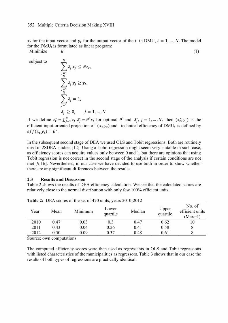
�+ for the input vector and ~+ for the output vector of the Z–th DMU, Z = 1, … , Â. The model for the DMUt is formulated as linear program: Minimize î (1)

subject to � D"

ï

"��

�" ≤ î�+,

� D"

ï

"��

~" ≥ ~+,

� D"

ï

"��

= 1,

D" ≥ 0, � = 1, … , Â

If we define �+∗ = ∑ �"

ï"�� D"

∗ = î∗�+ for optimal î∗ and D"∗, � = 1, … , Â, then (�+

∗, ~Z) is the efficient input-oriented projection of (�+,~+) and technical efficiency of DMUt is defined by���(�+,~+) = î∗.

In the subsequent second stage of DEA we used OLS and Tobit regressions. Both are routinely used in 2SDEA studies [12]. Using a Tobit regression might seem very suitable in such case, as efficiency scores can acquire values only between 0 and 1, but there are opinions that using Tobit regression is not correct in the second stage of the analysis if certain conditions are not met [9,16]. Nevertheless, in our case we have decided to use both in order to show whether there are any significant differences between the results.

2.3 Results and Discussion Table 2 shows the results of DEA efficiency calculation. We see that the calculated scores are relatively close to the normal distribution with only few 100% efficient units.

Table 2: DEA scores of the set of 470 units, years 2010-2012

Year Mean Minimum Lowerquartile Median Upper

quartile

No. of efficient units

(Max=1)2010 0.47 0.03 0.3 0.47 0.62 102011 0.43 0.04 0.26 0.41 0.58 82012 0.50 0.09 0.37 0.48 0.61 8

Source: own computations

The computed efficiency scores were then used as regressants in OLS and Tobit regressions with listed characteristics of the municipalities as regressors. Table 3 shows that in our case the results of both types of regressions are practically identical.

352 | Multiple Criteria Decision Making XVIII

Table 3: Effects of selected MSWM characteristics on efficiency scores

OLS TobitCoefficient St. Dev. Coefficient St. Dev.

constant 0.4597*** 0.0089 0.4597*** 0.0089Bin evidence 0.0318*** 0.0109 0.0318*** 0.0109Household waste recycling center

-0.0718*** 0.0132 −0.0718*** 0.0132

Separation incentive program 0.1024** 0.0514 0.1024** 0.0513Dwellings in multifamily houses ratio 0.1520*** 0.0464 0.1520*** 0.0463

Separated waste share 0.0566* 0.0303 0.0566* 0.0302Curbside collection -0.0045 0.0158 −0.0045 0.0158

Source: own computations

Both OLS and Tobit regressions have identified several statistically significant results with respect to the efficiency scores. Positive effect of bin evidence on efficiency can be explained by observed tendency to have lower MSWE per capita in municipalities that use some kind of evidence. Several municipal authorities said that after they started to register how many bins they have, collection company could no more ask the municipality to pay for more bins than there actually were registered, which obviously happened before. Negative effect of HWRC presence on efficiency can be explained by the fact that running an HRWC is accompanied by notable costs that can negate benefits, although positive environmental effects are undisputed. Positive effect of incentive scheme for increased collection of recyclables can be explained by the fact that incentives tend to work very well when trying to change people’s behavior in all kinds of areas. In this case are people typically rewarded with some discount from yearly waste management fee based on their level of waste separation. Most of the municipal authorities that use incentive scheme reported that using such scheme had very strong impact on the amount of collected separated waste together with the decrease in MSW production. Positive effect of higher ratio of dwellings in multifamily houses on efficiency can be explained by the fact that more people living in the multifamily houses implies that the population is more dense. This results in fewer waste collection points with rather larger waste containers, what is usually more efficient due to the lower related costs for waste collection and transport (less and larger bins mean less time spent collecting waste). Positive effect of higher separated waste share on efficiency can be explained by the fact that the more people separate, the less MSW they produce, what subsequently leads to the lower MSWE. In terms of efficiency we did not identify significant effects of curbside collection, although many municipal authorities noted that after the introduction of curbside collection the amount of collected separated waste increased notably. But again, with curbside collection come also additional costs that can offset the benefits. Furthermore, during our data collection when speaking with municipal representatives we have identified other variables that might have a notable effect on MSWM efficiency, like the attitudes and the habits of people towards their waste-related behavior, the collection company and level of competition, geographical location and conditions, MSWM perception of municipal authorities and the level of their activity in this area, and several other, that are difficult to collect and express in computable forms.

3 CONCLUSIONS We have used the Two-stage Data Envelopment Analysis to evaluate efficiency of municipal solid waste management of a selected sample of Czech municipalities. Municipal solid waste management represents a suitable area for DEA evaluation, as it is related with multiple outputs of different measures that are not easily transferable into the monetary form. The main

Quantitative Methods in Economics | 353

advantage of DEA is that it can overcome such issues. The subsequent regression of the computed efficiency scores of municipalities suggests several characteristics that can influence efficiency in this area. Some of them, like the housing structure, are difficult to change, but might help to understand better why some municipalities are more efficient than others. On the other hand, factors like bin evidence or incentive scheme can be adopted by another municipality, and are likely to increase the efficiency of waste management. Finally, providing a household waste recycling center or setting up a curbside collection certainly has positive environmental impacts in terms of increased separated waste, but it is also connected with additional costs, what has to be taken into account when deciding whether to set them up in the municipality.

Acknowledgements: This work was supported by research project GA15-08032S and specific research project no. MUNI/A/1047/2015.

References [1] Banker, R. D., Charnes, A. and Cooper, W. W. (1984). Some models for estimating

technical and scale inefficiencies in data envelopment analysis. Management Science, 30(9), pp.1078-1092.

[2] Charnes, A., Cooper, W. W. and Rhodes, E. (1978). Measuring the efficiency of decision making units. European Journal of Operational Research, 2(6), pp.429-444.

[3] Cook, W. D. and Seiford, L. M. (2009). Data envelopment analysis (DEA) – Thirty years on. European Journal of Operational Research, 192(1), pp.1–17.

[4] De Jaeger, S., Eyckmans, J., Rogge, N. and Van Puyenbroeck, T. (2011). Wasteful waste- reducing policies? The impact of waste reduction policy instruments on collection and processing costs of municipal solid waste. Waste Manag, 31(7), pp.1429-1440.

[5] Dyson, R. G., Allen, R., Camanho, A. S., Podinovski, V. V., Sarrico, C. S. and Shale, E. A. (2001). Pitfalls and protocols in DEA. European Journal of Operational Research, 132(2), pp.245-259.

[6] Førsund, F. R. (2013). Measuring efficiency and effectiveness in the public sector. Memorandum 16/2013. [online] Oslo: University of Oslo, Available at: http://www.sv.uio.no/econ/english/research/unpublished-works/working-papers/pdf-files/2013/memo-16-2013.pdf [Accessed 20 Apr. 2015].

[7] Garcıa-Sanchez, I. M. (2008). The performance of Spanish solid waste collection. Waste Management and Research, 26(4), pp.327-336.

[8] Hoff, A. (2007). Second stage DEA: Comparison of approaches for modelling the DEA score. European Journal of Operacional Research, 181(1), pp.425-435.

[9] Johnson, A. L. and Kuosmanen, T. (2012). One-stage and two-stage DEA estimation of the effects of contextual variables. European Journal of Operational Research, 220(2), pp.559-570.

[10] Liu, J. S., Lu, L. Y., Lu, W. M. and Lin, B. (2013). Data envelopment analysis 1978–2010: A citation-based literature survey. Omega, 41(1), pp.3-15.

[11] Marques, R. C. and Simoes, P. (2009). Incentive regulation and performance measurement of the Portuguese solid waste management services. Waste Management and Research, 27(2), pp.188-196.

[12] McDonald, J. (2009). Using least squares and tobit in second stage DEA efficiency analyses. European Journal of Operational Research, 197(2), pp.792-798.

[13] Subhash, R. (1988). Data envelopment analysis, nondiscretionary inputs and efficiency: an alternative interpretation. Socio-Economic Planning Sciences, 22(4), pp.167-176.

354 | Multiple Criteria Decision Making XVIII

[14] Rogge, N. and De Jaeger, S. (2012). Evaluating the efficiency of municipalities in collecting and processing municipal solid waste: A shared input DEA-model. Waste Management, 32(10), pp.1968-1978.

[15] Rogge, N. and De Jaeger, S. (2013). Measuring and explaining the cost efficiency of municipal solid waste collection and processing services. Omega, 41(4), pp.653- 664.

[16] Simar, L. and Wilson, P. W. (2011). Two-stage DEA: caveat emptor. Journal of Productivity Analysis, 36(2), pp.205-218.

[17] Struk, M. (2015). Efficiency factors in municipal solid waste management. In: Proceedings of the 15th International Waste Management and Landfill Symposium.Padova: CISA.

[18] Struk, M. (2014). Municipal Solid Waste Management and its Efficiency. In: Proceedings of the 18th International Conference: Current Trends in Public Sector Research. Brno: Masarykova univerzita, pp. 336-343.

Author’s addressIng. Michal Struk Faculty of Business and Economics, Mendel University in Brno Zemědělská 1, 613 00 Brno, and Faculty of Economics and Administration, Masaryk University Lipová 41a, 602 00 Brno Czech Republic email: struk@mail.muni.cz

Ing. Mgr. Markéta Matulová, PhD. Faculty of Economics and Administration, Masaryk University Lipová 41a, 602 00 Brno Czech Republic email: Marketa.Matulova@econ.muni.cz

Quantitative Methods in Economics | 355

MULTIPLE CONSTRAINTS APPLIED INTO THE DSGEMODEL: THE CASE OF UNCONVENTIONAL MONETARY

EASING IN THE CZECH ECONOMY.

Karolína Súkupová, Masaryk University Brno, Osvald Vašíček, Masaryk University Brno

Abstract In this paper, we deal with the nonlinear constraints applied into the standard small open economy DSGE model. As a real economy example, we study a case of the zero lower bound on the interest rate and the lower bound on the foreign exchange rate. We analyze the simulated trajectories of the model variables that represent the economy during a period of low interest rates that reach the zero lower bound. The second constraint represents the usage of the foreign exchange rate as an unconventional tool for monetary easing.

The tool used for our analysis is called DynareOBC and it was developed by Tom Holden. Its basic principle is based on the quadratic optimization. The toolbox is an extension of well-known toolbox Dynare and it is suitable for using under computational system Matlab. The results suggest that the foreign exchange rate may substitute the interest rate as a monetary tool when necessary.

Keywords: Zero Lower Bound, unconventional monetary policy, constraints in DSGE models

JEL Classification: C32, E17 AMS Classification: 91B51, 91B64

1 INTRODUCTION The period after the Great recession has brought many challenges to both academia and monetary authorities. The recovery after 2009 was quite weak, the renewed output growth rates were low and some countries experienced the secondary decline combined with severe deflationary risks. Monetary authorities used their usual tool to moderate economy and lowered the policy interest rates and reached the zero lower bound. That was scenario common for Czech economy and Eurozone. In the fourth quarter of 2012 bank board members of both Czech National Bank and ECB decided to lower the policy interest rates to technical zero. That induced important discussion about unconventional tools of monetary policy. Zero lower bound is a serious obstacle in a fulfillment of monetary policy targets and monetary authorities needed to find new tools to fight imminent deflation. ECB decided to use quantitative easing, Czech National Bank introduced new monetary policy tool - asymmetric exchange rate commitment.

In the November of 2013 CNB started to operate on the FX trade to depreciate Czech Koruna on the level 27 CZK/EUR. This decision was motivated by low inflation rates and risks of deflationary spiral that emerged from weak domestic demand and general pessimism. The bank board was broadly criticized immediately, nevertheless subsequent positive development of economy justified this policy. The aim of this paper is to simulate asymmetric commitment in the environment of zero interest rates and study the impact of this tool.

The paper is organized in a following way. In the first section we describe main features of a model we used and we provide brief description of a method used for simulating constraints

356 | Multiple Criteria Decision Making XVIII

in a DSGE model. The second section includes results of this simulation and we provide economic interpretation of these results.

2 METHOD

2.1 Model and FX rate intervention We used the model derived in the work of Malovaná (2014), who used the model of small open economy based on the standard DSGE framework, incorporated the foreign exchange rate intervention following Montoro, Ortiz (2013) and applied the basic version of algorithm published in Holden, Paetz (2012). The model consists of households, two stages of production, domestic retailers and monetary authority. The foreign economy is modeled as a closed version of domestic economy. We made some changes - we used forward looking monetary rule convenient for inflation targeting, we add more observed variables (consumption, exports, imports, price of imports). The model is now transformed for using log differences as input.

We used the UIP condition following Montoro, Ortiz (2013). The continuum of dealers is operating in a domestic economy. They obtain sale and purchase orders of domestic bonds ð+

ñ and ð+Úò from households and central bank and sale orders of foreign bonds ð+

∗ and ð+Úò∗

from foreign investors and domestic central bank. They maximize an objective −�+

ñ�CóôõöMá

,

where �+ñis the expectation operator, ÷ is the coefficient of absolute risk aversion and ø+l�

ñ is total investment after returns. The result of this optimization is the UIP condition

�+4+l� − 4+ = b+ − b+∗ + ÷��(ð+

Úò∗ + ð+∗),

where 4+ denotes nominal exchange rate, b+ denotes the nominal interest rate and � denotes the standard deviation of nominal exchange rate. The aim of authors was to model the possibility that the central bank may intervene into the foreign exchange rate by selling or purchasing bonds on FX rate market. The amount of bonds in this operation is determined by the equation

ð+Úò∗ = ùØ(4+ − 4Ø) + ù9(4+ − 4+C�) + ùúû+ + ü+

Úò,

where each parameter ù with lower index denotes weight on different policy. Possible policies are FX rate targeting, FX rate smoothing and real exchange rate intervention. We decided not to use this way to model intervention for several reasons. The most important is that this approach enables us to model only symmetric intervention. The second is that the impact of this type of intervention into a model is weak and the third reason is the impossibility of setting the exact level of FX rate target. The parameters in the equation above are calibrated to zero, which implies that only unexpected intervention shocks influence the foreign exchange rate. We use this setting to illustrate the impact of unexpected intervention into the economy. The intervention is modeled as the constraint in a model.

2.2 Constraints in a DSGE models Application of nonlinear constraints into the DSGE framework belongs to the growing area of interest. The method we used is introduced and derived in Holden and Paetz (2012) and it is based on so called shadow price shocks. The shadow price shock is incorporated into the equation of the constrained variable and it drives this variable from the negative values back to the zero level. The algorithm saves values of shadow shock and impulse responses of the model variables to all values of this shock. The impulse response to the model's shock ü under constraint may be written as

Quantitative Methods in Economics | 357

b�� = ýG + þ + �&, where þ denotes the impulse response to this shock without constraint, M is the matrix of the impulse response functions to the values of the shadow price shock and � is the magnitude of these shocks. As the magnitude � is not known, we need to solve quadratic programming problem

�∗ = \�ÿ�b. ����∗l�l�∗���

���(ý∗ + þ∗) +12

��!&∗ + &∗-#��.

The shadow shock may be interpreted as an expected shock in the economy. Economy participants know that the bounded variable cannot violate the constraint and that influences their expectations. That enables us to use constraint on foreign exchange rates as representation of the intervention.

Holden extended his algorithm into toolbox DynareOBC and published it on his github profile in Holden (2016). His aim was to bring easily applicable tool and the conditions of existence of the solution of the model with constraints. Using the tool is very similar to using toolbox Dynare. The model file is the basic .mod file that may include expressions with max, min or abs. The toolbox enables us to simulate and estimate models with multiple constraints. Its complexity brings to users powerful yet less understandable tool.

3 RESULTS Simulated trajectories capture the relationship between output and its components - consumption, exports and imports. Imports and consumption are strongly positively correlated, as well as output and exports. The provided results are more the illustrative examples of the function of the tool than representation of real economy.

3.1 Constraint on the nominal interest rate The simulated trajectories are depicted in the Figure 1. Constraint on interest rate has impact on exchange rate through UIP condition. It mutes the size of depreciation rate and that results in lower average value of nominal exchange rate. The exchange rate and the interest rate are strongly negatively correlated, so the constraint binds only when the exchange rate depreciates. Development of the output is influenced by two factors. First, monetary authority cannot adjust the bounded interest rate to boost output and second, the muted depreciation has negative impact on exports. The result is a deeper recession in the case of bounded interest rate. That is in line with observed situation in both Czech and European economy.

3.2 Constraint on the nominal exchange rate Constraint on the exchange rate represents the asymmetric foreign exchange rate commitment. The simulated trajectories depicted in the Figure 2 represent the environment where the monetary authority depreciated FX rate and now it is bounded from below. The unexpected depreciation and its impact was analyzed in our earlier work; see Súkupová, Vašíček (2015). The bound is active when the interest rate reaches its maximal values and the constraint leads to higher value of interest rate than in the unbounded case, because monetary authority tries to slow down the output growth caused by higher exports. These results suggest that asymmetric commitment can lead to desired outcomes, such as higher growth.

The results of simulation of a model where both exchange rate and interest rate are bounded are displayed in the Figure 3 and it is just a linear combination of previous cases. Due to the link between FX rate and interest rate in the UIP condition, there is not a period when both variables reach bound simultaneously. The combination of both constraints lowers the

358 | Multiple Criteria Decision Making XVIII

volatility of exchange rate, increases the growth rate of output in case of boom and causes a deeper recession.

Figure 1: Constraint on interest rate

Figure 2: Constraint on exchange rate

Quantitative Methods in Economics | 359

Figure 3: Combination of constraints

4 CONCLUSION In the paper we have dealt with application of constraints into the small open economy DSGE model. We used the new tool that uses so called shadow shock to model nonlinear constraints in dynamic models and that enables us to simulate multiple bounds in a model. We analyzed the impact of asymmetric foreign exchange rate commitment. Our results suggest that this policy may be suitable substitute to bounded interest rates. The future work will focus on construction of more precise model and application of the method into it.

Acknowledgements: This work is supported by funding of specific research at Faculty of Economics and Administration, project MUNI/A/1040/2015. This support is gratefully acknowledged.

References [1] Holden, T. and Paetz, M. Efficient simulation of DSGE models with inequality

constraints. 1 st ed. [pdf] Guildford: University of Surrey. pp. 1-20. Available at: http://www.fahs.surrey.ac.uk/economics/discussion_papers/2012/DP16-12.pdf.[Accessed: 15 May. 2016].

[2] Holden, T. Existence, uniqueness and computation of solutions to dynamic models with occasionally binding constraints. 1 st ed. [pdf] Guildford: University of Surrey. pp. 1-45. Available at: https://www.tcd.ie/Economics/assets/pdf/Seminars/20152016/Tom%20Holden%20paper.pdf. [Accessed: 15 May. 2016].

[3] Malovaná, S. (2014). The Effectiveness of Unconventional Monetary Policy Tools at the Zero Lower Bound: A DSGE Approach. Mgr. Karlova Univerzita, Fakulta sociálních studií.

[4] Montoro, C. and Ortiz, M. (2013). Foreign Exchange Intervention and Monetary Policy Design: A Market Microstructure Analysis, 3 rd draft, Switzerland [Online]. Bank for

360 | Multiple Criteria Decision Making XVIII

International Settlements. Available at: http://www.bis.org/events/ccaconf2013/montoroortiz.pdf [Accessed: 15 May. 2016].

[5] Súkupová, K. and Vašíček, O. (2015). Non–linear restrictions in DSGE models: The effect of foreign exchange interventions in Czech economy. In Proceedings of the 33rd International Conference Mathematical Methods in Economics. Plzeň: University of West Bohemia, pp. 761-766.

Authors' address Mgr. Bc. Karolína SůkupováFaculty of Economics and Administration, Masaryk University, Department of Economics Lipová 41a, 602 00 BrnoCzech Republic Email: 324246@mail.muni.cz

prof. Ing. Osvald Vašíček, CSc.Faculty of Economics and Administration, Masaryk University, Department of Economics Lipová 41a, 602 00 BrnoCzech Republic Email: Osvald.Vasicek@econ.muni.cz

Quantitative Methods in Economics | 361

STOCHASTIC MODEL OF SHORT-TIME PRICE DEVELOPMENT OF SHARES AND ITS PROFITABILITY IN ALGORITHMIC TRADING

Milan Svoboda, Pavla Říhová, University of West of Bohemia

Abstract The aim of this study is to verify the profitability of speculative algorithmic trading systems. The study was performed on historical daily prices (open and close) of the CEZ shares in a ten years period from the beginning of 2006 to the end of 2015. The profitability of algorithmic trading systems is compared to the passive ‘Buy and Hold’ strategy. In the study we present three trading systems, the basic one and two its modifications. The systems use business strategies based on assumptions of Technical Analysis (TA). TA assumes that stock prices move in three types of trends: primary, secondary and minor. The subject of our interest is the minor trend which usually lasts for several days. During the duration of this trend the share price accumulates a gain or loss in relation to the price at the beginning of the trend. We further assume that the probability of reversing this trend increases with accumulated loss or gain. For modelling the probability of trend reversal, we use the theory of Markov chains. States in which there is a high probability of a change in the trend are suitable for generating trading orders. The results of this study show that algorithmic trading systems employing this strategy are able to outperform the market.

Keywords: Algorithmic trading, technical analysis indicators, stock market predication Markov chains analysis,

JEL Classification: C44 AMS Classification: 60H35

1 INTRODUCTION Rapid development of information technology is, besides other things, connected with development of algorithmic trading. Algorithmic trading is understood as a method of share trading, where buy and sell orders are generated by a computer program based on an algorithm. Methods used for generating trading signals are mainly methods of Technical Analysis (TA), quantitative analysis, additionally also methods of fundamental analysis and findings of behavioural finance theory.

Principles and methods of TA are described, for example, in [3]. TA is understood as an extensive set of methods which from previous prices and trade volumes predict the future prices. One of the bases of TA is a thesis that share prices move in trends which have certain inertia. A trend change is determined by a change of the ratio between sellers and buyers. These trend changes are possible to be identified in time by studying historical prices and trade volumes. Technical analysts identify three types of trends: a primary trend, which lasts for a period from one year to several years, a secondary trend, which lasts for several months, and a minor trend, which lasts for days or weeks.

The aim of this empirical study is to analyse the algorithmic trading system which generates trading signals in the moment when it is assumed that there is a reversal in a minor trend. The Markov chains (MC) analysis is used for prediction of the time of the reversal. MC theory is described for example in [2]. MC is used for modelling stochastic processes which can be found in one of the finite (countable) numbers of states in discrete time moments. MC is

362 | Multiple Criteria Decision Making XVIII

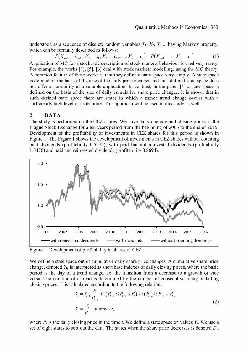
understood as a sequence of discrete random variables X1, X2, X3.... having Markov property, which can be formally described as follows:

� � � �nnnnnnn xXxXPxXxXxXxXP ������� ��� |,.......,| 1221111 (1) Application of MC for a stochastic description of stock markets behaviour is used very rarely. For example, the works [1], [5], [6] deal with stock markets modelling, using the MC theory. A common feature of these works is that they define a state space very simply. A state space is defined on the basis of the size of the daily price changes and thus defined state space does not offer a possibility of a suitable application. In contrast, in the paper [4] a state space is defined on the basis of the size of daily cumulative share price changes. It is shown that in such defined state space there are states in which a minor trend change occurs with a sufficiently high level of probability. This approach will be used in this study as well.

2 DATA The study is performed on the CEZ shares. We have daily opening and closing prices at the Prague Stock Exchange for a ten years period from the beginning of 2006 to the end of 2015. Development of the profitability of investments in CEZ shares for this period is shown in Figure 1. The Figure 1 shows the development of investments in CEZ shares without counting paid dividends (profitability 0.5979), with paid but not reinvested dividends (profitability 1.0476) and paid and reinvested dividends (profitability 0.8694).

Figure 1: Development of profitability in shares of CEZ

We define a state space out of cumulative daily share price changes. A cumulative share price change, denoted Yt, is interpreted as short base indexes of daily closing prices, where the basic period is the day of a trend change, i.e. the transition from a decrease to a growth or vice versa. The duration of a trend is determined by the number of consecutive rising or falling closing prices. Yt is calculated according to the following relations:

� � � �1 2 1 2 11

1

if or ,

otherwise,

tt t t t t t t t

t

tt

t

PY Y P P P P P PP

PYP

� � � � ��

�

� 0 0 4 4

�(2)

where Pt is the daily closing price in the time t. We define a state space on values Yt. We use a set of eight states to sort out the data. The states when the share price decreases is denoted Di,

0.5

1.0

1.5

2.0

2006 2007 2008 2009 2010 2011 2012 2013 2014 2015 2016

with reinvested dividends with dividends without counting dividends

Quantitative Methods in Economics | 363

the state when the share price grows is denoted Gi. D1 is the state with the lowest cumulative price decrease and the state D4 is the state with the highest cumulative price decrease. G1 isthe state with the lowest cumulative price growth and G4 is the state with the highest cumulative price growth. The width of the interval is equal to the standard deviation of daily changes in the share price during the studied period, which is 0.0184. A state space is thus defined as follows:

D4: Yt < 0.9448 G1: 1.0000 ≤ Yt < 1.0184;

(3)D3: 0.9448 ≤ Yt < 0.9632; G2: 1.0184 ≤ Yt < 1.0368;D2: 0.9632 ≤ Yt < 0.9816; G3: 1.0368 ≤ Yt < 1.0552D1: 0.9816 ≤ Yt < 1.000 G4: 1.0552 ≤ Yt ,

3 TRADING STRATEGIES Trading strategies are always realized according to the following rules. One trade (transaction) means the buying and subsequent selling of shares. If a buying or selling signal is generated one day, the trade is realized for the opening price from the following day. The whole capital is always invested, transaction costs are not considered, after-tax dividends are reinvested, a short selling is not taken into account and two consecutive buyings are not possible. The value of the invested capital is calculated according to the following equation:

01

ni i

ni i

S DC CB�

�� K (4)

where C0 = 1.000 is initial capital value, Cn is capital value after the nth transaction, Si is selling price in the ith transaction, Di are dividends after tax in case that during the ithtransaction there was a record day, Bi is buying price in the ith transaction. Trading strategies are created on the following principle. When a certain level of a share price decrease is reached, a buying signal is generated and when a certain level of a share price growth is reached, a selling signal is generated. We count three trading models. In each model we calculate 16 (4x4) trading strategies which we obtain by combining all four levels of decrease with all four levels of growth. For each trading strategy we calculate profitability (return on investment) and the number of realized trades denoted n. Profitability of calculated trading strategies is compared to a passive strategy ‘Buy and Hold’, which is represented by a passive investment with reinvesting dividends and whose profitability is 0.8694.

3.1 Model 1 In this basic model the buying signals are generated directly by the states D1, D2, D3 and D4and the selling signals are generated directly by the states G1, G2, G3 and G4. The reached profitability is given in Table 1. Strategies which beat the strategy ‘Buy and Hold’ are shown in bold.

Table 1. Results of Model 1 sell G1 G2 G3 G4

buy Cn n Cn n Cn n Cn n D1 0.735 416 1.155 223 1.499 93 1.210 54 D2 1.121 228 1.800 173 1.646 91 1.200 55 D3 1.707 82 1.935 76 0.939 54 0.991 40 D4 1.434 42 1.966 50 1.582 39 1.481 34

364 | Multiple Criteria Decision Making XVIII

The results show that the trading strategies beat the passive strategy in 15 cases. The average profitability was 1.40. The development of profitability in time is depicted in Figure 2. To make it clearer we show only four ‘inner’ strategies (combination of D2 and D3 with G2 and G3) and the strategy ‘Buy and Hold’ (B&H).

Figure 2: Development of profitability in Model 1

3.2 Model 2 A drawback of Model 1is the possibility that a signal does not have to be generated even when there is a big price change. For example when generating the selling signal by the state G2, the selling signal, with the following sequence of the states G1, G3, G4, G4, was not generated. We will eliminate this drawback in this Model 2. The state Bi will be the minimal decrease for generating a signal and Si will be the minimal growth for generating a signal. So S1 = {G1, G2, G3, G4}; S2 ={G2, G3, G4}; S3 ={G3, G4}; S4 ={G4}; B2 ={D2, D3, D4} etc. The results are given in Table 2. Strategies which beat the corresponding strategies in model 1 are shown in bold.

Table 2: Results of Model 2 sell S1 S2 S3 S4

buy Cn n Cn n Cn n Cn n B1 1.313 611 1.117 309 1.298 132 1.099 66B2 1.882 297 1.400 213 1.518 118 1.132 60B3 2.781 123 2.273 109 1.268 78 0.872 47B4 2.329 58 2.008 55 2.171 49 1.481 34

The average profitability of Model 2 was 1.62. Model 2 in comparison with Model 1 had better results in ‘underdiagonal strategies’. The profitability development of chosen strategies is shown in Figure 3.

0.5

1.0

1.5

2.0

2.5

2006 2007 2008 2009 2010 2011 2012 2013 2014 2015 2016B&H D2 - G2 D2 - G3 D3 - G2 D3 - G3

Quantitative Methods in Economics | 365

Figure 3: Development of profitability in Model 2

3.3 Model 3 In the last model we will try to use the whole length of a minor trend and a signal will be generated only after the trend change. So for example a selling signal S2 in time t occurs if in time t-1 the process is in one of the states G2, G3, G4 (minimal growth in G2) and in time t the process is in one of the states D1 D2, D3, D4 (a decreasing trend has begun). We expect that in comparison with Model 1this strategy will have better results in ‚top left corner’ (combination of D1 and D2 with G1 and G2).

Table 3: Results of Model 3 sell S1 S2 S3 S4

buy Cn n Cn n Cn n Cn n B1 0.656 610 0.899 308 1.212 131 0.980 65B2 0.517 296 0.630 212 0.918 117 0.832 59B3 0.465 122 0.551 108 0.536 77 0.477 46B4 0.508 58 0.669 55 0.986 48 0.823 33

The results show that our expectations were not fulfilled. No trading strategy beat corresponding strategy of the basic Model 1. The average profitability is 0.73. It was shown that the gain obtained in the residue of trend was lost in the beginning of the reverse trend. The profitability development of chosen strategies is shown in Figure 4.

0.5

1.0

1.5

2.0

2.5

2006 2007 2008 2009 2010 2011 2012 2013 2014 2015 2016B&H B2 - S2 B2 - S3 B3 - S2 B3 - S3

366 | Multiple Criteria Decision Making XVIII

Figure 4: Development of profitability in Model 3

4 CONCLUSION The results of this study show that a stochastic model which uses Markov chains analysis can be used in algorithmic trading systems. In two out of three calculated models the strategy ‘Buy and Hold’ was beaten significantly. We will carry on with this research. Our further research will be focused on the following areas:

� Confirmation of the results of this study on other shares. � More detailed analysis of success of trading strategies on growing, decreasing and

lateral primary trend. � Development of a dynamic model which would react to a changing volatility at stock

markets.

Acknowledgements: The article was supported by research project “The Research of Factors Affecting Share Price Movement, Prediction of Share Price Movement and Design of Algorithms for Self-acting Trading” SGS-2015-026 of the Faculty of Economics, University of West Bohemia in Pilsen.

References [1] Doubleday, K., J. and Esunge, J., N. (2011). Application of Markov Chains to Stock

Trends, Journal of Mathematics and Statistics, [online] Volume 7 (2), pp.103-106. Available at: http://thescipub.com/PDF/jmssp.2011.103.106.pdf [Accessed 8 Apr.2016]

[2] Hillier, F., S. and Lieberman, G., J. (1986). Introduction to Operations Research. 4th ed.NY: McGraw-Hill Publishing Company.

[3] Murphy, J. (1999). Technical Analysis of the Financial Markets: A Comprehensive Guide to Trading Methods and Applications. 1th ed. [pdf] New York: New York Institute of Finance, Available at: http://files.leopolds.com/books/Technical.Analysis.of.the.Financial.Markets.1st.Edition.1999.Murphy.pdf [Accessed 8 Apr.2016].

[4] Svoboda, M. (2013). Stock market modelling using Markov chain analysis. In Proceedings of the 11th International Conference Liberec Economic Forum 2013.Liberec: Technical University of Liberec, pp.551-557.

[5] Vasanthi, S., Subha M., V. and Nambi S., T. An empirical Study on Stock Index trend prediction using Markov Chain analysis, Journal of Banking Financial Services and Insurance Research, [online] 1(1), pp. 72-90. Available at:

0.5

1.0

1.5

2.0

2006 2007 2008 2009 2010 2011 2012 2013 2014 2015 2016K&D B2 - S2 B2 - S3 B3 - S2 B3 - S3

Quantitative Methods in Economics | 367

http://www.indianjournals.com/ijor.aspx?target=ijor:jbfsir&volume=1&issue=1&article=005 [Accessed 8 Apr. 2016].

[6] Zhang, D., Zhang, X. Study on Forecasting the Stock Market Trend Based on Stochastic Analysis Method. International Journal of Business and Management, [online] 4 (6), pp. 163-170. Available at: http://www.ccsenet.org/journal/index.php/ijbm/article/view/2336/2187 [Accessed 8 Apr. 2016].

Author’s address Ing. Mgr. Milan Svoboda, Ph.D. University of West of Bohemia, Faculty of Economics Department of Economics and Quantitative Methods Univerzitní 8, 30614 PilsenCzech Republic email: svobodm@kem.zcu.cz

Ing. Pavla ŘíhováUniversity of West of Bohemia, Faculty of Economics Department of Economics and Quantitative Methods Univerzitní 8, 30614 PilsenCzech Republic email: divisova@kem.zcu.cz

368 | Multiple Criteria Decision Making XVIII

THE EFFECT OF TERMS-OF-TRADE ON SLOVAK BUSINESS CYCLES: A THEORETICAL APPROACH

Karol Szomolányi, University of Economics, Bratislava, Martin Lukáčik, University of Economics, Bratislava,

Adriana Lukáčiková, University of Economics, Bratislava

Abstract The theoretical approach of business cycles in the economy with non-tradable goods cannot sufficiently explain the relatively minor role played of terms-of-trade shocks in driving short-run fluctuations observed by empirical models. It follows from calibrating MXN model using Slovak data and result compare with estimated SVAR model.

Keywords: terms of trade, business cycle, MXN model

JEL Classification: E32 AMS Classification: 37M10

1 INTRODUCTION Empirical and theoretical studies imply contradictory results about terms-of-trade effect on business cycles. Intuitively, small open economy is sensitive to trade shocks. Indeed, both Keynesian and real business cycle theories predict a positive impact of the terms-of-trade on output. However, these different theories predict a different impact of the terms-of-trade on trade balance. Harberger (1950) and Laursen and Metzler (1950) used traditional Keynesian model to show that trade balance grows with terms-of-trade.

On the contrary, dynamic optimizing models of Obstfeld (1982) and Svensson and Razin (1983) leads to a conclusion that positive effect of terms-of-trade on the trade balance is weaker the more persistent is a terms-of-trade shock. Uribe and Schmitt-Grohé (2016)showed that in small open economy real business cycle model (or dynamic stochastic general equilibrium model) with capital costs sufficiently permanent terms-of-trade shocks have negative impact on the trade balance. In order to reduce the importance of terms-of-trade shocks” Uribe and Schmitt-Grohé (2016) extended the small open real business cycle model by non-tradable goods – MXN model with import-able, export-able and non-tradable goods. However, model predictions do not match with observed data.

In the paper we confirm the inability of the MXN model to theoretically explain the terms-of-trade shocks. We calibrate the model using SVAR estimate of Slovak business cycle published by Lukáčik et al (2015) and Slovak data in the period 1997 – 2015. This period includes the entry into the European Union and the period of the financial crisis. Surmanováand Furková (2006) investigated the entrance of the country to union and Chocholatá (2013) dealt with the issue of the crisis in the environment of emerging economies.

2 MXN MODEL Uribe and Schmitt-Grohé (2016) presented the model with import-able (m), export-able (x) and non-tradable (n) sectors. The presence of non-tradable goods should reduce the importance of terms-of-trade shock.

Quantitative Methods in Economics | 369

2.1 Households We consider a large number of identical households with preferences described by the utility function

� � � � � �1

00

1

1

m x nm x nt t t

tm x n

t

t

h h hc

U E

@L L L

L L L;

@

�

3

�

$ %& '� � � �& '( )�

�� (1)

where ct denotes consumption, for sector j � {m,x,n}, htj denotes hours worked in the sector j

Sectoral labour supplies are wealth inelastic and parameters ωj denotes wage elasticity in the sector j. The symbol E0 denotes the expectations operator conditional on information available in initial period 0. The parameter σ measures the degree of relative risk aversion.

Households maximize the lifetime utility function (1) subject to the budget constraint

� � � � � �2 2 2

1 1 1

1 1

1

m x n m m x x n nt t t t m t t x t t n t t t t

m m x x n n m m x x n nt tt t t t t t t t t t t t

t

c i i i k k k k k k p d

p d w h w h w h u k u k u kr

8

8

H H H� � �

� �

� � � � � � � � � � �

� � � � � � ��

(2)

where for sector j � {m,x,n}, itj denotes gross investment, kt

j denotes capital, wtj denotes real

wage rate and utj denotes the rental rate of capital in the sector j. Quadratic terms of the

budget constraint (2) are capital adjustment costs, where ϕj denotes capital adjustment cost parameter in the sector j. The variable pt

τ denotes the relative price of the tradable composite good in terms of final goods, dt denotes the stock of debt in period t denominated in units of the tradable composite good and rt denotes the interest rate on debt held from period t to t + 1.Consumption, investment, wages, rental rates, debt, and capital adjustment costs are all in units of final goods.

The capital stocks accumulation is given by � � � �1 1 ; , ,j j j

t t tk k i j x m nF� � � � E � (3) where δ denotes constant depreciation rate.

2.2 Firms There are 5 types of large number of identical firms in the economy which differ according to their output: firms producing final goods, tradable composite goods, import-able goods, export-able goods and non-tradable goods.

Final goods are produced using non-tradable goods and a composite of tradable goods via the CES technology

� � � � � �� �1

1 1 11 1 1, 1n n nn n

t t t tB a a a a8 8 88 8 � � �

8 8M M� � �$ %

� � �& '( )

(4)

where atτ denotes the tradable composite good and at

n the non-tradable good, 0 < χτ < 1 denotes distribution parameter and μτn > 0 denotes the elasticity of substitution between tradable composite good and non-tradable good.

The tradable composite goods is produced using importable and exportable goods as intermediate inputs via the CES technology

370 | Multiple Criteria Decision Making XVIII

� � � � � �� �1

1 1 11 1 1, 1mx mx mxm x m x

t t t m t m ta A a a a a8 � � �M M� � �$ %

� � � �& '( )

(5)

where atm denotes import-able good and at

x the export-able good, 0 < χm < 1 denotes distribution parameter and μmx > 0 denotes the elasticity of substitution between import-able and export-able goods. Import-able, export-able and non-tradable goods are produced with capital and labour via the Cobb-Douglas technologies

� � � � � �1; , ,j jj j j j

t t ty A k h j x m n� ��

� E � (6) where sector j � {m,x,n}, yt

j denotes output and Atj denotes total factor productivity in the in

sector j.

To ensure a stationary equilibrium process for external debt, we assume that the country interest-rate premium is debt elastic

� �1* 1td dtr r e: � �� � � (7)

where r* denotes the sum of world interest rate and the constant component of the interest-rate premium, the last term of (7) is the debt-elastic component of the country interest-rate premium and we assume the parameter debt-elastic ψ > 0.

Model implied terms-of-trade et is assumed to follow AR(1) process 1log logt t

tf ff f

� ���� � (8)

where εt is a white noise with mean zero and unit variance, and f > 0. The serial correlation parameter is 0 < ρ < 1 and terms-of-trade standard error is π > 0.

For details of households’ and firms’ problem first-order conditions, market clearing and competitive equilibrium derivation and definitions see Uribe and Schmitt-Grohé (2016).

3 SVAR MODEL The theoretical model predictions are compared with the observed facts that are captured by the SVAR (Structural vector auto-regression) model of Slovak quarterly relative cyclical components of terms-of-trade, TOT, trade balance to output ratio, TB, output, Y, consumption, C, and investment, I, in years 1997-2014 estimated by Lukáčik, Szomolányi and Lukáčiková (2015). The responses to a change in the terms of trade are displayed in the Figure 1.

The trade balance is driven by rather Obsfeld-Svensson-Razin effect than by the Harberger-Laursen-Metzler effect. As pointed out in the Introduction, a negative reaction is theoretically possible, if capital costs are sufficiently high and (or) terms of trade shock is sufficiently persistent. On the other hand the immediate reactions of output, consumption and investment are negligible. In the first period is statistically significant only change in the consumption.

Quantitative Methods in Economics | 371

Figure 1: Impulse Response of the SVAR Model

4 CALIBRATION AND METHODOLOGY Calibrating the model we follow Uribe and Schmitt-Grohé (2016) process. The calibrated values of the model parameters are in the Table 1. We assume the values of σ, δ, r*, ωm, ωxand ωm from the small open economy real business cycle model calibrated for Slovak data by Jurkovičová (2015). We assume that wage elasticity is same in all three sectors. Torój (2012) calibrated Slovak elasticity of substitution between tradable composite good and non-tradable good, μτn, to be 0.76. Uribe and Schmitt-Grohé (2016) provide a rich discussion with literature references on calibrating the elasticity of substitution between import-able and export-able goods. Considering high-frequently (i.e. quarterly) data it is assumed that μmx = 0.8. Further we adopt Uribe and Schmitt-Grohé (2016) ideas to calibrate αm, αx, αn, f , Am and An.

The values of terms-of-trade serial correlation, ρ, and standard error, π, correspond to the data characteristics used by Lukáčik, Szomolányi and Lukáčiková (2015). To calibrate χm, χτ and Ax we follow a process of Uribe and Schmitt-Grohé (2016) and implied moment restrictions of average share of value-added exports in GDP, sx, average trade balance-to-GDP ratio, stb,and average share of non-tradable goods in GDP, sn. Likewise Uribe and Schmitt-Grohé (2016) we use OECD Trade in Value-Added (TiVA) and UNCTAD statistical databases to find values of these moment restriction. The values of the rest implied structural parameters, d and β come from the values of calibrated ones.

We fail to reach a negative reaction of the trade balance to a terms-of-trade shock in the theoretical MXN model using Slovak data to follow empirical fact observed in the Figure 1. Therefore we calibrate ϕj, j {m,x,n} and ψ to capture these observed moments. From the Figure 1 it follows that there is no reaction of investment to the terms-of-trade shock and, as Uribe and Schmitt-Grohé (2016) pointed out, the standard deviation of investment in the trade sector is 1.5 times as large as its counterpart in the non-traded sector.

-.004

.000

.004

.008

.012

.016

1 2 3 4 5 6 7 8 9 10

Response of TOT to TOT Shock

-.016

-.012

-.008

-.004

.000

.004

1 2 3 4 5 6 7 8 9 10

Response of TB to TOT Shock

-.004

-.002

.000

.002

.004

.006

.008

1 2 3 4 5 6 7 8 9 10

Response of Y to TOT Shock

-.002

.000

.002

.004

.006

.008

1 2 3 4 5 6 7 8 9 10

Response of C to TOT Shock

-.01

.00

.01

.02

.03

.04

.05

1 2 3 4 5 6 7 8 9 10

Response of I to TOT Shock

�

372 | Multiple Criteria Decision Making XVIII

Table 1: Calibration of the MXN Model Calibrated Structural Parameters Moment restrictions

σ 2

Jurkovičová (2015)

sn 0.27 UNCTADδ 0.1 sx 0.37

OECDr* 0.04 stb -0.015ωm 2.7 pmym/( pxyx) 1 Uribe and Schmitt-

Grohé (2016)ωx 2.7 σim+ix/σin 1.5ωn 2.7 no reaction of investmentμτn 0.76 Torój (2012) Implied Structural Parameter Valuesμmx 0.8

Uribe and Schmitt-Grohé (2016)

χm 0.875αm 0.35 χτ 0.78αx 0.35 d –0.509αn 0.25 Ax 1.374

f 1 β 0.962

Am 1 ϕm 0An 1 ϕx 0.159π 0.013 Lukáčik, Lukáčiková

and Szomolányi (2015)ϕn 0

ρ 0.464 ψ 1.5017x10-5

In order of finding model equilibrium the first order linear approximation to the nonlinear solution are applied using algorithms created and modified by Klein (2000) and Schmitt-Grohé and Uribe (2003). Responses to the terms-of-trade impulses and covariance-variance matrix conditional on the terms-of-trade shock is computed using algorithm of Uribe and Schmitt-Grohé (2016).

5 RESULTS The responses to a change in the terms of trade are displayed in the Figure 2.

Comparing Figure 2 with Figure 1 we can state the theoretical model failures. As we already pointed out, unlike the empiric observes, theoretical model predicts negative trade balance reaction. Predicted reactions of consumption and output are positive and to high.

Quantitative Methods in Economics | 373

Figure 2: Impulse Response of the MXN Model.

6 CONCLUSION Using Slovak data, theoretical MXN model responses to the terms-of-trade shock do not match with observed responses estimated by the SVAR model. Therefore we confirm the conclusion of Uribe and Schmitt-Grohé (2016) that “future research should refocus effort toward building models that can explain the relatively minor role played of terms-of-trade shocks in driving short-run fluctuations.

Acknowledgements: This paper was supported by the VEGA, grant no. 1/0444/15.

References [1] Chocholatá, M. (2013). The Global Financial Crisis and Stock Returns: Evidence from

the Czech Republic, Hungary and Poland. In: 31st International Conference on Mathematical Methods in Economics 2013. Jihlava: College of Polytechnics, pp. 315-320.

[2] Harberger, A. (1950). Currency Depreciation, Income, and the Balance of Trade. Journal of Political Economy, 58(1), pp.47-60.

[3] Jurkovičová, M. (2015) Model reálneho hospodárskeho cyklu v slovenskej ekonomike.Ing. University of Economics in Bratislava, Department of Operations Research and Econometrics.

[4] Klein, P. (2000). Using the generalized Schur form to solve a multivariate linear rational expectations model. Journal of Economic Dynamics and Control, 24(10), pp.1405-1423.

[5] Laursen, S. and Metzler L. (1950) Flexible Exchange Rates and the Theory of Employment. Review of Economics and Statistics, 32(4), pp. 281–299.

0 5 1005

10Terms of Trade

0 5 10-0.4-0.2

0Real Exchange Rate

0 5 10012

Rel Price of Nontradables

0 5 10-505

Trade Balance

0 5 10024

Imports

0 5 10024

Exports

0 5 10-505

GDP

0 5 10012

Consumption

0 5 10-202

Investment

0 5 10-4-20Output in Import Sector

0 5 10-505Output in Export Sector

0 5 100

0.5Output in Nontraded Sector

0 5 10-50

050Investment in Import Sector

0 5 10-20

020

Investment in Export Sector

0 5 10-505

Investment in Nontraded Sector

374 | Multiple Criteria Decision Making XVIII

[6] Lukáčik, M., Szomolányi, K. and Lukáčiková, A.: Impact of Terms-of-Trade on Slovak Business Cycles. International Scientific Conference INPROFORUM 2015, České Budějovice: University of South Bohemia, pp. 151–155.

[7] Obstfeld, M. (1982). Aggregate Spending and the Terms of Trade: Is There a Laursen-Metzler Effect?. The Quarterly Journal of Economics, 97(2), pp.251-270.

[8] Schmitt-Grohé, S. and Uribe, M. (2003). Closing small open economy models. Journal of International Economics, 61(1), pp.163-185.

[9] Surmanová, K. and Furková, A. (2006). Does the Entrance of the Country into European Union Influence an Inflation Convergence? In: Quantitative Methods in Economics,Multiple Criteria Decision Making. Bratislava: IURA EDITION, pp. 176–181.

[10]Svensson, L. and Razin, A. The Terms of Trade and the Current Account: The Harberger-Laursen-Metzler Effect. Journal of Political Economy 91(1), pp. 97–125.

[11] Torój, A. (2012). Poland and Slovakia during the crisis: would the euro (non-)adoption matter? [online] Working paper of Ministry of Finance in the Poland Republic no. 13-2012. Warsaw: Ministry of Finance in the Poland Republic. Available at: http://www.mf.gov.pl/documents/764034/1209344/mf_wp_13.pdf. [Accessed 4 Mar. 2016].

[12]OECD.org, (2016). Trade in Value Added database (OECD.STAT). [online] Available at: http://www.oecd.org/sti/ind/measuringtradeinvalue-addedanoecd-wtojointinitiative.htm. [Accessed 4 Mar. 2016].

[13]UNCTADSTAT, (2016). UNCTAD database. [online] Available at: http://unctadstat.unctad.org/wds/ ReportFolders/reportFolders.aspx?IF_ActivePath=P,15912. [Accessed 4 Mar. 2016].

[14]Uribe, M. and Schmitt-Grohé, S. Open Economy Macroeconomics. 1st ed. [pdf] New York: Columbia University, pp. 295-402. Available at: http://www.columbia.edu/~mu2166/book/. [Accessed 7 Jun. 2016].

Corresponding author’s addressdoc. Ing. Karol Szomolányi, PhD. University of Economics in Bratislava, Faculty of Economic Informatics, Department of Operations Research and Econometrics Dolnozemská 1/b, 852 35 BratislavaSlovak Republic email: szomolan@euba.sk

Quantitative Methods in Economics | 375

INNOVATION VERSUS PARASITIC SECURITY

Ľubica Šimková, Comenius University in Bratislava, Faculty of Social and Economic Sciences, Milan Horniaček, Comenius University in Bratislava,

Faculty of Social and Economic Sciences

Abstract We construct a model in the form of a difference game, in which banks choose between granting credit to innovating firms and buying the parasitic security, i.e. a security that is not linked to any innovative activity of its issuer. The effect of innovation by each firm depends also on innovation by the other firms in the preceding period. Therefore, successful innovative activity in the economy requires coordination between banks. A punishment of a single bank or a coalition of banks for not granting credit to innovating firms requires also coordination between firms and between firms and banks. Therefore, a strict strong perfect equilibrium is the solution concept that we apply to the analyzed game. It requires that there do not exist a proper subgame and a coalition that can weakly Pareto improve the vector of payoffs of its members in that subgame by a coordinated deviation.

Keywords: innovation, economic growth, coordination, difference game, strict strong perfect equilibrium.

JEL Classification: O33, C73, D43 AMS Classification: 91A25, 91B62

1 INTRODUCTION Innovation activity is one of the most important driving forces of economic growth. Theoretic justification of the importance of various types of innovation goes back at least to the pioneering works of Joseph Schumpeter, mainly [3]. In emerging market economies, industries with important foreign investments bringing innovation affect innovation in upstream industries. On the other hand, crisis in these industries spills into upstream industries. (The automobile industry in Slovakia is a typical example. See [1] for its analysis.) There are linkages between innovative activities of individual firms. Therefore, return on loan to a firm that wants to innovate depends on financing available for innovating activities of other firms. Moreover, benefits of innovation activity in the current period depend on the results of innovation activities in preceding periods. Besides this, it may happen that return on loans to innovating firms exceeds return on other investments only after several periods. Thus, successful innovative activity in the economy requires coordination between banks,between firms, and between firms and banks. Agreements between them should be self-enforceable and immune not only to unilateral deviations, but also to deviations by coalitions of firms and banks.

In the present paper, we analyze these issues using an infinite horizon difference game with discounting of future single period payoffs. Innovations considered here are product innovations. Nevertheless, some of them can require technological or organizational innovation. (Since results of innovative activities are stochastic, using a difference game rather than a truly stochastic game is a simplification. Nevertheless, this simplification enables us to analyze the essence of the problems outlined above and keep the set of states as narrow as possible). In our model, banks can either grant credit to innovating firm(s) or buy

376 | Multiple Criteria Decision Making XVIII

the security that is not linked to any innovative activity of its issuer (e.g. a derivative security or a foreign government's bond). Since it sucks financial resources from innovating firms, we call it "parasitic security." A strict strong perfect equilibrium (henceforth, SSPE) is the solution concept that we apply to the analyzed game. It is a refinement of Rubinstein's [2] concept of strong perfect equilibrium. SSPE requires that there do not exist a proper subgame and a coalition that can weakly Pareto improve the vector of payoffs of its members in that subgame by a coordinated deviation.

2 MODEL Throughout the paper, N (N ) denotes the set of positive integers (real numbers). We endow each finite dimensional real vector space with the Euclidean topology and each infinite dimensional Cartesian product of finite dimensional real vector spaces with the product topology. For a finite set A, #(A) is its cardinality and A2 is the set of all subsets of A(including the empty set).

The time horizon of the analyzed game is N. BJ 9 is the set of players in it. J is the finite set of firms and B is the finite set of commercial banks. Each BJk 9� discounts future single period payoffs (without discounting the current period payoff) using the same discount factor

� �1,0�F . We denote the analyzed game with discount factor F by � �FJ . For each Nt� ,each player observes in period t+1 all actions of each player in period t. In each period each firm Jj� can either innovate or not. In order to innovate in period t, it needs to invest the amount jc >0 into innovation activity in period t. It can obtain the latter amount only from credit. The effect of innovation by firm j in period t depends on innovation or lack of it by each firm in period t-1. In each period Nt� , each bank Bb� can grant credit � � - .jbj c,0tc �

for interest rate � � - .jbj ,0tr ;� ,where � �1,0j �; , to each firm Jj� or invest 0qbt 4 into the parasitic security. Credit granted in period t has to be repaid with interest in period t+1 and investment of one monetary unit into the parasitic security brings gross return

� �jJj0 min,0r ;�� in period t+1. We set � � 00cbj � , � � 00rbj � , and � � 00qb � for each Bb�and each Jj� . We define the state of the economy in period � �0Nt 9� by

� � � � � �� � � �Bb

bJjbjbj tq,tr,tct��

��

� �L (1)

and denote the set of all feasible states by O . For each Jj� and each � � N0t 9� ,� � � �� ��Bb jbj c,0tc and firm j innovates if and only if � �� ��Bb jbj ctc . We define function

� � � �J#1,0: /O� by setting � � 1j �L� if firm j innovates at state L and � � 0j �L� otherwise. For each Nt� and each Bb� the sum of credits granted by b and its investment into parasitic security in period t should not exceed � �� �1tLb �L . The latter sum is obtained by deducting compulsory reserves, the sum that bank b plans to use for granting of credits to other economic agents than firms and for granting of credit to firms for other purposes than financing innovation from b's reserves (that include repaid principal from loans to innovating firms in the preceding period and repaid principal invested into the parasitic security in the preceding period) in period t. It depends only on the sum of loans to firms and investment into the parasitic security. The more firms innovated in the preceding period, the more money

Quantitative Methods in Economics | 377

is available to each bank for lending to innovating firms and investing into the parasitic security in the current period. When all firms innovated in the preceding period, the sums of money available to banks for lending to firms and investing into the parasitic security in the current period do not depend on the sums of money available to them in the preceding period. A failure of any firm j to innovate decreases the sum of the money available to banks in the following period by at least the amount needed to finance j's innovation activity. At each state of the economy, all banks together are able to finance innovating activities of some firms. Moreover, banks are capable to finance innovating activities of all firms that innovated in the preceding period and (unless each firm innovated in the preceding period) also innovating activity of at least one additional firm. Firms' net returns on innovation activity in period

Nt� depend only on innovation activities of all firms in period t-1. An increase in the innovating activity in the preceding period cannot decrease net return of any firm on innovation in the current period. The more firms innovated in the preceding period, the higher is each firm's net return on innovation in the current period (unless it is already on its upper bound). When all firms innovated in the preceding period, net return on innovation by each of them in the current period is on its upper bound.

A credit contract between firm j and bank b is concluded if and only if j’s proposal to b and b’s proposal to j coincide and they contain a positive amount. We restrict attention to pure strategies in � �FJ . Let H be the set of non-terminal histories in � �FJ . A pure strategy of firm

Jj� assigns to each Hh� j's proposal of credit contract to each Bb� . A pure strategy of bank Bb� assigns to each Hh� b's proposal of credit contract to each Jj� . We denote the set of pure strategies of player BJi 9� by iS and set K� 9� BJi iSS . For each

� �BJ,\2C BJ 9�� 9 we let K� 9Ci iC SS . The restriction of a function or a set to the subgame following Hh� is indicated by subscript “(h)”. For each BJi 9� function

N/S:i� assigns to each Ss� i’s average discounted payoff in � �FJ when the players follow s.

Definition. A strategy profile Ss* � is an SSPE of � �FJ if

(a) there do not exist Hh� , � �BJ,\2C BJ 9�� 9 , and � �hCC Ss � such that

� � � �� � � � � �� �*hhiC

*hChi ss,s �� 4� for each Ci� with strict inequality for at least one Ci� , and

(b) there do not exist Hh� and � �hSs� such that � �� � � � � �� �*hhihi ss �� 4 for each BJi 9�

with strict inequality for at least one BJi 9� .

3 EXISTENCE OF AN SSPE Proposition 1. There exists � �1,0�F such that for each � �1,FF � � �FJ has an SSPE.

Outline of the proof. (With respect to space limitations, we give here only a verbal outline of the proof.) We construct the equilibrium strategy profile in such a way that the sum of average discounted payoffs of banks and firms is maximized (and, hence, the vector of their average discounted payoffs is strictly Pareto efficient) in each subgame. Therefore, it is immune to deviations by the grand coalition. During punishments only interest rates are changed. Hence, they do not change the sum of average discounted payoffs of banks and

378 | Multiple Criteria Decision Making XVIII

firms in subgames in which they take place. The latter sum is determined by the state of the economy emerging from a deviation.

Unilateral deviations by banks, as well as deviations by coalitions of banks, trigger punishment of all banks by a reduced interest rate for a finite number of periods. This number is high enough to wipe out any gain from deviation. The fact that all banks are punished makes impossible deviations by banks based on switching of granting of credit from a firm paying (according to the prescriptions of equilibrium strategy profile) a lower interest rate to a firm paying a higher interest rate. A deviation by a bank during its punishment triggers restarting of punishment of all banks.

Unilateral deviations by firms, as well as deviations by coalitions of firms, trigger punishment of deviating firms by an increased interest rate for a finite number of periods. The length of the punishment prevents a firm from taking advantage of higher net returns from innovation along a different path to a state of the economy, at which all firms innovate and earn the maximal return from innovation, brought about by a deviation. A deviation by a firm during its punishment triggers restarting of its punishment. An attempt by a bank to exploit different interest rates during punishment of some firm triggers punishment of all banks.

A deviation by a coalition of a bank and a firm, which consists only in a change of the interest rate paid by a firm to a bank, cannot increase the single period payoff of both of them. Moreover, it changes neither the sums of money available to a deviating bank for lending to firms nor a deviating firm's net return from innovation activity in the following periods. The same holds for any single period deviation by a coalition of firms and banks that can be decomposed to deviations by pairs of a bank and a firm described above. Therefore, it is not punished. Any other deviation by a coalition of banks and firms cannot increase the sum of deviators' average discounted payoffs if it starts at the state of the economy at which all firms innovate. If it starts at the state of the economy at which at least one firm does not innovate, then it triggers either the punishment of all banks (if at least one bank deviates in the period in which the deviation starts) or (otherwise) the punishment of all deviating firms. These punishments are constructed in such a way that the loss of each punished member of the deviating coalition equals or exceeds the sum of gains by the whole deviating coalition prior to reaching a state of the economy at which all firms innovate and earn the maximal net return from innovation.

CONCLUSIONS The model in the present paper illustrates how to get the economy to and then keep it on the innovation highway that is characterized by maintained high innovation activity.

In order to get the economy to the innovation highway, banks have to cooperate in financing innovation activities of firms. Their cooperation requires credible threats of punishment of those banks that (unilaterally or in a coalition) deviate from granting credit to innovating firms to purchase of parasitic security. In order to prevent punished banks from gaining by switching credit between firms, a deviation by any bank has to trigger punishment of all banks. This requires cooperation between firms in negotiating of credit contracts.

Quantitative Methods in Economics | 379

The requirements described above have important implications for economic policy. In order to facilitate high innovation activity, cooperation between banks, as well as cooperation between firms should be allowed. This calls for reform of competition policy. Since increase in innovation activity is an important (maybe, even the most important) mean of overcoming economic crises and preventing new economic crises, such a reform of competition policy should become one of the priorities of economic policy.

Acknowledgements: This work was supported by grant APVV-14-0020 from the Association for Support of Research and Development of the Slovak Republic.

References [1] Miťková, V. (2009). Modeling the crisis in automobile industry - the applied CGE study.

In: Proceedings of the Mathematical Methods in Economics. Prague: Czech University of Life Sciences, pp. 221-226.

[2] Rubinstein, A. (1980). Strong perfect equilibrium in supergames. International Journal of Game Theory, 9(1), pp.1-12.

[3] Schumpeter, J. A. (1947). Capitalism, socialism, and democracy. 2nd ed. New York: Harper and Brothers.

Authors’ addressMgr. Ľubica Šimková and doc. Ing. Milan Horniaček, CSc.Comenius University in Bratislava, Faculty of Social and Economic Sciences, Institute of Economics Mlynské luhy 4, 821 05 Bratislava Slovak Republic email: lubica.simkova@fses.uniba.sk

milan.horniacek@fses.uniba.sk

380 | Multiple Criteria Decision Making XVIII

PROPENSITY SCORE MATCHING AND ALTERNATIVE APPROACH TO INDIVIDUALS MATCHING FOR COUNTERFACTUAL

EVALUATION PURPOSES

Michal Švarc, University of Economics, Prague

Abstract The main goal of this paper is to provide brief explanation how the assignment problem can be used for counterfactual impact evaluation based on individuals matching. First part of this paper provides brief explanation of basic principles of counterfactual impact evaluation methods with focus on propensity score matching methods. Following part is dedicated to alternative approach to individuals matching which is using the assignment problem and its extension for better treatment and control group alignment. This part consists of two sections. The first one is theoretical and covers mathematical model extension. The second section is practical and applies theoretical part on real data.Keywords: propensity score matching, impact evaluation, assignment problem

JEL Classification: C44, C21 AMS Classification: 90C05, 91B68

1 INTRODUCTION Principles of counterfactual impact evaluation could be used for determining effects of activities like experimental new drug treatment, testing of new social policy or customer motivation via additional price discount coupons. The term counterfactual describes hypothetic situation expressing what has not happened but could, would, or might have occurred under differing conditions. In case of random assignment of individuals in to treatment and control group the treatment effect can be calculated as an average difference between change in observed variable for treatment and control group. However, on field of social policy experiments, the final decision on participation in a treatment is left to individuals and the assumption of random assignment is to treatment and control group is not valid. Due to this fact new methods for estimation of treatment effect were developed. These methods of estimation an average treatment effect (ATE) could be split into three groups: regression based methods, propensity score matching methods, methods which are using instrumental variables. [8] The first part of this paper focus on the next group of methods that are using propensity score and individuals matching based on estimated propensity score. The next one shows how the commonly known assignment problem model could be used for individuals matching and how this model can be extended with statistical tests.

2 PROPENSITY SCORE MATCHING Before explanation of the term propensity score should be defined several symbols and variables which will be used in following text. Variable w is binary variable which indicates if the individuals are in the treatment group (w = 1) or in control group (w = 0). Vector of individual characteristics will be labelled as x. For example a 35 years old man with seventeen years of education has this characteristic vector xi = (1,35,17). [1] Basic assumption for propensity score matching says that person with any vector xi has nonzero probability to be included in treatment group or otherwise in control group. For this verbal description exists mathematical notation:

0 < P(H = 1|`) < 1 (1)

Quantitative Methods in Economics | 381

In order to estimate ATE, is needed to have at least two individuals with similar characteristics vector, while one of the individuals is in treatment group and another one is in control group. The term propensity score refers to conditional probability of intervention on characteristic vector.

p(xx) = P(w = 1|XX = x) (2)This probability can be estimated with the help of logit or probit models. [2] Matching methods could be split into two groups: exact matching, approximate matching. Exact matching methods are using characteristic vector of individuals and create pairs of them with exactly same characteristic vector. This way of matching can be successfully used if the low number of variables is available. In case of huge number of variables which seems to be reasonable for individual matching it is more appropriate to use approximate matching methods.[7] After individuals are matched it can be calculated the treatment effect. Estimation of the treatment effect is calculated as difference between average change of observed variables for control and treatment group. [2]

3 PROPOSAL OF ASSIGNMENT PROBLEM EXTENSION Alternative approach to individuals matching could be represented by usage of assignment problem. This model deals with optimal matching of individuals from two different groups.The model uses binary variable ��," which takes the value one if individual (i) from group A is assigned to individuals (j) from group B. Group A has n individuals and group B has mindividuals. Each possible pair has assigned coefficient 2�,". This coefficient denotes how good performs the pair according to setup goals. [5]

3.1.1 Modification of assignment problem for matching purposes Mathematical model of assignment problem enables higher level of control in matching especially in comparison to approximate matching methods. Better control over matching is represented especially by the possibility to add further constrains. Even before showing how constrains of model can be modified it seems to be desirable to discuss options of cost coefficient construction. The first possibility how to get cost coefficients is a usage of estimated propensity score. The cost coefficient cij can be defined as the absolute value of the difference between estimated propensity score of individual(i) (~

^�) and individual(j) (~

^").

2�," = |~^

� − ~^

"| (3)Alternative approach to construction of cost matrix elements is a definition of normalized differences. Cost coefficient can be a simple sum or weighted sum of normalized difference in particular characteristics:

2�," = �  Q��,"Q .

�

Q��

(4)

Normalized differences for characteristic (k) are denoted as ��,"Q and  Q is symbol for weight

of characteristic (k). The way of calculation normalized differences differs by type of variables. Variables can be sorted into four groups: binary variables, nominal variables, ordinal variables, quantitative variables. In the text below are values for characteristic (k) andindividual (i) or (j) denoted as ��

Q eventually �"Q. Normalized difference for two binary

variables can be calculated with help of following formula:

��,"Q = |��

Q − �"Q| ↔

��,"Q = 0 ↔ ��

Q ≠ �"Q

��,"Q = 1 ↔ ��

Q = �"Q

(5)

382 | Multiple Criteria Decision Making XVIII

In case of nominal variables the formula for calculating normalized difference is pretty similar to previous formula:

��,"Q = |��

Q − �"Q| ↔

�!��Q, �"

Q# = 0 ↔ ��Q ≠ �"

Q

�(��Q, �"

Q) = 1 ↔ ��Q = �"

Q (6)

As long as two nominal variables have the same category, normalized difference is equal to zero. Otherwise the normalized difference is one. Ordinal variable includes additional information about categories order which need to be taken into account in calculation of normalized difference. Due to this fact has the formula for ��,"

Q has following form:

��,"Q

= |��Q − �"

Q|� − 1

(7)

Number of categories of ordinal variable is denoted as l. [3] Formula (8) shows how the normalized difference can be calculated for quantitative variables:

��,"Q

=|��

Q − �"Q|

�\�[�\��

(��Q), �\�

"(�"

Q)] − �b.[�b.�

(��Q), �b.

"(�"

Q)](8)

After above listed ways of calculating normalized differences for each type of variables it can be written the final form of formula for cost coefficients.

2�," = �  Q��Q − �"

Q�Q∈�

+ �  Q�!��Q, �"

Q#Q∈

+ �  Q ���

Q − �"Q

(� − 1) �Q∈�

+ �  Q �|��

Q − �"Q|

�\�[�\��

(�Q), �\�"

(�Q)] − �b.[�b.�

(�Q), �b."

(�Q)]�

Q∈�

(9)

In equation (9) is R set of binary variables, S is set of nominal variables, T relates to set of ordinal variables and U denotes set of quantitative variables.

3.2 Extension of basic assignment problem. Objective:

à = � E

���

� 2�,"��," 3

"��

(10.1)

Subject to:

� ��," E

���

= �" � = 1,2, … , . , (10.1)

� ��," 3

"��

= \� b = 1,2, … , �, (10.2)

� \� E

���

≥ � , (10.3)

� �" 3

"��

≥ � , (10.4)

� ≥ ÿ , (10.5)��," = 0/1 b = 1,2, … , �, � = 1,2, … , . , (10.6)

The first advantage of this extension is parameter ÿ. This parameter enables the possibility to control how many pairs will be created. Next deviation from basic mathematical model are

Quantitative Methods in Economics | 383

parameters \� and �". These parameters enable control over number of pairs which could be assigned to one individual. [4]Next possible extension of assignment problem relates to incorporation statistical tests to ensure that control and treatment group of matched individuals will be similar or better to say there will be no significant dissimilarity. Penultimate part of this text is divided in two sections. First section covers statistical tests where known characteristics from population are needed. Next section is dedicated to statistical test for analysing similarity of matched pairs. For all tests which will be used for additional mathematical model extension is used assumption that the number of required pairs is known.

3.2.1 The One-sample Binomial Test On the basics of previously established assumptions the One-sample binomial test can be used for testing the balance of characteristics which can be described by binary variables. In case of large population and known binomial distribution from the population it can be used approximate test criteria for statistical hypothesis in following form: [6]

� < ��� + P�C��Ó���(1 − ��), � > ��� − P�C��

Ó���(1 − ��). (11)The left side of formula (11) can be considered as constant and Y can be calculated in this way for control group Y = ∑ �"

Q ∑ ��,"E���

3"�� and alternatively for treatment group � =

∑ ��Q ∑ ��,"

3"��

E��� . Extension of mathematical model has four additional constrains for each

binary variable:

� 3

"��

�"Q �

E

���

��," < ��� + P�C��Ó���(1 − ��),

� 3

"��

�"Q �

E

���

��," > ��� − P�C��Ó���(1 − ��),

� E

���

��Q �

3

"��

��," < ��� + P�C��Ó���(1 − ��),

� E

���

��Q �

3

"��

��," > ��� − P�C��Ó���(1 − ��).

(12)

Symbol L denotes number of pairs which should be created and π�is the given relative frequency.

3.2.2 The chi-square test Several relative frequencies can be tested in the same time with the help of chi-square test. This is useful especially for nominal or ordinal variables. To ensure that the zero hypotheses will be accepted, following inequality must be met: [6]

� �

���

(.� − .��,�)�

.��,�< ù�C�

� (� − 1). (13)

The expression .�F,� can be considered as constant. Transformation matrix W contains only binary variables and helps calculate expression .F.

(14)

384 | Multiple Criteria Decision Making XVIII

The number of columns of matrix W is identical to count of categories of nominal or ordinal variable. Row number corresponds to number of individuals in treated or control group. Let’s denote ��,� transformation matrix for variable (k) and control group and ��,� is transfromtation matrixt for the same variable (k) but for treatment group. Additional constraints have this form:

TREATMENT GROUP:�(∑ 3

"�� H",�ØQ ∑ E

��� ��," − ���,�)�

���,�

�

���

< ù�C�� (� − 1),

CONTROL GROUP:�(∑ E

��� H�,�ØQ ∑ 3

"�� ��," − ���,�)�

���,�

�

���

< ù�C�� (� − 1).

(15)

Linearization of the constraints is feasible due to fact that ù�C�� (� − 1) is constant as well as

���,� and all variables in the model are binomial.

4 REAL DATA APPLICATION This part shows how the proposed assignment problem extension works in application on real data and compares its results with classical matching methods like nearest-neighbour matching or optimal matching. Also performance tests for model runtime are coved in this part.

NNM OM TM APM(v01) APM(v02)Nearest

NeighbourMatching

Optimal Matching

Threshold Matching

Assignment Problem Matching

Assignment Problem Matching

Created pairs 548 548 6225 548 548Number of paired persons from treatment group 548 548 459 548 548

Pairs with

different gender 275 233 0 0 4same gender 273 315 6225 548 544

Pairs with

different labour force status 104 108 0 0 58same labour force status 444 440 6225 548 490

Pairs with

different education level 223 249 0 1 6same education level 325 299 6225 547 542

Pairs with

age difference bigger than 2years 319 314 0 33 101

age difference less than 2 years 229 234 6225 515 447

Number of pairs which meets all thresholds

76 82 6225 514 393

Table no. 1

Dataset contains information about 1247 individuals, 548 of them are in the treatment group and the rest of them are members of control group. For all of these individuals are known characteristics like gender, age, education, labour force status before and after intervention as well as wage before and after intervention. Following table (no.1) indicates final results of four different types of matching: nearest-neighbour (NNM), optimal matching (OM) and matching that is based on analyst’s thresholds (TM) and creates only pairs which differences in particular characteristics are not bigger than threshold. In comparison to the first two methods the TM method creates firstly all possible pairs of individuals and then selects only the pairs which are matching predefined thresholds. This approach generates multiple pairs for one individual from treatment group. The last matching method is using proposed assignment problem extension (APM). In mathematical model of assignment problem was used all above mentioned additional constrains for statistical tests. One version (v01) of

Quantitative Methods in Economics | 385

mathematical model was allowed to use individuals from control group in multiple pairs. In the second model setup (v02) ensures that each individual could be used only once. Model performance and runtime was tested twice. Firstly, the performance test was made on personal computer with Lingo solver and then with the help of SAS optimizer. Model 1corresponds exactly with mathematical model defined in subsection 3.2. Mathematical model 2.a is adding additional four constrains to ensure gender balance. Model number 2.b covers extension for checking labour force status and education. Final model 3 includes all previously mentioned additional conditions.

Number of individuals in groups

Number of individuals in groups

Number of individuals in groups

treatment control treatment control treatment control50 50 100 100 500 500

SAS

Math. model 1 0 min 10.2 sec 0 min 25.8 sec 1 min 32.0 sec

Math. model 2.a 0 min 14.4 sec 0 min 32.8 sec 2 min 01.0 secMath. model 2.b 0 min 41.0 sec 1 min 10.0 sec 3 min 12.0 sec

Math. model 3 1 min 02.0 sec 2 min 26.0 sec 4 min 38.0 sec

LIN

GO

Math. model 1 0 min 09.2 sec 0 min 10.8 sec 1 min 32 sec

Math. model 2.a 0 min 12.1 sec 0 min 28.4 sec 1 min 51 secMath. model 2.b 1 min 18.0 sec 2 min 03.0 sec 5 min 00 sec

Math. model 3 2 min 45.0 sec 4 min 58.0 sec 8 min 38 secTable no. 2

5 CONCLUSIONS AND FINAL DISCUSSION Extension of assignment problem seems to be good alternative to commonly used matching methods especially for its potential to provide more similar pairs. This approach provides more control over created pairs and analysts can set up different properties like number of pair which can be assigned to one individual or add addition constrains to control balance between control and treatment group. Disadvantages of this approach are longer runtime and needed to use optimization software. One of the still open questions is the impact of usage this approach on estimated average treatment effect.

Acknowledgements The research is supported by the Internal Grant Agency of the University of Economics, Prague (grant no. F4/62/2015).

References [1] Becker, S., O. and Ichino, A. (2002). Estimation of average treatment effects based on

propensity scores. The Stata Journal, [online] 4, pp. 358-377. Available at:http://www.stata-journal.com/sjpdf.html?articlenum=st0026 [Accessed 8 Apr. 2016]

[2] Colin, C. A. and Trivedi, P. (2005). Microeconometrics: methods and applications. 1st ed. Cambridge: Cambridge University Press.

[3] Hebák, P. (2013). Statistické myšlení a nástroje analýzy dat. 1st ed. Praha: Informatorium.

[4] Jablonský, J. (2011). Programy pro matematické modelování. 2nd ed. Praha: Oeconomica.

386 | Multiple Criteria Decision Making XVIII

[5] Lagová, M. and Jablonský, J. (2009). Lineární modely. 2nd ed. Praha: Oeconomica. [6] Pecáková, I. (2008). Statistika v teréních průzkumech. 2nd ed. Praha: Professional

Publishing. [7] Rosenbaum, P. R. and Rubin. B. (1983). The central role of the propensity score in

observational studies for causal effects. Biometrika. 70(1), pp.41-55. [8] Wooldridge, J. M. (2010). Econometric analysis of cross section and panel data. 2nd ed.

Cambridge: MIT Press.

Author’s addressIng. Michal ŠvarcUniversity of Economics, Prague, Department of Econometrics W. Churchill Sq. 1938/4, 130 67 Prague 3 Czech Republic email: xsvam00@vse.cz

Quantitative Methods in Economics | 387

ABOUT AN UNCONVENTIONAL APPLICATION OF ASSIGNMENT PROBLEM

Dušan Teichmann, VŠB – Technical University of Ostrava, Michal Dorda, VŠB – Technical University of Ostrava

Abstract Operational research literature deals with many methods, one of them are mathematical methods that solve optimal organisation of activities. Two methods are usually described –Critical Path Method (CPM) and Program Evaluation and Review Technique (PERT). Human resources must be assigned to planned activities as well. Without the mutual connection of both problems results achieved by Critical Path Method need not be practically usable. It is known that assignment problem is used to plan human resources. This approach is used for static assignment (optimal assigning of human resources at a concrete time). Our contribution presents a combined approach based on the mutual connection of assignment problem with results obtained by Critical Path Method.

Keywords: critical path method, mathematical programming, assigning workers to activities

JEL Classification: C61AMS Classification: 90C05

1 INTRODUCTION – MOTIVATION TO SOLVE THE PROBLEM Our motivation to prepare the article was based on a real problem of planning real building operations. The authors of the article were asked to find out whether it is still possible to meet a deadline of a building process if a delay in the building process schedule had been caused due to technical difficulties. The task was to check if there were some hidden time reserves which could be used for elimination (or at least reducing) of the delay that was generated during the first period of the building process. To find the hidden time reserves critical path method (CPM) was employed.

In connection with the method a theoretical problem occurred to the authors; the problem deals with planning how many workers we need from the point of view of their qualification. In practice, some workers have only sole qualification but some workers can be qualified for several activities. Therefore a lot of possible optimization problems can be defined. For example we must define an order in which individual activities should be realized and assign the workers to the individual activities or to find out when new workers (and of which qualifications) should be recruited. There are also a lot of optimization criterions that could be used in this case. For example we can minimize the total number of workers needed for the project or the total sum of workers’ idle times. However, neither the number of workers nor their idle times can exactly express an economical profit of an investor (that is because the idle times of workers with different qualifications differ in costs), therefore we suggest usingthe total costs of workers as an optimization criterion. It is more than obvious that the total costs of workers should be minimized as well. In the article we present a basic modification of the task – the total number of the workers is minimized and each worker is qualified for an activity only.

388 | Multiple Criteria Decision Making XVIII

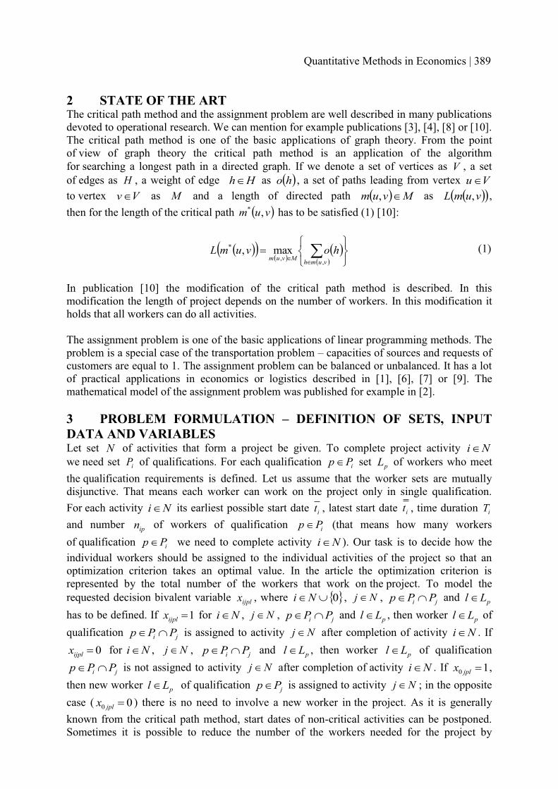
2 STATE OF THE ART The critical path method and the assignment problem are well described in many publications devoted to operational research. We can mention for example publications [3], [4], [8] or [10].The critical path method is one of the basic applications of graph theory. From the pointof view of graph theory the critical path method is an application of the algorithm for searching a longest path in a directed graph. If we denote a set of vertices as V , a set of edges as H , a weight of edge Hh� as � �ho , a set of paths leading from vertex Vu�to vertex Vv� as M and a length of directed path � � Mvum �, as � �� �vumL , ,then for the length of the critical path � �vum ,* has to be satisfied (1) [10]:

� �� �

� �� �

� � <=>

!"#

� ��� vumhMvum

hovumL,,

* max, (1)

In publication [10] the modification of the critical path method is described. In this modification the length of project depends on the number of workers. In this modification it holds that all workers can do all activities.

The assignment problem is one of the basic applications of linear programming methods. The problem is a special case of the transportation problem – capacities of sources and requests of customers are equal to 1. The assignment problem can be balanced or unbalanced. It has a lot of practical applications in economics or logistics described in [1], [6], [7] or [9]. The mathematical model of the assignment problem was published for example in [2].

3 PROBLEM FORMULATION – DEFINITION OF SETS, INPUT DATA AND VARIABLES Let set N of activities that form a project be given. To complete project activity Ni�we need set iP of qualifications. For each qualification iPp� set pL of workers who meet the qualification requirements is defined. Let us assume that the worker sets are mutually disjunctive. That means each worker can work on the project only in single qualification. For each activity Ni� its earliest possible start date it , latest start date it , time duration iTand number ipn of workers of qualification iPp� (that means how many workers of qualification iPp� we need to complete activity Ni� ). Our task is to decide how the individual workers should be assigned to the individual activities of the project so that an optimization criterion takes an optimal value. In the article the optimization criterion is represented by the total number of the workers that work on the project. To model the requested decision bivalent variable ijplx , where � �09�Ni , Nj� , ji PPp 7� and pLl�has to be defined. If 1�ijplx for Ni� , Nj� , ji PPp 7� and pLl� , then worker pLl� of qualification ji PPp 7� is assigned to activity Nj� after completion of activity Ni� . If

0�ijplx for Ni� , Nj� , ji PPp 7� and pLl� , then worker pLl� of qualification

ji PPp 7� is not assigned to activity Nj� after completion of activity Ni� . If 10 �jplx ,then new worker pLl� of qualification jPp� is assigned to activity Nj� ; in the opposite case ( 00 �jplx ) there is no need to involve a new worker in the project. As it is generally known from the critical path method, start dates of non-critical activities can be postponed. Sometimes it is possible to reduce the number of the workers needed for the project by

Quantitative Methods in Economics | 389

postponing the non-critical activities. That is the reason why it is necessary to include postponing of the activities in the model; that means the model also decides about postponing of the individual activities due to waiting for the worker who works on the postponed activity. To model the decisions we define new variable 04iz for Ni� ; the variable models the postponement of activity Ni� with relation of its earliest possible start date it .

4 MATHEMATICAL MODEL The mathematical model that assigns the workers to the activities can be defined as follows:

� � ���� � �

�Nj Pp Ll

jplj p

xzxf 0,min (2)

subject to:

� �

jpNi Ll

ijpl nxp

�� �9� �0

for Nj� , ji PPp 7� (3)

10��Nj

ijplx for Ni� , ji PPp 7� , pLl� (4)

� �

���9�

�Ni

jiplNi

ijpl xx0

for Nj� , ji PPp 7� , pLl� (5)

� �ijpljjiii xMztTzt ���0�� 1 for Ni� , Nj� , ji PPp 7� , pLl� (6)

iii ttz �0 for Ni� (7)

� �1;0�ijplx for Ni� , Nj� , ji PPp 7� a pLl� (8)

04iz for Ni� (9)

Function (2) represents the optimization criterion – the total number of the workers needed to realize the project. The group of constraints (3) ensures that the required number of the workers of the requested qualifications is assigned to each activity. Constraints (4)ensure that each worker is assigned maximally only to single subsequent activity after completion the previous activity. The group of constraints (5) ensures continuity of the workers for the individual activities. The group of constraints (6) models time restrictions of worker assignment (please note that it is assumed in the model that the time the worker need to change the activity is negligible in comparison with the time durations of the activities). Constraints (7) ensure that possible postponing of the activities is done only within admissible time intervals. The groups of constraints (8) and (9) define domains of definition of the variables used in the mathematical model.

The solving process is started with the critical path method which we need to calculate earliest possible start dates, earliest possible finish dates, latest start dates and latest finish dates of the activities. On the basis of the dates we can calculate float times of the individual activities. After calculation the float times (in the proposed mathematical model the calculated time floats are substituted into expression ii tt � ) we can create the proposed model and solve it. In the model it is assumed that all the workers who are assigned to the activity have to be available when the activity starts. But in practice the assumption has not to be satisfied sometimes. In such cases it is possible to decompose the activity into several partial sub-activities; the number of the sub-activities corresponds to the number of work groups that are assigned to the original activity.

390 | Multiple Criteria Decision Making XVIII

5 CALCULATION EXPERIMENTS Solvability of the proposed mathematical model is tested using a simple example. Let us consider a project consisting of 4 activities. Information about the individual activities and the results got by the critical path method are summarized in Table 1. Please note that all the time values are expressed in minutes. Due to the page limitation of the article we present only the simple example. Results of some additional experiments will be presented at the conference.

Table 1: The list of the project activities and the number of the workers of the single qualification

Activity Time duration

Earliest possible start date

Earliest possible

finish date

Latest start date

Latest finish date

Workers of qualification 1

Workers of qualification 2

1 6 0 6 2 8 2 02 3 6 9 8 11 0 13 8 0 8 0 8 0 24 3 8 11 8 11 3 0

To complete the project we need workers of two qualifications. For first qualification we have 3 workers, for second qualification we have 2 workers. The numbers of the workers needed for the individual activities are provided in Table 1 – columns 7 and 8.

Because the project has two isolated branches of activities, it is necessary to incorporate a constraint ensuring that the latest dates of activities 2 and 4 will not be exceeded.

Numerical experiments were performed on PC equipped with the processor Intel® Core™2 Duo E8400 and 3.25 GB of RAM (hardware configuration is important regarding calculation times). After finishing the optimization calculation we found out that the total number of the workers we need to complete the project is equal to 5. A summary of the results got by the experiment is provided in Table 2. A work schedule for the individual workers involved in the project is given in Table 3.

Table 2: Results of the numerical experiment – the time date of the start of the activities

Activity Time duration

Earliest possible start date

Real start date

Latest start date

Activity delay

Workers working on the activity

1 6 0 0 0 0 22 3 6 8 8 2 13 8 0 0 0 0 24 3 8 8 8 0 3

Table 3: Order of activities done by the worker Qualification Worker Order of activities done by the worker*

11 1 (0/6) -> 4 (8/3)2 1 (0/6) -> 4 (8/3)3 4 (8/3)

21 3 (0/8) -> 2 (8/3)2 3 (0/8)3 The worker is not used.

*the first value in round brackets represents the real start date of the activity, the second value the time duration of the activity. It is obvious that the sum of both values has not to be greater than the first value of the following activity for the same worker.

Quantitative Methods in Economics | 391

6 CONCLUSIONS The presented article deals with the combined approach to optimal project planning. It combines the critical path method with the linear mathematical model that is intended for staff planning. The proposed mathematical model is based on the assignment problem and assigns workers to the individual activities. It is assumed in the model that all the workers assigned to the activity must be available when the activity starts. The variables used in the model define assignment of the workers to the individual activities (create their work schedule) and model possible activity delays which bring a decrease in the number of the workers needed for the project. The optimization criterion used in the model expresses the total number of the workers who are involved in the project. In the future, we would like to modify model (2) – (9) so that other optimization criterions can be used (for example to total costs of the workers). Another improvement which could be mentioned is that the model should be able to work with multiple qualified workers.

References [1] Brázdová, M. (2011). Řešené úlohy lineárního programování. Pardubice: Univerzita

Pardubice. [2] Dantzig, G., B. (1993). Linear Programming and Extensions. Princeton: Princeton

University Press. [3] Jablonský, J. (2007). Operační výzkum. Praha: Professional Publishing. [4] Kelley, J., E. and Walker, M., R. (1959). Critical-Path Planning and Scheduling. In:

Proceedings of the Eastern Joint Computer Conference, pp.160–173. [5] Korda, B. (1967). Matematické metody v ekonomii. Praha: SNTL. [6] Palúch, S. (2004). Multi Criteria Optimization in Transport Scheduling. In: Proceedings

of the 12 International Conference Quantitative Methods in Economics (Multiple Criteria Decision Making XII). Bratislava: Ekonóm, pp. 164-169.

[7] Pastor, O., and Tuzar, A.(2007). Teorie dopravních systémů. Praha: ASPI. [8] Rowbotham, F., Galloway, L., and Azhashemi, M. (2007). Operations Management in

Context. 2nd ed. UK, Oxford: Taylor & Francis. [9] Rychetník, L., Zelinka, J., and Pelzbauerová, V. (1968). Sbírka příkladů z lineárního

programování. Praha: SNTL. [10]Volek, J. and Linda, B. (2012). Teorie grafů – aplikace v dopravě a veřejné správě.

Pardubice: Univerzita Pardubice.

Author’s addressdoc. Ing. Dušan Teichmann, Ph.D., Ing. Michal Dorda, Ph.D. VŠB – Technical University of Ostrava, Faculty of Mechanical Engineering, Institute of Transport 17. listopadu 15/2172, 708 33 Ostrava-Poruba Czech Republic email: dusan.teichmann@vsb.cz, michal.dorda@vsb.cz

392 | Multiple Criteria Decision Making XVIII

MULTICRITERIA COALITIONAL GAMES AND BARGAINING THEORY

Michaela Tichá, University of Economics, Prague

Abstract Multicriteria games model situations in which at least one player has more than one criterion. Let consider that every player is able to assign weights to the criteria. In case of noncooperative games, the game is reduced to a one-criterion classic game. In coalitional games the problem remains if players have different weights. It is not possible to simplify the vector payoff function to scalar payoff function. In this paper we analyze the problem using bargaining theory - Nash solution and Kalai-Smorodinsky solution. We formulate two models that by two different ways split the gain of the coalition and we can decide if the coalition can arise or not.Keywords: multicriteria games, game theory, vector payoffs, noncooperative games

JEL Classification: C72 AMS Classification: 91A10

1 INTRODUCTION The multicriteria coalitional game is a class of cooperative games with vector pay-off functions. The players create coalitions depending on what kind of benefit they obtain. The utility of player is the weighted sum of the gains in the individual criteria; the weights are the known preferences of the player. We can see easily what utility the player has if he remains outside the coalition. The problem is that we cannot evaluate the utility of the coalition easily, because it may be different for each player.

Multicriteria coalitional game with known preferences is a triplet (N, v, W ), where N = {1, 2, . . . , n}

is the set of players, n ∈ P represents the count of players. Nonempty subset S ⊆ N of the set of players is called coalition. The characteristic function of the game

v : S → Rm

assigns the gain v(S) ∈ Rm to any coaliton S ⊆ N, m ∈ N represents the count of the criteria (the count of all the criteria of players). We denote vτ (S) - the gain in the criterion τ .

���

���

�

�

nmn

m

ww

wwW

............

...

1

111

is the matrix of preferences of the players, waτ represents the weight of the criterion τ of the player a.

waτ ∈ [0, 1] a ∈ N, τ ∈ {1, 2 . . . , m}

Nawm

a �E���

;118

8

An allocation X(S) is a payoff matrix whose lines represent the payoff for each player from the coalition S. X(S) ∈ Rk×m, k = |S|, xaτ(S) represents the payoff of the player a in the criterion τ in the coalition S.

xaτ (S) ∈ [0, vτ (S)] a ∈ N, τ ∈ {1, 2, . . . , m},

� �mSvxk

aa ,...,2,1);(

1�E��

�

888

Quantitative Methods in Economics | 393

The characteristic function determines the total payoff of the coalition in each criterion. We assume that

vτ (S) ≥ 0 ∀τ ∈ {1, 2, . . . , m} for all the coalitions S. We assume that in the case of coalition membership the players can have only gain and they cannot lose. The allocation X(S) is then the particular allocation of the gain to the individual members of the coalition.

2 ASSUMPTIONS ABOUT THE BEHAVIOR OF PLAYERS We know the preferences of the players, which are expressed by the vector of weights. Weexpect they decide only according to the utility, which is the weighted sum of the gain of the individual criteria. Let us consider a player α ∈ S and the distribution of the gain of the coalition X(S). Then the utility of the player α from the coalition S is

uα(S) = wα xα (S) + wα xα (S) + . . . + wαmxαm(S).The players make decisions based on their utility and in the case of equal utilities they prefer a coalition with a smaller number of members in which they have greater strength. For this purpose we assume that players enter into a coalition with a larger number of members, if they obtain at least ε; ε > 0,. The players may have a different parameter εa; however, there is no loss of generality, if we assume that they all have the same parameter.. The player α wouldprefer a coalition of S before coalition S′, where |S| > |S′|, unless

uα(S) ≥ uα(S′) + εε symbolizes the amount which a player must obtain by entering into a coalition to be willing to cooperate and not to prefer a coalition with a smaller number of members in which he has more power. This parameter is important because otherwise the solution where only one player would get all the extra gain is possible. Another assumption is that the game allows transferable gain. The solution concept for the game with known preferences of the individual players has the difficulty that if the players do not have the same preferences, the problem remains, how to appreciate the gain of the coalition. For each player the gain of the coalition represents different utility, therefore the game is not simplified to a game with scalar payoff functions. Furthermore, we need to find a way how to divide the gain among the coalition members. We suggest using models of bargaining theory. There are four main ways of gains distribution - egalitarian solution, utilitarian solution, Nash solution and Kalai-Smorodinsky solution. In this article, we shall consider the Nash solution and the Kalai-Smorodinsky solution, eg. (Mas-Collel et al., 1995). In the case of Nash solution we assume about the distribution X(S) that the gain v(S) is distributed among the individual players of the coalition S so that the product of the utilities of the players of the coalition is maximized. Obviously, just under the conditions that each player has his utility higher by at least ε in comparison with smaller coalitions. The Kalai-Smorodinsky solution maximizes the benefits of the sum of guaranteed utility,provided that players get extra utility gained through cooperation divided in the same proportion as if everyone had a winning addition to himself. For example, if the first player has utility 1 if he is not in any coalition and the second player has utility 2 if he is not in any coalition then the extra utility from cooperation will be divided in proportion 1:2. 3 FINDING THE DISTRIBUTION OF THE GAIN IN COALITIONSFirst, we determine which coalitions arise and which do not. We proceed from the coalition with the least number of members to the grand coalition. For each coalition we determine whether it is rational for its members, i. e., whether each member has higher utility compared tocoalitions with fewer members, in which he is a member. If it is rational for each member,

394 | Multiple Criteria Decision Making XVIII

..

the coalition can arise. If there is any member for whom it is not rational, then the coalition cannot arise. 1) |S| = 1 For the player α, who is alone, his gain is given because it is not divided among several players. So his utility is given, too, it is easy to compute:uα({α}) = wα1v1({α}) + wα2v2({α}) + . . . + wαmvm({α}).2) |S| = 2 In the case of two-member coalition it is not so easy to determine the utility of the players from the coalition. First it is necessary to divide the gain of the coalition in all criteria among the players. The distribution must be nonnegative and the gain has to be completely divided. Both players must have higher utility compared to their utility when they are alone. If there is a solution that satisfies these conditions, the coalition is profitable for the players and it arises. The distribution is also important; we shall discuss it in the next step. Denote by f ((u(S) − u∗) function of the vector of the utility of players, where u∗ is a vectorof utilities that individual players have without any cooperation. We want to maximize this function. In the case of Nash solution the players split the gain so that they may maximize the product of the utility of the players (when no one has lower utility compared to the situation when he is not in any coalition), i.e., we maximize

f ((u(S) − u∗) = (uα({α, β}) − uα({α}))(uβ ({α, β}) − uβ ({β})).In the case of an Kalai-Smorodinsky solution the players split the gain so that they may maximize sum of the utility of the players reduced by their utility if they were alone under the following condition:

f ((u(S) − u∗) = (uα({α, β}) − uα({α}))+(uβ ({α, β}) − uβ ({β}))under the condition

� �� � � �� �� �� � � �� �

� �� � � �� � � �� �� �

� �� � � �� � � �� �� �.

,

,

,,

1

1

�

�

�

�

��

���

��

m

m

vvvw

vvvw

uuuu

8

888;8

8

888�8

;;

��

;�;�

;�;�

;;��;�

On the right side of the equation, there is share of the utilities from the gain, if it had been assigned to a given only one player (scalar product of the gain of the coalition and weights of the criteria of the player). On the left side of the equation is the share of utilities from the allocation. We find the allocation X({α, β}) of the two-member coalition of the player α and the player β by maximization

f ((u({α, β})) − u∗) under additional conditions:

� nonnegative allocation X({α, β})xα1 ≥ 0 …

xαm ≥ 0 xβ1 ≥ 0 …xβm ≥ 0

� the gain in individuals criteria 1, . . . , m is completely divided xα1 + xβ1 = v1({α, β}) …xαm + xβm = vm({α, β})

Quantitative Methods in Economics | 395

� the player α, respectively β has the utility from the coalition higher at least by ε,compared to the situation in which he is alone. uα({α, β}) ≥ uα({α}) + εuβ ({α, β}) ≥ uβ ({β}) + ε

And uα({α, β}) = wα1xα1({α, β}) + wα2xα2({α, β}) + . . . + wαmxαm({α, β})uβ ({α, β}) = wβ1xβ1({α, β}) + wβ2xβ2({α, β}) + . . . + wβmxβm({α, β}) The objective function is limited, so if there is a feasible solution, then there is an optimal solution - the distribution of the gain (Bisschop, 2001). If there is no feasible solution, the coalition is ineffective for at least one player and shall not arise. We solve this linear program for all two-member coalitions. This is what we assign to eachcoalition S, which does not arise because it is not profitable for any of players:

xaτ (S) := 0 ∀a ∈S, ∀τ ∈ 1,2, . . . m.3) |S| = z; z = 3, . . . , nWe use the same procedure for |S| = 3, then for |S| = 4 etc. up to |S| = n. For every coalition Swe solve the following program:

max f ((u(S) − u∗)xaτ ≥ 0 ∀a ∈ S, ∀τ ∈ {1, 2, . . . , m}

��Sa

xaτ = vτ (S) ∀τ ∈ {1, 2, . . . , m}

ua(S) ≥ ua(S′) + ε ∀a∈ S; ∀S′ ∈ {S′; a ∈ S′ ∧ |S′| < |S|}

Where ui(S) = ��

m

18

wiτ xiτ (S).

For all coalitions S, that shall not arise because they are not profitable, we assign xaτ (S) := 0 ∀a ∈S, ∀τ ∈ 1,2, . . . m.

Subsequently we solved ��

��

���

n

ï in

2

programs. In the case of Kalai-Smorodinsky solution there is

a linear objective function so we can solve it by methods of linear programming. In the case of Nash solution we maximize the product which is not a linear objective and we have to use methods of nonlinear programming. In the previous step we determined for each coalition whether it can arise and, if so, how wedivide the gain among the players. If the coalition is profitable for all its members and isformed, then the program will find a solution. If the program does not find any optimum, then the coalition shall not arise.

4 CONCLUSION In the paper, we examined the multicriteria cooperative game in which we know the preferences of the players in the form of weights. We can also consider that we know the preferences in any other form (e.g., order or scoring of individual criteria) and we can calculate the weights on the basis of modeling methods applied to user preferences (Vincke, 1992). Knowing the preferences of the players we compare the utility of the players. The utility of a player is the weighted sum of the individual criteria. We can easily determine the utility of a player when he is alone. However, in the case of (at least) two-member coalition we cannot easily determine the benefit of the coalition because the players usually have different preferences (weights). In this article we considered two solutions – the Nash solution and the Kalai-Smorodinsky solution. We maximized the objective function under the conditions that neither of the players attains lower utility, compared to being in coalition with a smaller

396 | Multiple Criteria Decision Making XVIII

number of members. As a result, we found out if the coalition is profitable for players and if it can arise or not.

Acknowledgements: This work was supported by IGA VŠE, project no. F4/54/2015.

References [1] Bisschop, J. (2001). Optimization modeling. Haarlem: Paragon Decision Technology Inc. [2] Mas-Collel, A. and Whinston, M. (1995). Microeconomic Theory. Oxford: Oxford

University Press. [3] Vincke, P. (1992). Multicriteria Decision-Aid . Chichester: Wiley.

Author’s addressRNDr. Ing. Michaela TicháUniversity of Economics, Prague, Faculty of informatics and statistics, Department of Operations research and Econometrics W. Churchill Sq. 4, 130 67 Prague Czech Republic email: xticm11@vse.cz

Quantitative Methods in Economics | 397

METHODOLOGY FOR DETERMINING INTEREST RATES - AN INTERNATIONAL TREND

�Nenad Vunjak, University of Novi Sad, Faculty of Economics in Subotica, Dragan Stoji�, University of Novi Sad, Faculty of Economics in Subotica,

Jelena Birovljev, University of Novi Sad, Faculty of Economics in Subotica, Jovana Ivan�evi�, University of Novi Sad, Faculty of Economics in Subotica,

Jelena Vitomir, University of Novi Sad, Faculty of Economics in Subotica

AbstractMeasuring and determining interest rate provides keys to using derivatives to control interest rate risk, and controlling interest rate risk in a mortgage-backed securities derivative portfolio. This paper objective includes necessity of measuring yield curve risk, swaps and exchange-traded options and related products, and describes how to measure and control the interest rate of risk of a bond portfolio or trading position. Measuring and determining interest rate is a systematic evaluation of how to measure and control the interest rate risk of a bond portfolio or trading position. The authors construct a verbal flow chart, defining and illustrating interest rate in regards to valuation, probability distributions, forecasting yield volatility, correlation and regression analyses. Hedging instruments discussed include futures contracts, interest rate swaps, exchange traded options, and credit derivatives. Outcomes of this paper will be that how to find up-to-date information on measuring interest rate with derivatives, quantifying the results of positions, and hedging. Keywords: interest rates projection, degree of risk, time series JEL Classification: E43 AMS Classification: 91B28 1 INTRODUCTIONThe sophistication of the financial markets, as well as the proliferation of new financial instruments for risk management (financial derivatives), spawned the need for the introduction of the reference interest rates on the money market. These new instruments have contributed to the expansion of liquidity of the London interbank market, it was necessary to establish a benchmark for rates on loans, as the price of the new financial products - swaps and options. The Association of Banks in the UK (BBA) established a set of working groups, whose work spawned BBA standard for interest rates on swaps (BBAIRS - British Bankers' Association Interest Rate Swaps). This standard also defined the interest rate for settlement between banks in a separate section, based on which the mechanism of today's LIBOR were derived. The first LIBOR interest rates were publishedon January 1st 19861. LIBOR is the rate of interest paid on aloan from one private or public bank to another (excluding centralbanks) and it serves as a reference for many types of interbankcredit as well as for bonds and household credit. LIBOR and EURIBOR are by far the most prevalent benchmark reference rates usedin euro, US dollar, and sterling over the counter (OTC) interest ratederivatives contracts and exchange traded interest rate contracts and mortgages. BELIBOR is the reference interest rate for dinar funds offered by the Panel of banks, on Serbian interbank market. It is calculated as the arithmetic average of quotations remaining

������������������������������������������������������������1 Taken from http://www.bbalibor.com/bbalibor-explained/the-basics

398 | Multiple Criteria Decision Making XVIII

after eliminating the highest and lowest rates, with two decimal places. Depending on the maturity of the offered funds varies weekly, biweekly, monthly, bimonthly, quarterly, and semi-annual BELIBOR. This is the basic interest rate for dinar loans from banks in Serbia, and has the function of the interest rate at which the leading Serbian banks are willing to lend to each other dinar deposits. This rate of interest shall be published for specific periods of time up to one year. 2 PRIOR LITERATURE ON LIBOR FIXING On 16 April 2008, theWall Street Journal published a front-page storyin its European edition that suggested that the turmoil in global financialmarkets had led panel banks to deliberately submit artificially lowrates to the daily US dollar LIBOR fixing to avoid the stigma that camewith submitting higher rates (Mollenkamp, C. (2008, April 16). Finance markets on edge as trust in Libor wanes; bankers and traders worry that key rate is being manipulated. The Wall StreetJournal, A1.) The effect of erroneous LIBOR extends beyond the financial markets. In addition to provide a biased interbank lending cost, Stenfors (2014) affirms that it corrupts a ‘‘key variable in the first stage of the monetary transmission mechanism’’.The importance of a good pricing system is based on its usefulness for making decisions. As Hayek affirmed ‘‘we must lookat the price system as such a mechanism for communicating information if we want to understand its real function’’. If the price system is contaminated, but perceived as pure, the effect could reach also the real economy, making it difficult to finda way out the financial crisis. Van Kan, J. (2008, May 6). Turn away from screens for the way to greater Libor accuracy. Financial Times, 23: Evidence that US dollar LIBOR was unduly low during early2008 came from several sources. Anecdotally, a number of bankerscomplained that they could not raise funding at the published LIBOR fixing. Snider and Youle (2010), who asserted that LIBOR submissions by some member banks were beingunderstated, suggested that the reason for this situation was notbecause the concerned banks were trying to appear strong, especiallyduring the financial crisis period of 2007 through 2008, butrather because the banks sought to make substantial profits on theirlarge LIBOR interest linked portfolios. The most complete study was made by Abrantes-Metz et al. (2012). The authors examined data on both the US dollar LIBOR fix andquote submissions by US dollar LIBOR panel banks for evidence consistentwith manipulation of the LIBOR fixing. Monticini and Thornton (2013) tested for evidence consistent withlowballing by examining the spread between US dollar LIBOR andrates on large certificates of deposit (CDs). The authors found four statisticallysignificant structural beaks in the three-month US dollar LIBOR –CD spread over the period from January 2004 to December 2010: a -13.0basis point break in mid-June 2005, a -4.3 basis point break in early July 2007, a +13.9 basis point break in December 2008 and a -10.5basis point break in mid-December 2009. Poskitt and Dassanayake (2015) We test the lowballing of submissions to the three-month US dollar LIBOR fixing by panel members using asimple two-equation model.We find evidence in the quote behaviour of a handful of banks during a period ofextreme stress in interbank markets that the submission of high quotes is associated with stock price declinesand that stock price declines encourage the submission of low quotes the following day. Bariviera et al. (2015) we uncover such unfair behavior by using a forecasting method based on the Maximum Entropyprinciple. Our results are robust against changes in parameter settings and could be of great help for market surveillance. Fouquau and Spieser (2015) in paper contributes to the crucial problem of LIBOR malfunctioning due to its manipulation by banks, aphenomenon described clearly in the FSA Inquiry Report published in September 2012.

Quantitative Methods in Economics | 399

Finally, Chen and Zhou (2013) analyzed financial products linked to seven-days and three-months-SHIBOR (The Shanghai Interbank Offered Rate) between 2010 and 2011, and do a hypothesistesting that are there some manipulations of SHIBOR.The testing result showed that during the date of salesfinancial products, the higher quoting SHIBOR behavior may be existing, in order to raise people's expectations ofyield of financial products, but lower quoting SHIBOR behavior may not be existing at the date of calculating interest of financial products. 3 DATA AND METHODOLOGY BELIBOR values for 1 and 3 months were taken from National Bank of Serbia Statistical office. These values are averaged daily values calculated monthly. Repo rates and deposit rates of individual banks were taken from National Bank and Belgrade Stock Exchange respectively. We use Eviews 7 for all the calculations in this paper. Following Poskitt and Dassanayake (2015) as well as Fouquau and Spieser (2015) we test whether the lowballing of LIBOR caused anomalous movements on Serbian financial market. We commence the investigation testing the stability of BELIBOR when put in relation with other benchmark rates. Naturally connected to BELIBOR is the repo rate (R), applied to open market operations (collateralized lending transactions) of the National Bank. Being economically close, it is natural to assume a linear relationship between these two rates. To take into account the difference between unsecuredand secured transactions, we added a proxy of risk representedby the banks’ deposit rates (D). We focus on the 1 monthBELIBOR because it is the natural indicator of the banks’ liquidityposition. For each institution, we then estimated the following equation:

1 2t t t tBELIBOR R D u� ; ;� C C C , Where ut represents residual terms. Stable relationship is a priori supposed. To testthe (in)validity of the hypothesis we first estimate the coefficients and then apply CUSUM test. Results are given in Table 1 and Figure 1 respectively. We observe the high level of explained variations in the BELIBOR values. Furthermore, the results of CUSUM test for a critical value of 5% are inconclusive, since there is no clear regime switching after a certain date. One can notice the short ‘escape’ from 5% band in July 2008, returning to ‘normal’ regime in April 20092. This is somewhat in line with the results of Fouquau and Spieser in terms of allocation the date of break. However, these authors rejected the stability since the CUSUM line broke the band without returning. Outside the crisis period, there is no evidence for possible manipulation. Further analysis applying Chow breakpoint test, as well as Quandt-Andrews Breakpoint test, suggest the existence of the break point in between July 2008 and April 2009. We continue the analysis of interest rates in Serbian market during the period of crisis eruption through the prism of market activity. Due to lack of reliable data, we are only able to pursue the equation concerning Commercial Bank of Serbia (Komercijalna banka) since it was the only still being listed on Belgrade Stock Exchange3. One of the risks that banks face especially during the period of crisis is that the investors may withdraw funding based on noisy signals of bank solvency (Huang & Ratnovski, 2008).

������������������������������������������������������������2For critical value of 10% we could not reject the regime switch 3Marfin Bank is also listed, but without trading or price change.

400 | Multiple Criteria Decision Making XVIII

Table 1. Coefficients outputDependent Variable: BELIBOR Method: Least Squares Sample: 2006M01 2012M06 Included observations: 78 Variable Coefficient Std. Error t-Statistic Prob. C 0.011769 0.003245 3.627251 0.0005 DEPO -0.238504 0.031613 -7.544390 0.0000 REPO 1.192501 0.023576 50.58155 0.0000 R-squared 0.973887 Mean dependent var 0.143196 Adjusted R-squared 0.973191 S.D. dependent var 0.042424

Figure 1: CUSUM test and the stability between BELIBOR, Repo and deposit rates

-30

-20

-10

0

10

20

30

IV I II III IV I II III IV I II III IV I II III IV I II III IV I II

2007 2008 2009 2010 2011 2012

CUSUM 5% Significance

One of the problems that e.g. Bank of America, Bank of Tokyo-Mitsubishi, Barclays, Citibank etc. had was the large holdings of increasinglyvalueless mortgage-backed securities. In such an environment, a high LIBOR submission could have been interpreted as a signal that the bank inquestion had a large amount of troubled assetsin its portfolio. Any such perception would be quickly reflected inthe panel member’s stock price (Poskitt and Dassanayake, 2015). We investigate whether this bank had deliberately reported lower BELIBOR. The lowballing hypothesis as follows can be stated as follows:

1 2 3 4 5 *jt mt jt jt jt tR R VOL rank dummy dummy rank u� ; ; ; ; ;� C C C C C C , where Rjt is the return on the stock of bank j (namely Komercijalna banka) on day t, Rm,t is the return on the market index, BELEX15 on day t, VOLjt is the change in price volatility of the underlined stock (given in the Figure 2), and serves as a signal for the change in probability of default; rankit is the ranking of the quote submitted by bank j on day t4, dummy is a variable that takes the value of 1 duringperiod of financial stress and 0 otherwise5, and ut is a random error term. The actual data used in the coefficients estimation range from August 2007 up to April 2009. Regression estimates are given in the Table 2.

������������������������������������������������������������4Due to impossibility of obtaining this piece of information we used a random number generator for obtaining various possible realizations of this variable and pursued the coefficient estimations accordingly. 5The period of financial stress was taken to be from March 1st 2008 until August 31st 2008, covering the period of colapse of Bear Stearns.

Quantitative Methods in Economics | 401

Figure 2: Volatility of returns – Komercijalna Banka(KMBN)

We observe extremely low R square value. Furthermore, the only statistically significantly different from zero are the coefficients of variables VOL and dummy. During periods of market stress, we expect higher BELIBOR submissions to stand for the sign that the bank is having trouble raising funds in the wholesale market and for the increased likelihood of default to be reflected in stock price decreases i.e., the OLS estimates of Ä5 will be significantly greater than zero: we test the hypothesis that:

1. Ä5 > 0 and 2. Ä3 + Ä5 > 0

Table 2: Coefficients output

Dependent Variable: KMBN (Rjt) Method: Least Squares Sample (adjusted): 1/03/2008 4/30/2009 Included observations: 334 after adjustments Variable Coefficient Std. Error t-Statistic Prob. C -0.022837 0.009978 -2.288649 0.0227 belex -0.086722 0.093089 -0.931599 0.3522 vol 0.221454 0.094406 2.345758 0.0196 rank 0.003341 0.003289 1.015854 0.3104 dummy 0.027142 0.015324 1.771222 0.0775 dummy*rank -0.008003 0.005350 -1.495955 0.1356 R-squared 0.024688 Mean dependent var -0.003885 F-statistic 2.660514 Durbin-Watson stat 2.260914

Table 3: Results of the Wald test

Wald Test: Test Statistic Value df Probability t-statistic -1.103687 328 0.2705 F-statistic 1.218126 (1, 328) 0.2705 Chi-square 1.218126 1 0.2697 Null Hypothesis: C(4)+C(6)=0

Using Wald test (Table 3) we can’t accept these hypotheses therefore we can conclude that the bank in question did not involve in spurious submissions of BELIBOR rate.

402 | Multiple Criteria Decision Making XVIII

5 CONCLUSION The money market is a powerful mechanism for the transfer of short-term financial resources from a surplus to deficient economic actors. Although the movements in the money market are directed through the activities of a large number of participants, it is alsoinfluenced by the lending activities of commercial banks. Money market functions as a collector of important information in the context of the risk profile of banks and systemic risk of the economy, and sublimates all the information in the reference price of money - interest rate on interbank loans. Based on the basic price of money, the bank defined set lending rates charged on loans. Besides the role ofproviding liquidity of the banking sector, money market through the mechanism of interest rates, to directing scarce financial resources in the most productive alternative to the tolerant (acceptable) level of risk. Also, it allows the marketisation of the budget deficit, as well as the transfer of monetary policy impulses to the banks, the financial and the real sector of the economy. References [1] Abrantes-Metz, R., Kraten, M., Metz, A. and Seow, G. (2012). Libor manipulation?.

Journal of Banking & Finance, 36(1), pp.136-150. [2] Bariviera, A., Martín, M., Plastino, A. and Vampa, V. (2016). LIBOR troubles:

Anomalous movements detection based on maximum entropy. Physica A: Statistical Mechanics and its Applications, 449, pp.401-407.

[3] Chen, L. and Zhou, Z. (2013). Are there Some Manipulations of SHIBOR: A Hypothesis Testing based on Financial Products Linked to SHIBOR. Procedia Computer Science, 17, pp.939-944.

[4] Fouquau, J. and Spieser, P. (2015). Statistical evidence about LIBOR manipulation: A “Sherlock Holmes” investigation. Journal of Banking & Finance, 50, pp.632-643.

[5] Gyntelberg, J. and Wooldridge, P. (2088). Interbank rate fixing during the recent turmoil. BIS Quarterly Review, 2008(March), pp. 59–72.

[6] Huang, R., and Ratnovski, L. (2008) The dark side of bank wholesale funding. Federal Reserve Bank of Philadelphia Working Paper No. 09-3.

[7] Mollenkamp, C. (2008). Finance markets on edge as trust in Libor wanes; bankers and traders worry that key rate is being manipulated. The Wall Street Journal, p. A1.

[8] Monticini, A. and Thornton, D. (2013). The effect of underreporting on LIBOR rates. Journal of Macroeconomics, 37, pp.345-348.

[9] Poskitt, R. and Dassanayake, W. (2015). Modelling the lowballing of the LIBOR fixing. International Review of Financial Analysis, 42, pp.270-277.

[10]Snider, C., and Youle, T. (2010). Does the LIBOR Reflect Banks’ Borrowing Costs? UCLA Working Paper.

[11]Stenfors, A. (2014). LIBOR deception and central bank forward (mis-)guidance: Evidence from Norway during 2007–2011. Journal of International Financial Markets, Institutions and Money, 32, pp.452-472.

[12]Taylor, J. and Williams, J. (2008). Further results on a black swan in the money market. Federal Reserve Bank of San Francisco Papers.

[13]Van Kan, J. (2008). Turn away from screens for the way to greater Libor accuracy. Financial Times. [online] Available at: http://www.ft.com/intl/cms/s/0/3e918d0e-1b04-11dd-aa67-0000779fd2ac.html#axzz4BGhUSjao [Accessed 11 Mar. 2016].

Author’s address Dragan Stojic, PhD, Assistant Professor University of Novi Sad, Faculty of Economics Subotica, Department of Business Informatics and Quantitative Methods Segedinski put 9-11, 24000 Subotica Serbia

Quantitative Methods in Economics | 403

CAN CONSUMERS' CONFIDENCE CONTRIBUTE TO CYCLIC MOVEMENT OF THE ECONOMIC ACTIVITY?

Jana Závacká, Faculty of Economics, VŠB-Technical University of Ostrava

Abstract The main goal of this paper is to present consumers' confidence as an important source of cyclical movement of the economic activity. I use a simplified agent-based model with a single production sector and consumers (agents). The confidence (optimism/stableness/ /pessimism) spreads by interactions among consumers and according to the macro state of the economy on the lattice of consumers. The aggregate level of confidence in society reflects the consumers' expectations about their future incomes together with their preferences between current and future consumption and determines aggregate demand for consumption spending. I found that the model is capable of generating persistent endogenous business cycles. The consumer confidence could be considered as a one of the variables contributing to the cyclical movement of the economic activity.

Keywords: ACE model, business cycle, consumer confidence

JEL Classification: C63, E27 AMS Classification: 91B69

1 INTRODUCTION The role of confidence in the determination of economic activity was already stressed by Keynes (2007). Acemoglu and Scott (1994), Bram and Ludvigson (1998), Carrol et al.(1994) and Souleles (2009) confirmed the significance of the confidence indicator to predict the behavior of economic activity. However, the significance was proved only on the empirical studies with the confidence measured on the macroeconomic level and the confidence was considered only as an instrument for prediction. In the recent years, the spread of the waves of optimism or pessimism in the society has started to be modeled also from the bottom up, by using agent-based models. In this paper, I model the spread of confidence in the society through interactions among consumers in an simplified agent-based model in the sense of Westerhoff (2010). I found that the model is generating a cyclical movement of consumers' confidence with the cyclical effect on aggregate demand and hence on economic activity. The article is organized as follows. In section 2, the model is introduced. In section 3, I present the simulation results of the model. Section 4 concludes.

2 THE MODEL The model is constructed to simulate the behavior of macroeconomic variables with respect to the level of consumers' confidence generated on micro economic level. The simulation of the model consists of two kinds of steps - macro steps and micro steps. The state of the economy, presented on macroeconomic variables such as an aggregate demand, an aggregate supply etc. is evaluated during macro steps. Each macro step consists of T micro steps. During these micro steps the simulation of consumer confidence is driven. Heterogeneous agents (consumers) form their confidence opinion on the basis of their neighbors and state of economy from last macro step. After this simulation the new macro step follows and the new state of the economy is evaluated. Following this way values of macroeconomic variables are determined from the bottom up. The distinction between two kinds of steps was already used in Westerhoff (2010) and increases the transparency of the model.

404 | Multiple Criteria Decision Making XVIII

2.1 Forming the state of confidence The behavior of agents is simulated on the lattice where interactions in neighborhood are allowed. In this lattice every agent is deciding to be either optimist ( i

tO 8 ), who wants to increase his consumption spending, a pessimist )( i

tPes 8 , who wants to decrease his consumption spending, or stable agent )( i

tSt 8 , who does not want to change the level of his consumption spending in no direction (proportional to his average income).

I divide the business cycle according to the state of confidence into four phases - two phases of expansion and two phases of contraction. During the expansion the wave of optimism is spread. The first phase covers the growth of optimism in the society, until its maximum when all agents became optimists (let us assign it as a moment A). The second phase stands for the decrease of optimism until all agents became stable. The contraction represents the spread of the wave of pessimism and is divided into the phase of growth of pessimism until its maximum (the moment B, all agents are pessimists) and decline of pessimism until all agents became stable again (forth phase). Following the idea of Westerhoff (2010), the level of confidence is formed between every macro step t and t+1 during T micro steps. In every micro step τ there is one agent randomly chosen. This agent decides about his state of confidence, according to probabilities

6!

6"#

�����

�n,contractioin 0

expansion,in )exp(1

)exp()( i

tSt

Yt

it

St

Yt

itOP

8

8

8 ;��;��

(1)

6!

6"#

���� n,contractioin

)exp(11

expansion,in 0)(

it

St

Yt

itPesP

8

8

;��(2)

).()(1)( it

it

it PesPOPStP 888 ��� (3)

The probabilities depend on two global parameters Yt� and S

t� and local parameter it8; . The

parameter Yt� is defined as

6!

6"

#

���0�

�����

����

����

),(41

),(41

4321

4321

tttttY

tttttY

Yt

YYYYY

YYYYY

�

�� (4)

and represents the sensitivity of consumer to the change in the aggregate income tY . To reduce the impact of temporary fluctuations in income, the comparison is done rather with the average from the last four period than with the last observed income. Differently from Westerhoff (2010) I introduce another global parameter S

t�

6!

6"

#

��else,0

B,moment after then contractioin A,moment after theexpansion in

S

S

St �

�� (5)

Quantitative Methods in Economics | 405

which represents the sensitivity to savings. The parameter is activated during the second phase of expansion to support the preference of savings (which are also covering investment into housing) and in the second phase of contraction, to decrease the preference for saving to maintain the consumption on the same level (in accordance with Pollin (1988)). In accordance to Westerhoff (2010) I introduce one local sensitivity parameter

),t###( it

it

it

it SPO 8888 ;; ��� (6)

where β is sensitivity parameter and itO 8# , i

tP8# , itS 8t# is the number of neighbors of the

chosen agent i,, which are optimists, pessimists and stable, respectively.

2.2 Macroeconomic part of the model The endogenous business cycle movement is presented on the simplified agent-based model of a closed economy, consisting of one type of heterogeneous agents - consumers, and of one production unit - firm. For the simplicity I do not consider any fiscal nor monetary authority. I take prices as constant and normalize the price of one unit of goods to 1. The investment is only in the form of inventory goods and the interest rate for saving is equal to 0. Consumers in the model determine the aggregate demand for goods. In every period they obtain a salary from firms i

tY . For the simplicity the total income tY is always uniformly

distributed among all agents (M). Every consumer forms his individual demand for consumption i

tID according to the rational expectation permanent income hypothesis (REPIH, Hall, 1978). The expectations about future incomes of consumer are built on the basis of consumer confidence and the average income from the last periods (to eliminate the effect of temporal fluctuations in accordance with the permanent income theory (Friedman, 1957). The consumer confidence is used as a proxy not only for the expectation of the consumer's future income, but also for his preferences between current and future consumption spending. In accordance with Abel (1990), I assume the habit in consumer behavior expressed as a share γ of the individual consumption spending from the previous period i

tC 1� . Each consumer i is in the time t forming his individual demand for consumption spending for future period i

tID according to his state of confidence as

666

!

666

"

#

������

�����

������

�

����

����

����

pessimist,)(41)1)(1(

stable,)(41)1(

optimist,)(41)1)(1(

3211

3211

3211

it

it

it

it

it

it

it

it

it

it

it

it

it

it

it

it

YYYYxC

YYYYC

YYYYxC

ID

,,

,,

,,

(8)

where x is an extrapolation constant. Summing up individual demands for all agents, I obtain the aggregate demand for consumption tAD

,4

)]#(#1)[1( 1231

1

ttttttt

M

i

itt

YYYYPO

MxCIDAD

��������� ���

��� ,, (9)

where tO# is the number of optimists and tP# the number of pessimists at time t.

406 | Multiple Criteria Decision Making XVIII

I assume that there is a competitive environment and the production is represented by a unique producer (firm) with the zero profit. This firm forms the aggregate supply tAS , which consists of the inventory goods of firm accumulated from previous periods 1�tI and the current production tQ . Consumers are always immediately paid for their production tQ .Because the profit is zero, the price of the goods is equal to their costs and so the total income at time t is equal to production. The firm always tries to satisfy the aggregate demand, but at the same moment does not want to let the amount of inventory goods grow too fast. For this reason the strategy of the firm about aggregate supply differs within the business cycle. In the case of contraction, the firm sets the aggregate supply as the quantity of goods demanded at the last period tAD and tries to get clear of the inventory, hence is willing to produce just

tt IAD Q��1 , where κ is the decreasing inventory parameter. During expansion, the firm has an intention to increase the production according to the confidence in the society and would like

to produce 1))#(#1( ��� ttt QPOMx at time t. The firm is also adjusting production with a

level of smoothing δ. The aggregate production tQ is

}))#(#1(,max{)1( 1111 ���� ������ ttttttt QPOMxIADQQ QFF . (13)

According to the matching on the goods market (which is also used in the agent-based model of Riccetti et al. (2014)) the final realized consumption at time t is determined as

tttt CASADEQ �� },min{ (14)

This result determines savings tS , the amount of consumers’ assets tA and other equalities

,.t

it

tit AD

IDCC � (15)

ttt CYS �� (16)

,1 ttt SAA �� � (17)

.ttt CASI ��(18)

3 SIMULATION RESULTS I programmed the whole model in the software R. I have constructed a simple lattice of 10000 agents in the form of a torus, so every agent has exactly four neighbors. I run the model for 10000 micro steps and 300 macro steps. The model was mainly calibrated in line with Westerhoff (2010). Values of all parameters could be found in Table 1. As each run of the model is according to randomness generating business cycles with different lengths and timing, I will present the evolvement of the key macroeconomic variables on one simulation of the model. Parameter Description Parameter DescriptionαY=5 Income sensitivity parameter γ=0.8 Consumption smoothing parameterαS=-10 Time preference parameter δ=0.7 Production smoothing parameterβ=1 Local sensitivity parameter κ=0.6 Melting inventory parameterx=0.1 Extrapolation parameter

Tab. 1. Model parameters.

Quantitative Methods in Economics | 407

Let us firstly look at the spread of the waves of optimism/pessimism on the micro level. To make it more transparent, I present the graphical spread of the mood in the lattice through the set of maps for the macro steps 60 till 120 in Figure 2. The optimists are depicted in green, stable agents with the black and pessimists with the red color. In Figure 2. we can see how the mood is spreading firstly from the majority of stable agents (macro step 60) into the majority of optimists (macro step 68), back into the majority of stable agents (macro step 84), then into the majority of pessimists (macro step 96) and again back into the majority of stable agents (macro step 108). Then the cycle repeats.

Fig. 2. The spread of the confidence. Fig. 3. The confidence, AD, AS and Y.

The spread of the confidence in the aggregate form together with the evolvement of the aggregate income (Y) and the aggregate supply (AS) and demand (AD) is presented in the Figure 3. The total number of optimists, stable agents and pessimists in the society is expressed by the green, black and red line, respectively. We can see from the Figure 3. how the waves of confidence are changing. The green optimistic wave starts from the state when all agents are stable, spreading until all the agents became optimists and returning back into the state of all stable agents. Then the pessimistic wave is spread in the similar way. In the second graph in the Figure 3 I present the evolvement of the aggregate demand and the aggregate supply. We can see that the cyclical movement of the aggregate demand corresponding to fluctuations in consumer confidence. The aggregate supply is typically in excess of aggregate demand: this was somewhat expected, as the firm prefers to accumulate some controlled inventory instead of failing to meet the aggregate demand. In case of expansion, the aggregate supply is following the growing trend of aggregate demand, holding some inventory goods. In case of contraction the production and the amount of inventory goods is decreasing. The aggregate income, representing the economic activity, is presented in the third graph in Figure 3. We can see that an endogenous cyclic movement of economic activity appears. The irregularity of cyclic movement is caused by randomness in the spread of optimistic/stable/pessimistic mood among agents. The contractions of the income corresponds to the pessimistic waves in confidence, the expansion to the optimistic waves. The turning points are occurring during the states when all agents became stable.

408 | Multiple Criteria Decision Making XVIII

4 CONCLUSION The paper introduced a possible endogenous source of business cycle movement in the economic activity. This source was presented on the simple agent-based model with heterogeneous consumers and one production unit - firm. The cyclical movement was, according to the model setting, coming up from the spread of consumer confidence, through the cyclical behavior of the aggregate demand. The model was set so that in the phases of expansion the growth of consumption was firstly supported by the growth of income, but after some period slowing by the preference of savings. This preference in the combination with the firm's expectations finally led to the stopping of the consumption growth. Then the economic activity turned down. The decline was from the beginning caused by the adjustment of desired consumption to decreasing incomes, and after some period influenced by the decreased preference to savings. Decreasing of savings finally helped to stabilize the economy again and allowed to turn it into the growth anew. The idea was presented on the model with a lot of simplified assumptions. The reason of that was to present the clear cyclical movement, without the side effects of other macroeconomic variables. Additional variables could help to make the model more realistic but the cyclical movement less traceable. The relaxation of all these assumptions, as well as deeper sensibility analysis, together with its statistical evaluation of results are all possible developments of this idea in future work.

Acknowledgements: I would like to thank to Mr. Paolo Pellizzari for his useful advice and comments during my work. The paper was funded by Student Grant Competition of VŠB-TU Ostrava within the project SP2016/112, within Operational Programme Education for Competitiveness – Project No. CZ.1.07/2.3.00/20.0296 and within the programme of Support of Research and Development in the Moravian-Silesian Region in 2013.

References [1] Abel, A. (1990). Asset prices under habit formation and catching up with the Joneses.

The American Economic Review 80(2), pp. 38-42. [2] Acemoglu, D. and Scott, A. (1994). Consumer Confidence and Rational Expectations:

Are Agents' Beliefs Consistent with the Theory?. The Economic Journal, 104(422), pp.1-19.

[3] Bram J. and Ludvigson, S. (1998). Does consumer confidence forecast household expenditure? A sentiment index horse race. Economic Policy Review 4(2).

[4] Carrol, Ch.D, Fuhrer J.C., and Wilcox, D. W.: Does consumer sentiment forecast household spending? If so, why? The American Economic Review 84 (1994) 1397-1408.

[5] Friedman, M. (1957). A theory of the consumption function: a study by the National Bureau of Economic Research. Princeton: Princeton University Press.

[6] Hall, R. (1978). Stochastic Implications of the Life Cycle-Permanent Income Hypothesis: Theory and Evidence. Journal of Political Economy, 86(6), pp.971-987.

[7] Keynes, J. (2007). The General Theory of Employment, Interest and Money. London: Macmillan.

[8] Pollin, R. (1988). The growth of U.S. household debt: Demand-side influences. Journal of Macroeconomics, 10(2), pp.231-248.

[9] Riccetti, L., Russo, A. and Gallegati, M. (2014). An agent based decentralized matching macroeconomic model. Journal of Economic Interaction and Coordination, 10(2), pp.305-332.

[10]Souleles, N. (2009). Consumer sentiment: its rationality and usefulness in forecasting expenditure - evidence from the Michigan micro data. NBER Working Papers 15049.

Quantitative Methods in Economics | 409

[11]Westerhoff, F. (2010). An agent-based macroeconomic model with interacting firms, socio-economic opinion formation and optimistic/pessimistic sales expectations. New Journal of Physics, 12(7), p. 075035.

Author’s addressMgr. Jana ZávackáVŠB – Technical University of Ostrava, Faculty of Economics, Department of Systems Engineering Sokolská třída 33, 701 21 Ostrava Czech Republic email: jana.zavacka1@vsb.cz

410 | Multiple Criteria Decision Making XVIII

TAX QUOTA VS. WORLD TAX INDEX: PANEL DATA COMPARISON

Petr Zimčík, Faculty of Economics and Administration, Masaryk University

Abstract The aim of this paper is to examine possible effects of tax burden on the real economic growth in 33 OECD countries. Research is focused on two tax burden indicators. A tax quota is used in most of similar studies and World Tax Index as an alternative. These indicators are separately added in the augmented endogenous growth model with physical capital approximation and other control variables. The fixed-effect panel regression was used as a method to analyze any tax burden effects in a time period 2000-2013. Because of nature of annual data, time fixed-effects were also added to regression. Main findings of this paper arethat a tax quota has significant adverse effects on growth whether time fixed-effects are used or not. World Tax Index has significant adverse effects only when time dummies are used.

Keywords: Economic growth, Tax quota, World Tax Index

JEL Classification: E62, H20 AMS Classification: 62P20

1 INTRODUCTION Taxes are the main source of an income for government budgets. Collection of taxes has important significance for governments to operate. They use these financial means to accomplish given goals and policies. Government then allocates funds to individual departments for public services, goods and transfers back to citizens. This is the key role of fiscal policy. If we pass over current problems with revenue and expenditures imbalance, collection of taxes also cause some troubles to the economy. Taxes are mandatory for citizens and companies and represent their contributions from wages, profits, properties and consumption.

This could cause distortions in economy and ultimately negatively affect the real economic growth. All this can be interpreted as a tax burden, which is perceived by all economic subjects.

Tax burden is more obvious in advanced economies. These countries usually have a large government sector and require significant revenues. Taxes serve as primary source of funding and their also need to be large to cover all expenditures. Tax burden is different in individual countries but it may have similar effects. For that reason the aim of this paper is to examine possible effects of tax burden on the real economic growth in 33 OECD countries. Two variables are used to approximate tax burden. Tax quota represents a share of total tax revenues in a relation to a nominal GDP. World Tax Index is an indicator, which consists of tax quota but also soft data regarding expertize opinions of economic institutions, researchers and others. It sets index of assumed tax burden in all examined countries.

2 LITERATURE REVIEW Main theoretical framework used to study long-term impacts of fiscal policy is the endogenous model of growth pioneered by Barro [3]. Fiscal policy in this model has impacts not only on the economic output but can also influence steady-state growth rate. Barro [3] predicted negative or neutral effects of taxation based on type of taxes.

Quantitative Methods in Economics | 411

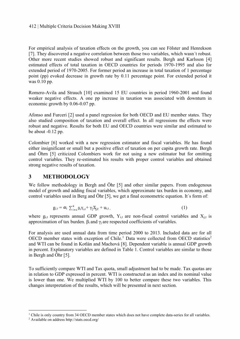
For empirical analysis of taxation effects on the growth, you can see Fölster and Henrekson [7]. They discovered a negative correlation between those two variables, which wasn´t robust. Other more recent studies showed robust and significant results. Bergh and Karlsson [4]estimated effects of total taxation in OECD countries for periods 1970-1995 and also for extended period of 1970-2005. For former period an increase in total taxation of 1 percentage point (pp) evoked decrease in growth rate by 0.11 percentage point. For extended period it was 0.10 pp.

Romero-Avila and Strauch [10] examined 15 EU countries in period 1960-2001 and found weaker negative effects. A one pp increase in taxation was associated with downturn in economic growth by 0.06-0.07 pp.

Afonso and Furceri [2] used a panel regression for both OECD and EU member states. They also studied composition of taxation and overall effect. In all regressions the effects were robust and negative. Results for both EU and OECD countries were similar and estimated to be about -0.12 pp.

Colombier [6] worked with a new regression estimator and fiscal variables. He has found either insignificant or small but a positive effect of taxation on per capita growth rate. Bergh and Öhrn [5] criticized Colombiers work for not using a new estimator but for omitting control variables. They re-estimated his results with proper control variables and obtained strong negative results of taxation.

3 METHODOLOGY We follow methodology in Bergh and Öhr [5] and other similar papers. From endogenous model of growth and adding fiscal variables, which approximate tax burden in economy, and control variables used in Berg and Öhr [5], we get a final econometric equation. It´s form of:

gi,t = i + + ui,t , (1)

where gi,t represents annual GDP growth, Yi,t are non-fiscal control variables and Xj,t is approximation of tax burden. βi and γj are respected coefficients of variables.

For analysis are used annual data from time period 2000 to 2013. Included data are for all OECD member states with exception of Chile.1 Data were collected from OECD statistics2

and WTI can be found in Kotlán and Machová [8]. Dependent variable is annual GDP growth in percent. Explanatory variables are defined in Table 1. Control variables are similar to those in Bergh and Öhr [5].

To sufficiently compare WTI and Tax quota, small adjustment had to be made. Tax quotas are in relation to GDP expressed in percent. WTI is constructed as an index and its nominal value is lower than one. We multiplied WTI by 100 to better compare these two variables. This changes interpretation of the results, which will be presented in next section.

1 Chile is only country from 34 OECD member states which does not have complete data-series for all variables.2 Available on address http://stats.oecd.org/

412 | Multiple Criteria Decision Making XVIII

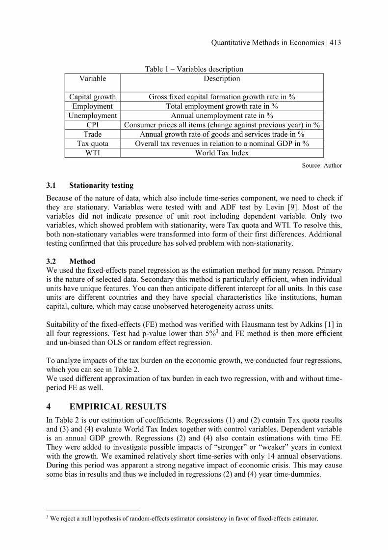
Table 1 – Variables description Variable Description

Capital growth Gross fixed capital formation growth rate in %Employment Total employment growth rate in %

Unemployment Annual unemployment rate in %CPI Consumer prices all items (change against previous year) in %

Trade Annual growth rate of goods and services trade in %Tax quota Overall tax revenues in relation to a nominal GDP in %

WTI World Tax IndexSource: Author

3.1 Stationarity testing Because of the nature of data, which also include time-series component, we need to check if they are stationary. Variables were tested with and ADF test by Levin [9]. Most of the variables did not indicate presence of unit root including dependent variable. Only two variables, which showed problem with stationarity, were Tax quota and WTI. To resolve this, both non-stationary variables were transformed into form of their first differences. Additional testing confirmed that this procedure has solved problem with non-stationarity.

3.2 Method We used the fixed-effects panel regression as the estimation method for many reason. Primary is the nature of selected data. Secondary this method is particularly efficient, when individual units have unique features. You can then anticipate different intercept for all units. In this case units are different countries and they have special characteristics like institutions, human capital, culture, which may cause unobserved heterogeneity across units.

Suitability of the fixed-effects (FE) method was verified with Hausmann test by Adkins [1] in all four regressions. Test had p-value lower than 5%3 and FE method is then more efficient and un-biased than OLS or random effect regression.

To analyze impacts of the tax burden on the economic growth, we conducted four regressions, which you can see in Table 2. We used different approximation of tax burden in each two regression, with and without time-period FE as well.

4 EMPIRICAL RESULTS In Table 2 is our estimation of coefficients. Regressions (1) and (2) contain Tax quota results and (3) and (4) evaluate World Tax Index together with control variables. Dependent variable is an annual GDP growth. Regressions (2) and (4) also contain estimations with time FE.They were added to investigate possible impacts of “stronger” or “weaker” years in context with the growth. We examined relatively short time-series with only 14 annual observations. During this period was apparent a strong negative impact of economic crisis. This may cause some bias in results and thus we included in regressions (2) and (4) year time-dummies.

3 We reject a null hypothesis of random-effects estimator consistency in favor of fixed-effects estimator.

Quantitative Methods in Economics | 413

Table 2 – Panel regression4

Regression (1) (2) (3) (4)

Constant 1.43***(5.25)

1.57***(5.36)

1.59***(6.36)

1.03***(3.72)

Capital growth

Employment

Unemployment

CPI

Trade

d_Tax quota

d_WTI

Within R2

DW Number of obs.

0.11***(4.55)

0.32***(3.97)

-0.09***(-2.72)-0.02*(-1.90)

0.21***(12.17)

-0.41***(-3.44)

0.821.83429

0.11***(4.24)

0.31***(4.10)

-0.09***(-3.56)

-0.04***(-4.46)

0.15***(7.52)

-0.46***(-3.55)

0.841.89429

0.11***(3.29)

0.31***(3.29)

-0.12***(-3.42)-0.02(-1.51)

0.20***(10.84)

-0.04(-1.19)

0.801.69429

0.11***(3.10)

0.31***(3.285)

-0.09***(-3.49)

-0.03**(-2.17)

0.17***(7.21)

-0.10**(-2.51)

0.831.79429

Source: Author´s calculations

Coefficients show that control variables have expected results as in Bergh and Öhr [5]. First differences in Tax quota show a robust negative correlation with economic growth. Results are similar for both year fixed-effects and without them. Coefficient in regression (1) means a one percentage point increase in overall tax quota is accompanied with a decrease in economic growth rate of 0.41 pp. Results for tax quota are quite discrepant. In regression (3) is the coefficient negative, but small and statistically insignificant. Adding year FE change results in regression (4). WTI is negative but statistically significant. If WTI rise by 0.015,economic growth is lowered by 0.1 pp.

Tax burden could be marked as growth-adverse after the consideration of our results in Table 2 and previous empirical studies. Tax quota shows a stronger negative effect than its WTI counterpart.

5 CONCLUSION Aim of this paper was to examine possible effects of a tax burden on the economic growth in 33 OECD countries. We used two tax burden indicators. First is overall tax quota, second is World Tax Index. The latter is created not only with hard data but also consists of qualified opinions of institutions and domestic experts.

4 In parenthesis are listed appropriate t-statistics to each variable. Number of stars next to coefficient represents significance level. For (*) it´s significance level 10%, for (**) it is 5% and for (***) it´s 1%.

5 In our work this responds to increase of WTI by 1 because we multiplied WTI by 100 earlier.

414 | Multiple Criteria Decision Making XVIII

Results of panel regression showed that tax quota has a strong negative correlation with the growth. WTI has a weaker negative correlation, which was statistically significant only if time fixed-effects were considered. WTI should reflect how economic subjects inside the country see a tax policy and tax burden upon themselves. This may cause differences in results between the two indicators.

This paper forms a foundation for a future research, which will be focused on a tax structure measured with individual tax quotas and components of World Tax Index to better cover problematics of tax burden and the economic growth as whole.

Acknowledgements: This work was supported by funding of specific research at Faculty of Economics and Administration - project MUNI/A/1055/2015. This support is gratefully acknowledged.

References [1] Adkins, L. (2010). Using gretl for Principles of Econometrics. 3rd ed. [ebook] Stillwater:

Oklahoma State University. Available at: http://www.learneconometrics.com/gretl/ebook.pdf [Accessed 14 Mar. 2016].

[2] Afonso, A. and Furceri, D. (2008). Government Size, Composition, Volatility and Economic Growth. ECB Working paper No. 849. Frankfurt am Main: ECB.

[3] Barro, R. (1990). Government Spending in a Simple Model of Endogeneous Growth. Journal of Political Economy, 98(5, Part 2), pp.S103-S125.

[4] Bergh, A. and Karlsson, M. (2009). Government size and growth: Accounting for economic freedom and globalization. Public Choice, 142(1-2), pp.195-213.

[5] Bergh, A. and Öhrn, N. (2011). Growth Effects of Fiscal Policies: A critical Appraisal of Colombier´s (2009) Study. IFN Working Paper No. 865. (2011). Stockholm: IFN.

[6] Colombier, C. (2009). Growth effects of fiscal policies: an application of robust modified M-estimator. Applied Economics, 41(7), pp.899-912.

[7] Fölster, S. and Henrekson, M. (2001). Growth effects of government expenditure and taxation in rich countries. European Economic Review, 45(8), pp.1501-1520.

[8] Levin, A., Lin, C. and James Chu, C. (2002). Unit root tests in panel data: asymptotic and finite-sample properties. Journal of Econometrics, 108(1), pp.1-24.

[9] Machová, Z. and Kotlán, I. (2013). World Tax Index: New Methodology for OECD Countries, 2000–2012. Danube, 4(2).

[10]Romero-Ávila, D. and Strauch, R. (2008). Public finances and long-term growth in Europe: Evidence from a panel data analysis. European Journal of Political Economy,24(1), pp.172-191.

Author’s addressIng. Petr ZimčíkMasaryk University, Faculty of Economics and Administration, Department of Economics Lipová 41a, Brno, 602 00Czech Republic e-mail: petr.zimcik@mail.muni.cz

Quantitative Methods in Economics | 415

APPLICATION OF DCC-GARCH MODEL FOR ANALYSIS OFINTERRELATIONS AMONG CAPITAL MARKETS OF POLAND,

CZECH REPUBLIC AND GERMANY

Marek Zinecker Brno University of Technology, Adam P. Balcerzak Nicolaus Copernicus University, Marcin Fałdziński Nicolaus Copernicus University, Tomáš Meluzín Brno University of Technology, Michał Bernard Pietrzak

Nicolaus Copernicus University

Abstract The phenomenon of growing capital market linkages is a significant exogenous factor affecting the effectiveness of national economic policies and risk management processes in enterprises. As a result the identification of interdependencies among capital markets is important both from the macro and microeconomic perspective. In this context the main aim of this article is to examine the relations among capital markets of Poland, Czech Republic and Germany. In the research DCC-GARCH model with the t-student conditional distribution was applied. The analysis was conducted for the years 1997-2015. The research findings confirmed significant interdependencies among analysed capital markets, which were evaluated here by conditional correlations.

Keywords: interdependences among capital markets, conditional variance and correlations, DCC-GARCH model

JEL Classification: G15, C58 AMS Classification: 62P20

INTRODUCTION The growing interdependencies among capital markets are currently considered as one of the most important forces responsible for globalisation of the world economy. As a result, these interrelations have been a subject of significant empirical investigations in recent years (Forbes and Rigobon, 2002; Baur, 2003; Corsetti et al., 2005; Billio and Caporin, 2010; Fałdziński and Pietrzak, 2015; Heryán and Ziegelbauer, 2016). The interdependencies of markets can be especially important during the time of international instability. They can provide transmission channels for negative impulses that destabilise the economies in the real sphere, which can be difficult to control at national level (Balcerzak, 2009a, 2009b). As a result, identification of the interdependencies among capital markets and analysis of their strength in time should be considered as a tool for managing risk related to financisation of economy. In this context the main purpose of this article is to examine interrelations between capital markets of Poland, Czech Republic and Germany. Polish and Czech stock exchanges can be treated as relatively young neighbouring markets. On the other hand, quite close geographically German capital market is mature and one of the biggest markets in Europe, thus it should have significant influence on Polish and Czech stock exchanges.

In the research DCC-GARCH model was applied as it enables to analyse the interrelations among markets by estimating the time-varying conditional correlation for given pairs of markets. The research was conducted for the years 1997-2015, which is a period long enough for drawing conclusions on the interrelations among chosen markets.

416 | Multiple Criteria Decision Making XVIII

DCC-GARCH MODEL SPECIFICATION Originally GARCH models enabled to model conditional variance for individual assets or indices. However, some early applications of the models showed that the capital markets should not be analysed separately but also interdependences between them should be taken into account. That problem was solved after introduction of DCC-GARCH models that enable to analyse interdependence among markets by estimating the time-varying conditional correlation (Engle, 2002). After adding ARMA (p, q) model to DCC-GARCH model, it is possible to catch the presence of autocorrelation of returns or autocorrelation of random disturbance. Model ARMA-DCC-GARCH can be given as follows:

1 1( ... ) ( ... )p qp qB B B B� � � � � � � �t t1 Φ Φ Y c 1 Θ Θ η , 1| F ~ (0, , )t t v�t t t tη D R D (1)

{ }, ( )diag� �2t t t t-1 tD H H V η (2)

2, , 1 , 1i t i i i t i i tH HL �* ;� �� � � (3)

� -1t t tε D η (4)

1/2 1/2{ } { }diag diag� ��t t t tR Q Q Q (5) , = (1� ; � ;1� � � � � �t t-1 t-1 t-1Q Ω ε ε Q Ω R , (6)

where: tY - the multivariate process of returns, tμ - the vector of conditional means of returns, ,i tH -

the conditional variance for i-th returns, where 1,...,i N� ,

tR - the time-varying conditional correlation matrix, ( )t-1 tV η - the conditional covariance matrix of the residuals tη ,

c – the vector of constant, Φ,Θ - the parameters of the ARMA(p, q)

, ,i i iL � ; - the parameters of the conditional variance equation, where 1,...,i N� ,� ;R - the parameters of the conditional correlation equation,

2v � - the number of degrees of freedom in the t-distribution,

1

1 T

iT �

� � 't tR ε ε

- the unconditional covariance matrix.

The estimation of parameters of DCC-GARCH model can be carried out using the maximum likelihood method. The two step estimation method can be applied here (Engle, 2002; 2009). In the first step the parameters of the conditional variance equations and means are estimated. In the second step the parameters of the conditional correlation equation are estimated.

APPLICATION OF THE MODEL In the research interdependencies among capital markets of Germany, Poland and Czech Republic were analysed. Thus, time series for three indices were used (DAX, WIG20 and PX 50). For this purpose a daily observations from 1 July 1997 to 30 September 2015 were taken, which gives T = 4592 observations. The data were obtained from the service http://www.finance.yahoo.com. In the study logarithmic returns ))ln()(ln(100 1��� ttt PPr were used. In the estimation of parameters of DCC-GARCH model the maximum likelihood method with a fat-tailed t-distribution was applied.

Quantitative Methods in Economics | 417

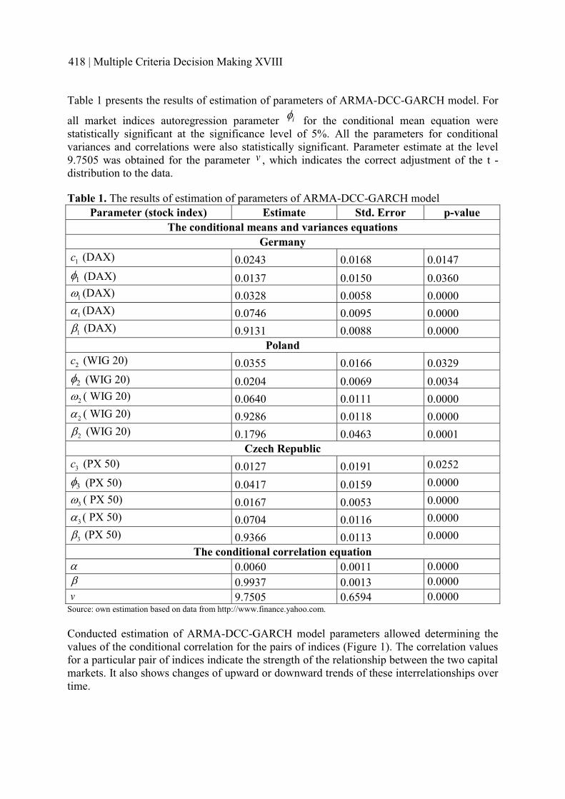
Table 1 presents the results of estimation of parameters of ARMA-DCC-GARCH model. For

all market indices autoregression parameter iH for the conditional mean equation were statistically significant at the significance level of 5%. All the parameters for conditional variances and correlations were also statistically significant. Parameter estimate at the level 9.7505 was obtained for the parameter v , which indicates the correct adjustment of the t -distribution to the data.

Table 1. The results of estimation of parameters of ARMA-DCC-GARCH model Parameter (stock index) Estimate Std. Error p-value

The conditional means and variances equationsGermany

1c (DAX) 0.0243 0.0168 0.01471H (DAX) 0.0137 0.0150 0.03601L (DAX) 0.0328 0.0058 0.00001� (DAX) 0.0746 0.0095 0.00001; (DAX) 0.9131 0.0088 0.0000

Poland2c (WIG 20) 0.0355 0.0166 0.03292H (WIG 20) 0.0204 0.0069 0.00342L ( WIG 20) 0.0640 0.0111 0.00002� ( WIG 20) 0.9286 0.0118 0.00002; (WIG 20) 0.1796 0.0463 0.0001

Czech Republic3c (PX 50) 0.0127 0.0191 0.0252

3H (PX 50) 0.0417 0.0159 0.0000

3L ( PX 50) 0.0167 0.0053 0.0000

3� ( PX 50) 0.0704 0.0116 0.0000

3; (PX 50) 0.9366 0.0113 0.0000The conditional correlation equation

� 0.0060 0.0011 0.0000; 0.9937 0.0013 0.0000v 9.7505 0.6594 0.0000

Source: own estimation based on data from http://www.finance.yahoo.com.

Conducted estimation of ARMA-DCC-GARCH model parameters allowed determining the values of the conditional correlation for the pairs of indices (Figure 1). The correlation values for a particular pair of indices indicate the strength of the relationship between the two capital markets. It also shows changes of upward or downward trends of these interrelationships over time.

418 | Multiple Criteria Decision Making XVIII

Figure 1. The conditional correlation between the DAX index, the WIG 20 and the PX 50 Source: own estimation based on data from: http://www.finance.yahoo.com.

Figure 1 shows the conditional correlations between the DAX, PX 50 and WIG20 indices. The findings allow making the following conclusions. Firstly, in the case of Czech Republic and Poland, the interdependences among these markets and German capital market are at a medium level. On the other hand, the interrelations between the Polish and Czech markets are much weaker. Next, it should be emphasized that in the period 2004-2015 trends in changes in the value of the conditional correlation (declines and increases) are similar between the capital market of Germany and Polish and Czech markets. It can be said that the shocksoccurring on the capital market in Germany have been transferred in a similar way to Czech and Polish markets since 2004. This finding confirms the results of previous financial studies that the situation on any stock exchange is to some extent dependent on the situation on the other markets.

CONCLUSIONS The article concentrates on the phenomena of growing interrelations among capital markets. Their strength is constantly increasing due to intensification of globalization process. The identification of the interdependencies among capital markets has been considered as an important scientific problem in recent years. It can be useful in developing of tools and regulations that can improve functioning of capital markets. The adoption of such tools can be helpful in determination of strategies during potential crisis.

The main aim of the article was to examine the interdependencies among the capital markets of Germany, Poland and Czech Republic. The research findings allow to assess the interrelations among these markets and enable to evaluate changes in these interrelationships over time. To some extent these interdependencies were shape differently depending on the selected pair of markets. This means that in spite of the interdependence among analysed indices, the markets in question cannot be treated as a homogeneous area. Thus, the single markets function in a specific way, and react differently to similar external shocks.

However, it should be noted that for all pairs of indices an increase in the value of the conditional correlation have been noticeable since 2004. This may be a result of the accession of Poland and Czech Republic to the European Union, which contributed significantly to the economic growth of these countries influencing also the dynamics of their capital markets. Then, in the years 2007-2008 there was a further increase in interdependence among the

Quantitative Methods in Economics | 419

markets. The increase in the interrelations among the analysed markets in this period could be the result of the contagion effect that occurred in the markets due to the global financial crisis. The increase in the level of interdependence lasted until the year 2012. In the subsequent period 2013-2015 a downward trend in the interdependencies can be observed. This may be a sign of a slow return to long term equilibrium on the capital markets, thus to the period of greater economic stability.

References [1] Balcerzak, A. (2009a). Monetary Policy under Conditions of Nairu "Flattening". Olsztyn

Economic Journal, 4(1), pp.95-105.[2] Balcerzak, A. (2009). Limitations of the National Economic Policy in the Face of

Globalization Process. Olsztyn Economic Journal, 4(2), pp.279-290.[3] Baur, D. (2003). Testing for contagion—mean and volatility contagion. Journal of

Multinational Financial Management, 13(4-5), pp.405-422.[4] Billio, M. and Caporin, M.: Market Linkages, Variance Spillover and Correlation

Stability: Empirical Evidences of Financial Contagion. Computational Statistics & Data Analysis 54(11) (2010), 2443–2458.

[5] Billio, M. and Caporin, M. (2010). Market linkages, variance spillovers, and correlation stability: Empirical evidence of financial contagion. Computational Statistics & Data Analysis, 54(11), pp.2443-2458.

[6] Engle, R. (2002). Dynamic Conditional Correlation: A Simple Class of Multivariate Generalized Autoregressive Conditional Heteroskedasticity Models. Journal of Busines & Economic Statistics, 20(3), pp.339-350.

[7] Engle, R. (2009). Anticipating Correlations a New Paradigm for Risk Management,Princeton and Oxford: Princeton University Press.

[8] Fałdziński, M. and Pietrzak, M. (2015). The Multivariate DCC-GARCH model with interdependence among markets in conditional variances’ equations. Przeglad Statystyczny, 62(1), pp. 397-413.

[9] Forbes, K. and Rigobon, R. (2002). No Contagion, Only Interdependence: Measuring Stock Market Comovements. The Journal of Finance, 57(5), pp.2223-2261.

[10] Heryán, T. and Ziegelbauer, J. (2016). VOLATILITY OF YIELDS OF GOVERNMENT BONDS AMONG GIIPS COUNTRIES DURING THE SOVEREIGN DEBT CRISIS IN THE EURO AREA. Equilibrium, 11(1), p.61.

[11] Yahoo Finance, (2016). Yahoo Finance - Business Finance, Stock Market, Quotes, News.[online] Yahoo Finance. Available at: http://finance.yahoo.com/ [Accessed 30 Oct. 2015].

Author’s addressdoc. Ing. Marek Zinecker, Ph.D. Brno University of Technology, Faculty of Business and Management Kolejní 2906/4612 00 Brno Czech Republic email: zinecker@fbm.vutbr.cz

Adam P. Balcerzak, Ph.D. Nicolaus Copernicus University, Department of Economics, Faculty of Economic Sciences and Management, Ul. Gagarina 13a 87-100 Toruń

420 | Multiple Criteria Decision Making XVIII

Poland email: adam.balcerzak@umk.pl

Marcin Fałdziński, Ph.D. Nicolaus Copernicus University, Department of Econometrics and Statistics, Faculty of Economic Sciences and Management, Ul. Gagarina 13a 87-100 ToruńPoland email: marf@umk.pl

Michał Bernad Pietrzak, Ph.D.Nicolaus Copernicus University, Department of Econometrics and Statistics, Faculty of Economic Sciences and Management, Ul. Gagarina 13a 87-100 ToruńPoland email: michal.pietrzak@umk.pl

doc. Ing. Tomáš Meluzín, Ph.D. Brno University of Technology, Faculty of Business and Management Kolejní 2906/4612 00 Brno Czech Republic email: meluzint@fbm.vutbr.cz

Quantitative Methods in Economics | 421

NOTES

.....................................................................................................................................................................................

.....................................................................................................................................................................................

.....................................................................................................................................................................................

.....................................................................................................................................................................................

.....................................................................................................................................................................................

.....................................................................................................................................................................................

.....................................................................................................................................................................................

.....................................................................................................................................................................................

.....................................................................................................................................................................................

.....................................................................................................................................................................................

.....................................................................................................................................................................................

.....................................................................................................................................................................................

.....................................................................................................................................................................................

.....................................................................................................................................................................................

.....................................................................................................................................................................................

.....................................................................................................................................................................................

.....................................................................................................................................................................................

.....................................................................................................................................................................................

.....................................................................................................................................................................................

.....................................................................................................................................................................................

.....................................................................................................................................................................................

.....................................................................................................................................................................................

.....................................................................................................................................................................................

.....................................................................................................................................................................................

.....................................................................................................................................................................................

.....................................................................................................................................................................................

.....................................................................................................................................................................................

.....................................................................................................................................................................................

.....................................................................................................................................................................................

.....................................................................................................................................................................................

.....................................................................................................................................................................................

.....................................................................................................................................................................................

.....................................................................................................................................................................................

.....................................................................................................................................................................................

.....................................................................................................................................................................................

422 | Multiple Criteria Decision Making XVIII

NOTES

.....................................................................................................................................................................................

.....................................................................................................................................................................................

.....................................................................................................................................................................................

.....................................................................................................................................................................................

.....................................................................................................................................................................................

.....................................................................................................................................................................................

.....................................................................................................................................................................................

.....................................................................................................................................................................................

.....................................................................................................................................................................................

.....................................................................................................................................................................................

.....................................................................................................................................................................................

.....................................................................................................................................................................................

.....................................................................................................................................................................................

.....................................................................................................................................................................................

.....................................................................................................................................................................................

.....................................................................................................................................................................................

.....................................................................................................................................................................................

.....................................................................................................................................................................................

.....................................................................................................................................................................................

.....................................................................................................................................................................................

.....................................................................................................................................................................................

.....................................................................................................................................................................................

.....................................................................................................................................................................................

.....................................................................................................................................................................................

.....................................................................................................................................................................................

.....................................................................................................................................................................................

.....................................................................................................................................................................................

.....................................................................................................................................................................................

.....................................................................................................................................................................................

.....................................................................................................................................................................................

.....................................................................................................................................................................................

.....................................................................................................................................................................................

.....................................................................................................................................................................................

.....................................................................................................................................................................................

.....................................................................................................................................................................................

Quantitative Methods in Economics | 423

NOTES

.....................................................................................................................................................................................

.....................................................................................................................................................................................

.....................................................................................................................................................................................

.....................................................................................................................................................................................

.....................................................................................................................................................................................

.....................................................................................................................................................................................

.....................................................................................................................................................................................

.....................................................................................................................................................................................

.....................................................................................................................................................................................

.....................................................................................................................................................................................

.....................................................................................................................................................................................

.....................................................................................................................................................................................

.....................................................................................................................................................................................

.....................................................................................................................................................................................

.....................................................................................................................................................................................

.....................................................................................................................................................................................

.....................................................................................................................................................................................

.....................................................................................................................................................................................

.....................................................................................................................................................................................

.....................................................................................................................................................................................

.....................................................................................................................................................................................

.....................................................................................................................................................................................

.....................................................................................................................................................................................

.....................................................................................................................................................................................

.....................................................................................................................................................................................

.....................................................................................................................................................................................

.....................................................................................................................................................................................

.....................................................................................................................................................................................

.....................................................................................................................................................................................

.....................................................................................................................................................................................

.....................................................................................................................................................................................

.....................................................................................................................................................................................

.....................................................................................................................................................................................

.....................................................................................................................................................................................

.....................................................................................................................................................................................

424 | Multiple Criteria Decision Making XVIII