Quantification of population exposure to nitrogen dioxide in Sweden 2005
68
REPORT Quantification of population exposure to nitrogen dioxide in Sweden 2005 Karin Sjöberg, Marie Haeger-Eugensson, Bertil Forsberg 1 , Stefan Åström, Sofie Hellsten, Lin Tang B 1749 September 2007 Rapporten godkänd: 2007-09-26 John Munthe 1 Umeå Universitet
-
Upload
independent -
Category
Documents
-
view
2 -
download
0
Transcript of Quantification of population exposure to nitrogen dioxide in Sweden 2005

REPORT
Quantification of population exposure to nitrogen dioxide
in Sweden 2005
Karin Sjöberg, Marie Haeger-Eugensson, Bertil Forsberg1, Stefan Åström, Sofie Hellsten, Lin Tang
B 1749 September 2007
Rapporten godkänd: 2007-09-26
John Munthe
1 Umeå Universitet

Report Summary
Organization
IVL Swedish Environmental Research Institute Ltd. Project title
Address P.O. Box 5302 SE-400 14 Göteborg Project sponsor
The National Board of Health and Welfare (Socialstyrelsen)
Telephone +46 (0)31- 725 62 00
Author Karin Sjöberg, Marie Haeger-Eugensson, Bertil Forsberg (Umeå Universitet), Stefan Åström, Sofie Hellsten, Lin Tang Title and subtitle of the report Quantification of population exposure to nitrogen dioxide in Sweden 2005 Summary The population exposure to NO2 in ambient air for the year 2005 has been quantified (annual and daily mean concentrations) and the health and associated economical consequences have been calculated based on these results. Almost 50% of the population were exposed to annual mean NO2 concentrations of less than 5 µg/m3. A further 30% were exposed to concentration levels between 5-10 µg NO2/m3, and only about 5% of the Swedish inhabitants experienced exposure levels above 15 NO2 µg/m3. Using 10 µg/m3 as a lower cut off for long-term exposure we estimate that concentations of NO2 in urban air resulted in more than 3200 excess deaths per year. Almost 600 of these could have been avoided if annual mean concentrations above the environmental goal 20 µg/m3 did not exist. Most excess deaths are estimated to occur due to annual levels in the range of 10-15 µg/m3. In addition we estimated more than 300 excess hospital admissions for all respiratory disease and almost 300 excess hospital admissions for cardiovascular disease due to the short-term effect of levels above 10 µg/m3. The results suggest that the health effects related to annual mean levels of NO2 higher than 10 µg/m3 can be valued to annual socio-economic costs of 18.5 billion Swedish crowns. These 18.5 billion Swedish crowns are to be considered as welfare losses. However, only 18 % of these costs are related to exceedance of the Swedish long term environmental objectives for NO2. The other 82 % of the costs are taken by the larger part of the Swedish population that are exposed to medium levels of NO2. This displacement in the distribution of the social costs indicates that the most cost effective abatement strategy for Sweden might be to reduce medium annual levels of NO2 rather than only focusing on abatement measures directed towards the highest annual mean levels. Keyword nitrogen dioxide, population exposure, health impact assessment, risk assessment, socio-economic valuation Bibliographic data
IVL Report B 1749
The report can be ordered via Homepage: www.ivl.se, e-mail: [email protected], fax+46 (0)8-598 563 90, or via IVL, P.O. Box 21060, SE-100 31 Stockholm Sweden

Quantification of population exposure to nitrogen dioxide in Sweden 2005 IVL report B 1749
1
Summary Sweden is one of the countries in Europe which experiences the lowest concentrations of air pollutants in urban areas. However, the health impact of exposure to ambient air pollution is still an important issue in the country and the concentration levels, especially of nitrogen dioxide (NO2) and particles (PM10,) exceed the air quality standards and health effects of exposure to air pollutants in many areas.
IVL Swedish Environmental Research Institute and the Department of Public Health and Clinical Medicine at Umeå University have, on behalf of the Swedish EPA and the health-related environmental monitoring programme, performed a health impact assessment (HIA) for the year 2005. The population exposure to NO2 in ambient air has been quantified (annual and daily mean concentrations) and the health and associated economical consequences have been calculated based on these results.
The results from the urban modelling show that in 2005 most of the country had low NO2 urban background concentrations compared to the environmental standard for the annual mean (40 µg/m3). In most of the small to medium sized cities the NO2 concentration was less than 15 µg/m3 in the city centre. In the larger cities and along the Skåne west coast the concentrations were higher, up to 20-25 µg/m3, which is of the same magnitude as the long-term environmental objective (20 µg/m3 as an annual mean).
Almost 50% of the population were exposed to annual mean NO2 concentrations of less than 5 µg/m3. A further 30% were exposed to concentration levels between 5-10 µg NO2/m3, and only about 5% of the Swedish inhabitants experienced exposure levels above 15 NO2 µg/m3.
The health impact calculation has four components: a relevant effect estimate from epidemiologic data, a baseline rate for the health effect, the affected number of persons and their estimated “exposure” (here pollutant concentration). We have used 10 µg/m3 as a lower cut off in our impact assessment scenarios for long-term exposure and mortality as well as in the assessment of short-term effects on hospital admissions. Exposure above 10 µg/m3 is therefore defined as excess exposure resulting in “excess cases”.
For our mortality assessment we have chosen to use the same estimate as in our previous similar HIA. The estimate came from a study in Auckland, and was 13% (95% CI: 11–15%) increase in non-external mortality per 10 µg/m3 increase in annual average NO2. This estimate is similar to what has been reported in some other referenced studies.
For respiratory hospital admissions we have used the risk estimates from a Norwegian study reporting a relative risk of 2.9% per 10 μg/m3. For cardiovascular hospital admissions we have used a meta-analysis presented by an expert group in UK, assuming a relative risk of 1.0 % per 10 μg/m3 in the health impact assessment.
Altogether we estimate that concentations of NO2 in urban air resulted in more than 3200 excess deaths per year. Almost 600 of these could have been avoided if annual mean concentrations above the environmental goal 20 µg/m3 did not exist. Most excess deaths are estimated to occur due to annual levels in the range of 10-15 µg/m3. We have crudely estimated the average years of life lost per excess death to be just over 11 years. In addition we estimated more than 300 excess hospital admissions for all respiratory disease and almost 300 excess hospital admissions for cardiovascular disease due to the short-term effect of levels above 10 µg/m3.
Quantification of population exposure to nitrogen dioxide in Sweden 2005 IVL report B 1749
2
The health effects related to high concentrations of NO2 in ambient air are related to socio-economic costs, as are the costs for abating these high concentrations. It is important for decision makers to use their economic resources in an efficient manner, which furthermore induces the need for assessments of what can be considered as an efficient use of resources. The socio-economic costs related to high levels of NO2 in air are derived from the cost estimates of resources required for treatment of affected persons, productivity losses from work absence and most prominently from studies on the social Willingness To Pay for the prevention of health effects related to these high levels of NO2.
In our study we have applied results from international socio-economic valuation studies to our calculated results on increased occurrences of hospital admissions and fatalities. The values from the studies have been adapted to Swedish conditions. The application of international results favours comparison with other estimates on economic valuation of health effects related to high levels of NO2.
The results suggest that the health effects related to annual mean levels of NO2 higher than 10 µg / m3 can be valued to annual socio-economic costs of 18.5 billion Swedish crowns. These 18.5 billion Swedish crowns are to be considered as welfare losses. However, only 18 % of these costs are related to exceedance of the Swedish long term environmental objectives for NO2. The other 82 % of the costs are taken by the larger part of the Swedish population that are exposed to medium levels of NO2. This displacement in the distribution of the social costs indicates that the most cost effective abatement strategy for Sweden might be to reduce medium annual levels of NO2 rather than only focusing on abatement measures directed towards the highest annual mean levels.
The trend analysis between 1990 and 2005 clearly shows an increasing number of people exposed to lower NO2 concentration levels. Comparing 2005 with 1990, about 15% less people were exposed to annual mean NO2 levels above 15 µg/m3, while almost 20% more people were exposed to annual mean NO2 levels in the lowest concentration class, 0-5 µg/m3.
In general, the improved URBAN model shows good performance. When using the actual weather instead of the normal weather the variability in air pollution concentrations governed by the meteorology is captured when applying the rather fine scaled meteorology. The difference between measurements and the calculated concentrations is less than 10%. It was determined that the use of normal year meteorology lead to much greater uncertainties and this method was therefore rejected.
The comparison between the URBAN model and detailed calculations on a regional scale shows a good agreement as regards the annual mean concentrations. For concentrations above the cut off level used in the exposure studies (10 µg/m3) the agreement between the two calculation methods lies within 5%. On the local scale the population weighted annual means correlate very well with the URBAN model calculations in Göteborg and Uppsala. For Umeå there are larger differences. The comparison of the number of people exposed to different concentration levels corresponds quite well (within 15%) in Göteborg, but the differences are larger in the two other cities (up to 45 %). This may be due to uncertainties in the concentration distribution pattern.
There are still a number of issues that can further improve the certainty of the calculations, i.e. the selection of population data to be used as well as application of relevant geographical areas and best degree of resolution to fit with the most valid epidemiological ER-functions. By increasing the asseessment frequency it is possible to minimize the uncertainties due to meteorological variations. Furthermore, the differences in exposure on the local level could be reduced if existing local dispersion concentration calculations were applied into the model.

Quantification of population exposure to nitrogen dioxide in Sweden 2005 IVL report B 1749
3
Sammanfattning
Drygt 2% av Sveriges befolkning utsätts för halter av kvävedioxid (NO2) i utomhusluft över det långsiktiga miljökvalitetsmålet, 20 µg/m3 som årsmedelvärde. Däremot exponeras ingen för halter över miljökvalitetsnormen (40 µg NO2/m3). Andelen som utsätts för förhöjda NO2-halter har minskat med cirka 7% sedan 1999 och nästan 20% sedan 1990. Med den lokala halten av NO2 som en indikator på förbränningsprodukter, främst fordonsavgaser, beräknas nuvarande halter ge upphov till mer än 3 200 extra dödsfall per år. Nästan 600 av dessa skulle kunna undvikas om miljökvalitetsmålet för årsmedelkoncentrationen av NO2 i luften var uppfyllt i hela landet. Kostnaden för samhället orsakade av hälsoeffekter relaterade till NO2-halter högre än det långsiktiga miljökvalitetsmålet värderar vi till 3368 miljoner svenska kronor per år, orsakade av 591 dödsfall årligen. Detta motsvarar 18 % av de totala hälsorelaterade samhällskostnaderna som kopplas till höga halter av NO2. Resterande 82 % av samhällskostnaderna orsakas av exponeringshalter i skiktet mellan 10 och 20 µg NO2/m3.
Minskade utsläpp av föroreningar till luft har lett till en avsevärd förbättring av luftkvaliteten och Sverige är ett av de länder i Europa som uppvisar de lägsta halterna av luftföroreningar i tätorter. Trots detta är hälsoeffekterna till följd av exponering för föroreningar i omgivningsluften fortfarande en viktig fråga. Koncentrationsnivåerna, särskilt av kvävedioxid (NO2) och partiklar (PM10) som till stor del härrör från biltrafik, överskrider på många håll såväl uppsatta miljömål som gällande miljökvalitetsnormer.
Under 1991/92 gjordes, inom ramen för Naturvårdsverkets utredning om miljötillståndet i Sverige, en beräkning av antalet personer som var överexponerade för NO2 i förhållande till då gällande riktvärden för utomhusluft. Beräkningar av överexponering med motsvarande metodik skedde även för vinterhalvåren 1995/96 och 1999/2000. Dessa beräkningar indikerade att 3% av Sveriges befolkning var överexponerade för halter av kvävedioxid i förhållande till då gällande gränsvärde (110 µg/m3 som 98-il för timme) i utomhusluft vintern 1990/91. Uppdateringen för 1999/2000 visade på en något minskad överexponering (0.3%) jämfört med tidigare års studier.
IVL har sedan 1986, i samarbete med totalt cirka 100 av Sveriges kommuner, genomfört mätningar av luftföroreningar i små och medelstora tätorter inom det s.k. URBAN-mätnätet. Baserat på framtagna mätdata avseende halter i tätorternas urbana bakgrundsluft har en empirisk modell (URBAN-modellen) utvecklats dels för haltberäkning i tätorter där mätningar saknas, dels för prognosticering av den framtida luftkvalitetssituationen. Utifrån denna yttäckande bild av haltsituationen i landet kan man också uppskatta befolkningens allmänna exponering för luftföroreningar. Lokala ventilationsförhållanden beskrivs i modellen genom ett meteorologiskt index som beräknats med hjälp av en avancerad spridnings- och meteorologisk modell (TAPM, The Air Pollution Model), vilken bl.a. tar hänsyn till topografi, havstemperatur, markanvändning, lokala vindsystem (sjö/landbris, omlandsbris) och inversioner. Indexet har beräknats för hela Sverige ner till en skala om 1x1 km.
Syftet med föreliggande studie var att ersätta den tidigare använda metodiken för beräkning av överexponering för kvävedioxid med den vidareutvecklade s.k. URBAN-modellen. På uppdrag av Naturvårdsverket och den hälsorelaterade miljöövervakningen har IVL Svenska Miljöinstitutet och Institutionen för folkhälsa och klinisk medicin vid Umeå universitet kvantifierat den svenska befolkningens exponering för halter i luft av kvävedioxid för år 2005, beräknat både för års- och dygnsmedelkoncentrationer. Även de samhällsekonomiska konsekvenserna av de uppskattade hälsoeffekterna har beräknats.

Quantification of population exposure to nitrogen dioxide in Sweden 2005 IVL report B 1749
4
Vidare har betydelsen av att använda meteorologiska indata för ett typiskt (”normalt”) år jämfört med det aktuella beräkningsårets data studerats. För att validera modellen och kunna uppskatta osäkerheten i dessa beräkningar har erhållna resultat avseende såväl halter som antal exponerade personer även jämförts med resultat från mer detaljerade spridningsberäkningar i både lokal och regional skala. För att säkerställa trenden bakåt med en enhetlig metodik har också beräkningarna för tidigare år (1990, 1995 och 1999) reviderats.
Resultaten visar att den urbana bakgrundshalten av NO2 i merparten av landets tätorter under 2005 var låg i förhållande till miljökvalitetsnormen för årsmedelvärdet (40 µg NO2/m3). I de flesta små till medelstora tätorter var halten inne i centrum lägre än 15 µg/m3. I de större orterna och längs Skånes västkust förekom haltnivåer upp till 20-25 µg/m3, vilket är i samma storleksordning som det långsiktiga miljökvalitetsmålet (20 µg/m3 som årsmedelvärde).
Nästan 50% av befolkningen exponerades för en lägre halt än 5 µg NO2/m3 som årsmedelvärde. Ytterligare 30% exponerades för nivåer mellan 5-10 µg/m3, och endast cirka 5% av landets invånare utsattes för exponeringsnivåer av NO2 över 15 µg/m3.
I epidemiologiska studier har halten av NO2 ofta använts som en indikator på fordonsavgaser, oavsett om studien avsett korttidshalter och akuta effekter eller effekter av långtidsexponering. Vid höga halter ger NO2 i sig påtagliga akuta effekter, men en betydande del av de hälsoeffekter som i epidemiologiska studier kopplats samman med variation i halten av NO2 bedöms bero på andra avgaskomponenter. NO2 förefaller ofta vara en bättre indikator på avgashalten än PM10 och PM2.5 som påverkas mycket av andra källor.
En hälsokonsekvensberäkning har fyra komponenter: ett antaget relevant exponerings-responssamband, en aktuell eller relevant grundfrekvens för studerad effekt, antal berörda personer samt personernas exponering (eller tänkt förändring av denna). Det kan vara lämpligt att tillämpa en nedre beräkningsgräns utgående från miniminivån för det haltintervall som sambandet påvisats inom. Vi har antagit att halter under 10 µg/m3 inte har någon inverkan på risken. Detta beror på att de studier vi hämtat exponerings-responsantaganden från inte styrker några effekter under denna nivå. Följaktligen ses fall på grund av högre halter än så som “extra fall”, vilka kunde undvikas genom en lägre exponering.
För skattningen av långtidseffekter på dödligheten har vi valt att använda samma exponerings-responsantagande som vid vår tidigare liknande studie. Detta samband erhölls i en studie i Auckland och innebär 13% (95% CI: 11–15%) ökning av totaldödligheten (exkluderat externa orsaker) per 10 µg/m3 ökat årsmedelvärde av NO2. En ungefär lika stor effekt har setts i flera andra studier som refereras i rapporten. Med den lokala halten av NO2 som en indikator på förbränningsprodukter, främst fordonsavgaser, beräknas nuvarande halter ge upphov till mer än 3 200 extra dödsfall per år. Nästan 600 av dessa skulle kunna undvikas om miljökvalitetsmålet för årsmedelkoncentrationen av NO2 i luften var uppfyllt i hela landet.
För beräkningen av korttidseffekten på antal akuta sjukhusinläggningar har vi hämtat exponerings-responsantaganden från en norsk studie av inläggningar för andningsorganen, vilken fann 2.9% per 10 μg NO2/m3. För inläggningar i hjärt-kärlsjukdom har vi valt att basera beräkningarna på sammanvägda resultat i en meta-analys presenterad av en brittisk expertgrupp, antagande en relativ risk på 1.0 % per 10 μg NO2/m3. Det beräknade antalet undvikbara akuta inläggningar är ganska lågt och inte jämförtbart med dödstalet eftersom det senare inkluderar effekter av längre tids exponering.
Hälsoeffekter orsakade av höga halter av luftföroreningar är oundvikligen kopplade till samhällskostnader. Det är även åtgärder för att minska dessa halter av luftföroreningar. Och eftersom det är viktigt för beslutsfattare att använda skattepengar och andra finansiella resurser på

Quantification of population exposure to nitrogen dioxide in Sweden 2005 IVL report B 1749
5
mest effektiva sätt blir det även viktigt att göra ordentliga bedömningar av vad som är att räkna som effektivt användande av resurser. Till detta hör en bedömning om värdet för samhället att slippa hälsoeffekter orsakade av höga halter av luftföroreningar. I den ekonomiska delen av denna rapport har genomförts en ekonomisk värdering av de hälsoeffekter som hänger ihop med höga halter av NO2 i luft.
Internationellt har det skett mycket arbete kring värdering av hälsoeffekter och vi har i denna studie valt att använda de värderingar som skett i tidigare studier som grund för värdering av Svenska samhällskostnader kopplade till höga halter av NO2. Detta gynnar jämförelse med andra resultat inom området kring ekonomisk värdering av hälsoeffekter.
Resultaten från vår studie visar att de negativa hälsoeffekter i form av sjukhusbesök och förtida dödsfall relaterade till höga halter av NO2 kan värderas till årliga välfärdsförluster för samhället motsvarande ca 18.5 miljarder kronor. Av dessa kostnader utgörs endast ca 18 % av välfärdsförluster, orsakade av att det långsiktiga svenska miljömålet för NO2 -halter i luft inte är uppnått. Resterande kostnader bärs av den stora merparten av Sveriges befolkning som utsätts för mellanhöga NO2 -halter. Detta innebär att det mest effektiva för samhället kan vara att generellt minska halterna av NO2 i tätbefolkade områden snarare än att endast fokusera på att minska de allra högsta halterna.
Trendberäkningarna visar på en generell minskning avseende haltnivåerna av NO2 och en tydligt förbättrad exponeringssituation under de senaste 15 åren. Under 2005 var det, jämfört med 1990, ungefär 15 % färre människor som exponerades för årsmedelhalter av NO2 över 15 µg/m3, och nästan 20 % fler vars årsmedelexponering var lägre än 5 µg/m3.
De resultat som erhålles med URBAN-modellen uppvisar en bra överensstämmelse med andra metoder för att uppskatta såväl haltnivåer som exponeringsbelastning med avseende på NO2. Med den relativt finskaliga geografiska upplösningen avspeglas variabiliteten i luftföroreningshalter bättre då man använder meteorologi för det aktuella året istället för en normalårssituation. Skillnaden mellan uppmätta och beräknade halter uppskattas till mindre än 10% med aktuell meteorologi, medan osäkerheten vid normalårsberäkningar blir 20-30%.
För beräkning av årsmedelvärden visar URBAN-modellen på en god jämförbarhet med mer detaljerade spridningsberäkningar i regional skala (Skåne). Däremot var variationen i exponering cirka 15% i koncentrationsklasser <10 µg/m3, vilket motsvarar ”cut off”-nivån för exponeringsberäknngarna. För högre koncentrationer var differensen mellan de båda metoderna mindre än 5%.
Vid jämförelser med spridningsberäkningar i mer lokal skala (tätort) var korrelationen avseende det populationsviktade årsmedelvärdet för NO2 mycket bra i Göteborg respektive Uppsala., medan avvikelse i Umeå var betydligt större. Även precisionen i antalet exponerade personer var relativt god i Göteborg (inom cirka 15%). I de två andra städerna uppgick variationen i vissa fall till 45%. En trolig förklaring till detta är osäkerheten i det lokala mönstret för den geografiska haltfördelningen.
URBAN-modellen fungerar väl som ett verktyg för exponeringsberäkningar i nationell och regional skala med den för ändamålet finskaliga meteorologin. Genom att applicera bättre populationsdata skulle osäkerheten i fördelningsmönstret, och därmed i beräkningarna, kunna reduceras ytterligare. Vidare skulle de meteorologiska variationerna kunna minimeras om man genomförde beräkningar med en högre tidsfrekvens än vart 5:e år. För att modellen bättre skall kunna spegla situationen även i lokal skala skulle man kunna inkludera resultat från mer detaljerade spridningsberäkningar för områden där detta finns tillgängligt.

Quantification of population exposure to nitrogen dioxide in Sweden 2005 IVL report B 1749
6
Contents
Summary .............................................................................................................................................................1 Sammanfattning .................................................................................................................................................3 1 Introduction ..............................................................................................................................................7 2 Background and aims ..............................................................................................................................7 3 Methods .....................................................................................................................................................8
3.1 Exposure calculations.....................................................................................................................9 3.1.1 The URBAN model .................................................................................................................9 3.1.2 Calculation of a normal meteorological year......................................................................14 3.1.3 Population data .......................................................................................................................18 3.1.4 Concentration distribution in urban areas..........................................................................19 3.1.5 Calculation of exposure .........................................................................................................22
3.2 Health impact assessment............................................................................................................23 3.2.1 Exposure-response function for mortality .........................................................................23 3.2.2 Exposure-response function for admissions .....................................................................28 3.2.3 Selected base-line rates ..........................................................................................................29
3.3 Socio-economic valuation............................................................................................................29 3.3.1 Why should we assess the value of socio-economic costs from health effects? ..........29 3.3.2 Valuation of socio-economic costs from health effects...................................................30 3.3.3 Quantified results from the literature ........................................................................................34
3.4 Evaluation of the URBAN model..............................................................................................37 3.4.1 Evaluation of the calculated NO2 concentrations.............................................................37 3.4.2 Evaluation of the calculated exposure levels .....................................................................37
4 Evaluation of meteorological conditions............................................................................................38 5 Results ......................................................................................................................................................42
5.1 NO2 concentrations and exposure situation in 2005 ..............................................................42 5.1.1 National distribution of NO2 concentrations ....................................................................42 5.1.2 Population exposure ..............................................................................................................44 5.1.3 Estimated health impacts ......................................................................................................45 5.1.4 Socio-economic cost ..............................................................................................................47
5.2 Trends in population exposure ...................................................................................................49 5.3 Model evaluation ...........................................................................................................................52
5.3.1 National NO2 concentration levels............................................................................................53 5.3.2 Regional NO2 concentrations and exposure levels ...........................................................53 5.3.3 Local NO2 concentrations and exposure levels.......................................................................55
6 Discussion ...............................................................................................................................................57 7 References ...............................................................................................................................................61
Quantification of population exposure to nitrogen dioxide in Sweden 2005 IVL report B 1749
7
1 Introduction Despite the successful work to improve the outdoor air quality situation in Sweden (Sjöberg et al., 2006a; de Facto, 2006) by reducing emissions from both stationary and mobile sources, the health impacts of exposure to ambient air pollution is still an important issue. As shown in many studies during recent years, the concentration levels, especially of nitrogen dioxide (NO2) and particles (PM10), in many areas exceed the air quality standards and health effects of exposure to air pollutants (Forsberg et al., 2003; Miljöhälsorapport 2001, WHO 2005).
Within the framework of the health-related environmental monitoring programme, conducted by the Swedish Environmental Protection Agency, a number of different activities are performed to monitor health effects that may be related to environmental factors.
IVL Swedish Environmental Research Institute and the Department of Public Health and Clinical Medicine at Umeå University have, on behalf of the Swedish EPA, performed a quantification of the population exposure to NO2 concentrations in ambient air (estimated both for a annual and daily mean concentrations) for the year 2005. The health and associated economical consequences have been calculated, based on these results.
2 Background and aims In a city the highest NO2 and PM10 concentration levels will normally be found in street canyons. However, for studies of population exposure to air pollution it is customary to use the urban background air concentration levels, since these data are used in dose-response relationship studies and health consequence calculations.
Environmental conditions and trends have been monitored for a long time in Sweden. Already in 1990/91 (winter half year, October-March) a study was performed, within the Swedish EPA´s investigation of the environmental status in the country, concerning the number of people exposed to the ambient air concentrations of nitrogen dioxide (NO2) in excess of the ambient air quality guidelines valid at that time (Steen and Cooper, 1992). Similar calculations have later been made for the conditions during the winter half years 1995/96 and 1999/2000 using the same technique (Steen and Svanberg, 1997; Persson et al., 2001a). The results indicated a slight decrease in the excess exposure (hourly NO2 concentrations above 110 µg/m3 as a 98 percentile) in 1999/2000 compared to the earlier years, from roughly 3% of the population in 1990/91 to about 0.3% in 1999/2000.
Experience from many years of measurements in urban areas in Sweden shows that high concentrations of various air pollutant components occur not only in large cities but also in smaller towns. One possible reason is that local meteorological conditions cause poor ventilation.
It is still difficult to perform calculations with dispersion models on a national basis with a reasonable resolution, due to scaling problems both according to emission inventories and type of models. Large scale models usually simplify meteorological processes due to local conditions. However, these conditions often prove to have an important influence on the air pollution concentrations, especially in a smaller scale (1x1 km). Consequently, in order to estimate the

Quantification of population exposure to nitrogen dioxide in Sweden 2005 IVL report B 1749
8
magnitude of the health effects on a national basis there is still a need for a method to provide a national distribution of air pollution concentrations on this finer scale.
Urban background air pollution levels related to health effects have been studied for almost 20 years in about one third of the small to medium sized towns in Sweden. The monitoring is undertaken within the framework of the urban air quality network, a co-operation between local authorities and IVL Swedish Environmental Research Institute (Persson et al., 2006a). Based on these results an empirical statistical model for air quality assessment, the so-called URBAN model, was developed as a screening method to estimate air pollution levels in small and medium sized towns in Sweden (Persson et al., 1999; Persson and Haeger-Eugensson, 2001b). It has later been further improved, by implementing local meteorological parameters, to be used for quantification of the general population exposure to ambient air pollutants on a national level (Haeger-Eugensson et al., 2002; Sjöberg et al., 2004).
The possibility to perform health impact assessments based on the calculated exposure to air pollutants and exposure-response functions for health effects, has also been previously demonstrated (Forsberg and Sjöberg, 2005a).
The aim of this study has been to replace the earlier methodology for calculations of excess exposure to NO2 by using the improved URBAN model. Furthermore, an assessment of the health impact, including long-term effects on mortality as well as short-term effects associated with hospital admissions, and the related economical consequences have been performed.
Exposure calculations will be repeated with an interval of 5 years, in order to gauge progress on the environmental objectives and associated interim targets. To evaluate the model and to be able to estimate the uncertainty in the results achieved, concerning concentrations as well as the number of people exposed in different concentration intervals, comparisons have been made with results from more detailed dispersion model calculations for a number of cities. To secure the historical trend re-calculations for the situation in 1990, 1995 and 1999 have also been done, using the same technique.
3 Methods The concentration pattern of NO2 over Sweden has been calculated by using the URBAN model, primarily based on urban background monitoring data and local meteorological parameters. The distribution of NO2 concentration levels within cities was estimated assuming a decreasing gradient towards the regional background areas. The calculated NO2 concentrations are valid for the similar height above ground level as the input data (4-8 m) in order to describe the relevant concentrations for exposure.
The quantification of the population exposure to NO2 (estimated both as a annual and a daily mean concentration) was based on a comparison between the pollution concentration and the population density. Population density data was used with a grid resolution of 100*100 meter.
To estimate the health consequences, exposure-response functions for both short-term and long-term health effects were used, together with the calculated exposure to NO2. For calculation of socio-economical costs, results from economic valuation studies and other cost calculations were used. These cost estimates were combined with the estimated quantity of health consequences performed in this study to give the total social cost of high levels of NO2 in ambient air.
Quantification of population exposure to nitrogen dioxide in Sweden 2005 IVL report B 1749
9
3.1 Exposure calculations
3.1.1 The URBAN model
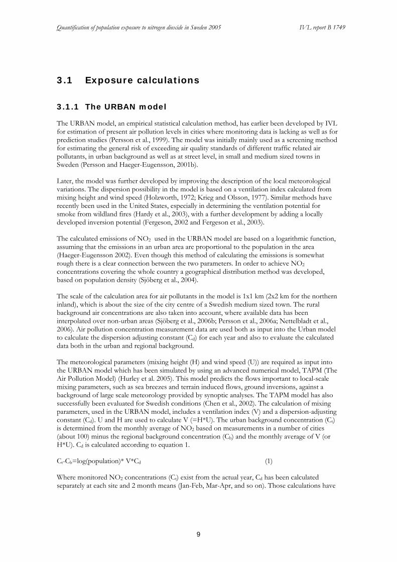
The URBAN model, an empirical statistical calculation method, has earlier been developed by IVL for estimation of present air pollution levels in cities where monitoring data is lacking as well as for prediction studies (Persson et al., 1999). The model was initially mainly used as a screening method for estimating the general risk of exceeding air quality standards of different traffic related air pollutants, in urban background as well as at street level, in small and medium sized towns in Sweden (Persson and Haeger-Eugensson, 2001b).
Later, the model was further developed by improving the description of the local meteorological variations. The dispersion possibility in the model is based on a ventilation index calculated from mixing height and wind speed (Holzworth, 1972; Krieg and Olsson, 1977). Similar methods have recently been used in the United States, especially in determining the ventilation potential for smoke from wildland fires (Hardy et al., 2003), with a further development by adding a locally developed inversion potential (Fergeson, 2002 and Fergeson et al., 2003).
The calculated emissions of NO2 used in the URBAN model are based on a logarithmic function, assuming that the emissions in an urban area are proportional to the population in the area (Haeger-Eugensson 2002). Even though this method of calculating the emissions is somewhat rough there is a clear connection between the two parameters. In order to achieve NO2 concentrations covering the whole country a geographical distribution method was developed, based on population density (Sjöberg et al., 2004).
The scale of the calculation area for air pollutants in the model is 1x1 km (2x2 km for the northern inland), which is about the size of the city centre of a Swedish medium sized town. The rural background air concentrations are also taken into account, where available data has been interpolated over non-urban areas (Sjöberg et al., 2006b; Persson et al., 2006a; Nettelbladt et al., 2006). Air pollution concentration measurement data are used both as input into the Urban model to calculate the dispersion adjusting constant (Cd) for each year and also to evaluate the calculated data both in the urban and regional background.
The meteorological parameters (mixing height (H) and wind speed (U)) are required as input into the URBAN model which has been simulated by using an advanced numerical model, TAPM (The Air Pollution Model) (Hurley et al. 2005). This model predicts the flows important to local-scale mixing parameters, such as sea breezes and terrain induced flows, ground inversions, against a background of large scale meteorology provided by synoptic analyses. The TAPM model has also successfully been evaluated for Swedish conditions (Chen et al., 2002). The calculation of mixing parameters, used in the URBAN model, includes a ventilation index (V) and a dispersion-adjusting constant (Cd). U and H are used to calculate V (=H*U). The urban background concentration (Ct) is determined from the monthly average of NO2 based on measurements in a number of cities (about 100) minus the regional background concentration (Cb) and the monthly average of V (or H*U). Cd is calculated according to equation 1.
Ct-Cb=log(population)* V*Cd (1)
Where monitored NO2 concentrations (Ct) exist from the actual year, Cd has been calculated separately at each site and 2 month means (Jan-Feb, Mar-Apr, and so on). Those calculations have

Quantification of population exposure to nitrogen dioxide in Sweden 2005 IVL report B 1749
10
then been used to determine the NO2 concentrations in all cities. Consequently, by assuming that Cd is similar for towns with similar V's, NO2 concentrations will be derived in cities where no data is available. For cities with existing data the concentrations will be recalculated.
Measurement data of air pollution concentrations are used both as input into the URBAN model to calculate the dispersion adjusting constant (Cd) for each year and also to evaluate the calculated data both in the urban and regional background.
3.1.1.1 Annual means
The determination of the annual mean values for NO2 in ambient air is based on all available monitoring data (including data from both active and diffusive sampling), as monthly averages, in urban background air. The regional background concentrations are interpolated over the country. Annual means are then calculated as described above (see Chapter 3.1.1) for all 1890 cities in Sweden.
3.1.1.2 Daily means
Since air pollutants can cause health effects due to both long-term and short-term exposure, there is a need to derive annual as well as daily mean concentrations. The input to the long-term exposure studies is the number of people being exposed to different annual means. For the short-term exposure the input is the number of days people are being exposed to different daily mean concentration levels. In order to derive data for short term calculation the relation between long-term (winter half-year means/annual means) and short-term (98 percentile of daily means/winter half-year or a year) concentrations for 2002-2005 in 98 urban background sites has been investigated. The result is presented in Figure 1.
R2 = 0.73
R2 = 0.86
0
20
40
60
80
100
120
0 5 10 15 20 25 30 35 40 45 50
Winter half year/annual mean NO2 (µg/m3)
98%
-ile
(Win
ter h
alf y
ear/a
nnua
l m
ean
(NO
2 (µg
/m3 )
Winter half yearAnnualLinear (Annual)Linear (Winter half year)
Figure 1 Relation between the winter half-year mean/annual means and corresponding 98 percentile of
daily means of the NO2 concentrations during 2002-2005 in 98 urban background sites.

Quantification of population exposure to nitrogen dioxide in Sweden 2005 IVL report B 1749
11
Each of the years was at first tested separately, but the results were very similar. For this reason they are presented together. This means that the meteorological influence does not have a great impact on the relation between winter half-year and daily means. It is known that the concentrations are higher during years with poor ventilation, but this obviously affects both long- and short-term concentrations in a similar way.
Since there was such a good relation between NO2 concentrations of the winter half-year means/annual means and the 98 percentile of daily means (Figure 1) it was assumed that there would also be a connection between the frequency of days in different daily mean concentration intervals and the winter half-year means/annual means. In order to derive this, the amount of days in the different concentration intervals (0-5 µg/m3, 5-10 µg/m3 and so on) of the daily means were calculated and compared to the winter half-year mean concentrations for each of the 98 sites. The results are presented in Figure 2. The three lowest concentration groups are presented in a) where the number of days decrease with increasing winter half-year means. For the higher concentration groups, presented in b), the number of days increase with increasing winter half-year mean concentrations. The equation for each group is derived by calculating the best fit curve.
In the groups presented in Figure 2a) 0-5 (blue) and 5-10 (pink) the frequencies decrease with increasing winter half-year mean concentrations. In the groups with higher concentrations than 20 (Figure 2b) the frequencies increase with increasing winter half-year means. In groups 10-15 (yellow) and 15-20 (turquoise) the curve contains an increasing part for winter half-year means up to 14 and 18 µg/m3 respectively. With higher winter half-year means these frequencies decrease. The calculation of R2 shows for most of the groups a fairly good agreement with the calculated line.

Quantification of population exposure to nitrogen dioxide in Sweden 2005 IVL report B 1749
12
a)
R2 = 0.7
R2 = 0.6
R2 = 0.8
0
10
20
30
40
50
60
70
80
90
100
5 8 10 13 15 18 20 23 25 28 30Winter half year mean
Am
ount
of d
ays
0-5
5-10
10-15
b)
R2 = 0.5R2 = 0.6
R2 = 0.7
R2 = 0.8
R2 = 0.7
R2 = 0.5
0
5
10
15
20
25
30
35
40
45
50
5 8 10 13 15 18 20 23 25 28 30 33 35Winter half year mean
Am
ount
of d
ays
15-2020-2525-3030-3535-4045-50Poly. (15-20)Log. (20-25)Linear (25-30)Linear (30-35)Linear (35-40)Linear (45-50)
Figure 2 Number of days in each daily mean concentration interval compared to the winter half year mean based on four years’ measurements in urban background sites in 98 cities. In a) the interval of daily means from 0 to 15 is presented. In b) the interval of daily means from 20 to ≥ 50 is presented. The equation for each group is derived by calculating the best curve fit. Observe the different scales in a) and b).
A comparison of the accuracy of applying the above derived equations for estimating the number of days in each group has been performed using monitoring data from the urban background site Femman in Göteborg. When comparing the number of days derived by calculated and monitored NO2 data for each group the result is reasonable good (Figure 3). A comparison has also been made between the distribution pattern of the number of days compared to both winter half year means

Quantification of population exposure to nitrogen dioxide in Sweden 2005 IVL report B 1749
13
and corresponding annual means based on monitored data. The same monitoring sites have been used to calculate the distribution pattern for both winter half year and the complete annual year distribution ( Figure 4).
0
10
20
30
40
50
60
70
80
90
100
5-10 10-15 15-20 20-25 25-30 30-35 35-40 >=40
Concentration class yearly means
Num
ber o
f day
s
MonitoredCalculated
Figure 3 Comparison of the number of days in each concentration class based on calculated and
monitored NO2 concentration data from 1999 at the urban background site Femman in Göteborg.
-15%
-10%
-5%
0%
5%
10%
15%
5-10 10-15 15-20 20-25 25-30 30-35
Annual/winter half year concentration interval
Diff
eren
ce in
dis
tribu
tion
annu
al-w
inte
r ha
lf ye
ar
0-5 5-10 10-15 15-20 20-25
25-30 30-35 35-40 40-45 45-50
50-55 55-60 >60
Figure 4 The difference in the distribution pattern of number of days in each long term concentration
interval based on both annual and winter half year means.
According to the result in Figure 4 the average difference is about 1 % with the largest difference in the lowest and the second lowest concentration classes. Negative values indicate that the number of days with low concentration levels is larger when the distribution pattern is based on a whole year calculation rather than a winter half year calculation. The difference is, however, less than 10 %
Quantification of population exposure to nitrogen dioxide in Sweden 2005 IVL report B 1749
14
which is assumed not to have any greater influence on the population exposure calculations. Thus, in order to determine the number of days of different concentration levels the above establish equations were used.
3.1.2 Calculation of a normal meteorological year
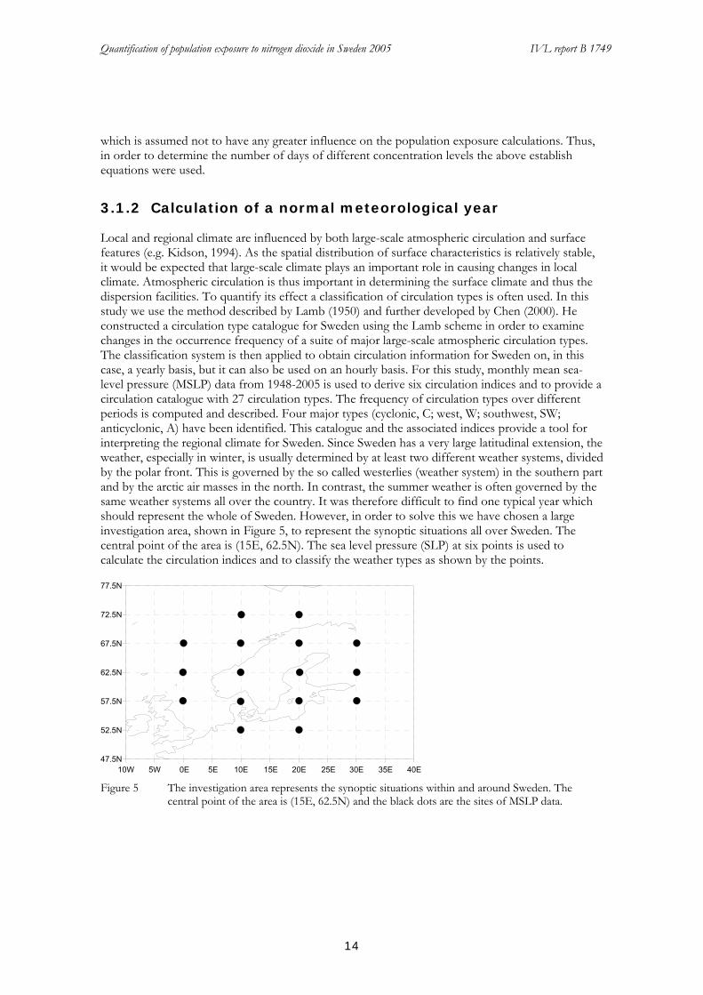
Local and regional climate are influenced by both large-scale atmospheric circulation and surface features (e.g. Kidson, 1994). As the spatial distribution of surface characteristics is relatively stable, it would be expected that large-scale climate plays an important role in causing changes in local climate. Atmospheric circulation is thus important in determining the surface climate and thus the dispersion facilities. To quantify its effect a classification of circulation types is often used. In this study we use the method described by Lamb (1950) and further developed by Chen (2000). He constructed a circulation type catalogue for Sweden using the Lamb scheme in order to examine changes in the occurrence frequency of a suite of major large-scale atmospheric circulation types. The classification system is then applied to obtain circulation information for Sweden on, in this case, a yearly basis, but it can also be used on an hourly basis. For this study, monthly mean sea-level pressure (MSLP) data from 1948-2005 is used to derive six circulation indices and to provide a circulation catalogue with 27 circulation types. The frequency of circulation types over different periods is computed and described. Four major types (cyclonic, C; west, W; southwest, SW; anticyclonic, A) have been identified. This catalogue and the associated indices provide a tool for interpreting the regional climate for Sweden. Since Sweden has a very large latitudinal extension, the weather, especially in winter, is usually determined by at least two different weather systems, divided by the polar front. This is governed by the so called westerlies (weather system) in the southern part and by the arctic air masses in the north. In contrast, the summer weather is often governed by the same weather systems all over the country. It was therefore difficult to find one typical year which should represent the whole of Sweden. However, in order to solve this we have chosen a large investigation area, shown in Figure 5, to represent the synoptic situations all over Sweden. The central point of the area is (15E, 62.5N). The sea level pressure (SLP) at six points is used to calculate the circulation indices and to classify the weather types as shown by the points.
47.5N
52.5N
57.5N
62.5N
67.5N
72.5N
77.5N
10W 5W 0E 5E 10E 15E 20E 25E 30E 35E 40E Figure 5 The investigation area represents the synoptic situations within and around Sweden. The
central point of the area is (15E, 62.5N) and the black dots are the sites of MSLP data.

Quantification of population exposure to nitrogen dioxide in Sweden 2005 IVL report B 1749
15
In the study 1948-2005 NCEP reanalysis was used to classify the daily SLP data set to the circulation types. There was no unclassified type in our classification.
The following calculations are performed to find out which years between 1948 and 2005 are typical years. By typical years we mean years with frequency of the weather types and/or index values near their respective long term means. Three steps are followed:
A. For the weather types
1) Calculate the frequency (100%) of 26 weather types for each year
2) Calculate the long term mean frequency for each type
3) Calculate the yearly standard deviation (SD) of the frequency
1
1 ( ) , 1, 2,N
j ij ii
SD x x j MN =
= − =∑ L ,
N= 26 weather types; M= 58 years
Then the years were sorted according to the SD from the least (closest to the long term mean) to the biggest (farthest to the long term mean)
B. For the six indices
1) Calculate the average of 6 indices for each year
2) Calculate the long term mean of each index
3) Calculate the yearly standard deviation (SD) of the index
1
1 ( ) , 1, 2,N
j ij ii
SD x x j MN =
= − =∑ L
N= 6 indices; M=58 years
After the yearly SD have been calculated the SD has been ordered from the least to the biggest, in a similar way as for the frequencies.
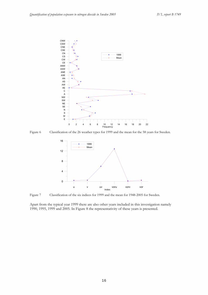
From the results the indices for 1999 were found to be very close to the long term mean and it is the second most representative year of all the 58 years. In terms of the weather types, 1999 is also fairly close to the long-term mean, being in the 9th place. If we assume that 20% of all the years can be considered as typical (normal), then we can accept any year up to the 12th closest. Thus, 1999 is well defined as a typical year. To show this clearly, we plot the indices and the frequencies of the long term mean together with those of 1999 in the following plots (Figure 6 and Figure 7).
Quantification of population exposure to nitrogen dioxide in Sweden 2005 IVL report B 1749
16
0 2 4 6 8 10 12 14 16 18 20 22Frequency
EWSN
SENESWNW
AC
AEAWASAN
ASEANEASWANW
CECWCSCN
CSECNECSWCNW
1999Mean
Figure 6 Classification of the 26 weather types for 1999 and the mean for the 58 years for Sweden.
u v uv voru vorv vorIndex
0
4
8
12
161999Mean
Figure 7 Classification of the six indices for 1999 and the mean for 1948-2005 for Sweden.
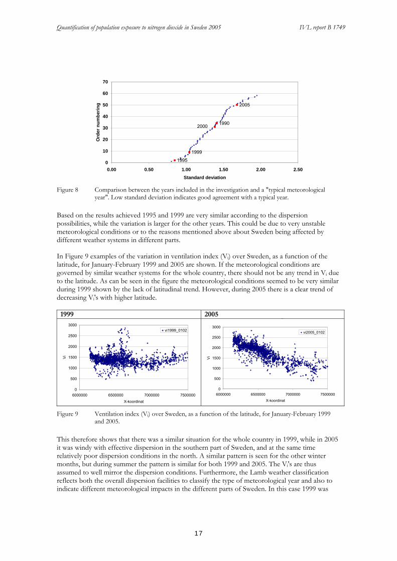
Apart from the typical year 1999 there are also other years included in this investigation namely 1990, 1995, 1999 and 2005. In Figure 8 the representativity of these years is presented.
Quantification of population exposure to nitrogen dioxide in Sweden 2005 IVL report B 1749
17
2005
1995
1999
19902000
0
10
20
30
40
50
60
70
0.00 0.50 1.00 1.50 2.00 2.50Standard deviation
Ord
er n
umbe
ring
Figure 8 Comparison between the years included in the investigation and a "typical meteorological
year". Low standard deviation indicates good agreement with a typical year.
Based on the results achieved 1995 and 1999 are very similar according to the dispersion possibilities, while the variation is larger for the other years. This could be due to very unstable meteorological conditions or to the reasons mentioned above about Sweden being affected by different weather systems in different parts.
In Figure 9 examples of the variation in ventilation index (Vi) over Sweden, as a function of the latitude, for January-February 1999 and 2005 are shown. If the meteorological conditions are governed by similar weather systems for the whole country, there should not be any trend in Vi due to the latitude. As can be seen in the figure the meteorological conditions seemed to be very similar during 1999 shown by the lack of latitudinal trend. However, during 2005 there is a clear trend of decreasing Vi's with higher latitude. 1999 2005
0
500
1000
1500
2000
2500
3000
6000000 6500000 7000000 7500000X-koordinat
Vi
vi1999_0102
_
0
500
1000
1500
2000
2500
3000
6000000 6500000 7000000 7500000X-koordinat
Vi
vi2005_0102
Figure 9 Ventilation index (Vi) over Sweden, as a function of the latitude, for January-February 1999
and 2005.
This therefore shows that there was a similar situation for the whole country in 1999, while in 2005 it was windy with effective dispersion in the southern part of Sweden, and at the same time relatively poor dispersion conditions in the north. A similar pattern is seen for the other winter months, but during summer the pattern is similar for both 1999 and 2005. The Vi's are thus assumed to well mirror the dispersion conditions. Furthermore, the Lamb weather classification reflects both the overall dispersion facilities to classify the type of meteorological year and also to indicate different meteorological impacts in the different parts of Sweden. In this case 1999 was

Quantification of population exposure to nitrogen dioxide in Sweden 2005 IVL report B 1749
18
found to be a typical or normal year according to dispersion conditions for the whole country. The accuracy of using a typical/normal weather from one year as an input in calculating the concentrations for another year was investigated by analysing 2005 using meteorology for both 1999 and 2005.
In Figure 10 the relative NO2 concentration difference in the 59 largest cities using meteorology of 1999 and 2005 as a function of the latitude is shown.
1
1.1
1.2
1.3
1.4
1.5
6000000 6500000 7000000 7500000X-coordinate
rela
tive
diffe
renc
e
diff 05_V99/05_V05
Figure 10 The relative NO2 concentration difference using meteorology of 1999 and 2005 as a function
of the latitude.
It becomes clear in Figure 10 that the differences increase with increasing latitude indicating that if the concentration calculations are based on Vis from 1999 then the pollution concentrations in 2005 can be over-estimated for some parts of Sweden. When comparing a national mean concentration for the largest cities (>20 000 inhabitants) the annual mean 2005 based on Vis of 1999 is 13.5 µg/m3 and 12 µg/m3 based on Vis of 2005. If 1999 is used for the calculation of the 2005 NO2 concentrations it will thus lead to an over-estimation in the concentration levels that increases with latitude. This indicates that it is not suitable to apply a typical/normal meteorology for individual years. However, it also shows that the method captures the variety in meteorology in different parts of the country and thus, if using the actual meteorology, properly reflects the dispersion facilities, which is very important for calculations on a national scale.
3.1.3 Population data
The previous estimate was based on population data at 1 x 1 km, derived from population statistics at parish level and municipality level (Sjöberg et al., 2004). The population statistics were redistributed within each parish/community at 1 x 1 km grid resolution, applying land use data based on the following assumptions: 60 % of the population were allocated to urban areas, 35 % to areas with open land, such as farmland, and the remaining 5 % to forest areas. Within the cities, the population was allocated to built-up areas, and the population density was assumed to decrease from the city centre to the city limit.
Quantification of population exposure to nitrogen dioxide in Sweden 2005 IVL report B 1749
19
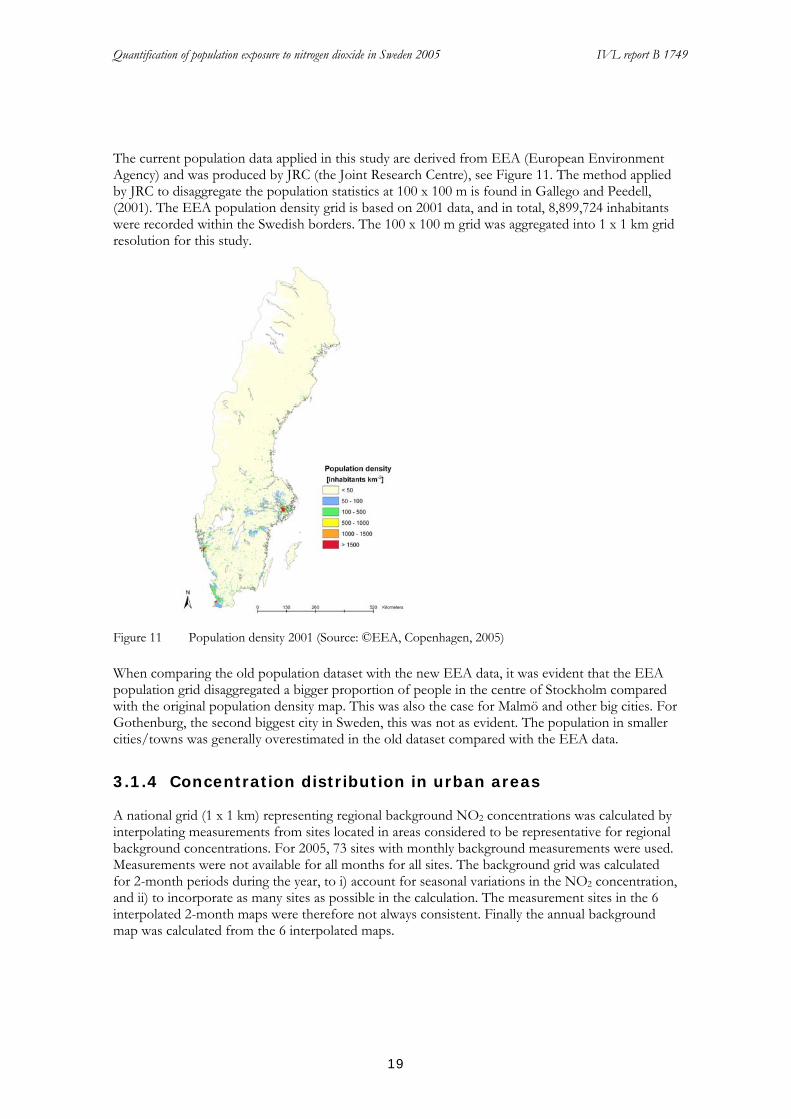
The current population data applied in this study are derived from EEA (European Environment Agency) and was produced by JRC (the Joint Research Centre), see Figure 11. The method applied by JRC to disaggregate the population statistics at 100 x 100 m is found in Gallego and Peedell, (2001). The EEA population density grid is based on 2001 data, and in total, 8,899,724 inhabitants were recorded within the Swedish borders. The 100 x 100 m grid was aggregated into 1 x 1 km grid resolution for this study.
Figure 11 Population density 2001 (Source: ©EEA, Copenhagen, 2005)
When comparing the old population dataset with the new EEA data, it was evident that the EEA population grid disaggregated a bigger proportion of people in the centre of Stockholm compared with the original population density map. This was also the case for Malmö and other big cities. For Gothenburg, the second biggest city in Sweden, this was not as evident. The population in smaller cities/towns was generally overestimated in the old dataset compared with the EEA data.
3.1.4 Concentration distribution in urban areas
A national grid (1 x 1 km) representing regional background NO2 concentrations was calculated by interpolating measurements from sites located in areas considered to be representative for regional background concentrations. For 2005, 73 sites with monthly background measurements were used. Measurements were not available for all months for all sites. The background grid was calculated for 2-month periods during the year, to i) account for seasonal variations in the NO2 concentration, and ii) to incorporate as many sites as possible in the calculation. The measurement sites in the 6 interpolated 2-month maps were therefore not always consistent. Finally the annual background map was calculated from the 6 interpolated maps.

Quantification of population exposure to nitrogen dioxide in Sweden 2005 IVL report B 1749
20
For each urban area the contribution from regional background NO2 concentration was calculated from the background grid, and subtracted from the urban NO2 concentration to avoid double counting. Hence only the additional NO2-concentration (on top of the background levels) in urban areas was distributed.
The NO2 concentration distribution methodology in urban areas is dependent on the size of the urban area. The size of the urban area is calculated from diameter information gathered from Statistics Sweden (www.scb.se) from 80 cities in Sweden. It was found that there was a strong relationship between the diameter and the number of inhabitants (Figure 12).
R2 = 0.8
0
500
1000
1500
2000
2500
3000
3500
4000
4500
0 1000 2000 3000 4000 5000 6000 7000 8000 9000 10000Population
City
dia
met
er (m
)
R2 = 0.9
0
2000
4000
6000
8000
10000
12000
10000 30000 50000 70000 90000 110000Population
City
dia
met
er (m
)
Figure 12 The connection between city diameter and number of inhabitants in small and large urban
areas respectively.
Based on this the urban areas were then divided into 4 different groups dependent on number of inhabitants (Figure 13):
1) 200 – 2,500 inhabitants 2) 2,500 – 5,000 inhabitants 3) 5,000 – 10,000 inhabitants 4) >10,000 inhabitants

Quantification of population exposure to nitrogen dioxide in Sweden 2005 IVL report B 1749
21
a) b) c) Figure 13 a) The distribution pattern of urban areas with a population of 200 – 2,500 people (Group 1),
b) The distribution pattern of urban areas with a population of 2,500 – 10,000 people (Group 2-3), and c) An example (Karlskoga) of the distribution pattern of urban areas with a population > 10,000 people (Group 4).
Group 1
The NO2 concentration was apportioned to the 1 km grid cell in which the town was located (Figure 13a).
Group 2-3
In towns with a population between 2,500 and 10,000 inhabitants, the NO2 concentration was distributed according to a bell-shape methodology. 100 % of the concentration was apportioned to the 1 km grid cell in which the town was located, and a proportion of the concentration was assigned in a circle around the town, applying a spatial decay function with smaller concentrations further away from the town (Figure 13b). The functions are derived by calculating mean radius from the cities in each group and best fit curve (Figure 14 and Figure 15).
0%
10%
20%
30%
40%
50%
60%
70%
80%
90%
100%
0 250 500 750 1000 1250 1500Distance from the centre (m)
Dec
reas
ed c
once
ntra
tion(
%)
Group 2Group 3
Figure 14 Calculated graphs of the decrease of the calculated urban back ground concentrations in cities
from group 1 and 3.
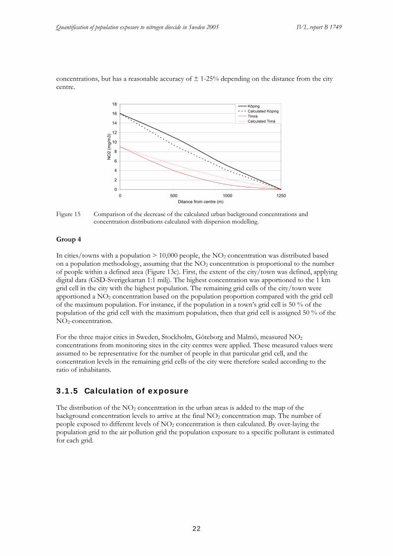
The calculated decrease of NO2 were tested in some cities by comparing the decrease of the calculated urban background concentrations and concentration distributions calculated with dispersion modelling. The comparison shows both some under- and overestimates of the calculated
Quantification of population exposure to nitrogen dioxide in Sweden 2005 IVL report B 1749
22
concentrations, but has a reasonable accuracy of ± 1-25% depending on the distance from the city centre.
0
2
4
6
8
10
12
14
16
18
0 500 1000 1250Ditance from centre (m)
NO
2 (m
g/m
3)KöpingCalculated KöpingTimråCalculated Timå
Figure 15 Comparison of the decrease of the calculated urban background concentrations and
concentration distributions calculated with dispersion modelling.
Group 4
In cities/towns with a population > 10,000 people, the NO2 concentration was distributed based on a population methodology, assuming that the NO2 concentration is proportional to the number of people within a defined area (Figure 13c). First, the extent of the city/town was defined, applying digital data (GSD-Sverigekartan 1:1 milj). The highest concentration was apportioned to the 1 km grid cell in the city with the highest population. The remaining grid cells of the city/town were apportioned a NO2 concentration based on the population proportion compared with the grid cell of the maximum population. For instance, if the population in a town’s grid cell is 50 % of the population of the grid cell with the maximum population, then that grid cell is assigned 50 % of the NO2-concentration.
For the three major cities in Sweden, Stockholm, Göteborg and Malmö, measured NO2 concentrations from monitoring sites in the city centres were applied. These measured values were assumed to be representative for the number of people in that particular grid cell, and the concentration levels in the remaining grid cells of the city were therefore scaled according to the ratio of inhabitants.
3.1.5 Calculation of exposure
The distribution of the NO2 concentration in the urban areas is added to the map of the background concentration levels to arrive at the final NO2 concentration map. The number of people exposed to different levels of NO2 concentration is then calculated. By over-laying the population grid to the air pollution grid the population exposure to a specific pollutant is estimated for each grid.

Quantification of population exposure to nitrogen dioxide in Sweden 2005 IVL report B 1749
23
3.2 Health impact assessment
Health impact assessments are built on epidemiological findings; exposure-response functions and population relevant rates. A typical health impact function has four components: an effect estimate from a particular epidemiologic study, a baseline rate for the health effect, the affected number of persons and the estimated “exposure” (here pollutant concentration).
The excess number of cases per year may be calculated as:
where y0 is the baseline rate, pop is the affected number of persons; ß is the exposure-response function (relative risk per change in concentration), and x is the estimated excess exposure.
Based on these data we have calculated the population weighted “mean exposure” to be approximately 10 µg/m3. We have used 10 µg/m3 as a lower cut off in our impact assessment scenarios and accordingly defined exposure above 10 µg/m3 as excess exposure resulting in “excess cases”.
3.2.1 Exposure-response function for mortality
The effect of air pollution on mortality is much larger when based on long-term exposure rather than on time-series studies of short-term levels and daily number of deaths. Given the exposure data in terms of estimated levels of nitrogen a literature survey was conducted to find a relevant exposure-response assumption for the association between air pollution levels (indicated by the annual nitrogen dioxide concentration) and mortality as well as hospital admissions. This process identified four studies with exposure data and a study design that made them potential providers of exposure-response functions for the association between long-term exposure to nitrogen dioxide and mortality. Nitrogen dioxide may be seen as an indicator of air pollution mainly from the transport sector and other combustion sources. Despite large differences in their design, the four studies, found very similar associations. A Dutch cohort study reported a 12 % increase in all-cause mortality per 10 µg/m3 increase in NO2 (Hoek et al, 2002), a French cohort study reported a 14 % increase in non-accidental mortality for 10 µg/m3 increase in NO2 (Filleul et al, 2005), an ecological study from Auckland, New Zealand, reported a 13 % increase in non-external mortality for 10 µg/m3 increase in NO2 (Scoggins et al, 2004), and a German follow up of women in several cross-sectional studies found an increase close to 11 % per 10 µg/m3 increase in NO2 (Gehring et al, 2006). A Norwegian cohort study used NOX as exposure indicator and could not be used for this impact assessment (Nafstad et al, 2004).
3.2.1.1 The Netherlands Cohort Study
The ongoing cohort study “The Netherlands Cohort Study (NLCS) on diet and cancer” (Hoek et al, 2002) has been used to study the association between traffic related air pollution and mortality. The baseline data collection took place in 1986, when subjects aged 55–69 years were included and information was collected about a large number of risk factors besides diet for the development of cancer. The study sample (n= 120 852) was recruited from 204 municipalities that had
Δy = (y0 • pop) (eß • Δx - 1)

Quantification of population exposure to nitrogen dioxide in Sweden 2005 IVL report B 1749
24
computerized population registries in 1986, and were sufficiently covered by cancer registries. The exact address of all study subjects in 1986 is known. A random sample of 5000 participants has been followed up every second year for migration and vital status. In the air pollution study, this sub sample from the NLCS cohort has been analyzed. 4492 persons had answered the questionnaires, and out of these, the geographical coordinates for the addresses were identified for 4466 subjects. 5% lived close to a major road and 3% within 100 m of a freeway. 3464 subjects had information enough for full adjustment for potential confounders. 489 participants in the sub sample died during the follow up 1986-1994, most from natural causes.
Exposure was estimated using the 1986 home address and residential history information to generate indicators, on an individual basis, of long-term exposure to traffic related air pollutants. About 90% of the study population lived 10 years or more at its 1986 home address, supporting the use of the estimated concentration at the 1986 address as a relevant exposure variable.
The long-term average exposure was considered to be determined by the regional background, additional pollution from urban sources (resulting in an urban background), and for a small proportion of the subjects, additional pollution from local sources (major roads and freeways). Two traffic related air pollutants, nitrogen dioxide (NO2) and black smoke (BS) were used as indicator pollutants. The regional component at the home address was estimated using interpolation of measurements at regional background stations. There were 24 sites for NO2. A regression model relating degree of urbanization to air pollution was used to allow for differences between different towns and neighbourhoods of cities. If only the regional scale is taken into account, the range in NO2 exposure between the 10th and 90th percentile was about 67%.When differences in urbanization degree were taken into account, the difference in exposure between the 10th and 90th percentile became 76% for NO2.
Distance to major roads was calculated to characterize the local contribution from traffic, using a Geographic Information System. The quantitative estimates of the contribution of living 50 m away from a freeway to the concentration was 11 and the contribution from major inner-city roads was estimated to be 8 µg/m3 NO2, respectively. These estimates were assigned to each ”exposed” address, independent of the actual distance to the road. However, the local contribution added this way increased only by 0.5 µg/m3 the estimated average regional + urban concentration, to 36.6 µg/m3. For NO2 the exposure range was 14.7 – 67.2 µg/m3, including the contribution from local traffic.
In the analyses, two types of models for exposure calculations were used with regard to how the local contribution was added to the urban background. One type of model had a qualitative indicator variable for living near a major road; the other added the estimated contribution from living near a major road as a concentration.
Adjustment was made in the analyses for a large set of potential confounding variables at individual level; age, active smoking, passive smoking, education, last occupation, Quetelet index (bodyweight divided by height squared), alcohol intake, fat intake, vegetable and fruit consumption. In addition, adjustment was made for regional indicators of poverty (income distribution, proportion of the population aged 15–64 years on social security).
Before adjustment for confounders, exposure to black smoke and nitrogen dioxide was significantly associated with all-cause mortality. The relative risk associated with an increase in NO2 of 30 µg/m3 was 1.45 (95% CI 1.05-2.01). After adjustment for confounders, the relative risk became smaller and non-significant, 1.36 (95% CI 0.93-1.98).

Quantification of population exposure to nitrogen dioxide in Sweden 2005 IVL report B 1749
25
The size is a clear limitation in the case of this study, which also resulted in a non-significant adjusted association. On the other hand the magnitude of the effect estimate is still not trivial, and corresponds to a 12% increase in all-cause mortality per 10 µg/m3 of NO2.
3.2.1.2 The PAARC Study
In the French PAARC survey long-term effects of air pollution on mortality were studied in 14 284 adults who resided in 24 areas from seven French cities (Bordeaux, Lille, Lyon, Mantes la Jolie, Marseille, Rouen, Toulouse) when enrolled in the study in 1974 (Filleul et al, 2005). For six monitoring sites, the NO/NO2 ratio suggested that the exposure measure was heavily influenced by the local traffic and not representative of the mean exposure of the population in these areas. Thus, the main conclusions from this study are based on a subgroup of 18 areas that could be characterised by urban background monitoring stations, defined by a ratio of NO/NO2 <3.
The choice of areas was based on a three step procedure, initially based on available historic air pollution data for the cities, followed by selection of potential areas and measurement points, taking into account all available information on pollution and feasibility regarding population density in the areas. Each area varied in diameter from 0.5 to 2.3 km. In the final step, air pollution measurements were set up at a centrally located pollution monitoring station in each of these areas, using available standard methods: sulphur dioxide (specific (SO2) and acidimetric method (AM)), total suspended particles (TSP, gravimetric method), black smoke (BS, reflectometry), nitrogen dioxide (NO2, colorimetric analyser), and nitric oxide (NO, colorimetric analyser). Daily measurements were conducted for three years (1974–76). Indicators of air pollution were the mean concentrations during the measurement period, when the area variation for NO2 was ranging from 12 to 61 µg/m3.
The inclusion criteria for enrolment between 1974 and 1976 were to be a member of a French family household in the area for three years or more, and to be aged 25–59 years. In an interview, a questionnaire was completed which included questions about weight, height, smoking history and
occupational exposures among other things. Vital status was first searched for all subjects born in France (17 805 subjects) over three years (1995–98) in each place of birth. In addition, searches through a national register were performed. Loss to follow up was primarily related to sex, with significantly more unknown vital status for women due to changes in surname, but was unrelated to air pollution. Vital status was available until June 2001 (2533 deaths, 11 753 alive, and 2619 unknown), and cause of death until December 1998. Causes of death were obtained through the specialised department (SC8) of the National Institute of Health and Medical Research (INSERM) and for 96% of subjects.
Cox proportional hazards models were used for the analysis, controlling for individual confounders (smoking, educational level, body mass index, occupational exposure), in addition frailty models were used to take into account spatial correlation.
Models were run before and after exclusion of the six areas with monitors influenced by local traffic. After exclusion of these areas, analyses showed that non-accidental mortality increased by 14% (95% CI 3-25%) for 10 µg/m3 increase in NO2. In particular, cardiopulmonary mortality was associated with NO2, the increase associated with a 10 µg/m3 change in the concentration was 27% (95% CI 4-56%).
A problem in this study is that people tended to move a lot, so the analysis was also restricted to deaths during the first 10 years of follow up (until 1986), which resulted in the same results in the
Quantification of population exposure to nitrogen dioxide in Sweden 2005 IVL report B 1749
26
estimated associations between air pollution and mortality, although with wide CIs according to the smaller number of deaths.
3.2.1.3 The Auckland Study
This study (Scoggins et al, 2004) is, in contrast to the above mentioned studies from The Netherlands and France, not a cohort study. This study is an ecological cross-sectional study with the aim to investigate the relation between ambient air pollution levels and mortality in Auckland, New Zealand. Thus, in this study the data analysis was undertaken at the national census area unit level, which means that adjustments for risk factors are not done at the individual level. The census area units (CAU) typically had 3000 inhabitants, and had an average size of approximately 14 km2, while in the central urban areas the average size was approximately 2 km2.
In the Auckland study urban airshed modelling and GIS-based techniques were used to quantify long-term exposure to air pollution. A comprehensive emission inventory and a climate database were used to simulate air pollution concentrations, which were validated with hourly observations from several air quality monitoring sites. The models were run on a 3 km grid that covered almost the entire Auckland region. The final grid had a total of 1296 grid cells, 36 rows by 36 columns, grid cell size 9 km2. The NO2 modelled concentrations were averaged over the whole year and annual average NO2 was used as a long-term air pollution exposure indicator. The evaluation with measured values showed that the urban airshed modelling carried out gave an index of agreement above 0.75 for NO2 at most sites, which is a good model performance. Modelled annual average NO2 concentrations were converted from point-based x, y coordinates into 3 km by 3 km polygon grid coverage. Then polygon grid coverage concentrations were converted to census area unit concentrations by calculating an area-weighted average concentration for all individual units that overlapped more than one grid cell.
Mortality data were collected from New Zealand Health Information Service, for the years 1996 to 1999. External causes of mortality (deaths due accidents, violence and suicide) were excluded. The 1996 Census provided information by CAU for the Auckland region on resident population, sex, age and ethnicity.
Logistic regression was used to investigate how air pollution influences the probability of dying, while controlling for potential confounders. A binomial model was applied because of the very small denominator populations in most cells. Relative risks produced from multivariate modelling, were used to estimate the percentage increase in mortality per increase in annual average NO2. These risk functions were also used to estimate the average annual (1996–1999) number of deaths attributed to air pollution in the Auckland region. A linear increase in mortality risk above each annual average threshold level was assumed. Several different annual threshold levels were tested.
After adjustment for age, sex, ethnicity, socio-economic status, and urban/rural domicile there was a 13% (95% CI: 11–15%) increase in non-external cause mortality per 10 µg/m3 increase in annual average NO2. There was no significant relationship between annual average NO2 and external cause mortality, which suggests that the effect on non-external cause mortality is less likely to be due to uncontrolled confounding. NO2 was however significantly and more strongly related to circulatory and respiratory mortality.
Based on this exposure–response relationship and applying an annual average threshold at 13 µg/m3, the proportion of deaths from non-external causes attributable to air pollution above this level was estimated to 3.9% of all deaths in Auckland. This cut off point was chosen as it represents

Quantification of population exposure to nitrogen dioxide in Sweden 2005 IVL report B 1749
27
the mean annual average NO2 in the Auckland region, and it was assumed that below this level, air pollution has negligible effects on mortality.
Besides the ecological design, one other limitation of this study is that the analytical methods did not control for potential spatial autocorrelations in the data, which may have resulted in an underestimation of the variance and to narrow confidence intervals.
3.2.1.4 The North Rhine-Westphalia Study
This study (Gehring et al, 2006) is a follow up of a series of cross-sectional studies on the effect of air pollution on women's health performed in the 1980s and 1990s in North Rhine-Westphalia, Germany. In each cross-sectional study, approximately 450 German women in their mid-50s from each of a number of industrial areas and 2 non industrial reference areas were randomly selected and invited to participate. In these cross-sectional studies the overall response rate was 70%. Between January 2002 and May 2003, approximately 4800 women from 10 areas in 7 towns, whose addresses were still available, were successfully followed up.
For each participant the exposure to NO2 and particles was estimated at their baseline address. Both 1-year average concentrations for the year of the baseline examination (1985-1994) and 5-year average concentrations for the year of the baseline examination and the preceding 4 years were estimated from continuous air pollution measurements at centrally located air monitoring stations in the study areas. Nitrogen dioxide concentrations were measured by means of chemiluminescence. The researchers were able to geo-code 4615 (97%) of the participants’ baseline addresses, and calculated proximity of homes to major roads (at least 10 000 cars/day). Associations between exposure and mortality were analyzed using Cox's proportional hazards models adjusting for confounders.
Relative risks were calculated for an interquartile range increase in exposure (16 µg/m3 for NO2). For all-cause mortality and the 1-year average NO2, RR was 1.17 (95% CI = 1.02–1.34), corresponding to 10.6 % per 10 µg/m3 increase.
3.2.1.5 Selected ERF for mortality
The use of any of the four identified studies as a basis for the impact calculations would only result in a small difference in comparison with the use of the others, since they all found mortality to increase around 11-14 % per 10 µg/m3 increase in annual average NO2. The lowest coefficients came from the German study of woman and the Dutch study with the local contribution from major roads and freeways added to the urban background. No such street contribution has been included in the Swedish exposure data for this assessment.
For our assessment we have chosen to use the same estimate as in our previous health impact assessment (HIA) (Forsberg and Sjöberg, 2005a), which was from the Auckland study, and was 13% (95% CI: 11–15%) increase in non-external caused mortality per 10 µg/m3 increase in annual average NO2.

Quantification of population exposure to nitrogen dioxide in Sweden 2005 IVL report B 1749
28
3.2.2 Exposure-response function for admissions
A large number of studies have shown short-term associations between air pollution levels and the daily number of respiratory and cardiovascular incidents. Mainly results from studies of hospital admissions have been used for health impact assessments, since the actual base-line frequencies usually can be obtained from health registers.
3.2.2.1 ERF for respiratory hospital admissions
An overview of hospital admission studies as a basis for health impact assessment found no relevant studies of nitrogen dioxide and all respiratory hospital admissions (Bellander et al, 1999). For respiratory admissions in elderly people over 65 years, two studies gave a weighted estimate of 1.1 % (0.2-2.1) per 10 μg/m3 in the urban background 24-hour nitrogen dioxide concentration after adjustment for PM10. This weighted estimate is of the same magnitude as the typical effect of PM10 on respiratory hospital admissions (usually not adjusted for nitrogen dioxide). In the WHO AirQ programme version 2.2.3 (WHO, 2004) some default values for relative risk estimates are given. For respiratory admissions in persons 15-64 years the value is 0.2 % per 10 μg/m3 (24-hour mean) based on the APHEA results from four European cities (Sunyer et al, 1997). A more recent study is a 6-year long study of 24-hour nitrogen dioxide levels and daily acute hospital admissions for respiratory disease in Drammen, Norway 1995–2000 (Oftedal et al, 2003). Time-series analysis of counts was performed by means of generalized additive models with adjustments for weather, influenza and time period. In this study the relative risk estimate for an increase of 20.8 μg/m3 (IQR) was 6.0 % (95% CI = 1.7-10.5 %), which corresponds to 2.9% per 10 μg/m3. In most areas do also the short-term levels of nitrogen dioxide correlate well with many other exhaust components and NO2 must be seen as an indicator of this type of pollutants.
3.2.2.2 ERF for CVD hospital admissions
The UK Department of Health asked the Committee on the Medical Effects of
Air Pollutants (COMEAP) to review the available studies on effects of outdoor air pollutants on cardiovascular disease (COMEAP, 2006). In the report COMEAP concludes that associations between daily measurements of air pollutants and daily admissions to hospital for a variety of diagnostic conditions or categories relating to cardiovascular disease are generally positive and significant. The associations with cardiac endpoints were generally found clearer than those with cerebrovascular endpoints. COMEAP found for its meta-analysis 17 published studies on 24-hour average nitrogen dioxide levels and cardiac admissions and 8 studies on cerebrovascular admissions. The combined relative risk was 1.3 % (95% CI = 1.0 – 1.7 %) per 10 µg/m3 increase in the 24-hour average NO2 for cardiac hospital admissions, and 0.4 % (95% CI = 0.0 – 0.8 %) for cerebrovascular admissions.
3.2.2.3 Selected ERF for hospital admissions
The most relevant published study identified for our health impact assessment is judged to be the Norwegian study of 24-hour nitrogen dioxide levels and daily acute hospital admissions for respiratory disease in Drammen 1995–2000 reporting a relative risk of 2.9% per 10 μg/m3 (Oftedal et al, 2003).

Quantification of population exposure to nitrogen dioxide in Sweden 2005 IVL report B 1749
29
For cardiovascular hospital admissions COMEAP presents the best overview, which in a meta-analysis found a relative risk of 1.3 % per 10 µg/m3 increase in the 24-hour average NO2 for cardiac hospital admissions, and 0.4 % for cerebrovascular admissions. We have used the proportion of admissions for cardiac and for cerebrovascular disease to calculate a combined risk estimate for all cardiovascular admissions, assuming 69 % of the admissions to be cardiac admissions. This resulted in a relative risk of 1.0 % per 10 μg/m3 to be used in the health impact assessment.
3.2.3 Selected base-line rates
In order to estimate how many deaths and hospital admissions that depend on elevated air pollution exposure we need to use a base-line rate. The national mean rate published (for 2002) by the register unit EpC, at The Swedish Board of Health and Welfare, was 1063 deaths per 100 000 persons. The national mean rate for non-external causes of death was approx. 1010.
The mean number of hospital admissions for respiratory disease in Sweden 2004 was 975 per 100 000 persons, and out of these 903 per 100 000 persons were acute (not planned) admissions. The mean number of cardiovascular hospital admissions in Sweden 2004 was 2602 per 100 000 persons. Out of these 2063 were acute (not planned) admissions.
There are variations in the rate between counties and cities, but air pollution data is not presented in such a way that it is possible to used specific base-line rates for specific parts of Sweden or regions within the country.
For our calculations we have used 1010 deaths per year from non-external causes per 100 000 persons in the entire population at the population weighted mean exposure level. It is sometimes assumed that there is no effect of air pollution on mortality in younger persons, which could motivate exclusion of deaths below a certain age (often 30 years) in the calculations. However, the number of deaths in age range 0-30 years is less than 40 per 100 000 in Sweden, so the impact calculation results only marginally would be changed by such an exclusion. In addition, the Auckland study included all ages (Scoggins et al, 2004). For hospital admissions we assume the baseline rate 903 respiratory admissions per 100 000 persons and 2602 cardiovascular admissions per 100 000 persons at the population weighted mean exposure level.
3.3 Socio-economic valuation
Opening comment: In this text, we use the term 'socio-economic valuation' to describe that the costs of health effects that we consider are social costs rather than private, governmental or corporate costs. The difference is that costs assigned to the above mentioned parties might be distorted due to subsidies, taxes or other transactions that take place. The term 'valuation' is used to signal that research activities need to be taken in order to estimate the social damage of the studied health effect (a very simplified description).
3.3.1 Why should we assess the value of socio-economic costs from health effects?
Health effects caused by high concentrations of air pollutants such as NO2 can be associated to consequential costs for society, via methods we will describe briefly in this chapter. Even if the association between premature deaths (for example) and an economic value can seem repulsive for

Quantification of population exposure to nitrogen dioxide in Sweden 2005 IVL report B 1749
30
some individuals, there are some important reasons to perform an economic assessment of health effects. Furthermore, it must be remembered that economic values connected to health effects should be used as measures that enable comparisons with traded goods and services rather than regarded as absolute measures of individuals’ worth as humans. Furthermore, when valuing mortality, it is important to remember that it is not the occurrence of death in itself that is valued; it is the risk of an early death that is valued.
Two important reasons for economic assessments of health effects should be remembered. First, if performing an economic assessment of health effects from high levels of air pollutants, one can compare the cost for air pollution abatement measures with the socioeconomic benefits from the following reduction in health impact. Second, an economic assessment of health effects related to air pollutants will enable policy makers to make a credible allocation of tax payer resources. A policy maker’s budget is restricted, and it must be remembered that resources used for health care are resources not used to pay for education, child care and other important welfare functions or tax reductions. The same argument is valid for private individuals.
3.3.2 Valuation of socio-economic costs from health effects
In general, valuation of socio-economic costs for negative health effects is performed by either measuring the actual costs for society of treating persons with the considered health effect, or by measuring individuals' willingness to pay or accept for exposing themselves to a larger risk of poor health or death. Examples of the first mentioned approach to socio-economic valuation are calculations of the cost for hospital admissions and treatments due to various illnesses and the production loss caused by absence from work or low productivity at work. This approach is closely related to wages, productivity and use of governmental resources and the suitable name of this approach is 'Production Function approach' or 'Human Capital approach'. Examples of the second approach to socio-economic valuation is to study the price premium of safer private cars that individuals are willing to pay, or the wage premium that is required in order for individuals to accept more dangerous occupations. This approach relates more strongly to individuals' consumption than a firms' production. One method that uses this approach to value health effects and mortality is the 'Avertive Behaviour Method'. Often, the socio-economic costs of negative health effects are calculated from observations of actual consumption and/or production behaviour. These methods are commonly called 'Revealed Preference methods'. In contrast to the 'Revealed Preference methods', the 'Stated Preference Methods' use surveys to perform socio-economic valuations of health effects. Examples of this group of methods are; Contingent Valuation Methods and Choice Experiments. Both the 'Revealed Preference methods' and the 'Stated Preference Methods' are examples of the second approach towards socio-economic valuation mentioned above.
Often, the health effect of largest concern for socio-economic valuation has been premature mortality. Recent developments, following the increased scientific knowledge concerning adverse health effects from high levels of air pollution, have increased the attention to valuation of morbidity (illness). Another consequence of the relatively new knowledge concerning mortality and air pollutants is that the approach to valuing premature mortality has changed. The context for valuation is no longer based on direct accidents, but rather on low impact and long term exposure of air pollutants. Below is a brief description of health effects and the valuation methods linked to these measures. The text supplies more detailed information to the reader with a special interest in economic valuation.

Quantification of population exposure to nitrogen dioxide in Sweden 2005 IVL report B 1749
31
3.3.2.1 Mortality
When valuing mortality, two main approaches are generally advocated: the Value of a Statistical Life (VSL) and the Value Of a Life Year lost (VOLY). Furthermore, there are aspects that make the valuation a bit more difficult: age, health, value children's life and latency of effect. In this text on mortality, we will briefly present the approaches and some of the complicating factors affecting the valuation.
Value of statistical life
The Value of a Statistical Life otherwise known as Value of Prevented Fatality (VSL, VOSL or VPF) is valued by estimating the willingness to pay for a certain risk reduction or by estimating the willingness to accept a compensation for exposure to an increased risk. As mentioned earlier in the text, paying extra for safer cars is an example of the willingness to pay for a risk reduction. Demanding higher salary for a high-risk job is an example of willingness to accept. The actual procedure of calculating VSL requires knowledge on the actual reduction in risk attached to a certain allocation of resources, e.g. what is the reduction of a fatal car accident if equipping the car with an air bag?
It is important to remember that the estimations of VSL are based on stochastic changes in death occurrence; it is not any certain death that is being valued. Aspects concerning whether it is a stranger in danger of dying or if it is a close friend will deeply affect the outcome of the valuation (Brent 1996). In the case of car safety, an individual buying an air bag reduces the risk of dying by an accident in that car by some 20 %. In 2000, the distance travelled on roads in Sweden was some 70 000 million vehicle kilometers and the number of fatal accidents were 600. Roughly speaking, this gives a risk of a mortal outcome when driving equal to 0,00000000857 mortal outcomes / vehicle-km (VTI 2002). A 20 % reduction of this risk wouldn't change much for any specific individual, but it makes a difference for society.
The standard derivation for VSL is presented below. It involves a number of aspects that we are not discussing in any detail in this chapter, but for the interested reader, we recommend the OECD report 'Cost-Benefit Analysis and the Environment' (OECD 2006). The following equation basically describes that VSL is equal to the difference in wealth (or utility) between surviving or dying divided by the change in risk of a mortal outcome (adapted from OECD 2006)
)(*)(*)1()()(
'' WupWupWuWuVSL
da
da
+−−
=
where: VSL = Value of a Statistical Life ua(W) = the utility of being alive (...) ud(W) = the utility conditional on dying (for example bequests) W = Wealth (most often interpreted as income) p = mortality risk. It is assumed that the utility of being alive is larger than then the utility of being dead: ua(W) > ud(W) And that more utility from increased wealth is derived if you are alive than if you are dead: ua'(W) > ud'(W)

Quantification of population exposure to nitrogen dioxide in Sweden 2005 IVL report B 1749
32
A more direct approach used when measuring and calculating VSL is represented by the equation
∑ Δ=n
n sNWTPVSL /
where: WTP = Willingness To Pay to avoid a higher risk of dying, N = total population at risk, and Δs = the change in risk to die. n = any individual
Value of life year lost
Within ExternE (www.externe.info) and other projects, a topic for discussion is whether VSL derived from accidents and wages and related to the 'average' person in presumably good health can be directly applied to mortality impacts from air pollutants, which in general affects older persons in poor health according to Holland et al. 1998 and OECD 2006 amongst others. This discussion is further motivated by research into the Value Of Life Year lost (VOLY), which illustrates the social value of one extra year of life. However, the health effects we study in this report are evenly distributed over all ages and health conditions, see chapter 3,2,3 for more details. In the ExternE project and other sources (building on earlier research), the following relation between VSL and VOLY for acute effects is derived
∑ +=−−+=
T
aiai
ira raPVOLYVSL1
1)1(*
where: VSL = Value of a Statistical Life a = the age of the person whose VSL is being estimated, aPi = the conditional probability to live until year i for a person at age a. T = the maximum expected life length and r = is the discount rate.
When trying to estimate VSL or VOLY, all of the above mentioned approaches and methods are commonly used. When discussing air pollution it is important to mention the stated preference method, more specifically the Contingent Valuation Method (CVM). In this method, a hypothetical market is created for the service or goods considered, and the respondents to the interviews are allowed to act as buyers or sellers on this market. This method captures the full socio-economic value of avoided premature mortality (not only productivity losses or health care costs), but is related to some methodological issues, one being the difficulties of constructing a credible market for avoided mortality (in this case). The CVM is the method estimated by ExternE (and many others) as most suitable for VSL and VOLY estimates related to air pollution. One of the reasons why this method is advocated in the context of air pollution and health effects is that there is no functioning market for health effects caused by air pollutants today (and probably never will be), and any other method for valuation is in risk of valuing other aspects than the Value of a Statistical Life.

Quantification of population exposure to nitrogen dioxide in Sweden 2005 IVL report B 1749
33
3.3.2.2 Aspects of consideration for valuation
Chronic Mortality (latency of effect)
Air pollution is generally considered to mainly affect the elderly, which causes valuation of mortality to be further complicated. The question is whether the number of life years remaining will affect the value of a prevented fatality for an individual. The importance of this problem is further strengthened by the fact that much valuation of mortality has previously been performed with regards to traffic accidents and similar contexts, where the number of life years at stake can be assumed to be equal to half the expected lifetime. Studies on the subject shows that the respondent's age affects the estimated WTP, but it remains unclear in which direction the results are affected (OECD 2006). When concerning other social costs such as productivity loss and health care costs, the issue becomes even more complicated. But it should be remembered that in the scientific and political community it is considered that valuation studies are the methods preferred to value social benefits of prevented fatalities linked to air pollution. We will therefore not linger more on the subject of production costs and opportunity costs as measures of the value of prevented fatalities.
Another aspect of mortality linked to air pollution is the fact that the effect of reduced levels of air pollution today can take some time to show effect. This latency of effect implies that the suitable WTP measure for mortality is the value of a future prevented fatality, especially for younger persons. The results when trying to estimate this prevented fatality in the future indicates that respondents in general value future prevented fatalities lower than acute prevented fatalities. This would implicate that cases of chronic mortality should be valued lower than cases of acute mortality.
Health effects of Children
Health effects such as the ones related to high levels of NO2 in the ambient air affect not only adults but also children. Children do not generally have their own income. Children are in general more vulnerable to air pollution and can also be exposed more than an adult due to differences in behavioural patterns. Therefore it is desirable to estimate the social cost of effects on children as well as adults. However, the social cost of health effects is largely based on consumer preferences, i.e., the individual's distribution of a certain budget including expenses on health. The problem with valuing the social cost of effects on children relates to the fact that it is difficult to derive children's preferences. This is both because children do not dispose of any budget of their own, but also because it is difficult to derive knowledge concerning children's preferences from their behaviour. The second best option is usually to derive the social cost from the WTP of care-takers. However, this option is also related to a number of problems out of which altruism is the most prominent one. Other general problems concerning the valuation of children's health concern age, latency and discounting. As a quick overview it can be said that age is an issue both because environmental effects such as air pollution seems to have more adverse effects on children than adults, and also because WTP has been shown to decrease with age. The problem with latency of effect is important for the valuation of children WTPs because in many cases exposure to certain pollutants may have an effect first after a number of years. This also relates to discounting, which becomes important for children, since the longer the expected life span, the larger the effect of the chosen discount rate in the valuation. All in all, it can be said that the valuation of health effects on children still needs to be further investigated.

Quantification of population exposure to nitrogen dioxide in Sweden 2005 IVL report B 1749
34
Discounting
In principal, discounting is used in cost benefit analysis (CBA) and other valuations so as to value future costs and benefits at a lower rate than current costs and benefits. The rationale for this feature is that future events come with an uncertainty of actually happening and that there are many cases when one can observe time preferences indicating that present consumption is worth more than future consumption. However, the use of a discount rate cause problems in long term cost benefit analysis since future costs and benefits can be negligible if studying a long enough period. This phenomenon is not very consistent with environmental aspects such as sustainability and care for future generations. However, to not use any discount rate will imply another type of violation. If we assume that there will be interest rates on capital in the future (a fairly valid assumption), but we don't allow for any discounting in our analysis, one result from an inter-generational analysis would be that the current generation should increase their savings so that future generations can have larger resources to consume. By doing this, which is a result of not discounting, the result would be that the current generation would become very poor in order to enrich the already richer future generations (OECD 2006).
In our study, the use of a discount rate raises some specific concerns. Firstly, deriving VOLY from VSL or vice versa is very sensitive to the choice of discount rate. This implies that many of our values on mortality will strongly be affected by the choice of discount rate. Secondly, the latency of effect which is common for air pollutants will also be affected by the choice of discount rate. Thirdly, since health effects include children, the remaining life expectancy will induce a large effect from the chosen discount rate. In our study we perform sensitivity analysis to illustrate the effect of the chosen discount rate on the valuation results.
3.3.3 Quantified results from the literature
OECD (2006) summarise the recent developments in the area of CBA and valuation and presents the results from several studies including the ExternE project and Chilton et al. (2004). Other results of relevance for our study are summarised in the Table 1 below.
Table 1 VSL estimates on mortality from previous studies (OECD, 2006).
VSL [$ million] Currency year
Hammit 2000 3 - 7 1990
Alberini et al. 2004 1,5 - 4,8 (small risk reduction) 0,9 - 3,7 (large risk reduction)
2000
Krupnick et al. 1999 0,2 - 0,4 1998
Markandya et al. 2004 1,2 - 2,8 0,7 - 0,8 0,9 - 1,9
2002
Chilton et al. 2004 0,3 - 1,5 2002
The values in the table are used mainly for illustration of the most common ranges of VSL in the literature on the subject. Valuations that are based on risk contexts such as occupational risks (accidents when at work), road traffic, and fires are excluded from this table. The column indicating the currency year is necessary for a potential transfer of the results to other valuation studies. The results from Alberini et al. (2004), Krupnick et al. (1999) and Markandya et al. (2004) are all results from studies on risk reductions for persons in the age class 70 - 80 year.

Quantification of population exposure to nitrogen dioxide in Sweden 2005 IVL report B 1749
35
Other values of interest for our study are the VOLY estimates comparing Chilton et al (2004) with Markandya et al. (2004), Table 2.
Table 2 VOLY estimates on mortality from previous studies (OECD, 2006).
VOLY [£ ] Currency Year
Chilton et al. 2004 27630 2002
Markandya et al. 2004 41975 2002
The VOLY given by Markandya et al. (2004) is an indirect estimate derived from the VSL estimate in the study while the VOLY from Chilton et al. 2004 is a direct estimate.
Furthermore, OECD (2006) also indicates morbidity valuations for several different health effects given in the available literature. The values of interest for our study are given in Table 3.
Table 3 Morbidity valuation estimates (OECD, 2006).
Study quoted
Type of Illness (morbidity) Ready et al. 2004 ExternE 1998 Maddison 2000
Hospital admission for treatment of respiratory disease
€ 490 € 7870 n.a.
3 days spent in bed with respiratory illness
€ 155 € 75 € 195
The values for morbidity are all taken from Contingent Valuation studies (see chapter 3.3.2) and should therefore be added to the health care resource costs and productivity loss. In OECD there is no suggestion as to why the ExternE values for hospital admissions is so much higher than in Ready et al. (2004).
The ExternE project (www.externe.info) and its followers (NewExt) is a long lasting research project funded by the European Commission's Directorate-General XII (Science, Research and Development) initiated in 1991. The main purpose of the project was to provide knowledge concerning the external costs of energy production in Europe. The first series of reports were published in 1995, with updates in 1998 and 2005.
The following Table 4 lists the central estimates of monetary values for health effects that are of relevance to our study as they are valued in the latest update of the ExternE project.
Table 4 Economic values of health effects (www.externe.info)
Mortality Value Unit
Value of a statistical life 1052000 €2000 /case
Value of Life year lost 50000 €2000 / year
Morbidity
Hospital admission, Health care resource costs 323 €2000 / day in Hospital
Hospital admission, cost for absenteeism from work 88 €2000 / day
Hospital admission, WTP for avoided hospitalisation 437* €2000 / occurrence
Hospital admission, total social cost 2000 €2000 / admission
*Hospital treatment for respiratory disease lasting three days, followed by five days at home in bed. The value is based on Ready et al. 2004 but differs from the same value given by OECD (2006) due to exchange rates and currency year used.
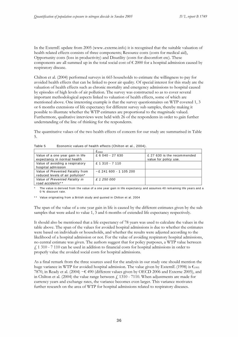
Quantification of population exposure to nitrogen dioxide in Sweden 2005 IVL report B 1749
36
In the ExternE update from 2005 (www..externe.info) it is recognised that the suitable valuation of health related effects consists of three components; Resource costs (costs for medical aid), Opportunity costs (loss in productivity) and Disutility (costs for discomfort etc). These components are all summed up in the total social cost of € 2000 for a hospital admission caused by respiratory disease.
Chilton et al. (2004) performed surveys in 665 households to estimate the willingness to pay for avoided health effects that can be linked to poor air quality. Of special interest for this study are the valuation of health effects such as chronic mortality and emergency admissions to hospital caused by episodes of high levels of air pollution. The survey was constructed so as to cover several important methodological aspects linked to valuation of health effects, some of which are mentioned above. One interesting example is that the survey questionnaires on WTP covered 1, 3 or 6 months extensions of life expectancy for different survey sub samples, thereby making it possible to illustrate whether the WTP estimates are proportional to the magnitude valued. Furthermore, qualitative interviews were held with 26 of the respondents in order to gain further understanding of the line of thinking for the respondents.
The quantitative values of the two health effects of concern for our study are summarised in Table 5.
Table 5 Economic values of health effects (Chilton et al., 2004).
£2002 Value of a one year gain in life expectancy in normal health
£ 6 040 - 27 630 £ 27 630 is the recommended value for policy use.
Value of avoiding a respiratory hospital admission
£ 1 310 - 7 110
Value of Prevented Fatality from reduced levels of air pollution*
~£ 241 600 - 1 105 200
Value of Prevented Fatality in road accidents**
£ 1 250 000
* The value is derived from the value of a one year gain in life expectancy and assumes 40 remaining life years and a 0 % discount rate.
** Value originating from a British study and quoted in Chilton et al. 2004
The span of the value of a one year gain in life is caused by the different estimates given by the sub samples that were asked to value 1, 3 and 6 months of extended life expectancy respectively.
It should also be mentioned that a life expectancy of 78 years was used to calculate the values in the table above. The span of the values for avoided hospital admissions is due to whether the estimates were based on individuals or households, and whether the results were adjusted according to the likelihood of a hospital admission or not. For the value of avoiding respiratory hospital admissions, no central estimate was given. The authors suggest that for policy purposes, a WTP value between £ 1 310 - 7 110 can be used in addition to financial costs for hospital admissions in order to properly value the avoided social costs for hospital admissions.
As a final remark from the three sources used for the analysis in our study one should mention the huge variance in WTP for avoided hospital admission. The value given by ExternE (1998) is €1995 7870, in Ready et al. (2004) ~€ 490 (different values given by OECD 2006 and Externe 2005), and in Chilton et al. (2004) the value range between £ 1310 - 7110. When adjustments are made for currency years and exchange rates, the variance becomes even larger. This variance motivates further research on the area of WTP for hospital admissions related to respiratory diseases.

Quantification of population exposure to nitrogen dioxide in Sweden 2005 IVL report B 1749
37
3.4 Evaluation of the URBAN model
3.4.1 Evaluation of the calculated NO2 concentrations
The calculated urban background concentrations of NO2 using the URBAN model were found reasonable when compared to monitoring data (Haeger-Eugensson et al., 2002). However, in order to validate the geographical distribution of the national calculated concentrations and thus the exposure levels, a comparison was made between the results from the URBAN model and local calculations of the NO2 concentration in three urban areas: Göteborg, Uppsala and Umeå (Table 6) (Modig och Forsberg, 2006). The local NO2 concentrations were calculated at a much higher resolution (50 x 50 m) compared with the national estimate (1 x 1 km). The local estimates were resampled into the same 1 x 1 km grid resolution to enable comparison with the national estimate. Furthermore, the corresponding area (i.e. the corresponding grid cells) in the national map was identified.
Table 6 The three local calculations of NO2-concentrations applied to validate the national calculation.
Urban area Source Area (km2)1 Year Resulution
Göteborg ENVIMAN 2 1,178 2000 50 x 50 m
Uppsala ENVIMAN 2 56 2000 50 x 50 m
Umeå TAPM 3 24 1999 50 x 50 m
1) Area when the local dataset had been adjusted to the 1 x 1 km grid.
2) www.opsis.se
3) Hurley, 2005
The URBAN model was further evaluated by comparison on a regional scale with the AERMOD model (a Gaussian dispersion model) for the Scania region by converting the AERMOD grid to the 1x1 km grid size. The AERMOD model was run with long time meteorological statistics and emissions for the year 2000.
3.4.2 Evaluation of the calculated exposure levels
The same data set for population density were used for calculation of the exposure from the different models. The number of people exposed to different levels of NO2 concentration was calculated by over-laying the population grid to the air pollution grid as described in chapter 3.1.5.
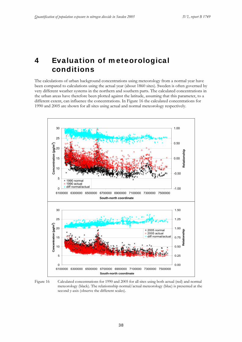
Quantification of population exposure to nitrogen dioxide in Sweden 2005 IVL report B 1749
38
4 Evaluation of meteorological conditions
The calculations of urban background concentrations using meteorology from a normal year have been compared to calculations using the actual year (about 1860 sites). Sweden is often governed by very different weather systems in the northern and southern parts. The calculated concentrations in the urban areas have therefore been plotted against the latitude, assuming that this parameter, to a different extent, can influence the concentrations. In Figure 16 the calculated concentrations for 1990 and 2005 are shown for all sites using actual and normal meteorology respectively.
0
5
10
15
20
25
30
6100000 6300000 6500000 6700000 6900000 7100000 7300000 7500000South-north coordinate
Con
cent
ratio
n (µ
g/m
3 )
-1.00
-0.50
0.00
0.50
1.00
Rel
atio
nshi
p1990 normal1990 actualdiff normal/actual
0
5
10
15
20
25
30
6100000 6300000 6500000 6700000 6900000 7100000 7300000 7500000South-north coordinate
Con
cent
ratio
n (µ
g/m
3 )
0.00
0.25
0.50
0.75
1.00
1.25
1.50
Rel
atio
nshi
p2005 normal2005 actualdiff normal/actual
Figure 16 Calculated concentrations for 1990 and 2005 for all sites using both actual (red) and normal
meteorology (black). The relationsship normal/actual meteorology (blue) is presented at the second y-axis (observe the different scales).
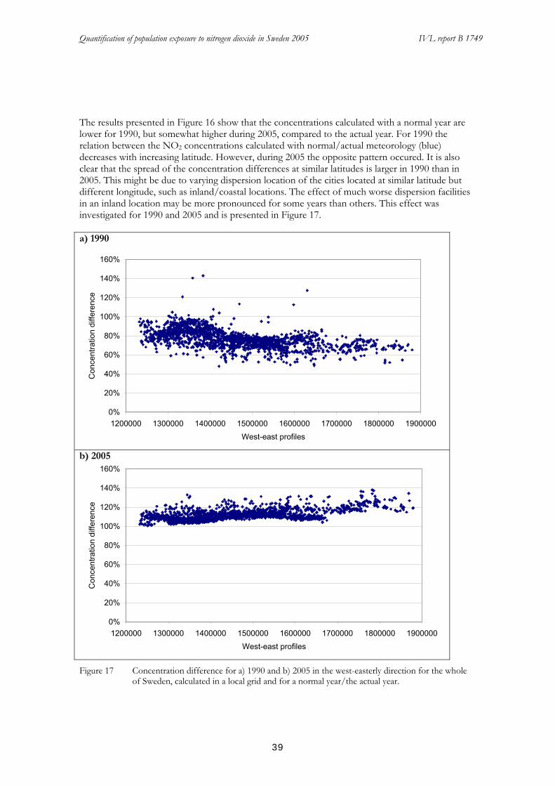
Quantification of population exposure to nitrogen dioxide in Sweden 2005 IVL report B 1749
39
The results presented in Figure 16 show that the concentrations calculated with a normal year are lower for 1990, but somewhat higher during 2005, compared to the actual year. For 1990 the relation between the NO2 concentrations calculated with normal/actual meteorology (blue) decreases with increasing latitude. However, during 2005 the opposite pattern occured. It is also clear that the spread of the concentration differences at similar latitudes is larger in 1990 than in 2005. This might be due to varying dispersion location of the cities located at similar latitude but different longitude, such as inland/coastal locations. The effect of much worse dispersion facilities in an inland location may be more pronounced for some years than others. This effect was investigated for 1990 and 2005 and is presented in Figure 17. a) 1990
0%
20%
40%
60%
80%
100%
120%
140%
160%
1200000 1300000 1400000 1500000 1600000 1700000 1800000 1900000West-east profiles
Con
cent
ratio
n di
ffere
nce
b) 2005
0%
20%
40%
60%
80%
100%
120%
140%
160%
1200000 1300000 1400000 1500000 1600000 1700000 1800000 1900000West-east profiles
Con
cent
ratio
n di
ffere
nce
Figure 17 Concentration difference for a) 1990 and b) 2005 in the west-easterly direction for the whole
of Sweden, calculated in a local grid and for a normal year/the actual year.

Quantification of population exposure to nitrogen dioxide in Sweden 2005 IVL report B 1749
40
In order to more clearly present the concentration differences between normal/actual year during all the three years studied (1990, 1995 and 2005) a calculation of the mean concentration difference for all sites located every 10 km in latitude (6130000, 6140000, etc.) has been made. According to Figure 18, 1990 and 1995 show a similar pattern nationally while 2005 has an opposite pattern. This indicates an underestimation in concentration levels for 1990 and 1995 if using normal meteorological statistics.
0.0
0.2
0.4
0.6
0.8
1.0
1.2
1.4
1.6
6000000
6200000
6400000
6600000
6800000
7000000
7200000
7400000
7600000
Local coordinates
Rel
atio
nshi
p
199019952005
Figure 18 The mean concentration difference (normal/actual meteorology) at each major change in the
local coordinate.
In Figure 17 there is a pattern of larger differences between the concentrations from normal year compared to the actual year in 1990 than in 2005. In 1990 there is also a larger difference around the longitude of 1350000 with a decreasing trend to the east, but also in the westerly direction. This longitude corresponds to the location of the inland of southern Sweden, for example the highland of Småland. That pattern is not at all visible in 2005, when the climate generally was more windy and the dispersion of air pollutants was more effective all over the country. In Figure 19 the west-easterly trajects are divided into three different latitudinal parts; one southern (<6500000), one middle (≥=6500000-<7000000) and one northern (>=700000) part. As can be seen in the figure there are no pronounced longitudinal differences in the middle and norther profile. However, in the southern part of Sweden, at the latitude of about 1350000, the concentration difference shows a large decrease in both the easterly and westerly direction. Altogether, the actual year meteorology better reflects the local dispersion differences, and hence gives a more accurate result of the concentration calculations.

Quantification of population exposure to nitrogen dioxide in Sweden 2005 IVL report B 1749
41
a)
0%
20%
40%
60%
80%
100%
120%
140%
160%
1200000 1300000 1400000 1500000 1600000 1700000 1800000 1900000
West-east profiles
Con
cent
ratio
n di
ffere
nce
b)
0%
20%
40%
60%
80%
100%
120%
140%
160%
1200000 1300000 1400000 1500000 1600000 1700000 1800000 1900000
West-east traject
Con
cent
ratio
n di
ffere
nse
c)
0%
20%
40%
60%
80%
100%
120%
140%
160%
1200000 1300000 1400000 1500000 1600000 1700000 1800000 1900000West-east profiles
Con
cent
ratio
n di
ffere
nce
Figure 19 Concentration difference for 1990 calculated for normal/actual year in west-easterly profiles at
three different longitudes (calculated in a local grid; a) north ≥ 700000 b) middle ≥ 6500000-<7000000 and c) south <6500000.

Quantification of population exposure to nitrogen dioxide in Sweden 2005 IVL report B 1749
42
5 Results As described earlier, the use of a ”normal meteorological year” is not suitable to apply in the URBAN model, since the input to the URBAN model is based on actual measurement data and corresponding meteorological conditions. Therefore, the results presented are all based on the meteorological situation during the actual year.
5.1 NO2 concentrations and exposure situation in 2005
5.1.1 National distribution of NO2 concentrations
5.1.1.1 Annual means
The annual mean concentration of NO2 for 2005 calculated with the URBAN model is presented in Figure 20. The result is based on calculated two-monthly means in order to capture the seasonal variations, where higher concentrations usually appear during the winter.
The input data used for the concentration calculations for the year 2005 comprised about
* 73 sites in rural/regional background air
* 98 sites in urban background air
In Figure 20 it can be seen that most of the country has relatively low NO2 urban background concentrations calculated for 2005, compared to the environmental standard for the annual mean value (40 µg/m3). Most of the small to medium sized cities have NO2 concentrations of less than 15 µg/m3 in the city centre. In the large cities and along the Skåne West Coast the concentration levels are higher, up to 20-25 µg/m3, which is of the same magnitude as the long-term environmental objective (20 µg/m3 as an annual mean).
There is an observable partition of Sweden north of Stockholm, possibly due to both a decreasing density of cities and meteorological factors. The locations of cities are determine the pattern of the concentrations, while the city size and the meteorological mixing parameters determine the concentrations levels. Thus, even in a small town high NO2 concentrations can occur due to poor ventilation in an area.
According to the calculated results, there are no exceedances of the annual air quality standards in Sweden. However, since the standards are also valid for concentrations in street canyons which normally are 1.5 times higher than the urban background (Persson and Haeger-Eugensson, 2006b), there may be exceedances at some “hot spots”.

Quantification of population exposure to nitrogen dioxide in Sweden 2005 IVL report B 1749
43
Figure 20 Calculated national distribution of annual mean NO2 in 2005.
5.1.1.2 98 percentile of daily means
In Figure 21 annual means of all cities are grouped into 5 µg/m3 intervals. Within each of these groups the number of days/year of different levels of daily mean concentrations are also divided into similar concentration intervals (represented by different coloured bars). For this calculation the formulas described in Figure 2 was used.

Quantification of population exposure to nitrogen dioxide in Sweden 2005 IVL report B 1749
44
0%
20%
40%
60%
80%
100%
0-5 5-10 10-15 15-20 20-25 25-30 30-35 35-40 ≥40Concentration groups annual means
Per
cent
age
dist
ribut
ion
of d
ays
0 - 5 5 - 10 10 - 15 15 - 2020 - 25 > 25
Figure 21 Percentage distribution of the number of days/year in concentration groups with different
daily means (represented by different coloured bars) in relation to the annual mean concentration of NO2.
In Figure 21 it can be seen that there is a clear relation between an increased number of days with a mean concentration > 25 µg/m3 and an increased annual mean, while daily mean values < 10 µg/m3 are scarcely observed in towns where the annual mean is above 15 µg/m3.
5.1.2 Population exposure
As mentioned above, the highest NO2 concentration levels normally will be found in street canyons. However, for studies of population exposure to air pollution it is custom to use the urban background air concentration levels or a relatively low geographic resolution, since this type of air quality data is used in the studies providing dose-response relationship for health impact calculations.
5.1.2.1 Long-term exposure
The number of people in Sweden exposed to certain levels of NO2 in 2005 is shown in Table 7. The largest group of people, almost 50%, were exposed to annual mean concentrations of NO2 less than 5 µg/m3. Another 30% were exposed to concentration levels between 5-10 µg NO2/m3, and only about 5% of the Swedish inhabitants experienced exposure levels of NO2 above 15 µg/m3.
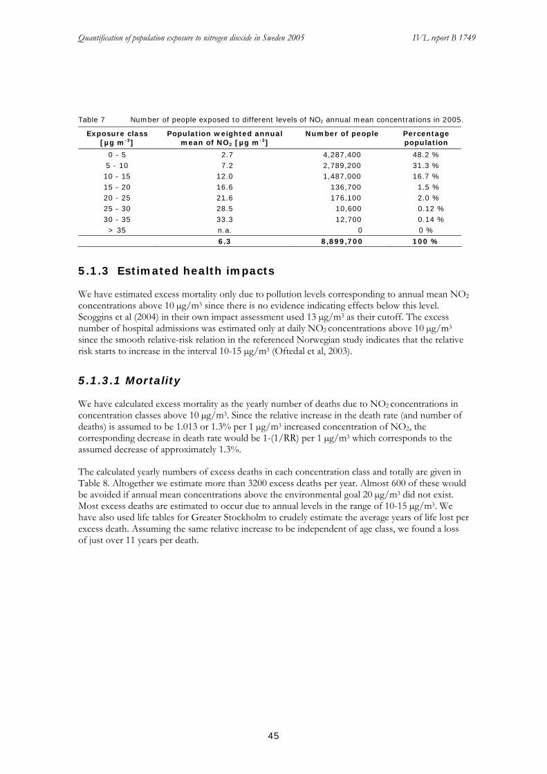
Quantification of population exposure to nitrogen dioxide in Sweden 2005 IVL report B 1749
45
Table 7 Number of people exposed to different levels of NO2 annual mean concentrations in 2005.
Exposure class [µg m-3]
Population weighted annual mean of NO2 [µg m-3]
Number of people Percentage population
0 - 5 2.7 4,287,400 48.2 % 5 - 10 7.2 2,789,200 31.3 % 10 - 15 12.0 1,487,000 16.7 % 15 - 20 16.6 136,700 1.5 % 20 - 25 21.6 176,100 2.0 % 25 - 30 28.5 10,600 0.12 % 30 - 35 33.3 12,700 0.14 % > 35 n.a. 0 0 %
6.3 8,899,700 100 %
5.1.3 Estimated health impacts
We have estimated excess mortality only due to pollution levels corresponding to annual mean NO2 concentrations above 10 µg/m3 since there is no evidence indicating effects below this level. Scoggins et al (2004) in their own impact assessment used 13 µg/m3 as their cutoff. The excess number of hospital admissions was estimated only at daily NO2 concentrations above 10 µg/m3 since the smooth relative-risk relation in the referenced Norwegian study indicates that the relative risk starts to increase in the interval 10-15 µg/m3 (Oftedal et al, 2003).
5.1.3.1 Mortality
We have calculated excess mortality as the yearly number of deaths due to NO2 concentrations in concentration classes above 10 µg/m3. Since the relative increase in the death rate (and number of deaths) is assumed to be 1.013 or 1.3% per 1 µg/m3 increased concentration of NO2, the corresponding decrease in death rate would be 1-(1/RR) per 1 µg/m3 which corresponds to the assumed decrease of approximately 1.3%.
The calculated yearly numbers of excess deaths in each concentration class and totally are given in Table 8. Altogether we estimate more than 3200 excess deaths per year. Almost 600 of these would be avoided if annual mean concentrations above the environmental goal 20 µg/m3 did not exist. Most excess deaths are estimated to occur due to annual levels in the range of 10-15 µg/m3. We have also used life tables for Greater Stockholm to crudely estimate the average years of life lost per excess death. Assuming the same relative increase to be independent of age class, we found a loss of just over 11 years per death.

Quantification of population exposure to nitrogen dioxide in Sweden 2005 IVL report B 1749
46
Table 8 Estimated annual number of excess deaths.
Annual NO2 Class
Population (n)
Pop*conc
Population weigthed mean conc
Excess deaths
Proportion of population (%)
1 0 - 5 4287407 11414129 2.7 48.2 2 5 - 10 2789238 19955530 7.2 31.3 3 10 - 15 1486972 17888962 12.0 2349 16.7 4 15 - 20 136716 2266116 16.6 298 1.5 5 20 - 25 176136 3797237 21.6 499 2.0 6 25 - 30 10590 302325 28.5 37 0.12 7 30 - 35 12665 422152 33.3 55 0.14 8 > 35 0 0 n.a. 0 0 totalt 8899724 56046451 6.3 3238 100
5.1.3.2 Hospital admissions
We have estimated excess hospital admissions as the yearly number of admissions in each class of annual means due to estimated daily NO2 concentrations above 10 µg/m3. The calculated yearly numbers of excess hospital admissions for respiratory disease and cardiovascular disease respectively, in each concentration class and totally are given in Table 9 and Table 10. Altogether we estimate more than 300 excess hospital admissions for all respiratory diseases and almost 300 hospital admissions for cardiovascular disease.
Table 9 Excess numbers of respiratory hospital admissions due to daily means in classes above 10 µg/m3 distributed over the population according to the annual NO2 mean categories.
Annual mean category
10-15 15-20 20-25 25- 30 30-35 35-40 > 40 Total
0 - 5 0,0 0,0 0,0 0,0 0,0 0,0 0,0 5 - 10 36,4 8,4 4,1 0,0 0,0 0,0 0,0 10 - 15 26,1 43,3 38,4 10,0 35,2 4,6 0,0 15 - 20 2,2 5,2 5,4 2,8 5,8 2,4 3,6 20 - 25 2,1 7,4 9,6 6,8 12,1 6,1 11,8 25 - 30 0,1 0,4 0,7 0,7 1,1 0,6 1,3 30 - 35 0,1 0,3 0,9 0,9 1,4 0,8 1,8 > 35 0,0 0,0 0,0 0,0 0,0 0,0 0,0 66,9 65,0 59,1 21,1 55,6 14,6 18,5 300,8
Table 10 Excess numbers of CVD hospital admissions due to daily means in classes above 10 µg/m3 distributed over the population according to the annual NO2 mean categories.
Annual mean category
10-15 15-20 20-25 25- 30 30-35 35-40 > 40
0 - 5 0,0 0,0 0,0 0,0 0,0 0,0 0,0 5 - 10 36,3 8,3 4,1 0,0 0,0 0,0 0,0 10 - 15 25,9 43,1 38,2 10,0 35,0 4,6 0,0 15 - 20 2,2 5,2 5,3 2,8 5,8 2,3 3,6 20 - 25 2,1 7,3 9,6 6,8 12,1 6,1 11,7 25 - 30 0,1 0,4 0,7 0,7 1,1 0,6 1,3 30 - 35 0,1 0,3 0,9 0,9 1,4 0,8 1,8 > 35 0,0 0,0 0,0 0,0 0,0 0,0 0,0 66,6 64,7 58,8 21,0 55,4 14,5 18,4 299,4

Quantification of population exposure to nitrogen dioxide in Sweden 2005 IVL report B 1749
47
5.1.4 Socio-economic cost
5.1.4.1 Results of socio-economic valuation
The social costs in Sweden caused by health effects that can be linked to annual ambient air concentration levels higher than 10 µg/m3 are estimated by adapting the socio-economic values of the considered health effects from available literature to the number of occurrences of the health effects as estimated in our study, see Table 11.
Table 11 Annual Socioeconomic costs of long term NO2 levels exceeding 10 µg/m3 in Sweden, 2005 - Central Estimate
Socio-economic Value of avoided Health Effect
Health effects in 2005
Socio-economic cost [million SEK2005]
Total Sweden
18450 million SEK2005
Out of which:
Value of Statistical Life (VSL/VPF) (11 years of prolonged life)
5691000 [SEK2005] 3238 excess death
occurrences 18429
Hospitalisation, cardiology
5592 [SEK2005 / day] 1823.9 excess days 10
Hospitalisation, generic (respiration)
3342 [SEK2005 / day] 1595.3 excess days 5
WTP to avoid hospital admissions*
4522 [SEK2005 / occurrence]
600 excess hospital admissions
3
*One hospital admission is in this case equal to three days at hospital followed by five days at home.
As shown, the total annual socio-economic costs related to NO2 levels exceeding 10 µg /m3 is 18 450 million SEK2005, and the absolute majority of these costs relate to loss of life years. This value can serve as a comparison with potential financial costs for abating high concentrations of NO2. For the Swedish society, this implies that implementation of abatement measures that lower NO2 levels below 10µg /m3 with an annual cost below 18 450 million SEK would be of net benefit for society. In these calculations all the estimates from the literature are recalculated to Swedish Crowns at year 2005 value. This is done by adjusting the currencies with respect to Consumer Price Indices (CPI) and Purchase Power Parity (PPP). CPI is used to adjust the values given to year 2005 values while PPP is used to adjust for national differences. In Appendix A all the values from the literature are expressed in Swedish Crowns with the 2005 year value.
The central estimates are based on the central values from the 2005 update of the ExternE project (www.externe.info). High and low estimates as well as other estimates from the literature are presented in the sensitivity analysis. The use of the ExternE project values is mainly due to reasons of comparability with other national and international calculations on health effects. In the table we indicate a VSL value of 5691000 SEK2005 to be used for the valuation. This value on VSL is lower than other common estimates of VSL. This is mainly an effect the adjustment of the VSL value for the fact that the expected life loss amounts to 11 years, as is the estimate in our study (see chapter 4.1.2.1). The normal number of years lost when estimating a VSL value is ~40. The VSL estimate in our central estimate is not discounted since the origin of the value specifically indicates that annual payments should be made during 10 years, thereby inducing discounted values given by the respondents (www.externe.info). Following the presentation of methods in chapter 3.3, it is important for the reader to keep in mind that the estimates of VSL and VOLY are based on the stated preference method, more specifically, the Contingent Valuation Method.

Quantification of population exposure to nitrogen dioxide in Sweden 2005 IVL report B 1749
48
The valuation problem with latency of effect is not under consideration in our study since we are not studying the implementation of an abatement measure, we are just studying the current situation in Sweden. Neither do we take into account any specific value for the health effects related to children as yet since there is no scientific/political agreement on how to treat these effects in monetary valuation.
5.1.4.2 Sensitivity Analysis
In order to estimate a plausible range of socio-economic costs related to high levels of NO2, some simple sensitivity analyses are performed. Matters of interest are what the results would be if health effect values from other studies were used and what effect a discounting of the VSL value would have on the total socio-economic cost. The VSL estimates quoted in OECD 2006 are not included in this sensitivity analysis since they relate to a larger loss in life expectancy than the 11 years we study. The VSL values given in OECD can be seen in the Appendix A.
First we estimate the effect of different values on VSL as shown in Table 12. These estimates are taken from ExternE (www.externe.info).
Table 12 Low / High Estimates of VSL from ExternE (www.externe.info)
Socio-economic cost [million SEK2005] Low estimate VSL 10061 High estimate VSL 82 951
The analysis shows that our central estimate is on the lower bound of the ExternE estimates.
Chilton et al. (2004) is one of the few studies that directly estimates VOLY related to air pollution induced health effects, Table 13. It also indicates WTP estimates related to hospital admissions caused by the same health effect. It thereby serves as a useful comparison with our central estimate.
Table 13 Low / High Estimates of health effects from Chilton et al. 2004
Socio-economic cost [million SEK2005] Low estimate 3336 High estimate 15203
Here it can be seen that the direct estimates from Chilton et al. 2004 results in lower socio-economic costs than our central estimate However, the values are within the range of the low / high estimate of ExternE.
Furthermore, discounting is of general interest when valuing health effects. For the sake of comparison we discount the VLS values previously used with a 4 % discount rate, which is a common rate used in valuation of health effects related to air pollution, Table 14 and Table 15.
Table 14 Discounted Low / Central / High Estimates of ExternE (www.externe.info).
Socio-economic cost [million SEK2005] Low estimate VSL 6748 Central estimate VSL 14698 High estimate VSL 55717
Quantification of population exposure to nitrogen dioxide in Sweden 2005 IVL report B 1749
49
Table 15 Discounted Low / High Estimates of health effects from Chilton et al. 2004.
Socio-economic cost [million SEK2005] Low estimate 2663 High estimate 12125
From the discounting it can be seen that the values are sensitive to the choice of discount rate, which have been previously mentioned. But it is our opinion that the values we use from ExternE and Chilton et al. 2004 should remain undiscounted in the central estimate since they are valued with a method that allows the survey respondents to discount the values themselves.
For policy purposes, our central estimate of the annual socio-economic costs related to high NO2 levels in Sweden seems to be fairly robust. Even if discounted with a 4 % discount rate, the socio-economic cost would still stay above 10 000 million SEK2005 annually.
If one would want to be extra cautious with the socio-economic cost estimates, annual socio-economic costs of 2 600 - 6 500 million SEK2005 can be used, but they would represent the very low end of valuations and not be suitable for comparison with other similar results.
5.2 Trends in population exposure
The NO2 concentrations and the corresponding exposure situation have also been calculated for the calendar years 1990, 1995 and 1999. The number of monitoring sites available for the different years are given in Table 16. Since there were only a few (5) sites of regional bakground measurements for 1990 new estimated concentrations, based on the geographical distribution in 1999, were developed. The relation between 1990 and 1999 at the five sites differ somewhat between the years, and therefore two-month means of the relation have been used. The calculated regional background concentrations have been evaluated with the two existing months of measurements (November and December), and the result shows that the differences in concentrations were ± 10%. However, the calculated concentrations were over-estimated more often than underestimated.
Table 16 The number of monitoring sites available for the different years.
Year Regional background sites Urban background sites
1990 5 62
1995 20 40
1999 73 45
2005 73 41
The calculated annual NO2 concentration, using the meteorology for the actual year, are presented in Figure 22. As can be seen from the figure the air quality has improved between 1990-2005.

Quantification of population exposure to nitrogen dioxide in Sweden 2005 IVL report B 1749
50
a)
b)
c)
d)
Figure 22 Calculated national NO2 concentrations for a) 1990, b) 1995, c) 1999 and d) 2005.

Quantification of population exposure to nitrogen dioxide in Sweden 2005 IVL report B 1749
51
For calculation of exposure the same population density was used for all years. Table 17 presents the extent of population exposure in different exposure classes for 1990, 1995, 1999 and 2005.
Table 17 Calculated NO2 concentrations and number of people exposed to different NO2 levels in a) 1990, b) 1995, c) 1999 and d) 2005.
a)
NO2 concentration as annual mean
[µg m-3]
Population weighted annual mean of NO2 [µg m-3]
Number of people
Percentage population
0 – 5 3.5 2,699,900 30 % 5 – 10 7.4 2,714,000 30 % 10 - 15 12.3 1,597,600 18 % 15 - 20 17.3 1,077,300 12 % 20 - 25 22.1 465,500 5.2 % 25 - 30 26.9 134,900 1.5 % 30 - 35 30.8 36,300 0.4 % 35 – 40 37.4 68,600 0.8 % 40 – 45 42.6 85,900 1.0 %
> 45 46.4 19,700 0.2 % Total: 10.1 8,899,700 100 %
b)
NO2 concentration as annual mean
[µg m-3]
Population weighted annual mean of NO2 [µg m-3]
Number of people
Percentage population
0 – 5 3.1 3,729,000 42 % 5 – 10 7.1 2,625,300 29 % 10 - 15 12.3 1,665,100 19 % 15 - 20 16.8 592,400 6.7 % 20 - 25 22.1 113,000 1.3 % 25 - 30 27.8 113,400 1.3 % 30 > 31.6 61,500 0.7 %
Total: 7.7 8,899,700 100 % c)
NO2 concentration as annual mean
[µg m-3]
Population weighted annual mean of NO2 [µg m-3]
Number of people
Percentage population
0 - 5 2.9 4,042,500 45.4 % 5 - 10 7.1 2,450,600 27.5 % 10 - 15 12.3 1,714,500 19.3 % 15 - 20 16.6 430,800 4.8 % 20 - 25 22.6 115,300 1.3 % 25 - 30 26.4 122,800 1.4 % 30 - 35 31.9 10,600 0.12 % > 35 37.2 12,700 0.14 %
7.2 8,899,700 100 %

Quantification of population exposure to nitrogen dioxide in Sweden 2005 IVL report B 1749
52
d)
NO2 concentration as annual mean
[µg m-3]
Population weighted annual mean of NO2 [µg m-3]
Number of people
Percentage population
0 - 5 2.7 4,287,400 48.2 % 5 - 10 7.2 2,789,200 31.3 % 10 - 15 12.0 1,487,000 16.7 % 15 - 20 16.6 136,700 1.5 % 20 - 25 21.6 176,100 2.0 % 25 - 30 28.5 10,600 0.12 % 30 - 35 33.3 12,700 0.14 % > 35 n.a. 0 0 %
Total: 6.3 8,899,700 100 %
Figure 23 illustrates the percentage of the population exposed to NO2, divided into concentration classes of 5 µg/m3, in the four studied years. An obvious trend of an increasing part of the population exposed to lower concentration levels can be observed. Compared to the situation in 1990 in 2005 about 15% less people were exposed to annual mean NO2 levels above 15 µg/m3, while almost 20% more people were exposed to annual mean NO2 levels in the lowest concentration class, 0-5 µg/m3.
0%
10%
20%
30%
40%
50%
60%
0 – 5 5 – 10 10 - 15 15 - 20 20 - 25 25 - 30 30 - 35 35 – 40 40 – 45 > 45NO2 concentration groups (µg/m3)
Perc
enta
ge o
f peo
ple
expo
sed
1990
1995
1999
2005
Figure 23 Percentage of the population exposed to NO2 (µg/m3) in different concentration groups in
1990, 1995, 1999 and 2005.
5.3 Model evaluation
In order to evaluate the model and to be able to estimate the uncertainty of the results achieved, as regards both concentrations and exposure, comparisons have been made with results from more detailed dispersion calculations on regional as well as local levels. On the national level the output from the URBAN model has been compared to observed data.

Quantification of population exposure to nitrogen dioxide in Sweden 2005 IVL report B 1749
53
5.3.1 National NO2 concentration levels
A comparison was made between calculated and monitored NO2 concentrations in towns with more than 20 000 inhabitants (about 25-30 each year) (Figure 24). The agreement is good with a difference between -2% to 10% depending on the year. The calculated concentrations are somewhat underestimated compared to measurements for all years except 1995. The agreement is best in 1995 and 1999. The dispersion facilities also show best ggreement in these years according to Figure 8. It can thus be assumed that the weather during these years was relatively homogeneous over the whole of Sweden.
0
5
10
15
20
25
1990 1995 1999 2005Yearly means
Con
cent
ratio
n of
NO
2 ( µ
g/m
3 )
MeasurementsCalculations actual metCalculations normal met
6%-2%
2%
10%
Figure 24 Comparison between the annual means of NO2 concentration in cities with > 20 000
inhabitants calculated with both actual and normal meteorology. The percentual difference of actual meteorology and measurements is also given in the figure.
According to the result presented in Figure 24 the variation between the calculated and measured concentrations is much larger for 1990 and 1995 when using a normal year instead of the actual year. However, for 2005 it is the opposite, with better agreement between the measurements and the NO2 concentration calculated with a normal year. The reason for this is assumed to be that the dispersion facilities during this year were rather similar compared to the normal year in the middle of Sweden but differed in the north and southern part (Figure 9). Since many of the largest cities are located in the middle of Sweden it did not become visible in this comparison.
5.3.2 Regional NO2 concentrations and exposure levels
A comparison between NO2 concentrations and exposure levels calculated with the URBAN model and the AERMOD model have been carried out for the Scania region. According to the result shown in Figure 25, Figure 26 and Table 18 the agreement between the result from the URBAN model and the AERMOD model was quite good. Nevertheless, one difference was that the, with the URBAN model, calculated urban background concentrations levels were underestimated along the west coast, compared to the local model. This is possibly due to the fact that the local model includes emissions from the Copenhagen and Malmö regions. On the other hand, the national model seems to capture increased concentration levels for small to medium sized cities. The difference in the population exposure was around 15% less for concentrations lower than 5 µg/m3, calculated with the AERMOD model, while the concentration class 5-10 µg/m3 showed a 15% higher exposure. For higher concentrations the exposure results were very similar.

Quantification of population exposure to nitrogen dioxide in Sweden 2005 IVL report B 1749
54
Figure 25 NO2 concentration in the south of Sweden a) Local distribution and b) National distribution.
Figure 26 The difference between the local and the national modelling results of the NO2 concentration
in the south of Sweden (1 x 1 km). Positive values indicate that the national model provides higher values compared with the local model.
Table 18 Population weighted annual NO2 concentrations and number of people exposed to different levels of NO2 in the national calculation (URBAN model) compared with the local calculation in the south of Sweden in 1999.
National calculation Local calculation NO2
class (µg m-3)
NO2 mean
(µg m-3)
People
People (%)
NO2 mean
(µg m-3)
People
People (%)
Southern < 5 4.0 233,000 16 % 3.6 435,000 29 % Sweden 5 - 10 6.7 737,700 50 % 7.3 507,800 34 %
10 - 15 12.8 343,300 23 % 12.4 320,600 22 % 15 - 20 16.7 144,100 9.7 % 17.0 196,000 13 % 20 - 25 21.8 23,900 1.6 % 20.5 22,500 1.5 % Mean 8.9 8.8

Quantification of population exposure to nitrogen dioxide in Sweden 2005 IVL report B 1749
55
5.3.3 Local NO2 concentrations and exposure levels
Figure 27 shows the grids used in the comparison of NO2 concentrations in Göteborg, 1999. The absolute and relative difference between the local and the national modelling result of the NO2 concentrations in Göteborg (1 x 1 km), 1999 is shown in Figure 28, where positive values indicate that the national model provides higher values compared with the local model.
a) b)
c) Figure 27 NO2 concentrations in Göteborg, 1999, based on a) the local model at a high resolution
(50 x 50 m), b) the local model result aggregated into 1 x 1 km and c) the national modelling result (1 x 1 km).

Quantification of population exposure to nitrogen dioxide in Sweden 2005 IVL report B 1749
56
Figure 28 The difference between the local and the national modelling result of the NO2 concentration
in Göteborg (1 x 1 km), 1999. Left figure: positive values indicate that the national model provides higher values compared with the local model.
In Figure 29 the comparison between the different calculation methods as well as the grid resolution in Umeå is shown.
a) b) c) Figure 29 NO2-concentration levels in Umeå 1999 based on a) the local calculation (1x1 km grid
resolution), b) the local calculation (50x50 m aggregated into 1x1 km resolution), c) the national calculation aggregated into 1 km grid resolution.
The local and national estimates were compared regarding NO2 concentration levels and number of people exposed to different levels of NO2 concentrations (Table 19). The results of the comparison indicate that the NO2 concentration is underestimated in the national calculation compared with the local estimate for all three urban areas. The mean NO2 concentration in the national estimate is 27 % lower in Göteborg, 13 % lower in Uppsala and 33 % lower in Umeå compared with the local estimate. Consequently, the number of people exposed to low levels of NO2 concentrations may be overestimated in the national calculation.

Quantification of population exposure to nitrogen dioxide in Sweden 2005 IVL report B 1749
57
Table 19 NO2 concentrations and number of people exposed to different levels of NO2 in the national calculation compared with the local calculation for Göteborg, Uppsala and Umeå in 1999.
National calculation Local calculation
NO2 class
(µg m-3)
NO2 mean
(µg m-3)
People People
(%)
NO2 mean
(µg m-3)
People People
(%)
Göteborg < 5 4.4 86,740 15 % 3.6 23,200 3.9 % 5 - 10 7.7 240,050 41 % 7.8 164,390 28 % 10 - 15 11.7 200,280 34 % 12.4 160,490 27 % 15 - 20 15.2 8,240 1.4 % 17.1 93,090 16 % 20 - 25 23.7 14,860 2.5 % 22.3 76,930 13 % 25 – 30 26.7 17,200 2.9 % 27.4 64,720 11 % 30-35 31.9 10,590 1.8 % 31.0 6,170 1.0 % > 35 37.2 12,670 2.1 % 35.8 1,640 0.3 %
Uppsala 5 – 10 8.3 164,500 52 % 8.4 57,360 18 %
10 – 15 11.1 22,540 7.2 % 12.2 164,210 52 % 15 – 20 16.7 127,000 40 % 15.5 140,930 45 %
Umeå < 5 3.0 19,560 24 % - - -
5 – 10 7.0 124,420 64 % 8.4 114,310 49 % 10 – 15 12.8 43,870 12 % 11.7 150,290 47 % 15 – 20 - - - 15.5 16,490 3.9 %
6 Discussion Some improvements have been made to the URBAN model compared to the previous calculations reported (Sjöberg et al., 2004). The impact of using meteorology for a typical/normal year compared to the actual dispersion conditions has been studied. However, it has been shown that the uncertainty increases to a different extent depending on both latitude and longitude. This is due to the large variations in dispersion facilities over the country as well as between years.
Furthermore, it has been shown that a more reliable distribution of annual NO2 concentration mean levels in urban areas with > 10,000 inhabitants is achieved when using population data in 100x100 m grids as a basis for the spatial pattern of the pollutant, see Figure 30. The advantage of this new concentration distribution methodology compared with the bell-shape methodology is that the spatial pattern of the NO2 concentration is consistent with the extent of the urban area, and that the concentration level is proportional to the density of the population within the city. It is difficult to identify the extent of the smaller urban geographical areas (< 10,000 inhabitants), and therefore the bell-shape approach was considered to be a suitable distribution approach in these areas.

Quantification of population exposure to nitrogen dioxide in Sweden 2005 IVL report B 1749
58
0
500000
1000000
1500000
2000000
2500000
3000000
3500000
4000000
4500000
0 - 5 5 - 10 10 - 15 15 - 20 20 - 25 > 25Concentration group
Old calculationNew calculation
Figure 30 Comparison between exposure calculations for 1999 based on the old (Sjöberg et al., 2004) and
new distribution pattern regarding both population and NO2 concentrations. The y axis shows the number of people exposed
The assumption that the NO2 concentration is proportional to the number of people in a grid cell fails to capture the spatial patterns of roads, where NO2 emissions are significant. However, the assumption is still considered appropriate for calculating the NO2 exposure at a national level and in the resolution of 1*1 km grid cells. Future development of the modelling methodology should concentrate on incorporating an improved spatial pattern of emissions. It might also be possible to use concentration maps available in larger cities, and apply the dispersion pattern to the URBAN model.
Regarding the calculation of short term NO2 values, as 98 percentiles of daily means, the evaluation showed a very good correlation to both the winter half year and annual means. Further, the calculation of the number of days divided into different concentration groups also showed a fairly good agreement with the long term means. This assumption was successfully verified by comparing calculated and monitored data.
Nitrogen dioxide is a good indicator of air pollution from the transport sector (cars, trucks, shipping) and from other types of combustion (e.g. power plants). Nitrogen dioxide is a regulated pollutant and is thus frequently measured and modelled. However, this does not mean that it is very important as a causal agent behind the health effects related to air pollution. For several years there have been different viewpoints on the health effects of nitrogen dioxide at current urban levels. Toxicologists and epidemiologists do not completely agree on how the existing body of evidence should be interpreted. Epidemiological studies have detected associations at low ambient air concentrations, most consistent for the prevalence of respiratory illness in children, but often also for the daily number of hospital admissions and the daily number of deaths. However, it is well known that NO2 and other combustion related pollutants co-vary in time and space, making it difficult or impossible to separate their effects. Thus, epidemiological studies cannot prove that it is nitrogen dioxide per se which is the causal factor. In addition, a lot of human exposure studies have shown that normal healthy individuals do not show adverse effects to NO2 below concentrations of

Quantification of population exposure to nitrogen dioxide in Sweden 2005 IVL report B 1749
59
about 4000 µg/m3, while subjects with asthma or chronic obstructive lung disease may react to concentrations of about 500 µg/m3, either by alterations in bronchial reactivity or by increased sensitivity to inhaled allergens. For the time being, nitrogen dioxide has to be seen as an indicator of air pollution mainly from the transport sector and other combustion sources. The fact that this report assesses the impact of air pollution on health using nitrogen dioxide, should also be viewed in the light of nitrogen dioxide as an indicator. We do not claim that it is nitrogen dioxide per se which causes the estimated several thousands of excess deaths and cardiorespiratory hospital admissions per year, but we expect actions that reduce emissions of nitrogen dioxide to reduce the number of cases resulting from air pollution.
The results from the urban modelling show that in 2005 most of the country had rather low NO2 urban background concentrations, compared to the environmental standard for the annual mean (40 µg/m3). However, in the central parts of the large cities and some smaller towns along the Skåne West Coast the concentration levels were of the same magnitude as the long-term environmental objective (20 µg/m3 as an annual mean). The majority of people, almost 80%, were exposed to annual mean concentrations of NO2 less than 10 µg/m3. Only about 5% of the Swedish inhabitants experienced exposure levels of NO2 above 15 µg/m3.
We have estimated that more than 3200 deaths per year are brought forward due to exposure to a local air pollution concentration at home, indicated by nitrogen dioxide levels above a cut off at 10 µg/m3 as an annual mean. This number is higher than the 2800 excess deaths we estimated in the previous calculation (Forsberg and Sjöberg, 2005a). The difference is a result of the improved exposure assessment methods with a higher resolution, and does not reflect a new relative risk assumption.
The cut off we use, roughly set at the population weighted mean, is rather arbitrary, since we do not know the shape of the exposure-response association in different concentration intervals. There is no evidence of a specific toxicological threshold level at the cut-off level. On the other hand, we know that the regional background level of nitrogen dioxide is lower than 10 µg/m3 in most parts of the country, so the assessment in principle reflects only effects of the local contribution and not always the whole part of it, so a lower cut off could have been used for most of the country.
In a recent paper, similar calculations for Sweden were presented using particulate matter (PM10 or PM2.5) as the air pollution indicator (Forsberg et al, 2005b). In that health impact assessment, the local contribution to urban levels of PM in Sweden was estimated to result in around 1800 deaths per year brought forward, while the impact of long-range transported pollutants was estimated to approximately 3500 deaths annually. However, the authors suggest that the effect of particle emissions from local traffic were likely to be underestimated with the applied risk coefficients for PM from American cohort studies across regions. Epidemiological studies as well as the method used in this study to assess the health impact of harmful air pollutants have shown that NO2 is a useful indicator for exposure estimates and calculations of effects on mortality of local air pollutants mainly originating from motor vehicle traffic. However, the relation between NO2 and NO is dependent on other factors such as ozone levels, so NOX may be an alternative indicator for traffic related pollutants.
We estimated around 600 hospital admissions due to the short-term effect of daily concentrations of NO2 above 10 µg/m3. This may seem to be a low number in comparison with the estimated number of deaths. However, for hospital admissions we can only estimate the short-term effect on admissions, not the whole effect of morbidity, due to NO2 and correlated air pollutants. The total yearly number of hospital admissions in persons that got their disease due to air pollution exposure may well be 10-20 times higher. It would be valuable to have morbidity indicators also for the long-

Quantification of population exposure to nitrogen dioxide in Sweden 2005 IVL report B 1749
60
term effects of air pollution exposure, for example the incidence (new cases) of respiratory diseases such as asthma and chronic bronchitis. The estimated numbers of hospital admissions due to air pollution also depends on the assumed cut off concentration for any adverse effect. With a lower cut off level a higher number of cases would be estimated.
As we have indicated earlier, 591 of the total 3238 excess deaths are related to annual mean levels of NO2 above the long term environmental goal of 20 µg/m3. This is equal to only ~18 % of the total effect on mortality and ~18 % of the total costs to society. From a socio-economic perspective (a perspective that seeks efficient allocation of resources), it must be stressed that an achievement of the environmental goal (annual NO2 concentration levels lower than 20 µg/m3) might be less cost efficient than a reduction of annual concentration levels in areas with higher population densities. The cost efficiency is dependent on a number of aspects. In our case the cost efficiency relates to; size of population exposed, cost of abatement measure as well as meteorological conditions affecting NO2 concentration levels and thereby impact of a measure. In our study we do not investigate which abatement measures could be considered and whether they differ between regions that exceed the environmental goal or not which is an issue of interest for future research. However, we do know that the population experiencing these high levels of NO2 only constitutes 2.24 % of the Swedish population (as shown in chapter 4.1.2.1), a percentage that is decreasing (chapter 4.3). We also know that the meteorological conditions related to these high levels are not favourable on all occasions (chapter 4.1). These aspects indicate that efforts towards lowering national annual mean NO2 concentrations might not be so cost efficient for society. It should not be forgotten that cost efficiency might very well be reached by abating NO2 emissions in areas with favourable conditions even where the annual mean NO2 level is lower than 20 µg/m3.
The trend analysis between 1990 and 2005 clearly shows an increasing number of people exposed to lower NO2 concentration levels. During the same period the population weighted annual mean of NO2 has decreased by almost 40%, accordingly to the 35% reduction of total NOX emissions in Sweden (www.naturvardsverket.se).
The improved URBAN model shows in general a good performance. When using the actual weather instead of the normal weather the variability in air pollution concentrations governed by the meteorology is captured when applying the rather fine scaled meteorology. The model is further calibrated by the dispersion adjusting constant (Cd), calculated from measurements. Since the meteorological variability is reflected both in the ventilation factor and the corresponding Cd's the uncertainty of using a normal year will become too large. The difference between measurements and the calculated concentrations, using meteorology for the normal year, is 20-30%, while the same comparison for the actual year gives less than 10% difference.
The comparison between the URBAN model and detailed calculations on a regional scale (Skåne) shows a good agreement as regards the annual mean concentrations. However, the variation in the number of people exposed is about 15% in the concentration classes <10 µg/m3, equal to the cut off level used in the exposure study. For higher concentrations the agreement between the two calculation method lies within 5%.
On the local scale the populated weighted annual means correlate very well with the URBAN model calculations in Göteborg and Uppsala. For Umeå there are larger differences. The comparison of the number of people being exposed to different concentration levels corresponds quite well (within 15%) in Göteborg, but the differences are larger in the two other cities (up to 45%). This is possibly mainly due to uncertainties in the concentration distribution pattern.

Quantification of population exposure to nitrogen dioxide in Sweden 2005 IVL report B 1749
61
There are still a number of issues that can further improve the certainty of the calculations, i.e. the selection of population data to be used as well as application of relevant geographical areas and best degree of resolution to fit with the most valid epidemiological ER-functions. By increasing the asseessment frequency it is possible to minimize the uncertainties due to meteorological variations. Furthermore, the differences in exposure on the local level could be reduced if existing local dispersion concentration calculations were applied into the model.
7 References Alberini A., Cropper M., Krupnick A., Simon N.B., (2004), Does the value of statistical life vary
with age and health status? Evidence from the US and CANADA, Journal of Environmental Economics and Management, Vol. 48, pp. 196-212
Bellander T, Svartengren M, Berglind, Staxler L, Järup L. SHAPE Part II: Particulate matter, nitrogen dioxide, and health effects – Exposure response relations and health consequences in Stockholm County. Stockholm, 1999.
Bickel P., Friedrich R., (ed.), 2005, ExternE - Externalities of Energy: Methodology 2005 Update
Brent R. J. (1996), Applied Cost-Benefit Analysis, Edward Elgar Publishing Limited, © Robert J. Brent 1996.
Chen, D (2000), A Mothly Circulation Climatology for Sweden and its Application to a Winter Temperature Case Study. Int. J. Climatol. 20: 1067-1076.
Chen, D., Wang, T., Haeger-Eugensson, M., Ashberger, C. and Borne, K. (2002). Application of TAPM (v.1) in Swedish West Coast: validation during 1999 and 2000. IVL Report L02/51.
Chilton S., Covey J., Jones-Lee M,. Loomes G., Metcalf H,. (2004), Valuation of health benefits associated with reduction in air pollution - final report, Department for Environment, Food and Rural Affairs (DEFRA), © Crown copyright 2004
COMEAP. Cardiovascular Disease and Air Pollution - A report by the Committee on the Medical Effects of Air Pollutants, UK Department of Health, 2006.
de Facto 2006, Miljömålsrådets årsrapport Miljömålen – miljömålen på köpet.
Fergeson, S. (2002). Ventilation Climate Information System. USDA Forest Service and FERA- Fire and Environmental Research Applications' (http:// www.fs.fed.us/pnw/fera/vent.html/.
Fergeson, S. (2003). The potential for smoke to ventilate from windland fires in the United States. Pre-prints for the Fourth Symposium on Fire and Forest Meteorology organised by American Meteorological Society in February 2003.
Filleul L, Rondeau V, Vandentorren S, Le Moual N, Cantagrel A, Annesi-Maesano I, Charpin D, Declercq C, Neukirch F, Paris C, Vervloet D, Brochard P, Tessier JF, Kauffmann F, Baldi I. Twenty five year mortality and air pollution: results from the French PAARC survey. Occup Environ Med. 2005 Jul;62(7):453-60.
Forsberg, B., Modig, L., Svanberg, P-A., Segerstedt, B. (2003). Hälsokonsekvenser av ozon – en kvantifiering av det marknära ozonets korttidseffekter på antalet sjukhusinläggningar och dödsfall i Sverige (in Swedish). På uppdrag av Statens folkhälsoinstitut.
Forsberg, B. and Sjöberg, K. (2005a). Quantification of deaths attributed to air pollution in Sweden using estimated population exposure to nitrogen dioxide as indicator. IVL Report B1648.

Quantification of population exposure to nitrogen dioxide in Sweden 2005 IVL report B 1749
62
Forsberg B, Hansson HC, Johansson C, Aureskoug H, Persson K. Järvholm B. (2005b). Comparative health impact assessment of local and regional particulate air pollutants in Scandinavia. Ambio 2005;34:11-19.
Gallego J. and Peedell S., 2001, Using CORINE Land Cover to map population density. Towards Agri-environmental indicators, Topic report 6/2001 European Environment Agency, Copenhagen, pp. 92-103.
Gehring U, Heinrich J, Kramer U, Grote V, Hochadel M, Sugiri D, Kraft M, Rauchfuss K, Eberwein HG, Wichmann HE. Long-term exposure to ambient air pollution and cardiopulmonary mortality in women. Epidemiology 2006;17(5):545-51.
Haeger-Eugensson, M., Borne, K., Chen, D., Persson, K. (2002). Development of a New Meteorological Ventilation Index for Urban Air Quality Studies. IVL Report L02/70.
Hammit J., (2000) Valuing Mortality Risk - Theory and Practice, Environmental Science and Technology, Vol. 34, pp. 1396 - 1400
Hardy, C., Ottmar, R. D., Petersen, J. and Core, J. (2003). Smoke management guide for prescribed and wildland fire. 2000 edition. Bois, ID: National Wildfire Coordinating Group.
Hoek G, Brunekreef B, Goldbohm S, Fischer P, van den Brandt PA. Association between mortality and indicators of traffic-related air pollution in the Netherlands: a cohort study. Lancet 2002 Oct 19;360(9341):1203-9.
Holland M., Berry J., Forster D., (ed.) (1998), ExternE - Externalities of Energy: Volume 7 Methodology 1998 Update
Holzworth, G. C (1972). Mixing heights, wind speeds, and potentials for urban air pollution throughout the contiguous United States. Office of Air Publication No. AP-101. Research Triangular Park, NC US Environmental Protection Agency, Office of Air Programs.
Hurley, P.J. (2005). The air pollution model (TAPM) version 3: User manual. Internal paper 31 of CSIRO Atmospheric Research Division 37 p.
Kidson JW. 1994. Relationship of New Zealand daily and monthly weather patterns to synoptic weather types. International Journal of Climatology 14: 723–737.
Krieg, R. and Olsson, L. (1977). Undersökning av ventilationsklimatet i Sverige (Investigation of the ventilation climate in Sweden, in Swedish). SMHI.
Krupnick A., Alberini A, Cropper M., Simon N., Itaoka K., Akai M., (1999), Mortality risk valuation for environmental policy, Discussion paper 99-47, Resources for the future, Washington, DC
Lamb HH. (1950). Types and spells of weather around the year in the British Isles. Quarterly Journal of the Royal Meteorological Society 76: 393–438.
Maddison D., (2000), Valuing the morbidity effects of air pollution, Centre for Social and Economic Research on the Global Environment (CSERGE), University College London, Mimeo
Markandya A., Hunt A., Ortiz R., Alberini A., (2004), EC Newext research project: mortality risk valuation - final report UK, European Commission
Miljöhälsorapport 2001 (in Swedish). Socialstyrelsen, Institutet för Miljömedicin, Miljömedicin Stockholms läns landsting. ISBN 91-7201-495-4.

Quantification of population exposure to nitrogen dioxide in Sweden 2005 IVL report B 1749
63
Modig, Lars och Forsberg, Bertil (2006). Besvärsförekomst i relation till luftföroreningshalter i tre svenska städer. En studie inom den hälsorelaterade miljöövervakningen 2005. Yrkes- och miljömedicin, Institutionen för folkhälsa och klinisk medicin, Umeå universitet, 2006.
Nafstad P, Haheim LL, Wisloff T, Gram F, Oftedal B, Holme I, Hjermann I, Leren P. Urban air pollution and mortality in a cohort of Norwegian men. Environ Health Perspect. 2004 Apr;112(5):610-5.
Nettelbladt, Anna; Westling, Olle; Akselsson, Cecilia; Svensson, Annika;Hellsten, Sofie (2006). Luftföroreningar i skogliga provytor - Resultat till och med september 2005 (in Swedish). IVL Report B1682.
OECD (2006), Cost-Benefit Analysis and the Environment - Recent Developments, © OECD 2006
Oftedal B, Nafstad P, Magnus P, Bjorkly S, Skrondal A. Traffic related air pollution and acute hospital admission for respiratory diseases in Drammen, Norway 1995-2000. Eur J Epidemiol. 2003;18(7):671-5.
Persson, K., Sjöberg, K., Svanberg, P-A. and Blomgren, H. (1999). Dokumentation av URBAN-modellen (Documentation of the URBAN model, in Swedish). IVL Rapport L99/7.
Persson, K., Sjöberg, K. and Boström, C-Å. (2001a). Kväveoxider i svenska tätorter – exponeringsförhållanden 1999/2000. För Naturvårdsverket. IVL Rapport L01/31.
Persson, K and Haeger-Eugensson, M (2001b). Luftkvalitetsituationen i svenska tätorter till år 2020 (in Swedish). IVL rapport L01/61.
Persson, K., Haeger-Eugensson, M., and Sjöberg, K. (2006a). Luftkvaliteten i Sverige sommaren 2005 och vintern 2005/06 (Air quality in Sweden summer 2005 and winter 2005/06, in Swedish). IVL Report B 1690.
Persson, K. and Haeger-Eugensson (2006b). Relation mellan halter av luftföroreningar i olika tätortsmiljöer (in Swedish). For Swedish EPA. IVL Report U1922.
Ready R., Navrud S., Day B., Dubourg W.R., Machado F., Mourato S., Spanninks F., Rodriquez M., (2004), Contingent valuation of ill-health caused by air pollution: testing for context and ordering effect, Portuguese Economic Journal 3
Scoggins A, Kjellstrom T, Fisher G, Connor J, Gimson N. Spatial analysis of annual air pollution exposure and mortality. Sci Total Environ. 2004 Apr 5;321(1-3):71-85.
Sjöberg, K., Haeger-Eugensson, M., Liljenberg M, Blomgren H, Forsberg B. (2004). Quantification of general population exposure to nitrogen dioxide in Sweden. IVL Report B1579.
Sjöberg, K., Persson, K., Pihl-Karlsson, G., Brodin, Y. (2006a). Luftkvalitet i tätorter 2005 (Air quality in urban areas, in Swedish). IVL Rapport B1667.
Sjöberg, K., Pihl-Karlsson, G., Svensson, A. and Blomgren, H. (2006b). Nationell miljöövervakning inom EMEP och Luft- och nederbördskemiska nätet 2004 & 2005 (National monitoring within EMEP and the air and precipitation chemistry network in 2004 & 2005, in Swedish). For the Swedish Environmental Protection Agency. IVL Report U 1911.
Steen, B. and Cooper, D. (1992). Kväveoxider i svenska tätorter – exponeringsförhållanden. IVL Rapport B1052.
Steen, B. and Svanberg, P-A. (1997). Kväveoxider i svenska tätorter – exponeringsförhållanden 1995/96. För Naturvårdsverket. IVL Rapport L97/231.
Quantification of population exposure to nitrogen dioxide in Sweden 2005 IVL report B 1749
64
Sunyer J, Spix C, Quenel P, Ponce-de-Leon A, Ponka A, Barumandzadeh T, Touloumi G, Bacharova L, Wojtyniak B, Vonk J, Bisanti L, Schwartz J, Katsouyanni K. Urban air pollution and emergency admissions for asthma in four European cities: the APHEA Project. Thorax 1997;52(9):760-5.
VTI (Väg- och transportforskningsinstitutet), Nilsson G., Andersson G., Brüde U., Larsson J., Thulin H., 2002, Trafiksäkerhetsutvecklingen i Sverige fram till år 2001, VTI rapport 486
WHO. AirQ Manual, Version 2.2. Bonn, 2004.
WHO. Health effects of transport related air pollution. WHO Regional Office for Europe, Copenhagen, 2005.
Web links:
www.externe.info, as of 2007-06-28
www.naturvardsverket.se, as of 2007-09-04
www.opsis.se, as of 2007-09-04 (EnviMan Reporter User’s Guide Version 1.0)
www.scb.se

Quantification of population exposure to nitrogen dioxide in Sweden 2005 IVL report B 1749
65
Appendix A Valuation Studies expressed in Swedish Crowns [SEK2005] Values on Mortality (VSL) given in OECD 2006 [SEK2005] VSL low VSL high Hammit 2000 40480000 94450000 Alberini et al. 2004 15360000 49159000 9217000 37894000 Krupnick et al. 1999 2164000 4328000 Markandya et al. 2004 11764000 27449000 6862000 7843000 8823000 18626000 Chilton et al. 2004 2941000 14705000 Values on Mortality (VSL) given in ExternE (www.externe.info) [SEK2005] Low / Central High Value of Statistical Life (VSL) 10886000 34252000 Values on Mortality (VPF) given in Chilton et al. 2004 [SEK2005] Low / Central High Value of Prevented Fatality (VPF) from reduced levels of air pollution*
3711000 16979000
Value of Prevented Fatality (VPF) in road accidents**
19204000 19204000
* The value is derived from the value of a one year gain in life expectancy and assumes 40 remaining life years and a 0 % discount rate. ** Value depicted from a British study and quoted in Chilton et al. 2004 Values on Mortality (VOLY) given in OECD 2006 [SEK2005] VOLY Chilton et al. 2004 424000 Markandya et al. 2004 645000 Values on Mortality (VOLY) given in ExternE (www.externe.info) [SEK2005] VOLY Low VOLY Central VOLY High Value of Life Year Lost (VOLY)
282000 517000 2328000
Values on Mortality (VOLY) in Chilton et al. 2004 [SEK2005] VOLY Low VOLY Central / High Value of Life Year Lost (VOLY)
93000 424000
Values on morbidity given in OECD 2006 Study quoted [SEK2005] Type of Illness (morbidity)
Ready et al. 2004 ExternE 1998 Maddison 2000
Hospital admission for treatment of respiratory disease
5070 81000 n.a.
3 days spent in bed with respiratory illness
1604 776 2018

Quantification of population exposure to nitrogen dioxide in Sweden 2005 IVL report B 1749
66
Values on morbidity given in ExternE (www.externe.info) Health related effect [SEK2005] Hospitalisation, generic (respiration) 3342 Hospitalisation, cardiology 5592 WTP to avoid hospital admissions* 4522 Productivity loss of absence from work 849 Values on morbidity given in Chilton et al. 2004 [SEK2005] low [SEK2005] high Value of a one year gain in life expectancy in normal health
93000 424000
Value of avoiding a respiratory hospital admission
20000 109000