QSPR modeling of the enthalpy of formation from elements bymeans of correlation weighting of local invariants of atomic

orbital molecular graphs

Andr�es Mercader a, Eduardo A. Castro a,*, Andrey A. Toropov b

a CEQUINOR, Departamento de Qu�õmica, Facultad de Ciencias Exactas, Universidad Nacional de La Plata, C.C. 962, 1900 La Plata,

Argentinab Vostok Innovation Company, S. Azimstreet 4, 700047 Tashkent, Uzbekistan

Received 15 June 2000; in ®nal form 10 August 2000

Abstract

A quantitative structure±property modeling of the enthalpy of formation from elements by means of correlation

weighting of local invariants of atomic orbital molecular graphs (AOMGs) is presented. The method is applied to a set

comprising 51 hydrocarbon molecules and results are quite good, with lower average deviations than experimental

uncertainties. Some possible applications and further extensions of the calculation procedure are pointed out. Ó 2000

Elsevier Science B.V. All rights reserved.

1. Introduction

The chemist is interested in the quantitative aspects of the changes accompanying the gain or loss of oneor more forms of energy by substances. These changes may be physical, chemical or both, and they maytake place under a wide variety of conditions. Thermochemical principles are useful in predicting the be-havior of reacting systems moving towards a more stable state of equilibrium. Reaction equilibria based onthermal and thermochemical measurements alone can be calculated from minimum experimental infor-mation.

Heat associated with the formation of a chemical compound by direct (or hypothetical) union of itselements at a constant pressure is termed the enthalpy (or heat) of formation, DH°f . Such data are useful tothe engineer in plant design problems and to the rocket expert in the evaluation of jet and rocket fuels.Modern chemical technology requires accurate enthalpies of formation for the calculation of equilibriumconstants of reaction. To the theoretician, enthalpies of formation are important in the investigation ofbond energies, resonance energies and the nature of the chemical bond. It is not surprising at all, therefore,that considerable endeavor has been directed towards the determination of enthalpies of formation over thepast century [1].

17 November 2000

Chemical Physics Letters 330 (2000) 612±623

www.elsevier.nl/locate/cplett

* Corresponding author.

E-mail addresses: castro@dalton.quimica.unlp.edu.ar (E.A. Castro), aator@saturn.silg.org (A.A. Toropov).

0009-2614/00/$ - see front matter Ó 2000 Elsevier Science B.V. All rights reserved.

PII: S 0 0 0 9 - 2 6 1 4 ( 0 0 ) 0 1 1 2 6 - X

Several methods have been presented for the estimation of primary thermochemical data from theo-retical calculations. Thus, the success of even simple levels of molecular orbital theory in reproducing theenergies of isodesmic reactions was exploited further in order to compute heats of formation [2]. Thesecalculated energy changes, combined with a limited number of experimental or high level theoreticalthermochemical data, yield direct estimates of heats of formation [3]. For example, the calculated STO-3G//STO-3G energy change of 2.6 kcal/mol for the bond separation chemical reaction

CH3CH2OH� CH4 ! CH3±CH3 � CH3OH �1�may be used in conjunction with experimental heats of formation at 298 K for ethane ()20.1 kcal/mol),methanol ()48.2 kcal/mol), and methane ()17.8 kcal/mol) to yield a value of ÿ53:1 kcal/mol for DH°f (298K) for ethanol:

DH°f�CH3CH2OH� � DH°f�CH3CH3� � DH°f�CH3OH� ÿ DH°f�CH4�ÿ bond separation energy of CH3CH2OH

The corresponding experimental value isÿ56:1 kcal/mol and this treatment neglects di�erences in zero-pointvibrational energies between reactants and products. An analogous calculation for dimethyl ether gives aheat of formation ofÿ39:5 kcal/mol, which compares favorably with the experimental valueÿ44:0 kcal/mol.

Another successful method was proposed by Wiberg [4] who ®tted 6-31G�//6-31G� total electronicmolecular energies for a variety of hydrocarbons to experimental heats of formation in order to deriveequivalents for ±CH3; ±CH2; ±CH and ±C groups. An estimate of the heat of formation of any hydro-carbon may then be obtained as the di�erence of its calculated (6-31G�//6-31G�) non-relativistic totalelectronic energy and the sum of the appropriate groups. Later on, this procedure was extended and im-proved to de®ne atomic equivalents which lead to average uncertainties of �2 kcal/mol for heats of for-mation calculated in this manner [5±10]. These uncertainties are similar to usual experimental deviations.

An additional alternative for modeling the molecular enthalpy of formation is to resort to the topo-logical indices through the quantitative structure±property relationships (QSPR), which also have provedto be useful in this regard [11±13]. The main advantage of this sort of methodology is its independence withrespect to molecular orbital theory, since heats of formation are calculated only on the basis of graph-theoretical structure descriptors, without being necessary to resort to total electronic molecular energies.

The aim of this Letter is to describe a QSPR modeling of enthalpies of formation from elements bymeans of correlation weighting of local invariants of atomic molecular graphs (MGs). This is the ®rstattempt to employ this particular sort of topological index to compute a thermodynamic parameter so thatwe have chosen a relatively simple set of molecules (i.e., hydrocarbons) to apply the method.

The Letter is organized as follows: Section 2 deals with the basic de®nitions related to the topologicaldescriptor, giving their foundations and pointing out its usefulness as well as analyzing the antecedents ofthis particular topological index. Section 3 describes the methodology applied to obtain the regressionequations. Section 4 presents some illustrative numerical results, comparing them with other data arisingfrom alternative theoretical procedures. Finally in Section 5, we discuss the possibility of extending the useof this kind of molecular descriptor to a di�erent set of molecules and for studying other physical chemistryproperties and biological activities.

2. Local invariants of atomic orbital molecular graphs

Many meaningful advances in mathematical chemistry during the last decades have had as a naturalconsequence for chemistry to become more than a collection of compounds, properties and reactions, givingrise to a coherent unique logical system [14]. Graph theory is a basic tool for fostering alternative ways tosolve chemical problems, both by the high degree of abstraction evidenced by the generality of such concepts

A. Mercader et al. / Chemical Physics Letters 330 (2000) 612±623 613

as points, lines and neighborhoods as well as by the combinatorial derivation of many graph-theoreticalconcepts which correspond to the essence of chemistry considered as `the study of combination betweenatoms' [15]. It o�ers a wide variety of concepts and methods of signi®cant importance to chemistry [16±26].

Graph theory helps in solving many chemical problems such as the systematization and enumeration ofchemical compounds, their coding and nomenclature, correlation of properties, molecular design, auto-mated structural formula search in mass spectrometry, infrared spectroscopy, NMR, alternativeapproaches to chemical reactivity, chemical kinetics, phase equilibria and chemical technology, among awell-known host of current possibilities.

A graph G is de®ned as a ®nite non-empty set V �G� of N -vertices (points) together with a set E�G� ofedges (lines), the latter being unordered pairs of distinct vertices. Thus, by de®nition, every graph is ®niteand has no loops (an edge initiating from and ending in one and the same vertex) and multiple edges. Whentwo vertices x and y are joined by an edge e � fx; yg, vertices x and y are said to be adjacent and each ofthem is incident with the edge e.

As a matter of fact, the structural (constitutional) formula of a chemical compound may be regarded as aMG, where the vertices represent atoms while the edges stand for valence bonds. The graph-theoreticalcharacterization of molecular structure is most often made by its translation into molecular descriptors,such as topological indices. A topological index is a real number, associated in an arbitrary way, charac-terizing the graph. It is based on a certain topological feature of the corresponding MG and represents agraph invariant, that is to say, it does not depend on the vertex numbering [27]. The main ®eld of appli-cation of topological indices is the structure±property and structure±activity quantitative correlations.

Di�erent graph characteristics or invariants have been used in the de®nition of molecular topologicalindices. For example, the kind of chemical element, the vertex degrees 0v�i� and the Morgan vertex degreesof ®rst-order 1v are well-known typical local invariants [28±30].

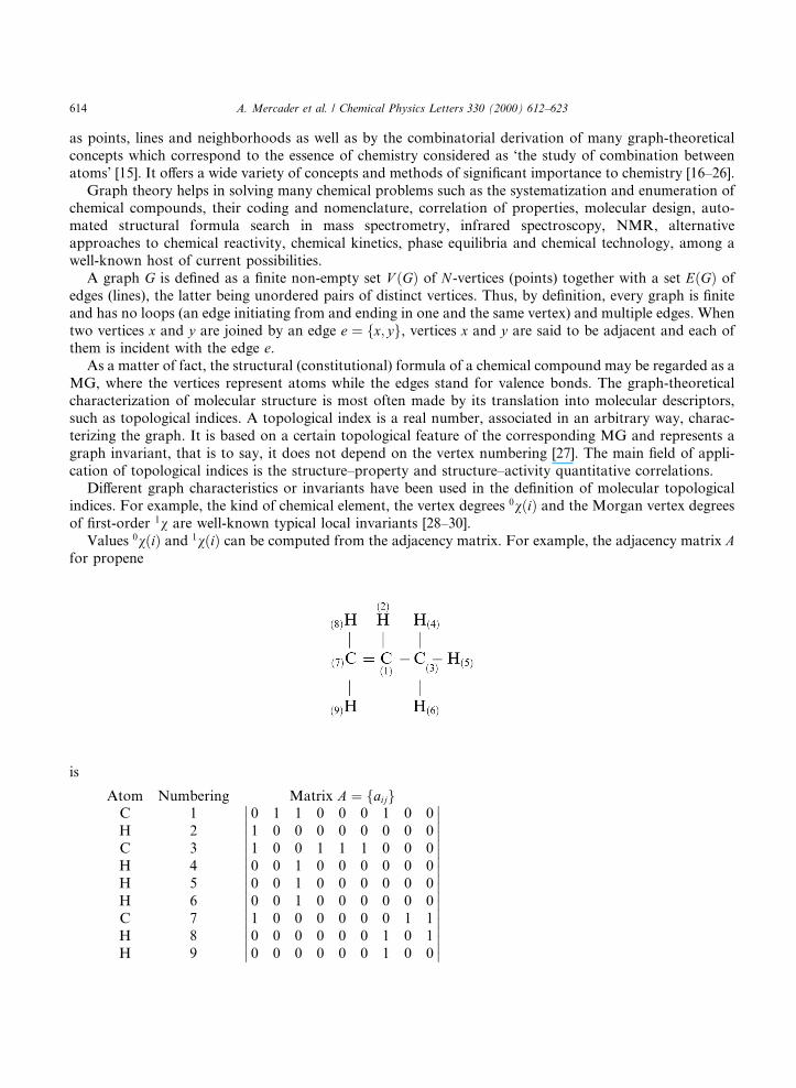
Values 0v�i� and 1v�i� can be computed from the adjacency matrix. For example, the adjacency matrix Afor propene

is

Atom Numbering Matrix A � faijgCHCHHHCHH

123456789

0 1 1 0 0 0 1 0 01 0 0 0 0 0 0 0 01 0 0 1 1 1 0 0 00 0 1 0 0 0 0 0 00 0 1 0 0 0 0 0 00 0 1 0 0 0 0 0 01 0 0 0 0 0 0 1 10 0 0 0 0 0 1 0 10 0 0 0 0 0 1 0 0

������������������

������������������

614 A. Mercader et al. / Chemical Physics Letters 330 (2000) 612±623

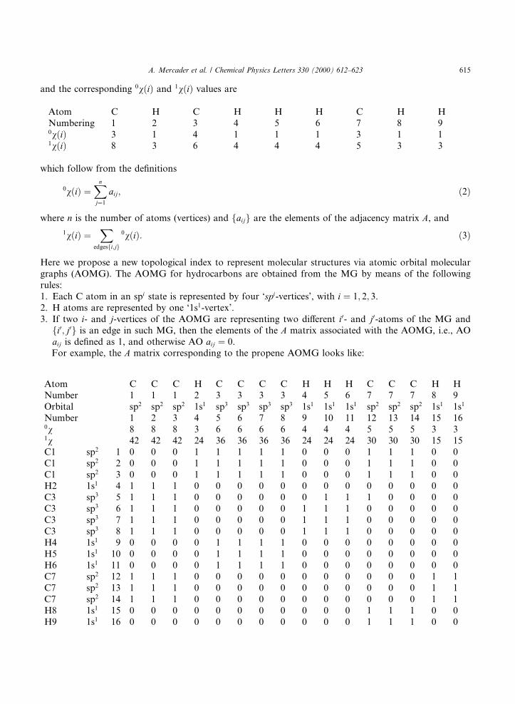
and the corresponding 0v�i� and 1v�i� values are

which follow from the de®nitions

0v�i� �Xn

j�1

aij; �2�

where n is the number of atoms (vertices) and faijg are the elements of the adjacency matrix A, and

1v�i� �X

edgesfi;jg

0v�i�: �3�

Here we propose a new topological index to represent molecular structures via atomic orbital moleculargraphs (AOMG). The AOMG for hydrocarbons are obtained from the MG by means of the followingrules:1. Each C atom in an spi state is represented by four `spi-vertices', with i � 1; 2; 3.2. H atoms are represented by one `1s1-vertex'.3. If two i- and j-vertices of the AOMG are representing two di�erent i0- and j0-atoms of the MG andfi0; j0g is an edge in such MG, then the elements of the A matrix associated with the AOMG, i.e., AOaij is de®ned as 1, and otherwise AO aij � 0.For example, the A matrix corresponding to the propene AOMG looks like:

Atom C H C H H H C H HNumbering 1 2 3 4 5 6 7 8 90v�i� 3 1 4 1 1 1 3 1 11v�i� 8 3 6 4 4 4 5 3 3

Atom C C C H C C C C H H H C C C H HNumber 1 1 1 2 3 3 3 3 4 5 6 7 7 7 8 9Orbital sp2 sp2 sp2 1s1 sp3 sp3 sp3 sp3 1s1 1s1 1s1 sp2 sp2 sp2 1s1 1s1

Number 1 2 3 4 5 6 7 8 9 10 11 12 13 14 15 160v 8 8 8 3 6 6 6 6 4 4 4 5 5 5 3 31v 42 42 42 24 36 36 36 36 24 24 24 30 30 30 15 15C1 sp2 1 0 0 0 1 1 1 1 1 0 0 0 1 1 1 0 0C1 sp2 2 0 0 0 1 1 1 1 1 0 0 0 1 1 1 0 0C1 sp2 3 0 0 0 1 1 1 1 1 0 0 0 1 1 1 0 0H2 1s1 4 1 1 1 0 0 0 0 0 0 0 0 0 0 0 0 0C3 sp3 5 1 1 1 0 0 0 0 0 0 1 1 1 0 0 0 0C3 sp3 6 1 1 1 0 0 0 0 0 1 1 1 0 0 0 0 0C3 sp3 7 1 1 1 0 0 0 0 0 1 1 1 0 0 0 0 0C3 sp3 8 1 1 1 0 0 0 0 0 1 1 1 0 0 0 0 0H4 1s1 9 0 0 0 0 1 1 1 1 0 0 0 0 0 0 0 0H5 1s1 10 0 0 0 0 1 1 1 1 0 0 0 0 0 0 0 0H6 1s1 11 0 0 0 0 1 1 1 1 0 0 0 0 0 0 0 0C7 sp2 12 1 1 1 0 0 0 0 0 0 0 0 0 0 0 1 1C7 sp2 13 1 1 1 0 0 0 0 0 0 0 0 0 0 0 1 1C7 sp2 14 1 1 1 0 0 0 0 0 0 0 0 0 0 0 1 1H8 1s1 15 0 0 0 0 0 0 0 0 0 0 0 1 1 1 0 0H9 1s1 16 0 0 0 0 0 0 0 0 0 0 0 1 1 1 0 0

A. Mercader et al. / Chemical Physics Letters 330 (2000) 612±623 615

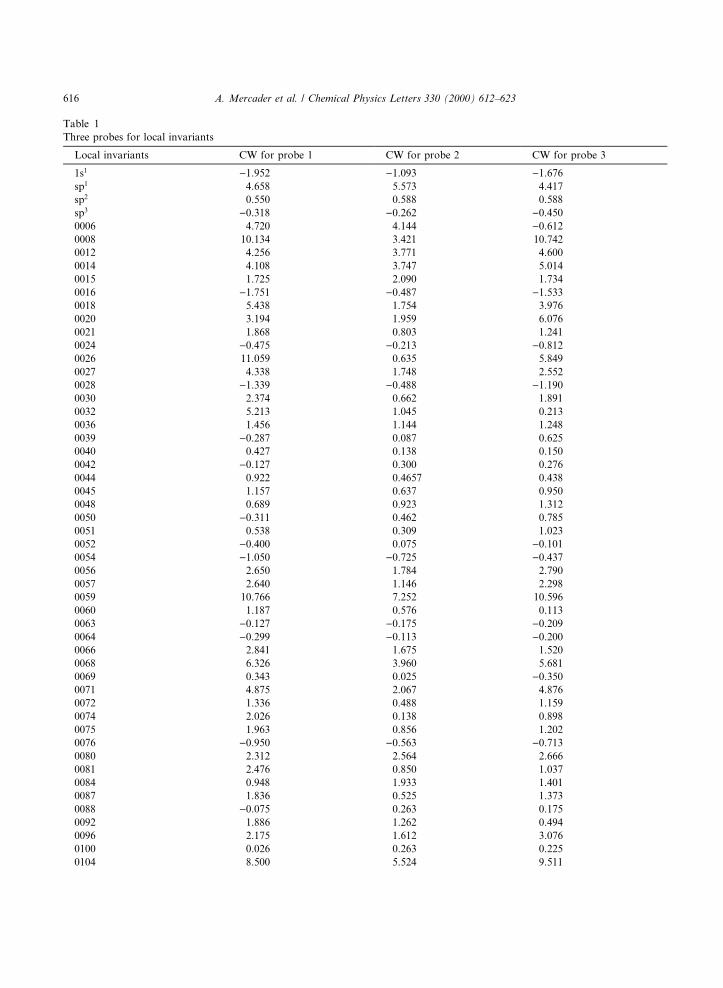
Table 1

Three probes for local invariants

Local invariants CW for probe 1 CW for probe 2 CW for probe 3

1s1 )1.952 )1.093 )1.676

sp1 4.658 5.573 4.417

sp2 0.550 0.588 0.588

sp3 )0.318 )0.262 )0.450

0006 4.720 4.144 )0.612

0008 10.134 3.421 10.742

0012 4.256 3.771 4.600

0014 4.108 3.747 5.014

0015 1.725 2.090 1.734

0016 )1.751 )0.487 )1.533

0018 5.438 1.754 3.976

0020 3.194 1.959 6.076

0021 1.868 0.803 1.241

0024 )0.475 )0.213 )0.812

0026 11.059 0.635 5.849

0027 4.338 1.748 2.552

0028 )1.339 )0.488 )1.190

0030 2.374 0.662 1.891

0032 5.213 1.045 0.213

0036 1.456 1.144 1.248

0039 )0.287 0.087 0.625

0040 0.427 0.138 0.150

0042 )0.127 0.300 0.276

0044 0.922 0.4657 0.438

0045 1.157 0.637 0.950

0048 0.689 0.923 1.312

0050 )0.311 0.462 0.785

0051 0.538 0.309 1.023

0052 )0.400 0.075 )0.101

0054 )1.050 )0.725 )0.437

0056 2.650 1.784 2.790

0057 2.640 1.146 2.298

0059 10.766 7.252 10.596

0060 1.187 0.576 0.113

0063 )0.127 )0.175 )0.209

0064 )0.299 )0.113 )0.200

0066 2.841 1.675 1.520

0068 6.326 3.960 5.681

0069 0.343 0.025 )0.350

0071 4.875 2.067 4.876

0072 1.336 0.488 1.159

0074 2.026 0.138 0.898

0075 1.963 0.856 1.202

0076 )0.950 )0.563 )0.713

0080 2.312 2.564 2.666

0081 2.476 0.850 1.037

0084 0.948 1.933 1.401

0087 1.836 0.525 1.373

0088 )0.075 0.263 0.175

0092 1.886 1.262 0.494

0096 2.175 1.612 3.076

0100 0.026 0.263 0.225

0104 8.500 5.524 9.511

616 A. Mercader et al. / Chemical Physics Letters 330 (2000) 612±623

In this way, the use of this sort of AOMG adjacency matrix through Eqs. (1) and (2) allows one tocalculate the local invariants 0v�i� and 1v�i�.

3. Computational procedure

We have chosen a hydrocarbon set comprising 65 molecules containing from 1 to 18 carbon atoms.Although this rather specialized set includes molecules with only C and H atoms, this option does notnecessarily imply a lack of molecular variations within such restricted choice. In fact, the hydrocarbon setincludes examples of planar, non-planar, alternant and non-alternant aromatic hydrocarbons, alkyl- andalkenyl-substituted benzene derivatives, acyclic and polycyclic alkanes, strained and unstrained ole®nsand alkynes and disparate structures of highly strained compounds such as cyclopropene and cubane,combined with polycyclic aromatics like anthracene and perylene, which do not require separate para-metrizations for di�erent types of C and H atoms. This molecular set has been used in previous studieson QSPR theory [31].

QSPR-modeling for heats of formation has been constructed by means of the following scheme [32±35]:1. A computer program reads adjacency matrices corresponding to the di�erent MGs.2. These matrices are translated into adjacency matrices associated with the AOMGs.3. Local invariants are then calculated.4. A suitable optimization procedure allows one to ®nd the correlation weights (CWs) of the local invari-

ants which yield maximum values for the correlation coe�cient in the regression equations for DH°f viadescriptors Oxc, de®ned as

Oxc �Xn

i�1

�CWfaig � CWf1v�i�g�; �4�

where n is the number of vertices in the AOMG, CWfaig the correlation weight associated with thepresence of vertex ai, such as 1s1; sp1; sp2, and sp3, and CWfEC1�i�g is the correlation weight for the givenvalue of the ®rst-order Morgan vertex degree. Similar AOMGs (but de®ned by alternative manners) havebeen tested as base of QSPR-modeling for normal boiling points of halogenated alkanes [34] and stabilityconstants of metal±organic complexes [35].

Results of three probes using this procedure are presented in Table 1These values allow us to determine CWs, which are applied in a least-squares ®tting method to obtain

DH°f via a general relationship

DH°f �Xt

i�1

Ai�Oxc�i � Bt; t � 1; 2; 3: �5�

Table 1 (Continued)

Local invariants CW for probe 1 CW for probe 2 CW for probe 3

0112 2.798 1.990 2.693

0116 7.547 4.636 6.018

0124 0.289 0.250 0.499

0136 6.633 4.144 5.916

0160 6.498 3.916 5.771

A. Mercader et al. / Chemical Physics Letters 330 (2000) 612±623 617

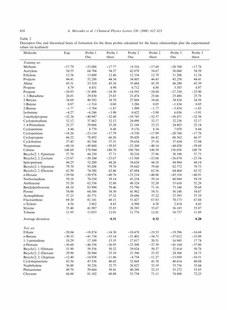
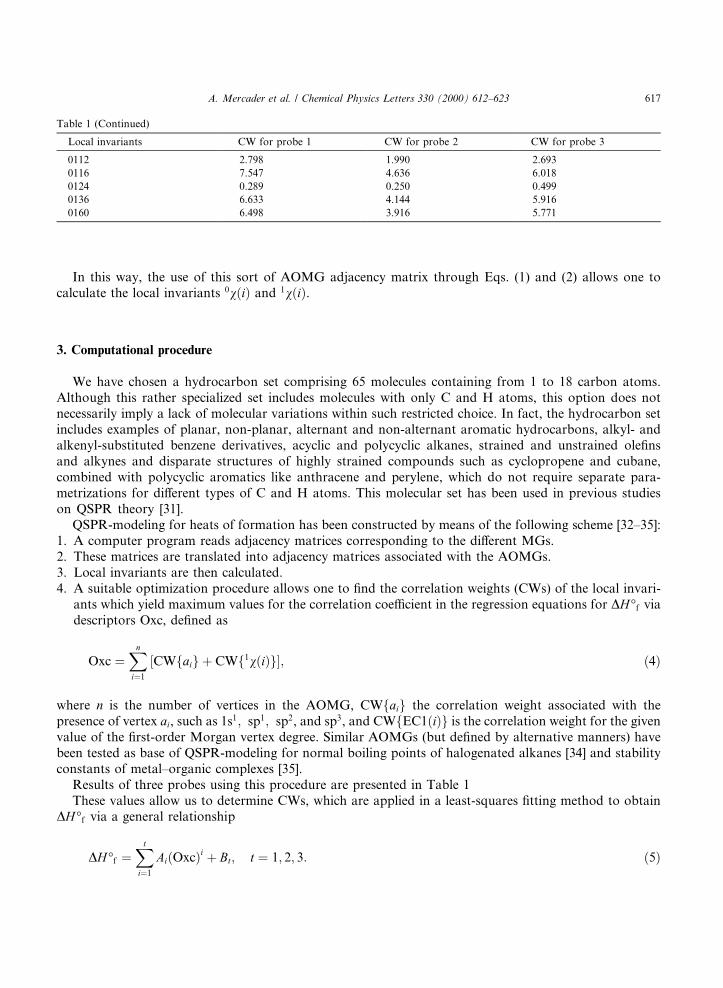
Table 2

Descriptor Oxc and theoretical heats of formation for the three probes calculated for the linear relationships plus the experimental

values (in kcal/mol)

Molecule Exp. Probe 1

Oxc

Probe 1

theor.

Probe 2

Oxc

Probe 2

theor.

Probe 3

Oxc

Probe 3

theor.

Training set

Methane )17.79 )23.088 )17.77 )9.316 )17.69 )20.768 )17.78

Acetylene 54.55 64.704 54.57 42.078 54.67 56.060 54.59

Ethylene 12.56 13.600 12.46 12.334 12.79 11.206 12.34

Propyne 44.41 52.288 44.34 34.805 44.43 45.258 44.41

Allene 45.31 53.510 45.34 35.484 45.39 46.290 45.39

Propene 4.79 4.431 4.90 6.712 4.88 3.385 4.97

Propane )24.93 )31.008 )24.30 )14.392 )24.84 )27.256 )23.90

1; 3-Butadiene 26.01 29.830 25.83 21.474 25.66 25.480 25.78

2-Butyne 34.69 40.592 34.70 27.868 34.66 34.824 34.58

1-Butene 0.07 )1.514 0.00 3.286 0.05 )1.836 0.05

2-Butene )1.77 )3.784 )1.87 1.990 )1.77 )3.854 )1.85

Isobutene )4.27 )6.246 )3.90 0.422 )3.98 6.036 )3.91

2-methylpropane )32.24 )40.947 )32.49 )19.743 )32.37 )36.471 )32.58

Cyclopentadiene 32.12 37.462 32.12 26.098 32.17 32.256 32.17

1; 4-Pentadiene 25.27 29.066 25.20 21.168 25.23 24.802 25.14

Cyclopentene 8.44 8.770 8.48 9.176 8.34 7.070 8.44

Cyclopentane )18.26 )23.110 )17.79 )9.530 )17.99 )20.760 )17.78

Cyclopropene 66.22 78.892 66.26 50.420 66.42 68.562 66.37

Cyclobutene 37.45 43.764 37.31 29.654 37.18 37.434 37.04

Neopentane )40.14 )49.860 )39.83 )25.260 )40.14 )44.028 )39.69

Cubane 148.69 178.944 148.70 108.784 148.59 156.056 148.78

Bicyclo�2; 1; 0�pentane 37.70 44.250 37.71 30.210 37.96 38.190 37.75

Bicyclo�2; 2; 2�octane )23.67 )30.244 )23.67 )13.568 )23.68 )26.874 )23.54

Spiropentane 44.25 52.200 44.26 34.624 44.18 44.964 44.14

Bicyclo�2; 1; 0�pentene 79.70 95.208 79.70 59.842 79.68 82.772 79.75

Bicyclo�2; 2; 0�hexene 62.50 74.286 62.46 47.684 62.56 64.464 62.52

n-Hexane )39.94 )50.978 )40.76 )25.214 )40.08 )45.316 )40.91

Norbornadiene 59.18 70.254 59.14 45.254 59.14 60.944 59.19

Anthracene 55.20 62.556 52.80 40.324 52.20 53.610 52.28

Benz[a]anthracene 68.10 83.994 70.46 53.790 71.16 73.146 70.68

Pyrene 54.00 64.386 54.30 41.962 54.51 56.148 54.67

Acenaphthene 37.23 43.771 37.32 29.686 37.22 37.593 37.19

Fluoranthene 69.20 81.141 68.11 51.427 67.83 70.173 67.88

o-Xyleno 4.56 3.862 4.43 6.500 4.58 2.814 4.43

Styrene 35.40 41.987 35.85 28.583 35.67 36.185 35.87

Toluene 11.95 13.055 12.01 11.776 12.01 10.737 11.89

Average deviation ± ± 0.31 0.32 ± 0.28

Test set

Ethane )20.04 )18.874 )14.30 )10.478 )19.33 )19.596 )16.68

n-Butane )30.33 )41.734 )33.14 )21.402 )34.71 )37.012 )33.09

1; 3-pentadiene 18.29 17.109 15.35 17.817 20.51 16.945 17.74

n-Pentane )36.60 )46.356 )36.95 )23.308 )37.39 )41.164 )37.00

Bicyclo�1; 1; 0�butane 51.90 59.556 50.32 39.024 50.37 52.014 50.78

Bicyclo�2; 2; 0�hexane 29.90 28.944 25.10 21.396 25.55 24.366 24.73

Bicyclo�2; 2; 1�heptane )12.40 )14.938 )11.06 )4.754 )11.27 )13.050 )10.51

Cycloheptatriene 43.56 47.536 40.42 32.868 41.70 40.614 40.04

Naphthalene 36.00 38.226 32.75 26.822 33.19 35.736 35.44

Phenantrene 49.70 59.664 50.41 40.288 52.15 55.272 53.85

Chrysene 66.00 81.102 68.08 53.754 71.11 74.808 72.25

618 A. Mercader et al. / Chemical Physics Letters 330 (2000) 612±623

4. Results

The testing of the procedure outlined before was made on the set of hydrocarbons [31] and it was veri®edthat there are nine outliers. We have chosen two alternative methods to calculate regression coe�cientsAi;Bt in Eq. (4):1. To divide the whole set in two subsets: a training set comprising 36 molecules and a test set including 15

molecules. We have not applied any special criterion for this particular partition, save to get to equilibrat-ed subsets regarding the number of C atoms. The training set is composed of methane, acethylene, eth-ylene, propyne, allene, propene, propane, 1; 3-butadiene, 2-butyne, 1-butene, 2-butene, isobutene,2-methylpropane, cyclopentadiene, 1,4-pentadiene, cyclopentene, cyclopentane, cyclopropene, cyclobu-

Table 2 (Continued)

Molecule Exp. Probe 1

Oxc

Probe 1

theor.

Probe 2

Oxc

Probe 2

theor.

Probe 3

Oxc

Probe 3

theor.

Perylene 78.40 99.258 83.04 62.382 83.26 84.558 81.43

Biphenyl 43.30 48.300 41.05 33.592 42.72 44.094 43.32

m-Xylene 4.14 5.278 5.60 8.798 8.07 1.245 2.95

p-Xylene 4.31 )4.112 )2.14 3.242 )0.01 )3.600 )1.61

Average deviation ± ± 2.90 ± 2.78 ± 2.66

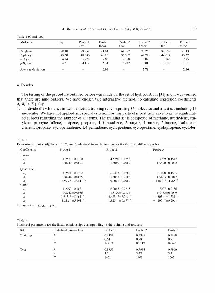
Table 3

Regression equation (4), for t � 1; 2; and 3, obtained from the training set for the three di�erent probes

Coe�cients Probe 1 Probe 2 Probe 3

Linear

B1 1.2537�0.1300 )4.5750�0.1758 1.7939�0.1547

A1 0.8240�0.0023 1.4080�0.0062 0.9420�0.0032

Quadratic

B2 1.2561�0.1332 )6.9413�0.1786 1.8028�0.1585

A1 0.8244�0.0035 1.8097�0.0106 0.9433�0.0047

A2 )3.996ÿ6�3.051ÿ 5a )0.0001�0.0002 )1.806ÿ5�4.765ÿ5

Cubic

B3 1.2293�0.1831 )6.9045�0.2215 1.8007�0.2186

A1 0.8242�0.0036 1.8120�0.0134 0.9433�0.0049

A2 1.643ÿ 5�5.161ÿ7 )2.483ÿ 4�6.715ÿ4 )1.605ÿ 5�1.531ÿ 4

A3 1.212ÿ7�5.161ÿ7 1.925ÿ 6�6.677ÿ6 )1.295ÿ 8�9.206ÿ7

aÿ3:996ÿ6 � ÿ3:996� 10ÿ6.

Table 4

Statistical parameters for the linear relationships corresponding to the training and test sets

Set Statistical parameters Probe 1 Probe 2 Probe 3

Training R 0.9999 0.9998 0.9998

s 0.64 0.78 0.77

F 127 890 87 749 89 765

Test R 0.9955 0.9998 0.9960

s 3.51 3.27 3.44

F 1431 1909 1607

A. Mercader et al. / Chemical Physics Letters 330 (2000) 612±623 619

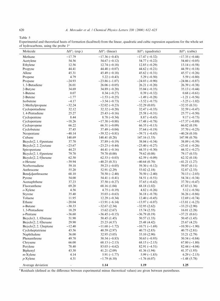
Table 5

Experimental and theoretical heats of formation (kcal/mol) from the linear, quadratic and cubic regression equations for the whole set

of hydrocarbons, using the probe 1a

Molecule DH°f (exp.) DH°f (linear) DH°f (quadratic) DH°f (cubic)

Methane )17.79 )17.36 ()0.43) )17.47 ()0.32) )17.35 ()0.44)

Acetylene 54.56 54.67 ()0.12) 54.77 ()0.22) 54.60 ()0.05)

Ethylene 12.56 12.74 ()0.18) 12.85 ()0.29) 13.14 ()0.58)

Propyne 44.41 44.48 ()0.07) 44.62 ()0.21) 44.59 ()0.18)

Allene 45.31 45.49 ()0.18) 45.62 ()0.31) 45.57 ()0.26)

Propene 4.79 5.22 ()0.43) 5.29 ()0.50) 5.59 ()0.80)

Propane )24.93 )23.86 ()1.07) )24.03 ()0.90) )24.06 ()0.87)

1; 3-Butadiene 26.01 26.06 ()0.05) 26.21 ()0.20) 26.39 ()0.38)

2-Butyne 34.69 34.89 ()0.20) 35.04 ()0.35) 35.13 ()0.44)

1-Butene 0.07 0.34 ()0.27) 0.39 ()0.32) 0.68 ()0.61)

2-Butene )1.77 )1.53 ()0.25) )1.49 ()0.28) )1.21 ()0.56)

Isobutene )4.17 )3.54 ()0.73) )3.52 ()0.75) )3.25 ()1.02)

2-Methylpropane )32.24 )32.02 ()0.23) )32.29 (0.05) )32.55 (0.31)

Cyclopentadiene 32.12 32.32 ()0.20) 32.47 ()0.35) 32.59 ()0.47)

1; 4-Pentadiene 25.27 25.43 ()0.16) 25.58 ()0.31) 25.77 ()0.50)

Cyclopentene 8.44 8.78 ()0.34) 8.87 ()0.43) 9.17 ()0.73)

Cyclopentane )18.26 )17.38 ()0.88) )17.48 ()0.78) )17.37 ()0.89)

Cyclopropene 66.22 66.31 ()0.09) 66.35 ()0.13) 66.02 (0.19)

Cyclobutene 37.45 37.49 ()0.04) 37.64 ()0.19) 37.70 ()0.25)

Neopentane )40.14 )39.32 ()0.81) )39.71 ()0.43) )40.24 (0.10)

Cubane 148.69 148.41 (0.28) 147.16 (1.53) 147.98 (0.70)

Bicyclo�2; 1; 0�pentane 37.70 37.89 ()0.19) 38.04 ()0.34) 38.09 ()0.39)

Bicyclo�2; 2; 2�octane )23.67 )23.23 ()0.44) )23.40 ()0.27) )23.41 ()0.26)

Spiropentane 44.25 44.41 ()0.16) 44.55 ()0.30) 44.52 ()0.27)

Bicyclo�2; 1; 0�pentene 79.70 79.70 (0.00) 79.62 (0.08) 79.17 (0.53)

Bicyclo�2; 2; 0�hexene 62.50 62.53 ()0.03) 62.59 ()0.09) 62.32 (0.18)

n-Hexane )39.94 )40.25 (0.31) )40.64 (0.70) )41.21 (1.27)

Norbornadiene 59.18 59.23 ()0.05) 59.30 ()0.12) 59.07 (0.11)

Anthracene 55.20 52.91 (2.29) 53.02 (2.18) 52.87 (2.33)

Benz[a]anthracene 68.10 70.50 ()2.40) 70.50 ()2.40) 70.13 ()2.03)

Pyrene 54.00 54.41 ()0.41) 54.51 ()0.51) 54.34 ()0.34)

Acenaphthene 37.23 37.50 ()0.27) 37.65 ()0.42) 37.70 ()0.47)

Fluoranthene 69.20 68.16 (1.04) 68.18 (1.02) 67.83 (1.36)

o-Xylene 4.56 4.75 ()0.19) 4.82 ()0.26) 5.12 ()0.56)

Styrene 35.40 35.03 ()0.63) 36.18 ()0.78) 36.26 ()0.86)

Toluene 11.95 12.29 ()0.34) 12.40 ()0.45) 12.69 ()0.74)

Ethane )20.04 )13.91 ()6.14) )13.97 ()6.07) )13.81 ()6.23)

n-Butane )30.33 )32.67 (2.34) )32.95 (2.62) )33.23 (2.90)

1; 3-Pentadiene 18.29 15.62 (2.67) 15.74 (2.55) 16.01 (2.28)

n-Pentane )36.60 )36.45 ()0.15) )36.79 (0.19) )37.21 (0.61)

Bicyclo�1; 1; 0�butane 51.90 50.45 (1.45) 50.57 (1.33) 50.45 (1.45)

Bicyclo�2; 2; 0�hexane 29.90 25.23 (4.57) 25.48 (4.42) 25.67 (4.23)

Bicyclo�2; 2; 1�heptane )12.40 )11.68 ()1.72) )10.71 ()1.69) )10.50 ()1.90)

Cycloheptatriene 43.56 40.59 (2.97) 40.73 (2.83) 40.75 (2.81)

Naphthalene 36.00 32.95 (3.05) 33.10 (2.90) 33.21 (2.79)

Phenanthrene 49.70 50.54 ()0.83) 50.65 ()0.95) 50.54 ()0.84)

Chrysene 66.00 68.13 ()2.13) 68.15 ()2.15) 67.80 ()1.80)

Perylene 78.40 83.03 ()4.62) 82.91 ()4.51) 82.44 ()4.04)

Biphenyl 43.30 41.21 (2.09) 41.36 (1.94) 41.37 (1.93)

m-Xylene 4.14 5.91 ()1.77) 5.99 ()1.85) 6.29 ()2.15)

p-Xylene 4.31 )1.79 (6.10) )1.76 (6.07) )1.48 (5.78)

Average deviation ± 1.14 1.19 1.25

a Residuals (de®ned as the di�erence between experimental minus theoretical values) are given between parentheses.

620 A. Mercader et al. / Chemical Physics Letters 330 (2000) 612±623

tene, neopentane, cubane, bicyclo�2; 1; 0�pentane, bicyclo�2; 2; 2�octane, spiropentane, bicyclo�2; 1; 0�pentene, bicyclo�2; 2; 0�hexene, n-hexane, norbornadiene, anthracene, bez(a)enthracene, pyrene,acenaphthene, ¯uoranthene, o-xylene, styrene and toluene, while the test set comprises the followingmolecules: ethane, n-butane, 1; 3-pentadiene, n-pentane, bicyclo�1; 1; 0�butane, bicyclo�2; 2; 0�hexane,bicyclo�2; 2; 1�heptane, cycloheptatriene, naphthalene, phenanthrene, chrysene, perylene, biphenyl, m-xylene and p-xylene.

2. To take the whole set of molecules.Furthermore, we tested up to third-order polynomial ®tting equations, (i.e., t � 1; 2; and 3 in Eq. (4)).

Some representative results are displayed in Tables 2±5 and Fig. 1. A complete listing of the numericalresults are available upon request to one of us (EAC).

The ®rst point to be noted is that the three probes presented in Table 1 are equally satisfactory tocompute DH°f . Besides, predictions are quite good for the di�erent ®tting procedures since average absolutedeviations fall within the interval �0:28; 2:90�, which is rather similar to the usual experimental uncertainties.Naturally, higher-order polynomials (second- and third-order) are better predictors than linear ones, sothat it seems sensible to resort to the former ones for these sorts of calculations.

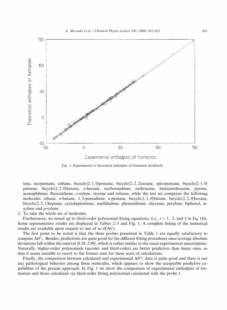
Finally, the comparison between calculated and experimental DH°f data is quite good and there is notany pathological behavior among these molecules, which appears to show the acceptable predictive ca-pabilities of the present approach. In Fig. 1 we show the comparison of experimental enthalpies of for-mation and those calculated via third-order ®tting polynomial calculated with the probe 1.

Fig. 1. Experimental vs theoretical enthalpies of formation (kcal/mol).

A. Mercader et al. / Chemical Physics Letters 330 (2000) 612±623 621

5. Discussion

Numerical data presented in the previous section make clear the high quality results based on thecorrelation weighting of local invariants of AOMGs, which yield very accurate molecular heats offormation and numerical correlations with signi®cantly low standard errors. Thus, these results point outthe possibility to extend this kind of method for other molecules including heteroatoms as well as to studyother physicochemical properties and biological activities resorting to this new topological descriptor.

It also could be interesting to employ multiple regression analysis supported by topological descriptorsand molecular indices combined with the orthogonalization procedure in order to obtain optimum QSAR/QSPR which most probably will lead to a meaningful interpretation of the regression formulae. Workalong these lines is presently being carried out in our laboratories and results will be given elsewhere in thenear future.

A ®nal comment on the de®nition of the Oxc descriptor. We have employed an additive relationshipbetween CWfaig and CWfEC1�i�g (see Eq. (3)), but it should be equally valid to take recourse of other sortof algebraic relationships between the local invariants 1v�i� and the elements of the adjacency matrix, suchas

Oxc0 �X

vertices

�CW�ai�CW�1v�i���; �6�

Oxc00 �Y

vertices

�CW�ai�CW�1v�i���; �7�

Oxc000 �Y

vertices

�CW�ai� � CW�1v�i��; �8�

Oxc0v �X

edges�i;j��CW�ai�CW�1v�i��CW�aj��CW�1v�j���: �9�

These sorts of algebraic alternatives have been used before for correlation weighting of local graphinvariants and results were quite good [32±35], so that they represent an interesting possibility to extend thissort of study in QSAR/QSPR. Work on this issue is also being carried out by us and results will be pre-sented elsewhere in the near future.

References

[1] D.R. Stull, E.F. Westrum Jr., G.C. Sinke, The Chemical Thermodynamics of Organic Compounds, Wiley, New York, 1969.

[2] W.J. Hehre, L. Radom, P.v.R. Schleyer, J.A. Pople, Ab Initio Molecular Orbital Theory, Wiley, New York, 1986.

[3] L. Radom, W.J. Hehre, J.A. Pople, J. Chem. Soc. A (1971) 2299.

[4] K.B. Wiberg, J. Comput. Chem. 5 (1984) 197.

[5] M.R. Ibrahim, P.v.R. Schleyer, J. Comput. Chem. 6 (1985) 157.

[6] E.A. Castro, J. Mol. Struct. THEOCHEM 304 (1994) 93.

[7] C. Vericat, E.A. Castro, Commun. Math. Comput. Chem. MATCH 34 (1997) 327.

[8] E.A. Castro, L. Gavernet, M. Firpo, Acta Chim. Slov. 44 (1997) 327.

[9] C. Vericat, E.A. Castro, Egyp. J. Chem. 41 (1998) 109.

[10] E.A. Castro, J. Mol. Struct. THEOCHEM 339 (1995) 239.

[11] E. Estrada, L. Torres, L. Rodrõguez, I. Gutman, Ind. J. Chem. A 37 (1998) 853.

[12] H.P. Schultz, T.P. Schultz, J. Chem. Inf. Comput. Sci. 38 (1998) 853.

[13] I. Gutman, J. Mol. Struct. THEOCHEM 428 (1998) 241.

[14] A.T. Balaban, Commun. Math. Comput. Chem. MATCH 1 (1975) 33.

[15] A.T. Balaban (Ed.), Chemical Applications of Graph Theory, Academic Press, New York, 1976.

622 A. Mercader et al. / Chemical Physics Letters 330 (2000) 612±623

[16] A.T. Balaban, D. Farcasiu, R. Banica, Rev. Roum. Chim. 11 (1966) 1205.

[17] A.T. Balaban, A. Chiriac, I. Motoc, Z. Simon, Steric Fit in QSAR, Lecture Notes in Chemistry, No. 15, Springer, Berlin, 1980.

[18] I. Gutman, N. Trinajstic, Top. Curr. Chem. 42 (1973) 49.

[19] O.E. Polansky, Commun. Math. Comput. Chem. MATCH 1 (1975) 11.

[20] M. Randic, Commun. Math. Comput. Chem. MATCH 7 (1979) 5.

[21] D.H. Rouvray, Amer. Sci. 61 (1973) 729.

[22] D.H. Rouvray, Chem. Brit. 10 (1974) 11.

[23] D.H. Rouvray, Commun. Math. Comput. Chem. MATCH 1 (1975) 61.

[24] D.H. Rouvray, A.T. Balaban, in: R.J. Wilson, L.W. Beineke (Eds.), Applications of Graph Theory, Academic Press, London,

1977.

[25] N. Trinajstic, The Chemical Graph Theory, CRC Press, New York, 1982.

[26] D. Bonchev, O. Mekenyan (Eds.), Graph Theoretical Approaches to Chemical Reactivity, Kluwer, Dordrecht, 1994.

[27] D. Bonchev, Information Theoretic Indices for Characterization of Chemical Structures, UMI, Bell & Howell Company, Ann

Arbor, Michigan, 1983.

[28] A.T. Balaban, J. Chem. Inf. Comput. Sci. 34 (1994) 398.

[29] A.T. Balaban, Rev. Roum. Chim. 39 (1994) 245.

[30] D. Bonchev, L.B. Kier, J. Chem. Inf. Comput. Sci. 9 (1992) 75.

[31] E.A. Castro, Comput. Chem. 21 (1997) 305.

[32] A. Toropov, A.P. Toropova, Russ. J. Coord. Chem. 24 (1998) 89.

[33] A.A. Toropov, A.P. Toropova, N.L. Voropaeva, I.N. Ruban, S.Sh. Rashidova, Russ. J. Coord. Chem. 24 (1998) 503.

[34] A.A. Toropov, A.P. Toropova, N.L. Voropaeva, I.N. Ruban, S.Sh. Rashidova, Russ. J. Struct. Chem. 40 (6) (1999) 1171.

[35] A.A. Toropov, A.P. Toropova, Russ. J. Coord. Chem. 26 (5) (2000) 423.

A. Mercader et al. / Chemical Physics Letters 330 (2000) 612±623 623