Pseudopotentials that work: From H to Pu

PHYSICAL REVIEW B VOLUME 26, NUMBER 8

Pseudopotentials that work: From H to Pu

15 OCTOBER 1982

G. B. Bachelet, ~ D. R. Hamann, and M. SchliiterBell Laboratories, Murray Hill, New Jersey 07974

(Received 28 April 1982)

Recent developments have enabled pseudopotential methods to reproduce accurately theresults of all-electron calculations for the self-consistent electronic structure of atoms,molecules, and solids. The properties of these potentials are discussed in the context ofearlier approaches, and their numerous recent successful applications are summarized.While the generation of these pseudopotentials from all-electron atom calculations is

straightforward in principle, detailed consideration of the differences in physics of various

groups of atoms is necessary to achieve pseudopotentials with the most desirable attri-butes. One important attribute developed here is optimum transferability to various sys-tems. Another is the ability to be fitted with a small set of analytic functions useful with

a variety of wave-function r'epresentations. On the basis of these considerations, a con-

sistent set of pseudopotentials has been developed for the entire Periodic Table. Relativis-tic effects are included in a way that enables the potentials to be used in nonrelativisticformulations. The scheme used to generate the numerical potentials, the fitting pro-cedure, and the testing of the fit are discussed. Representative examples of potentials areshown that display attributes spanning the set. A complete tabulation of the fitted poten-tials is given along with a guide to its use.

I. INTRODUCTION

Pseudopotentials were originally introduced tosimplify electronic structure calculations by elim-

inating the need to include atomic core states andthe strong potentials responsible for binding them.Considerable success was achieved in describingthe band structure of semiconductors and simplemetals with the use of the empirical pseudopoten-tial method. In this approach, the total effectivepotential acting on the electrons, includingCoulomb and exchange-correlation contributions aswell as the ionic parts, was represented by just afew terms in a Fourier expansion. The coefficientswere adjusted to agree with some experimentallydetermined features of the energy bands. ' In an al-ternative approach, a simple function representingthe ion-core potential was adjusted to fit the exper-imental ionization potential of the hydrogenic ion.The function typically consisted of a Coulombictail at large radius discontinuously changing to aconstant inside some "core radius. " These poten-tials were then screened using a linear dielectricfunction method, and gave band structures inreasonable agreement with the empirical potentials,provided the poorly convergent higher Fouriercomponents were set at zero. '

Aspects of these two approaches were combinedto deal with more complicated systems such as sur-

faces. A parametrized smooth model potential,with the appropriate Coulomb tail and a rapidlyconvergent Fourier expansion, was adjusted to fitexperimental band energies in a fully self-consistentcalculation. ' The charge density given by thesquare of the pseudo-wave-functions was treated asthe real valence charge, and used directly to com-pute the Coulomb and exchange-correlation poten-tials (the latter within the local-density-functional

approximation ). These model potentials were thenassumed to be transferable, that is, able to accu-rately represent the ion potential in other geome-tries such as surfaces, where the potential cannotbe represented by a few Fourier components, andwhere a self-consistent treatment of the screeningis essential. Considerable success was achieved indescribing the electronic properties of such sys-tems, and the current work is an outgrowth ofthis approach to the use of model potentials.

Paralleling the application of pseudopotentials, atheoretical justification for their use was devel-

oped. ' This was initially based upon theorthogonalized-plane-wave (OPW) method of bandstructure. In this method, plane ~aves were com-bined with Bloch sums of core wave functions insuch proportion that each basis function wasorthogonal to the core states. These combinationsthen formed a rapidly convergent basis for thevalence wave functions. If the linear combination

26 4199 1982 The American Physical Society

4200 G. B.BACHELET, D. R. HAMANN, AND M. SCHLUTER 26

of OPW's forming a band eigenstate was takenwithout including its core orthogonalization terms,the resulting smooth wave function could be identi-fied with the pseudo-wave-function. Phillips andKleinman showed that the effective potentialwhich has such plane-wave pseudo-wave-functionsas its eigenstates could be derived from the all-electron potential and the core-state wave functionsand energies. Thus a nonempirical approach tofinding a pseudopotential was introduced. Thispotential was nonlocal, in the sense that eachangular-momentum component of the valencepseudo-wave-function about an atomic center felt adifferent potential (arising from different corestates). Approximate self-consistent band-structurecalculations were carried out for Si and other semi-conductors with the use of this approach.

The wave functions of Phillips-Kleinman pseu-dopotentials have a certain problem. The norrnal-ized pseudo-wave-function and the normalizedOPW eigenfunction have the same shape in the re-gion of space outside the cores, but have differentamplitudes. The pseudo-wave-function is typicallysmaller than the OPW because neglect of the so-called "orthogonality hole" puts too much of itstotal charge in the core region. ' This problem isserious in the case of a self-consistent calculation,since the incorrect distribution of valence chargebetween the valence and core regions will cause er-rors in the Coulomb potential. In principle, thepseudo-wave-function can be orthogonalized to thecores before the charge density is calculated, butthis cumbersome procedure obviates most of theadvantages of using a pseudopotential.

The problem of the orthogonality hole is not, infact, a necessary consequence of replacing an all-electron potential by a valence pseudopotential. Itis a consequence of the Phillips-Kleinman con-struction, but that is by no means unique. Supposewe have a self-consistent local density calculationfor the ground state of some atom at hand. Apseudo-wave-function for the atom need have justtwo properties to be consistent with our intentions:it should be nodeless, and it should, when normal-ized, become identical to the true valence wavefunction beyond some "core radius, "R, . Such afunction can be constructed in arbitrarily manyways. For any particular such pseudo-wave-function, the radial Schrodinger equation can beinverted to yield a pseudopotential which has thefunction as its eigenfunction at the correct eigen-value. (Note that the nodeless property permits in-version with no further constraints on the func-tion. ) By this construction, it is clear that the

pseudopotential and full potential are identicalbeyond R, . The pseudopotential inside R, correct-ly mimics the scattering property of the full poten-tial inside R, at the eigenvalue energy (and, ofcourse, for the particular angular momentum ofthe wave function under discussion). We haveused the term "norm-conserving" to describe pseu-dopotentials constructed in this fashion.

The ability of a pseudopotential to reproduce asingle atomic state alone does not make it useful.To be useful, the core portion. of the pseudopoten-tial must be transferable to other situations wherethe external potential has changed, such as in mol-ecules, solids, or for excited atomic configurations,and where the eigenstates of interest are at dif-ferent energies. An identity related to the Friedelsum rule, and previously discussed in connectionwith pseudopotentials by Shaw and Harrison' and

Topp and Hopfield, " can be used to show that anynorm-conserving pseudopotential satisfies an im-

portant transferability criterion. The identity is (in

atomic units)r

—2m (rP) lng =4m J P r dr,de dr

where P is the solution of the radial Schrodingerequation at energy e (not necessarily an eigenvalue)which is regular at r=0. The radial logarithmicderivative of P is simply related to the scatteringphase shift. ' The consequence of (1.1) is that iftwo potentials v i and v2 yield solutions Pi and P2which have the same integrated charge inside asphere of radius R [for Pi(R) =$2(R)], the linearenergy variation around e of their scattering phaseshifts (at R) is identical. The requirement on theatomic pseudo-wave-function that it agree identi-cally with the full wave function for R & R, whenboth are normalized guarantees that the integratedcharge is identical for R y R„and thus that thescattering properties of the pseudopotential andfull potential have the same energy vari'. tion tofirst order when transferred to other systems.Since a given atomic valence state participates withthe most weight in molecular orbitals or energybands that are distributed around the atomic ener-

gy level, this optimizes transferability to leadingorder. Band-structure methods based on muffin-tin potentials such as the augmented-plane-wave(APW) method and Korringa-Kohn-Rostoker(KKR) method depend only on the logarithmicderivatives of the potential at the muffin-tin ra-dius. While such methods are not customarily

26 PSEUDOPOTENTIALS THAT WORK: FROM H TO Pu 4201

used for pseudopotentials, it is clear that the ener-

gy range over which the pseudopotential logarith-mic derivatives track those of the full potentialdirectly measures the range over which the pseudo-potential bands are accurate. The norm-conservingconstruction as defined so far does not guaranteethat the logarithmic derivatives track over any use-ful range. The loosely defined constraint that thepseudo-wave-function and the potential be smoothand physically reasonable in shape in fact yieldslogarithmic derivative agreement over a wide ener-

gy range. ' This close tracking for practicalpseudopotentials ensures, through (1.1), that thecore-region integrated charge is accurately repro-duced over a range of states. Conditions for exact-ly matching the second energy derivatives have re-cently been derived, and may be useful for furtherrefinement. '

Wave functions of norm-conserving pseudopo-tentials are designed to reproduce full-potentialwave functions accurately in the valence regions.Their definition makes no reference to the corestates. Orthogonalization of these wave functionsto the core states will not yield a well defined ob-

ject, in contrast to the Phillips-Kleinman case.While it may be desirable to reproduce the core-region structure of the all-electron wave functionin some after-the-fact manner to address questionslike nuclear hyperfine coupling, a rigorous pro-cedure consistent with the use of norm-conservingpseudopotentials has not yet been devised.

The first use of the norm-conservation conceptwas carried out within an empirical model poten-tial framework for Na by Topp and Hopfield. " Asmooth function with a 1/r tail for large r was fitto reproduce the experimental 3s-electron bindingenergy. It was then observed that the lowest excit-ed states had approximately correct energies, andthat this constituted a finite-difference approxima-tion to the energy derivative in (1.1). The impor-tance of obtaining the correct valence-region am-plitude for the normalized pseudo-wave-functionwas discussed in the context of chemical bonding. "

Systematic development of pseudopotentialsbased on ab initio atomic all-electron calculationswas first undertaken by Goddard and co-work-ers. ' ' They followed the Phillips-Kleinman ap-proach and expressed the pseudo-wave-function asa linear combination of the valence function andcore functions. The coefficients of the core func-tions were chosen to satisfy smoothness and expan-dability conditions, which included the requirementthat itii(r) go to zero as r +' at small r (the centri-fugal barrier enforces only r' behavior). The

ab initio calculations on which these pseudopoten-tials are based are Hartree-Fock calculations, sothat the radial equations for the. . wave functionscontain nonlocal exchange operators. This compli-cates the problem of finding a local pseudopoten-tial to replace the core. These authors dealt withthis complexity and the need to find a practicalrepresentation for the pseudopotential by introduc-ing a pseudopotential basis set (powers of r timesGaussians). They vary the coefficients to minimizethe error in integrals of the nonlocal Schrodingerequation satisfied by the pseudo-wave-functionwith members of the wave-function basis set usedfor the atom calculations' ' This criterion for afit also allows them to ignore the r divergence atsmall r of the exact pseudopotential (which arisesfrom the r'+' behavior of the wave function) withminimum error.

The above method for choosing pseudo-wave-functions was introduced in the context of calcula-tions based on the local-density-functional ap-proach by Topiol et al. ' These authors dealtdirectly with the numerical potential produced byinverting the Schrodinger equation, which is localin this case.

In both of the above approaches, the "ortho-gonality-hole" problem persists, since the pseudo-wave-function is strictly a sum of orthogonal coreand valence wave functions. In both cases, normconservation was later introduced with a minimumdeparture from the original approach. Redondoet al. modified the Goddard group's approach by amethod which explicitly depends on the use of abasis-function set in the original all-electron atomcalculation. ' The basis functions are partitionedinto two groups, with longer and shorter range.The coefficients of the longer-range basis functionsare fixed at their values in the normalized valencewave function. Members of the shorter-rangegroups are added with coefficients varied to satisfynodelessness, normalization, r +' behavior andsmoothness for the resulting pseudo-wave-function.The fitted potential is then found as previouslydescribed. ' This construction makes no explicituse of the core functions (which are particularlinear combinations of the short-range basis set).The pseudo-wave-function converges smoothly tothe valence function around a radius determined bythe division of the basis-function set. This in prin-ciple provides additional flexibility in optimizingthe pseudo-wave-function, but this was not dis-cussed by the authors. '

Zunger retained the Phillips-Kleinman construc-tion used in his earlier work with Topiol and


Ratner' in adding norm conservation to local-density-functional pseudopotentials. ' The linearcombination of core states added to the valencestate was fixed to satisfy r'+' behavior andsmoothness. A function of the form r +'e " wasthen added with a coefficient varied to give thecorrect tail amplitude for the normalized pseudo-wave-function. Choice of a gives some controlover the smooth transition to the valence function,but a minimum radius is set by the range of theleast-bound core function. '

An alternative approach to pseudopotential con-struction was introduced by Christiansen et al.specifically in the context of treating the norm-conservation problem. These authors chose thepseudo-wave-function to be identically theHartree-Fock valence function beyond somematching radius, and to be a polynomial inside. Afive-term polynomial with r +' as the leading

power was chosen to give the correct normaliza-

tion, and to match the value and first three deriva-

tives of the valence function at the matching ra-

dius. The matched derivatives ensure continuousbehavior of the pseudopotential, but some kinks

may occur in the potential in the core region. '

This construction does not guarantee a nodelesspseudo-wave-function, but the choice of matchingradius can be varied to achieve this goal.

All the above constructions give pseudopoten-tials which diverge with repulsive r behavior atsmall r. This is a consequence of the r'+'behavior of the pseudo-wave-function, which ap-pears to be an arbitrary requirement. For pseudo-wave-functions which are based on linear combina-tions of the valence (and possibly core) functions,however, the alternative to relaxing this conditionis a Zlr attractive sing—ularity at small r, where

Z is the nuclear charge, due to the cusp conditionsatisfied by the wave functions. ' In addition, ther +' requirement serves to minimize the core con-tent of a Phillips —Kleinman-type pseudo-wave-function, ' ' and hence minimize the orthogonalityhole problem. The retention of the r'+' require-ment in norm-conserving methods which do notuse eigenfunctions of the full potential at small r(the Redondo et al. ' and Christiansen et al.methods) seems to have purely historical origins.

A method very similar to that of Christiansenet al. was applied to local-density-functionalatoms by Kerker with attention to the above is-sue. Choosing polynomial or exponential of poly-nomial functions with ar +br + leading behaviorinside the matching radius guaranteed a nonsingu-lar pseudopotential, which is a significant advan-

tage whenever a basis-function expansion of thispotential is to be used. Pseudo-wave-function con-vergence is also improved. The use of the ex-

ponential form guarantees nodelessness, but thematching radius cannot be too small if a physicallyreasonable pseudo-wave-function is to be obtained.

The pseudopotentials which are presented in thispaper, which were introduced by two of the au-

thors, 9 are nonsingular and intended for use indensity-functional calculations. They are con-structed in two steps from the results of an all-

electron atom calculation. First, the full potentialat large r is smoothly merged into a parametrizedpotential inside a radius r, . The (single) parameteris adjusted to reproduce the valence eigenvalue, andhence eigenfunction for r & r„ for the highest-

energy bound state of each angular momentum /.

The norm is then corrected by the addition of ashort-range term to this eigenfunction, and theSchrodinger equation for the resulting pseudo-wave-function is analytically inverted, yielding a(typically small) correction to the potential. Non-

singular pseudopotentials can also be constructedfor coreless (hence nodeless) valence states.

Pseudopotentials constructed according to thisprescription have been used in self-consistentband-structure calculations, and shown to accurate-ly reproduce the results of all-electron calculations.Self-consistent band energies have been comparedfor Si, 3 Nb, ' and CsAu, with errors in therange of 0.05 eV for Si and 0.1 —0.2 eV in the oth-er cases.

More extensive use has been made of these pseu-dopotentials in total-energy calculations. They

have been shown to yield lattice constants, cohesiveenergies, bulk modulii, and phonon frequencieswith accuracies of a few percent compared to ex-perimen. t for Si, ' diamond, ' Ge, GaP,GaAs, ' AlAs, ' the Si2 molecule, and others.The excellent results obtained in these studies de-

pend, of course, on much more than the ability ofthe pseudopotentials to reproduce all-electron cal-culations. The accuracy of the local-density ap-proximation itself for such systems is critically

tested by these comparisons. In addition therigid-core approximation, which is central to anypseudopotential, must be accurate. This has beenestablished analytically by showing that first-ordercorrections to the total energy associated with corerelaxation cancel identically, and numerical testsindicate errors in the 0.05-eV range for the moredifficult case of transition metals. Moreover, thenonlinear density functional of the exchange andcorrelation potential induces errors if the pseudo-


potentials are used for different systems than thereference atom. This, too, leads to second-ordercorrections in the total energy. We shall comeback to these problems below.

In treating heavier atoms, it is necessary to con-sider relativistic effects. For valence states in thevalence region, the relativistic Dirac equationreduces to the nonrelativistic Schrodinger equation.This suggests that relativistic effects on the valenceelectrons, which occur in the core region, can belumped together with other properties of the corein creating a pseudopotential which can be used totreat heavy atoms in a nonrelativistic formalism.This approach was applied to relativistic Hartree-Fock calculations by several groups using aPhillips-Kleinman construction. ' The methodused in this paper to construct norm-conserving

pseudopotentials for local-density-approximationcalculations was generalized to the relativistic caseby Kleinman and subsequently tested for avariety of atoms.

For the relativistic atom, each electron's orbitalangular momentum and spin must be coupled, anddifferent energies and wave functions are found

for the two possible values of the total angular-

momentum quantum number, j =I + —, and

j =I ——,. Two different pseudopotentials are thus

found for each 1. The most convenient form forapplication is to take the weighted sum and differ-ence of these potentials. ' " The j-average poten-tial then yields results which are similar to thoseobtained using a "scalar" version of the Diracequation in which the spin-orbit term is removed.We have carried out tests on heavy atoms compar-ing the valence levels based on the j-average poten-tial (derived from the fully relativistic atom) withthose of completely "scalar relativistic" atoms.The results typically agree within a few hundredths

of an eV. This also establishes the fact that thescalar method closely reproduces the fully relativis-tic core charge. A further test of the j-averagepseudopotential was carried out by comparing theself-consistent band structure of CsAu with the useof this potential and with a scalar relativistic full-potential method. The agreement found, typical-ly 0.1 —0.3 eV, was excellent.

The "difference" pseudopotential is in fact aspin-orbit pseudopotential which should formallyappear multiplying the operator L S. Itreduces to zero outside the core, since the pseudo-potentials for all j converge to the full potential.Unlike the true spin-orbit potential, which divergesas r at small r, the spin-orbit pseudopotentialcan be smooth and nonsingular in the core region.

(Note that it would be completely inconsistent toapply the full potential spin-orbit operator to apseudo-wave-function. ) The approach used heregives spin-orbit pseudopotentials which are oftennearly constant over most of the core region.

A number of workers have already successfullyconstructed and used pseudopotentials based onRef. 9. It is clear, however, that experience is veryhelpful in choosing all-electron atom reference con-figurations, core radii, cutoff functions, etc., andthat extensive testing is mandatory for the best re-

sults. The principal purpose of this paper is tomake a good set of these pseudopotentials for all

the elements in the Periodic Table available to oth-ers. For many applications, analytic fits to the po-tentials are necessary. Here again, much exper-imentation and testing is necessary to find an accu-rate but economical fitting basis. The quality offit which could be achieved played an importantrole in guiding the choices to be made in the con-struction of the numerical pseudopotential. Thefitted form was also devised to permit its publica-tion in a compact table without loss of accuracy.

In Sec. II, the physics involved in choosingreference configurations and pseudopotential con-struction details for various groups of elements arediscussed. The fitting approach is motivated, andthe testing procedure for the tabulated results isdescribed. Section III presents examples illustrat-ing the several classes of behavior encountered invarious groups of elements. Section IV explainsthe arrangement and use of the pseudopotentialtables. In Sec. V some cases with ambiguouscore-valence separation are discussed. Section VIconcludes the paper.

II. THE CONSTRUCTIONOF PSEUDOPOTENTIALS

This section is divided into three parts: thedescription of full-core atom calculations fromwhich the pseudopotentials will be derived, theconstruction of numerical pseudopotentials fromenergies, wave functions, and potential of a refer-ence full-core atom, and the procedure of fittingsimple analytical functions to the set of num. ericalpseudopotentials.

For both the underlying full-core atom and thesubsequently constructed pseudoatom, electron in-

teraction effects are described in the local-density-functional framework. In this scheme theground-state energy of a system of interacting elec-trons in an external (nuclear) potential is written asfunctional of the electron density p(r):

G. B.BACHELET, D. R. HAMANN, AND M. SCHLUTER 26

E[pl= T[pl+Eco i[p]

+f V,„,(r)p(r)dr+E„, [p],where T[p] is the kinetic energy of the nonin-

teracting electrons,

(2.1)

E„,[p]=fp( r)E„,(p(r) )dr, (2.5)

The use of reliable approximations for theexchange-correlation energy E„,[p] in Eqs. (2.1)and (2.2) is of central importance. In the local-density approximation,

the usual electrostatic Coulomb energy of the elec-

trons, V,„,(r) = Zl—r, the nuclear potential, and

E„,[p], the exchange-correlation energy. Accord-

ing to Kohn and Sham, a variational solution ofEq. (2.1) can be obtained by solving a set ofSchrodinger-type equations self-consistently:

[T+V(r)]g;(r) =e;P;(r),

V(r) =f, dr'+ + V,„,(r),p(r'), &E..[p]r r'—5p r

(2.2)

occupiedstates i

To account for relativistic effects in a consistent

way for all atoms in the Periodic Table we useDirac's formulation of the kinetic energy. ' Thus,the Schrodinger equation [Eq. (2.2)] is replaced bya pair of coupled equations for minor and majorwave-function components G; (r) and F;(r), respec-tively, which in their radial form are

dF;(r)F;(r)+a [—e; —V(r)]G;(r) =0,

(2.3)

&c= '

—0. 1432

1+1.0529~r, +0.3334r,—0.0480+0.0311lnr, —0.0116r,

+0.0020rs lnrs for rs ( 1 .

for r, ) 1

Here r, is related to the density through

p '=(4al3)r, . The exchange-correlation poten-tial can be obtained from Eq. (2.6) as

where e„,(p) is the exchange-correlation energy perelectron of a homogeneous system with density p.Among a variety of interpolation formulas avail-able for e„,(p) here we use the recent results ofCeperly and Alder as parametrized by Perdewand Zunger. This choice was motivated byseveral factors: (i) Ceperley and Alder's results arebased on a stochastic sampling of an exact solutionof the interacting electron gas, (ii) their results areinterpolated by Perdew and Zunger to yield correcthigh- and low-density limits, and (iii) a consistentextension to finite spin-polarization exists.

For the unpolarized gas we have (in a.u. )

0.4582e„,=e +e, with e =—

rs

(2.6)

dG;(r) „2+ G;(r) —a — +e;—V(r) F;(r)=0 .d7"

~&xcPxc xc ~s ~

d~s(2.7)

We use atomic units A'= m =e = 1 andc =o. '=137.04. K is a nonzero integer quantumnumber

K= ~

1

I, for j=l ——,

—(l+1), for j=l+ —,

(2 4)

occupiedstates i

For one-electron potentials Dirac's equation in-

cludes all relativistic effects and yields spin-orbitsplitting energies.

The charge density is given by summing over bothcomponents, i.e.,

A detailed comparison of the interpolation formulafor e, given above and other existing prescriptions(i.e., Wigner, Hedin-Lundquist, Gunnarson-Lundquist, etc.) can be found in Ref. 43. On thebasis of several test calculations for atoms andsolids we found only very small differences be-tween using, e.g., Ceperley-Alder or Wigner expres-sions. The two expressions intersect each other forr, =2, i.e., for average atomic or crystalline densi-ties, while they deviate significantly from each oth-er in the low- and high-density regimes.

To account for relativistic quantum-electro-dynamical corrections to the Coulomb interaction,and to be consistent with the Dirac treatment ofthe free-particle kinetic energy, we modify the non-

relativistic density-functional exchange-correlation

PSEUDOPOTENTIALS THAT WORK: FROM H TO Pu 4205

energy e„, as proposed by MacDonald and

Vosko. This amounts to multiplying exchangeenergy e„and potential JM„by density-dependentcorrection factors f, and f„,respectively,

f, (r, )=1——3 (1+P)' In[P+( I+/ )' ]P p2

1 3 1n[P+(1+P )'~ ]2 2 P(1+P )

(2.8)

where the dimensionless expansion parameterP=O 0140. /r, measures the density-dependent Fer-mi velocity in units of the speed of light. Thecorrection which is due to retardation and magnet-ic effects decreases the effective exchange interac-tion appreciably only for rather high densities, i.e.,in the atomic core. For example, inclusion of thecorrection increases the total energy of atomic Pbby about 44 a.u. of which 42 a.u. result from the1s electrons. The 6s valence electrons are affectedby less than 0.1 eV. We nevertheless include thecorrection consistently in all atomic calculations.

For the full-core atom the Dirac equations [Eqs.(2.3)] are solved using a modified version of theoriginal Liberman-Waber-Crier program whichuses a logarithmically spaced radial integrationmesh. The numerical accuracy is about 10 a.u.Atomic states are specified as usual by orbital oc-cupation numbers. The atomic ground state withinthe local-density-functional (LDF) framework isdefined by occupying the lowest-lying orbitals.For the purpose, however, of obtaining eigensolu-tions for both spin-orbit components, j=I+—,, we

always occupy both components, regardless of theirorbital energies, weighted by noninteger values ac-cording to their multiplicities. Valence-electronwave functions and energies with angular momentathat are present in the ground state are obtainedfrom ground-state calculations. Higher-angular-momentum wave functions are calculated from ap-propriately excited atomic states (see also belowand Table II). For convenience, the atomic corecharge is allowed to relax. The most consistentway to generate these excited configurations wouldbe to keep the core charge frozen in its ground-state form. However, tests indicated that allowingcore relaxation in the excited-state configurationswhich we used had negligible effect on the pseudo-potentials. Valence-electron eigenfunctions and

1

eigenvalues for j=l+ —, up to l =2 (l =3 for ele-

ments with Z~ 55j, as well as the correspondingself-consistent potentials V(r) [Eqs. (2.2)], are cal-

culated for all elements from Z= 1(H) to Z=94(Pu).

The norm-conserving pseudopotentials are con-structed in five steps.

(i) Dirac's equations are solved for a chosenatomic reference configuration labeled by v. Theoutput is a set of one-electron eigenvalues (for thevalence states) and radial wave functions (F and G}as well as the self-consistent LDF potential. Aspointed out by Kleinman and later elaborated byBachelet and Schliiter, Dirac's equations [Eqs.(2.3)] can formally be replaced for valence elec-trons outside the core region by a Schrodinger-typeequation for the major wave-function componentG„(r):

+ V"(r) G„(r)=eG„(r), (2.9)2 dr 2r"

+c&'frcj

V', ~(r) = V"(r) 1 f-rcj

(2.10)

where f (r jr,J ) is a smooth cutoff function whichapproaches 0 as x~ oo, cutting off around r =r,jand approaching 1 as r —+0. The constant cJ' is ad-

justed, so that the lowest nodeless solution w &~(r}

of the radial Schrodinger equation containing V&l

has an energy equal to the original eigenvalue e~".

The normalized function w&J(r) agrees with thefull-core valence wave function beyond r,j within amultiplicative constant yJ,

(2.1 1)

since both satisfy the same differential equationand homogeneous boundary conditions for r g r,j.The choice of the cut-off function,

with v given in Eq. (2.4). This replacement iscorrect up to terms of order a . The minor wave-

function component F„(r) is strongly admixed with

G„(r) only in the core region of heavy atoms.Equation (2.9) can thus be thought of as the start-ing point for the construction of pseudopotentialsand pseudo-wave-functions. The construction stepsare carried out independently for each angular-momentum (lj) quantum state. For conveniencethis state is labeled by j only in the following dis-cussion.

(ii) We construct a first-step pseudopotential V&J.

by cutting off the singularity near r =0 in thescreened full-core potential V:


TABLE I. List of parameters ccI that determine theoptimum pseudopotential cutoff radii rd through

r,I——r,„/cc~, where r,„ is the radius of the outermost

peak in the radial wave function.

short range of the intermediate pseudo-wave-function wij(r) to

w2J(r) =yj'[w ij(r)+5&"r'+'f (r/r, j )], (2.13)

Elements

lH~2He3Li4Be~ )pNe

))Na)2Mg~ )gAr

i9K~30Zn31Ga~36Kr37Rb~4gCd49In~54Xe55Cs

56Ba

57La~7~Lu72Hf —+gpHg

g ITl~ g6Rn

g7Fr

ssRa~94Pu

I=O

3.02.01.82.01.81.81.81.81.61.81.81.451.61.61.61.6

3.63.03.01.81.451.61.71.71.71.71.71.61.61.71.61.6

3.63.53.53.52.23.02.01.62.01.451.451.451.452.21.451.45

l=3

4.53.03.03.03.04.52.0

f(r /r, j ) =exp[ (r /r, j )"], — (2.12)

with A, =3.5 was found to yield optimum results in

tests on a variety of atoms. The exponent A, =3.5guarantees nonsingular pseudopotentials for r =0and was found to allow better analytic fits thanlarger A. values. The "quality parameter" or cutoffradius r,z defines the range over which pseudo-wave-function and full-core wave functions are al-

lowed to deviate from each other. It is not to beregarded as an adjustable parameter but can beused to define the "quality" of the pseudopotential.Large r,j values produce rather smooth and j(l)-independent pseudopotentials at the expense oflarger inaccuracies of the pseudo-wave-functionaway from the core region. Small r,j values pro-duce stronger and more j(1)-dependent pseudopo-tentials with maximum accuracy. A strict lowerlimit for r,j is the position of the outermost nodein the full-core valence wave function, but numeri-

cal instabilities appear already for slightly largerr,j values. Optimum r,j values are obtained byscaling down from the radius (r,„)of the outer-most peak in the radial function 6„, r,~ =r,„/cc,where cc is typically in the range of 1.5 —2. Wepresent in Table I a complete list of optimum ccvalues used for the present calculations. Cutoff ra-dii for the two spin-orbit components j=l+ —, were

chosen to be identical and equal to the average ob-tained from r,„/cc.

(iii) The second step involves a modification at

V2, (r) = Vi1(r)+2wzi(r)

'2A,

—[2)Ll+ k(A, + 1)]Tqj.

p2

+ 2ej —2Vii(r) (2.15)

such that the normalized function w2i(r) agreeswith the full-core valence wave function for r & r/.This requires that 5J be the smaller solution of thequadratic equation

(yJ) f [w iJ(r)+5''+'f (r/r z)] dr =1 .(2.14)

The magnitude of the norm correction (yi) —1 is

typically small (-10 —10 ). While the ex-istence of a solution 5J is guaranteed, unphysicalresults can occur for weakly bound and thereforeextended excited states. "Bumpy" pseudo-wave-functions (and potentials) for angular momentapresent only in excited states (e.g., l =2 for Si) canbe avoided by using appropriately ionized excited-atom configurations (e.g. , for Si 3s' 3p

' 3d )

which tend to increase wave-function localization.This improves the transferability of the pseudopo-tential to systems of interest where the wave-

function components corresponding to excitedstates are confined by surrounding atoms.Nevertheless, the high-l-component potentials areless accurate and should not be used as local refer-ence potentials. Note that the atomic ground stateis used for all angular momenta present in theground state. This also minimizes systematictransferability errors. Table II contains a list ofatom reference configurations used in the presentwork.

(iv) In the third step the final screened pseudo-potentials V2J(r), producing the nodeless eigen-functions w2J(r) at eigenvalues ei, are found by in-

verting the radial Schrodinger equation. This canbe done analytically, knowing Vij(r) and w2J(r):


TABLE II. Atomic valence configurations (v) used to derive the l,j-dependent pseudopo-

tentials. Only excited-state configurations are shown. Angular momenta present in the (as-

sumed) ground state are derived from the ground state given in the Sargent-Welch table

(Ref. 47) and no configuration is indicated here. Potentials for I =3 are derived only for ele-

ments with Z )55. The symbol (~) indicates the systematic increase by 1 electron per in-

creasing nuclear charge, i.e., for Si one has s'p 'd while for Ar the configuration is$'p "d '. Ground states of the Sargent-Welch table are modified for the following few ex-

ceptions: &6Pd from s d' tos'd9, 57La from d'f to d0f', and»Np from dlf to d0f5.Moreover, for all rare-earth elements (Z =57—71) the 6$ - configuration is replaced bythe 5$ 5p 6$ - . configuration (see text}.

Elements

1H

2He

5Li —+Qe586C

7N —+809F

10Ne

11Na

12Mg

13Al

14Si~18Ar19K

2pCa

2lsc~50Zn31Ga

32Ge~36Kr

37Rb

38Sr

39Y~48Cd49In

50Sn~54Xe

55Cs

56Ba

57La —+71Lu72Hf ~80Hg

81Tl82Pb~86Rn

s7Fr88Ra

89Ac

9pTh

9]Pa~92U93Np —+94Pu

0.5

Sp.sp 0.2

0.25d 0.25

0.25d 0.25

$0.5 0.25d0. 25

p0.25

S0' 5 0 25d 0 25

$0.75 0.25d 1

p0.25

$0.5 0.25d0. 25

$0.75 0.25d 1

p0.25

0.75 0.25

S0.75 0.25d 2

0.25

$0'75 0 25

$0.75 0.25d 1

0.25d1.5f 0.25

l 0.5d0.5f l~

, 0.5 0.5d 0.5f5.5 '

Angular momentuml=2d"

S0'8d 0'2

as l=11d0.2

$0.75 1d0.25

I 1.75d 0.25

S 1.25 2.5d 0.25

S1 2.75d 0.25

as 1=1as 1=1$0.75d0. 25

1 0.75 d0.25

d 0.25

as 1=1

S0.75d0. 25

s' 0'75'd0. 25

d 0.25

as I =1

$0.75d0. 25

$1p0.75 d0.25

d 0.25

S0.75d 0.25

s p d'f'

0.75d 0.25

$1 ' 5 d025

d 0.25

$0.75d 0.25

as I =1as I =1

l=3

f0.25

$0.75 0.25

s0.75d 1 ~f0.25

s0.75f0.25

s0.75 0.75'f0.25

f0.25

s 0.75f0.25

s0.75d lf0.25

as l=1

The second term in Eq. (2.1S) is a smooth correc-tion which cuts off

-f=exp~CJ

No numerical instabilities are associated with thisprocedure.

(v) Finally, in the last step the screened poten-

2w q~(r)

p"(r) =occupted

valence states

tials V2f(R) are unscreened using the nodelesspseudo-wave-functions w 2J(r):

p"(r'), &E-I:p"1VI+1/2(r) V2j(r)—

5p"(r)

(2.16)


Vi'"(r) = [lVJ' in(r)+(1+1) Vi+i/z]2l+ 1

(2.17)

weighted by the different j degeneracies ofthe I+ —, states. This average potential is appropri-

ate for scalar relativistic use. Note, that the defini-tion of Vi""(r) in Eq. (2.17) differs from Eq. (2.12)

of Ref. 36; it is, however, consistent with Eq. (13)of Ref. 37. A difference potential Vi"(r) describ-

ing the strength of spin-orbit effects can according-ly be defined as

(Vi'+rii—Vi' "in) . -21 +1

(2.18)

Thus the total ionic pseudopotential to be used in

relativistic calculations is

V","(r)=g~

l)[Vi""(r)+Vi"(r)L S] &1~

l

(2.19)

The potential is appropriate for Schrodinger equa-tions yet contains relativistic effects to order a .

The pseudopotentials [Eqs. (2.17) and (2.18)],two (one for l =0) for each angular momentum fora given atom, are derived on a numerical radialgrid. To facilitate their tabulation and use, howev-

er, it is desirable to find high-precision fits involv-

ing few analytic functions. For this purposewe decompose Vi'"(r) into a long-range Coulombpart (l independent) and a short-range l-dependentpseudopotential part. We have

As pointed out in Ref. 48, this valence-

unscreening procedure, though exact by definitionfor the reference atom, represents a linearization ofthe exchange-correlation energy as a function ofcharge density. The systematic error occurring fordifferent valence configurations, though small forparamagnetic systems, increases with decreasingvalence electron density in the reference state. Forsystems with few valence electrons such as the al-

kali atoms, highly ionized reference configurationsshould thus be avoided. The bare-ion pseudopo-tentials Vi+i&z(r) of Eq. (2.16) are, to first order,independent of changes in the atomic prototypeconfiguration v. We therefore drop the index v in

all further discussions.It is convenient to define an average pseudopo-

tential

Vcore(r) = Z 2&coree &core 1/2

(2.21)

and therefore smoothly approaches a finite valuefor r~0. Z„denotes the valence charge. Theremaining potentials b, Vi'"(r) and Vi"(r) are both

expanded in Gaussian-type functions, e.g.,

3 —C 'Tb, V,""(r)=g (A, +re, +,)e (2.22)

Thus each atom is characterized by(i) a valence charge Z„and two sets of linear

coefficients and decay constants describing the

(ii) for each 1 value two sets of three linear coef-ficients each, A; and A;+3 corresponding to the de-

cay constants u;, I', =1,2, 3 for the average poten-tial, and

(iii) a similar set as (ii) for each spin-orbit differ-ence potential, provided the spin-orbit splitting ofthe eigenvalues is larger than a chosen thresholdvalue of 0.05 eV.

The choice of error function, Gaussian, and rtimes Gaussian functions was made to maximizethe number of calculational techniques which canmake direct use of the fitted form. Plane-wavematrix elements can be calculated analytically.The one-, two-, and three-center integrals neededfor Gaussian linear combination of atomic orbitals(LCAO) calculations can be expanded as sums ofanalytic functions, as can mixed-basis Gaussian-plane-wave matrix elements.

The core parameters are the starting point of thefitting procedure. For this purpose the self-consistent full-core potential V'(R) is first formal-

ly unscreened by the valence electrons. We write

p„,i(r') 5E„, p„„V;,„( )= V'( ) —J, d '—

(2.23)

V;,„(r) has the form —Z„lr for large r, but devi-

ates from this form in the core region to attain a

Zr„ii lr behavi—or for r —+0. The function V„„,(r)[Eq. (2.21)] is then fitted to V;,„(r) using the cutofffunction

Vi'"= V„„,(r)+b, Vi'" .

The core potential is thought of as originatingfrom Gaussian-type effective core charges:

(2.20)g= 1 f= 1 —exp[ (rlr,—&)]—

as a weighting function. Here r,~ denotes the atom


f (V„„—Vg, )'r 'f w2, J'dr, (2.24)

except in some special cases, like some excitedstates with a relatively long range where the wave-

function weighting r~ w2J

~

was replaced by 1.Equation (2.24) exhibits strong nonlinearities as afunction of the independent parameters and exhi-bits a large number of nearly equivalent minima.Random search and conventional simplex pro-cedures were used to find satisfactory solutions.

Linear dependencies of the fitting functions canlead to large values for some of the fitting coeffi-cients A; in (2.22). This effect is reduced by con-straining the nonlinear fit to maintain a finitespacing of the a;. Nonetheless, too many signifi-cant figures must be retained in the A s for practi-cal tabulation. To solve this problem we havetransformed the coefficients A;, A;+3, i =1,3 ofEq. (2.22) into a set of coefficients C;, i =1,6 foran orthonormal basis set,

6

C;= —g AIQ;I1=1

where the orthogonality matrix

(2.25)

average over the angular-momentum-dependentcutoff radii r,j given in Table I. V„„(r) thus hasthe built-in feature of simulating shallow corecharges that may extend beyond the pseudopoten-tial cutoff radii r,&. Examples, such as Cs, shall bedescribed below. Note that V„„,(r) is not uniquelydefined but determines the remainder A VI""

through Eq. (2.20). The choice of V„„(r)dis-cussed here both simplifies the shape and reducesthe range of b, VI'". In the context of a solid-stateor molecular calculation, matrix elements of an ionpseudopotential must be taken between wave-

function components which have angular momentaabout that center which are higher than the largestl value given. The most consistent procedure is touse the potential for the largest l given for allhigher I. However, the construction of V„„givenhere enables this term alone to be used as a "local"I-dependent potential for higher I's with little lossof accuracy. (Both approaches depend on the cen-

trifugal barrier to keep the high-I components outof the core region).

The nonlocal short-range components b, VI'"(r)and VI (r) are each fitted by nonlinear least-

squares procedures constraining the longest-rangecomponents to remain roughly within r,&.

The weighting of the fits was chosen to mini-mize the error in potential matrix elements, i.e.,

QI=

0 fori&l1

1/2

Ss —g Qk;2

k=1

Sl —g Qk~Qki

for i =I

fori &i .

(2.26)

The overlap matrix is defined by

S;I ——I r'@; (r)& I(r)«,

—a, r 2

e ' for i =1,2, 3

2

r e ' fori=

(2.27)

The Gaussian exponents n; are rounded to twodecimal places prior to a final linear fit determin-

ing the 2;. The coefficients C; in Eq. (2.25) arerounded to four digits. To test the overall accura-

cy of the fitting procedure including the rounding

as tabulated, the potentials are reassembled by firstperforming an inverse matrix transformation,

6

A;= —g C(Qs ',1=1

(2.28)

and then using Eqs. (2.20), (2.21), and (2.22).The minus signs in Eqs. (2.2S) and (2.28) corre-

spond to a particular choice of phase. The qualityof the fits can then be assessed by comparing twoindependent pseudoatom calculations for identicalconfigurations using the original numerical pseudo-potentials and the fitted analytical version. Typi-cal results for a variety of atoms are shown inTable III. The test results illustrate two differentand unrelated features: (i) transferability, i.e., thequality of describing atomic excitations (eigen-values and total energies) by pseudopotentials thathave been derived from a different reference state,usually the ground state, and (ii) the quality of thefitted potentials.

The issue of pseudopotential transferability hasbeen discussed before. ' ' Transferability isdetermined by the "frozen-core" approximationunderlying the construction of all pseudopotentials,by the linearization of core and valence exchange-correlation contributions, and by the norm-conservation feature. As can be, seen from TableIII, transferability is generally excellent. The errorincreases typically for "two-shell" systems, in par-


TABLE III. Results of test calculations for a variety of representative atoms. State 1 isreference state for the pseudopotential construction, state 2 represents the (de-) excited state.Differences in total energy are given in columns 4 (full-core atom), 5 (numerical pseudopo-tential atom), and 6 (fitted pseudopotential atom). Columns 7 and 8 show the differences ineigenvalues between the numerical pseudopotential case and the fitted pseudopotential casefor states 1 and 2, respectively. All energies are given in eV.

Element State 1 State 2

Excitation energiesFull core Pseudo Pseudo and fit

AE„, AE„, aE...(eV) (eV) (eV)

Eigenvalueshe Ae

(eV) (eV)State 1 State 2

Si

Ni

Pd

pt

Sm'+

$2p 2sp

$2p 2sp

s 2p 2sp

$2p 2sp

d's' d's'

d's'

d's'

d10 0

d10 0

f6d0 f5d1

8.23

6.79

8.01

7.02

—1.66

—1.47

—0.03

4.32

8.22

6.79

8.00

7.01

—1.57

—1.43

—0.003

4.56

8.25

6.79

7.97

6.96

—1.36

—1.17

+ 0.06

4.43

s 5X10p 2X10 's 1X10p 2X10 2

s 4X10p 1X10s 7X10 2

p 2X10s 3X10 2

d 2X10-'s 1X10 2

d 2X10-'s 1X10d 5X10-2d 2X10-'f 2X10

4X10-'3X 10-'1X10-'3X 10-'4X 10-'1X�1-'07X�-'2X 10-'4X10-'2X 103X10-'1X10-'1X10-'3X10-'3�X1-'02X�

ticular for the 3d transition elements and the 4frare-earth elements. The extreme localization of4f electrons in the rare-earth series necessitates theinclusion of the Ss,5p "core" electrons into thevalence shell (see Sec. V). This inclusion restores acore which remains "frozen" to a much better ap-proximation and decreases the error for a 4f5d-valence excitation from 1.7 to 0.2 eV."

The error due to fitting the analytical functionsgenerally varies between 10 and 10 " eV. Ex-ceptions are again the 3d and 4f elements whosed (f) pseudopotentials are extremely strong. Abso-lute errors in the d (f) eigenvalues range from 0.1

to 0.3 eV for the 3d elements and from 0.2 to 1.1eV for the 4f elements. These errors illustrate thelimitations given by the small set of six Gaussian-type fitting functions. Relative errors, however, inboth excitation energies and changes in eigenvaluesare considerably smaller. Note that the neglect ofspin-polarization for the magnetic 3d and 4f ele-ments amounts to systematic errors of equal orlarger magnitude. We point out in this contextthat the present pseudopotentials which are derivedfor paramagnetic reference atoms cannot be usedfor spin-polarized situations. The strong nonlinearities associated with the spin-polarizedexchange-correlation functionals require sys-

tematic modifications. ' . An extended version ofthe present work to include spin-polarization ef-fects and improved fits involving more parameterswill be published shortly for 3d and 4f elements. '

-40.0

O

c -20.0a

-30.0

I

1.0I

2.0 3.0

R (a. u. )

I

5.0 6.0

FIG. 1. Ion-core pseudopotential for oxygen. Dashedline corresponds to —Z„/r, the dotted line to V (r) asdefined in the text.


2.0

to.o4

I«l

10.0

CO -2.0

-4.0—l

1.0I

2.0l

3.0R (a. u. )

I

4.0 6.0

S.O— FIG. 3. Ion-core pseudopotentials for aluminum.Conventions as in Fig. 1.

CO

0

-4.0-

20.0

0

«I

4.0 "1

1

l ~ I

III. EXAMPLES OF REPRESENTATIVEPSEUDOPOTENTIALS

In this section we present some illustrative ex-

amples of pseudopotential behavior. Figure 1

shows the ion-core potentials (I =0, 1,2) for oxy-

gen. The nonlocality or 1 dependence is strongsince only s valence electrons experience ortho-

gonality repulsion in the core region. The dashedcurve corresponds to Z„lr. Spin-orb—it splittingis smaller than the chosen threshold value of 0.05eV and only one potential Vi+"~~q for both j =1+—,

is shown. Fitted and original numerical potentialscannot be distinguished on the scale of the plot.

I

Cs

10.0

0.5 1.0 1.5 2.0-1.0

0 (a. u. ) d 5/2

FIG. 2. Angular-momentum-dependent pseudopoten-tial components 4V~ (r) for oxygen. EVI""'"'=VI (r)—P (r) Numerical p. otentials are given by the full

lines, the analytical fits by the dashed lines.

-2.00 1.0 2.0

I

3.0R (a. u)

I

4.0I

5.0 6.0

FIG. 4. Ion-core pseudopotentials for cesium. Con-ventions as in Fig. 1.

4212 G. B.BACHELET, D. R. HAMANN, AND M. SCHLUTER

Figure 2 shows the nonlocal differences AVI"" forl

oxygen as defined in Eq. (2.20) and as fitted to theGaussian-type series.

A weakly I-dependent example is shown in Fig.3 for Al. The remaining weak nonlocality is aconsequence of optimizing the quality of thepseudo-wave-functions, i.e., minimizing the range(r,j-) of nonlocality. Relaxing this constraint froma range of -2.5 a.u. (present case) to -3.0 a.u. de-

creases the I dependence dramatically. The Al po-tentials are representative for "free-electron"-likes-p materials in the upper right-hand side of thePeriodic Table.

In Fig. 4 we show an extreme example of a largealkali atom, Cs. The pseudopotentials are weakbut long range. Spin-orbit splitting effects giverise to different potentials for different values

j=I+ —,. Cs exhibits shallow (-—13.6 eV) 5p"core" electrons. The charge density due to theseelectrons extends to -5 a.u. as is illustrated by thelarge difference in the Z„/r potent—ial (dashedcurve) and V""(r) (dotted curve). In spite of thislarge core radius, core polarization and exchangenonlinearity effects are relatively small since thevalence states (6s, 6p*, 5d*,4f*, etc.) are also spa-tially rather extended and core overlap is small.This is in contrast to the rare-earth series whichbegins with La only two atomic numbers higherthan Cs. As mentioned in Sec. II for rare-earthelements even 5s and 5p "core states" are stronglypolarized by 4f valence excitations.

Figure 5 shows the ion-core pseudopotentials forAu. The 5d electrons experience a strongly attrac-tive potential. This potential, however, is consider-

ably less attractive than for 3d or 4d transition ornoble elements due to ir creased orthogonality ef-fects. Strong spin-orbit-splitting effects are presentwith decreasing amplitude for p, d, and f electrons.The Au valence wave functions are illustrated in

Fig. 6. The 6s and Sd wave functions are calculat-ed from the atomic ground state (5d' 6s ') whilethe 6p and 5f states are obtained from excitedstates, respectively (Table II). Only the j=l ——,

spin-orbit components are shown. The multishellbehavior, typical for transition- noble-, and rare-earth elements is clearly visible.

I.O-

0.5

0)-„-

0.5 "

I

il

0.5

0s Ii ~~ O

~ ~I

~ ~~ ~Oy

-O.S-Cl

-5.0 O.S-

0 —...- I l

0-40.0

-O. S "

1.0 f..O 5.0I

4.0 5.0l

4.0

-15.0— I;II:a: I

1.0I

2.0 4.0 6.00 5.0R (a. u. )

FIG. 5. Ion-core pseudopotentials for gold. Conven-tions as in Fig. 1.

FIG. 6. Valence wave functions for gold. Dashedcurves correspond to the Dirac large component for thefull-core atom, the solid curves to the pseudopotential(see Fig. 5) atom.


TABLE IV. Pseudopotential parameters for atoms hydrogen through plutonium. Use of the table is explained in de-tail in Sec. IV in the text.

atom Z Za v c1 c2 c3 c4 c5

H core 16.2217.081.712. 44

23. 543.863.30

25. 428.084. 47

1.19240. 0950

-0.2475-0.6887

—0. 1924-0.0842-0.27270.0913

—0. 0443 —0. 0519 0. 0084 0.0122—0. 0301 -0.0094 -0.0291 0.0018-0. 1809 -0.0881 —0.0541 0.0058

He 2 2 core 56. 2365. 167.890.93

19.2480.7222. 1215 ~ 09

89.811. 19980. 1418

25. 92 -0. 593623. 06 —1. '1 044

—0. 1998-0. 1252-0.2780-0.6780

-0.0670 -0. 0749 0. 0110 0.01660.0535 0. 1278 0. 0246 0.01240. 0847 0. 2954 —0. 0699 0. 0057

Li 3 1 core 1.841.102. 480. 33

0.731.237.470.46

2. 90811.42 —1.45208.20 -0.00460.62 -0.6347

-1.90810. 2543

-0. 1402—0. 5406

0.0381 0. 0581 -0.0004 -0.01140. 1055 0. 1259 0.0241 0.0122

—0. 1712 —0. 0055 —0.0300 0.0316

4 2 core 2. 612. 202.451.14

1.002. 46

15.311.31

2. 7424. 62

1.47

1.5280—1.57940. 5140

-0. 5444

-0. 52800.4081

-0.0694-0. 3612

0.0459 0. 0746 —0.0007 —0.0157-0.0457 —0. 1549 -0.0300 0.0033-0.0488 -0.0664 0.0129 0.0156

core 6.213.852. 711.97

2.474. 242. 982. 46

1.65464.78 -2. 14257.48 0. 20762. 77 —0.8961

—0.65460.44620. 0707

-0.5528

0.0505 0. 0894 0. 0031 —0.0166—0. 1583 0.0919 -0.0411 0.0048-0.0688 -0.0508 —0.0069 0.0226

6 4 core 9.285.99

3.696.75 7.84

1.5222-2. 4586

—0. 52220. 5262 0. 0468 0. 0913 0.0037 -0.0171

4. 312. 97

4. 743.63

11.92 0. 25203.97 -0.9890

0. 0952-0.6244

—0. 1687 0. 1009 —0.0447 0.0046—0. 1027 —0. 0602 0.0118 0.0223

N 7 5 core 12.877.706.474. 15

5. 129. 137. 124. 95

11.4617.925. 36

1.4504-2. 70300. 3085

-1.1252

—0.45040.44790. 1260

—0. 6889

0.0930 0. 1109 —0.0006 —0.0208—0. 1754 0. 1091 —0.0483 0.0050-0. 1081 -0. 0669 0.0147 0.0292

8 6 core 18.0911.13

7. 1913.29

1.422416.72 —3.0282

—0.42240. 5619 0. 0579 0. 1023 0. 0040 —0. 0 187

9.31 10.24 26. 07 0. 3311 0. 1360 -0. 1867 0. 1150 —0.0504 0.00515.87 7. 12 8.05 -1.2035 -0.7542 -0. 1158 -0. 0806 0.0128 0.0274

23.78 1.3974 —0.397414.86 17.23 20. 40 -3.2328 0.6759 0. 0344 0. 1089 0.0108 —0.019613.00 14.30 36.72 0. 3796 0. 1601 -0. 1932 0. 1203 —0. 0524 0.0054

so 1

7.7815.51

9.02 10.17 —1.342522. 39 28. 43 -0. 0044

-0.8033-0.0008

-0. 1176 -0.0850 0. 0047 0.02850. 0002 0. 0000 0.0000 0.0000

Ne 10 8 core 29. 13 11.58 1.3711 —0. 3711

so 1

17.6116.059. 17

17.64

20. 9717.6611.3225. 73

26. 4745. 2212.33

—3.42640. 4077

-1.410234. 05 -0.0056

0. 61560. 1726

-0.8951—0. 0013

0. 0747 0. '124 1 0.0070 —0.0226—0. 2057 0. 1283 —0.0560 0. 0054-0. 1337 -0.09 11 0.0255 0.04500. 0002 0. 0000 0. 0000 0.0000

Na 11 1 core 1.710.990. 510. 38

0. 501.100.650. 55

5. 18151.24 —2. 47180.84 —1.62020. 73 -0.9415

-4. 18150. 3334

-0.4908—0.9710

0. 0619 0. 0890 -0.0014 -0.0123—0. 0861 0. 0375 -0.0161 0.0070—0. 2336 —0. 0593 —0. 0228 0. 0455


TABLE IV. (Continued. )

atom Z Z v cx 3 c1 c2 c3 c4 c5 c6

Ng 12 2 core 2. 041.380.820.47

0.811.491.290.66

1.811.600.88

3 ' 5602-2.8667—1.9343-1.1475

-2. 56020.4554

-0.2867—1.0778

0.0723 0.0876 —0.Q015 -0.0142-0.0215 0.0264 0.0097 0.0038—0. 3055 -0.0719 -0.0330 0.0588

Al 13 3 core 1.771.920.821.36

0.702. 101.131.59

2. 391.511.77

1.7905-2. 6670—1.5706-0.2574

-0.79050.7075

-0.2352-0.5358

0. 0251 0.0608 -0.0134 -0.01610. 0327 0.0262 -0.0090 -0.0047

-0.0668 —0. 1835 0.0187 0.0551

Si 14 4 core 2. 162. 481.241.89

0.862.811.6Q

2. 22

3.092. 122.48

1.6054-3.0575-1.7966-0. 1817

-0.60540.8096

-0.0986-0.5634

0. 0012 0.0511 —0.0217 —0.01280.0424 0.0284 -0.0030 -0.0039

—0. 0944 -0.2168 0.0215 0.0588

core 2. 59 1.03 1.49950

1

2

so 1

1.832. 390.43

2. 152.78

—2. 0001-0. 1719

2. 513. 16

0.53 0.70 -0.0073

2.82 3.21 4. 19 —3.3940-0.49950.73630.0851

-0.6077-0.0042

0. 0787 0.0639 -0.0318 —0.01030.0377 0.0271 —0.0008 -0.0044

-0. 1112 -0.2485 0.0206 0.0634—0. 0008 —0.0011 0.0003 —0.0016

16 6 core0

1

2

so 1

2.993.372. 092.970.54

1.19 1.4261 -0.4261

2.673.480.66

3.513.970.87

-2. 1440—0. 1018-0.0090

0.80280.0083

-0.6482-0.0051

3.71 4.69 -3.6230 0. 1087 0.0697 -0.0439 -0.00620.0601 0.0318 —0.0038 —0.0053

-0. 1307 -0.2799 0.0200 0.0672-0.0011 -0.0013 0.0003 -0.0020

Cl 17 7 core0

1

2

so 1

3.484.942.414. 040.70

1.389.613.164.830.86

15.054. 735.401.10

1.3860—3.6651-2.30890.0968

—0.0112

—0. 38601.2609

-0.0556-0.6838-0.0059

-0.5528 -0.3237 0.0368 0.01500. 0784 0.0357 -0.0080 -0.0060

-0. 1482 -0.3090 0.0218 0.0735—0. 0010 —0.0015 0.0005 —0.0020

Ar 18 8

1

2

so 1

2.915. 10

3.695.92

0.90 1.10

core 3.99 1.590 4.67 5.28 6.26

6.. 166.621.45

1.3622-4. 1009-2.46880. 1771

-0.0139

-0.36220.9478

-0.0363—0.7316-0.0068

0. 1062 0, 0805 -0.0524 -0.00790. 0854 0.0374 -0.0108 —0.0067

-0. 1536 —0. 3351 0.0117 0. 0742-0.0008 -0.0016 0.0009 -0.0018

19 1 core 1.420.580.392. 84

0.260.640.563. 12

0.710.73

55.36

6.3140-3.9287-3.22762. 0774

-5.31400.2938

—0.4254-0.7044

—0.0613 0. 1062 0.0000 —0.0092-0. 1754 0.0803 0.0067 0.0111-0. 1248 -0.3174 -0.0802 -0.0004

Ca 20 2 core01

2

1.61 0.450.75 1.190.67 2. 236.92 24. 35

2. 082.99

86.59

4.8360-4.7576-4. 15133.0392

-3.83600.31790.0156

—1.0190

-0. 1286 0.0279 0.0520 0.0054-0. 1494 -0.2563 -0.0404 -0.01790.2634 0.4961 -0.0295 0.0089

Sc 21 3 core0

1

2

3.960.930.725.01

0.691.251.085.96

1.651.206.78

3.7703-6.0205—5.01312. 3518

-2. 7703-0.3209-0.96270.4640

-0.4627-0.7049-0.3980

0. 1373 0.0055 0.01740. 1062 -0.0850 0.08030.2076 -0. 1778 0.0562

26 PSEUDOPOTENTIALS THAT %ORK: FROM H TQ Pg


4215

atom Z Za v C1 C3 C4 C5 c6

22 4

So

core 4. 681.100.854.470.22

0, 941.431.282. 030.30

1.881.42

14.240.36

-6.4327—5.39102. 2908

-0.0202

-0. 3723-1.1136-0.9185-0.0054

3.3889 -2. 3889-0.5592 0. 1547 -0.0074 0.0191-0.8023 0. 1263 —0. 1034 0.08510.4398 -0.5087 -0. 1470 0.34040. 0011 —0.0007 0.0005 —0.0004

V 23 5

SoSo

core 5. 14 1.111.541.333.281.30

2. 9680 —1.96801.231.03 1.43

17.66-5.5539 -0.9047 -0.8758 0. 1629 -0. 13692. 4040 -1.2280 0.4141 -0.4851 -0.24052 4. 60

-0.00250.0011

0. 57 -0.0011 -0.0001-0.0004 0.0000

1.36 -0.0221 0.00649. 12 12.58 16.56 -0.0074 -0.0022

1.97 -6.6485 -0. 3951 -0.5795 0. 1797 —0.0151 0.01760.08100.34510.00000.0002

Cr 24 6

SoSo

0.239.86

core 5. 191.240.891.42

1.371.521.33

14.490. 34

13.42

1.921.67

13.040.45

18.09

1.3296 2. 4992-0.0237 -0.0091-0.0084 -0.0026

0.67750.00100.0013

2.8897 —1.8897-6.5839 -0.7164 —0.6117-5.4905 —1.6271 -0.9456

0.23790.24770. 2743

-0.0011-0.0005

—0.0291—0. 12570. 31720.00120.0000

0.01850. 11320. 1432

-0.00050.0002

Mn 25 7 core

SoSo

6.031.39

1.631.81

1.17 1.642.421.77

2. 7024 —1.7024-7.0281 -0.8509 -0.6464 0.2240 -0.0292—5.7836 -1.3330 -0.9789 0.2018 —0. 1250

1.73 16.130.26 0.37

16.75 1.3989 2. 59370.47 -0.0261 -0.0094

-0.60730. 0011

0. 2667-0.0015

-0.30790.0013

12.01 16.16 20. 96 -0.0097 -0.0027 0.0012 -0.0005 0.0000

0.01570. 11880. 1595

-0.00060.0002

Fe 26 8 core 6.51 1.91 2. 6179 —1.6179

SoSo

. 67 2. 06 2. 33 -7.2356 -0.5601 -0.6868 0. 2287 -0.02711.221.95

1.77 1.96 -5.8685 —1.562720. 17 19.00 1.4849 2. 7562

—1.03920.7649

0.2321 -0. 14590. 2481 0.2996

0.28 0.40 0.51 —0.0283 -0.0104 0. 0012 -0.0018 0. 001515.25 23.70 30.81 —0.0108 -0.0023 0.0009 0.0000 -0.0001

0.01980. 12580. 1639

-0.00070.0001

CG 27 9

SoSo

core 6.95 2. 381.670.98

2. 156.55

2.829.51

2. 41 23.76 18.380.25 0.32

11.21 13.480.41

15.68

2. 7407 —1.7407-7 . 3964 —1 . 0257-5.5862 -2. 7886

-0.76330.6251

1.5732 2. 6419 0.8724—0.0273 —0.0124 -0.0008—0.0103 —0.0048 -0.0012

0.25320.22170. 3015

-0.00220. 0000

—0. 0369 0.0198-0. 1988 -0.06360. 3376 0. 14470.0021 -0.00190. 0001 —0.0001

Ni 28 10 core 7 ' 60 2. 74 2.6949-7.5612

—1.6949-1.1512 —0.8213

SoSO

-0.0351—0. 1929-0.2986-0. 0008

0. 25460. 27290. 28110. 0025

1.80 2. 38 3. 171.18 2. 10 2. 59 -5.8322 -2.4306 —1.2453

-0.65600. 0034

1.5867 2. 9229-0.0324 0.0022

2. 530. 51

23. 551.29

26. 601.50

31.7518.01 24. 17 —0 ~ 0155 -0.0044 0. 00'16 —0. 0008 0. 0001

0.02280. 16330. 1867

-0.00030.0002

Cu 29 11 core 7. 59 3.02

SoSO

2. 6959 -1.6959-7.2915 —1.4275 —0.8717 0. 3180 —0. 0558 0. 028975 2. 32 3.09

10.9327. 471.73

—0. 06910. 1973

1.25 7.802. 78 25. 700. 54 1.44

0. 1380 -0.20280. 2519 -0. 2938

0.6113-0 . 75 '16

-5.8592 -2.67991.7433 3.0657

-0.0347 0. 0022 0. 00350.0012

0.0029 -0.0008 -0.0003—0. 0004 0. 0000 0.000119.55 28. 16 37.61 —0.0158 —0. 0042


TABLE IV. {Continued. )

26

(Y2

IY3 C1 c2 c3 c5 c6

30 12 col. e 8. 78 3.49 2. 6313 -1.63132. 2. 80 3.67 —7.8453 —1.2476 —0. 90 16 0. 2734 —0.0392 0.0280

SO

So

1.38 2. 54 3. 12 —6. 0406 —2. 6215 —1.30623. 09 32. 58 30.83 1.7225 3. 1083 0. 92070. 58 1.48 1.72 -0.0374 0. 0024 0. 0041

16.48 18. 18 25. 99 —0. 0165 —0. 0077 —0.0025

0.26630. 25190. 00290.0000

—0.2050 0. 15990.2946 0. 1898

-0.0009 -0.00040.0001 —0. 0001

Ga 31 core 2. 01 0 F 80 4. 0433 -3.04332. 01 2. 23 2. 59 -3.9018 0.88351.23 1.71 2. 29 —2. 9715 0. 0100

0.0370 0. 1642 0.0385 —0. 0'1100. 0161 0.0992 0. 0525 0. 0134

1. 10 1.30 1.48 —3. 1017 —0 1879 0. 0293 —0. 0140 —0. 0692 —0.0181So 0. 34 0.45 0. 61 —0.0369 —0. 0168 0. 0001 -0.0043 0.0031 -0.0032

Ge 32 4 core 2. 28 0.91 3. 1110 2 ~ 1110

So

2. 22 2. 45 2. 87 -4. 26281.79 2. 29 2. 72 —3.23821.42 1.53 2. 07 —3.21710. 48 0.69 0.88 —0. 0487

0. 86530 . 51310. 0215

—0. 0181

0. 0826 0. 1446 0.0039 -0.0226-0. 1044 0.0547 0.0545 0. 01750. 0052 -0. 0495 -0.0816 —0.01750. 0025 —0.0040 0.0026 —0. 002 1

As 33 5 core 2. 60 1.03 2. 6218 -1.6218

SO

2. 41 2. 77 3.52 —4. 71621.74 1.92 2. 42 —3.71411.67 1.93 2. 22 -3.38450. 67 1.10 1.37 —0. 0624

0.79520. 18770. 0948

—0. 0173

0. 1146 0. 1326 -0.0152 -0.02690. 0987 0. 0830 —0.0171 —0 ~ 0106

-0.0020 —0. 0478 -0.0789 -0.02270. 0054 —0. 0023 0.0012 -0.0014

34 6 core 2. 88 1. 14 2. 2934 —1.29342. 64 3. 16 4. 27 —5 1201 0. 7585 0. 1318 0. 1236 -0.0295 —0. 0280

So

2. 04 2. 30 2. 83 -4. 00061.90 2. 32 2. 59 —3.51180. 78 1 ' 22 1.51 —0. 0715

0. 31390. 'I 192

—0. 0191

0. 0941 0. 0789 -0.0179 -0.0122-0.000 1 -0.0485 -0.0758 -0.02240. 0048 —0.0021 0.0004 —0.0017

35 7 core 3.20 1.27 2. 1007 -1.1007

So

3.07 3.66 4. 89 —5. 50592 ' 37 2. 76 3.29 -4. 34042. 26 2. 66 2.97 —3.67410. 91 1.53 1.90 —0. 0806

0.95010.42320. 2350

—0. 0191

0. 0931 0. 1101 -0.0322 -0.02790. 0832 0. 0741 -0.0192 —0.0121

-0.0095 -0.0527 -0.0789 -0.02470. 0064 -0.0009 -0.0005 -0.0018

36 8 core 3.49 . 39 1.9478 -0.94783.45 3.99 4. 73 —5.6969 1.1088 0.06082. 70 3.28 3.97 —4. 6594 0. 5027 0. 0713

0. 10880. 0671

-0.0277 -0.0306-0.0210 -0.0113

2. 62 3.05 3.45 —3.8018 0. 3188 —0.0171 -0.0609 -0.0845 —0.0267SoSO

0. 66 0 . 73 0.93 —0. 08'l 1 —0. 0419 -0.0132 0. 00410.60 0.74 0.97 -0.0115 —0. 0053 -0.0005 -0.0009

0.0065 0.00270.0009 -0.0003

Rb 37 1 core 1.37 0.21 6.8301 —5.83010. 37 0.41 0.57 —4. 63100. 35 0. 54 0.71 —4. 0288

—0.5824-0.4084

-0.0743 0. 1298 -0.0764 0.0240-0.2697 0. 0623 0.0150 0.0192

1.05 1.17 1.52 -1.4261 —0.4197 0.2694 0. 0335 -0. 1074 -0.0399SO 0. 08 0 ~ 10 0. 13 —0.0499 —0. 0176 —0.0011 —0.0033 -0.00 13 0. 0003

Sr 38 2 core 1.52 0. 33 4. 8514 -3.8514

SoSO

-0. 1884 -0.0028 0. 07270. 3031-5.49360.61 0.97 2. 170. 55 1.05 1.36 —0.2429 -0.0199

-0.0207 —0. 10260. 1477—5. 0728 -0.3858

0. 14220. 0085

2 ~ 02 2. 26 2. 56 —1.4177 —0. 06120. 15 0. 23 0. 28 0. 0027 -0.0039

0.00030. 0022-0.0551

0. 53 0.80 0.98 —0. 0083 - -0.0030 0. 0023 —0. 0014

0.00920.0028

-0.03690.00090.0009

PSEUDOPOTENTIALS THAT WORK: FROM H TO Pu 4217


atom Z Za v C1 C2 C3 C5 c6

39 3 core 2. 06 0.49 4. 1719 —3. 1719

SO

So

0.680.602. 18

1.241.003. 16

0. 0024-0.0849—0. 00330.0002

1.30 -5.8849 -0. 32154. 15 -2. 0082 -0. 1203

-0.4611 -0. 11680. 1371 0. 00650.0092 0.00160.0027 -0.0010

0. 17 0. 26 0 ' 32 -0.0643 -0.00240.68 1.12 1,40 -0. 0105 -0.0038

1.98 -6. 3823 —0. 0887 -0.2111 0. 0629 0.0746 0.01650.0164

-0.04340.00090.0015

Zr 40 4 core 2. 28 0.66 3.9162 -2. 9162

SO

So

0. 770. 85

1.40 2. 52 -6.84511.24 1.41 -6. 3813

0. 201.09

0. 301.48

0.37 -0.06851.60 —0. 0136

3. 15 4. 09 4.77 -2. 2570

-0. 14780. 27190.20310 ~ 0012

-0.0024

-0.2403-0.64860.04820.01130.0030

0. 0514 0.0956-0.2569 -0.0428-0. 0 127 -0.07340.0020 —0.0039

-0.0010 —0. 0002

0.01880. 0025

-0.04570.00150.0013

Nb 41 5 core 2. 41 0.82 3 ~ 7419 -2. 74190.83 1.69 2. 01 -7. 2106 -0.3737 —0. 1856 0. 0776 0. 0762 0.01980.68 1.03 1.35 -6.6026 —0.8640 —0.5452 0.0161 0. 0149 0.0212

SoSo

0.0288 -0.0238 —0.0757—2. 3809-0.0799

0. 2602-0.0241

5.570. 29

4. 740. 22

3.620. 17 0.0036 -0.00330.72 0.78 0.92 -0.0134 -0.0081 —0.0021 0. 0002

0.00070.0026

-0.04790.0008

-0.0024

Mo 42 6

SoSo

core 2. 57 1.021.000.744. 230. 31

1.551.075.560.87

1

2

1

2 0.77 0.85

2 171.366.471.041.07

3.8044 -2. 8044-7.6953 —0. 1283 —0.3159 0. 0214 0.0723 0.0147-6.8483-2. 5781

—1.02600. 3659

—0.6387 0.0532 0. 0128-0.0090 -0.0332 —0.0734

0.0265-0.0487

-0.0933 0. 0030 0.0032 0.0037 0.0016 0.0010—0. 0145 -0.0088 —0.0038 -0.0044 —0.0043 -0.0074

Tc 43 7 core 2. 82 1.121.32 1.660.81 1.16

2. 021.53

3.3669 -2. 3669-7.9427 0.8094 -0.5052 -0.0255-7. 1478 —1.0526 —0.6331 0.0629

0.0585 0.01440.0107 0.0183

SoSo

4. 260.20

6. 150. 25

8. 18 -2. 6530 0.2013 0 ~ 0267 —0. 0522 -0.0924 —0.04890.33 -0.0931 -0.0313 0.0012 -0.0048 0.0004 -0.0004

0.86 0.95 1.37 -0.0167 -0.0106 -0.0044 -0.0018 -0.0011 —0.0049

R11 44 8 core 3.001.22

1.191.75

3.0213 —2. 02132.82 -8. 1233 0. 1070 -0.3548 -0.0128 0.0818 0.0112

0.85 1.13 1.42 -7.2337 -1.1230 -0.6771 0. 1463 -0.0095 0.0235

SoSo

4.850.30

6.670.48

9.050.54

-2. 6367 0.2226-0. 1068 —0.0140

1.06 1.19 1.63 -0.0195 -0.0115

0.01530.0086

-0.0039

—0.0537—0.0014

—0.0886 —0. 11450.0006 -0.0003

-0.002 1 -0.0004 -0.0044

Rh 45 9 core 3.21 1.28 2. 7857 —1.7857

So

1.26 1.451.17 1.57

9.84—1.38600. 2534

-7.2953-2. 6828

0.865.530.29

-0.7192 0. 1676 —0.0091 0.0217-0.0003 -0. 1204 —0. 1344 -0.05737.41

0.49 0.60 -0. 1129 -0.0246 0.0091 -0.0006 0.00060.0011

—0.0016-0.00281.47 1.65 1.84 —0. 0235 —0. 0108 —0.0017 -0.0021

1.84 -8. 3853 —0.0860 —0.3080 0. 1507 0.0181 —0.0144

PQ 46 10 core 3.31 1.32 2. 5256 —1.5256

SoSO

5.670.291.30

7.480. 501.47

1.39 1.581.02 1.18

1.901.369.900.611.86

-8.4880-7.3583

0. 1180-0.8758

-2. 5474 0. 1555-0. 1179 -0.0320—0.0234 —0.0134

0.03200.0091

-0.0045

-0. 1258 -0. 1435 -0.0551-0.0019 0.0016 —0.0019-0.0024 -0.0008 -0.0052

-0.2996 0. 1352 0.0299 —0.0156-0.7000 0.2071 -0.0150 0.0246

4218 G. 9.BACHELET, D. R. HAMANN, AND M. SCHLUTER


atom Z Za v c1 c3 c4 c6

Ag 47 11

SO

1.371.066.39

1.661.238.34

0.29 0.491.54 1.83

core 3.53 1.412. 101.38

11.050.642. 34

2. 3857-8.6835-7.4504-2. 6206-0. 1220-0.0269

-1.3857-0.3273—1.02270. 1731

-0.0388-0.0147

-0.2831-0.73570.02260.0082

-0.0040

0. 15360.2462

-0. 1551-0.0033-0.0020

0.0235-0.0283-0. 16010.00250.0004

-0.02010.0285

-0.0569-0.0023-0.0035

Cd 48 12

SoSO

core0

1

1.561.167.280.481.84

1.871.389.471.362. 25

3.91 1.562. 351.54

12.621.632. 96

2. 3128-9. 1206-7.8625-2.8771-0. 1396-0.0308

-1.3128-O. Q844—1.09690.2491

-0.0013-0.0156

-0.3Q42-0.7517-0.00340.0081

-0.0035

0. 14890.2497

-0. 18180.0059

-0.0018

Q. 0246-0.0418-0. 17680.00180.0008

-0.01920.0235

-0.05960.0014

-0.0022

In 49 3

SoSO

core 1.791.090.990.640. 310. 20

0.711.661.240.720.490.29

2.961.530.910.610.39

6.7251-6.3577-5. 115Q-5.2975-0. 1208

-5.7251-0.3902-Q. 0727-1.1521-0.0381

-0.0203 -0, 0060

0.2686-0.0221-0.34800.0107

-0.0001

0.30240. 15520.0497

-0.00800.0005

0.00960.0791

-0.04930.0054

-0.0011

-0.02180.01390.0448

-0.0041-0.0006

Sn 50 4

SoSo

1.48 1.931.591.320.77

1.281.060.410. 24 0.29

core 1.97 0.782. 821.941.490.940.38

5.0086-6.7306-5.5160-5.6362—0. 1525-0.0203

-4. 00860.47600.50270. 0969

-0.0372-0.0047

0. 1040-0.0915-0.20820.01730.0005

0.21410. 1143

-0.0945-0.00360.0004

0.02980.0767

-0.07460.0036

-0.0014

-0.01660.0122

-0.0179-0.0036

O. 0011

Sb 51 5

SO

So

1.811.51

2. 191.90

2.812.29

1.270.570.28

1.42 1.570.930.34

0.970.45

core 2. 12 0.85 4. 0534-7.0275-5.7588-5.7899-0. 1759-0.0233

-3.05341.00690.83750.4770

-0.0179-0.0060

-0.0067-0. 1826-0.24600.01660.0004

0. 16200.0699

-0.0974-0.00290.0001

0.02020.0757

-0.06600.0038

-0.0010

-0.01890.0149

-0.0104-0.00350.0007

Te 52 6

SO

So

core 2. 372. 07

0.952.46 3.08

3.5696-7.4702

1.480.48

1.850.63

2. 150.84

0. 37 0.48 0.62

-6. 1700-0. 1852-0.0194

1.61 1.84 2.40 -6.5344

-2. 56961.31780.72420.5686

-0.05110.0016

-0.0530-0.0138-0.29990.01050.0040

0. 13930. 1103

-0. 1996-0.00640.0010

0.0120Q. 0171

-0. 11090.0008

-0.0027

-0.0217-0.0121-0.02180.00430.0021

53 7

SoSO

2. 081.801.700.400.42

2.472. 112. 120.700.58

core 2. 52 1.013. 132. 632.472. 640.77

3.0856-7.7267-6.8333-6.3176-Q. 1789-0.0206

-2. 08561.03390.90510.8200

-0.07230.0026

0.0336-0.0462-Q. 35410.02160.0051

0. 15590.0953

-0.2309-0.00410.0012

-0.01050.0055

-0. 1198-0.0162-0.0029

-0.0262-0.0101-0.02350.01050.0021

Xe 54 8 core01

SO

SO

2. 632. 471.811.830.420.44

1.Q5

2.852. 132. 130.460.64

3.292. 702. 310.630.85

2. 6837-7.7726-6.8951-6.4148-0.2015-0.0302

—1.6837.1 .65880.73620.9902

-0.0957-0.0059

-0.09020.0358

-0.3344

0. 11670. 1124

-0. 1465-0.0233 -0.00630.0031 -0.0001

-0.0116 -0.0293-0.0019 -0.0182-0.0759 -0.01480.0113 -0.0062

-0.0010 0.0007

26 PSEUDOPOTENTIALS THAT WORK: FROM H TO Pu


4219

atom Z Za v c1 c2 c4 c5 c6

Cs 55 1

soso

0. 100.21

0.290.32

core 1.29 0. 170.38 0.700.27 0.460.47 0.520. 36 0.41

0.890.580.670.480.350. 39

-4.8922 -0.7649-2.3938 -0.9885—1.2582 -2.6006-0. 1297 -0.0030-0.0156 -0.0058

-0.4366-0. 1755-0.70200.00900.0045

7.8924 -6.8924-5.7556 -0.0946 -0.2594 0.0450

0.06220.0125

-0.7802Q. 0061

—0.0028

0.05410.00280.07510.37520.00070.0005

0.01980.04690.07120.52780.00070.0018

aa 56 2

sososo

core 1.340.570.460.724.480. 110.33

13.56

0.250.720.720.79

11.550. 170.57

19.09

0.875.3338

-6.5072

1.1817.540.210.69

20. 63

-2.906610.4771-0. 1239-0.0234-0. 1393

0.90 -6. 1261

-4.33380.88490.2875

-0.66231.78580.0107

-0.00730.0474

-0.0283—0. 19050.02910.00570. 1806

-0.0097 0.0316Q. 8932 -0.23980.0021

-0.0023-0.0608

-0.00740.0000

-0.0421

-0.4698 -0.0209 0.0373-0.6345 -0.2950 -0.0459

0.01350.00190.03720. 30130.00430.00130.0630

La 57 11

sososo

core 5.002. 562. 551.504.64

2. 002. 793.032. 799.39

0.55 1.590.41 0.56

11.37 15.03

3.403.813.32

30.901.650.66

19.99

3.2494-10.6839-10.0938-8.38445.0661

-0.2335

-2.24940.06170.4797

—1.88373. 1425

-0.0690—0.0249 -0.0048-0.0272 -0.0065

0. 0545-0. 1510-Q. 3217-0.78020.07410.00560.0089

0.24460. 12250.0580Q. 4424

-0.0095-0.0018—0.0016

-0.00250.02620.0317

-0.5445-0.0049-0.0001-0.0019

-0.0350-0.01490.01790. 17270.00280.00250.0022

Ce 58 12

sososo

core 5. 322.95

2. 133.31

1.595.440.700.35

13.01

2.9211.160.800.59

17.35

2.66 3. 163.973.953.40

38.880.900.73

23. 09

3.0538-11.2263

-2.05380.5418

—8.54755.5065

-1.91143. 1187

-0.2686 —0.0795—0.0247 -0.0084-0.0301 -0.0073

—10.2554 0.41950.0074

-0. 1454—0.3301-0.92270.01540.00590.0086

Q. 22710. 12920.07190.3404

-0.0245-0.0020-0.0015

0.01320.03050.0353

-0.49130.02050.0005

-0.0018

-0.0307-0.01820.02020.0987

-0.00620.00300.0020

Pr 59 13

sososo

core 5.532.95

2. 213.45

0.3615.00

0.5720. 26

2. 79 3.280.83 1.275.48 12.470.86 1.23

4. 304. 053.92

36.991.600.71

26. 28

2.8422 —1.8422—11.2831 Q. 2599-10.2961 0.4690-7.3276 -4.52305.7790 3.5755

—0.2966 -0.0571-0.0251 -0.0087-0.0382 -0.0082

0.0406-0. 1388-1.9614-0.85050.03810.00600.0126

0.2377Q. 1338

-0.06970.3427

—0.0160-0.0026-0.0020

0.0103 -0.03420.0338 -0.0204

-0.0213 -0.0179-0.6118 0.2323-0.0014 —0.00220.0016 0.0033

-0.0026 0.0027

NQ 60 14 core

sososo

5.693.072.850.965.670.920.37

15.35

2. 283.623.391.20

13.031.380.59

20. 51

4. 524. 253.92

39.551.770.73

27. 37

2.6639 —1.6639-11.2815 0.2837 0.0442 0.2418

—7.6071 -4.06435.9335 3.6380

-0.3183 -0.0626-0.0258 -0.0091-0.0329 —0.0085

—2. 0017 -0.0662—0.8933 0.31470.0371 -0.01320.0062 -0.00270.0071 -0.0014

-10.3011 0.3799 -0. 1090 0. 14220.0171 -0.03620.0351 -0.0236

-0.0387 -0.0086-0.6081 0.2074-0.0033 -0.00500.0016 0.0036

-0.0014 0.0016

4220 G. B.BACHEI.ET, D. R. HAMANN, AND M. SCHI.UTER


atom Z c2 c3 c6

Pm 61 15

sososo

core0

5.913. 192. 860.856.470.960.39

17.63

2. 363.783.491.45

15.121.450.65

23. 78

4. 744.443.63

45. 491.850.79

31.49

2. 5202 —1.5202-11.3168 0.2798—10.3472 0. 1553-7.2561 -4.83866.4562 3.6610

-0. 3384 —0.0732-0.0270 -0.0092-0.0386 —0.0096

0. 0443-0.0743—1.8650-0.97140.0340Q. 00670.0082

0.2472.0. 15700.04530.2472

—0.0132-0.0023—O. 0016

0. 02270.0311

—O. 1202-0.6095-0.00330. 0004

—G. 0015

-0.0376-0.0269

O. 03180. 1915

-0.00700.00370.0017

Sm 62 16

sososo

core 6. 07 2. 432.982. 920.887. 25

3.72 5.53 —113.581.48

15.09

—104. 603.69

66. 56 60.98 1.48 1.910. 39 0. 65 0.81

-0-0

18.09 24. 34 32.44 -0

. 3958

. 2993

. 3462

.2714

. 7894

.3568

. 0275

. 0376

—1.3958—0.44080.0665

-4.85683.4372

—0.0880—0.0101-0.0100

0. 1275-0.0513—1.8893-1.01440.02990.00680.0066

0.26920. 16620. 04430.2271

-0.0008 —0.04610.0287 -0.0292

—0. 1299 0.0379-0.5059 -0.0087

-0.0027 0.0011-O. 0015 -0.0012

0. 00400.0014

-0.0145 —0.0033 —0.0087

Eu 63 17 core 6. 24 2. 50 2. 2886 —1.2886

sososo

0. 0230 -0.04480. 1098 0. 2707-0.025 1 G. 1764—1.8075 O. 0301

3.21 4. 09 5.57 —11.2950 —0. 15432. 95 3.63 4. 86 —10.3464 -0.08830.91 1.58 3.92 -7.2842 —4. 9156

0. 0249-0. 1176

7. 15 16.06 65. 19 6.8341 3.6642 —1.0629 G. 1867 —0.52470.0222 —0. 01700.0071 -0.0027G. 0037 -0.0013

—O. 10351.00 1.46 1.84 -0. 3752 -0.00370. 0008

-0.0004-0.0285 -0.0102-0.0351 —0.0100

0.8432. 39

0.41 0. 6718.63 24, 42

-0.03230.02200.0133

—0.01030. 00420.0008

Gd 64 183.233.090.94

4. 133.781.44

core 6.47 2. 596. 144. 943.72

—10.3903 —0.0394 -O. 0334-7.3243 -4.8653 -2. 1397

G. 17930. 0450

O. 0281-0. 1612

-0.03260.0740

2. 2076 -1.2076—11.3219 —O. 3734 O. 1301 0. 2828 0.0210 -0.0494

sososo

6. 09 20. 42 52. 53 6.6458 4. 70281.09 1.63 2. 03 -0. 395 1 —0. 09760. 50 0. 73 0. 77 -0.0305 —0.0069

—1.28970. 02790.0078

—G. 0164 -0.6041-0. 0153 -0.0022-0.0025 -0.0003

21.53 28. 93 38.31 -0. 0443 —Q. 0115 0. 0068 —O. 0015 —0. 0011

0.2209-0.01220.00410.0014

Tb 65 19 core 7. 15 2. 86 2. 2267 —1.22674. 01 4. 85 6.06 —12. 1597 0.5455 —G. 01783.78 4. 86 5.79 —11.0516 0.7319 -G. 22600.89 1.13 4. 80 -7.3381 -5. 1014 —3. 1648

0. 24250. 1016

—G. 2815

0.0331 -0.03750. 0552 —0.0174

-0.0193 -0.0042

so

so

8.09 19.92 63.65 6.9653 3.82781.41 1.81 1.93 -0.3912 —O. 00630.41 0. 61 0. 72 -0.0281 -0.0099

22. 20 29. 71 38.86 -0.0484 -0. 0 120

- 1 . 16420.05780.00750.0095

—G. 0148-0.0033-0.0020

—0.0044 —0.00120. 0019 0.0057

-0.0016 O. 0019

Q. 1398 -0.5686 0.0998

Dy 66 20 core 7. 34 2. 94 2. 1510 —1.1510

sososo

3.600.98

4. 46 6.43 —11.0914 0. 19251.07 4.95 -7.5499 -4.8079

8.61 19.67 77. 81 7. 1684 3.7722—0.4123 —O. 0485-0.0302 -0.0074

1.290.49

1.990. 64

2. 490.69

22. 54 30. 35 40. 40 —0.0418 -0.0123

-0.0897-3.2512—1.13000.06120.00790.0028

0. 1503-0.3080

O. 1562—O. 0107-0.0028-O. 0011

3.94 4. 90 6.48 —12. 1853 G. 1544 0.0476 0.2623 G. 0186 —0.04200.0384 -0.0288

-0.0226 -0.0046-0.5380 0.0147-0.0066 -0.00440.0009 0.0063

-0.0003 0.0005

PSEUDOPOTENTIALS THAT WORK: FROM H TO Pu


atom Z Za c1 c2 c3 c4 c5

Ho 67 21 core 7.61 3.04 2. 0909 —1.09094. 30 5. 13 6.43 —'l2. 2311 0.5302 —0.0108 0. 2540 0. 0334 —0.0391

SoSoSo

9.47 22. 29 67.95 7.6062 3.8647 —1.0828 0. 1853 -0.65861.39 1.97 2. 37 -0.4390 —0. 05160.46 0.63 0.73 -0.0302 -0.0094

26. 02 34. 97 46. 35 -0.0529 —0. 0141

0.05430.00810.0064

-0.0134 -0.0056—0. 0039 0.0021—0.0017 —0.0009

3.74 4. 54 6. 51 -11,1537 0. 1971 -0.0920 0. 1570 0. 03621.00 1.12 4. 98 -7. 5630 -4.9238 —3.2952 —0.2738 —0.0489

-0.02960.01870. 1766

-0.00540.00610.0012

Er 68 22 core 7 ~ 81 3. 12 2. 0304 —1.03044. 43 5. 33 6.72 —12.2358 0.5076 —0.0062 0.2585 0. 0377 -G. Q40'l

4. 07 4. 86 6. 27 —111.03 1.13 4. 91

. 1562

. 58530. 5467 —0. 1428 0. '1454 0.0442

-4. 9303 —3.3638 —0.2337 —0. 0844—0. 02600.0554

3 10.49 22. 24 96.01 7.9047 3.6124 -1.1072 0. 1830 -0.5547 —0.0141SoSO

SO

1.30 1.950.47 0.65

2. 510.75

-0.4587 —0. 0952—0.0311 —0 ' 0098

0. 04920. 0084

—0.0166 —0. 0052—0. 0041 0. 0022

26. 84 36.06 47. 83 -0.0523 -0.0144 0. 0047 -0.0014 -0.0006

-0.00600. 00640.0008

Tm 69 23 core 8. 00 3.20 1.9772 -0.97724. 33 5. 37 7. 25 —12.2384 0. 0973 0.0615 0.2781 Q. 0234 —0.04524. 16 5. 01 6. 32 -11.1663 0.48'l 3 -0. 1266 0. 1557 0. 0407 -0.02720.99 1.09 4. 76 -7.4010 -5.0757 -3.6580 -0.2274 -0 ~ 1009 0. 1168

3 10.70 23. 01 97.41 8.0188 3.7007 —1.1219 0. 1746 —0. 5675 —G. 0096SoSO

So

. 63 2. 12 2. 44 -0.4907 -0.04330.46 0.82 1.03 -0.0329 -0. 0119

0. 04840. 0088

—0.0127 -0.0049-0.0014 -0.0036

27. 19 36.08 47. 95 —0. 0507 -0. 0151 0.0022 -0.0013 0. 0000

-0.00930. 00520.0004

vb 70 244. 754. 280. 92

5.665. 161.01

core 8. 21 3.287.296. 515. 25

1.9271 —0.9271—'12. 2213 0. 5562 -0.0038 0. 2658 0.0464 -0.0411-11.1769 0.4612 -0. 119'l 0. 1603 0.0419 -0.0283-7. 1961 —5. 2544 —4. 0282 -0.4326 —0.0233 0.0352

3 10.84 23. 34104.93 8. 1067 3.8237 —1.1214 0. 1763 —0.5767 —0.0296SoSo

1.800. 39

28. 40

2. 350. 59

38.60

2. 520.75

53.04

-Q. 5165 -0.0274-0.0296 -0. 0137—0. 0513 —0. 0151

0. 04810.00820.0015

—0.0043-0.0009

0. 00490. 0000

-0.0093 -0.0027 -0.01000.00830.0002

Lu 71 25 core 8. 50 3.40 1.8919 -0.89194. 14 5.46 8.81 -12.2748 -0.7498 0. 1571 0. 3173 0.0005 —0.05804. 37 5. 26 6.65 -11.2713 0. 3629 —0. 0966 0. 1760 0.0399 —G. 03071.43 2. 07 5. 11 -8. 1746 -4. 8216 -2. 0022 0.0534 -0. 1323 0.0657

3 10.00 27. 95 77, 78 8. 1099 4. 6874 —1.1615 0. 0700 -0.7321 0.2595SO 1.43 2. 17 2. 78 -0. 5342 —0. 1358

0. 73 1.03 1.14 —0. 0448 —0. 01030.04060. 0103

—0. 0209 —0. 0045 -0.0146—0. 0043 0. 00 16 0. 0049

32. 21 44. 08 58. 94 -0. 0613 -0. 0177 0. 0028 -0.0013 —0. 0001 0.0004

Hf 72 4 core 2. 02 0.80 5.892 l -4. 89210. 96 1.28 1.5 1 —7. 5055 0. 1785 -0.2739 0.0967 0. 0822 0.03370.47 0.87 1.30 -6. 3572 —2. 0326 —0. 5975 0. 1046 0.0384 0.03561.48 1.66 2. 10 —3. 1747 —0. 7669 0.0457 —0.0085 0.0513 0. 0490

SO

SO

1.04 1.17 1.33 —4. 8138 —1.03210. 17 0. 26 0, 32 -0.2748 —0. 07690. 76 1.09 1.17 -0.0462 -0.0101

0. 23550.01730. 0113

—0.0104—0.0049

0. 00760. 0004

—0.00540.0047

0. 0761 —0. 0860 —0. 0208



atOm Z c1 c2 c3 c4 c5

Ta 73 5 core01

2

3

SO 1

SO 2

0.680.631.651.020. 180.76

0.750.941.821.190.301.24

2. 16 0.861.351.212. 531.470.391.49

4. 7264 -3.7264-7.7044 —1.6658-6.8198 -1.2014-3.2040 -0.6699-4.8229 —1.2430-0.2984 -0.0938-0.0512 -0.0161

-0.3376-0.60580.02520. 17750.01930.0115

0. 17270.0729

-0.01950.0635

-0.0086-0.0045

-0.09350.02850.0403

—0.09150.00680.0016

0.01280.03850.0407

-0.0207-0.00570.0051

74 6 core 2. 260.700.64

0.900.770.95

1.381.22

3.9028 -2.9028-7.7271 —1.7108 —0.3426-6.8405 —1.2895 -0.6084

0. 17510. 1061

-0.0995 0.01110.0304 0.0404

SoSo

1.901.070. 190.56

2. 321.210.290.63

2. 601.450. 360.75

—3. 1992 -0.4925-4.8452 —1.2223-0.3033 -0.0960-0.0503 -0.0304

0. 05500. 17830.0159

-0.0130

-0.02350.0535

—0.0132

0.0222 0.0360-0.0999 -0.02560.0103 —0.0074

-0.0144 —0.0142 —0.0248

Re 75 70.800.84

0.881.03

core 2.44 0.981.261.17

3.5075 -2. 5075-8.2984 —1.5845 —0.2659 0. 1969 —0. 1164 0.0271-7.3294 -0.5431 -0.6469 0.0843 0.0255 0.0401

3.49 4. 52 5.24 -3.3902 0.6188 -0. 1286 -0.0317 -0.0240 —0.0112

SoSo

1.140.220.63

1.250.330.70

0. 1765 0. 0644—0.0116

-0.0289-0.0086

—1.2739 —0. 10490.0087

1.46 -5.08540.40 -0.3363 0.0171-0.09730.91 -0.0573 -0.0336 -0.0163 -0.0188 -0.0200 -0.0266

OS 76 8 core 2.47 0.99 2. 9996 —1.9996

SoSO

0.820.73 0.0300

-0.01160. 0402

—0.0415-7. 1957 —1.2059 -0.5669 0. 1161-3.2781 0. 3440 —0. 0168 -0.0203

1.05 1.374. 943.20 4. 02

0. 12340. 0206

1.02 1.19 1.41 -5.0871 —1.6048 0. 0652 —0. 1268 —0.0371-0.01400.43 —0.3415 —0. 09940.23

0.61-0.0067-0.0267

0.0115-0.0181

0. 350.69 0.91 -0.0576 —0.0369 -0.0180 —0. 0148

0.91 1.24 -8.2345 —1.5905 —0.2208 0. 1894 —0. 1200 0.0269

77 9 core 2. 671.060.84

1.071.16

2. 8089 —1.80891.39 -8.9278 -0.7827 -0.0945 0.2077 -0.0766 0.0004

1.12 1.23 -7.4725 -0.9830 -0.6357 0. 1348 0.0252 0.04003.261.07

4. 261.22

5. 631.41

-3.5581 0.2703 —0.0036 —0.0238 -0.0415 -0.0083-5.3733 —1.7325 0.0969 0. 0796 —0. 1406 —0.0410

SO

So0.550.73

1.27 1.36 -0.3470 0.0921 —0.0279 —0 ~ 0111 —0.0032 -0.00190.82 1.21 -0.0669 -0.0401 -0.0160 —0. 0117 —0. 0082 -0.0200

Pt 78 10 core 2. 711.140.96

1.081.251.08

1.441.34

2. 5166 -1.5166-8.8888 -0.5626 —0. 0692 0.2058 -0.0575 -0.0091-7.7003 -0.5239 -0.5936 0. 1341 0.0364 0. 0254

SO

SO

3.230.970.260.75

4. 091.140.400.84

5.46 -3.4567 0. 1513 0. 0239 —0.0393 —0 ~ 0516 —0.00711.37 -5.4558 -2.0590 -0.0027 0. 0952 -0. 1650 -0.04380.49 -0.3813 -0. 1176 0. 0202 -0.0154 0.0116 -0.00941.13 -0.0680 -0.0405 -0.0179 -0.0165 -0.0161 -0.0259

Au 79 11 core 2.851.09

1.14 2. 3778 —1.37781.24 1.62 —8.9867 -1.0964 —0. 1164 0.2108 -0.0732 -0.0077

1.023.34

1.12 1.34 -7.8473 -0.52463.78 4. 97 -3.6440 0. 0850

-0.62300. 0286

0. 1483 0.0363 0.0278-0.0597 -0.0456 0.0047

1.03 1.17 1.39 -5.6797 -2. 0821 —0.0032 0. 1156 —0. 1733 —0.0507SoSO

0.260.89

0.391.04

0.49 -0.3833 -0. 12891.39 -0.0791 -0.0452

0.0164—0.0148

—0.0189—0.0113

0. 0144-0.0058

-0.0110-0.0191

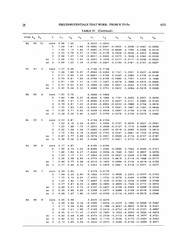
26 PSEUDOPOTENTIALS THAT WORK: FROM H TO Pu


4223

atom Z Za v c2 c4 c5 c6

Hg 80 12 core 2.991.241.023.33

1.201.411.123.79

1.40 -7.9485 -0.77335. 37 -3.7392 -0.0139

-0.66480.0408

2. 2533 —1.25331.84 -9.5486 —0.8291 —0.0650 0.2058

0. 1799-0.0636

-0.06410.0346

-0.0453

-0.00920.03150.0064

soso

0.940.660.89

1.071.52 1.63 -0.3943 -0.0023

-0.02570. 1059

—0.0457—0.0317 —0.0117 -0.0036-0.0193 -0.0181 —0.01571.00 1.39 -0.0796

1.18 -5.893 1 -2. 5065 -0.2075 0. 1636 -0.2383 -0.0339

T1 81 3

soso

core 1.771.240.710.700.910.310.20

0. 591.890.960.811.090.520. 24

6.7158 -5.71585.07 -7.6582 -0.03001.30 -5.8681 -1.0109

0. 3351 0.0637 -0.00590. 11610.0245 0. 2286 0.0178 -0.0129

0. 1048-0. 1761 0.03310. 1868 -0.0910

-6.0798 -0.8199 -0.54861.041.21 -4. 1125 -1.3267 -0.0456

-0.01090.45780.04510.62 -0.3984 —0. 1040 —0.0222 0.0174

0.32 0. 0288 0.0753 0.0435 0.0094 —0.0219 0.0369

Pb 82 4 0.761.981.21

core 1.92 6.5444 -5.54443.57 -8.3628 0. 1094 0. 11911.401.77 —6.9590 -0.51270.95 0.0637

-0.60330.79 0.91 1.20 -6.8182 -0.8903

0. 33050.2131

-0. 1888

0.05570.04850.0154

0.0032-0.01430.0916

soso

1.350.450.24

1.620.710. 30

1.820.820.40

-4. 0362 -1.0178-0.5058 —0.06540. 0257 0.0759

0.56410.04870.0376

0. 1487 -0. 1291 -0.0624—0.0128 0.0136 -0.01170.0130 —0.0275 0.0245

Bi 83

Soso

core 2. 031.621.230.92

0.812. 161.481.04

3.241.751.34

5.2104 -4. 2104—8.6521 0.5682—7. 2503-7.0492

0. 3928-0.4597

0.470.28

0.770.34

0.890.45

-0.55740. 0246

—0.09310.0777

1.70 1.92 2. 19 -3.6420 —. 0.7705

0.0727-0.0127-0.55180.53.27

0.26790. 1712

-0.20950.0841

0.02210.06690.0055

-0. 17220.0509 —0.0114 0.01070.0401 0.0112 -0.0261

-0.0041-0.00590.0813

-0.0752-0.01470.0260

Po 84 6

3

so 1

so '2

1.032. 280.460.31

core 2. 171.901.46

0.872. 721.821.172. 580.770.40

4. 41903.20 -8.8296

-3.41901.2562 -0.0868

-7.3062 -0.2355 -0.55271.512.99 0.4418

0.04940.0441

-3. . 0770 -0.5522-0. 14550.0854

0.96 —0.60120.02630.52

2. 27 -7.6222 0.9054 -0. 15480. 19220. 1081

-0.22280.0114

-0.01010.0076

0.03400.08570.0158 0.0829

-0. 1948 -0.0717-0.0116 0.0019 -0.01560.0114 -0.0277 0.0277

At 85 7

so80so

core0

1

2. 291.941.701.203.370.400.350.96

0.922. 252. 131.423.810.510.461.47

2.852. 67

3.8179-9. 1942-7.9335

-2.81790.97231.3792

1.78 -7.4567 0. 1638

0.0808 0.2203 -0.0377-0.3076 0.0369 0.0789-0.5722 -0.3036 -0.0089

-0.01000.01390.0768

4. 330.720.601.85

—0.6197 —0.24270.0338

-0.02070.0977

—0.0058

0.0068—0.0158 -0.02650.0488 0.0138 -0.03180.0114 -0.0050 -0.0015

-0.00220.03040.0046

-2. 2899 -0.3680 0.2809 —0. 1026 —0.2173 -0.0672

Rn 86 8 core 2.45 0.98 3.4235 -2.4235

sososo

2. 282. 111.394. 350.400.402. 13

2. 662. 581.616. 1.1

0.440. 522. 85

3.342.80

1.82542. 1388

-0.0335 0. 1692 -0.0066-9.2586-8.2305 0.0514

-0.0121-0.6641 -0.0823—0.6703 -0.3719-7.6190 0.52161.99

11.370.48 0. 1677-0.6370 -0.2736

0. 0462 0. 1135-0.0112 0.08340.0536 0.01750.0296 -0.0124

-0.0383-0.0069

0.673.04 -0.0620 —0.0072

—1.8307 -0.7487 0. 1902 -0.2562 -0.3020

-0.02470.02210.0857

-0.04720.07210.03530.0071



atom z Z c2 c5

Fr 87 1 core 1.23 0. 16 8.4416 —7.44160.36 0.53 0.69 -5.8904 -0. 1647 -0. 3018 0. 1280 0.0584 0. 03420. 16 0.31 0.96 -4.8581 -1.9964 —0. 6630 0.0699 0. 0869 0. 00080.36 0.40 0.63 -3.0529 —1.2715 —0. 2513 0. 0931 0.0451 0.06660.38 0.43 0. 52 —3.0166 —1.8140 0. 5796 0.4211 —0. 1318 —0. 0554

SoSo

0.060. 17

0.09 0. 11 —0. 3418 -0. 10790. 27 0.33 —0.0454 -0. 0141

0.01640. 0121

—0. 0148-0.0057

0.00900.0001

—0.01020. 0035

Ra 88 2 core 0.990.490.29

0.24 6. 1114 —5. 11140.63 0.74 —6.6907 0. 5888 —0. 2960 0. 0687 0. 064 1 0.03040.44 0.56 -6.0767 -0.6269 —0.4742 0. 0163 0.0270 0. 0352

4. 09 4. 68 5. 19 2. 2350 —2. 4528 0.91120. 50 0. 55 1.36 -3.4169 -0.8443 —0. 0162 0. 0274

0. 14230. 0222

—0.02040.02170.0303

So 0. 13 0.28 0. 32 —0.4357 0. 0239 0. 0183 0. 0086 0.0045 0.0032SoSo . 45 2. 17 2. 74 -0.0441 -0. 0127

0. 19 0.24 0.31 -0.0583 -0. 0278 0. 00110. 0412

—0.0084 0. 0076 0.0001-0.0203 -0.0025 0.0205

Ac 89 3 core 1.490. 54

0. 310.77

4. 7270 -3.72701.02 -8.2168 0. 0920 -0.3962 0. 0779 0. 0604 0. 0275

0.25 0.43 1.28 —6.95 13 -2 0 -0.8600 —O. Q054 0. 127'1 0., 00220.565.40

0. 626. 13 6.91 1.3312 -2. 5472 0.8208 0. 0024

1.23 —4.4657 -1.3359 —0. 1864 0. 0158 0.00180.0587

0.01840. 1169

SoSoSo

0. 15 0. 31 0. 33 -0.4745 0. 0254 0. 0224 0. 0063 0. 0042 0.00390. 17 0. 19 0. 25 -0.0590 -0. 0361 -0.0133 —0. 0101 —0.0071 —Q. 02201.84 2. 26 2. 98 —0.0409 —0. 0195 —0. 0022 —0. 0031 0. 0029 —0.0010

T21 90 4 core 1.59 0.40 4. 3902 -3.39020.62 0. 77 1.35 -9.0342 0. 2160 -0.4277 0. 0541 0.0790 0.02430.44 0.48 0.55 —8.4035 —0. 5210 —0. 8289 0.2778 —0. 0169 Q. 08880.71 0. 78 1.39 —5. 1907 —1. 1444 -0. 0440 0. 0631 0. 0061 0.01266. 1Q 6.99 7.92 0.9203 -2.4893 0. 8255 -Q. 0430 0.0225 0. 1112

SoSoSo

0. 13 0.25 0. 33 —0.4753 0. 0100 0. 0973 0. 0201 -0.0170 0.00180.23 0. 27 0. 36 —0.0754 —0. 0409 —0. 0109 —0. 0118 —0.0029 —0.01742. 08 2. 55 3.36 —0. 0449 -0. 0206 -0.0025 -0. 0029 0. 0026 -0.0010

Pa 91 5 core 2. 06 0.45 3.8349 -2. 83490. 56 0.80 1.07 -9.5369 —1. 1466 -0.5565 0. 2043 0. 0460 0 ' 03000. 56 0.66 0.75 -9.4357 —0. 2689 -1.1084 0.0661 —0. 0646 0. 04460.657.31

0.738.53 11.54 0.2527 —2. 0863 0. 8840 0. 0351 —0. 1739 0. 1578

0.94 —5.8109 -2. 0532 -0. 3147 0. 1394 —0. 0207 0. 0288

SoSoSo

0. 15 0. 29 0. 38 —0.4599 0. 0881 0. 1202 0. 0314 —0. 0267 Q. 00420.20 0.23 0.29 —0. 0656 -0.0390 -0.0133 -0.0131 -Q. 0080 —0. 02401.80 4. 20 11.43 -0.0460 -0. 0306 -0.0002 -0.0012 -0.0008 0.0012

92 6 core 2. 080.60

0. 500. 76

3.5183 —2. 51831.06 -9.6565 -1.0562 -0.6184 0.2244 0. 0435 0. 0270

SoSoSo

. 2

3

0.667.27

0.758.62

0. 16 0. 300. 201.84

0.222. 15

0.52 0.62 0. 700.86

12.500. 390.292. 34

—9.5702 -0.9102 -1.1087—5.8926 -2. 2312 -0. 34470.3088 -2. 0827 0. 8200

0. 24260. 15520. 0050

—0.0947 0.0639—0. 0291 0.0317—0. 1939 0. 1305

-0.5079 0.0599 0. 1053 0. 0283 —0. 0202 0.0011-0.0656 -0.0414 -0.0128 -0.0018 0.0019 -0.0199-0.0490 —0. 0311 -0.0134 0. 0041 —0.0002 —0.0007

I



atom Z Za cx 2 c2 c4 c5

Np 93 7

So 1

So 2

So 3

0.620.500.83

10.070. 140.302. 07

0.910.820.92

13.170.210.353.81

core 2. 72 0.601.171.031.06

17.300.260.43

15.69

—10.1156-7.3516

-2.4063-2.4042

-1.1744 -1.4501-0.5832 -0.0985-0.0880 -0.0427-0.0504 -0.0319

3.5099 -2.5099—10.4153 -2. 0222 -0.9596 0. 3000

—1.4851 0. 1011-0.3586 0.28020.9518 0.28630. 0640 —0.0126

-0.0064 -0.0079-0.0044 -0.0027

-0.0075-0. 1430-0.0396-0.29000.00030.0083

-0.0004

0.07780. 11410.0466

-0. 1468-0.0065-0.00760.0014

PL1 94 8

1

2

3So 1

So 2

So 3

0.590.590.93

10.230. 150.332. 12

core 2. 76 0.620.94 1.250.83 0.921.02 3.49

13.36 17.640.23 0.270.41 0.544. 64 13.73

3. 1671 -2. 1671—10.2963 -2.4940—10.2746 —1.6981-7.5476 -2. 1067—1.0461 —1.4985-0.6093 -0.0944-0.0987 -0.0487-0.0520 -0.0335

-0.9263—1.5450-0.30960.99080.0628

-0.0066-0.0004

0.3236 -0.00570. 1102 -0. 17800.0732 0. 11900.3096 -0.2679

-0.0075 0.0029-0.0083 0.0087-0.0019 -0.0005

0.06760. 1118

-0.0164-0. 1382-0.0069-0.00750.0010

TABLE V. Silicon 1 =0, 1,2 pseudopotentials on a real space mesh as derived from thecoefficients in Table IV. All units in a.u.

0.00.1

0.20.30.40.50.60.70.80.91.01.1121.31.41.51.61.71.81.92.02.1

2.22.32.42.5

1=0

2.23602.19292.06101.83271.50021.05980.5170

—0.1078—0.7729—1.4175

1.9743—2.3894—2.6395—2.7354—2.7133—2.6181—2.4893—2.3534—2.2245—2.1071—2.0016—1.9062—1.8196—1.7403—1.6676—1.6007

—2.4805—2.4857—2.5009—2.5258—2.5588—2.5971—2.6366—2.6724—2.7000—2.7158—2.7175—2.7037—2.6737—2.6275—2.5655—2.4895—2.4018—2.3058—2.2054—2.1043—2.0057—1.9119—1.8244—1.7436—1.6695—1.6016

1=2—4.6679—4.7191—4.8554—5.0375—5.2249—5.3899—5.5125—5.5657—5.5108—5.3107—4.9543—4.4725—3.9321—3.4117—2.9730—2.6438—2.4182—2.2690—2.1641—2.0782—1.9966—1.9143—1.8319—1.7518—1.6762—1.6063


IV. PERIODIC TABLE OF PSEUDOPOTENTIALSAND A GUIDE TO USE IT

In Table IV we compile the parameters neces-sary to synthesize ion-core pseudopotentials for theelements hydrogen through plutonium. Each ele-ment is identified by its symbol, its atomic num-ber, and its valence charge (i.e., the number of elec-trons chosen to be treated as valence electrons inthe ground state) in columns 1 —3. Column 4,denoted L, indicates the particular potential, i.e.,V""'(r) [Eq. (2.21)] or l=0, 1,2,3 for b VI""(r) [Eq.(2.22)] or the spin-orbit potential b, V&" for /=1,2,3.The nonlinear-fit parameters n,' ",i =1,2, or a;,i =1,2,3 are given in columns S, 6, 7, respectively,in atomic units, i.e., aB,h, . The linear coefficientsc "', i = 1,2 or C;, i = 1,6 defined through Eqs.(2.21), (2.22), and (2.25) are given in columns8 —13 in atomic units, i.e., 27.2116 eV. This tableis computer generated to eliminate transcription er-rors.

For the potentials b VI""(r) and b, VI"(r), but notfor V""(r), the coefficients C; have to betransformed by an inverse orthogonality transfor-mation [Eq. (2.28)] to obtain the linear coefficientsA; and A;+3 to be used in Eq. (2.22). Thistransformation either necessitates the inversion of a6&&6 matrix Q;I defined recursively in Eq. (2 26)

based on the analytical overlap matrix S;I and thesubsequent use of Eq. (2.28) or a direct solution ofthe linear equation system Eq. (2.25). Due to theinherent nonorthogonality of the fitting functions

4;(r) [Eq. (2.27)] high numerical accuracy, i.e.,double precision on a 32-bit computer or singleprecision on a 64-bit computer, is required for thecomputation. We found that computer routinesperforming least-squares approximations to thesolutions of the linear equation system (2.25) gavethe most stable answers. To provide the user withan independent check on the accuracy of his owninverse orthogonalization procedure we list in

Table V the l=0, 1,2 ion-core pseudopotentials ofSi. The results are obtained with single-precisionroutines on a cRAY-1 computer.

V. AMBIGUOUS CASES

The separation into a well-isolated core and intoa valence shell is not always unambiguously possi-ble. It may, therefore, be convenient in certaincases to have a choice of pseudopotentials availablewith more or less expanded valence shells. In thefollowing we briefly discuss four typical cases ofambiguous behavior.

(i) The heavy IA alkali atoms show relativelyshallow (n —1)p core shells. The eigenvalues of3p, 4p, Sp, and 6p for K, Rb, Cs, and Fr are,respectively, —18.8, —16.3, —13.6, and —10.9

'

eV. Accordingly, as discussed in the case of Cs inSec. III, the spatial extent of these p functions canbe large. However, the overlap with excited ns, p,or d states in the valence shell is small due tostrong orthogonality effects. Test calculations onCs atoms and also for the semiconducting com-pound CsAu show that errors due to Sp core po-larization and exchange nonlinearities amount toless than 0.2 eV. We therefore present only pseu-dopotentials for IA atoms with the (n —1)p shellincluded in the core (Table IV). Note that the l=0potentials are derived from the neutral ground-state configurations to minimize transferability er-rors due to the nonlinear charge dependence of theexchange-correlation potential.

(ii) The group IIB atoms Zn, Cd, and Hg im-

mediately following the transition and noble ele-

ments, show 3d, 4d, or Sd electrons with eigen-values of —10.3, 11.6, and 9.S eV, respectively,which put them into an ambiguous situation.While they are corelike in the elemental metals,they may fall within the valence-band region incompounds and play a role in bonding. In TableIV we present potentials for these atoms which in-clude the (n —1)d electrons into the valence shell,just as the preceding noble elements. The resultingd potentials are very strong and may lead to diffi-culties for certain applications, e.g., where plane-wave expansions are used. We therefore present inTable VI alternative potentials which assume the(n —1)d shell to be included in the core. These po-tentials are smooth and only weakly l dependent,similar to those for the neighboring group-IIIatoms.

(iii) As mentioned in the Sec. II the rare-earthelements La through Lu show extremely localized4f wave functions (r,„=0.5 a.u.). This wave-function "collapse" which occurs between Ba andCe is well documented in the literature and leadsto a number of curious effects. From the pointof view of pseudopotentials the collapse places the4f charge not only well inside the Sd,6s valenceelectrons, but also inside the Ss and Sp core elec-trons (r,„=1.5 a.u. ) with eigenvalues at about—SO and —30 eV, respectively. The result is thatexcitations involving changes in the 4f occupationwill alter the screening for the Ss and Sp electronsdramatically, such that a frozen core is no longer agood approximation. We therefore included the Ssand Sp electrons into the valence shell for a11 rare-

PSEUDOPOTENTIALS THAT WORK: FROM H TO Pu

TABLE VI. Pseudopotential parameters for the atoms Zn, Cd, and Hg which were constructed without 31, 4d, and

Sd electrons, respectively, in the valence shell. Table is to be used as Table IV.

Atom Z, Z„ l. a3 C) C6

ZIl 30 2 core0

1

2

so 1

2. 511.521.020.520.46

0.752. 061.130.720.70

7.621.281.300.86

6. 1450-4.8062-3.6742-2.9756-0.0443

-5. 14500.0120 0. 1552 0.2804 0.0430 -0 ~ 0133

—0.6484 0.0752 0. 1188 -0.0161 0.0266-1.8692 -0.5538 -0.0237 -0.0331 0.0837-0.0129 0.0030 -0.0017 0.0011 -0.0007

CQ 48 2 core0

1

2

so 1

2. 191.200.810.520.38

0.601.320.900.590.64

1.441.011.22

8.5331—7.0001-5.8819-5. 1735

0.79 -0. 1366

-7.5331—0. 1006 0.2713—1.0097 0.0258-2.0936 -0.7797-0.0241 0.0114

0. 1929 -0.0352 0.06750.2006 -0.0416 0.02870.0217 -0.0286 0.08800.0014 -0.0009 -0.0022

HQ 80 2 core0

1

2

3so 1

so 2

2. 091.100.790.440.410.360. 15

0.511.210.870.480.510.660. 18

0.991.320.970.810.23

-6.7759 -0.9047-5.9821-3.7143-0.4562-0.0218

-2.3858-3.3954-0.07720.0191

8.9048 -7.90481.33 -7.7678 -0.5451 0.2376

0.0686-1.0888-0.93220.04550.0150

0.22230.2543

-0.01860.09910.00650.0076

-0.0396-0.0154-0.0040-0. 1363-0.0017-0.0078

0.08900.04430.07300. 1480

-0.00660.0174

earth atom potentials given in Table IV. This de-creases the error for a 4f-Sd excitation associatedwith the frozen-core approximation from 1.7 to 0.2eV.

VI. CONCLUSIONS

We have developed a comprehensive and con-sistent set of pseudopotentials using guidelines

which have been found through extensive testing tomaximize transferability. Our chief goal has been

the publication of these potentials in a convenient

form for application. A second aim was to discussthe physics of the pseudopotentials thoroughly, and

explain the reasons underlying the many choicesmade in the development process. We anticipate

that the potentials will continue to be useful in

many contexts. When at some future time im-

proved exchange-correlation density functionals orfurther improvements in pseudopotential formal-ism are developed, the results reported here onreference configurations, radii, and fitting strategyshould greatly simplify the task of producing new

potentials.

ACKNOWLEDGMENTS

We would like to thank Dr. H. Greenside for his

help in developing efficient fitting procedures and

Dr. G. A. Baraff for stimulating discussions. Weare indebted to Dr. I. Batra and P. Feibelman

pointing out several misprints.

'New address: Scuola Normale Superiore, Pisa, Italy.For a review, see, M. L. Cohen and V. Heine, in Solid

State Physics, edited by H. E. Ehrenreich, F. Seitz,and D. Turnbull (Academic, New York, 1970), Vol.24, p. 38; and V. Heine and D. Weaire, ibid. , p. 249.

2J. A. Appelbaum and D. R. Hamann, Phys. Rev. 8 8,777 (1973).

M. Schluter, J. R. Chelikowsky, S. G. Louie, and M. L.

Cohen, Phys. Rev. Lett. 34, 1385 (1975).4W. Kohn and L. J. Sham, Phys. Rev. 140, A1133

(1965); M. Schluter and L. J. Sham, Physics Today,35(2), p. 35.

M. Schliiter, Festkorperprobleme (Advances in SolidState Physics), edited by J. Treusch (Vieweg, Braun-schweig, 1978), Vol. 18, p. 155.

C. Herring, Phys. Rev. 57, 1169 (1940).

G. B.BACHELET, D. R. HAMANN, AND M. SCHLUTER 26

7J. C. Phillips and L. Kleinman, Phys. Rev. 116, 287(1959).

SL. Kleinman and J. C. Phillips, Phys. Rev. 118, 1153(1960); F. Bassani and V. Celli, J. Phys. Chem. Solids20, 64 (1961).

9D. R. Hamann, M. Schluter, and C. Chiang, Phys.Rev. Lett. 43, 1494 (1979).

'OR. W. Shaw and W. A. Harrison, Phys. Rev. 163, 604

(1967).'~W. C. Topp and J. J. Hopfield, Phys. Rev. 8 7, 1295

(1974).~2L. I. Schiff, Quantum Mechanics iMcoraw-Hill, New

York, 1955), p. 106.'3D. R. Hamann and M. Schluter (unpublished).&4D. Allan and J. D. Joannopoulos (in press).~~L. R. Kahn and W. A. Goddard III, J. Chem. Phys.

56, 2685 (1972).C. F. Melius and W. A. Goddard III, Phys. Rev. A

10, 1528 (1974).S. Topiol, A. Zunger, and M. A. Ratner, Chem. Phys.

Lett. 49, 367 (1977).'8A. Redondo, W. A. Goddard III, and T. C. McGill,

Phys. Rev. 8 15, 5038 (1977).~9A. Zunger, J. Vac. Sci. Technol. 16, 1337 (1979).2 P. A. Christiansen, Y. S. Lee, and K. S. Pitzer, J.

Chem. Phys. 71, 4445 (1979).2'P. A. Christiansen, private communication.2G. P. Kerker, J. Phys. C 13, L189 (1980).

23M. T. Yin, private communication.24K. C. Pandey, private communication.25D. R. Hamann and M. Schluter (unpublished).~ D. R. Hamann and M. Schluter (unpublished).~7M. T. Yin and M. L. Cohen, Phys. Rev. Lett. 45,

1004 (1980).G. B. Bachelet, H. S. Greenside, G. A. Baraff, and M.Schluter, Phys. Rev. 8 24, 4745 (1981).

2 M. T. Yin and M. L. Cohen, Phys. Rev. 8 24, 6121

(1981).30M. T. Yin and M. L. Cohen, Solid State Commun.

38, 625 (1981).3~J. Ihm and J. D. Joannopulos, Phys. Rev. 8 24, 4191

(1981).2J. E. Northrup, J. Ihm, and M. L. Cohen, Phys. Rev.

Lett. 47, 1910 (1981).3U. vonBarth and C. D. Gelatt, Phys. Rev. 8 21, 2222

(1980).34Y. S. Lee, W. C. Ermler, and K. S. Pitzer, J. Chem.

Phys. 67, 5861 (1977).3~L. R. Kahn, P. J. Hay, and R. D. Cowan, J. Chem.

Phys. 68, 2386 (1978).L. Kleinman, Phys. Rev. 21, 2630 {1980).G. B. Bachelet and M. Schliiter, Phys. Rev. 8 25,2103 (1982).

W. C. Ermler, Y. S. Lee, P. A. Christiansen, and K. S.Pitzer, Chem. Phys. Lett. 81, 70 (1981).D. D. Koelling and B. N. Harmon, J. Phys. C 10,3107 (1977); H. Gollish and L. Fritsche, Phys. StatusSolidi B 86, 145 (1978);J. H. Wood and A. M. Bor-ing, Phys. Rev. B 18, 2701 (1978).

~L. H. Thomas, Nature 117, 514 (1926).'t~See, e.g., L. I. Schiff, in Quantum Mechanics

(McGraw-Hill, New York, 1968).42E. P. Wigner, Phys. Rev. 46, 1002 (1934), O. Gun-

narsson and B. L. Lundquist, Phys. Rev. 8 13, 4274{1976).L. Hedin and B. I. Lundquist, J. Phys. C 4,2064 (1971). D. M. Ceperley, Phys. Rev. 8 18, 3126(1978). D. M. Ceperley and B. J. Alder, Phys. Rev.Lett. 45, 566 {1980).

43J. Perdew and A. Zunger, Phys. Rev. 8 23, 5048(1981).

~The present calculations are all done in the spin-unpolarized mode. The exchange-correlation func-

tional of Ceperley and Alder is also parametrized by

Perdew and Zunger (Ref. 43) for the spin-polarized

case."5A. H. MacDonald and S. H. Vosko, J. Phys. C 12,

2977 (1979).D. Liberman, J. T. Waber, and D. T. Cromer, Phys.Rev. 137, A27 (1965).

47Periodic Table of the Elements, Sargent-Welch Scien-

tific Company, 1968, 4647 West Foster Ave. , Chi-

cago, Ill. 60630.S. G. Louie, S. Froyen and M. L. Cohen Phys. Rev. B26, 1738 (1982).

49A pseudopotential including the outer core states with

the valence states was previously introduced by

Starkloff and Joannopoulos. They showed that for a

transition metal like Nb a good approximation tovalence energies and wave functions could be obtained

with an I-independent potential. Th. Starkloff and J.D. Joannopulos, Phys. Rev. B 16, 5212 (1977).A. Zunger, Phys. Rev. 8 22, 649 (1980).

5'H. Greenside and M. Schliiter (unpublished).

J. L. Dehmer, A. F. Starace, U. Fano, T. Sugar, and

T. W. Cooper, Phys. Rev. Lett. 26, 1521 (1971);M.Schluter and C. M. Varma, in Proceedings of the International Conference on Valence Instabilities, Zu

rich, 1982 (in press).

Pseudopotentials that work: From H to Pu

Documents

Transcript of Pseudopotentials that work: From H to Pu