Prospects of Structural Similarity Index for Medical Image ...

Appl. Sci. 2022, 12, 3754. https://doi.org/10.3390/app12083754 www.mdpi.com/journal/applsci

Review

Prospects of Structural Similarity Index for Medical

Image Analysis

Vicky Mudeng 1,2, Minseok Kim 3,4,* and Se‐woon Choe 1,5,*

1 Department of Medical IT Convergence Engineering, Kumoh National Institute of Technology,

Gumi 39253, Korea; [email protected] 2 Department of Electrical Engineering, Institut Teknologi Kalimantan, Balikpapan 76127, Indonesia 3 Department of Mechanical System Engineering, Kumoh National Institute of Technology,

Gumi 39177, Korea 4 Department of Aeronautics, Mechanical and Electronic Convergence Engineering,

Kumoh National Institute of Technology, Gumi 39177, Korea 5 Department of IT Convergence Engineering, Kumoh National Institute of Technology, Gumi 39253, Korea

* Correspondence: [email protected] (M.K.); [email protected] (S.‐w.C.)

Abstract: An image quality matrix provides a significant principle for objectively observing an im‐

age based on an alteration between the original and distorted images. During the past two decades,

a novel universal image quality assessment has been developed with the ability of adaptation with

human visual perception for measuring the difference of a degraded image from the reference im‐

age, namely a structural similarity index. Structural similarity has since been widely used in various

sectors, including medical image evaluation. Although numerous studies have reported the use of

structural similarity as an evaluation strategy for computer‐based medical images, reviews on the

prospects of using structural similarity for medical imaging applications have been rare. This paper

presents previous studies implementing structural similarity in analyzing medical images from var‐

ious imaging modalities. In addition, this review describes structural similarity from the perspective

of a family’s historical background, as well as progress made from the original to the recent struc‐

tural similarity, and its strengths and drawbacks. Additionally, potential research directions in ap‐

plying such similarities related to medical image analyses are described. This review will be bene‐

ficial in guiding researchers toward the discovery of potential medical image examination methods

that can be improved through structural similarity index.

Keywords: medical image analysis; structural similarity index; computer‐based observer; image

quality assessment

1. Introduction

An image quality assessment (IQA) plays a crucial role in accurately measuring a

degraded image from a reference image. In general, there are two types of IQA used to

evaluate the quality of an image, i.e., subjective and objective [1–3]. A subjective measure

[4] involves individuals (mostly groups of experts) inspecting an image, and then con‐

ducting an evaluation according to their specialties. This measure is considered the best

strategy because it offers consistency when assessing the images. However, to reach a

reliable conclusion after image measurements, a subjective measure is often inconvenient,

time‐consuming, and expensive. This is natural because the involvement of human beings

is directly connected to their ability, knowledge, and insight. For instance, to analyze a

medical image, a medical doctor specializing in radiology is necessary. Renieblas et al.

reported inspecting bone plain films, magnetic resonance, and chest plain films, selecting

four medical doctors with diagnostic experiences in measuring such images to participate

[5]. By realizing the shortcomings of a subjective method, several attractive measurements

Citation: Mudeng, V.; Kim, M.;

Choe, S.‐w. Prospects of Structural

Similarity Index for Medical Image

Analysis. Appl. Sci. 2022, 12, 3754.

https://doi.org/10.3390/app12083754

Academic Editors: Yun Seop Yu,

Kwang‐Baek Kim, Dongsik Jo,

Hee‐Cheol Kim and Jeong Wook Seo

Received: 16 March 2022

Accepted: 6 April 2022

Published: 8 April 2022

Publisher’s Note: MDPI stays neu‐

tral with regard to jurisdictional

claims in published maps and institu‐

tional affiliations.

Copyright: © 2022 by the authors. Li‐

censee MDPI, Basel, Switzerland.

This article is an open access article

distributed under the terms and con‐

ditions of the Creative Commons At‐

tribution (CC BY) license (https://cre‐

ativecommons.org/licenses/by/4.0/).

Appl. Sci. 2022, 12, 3754 2 of 34

related to objectively evaluating such images have been developed during the past few

decades. The most popular image quality measures are the mean square error (MSE), sig‐

nal‐to‐noise ratio (SNR), contrast‐to‐noise ratio (CNR), and absolute error (AE), as well as

a derivation of such measures, such as Laplacian MSE (LMSE), peak MSE (PMSE), nor‐

malized MSE (NMSE), PSNR, and NAE [6,7]. Although such measures are accepted as a

universal image quality index, they provide less sensitivity compared with a human vis‐

ual system (HVS) [8]. They are considered common measurements because they can be

calculated easily and may interpret the physical meaning of an image [9,10]. In addition,

contrast‐and‐size detail (CSD) was developed to separate the visible and invisible inclu‐

sions in mimicking the breast environment through simulations by embedding a numer‐

ical tumor. In this case, an inclusion represents a breast tumor [11,12]. Again, this image

quality metric (IQM) has issues in terms of inconsistency when increasing the contrast

ratio with a raised inclusion size and an ambiguous threshold value. Therefore, it is chal‐

lenging to implement this method and distinguish seeable and unseeable inclusions inside

the breast tissue with a provided threshold value.

In early 2000, Wang et al. developed a new universal IQA and tried to replace con‐

ventional methods such as MSE and PSNR for measuring the quality of the images,

namely the structural similarity (SSIM) index, and adapt to the HVS [10,13]. Their first

attempt regarding the possibility of substituting traditional strategies with an applicable

metric to measure various images from numerous sectors was reported in 2002. It was

reported that the IQA calculates the distortions in a combination of the loss of correlation,

luminance distortion, and contrast distortion [14]. In addition, their results indicate that

the novel universal index is more exceptional than MSE because the new index measures

the information loss and is not focused on the energy loss. This is reasonable because the

MSE values of two different distorted images can be the same, although one image is more

flawless than another image. Their follow‐up study complementing their previous re‐

search was published in 2004, and one of the most popular IQMs in this era, i.e., SSIM,

was described [10]. They proposed a novel philosophy by considering that image degra‐

dation is the perceived changes in structural information, whereas error sensitivity is an

estimation of the perceived errors to assess a noised image in comparison with the origi‐

nal. This new philosophy is easy to understand because the human perceptual measure is

comfortable quantifying the changes in structural information when two images are com‐

pared, and it is more complicated to indicate the error. Moreover, the novel metric sug‐

gests the IQA by considering three factors, i.e., luminance, contrast, and structure com‐

parisons. In addition, they suggested that SSIM may be used for several applications [15]

other than image processing because SSIM quantifies two signals and compares them to

obtain the similarity score, regardless of the complexity in calculating the SSIM when com‐

pared to that of the MSE. Research on a single mean SSIM (MSSIM) motivated several

further developments of SSIM, and to date, numerous versions of SSIM have been

achieved, for example, multiscale SSIM (MS‐SSIM), gradient‐based SSIM (GSSIM), a

three‐component weighting region, a four‐component weighting region, a complex‐wave‐

let, and an improved SSIM with a sharpness comparison (ISSIM‐S) [16–22]. The SSIM

method has recently become popular as a way to improve the sensitivity according to the

measurement scope and goal by applying an image processing procedure [23]. Several

publications have even reported SSIM implementation in clinical applications and bio‐

medical fields [24–28].

SSIM has shown signs of progress, not only in digital images for communication,

video, monitor, television, and watermark technologies [29–35] but also in medical image

analyses [36–45] to assist clinicians or physicians in complementing an opinion before

making a final decision [46–49]. SSIM can be considered a “second opinion” in an assess‐

ment. By understanding the recent progression of SSIM related to medical image quanti‐

fication, this study reviewed articles concentrating on the SSIM implementation as an ob‐

jective measure used to evaluate medical images from several modalities, such as mag‐

netic resonance imaging (MRI), ultrasound (US), computerized tomography (CT) scans,

Appl. Sci. 2022, 12, 3754 3 of 34

X‐rays, and optical imaging, as well as other implementations in the medical field. More‐

over, we discuss the history and popular progress of SSIM from its origin to recent struc‐

tural similarities, its strengths and shortcomings, and its potential future research direc‐

tions in relation to medical image analyses. This review is expected to be a guide for re‐

searchers in identifying the potential application of SSIM when objectively measuring

medical images.

The remainder of this study is organized as follows. Section 2 describes the history

and basic principles of SSIM, and Section 3 describes the types of improvements made to

this index. Section 4 presents the use of SSIM in medical imaging, whereas Section 5 pre‐

sents some final concluding remarks by providing the future prospects of SSIM for med‐

ical image analyses.

2. Historical Review and Basic Principles of SSIM

Quantifying an image objectively to acquire quality statistics is a crucial task in an

image processing procedure because it can provide the feature and property information

of the image; thus, several attempts at developing a computer‐based observer have been

conducted by researchers. Nevertheless, creating a reliable algorithm for measuring an

image is challenging and is concerned with the HVS because humans are the end‐users of

the images. For example, in terms of video communication, a perfect IQM can be deployed

as a benchmark for measuring other IQMs when assessing a particular task. We can select

the best IQM algorithm based on performance [33,35,50,51]. Moreover, in the field of med‐

ical image analysis, with the assistance of computer vision, clinicians can improve their

confidence when diagnosing patients. This becomes more vital if the task is related to

human disease diagnosis [52–56].

Two traditional quality metrics, MSE and PSNR, are widely used to evaluate images

because they are able to provide a physical meaning and are relatively simple in terms of

their calculation. However, such quality measures are frequently inconsistent with the

HVS because they can provide the same value of quality for two completely different dis‐

torted images, even when one image is more perceivable than another [6,7]. The perfor‐

mances of common IQAs were shown by Eskicioglu and Fisher [9] in 1995, inspiring Wang

and Bovik [14] to develop a novel universal IQM to overcome the MSE and PSNR incom‐

patibility in 2002. At the time, MSE and SNR, along with their differentiations considered,

were incompatible with HVS, particularly when employing a specific condition directed

at an image with a particular level of degradation.

This first attempt in developing a new universal quality index can be utilized not

only in a two‐dimensional image processing system but also in other areas, such as speech

and pattern recognitions relative to a one‐dimensional analysis, because the new universal

quality metric offers comparisons between two signals. These two signals refer to one sig‐

nal as a reference and the other acting as the original signal with implemented noise. Us‐

ing these two signals, we can calculate the signal quality quantitatively. Therefore, their

study was recognized as a full‐reference (FR) [57] IQA when considering that the model

of the image distortion is influenced by three aspects, i.e., correlation loss, luminance dis‐

tortion, and contrast distortion. A description of the developed novel universal quality

index is as follows:

𝑄4𝜎 �̅�𝑦

𝜎 𝜎 �̅� 𝑦 , (1)

where 𝑥 𝑥 |𝑖 1, 2, 3, … ,𝑁 is the original image, and 𝑦 𝑦 |𝑖 1, 2, 3, … ,𝑁 de‐

notes the image under test, with �̅� 1𝑁∑ 𝑥 and 𝑦 1

𝑁∑ 𝑦 as the average grayscale level (luminance) for the original and test images, respectively. In addition,

𝜎 1𝑁 1∑ 𝑥 �̅� and 𝜎 1

𝑁 1∑ 𝑦 𝑦 are squares of the standard

deviation for the original and test images, and 𝜎 1𝑁 1∑ 𝑥 �̅� 𝑦 𝑦 refers

to the covariance between the original and test images. Moreover, the quality score 𝑄 is within the range of 1 to 1 ; however, in most cases, 𝑄 is from 0 to 1 with 0

Appl. Sci. 2022, 12, 3754 4 of 34

representing a non‐similarity and 1 demonstrating a perfect match between the reference

and noised images. To simplify Equation (1) into three important components, 𝑄 can be defined as

𝑄𝜎𝜎 𝜎

∙2�̅�𝑦

�̅� 𝑦∙

2𝜎 𝜎𝜎 𝜎

, (2)

Because an image is space‐variant, for measuring an image, a local assessment is pre‐

ferred over a global evaluation that quantifies the image by employing a sliding window.

This window slides over the entire image from the left‐top to right‐bottom corners pixel

by pixel both horizontally and vertically. During each stride, we obtain 𝑄 , and thus if the

window slides over the image for 𝑀 strides, we acquire the total quality 𝑄 ∑ 𝑄 ,

and 𝑄 can be written as

𝑄1𝑀

𝑄 , (3)

indicating the mean quality score.

Furthermore, Wang and Bovik indicated that the new quality metric is superior to

the MSE. They employed the same MSE value with various distortions to the “Lena” im‐

age. They set the MSE value to approximately 255; however, the 𝑄 score could validate the quality by showing the different scores with respect to the perception of a human ob‐

server. However, in this first effort, they did not claim to use any HVS models.

Two years later, in 2004, they published their study on SSIM with the help of two

additional co‐authors [10]. They reported that the assumption of HVS can be well adapted

with the perception of the structural information and that human observers have limita‐

tions in recognizing errors. This is reasonable because humans can easily identify changes

in physical information while complicatedly detecting the variations of an error in the

images. To match with the HVS, SSIM demonstrates comparisons of 𝑙 luminance, 𝑐 con‐trast, and 𝑠 structure, which are specified as

𝑙 𝒙,𝒚2𝜇 𝜇 𝐶𝜇 𝜇 𝐶

, (4)

𝑐 𝒙,𝒚2𝜎 𝜎 𝐶𝜎 𝜎 𝐶

, (5)

𝑠 𝒙,𝒚𝜎 𝐶𝜎 𝜎 𝐶

, (6)

where 𝜇 and 𝜇 denote the mean intensity for reference image 𝒙 and distorted image

𝒚, respectively. Compared with Equation (2), Equations (4) and (5) have the same defini‐

tions as luminance and contrast comparisons, and meanwhile, Equation (6) has a different

description from the correlation to be applied in a structural comparison. Likewise, SSIM

considers constant values to avoid instability when 𝜇 𝜇 , 𝜎 𝜎 , and 𝜎 𝜎 are ex‐

tremely close to zero. These constants are 𝐶 𝐾 𝐿 , 𝐶 𝐾 𝐿 , and 𝐶 𝐶2. In ad‐

dition, 𝐾 and 𝐾 should be ≪ 1 and 𝐿 is 255 for an 8‐bit grayscale image or an im‐

age in three channels, such as red, green, and blue (RGB). As in Equation (2), the SSIM

also can be formulated as

𝑆𝑆𝐼𝑀 𝒙,𝒚 𝑙 𝒙,𝒚 ∙ 𝑐 𝒙,𝒚 ∙ 𝑠 𝒙,𝒚 , (7)

with 𝛼 𝛽 𝛾 1, and thus a specific form can be defined as

𝑆𝑆𝐼𝑀 𝒙,𝒚2𝜇 𝜇 𝐶 2𝜎 𝐶

𝜇 𝜇 𝐶 𝜎 𝜎 𝐶 . (8)

Figure 1 shows a diagram of the SSIM measurement procedure. First, the luminance

is calculated over the two images by utilizing Equation (4) when employing a sliding win‐

dow; here, image 𝒙 is a reference image, whereas image 𝒚 denotes a noise‐degraded im‐age. The contrast is then measured using Equation (5). To obtain the structure, the covar‐

iance between 𝒙 and 𝒚 must be computed using Equation (6). Once these three factors

Appl. Sci. 2022, 12, 3754 5 of 34

have been obtained, the combination of the comparisons, as indicated in Equation (7),

shows a quality score within the range of 1 to 1 because of the structural influence. However, in various cases, the score is between 0 and 1. Therefore, the SSIM satisfies the following conditions:

1. Symmetry: 𝑆𝑆𝐼𝑀 𝒙,𝒚 𝑆𝑆𝐼𝑀 𝒚,𝒙 ; 2. Boundedness: 𝑆𝑆𝐼𝑀 𝒙,𝒚 1; 3. Unique maximum: 𝑆𝑆𝐼𝑀 𝒙,𝒚 1 if and only if 𝒙 𝒚.

Luminance Measurement

+

Image x

+

ـ

÷

Contrast Measurement


+

Image y

+

ـ

÷


Luminance Comparison

Contrast Comparison

Structure Comparison

Similarityx

Figure 1. SSIM procedures to quantify the image quality (adapted from [10]).

As in previous studies regarding the universal quality index (UQI) [14], SSIM is also

effective in inspecting the image locally by implementing a sliding window. Hence, ac‐

cording to the original article on SSIM [10], the sliding window was 11 11. In addition, there was an improvement in the sliding window by applying a Gaussian weighting func‐

tion 𝒘 𝑤 |𝑖 1, 2, 3, … ,𝑁 with a standard deviation of 1.5. The value of 𝒘 should fulfill a unit sum of ∑ 𝑤 1. Because of this Gaussian weighting function with a

11 11 local window, the local statistics, such as 𝜇 , 𝜇 , 𝜎 , 𝜎 , and 𝜎 , have the fol‐

lowing adjustments:

𝜇1𝑁

𝑤 𝑥 , (9)

𝜇1𝑁

𝑤 𝑦 , (10)

𝜎 𝑤 𝑥 𝜇 , (11)

𝜎 𝑤 𝑦 𝜇 , (12)

𝜎 𝑤 𝑥 𝜇 𝑦 𝜇 , (13)

where 𝐾 and 𝐾 are 0.01 and 0.03, respectively. When completing the SSIM computa‐

tion over the entire image using a local window, the mean SSIM (MSSIM) can be obtained

as

Appl. Sci. 2022, 12, 3754 6 of 34

𝑀𝑆𝑆𝐼𝑀 𝑿,𝒀1𝑀

𝑆𝑆𝐼𝑀 𝒙 ,𝒚 , (14)

where 𝑿 and 𝒀 denote the reference image and the image under testing, respectively,

whereas 𝒙 and 𝒚 are the images at the 𝑗‐th window when the local window slides over

the original and distorted images, and 𝑀 is the number of local windows in the image.

MSSIM showed consistency when compared with human observers. In addition,

these results were confirmed by implementing the PSNR as an evaluation tool to measure

other IQAs, which, in this case, is MSSIM. Further, the previous UQI with 𝐾 and 𝐾 is 0, which presents the smallest correlation with the human observers. These results indi‐

cate that MSSIM can improve the UQI ability in avoiding a zero in the denominator by

setting 𝐾 and 𝐾 as ≪ 1. Hence, SSIM has become popular as an objective investigative

tool for other fields included in medical image analysis [58–67].

To overcome the weakness of a single‐scale SSIM associated with a limitation of view,

a multi‐scale SSIM (MS‐SSIM) was established [22]. The viewing conditions are incorpo‐

rated with the display resolution, distance when reading the image, luminance back‐

ground, and other set environments that can affect the image investigation results. Figure

2 shows the procedure used by MS‐SSIM in evaluating an image. First, images 𝒙 and 𝒚 are processed inputs, as in a single‐scale SSIM for a scale of 1. In this process, we only

store the contrast 𝑐 and structure 𝑠 for such a scale, namely, 𝑐 and 𝑠 . Then, the refer‐

ence and noised images are filtered using an LPF followed by downsampling by 2. In this step, again, the downsampled images are computed using single‐scale SSIM formulas to

obtain 𝑐 and 𝑠 . This procedure is repeated until 𝐾 iterations. Once iteration 𝐾 is com‐pleted, we save all three parameters, 𝑐 , 𝑠 , and luminance 𝑙 . Thus, the MS‐SSIM is for‐

mulated as

𝑀𝑆 𝑆𝑆𝐼𝑀 𝒙,𝒚 𝑙 𝒙,𝒚 𝑐 𝒙,𝒚 ∙ 𝑠 𝒙,𝒚 . (15)

Here, 𝛼 , 𝛽 , and 𝛾 accommodate the comparative importance of the three com‐

ponents. In addition, for simplification, because 𝛼 𝛽 𝛾 , thus ∑ 𝛼 ∑ 𝛽∑ 𝛾 1 when the normalization of the cross‐scale setting is established. The genuine

MS‐SSIM sets 𝐾 5 with 𝛽 0.0448 , 𝛽 0.2856 , 𝛽 0.3001 , 𝛽 0.2363 , and 𝛽 0.1333 [20,22].

Image x

Image y

2L

c1 (x,y)s1 (x,y)

2L

c2 (x,y)s2 (x,y)

2L

2L

cK (x,y)sK (x,y)

2L

2L

lK (x,y) Similarity

...

...

Figure 2. MS‐SSIM procedures to quantify the image quality (adapted from [22]). 𝐿 is low‐pass fil‐tering, and 2 ↓ denotes downsampling by 2.

MS‐SSIM has shown promising results in comparison with a PSNR, single‐scale

SSIM, and Sarnoff. MS‐SSIM outperformed when evaluated by human observers’ percep‐

tion. Its correlation presented the highest.

We have reviewed the historical background of SSIM and several of its basic princi‐

ples, and have found that UQI, MSSIM, and MS‐SSIM are triggers acting as the founda‐

tions for all types of SSIM. Developed some years later, they have tried to complement

and improve on the original SSIM in terms of image processing when applied to a specific

area. In the next section, we described the types of SSIM developed from 2006 to 2021.

Appl. Sci. 2022, 12, 3754 7 of 34

3. Current Improvement in SSIM

This section describes several improvements in SSIM since it first emerged. The ob‐

jective of this section is to provide an adequate understanding of the development of

SSIM, thus allowing researchers to select the appropriate SSIM type for comparison when

applying a specific SSIM for medical image analysis.

3.1. Gradient‐Based SSIM

Gradient‐based SSIM (GSSIM) was the upgraded version of SSIM after realizing that

the original SSIM has a defect in evaluating badly blurred images. The concept was de‐

rived by Chen et al. in 2006 when comparing the similarity values between the “Camera‐

man” image with Gaussian white noise and a blurred image [16]. The original SSIM

showed a similarity score contrary to human perception by presenting a low MSSIM for

a Gaussian white‐noise‐contaminated image while exhibiting a high similarity score for a

blurred image. The image with Gaussian noise was perceived more subjectively than the

blurred image, and by identifying this flaw, a GSSIM attempts to resolve this discrepancy.

The background of GSSIM emphasizes the sensitivity of the human eye in detecting

the edge and contour information. From these two pieces of information, a human can

capture the image structure from the scene. Therefore, to modify the original SSIM into

GSSIM, the essential image processing insight is highlighting the edge of the images. In

the original article on GSSIM, Chen et al. utilized a Sobel operator to spot the edges in the

images because it simply generates masks and implements them over the entire image.

The Sobel masks consist of two 3 3 windows as filters, namely vertical and horizontal

edge masks. Figure 3 shows the Sobel operator masks.

Figure 3. Sobel operator masks for detecting the edge.

The vertical mask 𝐺 exposes the vertical edges, whereas the horizontal mask 𝐺 discovers the horizontal edges in the images. The magnitude of the gradient, otherwise

known as a gradient vector, can be calculated by

𝐺 𝐺 𝐺 |𝐺 | 𝐺 , (16)

and the edge angles can be formulated as

𝜃 𝑡𝑎𝑛𝐺𝐺

. (17)

By applying the masks over the entire image and using Equation (16), we can obtain a

gradient map indicating the edge and contour information [68].

Once we acquire the reference image gradient map 𝑿′ and noise‐contaminated im‐

age gradient map 𝒀′, the calculation technique for GSSIM is similar to that of SSIM by

changing the contrast comparison 𝑐 and structure comparison 𝑠 as follows:

𝑐 𝒙,𝒚2𝜎 𝜎 𝐶

𝜎 𝜎 𝐶 , (18)

𝑠 𝒙,𝒚𝜎 𝐶𝜎 𝜎 𝐶

, (19)

‐1 0 +1

‐2 0 +2

‐1 0 +1

‐1 ‐2 ‐1

0 0 0

+1 +2 +1

Vertical mask (Gx) Horizontal mask (Gy)

Appl. Sci. 2022, 12, 3754 8 of 34

where 𝜎 is the standard deviation of vector 𝒙′, 𝜎 denotes the standard deviation of

vector 𝒚′, and 𝜎 is the covariance for vectors 𝒙′ and 𝒚′. Hence, GSSIM can be written

as

𝐺𝑆𝑆𝐼𝑀 𝒙,𝒚 𝑙 𝒙,𝒚 ∙ 𝑐 𝒙,𝒚 ∙ 𝑠 𝒙,𝒚 , (20)

or

𝐺𝑆𝑆𝐼𝑀 𝒙,𝒚2𝜇 𝜇 𝐶 2𝜎 𝐶

𝜇 𝜇 𝐶 𝜎 𝜎 𝐶 . (21)

Using the same steps as formulated in Equations (9)–(13) and Figure 4, MGSSIM is

as follows

𝑀𝐺𝑆𝑆𝐼𝑀 𝑿,𝒀1𝑀

𝐺𝑆𝑆𝐼𝑀 𝒙 ,𝒚 . (22)

Figure 4 depicts the GSSIM approach used to obtain the similarity score. The entire

process is similar to that shown in Figure 1 in terms of the original SSIM; however, GSSIM

implements images 𝒙 and 𝒚 only to calculate the luminance. For contrast and structure

measures, however, they use the gradient images 𝑿′ and 𝒀′. Then, by utilizing Equations (20)–(22), the similarity score can be obtained.


+

Image x

+

ـ

÷



+

Image y

+

ـ

÷



Contrast Comparison

Structure Comparison

x Similarity

Image X’

Image Y’

Figure 4. GSSIM procedures to quantify the image quality.

Although GSSIM shows promising results when comparing two different images, it

is only effective when the badly blurred image is contaminated with Gaussian blur. In

addition, SSIM evolving into GSSIM was a breakthrough to the extent of MGSSIM evolv‐

ing into MS‐GSSIM, using the procedure shown in Figure 5.

Images 𝒙 and 𝒚 are inputs treated as in a single‐scale GSSIM for a scale of 1. Then, 𝒙 and 𝒚 are processed by applying a Sobel operator to obtain the gradient maps of the

reference and noise‐contaminated images. In this step, we calculate the contrast 𝑐 and

structure 𝑠 on a scale of 1. Next, the reference and distorted gradient map images are

filtered by LPF proceeded by downsampling by 2. The downsampled gradient map im‐

ages are calculated using single‐scale GSSIM formulas to obtain 𝑐 and 𝑠 . This method

is repeated until 𝐾 iterations. When iteration 𝐾 is complete, we collect three parameters,

𝑐 , 𝑠 , and luminance 𝑙 . For MS‐GSSIM, 𝑙 is obtained using the input images after

Appl. Sci. 2022, 12, 3754 9 of 34

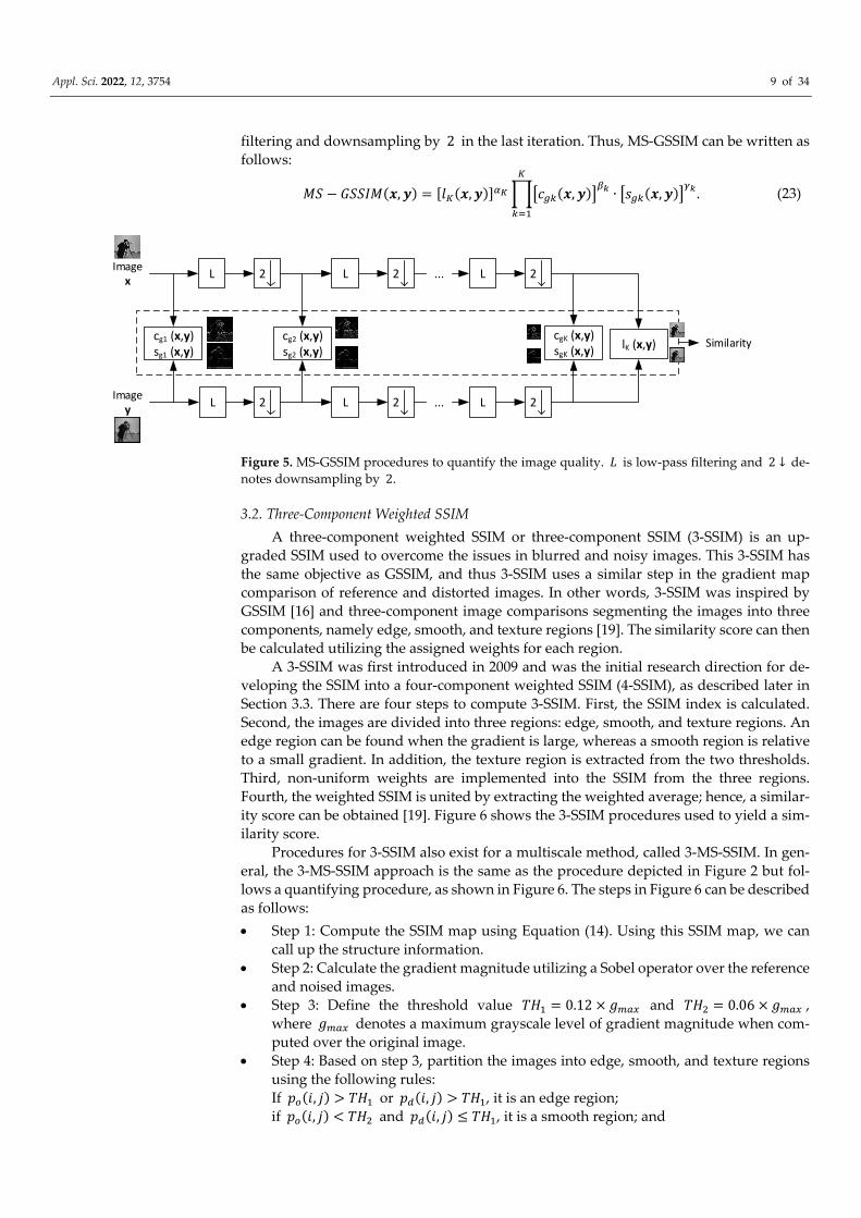
filtering and downsampling by 2 in the last iteration. Thus, MS‐GSSIM can be written as

follows:

𝑀𝑆 𝐺𝑆𝑆𝐼𝑀 𝒙,𝒚 𝑙 𝒙,𝒚 𝑐 𝒙,𝒚 ∙ 𝑠 𝒙,𝒚 . (23)

Image x

Image y

2L

cg1 (x,y)sg1 (x,y)

2L

cg2 (x,y)sg2 (x,y)

2L

2L

cgK (x,y)sgK (x,y)

2L

2L

lK (x,y) Similarity

...

...

Figure 5. MS‐GSSIM procedures to quantify the image quality. 𝐿 is low‐pass filtering and 2 ↓ de‐notes downsampling by 2.

3.2. Three‐Component Weighted SSIM

A three‐component weighted SSIM or three‐component SSIM (3‐SSIM) is an up‐

graded SSIM used to overcome the issues in blurred and noisy images. This 3‐SSIM has

the same objective as GSSIM, and thus 3‐SSIM uses a similar step in the gradient map

comparison of reference and distorted images. In other words, 3‐SSIM was inspired by

GSSIM [16] and three‐component image comparisons segmenting the images into three

components, namely edge, smooth, and texture regions [19]. The similarity score can then

be calculated utilizing the assigned weights for each region.

A 3‐SSIM was first introduced in 2009 and was the initial research direction for de‐

veloping the SSIM into a four‐component weighted SSIM (4‐SSIM), as described later in

Section 3.3. There are four steps to compute 3‐SSIM. First, the SSIM index is calculated.

Second, the images are divided into three regions: edge, smooth, and texture regions. An

edge region can be found when the gradient is large, whereas a smooth region is relative

to a small gradient. In addition, the texture region is extracted from the two thresholds.

Third, non‐uniform weights are implemented into the SSIM from the three regions.

Fourth, the weighted SSIM is united by extracting the weighted average; hence, a similar‐

ity score can be obtained [19]. Figure 6 shows the 3‐SSIM procedures used to yield a sim‐

ilarity score.

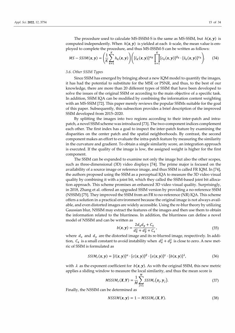
Procedures for 3‐SSIM also exist for a multiscale method, called 3‐MS‐SSIM. In gen‐

eral, the 3‐MS‐SSIM approach is the same as the procedure depicted in Figure 2 but fol‐

lows a quantifying procedure, as shown in Figure 6. The steps in Figure 6 can be described

as follows:

Step 1: Compute the SSIM map using Equation (14). Using this SSIM map, we can

call up the structure information.

Step 2: Calculate the gradient magnitude utilizing a Sobel operator over the reference

and noised images.

Step 3: Define the threshold value 𝑇𝐻 0.12 𝑔 and 𝑇𝐻 0.06 𝑔 ,

where 𝑔 denotes a maximum grayscale level of gradient magnitude when com‐

puted over the original image.

Step 4: Based on step 3, partition the images into edge, smooth, and texture regions

using the following rules:

If 𝑝 𝑖, 𝑗 𝑇𝐻 or 𝑝 𝑖, 𝑗 𝑇𝐻 , it is an edge region;

if 𝑝 𝑖, 𝑗 𝑇𝐻 and 𝑝 𝑖, 𝑗 𝑇𝐻 , it is a smooth region; and

Appl. Sci. 2022, 12, 3754 10 of 34

otherwise, if the pixels belong to a texture region but are not edge pixels, it is a texture

region.

Here, 𝑖, 𝑗 denotes the gradient coordinate, 𝑝 is the original image pixel, and 𝑝 denotes a degraded image pixel.

Reference ImageAnd

Distorted Image

Gradient Magnitude

∑

Edge Regions

Smooth Regions

Texture Regions

SSIM Map

SSIM Map for Edge

SSIM Map for Smooth

SSIM Map for Texture

Structure Information

Similarity

Weight 1

Weight 2

Weight 3

Figure 6. 3‐SSIM procedures to quantify the image quality (adapted from [19]).

Figure 7 shows the images for every process in a specific region. Figure 7a depicts

the original “Lena” image, whereas Figure 7b shows its blurred image, Figure 7c depicts

the edge region image, Figure 7d shows the smooth region image, and Figure 7e depicts

the texture region image.

(a) (b) (c) (d) (e)

Figure 7. Demonstration using “Lena” to present (a) original image, (b) blurred image, (c) edge pixel

image, (d) smooth pixel image, and (e) texture pixel image.

3.3. Four‐Component Weighted SSIM

The concept of 4‐SSIM was derived from the same authors as in 3‐SSIM to overcome

the SSIM issue related to blurred image measures. However, 4‐SSIM in the original article

is fractioned into 4‐SSIM itself, 4‐MS‐SSIM, 4‐GSSIM, and 4‐MS‐GSSIM. Therefore, using

the four‐component model, it is possible to compute four types of SSIM by partitioning

the original images into four regions, namely a changed‐edge region, preserved‐edge re‐

gion, smooth region, and texture region. The difference between 3‐SSIM and 4‐SSIM is in

the edge region: whereas 3‐SSIM has only one edge region, 4‐SSIM has two edge regions.

In addition, the condition used to determine which pixel belongs to which region is also

different [18,19].

Figure 8 shows the procedures used to yield the similarities of 4‐SSIM, 4‐MS‐SSIM,

4‐GSSIM, and 4‐MS‐GSSIM. The steps in Figure 8 can be defined as follows:

Appl. Sci. 2022, 12, 3754 11 of 34

Reference ImageAnd

Distorted Image

Gradient Magnitude

∑

Edge Regions

Smooth Regions

Texture Regions

SSIM Map

SSIM Map for Changed Edge

SSIM Map for Smooth

SSIM Map for Texture

Structure Information

Similarity

Weight 1

Weight 3

Weight 4

Changed Edge

Preserved Edge

SSIM Map for Preserved Edge

Weight 2

Figure 8. 4‐SSIM and its differentiation model procedures to quantify the image quality (adapted

from [18]).

Step 1: Calculate the SSIM map. This SSIM map is called the structure information.

Step 2: Compute the gradient magnitude applying the Sobel operator for the refer‐

ence and distorted images.

Step 3: Define the threshold value 𝑇𝐻 0.12 𝑔 and 𝑇𝐻 0.06 𝑔 ,

where 𝑔 denotes a maximum grayscale level of the gradient magnitude when

computed over the original image. Here, 𝑇𝐻 and 𝑇𝐻 have an effect on the com‐ponent regions under these situations, i.e., the smaller the first value, the more

“edgey” the region. Furthermore, the smaller the second value, the less smooth the

region is.

Step 4: Based on step 3, the images are segmented into the changed edge, preserved

edge, smooth, and texture regions using the following rules:

If 𝑝 𝑖, 𝑗 𝑇𝐻 and 𝑝 𝑖, 𝑗 𝑇𝐻 , the edge region is preserved;

If (𝑝 𝑖, 𝑗 𝑇𝐻 and 𝑝 𝑖, 𝑗 𝑇𝐻 ) or (𝑝 𝑖, 𝑗 𝑇𝐻 and 𝑝 𝑖, 𝑗 𝑇𝐻 ), edge re‐

gion is changed; and

If 𝑝 𝑖, 𝑗 𝑇𝐻 and 𝑝 𝑖, 𝑗 𝑇𝐻 , it is a smooth region.

Otherwise, the pixels belong to a texture region if they are not part of the edge pixels.

Here, 𝑖, 𝑗 denotes the gradient coordinate, 𝑝 is original image pixel, and 𝑝 de‐notes a degraded image pixel.

Figure 9 shows the images for every process within a specific region. Figure 9a de‐

picts a preserved edge image of “Lena,” whereas Figure 9b shows a changed edge region

image. In addition, Figure 9c displays a smooth region image, and Figure 9d depicts a

texture region image.

(a) (b) (c) (d)

Figure 9. Demonstration using “Lena” to present (a) preserved edge pixel image, (b) changed edge

pixel image, (c) smooth pixel image, and (d) texture pixel image.

Appl. Sci. 2022, 12, 3754 12 of 34

3.4. Complex‐Wavelet SSIM

After dealing with the SSIM issues in overestimating the similarity of the blurred

images, a complex‐wavelet SSIM was developed in 2009 to overcome the drawbacks of

the original SSIM in the spatial domain related to a high sensitivity when measuring im‐

ages with a few rotations, translations, and scaling in comparison with the original image

[21]. The fundamental aspect behind CW‐SSIM is using the wavelet coefficients inspired

from [69] over the images to extract the similarity value. Similarly, the main objective of

CW‐SSIM is to develop an insensitive IQA in evaluating the images under a nonstructured

geometric image distortion. CW‐SSIM is emphasized more to resolve the drawbacks of

the spatial domain by converting the images into a complex wavelet domain and acquir‐

ing the wavelet coefficients for determining the similarity score.

CW‐SSIM attempts to model the complex wavelet domain IQA with the ability to

separate the magnitude and phase distortion assessment. Moreover, it was developed to

be more sensitive to phase distortions than magnitude distortions and insensitive to con‐

sistent relative phase distortions. The symmetric complex wavelet can be formulated as

𝑤 𝑢 𝑔 𝑢 𝑒 for a low‐pass‐filter modulation, where 𝜔 denotes the modulated

band‐pass filter center frequency and 𝑔 𝑢 is a slowly varying and symmetric function.

The dilated and translated version of 𝑤 𝑢 can be written as follows:

𝑤 , 𝑢1

√𝑠𝑤

𝑢 𝑝𝑠

1

√𝑠𝑔

𝑢 𝑝𝑠

𝑒 ⁄ , (24)

where 𝑠 ∈ ℛ denotes the scale factor, and 𝑝 ∈ ℛ is the translation factor. In addition, the continuous wavelet transformation of the real signal 𝑥 𝑢 is expressed as

𝑋 𝑠,𝑝1

2𝜋𝑋 𝜔 √𝑠𝐺 𝑠𝜔 𝜔 𝑒 𝑑𝜔, (25)

where 𝑋 𝜔 and 𝐺 𝜔 are the Fourier transform (FT) of 𝑥 𝑢 and 𝑔 𝑢 , respectively. In

a complex wavelet domain, we can determine the coefficients within the same spatial do‐

main location represented in the same wavelet subbands of two images under comparison

as 𝒄 𝑐 , |𝑖 1,2,3 … ,𝑁 and 𝒄 𝑐 , |𝑖 1,2,3 … ,𝑁 , respectively. Then, CW‐SSIM can be

formulated as

𝑆 𝒄 , 𝒄2 ∑ 𝑐 , 𝑐 ,

∗ 𝐾

∑ 𝑐 , ∑ 𝑐 , 𝐾 , (26)

or can be written as a product of two components:

𝑆 𝒄 , 𝒄2∑ 𝑐 , 𝑐 , 𝐾

∑ 𝑐 , ∑ 𝑐 , 𝐾∙

2 ∑ 𝑐 , 𝑐 ,∗ 𝐾

2∑ 𝑐 , 𝑐 ,∗ 𝐾

, (27)

where 𝑐∗ is the complex conjugate of 𝑐, and 𝐾 denotes the small positive constant to im‐

prove the CW‐SSIM robustness at an extremely small local SNR. As in the original SSIM,

𝑆 𝒄 , 𝒄 is altered from 0 to 1 depending on the degree of similarity. The first compo‐

nent in Equation (27) is a maximum of 1 if 𝑐 , 𝑐 , . The first component is related to

the magnitude. By contrast, the second coefficient is relative to the phase changes.

3.5. Improved SSIM with Sharpness Comparison

In 2016, Lee and Lim developed an improved version of SSIM, called improved SSIM

with the sharpness comparison (ISSIM‐S) [17]. The idea behind this improvement is to

anticipate the shortcomings of SSIM in overestimating when quantifying blurred images

but underestimating when measuring the images with a spatial translation; however, the

spatial translated images are more visible from a human perspective than the blurred im‐

ages. ISSIM‐S uses the spatial domain with an improved assessment comparison in terms

of sharpness. Although the focus of ISSIM‐S is to accommodate the feasible IQA in meas‐

uring the images contaminating the rotation, translation, and scaling, ISSIM‐S shows

promising results in the assessment of images through several acquisitions, such as histo‐

gram equalization, mean luminance shifting, median filtering, impulsive noise, JPEG

compression, and mean filtering.

Appl. Sci. 2022, 12, 3754 13 of 34

The main shortcomings of SSIM are in the structural comparison, as in Equation (6).

When the calculated SSIM does not include a structural comparison and only consists of

the luminance and contrast, as in Equations (4) and (5), respectively, the similarity score

of the spatial translation is not predicted to be low and has a consistent measurement with

respect to HVS. However, if the three components of the SSIM are integrated into the SSIM

calculation, the measure index evaluates the blurred image with a high SSIM value. By

contrast, a slight vertical translated image has a low SSIM score, whereas the blurred im‐

age is noisier than the translated image.

Figure 10 shows a demonstration of using the “Lena” image to present the original,

spatial translated, and JPEG compressed images with a green line in the vertical center of

the images. As compared, the JPEG compression image is less perceptible than the image

with the spatial translation, as shown in Figure 10b,c when they are compared with the

reference image, as shown in Figure 10a.

(a) (b) (c)

Figure 10. Demonstration using “Lena” to present the comparison among (a) original, (b) vertical

translation, and (c) JPEG compressed images with a green line indicating the image’s vertical center

(adapted from [17]).

According to the original article on ISSIM‐S, the evaluation of the images shown in

Figure 10 offers an overestimation of the SSIM score for Figure 10c; however, there is an

underestimation of Figure 10b. Under normal circumstances, Figure 10b is more percep‐

tible than Figure 10c. This small SSIM score is obtained because of the drawback in the

structural comparison. Therefore, to fix this disadvantage, ISSIM‐S defines a new struc‐

ture factor to be

�̃� 𝒙,𝒚2𝜎 𝜎 𝐶 2𝜎 𝜎 𝐶

𝜎 𝜎 𝐶 𝜎 𝜎 𝐶 , (28)

where 𝜎 denotes a standard deviation for image 𝒙 smaller than 𝜇 , whereas 𝜎 is

the standard deviation for image 𝒙 larger than 𝜇 . In addition, 𝜎 denotes a standard

deviation for image 𝒚 smaller than 𝜇 , and meanwhile, 𝜎 is the standard deviation for

image 𝒚 larger than 𝜇 . The definition of �̃� 𝒙,𝒚 is the correlation of the standard devi‐ation when having positive or negative scores because 𝜎 and 𝜎 (or 𝜎 and 𝜎 )

can correspond to the object structure by fractioning into brighter and darker regions lo‐

cally. Nevertheless, by improving only 𝑠 𝒙,𝒚 into �̃� 𝒙,𝒚 , the presence of an overesti‐

mation even exists in the JPEG compressed image. Therefore, a new comparison is neces‐

sary to be added, namely a sharpness comparison ℎ 𝒙,𝒚 . With the added ℎ 𝒙,𝒚 , ISSIM‐

S has confidence in the improvement by two novel upgraded parameters. Here, ℎ 𝒙,𝒚 is the correspondence to the normalized digital Laplacian, which is formulated as

ℎ 𝒙,𝒚2|∇ 𝒙||∇ 𝒚| 𝐶

|∇ 𝒙| |∇ 𝒚| 𝐶 , (29)

where ∇ 𝒙 and ∇ 𝒚 are the normalized digital Laplacian determined by

Appl. Sci. 2022, 12, 3754 14 of 34

∇ 𝒙 𝒙 𝜇 , (30)

∇ 𝒚 𝒚 𝜇 . (31)

Therefore, ISSIM‐S is

𝐼𝑆𝑆𝐼𝑀 𝑆 𝒙,𝒚 𝑙 𝒙,𝒚 ∙ 𝑐 𝒙,𝒚 ∙ �̃� 𝒙,𝒚 ∙ ℎ 𝒙,𝒚 . (32)

Figure 11 shows the ISSIM‐S measure used to inspect the images. The luminance and

contrast are compared as in the original SSIM, whereas the structure is calculated using

the improved version. In addition, the sharpness calculation completes this new IQM. The

final step is to combine all comparisons and then obtain the dot product. As described

previously, SSIM is better in a local pixel utilizing a sliding window. Therefore, ISSIM‐S

applies the same method to yield the mean of ISSIM‐S (MISSIM‐S):


+

Image x

+

ـ

÷



+

Image y

+

ـ

÷



Contrast Comparison

Improved Structure

Comparison

Similarityx

Sharpness Measurement

Sharpness Measurement

Sharpness Comparison

Figure 11. ISSIM‐S procedures to quantify the image quality (adapted from [17]).

𝑀𝐼𝑆𝑆𝐼𝑀 𝑆 𝑿,𝒀1𝑀

𝐼𝑆𝑆𝐼𝑀 𝑆 𝒙 ,𝒚 . (33)

The similarity score is also a variant from 0 to 1, with 1 if 𝒙 𝒚. Several comparisons of SSIM have been conducted [70]. In 2021, Mudeng et al. at‐

tempted to use the benefit of MISSIM‐S for the first time to assess the reconstructed images

from simulated images of diffuse optical tomography (DOT) [71]. They compared four

types of SSIMs, i.e., MSSIM, MS‐SSIM, MISSIM‐S, and MS‐ISSIM‐S. MS‐ISSIM‐S can be

developed using MS‐SSIM and MISSIM‐S. Figure 12 shows the measurement processes of

MS‐ISSIM‐S.

Image x

Image y

2L

c1 (x,y)s1 (x,y)

h1 (x,y)

2L

c2 (x,y)s2 (x,y)

h2 (x,y)

2L

2L

cK (x,y)sK (x,y)

hK (x,y)

2L

2L

lK (x,y) Similarity

...

...

Mean h(x,y)

∑/K

~ ~ ~

Figure 12. MS‐ISSIM‐S procedures to quantify the image quality (adapted from [71]). 𝐿 is low‐pass filtering, and 2 ↓ denotes downsampling by 2.

Appl. Sci. 2022, 12, 3754 15 of 34

The procedure used to calculate MS‐ISSIM‐S is the same as MS‐SSIM, but ℎ 𝒙,𝒚 is computed independently. When ℎ 𝒙,𝒚 is yielded at each 𝑘‐scale, the mean value is em‐

ployed to complete the procedure, and thus MS‐ISSIM‐S can be written as follows:

𝑀𝑆 𝑆𝑆𝐼𝑀 𝒙,𝒚1𝐾

ℎ 𝒙,𝒚 𝑙 𝒙,𝒚 𝑐 𝒙,𝒚 ∙ �̃� 𝒙,𝒚 . (34)

3.6. Other SSIM Types

Since SSIM has emerged by bringing about a new IQM model to quantify the images,

it has had the potential to substitute for the MSE or PSNR, and thus, to the best of our

knowledge, there are more than 20 different types of SSIM that have been developed to

solve the issues of the original SSIM or according to the main objective of a specific task.

In addition, SSIM IQA can be modified by combining the information content weighting

with an MS‐SSIM [72]. This paper merely reviews the popular SSIMs suitable for the goal

of this paper. Subsequently, this subsection provides a brief description of the improved

SSIM developed from 2015–2020.

By splitting the images into two regions according to their inter‐patch and intra‐

patch, a novel SSIM scheme was introduced [73]. The two‐component indices complement

each other. The first index has a goal to inspect the inter‐patch feature by examining the

disparities on the center patch and the spatial neighborhoods. By contrast, the second

component makes an effort to evaluate the intra‐patch feature by measuring the similarity

in the curvature and gradient. To obtain a single similarity score, an integration approach

is executed. If the quality of the image is low, the assigned weight is higher for the first

component.

The SSIM can be expanded to examine not only the image but also the other scopes,

such as three‐dimensional (3D) video displays [74]. The prime major is focused on the

availability of a source image or reference image, and thus SSIM is called FR IQM. In [74],

the authors proposed using the SSIM as a perceptual IQA to measure the 3D video visual

quality by combining it with a joint bit, which they called the SSIM‐based joint bit alloca‐

tion approach. This scheme promises an enhanced 3D video visual quality. Surprisingly,

in 2018, Zhang et al. offered an upgraded SSIM version by providing a no‐reference SSIM

(NSSIM) [75]. They improved the SSIM from an FR to no‐reference (NR) IQA. This scheme

offers a solution in a practical environment because the original image is not always avail‐

able, and even distorted images are widely accessible. Using the re‐blur theory by utilizing

Gaussian blur, NSSIM may extract the features of the images and then use them to obtain

the information related to the blurriness. In addition, the blurriness can define a novel

model of NSSIM and can be written as

𝑏 𝒙,𝒚2𝑑𝒙𝑑𝒚 𝐶

𝑑𝒙 𝑑𝒚 𝐶 , (35)

where 𝑑 and 𝑑 are the distorted image and its re‐blurred image, respectively. In addi‐

tion, 𝐶 is a small constant to avoid instability when 𝑑𝒙 𝑑𝒚 is close to zero. A new met‐

ric of SSIM is formulated as

𝑆𝑆𝐼𝑀 𝒙,𝒚 𝑙 𝒙,𝒚 ∙ 𝑐 𝒙,𝒚 ∙ 𝑠 𝒙,𝒚 ∙ 𝑏 𝒙,𝒚 , (36)

with 𝜆 as the exponent coefficient for 𝑏 𝒙,𝒚 . As with the original SSIM, this new metric

applies a sliding window to measure the local similarity, and thus the mean score is

𝑀𝑆𝑆𝐼𝑀 𝑿,𝒀1𝑀

𝑆𝑆𝐼𝑀 𝒙 ,𝒚 . (37)

Finally, the NSSIM can be determined as

𝑁𝑆𝑆𝐼𝑀 𝒙,𝒚 1 𝑀𝑆𝑆𝐼𝑀 𝑿,𝒀 . (38)

Appl. Sci. 2022, 12, 3754 16 of 34

Another type of SSIM is the contrast sensitivity function SSIM (CSF + SSIM) [76]. This

CSF + SSIM combines the non‐linear characteristics of the luminance perception with the

contrast sensitivity characteristics from the HVS for a contrast‐distorted image evaluation.

However, CSF + SSIM is deemed complex in terms of its computations because it separates

the images in the color space transform into the luminance, red–green channel, and blue–

yellow channel to yield their perceptions. Moreover, CSF + SSIM employs a discrete cosine

transform (DCT) to acquire the weights corresponding to the CSF. It then deploys an in‐

verse DCT (IDCT) to obtain the color space for the perceived images, and as the last step,

it applies the SSIM to obtain the similarity score. In addition, a spherical SSIM is used to

objectively inspect the video quality of omnidirectional video [33]. A spherical uniform

SSIM for assessing panoramic video has also been established [77], and a multi‐exposure

image fusion (MEF) approach by optimizing the SSIM, which is called the color MEF

structural similarity (MEF‐SSIMc), has been presented [78]. Finally, a topological SSIM (T‐

SSIM) was introduced for a specific task to identify a nearby organ populated with tumor‐

organ distances and volumes for two compared patients [79].

4. SSIM in Medical Imaging

This section discusses the implementation of SSIM, particularly for imaging tech‐

niques such as MRI, ultrasonography, CT scan, X‐rays, and optical imaging. This section

aims to emphasize reviews of SSIM applied to the measurement of medical images. We

reviewed SSIM in medical imaging based on the published year of the articles.

To identify the relevant studies, a systematic methods overview [80] along with sev‐

eral major databases were used to search the matched keywords, such as “SSIM” AND

“Magnetic Resonance Imaging” OR “Computed Tomography” OR “Ultrasonography”

OR “Ultrasound” OR “X‐ray” OR “Optical Imaging” OR “Medical Images” OR “Medical

Imaging”. The main databases included Google Scholar, PubMed, IEEE, MDPI, Springer,

Elsevier, and others. There were 125 identified articles related to the keywords including

journals, conference proceedings, and book chapters, consisting of the original articles on

UQI, SSIM, MS‐SSIM, three‐ and four‐component weighted SSIMs, CW‐SSIM, ISSIM‐S,

and other SSIM families, as well as the SSIM implementation for MRI, CT, ultrasonogra‐

phy, X‐ray, and optical imaging. Overall, 72 articles relevant to the goal of this review paper regarding SSIM applied in medical imaging were reviewed. We did not exclude the

same SSIM implementation in medical imaging as with an IQA, and instead, we men‐

tioned, classified, and briefly reviewed them in Sections 4.1 and 4.5 according to the med‐

ical imaging technique used. We provided this method because we prefer to offer a wide

range of SSIM implementations and fulfill the objective of this review paper of providing

the readers or researchers with potential medical image examination research methods

that can be improved using SSIM. Additionally, Section 4.6 provided a thorough review

of 4 articles related to SSIM application in medical imaging for loss function in convolu‐

tional neural network (CNN), reducing metal artifact, contour extractor, and IQA. Thus,

we described in detail the image acquisition method, filtering, or the other approaches

used to acquire the distorted images for comparing with the original image from the med‐

ical modality imaging scheme. Additionally, this study’s limitation was stated in Section

4.7.

To avoid misleading and maintain the objective of this review, we emphasized that

the SSIM measure has an original goal to substitute the common measures, such as MSE

and PSNR in measuring any signals in 1D, 2D, and 3D, as long as there is a reference

signal. Thus, the SSIM measure can assess digital images including medical images. To

offer a better representation of the methodology when using SSIM to evaluate medical

images, we provided Figures 13–15 to depict medical images when they were processed

using three‐ and four‐component SSIMs, as well as ISSIM‐S. However, since this study’s

goal is to provide the SSIM prospect in medical images, we did not measure each SSIM

type (three‐component SSIM, four‐component SSIM, and ISSIM‐S) similarity score. We

used a digital database for screening mammography (DDSM) [81] containing 2620 cases

Appl. Sci. 2022, 12, 3754 17 of 34

of normal, benign, and malignant breast cancers extracted from calcification and breast

masses abnormalities. Figure 13 shows the images for every process in a specific region

for three‐component SSIM. Figure 13a depicts the original DDSM right breast masses be‐

nign cancer with craniocaudal (CC) view image, Figure 13b shows its blurred image, Fig‐

ure 13c depicts the edge region image, Figure 13d shows the smooth region image, and

Figure 13e depicts the texture region image. Figure 14 shows the images for every process

within a specific region for four‐component SSIM. Figure 14a depicts a preserved edge

image of DDSM right breast masses benign cancer with CC, whereas Figure 14b shows a

changed edge region image. In addition, Figure 14c displays a smooth region image, and

Figure 14d depicts a texture region image. Figure 15 shows a demonstration of using

DDSM right breast masses benign cancer with CC image to present the original, spatial

translated, and JPEG compressed images with a green line in the vertical center of the

images. As compared, the JPEG compression image is less perceptible than the image with

the spatial translation, as shown in Figure 15b,c when they are compared with the refer‐

ence image, as shown in Figure 15a. As depicted in Figures 13–15, using the image pro‐

cessing steps for medical images, we may compute the similarity score to obtain the image

quality. These motivated us to review articles related to SSIM in the medical field.

(a) (b) (c) (d) (e)

Figure 13. Demonstration using DDSM right breast masses benign cancer with CC view to present

(a) original image, (b) blurred image, (c) edge pixel image, (d) smooth pixel image, and (e) texture

pixel image.

(a) (b) (c) (d)


(a) preserved edge pixel image, (b) changed edge pixel image, (c) smooth pixel image, and (d) tex‐

ture pixel image.

(a) (b) (c)


the comparison among (a) original, (b) vertical translation, and (c) JPEG compressed images with a

green line indicating the image vertical center.

Appl. Sci. 2022, 12, 3754 18 of 34

4.1. Magnetic Resonance Imaging

To the best of our knowledge, the first SSIM implementation for evaluating the im‐

ages of MR was in 2005 [82,83]. The attempt in [83] used distorted MR images and then

compared them with the original MR image. Three modules creating a closed‐loop system

containing de‐noising filters, evaluations method, and adjustment rules were used. The

corrupted images were examined using SSIM along with the mean absolute error (MAE),

root‐mean‐square error (RMSE), SNR, and PSNR. Their results indicate that SSIM shows

a high similarity score when the distorted images are close to the reference image. This is

the first time an exploration of the original SSIM was started for use in other applications,

such as MR medical images. As we mentioned previously, the original SSIM may interpret

the blurred images with a high similarity score owing to the effect of the structural com‐

parison. However, their results indicate that SSIM has the potential to assess medical im‐

ages. In addition, in [82], the SSIM showed a relatively decent performance to quantify the

head MR images. However, there were inconsistencies in the 40% and 70% quality fac‐tors. Various quality factors were deployed to acquire the similarity value. Nonetheless,

with the higher quality factor of compression, the SSIM predicted the similarity with a

low score and was deemed unsuitable for the quality metric in [82].

In 2007, a group of researchers applied an SSIM application for security in the MR

and computed tomography (CT) images related to the watermarked medical images [31].

Medical image watermarks are crucial because they may comprise the medical infor‐

mation of the patients, proving ownership, and alternating location on the images. More‐

over, watermarked medical images frequently store hidden messages for later extraction

to obtain the reports. Their results showed that SSIM is less capable of measuring the deg‐

radation of medical images when the images are embedded with a watermark. They spec‐

ulated that the best metric for a watermarking measure is a steerable visual difference

predictor (SVDP). By contrast, SSIM and a quality index based on local variance (QILV)

have been exploited for the quality measure of estimating the magnitude of MR based on

the linear minimum mean squared error (LMMSE) [84]. The SSIM in this task performed

competitively in measuring images fused with an LMMSE estimator.

The compression of medical images is challenging in teleradiology because teleradi‐

ology requires transmission to transfer the images [85]. In the transferring process, the

image quality may be reduced owing to the limited communication, and thus the image

fidelity can be decreased. The quality measure is necessary to determine the threshold

value to compress these medical images; hence, in the transmission, the important infor‐

mation of the images is not diminished. A partitioning in hierarchical tree (SPIHT) com‐

pression algorithm has also been used to determine the maximum threshold standard for

compression. The compressed images were compared with their original to assess their

similarity. In this specific task, SSIM and PSNR showed agreeable results with the mean

opinion score (MOS), and thus for this case, SSIM is considered appropriate to cut off the

threshold value when the medical images are compressed with a defined bit rate. Subse‐

quently, medical image fusion to improve the confidence of radiologists in diagnosing a

specific disease was accomplished in 2009 by Zhang and Zheng [86]. The objective of this

research is to decrease the inconsistency of a diagnosis when subjective observers read the

medical images. In addition, SSIM contributed significantly to the fusion approach. A

unique SSIM implementation in this article was shown because SSIM was not used as the

IQA metric; instead, it was utilized as the image fusion itself. Based on an understanding

of the image fusion from several imaging modalities, the decision confidence may be im‐

proved, and the images combined from MRI and CT were employed to generate more

perceivable images. Because CT can offer better information in denser tissue with less dis‐

tortion and MRI provides adequate imaging for soft tissue, a fusion was executed to re‐

duce the workload of the radiologists. Their results indicated that image fusion using

SSIM is remarkable compared with existing image fusion methods, such as a Laplacian

pyramid (LP), gradient pyramid (GP), contrast pyramid (CP), steerable pyramid (StrP),

and discrete wavelet transform (DWT).

Appl. Sci. 2022, 12, 3754 19 of 34

For a denoising method to remove Rician noise from MR images, the SSIM and MSE

as objective metrics were compared with the MOS to measure the denoising methodology

using the discretized total variation [87]. In this study, SSIM performed suitably with the

MOS, which is related to HVS. With the highest standard deviation, the SSIM scores di‐

minished following the subjective measurement scores. In addition, in 2013, to reduce the

presence of aliasing, an improve compressed sensing technique was introduced, whereas

the SSIM and PSNR were the objective measures used to assess the effectiveness of this

approach [37]. Their results showed that SSIM is suitable for use with the proposed

method as an objective IQM. Subsequently, in 2015 and 2017, to restore the MR images

from the existence of noise during the acquisition steps, the SSIM along with SNR, PSNR,

MSE, and RMSE was used to evaluate novel denoising algorithms [40,88–90]. With the

computational improvements, an artificial intelligence (AI) method including deep learn‐

ing has been proposed to solve the medical image analysis issues, and the results were

compared using SSIM [38,39,91–94]. SSIM was also compared with other objective IQAs

to obtain comprehensive insight related to an effective IQM for diagnosis by five radiolo‐

gists [36] and was employed in measuring an image acquisition [95].

To conclude this subsection, Table 1 briefly presents the SSIM applications for MR

medical images. In Table 1, SSIM is adopted not only for IQA but also for other purposes,

such as image fusion, segmentation, clustering, and loss function. In addition, compared

to other metrics, SSIM performances are competitively adequate according to the applied

task. Most of the SSIM implementations as an IQA showed that SSIM is suitable for an

assigned task, indicating that it offers reliable performance for measuring an enhancement

of the image quality in comparison to the other traditional measures.

Table 1. Summary of published articles encompassing SSIM for MRI. MRI, magnetic resonance im‐

aging; CT, computed tomography; MAE, mean‐absolute error; RMSE, root‐mean‐square error; SNR,

signal‐to‐noise ratio; PSNR, peak‐signal‐to‐noise ratio; SVDP, steerable visual difference predictor;

QILV, quality index based on local variance; LN, level on noise; LP, Laplacian pyramid; GP, gradient

pyramid; CP, contrast pyramid; StrP, steerable pyramid; DWT, discrete wavelet transform; 𝑄 ⁄ ,

visual information quality; MOS, mean opinion score; SI, similarity index; NRMSE, normalized‐

root‐mean‐square error; VIF, visual information fidelity; FSIM, feature similarity index; NQM, noise

quality metric; GMSD, gradient magnitude similarity deviation; HDRVDP, high dynamic range vis‐

ible difference predictor; CNN, convolutional neural network.

Study Year Modality SSIM

Implementation

Compared

Matrix Results

Castellanos et al.

[83] 2005 MRI IQA

MAE, RMSE, SNR,

and PSNR

SSIM is suitable

for this task

Rajagopalan and

Robb [82] 2005 MRI IQA Subjective measure

The subjective

measure is supe‐

rior

Dowling et al. [31] 2007 MRI and CT IQA PSNR and SVDP SVDP is suitable

for this research

Aja‐Fernández et

al. [84] 2007 MRI IQA MSE, QILV, and LN

SSIM has compet‐

itive results com‐

pared to QILV

Kumar et al. [85] 2009 MRI and CT IQA PSNR SSIM is suitable

for this task

Xiao and Zheng

[86] 2009 MRI and CT Images fusion

LP, GP, CP, StrP,

and DWT 𝑄 ⁄ 0.62

Varghess et al. [87] 2012 MRI IQA MSE and MOS SSIM is suitable

with MOS

Zhu et al. [37] 2013 MRI IQA PSNR SSIM is suitable

for this task

Appl. Sci. 2022, 12, 3754 20 of 34

Srivastava et al.

[88] 2015 MRI IQA PSNR

SSIM is suitable

for this task

Srivastava et al.

[89] 2015 MRI IQA PSNR

SSIM is suitable

for this task

Saladi and Prabha

[40] 2017 MRI IQA

SNR, PSNR, MSE,

RMSE

SSIM is suitable

for this task

Chandrashekar

and Sreedevi [90] 2017 MRI IQA

PSNR, entropy, and

MSE

SSIM is suitable

for this task

Mostafa et al. [92] 2017 MRI Segmentation SI Accuracy =

97.5%

Duan et al. [39] 2019 MRI IQA MAE SSIM is suitable

for this task

Pawar et al. [93] 2019 MRI IQA NRMSE SSIM is suitable

for this task

Krohn et al. [95] 2019 MRI Clustering ‐ 𝑆𝑆𝐼𝑀 0.7 to

0.9

Wang et al. [94] 2020 MRI IQA PSNR and NRMSE

SSIM and NRMSE

performances are

decent

Mason et al. [36] 2020 MRI IQA

MOS, VIF, FSIM,

NQM, GMSD,

HDRVDP, PSNR,

and RMSE

VIF shows the de‐

cent results

Nirmalraj and Na‐

garajan [91] 2020 MRI IQA

PSNR, MSE, and

entropy

SSIM is suitable

for this task

Jaubert et al. [38] * 2021 MRI Loss function MAE 𝑝 value 0.05 * A detailed review is provided in Section 4.6.

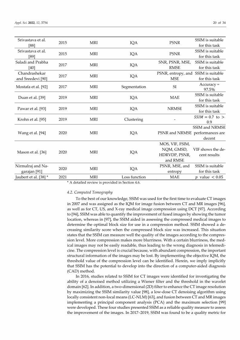
4.2. Computed Tomography

To the best of our knowledge, SSIM was used for the first time to evaluate CT images

in 2007 and was assigned as the IQM for image fusion between CT and MR images [96],

as well as for CT, US, and X‐ray medical image compression using DCT [97]. According

to [94], SSIM was able to quantify the improvement of fused images by showing the tumor

location, whereas in [97], the SSIM aided in assessing the compressed medical images to

determine the optimal block size for use in a compression method. SSIM showed a de‐

creasing similarity score when the compressed block size was increased. This situation

states that the SSIM can measure well the quality of the images according to the compres‐

sion level. More compression makes more blurriness. With a certain blurriness, the med‐

ical images may not be easily readable, thus leading to the wrong diagnosis in telemedi‐

cine. The compression level is crucial because, with abundant compression, the important

structural information of the images may be lost. By implementing the objective IQM, the

threshold value of the compression level can be identified. Herein, we imply implicitly

that SSIM has the potential to develop into the direction of a computer‐aided diagnosis

(CAD) method.

In 2016, studies related to SSIM for CT images were identified for investigating the

ability of a denoised method utilizing a Wiener filter and the threshold in the wavelet

domain [62]. In addition, a two‐dimensional (2D) filter to enhance the CT image resolution

by maximizing the SSIM similarity value [98], a low‐dose CT denoising algorithm using

locally consistent non‐local means (LC‐NLM) [63], and fusion between CT and MR images

implementing a principal component analysis (PCA) and the maximum selection [99]

were developed. These four studies presented SSIM as a reliable quality measure to assess

the improvement of the images. In 2017–2019, SSIM was found to be a quality metric for

Appl. Sci. 2022, 12, 3754 21 of 34

measuring the results from 3D printed lung vessels [100], an approach to reducing the

metal artifact in CT images by excluding the luminance comparison [101], an IQM for

deep learning [41,43,102], and an alternative random forest (ARF) regression tool [103]. It

was also used for CT tooth images extracted from denoised images filtered using a wave‐

let and bilateral filter [65], the removal of Gaussian noise [42], and image restoration and

reconstruction [64]. In [101], the role of SSIM was distinguished from IQA as a method to

reduce the artifacts caused by metal. In addition, a modified SSIM was utilized to con‐

struct this task by ignoring the luminance factor but maintaining the contrast and struc‐

tural comparisons. This modified SSIM should be completed because the metal artifacts

and a superposition map may vary substantially, whereas the structural or edge infor‐

mation can be indistinguishable. With the role of SSIM, correlated images can be obtained,

and two correlation maps can then be compared to acquire reduced metal artifact images.

In 2020–2021, SSIM was used as an evaluation metric for ovarian cancer [104], a generative

adversarial network (GAN) [105], and Franken‐CT [67].

To conclude this subsection, Table 2 describes SSIM used for CT medical images. As

indicated in Table 2, SSIM has been embraced not only for IQA but also for other objec‐

tives, such as noise reduction. In addition, compared to other metrics, SSIM performs com‐

petitively well according to the specialized task. In practical terms, all SSIM roles listed in

Table 2 are for image quality measures. They indicate that SSIM has the potential to be‐

come a favorable IQA.

Table 2. Summary of the published articles encompassing SSIM for CT. CT, computed tomography;

MRI, magnetic resonance imaging; RMSE, root‐mean‐square error; MSE, mean‐square error; PSNR,

peak‐signal‐to‐noise ratio; PRD, percent rate of distortion; CC, correlation coefficient; FF, fusion fac‐

tor; LI‐MAR, linear interpolation metal artifact reduction; NMAR, normalized metal artifact reduc‐

tion; RMAR, refined metal artifact reduction; IQI, image quality index; VIF, visual information fi‐

delity; ZNCC, zero‐normalized cross‐correlation; MAE, mean‐absolute error.


Implementation

Compared

Matrix Results

Senthilkumar and

Muttan [96] 2007 CT and MRI IQA RMSE

SSIM is suitable

for this task

Singh et al. [97] 2007 CT, US, and X‐ray IQA MSE, PSNR, PRD,

and CC

SSIM has the

highest score

Diwakar and Ku‐

mar [62] 2016 CT IQA PSNR

SSIM is suitable

for this task

Mahmoud et al.

[98] 2016 CT IQA PSNR

SSIM is suitable

for this task

Green [63] 2016 CT IQA ‐ SSIM is suitable

for this task

Himanshi et al.

[99] 2016 CT and MRI IQA FF

SSIM is suitable

for this task

Joemai and Gel‐

eijns [100] 2017 CT IQA ‐

SSIM is suitable

for this task

Zhang et al. [102] 2018 CT IQA RMSE SSIM is suitable

for this task

Kim and Byun [43] 2018 CT IQA ‐ SSIM is suitable

for this task

Hu and Zhang

[103] 2018 CT and MRI IQA PSNR

SSIM is suitable

for this task

Wang et al. [65] 2018 CT IQA PSNR SSIM is suitable

for this task

Appl. Sci. 2022, 12, 3754 22 of 34

Kuanar et al. [41] 2019 CT IQA PSNR SSIM is suitable

for this task

Kim et al. [99] * 2019 CT Reducing metal artifact LI‐MAR, NMAR,

and RMAR

𝑀𝐴𝐸 8.52 and 10. 12

Elaiyaraja et al.

[42] 2019 CT and MRI IQA PNSR, IQI, and VIF

SSIM is suitable

for this task

Sun et al. [64] 2019 CT IQA PSNR SSIM is suitable

for this task

Urase et al. [104] 2020 CT IQA PSNR SSIM is suitable

for this task

Gajera et al. [105] 2021 CT IQA PSNR SSIM is suitable

for this task

Martinez‐Girones

et al. [67] 2021 CT and MRI IQA

ZNCC, MAE, and

Dice coefficient for

bone class

SSIM is suitable

for this task

* A detailed review is provided in Section 4.6.

4.3. Ultrasonography

We review SSIM applications for ultrasonography in this section. We found that the

first implemented SSIM for US was in 2007. SSIM along with the SNR, coefficient of cor‐

relation (CoC), edge preservation index (EPI), and QI were used to quantify the image

enhancement when a versatile wavelet domain algorithm was utilized [106]. In the same

year, US with two other medical images, CT and X‐ray images, were measured using

SSIM, MSE, PSNR, CC, and PRD to identify the effectiveness of a novel algorithm for

compressing images in the field of teleradiology using an adaptive threshold value of var‐

iance [107]. In 2008, an algorithm was developed to reduce the effects of speckle, and the

developed algorithm was measured with the Michelson contrast measure (CM), the

Beghdadi and Le Négrate contrast measure (CBN), PSNR, and SSIM [108]. Their results

showed that SSIM has potential effectiveness as an IQM for the US, although, at the time,

SSIM had existed for only 3 or 4 years.

The reduction in speckle in US images has brought several types of studies to this

issue. In 2016, the least‐squares Bayesian [60], adaptive non‐local means [109], local statis‐

tic, and non‐local mean filter [110] algorithm estimations were established to reduce the

speckle in US images, and several IQAs including SSIM, SNR, MSE, and a sum of the

variance (SV) were designated to evaluate the improved algorithms. An uncommon SSIM

implementation was conducted using CW‐SSIM as a contour extractor of a tongue by Xu

et al. [61,111]. They compared the performance of MSSIM and CW‐SSIM with the normal‐

ized PSNR (NPSNR). MSSIM and the NPSNR demonstrated similar results, whereas CW‐

SSIM presented superior results by showing the tongue position with the peak of CW‐

SSIM.

Apparently, more attention from researchers was drawn in 2017–2021 for creating an

efficient algorithm to eliminate speckle in US images [58,59,66,112–118]. In addition, US

images can be analyzed using deep learning to conduct breast tumor segmentation and

reconstruct images from raw channel data [53,119]. In [53], the combination between SSIM

and L1‐norm in the loss function was applied to capture the local context information

from the surrounding tumor area, whereas in [119], MS‐SSIM and PSNR were utilized as

the loss function.

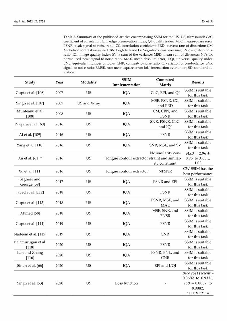
To conclude this subsection, Table 3 illustrates the purposes of using SSIM for US

medical images. As indicated in Table 3, SSIM is accepted not only for IQA but also for

other purposes, such as a contour extractor and loss function. In addition, compared to

other metrics, SSIM performances are competitively appropriate according to their dedi‐

cated assignment.

Appl. Sci. 2022, 12, 3754 23 of 34

Table 3. Summary of the published articles encompassing SSIM for the US. US, ultrasound; CoC,

coefficient of correlation; EPI, edge preservation index; QI, quality index; MSE, mean‐square error;

PSNR, peak‐signal‐to‐noise ratio; CC, correlation coefficient; PRD, percent rate of distortion; CM,

Michelson contrast measure; CBN, Beghdadi and Le Négrate contrast measure; SNR, signal‐to‐noise

ratio; IQI, image quality index; SV, a sum of the variance; MSD, mean sum of distances; NPSNR,

normalized peak‐signal‐to‐noise ratio; MAE, mean‐absolute error, UQI, universal quality index;

ENL, equivalent number of looks; CNR, contrast‐to‐noise ratio; C, variation of conductance; SNR,

signal‐to‐noise ratio; RMSE, root‐mean‐square error; IoU, intersection over union; SD, standard de‐

viation.


Implementation

Compared

Matrix Results

Gupta et al. [106] 2007 US IQA CoC, EPI, and QI SSIM is suitable

for this task

Singh et al. [107] 2007 US and X‐ray IQA MSE, PSNR, CC,

and PRD

SSIM is suitable

for this task

Munteanu et al.

[108] 2008 US IQA

CM, CBN, and

PSNR

SSIM is suitable

for this task

Nagaraj et al. [60] 2016 US IQA SNR, PSNR, CoC,

and IQI

SSIM is suitable

for this task

Ai et al. [109] 2016 US IQA PSNR SSIM is suitable

for this task

Yang et al. [110] 2016 US IQA SNR, MSE, and SV SSIM is suitable

for this task

Xu et al. [61] * 2016 US Tongue contour extractor

No similarity con‐

straint and similar‐

ity constraint

𝑀𝑆𝐷 2.960.95 to 3. 65

1.02

Xu et al. [111] 2016 US Tongue contour extractor NPSNR CW‐SSIM has the

best performance

Sagheer and

George [59] 2017 US IQA PSNR and EPI

SSIM is suitable

for this task

Javed et al. [112] 2018 US IQA PSNR SSIM is suitable

for this task

Gupta et al. [113] 2018 US IQA PSNR, MSE, and

MAE

SSIM is suitable

for this task

Ahmed [58] 2018 US IQA MSE, SNR, and

PNSR

SSIM is suitable

for this task

Gupta et al. [114] 2019 US IQA PSNR SSIM is suitable

for this task

Nadeem et al. [115] 2019 US IQA SNR SSIM is suitable

for this task

Balamurugan et al.

[118] 2020 US IQA PSNR

SSIM is suitable

for this task

Lan and Zhang

[116] 2020 US IQA

PSNR, ENL, and

CNR

SSIM is suitable

for this task

Singh et al. [66] 2020 US IQA EPI and UQI SSIM is suitable

for this task

Singh et al. [53] 2020 US Loss function ‐

𝐷𝑖𝑐𝑒 𝑐𝑜𝑒𝑓𝑓𝑖𝑐𝑖𝑒𝑛𝑡0.8682 to 0.9376, 𝐼𝑜𝑈 0.8037 to

0.8882, 𝑆𝑒𝑛𝑠𝑖𝑡𝑖𝑣𝑖𝑡𝑦

Appl. Sci. 2022, 12, 3754 24 of 34

0.9011 to 0.9155, and

𝑆𝑝𝑒𝑐𝑖𝑓𝑖𝑐𝑖𝑡𝑦0.9949 to 0.9973

Strohm et al. [119] 2020 US Loss function MAE

𝑚𝑒𝑎𝑛 𝑎𝑛𝑑 𝑆𝐷0.91 0.04 and

0.90 0.01

Bharadwaj [117] 2021 US IQA C, SNR, PSNR,

MSE, and RMSE

SSIM is suitable

for this task


4.4. X‐ray

The fourth discussion on medical images is focused on X‐ray images. Unlike MRI,

CT, and US images, SSIM implementation for medical X‐ray images was introduced in

2012 for the first time to the best of our knowledge. As is typical, SSIM was constructed to

measure a designated algorithm to estimate the similarity score between the ground‐truth

image and the denoised images. In 2012, SSIM, PSNR, SNR, and MSE were appointed to

evaluate an improved algorithm [120]. Similarly, in 2016, a method to eliminate Gaussian

noise was established using an edge preserved wavelet packet transformation [121], and

the denoising of a contrast‐enhanced X‐ray image was accomplished [122]. In addition,

SSIM was allocated together with the MSE, RMSE, SNR, PSNR, recall, accuracy, precision,

and error rate as an objective IQA. Subsequently, in 2017, a security watermark algorithm

was developed to secure the diagnostic information of a patient, as well as the ownership

and authentication [123] in X‐ray and MR images. Again, SSIM has a role as an IQM along

with wavelet domain SNR (WSNR) and PSNR. The feasibility of SSIM was not only shown

for a numerical analysis but also in regard to deep learning, such as a CNN. The improved

algorithm with deep learning may be measured using SSIM related to compression and

noise reduction [124–127]. Moreover, comparisons of filter techniques used to reduce the

noise and image reconstruction, as well as apply image compression, were conducted us‐

ing X‐ray images [44,128–130].

To conclude this subsection, Table 4 exemplifies the purposes of using SSIM for X‐

ray medical images. As in Table 4, we describe the whole article using X‐ray images con‐

veying the SSIM metric as an IQM.

Table 4. Summary of the published articles encompassing SSIM for X‐ray. PSNR, peak‐signal‐to‐

noise ratio; CT, computed tomography; MRI, magnetic resonance imaging; SNR, signal‐to‐noise ra‐

tio; MSE, mean‐square error; RMSE, root‐mean‐square error; WSNR, wavelet domain signal‐to‐

noise ratio; RMSE, root‐mean‐square error; FSIM, feature similarity index.


Implementation

Compared

Matrix Results

Cerciello et al.

[120] 2012 X‐ray IQA

PSNR, SNR, and

MSE

SSIM is suitable

for this task

Rajith et al. [121] 2016 X‐ray IQA

MSE, RMSE, SNR,

PSNR, recall, accu‐

racy, precision, and

error rate

SSIM is suitable

for this task

Jeon [122] 2016 X‐Ray IQA PSNR SSIM is suitable

for this task

Kunhu et al. [123] 2017 Xray and MRI IQA PSNR and WSNR SSIM is suitable

for this task

Zhang and Yu

[124] 2018 X‐ray CT IQA RMSE

SSIM is suitable

for this task

Appl. Sci. 2022, 12, 3754 25 of 34

Sushmit et al. [125] 2019 X‐ray IQA PSNR SSIM is suitable

for this task

Islam et al. [126] 2019 X‐ray IQA PSNR SSIM is suitable

for this task

Haiderbhai et al.

[127] 2020 X‐ray IQA RMSE and PSNR

SSIM is suitable

for this task

Roy and Maity

[128] 2020 X‐ray IQA

MSE, PSNR, and

SNR

SSIM is suitable

for this task

Saeed et al. [129] 2020 X‐ray IQA RMSE, PSNR, and

FSIM

SSIM is suitable

for this task

Villarraga‐Gómez

and Smith [130] 2020 X‐ray CT IQA RMSE and PSNR

SSIM is suitable

for this task

Pourasad and Ca‐

vallaro [44] * 2021 X‐ray IQA PSNR and MSE

SSIM is suitable

for this task


4.5. Optical Imaging

To complete the reviews of SSIM implementation in medical imaging systems, we

presented a novel modality using optical imaging. Because optical imaging is a relatively

new modality, acquiring SSIM applications in optical imaging is considered rare. Despite

our best efforts, we found only two articles comprising SSIM as an IQM to measure the

distorted medical images related to the reference images. We excluded optical imaging

using SSIM for a scope other than the medical field, such as optical imaging for commu‐

nication and simulations to predict the optical properties of a reconstruction. In 2020,

SSIM along with MAE were utilized to examine images from a single snapshot of optical

properties (SSOP) and the ground‐truth images [131].

In 2021, SSIM was used for comparing the optical images of a mouse with an embed‐

ded tumor [132]. The article reported the application of machine learning, such as K‐

means and fuzzy c‐means, to automatically cluster the tumor. They compared the results

between manual clustering and automatic clustering with the aid of SSIM and the Dice

coefficient to evaluate the similarity of two images. Here, SSIM performed satisfactorily

in objectively examining the segmentation results through a manual approach, showing a

similarity score of 0.9168. In addition, when Gaussian noise was added to the back‐

ground, SSIM demonstrated a robust performance by showing a stable similarity score.

With the assistance of SSIM, the article reported that their clustering algorithms are robust

to noise.

To conclude this subsection, Table 5 represents the purposes of using SSIM for optical

medical images. As in Table 5, we describe two articles using optical images assigning the

SSIM metric as an IQM.

Table 5. Summary of the published articles encompassing SSIM for optical imaging. MAE, mean‐

absolute‐error.


Implementation

Compared

Matrix Results

Aguénounon et al.

[131] 2020 Optical imaging IQA MAE

SSIM is suitable

for this task

Ren et al. [132] 2021 Optical imaging IQA Dice coefficient SSIM is suitable

for this task

4.6. Current Status of SSIM Research in Medical Imaging

We identified that the SSIM applications evolve from only for IQA to be able to im‐

plement as a loss function in CNN, reducing metal artifact, and contour extractor.

Appl. Sci. 2022, 12, 3754 26 of 34

Therefore, this section describes the articles using SSIM for such goals with a “*” mark, as

shown in Tables 1–4.

4.6.1. Loss Function

The loss function along with the activation function, optimizer, and other hyperpa‐

rameters in CNN is an essential parameter to predict the model architecture ability. A

common loss function is MSE since it can provide simple mathematical expressions. In

2021, Jaubert et al. attempted to develop a CNN‐based algorithm to suppress the artifact

of phase‐contrast cardiac MR images in real time. Here, they assigned MAE and SSIM as

the loss function when training the model architecture. They called their CNN model U‐

Net MAE and U‐Net SSIM [38].

To begin their study, they prepared the synthetic dataset using 520 breath‐hold, ret‐rospectively cardiac gated, uniform density phase‐contrast MR in the aortic position. The

dataset was comprised of 40 combinations between magnitude and phase subtracted im‐

ages. They split the dataset into 490 training images and 15 images were for validation

and test dataset each. The ground‐truth training dataset was obtained by interpolating the

phase‐contrast MR images to the target temporal resolution. To generate the corrupted

images, the original dataset was processed using Fourier transform and undersampled

utilizing the chosen trajectory. Then, with the inverse Fourier transform, they acquired

the aliased data. The ground‐truth and noise‐contaminated images were normalized and

cropped into 192 192 40. After the dataset preprocessing, they fed the dataset into the U‐Net architecture for

training. U‐Net model consisted of max‐pooling, transpose three‐dimensional (3D) con‐

volution, 3D convolution, and 1D convolution layers. They trained the model by imple‐

menting an adaptive moment estimation algorithm (Adam) as the optimizer, a batch size

of 2, an epoch of 100, as well as with an initial learning rate of 0.0005. To complete the

configuration, they assigned two loss functions, namely MAE and SSIM (AvgSSIM). Espe‐

cially for SSIM, the loss can be computed with the complex images over the real (real) and

imaginary (imag) elements, as follows

𝐴𝑣𝑔𝑆𝑆𝐼𝑀𝑆𝑆𝐼𝑀

𝑟𝑒𝑎𝑙 12 𝑆𝑆𝐼𝑀

𝑖𝑚𝑎𝑔 12

2 , (39)

These loss functions were utilized to obtain the selected best performance of the U‐

Net with the most minimum loss calculated from the validation dataset. To measure the

effectivity of their U‐Net, MAE, PSNR, average SSIM, magnitude SSIM, and phase SSIM

were applied.

According to their results, U‐Net MAE and U‐Net SSIM have a significant improve‐

ment to suppress the artifact when compared to the gridded images. Additionally, U‐Net

SSIM enhanced the images’ sharpness, whereas U‐Net MAE was deemed blurrier. U‐Net

MAE was superior when the metric evaluations were MAE and PSNR; meanwhile, U‐Net

SSIM was exceptional in the average SSIM, magnitude SSIM, and phase SSIM. Moreover,

they compared the U‐Net MAE and U‐Net SSIM using flow compensated, flow encoded,

and combined images to obtain the denoised images. Both U‐Net performed sufficiently

with the magnitude images. However, U‐Net SSIM was remarkable in denoising the

phase images compared to U‐Net MAE. With these results, U‐Net SSIM outperformed U‐

Net MAE for the 20 pediatric patients with congenital heart disease.

4.6.2. Reducing Metal Artifact

A metal artifact can exist due to the presence of high‐density objects, i.e., dental fill‐

ings and surgical clips. In CT imaging, the presence of metal artifacts causes issue of com‐

plications in imaging the region of interest (ROI) and may reduce the dose calculation

accuracy. In order to suppress the metal artifact, a robust metal artifact reduction (MAR)

algorithm is vital to be established. Therefore, in 2019, Kim et al. tried to develop a MAR

Appl. Sci. 2022, 12, 3754 27 of 34

algorithm based on the tilted CT scan images. Their idea began from the understanding

of the normal CT scan position may produce metal artifact contaminated images, and the

tilted CT scan can complement the original CT scan position by offering reconstructed

images with less metal artifact. Additionally, to obtain the less metal artifact images, they

implemented modified SSIM by neglecting the luminance factor and only considering the

contrast and structure components in the calculation. They claimed that the luminance

factor containing intensity in the areas with the metal artifact between CT images and the

superposition map is different completely, whereas the edge information is fairly identical.

Thus, the correlation map calculated using the original SSIM may not accurately predict

the metal artifact similarity score [99].

The algorithm steps are described in Algorithm 1 for MAR with SSIM.

Algorithm 1. MAR with SSIM

Input: Reconstructed original CT and tilted CT images

Output: Reconstructed image with the smallest SSIM

1. for reconstructed images of original CT and tilted CT do

2. Subtract original CT and tilted CT images

3. Obtain the artifact map

4. Modified SSIM calculation with 𝟓 𝟓 windows

5. Obtain the original CT and tilted CT correlation maps

6. Compare original CT and tilted CT correlation maps that contain SSIM score

7. if original CT SSIM < tilted CT SSIM do

8. Choose the intensity of the original CT image as the best reconstruction image

9. Otherwise do

10. Choose the intensity of the tilted CT image as the best reconstruction image

11. End if

12. End for

To show the superiority of their proposed MAR, they compared the proposed

method with well‐known linear interpolation metal artifact reduction (LI‐MAR), normal‐

ized metal artifact reduction (NMAR), and refined metal artifact reduction (RMAR). They

obtained an exceptional result when using MAR with SSIM by presenting a mean absolute

percentage error (MAPE) of 8.52%, whereas the original CT scan, tilted CT scan, LI‐MAR,

NMAR, and RMAR exhibited 62.98%, 9.27%, 19.97%, 14.12%, and 11.79%, respec‐

tively, in the simulation study. Moreover, in the experiment study, they extended the pro‐

posed method by combining it with RMAR and generated two new methods, namely

tilted CT‐based MAR (T‐MAR) and augmented tilted CT‐based MAR (AT‐MAR). Partic‐

ularly when employing AT‐MAR, their results indicated that the metal artifact suppres‐

sion algorithm can reduce the existence of streaks and bright/dark band artifacts near me‐

tallic objects by demonstrating MAPE of 10.12%, whereas original CT scan, tilted CT

scan, T‐MAR, LI‐MAR, NMAR, and RMAR had MAPE of 92.12%, 60.62%, 46.37%,

45.84%, 34.62%, and 29.93%, respectively.

4.6.3. Contour Extractor

Contour extraction for tongue image sequences may be beneficial for speech recog‐

nition, speech production, and swallowing study. The tongue images can be obtained uti‐

lizing the US modality. In 2016, Xu et al. compensated the manual tongue contour tracking

by employing CW‐SSIM for re‐initializing the tongue contour position automatically [61].

They considered CW‐SSIM due to its invariant with a few rotations, translations, and scal‐

ing distortions. They started the procedure by computing the similarity score between the

reference image (the first frame image in this case) and the current frame image. In total,

they can have a thousand images depending on the number of frames. Then, they set a

threshold value of CW‐SSIM for the purpose of re‐initializing the contour position to the

Appl. Sci. 2022, 12, 3754 28 of 34

first frame if the similarity score was greater than the designed threshold value (0.8). Their results indicated that the CW‐SSIM along with similarity constraint achieved the best per‐

formance by showing the less mean sum of distances (MSD) for three subjects, i.e., 3.360.86, 3.65 1.02, and 2.96 0.95.

4.6.4. Image Quality Assessment

Most of the SSIM implementation is for IQA/IQM since the initial objective of SSIM

is to substitute the traditional measures, such as MSE and PSNR. Thus, in this subsubsec‐

tion, we reviewed one article allocating SSIM as an IQA to complete the comprehensive

insight regarding the SSIM prospect for medical image analysis.

The image compression and quality enhancement in medical image processing are

substantial factors in reducing the content redundancy to attain the image optimal form

when storing and transferring the images. Thus, Pourasad and Cavallaro in 2021 demon‐

strated two novel algorithms, namely lossless and lossy compression algorithms [44]. Af‐

ter they compressed the images, they applied several enhancement techniques to acquire

the leverage image quality from the compressed images. To assess the algorithms’ perfor‐

mance, they analyzed them with MSE, PSNR, and SSIM. Moreover, lossy compression

was used to execute DCT and DWT. Likewise, the lossless method with run‐length en‐

coding (RLE) and block truncation coding (BTC) was operated for the study. To achieve a

satisfactory medical image quality, two spatial domain enhancement techniques have

been used, such as adaptive histogram equalization (AHE) and morphological operations

(MO).

Their study employed the medical images from MedPix®, which is a free and open

access medical images, teaching cases, and clinical topics database. This database has ap‐

proximately 59,000 medical images with 12,000 patients case scenarios and 9000 top‐ics. Their findings indicated that neither AHE nor MO is not suitable for image quality

enhancement because the SSIM and PSNR score is decreased after processing the image

quality enhancement algorithms. However, their image compression methods are out‐

standing compared to the other studies, such as the joint photographic experts group

(JPEG) and JPEG2000. The best compression can be achieved using DCT with an SSIM of

0.9761.

4.7. Limitation

We attempted to collect the SSIM‐related articles in the medical image analysis to

provide a comprehensive review for researchers in guiding the SSIM application for the

medical field. However, we limited our reviews by merely describing more detailed in‐

formation about SSIM implementation as a loss function, MAR, contour extractor, and

IQA. We did not describe the SSIM implementation as the segmentation and clustering

algorithms as in [90,93] in detail. Additionally, for effectiveness, we reviewed one article

on the IQA SSIM because SSIM‐related articles are usually relative to IQA; thus, it is rea‐

sonable to review only one article representing the other IQA SSIM studies. Furthermore,

by providing a brief review in Sections 4.1–4.5, we may hope this review is valuable for

readers.

5. Future Potential of SSIM in Medical Image Analyses and Conclusions

This review offers comprehensive insight related to state‐of‐the‐art SSIM approaches

for medical imaging, as well as the potential medical image examination research methods

that can be improved using SSIM. It is likely that, in the future, SSIM may be used not

only for IQM but also for segmentation, clustering, classification, image fusion, and object

detection in regard to image processing in medical imaging, and as a feature extractor and

loss function relative to the deep learning method [133–135]. Furthermore, SSIM can be

extended to CAD for assisting physicians and clinicians in their predictions and for

providing conclusions when diagnosing a specific disease based on the work of

Appl. Sci. 2022, 12, 3754 29 of 34

radiologists. Here, SSIM can act as a second opinion to improve the confidence of radiol‐

ogists. In addition, using an objective measure, SSIM can be efficient in terms of cost and

time consumption. However, we must give more attention to the drawbacks of SSIM. As

reviewed, the original SSIM showed some shortcomings when evaluating badly blurred

images, scaling, rotation, and spatial translation images. Nevertheless, these issues can be

overcome by implementing an improved SSIM, such as MS‐SSIM, three‐ and four‐com‐

ponent weighted SSIMs, GSSIM, CW‐SSIM, ISSIM‐S, and other types of SSIM. SSIM has

been identified as easy to use and improve because, based on image processing

knowledge, it can be upgraded based on the goal of a particular study. Therefore, future

studies should address the SSIM implementation by focusing on the improved SSIM for

obtaining the optimal SSIM model when assigning it as an IQM or other image processing

approach in medical imaging.

Author Contributions: Conceptualization, V.M. and S.‐w.C.; investigation, V.M. and S.‐w.C.; writ‐

ing—original draft preparation, V.M. and S.‐w.C.; writing—review and editing, V.M., M.K. and S.‐

w.C.; supervision, V.M. and S.‐w.C.; project administration, S.‐w.C.; funding acquisition, M.K. and

S.‐w.C. All authors have read and agreed to the published version of the manuscript.

Funding: This research was supported by a National Research Foundation of Korea (NRF) grant

funded by the Korean government (MSIT) [NRF‐2019R1F1A1062397, NRF‐2020R1I1A3074098] and

the Brain Korea 21 FOUR Project (Dept. of IT Convergence Engineering and Dept. of Aeronautics,

Mechanical and Electronic Convergence Engineering, Kumoh National Institute of Technology).

Data Availability Statement: Not applicable.

Conflicts of Interest: The authors declare no conflict of interest. The funders had no role in the

design of the study; in the collection, analyses, or interpretation of data; in the writing of the manu‐

script, or in the decision to publish the results.

References

1. Kowalik‐Urbaniak, I.A.; Castelli, J.; Hemmati, N.; Koff, D.; Smolarski‐Koff, N.; Vrscay, E.R.; Wang, J.; Wang, Z. Modelling of

subjective radiological assessments with objective image quality measures of brain and body CT images. In Image Analysis and

Recognition; Kamel, M., Campilho, A., Eds.; Springer International Publishing: Cham, Switzerland, 2015; Volume 9164, pp. 3–

13. https://doi.org/10.1007/978‐3‐319‐20801‐5_1.

2. Thung, K.‐H.; Raveendran, P. A survey of image quality measures. In Proceedings of the 2009 International Conference for

Technical Postgraduates (TECHPOS), Kuala Lumpur, Malaysia, 14–15 December 2009.

https://doi.org/10.1109/TECHPOS.2009.5412098.

3. khodaskar, A.; Ladhake, S. Semantic image analysis for intelligent image retrieval. Procedia Comput. Sci. 2015, 48, 192–197.

https://doi.org/10.1016/j.procs.2015.04.169.

4. Yang, J., Lin, Y., Ou, B.; Zhao, X. Image decomposition‐based structural similarity index for image quality assessment. EURASIP

J. Image Video Process. 2016, 2016, 31. https://doi.org/10.1186/s13640‐016‐0134‐5.

5. Renieblas, G.P.; Nogués, A.T.; González, A.M.; Gómez‐Leon, N.; del Castillo, E.G. Structural similarity index family for image

quality assessment in radiological images. J. Med. Imaging 2017, 4, 035501. https://doi.org/10.1117/1.JMI.4.3.035501.

6. Hore, A.; Ziou, D. Image quality metrics: PSNR vs. SSIM. In Proceedings of the 2010 20th International Conference on Pattern

Recognition, Istanbul, Turkey, 23–26 August 2010. https://doi.org/10.1109/ICPR.2010.579.

7. Wang, Z.; Bovik, A.C. Mean squared error: Love it or leave it? A new look at signal fidelity measures. IEEE Signal. Process. Mag.

2009, 26, 98–117. https://doi.org/10.1109/MSP.2008.930649.

8. Lu, Y. The level weighted structural similarity loss: A step away from MSE. In Proceedings of the AAAI Conference on Artificial

Intelligence, Honolulu, HI, USA, 27 January–1 February 2019; pp. 9989–9990. https://doi.org/10.1609/aaai.v33i01.33019989.

9. Eskicioglu, A.M.; Fisher, P.S. Image quality measures and their performance. IEEE Trans. Commun. 1995, 43, 2959–2965.

https://doi.org/10.1109/26.477498.

10. Wang, Z.; Bovik, A.C.; Sheikh, H.R.; Simoncelli, E.P. Image quality assessment: From error visibility to structural similarity.

IEEE Trans. Image Process. 2004, 13, 600–612. https://doi.org/10.1109/TIP.2003.819861.

11. Chen, L.‐Y.; Pan, M.‐C.; Pan, M.‐C. Visualized numerical assessment for near infrared diffuse optical tomography with contrast‐

and‐size detail analysis. Opt. Rev. 2013, 20, 19–25. https://doi.org/10.1007/s10043‐013‐0004‐7.

12. Davis, S.C.; Pogue, B.W.; Dehghani, H.; Paulsen, K.D. Contrast‐detail analysis characterizing diffuse optical fluorescence

tomography image reconstruction. J. Biomed. Opt. 2005, 10, 050501. https://doi.org/10.1117/1.2114727.

13. Brunet, D.; Vrscay, E.R.; Wang, Z. On the mathematical properties of the structural similarity index. IEEE Trans. Image Process.

2012, 21, 1488–1499. https://doi.org/10.1109/TIP.2011.2173206.

14. Wang, Z.; Bovik, A.C. A universal image quality index. IEEE Signal. Process. Lett. 2002, 9, 81–84. https://doi.org/10.1109/97.995823.

Appl. Sci. 2022, 12, 3754 30 of 34

15. Jin, C.; Nara, A., Yang, J.; Tsou, M. Similarity measurement on human mobility data with spatially weighted structural similarity

index (SpSSIM). Trans. GIS 2020, 24, 104–122. https://doi.org/10.1111/tgis.12590.

16. Chen, G.; Yang, C.; Xie, S. Gradient‐based structural similarity for image quality assessment. In Proceedings of the 2006

International Conference on Image Processing, Atlanta, GA, USA, 8–11 October 2006. https://doi.org/10.1109/ICIP.2006.313132.

17. Lee, D.; Lim, S. Improved structural similarity metric for the visible quality measurement of images. J. Electron. Imaging 2016,

25, 063015. https://doi.org/10.1117/1.JEI.25.6.063015.

18. Li, C.; Bovik, A.C. Content‐partitioned structural similarity index for image quality assessment. Signal. Process. Image Commun.

2010, 25, 517–526. https://doi.org/10.1016/j.image.2010.03.004.

19. Li, C.; Bovik, A.C. Three‐component weighted structural similarity index. In Proceedings of the SPIE 7242, Image Quality and

System Performance VI, San Jose, CA, USA, 19 January 2009. https://doi.org/10.1117/12.811821.

20. Rouse, D.M.; Hemami, S.S. Analyzing the role of visual structure in the recognition of natural image content with multi‐scale

SSIM. In Proceedings of the SPIE 6806, Human Vision and Electronic Imaging XIII, San Jose, CA, USA, 14 February 2008.

https://doi.org/10.1117/12.768060.

21. Sampat, M.P.; Wang, Z.; Gupta, S.; Bovik, A.C.; Markey, M.K. Complex wavelet structural similarity: A new image similarity

index. IEEE Trans. Image Process. 2009, 18, 2385–2401. https://doi.org/10.1109/TIP.2009.2025923.

22. Wang, Z.; Simoncelli, E.P.; Bovik, A.C. Multiscale structural similarity for image quality assessment. In Proceedings of the

Thrity‐Seventh Asilomar Conference on Signals, Systems & Computers, Pacific Grove, CA, USA, 9–12 November 2003.

https://doi.org/10.1109/ACSSC.2003.1292216.

23. Aljanabi, M.A.; Hussain, Z.M.; Shnain, N.A.A.; Lu, S.F. Design of a hybrid measure for image similarity: A statistical, algebraic,

and information‐theoretic approach. Eur. J. Remote Sens. 2019, 52, 2–15. https://doi.org/10.1080/22797254.2019.1628617.

24. Jiao, Y.; He, Y.R.; Kandel, M.E.; Liu, X.; Lu, W.; Popescu, G. Computational interference microscopy enabled by deep learning.

APL Photonics 2021, 6, 046103. https://doi.org/10.1063/5.0041901.

25. Kumar, B.; Kumar, S.B.; Kumar, C. Development of improved SSIM quality index for compressed medical images. In

Proceedings of the 2013 IEEE Second International Conference on Image Information Processing (ICIIP‐2013), Shimla, India, 9–

11 December 2013. https://doi.org/10.1109/ICIIP.2013.6707593.

26. Li, J.; Yang, L.Z.; Ding, W.J.; Zhan, M.X.; Fan, L.L.; Wang, J.F.; Shang, H.F.; Ti, G. Image reconstruction with the chaotic fiber

laser in scattering media. Appl. Opt. 2021, 60, 400. https://doi.org/10.1364/AO.420441.

27. Uddin, K.M.S.; Zhu, Q. Reducing image artifact in diffuse optical tomography by iterative perturbation correction based on

multiwavelength measurements. J. Biomed. Opt. 2019, 24, 1. https://doi.org/10.1117/1.JBO.24.5.056005.

28. Zhang, L.; Zhang, G. Brief review on learning‐based methods for optical tomography. J. Innov. Opt. Health Sci. 2019, 12, 1930011.

https://doi.org/10.1142/S1793545819300118.

29. Li, Y.; Mou, X. Joint optimization for SSIM‐based CTU‐level bit allocation and rate distortion optimization. IEEE Trans. Broadcast.

2021, 67, 500–511. https://doi.org/ 10.1109/TBC.2021.3068871. 30. Zeng, K.; Wang, Z. 3D‐SSIM for video quality assessment. In Proceedings of the 2012 19th IEEE International Conference on

Image Processing, Orlando, FL, USA, 30 September–3 October 2012. https://doi.org/10.1109/ICIP.2012.6466936.

31. Dowling, J.A.; Planitz, B.M.; Maeder, A.J.; Du, J.; Pham, B.; Boyd, C.; Chen, S.; Bradley, A.P.; Crozier, S. Visual quality assessment

of watermarked medical images. In Proceedings of the SPIE 6515, Medical Imaging 2007: Image Perception, Observer

Performance, and Technology Assessment, San Diego, CA, USA, 8 March 2007. https://doi.org/10.1117/12.707571.

32. Wang, Z.; Lu, L.; Bovik, A.C. Video quality assessment based on structural distortion measurement. Signal. Process. Image

Commun. 2004, 19, 121–132. https://doi.org/10.1016/S0923‐5965(03)00076‐6.

33. Chen, S.; Zhang, Y.; Li, Y.; Chen, Z.; Wang, Z. Spherical structural similarity index for objective omnidirectional video quality

assessment. In Proceedings of the 2018 IEEE International Conference on Multimedia and Expo (ICME), San Diego, CA, USA,

23–27 July 2018. https://doi.org/10.1109/ICME.2018.8486584.

34. Danilo de Miranda Regis, C.; de Pontes Oliveira, I.; Vinicius de Miranda Cardoso, J.; Sampaio de Alencar, M. Design of objective

video quality metrics using spatial and temporal informations. IEEE Lat. Am. Trans. 2015, 13, 790–795.

https://doi.org/10.1109/TLA.2015.7069106.

35. Chikkerur, S.; Sundaram, V.; Reisslein, M.; Karam, L.J. Objective video quality assessment methods: A classification, review,

and performance comparison. IEEE Trans. Broadcast. 2011, 57, 165–182. https://doi.org/10.1109/TBC.2011.2104671.

36. Mason, A.; Rioux, J.; Clarke, S.E.; Costa, A.; Schmidt, M.; Keough, V.; Huynh, T.; Beyea, S. Comparison of Objective image

quality metrics to expert radiologists’ scoring of diagnostic quality of MR images. IEEE Trans. Med. Imaging 2020, 39, 1064–1072.

https://doi.org/10.1109/TMI.2019.2930338.

37. Zhu, Z.; Wahid, K.; Babyn, P.; Yang, R. Compressed sensing‐based MRI reconstruction using complex double‐density dual‐tree

DWT. Int. J. Biomed. Imaging 2013, 2013, 10. https://doi.org/10.1155/2013/907501.

38. Jaubert, O.; Steeden, J.; Montalt‐Tordera, J.; Arridge, S.; Kowalik, G.T.; Muthurangu, V. Deep artifact suppression for spiral real‐

time phase contrast cardiac magnetic resonance imaging in congenital heart disease. Magn. Reson. Imaging 2021, 83, 125–132.

https://doi.org/10.1016/j.mri.2021.08.005.

39. Duan, C.; Deng, H.; Xiao, S.; Xie, J.; Li, H.; Sun, X.; Ma, L.; Lou, X.; Ye, C.; Zhou, X. Fast and accurate reconstruction of human

lung gas MRI with deep learning. Magn. Reson. Med. 2019, 82, 2273–2285. https://doi.org/10.1002/mrm.27889.

40. Saladi, S.; Prabha, N.A. Analysis of denoising filters on MRI brain images. Int. J. Imaging Syst. Technol. 2017, 27, 201–208.

https://doi.org/10.1002/ima.22225.

Appl. Sci. 2022, 12, 3754 31 of 34

41. Kuanar, S.; Athitsos, V.; Mahapatra, D.; Rao, K.R.; Akhtar, Z.; Dasgupta, D. Low dose abdominal CT image reconstruction: An

unsupervised learning based approach. In Proceedings of the 2019 IEEE International Conference on Image Processing (ICIP),

Taipei, Taiwan, 22–25 September 2019. https://doi.org/10.1109/ICIP.2019.8803037.

42. Elaiyaraja, G.; Kumaratharan, N.; Rao, T.C.S. Fast and efficient filter using wavelet threshold for removal of Gaussian noise

from MRI/CT scanned medical images/color video sequence. IETE J. Res. 2019, 1–13.

https://doi.org/10.1080/03772063.2019.1579679.

43. Kim, W.; Byun, B.H. Contrast CT image generation model using CT image of PET/CT. In Proceedings of the 2018 IEEE Nuclear

Science Symposium and Medical Imaging Conference Proceedings (NSS/MIC), Sydney, NSW, Australia, 10–17 November 2018.

https://doi.org/10.1109/NSSMIC.2018.8824278.

44. Pourasad, Y.; Cavallaro, F. A novel image processing approach to enhancement and compression of X‐ray images. Int. J. Environ.

Res. Public. Health 2021, 18, 6724. https://doi.org/10.3390/ijerph18136724.

45. Dey, P.; Neumann, A.; Brueck, S. Image quality improvement for optical imaging interferometric microscopy. Opt. Express 2021,

29, 38415–38428. https://doi.org/10.1364/OE.444142.

46. Park, H.J.; Kim, S.M.; Yun, B.L.; Jang, M.; Kim, B.; Jang, J.Y.; Lee, J.Y.; Lee, S.H. A computer‐aided diagnosis system using

artificial intelligence for the diagnosis and characterization of breast masses on ultrasound: Added value for the inexperienced

breast radiologist. Medicine 2019, 98, e14146. https://doi.org/10.1097/MD.0000000000014146.

47. Doi, K. Computer‐aided diagnosis in medical imaging: Historical review, current status and future potential. Comput. Med.

Imaging Graph. 2007, 31, 198–211. https://doi.org/10.1016/j.compmedimag.2007.02.002.

48. Summers, S.M.; Chin, E.J.; Long, B.J.; Grisell, R.D.; Knight, J.G.; Grathwohl, K.W.; Ritter, J.L.; Morgan, J.D.; Salinas, J.;

Blackbourne, L.H. Computerized Diagnostic Assistant for the Automatic Detection of Pneumothorax on Ultrasound: A Pilot

Study. West. J. Emerg. Med. 2016, 17, 209–215. https://doi.org/10.5811/westjem.2016.1.28087.

49. Chan, H.; Hadjiiski, L.M.; Samala, R.K. Computer‐aided diagnosis in the era of deep learning. Med. Phys. 2020, 47, e218–e227.

https://doi.org/10.1002/mp.13764.

50. Wang, Z.; Sheikh, H.R.; Bovik, A.C. Objective video quality assessment. In The Handbook of Video Databases: Design and

Applications; Furht, B., Marqure, O., Eds.; CRC Press: Boca Raton, FL, USA, 2003; pp. 1041–1078.

51. Lu, L.; Wang, Z.; Bovik, A.C.; Kouloheris, J. Full‐reference video quality assessment considering structural distortion and no‐

reference quality evaluation of MPEG video. In Proceedings of the IEEE International Conference on Multimedia and Expo,

Lausanne, Switzerland, 26–29 August 2002. https://doi.org/10.1109/ICME.2002.1035718.

52. Khan, M.H.‐M.; Boodoo‐Jahangeer, N.; Dullull, W.; Nathire, S.; Gao, X.; Sinha, G.R.; Nagwanshi, K.K. Multi‐ class classification

of breast cancer abnormalities using Deep Convolutional Neural Network (CNN). PLoS ONE 2021, 16, e0256500.

https://doi.org/10.1371/journal.pone.0256500.

53. Singh, V.K.; Abdel‐Nasser, M.; Akram, F.; Rashwan, H.A.; Sarker, Md.M.K.; Pandey, N.; Romani, S.; Puig, D. Breast tumor

segmentation in ultrasound images using contextual‐information‐aware deep adversarial learning framework. Expert Syst. Appl.

2020, 162, 113870. https://doi.org/10.1016/j.eswa.2020.113870.

54. Uddin, K.M.S. Ultrasound Guided Diffuse Optical Tomography for Breast Cancer Diagnosis: Algorithm Development. Ph.D.

Dissertation, Washington University, St. Louis, MO, USA, 15 May 2020.

55. Mostavi, M.; Chiu, Y.‐C.; Huang, Y.; Chen, Y. Convolutional neural network models for cancer type prediction based on gene

expression. BMC Med. Genom. 2020, 13, 44. https://doi.org/10.1186/s12920‐020‐0677‐2.

56. Shahidi, F.; Daud, S.M.; Abas, H.; Ahmad, N.A.; Maarop, N. Breast cancer classification using deep learning approaches and

histopathology image: A comparison study. IEEE Access 2020, 8, 187531–187552. https://doi.org/10.1109/ACCESS.2020.3029881.

57. Chandler, D.M. Most apparent distortion: Full‐reference image quality assessment and the role of strategy. J. Electron. Imaging

2010, 19, 011006. https://doi.org/10.1117/1.3267105.

58. Ahmed, L.J. Discrete shearlet transform based speckle noise removal in ultrasound images. Natl. Acad. Sci. Lett. 2018, 41, 91–95.

https://doi.org/10.1007/s40009‐018‐0620‐7.

59. Sagheer, S.V.M.; George, S.N. Ultrasound image despeckling using low rank matrix approximation approach. Biomed. Signal.

Process. Control. 2017, 38, 236–249. https://doi.org/10.1016/j.bspc.2017.06.011.

60. Nagaraj, Y.; Asha, C.S.; Narasimhadhan, A.V. Assessment of speckle denoising in ultrasound carotid images using least square

Bayesian estimation approach. In Proceedings of the 2016 IEEE Region 10 Conference (TENCON), Singapore, 22–25 November

2016. https://doi.org/10.1109/TENCON.2016.7848156.

61. Xu, K.; Yang, Y.; Stone, M.; Jaumard‐Hakoun, A.; Leboullenger, C.; Dreyfus, G.; Roussel, P.; Denby, B. Robust contour tracking

in ultrasound tongue image sequences. Clin. Linguist. Phon. 2016, 30, 313–327. https://doi.org/10.3109/02699206.2015.1110714.

62. Diwakar, M.; Kumar, M. Edge preservation based CT image denoising using Wiener filtering and thresholding in wavelet

domain. In Proceedings of the 2016 Fourth International Conference on Parallel, Distributed and Grid Computing (PDGC),

Waknaghat, India, 22–24 December 2016. https://doi.org/10.1109/PDGC.2016.7913171.

63. Green, M.; Marom, E.M.; Kiryati, N.; Konen, E.; Mayer, A. Efficient low‐dose CT denoising by locally‐consistent non‐local means

(LC‐NLM). In Medical Image Computing and Computer‐Assisted Intervention—MICCAI 2016; Ourselin, S., Joskowicz, L., Sabuncu,

M.R., Unal, G., Wells, W., Eds.; Springer International Publishing: Cham, Switzerland, 2016; Volume 9902, pp. 423–431.

https://doi.org/10.1007/978‐3‐319‐46726‐9_49.

64. Sun, Y.; Zhang, L.; Li, Y.; Meng, J. A novel blind restoration and reconstruction approach for CT images based on sparse

representation and hierarchical Bayesian‐MAP. Algorithms 2019, 12, 174. https://doi.org/10.3390/a12080174.

Appl. Sci. 2022, 12, 3754 32 of 34

65. Wang, C.; Chen, Z.; Wang, Y.; Wang, Z. Denoising and 3D reconstruction of CT images in extracted tooth via wavelet and

bilateral filtering. Int. J. Pattern Recognit. Artif. Intell. 2018, 32, 1854010. https://doi.org/10.1142/S0218001418540101.

66. Singh, P.; Mukundan, R.; Ryke, R.D. Feature enhancement in medical ultrasound videos using contrast‐limited adaptive

histogram equalization. J. Digit. Imaging 2020, 33, 273–285. https://doi.org/10.1007/s10278‐019‐00211‐5.

67. Martinez‐Girones, P.M.; Vera‐Olmos, J.; Gil‐Correa, M.; Ramos, A.; Garcia‐Cañamaque, L.; Izquierdo‐Garcia, D.; Malpica, N.;

Torrado‐Carvajal, A. Franken‐CT: Head and neck MR‐Based Pseudo‐CT synthesis using diverse anatomical overlapping MR‐

CT scans. Appl. Sci. 2021, 11, 3508. https://doi.org/10.3390/app11083508.

68. Ravivarma, G.; Gavaskar, K.; Malathi, D.; Asha, K.G.; Ashok, B.; Aarthi, S. Implementation of Sobel operator based image edge

detection on FPGA. Mater. Today Proc. 2021, 45, 2401–2407. https://doi.org/10.1016/j.matpr.2020.10.825.

69. Portilla, J.; Simoncelli, E.P. A parametric texture model based on joint statistics of complex wavelet coefficients. Int. J. Comput.

Vis. 2000, 40, 49–70.

70. Dosselmann, R.; Yang, X.D. A comprehensive assessment of the structural similarity index. Signal. Image Video Process. 2011, 5,

81–91. https://doi.org/10.1007/s11760‐009‐0144‐1.

71. Mudeng, V.; Kim, M.; Choe, S. Objective numerical evaluation of diffuse, optically reconstructed images using structural

similarity index. Biosensors 2021, 11, 504. https://doi.org/10.3390/bios11120504.

72. Wang, Z.; Li, Q. Information content weighting for perceptual image quality assessment. IEEE Trans. Image Process. 2011, 20,

1185–1198. https://doi.org/10.1109/TIP.2010.2092435.

73. Zhou, F.; Lu, Z.; Wang, C.; Sun, W.; Xia, S.‐T.; Liao, Q. Image quality assessment based on inter‐patch and intra‐patch similarity.

PLoS ONE 2015, 10, e0116312. https://doi.org/10.1371/journal.pone.0116312.

74. Harshalatha, Y.; Biswas, P.K. SSIM‐based joint‐bit allocation for 3D video coding. Multimed. Tools Appl. 2018, 77, 19051–19069.

https://doi.org/10.1007/s11042‐017‐5327‐0.

75. Zhang, H.; Yuan, B.; Dong, B.; Jiang, Z. No‐reference blurred image quality assessment by structural similarity index. Appl. Sci.

2018, 8, 2003. https://doi.org/10.3390/app8102003.

76. Yao, J.; Liu, G. Improved SSIM IQA of contrast distortion based on the contrast sensitivity characteristics of HVS. IET Image

Process. 2018, 12, 872–879. https://doi.org/10.1049/iet‐ipr.2017.0209.

77. Zhou, Y.; Yu, M.; Ma, H.; Shao, H.; Jiang, G. Weighted‐to‐spherically‐uniform ssim objective quality evaluation for panoramic

video. In Proceedings of the 2018 14th IEEE International Conference on Signal Processing (ICSP), Beijing, China, 12–16 August

2018. https://doi.org/10.1109/ICSP.2018.8652269.

78. Ma, K.; Duanmu, Z.; Yeganeh, H.; Wang, Z. Multi‐exposure image fusion by optimizing a structural similarity index. IEEE Trans.

Comput. Imaging 2018, 4, 60–72. https://doi.org/10.1109/TCI.2017.2786138.

79. Wentzel, A.; Hanula, P.; Luciani, T.; Elgohari, B.; Elhalawani, H.; Canahuate, G.; Vock, D.; Fuller, C.D.; Marai, G.E. Cohort‐

based T‐SSIM visual computing for radiation therapy prediction and exploration. IEEE Trans. Vis. Comput. Graph. 2019, 26, 949–

959. https://doi.org/10.1109/TVCG.2019.2934546.

80. Gentles, S.J.; Charles, C.; Nicholas, D.B.; Ploeg, J.; McKibbon, K.A. Reviewing the research methods literature: Principles and

strategies illustrated by a systematic overview of sampling in qualitative research. Syst. Rev. 2016, 5, 172.

https://doi.org/10.1186/s13643‐016‐0343‐0.

81. Heath, M.; Bowyer, K.; Kopans, D.; Moore, R.; Kegelmeyer, W.P. The digital database for screening mammography. In Proceed‐

ings of the Fifth International Workshop on Digital Mammography, Toronto, ON, Canada, 11–14 June 2000.

https://doi.org/10.1016/S0899‐7071(01)00403‐X.

82. Rajagopalan, S.; Robb, R. Phase‐based image quality assessment. In Proceedings of the SPIE 5749, Medical Imaging 2005: Image

Perception, Observer Performance, and Technology Assessment, San Diego, CA, USA, 6 April 2005.

https://doi.org/10.1117/12.594655.

83. Castellanos, J.; Rohr, K.; Tolxdorff, T.; Wagenknecht, G. De‐noising MRI Data—An iterative method for filter parameter

optimization. In Bildverarbeitung für die Medizin 2005; Meinzer, H.‐P., Handels, H., Horsch, A., Tolxdorff, T., Eds.; Springer:

Berlin/Heidelberg, Germany, 2005; pp. 40–44. https://doi.org/10.1007/3‐540‐26431‐0_9.

84. Aja‐Fernández, S.; Alberola‐López, C.; Westin, C.‐F. Signal LMMSE estimation from multiple samples in MRI and DT‐MRI. In

Medical Image Computing and Computer‐Assisted Intervention—MICCAI 2007; Ayache, N., Ourselin, S., Maeder, A., Eds.; Springer:

Berlin/Heidelberg, Germany, 2007; Volume 4792, pp. 368–375. https://doi.org/10.1007/978‐3‐540‐75759‐7_45.

85. Kumar, B.; Singh, S.P.; Mohan, A.; Singh, H.V. MOS prediction of SPIHT medical images using objective quality parameters. In

Proceedings of the 2009 International Conference on Signal Processing Systems, Singapore, 15–17 May 2009.

https://doi.org/10.1109/ICSPS.2009.34.

86. Xiao, Z.‐S.; Zheng, C.‐X. Medical image fusion based on the structure similarity match measure. In Proceedings of the 2009

International Conference on Measuring Technology and Mechatronics Automation, Zhangjiajie, China, 11–12 April 2009.

https://doi.org/10.1109/ICMTMA.2009.558.

87. Varghees, V.N.; Manikandan, M.S.; Gini, R. Adaptive MRI image denoising using total‐variation and local noise estimation. In

Proceedings of the IEEE International Conference on Advances in Engineering, Science and Management (ICAESM‐2012),

Nagapattinam, India, 30–31 March 2012.

Appl. Sci. 2022, 12, 3754 33 of 34

88. Srivastava, A.; Bhateja, V.; Tiwari, H.; Satapathy, S.C. Restoration algorithm for gaussian corrupted MRI using non‐local

averaging. In Information Systems Design and Intelligent Applications; Mandal, J.K., Satapathy, S.C., Sanyal, M.K., Sarkar, P.P.,

Mukhopadhyay, A., Eds.; Springer: New Delhi, India, 2015; Volume 340, pp. 831–840. https://doi.org/10.1007/978‐81‐322‐2247‐

7_84.

89. Srivastava, A.; Bhateja, V.; Tiwari, H. Modified anisotropic diffusion filtering algorithm for MRI. In Proceedings of the 2015 2nd

International Conference on Computing for Sustainable Global Development (INDIACom), New Delhi, India, 11–13 March

2015.

90. Chandrashekar, L.; Sreedevi, A. Assessment of non‐linear filters for MRI images. In Proceedings of the 2017 Second

International Conference on Electrical, Computer and Communication Technologies (ICECCT), Coimbatore, India, 22–24

February 2017. https://doi.org/10.1109/ICECCT.2017.8117852.

91. Nirmalraj, S.; Nagarajan, G. Biomedical image compression using fuzzy transform and deterministic binary compressive

sensing matrix. J. Ambient Intell. Humaniz. Comput. 2021, 12, 5733–5741. https://doi.org/10.1007/s12652‐020‐02103‐x.

92. Mostafa, A.; Hassanien, A.E.; Houseni, M.; Hefny, H. Liver segmentation in MRI images based on whale optimization algorithm.

Multimed. Tools Appl. 2017, 76, 24931–24954. https://doi.org/10.1007/s11042‐017‐4638‐5.

93. Pawar, K.; Chen, Z.; Shah, N.J.; Egan, G.F. Suppressing motion artefacts in MRI using an Inception‐ResNet network with motion

simulation augmentation. NMR Biomed. 2019, e4225. https://doi.org/10.1002/nbm.4225.

94. Wang, J.; Chen, Y.; Wu, Y.; Shi, J.; Gee, J. Enhanced generative adversarial network for 3D brain MRI super‐resolution. In

Proceedings of the 2020 IEEE Winter Conference on Applications of Computer Vision (WACV), Snowmass Village, CO, USA,

1–5 March 2020. https://doi.org/10.1109/WACV45572.2020.9093603.

95. Krohn, S.; Froeling, M.; Leemans, A.; Ostwald, D.; Villoslada, P.; Finke, C.; Esteban, F.J. Evaluation of the 3D fractal dimension

as a marker of structural brain complexity in multiple‐acquisition MRI. Hum. Brain Mapp. 2019, 40, 3299–3320.

https://doi.org/10.1002/hbm.24599.

96. Senthilkumar, S.; Muttan, S. Effective multiresolute computation to remote sensed data fusion. In Proceedings of the

International Conference on Computational Intelligence and Multimedia Applications (ICCIMA 2007), Sivakasi, India, 13–15

Dec. 2007. https://doi.org/10.1109/ICCIMA.2007.57.

97. Singh, S.; Kumar, V.; Verma, H.K. Optimization of block size for DCT‐based medical image compression. J. Med. Eng. Technol.

2007, 31, 129–143. https://doi.org/10.1080/03091900500421255.

98. Mahmoud, A.; Taher, F.; Al‐Ahmad, H. Two dimensional filters for enhancing the resolution of interpolated CT scan images.

In Proceedings of the 2016 12th International Conference on Innovations in Information Technology (IIT), Al‐Ain, United Arab

Emirates, 28–30 November 2016. https://doi.org/10.1109/INNOVATIONS.2016.7880034.

99. Himanshi; Bhateja, V.; Krishn, A.; Sahu, A. Medical image fusion in curvelet domain employing PCA and maximum selection

rule. In Proceedings of the Second International Conference on Computer and Communication Technologies; Satapathy, S.C., Raju, K.S.,

Mandal, J.K., Bhateja, V., Eds. Springer: New Delhi, India, 2016, Volume 379, pp. 1–9. https://doi.org/10.1007/978‐81‐322‐2517‐

1_1.

100. Joemai, R.M.S.; Geleijns, J. Assessment of structural similarity in CT using filtered backprojection and iterative reconstruction:

A phantom study with 3D printed lung vessels. Br. J. Radiol. 2017, 90, 20160519. https://doi.org/10.1259/bjr.20160519.

101. Kim, C. Pua, R.; Lee, C.‐H.; Choi, D.‐I.; Cho, B.; Lee, S.‐W.; Cho, S.; Kwak, J. An additional tilted‐scan‐based CT metal‐artifact‐

reduction method for radiation therapy planning. J. Appl. Clin. Med. Phys. 2019, 20, 237–249. https://doi.org/10.1002/acm2.12523.

102. Zhang, Z.; Liang, X.; Dong, X.; Xie, Y.; Cao, G. A sparse‐Vvew CT reconstruction method based on combination of DenseNet

and deconvolution. IEEE Trans. Med. Imaging 2018, 37, 1407–1417. https://doi.org/10.1109/TMI.2018.2823338.

103. Hu, Y.; Zhang, L. Pseudo CT generation based on 3D group feature extraction and alternative regression forest for MRI‐only

radiotherapy. Int. J. Pattern Recognit. Artif. Intell. 2018, 32, 855009. https://doi.org/10.1142/S0218001418550091.

104. Urase, Y.; Nishio, M.; Ueno, Y.; Kono, A.K.; Sofue, K.; Kanda, T.; Maeda, T.; Nogami, M.; Hori, M.; Murakam, T. Simulation

study of low‐dose sparse‐sampling CT with deep learning‐based reconstruction: Usefulness for evaluation of ovarian cancer

metastasis. Appl. Sci. 2020, 10, 4446. https://doi.org/10.3390/app10134446.

105. Gajera, B.V.; Kapil, S.R.; Ziaei, D.; Mangalagiri, J.; Siegel, E.; Chapman, D. CT‐scan denoising using a charbonnier loss generative

adversarial network. IEEE Access 2021, 9, 84093–84109. https://doi.org/10.1109/ACCESS.2021.3087424.

106. Gupta, S.; Kaur, L.; Chauhan, R.C.; Saxena, S.C. A versatile technique for visual enhancement of medical ultrasound images.

Digit. Signal. Process. 2007, 17, 542–560. https://doi.org/10.1016/j.dsp.2006.12.001.

107. Singh, S.; Kumar, V.; Verma, H.K. Adaptive threshold‐based block classification in medical image compression for teleradiology.

Comput. Biol. Med. 2007, 37, 811–819. https://doi.org/10.1016/j.compbiomed.2006.08.021.

108. Munteanu, C.; Morales, F.C.; Ruiz‐Alzola, J. Speckle reduction through interactive evolution of a general order statistics filter

for clinical ultrasound imaging. IEEE Trans. Biomed. Eng. 2008, 55, 365–369. https://doi.org/10.1109/TBME.2007.897833.

109. Ai, L.; Ding, M.; Zhang, X. Adaptive non‐local means method for speckle reduction in ultrasound images. In Proceedings of the

SPIE 9784, Medical Imaging 2016: Image Processing, San Diego, CA, USA, 21 March 2016. https://doi.org/10.1117/12.2214959.

110. Yang, J.; Fan, J.; Ai, D.; Wang, X.; Zheng, Y.; Tang, S.; Wang, Y. Local statistics and non‐local mean filter for speckle noise

reduction in medical ultrasound image. Neurocomputing 2016, 195, 88–95. https://doi.org/10.1016/j.neucom.2015.05.140.

111. Xu, K.; Csapó, T.G.; Roussel, P.; Denby, B. A comparative study on the contour tracking algorithms in ultrasound tongue images

with automatic re‐initialization. J. Acoust. Soc. Am. 2016, 139, EL154–EL160. https://doi.org/10.1121/1.4951024.

Appl. Sci. 2022, 12, 3754 34 of 34

112. Javed, S.G.; Majid, A.; Lee, Y.S. Developing a bio‐inspired multi‐gene genetic programming based intelligent estimator to reduce

speckle noise from ultrasound images. Multimed. Tools Appl. 2018, 77, 15657–15675. https://doi.org/10.1007/s11042‐017‐5139‐2.

113. Gupta, P.K.; Lal, S.; Kiran, M.S.; Husain, F. Two dimensional cuckoo search optimization algorithm based despeckling filter for

the real ultrasound images. J. Ambient Intell. Humaniz. Comput. 2018. https://doi.org/10.1007/s12652‐018‐0891‐3.

114. Gupta, A.; Bhateja, V.; Srivastava, A.; Gupta, A.; Satapathy, S.C. Speckle noise suppression in ultrasound images by using an

improved non‐local mean filter. In Soft Computing and Signal Processing; Wang, J., Reddy, G.R.M., Prasad, V.K., Reddy, V.S., Eds.;

Springer: Singapore, 2019; Volume 898, pp. 13–19. https://doi.org/10.1007/978‐981‐13‐3393‐4_2.

115. Nadeem, M.; Hussain, A.; Munir, A. Fuzzy logic based computational model for speckle noise removal in ultrasound images.

Multimed. Tools Appl. 2019, 78, 18531–18548. https://doi.org/10.1007/s11042‐019‐7221‐4.

116. Lan, Y.; Zhang, X. Real‐time ultrasound image despeckling using mixed‐attention mechanism based residual UNet. IEEE Access

2020, 8, 195327–195340. https://doi.org/10.1109/ACCESS.2020.3034230.

117. Bharadwaj, S. Anisotropic diffusion technique to eliminate speckle noise in continuous‐wave Doppler ultrasound spectrogram.

J. Med. Eng. Technol. 2021, 45, 35–40. https://doi.org/10.1080/03091902.2020.1847210.

118. Balamurugan, M.; Chung, K.; Kuppoor, V.; Mahapatra, S.; Pustavoitau, A.; Manbachi, A. USDL: Inexpensive medical imaging

using deep learning techniques and ultrasound technology. In Proceedings of the 2020 Design of Medical Devices Conference,

Minneapolis, MN, USA, 6–9 April 2020. https://doi.org/10.1115/DMD2020‐9109.

119. Strohm, H.; Rothlübbers, S.; Eickel, K.; Günther, M. Deep learning‐based reconstruction of ultrasound images from raw channel

data. Int. J. Comput. Assist. Radiol. Surg. 2020, 15, 1487–1490. https://doi.org/10.1007/s11548‐020‐02197‐w.

120. Cerciello, T.; Bifulco, P.; Cesarelli, M.; Fratini, A. A comparison of denoising methods for X‐ray fluoroscopic images. Biomed.

Signal. Process. Control. 2012, 7, 550–559. https://doi.org/10.1016/j.bspc.2012.06.004.

121. Rajith, B.; Srivastava, M.; Agarwal, S. Edge preserved de‐noising method for medical X‐ray images using wavelet packet

transformation. In Emerging Research in Computing, Information, Communication and Applications; Shetty, N.R., Prasad, N.H.,

Nalini, N., Eds.; Springer: New Delhi, India, 2016; pp. 449–467. https://doi.org/10.1007/978‐81‐322‐2553‐9_41.

122. Jeon, G. Denoising in Contrast‐Enhanced X‐ray Images. Sens. Imaging 2016, 17, 1–11. https://doi.org/10.1007/s11220‐016‐0140‐9.

123. Kunhu, A.; Al‐Ahmad, H.; Taher, F. Medical images protection and authentication using hybrid DWT‐DCT and SHA256‐MD5

hash functions. In Proceedings of the 2017 24th IEEE International Conference on Electronics, Circuits and Systems (ICECS),

Batumi, Georgia, 5–8 December 2017. https://doi.org/10.1109/ICECS.2017.8292084.

124. Zhang, Y.; Yu, H. Convolutional neural network based metal artifact reduction in X‐ray computed tomography. IEEE Trans.

Med. Imaging 2018, 37, 1370–1381. https://doi.org/10.1109/TMI.2018.2823083.

125. Sushmit, A.S.; Zaman, S.U.; Humayun, A.I.; Hasan, T.; Bhuiyan, M.I.H. X‐ray image compression using convolutional recurrent

neural networks. In Proceedings of the 2019 IEEE EMBS International Conference on Biomedical & Health Informatics (BHI),

Chicago, IL, USA, 19–22 May 2019. https://doi.org/10.1109/BHI.2019.8834656.

126. Islam, S.R.; Maity, S.P.; Ray, A.K.; Mandal, M. Automatic detection of pneumonia on compressed sensing images using deep

learning. In Proceedings of the 2019 IEEE Canadian Conference of Electrical and Computer Engineering (CCECE), Edmonton,

AB, Canada, 5–8 May 2019. https://doi.org/10.1109/CCECE.2019.8861969.

127. Haiderbhai, M.; Ledesma, S.; Navab, N.; Fallavollita, P. Generating X‐ray images from point clouds using conditional generative

adversarial networks. In Proceedings of the 2020 42nd Annual International Conference of the IEEE Engineering in Medicine &

Biology Society (EMBC), Montreal, QC, Canada, 20–24 July 2020. https://doi.org/10.1109/EMBC44109.2020.9175420.

128. Roy, A.; Maity, P. A comparative analysis of various filters to denoise medical X‐ray images. In Proceedongs of the 2020 4th

International Conference on Electronics, Materials Engineering & Nano‐Technology (IEMENTech), Kolkata, India, 2–4 October

2020. https://doi.org/10.1109/IEMENTech51367.2020.9270073.

129. Saeed, K.; Datta, S.; Chaki, N. A granular level feature extraction approach to construct HR image for forensic biometrics using

small training dataset. IEEE Access 2020, 8, 123556–123570. https://doi.org/10.1109/ACCESS.2020.3006100.

130. Villarraga‐Gómez, H.; Smith, S.T. Effect of the number of projections on dimensional measurements with X‐ray computed

tomography. Precis. Eng. 2020, 66, 445–456. https://doi.org/10.1016/j.precisioneng.2020.08.006.

131. Aguénounon, E.; Smith, J.T.; Al‐Taher, M.; Diana, M.; Intes, X.; Gioux, S. Real‐time, wide‐field and high‐quality single snapshot

imaging of optical properties with profile correction using deep learning. Biomed. Opt. Express 2020, 11, 5701.

https://doi.org/10.1364/BOE.397681.

132. Ren, S.; Luo, Y.; Yan, T.; Wang, L.; Chen, D.; Chen, X. Machine learning‐based automatic segmentation of region of interest in

dynamic optical imaging. AIP Adv. 2021, 11, 015029. https://doi.org/10.1063/5.0033605.

133. van Eijnatten, M.; Rundo, L.; Batenburg, K.J.; Lucka, F.; Beddowes, E.; Caldas, C.; Gallagher, F.A.; Sala, E.; Schönlieb, C.‐B.;

Woitek, R. 3D deformable registration of longitudinal abdominopelvic CT images using unsupervised deep learning. Comput.

Methods Programs Biomed. 2021, 208, 106261. https://doi.org/10.1016/j.cmpb.2021.106261.

134. Xie, H.; Zhang, T.; Song, W.; Wang, S.; Zhu, H.; Zhang, R.; Zhang, W.; Yu, Y.; Zhao, Y. Super‐resolution of Pneumocystis carinii

pneumonia CT via self‐attention GAN. Comput. Methods Programs Biomed. 2021, 212, 106467.

https://doi.org/10.1016/j.cmpb.2021.106467.

135. Phung, V.H.; Rhee, E.J. A deep learning approach for classification of cloud image patches on small datasets. J. lnf. Commun.

Converg. Eng. 2018, 16, 173–178. https://doi.org/10.6109/jicce.2018.16.3.173.

Prospects of Structural Similarity Index for Medical Image ...

Documents

Transcript of Prospects of Structural Similarity Index for Medical Image ...