International Journal of Assessment Tools in Education

2019, Vol. 6, No. 5-Special Issue, 1–19

https://dx.doi.org/10.21449/ijate.527299

Published at http://www.ijate.net http://dergipark.gov.tr/ijate Research Article

1

Computation of the Response Similarity Index M4 in R under the Dichotomous and Nominal Item Response Models

Cengiz Zopluoglu 1,*

1 School of Education and Human Development, University of Miami, USA

ARTICLE HISTORY

Received: 26 October 2018

Revised: 12 February 2019

Accepted: 14 February 2019

KEYWORDS

response similarity, M4, test fraud, item response theory, test security

Abstract: Unusual response similarity among test takers may occur in testing data and be an indicator of potential test fraud (e.g., examinees copy responses from other examinees, send text messages or pre-arranged signals among themselves for the correct response, item pre-knowledge). One index to measure the degree of similarity between two response vectors is M4 proposed by Maynes (2014). M4 index is based on a generalized trinomial distribution and it is computationally very demanding. There is currently no accessible tool for practitioners who may want to use M4 in their research and practice. The current paper introduces the M4 index and its computational details for the dichotomous and nominal item response models, provides an R function to compute the probability distribution for the generalized trinomial distribution, and then demonstrates the computation of the M4 index under the dichotomous and nominal item response models using R.

1. INTRODUCTION

In an era of high-stakes testing, maintaining the integrity of test scores has become an important issue and another aspect of test score validity. Unusual response similarity among test takers is a type of irregularity which may occur in testing data and be an indicator of potential test fraud such as sharing item responses among students during an exam, coaching of students by a teacher or a test proctor during an exam, or item pre-knowledge. In order to identify unusual response similarity among examinees, response similarity indices focus on the likelihood of agreement between two response vectors under the assumption of independent responding. The response indices differ in how they utilize the evidence of agreement and also in the reference statistical distribution used for computing the likelihood of observed agreement between two response vectors. For instance, while a well-known index developed by van der Linden and Sotaridona (2006) uses a generalized binomial distribution to model the number of all matching responses, the M4 index (Maynes, 2014) is using a generalized trinomial distribution to model the joint distribution of the number of matching correct responses and matching incorrect responses. In this paper, I first introduce the computational details of the M4 index as provided

CONTACT: Cengiz Zopluoglu c.zopluoglu@miami.edu School of Education and Human Development, University of Miami, USA

ISSN-e: 2148-7456 /© IJATE 2019

Zopluoglu

2

by Maynes (2014, 2017), then discuss how it can be computed in R and illustrate its use under the dichotomous and nominal item response models.

2. THE M4 INDEX

Suppose that 𝑃 and 𝑄 are two disjoint events and 𝑅 = 𝑃 ′𝑄 ′, where 𝑃 represents the probability of matching correct response, 𝑄 represents the probability of matching incorrect response, and 𝑅 represents the probability of nonmatching response between two test takers for the ith item. By definition, we know that 𝑅 = 1 − (𝑃 + 𝑄 ). The probability of observing m correct matches and n incorrect matches between two test takers for I items is equal to

𝑇 (𝑚, 𝑛) = ( − 1)𝑏𝑚

𝑎𝑛

𝑆 ; ,

where 𝑆 ; , = ∑𝑃 𝑃 . . . 𝑃 𝑄 𝑄 . . . 𝑄 and summation is extended over all possible pairs of disjoint subsets {𝑢 , 𝑢 , . . . , 𝑢 } and {𝑣 , 𝑣 , . . . , 𝑣 } of the set {1,2,…,I} (Charalambides, 2005). Maynes (2017) indicated that this quantity may be computed using a recursive formula as shown below:

𝑇 (𝑚, 𝑛) = 𝑃 𝑇 (𝑚 − 1, 𝑛) + 𝑄 𝑇 (𝑚, 𝑛 − 1) + 𝑅 𝑇 (𝑚, 𝑛)

with boundary conditions 𝑇 (0,0) = 1 and 𝑇 (𝑚, 𝑛) = 0. The recursive formula starts with k=0 and ends with k=I-1. When 𝑇 (𝑚, 𝑛) is computed for all possible combinations of m and n, the desired tail probability can be computed using a sub-ordering principle. First, the probabilities for all bivariate points (𝑢, 𝑣) are added where u is greater than m and v is greater than n. Let this quantity be 𝐷 , . Then, all values of 𝑇 (𝑎, 𝑏) where 𝐷 , ≥ 𝐷 , are found and summed up to obtain the desired tail probability.

2.1 Calculating the P and Q vectors using Item Response Models

In order to compute the M4 index, one has to obtain the vectors of probabilities for the correct match and incorrect match between two test takers. While these values could be empirically derived from a large dataset, they can be obtained based on item response models as this is a typical practice for other similar indices in the literature such as 𝜔 (Wollack, 1997) and generalized binomial test (van der Linden and Sotaridona, 2006).

2.2. Dichotomous Item Response Data

Suppose a researcher or practitioner has dichotomous item response data (e.g., 0/1, correct/incorrect, true/false) and wants to compute the M4 index. A variety of dichotomous IRT models are available for use depending on which one fits better to the data. The most general version of a dichotomous IRT model can be written as

𝜋 (𝑌 = 1|𝜃 , 𝑎 , 𝑏 , 𝑐 , 𝑑 ) = 𝑐 + (𝑑 − 𝑐 )𝑒 ( )

1 + 𝑒 ( ),

where 𝜋 (𝑌 = 1|𝜃 , 𝑎 , 𝑏 , 𝑐 , 𝑑 ) is the probability of correct response for the jth person on the ith item given the item and person parameters; 𝑎 , 𝑏 , 𝑐 , and 𝑑 are the discrimination, difficulty, guessing, and slipping parameters, respectively, for the ith item; and, 𝜃 is the person location parameter for the jth person. These parameters have to be estimated from the item response data prior to computing the M4 index. If the 𝑑 parameter is fixed to one for all items, the model reduces to a 3-PL IRT model. In addition, if the 𝑐 parameter is also fixed to zero for all items, the model reduces to a 2-PL IRT model. In addition, if the 𝑎 parameter is constrained to be equal for all items, the model reduces to a 1-PL IRT model.

Int. J. Asst. Tools in Educ., Vol. 6, No. 5-Special Issue, (2019) pp. 1-19

3

Once the item and person parameters are estimated, the probability of matching correct response on the 𝑖th item for two test takers, person 𝑗 and person 𝑠, can be computed as

𝑃 = 𝜋 (𝑌 = 1|𝜃 ) × 𝜋 (𝑌 = 1|𝜃 ).

Similarly, the probability of matching incorrect response on the 𝑖th item for these test takers can be computed as

𝑄 = 1 − 𝜋 (𝑌 = 1|𝜃 ) × (1 − 𝜋 (𝑌 = 1|𝜃 )).

Finally, the probability of not matching on the 𝑖th item can simply be computed as

𝑅 = 1 − (𝑃 + 𝑄 ).

2.3. Nominal Response Data

Suppose that a researcher or practitioner has a multiple-choice test data with multiple response alternatives available for each item. One of these response alternatives is the correct response (key) and the remaining response alternatives are the incorrect responses (distractors). Note that there are a few number of alternative models proposed in the literature for such nominal response data (Bock, 1972; Penfield and de la Torre, 2008; Thissen & Steinberg, 1997). One can choose any of these models for modeling probabilities. We consider here the original Nominal Response Model (NRM; Bock, 1972) as it has been used in the literature for other indices and there are already available existing tools in R to reliably estimate the parameters of NRM. In NRM, the probability of selecting the 𝑘th response alternative among 𝑚 alternatives of the 𝑖th item for the 𝑗th person is written as

𝜋 =∑

,

where 𝜁 is the intercept and 𝜆 is the slope parameter for the 𝑘th response alternative of the 𝑖th item, and 𝜃 is the person location parameter for the jth person.

Once the item and person parameters are estimated for NRM, the probability of matching correct response on the 𝑖th item for two test takers, person 𝑗 and person 𝑠, can be computed as

𝑃 = 𝜋 × 𝜋 × 𝐼(𝑘 = 𝑟 ),

where 𝑟 is the correct response alternative for the 𝑖th item and 𝐼(. ) is an indicator variable that equals to 1 if the statement in parentheses is true, 0 otherwise. In a similar way, the probability of matching incorrect response on the 𝑖th item for these two test takers can be computed as

𝑄 = 𝜋 × 𝜋 × 𝐼(𝑘 ≠ 𝑟 ).

The probability of not matching on the 𝑖th item can be computed as shown before.

3. R CODE FOR COMPUTING THE M4 INDEX

3.1. Computing the generalized trinomial distribution for a given P and Q vectors

Table 1 shows an R function to compute the joint distribution of matching correct and matching incorrect responses using the recursive algorithm. The function requires two vectors as input 𝐏 and 𝐐. 𝐏 is a vector of probabilities for matching on a correct response and 𝐐 is a vector of probabilities for matching on an incorrect response for 𝐼 items. Both vectors have a length of 𝐼. The function also requires two numbers 𝑚 and 𝑛, 𝑚 representing the observed number of correct matches and 𝑛 is the observed number of incorrect matches between two test takers.

Zopluoglu

4

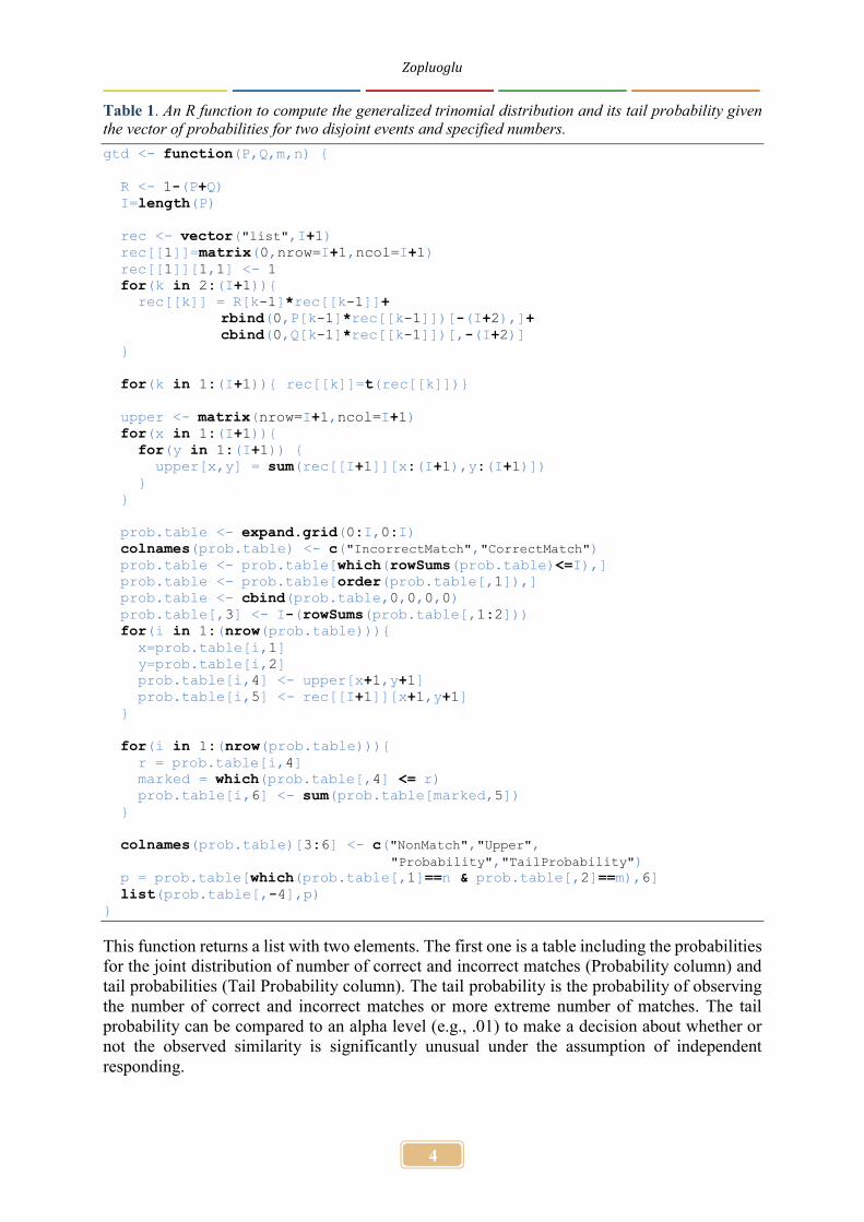
Table 1. An R function to compute the generalized trinomial distribution and its tail probability given the vector of probabilities for two disjoint events and specified numbers.

gtd <- function(P,Q,m,n) { R <- 1-(P+Q) I=length(P) rec <- vector("list",I+1) rec[[1]]=matrix(0,nrow=I+1,ncol=I+1) rec[[1]][1,1] <- 1 for(k in 2:(I+1)){ rec[[k]] = R[k-1]*rec[[k-1]]+ rbind(0,P[k-1]*rec[[k-1]])[-(I+2),]+ cbind(0,Q[k-1]*rec[[k-1]])[,-(I+2)] } for(k in 1:(I+1)){ rec[[k]]=t(rec[[k]])} upper <- matrix(nrow=I+1,ncol=I+1) for(x in 1:(I+1)){ for(y in 1:(I+1)) { upper[x,y] = sum(rec[[I+1]][x:(I+1),y:(I+1)]) } } prob.table <- expand.grid(0:I,0:I) colnames(prob.table) <- c("IncorrectMatch","CorrectMatch") prob.table <- prob.table[which(rowSums(prob.table)<=I),] prob.table <- prob.table[order(prob.table[,1]),] prob.table <- cbind(prob.table,0,0,0,0) prob.table[,3] <- I-(rowSums(prob.table[,1:2])) for(i in 1:(nrow(prob.table))){ x=prob.table[i,1] y=prob.table[i,2] prob.table[i,4] <- upper[x+1,y+1] prob.table[i,5] <- rec[[I+1]][x+1,y+1] } for(i in 1:(nrow(prob.table))){ r = prob.table[i,4] marked = which(prob.table[,4] <= r) prob.table[i,6] <- sum(prob.table[marked,5]) } colnames(prob.table)[3:6] <- c("NonMatch","Upper", "Probability","TailProbability") p = prob.table[which(prob.table[,1]==n & prob.table[,2]==m),6] list(prob.table[,-4],p) }

This function returns a list with two elements. The first one is a table including the probabilities for the joint distribution of number of correct and incorrect matches (Probability column) and tail probabilities (Tail Probability column). The tail probability is the probability of observing the number of correct and incorrect matches or more extreme number of matches. The tail probability can be compared to an alpha level (e.g., .01) to make a decision about whether or not the observed similarity is significantly unusual under the assumption of independent responding.

Int. J. Asst. Tools in Educ., Vol. 6, No. 5-Special Issue, (2019) pp. 1-19

5

Table 2. An example of use for the R function to compute the generalized trinomial distribution and its tail probability given the vector of probabilities for two disjoint events and specified numbers.

P <- c(0.45,0.60,0.30,0.55,0.58,0.42,0.60,0.25) Q <- c(0.15,0.20,0.07,0.10,0.12,0.18,0.30,0.05) M4 <- gtd(P, Q, m=3,n=2) M4 [[1]] IncorrectMatch CorrectMatch NonMatch Probability TailProbability 1 0 0 8 0.00014817600 1.00000000000 10 0 1 7 0.00229866840 0.99985182400 19 0 2 6 0.01383419478 0.99755315560 28 0 3 5 0.04290090345 0.98371896082 37 0 4 4 0.07560196143 0.88706918856 46 0 5 3 0.07769363787 0.52528666715 55 0 6 2 0.04534833951 0.21852241329 64 0 7 1 0.01366565580 0.05554589926 73 0 8 0 0.00162785700 0.00412010397 2 1 0 7 0.00084360360 0.94081805737 11 1 1 6 0.00964994464 0.93997445377 20 1 2 5 0.04325532057 0.93032450913 29 1 3 4 0.09890315828 0.81146722713 38 1 4 3 0.12439288143 0.71256406885 47 1 5 2 0.08552521188 0.36981797220 56 1 6 1 0.02949871068 0.11179242607 65 1 7 0 0.00393499620 0.01063825410 3 2 0 6 0.00161592858 0.58817118742 12 2 1 5 0.01406754191 0.58655525884 21 2 2 4 0.04720104978 0.57248771693 30 2 3 3 0.07777505708 0.44759302928 39 2 4 2 0.06577034703 0.28429276032 48 2 5 1 0.02674781613 0.08229371539 57 2 6 0 0.00408353481 0.01472178891 4 3 0 5 0.00147975807 0.17317407378 13 3 1 4 0.00975200588 0.17169431571 22 3 2 3 0.02374799388 0.16194230983 31 3 3 2 0.02640188988 0.13819431595 40 3 4 1 0.01320810993 0.04114389883 49 3 5 0 0.00237669012 0.00670325790 5 4 0 4 0.00073634463 0.04188024346 14 4 1 3 0.00354190993 0.02793578890 23 4 2 2 0.00583529943 0.02439387897 32 4 3 1 0.00383679063 0.01855857954 41 4 4 0 0.00084883518 0.00116303490 6 5 0 3 0.00020646381 0.00432656778 15 5 1 2 0.00067335552 0.00249224697 24 5 2 1 0.00065585655 0.00181889145 33 5 3 0 0.00019058868 0.00031419972 7 6 0 2 0.00003170475 0.00012361104 16 6 1 1 0.00006111576 0.00009190629 25 6 2 0 0.00002628801 0.00003079053 8 7 0 1 0.00000239652 0.00000450252 17 7 1 0 0.00000203796 0.00000210600 9 8 0 0 0.00000006804 0.00000006804 [[2]] [1] 0.4476

Zopluoglu

6

Suppose that two test takers responded to eight items and we know the probability of matching correct and matching incorrect responses for each item (𝐏 and 𝐐 vectors). Also, suppose that these two test takers have the same correct answer for three items and the same incorrect response for two items. How likely this outcome would be? Table 2 presents the results obtained from the R function provided in Table 1 for this specific scenario.

The Table 2 indicates that observing three correct and two incorrect matches for a pair of test takers with the given 𝐏 and 𝐐 is 0.0778. For the same pair, observing three correct and two incorrect matches or more extreme similarity is 0.4476. If we use a type-I error rate of 0.01, then we can decide that the response similarity between these two test takers is not significantly unusual because the tail probability is not smaller than .01.

3.2. Computing M4 for Dichotomous Data

For a given dichotomous dataset, the steps to compute the M4 statistics between two test takers are below:

1. Decision about the dichotomous IRT model to use. Researchers can choose a particular model based on their own judgement, or can fit all possible models and then empirically decide the best fitting model. The researchers are strongly encouraged to evaluate the plausibility of model assumptions such as unidimensionality and local independent before proceeding.

2. Estimation of item and person parameters based on the chosen dichotomous IRT model in Step 1.

3. Computation of the P and Q vectors for two test takers given their estimated person parameters and the estimated item parameters.

4. Computation of the tail probability for the observed number of correct and incorrect matches between these two test takers using the gtd() function introduced above.

For demonstration, I will use a dichotomous dataset that is publicly available on the following link https://itemanalysis.com/example-data-files/. This dataset includes binary responses to 56 items for 6,000 test takers. Table 3 and Table 4 shows the code to import the dataset and then fitting the 1-, 2-, and 3-PL IRT models using the mirt package (Chalmers, 2012) to decide the best fitting model. Based on the model fit indices, the best fitting model is the 3-PL IRT model.

Table 3. R code to import the dataset and display the first few rows

setwd("Path to file") # Here you put the path to the folder for the dataset exam1 <- read.csv("exam1_scored.txt") # Import the dataset dim(exam1) # Ask R to show the dimensions of the dataset [1] 6000 56 # This indicates there are 6,000 rows and 56 columns head(exam1,3) # Ask R to display the first three rows of the dataset item1 item2 item3 item4 item5 item6 item7 item8 item9 item10 item11 1 1 0 0 0 1 1 1 1 0 1 1 2 1 0 1 0 1 1 0 1 1 1 1 3 1 0 0 1 0 0 0 1 1 1 1 item12 item13 item14 item15 item16 item17 item18 item19 item20 item21 1 1 1 1 1 1 1 1 1 0 0 2 1 1 1 1 1 0 0 1 1 0 3 1 1 0 1 1 0 0 1 1 0

Int. J. Asst. Tools in Educ., Vol. 6, No. 5-Special Issue, (2019) pp. 1-19

7

Table 3. Continued

item22 item23 item24 item25 item26 item27 item28 item29 item30 item31 1 1 0 1 1 1 0 0 1 0 0 2 1 1 1 0 1 0 1 0 0 1 3 0 1 1 0 1 0 0 0 1 0 item32 item33 item34 item35 item36 item37 item38 item39 item40 item41 1 1 1 1 1 1 0 1 1 1 1 2 0 1 1 0 0 1 0 0 1 0 3 1 1 0 0 1 0 1 0 1 1 item42 item43 item44 item45 item46 item47 item48 item49 item50 item51 1 1 1 0 1 0 0 0 0 0 1 2 0 1 0 0 0 0 0 0 0 1 3 0 1 0 0 1 1 0 1 1 1 item52 item53 item54 item55 item56 1 0 1 0 0 1 2 0 1 1 1 0 3 1 1 0 1 1

Table 4. R code to fit dichotomous IRT models, to choose the best fitting model, and to estimate item and person parameters for the best fitting model

install.packages("mirt") # Install the mirt package into your computer require(mirt) # Load the library to the R session # Fit 1PL model mod <- 'F = 1-56 CONSTRAIN = (1-56,a1)' onePL <- mirt(data = exam1, model = mod, itemtype="2PL",SE=TRUE) # Fit 2PL model twoPL <- mirt(data = exam1, model = 1,itemtype="2PL",SE=TRUE) # Fit 3PL model threePL <- mirt(data = exam1, model = 1,itemtype="3PL",SE=TRUE) # Compare the model fit anova(onePL,twoPL) # 1PL vs 2PL anova(twoPL,threePL) # 2PL vs 3PL # 3 PL fits best. # Item parameters for the 3PL model ipar <- coef(threePL,IRTpars=TRUE,simplify=TRUE)$items[,1:3] head(ipar,3) # display the item parameters for the first 3 rows a b g item1 1.0503 -0.37464 0.306052 item2 0.6379 -0.02992 0.050127 item3 1.5072 -1.27318 0.064474 # Estimate the ML theta estimates

Zopluoglu

8

Table 4. Continued

mle <- fscores(threePL,method="ML") # This generates a 6000 x 1 matrix head(mle,3) # display the ML theta estimates for the first 3 rows F1 [1,] 0.32301 [2,] -0.07246 [3,] 0.25915

Then, I save the estimated item parameters for the 3PL model into an object (ipar) and estimate the maximum likelihood person parameter estimates. Given these estimated item and person parameters based on the 3-PL model, suppose that we want to compute the M4 response similarity statistic for two test takers, subjects 1035 and 1567. We need to compute P and Q vectors. In order to compute the P and Q vectors, we have to compute the probability of correct response for each item for these two test takers using the estimated item parameters and their estimated person parameters. Table 5 shows the R code to compute the P and Q vectors for individuals 1035 and 1567 based on the estimated person parameters and item parameters.

These two test takers are matching on the correct response for 40 items and matching on the incorrect response for three items. Given their joint probability vectors for the correct and incorrect responses across all items (P and Q vectors), Table 6 shows how to use the gtd() function to compute the probability for the degree of the observed similarity or more extreme similarity between these two test takers. The tail probability is 0.557. This indicates that the observed similarity between these two test takers are not very unlikely. Therefore, we can conclude that there is no unusual degree of response similarity between the two test takers. It may be sometimes useful to visually present the results. Table 7 shows the R code to create a contour plot which was also discussed in Maynes (2017). In this contour plot, the boundary lines represent the likelihood of .01, .001, .0001, and .0001 for the number of correct and incorrect matches between two response vectors. In addition, the observed number of correct and incorrect matches is marked in the plot. One can easily demonstrate how likely the observed similarity is between two response vectors using this plot.

Int. J. Asst. Tools in Educ., Vol. 6, No. 5-Special Issue, (2019) pp. 1-19

9

Table 5. R code to compute the P and Q vectors for individuals 1035 and 1567 based on the estimated person parameters and item parameters

# Estimated theta for Person 1035 and person 1567 th1 <- mle[1035,1] th1 F1 1.415 th2 <- mle[1567,1] th2 F1 1.577 # A small function to compute the probability of correct response # given the item and person parameters for the 3-PL model prob <- function(ip,th){ # ip - n x 3 item parameter matrix. Columns are a, b, g respectively # th - a numeric value ip[,3]+((1-ip[,3])*(1/(1+exp(-ip[,1]*(th-ip[,2]))))) } # Probability of correct response across items for the two test takers P1 <- prob(ip=ipar,th=th1) # Test taker 1035 P1 item1 item2 item3 item4 item5 item6 item7 item8 item9 item10 0.9081 0.7296 0.9840 0.7483 0.8505 0.9322 0.7347 0.9950 0.7968 0.9924 item11 item12 item13 item14 item15 item16 item17 item18 item19 item20 0.9939 0.7983 0.9855 0.7202 0.9288 0.7388 0.6960 0.7229 0.9820 0.8225 item21 item22 item23 item24 item25 item26 item27 item28 item29 item30 0.8964 0.8104 0.7232 0.9633 0.8764 0.9615 0.3099 0.6112 0.7061 0.7084 item31 item32 item33 item34 item35 item36 item37 item38 item39 item40 0.5605 0.5130 0.9455 0.8687 0.9789 0.9653 0.8835 0.6294 0.5555 0.8618 item41 item42 item43 item44 item45 item46 item47 item48 item49 item50 0.9160 0.7597 0.8911 0.7167 0.9202 0.9097 0.8501 0.8702 0.7808 0.9943 item51 item52 item53 item54 item55 item56 0.9947 0.8833 0.8771 0.5813 0.7557 0.9771 P2 <- prob(ip=ipar,th=th2) # Test taker 1567 P2 item1 item2 item3 item4 item5 item6 item7 item8 item9 item10 0.9208 0.7491 0.9874 0.7646 0.8650 0.9421 0.7658 0.9963 0.8196 0.9944 item11 item12 item13 item14 item15 item16 item17 item18 item19 item20 0.9955 0.8186 0.9889 0.7465 0.9420 0.7773 0.7228 0.7476 0.9874 0.8556 item21 item22 item23 item24 item25 item26 item27 item28 item29 item30 0.9173 0.8493 0.7807 0.9750 0.9040 0.9686 0.3673 0.6409 0.7358 0.7469 item31 item32 item33 item34 item35 item36 item37 item38 item39 item40 0.5960 0.5637 0.9583 0.8986 0.9857 0.9754 0.9059 0.6572 0.5921 0.8797 item41 item42 item43 item44 item45 item46 item47 item48 item49 item50 0.9302 0.7822 0.9076 0.7676 0.9413 0.9284 0.8868 0.9025 0.8103 0.9968

Zopluoglu

10

Table 5. Continued

item51 item52 item53 item54 item55 item56 0.9969 0.9092 0.9061 0.6091 0.7960 0.9841 # Joint probability of correct response across items (P vector) P <- P1*P2 P item1 item2 item3 item4 item5 item6 item7 item8 item9 item10 0.8362 0.5466 0.9716 0.5722 0.7357 0.8782 0.5626 0.9914 0.6530 0.9868 item11 item12 item13 item14 item15 item16 item17 item18 item19 item20 0.9894 0.6535 0.9746 0.5376 0.8750 0.5743 0.5031 0.5405 0.9696 0.7037 item21 item22 item23 item24 item25 item26 item27 item28 item29 item30 0.8223 0.6882 0.5647 0.9392 0.7923 0.9313 0.1138 0.3918 0.5195 0.5292 item31 item32 item33 item34 item35 item36 item37 item38 item39 item40 0.3341 0.2892 0.9061 0.7806 0.9649 0.9416 0.8003 0.4137 0.3290 0.7581 item41 item42 item43 item44 item45 item46 item47 item48 item49 item50 0.8521 0.5943 0.8088 0.5501 0.8662 0.8446 0.7539 0.7854 0.6326 0.9911 item51 item52 item53 item54 item55 item56 0.9916 0.8032 0.7947 0.3541 0.6015 0.9616 # Joint probability of incorrect response across items (Q vector) Q <- (1-P1)*(1-P2) Q item1 item2 item3 item4 item5 item6 0.00727836 0.06782913 0.00020138 0.05923844 0.02017187 0.00392514 item7 item8 item9 item10 item11 item12 0.06213472 0.00001822 0.03665862 0.00004270 0.00002744 0.03658889 item13 item14 item15 item16 item17 item18 0.00016096 0.07092701 0.00412716 0.05816974 0.08425009 0.06993389 item19 item20 item21 item22 item23 item24 0.00022726 0.02563475 0.00855995 0.02857902 0.06068258 0.00091665 item25 item26 item27 item28 item29 item30 0.01186580 0.00120889 0.43662558 0.13959138 0.07765921 0.07378293 item31 item32 item33 item34 item35 item36 0.17755613 0.21249479 0.00227399 0.01332128 0.00030215 0.00085127 item37 item38 item39 item40 item41 item42 0.01096429 0.12702758 0.18128293 0.01663444 0.00586350 0.05232573 item43 item44 item45 item46 item47 item48 0.01005836 0.06584107 0.00468136 0.00646589 0.01696561 0.01265535 item49 item50 item51 item52 item53 item54 0.04159484 0.00001832 0.00001658 0.01059035 0.01153943 0.16365438 item55 item56 0.04983442 0.00036321 # Observed number of correct matches between the two test takers m = sum (exam1[1035,]==1 & exam1[1567,]==1) m [1] 40 # Observed number of incorrect matches between the two test takers n = sum (exam1[1035,]==0 & exam1[1567,]==0) n [1] 3

Int. J. Asst. Tools in Educ., Vol. 6, No. 5-Special Issue, (2019) pp. 1-19

11

Table 6. R code to compute the M4 response similarity index between examinees 1035 and 1567 based on the P and Q vectors computed from dichotomous item response data

M4 <- gtd(P=P,Q=Q,m=m,n=n) M4[[1]] # Probabilities for the trinomial distribution IncorrectMatch CorrectMatch NonMatch Probability TailProbability 1 0 0 56 3.278e-46 1.000e+00 58 0 1 55 2.769e-43 1.000e+00 115 0 2 54 1.070e-40 1.000e+00 ……………………………………………………………………………………………………………………………………………………………………………………… 3136 0 55 1 5.728e-09 4.383e-08 3193 0 56 0 2.057e-10 7.333e-10 2 1 0 55 2.259e-45 9.985e-01 59 1 1 54 1.904e-42 9.985e-01 116 1 2 53 7.336e-40 9.985e-01 ……………………………………………………………………………………………………………………………………………………………………………………… 3080 1 54 1 4.626e-08 3.585e-07 3137 1 55 0 1.814e-09 8.515e-09 3 2 0 54 7.426e-45 9.685e-01 60 2 1 53 6.242e-42 9.685e-01 117 2 2 52 2.399e-39 9.685e-01 ……………………………………………………………………………………………………………………………………………………………………………………… 3024 2 53 1 1.505e-07 9.657e-07 3081 2 54 0 6.304e-09 3.612e-08 ……………………………………………………………………………………………………………………………………………………………………………………… 54 53 0 3 2.169e-106 6.136e-101 111 53 1 2 4.364e-104 6.136e-101 168 53 2 1 2.826e-102 6.131e-101 225 53 3 0 5.848e-101 5.849e-101 55 54 0 2 2.227e-109 1.082e-105 112 54 1 1 3.108e-107 1.082e-105 169 54 2 0 1.051e-105 1.051e-105 56 55 0 1 1.391e-112 1.021e-110 113 55 1 0 1.007e-110 1.007e-110 57 56 0 0 3.968e-116 3.968e-116 M4[[2]] # Tail Probability [1] 0.5571

Zopluoglu

12

Table 7. R code to create a contour plot for a visual representation of the result provided by the M4 index

install.packages("lattice") library(lattice) obs <- c(40,3) contourplot(TailProbability ~ CorrectMatch + IncorrectMatch, data=M4[[1]], labels=FALSE, xlab="Number of Correct Matches", ylab="Number of Incorrect Matches", panel=function(at,lty,...){ panel.contourplot(at = .00001, lty = 1,...) panel.contourplot(at = .0001, lty = 2,...) panel.contourplot(at = .001, lty = 3,...) panel.contourplot(at = .01, lty = 4,...) panel.points(x=obs[1],y=obs[2], pch=15, cex=1) }, key=list(corner=c(1,.9),lines=list(lty=c(1,2,3)), text=list(c("p=0.00001","p=0.0001","p=0.001","p=0.01"))), scales=list(y=list(at=seq(0,56,4)),x=list(at=seq(0,56,4)))

Figure 1. Contour plot for the joint probability distribution of correct and incorrect matches

Int. J. Asst. Tools in Educ., Vol. 6, No. 5-Special Issue, (2019) pp. 1-19

13

3.3. Computing M4 for Nominal Response Data

The steps to compute the M4 index for nominal response data are identical to the dichotomous dataset. In particular, we are interested in multiple-choice test data where one of the response options is considered as the correct response (key) and other response options are considered as the incorrect responses (distractors). As mentioned before, there are a few number of alternative models proposed in the literature for multiple-choice test data (Bock, 1972; Penfield and de la Torre, 2008; Thissen & Steinberg, 1997). One can choose any of these models for modeling probabilities. We consider here the original Nominal Response Model (NRM; Bock, 1972). For this section, I will use the nominal version of the dichotomous dataset used before. We will also need a vector of correct response option for these 56 items. In order to fit NRM in the mirt package, we first transform these nominal A, B, C, and D response categories in the dataset to numbers 1, 2, 3, and 4, respectively. Then, we also need to recode data such that the correct response option is always assigned to the highest number possible (e.g., four in this case). Table 8 shows a compilation of R code to prepare the dataset for the data analysis.

Table 8. R code to prepare nominal response data for data analysis

# Import dataset exam1_nom <- read.csv("exam1_nominal.txt") dim(exam1_nom) [1] 6000 56 head(exam1_nom,3) # display the first 3 rows of the dataset item1 item2 item3 item4 item5 item6 item7 item8 item9 item10 item11 1 A A D D C B C D D D C 2 A B C C C B A D A D C 3 A C D B D D D D A D C item12 item13 item14 item15 item16 item17 item18 item19 item20 item21 1 A D C A B D B A B B 2 A D C A B A D A C B 3 A D D A B A A A C B item22 item23 item24 item25 item26 item27 item28 item29 item30 item31 1 A D B C B A C A C A 2 A C B D B C A D B C 3 C C B B B B D D A A item32 item33 item34 item35 item36 item37 item38 item39 item40 item41 1 B B A B D C A D C D 2 A B A D B D B C C A 3 B B C C D B A C C D item42 item43 item44 item45 item46 item47 item48 item49 item50 item51 1 A B C C C D B D D D 2 D B C A B A D A D D 3 D B D A D B D C B D item52 item53 item54 item55 item56 1 D C A D D 2 C C B A C 3 A C C A D # Key response vector (correct responses for 56 items) key <- c("A","D","C","B","C","B","C","D","A","D","C","A","D","C", "A","B","D","B","A","C","A","A","C","B","C","B","D","A",

Zopluoglu

14

Table 8. Continued

"A","A","C","B","B","A","B","D","D","A","D","C","D","A", "B","B","C","D","B","C","C","B","D","A","C","B","A","D") # Recode A,B,C,D to 1,2,3,4 for(i in 1:ncol(exam1_nom)){ exam1_nom[,i]=ifelse(exam1_nom[,i]=="A",1, ifelse(exam1_nom[,i]=="B",2, ifelse(exam1_nom[,i]=="C",3, ifelse(exam1_nom[,i]=="D",4,NA)))) } # Recode the vector of key responses new.key <- ifelse(key=="A",1, ifelse(key=="B",2, ifelse(key=="C",3, ifelse(key=="D",4,NA)))) # Recode the data so that the correct option is always scored as 4 for(i in 1:ncol(exam1_nom)) { hold1 <- which(exam1_nom[,i]==new.key[i]) hold2 <- which(exam1_nom[,i]==4) exam1_nom[hold1,i]= 4 exam1_nom[hold2,i]= new.key[i] } head(exam1_nom,3) # display the first 3 rows of recoded data item1 item2 item3 item4 item5 item6 item7 item8 item9 item10 item11 1 4 1 3 2 4 4 4 4 1 4 4 2 4 2 4 3 4 4 1 4 4 4 4 3 4 3 3 4 3 2 3 4 4 4 4 item12 item13 item14 item15 item16 item17 item18 item19 item20 item21 1 4 4 4 4 4 4 4 4 2 2 2 4 4 4 4 4 1 2 4 4 2 3 4 4 3 4 4 1 1 4 4 2 item22 item23 item24 item25 item26 item27 item28 item29 item30 item31 1 4 3 4 4 4 1 3 4 3 1 2 4 4 4 3 4 3 4 1 2 4 3 3 4 4 2 4 2 1 1 4 1 item32 item33 item34 item35 item36 item37 item38 item39 item40 item41 1 4 4 4 4 4 3 4 4 4 4 2 1 4 4 2 2 4 2 3 4 1 3 4 4 3 3 4 2 4 3 4 4 item42 item43 item44 item45 item46 item47 item48 item49 item50 item51 1 4 4 3 4 3 2 2 3 2 4 2 1 4 3 1 2 1 3 1 2 4 3 1 4 2 1 4 4 3 4 4 4 item52 item53 item54 item55 item56 1 1 4 1 1 4 2 3 4 4 4 3 3 4 4 3 4 4

Int. J. Asst. Tools in Educ., Vol. 6, No. 5-Special Issue, (2019) pp. 1-19

15

Once the dataset is prepared, we fit the nominal response model using the mirt package and extract the item parameters. In the nominal response model, each response category has one slope and one intercept parameter. Table 9 shows the R code to fit the model and estimate the item and person parameters. As it is seen, the item parameter matrix has eight columns with the first four columns (labeled as a1, a2, a3, and a4) are response category slope parameters and the last four columns (labeled as c1, c2, c3, and c4) are response category intercept parameters. Once these item parameters are obtained, we also estimate a person parameter for each individual based on maximum likelihood estimation.

Table 9. R code to fit the nominal response model and estimate item and person parameters

# Fit the Nominal Response Model nrm <- mirt(exam1_nom, 1, 'nominal') # Item parameter estimates ipar.nrm <- coef(nrm, simplify=T, IRTpars = TRUE)$item head(ipar.nrm,3) # display the first 3 rows of item parameter matrix a1 a2 a3 a4 c1 c2 c3 c4 item1 0.29203 -0.36571 -0.69963 0.7733 0.0001801 -0.7811 -0.95435 1.7352 item2 0.14899 -0.17617 -0.43625 0.4634 -0.3189671 -0.3362 -0.29905 0.9542 item3 -0.71860 -0.45263 -0.17098 1.3422 -1.3477243 -0.8299 -0.37141 2.5490 # Person parameter estimates theta.ML <- fscores(nrm,method="ML") head(theta.ML,3) # display the first 3 rows of the person parameter matrix F1 [1,] 0.21598 [2,] -0.32331 [3,] -0.05163

In order to compute the P and Q vectors based on nominal response data, we first need to create a function to compute the probability of selecting each response category on each item for a person given the nominal response model item parameter and the person parameter estimates. The R code in Table 10 takes the nominal response model estimated item parameter matrix obtained from the mirt package and the person parameter estimates for an individual as inputs and returns a matrix of probabilities for each response option on each item for the individual. For instance, we can see that the model predicted probabilities of choosing response categories 1, 2, 3, and 4 (correct response) for subject 1035 on the first item are .071, .011, .005, and .913, respectively. Similarly, the model probabilities of choosing response categories 1, 2, 3, and 4 (correct response) for subject 1567 on the first item are .050, .004, .002, and .944. Once the probability matrix for each subject is obtained, then the P vector, joint probability of matching on the correct response for each item, and Q vector, joint probability of matching on an incorrect response for each item, are computed. For instance, the probability of matching on the response category 4 (correct response) for subject 1035 and subject 1567 would be equal to 0.913*0.944 = 0.861 and the probability of matching on the response category 1, 2, or 3 would be (0.071*0.050 + 0.011*0.004 + 0.005*0.002) = 0.004. You can see at the end of Table 10 that we do this computation for each item and create the P and Q vectors.

Zopluoglu

16

After we obtain the P and Q vectors, we can now compute the M4 index for the same two test takers 1035 and 1567 using the nominal response data. Table 11 shows the R code to run gtd() function again taking the P and Q vectors, observed number of matches on correct responses (m), and observed number matches on incorrect responses (n) as inputs, and returns the generalized trinomial distribution for the number of correct and incorrect matches for every possible outcome. Also, the function returns the tail probability for observing more extreme similarity between two test takers. The tail probability is 0.9378 and can be compared to a conventional alpha level (e.g., 0.01) to make a decision about the degree of unusual similarity.

4. FINAL REMARKS A very nice theoretical introduction and discussion of the M4 index have been provided by Maynes (2017); however, there has not been an accessible tool to compute the M4 index for other practitioners and researchers in the field of educational testing. The M4 index is a computationally demanding method. Its computation requires recursive algorithms that may not very easy to understand and implement. In this paper, I introduced an R function to compute the probabilities of the generalized trinomial distribution for two disjoint events, and demonstrated how this function can be used along with other R item response theory packages (e.g., mirt) to compute the M4 index under the dichotomous and nominal item response models. The availability of an open source computational tool will help the practitioners and the consumers of this index understand the nature of the M4 index better and will also help researchers conduct deeper investigations in the future about the properties of the M4 index under different conditions with real and simulated datasets.

Table 10. R code to compute the P and Q vectors based on nominal response dataset for individuals 1035 and 1567 based on the estimated person parameters and item parameters

# An internal function to compute the probability of choosing each response # category of each item given the item parameter matrix and a person # parameter estimate irtprob <- function(th, item.param) {

# Inputs:

# item.param - n x 4 item parameter matrix. # First four columns are slopes, and the last four columns are

# intercepts # th - ability - a numeric value

n.opt = ncol(item.param)/2 prob <- matrix(nrow = nrow(item.param), ncol = ncol(item.param)/2) for (j in 1:ncol(prob)) { prob[,j] = exp((item.param[, j] * th) + item.param[,j + n.opt]) } prob <- prob/rowSums(prob) prob }

# Estimated theta for Person 1035 and person 1567 based on nominal response # model

Int. J. Asst. Tools in Educ., Vol. 6, No. 5-Special Issue, (2019) pp. 1-19

17

Table 10. Continued

th1 <- theta.ML[1035,1] th1 F1 1.692 th2 <- theta.ML[1567,1] th2 F1 2.514 # Probability matrices. These have 56 rows, each row is representing an item # They have four columns, each column is representing a response category P1 <- irtprob(item.param=ipar.nrm,th=th1) # Test taker 1035 P1 [,1] [,2] [,3] [,4] [1,] 0.07131223 0.0107270 0.0051265 0.9128 [2,] 0.12456912 0.0706226 0.0472016 0.7576 ……………………………………………………………………………………………………………. [55,] 0.15651175 0.0552107 0.0473266 0.7410 [56,] 0.00444109 0.0067377 0.0093141 0.9795 P2 <- irtprob(item.param=ipar.nrm,th=th2) # Test taker 1567 P2 [,1] [,2] [,3] [,4] [1,] 0.049684924 0.0043540 0.00158164 0.9444 [2,] 0.104793552 0.0454847 0.02455257 0.8252 ……………………………………………………………………………………………………………… [55,] 0.102024390 0.0296282 0.02506444 0.8433 [56,] 0.001038142 0.0017010 0.00266656 0.9946 # Joint probability of correct and incorrect responses across items #(P and Q vector) # Note that in this recoded dataset used to fit the model, # we re-coded the correct response as 4 for all items # So, 1, 2, and 3 are incorrect responses. P <- P1[,4]*P2[,4] Q <- rowSums(P1[,1:3]*P2[,1:3]) # Observed number of correct matches between the two test takers m <- sum((exam1_nom[1035,]==exam1_nom[1567,] & exam1_nom[1035,]==4)*1,na.rm=TRUE) # Observed number of incorrect matches between the two test takers n <- sum((exam1_nom[1035,]==exam1_nom[1567,] & exam1_nom[1035,]!=4)*1,na.rm=TRUE)

Zopluoglu

18

Table 11. R code to compute the M4 response similarity index between examinees 1035 and 1567 based on the P and Q vectors computed from nominal response data

M4 <- gtd(P=P,Q=Q,m=m,n=n) M4[[1]] # Probabilities for the trinomial distribution IncorrectMatch CorrectMatch NonMatch Probability TailProbability 1 0 0 56 1.251e-50 1.000e+00 58 0 1 55 2.847e-47 1.000e+00 115 0 2 54 2.717e-44 1.000e+00 ……………………………………………………………………………………………………………………………………………………………………………………… 3136 0 55 1 5.428e-08 2.222e-07 3193 0 56 0 1.836e-09 8.750e-09 2 1 0 55 3.301e-50 9.034e-01 59 1 1 54 7.505e-47 9.034e-01 116 1 2 53 7.153e-44 9.034e-01 ……………………………………………………………………………………………………………………………………………………………………………………… 3080 1 54 1 1.661e-07 9.390e-07 3137 1 55 0 6.320e-09 2.739e-08 3 2 0 54 4.188e-50 5.360e-01 60 2 1 53 9.512e-47 5.360e-01 117 2 2 52 9.054e-44 5.360e-01 ……………………………………………………………………………………………………………………………………………………………………………………… 3024 2 53 1 2.111e-07 1.202e-06 3081 2 54 0 8.794e-09 5.272e-08 4 3 0 53 3.405e-50 2.439e-01 61 3 1 52 7.727e-47 2.439e-01 118 3 2 51 7.345e-44 2.439e-01 ……………………………………………………………………………………………………………………………………………………………………………………… 2968 3 52 1 1.538e-07 7.729e-07 3025 3 53 0 6.912e-09 3.431e-08 ……………………………………………………………………………………………………………………………………………………………………………………… 56 55 0 1 3.362e-144 1.259e-141 113 55 1 0 1.256e-141 1.256e-141 57 56 0 0 9.791e-149 9.791e-149 M4[[2]] # Tail Probability [1] 0.9378

ORCID Cengiz Zopluoglu https://orcid.org/0000-0002-9397-0262

5. REFERENCES

Bock, R. D. (1972). Estimating item parameters and latent ability when responses are scored in two or more nominal categories. Psychometrika, 37(1), 29-51.

Chalmers, R.P. (2012). mirt: A Multidimensional Item Response Theory Package for the R Environment. Journal of Statistical Software, 48(6), 1 - 29. URL http://www.jstatsoft.org/v48/i06/

Charalambides, C. A. (2005). Combinatorial methods in discrete distributions (Vol. 600). John Wiley & Sons.

Gabriel, T. (2010, December 27). Cheaters find an Adversary in Technology. The New York Times. Retrieved from https://www.nytimes.com/2010/12/28/education/28cheat.html

Int. J. Asst. Tools in Educ., Vol. 6, No. 5-Special Issue, (2019) pp. 1-19

19

Maynes, D.D. (2014). Detection of non-independent test taking by similarity analysis. In N. M. Kingston and A. K. Clark (Eds.) Test fraud: Statistical detection and methodology (pp. 53-82). Routledge: New York, NY.

Maynes, D. D. (2017). Detecting potential collusion among individual examinees using similarity analysis. In GJ Cizek and JA Wollack (eds.), Handbook of quantitative methods for detecting cheating on tests, Chapter 3, 47-69. Routledge, New York, NY.

Penfield, R. D., de la Torre, J., & Penfield, R. (2008). A new response model for multiple-choice items. Presented at the annual meeting of the National Council on Measurement in Education, New York.

Thissen, D., & Steinberg, L. (1984). A response model for multiple choice items. Psychometrika, 49(4), 501-519.

van der Linden, W. J., & Sotaridona, L. (2006). Detecting answer copying when the regular response process follows a known response model. Journal of Educational and Behavioral Statistics, 31(3), 283-304.

Wollack, J. A. (1997). A nominal response model approach for detecting answer copying. Applied Psychological Measurement, 21(4), 307-320.