Properties of the ionized gas in HH 202 - II. Results from echelle spectrophotometry with...

Mon. Not. R. Astron. Soc. 395, 855–876 (2009) doi:10.1111/j.1365-2966.2009.14554.x

Properties of the ionized gas in HH 202 – II. Results from echellespectrophotometry with Ultraviolet Visual Echelle Spectrograph�

A. Mesa-Delgado,1† C. Esteban,1 J. Garcıa-Rojas,2 V. Luridiana,3 M. Bautista,4

M. Rodrıguez,5 L. Lopez-Martın1 and M. Peimbert21Instituto de Astrofısica de Canarias, E-38200 La Laguna, Tenerife, Spain2Instituto de Astronomıa, UNAM, Apdo. Postal 70-264, 04510 Mexico D.F., Mexico3Instituto de Astrofısica de Andalucıa (CSIC), Apdo. Correos 3004, E-18080 Granada, Spain4Deparment of Physics, Virginia Polytechnic and State University, Blacksburg, VA 24061, USA5Instituto Nacional de Astrofısica, Optica y Electronica INAOE, Apdo. Postal 51 y 216, 7200 Puebla, Pue., Mexico

Accepted 2009 January 23. Received 2008 December 23; in original form 2008 October 24

ABSTRACTWe present results of deep echelle spectrophotometry of the brightest knot of the Herbig–Haro object HH 202 in the Orion Nebula – HH 202-S – using the Ultraviolet Visual EchelleSpectrograph in the spectral range from 3100 to 10 400 Å. The high spectral resolution of theobservations has permitted to separate the component associated with the ambient gas fromthat associated with the gas flow. We derive electron densities and temperatures from differentdiagnostics for both components, as well as the chemical abundances of several ions andelements from collisionally excited lines, including the first determinations of Ca+ and Cr+

abundances in the Orion Nebula. We also calculate the He+, C2+, O+ and O2+ abundancesfrom recombination lines. The difference between the O2+ abundances determined fromcollisionally excited and recombination lines – the so-called abundance discrepancy factor –is 0.35 and 0.11 dex for the shock and nebular components, respectively. Assuming thatthe abundance discrepancy is produced by spatial variations in the electron temperature,we derive values of the temperature fluctuation parameter, t2, of 0.050 and 0.016 for theshock and nebular components, respectively. Interestingly, we obtain almost coincident t2

values for both components from the analysis of the intensity ratios of He I lines. We findsignificant departures from case B predictions in the Balmer and Paschen flux ratios of linesof high principal quantum number n. We analyse the ionization structure of HH 202-S, findingenough evidence to conclude that the flow of HH 202-S has compressed the ambient gasinside the nebula trapping the ionization front. We measure a strong increase of the totalabundances of nickel and iron in the shock component, the abundance pattern and the resultsof photoionization models for both components are consistent with the partial destruction ofdust after the passage of the shock wave in HH 202-S.

Key words: ISM: abundances – dust, extinction – ISM: Herbig–Haro objects – ISM: individ-ual: Orion Nebula – ISM: individual: HH 202.

1 IN T RO D U C T I O N

HH 202 is one of the brightest and most conspicuous Herbig–Haro(HH) objects of the Orion Nebula. It was discovered by Canto et al.(1980). The origin of this outflow is not clear, though the radialvelocity and proper motion studies suggest that this object forms a

�Based on observations collected at the European Southern Observatory,Chile, proposal number ESO 70.C-0008(A).†E-mail: [email protected]

great complex together with HH 203, 204, 269, 529, 528 and 625,with a common origin in one or more sources embedded within theOrion Molecular Cloud 1 South (OMC 1S; see Rosado et al. 2002;O’Dell & Doi 2003; O’Dell & Henney 2008). Recently, Henneyet al. (2007) have summarized the main characteristics of theseoutflows, and an extensive study of their kinematics can be foundin Garcıa-Dıaz et al. (2008). HH 202 shows a wide parabolic formwith several bright knots of which HH 202-S is the brightest one(see Fig. 1).

The kinematic properties of HH 202-S have been studied bymeans of high spectral resolution spectroscopy by several authors.

C© 2009 The Authors. Journal compilation C© 2009 RAS

856 A. Mesa-Delgado et al.

Figure 1. HST image of the central part of the Orion Nebula combined with Wide Field Planetary Camera 2 images in different filters (O’Dell & Wong 1996).The white square corresponds to the FOV of the PMAS and the separate close-up image at the right-hand side shows the rebinned Hα map presented in Paper I.Inside of this box, the black rectangle indicates the slit position and the area covered by the UVES spectrum analysed in this paper (1.5 × 2.5 arcsec2).

Doi, O’Dell & Hartigan (2004) have found a radial velocity of−39 ± 2 km s−1, in agreement with previous results by Meaburn(1986) and O’Dell, Wen & Hester (1991). O’Dell & Henney (2008)have determined a tangential velocity of 59 ± 8 km s−1, which is inagreement with previous determinations by O’Dell & Doi (2003).O’Dell & Henney (2008) have calculated a spatial velocity of89 km s−1 and an angle of the velocity vector of 48◦ with respectto the plane of the sky, similar to the values found by Henney et al.(2007). Imaging studies by O’Dell et al. (1997) with the HubbleSpace Telescope (HST) of the HH objects in the Orion Nebula showan extended [O III] emission in HH 202 and a strong [O III] emissionin HH 202-S. This fact, together with the closeness of HH 202 tothe main ionization source of the Orion Nebula, θ 1 Ori C, indicatesthat the excitation of the ionized gas is dominated by photoioniza-tion in HH 202-S, though the observed radial velocities imply thatsome shocked gas can be mixed in the region (Canto et al. 1980).Photoionization-dominated flows are a minority in the inventory ofHH objects, which are typically excited by shocks. This kind ofHH objects is also known as ‘irradiated jets’ (Reipurth et al. 1998),since they are excited by the ultraviolet (UV) radiation from nearbymassive stars. Irradiated jets have been found in the Orion Nebula(e.g. Bally & Reipurth 2001; O’Dell et al. 1997; Bally et al. 2006),the Pelican Nebula (Bally & Reipurth 2003), the Carina Nebula(Smith, Bally & Brooks 2004), NGC 1333 (Bally et al. 2006) andthe Trifid Nebula (Cernicharo et al. 1998; Reipurth et al. 1998).

Mesa-Delgado, Esteban & Garcıa-Rojas (2008) have obtainedthe spatial distributions of the physical conditions and the ionicabundances in the Orion Nebula using long-slit spectroscopy atspatial scales of 1.2 arcsec. The goal of that work was to studythe possible correlations between the local structures observed inthe Orion Nebula – HH objects, proplyds, ionization fronts – and theabundance discrepancy (AD) that is found in H II regions. The AD isa classical problem in the study of ionized nebulae: the abundancesof a given ion derived from recombination lines (RLs) are often be-tween 0.1 and 0.3 dex higher than those obtained from collisionallyexcited lines (CELs) in H II regions (see Garcıa-Rojas & Esteban2007; Esteban et al. 2004; Tsamis et al. 2003). The difference be-tween those independent determinations of the abundance definesthe AD factor (ADF). The predictions of the temperature fluctuationparadigm proposed by Peimbert (1967) – and parametrized by themean square of the spatial distribution of temperature, the t2 param-eter – seem to account for the discrepancies observed in H II regions

(see Garcıa-Rojas & Esteban 2007). A striking result found in thespatially resolved study of Mesa-Delgado et al. (2008) is that theADF of O2+, ADF(O2+), shows larger values at the locations of HHobjects as is the case of HH 202. Using integral-field spectroscopywith intermediate spectral resolution and a spatial resolution of1 × 1 arcsec2, Mesa-Delgado et al. (2009, hereafter Paper I) havemapped the emission line fluxes, the physical properties and theO2+ abundances derived from RLs and CELs of HH 202. Theyhave found extended [O III] emission and higher values of the elec-tron density and temperature as well as an enhanced ADF(O2+) inHH 202-S, confirming the earlier results of Mesa-Delgado et al.(2008).

HH 529 is another HH object that is photoionized by θ 1 Ori Cand shows similar characteristics to those of HH 202. Blagrave,Martin & Baldwin (2006) have performed deep optical echellespectroscopy of that object with a 4 m class telescope and havedetected and measured about 280 emission lines. Their high spec-tral resolution spectroscopy allowed them to separate the kinematiccomponents associated with the ambient gas and with the flow. Theyhave determined the physical conditions and the ionic abundancesof oxygen from CELs and RLs in both components. However, theydo not find high ADF(O2+) and t2 values in neither component. An-other interesting result of Blagrave et al. (2006) is that the ionizationstructure of HH 529 indicates that it is a matter-bounded shock.

Motivated by the results found by Mesa-Delgado et al. (2008),inspired by the work of Blagrave et al. (2006) and in order tocomplement the results presented in Paper I, we have isolated theemission of the flow of HH 202-S knot using high spectral resolutionspectroscopy, presenting the first complete physical and chemicalanalysis of this knot.

In Section 2, we describe the observations of HH 202 and thereduction procedure. In Section 3, we describe the emission linemeasurements, identifications and the reddening correction, we alsocompare our reddening determinations with those available in theliterature. In Section 4, we describe the determinations of the phys-ical conditions, the chemical – ionic and total – abundances and theADF for O+ and O2+. In Section 5, we discuss (i) some inconsisten-cies found in the Balmer decrement of the lines of higher principalquantum number, (ii) the ionization structure of HH 202-S, (iii)the radial velocity pattern of the lines of each kinematic compo-nent, (iv) the t2 parameter obtained from different methods and itspossible relation with the ADF and (v) the evidences of dust grain

C© 2009 The Authors. Journal compilation C© 2009 RAS, MNRAS 395, 855–876

Echelle spectrophotometry of HH 202 857

destruction in HH 202-S. Finally, in Section 6 we summarize ourmain conclusions.

2 O B S E RVAT I O N S A N D DATA R E D U C T I O N

HH 202 was observed on 2003 March 30 at Cerro Paranal Obser-vatory, Chile, using the UT2 (Kueyen) of the Very Large Telescope(VLT) with the Ultraviolet Visual Echelle Spectrograph (UVES;D’Odorico et al. 2000). The standard settings of UVES were usedcovering the spectral range from 3100 to 10 400 Å. Some narrowspectral ranges could not be observed. These are: 5783–5830 and8540–8650 Å, due to the physical separation between the CCDs ofthe detector system of the red arm and 10 084–10 088 and 10 252–10 259 Å, because the last two orders of the spectrum do not fitcompletely within the size of the CCD. Five individual exposuresof 90 s – for the 3100–3900 and 4750–6800 Å ranges – and 270 s –for the 3800–5000 and 6700–10 400 Å ranges – were added to obtainthe final spectra. In addition, exposures of 5 and 10 s were taken toobtain good flux measurements – i.e. non-saturated – for the bright-est emission lines. The spectral resolution was λ/�λ ≈ 30 000.This high spectral resolution enables us to separate two kinematiccomponents: one corresponding to the ambient gas – which we willcall nebular component and whose emission mainly arises frombehind HH 202 and, therefore, could not entirely correspond to thepre-shock gas – and another one corresponding to the gas flow of theHH object, the post-shock gas, which we will call shock component.

The slit was oriented north–south, and the atmospheric dispersioncorrector (ADC) was used to keep the same observed region withinthe slit regardless of the airmass value. The HH object was observedbetween airmass values of 1.20 and 1.35. The average seeing duringthe observation was 0.7 arcsec. The slit width was set to 1.5 arcsecas a compromise between the spectral resolution needed and thedesired signal-to-noise ratio of the spectra. The slit length wasfixed to 10 arcsec. The one-dimensional spectra were extracted foran area of 1.5×2.5 arcsec2. This area covers the apex of HH 202,the so-called knot HH 202-S, as we can see in Fig. 1. This zoneshows the maximum shift in velocity between the shock and nebularcomponents (see Fig. 2) allowing us to appropriately separate andstudy the spectra of both kinematic components.

The spectra were reduced using the IRAF1 echelle reduction pack-age, following the standard procedure of bias subtraction, apertureextraction, flat-fielding, wavelength calibration and flux calibration.The standard stars EG 247, C-32 9927 (Hamuy et al. 1992, 1994)and HD 49798 (Turnshek et al. 1990; Bohlin & Lindler 1992) wereobserved to perform the flux calibration. The error of the absoluteflux calibration was of the order of 3 per cent.

3 LIN E MEA SUREMENTS, IDENTIFICATI ONSA N D R E D D E N I N G C O R R E C T I O N

Line fluxes were measured applying a double Gaussian profile fitprocedure over the local continuum. All these measurements weremade with the SPLOT routine of IRAF.

All line fluxes of a given spectrum have been normalized toa particular bright emission line present in the common range oftwo consecutive spectra. For the bluest spectrum (3100–3900 Å),the reference line was H9 3835 Å. For the range from 3800 to

1 IRAF is distributed by National Optical Astronomy Observatories, which isoperated by AURA (Association of Universities for Research in Astronomy),under cooperative agreement with NSF (National Science Foundation).

Figure 2. Sections of the bidimensional UVES spectrum showingthe spatio-kinematic profiles of different oxygen lines: [O I] 6300 Å,O I 7772 Å, [O II] 3728 Å, O II 4649 Å and [O III] 4959 Å. Wavelengthincreases to the right and north points up. The solid straight lines in all thesections correspond to the slit centre and the dashed lines – only representedin the case of the [O II] 3728 Å profile – correspond to the extracted area2.5 arcsec wide.

5000 Å, the reference line was Hβ. In the case of the spectrumcovering 4750–6800 Å, the reference was [O III] 4959 Å. Finally,for the reddest spectrum (6700–10 400 Å), the reference line was[S II] 6731 Å. In order to produce a final homogeneous set of lineflux ratios, all of them were rescaled to the Hβ flux. In the caseof the bluest spectra, the ratios were rescaled by the H9/Hβ ratioobtained from the 3800–5000 Å range. The emission line ratios ofthe 4750–6800 Å range were multiplied by the [O III] 4959/Hβ ratiomeasured in the 3800–5000 Å range. In the case of the last spectralsection, 6700–10 400 Å, the rescaling factor was the [S II] 6731/Hβ

ratio obtained from the 4750–6800 Å spectrum. All rescaling factorswere measured in the short exposure spectra in order to avoid thepossible saturation of the brightest emission lines. This process wasdone separately for both the nebular and shock components.

The spectral ranges present overlapping regions at the edges. Theadopted flux of a line in the overlapping region was obtained asthe average of the values obtained in both spectra. A similar proce-dure was considered in the case of lines present in two consecutivespectral orders of the same spectral range. The average of both mea-surements was considered for the adopted value of the line flux. Inall cases, the differences in the line flux measured for the same linein different orders and/or spectral ranges do not show systematictrends and are always within the uncertainties.

The identification and laboratory wavelengths of the lines wereobtained following a previous work on the Orion Nebula by Estebanet al. (2004), the compilations by Moore (1945) and the Atomic LineList v2.04.2 The identification process and the measurement of line

2 Webpage at http://www.pa.uky.edu/∼peter/atomic/.



fluxes were done simultaneously. The inspection of the line shapesat the bidimensional echelle spectrum was always used to iden-tify which component – nebular or shock – was measured at eachmoment. The rather different spatial and spatio-kinematic structureof the two kinematic components is illustrated in Fig. 2. We haveidentified 360 emission lines in the spectrum of HH 202-S, 115of them only show one component – eight belong to the nebularcomponent and 107 belong to the shock one – and eight are dubiousidentifications.

For a given line, the observed wavelength is determined by thecentroid of the Gaussian fit to the line profile. For lines measured indifferent orders and/or spectral ranges, the average of the differentwavelength determinations has been adopted. From the adoptedwavelength, the heliocentric velocity, Vhel, has been calculated usingthe heliocentric correction appropriate for the coordinates of theobject and the moment of observation. The typical error in theheliocentric velocity measured is about 1–2 km s−1.

All line fluxes with respect to Hβ, F(λ)/F(Hβ), were dereddenedusing the typical relation,

I (λ)

I (Hβ)= F (λ)

F (Hβ)10c(Hβ)f (λ). (1)

The reddening coefficient, c(Hβ), represents the amount of inter-stellar extinction which is the logarithmic extinction at Hβ, whilef (λ) is the adopted extinction curve normalized to f (Hβ) = 0. Thereddening coefficient was determined from the comparison of theobserved flux ratio of Balmer and Paschen lines – those not contam-inated by telluric or other nebular emissions – with respect to Hβ

and the theoretical ones computed by Storey & Hummer (1995) forthe physical conditions of Te = 10 000 K and ne = 1000 cm−3. Asin Paper I, we have used the reddening function, f (λ), normalizedto Hβ derived by Blagrave et al. (2007) for the Orion Nebula. Theuse of this extinction law instead of the classical one (Costero &Peimbert 1970) produces slightly higher c(Hβ) values and alsoslightly different dereddened line fluxes depending on the spectralrange (see Paper I). The final c(Hβ) values obtained for the two kine-matic components were weighted averages of the values obtainedfor the individual lines: c(Hβ)neb = 0.41 ± 0.02 and c(Hβ)sh =0.45 ± 0.02. Although not all the c(Hβ) values are consistent witheach other (see Section 5.1), the average values obtained are quitesimilar and consistent within the uncertainties.

We can compare the reddening values with those obtained fromintegral-field spectroscopy data presented in Paper I in the samearea of HH 202-S (see Fig. 1) and corresponding to the section�α = [−4, −6] and �δ = [−8, −5] (see fig. 3 of Paper I). Theaverage c(Hβ) in this zone is 0.65 ± 0.15, which is higher than thosedetermined for UVES data. However, if we recalculate the value ofc(Hβ) from the UVES data using the same Balmer lines as inPaper I, we obtain a value 0.5 ± 0.1 in both kinematic components,a value consistent with the Potsdam Multi-Aperture Spectrograph(PMAS) one within the errors. These differences can be relatedto several systematical disagreements found between the c(Hβ)values obtained from different individual Balmer or Paschen lines(see Section 5.1).

In the most complete work on the reddening distribution acrossthe Orion Nebula, O’Dell & Yusef-Zadeh (2000) obtain values ofc(Hβ) between 0.2 and 0.4 in the zone around HH 202-S, somewhatlower than our reddening determinations. This can be due to thefact that O’Dell & Yusef-Zadeh use the extinction law by Costero& Peimbert (1970) which, as we discuss in Paper I, produces lowerc(Hβ) values than the more recent extinction law (Blagrave et al.2007). We have also recalculated c(Hβ) from our UVES spectra

making use of the Costero & Peimbert law, and we obtain valuesabout 0.3, being now in agreement with the determinations of O’Dell& Yusef-Zadeh (2000).

In Table 1, the final list of line identifications (Columns 1–3),f (λ) values (Column 4), heliocentric velocities (Columns 5 and 8)and dereddened flux line ratios (Columns 6 and 9) for the nebularand shock components are presented. The observational errors as-sociated with the line dereddened fluxes with respect to Hβ – inpercentage – are also presented in Columns (7) and (10) of Table 1.These errors include the uncertainties in line flux measurement, fluxcalibration and error propagation in the reddening coefficient.

In Column (11) of Table 1, we present the shock-to-nebular lineflux ratio for those lines in which both kinematic components havebeen measured. This ratio is defined as

Ish

Ineb= [I (λ)/I (Hβ)]sh

[I (λ)/I (Hβ)]neb= I (λ)sh

I (λ)neb× I (Hβ)neb

I (Hβ)sh, (2)

where the integrated dereddened Hβ fluxes are I(Hβ)neb = (3.80 ±0.20) × 10−12 and I(Hβ)sh = (6.00 ± 0.20) × 10−12 erg cm−2 s−1.The Ineb/Ish ratios depend on each particular line. In general, theyare close to 1 for H I lines but become less than 1 for higher ionizedspecies – except Fe ions – and are typically greater than 1 for neutralspecies. A more extensive discussion on this particular issue will bepresented in Section 5.2.

In Fig. 3, we show a section of our flux-calibrated echellespectra around the lines of multiplet 1 of O II. It can be seenthat both the nebular and the shock components are wellseparated and show a remarkable high signal-to-noise ratio.

4 R ESULTS

4.1 Excitation mechanism of the ionized gas in HH 202-S

In their recent work, O’Dell & Henney (2008) argue that the pres-ence of a variety of ionization stages in the ionized gas of HH 202indicates that the flow also contains neutral material. They interpretthat fact as due to the impact of the flow with pre-existing neutralmaterial – perhaps of the foreground veil – or that the flow com-presses the ambient ionized gas inside the nebula to such degreethat it traps the ionization front. Our results provide some clues thatcan help to ascertain this issue. The value of some emission lineratios are good indicators of the presence of shock excitation in ion-ized gas, especially [S II]/Hα and [O I]/Hα. In our spectra, we findlog([S II] 6717+31/Hα) values which are almost identical in bothkinematic components (−1.49 and −1.44 for the nebular and shockcomponents, respectively). These values are completely consistentwith those expected for photoionized nebulae and far from the rangeof values between −0.5 and 0.5, which is the typical of supernovaremnants and HH objects (see fig. 10 of Riera et al. 1989). Onthe other hand, the values of log([O I] 6300/Hα) that we obtain forthe nebular and shock components are of −2.66 and −2.22, some-what different in this case, but also far from the values expected inthe case of substantial contribution of shock excitation (Hartigan,Raymond & Hartmann 1987). Finally, we have also used the di-agnostic diagrams of Raga et al. (2008) where the [N II] 6548/Hα

and [S II] 6717+31/Hα versus [O III] 5007/Hα ratios of HH 202 arefound in the zone dominated by photoionized shocks. Therefore, thespectrum of HH 202-S seems to be consistent with the picture thatthe bulk of the emission in this area is produced by photoionizationacting on compressed ambient gas that has trapped the ionizationfront inside the ionized bubble of the nebula. In the rest of the



Table 1. Identifications, reddening-corrected line ratios [I(Hβ) = 100] for an area of 1.5 × 2.5 arcsec2 and heliocentric velocities for the nebular and shockcomponents.

Nebular component Shock componentλ0 (Å)a Iona Multa f (λ)b Vhel

c I(λ)d Error (per cent)e Vhelc I(λ)d Error (per cent)e Ish/Ineb

f Notes

3187.74 He I 3 0.195 15 3.450 6 -34 3.682 6 1.0673239.74 [Fe III] 6F 0.194 – – – −35 0.806 15 –3286.19 [Fe III] 6F 0.192 – – – −35 0.206 15 –3319.21 [Fe III] 6F 0.191 – – – −38 0.114 40 –3322.54 [Fe III] 5F 0.191 – – – −48 0.744 9 –3334.90 [Fe III] 6F 0.190 – – – −36 0.320 9 –3354.55 He I 8 0.189 14 0.148 10 −33 0.159 10 1.0793355.49 [Fe III] 6F 0.189 – – – −37 0.189 10 –3356.57 [Fe III] 6F 0.189 – – – −35 0.262 9 –3366.20 [Fe III] 6F 0.189 – – – −35 0.119 40 –3371.41 [Fe III] 5F 0.188 – – – −47 0.543 11 –3406.18 [Fe III] 5F 0.186 – – – −48 0.250 11 –3447.59 He I 7 0.184 16 0.241 9 −34 0.246 9 1.0193498.66 He I 40 0.180 10 0.090 15 −36 0.054 18 0.5953512.52 He I 38 0.179 13 0.195 10 −38 0.176 10 0.9013530.50 He I 36 0.178 12 0.129 10 −34 0.147 10 1.1363554.42 He I 34 0.176 15 0.224 10 −36 0.219 10 0.9763587.28 He I 32 0.173 13 0.331 9 −36 0.339 9 1.0243613.64 He I 6 0.171 15 0.435 9 −37 0.462 9 1.0613634.25 He I 28 0.169 13 0.425 9 −35 0.464 9 1.0903664.68 H I H28 0.166 13 0.172 10 −36 0.251 9 1.4573666.10 H I H27 0.166 13 0.355 9 −36 0.347 9 0.9773667.68 H I H26 0.166 13 0.414 9 −36 0.458 9 1.1053669.47 H I H25 0.166 13 0.468 9 −36 0.502 9 1.0723671.48 H I H24 0.165 13 0.543 9 −36 0.586 9 1.0793673.76 H I H23 0.165 14 0.557 9 −36 0.645 9 1.1573676.37 H I H22 0.165 15 0.661 9 −36 0.721 9 1.0913679.36 H I H21 0.165 15 0.761 9 −36 0.841 9 1.1053682.81 H I H20 0.164 14 0.822 9 −36 0.887 9 1.0793686.83 H I H19 0.164 15 0.867 9 −36 0.993 9 1.1463691.56 H I H18 0.163 14 1.106 9 −37 1.148 9 1.0383697.15 H I H17 0.163 14 1.271 6 −36 1.312 6 1.0323703.86 H I H16 0.162 13 1.409 6 −37 1.502 6 1.0653705.04 He I 25 0.162 10 0.646 9 −39 0.717 9 1.1083711.97 H I H15 0.161 14 1.745 6 −36 1.834 6 1.0503721.83 [S III] 2F 0.160 10 4.041 6 −39 3.363 6 0.8323721.93 H I H143726.03 [O II] 1F 0.160 22 87.30 5 −34 70.12 5 0.8033728.82 [O II] 1F 0.160 18 52.04 5 −36 28.15 5 0.5403734.37 H I H13 0.159 13 2.542 6 −36 2.581 6 1.0153750.15 H I H12 0.158 14 3.081 6 −36 3.143 6 1.0203770.63 H I H11 0.155 14 3.967 6 −36 4.087 6 1.0303797.63 [S III] 2F 0.152 35 5.240 5 −15 5.381 5 1.0273797.90 H I H103805.74 He I 58 0.152 12 0.063 15 −37 0.045 18 0.7203819.61 He I 22 0.150 14 1.129 9 −35 1.153 7 1.0203833.57 He I 62 0.149 14 0.067 15 −39 0.077 15 1.1583835.39 H I H9 0.148 13 7.271 6 −37 7.242 6 0.9963856.02 Si II 1 0.146 16 0.211 10 −38 0.309 10 1.4693862.59 Si II 1 0.145 16 0.120 12 −38 0.175 12 1.4503868.75 [Ne III] 1F 0.145 12 12.94 5 −34 8.096 6 0.6253871.82 He I 60 0.144 10 0.084 15 −39 0.087 15 1.0343888.65 He I 2 0.142 16 6.717 6 −39 5.625 6 0.8373889.05 H I H8 0.142 13 11.52 4 −45 9.043 6 0.7843918.98 C II 4 0.139 9 0.049 18 −39 0.062 18 1.2673920.68 C II 4 0.139 9 0.098 15 −39 0.106 15 1.0863926.53 He I 58 0.138 15 0.122 10 −36 0.135 10 1.1023964.73 He I 5 0.133 13 0.906 9 −36 0.937 9 1.0343967.46 [Ne III] 1F 0.133 13 3.866 6 −36 2.574 6 0.6653970.07 H I H7 0.133 13 15.68 4 −37 15.93 4 1.0163993.06 [Ni II] 4F 0.130 28 0.033 20 −40 0.041 18 1.2274008.36 [Fe III] 4F 0.128 – – – −42 0.587 9 – g



Table 1 – continued



f Notes

4009.22 He I 55 0.128 16 0.170 10 −35 0.222 10 1.312 g4023.98 He I 54 0.126 16 0.028 20 −39 0.026 20 0.9354026.08 N II 40 0.126 13 2.195 6 −37 2.110 6 0.9614026.21 He I 184046.43 [Fe III] 4F 0.123 – – – −38 0.084 15 –4068.60 [S II] 1F 0.121 23 0.887 9 −35 5.318 6 5.9964069.62 O II 10 0.121 25 0.288 10 −28 0.197 15 0.683 g4069.89 O II 104072.15 O II 10 0.120 15 0.066 15 −38 0.045 18 0.6834076.35 [S II] 1F 0.120 23 0.362 9 −35 1.800 6 4.9684079.70 [Fe III] 4F 0.119 – – – −42 0.154 10 –4089.29 O II 48 0.118 13 0.012 30 −38 0.021 28 1.7544092.93 O II 10 0.118 11 0.014 30 −34 0.008 35 0.5954096.61 [Fe III] 4F 0.117 9 0.028 40 −37 0.036 20 1.2954097.22 O II 20 0.117 15 0.025 25 −34 0.020 40 0.7894097.26 O II 484101.74 H I H6 0.117 14 24.75 4 −37 25.10 4 1.0144114.48 [Fe II] 23F 0.115 – – – −42 0.083 15 –4119.22 O II 20 0.114 12 0.014 30 −40 0.019 28 1.3554120.82 He I 16 0.114 12 0.175 10 −35 0.199 10 1.134 g4121.46 O II 19 0.114 7 0.031 20 −34 0.047 18 1.511 g4132.80 O II 19 0.113 9 0.027 20 −45 0.051 18 1.8814143.76 He I 53 0.111 13 0.281 9 −37 0.304 9 1.0824153.30 O II 19 0.110 10 0.037 18 −42 0.042 18 1.1414156.36 N II 19 0.110 14 0.034 18 −37 0.030 20 0.896 h4168.97 He I 52 0.108 18 0.052 18 −34 0.055 18 1.0444177.20 [Fe II] 21F 0.107 26 0.015 40 −41 0.041 20 2.6954178.96 [Fe II] 23F 0.107 – – – −42 0.023 30 –4185.45 O II 36 0.106 11 0.026 20 −36 0.009 35 0.3634189.79 O II 36 0.105 10 0.024 20 −51 0.023 20 0.9394201.17 [Ni II] 4F 0.104 – – – −40 0.015 30 –4211.10 [Fe II] 23F 0.103 – – – −40 0.034 18 –4243.97 [Fe II] 21F 0.098 22 0.104 10 −41 0.275 9 2.6494251.44 [Fe II] 23F 0.097 – – – −41 0.018 40 –4267.15 C II 6 0.095 15 0.247 9 −35 0.211 10 0.8544276.83 [Fe II] 21F 0.094 26 0.039 18 −40 0.147 10 3.7764287.39 [Fe II] 7F 0.093 27 0.083 15 −41 0.280 9 3.3794303.82 O II 53 0.091 10 0.027 20 −34 0.016 30 0.5744317.14 O II 2 0.089 9 0.021 28 −49 0.045 18 2.1744319.62 [Fe II] 21F 0.088 – – – −41 0.077 15 –4326.24 [Ni II] 2D-4P 0.088 28 0.041 18 −28 0.311 : 7.6034340.47 H I Hγ 0.086 13 46.21 4 −37 46.56 4 1.0074345.55 O II 63.01 0.085 11 0.035 18 −42 0.069 15 1.9584346.85 [Fe II] 21F 0.085 – – – −41 0.056 18 –4349.43 O II 2 0.084 11 0.047 18 −37 0.051 18 1.0884352.78 [Fe II] 21F 0.084 26 0.027 40 −41 0.071 18 2.6474358.36 [Fe II] 21F 0.083 – – – −41 0.046 15 –4359.34 [Fe II] 7F 0.083 26 0.060 15 −41 0.209 10 3.4884363.21 [O III] 2F 0.082 13 0.944 9 −36 0.934 9 0.9894366.89 O II 2 0.081 10 0.025 20 −41 0.046 18 1.8434368.19 O I 5 0.081 29 0.082 15 −29 0.030 20 0.3614368.25 O I 54372.43 [Fe II] 21F 0.081 – – – −41 0.032 20 –4387.93 He I 51 0.078 14 0.523 9 −37 0.563 9 1.0764413.78 [Fe II] 7F 0.073 28 0.055 15 −41 0.151 10 2.766 g4414.90 O II 5 0.073 15 0.037 20 −32 0.024 20 0.638 g4416.27 [Fe II] 6F 0.073 23 0.054 15 −41 0.237 9 4.412 g4416.97 O II 5 0.073 13 0.021 28 −33 0.343 20 16.53 g4432.45 [Fe II] 6F 0.070 – – – −41 0.020 28 –4437.55 He I 50 0.069 14 0.063 15 −36 0.071 15 1.1214452.11 [Fe II] 7F 0.067 26 0.034 18 −42 0.095 15 2.7644452.38 O II 54457.95 [Fe II] 6F 0.066 27 0.022 20 −42 0.102 10 4.599






f Notes

4471.47 He I 14 0.064 15 4.303 6 −35 4.405 6 1.0234474.91 [Fe II] 7F 0.063 25 0.012 : −42 0.044 18 3.6554488.75 [Fe II] 6F 0.061 – – – −42 0.033 20 –4492.64 [Fe II] 6F 0.060 26 0.011 : −41 0.032 20 3.0254509.60 [Fe II] 6F 0.057 – – – −38 0.011 : – h4514.90 [Fe II] 6F 0.056 – – – −41 0.024 40 – h4528.38 [Fe II] 6F 0.054 – – – −42 0.010 : – h4563.18 [Cr III]? 0.048 – – – −78 0.020 40 –4571.10 Mg I] 1 0.047 10 0.034 30 −41 0.215 9 6.3774581.14 [Cr II]? 0.045 – – – −49 0.024 30 –4590.97 O II 15 0.044 14 0.016 40 −36 0.017 40 1.0714597.00 [Co IV]? 0.043 – – – −39 0.122 10 –4601.48 N II 5 0.042 14 0.027 40 −42 0.020 40 0.7534607.13 [Fe III] 3F 0.041 13 0.065 15 −43 0.752 9 11.514607.16 N II 54628.05 [Ni II] 2D-4P 0.037 29 0.008 : −39 0.014 40 1.6854630.54 N II 5 0.037 13 0.035 18 −37 0.041 18 1.1784638.86 O II 1 0.036 10 0.065 15 −41 0.044 18 0.6784641.81 O II 1 0.035 12 0.072 15 −39 0.077 15 1.0654641.85 N III 24649.13 O II 1 0.034 13 0.102 10 −38 0.093 15 0.9084650.84 O II 1 0.034 15 0.049 18 −43 0.045 18 0.9294658.10 [Fe III] 3F 0.032 18 0.870 9 −39 10.98 5 12.624661.63 O II 1 0.032 11 0.048 18 −38 0.059 15 1.2074667.01 [Fe III] 3F 0.031 9 0.047 30 −40 0.531 9 11.424673.73 O II 1 0.030 13 0.008 35 −38 0.006 40 0.7384676.24 O II 1 0.030 11 0.024 20 −38 0.026 20 1.1064701.62 [Fe III] 3F 0.025 14 0.237 9 −43 3.915 6 16.524711.37 [Ar IV] 1F 0.024 12 0.014 40 – – – –4713.14 He I 12 0.023 15 0.570 9 −35 0.551 9 0.9664728.07 [Fe II] 4F 0.021 – – – −41 0.054 15 –4733.93 [Fe III] 3F 0.020 14 0.125 10 −42 1.842 6 14.774740.16 [Ar IV] 1F 0.019 15 0.016 40 – – – –4754.83 [Fe III] 3F 0.017 13 0.167 10 −46 2.070 6 12.394769.60 [Fe III] 3F 0.014 7 0.098 10 −48 1.391 6 14.214774.74 [Fe II] 20F 0.014 24 0.007 : −42 0.044 18 6.6074777.88 [Fe III] 3F 0.013 7 0.036 25 −51 0.901 9 24.924814.55 [Fe II] 20F 0.007 26 0.071 15 −41 0.211 10 2.9474861.33 H I Hβ 0.000 14 100.0 4 −37 100.0 4 1.0004874.48 [Fe II] 20F −0.002 – – – −41 0.039 18 –4881.00 [Fe III] 2F −0.003 20 0.342 9 −38 5.776 6 16.864889.70 [Fe II] 3F −0.005 23 0.074 18 −45 0.159 10 2.1714902.65 Si II 7.23 −0.007 10 0.016 : −39 0.010 30 0.642 g4905.34 [Fe II] 20F −0.007 19 0.031 : −40 0.071 20 2.311 g4921.93 He I 48 −0.010 13 1.195 6 −37 1.181 6 0.9884924.50 [Fe III] 2F −0.010 21 0.063 20 −37 0.074 15 1.2214924.53 O II 284930.50 [Fe III] 1F −0.011 25 0.195 15 −32 0.527 9 2.706 g4931.32 [O III] 1F −0.011 11 0.038 22 −38 0.027 20 0.702 g4947.38 [Fe II] 20F −0.013 23 0.016 35 −39 0.031 20 2.3094950.74 [Fe II] 20F −0.014 – – – −40 0.030 19 –4958.91 [O III] 1F −0.015 13 101.9 5 −35 71.55 5 0.7024973.39 [Fe II] 20F −0.017 – – – −41 0.029 20 –4985.90 [Fe III] 2F −0.019 – – – −44 0.045 40 –4987.20 [Fe III] 2F −0.019 22 0.097 30 −38 1.069 6 11.074987.38 N II 245006.84 [O III] 1F −0.022 13 303.8 5 −35 213.5 5 0.7025011.30 [Fe III] 1F −0.023 18 0.182 15 −40 1.968 6 10.805015.68 He I 4 −0.024 13 2.357 6 −37 2.396 6 1.0165020.23 [Fe II] 20F −0.024 – – – −39 0.035 25 –5041.03 Si II 5 −0.028 15 0.178 10 −37 0.141 10 0.7925043.52 [Fe II] 20F −0.028 – – – −40 0.020 : –5047.74 He I 47 −0.028 – – – −37 0.148 10 – g






f Notes

5055.98 Si II 5 −0.030 17 0.224 9 −36 0.274 9 1.2235084.77 [Fe III] 1F −0.034 – – – −40 0.332 9 –5111.63 [Fe II] 19F −0.038 – – – −41 0.103 10 –5146.61 O I 28 −0.043 28 0.041 18 – – – –5146.65 O I 285158.00 [Fe II] 18F −0.045 – – – −41 0.061 15 – g5158.81 [Fe II] 19F −0.045 25 0.077 15 −42 0.722 9 9.373 g5163.95 [Fe II] 35F −0.045 – – – −40 0.044 18 –5181.95 [Fe II] 18F −0.048 – – – −39 0.023 25 –5191.82 [Ar III] 3F −0.049 6 0.045 20 −41 0.059 20 1.3035197.90 [N I] 1F −0.050 28 0.224 9 −32 0.037 18 0.164 i5200.26 [N I] 1F −0.051 28 0.111 10 −33 0.010 30 0.091 i5220.06 [Fe II] 19F −0.053 – – – −40 0.073 18 –5261.61 [Fe II] 19F −0.059 28 0.052 15 −40 0.318 9 6.0835268.88 [Fe II] 18F −0.060 – – – −40 0.022 20 –5270.40 [Fe III] 1F −0.060 24 0.418 9 −33 6.378 6 15.245273.38 [Fe II] 18F −0.061 25 0.037 18 −42 0.160 10 4.3745296.83 [Fe II] 19F −0.064 – – – −41 0.032 25 –5298.89 O I 26 −0.064 25 0.030 30 – – – –5299.04 O I 265333.65 [Fe II] 19F −0.069 23 0.028 40 −41 0.165 10 5.8275376.45 [Fe II] 19F −0.075 – – – −41 0.111 10 –5412.00 [Fe III] 1F −0.080 23 0.054 40 −33 0.597 9 11.015412.65 [Fe II] 17F −0.080 – – – −41 0.055 40 –5433.13 [Fe II] 18F −0.082 – – – −41 0.050 25 –5436.43 [Cr III] 2F −0.083 – – – −44 0.048 25 –5454.72 [Cr III] 2F −0.085 – – – −41 0.056 20 –5472.35 [Cr III] 2F −0.088 – – – −43 0.083 15 –5485.03 [Cr III] 2F −0.089 – – – −44 0.052 20 –5495.82 [Fe II] 17F −0.091 – – – −40 0.034 30 –5506.87 [Cr III] 2F −0.092 – – – −41 0.153 10 –5512.77 O I 25 −0.093 26 0.020 20 −42 0.012 30 0.6185517.71 [Cl III] 1F −0.093 12 0.507 9 −36 0.271 9 0.5355527.34 [Fe II] 17F −0.095 – – – −41 0.173 10 –5537.88 [Cl III] 1F −0.096 12 0.507 9 −39 0.555 9 1.0955551.96 [Cr III] 2F −0.098 – – – −45 0.278 9 –5554.83 O I 24 −0.098 34 0.041 18 – – – –5555.03 O I 245654.86 [Fe II] 17F −0.111 – – – −42 0.018 28 –5666.64 N II 3 −0.113 13 0.022 40 −37 0.017 40 0.7655679.56 N II 3 −0.114 13 0.024 40 −34 0.031 40 1.3025714.61 [Cr III] 1F −0.119 – – – −43 0.132 10 –5746.97 [Fe II] 34F −0.123 – – – −41 0.022 25 –5754.64 [N II] 3F −0.124 21 0.646 9 −37 1.565 6 2.4215875.64 He I 11 −0.138 13 12.969 5 −37 13.024 5 1.0045885.88 [Cr III] 1F −0.140 – – – −45 0.106 18 –5887.67 [Mn II]? −0.140 – – – −32 0.039 25 – i5890.27 [Co II] b3P-c3F −0.140 – – – −54 0.095 25 – i5931.78 N II 28 −0.145 25 0.027 18 −42 0.026 : 0.9765941.65 N II 28 −0.147 10 0.009 30 −39 0.024 : 2.5545957.56 Si II 4 −0.148 19 0.087 30 −39 0.102 15 1.1775958.39 O I 23 −0.149 31 0.037 : – – – –5958.58 O I 235978.93 Si II 4 −0.151 19 0.129 15 −38 0.182 11 1.4105983.32 [Cr III] 1F −0.152 – – – −47 0.047 18 –5987.62 [Co II] b3P-c3F −0.152 – – – −54 0.040 20 –6000.10 [Ni III] 2F −0.154 – – – −34 0.167 15 –6046.23 O I 22 −0.159 35 0.086 15 −27 0.023 25 0.2686046.44 O I 226046.49 O I 226300.30 [O I] 1F −0.189 27 0.544 9 −32 1.691 6 3.106 j6312.10 [S III] 3F −0.191 14 1.700 6 −38 2.248 6 1.3226347.11 Si II 2 −0.195 18 0.194 12 −39 0.297 9 1.531






f Notes

6363.78 [O I] 1F −0.197 26 0.207 9 −32 0.554 9 2.676 j6371.36 Si II 2 −0.198 15 0.107 15 −39 0.150 12 1.4066440.40 [Fe II] 15F −0.206 – – – −41 0.037 18 –6533.80 [Ni III] 2F −0.217 – – – −51 0.264 9 –6548.03 [N II] 1F −0.218 24 15.60 5 −34 24.83 5 1.5916562.82 H I Hα −0.220 13 279.4 4 −38 283.1 4 1.0136576.30 [Co III] a4F-a4P −0.222 – – – −48 0.049 20 –6578.05 C II 2 −0.222 13 0.196 12 −38 0.215 12 1.0936583.41 [N II] 1F −0.223 24 46.67 5 −35 76.64 5 1.6426666.80 [Ni II] 8F −0.232 – – – −40 0.068 20 –6678.15 He I 46 −0.234 13 3.462 6 −37 3.532 6 1.0206682.20 [Ni III] 2F −0.234 – – – −53 0.085 15 –6716.47 [S II] 2F −0.238 22 3.715 6 −36 3.211 6 0.8646730.85 [S II] 2F −0.240 23 5.405 6 −36 7.041 6 1.3026739.80 [Fe IV] – −0.241 – – – −37 0.015 30 –6747.50 [Cr IV]? – −0.242 – – – −37 0.038 25 –6797.00 [Ni III] 2F −0.247 – – – −53 0.035 20 –6809.23 [Fe II] 31F −0.249 – – – −40 0.008 35 –6813.57 [Ni II] 8F −0.249 – – – −42 0.007 35 –6946.40 [Ni III] 2F −0.265 – – – −51 0.046 18 –6961.50 [Co III] a4F-a4P −0.266 – – – −49 0.011 35 –7001.92 O I 21 −0.271 36 0.088 15 −25 0.053 15 0.603 i7002.23 O I 217035.30 [Co II]? a1D-c3P −0.275 – – – −74 0.011 35 –7065.28 He I 10 −0.278 11 5.366 6 −40 4.677 6 0.8717078.10 [V II]? −0.280 – – – −33 0.010 40 –7088.30 [Cr III]? −0.281 – – – −33 0.026 30 –7125.74 [V II]? −0.285 – – – −63 0.009 30 –7135.78 [Ar III] 1F −0.286 13 12.88 6 −37 14.46 6 1.1227152.70 [Co III]? a4F-a4P −0.288 – – – −32 0.025 18 –7155.16 [Fe II] 14F −0.289 25 0.057 15 −42 1.045 6 18.487160.58 He I 1/10 −0.289 12 0.027 18 −38 0.023 18 0.8477172.00 [Fe II] 14F −0.291 – – – −43 0.286 9 –7231.34 C II 3 −0.297 12 0.081 15 −39 0.069 15 0.856 i7236.42 C II 3 −0.298 12 0.164 12 −36 0.117 15 0.712 i7254.15 O I 20 −0.300 34 0.133 11 −25 0.030 18 0.221 i7254.45 O I 207254.53 O I 207281.35 He I 45 −0.303 14 0.594 9 −36 0.709 9 1.1917291.47 [Ca II] 1F −0.304 – – – −43 0.480 9 –7298.05 He I 1/9 −0.305 13 0.026 18 −39 0.024 18 0.918 i7318.92 [O II] 2F −0.307 28 0.880 6 −30 3.061 6 3.476 g, i7319.99 [O II] 2F −0.308 27 3.257 6 −32 10.19 5 3.129 g, i7323.89 [Ca II] 1F −0.308 – – – −43 0.342 9 –7329.66 [O II] 2F −0.309 23 1.589 6 −36 5.548 6 3.492 g, i7330.73 [O II] 2F −0.309 22 1.814 6 −36 5.502 6 3.032 g, i7377.83 [Ni II] 2F −0.314 29 0.070 11 −40 0.965 6 13.737388.16 [Fe II] 14F −0.315 – – – −42 0.202 9 –7411.61 [Ni II] 2F −0.318 28 0.026 18 −40 0.101 11 3.8697452.54 [Fe II] 14F −0.323 25 0.021 20 −41 0.333 9 15.587499.85 He I 1/8 −0.328 13 0.038 15 −37 0.038 15 0.9907637.54 [Fe II] 1F −0.344 – – – −43 0.120 20 –7686.94 [Fe II] 1F −0.349 – – – −43 0.108 18 –7751.10 [Ar III] 2F −0.356 14 3.118 6 −37 3.488 6 1.118 i7771.94 O I 1 −0.359 25 0.011 30 −42 0.012 28 1.115 g, i7774.17 O I 1 −0.359 – – – −43 0.026 18 – g, i7775.39 O I 1 −0.359 21 0.005 35 −42 0.006 35 1.115 g, i7816.13 He I 1/7 −0.363 14 0.062 15 −37 0.051 15 0.8307889.90 [Ni III] 1F −0.372 22 0.049 15 −35 0.736 6 15.138000.08 [Cr II] 1F −0.384 26 0.014 28 −43 0.053 15 3.7048125.30 [Cr II] 1F −0.397 26 0.013 28 −41 0.045 15 3.3838260.93 H I P36 −0.411 15 0.033 18 −37 0.046 15 1.4008264.28 H I P35 −0.412 16 0.068 11 −34 0.064 11 0.936






f Notes

8267.94 H I P34 −0.412 15 0.053 15 −37 0.067 11 1.2458271.93 H I P33 −0.413 14 0.067 11 −39 0.068 11 1.0098276.31 H I P32 −0.413 14 0.076 11 −38 0.086 11 1.1278281.12 H I P31 −0.414 23 0.057 15 −36 0.104 11 1.8318286.43 H I P30 −0.414 10 0.075 11 −46 0.042 15 0.563 i8292.31 H I P29 −0.415 13 0.091 11 −37 0.111 11 1.2218298.83 H I P28 −0.415 12 0.101 11 −38 0.112 11 1.104 i8300.99 [Ni II] 2F −0.416 – – – −38 0.040 15 – g8306.11 H I P27 −0.416 15 0.120 11 −36 0.129 11 1.075 g8308.49 [Cr II] 1F −0.416 – – – −41 0.027 18 – g8314.26 H I P26 −0.417 14 0.131 11 −37 0.154 9 1.1738323.42 H I P25 −0.418 15 0.151 9 −36 0.171 9 1.1388333.78 H I P24 −0.419 14 0.153 9 −38 0.173 9 1.1318345.55 H I P23 −0.420 15 0.185 9 −36 0.189 9 1.026 i8357.64 [Cr II] 1F −0.422 – – – −39 0.011 28 – g8359.00 H I P22 −0.422 15 0.214 9 −37 0.241 9 1.128 g8361.67 He I 1/6 −0.422 16 0.094 11 −35 0.091 11 0.968 g8374.48 H I P21 −0.423 15 0.233 9 −37 0.242 9 1.0398392.40 H I P20 −0.425 14 0.248 9 −37 0.277 9 1.1168413.32 H I P19 −0.427 14 0.277 9 −37 0.327 9 1.178 g, i8437.96 H I P18 −0.430 15 0.338 9 −37 0.353 9 1.0458446.25 O I 4 −0.431 30 0.566 9 −38 0.035 15 0.0618446.36 O I 48446.76 O I 4 −0.635 27 0.279 9 – – – –8446.76 O I 4 −0.431 27 0.282 9 – – – –8467.25 H I P17 −0.433 14 0.398 9 −37 0.403 9 1.012 g, i8499.60 [Ni III] 1F −0.436 – – – −37 0.280 9 –8502.48 H I P16 −0.436 15 0.453 9 −37 0.486 9 1.071 i8665.02 H I P13 −0.453 14 0.840 7 −38 0.835 7 0.9948728.90 [Fe III] 8F −0.459 – – – −37 0.105 11 – i8728.90 N I 218733.43 He I 6/12 −0.459 13 0.033 15 −37 0.035 15 1.082 g8736.04 He I 7/12 −0.460 15 0.010 28 −40 0.012 28 1.209 g8750.47 H I P12 −0.461 15 1.028 7 −37 1.032 7 1.0048838.20 [Fe III] 8F −0.469 – – – −41 0.064 11 – g, i8845.38 He I 6/11 −0.470 13 0.050 15 −36 0.054 15 1.0688848.05 He I 7/11 −0.470 6 0.023 18 −40 0.020 18 0.852 g, i8862.79 H I P11 −0.472 14 1.327 7 −37 1.311 7 0.9878891.91 [Fe II] 13F −0.475 – – – −41 0.397 9 –8914.77 He I 2/7 −0.477 13 0.022 18 −38 0.017 20 0.7788996.99 He I 6/10 −0.484 13 0.057 11 −38 0.059 11 1.0229014.91 H I P10 −0.486 10 1.545 7 −37 1.764 7 1.141 g, i9033.50 [Fe II] 13F −0.488 – – – −42 0.135 9 –9051.95 [Fe II] 13F −0.489 – – – −42 0.266 9 –9063.29 He I 4/8 −0.490 14 0.056 15 −36 0.053 15 0.9449068.60 [S III] 1F −0.491 26 34.83 6 −28 37.41 6 1.0749123.60 [Cl II] 1F −0.485 27 0.025 25 −35 0.078 15 3.1179210.28 He I 6/9 −0.494 14 0.078 11 −36 0.094 11 1.1939213.20 He I 7/9 −0.494 12 0.020 18 −39 0.033 15 1.7109226.62 [Fe II] 13F −0.495 – – – −42 0.233 9 –9229.01 H I P9 −0.496 15 2.293 7 −37 2.330 7 1.0159267.56 [Fe II] 13F −0.499 – – – −42 0.168 9 – g, i9399.04 [Fe II] 13F −0.512 – – – −43 0.037 15 –9444.60 [Co III] b4P-b4D −0.517 – – – −49 0.049 15 –9463.57 He I 1/5 −0.518 13 0.095 11 −37 0.127 9 1.3419526.16 He I 6/8 −0.524 14 0.094 11 −36 0.114 11 1.2059530.60 [S III] 1F −0.525 26 80.05 6 −26 94.51 6 1.1809545.97 H I P8 −0.526 15 3.301 7 −40 2.524 7 0.764 i9701.20 [Fe III] 11F −0.540 – – – −27 0.214 9 –9705.30 [Ti III] 2F −0.540 – – – −34 0.019 18 –9903.46 C II 17.02 −0.557 14 0.048 40 −33 0.045 40 0.9479960.00 [Fe III] 8F −0.562 – – – −42 0.022 30 –10 027.7 He I 6/7 −0.567 14 0.152 9 −36 0.159 9 1.048






f Notes

10 031.2 He I 7/7 −0.568 11 0.045 15 −38 0.054 11 1.18510 049.4 H I P7 −0.569 13 5.425 7 −38 5.016 7 0.92410 320.5 [S II] 3F −0.590 22 0.194 9 −37 1.016 7 5.23410 336.4 [S II] 3F −0.591 22 0.216 9 −38 0.891 7 4.11710 370.5 [S II] 3F −0.593 – – – −38 0.396 9 –

aIdentification of each line: laboratory wavelength, ion and multiplet. Dubious identifications are marked with ‘?’.bValue of the extinction curve adopted (Blagrave et al. 2007).cHeliocentric velocity in units of km s−1, the typical error is 1–2 km s−1.dDereddened fluxes with respect to I(Hβ) = 100.eError of the dereddened flux ratios. Colons indicate errors larger than 40 per cent.f Shock-to-nebular line flux ratio. See definition in equation (2).gLine blended with another line and deblended via Gaussian fitting.hContaminated by ‘ghost’.iContaminated by telluric emissions and not deblended.jDeblended from telluric emissions.

Figure 3. Section of the echelle spectrum of HH 202-S showing the shock(left-hand side) and nebular (right-hand side) components of each emissionline of multiplet 1 of O II.

paper, we will provide and discuss further indications thatHH 202-S contains an ionization front.

4.2 Physical conditions

We have computed physical conditions of the two kinematic compo-nents using several ratios of CELs following the same methodologyas in Paper I and in Mesa-Delgado et al. (2008). The electron tem-peratures, Te, and densities, ne, are presented in Table 2.

We have determined ne from [O II], [S II], [Cl III] and [Ar IV] lineratios using the NEBULAR package (Shaw & Dufour 1995). In thecase of the ne obtained from [Fe III] lines, we have used flux ratiosof 31 and 12 lines for the shock and nebular components, respec-tively, following the procedure described by Garcıa-Rojas et al.(2006). For the nebular component, we have adopted the averagevalue of ne([O II]), ne([S II]) and ne([Cl III]) excluding ne([Fe III]) andne([Ar IV]) due to their discrepant values and very large uncertain-ties. For the shock component, we have adopted the average ofne([O II]), ne([Cl III]) and ne([Fe III]), while ne([S II]) has not beenincluded because the [S II] line ratio is out of the range of validityof the indicator. As we can see in Table 2, the density of the shockcomponent (∼17 000 cm−3) is much higher than the density of thenebular one (∼3000 cm−3).

Table 2. Physical conditions.

Nebular ShockIndicator component component

ne (cm−3) [O II] 3490 ± 810 18 810 ± 8280[S II] 2350 ± 910 >14 200[Cl III] 2470 ± 1240 23 780 ± 13 960[Fe III] 11 800 ± 9000 17 100 ± 2500[Ar IV] 5800 :a –Adopted 2890 ± 550 17 430 ± 2360

Te (K) [N II] 9610 ± 390 9240 ± 300[O II] 8790 ± 250 9250 ± 280[S II] 8010 ± 440 8250 ± 540[O III] 8180 ± 200 8770 ± 240[S III] 8890 ± 270 9280 ± 300[Ar III] 7920 ± 450 8260 ± 410He I 8050 ± 150 7950 ± 200

aError larger than 60 per cent.

However, the bulk of the emission of the nebular componentmight come from behind HH 202, and the electron density that wehave found for that component might not be the true one of thepre-shock gas. In fact, taking into account that the velocity of thegas flow is 89 km s−1 (O’Dell & Henney 2008) and the typicalspeed of sound in an ionized gas is about 10–20 km s−1, we haveadopted a Mach number, M, for HH 202 of about 5 and, thus, theshock compression ratio should be M2 ∼ 25. Using the density ofthe shock component (see Table 2), we obtain a pre-shock density∼17 430/25 ≈ 700 cm−3. This value is lower than the 2890 cm−3

determined for the nebular component. Therefore, it seems clear thatthe bulk of the nebular component does not refer to the gas in theimmediate vicinity of HH 202 as we have mentioned in Section 2.

Electron temperatures have been derived from the classical CELratios of [N II], [O II], [S II], [O III], [S III] and [Ar III]. Under the two-zone ionization scheme, we have adopted Te([N II]) as representativefor the low-ionization zone and Te([O III]) for the high-ionizationzone. We have also derived Te(He I) using the method of Peimbert,Peimbert & Luridiana (2002) and state-of-the-art atomic data (seeSection 4.4).

We have compared these temperature determinations with thoseobtained from the integral field unit (IFU) data presented in Paper I.



We have determined the mean Te values of the spaxels of the sectionof the field of view (FOV) of the PMAS data that encompassesthe area covered by our UVES spectrum, finding 〈Te([OIII])〉 =8760 ± 260 K and 〈Te([NIII])〉 = 9730 ± 590 K. These values are inagreement within the errors with those obtained in this paper (seeTable 2). The average density from the IFU data, obtained fromthe [S II] line ratio, is 7300 ± 3000 cm−3, a value between the ne

adopted for each kinematic component from the UVES data.As we can see in Table 2, the Te values are quite similar in both

components with differences of the order of a few 100 K. Thetemperatures derived from [N II] lines are higher than those derivedfrom [O III] lines, which is a typical result observed in previousworks on the Orion Nebula (e.g. Rubin et al. 2003; Mesa-Delgadoet al. 2008) as well as in Paper I. This is a likely result of theionization stratification in the nebula. It is interesting to note thatthe difference between both temperatures is smaller in the case ofthe shock component, in this case all the emission comes from a –probably – much narrower slab of ionized gas.

The relatively low uncertainties in the physical conditions are dueto the high signal-to-noise ratio of the emission lines used in thediagnostics. Blagrave et al. (2006) computed the physical conditionsfor HH 529 and they obtained similar results – higher densitiesin the shock component but similar temperatures in both compo-nents – though with comparatively larger errors.

4.3 Ionic abundances from CELs

Ionic abundances of N+, O+, O2+, Ne2+, S+, S2+, Cl+, Cl2+, Ar2+

and Ar3+ have been derived from CELs under the two-zone schemeand t2 = 0, using the NEBULAR package. All abundances were calcu-lated for the shock and nebular components, except for Ar3+, whichwere not detected in the spectrum of the shock component. Theatomic data for Cl+ are not implemented in the NEBULAR routines,so we have used an old version of the five-level atom program ofShaw & Dufour (1995) – FIVEL – that is described by De Robertis,Dufour & Hunt (1987). This program uses the atomic data for thision compiled by Mendoza (1983).

We have also measured [Ca II], [Cr II], [Fe II], [Fe III], [Fe IV], [Ni II]and [Ni III] lines. The abundances of these ions are also presented inTable 3. They were computed assuming the appropriate temperatureunder the two-zone scheme and the procedures indicated below.In addition and only in the shock component, we have detected asubstantial number of lines of other quite rare heavy-element ions as[Cr III], [Co II], [Co III], [Ti III] and, possibly, [Cr IV], [Co IV], [Mn II]and [V II]. Unfortunately, we cannot derive abundances from theselines due to the lack of atomic data for these ions.

Two [Ca II] lines at 7291 and 7324 Å were detected in the shockcomponent. In order to derive the Ca+ abundance, we solved a five-level model atom using the single atomic data set available for thision (Melendez, Bautista & Badnell 2007). Note that this is the firstdetermination of the Ca+ abundance in the Orion Nebula and thisposes a lower limit to the gas-phase Ca/H ratio in this object.

Two and four [Cr II] lines were measured in the nebular and shockcomponents, respectively, although those at 8309 and 8368 Å arevery faint. [Cr II] lines can be affected by continuum or starlightfluorescence as is also the case for the [Fe II] and [Ni II] lines. Wehave computed the Cr+ abundances using a 180-level model atomthat treat continuum fluorescence excitation as in Bautista, Peng &Pradhan (1996) and include the atomic data of Bautista et al. (2009).In order to consider the continuum fluorescence excitation, we haveassumed that the incident radiation field derives entirely from thedominant ionization star θ 1 Ori C. As Bautista et al. (1996), we have

Table 3. Ionic abundances and AD factors.

Nebular component Shock componentIonic abundances from CELs

t2 = 0 t2 > 0 t2 = 0 t2 > 0

C2+ 7.87b – – –N+ 7.02 ± 0.04 7.07 ± 0.05 7.35 ± 0.03 7.52 ± 0.04O+ 8.00 ± 0.06 8.05 ± 0.09 8.29 ± 0.06 8.48 ± 0.08O2+ 8.35 ± 0.03 8.46 ± 0.04 8.08 ± 0.03 8.43 ± 0.05Ne2+ 7.46 ± 0.11 7.58 ± 0.12 7.13 ± 0.10 7.51 ± 0.11S+ 5.50 ± 0.07 5.54 ± 0.08 6.03 ± 0.04 6.22 ± 0.05S2+ 6.90 ± 0.25 6.98 ± 0.25 6.89 ± 0.22 7.16 ± 0.21Cl+ 3.99 ± 0.09 4.04 ± 0.10 4.52 ± 0.06 4.68 ± 0.06Cl2+ 5.13 ± 0.04 5.23 ± 0.05 5.05 ± 0.05 5.38 ± 0.06Ar2+ 6.30 ± 0.04 6.39 ± 0.04 6.26 ± 0.05 6.56 ± 0.04Ar3+ 3.73 ± 0.11 3.85 ± 0.12 – –Ca+ – – 3.86 ± 0.07 4.03 ± 0.07Cr+ 2.88 ± 0.11 2.92 ± 0.11 3.75 ± 0.07 3.91 ± 0.07Fe+ 5.18 ± 0.26 5.23 ± 0.27 5.82 ± 0.03 6.01 ± 0.06Fe2+ 5.66 ± 0.13 5.72 ± 0.13 6.77 ± 0.09 6.96 ± 0.10Fe3+ – – 5.87 ± 0.16 6.16 ± 0.20Ni+ 3.83 ± 0.10 3.88 ± 0.11 4.78 ± 0.09 4.96 ± 0.09Ni2+ 4.42 ± 0.14 4.47 ± 0.15 5.60 ± 0.09 5.77 ± 0.09

Ionic abundances from RLsHe+ 10.94 ± 0.01 10.93 ± 0.01C2+ 8.32 ± 0.07 8.25 ± 0.08O+ 8.01 ± 0.12 8.25 ± 0.16O2+ 8.46 ± 0.03 8.44 ± 0.03

ADFsC2+ 0.45 -O+ 0.01 ± 0.17 −0.04±0.14O2+ 0.11 ± 0.04 0.35 ± 0.05

aIn units of 12 + log (X+n/H+).bAverage value from positions 8b and 11 of Walter et al. (1992).

calculated a dilution factor assuming a Teff = 39 000 K, Rstar =9.0 R� (see Section 5.3) and a distance to the Orion Nebula of414 pc (Menten et al. 2007). In Table 3, we include the Cr+/H+ ratiofor the nebular and shock components. This is the first estimationof the Cr+ abundance in the Orion Nebula.

Several [Fe II] lines have been detected in our spectra. As inthe case of [Cr II] lines, most of them are affected by continuumfluorescence (see Rodrıguez 1999; Verner et al. 2000). Followingthe same procedure as for Cr+, we considered a 159 model atomin order to compute the Fe+ abundances using the atomic datapresented in Bautista & Pradhan (1998).

Many [Fe III] lines have been detected in the two kinematic com-ponents and their flux is not affected by fluorescence. For the cal-culations of the Fe2+/H+ ratio, we have implemented a 34-levelmodel atom that uses collision strengths taken from Zhang (1996)and the transition probabilities of Quinet (1996) as well as the newtransitions found by Johansson et al. (2000). The average value ofthe Fe2+ abundance has been obtained from 31 and 12 individualemission lines for the shock and nebular components, respectively.

One [Fe IV] line has been detected in the shock component at6740 Å. The Fe3+/H+ ratio has been derived using a 33-level modelatom where all collision strengths are those calculated by Zhang& Pradhan (1997) and the transition probabilities recommended byFroese Fischer & Rubin (2004).

Several [Ni II] lines have been measured in both kinematic com-ponents but they are strongly affected by continuum fluorescence(see Lucy 1995). As for the Cr+ and Fe+ ions, we have used a76-level model that includes continuum fluorescence excitation and



the new collisional data of Bautista (2004) in order to compute theNi+ abundances.

We have measured several [Ni III] lines in the shock and nebularcomponents. These lines are not expected to be affected by fluores-cence. The Ni2+/H+ ratio has been derived using a 126-level modelatom and the atomic data of Bautista (2001).

The final adopted values of the ionic abundances are listed inColumns (1) and (3) of Table 3 for the nebular and shock com-ponents, respectively. Columns (2) and (4) correspond to the ionicabundances of both components assuming the presence of temper-ature fluctuations (see Section 5.5). In this table, we have alsoincluded the C2+/H+ ratio obtained from UV CELs by Walter,Dufour & Hester (1992). We have taken the average of the valuescorresponding to their slit positions 8b and 11, the nearest positionsto HH 202. The uncertainties shown in the table are the quadraticsum of the independent contributions of the error in the density,temperature and line fluxes.

The abundance determinations presented in Table 3 show thefollowing behaviour: ionic abundances determined from CELs ofonce ionized species are always higher in the shock than in thenebular component; the twice-ionized species of elements lighterthan Ne (included) show lower abundances in the shock than inthe nebular component and the twice-ionized species of elementsheavier than Ne show similar abundances in both components exceptfor iron, chromium and nickel abundances that show substantiallylarger abundances in the shock component, something that can beexplained if a significant dust destruction occurs in this component(see Section 5.6).

Finally, we have compared our abundance determinations fromUVES data with those obtained in the HH 202-S region from the IFUdata presented in Paper I. Integrating the spaxels of the section of theFOV indicated in Section 3, we obtain 12 + log (O2+/H+) = 8.18 ±0.07 from CELs, which is in good agreement with the numberspresented in Table 3 for both kinematic components. On the otherhand, the average value of the O+ abundance from CELs is 8.06 ±0.l4. However, considering the large density dependence of thisionic abundance, we have recalculated the O+/H+ ratio adopting thephysical conditions measured in the shock component from UVES,finding a value of 8.26 ± 0.09, which is in better agreement withthe UVES determinations for the shock component, the brightestone in the [O II] line emission.

4.4 Ionic abundances from RLs

We have measured several He I emission lines in the spectra ofHH 202, both in the nebular and in the shock components. Theselines arise mainly from recombination, but they can be affected bycollisional excitation and self-absorption effects. We have used theeffective recombination coefficients of Storey & Hummer (1995)for H I and those computed by Porter et al. (2005), with the inter-polation formulae provided by Porter, Ferland & MacAdam (2007)for He I. The collisional contribution was estimated from Sawey &Berrington (1993) and Kingdon & Ferland (1995), and the opticaldepth in the triplet lines was derived from the computations byBenjamin, Skillman & Smits (2002). We have determined the He+/H+ ratio from a maximum likelihood method (MLM, Peimbert,Peimbert & Ruiz 2000; Peimbert, Peimbert & Luridiana 2002).

To self-consistently determine ne(He I), Te(He I), He+/H+ andthe optical depth in the He I 3889 line, τ 3889, we have used theadopted density obtained from the CEL ratios for each componentas ne(He I) (see Table 2) and a set of 16 He I lines (at 3614, 3819,3889, 3965, 4026, 4121, 4388, 4471, 4713, 4922, 5016, 5048, 5876,

6678, 7065 and 7281 Å). We have discarded the He I 5048 Å linein the nebular component because it is affected by charge transferin the CCD. So, for the nebular component of HH 202, we have atotal of 16 observational constraints (15 lines plus ne), and for theshock component we have 17 observational constraints (16 linesplus ne). Finally, we have obtained the best value for the threeunknowns and t2 by minimizing χ 2. The final χ 2 parameters wehave obtained are 7.53 for the nebular component and 12.34 for theshock component, which indicate very good fits, taking into accountthe degrees of freedom. The final adopted value of the He+/H+ ratiofor each component is included in Table 3.

We have detected C II lines of multiplets 2, 3, 4, 6 and 17.02. Thebrightest of these lines is C II 4267 Å, which belongs to multiplet6 and can be used to derive a proper C2+/H+ ratio. The rest of theC II lines are affected by fluorescence, like multiplets 2, 3 and 4 (seeGrandi 1976) or are very weak, as in the case of the line multiplet17.02 that has an uncertainty of 40 per cent in the line flux.

We have derived the O+/H+ ratio from RLs for the shock andnebular components. The O I lines of multiplet 1 are very weak andthey are partially blended with bright telluric emission. In orderto obtain the best possible abundance determination, we have useddifferent lines for each component: O I 7775 Å for the nebularcomponent and O I 7772 Å for the shock one, these are preciselythe lines least affected by line blending.

The high signal-to-noise ratio of the spectra allowed us to detectand measure seven lines of the multiplet 1 of O II as we can see inFig. 3. These lines are affected by non-local thermal equilibrium(NLTE) effects (Ruiz et al. 2003), therefore to obtain a correct O2+

abundance it is necessary to observe the eight lines of the multiplet.However, these effects are rather small in the Orion Nebula – aswell as in the observed components – due to its relatively largedensity. Then, assuming LTE, the O2+ abundance from RLs hasbeen calculated considering the abundances obtained from the fluxof each line of multiplet 1 and the abundance from the estimatedtotal flux of the multiplet (see Esteban et al. 1998).

The abundance determinations in Table 3 show that the He+/H+,C2+/H+ and O2+/H+ ratios derived from RLs are always very simi-lar in both shock and nebular components. In the case of O+ abun-dances, the nominal values determined for both components seem tobe somewhat different (about 0.24 dex), but they are marginally inagreement considering the large uncertainties of this ion abundance.

As in the previous section, we have compared our abundancedeterminations from RLs with those obtained for HH 202-S inPaper I. From the data of Paper I, we obtain 12 + log (O2+/H+) =8.39 ± 0.13 and 12 + log (C2+/H+) = 8.29 ± 0.11, values whichare in good agreement with those obtained in this paper.

4.5 Abundance discrepancy factors

We have calculated ionic abundances from two kinds of lines – RLsand CELs – for three ions: C2+, O+ and O2+. We present their valuesfor the two components in Table 3. We have computed the ADF forthese ions using the following definition:

ADF(X+i) = log

(X+i

H+

)RL

− log

(X+i

H+

)CEL

. (3)

In the case of the ADF(C2+), it can only be estimated for the nebularcomponent and from the comparison of our determination from RLsand those from CELs for nearby zones taken from the literature. Thevalue of the ADF(C2+) amounts to 0.45 dex.

On the one hand, the ADF(O+) can also be estimated in ourspectrum and shows values very close to zero. However, these ADF



values are rather uncertain. On the other hand, as we can see inTable 3, the O2+ abundance from RLs is the same for both com-ponents while that from CELs is lower in the shock component,probably because the recombination rate increases in the shockone. This fact produces an ADF(O2+) about 0.2 dex higher in theshock component than in the nebular one. This striking result willbe discussed in Section 5.5.

The values of the ADFs of C2+ and O2+ for the nebular componentare in good agreement with those obtained by Esteban et al. (2004)for a zone closer to the Trapezium cluster than HH 202. In the caseof the ADF(O+), both determinations disagree, Esteban et al. (2004)report a much larger value (0.39 dex).

4.6 Total abundances

In order to derive the total gaseous abundances of the differentelements present in our spectrum, we have to correct for the unseenionization stages by using a set of ionization correction factors

Table 4. Adopted ICF values.

Nebular component Shock component

Elements Unseen ion t2 = 0 t2 > 0 t2 = 0 t2 > 0

He He0 1.04 ± 0.02 1.03 ± 0.02 1.12 ± 0.06 1.08 ± 0.04Ca C+ 1.31 ± 0.46 1.50 ± 0.47N N2+ 3.21 ± 0.54 3.82 ± 0.83 1.62± 0.27 2.29 ± 0.46Ne Ne+ 1.45 ± 0.15 1.35 ± 0.19 2.61± 0.31 1.78 ± 0.26S S3+ 1.01 ± 0.01 1.01 ± 0.01 1.09± 0.03 1.03 ± 0.01Arb Ar+ 1.33 – – –Arc Ar+ 1.20 ± 0.36 1.16 ± 0.36 2.00± 0.51 1.71 ± 0.46Fed Fe3+ 2.71 ± 0.46 3.16 ± 0.69 1.52± 0.25 2.02 ± 0.41Ni Ni3+ 3.21 ± 0.54 3.82 ± 0.83 1.62± 0.27 2.29 ± 0.46

aFrom photoionization models by Garnett et al. (1999).bMean of Orion Nebula models.cFrom correlations obtained by Martın-Hernandez et al. (2002).dFrom photoionization models by Rodrıguez & Rubin (2005).

Table 5. Total abundances.a

Nebular component Shock component

t2 = 0 t2 > 0 t2 = 0 t2 > 0

He 10.95 ± 0.01 10.95 ± 0.02 10.98 ± 0.03 10.98 ± 0.02Cb 8.07 – – –Cc 8.43 ± 0.17 8.43 ± 0.16N 7.53 ± 0.08 7.62 ± 0.11 7.56 ± 0.08 7.81 ± 0.10O 8.51 ± 0.03 8.60 ± 0.04 8.50 ± 0.04 8.76 ± 0.05Oc 8.59 ± 0.05 8.65 ± 0.05Ne 7.62 ± 0.12 7.72 ± 0.13 7.54 ± 0.11 7.83 ± 0.12S 6.92 ± 0.24 7.00 ± 0.24 6.98 ± 0.19 7.23 ± 0.19Cl 5.16 ± 0.04 5.26 ± 0.05 5.16 ± 0.04 5.46 ± 0.05Ard 6.42 ± 0.04 6.52 ± 0.04 – –Are 6.38 ± 0.19 6.46 ± 0.14 6.56 ± 0.21 6.79 ± 0.12Fef – – 6.86 ± 0.07 7.06 ± 0.08Feg 6.10 ± 0.15 6.19 ± 0.16 6.95 ± 0.12 7.19 ± 0.13Ni 5.03 ± 0.14 5.12 ± 0.15 5.87 ± 0.11 6.11 ± 0.12

aIn units of 12 + log (X+n/H+).bAverage value from positions 8b and 11 of Walter et al. (1992).cValue derived from RLs.dAdopting the ICF from the mean of Orion Nebula models.eAdopting the ICF from ISO observations (Martın-Hernandez et al. 2002).f From Fe+ + Fe2+ + Fe3+.gAssuming the ICF of equation (6).

(ICFs). The adopted ICF values are presented in Table 4 and thetotal abundances in Table 5. As in the case of the ionic abundancesfrom CELs, these tables include values under the assumption oft2 = 0 (Columns 1 and 3) and under the presence of temperaturefluctuations (see Section 5.5; Columns 2 and 4).

The total helium abundance has been corrected for the presence ofneutral helium using the expression proposed by Peimbert, Torres-Peimbert & Ruiz (1992) based on the similarity of the ionizationpotentials (IPs) of He0 (24.6 eV) and S+ (23.3 eV):

He

H=

(1 + S+

S − S+

)× He+

H+ = ICF(He0) × He+

H+ . (4)

For C, we have adopted the ICF(C+) derived from photoionizationmodels of Garnett et al. (1999) for the shock and nebular compo-nents. In order to derive the total abundance of nitrogen, we haveused the usual ICF:

N

H= O+ + O2+

O+ × N+

H+ = ICF(N2+) × N+

H+ . (5)



This expression gives very different values of the ICF(N2+) for bothcomponents due to their rather different ionization degree.

The total abundance of oxygen is calculated as the sum of O+ andO2+ abundances. The absence of He II lines in the spectra, and thesimilarity between the IPs of He+ and O2+, implies the absence ofO3+. In Table 5, we present the O abundances from RLs and CELs.

The only measurable CELs of Ne in the optical range are thoseof Ne2+ but the fraction of Ne+ can be important in the nebula. Wehave adopted the usual expression (Peimbert & Costero 1969) toobtain the total Ne abundance:

Ne

H= O+ + O2+

O2+ × Ne2+

H+ = ICF(Ne+) × Ne2+

H+ . (6)

We have measured CELs of two ionization stages of S: S+ and S2+.Then, we have used an ICF to take into account the presence of S3+

(Stasinska 1978) which is based on photoionization models of H II

regions,

S

H=

[1 −

(O+

O+ + O2+

)3]−1/3

S+ + S2+

H+ =

= ICF(S3+) × S+ + S2+

H+ . (7)

Following Esteban et al. (1998), we expect that the amount of Cl3+

is negligible in the Orion Nebula. Therefore, the total abundance ofchlorine is simply the sum of Cl+ and Cl2+ abundances.

For argon, we have determinations of Ar2+ and Ar3+ but somecontribution of Ar+ is expected. In Table 4, we present the valuesobtained from two ICF schemes: one obtained from correlationsbetween N2+/N+ and Ar2+/Ar+ from Infrared Space Observatory(ISO) observations of compact H II regions by Martın-Hernandezet al. (2002) and another one – following Osterbrock, Tran &Veilleux (1992) – derived as the mean of Orion Nebula modelsby Rubin et al. (1991) and Baldwin et al. (1991).

We have measured lines of three ionization stages of iron inthe shock component – Fe+, Fe2+ and Fe3+ – and two stages ofionization in the nebular component – Fe+ and Fe2+. For the shockcomponent, we can derive the total Fe abundance from the sum ofthe three ionization stages. For the nebular component – and also forthe shock one in order to compare – we have used an ICF schemebased on photoionization models of Rodrıguez & Rubin (2005) toobtain the total Fe/H ratio using only the Fe2+ abundances, whichis given by

Fe

H= 0.9 ×

(O+

O2+

)0.08

× Fe2+

O+ × O

H. (8)

Finally, there is no ICF available in the literature to correct forthe presence of Ni3+ in order to calculate the total Ni abundance.Nevertheless, we have applied a first-order ICF scheme basedon the similarity between the IPs of Ni3+ (35.17 eV) and O2+

(35.12 eV):

Ni3+

Ni= O2+

O. (9)

Therefore,

Ni

H= O

O+ ×(

Ni+

H+ + Ni2+

H+

). (10)

In general, the total abundances shown in Columns (1) and (3) ofTable 5 are quite similar for the shock and nebular componentswithin the errors, except for the nickel and iron abundances, whichare much larger in the shock component – see Section 5.6 for apossible explanation. The set of abundances for the nebular com-ponent are in very good agreement with previous results of Esteban

et al. (2004). We have also compared our Ni abundance values withthe previous determination of Osterbrock et al. (1992) finding thatour Ni/H ratio for the nebular component is an order of magnitudelower. This difference is due to the large uncertainties in the atomicdata used by those authors (see Bautista 2001).

5 D ISCUSSION

5.1 Differences between the c(Hβ) coefficient determinedwith different lines

A puzzling feature of our UVES data is that the c(Hβ) values deter-mined with different lines ratios appear to be inconsistent with eachother, even with observational errors taken into account. Possibleexplanations are either a bias in the extinction curve or an extramechanism, in addition to extinction, altering the individual lineintensities from case B predictions.

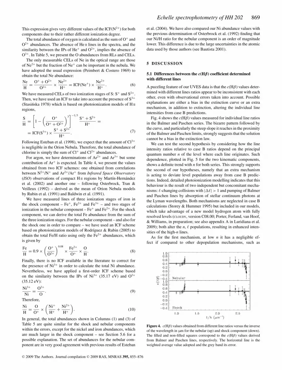
Fig. 4 shows the c(Hβ) values measured for individual line ratiosin the Balmer and Paschen series. The bizarre pattern followed bythe curve, and particularly the steep slope it reaches in the proximityof the Balmer and Paschen limits, strongly suggests that the solutioncannot be a bias in the extinction law.

We can test the second hypothesis by considering how the lineintensity ratios relative to case B ratios depend on the principalquantum number n of the level where each line originates. Suchdependence, plotted in Fig. 5 for the two kinematic components,shows a definite trend with n for both series. This strongly supportsthe second of our hypotheses, namely that an extra mechanismis acting to deviate level populations away from case B predic-tions. Indeed, detailed photoionization modelling indicates that thisbehaviour is the result of two independent but concomitant mecha-nisms: �-changing collisions with |��| > 1 and pumping of Balmerand Paschen lines by absorption of stellar continuum photons atthe Lyman wavelengths. Both mechanisms are neglected in case Bcalculations (Storey & Hummer 1995) but included in our models,which take advantage of a new model hydrogen atom with fullyresolved levels (CLOUDY, version C08.00; Porter, Ferland, van Hoof,& Williams, in preparation; see also appendix A in Luridiana et al.2009); both alter the n, � populations, resulting in enhanced inten-sities of the high-n lines.

As for the first mechanism, at low n it has a negligible ef-fect if compared to other depopulation mechanisms, such as

Figure 4. c(Hβ) values obtained from different line ratios versus the inverseof the wavelength in μm for the nebular (up) and shock component (down).The filled and non-filled squares correspond to the c(Hβ) values derivedfrom Balmer and Paschen lines, respectively. The horizontal line is theweighted average value adopted and the grey band its error.



Figure 5. Dereddened fluxes of Balmer (filled squares) and Paschen (non-filled squares) lines to their theoretical flux under the case B predictionratio versus the principal quantum number n for the nebular (up) and shockcomponents (down).

energy-changing collisions and horizontal collisions with |��| =1; at high n, it becomes increasingly important. Case B calculationsneglect this mechanism by construction, so a discrepancy is doomedto appear whenever high-n lines are compared to case B results.

The effectiveness of the second mechanism strongly depends onthe availability of the exciting photons, i.e. on the stellar flux atthe Lyman wavelengths; the results of Luridiana et al. (2009) andfurther preliminary calculations (Luridiana et al., in preparation)suggest that its impact on line intensities might increase with n.

A full account of both processes in H II regions can be found inLuridiana et al. (2009) and Luridiana et al. (in preparation).

5.2 Comparison of line ratios in the shock and nebularcomponents and the ionization structure

To maximize the shock-to-nebula ratio, the echelle spectra wereextracted over the area where the shock component is brighter andthe velocity separation with respect to the nebular background gasis maximum (see Fig. 2).

In Fig. 6, we present the weighted average shock-to-nebular ratiofor different ionic species, I(λ)sh/I(λ)neb – which was defined inequation (1) – with respect to the IP needed to create the associatedoriginating ion. In general, as we can see in this figure, the lineratios of the shock component relative to those of the ambient gas

Figure 6. Weighted average of shock-to-nebular line ratios versus the IPneeded to create the associated originating ion. Non-filled circles correspondto ratios measured from RLs (only for O+ and O++). Smaller error bars areof about 3 per cent.

are between 1 and 2 for most ionic species with IP above 10 eVand close to one for the most ionized species as O2+ and Ne2+.Since the illumination of the shock should be approximately thesame as that of the nebula at this particular zone of the slit, shock-to-nebular ratios of the order of one imply that the shock shouldbe ionization-bounded. This is exactly the opposite situation thatBlagrave et al. (2006) find in HH 529, where the shock-to-nebularratios are clearly lower than 1 indicating that the shock associatedto HH 529 is matter-bounded.

As we have commented above and can be seen in Fig. 6, theshock-to-nebular ratio varies from 1 to 2 for species with an IPhigher than 10 eV except in two cases: (i) Fe2+, whose lines showa substantial enhancement in the shock component, probably dueto dust destruction (see Section 5.6) and (ii) Cl+, but this can beaccidental because this ionic abundance is derived from a singlerather faint line with a very large uncertainty. Ionic species with anIP lower than 10 eV show a shock-to-nebular ratio always higherthan 2 in Fig. 6. In particular, Fe+, Ni+ and Cr+ show ratios largerthan 2 and these ions may be also affected by an increase of thegas-phase abundance due to dust destruction.

Neutral species like O0 or N0 are associated with the presenceof an ionization front. In the case of O0, the shock-to-nebular ra-tio has been calculated from the [O I] 6300 and 6363 Å lines thatare contaminated by telluric emissions but only in the shock com-ponent. We extracted the telluric emissions from the zone free ofshock emission along the slit and subtracted this feature to the shockcomponent. The shock-to-nebular ratio of [O I] lines is the largestone for those ions which are not heavily affected by possible dustdestruction. This is a further indication of the presence of an ioniza-tion front in HH 202-S. In the case of [N I] lines, those belonging tothe nebular component are also contaminated by telluric emissionbut, in this case, it was impossible to deblend properly these lines.

In Fig. 2, we can see the spatio-kinematic profiles of lines ofdifferent ionization stages of oxygen: O0, O+ and O2+, includingRLs and CELs. In the shock component, we can clearly distinguish astratification in the location of the ions: the bulk of the O2+ emissionis located at the south of the extracted area, O0 at the north and O+

is located approximately at the centre of the extracted area. Anotherinteresting feature that can be seen in Fig. 2 is that the emissionsfrom RLs and CELs of the same ion seem to show the same spatio-kinematic profiles. These profiles provide further indication thatHH 202-S is an ionization-bounded shock.

The peak emission of the spatio-kinematic profiles of ions withIP lower or similar to the one of O+: Cr+, Ni+, S+, Fe+ or H+ islocated to the north of HH 202-S, as in the case of O+. Ions asHe+, C2+ or Fe2+ show their peak emission about the centre of theaperture, while the ions with the highest IP, as Ne2+ or Ar3+, showspatio-kinematic profiles similar to that of O2+.

5.3 Width of the ionized slab and the physical separationbetween θ 1Ori C and HH 202-S

An interesting result of this paper is the claim that HH 202-S con-tains an ionization front as we have shown in Sections 4.1 and 5.2.Due to this fact, we can estimate the width of the ionized slab of HH202-S and its physical separation with respect to the main ionizationsource of the Trapezium cluster, θ 1Ori C.

On the one hand, from the maximum emission of the shockcomponent in the spatio-kinematic profiles of O2+ and O0 shownin Fig. 2, we can measure an angular distance on the plane ofthe sky of about 3.9 ± 0.5 arcsec. Using the distance to the OrionNebula obtained by Menten et al. (2007), d = 414 ± 7 pc, and



the inclination angle of HH 202-S with respect to the plane of thesky calculated by O’Dell & Henney (2008), θ = 48◦, we estimate(11.7 ± 1.5) × 10−3 pc for the width of the ionized slab.

On the other hand, to trap the ionization front in HH 202-S, theincident Lyman continuum flux must be balanced by the recombi-nations in the ionized slab, i.e.

FLy = Q(H 0)

4πD2= n2

shαB (H 0, T )L, (11)

where D is the physical separation between HH 202-S and θ 1OriC, Q(H0) is the ionizing photon rate, nsh the density in the shockcomponent, αB (H0, T) is the case B recombination coefficient for Hand L is the width of the slab. In order to estimate Q(H0), we haveused a spectral energy distribution of FASTWIND code with the stel-lar parameters for θ 1Ori C obtained by Simon-Dıaz et al. (2006) –Teff = 39 000 ± 1000 K and log g = 4.1 ± 0.1 dex – and thedistance to the Orion Nebula calculated by Menten et al. (2007).Then, the output parameters have been: the stellar radius R =(9.0 ± 1.3) R�, the stellar luminosity log L = 38.80 ± 0.14dex and the ionizing photon rate Q(H0) = (6.30 ± 2.00) × 1048 s−1.Taking a value for the recombination coefficient, αB = 2.59 ×10−13 cm−3 s−1 at 104 K, we have finally calculated a physical sep-aration of D = 0.14 ± 0.05 pc. This result suggests that HH 202 isquite embedded within the body of the Orion Nebula and, therefore,discards the origin of the ionized front as result of the interactionof the gas flow with the veil (see Section 4.1), which is between 1and 3 pc in front of the Trapezium cluster (see Abel et al. 2004).

5.4 Radial velocity analysis

In Fig. 7, we show the average heliocentric velocity of the linesthat belong to a given ionic species as a function of the IP needed

Figure 7. Heliocentric velocities of the nebular (up) and shock (down)components emission lines versus the IP needed to create the associatedoriginating ion. The velocity of the PDR (dashed horizontal line) is alsoshown. Non-filled triangles correspond to ions observed in only one kine-matic component. Non-filled circles correspond to heliocentric velocitiesmeasured from RLs (only for O+ and O++).

Table 6. Estimates of the t2 parameter.

HH 202 HH 529a

Nebular Shock Nebular ShockIon component component component component Esteban et al. (2004)

O2+ 0.016 ± 0.006 0.050 ± 0.007 0.009 ± 0.004 0.010 ± 0.010 0.022 ± 0.002C2+ 0.040 – – – 0.039 ± 0.011He+ 0.014 ± 0.013 0.049 ± 0.011 – – –

aBlagrave et al. (2006).

to create the associated originating ion. We have used two sepa-rate graphs to distinguish between the behaviour of the nebular andthe shock components. The nebular component shows the typicalvelocity gradient that has been observed in other positions of theOrion Nebula and other H II regions (e.g. Bautista & Pradhan 1998;Esteban & Peimbert 1999), with a velocity difference of the orderof −15 km s−1 between the neutral and the most ionized species.This gradient is likely produced by the presence of flows of ionizedgas originating from the ionization front inside the nebula. In con-trast, the ions in the shock component show a rather similar radialvelocity independently of their IP. This indicates that the bulk of theionized gas at the HH 202-S is moving at approximately the samevelocity with respect to the rest of the nebula. The H II lines (Balmerand Paschen series) of the shock component are shifted by −50.7 ±1.0 km s−1 relative to the H II lines of the nebular component and−64.8 ± 1.0 km s−1 relative to the velocity of the photon-dominatedregion (PDR,+28 km s−1; Goudis 1982). The zone covered byour UVES slit (see Fig. 1) coincides with position 117−256 ofDoi et al. (2004). These authors detect two radial velocity com-ponents belonging to the shock gas in this zone, a fast component(−57 km s−1) and a slower brighter one (−31 km s−1). Our valueof the radial velocity for the shock component of HH 202 (−36.8 ±1.0 km s−1) is somewhat more negative than the slower velocitycomponent of Doi et al. (2004), probably our shock componentcorresponds to the unresolved blend of the two velocity systemsdetected by those authors.

5.5 The abundance discrepancy and temperature fluctuations

Assuming the validity of the temperature fluctuations paradigm andthat this phenomenon produces the AD, we can estimate the valuesof the t2 parameter from the ADFs obtained for each componentand ion (see Table 3). In Table 6, we include the t2 values thatproduce the agreement between the abundance determinations ob-tained from CELs and RLs of O2+ and C2+. These calculations havebeen made following the formalism outlined by Peimbert & Costero(1969). Adopting the t2 value obtained for O2+ zone, t2(O2+), wehave calculated the ionic abundances, the ICFs and the total abun-dances under the presence of temperature fluctuations and they arepresented in Tables 3–5, respectively.

As we can see in Table 5, the high t2(O2+) value used to de-rive the abundances for the shock component implies that the totalabundances obtained from CELs considering t2 > 0 are higher inthe shock component than in the nebular one for all the elements.On the other hand, the abundances of C and O obtained from RLsare very similar in both components. Moreover, the O/H ratio com-puted from CELs for t2 > 0 is higher than that obtained from RLs.However, for the nebular component, we find that the total abun-dance of oxygen determined from CELs considering t2 > 0 agreeswith the oxygen abundance from RLs.

These results can suggest that, perhaps, the t2 value we havefound for the shock component is too high and, therefore, that the



t2 paradigm is not applicable in this case. However, we have toconsider that we have used a t2 value representative of the high-ionization zone for all the ions. The increase of the O+/O2+ ratioin the shock component with respect to the nebular one, due to anenhanced recombination rate, makes the O+ zone more extendedin this component and a lower t2(O+) would lead to a better agree-ment between the O abundances of both components. We have alsocomputed the t2 parameter for the He+ zone using a MLM (seeSection 4.4). The determination of the t2(He+) weighs the O+ andthe O2+ zones depending on their extension. It is remarkable thatthe t2 values obtained from different methods, such as the He+ linesand the ADF(O2+), which assume the presence of temperature fluc-tuations in the observed volume, produce almost identical valuesin both components, though t2(He+) has large uncertainties. Theseones can reconcile the total abundances of both components for t2 >

0 considering that the MLM depends strongly on the He I 3889 Åline flux and that the shock components of this line and H8 areseverely blended.

In Table 6, we have also included the values of t2 obtained byBlagrave et al. (2006) from the ADF(O2+) that they estimate forthe nebular and shock components of HH 529 and those obtainedby Esteban et al. (2004) from the ADF of O2+ and C2+. The dataof Esteban et al. (2004) correspond to a zone free of high-velocityflows and can be considered as representative of the nebular com-ponent but closer to the Trapezium. The values of the t2 obtainedfor the nebular component of HH 202-S are quite consistent withthose obtained by Esteban et al. (2004). The t2(O2+) of the nebularcomponent of HH 529 obtained by Blagrave et al. (2006) is lowerthan the two other determinations, but still consistent with our val-ues within the uncertainties. As has been commented above, the t2

values found in the shock component of HH 202 are much higherthan those of the nebular component and the value determined byBlagrave et al. (2006) for the shock component of HH 529.

The effect of temperature fluctuations in the spectra of ionizednebulae and their existence has been a controversial problem fromthe first work of Peimbert (1967). Peimbert (1995), Esteban (2002),Peimbert & Peimbert (2006) have reviewed the possible mecha-nisms that could produce such temperature fluctuations. Among thepossible sources of temperature fluctuations, we can list the depo-sition of mechanics energy by shocks and the gas compression dueto turbulence. Peimbert, Sarmiento & Fierro (1991) have studied

Table 7. Comparison of abundances and depletion factors.

Nebular component Shock componentSuna t2 = 0 t2 > 0 t2 = 0 t2 > 0

C 8.39 ± 0.05 8.43 ± 0.17 8.43 ± 0.16O 8.66 ± 0.05 8.59 ± 0.05 8.65 ± 0.05Fe 7.45 ± 0.05 6.10 ± 0.15 6.19 ± 0.16 6.95 ± 0.12 7.19 ± 0.13Ni 6.23 ± 0.04 5.03 ± 0.14 5.12 ± 0.15 5.87 ± 0.11 6.11 ± 0.12Fe/Ni 1.22 ± 0.06 1.07 ± 0.23 1.07 ± 0.25 1.08 ± 0.17 1.08 ± 0.19Cr+ - 2.88 ± 0.11 2.92 ± 0.11 3.75 ± 0.07 3.91 ± 0.07

Shock−Nebular Nebular−Sun Shock−Sunt2 = 0 t2 > 0 t2 = 0 t2 > 0 t2 = 0 t2 > 0

C 0.00 ± 0.27 0.04 ± 0.19 0.04 ± 0.18O 0.06 ± 0.07 −0.07 ± 0.07 −0.01 ± 0.07Fe 0.85 ± 0.13 1.00 ± 0.14 −1.35 ± 0.05 −1.26 ± 0.05 −0.50 ± 0.06 −0.26 ± 0.09Ni 0.84 ± 0.12 0.99 ± 0.13 −1.20 ± 0.04 −1.11 ± 0.04 −0.36 ± 0.06 −0.12 ± 0.10Fe/Ni – – – – – –Cr+ 0.87 ± 0.07 0.99 ± 0.07 – – – –

a Grevesse et al. (2007).

the effect of shock waves in H II regions using shock models byHartigan et al. (1987). They found that high t2 values can be ex-plained by the presence of shocks with velocities larger than 100km s−1. In the case of the flow of 89 km s−1 that produces HH 202,this effect should produce very small t2 values. Therefore, anotherprocess or other formalisms of the problem should be taken intoaccount in this case. Further discussion of this problem is beyondthe scope of this article.

5.6 Dust destruction

As indicated in Section 5.2, the emission lines of refractory elementsas Fe, Ni or Cr are much brighter in the gas flow than in the ambientgas. Moreover, the shock component shows relatively bright [Ca II]lines which are not detected in the spectrum of the ambient gas.On the other hand, in Section 4.1 we have stated that HH 202-Sdoes not contain a substantial contribution of shock excitation and,therefore, we need other mechanisms to explain those abnormallyhigh line fluxes. It is well known that Fe, Ni, Cr and Ca are expectedto be largely depleted in neutral and molecular interstellar cloudsas well as in H II regions. However, theoretical studies have shownthat fast shocks – as those typical in HH objects and supernova rem-nants – should efficiently destroy grains by thermal and non-thermalsputtering in the gas behind the shock front and by grain–grain col-lisions (McKee, Chernoff & Hollenbach 1984; Jones et al. 1994;Mouri & Taniguchi 2000). Several works have shown that some non-photoionized HH flows show a decrease in the amount of Fe deple-tion as determined from the analysis of [Fe II] lines (Beck-Winchatz,Bohm & Noriega-Crespo 1996; Bohm & Matt 2001; Nisini et al.2005). On the other hand, HH 399 is the first precedent of a fullyionized HH object where an overabundance in Fe was detected andthis one was related with dust destruction (Rodrıguez 2002).

In Table 7, we compare the values of the C, O, Fe, Ni and Cr+

abundances and the Fe/Ni ratios of the Sun (Grevesse, Asplund &Sauval 2007) and the nebular and shock components for t2 = 0and t2 > 0. In the case of Fe and Ni, we can see that the differ-ence between the abundances of the shock and nebular componentsare of the order of 0.85 dex for t2 = 0 and 1.00 dex for t2 >

0. This result indicates that the gas-phase abundance of Fe andNi increases by a factor between 7 and 10 after the passage ofthe shock wave. The fact that the Fe/Ni ratio is the same in both



components – because the increase of the gas-phase abundance ofboth elements is the same – and consistent with the solar Fe/Ni ratiowithin the errors suggests that the abundance pattern we see in HH202-S is the likely product of dust destruction. In fact, observationsof Galactic interstellar clouds indicate that Fe, Ni – as well as Cr– have the same dust-phase fraction (Savage & Sembach 1996b;Jones 2000). It is also remarkable that, although it could be mod-ulated by ionization effects, the behaviour of the Cr+ abundanceis also consistent with the dust-destruction scenario. The increaseof the Cr+/H+ ratio between the nebular and shock components isidentical to that of Fe and Ni.

Considering the solar Fe/H ratio as the reference (12 +log (Fe/H) = 7.45 ± 0.05; Grevesse et al. 2007) – which is al-most identical to the Fe/H ratio determined for the B-type stars ofthe Orion association (12 + log (Fe/H) = 7.44 ± 0.04; Przybilla,Nieva & Butler 2008) – we estimate that the Fe dust-phase abun-dance decreases by about 30 per cent for t2 = 0 and about53 per cent for t2 > 0 after the passage of the shock wave in HH202-S. This result is in good agreement with the predictions of themodels of Jones et al. (1994) and Mouri & Taniguchi (2000). In par-ticular, for the velocity determined for HH 202 (89 km s−1; O’Dell& Henney 2008), Jones et al. (1994) obtain a level of destruction ofiron dust particles of the order of 40 per cent. On the other hand, theFe gas-phase abundance we measure in HH 202-S follows closelythe empirical correlation obtained by Bohm & Matt (2001) from[Fe II] and [Ca II] emission line fluxes of several non-photoionizedHH flows. Further evidence that the dust is not completely destroyedin HH 202 is the detection of 11.7 μm emission coincident with thebright ionized gas around HH 202-S (Smith et al. 2005). As we cansee in Table 7, the depletion factors of Fe and Ni in the nebularcomponent are similar to those found in warm neutral interstellarenvironments and those at HH 202-S of the order of the depletionsobserved in the Galactic halo (see Welty et al. 1999 and referencestherein).

In the cases of C and O, the effect of dust destruction in their gas-phase abundance is more difficult to estimate. First, these elementsare far less depleted in dust grains than Fe or Ni in neutral interstellarclouds and in H II regions. Secondly, there is still a controversy aboutthe correct solar abundance of these two elements (see Holweger2001; Grevesse et al. 2007). Finally, chemical evolution modelspredict some increase in the C/H and O/H ratios in the 4.6 Gyrsince the formation of the Sun (0.28 and 0.13 dex; Carigi et al.2005). All these problems make impossible to estimate confidentvalues of the depletion factors for C and O.

Considering the data gathered in Table 7, the C abundance isvirtually the same in the nebular and shock components, althoughany possible small difference may be washed out due to the intrinsicrelatively large error of the abundance determination of this element.In any case, only a slight increase of the C gas-phase abundancewould be expected after the passage of the shock wave for a shockvelocity of about 89 km s−1 (Jones et al. 1994).

The uncertainties in the determination of the O abundances aremuch lower than in the case of C and its determination does notdepend on the selection of an appropriate ICF scheme. In Table 7,we see an increase of 0.06 dex in the O abundance in the shockcomponent with respect to the nebular one. These results suggesta possible moderate decrease of the depletion for this element inthe shocked material. Very recent detailed determinations of the Oabundance of B-type stars in the Orion association (Simon-Dıaz,in preparation) indicate that the mean O/H ratio in this zone is8.76 ± 0.04. In principle, one would expect that this is a betterreference for estimating the dust depletion in the Orion Nebula than

the solar one because it corresponds to the actual O abundance atthe same location. If we take the B-type stars determination as areference for the total O/H ratio, the amount of O depletion in theambient gas would be −0.17 ± 0.06 dex and −0.11 ± 0.06 dexin the gas flow. Therefore, a 30 per cent of the O tied up into dustgrains would be destroyed after the passage of the shock front.

There are two other alternative methods to estimate the oxygendepletion factor. The first one can be drawn following Estebanet al. (1998). This one is based on the fact that Mg, Si and Feform molecules with O which are trapped in dust grains. We haveused Mg, Si and Fe depletions in order to obtain the fraction of Otrapped in dust grains. These depletions are estimated consideringthe Orion gas abundances of Mg and Si given by Esteban et al.(1998), our Fe abundance for t2 > 0, the O abundances derivedfrom RLs, the stellar abundances of the Orion association of Si(12 + log(Si/H) = 7.41 ± 0.10) from Simon-Dıaz (in preparation)and Mg and Fe from Przybilla et al. (2008). By assuming that Ois trapped in olivine (Mg, Fe)2SiO4, pyroxene (Mg, Fe)SiO3 andseveral oxides like MgO, Fe2O3 and Fe3O4 (see Savage & Sembach1996a and references therein), we have estimated an O depletionfactor of −0.10±0.04 dex for the nebular component. If we considerthe older stellar abundances of Si and Fe from Cunha & Lambert(1994) and the Mg/Fe ratio from Grevesse et al. (2007), this valuebecomes −0.08±0.05, which is almost identical to that computedfrom the new stellar Mg, Si and Fe abundances.

The last method to obtain O depletion factors assumes that oxygenand iron are destroyed in the same fraction. The fraction of iron dustparticles is calculated using the Fe abundances for t2 >0 presented inTable 7 and Fe abundance of B-type stars of the Orion association.From this assumption, and taking into account the O abundancefrom RLs, we have derived a depletion factor of −0.11+0.11

−0.14 dexin the nebular component. Finally, we have calculated the averageof the values obtained from the three methods, finding that the Odepletion factor of the ambient gas is −0.12 ± 0.03. In all cases, thedepletion becomes larger by about 0.08 dex if we adopt abundancesfor t2 = 0. Additionally, the depletion factor in the shock componentis smaller than in the ambient gas, probably due to gas destruction.

5.7 Photoionization models for HH 202-S

To test the role of dust destruction both in the temperature structureobserved in the shock component and in the iron abundance inthe gas, we have run some simple photoionization models for thenebular and the shock components. The models were constructedusing CLOUDY (Ferland et al. 1998), version 07.02, and assuminga plane–parallel open geometry with density equal to the valueadopted from the observations (see Table 2). We used a WM-basic(Pauldrach, Hoffmann & Lennon 2001) model stellar atmosphere,with Teff = 39 000 K and log g = 4.0, values very similar to thosederived by Simon-Dıaz et al. (2006) for θ 1 Ori C. The number ofionizing photons entering the ionized slab was specified using theionization parameter, U, the ratio of hydrogen-ionizing photons tothe hydrogen density. We changed the value of this parameter tillthe degrees of ionization (given by O+/O2+) derived for the modelswere close to the observed ones. The final values used for U implysimilar numbers of hydrogen-ionizing photons in the nebular andshock models, with a difference of ∼40 per cent.

We have used the CLOUDY ‘H II region’ abundances, based on theabundances derived by Baldwin et al. (1991), Rubin et al. (1991) andOsterbrock et al. (1992) in the Orion Nebula, for all elements exceptiron, which we have rescaled in order to reproduce the observed[Fe III] 4658/Hβ line ratios. The models also have ‘Orion’ type



Table 8. Input parameters for photoionization models.

Parameter Nebular model Shock model A Shock model B Shock model C

log(ne) (cm−3) 3.46 4.24 4.24 4.24log(U) −1.95 −2.53 −2.53 −2.53Dust Orion Orion Orion 0.5 × Orion(Fe/H)gas 2.1 × 10−6 2.1 × 10−6 1.5 × 10−5 1.5 × 10−5

Table 9. Results of photoionization models.

Constraint Nebular Obs. Nebular Mod. Shock Obs. Shock model A Shock model B Shock model C

ne (cm−3) 2890 ± 550 2960 17 430 ± 2360 17 540 17 670 17 650Te([N II]) (K) 9610 ± 390 9340 9240 ± 300 9510 9220 9210Te([O III]) (K) 8180 ± 200 8230 8770 ± 240 8810 8670 8640log(O+/O2+) −0.35±0.07 −0.37 0.20 ± 0.07 0.21 0.23 0.22I([Fe III] 4658)/I(Hβ) 0.009 ± 0.001 0.010 0.110 ± 0.006 0.017 0.111 0.107

dust: graphite and silicate grains with the Orion size distribution(deficient in small grains; see Baldwin et al. 1991) and an originaldust to gas mass ratio of 0.0055. For each model, we used thecalculated line intensities to derive the physical conditions and theO+ and O2+ abundances, following a similar procedure to the oneused to derive the observational results.

We computed three shock models. Model A has similar charac-teristics to the nebular model except for the density, and can beused to assess the influence of this parameter on the electron tem-peratures. Model B has the same input parameters as model A, butwith the Fe abundance multiplied by a factor of 7. Model C has thesame input parameters as model B but with half the amount of dust.The input model parameters are listed in Table 8. Table 9 shows acomparison for observations and models of the physical conditions,the degree of ionization given by O+/O2+, and the [Fe III] 4658/Hβ

line ratio. We can see that the nebular model reproduces well theobservational constraints. As for the shock models, the incrementin the density of model A is enough to explain the temperaturesfound for the shock component, but does not reproduce the [Fe III]flux, whereas the higher Fe abundance of model B reproduces wellthis flux. Model C illustrates that a reduction in the amount of dustdoes not change significantly the values of the chosen constraints.The introduction of grains smaller than the ones considered in theOrion size distribution of CLOUDY will lead to higher temperaturesthrough photoelectric heating, but we do not know what grain sizedistribution would be suitable for the shock component.

The iron abundances in those models that reproduce the observed[Fe III] line fluxes are somewhat higher than the ones derived fromthe observations, but they reproduce the value of the shock to neb-ular abundance ratio. This can be considered a confirmation of theincrement in the iron abundance in the shock component, which ismost probably due to dust destruction. As it has been discussed inSection 5.6, dust destruction could also increase the gaseous abun-dances of other elements like carbon or oxygen and this incrementwill change the amount of cooling and hence the electron temper-ature. We ran a model where the abundances of O and C wereincreased by 14 per cent and found that the derived temperaturesdecrease by about 200 K.

6 C O N C L U S I O N S

We have obtained deep echelle spectrophotometry of HH 202-S, thebrightest knot of the HH object HH 202. Our high spectral resolution

has permitted to separate two kinematic components: the nebularcomponent – associated with the ambient gas – and the shock one– associated with the gas flow. We have detected and measured 360emission lines of which 352 lines were identified.

We have found a clear disagreement between the individual c(Hβ)values obtained from different Balmer and Paschen lines. We out-line a possible solution for this problem based on the effects ofLy-continuum pumping and �-changing collisions with protons.

We have analysed the ionization structure of HH 202-S con-cluding that the dominant excitation mechanism in HH 202-S isphotoionization. Moreover, the dependence of the I(λ)sh/I(λ)neb ra-tios and the IP, the comparison of the spatio-kinematic profiles ofthe emission of different ions as well as the physical separation es-timated of 0.14 ± 0.05 pc between HH 202-S and θ 1Ori C indicatethat an ionization front is trapped in HH 202-S due to compressionof the ambient gas by the shock.

We have derived a high ne, about 17 000 cm−3, and similar Te forthe low- and high-ionization zones for the shock component, whilefor the ambient gas we obtain an ne of about 3000 cm−3, and a higherTe in the low-ionization zone than in the high-ionization one. Wehave estimated that the pre-shock gas in the immediate vicinity ofHH 202 has a density of about 700 cm−3, indicating that the bulk ofthe emission of the ambient gas comes from the background behindHH 202.

We have derived chemical abundances for several ions and el-ements from the flux of CELs. In particular, we have determinedthe Ca+ and Cr+ abundances for the first time in the Orion Nebulabut only for the shock component. The abundance of C2+, O+ andO2+ have been determined using RLs for both components. The ADfactor for O2+, ADF(O2+), is 0.35 dex in the shock component andmuch lower in the ambient gas component.

Assuming that the ADF and temperature fluctuations are relatedphenomena, we have found a t2(O2+) of 0.050 for the shock com-ponent and 0.016 for the nebular one. The high t2 value of theshock component produces some apparent inconsistencies betweenthe total abundances in both components that cast some doubts onthe suitability of the t2 paradigm, at least for the shock component.However, the fact that the values of the t2 parameter determinedfrom the analysis of the He I line ratios are in complete agreementwith those obtained from the ADF(O2+) supports that paradigm.

Finally, the comparison of the abundance patterns of Fe and Ni inthe nebular and shock components and the results of photoionzationmodels of both components indicate that a partial destruction of dust



grains has been produced in HH 202-S after the passage of the shockwave. We estimate that the percentage of destruction of iron dustparticles is of the order of 30–50 per cent.

AC K N OW L E D G M E N T S

We are very grateful to the referee of this paper, J. Bally, for hiscomments, which have improved the scientific content of the paper.We also thank S. Simon-Dıaz for providing us the stellar param-eters for θ 1 Ori C. This work has been funded by the SpanishMinisterio de Ciencia y Tecnologıa (MCyT) under projectAYA2004-07466 and Ministerio de Educacion y Ciencia (MEC)under project AYA2007-63030. VL acknowledges support fromMEC under project AYA2007-64712. JGR is supported by anUNAM postdoctoral grant. MR acknowledges support from Mexi-can CONACYT project 50359-F.

REFER ENCES

Abel N. P., Brogan C. L., Ferland G. J., O’Dell C. R., Shaw G., TrolandT. H., 2004, ApJ, 609, 247

Baldwin J. A., Ferland G. J., Martin P. G., Corbin M. R., Cota S. A., PetersonB. M., Slettebak A., 1991, ApJ, 374, 580

Bally J., Reipurth B., 2001, ApJ, 546, 299Bally J., Reipurth B., 2003, AJ, 126, 893Bally J., Licht D., Smith N., Walawender J., 2006, AJ, 131, 473Bautista M. A., 2001, A&A, 365, 268Bautista M. A., 2004, A&A, 420, 763Bautista M. A., Pradhan A. K., 1998, ApJ, 492, 650Bautista M. A., Peng J., Pradhan A. K., 1996, ApJ, 460, 372Bautista M. A., Ballance C., Gull T., Lodders K., Martınez M., Melendez

M., 2009, MNRAS, 393, 1503Beck-Winchatz B., Bohm K.-H., Noriega-Crespo A., 1996, AJ, 111, 346Benjamin R. A., Skillman E. D., Smits D. P., 2002, ApJ, 569, 288Blagrave K. P. M., Martin P. G., Baldwin J. A., 2006, ApJ, 644, 1006Blagrave K. P. M., Martin P. G., Rubin R. H., Dufour R. J., Baldwin J. A.,

Hester J. J., Walter D. K., 2007, ApJ, 655, 299Bohlin R. C., Lindler D., 1992, STScI Newsletter, 9, 19Bohm K.-H., Matt S., 2001, PASP, 113, 158Canto J., Goudis C., Johnson P. G., Meaburn J., 1980, A&A, 85, 128Carigi L., Peimbert M., Esteban C., Garcıa-Rojas J., 2005, ApJ, 623, 213Cernicharo J. et al., 1998, Sci, 282, 462Costero R., Peimbert M., 1970, Bol. Obser., 5, 229Cunha K., Lambert D. L., 1994, ApJ, 426, 170De Robertis M. M., Dufour R. J., Hunt R. W., 1987, J. R. Astron. Soc. Can.,

81, 195D’Odorico S., Cristiani S., Dekker H., Hill V., Kaufer A., Kim T., Pri-

mas F., 2000, in Bergeron J., ed., Proc. SPIE, Vol. 4005, Discoveriesand Research Prospects from 8- and 10-Meter-Class Telescopes. SPIE,Bellingham, WA, p. 121

Doi T., O’Dell C. R., Hartigan P., 2004, AJ, 127, 3456Esteban C., 2002, in Henney W. J., Franco J., Martos M., eds, Rev. Mex.

Astron. Astrofis. Conf. Ser. Vol. 12, Ionized Gaseou Nebulae. UNAM,Mexico City, p. 56

Esteban C., Peimbert M., 1999, A&A, 349, 276Esteban C., Peimbert M., Torres-Peimbert S., Escalante V., 1998, MNRAS,

295, 401Esteban C., Peimbert M., Garcıa-Rojas J., Ruiz M. T., Peimbert A.,

Rodrıguez M., 2004, MNRAS, 355, 229Ferland G. J., Korista K. T., Verner D. A., Ferguson J. W., Kingdon J. B.,

Verner E. M., 1998, PASP, 110, 761Froese Fischer C., Rubin R. H., 2004, MNRAS, 355, 461Garcıa-Dıaz M. T., Henney W. J., Lopez J. A., Doi T., 2008, Rev. Mex.

Astron. Astrofis., 44, 181Garcıa-Rojas J., Esteban C., 2007, ApJ, 670, 457

Garcıa-Rojas J., Esteban C., Peimbert M., Costado M. T., Rodrıguez M.,Peimbert A., Ruiz M. T., 2006, MNRAS, 368, 253

Garnett D. R., Shields G. A., Peimbert M., Torres-Peimbert S., SkillmanE. D., Dufour R. J., Terlevich E., Terlevich R. J., 1999, ApJ, 513, 168

Goudis C., 1982, The Orion complex: A case study of interstellar matter.Reidel, Dordrecht

Grandi S. A., 1976, ApJ, 206, 658Grevesse N., Asplund M., Sauval A. J., 2007, Space Sci. Rev., 130, 105Hamuy M., Walker A. R., Suntzeff N. B., Gigoux P., Heathcote S. R., Phillips

M. M., 1992, PASP, 104, 533Hamuy M., Suntzeff N. B., Heathcote S. R., Walker A. R., Gigoux P., Phillips

M. M., 1994, PASP, 106, 566Hartigan P., Raymond J., Hartmann L., 1987, ApJ, 316, 323Henney W. J., O’Dell C. R., Zapata L. A., Garcıa-Dıaz M. T., Rodrıguez

L. F., Robberto M., 2007, AJ, 133, 2192Holweger H., 2001, in Wimmer-Schweingruber R. F., ed., Solar and Galactic

Composition. Springer, Berlin, p. 23Johansson S., Zethson T., Hartman H., Ekberg J. O., Ishibashi K., Davidson

K., Gull T., 2000, A&A, 361, 977Jones A. P., 2000, J. Geophys. Res., 105, 10257Jones A. P., Tielens A. G. G. M., Hollenbach D. J., McKee C. F., 1994, ApJ,

433, 797Kingdon J., Ferland G. J., 1995, ApJ, 442, 714Lucy L. B., 1995, A&A, 294, 555Luridiana V., Simon-Dıaz S., Cervino M., Gonzalez Delgado R. M., Porter

R. L., Ferland G. J., 2009, ApJ, 691, 1712McKee C. F., Chernoff D. F., Hollenbach D. J., 1984, in Kessler M. F.,

Phillips J. P., eds, Galactic and Extragalactic Infrared Spectroscopy.Reidel, Dordrecht, p. 103

Martın-Hernandez N. L. et al., 2002, A&A, 381, 606Meaburn J., 1986, A&A, 164, 358Melendez M., Bautista M. A., Badnell N. R., 2007, A&A, 469, 1203Mendoza C., 1983, in Flower D. R., ed., Proc. IAU Symp. 103, Planetary

Nebulae. D. Reidel Publishing Co., Dordrecht, p. 143Menten K. M., Reid M. J., Forbrich J., Brunthaler A., 2007, A&A, 474, 515Mesa-Delgado A., Esteban C., Garcıa-Rojas J., 2008, ApJ, 675, 389Mesa-Delgado A., Lopez-Martın L., Esteban C., Garcıa-Rojas J., Luridiana

V., 2009, MNRAS, 394, 693 (Paper I)Moore C. E., 1945, A Multiplet Table of Astrophysical Interest. Princeton

Univ. Obs., Princeton, NJ, p. 20Mouri H., Taniguchi Y., 2000, ApJ, 534, L63Nisini B., Bacciotti F., Giannini T., Massi F., Eisloffel J., Podio L., Ray T.

P., 2005, A&A, 441, 159O’Dell C. R., Doi T., 2003, AJ, 125, 277O’Dell C. R., Henney W. J., 2008, AJ, 136, 1566O’Dell C. R., Wen Z., Hester J. J., 1991, PASP, 103, 824O’Dell C. R., Wong K., 1996, AJ, 111, 846O’Dell C. R., Yusef-Zadeh F., 2000, AJ, 120, 382O’Dell C. R., Hartigan P., Lane W. M., Wong S. K., Burton M. G., Raymond

J., Axon D. J., 1997, AJ, 114, 730Osterbrock D. E., Tran H. D., Veilleux S., 1992, ApJ, 389, 305Pauldrach A. W. A., Hoffmann T. L., Lennon M., 2001, A&A, 375, 161Peimbert M., 1967, ApJ, 150, 825Peimbert M., 1995, in Williams R., Livio M., eds, The Analysis of Emission

Lines. Cambridge Univ. Press, Cambridge, p. 165Peimbert M., Costero R., 1969, Bol. Obs. Tonantzintla y Tacubaya, 5, 3Peimbert M., Peimbert A., 2006, in Barlow M. J., Mendez R. H., eds,

Proc. IAU Symp. 234, Planetary Nebulae in our Galaxy and Beyond.Cambridge Univ. Press, Cambridge, p. 227

Peimbert M., Sarmiento A., Fierro J., 1991, PASP, 103, 815Peimbert M., Peimbert A., Ruiz M. T., 2000, ApJ, 541, 688Peimbert A., Peimbert M., Luridiana V., 2002, ApJ, 565, 668Peimbert M., Torres-Peimbert S., Ruiz M. T., 1992, Rev. Mexicana Astron.

Astrofis., 24, 155Porter R. L., Bauman R. P., Ferland G. J., MacAdam K. B., 2005, ApJ, 622,

L73Porter R. L., Ferland G. J., MacAdam K. B., 2007, ApJ, 657, 327Przybilla N., Nieva F. M., Butler K., 2008, ApJ, 688, L103



Quinet P., 1996, A&AS, 116, 573Raga A. C., Canto J., De Colle F., Esquivel A., Kajdic P., Rodrıguez-

Gonzalez A., Velazquez P. F., 2008, ApJ, 680, L45Reipurth B., Bally J., Fesen R. A., Devine D., 1998, Nat, 396, 343Riera A., Mampaso A., Vilchez J. M., Phillips J. P., 1989, A&A, 210, 351Rodrıguez M., 1999, A&A, 348, 222Rodrıguez M., 2002, A&A, 389, 556Rodrıguez M., Rubin R. H., 2005, ApJ, 626, 900Rosado M., de La Fuente E., Arias L., Le Coarer E., 2002, Rev. Mexicana

Astron. Astrofis. Conf. Ser., 13, 90Rubin R. H., Simpson J. P., Haas M. R., Erickson E. F., 1991, ApJ, 374,

564Rubin R. H., Martin P. G., Dufour R. J., Ferland G. J., Blagrave K. P. M.,

Liu X.-W., Nguyen J. F., Baldwin J. A., 2003, MNRAS, 340, 362Ruiz M. T., Peimbert A., Peimbert M., Esteban C., 2003, ApJ, 595, 247Savage B. D., Sembach K. R., 1996a, ARA&A, 34, 279Savage B. D., Sembach K. R., 1996b, ApJ, 470, 893Sawey P. M. J., Berrington K. A., 1993, At. Data Nucl. Data Tables, 55, 81Shaw R. A., Dufour R. J., 1995, PASP, 107, 896Simon-Dıaz S., Herrero A., Esteban C., Najarro F., 2006, A&A, 448, 351

Smith N., Bally J., Brooks K. J., 2004, AJ, 127, 2793Smith N., Bally J., Shuping R. Y., Morris M., Kassis M., 2005, AJ, 130,

1763Stasinska G., 1978, A&A, 66, 257Storey P. J., Hummer D. G., 1995, MNRAS, 272, 41Tsamis Y. G., Barlow M. J., Liu X.-W., Danziger I. J., Storey P. J., 2003,

MNRAS, 338, 687Turnshek D. A., Bohlin R. C., Williamson R. L., Lupie O. L., Koornneef J.,

Morgan D. H., 1990, AJ, 99, 1243Verner E. M., Verner D. A., Baldwin J. A., Ferland G. J., Martin P. G., 2000,

ApJ, 543, 831Walter D. K., Dufour R. J., Hester J. J., 1992, ApJ, 397, 196Welty D. E., Hobbs L. M., Lauroesch J. T., Morton D. C., Spitzer L., York

D. G., 1999, ApJS, 124, 465Zhang H., 1996, A&AS, 119, 523Zhang H. L., Pradhan A. K., 1997, A&AS, 126, 373

This paper has been typeset from a TEX/LATEX file prepared by the author.


Properties of the ionized gas in HH 202 - II. Results from echelle spectrophotometry with...

Documents

Transcript of Properties of the ionized gas in HH 202 - II. Results from echelle spectrophotometry with...