Catena 75 (2008) 268–277

Contents lists available at ScienceDirect

Catena

j ourna l homepage: www.e lsev ie r.com/ locate /catena

Prolegomena to sediment and flow connectivity in the landscape: A GIS and fieldnumerical assessment

Lorenzo Borselli ⁎, Paola Cassi, Dino TorriCNR-IRPI, Via Madonna del Piano 10, 50019 Sesto Fiorentino(FI), Italy

⁎ Corresponding author. CNR-IRPI, Florence, Italy.E-mail address: borselli@irpi.fi.cnr.it (L. Borselli).

0341-8162/$ – see front matter © 2008 Elsevier B.V. Aldoi:10.1016/j.catena.2008.07.006

a b s t r a c t

a r t i c l e i n f o

Article history:

This paper presents two new Received 30 April 2008Received in revised form 10 July 2008Accepted 16 July 2008

Keywords:Sediment connectivitySediment delivery ratioConnectivity indexSoil erosion

definitions of sediment and water flux connectivity (from source through slopesto channels/sinks) with examples of applications to sediment fluxes. The two indices of connectivity areoperatively defined, one (IC) that can be calculated in a GIS environment and represents a connectivityassessment based on landscape's information, and another that can be evaluated in the field (FIC) throughdirect assessment. While IC represent a potential connectivity characteristic of the local landscape, sincenothing is used to represent the characteristics of causative events, FIC depend on the intensities of theevents that have occurred locally and that have left visible signs in the fields, slopes, etc.IC and FIC are based on recognized major components of hydrological connectivity, such as land use andtopographic characteristics. The definitions are based on the fact that the material present at a certainlocation A reaches another location B with a probability that depends on two components: the amount ofmaterial present in A and the route from A to B. The distance to B is weighted by the local gradient and thetype of land use that the flow encounters on its route to B, while the amount of material present in A dependson the catchment surface, slope gradient and type of land use of said catchment.Although IC and FIC are independent from each other, and are calculated using different equations anddifferent inputs, they complement each other. In fact, their combined use improves IC's accuracy. Hence,connectivity classes can afterward be rated using IC alone.This procedure has been applied in a medium-size watershed in Tuscany (Italy) with the aim of evaluatingconnectivity, identifying connected sediment sources and verifying the effects of mitigation measures.The proposed indices can be used for monitoring changes in connectivity in areas with highgeomorphological or human induced evolution rates.

© 2008 Elsevier B.V. All rights reserved.

1. Introduction

Hydrological connectivity is a term often used to describe theinternal linkages between runoff and sediment sources in upper partsof catchments and the corresponding sinks (Croke et al., 2005). Crokeet al. (2005) identifies two types of connectivity: direct connectivityvia new channels or gullies, and diffuse connectivity as surface runoffreaches the stream network via overland flow pathways.

Of course, connectivity varies both in space and in time. Spatialaspects concern the catchment physiography. Recent investigations byHooke (2003) have shown that sediment production, transport anddelivery to river channels downstream are not only dependent on theoverall catchment physiography, but also on the spatial organization

l rights reserved.

and the internal connectivity of various physiographic units. Theimpact of a given type of impediment on water and sediment flowdepends upon its size and position in the catchment (Fryirs et al.,2007a). Overall flow connectivity in a given catchment changes withthe processes that occur within it. In particular, with increasingcatchment size, floodplains substitute slopes as the direct source ofsediment to the channels. This will certainly affect the overallsediment export from the basin (De Vente and Poesen, 2005).

Temporal aspects are related to magnitude and frequencycharacteristics (Wolman and Miller, 1960) of sediment transferprocesses and the temporal evolution of land use and management.Only a few events can generate flux pathways connecting large part ofthe slopes to the higher order streams or the local sinks. Eventmagnitudes and a mixture of physically and biologically controlledthresholds have to be overcome to connect runoff generating areas tolower channel areas (Puigdefabregas et al., 1999; Cammeraat, 2002;Croke et al., 2005).

Attempts to model connectivity have been made by studying thesediment delivery ratio in order to accommodate gross erosion

269L. Borselli et al. / Catena 75 (2008) 268–277

estimates of soil loss to the values observed at catchment outlets afterthe occurrence of (internal) deposition. Among the most recent ofthem,wemention Ferro and Porto, (2000); Van Rompaey et al. (2001);Mitasova et al. (2001).

Runoff and erosion rates can be highly heterogeneous across alandscape and this can have implications for hydrological andsediment connectivity in a drainage basin. Cammeraat (2002)indicates three main factors influencing diffuse connectivity:

1) soil surface irregularity (roughness), which could be very low onthe patch scale, but higher at the hillslope and catchment scales,

2) spatial organization of the vegetation on the hillslope scale and thespatial arrangement between land units at the catchment scale,

3) rainfall intensity, event duration and thus the effective rainfall.

Vegetation plays an important role because it influences surfaceroughness and local capacity to store sediments and water (Puigdefab-regas et al., 1999); it also increases infiltration (e.g. Bochet et al., 1999;Cammeraat, 2004). Hence, vegetation contributes towards disconnect-ing upstream and downstream areas. Badlands and severely erodedareas have a higher degree of connection than agricultural and forestland (Harvey, 2001; Kirkby et al., 2002; Hooke and Sandercock, 2007).The capacity of vegetation to influence flux connectivity shows strongtime and space dynamics, which varies according to season, climaticextremes (e.g. droughts), climate changes, land use and managementpractice as well as other forms of anthropic and natural pressure.

Knowledge of the spatial distribution and the temporal evolution ofconnectivity in the actual landscape is important because it can beused as a tool to estimate the probability that a given part of thelandscape transfer its contribution elsewhere in the catchment.Usually source areas can be identified using a specialized model forsoil erosion and/or runoff generation (USLE, RUSLE, SCS-CN) (Whish-meier and Smith, 1978; USDA-SCS, 1986; Renard et al., 1997), afterwhich the generatedmaterial (sediment andwater) travels to the sink.Here connectivity plays its role: the easier it is for the flux the reach thesink, the better connected the source and the sink areas are. Severalauthors have discussed this concept qualitatively (Harvey, 2001, 2002;Hooke, 2003) but an analogous quantitative index, based on informa-tion commonly available in a GIS environment, remains to be defined.

The aim of this paper is to introduce a set of tools for theassessment of connectivity using both GIS data and field observations.The index based on GIS data (e.g. landuse, DTM) is designed to assessconnectivity using only the available landscape information, inde-pendent of event characteristics. The other index, instead, depends onrainfall characteristics and represents a sort of ground truth to validatethe GIS deduced connectivity.

2. Background and definition of a landscape-based index ofconnectivity

Many geomorphological studies identify sediment transport fromthe source areas to the channel network as the primary process whichdetermines landscape evolution (Harvey, 2001; Hooke, 2003; Hookeand Sandercock, 2007). If a system is characterized byhighmass transferefficiency it is also characterized by a significant degree of connectivity(Harvey, 2002; Hooke, 2003, Hooke and Sandercock, 2007; Bracken andCroke, 2007). Thedegree of connectivity influences theprobability that alocal on-site effect propagates downslope causing off-site effects.

These concepts have already found different applications. Forexample, geomorphologists focus on the sensitivity of the landscapeand the way in which high connectivity within a landscape ensuresthat site instabilities can be propagated within a multiple-eventsfeedback system (Fryirs et al., 2007b). Hydrologists and soil conserva-tionist, in the past, tried to approach connectivity numerically bydefining the sediment delivery ratio (SDR), a parameter that describesand predicts the relationship between erosion and sediment yield in awatershed (e.g., Atkinson, 1995). SDR is a spatially lumped parameter

that represents, atmean annual temporal scale, the sediment transportefficiency of the hillslopes and the channel network (Walling, 1983).

Many models, such as the USLE-type models (Renard et al., 1997;Whishmeier and Smith, 1978), do not take into account depositionprocesses explicitly. These models allow for unbounded transport andcan produce unrealistic outputs at watershed level (Kinnell, 2004).Many authors have used the SDR to correct the model's output (Ferroand Porto 2000; Lu et al., 2006).

Many algorithms and methods for evaluating the SDR at field orwatershed scale are based on:

– geometrical topographical properties of watershed and drainagepaths (Greenfield et al., 2001);

– long term transport capacity assessment (Van Rompaey et al.,2001)—SEDEM;

– sediment properties and trap efficiency along the flow path (Lu et al.,2006).

Greenfield et al. (2001) distinguish between 2 types of algorithms,both dominated by the geometrical topographical properties ofwatershed and drainage paths:

• The upslope approach (USDA-NRCS. 1983; Lu et al., 2006) takes intoaccount the characteristics of the drainage area: morphology andland use. The SDR decreases with respect to increasing basin size;this is because large basins have a lower average slope and tend tohave more sediment storage sites located between the sedimentsource areas and the outlet (Boyce, 1975). Williams (1977) foundthat sediment delivery ratio is correlated with drainage area, relief-length ratio and runoff curve numbers (based on the sediment yielddata for 15 basins located in Texas).

• The downslope approach takes into account the flow path length thata particle has to travel to arrive at the nearest sink. The distancebetween the source area and the sink is affected by surfaceroughness and slope. Hence, the SDR is influenced by the lengthand the surface characteristics of the shortest path to the nearestsink (Yagow et al., 1988; Novotny and Chesters, 1989; Sun andMcNulty 1998; Ferro and Porto, 2000).

Both approaches are important in evaluating the actual sedimentyield that reaches the channel network. The latter approach tells us thatthe probability of a particle reaching the nearest sink depends on thedistance to the sink, the characteristics of the route and thewater that isgained/lost along thedownslope route. The formerapproach tells us thatthe particle's chances depend on the availability of water to transport it,which can be generated on the spot and/or come from upslope. Herewepropose and discuss an intermediate position becausewemaintain thatthe degree of connectivity is in fact influenced by both factors.

2.1. The GIS approach

Any index of connectivity based on GIS data, rather than describingconnectivity in the context of specific events, will express generalproperties of the catchment/landscape under evaluation. In particular,the connectivity map will represent the potential connectivitybetween the different parts of a watershed.

In order to develop such an index let us limit ourselves to thesimple case of a slope. As an initial simplification let us suppose thatthe slope is homogeneous from the point of view of connectivity(constant roughness, gradient and vegetation). Let us consider a pointA (Fig. 1) somewhere which divides flow lines into those contributingsediment to the point A itself (upslope oncoming sediment=UOS) andthose bringing the sediment downslope towards a sink B (e.g. adrainage channel). The probability pd that sediment arrives at B alongthe flow line joining A to B is inversely proportional to the downslopedistance along the flow line. Obviously the more UOS there is, the lessprobable it is that all the sediment is completely caught beforearriving at the downslope sink/channel. If the mass ready to flow to A

Fig. 2. Definition of IC upslope and downslope component in the landscape for index ofconnectivity (IC).

Fig. 1. Simple slope with flow path between the source area A and the local sink B.

270 L. Borselli et al. / Catena 75 (2008) 268–277

is mA, then the amount that will probably reach B is proportional tothe product between mA and the probability pd. But this product hasthe dimension ofmA, which is a mass. This is not what we want for anindex of connectivity because we want an index giving us a potential:the real quantity will depend on the event intensity at least. Hence wemay simply consider that mA is also the result of the probability thatA's upslope source zone is more or less connected to A. Hence, mA isthe product of the mass of sediment put in motion upslope of A timesits probability pu to reach A. If we refer all to a unit mass we can workwith probabilities alone: the probability that a unit mass convergingin A reaches B is the product of the two probabilities:

p ¼ pupd ð1Þ

In order to find out a way to estimate the two quantities pu and pdwe will refer to the sketch shown in Figs 1 and 2. Let begin with pd.

2.1.1. The downslope component, Ddn

As a first approximation we stated that pd is inversely proportionalto segment length d, but it must also depend on others factors. Forexample, if the sediment traverses a wood with dense undergrowth,moss, lichens and litter, it will lose a large amount of its mass along theway. On the other hand, if it passes through a seedbed field or acompacted or sealed bare soil surface of the same length d, the oppositewill happen; the sediment will gain mass. Hence the degree to whichthe segment is able to connect depends on land use and management,and the hydrological conditions of the spot across which the segmentlies. This means that we need to assign a weight (W) to each flow linesegment which takes account of the local conditions. Slope gradient ofthe segment is also relevant as any sediment transferwill soon stop on asegment with zero slope. Hencewe need a gradient factor (S). IfW and Sattain their maximumwhen vegetation, land use and management arepoorer or slope gradients are larger, then the ratio d/WS can weight thedistance as needed. Summing all the segments along the route fromA toB we can estimate the weighted distance Ddn:

Ddn ¼ ∑i

diWiSi

ð2Þ

di length of the ith cell along the downslope path (in m)Wi weight of the ith cell (dimensionless)Si slope gradient of the ith cell (m/m)

Finally, as discussed, the probability pd is inversely proportional toDdn:

pd~D−1dn ð3Þ

2.1.2. The upslope component Dup

The upslope component Dup is the potential for downward routingof the sediment produced upslope. It depends on the area draininginto A. Moreover, it must depend on the same factors as Ddn. Thedifference is that we now have to expand our analysis to an area. In

order to keep the structure of the estimationmethod as simple as possible(deferring to a later stage the development of a more elaborate methodshould the need arise) we can use average values of the two weightingfactors over the contributing upslope area. Moreover, we can use thesquare root of the upslope area in order to give to Dup the same unit ofmeasure asDdn. Under such assumptions we can estimateDup as follows:

Dup ¼W̄ S̄ffiffiffiA

pð4Þ

W̄ average weighing factor of the upslope contributing area(dimensionless);

S̄ average slopegradientof theupslope contributing area (m/m)A upslope contributing area (m2)

Eq. (4) is directly proportional to the probability pu since, bydefinition, pu increases with increasing Dup:

pu~Dup ð5Þ

2.1.3. Index of connectivity (IC) calculationBased on Eqs. (3) and (5) we can write that probability p is

proportional to:

p ¼ pupd~Dup

Ddn¼ W̄ S̄

ffiffiffiA

p

∑idi

WiSi

ð6Þ

where the minimum value of A equals the area of the reference cell.Eq. (6) is not a probability because it is not a normalized equation and

the right side can easily varyoverorders ofmagnitudes. Normalization isnot easy to achieve unless we relativize probability to the particularcatchment summing all the probabilities of the cells in which thecatchment is subdivided. Hence, it is more convenient to introduce herean index of connectivity (IC) defined as the logarithm of Eq. (6):

ICk ¼ log10Dup;k

Ddn;k

� �¼ log10

W̄k S̄kffiffiffiffiffiAk

p∑i¼k;nk

diWiSi

0B@

1CA ð7Þ

The subscript k indicates that each cell has its own IC-valuewhich iscalculated on the basis of the above equation. IC is defined in the rangeof [−∞, +∞] and connectivity increases when IC grows towards +∞.

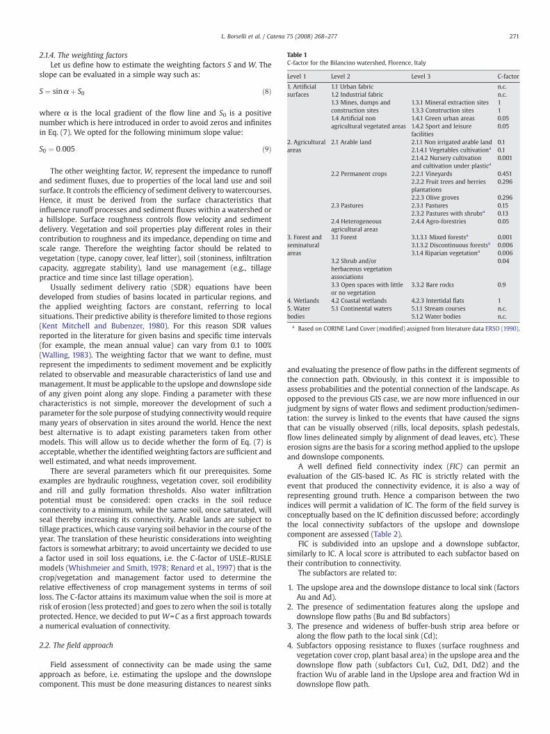
Table 1C-factor for the Bilancino watershed, Florence, Italy

Level 1 Level 2 Level 3 C-factor

1. Artificialsurfaces

1.1 Urban fabric n.c.1.2 Industrial fabric n.c.1.3 Mines, dumps andconstruction sites

1.3.1 Mineral extraction sites 11.3.3 Construction sites 1

1.4 Artificial nonagricultural vegetated areas

1.4.1 Green urban areas 0.051.4.2 Sport and leisurefacilities

0.05

2. Agriculturalareas

2.1 Arable land 2.1.1 Non irrigated arable land 0.12.1.4.1 Vegetables cultivationa 0.12.1.4.2 Nursery cultivationand cultivation under plastica

0.001

2.2 Permanent crops 2.2.1 Vineyards 0.4512.2.2 Fruit trees and berriesplantations

0.296

2.2.3 Olive groves 0.2962.3 Pastures 2.3.1 Pastures 0.15

2.3.2 Pastures with shrubsa 0.132.4 Heterogeneousagricultural areas

2.4.4 Agro-forestries 0.05

3. Forest andseminaturalareas

3.1 Forest 3.1.3.1 Mixed forestsa 0.0013.1.3.2 Discontinuous forestsa 0.0063.1.4 Riparian vegetationa 0.006

3.2 Shrub and/orherbaceous vegetationassociations

0.04

3.3 Open spaces with littleor no vegetation

3.3.2 Bare rocks 0.9

4. Wetlands 4.2 Coastal wetlands 4.2.3 Intertidal flats 15. Waterbodies

5.1 Continental waters 5.1.1 Stream courses n.c.5.1.2 Water bodies n.c.

a Based on CORINE Land Cover (modified) assigned from literature data ERSO (1990).

271L. Borselli et al. / Catena 75 (2008) 268–277

2.1.4. The weighting factorsLet us define how to estimate the weighting factors S and W. The

slope can be evaluated in a simple way such as:

S ¼ sinα þ S0 ð8Þ

where α is the local gradient of the flow line and S0 is a positivenumber which is here introduced in order to avoid zeros and infinitesin Eq. (7). We opted for the following minimum slope value:

S0 ¼ 0:005 ð9Þ

The other weighting factor, W, represent the impedance to runoffand sediment fluxes, due to properties of the local land use and soilsurface. It controls the efficiency of sediment delivery towatercourses.Hence, it must be derived from the surface characteristics thatinfluence runoff processes and sediment fluxes within a watershed ora hillslope. Surface roughness controls flow velocity and sedimentdelivery. Vegetation and soil properties play different roles in theircontribution to roughness and its impedance, depending on time andscale range. Therefore the weighting factor should be related tovegetation (type, canopy cover, leaf litter), soil (stoniness, infiltrationcapacity, aggregate stability), land use management (e.g., tillagepractice and time since last tillage operation).

Usually sediment delivery ratio (SDR) equations have beendeveloped from studies of basins located in particular regions, andthe applied weighting factors are constant, referring to localsituations. Their predictive ability is therefore limited to those regions(Kent Mitchell and Bubenzer, 1980). For this reason SDR valuesreported in the literature for given basins and specific time intervals(for example, the mean annual value) can vary from 0.1 to 100%(Walling, 1983). The weighting factor that we want to define, mustrepresent the impediments to sediment movement and be explicitlyrelated to observable and measurable characteristics of land use andmanagement. It must be applicable to the upslope and downslope sideof any given point along any slope. Finding a parameter with thesecharacteristics is not simple, moreover the development of such aparameter for the sole purpose of studying connectivity would requiremany years of observation in sites around the world. Hence the nextbest alternative is to adapt existing parameters taken from othermodels. This will allow us to decide whether the form of Eq. (7) isacceptable, whether the identified weighting factors are sufficient andwell estimated, and what needs improvement.

There are several parameters which fit our prerequisites. Someexamples are hydraulic roughness, vegetation cover, soil erodibilityand rill and gully formation thresholds. Also water infiltrationpotential must be considered: open cracks in the soil reduceconnectivity to a minimum, while the same soil, once saturated, willseal thereby increasing its connectivity. Arable lands are subject totillage practices, which cause varying soil behavior in the course of theyear. The translation of these heuristic considerations into weightingfactors is somewhat arbitrary; to avoid uncertainty we decided to usea factor used in soil loss equations, i.e. the C-factor of USLE–RUSLEmodels (Whishmeier and Smith, 1978; Renard et al., 1997) that is thecrop/vegetation and management factor used to determine therelative effectiveness of crop management systems in terms of soilloss. The C-factor attains its maximum value when the soil is more atrisk of erosion (less protected) and goes to zero when the soil is totallyprotected. Hence, we decided to put W=C as a first approach towardsa numerical evaluation of connectivity.

2.2. The field approach

Field assessment of connectivity can be made using the sameapproach as before, i.e. estimating the upslope and the downslopecomponent. This must be done measuring distances to nearest sinks

and evaluating the presence of flow paths in the different segments ofthe connection path. Obviously, in this context it is impossible toassess probabilities and the potential connection of the landscape. Asopposed to the previous GIS case, we are now more influenced in ourjudgment by signs of water flows and sediment production/sedimen-tation: the survey is linked to the events that have caused the signsthat can be visually observed (rills, local deposits, splash pedestals,flow lines delineated simply by alignment of dead leaves, etc). Theseerosion signs are the basis for a scoring method applied to the upslopeand downslope components.

A well defined field connectivity index (FIC) can permit anevaluation of the GIS-based IC. As FIC is strictly related with theevent that produced the connectivity evidence, it is also a way ofrepresenting ground truth. Hence a comparison between the twoindices will permit a validation of IC. The form of the field survey isconceptually based on the IC definition discussed before; accordinglythe local connectivity subfactors of the upslope and downslopecomponent are assessed (Table 2).

FIC is subdivided into an upslope and a downslope subfactor,similarly to IC. A local score is attributed to each subfactor based ontheir contribution to connectivity.

The subfactors are related to:

1. The upslope area and the downslope distance to local sink (factorsAu and Ad).

2. The presence of sedimentation features along the upslope anddownslope flow paths (Bu and Bd subfactors)

3. The presence and wideness of buffer-bush strip area before oralong the flow path to the local sink (Cd);

4. Subfactors opposing resistance to fluxes (surface roughness andvegetation cover crop, plant basal area) in the upslope area and thedownslope flow path (subfactors Cu1, Cu2, Dd1, Dd2) and thefraction Wu of arable land in the Upslope area and fraction Wd indownslope flow path.

Table 2Table for scoring and rapid appraisal of connectivity in the field

Place Coordinates Date

Local connectivity subfactor (LCS) Description Rating

Upslope subfactors

Range Scores Score notes

Au) Upslope catchment area A (ha) Ab0.1 00.1bAb0.5 150.5bAb1.0 301.0bAb2.0 45AN2.0 60

Bu) Presence of deposition evidences in upslope catchmentNote: in the absence of erosion processes assign score 0

Strong deposition 0

Clear evidences 5Discontinue evidences 10Minimum evidences 15Absent 20

Bare soil surface Cu1) Average roughness upslope catchment(standard deviation of elevations normal to soil surface—in cm)[computed along 3 m transects]

RRN4 0 Wu) fraction of area that is bare withrespect to the area that is covered byvegetation (0.0–1.0)

Wu

2bRRb4 51bRRb2 100.3bRRb1.0 15RRb0.3 20

Woodland, pasture,rangelands, crops

Cu2) at ground level: Average canopy cover % + plantbasal area % in upslope catchment (Cv) (in %)

80bCvb100 0

60bCvb80 540bCvb60 1020bCvb40 15Cvb20 20

Total score upslope component *Notes: * The total score of the upslope component is given by:Su=Au+Bu+WuCu1+(1−Wu)Cu2

Local connectivity subfactor (LCS) Description Rating

Downslope subfactors

Range Scores Score notes

Ad) Distance from local sink: d (m) dN100 0100bdb50 1050bdb10 2010bdb5 30db5 40

Bd) Presence of buffer/bush strip at the end of the flux pathway WideN4 m and dense 0Continue and dense 5Discontinue—sparse 10Minimum evidences 15Absent 20

Cd) Presence of deposition evidences along downslope pathwayNote: in the absence of erosion processes assign score 0

Strong deposition 0

Clear evidences 5Discontinue evidences 10Minimum evidences 15Absent 20

Bare soil surface Dd1) Average Roughness along downslope pathway(standard deviation of elevations normal to soilsurface—in cm) [computed along 3 m transects]

RRN4 0 Wd) fraction of area that is bare withrespect to the area that is covered byvegetation (0.0–1.0)

Wd

2bRRb4 51bRRb2 100.3bRRb1.0 15RRb0.3 20

Woodland, pasture,rangeland, crops

Dd2) at ground level: Average canopy cover % + plantbasal area % in downslope pathway (Cv) (in %)

80bCvb100 0

60bCvb80 540bCvb60 1020bCvb40 15Cvb20 20

Total score downslope component**Notes: ** The total score of the upslope component is given by: Sd=Ad+Bd+Cd+WdDd1+(1−Wd)Dd2The Field index of connectivity is given by FIC ¼ SuþSd

2

272 L. Borselli et al. / Catena 75 (2008) 268–277

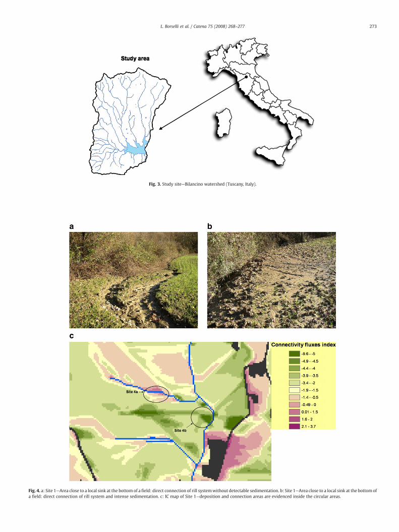
Fig. 3. Study site—Bilancino watershed (Tuscany, Italy).

Fig. 4. a: Site 1—Area close to a local sink at the bottom of a field: direct connection of rill systemwithout detectable sedimentation. b: Site 1—Area close to a local sink at the bottom ofa field: direct connection of rill system and intense sedimentation. c: IC map of Site 1—deposition and connection areas are evidenced inside the circular areas.

273L. Borselli et al. / Catena 75 (2008) 268–277

274 L. Borselli et al. / Catena 75 (2008) 268–277

The items 1–4 are scored in a way that will be discussed later. Thescoring allows for the FIC to be calculated as follows:

FIC ¼ Suþ Sd2

ð10Þ

Where the total upslope component score Su is given by

Su ¼ Auþ BuþWuCu1 þ 1−Wuð ÞCu2 ð11Þ

and the total downslope component score Sd is given by

Sd ¼ Adþ Bdþ CdþWdDd1 þ 1−Wdð ÞDd2 ð12ÞEq. (10) gives FIC values in the range [0,100] with connectivity

increasing with the FIC value.

3. Application at watershed scale

We have produced a complete example of the application of the ICatwatershed scale in order to test the efficacy of the newmethodology.

3.1. Watershed characteristics

The study site is the watershed of the Bilancino reservoir (NorthTuscany, Italy) (Fig. 3). It extends over an area of about 150 km2,ranging between a minimum of 225 m a.s.l. and maximum of 1094 ma.s.l. The climate is temperate with a relatively high level of humidity(Köppen classification Cfa–Cfb depending from altitude, Borselli et al.,2007). The catchment lies between the main divide of the Apennineson the north andMount Calvana and the dam of Bilancino reservoir onthe south (Fig. 1). Land use is represented by woodland (coppice andconiferous plantation) in the steepest mountain area, pasture or cropin piedmont zone and crops in the hills and valley bottoms;abandoned land is abundant in zones unsuitable for cropping andpasture. The present abandoned area was intensively cropped until1953 (Borselli et al., 2007), but the abandonment of the land is aprocess still in act under the current economic and social conditions.

Potential soil erosion in the basin was assessed using U.S.L.E.equation (Whishmeier and Smith, 1978). The assessment was basedon the following maps: rainfall erosivity, soil erodibility, DTM at a

Table 3Subfactors for field assessment of connectivity index FIC

Soil USDAclassification(8th Ed. 1998)

Land use Rainfall Season

Site 1 Typic udorthentsfine mixed mesic

Wheat crop at thebeginning of thegrowing season

2 events30 mm/day

Autumn

Site 2 Typic udorthentsclayey skeletal,mixed mesic

Wheat crop at thebeginning of thegrowing season

2 events30 mm/day

Autumn

Sub factors Component Site 1a Site 1b Site 2a Site 2b

Au Upslopecomponent

45 45 45 30Bu 20 5 20 5Cu1 5 5 10 10Cu2 – – 20 –

Wu 1 1 0.8 1Ad Downslope

component40 40 20 20

Bd 20 10 15 10Cd 20 20 20 10Dd1 – – – –

Dd2 20 10 15 5Wd 1 1 1 1Connectivity indexesFIC (Eq. (10)) 85 67.5 85 45IC (Eq. (7)) 0.5 −2.3 0.5 −3

The last row reports and the corresponding values of IC.

5×5 m cell resolution and a land use map at 1:10,000 scale. Details ofthis part of the application are described in Borselli et al. (2007).

3.2. Evaluation of the IC connectivity index

The calculation of the connectivity index is raster based. A DTMand a raster map of weighting factors with 5×5 m cell resolutionrepresent the main input data. The analysis is performed usingstandard GIS software (ArcGIS). We also limited ourselves to within-slope connectivity: the study site was examined in order to evaluatethe amount of sediment able to enter into the drainage network. Wemodelled permanent drainage lines (streams, roads, urban sites andlakes) as local sinks for sediments.

The procedure is described in more details in Appendix A. In brief,input data are analyzed to produce a set of intermediary themes. Wecalculated the following raster maps:

• Slope without null value (zeros are replaced with 0.005).• Road/urban mask: masking obliges the connectivity calculation toclose at the border with the masked area.

• Flow direction: computed once the road/urban mask and blue linemask are applied over the superposition of DTM andweighing indexmaps.

• Flow accumulation: cells positioned at a divide have a positive valueas accumulation at a cell is calculated at the downstream border ofeach cell.

• Weight map is represented by the raster map of canopy cover (C)USLE factor (Table 1).

• The Ddn is the map of weighed sediment length and is evaluatedwith Eq. (2)

• The Dup is the map of the drainage area of the cell and is evaluatedwith Eq. (4)

• The IC map is evaluated from the application of the Eq. (7)

We found that IC values varied between −3 and 10.

3.3. Field survey and connectivity assessment

To evaluate the degree to which the map represented realsediment flow connectivity, we compared it with field observations,conducted in autumn–winter 2003–2004 after several rainfall eventsof medium magnitude for the area.

During the surveys, 18 hot spot areas were identified within thewatershed in proximity of the main streams. They are representativeof the landuse and management of the basin. Figs. 4 and 5 showsexample of connection signatures (rills) observed at sites 1 and 2.Some site details (soil, landuse) are given in Table 3.

An example of the evaluation of the FIC up and downslopesubfactors is shown in Table 3. The overall FIC score and thecorresponding GIS computed IC values are also shown in Table 3.

The FIC values have been compared to the IC flux map obtainedwith the ArcGIS procedure for the entire study site (Fig. 6).

4. Discussion

Data plotted in Fig. 6 show a general agreement between IC andFIC. There are some mismatches which are strictly related to theresolution of the input raster map applied in the IC evaluation. Theseerrors could be avoided with a more detailed DTM (some cells drainedin cells different from the ones identified in the DTM) and land usemap also was too coarse in laying borders. This can be avoided usingbetter maps. Anyhow, the good correspondence between the GIS-based IC and the field based FIC, invites to further improve theproposed approach.

The structure of the IC model, Eq. (7), indicates that the quality andresolution of basic input data (DEM quality, DEM resolution, etc)influence final results (e.g. segment length or distance term di, slope

Fig. 5. a: Site 2—Area close to a local sink at the bottom of a field: direct connection of rill system without detectable sedimentation. b: Site 2—Area in proximity of local sink at thebottom of a field: direct connection of rill system with intense sedimentation. c: IC map of Site 2: deposition and connection areas are evidenced inside circular areas.

275L. Borselli et al. / Catena 75 (2008) 268–277

gradient). The use in our application of a 5×5 m resolution is acompromise to obtain an adequate DEM quality to represent manyerosion and deposition processes at field scale.

With the use of themodel of Eq. (7) we have a continuous dynamicform where each pixel in the downslope and upslope area gives its

Fig. 6. Relationships between FIC and IC (Bilancino watershed).

own contribution to connectivity. The detailed description of thealgorithm given in Appendix A, allows for easy implementationwithina GIS raster computation engine, where basic hydrologic routines areavailable.

The use of the FIC rating procedure helps to establish connectivityclass separation for corresponding IC values in relation to the eventintensity. The correspondence between FIC and IC is valid only locallybecause the climatic component and the event magnitude play animportant role in the connectivity evaluation. Nevertheless the FICprocedure can help to identify general relationships between IC andevent magnitudes. Using FIC as we did in the example shown in theprevious paragraphs transforms the absolute IC scale into a local scalecorresponding to typical erosive events with an annual return period.Values of FIC higher than 75 correspond to high connectivity withlimited storage of sediments in the pathway to the nearest sink. In ourdataset this corresponds to IC values equal or higher than −0.5. Thishas been observed for a set of connectivity signs produced by twoautumn events with a 2-year return period (see Table 3).

The IC model and FIC procedure have a large set of potentialapplications such as:

• Combined with soil erosion models (event based or conceptuallydistributed).

• Combined with model for debris flow and flash flood riskassessment.

276 L. Borselli et al. / Catena 75 (2008) 268–277

• Hot spot identification of primary sediment sources to permanentdrainage line.

• Verification of eco-compatible mitigation measures to reduceconnectivity (Hooke and Sandercock, 2007).

• Monitoring change in connectivity degree in areas with intensedynamics (of land use changes, geomorphologic evolution).

• Scenario analyses of connectivity evolution: modeling changes inthe management or land use in some areas, modifying the weighingfactor values.

5. Conclusions

Our definition of the indexof connectivity (IC) provides an estimate ofthe potential connection between the sediment eroded from hillslopesand the stream system. It takes into account the distribution of land useand topographic characteristic and as well as characteristics of thesurfaces and land use that can produce or store sediment and water.

The IC definition can be integrated with the proposed FICprocedure for assessing real connections during a series of events ofdifferent magnitudes.

The IC model and FIC procedure can be used separately but theirintegration allow IC validation and connectivity class rating based onIC index values calculated in a GIS context.

The IC model and FIC procedure have a large set of potentialapplications such as hot spot identification of primary sedimentsources to permanent drainage lines, verification of effects of eco-compatible mitigation measures to reduce or favour connectivity(Hooke and Sandercock, 2007), monitoring changes in the degreeof connectivity in areas with high geomorphological evolutionrates.

In particular the IC model may be used to perform scenarioanalyses. This last application of the IC may be useful to assess theefficiency of conservation measures against soil erosion and sedimenttransport, which are strongly related to flux connectivity.

Acknowledgements

This paper was funded by the European Commission, Directorate-General of Research, Global Change and Desertification Programme,RECONDES project (2004–2007) “Conditions for Restoration andMitigation of Desertified Areas using Vegetation” no. GOCE-CT-2003-505361 and by Autorità di Bacino del fiume Arno-Italy; BABIproject (2003–2007) “Studio della dinamica delle aree sorgentiprimarie di sedimento nell'area pilota del bacino di Bilancino”.

Appendix A. ArcGIS 8.3, ArcMap (spatial analyst extension)

Given datagrid: elevation, Cshapefile: road, urban areaComputation of input data

1. Slope without null valuea. Enable Spatial Analyst

under View… Toolbars, select Spatial Analyst

b. Calculate Slope

from the Spatial Analyst toolbar, select Surface Analysis… Slopename the new theme Slope

c. Raster Calculator

from the Spatial Analyst toolbar, select Raster Calculatorbuild an expression (([Slope]==0)⁎0.005)+[Slope]);name the new theme S

2. Road/urban maska. create a raster map of road and urban areas

from the Spatial Analyst toolbar, select Convert.. feature to raster

b. give 0 value to road and urban areas and value 1 to other area

from the Spatial Analyst toolbar, select Reclassifyname the new theme ROAD_MASK

3. Flow Direction with road/urban mask and blue line maska. Raster Calculator

from the Spatial Analyst toolbar, select Raster Calculatorbuild an expression:FlowDirection([elevation]))Evaluatename the new theme FlowDir

b. Raster Calculator

from the Spatial Analyst toolbar, select Raster Calculatorbuild an expression:[FlowDir]⁎ [ROAD_MASK]Evaluategive the new theme name DIRMASK1

c. Raster Calculator

from the Spatial Analyst toolbar, select Raster Calculatorbuild an expression:

flowaccumulation([DIRMASK1])Evaluatename the new theme ACCMASK1

d. Raster Calculator

from the Spatial Analyst toolbar, select Raster Calculator

build an expression:[ACCMASK1]b=1000Evaluategive the new theme name RIVERMASK

e. Raster Calculator

from the Spatial Analyst toolbar, select Raster Calculatorbuild an expression:[DIRMASK1]⁎ [RIVERMASK]Evaluategive the new theme name DIRFINAL

4. Flow Accumulation without null valuea. Raster Calculator

from the Spatial Analyst toolbar, select Raster Calculatorbuild an expression:flowaccumulation([DIRFINAL])+1Evaluategive the new theme name ACCFinal

Computation Ddn component

a. Raster Calculatorfrom the Spatial Analyst toolbar, select Raster Calculatorbuild an expression1/([C]⁎ [S])Evaluatename the new theme inv_CS

b. Raster Calculatorfrom the Spatial Analyst toolbar, select Raster Calculatorbuild an expression:flowlength([DIRFINAL], [inv_CS], downstream)Evaluatename the new theme X

c. Raster Calculatorfrom the Spatial Analyst toolbar, select Raster Calculatorbuild an expression:(([X]==0)⁎ [inv_CS])+ [X])Evaluatename the new theme Ddn

277L. Borselli et al. / Catena 75 (2008) 268–277

Computation Dup component

a. Raster Calculatorfrom the Spatial Analyst toolbar, select Raster Calculatorbuild an expression(flowaccumulation([[DIRFINAL], [C])+ [C]) / [ACCFinal]Evaluatename the new theme Cmean

b. Raster Calculatorfrom the Spatial Analyst toolbar, select Raster Calculatorbuild an expression(flowaccumulation([DIRFINAL], [S])+ [S]) / [ACCFinal]Evaluatename the new theme name Smean

c. Raster Calculatorfrom the Spatial Analyst toolbar, select Raster Calculatorbuild an expression[Cmean]⁎ [Smean]⁎Sqrt([ACCFinal]⁎25)Evaluatename the new theme Dup

Computation of Ic (Eq. (7))

a. Raster Calculator

from the Spatial Analyst toolbar, select Raster Calculator

build an expressionLog10([Dup/Ddn])Evaluatename the new theme name Ic

References

Atkinson, E., 1995. Methods for assessing sediment delivery in river system.Hydrological Sciences 40 (2), 273–280.

Bochet, E., Rubio, J.L., Poesen, J., 1999. Modified topsoil islands within patchyMediterranean vegetation in SE Spain. Catena 38 (1), 23–44.

Borselli, L., Cassi, P., Torri, D., Ungaro, F., Rodolfi, G., Pelacani, S., Sulli, L., 2007. Bilancinowatershed. Field trip guide—Part I. International Conference “Soil and HillslopeManagement Using Scenario Analysis and Runoff-erosion Models: A CriticalEvaluation of Current Techniques” Florence 7–9 May 2007. http://www.fi.cnr.it/irpi/cost634/field_trip_guide_cost634_florence2007.pdf.

Boyce, R.C., 1975. Sediment routing with sediment delivery ratios. Present andProspective Technology for Predicting Sediment Yield and Sources, Publ. ARS-S-40. U.S. Department of Agriculture, Washington, D.C., pp. 61–65.

Bracken, J.L., Croke, J., 2007. The concept of hydrological connectivity and itscontribution to understanding runoff dominated geomorphic system. HydrologicalProcesses 21 1749–1763 pp.

Cammeraat, E.L.H., 2002. A review of two strongly contrasting geomorphologicalsystems within the context of scale. Earth Surface Processes and Landforms 27 (11),1201–1222.

Cammeraat, E.L.H., 2004. Scale dependent thresholds in hydrological and erosionresponse of a semi-arid catchment in Southeast Spain. Agriculture, Ecosystems andEnvironment 104, 317–332.

Croke, J., Mockler, S., Fogarty, P., Takken, I., 2005. Sediment concentration changes inrunoff pathways from a forest road network and the resultant spatial pattern ofcatchment connectivity. Geomorphology 68, 257–268.

De Vente, J., Poesen, J., 2005. Predicting soil erosion and sediment yield at the basinscale: scale issues and semi-quantitative models. Earth-Science Reviews 71,95–125.

ERSO-RER. 1990. I suoli della collina cesenate, Regione Emilia Romagna, ArchivioCartografico.Ellebi, pp98.

Ferro, V., Porto, P., 2000. Sediment delivery distributed (SEDD) model. Journal ofHydraulic Engineering 5, 411–422.

Fryirs, K.A., Brierley, G.J., Preston, N.J., Spencer, J., 2007a. Catchment-scale (dis)connectivity in sediment flux in the upper Hunter catchment, New South Wales,Australia. Geomorphology 84, 297–316.

Fryirs, K.A., Brierley, G.J., Preston, N.J., Kasai, M., 2007b. Buffers, barriers and blankets:the (dis)connectivity of catchment-scale sediment cascades. Catena 70, 49–67.

Greenfield, J., Lahlou, M., Swift Jr., L., Manguerra, H.B., 2001. Watershed erosion andsediment load estimation tool. in Soil Erosion Research for the 21st Century. In:AscoughII II, J.C., Flanagan, D.C. (Eds.), Proc. Int. Symp. (3–5 January 2001, Honolulu,HI, USA). ASAE, St. Joseph, MI, pp. 302–305. 701P0007.

Harvey, A.M., 2001. Coupling between hillslopes and channels in upland fluvial system:implications for landscape sensitivity, illustrated from Howgill Fells, northwestEngland. Catena 42 225–250 pp.

Harvey, A.M., 2002. Effective timescales of coupling within fluvial systems. Geomor-phology 44 (3–4), 175–201.

Hooke, J., 2003. Coarse sediment connectivity in river channel systems: a conceptualframework and methodology. Geomorphology 56 79–94 pp.

RECONDES: conditions for restoration and mitigation of desertified areas in SouthernEurope using vegetation. In: Hooke, J.M., Sandercock, P.J. (Eds.), Final Report toEuropean Commission. University of Portsmouth. 250 pp.

KentMitchell, J., Bubenzer, G.D.,1980. Soil loss estimation. In: Kirkby, M.J., Morgan, R.P.C.(Eds.), Soil erosion. John Wiley, New York, USA, pp. 51–54.

Kinnell, P.I.A., 2004. Sediment delivery ratios: a misaligned approach to determiningsediment delivery from hillslopes. Hydrological Processes 18 (16) 3191–3194 pp.

Kirkby, M., Bracken, L., Reaney, S., 2002. The influence of land use, soils and topographyon the delivery of hillslope runoff to channels in SE Spain. Earth Surface Processesand Landforms 27 (13), 1459–1473.

Lu, H., Moran, C.J., Prosser, I.P., 2006. Modelling sediment delivery ratio over the MurrayDarling Basin. Environmental Modelling & software 21, 1297–1308.

Mitasova, H., Mitas, L., Brown, W.M., 2001. Multiscale simulation of land use impact onsoil erosion and deposition patterns. In: Stott, D.E., Mohtar, R.H., Stainhardt, G.C.(Eds.), Sustaining the Global Farm. Selected Papers from the International SoilConservation Organization Meeting, May 24–29, 1999, Purdue University andUSDA-ARS National Soil Erosion Research Laboratory, pp. 1163–1169.

Novotny, V., Chesters, G., 1989. Delivery of sediment and pollutants from nonpointsources: a water quality perspective. Journal of Soil and Water Conservation 44 (6),568–576.

Puigdefabregas, J., Sole, A., Gutierrez, L., Del Barrio, G., Boer, M., 1999. Scales andprocesses of water and sediment redistribution in drylands: results from theRambla Honda field site in Southeast Spain. Earth-Science Reviews 48 (1–2), 39–70.

Renard, K., Foster, G.R., Weessies, G.A., Mc Cool, D.K., Yodler, D.C., 1997. Predicting soilerosion by water—a guide to conservation planning with the Revised Universal SoilLoss Equation (RUSLE). U.S. D.A.- A.R.S., Handbook No 703. 384 pp.

Sun, G., McNulty, S.G., 1998. Modeling Soil Erosion and Transport on ForestLandscape. Proceedings of Conference, vol. 29. International Erosion ControlAssociation, pp. 187–198.

Van Rompaey, A.J.J., Verstraeten, G., Van Oost, K., Govers, G., Poesen, J., 2001. Modellingmean annual sediment yield using a distributed approach. Earth Surface Processesand Landforms 26, 1221–1236.

Whishmeier, W.H., Smith, D.D., 1978. Predicting Rainfall Erosion Losses—A Guide toConservation Planning. U.S. department of Agriculture. 537.

Walling, D.E., 1983. The sediment delivery problem. Journal of Hydrobiology 65,209–237.

Williams, J.R., 1977. Sediment delivery ratios determined with sediment and runoffmodels. Erosion and Solid Matter Transport in Inland Waters. IAHS-AISHpublication, vol. 122, pp. 168–179.

Wolman, M.G., Miller, J.P., 1960. Magnitude and frequency of forces in geomorphicprocesses. Journal of Geology 68, 54–74.

Yagow, E.R., Shanholtz, V.O., Julian, B.A., Flagg, J.M., 1988. A water quality module forCAMPS. Paper Presented at the 1988 International Winter Meeting of ASAE,December 13–16, 1988, Chicago, Illinois.

USDA-NRCS, 1983. Sediment sources, yields, and delivery ratios. Chapter 6 in NationalEngineering Handbook, Section 3, Sedimentation. US Department Agriculture,Natural Resources Conservation Service (USDA-NRCS) formerly Soil ConservationService (SCS), pp. 6.2–6.19.

USDA-SCS, Soil Conservation Service, 1986. National Engineering Handbook—Sect. 4,Hydrology. Washington D.C.