Productivity, Efficiency and Economic Growth:

East Asia and the Rest of the World*

Gaofeng Han

Department of Economics

University of California, Santa Cruz

Kaliappa Kalirajan

Foundation for Advanced Studies on International Development

Tokyo

Nirvikar Singh

Department of Economics

University of California, Santa Cruz

Contact Address: Professor K.P. Kalirajan, GRIPS, 2-2, Wakamatsucho, Shinjuku-ku, Tokyo

162-8677, Japan. Tel: 81-3-3341-0647; Fax: 81-3-3341-1030; e-mail: kalirajan@grips.ac.jp

* This research was generously supported by the Pacific Rim Research Program of the University of California. We

are grateful to seminar audiences at GRIPS/FASID in Tokyo, particularly Professors Hayami and Otsuka and

ICRIER in New Delhi, particularly Professor K.L. Krishna, and an anonymous referee of this Journal for helpful

comments and discussions on an earlier version of this paper. However, we alone are responsible for any remaining

shortcomings.

2

Productivity, Efficiency and Economic Growth:

East Asia and the Rest of the World

Abstract

This study compares the sources of growth in East Asia with the rest of the world, using a

methodology that allows one to decompose total factor productivity (TFP) growth into technical

efficiency changes (catching up) and technological progress. It applies a varying coefficients

frontier production function model to aggregate data for the period 1970-1990, for a sample of

45 developed and developing countries. Our results are consistent with the view that East Asian

economies were not outliers in terms of TFP growth. Of the high-performing East Asian

economies, our methodology identifies South Korea as having the highest TFP growth, followed

by Singapore, Taiwan and Japan. Our methodology also allows us to separately estimate

technical efficiency change, which is a component of TFP growth, and we find that, in general,

the estimated technical efficiency of the high-performing East Asian economies was not out of

line with the rest of the world.

Keywords: Total factor productivity growth, technical efficiency change, technical progress,

sources of growth, varying coefficients frontier production functions.

JEL codes: C21, O30, O47

3

Productivity, Efficiency and Economic Growth: East Asia and the Rest of the World

1. Introduction

Starting from the 1960s several East Asian countries achieved sustained high rates of

growth that were unprecedented. This growth experience not only dramatically changed

people's lives in those countries, but also raised issues such as what had been the contributing

factors, and whether the East Asian experience was replicable. While the East Asian economies,

such as Singapore, South Korea, Taiwan and Japan, are a diverse group, economic analysis

focuses on sources of growth that are quantifiable and have potentially the same impact across

countries. These include the role of factor accumulation and of technological change. While

institutional, cultural and political factors are certainly relevant, and have been addressed by

economists to the extent that they can be quantified (e.g., Barro and Sala-i-Martin, 1995,

Barro,1997), much of the attention has been on the relative roles of increases in the quantities of

the basic economic inputs, namely capital and labor, versus changes in the productivity of those

inputs.

While some assessments of the “sources of growth” literature (e.g., Felipe, 1999) have

questioned this entire approach and its theoretical basis, it remains true that empirical studies

have been both numerous and influential. For example, the World Bank (1993) and Hughes

(1995) examined the contribution of public policy in economic development; Kim and Lau

(1994), Young (1992, 1995) and Krugman (1994) emphasized capital accumulation in the high

performing East Asian economies; Sonobe and Otsuka (2001) advanced a hypothesis that

capital deepening associated with transformation of industrial structure has been the major

factor for sustaining growth for a long period in East Asia; Hayami and Ogasawara (1999)

argued that Japan has continued to depend more heavily on physical capital accumulation

mainly due to its characteristic of borrowed-technology based economic growth; and Singh and

Trieu (1997, 1999) focused more on the role of technological change. Despite many differences

in data and analytical methodologies, these and numerous other studies tended to have one

common assumption in analyzing the relative role of input accumulation and productivity

change: they assumed that production was always on the frontier without any slack in

production.

In this paper, we relax this assumption of full technical efficiency, instead allowing for

the possibility that an economy may be inside the best practice frontier. This approach is

4

justified by the fact that the production process is not simply an engineering relationship

between a set of inputs and observed output, but instead is the result of a series of economic

decisions based on various non-price and organizational factors, which influence the method of

application of inputs. Hence the relevant economic institutions will also play an important part

in an economy’s output. Our approach allows us to calculate total factor productivity growth in

an alternative manner to most previous studies. More importantly, it allows us to distinguish

between changes in technical efficiency (movement towards the frontier) and technological

progress (shifting the frontier) in analyzing the sources of growth in East Asia. Making this

distinction in a cross-country analysis represents the main contribution of the paper.

The structure of the paper is as follows. Section 2 provides a brief literature review,

focusing on papers that are most relevant to our work. The methodology followed in this paper,

as well as the data used, are explained in Section 3. In Section 4, we present the empirical results

for our cross-country analysis. Section 5 provides a summary conclusion.

2. Sources of Growth in East Asia: Previous Studies

The work closest in spirit to ours is that of Young (1994), Fischer (1993), Marti (1996)

and Collins and Bosworth (1997), who all looked at large cross-sections of countries. Young

regressed the output growth rate per worker on a constant and the growth of capital per worker

for the period 1970-1985 using cross-country data constructed from the Penn World Tables. The

capital stock was constructed by the perpetual inventory method with the accumulating

investment flows for 1960-1969 as benchmark, and a 6% depreciation rate. Young’s results from

this exercise were that, while TFP growth in Hong Kong was relatively high, it was not out of the

ordinary in South Korea and Taiwan, and very low in Singapore. Fischer (1993) used the growth

accounting method to estimate three sets of TFP growth rates, each with a different weight for

labor and capital, on data from the Penn World Tables. He obtained a negative TFP growth rate

for Singapore, and fairly low rates of TFP growth for Taiwan. Marti (1996) examined Young’s

(1994) results with slightly fewer countries but more periods than Young’s data set, again using

the Penn World Tables. She obtained a positive TFP contribution to the growth rate for

Singapore, while her results for other East Asian high performers were roughly consistent with

Young’s. Using growth accounting, Collins and Bosworth also found rates of TFP growth for

East Asian high performers that were not extraordinarily high.

Not all detailed growth accounting exercises agree with the results of cross-country

analyses. Looking at Hong Kong, Singapore, South Korea, and Taiwan, Young (1995) argued

5

that East Asia was not very different from Latin America in its TFP changes. However, Singh

and Trieu (1999) showed that this conclusion might be flawed, since it was based on comparing

results from different methodologies. Other growth accounting exercises for individual East

Asian countries have also given mixed results (Felipe, 1999).

The use of a frontier production function approach to analyze TFP growth in East Asia is

more recent than growth accounting estimates. For example, in a wider-ranging study, Han,

Singh and Kalirajan (2001) apply the stochastic production frontier methodology to

manufacturing sector data for Hong Kong, Japan, Singapore and South Korea, performing

analyses across sectors as well as across countries. They demonstrated that this methodology has

facilitated decomposing TFP growth into technical efficiency changes and technological

progress, and found that input growth has been the major contributor to economic growth in the

four economies considered. However, that analysis leaves an unanswered question of how do the

East Asian high performers compare to the rest of the world in terms of sources of growth. This

paper fills this gap by applying the frontier production analysis to a cross-section of countries

that includes most of the East Asian high performers.

3. Methodology and Data

A variety of techniques have been used to measure TFP growth (e.g., Fried, Lovell and

Schmidt 1993). This study applies a recently developed technique, i.e., the varying coefficient

production frontier approach, which isolates catching up to the frontier (technical efficiency

improvement) from shifts in the frontier (technical progress) (Kalirajan, Obwona and Zhao,

1996). This approach assumes that an economy obtains its full technical efficiency by following

best practice techniques, given the technology. In other words, technical efficiency is determined

by the method of application of inputs, regardless of the levels of inputs (that is, scale of

operation). This implies that different methods of applying various inputs will influence the

output differently, and the slope coefficients will vary from economy to economy. This varying

coefficient production frontier approach is an improvement over the conventional constant-slope

production frontier approach to measuring technical efficiency (Aigner et al, 1977; Meeusen et

al, 1977).

For a given technology, it may be interesting to know whether the gap between "best

practice" techniques and realized production methods is diminishing or widening over time.

Changes in technical efficiency can be substantial and may outweigh gains from technical

progress itself. It is, therefore, important to know how far one is off the production (technology)

6

frontier at any point in time, and how quickly one can reach the frontier. For instance, in the case

of economies such as East Asian countries, which borrow technology extensively from abroad,

failure to acquire and adapt the new technology to local production environment will result in not

operating on the production frontier, but below it without realizing the full potential of the

borrowed technology. The movement of the production or technology frontier over time, on the

other hand, reflects the success of explicit policies to facilitate the acquisition of foreign

technology. Similarly, changes in technical efficiency over time and across individual countries

will indicate the level of success of a number of important dimensions of industrial policies.

Technical efficiency and technical progress are examined for a given level of inputs.

The technological change component of productivity growth captures shifts in the

frontier technology and can be interpreted as providing a measure of innovation. This

decomposition of total factor productivity growth into technical efficiency improvement

(catching-up) and technological change is, therefore, useful in distinguishing innovation or

adoption of new technology by "best practice" firms from the diffusion of technology.

Co-existence of a high rate of technological progress and a low rate of change in technical

efficiency may reflect the failures in achieving technological mastery or diffusion.

3.1. The Varying Coefficients Stochastic Frontier model

Assuming a Cobb Douglas production technology, the varying coefficients production

frontier for the tth

period can be written as follows:

(1) kit

K

k

kiiit XY lnln2

1 ∑=+= βα i = 1,...,N.

where α α1 1i u= + 1i ; and Yit is the output level of the ith

economy in period t; Xkit is the level of

the kth

input used by the ith

economy in period t; α 1i is the intercept term for the ith

economy;

kiβ is the actual response of the output to the method of application of the kth

input by the ith

economy; and u refers to the random variable term which has mean zero and variance ki σ ukk .

Let

;kikki u+= ββ k = 1,2,...K and i = 1,2,...N

where,

( )kkiE ββ = ,

and ( )E uki = 0

7

for j = k and 0 otherwise. ( )Var uki ujk= σ

With these assumptions, model (1) can be written as

kitkit

K

k

kit wXY ++= ∑= lnln2

1 βα (2)

where

itkit

K

k

kikit uXuw 1

2

ln +=∑= for all i and k. ( ) 0=kitwE

( ) kit

K

k

ukkukit XwVar 2

2

11 ln∑=+= σσ ( ) 0, =jitkit wwCOV for . k j≠

Following the estimation procedures suggested by Hildreth and Houck (1968), the mean

response coefficients (α ’s) and the variances (σ ukk ) can be estimated and the individual

response coefficients ( kiβ ’s) can be obtained as described in Griffiths (1972). Drawing on

Kalirajan and Obwona (1994), the assumptions underlying model (2) are as follows:

(i) Technical efficiency is achieved by adopting the best practice techniques, which

involve the efficient use of inputs. Technical efficiency stems from two sources: (1) the efficient

use of each input which contributes individually to technical efficiency and can be measured by

the magnitudes of the varying slope coefficients, kiβ ’s; and (2) any other economy-specific

intrinsic characteristics which are not explicitly included may produce a combined contribution

over and above the individual contributions. This ‘lump sum’ contribution, if any, can be

measured by the varying intercept term.

(ii) The highest magnitude of each response coefficient and the intercept form the

production coefficients of the potential frontier production function. Let ( ’s) and ( ’s) be

the estimates of the coefficients of the frontier production function, that is,

α ∗ ∗β

{ } { };max;max jiijkiik ββαα == ∗∗ k = 1,...K; i = 1,. . .,N and j = 2,...,T.

Now the potential frontier output for individual observations can be calculated as

8

; i = 1,...N (3) kit

K

k

kit XY lnln2

1 ∑= ∗∗∗ += βαwhere Xkit is the actual level of the k

th input used by the i

th economy in period t. A measure of

technical efficiency denoted by, say, E, can be defined as

( )∗=t

it

itY

YE

lnexp (4)

where the numerator refers to the realized output and the denominator shows the potential

frontier output calculated from (3).

3.2. Decomposition of TFP growth

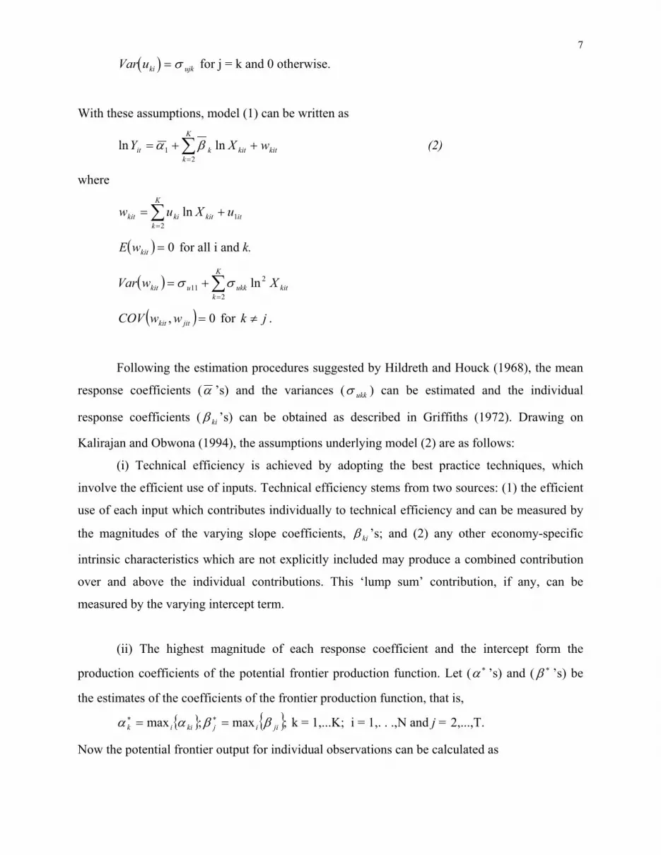
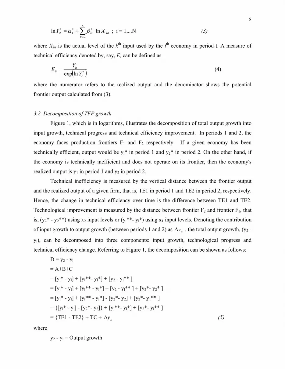
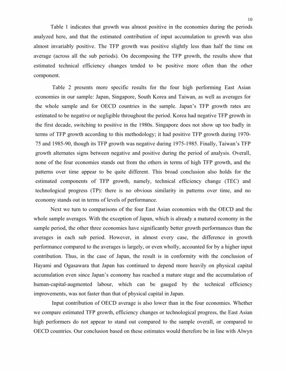
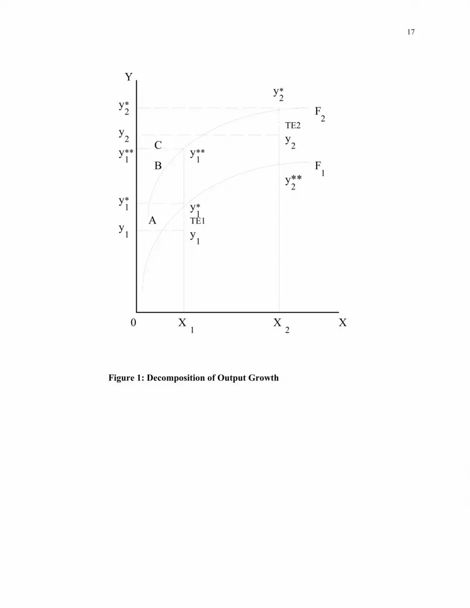
Figure 1, which is in logarithms, illustrates the decomposition of total output growth into

input growth, technical progress and technical efficiency improvement. In periods 1 and 2, the

economy faces production frontiers F1 and F2 respectively. If a given economy has been

technically efficient, output would be yl* in period 1 and y2* in period 2. On the other hand, if

the economy is technically inefficient and does not operate on its frontier, then the economy's

realized output is y1 in period 1 and y2 in period 2.

Technical inefficiency is measured by the vertical distance between the frontier output

and the realized output of a given firm, that is, TE1 in period 1 and TE2 in period 2, respectively.

Hence, the change in technical efficiency over time is the difference between TE1 and TE2.

Technological improvement is measured by the distance between frontier F2 and frontier F1, that

is, (y2* - y2**) using x2 input levels or (yl**- yl*) using x1 input levels. Denoting the contribution

of input growth to output growth (between periods 1 and 2) as ∆yx , the total output growth, (y2 -

yl), can be decomposed into three components: input growth, technological progress and

technical efficiency change. Referring to Figure 1, the decomposition can be shown as follows:

D = y2 - yl

= A+B+C

= [yl* - yl] + [yl**- yl*] + [y2 - yl** ]

= [yl* - yl] + [yl** - yl*] + [y2 - yl** ] + [y2*- y2* ]

= [yl* - yl] + [yl** - yl*] - [y2*- y2] + [y2*- y1** ]

= {[yl* - yl] - [y2*- y2]} + [yl**- yl*] + [y2*- yl** ]

= {TE1 - TE2} + TC + (5) ∆yx

where

y2 - yl = Output growth

9

TE1 - TE2 = Technical efficiency change

TC = Technical change and

= Output growth due to input growth. ∆yx

Solow (1957) attributed output growth to input growth and technical change. The

decomposition in (5) enriches Solow’s dichotomy by attributing observed output growth to

movements along a path on or beneath the production frontier (input growth), movement toward

or away from the production frontier (technical efficiency change), and shifts in the production

frontier (technological progress).

3.3 Data

The data is from the Penn World Tables and the World Bank STARS database. We

choose sample countries based on the data quality ranking by Summers (1992) (see Appendix).

Any economy chosen is at least at the three-star level, which leaves a total of 45 economies in

our sample. Unfortunately, Hong Kong is not in our sample, but other East Asian high

performers are included. The series retrieved from the Penn World tables are capital stock per

worker (1985 international prices), real GDP per capita (1985 international prices), and the series

from STARS are population and labor force. We multiply capital per worker by labor force to

get capital stock, and multiply real GDP per capita by population to get real GDP. The GDP and

capital stock are measured in dollars, and labor force is measured in persons.

4. Empirical Results

Using the methodology described in the previous section, we estimated frontier production

functions for the 45 country sample year by year for 1970, 1975, 1980, 1985, and 1990. Given

the objective of this paper, we used the frontier production function estimates to calculate the

technical efficiency, technical progress and inputs growth for each country by decomposing the

growth rates for 1970-1975, 1975-1980, 1980-1985, and 1985-1990. Detailed results are

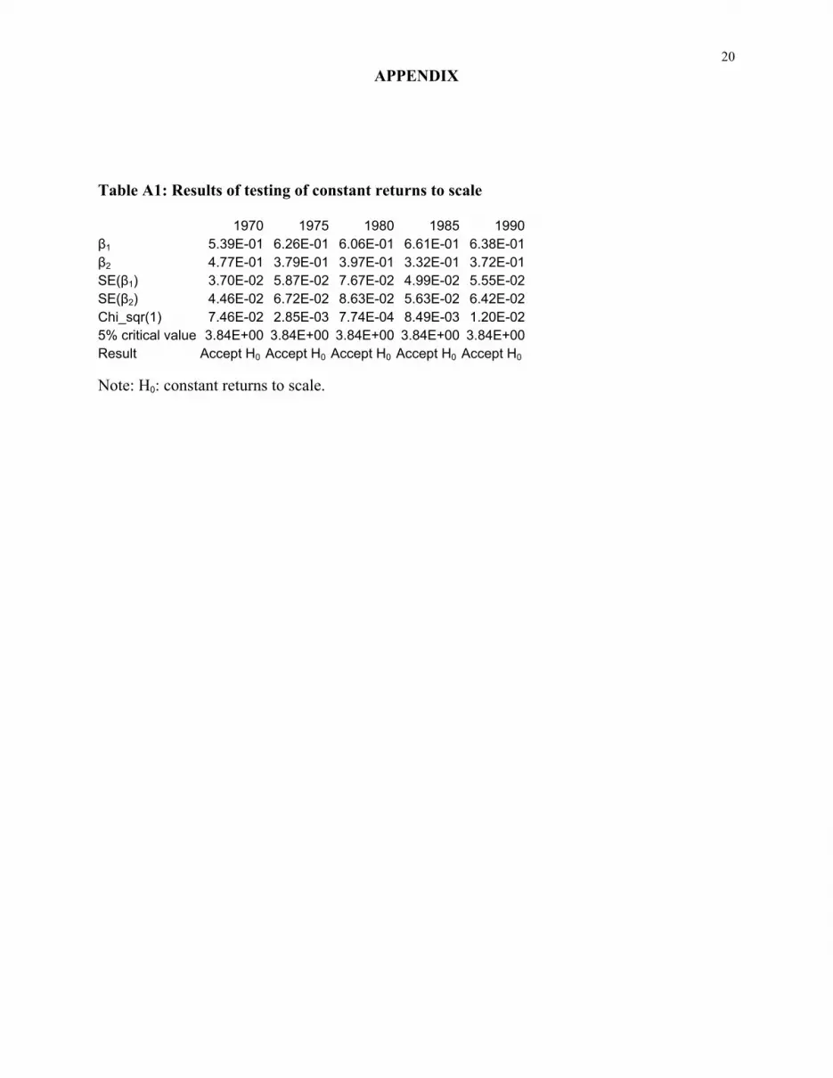
presented in the Appendix, while we discuss the overall results in this section. Though we could

not test individual country’s production function because of the sample property, the mean

response coefficients estimates of all countries for the chosen 5 years are tested for individual

years for constant returns to scale. Results based on Wald’s test statistics indicate that the

hypothesis of constant returns to scale could not be rejected for the chosen data set. The results

are given in Appendix Table A1.

10

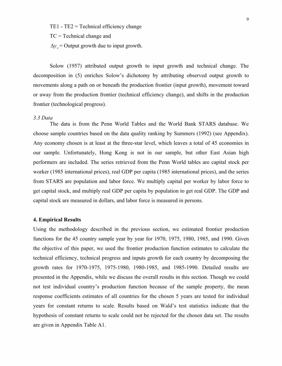
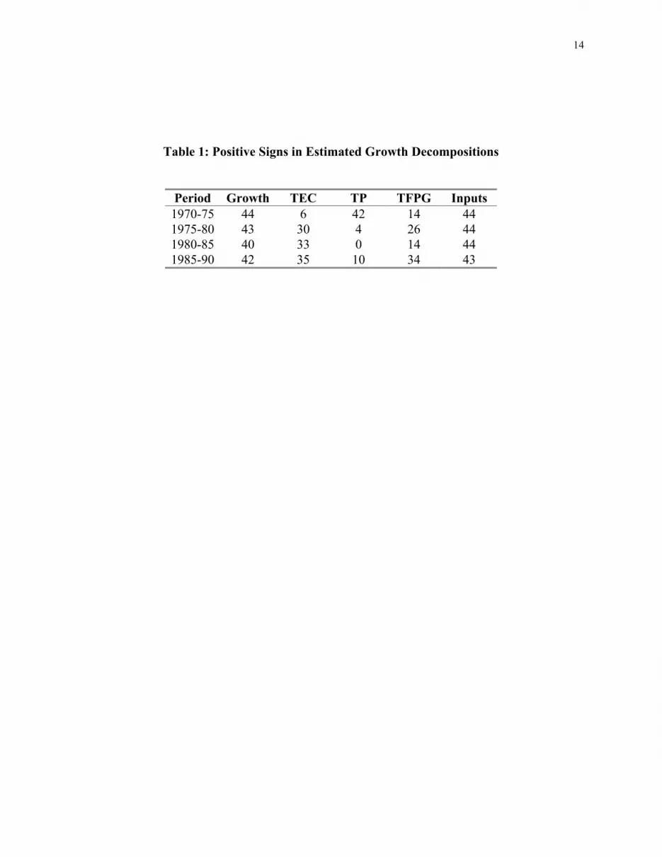
Table 1 indicates that growth was almost positive in the economies during the periods

analyzed here, and that the estimated contribution of input accumulation to growth was also

almost invariably positive. The TFP growth was positive slightly less than half the time on

average (across all the sub periods). On decomposing the TFP growth, the results show that

estimated technical efficiency changes tended to be positive more often than the other

component.

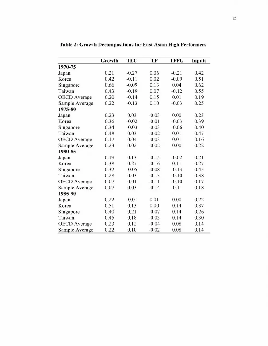
Table 2 presents more specific results for the four high performing East Asian

economies in our sample: Japan, Singapore, South Korea and Taiwan, as well as averages for

the whole sample and for OECD countries in the sample. Japan’s TFP growth rates are

estimated to be negative or negligible throughout the period. Korea had negative TFP growth in

the first decade, switching to positive in the 1980s. Singapore does not show up too badly in

terms of TFP growth according to this methodology; it had positive TFP growth during 1970-

75 and 1985-90, though its TFP growth was negative during 1975-1985. Finally, Taiwan’s TFP

growth alternates signs between negative and positive during the period of analysis. Overall,

none of the four economies stands out from the others in terms of high TFP growth, and the

patterns over time appear to be quite different. This broad conclusion also holds for the

estimated components of TFP growth, namely, technical efficiency change (TEC) and

technological progress (TP): there is no obvious similarity in patterns over time, and no

economy stands out in terms of levels of performance.

Next we turn to comparisons of the four East Asian economies with the OECD and the

whole sample averages. With the exception of Japan, which is already a matured economy in the

sample period, the other three economies have significantly better growth performances than the

averages in each sub period. However, in almost every case, the difference in growth

performance compared to the averages is largely, or even wholly, accounted for by a higher input

contribution. Thus, in the case of Japan, the result is in conformity with the conclusion of

Hayami and Ogasawara that Japan has continued to depend more heavily on physical capital

accumulation even since Japan’s economy has reached a mature stage and the accumulation of

human-capital-augmented labour, which can be gauged by the technical efficiency

improvements, was not faster than that of physical capital in Japan.

Input contribution of OECD average is also lower than in the four economies. Whether

we compare estimated TFP growth, efficiency changes or technological progress, the East Asian

high performers do not appear to stand out compared to the sample overall, or compared to

OECD countries. Our conclusion based on these estimates would therefore be in line with Alwyn

11

Young’s, though the methodology used is quite different: East Asian growth can be mostly

explained by high rates of input accumulation.

Aside from the issue of TFP growth and its decomposition into efficiency change and

technological progress, another measure of East Asian growth performance is the calculation of

their relative efficiency, and how that changes over time. In Table 3, we present the technical

efficiency (catching up with the production frontier) rankings for each of the five years in our

data. By fitting a production frontier to each year’s data, we are able to estimate where each

country in the sample lies relative to the global production frontier involving sample countries.

Technical efficiency is defined as the ratio of realized output to potential output.

On the whole, the results on efficiency rankings seem reasonable. The bulk of the high-

efficiency group made up of developed economies such as the United States, United Kingdom

and Canada are high in the rankings, whereas economies typically perceived as inefficient are

much lower down. Of the four high-performing East Asian economies in our sample, only

Taiwan appears high in the efficiency rankings. Japan moves around in the middle of the pack

over this period, while Singapore and Korea are invariably in the lower third and fourth groups

for all the sample years. Thus, the frontier estimations suggest that in general the high

performing East Asian economies did not stand out in terms of levels or improvements in

technical efficiency compared to the rest of the world, even as they were achieving great strides

in development and growth during these years. In other words, during the study period, these

East Asian countries had been producing inside the frontier and slightly shifting the frontier

without realizing fully the frontier with which they were operating.

5. Conclusion

In this paper, we use the varying coefficients stochastic production frontier approach and cross-

section data for 45 countries to analyze the sources of economic growth in East Asia and

compare them with the rest of the world, particularly the OECD countries. Our methodology

allows us to decompose the TFP growth into technical efficiency change and technological

progress. Further, this methodology facilitated carrying out additional analysis, which was not

done by Young or other researchers earlier. One such extension of analysis is that of the

efficiency ranking and comparison across the countries. Other methodologies might allow for

TFP ranking, but not the Technical Efficiency ranking. We can do both, though we have

emphasized the latter in our paper.

12

Our findings elaborate on the status of the components of TFP. Technical efficiency

rankings need not necessarily be consistent with TFP rankings. For example, (a) Taiwan has a

much higher rank in terms of technical efficiency, compared to the TFP rank; (b) Industrialized

economies, such as US, UK, Canada, New Zealand, Sweden, Austria, Australia, are well on the

top of the efficiency ranking, while in Young (94), they are at mediocre or low level in terms of

the TFP ranking. The difference of these two rankings indeed gives our methodology some

leverage. For those industrialized countries, even TFP is low at certain period of time, they stand

out by their high technical efficiency, which is one of the important criterions for sustaining a

country’s competitiveness gloablly. Thus, our analysis adds another valuable dimension in

sources of growth analysis.

Our estimation results suggest that during 1970-1990, the four high-performing East

Asian economies in our sample – Japan, Singapore, South Korea and Taiwan – do not stand out

from the rest of the world in terms of their TFP growth performance, or in terms of their

efficiency in input use. Input growth appears to be the main contributor to their overall economic

growth. It may be argued that institutions have been playing important roles in fostering such a

pattern of growth in East Asia. In the context of the labour input, these Asian economies have

large populations and so it is natural that their usage of labor input is large compared to the

Western countries. In the context of capital input, Asian economies have high savings, which is

exactly related to Asian Culture. People work and save much, which is obviously opposite to

Western countries. The high savings finally have to be transformed into high investment.

Besides, Governments in these countries intend to keep high employment, which is also related

to Policy as well as Asian Culture. The culture makes layoff more difficult than in other regions

and also there are no unemployment benefits as in the case of Western countries.

Considering the policy implications, it is clear from Table 3 that East Asian countries

appear to have a lot of catching up to do in technical efficiency improvements. Why Japan,

Korea and Singapore have mediocre or low Tech efficiency? Japanese, Korean and Singaporean

firms are well guided or backed by their governments upon development. They are not as

flexible as US firms with respect to human resources policy and investment policy. Korea’s

Chaebol and Japan’s Harachu are typical institutions (structure) that could lead to high

efficiency as we as low efficiency. The low efficiency emerges if: [a] employees feel that they

have lifetime employment (as in China) and so people would shirk; [2] rigid firm structure could

not response to the varying goods demand outside. Japan and Korea had, and Japan still has,

13

such problem once world demand declined. Over capacity and lack of quick adjustment policy

such as in US could tie down efficiency easily. It is not surprising that most of the firms in these

economies have mediocre technical efficiency. As for Singapore, low technical efficiency might

be from the fact, that there are vast new technical introductions from abroad during the period,

but the human capital did not match the requirements of new technologies in terms of knowledge

and experience. It may be noted that Singapore recently brought many educated employees from

countries like China and India to improve their human capital. Why Taiwan has high technical

efficiency? Taiwan has government guidance too just like other East Asian economies. However,

firms are more flexible than in other economies. It has no firm structure such as Chaebol and

Harachu, this might contribute to its relatively high technical efficiency. Efficiency is

dynamically changing, rather than being static. What we see from table 2, is that, the efficiency

improvement had lead to a big TFP growth for most of the economies during 1985-1990. In all,

culture, institutions, and policies appear to matter in the development as well as efficiency

improvement, particularly in East Asia.

14

Table 1: Positive Signs in Estimated Growth Decompositions

Period Growth TEC TP TFPG Inputs

1970-75 44 6 42 14 44

1975-80 43 30 4 26 44

1980-85 40 33 0 14 44

1985-90 42 35 10 34 43

15

Table 2: Growth Decompositions for East Asian High Performers

Growth TEC TP TFPG Inputs

1970-75

Japan 0.21 -0.27 0.06 -0.21 0.42

Korea 0.42 -0.11 0.02 -0.09 0.51

Singapore 0.66 -0.09 0.13 0.04 0.62

Taiwan 0.43 -0.19 0.07 -0.12 0.55

OECD Average 0.20 -0.14 0.15 0.01 0.19

Sample Average 0.22 -0.13 0.10 -0.03 0.25

1975-80

Japan 0.23 0.03 -0.03 0.00 0.23

Korea 0.36 -0.02 -0.01 -0.03 0.39

Singapore 0.34 -0.03 -0.03 -0.06 0.40

Taiwan 0.48 0.03 -0.02 0.01 0.47

OECD Average 0.17 0.04 -0.03 0.01 0.16

Sample Average 0.23 0.02 -0.02 0.00 0.22

1980-85

Japan 0.19 0.13 -0.15 -0.02 0.21

Korea 0.38 0.27 -0.16 0.11 0.27

Singapore 0.32 -0.05 -0.08 -0.13 0.45

Taiwan 0.28 0.03 -0.13 -0.10 0.38

OECD Average 0.07 0.01 -0.11 -0.10 0.17

Sample Average 0.07 0.03 -0.14 -0.11 0.18

1985-90

Japan 0.22 -0.01 0.01 0.00 0.22

Korea 0.51 0.13 0.00 0.14 0.37

Singapore 0.40 0.21 -0.07 0.14 0.26

Taiwan 0.45 0.18 -0.03 0.14 0.30

OECD Average 0.23 0.12 -0.04 0.08 0.14

Sample Average 0.22 0.10 -0.02 0.08 0.14

16

Table 3: Technical Efficiency (catching up) Ranking Across Economies

1970 1975 1980 1985 1990

Argentina Argentina Argentina Australia Canada Austria Austria Australia Canada Denmark Denmark Canada Austria Denmark Ireland Germany New Zealand Canada Morocco Israel New Zealand Sweden Denmark New Zealand Morocco Sweden Taiwan New Zealand Sweden Portugal Taiwan United Kingdom Sweden Taiwan Taiwan United Kingdom United States Taiwan United Kingdom United Kingdom United States Denmark United Kingdom United States United States

Venezuela Venezuela United States Argentina Australia

Australia Australia Belgium Austria Austria Belgium France France France Belgium Canada Germany Germany Ireland France Chile Ireland Ireland Israel Italy Ireland Israel Israel Italy Jamaica Israel Jamaica Italy Jamaica Japan Italy Japan Japan Japan Luxembourg Jamaica Malaysia Luxembourg Malaysia Malaysia Japan Mexico Malaysia Mexico Netherlands Luxembourg Morocco Mexico Netherlands New Zealand Malaysia Netherlands Morocco Norway Norway Netherlands Portugal Netherlands Portugal Sweden Spain Spain Norway Thailand Thailand Switzerland Belgium Portugal Belgium Argentina

Bolivia Chile Chile Chile Chile

Finland Finland Finland Finland Finland Greece Greece Greece Germany Germany Korea Italy Jamaica India Greece Mexico Luxembourg Peru Korea India Morocco Norway Philippines Luxembourg Korea Norway Peru Singapore Singapore Mexico Panama Philippines Spain Spain Philippines Peru Singapore Switzerland Switzerland Singapore Philippines Switzerland Thailand Turkey Spain Portugal Thailand Turkey Venezuela Switzerland Singapore Turkey Venezuela Bolivia Turkey

Thailand Bolivia Bolivia Colombia Venezuela

Turkey Colombia Colombia Ecuador Bolivia

Colombia Ecuador Ecuador Greece Colombia Ecuador Honduras Honduras Honduras Ecuador France India India Panama Honduras Honduras Korea Korea Peru Panama India Panama Panama Philippines Peru Sri Lanka Sri Lanka Sri Lanka Sri Lanka Sri Lanka Zimbabwe Zimbabwe Zimbabwe Zimbabwe Zimbabwe

17

0 X1

X2

X

Y

y1

y1*

y1**

y2

y2*

A

B

C

y2*

y2

y1**

y1*

y1

F

F

TE1

TE22

1y**

2

Figure 1: Decomposition of Output Growth

18

References

Aigner, D. J., C.A.K. Lovell, and P. Schmidt (1977), “Formulation and estimation of stochastic

frontier production function models”, Journal of Econometrics, 6, 21-37.

Barro, R. and X. Sala-I-Martin (1995), Economic growth . New York: McGraw-Hill.

Barro, R. (1997), Determinants of economic growth: a cross-country empirical study.

Cambridge, Mass. : The MIT Press.

Collins, S. and B. Bosworth (1997), ‘Economic Growth in East Asia: Accumulation versus

Assimilation,’ in W.C. Brainard and G.L. Perry, eds. Brookings Papers in Economic

Activity, 2, Washington DC: Brookings Institution.

Felipe, J. (1999), “Total Factor Productivity Growth in East Asia: A Critical Survey,” Journal of

Development Studies, v 35 n 4, 1-41.

Fischer, S. (1993), “The Role of Macroeconomic Factors in Growth,” Journal of Monetary

Economics, 32, 485-512.

Fried, H., C.A. K. Lovell and S. Schmidt (1993), The measurement of productive efficiency,

Oxford University Press.

Griffiths, W. E. (1972), “Estimating actual response coefficients in the Hildreth-Houck random

coefficient model”, Journal of the American Statistical Association, 67, 633-35.

Han, G., K.P. Kalirajan and N. Singh (2001), ‘Productivity and Economic Growth in East Asia:

Innovation, Efficiency and Accumulation’, Santa Cruz Center for International

Economics Working Paper #01-20, http://sccie.ucsc.edu/workingpapers/index.html.

Hayami. Y. and J. Ogasawara (1999), “Changes in the Sources of Modern Economic Growth:

Japan Compared with the United States”, Journal of the Japanese and International

Economies, 13, 1-21.

Hildreth, C. and J.P. Houck (1968), “Some estimators for a linear model with random

coefficients”, Journal of the American Statistical Association, 63, 584-95.

Hughes, H. (1995), "Why have East Asia countries led economic development", Economic

Record, 71(212), 88-104.

Kalirajan, K.P. and M.B. Obwona (1994), “Frontier Production Function: The Stochastic

Coefficients Approach”, Oxford Bulletin of Economics and Statistics, 56, 87-96.

Kalirajan, K.P., M.B. Obwona and S. Zhao (1996), “A Decomposition of Total Factor

Productivity Growth: The Case of Chinese Agricultural Growth Before and After

Reforms”, American Journal of Agricultural Economics 78, 331-38.

Kim, Jong-Il and L. Lau (1994), "The sources of economic growth in the East Asian newly

industrialized countries", Journal of the Japanese and International Economies, 8(3), 235-

271.

19

Krugman, Paul (1994), "The myth of Asia's miracle", Foreign Affairs, November/December.

Mahadevan, R., and K.P. Kalirajan, ‘Singapore’s Manufacturing Sector’s TFP Growth: A

Decomposition Analysis’, Journal of Comparative Economics, 2000, vol.28: 828-839.

Marti, C., (1996), “Is There an East Asian Miracle?” Union Bank of Switzerland Economic

Research Working Paper, October.

Meeusen, W. and J. van den Broeck (1977), “Efficiency estimation from Cobb-Douglas

production functions with composed error”, International Economic Review, 18, 435-44.

Singh, N. and H. Trieu (1999), "Accounting for East Asian Growth: Japan, Korea and Taiwan",

Indian Economic Review.

Singh, N. and H. Trieu (1997), "The role of R&D in explaining total factor productivity growth

in Japan, Korea and Taiwan", UCSC Dept. of Economics Working Paper.

Solow, R.M. (1957), “Technical change and the aggregate production”, Review of Economics

and Statistics, 39(3), 312-20.

Sonobe, T. and K. Otsuka (2001), “A New Decomposition Approach to Growth Accounting:

Derivation of the Formula and its Application to Prewar Japan”, Japan and the World

Economy, 13, 1-14.

Summers, R. and A. Heston (1991), "The Penn World Table (Mark 5): an expanded set of

international comparisons, 1950-1987", Quarterly Journal of Economics, 106(2), 1-41.

World Bank (1993), The East Asian Miracle, a World Bank policy research report, Oxford

University Press.

Young, A. (1992), "A tale of two cities: factor accumulation and technical change in Hong Kong

and Singapore", NBER Macroeconomic Annual, NRT Press.

Young, A. (1994), "Lessons from the East Asian NICs: a contrarian view", European Economic

Review, 110(3), 641-680.

Young, A. (1995), "The tyranny of numbers: confronting the statistical realities of the East Asian

growth experience", Quarterly Journal of Economics, 110(3), 641-680.

20

APPENDIX

Table A1: Results of testing of constant returns to scale

1970 1975 1980 1985 1990

β1 5.39E-01 6.26E-01 6.06E-01 6.61E-01 6.38E-01

β2 4.77E-01 3.79E-01 3.97E-01 3.32E-01 3.72E-01

SE(β1) 3.70E-02 5.87E-02 7.67E-02 4.99E-02 5.55E-02

SE(β2) 4.46E-02 6.72E-02 8.63E-02 5.63E-02 6.42E-02

Chi_sqr(1) 7.46E-02 2.85E-03 7.74E-04 8.49E-03 1.20E-02

5% critical value 3.84E+00 3.84E+00 3.84E+00 3.84E+00 3.84E+00

Result Accept H0 Accept H0 Accept H0 Accept H0 Accept H0

Note: H0: constant returns to scale.

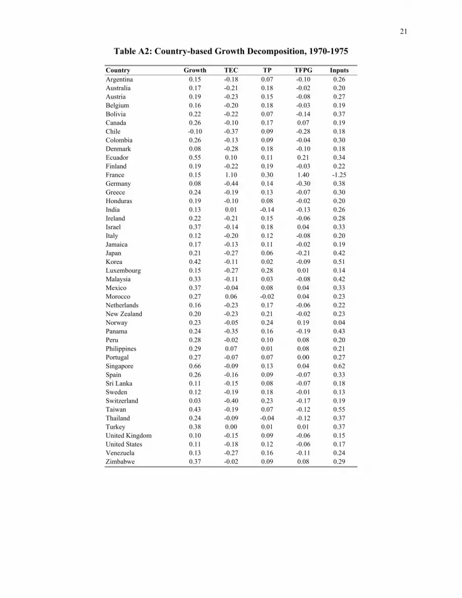
21

Table A2: Country-based Growth Decomposition, 1970-1975

Country Growth TEC TP TFPG Inputs

Argentina 0.15 -0.18 0.07 -0.10 0.26

Australia 0.17 -0.21 0.18 -0.02 0.20

Austria 0.19 -0.23 0.15 -0.08 0.27

Belgium 0.16 -0.20 0.18 -0.03 0.19

Bolivia 0.22 -0.22 0.07 -0.14 0.37

Canada 0.26 -0.10 0.17 0.07 0.19

Chile -0.10 -0.37 0.09 -0.28 0.18

Colombia 0.26 -0.13 0.09 -0.04 0.30

Denmark 0.08 -0.28 0.18 -0.10 0.18

Ecuador 0.55 0.10 0.11 0.21 0.34

Finland 0.19 -0.22 0.19 -0.03 0.22

France 0.15 1.10 0.30 1.40 -1.25

Germany 0.08 -0.44 0.14 -0.30 0.38

Greece 0.24 -0.19 0.13 -0.07 0.30

Honduras 0.19 -0.10 0.08 -0.02 0.20

India 0.13 0.01 -0.14 -0.13 0.26

Ireland 0.22 -0.21 0.15 -0.06 0.28

Israel 0.37 -0.14 0.18 0.04 0.33

Italy 0.12 -0.20 0.12 -0.08 0.20

Jamaica 0.17 -0.13 0.11 -0.02 0.19

Japan 0.21 -0.27 0.06 -0.21 0.42

Korea 0.42 -0.11 0.02 -0.09 0.51

Luxembourg 0.15 -0.27 0.28 0.01 0.14

Malaysia 0.33 -0.11 0.03 -0.08 0.42

Mexico 0.37 -0.04 0.08 0.04 0.33

Morocco 0.27 0.06 -0.02 0.04 0.23

Netherlands 0.16 -0.23 0.17 -0.06 0.22

New Zealand 0.20 -0.23 0.21 -0.02 0.23

Norway 0.23 -0.05 0.24 0.19 0.04

Panama 0.24 -0.35 0.16 -0.19 0.43

Peru 0.28 -0.02 0.10 0.08 0.20

Philippines 0.29 0.07 0.01 0.08 0.21

Portugal 0.27 -0.07 0.07 0.00 0.27

Singapore 0.66 -0.09 0.13 0.04 0.62

Spain 0.26 -0.16 0.09 -0.07 0.33

Sri Lanka 0.11 -0.15 0.08 -0.07 0.18

Sweden 0.12 -0.19 0.18 -0.01 0.13

Switzerland 0.03 -0.40 0.23 -0.17 0.19

Taiwan 0.43 -0.19 0.07 -0.12 0.55

Thailand 0.24 -0.09 -0.04 -0.12 0.37

Turkey 0.38 0.00 0.01 0.01 0.37

United Kingdom 0.10 -0.15 0.09 -0.06 0.15

United States 0.11 -0.18 0.12 -0.06 0.17

Venezuela 0.13 -0.27 0.16 -0.11 0.24

Zimbabwe 0.37 -0.02 0.09 0.08 0.29

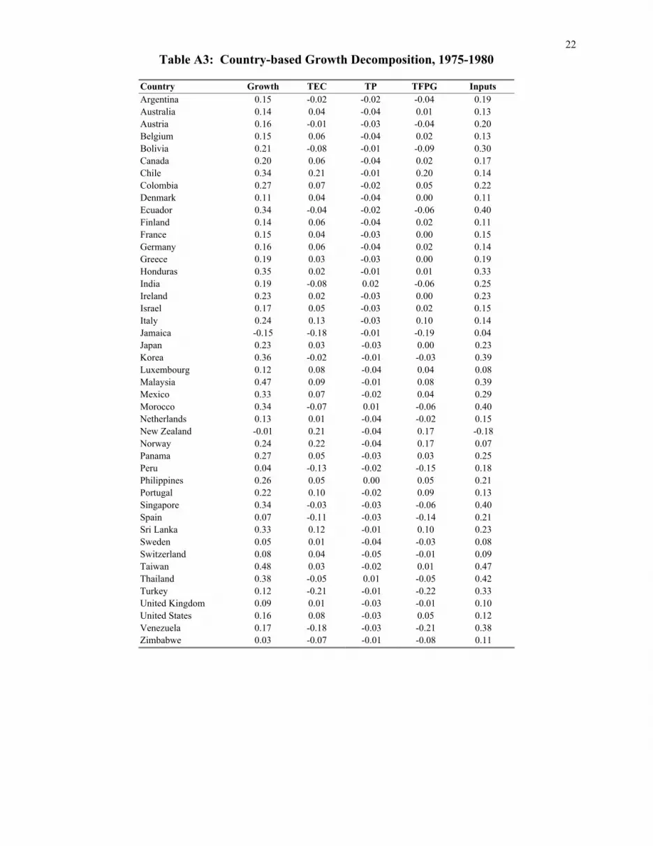
22

Table A3: Country-based Growth Decomposition, 1975-1980

Country Growth TEC TP TFPG Inputs

Argentina 0.15 -0.02 -0.02 -0.04 0.19

Australia 0.14 0.04 -0.04 0.01 0.13

Austria 0.16 -0.01 -0.03 -0.04 0.20

Belgium 0.15 0.06 -0.04 0.02 0.13

Bolivia 0.21 -0.08 -0.01 -0.09 0.30

Canada 0.20 0.06 -0.04 0.02 0.17

Chile 0.34 0.21 -0.01 0.20 0.14

Colombia 0.27 0.07 -0.02 0.05 0.22

Denmark 0.11 0.04 -0.04 0.00 0.11

Ecuador 0.34 -0.04 -0.02 -0.06 0.40

Finland 0.14 0.06 -0.04 0.02 0.11

France 0.15 0.04 -0.03 0.00 0.15

Germany 0.16 0.06 -0.04 0.02 0.14

Greece 0.19 0.03 -0.03 0.00 0.19

Honduras 0.35 0.02 -0.01 0.01 0.33

India 0.19 -0.08 0.02 -0.06 0.25

Ireland 0.23 0.02 -0.03 0.00 0.23

Israel 0.17 0.05 -0.03 0.02 0.15

Italy 0.24 0.13 -0.03 0.10 0.14

Jamaica -0.15 -0.18 -0.01 -0.19 0.04

Japan 0.23 0.03 -0.03 0.00 0.23

Korea 0.36 -0.02 -0.01 -0.03 0.39

Luxembourg 0.12 0.08 -0.04 0.04 0.08

Malaysia 0.47 0.09 -0.01 0.08 0.39

Mexico 0.33 0.07 -0.02 0.04 0.29

Morocco 0.34 -0.07 0.01 -0.06 0.40

Netherlands 0.13 0.01 -0.04 -0.02 0.15

New Zealand -0.01 0.21 -0.04 0.17 -0.18

Norway 0.24 0.22 -0.04 0.17 0.07

Panama 0.27 0.05 -0.03 0.03 0.25

Peru 0.04 -0.13 -0.02 -0.15 0.18

Philippines 0.26 0.05 0.00 0.05 0.21

Portugal 0.22 0.10 -0.02 0.09 0.13

Singapore 0.34 -0.03 -0.03 -0.06 0.40

Spain 0.07 -0.11 -0.03 -0.14 0.21

Sri Lanka 0.33 0.12 -0.01 0.10 0.23

Sweden 0.05 0.01 -0.04 -0.03 0.08

Switzerland 0.08 0.04 -0.05 -0.01 0.09

Taiwan 0.48 0.03 -0.02 0.01 0.47

Thailand 0.38 -0.05 0.01 -0.05 0.42

Turkey 0.12 -0.21 -0.01 -0.22 0.33

United Kingdom 0.09 0.01 -0.03 -0.01 0.10

United States 0.16 0.08 -0.03 0.05 0.12

Venezuela 0.17 -0.18 -0.03 -0.21 0.38

Zimbabwe 0.03 -0.07 -0.01 -0.08 0.11

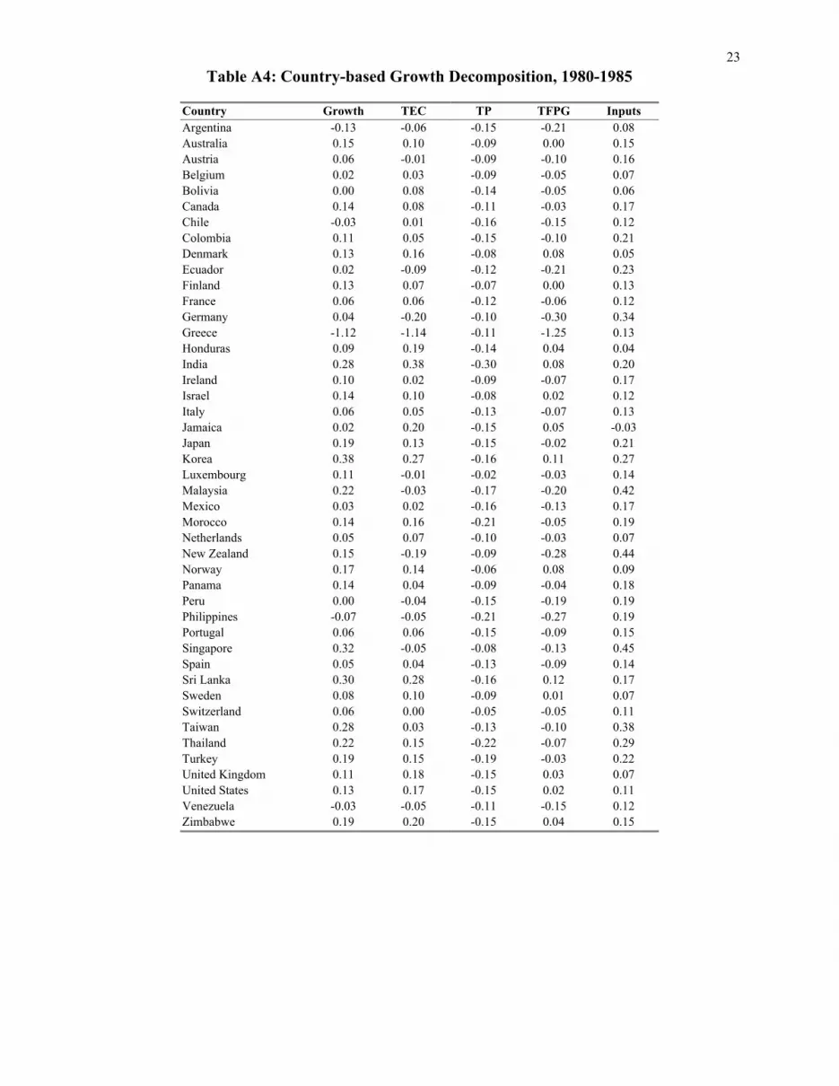
23

Table A4: Country-based Growth Decomposition, 1980-1985

Country Growth TEC TP TFPG Inputs

Argentina -0.13 -0.06 -0.15 -0.21 0.08

Australia 0.15 0.10 -0.09 0.00 0.15

Austria 0.06 -0.01 -0.09 -0.10 0.16

Belgium 0.02 0.03 -0.09 -0.05 0.07

Bolivia 0.00 0.08 -0.14 -0.05 0.06

Canada 0.14 0.08 -0.11 -0.03 0.17

Chile -0.03 0.01 -0.16 -0.15 0.12

Colombia 0.11 0.05 -0.15 -0.10 0.21

Denmark 0.13 0.16 -0.08 0.08 0.05

Ecuador 0.02 -0.09 -0.12 -0.21 0.23

Finland 0.13 0.07 -0.07 0.00 0.13

France 0.06 0.06 -0.12 -0.06 0.12

Germany 0.04 -0.20 -0.10 -0.30 0.34

Greece -1.12 -1.14 -0.11 -1.25 0.13

Honduras 0.09 0.19 -0.14 0.04 0.04

India 0.28 0.38 -0.30 0.08 0.20

Ireland 0.10 0.02 -0.09 -0.07 0.17

Israel 0.14 0.10 -0.08 0.02 0.12

Italy 0.06 0.05 -0.13 -0.07 0.13

Jamaica 0.02 0.20 -0.15 0.05 -0.03

Japan 0.19 0.13 -0.15 -0.02 0.21

Korea 0.38 0.27 -0.16 0.11 0.27

Luxembourg 0.11 -0.01 -0.02 -0.03 0.14

Malaysia 0.22 -0.03 -0.17 -0.20 0.42

Mexico 0.03 0.02 -0.16 -0.13 0.17

Morocco 0.14 0.16 -0.21 -0.05 0.19

Netherlands 0.05 0.07 -0.10 -0.03 0.07

New Zealand 0.15 -0.19 -0.09 -0.28 0.44

Norway 0.17 0.14 -0.06 0.08 0.09

Panama 0.14 0.04 -0.09 -0.04 0.18

Peru 0.00 -0.04 -0.15 -0.19 0.19

Philippines -0.07 -0.05 -0.21 -0.27 0.19

Portugal 0.06 0.06 -0.15 -0.09 0.15

Singapore 0.32 -0.05 -0.08 -0.13 0.45

Spain 0.05 0.04 -0.13 -0.09 0.14

Sri Lanka 0.30 0.28 -0.16 0.12 0.17

Sweden 0.08 0.10 -0.09 0.01 0.07

Switzerland 0.06 0.00 -0.05 -0.05 0.11

Taiwan 0.28 0.03 -0.13 -0.10 0.38

Thailand 0.22 0.15 -0.22 -0.07 0.29

Turkey 0.19 0.15 -0.19 -0.03 0.22

United Kingdom 0.11 0.18 -0.15 0.03 0.07

United States 0.13 0.17 -0.15 0.02 0.11

Venezuela -0.03 -0.05 -0.11 -0.15 0.12

Zimbabwe 0.19 0.20 -0.15 0.04 0.15

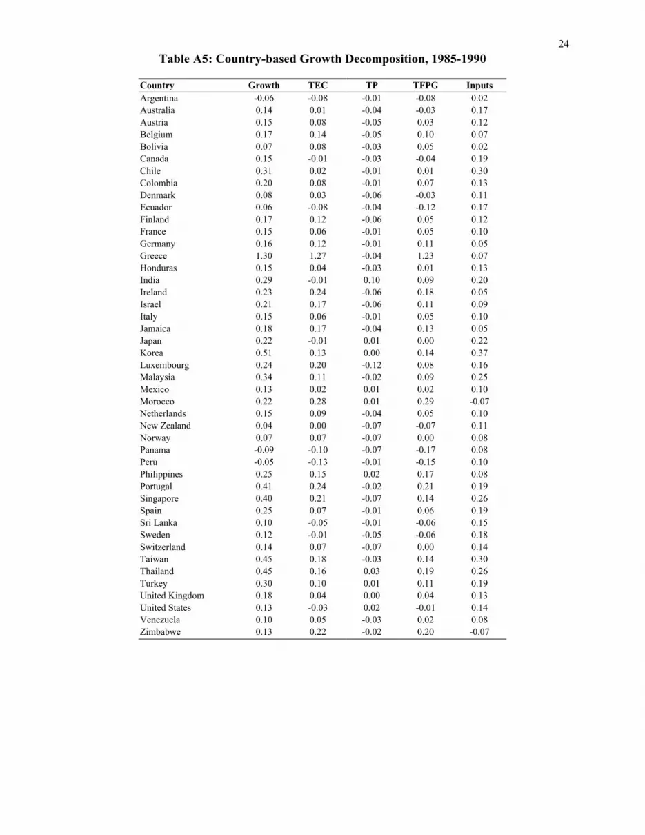
24

Table A5: Country-based Growth Decomposition, 1985-1990

Country Growth TEC TP TFPG Inputs

Argentina -0.06 -0.08 -0.01 -0.08 0.02

Australia 0.14 0.01 -0.04 -0.03 0.17

Austria 0.15 0.08 -0.05 0.03 0.12

Belgium 0.17 0.14 -0.05 0.10 0.07

Bolivia 0.07 0.08 -0.03 0.05 0.02

Canada 0.15 -0.01 -0.03 -0.04 0.19

Chile 0.31 0.02 -0.01 0.01 0.30

Colombia 0.20 0.08 -0.01 0.07 0.13

Denmark 0.08 0.03 -0.06 -0.03 0.11

Ecuador 0.06 -0.08 -0.04 -0.12 0.17

Finland 0.17 0.12 -0.06 0.05 0.12

France 0.15 0.06 -0.01 0.05 0.10

Germany 0.16 0.12 -0.01 0.11 0.05

Greece 1.30 1.27 -0.04 1.23 0.07

Honduras 0.15 0.04 -0.03 0.01 0.13

India 0.29 -0.01 0.10 0.09 0.20

Ireland 0.23 0.24 -0.06 0.18 0.05

Israel 0.21 0.17 -0.06 0.11 0.09

Italy 0.15 0.06 -0.01 0.05 0.10

Jamaica 0.18 0.17 -0.04 0.13 0.05

Japan 0.22 -0.01 0.01 0.00 0.22

Korea 0.51 0.13 0.00 0.14 0.37

Luxembourg 0.24 0.20 -0.12 0.08 0.16

Malaysia 0.34 0.11 -0.02 0.09 0.25

Mexico 0.13 0.02 0.01 0.02 0.10

Morocco 0.22 0.28 0.01 0.29 -0.07

Netherlands 0.15 0.09 -0.04 0.05 0.10

New Zealand 0.04 0.00 -0.07 -0.07 0.11

Norway 0.07 0.07 -0.07 0.00 0.08

Panama -0.09 -0.10 -0.07 -0.17 0.08

Peru -0.05 -0.13 -0.01 -0.15 0.10

Philippines 0.25 0.15 0.02 0.17 0.08

Portugal 0.41 0.24 -0.02 0.21 0.19

Singapore 0.40 0.21 -0.07 0.14 0.26

Spain 0.25 0.07 -0.01 0.06 0.19

Sri Lanka 0.10 -0.05 -0.01 -0.06 0.15

Sweden 0.12 -0.01 -0.05 -0.06 0.18

Switzerland 0.14 0.07 -0.07 0.00 0.14

Taiwan 0.45 0.18 -0.03 0.14 0.30

Thailand 0.45 0.16 0.03 0.19 0.26

Turkey 0.30 0.10 0.01 0.11 0.19

United Kingdom 0.18 0.04 0.00 0.04 0.13

United States 0.13 -0.03 0.02 -0.01 0.14

Venezuela 0.10 0.05 -0.03 0.02 0.08

Zimbabwe 0.13 0.22 -0.02 0.20 -0.07