Productive Relations in the Northeast and the Rest-of-Brazil Regions in 1995: Decomposition and...

MPRAMunich Personal RePEc Archive

Productive relations in the northeast andthe rest of Brazil regions in 1995:decomposition & synergy in input-outputsystems

Joaquim J.M. Guilhoto and Geoffrey J.D. Hewings and

Michael Sonis

University of Sao Paulo, University of Illinois

2002

Online at http://mpra.ub.uni-muenchen.de/38326/MPRA Paper No. 38326, posted 23. April 2012 23:48 UTC

http://mpra.ub.uni-muenchen.de/

http://mpra.ub.uni-muenchen.de/38326/

The Regional Economics Applications Laboratory (REAL) is a cooperative venture between the University of Illinois and the Federal Reserve Bank of Chicago focusing on the development and use of analytical models for urban and regional economic development. The purpose of the Discussion Papers is to circulate intermediate and final results of this research among readers within and outside REAL. The opinions and conclusions expressed in the papers are those of the authors and do not necessarily represent those of the Federal Reserve Bank of Chicago, Federal Reserve Board of Governors or the University of Illinois. All requests and comments should be directed to Geoffrey J. D. Hewings, Director, Regional Economics Applications Laboratory, 607 South Matthews, Urbana, IL, 61801-3671, phone (217) 333-4740, FAX (217) 244-9339. Web page: www.uiuc.edu/unit/real

PRODUCTIVE RELATIONS IN THE NORTHEAST AND

THE REST OF BRAZIL REGIONS IN 1995: DECOMPOSITION & SYNERGY IN INPUT-OUTPUT

SYSTEMS

by

Joaquim J.M. Guilhoto, Michael Sonis and Geoffrey J.D. Hewings

REAL 00-T-3 February, 2000

Productive Relations in the Northeast and the Rest of Brazil

Regions in 1995: Decomposition & Synergy in Input-Output Systems

Joaquim J.M. Guilhoto,1 Geoffrey J.D. Hewings,2 and Michael Sonis3

Abstract: Using a set of interregional input-output tables built by Guilhoto (1998) for 1995 for two Brazilian regions (Northeast and rest of the economy), the methodology developed by Sonis et al. (1997) is applied in the construction of a series of linkages such that it is possible to examine, through the nature of the internal and external interdependencies, the structure of trading relationships between the two regions. The methodology uses a partitioned input-output system and exploits techniques that produce left and right matrix multipliers of the Leontief Inverse. This procedure facilitates the classification of the types of synergetic interactions within a preset pair-wise hierarchy of economic linkages sub-systems. In general, the results show that the Northeast region has a greater dependence on the rest of the economy region than the rest of the economy has on the Northeast region, and at the same time the rest of the economy region seems to be more developed as it presents a more complex productive structure than the Northeast region.

I. Introduction

In this paper, the methodology developed by Sonis et al. (1997) that classifies types of

synergetic interactions is used to explore the structure of trading relations among regions. This

methodology is applied to a set of interregional input-output tables built by Guilhoto (1998) for

two Brazilian regions (Northeast and rest of the economy). The objective is to explore the

degree to which the structure of interactions is dominated by intraregional and interregional

components and the extent to which the interregional interactions are symmetric in magnitude.

The two-region system that has been chosen highlights important, strategic development issues

in an economy that is struggling to address both equity and efficiency issues in a spatial context

(see Baer, et al., 1998). The Northeast of Brazil has received significant, continuing

development initiatives over the past four decades; by 1995, the Northeast’s share in GDP had

risen to 13.4% from 13.2% in 1960 while per capita GDP grew from 42% to 55% of the national

average. When attention is just directed to shares in industrial production, the Northeast

declined from 8.3% (1959) to 7.9% (1994). The present paper attempts to explore some

1 Department of Economics, Business and Sociology, ESALQ - University of São Paulo (USP), Brazil and Regional Economics Applications Laboratory (REAL), University of Illinois – E-mail: [email protected]. 2 Regional Economics Applications Laboratory (REAL), University of Illinois.

R E A L

Productive Relations in the NE and Rest of Brazil ___________________________________________________________________________________

2

structural reasons that might shed light on this problem; while the focus will be on the economic

structure of the Northeast and the Rest of Brazil (hereafter, NE and RB respectively) at one point

in time, 1995, the findings will reflect long-term structural issues that have remained unresolved.

In the next section the theoretical background will be presented. In the third section the theory

will be applied to the Brazilian interregional tables, while in the fourth section policy

interpretations will be reviewed prior to the presentation of some concluding comments in the

final section.

II. Theoretical Background4

Consider a two-region, mutually exclusive division of a national economy. Following the

adaptation of the Dixit-Stiglitz model by Fujita et al., (1999) assume that there are two goods, a

tradable and a nontradable, and that there are no external to the national economy interactions.

Further assume that labor employed in the tradable commodity is mobile between regions and

that labor moves to regions paying higher than average real wages. Given a transportation costs

structure in which costs are assumed to be a linear increasing function of distance, then it can be

shown that the equilibrium distribution of production will depend in large part on the magnitude

of the transportation costs and their interaction with increasing returns at the firm level and labor

mobility. Fujita et al. (1999) show that with high transportation costs there will be a tendency

for production to be divided between the two regions; if labor mobility is limited (by higher

transportation or search costs), and the transportation costs are reduced, there is a tendency to

develop a core-periphery outcome in which the tradable good becomes concentrated in one of

the two regions.

Obviously, with a more complex system in which goods are all tradable to some extent, the

search for greater variety by consumers may tend to exacerbate concentration tendencies,

tendencies that will be reinforced by the existence of increasing returns. The competition

3 Bar Ilan University, Israel, and Regional Economics Applications Laboratory (REAL), University of Illinois. 4 This section draws heavily on Sonis, Hewings, and Miyazawa (1997).

R E A L


3

between the NE and RB presents a very strikingly familiar scenario. Transportation costs

between NE and RB are high but not high enough to create a protective, spatially monopolistic

market in the NE; producers in the RB have been able to exploit scale economies and penetrate

the NE market to the exclusion of NE producers. In this paper, the resultant interregional

structure will be explored and interpreted using a set of input-output tables.

Consider an input-output system represented by the following block matrix, A, of direct inputs:

11 12

21 22

A AA

A A⎡ ⎤

= ⎢ ⎥⎣ ⎦

(1)

where 11A and 22A are the quadrat matrices of direct inputs within the first and second regions,

and 12A and 21A are the rectangular matrices showing the direct inputs purchased by the second

region and vice versa.

The building blocks of the pair-wise hierarchies of sub-systems of intra/interregional linkages of

the block-matrix Input-Output system are the four matrices 11, 12 21 22, and A A A A , corresponding to

four basic block-matrices:

11 1211 12 21 22

21 22

0 0 0 00 0= ; = ; = ; =

0 00 0 0 0A A

A A A AA A

⎡ ⎤ ⎡ ⎤ ⎡ ⎤ ⎡ ⎤⎢ ⎥ ⎢ ⎥ ⎢ ⎥ ⎢ ⎥

⎣ ⎦ ⎣ ⎦⎣ ⎦ ⎣ ⎦ (2)

This paper will usually consider the decomposition of the block-matrix (1) into the sum of two

block-matrices, such that each of them is the sum of the block-matrices (2) 11, 12 21 22, and A A A A .

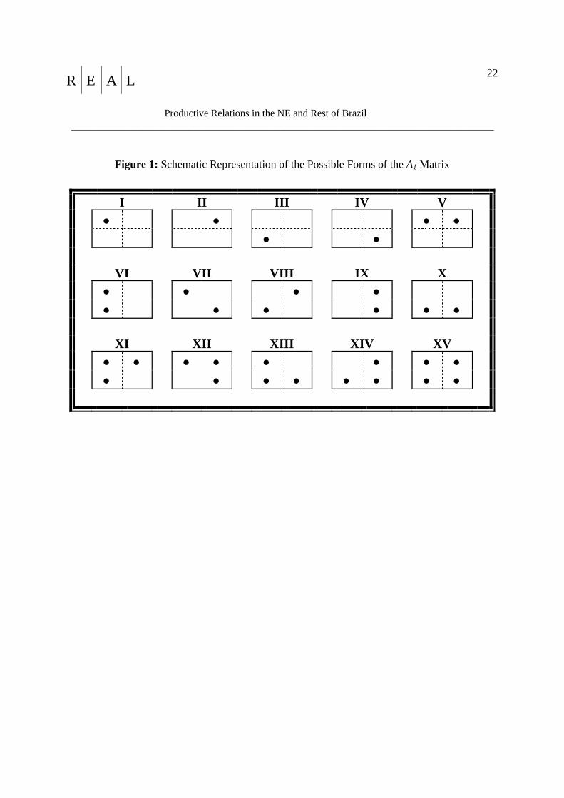
From (1), 14 types of pair-wise hierarchies of economic sub-systems can be identified by the

decompositions of the matrix of the block-matrix A (see Figure 1 and Table A2 in the appendix).

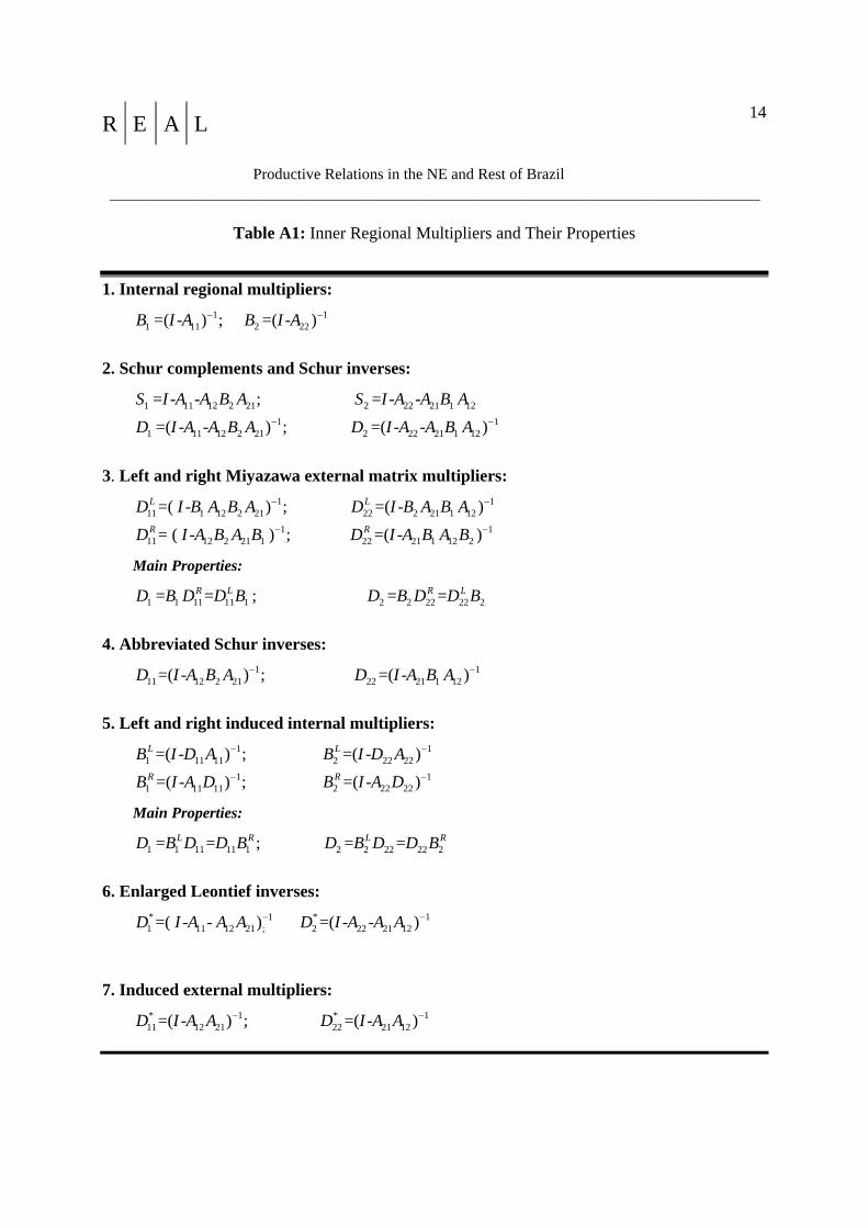
A set of inner regional multipliers, the set of inverse matrices that are the "building blocks" of

the synergetic interactions between the economic sub-systems are presented in table A1 in the

appendix. Hereafter, some comments are provided on the entries in this table (the bold

numbering refers to the corresponding entries in this table).

R E A L


4

1. The matrices -11 11=( )B I A− and 1

2 22=( )B I A −− represent the Miyazawa internal matrix

multipliers of the first and second regions showing the interindustrial propagation effects within

each region, while the matrices, 21 1 1 12 12 2 2 21, , , A B B A A B B A show the induced effects on output or

input activities in the two regions.

2. The expressions

1 11 12 2 21 2 22 21 1 12= , = S I A A B A S I A A B A− − − − (3)

are usually referred to as the Schur complements. The inverses, 1D and 2D of the Schur

complements (3) are referred to as the Schur inverses for the first and second regions. They

represent the enlarged Leontief inverse for one region revealing the induced economic influence

of the other region; i.e., the Schur inverses represent total propagation effects in the first and

second regions.

3. Miyazawa (1966) introduced the concept of left and right external matrix multipliers of the

first and second regions, 11 11 22 22, , ,L R L RD D D D . These multipliers are incorporated in the

multiplicative decompositions of the Schur inverses and they represent the total propagation

effects in the first and second regions as the products of internal and external regional matrix

multipliers.

4, 5. By introducing the abbreviated Schur inverses, 11 22,D D , and the left and right induced

internal multipliers for the first and second regions, 1 1 2 2, , ,L R L RB B B B , one can obtain the

multiplicative decompositions of the Schur inverses:

1 1 11 11 1 2 2 22 22 2= = ; = =L R L RD B D D B D B D D B (4)

and their corresponding additive representations.

6-10. The formulae for this group of multipliers can be obtained by considering the block-

matrices:

R E A L


5

11 12 12 12

21 21 22 21

0 0= , = , =

0 0A A A A

M N SA A A A⎡ ⎤ ⎡ ⎤ ⎡ ⎤⎢ ⎥ ⎢ ⎥ ⎢ ⎥⎣ ⎦ ⎣ ⎦ ⎣ ⎦

(5)

Those represent the backward and forward linkages of the first region, the second region and the

interregional relations of both regions.

The following Schur inverse

* 11 11 12 21=( )D I A A A −− − (6)

may be referred to as the enlarged Leontief inverse, and the inverses

* 1 * 111 1 12 21 11 12 21 1=( ) ; =( )L RD I B A A D I A A B− −− − (7)

are called the left and right subjoined inverse matrix multipliers.

Consider the hierarchy of Input-Output sub-systems represented by the decomposition

1 2 = +A A A . Introducing the Leontief block-inverse 1( )= =( )L A L I A −− and the Leontief block-

inverse 11 1 1( )= =( )L A L I A −− corresponding to the first sub-system, the outer left and right block-

matrix multipliers LM and RM are defined by equalities:

1 1= =R LL L M M L (8)

The definition (8) implies that:

11 1 2= ( )=( )LM L I A I L A −− − (9)

11 2 1=( ) =( )RM I A L I A L −− − (10)

In this paper, the following form of the Leontief block-inverse will be used:

1 1 12 2

2 21 1 2

=D D A B

LD A B D⎡ ⎤⎢ ⎥⎣ ⎦

(11)

This expression can be verified by direct matrix multiplication, using definitions of the Schur

inverses and their properties (see table A1, entries 1 and 2). Further, the application of (9), (10)

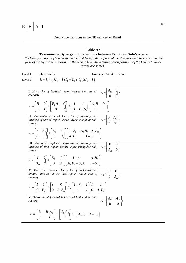
and (11) will be directed towards the derivation of a taxonomy of synergetic interactions

R E A L


6

between the two regions. The results are presented in the first and second levels of table A2,

while figure 1 shows the schematic representation of the possible forms of the A1 matrices.

<insert figure 1 here>

Consider the hierarchy of input-output sub-systems represented by the decomposition

1 2 = + A A A and their Leontief block-inverse 1( ) = = ( )L A L I A −− and the Leontief block-inverse

11 1 1( ) = = ( )L A L I A −− corresponding to the first sub-system. The multiplicative decomposition

of the Leontief inverse 1 1 = = R LL L M M L can be converted to the sum:

1 1 1 1 = + ( ) = + ( )L RL L M I L L L M I− − (12)

If f is the vector of final demand and x is the vector of gross output, then the decomposition (12)

generates the decomposition of gross output into two parts: 1 1= x L f and the increment

1 = - Dx x x . Such decomposition is important for the empirical analysis of the structure of actual

gross output. In the second level of table A2, the classification is revealed of possible additive

decompositions of the Leontief block-inverse for all decompositions of input-output system into

pair-vise hierarchies.

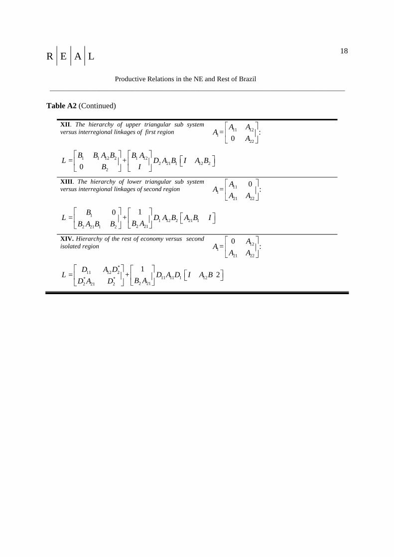
While 14 types of pair-wise hierarchies of economic linkages have been developed (figure 1 and

table A2), it is possible to suggest a typology of categories into which these types may be placed.

The following characterization is suggested:

1. backward linkage type (VI, IX): power of dispersion

2. forward linkage type (V, X): sensitivity of dispersion

3. intra- and inter- linkages type (VII, VIII): internal and external dispersion

4. isolated region vs. the rest of the economy interactions style (I, XIV, IV, XI)

5. triangular sub-system vs. the interregional interactions style (II, XIII, III, XII).

By viewing the system of hierarchies of linkages in this fashion, it will be possible to provide

new insights into the properties of the structures that are revealed. For example, the types

R E A L


7

allocated to category 5 reflect structures that are based on order and circulation. Furthermore,

these partitioned input-output systems can distinguish among the various types of dispersion

(such as 1, 2 and 3) and among the various patterns of interregional interactions (such as 4 and

5). Essentially, the 5 categories and 14 types of pair-wise hierarchies of economic linkages

provide the opportunity to select according to the special qualities of each region’s activities and

for the type of problem at hand; in essence, the option exists for the basis of a typology of

economy types based on hierarchical structure.

III. An Application to Brazil

Using a set of interregional input-output tables built by Guilhoto (1998) at the level of 40 sectors

for the year of 1995 for 2 Brazilian regions (NE - Region 1 - and the rest of the economy -

Region 2), the methodology presented in section II is applied, and the results are presented in

tables 3 to 5 and figures 2 to 4.

<<insert table 1 here>>

Table 1 illustrates the results taking into consideration the vector f of final demand and the

vector x of gross output; then the gross output is decomposed into two parts: 1 1= x L f and the

increment 1 = - Dx x x . The values for x and 1x are added for all sectors in regions 1 and 2 such

that it is possible to estimate the contribution of each interaction to the total production in each

region. As the shares of x1 in x take also into consideration the value of the final demand, it is

interesting to isolate the shares of the final demand in each region to reveal how the pair-wise

interaction takes place in the regions.

Focusing on the results presented into table 1, one can see that the value of the final demand in

region 1 (NE) is responsible for 63.46 % of the production in this region (the remaining 36.54%

is generated in the process of production) while for region 2 (RB), this value is 60.25 % (39.75

% in the process of production). In a certain sense this is an indication that the rest of the

R E A L


8

economy is more developed than the NE region as the internal transactions in region 2 are

responsible for a greater share of the total production than is the case in region 1.

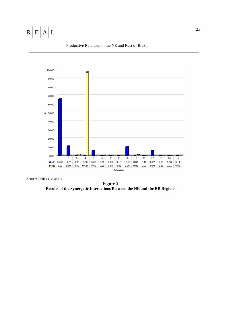
<<insert figure 2 here>>

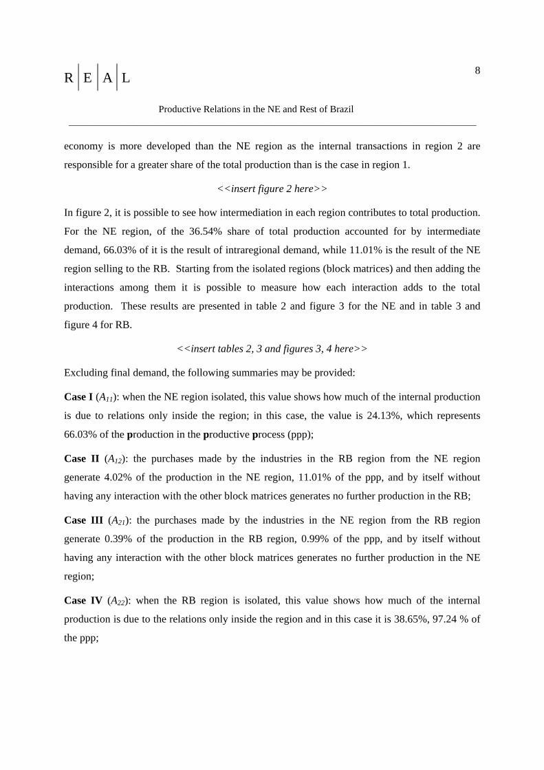
In figure 2, it is possible to see how intermediation in each region contributes to total production.

For the NE region, of the 36.54% share of total production accounted for by intermediate

demand, 66.03% of it is the result of intraregional demand, while 11.01% is the result of the NE

region selling to the RB. Starting from the isolated regions (block matrices) and then adding the

interactions among them it is possible to measure how each interaction adds to the total

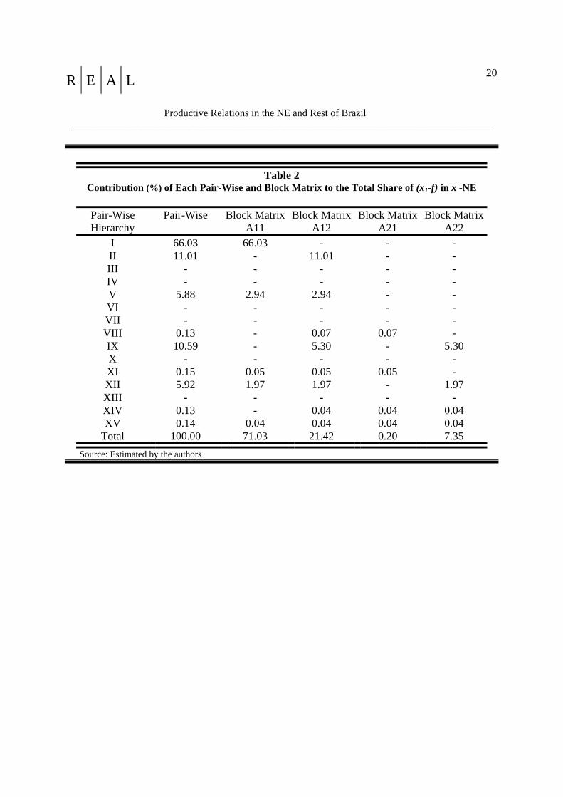
production. These results are presented in table 2 and figure 3 for the NE and in table 3 and

figure 4 for RB.

<<insert tables 2, 3 and figures 3, 4 here>>

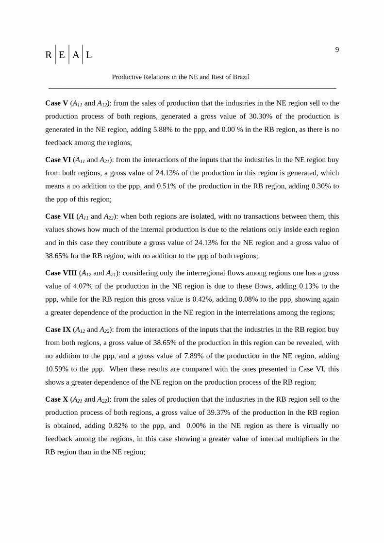
Excluding final demand, the following summaries may be provided:

Case I (A11): when the NE region isolated, this value shows how much of the internal production

is due to relations only inside the region; in this case, the value is 24.13%, which represents

66.03% of the production in the productive process (ppp);

Case II (A12): the purchases made by the industries in the RB region from the NE region

generate 4.02% of the production in the NE region, 11.01% of the ppp, and by itself without

having any interaction with the other block matrices generates no further production in the RB;

Case III (A21): the purchases made by the industries in the NE region from the RB region

generate 0.39% of the production in the RB region, 0.99% of the ppp, and by itself without

having any interaction with the other block matrices generates no further production in the NE

region;

Case IV (A22): when the RB region is isolated, this value shows how much of the internal

production is due to the relations only inside the region and in this case it is 38.65%, 97.24 % of

the ppp;

R E A L


9

Case V (A11 and A12): from the sales of production that the industries in the NE region sell to the

production process of both regions, generated a gross value of 30.30% of the production is

generated in the NE region, adding 5.88% to the ppp, and 0.00 % in the RB region, as there is no

feedback among the regions;

Case VI (A11 and A21): from the interactions of the inputs that the industries in the NE region buy

from both regions, a gross value of 24.13% of the production in this region is generated, which

means a no addition to the ppp, and 0.51% of the production in the RB region, adding 0.30% to

the ppp of this region;

Case VII (A11 and A22): when both regions are isolated, with no transactions between them, this

values shows how much of the internal production is due to the relations only inside each region

and in this case they contribute a gross value of 24.13% for the NE region and a gross value of

38.65% for the RB region, with no addition to the ppp of both regions;

Case VIII (A12 and A21): considering only the interregional flows among regions one has a gross

value of 4.07% of the production in the NE region is due to these flows, adding 0.13% to the

ppp, while for the RB region this gross value is 0.42%, adding 0.08% to the ppp, showing again

a greater dependence of the production in the NE region in the interrelations among the regions;

Case IX (A12 and A22): from the interactions of the inputs that the industries in the RB region buy

from both regions, a gross value of 38.65% of the production in this region can be revealed, with

no addition to the ppp, and a gross value of 7.89% of the production in the NE region, adding

10.59% to the ppp. When these results are compared with the ones presented in Case VI, this

shows a greater dependence of the NE region on the production process of the RB region;

Case X (A21 and A22): from the sales of production that the industries in the RB region sell to the

production process of both regions, a gross value of 39.37% of the production in the RB region

is obtained, adding 0.82% to the ppp, and 0.00% in the NE region as there is virtually no

feedback among the regions, in this case showing a greater value of internal multipliers in the

RB region than in the NE region;

R E A L


10

Case XI (A11, A12 and A21): taking the relations inside the NE region and the sales and purchases

that it makes from the RB region, a gross value of 30.40% of the production in this region is

accounted for, adding 0.15% to the ppp, and a gross value of 0.56% in the RB region, adding

0.03% to the ppp, values greater than the ones presented in case VI since more transactions are

now being taking into consideration;

Case XII (A11, A12 and A22): taking the relations inside both regions and the purchases that the

NE region makes from the RB region, a gross value of 36.33% of the production in the NE

region is generated, adding 5.92% to the ppp, and a gross value of 38.65% in the RB region, with

no addition to the ppp;

Case XIII (A11, A21 and A22): taking the relations inside both regions and the purchases that the

NE region makes from the RB region, a gross values of 24.13% of the production in the NE

region can be ascertained, with no addition to the ppp, and a gross value of 39.59% in the RB

region, adding 0.26% to the ppp;

Case XIV (A12, A21 and A22): taking the relations inside the RB region and the sales and

purchases that it makes from the NE region, a gross value of 39.49% of the production in this

region is generated, adding 0.21% to the ppp, and a gross value of 7.99% in the NE region,

adding 0.13% to the ppp, values greater than the ones presented in case IX since more

transactions are now being taking into consideration.

Case XV (A11, A12, A21 and A22): this case is not displayed in table 2 because it considers all the

interactions in the economy, it is listed here only to call attention for the contribution that this

last case has to the ppp, i.e., adding 0.14% to the ppp in the NE region and 0.08% to the ppp in

the RB region.

Tables 2 and 3 and figures 3 and 4 show for both regions the contribution that each block matrix

in each pair wise decomposition has to the ppp; they also present the total contribution of each

block matrix. From these data, it is possible to see a greater dependence of the NE region on the

RB region, for while 71.03% of the ppp in the NE region is due to interactions inside the region,

the corresponding value for the RB region is 97.82%. Hence, it is possible to observe and to

R E A L


11

measure how the relations between the 2 Brazilian regions take place. The NE region has a

greater dependence on the rest of the economy region than the rest of the economy has on the NE

region, and at the same time the rest of the economy region seems to be more developed as it

presents a more complex productive structure than the NE region.

IV Policy Implications

One of the major changes that has occurred within the economic structure of many economies is

the apparent increase in specialization and diversification at the same time. Overall, regional

economies are becoming more diversified, in terms of their macro structure. However,

establishments (plants) within sectors are becoming more specialized, responding in large part to

consumer demands for greater product variety. As a result, trade between regions tends to be

concentrated in intraindustry rather than interdindustry trade (see Krugman, 1990). However,

these developments are associated with trade between regions with similar levels of per capita

income and with excellent transportation connections. Neither is the case for the NE-RB

interaction; transportation costs are low enough to allow penetration from the other region but

not sufficiently low enough to allow for the full realization of the benefits of increasing returns.

Having discerned significant imbalances in the trading relationships and the complexity of

internal to the region intermediation, the next issue centers on the policy implications.

Comparative analysis recently conducted for the NE economy with that of the Midwest of the

US (Magalhães et al., 2000) revealed dramatically significant differences in the level and

volume of interactions for two regions. While both regions account for about the same

percentage of their nation’s GDP, the Midwest US economy’s GDP per capita is above the

national average in contrast to the NE Brazil economy (about 55% of the Brazil GDP per capita).

While the Midwest region is highly connected to the rest of the US economy (with an overall

positive balance of trade), a huge volume of interactions flow between the member states; in the

NE, the level of internal intermediation is lower and there is a negative balance of trade (imports

> exports) with the RB. Clearly, appeals to development of clusters of activities to enhance the

level of intermediation may not reflect the realities of an economy whose capacity to sustain

R E A L


12

further levels of activity may be circumscribed by poor internal transportation connectivities that

reduce the effective demand for goods and services.

In addition, as noted by Baer et al. (1998), the promotion of more open markets within the

context of WTO guidelines may make traditional forms of market intervention less feasible; in

any case, the record from prior interventions suggest that the prior policies had little success in

significantly changing the structure of the NE region’s economy to ensure that it would be in a

position to compete successfully in the national and international marketplace in the next several

decades.

V. Conclusions

The main contribution of this paper was to show, using different synergetic interactions, that it is

possible to analyze and to measure how the trading relationship between two regions takes place.

This was accomplished using a two-region interregional input-output table constructed for the

Brazilian economy for the year of 1995. From the results, it was possible to see that NE region

has a greater dependence on the rest of the economy region than the rest of the economy has on

the NE region, and at the same time the rest of the economy region seems to be more developed

as it presents a more complex productive structure than the NE region.

This study was conducted using one point in time and two regions; it would be interesting to

compare how the relations between the two regions change trough time and also how these

relations would evolve if the RB region were to be divided into several subregions.

VI. References Baer, W., E.A. Haddad and G.J.D. Hewings (1998) “The regional impact of neo-liberal policies

in Brazil,” Economia Aplicada 2, 219-242.

Guilhoto, J.J.M. (1998). “Análise Inter e Intra-Regional das Estruturas Produtivas das Economias do Nordeste e do Resto do Brasil: 1985 e 1995 Comparados”. Departamento de Economia e Sociologia Rural - ESALQ - USP, Mimeo.

Krugman, P.R. (1990) Rethinking International Trade. MIT Press: Cambridge, Massachusetts.

R E A L


13

Magalhães, A., M. Sonis and G.J.D. Hewings (2000) “Regional competition and complementarity reflected in Relative Regional Dynamics and Growth of GSP: a Comparative Analysis of the Northeast of Brazil and the Midwest States of the U.S,” in J.J.M. Guilhoto and G.J.D. Hewings (eds) Structure and Structural Change in the Brazilian Economy (Ashgate, forthcoming)

Miyazawa, K., (1966) "Internal and external matrix multipliers in the Input-Output model." Hitotsubashi Journal of Economics, 7 (1) 1966, pp. 38-55.

Sonis, M., G.J.D. Hewings, and K. Miyazawa (1997) "Synergetic Interactions Within the Pair-Wise Hierarchy of Economic Linkages Sub-Systems." Hitotsubashi Journal of Economics, 38, December.

R E A L


14

Table A1: Inner Regional Multipliers and Their Properties

1. Internal regional multipliers: 1 1

1 11 2 22=( - ) ; =( - )B I A B I A− −

2. Schur complements and Schur inverses:

1 11 12 2 21 2 22 21 1 121 1

1 11 12 2 21 2 22 21 1 12

= - - ; = - -

=( - - ) ; =( - - )

S I A A B A S I A A B A

D I A A B A D I A A B A− −

3. Left and right Miyazawa external matrix multipliers: 1 1

11 1 12 2 21 22 2 21 1 121 1

11 12 2 21 1 22 21 1 12 2

=( - ) ; =( - )

= ( - ) ; =( - )

L L

R R

D I B A B A D I B A B A

D I A B A B D I A B A B

− −

− −

Main Properties:

1 1 11 11 1 2 2 22 22 2= = ; = =R L R LD B D D B D B D D B

4. Abbreviated Schur inverses: 1 1

11 12 2 21 22 21 1 12=( - ) ; =( - )D I A B A D I A B A− −

5. Left and right induced internal multipliers: 1 1

1 11 11 2 22 221 1

1 11 11 2 22 22

=( - ) ; =( - )

=( - ) ; =( - )

L L

R R

B I D A B I D A

B I A D B I A D

− −

− −

Main Properties:

1 1 11 11 1 2 2 22 22 2= = ; = =L R L RD B D D B D B D D B

6. Enlarged Leontief inverses: * 1 * 11 11 12 21 ; 2 22 21 12=( - - ) =( - - )D I A A A D I A A A− −

7. Induced external multipliers: * 1 * 111 12 21 22 21 12=( - ) ; =( - )D I A A D I A A− −

R E A L


15

Table 1 (Continued) 9. Left and right subjoined inverses:

* 1 * 111 1 12 21 22 2 21 12* 1 * 111 12 21 1 22 21 12 2

=( - ) ; =( - )=( - ) =( - )

L L

R R

D I B A A D I B A AD I A A B D I A A B

− −

− −

Main Properties: * * * * * *1 1 11 11 1 2 2 22 22 2= = ; = =R L R LD B D D B D B D D B

10. Left and right induced subjoined inverses: ** 1 ** 111 11 11 12 2 22 21 22 22 22 21 1 11 12** 1 ** 111 11 12 2 22 21 11 22 22 21 1 11 12 22

=[ - ( )] ; =[ - ( )] ; =[ -( - ) ] ; =[ -( - ) ]

L L

R R

D I D A A B A A D I D A A B A AD I A A B A A D D I A A B A A D

− −

− −

− −

Main Properties: * ** ** * ** **1 11 11 11 11 2 22 22 22 22 = = ; = =L R L RD D D D D D D D D D

R E A L


16

Table A2 Taxonomy of Synergetic Interactions between Economic Sub-Systems

[Each entry consists of two levels: in the first level, a description of the structure and the corresponding form of the A1 matrix is shown. In the second level the additive decompositions of the Leontief block-

matrix are shown]

Level 1 Description Form of the 1A matrix

Level 2 ( ) ( )1 1 1 1L RL L M I L L L M I= + − = + −

I. Hierarchy of isolated region versus the rest of economy

111

0= :

0 0A

A⎡ ⎤⎢ ⎥⎣ ⎦

1 1 12 21 12

2

0 0 0 = + .

0 0 0I IB B A A B

L D II I SI I

⎡ ⎤ ⎡ ⎤ ⎡ ⎤⎡ ⎤⎢ ⎥ ⎢ ⎥ ⎢ ⎥⎢ ⎥−⎣ ⎦⎣ ⎦ ⎣ ⎦ ⎣ ⎦

II. The order replaced hierarchy of interregional linkages of second region versus lower triangular sub system

121

0= :

0 0A

A⎡ ⎤⎢ ⎥⎣ ⎦

1 1 12 2 1 1212

2 21 1 2

0 = +

00D I S A B S AI A

LD A B I SI

⎡ ⎤ ⎡ ⎤⎡ ⎤ − −⎢ ⎥ ⎢ ⎥⎢ ⎥ −⎣ ⎦ ⎣ ⎦ ⎣ ⎦

III. The order replaced hierarchy of interregional linkages of first region versus upper triangular sub system

121

0 0= :

0A

A⎡ ⎤⎢ ⎥⎣ ⎦

1 1 12 2

21 2 21 1 2 21 2

0 0= +

0I D I S A B

LA I D A B S A I S

⎡ ⎤ ⎡ ⎤−⎡ ⎤⎢ ⎥ ⎢ ⎥⎢ ⎥ − −⎣ ⎦ ⎣ ⎦ ⎣ ⎦

IV. The order replaced hierarchy of backward and forward linkages of the first region versus rest of economy

122

0 0= :

0A

A⎡ ⎤⎢ ⎥⎣ ⎦

11

2 2 21 12 2

0 0 0 = +

0 0 0I I II S I

L DB B A A BI I

⎡ ⎤−⎡ ⎤ ⎡ ⎤ ⎡ ⎤⎢ ⎥⎢ ⎥ ⎢ ⎥ ⎢ ⎥

⎣ ⎦ ⎣ ⎦ ⎣ ⎦⎣ ⎦

V. Hierarchy of forward linkages of first and second regions 11 12

1= :0 0

A AA

⎡ ⎤⎢ ⎥⎣ ⎦

1 1 12 1 122 21 1 2 = +

0B B A B A

L D A B I SI I

⎡ ⎤ ⎡ ⎤⎡ ⎤−⎢ ⎥ ⎢ ⎥ ⎣ ⎦

⎣ ⎦ ⎣ ⎦

R E A L


17

Table A2 (Continued)

VI. Hierarchy of backward linkages of first and second regions 11

121

0=

0A

AA⎡ ⎤⎢ ⎥⎣ ⎦

:

1 1 122 21 1

21 1 2

0 = +

B B AL D A B I

A B I I S⎡ ⎤ ⎡ ⎤

⎡ ⎤⎢ ⎥ ⎢ ⎥ ⎣ ⎦−⎣ ⎦ ⎣ ⎦

VII. The hierarchy of intra- versus interregional relationships 11

122

0:

0A

AA

⎡ ⎤= ⎢ ⎥⎣ ⎦

:

1 1 12 2 21 22 1

2 2 21 1 11 12 2

0 0 0L = +

0 0 0B D A B A I A B

B D A B I A A B⎡ ⎤ ⎡ ⎤ ⎡ ⎤ ⎡ ⎤−⎢ ⎥ ⎢ ⎥ ⎢ ⎥ ⎢ ⎥−⎣ ⎦ ⎣ ⎦ ⎣ ⎦ ⎣ ⎦

VIII. The hierarchy of inter versus intra regional relationships 12

121

0= :

0A

AA⎡ ⎤⎢ ⎥⎣ ⎦

* * **11 11 12 1 12 121 11 11

2 22 22* *22 21 22 2 21 21

0 = +

0D D A I B A I AD A D

L D A DD A D B A I A I⎡ ⎤ ⎡ ⎤ ⎡ ⎤⎡ ⎤⎢ ⎥ ⎢ ⎥ ⎢ ⎥⎢ ⎥

⎣ ⎦⎣ ⎦ ⎣ ⎦ ⎣ ⎦

IX. Order replaced hierarchy of backward linkages 12

122

0=

0A

AA

⎡ ⎤⎢ ⎥⎣ ⎦

:

12 2 11 12 2

2 2 21

1 = +

0I A B S

L D I A BB B A

⎡ ⎤ ⎡ ⎤−⎡ ⎤⎢ ⎥ ⎢ ⎥ ⎣ ⎦

⎣ ⎦ ⎣ ⎦

X. Order replaced hierarchy of forward linkages 1

21 22

0 0= :A

A A⎡ ⎤⎢ ⎥⎣ ⎦

1 1 12 22 21 2 2 21

0 1 = +

IL D I S A B

B A B B A⎡ ⎤ ⎡ ⎤

⎡ ⎤−⎢ ⎥ ⎢ ⎥ ⎣ ⎦⎣ ⎦ ⎣ ⎦

XI. The hierarchy of backward and forward linkages of the first region versus rest of economy 11 12

121

= :0

A AA

A⎡ ⎤⎢ ⎥⎣ ⎦

* *1 1 12 1 12

2 22 22 21 1*21 1 22

= +D D A B A

L D D A A B IA D D I⎡ ⎤ ⎡ ⎤

⎡ ⎤⎢ ⎥ ⎢ ⎥ ⎣ ⎦⎣ ⎦⎣ ⎦

R E A L


18

Table A2 (Continued)

XII. The hierarchy of upper triangular sub system versus interregional linkages of first region 11 12

122

= :0

A AA

A⎡ ⎤⎢ ⎥⎣ ⎦

1 1 12 2 1 122 21 1 12 2

2

= +0B B A B B A

L D A B I A BB I

⎡ ⎤ ⎡ ⎤⎡ ⎤⎢ ⎥ ⎢ ⎥ ⎣ ⎦

⎣ ⎦⎣ ⎦

XIII. The hierarchy of lower triangular sub system versus interregional linkages of second region 11

121 22

0= :

AA

A A⎡ ⎤⎢ ⎥⎣ ⎦

11 12 2 21 1

2 212 21 1 2

10 = +

BL D A B A B I

B AB A B B⎡ ⎤ ⎡ ⎤

⎡ ⎤⎢ ⎥ ⎢ ⎥ ⎣ ⎦⎣ ⎦⎣ ⎦

XIV. Hierarchy of the rest of economy versus second isolated region 12

121 22

0= :

AA

A A⎡ ⎤⎢ ⎥⎣ ⎦

*11 12 2

11 11 1 12* *2 212 21 2

1 = + 2

D A DL D A D I A B

B AD A D⎡ ⎤ ⎡ ⎤

⎡ ⎤⎢ ⎥ ⎢ ⎥ ⎣ ⎦⎣ ⎦⎣ ⎦

R E A L


19

Table 1 Results of the Synergetic Interactions Between the NE and the RB Regions

Pair-Wise Hierarchy

Share (%) of x1 in x

NE

Share (%) of x1 in x

Rest of BR

Share (%) of (x1-f) in x

NE

Share (%) of (x1-f) in x Rest of BR

Share (%) of f in x

NE

Share (%) of f in x

Rest of BRI 87.59 60.25 24.13 0.00 63.46 60.25II 67.49 60.25 4.02 0.00 63.46 60.25 III 63.46 60.64 0.00 0.39 63.46 60.25IV 63.46 98.90 0.00 38.65 63.46 60.25 V 93.76 60.25 30.30 0.00 63.46 60.25 VI 87.59 60.76 24.13 0.51 63.46 60.25 VII 87.59 98.90 24.13 38.65 63.46 60.25 VIII 67.54 60.67 4.07 0.42 63.46 60.25IX 71.36 98.90 7.89 38.65 63.46 60.25 X 63.46 99.62 0.00 39.37 63.46 60.25 XI 93.87 60.81 30.40 0.56 63.46 60.25 XII 99.79 98.90 36.33 38.65 63.46 60.25 XIII 87.59 99.84 24.13 39.59 63.46 60.25XIV 71.45 99.74 7.99 39.49 63.46 60.25

Source: Estimated by the authors

R E A L


20

Table 2 Contribution (%) of Each Pair-Wise and Block Matrix to the Total Share of (x1-f) in x -NE

Pair-Wise Hierarchy

Pair-Wise Block Matrix A11

Block Matrix A12

Block Matrix A21

Block Matrix A22

I 66.03 66.03 - - - II 11.01 - 11.01 - - III - - - - - IV - - - - - V 5.88 2.94 2.94 - - VI - - - - - VII - - - - - VIII 0.13 - 0.07 0.07 - IX 10.59 - 5.30 - 5.30 X - - - - - XI 0.15 0.05 0.05 0.05 - XII 5.92 1.97 1.97 - 1.97 XIII - - - - - XIV 0.13 - 0.04 0.04 0.04 XV 0.14 0.04 0.04 0.04 0.04

Total 100.00 71.03 21.42 0.20 7.35 Source: Estimated by the authors

R E A L


21

Table 3 Contribution (%) of Each Pair-Wise and Block Matrix to the Total Share of (x1-f) in x – RB

Pair-Wise Hierarchy

Pair-Wise Block Matrix A11

Block Matrix A12

Block Matrix A21

Block Matrix A22

I - - - - - II - - - - - III 0.99 - - 0.99 - IV 97.24 - - - 97.24V - - - - - VI 0.30 0.15 - 0.15 - VII - - - - - VIII 0.08 - 0.04 0.04 - IX - - - - - X 0.82 - - 0.41 0.41 XI 0.03 0.01 0.01 0.01 - XII - - - - - XIII 0.26 0.09 - 0.09 0.09 XIV 0.21 - 0.07 0.07 0.07 XV 0.08 0.02 0.02 0.02 0.02

Total 100.00 0.27 0.14 1.77 97.82 Source: Estimated by the authors

R E A L


22

Figure 1: Schematic Representation of the Possible Forms of the A1 Matrix

I II III IV V • • • • • •

VI VII VIII IX X • • • •

• • • • • • XI XII XIII XIV XV • • • • • • • • • • • • • • • •

R E A L


23

0.00

10.00

20.00

30.00

40.00

50.00

60.00

70.00

80.00

90.00

100.00

%

Pair-Wise

NE 66.03 11.01 0.00 0.00 5.88 0.00 0.00 0.13 10.59 0.00 0.15 5.92 0.00 0.13 0.14

RB 0.00 0.00 0.99 97.24 0.00 0.30 0.00 0.08 0.00 0.82 0.03 0.00 0.26 0.21 0.08

1 2 3 4 5 6 7 8 9 10 11 12 13 14 15

Source: Tables 1, 2, and 3 Figure 2

Results of the Synergetic Interactions Between the NE and the RB Regions

R E A L


24

0.00

10.00

20.00

30.00

40.00

50.00

60.00

70.00

80.00

%

A11 A12 A21 A22Block Matrix

1 2 3 4 5 6 7 8 9 10 11 12 13 14 15

Source: Table 2 Figure 3

Contribution (%) of Each Pair-Wise and Block Matrix to the Total Share of (x1-f) in x – NE

R E A L


25

0.00

10.00

20.00

30.00

40.00

50.00

60.00

70.00

80.00

90.00

100.00

%

A11 A12 A21 A22Block Matrix

1 2 3 4 5 6 7 8 9 10 11 12 13 14 15

Source: Table 3 Figure 4

Contribution (%) of Each Pair-Wise and Block Matrix to the Total Share of (x1-f) in x – RB

Productive Relations in the Northeast and the Rest-of-Brazil Regions in 1995: Decomposition and...

Documents

Transcript of Productive Relations in the Northeast and the Rest-of-Brazil Regions in 1995: Decomposition and...