Production and Sales Planning with Limited Shared Tooling at the Key Operation

Production and Sales Planning with Limited Shared Tooling at the KeyOperation

Gerald G. Brown; Arthur M. Geoffrion; Gordon H. Bradley

Management Science, Vol. 27, No.3 (Mar., 1981),247-259.

1IIiiiiil..1IiiiII@

Stable URL:http://links.jstor.org/sici?sici=0025-1909%28198103%2927%3A3%3C247%3APASPWL%3E2.0.CO%3B2-N

Management Science is currently published by INFORMS.

Your use of the JSTOR archive indicates your acceptance of JSTOR' s Terms and Conditions of Use, available athttp://www.jstor.org/about/terms.html. JSTOR's Terms and Conditions of Use provides, in part, that unless you

have obtained prior permission, you may not download an entire issue of a journal or multiple copies of articles, andyou may use content in the JSTOR archive only for your personal, non-commercial use.

Please contact the publisher regarding any further use of this work. Publisher contact information may be obtained athttp://www.jstor.org/journals/informs.html.

Each copy of any part of a JSTOR transmission must contain the same copyright notice that appears on the screen orprinted page of such transmission.

JSTOR is an independent not-for-profit organization dedicated to creating and preserving a digital archive ofscholarly journals. For more information regarding JSTOR, please [email protected].

http://www.jstor.org/Tue Jan 27 14:06:122004

MANAGEMENT SCIENCEVol. 27, No.3, March 1981

Printed in U.S.A.

PRODUCTION AND SALES PLANNING WITH LIMITEDSHARED TOOLING AT THE KEY OPERATION*

GERALD G. BROWN, t ARTHUR M. GEOFFRIONt AND GORDON H.BRADLEYt

The focus of this paper is multiperiod production and sales planning when there is a singledominant production operation for which tooling (dies, molds, etc.) can be shared amongparts and is limited in availability. Our interest in such problems grew out of managementissues confronting an injection molding manufacturer of plastic pipes and fittings for thebuilding and chemical industries, but similar problems abound in the manufacture of manyother cast, extruded, molded, pressed, or stamped products. We describe the development andsuccessful application of a planning model and an associated computational approach for thisclass of problems.

The problem is modeled as a mixed integer linear program. Lagrangean relaxation isapplied so as to exploit the availability of highly efficient techniques for minimum costnetwork flow problems and for single-item dynamic lot-sizing type problems. For the practicalapplication at hand, provably good solutions are routinely being obtained in modest computing time to problems far beyond the capabilities of available mathematical programmingsystems.(INVENTORY/PRODUCTION APPLICATIONS; PRODUCTION-FLOW SHOP; INTEGER PROGRAMMING APPLICATIONS)

1. Introduction

This paper addresses production and sales planning in a seasonal industry with asingle principal production operation for which tooling can be shared among parts andis limited in availability.

The specific context of our experience is the production of injection molded plasticpipes and fittings for the building and chemical industries. The principal productionoperation is injection molding and the tooling consists of mold bases used to adapt theinjection molding machines to the molds proper. Mold bases typically require 4-6calendar months to obtain at a cost which can approach the cost of the moldingmachine itself, so their availability is limited and good utilization is important.

Other possible domains of application include production facilities based on casting,molding, stamping, extrusion, or pressing of finished or nearly finished products. Diesand molds and associated adaptive tooling are usually expensive and often designedfor use with more than one end product. Machine tooling with elaborate jigs andfixtures constitutes another large area of potential application. Although there can bejust one principal operation to be modeled, there may also be preparatory and finalfinishing operations.

An informal statement of the problem treated is as follows. A facility producesmany different parts (products), each by a principal operation calling for a specifictype of tool and anyone of a number of machines compatible with the tool. Machines

*Accepted by Martin K. Starr, Special Editor; received March 24, 1980. This paper has been with theauthors 2 months for 1 revision.

tNaval Postgraduate School.:t:Universityof California, Los Angeles.

247

0025-1909/81/2703/0247$01.25Copyright © 1981, The Institute of Management Sciences

248 GERALD G. BROWN, ARTHUR M. GEOFFRION AND GORDON H. BRADLEY

are aggregated into machine groups and tools into tool types. Production and sales areto be planned for each part over a multiperiod horizon (typically monthly for a fullyear):

Determine* how much of each part to produce in each time period* how much of each part to sell in each time period* how much of each part to carry forward as inventory from each time period into

the next* a tool/machine assignment schedule specifying, for each time period, the number

of days of production of each tool type in conjunction with each compatiblemachine group

so as to satisfy all necessary constraints* limited availability of tools in each time period* limited availability of machines in each time period* tool/machine compatibility restrictions* for each part in each time period, sales cannot exceed forecast demand

and so as to satisfy desired managerial policy constraints* for each part in each time period, sales must exceed a certain fraction of demand

stipulated by management* for each part, the ending inventory at the conclusion of the planning horizon must

take on a stipulated value* no planned backlogging (unfilled demand is lost)

in such a manner as to maximize total profits over all parts for the duration of theplanning horizon, calculated according to

* incremental net profit contribution per unit sold* less variable operating costs associated with production (by tool type and machine

group)* less fixed costs associated with production (by part, for each period with positive

production)* less part-specific inventory holding costs.

The problem as stated has elements in common with many familiar dynamicplanning and resource allocation problems. It is more detailed than most seasonalplanning problems in that discrete fixed costs are included and no aggregation isnecessary over parts, yet it stops short of encompassing detailed scheduling becauseother aggregations are employed (tools ~ tool types, machines ~ machine groups,time ~ time periods). Related production planning and scheduling problems in themolding industry can be found in [3], [7], [9].

A proper mathematical formulation as a mixed integer linear program is given in §2.The next section presents a solution approach based on a particularly attractiveLagrangean relaxation and sketches our full scale computational implementation. §4describes computational experience with the injection molding application mentionedearlier. For this application, solutions well within 2% of optimum are routinelyproduced in about 3 minutes of IBM 370/168 time for mixed integer linear programson the order of 12,000 binary variables, 40,000 continuous variables, and 26,000constraints.

PRODUCTION AND SALES PLANNING 249

2. Problem Formulation

This section formally defines and discusses the problem as a mixed integer linearprogram.

We adopt the following notation. Essential use is made of the concept of a standardday, which is a part-specific measure of quantity. It is, for a given part, the quantitythat would be produced in one calendar day if a tool of the required type wereoperating normally on any compatible machine.

Indicesi indexes partsj indexes tool typesk indexes machine groupst indexes time. periods, t = 1, ... , Tg(j) index set of the parts requiring tool type j (these index sets must be mutually

exclusive and exhaustive)CX(j) index set of the machine groups compatible with tool type j

Given Dataaj t days of availability of type j tools during period tbk t days of availability of machine group k during period tCj k t variable daily operating cost during period t of tool type j on machine group k,

for compatible combinations of j and kdit demand forecast for part i in period t, in standard daysfit fixed cost associated with the production of part i in period thit cost of holding one standard day of part i for the duration of period t10 initial inventory in period 1 of part i, in standard days (must be > 0)I(T terminal inventory desired for part i, in standard days, at the conclusion of the

last period (must be > 0)mit maximum possible production of part i in period t, in standard daysPit profit contribution associated with selling one standard day's worth of part i in

period t, exclusive of the other costs included in the modelait minimum fraction of d., which must be satisfied as a matter of marketing policy

(0 < «, < 1)

Decision Variableslit planned inventory of part i at the end of period t, in standard days (1 < t < T)Sit planned sales of part i in period t, in standard daysJ/jt planned production days for tool type j in period t"Wjkt planned production days for tool type j on machine group k during period t,

for compatible combinations of j and kX it planned production of part i during period t, in standard daysr:t a binary variable indicating whether or not part i is produced during period tUsing this notation, the problem can be posed as the following mixed integer linear

program.

MINIMIZE - 2: 2: Pit Sit+ 2: 2: 2: Cj k t "WjktI, S, V, w,x, Y i t j k t

+ 2: 2: hit(Ii ,t- 1+ I i ,t )/ 2+ 2: 2:fit Yiti tit

(1)


subject to

2: J¥jkt = J/jt, all it, (2)k E:J{(j)

J/jt= 2: x., all it, (3)iE<J(j)

2: J¥jkt < bkt, all kt, (4)j

lit = I i,t - l + X; - Sit' all it, (5)aitdit < Sit < d it, all it, (6)

0< x; < mitYit, all it, (7)

o< }j't < ajt, all it, (8)

lit > 0, all it (1 < t < T), (9)

J¥jkt > 0, all jkt, (10)

Yit = 0 or 1, all it. (11)

It is understood that any summations or constraint enumerations involving j and ktogether will run only over compatible combinations of i and k.

The objective function is the negative of total profit over the duration of theplanning horizon. It is the negative of profit contribution associated with sales over theplanning horizon, plus: machine operating costs, inventory holding costs (applied to asimple 2-point estimate of the average inventory level of each part in each period), andfixed costs.

Constraints (2) and (3) serve to interrelate machines, tools, and parts. Constraints (4)and (8) respectively enforce the availability limitations on machines and tools. Constraint (5) defines ending inventories in the standard way. Constraint (6) requires theplanned sales to be between forecast demand and some specified fraction thereof.Constraint (7) keeps production within possible limits and also forces Yit to be 1 whenX it is positive. Constraint (9) specifies that there be no planned backlogging. Constraints (10) and (11) require no comment.

Some additional comments are appropriate.1. There can be more than one tool (resp. machine) available of a given type (resp.

group). Such census information, along with downtime estimates, determines the aj t(resp. bkt) coefficients.

2. The index sets g(.) specify a unique tool type for each part. Typically these indexsets will not be singletons, so that a number of parts compete for the same tooling.

3. The fixed cost coefficients fit are perhaps best interpreted as surrogates fordetailed setup costs; fit is incurred in the model when part i is produced in period tirrespective of whether this requires a tool changeover (part i's tool type may becommon to the part run previously), and irrespective of whether more than onemachine must simultaneously make part i in order to achieve the planned productionXit. To specify setup costs at a greater level of detail would require a major revision ofthe model that would transport it from the realm of planning to the realm of detailedscheduling. Yet setup costs cannot be ignored entirely because this tends to cause someof every part to be produced during every period, a situation clearly unacceptablefrom the production viewpoint. Our solution is to take the fit'S as empirically weightedaverage setup costs.


4. The terminal inventory level is the only significant terminal condition of themodel. It is known from studies of related models (e.g., [8]) that liT can have asignificant effect on solution quality, and hence that it should be set at some estimateof what the optimal inventory would be for part i at the end of period T in a similarmodel with many more periods. In practice, this means drawing on historical operatingexperience, insights obtained previously with the help of the model, and managerialjudgment.

5. The maximum possible production mit is the smaller of two limits: the physicallimit imposed by full utilization of all available tooling and machines, and the limit onthe amount of production that could be absorbed considering demand over theplanning horizon, specified terminal inventory, and initial inventory. The second limitis redundant in view of (5) and (6); it is incorporated only to tighten the standard LPrelaxation to be discussed later. The first limit, however, may well be binding (as it wasin our application owing to part-specific limitations not subsumed by (4) and (8)).

6. The policy parameters ail can be used, for instance, to maintain desired productline breadth when profit considerations alone would tend to narrow excessively therange of products produced.

7. There are several alternative problem representations which are equivalent to(1)-(11) and just as natural. Some of these are more compact; for example, the J/jtvariables can be eliminated. The representation given is designed, principally throughthe introduction of the J/jt variables and the use of the standard day concept, to renderthe algorithmic manipulations of the next section as transparent as possible.

Before turning to the question of solving (1)-(11), we pause to define

h!t = t(hil + hi,t+l) for all i and 1 < t < T,

H = t 2: (hi1liQ + hiTliT)i

so that the third term of (1) can be expressed equivalently as

T-l

2: 2: h!tlit+ H.i t=1

3. Solution Via Lagrangean Relaxation

For the practical application at hand, there are -approximately 1000 parts, 90 tooltypes, 15 machine groups, 12 time periods, and 480 compatible combinations of tooltypes and machine groups. This leads to dimensions of approximately

40,000 continuous variables (l, S, V, W,X)

12,000 integer variables (Y)

26,000 constraints of type (2), (3), (4), (5), (7).

Problems of this magnitude are generally considered to be far beyond the currentstate-of-the-art of general mixed integer linear programming. Consequently, we soughta way to exploit the special structure of the problem.

The key was to recognize that (1)-(11) is a network flow problem with fixed chargesfor certain arcs, and that Lagrangean relaxation [4] [5] [10] with respect to (3) is anattractive way to generate lower bounds on the optimal value of (1)-(11). The resulting


Lagrangean subproblem separates into as many independent simple transportationproblems in the W variables as there are time periods, and as many independentdynamic single-item lot-size problems as there are parts. The original monolith isthereby decomposed into manageable fragments.

It is easy to see that (1)-(11) is a fixed charge minimum cost network flow problem.See Figure 1 for an example with 3 parts, 2 tool types, 3 machine groups, 3 timeperiods, g(l) = {I}, g(2) = {2, 3}, %(1) = {I, 2}, and %(2) = {2, 3}. The notationalconventions followed in Figure 1 and subsequent figures are: the minimand termcorresponding to each arc is written over the arc, the upper capacity limit or' each arc iswritten under it (omission implies infinite capacity), the constraint on the net outflowof each node is written under it (omission implies = 0, or strict conservation), and afixed cost arc is drawn as a dashed line, with the amount of the fixed charge incurredfor its use given as the first of the two annotations written over it. The curved arcsbetween the part nodes are not annotated for lack of room; the typical arc is:

period t period t+1

Now consider the Lagrangean relaxation of (1)-(11) using multipliers ~t for (3):drop (3) and replace the objective function (I) by

T-l

MINIMIZE - 2: 2: Pit Sit + 2: 2: 2: Cjkt»jkt+ 2: 2: hitlitI,S,V,W,X,Y i t j k t i (=1

+ 2: 2:fit Yit+ 2: 2:~t( 2: x, - l/}t) + H.i ( j ( iE1(j)

(1 - A)

FIGURE 1.

TOOLS

t11'~!j1- --1------~T1B ------ 11\11

t21,:> !~1__---,- 11\21---~1.!~~31

m31

t12~!.!2_---- 11\12

t22E!1~-_-,- 11\22- - -32!.P_X~2

m32

PARTS-P11 811

d11

-P21 821

d21

-P31 831

d31

-P12 812d12

-P22 822

d22

.-P32532

d32

-P13 513

d13

-P23 523


Dropping (3) causes the variables {V, W} to become completely decoupled from thevariables {I, S, X, Y}. In fact, the decoupling extends even farther: the first set ofvariables is decoupled over t and the second set over i. Thus the indicated Lagrangeanrelaxation of (1)-(11) yields the following independent problems: for each t,

MINIMIZE 2: 2: 2: ej kt Ujkt - 2: 2: Ajt JtjtV,W jkt jt

subject to (2), (4), (8), (10) for fixed t

and for each i,

T-I

MINIMIZE - 2: Pit Sit + 2: h;t1it + 2: fit r,+ 2: Aj(i)tXitI, S, Y, Y t t = 1 t t

subject to (5), (6), (7), (9), (11) for fixed i

where j (i) is the index of the tool type required by part i.Using v(·) to stand for the optimal value of problem (.), the optimal value of the

full Lagrangean relaxation can be expressed as

2: v(R t) + 2:V(Ri) + H.

t i(12)

This quantity is a lower bound on the optimal value of (1)-(11) for any choice of A.Figures 2 and 3 portray (R t

) and (Ri ) for the example illustrated in Figure 1. Thesame notational conventions apply. Observe that the network for (R t) has beensimplified by using (2) to eliminate the V-variables, and that the network for (Ri ) hasbeen simplified by tying the pure source nodes together. Notice that Lagrangeanrelaxation amounts to "scissoring" the B-type tool nodes in Figure 1 and placing apenalty or premium on the incident arc flows.

How good a bound is (12)? The answer depends on the choice of A. It is known thata good choice is the optimal dual vector associated with (3) in the standard LPrelaxation of (1)-(11), in which (11) is relaxed to 0 < Y it < 1 for all it. This choice of Ayields a value for (12) that is at least as high as the optimal value of the standard LPrelaxation itself. Moreover, strict improvement is likely because the Integrality Property defined in [5] does not hold. Superior choices of A may well exist, and might be

MACHINES TOOLS

~b3t

FIGURE 2. Sample Equivalent Network for (R t) .

254 GERALD G. BROWN, ARTHUR M. GEOFFRION Al~D GORDON H. BRADLEY

5it=2

5it=1

::r:;-

Pi -P115i1

t=1= I iO

5it=3

s -ai3di3

FIGURE 3. Sample Equivalent Fixed Charge Network for (R;).

found by auxiliary calculations other than the standard LP relaxation, but we do notpursue such possibilities here. 1

One can build a branch-and-bound procedure around this Lagrangean relaxation.For the industrial application which stimulated this work, however, it has provensufficient to generate a feasible solution to (1)-(11) based on the Lagrangean solution.The objective value of this solution has consistently been sufficiently close to the lowerbound from Lagrangean relaxation that no further refinement has been needed.

A formal description of the solution procedure is now presented.Step 1. Solve the standard LP relaxation of (1)-(11) via an equivalent capacitated

network formulation. Denote the associated dual variables for (3) by Xj t •

Step 2. Form the Lagrangean relaxation of (1)-(11) with respect to (3) using thevalues of ~t from Step 1. Solve it via the independent subproblems (R t

) and (R;).Denote the combined optimal solution to the full Lagrangean relaxation by (1°, So, V O

,

WO,Xo, yo) and its optimal objective value by LB.Step 3. Form the standard LP relaxation of (1)-(11) with fit revised to 0 if Y;? = 1

and augmented by a large positive constant if Y;? = o. Solve for an optimal solution(I', S', V', W',X', Y') via an equivalent capacitated network formulation. Let Y" beY' with all fractional components rounded up to unity. Form the revised solution withY' replaced by Y" and denote its objective value under (1) by UB. This solution isfeasible in (1)-(11) and is within UB-LB of being optimal. Stop.

We comment on the nature of the problems needing to be solved at each step.Steps 1 and 3 each. yield an equivalent capacitated minimum cost network flow

problem, and hence can be executed efficiently using one of the modern primalsimplex codes developed for such problems (e.g., [2]). It is evident that, when (11) isrelaxed to 0 < Yit < 1 for all it, the right-hand inequality of (7) must hold with strictequality for all it at optimality. This permits elimination of Y, whereupon (7) and (11)can be replaced by

(11)'

'See [4], [5], [10], and the new convergent procedure in [6].

PRODUCTION AND SALES PLANNING

and the ~i~tfit Yit term of (1) is replaced by

2: 2: fit x;i t mit

255

In other words, the standard LP relaxation of (1)-(11) has no fixed cost feature.Problem (R t) can be converted easily to a simple transportation problem. However,

using LP duality theory it can be shown that the values of Ujkt found at Step 1 .arealso optimal in (R t) for all t. Thus no work at all need be performed in connectionwith these subproblems.

Problem (RJ is a mixed integer linear program with T equations, 3T - 1 continuousvariables and T binary variables. Tying the S, nodes of Figure 3 together with the Qinode and performing a change of variables Sit = Si~ + aitdit to eliminate the lowerbounds on the sales variables yields an equivalent capacitated transshipment problemwith fixed charges on T of the arcs. The transshipment problem has T + 1 nodes, Tcapacitated sales arcs (Si~)' T - 1 inventory arcs (lit) and T capacitated productionarcs (Xit) with fixed charges. Because only the minimum sales demand must besatisfied, this problem has T more variables than the closely related dynamic lot-sizeproblem presented in [1]. This feature of our model allows "lost sales," which is animportant aspect of the planning problem for the application at hand.

4. Application and Computational Results

The model and computational procedure just described have been under development and application since 1977 at plants of R&d Sloane Manufacturing Companyof Sun Valley, California. The following identifications and specializations are appropriate.

General Model

parts (i)

tool types (j)

machine groups (k)

tool/machine compatibility

time periods (t)Cjkt, fit, «; Pit

Molding Application (main plant)

the top 1000 injection moldedfittings (about 92% of all salesvolume)about 90 types of interchangeablemold bases (total mold base censusabout 130)about 15 groups of interchangeableinjection molding machines (totalmachine census about 60)about 480 jk combinations permissibletypically the next 12 monthstaken as independent of t

The problem faced by R & G Sloane is a strongly seasonal one. Since the bulk ofthe company's business involves residential plumbing products, demand peaks alongwith residential construction in the summer months. Since the peak season demandrate exceeds the available capacity of mold bases and machines, constraints (4) and (8)tend to be binding at that time of year (typically, about 40% of the mold base


constraints and 80% of the machine constraints are binding 5-8 months of the year).Typical relative magnitudes of the major cost categories associated with an optimalsolution are:

fixed costsinventory carryingvariable operating

14.316.968.8

100.0

Unfilled demand typically occurs for well under 10% of all parts.

Computational Implementation

A full scale computational implementation has been carried out for this application.The computer ,programs are in three modules:

1. data extraction and data base definition2. problem preprocessing and diagnosis3. optimization and report writing.

Data extraction primarily involves conversion of current production, marketing, andinventory control operating data to the form required by the model. The data base isorganized and generated in sections:

· problem parameters and conditions· machine group descriptions· mold bases and their machine compatibility· part descriptions and demand forecasts.

Preprocessing identifies structural and mathematical inconsistencies in the problemposed, and assists in preliminary diagnosis of critical shortages in equipment availability.

The optimization module solves the capacitated pure networks presented in Steps 1and 3 with a GNET variant (XNET/Depth) [2]; an advanced starting solution is usedwhich assumes high equipment utilization.

The fixed charge problems (Ri ) are addressed with an enumeration algorithm thatalso employs GNET [2]. The overall algorithm applies implicit enumeration using astandard backtrack method to specify the binary variables. For each setting of thebinary variables (or "case"), a capacitated transshipment problem is solved with ahighly specialized version of GNET/DEPTH. The algorithm has several externalparameters that permit tuning for high performance.

Extensive pre-solution analysis is performed to identify periods where production ismandatory (e.g., first period minimum demand greater than initial inventory) orprecluded (e.g., large initial inventory). Additional dominance tests reduce the numberof cases to be examined (a particularly effective technique involves keeping a runningbound on the number of periods that can have positive production in an optimalsolution).

Early analysis of this algorithm showed that a small number of problems (.-"10%)consumed a large fraction (.-,,75%) of the total computer time in Step 2. Furtheranalysis of the time-consuming problems showed that solution trajectories were characterized by frequent incumbent improvements in the initial cases followed by largenumbers of cases with little or no improvement. This suggested a modification to


construct very good (but not necessarily optimal) solutions in significantly less time. Asingle parameter, JUMP, directs the enumeration to skip over a number of cases whenthe number of cases since the last improvement increases; the enumeration skips theinteger part of the number of cases since last improvement divided by JUMP.

Solving Step 2 with the modified algorithm actually yields final solutions at Step 3that are better than those from the exact algorithm. Although the exact and estimatedbounds in Step 2 are nearly equal, the modified algorithm produces solutions withmore setups than the exact algorithm. Up to a point, more setups improve the value ofthe final solution in Step 3. Since the final solution from Step 3 always has more setupsthan the optimal solutions from Step 2, it is better to allow Step 2 to construct good,but not necessarily optimal, solutions with more setups than to require Step 3 to insertthe setups.

The parameter JUMP is a very effective control on the number of setups. As JUMPdecreases from the value that yields an exact algorithm (2T

) , the number of setupstends to increase. Experimentally, JUMP = 3 has been shown to produce superior finalsolution values from Step 3 for a wide variety of problems.

The bound produced from Step 2 is a valid lower bound only if the optimal solutionis obtained for each (RJ problem. However, the estimated bound has been repeatedlyverified to be very close (less than 1%) to the correct bound. It would be possible to usethe modified algorithm to construct solutions for Step 3 and the exact algorithm toconstruct a valid lower bound; however, we have chosen to utilize routinely just themodified algorithm, with occasional use of the exact algorithm to verify the quality ofthe estimated bound.

After Step 3, solution reports are presented at several levels of aggregation so as tofacilitate managerial interpretation. They display all detailed solution features, estimated opportunity costs for critical mold bases and machines, and an overall analysisof profi tabili ty, turnover, and customer service.

Computational Results

Approximately 30 runs per year are carried out. Computational performance hasexhibited a high degree of run-to-run stability in terms of solution quality andcomputer resources consumed.

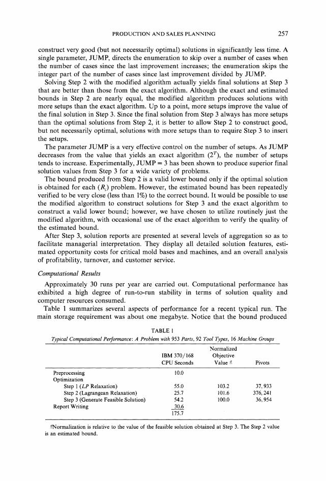
Table 1 summarizes several aspects of performance for a recent typical run. Themain storage requirement was about one megabyte. Notice that the bound produced

TABLE 1

PivotsIBM 370/168CPU Seconds

Typical Computational Performance: A Problem with 953 Parts, 92 Tool Types, 16 Machine Groups

NormalizedObjectiveValue !!.-

PreprocessingOptimization

Step 1 (LP Relaxation)Step 2 (Lagrangean Relaxation)Step 3 (Generate Feasible Solution)

Report Writing

10.0

55.025.754.230.6

175.7

103.2101.6100.0

37,933376,241

36,954

~ormalizationis relative to the value of the feasible solution obtained at Step 3. The Step 2 valueis an estimated bound.


by the Lagrangean relaxation is significantly better than the standard linear programming relaxation bound. Notice also that the time in Step 2 is smaller than what onemight expect; the 12-period fixed charge problems were processed in an average ofonly .027 seconds each (for comparison, the typical time quoted in [1] for exactsolution of a proper subclass of these problems of the same size was 0.25 seconds onan IBM 370/158). For this run, 142 (resp. 10) of the 11,436 binary Y variableschanged from value 0 (resp. 1) in Step 2 to value 1 (resp. 0) in Step 3. This shows thatthe solution to the Lagrangean relaxation of Step 2 required but minor adjustmentwith respect to the fixed charge arcs in order to yield the good feasible solution of Step3.

More generally, our experience has been that optimization CPU time for similarsized problems seldom varies more than ± 10%. Computing time is very nearlyproportional to the total number of parts. The final estimated optimality tolerance(which was 1.6% in the Table 1 run) tends to become smaller the more tightlycapacitated tool and machine availability is; tolerances in the vicinity of 2/10 of 1%are commonly observed in the most tightly constrained situations. In no case has thetolerance ever exceeded 2%.

5. Conclusion

This paper has demonstrated the practical applicability of a procedure based onLagrangean relaxation to a significant class of integrated production and sales planning models. The particular way in which this procedure is designed thoroughlyexploits the recent major advances made for minimum cost network flow problems.Provably good solutions are routinely being obtained in modest computing time tomixed integer linear programs of a size far beyond the capabilities of generallyavailable mathematical programming systems.

The system is used regularly at R & G Sloane Manufacturing Company. Day-to-dayproduction scheduling is still performed manually, but with the benefit of the system'sguidance and predictions of bottlenecks in the future. The integrated nature of themodel has made the system valuable as a focal point for coordinating planningactivities among the key functional areas of the firm: inventory control, finance,marketing, and production operations. Two specific illustrations are the evaluation ofmajor capital expenditure and interplant equipment transfer opportunities. A recentBusiness Week article [11] featured this application, with the Vice President ofOperations quoted as crediting the new system for an increase in total operating profitsduring a recent year of $500,000.2

2partially supported by the National Science Foundation and by the Office of Naval Research. This workcould not have been completed without the abiding cooperation and support of R & G Sloane Manufacturing Company. Special thanks are due to Mr. Ralph G. Schmitt, Vice President of Operations. Valuablecomments from the referees and from Jay Brennan are also gratefully acknowledged.

References1. BAKER, K. R., DIXON, P., MAGAZINE, M. J. AND SILVER, E. A., "An Algorithm for the Dynamic

Lot-Size Problem with Time-Varying Production Capacity Constraints," Management Sci. Vol. 24,No. 16 (1978).

2. BRADLEY, G. H., BROWN, G. G. AND GRAVES, G. W., "Design and Implementation of Large ScalePrimal Transshipment Algorithms," Management Sci., Vol. 24, No.1 (1977).


3. CAIE, J., LINDEN, J. AND MAXWELL, W., "Solution of a Single Stage Machine Load Planning Problem,"OMEGA, Vol. 8, No.3 (1980).

4. FISHER, M. L., "Lagrangean Relaxation Method for Solving Integer Programming Problems," Management Sci., Vol. 27, No.1 (1981).

5. GEOFFRION, A. M., "Lagrangean Relaxation for Integer Programming," Mathematical ProgrammingStudy 2, North-Holland Publishing Co., Amsterdam, 1974.

6. GRAVES, G. W. AND VAN Roy, T. J., "Decomposition for Large-Scale Linear and Mixed Integer LinearPrograming," Working Paper, Graduate School of Management, UCLA, November 1979, Mathematical Programming (to appear).

7. LOVE, R. R. AND VEMUGANTI, R. R., "The Single-Plant Mold Allocation Problem .with Capacity andChangeover Restrictions," Operations Res. , Vol. 26, No. 1 (1978).

8. MCCLAIN, J. O. AND THOMAS, J., "Horizon Effects in Aggregate Production Planning with SeasonalDemand," Management Sci., Vol. 23, No.7 (1977).

9. SALKIN, H. M. AND MORITO, S., "A Search Enumeration Algorithm for a Multiplant, MultiproductScheduling Problem," Proceedings of the Bicentennial Conference on Mathematical Programming, NBS,Gaithersburg, Maryland, December 1976.

10. SHAPIRO, J. F., "A Survey of Lagrangean Techniques for Discrete Optimization," in Annals of DiscreteMathematics 5: Discrete Optimization, P. L. Hammer, E. L. Johnson, and B. H. Korte (eds.), NorthHolland, Amsterdam, 1979.

11. " 'What if' Help for Management," Business Week, 21 January 1980, pp. 73-74.

INSTITUTIONAL MEMBERS

BANK OF AMERICASan Francisco, California

THE BOSTON CONSULTING GROUP, INC.Boston, Massachusetts

DIAGMA CONSULTANTSParis, France

GENERAL ELECTRICNew York, New York

THE HENDRY CORPORATIONCroton-on-Hudson, New York

IBMArmonk, New York

LEVER BROTHERS COMPANYNew York, New York

MANAGEMENT DECISION SYSTEMS, INC.Weston, Massachusetts

McGRAW-HILL BOOK COMPANYNew York, New York

MOBIL OIL CORPORATIONNew York, New York

THE PROCTER & GAMBLE COMPANYCincinnati, Ohio

R.J. REYNOLDS TOBACCO COMPANYWinston-Salem, North Carolina 27102

STANDARD OIL COMPANY(Indiana)

Chicago, Illinois

XEROX CORPORATIONStamford, Connecticut

For information regarding Institutional Membership, write to:Mrs. Mary R. DeMelim, 146 Westminster Street, Providence, Rhode Island 02903

Production and Sales Planning with Limited Shared Tooling at the Key Operation

Documents

Transcript of Production and Sales Planning with Limited Shared Tooling at the Key Operation