Proceedings

15th ANZIAM Mathsport

Wellington, New Zealand

9-11 November 2020Edited by Ray Stefani and Adrian Schembri

Grant Elliott Liz Perry

1

Proceedings

15th Australasian Conference on

Mathematics and Computers in Sport

(ANZIAM Mathsport 2020)

Wellington, New Zealand

9-11 November 2020

Edited by Ray Stefani and Adrian Schembri

Published by ANZIAM Mathsport

All abstracts and papers have undergone a peer review.

ISBN: 978-0-646-82267-9

2

Great New Zealand Athletes

These present and past athletes have impressed the world with their excellence and also

their personalities.

Peter Snell was a premier middle-distance runner. He won 3 gold medals in Olympic

competition. In the 1964 Olympics, he became the only man then or since to win the 800 m

and 1500 m in the same Games.

Valerie Adams made her mark in the shot put. Her remarkable career includes four World

Championships, Four World Indoor Championships, two Olympic Gold Medals and three

Commonwealth Games Gold Medals. She was named IAAF Continental Cup winner twice. Her

brother Steven plays in the NBA.

Grant Elliott is a former New Zealand international cricketer. An all-rounder, his finest moment

came in the 2015 World Cup semi-final against South Africa where he scored an unbeaten 84

and was adjudged the Man of the Match, putting New Zealand into their first ever Cricket

World Cup Final, where he scored 83 runs against Australia. Elliott is the maker of the Buzz

Cricket Bat. Luke Woodcock scored 220 with it in a first-class game. Elliot is general manager of

CricHQ, a widely-used digital platform for cricket.

Liz Perry’s 18-year career as a cricket all-rounder spanned 2002-2020. In 2005, Perry began

competing in Wellington. She appeared for the Blaze in 81 T20 matches and 115 List A

matches, scoring 3441 runs. Her teams won six T20 championship, the last three in a row,

including a championship in her final match. Liz played internationally for the Silver Ferns in 48

matches, scoring 570 runs, including an appearance in the ICC T20 grand final in 2010. She also

represented New Zealand in field hockey. Since 2017, Perry has served as General Manager for

Cricket Wellington.

Formerly a marathon runner himself, Arthur Lydiard was named the World’s All Time

Greatest Coach by Runners’ World. During the 1960 Olympics, he coached Murray Halberg,

Peter Snell and Barry Magee to gold medals. He also coached Rod Dixon, John Walker, Dick

Quax and Dick Taylor. His methodology changed the concept of effective training.

In 1952, Yvette Williams earned New Zealand’s first women’s Olympic gold medal by winning

the long jump. She won 21 national championships in the shot put, javelin, discus, long jump and

80 m hurdles. She won three gold medals in the 1954 Empire Games.

3

At the age of 19, Jonah Lomu became the youngest All Black ever. During his rugby career, he

earned 63 caps and score 37 tries. He has been selected for the International Rugby Hall of

Fame. Lomu took part in the famous World Cup in South Africa won by the Springboks. He

played aggressively throughout his career, generally hiding a severe kidney disease that

eventually took his life.

As a Paralympian, Sophie Pascoe has represented New Zealand with remarkable success. She

showed us that with hard work and dedication, seemingly insurmountable barriers can be

overcome. She won 9 gold and 6 silver medals in the Paralympics; 12 gold, 6 silver and 4 bronze

medals at World Championships and 4 gold medals at the Commonwealth Games.

To simply write that Sonny Bill Williams is a versatile athlete would be an understatement. In

boxing, he won all 7 professional bouts. Competing in rugby league, he earned 12 caps for the

Kiwis. He then switched codes and earned 58 caps with the All Blacks in rugby union, playing

for the World Championship winning teams in 2011 and 2015. He competed in rugby 7s

during the 2015-16 World Cup and during the 2016 Olympics. Sonny Bill showed what being a

man among men means, when a 14-year old boy left the stands to congratulate his heroes

after the 2015 World Cup had ended. Security was about to grab the youth and drag him back

into the stands, when Sonny Bill gently intervened and walked with the boy to meet the All

Blacks. Sonny Bill gave the boy his gold medal so the boy would feel part of the celebration.

Sonny Bill walked the boy back to the grandstands and insisted that the boy keep that coveted

gold medal. That wonderful act of kindness shows us what sports can be, at its best.

Ray Stefani

4

PLANNING ANZIAM MATHSPORT 2020

The Executive Committee of ANZIAM Mathsport, led by Chair Anthony Bedford and Secetary Ray Stefani as well as the ANZIAM Mathsport 2020 Organizing Committee, led by Chair Paul Bracewell, have closely followed the heath and economic issues wrought by the Covid pandemic. A decision was made for the best interests of all ANZIAM Mathsport members to move the meeting from May to November.

We encourage readers of these Proceedings to contact the corresponding authors of papers of interest and to establish a dialog. We look forward to the mutual knowledge and insight these Proceedings will provide our readers.

ANZIAM Mathsport 2020 will most likely involve pre-recorded talks along with Zoom question and answer sessions. As a major benefit of a largely virtual meeting, the talks will remain available for future viewing online.

We hope all of our Mathsport friends will remain safe and healthy.

Ray Stefani, Secretary, ANZIAM Mathsport Anthony Bedford, Chair, ANZIAM Mathsport Paul Bracewell, Chair, ANZIAM Mathsport 2020 Meeting; Owner, DOT Loves Data

5

Table of Contents

Topic Authors Title Page

Keynote Speaker Grant Elliott CRICKET PLAYING AND DATA COLLECTION 7

Keynote Speaker Liz Perry 7

Keynote Speaker Niven Winchester RUGBY POINTS SYSTEMS 7

Australian Rules Football Timothy Bedin BUILDING A NATURAL LANGUAGE GENERATION SYSTEM FOR

AUSTRALIAN RULES FOOTBALL CONTENT USING PARAMETRIC

DISTRIBUTION FITTING

8

Australian Rules Football Jeremy Alexander, Sam

Robertson, Karl Jackson ASSESSING TEAM SPATIAL CONTROL IN AUSTRALIAN RULES

FOOTBALL

9

Australian Rules Football Matthew Gloster EXPECTED SCORE MODELS IN AUSTRALIAN FOOTBALL WITH

REPEATED SHOTS

10

Cricket Moinak Bhaduri QUANTIFYING THE INTERESTING-NESS OF A LIMITED-OVER CRICKET

MATCH THROUGH EMPIRICAL RECURRENCE RATES RATIO-BASED CHANGE-DETECTION ANALYSIS

11

Cricket Paul J. Bracewell,

Jason D. Wells

ORIGINS OF CONTRACTED CRICKETERS IN NEW ZEALAND 123

Cricket Bernard Kachoyan,

Mark West

PREDICTING THE EXPECTED BATTING PARTNERSHIPS OF CRICKET

BATSMEN

20

Cricket Robert Nguyen,

James Thomson

OPTIMIZING THE POWERPLAY IN T20 CRICKET 124

Cricket Jonathan Sargent BUILDING AND EXECUTING A T20 CRICKET BETTING MODEL IN“R” 30

Cricket Steven Stern DID HERSHELLE GIBBS REALLY DROP THE CRICKET WORLD CUP?

THE COST OF A CATCH, THE MARGIN OF VICTORY AND OTHER USES OF THE DL-METHODOLOGY

37

Cricket Adelaide Wilson

Holly E. Trowland,

Paul J. Bracewell

COMMUNITY DRIVERS OF JUNIOR CRICKET PARTICIPATION

IN NEW ZEALAND

125

Gambling Tristan Barnett RESOLVING PROBLEM GAMBLING: A MATHEMATICAL APPROACH 38

Machine Vision Rob G. McDonald,

Paul J. Bracewell,

Holly E. Trowland, Aristarkh Tikhonov

DISCOUNTING CAMERA MOVEMENT IN CALCULATION OF PLAYER

PATHS USING MACHINE VISION IN RUGBY UNION

39

Machine Vision Holly E. Trowland,

Paul J. Bracewell,

Rob G. McDonalda

Aristarkh Tikhonov

VALIDATING PLAYER PATH TRACKING USING MACHINE VISION 45

Machine Vision Paul J. Bracewell,

Fergus Scott,

Brendon P. Bracewell

HISTORICAL EVALUATION OF BOWLING SPEEDS IN CRICKET USING

MACHINE VISION

51

Machine Vision Paul J. Bracewell, Holly Trowland,

Jordan K. Wilson, Aristarkh Tikhonov

USING MACHINE VISION TO TRACK THE LOCUS OF PLAY IN RUGBY

UNION

57

Netball Anthony Bedford,

Kiera Bloomfield, Paul Smith

ATHLETE AND ANALYST COMPARISON OF

PERFORMANCE OUTCOMES IN ELITE NETBALL

126

Netball Anthony Bedford,

Paul Smith, Kiera Bloomfield

ASCERTAINING PERFORMANCE STANDARDS BETWEEN

INTERNATIONAL LEVELS OF NETBALL

127

Netball Paul Smith,

Anthony Bedford

MATCH OUTCOME OF SUPER NETBALL LEAGUE MATCHES BASED ON

PERFORMANCE INDICATORS

61

Netball Paul Smith, Anthony

Bedford

COMPUTER VISION IN NETBALL 70

Netball Paul Smith, Anthony

Bedford

A SEMI-AUTOMATED EVENT LOCATION RECORDER FOR NETBALL 79

6

Topic Authors Title Page

Olympics Sports-New Raymond Stefani UNDERSTANDING HOW SPORTS LIKE SPORT CLIMBING AND BREAK DANCING WERE ADDED TO THE OLYMPICS: COULD E-SPORTS BE NEXT?

85

Rating Systems Ankit K. Patel,

Paul J. Bracewell,

Ivy Liu

RATING RATINGS: A QUANTITATIVE FRAMEWORK FOR

CONSTRUCTING HUMAN-BASED RATING SYSTEMS

128

Rating Systems Ankit K. Patel,

Paul J. Bracewell

APPLYING THE SPHERICAL SCORING RULE TO QUANTIFY THE

EFFECTIVENESS OF SPORT RATINGS SYSTEMS

129

Rugby Harini Dissanayake,

Paul J. Bracewell,

Holly E. Trowland,,

Emma C. Campbell

LATENT DRIVERS OF PLAYER RETENTION IN JUNIOR RUGBY 92

Rugby Robert Nguyen,

Tianyu Guan, Jiguo Cao

and Tim B. Swartz

IN-GAME WIN PROBABILITIES FOR THE NATIONAL RUGBY

LEAGUE

130

Squash Ken Louie, Bruce Morgan, Paul Ewart

HOME AND AWAY: NOT A DAYTIME DRAMA BUT A SQUASH SCHEDULING STORY

98

Swimming Raymond Stefani UNDERSTANDING THE FEMALE/MALE VELOCITY RATIO VERSUS

DISTANCE FOR ALL SWIMMING STROKES, INCLUDING ENGLISH AND CATALINA CHANNEL SWIMS

106

Tennis Thomas H.

Pappafloratos,

Tamsyn A. Hilder, Paul J. Bracewell

SOCIETAL BIAS AND THE REPORTING OF TOP TENNIS PLAYERS IN

NEW ZEALAND SPORT MEDIA

114

7

Keynote Speakers

Grant Elliot

Grant is a former New Zealand international cricketer. An all-rounder, his finest moment came in

the 2015 World Cup semi-final against South Africa where he scored an unbeaten 84 and was

adjudged the Man of the Match, putting New Zealand into their first ever Cricket World Cup Final,

where he scored 83 runs against Australia. Elliott is the maker of the Buzz Cricket Bat. Luke

Woodcock scored 220 with it in a first-class game. Elliot is general manager of CricHQ, a widely-

used digital platform for cricket.

Liz Perry

Liz’ 18-year career as a cricket all-rounder spanned 2002-2020. In 2005, Perry began competing

in Wellington. She appeared for the Blaze in 81 T20 matches and 115 List A matches, scoring 3441

runs. Her teams won six T20 championship, the last three in a row, including a championship in

her final match. Liz played internationally for the Silver Ferns in 48 matches, scoring 570 runs,

including an appearance in the ICC T20 grand final in 2010. She also represented New Zealand in

field hockey. Since 2017, Perry has served as General Manager for Cricket Wellington.

Niven Winchester

Niven is an economist specializing in the analyses of climate, energy and trade policies using

applied equilibrium modelling. His work estimating the predictive ability added to rugby (union)

league tables by various bonus point schemes led to changes in international and domestic rugby

bonus point systems. He is currently a professor of economics at Auckland University of Technology

and a senior fellow at Motu Economic & Public Policy Research. He previously held positions at the

Massachusetts Institute of Technology and the University of Otago.

Submitted to MATHSPORT 2020 February 24, 2020

BUILDING A NATURAL LANGUAGE GENERATION SYSTEM FOR

AUSTRALIAN RULES FOOTBALL CONTENT USING PARAMETRIC

DISTRIBUTION FITTING

Timothy Bedin a

a Champion Data, Melbourne a Corresponding author: tim.bedin@championdata.com.au

Abstract This paper describes our approach to creating a system to generate natural language content from ‘box-score’

statistical summaries of Australian Football matches. Our key assumption is that the most interesting aspects

of a player’s performance can be found by examining where their statistical representation sits in relation to a

historical probability distribution for that statistic.

In this work we use the maximum likelihood method to fit parameters for discrete distributions to various

aggregated statistics in elite Australian Football matches from 1999 to the present. The individual statistics are

modelled as independent variables drawn from an underlying distribution chosen by examining historical

values of these statistics. For the statistics that we have examined the data consists of discrete counts. As the

data is overdetermined (𝑣𝑎𝑟(𝑥) > 𝑚𝑒𝑎𝑛 (𝑥)), the negative binomial distribution was found to be an

appropriate distribution choice. We made the choice to represent the historical information parametrically so

that confidence intervals and z-scores can be calculated efficiently. This is especially convenient when

streaming data through a live system. This parametric approach also simplifies comparing distribution

parameters across competitions and time.

We used the fitted distributions to score out individual player performances. Once transformed to a z-score

representation we used these scores to create visualisations and basic text summaries of the most noteworthy

elements of a player’s performance.

Keywords: Natural Language Generation, Australian Football, Parametric Distribution Fitting

8

Submitted to MATHSPORT 2020 April 30, 2020

Assessing team spatial control in Australian Rules football

Jeremy Alexander a,b, Sam Robertson a, Karl Jackson b

a Institute for Health and Sport (IHES), Victoria University, b Champion Data Pty Ltd, Melbourne, Australia

a Corresponding author: jeremyalexander60@gmail.com

Abstract

The inception of tracking technologies has allowed for increased access to the positioning data of team sport athletes (1). This information assists in understanding the collective behaviour of teams by measuring the continuous movement patterns of players (1). Complex interactions between teammates and opponents can now be captured in a continuous manner that reflect the emerging nature of match play (2). Such information has been used to inform the pattern forming behaviour of teams by determining how teams position players to generate a certain degree of spatial control across a playing surface (3). However, the extent to which team spatial control varies with respect to specific match play events is yet to be established. Therefore, the primary aim of this study was to determine the extent to which continuously represented team spatial control varies with respect to specific match play events in Australian football. The secondary aim was to determine whether differences in team spatial control exist during different match phases and ball location. Data from Australian football athletes were collected via 10 Hz local positioning system (GPS) devices. Team spatial control was analysed during three match phases (offensive, defensive, and contested) and four field positions (defensive 50, defensive midfield, forward midfield, and forward 50). Results revealed that teams obtained greater spatial control during offence, but experienced reduced control during defence. Notwithstanding, both teams were able to seize spatial control when forcing a turnover in possession. A trade-off scenario may apply as specific formations may generate a competitive advantage in particular aspects of match play, whilst concurrently triggering a disadvantage in other facets of match play. Continuously quantifying the resistive exchange in spatial control between teams and detecting the value placed on controlling specific regions may contribute to providing a more representative understanding of tactical team behaviour.

Keywords: Team Tactics, Performance Analysis, Sports Analytics

References

(1) Rein, R., & Memmert, D. (2016). Big data and tactical analysis in elite soccer: futurechallenges and opportunities for sports science. Springerplus, 5(1), 1410.

(2) Clemente, F., Sequeiros, J., Correia, A., Silva, F., & Martins, F. (2018). Brief Review AboutComputational Metrics Used in Team Sports: Springer.

(3) Fernandez, J., & Bornn, L. (2018). Wide Open Spaces: A statistical technique for measuringspace creation in professional soccer. Sloan Sports Analytics Conference.

9

Submitted to MATHSPORT 2020 March 3, 2020

EXPECTED SCORE MODELS IN AUSTRALIAN FOOTBALL WITH

REPEATED SHOTS

Matthew Gloster a,b

a Champion Data

b corresponding author: matthew.gloster@championdata.com.au

Abstract

In many sports, measuring the opportunity for scoring is often considered a more valuable metric to describe

the performance of a team or player in a match than the score itself. This may be especially valuable in low

scoring sports where teams can regularly lose, despite creating higher quality scoring opportunities than their

opponent. Expected score (xS) models give us a tangible way to measure these opportunities. In Australian

football expected score models are reliant on estimating the probability of a successful shot at goal. Champion

Data has been recording detailed metrics for shots at goal since 2013 in order to create an empirical expected

score model. This model takes the sum of expected scores across all individual shots at goal by a team within a

match. At the player level, a model with no memory is valid since the desired outcome is a measure of a

player’s conversion ability accounting for the difficulty of shots taken. For teams though, the model may

overestimate a team’s scoring opportunities by introducing bias from ‘repeated shots’ in a single attacking

phase that would not have been taken if the first shot was converted. In the present study, we extend the

existing model by accounting for repeated shots, to ensure that the likelihood of scoring from a single

attacking phase does not exceed 100%, and that the expected points from that phase does not exceed the

maximum single-shot score of six points.

Keywords: Expected score, AFL, Champion Data, Shot Quality, Australian football, Shot Probability

10

QUANTIFYING THE INTERESTING-NESS OF A LIMITED-OVER

CRICKET MATCH THROUGH EMPIRICAL RECURRENCE RATES

RATIO-BASED CHANGE-DETECTION ANALYSIS Moinak Bhaduri

Department of Mathematical Sciences,

Bentley University, Massachusetts, USA

Corresponding author: mbhaduri@bentley.edu

Abstract

Ever since the first ball got bowled, the game of cricket has enthralled its audience – purists and liberals alike.

Despite its rich history and critics questioning the relevance of several of its facets, the game has found a way

to remain stubbornly germane. Several of those questions, however, boil down to the perceived excitement one

feels while watching a game. Quantitative measures like runs scored per over, the frequency at which wickets

fall, the margin of victory, or the number of overs a game lasts quantify excitement with varying, and at times,

questionable degrees of reliability. This work puts forth a quantitative framework in which to define this notion

of “interesting-ness” in a stronger way. The oscillations in Empirical Recurrence Rates Ratio (ERRR), a statistic

we proposed to tackle applied problems, are shown to indicate levels of excitement. Using simulated and real examples, we propose several measures on ERRR, and apply techniques such as block bootstrapping to find that

overall interestingness gets maximized when several of these measures reach their optimal values. ERRR, shown

to be a function of the more established “runs per over”, is intuitive, and offers analysts freedom in quantifying

the “interesting-ness” of the match as a whole, or specific sections of it, in an on-line fashion, i.e., as the match

evolves. Applications of the proposed methods will enable matches to be ordered on an “interesting-ness” scale

and let us unearth unifying features of exciting matches, prompting changes in rules, if need be.

Keywords: T20 cricket, empirical recurrence rates and ratios, time series, entropy, block bootstrapping, change-point detection.

1. INTRODUCTION

It is no exaggeration to claim that today’s computing prowess and data-collection ability have led to a deluge of

cricketing statistics, ushering novel ways of forging strange connections. The archaic “batting average”,

“bowling average”, “runs-per-over”, etc., have given way to the more exotic “pressure index”, “market valuation

of players”, “wicket weights of different batting positions”, and the like. Saikia et al. (2019) offer a wonderful

resource. Despite such innovations in ways of reporting data and making the game palatable, cricket is still confronting stiff competition in maintaining popularist foothold. Much of this is attributable to the speed at

which a spectator loses interest in a game, owing to it being too predictable too soon. This paper examines this

question of “interesting-ness”. It seeks to clarify what it means, define it through a tool termed Empirical

Recurrence Rates Ratio (ERRR), and calculate it through several novel measures imposed on ERRR – while

insisting on a conceptual proximity to more established tools (runs-per-over, for instance) to ensure ready

applicability.

Our work is organized in sections. The next highlights the striking resemblance our construct has with a time

series problem, and subsequently introduces the crucial statistic we intend to promote. The third introduces

several measures on this statistic, and analyses eight games, three simulated, and five real to demonstrate our

proposal’s effectiveness. A few advanced ideas such as bootstrapping and sequential analysis are also discussed

here. The final section concludes with a summary and an eye towards the future.

2. METHODS

SOME DESCRIPTIVE GRAPHICS

Regardless of the way one chooses to define a convenient unit of time, be it one delivery, one over, or a collection

of five-over spells by a specific bowler, the benefits of drawing inspiration from longitudinal techniques are both

necessary and immediate. To demonstrate, we have sampled two T20 internationals featuring New Zealand, one

against India, played on 9/11/2012 in Chennai and another against England, played more recently on 11/5/2019

at Saxton Oval. The data are collected from www.cricsheet.org, an online site storing ball-by-ball statistics for

a range of cricket matches.

11

Figure 1: Polar maps showing scoring tendencies over balls every over, Match 1, between New Zealand (batting

first) and India (batting second).

Figure 2: Tapered ACF plots showing scoring “recollection”, Match 1.

Polar plots, of the kind shown in Figures 1 and 3 are intuitive and visually appealing ways of unearthing hidden

seasonalities in a sequence monitored over temporal hierarchies – seasons (months, say) and years, for instance. In the present context, the role of years could be played by overs, and of months, by balls in an over, while our

variable of interest would be the number of runs scored. The angle at which a point is located represents the

delivery (one through six legal ones) that generated it, while its distance from the origin gives the number of

runs accumulated. The colours are indicative of match progression, with the darker shades showing the earlier

overs and the lighter the later overs in an innings. In match 1, while New Zealand have shown strong tendencies

to score off balls 3 and 6, India have chosen to attack almost every delivery in an over with similar likelihood,

generating a more uniform spread. Polar plots may be deployed to replace traditional line charts, which merely

show the scoring trend, without offering clear insights into seasonality. This is because the presence of a colour

gradient in a polar map demonstrates a change in scoring trend, with lighter shades on the outside indicating

increased scoring rates towards the closing half of an innings. Controlling other factors to negate any contextual

dependence, plots such as these may reveal, for instance, a chasing team’s general inclination to target specific

delivery(ies) in an over, or a bowler’s tendency to leak runs at specific points in a spell.

12

Figure 3: Polar maps showing scoring tendencies over balls every over, Match 2, between New Zealand (batting

first) and England (batting second).

Figure 4: Tapered ACF plots showing scoring “recollection”, Match 2.

Under the assumption of no drastic changes, just as the profit margin of a sales company in a given quarter may

be expected to be similar to the one preceding, tactical approaches to cricket often make the number of runs scored off a specific ball depend on the one scored of the previous (or a set of previous balls). A chasing team,

trying to recover from the loss of quick wickets, for instance, might not want to take unnecessary chances,

especially if a boundary has been hit in the over ongoing. The variables counting the number of runs per ball

may, therefore, in general, be assumed to be dependent on each other. To confirm, we recommend the use of

tapered autocorrelation plots, introduced by Hyndman (2015), graphed in Figures 2 and 4. The point estimates,

represented by the red dots, of these autocorrelations at any given lag shows how strongly the number of runs

scored depends on that scored that many lag-balls prior. Usual auto-correlation functions do a similar job under

the assumption of normality and large sample sizes. These are unattainable in a cricketing context and hence the

need for the tapered version which has the added benefit of providing bootstrapped (we have implemented 500

bootstrap replicates) interval estimates, strengthening our confidence in these estimates at large lags. It is

interesting to note that in both the matches analysed, for the team batting first, most of the run-memory is lost

by the second lag, while for the chasing team, it is retained till the fourth. The first team, in an attempt to post a big total, seems to maintain similar scoring patterns for a period of three consecutive deliveries (seems to relax,

say, for no more than three deliveries since a boundary has been hit), while the chasing team, aided by the

knowledge of the total posted, seems to do so over a period of five, adopting a more measured approach to the

run chase.

EMPIRICAL RECURRENCE RATES RATIO

Motivated by applications in weather science and geology, the notion of Empirical Recurrence Ratio (ERR) was

introduced by Tan, Ho, and Bhaduri (2014) and Ho and Bhaduri (2015) and its modeling performance was found

13

to be attractive in both seasonal (the former work, dealing with sand-storms) and non-seasonal (the later work,

dealing with earthquakes) cases. Given a time series tX observed at discrete times

1,2,3,..., ERR, denoted at time by is given by:tt t Z

1

t

k

kt

X

Zt

. (1)

Its continuous counterpart, under the assumption of time homogeneity, can be shown to track the maximum

likelihood estimate of the intensity of some governing Poisson process. For our purpose, with kX representing

the number of runs scored off ball ( 1, 2,...,120)k k assuming all valid deliveries and no failure truncation,

tZ will represent the average run-rate per ball (at time t), similar to the more established runs per over. In the

presence of another (possibly) related time series tY tracked at the same frequency, ERR can be generalized

to Empirical Recurrence Rates Ratio, notationally tR , defined by

1

1 1

t

k

kt t t

k k

k k

X

R

X Y

. (2)

Introduced by Ho et al. (2016) in the context of financial modeling, ERRR, readily seen as the ratio of two ERRs,

has found subsequent use in volcanology (Ho and Bhaduri (2017)), oceanography (Bhaduri and Ho (2018)), time series classification (Bhaduri and Zhan (2018)), and others (Zhan et al. (2019), Bhaduri, Zhan, and Chiu

(2017), Bhaduri et al. (2017)). These studies have demonstrated ways to exploit ERRR as a tool to understand

the interplay between the competing time series. In the following section, we revisit some of those ideas, propose

a few more, and bring out ERRR’s relevance in quantifying the “interesting-ness” through handling a few

simulated examples and some actual T20s.

3. RESULTS

Since cricket is predominantly a “batsman’s game”, with the team scoring more runs winning, regardless of the

number of balls taken or the wickets lost to achieve them, the relation

w w l l

w wl

l

p b p b

p bp

b

is always true, where w

p and w

b are the run-rate per ball and the total number of balls the winning team lasted,

lp and lb representing similar quantities for the losing side. Dividing the numerator and denominator of (2) by

t, the following inequality holds for ERRR value at the terminal point:

w w lterm

w ww l w lw

l

p p br

p bp p b bp

b

.

This expression, providing a non-stochastic lower bound for the final ERRR value in terms of the ratio of

deliveries consumed, however, fails to describe the “interesting-ness” online, i.e., as the match progresses. To

achieve that, and inspire our analyses of the five real T20 internationals, we construct three simulated examples.

We assume each of these matches lasted the full twenty overs and wickets were not lost.

14

Simulation 1: The team batting first hit a six every ball, while the one batting second failed to score in any. This match, intuitively, is extremely boring to witness, especially because of its one-sidedness, and the ERRR curve,

calculated through (2), will be a horizontal line located at 1.

Simulation 2: Here, once again, the team batting first hit a six every ball, but now, the one bating second hit a

four every ball. Clearly, this is slightly more interesting than the previous one, but still lacks sufficient

competitiveness. The resulting ERRR curve, through (2), will generate a constant line again, this time located at

0.6.

Simulation 3: Let’s assume that the first team had a scoring pattern: (6,4,6,4,6,4,…) while the second had one

like (4,6,4,6,4,6,…). This clash, representing a constant tug-of-war, is extremely interesting to watch, and the

resulting ERRR curve will be extremely oscillatory, centered around 0.503, with half of its time spent above this

threshold.

The simulation exercise seems to demonstrate that the more an ERRR curve moves towards the 0.5 line, the

more interesting a match gets, and the more often it crosses this threshold, the more engaging its features. Clearly, these simulations, especially numbers 1 and 3, lie at extreme ends of the “interesting-ness” spectrum

and will hardly be realized in practice, but they provide intuitive insights into the way ERRR operates.

Figure 5: ERRR curves from five T20 internationals, showing varying degrees of “interesting-ness”

Figure 5 above shows the ERRR curves from the five T20 internationals we analyzed, the first two featuring

New Zealand described previously in Section 2. Table 1 summarizes the details. With some of these matches

showing greater ERRR oscillations than others, we proceed to define a sequence of measures to quantify the

property.

Index of competitiveness (IC): Ho and Bhaduri (2017) defines the index of competitiveness as the proportion

of time the ERRR curve stays above the 0.5 threshold. Thus, a value of IC significantly close to either 0 or 1

indicates a stark difference in run-scoring intensities, for instance, in Simulations 1 and 2 in Table 1, while a

value around 0.5 at any point indicates the two teams are similar in terms of run-scoring at that point.

Index of waviness (IW): A match can be exciting even with an extremely high or low value of IC. Simulation 3

offers a case in point. The non-strictness above 0.5 made IC = 1 in this case, if we exclude the equality in the

definition, this drops to 0.5, which is more acceptable from an intuitive viewpoint. Focusing on a fixed threshold

15

that is independent of the match context, IC is blind to the possible oscillatory motion of ERRR, which, as the simulations showed, is extremely crucial in quantifying a match’s “interesting-ness”. We, therefore, need to

generalize the threshold to a match dependent process mean. Ho and Bhaduri (2017) defines the index of

waviness (IW) as the proportion of time the ERRR curve spends above its overall average. Interpretations remain

otherwise similar to IC.

Match id Description IC IW IE IEnt

Simulation 1 1 1 0 0.0084

Simulation 2 107 1 1 0 0.0084

Simulation 3 73 1 0.1667 0.9833 0.0234

Match 1 87 0.1721 0.7131 0.4426 0.1052

Match 2 82 0.4108 0.3643 0.4341 0.2049

Match 3 36 0.9837 0.3577 0.4715 0.2086

Match 4 33 0.3966 0.3707 0.4741 0.3355

Match 5 41 0.9680 0.3360 0.5360 0.2294

Table 1:

Index of extremeness (IE): The fixed mean threshold that IW uses may lose some of its justifiability, especially

in the face of a long burn-in period. While we introduce shortly the sequential IW to combat this issue, some of

the computational labor involved in that calculation may be reduced through an alternate route. We observe that

the wave-like property in an ERRR curve can also be captured through the index of extremeness (IE), essentially

taken to be the proportion of peaks and valleys that an ERRR curve brings out. Higher the IE, the more twists

and turns the match takes. It is interesting to note from Table 1 that IE is not necessarily correlated with IW. Index of entropy (IEnt): A high IE might not, on its own, always imply unpredictable interestingness. We may

turn to simulation 3, once again. Although this match is interesting, reflected through the several twists and turns

its ERRR takes (leading to a high IE), the second team’s (4,6,4,…) response to the first’s (6,4,6,…) is extremely

predictable. So, to quantify the quantity of “turbulence” or “chaos” that comes with a t20 international, we agree

to measure the entropy content in its ERRR. We store these numbers through IEnt, the index of entropy.

It emerges, therefore, with some degree of certainty, that the idea of interestingness cannot be captured through

a single measure. A quantitative confirmation on whether a cricket match is engaging, thus, rests on several of

these measures finding their optimal values simultaneously – IC, IW hovering around 0.5 with IE, IEnt being high.

Using such a condition, we find that match 4, played between India and the West Indies on 12/8/2019 turns out

to be the most exciting among the five real examples we have worked out.

A NOTE ON SEQUENTIAL INDICES

The measures introduced previously operate on the eventual ERRR curve, i.e., the graph obtained once the

match gets over. The strong law of large numbers guarantees the variation in ERRR will die down as the

match progresses if the calculations are done from the very beginning. This is observed in Figure 5 as well.

Consequently, the overall mean used in the calculation of IW, for instance, will be influenced by the wild

observations during the initial burn-in period. While this may be rectified by choosing a more robust quantity

like the median or the trimmed mean as the threshold, it will not generate the ability to focus on specific

periods of the match, which a sequential approach, described below, shall.

16

Figure 6: Sequential IW curves from five T20 internationals

We demonstrate the sequential paradigm using IW, the other measures can be modified similarly. With a pre-

defined burn-in period k, this approach consists of deleting the first k ERRR vales and calculating IW from the

residual sequence, once for each value of k. Figure 6 shows the effect as k varies. The case k = 0 corresponds to

the usual non-sequential IW value found previously in Table 1, and the sequential IWs for large ks are free of the

outlier-plagued mean problem in their thresholds. With k representing the final ball of the match (both teams

assumed to play the same number of deliveries), the condition of exceeding the mean is trivially satisfied, making

the IW index hit 1. Large variations in these sequential curves may also be taken as an index of “interesting-

ness”, by which criteria, match 4, once again, turns out to be quite engaging.

BLOCK BOOTSRAPPING

We next seek generalization in the following sense: if a match turns out to be boring, could there have been

some other sequence of run progression under which it could have turned out to be interesting? Equivalently, if

a match turns out to be interesting, could there have been some other sequence of run progression under which

it could have turned out to be boring? To answer these, we shuffle or permute chunks of the teas’ score sequence

several times, reconstruct the ERRR curve each time, and recalculate the measure(s) of interest. In contrast

with ordinary bootstrapping introduced by Efron (1979), the reordering has to be done in blocks to retain the

temporal dependence (Hall, Horowitz, Jing (1995)). The block size was chosen to e an over, i.e., six

consecutive legal deliveries. Once again, we have shown the results with IW in Figure 7. Similar outputs can

be had from other indices. With 500 bootstrap replicates, the graph shows the distribution of the 500 IW values

for each match. The densities for the first two simulated scenarios (shown here as Boring 1 and Boring 2) are

degenerate at 1. This is intuitive since under no rearrangement of the scoring pattern, can those two matches

turn out to be interesting. A strong concentration and density around 0.5 will indicate the “match property”

is stable, i.e., even under rearrangement of the scoring patterns, an interesting match will stay interesting – a

stronger statement than one claiming a given match was “interesting”.

17

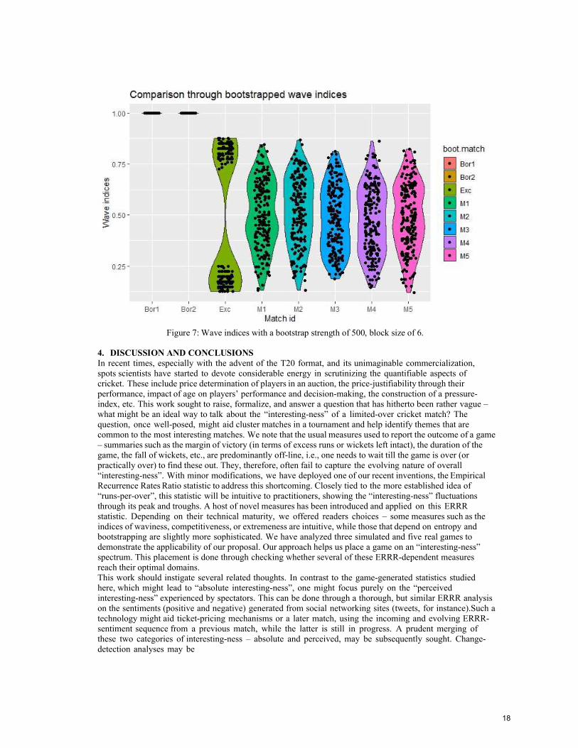
Figure 7: Wave indices with a bootstrap strength of 500, block size of 6.

4. DISCUSSION AND CONCLUSIONS

In recent times, especially with the advent of the T20 format, and its unimaginable commercialization,

spots scientists have started to devote considerable energy in scrutinizing the quantifiable aspects of

cricket. These include price determination of players in an auction, the price-justifiability through their

performance, impact of age on players’ performance and decision-making, the construction of a pressure-

index, etc. This work sought to raise, formalize, and answer a question that has hitherto been rather vague –

what might be an ideal way to talk about the “interesting-ness” of a limited-over cricket match? The

question, once well-posed, might aid cluster matches in a tournament and help identify themes that are

common to the most interesting matches. We note that the usual measures used to report the outcome of a game

– summaries such as the margin of victory (in terms of excess runs or wickets left intact), the duration of the

game, the fall of wickets, etc., are predominantly off-line, i.e., one needs to wait till the game is over (or

practically over) to find these out. They, therefore, often fail to capture the evolving nature of overall

“interesting-ness”. With minor modifications, we have deployed one of our recent inventions, the Empirical

Recurrence Rates Ratio statistic to address this shortcoming. Closely tied to the more established idea of

“runs-per-over”, this statistic will be intuitive to practitioners, showing the “interesting-ness” fluctuations

through its peak and troughs. A host of novel measures has been introduced and applied on this ERRR

statistic. Depending on their technical maturity, we offered readers choices – some measures such as the

indices of waviness, competitiveness, or extremeness are intuitive, while those that depend on entropy and

bootstrapping are slightly more sophisticated. We have analyzed three simulated and five real games to

demonstrate the applicability of our proposal. Our approach helps us place a game on an “interesting-ness”

spectrum. This placement is done through checking whether several of these ERRR-dependent measures reach their optimal domains.

This work should instigate several related thoughts. In contrast to the game-generated statistics studied

here, which might lead to “absolute interesting-ness”, one might focus purely on the “perceived

interesting-ness” experienced by spectators. This can be done through a thorough, but similar ERRR analysis

on the sentiments (positive and negative) generated from social networking sites (tweets, for instance).Such a

technology might aid ticket-pricing mechanisms or a later match, using the incoming and evolving ERRR-

sentiment sequence from a previous match, while the latter is still in progress. A prudent merging of

these two categories of interesting-ness – absolute and perceived, may be subsequently sought. Change-

detection analyses may be

18

conducted to identify “turning-points” in a match – another notion that is often talked about, but one that harbours subjectivity and vagueness. The schedule ahead, therefore, looks hectic, but enticing.

References

Bhaduri, M., Zhan, J., Chiu, C. (2017). A Novel Weak Estimator For Dynamic Systems. IEEE ACCESS, 5, 27354-27365.

Bhaduri, M., Zhan, J., Chiu, C., Zhan, F. (2017). A Novel Online and Non-Parametric Approach for Drift Detection in Big

Data. IEEE ACCESS, 5, 15883-15892. Bhaduri, M., Ho, C. (2018). On a Temporal Investigation of Hurricane Strength and Frequency. Journal of Environmental

Modeling and Assessment, 24 (5), 495–507.

Bhaduri, M., Zhan, J. (2018). Using Empirical Recurrence Rates Ratio for Time Series Data Similarity. IEEE ACCESS, 6, 30855-30864.

Efron B (1979) Bootstrap methods: another look at the jackknife. Ann Stat 7:1–26 Hall P, Horowitz JL, Jing B-Y (1995) On blocking rules for the bootstrap with dependent data. Biometrika 82:561–574

Saikia, H., Bhattacharjee D., Mukherjee, D. (2019). Cricket performance management: mathematical formulation ad

analytics, Springer. Ho, C., Bhaduri, M. (2015). On a novel approach to forecast sparse rare events: applications to Parkfield earthquake

prediction. NATURAL HAZARDS, 78 (1), 669-679. Ho, C., Zhong, G., Cui, F., Bhaduri, M. (2016). Modeling interaction between bank failure and size. Journal of Finance and

Bank Management, 4 (1), 15-33. Ho, C., Bhaduri, M. (2017). A Quantitative Insight into the Dependence Dynamics of the Kilauea and Mauna Loa Volcanoes,

Hawaii. MATHEMATICAL GEOSCIENCES, 49 (7), 893-911.

Hyndman, R.J. (2015). Discussion of ``High-dimensional autocovariance matrices and optimal linear prediction''. Electronic Journal of Statistics, 9, 792-796.

Tan, S., Bhaduri, M., Ho, C. (2014). A statistical model for long term forecasts of strong dust sand storms. Journal of Geoscience and Environment Protection, 2, 16-26.

Zhan, F., Martinez, A., Rai, N., McConnell, R., Swan, M., Bhaduri, M., Zhan, J., Gewali, L., Oh, P. (2019). Beyond

Cumulative Sum Charting in Non-Stationarity Detection and Estimation. IEEE Access, 7, 140860 - 140874.

19

PREDICTING THE EXPECTED BATTING PARTNERSHIPS IN CRICKET Bernard Kachoyan a,c Marc West b

a University of New South Wales b University of Technology, Sydney

c Corresponding author: b.kachoyan@unsw.edu.au

Abstract

Many previous studies have explored the question of whether a batsman’s survival function follows a

geometric, and hence memoryless, distribution. Kachoyan and West (2018), expanding on previous work,

showed that a limiting geometric distribution can be derived from simple assumptions while still maintaining a

large amount of flexibility, making it a natural baseline performance predictor. This paper will explore

evidence that an ensemble of batsmen closely approaches a memoryless distribution. This will be done by

scaling the batting averages appropriately and by considering mixed exponential distributions. This paper will

show how a mixed exponential model can be used to derive very good agreement with survival data for all

male Test cricketers. This implies that an individual batsman’s survival function may be considered in terms of

variation around a “true” memoryless survival function for a class of batsmen of similar standard. The

question can now be asked whether this can be used to predict batting partnerships or team scores. The latter is

difficult to validate as the number of times exactly the same team is fielded is rare. However, batting

partnerships are relatively easy to model directly under these assumptions and data are readily available. The

paper will derive the expected performance of batting pairs using the memoryless property and compare with

historical data. The comparison shows good agreement in the mean but there is a large variance in the

historical data with both under- and over- achieving pairs.

Keywords: Batting partnerships, cricket, memoryless

INTRODUCTION

Since as far back as 1945, there has been considerable academic interest in whether a batsman’s survival

function can be modelled by a geometric survival function (Wood, 1945). The importance of this is the

memoryless nature of the geometric distribution and what that implies about the nature of batting. Moreover,

the traditional batting average is the Maximum Likelihood Estimation (MLE) of the mean under the

assumption that runs scored in an innings constitute a random sample of lifetimes drawn from the

exponential/geometric distribution, where the runs scored in a not-out (NO) innings are considered to be a

right-censored lifetime.

The ability to derive a “true” underlying survival characteristic is seen as a way of avoiding the drawbacks

of using non-parametric estimates such as the Product Limit Estimate (PLE), and hence perhaps provide a

better estimate of batting performance. These drawbacks include its step function nature1 and that it does not

satisfactorily account for the cases where a batsman’s highest score is not out.

Das (2017) considered ten generalised geometric models of batting survival. These models assumed that

different hazard rates could apply over different parts of the innings2. They then used MLE techniques to

estimate these free parameters for each batsman. The PLE is equivalent to assuming that the hazard at each

point is different and has maximum flexibility. This type of modelling provides more degrees of freedom that

simply fitting a more complex distribution3, and also better takes into account cricket folklore such as “getting

one’s eye in”. Das found that models that assume a constant hazard for a large proportion of the run space are

the best4 fit for the batsmen they considered. For the Test batsmen, 7 out of the 10 could be well represented

by either a pure geometric (all hazards equal), or the zero hazard separate and all others equal. A further two

had a best fit of separate hazards at 0 and 1 and all others equal.

Brewer (2008) used a Bayesian method for inferring how a batman’s hazard varies throughout an innings

to consider the question of whether a batsman improves after “getting their eye in,” and if so, how long that

takes. They found (albeit with a small sample size and large estimation errors) that any such transition, if it

1 Hence, an unrealistic zero hazard if a batsman has never been dismissed on a particular score. 2 For example, one model assumed that the hazard at zero, between 1 and 9, and for 10 and over were all

distinct. 3 For example, a Weibull instead of a geometric. 4 In the sense that extra complexity did not improve the fit.

20

occurs at all, happens very early (<10 runs) and happens very quickly (over < 3 runs), and that the hazard is

subsequently constant.

Koulis, Muthukumarana et al. (2014) modelled batting performance by analysing 20 world-class batsmen

in One Day Internationals (ODIs) using a batsman-specific hidden Markov model (HMM) to compute

availability, reliability, failure rates and mean time between failure for each batsman. The failure rate was

shown to be constant under the HMM model as would be expected in a memoryless framework.

Sarkar and Banerjee (2016) critique the exponential model as not being flexible enough to model a

batsman’s inconsistency, as the standard deviation is uniquely determined by the batting mean. They use the

continuous Weibull distribution to fit to the batting data of 28 players allowing separate estimation of mean

and SD5. The resulting estimated shape parameters are in general about 0.8; close to the value of 1 which

corresponds to the exponential distribution. Comparing the MLE Weibull distribution and the exponential

distribution with the same mean shows that the percentage difference between the two is small (<10%) until

greater than about 130 runs, at which point the Weibull distribution predicts a significantly higher relative

probability of achieving these high scores6. This agrees with previous assessments (originally noted in the

analysis of Wood) that the geometric/exponential distributions underestimate the expected number of very

high scores. On the other hand, there is a consistent trend for the MLE of the mean to be greater than that

given by conventional batting average. This may reflect the infinitely long tail of the theoretical Weibull

distribution being used. Similarly, the Weibull distribution has an infinite hazard at 0 and thus cannot be made

to fit this very important data point.

All these analyses suffer from the necessary limitation on the number of batsmen that can be analysed7

and most focus on identifying differences between batsmen rather than seeking broad similarities. There is also

a tendency in batting analysis to concentrate on only batsmen of high quality. This is understandable both from

the cricketing viewpoint of trying to rank batsmen, and the analysis viewpoint of wanting to maximise the

sample size and reduce the relative number of not outs. The small sample size often leads to large nominal

statistical errors in estimation, and the bias towards quality batsmen may cast doubt on the general validity of

any broader conclusions for all batsmen. Nevertheless, the results are largely indicative that while individual

batsmen can be possibly best modelled by more complex tailored models, taken as an ensemble, the simple

memoryless model may be the best. The analysis in this paper will address this question as it is important for

the generalisation of estimating performance in general.

The paper uses the memoryless result to predict the average value of a batting partnership8. Batting

partnerships are relatively easy to model directly under these assumptions and data are readily available. The

paper will derive the expected performance of batting pairs using the memoryless property and compare with

historical data. Modelling team scores is also possible using this framework, but validation of the outcomes

with real data is a challenge, since the number of times exactly the same team is fielded is rare.

Finally, we note that many analyses use the continuous exponential distribution as an approximation for

the necessarily discrete geometric formulation, since runs are accumulated in discrete steps, as it often

simplifies the mathematical analysis and they both retain the memoryless property. Hence, there is a tendency

in the literature to use and conflate the continuous and discrete formulations; for example, using a continuous

Weibull or other distributions to fit to the discrete data.

MIXED MEMORYLESS BATTING SURVIVAL

Suppose the batting survival function for an individual batsman i follows a geometrical distribution:

𝑆𝑗(𝜇𝑖) = Pr (batsman 𝑖 survived > 𝑗 runs) = 𝑆0𝑖 (1 −

𝑆0𝜇𝑖

⁄ )𝑗

, 𝑗 = 0, 1, 2, … (1)

5 The exponential distribution is a subset of the Weibull distribution with one less free parameter, so the

Weibull will always provide a better fit to any dataset. 6 Albeit that both probabilities are still very small, and since there are a very small number of these scores for

any individual batsmen, it will be very hard to estimate which tail distribution is more reflective of the “true”

underlying distribution. 7 For example, Das (2017) only considered the top ten batsmen in both test match and one day cricket, albeit

spanning different eras. Sarkar and Banerjee (2016) analysed 28 players. 8 In cricket, batsmen bat in pairs.

21

The term S0 is included to account for the general observation that the number of ducks is more than

would be expected from a pure geometric distribution and is estimated by the actual fraction of non-ducks for

each batsman (Kachoyan and West, 2016).

The mean of this distribution, 𝜇𝑖 is assumed to be equivalent to the batsman’s traditional batting average.

It can be shown that a limiting9 geometric distribution can be derived despite the different number of runs that

can be scored at each instant, and that the traditional batting average is a good first estimate of the underlying

parameter 𝜇 (Kachoyan and West, 2018). In this analysis, we shall model the two free parameters in the

analysis (S0 and 𝜇) for each batsman.

In principle, the S0 could be different for each batsman, even if they may have the same mean. This should

be taken into account in the formulation, but that would greatly complicate the subsequent calculations. For the

purpose of this analysis, S0 is chosen to be that as given by the actual data for all batsmen taken together

(S0 = 0.899). This allows us to better compare the shape of the actual and modelled curves themselves.

Now suppose that µ is distributed according to probability distribution P(µ). Then

𝐸(𝑆𝑗) = ∫ 𝑆𝑗(𝜇)𝑃(𝜇) 𝑑𝜇 , for j = 0, 1, 2, … (2)

Or, if either a discrete distribution or binned real data is assumed for µ, then

𝐸(𝑆𝑗) = ∑ 𝑆𝑗(𝜇𝑖)𝑃(𝜇𝑖)𝑖 (3)

It is interesting to note that there are particular advantages to a considering survival function that is

completely monotonic (Keatinge, 1999) 10. That being the case, Bernstein’s theorem (Bernstein, 1929) states

that a function S(x) on [0, ] is completely monotonic if and only if it is a mixture of exponential distributions,

and vice versa. In particular, for discrete weights

𝑆(𝑥) = ∑ 𝑒−𝜌𝑖𝑥𝑤𝑖𝑛𝑖=1 with ∑ 𝑤𝑖

𝑛𝑖=1 = 1 (4)

In order to evaluate the overall expected survival, we need to consider the actual data that contributes to

batsmen’s averages, as was suggested in equation (4). Figure 2 plots a histogram of the averages of all Test

batmen who had greater than 20 innings. We have used this (somewhat arbitrary) limit to remove outliers11. As

justification for the use of a minimum limit, Figure 1 shows the distribution of career averages for all Test

players plotted as a function of the number of completed innings. It is clear that for a small number of

completed innings, there is both a much greater span of averages and a much larger number of low averages,

as well as a larger relative number of NOs. In the modelling, we have binned averages to the nearest whole

number. This reflects a typical trade-off between the resolution of the binning12 and having a sufficient number

of members in each bin to be statistically significant13. Although noisy, a gap at the 15 to 25 band is evident

Figure 2, possibly indicating the difference between specialist bowlers and batsmen, which the relatively small

number of quality Test all-rounders does not fill. The shape of the Figure 2 histogram hints that any attempt to

model the distribution of averages using a unimodal continuous distribution is likely to be problematic.

Directly using the averages for each player has the tendency to underestimate the probability of scoring a

high number of runs as it neglects the broad tendency of batsmen with higher averages to have greater number

of innings (see Figure 1). In order to more properly use the batting average data to calculate a theoretical

survival curve, each average need to be weighted by the number of innings played by each batsman who has

9 Even for a theoretically ideal case, the survival is not purely geometric at low scores due to the possibility of

scoring more than one run at a time. 10 A completely monotonic function has derivatives that alternate in sign (−1)𝑛𝑆(𝑛)(𝑥) ≥ 0 (first derivative is

negative, second is positive, third is negative etc.) for all x. 11 This value of 20 has been varied without greatly changing the results. 12 We are treating the batting averages of Test batsmen as a sample of an infinite number of batmen with the

averages taken from some underlying theoretical distribution. 13 Variations with bin size have been tested with only minor changes in the result.

22

that average. To demonstrate that this is the case, consider the definition of survival functions in the absence of

not outs:

S(𝑟) = 𝑃(𝑅 > 𝑟) = 𝑛𝑢𝑚𝑏𝑒𝑟 𝑜𝑓 𝑖𝑛𝑛𝑖𝑛𝑔𝑠 > 𝑟 𝑟𝑢𝑛𝑠

𝑛𝑢𝑚𝑏𝑒𝑟 𝑜𝑓 𝑖𝑛𝑛𝑖𝑛𝑔𝑠 (5)

Therefore, the combined survival curve for two batsmen is

𝑆(𝑟) = 𝑃(𝑅 > 𝑟) =𝑡𝑜𝑡𝑎𝑙 𝑛𝑢𝑚𝑏𝑒𝑟 𝑜𝑓 𝑖𝑛𝑛𝑖𝑛𝑔𝑠 > 𝑟 𝑟𝑢𝑛𝑠

𝑡𝑜𝑡𝑎𝑙 𝑛𝑢𝑚𝑏𝑒𝑟 𝑜𝑓 𝑖𝑛𝑛𝑖𝑛𝑔𝑠

=𝑆1(𝑟) 𝑁1+ 𝑆2(𝑟) 𝑁2

𝑁1+𝑁2 (6)

S1,2 and N1,2 refers to the survival function and number of innings for batsman 1 and 2 respectively. The

same formulation can be extrapolated to any number of batsmen. Including the NOs is not straightforward. We

have used the number of completed innings as a first approximation which as we will see below provides good

results, probably because the fraction of not outs is generally small (<10% for about 50% of players). The

revised probability distribution given this weighting is shown on the right hand side of Figure 2. This shows a

greater frequency of higher averages, as expected.

Figure 3 shows the resultant survival function using the weighted histogram of averages in Figure 2 and

compares to the combined PLE survival function of all batsmen in our database, which contains all Test

innings up to and including Tests starting 17 December 2014. Unless otherwise noted, this database has been

used throughout this paper (Cricinfo, 2020). The fit to the real data seems remarkably good, especially

considering the somewhat arbitrary binning of the averages and the anchoring of the zero point. The latter may

be seen as a post-facto justification for this approximation. The main discrepancies are a slight tendency to

overestimate the number of low sores and underestimate the number of high scores. Since this is derived from

the assumption that a geometric survival applies to all batsmen irrespective of quality, it is evidence that this is

a reasonable approximation to the general art of Test match batting, even though it may not be equally

applicable to all batsmen if analysed individually.

Figure 1: Test batting average of batsmen plotted against their number of completed innings (minimum 20

innings). Only average < 60 plotted.

23

Figure 2: (Left) Frequency of batting averages for all Test batsmen (> 20 innings), taken to the nearest integer.

(Right) Weighted frequency histogram of player averages (> 20 innings), to the nearest integer.

Figure 3: Mixed exponential survival function using the weighted histogram of averages compared with the

PLE survival curve for all players (minimum 20 innings).

Given the close agreement to the overall survival of all batsmen, we use the approximation of the

geometric by the exponential distribution to make a further prediction, that the combined survival of every

batsman when the runs are scaled by their batting averages should be exponential since they are all of the form

𝑒−𝑥∗ where 𝑥∗ = 𝑥/𝜇 . The analysis has been omitted here but the striking results are shown in Figure 4,

where on the logarithmic scale, an exponential would show as a straight line. The bold line in Figure 4 is the

resultant curve and is indeed indistinguishable from a straight line (R2 > 0.999) except at very low scores. The

sample size for this red curve is all Test innings in our database; that is, as large as possible. The dotted lines in

this figure are the survival functions for all batmen at each integer average, where players are binned into the

closest integer value to their average. This shows how individual batsmen or groups vary around the central

linear trend. These blues lines also have substantial sample sizes.

24

Figure 4: The survival curve of curve of all batsmen with scores scaled by their batting average.

MODELLING BATTING PARTNERSHIPS

Having set the scene by providing further evidence for the use of memoryless distributions on the

ensemble average of many players, we now address the question of how that can be used to predict the

expected performance of batsmen batting together. One major consequence of the memoryless analysis is just

that; that one batsman’s survival does not depend on any other factors, including the dismissal of their batting

partners. Hence any batting partnership, irrespective of partner or the score of the batsman who has not been

dismissed, can be considered independently. There has not been much research into this particular aspect of

cricket. Pollard, Benjamin et al., (1977) used the negative binomial distribution to model partnerships in

English county cricket and found behaviour similar to described here, albeit with coarse data resolution.

Valero and Swartz (2013) examined the assumed synergies in opening batting partnerships between certain

pairs and concluded that this may be considered a sporting myth. Another common cricket myth is that

batsmen often fall in quick succession following a long partnership, although analysis of post-World War II

Australia-England Test matches found the opposite to be the case (Croucher, 1979). It is also important to bear

in mind that the results of the previous section apply to an ensemble of players over a large number of innings,

and whereas the “hot hand” view of sports is generally not well evidenced (Avugos, Koppen et al., 2013),

factors such as home ground advantage are real effects (Allsopp, 2005). One must proceed carefully if you

wish to make short term predictions based on this analysis.

A partnership can be seen as a two-item series system – the system fails if either item fails. If we assume

that failure rates are independent random variables, then

𝑆(𝑡) = ∏ 𝑆𝑖(𝑡)𝑛𝑖 (7)

where S(t) is the overall system reliability and Si(t) is the reliability of the individual components over time t.

Note that 𝑆(𝑡) ≤ min[𝑆𝑖(𝑡)] hence a series system is less reliable than its weakest link. In cricket parlance, this

means that the expected lifetime of a partnership is (unsurprisingly) expected to be dominated by the weaker

batsmen. In our application, n = 2 and Si(t) corresponds to the survival rates of the individual batsmen. The

latter are assumed to be geometric, with each batsman having a different starting point S0 and average .

Hence,

𝑆(𝑥) = 𝑆1(𝑥)𝑆2(𝑥) (8)

𝑆(𝑥) = 𝑆01𝑆0

2 (1 − 𝑆01

𝜇1)

𝑥

(1 − 𝑆02

𝜇2)

𝑥

, 𝑥 = 0, 1, 2. …, (9)

25

The resultant partnership distribution is also geometric, with mean equal to 𝑆01𝑆0

2 𝜇1𝜇2

𝑆02𝜇1+𝑆0

1𝜇2−𝑆01𝑆0

2. Unlike a

standard series system, for a partnership we want the total time the systems were in operation, not just the time

to first failure. Moreover, the components in a batting partnership are possibly accumulating time (runs) at

different rates. In order to use the above formulation, assumptions must be made about the relative

accumulation rate. The easiest assumption is that the runs are accumulated at the same rate (for example, if the

overall two-component series survival is ten runs, the partnership is worth 20 runs). One may justify this by

noting this is equivalent to each batter in a partnership scoring at the same rate. Therefore, when batsman is

dismissed (one component fails), the other batsman has scored the same number of runs (survived the same

amount of time). The partnership survival function in this discrete formulation can only be an even number

and is given by

𝑆(𝑥) = 𝑆01𝑆0

2 (1 − 𝑆01

𝜇1)

𝑥/2

(1 − 𝑆02

𝜇2)

𝑥/2

, 𝑥 = 0, 2, 4. … 𝑎𝑛𝑑 𝑆(𝑥) = 𝑆(𝑥 − 1) 𝑓𝑜𝑟 𝑥 𝑜𝑑𝑑 (10)

This has the effect of doubling the expected average to 2𝑆01𝑆0

2 𝜇1𝜇2

𝑆02𝜇1+𝑆0

1𝜇2−𝑆01𝑆0

2. For two identical batsmen,

the average partnership is ≈ 𝑆0𝜇; that is, the batting average modified by the non-zero probability of scoring

no runs. This formulation of even and odd survival looks artificial in the discrete context, but less so when

using the continuous exponential distribution to approximate the geometric distribution, where

𝑆(𝑥) = 𝑆01𝑆0

2𝑒−𝑥 2𝜇⁄ where1

𝜇=

𝑆01

𝜇1+

𝑆02

𝜇2(11)

The analysis above does not include extras (such as no-balls and wides) scored during a partnership.

These are included in the overall partnership total yet are not reported separately, nor counted in the statistics

of each individual batsman. In order to quantify the increase in expected partnerships caused by sundries, we

make the assumption that the fraction of sundries scored during any partnership is a constant . The total

resulting partnership expectation P is

𝑃 = 2 (1

1−𝜀) 𝑆0

1𝑆02 (

𝜇1𝜇2

𝑆02𝜇1+𝑆0

1𝜇2−𝑆01𝑆0

2) = 2 (

1

1−𝜀) (

𝜇1𝜇2

𝜇1/𝑆01+𝜇2/𝑆0

2−1) (12)

It is possible to include in the analysis that the sundries vary with the particular batting pair in question,

but there is little reason to suspect that this would be the case other than natural variations in the game.14 This

analysis is arguably at its weakest near 0 runs, so this is worth specific consideration. The above analysis is

equivalent to assuming that the partnership is worth 0 if either of the batsmen gets a duck (reflected in

𝑆01𝑆0

2 term). Although reasonable in a true two independent component series system, intuitively this seems

unduly pessimistic in our application. This also has the effect of the partnership curve crossing the worse

batsman’s survival curve (see Figure 5). Nevertheless, when considering the overall partnership average, this

is only expected to have a small impact unless the fraction of ducks is high. Figure 5 shows the survival curves

of two batmen, one with an average of 40, the other with an average of 20, both with 8% ducks and no extras.

It also shows their expected partnership survival. The mean partnership is estimated as 24.5. As expected, the

performance of the partnership is driven by the lowest scoring batsman.

To compare this analysis with real data, we have examined 1668 partnerships of batsmen who partnered

more than 10 innings together in Test cricket (Cricinfo, 2020). The behaviour of the partnership size when

ordered is fairly linear except at high (say > 50) and low (say <20) average partnership. The former is

dominated by whoever happened to partner Don Bradman15.

14 For example, certain bowlers/teams may give away more extras than others. The West Indies in the 1980s

were notorious in this regard. 15 The record for the highest average partnership (greater than 10 innings) is Bradman and Ponsford (average

128, 10 partnerships), and second highest is Bradman and Morris, (13 innings, average 104.4). This once again

reinforces the case for Bradman to be considered an outlier to be deleted from any statistical analysis.

26

Figure 5: Survival function of one batsman with average of 40 and the other with an average of 20, and their

expected batting partnership.

Before we can use the previous analysis, we must deal with the number of ducks. Figure 6 plots the

fraction of ducks and batting average for all batsmen in the database. It shows the general trend that poor

quality batsmen tend to have a higher percentage of ducks (a somewhat circular argument since that is

reflected in the batting average) and is roughly the same for all higher quality batsmen. However, like all

cricket statistics, there is a large spread in the data and a significant number of outliers.

Figure 6: The fraction of ducks for each batsman plotted against their batting average. This figure is restricted

to batsmen with at least 20 Test innings.

It is possible to use the estimate of the number of ducks as a function of batting average in the analysis,

but in the present study it is just as easy to use the fraction of ducks applicable to each specific batting pair and

this is how the analysis was conducted. Figure 7 compares the average partnership of each batting pair with the

expected average from the above analysis. Inspection of the raw data shows the extent of the scatter between

27

partnerships of nominally similar capability. For example, for an expected batting average of 40, the actual

partnership averages range from less than 20 to more than 80. This would indicate that any statistical attempt

to model this data is difficult. The line of best fit in Figure 7 has a slope close to 1, however it is clear that the

large span of actual data restricts the R2 to only 0.5. Thus, while it seems to be possible to broadly predict the

behaviour of batting pairs in the ensemble of Test cricketers, it is very difficult to predict the performance of

individual batting pairs. For this plot, a fraction of sundries of 5.6% was assumed for all partnerships. This is

the percentage of runs that are sundries from all Test matches (Cricinfo ,2020).

Figure 7 also shows the percentage error between the expected and actual performance plotted against the

number of innings each batting pair played together. There is a clear indication that the agreement improves

with increasing sample size. However, the number of partnerships in the analysis decreases as the number of

innings increase; many players will bat a small number of times together, but few will bat together very often.

Note that the predicted partnership (less sundries) is always less than the average of the better batsman, so any

partnership that has an actual average greater than ~60 will be under-predicted as evident in Figure 7. An

analysis of the error compared to the difference in batting average between the batsmen in the pair showed no

correlation, supporting the assumption that there is no systematic difference in run accumulation rates.

Figure 7: (Left) Expected vs. actual partnership average. (Right) Percentage error of the predicted vs. the

actual partnership average.

DISCUSSION AND CONCLUSIONS

Most published cricket analysis has focused on individual players, likely stemming from the complex nature of

a team game played by individuals, and the social pre-eminence of individual statistics (Bhattacharya, 2009),

Vaidyanathan, 2015). The authors note their own role in the perpetuation of these ideas. Our analysis has

shown that for individual players, their survival functions may be considered in terms of variation around a

“true” memoryless survival function for a class of batsmen of similar standard. This suggests that much of the

beauty of the game is in the noise; a player being out of form for a period of time, or simply at the mercy of an

unfortunate series of random events. As the number of innings played increases, we see less variance about the

memoryless survival curve. This is similarly true for partnerships, although the variance has increased as we

are now manipulating the statistics of two players and their associate noise. Our results again suggest a good

agreement between predicted and actual partnerships for players with known individual averages, but with a

large variance about the average. Some partnerships on average over-achieve, while others are disappointingly

poor. The cricketing myth is that there is a certain magic to be found with some batting pairs, despite evidence

to the contrary (Valero and Swartz 2013). As the noise decreases quite considerably with the number of

innings batted together, we can see that it is not the notion of batting romance that determines the effectiveness

of a batting partnership, but rather the cold calculus of sample size.

28

REFERENCES

Allsopp, P. (2005). Measuring team performance and modelling the home advantage effect in cricket. PhD

Thesis, Swinburne University of Technology.

Avugos, S., J. Köppen, U. Czienskowski, M. Raab and M. Bar-Eli (2013). The “hot hand” reconsidered: A

meta-analytic approach. Psychology of Sport and Exercise 14(1): 21-27.

Bernstein, S. (1929). Sur les fonctions absolument monotones. Acta Math. 52: 1-66.

Bhattacharya, R. (2009). Alone in the middle. (https://www.espncricinfo.com/story/_/id/22660567/why-

cricket-even-more-individual-sport-tennis)." Retrieved 31/5/2020.

Brewer, B. J. 2008. Getting your Eye in: A Bayesian Analysis of Early Dismissals in Cricket. ArXiv preprint:

0801.4408v2.

Cricinfo. (2020). statsguru (https://stats.espncricinfo.com/ci/engine/stats/index.html)."

Croucher, J. S. (1979). The battle for the ashes-a statistical analysis of post-war Australia-England cricket. 4th

National Conference of the Australian Society of Operations Research: 44-58.

Das, S. (2017). On generalized geometric distributions and improved estimation of batting average in cricket.

Communications in Statistics - Theory and Methods 46(6): 2736-2750.

Kachoyan, B. and M. West (2016). Cricket as life and death. 13th Australasian Conference on Mathematics

and Computers in Sport. R. Stefani and A. Schembri. Melbourne, ANZIAM MathSport.

Kachoyan, B. and M. West (2018). Deriving an exact batting survival function in cricket. 14th Australasian

Conference on Mathematics and Computers in Sport. R. Stefani and A. Bedford. University of the Sunshine

Coast, ANZIAM MathSport.

Keatinge, C. (1999). Modeling losses with the mixed exponential distribution. Proceedings of the Casualty

Actuarial Society 86., 654-682.

Koulis, T., S. Muthukumarana and C. Briercliffe (2014). A Bayesian stochastic model for batting performance

evaluation in one-day cricket. Journal of Quantitative Analysis in Sports 10(1), 1-13..

Pollard, R., B. Benjamin and C. Reep (1977). Sport and the negative binomial distribution. Optimal Strategies

in Sports. S. P. Ladany and R. E. Machol, North Holland Publishing Company: 188-195.

Sarkar, S. and A. Banerjee (2016). Measuring batting consistency and comparing batting greats in test cricket:

innovative applications of statistical tools. Decision 43(4), 365-400.

Vaidyanathan, S. (2015). Is cricket a team game? (https://www.thecricketmonthly.com/story/889575/is-

cricket-a-team-game)." Retrieved 31/5/2020.

Valero, J. and T. B. Swartz (2013). An Investigation of Synergy between Batsmen in Opening Partnerships.

Sri Lankan Journal of Applied Statistics. 13: 87-98.

Wood, G. H. (1945). "Cricket scores and geometrical progression." Journal of the Royal Statistical Society

108: 12-22.

29

BUILDING AND EXECUTING A T20 CRICKET MODEL IN R Jonathan Sargent

STATS ON

Corresponding author: jon@statson.com.au

Abstract

The objective of statistically motivated betting projects is to gather and process relevant information that reveals inefficiencies in a betting market, not immediately obvious to the everyday punter. This paper demonstrates how the statistical software, “R”, can be efficiently programmed to develop and test a classification betting model, then to recognise and bet on T20 cricket matches that hold value in a head-to-head betting market. Using historical and upcoming data from the Pakistan Super League (PSL), the likelihood of team i defeating j in each match was calculated, then compared to Betfair’s head-to-head odds to determine the expected value of the bet. These market odds were parsed to R with the betfaiR library which allows the user to readily query and retrieve data from numerous betting markets across a range of sports on the Betfair API. Importantly, the library also gives the bettor the ability to auto-place bets from the R console, either prior to, or while a match is “in-play”. A stratified betting strategy with a fixed amount wager on the author’s head-to-head PSL favourite, above a value threshold, produced an attractive return on investment.

Keywords: Classification model, betting, return on investment.

1. INTRODUCTION

Twenty20 cricket (T20) is a bat and ball sport comprising a maximum of 120 legitimate independent trials, or deliveries from the bowling team to the batting team, over two innings. Each team needs to accumulate as many runs as possible for a maximum of 20 “overs” (one innings) or until 10 of the 11 batsmen in the batting team are dismissed. The team batting first is declared the winner if one of these terminal points is reached in the second innings with the second batting team victorious if they surpass the first innings team’s total with wickets and/or

overs remaining.1 The discrete composition of limited overs cricket, in comparison to test cricket which lasts a

maximum of five days with each team allotted two innings each to score their runs, has provided statisticians and mathematicians with countless research opportunities through the game’s lifetime; Lewis (2005) described the game of cricket as a “sporting statistician’s dream”. Statistical modelling for predictive purposes was applied as early as Elderton (1945), proving the geometric distribution to be an adequate fit for test match cricket runs. In the 50-over game (One-Day Internationals, or ODI), Clarke and Allsopp (2001) and de Silva et al (2001) made use of the Duckworth-Lewis rain interruption rules (Duckworth and Lewis, 1998) to project a second innings winning score, after the match’s completion, to calculate a true margin of victory with respect to runs, not just wickets. Sargent and Bedford (2012) simulated in-play outcomes through conditional probability distributions where the likelihood of a run(s) or a dismissal was estimated prior to any delivery. More recently, Jayalath (2018) investigated the possible predictors of ODI match outcomes using Machine Learning methodology.

The huge volumes of money wagered on limited-overs matches have whet the appetites of researchers attempting to exploit betting market inefficiencies. Bailey and Clarke (2004) designed strategies to maximize profits derived from wagering on one batsman outscoring another during the 2003 ODI World Cup, while Easton and Uylangco (2007) were able to provide some evidence of the ability of market odds to predict the outcomes of impending deliveries in ODI matches. Sargent and Bedford (2014) generated probabilities from the Weibull Distribution to derive a profit from the second innings of an ODI match.

This paper demonstrates how a profit can be made in T20 “match odds” (win/loss) betting market, and that the end-to-end process is achievable using the “R” statistical software. A classification model was initially built and optimized by minimizing the log loss from matches in the Pakistan Super League (PSL) since 2016. Every PSL match’s team and player data was parsed to R, cleaned, and converted to rolling form guides for teams i and j for subsequent pre-match simulations. This historical match data also provided important information on innings and venue effects in Pakistan, augmenting the model probabilities. Upcoming PSL match data was also collected and stored so the model could generate a pre-match probability in a live betting environment.

With an established and reliable model, the probabilities of any team i defeating team j were further examined through their ability to generate a positive return on investment (ROI) from the PSL test samples. This test stage was dependent on the detection of “value bets” in the match odds betting market. Value is derived from the mathematical comparison of model to market likelihoods and informs the bettor of their “edge”, as well as the percentage of their wallet to be outlaid (the stake). For betting on the PSL matches, prices were collected and examined from the online betting exchange, Betfair, due to the high liquidity in their markets. These market prices were parsed directly to the R console with the betfaiR library (https://github.com/durtal/betfaiR) which allows its users to query and retrieve market data from the Betfair API. For this project, all incomplete T20 cricket match

1 The winning runs may be struck from the final delivery of the innings.

30

prices were called by a daily routine over several years and stored in a SQL database where they could be recalled to R and matched to archived PSL games to recalibrate model weights.

Once the model consistently provided a minimum 10% ROI through repeated sampling, live PSL betting was undertaken from the latter half of the 2019 competition and into 2020. The live model required a real-time data feed into R of coin toss result (bat first or second) and a final list of the 22 players in any match, to get the most accurate measure of the competitive balance between the two teams. A real-time market data loop for each live match from the betfaiR library was also necessary for comparison with the post-toss/final team probabilities. Fourteen pre-match value bets were placed through 36 matches until the COVID-19 pandemic forced the suspension of the PSL tournament. To that stage, the model had returned 22% of outlay in profit, which exceeded expectation.

2. METHODS

DATA, LIBRARIES AND AUTOMATION The ever-increasing demand for online sports data from Websites, API’s, and other sources, necessitates a knowledge of the most effective means to gather and analyze it, particularly for recurring processes. The end-to-end procedure outlined in this paper, from data ingestion through to placing a bet, was all achieved locally with “R”, a programming language and software environment for statistical computing, readily available for download (https://www.r-project.org/). The base and downloadable R libraries allowed for convenient collection and analysis of cricket data, the generation of probabilities associated with the outcome of T20 cricket matches, access to market betting data from the Betfair API, the ability to automatically place or cancel a bet, and efficient storage of all data (Figure 1).

Figure 1: Data flow to and from R (libraries listed).

The project originally needed access to the results of every completed T20 cricket match from 2010 to build

a predictive model that could learn and adapt to the nuances of the various T20 competitions played around the world. This access was possible with the jsonlite library where external JSON (JavaScript Object Notation) cricket match data was parsed then converted to R objects. The rvest library was adequate for any Web scraping. The compilation of completed T20 match data has become a daily routine for this project as the sport’s popularity has increased to the point where multiple tournament matches can take place on a single day. In December 2019, six domestic T20 tournaments overlapped in Australia (Women’s then Men’s), Bangladesh, South Africa, New Zealand, and Qatar, as well as multiple Men’s and Women’s international fixtures.

To cope with this growth in T20 cricket matches, particularly where there was liquidity in those tournaments’ betting markets, an R script was scheduled to run each day from a Web service to ensure all data was captured. This T20 data facilitated the development of a series of statistical models, capable of recognizing the varying characteristics between the tournaments, for example, the advantages of batting or bowling first (Table 1).

Tournament Matches Win%

Big Bash League 2019-20 59 59.3%

Caribbean Premier League 2019 33 57.6%

Mzansi Super League 2019 24 50.0%

T20 Blast 2019 109 49.5%

Super Smash 2019-20 29 48.3%

Women’s Cricket Super League 2019 31 41.9%

Women’s Big Bash League 2019 58 39.7%

Indian Premier League 2019 59 39.0%

Pakistan Super League 2019 34 38.4%

Table 1: Bat first win % through recent T20 tournaments.

31

St Helen’s cricket ground in Wales, for example, overlooks Swansea Bay where tidal conditions affect underground moisture that can aid swing bowling. A captain will often make their decision to bat or bowl first at this venue depending on the tide.

Team and player form (ratings) were calculated with rolling mean and variance, which required immediate access to the data collected and stored from the daily routine mentioned, to track movements in form and other match features. The dplyr library provided a fast solution for such calculations on typically large datasets, particularly when features were dependent on multiple grouping variables, for example, international travel and venue-based performance. The team and player features were significant inputs for the classification model in the proceeding section (win=1; loss=0) and were valuable for eventually exploiting betting markets beyond head-to-head, such as futures and players markets.

Like any statistically motivated betting project, this relied on historical betting data to track and forecast market movements and to recognize value bets by comparing the data to the pre-match model probabilities from (1). By executing a series of queries and commands from an R script (Figure 2a), the betfaiR library allows the user to parse real-time betting odds for various markets from the Betfair API to the R console (Figure 2b).

Figure 2a: R script querying upcoming PSL matches (betfaiR).

Figure 2b: Scheduled PSL matches and market odds in R console.

This routine was run one hour prior to each match, repeating every 10 seconds until the match completion. This ensured the capture of any significant market fluctuations in the moments before a match, which may have impacted the decision to bet or not, for example, team i’s price shortening after winning the toss or from the addition of a key player. Figure 3 shows the real-time, pre-match (x < 0) to in-play (x > 0) market data feed for the Islamabad versus Quetta match on the 28th February. Islamabad’s opening head-to-head price, one hour prior to the match start (x = -60) was around $1.70. They lost the toss (x = -30), were ordered to bat first, then drifted to $1.80 at the start of the match (x = 0), meaning the market sensed a slight advantage in batting second. Islamabad started aggressively, and their odds shifted from a starting price of $1.80 to $1.44, then out to $1.58 in reaction to a dismissal approximately 15 minutes into the match. They continue scoring runs (back into $1.40 after 50 minutes) before another dismissal, then more scoring seeing them reach $1.36 (Figure 2b) about 63 minutes into the match.

Immediately prior to the commencement of a match, after being used to generate that match’s betting rules, the market prices, model probabilities and all match, team and player data are exported from R to SQL tables with the RODBC library. The live market prices and match scores continue to be parsed and stored through the duration of the matches to assist with in-play modelling projects. From SQL, the market and match data are easily retrieved to the R console for retrospective match and/or market analysis.

32

Figure 3: Islamabad United pre-match and in-play market odds movement (betfaiR). CLASSIFICATION MODEL The objective of building a statistical betting model is to help detect inefficiencies in a betting market, resulting from, say, uncertainty, or overreaction to events before or during a match (Bailey and Clarke, 2004). Machine Learning is useful for identifying matches and tournaments that provide opportunities to outperform the market, with easy access to libraries in R. For ODI (50-over) cricket match prediction, Jayalath (2018) used routines in the rpart (recursive partitioning) library. He preferred a classification and regression tree (CART) approach, concluding a logistic regression model failed to capture certain ODI match effects, such as advantages in winning the toss in various nations. The approach in this paper, however, favoured 2-class logistic regression as it accounted for the variance associated with the shorter playing time of T20 cricket more effectively than other classification models. A CART model was trialled, but some win likelihoods were unrealistic compared to logistic regression; often below 5% for the home team. Logistic regression also accommodated the numerous team and player features better than the CART model, which can become difficult to interpret as a tree’s nodes increase (Lantz, 2013). The PSL logistic equation is:

ln � ��������

= �� + ���� + ⋯ + ���� (1)

where ��� is the cumulative probability of team i defeating team j, �� is the historical tournament home venue

advantage (intercept) and �� are layered team and player features with associated weights, �� . It is important to note that the 2020 season was the first scheduled season to be played entirely in Pakistan due to improved player safety. Matches in prior seasons (excluding finals) were played at two venues in the UAE, therefore the competition did not possess a statistically significant, team-level home advantage.

In the live betting environment, the probabilities from (1) were calculated one hour prior to each match then adjusted for whether the “home team” batted first or second and for the relative team strength derived from the 11 listed players on each team, typically finalized after the toss.

The initial training sample consisted of all PSL matches from the competition’s inception in 2016 to the half-way point of the 2019 season. The model success rate was dependent on minimizing the log loss across repeated, dynamic test samples in the latter half of 2019 and into 2020 after that season commenced, denoted by the function:

� = ∑ �� log(��) + (1 − ��) log (1 − ��!�"� ) (2)

where �� is the home team probability and yt is a binary outcome of match t:

�� = #1 $% i defeats -0 $% i loses to, draws with - (3)

33

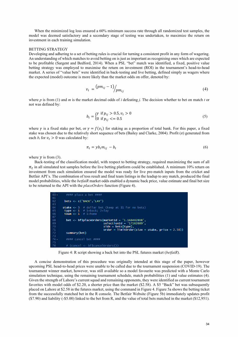
When the minimized log loss ensured a 60% minimum success rate through all randomized test samples, the model was deemed satisfactory and a secondary stage of testing was undertaken, to maximize the return on investment in each training simulation. BETTING STRATEGY Developing and adhering to a set of betting rules is crucial for turning a consistent profit in any form of wagering. An understanding of which matches to avoid betting on is just as important as recognising ones which are expected to be profitable (Sargent and Bedford, 2014). When a PSL “bet” match was identified, a fixed, positive value betting strategy was employed to maximise the return on investment (ROI) in the tournament’s head-to-head market. A series of “value bets” were identified in back-testing and live betting, defined simply as wagers where the expected (model) outcome is more likely than the market odds on offer, denoted by:

3� = 4�5�� − 16 �5��7 (4)

where p is from (1) and m is the market decimal odds of i defeating j. The decision whether to bet on match t or not was defined by:

8� = #9 if ��� > 0.5, 3� > 00 if ��� <= 0.5 (5)

where 9 is a fixed stake per bet, or 9 = %(3�) for staking as a proportion of total bank. For this paper, a fixed

stake was chosen due to the relatively short sequence of bets (Bailey and Clarke, 2004). Profit (π) generated from

each bt for 3� > 0 was calculated by:

=� = �8�5�� − 8� (6)

where � is from (3).

Back-testing of the classification model, with respect to betting strategy, required maximizing the sum of all

=� in all simulated test samples before the live betting platform could be established. A minimum 10% return on

investment from each simulation ensured the model was ready for live pre-match inputs from the cricket and Betfair API’s. The combination of toss result and final team listings in the leadup to any match, produced the final model probabilities, while the betfaiR market odds enabled a dynamic back price, value estimate and final bet size to be returned to the API with the placeOrders function (Figure 4).

Figure 4: R script showing a back bet into the PSL futures market (betfaiR). A concise demonstration of this procedure was originally intended at this stage of the paper, however upcoming PSL head-to-head prices were unable to be called due to the tournament suspension (COVID-19). The tournament winner market, however, was still available so a model favourite was predicted with a Monte Carlo simulation technique, using the remaining tournament schedule, match probabilities (1) and value estimates (4). Given the strength of Lahore’s current squad and remaining opponents, they were identified as current tournament favorites with model odds of $2.20, a shorter price than the market ($2.58). A $5 “Back” bet was subsequently placed on Lahore at $2.58 in the futures market, using the command in Figure 4. Figure 5a shows the betting ticket from the successfully matched bet in the R console. The Betfair Website (Figure 5b) immediately updates profit ($7.90) and liability (-$5.00) linked to the bet from R, and the value of total bets matched in the market ($12,951).

34

Figure 5a: Ticket for successfully matched PSL Winner bet (betfaiR).

Figure 5b: Betfair UI updated for successfully matched PSL Winner bet.

3. RESULTS

Table 2 is a snapshot of the model performance in a live betting (head-to-head) environment from the last half of the 2019 season through to the abbreviated 2020 season. The model metrics — accuracy, or predictive rate, and return on investment (ROI) — were compared to Betfair’s corresponding market odds (BF) with respect to expected value (EV), where each value increment represents performance above that level. All model favourites fell above EV=-20%, yielding a 55% prediction rate and 5% return on investment, from 36 matches. Betting on each equivalent BF market favourite yielded a higher percentage of correct bets, but no associated profit. The pre-determined value minimum for betting in this paper (EV=0%) resulted in 14 bets with 60% accuracy and a 22% return, which exceeded the pre-tournament expectation of 10%. Betting on all EV=0% market favourites only yielded a 33% success rate and a 39% loss. A reliable model should observe a positive correlation between ROI and expected value while outperforming the market at each level, which is evident in Table 2.

Metric

Expected Value (minimum)

-20% -10% 0% 10% 20%

Bets 36 29 14 4 2

Accuracy 55% 58% 60% 75% 100%

ROI 5% 12% 22% 65% 143%

BF Accuracy 57% 52% 33% 25% 0%

BF ROI 0% -12% -39% -52% -100%

Table 2: Model and market (BF) performance.

4. DISCUSSION

The free statistical software and languages available online should be exploited for the benefit of all aspects of statistical work. Sport statistics research is no exception, particularly where datasets exceed sizes deemed practical for storage and analysis in spreadsheets. This is indeed the case when analysing in-play transactional data. The random variables resulting from each of the 600 legal deliveries in an ODI cricket match can become disorderly if not stored and analysed efficiently, especially with multiple tournaments over multiple seasons. The R data frames for the pre-match analysis of the Pakistan Super League matches were not excessive in size, however, there was still a need for specialised statistical software to locally run the automated processes, from

35

gathering data through to placing a bet. While R might not be the most robust software available, it is convenient and simple to learn, offering a window to more advanced programming. Python, a programming language that is often compared with R, offers similar features as described in this paper, including a wrapper for access to the Betfair API, but is seems to be preferred for integration with Web applications, and in production. A drawback of certain functions mentioned in this paper, for example, running the script to place bets, is the requirement for the R console to be actively running on a desktop. The end-to-end procedure can be fully automated by executing all commands from a Web service or in R.Net, however, this is the subject of a follow-up paper. 5. CONCLUSION

The main objective in betting is to find inefficiencies in the market, and hence, outperform it. The 2020 Pakistan Super League head-to-head market was proven to be inefficient up until the competition’s postponement, which was supported by a 22% return on investment from a relatively low hit rate (Table 2). Selective wagering was also confirmed to be financially prudent where a 17% edge was realised when betting on matches with a positive expected value rather than betting on every match in the tournament schedule. The processes detailed in this paper, leading up to placing a bet, were all efficiently executed from the R console, and extend to in-play betting. Market overreactions are more pronounced after the match commences (Figure 3) in line with frequent dismissals and fluctuating scoring rates. The ability to buy into the market (back), forecast one of these events, then sell that position (lay) just prior to the event, forms the basis of successful trading. Such is the frenetic pace of T20 cricket, a trader may take a position, then lay it off in a matter of deliveries and still realise a healthy profit. Any pre-match market reactions typically only occur after the toss and are rarely considered significant movements. This established, pre-match R platform is robust enough to facilitate in-play betting; the challenge is the ability to predict not just one event (match outcome), but the outcomes of many events within the match. Acknowledgements

I wish to acknowledge and thank the betfaiR library author (https://github.com/durtal/betfaiR), the Betfair

exchange (https://www.betfair.com.au/exchange/plus/cricket), and Oriana for her tireless data gathering.

References Bailey, M.J. & Clarke, S.R. (2004). Market inefficiencies in player head-to-head betting on the 2003 cricket world cup.

Economics, Management and Optimization in Sports (P.Pardalos & S. Butenko eds.) pp. 185-201, New York: Springer. Clarke, S.R. & Allsopp, P. (2001). Fair measures of performance: The World Cup of cricket. Journal of the Operational

Research Society, 52, pp. 471-479. de Silva, B.M., Pond, G.R. & Swartz, T.B. (2001). Estimation of the magnitude of victory in one-day cricket. Australian and

New Zealand Journal of Statistics, 43, 3, pp. 259-268. Duckworth, F.C. & Lewis, A.J. (1998). A fair method for resetting the target in interrupted one-day cricket matches. Journal

of Operational Research Society, 49, pp. 220-227. Easton, S. & Uylangco, K. (2007). An examination of in-play sports betting using one-day cricket matches. Journal of

Prediction Markets, Vol. 1, Iss. 2, pp. 93-109. Elderton, W.P. (1945). Cricket scores and some skew correlation distribution. Journal of the Royal Statistical Society, Series

A. 108, pp. 1-11. Jayalath, K.P. (2018). A machine learning approach to analyze ODI cricket predictors. Journal of Sports Analytics, 4, 1, pp.

73-84. Lantz, B. (2013). Machine Learning with R. Birmingham: Packt Publishing. Lewis, A.J. (2005). Towards fairer measures of player performance in one-day cricket. Journal of the Operational Research

Society, 56, 7, pp. 804-815. Sargent, J. and Bedford, A. (2012). Using Conditional Estimates to Simulate In-Play Outcomes in Limited Overs Cricket.

Journal of Quantitative Analysis in Sports. 8, 2, pp. 1-20. Sargent, J. and Bedford, A. (2014). ‘Profiting from the Run Chase in 50-Over Cricket’, Proceedings for the Twelfth

Mathematics and Computers in Sport Conference (12MCS), Darwin, Australia, 2014.

36

Submitted to MATHSPORT 2020 February 12, 2020

DID HERSHELLE GIBBS REALLY DROP THE CRICKET WORLD CUP? THE COST OF A CATCH, THE MARGIN OF VICTORY AND OTHER

USES OF THE DL-METHODOLOGY

Steven Stern a,d

a Bond Business School, Bond University, Gold Coast, Australia d Corresponding author: sstern@bond.edu.au

Abstract The Duckworth-Lewis methodology introduced in the mid-1990’s forms the basis for the current DLS method used to set targets in interrupted limited-overs cricket matches. The essence of the methodology is the determination of a measure of scoring “resources” associated with any given collection of overs and a given number of available wickets. As has been discussed in various other venues, this concept of scoring resources can be used in ways beyond that of target resetting. In this talk, I will discuss two such ways: determining the cost of a missed dismissal (e.g., a dropped catch or missed stumping or run out) and constructing a consistent measure of winning margin for first and second innings victories. The ideas will be illustrated by several examples including Herschelle Gibbs’ famous drop in the 1999 Cricket World Cup as well as an alternative team ranking methodology to the current method developed by David Kendix which incorporates victory margin and some telling examples regarding the inadequacy of net run rate as a secondary ranking criterion in league and tournament group-stage play. Keywords: Cricket, Fielding Metrics, Team Rankings, Victory Margin Acknowledgements We wish to thank Frank Duckworth and Tony Lewis for their continued friendship and advice. References Duckworth, FC & Lewis, AJ (1998). A fair method of resetting the target in interrupted one-day cricket matches. The

Journal of the Operational Research Society, 49, 220-227. Duckworth, FC & Lewis, AJ (2004). “A successful operational research intervention in one-day cricket.” The Journal of

the Operational Research Society 55, 749-759.

37

RESOLVING PROBLEM GAMBLING: A MATHEMATICAL APPROACH Tristan Barnetta

a Macquarie University (alumni)

Corresponding author: strategicgames@hotmail.com

Abstract

The current model for treating problem gambling is either control your gambling (known as Controlled

Gambling) and quit Gambling (known as Abstinence). In Controlled Gambling the patient is allowed to

gamble on a limited basis. In Abstinence, the patient in recovery must completely abstain from all gambling.

Abstinence is the goal of Gamblers Anonymous and most, though not all, treatment professionals. A new

model is devised for treating problem gambling as a generalization of the current model by including

Controlled Gambling and Abstinence as treatment possibilities; but also including Optimal Gambling, Correct

Gambling and Eradication. The model is based on a process which is trying to maximize the return to the

player whilst allowing for the entertainment factor in gambling. The following strategies are now identified:

Optimal Gambling → Correct Gambling → Controlled Gambling → Abstinence → Eradication

The process is a one-way path whereby if a strategy fails for a particular gambler then the next strategy to

consider is the next one in line. Every gambler starts at the Optimal Gambling strategy, where the best way to

maximize return and gamble is to be playing games where the odds are actually in your favour e.g. card-

counting in blackjack. If the Optimal Gambling strategy would not be successful for the particular gambler,

then the next strategy would be a new option known as Correct Gambling, where the approach is to allow

gambling whilst playing the right games and strategies to minimize losses and to take advantage of the free

food and drinks on offer (more commonly known as comp points). Note that this approach allows the gambler

to keep playing, whereas in Controlled Gambling the gambler is only allowed to gamble on a limited basis. If

the strategies of Correct Gambling followed by Controlled Gambling followed by Abstinence would not be

successful for the particular gambler, then the final strategy is Eradication. This could be in the form of

moving to a country or state where gambling is illegal or a location which is a great distance (say 100+ km) to

the nearest gambling venue.

Casino games are comprised of mathematical formulations which can be found readily in the literature. The

percent house margin (or return to player) establishes how much a player is expected to lose in the long run.

While the percent house margin is important to consumers (players are consumers of casino games) in

determining the choice of games or how long to play a particular game, there is other information which could

also influence these decisions. For example, the probability of the consumer ending up in profit after 100 trials,

or the probability of the consumer losing more than $100 after 200 trials, would be valuable information. The

analysis of casino games is covered to obtain distributional characteristics of profits, the distribution of profits

and the percent house margin. For Correct Gambling, the analysis of casino games consists of poker machines,

pontoon, blackjack and video poker.

A consumer’s decision as to the choice or how long to play a particular game, may consist of knowing the

distribution of payouts. To calculate the distribution of payouts on a poker machine requires the probabilities

associated with each particular payout. The probabilities on poker machines cannot be obtained from the

playing rules (as is the case with table games), and therefore poker machines could be considered as being

“unfair”. Mathematical and logical reasoning to poker machine regulations are given as suggestions for

amendments to the “the Standard” with the purpose to increase consumer protection.

For Optimal Gambling, the analysis of casino games consists of video poker and blackjack; and a

predictions model in tennis is given as another means for optimal gambling. A question that arises whenever a

game is favourable to the player, is how much to wager on each event? The famous Kelly criterion is

addressed and an explicit formula is derived for when multiple outcomes exist which typically applies to video

poker. Blackjack is typically recognized as the “best” gambling game for profit as depicted in the movie “21”.

The author will provide evidence that automating online video poker is not only the “best” but "optimally" the

best gambling game for profit.

Keywords: Problem gambling, poker machine regulations, casino game analysis, tennis betting, profitable

gambling, Kelly Criterion

38

DISCOUNTING CAMERA MOVEMENT IN CALCULATION OF PLAYER

PATHS USING MACHINE VISION IN RUGBY UNION

Rob G. McDonalda, Paul J. Bracewella,b, Holly E. Trowlanda, Aristarkh Tikhonov aPlay in the Grey, Wellington, NZ

bCorresponding author: paul@playinthegrey.com

Abstract

Tracking player paths in rugby union using machine vision requires mapping the location of a player to a set of

coordinates bounded within the playing area per frame of video footage. However, an issue arising from the use

of object tracking from a single camera is that the estimation of the player’s position on the sports field may be

corrupted in the absence of an automatically generated frame of reference due to the movement of the camera

through pan, tilt or zoom. The field position is estimated through homography, where small errors can result in

large errors in the estimated position. Here, we demonstrate an iterative backward correction algorithm using a

second order polynomial which is applied on a frame by frame basis. When implemented, this algorithm repairs

the path of an individual within rugby union tracked using a single camera with pan, tilt and zoom capabilities.

The outcome of this process is the ability to accurately track a player’s movement without the need to access

wearables.

Keywords: homography, computer vision, pan tilt zoom

1. INTRODUCTION

Computer vision shows considerable promise in offsetting the limitations of manual coding sports events (Cust

et. al., 2018). As described in the review undertaken by Cust et. al. (2018) the automation of recognising human

movements has the potential to improve the efficiency and accuracy of sports performance analysis. The ability

to track player movement without wearables enables wider application by scouting historical footage, opposition

teams and other ad hoc situations. However, a challenge with the use of computer vision to track player movement

is ensuring accuracy and completeness of player paths. Early attempts at player tracking required the automatic

tracking process to be manually interrupted with human supervision required (Pers, et. al., 2000).

2. DATA PROCESSING

PLAYER DETECTION

The player detection module detects all the players. More specifically, it detects the presence of all the humans in

a scene, which can include spectators. The output of the player detection module is a set of two-dimensional

positional coordinates describing where the player is on the field per frame. To identify player’s positions, we

first need to identify their locations in footage. For this, we use a Mask-RCNN network (He et. al., 2017). The

output of this network is a bounding box per player, per frame. This identifies the placement of players in frame,

as well as masks, which identify the outlines of players in the footage. Due to the depth of the information that is

received, further steps covering tracking and position estimation yield a significant gain in accuracy through the

use of this additional data.

AUTOMATIC TRACKING

This module tracks the players over time. The purpose of the automatic tracking module is to identify the same

player and annotate that player with a unique track identifier throughout all the frames. Consequently, this means

that we can now track a player with the unique track identifier throughout the video to produce a continuous player

track.

The automatic tracking algorithm works based on two core algorithms: the Kalman filter and visual feature

matching. The Kalman filter algorithm tracks a player’s position in time based on their velocity, computed from

previous frames, and probabilistic modelling. The visual feature matching algorithm helps the Kalman filter based

tracker to pick up on lost tracklets based on the visual appearance of the player.

The tracks obtained from the automatic tracking are sometimes broken. That means the same player has been

assigned more than one TrackID. There are many reasons for that. One of the major reasons is occlusion. As we

are using a 2D camera to track a player in the three dimensional world, the automatic tracking algorithm cannot

resolve occlusions in the third dimension. This issue of data association is commonly encountered in Multi Target

Tracking (MTT), and is an area of ongoing research with a number of promising solutions such as Multiple

Hypothesis Tracking (MHT). Creating a multi target tracker both accurate enough for use in sports analytics and

efficient enough to handle the millions of detections present in team sports (i.e. not susceptible to the combinatorial

explosion) is an ongoing area of research. Another issue with tracking is the movement of the camera through

39

panning, tilting or zooming. This changes the frame of reference. The resolution of this issue is the subject of

this research.

HOMOGRAPHY ESTIMATION

To be able to estimate the positions of players on the field, the player positions need to be projected from a camera

view to top down view. This is achieved using homography (Chum, et. al., 2005). Homography is a matrix that

project points from one plane of view to another. Starting with an initial set of key-frames, the homography

matrices for all frames in a video are estimated. We do so using visual feature detection and matching between

the frames of the video using the deep sort algorithm (Wojke, 2017).

In a small number of cases, this approach leads to faulty results. To combat that, we have developed a

proprietary convolutional neural network to detect faulty matrices which thereby enables these to be corrected

during a post-processing procedure.

3. DEMONSTRATION OF PROBLEM

Here, we examine a broken tracking arising from a 13 second clip from a test match between England and

Argentina contested at the 2019 Rugby World Cup on October 5. Figure 1 shows a mosaic of screen grabs where

the Argentine second five eighth is circled. Figure 2 shows the extracted track with breaks clearly visible.

Figure 1: Mosaic visualising actual position of the Argentine Second Five Eighth over a 13 second period

The 14 clips are approximately 1 second apart. Using the half

way line (solid white near middle of screen in top left) and the

10m line (dotted line either side of the halfway line) the effect of

the pan-tilt- zoom of the camera is observed.

1

5

9

13

40

Figure 2. Initial Player Track for the Argentine Second Five Eighth over a 13 second period.

4. METHODOLOGY

There are 𝑁frames, each frame being denoted by the time corresponding to that frame 𝑡𝑖 where 𝑖 ∈ [1, 𝑁]. Each

frame contains a varying number of detections. Detections corresponding to a single entity can be associated

across time forming a track, characterised by a unique ID 𝑗 ∈ 𝐽, where 𝐽is the set of all track IDs. The position of

the entity with ID 𝑗at time 𝑡𝑖 is 𝑟𝑗(𝑡𝑖). There is no guarantee that, if both 𝑖 ∈ [1, 𝑁] and 𝑗 ∈ 𝐽, then 𝑟𝑗(𝑡𝑖)exists.

That is, every unique entity is not necessarily detected in every frame. The set of times at which the entity with

ID 𝑗is identified is denoted 𝑇𝑗 = {𝑖: ∃𝑟𝑗(𝑡𝑖)}. The set of IDs that appear in frame 𝑖 is 𝐾𝑖 = {𝑗: ∃𝑟𝑗(𝑡𝑖)}.

The shift of entity 𝑗 in frame 𝑖 is defined by:

𝛥𝑖𝑗 ≡ 𝑟𝑗(𝑡𝑖) − 𝑟𝑗(𝑡𝑖−1), (1)

where it is assumed that 𝑗 ∈ 𝐾𝑖 ∩ 𝐾𝑖−1, that is the entity is detected in both frame 𝑖 and frame 𝑖 − 1. The 𝑦

component of the individual shifts in frame 126 is shown in Figure 3, where we see that generally the shifts are

more significant in detections closer to the camera side of the field. The overall spatial dependence of the shift

size is not obvious, however it is clear that it depends on both 𝑥 and 𝑦.

Figure 3: Left: projected field positions of detections in frame 126. The color indicates predicted team while the

size of the marker represents the size of the y shift that occurs in the next frame. The black cross indicates the

camera side of the field. Right: The shift in y with respect to vertical position.

We fit the shift to a second order polynomial:

𝛥(𝑥, 𝑦) = (𝛥𝑥(𝑥, 𝑦), 𝛥𝑦(𝑥, 𝑦)) (2)

𝛥𝑥(𝑥, 𝑦) = 𝑎𝑥 + 𝑏𝑥𝑥 + 𝑐𝑥𝑦 + 𝑑𝑥𝑥2 + 𝑒𝑥𝑦2 + 𝑓𝑥𝑥𝑦 (3)

𝛥𝑦(𝑥, 𝑦) = 𝑎𝑦 + 𝑏𝑦𝑥 + 𝑐𝑦𝑦 + 𝑑𝑦𝑥2 + 𝑒𝑦𝑦2 + 𝑓𝑦𝑥𝑦 (4)

using curve_fit from the scipy package in Python, where the spatial coordinates used are from 𝑖 − 1. As is

demonstrated in Figure 4 these functions are adequately able to represent the spatial dependence of the shift for

each frame, with each having 𝑅2 > 0.99.

41

Figure 4: Fitting the shift in y to Equation (4) for the six largest jumps, occurring at frames 126, 168, 253, 379,

380, and 381.

We now outline our method for ‘undoing’ the anomalous shifts. In what follows the unprimed terms refer to the

original positions and the primed terms are the new corrected positions. To proceed we need to assume that some

portion of the track is correct. It is most convenient to assume that the initial track segments before the first

anomalous shift is correct. In a particular frame 𝑖, the average shift is defined by:

𝛥𝑖 ≡1

|𝐾𝑖∩𝐾𝑖−1|𝛴𝑗∈𝐾𝑖∩𝐾𝑖−1

𝛥𝑖𝑗 . (5)

Repairing the shifts then requires iterating forward through the frames. We start with the initial shift function

𝛥(𝑥, 𝑦) (2-4) with all constants set to zero. At each frame 𝑖 we calculate the average shift 𝛥𝑖 using the original

positions. If neither component of the shift is larger than some threshold 𝛥𝑐, we apply the current shift function

to all detections in this frame:

𝑟𝑗′(𝑡𝑖) = 𝑟𝑗(𝑡𝑖) + 𝛥(𝑥𝑗(𝑡𝑖), 𝑦𝑗(𝑡𝑖)), (6)

and proceed to the next iteration. If either component of the shift is larger than 𝛥𝑐, then we need to update the

shift function. The individual shifts are recalculated using the corrected positions in frame 𝑖 − 1 and the original

positions in frame 𝑖:

𝛥′𝑖𝑗 ≡ 𝑟𝑗(𝑡𝑖) − 𝑟′𝑗(𝑡𝑖−1), (7)

Equation (3) and/or Equation (4) are fitted to 𝛥′𝑖𝑗 giving the new shift function 𝛥(𝑥, 𝑦) . We then apply the

current shift function to all detections in this frame (6) and proceed to the next iteration.

5. RESULTS

The outcomes of our method on the broken tracks are demonstrated in Figure 5 for a single entity, and Figure 6

for the entire clip.

42

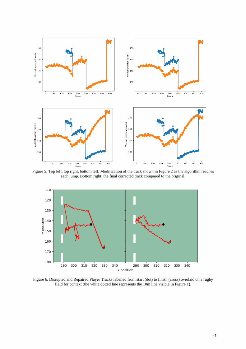
Figure 5: Top left, top right, bottom left: Modification of the track shown in Figure 2 as the algorithm reaches

each jump. Bottom right: the final corrected track compared to the original.

Figure 6. Disrupted and Repaired Player Tracks labelled from start (dot) to finish (cross) overlaid on a rugby

field for context (the white dotted line represents the 10m line visible in Figure 1).

43

Figure 7: Left: raw x (top) and y (bottom) positions of all on-field detections over the course of a short clip.

Right: the same detections after applying the jump-repairing algorithm.

6. DISCUSSION AND CONCLUSION

We note that our goal is to compensate for large anomalous position shifts. There are also many smaller anomalous

shifts, however these can be accounted for using more traditional methods such a rolling average or a Savitzky-

Golay filter (Orfanidis, 1996). We thus set our threshold for triggering the algorithm relatively high.

Furthermore we have noted that occasionally the presence of degenerate IDs can cause an individual track to have

a large shift, while the other tracks remain unaffected. This is not due to the camera zoom error, but can potentially

be flagged as one if the individual shift is large enough. Potential criteria to ignore this are requiring a certain

proportion of detections are above the threshold, or similarly for the 𝑅2 value of the shift function fit.

References He, K., Gkioxari, G., Dollar, P., & Girshick, R. (2017). Mask R-CNN. arXiv:1703.06870. Accessed 6 January 2020.

Chum, O., Pajdla, T., & Sturm, P. (2005). The Geometric Error for Homographies. Computer Vision and Image

Understanding. 97(1), pp. 86–102.

Wojke, N., Bewley, A., & Paulus, D. (2017). Simple online and realtime tracking with a deep association metric. In: 2017

IEEE International Conference on Image Processing (ICIP). IEEE.; 2017. pp. 3645-3649.

Orfanidis, S. J. (1996). Introduction to Signal Processing. Englewood Cliffs, NJ: Prentice-Hall.

Cust, E.E., Sweeting, A.J., Ball K. & Robertson, S. (2019). Machine and deep learning for sport-specific movement

recognition: a systematic review of model development and performance, Journal of Sports Sciences, 37(5), pp. 568-600.

Pers, Janez & Kovačič, Stanislav. (2000). Computer Vision System for Tracking Players in Sports Games. Pp. 177 - 182.

10.1109/ISPA.2000.914910. First Int’l Workshop on Image and Signal Processing and Analysis, June 14-15, 2000, Pula,

Croatia

44

Submitted to MATHSPORT 2020 June 4, 2020

VALIDATING PLAYER PATH TRACKING USING MACHINE VISION

Holly E. Trowlanda, Paul J. Bracewella,b, Rob G. McDonalda, Aristarkh Tikhonova

aPlay in the Grey, Wellington, NZ bCorresponding author: paul@playinthegrey.com

Abstract

Machine vision is gaining acceptance as an alternative to GPS devices for tracking sports player movement.

However, limited information regarding the accuracy of these approaches is available. Camera pan, tilt and

zoom are accounted for in estimating the width-length positioning of a player on the sports ground.

Homography is used to account for this systematic bias. To demonstrate the accuracy of machine vision for

the purpose of player tracking, an experiment was conducted.

The experiment stage is the inner third of a standard netball court. We placed cones on a grid throughout

the experiment area. A subject was instructed to run a predetermined path through the cones, providing us with

a ground truth of position when they were at a cone. The sequence was recorded using two cameras, one fixed

from a low angle and one moving from a high angle. This was repeated for a number of sequences. Using the

footage we obtained the predicted position of the subject over time via a homography, allowing a comparison

with the ground truth and therefore a measure of the accuracy.

Post-processing, the error was estimated to be 0.4m and highlighted key issues associated with estimating

homography and its limitations.

Keywords: homography, optimisation

1. INTRODUCTION

Sporting organisations are embracing analytics as a potential competitive advantage through the identification

of trends and patterns of play that increase the likelihood of winning. However, the generation of data can be

resource intensive which can be costly and time consuming. Machine vision shows considerable promise in

offsetting the limitations of manual coding sports events (Cust et. al., 2018). Automated event detection,

based on player interaction, has the potential to improve the efficiency and accuracy of sports performance

analysis (Cust et. al., 2018). Early attempts at player tracking required the automatic tracking process to be

manually interrupted with human supervision required (Pers, et. al., 2000). However, a challenge with the use

of machine vision to track player movement is ensuring accuracy and completeness of player paths. This starts

with accurately projecting the observed individual from the viewing plane into a xy coordinate system.

Here, we investigate the accuracy of machine vision compared to a physical ground truth. A number of

studies have been undertaken to explore the effectiveness of a range of systems. Hoppe et. al. (2018) compared

the validity and reliability of Global Positioning Systems (GPS) and Local Positioning Systems (LPS),

concluding “18 Hz GPS has enhanced validity and reliability for determining movement patterns in team

sports compared to 10 Hz GPS, whereas 20 Hz LPS had superior validity and reliability overall. However,

compared to 10 Hz GPS, 18 Hz GPS and 20 Hz LPS technologies had more outliers due to measurement

errors, which limits their practical applications at this time.” Castillo et. al. (2018) compared GPS with Ultra

Wide Band (UWB) based systems finding UWB technology had greater accuracy for distance covered and

player speeds. From an accessibility perspective, Wearables manufacturer, Garmin (2020), describe that with a

strong satellite signal, the GPS position reported by an outdoor watch should be accurate to 3 meters. Van

Diggelen et. al. (2020) outlined a solution that promised to increase location accuracy to within one metre

using WiFi Round Trip Time (RTT), GPS dual-frequency and carrier phase measurements. In an assessment

of Australian Football, in an older paper Edgecomb et. al. (2006) found the distances measured for computer

based tracking systems were as accurate as GPS. However, in recent years, the shift has been to RFID

devices. Chawla et. al. (2018) proposed a localisation system capable of functioning in a realistically radio-

noisy indoor environment, is highly extensible, and provided use-case-driven average accuracy as low as

0.15 metres. However, for mobile objects, the accuracy was at best 0.68m. Most appropriately, Pollard (2019)

outlined the use of RFID technology to generate data in the National Football League (NFL) using tracking

data generated by tags embedded inside footballs and player uniforms. This provides xy coordinates of

players within 6 inches (15cm) (McLennan, E., 2019). However, a substantial hardware investment is

45

required, with Porter (2019) describing that 22 sensors were required. In addition, there are challenges with

accessing historical, competitor and scouting data. Here, we explore the use of machine vision and conduct an

experiment to determine the level of accuracy in generating xy coordinates.

2. EXPERIMENT

The experiment stage is the inner third of a standard netball court. We placed cones on a grid throughout the

experiment area. A subject was instructed to run a predetermined path through the cones, providing us with a

ground truth of position when they were at a cone. The subject was a Wellington age group representative in

both cricket and rugby. At the time of the experiment, he was 182cm and 65 kilograms (February 2nd, 2020).

These physical attributes are aligned with other studies (Castillo et. al., 2018; Hoppe et. al., 2018). The

sequence was recorded using two smartphone cameras (iPhone Xs Max, iPhone 11 Pro) one fixed from a low

angle and one moving from a high angle. This was repeated for a number of sequences. Using the footage

from the moving camera, we obtained the predicted position of the subject over time via a homography,

allowing a comparison with the ground truth and therefore a measure of the accuracy in both time and space.

The intent of the fixed camera was to provide an additional form of validation.

3. INITIAL DATA

The true position in metres and predicted position in pixels of the entity with ID j should be related by:

where (xT

j, yTj) is the true position in metres, (xH

j, yHj) is the observed position in pixels, (αx , αy) are scaling

constants, and (βx , βy) are shift constants. Note that the true x (y) position is related to the y (x) position; this is

because the homography is performed relative to the field schematic Figure 1 which is rotated by π/2 relative

to our manual coordinate system. Note that the homography for each clip uses a single key frame that is the

first frame of that clip.

In theory, the values of the transformation constants are known from the outset using two known points in

both coordinate systems. If we have two points at (xHa, yH

α) and (xHb, yH

b) in the schematic coordinates and

(xTα, yT

α) and (xTb, yT

b) in the true coordinates, then the constants are:

We use O and P, the top left and bottom right corner of the central third respectively. In the two coordinate

systems OT= (0,0)m, PT= (10.17,15.25)m, OH= (1158,90)px, PH= (127,635)px, which gives the transformation

constants αx=-0.0148m/px, αy=0.0187m/px, βx=17.13m and βy=-1.68m.

We have obtained data from three running sequences giving six pieces of footage. When displaying a list of

results, they refer to (clip A fixed, clip A moving, clip B fixed, clip B moving, clip C fixed, clip C moving).

The mean distance between the manual and transformed observed positions for each clip is (7.01, 4.13, 7.10,

4.28, 7.02, 4.19) metres, with standard deviations (1.80, 1.13, 2.19, 1.35, 1.89, 1.23) metres. The moving clips

have higher accuracy than the fixed clips, most likely due to the fixed clips having a low camera angle. A

typical comparison between the manual and automated data is shown in Figure 3.

3. OPTIMISING

When looking at the displacement between the manual and automated positions, it is clear that we can improve

on the errors by tweaking the transformation constants. From Figure 3 there is clearly a linear trend in the

error. Such a trend indicates that in particular choosing a different scaling may give better results. For

detection i the difference between the true position and transformed observed position is:

for each clip we minimise σ2({∆xi}) and σ2({∆yi}) to obtain the optimal αx and αy respectively, then minimise

⟨{∆xi}⟩ and ⟨{∆yi}⟩ to obtain the optimal βx and βy respectively.

46

Figure 1. Experiment dimensions and cone layout. O and P are points we use for reference while C is the

approximate camera location.

Figure 2. Experimental cone layout. O and P are points we use for reference.

Figure 3. Left: Position over time for clip A fixed. Left column includes the entire observed sequence while

right shows only those corresponding to the manually annotated frames. Right: Error with respect to position

for clip A fixed.

47

The averages (standard deviations) of the transformation constants obtained for each clip are αx = -0.0110m

(0.0007m), αy = -0.0140m (0.001m), βx = 18.6m (0.4m) and βy = 0.4m (0.5m). In particular the scaling

constants are lower in magnitude than the given values by 26% and 24% respectively. With these new

constants the mean distance between the manual and transformed observed positions for each clip is (1.17,

1.08, 1.08, 1.05, 1.18, 1.00) metres, with standard deviations (0.65, 0.50, 0.76, 0.19, 0.54, 0.39) metres. In

Figure 4 we show a typical comparison between the manual and new transformed observed positions and the

updated errors.

Figure 4. Left: Position over time for clip A fixed using the optimized transformation constants. Left column

includes the entire observed sequence while right shows only those corresponding to the manually annotated

frames. Right: Error with respect to position for clip A fixed using the optimized transformation constants.

INDIVIDUAL CLIP OPTIMISATION

We hypothesise that each key frame used for homography has a distinct set of transformation constants that

differ slightly from the given values. If this were to be the case, we would expect the values for the fixed

camera constants to be similar to each other as they have similar key frame, and same for the moving camera

constants. However we would expect the fixed camera and moving camera constants to differ from each other

(though not by a huge amount, as the key frames are still relatively similar). We show the constants for the

fixed and moving camera clips in Figure 5, which does suggest the expected behaviour. To truly verify, we

would need a larger data set.

Figure 5. The optimized scaling constants for the fixed and moving clips.

Using the optimized transformation constants for each clip we find the mean distance between the manual

and transformed observed positions for each clip is (0.57, 0.34, 0.47, 0.24, 0.47, 0.31) metres, with standard

deviations (0.52, 0.28, 0.36, 0.13, 0.30, 0.21) metres. That is, the average error 0.40m. In Figure 6 we show a

typical comparison between the manual and new transformed observed positions and the new, final errors.

48

Figure 6. Left: Position over time for clip A fixed using the individually optimized transformation constants.

Left column includes the entire observed sequence while right shows only those corresponding to the manually

annotated frames. Right: Error with respect to position for clip A fixed using the individually optimized

transformation constants.

CONSEQUENCES FOR PLAYER TRACKING USING MACHINE VISION

The initial goal of this experiment was simply to quantify the accuracy of player tracking in machine vision.

However the potential of consistent errors in scaling that vary with key frame requires significant attention,

and is likely of more immediate concern. When the key frame being used as a reference for the homography is

changed, any difference in scaling would appear as a spatially dependent shift in player positions between the

two frames; such errors have been observed in the data. A way in which this could be mitigated is by the

manual annotation of player positions in the key frame, which can then be used with the automatically detected

positions in that frame to find the optimized transformation parameters. Currently, since the key frame is being

annotated manually, this would introduce little overhead. However for scalability the entire process must be

eventually automated, and so a non-manual method for this must be found.

Figure 7. Two key frames and positions obtained via homography from a rugby match. The top row is frame

100 and the bottom row is frame 150. The left column is from the raw footage and the right column is the

estimated positions in pixels. A notable player is indicated in red.

In Figure 7 we show two key frames from a rugby clip, as well as the detected positions from those frames.

It would be reasonable for one to expect that these frames would be the most accurate. In frame 100 the

indicated player is slightly inside the 15 metre line, which appears to be accurately reflected in the top down

position. In frame 150 the indicated player has not significantly changed position and remains inside the 15

metre line. However their estimated top down position has moved significantly to just inside the 5 metre line;

the change in key frame has dramatically changed the accuracy of the homography. Indeed, when inspecting

the positions we see that between these two frames there is an anomalous shift in the player positions. In

Figure 8 we show the result of our ad hoc jump repairing algorithm (Trowland et. al., 2020) when applied to

frames 100 and 150.

49

Figure 8. Top: Positions in frame 100 before (left) and after (right) application of our ad hoc jump repairing

algorithm. Bottom: Positions in frame 150 before (left) and after (right) application of our ad hoc jump

repairing algorithm. The red circles show a single player.

DISCUSSION AND CONCLUSION

Machine vision is a viable alternative to GPS and RFID devices for tracking sports player movement. To

demonstrate the accuracy of machine vision for the purpose of player tracking, an experiment was conducted

using both fixed and moving cameras. Using the footage we obtained the predicted position of the subject

over time via a homography, allowing a comparison with the ground truth and therefore a measure of the

accuracy. This process highlighted key issues associated with estimating homography and its limitations.

Specifically, the key frames become somewhat irrelevant when the camera pan-tilts-zooms. This is an

important issue for generating xy coordinate data from sports events, where the cameras typically follow the

action. This issue is addressed by McDonald et. al. (2020). Nonetheless, with post-processing errors

estimated to be 0.4m demonstrates the viability of tracking sports players using accessible technology.

References Castillo, A.B., Gomez Caroma, C. D., De la Cruz Sanchez, E., & Pino Ortega, J. (2018). Accuracy, intra- and inter-unit

reliability, and comparison between GPS and UWB-based position-tracking systems used for time–motion analyses in

soccer. Applied Sport Sciences, 18(4), pp 450-457.

Chawla, K., McFarland, C., Robins, G., & Thomason, W. (2018). An accurate real-time RFID-based location system. Int.

J. Radio Frequency Identification Technology and Applications, 5(1), pp 48-76.

Cust, E.E., Sweeting, A.J., Ball K. & Robertson, S. (2019). Machine and deep learning for sport-specific movement

recognition: a systematic review of model development and performance, J. of Sports Sciences, 37(5), pp. 568-600.

Edgecomb, S.J., & Norton, K.I. (2006). Comparison of global positioning and computer-based tracking systems for

measuring player movement distance during Australian Football. J. of Science and Medicine in Sport, 9(1), pp. 25-32.

Garmin (2020). Improving the GPS Accuracy, Distance and Speed Readings of an Outdoor Watch.

https://support.garmin.com/en-NZ. Accessed 14 February 2018.

Hoppe, M. W., Baumgart, C., Polglaze, T., & Freiwald, J. (2018). Validity and reliability of GPS and LPS for measuring

distances covered and sprint mechanical properties in team sports. PloS one, 13(2), e0192708.

https://doi.org/10.1371/journal.pone.0192708

McDonald, R. G., Bracewell, P. J., Trowland, H. E., & Tikhonov A (2020). Discounting camera movement in calculation

of player paths using machine vision in rugby union. 1. Proceedings of the 15th Australian Conference on Mathematics

and Computers in Sports. Ray Stefani & Adrian Schembri eds. Wellington, New Zealand: ANZIAM Mathsport.

McLennan, E. (2019, November 13). How RFID technology is transforming the NFL. https://www.verdict.co.uk/rfid-

technology-nfl. Accessed 14 February 2018.

Pers, Janez & Kovačič, Stanislav. (2000). Computer Vision System for Tracking Players in Sports Games. Pp. 177 - 182..

First Int’l Workshop on Image and Signal Processing and Analysis, June 14-15, 2000, Pula, Croatia.

Pollard, J. (2019). Five years ago, a nickel-sized RFID sensor changed the NFL forever.

https://www.zebra.com/us/en/blog/posts/2019/five-years-ago-nickel-sized-RFID-sensor-changed-NFL-forever.html.

Accessed 14 February 2018.

Porter, M. (2019). How the NFL's smart player-tracking technology is revolutionising the way teams play American

football... and improving the experience for the fan watching at home. https://www.dailymail.co.uk/sport/nfl/article-

7622357/player-tracking-technology-Wembley-NFL.html. Accessed 14 February 2018.

50

HISTORICAL EVALUATION OF BOWLING SPEEDS IN CRICKET USING

MACHINE VISION

Paul J. Bracewella,d, Fergus Scottb, Brendon P. Bracewellc

aDOT loves data, Wellington, NZ bNortheastern University, Boston, Massachusetts, USA

cBracewell Cricket Academy, Northland, NZ d Corresponding author: paul@dotlovesdata.com

Abstract

A simple method to calculate bowling speed from video clips using a machine vision framework is applied to historical

footage from a 1979 television show in Australia. The potential implementation of a framework using machine vision

is validated using the speed gun measurements applied in a controlled setting. Comparison of the estimated speed

with speed gun speeds for 12 bowlers reveals the estimates are unbiased, the intercept is equivalent to 0, and calibrated,

with the slope being equivalent to 1. Several prominent international fast bowlers are then assessed and ranked.

Keywords: Frame rate

1. INTRODUCTION Legendary host of Australian Channel 9’s Cricket Commentary team, the late Richie Benaud, marvelously summed

up the debate about who the quickest bowlers are in world cricket as he introduced a programme “The World’s Fastest

Bowler” (Channel 9, 1979). In his opening remarks, Benaud stated: “Fast Bowlers. Marvelously controversial aren’t

they? Right from the time of Spofforth and Jones, and Gregory and McDonald, and Larword, those arguments have

raged and there’s been controversy over who is the fastest bowler, or who was the fastest bowler, in the

world.” However, the debate around bowling speeds continues to be at the forefront of discussions, most recently

with Jofra Archer claiming the speed guns used in the first test between New Zealand and England, played at Bay

Oval, Mt Maunganui on 21st to 25th November, 2019 were “faulty” (1 News, 2019). According to Archer (2019),

“all the bowlers were made to look a bit slower than … they really are”. ABC News (2015) stated “there is no

standardised approach to clocking deliveries in international cricket and much debate about how accurately radars

track the ball.” Former Australian paceman, Jeff Thomson, has also weighed in on this debate, discussing perceived

inconsistencies in measuring bowling speeds. He was quoted in the Daily Telegraph (News Corp Australia, 2014):

“When they timed me around the 161km/h, that was done at the batting end. These guys today are timed at the bowlers’

end. Who’s standing two metres in front of a bowler facing the ball? Nobody. They’re trying to make them look as

quick as us. We were timed further down the pitch, where it slows down.”

To settle the debate in 1979, The Channel 9 Team utilised the “the most sophisticated equipment available” under

the guidance of Dr. Frank Pyke. However, the issue with the use of speed guns is the data needs to be captured at the

event. This means historical performances cannot be objectively compared. In addition, as mentioned previously in

the Daily Telegraph and ABC News, there are perceived inconsistencies in the protocols used for measuring the speed.

As a consequence, we use an approach that estimates bowling speed using historical match footage. With the

quality and quantity of video footage available, this becomes an accessible technique. We are presently developing

software to automate this task.

2. METHODS To measure the speed, we need a distance and the time taken to travel that distance. Given cricket pitches are

standardised, approximations of distance are readily obtained. The ball is generally assumed to be delivered from the

running crease, also referred to as the non-strikers popping crease. There are two scenarios to consider. The first

scenario is where the ball comes into contact with the batter, which will generally be at the popping crease, meaning

the ball has travelled approximately 17.68m. The other scenario is where the ball beats the batter and passes, or comes

into contact with, the stumps on the bowling crease. In that scenario, the ball has travelled 18.90m (17.68m + 1.22m).

51

Figure 1: Stylised diagram showing the dimensions of a cricket pitch produced by the Government of Western

Australia (2019).

The time taken to travel this distance can be estimated using the number of frames the ball takes to move between

the points of interest. This is then converted to time using the frame rate of the footage. For standalone videos, this

is an embedded property of the file. For instance, the frame rate of iPhone Max Xs is 29. With YouTube footage, the

framerate of the clip is identified within the browser by right clicking within the video and selecting the option “Stats

for nerds”.

Delivery Speed = 3.6 x Pitch_Length / (Observed_Frames/Frame_Rate). (1)

To convert from metres per second to kilometers per hour, as standard for television reporting, a multiplier of 3.6

is used. It is important to note, that this formula is an approximation. For greater accuracy, the height of release should

also be considered, as well as the point of contact between the ball and the ground. In addition, allowance should also

be made for due to loss of energy upon contact. That will be the subject of future research. As shown in the validation

section that follows, the method outlined in equation (1) is a sufficient approximation.

3. VALIDATION & RESULTS

To determine the appropriateness of equation (1) we compare bowling speeds from the “World’s Fastest Bowler”

competition (Channel 9, 1979) with estimated speed based on the proposed approach. This competition was conducted

under a controlled environment at Gloucester Park trotting track in Perth with $1000AUD prize money on offer for

the individual awarded the fastest bowler title. Bowlers each had eight deliveries and were measured based on speed

and accuracy. No batsman was present, so we estimate when the ball passed the stumps. To do so, we first identify

when the ball leaves the bowler's hand. Then, we count the number of frames until the ball passes the stumps. An

example is shown below for Australian great, Dennis Lillie which appears approximately 7 minutes and 46 seconds

into the footage, which has a frame rate per second of 25.

Figure 2A shows the ball in the last frame before the ball leaves Lillie’s hand. In Figure 2B, the ball has left the

hand and is counted as the first frame. In 2C, some 12 frames later, the ball is just about to make contact. In Figure

2C which is the frame immediately following 2D it can be seen that the stump has been hit by the ball. This is taken

as the last frame, meaning that the ball took 13 frames to travel the 18.90metres from the hand to the stumps. Based

on the formula, this ball speed is: 3.6 x 18.9 / (13/25) = 130.8kph. The speed gun reading is 134.8kph. Each delivery

in the video was assessed. The average result per bowler is shown in Table 1.

52

Figures 2A-D: Identification of visual cues to determine number of frames taken to travel a given distance

A general linear model was fitted to compare the proposed approach as the dependent variable with the average

speed gun reading as the independent variable. The number of televised instances were used as the frequency count,

providing 20 observations. Interestingly, not all bowlers were televised. However, average speeds were found for all

bowlers (Mihindukulasuriya, 2014)

It is expected that if the frame rate estimation method is appropriate, then the intercept in the GLM should be

equivalent to 0 and the slope equivalent to 1.

The first model fitted, shown in Table 2, included the intercept, which had a p-value of 0.0608, meaning that at the

at the 5% level of significance this is not statistically significantly to 0. Setting the intercept to zero, and refitting the

model, yields a slope of 1.02, with a standard error of 0.0037, as shown in Table 3. Whilst this is statistically

significant to 1 at the 5% level of significance, it is not practically significant, as highlighted in Figure 3.

Figure 3 highlights the impact of the frame rate calculation. Several features are evident in Figure 3. Firstly, there

are only four frame states corresponding to 11, 12, 13 and 14 frames, with estimated frame rate speed ranging 121.8kph

to 146kph. Importantly, within each of these four bands, the corresponding average speed readings do not

overlap. This demonstrates that on an individual level the relative ranking of performances is appropriate. To

understand the practical significance of the estimate slope represented as the AverageFrameRate coefficient in Table

3, consider the following example. When this coefficient is applied to an observed speed of 130.8 (from 13 frames)

the estimated speed is expected to be 133.4, an increase of 2.6kph. If a continuity correction was to be applied by

considering the halfway mark between 12 and 13 frames then the corresponding difference is 4kph. Thus, in this

context there is no material difference between the observed slope parameter of 1.02 and 1. As a consequence the

frame rate method is an appropriate method for estimating bowling speeds.

Importantly, the key features identified in Figure 2 can be used to train a machine vision model. This encompasses

pose analysis and ball detection. From a pose perspective, identifying the movement of the wrist and elbow will

enable the ball release to be tracked (for example, see: Hidalgo et. al., 2017).

53

Surname Average KPH Reading Average Frame KPH Estimate Televised Instances

Thomson 147.9 146.0 3

Holding 141.3 138.1 3

Imran 139.7 138.1 3

Croft 139.2 NA 0

Roberts 138.6 138.1 3

Lillie 136.4 130.8 3

Le Roux 135.9 130.8 1

Daniel 133.5 130.8 1

Pascoe 131.6 NA 0

Hadlee 129.8 130.8 1

Procter 128.6 121.5 1

Nawaz 121.7 121.5 1

Table 1: Summary of Data Extracted from Channel 9’s (1979) “The World’s Fastest Bowler”

Parameter Estimate Standard Error t Value Pr > |t|

Intercept 18.67 9.3351 2.00 0.0608

AverageFrameEstimate 0.88 0.0688 12.81 <.0001

Table 2: Parameter Estimates from GLM output with intercept and slope modelled

Parameter Estimate Standard Error t Value Pr > |t|

AverageFrameEstimate 1.02 0.0037 275.64 <.0001

Table 3: Parameter Estimates from GLM output with slope only modelled

Figure 3. Scatter plot showing linear relationship between the average frame speed

estimate and average speed reading.

54

4. EXPLORATION OF HISTORICAL BOWLERS To demonstrate the potency of this approach, a list of historical bowlers is examined. This process in itself is

seemingly controversial. With sufficient time, many bowlers could be assessed. Here, we use names generated from

mainstream media lists including ESPN Cricinfo’s Becca (2010), News Corp Australia (2014) and ABC News (2015)

combined with limited personal interests. Footage of each bowler was found using a simple search query in google,

consisting of [<lastname> fastest delivery youtube]. The assumption is that the google search results return the

highlights which align with the bowlers best efforts. In Table 4, the data for each bowler is outlined, and includes the

source footage, frame rate, approximate location of the delivery within that clip and reported speed if available. In

addition, match type: Test, One Day International (ODI) or T20 is specified, which provides some indication of the

likely workload during that game. The era in which the player participated in international cricket is also broadly

outlined. Using the proposed approach, the estimated speed in kph is estimated. In all instances, the distance measured

was from release to the popping crease (17.68m).

Name Footage Frame

Rate

Approx

Start

Num. of

Frames

Frame

Speed (kph)

Reported

Speed(kph)

Match

Type Era

Shoaib Akhtar, Pakistan https://www.youtube.com/watch?v=IFzJ7cgsL_Q

30 0m09s 12 159.1 161.3 ODI 1990-00

Brett Lee, Australia https://www.youtube.com/

watch?v=SH3EdnJyhKQ 25 3m58s 10 159.1 161 ODI 1990-10

Shaun Tait, Australia https://www.youtube.com/watch?v=3lZ4L8mmjcg

30 0m17s 12 159.1 160.7 ODI 2000-10

Mitchell Starc, Australia https://www.youtube.com/

watch?v=AvHrbF4lDv0 25 0m03s 10 159.1 160.4 Test 2010-20

Jeff Thomson, Australia https://www.youtube.com/watch?v=g7dQ3UABXJk

30 0m19s 13 146.9 Test 1970-80

Wasim Akram, Pakistan https://www.youtube.com/

watch?v=l6o9qDEmbQE 30 0m01s 13 146.9 Test 1980-00

Mohammad Sami, Pakistan https://www.youtube.com/

watch?v=YScmxVnQtNA 25 0m01s 11 144.7 164 ODI 2000-10

Shane Bond, New Zealand https://www.youtube.com/watch?v=RIuRFA4pMYc

25 1m35s 11 144.7 148.9 ODI 2000-10

Andy Roberts, West Indies https://www.youtube.com/

watch?v=xq3TlmNFeYM 25 0m45s 11 144.7 Test 1970-80

Mitchell Johnson, Australia https://www.youtube.com/watch?v=0nJ8WxOb9Sk

25 1m07s 11 144.7 T20 2000-10

Dale Steyn, South Africa https://www.youtube.com/

watch?v=ys6hzw4__ZI 25 0m43s 11 144.7 ODI 2000-10

Michael Holding, West Indies https://www.youtube.com/watch?v=CMmKSR2Pfes

25 0m16s 11 144.7 Test 1970-80

Allan Donald, South Africa https://www.youtube.com/

watch?v=uEhOWWHcib8 25 1m14s 11 144.7 ODI 1990-00

Waqar Younis, Pakistan https://www.youtube.com/

watch?v=mKIXUhcv69I 25 0m01s 11 144.7 Test 1980-00

Fidel Edwards, West Indies https://www.youtube.com/watch?v=qUau_Jo916A

30 4m00s 14 136.4 140.6 Test 2000-10

Harold Larwood, England https://www.youtube.com/

watch?v=U3QEd-VRltY 30 1m18s 14 136.4 Test 1920-30

Wes Hall, West Indies https://www.youtube.com/watch?v=NOZCht-zQN4

30 2m24s 14 136.4 Test 1950-60

Charlie Griffith, West Indies https://www.youtube.com/

watch?v=zRVpPV0pw1I 30 0m35s 14 136.4 Test 1960

Colin Croft, West Indies https://www.youtube.com/watch?v=xBOnPRYO7N0

30 0m03s 14 136.4 Test 1970-80

Ishant Sharma, India https://www.youtube.com/

watch?v=0kkHTGf3jBY 25 0m08s 12 132.6 141 Test 2000-20

Table 4: Ranked estimates of bowling speeds for 20 international fast bowlers from sample YouTube footage

55

5. LIMITATIONS To offset the limitations of this approach, future research will leverage advances in machine vision. By tracking the

ball’s path over time, we can accurately determine fractions of frames for a ball to pass over a defined set of two

points. Practically, this is to be achieved with machine vision using a combination of pose analysis and ball detection.

Importantly, the validation of speeds derived from match footage indicates that this is a viable option.

6. DISCUSSION AND CONCLUSION We have demonstrated a simple method to calculate bowling speed from video clips using machine vision and

validated using footage from a 1979 television show in Australia in a controlled setting using a speed gun. Comparison

of the estimated speed with speed gun speeds for 12 bowlers reveals the estimates are unbiased, the intercept is

equivalent to 0, and calibrated, with the slope being equivalent to 1. Several prominent international fast bowlers are

then assessed. This demonstrates the applicability of this approach to review and compare bowlers. As a consequence,

this provides confidence to pursue further research in the application of pose analysis and ball detection to provide

estimates of bowling speeds. Furthermore, this approach can be applied to any instance where footage is obtained and

the length of the pitch and framerate of the camera used is known.

In the words of Bruce Walker, presenter on the World’s Fastest Bowler Competition (Channel 9, 1979), “that’s

certainly going to settle a lot of arguments, right around the world.”

References ABC News (November, 2015) Mitchell Starc bowls one of the fastest balls ever recorded in Australia v New Zealand second Test.

https://mobile.abc.net.au/news/2015-11-15/mitchell-starc-fastest-ball-australia-new-zealand-cricket/6942872. Accessed January

15 2020.

Archer, J. (2019). Those Kiwi speed guns definitely faulty. Dailymail. https://www.dailymail.co.uk/sport/cricket/article-

7755637/JOFRA-ARCHER-Kiwi-speed-guns-definitely-faulty.html Accessed: 27 January 2020.

Becca, T. (2010). Lean, mean pace machines. ESPN Cricinfo. Available at:

https://www.espncricinfo.com/story/_/id/22527674/fast-bowling-shortlist. Accessed: 15 January 2020.

Channel 9 (1979). The World’s Fastest Bowler. Channel 9. Channel 9 (1979). The World’s Fastest Bowler. Available at:

https://www.youtube.com/watch?v=YGcZRxE3kQA. Accessed January 15 2020.

Hidalgo, G., Cao, Z., Simon, T., Wei, S. Joo, H., & Sheikh, Y. (2017). OpenPose: Real-time multi-person keypoint detection

library for body, face, hands, and foot estimation. Available at: https://github.com/CMU-Perceptual-Computing-Lab/openpose.

Accessed 3 March 2020.

Mihindukulasuriya, N. (2014). Hail, the speed terrorists are back! The Top of Off Stump.

http://topofoffstump.blogspot.com/2014/03/hell-speed-terrorists-are-back.html. Accessed: 27 January 2020.

News Corp Australia (November, 2014). Ten fastest deliveries in cricket history, Shoaib Akhtar, Shaun Tait, Brett Lee, Jeff

Thomson. The Daily Telegraph. https://www.dailytelegraph.com.au/sport/cricket/ten-fastest-deliveries-in-cricket-history-

shoaib-akhtar-shaun-tait-brett-lee-jeff-thomson/news-story/3b5b675a9681e1981abdaac6a3704fc3. Accessed January 15th

2020.

One News, (December, 2019). England's Jofra Archer hits out at 'faulty' speed guns after series loss to Black Caps.

https://www.tvnz.co.nz/one-news/sport/cricket/englands-jofra-archer-hits-faulty-speed-guns-after-series-loss-black-caps

Accessed January 15th 2020.

Government of Western Australia (July, 2019) https://www.dlgsc.wa.gov.au/sport-and-recreation/sports-dimensions-guide/cricket

Accessed January 27th, 2020

Yu, X., Jiang, N., & Ang, E.L. (2007). Trajectory-based ball detection and tracking with aid of homography in broadcast tennis

video. Proceedings Volume 6508, Visual Communications and Image Processing 2007. Electronic Imaging 2007, San Jose,

CA, United States.

56

Submitted to MATHSPORT 2020 June 4, 2020

USING MACHINE VISION TO TRACK THE LOCUS OF PLAY IN

RUGBY UNION

Paul J. Bracewella,b, Holly E. Trowlanda, Jordan K. Wilsona, Aristarkh Tikhonova

aPlay in the Grey, Wellington, NZ bCorresponding author: paul@playinthegrey.com

Abstract

A key factor in evaluating playing strategies in team sports, like rugby union, is determining where the ball is at

any given point in time. A challenge with tracking in rugby union is that the ball is often obscured in match

footage due to events such as rucks, mauls and scrums. Furthermore, the ball is often obscured as players go

into contact as they seek to protect the ball to increase their team’s chances of retention.

However, a feature of 15-aside rugby is that the positioning of players with respect to the ball enables the

relative location of the ball to be established. This process starts with the use of machine vision to identify every

individual competing on a rugby union field per frame. From a single camera, we can obtain width-length

coordinates for every individual at typically 25 frames per second. Based on the concentration of players within

the field of play, the most likely on-field focus of play is estimated per frame. Loess smoothing is then applied

to the initial width-length estimates to determine the most likely locus of play per frame.

Keywords: homography, loess smoothing

1. INTRODUCTION

A new wave of technology is unlocking data on player movements enabling unparalleled analyses of team and

individual performance. For instance, in American Football, the National Football League are using RFID chips

to track player movements and the ball to within approximately six inches, or 0.15m (Porter, 2019; Pollard,

2019; McLennan, 2019). However, such an approach requires a substantial hardware investment. Furthermore,

the ability to process competitors, historical footage or scout emerging talent is extremely difficult and

potentially impossible.

Advancements in machine vision have led to this technology becoming a viable alternative (McDonald et.

al., 2020; Trowland et. al., 2020). Here, a novel approach designed to work with noisy and potentially

incomplete data is presented for tracking the locus of play. In rugby union, where two teams of 15 players

compete, the locus of play indicates where the greatest density of human effort is located on the field for any

given frame. More simply, it’s a useful approximation of where the ball is, without having to track the ball. As

a consequence, this time-space metric is useful for determining patterns of play.

2. METHODOLOGY

The initial three stage approach outlined by McDonald et. al. (2020) is used to convert raw match footage into

a set of xy coordinates per player per frame. This first stage of this process is player detection. In order to

identify player’s positions, we first need to identify their locations in footage. For this, we use a Mask-RCNN

network (He et. al., 2017).

The second stage is automatic tracking. The output of the player detection module is a set of two-dimensional

positional coordinates describing where the player is on the field per frame. The purpose of the automatic

tracking module is to identify the same player and annotate that player with a unique track identifier throughout

all the frames. Consequently, this means that we can now track a player with the unique track identifier

throughout the video to produce a continuous player track. This helps repair broken tracks due to occlusion.

The third stage is homography estimation (Chum, et. al., 2005), where player positions are projected from a

camera view to top down view. Homography is a matrix that project points from one plane of view to another.

Starting with an initial set of key-frames, the homography matrices for all frames in a video are estimated. We

do so using visual feature detection and matching between the frames of the video using the deep sort algorithm

(Wojke, 2017).

57

The next part of the process is to meaningfully aggregate this information to yield the location on the field

where there is the greatest density of players. In rugby union, the location on the field where the most players

are present also tends to coincide with high contact situations such as rucks, mauls and scrums. As a

consequence, the algorithm needs to be resistant to the inevitable occlusion that occurs in these scenarios.

A rugby union field is typically 100m long by 70m wide (World Rugby, 2019). As outlined in McDonald et.

al. (2020) and Trowland et. al. (2020) there are substantial challenges in the conversion of footage to accurate

xy coordinates. The biggest motivator of the adopted solution is player occlusion, specifically at the tackle, ruck,

maul and scrums. As a consequence, rather than examine the density of individuals, players are grouped within

bins. The playing area of the field is broken into approximately 4m2 squares. This results in a grid 25x17. Every

observed player is played into one of the 425 bins based on their xy coordinates. This approach is designed to

be robust, resilient and repeatable.

The underlying assumption requires the relatively greatest concentration of players near the ball. This

assumption regarding playing densities holds in rugby union. However, this is not suitable for sports like Sevens

(7 aside Rugby Union), Soccer, American Football or Field Hockey, where we have developed a proprietary

algorithm which caters for those sports.

3. RESULTS

Figure 1 shows the process of converting raw match footage (left) to a top down view showing each player

(middle) followed by binning and highlighting with yellow the square containing the greatest number of

individuals (right).

Figure 1: Process flow for determining locus of play per frame.

Using broadcast footage from the All Blacks versus France test played at Eden Park in Auckland on 9th June,

2018 (Highlights available here: https://www.youtube.com/watch?v=wK7LNid9e9A) we show the estimated

position of the ball relative to the length of the pitch for first seven seconds of the match, which covers 175

frames. This covers the kick-off by the French from halfway (0.50) with the ball being kicked to just inside the

All Blacks 22-metre line (0.22).

Figure 2: Raw length estimate per frame with loess smoothing for the length estimate overlaid for a kick-off.

58

In Figure 2, the green solid line shows the volatility between frames arising from the identification of the

centre of play based on the greatest density of players. However, when loess smoothing is applied, this yields a

more informative result. In this instance, the smoothing parameter was chosen to be approximately 50 frames.

Based on player densities, we can establish where the on-field focus is most likely to be based on width,

length and by frame. Using loess smoothing, the most likely centre of play to be found per frame is estimated.

This yields the locus of play statistic which is a valuable approximation of the ball’s location. This statistic was

built specifically for rugby union, characterised by fast moving, repeated passages of play with concentrated,

multiple body collisions, leading to multiple occlusions.

4. APPLICATION

In this section, we show a working case study which aligns with comments made by sports reporter, Richard

Knowler, in the New Zealand media previewing the South African side before their opening World Cup match

against the All Blacks.

South Africa secured the Investec Rugby Championship title for 2019 with a 46-13 win over Argentina in

Buenos Aires on 10th August 2019 (see: https://www.youtube.com/watch?v=2Yoj_qxJtyc). We examine the

third try scored by South Africa, which occurs approximately 3 minutes and 4 seconds into the footage.

Figure 3. Locus of play showing length and width per frame for the passage of play resulting in the third South

African try against Argentina, 10 August 2019.

Figure 3 is a top down view of play, and enables the direction of play within an event, or series of events, to be

determined. For this clip, comparison with footage demonstrates this is a viable interpretation. Further

exploration of Figure 3 reveals the South Africans work from left to right, leading into the Line Break. At this

point, the ball carrier heads back infield. From the ensuing break, the South Africans once again head to the

right. This is a pattern of play that had been observed, with Knowler (2019) reporting “The All Blacks have

noted their opponents [South Africa] like to shift the ball to the edges, push it infield, return to the tram lines.”

5. DISCUSSION AND CONCLUSION

A key factor in evaluating playing strategies in team sports, like rugby union, is determining where the ball is at

any given point in time. This then enables patterns of play to be determined. A challenge with tracking in

rugby union is that the ball is often obscured in match footage due to events such as rucks, mauls and scrums.

However, a feature of 15-aside rugby is that the positioning of players with respect to the ball enables the

relative location of the ball to be established. This is achieved by first using machine vision to generate the xy

coordinates of all visible players using footage from a single camera. It is assumed that the area of greatest

density of players on the field is indicative of the ball’s likely position. However, due to player occlusion,

specifically at the tackle, ruck, maul and scrums, players are grouped within bins. This also helps address pre-

processing issues that can arise from pan-tilt-zoom cameras. Although the raw results are volatile, using loess

Start

End

Line Break

59

smoothing yields a useful approximation which has been shown in commercial testing to be robust, resilient and

repeatable. Observing the estimated patterns of play alongside match footage assists in demonstrating that these

estimations are viable. The resultant data is a powerful asset for determining and evaluating playing strategies.

References Chum, O., Pajdla, T., & Sturm, P. (2005). The Geometric Error for Homographies. Computer Vision and Image

Understanding. 97(1), pp. 86–102.

He, K., Gkioxari, G., Dollar, P., & Girshick, R. (2017). Mask R-CNN. arXiv:1703.06870. Accessed 6 January 2020.

Knowler, R. (2019, September 16). Rugby World Cup: Full-strength All Blacks eye risky Springboks' defensive tactic. Stuff.

https://www.stuff.co.nz/sport/rugby/rugby-world-cup/rwc-2019-japan/115818094/rugby-world-cup-fullstrength-all-

blacks-eye-risky-springboks-defensive-tactic. Accessed: 17 September 2019.

McDonald, R. G., Bracewell, P. J., Trowland, H. E., & Tikhonov A (2020). Discounting camera movement in calculation of

player paths using machine vision in rugby union. Proceedings of the 15th Australian Conference on Mathematics and

Computers in Sports. Ray Stefani & Adrian Schembri eds. Wellington, New Zealand: ANZIAM Mathsport.

McLennan, E. (2019, November 13). How RFID technology is transforming the NFL. https://www.verdict.co.uk/rfid-

technology-nfl. Accessed 14 February 2018.

Pollard, J. (2019). Five years ago, a nickel-sized RFID sensor changed the NFL forever.

https://www.zebra.com/us/en/blog/posts/2019/five-years-ago-nickel-sized-RFID-sensor-changed-NFL-forever.html.

Accessed 14 February 2018.

Porter, M. (2019). How the NFL's smart player-tracking technology is revolutionising the way teams play American

football... and improving the experience for the fan watching at home. https://www.dailymail.co.uk/sport/nfl/article-

7622357/player-tracking-technology-Wembley-NFL.html. Accessed 14 February 2018.

Trowland, H. E., Bracewell, P. J., McDonald, R. G., & Tikhonov A (2020). Validating player path tracking using machine

vision. Proceedings of the 15th Australian Conference on Mathematics and Computers in Sports. Ray Stefani & Adrian

Schembri eds. Wellington, New Zealand: ANZIAM Mathsport.

Wojke, N., Bewley, A., & Paulus, D. (2017). Simple online and realtime tracking with a deep association metric. In: 2017

IEEE International Conference on Image Processing (ICIP). IEEE.; 2017. pp. 3645-3649.

World Rugby (2019). 1 The Ground. https://laws.worldrugby.org/?law=1&language=EN. Accessed 28 February 2020

60

MATCH OUTCOME OF SUPER NETBALL LEAGUE MATCHES BASED

ON PERFORMANCE INDICATORS Paul Smith

a , Anthony Bedford

a,b

a University of the Sunshine Coast b Sunshine Coast Lightning

a Corresponding author: paul.smith@research.usc.edu.au

Abstract

The power and utility of performance indicators in sport is well documented. Hughes (2002) suggested to

enable a full and objective interpretation of the data gathered from a sports performance, comparisons between

the data are vital. Previous work in a range sports has examined the use of modelling sports performance data

to ascertain the influence of such variables with varying success. In the world of netball, insights and analysis

are slowly emerging from the movement and work load field, technical game aspects, and analytics. However,

to our knowledge there has been no research into the key performance indicators that are related to match

success. In this study, we analyse 170 netball games from the 2017-2019 Australian Super Netball competition

and explore the performance variables and their meaning, and attempt to forge outcomes tied to these

performance measures. We utilise relative, standard and derived metrics and run this against multiple

modelling methodologies to identify useful and explanatory predictors. For example, what are the basic and

minimum factors required to explain game outcome, and what sequence of predictors drive team match

success. This process resulted in classifying game outcome (win/loss) with an accuracy of 92.6%. This

analysis was conducted retrospectively; however its application as a possible in-game performance monitoring

system using data collected by team analysts or outlets such as Champion Data is possible. The power of this

research is the data has been collated over the entire three year duration of Super Netball competition, so as to

compare elementary aspects of netball performed at the highest level of the sport. The findings of this research

will have practical applications for both in-game coaching and tactical analysis, and building training

programs linked to critical performance measures.

Keywords: Sports analytics, performance indicators, performance analysis, machine learning,

netball.

1. INTRODUCTION The power and utility of performance indicators (PIs) in sport is well documented. With PIs defined as a

selection or combination of action variables that aim to define some or all aspects of a sports performance

(Hughes and Bartlett 2002), defining these PIs has become an area of great interest within the sports domain.

The growing availability of quantitative data acquired through in-team analysts and agencies provides a

platform to objectively assess team performance. Determining which of these parameters have the highest

correlation to match outcome then enables coaches and training staff to develop systems to improve player

skills and tactical structures to maximise team performance. Another powerful application of these key

features is if they can be captured in near real-time, it will allow coaches to react to in-game events in an

informed manner.

Univariate analysis of PIs has found specific features that are significant to success in many sports.

Football has found features including total shots, and shots on target to be highly correlated to match outcome

(Castellano et al. 2012, Lago-Penas, Lago-Ballesteros, & Rey, 2011), while rugby found penalties conceded in

the opposition 50-22 metre zone and total kicks out of hand to be statistically significant (Bishop, L. &

Barnes, A., 2013). High classification accuracy has also been achieved using multiple PIs to model match

outcome. Young et al. (2019) used decision trees and 103 PIs to achieve 88.9% accuracy of predicting game

outcome in Australian football, while Leicht (2017) used conditional interference classification trees on 12 PIs

to achieve 85.5% in classifying Olympic basketball results.

In the world of netball, insights and analysis are slowly emerging from the movement and work load field,

technical game aspects, and analytics. However, despite research on predictors in many elite sports, to our

knowledge there has been no study into the key PIs that are related to match success in netball. The Australian

Super Netball league (SSN) has been contested between 2017-2019 and is regarded as the highest level of

competition in the sport. Eight teams compete over a 14-round season, with the top four teams competing in a

final series. Excluding drawn matches, this has resulted in 170 games played in this period. Within this

competition game statistics are collected by in-team analysts and an official statistics provider (Champion

Data). With the relative form of performance features being suggested as more valuable than absolute values

61

(Young, 2019), relative standard action features, and derived features calculated throughout the SSN

competition will provide an opportunity to assess their relationship to game outcome.

The power of this research is the collation of data is taken over the first three year duration of the SSN

competition. It compares elementary aspects of netball performed at the highest level of the sport, and analyses

different modelling techniques and data sets to find the most appropriate methods. Specifically, it will; First:

assess the significance of each relative team feature in classifying game outcome; Second; assess the accuracy

of several popular machine learning and regression techniques to classify match outcome; Third: assess the

effect on model accuracy of using combined and derived features to build the model; Finally: demonstrate the

minimal number of features that can be used to classify match outcome. The findings of this research will have

practical applications for both in-game coaching and tactical analysis, and building training programs linked to

critical performance measures.

2. METHOD Data from 170 matches from the 2017-2019 SSN competition were analysed. Match statistics were gathered

by trained analysts using purpose-built software either sitting courtside or from video review. This was

supplemented by data collected by the official series statistics collection agency Champion Data (Champion

Data, Southbank, Australia). Twenty-two of the features were directly measured from player actions, nine

features were calculated as a sum of direct features, and six as the ratio of two or more of the measured

features. A custom spreadsheet was built (Excel 2007, Microsoft Corp.) and the difference between each

feature was calculated between the winning and losing team. This “descriptive conversion” was performed as

the relative performance of each feature provides a better understanding of the difference between the two

team’s performances (Ofoghi, Zelenzikow, MacMahon, & Raab, 2013).

To evaluate the relationship between each feature, t-tests and Wilcoxon Rank Sum tests were performed.

Features that were found to be not significant to game outcome were excluded from the data sets. Additionally,

one feature was removed from classification modelling (goal assists). This feature is credited to a player that

passes the ball to the shooter that then directly results in a goal being scored. As it is considered to be a proxy

for goals scored, and therefore an output variable, it does not give insight into what features drive team

success. Box plots and distribution histograms were created to examine the differences between winning and

losing teams.

To assess and/or avoid direct goal scoring features dominating each model the data was replicated into

four sets. The first set included all features; the second set excluded goal attempts; the third excluded missed

goal attempts; the fourth excluded goal attempts and misses. To evaluate the effect on classification accuracy

using derived features each data set was duplicated, one including the derived features and one without. This

resulted in eight separate data sets.

Several techniques were tested to evaluate the most appropriate modelling method for each data set. These

included classification tree, discriminant analysis, logistic regression, support vector machines (SVM), k-

nearest neighbour (kNN), artificial neural network (ANN) and ensemble techniques. To minimise over-fitting

each of the eight data sets were modelled using a 10-fold cross-validation method to classify match outcome

(win or loss). Overall model accuracy of each algorithm, and the accuracy of the most successful of each

model to classify win and loss are provided. To evaluate the overall performance of each modelling technique

the difference between each model to the most accurate method, and the sum of the differences for each of the

data set were calculated.

3. RESULTS

A t-test found 33 features were significant (sig. level 0.05). The Wilcoxon Rank sum test found 30 (sig. level

0.05). Goal assists were the most significant as excepted as it is directly related to goals scored. Defensive

pressure/pass was the most significant derived feature (Table 1).

62

Feature t-test Wilcoxon Rank Sum

h sig confidence interval h p

Goal Assists TRUE <0.001 15.09 18.36 TRUE <0.001 Defensive Pressure/Pass* TRUE <0.001 7.04 8.77 TRUE <0.001

Goal Attempts TRUE <0.001 15.11 18.84 TRUE <0.001 Disposals TRUE <0.001 36.48 46.31 TRUE <0.001

Passes total* TRUE <0.001 99.95 127.40 TRUE <0.001 Defensive Pressure* TRUE <0.001 17.70 22.31 TRUE <0.001

Possession TRUE <0.001 24.87 31.88 TRUE <0.001 Penalties/Pass* TRUE <0.001 -6.77 -5.10 TRUE <0.001

Turnovers* TRUE <0.001 -7.61 -5.60 TRUE <0.001 Feeds TRUE <0.001 18.76 25.26 TRUE <0.001

Passes TRUE <0.001 18.64 25.14 TRUE <0.001 Gains* TRUE <0.001 4.15 6.03 TRUE <0.001

Penalties (Obstruction+Contact)* TRUE <0.001 -16.69 -10.71 TRUE <0.001 Penalties* TRUE <0.001 -16.75 -10.60 TRUE <0.001 Intercepts TRUE <0.001 2.35 3.90 TRUE <0.001

Offensive Error (Bad Hands+Bad Pass)* TRUE <0.001 -0.92 -0.55 TRUE <0.001 Obstruction Penalties TRUE <0.001 -6.83 -3.77 TRUE <0.001

Contact Penalties TRUE <0.001 -10.67 -5.72 TRUE <0.001 Feeds/Pass* TRUE <0.001 0.43 0.98 TRUE <0.001

Pickups TRUE <0.001 1.11 3.12 TRUE <0.001 Bad Hands TRUE <0.001 -1.81 -0.65 TRUE <0.001

Intercepts/Pass* TRUE <0.001 0.123 0.43 TRUE <0.001 Bad Passes TRUE 0.001 -1.28 -0.32 TRUE 0.004

Centre Pass Receives TRUE 0.005 0.293 1.63 TRUE 0.008

Rebounds TRUE 0.005 0.411 2.27 TRUE 0.008

Offensive Rebounds/Missed Shot* TRUE 0.005 2.89 15.72 TRUE 0.011

Goal Misses TRUE 0.011 -2.54 -0.32 TRUE 0.025

Offsides TRUE 0.030 -0.896 -0.04 TRUE 0.028

Defensive Rebounds TRUE 0.050 0.001 1.26 TRUE 0.033

Blocked TRUE 0.004 0.081 0.41 TRUE 0.040

Pickups/Deflection* FALSE 0.061 -0.639 29.51 FALSE 0.081

Breaks TRUE 0.029 0.031 0.55 FALSE 0.103

Shots/Feed* FALSE 0.156 -4.91 0.78 FALSE 0.106

Blocks TRUE 0.018 -0.365 -0.03 FALSE 0.159

Deflections FALSE 0.134 -0.316 2.36 FALSE 0.177

Offensive Rebounds TRUE 0.040 0.032 1.37 FALSE 0.292

Defensive Rebounds/Missed Shot* FALSE 0.960 -7.955 8.371 FALSE 0.385

*Derived feature – sum of two or more direct features, or ratio of features

Table 1. t-test and Wilcoxon rank sum test for the 37 predictor features at 95% confidence level. Data gathered

from side-line and video review of matches in the 2017-2019 Suncorp Super Netball competition.

Box plots for Relative Pressure to match outcome are shown in Figure 1. The right-side plot shows the

combined feature of Defensive Pressure and the left side Defensive Pressure/Pass. Both features are highly

significant however the ratio feature of Defensive Pressure/Pass shows greater correlation to match outcome.

Six other key PIs are displayed in Figure 2 with Relative Goal Misses found to be not significant to match

outcome.

63

Figure 1. Box plots of Relative Defensive Pressure/Pass (left) and Relative Defensive Pressure (right) to match

outcome for the 2017-2019 Australian Super Netball league.

Figure 2. Box plots for six performance indicators to match outcome for the 2017-2019 Australian Super

Netball league.

The accuracy of each algorithm for each of the data sets is presented in Table 2. Maximum accuracy was

achieved when including Goal Attempts and Missed Shots. When not including derived features, logistic

regression had the highest classification accuracy (92.6%) and including derived features SVMlinear achieved

the next highest classification accuracy (91.5%). Overall model accuracy tended to decrease with the reduced

number of features available for the model. The difference between each algorithm and the most accurate is

presented in Table 3.

64

Model Type Features included additional to non-goal related features

Goal

Atmpt,

Misses

Goal

Atmpt,

Misses.

(No

Derived)

Goal

Atmpt

Goal

Atmpt

(No

Derived)

Goal

Misses

Goal

Misses.

(No

Derived)

No Goal

Atmpt,

&

Misses

No Goal

Atmpt,

Misses,

&

Derived

Tree Fine 83.5 85.9 79.1 84.7 81.8 83.8 81.5 83.8

Medium 83.5 85.9 79.1 84.7 81.8 83.8 81.5 83.5

Coarse 87.1 84.7 85.6 85.0 84.7 87.4 84.4 87.4

Linear Discriminant 83.8 88.8 84.7 83.6 85.6 85.6 84.7 86.2

Logistic Regression 89.1 92.6 87.4 85.6 90.0 88.5 88.8 85.3

SVM Linear 91.5 90.6 89.4 89.4 89.7 87.9 87.6 87.4

Quadratic 90.3 88.2 86.2 85.9 87.6 84.4 85.0 84.1

Cubic 90.9 89.1 87.4 86.8 88.8 84.4 87.4 85.9

Fine Gaussian 59.7 59.4 58.2 57.6 60.3 57.4 56.2 57.6

Medium

Gaussian

88.8 89.7 87.6 87.9 88.2 87.1 86.2 89.1

Coarse Gaussian

87.9 89.1 88.8 87.6 87.6 88.2 88.2 87.1

KNN Fine 73.2 72.1 70.9 71.8 71.5 69.1 70.9 69.7

Medium 85.0 84.4 84.7 85.6 85.6 83.2 82.9 82.6

Coarse 87.9 88.5 88.2 88.8 86.8 85.0 87.4 87.1

Cosine 84.4 83.5 85.0 85.0 80.3 81.2 83.5 83.5

Cubic 85.3 84.4 83.8 83.5 84.7 82.4 83.8 82.4

Weighted 84.7 83.8 83.5 85.3 84.4 82.9 83.2 83.8

Ensemble Boosted Tree 64.1 72.6 70.6 77.6 70.3 83.2 7.3 82.9

Bagged Tree 88.8 87.9 89.7 87.4 89.1 87.9 88.5 88.5

Sub-space Discriminant

88.5 91.5 88.5 86.5 88.2 89.4 88.5 87.4

Subspace KNN 86.2 81.5 84.4 82.1 84.7 81.5 84.1 80.9

RUS-Boosted 63.5 71.5 69.7 74.1 69.4 82.6 69.4 83.5

Maximum Accuracy 91.5 92.6 89.7 89.4 90.0 89.4 88.8 89.1

Table 2. Overall classification accuracy for each algorithm and each feature set in classifying match outcome

(win/loss) in the 2017-219 Australian Super Netball league.

Model Type Difference between classification accuracy to the most accurate model Sum

of

the Diff.

Features Included Goal

Atmpt,

Misses

Goal

Atmpt,

Misses.

(No

Derived)

Goal

Atmpt

Goal

Atmpt

(No

Derived)

Goal

Misses

Goal

Misses.

(No

Derived)

No Goal

Atmpt,

&

Misses

No Goal

Atmpt,

Misses

&

Derived

Tree Fine 8 6.7 10.6 4.7 8.2 5.6 7.3 5.3 56.4

Medium 8 6.7 10.6 4.7 8.2 5.6 7.3 5.6 56.7

Coarse 4.4 7.9 4.1 4.4 5.3 2 4.4 1.7 34.2

Lin. Discr. 7.7 3.8 5 5.8 4.4 3.8 4.1 2.9 37.5

Log. Regr. 2.4 0 2.3 3.8 0 0.9 0 3.8 13.2

SVM Linear 0 2 0.3 0 0.3 1.5 1.2 1.7 7

Quadratic 1.2 4.4 3.5 3.5 2.4 5 3.8 5 28.8

Cubic 0.6 3.5 2.3 2.6 1.2 5 1.4 3.2 19.8

Fine Gauss. 31.8 33.2 31.5 31.8 29.7 32 32.6 31.5 255

Medium Gauss. 2.7 2.9 2.1 1.5 1.8 2.3 2.6 0 15.9

Coarse Gaussian 3.6 3.5 0.9 1.8 2.4 1.2 0.6 2 16

KNN Fine 18.3 20.5 18.8 17.6 18.5 20.3 17.9 19.4 152

Medium 6.5 8.2 5 3.8 4.4 6.2 5.9 6.5 46.5

Coarse 3.6 4.1 1.5 0.6 3.2 4.4 1.4 2 20.8

Cosine 7.1 9.1 4.7 4.4 9.7 8.2 5.3 5.6 54.1

Cubic 6.2 8.2 5.9 5.9 5.3 7 5 6.7 50.2

Weighted 6.8 8.8 6.2 4.1 5.6 6.5 5.6 5.3 48.9

Ensemble Boosted Tree 27.4 20 19.1 11.8 19.7 6.2 81.5 6.2 192

Bagged Tree 2.7 4.7 0 2 0.9 1.5 0.3 0.6 12.7

Sub-space Discr 3 1.1 1.2 2.9 1.8 0 0.3 1.7 12

Subspace KNN 5.3 11.1 5.3 7.3 5.3 7.9 4.7 8.2 55.1

RUS-Boosted 28 21.1 20 15.3 20.6 6.8 19.4 5.6 137

Table 3. Relative classification accuracy for each algorithm and each feature set compared to the most

successful method of classifying match outcome (win/loss) in the 2017-219 Australian Super Netball league.

65

The classification accuracy for the most accurate algorithms for each data set is presented in Table 4.

Displayed are the overall accuracy and the ability of the model to classify a win or loss.

Features included Model Clasfn. Acc.

Total (%)

Clasfn. Acc.

Win (%)

Clasfn. Acc.

Loss (%)

Goal Attmpts & Misses SVMLinear 91.5 91 92

Goal Attmpts & Misses

(No Derived)

Logistic Regression 92.6 94 91

Goal Attmpts Bagged Tree 89.7 89 90

Goal Attmpts (No Derived) SVMLinear 89.4 90 89

Goal Misses Logistic Regression 90.0 92 88

Goal Misses (No Derived) Sub-space Discriminant 89.4 88 91

No Goal Attmpts Logistic Regression 88.8 88 90

No Goal Attmpts or Derived SVMMedium Gaussian 89.1 89 89

Table 4. Classification accuracy of the most successful algorithm for each feature set for the 2017-2019

Australian Super Netball league.

The Decision Tree using no goal parameters (goal attempts & missed shots) is presented in Figure 3. The

model uses Gini’s diversity index and the tree has been limited to 4 splits. This model achieved an overall

classification accuracy of 84.4% using just two features to classify game outcome.

Figure 3. Decision tree of classifying match outcome for the 2017-2019 Australian Super Netball league using

standard and derived features, excluding goal attempts and missed shots.

66

Year Round Opponent Result

Relative

Goals

Relative Defensive

Pressure/Pass

2017 2 Adelaide Thunderbirds Win 10 1.8

2017 10 Adelaide Thunderbirds Win 3 -1.9

2017 11 West Coast Fever Win 2 -3.2

2018 1 Queensland Firebirds Win 1 2.8

2018 3 GWS Giants Win 1 -0.6

2018 5 Collingwood Magpies Win 10 4.3

2018 6 Adelaide Thunderbirds Win 2 8.4

2018 7 Sunshine Coast Lightning Win 3 0.7

2018 14 Adelaide Thunderbirds Win 28 12.1

2019 1 GWS Giants Win 7 4.4

2019 2 Adelaide Thunderbirds Win 18 6.4

2019 3 West Coast Fever Win 14 4.8

2019 5 Melbourne Vixens Win 10 3.6

2019 6 Collingwood Magpies Win 16 7.8

2019 7 Queensland Firebirds Win 22 6.7

2019 8 GWS Giants Win 4 2.4

2019 10 West Coast Fever Win 4 -1.2

2019 12 Melbourne Vixens Win 6 1.2

2019 14 Queensland Firebirds Win 1 -1.2

2019 16 Melbourne Vixens Win 13 2.4

2019 17 Sunshine Coast Lightning Win 17 4.6

2017 1 GWS Giants Loss -5 -0.4

2017 4 Queensland Firebirds Loss -9 -2.5

2017 5 West Coast Fever Loss -5 -2.4

2017 6 Collingwood Magpies Loss -1 -2.7

2017 7 GWS Giants Loss -3 -1.7

2017 8 Sunshine Coast Lightning Loss -5 -2.9

2017 9 Melbourne Vixens Loss -8 -4.8

2017 12 Collingwood Magpies Loss -12 -6.5

2017 13 Sunshine Coast Lightning Loss -14 -5.0

2017 14 Queensland Firebirds Loss -19 -8.0

2018 2 Melbourne Vixens Loss -2 -1.1

2018 4 West Coast Fever Loss -9 -5.2

2018 8 Queensland Firebirds Loss -3 -0.4

2018 9 Melbourne Vixens Loss -7 -7.3

2018 10 GWS Giants Loss -10 -5.6

2018 11 West Coast Fever Loss -6 -0.4

2018 13 Sunshine Coast Lightning Loss -10 -3.3

2019 4 Sunshine Coast Lightning Loss -2 -0.5

2019 11 Sunshine Coast Lightning Loss -2 -5.9

2019 13 Collingwood Magpies Loss -8 -2.9

2019 15 Sunshine Coast Lightning Loss -10 -5.9

Table 5. New South Wales Swifts results showing game outcome and predictive feature “Relative Defensive

Pressure/Pass”. Shaded feature cells indicate if the feature is above the Relative Defensive Pressure/Pass

threshold found using the Classification Tree model.

4. DISCUSSION

Thirty-seven features, including 15 derived features, were used to classify match outcome for the SSN series.

t-tests showed 33 features were found to be statistically significant, and 30 using a Wilcoxon Rank Sum test

(Table 1). Of these, 50% (5/10) of the top ten most significant predictors of match victory were found to be

derived features. Defensive Pressure/Pass was found to be the most significant feature. This may suggest that

simple player or team predictors may not be the most optimal in elite netball as outcome may be a more

complex multi-layer relationship to the performance of both offensive and defensive phases. This can also be

seen with derived features; Defensive Pressure, Penalties/Pass and Turnovers all found to be highly significant

in classifying match outcome.

67

Previous research has used multiple methods to predict match outcome including decision trees, logistic

regression, generalised estimating equations, mixed models and principle component analysis. Although high

classification accuracy has been achieved no one technique is regarded as being the most successful, but

instead, like all modelling will depend on the available data and the relationship of the predictors (features) to

the outcome. To evaluate the most appropriate for our application multiple machine learning methods were

applied. From the 8 feature sets evaluated logistic regression was the most successful for three data sets,

SVMLinear twice, SVMMedium Gaussian, Bagged tree, Subspace Discriminant were the most accurate methods once.

When evaluating each method over all data sets SVMlinear showed consistently high accuracy compared to the

other tested techniques totalling a sum of 7 percentage points away from the most successful method for each

set (Table 3). Although it has been shown that SVMlinear should prove to provide a robust model for all

conditions it is suggested that as the most successful method was dependant on the data set, multiple

techniques should be tested for each specific application.

The highest classification accuracy achieved was using logistic regression on the data set that included

goal attempts, goal misses and no derived features (92.6%). This compares to the data set that included the

derived features being 3.5% lower (89.1%). This was seen in several of the model outputs that had a higher

accuracy with the less features available to create the model. However, most of the tested techniques including

logistic regression and SVMlinear models showed a decreasing accuracy from the full data set to the most

restricted data set where no goal attempts, misses or derived features are included. With multiple features

being highly significant to match outcome, it is suggested that this resulted in the marginal increase in model

performance with an increase in available predictors.

The highest accuracy over all datasets was achieved using SVMlinear. This suggests that using this

technique will provide a robust model that will classify match outcome with high success, independent of the

data set used. However, one of the limitations of these types of machine learning techniques is they do not

provide an insight to the most critical predictors or the multi-dimensional relationship of the key features. It

therefore may be beneficial for the practical application of the modelling process to utilise the classification

trees graphic hierarchical representation of the model. Cust stated that “decision trees provide a set of

parsimonious rule set for coaches who may be focused on the influential performance indicators” (Cust et al.

2019). This can be observed in the Classification TreeCoarse where two features (Defensive Pressure/Pass and

Turnovers) were identified as being able to classify match outcome to 84.4% over three branches (Figure 3).

Utilising this method in combination with the more complex predictive methods should enable coaches to not

only understand the key drivers of match outcome, but also objectively build training sessions, or run in-game

analysis of team performance and probability of winning. As a practical application of this table 5 shows the

performance history of a team in the SSN. Here it can be seen that this team has never won a match when they

were unable to perform above the threshold found in the classification model.

One of the limitations of outcome modelling is it does not indicate the amount of match victory or loss.

This is particularly relevant from an application perspective with coaches requiring a clear relationship of

player or team performance to that achieved by the opposition, and how this is reflected on the scoreboard. To

gain a greater understanding of this relationship future research should assess the ability to predict the goal

margin of netball games based on team performance indicators. If this is possible it should also assess if the

key performance indicators of elite netball are universal to all standards of the game.

5. SUMMARY This research has analysed an extensive data base of elite netball matches using multiple modelling methods

and found SVMlinear and logistic regression to be highly successful in classifying match outcome. The most

influential features of measuring team performance were identified and shown that high classification accuracy

can be achieved using a minimal amount of predictors. This analysis was conducted retrospectively; however

its application as a possible in-game performance monitoring system using data collected by team analysts or

statistics agencies is possible. The findings of this research will have practical applications for both in-game

coaching and tactical analysis, and building training programs linked to critical performance measures.

Acknowledgements We wish to thank the Sunshine Coast Lightning netball team for the availability of game data and Isabelle

Packer for her data integrity work.

68

References Cust, E., Sweeting, A., Ball, K., Anderson, H., Robertson, S. (2019). The relationship of team and individual athlete

performance on match quater outcome in elite women’s Australian Rules football. (2019). Journal of Science and

Medicine in Sport 22, 1157-1162.

Gunal Bilek & Efehan Ulas (2019) Predicting match outcome according to the quality of opponent in the English premier

league using situational variables and team performance indicators, International Journal of Performance Analysis in

Sport, 19:6, 930-941, DOI:10.1080/24748668.2019.1684773.

Hughes, M,. and Bartlett, R. (2002). The use of performance indicators in performance analysis. Journal of Sports

Sciences, (20), 739-754.

Hughes, M,. and Bartlett, R. What is performance analysis? In M. Hughes & I.M. Franks (Eds.), Essentials of Performance

Analysis: An introduction London: Routledge, 8-20; 2008.

Hughes, M., & Franks, I. (2015). Essentials of performance analysis in sport (2nd ed., Vol. 53).

Milanović, D., Vuleta, D., & Ohnjec, K. (2018). Performance indicators of winning and defeated female handball teams in

matches of the 2012 Olympic Games tournament. Journal of Human Kinetics, 64(1), 247–253.

Young, C., Luo, W., Gastin, P., Tran, J., Dwyer, D. (2019). The relationship between match performance indicators and

outcome in Australian Football. Journal of science and Medicine in Sport, (22), 467-471.

69

COMPUTER VISION IN NETBALL Paul Smith

a,c, Anthony Bedford

a,b

a University of the Sunshine Coast b Sunshine Coast Lightning

c Corresponding author: Paul.Smith@research.usc.edu.au

Abstract Understanding the location of a player and the positional relationship to their teammates and opposition is

fundamental in sports analysis. Acquiring this information is challenging and traditionally relied on subjective,

labour intensive manual notation, or compiling video edits. Although wearable devices have made this

process more efficient, they are still limited in their application as team analysts don’t receive location

data of the opposition. Computer vision, a statistical modelling process of classifying or detecting an object

of interest in an image or video presents a practical option to acquire location data of players in a match.

Computer vision has been successfully implemented using the combination of multiple camera video to

provide the model with optimum conditions for player detection. Due to the extensive cost and non-portable

nature of this set-up, its application is generally limited to large TV broadcast installations. This research

presents a preliminary study of the ability and practicality of performing a player location process using a

single fixed camera computer vision application within netball. Netball presents as a challenge to computer

vision due to the fast rate of play, and the erratic movement of players through a confined space. Results

from this study show that using computer vision to define player location in netball is possible. The

application of an Aggregated Channel Features (ACF) model on 5391 ground truth images of players was

shown to provide sufficient data to detect players in match conditions, and derive a valid representation of

player location on the court. This research outlines the process used and the difficulties in its

implementation as part of a team analysis system. It also targets areas of model improvement for future

research. The findings from this study highlight the potential strength of using computer vision in netball to

objectively define player location and provide context to key performance indicators.

Keywords: Computer vision, performance analysis, performance indicators, netball.

1. INTRODUCTION

Understanding the location and movement patterns of players during a match is fundamental to sports analysis.

Acquiring this information has traditionally been a time consuming and labour intensive task relying on

manual annotation of the game, or compiling selected video edits of the match (Steele & Chad, 1991). In an

attempt to resolve this issue, the miniaturisation of electronic components and batteries has allowed athletes to

wear GPS tracking devices in matches. However, the positional data gathered by these devices is limited to a

locational accuracy of three metres in optimal conditions (Barbero-Alvarez, Coutts, Granda, Barbero-Alvarez,

& Castagna, 2010; Coutts & Duffield, 2010; Cummins, Orr, O'Connor, & West, 2013). Additionally, these

devices do not allow the relative positional analysis of players to the opposition as each team only receives

data from their players. With GPS relying on receiving electromagnetic signals from satellites it is also only

available to outdoor sports. For indoors sports, ultra-wideband frequency (UWF) devices provide a solution

(Luteberget, Spencer, & Gilgien, 2018; Serpiello et al., 2018), but like GPS, the opposition positional data will

be unknown.

An area that shows great promise to resolve these issues is computer vision (CV). CV is a process where a

model either classifies an image to a set of known classes, or detects an object of interest in an image. Most

CV research and application has been in facial (Viola & Jones, 2004) and text recognition (Shi, Bai, & Yao,

2016), and has become a major research focus area for autonomous driving (Dollar, 2011; Viola, Jones, &

Snow, 2005). CV may provide an efficient option in sports to acquire player location data while overcoming

the issues of manual notation and wearable devices. However, CV in sports poses its own problems due to the

fast, non-linear movement of players, and the frequent occlusion of players as they bunch together. Previous

research has attempted to overcome these obstacles by implementing multiple video sources that are stitched

together to create a three dimensional image of the playing area (Liang et al., 2020; Seidel, Cherukumunidi,

Harnett, Carr, & Lucey, 2018; Tamir & Oz, 2008), or by mounting a single camera on the ceiling of an indoor

arena (Kristan, Perš, Perše, & Kovačič, 2009; Ngali, Ibrahim, Md Salleh, & Swiswanto, 2016; Pers &

Kovacic, 2000). The multi-camera solution however is price restrictive, and like the ceiling install doesn’t

provide a portable solution for each team. The ceiling install is also only available to indoor sports.

70

With recent development and improvements of object detection algorithms, grandstand mounted single

video analysis has been shown to be possible in sport including football (Gade & Moeslund, 2018; Gerke,

Linnemann, & Müller, 2017; Lehuger, Duffner, & Garcia, 2007) and basketball (Monezi, Calderani Junior,

Mercadante, Duarte, & Misuta, 2020; Pers & Kovacic, 2000). To our knowledge there has been no successful

study on its application to netball. With netball comprising of seven players per team on the court (30 x 15

meters), and positional restrictions of players to specific zones, the game requires specialised players in each

position. This has resulted in a fast, physical game where player movement patterns are critical as they

continually try to create space from their opponent. The purpose of this research is to make an assessment of

the strengths and weaknesses of using single camera CV in elite netball. Specifically it will, First; step through

a process to create a player detection model in a competitive elite netball match. Second; transform the

detection of a player to the screen pixel location and to court location. Third; from the findings from step one

and two, propose areas where future research in CV in netball should be targeted.

If the application of CV in netball is found to be feasible and practical it will provide a substantial missing

piece of information for match analysis. It will enable greater context of the performance indicators (PIs)

currently used at the elite level which have been found to be significant in retrospectively classifying match

outcome and margin (Smith & Bedford, 2020b, 2020c). By knowing the location of these PIs, and the

movement paths of players throughout the match will also provide a new suit of performance indicators and

tactical understanding of the way the match is played.

2. METHODS

DATA PREPARATION

A match from the 2019 Australian Super Netball completion (SSN) was recorded (Panasonic HC-W580M HD @25 frame/second) from a fixed tripod 10 metres behind the goal and 10 metres above. To generate the object detection model, in this case the object being a player on court, the video was imported into the video labelling software application (Video Labeller, Matlab 2020a, The Mathworks, Natick, Massachusetts). A database of files (n = 5391) were created by manually labelling each frame of the video with a bounding box (BBx) around each player (Figure 1). This process was completed for two sets of video, the first to be used to train the model, the second as ground truth (GT) test data (n = 1564) to assess the accuracy of the model.

Figure 1. Bounding boxes shown for four players on a single video frame (image) taken form 1280 x 720

video recorded during a match in the 2019 Australian Super Netball competition.

BUILD AND STATISTICAL ANALYSIS

The object detection model was built using an Aggregated Channel Model (ACF model). ACM modelling was

selected as it has been shown to provide the lowest miss rates compared to many popular object detection

models over four popular GT data sets, while its computational efficiency results in one of the fastest

processing rates (Dollar, Appel, Belongie, & Perona, 2014). An eight pass model was used on the GT training

data set. To evaluate model accuracy it was tested on the unseen GT video with precision and miss rate

presented.

TRANSFORM OF PLAYER LOCATION

The BBxs of each detected player from the test video were parsed into a file of time-stamped pixel location on

the video. To ensure the continuity of player tracking, and minimise player identification switching, location

data was checked using self-developed code. This code steps through each time-stamped player BBx

coordinate and calculates the distance from its previous position. It then allocates each player the coordinate

value with the smallest distance from its previous detection. If a player is found to be obscured or “overlap”

71

with another player, the coordinates are highlighted in the file for future reference if data cleaning is required.

The BBxs were then converted to the centroid of the player. This was defined as the intersection of the centre

of the BBx width, with the base of the BBx. This was chosen as this point should represent the central location

of the player’s feet, and hence their contact point with the court.

This script also minimises the effect of frame dropouts of the BBxs due the model not detecting the player

within the frame, or the confidence level of detection being below the set threshold. These missing positions

were filled through the use of a linear fit between the surrounding known points. A Savitzky-Golay filter was

then applied to the location data to minimise positional noise of the BBxs to smooth out the translational

vectors.

The last step was to transform the BBx reference as the pixel value on the video, to the court axis

reference system. This was done through an affine transform of known court position points e.g. court

boundary line intersections, to video pixel reference points (Figure 2). Visual examples of a player

detection translocation path are presented.

Figure 2. Video and court positions for an affine transformation to transform the video pixel coordinate axis to

the court coordinate reference axis.

3. RESULTS

5391 positives and 13128 negative examples of the players were used to train the model taking 14251sec (Dell

Inspiron 5559, Intel i7-6500U @2.5GHz, 16GB ram). Average precision for the model was 0.7 using an

overlap of 0.5 of each BBx, with log average miss rate of 0.6 per frame(Figure 3).

Figure 3. Average Precision and Miss Rate for an Aggregated Channel Features (ACF) computer vision model

of player detection on a 2019 Australian Super Netball match built from 5391 ground truth images of the

players.

An example of a players output BBxs over a two second epoch, and the derived location are presented in

Table 1. Here it can be seen that the model fails to detect the player intermittently through this epoch.

These missed values were calculated using a linear fit between the previous and next recorded location

value. To minimise noise a Savitzky-Golay filter was applied to the location data. Figure 4 shows the raw

and filtered vectors of the player through this sequence.

72

Raw Coordinates Bounding

Box

Centroid

(centre of feet)

Coordinates including

missed frames

Coordinates

filtered

x y Lgth Hght x y x y x y

744 324 79 114 784 210 784 210 786 210

752 323 81 115 792 208 792 208 792 208

759 323 82 116 800 206 800 206 800 206

767 322 83 118 809 205 809 205 807 205

775 321 84 119 817 203 817 203 815 203

782 321 85 120 825 201 825 201 824 201

790 320 87 121 833 199 833 199 832 199

797 320 88 123 841 197 841 197 842 197

851 195 851 195

817 320 86 127 860 194 860 194 861 194

829 322 83 129 870 193 870 193 871 193

841 323 80 132 880 192 880 192 882 192

861 325 67 134 895 191 895 191 894 191

877 316 60 127 907 189 907 189 905 190

890 310 56 121 918 189 918 189 917 189

897 305 67 118 931 187 931 187 928 185

940 182 939 181

912 304 74 128 949 176 949 176 949 178

923 311 72 136 959 175 959 175 958 178

935 317 61 134 966 183 966 183 967 179

947 325 52 144 973 181 973 181 975 181

959 338 49 158 984 180 984 180 981 180

964 334 52 157 990 177 990 177 988 177

968 330 55 155 996 175 996 175 996 175

1002 172 1004 172

977 322 61 153 1008 169 1008 169 1012 169

982 318 64 152 1014 166 1014 166 1020 166

997 314 71 150 1033 164 1033 164 1028 164

1006 310 62 148 1037 162 1037 162 1037 162

1016 306 62 147 1047 159 1047 159 1045 159

Table 1. Coordinates of a player over a two second epoch. From left to right: Raw coordinates of bounding

box showing top left corner, length and width. Centroid calculated as central position of the bottom of the

bounding box (centre of feet). Coordinates of centroid, with missing frames calculated as the linear

interpretation between previous and subsequent coordinates. Centroid coordinates with a Savitzky-Golay filter.

73

Figure 4. Raw and filtered court location of a player over a four second epoch. Red crosses represent location

at each frame of video recorded at 25 frames/second (0.04sec intervals). Blue line represents the linear fit

between points.

Using the found pixel locations of the video in relation to the known court dimensions, the filtered

location values were transformed into the court axis system. A sample from a 15 second sequence of the

location of a player’s court position from the detection model, and court location, are presented in Figure 5.

1 2

3 4

5 6

Figure 5. Location of a player through a passing sequence. Six video frames shown with model bounding box,

and projected player path shown with the corresponding location.

4. DISCUSSION

The purpose of this study was to test the feasibility and practicality of using CV in netball. With other forms of performance analysis having been shown to give an insight into team and player performance (Smith & Bedford, 2020b, 2020c) and movement (Smith & Bedford, 2020a, 2020d), the location of game events and player movement vectors has remained a missing piece of the PA framework. Results from this study show CV in netball is feasible with model accuracy of 0.7/frame, and plots of player vectors have shown it to be possible (Figure 5). The player location data derived from this process can now be used to give a greater insight

74

into many aspects of the game. By using a location recording system that doesn’t require the athlete to be fitted

with the device also reduces the operational complexity of the process encountered with wearable devices.

This includes charging multiple devices, allocating time to fit the device to a dedicated pocket during a period

of high stress before and after matches, and downloading and processing multiple files which are often

uploaded to a remote, relatively slow cloud location. These wearable devices also require frequent calibration

for optimal accuracy, and due to the physical nature of netball frequent device failure is inevitable creating

holes in the data set. In contrast, CV requires no devices to be worn by the athlete negating fitting stress and

device failure, requires a single recording unit, and all data can be stored locally. One of the greatest strength

of a CV system however is for the first time it also provides an analytics tool for not only the analyst’s team

but also their opposition.

Although CV does appear to be feasible, it presents several practical obstacles that need to be addressed.

This study used a fixed camera located behind and above the goal (long court video). This requires the camera

to be permanently fixed in one position to avoid having to transform the axis coordinate from the video

coordinate system to the court axis system each time a recording is made. Although this may be possible, each

time the match is at an away court, this transform, although a trivial process, will be required.

Another issue using a long court camera is the smaller pixel size of players at the far end of the court from

the camera. This reduced pixel size of players makes it more challenging for the model to define and detect

players. This occurs due to the model comparing each pixel value to its neighbours and building a set of

distinguishing features of the region of interest (the athlete). The reduction in the amount of pixels the model

can use for a given object causes larger step changes across the object rather than smooth transitions between

features. To minimise this effect it is suggested that full-high definition (FHD) video (1920 x 1080), 4K video

(3840 x 2160), or 8K video (3840 x 2160) is used. Using 4K video would have the effect of a nine times

increase in pixel count of each BBx when compared to High Definition (1280 x 720) video. This will provide

greater resolution of the image resulting in improved player separation from the background, and therefore

should improve detection accuracy (Figure 6). With studies also showing pre-processing of video may increase

model accuracy, increasing contrast, sharpness, and vibrancy of the image should be examined. It is suggested

that by applying these video filters will help model development and detection as it helps define player outline

and features. This will provide a feature set that has greater separation between each player and the court.

Figure 6. Effects of decrease in video resolution (4k, UHD, HD) to the definition of the player, and their

separation from the background.

Although not applicable to the video used in this study, it is envisaged that camera placement may not

always be optimal as to only include players on the court. This will result false positives as the model detects

people courtside or in the crowd. To resolve this it is suggested that an additional pre-processing step would be

required where a mask is applied to the video so only the playing area is visible (Figure 7).

75

Figure 7. Frame of long court video showing an example of the raw video (left), and with a mask applied

(right) to minimise non-player detection.

The greatest limitation of CV found in this study is the tracking of each player. Due to the nature of

netball, players are frequently in contact with an opponent creating partial occlusion of the player in relation to

the video recorder. This makes error free tracking of players unlikely as when two BBxs overlap then separate,

this may result in swapping of the players’ identification. Although the developed code does make data

cleaning easier, with the frequent occlusions occurring during a typical match it still remains a time consuming

process. To resolve this issue future research should target building a model not to just detect people, but to

detect and identify each of the playing teams. With teams in the SSN competition having distinctively

coloured dresses, by providing an appropriate amount of GT images of the two competing teams may provide

distinguishable colour and pattern characteristics for the model. This would enable the model to not only

detect people on the court, but detect and track Team A and Team B. This would enable a conditional tracking

method to be integrated where player location can be assessed based on the previous location of that team’s

players location, and differentiated by the location of the opposition. Additionally, text recognition may be

feasible in netball as each playing position is displayed on the front and back of each player. In preliminary

research outside the scope of this study, it has been observed that text recognition was successful in identifying

the bib letters worn during competition (Figure 8). If this can be applied using the match video for

player detection, it would provide an additional feature to develop the model, or could ran as an

independent detection system that could be cross-referenced with the standard player detection model.

Figure 8. Successful Optical Character Recognition (OCR) of a player to detect their position from their

bib (Goal Attack – “GA”).

Following on from team detection, future research should also to test the ability of the model to identify

each player. With high accuracy being achieved in facial recognition models, this along with hair, skin tone,

body shape and bib label may be achievable for the pixel size that would be expected during matches. If this

were shown to be possible it would provide an addition layer of player tracking confidence. Conversely, this

would require a substantial amount of time to build the GT data files, and exponentially increase the

76

complexity of the model and time to train it. Additionally, with locomotion classification shown to be possible

in competitive matches (Smith & Bedford, 2020a), combining accelerometer and gyroscope data would

provide an additional check to identify the players. Although this would only be available for the analyst’s

team and not the opposition, locomotion calculated from the CV translocation vectors could be matched to the

derived locomotion of each player from the MEMs device. This could provide a confidence level of the

players to each of the location vectors e.g. if the goal attack (GA) is known to be standing as classified by the

MEMS device locomotion algorithm, and only one CV location vector is stationary through that epoch, this

would result in a high level of confidence that the GA is the stationary CV vector. This being notable as the

player classification and position was made independent of any previous knowledge of the location of the GA

or any other player.

The outcome of this study suggests that CV in netball is possible, and with the required ground truthing

process could provide a key analysis tool for the team. Once the model is established, this will for the first time

provide a relatively cheap, mobile, automated system to define player position of all players on the court.

Importantly this will provide context to existing team PI such as velocity of the player at interception or

turnover, or translocation path before shot or rebound. It will also allow for a new suit of PI that relate player

distances either relative to each other, or from defined locations on the court. This location data may also be

combined with MEMs inertial data to quantify parameters such as distance and workload within defined court

areas, distance travelled and heart rate zone before missed shot or turnover, locomotion and movement vectors

pre and post circle-feed, or location and intensity of high intensity events such as jumping or change of

direction. The quantification of player location and the multi-dimension PIs that can be derived will give

coaching staff new insights into how the game is played, and the success of tactical strategies employed

through the match. It will also provide new insight for strength and conditioning staff as to the movement

patterns of players and the distribution of workload and high intensity events through the match. Practically,

this will allow coaches to make informed decisions on tactical strategies either at a team or a player level, and

to ensure trainers can better prepare the athletes for the rigours of match competition.

Acknowledgements

We wish to thank the Sunshine Coast Lightning for the use of match video used in this study.

References Barbero-Alvarez, J. C., Coutts, A., Granda, J., Barbero-Alvarez, V., & Castagna, C. (2010). The validity and reliability of a

global positioning satellite system device to assess speed and repeated sprint ability (RSA) in athletes. J Sci Med

Sport, 13(2), 232-235. doi:10.1016/j.jsams.2009.02.005

Coutts, A. J., & Duffield, R. (2010). Validity and reliability of GPS devices for measuring movement demands of team

sports. J Sci Med Sport, 13(1), 133-135. doi:10.1016/j.jsams.2008.09.015

Cummins, C., Orr, R., O'Connor, H., & West, C. (2013). Global positioning systems (GPS) and microtechnology sensors

in team sports: a systematic review. Sports Med, 43(10), 1025-1042. doi:10.1007/s40279-013-0069-2

Dollar, P. (2011). Pedestrian detection: An evaluation of the state of the art. IEEE Transactions on pattern analysis and

machine intelligence, 34(4), 743-761.

Dollar, P., Appel, R., Belongie, S., & Perona, P. (2014). Fast Feature Pyramids for Object Detection. IEEE Transactions

on pattern analysis and machine intelligence, 36(8), 1532-1545.

Gade, R., & Moeslund, T. B. (2018). Constrained multi-target tracking for team sports activities. IPSJ Transactions on

Computer Vision and Applications, 10(1). doi:10.1186/s41074-017-0038-z

Gerke, S., Linnemann, A., & Müller, K. (2017). Soccer player recognition using spatial constellation features and jersey

number recognition. Computer Vision and Image Understanding, 159, 105-115. doi:10.1016/j.cviu.2017.04.010

Kristan, M., Perš, J., Perše, M., & Kovačič, S. (2009). Closed-world tracking of multiple interacting targets for indoor-

sports applications. Computer Vision and Image Understanding, 113(5), 598-611.

doi:10.1016/j.cviu.2008.01.009

Lehuger, A., Duffner, S., & Garcia, C. (2007). A robust method for automatic player detection in sport videos.

Liang, Q., Wu, W., Yang, Y., Zhang, R., Peng, Y., & Xu, M. (2020). Multi-Player Tracking for Multi-View Sports Videos

with Improved K-Shortest Path Algorithm. Applied Sciences, 10(3). doi:10.3390/app10030864

Luteberget, L. S., Spencer, M., & Gilgien, M. (2018). Validity of the Catapult ClearSky T6 Local Positioning System for

Team Sports Specific Drills, in Indoor Conditions. Front Physiol, 9, 115. doi:10.3389/fphys.2018.00115

Monezi, L. A., Calderani Junior, A., Mercadante, L. A., Duarte, L. T., & Misuta, M. S. (2020). A Video-Based Framework

for Automatic 3D Localization of Multiple Basketball Players: A Combinatorial Optimization Approach. Front

Bioeng Biotechnol, 8, 286. doi:10.3389/fbioe.2020.00286

Ngali, M. Z., Ibrahim, N. S. S., Md Salleh, S., & Swiswanto, W. A. (2016). Single-camera motion capture system for

netball team strategic tool. Asian Reasearch Publishing Network, 11(14), 8653-8657.

77

Pers, J., & Kovacic, S. (2000). Computer vision system for tracking player in sports games. Paper presented at the IWISPA

2000. First International Workshop on Image and Signal Processing and Analysis in conjunction with 22nd

International Conference on Information Technology Interfaces, Pula, Croatia.

Seidel, T., Cherukumunidi, A., Harnett, A., Carr, P., & Lucey, P. (2018). Bhostgusters :Realtime interactive play sketching

with synthesized NBA defenses. Paper presented at the MIT Sloan Sports Analytics Conference.

Serpiello, F. R., Hopkins, W. G., Barnes, S., Tavrou, J., Duthie, G. M., Aughey, R. J., & Ball, K. (2018). Validity of an

ultra-wideband local positioning system to measure locomotion in indoor sports. J Sports Sci, 36(15), 1727-1733.

doi:10.1080/02640414.2017.1411867

Shi, B., Bai, X., & Yao, C. (2016). An end-to-end trainable neural network for image-based sequence recognition and its

application to scene text recognition. IEEE Transactions on pattern analysis and machine intelligence, 39(11),

2298-2304. doi:10.1109/TPAMI.2016.2646371

Smith, P., & Bedford, A. (2020a). Automatic classification of locomotion in sport: A case study from elite netball.

Smith, P., & Bedford, A. (2020b). Match outcome and margin in elite and junior netball.

Smith, P., & Bedford, A. (2020c). Match outcome of Super Netball league based on peformance indicators. Paper

presented at the Proceedings of the 15th Australasian Conference on Mathematics and Computers in Sport,

Wellington, New Zealand.

Smith, P., & Bedford, A. (2020d). A semi-automated event recorder for netball. Paper presented at the In Proceedings of

the 15th Australasian Conference on Mathematics and Computers in Sport, Wellington, New Zealand.

Steele, J., & Chad, K. (1991). Relationship between movement patterns performed in match play and in trining by skilled

netball players. Journal of Human Movement Studies, 20, 249-278.

Tamir, M., & Oz, G. (2008).

Viola, P., & Jones, M. (2004). Rapid object detection using bootstrap cascade of simple features. Paper presented at the

Proceedings of the 2001 IEEE computer society conference on computer vision and pattern recognition. CVPR

2001.

Viola, P., Jones, M., & Snow, D. (2005). Detecting pedestrians using patterns of motion and appearance. International

Journal of Computer Vision, 63(2), 153-161.

78

A SEMI-AUTOMATED EVENT LOCATION RECORDER FOR NETBALL Paul Smith

a, Anthony Bedford

a, b

a University of the Sunshine Coast b Sunshine Coast Lightning

Corresponding author: Paul.Smith@research.usc.edu.au

Abstract

Analysing the movement patterns of athletes in team sport is essential to understanding and maximising their

performance. Previous research has shown performance indicators (PIs) can be directly related to match

outcome, and these key PIs can be used to successfully model match margin. However, most PIs do not include

the location they occurred and therefore lack the context to which the event happened. This research provides a

solution to this issue for netball by developing an event location recording system. The user interface was

created using Visual Basic embedded into Microsoft Excel where a trained operator can efficiently record key

statistical data of a match. This software has allowed a deeper understanding of player passing combinations and

the location where they occur, as well as providing key match statistics including quantitative analysis of player

passing, circle feeds, centre pass receives and turnovers. The output of this research has provided a much richer

analysis of the match, and greatly reduced the time taken and complexity to achieve an equivalent data set.

Importantly it has allowed coaching and training staff to integrate the information into existing player and team

analysis systems to develop informed training sessions, and in game tactical analysis.

1. INTRODUCTION

Great insights into team sports performance have been made in recent years. Inertial Measurement Units (IMUs)

have allowed the quantification of player work load within a match, semi-automated video software has allowed

relatively quick retrieval and review of game play, and GPS has allowed recording of player movement paths.

However, these techniques do not allow coaching staff an efficient method to understand ball movement and the

passing network and connections between players. This performances metrics are important as they highlight the

fundamental passing strategies employed by teams to advance the ball through the playing area. Recording this

information has traditionally required manual notation of the game to count player to player passes. However,

despite giving critical information on successful passing links, this is limited as a performance analysis tool as

the positional context of the successful and unsuccessful passes are not captured by this method.

The purpose of this study is to give an overview of a bespoke computer software system where a trained user

can record passing events as well as the location they occur. In addition to this, other match events and PIs are

recorded including turnovers, shots, goals and centre passes, to provide a more holistic record of the match.

2. Methods

SUBJECTS

In the building and application of the software teams of ten elite female netballers competing in the 2018

Australian Suncorp Super Netball league (SSN) season were used in this study. The matches were played on a

sprung wooden floor overlaid on concrete. The subjects had no known injuries or physical limitations during the

matches that would restrict or alter their natural movements, and therefore provide representative examples of

the pace of the game. Ethics approval was granted by the university research ethics committee prior to the

commencement of research (A/16/885).

DESIGN

A match from the 2018 SSN was used as a reference for building the code. The camera (Panasonic HC-W580M

HD @25 frame/second) was placed on a fixed tripod five metres behind the goal and eight metres above. Taken

from existing match analysis systems key performance indicators were identified that should be included in the

new system. These included; centre pass, to establish the start of the passing sequence; centre pass receive, to

count the first and second pass after the centre pass; player pass, to count individual player passes; player catch,

to count player catches and the passing combinations; turnovers, to identify and count broken sequences of play;

circle edge feeds, to count passes into the shooting circle from the edge of the shooting circle; off-circle feeds, to

count passes into the shooting circle from a distance between one and four metres from the shooting circle edge;

deep feeds, to count passes into the shooting circle from a distance greater than four metres outside the shooting

circle; goal attempts/goal misses/goal scored, to count scoring metrics; rebounds, to count retrieval of the ball

after a missed shot. All of these metrics should not only record the player involved in the event, but also record

the location they occurred.

To reference the location of match events the court was segmented into one metre squares. This resulted in

a 30 x 15 metre grid superimposed over the court (Figure 3). This grid was segmented into three main areas, the

centre third, shooting third, and defending third, as referenced to the home team. The shooting third was further

segmented into four areas; the shooting circle; circle-edge, taken as a one metre segment around the shooting

79

circle; off-circle edge, taken as the one-four metre segment outside the shooting circle; and deep-edge, defined

as the area between four metres outside the shooting circle and the shooting transverse line.

METHODOLOGY

To create the event location recorder Microsoft Excel (Microsoft Excel, Redmond, Washington, USA:

Microsoft 2007) was used as the front end. Code was written in Visual Basic (Microsoft Visual Basic Studio,

Redmond, Washington, USA: Microsoft 2007) and deployed through a series of macros. The first stage of the

data setup is inputting all players into the team list area that is referenced to the playing position. At the start of

the match a button (macro) is pressed to reference the game time to all computer key entries or mouse clicks that

are made to register each event. The operator then presses the centre circle to start the play sequence. On

catching the first phase pass the operator visually identifies the location of the catch and presses this grid point

on the court interface. This activates an “on click” recognition sequence that outputs the grid cell coordinate and

game time in the play sequence column. The operator then inputs the reference number for the playing position

that caught the ball e.g. “5” that represents the player allocated to wing attack. The code then outputs these three

values; position number, position, and player, into the player sequence column next to the grid cell coordinate

and game time. This process is repeated for the complete sequence of the play with one additional check made

within the code. To check if the pass is also classified as a circle feed, whenever a catch is detected within the

shooting circle a code loop is initiated to check if the previous pass was from outside the shooting area. If this

condition is true a circle feed is allocated to the player either as circle-edge, off-circle, or deep circle feed,

depending on the grid reference and court segmentation that they passed the ball.

The play sequence is finished by one of two possible events. The first occurs when the play ends with a

goal. This event is recorded as described above with an additional step. After registering a catch by the shooter,

the operator presses a dedicated shot button (macro) for the player that shoots the ball. This is registered in the

play sequence column as standard. The operator then presses the goal button (macro) that is registered in the

play sequence column. If the player misses, the missed shot button (macro) is pressed and is recorded in the play

sequence column. If an offensive player gets the rebound, the rebound button is pressed and the sequence

continues. For each stage of these events, the shot, missed shot or rebound, are also recorded for the individual

player. The second way of ending the sequence is if a turnover occurs, either by rebound, general play turnover,

bad pass out of bounds, or penalty. If this occurs the operator presses the applicable turnover button (rebound,

general play turnover, out of bounds, or penalty). This does two things, first it allocates the turnover or rebound

statistic to the defensive player, or the bad pass or penalty to the offensive player. The second part of the code

initiates a new pass sequence, either; from within the court for defensive rebounds, penalties, out of bounds; or a

reset of the code with a new centre pass. This process is repeated until the end of the quarter which is recorded

by the operator pressing the end quarter button. See Figure 1 for code overview.

Figure 1. Overview of code for the event location recorder. The code is written in Visual Basic and run in

Microsoft Excel.

80

3. RESULTS

Figure 2 shows the team playing roster for the match. Each playing position is filled in before each match

quarter, and is manually updated during the quarter for any substitutions that occur. The user interface is shown

in Figure 3. This displays the interface that the operator clicks to register the appropriate grid square where the

player catches the ball.

Figure 2. Player roster for the match with on court players listed by their playing position. This is completed

before each match quarter.

Figure 3. The user interface for inputting match data.

Sample outputs of the event recorder are presented in the following figures. Figure 4 shows the passing

sequence from centre pass, Figure 5 the passing matrix for one team, and Figure 6 a heat map of

passing locations. Figure 7 displays an example of circle feeds for the game.

81

Figure 4. Display of the passing sequence from centre pass to scoring a goal for one team.

Figure 5. Passing matrix for one team. The darker the colour represents a greater amount of passes.

Figure 6. Heat map of one team for one quarter. The darker the colour represents more passes in that location.

Figure 7. Output of passing vectors of circle feeds.

82

4. DISCUSION

The purpose of this research was to present an overview of the design process of building a semi-automated event location recording system to be used in netball. This was achieved using Microsoft Excel as the user interface with the backend code written in Visual Basic. Building the software in Excel has provided a minimal barrier for entry for the users due to the wide availability of the product and its cheap cost. Using this format allowed the recording method to be easily set up at matches and practice sessions, and shallow learning curve due to Excels broad use and familiarity by all levels of performance analysts (PAs).

The three main outputs of this system have allowed a fusion of traditional performance analysis systems.

The passing matrix (Figure 5) has allowed a near real-time display of all passing combinations of both teams.

This, along with the passing sequence list (Figure 4), has allowed PAs and coaching staff to see a quantified set

of data that shows the most frequent passing combinations as the teams progress the ball through the court. This

can be used for analysing both phases of the game. Firstly to assess the successful passing combinations in their

own team and how this relates to pre-defined baselines of known success. Secondly, to describe the successful

passing routes of the opposition, and the patterns of tactical play that they are employing for ball progression.

This has allowed not just a deeper understanding of the way the players are interacting on the court, but has been

employed to make informed decisions within the game to maximise the strengths of their team, and to disrupt

the preferred ball movement of the opposition. The passing sequence list also gives an indication of the

efficiency of the teams by giving a quantitative and visual representation of the number of passes from centre

pass to scoring. The suggestion being a dominant team will require fewer passes from centre pass to the goal,

than opposing a defensively strong team. Conversely, using this software to analyse SSN matches has also given

insights into the style of play that teams may employ. Certain teams were found to play in a style where they

appear comfortable using a high amount of passes to get the ball to the goal, yet had high levels of success

compared to the league average (unpublished data).

Figure 8. Event recorder and passing matrix being used during training.

The second output of the software gives a visual representation of the location of circle feed passing (Figure

7). Traditionally this information has not been available at this fine scale. PAs have traditionally used a coarse

recording system where circle feeds occur, generally limited to broad zones around the shooting circle counting

feeds. The power of this system is that not only a fine resolution of passing and shooting location is recorded,

but also the players involved in the play. This has resulted in a previously unavailable analysis tool that

quantifies, and provides a visual representation, of passing patterns. This information has been used in a game

environment to assess and change the strategy of the defence to prevent targeted opponents from receiving

83

passes in defined zones, and informing offensive players to run certain routes to maximise the probability to get

the ball into a shooting position (Figure 9).

Figure 9. Setup of match recording during game day, with live feed to the coaching bench during the match.

The third major outcome of the software is the inclusion of a detailed statistics scoresheet. This information

is collected as standard practice at the elite level of netball, however the event location system compiles this

information as a secondary process to event location recording. This provides a stand-alone system that

compiles and presents all standard netball statistics such as centre-pass analysis, shooting statistics, turnover

analysis, and defensive strength properties. It has also provided an in-game and post analysis reference sheet to

parallel statistics systems. This may include confirming players on the court, when timeouts were taken, or game

score.

5. CONCLUSION

This study and software has provided for the first time a system that provides an efficient method of pass and

catch location in a netball match. It also provides a detailed summary of match statistics that traditionally have

been performed in the game. Despite this, there are weaknesses within the process related to the inputting of

data into the system. Due to the speed of netball, particularly at the highest level, recognition of the players on

the court and their playing position for data input does require a high degree of familiarity of the teams. Also

determining the location of the pass and catch requires a high level of visual perception, and relating this to the

computers input grid requires a reasonably high level touch-typing skills. Although the required skill level for

data input can be reduced by using a caller to describe the players catching and passing the ball, this does reduce

the efficiency of the process by the inclusion of another member of the PA team. With the advancement of

automatic object detection and tracking from the computer vision field future research should examine the use

of these machine learning techniques on recorded or live video to detect and track player movement. If this were

shown to be possible in the confined, fast movements of netball, it would provide a critical missing piece of

information of match analysis by providing the full movement vectors of all players on the court. This would

enable the context of key performance indicators to be better understood as it allows the location of key events

to be defined. For the first time it would also enable a deeper understanding of player movement of both teams,

and how they spatially approach the match.

84

UNDERSTANDING HOW SPORTS LIKE SPORT CLIMBING AND

BREAK DANCING WERE ADDED TO THE OLYMPICS: COULD

ESPORTS BE NEXT? Raymond Stefani a,b

a California State University, Long Beach (USA) d Corresponding author: Raystefani@aol.com

Abstract

Any sport can be added to the Olympics, if recognized by the International Olympic Committee (IOC).

However, there is no limiting definition of what constitutes a sport. First, the IOC recognizes international

federations, immediately called Sports Federations (SFs). Next, any competition organized by those SFs

becomes a recognized “sport”. There are currently 39 Summer and 15 Winter Olympic sports and another 72

recognized sports that theoretically could be added. Among those 72 are eclectic competitions such as chess,

bridge, skydiving, Formula 1 racing and guts frisbee. Through 1992, exhibition sports were included on a trial

basis, a number of which became medal-sports, such as badminton, handball, baseball and taekwondo. In

2002, the IOC decided to add a summer sport only if one of the then 28 SFs was dropped. Baseball and

softball were dropped effective 2012, allowing golf and rugby sevens to be added effective 2016. Following

the debacle in 2013 of dropping and then reinstating wrestling, the IOC changed to Olympic Agenda 2020,

allowing the 2020 Tokyo Olympics to add any recognized requested and then approved new sports not to

exceed 500 athletes. Baseball, softball, surfing, skateboarding, karate and sport climbing were added for 2020.

For 2024 and beyond, the number of any new sports athletes has to be included in a Summer Olympics limit of

10,500. For Paris in 2024, surfing, skateboarding, sport climbing and break dancing have been added.

Meanwhile, international esports have become immensely popular. Thomas Bach, IOC president, has said that

organizations such as the International eSports Federation are too commercial to be recognized and esports are

too violent. However, esports that simulate other recognized sports could be considered if requested by the

recognized SF, making the various soccer FIFA esports quite viable. Various e-motor sports and simulations

of other Olympic sports would also be viable.

Keywords: Olympic sports, esports, adding new sports, Summer Olympics

1. INTRODUCTION

Organizers of both the Ancient Olympics and the Modern Olympics have not hesitated to add new sports and

events so that the Games would remain current and relevant, Stefani (2019, 2020). In the ancient world, it was

a matter of drawing spectators and therefore of giving relevance and fame to the winners for all their training

and cunning. That is equally true today, with the added need to maintain television and spectator revenue.

The Ancient Olympics featured only one running event of about 400 meters for nearly the first 150 years

after competition began in 776 BC. A number of additional athletics events were soon added, along with

combat sports (such as wrestling and boxing), chariot racing and equestrian racing. Since there were no

loudspeakers, heralds were commonly seen at public gatherings to announced loudly and clearly what was

happening. Trumpeters performed a similar function at public gatherings and in warfare. Olympic organizers

recognized those ubiquitous public experiences by adding events for heralds and trumpeters. One of the most

successful competitors of all time was Herodoros of Megara, who won the trumpeters’ event nine consecutive

times. As today, keeping in the good graces of world leaders was essential for successful Games. In AD 65,

events were added in lyre playing and dramatic acting for Nero to win. Nero added four other carefully-chosen

events to his list of championships, making him the fourth highest events winner of the Ancient Games, due in

large part to an obvious boost by the organizers. To provide recognition for women in ancient Greece, a

parallel set of Games was created, the Heraean Games, Stefani (2019, 2020).

When the Modern Olympics began again in 1896, competition was only for men, following Baron de

Coubertin’s wishes. Beginning with 1900, the IOC widened its scope. Women’s events were added until equal

numbers of men and women now compete. When the Games resumed in 1948 after WW2 through the

85

upcoming 2028 Games, three distinct periods may be identified for the adding of new sports to maintain the

vitality of the Olympic movement. The goal of this paper is to explain those three periods in detail.

During the first of the three periods, from 1948 through 1992, demonstration sports were added to the

Summer Olympics, sometimes due to local interest and sometimes on a trial basis to determine whether the

sports would be viable on a continuing basis. The disadvantage of a demonstration sport was that no medals

were awarded. As of 1992, the Summer Olympic program had become too full to add more sports, which led

to the discontinuance of demonstration sports. After 1992, some former demonstration sports continued to be

added as continuing sports.

In 2002, the IOC embarked on the second period, in which the number of Sports Federations (SFs) that

organized the various continuing Summer Olympic sports was frozen at 28, to limit the size of the Olympic

Games. Every four years, the entire slate of 28 SFs had to be reaffirmed. Any that were not reaffirmed would

be removed. Four years later, a like number of SF’s could take their place, chosen from the IOC-recognized

SFs that did not then organize Olympic competition. That system had to be scrapped in 2013 after a highly

controversial action that will be discussed shortly.

The third period began in 2014 with the enactment of Olympic Agenda 2020 (see the References for a link

to that document). The procedures were applied somewhat differently for Tokyo 2020 (which is now

scheduled for 2021) as compared to Paris 2024. At present, the LA 2028 Olympic organizers are expected

would follow the Paris implementation. The system is highly flexible. An Olympic Organizing Committee

(OOC) may request adding sports organized by an IOC-recognized SF, on a one-off basis, under rules to be

discussed below.

The three periods will now be considered in detail. Given that in ancient Greece, heralds and trumpeters

became so ubiquitous that Olympic events were created for them, we will consider the possibility of adding

esports, which have become similarly ubiquitous in today’s society.

2. DEMONSTRATION SPORTS COULD BECOME CONTINUING SPORTS (1948-2000)

The top portion of Table 1 shows the 14 Games contested from 1948 through 2000, Stefani (2016, 2017).

Though 1992, 15 demonstration sports were offered, five of which had strong regional interest (Swedish

gymnastics, Finnish baseball, Australian Rules football, budo which means Japanese martial arts and pelota

vasca). Six of the 15 demonstration sports became continuing sports: handball, tennis, badminton, baseball,

judo for women and taekwondo, which gained continuing status in 2000, after demonstration sports had ended

in 1992 because the Games had become too extensive to make room for non-medal competitions. The IOC

added six sports competitions directly as continuing sports: judo for men, volleyball, archery, table tennis,

softball and triathlon.

3. SPORTS ADDED AND DROPPED BY IOC ACTION TO MAINTAIN 28 SFs (2002-2013)

After 2000, It became necessary to limit the size of the Games. In 2002, the IOC voted to freeze the number of

SFs for the Summer Olympics to the then total of 28, Stefani (2016, 2017). Every four years, a vote would be

taken on whether to continue the 28 SFs (and therefore the sports they organized). Any that were not continued

would be replaced by a vote four years later from a list of IOC-recognized SFs.

The system worked reasonably well at first, as shown in the bottom portion of Table 1. In 2005, the IOC

voted to drop baseball (contested by men) from the 2012 London Games because the federation would not

clear professional baseball players to compete in Olympic and international competition. Of course, the IOC

had acted previously to add women’s events when men’s events were added; however, there was no logical

reason why the IOC dropped softball for 2012, played by women, just because baseball was to be dropped. In

2009, the IOC voted to add golf and rugby sevens as replacements effective with the 2016 Rio Olympics.

The end for that system came in 2013, Stefani (2016, 2017). There had been a motto in cricket “T20 in

2020”, which would mean that an Olympic sport would have to be dropped to make room for T20 cricket to be

added in 2020. In 2013, the IOC considered dropping the five-sport modern pentathlon, the only sport invented

directly for the Olympics by Baron de Coubertin, who selected cross-country horseback riding, fencing, rapid

fire pistol shooting, running and swimming, which to simulated the skills of a wartime courier in Napoleon’s

time. Some of the Baron’s descendants convinced the IOC not to drop their ancestor’s sport. Acting in haste to

drop some sport, they voted to drop a pillar of the Ancient Olympics, wrestling. A huge international outcry of

disapproval ensued. A second meeting was quickly called in 2013 to restore wrestling and discontinue the

unworkable 28 SF quota system.

86

Year City IOC Olympic Organizing Committee

Sports Added Sports Dropped Demonstration Sports

Demonstration Sports Could Become Continuing Sports

1948 London Polo, Handball Lacrosse, Swedish Gymnastics

1952 Helsinki Finnish Baseball, Handball

1956 Melbourne Australian Rules Football, Baseball

1960 Rome

1964 Tokyo Judo, Volleyball Baseball, Budo

1968 Mexico City Judo Pelota Vasca, Tennis

1972 Munich Archery, Handball, Judo Badminton, Water Skiing

1976 Montreal

1980 Moscow

1984 Los Angeles Baseball, Tennis

1988 Seoul Table Tennis, Tennis Badminton, Baseball, Bowling,

Judo(W), Taekwondo

1992 Barcelona Badminton, Baseball, Judo

(W)

Pelota Vasca, Roller Hockey,

Taekwondo

1996 Atlanta Softball,

2000 Sydney Taekwondo, Triathlon

Sports Added and Dropped by IOC Action

2004 Athens

2008 Beijing

2012 London Baseball, Softball

2016 Rio Golf, Rugby 7s

Table 1- Demonstration Sports Selected by the Olympic Organizing Committees (Those that Later Became

Continuing Spots are in Bold Type, W = Women) and Sports Added and Dropped by IOC Action

4. OLYMPIC AGENDA 2020 (2014-2028)

The IOC was embarrassed by the public’s reaction to their ill-fated attempt in 2013 at maintaining 28 SFs.

After a thorough review of the entire spectrum of Olympic Games issues, Olympic Agenda 2020 was agreed to

in 2014. See the References for a link to that document. Among the many areas covered in Olympic Agenda

2020 was a simplified bidding and Games awarding procedure as well as advice to the potential OOCs for

responsible budgeting the Games while providing a legacy for the future.

Relevant to our study was a new method for controlling the Games size. Gone was the freezing of the

number of SFs. Instead, a limit was placed for the Summer Olympics at 310 events contested by 10,500

athletes. An OOC could request adding new sports on a one-off basis, as long as those new sports were

organized by a recognized SF and as long as an athlete capping procedure was adhered to, including new and

continuing sports. Different capping rules were used for Tokyo 2020 (now 2021) and for Paris 2024, as will be

discussed shortly.

What then are the physical demands required of a sport before it can become IOC-recognized and

therefore Olympic-eligible? Actually, there are no such requirements. The IOC is as flexible in our Modern

Olympics as were the organizers of the Ancient Olympics when they conducted events for heralds and

trumpeters. When the IOC recognizes an international federation for its excellence in responsible management

as well as for the international interest in the competition being organized, by IOC terminology, that

87

international federation, becomes a Sports Federation, making any competition organized by that SF, a sport.

For example, the IOC recognizes the chess federation FIDE, making FIDE an SF and making chess a sport,

eligible for Olympic inclusion, although that is highly unlikely. Similarly, by recognizing the federation WSF

that organizes bridge competition, bridge became a sport. For a complete linkable list of federations and sports

for the Summer Olympics (ASOIF), Winter Olympics (AIOSF) and for IOC-recognized federations and sports

that are therefore Olympic-eligible (ARISF), see the References, regarding Wikipedia’s List of International

Sports Federations

Recognition Sports

Federations

Mind

Sports

Combat

Sports

Independent

Sports

Object

Sports

Total

Sports

IOC Summer 28 0 6 22 11 39

IOC Winter 7 0 0 13 2 15

IOC Recognized 42 2 7 32 31 72

Table 2- IOC Continuing Summer and Winter Olympic Sports and Recognized Sports that Can be Added

Table 2 summarizes the numbers of SFs, continuing sports for the Summer Olympics, continuing sports

for the Winter Olympics and the IOC-recognized sports that are eligible for Olympic inclusion. A combat

sport involves direct contact between athletes as in wrestling and boxing where the goal is to physically

dominate an opponent. The exact opposite is true for independent sports like swimming and running, where

contact is not allowed and the athletes perform independently. Intermediate between those two extremes are

the object sports where contact is allowed only to control an object such as for football, basketball and tennis.

The only two mind sports are chess and bridge, which are IOC recognized. There are about as many combat

sports and independent sports that are recognized as there are in the Olympics. There are about twice as many

recognized object sports as in the Olympics.

The list below is a sample of the popular (and often recreational) 72 sports that are IOC-recognized and

could be requested to be in a future Olympics by an OOC. The IOC increased the number of recognized sports

by almost 1/3 from 57 in 2013 to the current 72, to keep the list contemporary.

2 Mind Spots (Chess, Bridge)

6 Aeronautical Sports, including Hang Gliding and Sky Diving

8 Land Powered Sports, including Formula 1, Power Boating and Motorcycle Racing

4 Roller Sports, including Roller Derby and Inline Roller Hockey

5 Frisbee Sports, including Frisbee Golf and Guts Frisbee

3 Climbing Sports

4 Billiards Sports and Pool

4 Outdoor Bowls Sports, including Bocci and Lawn Bowls

2 Recreational Court Sports (Racquetball, Squash)

2 Popular Recreational Sports (Bowling and Dance Sport)

2 Water Recreational Sports (Surfing and Water Skiing)

3 International Sports (Cricket, Lacrosse and Jai Lai)

3 Breath Holding Sports, including Underwater Hockey and Underwater Rugby

Cheer Sport, also called Cheerleading

In stark contrast to the rigidity of voting on all 28 Summer Olympic SFs to add a new sport, flexibility

was built into Olympic Agenda 2020, so that an OOC could request adding some of those 72 recognized sports

to their program. In different ways, the 10,500-athlete limit had to be adhered to by Tokyo and Paris OOCs.

ADDING NEW SPORTS FOR TOKYO 2020 (NOW 2021) AND FOR PARIS 2024

For Tokyo 2020/2021, the IOC relaxed the letter of the law in Olympic Agenda 2020, which mandated a strict

limit of 10,500 athletes in the Summer Olympics. The Tokyo OOC was authorized to request up to an

additional 500 athletes (beyond the 10,500-limit for continuing sports) to compete in requested recognized

sports. Their request for 474 additional athletes and six additional sports was approved in 2015, as shown in

the leftmost third of Table 3.

88

Tokyo 2020/2021

(10,500 + 474 Athletes)

Paris 2024

(10,500 Athletes)

Possible LA 2028

(10,500 Athletes)

Sports Athletes Sports Athletes Sports Athletes

Surfing 40 Surfing 48 Surfing 48

Skateboarding 80 Skateboarding 96 Skateboarding 96

Sport Climbing 40 Sport climbing 72 Sport climbing 72

Karate 80 Break Dancing 32 Stand Up

Paddle-boarding

or eSoccer

32

Baseball and

Softball

234 (Baseball and

Softball ?)

(234?)

Total 474 Total 248 Total 248 (482?)

Table 3- Recognized Sports Approved for Tokyo 2020 (2021) and Paris 2024, with Possibilities for LA 2028

Surfing, skateboarding and sport climbing were added for Tokyo 2020/2021, all of which have a strong

following among young athletes and fans. Karate (as with several of the former demonstration sports) has a

strong regional interest. The OOC was allowed to offer previously-deleted baseball and softball, but, like the

other four sports, that allowance only applied to Tokyo 2020/2021.

The IOC changed the athlete-capping rules for the Paris 2024 OOC, to be in strict compliance to the letter

of Olympic Agenda 2020, by requiring that the limit of 10,500 athletes had to include any athletes from the

added sports (see the middle third of Table 3). That is, any athletes added from those recognized sports had to

be compensated for by deleting a like number from the continuing sports. The Paris 2024 OOC probably

decided that adding karate, baseball and softball, which required 314 athletes for Tokyo, would present too

much of a challenge to drop 314 athletes from the continuing sports, therefore, those three sports were not

requested. On the other hand, the three very popular sports of surfing, skateboarding and sport climbing could

be accommodated for a second consecutive Games by a budget of 216 athletes. The Paris 2024 OOC also

made a request that got a great deal of media attention: they requested adding break dancing (also called

breaking) with 32 athletes. That sport is organized by the IOC-recognized Dance Sport federation and

therefore Olympic-eligible. Perhaps the presence in Paris of break dancers in the Metro and in public squares

affected that request. In total, 248 athletes were authorized in 2019 for the four sports in Table 3, with 248

fewer athletes being authorized for the continuing Summer Olympic sports to maintain the cap of 10,500

athletes.

Attention now turns to options for the LA 2028 OOC and for the possibility that electronic video sports

(esports) could be included.

ESPORTS AND POSSIBILITIES FOR LA 2028

The earliest that the ubiquitous esports could be held in the Olympics would be at LA 2028, whose OOC will

probably request its list of recognized sports in 2023. IOC President Thomas Bach made his opinions clear

regarding esports in the Olympics. In Japan Times (December 3, 2018) Bach was pessimistic when he said he

was not confident in being able to find an organizer (which would presumably function as an SF) to help the

IOC prepare for future Olympic esports competition, because the various potential organizers are deeply

involved with games marketing and sales, which changes so quickly that none could provide the appropriate

level of long-term control over the games, competition, rules and player selection that an IOC-recognized

federation should provide. His opinion is supported by Bruno and Santache (2019) which is specifically

critical of the major esports federation, IeSF. Bach also said that there was no place in the Olympics for games

that promote violence.

He was much more optimistic in Reuters (January 10, 2020) when he said that simulation games for

existing sports could very well find their way into the Olympics. His was probably also implying that the IOC

could then work with a stable SF that already organizes the actual game being simulated, therefore that SF

could provide the expected level of control over the esports competition to be organized.

Are there any esports games that fit Bach’s criteria for Olympic inclusion? The best-known esports

games, economically and socially, are those that were used in the first six world championships. The

89

International eSports Federation selected the 10 games listed below the indicated number of times. Each game

is ether combat in nature or a simulation of an existing sport.

Starcraft II (7) combat

Hearthstone (4) combat

League of Legends (4) combat

Tekken Tag Tournament 2 (4) combat

FIFA Online 2 (3) simulation

AVA (2) combat

Warcraft 3 (2) combat

Counter Strike: GO (1) combat

DOTA 2 (1) combat

Ultra Street Fighter 4 (1) combat

Although Bach would clearly not consider the nine combat games, he would certainly consider the only

simulation game, which simulates a soccer match, using the video game FIFA Online 2. Of course, FIFA is the

IOC-official SF that organizes the continuing Summer Olympic sport of soccer and FIFA also sponsors a

family of soccer simulation games, all bearing the mnemonic FIFA, It is likely that LA 2028 would be

successful in asking FIFA to help organize an esoccer competition, using a game that FIFA sponsors, therefore

FIFA could exert control over rules and conditions for Olympic competition. It is likely that LA 2028 would

then be successful in asking the IOC to agree to a request for holding e-soccer as part of LA 2028, since

esoccer would be organized by an IOC-official SF.

The rightmost third of Table 3 summarizes the possibilities available to the LA 2028 OOC. These

possibilities have been shared with the LA 2028 OOC. They will inherit the athlete allotments from Paris

2024, which provides space for 248 athletes to compete in to-be-requested recognized sports, without

displacing any additional athletes from continuing sports. LA 2028 could ask to offer surfing, skateboarding

and sports climbing for what would become the third consecutive Games, all three of which are very popular

in California, using 216 of the 248 positions. There is also room for an additional 32 competitors. One option

would be to follow the lead of Tokyo (which offered karate) and Paris (which offered break dancing) and offer

a regional sport, for example, stand up paddle-boarding which is seen throughout the beaches and marinas of

Southern California.

Another option for those 32 athletes, would be to become a pacesetter in Olympic history and ask to

schedule competition in esoccer (or call it efootball), based on the reasoning above. That choice would be open

minded and forward looking, much as in the Ancient Olympics when organizers rewarded the ubiquitous

actions of heralds and trumpeters by scheduling Olympic competition for both groups. At LA 2028, there

could be 16 men and 16 women, competing in pairs, using a FIFA match simulator game, with each person

controlling an esoccer team.

Since baseball and softball are popular in the USA, LA 2028 could ask to offer those sports. If the same

total of 234 athletes would be requested as for Tokyo 2020/2021, then 234 athletes would have to be deleted

from among the continuing sports to maintain the 10,500-athlete limit. Although that would be a difficult task,

the Paris 2024 OOC had to delete a similar number of continuing athletes, 248.

5. CONCLUSIONS

The IOC has worked diligently to keep the Olympic Games current and interesting by adding continuing new

and popular sports and by recognizing 72 sports that could eventually enter Olympic competition. From 1948

through 1992, 15 non-medal demonstration Summer Olympic sports were offered, including local interest

sports such as Finnish baseball at Helsinki, Australian Rules football at Melbourne and pelota vasca at

Barcelona. Six of those demonstration sports became continuing Olympic sports; handball, tennis, badminton,

baseball, judo for women and taekwondo. That process worked well, but had to be ended when the Olympics

became too large to include non-medal sports. A rather short-lived experiment (2002-3013) was implemented

to both cap Games size and add new sports, by freezing the Summer Olympics at 28 Sports Federations and by

requiring regular votes to reaffirm, drop, or add SFs. Baseball and softball were dropped while rugby sevens

and golf were added. The IOC realized how cumbersome that system was and discontinued it in 2013. The

comprehensive Olympic Agenda 2020 was approved in 2014, making it possible for an Olympic Organizing

Committees to request adding sports taken from the list of recognized non-Olympic sports, as long as certain

limits were adhered to regarding the number of athletes. Tokyo 2020/2021 was authorized to add six sports

while Paris 2024 was authorized to add four. This system worked well, in that three very contemporary and

90

popular sports were offered by each: surfing, skateboarding and sport climbing. Paris 2024 showed the

flexibility of Olympic Agenda 2020 by offering break dancing. Thanks to the athlete allocations created by the

Paris 2024 Olympic Organizing Committee, the LA 2028 OOC can easily ask to add surfing, skateboarding

and sport climbing, as well as become a pacesetter in Olympic history by asking to schedule competition in

esoccer, based on the IOC President Bach’s comments that the IOC would look favourably on a simulation

esport organized by an official IOC Sports Federation, in this case, FIFA. LA 2028 could also offer baseball

and softball as was done for Tokyo 2020/2021; however, 234 athletes from continuing sports would have to be

eliminated. Future Olympics are likely to schedule other simulation esports games, based on encouraging

statements by IOC President Thomas Bach.

References Bruno, S. and Santache,P (2019) No Pixel Podiums: Lack of governance in esports excludes them from the Olympic

Games, McCarthy and Tetrault Opinion Article, October 24, 2019. https://www.mccarthy.ca/en/insights/articles/no-pixel-

podiums-lack-governance-esports-excludes-them-olympic-games.

Japan Times (December 3, 2018), https://www.japantimes.co.jp/sports/2018/12/03/olympics/ioc-continues-review-esports/

Olympic Agenda 2020 (2014), https://stillmed.olympic.org/Documents/Olympic_Agenda_2020/Olympic_Agenda_2020-

20-20_Recommendations-ENG.pdf

Reuters (January 10, 2020), https://www.reuters.com/article/us-olympics-ioc/olympics-games-must-connect- with-gamers-

to-keep-olympics-relevant-bach-idUSKBN1Z91M2.

Stefani, R.T. (2016) Olympic Sports of the Future, The Sport Journal, March 30, 2016,

http://thesportjournal.org/article/olympic-sports-of-the-future/

Stefani, R.T. (2017) E-Sports, Mind Sports and the Olympics: What is a Sport, Anyway? Significance, March 15, 2017.

https://www.significancemagazine.com/sports/539-e-sports-mind-sports-and-the-olympics-what-is-a-sport-

anyway?highlight=WyJzdGVmYW5pIl0=.

Stefani, R.T. (2019) The Ancient Olympics: Events, Technology, Superstars, Women, Lessons for Them and for Us,

Proceedings, Mathsport International, Mathsport 2019, Athens Greece, 1-3 July 2019.

Stefani, R.T. (2020) Ancient Olympic Superstars and the Remarkable Skills They Could Teach Today’s Athletes, The

Sport Journal, January 17, 2020

http://thesportjournal.org/article/ancient-olympic-superstars-and-the-remarkable-skills-they-could-teach-todays-athletes/.

Wikipedia List of International Sports Federations,

https://en.wikipedia.org/wiki/List_of_international_sports_federations.

91

Submitted to MATHSPORT 2020 June 17, 2020

LATENT DRIVERS OF PLAYER RETENTION IN JUNIOR RUGBY Harini Dissanayake a,b,d, Paul J. Bracewell a,b, Emma C. Campbell b, Holly E. Trowland b and Simon Devoy c

a Victoria University of Wellington b DOT Loves Data

c Auckland Rugby Union dCorresponding author: Harini@dotlovesdata.com

Abstract

To help key stakeholders cultivate an environment that fosters long-term participation in rugby, drivers that

encourage young athletes to remain in the sport must be identified and understood. This study investigates the

latent drivers of engagement in a junior rugby system for better data informed decisions. This study then

demonstrates how combining administrative data with dynamic social datasets objectifies biased perceptions to

some degree. Administration-level data was collected each annual season across a three-year period (2017-2019)

by the Auckland Rugby Union and analysed to identify the predictors of player retention. Players were

categorised according to whether they remained in (or departed from) the sport at the end of each playing season.

A multivariate logistic regression model with a stepwise AIC variable selection was employed to identify

significant independent predictors of player retention. Squad size, rugby sentiment in the media and deprivation

were significant contributors to junior rugby player retention. This demonstrates that player retention is not only

driven by weight and peer group participation, which has been the main focus of engaging juniors in rugby in

the past, there are other social factors associated with churn.

Keywords: churn, logistic regression, repeated measures, junior sport

1. INTRODUCTION

In recent years safety issues at the junior level (under 13 years of age) has been topical amongst the New Zealand

Rugby community. Some provinces, including Auckland have applied weight limits for each tackle grade to

minimise injury risk by having players of similar size play against each other. However, these weight-based

systems can create an unaccommodating situation for heavier players who are required to play outside their peer

group. Campbell, Bracewell, Blackie & Patel (2018) revealed churn due to the impact of weight limits had a

statistically significant effect for Auckland junior rugby players across the 2009-2016 seasons. The significance

of playing with peers on player retention is thus established and has in recent years played an important

consideration in shaping the framework for creating an age-weight grading system that optimises weight limits

in New Zealand (Campbell, Patel & Bracewell, 2018). It has been encouraging that this current study (for

seasons 2017-2019) revealed that weight limit effects are much less a driver for juniors leaving the sport (only

significant for 10 year olds, where 64% are more likely to leave the game). However, this is amid a backdrop of

falling player numbers (Campbell et. al., 2018) and does not coincide with a decrease in the churn rate. Of

concern is the growing level of churn (from 42% in 2012 to 47% in 2019) suggesting that endeavours to retain

players in junior sport by minimizing weight limit effects may be a limited approach that needs to be

implemented alongside consideration of other drivers of rugby engagement.

While there is wide spread agreement that playing with peers of the same physical and mental age is an

important factor for junior player retention (World Rugby, 2013), the aforementioned increase in churn amid

efforts to address age-weight issues suggests that this is an incomplete view. As a consequence, we will

investigate if there are factors beyond weight limits that are impacting successful engagement with young kiwis

in New Zealand’s national sport.

2. METHODS

DATA ANALYSIS

The cleaned data contained approximately 8,000 observations (for the seasons 2017-2019) across 10 variables;

churn, age, date of birth, weight, peer group indicator (indicating whether a junior is playing outside peer group

because their weight falls outside weight band) and additional variables for the social model; squad size,

deprivation index, segment, rugby sentiment, player proximity to club). The study adopts a logistic regression

analysis to determine the likelihood of player churn driven by weight limit effect (model 1). We then employ a

logistic regression to determine the likelihood of player churn driven by social factors (model 2).

92

ADMINISTRATIVE DATA Auckland Rugby Union provided data for all children aged 3 to 18 years who enrolled in Auckland junior

competition 2017 to 2019. On the day of enrolment (January 1st for any given year) basic player information,

such as Player ID, Weight, Date of Birth, Year of Registration, Player Address and Club were recorded. Hashed

Player ID numbers were used to anonymously track player participation across the seasons to determine churn.

Players under the age of 7 have been removed from the dataset as they do not play tackle rugby and therefore

are not influenced by the age-weight bandings. Whilst players over 13 years old are affected by age-weight

bands, as they move in to a different competition governed by college, they have also been removed from the

dataset. One of the limitations of the previous studies by (Campbell et. al., 2018, Campbell et. al., 2018) was

the absence of player’s home address and club details of each player which restricted the ability to combine

proprietary data sources form DOT loves data (ww.dotlovesdata.com) and investigate the impact of social

factors on player retention. Each player address and the address of the club which they belonged to were geo-

coded to calculate club proximity and assign a meshblock. A meshblock is the smallest geographic unit for

which statistical data is reported by government agency, Stats NZ. In 2020, there are 53,596 meshblocks to

which NZ’s population of 5 million is allocated.

DYNAMIC SOCIAL DATASETS

Geo-coded player addresses enabled merging of external data sets using time (month) and place (meshblock) as

the match keys. One such data set, DOT loves data’s Dynamic Deprivation Index (DDI) (Ward et. al., 2019)

was incorporated into the analysis. The DDI incorporates a combination of massive public and proprietary data

sets shaping five dimensions of deprivation: employment, support, income, education and material deprivation.

The DDI is a world-first dynamic measure of the monthly changes in socio-economic status of communities

where the tool has been three years in the making, due to the scientific rigour, ethical considerations and market

testing that underpins the development of this data source for small areas within New Zealand.

Figure 1: The Dynamic Deprivation Index (DDI)

Geo-coded player addresses enabled the investigation of the impact of how the media portrayal of a player’s

community rugby impacts player retention in the sport. We looked at the sentiment of rugby in mainstream

digital media in the home communities of players using a geographical focused implementation of the approach

described by Bracewell, et. al., 2016. This used a natural language processing tool to describe the commentary

regarding rugby events in the media, reporting the sentiment and noise around rugby across the different

communities of New Zealand. For the purpose of reporting on current events, DOT loves data has collected an

archive of news content from publicly available sources incorporating approximately 25 million articles

spanning from 2005 to 2018. Ethel is used to extract news content which is relevant to a given set of search

terms, in this case “rugby”. Ethel tracks the sentiment of these articles over time allowing it to be measured

against other metrics such as churn. Ethel also provides details of the geographic location of the community, in

which the article mentions (for example: suburb, school, club or ground), allowing the geocoded junior player

addresses in the administrative dataset to be linked.

Segmomento (DOT loves data, 2019) is a data driven, New Zealand specific segmentation tool which groups

small areas of New Zealand into regions with similar demographic composition via a regionalisation clustering,

size-constrained algorithm, largely implemented using the scclust package in R (Savje, 2017). Updated

annually, the September 2019 release of Segmomento had 25 segments covering all of New Zealand. Attributes

such as family composition, education, urbanality and deprivation are used to shape these segments. Junior

players are tagged to a segment using the meshblock associated with their addresses to investigate the junior

drop out behaviour against the combination of urbanality and deprivation.

METHODOLOGY

The status of each player at the time of registering for a new season of rugby was categorised as departed (churn

= 1) or returned (churn = 0). For the purposes of this study, players who changed their club but still played within

the association were considered to be “returned” players. This approach was used to provide broad understanding

of what factors influence a player to continue participating in the sport of rugby. As improving player retention

across all clubs was a priority for the rugby union, this approach is consistent with the intended use of this

administratively collected data. Players who left because they were too old to play in the junior competition

93

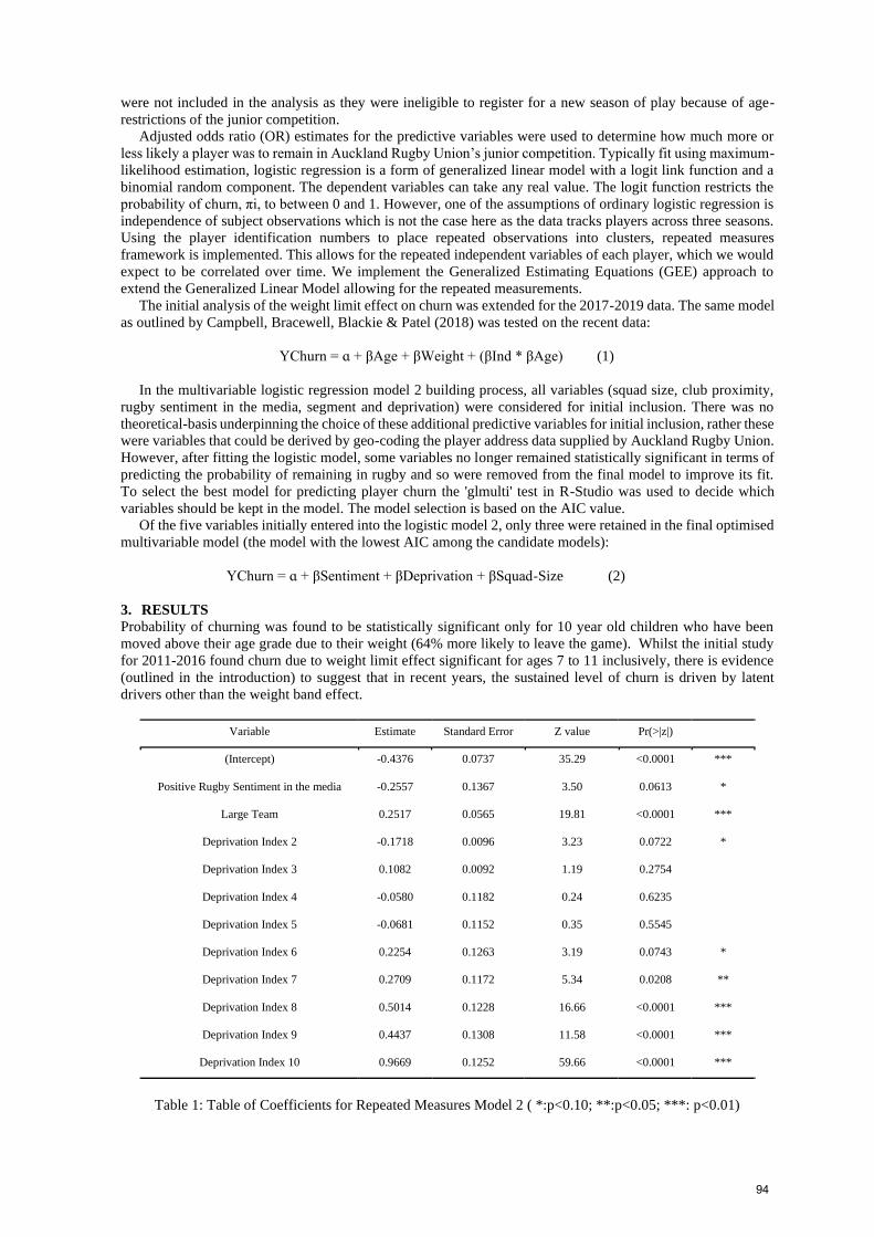
were not included in the analysis as they were ineligible to register for a new season of play because of age-

restrictions of the junior competition.

Adjusted odds ratio (OR) estimates for the predictive variables were used to determine how much more or

less likely a player was to remain in Auckland Rugby Union’s junior competition. Typically fit using maximum-

likelihood estimation, logistic regression is a form of generalized linear model with a logit link function and a

binomial random component. The dependent variables can take any real value. The logit function restricts the

probability of churn, πi, to between 0 and 1. However, one of the assumptions of ordinary logistic regression is

independence of subject observations which is not the case here as the data tracks players across three seasons.

Using the player identification numbers to place repeated observations into clusters, repeated measures

framework is implemented. This allows for the repeated independent variables of each player, which we would

expect to be correlated over time. We implement the Generalized Estimating Equations (GEE) approach to

extend the Generalized Linear Model allowing for the repeated measurements.

The initial analysis of the weight limit effect on churn was extended for the 2017-2019 data. The same model

as outlined by Campbell, Bracewell, Blackie & Patel (2018) was tested on the recent data:

YChurn = ɑ + βAge + βWeight + (βInd * βAge) (1)

In the multivariable logistic regression model 2 building process, all variables (squad size, club proximity,

rugby sentiment in the media, segment and deprivation) were considered for initial inclusion. There was no

theoretical-basis underpinning the choice of these additional predictive variables for initial inclusion, rather these

were variables that could be derived by geo-coding the player address data supplied by Auckland Rugby Union.

However, after fitting the logistic model, some variables no longer remained statistically significant in terms of

predicting the probability of remaining in rugby and so were removed from the final model to improve its fit.

To select the best model for predicting player churn the 'glmulti' test in R-Studio was used to decide which

variables should be kept in the model. The model selection is based on the AIC value.

Of the five variables initially entered into the logistic model 2, only three were retained in the final optimised

multivariable model (the model with the lowest AIC among the candidate models):

YChurn = ɑ + βSentiment + βDeprivation + βSquad-Size (2)

3. RESULTS

Probability of churning was found to be statistically significant only for 10 year old children who have been

moved above their age grade due to their weight (64% more likely to leave the game). Whilst the initial study

for 2011-2016 found churn due to weight limit effect significant for ages 7 to 11 inclusively, there is evidence

(outlined in the introduction) to suggest that in recent years, the sustained level of churn is driven by latent

drivers other than the weight band effect.

Variable Estimate Standard Error Z value Pr(>|z|)

(Intercept) -0.4376 0.0737 35.29 <0.0001 ***

Positive Rugby Sentiment in the media -0.2557 0.1367 3.50 0.0613 *

Large Team 0.2517 0.0565 19.81 <0.0001 ***

Deprivation Index 2 -0.1718 0.0096 3.23 0.0722 *

Deprivation Index 3 0.1082 0.0092 1.19 0.2754

Deprivation Index 4 -0.0580 0.1182 0.24 0.6235

Deprivation Index 5 -0.0681 0.1152 0.35 0.5545

Deprivation Index 6 0.2254 0.1263 3.19 0.0743 *

Deprivation Index 7 0.2709 0.1172 5.34 0.0208 **

Deprivation Index 8 0.5014 0.1228 16.66 <0.0001 ***

Deprivation Index 9 0.4437 0.1308 11.58 <0.0001 ***

Deprivation Index 10 0.9669 0.1252 59.66 <0.0001 ***

Table 1: Table of Coefficients for Repeated Measures Model 2 ( *:p<0.10; **:p<0.05; ***: p<0.01)

94

SQUAD SIZE

The base probability for churn is 0.6456 (e-0.4376). For large squad size, the probability to churn rises to 0.8304

(e-0.4376 + 0.2527). Juniors in large teams, where the team is larger than required team size by more than three, are

29% [(0.8304/0.6456) -1] more likely to leave the game compared to a player not in a large team. That is, at

U10 level, where the match is 10 aside, a squad of 14 or more is deemed to be large.

RUGBY IN THE MEDIA

With positive rugby in the media, the probability of churn falls to 0.4999 (e-0.4376 -0.2557). Juniors from

communities where their community rugby is showcased positively in digital mainstream media are 23% [1-

(0.4999/0.6456)] less likely to leave the game compared to a player from a community where their community

rugby is portrayed negatively.

DEPRIVATION

When a junior is from a community with the lowest socio-economic status (the most deprived: deprivation index

= 10), the probability of not signing up rises to 0.9674 (e-1 + 0.9669), if we use -1 to represent the intercept plus

estimated factors for a representative set of playing conditions, under which the effect of various deprivation

levels can be judged. Juniors from the most deprived communities are 2.6 times (0.9674/0.3679) more likely to

leave the game compared to a player from one of the most affluent communities (the least deprived: deprivation

index = 1). Juniors from communities of deprivation index 8 and 9 are 1.7 (0.6074/0.3679) and 1.6

(0.5733/0.3679) respectively times more likely to churn compared to a player from a community of deprivation

index 1.

Variable Odds Ratio

Positive Rugby Sentiment in the media 0.7744

Large Team 1.2862

Deprivation Index 2 0.8421

Deprivation Index 6 1.2528

Deprivation Index 7 1.3111

Deprivation Index 8 1.6510

Deprivation Index 9 1.5583

Deprivation Index 10 2.6300

Table 2: Odds ratios (OR) for the significant variables from model 2

SEGMOMENTO SEGMENT

Whilst the geo-spatially tagged segment provided by DOT loves data Segmomento product was not included in

the final model, most likely due to the strong relationship with deprivation, the Segmomento grid system (Figure

2) revealed the impact of deprivation on player retention, with additional insight into the influence of urbanality

on churn. The grid system is driven by the two dimensions (urban to rural across the top, low deprivation to high

deprivation down the side). Figure 2 reveals how juniors that leave the game are populated in the bottom left

hand corner of the matrix (representing the poorer urban communities whilst the top right hand corner represents

the better off communities). In 2019, 53% of players from segment ‘03’ left the game compared to only 30% of

players from segment ‘05’ who left the game. Using data provided by the University of Otago, Sport New

Zealand also found that the most deprived areas are typically urban.

95

Figure 2: Segmomento Matrix for 2019 rate of players who churned in each segment

Overall, the repeated measures analysis clearly supports the hypothesis that social factors; large squad size,

negative rugby sentiment in the media and high deprivation are negatively affecting player retention in Auckland

junior rugby.

4. DISCUSSION

In recent years, New Zealand media have addressed how children’s sport can be an “unequal playing field”

where some simply miss out due to unaffordability (Keogh, 2018). This study provides evidence of its reality in

the junior rugby competition in Auckland, supporting that to retain junior players from struggling communities,

Rugby Union must seriously consider how to increase accessibility of New Zealand’s national sport for all New

Zealanders. This means putting in place financial support systems for poorer families to afford keeping their

children playing in the sport. Furthermore, our study provides motivation to increase government initiatives such

as the recent agreement between New Zealand’s Ministry for Vulnerable Children and Sport New Zealand to

help children depending on government care to engage in sport, by reducing the preventive barriers (Stuff NZ,

2019).

“A process by which people are inspired by elite sport, sports people or sports events to participate

themselves” is known as the trickledown effect (Weed, 2009). Wicker & Sotiriadou (2013) describes this

concept as a “result of athlete performances, sports stars as personalities, and major sporting events” and

establishes the positive relationship between hosting major sports events on sport participation using the 2006

Melbourne Commonwealth Games. Regression results showed that younger people, less educated people, and

Indigenous people are more likely to spend more time participating in sport as a result. Our study has established

how sensitive the trickledown effect is, even at a community level; the impact of local rugby media on junior

rugby engagement. England’s Football Association encourages that in the social media context, clubs could

provide hash tags for players, to widely promote and positively engage clubs with the wider community actively

and in real time (Kirkham, 2015). With greater club rugby experiences voiced online this would drive greater

positive news articles around the sport, motivating players to stay in the game.

Our study had some limitations which in turn represent directions for future research. Trickledown effect is

analysed only through the consumption of local rugby news media whilst further insight can be gained by

incorporating the magnitude of how young kiwis are inspired by elite sports and elite sports figures. We

anticipate this can be quantified by investigating viewing patterns with subscriptions to paid television that gives

access to international-level sports matches. An interesting experience Marlborough Cricket Association general

manager Ed Gilhooly shared was whilst many were articulating the declining of children playing team sports in

New Zealand, signups for Cricket in the region increased which he attributed to the ‘Cricket World Cup effect’

and the continued high performance of the Black Caps (Lewis, 2016). Establishing the magnitude of the

influence of elite sports, such as world-class rugby, on junior players would encourage coaches and clubs to

showcase national level sport to young New Zealanders. As an example, could sponsor live international matches

in public spaces, encouraged by the evidence found here of its ability to attract and retain more young kiwis in

the sport.

Sports for children must ensure that children registered to play be given an opportunity to in fact participate.

Kirkham, Participation Manager of the West Australian Football Commission (2015) describes how children

“want equality in a sports experience, they do not want to be the player that sits on the bench with little game

time and do not want their friends sitting on the bench either.” Cases such as these increase when large teams

are formed than the standard squad size. Kirkham argues youth sports is no place for coaches that fail to provide

96

a fair and equitable environment for all juniors and recommends an equal player rotation policy for all coaches.

Coaches, often with a ‘win at all costs mentality’, that fail to include certain participants must be held to account

by parents and the club. Visek’s (2016) work on the ‘Not Fun Maps’ reveal that “coaches that favour some kids”

discourages children from sport and often leads to youth sport participants dropping out of sport. Junior rugby

coaches must actively ensure that team sizes are appropriate otherwise ensure regardless of talent level, that

players get equal time on field as our study has found significant evidence that juniors in large teams are more

likely to leave the game.

5. CONCLUSIONS

The negative impact of high deprivation, large team size and negative rugby media on junior rugby retention is

a new knowledge area, where once existed a gap in the literature. The contribution from this study for this area

positions junior rugby coaches and clubs to more informed evidence-based decisions in improving player

retention alongside age-weight grading systems. Rugby Union must seriously consider how to increase

accessibility of New Zealand’s national sport for all New Zealanders.

Acknowledgements

This research is part of a larger body of work, “Data informed decision bias”, a PhD Thes is supported by

Callaghan Innovation and DOT loves data, supervised by Associate Professor Ivy Liu of Victoria University of

Wellington and Dr Paul Bracewell.

References Bracewell, P.J., McNamara, T.S, & Moore, W.E. (2016). How Rugby Moved the Mood of New Zealand. Journal of Sport

and Human Performance. 4(4). pp. 1-9.

Campbell, E. C., Bracewell, P. J., Blackie, E. & Patel, A. K. (2018). The Impact of Auckland Junior Rugby Weight Limits

on Player Retention. Journal of Sport and Health Research. In press (accepted January 3, 2018).

Campbell, E. C., Patel, A. K. & Bracewell, P. J. (2018). Optimising Junior Rugby Weight Limits in New Zealand. Retrieved

from: http://www.mathsportinternational.com/anziam/Mathsport%2014.pdf

Hart, M. & Macandrew, R.(2019). National sporting body warns of drop in pupils playing sport. Retrieved

from:https://www.stuff.co.nz/sport/113355381/national-sporting-body-warns-of-drop-in-pupils-playing-sport

Keogh, B. (2018). Kids missing out on playing sport due to cost, families re-mortgaging homes to pay fees. Retrieved from:

https://www.stuff.co.nz/sport/108818305/kids-missing-out-on-playing-sport-due-to-cost-families-remortgaging-homes-

to-pay-fees Kirkham, T. (2015). To investigate innovative and inclusive retention strategies for youth participants in

community sport. The Winston Churchill Memorial Trust of Australia. Retrieved from:

https://www.churchilltrust.com.au/media/fellows/Kirkham_T_2015_Retention_strategies_for_youth_participants_in_com

munity_sport.pdf

Lewis, O. (2016). Participation rates down as people move away from team sports. Retrieved from:

https://www.stuff.co.nz/marlborough-express/sport/78031272/participation-rates-down-as-people-move-away-from-

team-sports

Savje, F., (2017). scclust. RDocumentation. https://www.rdocumentation.org/packages/scclust/versions/0.2.2 Accessed: 7

November 2019.

Sport New Zealand. (2019). Active NZ Spotlight on the impact of deprivation on participation. Retrieved from:

https://sportnz.org.nz/assets/Uploads/Active-NZ-Spotlight-on-Deprivation-August-2019.pdf

Sport New Zealand. (2011). 2011 Young People’s Survey Series. Retrieved from:

https://www.srknowledge.org.nz/researchseries/sport-new-zealands-young-peoples-survey-series/

Stuff NZ. (2019). Oranga Tamariki and Sport New Zealand to increase sport participation for kids. Retrieved from:

https://www.stuff.co.nz/sport/112866621/oranga-tamariki-and-sport-new-zealand-to-increase-sport-participation-for-kids

Thomas, J. (2019). Sir Graham Henry's silver bullet to fix New Zealand Rugby's participation issues. Retrieved from:

https://www.stuff.co.nz/sport/rugby/114329935/sir-graham-henrys-silver-bullet-to-fix-new-zealand-rugbys-participation-

issues

Visek, A. J., Achrati, S. M., Manning, H., McDonnell, K., Harris, B. S., & DiPietro, L. (2014). The Fun Integration Theory:

Towards sustaining children and adolescents sport participation. Journal of Physical Activity & Health. 12, 424.

Visek, et al. (2016). Not Fun Maps. Preliminary analyses of unpublished data. George Washington University.

Ward, A., Trowland, H., & Bracewell. (2019). The Dynamic Deprivation Index: measuring relative socio-economic

deprivation in NZ on a monthly basis. Kōtuitui: New Zealand Journal of Social Sciences Online.

https://doi.org/10.1080/1177083X.2019.1578807

Weed, M. (2009). The potential of the demonstration effect to grow and sustain participation in sport. Review Paper for

Sport England. Canterbury Christ Church University: Centre for Sport, Physical Education & Activity Research (SPEAR).

Wicker, P. and Sotiriadou, P. (2013), "The trickle-down effect: What population groups benefit from hosting major sport

events?", International Journal of Event Management Research, 8, 2, 25-41.

Widmeyer, W. Neil; Brawley, Lawrence R.; Carron, Albert V. (1990). The Effects of Group Size in Sport. Journal of Sport

& Exercise Psychology . Jun1990, Vol. 12 Issue 2, p177-190. 14p.

World Rugby. (2013). Relative Age Effect. Retrieved from World Rugby:

https://playerwelfare.worldrugby.org/?documentid=110. Accessed: 7 November 2019.

97

HOME AND AWAY: NOT A DAYTIME DRAMA BUT A SQUASH

SCHEDULING STORY

Ken Louie a,d, Bruce Morgan b, Paul Ewart c

a Waikato Institute of Technology, Hamilton, N.Z.

b Squash Waikato, Hamilton, N.Z. c Waikato Institute of Technology, Hamilton, N.Z.

d Corresponding author: ken.louie@wintec.ac.nz

Abstract

Squash Waikato is responsible for organising Winter and Spring interclub competition for the 25 affiliated

clubs in the Waikato district of New Zealand. The Winter competition typically consists of up to 120 teams

playing in graded eight-team divisions from April to July whilst the Spring competition has approximately 100

teams in smaller six-team divisions playing from August to October. The format is weekly games in a double

round robin tournament for each division. This is followed by semi-finals for the top four placed teams and

then a grand final for the winning semi-finalists. Women and men play in separate competitions on different

nights and the numbers of women’s teams is smaller. The clubs vary in size from two to six courts. Some clubs

enter only one team into either the men’s or women’s competition whilst some have up to 14 teams in both.

The number of team entries is not necessarily related to club size. The Waikato district covers a large

geographical region, requiring five hours driving between the most distant clubs.

Scheduling of home and away round-robin fixtures for tournaments has been extensively researched in other

sports. In a double round-robin tournament each team plays every other team in their division twice, once at

their HOME venue and again at the opponents’ venue (AWAY). If the tournament is mirrored, the second half

of the draw is a repetition of the first half, with only the venue being reversed. Theoretical results for

scheduling a mirrored double round-robin tournament so that no team has more than 3 successive AWAY

fixtures are available in the literature. This is a highly desirable feature for the Squash Waikato interclub

competition given the distances between some clubs. The novel aspects for squash scheduling in the Waikato

district are the highly variable number of teams entered by each club and the number of courts available for

home fixtures. For example, in the men’s Winter league one club having three courts had entered eight teams

whilst a six-court club entered six teams. These clubs would have a team:home court ratio of 8:3 and 1:1

respectively.

Squash NZ is the governing body for the sport in New Zealand and has provided software to all districts to

help prepare interclub schedules (iSquash interclub module). However, this software does not minimise the

home and away breaks which can lead to long stretches of multiple home or away fixtures for some teams. It

also does not account for the highly variable team:home court ratio. This paper addresses how we used the

theoretical results available from the literature to produce a schedule with minimum away breaks whilst also

accounting for the highly variable team:home court ratio. This has been used to significantly improve the

default iSquash schedule for the Winter and Spring interclub competition events in the Waikato district. It is

hoped that this procedure can be automated in a future version of the software.

Keywords: Squash, mirrored double round-robin tournament scheduling, minimising home and away

breaks

1. INTRODUCTION

In New Zealand, the game of squash is played competitively by approximately 12 000 people and

administered by Squash New Zealand. Every competitive player (i.e. those taking part in interclub events or

tournaments) is assigned a player code and grade which allows even matches amongst similarly graded players

nation-wide. The country is divided into eleven playing districts, with each district manager being responsible

for organising their own interclub competition. Tournaments are usually organised by the clubs themselves,

98

apart from those with district or national importance. This paper will be concerned only with the scheduling of

interclub competition in the Waikato district of N.Z.

There are 25 clubs affiliated to Squash N.Z. in the Waikato district with about 20 of those usually entering one

team or more into the interclub competition. These clubs vary widely in competitive player numbers and court

availability. Some small rural clubs may only have 10 competitive players with one court whilst a city-based

club may have 200 competitive players and six courts. However, competitive player numbers and court

availability are not necessarily correlated, particularly with city-based clubs where there is a wide choice of

clubs to join. Some clubs thus enter many teams and have a team:home court ratio as high as 8:3 whilst the

lowest might be 1:4. This large variability in team:home court ratio leads to some of the difficulties associated

with scheduling the interclub competition. Another factor that affects the scheduling are the large distances

between some of the clubs as shown in Figure 1. To drive between the southern and northern-most clubs

would take at least 5 hours.

Figure 1: The 25 affiliated clubs in the Squash Waikato district of New Zealand

Interclub competition in the Waikato district takes place from early April to late October, with a three-week

break in mid-July. The competition is divided into separate Winter (April—July) and Spring (August—

October) rounds, with men and women playing on Tuesday and Wednesday nights respectively. The Winter

round has eight-team divisions, with four players required in each team per night. There are usually nine

divisions for the men and six or seven divisions for the women, although sometimes entry numbers have meant

that one or two divisions have only four or six teams rather than eight. Each division consists of players of

roughly the same grade so that reasonably even matches are expected. Each team plays every other team in

99

their division twice, once at their home court and then again at their opponents’ court. This format is called a

double round robin tournament and requires 14 weeks to complete for an eight-team division. The top four

teams in each division after the double round robin then have semi-finals with 1st playing 4th, 2nd playing 3rd

and the semi-final winners then play a grand final to determine the division winner. The Spring event has a

similar format but each division consists of only six teams and there are no semi-finals. This requires only 11

weeks to complete, including the grand final between the 1st and 2nd placed teams after the double round robin.

The scheduling problem is to assign the weekly games in each division so that a variety of constraints are

satisfied. Techniques from graph theory for scheduling round robin tournaments are well-known (e.g. de

Werra 1981, Rosa & Wallis 1982) but the addition of sports-specific constraints has not been addressed until

more recently (Post & Woeginger, 2006). For our problem the constraints in decreasing order of importance

are:

1. Clubs with team:home court ratios greater than or equal to 2:1 should have their courts fully used

every week

2. No team should play away (or at home) more than 3 weeks in succession (i.e. minimise the number of

breaks)

3. Clubs with more than two teams entered and team:home court ratio of 1:1 or less should have at least

two of those teams at home on the same weeks

These constraints are usually requested by the clubs themselves but not expressed in this precise form. For

example, the first constraint is to “reward” those clubs entering many teams with full utilisation of their

courts every week, and consequent increase in bar revenue. Constraint 2 was introduced to minimise the

impact of travel time for those clubs located on the outskirts of the district. The third constraint arises from

the club desire to maximise “atmosphere” and bar revenue because the presence of more clubmates and

another visiting team should enhance social interaction. Although Squash N.Z. has provided all districts with

software capable of producing the draws, it was usually the case that only one (and sometimes none) of these

constraints were met.

Figure 2: The schedule for one two-court club (TRAP stands for Te Rapa) produced by iSquash

An example of this is provided in Figure 2, which shows the schedule for Te Rapa, a two-court club which

entered four teams in the 2019 Winter men’s event, thus having a team:home court ratio of 4:2 = 2:1. The four

teams in different divisions are indicated by the four colours and the allocated court by the number 1 or 2. The

purple division only had 7 teams resulting in a bye week which is why there are only 6 home fixtures. All

courts are allocated every week except for week 8 when the team playing in purple division had a bye at home.

Constraint 2 is not met—the team in division blue have two home games and then seven away games in

succession from weeks 3 to 9 before playing their last five home games in weeks 10 to 14. Moreover, the team

in division grey have five home games in succession from weeks 2 to 6 and then a sequence of five away

games from weeks 9 to 13. These long sequences of away games may not cause concern if the away venues

are nearby but this depends on the other teams entered in those divisions (see Figure 1). We use existing

schedules from the literature for mirrored double round robin events (Rasmussen & Trick, 2008) to produce a

draw which satisfies all 3 constraints for the majority of clubs.

2. METHODS

We follow the procedure outlined in Rasmussen & Trick, 2008 for tackling constrained minimum break

problems to produce a more satisfactory draw for the Men’s Winter interclub competition of 2019. This

competition involved 71 teams from 18 clubs, including five clubs with a team:home court ratio greater than or

equal to 2:1. The clubs and their number of team entries are summarised in Table 1. The three full-capacity

clubs (team:home court ratio = 2:1) are indicated with an asterisk and the two over-capacity clubs (team:home

court ratio > 2:1) with a double asterisk.

100

Club Number of teams entered Number of courts Team:home court ratio

Aria 1 2 1:2

Cambridge* 8 4 8:4 = 2:1

Hamilton Old Boys 1 2 1:2

Hamilton Squash and Tennis 6 6 6:6 = 1:1

Huntly 1 2 1:2

Leamington 4 3 4:3

Lugton Park** 8 3 8:3

Morrinsville 4 3 4:3

Ngaruawahia 3 2 3:2

Paeroa 2 2 2:2 = 1:1

Ruakura** 5 2 5:2

Taupiri* 4 2 4:2 = 2:1

Te Aroha 2 3 2:3

Te Awamutu 5 3 5:3

Te Kuiti 3 2 3:2

Te Rapa* 4 2 4:2 = 2:1

Thames 4 3 4:3

United Matamata 6 4 6:4 = 3:2

Table 1: Club entries in Men’s Winter Interclub 2019 with team:home court ratios

For those two clubs with a team:home court ratio exceeding 2:1, a “home” court from another club needs to be

allocated. Fortunately, Lugton Park and Ruakura are located in Hamilton (main city of the Waikato district) so

the extra “home” courts could be located at Hamilton Squash and Tennis which had three spare courts

available. The 71 teams were allocated into 9 divisions with eight teams per division based on the team

members’ grading points. The top division had only seven teams, thus necessitating a bye team. In the first

phase of the procedure, the canonical schedule for eight teams from Rasmussen & Trick, 2008 was reproduced

as Table 2.

Week 1 2 3 4 5 6 7

Team 1 -8 +3 -5 +7 -2 +4 -6

Team 2 -7 +8 +4 -6 +1 -3 +5

Team 3 +6 -1 -8 +5 -7 +2 -4

Team 4 -5 +7 -2 +8 +6 -1 +3

Team 5 +4 -6 +1 -3 -8 +7 -2

Team 6 -3 +5 -7 +2 -4 +8 +1

Team 7 +2 -4 +6 -1 +3 -5 -8

Team 8 +1 -2 +3 -4 +5 -6 +7

Table 2: The canonical round robin schedule for eight teams with minimum breaks

In Table 2, the column heading indicates the round played and each row gives the team’s opponents for the

first half of the competition. The “-” shows that game is to be played away whilst the “+” means it is a home

game for that team. In the second half of the competition from weeks 8 to 14, the table is repeated but with all

the “-” being replaced by “+” and vice versa. Each team plays every other team twice, once at their home

venue and again at their opponent’s. When the second half of the competition repeats the first half in order,

with only the venues reversed, it is called a mirrored double round robin event. Recall from the Introduction

that a break means a disruption from the alternating “+” and “-” sequence. For example, Team 3 has a break at

week 2 and Team 6 has a break at week 6. Post & Woeginger (2006) has shown that this canonical schedule

minimises the overall number of breaks. Note that the schedule is complementary for teams 1–8, 2–3, 4–5 and

6–7 respectively. This means that those pairs of teams are never at home or away together in the same week.

We exploit this complementarity property in the second phase to assign teams for those five clubs at full

capacity.

101

In the second phase we assign teams in each of the nine divisions to the canonical schedule in Table 2. The

particular assignation we chose is summarised in Table 3. In assigning the teams we followed this scheme

which ensures that constraints 1 and 2 are satisfied

• Deal with the full capacity clubs first by assigning their teams to complementary positions from Table 2

• Next assign clubs with team:home court ratio ≥ 3:2, assigning pairs of their teams to complementary

positions (ensures that teams will not all be given home games in the same week)

• Then deal with clubs entering more than two teams but with team:home court ratio ≤ 1:1 by assigning

their teams the same position (ensures those teams will always be at home together but not exceed court

capacity)

• Finally assign any remaining club teams to vacant positions

Divisions

Tea

ms

One Two Three Four Five Six Seven Eight Nine

1 Lug A Rua A Cam C Mor A UMat C Tawa C Tha C UMat F Tkui B

2 Ham A Lea A Lug C Cam E Mor C Rua C Tau C Nga C Tau D

3 Tau A Ham B Tau B Lug D Hun A Cam F Rua D Mor D Tha D

4 Cam A Tawa A TKui A Nga B Lug E Lea C Taro B Ham E Rua E@Ham

5 Cam B Nga A HOB Tawa B Pae A Lug F Aria Pae B Ham F

6 Trap A Tha A UMat B Taro A Trap C UMat D Cam H Lea D Lug H@Ham

7 UMat A Trap B Ham C Lea B Tha B Cam G UMat E Trap D Lug G@Ham

8 Bye Lug B Cam D Rua B Mor B Ham D Tawa D Tawa E Tkui C

Table 3: Team allocation to the canonical schedule for each division

As an example of how Table 3 is to be used in conjunction with Table 2, consider for example Division Two.

The games to be played in Week 1 (from Table 2) with assigned teams (from Table 3) would be:

(1) Rua A v (8) Lug B*, (2) Lea A v (7) Trap B*, (3) Ham B* v (6) Tha A and (4) Tawa A v (5) Nga A* with

the * indicating the home team as it has the “+” associated with it.

To take advantage of the complementarity we have highlighted one of the full-capacity clubs (Te Rapa with 4

teams and 2 home courts) in Table 3 and allocated their four teams in the complementary positions of 6–7 for

teams A and C and teams B and D respectively. This ensures that their teams A and B are never at home

together and neither are teams C and D. By assigning the A and C teams to position 6, and the B and D to

position 7, we also ensure those pairs are at home together. This allocation enables constraints 1 and 2 to be

automatically satisfied. The same allocation procedure is followed for the other four full-capacity clubs using

the other complementary positions 1–8, 2–3 and 4–5.

In the final phase we attempt to satisfy constraint 3 by allocating the relevant clubs’ teams to the same position

in the canonical schedule, thus ensuring those teams will be playing at home together. This may not always

possible if constraints 1 and 2 are to be satisfied first and there are a large number of full-capacity clubs.

3. RESULTS

After applying the three phases described in the Methods section, a draw was produced which satisfies the

three required constraints for most clubs. This is summarised by the court allocation schedule in Figure 3. If

we focus on the full-capacity club Te Rapa as before and compare with Figure 2, we see that there is more

uniform home and away pattern of games for all divisions. No team plays more than three away (or home)

games in succession (note that colours have changed for the divisions). Because the same canonical schedule

is used for all divisions, then all teams will satisfy constraint 2. Furthermore, as the full-capacity club teams

have been allocated first using the complementary pattern, then their courts will always be fully utilised, thus

satisfying the top constraint.

There are three clubs which should satisfy the third constraint: Hamilton, Paeroa and Te Aroha. From Figure 3

we see that Paeroa satisfies the constraint whereas Te Aroha have four weeks where one of their two teams are

at home alone. The Hamilton Squash and Tennis club’s six courts are also not fully utilised despite loaning

three courts to other clubs for use. This is because the Hamilton club has not been treated as a full-capacity

club which means its teams were not assigned complementary positions from the canonical schedule.

102

Mens Court Allocations - Winter InterclubRounds:

1 2 3 4 5 6 7 8 9 10 11 12 13 14

2-Apr 9-Apr 16-Apr 30-Apr 7-May 14-May 21-May 28-May 4-Jun 11-Jun 18-Jun 25-Jun 2-Jul 9-Jul

ARIA 1 ARIA 1 ARIA 1 ARIA 1 ARIA 1 ARIA 1 ARIA 1 ARIA 1 ARIA 1 ARIA 1 ARIA 1 ARIA 1 ARIA 1 ARIA 1 DIV 1

ARIA 2 ARIA 2 ARIA 2 ARIA 2 ARIA 2 ARIA 2 ARIA 2 ARIA 2 ARIA 2 ARIA 2 ARIA 2 ARIA 2 ARIA 2 ARIA 2 DIV 2

CAMB 1 CAMB 1 CAMB 1 CAMB 1 CAMB 1 CAMB 1 CAMB 1 CAMB 1 CAMB 1 CAMB 1 CAMB 1 CAMB 1 CAMB 1 CAMB 1 DIV 3

CAMB 2 CAMB 2 CAMB 2 CAMB 2 CAMB 2 CAMB 2 CAMB 2 CAMB 2 CAMB 2 CAMB 2 CAMB 2 CAMB 2 CAMB 2 CAMB 2 DIV 4

CAMB 3 CAMB 3 CAMB 3 CAMB 3 CAMB 3 CAMB 3 CAMB 3 CAMB 3 CAMB 3 CAMB 3 CAMB 3 CAMB 3 CAMB 3 CAMB 3 DIV 5

CAMB 4 CAMB 4 CAMB 4 CAMB 4 CAMB 4 CAMB 4 CAMB 4 CAMB 4 CAMB 4 CAMB 4 CAMB 4 CAMB 4 CAMB 4 CAMB 4 DIV 6

FRAK 1 FRAK 1 FRAK 1 FRAK 1 FRAK 1 FRAK 1 FRAK 1 FRAK 1 FRAK 1 FRAK 1 FRAK 1 FRAK 1 FRAK 1 FRAK 1 DIV 7

HAM 1 HAM 1 HAM 1 HAM 1 HAM 1 HAM 1 HAM 1 HAM 1 HAM 1 HAM 1 HAM 1 HAM 1 HAM 1 HAM 1 DIV 8

HAM 2 HAM 2 HAM 2 HAM 2 HAM 2 HAM 2 HAM 2 HAM 2 HAM 2 HAM 2 HAM 2 HAM 2 HAM 2 HAM 2 DIV 9

HAM 3 HAM 3 HAM 3 HAM 3 HAM 3 HAM 3 HAM 3 HAM 3 HAM 3 HAM 3 HAM 3 HAM 3 HAM 3 HAM 3

HAM 4 HAM 4 HAM 4 HAM 4 HAM 4 HAM 4 HAM 4 HAM 4 HAM 4 HAM 4 HAM 4 HAM 4 HAM 4 HAM 4

HAM 5 HAM 5 HAM 5 HAM 5 HAM 5 HAM 5 HAM 5 HAM 5 HAM 5 HAM 5 HAM 5 HAM 5 HAM 5 HAM 5

HAM 6 HAM 6 HAM 6 HAM 6 HAM 6 HAM 6 HAM 6 HAM 6 HAM 6 HAM 6 HAM 6 HAM 6 HAM 6 HAM 6

HOB 1 HOB 1 HOB 1 HOB 1 HOB 1 HOB 1 HOB 1 HOB 1 HOB 1 HOB 1 HOB 1 HOB 1 HOB 1 HOB 1

HOB 2 HOB 2 HOB 2 HOB 2 HOB 2 HOB 2 HOB 2 HOB 2 HOB 2 HOB 2 HOB 2 HOB 2 HOB 2 HOB 2

HUNT 1 HUNT 1 HUNT 1 HUNT 1 HUNT 1 HUNT 1 HUNT 1 HUNT 1 HUNT 1 HUNT 1 HUNT 1 HUNT 1 HUNT 1 HUNT 1

HUNT 2 HUNT 2 HUNT 2 HUNT 2 HUNT 2 HUNT 2 HUNT 2 HUNT 2 HUNT 2 HUNT 2 HUNT 2 HUNT 2 HUNT 2 HUNT 2

FRNK 1 FRNK 1 FRNK 1 FRNK 1 FRNK 1 FRNK 1 FRNK 1 FRNK 1 FRNK 1 FRNK 1 FRNK 1 FRNK 1 FRNK 1 FRNK 1

FRNK 2 FRNK 2 FRNK 2 FRNK 2 FRNK 2 FRNK 2 FRNK 2 FRNK 2 FRNK 2 FRNK 2 FRNK 2 FRNK 2 FRNK 2 FRNK 2

LUGT 1 LUGT 1 LUGT 1 LUGT 1 LUGT 1 LUGT 1 LUGT 1 LUGT 1 LUGT 1 LUGT 1 LUGT 1 LUGT 1 LUGT 1 LUGT 1

LUGT 2 LUGT 2 LUGT 2 LUGT 2 LUGT 2 LUGT 2 LUGT 2 LUGT 2 LUGT 2 LUGT 2 LUGT 2 LUGT 2 LUGT 2 LUGT 2

LUGT 3 LUGT 3 LUGT 3 LUGT 3 LUGT 3 LUGT 3 LUGT 3 LUGT 3 LUGT 3 LUGT 3 LUGT 3 LUGT 3 LUGT 3 LUGT 3

LEAM 1 LEAM 1 LEAM 1 LEAM 1 LEAM 1 LEAM 1 LEAM 1 LEAM 1 LEAM 1 LEAM 1 LEAM 1 LEAM 1 LEAM 1 LEAM 1

LEAM 2 LEAM 2 LEAM 2 LEAM 2 LEAM 2 LEAM 2 LEAM 2 LEAM 2 LEAM 2 LEAM 2 LEAM 2 LEAM 2 LEAM 2 LEAM 2

LEAM 3 LEAM 3 LEAM 3 LEAM 3 LEAM 3 LEAM 3 LEAM 3 LEAM 3 LEAM 3 LEAM 3 LEAM 3 LEAM 3 LEAM 3 LEAM 3

MORR 1 MORR 1 MORR 1 MORR 1 MORR 1 MORR 1 MORR 1 MORR 1 MORR 1 MORR 1 MORR 1 MORR 1 MORR 1 MORR 1

MORR 2 MORR 2 MORR 2 MORR 2 MORR 2 MORR 2 MORR 2 MORR 2 MORR 2 MORR 2 MORR 2 MORR 2 MORR 2 MORR 2

MORR 3 MORR 3 MORR 3 MORR 3 MORR 3 MORR 3 MORR 3 MORR 3 MORR 3 MORR 3 MORR 3 MORR 3 MORR 3 MORR 3

MATA 1 MATA 1 MATA 1 MATA 1 MATA 1 MATA 1 MATA 1 MATA 1 MATA 1 MATA 1 MATA 1 MATA 1 MATA 1 MATA 1

MATA 2 MATA 2 MATA 2 MATA 2 MATA 2 MATA 2 MATA 2 MATA 2 MATA 2 MATA 2 MATA 2 MATA 2 MATA 2 MATA 2

MATA 3 MATA 3 MATA 3 MATA 3 MATA 3 MATA 3 MATA 3 MATA 3 MATA 3 MATA 3 MATA 3 MATA 3 MATA 3 MATA 3

MATA 4 MATA 4 MATA 4 MATA 4 MATA 4 MATA 4 MATA 4 MATA 4 MATA 4 MATA 4 MATA 4 MATA 4 MATA 4 MATA 4

NGA 1 NGA 1 NGA 1 NGA 1 NGA 1 NGA 1 NGA 1 NGA 1 NGA 1 NGA 1 NGA 1 NGA 1 NGA 1 NGA 1

NGA 2 NGA 2 NGA 2 NGA 2 NGA 2 NGA 2 NGA 2 NGA 2 NGA 2 NGA 2 NGA 2 NGA 2 NGA 2 NGA 2

OTO 1 OTO 1 OTO 1 OTO 1 OTO 1 OTO 1 OTO 1 OTO 1 OTO 1 OTO 1 OTO 1 OTO 1 OTO 1 OTO 1

OTO 2 OTO 2 OTO 2 OTO 2 OTO 2 OTO 2 OTO 2 OTO 2 OTO 2 OTO 2 OTO 2 OTO 2 OTO 2 OTO 2

PAE 1 PAE 1 PAE 1 PAE 1 PAE 1 PAE 1 PAE 1 PAE 1 PAE 1 PAE 1 PAE 1 PAE 1 PAE 1 PAE 1

PAE 2 PAE 2 PAE 2 PAE 2 PAE 2 PAE 2 PAE 2 PAE 2 PAE 2 PAE 2 PAE 2 PAE 2 PAE 2 PAE 2

RUAK 1 RUAK 1 RUAK 1 RUAK 1 RUAK 1 RUAK 1 RUAK 1 RUAK 1 RUAK 1 RUAK 1 RUAK 1 RUAK 1 RUAK 1 RUAK 1

RUAK 2 RUAK 2 RUAK 2 RUAK 2 RUAK 2 RUAK 2 RUAK 2 RUAK 2 RUAK 2 RUAK 2 RUAK 2 RUAK 2 RUAK 2 RUAK 2

TAUP 1 TAUP 1 TAUP 1 TAUP 1 TAUP 1 TAUP 1 TAUP 1 TAUP 1 TAUP 1 TAUP 1 TAUP 1 TAUP 1 TAUP 1 TAUP 1

TAUP 2 TAUP 2 TAUP 2 TAUP 2 TAUP 2 TAUP 2 TAUP 2 TAUP 2 TAUP 2 TAUP 2 TAUP 2 TAUP 2 TAUP 2 TAUP 2

TARO 1 TARO 1 TARO 1 TARO 1 TARO 1 TARO 1 TARO 1 TARO 1 TARO 1 TARO 1 TARO 1 TARO 1 TARO 1 TARO 1

TARO 2 TARO 2 TARO 2 TARO 2 TARO 2 TARO 2 TARO 2 TARO 2 TARO 2 TARO 2 TARO 2 TARO 2 TARO 2 TARO 2

TARO 3 TARO 3 TARO 3 TARO 3 TARO 3 TARO 3 TARO 3 TARO 3 TARO 3 TARO 3 TARO 3 TARO 3 TARO 3 TARO 3

TAWA 1 TAWA 1 TAWA 1 TAWA 1 TAWA 1 TAWA 1 TAWA 1 TAWA 1 TAWA 1 TAWA 1 TAWA 1 TAWA 1 TAWA 1 TAWA 1

TAWA 2 TAWA 2 TAWA 2 TAWA 2 TAWA 2 TAWA 2 TAWA 2 TAWA 2 TAWA 2 TAWA 2 TAWA 2 TAWA 2 TAWA 2 TAWA 2

TAWA 3 TAWA 3 TAWA 3 TAWA 3 TAWA 3 TAWA 3 TAWA 3 TAWA 3 TAWA 3 TAWA 3 TAWA 3 TAWA 3 TAWA 3 TAWA 3

TKUI 1 TKUI 1 TKUI 1 TKUI 1 TKUI 1 TKUI 1 TKUI 1 TKUI 1 TKUI 1 TKUI 1 TKUI 1 TKUI 1 TKUI 1 TKUI 1

TKUI 2 TKUI 2 TKUI 2 TKUI 2 TKUI 2 TKUI 2 TKUI 2 TKUI 2 TKUI 2 TKUI 2 TKUI 2 TKUI 2 TKUI 2 TKUI 2

THAM 1 THAM 1 THAM 1 THAM 1 THAM 1 THAM 1 THAM 1 THAM 1 THAM 1 THAM 1 THAM 1 THAM 1 THAM 1 THAM 1

THAM 2 THAM 2 THAM 2 THAM 2 THAM 2 THAM 2 THAM 2 THAM 2 THAM 2 THAM 2 THAM 2 THAM 2 THAM 2 THAM 2

THAM 3 THAM 3 THAM 3 THAM 3 THAM 3 THAM 3 THAM 3 THAM 3 THAM 3 THAM 3 THAM 3 THAM 3 THAM 3 THAM 3

TAUM 1 TAUM 1 TAUM 1 TAUM 1 TAUM 1 TAUM 1 TAUM 1 TAUM 1 TAUM 1 TAUM 1 TAUM 1 TAUM 1 TAUM 1 TAUM 1

TAUM 2 TAUM 2 TAUM 2 TAUM 2 TAUM 2 TAUM 2 TAUM 2 TAUM 2 TAUM 2 TAUM 2 TAUM 2 TAUM 2 TAUM 2 TAUM 2

TAUM 3 TAUM 3 TAUM 3 TAUM 3 TAUM 3 TAUM 3 TAUM 3 TAUM 3 TAUM 3 TAUM 3 TAUM 3 TAUM 3 TAUM 3 TAUM 3

TAUM 4 TAUM 4 TAUM 4 TAUM 4 TAUM 4 TAUM 4 TAUM 4 TAUM 4 TAUM 4 TAUM 4 TAUM 4 TAUM 4 TAUM 4 TAUM 4

TRAP 1 TRAP 1 TRAP 1 TRAP 1 TRAP 1 TRAP 1 TRAP 1 TRAP 1 TRAP 1 TRAP 1 TRAP 1 TRAP 1 TRAP 1 TRAP 1

TRAP 2 TRAP 2 TRAP 2 TRAP 2 TRAP 2 TRAP 2 TRAP 2 TRAP 2 TRAP 2 TRAP 2 TRAP 2 TRAP 2 TRAP 2 TRAP 21 2 3 4 5 6 7 8 9 10 11 12 13 14

2-Apr 9-Apr 16-Apr 30-Apr 7-May 14-May 21-May 28-May 4-Jun 11-Jun 18-Jun 25-Jun 2-Jul 9-Jul

Figure 3: Court allocation from new draw showing minimum breaks and full utilisation

Me

ns

Co

urt

All

oca

tio

ns

- W

inte

r In

terc

lub

Ro

un

ds:

12

34

56

78

910

1112

1314

2-A

pr

9-A

pr

16-A

pr

30-A

pr

7-M

ay14

-May

21-M

ay28

-May

4-Ju

n11

-Ju

n18

-Ju

n25

-Ju

n2-

Jul

9-Ju

l

AR

IA 1

AR

IA 1

AR

IA 1

AR

IA 1

AR

IA 1

AR

IA 1

AR

IA 1

AR

IA 1

AR

IA 1

AR

IA 1

AR

IA 1

AR

IA 1

AR

IA 1

AR

IA 1

DIV

1

AR

IA 2

AR

IA 2

AR

IA 2

AR

IA 2

AR

IA 2

AR

IA 2

AR

IA 2

AR

IA 2

AR

IA 2

AR

IA 2

AR

IA 2

AR

IA 2

AR

IA 2

AR

IA 2

DIV

2

CA

MB

1C

AM

B 1

CA

MB

1C

AM

B 1

CA

MB

1C

AM

B 1

CA

MB

1C

AM

B 1

CA

MB

1C

AM

B 1

CA

MB

1C

AM

B 1

CA

MB

1C

AM

B 1

DIV

3

CA

MB

2C

AM

B 2

CA

MB

2C

AM

B 2

CA

MB

2C

AM

B 2

CA

MB

2C

AM

B 2

CA

MB

2C

AM

B 2

CA

MB

2C

AM

B 2

CA

MB

2C

AM

B 2

DIV

4

CA

MB

3C

AM

B 3

CA

MB

3C

AM

B 3

CA

MB

3C

AM

B 3

CA

MB

3C

AM

B 3

CA

MB

3C

AM

B 3

CA

MB

3C

AM

B 3

CA

MB

3C

AM

B 3

DIV

5

CA

MB

4C

AM

B 4

CA

MB

4C

AM

B 4

CA

MB

4C

AM

B 4

CA

MB

4C

AM

B 4

CA

MB

4C

AM

B 4

CA

MB

4C

AM

B 4

CA

MB

4C

AM

B 4

DIV

6

FRA

K 1

FRA

K 1

FRA

K 1

FRA

K 1

FRA

K 1

FRA

K 1

FRA

K 1

FRA

K 1

FRA

K 1

FRA

K 1

FRA

K 1

FRA

K 1

FRA

K 1

FRA

K 1

DIV

7

HA

M 1

HA

M 1

HA

M 1

HA

M 1

HA

M 1

HA

M 1

HA

M 1

HA

M 1

HA

M 1

HA

M 1

HA

M 1

HA

M 1

HA

M 1

HA

M 1

DIV

8

HA

M 2

HA

M 2

HA

M 2

HA

M 2

HA

M 2

HA

M 2

HA

M 2

HA

M 2

HA

M 2

HA

M 2

HA

M 2

HA

M 2

HA

M 2

HA

M 2

DIV

9

HA

M 3

HA

M 3

HA

M 3

HA

M 3

HA

M 3

HA

M 3

HA

M 3

HA

M 3

HA

M 3

HA

M 3

HA

M 3

HA

M 3

HA

M 3

HA

M 3

HA

M 4

HA

M 4

HA

M 4

HA

M 4

HA

M 4

HA

M 4

HA

M 4

HA

M 4

HA

M 4

HA

M 4

HA

M 4

HA

M 4

HA

M 4

HA

M 4

HA

M 5

HA

M 5

HA

M 5

HA

M 5

HA

M 5

HA

M 5

HA

M 5

HA

M 5

HA

M 5

HA

M 5

HA

M 5

HA

M 5

HA

M 5

HA

M 5

HA

M 6

HA

M 6

HA

M 6

HA

M 6

HA

M 6

HA

M 6

HA

M 6

HA

M 6

HA

M 6

HA

M 6

HA

M 6

HA

M 6

HA

M 6

HA

M 6

HO

B 1

HO

B 1

HO

B 1

HO

B 1

HO

B 1

HO

B 1

HO

B 1

HO

B 1

HO

B 1

HO

B 1

HO

B 1

HO

B 1

HO

B 1

HO

B 1

HO

B 2

HO

B 2

HO

B 2

HO

B 2

HO

B 2

HO

B 2

HO

B 2

HO

B 2

HO

B 2

HO

B 2

HO

B 2

HO

B 2

HO

B 2

HO

B 2

HU

NT

1H

UN

T 1

HU

NT

1H

UN

T 1

HU

NT

1H

UN

T 1

HU

NT

1H

UN

T 1

HU

NT

1H

UN

T 1

HU

NT

1H

UN

T 1

HU

NT

1H

UN

T 1

HU

NT

2H

UN

T 2

HU

NT

2H

UN

T 2

HU

NT

2H

UN

T 2

HU

NT

2H

UN

T 2

HU

NT

2H

UN

T 2

HU

NT

2H

UN

T 2

HU

NT

2H

UN

T 2

FRN

K 1

FRN

K 1

FRN

K 1

FRN

K 1

FRN

K 1

FRN

K 1

FRN

K 1

FRN

K 1

FRN

K 1

FRN

K 1

FRN

K 1

FRN

K 1

FRN

K 1

FRN

K 1

FRN

K 2

FRN

K 2

FRN

K 2

FRN

K 2

FRN

K 2

FRN

K 2

FRN

K 2

FRN

K 2

FRN

K 2

FRN

K 2

FRN

K 2

FRN

K 2

FRN

K 2

FRN

K 2

LUG

T 1

LUG

T 1

LUG

T 1

LUG

T 1

LUG

T 1

LUG

T 1

LUG

T 1

LUG

T 1

LUG

T 1

LUG

T 1

LUG

T 1

LUG

T 1

LUG

T 1

LUG

T 1

LUG

T 2

LUG

T 2

LUG

T 2

LUG

T 2

LUG

T 2

LUG

T 2

LUG

T 2

LUG

T 2

LUG

T 2

LUG

T 2

LUG

T 2

LUG

T 2

LUG

T 2

LUG

T 2

LUG

T 3

LUG

T 3

LUG

T 3

LUG

T 3

LUG

T 3

LUG

T 3

LUG

T 3

LUG

T 3

LUG

T 3

LUG

T 3

LUG

T 3

LUG

T 3

LUG

T 3

LUG

T 3

LEA

M 1

LEA

M 1

LEA

M 1

LEA

M 1

LEA

M 1

LEA

M 1

LEA

M 1

LEA

M 1

LEA

M 1

LEA

M 1

LEA

M 1

LEA

M 1

LEA

M 1

LEA

M 1

LEA

M 2

LEA

M 2

LEA

M 2

LEA

M 2

LEA

M 2

LEA

M 2

LEA

M 2

LEA

M 2

LEA

M 2

LEA

M 2

LEA

M 2

LEA

M 2

LEA

M 2

LEA

M 2

LEA

M 3

LEA

M 3

LEA

M 3

LEA

M 3

LEA

M 3

LEA

M 3

LEA

M 3

LEA

M 3

LEA

M 3

LEA

M 3

LEA

M 3

LEA

M 3

LEA

M 3

LEA

M 3

MO

RR

1M

OR

R 1

MO

RR

1M

OR

R 1

MO

RR

1M

OR

R 1

MO

RR

1M

OR

R 1

MO

RR

1M

OR

R 1

MO

RR

1M

OR

R 1

MO

RR

1M

OR

R 1

MO

RR

2M

OR

R 2

MO

RR

2M

OR

R 2

MO

RR

2M

OR

R 2

MO

RR

2M

OR

R 2

MO

RR

2M

OR

R 2

MO

RR

2M

OR

R 2

MO

RR

2M

OR

R 2

MO

RR

3M

OR

R 3

MO

RR

3M

OR

R 3

MO

RR

3M

OR

R 3

MO

RR

3M

OR

R 3

MO

RR

3M

OR

R 3

MO

RR

3M

OR

R 3

MO

RR

3M

OR

R 3

MA

TA

1M

AT

A 1

MA

TA

1M

AT

A 1

MA

TA

1M

AT

A 1

MA

TA

1M

AT

A 1

MA

TA

1M

AT

A 1

MA

TA

1M

AT

A 1

MA

TA

1M

AT

A 1

MA

TA

2M

AT

A 2

MA

TA

2M

AT

A 2

MA

TA

2M

AT

A 2

MA

TA

2M

AT

A 2

MA

TA

2M

AT

A 2

MA

TA

2M

AT

A 2

MA

TA

2M

AT

A 2

MA

TA

3M

AT

A 3

MA

TA

3M

AT

A 3

MA

TA

3M

AT

A 3

MA

TA

3M

AT

A 3

MA

TA

3M

AT

A 3

MA

TA

3M

AT

A 3

MA

TA

3M

AT

A 3

MA

TA

4M

AT

A 4

MA

TA

4M

AT

A 4

MA

TA

4M

AT

A 4

MA

TA

4M

AT

A 4

MA

TA

4M

AT

A 4

MA

TA

4M

AT

A 4

MA

TA

4M

AT

A 4

NG

A 1

NG

A 1

NG

A 1

NG

A 1

NG

A 1

NG

A 1

NG

A 1

NG

A 1

NG

A 1

NG

A 1

NG

A 1

NG

A 1

NG

A 1

NG

A 1

NG

A 2

NG

A 2

NG

A 2

NG

A 2

NG

A 2

NG

A 2

NG

A 2

NG

A 2

NG

A 2

NG

A 2

NG

A 2

NG

A 2

NG

A 2

NG

A 2

OT

O 1

OT

O 1

OT

O 1

OT

O 1

OT

O 1

OT

O 1

OT

O 1

OT

O 1

OT

O 1

OT

O 1

OT

O 1

OT

O 1

OT

O 1

OT

O 1

OT

O 2

OT

O 2

OT

O 2

OT

O 2

OT

O 2

OT

O 2

OT

O 2

OT

O 2

OT

O 2

OT

O 2

OT

O 2

OT

O 2

OT

O 2

OT

O 2

PA

E 1

PA

E 1

PA

E 1

PA

E 1

PA

E 1

PA

E 1

PA

E 1

PA

E 1

PA

E 1

PA

E 1

PA

E 1

PA

E 1

PA

E 1

PA

E 1

PA

E 2

PA

E 2

PA

E 2

PA

E 2

PA

E 2

PA

E 2

PA

E 2

PA

E 2

PA

E 2

PA

E 2

PA

E 2

PA

E 2

PA

E 2

PA

E 2

RU

AK

1R

UA

K 1

RU

AK

1R

UA

K 1

RU

AK

1R

UA

K 1

RU

AK

1R

UA

K 1

RU

AK

1R

UA

K 1

RU

AK

1R

UA

K 1

RU

AK

1R

UA

K 1

RU

AK

2R

UA

K 2

RU

AK

2R

UA

K 2

RU

AK

2R

UA

K 2

RU

AK

2R

UA

K 2

RU

AK

2R

UA

K 2

RU

AK

2R

UA

K 2

RU

AK

2R

UA

K 2

TA

UP

1T

AU

P 1

TA

UP

1T

AU

P 1

TA

UP

1T

AU

P 1

TA

UP

1T

AU

P 1

TA

UP

1T

AU

P 1

TA

UP

1T

AU

P 1

TA

UP

1T

AU

P 1

TA

UP

2T

AU

P 2

TA

UP

2T

AU

P 2

TA

UP

2T

AU

P 2

TA

UP

2T

AU

P 2

TA

UP

2T

AU

P 2

TA

UP

2T

AU

P 2

TA

UP

2T

AU

P 2

TA

RO

1T

AR

O 1

TA

RO

1T

AR

O 1

TA

RO

1T

AR

O 1

TA

RO

1T

AR

O 1

TA

RO

1T

AR

O 1

TA

RO

1T

AR

O 1

TA

RO

1T

AR

O 1

TA

RO

2T

AR

O 2

TA

RO

2T

AR

O 2

TA

RO

2T

AR

O 2

TA

RO

2T

AR

O 2

TA

RO

2T

AR

O 2

TA

RO

2T

AR

O 2

TA

RO

2T

AR

O 2

TA

RO

3T

AR

O 3

TA

RO

3TA

RO

3T

AR

O 3

TA

RO

3T

AR

O 3

TA

RO

3T

AR

O 3

TA

RO

3T

AR

O 3

TA

RO

3T

AR

O 3

TA

RO

3

TA

WA

1T

AW

A 1

TA

WA

1T

AW

A 1

TA

WA

1T

AW

A 1

TA

WA

1T

AW

A 1

TA

WA

1T

AW

A 1

TA

WA

1T

AW

A 1

TA

WA

1T

AW

A 1

TA

WA

2T

AW

A 2

TA

WA

2T

AW

A 2

TA

WA

2T

AW

A 2

TA

WA

2T

AW

A 2

TA

WA

2T

AW

A 2

TA

WA

2T

AW

A 2

TA

WA

2T

AW

A 2

TA

WA

3T

AW

A 3

TA

WA

3T

AW

A 3

TA

WA

3T

AW

A 3

TA

WA

3T

AW

A 3

TA

WA

3T

AW

A 3

TA

WA

3T

AW

A 3

TA

WA

3T

AW

A 3

TK

UI

1T

KU

I 1

TK

UI

1T

KU

I 1

TK

UI

1T

KU

I 1

TK

UI

1T

KU

I 1

TK

UI

1T

KU

I 1

TK

UI

1T

KU

I 1

TK

UI

1T

KU

I 1

TK

UI

2T

KU

I 2

TK

UI

2T

KU

I 2

TK

UI

2T

KU

I 2

TK

UI

2T

KU

I 2

TK

UI

2T

KU

I 2

TK

UI

2T

KU

I 2

TK

UI

2T

KU

I 2

TH

AM

1T

HA

M 1

TH

AM

1T

HA

M 1

TH

AM

1T

HA

M 1

TH

AM

1T

HA

M 1

TH

AM

1T

HA

M 1

TH

AM

1T

HA

M 1

TH

AM

1T

HA

M 1

TH

AM

2T

HA

M 2

TH

AM

2T

HA

M 2

TH

AM

2T

HA

M 2

TH

AM

2T

HA

M 2

TH

AM

2T

HA

M 2

TH

AM

2T

HA

M 2

TH

AM

2T

HA

M 2

TH

AM

3T

HA

M 3

TH

AM

3T

HA

M 3

TH

AM

3T

HA

M 3

TH

AM

3T

HA

M 3

TH

AM

3T

HA

M 3

TH

AM

3T

HA

M 3

TH

AM

3T

HA

M 3

TA

UM

1T

AU

M 1

TA

UM

1T

AU

M 1

TA

UM

1T

AU

M 1

TA

UM

1T

AU

M 1

TA

UM

1T

AU

M 1

TA

UM

1T

AU

M 1

TA

UM

1T

AU

M 1

TA

UM

2T

AU

M 2

TA

UM

2T

AU

M 2

TA

UM

2T

AU

M 2

TA

UM

2T

AU

M 2

TA

UM

2T

AU

M 2

TA

UM

2T

AU

M 2

TA

UM

2T

AU

M 2

TA

UM

3T

AU

M 3

TA

UM

3T

AU

M 3

TA

UM

3T

AU

M 3

TA

UM

3T

AU

M 3

TA

UM

3T

AU

M 3

TA

UM

3T

AU

M 3

TA

UM

3T

AU

M 3

TA

UM

4T

AU

M 4

TA

UM

4T

AU

M 4

TA

UM

4T

AU

M 4

TA

UM

4T

AU

M 4

TA

UM

4T

AU

M 4

TA

UM

4T

AU

M 4

TA

UM

4T

AU

M 4

TR

AP

1T

RA

P 1

TR

AP

1T

RA

P 1

TR

AP

1T

RA

P 1

TR

AP

1T

RA

P 1

TR

AP

1T

RA

P 1

TR

AP

1T

RA

P 1

TR

AP

1T

RA

P 1

TR

AP

2T

RA

P 2

TR

AP

2T

RA

P 2

TR

AP

2T

RA

P 2

TR

AP

2T

RA

P 2

TR

AP

2T

RA

P 2

TR

AP

2T

RA

P 2

TR

AP

2T

RA

P 2

12

34

56

78

910

1112

1314

2-A

pr

9-A

pr

16-A

pr

30-A

pr

7-M

ay14

-May

21-M

ay28

-May

4-Ju

n11

-Ju

n18

-Ju

n25

-Ju

n2-

Jul

9-Ju

l

103

4. DISCUSSION

From Figure 3 we see that although the first two constraints of the scheduling problem have been fully

satisfied, constraint three has not. However, this is easily remedied by swapping team allocations from the

canonical schedule for the relevant clubs. If we require Te Aroha to play their two teams at home together,

then from Table 3 we could swap Te Aroha A (team 6) and Ngaruawahia B (team 4) in Division 4. Then Te

Aroha A occupies the same position as their B team in Division 7 ensuring they follow the same home and

away pattern. In doing this swap, we must then check that Ngaruawahia do not have their three teams all

playing at home the same week as they are a two-court club. From Table 3, we see that the three Ngaruawahia

teams occupy positions 2, 5 and 6 in Divisions Eight, Two and Four respectively. Then the canonical schedule

for team positions 2, 5 and 6 show that only two of these teams are at home on any given week so this swap

will work. We have possibly been fortunate in this case as clearly there are combinations of three teams where

all are at home in certain weeks.

This raises the interesting question of whether the procedure we have described can be fully automated.

Currently, it is a semi-heuristic approach in that Table 3 is produced by hand following the three phases

described in the Methods section, whereas Table 2 has been automated in Excel format. This is then used to

generate an input Excel file which is used by the existing iSquash software to produce properly formatted

draws as in Figure 4.

Figure 4: Example of a formatted draw produced by iSquash (for six-team divisions)

Given the unpredictability of team entry numbers from year to year, it may be difficult to fully automate the

procedure. This is because the third constraint may not be compatible with the first two when there is a higher

number of full-capacity clubs. We have already mentioned this difficulty and provided a workaround when

there were only five full-capacity clubs.

The same procedure is readily adaptable for the Spring interclub competition where the divisions consist of six

teams. In last year’s event for men, there were 64 teams split into ten divisions of six plus a division of four.

There is also a canonical schedule for six teams with minimum breaks so phase one is straightforward. The

addition of a four-team division complicates the draw if one of those teams belongs to a full-capacity club.

This is because the four-team division is scheduled to play a triple round-robin taking 9 weeks (with one rest

week to make it the same duration as the six-team divisions) The canonical schedule for the four-team division

will not synchronise with the other divisions and then care must be taken to ensure the full-capacity clubs are

not scheduled too many home matches in a given week.

The procedure used is readily adaptable to other sports with similar characteristics of multiple teams sharing

home venues and requiring an equitable travel schedule for all clubs. Such sports might include district tennis

104

leagues where court availability for some clubs is limited, or rugby and soccer interclub leagues with shared

playing grounds.

5. CONCLUSIONS

By using canonical round robin schedules from the literature which minimise breaks, the draw for interclub

squash competition in the Waikato district has been significantly improved. All clubs which are at capacity are

allocated team positions first and have their courts fully occupied every week. Any clubs at half capacity or

lower but with two teams or more can be assured two teams will be at home together. These two constraints

were the main complaints from club captains regarding the previous draw produced by the iSquash scheduling

software.

Acknowledgements

We wish to thank Squash NZ for providing iSquash documentation describing the Interclub module.

References Post, G., & Woeginger, G. J. (2006). Sports tournaments, home–away assignments, and the break minimization problem

Discrete Optimization, 3 (2),165-173.

Rasmussen, R. V. & Trick, M. A. (2008). Round robin scheduling – a survey. European Journal of Operational Research,

188, 617-636.

Rosa, A. & Wallis, W. D. (1982). Premature sets of 1-factors or how not to schedule round-robin tournaments

Discrete Applied Mathematics, 4, 291-297.

de Werra, D. (1981) Scheduling in sports. In P. Hansen (Ed.), Studies on Graphs and Discrete Programming, North-

Holland, Amsterdam, pp. 381-395.

Squash New Zealand (n.d). iSquash Interclub Module. Retrieved from http://squashnz.co.nz

105

UNDERSTANDING THE FEMALE/MALE VELOCITY RATIO VERSUS

DISTANCE FOR ALL SWIMMING STROKES, INCLUDING ENGLISH

AND CATALINA CHANNEL SWIMS Raymond Stefani a,b

a California State University, Long Beach (USA) d Corresponding author: Raystefani@aol.com

Abstract

A previous study of aggregated swimming events showed that male and female Olympic champions were

equally trained and efficient. Here, events are disaggregated for 17 Olympic and World Championship

competitions involving 18 events at various distances for all four stokes and for the individual medley. The

velocity ratio of female/male champions increased for all 11 longer freestyle, backstroke, breaststroke and

individual medley distances. That result is constant with women having relatively less drag than for men at

slower velocities. For the butterfly stroke, champion women had a lower velocity ratio than men at 100 m than

at 50 m but a slightly higher velocity ratio at 200 m than at 50 m, consistent with the much higher energy

demands of that stroke and with women having a lower anaerobic capacity than men which adversely affects

the 100 m butterfly. Studies of yearly bests for men and women and of all-time bests in each direction for men

and women across the 34 km English Channel and across the 32.2 km Catalina (California USA) Channel

showed that the best women were 94% as fast as men across the English Channel but 107% as fast (7 % faster

than men) across the Catalina Channel. Those results are constant with women being better able to convert

body fat to energy after about 2 hours across each Channel but losing drag advantage due to cross-English

Channel tides while gaining drag advantage across the Catalina Channel where the swim is directly with or

against the tides.

Keywords: Swimming, gender equity, distance effects, freestyle, backstroke, breaststroke, butterfly,

individual medley, channel swimming

1. INTRODUCTION

The goal of this paper is to significantly extend the results of Stefani (2017). In that paper, kinesiology and

physics were employed to establish the equations of motion for a swimmer and thereby to solve for the

velocity ratio of women/men based on the derived equations. Using past evaluations of the kinesiology and

swimming parameters by gender, it was possible to estimate what the average velocity ratio should be under

the assumption that women and men were equally trained and efficient. An average was aggregated for the

actual velocity ratio of Olympic champion women/men for all common swimming events of a given Olympics

and then across all Olympics for the five Olympic time periods starting when women entered competition in

1912. It was concluded that female champions had gained in velocity ratio until values became consistent with

equal training and efficiency compared to their male counterparts.

In this paper, we will tabulate average velocity ratios for each distance of each of the four strokes and the

individual medley using winning male and female velocities for an ensemble of 7 Olympics plus 10 World

Championships. We will then seek to explain the causes of those trends versus distance using kinesiology and

physics, thus creating a much higher level of understanding of gender differences. The distances used

previously will be extended to the more than 30 km of swimming across the Catalina Channel (California,

USA) and the English Channel.

The kinesiology and hydrodynamics of swimming will now be developed as discussed by Lerner (1996),

Stefani (2008, 2014 and 2017) and Barbosa (2010). A swimmer applies power to the water causing the water

to apply an equal and opposite power to the swimmer. Power has units of force times velocity.

Power x Efficiency = Drag Force x Velocity (1)

The Power in (1) refers to the power an athlete can produce on an ergometer such as a treadmill or stationary

bicycle, which depends on the product of lean body mass (LBM) times training (Tr), Maffetone, and Laursen

106

(2017). Just some of that power will cause the swimmer to move forward. Efficiency denotes the multiplying

factor less than one that gives the actual applied power that causes the swimmer to move forward. For sports in

general, efficiency depends on coaching, technique, equipment (all of which can be denoted e). In swimming,

efficiency also depends body mass (m), which is due to what Toussaint et al. (1992) call propelling efficiency.

We can write

Power x Efficiency = LBM Tr e m (2)

The Drag Force in (1) depends on dynamic pressure (force per unit of affected area) times the body area

affected by moving through the water (A). As with automobiles, aircraft, boats and swimmers, the area A

cannot easily be calculated directly. Instead, A is defined as the product of a reference area that can be

calculated (Ar) times what is called the drag coefficient (Cd) equal to the ratio A/Ar. Drag Force becomes:

Drag Force = (.5 ρ v2) A = (.5 ρ v2) Ar Cd (3)

The streamlining of automobiles and aircraft results in low values of Cd. Similarly, using good form can

reduce Cd for a swimmer. For a given applied power, anything that reduces Cd reduces Drag Force, which, in

turn, increases velocity (v) in (1), a conclusion which is of major importance to what follows. See Wikipedia-

Drag Coefficient (2019) for a discussion of finding Cd for various applications and for various methods to find

the constant Ar. Once a value of Ar is selected, Cd can be found by dividing measured Drag Force by

everything calculated on the right most side of (3) other than Cd, as done by Toussaint (1988), Vilas-Boas

(2010) and Zamparo (2009).

Cd = Drag Force / [ (.5 ρ v2) Ar ] (4)

A difficulty in this process is to find an appropriate reference area Ar, often chosen as a frontal area or

projection which may be found photographically or by other measurement. A simple alternative, as mentioned

in Wikipedia-Drag Coefficient (2019) and used in the earlier Stefani papers, is to calculate a “volumetric” Ar,

depending on the 2/3 power of the volume of water the swimmer displaces. A volumetric area that has been

found to provide a good fit to values and ratios of Ar in Toussaint (1988) and Zamparo (2009) is 0.5 (m/ρ)2/3,

where m is the body mass of the swimmer and ρ is the density of water. If a volumetric value of Ar is used, the

resulting Cd is called the volumetric drag coefficient.

Now that all the terms in (1) have been defined and the volumetric drag coefficient is to be used, we can

find the relative velocity of women/men. On the right side of (1), velocity is raised to the third power which

leads to the exponents in (5). Also, LBM is divided by m (and multiplied by m) yielding an expression in what

is called the lean-to-weight ratio, LTW. That ratio is akin to the very important power-to-weight ratio since

power depends strongly on LBM.

vW/vM = [ (TrW/TrM) (eW/eM) ]1/3 [ (LTWW/LTWM) / (CdW/CdM) ]1/3 (mW /mM )4/9 (5)

According to (5), women gain in their velocity relative to men by increasing relative training and

efficiency. Also, an increase in relative LTW implies greater production of power and higher relative velocity.

Any reduction in the women’s relative drag coefficient would increase the relative velocity since the relative

velocity is inversely proportional to the relative drag coefficient. Those observations will be important in what

is to follow. The relative mass ratio for elite athletes is shown to be nearly constant across sports, Stefani

(2017), so the last term to the right in (3) can be considered constant with swimming distance.

In Stefani (2017), several tables containing a total 1815 athlete performances were used to calculate

(5) for two time periods, depending on data time-marking, but excluding training and efficiency. Table 1,

taken from that paper, contains those expected velocity ratios for the most recent two time periods and the

actual velocity ratios for all five time periods. In total. 181 velocity ratios were calculated from 362 winners.

The data supports the hypotheses that female Olympic champions improved their training and efficiency

relative to men during the first three time periods, thus increasing their relative velocities. For the most recent

two time periods, women’s velocity ratios were within tenths of one percent compared to what we would

expect assuming equal training and efficiency. Given that women appear to have achieved equal training and

efficiency, we can base further analysis of velocity ratios on the remainder of (5).

107

Period Estimates From

Athletes Data

N=1815

Velocity Ratios (N=181)

Olympic Champions (N=362)

1896-1924(WW1 and Recovery)

83

1928-1952(WW2 and Recovery)

87

1956-1976 (Cold War)

90

1980-1988 (Boycotts and Recovery) 91 91

1992-2016 (Anti-Drug) 90 90

Table 1: Velocity Ratios for Women/Men Olympic champions Estimated from Physiology and

Kinesiology Assuming Equal Training and Efficiency Versus Actual Ratios for Olympic Champions by Period

In Section 2, the most recent time period, 1992-2016, will be explored in detail, including both Olympic

and World Championship results. Period four (1980-1988) will not be covered because that period was tainted

by boycotts and the 1988 observation of rampant use of performance enhancing drugs. In Section 2, a data

base is created. The relative velocity ratios are found for all four strokes plus the individual medley versus

distance. Trends are then explained using results just reviewed and using many additional references covering

all four strokes and the individual medley. Distances through the freestyle 10 km open water swim are

included.

Section 3 extends the distances to more than 30 km by presenting crossing data for both the English

Channel and Catalina Channel. The relative velocities of women/men are explained. Section 4 contains

conclusions.

2. WOMEN/MEN VELOCITY RATIO VERSUS DISTANCE THROUGH 10 KM

DATA BASE

In order to have a reasonably large number of velocity ratios by distance for each of the four strokes and the

individual medley, data for the champions in seven Olympic competitions for 1992 through 2016 were

augmented by data for the champions in ten world championship competitions for 2001 through 2019. Data

were taken from Wikipedia. A total of 18 swimming events were included, where distances varied from 50 m

to the 10 km open-water freestyle swim. The data included 17 competitions involving 12 events: freestyle (50,

100, 200 and 400 m); each of the breaststroke, backstroke and butterfly (100 and 200 m); and the four-stroke

individual medley (200 and 400 m). Also included were 10 competitions involving five events: freestyle (800

and 1500 m) and each of the backstroke, breaststroke and butterfly (50 m). Also included were 13

competitions involving the 10 km open-water freestyle swim. Altogether there are 267 men’s winners, 267

women’s winners and therefore 267 velocity ratios spread over 18 events, an average of 15 velocity ratios per

event.

RESULTS

Table 2 contains results for freestyle and backstroke events. Table 3 covers breaststroke and individual medley

events while Table 4 cover butterfly events. Each data set includes the average of the men’s winning

velocities, the average of the women’s winning velocities, the average women/men velocity ratios (vW/vM) and

the standard deviation (SD) of the velocity ratios. The SD of the means of the velocity ratios would be about ¼

of the SD values shown.

Notice that the men’s and women’s average winning velocities drop with distance for all 18 events. What

happens to the women/men velocity ratio as distances increase while velocities decrease? Answering that

question is the main purpose for this paper. In Table 2, beginning with the 50 m freestyle, vW/vM increases

with distance going stepwise to each of the six longer distances, the first five increases being statistically

significant while the increase going from a 1500 m pool swim to the 10 km open-water swim is relatively

modest. For Tables 2 and 3, starting with the 50 m backstroke and the 50 m breaststroke, vW/vM increases with

each of the two longer distances, all four of which are statistically significant. Similarly, for Table 3, from the

200 m individual medley to 400 m, vW/vM increases and that increase is statistically significant. Summing up,

vW/vM increases with distance for all 11 comparisons, 10 of which are statistically significant. Put another way,

according to random chance, 11 changes in the same direction would happen with a probability of 1/211 which

is 1/2048. The result is clearly significant.

For the butterfly stroke in Table 4, from 50 m to 100 m, vW/vM decreases, then increases from 100 m to

200 m to a value that exceeds that at 50 m. We wish to understand why the trend for the butterfly stroke differs

108

from the other three strokes and the individual medley. Also, what is the explanation for the 11 increases for

the women/men velocity ratio at all 11 longer distances in other than the butterfly.

Distance (m) Freestyle Backstroke

VW

(m/s)

VM

(m/s)

VW/VM

(%)

SD

(%)

VM

(m/s)

VM

(m/s)

VW/VM

(%)

SD

(%)

50 2.06 2.32 88.92 0.75 1.80 2.03 88.68 0.94

100 1.87 2.09 89.81 0.73 1.68 1.88 89.40 0.58

200 1.72 1.91 90.16 1.20 1.58 1.74 90.67 1.14

400 1.65 1.80 91.61 1.29

800 1.61 1.74 92.52 1.27

1500 1.58 1.71 92.90 1.22

10000 1.38 1.49 92.94 1.94

Table 2: Average Velocities and Velocity Ratios for Women and Men Who Were Olympic

and World Champions in Freestyle and Backstroke Events

Distance (m) Breaststroke Individual Medley

VW

(m/s)

VM

(m/s)

VW/VM

(%)

SD

(%)

VM

(m/s)

VM

(m/s)

VW/VM

(%)

SD

(%)

50 1.66 1.85 89.29 1.14

100 1.52 1.69 89.77 0.88

200 1.41 1.55 90.67 0.69 1.55 1.72 90.02 1.13

400 1.47 1.61 91.26 0.74

Table 3: Average Velocities and Velocity Ratios for Women and Men Who Were Olympic

and World Champions in Breaststroke and Individual Medley Events

Distance (m) Butterfly

VW

(m/s)

VM

(m/s)

VW/VM

(%)

SD

(%)

50 1.96 2.17 90.26 1.41

100 1.76 1.96 89.63 1.21

200 1.59 1.76 90.39 1.09

Table 4: Average Velocities and Velocity Ratios for Women and Men

Who Were Olympic and World Champions in Butterfly Events

EXPLANATION

The women/men velocity ratio depends on the terms in (5). Thus far we know that relative training and

efficiency are close to one and that the mass ratio term is constant for our purposes. That leaves the effective

use of power as measured by the relative LTW and drag effects as measured by the relative drag coefficient to

be considered.

In Toussaint et al. (1988), testing was performed on 32 male and 9 female elite freestyle swimmers, at

various velocities. Measured Drag Force was divided by v2 yielding values for (.5 ρ Ar ) Cd as per (3), values

which are proportional to drag coefficient, and are plotted in Table 2 of that paper for each gender. If two

relative women/men ratios of that statistic are divided, then the proportionality constants cancel, leaving

changes in the drag ratio. Taking velocity values from Table 2 for the 400 m swim, with a velocity ratio of

91.61%, the women/men drag coefficient ratio from Toussaint et al., Figure 2, is 23.3/30.5 or 0.764. Using

velocities from Table 2 for the 1500 m swim with a velocity ratio of 92.9%, the Toussaint et al. value for the

women/men drag coefficient ratio is 22.6/30.2 or 0.748. The velocity ratio increases by 92.9/91.62 or 1.4%.

The 1/3 power of the inverse of the ratio of drag ratios is (0.764/0.748)1/3 or 0.7%. Thus, the increase in

velocity is within 0.7% of what would be expected for a lower drag coefficient ratio, validating a cause-effect.

Zaparo (2009) produced a figure like that in Toussaint et al. (1988) for freestyle swimmers, which

provides a qualitative validation of lower drag coefficient causing higher velocity ratios for female champions

versus their male counterparts at longer distances. Further, Klentrou and Pontpetit (1992) performed a power

analysis of 22 male and 16 female backstroke swimmers. Figure 1 of that paper showed a linear regression

curve for men and for women where required body power generated (measured by maximum oxygen volume

109

used) was plotted versus power applied to the water (velocity cubed). As velocity became less, the power

required by women dropped relative to men for a given velocity, consistent with lower drag effects.

For 50 m, 100 m, and 200 m breaststroke competition, Wolfram (2013) indicates that women are more

competitive at longer distances. The analysis in Vilas-Boas et al. (2010) shows that the drag coefficient for

women decreases with distance, cross-validating the cause-effects shown above.

Gatta et al. (2015) analysed the performances of six male swimmers and four female swimmers for all

four strokes. They plotted the distribution of affected body areas (called A in (5), proportional to the drag

coefficient) over the duration of a stroke. The width of the distributions is the same for the freestyle,

backstroke and breaststroke, suggesting that the effect of reduced drag coefficient on increasing the velocity

ratio for women/ men would be about the same for all three strokes. On the other hand, the width of the

distribution of affected areas for the butterfly was much less than for the other three strokes, suggesting a

lesser affect. To understand why the women/men velocity ratio decreased from 50 m to 100 m, and then

increased from 100 m to 200 m, we now examine power considerations, the remaining factor to consider in

(5).

Power is defined as the rate at which energy is used. The energy sources generated by an athlete’s body

that enable muscles to contract and release as required by a sport are described by Mac (2019), Galiardi (2019)

and Fernandes at al. (2005). Muscles contract and release using a chemical called adenosine triphosphate

(ATP). From seconds to minutes, anaerobic (without oxygen) chemical processes generate the energy needed

to release ATP from muscles, convert creatine phosphate in muscles to ATP and/or convert muscle glycogen

to ATP. Early in intense exercising or racing, there is an experience of stiffness and discomfort as anaerobic

processes cause lactic acid to build up, inhibiting continuation at that rate of energy use (power) until aerobic

processes kick in after a minute or two. Next, from minutes to hours, aerobic energy becomes available in

which the lungs transport oxygen to the blood. That oxygen converts glycogen in the blood to ATP and clears

lactic acid build up. Women generally have less anaerobic energy capacity relative to body weight than do

men, Knechtlet (2007), Hubner-Wozniak et al. (2004), Maud and Schultz (1986) and Weber et al. (2006).

We can now interpret results in Pyne and Sharp (2014). Their Figure 1 shows the power demands versus

velocity for each of the four strokes. The power demands for the butterfly stroke can be about twice that of the

freestyle and the backstroke and significantly more than that of the breaststroke. It is likely that the much

higher energy demand for the butterfly depletes women’s anaerobic energy sources faster than men during a

100 m competition, a disadvantage that causes women to lose relative velocity going from 50 m to 100m. For

the 200m butterfly event, women and men first use anerobic energy followed by aerobic energy. Women have

a somewhat better velocity ratio at 200 m than at 50 m due to a modest benefit of reduced drag.

As mentioned earlier, the 11 increases in velocity ratio versus distance for women/men in freestyle,

backstroke, breaststroke and individual medley competition are consistent with women having reduced drag at

lower speeds.

3. WOMEN/MEN VELOCITY RATIO FOR ENGLISH AND CATALINA CHANNEL SWIMS

DATA BASE AND RESULTS

Distances up to the 10 m open-water swim (with a velocity ratio of 93%) have been analysed in Section 2. We

now extend to more than 30 km for the fastest swims across the English Channel and the Catalina Channel

(California, USA). The crossing times covered in this section are all certified by the English Channel

Association and the Catalina Channel Association, where inspectors monitor start point, end point and support

along the way for compliance with standards: English Channel Official Record Crossings (2019) and Catalina

Channel Official Record Crossings (2019).

Eichenberger et al. (2012) analysed the best yearly English Channel crossings by woman and men from

1900-2010. In Table 5, they found vW/vM to be 94.4%. For the Catalina Channel, a similar study by Knechtle et

al. (2015) for the best yearly crossings from 1927-2010 resulted in women being faster than men with a

velocity ratio of 108%, making the average ratio 101.2%. To cross validate those values, in Table 6, the best

all-time crossings in each direction are tabulated. The velocity ratio for the English Channel is 93.4%, while

women were faster across the Catalina Channel with a velocity ratio of 105.6% for a ratio of 99.5% over-all,

similar to the Table 5 values.

In Table 7, the values from Tables 5 and 6 are averaged, where vW/vM is 93.9% across the English Channel

and women are faster across the Catalina Channel with a ratio of 106.8% giving a combined average of

100.4%. Peggy Lee Dean provides a cross validation, in that she has a best crossing in one direction across

110

both channels. For the English Channel she was 23 minutes slower than her male counterpart while across the

Catalina Channel she was 22 minutes faster making her about equal over-all, consistent with Table 7 values.

We now ask, what factors explain the faster crossing of the Catalina Channel by women and in what way

are the two Channels different so that women are slower than men across the English Channel?

Channel Authors Dates Average Yearly

Fastest Man

Average Yearly

Fastest Woman

Vw/Vm

English Eichenberger et al. 1900-2010 0.89 m/s 0.84 m/s 94.4%

Catalina Knechtle et al. 1927-2010 11:44 10:51 108.0%

Average 101.2%

Table 5: Velocity Ratios Based on Yearly Best Crossings for Men and Women

Channel (Direction) Best Woman Time Best man Time Vw/Vm

English (Eng-Fr) Peggy Lee Dean

(1978)

7:40 Chad Hundeby

(1994)

7:17 95.0 %

English (Fr-Eng) Allison Streeter

(1988)

8:48 Richard Davey

(1988)

8:05 91.9

Average 93.4%

Catalina (Cat-Main) Grace Van Der Byl

(2012)

7:27.25 Frank Wise

(2018)

7:55.06 106.2%

Catalina (Main-Cat Peggy Lee Dean

(1976)

7:15.55 Pete Huisveld

(1992)

7:37.31 105.0 %

Average 105.6%

Over-all Average 99.5%

Table 6: Velocity Ratios Based on All-Time Best Crossings in Each Direction for Men and Women

Channel Vw/Vm for Best Yearly

Crossings

Vw/Vm for All-Time

Bests (Both Directions)

Average

English 94.4% 93.4% 93.9%

Catalina 108.0% 105.6% 106.8%

Over-all

Average

101.2% 99.5% 100.4%

Table 7: Velocity Ratios Averaging Results from Tables 5 and 6

EXPLANATION

From (5) and from the results of Section 2, the two important factors influencing vW/vM are effective power

use and drag effects as measured by changes in the drag coefficient. After about two hours of performance,

depending on the amount of power applied which denotes the rate of energy use, the anaerobic and aerobic

energy capacities are largely used up, requiring the athlete to burn body fat as an energy source: Knechtlet et al.

(2007) and Maffetone and Laursen (2017). For the channel swims, both of which exceed seven hours, women

gain compared to men by having more body fat for energy use and for insulation.

There is a significant tidal difference between the two channels which affects the relative drag advantage

normally enjoyed by women at slower speeds. I live in Southern California and can see Catalina Island on

most days. I am also familiar with tidal changes. The tide comes toward the mainland for about six hours

forming a high tide and then the tide moves outward (toward Catalina island and beyond) for about six hours

forming low tide. The largest high-low tidal differences and thus tidal flows occur at the new and full moons.

Conversely, the least tidal effects occur halfway between the new and full moons, called neap tides. The

Catalina Channel is completely open, so that swimmers move either with or against the tide, preserving any

velocity advantage for women at lower velocities and lower drag coefficients.

Since England blocks the movement of ocean tides to and from France, these tides move around England

and enter the English Channel from either end, oscillating back and forth, English Channel Tides and

Distances (2019). Channel swimmers follow a series of s-shaped paths with the buffeting tides moving

111

crosswise to the swimmer’s path, raising the drag coefficient toward one for both genders, negatively

impacting the usual women’s advantage in drag reduction. The English Channel Association suggests

swimming the Channel only at neap tides.

In summary, moving from the 10 km open-water swim to the Catalina Channel swim, women gain

advantage in the ability to burn body fat as an energy source and also and gain by reduced drag coefficient at

lower speed, consistent with an increased velocity ratio from 93% to 107%. For the English Channel, women

gain with the burning of body fat but lose drag reduction benefit due to cross tides, consistent with negligible

velocity ratio change from 93% to 94%.

5. CONCLUSIONS

The 11 increases in velocity ratio versus distance for women/men champions in freestyle, backstroke,

breaststroke and individual medley competition are consistent with women having reduced drag at lower

speeds. It is likely that the much higher energy demand for the butterfly depletes women’s anaerobic energy

sources faster than men during a 100 m competition, a disadvantage that causes women to lose relative

velocity going from 50 m to 100m. For the 200m butterfly event, women and men first use anerobic energy as

available followed by aerobic energy, giving women a somewhat better velocity ratio at 200 m than at 50 m

due to a modest benefit of reduced drag.

Moving from the 10 km open-water swim to the Catalina Channel swim, women gain advantage in the

ability to burn body fat as an energy source and gain by reduced drag coefficient at lower speed, consistent

with an increased velocity ratio from 93% to 107% (where the fastest women are 7% faster than the best men).

For the English Channel, women gain with the burning of body fat but lose drag reduction benefit due to cross

tides, consistent with negligible velocity ratio change from 93% to 94%.

There are several takeaways for swimmers to employ. For each percent the lean-to-weight ratio is

increased and drag coefficient is reduced, velocity increases about 1/3 percent. Many systems are available to

evaluate and improve stroke efficiency and drag coefficient through the entire stroke. Effective training can

adjust anaerobic and aerobic capacities to fit the stroke and distances to be used.

References Baker, J.S et al. (2010). Interaction among skeletal muscle metabolic energy systems during intense exercise. Journal of

Nutrition and Metabolism, 2010, Article ID 905612, 13 pages.

Barbosa, T.M. et al. (2010). A model for active drag exogenous variables in young swimmers. Journal of Human Sport

and Exercise, 5:3, 379-386

Catalina Channel Official Record Crossings. (2019). https://swimcatalina.org/individuals-records/. Eichenberger, E. et al. (2012). Best performances by men and women open water swimmers during the English Channel

Swim from 1900-2010. Journal of Sports Science, 30:12, 1295-1301.

English Channel Official Record Crossings. (2019). https://www.channelswimmingassociation.com/records .

English Channel Tides and Distances. (2019). https://www.channelswimmingassociation.com/faq. Fernandes, R.J. at al. (2005). Has gender any effect on the relationship between time limit at VO2 max velocity and

swimming economy? Journal of Human Movement Studies, 49, 127-148.

Galiardi, C. (2019). The three primary energy pathways explained. https://www.acefitness.org/fitness-certifications/ace-

answers/exam-preparation-blog/3256/the-three-primary-energy-pathways-explained .

Gatta, G. et al. (2015). Planimetric frontal area in the four swimming strokes: implications for drag, energetics and speed.

Human Movement Science, 39, 41-54.

Hubner-Wozniak, E. et al. (2004). Anaerobic Performance of Arms and Legs in Male and Female Free-Style Wrestlers,

Journal of Science and Medicine in Sport, 7(4), 473-480.

Klentrou, P.P and Montpetit, R.R. (1992). Energetics of backstroke swimming in males and females. Medicine and Science

in Sports and Exercise, 24:3, 371-377.

Knechtle, B. et. al. (2015). Women cross the Catalina Channel faster than men. SpingerPlus, 4:332.

Knechtlet, B. et al. (2007). Decrease in body fat during an ultra-endurance marathon is associated with race intensity.

British Journal of Sports Medicine, 42:2, http://dx.doi.org/10.1136/bjsm.2007.040956. Lerner, L. (1996). Physics for Scientists and Engineers, Jones and Bartlett, Boston, London, Singapore, 1996.

Mac, B. (2019) Energy pathways. Sports Coach, https://www.brianmac.co.uk/energy.htm.

Maud, P.J. and Schultz, B.B. (1986). Gender Comparisons in Anaerobic Power and Anaerobic Capacity Tests. British

Journal of Sports Medicine, 20(2), 51-54.

Maffetone, P.B. and Laursen, P.B. (2017). Reductions in training load and dietary carbohydrates help restore health and

improve performance in an Ironman triathlete. International Journal of Sports Science and Coaching, 12:4, 514-519.

Pyne, D.B. and Sharp, R. L. (2014). Physical and energy requirements of competitive swimming events. International

Journal of Sort Nutrition and Exercise Metabolism, 24, 351-359.

Stefani, R.T. (2008). The Physics and Evolution of Olympic Wining Performances. Chapter 3, Statistical Thinking in

Sports. Chapman and Hall/CRC Press: Boca Raton, London, New York.

112

Stefani, R.T. (2014). Understanding the Velocity Ratio of Male and Female Olympic Champions in Running, Speed

Skating, Rowing and Swimming, Proceedings of the 12th Australasian Conference on Mathematics and Computers in

Sport, Darwin Australia, 25-27 June, 2014.

Stefani, R.T. (2017). Kinesiology analysis of athletics at the Ancient Olympics and of performance differences between

male and female Olympic champions in running, swimming and rowing. Athens Journal of Sports, June 2017, 123-137.

Toussaint, H.M and Beek, P.J. (1992). Biomechanics of competitive front crawl swimming. Sports Medicine, 13:1, 8-24.

Toussaint, H.M. et al. (1988). Active drag related to velocity in male and female swimmers. Journal of Biomechanics,

21:5, 435-438.

Vilas-Boas, J.P. et al. (2010). Determination of the drag coefficient during the first and second gliding positions of the

breastbone underwater stroke. Journal of Applied Biomechanics, 26, 324-331.

Weber, C.L. et al. (2006). Gender Differences in Aerobic Power of the Arms and Legs-a Scaling Factor, Medicine and

Science in Sport and Exercise, 38(10), 129-137.

Wikipedia-Drag Coefficient (2019). https://en.wikipedia.org/wiki/Drag_coefficient

Wolfram, M. (2013). Sex-related differences and peak performance in breastbone versus freestyle swimming. BMC Sports

Science, Medicine and Rehabilitation, 5:29, 1-10.

Zamparo, P. et al. (2009). Active and passive drag: the role of trunk incline. European Journal of Applied Physiology, 106,

195-205.

113

SOCIETAL BIAS AND THE DISCOURSE ON TOP TENNIS PLAYERS INNEW ZEALAND SPORT MEDIA

Thomas. H. Pappafloratos a, Tamsyn A. Hilder a,b, Paul J. Bracewell a

a DOT Loves Data, Wellingtonb Corresponding author: tamsyn@dotlovesdata.com

Abstract

Although the bias of media in sport reporting has long been recognised, the degree of bias can differsubstantially depending on the sport and country in question. In the context of tennis, prior studies havecriticised the under-representation of female players, whilst even those studies which note a positive trendtowards greater representation yet criticise the manner in which the media portrays female players. Otherstudies have noted the nationalistic bias some players have received when representing their country at a majorchampionship on home soil. Much of the research in this area has been conducted in the context of media fromthe United Kingdom, Australia, Canada, and the United States of America, however it has not been exploredfully within a New Zealand context. Within this paper we aim to explore the coverage given to tennis playersin New Zealand sport media, specifically in the context of player gender and nationality, examining thequantity of representation, and the sentiment underlying this representation, as well as whether the worldregion they come from influences these aspects.

Keywords: Bias, culture, ethnicity, gender, media, New Zealand, nationalism, nationality, sentiment, society, sport, tennis

1. INTRODUCTIONMedia and other cultural industries produce narratives that affect the values and beliefs of a society, as well asthe way in which individuals within that society view themselves. The dominant cultural views of a society aredeeply entwined with the various aspects of said culture, woven into the fabric of society through the media(Crossman, Vincent, & Gee, 2010). Two of the most distinguishing aspects of our appearance as humans aregender and ethnicity. With respect to the latter, journalism may tend to be more positive when writing about anindividual perceived to be more similar to the author, subconsciously or otherwise; a more positive view ofsomeone with whom there is a common expression of connection to the collectivity (Topič & Coakley, 2010),that is, a common sense of national or cultural identity, compared to someone with whom there is little tonothing in common in such respects. This can also apply to gender, with media able to serve as a powerful andeffective tool to legitimise and preserve the masculine hegemony of sport (Kane, LaVoi, & Fink, 2013), and tomarginalise and trivialise alternative ideologies (McKay & Rowe, 1987, as cited in Crossman et al., 2010).

Indeed, the representation and attention afforded to female athletes in press media can often be foundwanting, even grossly underrepresented in comparison to the attention afforded to male athletes (Kane, 1996).Women's sporting events, as well as the female athletes that participate in them, are widely under-reportedcompared to their men's counterparts, and when they are depicted in media they are often portrayed instereotypical ways (Kane, 1989). However, there are instances wherein fair media attention had been affordedto female athletes, notably during the 1996 Summer Olympic Games (Vincent, Imwold, Masemann, &Johnson, 2002) and during the 2000 Wimbledon Tennis Championships (Vincent, 2004). Additionally, Rintala& Birrell's (1984, as cited in Crossman, Hyslop, & Guthrie, 1994) note that while some media, notably inCanada, may afford attention to female athletes proportional to their participation rate, it may still exhibit amale-dominated sport-world bias in regards to photo representation. This comes with the important additionalcaveat that much of this attention was afforded to the female athletes in aesthetic sports, rather than contactsports.

This notion of sports appropriate for females is also observed by Kane (1988), who notes that even afterthe Title IX legislation was passed in the United States, legislation guaranteeing equal funding for sports foreach of the sexes in federally funded educational institutions (Bernstein, 2002), women were given muchgreater attention, although mostly in sports deemed sex appropriate. Sports in which female athletes are givenmore media cover, that is, those deemed feminine and socially acceptable (Kane, 1989), were sportsarticulating traditionally feminine qualities such as grace, balance, and aesthetics, including the likes ofgymnastics, swimming, diving, figure skating, and tennis (Crossman, Vincent, & Speed, 2007). This is despitethe fact that females are participating not just in unprecedented numbers, but particularly in team sports and

1

114

sports considered traditionally masculine (Kane, 1989). This idea of sex appropriateness extends beyond themedia's attention to the sports themselves, to the way the players themselves are represented in this mediaattention. The media representation given to female athletes at the Olympic Games was examined by Williams(1986, as cited in Crossman et al., 1994), who found that the representation was concerned more with thegender characteristics than athletic skill. Fink & Kensicki (2002) corroborate this observation, and claim that,in general, media representation of female athletes focuses more on their sex appeal, femininity,heterosexuality, and details of their lives outside of their respective sport, rather than their athleticaccomplishments.

Although there is apparent bias internationally, as observed by prior literature, the state of New Zealandsport media remains largely unobserved in this context. Consequently, does the New Zealand media exhibitsimilar trends as those observed historically by scholars researching sport media overseas? How biased is NewZealand sport media in regards to gender and nationality? McNamara, Hilder, Campbell, & Bracewell (2018)have researched gender bias in the New Zealand media's reporting of Olympic athletes, where it was foundthat female gold medallists receive less coverage on average across their career than their male counterpartsregardless of success. Sentiment regarding female athletes in New Zealand may yet show promise, however,as women's sport has proven itself to be an important topic in New Zealand sport media (Devlin, 2019).However, for the purposes of this research, we examine the media climate in respect to both gender andnationality in one sporting context: tennis. Tennis is an optimal sport to analyse for the topic of bias in sportmedia, as it is one of the few professional sports with near equal popularity between the women's game and themen's (Kian, Fink, & Hardin, 2011). That is not to say that even within tennis, however, articles aboutprominent female tennis players no longer downplay their athletic ability and do not focus on the physicalattractiveness of the athletes; indeed, this had been notably prevalent, as noted by Hilliard (1984, as cited inKane, 1989).

BACKGROUNDCrossman et al. (2007) analysed three major newspapers from the UK, the US, and Canada, during the 2004Wimbledon Tennis Championships, and found that the player with the most press attention was actually afemale player; Maria Sharapova won not only the Women's Singles, but did so at the young age of 17, havingdebuted in professional tennis only a year prior and being named Women's Tennis Association Newcomer ofthe Year (Women's Tennis Association, 2019). These factors likely helped her become a media sensation, withmore articles and photos about her than the men's winner, Roger Federer, or the most discussed male playerTim Henman, the British player who the local media believed could have given Britain their first home victoryin decades. The runner-up finalists of the Women's and Men's Singles, Serena Williams and Andy Roddick,respectively, also received similar press coverage, indicating some semblance of equal attention at least amongsome of the more notable players.

The prominence of Tim Henman's media presence during Wimbledon, despite only reaching the quarter-finals, is highly analogous to and explained by Vincent & Crossman's (2009) account of Lleyton Hewitt andAlicia Molik, two Australian players, at the 2005 Australian Open. Vincent & Crossman (2009) describeHewitt and Molik as potential victors for the home country, in a position similar to Tim Henman, where thehome country of the championship had not experienced a singles win for over two decades. Molik wasreportedly subject to a level of nationalistic identity in Australia that allowed her media representation to breakthe mould of stereotypical female athlete representation, and the coverage she received focused on herathleticism and skill, while coverage of other major players in the championship conformed to the pervasivegender-biased representation (Vincent & Crossman, 2009). This implies that there exists some definitivenationalistic bias in sport media reporting, which is an important factor to consider.

Bernstein (2002) notes, however, that while media visibility has been improving for the better in respect towomen's sport, and that many steps have been taken in the right direction regarding coverage of these eventsand female athlete participation. It is important, then, to question whether more media coverage is necessarilybetter, or worse, if this coverage continues to perpetuate the stereotypes of which female athletes have beendescribed throughout their fight for representation. Kian et al. (2011) looked at the type of attention tennisplayers received in newspaper and web media during the 2007 U.S. Open tennis major, with respect to thegender of the author discussing the players, and found that both male and female authors continue to placemore importance on skill level when discussing male players, rather than female players. Some noteworthypoints were that female authors discussed skill level of female players less than the male authors, and female

2

115

newspaper article authors were most likely to place greater focus on the female players' physical appearance.Meanwhile, male newspaper article authors placed more focus on female players' athleticism than with maleplayers, and described the personal lives of male players more than female players. Further, male web articleauthors actually discussed physical strengths more for female players, while discussing physical weaknessesmore for male players.

Kian et al. (2011) also note that a majority of newspaper articles about the U.S. Open, in USA Today, TheNew York Times, and The Los Angeles Times, were written by female authors. This perhaps indicates thateditors may view tennis as one of the feminine/neutral and sex-appropriate sports where they can assignfemale sports journalists to report on not just the female athletes, but also the male athletes. Given the focusesof the male authors as mentioned above, it is promising to see the suggestion of a shift in how female playersare being framed. However, Kian et al. (2011) state that female players still receive roughly half the attentionof male players, counting 40 articles about females and 84 for males, despite female authors counting for 45%of total articles. It is noteworthy that these findings are quite counter to Bernstein's (2002) remarks ofincreased visibility for female athletes, albeit with remaining concern for the way they are represented.

Beyond gender, Biscomb & Matheson (2017) mention that nationality has become an increasing focus ofpress media in recent decades, citing the rise in prominence of identity politics through globalisation. This iscomparable to the earlier notes from Crossman et al. (2007) and Vincent & Crossman (2009) of thenationalistic representations of tennis players local to a media source's place of origin, notably the Britishmedia representation of Tim Henman during Wimbledon, and the Australian media representation of LleytonHewitt and Alicia Molik during the Australian Open, respectively. However, without any New Zealand tennisplayers in the top 100 in either the ATP or WTA, nationalistic bias isn't something that would necessarilyapply to New Zealand media coverage of tennis events and the players. This raises the question, beyondsimple nationalism, of potential regional and racial bias towards players: are tennis players from certain partsof the world viewed differently, and more importantly, are they represented differently?

Isolated from the rest of the world as a remote island nation in the South Pacific, New Zealand facesfundamentally different societal issues than, for instance, European nations. Wodak & Busch (2004) mentionthe border issues Europe has faced, among many notable major events, the fall of the Iron Curtain dividingEurope in two, following which, when westward migration started, xenophobic attitudes and beliefsintensified. Further, Wodak & Busch (2004) highlight the September 11 2001 tragedy in the United Stateswhere the media generalised fears of terrorism from a specific group to those who look different. It is thissense of other that pervades in much of the world, and has likely pervaded throughout the history of humanityas a whole; Cikara, Bruneau, & Saxe (2011) mention we often fail to empathise with people if they are of adifferent social or cultural group: those different from what a group considers normal are viewed differently,that is, as not us, whatever 'us' means.

Despite being a nation where a majority can claim some European ethnic origin, with New Zealand'srather unique and relatively shorter colonial history, this majority is only around two-thirds of the nation(Statistics New Zealand, 2013), so what is considered other in New Zealand may not necessarily align witheven other 'western' or anglophone nations such as the United States of America or the United Kingdom wheredemographics and ethnic identity are vastly different to New Zealand. This research aims to examine what, ifany, bias is currently present in New Zealand sport media in respect to the regional origins of tennis playersand how they are reported. Further, this research aims to explore the discord of the gender-bias found in priorresearch, examining the effect of gender on a tennis player's presence in mainstream digital press media inNew Zealand, analysing not just the attention the receive, but the underlying sentiment surrounding theirmedia presence. Understanding this would grant insight into potential gender and nationalistic biases thatpotentially exists in the New Zealand media's reporting of tennis events and its participants.

2. METHODSA dataset of the top 100 tennis players of each gender was compiled using their ATP or WTA standing points,at the time of collection; from this, their standing rank is inferred. The dataset's record for an athlete hasadditional assigned variables including name, rank, points, gender (binary value such that 1 = female), andnation of representation. Due to many nations having only a few individual players in the dataset, eachathlete's location was encoded as a one-hot vector of regional variables for the major geographical regionbased on United Nations geoschemes. Notably, these are the regions of North America, Western Europe,

3

116

Eastern Europe, Asia-Pacific, and additionally an 'Other' category was used to pool together the two smallestgroups, South America and Africa, the latter having only two players.

Each athlete was attributed a collection of articles in which they feature, sourced from a transitionalarchive maintained by DOT Loves Data known as Pressroom (McNamara et al., 2018), which contains newscontent from publicly available sources which is used for the purpose of reporting on current events andtrends. As of this paper's publishing, Pressroom incorporates over 25 million articles dating back to 2005. Thearchive indexes the content produced by digital press publications, including comprehensive collections ofarticles published on the news websites for the NZ Herald (of New Zealand Media and Entertainment) andStuff (of Fairfax Media). For every athlete, a query was made to Pressroom using a string-match of the format"[FIRSTNAME] [LASTNAME]" AND tennis. The AND tennis suffix following the name was a necessaryaddition in order to account for the possibility of the archive returning false matches for articles that mentionan individual that might share the player's name but is unrelated to this research. Filtering for New Zealandsources, Pressroom returned 52,992 mentions of the tennis players, in a rather wide range between only 2articles for the least mentioned player, and 4,611 for the most mentioned player. 111 was the median numberof articles attributed to a given player.

The athletes were then attributed in the dataset their number of mentions, as well as a sentiment indexscore. This sentiment index score is derived from sentiment analysis in Python (Bird, Klein, & Loper, 2009;Bracewell, McNamara, & Moore, 2016), performed on the articles associated with each of the players, andreturning a raw sentiment score which was then standardised against a historical benchmark of sentimentstatistics generated from the archive's articles dated between 2013 and 2018. Each article was assigned a z-value relative to the benchmark's standard deviation and mean, and was normalised using standard normaldistribution to return a p-value such that 0 ≤ p ≤ 1. A p-value ≥ 0.7 indicates positive sentiment, and ≤ 0.3indicates negative sentiment. Values between these ranges are treated as neutral. The player was then assignedtheir final sentiment index score by taking the percentage of positive articles less the negative, for a given timeperiod.

Linear regression with an ordinary least squares model was performed on the standardised dataset usingthe regression modules from the StatsModels Python library (Seabold & Perktold, 2010). This was to examinethe relationships between groupings of variables, in particular we compared the relationship between gender,region, and points with the players' sentiment index scores and number of mentions. Each analysis wasperformed separately for gender and region for each of sentiment and mentions, all measured against points soas to gauge statistical significance of gender/region in comparison to player performance. These analyses werethen contrasted with one another to discern differences in the results between categories of players, and toconfirm whether any bias was exhibited in the results.

3. RESULTSLinear regression analyses were modelled over the two variables we wished to evaluate, sentiment andmentions, comparing their relationships with a number of other features: gender, region, and points. Theresults of these analyses are detailed below.

EFFECT OF GENDER AND REGIONALISM ON NUMBER OF MENTIONSThe first analysis looks at how gender and points influence the number of mentions a player receives, and howregion and points influence mentions. In this regard, gender is a binary value, where 1 represents female.Tables 1 and 2, below, outline the results of these analyses.

The analysis in Table 1 indicates that gender is not a significant factor in determining how many mentionsa player will receive, but rather a player's points is what is statistically significant in determining the number ofmentions they receive. Even when the linear regression is run over gender and mentions without points, thelow r2 value indicates further its insignificance in influencing mentions.

Points appears to yet be the most important influence in mentions, although the region of North Americadoes also appear to have a significant p-value, indicating that it is also an important influence on the number ofmentions a player will receive. However, the other regions are insignificant in determining the number ofmentions, with all of these other regions having insignificantly low coefficients, r2 values, and large p-values.The interaction analysis between gender and region and their influence on mentions showed much of thesame, gender having the lowest coefficient at 0.0016 and the highest p-value at 0.988. None of the regions orinteraction terms resulted in a p-value under 0.1, while points returned a p-value of 0.000 and a higher

4

117

coefficient of 0.3440. Points remains the most significant factor in determining how many mentions a playerreceives, far more so than gender or region appear to influence it. Therefore we conclude that neither gendernor region are particularly significant factors in influencing the number of mentions a player will receive.

Dep. Variable Model R-SquaredMentions OLS 0.349

coef std err t p > |t| [0.025 0.975] r2*Gender 0.0099 0.012 0.802 0.423 -0.014 0.034 0.091Points 0.3717 0.042 8.859 0.000 0.289 0.454 0.347

Table 1. Linear regression model results for mentions compared with gender and points. *r2 calculatedindividually for all tables herewith.

Dep. Variable Model R-SquaredMentions OLS 0.407

coef std err t p > |t| [0.025 0.975] r2*N. America 0.0865 0.020 4.286 0.000 0.047 0.126 0.107W. Europe 0.0167 0.014 1.184 0.238 -0.011 0.044 0.076E. Europe -0.0047 0.014 -0.328 0.743 -0.033 0.024 0.026

Asia-Pacific 0.0132 0.022 0.609 0.543 -0.029 0.056’ 0.012Other* -0.0075 0.033 -0.229 0.819 -0.072 0.057 0.005Points 0.3435 0.044 7.828 0.000 0.257 0.430 0.347

Table 2. OLS linear regression results for mentions compared with region and points. *Final category left outof initial group calculation, as only k−1 variables is necessary to describe k categories, to avoid

multicollinearity issues in the analysis.

EFFECT OF GENDER AND REGIONALISM ON SENTIMENTThe second analysis looks at how gender and points, as well as region and points, influence sentiment. Tables3 to 4, below, outline the results of theses analyses.

Table 3 shows that both gender and points are statistically significant in determining sentiment, with highcoefficients and individual r2 values, as well as significant p-values. Interestingly, the higher r2 value of genderis particularly interesting considering it was entirely insignificant prior when examining its influence onmentions.

The analysis between sentiment and region, however, as shown in Table 4, exhibits some interestingresults: the extremely high group r2 value is particularly salient, and indicates that region may be an even moresignificant factor in determining sentiment than gender. Interestingly, unlike when looking at mentions, theNorth America region appears to be less significant than the European regions.

Table 5 below shows the results of the following formula to determine how gender and region interact toinfluence sentiment:

sentiment ~ gender + gender region + region + points −1(intercept)∗The results indicate that both gender and region are very important in determining sentiment, potentially moreso than points. All variables have very low p-values and significantly high r2 values, with the interactionbetween Gender and the Western Europe region displaying the largest r2 value of all, signifying its importancein influencing sentiment.

Dep. Variable Model R-SquaredSentiment OLS 0.571

coef std err t p > |t| [0.025 0.975] r2*Gender 0.4635 0.044 10.549 0.000 0.377 0.550 0.482Points 0.9609 0.149 6.437 0.000 0.667 1.255 0.330

Table 3. OLS linear regression results for sentiment compared with gender and points.

5

118

Dep. Variable Model R-SquaredSentiment OLS 0.900

coef std err t p > |t| [0.025 0.975] r2*N. America 0.6147 0.036 16.956 0.000 0.543 0.686 0.162W. Europe 0.5773 0.025 22.821 0.000 0.527 0.627 0.358E. Europe 0.5163 0.026 20.037 0.000 0.465 0.567 0.267

Asia-Pacific 0.5464 0.039 14.056 0.000 0.470 0.623 0.111Other* 0.5868 0.072 8.163 0.000 0.445 0.729 0.059Points 0.2091 0.079 2.652 0.009 0.054 0.365 0.330

Table 4. OLS linear regression results for sentiment compared with region and points. Final category leftout of initial group calculation.

Dep. Variable Model R-SquaredSentiment OLS 0.909

coef std err t p > |t| [0.025 0.975] r2*Gender 0.726 0.186 3.904 0.000 0.359 1.093 0.482

N. America 0.6389 0.048 13.222 0.000 0.544 0.734 0.162W. Europe 0.5728 0.031 18.661 0.000 0.512 0.633 0.358E. Europe 0.4863 0.041 11.992 0.000 0.406 0.566 0.267

Asia-Pacific 0.5334 0.054 9.903 0.000 0.427 0.640 0.111G : N.A. -0.7743 0.198 -3.904 '0.000 -1.166 -0.383 0.571G : W.E. -0.7117 0.191 -3.720 '0.000 -1.089 -0.334 0.687G : E.E. -0.6787 0.192 -3.531 0.001 -1.058 -0.300 0.562G : A.P. -0.6992 0.200 -3.492 0.001 -1.094 -0.304 0.531Points 0.1987 0.077 2.588 0.010 0.047 0.350 0.330

Table 5. OLS linear regression results for the interaction between gender and region with sentiment.

VISUALISING THE RELATIONSHIP BETWEEN GENDER, REGION, AND SENTIMENTFigures 1 and 2 below consist of series of regression plots visualising the relationship between gender andsentiment, by region. A few observations can be drawn from the plots in Figure 1, notably as sentimentincreases, generally, the likelihood of the player being female also increases, ultimately becoming more likelythan being a male player at the high sentiment ranges. In North America, however, this trend is reversed, withthe likelihood of being female decreasing as sentiment increases. The players' regions where the New Zealandmedia appears to be most pro-female, however, happen to be Eastern Europe and Asia-Pacific, each reachingover 80% likelihood of being female at their respective highest sentiment range, and Asia-Pacific having onlyaround 20% likelihood at its lowest sentiment range. Therefore, while for all regions gender has only a minor,but noticeable, impact, in which it slightly favours female players, in each of these regions individually genderdoes appear to play a very important, yet differing, role. Below are a second series of regression plots,visualising the relationship between region and sentiment.

The primary observation that can be drawn from Figure 2 is that there is a remarkable bias in sentimentdepending on the player's region. In particular, the greatest negative bias is shown towards Eastern Europeans,who are considerably more likely to have poor sentiment than players from any other region. Meanwhile,Western Europeans display the greatest positive bias, being the most likely to have high sentiment, followedclosely by North Americans. From this we can conclude that, for the most part, gender and region are verysignificant in influencing sentiment.

6

119

Figure 1. Box-plot comparisons between gender and sentiment, by region. Error bar along the left of each box.

Figure 2. Box-plot comparisons between region and sentiment. Error bar along the left of each box.

4. DISCUSSIONThese findings appear promising for gender equality in New Zealand sports reporting, seeing positive attentionfor female athletes in respect to their number of mentions and the sentiment surrounding them. Although, asBernstein (2002) mentions, and as discussed above, it is important to question whether this media coverage isnecessarily better if this coverage continues to perpetuate the stereotypes of which female athletes have beendescribed throughout their fight for representation. The scope of this research does not address the content ofthese articles, only sentiment. That is, what precisely the articles are saying about the players, rather than justhow positively/negatively they are being talked about. But how they are being talked about is nonetheless verytelling about New Zealand sport media, and these promising results, rather different to those found overseas,provide an impetus for an even closer look. Therefore, further research will need to be carried out analysingthe finer content of articles in New Zealand media, before we are able to take a victory lap, as Bernstein (2002)

7

120

would put it, for the positive changes in media coverage for women in sport. This further research could beconducted through a statistical topic model such as Latent Dirichlet Allocation to summarise articles in majortopics and analyse the trends in the content between the genders and regions of the players, to see if there aredifferences in what the New Zealand media talks about when reporting on different players.

5. CONCLUSIONSThis research aimed to look at what, if any, bias is present in New Zealand sport media in respect to theregional origins of tennis players and how they are reported. This research also aimed to explore the discord ofthe gender-bias found in prior research. Having analysed articles relating to the top 100 players in each theATP and the WTA, a sentiment score was calculated and assigned to each player. These sentiment scores,along with the number of mentions a player had, were compared in the contexts of player gender and region todiscern potential biases in the New Zealand media, where the articles were sourced from.

Regional bias is largely in favour of Western European and North American players, while against EasternEuropean players, and to a lesser extent Asia-Pacific players. Gender bias, outside of North American players,is interestingly in favour of female players, indicating that female tennis players are, for the most part, viewedpositively in New Zealand media. Additionally, there is no significant bias in the number of mentions a playerreceives, this being primarily influenced by the player's number of points. That is, better performing playersare mentioned more often.

Compared to the literature analysing sport media overseas, New Zealand sport media appears to be not justmore gender-neutral, but in fact pro-female, with female players more likely to have higher sentiment.Although female tennis players appear to be in the clear at least in terms of sentiment, it is players fromcultures more disparate from New Zealand's own that struggle to get into its media's good graces, as it were,and this is where New Zealand sport media may need to make some improvements going forward in order topromote cultural inclusivity and openness in an increasingly globalist world.

ReferencesBernstein, A. (2002). Is it time for a victory lap? Changes in the media coverage of women in sport. International review

for the sociology of sport, 37(3-4), 415-428.Bird, S., Klein, E., & Loper, E. (2009). Natural language processing with Python: analyzing text with the natural language

toolkit. O'Reilly Media, Inc.Biscomb, K., & Matheson, H. (2017). Are the times changing enough? Print media trends across four decades.

International Review for the Sociology of Sport, 1012690217716574.Bracewell, P. J., McNamara, T. S., & Moore, W. E. (2016). How Rugby Moved the Mood of New Zealand. Journal of

Sport and Human Performance, 4(4). pp. 1-9.Cikara, M., Bruneau, E. G., & Saxe, R. R. (2011). Us and them: Intergroup failures of empathy. Current Directions in

Psychological Science, 20(3), 149-153.Crossman, J., Hyslop, P., & Guthrie, B. (1994). A content analysis of the sports section of Canada's National newspaper

with respect to gender and professional/amateur status. International Review for the Sociology of Sport, 29(2), 123-132.Crossman, J., Vincent, J., & Gee, S. (2010). Is Dorothy treated fairly by the press in the Land of Oz? Three Australian

newspapers' gendered coverage of the centennial Australian Open Tennis Championships. International journal of sportmanagement and marketing, 8(3-4), 223-243.

Crossman, J., Vincent, J., & Speed, H. (2007). The Times They are A-Changin' Gender Comparisons in Three NationalNewspapers of the 2004 Wimbledon Championships. International Review for the Sociology of Sport, 42(1), 27-41.

Devlin, M. (2019, July 19). Martin Devlin: Basin Reserve name is here to stay. Radio Sport. retrieved fromhttps://www.radiosport.co.nz/

Fink, J. S. (2015). Female athletes, women's sport, and the sport media commercial complex: Have we really “come a longway, baby”?. Sport management review, 18(3), 331-342.

Fink, J. S., & Kensicki, L. J. (2002). An imperceptible difference: Visual and textual constructions of femininity in SportsIllustrated and Sports Illustrated for Women. Mass Communication & Society, 5(3), 317-339.

Kane, M. J. (1988). Media coverage of the female athlete before, during, and after Title IX: Sports Illustrated revisited.Journal of sport management, 2(2), 87-99.

Kane, M. J. (1989). The post Title IX female athlete in the media: Things are changing, but how much?. Journal ofPhysical Education, Recreation & Dance, 60(3), 58-62.

Kane, M. J. (1996). Media coverage of the post Title IX female athlete: A feminist analysis of sport, gender, and power.Duke J., Gender L. & Pol'y, 3, 95.

Kane, M. J. (2013). The better sportswomen get, the more the media ignore them. Communication & Sport, 1(3), 231-236.

8

121

Kane, M. J., LaVoi, N. M., & Fink, J. S. (2013). Exploring elite female athletes’ interpretations of sport media images: Awindow into the construction of social identity and “selling sex” in women’s sports. Communication & Sport, 1(3), 269-298.

Kian, E. M., Fink, J. S., & Hardin, M. (2011). Examining the impact of journalists’ gender in online and newspaper tennisarticles. Women in Sport and Physical Activity Journal, 20(2), 3-21.

McNamara, T. S., Hilder, T., Campbell, E. C., & Bracewell, P. J. (2018). Gender bias and the New Zealand media’sreporting of elite athletes. Proceedings of the 14th Australian Conference on Mathematics and Computers in Sports. RayStefani & Anthony Bedford eds. Sunshine Coast, Australia: ANZIAM Mathsport, pp. 84-88.

Seabold, S., & Perktold, J. (2010). Statsmodels: Econometric and statistical modeling with python. In Proceedings of the9th Python in Science Conference (Vol. 57, p. 61). Scipy.

Statistics New Zealand, Tatauranga Aotearoa (2013). 2013 Census Ethnic Group Profiles. Retrieved fromhttps://www.stats.govt.nz/

Topič, M. D., & Coakley, J. (2010). Complicating the relationship between sport and national identity: the case of post-socialist Slovenia. Sociology of sport journal, 27(4), 371-389.

Vincent, J. (2004). Game, sex, and match: The construction of gender in British newspaper coverage of the 2000Wimbledon Championships. Sociology of sport journal, 21(4), 435-456.

Vincent, J., & Crossman, J. (2009). ‘Alicia in Wonderland’ at the ‘Little Lleyton Open’: selected Australian newspapers’narratives about Alicia Molik and Lleyton Hewitt at the centennial Australian Open. Qualitative research in sport andexercise, 1(3), 258-278.

Vincent, J., Imwold, C., Masemann, V., & Johnson, J. T. (2002). A Comparison of Selected ‘Serious’ and ‘Popular’British, Canadian, and United States Newspaper Coverage of Female and Male Athletes Competing in the CentennialOlympic Games: Did Female Athletes Receive Equitable Coverage in the ‘Games of the Women’?. International Reviewfor the Sociology of Sport, 37(3-4), 319-335.

Wodak, R., & Busch, B. (2004). Approaches to media texts.Women's Tennis Association (2019). WTA Awards. Retrieved from

https://web.archive.org/web/20130517115202/http://www.wtatennis.com/scontent/article/3010014/title/wta-awards

9

122

Submitted to MATHSPORT 2020 March 3, 2020

ORIGINS OF CONTRACTED CRICKETERS IN NEW ZEALAND

Paul J. Bracewella,b, Jason D. Wellsa

aDOT loves data, Wellington, NZ bCorresponding author: paul@dotlovesdata.com

Abstract

New Zealand Cricket presently has 116 contracted cricketers. 20 are centrally contracted, with the other 96

evenly distributed across the six major associations. Amid a backdrop of declining player numbers, which has

seen the number of high-school students playing cricket almost half from 17,794 to 9,096 over the last twenty

years (Collins, 2020), the New Zealand cricket team remains competitive, as evidenced by a tie in the 2019

One Day Cricket World Cup Final and (as at March 2020) ranked second in the world for Test Cricket.

However, Bracewell et. al (2017) argued that the quality of talent is related to the depth of available talent.

This is investigated from a New Zealand centric domestic cricket perspective.

The origins of the 116 contracted players for the 2019/20 season are investigated. The origin is defined as

where they spent their final year of high school. These high schools were then grouped based on their minor

association. Additional data was incorporated at the grouped minor association level. Regression was used to

identify factors that are associated with the production of contracted cricketers. Within each grouped minor

association, weather leading into the early stages of the cricket season and junior playing numbers are

predictive of the number of contracted players produced. This enables major associations to identify areas of

interest to implement initiatives that can contribute to future success.

Keywords: Retention, Youth Sport

References

Collins, S. (February 20, 2020). Kids playing less sport: Surfing, skateboarding seen as way to reverse decline.

NZ Herald. Available at: https://www.nzherald.co.nz/nz/news/article.cfm?c_id=1&objectid=12309955. Accessed

20 February 2020. Bracewell, P.J., Patel, A.K., Blackie, E.J., & Boys, C. (2017). Using a Predictive Rating System for Computer

Programmers to Optimise Recruitment. Journal of Cases on Information Technology 19(3), pp. 1-14.

123

Submitted to MATHSPORT 2020 March 3, 2020

OPTIMIZING THE POWERPLAY IN T20 CRICKET

Robert Nguyen a,c , James Thomson b

a University of New South Wales

b Simon Fraser University c Corresponding author: nguyen.n.robert@gmail.com

Abstract

Evidence suggests that across IPL, BBL and international cricket T20 games since 2015 that the team batting

second is underutilizing its resources (wickets and overs remaining). The batting team overvalues wickets even

though the data shows that the tradeoff between lowering the required run rate and wickets lost is such that

you have a higher probability of winning being down two wickets in the powerplay provided you force the run

rate down compared to only losing one wicket but having the run rate being forced up. Using the change in

required run rate per ball we look at players in three phases of play, the power play, the middle overs and the

death.

We also look at the three most likely scenarios for a team exiting the powerplay (0, 1, or 2 wickets down).

Importantly we look at each batters ability in the phase of play they enter, be it powerplay, the middle overs or

death. We also construct metrics for not only individual batsmen but batting partnerships to see what does

better in each phase of play.

Our analysis of bowlers goes with current consensus that spin is being underutilized. Given the ball by ball

data from ESPNCricinfo we are able to optimize for when bowlers have historically had the most success in

T20 given their bowling style and over. We then take a combinatorics approach allowing for flexibility of

styles of bowlers to minimize the teams economy rate given constraints such as overs bowled.

Keywords: cricket, powerplay, batting, bowling, lineups

Acknowledgements

We wish to thanks Dr. Perera and Dr. Swartz of Simon Fraser University for their support.

References

Kimber, Jarrod, (2017, Jan 21). Why your opening bowler in the BBL needs to be a spinner. ESPNCricinfo. Retrieved

from https://www.espncricinfo.com/story/_/id/18531669/why-your-opening-bowler-bbl-needs-spinner

Rajesh, S. (2016, April 1). Dots, boundaries, and a WT20 for spinners. ESPNCricinfo. Retrieved from

http://www.espncricinfo.com/magazine/content/story/993931.html

124

COMMUNITY DRIVERS OF JUNIOR CRICKET

PARTICIPATION IN NEW ZEALAND

Adelaide Wilsona, Holly E. Trowlandb,c, Paul J. Bracewell a,b

a Victoria University of Wellington, New Zealand

b DOT loves data, Wellington, NZ cCorresponding author: holly@dotlovesdata.com

Abstract

Physical activity including sports has been shown to increase positive health outcomes and decrease negative health

outcomes, including both physical and mental health (Ministry of Health, NZ., 2017). This paper explores the

attributes of communities that contribute to driving participation in junior cricket. Participation was estimated from

playing draws available online at www.crichq.com. A Huff model was used to distribute team members from club

locations to immediately surrounding areas. This enabled a range of dynamic socio-economic data to be incorporated

at a small area level.

Several community factors are found to be correlated with participation including: deprivation, ethnicity,

occupation-types and purchasing behaviour. These correlates can be used to assess barriers to participation, identify

opportunities for growing junior participation and create a monitoring framework for expected participation rates.

Keywords: deprivation, youth sport

References Andersen, M. H., Ottesen, L., and Thing, L. F. (2018). The social and psychological health outcomes of team sport participation

in adults: An integrative review of research. Scandinavian Journal of Public Health, 47(8):832-850. Ministry of Health, New Zealand (2017). How much activity is recommended? https:// www.health.govt.nz/your-health/healthy-

living/food-activity-and-sleep/physical-activity/how-much-activity-recommended. Sport New Zealand (2019). Active New Zealand: Spotlight on the impact of deprivation on participation.

https://sportnz.org.nz/assets/Uploads/Active-NZ-Spotlight-on-Deprivation-August-2019.pdf.

Ward, A.D., Trowland, H., & Bracewell, P.J. The Dynamic Deprivation Index: Measuring Relative Socio-economic Deprivation

in NZ on a Monthly Basis". Kōtuitui: New Zealand Journal of Social Sciences Online, pp. 157-176.

125

Submitted to MATHSPORT 2020 January 31, 2020

ATHLETE AND ANALYST COMPARISON OF PERFORMANCE OUTCOMES IN ELITE NETBALL

Anthony Bedford a,b,c , Kiera Bloomfield b , Paul Smith a

a University of the Sunshine Coast

b Sunshine Coast Lightning c Corresponding author: abedford@usc.edu.au

Abstract Performance analysts and coaches are often confronted with the challenge of decomposing complex models, and their ideas and results, into tractable methods and outcomes at the expense of athlete understanding. Moving from a didactic approach to inclusive learning can be a challenge in a high-performance team environment. The coach and analyst stating their ideas to winning without ensuring, or explaining, the underlying principles is a common perception of the coach-athlete model. In this paper we discuss the findings from four sessions involving athletes from an elite-national and international squad. The aim was to see both the differences in coaches and athlete’s ideas as to what we see as winning, and how results presented from complex analysis can be easily embedded into thinking through decomposition into simple variables. The delivery was three-fold – firstly we ask openly for athletes own keys to winning based upon their playing position; secondly we use variables from the outcomes of our work as a list for athletes to choose and govern what they think is valuable; and finally the athletes are asked to rank importance of the aforementioned variables for the squad’s success. The follow-up session brings all this together and the links to models are then covered. We discuss the open-ended nature of the athlete intelligence sessions run by the lead author, and look at the results and methods of discussing simple variables from modelling techniques into ‘how-to’ that translate to action. We look at a comparison of the athlete as context-expert to the performance analyst as content-expert. There was no pre-empting the athletes as to the nature of the outcomes, and we consider not only the variables used in the analytical analyses, but those raised by the athletes outside of those in the study. Keywords: Netball, teaching, survey, modelling, performance analysis Acknowledgements We wish to acknowledge Sunshine Coast Lightning and Australian U21 Netball teams for their participation in the study

126

Submitted to MATHSPORT 2020 January 31, 2020

ASCERTAINING PERFORMANCE STANDARDS BETWEEN INTERNATIONAL LEVELS OF NETBALL

Anthony Bedford a,b,c , Paul Smith a , Kiera Bloomfield b

a University of the Sunshine Coast

b Sunshine Coast Lightning c Corresponding author: abedford@usc.edu.au

Abstract One of the challenges in ascertaining international differences in athlete’s ability, and that of their clubs, is that they often do not complete at a club level internationally - save for practice matches, tours or scratch matches. In netball, there is a clear transition from elite-national to elite-international competitions, however elite-national clubs playing internationally is a rare event. This makes the setting of performance standards across competitions difficult, especially in terms of recruitment, talent identification, and likelihood of a player reaching standards needed for international representative events, such as the Commonwealth Games or World Cup. A big interest in the performance analysis and coaching space is the ability of a player to transition from a ‘super star’ status for one league into another higher league. In this work we use the Super Club tournament, hosted annually in New Zealand, as our guide as this competition has representative clubs from different netball nations of differing levels. In this way we yield a method of comparison for the standard of each competition. Furthermore, we hypothesise the necessary preliminary benchmarks required for progression between competitions. We build a positional based model that maps each player’s outcomes against their peers using individual performance variables by margin of victory. Setting this as a pseudo-league standard we map a few key players to compare the performance of this idea for a future larger body of work that looks at mapping entire competitions nationally and internationally. Keywords: Netball, super club, talent identification, modelling, performance analysis Acknowledgements We wish to acknowledge Isabelle Packer for her work on the cleaning of data and Champion Data for provision of match results and data made publicly available

127

Submitted to MATHSPORT 2020 March 3, 2020

RATING RATINGS: A QUANTITATIVE FRAMEWORK FOR

CONSTRUCTING HUMAN-BASED RATING SYSTEMS

Ankit K. Patela,b,c Paul J. Bracewella,b, Ivy Liub

aDOT loves data, Wellington, NZ bVictoria University of Wellington, NZ

c Corresponding author: ankit@dotlovesdata.com

Abstract

This paper examines the multivariate nature of human behaviour, expressed as performance on context

specific tasks, to develop a novel framework for constructing human-based rating systems, also referred to as

scoring models. The developed framework can be used to derive rating systems across multiple domains. The

intent of this framework is to produce reliable, robust, intuitive and transparent ratings, regarded as

meaningful, for behaviour prevalent in credit risk, sport player and team evaluation and computer developer

assessment domains. In this thesis, Bracewell’s (2003) definition of a rating as an elegant form of dimension

reduction is extended to a humanistic sense. Specifically, ratings are an elegant and excessive form of

dimension reduction whereby a single numerical value provides an objective interpretation of human

behaviour or performance.

The data, provided by numerous vendors, is a summary of actions and performances completed by an

individual during the evaluation period. Reviewing the literature of rating systems to measure human

behaviour and performance across the three domains, revealed a set of common methodologies, which are

commonly applied to produce a set of rating systems to garner a set of learnings and limitations surrounding

the current literature.

By reviewing rating methodologies and developing rating systems a set of limitations and communalities

surrounding the current literature are identified and used to develop a novel framework for constructing

human-based rating systems. The proposed framework adopts a multi-objective ensembling strategy with a

layered approach analogous to the neural network framework and implements five key communalities present

within many rating methodologies. These communalities are the application of 1) dimension reduction and

feature selection techniques, 2) feature engineering tasks, 3) a multi-objective framework, 4) time-based

variables and 5) an ensembling procedure to produce an overall rating

Keywords: ratings systems, proper scoring rules, spherical scoring, rugby ratings

128

Submitted to MATHSPORT 2020 March 3, 2020

APPLYING THE SPHERICAL SCORING RULE TO QUANTIFY THE

EFFECTIVENESS OF SPORT RATINGS SYSTEMS

Ankit K. Patela,b,c Paul J. Bracewella,b aDOT loves data, Wellington, NZ

bVictoria University of Wellington, NZ c Corresponding author: ankit@dotlovesdata.com

Abstract

When applied to sport rating systems, current model evaluation metrics such as RMSE, MAE and SMAPE are

limited as they do not evaluate forecasting difficulty, capture the introduction of human bias, nor distinguish

between ‘good’ and ‘bad’ ratings. The proposed performance metric addresses these issues and quantifies

elements of the human decision-making process within sport rating systems by 1) evaluating the distance

between reported ratings, actual outcomes and averaged forecasts, 2) providing an indication of good or

meaningful ratings, 3) accounting for the context and the difficulty of the forecasting scenario and 4) capturing

the introduction of human bias within human-based ratings. To account for forecasting difficulty and

forecasting scenario, the constructed metric embeds an analytical hierarchy approach to assign objective

weights to magnitude and angle-based distance metrics during various times of the evaluation period. The

constructed evaluation metric is time-dependent and meets the necessary requirements to evaluate human-

based ratings. A proper scoring rule is the underlying methodology of the novel metric, specifically a spherical

scoring mechanism has been applied to quantify the effectiveness of human-based ratings. The spherical

metric measures how well the ratings produce an objective interpretation of performance and is shown to

outperform the well-known log-loss metric when applied in the cricketing context.

Keywords: ratings systems, proper scoring rules, spherical scoring, rugby ratings

129

In-game Win Probabilities for the National Rugby

League

Robert Nguyen, Tianyu Guan, Jiguo Cao and Tim B. Swartz ∗

Abstract

This paper develops methods for providing instantaneous in-game win probabilities

for the National Rugby League. The approach is applicable to other sports where a

Bayesian model is developed with underlying distributions specified using functional

data analysis techniques. Betting odds and real-time features extracted from match

data are inputs that are used to inform the probabilities.

Keywords : Bayesian analysis, event data, functional data analysis, model validation.

∗R. Nguyen is a PhD candidate, Department of Statistics, School of Mathematics and Statistics,University of New South Wales, Sydney, NSW 2052, Australia, J. Cao and T. Swartz are Professors andT. Guan is a PhD candidate, Department of Statistics and Actuarial Science, Simon Fraser University,8888 University Drive, Burnaby BC, Canada V5A1S6. Cao and Swartz have been partially supportedby the Natural Sciences and Engineering Research Council of Canada. This work was initiated whileNguyen visited the Department of Statistics and Actuarial Science at Simon Fraser University.

1

130