Problem Book Quantum Field Theory

Voja Radovanovic

Problem Book QuantumField Theory

ABC

Voja RadovanovicFaculty of PhysicsUniversity of BelgradeStudentski trg 12-1611000 BelgradeYugoslavia

Library of Congress Control Number: 2005934040

ISBN-10 3-540-29062-1 Springer Berlin Heidelberg New YorkISBN-13 978-3-540-29062-9 Springer Berlin Heidelberg New York

This work is subject to copyright. All rights are reserved, whether the whole or part of the material isconcerned, specifically the rights of translation, reprinting, reuse of illustrations, recitation, broadcasting,reproduction on microfilm or in any other way, and storage in data banks. Duplication of this publicationor parts thereof is permitted only under the provisions of the German Copyright Law of September 9,1965, in its current version, and permission for use must always be obtained from Springer. Violations areliable for prosecution under the German Copyright Law.

Springer is a part of Springer Science+Business Mediaspringeronline.comc© Springer-Verlag Berlin Heidelberg 2006

Printed in The Netherlands

The use of general descriptive names, registered names, trademarks, etc. in this publication does not imply,even in the absence of a specific statement, that such names are exempt from the relevant protective lawsand regulations and therefore free for general use.

Typesetting: by the author and TechBooks using a Springer LATEX macro package

Cover design: design & production GmbH, Heidelberg

Printed on acid-free paper SPIN: 11544920 56/TechBooks 5 4 3 2 1 0

To my daughter Natalija

Preface

This Problem Book is based on the exercises and lectures which I have givento undergraduate and graduate students of the Faculty of Physics, Universityof Belgrade over many years. Nowadays, there are a lot of excellent QuantumField Theory textbooks. Unfortunately, there is a shortage of Problem Booksin this field, one of the exceptions being the Problem Book of Cheng and Li [7].The overlap between this Problem Book and [7] is very small, since the lattermostly deals with gauge field theory and particle physics. Textbooks usuallycontain problems without solutions. As in other areas of physics doing moreproblems in full details improves both understanding and efficiency. So, I feelthat the absence of such a book in Quantum Field Theory is a gap in theliterature. This was my main motivation for writing this Problem Book.

To students: You cannot start to do problems without previous study-ing your lecture notes and textbooks. Try to solve problems without usingsolutions; they should help you to check your results. The level of this Prob-lem Book corresponds to the textbooks of Mandl and Show [15]; Greiner andReinhardt [11] and Peskin and Schroeder [16]. Each Chapter begins with ashort introduction aimed to define notation. The first Chapter is devoted tothe Lorentz and Poincare symmetries. Chapters 2, 3 and 4 deal with the rela-tivistic quantum mechanics with a special emphasis on the Dirac equation. InChapter 5 we present problems related to the Euler-Lagrange equations andthe Noether theorem. The following Chapters concern the canonical quanti-zation of scalar, Dirac and electromagnetic fields. In Chapter 10 we considertree level processes, while the last Chapter deals with renormalization andregularization.

There are many colleagues whom I would like to thank for their supportand help. Professors Milutin Blagojevic and Maja Buric gave many usefulideas concerning problems and solutions. I am grateful to the Assistants at theFaculty of Physics, University of Belgrade: Marija Dimitrijevic, Dusko Latasand Antun Balaz who checked many of the solutions. Dusko Latas also drewall the figures in the Problem Book. I would like to mention the contributionof the students: Branislav Cvetkovic, Bojan Nikolic, Mihailo Vanevic, Marko

VIII Preface

Vojinovic, Aleksandra Stojakovic, Boris Grbic, Igor Salom, Irena Knezevic,Zoran Ristivojevic and Vladimir Juricic. Branislav Cvetkovic, Maja Buric,Milutin Blagojevic and Dejan Stojkovic have corrected my English translationof the Problem Book. I thank them all, but it goes without saying that allthe errors that have crept in are my own. I would be grateful for any readers’comments.

Belgrade, August 2005 Voja Radovanovic

Contents

Part I Problems

1 Lorentz and Poincare symmetries . . . . . . . . . . . . . . . . . . . . . . . . . . 3

2 The Klein–Gordon equation . . . . . . . . . . . . . . . . . . . . . . . . . . . . . . . 9

3 The γ–matrices . . . . . . . . . . . . . . . . . . . . . . . . . . . . . . . . . . . . . . . . . . . . 13

4 The Dirac equation . . . . . . . . . . . . . . . . . . . . . . . . . . . . . . . . . . . . . . . . 17

5 Classical field theory and symmetries . . . . . . . . . . . . . . . . . . . . . 25

6 Green functions . . . . . . . . . . . . . . . . . . . . . . . . . . . . . . . . . . . . . . . . . . . 31

7 Canonical quantization of the scalar field . . . . . . . . . . . . . . . . . . 35

8 Canonical quantization of the Dirac field . . . . . . . . . . . . . . . . . . 43

9 Canonical quantization of the electromagnetic field . . . . . . . . 49

10 Processes in the lowest order of perturbation theory . . . . . . . 55

11 Renormalization and regularization . . . . . . . . . . . . . . . . . . . . . . . . 61

Part II Solutions

1 Lorentz and Poincare symmetries . . . . . . . . . . . . . . . . . . . . . . . . . . 67

2 The Klein–Gordon equation . . . . . . . . . . . . . . . . . . . . . . . . . . . . . . . 77

3 The γ–matrices . . . . . . . . . . . . . . . . . . . . . . . . . . . . . . . . . . . . . . . . . . . . 85

X Contents

4 The Dirac equation . . . . . . . . . . . . . . . . . . . . . . . . . . . . . . . . . . . . . . . . 93

5 Classical fields and symmetries . . . . . . . . . . . . . . . . . . . . . . . . . . . . 121

6 Green functions . . . . . . . . . . . . . . . . . . . . . . . . . . . . . . . . . . . . . . . . . . . 131

7 Canonical quantization of the scalar field . . . . . . . . . . . . . . . . . 141

8 Canonical quantization of the Dirac field . . . . . . . . . . . . . . . . . . 161

9 Canonical quantization of the electromagnetic field . . . . . . . . 179

10 Processes in the lowest order of the perturbation theory . . . 191

11 Renormalization and regularization . . . . . . . . . . . . . . . . . . . . . . . . 211

References . . . . . . . . . . . . . . . . . . . . . . . . . . . . . . . . . . . . . . . . . . . . . . . . . . . . . 239

Index . . . . . . . . . . . . . . . . . . . . . . . . . . . . . . . . . . . . . . . . . . . . . . . . . . . . . . . . . . 241

Part I

Problems

1

Lorentz and Poincare symmetries

• Minkowski space, M4 is a real 4-dimensional vector space with metric tensordefined by

gµν =

1 0 0 00 −1 0 00 0 −1 00 0 0 −1

. (1.A)

Vectors can be written in the form x = xµeµ, where xµ are the contravariantcomponents of the vector x in the basis

e0 =

1000

, e1 =

0100

, e2 =

0010

, e3 =

0001

.

The square of the length of a vector in M4 is x2 = gµνxµxν . The square ofthe line element between two neighboring points xµ and xµ + dxµ takes theform

ds2 = gµνdxµdxν = c2dt2 − dx2. (1.B)

The space M4 is also a manifold; xµ are global (inertial) coordinates. Thecovariant components of a vector are defined by xµ = gµνxν .

• Lorentz transformations,x′µ = Λµ

νxν , (1.C)

leave the square of the length of a vector invariant, i.e. x′2 = x2. The matrix Λis a constant matrix1; xµ and x′µ are the coordinates of the same event in twodifferent inertial frames. In Problem 1.1 we shall show that from the previousdefinition it follows that the matrix Λ must satisfy the condition ΛT gΛ = g.The transformation law of the covariant components is given by

x′µ = (Λ−1)ν

µxν = Λ νµ xν . (1.D)

1 The first index in Λµν is the row index, the second index the column index.

4 Problems

• Let u = uµeµ be an arbitrary vector in tangent space2, where uµ are itscontravariant components. A dual space can be associated to the vector spacein the following way. The dual basis, θµ is determined by θµ(eν) = δµ

ν . Thevectors in the dual space, ω = ωµθµ are called dual vectors or one–forms.The components of the dual vector transform like (1.D). The scalar (inner)product of vectors u and v is given by

u · v = gµνuµvν = uµvµ .

A tensor of rank (m,n) in Minkowski spacetime is

T = Tµ1...µmν1...νn

(x)eµ1 ⊗ . . . ⊗ eµm⊗ θν1 ⊗ . . . ⊗ θνn .

The components of this tensor transform in the following way

T ′µ1...µmn1...νn

(x′) = Λµ1ρ1 . . . Λµm

ρm(Λ−1)σ1

ν1. . . (Λ−1)

σn

νnT ρ1...ρm

σ1...σn(x) ,

under Lorentz transformations. A contravariant vector is tensor of rank (1, 0),while the rank of a covariant vector (one-form) is (0, 1). The metric tensor isa symmetric tensor of rank (0, 2).

• Poincare transformations,3 (Λ, a) consist of Lorentz transformations andtranslations, i.e.

(Λ, a)x = Λx + a . (1.E)

These are the most general transformations of Minkowski space which do notchange the interval between any two vectors, i.e.

(y′ − x′)2 = (y − x)2 .

• In a certain representation the elements of the Poincare group near the identityare

U(ω, ε) = e−i2 Mµνωµν+iPµεµ

, (1.F)

where ωµν and Mµν are parameters and generators of the Lorentz subgrouprespectively, while εµ and Pµ are the parameters and generators of the trans-lation subgroup. The Poincare algebra is given in Problem 1.11.

• The Levi-Civita tensor, εµνρσ is a totaly antisymmetric tensor. We will usethe convention that ε0123 = +1.

2 The tangent space is a vector space of tangent vectors associated to each pointof spacetime.

3 Poincare transformations are very often called inhomogeneous Lorentz transfor-mations.

Chapter 1. Lorentz and Poincare symmetries 5

1.1. Show that Lorentz transformations satisfy the condition ΛT gΛ = g. Also,prove that they form a group.

1.2. Given an infinitesimal Lorentz transformation

Λµν = δµ

ν + ωµν ,

show that the infinitesimal parameters ωµν are antisymmetric.

1.3. Prove the following relation

εαβγδAα

µAβνAγ

λAδσ = εµνλσdetA ,

where Aαµ are matrix elements of the matrix A.

1.4. Show that the Kronecker δ symbol and Levi-Civita ε symbol are forminvariant under Lorentz transformations.

1.5. Prove that

εµνρσεαβγδ = −

∣∣∣∣∣∣∣

δµα δµ

β δµγ δµ

δ

δνα δν

β δνγ δν

δ

δρα δρ

β δργ δρ

δ

δσα δσ

β δσγ δσ

δ

∣∣∣∣∣∣∣,

and calculate the following contractions εµνρσεµβγδ, εµνρσεµνγδ, εµνρσεµνρδ,εµνρσεµνρσ.

1.6. Let us introduce the notations σµ = (I,σ); σµ = (I,−σ), where I is aunit matrix, while σ are Pauli matrices4 and define the matrix X = xµσµ.

(a) Show that the transformation

X → X ′ = SXS†,

where S ∈ SL(2,C)5, describes the Lorentz transformation xµ → Λµνxν .

This is a homomorphism between proper orthochronous Lorentz transfor-mations6 and the SL(2,C) group.

(b) Show that xµ = 12 tr(σµX).

1.7. Prove that Λµν = 1

2 tr(σµSσνS†), and Λ(S) = Λ(−S). The last relationshows that the map is not unique.4 The Pauli matrices are

σ1 =

(0 11 0

), σ2 =

(0 −ii 0

)and σ3 =

(1 00 −1

).

5 SL(2, C) matrices are 2 × 2 complex matrices of unit determinant.6 The proper orthochronous Lorentz transformations satisfy the conditions: Λ0

0 ≥1, detΛ = 1.

6 Problems

1.8. Find the matrix elements of generators of the Lorentz group Mµν in itsnatural (defining) representation (1.C).

1.9. Prove that the commutation relations of the Lorentz algebra

[Mµν ,Mρσ] = i(gµσMνρ + gνρMµσ − gµρMνσ − gνσMµρ)

lead to

[Mi,Mj ] = iεijlMl, [Ni, Nj ] = −iεijlNl, [Mi, Nj ] = iεijlNl ,

where Mi = 12εijkMjk and Nk = Mk0. Further, one can introduce the following

linear combinations Ai = 12 (Mi + iNi) and Bi = 1

2 (Mi − iNi). Prove that

[Ai, Aj ] = iεijlAl, [Bi, Bj ] = iεijlBl, [Ai, Bj ] = 0 .

This is a well known result which gives a connection between the Lorentzalgebra and ”two” SU(2) algebras. Irreducible representations of the Lorentzgroup are classified by two quantum numbers (j1, j2) which come from abovetwo SU(2) groups.

1.10. The Poincare transformation (Λ, a) is defined by:

x′µ = Λµνxν + aµ .

Determine the multiplication rule i.e. the product (Λ1, a1)(Λ2, a2), as well asthe unit and inverse element in the group.

1.11. (a) Verify the multiplication rule

U−1(Λ, 0)U(1, ε)U(Λ, 0) = U(1, Λ−1ε) ,

in the Poincare group. In addition, show that from the previous relationfollows:

U−1(Λ, 0)PµU(Λ, 0) = (Λ−1)νµPν .

Calculate the commutator [Mµν , Pρ].(b) Show that

U−1(Λ, 0)U(Λ′, 0)U(Λ, 0) = U(Λ−1Λ′Λ, 0) ,

and find the commutator [Mµν ,Mρσ].(c) Finally show that the generators of translations commute between them-

selves, i.e. [Pµ, Pν ] = 0.

1.12. Consider the representation in which the vectors x of Minkowski spaceare (x, 1)T , while the element of the Poincare group, (Λ, a) are 5× 5 matricesgiven by (

Λ a0 1

).

Check that the generators in this representation satisfy the commutation re-lations from the previous problem.

Chapter 1. Lorentz and Poincare symmetries 7

1.13. Find the generators of the Poincare group in the representation of a clas-sical scalar field7. Prove that they satisfy the commutation relations obtainedin Problem 1.11.

1.14. The Pauli–Lubanski vector is defined by Wµ = 12εµνλσMνλP σ.

(a) Show that WµPµ = 0 and [Wµ, Pν ] = 0.(b) Show that W 2 = − 1

2MµνMµνP 2 + MµσMνσPµPν .(c) Prove that the operators W 2 and P 2 commute with the generators of the

Poincare group. These operators are Casimir operators. They are used toclassify the irreducible representations of the Poincare group.

1.15. Show that

W 2|p = 0,m, s, σ〉 = −m2s(s + 1)|p = 0,m, s, σ〉 ,

where |p = 0,m, s, σ〉 is a state vector for a particle of mass m, momentump, spin s while σ is the z–component of the spin. The mass and spin classifythe irreducible representations of the Poincare group.

1.16. Verify the following relations

(a) [Mµν ,Wσ] = i(gνσWµ − gµσWν) ,(b) [Wµ,Wν ] = −iεµνσρW

σP ρ .

1.17. Calculate the commutators

(a) [Wµ,M2] ,(b) [Mµν ,WµW ν ] ,(c) [M2, Pµ] ,(d) [εµνρσMµνMρσ,Mαβ ] .

1.18. The standard momentum for a massive particle is (m, 0, 0, 0), while fora massless particle it is (k, 0, 0, k). Show that the little group in the first caseis SU(2), while in the second case it is E(2) group8.

1.19. Show that conformal transformations consisting of dilations:

xµ → x′µ = e−ρxµ ,

special conformal transformations (SCT):

xµ → x′µ =xµ + cµx2

1 + 2c · x + c2x2,

and usual Poincare transformations form a group. Find the commutation re-lations in this group.

7 Scalar field transforms as φ′(Λx + a) = φ(x)8 E(2) is the group of rotations and translations in a plane.

2

The Klein–Gordon equation

• The Klein–Gordon equation,

( + m2)φ(x) = 0, (2.A)

is an equation for a free relativistic particle with zero spin. The transformationlaw of a scalar field φ(x) under Lorentz transformations is given by φ′(Λx) =φ(x).

• The equation for the spinless particle in an electromagnetic field, Aµ is ob-tained by changing ∂µ → ∂µ + iqAµ in equation (2.A), where q is the chargeof the particle.

2.1. Solve the Klein–Gordon equation.

2.2. If φ is a solution of the Klein–Gordon equation calculate the quantity

Q = iq∫

d3x(

φ∗ ∂φ

∂t− φ

∂φ∗

∂t

).

2.3. The Hamiltonian for a free real scalar field is

H =12

∫d3x[(∂0φ)2 + (∇φ)2 + m2φ2] .

Calculate the Hamiltonian H for a general solution of the Klein–Gordon equa-tion.

2.4. The momentum for a real scalar field is given by

P = −∫

d3x∂0φ∇φ .

Calculate the momentum P for a general solution of the Klein–Gordon equa-tion.

10 Problems

2.5. Show that the current1

jµ = − i2(φ∂µφ∗ − φ∗∂µφ)

satisfies the continuity equation, ∂µjµ = 0.

2.6. Show that the continuity equation ∂µjµ = 0 is satisfied for the current

jµ = − i2(φ∂µφ∗ − φ∗∂µφ) − qAµφ∗φ ,

where φ is a solution of Klein–Gordon equation in external electromagneticpotential Aµ.

2.7. A scalar particle in the s–state is moving in the potential

qA0 =−V, r < a0, r > a

,

where V is a positive constant. Find the dispersion relation, i.e. the relationbetween energy and momentum, for discrete particle states. Which conditionhas to be satisfied so that there is only one bound state in the case V < 2m?

2.8. Find the energy spectrum and the eigenfunctions for a scalar particle ina constant magnetic field, B = Bez.

2.9. Calculate the reflection and the transmission coefficients of a Klein–Gordon particle with energy E, at the potential

A0 =

0, z < 0U0, z > 0 ,

where U0 is a positive constant.

2.10. A particle of charge q and mass m is incident on a potential barrier

A0 =

0, z < 0, z > aU0, 0 < z < a

,

where U0 is a positive constant. Find the transmission coefficient.

2.11. A scalar particle of mass m and charge −e moves in the Coulomb fieldof a nucleus. Find the energy spectrum of the bounded states for this systemif the charge of the nucleus is Ze.

2.12. Using the two-component wave function(

θχ

), where θ = 1

2 (φ + im

∂φ∂t )

and χ = 12 (φ − i

m∂φ∂t ), instead of φ rewrite the Klein–Gordon equation in the

Schrodinger form.1 Actually this is current density.

Chapter 2. The Klein–Gordon equation 11

2.13. Find the eigenvalues of the Hamiltonian from the previous problem.Find the nonrelativistic limit of this Hamiltonian.

2.14. Determine the velocity operator v = i[H,x], where H is the Hamiltonianobtained in Problem 2.12. Solve the eigenvalue problem for v.

2.15. In the space of two–component wave functions the scalar product isdefined by

〈ψ1|ψ2〉 =12

∫d3xψ†

1σ3ψ2 .

(a) Show that the Hamiltonian H obtained in Problem 2.12 is Hermitian.(b) Find expectation values of the Hamiltonian 〈H〉, and the velocity 〈v〉 in

the state(

10

)e−ip·x.

3

The γ–matrices

• In Minkowski space M4, the γ–matrices satisfy the anticommutation relations1

γµ, γν = 2gµν . (3.A)

• In the Dirac representation γ–matrices take the form

γ0 =(

I 00 −I

), γ =

(0 σ

−σ 0

). (3.B)

Other representations of the γ–matrices can be obtained by similarity trans-formation γ′

µ = SγµS−1. The transformation matrix S need to be uni-tary if the transformed matrices are to satisfy the Hermicity condition:(γ′µ)† = γ′0γ′µγ′0. The Weyl representation of the γ–matrices is given by

γ0 =(

0 II 0

), γ =

(0 σ

−σ 0

), (3.C)

while in the Majorana representation we have

γ0 =(

0 σ2

σ2 0

), γ1 =

(iσ3 00 iσ3

),

γ2 =(

0 −σ2

σ2 0

), γ3 =

(−iσ1 0

0 −iσ1

).

(3.D)

• The matrix γ5 is defined by γ5 = iγ0γ1γ2γ3, while γ5 = −iγ0γ1γ2γ3. In theDirac representation, γ5 has the form

γ5 =(

0 II 0

).

1 The same type of relations hold in Md, where d is the dimension of spacetime.

14 Problems

• σµν matrices are defined by

σµν =i2[γµ, γν ] . (3.E)

• Slash is defined as/a = aµγµ . (3.F)

• Sometimes we use the notation: β = γ0, α = γ0γ. The anticommutationrelations (3.A) become

αi, αj = 2δij , αi, β = 0 .

3.1. Prove:

(a) ㆵ = γ0γµγ0 ,

(b)σ†µν = γ0σµνγ0 .

3.2. Show that:

(a) γ†5 = γ5 = γ5 = γ−1

5 ,(b) γ5 = − i

4!εµνρσγµγνγργσ ,(c) (γ5)2 = 1 ,(d) (γ5γµ)† = γ0γ5γµγ0 .

3.3. Show that:

(a) γ5, γµ = 0 ,

(b) [γ5, σµν ] = 0 .

3.4. Prove /a2 = a2.

3.5. Derive the following identities with contractions of the γ–matrices:

(a) γµγµ = 4 ,(b) γµγνγµ = −2γν ,(c) γµγαγβγµ = 4gαβ ,(d) γµγαγβγγγµ = −2γγγβγα ,(e) σµνσµν = 12 ,(f) γµγ5γ

µγ5 = −4 ,(g) σαβγµσαβ = 0 ,(h)σαβσµνσαβ = −4σµν ,(i) σαβγ5γµσαβ = 0 ,(j) σαβγ5σαβ = 12γ5 .

Chapter 3. The γ–matrices 15

3.6. Prove the following identities with traces of γ–matrices:

(a) trγµ = 0 ,(b) tr(γµγν) = 4gµν ,(c) tr(γµγνγργσ) = 4(gµνgρσ − gµρgνσ + gµσgνρ) ,(d) trγ5 = 0 ,(e) tr(γ5γµγν) = 0 ,(f) tr(γ5γµγνγργσ) = −4iεµνρσ ,(g) tr(/a1 · · · /a2n+1) = 0 ,(h) tr(/a1 · · · /a2n) = tr(/a2n · · · /a1) ,(i) tr(γ5γµ) = 0 ,

3.7. Calculate tr(/a1/a2 · · · /a6).

3.8. Calculate tr[(/p − m)γµ(1 − γ5)(/q + m)γν ].

3.9. Calculate γµ(1 − γ5)(/p − m)γµ.

3.10. Verify the identity

exp(γ5/a) = cos√

aµaµ +1√

aµaµγ5/a sin

√aµaµ ,

where a2 > 0 .

3.11. Show that the set

Γ a = I, γµ, γ5, γµγ5, σµν ,

is made of linearly independent 4 × 4 matrices. Also, show that the productof any two of them is again one of the matrices Γ a, up to ±1, ±i.

3.12. Show that any matrix A ∈ C44 can be written in terms of Γ a =I, γµ, γ5, γµγ5, σµν, i.e. A =

∑a caΓ a where ca = 1

4 tr(AΓa).

3.13. Expand the following products of γ–matrices in terms of Γ a:

(a) γµγνγρ ,(b) γ5γµγν ,(c) σµνγργ5 .

3.14. Expand the anticommutator γµ, σνρ in terms of Γ–matrices.

3.15. Calculate tr(γµγνγργσγaγβγ5).

3.16. Verify the relation γ5σµν = i

2εµνρσσρσ.

3.17. Show that the commutator [σµν , σρσ] can be rewritten in terms of σµν .Find the coefficients in this expansion.

16 Problems

3.18. Show that if a matrix commutes with all gamma matrices γµ, then it isproportional to the unit matrix.

3.19. Let U = exp(βα · n), where β and α are Dirac matrices; n is a unitvector. Verify the following relation:

α′ ≡ UαU† = α − (I − U2)(α · n)n .

3.20. Show that the set of matrices (3.C) is a representation of γ–matrices.Find the unitary matrix which transforms this representation into the Diracone. Calculate σµν , and γ5 in this representation.

3.21. Find Dirac matrices in two dimensional spacetime. Define γ5 and cal-culate

tr(γ5γµγν) .

Simplify the product γ5γµ.

4

The Dirac equation

• The Dirac equation,(iγµ∂µ − m)ψ(x) = 0 , (4.A)

is an equation of the free relativistic particle with spin 1/2. The general solu-tion of this equation is given by

ψ(x) =1

(2π)32

2∑r=1

∫d3p√

m

Ep

(ur(p)cr(p)e−ip·x + vr(p)d†r(p)eip·x) , (4.B)

where ur(p) and vr(p) are the basic bispinors which satisfy equations

(/p − m)ur(p) = 0 ,

(/p + m)vr(p) = 0 .(4.C)

We use the normalization

ur(p)us(p) = −vr(p)vs(p) = δrs ,

ur(p)vs(p) = vr(p)us(p) = 0.(4.D)

The coefficients cr(p) and dr(p) in (4.B) being given determined by boundaryconditions. Equation (4.A) can be rewritten in the form

i∂ψ

∂t= HDψ ,

where HD = α · p + βm is the so-called Dirac Hamiltonian.• Under the Lorentz transformation, x′µ = Λµ

νxν , Dirac spinor, ψ(x) trans-forms as

ψ′(x′) = S(Λ)ψ(x) = e−i4 σµνωµν ψ(x) . (4.E)

S(Λ) is the Lorentz transformation matrix in spinor representation, and itsatisfies the equations:

S−1(Λ) = γ0S†(Λ)γ0 ,

18 Problems

S−1(Λ)γµS(Λ) = Λµνγν .

• The equation for an electron with charge −e in an electromagnetic field Aµ isgiven by

[iγµ(∂µ − ieAµ) − m] ψ(x) = 0 . (4.F)

• Under parity, Dirac spinors transform as

ψ(t,x) → ψ′(t,−x) = γ0ψ(t,x) . (4.G)

• Time reversal is an antiunitary operation:

ψ(t,x) → ψ′(−t,x) = Tψ∗(t,x) . (4.H)

The matrix T , satisfiesTγµT−1 = γµ∗ = γT

µ . (4.I)

The solution of the above condition is T = iγ1γ3, in the Dirac representationof γ–matrices. It is easy to see that T † = T−1 = T = −T ∗.

• Under charge conjugation, spinors ψ(x) transform as follows

ψ(x) → ψc(x) = CψT . (4.J)

The matrix C satisfies the relations:

CγµC−1 = −γTµ , C−1 = CT = C† = −C . (4.K)

In the Dirac representation, the matrix C is given by C = iγ2γ0.

4.1. Find which of the operators given below commute with the Dirac Hamil-tonian:

(a) p = −i∇ ,(b)L = r × p ,(c) L2 ,(d)S = 1

2Σ , where Σ = i2γ × γ ,

(e) J = L + S ,(f) J2 ,(g) Σ · p

|p| ,

(h)Σ · n, where n is a unit vector.

4.2. Solve the Dirac equation for a free particle, i.e. derived (4.B).

4.3. Find the energy of the states us(p)e−ip·x and vs(p)eip·x for the Diracparticle.

Chapter 4. The Dirac equation 19

4.4. Using the solution of Problem 4.2 show that

2∑r=1

ur(p)ur(p) =/p + m

2m≡ Λ+(p) ,

−2∑

r=1

vr(p)vr(p) = −/p − m

2m≡ Λ−(p) .

The quantities Λ+(p) and Λ−(p) are energy projection operators.

4.5. Show that Λ2± = Λ±, and Λ+Λ− = 0. How do these projectors act on the

basic spinors ur(p) and vr(p)? Derive these results with and without usingexplicit expressions for spinors.

4.6. The spin operator in the rest frame for a Dirac particle is defined byS = 1

2Σ. Prove that:

(a) Σ = γ5γ0γ ,(b) [Si, Sj ] = iεijkSk ,(c) S2 = − 3

4 .

4.7. Prove that:Σ · p|p| ur(p) = (−1)r+1ur(p) ,

Σ · p|p| vr(p) = (−1)rvr(p) .

Are spinors ur(p) and vr(p) eigenstates of the operator Σ · n, where n is aunit vector? Check the same property for the spinors in the rest frame.

4.8. Find the boost operator for the transition from the rest frame to theframe moving with velocity v along the z–axis, in the spinor representation.Is this operator unitary?

4.9. Solve the previous problem upon transformation to the system rotatedaround the z–axis for an angle θ. Is this operator a unitary one?

4.10. The Pauli–Lubanski vector is defined by Wµ = 12εµνρσMνρP σ, where

Mνρ = 12σνρ + i(xν∂ρ − xρ∂ν) is angular momentum, while Pµ is linear mo-

mentum. Show that

W 2ψ(x) = −12(1 +

12)m2ψ(x) ,

where ψ(x) is a solution of the Dirac equation.

20 Problems

4.11. The covariant operator which projects the spin operator onto an arbi-trary normalized four-vector sµ (s2 = −1) is given by Wµsµ, where s · p = 0,i.e. the vector polarization sµ is orthogonal to the momentum vector. Showthat

Wµsµ

m=

12m

γ5/s/p .

Find this operator in the rest frame.

4.12. In addition to the spinor basis, one often uses the helicity basis. Thehelicity basis is obtained by taking n = p/|p| in the rest frame. Find theequations for the spin in this case.

4.13. Find the form of the equations for the spin, defined in Problem 4.12 inthe ultrarelativistic limit.

4.14. Show that the operator γ5/s commutes with the operator /p, and that theeigenvalues of this operator are ±1. Find the eigen-projectors of the operatorγ5/s. Prove that these projectors commute with projectors onto positive andnegative energy states, Λ±(p).

4.15. Consider a Dirac’s particle moving along the z–axis with momentum p.The nonrelativistic spin wave function is given by

ϕ =1√

|a|2 + |b|2

(ab

).

Calculate the expectation value of the spin projection onto a unit vector n,i.e. 〈Σ · n〉. Find the nonrelativistic limit.

4.16. Find the Dirac spinor for an electron moving along the z−axis withmomentum p. The electron is polarized along the direction n = (θ, φ = π

2 ).Calculate the expectation value of the projection spin on the polarizationvector in that state.

4.17. Is the operator γ5 a constant of motion for the free Dirac particle? Findthe eigenvalues and projectors for this operator.

4.18. Let us introduceψL =

12(1 − γ5)ψ ,

ψR =12(1 + γ5)ψ ,

where ψ is a Dirac spinor. Derive the equations of motion for these fields.Show that they are decoupled in the case of a massless spinor. The fields ψL

ψR are known as Weyl fields.

Chapter 4. The Dirac equation 21

4.19. Let us consider the system of the following two–component equations:

iσµ ∂ψR(x)∂xµ

= mψL(x) ,

iσµ ∂ψL(x)∂xµ

= mψR(x) ,

where σµ = (I,σ); σµ = (I, −σ).

(a) Is it possible to rewrite this system of equations as a Dirac equation? If thisis possible, find a unitary matrix which relates the new set of γ–matriceswith the Dirac ones.

(b) Prove that the system of equations given above is relativistically covariant.Find 2 × 2 matrices SR and SL, which satisfy ψ′

R,L(x′) = SR,LψR,L(x),where ψ′

R,L is a wave function obtained from ψR,L(x) by a boost along thex–axis.

4.20. Prove that the operator K = β(Σ·L+1), where Σ = − i2α×α is the spin

operator and L is orbital momentum, commutes with the Dirac Hamiltonian.

4.21. Prove the Gordon identities:

2mu(p1)γµu(p2) = u(p1)[(p1 + p2)µ + iσµν(p1 − p2)ν ]u(p2) ,

2mv(p1)γµv(p2) = −v(p1)[(p1 + p2)µ + iσµν(p1 − p2)ν ]v(p2) .

Do not use any particular representation of Dirac spinors.

4.22. Prove the following identity:

u(p′)σµν(p + p′)νu(p) = iu(p′)(p′ − p)µu(p) .

4.23. The current Jµ is given by Jµ = u(p2)/p1γµ/p2u(p1), where u(p) andu(p) are Dirac spinors. Show that Jµ can be written in the following form:

Jµ = u(p2)[F1(m, q2)γµ + F2(m, q2)σµνqν ]u(p1) ,

where q = p2 − p1. Determine the functions F1 and F2.

4.24. Rewrite the expression

u(p)12(1 − γ5)u(p)

as a function of the normalization factor N = u†(p)u(p).

4.25. Consider the current

Jµ = u(p2)pρqλσµργλu(p1) ,

where u(p1) and u(p2) are Dirac spinors; p = p1 + p2 and q = p2 − p1. Showthat Jµ has the following form:

Jµ = u(p2)(F1γµ + F2qµ + F3σµρqρ)u(p1) ,

and determine the functions Fi = Fi(q2,m), (i = 1, 2, 3).

22 Problems

4.26. Prove that if ψ(x) is a solution of the Dirac equation, that it is also asolution of the Klein-Gordon equation.

4.27. Determine the probability density ρ = ψγ0ψ and the current densityj = ψγψ, for an electron with momentum p and in an arbitrary spin state.

4.28. Find the time dependence of the position operator rH(t) = eiHtre−iHt

for a free Dirac particle.

4.29. The state of the free electron at time t = 0 is given by

ψ(t = 0,x) = δ(3)(x)

1000

.

Find ψ(t > 0,x).

4.30. Determine the time evolution of the wave packet

ψ(t = 0, x) =1

(πd2)34exp(− x2

2d2

)1000

,

for the Dirac equation.

4.31. An electron with momentum p = pez and positive helicity meets apotential barrier

−eA0 =

0, z < 0V, z > 0 .

Calculate the coefficients of reflection and transmission.

4.32. Find the coefficients of reflection and transmission for an electron mov-ing in a potential barrier:

−eA0 =

0, z < 0, z > aV, 0 < z < a

.

The energy of the electron is E, while its helicity is 1/2. Also, find the energyof particle for which the transmission coefficient is equal to one.

4.33. Let an electron move in a potential hole 2a wide and V deep. Consideronly bound states of the electron.

(a) Find the dispersion relations.(b) Determine the relation between V and a if there are N bound states. Take

V < 2m. If there is only one bound state present in the spectrum, is itodd or even?

Chapter 4. The Dirac equation 23

(c) Give a rough description of the dispersion relations for V > 2m.

4.34. Determine the energy spectrum of an electron in a constant magneticfield B = Bez.

4.35. Show that if ψ(x) is a solution of the Dirac equation in an electromag-netic field, then it satisfies the ”generalize” Klein-Gordon equation:

[(∂µ − ieAµ)(∂µ − ieAµ) − e

2σµνFµν + m2]ψ(x) = 0 ,

where Fµν = ∂µAν − ∂νAµ is the field strength tensor.

4.36. Find the nonrelativistic approximation of the Dirac Hamiltonian H =α · (p + eA) − eA0 + mβ, including terms of order v2

c2 .

4.37. If Vµ(x) = ψ(x)γµψ(x) is a vector field, show that Vµ is a real quantity.Find the transformation properties of this quantity under proper orthochro-nous Lorentz transformations, charge conjugation C, parity P and time re-versal T .

4.38. Investigate the transformation properties of the quantity Aµ(x) =ψ(x)γµγ5ψ(x), under proper orthochronous Lorentz transformations and thediscrete transformations C, P and T .

4.39. Prove that the quantity ψ(x)γµ∂µψ(x) is a Lorentz scalar. Find itstransformation rules under the discrete transformations.

4.40. Using the Dirac equation, show that CuT (p, s) = v(p, s), where C ischarge conjugation. Also, prove the above relation in a concrete representa-tion.

4.41. The matrix C is defined by

CγµC−1 = −γTµ .

Prove that if matrices C ′ and C ′′ satisfy the above relation, then C ′ = kC ′′,where k is a constant.

4.42. If

ψ(x) = Np

(10

)

σ3pEp+m

(10

)

e−iEt+ipz ,

is the wave function in frame S of the relativistic particle whose spin is 1/2,find:

(a) the wave function ψc(x) = CψT (x) of the antiparticle,(b) the wave function of this particle for an observer moving with momentum

p = pez,

24 Problems

(c) the wave functions which are obtained after space and time inversion,(d) the wave function in a frame which is obtained from S by a rotation about

the x–axis through θ.

4.43. Find the matrices C and P in the Weyl representation of the γ–matrices.

4.44. Prove that the helicity of the Dirac particle changes sign under spaceinversion, but not under time reversal.

4.45. The Dirac Hamiltonian is H = α · p + βm. Determine the parameterθ from the condition that the new Hamiltonian H ′ = UHU†, where U =eβα·pθ(p) has even form, i.e. H ′ ∼ β. (Foldy–Wouthuysen transformation).

4.46. Show that the spin operator Σ = i2γ × γ and the angular momentum

L = r × p, in Foldy-Wouthuysen representation, have the following form:

ΣFW =m

EpΣ +

p(p · Σ)2Ep(m + Ep)

+iβ(α × p)

2Ep,

LFW = L − p(p · Σ)2Ep(m + Ep)

+p2Σ

2Ep(m + Ep)− iβ(α × p)

2Ep.

4.47. Find the Foldy-Wouthuysen transform of the position operator x andthe momentum operator p. Calculate the commutator [xFW,pFW].

5

Classical field theory and symmetries

• If f(x) is a function and F [f(x)] a functional, the functional derivative, δF [f(x)]δf(y)

is defined by the relation

δF =∫

dyδF [f(x)]

δf(y)δf(y) , (5.A)

where δF is a variation of the functional.• The action is given by

S =∫

d4xL(φr, ∂µφr), (5.B)

where L is the Lagrangian density, which is a function of the fields φr(x), r =1, . . . , n and their first derivatives. The Euler–Lagrange equations of motionare

∂µ

(∂L

∂(∂µφr)

)− ∂L

∂φr= 0 . (5.C)

• The canonical momentum conjugate to the field variable φr is

πr(x) =∂L∂φr

. (5.D)

The canonical Hamiltonian is

H =∫

d3xH =∫

d3x(φrπr − L) . (5.E)

• Noether theorem: If the action is invariant with respect to the continous in-finitesimal transformations:

xµ → x′µ = xµ + δxµ ,

φr(x) → φ′r(x

′) = φr(x) + δφr(x) ,

26 Problems

then the divergence of the current

jµ =∂L

∂(∂µφr)δφr(x) − Tµνδxν , (5.F)

is equal to zero, i.e. ∂µjµ = 0. The quantity

Tµν =∂L

∂(∂µφr)∂νφr − Lgµν , (5.G)

is the energy–momentum tensor . The Noether charges Qa =∫

d3xja0 (x) are

constants of motion under suitable asymptotic conditions. The index a isrelated to a symmetry group.

5.1. Let

(a) Fµ = ∂µφ ,(b)S =

∫d4x[12 (∂µφ)2 − V (φ)

],

be functionals. Calculate the functional derivatives δFµ

δφ in the first case, andδ2S

δφ(x)δφ(y) in the second case.

5.2. Find the Euler–Lagrange equations for the following Lagrangian densi-ties:

(a) L = −(∂µAν)(∂νAµ) + 12m2AµAµ + λ

2 (∂µAµ)2 ,(b)L = − 1

4FµνFµν + 12m2AµAµ , where Fµν = ∂µAν − ∂νAµ ,

(c) L = 12 (∂µφ)(∂µφ) − 1

2m2φ2 − 14λφ4 ,

(d)L = (∂µφ − ieAµφ)(∂µφ∗ + ieAµφ∗) − m2φ∗φ − 14FµνFµν ,

(e) L = ψ(iγµ∂µ − m)ψ + 12 (∂µφ)2 − 1

2m2φ2 + 14λφ4 − igψγ5ψφ .

5.3. The action of a free scalar field in two dimensional spacetime is

S =∫ ∞

−∞dt

∫ L

0

dx

(12∂µφ∂µφ − m2

2φ2

).

The spatial coordinate x varies in the region 0 < x < L. Find the equation ofmotion and discuss the importance of the boundary term.

5.4. Prove that the equations of motion remain unchanged if the divergenceof an arbitrary field function is added to the Lagrangian density.

5.5. Show that the Lagrangian density of a real scalar field can be taken asL = − 1

2φ( + m2)φ.

Chapter 5. Classical field theory and symmetries 27

5.6. Show that the Lagrangian density of a free spinor field can be taken inthe form L = i

2 (ψ/∂ψ − (∂µψ)γµψ) − mψψ.

5.7. The Lagrangian density for a massive vector field Aµ is given by

L = −14FµνFµν +

12m2AµAµ .

Prove that the equation ∂µAµ = 0 is a consequence of the equations of motion.

5.8. Prove that the Lagrangian density of a massless vector field is invariantunder the gauge transformation: Aµ → Aµ + ∂µΛ(x), where Λ = Λ(x) is anarbitrary function. Is the relation ∂µAµ = 0 a consequence of the equationsof motion?

5.9. The Einstein–Hilbert gravitation action is

S = κ

∫d4x

√−gR ,

where gµν is the metric of four-dimensional curved spacetime; R is scalarcurvature and κ is a constant. In the weak-field approximation the metric issmall perturbation around the flat metric g

(0)µν , i.e.

gµν(x) = g(0)µν + hµν(x) .

The perturbation hµν(x) is a symmetric second rank tensor field. The Einstein–Hilbert action in this approximation becomes an action in flat spacetime (any-one familiar with general relativity can easily prove this):

S =∫

d4x

(12∂σhµν∂σhµν − ∂σhµν∂νhµσ + ∂σhµσ∂µh − 1

2∂µh∂µh

),

where h = hµµ. Derive the equations of motion for hµν . These are the linearized

Einstein equations. Show that the linearized theory is invariant under thegauge symmetry:

hµν → hµν + ∂µΛν + ∂νΛµ ,

where Λµ(x) is any four-vector field.

5.10. Find the canonical Hamiltonian for free scalar and spinor fields.

5.11. Show that the Lagrangian density

L =12[(∂φ1)2 + (∂φ2)2] −

m2

2(φ2

1 + φ22) −

λ

4(φ2

1 + φ22)

2 ,

is invariant under the transformation

φ1 → φ′1 = φ1 cos θ − φ2 sin θ ,

φ2 → φ′2 = φ1 sin θ + φ2 cos θ .

Find the corresponding Noether current and charge.

28 Problems

5.12. Consider the Lagrangian density

L = (∂µφ†)(∂µφ) − m2φ†φ ,

where(

φ1

φ2

)is an SU(2) doublet. Show that the Lagrangian density has

SU(2) symmetry. Find the related Noether currents and charges.

5.13. The Lagrangian density is given by

L = ψ(iγµ∂µ − m)ψ ,

where ψ =(

ψ1

ψ2

)is a doublet of SU(2) group. Show that L has SU(2) sym-

metry. Find Noether currents and charges. Derive the equations of motion forspinor fields ψi, where i = 1, 2.

5.14. Prove that the following Lagrangian densities are invariant under phasetransformations

(a) L = ψ(iγµ∂µ − m)ψ ,(b)L = (∂µφ†)(∂µφ) − m2φ†φ .

Find the Noether currents.

5.15. The Lagrangian density of a real three-component scalar field is givenby

L =12∂µφT ∂µφ − m2

2φT φ ,

where φ =

φ1

φ2

φ3

. Find the equations of motions for the scalar fields φi.

Prove that the Lagrangian density is SO(3) invariant and find the Noethercurrents.

5.16. Investigate the invariance property of the Dirac Lagrangian density un-der chiral transformations

ψ(x) → ψ′(x) = eiαγ5ψ(x) ,

where α is a constant. Find the Noether current and its four-divergence.

5.17. The Lagrangian density of a σ-model is given by

L =12[(∂µσ)(∂µσ) + (∂µπ) · (∂µπ)] + iΨ/∂Ψ

+ gΨ(σ + iτ · πγ5)Ψ − m2

2(σ2 + π2) +

λ

4(σ2 + π2)2 ,

Chapter 5. Classical field theory and symmetries 29

where σ is a scalar field, π is a tree-component scalar field, Ψ a doublet ofspinor fields, while τ are Pauli matrices. Prove that the Lagrangian densityL has the symmetry:

σ(x) → σ(x),π(x) → π(x) − α × π(x),

Ψ(x) → Ψ(x) + iα · τ

2Ψ(x) ,

where α is an infinitesimal constant vector. Find the corresponding conservedcurrent.

5.18. In general, the canonical energy–momentum tensor is not symmetricunder the permutation of indices. The energy–momentum tensor is not unique:a new equivalent energy–momentum tensor can be defined by adding a four-divergence

Tµν = Tµν + ∂ρχρµν ,

where χρµν = −χµρν . The two energy–momentum tensors are equivalent sincethey lead to the same conserved charges, i.e. both satisfy the continuity equa-tion. If we take that the tensor χµνρ is given by1

χµνρ =12

(− ∂L

∂(∂µφr)(Iρν)rs +

∂L∂(∂ρφr)

(Iµν)rs +∂L

∂(∂νφr)(Iµρ)rs

)

then Tµν is symmetric2. The quantities (Iρν)rs in the previous formula aredefined by the transformation law of fields under Lorentz transformations:

δφr ≡ φ′r(x

′) − φr(x) =12ωµν(Iµν)rsφs(x) .

(a) Find the energy–momentum and angular momentum tensors for scalar,Dirac and electromagnetic fields employing the Noether theorem.

(b) Applying the previously described procedure, find the symmetrized (or Be-linfante) energy–momentum tensors for the Dirac and the electromagneticfield.

5.19. Under dilatation the coordinates are transformed as

x → x′ = e−ρx .

The corresponding transformation rule for a scalar field is given by

φ(x) → φ′(x′) = eρφ(x) ,

1 Belinfante, Physica 6, 887 (1939)2 Symmetric energy–momentum tensors are not only simpler to work with but give

the correct coupling to gravity.

30 Problems

where ρ is a constant parameter. Determine the infinitesimal form variation3

of the scalar field φ. Does the action for the scalar field possess dilatationinvariance? Find the Noether current.

5.20. Prove that the action for the massless Dirac field is invariant under thedilatations:

x → x′ = e−ρx, ψ(x) → ψ′(x′) = e3ρ/2ψ(x) .

Calculate the Noether current and charge.

3 A form variation is defined by δ0φr(x) = φ′r(x)−φr(x); total variation is δφr(x) =

φ′r(x

′) − φr(x).

6

Green functions

• The Green function (or propagator) of the Klein-Gordon equation, ∆(x − y)satisfies the equation

(x + m2)∆(x − y) = −δ(4)(x − y) . (6.A)

To define the Green function entirely, one also needs to fix the boundarycondition.

• The Green function (or propagator) S(x− y) of the Dirac equation is definedby

(iγµ∂xµ − m)S(x − y) = δ(4)(x − y) , (6.B)

naturally, again with the appropriate boundary conditions fixed.• The retarded (advanced) Green function is defined to be nonvanishing for

positive (negative) values of time x0 − y0. The boundary conditions for theFeynman propagator are causal, i.e. positive (negative) energy solutions prop-agate forward (backward) in time. The Dyson propagator is anticausal.

6.1. Using Fourier transform determine the Green functions for the Klein–Gordon equation. Discus how one goes around singularities.

6.2. If ∆F is the Feynman propagator, and ∆R is the retarded propagator ofthe Klein–Gordon equation, prove that the difference between them, ∆F −∆R

is a solution of the homogeneous Klein–Gordon equation.

6.3. Show that∫

d4kδ(k2 − m2)θ(k0)f(k) =∫

d3k

2ωkf(k) ,

where ωk =√

k2 + m2.

32 Problems

6.4. Prove the following properties:

∆R(−x) = ∆A(x) ,

∆F(−x) = ∆F(x) .

∆A and ∆R are the advanced and retarded Green functions; ∆F is the Feyn-man propagator.

6.5. If the Green function ∆(x) of the Klein–Gordon equation is defined as1

∆(x) = P∫

d4k

(2π)4e−ik·x

k2 − m2,

prove the relations:

∆(x) =12(∆R(x) + ∆A(x)) ,

∆(−x) = ∆(x) .

P denotes the principal value.

6.6. Write

∆(x) = − 1(2π)4

∮

C

d4ke−ik·x

k2 − m2,

and

∆±(x) = − 1(2π)4

∮

C±

d4ke−ik·x

k2 − m2

in terms of integrals over three momentum, k. The integration contours aregiven in Fig. 6.1.

Fig. 6.1. The integration contours C and C±.

In addition, prove that ∆(x) = ∆+(x) + ∆−(x).

1 ∆(x) is also called the principal-part propagator.

Chapter 6. Green functions 33

6.7. Show that∂∆(x)∂xi

∣∣∣∣x0=0

= 0 ,

∂∆(x)∂x0

∣∣∣∣x0=0

= −δ(3)(x) .

6.8. Prove that ∆(x) is a solution of the homogeneous Klein–Gordon equation.

6.9. Prove the following relation:

∆F(x)|m=0 = − 14π

δ(x2) +i

4π2P

1x2

,

where ∆F is the Feynman propagator of the Klein–Gordon equation.

6.10. Prove that∆R,A|m2=0 = − 1

2πθ(±t)δ(x2) .

6.11. If the source ρ is given by ρ(y) = gδ(3)(y), show that

φR =g

4π

exp(−m|x|)|x| ,

where φR(x) = −∫

d4y∆R(x − y)ρ(y).

6.12. Show that the Green function of the Dirac equation, S(x) has the fol-lowing form

S(x) = (i/∂ + m)∆(x) ,

where ∆(x) is the Green function of the Klein–Gordon equation with corre-sponding boundary conditions.

6.13. Starting from definition (6.B), determine the retarded, advanced, Feyn-man and Dyson propagators of the Dirac equation. Also, prove that the differ-ence between any two of them is a solution of the homogenous Dirac equation.

6.14. If the source is given by j(y) = gδ(y0)eiq·y(1, 0, 0, 0)T, where g is aconstant while q is a constant vector, calculate

ψ(x) =∫

d4ySF(x − y)j(y) .

SF is the Feynman propagator of the Dirac field.

6.15. Calculate the Green function in momentum space for a massive vectorfield, described by the Lagrangian density

L = −14FµνFµν +

12m2AµAµ .

Fµν = ∂µAν − ∂νAµ is the field strength.

34 Problems

6.16. Calculate the Green function of a massless vector field for which theLagrangian density is given by

L = −14FµνFµν +

12λ(∂A)2 .

The second term is known as the gauge fixing term; λ is a constant.

7

Canonical quantization of the scalar field

• The operators of a complex free scalar field are given by

φ(x) =1

(2π)32

∫d3k√2ωk

(a(k)e−ik·x + b†(k)eik·x) , (7.A)

φ†(x) =1

(2π)32

∫d3k√2ωk

(b(k)e−ik·x + a†(k)eik·x) , (7.B)

where a(k) and b(k) are annihilation operators; a†(k) and b†(k) creation op-erators and a(k) = b(k) is valid for a real scalar field. Real scalar fields areassociated to neutral particles, while complex fields describe charged particles.

• The fields canonically conjugate to φ and φ† are

π =∂L∂φ

= φ†, π† =∂L∂φ†

= φ .

Equal–time commutation relations take the following form:

[φ(x, t), π(y, t)] = [φ†(x, t), π†(y, t)] = iδ(3)(x − y) ,

[φ(x, t), φ(y, t)] = [φ(x, t), φ†(y, t)] = [π(x, t), π(y, t)] = 0 , (7.C)

[π(x, t), π†(y, t)] = [φ(x, t), π†(y, t)] = 0 .

From (7.C) we obtain:

[a(k), a†(q)] = [b(k), b†(q)] = δ(3)(k − q) ,

[a(k), a(q)] = [a†(k), a†(q)] = [a(k), b†(q)] = [a†(k), b†(q)] = 0 , (7.D)

[b(k), b(q)] = [b†(k), b†(q)] = [a(k), b(q)] = [a†(k), b(q)] = 0 .

• The vacuum |0〉 is defined by a(k) |0〉 = 0, b(k) |0〉 = 0, for all k. A statea†(k) |0〉 describes scalar particle with momentum k, b†(k) |0〉 an antiparticlewith momentum k. Many–particle states are obtained by acting repeatedlywith creation operators on the vacuum state.

36 Problems

• In normal ordering, denoted by : :, the creation operators stand to the left ofall the annihilation operators. For example:

: a1a2a†3a4a

†5 := a†

3a†5a1a2a4 .

• The Hamiltonian, linear momentum and angular momentum of a scalar fieldare

H =12

∫d3x[(∂0φ)2 + (∇φ)2 + m2φ2] ,

P = −∫

d3x∂0φ∇φ ,

Mµν =∫

d3x(xµT 0ν − xνT 0µ) .

• The Feynman propagator of a complex field is defined by

i∆F(x − y) = 〈0|T (φ(x)φ†(y)) |0〉 . (7.E)

Time ordering is defined by

T(φ(x)φ†(y)

)= θ(x0 − y0)φ(x)φ†(y) + θ(y0 − x0)φ†(y)φ(x) .

• The transformation rules for a scalar field under Poincare transformations aregiven in Problem 7.20. Problems 7.21, 7.22 and 7.23 present the transforma-tions of a scalar field under discrete transformations.

7.1. Starting from the canonical commutators

[φ(x, t), φ(y, t)] = iδ(3)(x − y) ,

[φ(x, t), φ(y, t)] = [φ(x, t), φ(y, t)] = 0 ,

derive the following commutation relations for creation and annihilation op-erators:

[a(k), a†(q)] = δ(3)(k − q) ,

[a(k), a(q)] = [a†(k), a†(q)] = 0 .

7.2. At t = 0, a real scalar field and its time derivative are given by

φ(t = 0,x) = 0, φ(t = 0,x) = c ,

where c is a constant. Find the scalar field φ(t,x) at an arbitrary momentt > 0.

Chapter 7. Canonical quantization of the scalar field 37

7.3. Calculate the energy : H :, momentum : P : and charge : Q : of a complexscalar field. Compare these results to the results obtained in Problems 2.2, 2.3and 2.4.

7.4. Prove that the modes

uk =1√

2(2π)3ωk

e−iωkt+ik·x ,

are orthonormal with respect to the scalar product

〈f |g〉 = −i∫

d3x[f(x)∂0g∗(x) − g∗(x)∂0f(x)] .

7.5. Show that the vacuum expectation value of the scalar field Hamiltonianis given by

〈0|H |0〉 = −14πm4δ(3)(0)Γ (−2) .

As one can see, this expression is the product of two divergent terms. Notethat normal ordering gets rid of this c–number divergent term.

7.6. Calculate the following commutators: (Assume that the scalar field is areal one except for case (d))

(a) [Pµ, φ(x)] ,(b) [Pµ, F (φ(x), π(x))], where F is an arbitrary polynomial function of fields

and momenta,(c) [H, a†(k)a(q)] ,(d) [Q,Pµ] ,(e) [N,H], where N =

∫d3ka†(k)a(k) is the particle number operator,

(f)∫

d3x[H,φ(x)]e−ip·x .

7.7. Prove that eiQφ(x)e−iQ = e−iqφ(x).

7.8. The angular momentum of a scalar field Mµν , is obtained in Problem5.18. Instead of the classical field, use the corresponding operator. Prove thefollowing relations:

(a) [Mµν , φ(x)] = −i(xµ∂ν − xν∂µ)φ(x) ,(b) [Mµν , Pλ] = i(gλνPµ − gλµPν) ,(c) [Mµν ,Mρσ] = i(gµσMνρ + gνρMµσ − gµρMνσ − gνσMµρ) .

7.9. Prove that φk(x) = 〈k|φ(x)|0〉 satisfies the Klein–Gordon equation.

7.10. Calculate the charges Qa =∫

d3xja0 (x), where ja

0 are zero componentsof the Noether currents for the symmetries defined in Problems 5.12 and 5.15.

(a) Prove that in both cases the charges satisfy the commutation relations ofthe SU(2) algebra.

38 Problems

(b) Calculate[Qa, φi], [Qa, φ†

i ], (i = 1, 2) ,

for the symmetry defined in Problem 5.12 and

[Qk, φi], (i = 1, 2, 3) ,

for the symmetry defined in 5.15.

7.11. In Problem 5.19, it is shown that the action of a free massless scalarfield is invariant under dilatations.

(a) Calculate the conserved charge D =∫

d3xj0 .(b) Prove that relations ρ[D,φ(x)] = iδ0φ(x) and ρ[D,π(x)] = iδ0π(x) hold.(c) Calculate the commutator [D,F (φ, π)], where F is an arbitrary analytic

function.(d) Prove that [D,Pµ] = iPµ .

7.12. If, instead of the field φ(x), we define the smeared field

φf (x, t) =∫

d3yφ(t,y)f(x − y) ,

where f is given by

f(x) =1

(a2π)3/2e−x2/a2

,

calculate the vacuum expectation value 〈0|φf (t,x)φf (t,x) |0〉 . Find the resultin the limit of vanishing mass.

7.13. The creation and annihilation operators of the free bosonic string αµm

(0 < m ∈ Z), and αµm (0 > m ∈ Z), satisfy the commutation relations

[αµm, αν

n] = −mδm+n,0gµν .

Show that the operators Lm = − 12

∑αµ

m−nαnµ satisfy

[Lm, Ln] = (m − n)Lm+n .

The operators Lm form the classical Virasora algebra. Upon normal orderingof the L ′

ms one can obtain the full algebra (with central charge):

[Lm, Ln] = (m − n)Lm+n +D − 2

12(m3 − m)δm+n,0 .

D is number of scalar fields.

7.14. Calculate the vacuum expectation value

〈0| φ(x), φ(y) |0〉 ,

where , is the anticommutator. Assume that the scalar field is massless.Prove that the obtained expression satisfies the Klein–Gordon equation.

Chapter 7. Canonical quantization of the scalar field 39

7.15. Calculate〈0|φ(x1)φ(x2)φ(x3)φ(x4) |0〉

for a free scalar field.

7.16. Find〈0|φ(x)φ(y) |0〉

in two dimensions, for a massless scalar field.

7.17. Prove the relation

(x + m2) 〈0|T (φ(x)φ(y)) |0〉 = −iδ(4)(x − y) .

7.18. The Lagrangian density of a spinless Schrodinger field ψ, is given by

L = iψ† ∂ψ

∂t− 1

2m∇ψ† · ∇ψ − V (r)ψ†ψ .

(a) Find the equations of motion.(b) Express the free fields ψ and ψ† in terms of creation and annihilation

operators and find commutation relations between them.(c) Calculate the Green function

G(x0,x, y0,y) = −i 〈0|ψ(x0,x)ψ†(y0,y) |0〉 θ(x0 − y0)

and prove that it satisfies the equation(

i∂

∂t+

12m

)

G(t,x, 0, 0) = δ(t)δ(3)(x) .

(d) Calculate the Green function for one-dimensional particle in the potential

V =

0, x > 0∞, x < 0 .

(e) Show that the free Schrodinger equation is invariant under Galilean trans-formations, which contain:- spatial translations ψ′(t, r + ε) = ψ(t, r) ,- time translations ψ′(t + δ, r) = ψ(t, r) ,- spatial rotations ψ′(t, r + θ × r) = ψ(t, r) ,

- ”boost” ψ′(t, r − vt) = e−imv·r+imv2t/2ψ(t, r) .Without the phase factor in the last transformation rule the Schrodingerequation will not be invariant, unless m = 0. Consequently this represen-tation of the Galilean group is projective.

(f) Find the conserved quantities associated with these transformations andcommutations relations between them, i.e. the Galilean algebra.

40 Problems

7.19. Let

f(x) =∫

d3p

2ωpf(p)e−ip·x,

be a classical function which satisfies the Klein–Gordon equation. Introducethe operators

a = C

∫d3p√2ωp

f∗(p)a(p) ,

a† = C

∫d3p√2ωp

f(p)a†(p) ,

where a(p) and a†(p) are annihilation and creation operators for scalar field,and C is a constant given by

C =1√∫

d3p2ωp

|f(p)|2.

A coherent state is defined by

|z〉 = e−|z|2/2eza† |0〉 ,

where z is a complex number.

(a) Calculate the following commutators:

[a(p), a†], [a(p), a] .

(b) Prove the relation

[a(p), (a†)n] = Cnf(p)√

2ωp

(a†)n−1 .

(c) Show that the coherent state is an eigenstate of the operator a(p) .(d) Calculate the standard deviation of a scalar field in the coherent state

√〈z| : φ2(x) : |z〉 − (〈z|φ(x) |z〉)2 .

(e) Find the expectation value of the Hamiltonian in the coherent state,〈z|H |z〉 .

7.20. Under the Poincare transformation, x → x′ = Λx + a, the real scalarfield transforms as follows:

U(Λ, a)φ(x)U−1(Λ, a) = φ(Λx + a) ,

where U(Λ, a) is a representation of the Poincare group in space of the fields.

Chapter 7. Canonical quantization of the scalar field 41

(a) Prove the following transformation rules for creation and annihilation op-erators:

U(Λ, a)a(k)U−1(Λ, a) =√

ωk′

ωkexp(−iΛµ

νkνaµ)a(Λk) ,

U(Λ, a)a†(k)U−1(Λ, a) =√

ωk′

ωkexp(iΛµ

νkνaµ)a†(Λk) .

(b) Prove that the transformation rule of the n–particle state |k1, . . . , kn〉 isgiven by

U(Λ, a) |k1, k2, . . . , kn〉 =√

ωk′1· · ·ωk′

n

ωk1 · · ·ωkn

eiaµΛµν(kν

1+...+kνn) |Λk1, . . . , Λkn〉 .

(c) Prove that the momentum operator, Pµ of a scalar field is a vector underLorentz transformations:

U(Λ, 0)PµU−1(Λ, 0) = ΛνµP ν .

(d) Prove that the commutator [φ(x), φ(y)] is invariant with respect to Lorentztransformations.

7.21. The parity operator of a scalar field is given by

P = exp[−i

π

2

∫d3k(a†(k)a(k) − ηpa

†(k)a(−k))]

,

where ηp = ±1 is the intrinsic parity of the field.

(a) Prove that P commutes with the Hamiltonian.(b) Prove the relation PMijP

−1 = Mij , where Mij is the angular momentumfor scalar field.

7.22. Under time reversal, the scalar field is transformed according to

τφ(x)τ−1 = ηφ(−t, x) ,

where τ is an antiunitary operator, while η is a phase.

(a) Prove the relations:τa(k)τ−1 = ηa(−k) ,

τa†(k)τ−1 = η∗a†(−k) .

(b) Derive the transformation rules for the Hamiltonian and momentum underthe time reversal.

7.23. Charge conjugation for the charged scalar field is defined by

Cφ(x)C−1 = ηcφ†(x) ,

where ηc is a phase factor. Prove that

CQC−1 = −Q ,

where Q is the charge operator.

8

Canonical quantization of the Dirac field

• The operators of a Dirac field are:

ψ(x) =1

(2π)32

2∑r=1

∫d3p√

m

Ep

(ur(p)cr(p)e−ip·x + vr(p)d†r(p)eip·x) , (8.A)

ψ(x) =1

(2π)32

2∑r=1

∫d3p√

m

Ep

(ur(p)c†r(p)eip·x + vr(p)dr(p)e−ip·x) . (8.B)

The operators c†r(p) and d†r(p) are creation operators, while cr(p), dr(p) areannihilation operators.

• From the Dirac Lagrangian density,

L = ψ(iγµ∂µ − m)ψ ,

one obtains the expressions for the conjugate momenta:

πψ =∂L∂ψ

= iψ†, πψ =∂L∂ ˙ψ

= 0 .

Particles of spin 1/2 obey Fermi-Dirac statistics. We impose the canonicalequal-time anticommutation relations:

ψa(t,x), ψ†b(t,y) = δabδ

(3)(x − y) , (8.C)

ψa(t,x), ψb(t,y) = ψ†a(t,x), ψ†

b(t,y) = 0 . (8.D)

From this we obtain the corresponding anticommutation relations betweencreation and annihilation operators:

cr(p), c†s(q) = dr(p), d†s(q) = δrsδ(3)(p − q) . (8.E)

All other anticommutators are zero.

44 Problems

• The Fock space of states is obtained as usual, by acting with creation operatorson the vacuum |0〉 . The states c†(p, r) |0〉 , and d†(p, r) |0〉 are the electronand positron one–particle states, respectively with defined momentum andpolarization.

• Normal ordering is defined as in the case scalar field but now the anticommu-tation relations (8.E) have to be taken into account, e.g.

: c(q)c†(p) := −c†(p)c(q) ,

: c(q)c(k)c†(p) := c†(p)c(q)c(k) .

• The Hamiltonian, momentum and angular moment of the Dirac field are:

H =∫

d3xψ[−iγ∇ + m]ψ ,

P = − i∫

d3xψ†∇ψ ,

Mµν =∫

d3xψ†(i(xµ∂ν − xν∂µ) +12σµν)ψ .

• The Feynman propagator is given by

iSF (x − y) = 〈0|T(ψ(x)ψ(y)

)|0〉 . (8.F)

Time ordering is defined by

T(ψ(x)ψ(y)

)= θ(x0 − y0)ψ(x)ψ(y) − θ(y0 − x0)ψ(y)ψ(x) .

• Under the Lorentz transformation, x′ = Λx the operator ψ(x) transformsaccording to:

U(Λ)ψ(x)U−1(Λ) = S−1(Λ)ψ(Λx) . (8.G)

Here U(Λ) is a unitary operator in spinor representation which generates theLorentz transformation.

• Parity, t′ = t, x′ = −x changes the Dirac field as follows

Pψ(t,x)P−1 = γ0ψ(t,−x) , (8.H)

where P is the appropriate unitary operator.• Time reversal, t′ = −t, x′ = x is represented by an antiunitary operator. The

transformation law is given by

τψ(t,x)τ−1 = Tψ(−t,x) . (8.I)

Properties of the matrix T , are given in Chapter 4. One should not forget thattime reversal includes complex conjugation:

τ(c . . .)τ−1 = c∗τ . . . τ−1 .

Chapter 8. Canonical quantization of the Dirac field 45

• The operator C generates charge conjugation in the space of spinors:

Cψa(x)C−1 = (CγT0 )abψ

†b(x) . (8.J)

Properties of the matrix C are given in Chapter 4. The charge conjugationtransforms a particle into an antiparticle and vice–versa.

• In this chapter we will very often use the identities:

[AB,C] = A[B,C] + [A,C]B ,

[AB,C] = AB,C − A,CB . (8.K)

8.1. Starting from the anticommutation relations (8.E) show that:

iS(x − y) = ψ(x), ψ(y) = i(iγµ∂µ + m)∆(x − y)

ψ(x), ψ(y) = 0 ,

where the function ∆(x − y) is to be determined. Prove that for x0 = y0 thefunction iS(x−y) becomes γ0δ

(3)(x−y), i.e. the equal-time anticommutationrelations for the Dirac field is obtained.

8.2. Express the following quantities in terms of creation and annihilationoperators:

(a) charge Q = −e∫

d3x : ψ+ψ : ,(b) energy H =

∫d3x[: ψ(−iγi∂i + m)ψ :] ,

(c) momentum P = −i∫

d3x : ψ†∇ψ : .

8.3. (a) Show that i[H, ψ(x)] = ∂∂tψ(x). Comment on this result.

(b) If the Dirac field is quantized according to the Bose-Einstein rather thanFermi-Dirac statistics, what would be the energy of the field?

8.4. Calculate [H, c†r(p)cr(p)].

8.5. Starting from the transformation law for the classical Dirac field underLorentz transformations show that the generators of these transformationsare given by

Mµν = i(xµ∂ν − xν∂µ) +12σµν .

8.6. The angular momentum of the Dirac field is

Mµν =∫

d3xψ†(x)[i(xµ∂ν − xν∂µ) +

12σµν

]ψ(x) .

46 Problems

(a) Prove that

[Mµν , ψ(x)] = −i(xµ∂ν − xν∂µ)ψ(x) − 12σµνψ(x) ,

and comment on this result.(b) Also, prove

[Mµν , Pρ] = i(gνρPµ − gµρPν) ,

where Pµ is the four-vector of momentum.

8.7. Show that the helicity of the Dirac field is given by

Sp =12

∑r

∫d3p(−1)r+1[c†r(p)cr(p) + d†r(p)dr(p)] .

8.8. Let |p1, r1;p2, r2〉 = c†r1(p1)c†r2

(p2) |0〉 be a two-particle state. Find theenergy, charge and helicity of this state. Here r1,2 are helicities of one-particlestates.

8.9. Prove that the charges found in Problem 5.13 satisfy the commutationrelation:

[Qa, Qb] = iεabcQc .

8.10. Find conserved charges for the symmetry in Problem 5.17 and calculatethe commutators:

(a) [Qa, Qb] ,(b) [Qb, πa(x)], [Qb, ψi(x)], [Qb, ψi(x)] .

8.11. In Problem 5.20 we showed that the action for a massless Dirac field isinvariant under dilatations. Find the conserved charge D =

∫d3xj0 for this

symmetry and show that the relation

[D,Pµ] = iPµ ,

is satisfied.

8.12. Let the Lagrangian density be given by

L = iψγµ∂µψ − gx2ψψ ,

where g is a constant.

(a) Derive the expression for the energy–momentum tensor Tµν . Find its di-vergence, ∂µTµν . Comment on this result.

(b) Calculate the commutator [P 0(t), P i(t)].(c) Find the four divergence of the angular momentum operator Mµαβ .

8.13. Consider the current commutator [Jµ(x), Jν(y)] where Jµ = ψγµψ.

Chapter 8. Canonical quantization of the Dirac field 47

(a) Prove that the commutator given above is Lorentz covariant.(b) Show that the commutator is equal to zero for space–like interval, i.e. for

(x − y)2 < 0.

8.14. Calculate 〈0| ψ(x1)ψ(x2)ψ(x3)ψ(x4) |0〉 . The result should be expressedin terms of vacuum expectation value of two fields.

8.15. Prove that : ψγµψ := 12 [ψ, γµψ].

8.16. Prove that 〈0|T (ψ(x)Γψ(y)) |0〉 is equal to zero for Γ = γ5, γ5γµ,while for Γ = γµγν one gets the result −4imgµν∆F (y − x).

8.17. The Dirac spinor in terms of two Weyl spinors ϕ and χ is of the form

ψ =(

ϕ−iσ2χ

∗

).

(a) Show that the Majorana spinor equals

ψM =(

χ−iσ2χ

∗

).

(b) Prove the identities:ψMφM = φMψM ,

ψMγµφM = −φMγµψM ,

ψMγ5φM = φMγ5ψM ,

ψMγµγ5φM = φMγµγ5ψM ,

ψMσµνφM = −φMσµνψM .

(c) Express the Majorana field operator, ψM = 1√2(ψ+ψc) using creation and

annihilation operators of a Dirac field. Introduce creation and annihilationoperators for Majorana spinors and find corresponding anticomutation re-lations.

(d) Rewrite the QED Lagrangian density using Majorana spinors.

8.18. Find the transformation laws of the quantities Vµ(x) = ψ(x)γµψ(x) andAµ(x) = ψ(x)γ5∂µψ(x) under Lorentz and discrete transformations.

8.19. Show that the Lagrangian density

L = iψ(x)γµ∂µψ(x) + mψ(x)ψ(x) ,

is invariant under the Lorentz and discrete transformations.

8.20. Show that the quantity Tµν(x) = ψ(x)σµνψ(x) transforms as a tensorunder Lorentz transformations. Find its transformation rules under discretesymmetries.

9

Canonical quantization of the electromagneticfield

• The Lagrangian density of the electromagnetic field in the presence of anexterior current jµ is

L = −14FµνFµν − jµAµ .

From this expression we derive the equations of motion to be:

∂µFµν = jν ⇒ (δνµ − ∂µ∂ν)Aµ = jν . (9.A)

It is easy to see that the field strength Fµν satisfies the identity:

∂µFνρ + ∂νFρµ + ∂ρFµν = 0 . (9.B)

Equations (9.A-B) are the Maxwell equations; (9.B) is the so–called, Bianchiidentity and is a kinematical condition.

• Electrodynamics is invariant under the gauge transformation

Aµ → Aµ + ∂µΛ(x) ,

where Λ(x) is an arbitrary function. The gauge symmetry can be fixed byimposing a ”gauge condition”. The following choices are often convenient:

Lorentz gauge ∂µAµ = 0 ,Coulomb gauge ∇ · A = 0 ,

Time gauge A0 = 0 ,Axial gauge A3 = 0 .

• The general solution of the vacuum Maxwell equations (jµ = 0) takes theform:

Aµ(x) =3∑

λ=0

1(2π)

32

∫d3k√2ωk

(aλ(k)εµ

λ(k)e−ik·x + a†λ(k)εµ

λ(k)eik·x)

, (9.C)

where ωk = |k|,εµλ(k) are polarization vectors. The transverse polarization

vectors which satisfy ε(k) · k = 0 we denote by εµ1 (k) and εµ

2 (k). The scalar

50 Problems

polarization vector is εµ0 = nµ, where nµ is a unit time–like vector. We can

choose nµ = (1, 0, 0, 0). The longitudinal polarization vector, εµ3 (k) is given

by

εµ3 (k) =

kµ − (n · k)nµ

(n · k).

Due to gauge symmetry only two polarizations are independent. The polar-ization vectors satisfy the orthonormality relations:

gµνεµλ(k)εν

λ′(k) = −δλλ′ .

In (9.C) we assumed the polarization vectors to be real valued.• The polarization vectors satisfy the following completeness relations:

3∑λ=0

gλλεµλ(k)εν

λ(k) = gµν . (9.D)

From (9.D) follows that the sum over transverse photons is

2∑λ=1

εiλ(k)εj

λ(k) = −gij − kikj

(k · n)2+

kinj + kjni

k · n . (9.E)

• In the Lorentz gauge the equal-time commutation relations are:

[Aµ(t,x), πν(t,y)] = igµνδ(3)(x − y) ,

[Aµ(t,x), Aν(t,y)] = 0 , (9.F)

[πµ(t,x), πν(t,y)] = 0 .

where πν = −Aν . Creation and annihilation operators of the photon fieldsatisfy the following commutation relations:

[aλ(k), a†λ′(q)] = −gλλ′δ(3)(k − q) ,

[aλ(k), aλ′(q)] = 0 , (9.G)

[a†λ(k), a†

λ′(q)] = 0 .

The physical states, |Φ〉 satisfy the operator condition

∂µA(+)µ |Φ〉 = 0.

This is the Gupta–Bleuler method of quantization.• In the Coulomb gauge we have

A(x) =2∑

λ=1

1(2π)

32

∫d3k√2ωk

(aλ(k)ελ(k)e−ik·x + a†

λ(k)ελ(k)eik·x)

, (9.H)

Chapter 9. Canonical quantization of the electromagnetic field 51

while A0 = 0. The equal-time commutation relations are:

[Ai(t,x), πj(t,y)] = −iδ(3)⊥ij(x − y) ,

[Ai(t,x), Aj(t,y)] = 0 , (9.I)

[πi(t,x), πj(t,y)] = 0 ,

where π = E and δ(3)⊥ij(x − y) is the transversal delta function given by

δ(3)⊥ij(x − y) =

1(2π)3

∫d3keik·(x−y)

(δij −

kikj

k2

).

Creation and annihilation operators obey

[aλ(k), a†λ′(q)] = δλλ′δ(3)(k − q) ,

[aλ(k), aλ′(q)] = 0 , (9.J)

[a†λ(k), a†

λ′(q)] = 0 .

• The Feynman propagator for the electromagnetic field is given by

iDµνF (x − y) = 〈0|T (Aµ(x)Aν(y)) |0〉 . (9.K)

9.1. Starting from the commutation relations (9.G) prove that

[Aµ(t,x), Aν(t,y)] = −igµνδ(3)(x − y) .

9.2. Find the commutator

iDµν(x − y) = [Aµ(x), Aν(y)] ,

in the Lorentz gauge.

9.3. Calculate the commutators between components of the electric and themagnetic fields:

[Ei(x), Ej(y)] ,

[Bi(x), Bj(y)] ,

[Ei(x), Bj(y)] .

Also calculate the previous commutators for equal times, x0 = y0.

9.4. Prove that [Pµ, Aν ] = −i∂µAν .

52 Problems

9.5. Determine the helicity of photons described by polarization vectorsεµ+(kez) = 2−1/2(0, 1, i, 0)T and εµ

−(kez) = 2−1/2(0, 1,−i, 0)T.

9.6. A photon linearly polarized along the x–axis is moving along the z–direction with momentum k. Determine the polarization of the photon forobserver S′ moving in the x–direction with velocity v.

9.7. The arbitrary state not containing transversal photons has the form

|Φ〉 =∑

n

Cn |Φn〉 ,

where Cn are constants and

|Φn〉 =∫

d3k1 . . . d3knf(k1, . . . ,kn)n∏

i=1

(a†0(ki) − a†

3(ki)) |0〉 ,

where f(k1, . . . ,kn) are arbitrary functions. The state |Φ0〉 is a vacuum.

(a) Prove that 〈Φn|Φn〉 = δn,0 .(b) Show that 〈Φ|Aµ(x) |Φ〉 is a pure gauge.

9.8. Let

Pµν = gµν − kµkν + kν kµ

k · k ,

and

Pµν⊥ =

kµkν + kν kµ

k · k ,

where kµ = (k0,−k).Calculate: PµνPνσ, Pµν

⊥ P⊥νσ, Pµν + Pµν

⊥ , gµνPµν , gµνP⊥µν , Pµ

νP νσ⊥ , if k2 = 0.

9.9. The angular momentum of the photon field is defined by J l = 12εlijM ij ,

where M ij was found in Problem 5.18.

(a) Express J in terms of the potentials in the Coulomb gauge.(b) Express the spin part of the angular momentum in terms of aλ(k), a†

λ(k)and diagonalize it.

(c) Show that the states

a†±(q) |0〉 =

1√2(a†

1(q) ± ia†2(q)) |0〉 ,

are the eigenstates of the helicity operator with the eigenvalues ±1.(d) Calculate the commutator [J l, Am(y, t)].

9.10. Calculate:

(a) 〈0| Ei(x), Bj(y) |0〉 ,(b) 〈0| Bi(x), Bj(y) |0〉 ,

Chapter 9. Canonical quantization of the electromagnetic field 53

(c) 〈0| Ei(x), Ej(y) |0〉 .

9.11. Consider the quantization of the electromagnetic field in space betweentwo parallel square plates located at z = 0 and z = a. The plates are squareswith size of length L. They are perfect conductors.

(a) Find the general solution for the electromagnetic potential inside this ca-pacitor.

(b) Quantize the electromagnetic field using canonical quantization.(c) Find the Hamiltonian H and show that the vacuum energy is

E =12L2

∫d2k

(2π)2

[2

∞∑n=1

√k21 + k2

2 +(nπ

a

)2

+√

k21 + k2

2

]. (9.1)

(d) Define the quantity

ε =E − E0

L2,

which is the difference between the vacuum energies per unit area in thepresence and in the absent of plates. This quantity is divergent and canbe regularized introducing the function

f(k) =

1, k < Λ0, k > Λ

,

into the integral; Λ is a cutoff parameter. Calculate ε and show that thereis an attractive force between the plates. This is the Casimir effect.

(e) The energy per unit area, E/L2 can be regularized in a different way.Calculate integral

I =∫

d2k1

(k2 + m2)α,

for Re α > 0, and then analitically continue this integral to Reα ≤ 0. Showthat

E/L2 = − π2

6a3

∞∑n=1

n3 .

Regularize the sum in the previous expression using the Rieman ζ–function

ζ(s) =∞∑

n=1

n−s .

Calculate the energy and the force per unit area.

10

Processes in the lowest orderof perturbation theory

• The Wick’s theorem states

T (ABC . . . Y Z) =: ABC . . . Y Z + ”all contractions” : . (10.A)

In the case of fermions we have to take care about anticommutation relations,i.e. every time when we interchange neighboring fermionic operators a minussign appears.

• The S–matrix is given by

S =∞∑

n=0

(−i)n

n!

∫. . .

∫d4x1 . . . d4xn T (HI(x1) · · ·HI(xn)) , (10.B)

where HI is the Hamiltonian density of interaction in the interaction pictures.• S–matrix elements have the general form

Sfi = (2π)4δ(4)(pf − pi)iM∏b

1√2V E

∏f

√m

V E, (10.C)

where pi and pf are the initial and the final momenta, respectively; iM is theFeynman amplitude for the process, which will be determined using Feynmandiagrams. The delta function in (10.C) is a consequence of the conservation ofenergy and momentum in the process. Normalization factors also appear in theexpression (10.C) and they are different for bosonic and fermionic particles.In this Chapter we will use so–called box normalization.

• The differential cross section for the scattering of two particles into N finalparticles is

dσ =|Sfi|2

T

1|Jin|

N∏i=1

V d3pi

(2π)3, (10.D)

where Jin is the flux of initial particles:

|Jin| =vrel

V.

56 Problems

The relative velocity vrel is given by

vrel =|p1|E1

,

in the laboratory frame of reference (particle 2 is at rest), while in the center–of–mass frame we have

vrel = |p1|E1 + E2

E1E2,

p1 is the momentum of particle 1, and E1,2 are energies of particles. In ex-pression (10.D), V d3p/(2π)3 is the volume element of phase space.

• Feynman rules for QED : Vertex:

= ieγµ

Photon and lepton propagators:

iDFµν = = − igµν

k2 + iε,

iSF (p) = =i

/p − m + iε.

External lines:= u(p, s) initial

a) leptons (i.e. electron):= u(p, s) final

= v(p, s) initialb) antileptons (i.e. positron):

= v(p, s) final

= εµ(k, λ) initial

c) photons:= ε∗µ(k, λ) final

Spinor factor are written from the left to the right along each of thefermionic lines. The order of writing is important, because it is a ques-tion of matrix multiplication of the corresponding factors.

For all loops with momentum k, we must integrate over the momentum:∫d4k/(2π)4. This corresponds to the addition of quantum mechanical

amplitudes. For fermion loops we have to take the trace and multiply it by the

factor −1.

Chapter 10. Processes in the lowest order of perturbation theory 57

If two diagrams differ for an odd number of fermionic interchanges,then they must differ by a relative minus sign.

10.1. For the process

A(E1,p1) + B(E2,p2) → C(E′1,p

′1) + D(E′

2,p′2)

prove that the differential cross section in the center of mass frame is givenby (

dσ

dΩ

)

cm

=1

4π2(E1 + E2)2|p′

1||p1|

mAmBmCmD|M|2 ,

where iM is the Feynman amplitude. Assume that all particles in the processare fermions.

10.2. Consider the following integral:

I =∫

d3p2Ep

d3q2Eq

δ(3)(p + q − P)δ(Ep + Eq − P 0) ,

where E2p = p2 + m2 and E2

q = q2 + m′2. Show that the integral I is Lorentzinvariant. Calculate it in the frame where P = 0.

10.3. IfiM = u(p, r)γµ(1 − γ5)u(q, s)εµ(k, λ) ,

calculate the sum2∑

λ=1

2∑r,s=1

|M|2 .

10.4. Using the Wick theorem evaluate:

(a) 〈0|T (φ4(x)φ4(y)) |0〉 ,(b)T (: φ4(x) : : φ4(y) :) ,(c) 〈0|T (ψ(x)ψ(x)ψ(y)ψ(y)) |0〉 .

10.5. In φ4 theory the interaction Lagrangian density is Lint = − λ4!φ

4. Us-ing the Wick theorem determine the symmetry factor S, for the followingdiagrams:

(a) x2

x1

58 Problems

(b)x

2x

1

(c)x

2x

1

Also, check the results using the formula [6]:

S = g∏

n=2,3,..

2β(n!)αn ,

where g is the number of possible permutations of vertices which leave un-changed the diagram with fixed external lines, αn is the number of vertexpairs connected by n identical lines, and β is the number of lines connectinga vertex with itself.

10.6. In φ3 theory calculate

12

(−iλ3!

)2 ∫d4y1d4y2 〈0|T (φ(x1)φ(x2)φ3(y1)φ3(y2)) |0〉 .

10.7. For the QED processes :

(a) µ−µ+ → e−e+ ,(b) e−µ+ → e−µ+ ,

write the expressions for amplitudes using Feynman rules. Calculate⟨|M|2

⟩averaging over all initial polarization states and summing over the final polar-ization states of particles. Calculate the differential cross sections in center–of–mass system in an ultrarelativistic limit.

10.8. Show that the Feynman amplitude for the Compton scattering is agauge invariant quantity.

10.9. Find the differential cross section for the scattering of an electron in theexternal electromagnetic field (a, g, k are constants)

(a) Aµ(x) = (ae−k2x2, 0, 0, 0) ,

(b)Aµ(x) = (0, 0, 0, gr e−r/a) .

10.10. Calculate the cross section per unit volume for the creation of electron–positron pairs by the electromagnetic potential

Aµ = (0, 0, ae−iωt, 0) ,

where ω and a are constants.

Chapter 10. Processes in the lowest order of perturbation theory 59

10.11. Find the differential cross section for the scattering of an electron inthe external potential

Aµ = (0, 0, 0, ae−k2x2) ,

for a theory which is the same as QED except the fact that the vertex ieγµ isreplaced by ieγµ(1 − γ5).

10.12. Find the differential cross section for the scattering of a positron inthe external potential

Aµ = (g

r, 0, 0, 0) ,

where g is a constant. The S–matrix element is given by

Sfi = ie∫

d4xψf(x)∂µψi(x)Aµ(x) .

10.13. Calculate the cross section for the scattering of an electron with posi-tive helicity in the electromagnetic potential

Aµ = (aδ(3)(x), 0, 0, 0) ,

where a is a constant.

10.14. Calculate the differential cross section for scattering of e− and a muonµ+

e−µ+ → e−µ+ ,

in the center–of–mass system. Assume that initial particles have negative he-licity, while the spin states of final particles are arbitrary.

10.15. Consider the theory of interaction of a spinor and scalar field:

L =12(∂φ)2 − M2

2φ2 + ψ(iγµ∂µ − m)ψ − gψγ5ψφ .

Calculate the cross section for the scattering of two fermions in the lowestorder.

10.16. Write the expressions for the Feynman amplitudes for diagrams givenin the figure.

(a) (b)

(c) (d) (e)

60 Problems

(f) (g)

(h) (i)

11

Renormalization and regularization

• Table of D-dimensional integrals in Minkowski spacetime:∫

dDk1

(k2 + 2p · k − m2 + iε)n=

i(−1)nπD2

Γ (n)(m2 + p2)n−D2

Γ (n − D

2), (11.A)

∫dDk

kµ

(k2 + 2p · k − m2 + iε)n=

−i(−1)nπD2

Γ (n)(m2 + p2)n−D2

pµΓ (n − D

2) , (11.B)

∫dDk

kµkν

(k2 + 2p · k − m2 + iε)n=

i(−1)nπD2

Γ (n)(m2 + p2)n−D2

[pµpνΓ (n − D

2)

− 12gµν(p2 + m2)Γ (n − D

2− 1)]

, (11.C)

∫dDk

kµkνkρ

(k2 + 2p · k − m2 + iε)n=

−i(−1)nπD2

Γ (n)(m2 + p2)n−D2

[pµpνpρΓ (n − D

2)

−12(gµνpρ + gµρpν + gνρpµ)(p2 + m2)Γ (n − D

2− 1)]

, (11.D)

∫dDk

kµkνkρkσ

(k2 + 2p · k − m2 + iε)n=

i(−1)nπD/2

Γ (n)(m2 + p2)n−D2

[pµpνpρpσΓ (n − D

2)

− 12(gµνpρpσ + gµρpνpσ + gµσpνpρ + gνρpµpσ + gνσpρpµ + gρσpµpν)

× (p2 + m2)Γ (n − D

2− 1)

+14(gµνgρσ + gµρgνσ + gµσgρν)(p2 + m2)2Γ (n − D

2− 2)]

. (11.E)

62 Problems

• The gamma–function obeys

Γ (−n + ε) =(−1)n

n!

(1ε

+ ψ(n + 1) + o(ε))

, (11.F)

where n ∈ N andψ(n + 1) = 1 +

12

+ . . . +1n− γ .

The γ = 0, 5772 is the Euler–Mascheroni constant.• The general expression for Feynman parametrization is given in Problem 11.1.

The most frequently used parameterizations are:

1AB

=∫ 1

0

dx1

[xA + (1 − x)B]2, (11.G)

1ABC

= 2∫ 1

0

dx

∫ 1−x

0

dz1

[A + (B − A)x + (C − A)z]3. (11.H)

• Cutkosky rule for computing discontinuity of any Feynman diagram containsthe following steps:1. Cut through the diagram in all possible ways such that the cut propagators

can be put on–shell.2. For each cut, make the replacement

1p2 − m2

→ (−2iπ)δ(4)(p2 − m2)θ(p0) .

3. Sum the contributions of all possible cuts.

11.1. Prove the following formula (the Feynman parametrization)

1A1 . . . An

= (n − 1)!∫ 1

0

. . .

∫ 1

0

dx1 . . . dxnδ(x1 + . . . + xn − 1)

(x1A1 + . . . + xnAn)n.

11.2. Show that expression (11.A) holds.

11.3. Prove the formula (11.F).

11.4. Regularize the integral

I =∫

d4k1k2

1(k + p)2 − m2

,

using Pauli–Villars regularization.

Chapter 11. Renormalization and regularization 63

11.5. Compute

Iαβµνρσ =∫

dDkkαkβkµkνkρkσ

(k2)n.

Also, find the divergent part of the previous integral for n = 5. Apply thedimensional regularization.

11.6. Consider the interacting theory of two scalar fields φ and χ:

L =12(∂φ)2 − 1

2m2φ2 +

12(∂χ)2 − 1

2M2χ2 − gφ2χ .

(a) Find the self–energy of the χ particle, −iΠ(p2).(b) Calculate the decay rate of the χ particle into two φ particles.(c) Prove that

Im Π(M2) = −MΓ.

11.7. Consider the theory

L =12(∂µφ)2 − m2

2φ2 − g

3!φ3 − λ

4!φ4 .

Find the expression for the self–energy and the mass shift δm.

11.8. The Lagrangian density is given by

L =12(∂µσ)2 +

12(∂µπ)2 − m2

2σ2 − λvσ3 − λvσπ2 − λ

4(σ2 + π2)2 ,

where σ and π are scalar fields, and v2 = m2

2λ is constant. Classically, π fieldis massless. Show that it also remains massless when the one–loop correctionsare included.

11.9. Find the divergent part of the diagram

Prove that this diagram cancels with the diagram of the reverse orientationinside the fermion loop.

11.10. The polarization of vacuum in QED has form

−iΠµν(q) = −i(qµqν − q2gµν)Π(q2) .

Prove the following expression:

Im Π(q2) = − e2

12π

(1 +

2m2

q2

)√1 − 4m2

q2θ

(1 − 4m2

q2

).

64 Problems

11.11. In scalar electrodynamics two diagrams give contribution to the po-larization of vacuum. Using dimensional regularization derive the followingexpression for the divergent part of the vacuum polarization:

ie2

24π2

1ε(pµpν − p2gµν) .

11.12. The Lagrangian density for the pseudoscalar Yukawa theory is givenby

L =12(∂φ)2 − m2

2φ2 + ψ(iγµ∂µ − M)ψ − igψγ5ψφ − λ

4!φ4 .

(a) Find the superficial degree of divergence for this theory and the corre-sponding divergent amplitudes. Write the bare Lagrangian density as asum of the initial Lagrangian density and counterterms. Write out theFeynman rules in the renormalized theory.

(b) Find the self–energy of the spinor field at one–loop and determine thecorresponding counterterms.

(c) Find the self–energy of the scalar field at one–loop and determine thecorresponding counterterms.

(d) Calculate the one–loop vertex correction φψψ and δg.(e) Calculate the one–loop vertex correction φ4 and δλ.

11.13. Consider massless two-dimensional QED, the so–called Schwinger mo-del.

(a) Calculate the vacuum polarization at one–loop.(b) Find the full photon propagator and read off the mass of the photon.

11.14. Consider φ3 theory in six–dimensional spacetime, with the Lagrangiandensity given by

L =12(∂φ)2 − m2

2φ2 − g

3!φ3 − hφ .

(a) Determine the superficial divergent amplitudes. Write the renormalizedLagrangian density and derive the Feynman rules.

(b) Calculate the tadpole one–loop diagram and explain why the contributionof the tadpole diagrams can be ignored.

(c) Calculate the propagator correction at one–loop order and determine δZand δm. Use the minimal subtraction (MS) scheme.

(d) Calculate the vertex correction and find δg.(e) Derive the relations m0 = m0(m, g, ε) and g0 = g0(m, g, ε).

Part II

Solutions

1

Lorentz and Poincare symmetries

1.1 The square of the length of a four-vector, x is x2 = gµνxµxν . By substi-tuting x′µ = Λµ

ρxρ into the condition x′2 = x2 one obtains:

gµνΛµρΛ

νσxρxσ = gρσxρxσ . (1.1)

Since (1.1) is valid for any vector x ∈ M4, we get ΛµρgµνΛν

σ = gρσ. Theprevious condition can be rewritten in the following form

(ΛT )ρµgµνΛν

σ = gρσ ⇒ ΛT gΛ = g , (1.2)

and we have obtained the requested expression.Now, we shall show that the Lorentz transformations form a group. If

Λ1 and Λ2 are Lorentz transformations then their product, Λ1Λ2 is Lorentztransformation because it satisfies the condition (1.2):

(Λ1Λ2)T g(Λ1Λ2) = ΛT2 (ΛT

1 gΛ1)Λ2 = ΛT2 gΛ2 = g .

Thus, we have shown the closure axiom. Multiplication of matrices is generallyan associative operation, so this property is valid for Lorentz matrices Λ.Identity matrix I satisfies the condition (1.2) and it is the unit element of thegroup. Taking determinant of the expression (1.2) we obtain detΛ = ±1. SincedetΛ = 0 the inverse element Λ−1 exists for every Lorentz matrix. From (1.2)we see that the inverse element is given by Λ−1 = g−1ΛT g. In the componentnotation the previous relation takes the following form:

(Λ−1)µν = gµρΛσ

ρgσν = Λνµ .

1.2 By substituting infinitesimal form of the Lorentz transformation into theformula (1.2), one gets:

(δµρ + ωµ

ρ)gµν(δνσ + ων

σ) + o(ω2) = gρσ ,

68 Solutions

gρσ + ωµρgµνδν

σ + ωνσgµνδµ

ρ + o(ω2) = gρσ .

from which follows that

ωρσ + ωσρ = 0 ⇒ ωρσ = −ωσρ .

Since the parameters of the Lorentz group ωµν are antisymmetric only six ofthem are independent, so the Lorentz group is six–parameters group. Moreoverthe Lorentz group is a Lie group.

1.3 Given relation is in agreement with definitions of the ε symbol anddeterminant.

1.4 From (1.2) follows that δσρ = δν

µΛµρΛν

σ, so we conclude that δ′σρ = δσρ .

In the same way we have

ε′µνρσ = ΛµαΛν

βΛργΛσ

δεαβγδ = det(Λ−1)εµνρσ = εµνρσ ,

since detΛ−1 = 1 for the proper orthochronous Lorentz transformations. Thus,Levi-Civita symbol is defined independently of the inertial frame. Note thatthe components εµνρσ are obtained by applying the antisymmetric tensor ε onbasis vectors e0, . . . , e3:

ε(eµ, eν , eρ, eσ) = εµνρσ .

The ε tensor can be written in the form

ε = θ0 ∧ θ1 ∧ θ2 ∧ θ3 ,

where θµ are basic one-forms.

1.5 The results are given below

εµνρσεµβγδ = −δνβδρ

γδσδ + δν

γδρβδσ

δ + δνβδρ

δ δσγ − δν

γδρδ δσ

β − δνδ δρ

βδσγ + δν

δ δργδσ

β ,

εµνρσεµνγδ = −2(δργδσ

δ − δρδ δσ

γ ) ,

εµνρσεµνρδ = −6δσδ ,

εµνρσεµνρσ = −24 .

1.6

(a) The matrix X is

X =(

x0 − x3 −x1 + ix2

−x1 − ix2 x0 + x3

),

so detX = (x0)2 − (x)2 = x2. It is not difficult to see that from thetransformation law, X ′ = SXS

†, follows that

detX ′ = detSdetXdetS†

= detX ,

which means that x′2 = x2.

Chapter 1. Lorentz and Poincare symmetries 69

(b) Multiplying the expression X = xµσµ by σν and taking trace we obtainthe requested relation. The matrices σµ satisfy the following orthogonalityrelation tr[σµσν ] = 2gµν .

1.7 The result follows from

x′µ =12tr(σµX ′) =

12xνtr(σµSσνS

†) = Λµ

νxν .

1.8 An arbitrary Lorentz transformation, which is connected with the unitelement, can be written in the form U(ω) = exp

(− i

2Mµνωµν), where Mµν

are generators. There are three (independent) rotations and three (also in-dependent) boosts. Rotation around z−axis for angle θ3 is represented bymatrix

Λ(θ3) =

1 0 0 00 cos θ3 sin θ3 00 − sin θ3 cos θ3 00 0 0 1

≈ I +

0 0 0 00 0 θ3 00 −θ3 0 00 0 0 1

.

From the previous expression we conclude that ω12 = −ω12 = θ3. The gener-

ator of this transformation is

M12 = idΛ(θ3)dω12

∣∣∣∣ω12=0

= − idΛ(θ3)

dθ3

∣∣∣∣θ3=0

= i

0 0 0 00 0 −1 00 1 0 00 0 0 0

. (1.3)

In the same way we obtain the other two generators:

M13 = i

0 0 0 00 0 0 −10 0 0 00 1 0 0

, M23 = i

0 0 0 00 0 0 00 0 0 −10 0 1 0

. (1.4)

In this case the relation between the parameters ωij and the angles of rotationsθi around xi−axis is θi = − 1

2εijkωjk.The matrix of the boost along x−axis is

Λ(ϕ1) =

chϕ1 −shϕ1 0 0−shϕ1 shϕ1 0 0

0 0 1 00 0 0 1

≈ I +

0 −ϕ1 0 0−ϕ1 0 0 0

0 0 0 00 0 0 0

,

where ω01 = −ϕ1 = −arc th v1. The corresponding generator is

M01 = idΛ(ϕ1)dω01

∣∣∣∣ϕ1=0

= idΛ(ϕ1)

dϕ1

∣∣∣∣ϕ1=0

= −i

0 1 0 01 0 0 00 0 0 00 0 0 0

. (1.5)

70 Solutions

The other two generators are

M03 = −i

0 0 0 10 0 0 00 0 0 01 0 0 0

, M02 = −i

0 0 1 00 0 0 01 0 0 00 0 0 0

. (1.6)

The boost parameters (rapidity) are ωoi = −ϕi = −arc th(vi), where vi is thevelocity of the inertial frame moving along the xi−axis.

1.10 The multiplication rule is

(Λ1, a1)(Λ2, a2) = (Λ1Λ2, Λ1a2 + a1) .

Unit element is (I, 0), while the inverse is (Λ, a)−1 = (Λ−1,−Λ−1a) .

1.11

(a) Since this relation is valid in the defining representation then it is alsovalid in any arbitrary representation. By using this relation one gets:

U−1(Λ, 0)(1 + iεµPµ)U(Λ, 0) = 1 + i(Λ−1)µνενPµ . (1.7)

From the expression (1.7) we obtain

U−1(Λ, 0)PµU(Λ, 0) = (Λ−1)νµPν . (1.8)

The formula (1.8) is transformation law of the momentum Pµ underLorentz transformations; the momentum is a four-vector. By substitut-ing

U(ω, 0) = exp(− i

2Mµνωµν

)= 1 − i

2Mµνωµν + o(ω2)

into (1.8) we get

(1 +i2Mρσωρσ)Pµ(1 − i

2Mρσωρσ) = (δα

µ − ωαµ)Pα , (1.9)

and then

iωρσ(MρσPµ − PµMρσ) = −ωρσ(gµσPρ − gµρPσ) . (1.10)

We had to antisymmetrize the right hand side of Equation (1.10) in orderto eliminate antisymmetric parameters ωρσ. Finally, we obtain

[Mρσ, Pµ] = i(gµσPρ − gµρPσ) . (1.11)

(b) If we take an infinitesimal transformation Λ′ = I + ω′ then

(Λ−1Λ′Λ)µν = δµ

ν + (Λ−1)µρΛ

σνω′ρ

σ , (1.12)

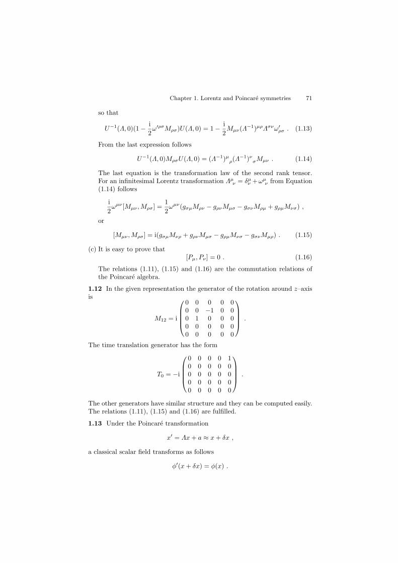
Chapter 1. Lorentz and Poincare symmetries 71

so that

U−1(Λ, 0)(1 − i2ω′ρσMρσ)U(Λ, 0) = 1 − i

2Mµν(Λ−1)µρΛσνω′

ρσ . (1.13)

From the last expression follows

U−1(Λ, 0)MρσU(Λ, 0) = (Λ−1)µρ(Λ

−1)νσMµν . (1.14)

The last equation is the transformation law of the second rank tensor.For an infinitesimal Lorentz transformation Λµ

ν = δµν +ωµ

ν from Equation(1.14) follows

i2ωµν [Mµν ,Mρσ] =

12ωµν(gσµMρν − gρνMµσ − gσνMρµ + gρµMνσ) ,

or

[Mµν ,Mρσ] = i(gσµMνρ + gρνMµσ − gρµMνσ − gσνMµρ) . (1.15)

(c) It is easy to prove that[Pµ, Pν ] = 0 . (1.16)

The relations (1.11), (1.15) and (1.16) are the commutation relations ofthe Poincare algebra.

1.12 In the given representation the generator of the rotation around z–axisis

M12 = i

0 0 0 0 00 0 −1 0 00 1 0 0 00 0 0 0 00 0 0 0 0

.

The time translation generator has the form

T0 = −i

0 0 0 0 10 0 0 0 00 0 0 0 00 0 0 0 00 0 0 0 0

.

The other generators have similar structure and they can be computed easily.The relations (1.11), (1.15) and (1.16) are fulfilled.

1.13 Under the Poincare transformation

x′ = Λx + a ≈ x + δx ,

a classical scalar field transforms as follows

φ′(x + δx) = φ(x) .

72 Solutions

From the last relation we have

φ′(x) = φ(x − δx) = φ(x) − δxµ∂µφ . (1.17)

Form variation of a scalar field is given by

δ0φ = φ′(x) − φ(x) = −δxµ∂µφ . (1.18)

For the Lorentz transformation δxµ = ωµνxν , and therefore

δ0φ = −ωµνxν∂µφ = −12ωµν(xν∂µ − xµ∂ν)φ . (1.19)

On the other handδ0φ = − i

2ωµνMµνφ . (1.20)

By comparing two previous results we get that Lorentz’s generators are

Mµν = i(xµ∂ν − xν∂µ) . (1.21)

For translations δxµ = εµ and

δ0φ = −εµ∂µφ = iεµPµφ . (1.22)

HencePµ = i∂µ . (1.23)

Since[xµ∂ν , xρ∂σ] = gνρxµ∂σ − gσµxρ∂ν , (1.24)

and[xµ∂ν , ∂ρ] = −gρµ∂ν (1.25)

we get the commutation relations of the Poincare algebra:

[Pµ, Pν ] = 0[Mρσ, Pµ] = i(gµσPρ − gµρPσ)

[Mµν ,Mρσ] = i(gσµMνρ + gρνMµσ − gρµMνσ − gσνMµρ) .

1.14

(a) WµPµ = 12εµνρσMνρP σPµ = 0, since product of an antisymmetric with

a symmetric tensor equals zero. Using the same argument, we obtain[Wµ, Pν ] = 0.

(b) Using the result of Problem 1.11 we obtain

W 2 =14εµνρσεµαβγMνρP σMαβPγ

=14εµνρσεµαβγMνρ

(MαβP σ − iδσ

βPα + iδσαPβ

)Pγ

=14εµνρσεµαβγMνρMαβP σPγ . (1.26)

Chapter 1. Lorentz and Poincare symmetries 73

The contraction of two ε symbols in the last line of (1.26) has been calcu-lated in 1.5 so that:

W 2 = −14(δα

ν δβρ δγ

σ + δβν δγ

ρ δασ + δγ

ν δαρ δβ

σ − δβν δα

ρ δγσ − δα

ν δγρ δβ

σ − δγν δβ

ρ δασ )

× MνρMαβP σPγ

= −14(2MνρMνρP

2 − MνρMνσP σPρ + MνρMσνP σPρ+

+ MνρMρσP σPν − MνρMσρPσPν)

= −12MνρMνρP

2 + MνρMνσP σPρ . (1.27)

(c) Using the previous result we have

[W 2,Mρσ] = −12[MµνMµνP 2,Mρσ] + [MµαMναPµPν ,Mρσ] . (1.28)

The first commutator in (1.28) we denote by A, while the second one byB. Using (1.15) we obtain that A = 0; this result is obvious since the P 2

and MµνMµν are Lorentz scalars. The commutator B is

B = MµαMνα (Pµ[Pν ,Mρσ] + [Pµ,Mρσ]Pν) ++Mµα[Mνα,Mρσ]PµPν + [Mµα,Mρσ]MναPµPν . (1.29)

Using the commutation relations (1.11) and (1.15) we get B = 0. There-fore, we have

[W 2,Mρσ] = 0 .

1.15 By using the result of Problem 1.14 (b) and Pµ |pµ, s, σ〉 = pµ |pµ, s, σ〉we get

W 2 |p = 0,m, s, σ〉 = −m2

(12MµνMµν − M0iM

0i

)|p = 0,m, s, σ〉

= −12MijM

ijm2 |p = 0,m, s, σ〉

= −m2((M12)2 + (M13)2 + (M23)2

)|p = 0,m, s, σ〉

= −m2J2 |p = 0,m, s, σ〉= −m2s(s + 1) |p = 0,m, s, σ〉 ,

because Ji = 12εijkMjk are the components of the angular momentum tensor.

1.16

(a) Under Lorentz transformations Wµ transforms according to:

U−1(Λ)WσU(Λ) = ΛσαWα . (1.30)

From Equation (1.30) we have

74 Solutions

i2[Mµν ,Wσ]ωµν = ωµνgσµWν =

12(gσµWν − gσνWµ)ωµν .

From the previous expression we easily obtain the requested result.(b) Using the result of the previous part we have

[Wµ,Wν ] =12εµαβγ [MαβP γ ,Wν ]

=12εµαβγ

(Mαβ [P γ ,Wν ] + [Mαβ ,Wν ]P γ

)

= iεµανγWαP γ .

1.17

(a) Applying the result of Problem 1.16 (a) we get

[Wµ, M2] = −2i(WαMαµ + MαµWα) .

(b) [Mµν ,WµW ν ] = 0. Take care that δµµ = 4.

(c) Using the formula (1.11) we obtain [M2, Pµ] = 2i(PαMαµ + MαµPα) .This result and the result in the first part of this Problem are similar,since Wµ and Pµ are both four-vectors.

(d) [εµνρσMµνMρσ,Mαβ ] = 0.

1.18 In the case of massive particles, m2 > 0 since the Lorentz transfor-mations, Λµ

ν = δµν + ωµ

ν leave pµ invariant (i.e. Λµνpν = pµ) the following

relation is satisfied:

0 ω01 ω02 ω03

ω01 0 −ω12 −ω13

ω02 ω12 0 −ω23

ω03 ω13 ω23 0

m000

=

0000

.

From here followsω01 = ω02 = ω03 = 0, ωij = 0 .

The corresponding generators are M12, M13 and M23 and they are gener-ators of the spatial rotations. Therefore, for massive particles little groupis SO(3). The little group for the quantum mechanical Lorentz group, i.e.SL(2,C) group, is SO(3) = SU(2).For massless particles we have

0 ω01 ω02 ω03

ω01 0 −ω12 −ω13

ω02 ω12 0 −ω23

ω03 ω13 ω23 0

k00k

=

0000

,

which gives ω03 = 0, ω01 = ω13, ω02 = ω23 while the parameter ω12 isarbitrary. It corresponds to the rotation around z–axis. The generator of thistransformation is M12. From the conditions derived above follows that there

Chapter 1. Lorentz and Poincare symmetries 75

are two independent generators M01 + M13 and −(M02 + M23). Note thatW1 = (M02 + M23)k , W2 = −(M01 + M13)k as well as W0 = −M12k. Then,using Problem 1.16 (b) we obtain

[W1,W2] = 0, [W0/k,W1] = −iW2, [W0/k,W2] = iW1 .

These commutation relations define E(2) algebra. Thus, for massless particleslittle group is euclidian group E(2) in two dimensions.

1.19 It is easy to prove that Lorentz transformations, dilatations and SCTform a group. It is the conformal group, C(1, 3). An arbitrary element of thisgroup is

U(ω, ε, ρ, c) = ei(Pµεµ− 12 Mµνωµν+ρD+cµKµ) ,

where D is generator of dilatation, and Kµ are four generators for SCT .Conformal group has 15 parameters. The commutation relations of the algebracan be evaluated from multiplication rules of the group. Let (Λ, a, ρ, c) denotegroup element. If we start from

(Λ−1, 0, 0, 0)(I, 0, 0, c)(Λ, 0, 0, 0) = (I, 0, 0, Λ−1c)

for infinitesimal SCT we obtain

U−1(Λ)KρU(Λ) = (Λ−1)µρKµ .

For infinitesimal Lorentz transformations we get:

[Mµν ,Kρ] = i(gνρKµ − gµρKν). (1.31)

From U−1(Λ, 0, 0, 0)U(I, 0, ρ, 0)U(Λ, 0, 0, 0) = U(I, 0, ρ, 0) , follows

[Mµν ,D] = 0 . (1.32)

Starting from

(I, 0, ρ, 0)−1(I, 0, 0, c)(I, 0, ρ, 0)xµ = (I, 0, ρ, 0)−1(I, 0, 0, c)e−ρxµ

= (I, 0, ρ, 0)−1 e−ρxµ + cµe−2ρx2

1 + 2(c · x)e−ρ + c2e−2ρx2

=xµ + cµe−ρx2

1 + 2(c · x)e−ρ + c2e−2ρx2

= (I, 0, 0, e−ρc)xµ ,

we obtaine−iρD(1 + iKµcµ)eiρD = 1 + iKµe−ρcµ ,

for infinitesimal SCT. From the last expression follows

e−iρDKµeiρD = e−ρKµ .

76 Solutions

This is the transformation law of SCT generators under dilatation. For infin-itesimal dilatations we get:

[D,Kµ] = −iKµ . (1.33)

Similar procedure gives us the following commutators:

[Pµ,D] = −iPµ , (1.34)

[D,D] = 0, (1.35)

[Kµ,Kν ] = 0, (1.36)

[Pµ,Kν ] = 2i(gµνD + Mµν). (1.37)

Equations (1.31)–(1.37) together with (1.11), (1.15) and (1.16) are commuta-tion relations of the conformal algebra.

2

The Klein–Gordon equation

2.1 A particular solution of the Klein–Gordon equation

( + m2)φ(x) = 0 , (2.1)

is plane wave,e−ik·x = e−iEt+ik·x , (2.2)

where E and k are energy and momentum respectively. We see that from

i∂

∂te−ik·x = Ee−ik·x ,

and−i∇e−ik·x = ke−ik·x .

By inserting the solution (2.2) into (2.1) we obtain k2 = m2 i.e. E =±√

k2 + m2 = ±ωk. Therefore, the plane wave (2.2) is a solution of the Klein–Gordon equation if the previous relation is satisfied.

For momentum k there are two independent solutions e−iωkt+ik·x ande+iωkt+ik·x. The general solution of (2.1) is

φ(x) =1

(2π)3/2

∫d3k√2ωk

(a(k)e−i(ωkt−k·x) + b†(−k)ei(ωkt+k·x)

), (2.3)

where a(k) and b†(k) are complex coefficients. In the second term in (2.3) wemake the following change k → −k. After that the formula (2.3) becomes

φ(x) =1

(2π)3/2

∫d3k√2ωk

(a(k)e−ik·x + b†(k)eik·x) , (2.4)

where kµ = (ωk,k). If φ(x) is a real field then a(k) = b(k).

2.2 Using (2.4) we get

78 Solutions

Q = iq∫

d3x

(φ∗ ∂φ

∂t− φ

∂φ∗

∂t

)

= iq

2(2π)3

∫d3xd3kd3k′√

ωkωk′

[(a†(k)eik·x + b(k)e−ik·x)

×(−iωk′a(k′)e−ik′·x + iωk′b†(k′)eik′·x

)−(a(k)e−ik·x + b†(k)eik·x)

×(iωk′a†(k′)eik′·x − iωk′b(k′)e−ik′·x

)]. (2.5)

By integrating over x in (2.5), we obtain

Q = −q

2

∫d3kd3k′

√ωk′

ωk

(−a†(k)a(k′)ei(ωk−ωk′ )tδ(3)(k − k′)

+ a†(k)b†(k′)ei(ωk+ωk′ )tδ(3)(k + k′) − b(k)a(k′)e−i(ωk+ωk′ )tδ(3)(k + k′)

+ b†(k)b(k′)e−i(ωk−ωk′ )tδ(3)(k − k′) + c.c.)

. (2.6)

where c.c. denotes complex conjugation. If in expression (2.6) we integrateover the momentum k′ we obtain

Q =q

2

∫d3k[a†(k)a(k) + a(k)a†(k) − b†(k)b(k) − b(k)b†(k)

]. (2.7)

In the result (2.7) we do not take care about ordering of a(k), a†(k) andb(k), b†(k) since they are complex numbers. This will be different in the Chap-ter 7 where a(k) and b†(k) are going to be operators.

2.3 If we first integrate over x we get

H = −14

∫d3kd3k′√

ωkωk′

(a(k)a(k′)(ωkωk′ + k · k′ − m2)e−i(ωk+ωk′ )tδ(3)(k + k′)

+ a†(k)a†(k′)(ωkωk′ + k · k′ − m2)ei(ωk+ωk′ )tδ(3)(k + k′)− a(k)a†(k′)(ωkωk′ + k · k′ + m2)e−i(ωk−ωk′ )tδ(3)(k − k′)

− a†(k)a(k′)(ωkωk′ + k · k′ + m2)ei(ωk−ωk′ )tδ(3)(k − k′))

. (2.8)

Performing integration over momentum k′, and using the relation k2 + m2 =ω2

k, we obtain

H =12

∫d3kωk

(a†(k)a(k) + a(k)a†(k)

). (2.9)

2.4 Solution of this problem is very similar to the solutions of the previoustwo. The result is

P =∫

d3kka†(k)a(k) .

2.5 The four-divergence of the current jµ is

Chapter 2. The Klein–Gordon equation 79

∂µjµ = − i2(∂µφ∂µφ∗ + φφ∗ − ∂µφ∂µφ∗ − φ∗φ) .

Using the equations of motion we obtain the requested result ∂µjµ = 0.

2.6 It is easy to see that

∂µjµ = − i2

(∂µφ∂µφ∗ + φφ∗ − ∂µφ∂µφ∗ − φ∗φ) −

− q(φAµ∂µφ∗ + φφ∗∂µAµ + φ∗Aµ∂µφ) . (2.10)

The equations of motion are[ − iq(∂µAµ + 2Aµ∂µ − iqAµAµ) + m2

]φ∗(x) = 0 , (2.11)

[ + iq(∂µAµ + 2Aµ∂µ + iqAµAµ) + m2

]φ(x) = 0 . (2.12)

If we multiply Equation (2.11) by φ and Equation (2.12) by φ∗ and thensubtract obtained equations we get

φφ∗ − φ∗φ − 2iq(φφ∗∂µAµ + Aµφ∗∂µφ + Aµφ∂µφ∗) = 0 .

Combining the previous expression and (2.10), one easily obtains

∂µjµ = 0 .

2.7 The equation of motion for a scalar particle in a electromagnetic field is[(∂µ + iqAµ)(∂µ + iqAµ) + m2

]φ(x) = 0 . (2.13)

In the region r < a Equation (2.13) becomes[(

∂

∂t− iV

)(∂

∂t− iV

)− ∆ + m2

]φ(x) = 0 . (2.14)

For stationary states φ(x) = e−iEtF (r) one gets[−(E + V )2 − ∆ + m2

]F (r) = 0 . (2.15)

If we assume that a solution of the previous equation is given by

F =f(r)

rQ(θ, ϕ) ,

then from (2.15) we get the following two equations:

d2f

dr2+[(E + V )2 − m2

]f =

l(l + 1)r2

f , (2.16)

1sin θ

∂

∂θ

(sin θ

∂Q

∂θ

)+

1sin2 θ

∂2Q

∂ϕ2= −l(l + 1)Q . (2.17)

80 Solutions

The particular solutions of (2.17) are spherical harmonics, Ylm. In the casel = 0, the corresponding spherical harmonic Y00 is a constant. The solutionof (2.16) is

f = A sin(qr) + B cos(qr) , (2.18)

whereq2 = [(E + V )2 − m2] > 0 . (2.19)

Constant B has to be zero since function f(r)/r should not be singular in ther → 0 limit. In the region r > a (A0 = 0) the solution is given by

f = Ce−kr + Dekr , (2.20)

where k2 = m2 − E2. But, the constant D has to be zero since the wavefunction has to be finite in the large r limit. Therefore, the wave function is

φ< = Asin qr

r, r < a (2.21)

φ> = Ce−kr

r, r > a . (2.22)

At r = a we should apply the continuity conditions: φ<(a) = φ>(a) andφ′

<(a) = φ′>(a) for the wave function and its first derivative. These boundary

conditions give:A sin(qa) − Ce−ka = 0 , (2.23)

Aq cos(qa) + Cke−ka = 0 . (2.24)

The homogenous system (2.23–2.24) has non-trivial solutions if and only if itsdeterminant is equal to zero. Finally, we obtain the condition

tan(qa)q

= −1k

. (2.25)

The dispersion relation (2.25) will be analyzed graphically in the case V < 2m.Solid line in Fig. 2.1 is function tan(qa)/q while dashed line is

f(q) = −1k

= − 1√2V√

q2 + m2 − V 2 − q2

.

There is only one bound state (in case V < 2m) if the condition

π

2a<√

V (V + 2m) ≤ 3π

2a.

is satisfied.

2.8 The wave equation is

Chapter 2. The Klein–Gordon equation 81

Fig. 2.1. Graphical solution of the dispersion relation (2.25) for V < 2m

[∂2

∂t2−(

∂

∂x+ iqBy

)2

− ∂2

∂y2− ∂2

∂z2+ m2

]φ(x) = 0 . (2.26)

It is easy to see that the operators px = −i ∂∂x and pz = −i ∂

∂z commute withthe Hamiltonian, so we can assume that the solution of (2.26) has the followingform

φ = e−i(Et−kxx−kzz)ϕ(y) . (2.27)

From (2.26) and (2.27) we get(

d2

dy2− (kx + qBy)2 + E2 − k2

z − m2

)ϕ(y) = 0 . (2.28)

Introducing the new variable ξ = kx + qBy, Equation (2.28) takes the sameform as the Schrodinger equation for the oscillator

(d2

dξ2− 1

(qB)2ξ2 +

E2 − k2z − m2

(qB)2

)ϕ(ξ) = 0 .

Then the energy levels are

En =√

m2 + k2z + (2n + 1)qB , n = 0, 1, 2, . . . .

Eigenfunctions are

φn(x) = (qπB)−1/4 1√2nn!

e−iEnt+ikxx+ikzze−(kx+qBy)2/2qBHn(kx + qBy√

qB) ,

(2.29)where Hn are the Hermite polynomials.

2.9 In the region z > 0 the equation of motion is[ − q2U2

0 + 2iqU0∂

∂t+ m2

]φII(x) = 0 . (2.30)

82 Solutions

Substituting φII = Ce−iEt+ikz in (2.30), we get

k = ±K = ±√

(E − qU0)2 − m2 , (2.31)

orE = ±

√k2 + m2 + qU0 . (2.32)

For z < 0 the particle is free and the solution is

φI = Ae−iEt+ipz + Be−iEt−ipz , (2.33)

where p =√

E2 − m2 . The first term in (2.33) is the incident wave, the secondone is the reflected wave. At z = 0 we have to apply the continuity conditions:

φI(0) = φII(0), φ′I(0) = φ′

II(0) .

They give

A =12

(1 +

k

p

)C, B =

12

(1 − k

p

)C . (2.34)

We will separately discuss three different possibilities:Case 1: E > m + qU0.For this value of energy the sign in the expressions (2.31) and (2.32) is plus.The formula for the current has been given in Problem 2.5. The reflectioncoefficient is

R =−(jr)z

(jin)z=

|B|2|A|2 =

∣∣∣∣p − K

p + K

∣∣∣∣2

,

while the transmission coefficient is T = 1 − R.Case 2: E < −m + qU0.In this case the momentum is negative, k = −K. The reflection coefficient isdifferent comparing to the previous case:

R =∣∣∣∣p + K

p − K

∣∣∣∣2

, T = 1 − R .

As we immediately see the reflection coefficient is larger than 1: the potentialis strong enough to create particle–antiparticle pairs. The antiparticles aremoving to the right producing a negative charge current and therefore weobtain negative transmission coefficient. This is Klein paradoxCase 3: |E − qU0| < m.We leave to the reader to show that in this case R = 1, T = 0 .

2.10 For z < 0 and z > 0 a wave function satisfies the free Klein–Gordonequation, while in the region 0 < z < a the equation is

[ − q2U2

0 + 2iqU0∂

∂t+ m2

]φII(x) = 0 .

The solution is given by:

Chapter 2. The Klein–Gordon equation 83

φI = Ae−iEt+ipz + Be−iEt−ipz ,

φII = Ce−iEt+ikz + De−iEt−ikz

φIII = F e−iEt+ipz , (2.35)

where k =√

(E − qU0)2 − m2 and p =√

E2 − m2. From the continuity con-ditions follows:

A + B = C + D ,

A − B =k

p(C − D) ,

Ceika + De−ika = F eipa ,

Ceika − De−ika =p

kF eipa . (2.36)

Thus, one gets:

T =∣∣∣FA

∣∣∣2

=16

|2 + pk + k

p + (2 − pk − k

p )e2ika|2.

If (E − qU0)2 − m2 < 0 the momentum k becomes imaginary, i.e.

k = iκ = i√

m2 − (E − qU0)2 .

2.11 The Klein–Gordon equation for a particle in the Coulomb potential is[(

∂

∂t− ie

Ze

r

)2

− ∆ + m2

]φ(x) = 0 . (2.37)

By substituting φ = e−iEtR(r)Y (θ, ϕ) in (2.37) and using (2.17) we obtain:

− 12m

1r

d2

dr2(rR) +

l(l + 1) − Z2e4

2mr2R − Ze2E

mrR =

E2 − m2

2mR .

This equation has the same form as the Schrodinger equation for hydrogenatom. By comparing these equations we get

En,l = m1√

1 + Z2e4(n − l − 12 ) +

√(l + 1

2 )2 − Z2e4

.

In the nonrelativistic limit the result is

En − m = −mZ2e4

2n2− Z3e6 m

n3

(1

2l + 1− 3

8n

).

2.12 The Klein–Gordon equation in the Schrodinger form is

i∂

∂t

(θχ

)= H

(θχ

), (2.38)

84 Solutions

where the Hamiltonian is given by

H =[− ∆

2m

(1 1−1 −1

)+ m

(1 00 −1

)].

2.13 The eigenequation, Hφ = Eφ in the momentum representation takesthe following form

(p2

2m + m p2

2m

− p2

2m − p2

2m − m

)(θ0

χ0

)= E

(θ0

χ0

). (2.39)

The eigenvalues of the Hamiltonian are evaluated easily and they are E =±ωp = ±

√p2 + m2.

In order to find nonrelativistic limit we suppose that the solution has thefollowing form (

θχ

)=(

θ0

χ0

)e−i(m+T )t , (2.40)

where T is the kinetic energy of the particle. From (2.38) we get(−

2m + m − 2m

2m

2m − m

)(θ0

χ0

)= (m + T )

(θ0

χ0

), (2.41)

i.e. (−

2m+ m

)θ0 −

2m

χ0 = (m + T )θ0 ,

2m

θ0 +(

2m

− m

)χ0 = (T + m)χ0 . (2.42)

From the second equation in (2.42) we obtain

χ0 ≈ 4m2

θ0 , (2.43)

in nonrelativistic limit. Using this the first equation in (2.42) becomes

Tθ0 =(−

2m− 2

8m3

)θ0 . (2.44)

Also, from (2.43) we see that χ0 θ0 and χ is so called small component.From the expression (2.44) follows that first relativistic correction of nonrel-ativistic Hamiltonian is −∇4/8m3.

2.14 Velocity operator is

v =∂H

∂p=

pm

(1 1−1 −1

).

The eigenvalue of the velocity operator is zero.

2.15 Show that⟨ψ†|Hψ

⟩=⟨Hψ†|ψ

⟩. The average value is 〈v〉 = p

m .

3

The γ–matrices

3.1

(a) In the Dirac representation of γ–matrices we have

(γ0)† =(

I 00 −I

)†=(

I 00 −I

)= γ0γ0γ0 = γ0 ,

(γi)† =(

0 σi

−σi 0

)†= −(

0 σi

−σi 0

)= −γ0γ0γi = γ0γiγ0 ,

where we used the facts that (γ0)2 = 1, γ0 and γi anticommute, and thePauli matrices are hermitian. This relation is true in any representation ofγ–matrices which is obtained by a unitary transformation from the Diracrepresentation.

(b) Using the previous result we find

σ†µν = − i

2(γµγν − γνγµ)†

= − i2(γ†

νㆵ − γ†

µγ†ν)

= − i2γ0(γνγµ − γµγν)γ0

= γ0σµνγ0 .

3.2

(a) Taking the adjoint of γ5 we obtain

γ†5 = iγ†

3γ†2γ

†1γ

†0

= iγ0γ3γ0γ0γ2γ0γ0γ1γ0γ0γ0γ0

= iγ0γ3γ2γ1

= −iγ0γ1γ2γ3 = γ5 .

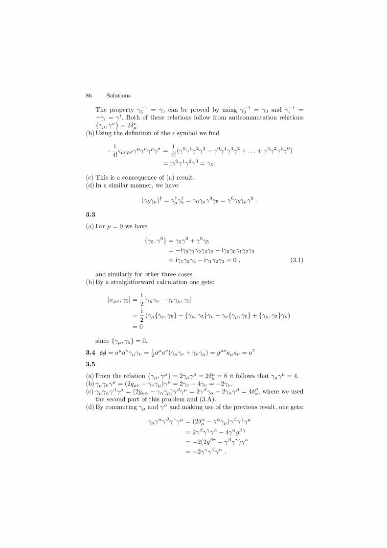
86 Solutions

The property γ−15 = γ5 can be proved by using γ−1

0 = γ0 and γ−1i =

−γi = γi. Both of these relations follow from anticommutation relationsγµ, γν = 2δν

µ.(b) Using the definition of the ε symbol we find

− i4!

εµνρσγµγνγργσ =i4!

(γ0γ1γ2γ3 − γ0γ1γ3γ2 + . . . + γ3γ2γ1γ0)

= iγ0γ1γ2γ3 = γ5.

(c) This is a consequence of (a) result.(d) In a similar manner, we have:

(γ5γµ)† = ㆵγ†

5 = γ0γµγ0γ5 = γ0γ5γµγ0 .

3.3

(a) For µ = 0 we have

γ5, γ0 = γ5γ

0 + γ0γ5

= −iγ0γ1γ2γ3γ0 − iγ0γ0γ1γ2γ3

= iγ1γ2γ3 − iγ1γ2γ3 = 0 , (3.1)

and similarly for other three cases.(b) By a straightforward calculation one gets:

[σµν , γ5] =i2[γµγν − γνγµ, γ5]

=i2

(γµγν , γ5 − γµ, γ5γν − γνγµ, γ5 + γµ, γ5γν)

= 0

since γµ, γ5 = 0.

3.4 /a/a = aµaνγµγν = 12aµaν(γµγν + γνγµ) = gµνaµaν = a2

3.5

(a) From the relation γµ, γµ = 2γµγµ = 2δµµ = 8 it follows that γµγµ = 4.

(b) γµγνγµ = (2gµν − γνγµ)γµ = 2γν − 4γν = −2γν .(c) γµγαγβγµ = (2gµα − γαγµ)γβγµ = 2γβγα + 2γαγβ = 4δβ

α, where we usedthe second part of this problem and (3.A).

(d) By commuting γµ and γα and making use of the previous result, one gets:

γµγαγβγγγµ = (2δαµ − γαγµ)γβγγγµ

= 2γβγγγα − 4γαgβγ

= −2(2gβγ − γβγγ)γα

= −2γγγβγα .

Chapter 3. The γ–matrices 87

(e) By using the definition σµν–matrices, one obtains:

σµνσµν = −14(γµγνγµγν − γµγνγνγµ − γνγµγµγν + γνγµγνγµ) .

By using parts (a) and (b) of this problem, one gets σµνσµν = 12.(f) Use Problem 3.3 and parts (a) and (b) of this problem.(g) By direct calculation, one finds

σαβγµσαβ = −14(γαγβγµγαγβ − γαγβγµγβγα

−γβγαγµγαγβ + γβγαγµγβγα)

= −14(4δβ

µγβ − 4γµ − 4γµ + 4gµβγβ) = 0 .

(h)

σαβσµνσαβ = − i8(γαγβγµγνγαγβ − γαγβγµγνγβγα

−γαγβγνγµγαγβ + γαγβγνγµγβγα − γβγαγµγνγαγβ

+γβγαγµγνγβγα + γβγαγνγµγαγβ − γβγαγνγµγβγα)

= − i8(−8γνγµ − 16gµν + 8γµγν

+16gµν − 16gµν − 8γνγµ + 16gµν + 8γµγν)= −2i(γµγν − γνγµ) = −4σµν .

(i) Use part (g) of this problem.(j) σµνγ5σ

µν = i2 (γµγν − γνγµ)γ5σ

µν = γ5σµνσµν = 12γ5.

3.6

(a) By using the trace property tr(A1A2 . . . An) = tr(A2A3 . . . AnA1), Prob-lem 3.3(a), and (γ5)2 = 1, it follows that

tr(γµ) = tr(γµγ5γ5)= −tr(γ5γµγ5)= −tr((γ5)2γµ)= −tr(γµ) .

From the previous expression we get tr(γµ) = 0.(b) Taking trace of the relation γµ, γν = 2gµν , we easy obtain the requested

result.(c) By applying the basic anticommutation relation (3.A), one gets:

tr(γµγνγργσ) = tr [(2gµν − γνγµ)γργσ]= 2gµνtr(γργσ) − tr[γν(2gµρ − γργµ)γσ]= 2gµνtr(γργσ) − 2gµρtr(γνγσ) + 2gµσtr(γνγρ)− tr(γνγργσγµ) .

88 Solutions

From the previous part of this problem and relation tr(γµγνγργσ) =tr(γνγργσγµ), one easily obtains the requested result.

(d) trγ5 = tr(γ5γ0γ0) = −tr(γ0γ5γ0), where we used Problem 3.3 (a). Further,from the trace property and (γ0)2 = 1 it follows that:

trγ5 = −tr(γ0γ0γ5) = −trγ5 ,

which implies trγ5 = 0.(e) Since γαγα = 4, we have

tr(γ5γµγν) =14tr(γ5γ

αγαγµγν)

=14tr(γαγµγνγ5γ

α)

= −14tr(γ5γαγµγνγα)

= −gµνtr(γ5) = 0 .

In the previous calculation we used the trace property and Problem 3.5(c).

(f) The quantity tr(γ5γµγνγργσ) is an antisymmetric tensor with respect tothe indexes (µ, ν, ρ, σ). Thus, it must be proportional to the Levi-Civitatensor. The constant of proportionality can be determined by substitutingµ = 0, ν = 1, ρ = 2 and σ = 3.

(g) From (γ5)2 = 1, γ5, γµ = 0 and the trace property follows:

tr(/a1 . . . /a2n+1) = tr(γ5γ5/a1 · · · /a2n+1)= (−1)2n+1tr(γ5/a1 · · · /a2n+1γ5)= −tr(γ5γ5/a1 · · · /a2n+1)= −tr(/a1.../a2n+1) .

Hence, tr(/a1 . . . /a2n+1) = 0 .(h) tr(/a1 · · · /a2n) = tr(C/a1C

−1C · · ·C−1C/a2nC−1) , where the matrix C sat-isfies the relation CγµC−1 = −γT

µ . Thus,

tr(/a1 · · · /a2n) = (−1)2ntr(/aT1 · · · /aT

2n) = tr(/a2n · · · /a1) .

(i) tr(γ5γµ) = −itr(γ0γ1γ2γ3γµ) = 0, since it is the trace of odd number ofγ–matrices.

3.7

tr(/a1/a2 · · · /a6) =4 (a1 · a2) [(a3 · a4)(a5 · a6) − (a3 · a5)(a4 · a6) + (a3 · a6)(a4 · a5)]−(a1 · a3) [(a2 · a4)(a5 · a6) − (a2 · a5)(a4 · a6) + (a2 · a6)(a4 · a5)]+(a1 · a4) [(a2 · a3)(a5 · a6) − (a2 · a5)(a3 · a6) + (a2 · a6)(a3 · a5)]−(a1 · a5) [(a2 · a3)(a4 · a6) − (a2 · a4)(a3 · a6) + (a2 · a6)(a3 · a4)]+(a1 · a6) [(a2 · a3)(a4 · a5) − (a2 · a4)(a3 · a5) + (a2 · a5)(a3 · a4)] .

Chapter 3. The γ–matrices 89

3.8 4[pµqν − (p · q)gµν + pνqµ + iεαµβνpαqβ − m2gµν

].

3.9 −2/p − 2γ5/p − 4m − 4mγ5 .

3.10 Expanding the exponential function in series, we find

eγ5/a = 1 + (γ5/a) +12(γ5/a)2 +

13!

(γ5/a)3 + · · · . (3.2)

By substituting (γ5/a)2 = −a2, (γ5/a)3 = −a2(γ5/a), . . . into expression (3.2),we get

eγ5/a = (1 − a2

2!+

a4

4!+ · · ·) + (γ5/a)(1 − a2

3!+

a4

5!− · · ·)

= cos(√

a2) +1√a2

sin(√

a2)γ5/a ,

where a2 = aµaµ.

3.11 The fact that the product of any two Γ–matrices is again a Γ matrix(modulo ±1,±i) can be proved directly. For example, γ5σ01 = −iσ23.Now, we shall prove that Γ–matrices are linearly independent. Multiplyingthe relation

∑a caΓ a = 0 by Γb = (Γ b)−1, we obtain

cbΓbΓb +

∑a=b

caΓ aΓb = 0 ,

where the b–term is separated. Using the ordering lemma, the last expressionbecomes

cbI +∑

d,Γ d =I

cdηΓ d = 0 , (3.3)

where η ∈ ±1,±i. After taking trace of (3.3) and using the fact that

tr(Γ a) =

0, Γ a = I4, Γ a = I

,

one obtains cb = 0 (∀b). This means that Γ–matrices are linearly independentone.

3.12 Multiplying the equation A =∑

a caΓ a by Γb from the right and sepa-rating the b–term in the sum, we have

AΓb = cbΓbΓb +

∑a=b

caΓ aΓb = cbI +∑

d,Γ d =I

cdηΓ d.

Taking the trace of previous relation we obtain the requesting relation.

3.13 The coefficients can be calculated by using the formula obtained in theprevious problem.

90 Solutions

(a) From the traces (which were actually calculated in Problem 3.6):

tr(γµγνγρ) = 0 ,

tr(γµγνγργσ) = 4(gµνgρσ − gµρgνσ + gµσgνρ) ,

tr(γµγνγργσγ5) = −4iεµνρσ ,

tr(γµγνγργ5) = tr(γµγνγρσαβ) = 0 ,

follows γµγνγρ = (gµνgρσ − gµρgσν + gµσgρν)γσ + iεσµνργ5γσ .

(b) γ5γµγν = gµνγ5 + 12εαβ

µνσαβ ,(c) σµνγργ5 = εαµνργ

α − igνργ5γµ + igµργ5γν .

3.14 From Problem 3.13 (a), it follows that γµ, σνρ = −2εαµνργ5γα .

3.15 By applying the result of Problem 3.13 (a) the trace can be transformedas follows

tr(γµγνγργσγαγβγ5) = (gµνgρδ − gµρgνδ + gµδgρν)tr(γδγσγαγβγ5)+ iεδµνρtr(γδγσγαγβ) .

Using 3.6 (c), (f), we get

tr(γµγνγργσγαγβγ5) = 4i(−gµνερσαβ + gµρενσαβ

− gρνεµσαβ + gαβεσµνρ − gσβεαµνρ + gσαεβµνρ) .

3.16 Use the solution of Problem 3.13 (b).

3.17 Applying the formulae

[A,BC] = [A,B]C + B[A,C] ,

and[AB,C] = AB,C − A,CB ,

as well as the anticommutation relations (3.A), we obtain

[γµγν , γργσ] = γµγν , γργσ − γµ, γργνγσ

+ γργµγν , γσ − γργµ, γσγν

= 2gνργµγσ + 2gνσγργµ − 2gµσγργν − 2gµργνγσ .

From the above result we obtain:

[σµν , σρσ] = 2i(gνρσµσ + gµσσνρ − gµρσνσ − gνσσµρ) .

The matrices 12σµν are generators of the Lorentz group in the spinor repre-

sentation.

3.18 Let M be a matrix which commutes with all γ–matrices. Using theProblem 3.11, we can write (Γ b = I)

Chapter 3. The γ–matrices 91

M = cbΓb +∑a=b

caΓ a . (3.4)

On the other hand, we know that there is always a matrix Γ d which anticom-mute with Γ b = I. Multiplying the expression (3.4) by matrix Γd from theleft, and by Γ d from the right, we get:

ΓdMΓ d = −cbΓb +∑a=b

ηcaΓ a . (3.5)

The matrix M commutes with γµ, and therefore with Γ d, so we get

M = −cbΓb +∑a=b

ηcaΓ a . (3.6)

If we now multiply equations (3.4) and (3.6) by Γb and take trace of the re-sulting expressions, we get cb = 0. So, each of the coefficients in the expansion(3.4) is equal to zero except the unit matrix coefficient.

3.19 By applying the Baker–Hausdorff formula

eBAe−B = A + [B,A] +12!

[B, [B,A]] + · · ·

we get

UαU† = α + 2βn − 2(n · α)n − 83!

βn +164!

(α · n)n + · · ·

= α +∞∑

k=1

(−1)k22k

(2k)!(α · n)n +

∞∑k=0

(−1)k22k+1

(2k + 1)!βn , (3.7)

since[βα · n, αi] = nj(βαj , αi − β, αiαj) = 2βni ,

[βα · n, [βα · n, αi]] = −4(α · n)ni ,

[βα · n, [βα · n, [βα · n, αi]]] = −8βni ,

[βα · n, [βα · n, [βα · n, [βα · n, αi]]]] = 16(α · n)ni , etc.

On the other hand, we have the following identities (βα·n)2 = −1, (βα·n)3 =−(βαn), (βα · n)4 = 1, . . . so that

α + (U2 − I)(α · n)n = α + 2βn − 2(α · n)n − 83!

βn + · · ·

= α +∞∑

k=1

(−1)k22k

(2k)!(α · n)n +

∞∑k=0

(−1)k22k+1

(2k + 1)!βn . (3.8)

It is clear that the results (3.7) and (3.8) are equal.

92 Solutions

3.20 It is straightforward to show that the γ–matrices satisfy the relationγµ, γν = 2gµν . The connection with Dirac representation γDirac

µ is given by

γµS = SγDiracµ . (3.9)

This statement is known as the fundamental (Pauli) theorem. If we substitute

S =(

a bc d

), where a, b, c, d are 2 × 2 matrices, into (3.9) we find

(c da b

)=(

a −bc −d

),

(−σic −σidσia σib

)=(

bσi −aσi

dσi −cσi

). (3.10)

The solution of (3.10) is a = −b = c = d = I. A particular solution for S isgiven by

S =1√2

(I −II I

).

The matrices σµν are

σoi = −i(−σi 00 σi

), σij = εijk

(σk 00 σk

), (3.11)

while

γ5 = iγ0γ1γ2γ3 =(−I 00 I

). (3.12)

3.21 Matrices

γ0 = σ1 =(

0 11 0

)

and

γ1 = −iσ2 =(

0 −11 0

)

have the following properties:

(γ0)2 = 1, (γ1)2 = −1, γ0γ1 = −γ1γ0 ,

hence, they satisfy the Clifford algebra (3.A). The matrix γ5 is defined by

γ5 = γ0γ1 =(

1 00 −1

).

tr(γ5γµγν) is an antisymmetric tensor and it should be proportional to εµν :

tr(γ5γµγν) = Cεµν .

By fixing µ = 0, ν = 1 we obtain1 C = 2. One can easily show that

γ5γµ = εµνγν .

1 Our sign convention is ε01 = +1 .

4

The Dirac equation

4.1 In terms of α and β matrices, the Dirac Hamiltonian has the formHD = α · p + βm, so that:

(a) [HD,p ] = 0,(b) [HD, Li] = εijk[α · p + βm, xjpk] = εijkαl[pl, xj ]pk = −iεijkαjpk = i(p ×

α)i,(c) [HD,L2] = −iεijkαj(Lipk + pkLi) = 0,(d) [HD, Si] = − i

4 [HD, εijkαjαk] = iεijkpkαj = −i(p × α)i,(e) By applying (b) and (d) we get that this commutator vanishes.(f) [HD,J2] = 0,(g) From (d) we have [HD,Σ · p] = − i

2|p|εijkpjαkpi = 0,

(h) If vectors n and p are collinear, then the commutator vanishes. In theopposite case it is not zero.

4.2 The plane wave

ψ =(

ϕχ

)e−ip·x , (4.1)

is a particular solution of the Dirac equation,

(iγµ∂µ − m)ψ(x) = 0 . (4.2)

By substituting (4.1) in (4.2) (in the Dirac representation of γ–matrices) weobtain (

E − m −σ · pσ · p −E − m

)(ϕχ

)= 0 , (4.3)

where E and p are the energy and momentum of the particle, respectively.Nontrivial solutions of the homogeneous system (4.3) exist if and only if itsdeterminant vanishes. This gives the following relation between energy andmomentum: E = ±

√p2 + m2 = ±Ep, which tells us that there are solutions

of positive and negative energy as we expected.

94 Solutions

For the positive energy solution, E = Ep, the system (4.3) has the followingform:

(Ep − m)ϕ − (σ · p)χ = 0 ,

(σ · p)ϕ − (Ep + m)χ = 0 . (4.4)

These relations imply:χ =

σ · pEp + m

ϕ , (4.5)

or

u(Ep,p) =(

ϕχ

)=(

ϕσ·p

Ep+mϕ

), (4.6)

where ϕ is arbitrary. For the negative energy solution, E = −Ep, the system(4.3) is solved by

u(−Ep,p) =(

ϕχ

)=(− σ·p

Ep+mχχ

). (4.7)

If we introduce the notation v(p) = u(−Ep,−p) and u(p) = u(Ep,p), linearlyindependent solutions of Equation (4.2), for fixed p, are given as

u(p)e−ip·x, v(p)eip·x,

where pµ = (Ep,p). Note the change of sign in the negative energy solu-tion. The energy and momentum of the solution u(p)e−ip·x are Ep and p,respectively, while for v(p)eip·x, they are −Ep and −p. In order to find theadditional degrees of freedom, let us recall that the helicity operator 1

2Σ · p,where p = p/|p|, commutes with the Dirac Hamiltonian [see Problem 4.1 (g)].From the eigenequation

σ · pϕ = ±ϕ ,

(and a similar equation for χ) we obtain

ϕ1 =1√

2(1 + p3)

(p3 + 1

p1 + ip2

), ϕ2 =

1√2(1 + p3)

(−p1 + ip2

p3 + 1

), (4.8)

(and similarly for χr, r = 1, 2). If we take p = pez, the basis vectors become(

10

),

(01

). (4.9)

Then, the basis bispinors are

Chapter 4. The Dirac equation 95

u1(p) = Np

(10

)

σ·pEp+m

(10

)

, u2(p) = Np

(01

)

σ·pEp+m

(01

)

,

v1(p) = Np

σ·pEp+m

(01

)

(01

)

, v2(p) = Np

σ·pEp+m

(10

)

(10

)

,

(4.10)

where Np =√

Ep+m2m is the normalization factor. Do not forget that p = pez

i.e. p · σ = pσ3. In this case, the bispinors (4.10) form the helicity basis. Forarbitrary momentum p we have to use (4.8) instead of (4.9), if we want toconstruct the helicity basis. Although, in that case vectors in (4.10) are alsoa base, but not the helicity one. Spinors u and v are normalized according to(4.D).

General solution of (4.2) is given by

ψ =1

(2π)3/2

2∑r=1

∫d3p

√m

Ep

(ur(p)cr(p)e−ip·x + vr(p)d

†

r(p)eip·x)

. (4.11)

The Dirac spinor (bispinor) ψ contains two SL(2,C) spinors, as is easily seen inthe chiral (Weyl) representation. The Dirac spinor is transformed accordingto the (1/2, 0) ⊕ (0, 1/2) reducible representation of the quantum Lorentzgroup (i.e. SL(2,C) group, which is universally covering group for the Lorentzgroup).

4.3 The states us(p), vs(p) are eigenstates of the energy operator, i ∂∂t with

eigenvalues Ep and −Ep, respectively.

4.4 By using the expressions for the Dirac spinors found in Problem 4.2, weobtain

∑r ur(p)ur(p) =

Ep+m2m

(ϕ1ϕ

†1 + ϕ2ϕ

†2 −(ϕ1ϕ

†1 + ϕ2ϕ

†2)

σ·pEp+m

σ·pEp+m (ϕ1ϕ

†1 + ϕ2ϕ

†2) − σ·p

Ep+m (ϕ1ϕ†1 + ϕ2ϕ

†2)

σ·pEp+m

),

where ϕr (r = 1, 2) are given by (4.8). They satisfy the completeness relationϕ1ϕ

†1 + ϕ2ϕ

†2 = I. Using also (p · σ)2 = p2 = E2

p − m2, we get

2∑r=1

ur(p)ur(p) =1

2m

(Ep + m −σ · pσ · p −Ep + m

)=

/p + m

2m.

The second identity can be shown in a similar manner.

4.5 Using the expressions for the projectors given in Problem 4.4, we see that

96 Solutions

Λ2+ =

14m2

(/p2 + 2m/p + m2) = Λ+ ,

where we have used /p2 = p2 = m2. Similarly, we obtain Λ2− = Λ−. Orthogo-

nality of the projectors follows from the identity

(/p + m)(/p − m) = p2 − m2 = 0 .

At this stage we apply the Dirac equation in momentum space (4.C). Namely,

Λ+ur(p) =1

2m(/p + m)ur(p) =

12m

(m + m)ur(p) = ur(p) ,

Λ−ur(p) =1

2m(/p − m)ur(p) =

12m

(m − m)ur(p) = 0 .

Similarly, one can prove the identities Λ−vr(p) = 0, Λ+vr(p) = vr(p).

4.6

(a) We can directly prove this property. For example, the x–component of thevector Σ is

Σ1 =i2(γ2γ3 − γ3γ2) = iγ2γ3 .

On the other hand, γ5γ0γ1 = iγ1γ2γ3γ

1 = iγ2γ3. The corresponding iden-tities for the y and z–components can be proven in a similar way.

(b) By applying the definition of Σ, we have

[Σi, Σj ] = −14εilmεjpq[γlγm, γpγq]

= −14εilmεjpq

([γlγm, γp]γq + γp[γlγm, γq]

). (4.12)

Next step is to expand the commutators in terms of the anticommutators:

[Σi, Σj ] = −14εilmεjpq

(γlγm, γpγq − γl, γpγmγq

+γpγlγm, γq − γpγl, γqγm)

. (4.13)

Then, using anticommutation relations (3.A) we get

[Σi, Σj ] = −12εilmεjpq

(gmpγlγq − glpγmγq + gmqγpγl − glqγpγm

).

(4.14)The first term in (4.14) has the form

εilmεjpqgmpγlγq = (δijδlq − δiqδlj)γlγq = −3δij − γjγi .

Others terms in (4.14) can be transformed in the same way. Finally,

[Σi, Σj ] = γjγi − γiγj .

Chapter 4. The Dirac equation 97

On the other hand,

2iεijkΣk = −εijkεklmγlγm = γjγi − γiγj ,

so that[Σi, Σj ] = 2iεijkΣk .

We conclude that operators 12Σ are the generators of SU(2) subgroup of

the Lorentz group1

(c) S2 = − 14Σ

2 = − 14 (γ5γ0γ)2 = 1

4γ · γ = − 34 .

4.7 Use the expressions σ · pϕr = (−1)r+1ϕr and σ · pχr = (−1)rχr fromProblem 4.2. For example:

Σ · p|p| ur(p) =

Σ · p|p| N

(ϕr

σ·pEp+mϕr

)

= N(

σ · p 00 σ · p

)(ϕr

σ·pEp+mϕr

)

= N(

σ · pϕr(σ·p)(σ·p)

Ep+m ϕr

)

= (−1)r+1N(

ϕrσ·p

Ep+mϕr

)

= (−1)r+1ur(p) ,

where N is the normalization factor. It is easy to see that the spinors ur(p)and vr(p) are not eigenspinors of the operator Σ · n, unless vectors n and pare parallel.

4.8 The transformation operator from the rest frame to the frame movingalong the z–axis with velocity v, is S(Λ(vez)) = e−

i2 ω03σ03

. By using therelation ω03 = −ϕ = − arctan(v), we obtain

S(Λ) = cosh(ϕ

2

)I − sinh

(ϕ

2

)( 0 σ3

σ3 o

)

=

√Ep + m

2m

(I − pσ3

Ep+m

− pσ3Ep+m I

).

For arbitrary boost, σ3p should be replaced by σ ·p. The operator S(Λ) is notunitary one. Since the Lorentz group is noncompact, it does not have finitedimensional irreducible unitary representations.

4.9 In this case we have

S =(

cos(

θ2

)+ i sin

(θ2

)σ3 0

0 cos(

θ2

)+ i sin

(θ2

)σ3

).

1 Recall that Σk = 12εkijσij .

98 Solutions

This operator is unitary because SO(3) is a compact subgroup of the Lorentzgroup.

4.10 The Pauli–Lubanski vector is

Wµ =12εµνρσ(ixν∂ρ − ixρ∂ν +

12σνρ)i∂σ =

i4εµνρσσνρ∂σ , (4.15)

since the product of a symmetric and an antisymmetric tensors vanishes. Then

W 2ψ(x) = − 116

εµνρσεµαβγσνρσαβ∂σ∂γψ(x)

=116

(δναδρ

βδσγ − δν

αδσβδρ

γ + δραδσ

βδνγ−

− δραδν

βδσγ + δσ

αδνβδρ

γ − δσαδρ

βδνγ

)σνρσ

αβ∂σ∂γψ(x)

=116(2σαβσαβ − 4σαγσαρ∂

ρ∂γ

)ψ

=34ψ

= −34m2ψ ,

where we used identityσµσσµν = 2γσγν + δν

σ

and the results of Problems 1.5 and 3.5.

4.11 It is easy to see (Problem 3.16 and the condition s · p = 0) that

Wµsµ

m=

14m

εµνρσσνρP σsµ =1

2mγ5σµσsµ∂σ

=i

2mγ5(γµγσ − gµσ)(∓ipσ)sµ = ± 1

2mγ5/s/p =

12γ5/s .

The previous equation holds on space of plane wave solutions; upper (lower)sing is related to positive (negative) energy solutions. In the rest frame, the

vector sµ becomes (0,n), so /s = −n · γ, and we can use /pm = p0γ0

m = γ0, sothat

W · sm

= ±12γ5γ0n · γ = ±1

2Σ · n .

where Problem 4.6 has been used.

4.12 Positive energy solutions satisfy

γ5/su(p,±s) = ±u(p,±s) . (4.16)

If we choose that polarization vector sµ in the rest frame equals (0,n = p|p| ),

according to the formulation of this problem, then in the frame in which

Chapter 4. The Dirac equation 99

electron has momentum p, the polarization vector is obtained by applying aLorentz boost:

sµ =

(Ep

mpj

mpi

m δij + pipj

m(Ep+m)

)(0nj

)

=( p·n

m

n + (n·p)pm(Ep+m)

).

For n = p/|p| we get sµ = ( |p|m ,Ep

m n). Using that, we find

γ5/su(p,±s) =1m

γ5/s/pu(p,±s)

=1m

γ5

(|p|m

γ0 −Ep

mγ · n

)(Epγ0 − p · γ)u(p,±s) .

If we insert (p · γ)2 = −p2 in the previous formula we obtain:

γ5/su(p,±s) = γ5γ0γ · p|p|u(p,±s) =

Σ · p|p| u(p,±s) . (4.17)

From the expressions (4.16) and (4.17) we get

Σ · p|p| u(p,±s) = ±u(p,±s) .

The similar procedure can be done for negative energy solutions. Startingfrom

γ5/sv(p,±s) = ±v(p,±s) ,

one getsΣ · p|p| v(p,±s) = ∓v(p,±s) .

4.13 In the ultrarelativistic limit, m Ep, the vector sµ is given by

sµ ≈(

Ep

m,pm

)≈ pµ

m.

Then we have

γ5/su(p,±s) ≈ γ5/pm

u(p,±s) = γ5u(p,±s) , (4.18)

where we used the Dirac equation /pu(p,±s) = mu(p,±s). From (4.18) weconclude that the helicity operator Σ ·p/|p| is equal to the chirality operatorγ5. The eigenequation becomes

γ5u(p,±s) = ±u(p,±s) .

100 Solutions

For v spinors the situation is similar. So, for the particles of high energy (i.e.neglected mass) helicity and chirality are approximatively equal, while formassless particles these two quantities exactly are equal.

4.14 The commutator between γ5/s and /p is

[γ5/s, /p] = γ5/s/p − /pγ5/s= γ5(/s/p + /p/s)= γ5s

µpνγµ, γν= 2s · pγ5 = 0 .

From (γ5/s)2 = −s2 = 1 it follows that eigenvalues of the operator γ5/s are ±1.Then the eigen projectors are

Σ(±s) =1 ± γ5/s

2.

4.15 The average value of Σ · n in state

ψ(x) =

√Ep + m

2m

(ϕ

σ·pEp+mϕ

)e−ip·x , (4.19)

is

〈Σ · n〉 =∫

d3xψ†(x)Σ · nψ(x)∫d3xψ†(x)ψ(x)

=Ep + m

2Ep

(ϕ†σ · nϕ +

ϕ†(σ · p)(σ · n)(σ · p)ϕ(Ep + m)2

). (4.20)

Since(σ · A)(σ · B) = A · B + i(A × B) · σ (4.21)

it follows that

(σ · p)(σ · n)(σ · p) = |p|2(n3σ3 − n2σ2 − n1σ1) . (4.22)

By substituting (4.22) into (4.20) we get:

〈Σ · n〉 =1

|a|2 + |b|2

×[Ep + m

2Ep

(n3|a|2 + (n1 + in2)b∗a + (n1 − in2)a∗b − n3|b|2

)

+Ep − m

2Ep

(n3|a|2 + (−n1 + in2)a∗b − (n1 + in2)b∗a − n3|b|2

)].

In the nonrelativistic limit we obtain

〈Σ · n〉 = ϕ†σ · nϕ =n3|a|2 + (n1 + in2)b∗a + (n1 − in2)a∗b − n3|b|2

|a|2 + |b|2 .

Chapter 4. The Dirac equation 101

4.16 In the rest frame a spinor takes the following form(

ϕ0

)e−imt, where

ϕ satisfies12Σ · n

(ϕ0

)=

12

(ϕ0

).

The last condition becomes(

cos θ −i sin θi sin θ − cos θ

)(ab

)=(

ab

), (4.23)

where we put ϕ =(

ab

). From the last expression we obtain

ϕ =(

cos θ2

i sin θ2

). (4.24)

In the rest frame the Dirac spinor takes the form

ψ0 =

cos θ2

i sin θ2

00

e−imt . (4.25)

Applying the boost along z−axis, we obtain

ψ(x) = S(−pez)ψ0 , (4.26)

where S is given in Problem 4.8. Note a minus sign appearing in S(−pez)!After a simple calculation, we obtain

ψ(x) =

√Ep + m

2m

cos θ2

i sin θ2

p·σEp+m

(cos θ

2

i sin θ2

)

e−ip·x . (4.27)

The mean value of the operator 12γ5/s is

⟨12γ5/s⟩

=12

∫d3xψ†γ5/sψ∫

d3xψ†ψ, (4.28)

where the vector sµ is obtained from (0,n) by the Lorentz boost along thez–axis. The components of vector sµ are (see Problem 4.12)

s0 =n · pm

, s = n +(n · p)p

m(Ep + m).

In our case we have

102 Solutions

sµ =(

p

mcos θ, 0, sin θ,

Ep

mcos θ

).

Thus, in the Dirac representation of γ–matrices, γ5/s is given by

γ5/s =(

s · σ −s0Is0I −s · σ

), (4.29)

and finally

γ5/s =

Ep

m cos θ −i sin θ − pm cos θ 0

i sin θ −Ep

m cos θ 0 − pm cos θ

pm cos θ 0 −Ep

m cos θ i sin θ

0 pm cos θ −i sin θ

Ep

m cos θ

. (4.30)

By substituting (4.30) and (4.27) in the formula (4.28), we obtain:⟨

12γ5/s⟩

=12

,

as we expected, because ψ(x) is the eigenstate of the operator 12γ5/s, with

eigenvalue 12 .

4.17 The Dirac Hamiltonian can be rewritten in terms of γ–matrices so that

[HD, γ5] = [γ0γ · p + γ0m, γ5] = 2mγ0γ5 .

Thus, the operator γ5 is a constant of motion in the case of massless Diracparticle. Its eigenvalues and eigen projectors are ±1, Σ± = 1

2 (1± γ5), respec-tively. The operator γ5 is known as the chirality operator.

4.18 By multiplying the Dirac equation from the left by γ5, we obtain (i/∂ +m)γ5ψ = 0. By adding and subtracting the previous equations and the Diracequation, we get

i/∂ψL − mψR = 0,

i/∂ψR − mψL = 0 .

4.19

(a) The system of equations can be rewritten as the Dirac equation. The Diracspinor takes form

ψ =(

ψL

ψR

),

while

γµ =(

0 σµ

σµ 0

),

are γ–matrices (see Problem 3.20).

Chapter 4. The Dirac equation 103

(b) In order to be covariant, these equations have to have the following form

iσµ∂′µψ′

R(x′) = mψ′L(x′) , (4.31)

iσµ∂′µψ′

L(x′) = mψ′R(x′) , (4.32)

in the primed frame (x′ = Λx). If we assume that the new spinors takethe form ψ′

L(x′) = SLψL(x) and ψ′R(x′) = SRψR(x), where SL and SR are

nonsingular 2 × 2 matrices, Equations (4.31) and (4.32) become

iσµSRΛµν∂νψR(x) = mSLψL(x) , (4.33)

iσµSLΛµν∂νψL(x) = mSRψR(x) . (4.34)

By multiplying Equation (4.33) by S−1L from left, and (4.34) by S−1

R alsofrom left we obtain

iS−1L σµSRΛµ

ν∂νψR(x) = mψL(x) , (4.35)

iS−1R σµSLΛµ

ν∂νψL(x) = mψR(x) . (4.36)

The system of equations is covariant if the conditions

S−1R σµSL = Λµ

ν σν ,

S−1L σµSR = Λµ

νσν

hold. The solution for matrices SL and SR is given as

SL = exp(

12ϕiσ

i +i2θkσk

)≈ 1 +

12ϕiσ

i +i2θkσk , (4.37)

SR = exp(−1

2ϕiσ

i +i2θkσk

)≈ 1 − 1

2ϕiσ

i +i2θkσk . (4.38)

The parameters θi and ϕi were defined in Problem 1.8. Boost along thex–axis is defined by :

SL = cosh(ϕ1

2

)+ σ1 sinh

(ϕ1

2

)(4.39)

SR = cosh(ϕ1

2

)− σ1 sinh

(ϕ1

2

). (4.40)

Note that ψL and ψR transform in the same way under rotations, but dif-ferently under boosts. The left ψL, and right ψR spinors transform under( 12 , 0) and (0, 1

2 ) irreducible representation of the Lorentz group respec-tively.

104 Solutions

4.20 First note that

[HD,K] = [α · p, β(Σ · L)] + [α · p, β] + m[β, β(Σ · L)] . (4.41)

The first term in the expression (4.41) is

[α · p, β(Σ · L)] = β[α · p,Σ · L] + [α · p, β]Σ · L

= − i2εmnpεmjlβ

(piαi, αnαpxjpl − piαnαi, αpxjpl+

+ αnαpαi[pi, xj ]pl − 2αiαnαppixjpl)

.

Using the relations αi, αj = 2δij and [xi, pj ] = iδij , we obtain

[α · p, β(Σ · L)] = − i2β(4αlpnxnpl − 4αjplxjpl−

− iαjαlαjpl + 3iαipi − 2αiαjαlpixjpl + 2αiαlαjpixjpl)

= iβ(2αiplxipl − 2iα · p − αjαiαlpixjpl − αiαlαjpixjpl

),

where we used αiαjαi = −αj . By substituting pixj = xjpi − iδij into the lastline of previous formula, we have

[α · p, β(Σ · L)] = 2β(α · p) . (4.42)

The second term in (4.41) is −2β(α ·p), while the third term vanishes. Thus,

[HD,K] = 0 .

4.21 From (3.E) we have

iu(p1)σµν(p1 − p2)νu(p2) =12u(p1)(γνγµ − γµγν)(p1 − p2)νu(p2)

=12u(p1)[−γµ(/p1 − /p2) + (/p1 − /p2)γµ]u(p2)

=12u(p1)[−γµ(/p1 − m) + (m − /p2)γµ]u(p2) .

By using γµ/p1 = 2pµ1 − /p1γ

µ and /p2γµ = 2pµ

2 − γµ/p2 we obtain

iu(p1)σµν(p1 − p2)νu(p2) = 2mu(p1)γµu(p2) − (p1 + p2)µu(p1)u(p2) ,

where we used that u(p) and u(p) satisfy the Dirac equation. The last expres-sion is the requested identity. The second identity can be proven similarly.

4.23 It is easy to see that

γαγµγβ = 2gαµγβ − 2gαβγµ + 2gµβγα − γβγµγα . (4.43)

From (4.43) we have

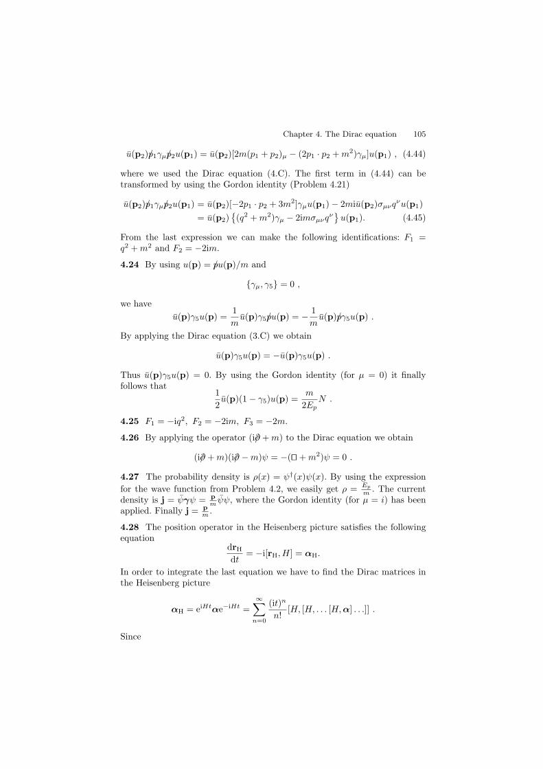
Chapter 4. The Dirac equation 105

u(p2)/p1γµ/p2u(p1) = u(p2)[2m(p1 + p2)µ − (2p1 · p2 + m2)γµ]u(p1) , (4.44)

where we used the Dirac equation (4.C). The first term in (4.44) can betransformed by using the Gordon identity (Problem 4.21)

u(p2)/p1γµ/p2u(p1) = u(p2)[−2p1 · p2 + 3m2]γµu(p1) − 2miu(p2)σµνqνu(p1)= u(p2)

(q2 + m2)γµ − 2imσµνqν

u(p1). (4.45)

From the last expression we can make the following identifications: F1 =q2 + m2 and F2 = −2im.

4.24 By using u(p) = /pu(p)/m and

γµ, γ5 = 0 ,

we haveu(p)γ5u(p) =

1m

u(p)γ5/pu(p) = − 1m

u(p)/pγ5u(p) .

By applying the Dirac equation (3.C) we obtain

u(p)γ5u(p) = −u(p)γ5u(p) .

Thus u(p)γ5u(p) = 0. By using the Gordon identity (for µ = 0) it finallyfollows that

12u(p)(1 − γ5)u(p) =

m

2EpN .

4.25 F1 = −iq2, F2 = −2im, F3 = −2m.

4.26 By applying the operator (i/∂ + m) to the Dirac equation we obtain

(i/∂ + m)(i/∂ − m)ψ = −( + m2)ψ = 0 .

4.27 The probability density is ρ(x) = ψ†(x)ψ(x). By using the expressionfor the wave function from Problem 4.2, we easily get ρ = Ep

m . The currentdensity is j = ψγψ = p

m ψψ, where the Gordon identity (for µ = i) has beenapplied. Finally j = p

m .

4.28 The position operator in the Heisenberg picture satisfies the followingequation

drH

dt= −i[rH,H] = αH.

In order to integrate the last equation we have to find the Dirac matrices inthe Heisenberg picture

αH = eiHtαe−iHt =∞∑

n=0

(it)n

n![H, [H, . . . [H,α] . . .]] .

Since

106 Solutions

[H,α] = 2(p − αH) , (4.46)

[H, [H,α]] = −22(p − αH)H , (4.47)

[H, [H, [H,α]]] = 23(p − αH)H2 , etc. (4.48)

we get

αH = α + (αH − p)(−2it +

(2it)2

2!H − (2it)3

3!H2 + . . .

)

=pH

+(α − p

H

)e−2itH . (4.49)

Then, equationdrH

dt=

pH

+(α − p

H

)e−2itH (4.50)

implies

rH = r +pH

t − i(α − p

H

) 12H

+ i(α − p

H

) 12H

e−2iHt.

The integration constant is determined using the condition rH(t = 0) = r.As we see ”the motion of particle” is a superposition of classical uniform andrapid oscillatory motions.

4.29 We should calculate the coefficients cr(p) and d∗r(p) in the expansion

ψ(0,x) =1

(2π)3/2

∑r

∫d3p√

m

Ep(cr(p)ur(p)eip·x + d∗r(p)vr(p)e−ip·x) .

(4.51)If we multiply this expression by u†

s(q)e−iq·x from left and integrate over x,we get

cs(q) =1

(2π)3/2

√m

Eq

∫d3xu†

s(q)ψ(0,x)e−iq·x ,

where we applied the relations

u†r(p)us(p) = v†

r(p)vs(p) =Ep

mδrs, v†

r(−p)us(p) = u†r(−p)vs(p) = 0 .

(4.52)These relations can be obtained from (4.D) by using the Gordon identity.Similarly for d coefficients we get

d∗s(q) =1

(2π)3/2

√m

Eq

∫d3xv†

s(q)ψ(0,x)eiq·x .

Carrying out the integrations, we find

Chapter 4. The Dirac equation 107

c1(p) =1

(2π)3/2

√Ep + m

2Ep,

c2(p) = 0,

d∗1(p) =1

(2π)3/2

1√2Ep(Ep + m)

(px + ipy) ,

d∗2(p) =1

(2π)3/2

1√2Ep(Ep + m)

pz . (4.53)

The wave function at time t > 0 is

ψ(x) =1

(2π)3/2

∑r

∫d3p

√m

Ep(cr(p)ur(p)re−ip·x+d∗r(p)vr(p)eip·x) , (4.54)

where the coefficients cr(p) and d∗r(p) are given in (4.53).

4.30 In this case the coefficients cr(p) and d∗r(p) in expansion (4.51) are:

c1(p) =(

d2

π

)3/4√

Ep + m

2Epe−d2p2/2 ,

c2(p) = 0 ,

d∗1(p) =(

d2

π

)3/4 1√2Ep(Ep + m)

e−d2p2/2(px + ipy) ,

d∗2(p) =(

d2

π

)3/4 1√2Ep(Ep + m)

pze−d2p2/2 .

4.31 The equation for spin 1/2 particle in the electromagnetic field has thefollowing form

[iγµ(∂µ − ieAµ) − m]ψ = 0 . (4.55)

If we assume that a wave function for z > 0 has the form

ψ =(

ϕχ

)e−iEt+iqz , (4.56)

then (4.55) becomes(

E − m − V −σ3qσ3q −E − m + V

)(ϕχ

)= 0 . (4.57)

The system of equations (4.57) has a nontrivial solution if and only if

E = V ±√

q2 + m2 . (4.58)

The wave function2 is2 From the boundary conditions it follows that there is no spin flip.

108 Solutions

ψI = a

10

pσ3(E+m)

(10

) e−iEt+ipz

+ b

10

−pσ3(E+m)

(10

) e−iEt−ipz , z < 0 , (4.59)

ψII = d

10

qσ3(E+m−V )

(10

) e−iEt+iqz, z > 0 ,

where p =√

E2 − m2. The terms proportional to the coefficient a, b and din (4.59) are the initial ψin, reflected ψr and transmitted wave ψt. Since theDirac equation is the first order equation, the continuity condition is satisfiedfor the wave function only. The condition ψI(0) = ψII(0) gives

a + b = d , (4.60)a − b = rd , (4.61)

where r = E+mE+m−V

qp . Now, we will consider three cases:

1. If |E − V | ≤ m, the momentum q is imaginary, q = iκ so that the wavefunction exponentially decreases in the region z > 0, as is the case in nonrela-tivistic quantum mechanics. The transmitted, reflected and incident currentsare:

jr = ψtrγ3ψtrez = 0 , (4.62)

jr = ψrγ3ψrez = − 2p

E + m|b|2ez , (4.63)

jin = ψinγ3ψinez =2p

E + m|a|2ez . (4.64)

Since jtr = 0 the transmission coefficient is zero. The reflection coefficient is

R =−jr

jin=∣∣∣∣p(E + m − V ) − iκ(E + m)p(E + m − V ) + iκ(E + m)

∣∣∣∣2

= 1 . (4.65)

2. If V < E − m, the momentum q is real. The currents are:

jtr =2q

E + m − V|d|2ez , (4.66)

jr = − 2p

E + m|b|2ez , (4.67)

jin =2p

E + m|a|2ez . (4.68)

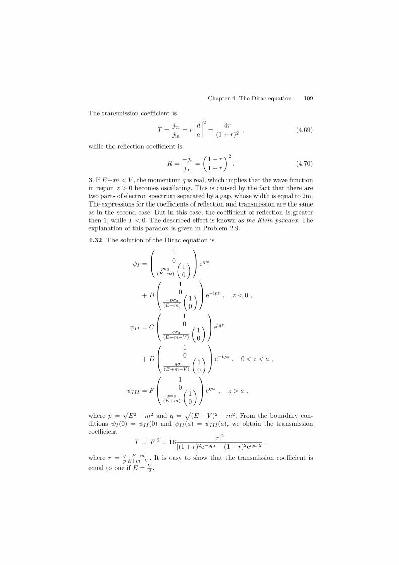
Chapter 4. The Dirac equation 109

The transmission coefficient is

T =jtrjin

= r

∣∣∣∣d

a

∣∣∣∣2

=4r

(1 + r)2, (4.69)

while the reflection coefficient is

R =−jrjin

=(

1 − r

1 + r

)2

. (4.70)

3. If E+m < V , the momentum q is real, which implies that the wave functionin region z > 0 becomes oscillating. This is caused by the fact that there aretwo parts of electron spectrum separated by a gap, whose width is equal to 2m.The expressions for the coefficients of reflection and transmission are the sameas in the second case. But in this case, the coefficient of reflection is greaterthen 1, while T < 0. The described effect is known as the Klein paradox. Theexplanation of this paradox is given in Problem 2.9.

4.32 The solution of the Dirac equation is

ψI =

10

pσ3(E+m)

(10

) eipz

+ B

10

−pσ3(E+m)

(10

) e−ipz , z < 0 ,

ψII = C

10

qσ3(E+m−V )

(10

) eiqz

+ D

10

−qσ3(E+m−V )

(10

) e−iqz , 0 < z < a ,

ψIII = F

10

pσ3(E+m)

(10

) eipz , z > a ,

where p =√

E2 − m2 and q =√

(E − V )2 − m2. From the boundary con-ditions ψI(0) = ψII(0) and ψII(a) = ψIII(a), we obtain the transmissioncoefficient

T = |F |2 = 16|r|2

|(1 + r)2e−iqa − (1 − r)2eiqa|2 ,

where r = qp

E+mE+m−V . It is easy to show that the transmission coefficient is

equal to one if E = V2 .

110 Solutions

4.33

(a) The wave function is

ψI =

BB′

−iκσ3(E+m)

(BB′

) eκz, z < −a,

ψII =

CC ′

qσ3(E+m+V )

(CC ′

) eiqz (4.71)

+

DD′

−qσ3(E+m+V )

(DD′

) e−iqz, −a < z < a,

ψIII =

FF ′

iκσ3(E+m)

(FF ′

) e−κz, z > a,

where κ =√

m2 − E2 and q =√

(E + V )2 − m2. Since there is no spinflip, we can take B′ = C ′ = D′ = F ′ = 0. From the boundary conditionsψI(−a) = ψII(−a) and ψII(a) = ψIII(a), it follows that

e−κaB = e−iqaC + eiqaD

e−κaF = eiqaC + e−iqaD

−ire−κaB = e−iqaC − eiqaD

ire−κaF = eiqaC − e−iqaD ,

where r = κq

E+m+VE+m . By combining previous equations we obtain

e−κa(B − F ) = 2i sin(qa)(D − C)ire−κa(B − F ) = 2 cos(qa)(D − C)

e−κa(B + F ) = 2 cos(qa)(D + C)re−κa(B + F ) = 2 sin(qa)(D + C) .

Further, we will distinguish two classes of solutions: odd and even. If B = Fand C = D, the third and the fourth equations give the following dispersionrelation:

tan(qa) =κ

q

E + m + V

E + m.

These solutions satisfy the following property: ψ′(z) = γ0ψ(−z) = ψ(z);thus they are even. On the other hand, if B = −F and C = −D, thedispersion relation is

Chapter 4. The Dirac equation 111

cot(qa) = −κ

q

E + m + V

E + m.

This class of solutions satisfy ψ′(z) = γ0ψ(−z) = −ψ(z), and thereforethey are odd.

(b) The dispersion relations are transcendental equations and they cannot besolved analytically. We can analyze them graphically.For even solutions, the dispersion relation has the form

q tan(qa) = f(q) , (4.72)

where

f(q) =√

2V√

q2 + m2 − q2 − V 2m +

√q2 + m2

m +√

q2 + m2 − V,

and its graphical solution is given in Fig. 4.1.

Fig. 4.1. Graphical solution of Equation (4.72) for even states (V < 2m)

In the case of odd solutions, the dispersion relation

q cot(qa) = −f(q) (4.73)

is shown in Fig. 4.2. From these figures we see that the spectrum of electronbound states will contain N states if the condition

(N − 1)π2a

≤√

V (V + 2m) <Nπ

2a

is satisfied. It is easy to see that if N = 1 then this solution is even.(c) Graphical solutions for odd and even part of spectrum are given in Fig.

4.3 and Fig. 4.4.

112 Solutions

Fig. 4.2. Graphical solution of Equation (4.73) for odd states (V < 2m)

Fig. 4.3. Graphical solution for odd states (V > 2m)

Fig. 4.4. Graphical solution for even states (V > 2m)

Chapter 4. The Dirac equation 113

4.34 The Dirac equation in this case has following form[iγ0 ∂

∂t+ iγ1

(∂

∂x− ieBy

)+ iγ2 ∂

∂y+ iγ3 ∂

∂z− m

]ψ = 0 . (4.74)

A particular solution of (4.74) is

ψ = e−iEt+ipxx+ipzz

(ϕ(y)χ(y)

). (4.75)

By substituting (4.75) in (4.74) we obtain(

E − m (eBy − px)σ1 − pzσ3 + iσ2ddy

(px − eBy)σ1 + pzσ3 − iσ2ddy −E − m

)(ϕχ

)= 0 .

(4.76)From the second equation in (4.76), follows

χ(y) =1

E + m

(pxσ1 + pzσ3 − eByσ1 − iσ2

ddy

)ϕ(y) , (4.77)

and plugging it into the first equation of (4.76), we get(

d2

dy2− (px − eBy)2 + E2 − m2 − p2

z − eBσ3

)ϕ = 0 , (4.78)

where we used the following identity

σiσj = δij + iεijkσk .

By introducing new variable ξ = px − eBy, Equation (4.78) becomes theSchrodinger equation for a linear oscillator (parameters M, ω and ε ), where

M2ω2 =1

(eB)2, 2Mε =

E2 − m2 − p2z ∓ eB

(eB)2.

We assumed that the spinor ϕ is an eigenstate of σ3/2, i.e.

12σ3ϕ = ±1

2ϕ .

The energy eigenvalues are

En,pz=√

m2 + p2z ± eB + (2n + 1)eB , (4.79)

where n = 0, 1, 2, . . .

4.35 Acting by (i/∂ + e/A + m) on (i/∂ + e/A − m)ψ(x) = 0, we get

[ − ieγµγν∂µAν − 2ieAµ∂µ − e2A2 + m2]ψ = 0 .

114 Solutions

On the other hand, one can show that

−e

2σµνFµν = ie(∂µAµ − γµγν∂µAν) .

The requested result can be obtained by combining these expressions.

4.36 By substituting

ψ =(

ϕχ

)e−imt

in the Dirac equation(i/∂ + e/A − m)ψ(x) = 0,

we obtain the following equations:(

i∂

∂t+ eA0

)ϕ = cσ · (p + eA)χ ,

(i∂

∂t+ 2mc2 + eA0

)χ = cσ · (p + eA)ϕ .

In the case A = 0, the second equation yields:

χ =1

2mc

(σ · pϕ − i

2mc2σ · p∂ϕ

∂t− eA0

2mc2σ · pϕ

).

Combining this relation with the first equation, we obtain

i∂ϕ

∂t= H ′ϕ ,

where

H ′ =[

p2

2m− eA0 −

p4

8m3c2+

e

4m2c2(2iE · p − ∆A0)

− e

4m2c2(iE · p + σ · (E × p))

].

The operator H ′ is not the Hamiltonian, since it is not hermitian. This isrelated to the fact that ϕ†ϕ is not the probability density. Actually, the prob-ability density should be taken in the following form:

ρ = ψψ = ϕ†ϕ − χ†χ

= ϕ†(1 +p2

4m2c2)ϕ + o

(v2

c2

).

We introduce the new wave function

ϕs =(

1 +p2

8m2c2

)ϕ .

Chapter 4. The Dirac equation 115

Then, the new Hamiltonian is given by

H =(

1 +p2

8m2c2

)H ′(

1 − p2

8m2c2

).

After that, we obtain

H =p2

2m− eA0 −

p4

8m3c2− e

8m2c2∆A0 +

e

4m2c2σ · (E × p) .

In the case A = 0, the Hamiltonian is

H =(p + eA)2

2m− eA0 +

e

2mcσ · B − p4

8m3c2

− e

8m2c2∆A0 +

e

4m2c2σ · (E × (p + eA)) .

4.37 First, we are going to show that Vµ(x) is a real quantity:

V ∗µ = V †

µ = (ψγµψ)†

= ψ†γ†µ(ψ†γ0)†

= ψ†γ0γµγ0γ0ψ

= ψγµψ

= Vµ . (4.80)

Under proper orthochronous Lorentz transformations, Vµ is transformed inthe following way:

V ′µ(x′) = ψ′(x′)γµψ′(x′) = ψ†(x)γ0S

−1γµSψ(x) ,

where we used the fact that γ0S−1 = S†γ0. Using S−1γµS = Λ ν

µ γν , we obtainV ′

µ(x′) = Λ νµ Vν(x). So, the quantity Vµ is a Lorentz four-vector.

Under parity we have

Vµ(t,x) → V ′µ(t,−x) = ψ(t,x)γ0γµγ0ψ(t,x) .

This implies

V ′0(t,x) = V0(t,−x), V ′

i (t,x) = −Vi(t,−x) .

As we know, under charge conjugation the spinors transform according to:

ψ(x) → ψc(x) = CψT ,

ψ = ψ†γ0 → (CψT )†γ0

= (C(γ0)T ψ∗)†γ0

= ψT ((γ0)T C(γ0)†)T

= −ψT (Cγ0γ0)T

= ψT C . (4.81)

116 Solutions

Then, we can find the transformation law for Vµ:

Vµ → −ψT CγµC−1ψT = (ψγµψ)T = Vµ .

The following formulae CγµC−1 = −γTµ , C = −C−1 have been used (Prove

the last one).For time reversal we have ψ(x) → ψ′(−t,x) = Tψ∗(t,x), where matrix Tsatisfies TγµT−1 = γµ∗ = γT

µ and T † = T−1 = T = −T ∗. It is easy to seethat

ψ(x) → ψ′(−t,x) = ψT (t,x)Tγ0 .

Then

V µ(t,x) → ψT Tγ0γµTψ∗

= ψT Tγ0T−1TγµT−1ψ∗

= ψT (γ0)T (γµ)T ψ∗

= (ψ†γµγ0ψ)T

= ψ†γµγ0ψ . (4.82)

Therefore,V ′

0(−t,x) = V0(t,x), V ′i (−t,x) = −Vi(t,x) .

4.38 The quantity Aµ transforms under Lorentz transformations in the fol-lowing way:

A′µ(x′) = Λµνψ(x)γνS−1γ5Sψ(x)

= detΛ Λµνψ(x)γνγ5ψ(x) = detΛ Λµ

νAν(x) ,

where we used

S−1γ5S = − i4!

εµνρσS−1γµSS−1γνSS−1γρSS−1γσS

= − i4!

εµνρσΛµαΛν

βΛσγΛρ

δγαγβγγγδ

= − i4!

εαβγδdetΛ γαγβγγγδ

= detΛ γ5 .

The charge conjugation changes the sign of Aµ. The parity changes the signof the time component, but does not change the sign of spatial components.The effect of time reversal is exactly opposite.

4.39 The quantity ψγµ∂µψ transforms as a scalar under Lorentz transfor-mations. The parity does not change it. The action of the charge conjugationyields (∂µψ)γµψ, while the time reversal produces −(∂µψ)γµψ.

4.40 By transposing the Dirac equation,

Chapter 4. The Dirac equation 117

u(p, s)(/p − m) = 0 ,

and using C−1γµC = −(γµ)T , one gets the requested result.

4.41 Let us assume that there are two different matrices C ′ and C ′′,which both satisfy the relation CγµC−1 = −(γµ)T . Then from C ′′γµC ′′−1 =C ′γµC ′−1 follows that [C ′−1C ′′, γµ] = 0, whereupon (see Problem 3.18) therequested relation follows.

4.42 We directly obtain:

(a)

ψc(x) = Np

− pE+m

(01

)

(01

)

e−iEt−ipz .

(b)

ψ′(x′) =

1000

e−imt′ .

(c)

ψp(t,x) = Np

(10

)

− pEp+m

(10

)

e−i(Et+pz) .

Momentum is inverted under parity. Time reversal transforms the wavefunction into

ψt(t,x) = −iNp

(01

)

pEp+m

(01

)

ei(−Et−pz) ,

and we see that spin and the direction of the momentum are inverted.(d) The wave function for S′ observer is

ψ′(x′) = Np

(ϕp

Ep+mϕ

)ei(Et−p′z′)

where

ϕ =(

cos(

θ2

)i sin(

θ2

))

.

4.43 P = γ0 =(

0 II 0

), C = iγ2γ0 = i

(σ2 00 −σ2

).

4.44 Multiplying the equation

118 Solutions

Σ · p|p| ur(p) = (−1)r+1ur(p) , (4.83)

by γ0 from left, we obtain

Σ · (−p)|p| ur(−p) = (−1)rur(−p) , (4.84)

since γ0ur(p) = ur(−p). From (4.84) we see that the helicity is inverted.Under the time reversal, the wave function of the Dirac particle (4.6) becomes

ψt(t,x) = iγ1γ3ψ∗r (−t,x)

= −N(

σ2ϕ∗r

σ2(σ∗·p)Ep+m ϕ∗

r

)ei(−Ept−p·x)

= −N(

σ2ϕ∗r

− (σ·p)σ2

Ep+m ϕ∗r

)ei(−Ept−p·x) , (4.85)

where we used σ2σ∗ = −σσ2 in the second step. From the last expression, weconclude that the momentum changes its direction, i.e. p → −p. Prove thatσ2ϕ∗

1 = iϕ2 and σ2ϕ∗2 = −iϕ1. Now, we consider the case r = 1 (the other

case r = 2 is similar). From (4.85) it follows that

ψt(t,x) = −iN(

ϕ2

− p·σEp+mϕ2

)ei(−Ept−p·x) . (4.86)

By applying Σ·(−p)|p| on (4.86), we see that the helicity is unchanged. The same

result can be obtained by complex conjugation and multiplication of Equation(4.83) from left by iγ1γ3. You can prove the same for v spinors.

4.45 The transformed Hamiltonian is

H ′ = α · p(

cos(2pθ) − m

psin(2pθ)

)+ mβ

(cos(2pθ) +

p

msin(2pθ)

),

where p = |p|. In order to have even form of the Hamiltonian, the coefficientmultiplying α · p has to be zero. This is satisfied if tan(2pθ) = p/m .

4.47 First prove that:

U = cos(pθ) +βα · p

psin(pθ) =

√Ep + m

2Ep+

βα · p√2Ep(Ep + m)

,

hence

xFW =

(√Ep + m

2Ep+

βα · p√2Ep(Ep + m)

)x

(√Ep + m

2Ep− βα · p√

2Ep(Ep + m)

).

From the well known identity [x, f(p)] = i∇f(p) we get two auxiliary results:

Chapter 4. The Dirac equation 119

x

√Ep + m

2Ep= − i

2

√Ep

2(Ep + m)m

E3p

p +

√Ep + m

2Epx,

xβα · p√

2Ep(Ep + m)=

iβα√2Ep(Ep + m)

− iβ(α · p)(2Ep + m)2√

2(Ep(Ep + m))3/2

pEp

+βα · p√

2Ep(Ep + m)x .

Using these formulae we get

xFW = x − ip

2Ep(Ep + m)+ i

p(βα · p)2E2

p(Ep + m)− i

βα

2Ep+ i

α(α · p)2Ep(Ep + m)

.

The last expression can be rewritten in the form

xFW = x + ip(βα · p)

2E2p(Ep + m)

− iβα

2Ep− Σ × p

2Ep(Ep + m).

The Foldy–Wouthuysen transformation does not change the momentum, sothat

[xkFW, pl

FW] = iδkl .

5

Classical fields and symmetries

5.1 We apply the definition of functional derivative (5.A).

(a) From

δFµ = ∂µδφ =∫

d4y(∂µδφ)yδ(4)(y − x) = −∫

d4y∂yµδ(4)(y − x)δφ(y) ,

we haveδFµ[φ(x)]

δφ(y)= −∂y

µδ(4)(y − x) ,

(b) The first functional derivative of the action with respect to φ is

δS

δφ(x)= −φ − ∂V

∂φ.

Then

δ

(δS

δφ(x)

)= −δφ(x) − ∂2V

∂φ2(x)δφ(x)

=∫

d4y[−yδ(4)(x − y)−

− ∂2V

∂φ(x)∂φ(y)δ(4)(x − y)

]δφ(y) .

Hence,

δ2S

δφ(x)δφ(y)= −yδ(4)(y − x) − ∂2V

∂φ(x)∂φ(y)δ(4)(x − y) .

5.2 In this problem we use the Euler–Lagrange equations of motion (5.B).

(a) First note that ∂L∂Aρ

= m2Aρ and ∂L∂(∂σAρ) = −2∂ρAσ +λgρσ(∂µAµ) so that

the equations of motion are given by

(λ − 2)∂σ∂ρAσ − m2Aρ = 0 .

122 Solutions

(b) The derivative of the Lagrangian density with respect to ∂σAρ is

∂L∂(∂σAρ)

= −12Fµν ∂Fµν

∂(∂σAρ)= −1

2Fµν(δσ

µδρν − δσ

ν δρµ) = −F σρ .

In the last step we used the fact that Fρσ is an antisymmetric tensor, i.e.Fρσ = −Fσρ. The Euler-Lagrange equations of motion are

∂σF σρ + m2Aρ = 0 .

By using the definition of field strength F ρσ, the Euler-Lagrange equationsbecome (

δρσ − ∂σ∂ρ + m2δρ

σ

)Aσ = 0 .

(c) ( + m2)φ = −λφ3.(d) The equations of motion are:

−Aρ + ∂σ∂ρAσ = −ie[φ(∂ρφ∗ + ieAρφ∗) − φ∗(∂ρφ − ieAρφ)] ,

φ∗ + 2ieAρ∂ρφ∗ + ieφ∗∂ρA

ρ − e2A2φ∗ + m2φ∗ = 0 ,

φ − 2ieAρ∂ρφ − ieφ∂ρAρ − e2A2φ + m2φ = 0 .

(e) The equations are:

(iγµ∂µ − m)ψ = igγ5ψφ , ψ(iγµ←−∂µ + m) = −igψγ5φ ,

φ + m2φ = λφ3 − igψγ5ψ .

5.3 The variation of the action is

δS =∫ ∞

−∞dt

∫ L

0

dx(∂µφ∂µ(δφ) − m2φδφ

)

=∫ ∞

−∞dt

∫ L

0

dx[∂µ(∂µφδφ) − ( + m2)φδφ]

=∫ L

0

dx∂0φδφ∣∣∣t=∞

t=−∞−∫ ∞

−∞dt

∂φ

∂xδφ∣∣∣x=L

x=0

−∫ ∞

−∞dt

∫ L

0

dx(φ + m2φ)δφ ,

where we integrated by parts. As the first term vanishes, from Hamiltonianprincipe one obtains the equation of motion

( + m2)φ = 0 ,

and the boundary conditions:

δφ(t, x = 0) = δφ(t, x = L) = 0 , (Dirichlet boundary conditions)

Chapter 5. Classical fields and symmetries. 123

or

φ′(t, x = 0) = φ′(t, x = L) = 0 , (Neumann boundary conditions),

where prime denote the partial derivative with respect to x. Here, we see thatbeside the equation of motion we get the boundary conditions in order to elim-inate the surface term. Let us mention that the mixed boundary conditionscan be imposed.

5.4 In order to show that the change L → L+∂µFµ(φr) does not change theequations of motion, we have to prove that

δ

∫

Ω

d4x∂µFµ(φr) = 0 .

Applying the Gauss theorem we get

δ

∫

Ω

d4x∂µFµ(φr) =∮

∂Ω

dΣµδFµ =∮

∂Ω

dΣµ ∂Fµ

∂φrδφr = 0 ,

since the variation of fields on the boundary is equal to zero.

5.5 Add to the Lagrangian density the term − 12∂µ(φ∂µφ). Note that it does

not have the form as in Problem 5.4, because here the function Fµ dependson the field derivatives. However,

δ

∫

Ω

d4x∂µ(φ∂µφ) =∮

∂Ω

dΣµδ(φ∂µφ) =∮

∂Ω

dΣµ(δφ∂µφ + φδ∂µφ) .

The first term is zero since δφ|∂Ω = 0 . If we take that the boundary is atinfinity ( r → ∞), the second term is also zero because the fields tend to zeroat infinity.

5.6 Use the similar reasoning as in the previous problem.

5.7 The equation of motion for the vector field was derived in Problem 5.2(b). Acting by ∂ρ on this equation we obtain m2∂ρA

ρ = 0 . Since m = 0, weconclude that ∂ρA

ρ = 0 .

5.8 The field strength tensor, Fµν is invariant under the gauge transforma-tions. From this, it follows that the Lagrangian is also invariant. The condition∂µAµ = 0 does not follow from the equations of motion, but by using gaugesymmetry we can transform the potential so that it satisfies this condition.This condition is called the Lorentz gauge.

5.9 Firstly, show that

∂L∂(∂αhρσ)

= ∂αhρσ − ∂σhρα − ∂ρhσα +12gρα∂σh

+12gσα∂ρh + gρσ∂µhµα − gρσ∂αh .

124 Solutions

The equations of motion are

hρσ − ∂α∂σhρα − ∂α∂ρhσα + ∂ρ∂σh

+ gρσ∂µ∂νhµν − gρσh = 0.

In order to prove gauge invariance of the action show that the Lagrangiandensity is changed up to four-divergence term.

5.11 This transformation is an internal one, so it is enough to prove theinvariance of the Lagrangian density. The transformation law for the kineticterm is

12[(∂φ1)2 + (∂φ2)2] →

12[(∂φ′

1)2 + (∂φ′

2)2]

=12[(∂φ1 cos θ − ∂φ2 sin θ)2 + (∂φ1 sin θ + ∂φ2 cos θ)2]

=12[(∂φ1)2 + (∂φ2)2] .

Similarly, we can prove that the other two terms are invariant. The infinites-imal variations of the fields φi are δφ1 = −θφ2 and δφ2 = θφ1, so that

jµ =∂L

∂(∂µφi)δφi = θ(φ1∂µφ2 − φ2∂µφ1) .

The parameter θ can be dropped out since it is a constant. The charge corre-sponding to the SO(2) symmetry is Q =

∫d3x(φ1φ2 − φ2φ1) .

5.12 Under the SU(2) transformations, the fields are transformed accord-ing to φ′ = e

i2 τaθa

φ , where τa (a = 1, 2, 3) are the Pauli matrices. For aninfinitesimal transformation we obtain

δφi =i2τaijθ

aφj , δφ∗i = − i

2φ∗

jτajiθ

a .

The Noether current is determined by

jµ =∂L

∂(∂µφi)δφi + δφ∗

i

∂L∂(∂µφ∗

i )

=i2θa(∂µφ∗

i τaijφj − φ∗

i τaij∂µφj

).

From the previous relation (θa are constant independent parameters) it followsthat the conserved currents are:

jaµ = − i

2(∂µφ∗

i τaijφj − φ∗

i τaij∂µφj

).

The charges are

Qa = − i2

∫d3x(∂0φ

∗i τ

aijφj − φ∗

i τaij∂0φj) .

Chapter 5. Classical fields and symmetries. 125

5.13 The currents and charges are

jaµ =

12ψiγµτa

ijψj , Qa =12

∫d3xψ†

i τaijψj .

The equations of motion are (iγµ∂µ − m)ψi = 0 and ψi(iγµ←−∂µ + m) = 0. Thecurrent conversation law, ∂µjµa = 0 can be proved easily:

2∂µjµa = (∂µψi)γµτaijψj + ψiγ

µτaij∂µψj = imψiτ

aijψj + ψiτ

aij(−imψj) = 0 ,

where we used the equations of motion. The Noether theorem is valid on–shell.

5.14

(a) The phase invariance is the U(1) symmetry, where ψ → ψ′ = eiθψ andψ → ψ′ = e−iθψ . The Noether current is jµ = ψγµψ, while the charge isgiven by Q = −e

∫d3xψ†ψ. Note that the current does not have additional

indices since U(1) is a one–parameter group.(b) jµ = i(φ∗∂µφ − φ∂µφ∗) , Q = iq

∫d3x(φ∗∂0φ − φ∂0φ

∗) .

5.15 The equations of motion are ( + m2)φi = 0. The expression φT φ isinvariant under SO(3) transformations, hence the Lagrangian density has thesame symmetry. The generators of SO(3) group are

J1 =

0 0 00 0 −i0 i 0

, J2 =

0 0 i0 0 0−i 0 0

, J3 =

0 −i 0i 0 00 0 0

. (5.1)

Note that we can write(Jk)ij = −iεkij .

Under SO(3) transformations, the infinitesimal variations of the fields areδφi = i(Jk)ijθ

kφj = εkijθkφj and the Noether current is

jµ =∂L

∂(∂µφi)δφi

= εkijφj∂µφiθk

= −θ · (φ × ∂µφ) .

The parameters of rotations θk, are arbitrary and therefore the currents

jµk = −εkijφj∂

µφi

are also conserved.

5.16 First, derive the following formula eiαγ5 = cos α+iγ5 sin α. The transfor-mation law for the Dirac Lagrangian density under the chiral transformationis given by

126 Solutions

L → ψ†e−iαγ5γ0(iγµ∂µ − m)eiαγ5ψ

= (cos2 α + sin2 α)ψiγµ∂µψ − mψ(cos α + iγ5 sinα)2ψ= ψiγµ∂µψ − mψ(cos 2α + iγ5 sin 2α)ψ .

From the previous expression we can conclude that the Lagrangian densityis invariant only for massless fermions. The Noether current is jµ = ψγµγ5ψ.Prove that ∂µjµ is proportional to the mass m of the field.

5.17 The current is given by

jµ =∂L

∂(∂µσ)δσ +

∂L∂(∂µπa)

δπa +∂L

∂(∂µΨi)δΨi + δΨi

∂L∂(∂µΨi)

= −εabcαb∂µπaπc − 12Ψiγµαaτa

ijΨj .

The final result has the form

jµ = π × ∂µπ +12ΨγµτΨ .

5.18

(a) For translations, we have δxµ = εµ, while the total variations of the fieldsequal zero. The Noether current is

Tµν =∂L

∂(∂µφr)∂φr

∂xν− Lgµν . (5.2)

The index ν in (5.2) comes from the group of translations. For a real scalarfield, from (5.2) we obtain

Tµν = ∂µφ∂νφ − 12[(∂φ)2 − m2φ2

]gµν . (5.3)

The conserved charges are the Hamiltonian (for ν = 0),

H =∫

d3xT 00 =12

∫d3x[(∂0φ)2 + (∇φ)2 + m2φ2

], (5.4)

and the momentum (for ν = i)

P i =∫

d3xT 0i =∫

d3x∂0φ∂iφ . (5.5)

For the Dirac field the energy–momentum tensor is given by

Tµν = iψγµ∂νψ − Lgµν .

The Hamiltonian and momentum are given by

Chapter 5. Classical fields and symmetries. 127

H =∫

d3xψ[−iγ∇ + m]ψ , (5.6)

P = −i∫

d3xψ†∇ψ . (5.7)

For electromagnetic field the energy–momentum tensor is

Tµν =∂L

∂(∂µAρ)∂Aρ

∂xν− Lgµν

from which we obtain

Tµν = −Fµρ∂νAρ +14F 2gµν . (5.8)

For the Lorentz transformations δxν = ωνρxρ and

δφ = 0 , δψ = − i4σνρω

νρψ, δAµ = ω νµ Aν ,

The Noether currents for scalar, spinor and electromagnetic field are

jµ = [xνTµρ − xρTµν ]ωνρ ,

jµ = [12ψγµσνρψ + xνTµρ − xρTµν ]ωνρ , (5.9)

jµ = [FµρAν − FµνAρ + (xνTµρ − xρTµν)]ωνρ .

Dropping the parameters of the Lorentz transformations ωνρ, the con-served currents have the form Mµνρ, and they are given by the expressionin square brackets in (5.9). The angular-momentum is Mνρ =

∫d3xM0νρ.

(b) As we see, the energy–momentum tensors for Dirac and electromagneticfields are not symmetric. To find the symmetrized energy–momentum ten-sors we employ the procedure given in the problem. For the Dirac field wehave

χρµν =14(−ψγµσρνψ + ψγρσµνψ + ψγνσµρψ)

=i8ψ(4gµνγρ − 4gρνγµ + γµγνγρ − γργνγµ)ψ .

Using (4.43) we find

∂ρχρµν = − i4∂νψγµψ − i

4∂µψγνψ − 3i

4ψγµ∂νψ

+i4ψγν∂µψ + gµν

i2(∂νψγνψ + ψ/∂ψ) .

The symmetrized energy–momentum tensor for Dirac field is

128 Solutions

Tµν =i4(ψγν∂µψ + ψγµ∂νψ − ∂µψγνψ − ∂νψγµψ) −

− gµν(i2∂νψγνψ − i

2ψ/∂ψ − mψψ) .

Similarly we determine the symmetrized energy–momentum tensor for theelectromagnetic field. From transformation rule of the electromagnetic po-tential with respect to Lorentz transformations

δAα = ωαβAβ ≡ 12ωµν(Iµν)αβAβ ,

follows that(Iµν)αβ = gµαgνβ − gµβgνα .

Then χρµν = FµρAν and the new energy–momentum tensor is

Tµν = −FµρF νρ +

14F 2gµν . (5.10)

If we introduce the electric and magnetic fields: F 0i = −Ei, Fij =−εijkBk, then the components of energy–momentum tensor are:

T 00 = −F 0iF 0i +

14(2F0iF

0i + FijFij)

= E2 +14(−2E2 + 2B2)

=12(E2 + B2) ,

T 0i = −F 0jF ij

= εijkEjBk

= (E × B)i , (5.11)

T ij = −EiEj + εiklεjknBlBn +12(E2 − B2)δij

= −(EiEj + BiBj − δijT00

).

From the expression (5.11) we conclude that T00 T 0i, −Tij are the energydensity of electromagnetic field, the Poynting vector, and the componentsof the Maxwell stress tensor.

5.19 The variation of form is defined by δ0φ(x) = φ′(x) − φ(x). From

δ0φ = δφ − ∂µφδxµ,

where δφ = φ′(x′) − φ(x) is the total variation of a field, it follows that theinfinitesimal form variation of φ is

δ0φ = ρ(φ(x) + xµ∂µφ) . (5.12)

Chapter 5. Classical fields and symmetries. 129

The induced change of the action is

S′ − S =12

∫d4x′ [(∂′φ′)2 − m2φ′2(x′)

]− 1

2

∫d4x[(∂φ)2 − m2φ2(x)

].

(5.13)The transformed volume of integration is given by

d4x′ = |J |d4x = det(e−ρI)d4x = e−4ρd4x . (5.14)

The field derivative is changed according to the following rule:

∂µφ(x) → ∂φ′

∂x′µ =∂xν

∂x′µ∂

∂xν(eρφ) = e2ρ∂µφ . (5.15)

Thus, the change of the action is

S′ − S =12

∫d4xe−4ρ

[e4ρ(∂φ)2 − m2e2ρφ2(x)

]

− 12

∫d4x[(∂φ)2 − m2φ2(x)

]

=12m2(1 − e−2ρ)

∫d4xφ2(x) .

For an infinitesimal dilatation (ρ 1), the variation of the action is

δS = m2ρ

∫d4xφ2(x) . (5.16)

From (5.16) it is clear that the theory of massless scalar field is invariant underdilatations.The conserved current is

jµ = −φ∂µφ − xν∂µφ∂νφ + Lxµ . (5.17)

By calculating ∂µjµ one obtains that ∂µjµ is proportional to the mass m.

5.20 Fromd4x′ = e−4ρd4x ≈ (1 − 4ρ)d4x , (5.18)

andψ′(x′)γµ∂′

µψ′(x′) = e4ρψγµ∂µψ ≈ (1 + 4ρ)ψγµ∂µψ , (5.19)

it follows that this transformation leaves the action unchanged. The Noethercurrent is jµ = − 3

2 iψγµψ − ixνψγµ∂νψ + xµL.

6

Green functions

6.1 The Green function of the Klein-Gordon equation satisfies the equation

(x + m2)∆(x − y) = −δ(4)(x − y) . (6.1)

Fourier transformations of the Green function and the δ-function in (6.1) gives

(x + m2)1

(2π)4

∫d4k∆(k)e−ik·(x−y) = − 1

(2π)4

∫d4ke−ik·(x−y) . (6.2)

From (6.2) follows

∆(k) =1

k2 − m2=

1k20 − k2 − m2

.

Then, the Green function is defined by

∆(x − y) =∫

d4k

(2π)41

k20 − k2 − m2

e−ik·(x−y) . (6.3)

The integral (6.3) is divergent, since the integrand has the poles in k0 = ±ωk.We shall modify the contour of integration to make the integral (6.3) conver-gent. It is clear that we have to give the physical reasons for this modificationof integral. The poles can be evaded in four different ways. The first one isfrom the upper side (Fig. 6.1). The exponential term in (6.3) for large energyk0 behaves as e(x0−y0)Imk0 , therefore the contour for x0 > y0 has to be closedfrom the lower side (Imk0 < 0), while in the case x0 < y0 we will close theintegration contour on the upper side. By applying the Cauchy theorem weget

∆(x − y) = − 1(2π)4

∫d3keik·(x−y)2πi(Resωk

+ Res−ωk)θ(x0 − y0) . (6.4)

From (6.4) follows

132 Solution

∆R = − i(2π)3

∫d3k2ωk

eik·(x−y)(e−iωk(x0−y0) − eiωk(x0−y0))θ(x0 − y0) . (6.5)

∆R(x− y) is the retarded Green function. The solution of the inhomogeneousequation ( + m2)φ = J is

φ(x) = −∫

d4y∆(x − y)J(y) + φ0 , (6.6)

where φ0 is a solution of homogeneous equation. From the expressions (6.5)and (6.6) (because of θ−function), we conclude that we integrate over y0 from−∞ to x0. The value of the field φ at time x0 is determined by the sourceJ at earlier times. For this reason this function is called the retarded Greenfunction.

Fig. 6.1. The integration contour for the retarded boundary conditions

Fig. 6.2. The integration contour for the advanced boundary conditions

By evading poles as in Fig. 6.2 we get the so-called advanced Green function

∆A =i

(2π)3

∫d3k2ωk

eik·(x−y)(e−iωk(x0−y0) − eiωk(x0−y0))θ(y0 − x0) . (6.7)

The advanced Green function contributes nontrivially to the field φ(x) fory0 > x0. If we evade poles as in Fig. 6.3, we get the Feynman propagator :

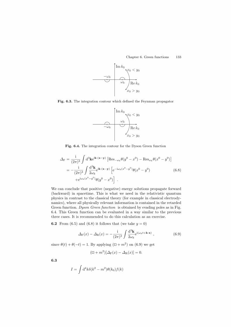
Chapter 6. Green functions 133

Fig. 6.3. The integration contour which defined the Feynman propagator

Fig. 6.4. The integration contour for the Dyson Green function

∆F =i

(2π)3

∫d3keik·(x−y)

[Res−ωk

θ(y0 − x0) − Resωkθ(x0 − y0)

]

= − i(2π)3

∫d3k2ωk

eik·(x−y)[e−iωk(x0−y0)θ(x0 − y0) (6.8)

+eiωk(x0−y0)θ(y0 − x0)]

.

We can conclude that positive (negative) energy solutions propagate forward(backward) in spacetime. This is what we need in the relativistic quantumphysics in contrast to the classical theory (for example in classical electrody-namics), where all physically relevant information is contained in the retardedGreen function. Dyson Green function is obtained by evading poles as in Fig.6.4. This Green function can be evaluated in a way similar to the previousthree cases. It is recommended to do this calculation as an exercise.

6.2 From (6.5) and (6.8) it follows that (we take y = 0)

∆F(x) − ∆R(x) = − i(2π)3

∫d3k2ωk

ei(ωkt+k·x) , (6.9)

since θ(t) + θ(−t) = 1. By applying ( + m2) on (6.9) we get

( + m2)[∆F(x) − ∆R(x)] = 0.

6.3

I =∫

d4kδ(k2 − m2)θ(k0)f(k)

134 Solution

=∫

d4kδ(k20 − ω2

k)θ(k0)f(k)

=∫

d3kdk01

2ωk[δ(k0 − ωk) + δ(k0 + ωk)] θ(k0)f(k)

=∫

d3k2ωk

f(k)∣∣∣∣k0=ωk

.

From this calculation it is clear that the expression d3k/(2ωk) is a Lorentzinvariant measure.

6.5 Let us take x0 < 0. The integral over the contour in Fig. 6.5 vanishessince there are no poles within the contour of integration. So, we get

∫ −ωk−ρ

−R

+∫

C−ρ

+∫ ωk−ρ

−ωk+ρ

+∫

C+ρ

+∫ R

ωk+ρ

+∫

CR

= 0 . (6.10)

Fig. 6.5. The integration contour that defined the principal-part propagator

The integral along the half–circle, CR tends to zero for large R, which canbe seen if we take that limit in the integrand. If in the integral

∫C+

ρwe take

k0 = ωk + ρeiϕ, it becomes∫

C+ρ

=∫ 0

π

ie−ix0(ωk+ρeiϕ) 1ρeiϕ + 2ωk

dϕ . (6.11)

By taking ρ → 0 in (6.11) we get∫

C+ρ

= − iπ2ωk

e−iωkx0 . (6.12)

In the same way we can show that∫

C−ρ

=iπ

2ωkeiωkx0 . (6.13)

From (6.10), (6.12) and (6.13) we get (for x0 < 0)

Chapter 6. Green functions 135

∆(x) =iπ

(2π)4

∫d3k2ωk

eik·x [e−iωkx0 − eiωkx0]θ(−x0). (6.14)

The case x0 > 0 is analogous to the previous one. The result is

∆(x) = − iπ(2π)4

∫d3k2ωk

eik·x [e−iωkx0 − eiωkx0]θ(x0) . (6.15)

By comparing equations (6.14) and (6.15) with the expressions for ∆R and∆A we obtain

∆(x) =12(∆R(x) + ∆A(x)) .

6.6

∆(x) = − i(2π)3

∫d3k2ωk

eik·x(e−iωkt − eiωkt) , (6.16)

∆±(x) = ∓ i(2π)3

∫d3k2ωk

ei(k·x∓ωkt) . (6.17)

6.7 By using the expression for ∆ obtained in Problem 6.6 we get

∂i∆(x) = − i(2π)3

∫d3k2ωk

ikieik·x(e−iωkt − eiωkt) = 0 , (6.18)

since the integrand is an odd function of k. The second identity can be proveneasily.

6.8 By applying the operator ( + m2) to the expression (6.16) we get

(+m2)∆(x) = − i(2π)3

∫d3k2ωk

(−ω2k +k2 +m2)

[ei(−ωkt+k·x) − ei(ωkt+k·x)

],

from which follows that ( + m2)∆(x) = 0, as k2 = m2.

6.9 For m = 0 from (6.8) it follows that

∆F|m=0 = − i(2π)3

∫d3k2k

eik·x[e−ikx0

θ(x0) + eikx0θ(−x0)]

= − i2(2π)2

∫ ∞

0

∫ π

0

k sin θdkdθ

×[eik(−t+r cos θ)θ(t) + eik(t+r cos θ)θ(−t)

], (6.19)

where in the second line we integrated over the polar angle ϕ. Integration overθ gives

∆F(x)|m=0 = − 12(2π)2r

∫ ∞

0

dk[(e−ik(t−r) − e−ik(t+r))θ(t)

+(eik(t+r) − eik(t−r))θ(−t)]

. (6.20)

136 Solution

Now, we shall consider separately two cases: t > 0 and t < 0. In the firstone, t > 0 the second term in the integrand of (6.20) is zero. The first partof the integrand has bad behavior for large k. We regularize it by makingsubstitution t → t − iε, where ε → 0+ . In this way we ensure convergence ofthis integral. Then from (6.20) it follows that

∆F|m=0 =i

2(2π)2r

(1

t − r − iε− 1

t + r − iε

)(6.21)

=i

(2π)21

t2 − r2 − iε=

i(2π)2

1x2 − iε

. (6.22)

By applying the formula

1z ± iε

= P1z∓ iπδ(z) , (6.23)

in expression (6.22) we get

∆F(x) |m=0= − 14π

δ(x2) +i

4π2P

1x2

. (6.24)

For the case t < 0 one also obtains the expression (6.24); this is left as anexercise.

6.10 We shall start from (6.5) and use spherical coordinates. Integration overangles θ and ϕ leads to

∆R(x) = − 12(2π)2r

∫ ∞

0

dk[e−ik(t−r) − eik(t+r) − e−ik(t+r) + eik(t−r)

]θ(t) .

(6.25)The change of variable k′ = −k in the third and the fourth integral in expres-sion (6.25) gives

∆R(x) = − 12(2π)2r

∫ ∞

−∞dk(e−ik(t−r) − eik(t+r))θ(t) . (6.26)

Note the change of the lower integration limit in the expression (6.26). From(6.26) follows

∆R|m=0 (x) = − 14πr

[δ(t − r) − δ(t + r)] θ(t) . (6.27)

The second term in (6.27) has a ”wrong” sign but it is irrelevant as this termvanishes (t > 0 and r > 0). By changing this minus into a plus in (6.27) wefinally obtain:

∆R|m=0 (x) = − 12π

δ(t2 − r2)θ(t) = − 12π

δ(x2)θ(t) . (6.28)

The case of advanced Green function is left for an exercise.

Chapter 6. Green functions 137

6.11 In the Problem 6.1, we modified the the contour of integration accordingto the boundary conditions, while the poles were not moved. Sometimes it isuseful to do the opposite, i.e. to move the poles and to integrate over the realk0–axis. For the retarded Green function this can be done by changing

k2 − m2 → k2 − m2 + iηk0

in the propagator denominator, where η is a small positive number. Therefore,

∆R(x − y) =∫

d4k

(2π)4e−ik·(x−y)

k2 − m2 + iηk0. (6.29)

Now the poles of the integrand in (6.29) are k0 = ±ωk − iη/2. From (6.6) and(6.29) we have

φR(x) = − g

(2π)4

∫d4k

e−ik·x

k2 − m2 + iηk0

∫dy0eik0y0

∫d3yδ(3)(y)e−ik·y .

(6.30)First in (6.30) we shall integrate over y0, then over y and finally over k0; thisgives

φR(x) =g

(2π)3

∫d3k

eik·x

k2 + m2. (6.31)

In order to compute this three-dimensional momentum integral we introducespherical coordinates; also we take x = rez. The angular integrations give (inone integral use the change k′ = −k )

φR(x) = − g

(2π)2ir

∫ ∞

−∞

kdk

k2 + m2e−ikr . (6.32)

Fig. 6.6.

The integral in (6.32) has the poles at k0 = ±im. The integration contour isgiven in Fig. 6.6. By applying the Cauchy theorem in (6.32) we obtain:

φR(x) =g

4πre−mr , (6.33)

which is the requested result.

138 Solution

6.12 Apply i/∂ − m on S(x).

6.13 The Fourier transformation of the equation (i/∂−m)S(x−y) = δ(4)(x−y)leads to

(i/∂ − m)1

(2π)4

∫d4pS(p)e−ip·(x−y) =

1(2π)4

∫d4pe−ip·(x−y) . (6.34)

From (6.34) follows

S(p) =/p + m

p2 − m2.

Therefore, the Green function is given by

S(x − y) =∫

d4p

(2π)4/p + m

p20 − p2 − m2

e−ip·(x−y) . (6.35)

The poles of the integrand in (6.35) are p0 = ±Ep = ±√

p2 + m2. Thepropagator is

SF(x − y) =1

(2π)4

∫d3peip·(x−y)

∫

CF

dp0p0γ

0 + piγi + m

p20 − E2

p

e−ip0(x0−y0) ,

(6.36)where the integration contour CF is defined in Problem 6.1. Applying theCauchy theorem we get

SF(x − y) = − i(2π)3

∫d3p2Ep

eip·(x−y)

[(Epγ

0 + piγi + m)e−iEp(x0−y0)θ(x0 − y0)+

+(−Epγ0 + piγ

i + m)eiEp(x0−y0)θ(y0 − x0)]

= − i(2π)3

∫d3p2Ep

[(/p + m)e−ip·(x−y)θ(x0 − y0)−

−(/p − m)eip·(x−y)θ(y0 − x0)]

. (6.37)

The advanced Green function can be found in the same way. The result is

SA(x − y) =i

(2π)3

∫d3p2Ep

eip·(x−y)[(Epγ

0 + piγi + m)e−iEp(x0−y0)−

−(−Epγ0 + piγ

i + m)eiEp(x0−y0)]θ(y0 − x0) . (6.38)

For simplicity we take y = 0 in (6.37) and (6.38). We have

SF − SA = − i(2π)3

∫d3p2Ep

ei(p·x−Epx0)(Epγ0 + piγ

i + m)(θ(x0) + θ(−x0))

= − i(2π)3

∫d3p2Ep

ei(p·x−Epx0)(Epγ0 + piγ

i + m) . (6.39)

Chapter 6. Green functions 139

Thus,

SF − SA = − i(2π)3

∫d3p2Ep

(Epγ0 + piγi + m)e−ip·x . (6.40)

By applying i/∂ − m on (6.40) we get (i/∂ − m)(SF − SA) = 0, since

(/p + m)(/p − m) = p2 − m2 = 0.

6.14 The integration along the curve CF is equivalent to the integration alongthe real p0–axis if we make the replacement p2 −m2 → p2 −m2 + iε, where εis a small positive number in the propagator denominator. The simple polesare p0 = ±Ep ∓ iε. So we get

ψ(x) =g

(2π)4

∫d4y

∫dp0

∫d3p

/p + m

p2 − m2 + iεe−ip·(x−y)δ(y0)eiq·y

1000

.

After the integration over the variables y0 and y we get

ψ(x) =g

2π

∫dp0d3p

/p + m

p2 − m2 + iεe−i(p0x0−p·x)δ(3)(p − q)

1000

. (6.41)

Integration over the momentum p is simple and it gives

ψ(x) =g

2πeiq·x

∫ ∞

−∞dp0

p0γ0 − q · γ + m

p20 − q2 − m2 + iε

e−ip0x0

1000

. (6.42)

Employing the Cauchy theorem we find that

ψ(x) = − ig2Eq

eiq·x [(−Eqγ0 − q · γ + m)eiEqx0θ(−x0)

+(Eqγ0 − q · γ + m)e−iEqx0θ(x0)]

1000

, (6.43)

which finally gives:

ψ(x) = − ig2Eq

eiq·x

×

eiEqx0

−Eq + m0q3

q1 + iq2

θ(−x0) + e−iEqx0

Eq + m0q3

q1 + iq2

θ(x0)

. (6.44)

140 Solution

6.15 The equation for the free massive vector field Aµ is given by

(gρσ − ∂ρ∂σ + m2gρσ)Aσ = 0 . (6.45)

The Green function (it is in fact the inverse kinetic operator) is defined by

(gρσ − ∂ρ∂σ + m2gρσ)xGσν(x − y) = δ(4)(x − y)δρν . (6.46)

If we introduce

Gσν =1

(2π)4

∫d4ke−ik·(x−y)Gσν(k) ,

in (6.46), we get

(−k2gρσ + kρkσ + m2gρσ)Gσν = δρν . (6.47)

We shall assume that the solution of (6.47) has the form Gρσ = Ak2gρσ +Bkρkσ, where A and B are scalars, i.e. they depend on k2 and m2. Insertingthe solution into (6.47), after comparing of the appropriate coefficients, weget

A =1

−k4 + k2m2, B = − 1

m2(m2 − k2).

The final result takes the following form

Gµν =1

k2 − m2

(−gµν +

kµkν

m2

). (6.48)

6.16 Use the same procedure as in the previous problem. The result is

Gµν = −gµν

k2+

1 + λ

λk4kµkν .

7

Canonical quantization of the scalar field

7.1 Starting from the expressions for scalar field φ and its canonical momen-tum π = φ,

φ =∫

d3k√2(2π)3ωk

[a(k)e−ik·x + a†(k)eik·x] ,

φ = i∫

d3k√(2π)32ωk

ωk

[−a(k)e−ik·x + a†(k)eik·x] ,

we have∫

d3xφ(x)e−ik′·x =(2π)3/2

√2ωk′

[a(k′)e−iωk′ t + a†(−k′)eiωk′ t

], (7.1)

∫d3xφ(x)e−ik′·x = i(2π)3/2

√ωk′

2[a†(−k′)eiωk′ t − a(k′)e−iωk′ t

]. (7.2)

From (7.1) and (7.2) it follows that

a(k) =1

(2π)3/2

1√2ωk

∫d3xeik·x

[ωkφ(x) + iφ(x)

], (7.3)

a†(k) =1

(2π)3/2

1√2ωk

∫d3xe−ik·x

[ωkφ(x) − iφ(x)

]. (7.4)

By using the expressions (7.3) and (7.4), we find:

[a(k), a†(k′)] =i

2(2π)31√

ωkωk′

∫d3xd3yei(k·x−k′·y)

(−ωk[φ(x), φ(y)]+

+ωk′ [φ(x), φ(y)])

=1

2(2π)31√

ωkωk′

∫d3xei(ωk−ωk′ )t+i(k′−k)·x(ωk + ωk′)

= δ(3)(k − k′) . (7.5)

142 Solutions

In the previous formula, we used the equal–time commutation relations forreal scalar field (7.C) i.e. we took1 x0 = y0. We can do this because thecreation and annihilation operators are time independent. This can be proveddirectly:

da(k)dt

=1

(2π)3/2

1√2ωk

∫d3xeik·x [iω2

kφ + i∇2φ − im2φ]

.

After two partial integrations in the second term we get

da(k)dt

=i

(2π)3/2

1√2ωk

∫d3xeik·x [ω2

k − k2 − m2]φ .

The dispersion relation, ω2k = m2 + k2 gives da(k)/dt = 0. It is clear that

a†(k) is also time independent.Similarly, we can prove that:

[a(k), a(k′)] = [a†(k), a†(k′)] = 0 .

7.2 In this problem, φ(x) is a classical field, so that a(k) and a†(k) are thecoefficients rather then operators. We can calculate them from the expressions(7.3) and (7.4) inserting φ(t = 0,x) = 0 and φ(t = 0,x) = c:

a(k) =1

(2π)3/2

1√2ωk

∫d3xe−ik·xic

=ic√2m

(2π)3/2δ(3)(k) .

Then, the scalar field is

φ(t,x) =c

msin(mt) .

Generally, if we know a field and its normal derivative on some space–likesurface σ, then the field at an arbitrary point is given by

φ(y) =∫

σ

[φ(x)∂xµ∆(x − y) − ∆(y − x)∂µφ(x)]dΣµ .

Solve this problem using the previous theorem.

7.3 The results are:

: H : =∫

d3kωk

[a†(k)a(k) + b†(k)b(k)

], (7.6)

: Q : = q

∫d3k[a†(k)a(k) − b†(k)b(k)

], (7.7)

: P : =∫

d3kk[a†(k)a(k) + b†(k)b(k)

]. (7.8)

1 This will be done in the forthcoming problems, too.

Chapter 7. Canonical quantization of the scalar field 143

7.4 (up, uk) = δ(3)(k − p), (up, u∗k) = 0.

7.5 From (2.9), we have

〈0|H |0〉 =12

∫d3kωk 〈0| (a†(k)a(k) + a(k)a†(k)) |0〉

=12

∫d3kωk 〈0| a(k)a†(k) |0〉

=12

∫d3kωk(δ(3)(0) − 〈0| a†(k)a(k) |0〉)

=12δ(3)(0)

∫d3k√

k2 + m2

= 2πδ(3)(0)∫ ∞

0

dkk2√

k2 + m2 .

By change of variable k = m√

t, the last integral becomes Euler’s beta function

〈0|H |0〉 = πm4δ(3)(0)B(32,−2) = −πm4

4δ(3)(0)Γ (−2) .

7.6 Use the formulae from Problem 7.3 and the commutation relations (7.D).

(a) Direct calculation yields

[Pµ, φ] =1

(2π)3/2

∫d3kd3k′√

2ωk′kµ[a†(k)a(k), a(k′)e−ik′·x + a†(k′)eik′·x

]

=1

(2π)3/2

∫d3k√2ωk

kµ(−a(k)e−ik·x + a†(k)eik·x)

= −i∂µφ . (7.9)

The same result can be obtained if we start from the transformation lawof the field φ under translations (see Problem 7.20):

φ(x + ε) = eiε·P φ(x)e−iε·P = φ(x) + iεµ[Pµ, φ(x)] + o(ε2) . (7.10)

On the other hand, we have

φ(x + ε) = φ(x) + εµ∂µφ + o(ε2) . (7.11)

From (7.11) and (7.10) the result (7.9) comes.(b) First, we calculate the commutator [Pµ, φn(x)]:

[Pµ, φn(x)] =n∑

k=1

φk−1[Pµ, φ]φn−k

=n∑

k=1

φk−1(−i∂µφ)φn−k

= −i∂µφn .

144 Solutions

In the same way one can prove that

[Pµ, πn(x)] = −i∂µπn .

As a consequence,

[Pµ, φn(x)πm(x)] = −i∂µ(φn(x)πm(x)) .

An arbitrary analytical function F (φ, π) can be expanded in series as

F (φ, π) =∑nm

Cnmφnπm .

Then[Pµ, F (φ, π)] = −i∂µF .

(c) [H, a†(k)a(q)] = (ωk − ωq)a†(k)a(q).(d) [Q,Pµ] = 0.(e) [H,N ] = 0.

(f)∫

d3x[H,φ(x)]e−ip·x = (2π)3/2√

ωp

2

(−a(p)e−iωpt + a†(−p)eiωpt

)

7.7 From the Baker–Hausdorff relation follows

eiQφe−iQ = φ + i[Q,φ] +i2

2![Q, [Q,φ]] + . . . . (7.12)

The first commutator in the previous expansion is given by

[Q,φ] = iq∫

d3y[φ†(y)π†(y) − φ(y)π(y), φ(x)]

= −q

∫d3yδ(3)(x − y)φ(y) = −qφ(x) .

Then[Q, [Q,φ]] = (−q)2φ , [Q, [Q, [Q,φ]]] = (−q)3φ , . . . (7.13)

Finally,

eiQφe−iQ =(

1 − iq +(−iq)2

2+ . . .

)φ = e−iqφ . (7.14)

7.8 The angular momentum of a scalar field has the form

Mµν =∫

d3x(xµT 0ν − xνT 0µ) .

(a) By inserting the previous formula in the commutator, we have

[Mµν , φ(x)] =∫

d3y[yµ(φ∂νφ − g0νL) − yν(φ∂µφ − g0µL), φ(x)] . (7.15)

The following equal–time commutators can be easily evaluated:

Chapter 7. Canonical quantization of the scalar field 145

[L(y), φ(x)] = −iδ(3)(x − y)π(y) ,

[π(y)∂µφ(y), φ(x)] = −i∂µφδ(3)(x − y) − iδµ0π(y)δ(3)(x − y) .

By substituting these expressions in (7.15) and performing integration, weget

[Mµν , φ(x)] = i(xν∂µ − xµ∂ν)φ(x) . (7.16)

The same result can be obtained if we start from the transformation lawfor the field φ(x) under Lorentz transformations,

ei2 ωµνMµν

φ(x)e−i2 ωµνMµν

= φ(Λ−1(ω)x) .

(b) We first calculate the commutator [Mµν , P0]:

[Mµν , P0] =∫

d3x[xµT0ν − xνT0µ, P0]

=∫

d3x (xµ[T0ν , P0] − xν [T0µ, P0])

= i∫

d3x (xµ∂0T0ν − xν∂0T0µ)

= i∫

d3x(−xµ∂iT

iν + xν∂iT

iµ

)

= i∫

d3x(gµiT

iν − giνT i

µ

)

= i∫

d3x(Tµν − gµ0T

0ν − Tνµ + g0νT 0

µ

)

= −i(gµ0Pν − gν0Pµ) . (7.17)

In (7.17), we used the results of Problem 7.6 (b), the continuity equation∂µTµν = 0 and integrated by parts. In the case λ = i we can use of apartial integration. The result is [Mµν , Pi] = −i(giµPν − giνPµ). Thus,

[Mµν , Pλ] = i(gλνPµ − gλµPν) . (7.18)

(c) Let us calculate firstly the commutator [Mij ,Mkl].

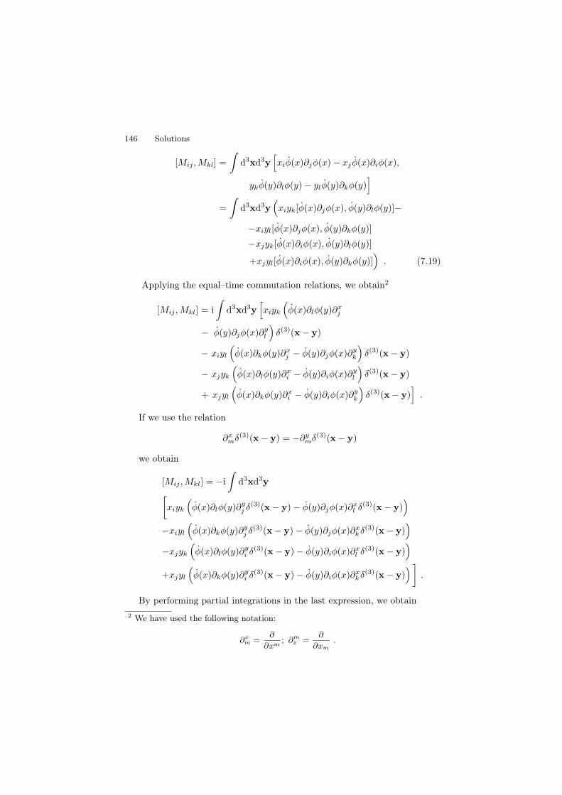
146 Solutions

[Mij ,Mkl] =∫

d3xd3y[xiφ(x)∂jφ(x) − xj φ(x)∂iφ(x),

ykφ(y)∂lφ(y) − ylφ(y)∂kφ(y)]

=∫

d3xd3y(xiyk[φ(x)∂jφ(x), φ(y)∂lφ(y)]−

−xiyl[φ(x)∂jφ(x), φ(y)∂kφ(y)]

−xjyk[φ(x)∂iφ(x), φ(y)∂lφ(y)]

+xjyl[φ(x)∂iφ(x), φ(y)∂kφ(y)])

. (7.19)

Applying the equal–time commutation relations, we obtain2

[Mij ,Mkl] = i∫

d3xd3y[xiyk

(φ(x)∂lφ(y)∂x

j

− φ(y)∂jφ(x)∂yl

)δ(3)(x − y)

− xiyl

(φ(x)∂kφ(y)∂x

j − φ(y)∂jφ(x)∂yk

)δ(3)(x − y)

− xjyk

(φ(x)∂lφ(y)∂x

i − φ(y)∂iφ(x)∂yl

)δ(3)(x − y)

+ xjyl

(φ(x)∂kφ(y)∂x

i − φ(y)∂iφ(x)∂yk

)δ(3)(x − y)

].

If we use the relation

∂xmδ(3)(x − y) = −∂y

mδ(3)(x − y)

we obtain

[Mij ,Mkl] = −i∫

d3xd3y[xiyk

(φ(x)∂lφ(y)∂y

j δ(3)(x − y) − φ(y)∂jφ(x)∂xl δ(3)(x − y)

)

−xiyl

(φ(x)∂kφ(y)∂y

j δ(3)(x − y) − φ(y)∂jφ(x)∂xk δ(3)(x − y)

)

−xjyk

(φ(x)∂lφ(y)∂y

i δ(3)(x − y) − φ(y)∂iφ(x)∂xl δ(3)(x − y)

)

+xjyl

(φ(x)∂kφ(y)∂y

i δ(3)(x − y) − φ(y)∂iφ(x)∂xk δ(3)(x − y)

)].

By performing partial integrations in the last expression, we obtain2 We have used the following notation:

∂xm =

∂

∂xm; ∂m

x =∂

∂xm.

Chapter 7. Canonical quantization of the scalar field 147

[Mij ,Mkl] = −i∫

d3x[gjk(xlφ(x)∂iφ(x) − xiφ(x)∂lφ(x))

+gil(xkφ(x)∂jφ(x) − xj φ(x)∂kφ(x))

+gik(xj φ(x)∂lφ(x) − xlφ(x)∂jφ(x))

+gjl(xiφ(x)∂kφ(x) − xkφ(x)∂iφ(x))]

= i(gjkMil + gliMjk − gikMjl − gjlMik) . (7.20)

The next two commutators [Mij ,M0k], [M0j ,M0k] can be evaluated in thesame way. Do this explicitly, please.

7.10

(a) The commutator is given by

[Qa, Qb] = −14

∫d3xd3yτa

ijτbmn

×[φ†

i (x)φj(x) − φ†i (x)φj(x), φ†

m(y)φn(y) − φ†m(y)φn(y)

].

Recall that as the charges are time-independent we can work with theequal–time commutators and we have

[Qa, Qb] = − i4

∫d3x(φ†[τa, τ b]φ − φ†[τa, τ b]φ

).

By using [τa, τ b] = 2iεabcτ c, we get

[Qa, Qb] = iεabcQc .

The second case is similar to the previous one:

[Qi, Qj ] = εimnεjpq

∫d3x∫

d3y[φm(x)φn(x), φp(y)φq(y)]

= i∫

d3x(−εimnεjnqφmφq + εimnεjpmφpφn)

= i∫

d3x(δijφmφm − φj φi − δijφmφm + φiφj)

= i∫

d3x(φiφj − φj φi)

= iεijkεkmn

∫d3xφmφn

= iεijkQk .

As in the first part of this problem, we used the equal–time commutationrelations and the formula for appropriate product of two three–dimensionalε symbols.

148 Solutions

(b) The commutator between the charges Qa and the field φm can be foundsimilarly:

[Qa, φm(x)] = − i2

∫d3yτa

ij [φ†i (y)φj(y) − φ†

i (y)φj(y), φm(x)]

= − i2τaij

∫d3y[φ†

i (y), φm(x)]φj(y)

= −12τaij

∫d3yδ(3)(x − y)δimφj(y)

= −12τamjφj(x) .

In the same way, we find:

[Qa, φ†m(x)] =

12τaimφ†

i .

The previous two results can be rewritten in the form

[θaQa, φm(x)] = iδ0φm(x) ,

[θaQa, φ†

m(x)] = iδ0φ†

m(x) .

In the case of SO(3) symmetry, the calculation is the same as above. Theresult is

[Qk, φm(x)] = iεkmjφj(x) .

7.11 The dilatation current is

jµ = −φ∂µφ − xν∂µφ∂νφ + Lxµ .

(a) The dilatation generator is

D = −∫

d3x(

φφ + xiφ∂iφ +12x0(φ2 − ∂iφ∂iφ)

).

(b) The commutator between the generator D and the field φ(x) is given by

[D,φ(y)] = −∫

d3x[φ(x)π(x) + xiπ(x)∂iφ(x)

+12x0π2(x) − 1

2x0∂iφ(x)∂iφ(x), φ(y)]

= −∫

d3x(φ(x)[π(x), φ(y)] + x0π(x)[π(x), φ(y)]

+ xi[π(x), φ(y)]∂iφ(x))

.

By using the commutation relations (7.C), we have

Chapter 7. Canonical quantization of the scalar field 149

ρ[D,φ(y)] = iρ(φ(y) + y0π(y) + yi∂iφ)= iρ(φ(y) + yµ∂µφ(y)) = iδ0φ .

In the same way, we obtain:

ρ[D,π(x)] = iρ(2π + xµ∂µπ) = iδ0π .

(c) By applying the previous result, we easily get

ρ[D,φ2] = ρ([D,φ]φ + φ[D,φ])= i((δ0φ)φ + φδ0φ) = iδ0(φ2) ,

and generallyρ[D,φa] = iδ0(φa) .

Similarly, one can show that

ρ[D,πa] = iδ0(πa) .

An arbitrary analytic function can be expanded in the following form

F (φ, π) =∑ab

cabφaπb ,

so that

ρ[D,F ] = ρ∑a,b

cab[D,φaπb]

= ρ∑a,b

cab

([D,φa]πb + φb[D,πb]

)

= i∑a,b

cab

(δ0(φa)πb + φaδ0(πb)

)

= iδ0

∑

a,b

cabφaπb

= iδ0F .

(d) We first consider the case µ = i:

[D,P i] =∫

d3x[D,π∂iφ]

=∫

d3x(π[D, ∂iφ] + [D,π]∂iφ

).

By using part (b) of this problem, we obtain

150 Solutions

[D,P i] = i∫

d3x[(2π + x0∂0π + xj∂jπ)∂iφ

+ π(2∂iφ + x0∂iπ + xj∂i∂jφ)]

. (7.21)

The second term in this expression is transformed in the following way∫

d3xx0∂k∂kφ∂iφ = −∫

d3xx0∂kφ∂k∂iφ = −12

∫d3x∂i(x0∂kφ∂kφ) ,

where we used the Klein-Gordon equation, ∂0π = −∂i∂iφ and then per-formed a partial integration. Thus, we conclude that the second term canbe dropped as a surface term. The expression

∫d3xπx0∂iπ is also a surface

term. Similarly, one can show that∫

d3xxj∂jπ∂iφ = −3∫

d3xπ∂iφ −∫

d3xxjπ∂j∂iφ .

Inserting these results in the formula (7.21) we obtain

[D,P i] = iP i .

The commutator [D,P 0] = iP 0 can be calculated in the same way.

7.12 In the expression for the vacuum expectation value, express the fieldsφf in terms of the creation and annihilations operators. From four terms,only one, which is proportional to 〈0| a(k)a†(k′) |0〉 = δ(3)(k−k′), is nonzero.Then, we have

〈0|φf (t,x)φf (t,x) |0〉 =1

(a2π)31

(2π)3

∫d3k2ωk

(∫d3ye−(x−y)2/a2+ik·(x−y)

)2

.

Calculating the Poisson integral in this formula, we obtain

〈0|φf (t)φf (t) |0〉 =1

2(2π)3

∫d3kωk

e−k2a2/2

=1

(2π)2

∫ ∞

0

k2dk√k2 + m2

e−k2a2/2 .

By the change of variable k2 = t, the last integral becomes

〈0|φf (t)φf (t) |0〉 =1

8π2

∫ ∞

0

√tdt√

t + m2e−ta2/2

=m2

16π2em2a2/4

[K1(

m2a2

4) − K0(

m2a2

4)]

, (7.22)

where Kν(x) are modified Bessel functions of the third kind (MacDonaldfunctions). Using the asymptotic expansions:

Chapter 7. Canonical quantization of the scalar field 151

K1(x) =1x

,

K0(x) = −(log(x/2) + 0, 5772)

for x 1, we obtain in the limit m → 0

〈0|φf (t)φf (t) |0〉 =1

4π2a2.

7.13 Express the operators Lm and Ln in terms of αµm and use the commu-

tation relations.

7.14 After a very simple calculation, we find that

〈0| φ(x), φ(y) |0〉 =i

2(2π)21

|x − y| limε→0

∫ ∞

0

dke−εk(eik(y0−x0−|x−y|)

− eik(y0−x0+|x−y|) + eik(x0−y0−|x−y|)

− eik(x0−y0+|x−y|))

. (7.23)

The integrals in the previous expression are regularized by introducing ε asa regularization parameter. At the end we have to take the limit ε → 0. Theresult is

〈0| φ(x), φ(y) |0〉 = − 12π2

1(x − y)2

.

7.15 The vacuum expectation value 〈φ(x)φ(y)〉 is given by

〈φ(x)φ(y)〉 =⟨φ+(x)φ−(y)

⟩

=∫

d3k(2π)3/2

√2ωk

d3q(2π)3/2

√2ωq

ei(q·y−k·x)δ(3)(k − q)

=1

(2π)3

∫d3k2ωk

e−ik·(x−y) ,

where we split the field φ into positive and negative energy parts, φ = φ++φ−.If we do the same in the vacuum expectation value of four scalar fields, wesee that only two terms remain:

〈φ(x1)φ(x2)φ(x3)φ(x4)〉 =⟨φ+(x1)φ+(x2)φ−(x3)φ−(x4)

⟩

+⟨φ+(x1)φ−(x2)φ+(x3)φ−(x4)

⟩. (7.24)

The first term in the last expression is

⟨φ+(x1)φ+(x2)φ−(x3)φ−(x4)

⟩=

4∏i=1

∫d3qi

(2π)3/2√

2ωi

⟨a1a2a

†3a

†4

⟩

× ei(−q1·x1−q2·x2+q3·x3+q4·x4) ,

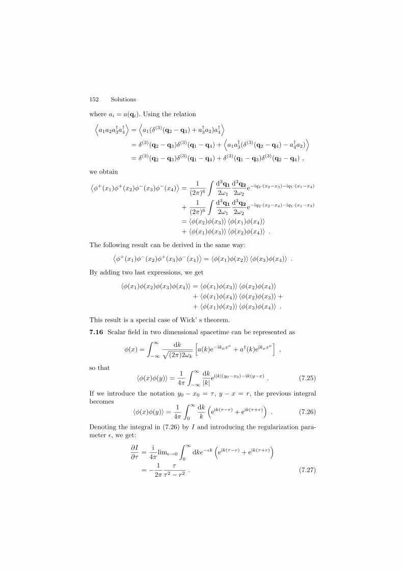
152 Solutions

where ai = a(qi). Using the relation⟨a1a2a

†3a

†4

⟩=⟨a1(δ(3)(q2 − q3) + a†

3a2)a†4

⟩

= δ(3)(q2 − q3)δ(3)(q1 − q4) +⟨a1a

†3(δ

(3)(q2 − q4) − a†4a2)⟩

= δ(3)(q2 − q3)δ(3)(q1 − q4) + δ(3)(q1 − q3)δ(3)(q2 − q4) ,

we obtain

⟨φ+(x1)φ+(x2)φ−(x3)φ−(x4)

⟩=

1(2π)6

∫d3q1

2ω1

d3q2

2ω2e−iq2·(x2−x3)−iq1·(x1−x4)

+1

(2π)6

∫d3q1

2ω1

d3q2

2ω2e−iq2·(x2−x4)−iq1·(x1−x3)

= 〈φ(x2)φ(x3)〉 〈φ(x1)φ(x4)〉+ 〈φ(x1)φ(x3)〉 〈φ(x2)φ(x4)〉 .

The following result can be derived in the same way:⟨φ+(x1)φ−(x2)φ+(x3)φ−(x4)

⟩= 〈φ(x1)φ(x2)〉 〈φ(x3)φ(x4)〉 .

By adding two last expressions, we get

〈φ(x1)φ(x2)φ(x3)φ(x4)〉 = 〈φ(x1)φ(x3)〉 〈φ(x2)φ(x4)〉+ 〈φ(x1)φ(x4)〉 〈φ(x2)φ(x3)〉 ++ 〈φ(x1)φ(x2)〉 〈φ(x3)φ(x4)〉 .

This result is a special case of Wick’ s theorem.

7.16 Scalar field in two dimensional spacetime can be represented as

φ(x) =∫ ∞

−∞

dk√(2π)2ωk

[a(k)e−ikµxµ

+ a†(k)eikµxµ]

,

so that〈φ(x)φ(y)〉 =

14π

∫ ∞

−∞

dk

|k|ei|k|(y0−x0)−ik(y−x) . (7.25)

If we introduce the notation y0 − x0 = τ , y − x = r, the previous integralbecomes

〈φ(x)φ(y)〉 =14π

∫ ∞

0

dk

k

(eik(τ−r) + eik(τ+r)

). (7.26)

Denoting the integral in (7.26) by I and introducing the regularization para-meter ε, we get:

∂I

∂τ=

i4π

limε→0

∫ ∞

0

dke−εk(eik(τ−r) + eik(τ+r)

)

= − 12π

τ

τ2 − r2. (7.27)

Chapter 7. Canonical quantization of the scalar field 153

From (7.27), it follows that

〈φ(x)φ(y)〉 = − 14π

logτ2 − r2

µ2= − 1

4πlog

(x − y)2

µ2,

where µ is an integration constant which has the dimension of length.

7.17 By taking partial derivative of the expression 〈0|T (φ(x)φ(y)) |0〉 withrespect to x0, we get:

∂x0 〈0|T (φ(x)φ(y)) |0〉 = δ(x0 − y0) 〈0| [φ(x), φ(y)] |0〉 ++ θ(x0 − y0) 〈0| ∂x0φ(x)φ(y) |0〉 + θ(y0 − x0) 〈0|φ(y)∂x0φ(x) |0〉 .

The first term is equal to zero as a consequence of the equal–time commutationrelation. By taking second order partial derivative with respect to x0, we get:

∂2x0 〈0|T (φ(x)φ(y)) |0〉 = δ(x0 − y0)[π(x), φ(y)]

+ θ(x0 − y0) 〈0| ∂2x0φ(x)φ(y) |0〉 +

+ θ(y0 − x0) 〈0|φ(y)∂2x0φ(x) |0〉 .

In the first term, we use the equal–time commutation relation, and finally getthe result

∂2x0 〈0|T (φ(x)φ(y)) |0〉 = −iδ(4)(x − y) +

+ θ(x0 − y0) 〈0| ∂2x0φ(x)φ(y) |0〉 +

+ θ(y0 − x0) 〈0|φ(y)∂2x0φ(x) |0〉 ,

which implies

(x + m2) 〈0|T (φ(x)φ(y)) |0〉 = −iδ(4)(x − y) ++ θ(x0 − y0) 〈0| (x + m2)φ(x)φ(y) |0〉 ++ θ(y0 − x0) 〈0|φ(y)(x + m2)φ(x) |0〉 .

The last two terms vanish since the field φ satisfies the Klein–Gordon equation.Therefore,

(x + m2) 〈0|T (φ(x)φ(y)) |0〉 = −iδ(4)(x − y) . (7.28)

7.18

(a) Applying the variational principle to the given action leads to the equa-tions:

i∂ψ

∂t=(− 1

2m∆ + V (r)

)ψ

−i∂ψ

†

∂t=(− 1

2m∆ + V (r)

)ψ

†.

The first of these equations is the Schrodinger equation, the second one isits conjugation equation.

154 Solutions

(b) A particular solution of the free Schrodinger equation is a plane wavee−iEkt+ik·r, where Ek = k2/2m so that the general solution is

ψ(t, r) =∫

d3k(2π)3/2

a(k)e−iEkt+ik·r . (7.29)

The negative energy solutions are not present in previous expression sinceEk > 0 in nonrelativistic quantum mechanics. The field ψ† is

ψ†(t, r) =∫

d3k(2π)3/2

a†(k)eiEkt−ik·r . (7.30)

In the quantum theory these classical fields are replaced by operators inthe Hilbert space. The field conjugate to ψ is

π =∂L∂ψ

= iψ† .

The equal–time commutation relations are

[ψ(t,x), ψ†(t,y)] = δ(3)(x − y) ,

[ψ(t,x), ψ(t,y)] = [ψ†(t,x), ψ†(t,y)] = 0 . (7.31)

From the relations (7.29) and (7.30) follows

a(k) =1

(2π)3/2eiEkt

∫d3xψ(t,x)e−ik·x

a†(k) =1

(2π)3/2e−iEkt

∫d3xψ†(t,x)eik·x .

From (7.31) and previous relations one easily gets the commutation rela-tions:

[a(k), a†(p)] = δ(3)(p − k) , (7.32)

[a(k), a(p)] = [a†(k), a†(p)] = 0 . (7.33)

(c) Substituting (7.29) and (7.30) into the expression for the Green functionone obtains

G(x0,x, y0,y) = −i 〈0|ψ(x0,x)ψ†(y0,y) |0〉 θ(x0 − y0)

= − i(2π)3

∫d3kd3pe−i(Ekx0−k·x−Epy0+p·y)

× 〈0| a(k)a†(p) |0〉 θ(x0 − y0)

= − i(2π)3

∫d3kd3pe−i(Ekx0−k·x−Epy0+p·y)

× δ(3)(p − k)θ(x0 − y0)

= − i(2π)3

∫d3ke−i k2

2m (x0−y0)+ik·(x−y)θ(x0 − y0)

= −i(

m

2πi(x0 − y0)

)3/2

eim(x−y)2

2(x0−y0) θ(x0 − y0) .

Chapter 7. Canonical quantization of the scalar field 155

(d) The eigenfunctions are

uk =

√2π

sin(kx) ,

hence the (nonrelativistic) field operators are

ψ =

√2π

∫ ∞

0

dka(k)e−i k22m t sin(kx) , (7.34)

ψ† =

√2π

∫ ∞

0

dka†(k)ei k22m t sin(kx) . (7.35)

We shall leave to the reader to prove that

G(x0, x, y0, y) = −i(

m

2πi(x0 − y0)

)1/2 [e

im(x−y)2

2(x0−y0) − eim(x+y)2

2(x0−y0)

]θ(x0 − y0) .

(7.36)Generally, if the eigenfunctions of the Hamiltonian are un(x) the Greenfunction is

G(x0,x, y0,y) = −i∑

n

e−iEn(x0−y0)un(x)u∗n(y)θ(x0 − y0) . (7.37)

(e) The invariance of the Schrodinger equation can be proven directly. Weleave that to reader.

(f) In order to find the conserved charges we should calculate only time com-ponents of the conserved currents. For the spatial translations the timecomponent of the current is

j0 = − ∂L∂(∂0ψ)

∂iψεi

= −iψ†∂iψεi = −iψ†∇ψ · ε . (7.38)

The conserved charge is the linear momentum

P = −∫

d3xψ†(i∇)ψ . (7.39)

The HamiltonianH =

∫d3xψ†(− 1

2m)∆ψ (7.40)

is generator of time translations. The angular momentum

J = −i∫

d3xψ†(x ×∇)ψ (7.41)

is generator of rotations. Under Galilean boosts we have δxi = −vit, δψ =−imv · xψ so that

156 Solutions

j0 = v · j0 = mv · xψ†ψ + ivtψ†∇ψ. (7.42)

Consequently, the boost generator is

G =∫

d3xψ†(mx + it∇)ψ . (7.43)

The commutation relations can be found using the commutation relations(7.31). Let us start with [Pi, Gj ]:

[Pi, Gj ] = i∫

d3xd3y[−ψ†(y)∂yi ψ(y), ψ†(x)(mxj + it∂j)ψ(x)]

= −im∫

d3xd3y(ψ†(y)[∂iψ(y), ψ†(x)xjψ(x)]

+ [ψ†(y), ψ†(x)xjψ(x)]∂iψ(y))

= −im∫

d3x(−∂iψ†xjψ(x) − xjψ

†∂iψ)

= −iMδij , (7.44)

where M = m∫

d3xψ†ψ is the mass operator. It appears since the rep-resentation is projective. We have two possibilities either to enlarge theGalilean algebra with this operator or to add a superselection rule whichforbids superposition of particles of different masses.In the similar manner the other commutation relations can be obtained:

[Gi, Gj ] = [H,P] = [H,J] = 0

[Ji, Jj ] = iεijkJk

[Ji, Gj ] = iεijkGk

[Ji, Pj ] = iεijkPk

[H,Gi] = −iPi .

The Galilean algebra can also be derived from the Poincare algebra [23].

7.19

(a) By using the first commutation relation in (7.D), we get

[a(p), a†] = C

∫d3q√2ωq

[a(p), a†(q)]f(q)

= C

∫d3q√2ωq

f(q)δ(3)(p − q)

= C1√2ωp

f(p) . (7.45)

The second commutator can be evaluated in the same way. The result is

[a†(p), a] = −C1√2ωp

f∗(p) . (7.46)

Chapter 7. Canonical quantization of the scalar field 157

(b) Using (7.45), we have

a(p)(a†)n = C1√2ωp

f(p)(a†)n−1 + a†a(p)(a†)n−1 . (7.47)

By repeating this procedure n times, we get

a(p)(a†)n = C1√2ωp

nf(p)(a†)n−1 + (a†)na(p) . (7.48)

Hence,

[a(p), (a†)n] = Cnf(p)√

2ωp

(a†)n−1 . (7.49)

(c) This calculation is straightforward:

a(p) |z〉 = e−|z|2/2a(p)∞∑

n=0

zn(a†)n

n!|0〉

= e−|z|2/2∞∑

n=1

C√2ωp

znf(p)(n − 1)!

(a†)n−1 |0〉

=C√2ωp

f(p)z |z〉 . (7.50)

(d) By using the previous relation and the property 〈z|z〉 = 1, we have

〈z|φ |z〉 =∫

d3p(2π)3/2

√2ωp

(〈z| a(p) |z〉 e−ip·x + 〈z| a†(p) |z〉 eip·x)

= C

∫d3p

(2π)3/22ωp

(zf(p)e−ip·x + z∗f∗(p)eip·x

)

=C

(2π)3/2(zf(x) + z∗f∗(x)) . (7.51)

In the same manner we have

〈z| : φ2 : |z〉 =∫

d3p(2π)3/2

√2ωp

d3q(2π)3/2

√2ωq

(〈z| a(p)a(q) |z〉 e−i(p+q)·x

+ 〈z| a†(q)a(p) |z〉 ei(q−p)·x

+ 〈z| a†(p)a(q) |z〉 ei(p−q)·x + 〈z| a†(p)a†(q) |z〉 ei(q+p)·x)

= C2

∫d3p

(2π)3/22ωp

d3q(2π)3/22ωq

(f(p)f(q)z2e−i(p+q)·x

+ f(p)f∗(q)|z|2e−i(p−q)·x

+ f∗(p)f(q)|z|2ei(p−q)·x + f∗(p)f∗(q)(z∗)2ei(p+q)·x)

=C2

(2π)3(zf(x) + z∗f∗(x))2 . (7.52)

158 Solutions

Hence,(∆φ)2 = 0 . (7.53)

(e) It is easy to see that

〈z|H |z〉 = C2|z|2∫

d3p|f(p)|2 . (7.54)

7.20

(a) By substituting the expression for φ in the relation

U(Λ, a)φ(x)U−1(Λ, a) = φ(Λx + a)

we obtain∫

d3k(2π)3/2

√2ωk

U(Λ, a)(a(k)e−ik·x + a†(k)eik·x)U−1(Λ, a)

=∫

d3k′

(2π)3/2√

2ωk′

(a(k′)e−ik′·(Λx+a) + a†(k′)eik′·(Λx+a)

). (7.55)

In the integral on the right hand side we make the changing of variablesk′µΛ ν

µ = kν . In Problem 6.3, we proved that d3k/(2ωk) is a Lorentzinvariant measure, so that

d3k′√

2ωk′=√

ωk′

2d3kωk

.

By performing the inverse Fourier transformation, we obtain the requestedresult.

(b) It is easy to see that

U(Λ, a) |k1, . . . , kn〉 = U(Λ, a)a†(k1)U−1(Λ, a)U(Λ, a) · · ·

· · ·U(Λ, a)a†(kn)U−1(Λ, a) |0〉

=√

ωk′1· · ·ωk′

n

ωk1 · · ·ωkn

eiaµΛµν(kν

1+...+kνn) |Λk1, . . . , Λkn〉 .

(c) From the expressions (7.6) and (7.8) and the first part of this problem, wehave

U(Λ)PµU−1(Λ) =∫

d3kkµU(Λ)a†(k)a(k)U−1(Λ)

=∫

d3kkµ ωk′

ωka

†(Λk)a(Λk)

= Λ µν

∫d3k′k′νa†(k′)a(k′)

= Λ µν P ν ,

where we made the change of variables kµ = Λ µν k′ν in the integral.

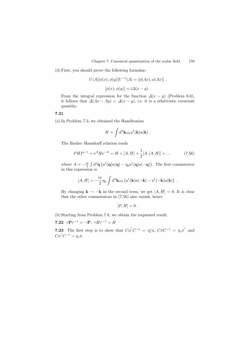
Chapter 7. Canonical quantization of the scalar field 159

(d) First, you should prove the following formulae:

U(Λ)[φ(x), φ(y)]U−1(Λ) = [φ(Λx), φ(Λx)] ,

[φ(x), φ(y)] = i∆(x − y) .

From the integral expression for the function ∆(x − y) (Problem 6.6),it follows that ∆(Λx − Λy) = ∆(x − y), i.e. it is a relativistic covariantquantity.

7.21

(a) In Problem 7.3, we obtained the Hamiltonian

H =∫

d3kωka†(k)a(k) .

The Backer–Hausdorff relation reads

PHP−1 = eAHe−A = H + [A,H] +12[A, [A,H]] + . . . (7.56)

where A = − iπ2

∫d3q(a†(q)a(q) − ηpa

†(q)a(−q)). The first commutator

in this expression is

[A,H] = − iπ2

ηp

∫d3kωk

(a†(k)a(−k) − a†(−k)a(k)

).

By changing k → −k in the second term, we get [A,H] = 0. It is clearthat the other commutators in (7.56) also vanish, hence

[P,H] = 0 .

(b) Starting from Problem 7.8, we obtain the requested result.

7.22 τPτ−1 = −P, τHτ−1 = H

7.23 The first step is to show that Cφ†C−1 = η∗

cφ, CπC−1 = ηcπ†

andCπ

†C−1 = ηcπ.

8

Canonical quantization of the Dirac field

8.1 If we use the anticommutation relation (8.E) the anticommutator iSab(x−y) = ψa(x), ψb(y), where a, b = 1, . . . , 4 are Dirac indices, becomes

ψa(x), ψb(y) =∑r,s

1(2π)3

∫d3pd3q

m√EpEq

δrsδ(3)(p − q)

×(ua(p, r)ub(q, s)ei(q·y−p·x)

+ va(p, r)vb(q, s)e−i(q·y−p·x))

.

Applying the solution of Problem 4.4 we have

iSab =1

(2π)3

∫d3p2Ep

[(/p + m)abe−ip·(x−y) + (/p − m)abeip·(x−y)

]. (8.1)

The last expression can be easily transformed into the following form

ψa(x), ψb(y) = (iγµ∂xµ + m)ab

1(2π)3

∫d3p2Ep

[e−ip·(x−y) − eip·(x−y)

]. (8.2)

From (8.2) we see that ∆(x − y) is given by

∆(x − y) = − i(2π)3

∫d3p2Ep

[e−ip·(x−y) − eip·(x−y)

].

The function ∆(x−y) was defined in Problem 6.6. In the special case x0 = y0

we shall make change p → −p in the second term of expression (8.1) andobtain

ψa(x), ψb(y)|x0=y0 = (γ0)ab

∫d3p

(2π)3eip·(x−y) = (γ0)abδ

(3)(x − y) . (8.3)

162 Solutions

8.2

(a) Substituting (8.A,B) in the expression for charge Q we obtain

Q = −e

∫d3x : ψ†ψ :

= −e∑r,s

∫d3p

m

Ep

[c†r(p)cs(p)u†

r(p)us(p)

+ : dr(p)d†s(p) : v†r(p)vs(p) + c†r(p)d†s(−p)u†

r(p)vs(−p)e2iEpt

+dr(p)cs(−p)v†r(p)us(−p)e−2iEpt

]. (8.4)

From (4.52) and (8.4) we get

Q = −e∑

r

∫d3p(c†r(p)cr(p) − d†r(p)dr(p)

). (8.5)

(b) As ψ satisfy the Dirac equation, (−iγi∂i +m)ψ = iγ0∂0ψ the Hamiltonianis

H = i∫

d3x : ψ†∂0ψ :

=∑r,s

1(2π)3

∫d3xd3pd3q

√m

Ep

√m

Eq:(u†

r(p)c†r(p)eip·x

+v†r(p)dr(p)e−ip·x)Eq

(us(q)cs(q)e−iq·x − vs(q)d†s(q)eiq·x) :

=∑

r

∫d3pEp

(c†r(p)cr(p) + d†r(p)dr(p)

). (8.6)

(c)

P =∑

r

∫d3pp

(c†r(p)cr(p) + d†r(p)dr(p)

). (8.7)

8.3

(a) It is easy to see that

[H,ψ] =∑r,s

1(2π)3/2

∫d3pd3qEp

√m

Eq

×[c†r(p)cr(p) + d†r(p)dr(p), cs(q)us(q)e−iq·x + d†s(q)vs(q)eiq·x]

=∑r,s

1(2π)3/2

∫d3pd3qEp

√m

Eqδrsδ

(3)(p − q)

×(−cr(p)us(q)e−iq·x + d†r(p)vs(q)eiq·x)

=∑

r

∫d3p

(2π)3/2

√mEp

(−cr(p)ur(p)e−ip·x + d†r(p)vr(p)eip·x)

= −i∂ψ

∂t,

Chapter 8. Canonical quantization of the Dirac field 163

where we have used:

[c†r(p)cr(p), cs(q)] = −c†r(p), cs(q)cr(p)= −δrsδ

(3)(p − q)cr(p) ,

and the similar expression for d−operators.(b) If we had used commutation relations instead of anticommutation rela-

tions in the quantization process we would have obtained:

H =∑

r

∫d3pEp

(c†r(p)cr(p) − d

†

r(p)dr(p))

.

From here we conclude that the energy spectrum would have been un-bounded from below, which is physically unacceptable.

8.4

[H, c†r(p)cr(p)] =∑

s

∫d3qEq[c†s(q)cs(q) + d†s(q)ds(q), c†r(p)cr(p)]

=∑

s

∫d3qEq

([c†s(q)cs(q), c†r(p)]cr(p)

+ c†r(p)[c†s(q)cs(q), cr(p)]

=∑

s

∫d3qEq

(c†s(q)cs(q), c†r(p)cr(p)

− c†s(q), c†r(p)cs(q)cr(p)+ c†r(p)(c†s(q)cs(q), cr(p) − c†s(q), cr(p)cs(q))

)

= Ep

(c†r(p)cr(p) − c†r(p)cr(p)

)= 0

8.5 The form variation of a spinor field is

δ0ψ = δψ − δxµ∂µψ =

= − i4ωµνσµνψ − ωµνxν∂µψ

=12ωµν

(xµ∂ν − xν∂µ − i

2σµν

)ψ .

On the other hand we have δ0ψ = − i2ωµνMµνψ . Comparing these results we

conclude that the generators are given by

Mµν = i(xµ∂ν − xν∂µ) +12σµν .

8.6

(a) Applying the formula [AB,C] = AB,C − A,CB we obtain

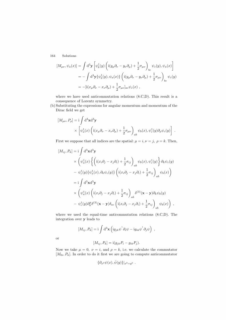
164 Solutions

[Mµν , ψa(x)] =∫

d3y[ψ†

b(y)(

i(yµ∂ν − yν∂µ) +12σµν

)

bc

ψc(y), ψa(x)]

= −∫

d3yψ†b(y), ψa(x)

(i(yµ∂ν − yν∂µ) +

12σµν

)

bc

ψc(y)

= −[i(xµ∂ν − xν∂µ) +12σµν ]acψc(x) ,

where we have used anticommutation relations (8.C,D). This result is aconsequence of Lorentz symmetry.

(b) Substituting the expressions for angular momentum and momentum of theDirac field we get

[Mµν , Pρ] = i∫

d3xd3y

×[ψ†

a(x)(

i(xµ∂ν − xν∂µ) +12σµν

)

ab

ψb(x), ψ†c(y)∂ρψc(y)

].

First we suppose that all indices are the spatial: µ = i, ν = j, ρ = k. Then,

[Mij , Pk] = i∫

d3xd3y

×(

ψ†a(x)(

i(xi∂j − xj∂i) +12σij

)

ab

ψb(x), ψ†c(y)

∂kψc(y)

− ψ†c(y)ψ†

a(x), ∂kψc(y)(

i(xi∂j − xj∂i) +12σij

)

ab

ψb(x))

= i∫

d3xd3y

×(

ψ†a(x)(

i(xi∂j − xj∂i) +12σij

)

ab

δ(3)(x − y)∂kψb(y)

− ψ†c(y)∂y

kδ(3)(x − y)δac

(i(xi∂j − xj∂i) +

12σij

)

ab

ψb(x))

,

where we used the equal-time anticommutation relations (8.C,D). Theintegration over y leads to

[Mij , Pk] = i∫

d3x(igjkψ

†∂iψ − igikψ

†∂jψ)

,

or[Mij , Pk] = i(gjkPi − gikPj).

Now we take µ = 0, ν = i, and ρ = k, i.e. we calculate the commutator[M0i, Pk]. In order to do it first we are going to compute anticommutator

∂x0ψ(x), ψ(y)|x0=y0 .

Chapter 8. Canonical quantization of the Dirac field 165

Taking partial derivative of (8.1) with respect to x0 and substituting x0 =y0 we get

∂x0ψa(x), ψb(y)|x0=y0 =i

2(2π)3

∫d3p[(−Epγ

0 + p · γ − m)abeip·(x−y)

+ (Epγ0 − p · γ − m)abe−ip·(x−y)

]

=i

(2π)3

∫d3p(p · γ − m)abeip·(x−y)

= γab∇xδ(3)(x − y) − imδabδ(3)(x − y) .

Then

[M0i, Pk] = i∫

d3xd3y

×(

ψ†a(x)(

i(x0∂i − xi∂0) +12σ0i

)

ab

ψb(x), ψ†c(y)

∂kψc(y)

− ψ†c(y)ψ†

a(x), ∂kψc(y)(

i(x0∂i − xi∂0) +12σ0i

)

ab

ψb(x))

= i∫

d3xd3y(ix0ψ

†(x)∂xi δ(3)(x − y)∂kψ(y)

− ixiψ†a(x)(γγ0∇x − imγ0)acδ

(3)(x − y)∂kψc(y)

+ ψ†a(x)

12(σ0i)abδ

(3)(x − y)∂kψb(y)

− ix0ψ†(y)∂y

kδ(3)(x − y)∂iψ(x)

+ ixiψ†(y)∂y

kδ(3)(x − y)∂0ψ(x)

− ψ†a(y)

12(σ0i)ab∂

ykδ(3)(x − y)ψb(x)

)

= i∫

d3x(−ixiψ

†γγ0∂k∇ψ − mxiψ†γ0∂kψ − ixi∂kψ†∂0ψ

)

= i∫

d3x(igikψ†∂0ψ + xiψ(iγ0∂0 + iγ∇− m)∂kψ

).

The second term in the last line vanishes since ψ satisfies the Dirac equa-tion. Then we get

[M0i, Pk] = igikP0 .

The remaining commutators [M0i, P0] and [Mij , P0] can be computed inthe same way.

8.7 The helicity operator is

Sp =12

∫d3x : ψ†Σ · p

|p| ψ : . (8.8)

166 Solutions

Inserting expressions for fields ψ and ψ†

in the previous formula and usingthe fact that ur(p) and vr(p) are eigenspinors of Σ · p/|p| with eigenvalues(−1)r+1 and (−1)r , respectively (see Problem 4.7) we get

Sp =1

2(2π)3

∫d3x

2∑r,s=1

∫d3pd3q

m√EpEq

×[c†r(q)cs(p)(−1)s+1u†

r(q)us(p)ei(q−p)·x

+ c†r(q)d†s(p)(−1)su†r(q)vs(p)ei(q+p)·x

+ dr(q)cs(p)(−1)s+1v†r(q)us(p)e−i(q+p)·x

− d†s(p)dr(q)(−1)sv†r(q)vs(p)ei(p−q)·x

]. (8.9)

Performing the x integration and applying orthogonality relations (4.52) onegets that the second and the third term in the expression (8.9) vanish. Finally,integration over the momentum q gives

Sp =12

2∑r=1

∫d3p(−1)r+1

(c†r(p)cr(p) + d†r(p)dr(p)

). (8.10)

Let us emphasize that we have used the expansion of the fields with respectto helicity basis.

8.8 The two-particle state given in the problem is eigenstate of the operatorsH, Q, and Sp. Using the explicit form of the Hamiltonian from Problem 8.2we have

Hc†r1(p1)c†r2

(p2) |0〉 =∑

r

∫d3pEp

(c†r(p)cr(p)

+ d†r(p)dr(p))c†r1

(p1)c†r2(p2) |0〉 . (8.11)

Let us calculate the first term in the previous expression. Commuting cr(p)to the right we get

c†r(p)cr(p)c†r1(p1)c†r2

(p2) |0〉 = δr1rδ(3)(p − p1)c

†

r(p)c†r2(p2) |0〉

− c†r(p)c†r1(p1)cr(p)c†r2

(p2) |0〉 . (8.12)

Repeating once more we get

c†r(p)cr(p)c†r1(p1)c†r2

(p2) |0〉 = δr1rδ(3)(p − p1)c

†

r(p)c†r2(p2) |0〉

− c†r(p)c†r1(p1)δrr2δ

(3)(p − p2) |0〉 . (8.13)

It is easy to see that

d†r(p)dr(p)c†r1(p1)c†r2

(p2) |0〉 = 0 . (8.14)

Chapter 8. Canonical quantization of the Dirac field 167

Inserting (8.13) and (8.14) in (8.11) and integrating over momentum p weobtain

Hc†r1(p1)c†r2

(p2) |0〉 = (Ep1 + Ep2)c†r1

(p1)c†r2(p2) |0〉 . (8.15)

Similar as before we have:

Qc†r1(p1)c†r2

(p2) |0〉 = −2ec†r1(p1)c†r2

(p2) |0〉 , (8.16)

for charge and

Sp c†r1(p1)c†r2

(p2) |0〉

=12((−1)r1+1 + (−1)r2+1

)c†r1

(p1)c†r2(p2) |0〉 (8.17)

for helicity. To summarize: energy, charge and helicity of the two–particle state|p1, r1;p2, r2〉 are

Ep1 + Ep2 , −2e,12((−1)r1+1 + (−1)r2+1

), (8.18)

respectively.

8.9 The commutator is

[Qa, Qb] =14

∫d3xd3yτa

ijτbkl[ψ

†i (x)ψj(x), ψ†

k(y)ψl(y)]

=14

∫d3xd3yτa

ijτbkl(ψ

†i (x)ψl(y)δjk − ψ†

k(y)ψj(x)δil)δ(3)(x − y)

=14

∫d3x(ψ†

i τaijτ

bjlψl − ψ†

kτ bklτ

aljψj)

=14

∫d3xψ†[τa, τ b]ψ

=i2εabc

∫d3xψ†τ cψ = iεabcQc .

The generators Qa satisfy the commutation relations of SU(2) algebra as weexpected.

8.10 The charges are

Qb =∫

d3xjb0 =∫

d3x(εabcπaπc +12Ψ †

i τ bijΨj) . (8.19)

(a) The commutator is

[Qb, Qe] =∫

d3xd3y(εabcεdef [πa(x)πc(x), πd(y)πf (y)]

+τ bij

2τemn

2[Ψ †

i (x)Ψj(x), Ψ †m(y)Ψn(y)]

)

168 Solutions

=∫

d3xd3y(εabcεdef (iδ(3)(x − y)δcdπa(x)πf (y)

− iδ(3)(x − y)δaf πd(y)πc(x))

+τ bij

2τemn

2δ(3) (x − y)(δjmΨ †

i (x)Ψn(y) − δinΨ †m(y)Ψj(x))

)

=∫

d3x(

i(πeπb − πbπe) +i2εbedΨ †τdΨ

)

= iεbed

∫d3x(

εadcπaπc +12Ψ †τdΨ

)

= iεbedQd .

(b) The results are[Qb, πa(x)] = −iεabcπc(x) ,

[Qb, ψi(x)] = −τ bin

2ψn(x) ,

[Qb, ψi(x)] = −ψn(x)τ bni

2.

8.11 The conserved charge for dilatation is

D =∫

d3xj0 = −i∫

d3x(

32ψ†ψ + xjψ†∂jψ − x0ψγj∂jψ

). (8.20)

Let us find the commutator between the operator D and momentum P i

[D,P i] =∫

d3xd3y(

[32ψ†(x)ψ(x) + xjψ†(x)∂jψ(x), ψ†(y)∂iψ(y)]

− [x0ψ(x)γj∂jψ(x), ψ†(y)∂iψ(y)])

.

We decompose the previous expression on three commutators. The first oneis

[ψ†(x)ψ(x), ψ†(y)∂iψ(y)] = [ψ†a(x)ψa(x), ψ†

b(y)]∂iψb(y)

+ ψ†b(y)[ψ†

a(x)ψa(x), ∂iψb(y)]

= ψ†a(x)ψa(x), ψ†

b(y)∂iψb(y)

− ψ†b(y)ψ†

a(x), ∂iψb(y)ψa(x) ,

where we have dropped the vanishing terms. The anticommutation relations(8.C–D) give the following result

[ψ†(x)ψ(x), ψ†(y)∂iψ(y)] = ψ†(x)∂iψ(y)δ(3)(x − y)− ψ†(y)ψ(x)∂i

yδ(3)(x − y) . (8.21)

The remaining commutators can be calculated in the same way. The result is:

Chapter 8. Canonical quantization of the Dirac field 169

[ψ†(x)∂jψ(x), ψ†(y)∂iψ(y)] = ψ†(x)∂iψ(y)∂xj δ(3)(x − y)

− ψ†(y)∂jψ(x)∂iyδ(3)(x − y) , (8.22)

[ψ(x)γj∂jψ(x), ψ†(y)∂iψ(y)] = ψ(x)γj∂iψ(y)∂xj δ(3)(x − y)

− ψ(y)γj∂jψ(x)∂iyδ(3)(x − y) . (8.23)

Inserting (8.21), (8.22) and (8.23) in (8.21) and applying

∂kxδ(3)(x − y) = −∂k

y δ(3)(x − y) , (8.24)

we get

[D,P i] = −∫

d3xψ†∂iψ = iP i . (8.25)

Similarly one can show that

[D,P 0] = iP 0 . (8.26)

8.12

(a) Using the expression (5.G) the energy–momentum tensor is

Tαβ = iψγα∂βψ − gαβ(iψ/∂ψ − gx2ψψ) .

Taking derivative of the previous expression we get

∂αTαβ = 2gxβψψ ,

where we have used the equations of motion:

i/∂ψ − gx2ψ = 0 ,

i∂µψγµ + gx2ψ = 0 .

The result ∂αTαβ = 0 shows that there is no translation symmetry in thetheory. As a consequence, the energy and momentum are not conserved inthis theory.

(b) From the expression for the four-momentum (5.6) we have

P 0(t) =∫

d3x(−iψγj∂jψ + gx2ψψ) ,

P i(t) = i∫

d3xψ†∂iψ ,

so

170 Solutions

[P 0(t), P i(t)] =∫ ∫

d3xd3y

×([ψ(t,x)γj∂jψ(t,x), ψ

†(t,y)∂iψ(t,y)]

+ igx2[ψ(t,x)ψ(t,x), ψ†(t,y)∂iψ(t,y)]

)

=∫ ∫

d3xd3y

×((γ0γj)ab[ψ

†

a(t,x)∂jψb(t,x), ψ†

c(t,y)∂iψc(t,y)]

+ igx2γ0ab[ψ

†

a(t,x)ψb(t,x), ψ†

c(t,y)∂iψc(t,y)])

.

The commutators in the previous expression can be found in the same wayas in the previous problem

[P 0(t), P i(t)] =∫

d3x(−∂jψγj∂iψ − ψγj∂j∂iψ

+ igx2(ψ∂iψ + (∂iψ)ψ))

=∫

d3x(−∂j(ψγj∂iψ) + igx2∂i(ψψ)

)

= −2ig∫

d3xxiψψ ,

where we dropped the surface terms.(c) It is easy to show that ∂µMµνρ = 0, which is a consequence of the Lorentz

symmetry of the Lagrangian density.

8.13

(a) Under the Lorentz transformation the commutator [Jµ(x), Jν(y)] trans-forms in the following way

U(Λ)[Jµ(x), Jν(y)]U−1(Λ)= U(Λ)[ψa(x)γµ

abψb(x), ψc(y)γνcdψd(y)]U−1(Λ) (8.27)

= [Uψa(x)U−1γµabUψb(x)U−1, Uψc(y)U−1γν

cdUψd(y)U−1] .

Taking the adjoint of (8.G) and multiplying by γ0 we obtain

U(Λ)ψ(x)U−1(Λ) = ψ(Λx)S(Λ) . (8.28)

By using (8.G), last expression and S−1γµS = Λµνγν in (8.27) we get

U(Λ)[Jµ(x), Jν(y)]U−1(Λ) = Λ µρ Λ ν

σ [Jρ(Λx), Jσ(Λy)] . (8.29)

From the last result we see that the commutator [Jµ(x), Jν(y)] is a covari-ant quantity.

Chapter 8. Canonical quantization of the Dirac field 171

(b) Using the fact that the commutator is a Lorentz tensor we calculate it inthe frame where x0 = y0 = t, x = y. We get

[Jµ(t,x), Jν(t,y)]= (γ0γµ)ab(γ0γν)cd[ψ†

a(t,x)ψb(t,x), ψ†c(t,y)ψd(t,y)]

= (γ0γµ)ab(γ0γν)cd

(ψ†

a(t,x)ψb(t,x), ψ†c(t,y)ψd(t,y)

− ψ†c(t,y)ψ†

a(t,x), ψd(t,y)ψb(t,x))

. (8.30)

Using the anticommutation relation (8.D) in (8.30) gives

[Jµ(t,x), Jν(t,y)]

=(ψ(t,x)γµγ0γνψ(t,y) − ψ(t,y)γνγ0γµψ(t,x)

)δ(3)(x − y) .

Since x = y then δ(3)(x − y) = 0 and the commutator is equal to zero inthe special frame we have chosen. Because of the covariance it follows thatit is equal to zero for (x − y)2 < 0. Therefore, microcausality principle isvalid.

8.14 First show that

⟨ψa(x)ψb(y)

⟩=

1(2π)3

∫d3p2Ep

(/p + m)abe−ip·(x−y) , (8.31)

⟨ψa(x)ψb(y)

⟩=

1(2π)3

∫d3p2Ep

(/p − m)bae−ip·(x−y) . (8.32)

If in the expression⟨ψa(x1)ψb(x2)ψc(x3)ψd(x4)

⟩, we substitute the expan-

sions (8.A–B), we obtain⟨ψa(x1)ψb(x2)ψc(x3)ψd(x4)

⟩

=∑

r1,...,r4

m2

(2π)6

(4∏

i=1

∫d3pi√

Epi

)

×(⟨

d1c2d†3c

†4

⟩v1au2bv3cu4dei(−p1·x1−p2·x2+p3·x3+p4·x4)

+⟨d1d

†2c3c

†4

⟩v1av2bu3cu4dei(−p1·x1+p2·x2−p3·x3+p4·x4)

),

where the vanishing terms are discarded. Also, we use the abbreviations:

d1 = dr1(p1), u1 = ur1(p1), etc.

Applying the expressions for projectors to positive and negative energy solu-tions from Problem 4.4 and using

⟨d1c2d

†3c

†4

⟩= −δr1r3δr2r4δ

(3)(p1 − p3)δ(3)(p2 − p4) ,

172 Solutions

⟨d1d

†2c3c

†4

⟩= δr1r2δr3r4δ

(3)(p1 − p2)δ(3)(p3 − p4)

we have⟨ψa(x1)ψb(x2)ψc(x3)ψd(x4)

⟩

= − 1(2π)6

∫d3p1d3p2

4Ep1Ep2

(/p1 − m)ca(/p2 + m)bde−ip1·(x1−x3)−ip2·(x2−x4)

+1

(2π)6

∫d3p1d3p3

4Ep1Ep3

(/p1 − m)ba(/p3 + m)cde−ip1·(x1−x2)−ip3·(x3−x4) .

By using (8.31) and (8.32) the last expression takes the form⟨ψa(x1)ψb(x2)ψc(x3)ψd(x4)

⟩= −

⟨ψa(x1)ψc(x3)

⟩ ⟨ψb(x2)ψd(x4)

⟩

+⟨ψa(x1)ψb(x2)

⟩ ⟨ψc(x3)ψd(x4)

⟩.

The previous formula is special case of the Wick theorem.

8.15 Substituting (8.A-B) in the commutator we obtain

12[ψ, γµψ] =

12(2π)3

∑r,s

∫d3pd3q

m√EpEq

[ur(p)γµus(q)

× (c†

r(p)cs(q) − cs(q)c†

r(p))ei(p−q)·x

+ ur(p)γµvs(q)(c†

r(p)d†

s(q) − d†

s(q)c†

r(p))ei(p+q)·x

+ vr(p)γµus(q)(dr(p)cs(q) − cs(q)dr(p))e−i(p+q)·x

+ vr(p)γµvs(q)(dr(p)d†

s(q) − d†

s(q)dr(p))ei(q−p)·x]

.

(8.33)

Using the anticommutation relations (8.E) we obtain

12[ψ, γµψ] = : ψγµψ : −

− 12(2π)3

∫d3p

pµ

Ep

∑r

(ur(p)ur(p) + vr(p)vr(p)) ,

where we have used the Gordon identities (Problem 4.21) in addition. Therequested result follows after applying the orthogonality relations (4.D).

8.16 Let us first prove that

〈0|T (ψa(x)ψb(y)) |0〉 = −iSFba(y − x) .

Using the definition of time ordering and the expressions (8.31) and (8.32) weobtain

Chapter 8. Canonical quantization of the Dirac field 173

〈0|T (ψa(x)ψb(y)) |0〉 =1

(2π)3

∫d3p2Ep

[(/p − m)baeip·(y−x)θ(x0 − y0)

− (/p + m)baeip·(x−y)θ(y0 − x0)]

. (8.34)

With a help of Problem 6.13 we see that right hand side of the expression(8.34) is −iSFba(y − x) and we have

〈0|T (ψ(x)Γψ(y)) |0〉 = Γab 〈0|T (ψa(x)ψb(y)) |0〉= −iΓabSFba(y − x)= −i tr [ΓSF (y − x)]

= −i∫

d4p

(2π)4e−ip·(y−x)

p2 − m2 + iεtr [(/p + m)Γ ] .

Using the identities from the Problems 3.6(b),(d),(e) and (i) we obtain

tr [(/p + m)γ5] = tr [(/p + m)γ5γµ] = 0, tr [(/p + m)γµγν ] = 4mgµν .

From here the requested result follows.

8.17

(a) In the Weyl representation for γ–matrices the charge conjugate spinor is

ψc = CψT

= i(

σ2 00 −σ2

)(0 11 0

)(ϕ∗

−iσ2χ

)

=(

χ−iσ2ϕ

∗

).

The condition ψM = ψcM gives ϕ = χ.

(b) If

ψM =(

χ−iσ2χ

∗

)and φM =

(ϕ

−iσ2ϕ∗

),

then

ψMφM = −iχ†σ2ϕ

∗ + iχT σ2ϕ

= −iσ2abχ∗aϕ∗

b + iσ2abχaϕb

= −iσ2baϕ∗bχ

∗a + iσ2baϕbχa

= −iϕ†σ2χ

∗ + iϕT σ2χ = φMψM .

In the last expression we used that ϕ and χ are Grassmann variables. Theother identities can be proved in the same way. For the second one thefollowing identity is useful: σ2σ

µσ2 = σµT .

174 Solutions

(c) The Majorana field operator is

ψM =1√2(ψ + ψc)

=∫

d3p(2π)3

√m

Ep

∑r

(cr(p) + dr(p)√

2ur(p)e−ip·x

+c†r(p) + d†r(p)√

2vr(p)eip·x

).

The annihilation and creation operators can easily be read off:

bM (p, r) =cr(p) + dr(p)√

2, b

†

M (p, r) =c†

r(p) + d†

r(p)√2

.

The anticommutation relations are derived from (8.E):

bM (p, r), b†M (q, s) = δrsδ(3)(p − q) ,

bM (p, r), bM (q, s) = b†

M (p, r), b†M (q, s) = 0 .

(d) The Dirac spinor is ψD = ψ1 + iψ2 where ψ1,2 are Majorana spinors. TheLagrangian density is

L = iψ1/∂ψ1 + iψ2/∂ψ2 − m(ψ1ψ1 + ψ2ψ2) + ie(ψ1/Aψ2 − ψ2/Aψ1) .

8.18 Under Lorentz transformations the operator Vµ(x) = ψ(x)γµψ(x) trans-forms in the following way:

U(Λ)Vµ(x)U−1(Λ) = U(Λ)ψ(x)U−1(Λ)γµU(Λ)ψ(x)U−1(Λ)= ψ(Λx)S(Λ)γµS−1(Λ)ψ(Λx) = Λν

µVν(Λx) ,

(8.35)

since SγµS−1 = Λνµγν . The other operator Aµ(x) = ψ(x)γ5∂µψ(x) trans-

forms as

U(Λ)Aµ(x)U−1(Λ) = U(Λ)ψ(x)U−1(Λ)γ5∂µU(Λ)ψ(x)U−1(Λ)= ψ(Λx)γ5∂µψ(Λx) ,

where we used well known relation Sγ5S−1 = γ5 (see Problem 4.38). Since

∂µ = Λρµ∂′

ρ we have

U(Λ)Aµ(x)U−1(Λ) = ΛρµAρ(Λx) . (8.36)

Under parity vector Vµ transforms as follows:

Vµ(x) → PVµ(x)P−1 = ψ†(t,−x)γµγ0ψ(t,−x)

=

V0(t,−x), for µ = 0−Vi(t,−x), for µ = i

= V µ(t,−x) ,

Chapter 8. Canonical quantization of the Dirac field 175

since

Pψ(x)P−1 = (Pψ(x)P−1)†γ0 = (γ0ψ(t,−x))†γ0 = ψ†(t,−x) .

In the similar way we get

PAµ(x)P−1 = −ψ(t,−x)γ5∂µψ(t,−x)

=−ψ(t,−x)γ5∂

′0ψ(t,−x), for µ = 0

ψ(t,−x)γ5∂′iψ(t,−x), for µ = i

= −Aµ(t,−x) .

From τψ(t,x)τ−1 = Tψ(−t,x), where τ is an antiunitary operator of timereversal follows

τψ(t,x)τ−1 = τψ†(t,x)τ−1γ∗0 = ψ†(−t,x)T †γ∗

0 .

From the previous expressions we get

τVµ(t,x)τ−1 = ψ†(−t,x)T †(γ0γµ)∗Tψ(−t,x) . (8.37)

With a help of TγµT−1 = γµ∗ we get

τVµ(x)τ−1 = ψ(−t,x)γµψ(−t,x) = V µ(−t,x) . (8.38)

We would suggest to reader to prove the previous result by taking T = iγ1γ3.The identity

(iγ1γ3)†γ∗0γ∗

µiγ1γ3 = γ0γµ , (8.39)

has to be shown. Under time reversal the operator Aµ(x) transforms as

τAµ(x)τ−1 = −ψ(−t,x)γ5∂′µψ(−t,x) = −Aµ(−t,x) . (8.40)

From Cψa(x)C−1 = (CγT0 )abψ

†b(x) follows CψaC−1 = −ψbC

−1ba , where C is

a unitary charge conjugation operator while C is a matrix. It is easy to see

CV µC−1 = −ψcC−1ca γµ

abCbdψd

= ψc(γµ)Tcdψd

= ψc(γµ)dcψd

= −ψdγµdcψc

= −V µ .

The minus sign in the forth line of the previous calculation appears sincethe fields ψ and ψ anticommute. An infinity constant is ignored. Comparethis result with result of Problem 4.37. In the similar way result CAµC−1 =∂µψγ5ψ is derived.

8.19 The Dirac Lagrangian density transforms as

176 Solutions

U(Λ) . . . U−1(Λ) ,

with respect to Lorentz transformations. Therefore, we have:

U(Λ)L(x)U−1(Λ)= iU(Λ)ψ(x)U−1(Λ)γµ∂µU(Λ)ψ(x)U−1(Λ) − mU(Λ)ψ(x)ψ(x)U−1(Λ)= iψ(Λx)Sγµ∂µS−1ψ(Λx) − mψ(Λx)SS−1ψ(Λx)= i(Λ−1)µ

νψ(Λx)γνΛρµ∂′

ρψ(Λx) − ψ(Λx)ψ(Λx)

= iψ(Λx)γµ∂′µψ(Λx) − mψ(Λx)ψ(Λx)

= L(Λx) .

Under the parity L transforms as follows

PLP−1 = iψ†(t,−x)γµ∂µγ0ψ(t,−x) −− mψ(t,−x)ψ(t,−x) .

Fromγµγ0∂µ = γ0γ0∂′

0 + γ0γi∂′i = γ0γµ∂′

µ ,

we getPL(t,x)P−1 = L(t,−x) .

The transformation rules under time reversal and charge conjugation in theprevious problem were found using the general properties of matrices T andC. Here, we use explicit expressions for them. Starting from

τψ(t,x)τ−1 = iγ1γ3ψ(−t,x) , (8.41)

we obtain

τψ(t,x)τ−1 = τψ†(t,x)τ−1γ∗0

= −iψ†(−t,x)(γ3)†(γ1)†(γ0)∗

= −iψ(−t,x)γ3γ1 .

Further,

τLτ−1 = −iψ(−t,x)γ3γ1(γµ)∗γ1γ3∂µψ(−t,x)− mψ(−t,x)γ3γ1γ1γ3ψ(−t,x) .

Applying

(γ0)∗ = γ0, (γ1)∗ = γ1, (γ2)∗ = −γ2, (γ3)∗ = γ3 ,

the anticommutation relation among γ–matrices and introducing derivativeswith respect to new coordinates t′ = −t, x′ = x instead of the old ones gives

Chapter 8. Canonical quantization of the Dirac field 177

τLτ−1 = iψ(−t,x)γµ∂′µψ(−t,x) − mψ(−t,x)ψ(−t,x)

= L(−t,x) .

The transformation law for field ψ under charge conjugation

CψaC−1 = i(γ2)abψ†b

inducesCψaC−1 = iψb(γ2γ0)ba .

Then Lagrangian density transforms as

CLC−1 = −iψc(γ2γ0γµγ2)ca∂µψ†a + mψb(γ2γ0γ2)baψ†

a .

Sinceγ2γ0γµγ2∂µ = (−γ0∂0 + γ1∂1 − γ2∂2 + γ3∂3)γ0 ,

then the kinetic term becomes

−iψc

[−γ0∂0 + γ1∂1 − γ2∂2 + γ3∂3)

]cd

ψd .

In the Dirac representation of γ–matrices the following relations are satisfied:

(γ0)T = γ0 , (γ1)T = −γ1 , (γ2)T = γ2 , (γ3)T = −γ3 ,

and the kinetic term is

iψc(γµT )cd∂µψd = −i∂µψdγµdcψc .

As in the previous problem we anticommute the fields ψ and ψ, and ignorethe infinity constant δ(3)(0). At the end we obtain

CLC−1 = −i∂µψγµψ − mψψ ,

which is the starting Lagrangian density up to four divergence.

8.20 FromS(Λ)σµνS−1(Λ) = Λρ

µΛσνσρσ , (8.42)

followsU(Λ)TµνU−1(Λ) = Λρ

µΛσνTρσ(Λx) , (8.43)

and therefore Tµν is a second rank tensor. Under parity the transformationrule is:

PT0i(t,x)P−1 = −T0i(t,−x) ,

PTij(t,x)P−1 = Tij(t,−x) .

Charge conjugation act on a Tµν tensor according to

CTµν(x)C−1 = −Tµν(x) . (8.44)

178 Solutions

In order to confirm the previous result you should to prove that

C−1σµνC = −(σµν)T . (8.45)

The identityTσµνT−1 = −(σµν)∗ , (8.46)

can be derived easily. Consequently,

τT0i(t,x)τ−1 = T0i(−t,x) ,

τTij(t,x)τ−1 = −Tij(−t,x) .

9

Canonical quantization of the electromagneticfield

9.1 The commutator is

[Aµ(t,x), Aν(t,y)] =∑λ,λ′

i(2π)3

∫d3kd3q2√ωkωq

ωqεµλ(k)εν

λ′(q)

×([aλ(k), a

†

λ′(q)]ei(k·x−q·y)

− [a†

λ(k), aλ′(q)]e−i(k·x−q·y))

.

Using the commutation relations (9.G) as well as orthogonality relations (9.D)we obtain

[Aµ(t,x), Aν(t,y)] = − i2(2π)3

gµν

∫d3k(eik·(x−y) + eik·(y−x)

)

= −igµνδ(3)(x − y) .

9.2 Using the commutation relations (9.G) and the completeness relation(9.D) we get

iDµν = [Aµ(x), Aν(y)] = −gµν 1(2π)3

∫d3k2|k|(e−ik·(x−y) − eik·(x−y)

). (9.1)

In order to calculate the integral (9.1) we shall use spherical coordinates (usingnotation x0 − y0 = t, |x − y| = r)

iDµν(x − y) = −gµν 12(2π)2

∫ ∞

0

kdk

∫ π

0

dθ sin θ

×(e−i(kt−kr cos θ) − ei(kt−kr cos θ)

)

= −gµν 12(2π)2

1ir

∫ ∞

0

dk(e−ikt(eikr − e−ikr) + eikt(e−ikr − eikr)

)

180 Solutions

= −gµν 12(2π)2

1ir

∫ ∞

−∞dk(e−ikt+ikr − e−ikt−ikr

)

= −gµν 14πir

(δ(t − r) − δ(t + r))

= igµν 12π

ε(t)δ(t2 − r2) , (9.2)

where

ε(t) =

1, t > 0−1, t < 00, t = 0

.

The previous result in terms of x and y coordinates has the form

iDµν(x − y) = −igµνD(x − y)

= gµν i4π|x − y| (δ(x0 − y0 − |x − y|) − δ(x0 − y0 + |x − y|))

=i

2πgµνε(x0 − y0)δ(4)((x − y)2) .

9.3 Both the electric and magnetic fields are gauge invariants. The simplestway to calculate the commutators is in the Lorentz gauge. The first commu-tator is

[Ei(x), Ej(y)] = ∂ix∂j

y[A0(x), A0(y)] + ∂0x∂0

y [Ai(x), Aj(y)] , (9.3)

where we used relation between the electric field and the electromagneticpotential:

E = −∇A0 − ∂A∂t

.

Using Problem 9.2 we get

[Ei(x), Ej(y)] = i(∂ix∂j

x − δij∂0x∂0

x)D(x − y) .

The commutator between the components of the magnetic field is:

[Bi(x), Bj(y)] = εiklεjmn∂xk∂y

m[Al(x), An(y)]= iεiklεjml∂x

k∂ymD(x − y)

= i(δijδkm − δimδkj)∂xk∂y

mD(x − y)= i(−δij∆ + ∂x

i ∂xj )D(x − y) .

In the similar way one can get

[Ei(x), Bj(y)] = iεjki∂x0 ∂x

kD(x − y) .

Now, consider the equal–time commutators i.e. take that x0 = y0. First showthat

∂x0D(x − y)|x0=y0 = −δ(3)(x − y) ,

Chapter 9. Canonical quantization of the electromagnetic field 181

∂2x0D(x − y)|x0=y0 = 0 ,

∂ixD(x − y)|x0=y0 = 0 ,

∂ix∂j

xD(x − y)|x0=y0 = 0 ,

∂xi ∂x

0 D(x − y)|x0=y0 = −∂xi δ(3)(x − y) .

The easiest way to prove the previous formulae is to start with the integralexpression for D–function:

D(x) = − i(2π)3

∫d3k2|k|(e−ik·(x−y) − eik·(x−y)

).

The results for the equal–time commutators are:

[Ei(x), Ej(y)]|x0=y0 = 0 ,

[Bi(x), Bj(y)]|x0=y0 = 0 ,

[Ei(x), Bj(y)]|x0=y0 = −iεijk∂xk δ(3)(x − y) .

9.4 We shall first calculate the commutator between the Hamiltonian andthe electromagnetic potential Aν(x):

[H,Aν(x)] = −12

∫d3y[πµπµ + ∇Aµ∇Aµ, Aν(x)]

= −12

∫d3y (πµ(y)[πµ(y), Aν(x)] + [πµ(y), Aν(x)]πµ(y))

= −12

∫d3yδ(3)(x − y)

(πµ(y)(−i)gν

µ − igµνπµ(y))

= iπν(x)= −i∂0Aν .

The commutator between three–momentum of electromagnetic field and elec-tromagnetic potential can be calculated in the similar manner

[P i, Aν(x)] = −∫

d3y[Aρ(y)∂iAρ(y), Aν(x)]

= −igρν

∫d3yδ(3)(x − y)∂iAρ(y)

= −i∂iAν(x) .

9.5 The helicity of the state εµ(±)(k) is determined under the rotation for

angle θ about k/|k| = ez–axis. Namely,

182 Solutions

ε′± = Λ(θ)ε±

=

1 0 0 00 cos θ sin θ 00 − sin θ cos θ 00 0 0 1

01/√

2±i/

√2

0

= e±iθ

01/√

2±i/

√2

0

= e±iθε± .

From the last line we can read off that helicity is λ = ±1. Polarization of thesephotons is circular.

9.6 The four–momentum of the photon for observer S′ is

k′µ = Λµνkν =

γ −βγ 0 0−βγ γ 0 0

0 0 1 00 0 0 1

k00k

=

kγ−kβγ

0k

.

Under the Lorentz transformation the polarization vector εµ(k) transforms as

ε′µ(k′) = Λµνεν(k) − iα(k′)k′µ .

The second term comes from the gauge transformation of the electromagneticpotential; α(κ′) is an arbitrary function of the momentum. This term can beeasily obtained by substituting

A′µ = ε′µ(k′)e−ik′·x′,

andΛ(x′) = αe−ik′·x′

in the gauge transformation rule

Aµ = A′µ + ∂′µΛ(x′) .

If we choose the function α = iβ/k we get

ε′µ(k′) =

0γ−1

0β

.

Note that the vector ε′ is orthogonal to the photon direction of motion k′/k′.This was a condition to determine the function α(k′). Thus, the polarizationof photon is transversal for both observers.

Chapter 9. Canonical quantization of the electromagnetic field 183

9.7

(a) In the first step use the commutation relations (9.G) to derive the expres-sion:

[a3(k) − a0(k), a†

3(q) − a†

0(q)] = 0 .

From the previous result it is not hard to show that 〈Φn|Φn〉 = δn0.(b) There are only two terms in the expression 〈Φ|Aµ |Φ〉 which are not equal

to zero:

〈Φ|Aµ |Φ〉 = C∗0C1 〈Φ0|Aµ |Φ1〉 + C0C

∗1 〈Φ1|Aµ |Φ0〉 .

It is easy to see that

〈Φ0|Aµ |Φ1〉 = − 1(2π)3/2

∫d3k√2|k|

f(k)e−ik·x(εµ(0)(k) + εµ

(3)(k))

.

By applying the relation

εµ(0)(k) + εµ

(3)(k) =kµ

|k| ,

we get〈Φ|Aµ |Φ〉 = ∂µΛ ,

where Λ is given by

Λ = − i(2π)3/2

∫d3k√2|k||k|

(C∗

0C1f(k)e−ik·x − C0C∗1f∗(k)eik·x) .

9.8 The quantities defined in this problem are projectors on massless stateswith the helicities ±1 and 0. Let us first calculate Pµν

⊥ Pνσ⊥:

Pµν⊥ Pνσ⊥ =

kµkν + kν kµ

k · kkν kσ + kσkν

k · k

=kµkσ + kσkµ

k · k= Pµ

σ⊥ ,

since k · k = 0. The other expressions can be evaluated in the same way. Theresults are:

PµνPνσ = Pµσ , Pµν + Pµν

⊥ = gµν ,

gµνPµν = 2 , gµνP⊥µν = 2 , PµνP νσ

⊥ = 0 .

9.9

(a) The components of the angular momentum M ij were calculated in Prob-lem 5.18 using the Nether technique. It follows that (in the Coulomb gauge)

J l = εlij

∫d3x(AjAi + xiAk∂jAk

).

184 Solutions

(b) The spin part of the angular momentum is

Sl = εlij

∫d3xAjAi .

By substituting the explicit expression for the electromagnetic potentialwe get

Sl =i2εlij∑λ,λ′

∫d3k(−εj

λ(k)εiλ′(−k)aλ(k)aλ′(−k)e−2iωkt−

− εjλ(k)εi

λ′(k) : aλ(k)a†

λ′(k) : +εjλ(k)εi

λ′(k)a†

λ(k)aλ′(k) +

+ εjλ(k)εi

λ′(−k)a†

λ(k)a†

λ′(−k)e2iωkt)

.

The first and the last term are symmetric under the change of indices i andj, so that the multiplication by the antisymmetric ε symbol give vanishingcontribution. Then:

S =i2

∑λ,λ′

∫d3k (ελ′(k) × ελ(k))

(a

†

λ(k)aλ′(k) − a†

λ′(k)aλ(k))

.

By using ε1(k) × ε2(k) = k/|k| we get

S = i∫

d3kk|k|(a

†

2(k)a1(k) − a†

1(k)a2(k))

.

By using the operators a±(k) which were defined in the problem, the spinS becomes diagonal

S =∫

d3kk|k|(a

†

+(k)a+(k) − a†

−(k)a−(k))

.

From the previous result we conclude that the operator

Λ =∫

d3k(a

†

+(k)a+(k) − a†

−(k)a−(k))

,

is the helicity.(c) By applying the commutation relations (9.J) we get

[a†

±(k), a±(q)] = −δ(3)(k − q) ,

from which we have

Λa†

±(q) |0〉 = [Λ, a†

±(q)] |0〉

= ±∫

d3kδ(3)(k − q)a†

±(k) |0〉

= ±a†

±(q) |0〉 .

Chapter 9. Canonical quantization of the electromagnetic field 185

(d) The commutator between the angular momentum and the electromagneticpotential is:

[J l, Am(t,x)] = εlij

∫d3y[Aj(t,y), Am(t,x)

]Ai(t,y) +

+ yi[An(t,y), Am(t,x)]∂jAn(t,y)

= −iεlij

∫d3yδ

(3)⊥nm(x − y)

(δnjA

i(t,y) + yi∂jAn(t,y))

= −iεlij 1(2π)3

∫d3y∫

d3keik·(x−y)

(δnm − knkm

k2

)

×(δjnAi(t,y) + yi∂jAn(t,y)

). (9.4)

The term which contains knkm/k2 is equal to zero:∫

d3y∫

d3kknkm

k2eik·(x−y)

(Aiδnj + yi∂jAn

)

=∫

d3y∫

d3k(Aiδnj + yi∂jAn

) km

k2(i

∂

∂yneik·(x−y)) . (9.5)

Integrating by parts in (9.5) we get that it vanishes. Then from (9.4)follows

[J l, Am(t,x)] = iεlmiAi + i(r ×∇)lAm .

9.10 The electric field is

E =∫

d3k√2(2π)3ωk

2∑λ=1

iωkελ(k)(aλ(k)e−ik·x − a

†

λ(k)eik·x)

,

while the magnetic field is given by

B =∫

d3k√2(2π)3ωk

2∑λ=1

i(k × ελ(k))(aλ(k)e−ik·x − a

†

λ(k)eik·x)

.

(a) The vacuum expectation value of the anticommutator between the electricand the magnetic field is

〈0| Em(x), Bn(y) |0〉 = 〈0|Em(x)Bn(y) |0〉 + 〈0|Bn(y)Em(x) |0〉

=∫

d3kd3q2(2π)3√ωkωq

2∑λ=1

2∑λ′=1

ωkεmλ (k)(q × ελ′(q))n

×(〈0| aλ(k)a†

λ′(q) |0〉 e−ik·x+iq·y + 〈0| aλ′(q)a†λ(k) |0〉 eik·x−iq·y

)

=∫

d3k2(2π)3

2∑λ=1

εmλ (k)(k × ελ(k))n

(e−ik·(x−y) + eik·(x−y)

). (9.6)

By using

186 Solutions

2∑λ=1

εnijkiεjλ(k)εm

λ (k) = εnimki ,

the formula (9.6) becomes

〈0| Em(x), Bn(y) |0〉 =∫

d3k2(2π)3

εnjmkj(e−ik·(x−y) + eik·(x−y)

).

The result can be rewritten in the following form:

〈0| Em(x), Bn(y) |0〉 = εnjm ∂2

∂x0∂xj

∫d3k

2(2π)3ωk

×(e−ik·(x−y) + eik·(x−y)

)

= − 12π2

εnjm ∂2

∂xo∂xj

1(x − y)2

. (9.7)

The integral in the first line was calculated in Problem 7.14.(b) As before,

〈0| Bi(x), Bj(y) |0〉 =∫

d3k2(2π)3ωk

2∑λ=1

(k × ελ(k))i(k × ελ(k))j

×(e−ik·(x−y) + eik·(x−y)

).

Since

(k × ελ(k))i(k × ελ(k))j =2∑

λ=1

εimnεjpqkmkpεnλ(k)εq

λ(k)

= εimnεjpnkmkp

= (k2δij − kikj) .

we have

〈0| Bi(x), Bj(y) |0〉 =∫

d3k2(2π)3ωk

(k2δij − kikj)

×(e−ik·(x−y) + eik·(x−y)

)

= − 12π2

(∂2

∂xi∂xj−δij

)1

(x − y)2.

(c) This expectation value can be obtained in the same way as the previousones. The result is

〈0| Ei(x), Ej(y) |0〉 = − 12π2

(− ∂2

∂(x0)2δij +

∂2

∂xi∂xj

)1

(x − y)2. (9.8)

Chapter 9. Canonical quantization of the electromagnetic field 187

9.11

(a) The vector potential A can be decomposed into parallel and normal com-ponents:

A = A⊥ + A‖.

The normal component of the vector potential is along the z−axis, whileA‖ is parallel to the plates. In the Coulomb gauge (A0 = 0, divA = 0)the electric field is

E = −∂A∂t

.

Since the plates are ideal conductors, the parallel component of the electricfield and the normal component of magnetic field vanish on the plates, i.e.

∂A‖∂t

∣∣∣∣z=0

=∂A‖∂t

∣∣∣∣z=a

= 0 , (9.9)

Bz|z=0 = Bz|z=a = 0 . (9.10)

The vector potential A satisfies the equation(

∂2

∂t2− ∆

)A = 0 .

If we assume that a particular solution of this equation has the followingform

A = F (t, x, y)(Z1(z)e1 + Z2(z)e2 + Z3(z)e3) , (9.11)

then we get:d2Zi

dz2+ k2

3Zi = 0 (9.12)

and (∂2

∂t2− ∂2

∂x2− ∂2

∂y2+ k2

3

)F = 0 . (9.13)

The solution of the first equation is

Zi = ai sin(k3z) + bi cos(k3z) .

The boundary conditions (9.9–9.10) give b1 = b2 = 0 and k3 = nπ/a (n =0, 1, 2, . . .). A particular solution for the function F is F = e−iωt+ik1x+ik2y .Inserting it into (9.13) we obtain

ω = ±ωk,n = ±√

k21 + k2

2 +(nπ

a

)2

.

From the Coulomb gauge condition follows that a3 = 0 and

ia1k1 + ia2k2 −nπ

ab3 = 0

188 Solutions

for (n = 0); obviously there are two independent states of polarization,unless n = 0. For n = 0 polarization vector is e3, and there is only onemode. Thus, a particular solution is

A = F(ε‖ sin(nπz/a) + b3 cos(nπz/a)

),

where ε‖ belongs to the xy–plane. Then, the general solution reads:

A =∞∑

n=1

∫d2k

2π

1√2ωk,n

2∑λ=1

[aλ(k1, k2, n)e−iωk,nt+ik1x+ik2y

× (sin(nπz/a)ε‖(k, n, λ) + cos(nπz/a)e3) +

+ a†λ(k1, k2, n)eiωk,nt−ik1x−ik2y

× (sin(nπz/a)ε∗‖(k, n, λ) + cos(nπz/a)ez)] +

+∫

d2k

2π

1√2ωk

[a(k1, k2)e−iωkt+ik1x+ik2y +

+ a†(k1, k2)eiωkt−ik1x−ik2y]e3 , (9.14)

where ωk =√

k21 + k2

2.(b) The canonical commutation relations have the following form

[aλ(k1, k2, n), a†λ′(k′

1, k′2,m)] = δnmδλλ′δ(k1 − k′

1)δ(k2 − k′2) ,

[a(k1, k2), a†(k′1, k

′2)] = δ(k1 − k′

1)δ(k2 − k′2) ,

while the other commutators vanish. The Hamiltonian is given by

H =∫

d2k∞∑

n=1

12ωk,n

2∑λ=1

[a†λ(k1, k2, n)aλ(k1, k2, n)

+ aλ(k1, k2, n)a†λ(k1, k2, n)]

+12

∫d2kωk[a†(k1, k2)a(k1, k2) + a(k1, k2)a†(k1, k2)] . (9.15)

(c) The energy of the ground state |0〉 is

〈0|H |0〉 =∞∑

n=1

2∑λ=1

∫d2k

12ωk,n 〈0| aλ(k1, k2, n)a†

λ(k1, k2, n) |0〉

+∫

d2k12ωk 〈0| a(k1, k2)a†(k1, k2) |0〉

=∞∑

n=1

12

∫d2kωk,n2δ(2)(0) +

12

∫d2kωkδ(2)(0) .

Since

Chapter 9. Canonical quantization of the electromagnetic field 189

δ(2)(0) =∫

dxdy

(2π)2eik1x+ik2y

∣∣∣k‖=0

=L2

(2π)2

we have

E =L2

2(2π)2

∫d2k

(2

∞∑n=1

√k21 + k2

2 +(nπ

a

)2

+√

k21 + k2

2

). (9.16)

(d) The vacuum energy of the same part of space in the absence of the platesis given by

E0 =12

∫L2d2k

(2π)2

∫adk3

2π2√

k21 + k2

2 + k23

=∫

L2d2k

(2π)2

∫ ∞

0

dn

√k21 + k2

2 +(nπ

a

)2

.

Then ε is

ε =12

∫ ∞

0

kdk

2π

[k + 2

∞∑n=1

√k2 +

(nπ

a

)2

− 2∫ ∞

0

dn

√k2 +

(nπ

a

)2]

.

(9.17)The last integral can be rewritten as follows

ε =π2

8a3

∫ ∞

0

du

(√

u + 2∞∑

n=1

√u + n2 − 2

∫ ∞

0

dn√

u + n2

), (9.18)

where a new variable u = a2k2/π2 was introduced. After the regularizationε takes the form

ε =π2

8a3

∫ ∞

0

du

(√

uf(π√

u

a) + 2

∞∑n=1

√u + n2f(

π√

u + n2

a)−

− 2∫ ∞

0

dn√

u + n2f(π√

u + n2

a)

), (9.19)

and becomes finite. If we define a new function

F (n) =∫ ∞

0

du√

u + n2f(π√

u + n2

a) ,

ε becomes

ε =π2

8a3

(F (0) + 2

∞∑n=1

F (n) − 2∫ ∞

0

dnF (n)

). (9.20)

To calculate the previous expression we will use the Euler-Maclaurin for-mula:

190 Solutions

∞∑n=1

F (n) −∫ ∞

0

dnF (n) +12F (0) = − 1

2!B2F

′(0) − 14!

B4F′′′(0) + . . . .

B2, B4, . . . are Bernouli numbers and they are defined by

y

ey − 1=

∞∑ν=0

Bνyν

ν!.

Consequently,

ε =π2

4a3

(− 1

2!B2F

′(0) − 14!

B4F′′′(0) + . . .

). (9.21)

It is easy to get F ′(0) = 0, F ′′′(0) = −4. Then the vacuum energy per unitsurface is

ε = − π2

720a3.

From the expression for the energy we can derive the force:

f = − ∂ε

∂a= − π2

240a4.

If a = 1µm and L = 1cm the force is 10−8N . The vacuum energy of theelectromagnetic field between the two conducting plates produces a weakattractive force between them. This effect was measured in 1958.

(e) The integral I can be found in [9]:

I = 2π

∫ ∞

0

kdk

(k2 + m2)α

= πΓ (α − 1)

Γ (α)1

(m2)α−1. (9.22)

Then

E

L2=

12

∫d2k

(2π)2

lim

µ→0

1(k2 + µ2)−1/2

+ 2∞∑

n=1

1√k2 +

(nπa

)2

= − 112π

(limµ→0

(µ2)3/2 + 2π3

a3

∞∑n=1

n3

)

= − π2

6a3

∞∑n=1

n3 . (9.23)

From

ζ(1 − n) =(−1)1+nBn

n,

follows that ζ(−3) = 1/120 since B4 = −1/30. Finally, we get the sameresult as before

E

L2= − π2

720a3.

10

Processes in the lowest order of theperturbation theory

10.1 The transition probability is

|Sfi|2 = (2π)8[δ(4)(p′1 + p′2 − p1 − p2)]2mAmBmCmD

V 4E1E2E′1E

′2

|M|2 . (10.1)

The square of the four-dimensional delta function is

[δ(4)(pf − pi)]2 = δ(4)(pf − pi)δ(4)(0)

=1

(2π)4δ(4)(pf − pi)

∫

V

d3x∫ T

2

−T2

dt

=TV

(2π)4δ(4)(pf − pi) , (10.2)

where: pi = p1 + p2 and pf = p′1 + p′2 are initial and final four-momentumrespectively. The differential cross section (10.D) is

dσ =|Sfi|2

T

1|Jin|

V 2d3p′1d3p′

2

(2π)6. (10.3)

The current density flux, in the center–of–mass frame is

|Jin| = |ψγψ| =|p1|(E1 + E2)

V E1E2. (10.4)

By substituting (10.1), (10.2 ) and (10.4) into (10.3) the following formula isobtained

dσ =1

(2π)2δ(E′

1 + E′2 − E1 − E2)δ(3)(p′

1 + p′2 − p1 − p2)|M|2

× mAmBmCmD

(E1 + E2)E′1E

′2|p1|

d3p′1d3p′

2 . (10.5)

By integrating over p′2 we get

192 Solutions

dσ

dΩ=

1(2π)2

∫δ(√

p′21 + m2C +√

p′21 + m2D − E1 − E2)|M|2

× mAmBmCmD

(E1 + E2)E′1E

′2

p′21 dp′1p1

,

where the fact that we are doing calculations in the center–of–mass framehave been used. By applying formula

∫dxg(x)δ(f(x)) =

g(x)|f ′(x)|

∣∣∣∣f(x)=0

(10.6)

the requested result is obtained.

10.2 Four–dimensional delta function and integration measure are Lorentzinvariant quantities (Problem 6.3) so is the given integral. In the inertial framein which P = 0 the integral becomes

I =14

∫d3p√

p2 + m2

d3q√q2 + m′2

δ(3)(p + q)δ(Ep + Eq − P 0) . (10.7)

By integrating over q in (10.7) and introducing spherical coordinates we obtain

I = π

∫ ∞

0

p2dp1√

p2 + m2√

p2 + m′2δ(√

p2 + m2 +√

p2 + m′2 − P 0) .

By applying the formula (10.6) one gets

I =π

P0

√(m2 − m′2 − P 2

0 )2

4P 20

− m′2 .

10.3 The Feynman amplitude, iM is a complex number so that

(iM)∗ = (iM)†

= (u(p, r)γµ(1 − γ5)u(q, s))†εµ∗(k, λ)

= u†(q, s)(1 − γ5)γ0γµγ0γ0u

†(p, r)εµ∗(k, λ)

= u(q, s)(1 + γ5)γµu(p, r)εµ∗(k, λ) ,

where identities from Problems 3.1 and 3.3 are used. The average value of thesquared amplitude is (a, b, . . . are Dirac’s indices)

2∑λ=1

2∑r,s=1

|M|2 =2∑

λ=1

2∑r,s=1

ua(p, r)[γµ(1 − γ5)]abub(q, s)

× uc(q, s)[(1 + γ5)γν ]cdud(p, r)εµ(k, λ)εν∗(k, λ)

=

(2∑

r=1

ud(p, r)ua(p, r)

)[γµ(1 − γ5)]ab

×(

2∑s=1

ub(q, s)uc(q, s)

)[(1 + γ5)γν ]cd

2∑λ=1

εµ∗(k, λ)εν(k, λ) .

Chapter 10. Processes in the lowest order of the perturbation theory 193

By applying expression for the projection operator into positive-energy solu-tions (Problem 4.4) we have

2∑λ=1

2∑r,s=1

|M|2 =(

/p + m

2m

)

da

[γµ(1 − γ5)]ab

×(

/q + m

2m

)

bc

[(1 + γ5)γν ]cd

2∑λ=1

εµ(k, λ)εν∗(k, λ)

=1

4m2

2∑λ=1

εµ(k, λ)εν∗(k, λ)

× tr [(/p + m)γµ(1 − γ5)(/q + m)(1 + γ5)γν ] .

Using the facts that γ5 anticommutes with γµ matrices and that (γ5)2 = 1,the last expression becomes

2∑λ=1

2∑r,s=1

|M|2 =1

2m2tr [(/p + m)γµ(1 − γ5)/qγν ]

2∑λ=1

εµ(k, λ)εν∗(k, λ) .

By applying the corresponding traces form Problem 3.6 one obtains

2∑λ=1

2∑r,s=1

|M|2 =2

m2

[pµqν + pνqµ − (p · q)gµν + iεανβµqαpβ

]

×2∑

λ=1

εµ(k, λ)εν∗(k, λ) . (10.8)

To sum over the photon polarizations is reduced to replacement

2∑λ=1

εµ(k, λ)εν∗(k, λ) → −gµν (10.9)

in the expression (10.8) because the other two terms in (9.E) do not give anycontribution. The result is 4p · q/m2.

10.4 In the first part of the Problem we shall apply Wick’s theorem for bosonsand in the second part we shall make use of the Wick’s theorem for fermions.

(a) It is clear that all normal-ordered terms fall off, because their vacuumexpectation value is equal to zero. Thus the only remaining terms arethose with four contractions. If we contract one φ(x) with one φ(y) fourtimes we shall get (〈0|T (φ(x)φ(y)) |0〉)4. This can be done in 4! = 24 ways.The next possibility is to make two contractions between fields φ(x) andφ(y). One field φ(x) can be contracted in 4 ways with one of the φ(y)′s.The next φ(x) can be contracted in three ways with one of the remaining

194 Solutions

φ(y)′s . The obtained result has to be multiplied by 6, because this isthe number of ways in which two fields φ(x) can be chosen from the fourpossible. Thus, there are 4 · 3 · 6 = 72 possible contractions of this type.There are three mutual contractions between two fields φ(x), the similaris obtained for fields φ(y), so the corresponding coefficient is 9. Thus,

〈0|T (φ4(x)φ4(y)) |0〉) = 24(〈0|T (φ(x)φ(y)) |0〉)4

+ 72 〈0|T (φ(x)φ(x)) |0〉 〈0|T (φ(y)φ(y)) |0〉 (〈0|T (φ(x)φ(y)) |0〉)2

+ 9(〈0|T (φ(x)φ(x)) |0〉)2(〈0|T (φ(y)φ(y)) |0〉)2

= 24(i∆F(x − y))4 + 72(i∆F(x − x))i∆F(y − y)(i∆F(x − y))2

+ 9(i∆F(x − x))2(i∆F(y − y))2 .

The last expression can be represented by the following diagram:

24· yx +72·x y

+9· x y

(b) Here, the equal-time contractions are forbidden. The result is

T (: φ4(x) :: φ4(y) :) = 16 : φ3(x)φ3(y) : i∆F(x − y)+ 72 : φ2(x)φ2(y) : (i∆F(x − y))2

+ 96 : φ(x)φ(y) : (i∆F(x − y))3

+ 24(i∆F(x − y))4 . (10.10)

(c) By applying Wick’s theorem for fermions one obtains

〈0|T (ψ(x)ψ(x)ψ(y)ψ(y)) |0〉= iSF(x − x)iSF(y − y) − iSF(x − y)iSF(y − x) .

10.5

(a) The given diagram is obtained from the expression

− iλ4!

∫d4y 〈0|T (φ(x1)φ(x2)φ4(y)) |0〉 ,

where φ(x1) is to be contracted with one φ(y) (there are four ways to dothis) and φ(x2) with one of the remaining three φ(y)′s. The symmetryfactor is 1

4!4 ·3 = 12 . This result can be easily checked by using the formula

given in the problem, where g = 1, α = 0 i β = 1.

Chapter 10. Processes in the lowest order of the perturbation theory 195

(b) This diagram is one of the terms in the

12!

(− iλ

4!

)2 ∫d4y1d4y2 〈0|T (φ(x1)φ(x2)φ4(y1)φ4(y2)) |0〉 ,

where φ(x1) is contracted with one of the four φ(y1)′s (there are four waysto do this); φ(x2) with one of the remaining φ(y1) fields (there are threeways to do this). It is necessary to make two more contractions betweenφ(y1) and φ(y2) which can be done in 4 · 3 = 12 ways. Thus we have:

S−1 = 2!12!

(14!

)2

4 · 3 · 4 · 3 =14

,

so the symmetry factor is S = 4. The same result is obtained by pluggingg = 1, α2 = 1 i β = 1 into the formula given in the problem.

(c) In order to get this diagram it is necessary to make the following contrac-tions in this third-order expression:

13!

(− iλ

4!

)3 ∫d4y1d4y2d4y3 〈0|T (φ(x1)φ(x2)φ4(y1)φ4(y2)φ4(y3)) |0〉 ,

(10.11)φ(x1) with one of the four φ(y1)′s (four ways); φ(x2) with one of theremaining φ(y1) fields (three ways); two φ(y1) fields with four φ(y2) fields(4 · 2 = 8 ways); the remaining φ(y1) field with φ(y3) fields (4 ways); threecontractions between three φ(y2)′s and three φ(y3) fields (3 · 2 = 6 ways).Finally, one has to divide the obtained expression by two, because of thesymmetry y2 ↔ y3. By combining all the factors we have:

S−1 = 3!13!

(14!

)3

4 · 3 · 4 · 2 · 4 · 3 · 2 · 12

=112

, (10.12)

so S = 12. This result can be checked by applying the formula given inthe problem: g = 2, n = 3, α3 = 1, β = 0.

10.6 The result is

12

(−iλ3!

)2 ∫d4y1d4y2 〈0|T (φ(x1)φ(x2)φ3(y1)φ3(y2)) |0〉 =

=∫

d4y1d4y2(−iλ)2[12i∆F(x1 − y1)i∆F(x2 − y2)(i∆F(y1 − y2))2

+112

i∆F(x1 − x2)(i∆F(y1 − y2))3

+18i∆F(x1 − x2)i∆F(y1 − y1)i∆F(y2 − y2)i∆F(y1 − y2)

+12i∆F(x1 − y1)i∆F(x2 − y1)i∆F(y1 − y2)i∆F(y2 − y2)

+14i∆F(x1 − y1)i∆F(x2 − y2)i∆F(y1 − y1)i∆F(y2 − y2)

](10.13)

196 Solutions

which can be represented by the following diagram:

12· x

2x

1 1y

2y +

112

·x

2x

1

1y

2y

+18·

x2

x1

1y

2y

+12·

x2

x1

1y

2y +

14· x

2x1

1y

2y

The coefficient 12 in the first term (10.13) can be obtained in the following

way: contraction φ(x1) with φ(y1) can be done in three ways, as well as thecontraction φ(x2) with φ(y2). Two contractions φ(y1) with φ(y2) can be donein two ways. The obtained result has to be multiplied by 2! which comes fromthe interchange y1-vertices with y2-vertices, because, for instance, we couldcontract φ(x1) with φ(y2) instead of φ(y1). Thus, the overall coefficient is

12

3 · 3 · 23! · 3!

· 2 =12

. (10.14)

In the second and third term there is no additional multiplying by 2 whichcomes from the y1 ↔ y2 interchange!

10.7

(a) Diagram for this process is represented in Fig. 10.1.

Fig. 10.1. The three-level Feynman diagram for the scattering µ−(p1) + µ+(p2) →e−(q1) + e+(q2)

The Feynman amplitude is given by the following expression

iM =ie2

(p1 + p2)2 + iεv(p2, s)γµu(p1, r)u(q1, r

′)γµv(q2, s′) ,

hence

Chapter 10. Processes in the lowest order of the perturbation theory 197

⟨|M|2

⟩=

e4

41

(p1 + p2)4

2∑r,s=1

2∑r′,s′=1

va(p2, s)γµabub(p1, r)

× uc(q1, r′)(γµ)cdvd(q2, s

′)ue(p1, r)γνefvf (p2, s)

× vg(q2, s′)(γν)ghuh(q1, r

′)

=e4

4(p1 + p2)4∑

s

(vf (p2, s)va(p2, s)) γµab

×∑

r

(ub(p1, r)ue(p1, r)) (γν)ef

×∑r′

(uh(q1, r′)uc(q1, r

′)) (γµ)cd

×∑s′

(vd(q2, s′)vg(q2, s

′)) (γν)gh .

By performing matrix multiplying in the preceding expression we obtaintwo traces (Problem 4.4)

⟨|M|2

⟩=

e4

4(p1 + p2)41

16m2em

2µ

tr[(/q1 + me)γµ(/q2 − me)γν ]

× tr[(/p2 − mµ)γµ(/p1 + mµ)γν ] .

By applying corresponding identities from Problem 3.6 we get

⟨|M|2

⟩=

e4

4(p1 + p2)41

m2em

2µ

[q1µq2ν + q2µq1ν − (q1 · q2)gµν − m2

egµν

]

×[pµ1pν

2 + pµ2pν

1 − (p1 · p2)gµν − m2µgµν

].

After multiplying and reducing the preceding expression one obtains

⟨|M|2

⟩=

e4

4(p1 + p2)4m2em

2µ

[2(p2 · q1)(p1 · q2) + 2(p2 · q2)(p1 · q1)

+ 2m2e(p1 · p2) + 2m2

µ(q1 · q2) + 4m2em

2µ

]. (10.15)

In the center–of–mass frame the four-momenta are

p1 = (E, 0, 0, p) ,

p2 = (E, 0, 0,−p) ,

q1 = (E′, q sin θ, 0, q cos θ) ,

q2 = (E′,−q sin θ, 0,−q cos θ) ,

where p and q are intensities of the corresponding three–momenta vectors.After simple scalar product computations in (10.15) one gets:

⟨|M|2

⟩=

e4

32E4m2em

2µ

[2((EE′)2 + m2

em2µ)(1 + cos2 θ)

+ 2(E2m2e + E′2m2

µ)(1 − cos2 θ) − m4e − m4

µ

]. (10.16)

198 Solutions

In the high energy limit (p ≈ E) expression (10.16) becomes

⟨|M|2

⟩=

e4

16m2em

2µ

(1 + cos2 θ) . (10.17)

Using the previous expression and Problem 10.1 the differential cross sec-tion is

dσ

dΩ=

e4

256π2E2(1 + cos2 θ) .

(b) We shall discuss just the main results. From the diagram

Fig. 10.2. The Feynman diagram for the scattering e−(p1) + µ+(q1) → e−(p2) +µ+(q2) in the lowest order

the amplitude is

iM = u(p2, r2)(ieγµ)u(p1, r1)−igµν

(p1 − p2)2 + iεv(q1, s1)(ieγν)v(q2, s2) .

The squared Feynman amplitude module (averaged over spin states of theinitial particles and summed over spin states of the final particles) is:

⟨|M|2

⟩=

e4

4(p1 − p2)41

16m2em

2µ

tr [(/p2 + me)γµ(/p1 + me)γν ]

× tr [(/q1 − mµ)γµ(/q2 − mµ)γν ]

=e4

2(p1 − p2)4m2em

2µ

[(p2 · q1)(p1 · q2) + (p1 · q1)(p2 · q2)

− m2µ(p1 · p2) − m2

e(q1 · q2) + 2m2em

2µ

].

Finally in the center–of–mass frame (in the high energy limit) we have:

⟨|M|2

⟩=

e4

8m2em

2µ

4 + (1 + cos θ)2

(1 − cos θ)2. (10.18)

The differential cross section in the center–of–mass frame is:

dσ

dΩ=

e4

128π2E2

4 + (1 + cos θ)2

(1 − cos θ)2. (10.19)

Note that for θ ≈ 0 differential cross section diverges. This is a consequenceof the fact that for these angles the prevailing contribution in the expres-sion for iM comes from the virtual photon (this contribution is actuallydivergent because k2 = (p1 − p2)2 ≈ 0).

Chapter 10. Processes in the lowest order of the perturbation theory 199

10.8 The Compton scattering is the process e−γ → e−γ. In the lowest ordercontribution to this scattering is given by the following two diagrams:

so that the Feynman amplitude is

iM = u(p′, s′)(ieγµ)ε∗µ(k′, λ′)i(p/ + k/ + m)

(p + k)2 − m2(ieγν)εν(k, λ)u(p, s) +

+ u(p′, s′)(ieγν)εν(k, λ)i(p/ − k/′ + m)

(p − k′)2 − m2(ieγµ)ε∗µ(k′, λ′)u(p, s)

= −ie2ε∗µ(k′, λ′)εν(k, λ)u(p′, s′)[γµ(p/ + k/ + m)γν

(p + k)2 − m2+

+γν(p/ − k/′ + m)γµ

(p − k′)2 − m2

]u(p, s) . (10.20)

As we see the Feynman amplitude has the following form

iM = iMµνε∗µ(k′, λ′)εν(k, λ) .

In order to prove the gauge invariance of M it is enough to show that

iMµνkν = iMµνk′µ = 0 . (10.21)

First we prove that iMµνkν = 0. In the second term in (10.20) we will usep − k′ = p′ − k. Hence

iMµν = −ie2u(p′, s′)[γµ(p/ + k/ + m)γν

(p + k)2 − m2+

γν(/p′ − k/ + m)γµ

(p′ − k)2 − m2

]u(p, s) .

(10.22)The numerators can be also simplified using:

(p/ + m)γνu(p) = (γµpµ + m)γνu(p) = (2gµν − γνγµ)pµu(p) + mγνu(p)= 2pνu(p) − γν(p/ − m)u(p) = 2pνu(p),

and similarlyu(p′)γν(/p′ + m) = 2p′ν u(p′) . (10.23)

After performing these two simplifications iMµνkν becomes

200 Solutions

iMµνkν = −ie2kν u(p′, s′)[γµ/kγν + 2γµpν

2p · k +−γν/kγµ + 2γµp′ν

−2p · k′

]u(p, s)

= −ie2u

[γµk2 + 2γµp · k

2p · k +−k2γµ + 2γµp′ · k

−2p · k′

]u(p, s) = 0 ,

where we used p2 = m2 and k2 = 0. The second condition iMµνk′µ = 0 can

be proved in the same way.

10.9 The initial state, |i〉 = c†(pi, r) |0〉 is the electron with momentum pi and

polarization r, while the final state in the process is the electron with momen-tum pf and polarization s, i. e. |f〉 = c

†(pf , s) |0〉. The transition amplitude

matrix element is:

Sfi = ie∫

d4x 〈f| ψ(x)γµψ(x) |i〉Aµ(x) , (10.24)

where ψ and ψ are field operators and Aµ is a classical electromagnetic field.

(a) From (10.24) one obtains

Sfi = iea√

m

EiV

√m

EfV

∫d4xu(pf , s)γ0u(pi, r)e−ipi·x+ipf ·xe−k2x2

.

(10.25)Because of

∫d3xe−k2x2+i(pi−pf)·x =

( π

k2

)3/2

e−(pi−pf)2/4k2

,

we have

Sfi = iea√

m

EiV

√m

EfV

( π

k2

)3/2

2πδ(Ei − Ef)

× e−(pi−pf )

2

4k2 u(pf , s)γ0u(pi, r) . (10.26)

Delta function which appears in the transition amplitude (10.26) indicateson the energy conservation law, which is satisfied because potential Aµ

does not depend on time. As three–space is inhomogeneous (the potentialdepends on x), the three-momentum is not conserved. The average valueof the squared transition amplitude is obtained from (10.26)

⟨|Sfi|2

⟩=

12

e2m2a2

V 2EiEf2πTδ(Ei − Ef)

( π

k2

)3

× e−(pi−pf )

2

2k2

2∑r,s=1

|u(pf , s)γ0u(pi, r)|2 . (10.27)

Because of(u(pf , s)γ0u(pi, r))

∗ = u(pi, r)γ0u(pf , s) ,

Chapter 10. Processes in the lowest order of the perturbation theory 201

we have:2∑

r,s=1

|u(pf , s)γ0u(pi, r)|2 =2∑

r=1

(ua(pf , s)ub(pf , s)) γ0bc

×2∑

r=1

(uc(pi, r)ud(pi, r)) γ0da

=1

4m2tr[(/pf + m)γ0(/pi + m)γ0]

=1

m2(EiEf + pi · pf + m2) . (10.28)

By plugging (10.28) into (10.27) one obtains

⟨|Sfi|2

⟩=

e2a2π

V 2EiEf

( π

k2

)3

Tδ(Ei − Ef)

× e−(pi−pf )

2

2k2 (EiEf + |pi||pf | cos θ + m2) . (10.29)

By substituting (10.29) into the expression for the differential cross section,

dσ =|Sfi|2

T

V Ei

|pi|V d3pf

(2π)3,

one gets

dσ =e2a2π

8k6

(EiEf + |pi||pf | cos θ + m2

)

× exp(−|pi|2

1 − cos θ

k2

)δ(Ef − Ei)

|pf ||pi|

dEfdΩ .

The Ef–integration gives

dσ

dΩ=

e2a2π

8k6

(E2

i + |p|2 cos θ + m2)e−|p|2 1−cos θ

k2 .

(b) This problem is analogous to the previous one, so we shall discuss only themain steps. The transition amplitude is:

Sfi = − 2iegm

V√

EiEf

(2π)δ(Ef − Ei)2π

q2 + 1a2

u(pf , s)γ3u(pi, r) ,

where q = pf − pi. The next step is to calculate the squared amplitude:

2∑r,s=1

|u(pf , s)γ3u(pi, r)|2 =1

4m2tr[(/pf + m)γ3(/pi + m)γ3]

=1

m2(2p3

i p3f + pi · pf − m2)

=1

m2(EiEf + |pi||pf | cos θ − m2) .

202 Solutions

The average value of the squared transition amplitude is:

⟨|Sfi|2

⟩=

16π3e2g2T

V 2EiEf

1(q2 + 1

a2

)2 δ(Ef − Ei)(EiEf + |pi||pf | cos θ − m2) .

The differential cross section is:

dσ

dΩ= 2e2g2 (E2 − m2)(1 + cos θ)(

1a2 + 2(E2 − m2)(1 − cos θ)

)2 .

10.10 The initial state is vacuum |0〉, while the final state is

|f〉 = c†(p1, r)d

†(p2, s) |0〉 .

The transition amplitude is

Sfi =ieV

∫d4x∑r′s′

∫d3q1d3q2

√m

Eq1

√m

Eq2

〈0| d(p2, s)c(p1, r)

× (c†(q1, r

′)d†(q2, s

′)u(q1, r′)γµAµ(x)v(q2, s

′)eiq1·x+iq2·x + . . .) |0〉 ,

where we have dropped the vanishing terms. After reducing the last expressionone obtains

Sfi = iema

V√

E1E2

∫d4x u(p1, r)γ2v(p2, s)ei(p2+p1)·xe−iωt

= ie(2π)4ma

V√

E1E2

× u(p1, r)γ2v(p2, s)δ(3)(p1 + p2)δ(E1 + E2 − ω) .

The average value of the squared transition amplitude is⟨|Sfi|2

⟩= (2π)4TV δ(3)(p1 + p2)δ(E1 + E2 − ω)

× e2a2

4V 2E1E2tr[(/p1 + m)γ2(/p2 − m)γ2]

= (2π)4Tδ(3)(p1 + p2)δ(E1 + E2 − ω)e2a2

V E1E2

× (E1E2 + |p1||p2| − 2|p1||p2| sin2 θ cos2 φ + m2) ,

since the four-momenta are:

pµ1 = (E1, p1 sin θ cos φ, p1 sin θ sin φ, p1 cos θ) ,

pµ2 = (E2,−p2 sin θ cos φ,−p2 sin θ sinφ,−p2 cos θ) .

The differential cross section is:

dσ =

⟨|Sfi|2

⟩T

V d3p1

(2π)3V d3p2

(2π)3.

Chapter 10. Processes in the lowest order of the perturbation theory 203

By integrating over p2 and p1 one obtains the scattering cross section (perunit volume)

σ =e2a2

3πω(ω2 + 2m2)

√ω2

4− m2 .

10.11 The transition amplitude is

Sfi =ieam

V

1√EiEf

u(pf , s)γ3(1 − γ5)u(pi, r)∫

d4xe−ipi·x+ipf ·xe−k2x2.

By integrating over t and x we get

Sfi = iea√

m

EiV

√m

EfV

( π

k2

)3/2

e−(pi−pf )

2

4k2

× 2πδ(Ei − Ef)u(pf , s)γ3(1 − γ5)u(pi, r) .

The average value of the squared transition amplitude is:

⟨|Sfi|2

⟩=

e2a2m2

V 2EiEf2πTδ(Ei − Ef)

( π

k2

)3

e−(pi−pf )

2

2k2⟨|M|2

⟩,

where

⟨|M|2

⟩=

12

2∑r,s=1

|u(pf , s)γ3(1 − γ5)u(pi, r)|2

=12

14m2

tr [(/pf + m)γ3(1 − γ5)(/pi + m)(1 + γ5)γ3]

=1

m2(2p3

f p3i + pi · pf) .

The differential cross section is:

dσ

dΩ=

e2a2π

4k6

(E2

i + |pi|2 cos θ)e−

1k2 |pi|2(1−cos θ) .

10.12 We shall present the expression for the transition amplitude and finalresult for the differential cross section only:

Sfi = iem

V√

EiEf

v(pi, s)v(pf , r)∫

d4x(iEf)g

|x|e−i(pi−pf )·x ,

dσ

dΩ=

e2g2E2(E2 + m2 − p2 cos θ)2|p|4(1 − cos θ)2

.

10.13 The transition amplitude Sfi is

Sfi = iea√

m

V Ei

√m

V Efu(pf , sf)γ0u(pi, si)

∫d4xδ(3)(x)e−i(pi−pf )·x

= ieam

V√

EiEf

(2π)δ(Ei − Ef)u(pf , sf)γ0u(pi, si) ,

204 Solutions

where si i sf are initial and final electron polarizations. In order to calculate|Sfi|2 it is necessary to compute squared spin-part of the amplitude. Since

u(p, s)u(p, s) =1 + γ5/s

2/p + m

2m,

we have

|u(pf , sf)γ0u(pi, si)|2 =1

16m2tr [(1 + γ5/sf)(/pf + m)γ0(1 + γ5/si)(/pi + m)γ0]

=1

16m2

(tr[/pfγ0/piγ0] + m2tr[1]

− tr[/sf/pfγ0/si/piγ0] + m2tr[/sfγ0/siγ0])

, (10.30)

where we have kept only the nonvanishing traces. The components of momentaand polarization vectors are:

pµi = (Ei, 0, 0, |pi|) ,

pµf = (Ef , |pf | sin θ cos φ, |pf | sin θ sinφ, |pf | cos θ) ,

sµi = (|pi|/m, 0, 0, Ei/m),

sµf = (|pf |/m, (Ef/m) sin θ cos φ, (Ef/m) sin θ sinφ, (Ef/m) cos θ) .

The traces in the sum (10.30) are:

tr[/sf/pfγ0/si/piγ0] = −4m2 cos θ ,

trI = 4 ,

tr[/sfγ0/siγ0] = 4(

k2

m2+

E2

m2cos θ

),

tr[/pfγ0/piγ0] = 4(E2 + k2 cos θ) ,

where Ei = Ef = E while k = |pi| = |pf |. By summing all the terms we get

|u(pf , sf)γ0u(pi, si)|2 =E2

m2cos2(

θ

2

). (10.31)

The differential cross section for the scattering is computed in the usual way.The result is:

dσ

dΩ=

e2a2

4π2E2 cos2(θ/2) .

10.14 The amplitude for this process is (see Fig. 10.2)

iM =ie2

k2u(p2, r)γµu2(p1)v2(q1)γµv(q2, s) ,

where subscript 2 in u and v spinors indicates that these are negative helicityparticles. The squared Feynman amplitude module is

Chapter 10. Processes in the lowest order of the perturbation theory 205

⟨|M|2

⟩=

e4

64m2em

2µk4

tr[(/p2 + me)γµ(/p1 + me)(1 − γ5/s1)γν ]

× tr[(/q1 − mµ)(1 − γ5/s2)γµ(/q2 − mµ)γν ] ,

where we have summed over polarization states of the final particles in theprocess. Here s1 and s2 are polarization vectors of the initial electron andmuon which are going to be evaluated later. By applying corresponding iden-tities from Problem 3.6 and corresponding expression for contractions of twoε symbols from Problem 1.5 we get

⟨|M|2

⟩=

e4

2m2em

2µk4

[(p2 · q1)(p1 · q2) + (p2 · q2)(p1 · q1)−

− m2µ(p2 · p1) − m2

e(q1 · q2) + 2m2em

2µ +

+ memµ ((s1 · s2)(p2 · q2) − (s1 · s2)(p2 · q1)−− (s1 · s2)(p1 · q2) + (s1 · s2)(p1 · q1) −− (s1 · q2)(s2 · p2) + (s1 · q1)(s2 · p2) ++ (s1 · q2)(s2 · p1) − (s1 · q1)(s2 · p1))] . (10.32)

Since mµ ≈ 200me we will neglect the electron mass. In the center–of–massframe four momenta are

pµ1 = (E, 0, 0, p) ,

qµ1 = (E′, 0, 0,−p) ,

pµ2 = (E, p sin θ cos φ, p sin θ sin φ, p cos θ) ,

qµ2 = (E′,−p sin θ cos φ,−p sin θ sinφ,−p cos θ) .

Polarization vectors s1 and s2 are

sµ1 = (

p

me, 0, 0,

E

me) ,

sµ2 = (

p

mµ, 0, 0,− E′

mµ) .

After finding scalar products between four-vectors in (10.32) and reducing theobtained expression one gets

⟨|M|2

⟩=

e4

32m2em

2µp4 sin4( θ

2 )

[(EE′ + p2)2 − 2p2(m2

e + m2µ) sin2

(θ

2

)

+ (EE′ + p2 cos θ)2 + p2

(4p2 sin2

(θ

2

)+ EE′ sin2 θ

)], (10.33)

hence the differential cross section is

dσ

dΩ=

e4

128π2(E + E′)2p4 sin4(θ/2)

[(EE′ + p2)2 − 2p2(m2

e + m2µ) sin2

(θ

2

)

+ (EE′ + p2 cos θ)2 + p2

(4p2 sin2

(θ

2

)+ EE′ sin2 θ

)]. (10.34)

206 Solutions

10.15 The interaction Hamiltonian is

Hint = g

∫d3xψγ5ψφ ,

where the field operators are written in the interaction picture. In the lowest(”tree-level”) order of the perturbation theory the transition amplitude is:

Sfi =12(−ig)2 〈p′k′|

∫d4xd4yT: (ψγ5ψφ)x :: (ψγ5ψφ)y : |pk〉 . (10.35)

Because ofψ(x) |p, r〉 =

√m

V Epu(p, r)e−ip·x ,

〈p, r| ψ(x) =√

m

V Epu(p, r)eip·x ,

from the expression (10.35) we conclude that there are four ways to makecontractions which correspond to the given process. In that way we obtain(note that there are two couples containing two identical terms)

Sfi = −g2 m2

V 2√

E1E2E′1E

′2

∫d4xd4yi∆F(x − y)

×[−u(k′, s′)γ5u(k, s)u(p′, r′)γ5u(p, r)ei(p′−p)·y+i(k′−k)·x

+ u(p′, r′)γ5u(k, s)u(k′, s′)γ5u(p, r)ei(k′−p)·y+i(p′−k)·x]

. (10.36)

The minus sign in the first term is a consequence of the Wick theorem forfermions. After integrating the last expression and having in mind that

i∆F(x − y) =i

(2π)4

∫d4q

e−iq·(x−y)

q2 − M2 + iε,

one obtains

Sfi = i(2π)4g2m2

V 2√

E1E2E′1E

′2

δ(4)(p′ + k′ − p − k)

×[

1(p′ − p)2 − M2 + iε

u(k′, s′)γ5u(k, s)u(p′, r′)γ5u(p, r)−

− 1(p′ − k)2 − M2 + iε

u(p′, r′)γ5u(k, s)u(k′, s′)γ5u(p, r)]

.

Feynman diagrams for the scattering are represented in the figure.

Chapter 10. Processes in the lowest order of the perturbation theory 207

The squared amplitude is

⟨|Sfi|2

⟩=

g4(2π)4Tδ(4)(p′ + k′ − p − k)4V 3E1E2E′

1E′2

×[(k · k′)(p · p′) − (k · k′)m2 − (p · p′)m2 + m4

((p′ − p)2 − M2)2+

+(p · k′)(k · p′) − (p · k′)m2 − (k · p′)m2 + m4

((p′ − k)2 − M2)2

− 12

1(p′ − p)2 − M2

1(p′ − k)2 − M2

Re [(k · k′)(p · p′)

−(p′ · k′)(k · p) + (p · k′)(k · p′)− (k · k′)m2 − (p · p′)m2 − (k · p′)m2

− (p · k′)m2 + (k · p)m2 + (k′ · p′)m2 + m4]]

.

The squared amplitude per unit time as viewed from the center–of–mass frameis:

⟨|Sfi|2

⟩T

=g4(2π)4δ(4)(p′ + k′ − p − k)

4V 3E2|p|4

×[

(1 − cos θ)2

(2|p|2(cos θ − 1) − M2)2+

(1 + cos θ)2

(2|p|2(cos θ + 1) + M2)2

− sin2 θ

(2|p|2(cos θ − 1) − M2)(2|p|2(cos θ + 1) + M2)

], (10.37)

where E1 = E2 = E′1 = E′

2 = E are the energies of the initial and finalparticles. All four fermions carry the momenta of the identical intensity |p|.In the high energy limit from (10.37) one obtains

⟨|Sfi|2

⟩T

=3g4(2π)4δ(4)(p′ + k′ − p − k)

16V 3E2. (10.38)

The total cross section for the scattering is

σ =∫ ∫ ⟨|Sfi|2

⟩T

V E

2|p1|V d3p′

1

(2π)3V d3p′

2

(2π)3

=3g4

4π2

δ(2E − 2E′)16E

dE′1dΩ′

1

2E1

=3g4

64πE2.

10.16 By direct application of the Feynman rules we obtain the expression forthe corresponding amplitudes. In the following expressions we drop externallines.

208 Solutions

(a)

iM =

= (ie)2∫

d4k

(2π)4

(γν

1/p − /k − m + iε

γµgµν

k2 + iε

)

(b)

iM =

= i(ie)4∫ ∫

d4k

(2π)4d4q

(2π)4

(γµ 1

/p − /k − m + iεγσ

× 1/p − /k − /q − m + iε

γσ1

/p − /k − m + iε

× γµ1

k2 + iε1

q2 + iε

)

(c)

iM =

= −(ie)3i3∫

d4p

(2π)4tr[γν 1

/p − /q − m + iεγρ

× 1/p + /k − m + iε

γµ 1/p − m + iε

]

(d)

iM =

= i(ie)3∫

d4p

(2π)4

(γν 1

/p + /k − /q − m + iε

Chapter 10. Processes in the lowest order of the perturbation theory 209

× γρ 1/p − /q − m + iε

γν1

q2 + iε

)

(e)

iM =

= (ie)7i6(−i)3∫ ∫ ∫

d4k1

(2π)4d4q

(2π)4d4k

(2π)4

×[γν 1

/p1 + /q − m + iεγα 1

/q − m + iεγµ

× gµρ

(p − q)2 + iεgσν

(p − q)2 + iε

× tr(

1/k − m + iε

γσ 1/p − /q + /k − m + iε

γρ

)

× gαβ

p21 + iε

tr(

1/p1 + /k1 − m + iε

γδ 1/k1 − m + iε

γβ

)]

(f)

−iΠµν(k) =

= (ie)2∫

d4p

(2π)4tr[

1/p − /k − m + iε

γν 1/p − m + iε

γµ

]

(g)

−iM = = (−i)Πµν(k)−igνρ

k2 + iε(−i)Πρσ(k)

(h)

−iM =

= −i4(−i)(ie)4∫

d4p

(2π)4d4q

(2π)4tr[

1/p − /k − m + iε

γσ

× 1/p + /q − /k − m + iε

γν 1/p + /q − m + iε

γρ

× 1/p − m + iε

γµ

]gρσ

q2 + iε

210 Solutions

(i)

iM =

= −(ie)4∫

d4p

(2π)4tr[

1/p − /k1 − m + iε

γµ 1/p − /k1 − /k2 − m + iε

× γσ 1/p − /q1 − m + iε

γρ 1/p − m + iε

γν

]

11

Renormalization and regularization

11.1 In order to prove the Feynman formula we shall use mathematicalinduction. For n = 2 we have

I2 =∫ 1

0

dx1

∫ 1

0

dx2δ(x1 + x2 − 1)1

[x1A1 + x2A2]2

=∫ 1

0

dx11

[x1A1 + (1 − x1)A2]2

=1

A1A2. (11.1)

By taking n-th derivative of (11.1) we get the useful identity

1ABn

=∫ 1

0

dx

∫ 1

0

dyδ(x + y − 1)nyn−1

[xA + yB]n+1. (11.2)

Now we shall assume that the Feynman formula is valid for n = k and showthat it holds for n = k + 1

1A1...AkAk+1

=∫ 1

0

dz1...dzkδ(z1 + ... + zk − 1)(k − 1)!

[z1A1 + ... + zkAk]kAk+1

=∫ 1

0

dz1...dzkdy k! δ(z1 + ... + zk − 1)

× yk−1

[yz1A1 + ... + yzkAk + (1 − y)Ak+1]k+1. (11.3)

By using substitution x1 = yz1, ..., xk = yzk, xk+1 = 1 − y and a well knownproperty of the δ–function

δ(ax) =1|a|δ(x) ,

we obtain

212 Solutions

1A1...AkAk+1

=∫

dx1...dxkdxk+1 δ(x1 + ... + xk + xk+1 − 1)

× k![x1A1 + ... + xk+1Ak+1]k+1

, (11.4)

which concludes the proof.

11.2 By introducing a new variable q = k + p, the integral I becomes

I =∫

dDq1

(q2 − m2 − p2 + iε)n. (11.5)

If we do a Wick rotation to the Euclidian space, q0 = iq0E, q = qE, the integral

I becomesI = i

∫dDqE

1(−q2

E − m2 − p2 + iε)n. (11.6)

The contour of the integration along the real axis can be rotated to the imagi-nary axis without passing through the poles. Transition from Minkowski spaceto Euclidian space is so-called Wick rotation.

The relation between the Cartesian and the spherical coordinates in theD dimensional space is

x1 = r sin θD−2 sin θD−3 . . . sin θ1 sinφ ,

x2 = r sin θD−2 sin θD−3 . . . sin θ1 cos φ ,

x3 = r sin θD−2 sin θD−3... sin θ2 cos θ1 ,

...

xD = r cos θD−2 ,

where 0 < φ < 2π, 0 < θ1, . . . , θD−2 < π. The volume element, dVD is

dVD = rD−1dr dφ

D−2∏1

(sin θm)mdθm .

Therefore

I =i

(−1)n2π

D−2∏m=1

∫ π

0

dθm (sin θm)m

∫ ∞

0

drrD−1

(r2 + m2 + p2)n. (11.7)

If we use [9] ∫ π

0

dθ (sin θ)m =√

πΓ(

m+12

)

Γ(

m+22

) ,

and ∫ ∞

0

dxxb

(x2 + M)a=

Γ(

1+b2

)Γ(a − 1+b

2

)

2Ma− 1+b2 Γ (a)

,

Chapter 11. Renormalization and regularization 213

we obtain

I = i(−1)nπD2

Γ(n − D

2

)Γ (n)

1

(m2 + p2)n−D2

.

11.3 As we know, the Gamma–function is defined by

Γ (z) =∫ ∞

0

dte−ttz−1 . (11.8)

¿From the property Γ (z) = Γ (z + 1)/z follows that

Γ (z) = Γ (z + n + 1)n∏

k=0

1z + k

. (11.9)

By using the definition of number e, the integral (11.8) becomes

Γ (z) = limn→∞

∫ n

0

dt tz−1(1 − t/n)n .

By introducing a new variable, t/n = x the last integral is

Γ (z) = limn→∞

nz

∫ 1

0

dx xz−1(1 − x)n

= limn→∞

nzB(n + 1, z)

= limn→∞

nz Γ (n + 1)Γ (z)Γ (n + z + 1)

= limn→∞

nz Γ (n + 1)z(z + 1) . . . (z + n)

=1z

limn→∞

nz 1(1 + z)(1 + z

2 ) . . . (1 + zn )

, (11.10)

where we used (11.9).Euler-Mascheroni constant, γ is defined by

γ = limn→∞

(1 +

12

+13

+ . . . +1n− ln n

).

Thene−γz = lim

n→∞nze−z(1+ 1

2+...+ 1n ) . (11.11)

From (11.10) and (11.11) follows

Γ (z) = e−zγ 1z

∞∏n=1

ez/n

1 + zn

.

By taking the logarithm of the previous formula we get

214 Solutions

ln Γ (z) = −γz − ln z +∞∑

n=1

( z

n− ln(1 +

z

n))

.

Hence

ψ(z) =d ln Γ (z)

dz=

Γ ′(z)Γ (z)

= −γ − 1z

+∞∑

k=1

(1k− 1

k + z

). (11.12)

For z = n from the previous expression we get

ψ(n) = −γ + 1 +12

+13

+ . . . +1

n − 1. (11.13)

Expanding Γ (1 + ε) according the Taylor formula we obtain

Γ (1 + ε) = Γ (1) + εΓ ′(1) + . . .

= 1 − γε + o(ε) . (11.14)

By using (11.9) and the previous expression we have

Γ (−n + ε) =Γ (1 + ε)

ε(ε − 1) . . . (ε − n)

=(−1)n(1 − εγ + o(ε))

n!ε(1 − ε)(1 − ε/2) . . . (1 − ε/n)

=(−1)n

n!

(1ε− γ

)(1 + ε

(1 +

12

+ . . . +1n

))+ o(ε)

=(−1)n

n!

(1ε− γ + 1 +

12

+ . . . +1n

+ o(ε))

=(−1)n

n!

(1ε

+ ψ(n + 1) + o(ε))

. (11.15)

11.4 By applying the Feynman parametrization (11.G), the integral becomes

I =∫ 1

0

dx

∫d4k

1[(k + px)2 − ∆]2

,

where ∆ = p2(x2 − x) + m2x . By making change of variable l = k + px andgoing to Euclidian space (l0 = il0E, l = lE) we get

I = i∫ 1

0

dx

∫d4lE

1[l2E + ∆]2

.

In order to compute the integral we introduce spherical coordinates. The an-gular integration can be done immediately

Chapter 11. Renormalization and regularization 215

I = i∫ 1

0

dx

∫ 2π

0

dφ

∫ π

0

dθ1 sin θ1

∫ π

0

dθ2 sin2 θ2

∫ ∞

0

dlEl3E

(l2E + ∆)2

= iπ2

∫ 1

0

dx

∫ ∞

0

dl2El2E1

(l2E + ∆)2= iπ2

∫ 1

0

dx[ln(l2E + ∆)|∞0 − 1

].

The previous integral diverges logarithmically. Performing the Pauli–Villarsregularization the propagator 1/k2 in the integral I becomes

1k2

→ 1k2

− 1k2 − Λ2

,

where Λ is a large parameter. A contribution of the second term in the previousexpression to the integral is

IΛ = iπ2

∫ 1

0

dx[ln(l2E + ∆Λ)|∞0 − 1

],

where we introduced

∆Λ = Λ2 + p2(x2 − x) + x(m2 − Λ2).

By subtracting these two results we get

I − IΛ = iπ2

∫ 1

0

dx ln(

Λ2 + p2(x2 − x) + x(m2 − Λ2)p2(x2 − x) + m2x

)

= iπ2

∫ 1

0

dx ln(

Λ2(1 − x)p2(x2 − x) + m2x

).

11.5 The integrand is symmetric with respect to any two indices and thereforeIαβµνρσ is of the form

Iαβµνρσ = C [gαβ(gµνgρσ + gµρgνσ + gµσgνρ)+ gαµ(gβνgρσ + gβρgνσ + gβσgνρ)+ gαν(gβµgρσ + gβρgµσ + gβσgµρ)+ gαρ(gβµgνσ + gβνgµσ + gβσgνµ)+ gασ(gβµgνρ + gβνgµρ + gβρgµν)] ,

where C is a constant. In order to determine C we will compute the contractiongαβgµνgρσIαβµνρσ . It is easy to get

gαβgµνgρσIαβµνρσ = C(D3 + 6D2 + 8D) .

On the other hand

gαβgµνgρσIαβµνρσ =∫

dDk

(k2)n−3= lim

µ→0

∫dDk

(k2 − µ2)n−3

= limµ→0

i(−1)n−3π2 Γ (n − 3 − D2 )

Γ (n − 3)(µ2)3−n+ D

2 ,

216 Solutions

where µ is a infrared parameter. Comparing these results we get

C =1

D3 + 6D2 + 8Dlimµ→0

i(−1)n−3π2 Γ (n − 3 − D2 )

Γ (n − 3)(µ2)3−n+ D

2 .

Specially, for n = 5 the divergent part of the integral Iαβµνρσ is

Iαβµνρσ|div =iπ2

96ε[gαβ(gµνgρσ + gµρgνσ + gµσgνρ)

+ gαµ(gβνgρσ + gβρgνσ + gβσgνρ)+ gαν(gβµgρσ + gβρgµσ + gβσgµρ)+ gαρ(gβµgνσ + gβνgµσ + gβσgνµ)+ gασ(gβµgνρ + gβνgµρ + gβρgµν) .

11.6 In D–dimensional space the interaction term takes the form −gµε/2χφ2.

(a) The self–energy of the χ particle is determined by the diagram

pk

k

p

p+

from which we read

−iΠ(p2) = 2g2µε

∫dDk

(2π)D

1k2 − m2 + i0

1(k + p)2 − m2 + i0

. (11.16)

By introducing the Feynman parametrization (11.G) and integrating overthe momentum k we get:

−iΠ(p2) =ig2

8π2

(2ε− γ −

∫ 1

0

dx lnm2 + p2x(x − 1) − i0

4πµ2

)

=ig2

8π2

[2ε− γ − ln

m2

4πµ2

−∫ 1

0

dx ln(

1 +p2

m2x(x − 1) − i0

)]. (11.17)

As we know from the complex analysis the logarithm function, w = ln zhas a branch cut along the positive x–axis which starts at the branch pointz = 0. This branch cut is necessary if we want that branches of logarithmfunction to be single valued and holomorphic functions. Let us find thebranch point for function

ln[1 +p2

m2x(x − 1)] .

It is the smallest value of p2 for which the argument of logarithm functionvanishes:

Chapter 11. Renormalization and regularization 217

1 +p2

m2(x2 − x) = 0 ,

i.e.∂p2

∂x= m2 2x − 1

(x2 − x)2= 0 ,

from which we get x = 12 . The point p2 = 4m2, which is step energy for the

decay χ → 2φ, is the branch point. A branch cut starts at this point andgoes along x–axis in the positive direction to the infinity. Let us introducethe following notation

I =g2

8π2

∫ 1

0

dx ln(

1 +p2

m2x(x − 1) − iδ

).

We shall calculate first this integral in the case p2 > 4m2. For X > 0 wehave

log[−X − i0] = log |X| − iπ .

The zeroes of 1 + p2

m2 x(x − 1) are

x1,2 =1 ±√

1 − 4m2

p2

2.

For x1 < x < x2 the expression X is negative, otherwise it is positive.Then

I =g2

8π2

[∫ x1

0

dx ln(

1 +p2

m2x(x − 1)

)

+∫ 1

x2

dx ln(

1 +p2

m2x(x − 1)

)

+∫ x2

x1

dx ln(−1 − p2

m2x(x − 1)

)− iπ(x2 − x1)

]. (11.18)

By doing partial integration we have

I =g2

8π2

[x ln(

1 +p2

m2x(x − 1)

) ∣∣∣x1

0− p2

m2

∫ x1

0

dxx(2x − 1)

1 + p2(x2 − x)/m2

+ x ln(

1 +p2

m2x(x − 1)

) ∣∣∣1

x2

− p2

m2

∫ 1

x2

dxx(2x − 1)

1 + p2(x2 − x)/m2

+ x ln(−1 − p2

m2x(x − 1)

) ∣∣∣x2

x1

− p2

m2

∫ x2

x1

dxx(2x − 1)

1 + p2(x2 − x)/m2

− iπ(x2 − x1)] . (11.19)

Combining the terms in the previous formula we get

218 Solutions

I =g2

8π2

[−iπ(x2 − x1) −

p2

m2

∫ 1

0

dxx(2x − 1)

1 + p2(x2 − x)/m2

]. (11.20)

The integral in the previous formula can be simplified by introducing thenew variable t = 2x − 1. The result is (see [9])

I = −ig2

8π

√1 − 4m2

p2− g2

4π2

1 +

12

√1 − 4m2

p2ln

1 −√

1 − 4m2

p2

1 +√

1 − 4m2

p2

.

For 0 < p2 < 4m2 we get [9]

I =g2

4π2

[−1 +

√4m2

p2− 1 arcsin

√p2

4m2

].

The final result for the vacuum polarization, −iΠ(p2) is

−iΠ(p2) =ig2

8π2

(2ε− γ − ln

m2

4πµ2+ 2)

+ π(p2) , (11.21)

where

π(p2) = − ig2

4π2

√4m2

p2− 1 arcsin

√p2

4m2

for 0 < p2 < 4m2 and

π(p2) =ig2

8π2

i

√1 − 4m2

p2+

√1 − 4m2

p2ln

1 −√

1 − 4m2

p2

1 +√

1 − 4m2

p2

for p2 > 4m2.(b) In the lowest order of the perturbation theory the transition amplitude is

given by

Sfi = −ig∫

d4x 〈p1,p2|χ(x)φ(x)φ(x) |M,p = 0〉

= (2π)4δ(4)(p − p1 − p2)

√1

2V M

√1

2V E1

√1

2V E2(−2ig) ,

where p1,2 are the momenta of the decay products. Also we take that χparticle is in the rest. The decay rate is

dΓ =|Sfi|2

T

V 2d3p1d3p2

(2π)6.

By integrating over the momentum p2 we get:

Chapter 11. Renormalization and regularization 219

Γ =4g2

(2π)2

∫dEpE

18ME2

δ(M − 2E)∫ π

0

dθ

∫ π

0

dφ ,

and the space angle integration gives 2π (not 4π, because the final particlesare identical). The final result is given by:

Γ =g2

4πM2

√M2

4− m2 .

(c) The imaginary part of Π(p2) can be read off the part (a):

ImΠ(p2) = − g2

8π

√1 − 4m2

p2θ(p2 − 4m2) . (11.22)

This result also can be obtain using Cutkosky rule. The expression (11.16)can be rewritten in the following form

−iΠ(p2) = 2g2

∫d4k

(2π)41

(−k)2 − m2 + i01

(k + p)2 − m2 + i0. (11.23)

The discontinuity of the amplitude

Disc Π(p2) = Π(p2 + iε) − Π(p2 − iε) ,

is obtained by making the substitution

1p2 − m2

→ (−2iπ)δ(4)(p2 − m2)θ(p0) ,

in the expression (11.23). Since Π(p2) is a Lorentz scalar we shall takethat pµ = (p0,p = 0) i.e. we shall calculate it in the rest frame of theparticle χ. In this way we obtain

DiscΠ(p2) = 2ig2(−2iπ)2∫

d4k

(2π)4δ(4)(k2 − m2)

× δ(4)((k + p)2 − m2)θ(−k0)θ(k0 + p0)

= − g2i8π2

∫d4k

1ω2

k

δ(k0 + ωk)δ(k0 + p0 − ωk)

= − ig2

8π2

∫d3k

δ(p0 − 2ωk)ω2

k

. (11.24)

By performing the integration over the momentum k we get

Disc Π(p2) = − ig2

4π

√1 − 4m2

p2.

Since

220 Solutions

Im Π(p2) =12i

DiscΠ(p2) ,

we again obtain the result (11.22). From the expressions for Γ and Π(M2)we immediately see that the relation which was given in problem is valid.This relation is a consequence of the optic theorem.

11.7 In D = 4 − ε dimensional spacetime the dimension of a scalar field isD/2 − 1, while the dimensions of the coupling constants are the same as infour dimensions: [λ] = 0, [g] = 1. The dimension of the Lagrangian densitymust be [L] = D, so it is given by

L =12(∂µφ)2 − m2

2φ2 − gµε/2

3!φ3 − λµε

4!φ4 ,

where we introduced the parameter µ which has the dimension of mass. Theself–energy is determined by diagrams shown in Fig. 11.1.

Fig. 11.1. The one-loop contribution to the self–energy of φ field

The contribution of the first one is

−iΣ1 = − iλ2

µε

∫dDk

(2π)D

ik2 − m2

.

By applying the formula (11.A) we get

−iΣ1 = − iλm2

32π2

(4πµ2

m2

)ε/2

Γ(−1 +

ε

2

),

which, using (11.F), gives

−iΣ1 =iλm2

32π2

(1 +

ε

2ln(

4πµ2

m2

)+ o(ε)

)(2ε

+ 1 − γ + o(ε))

=iλm2

32π2

(2ε

+ 1 − γ + ln(

4πµ2

m2

)+ o(ε)

).

The second integral is

−iΣ2(p) =(−ig)2

2µε

∫dDk

(2π)D

ik2 − m2

i(k − p)2 − m2

.

By using the Feynman parametrization formula (11.G) the last expressionbecomes

Chapter 11. Renormalization and regularization 221

−iΣ2(p) = − (−ig)2

2µε

∫ 1

0

dx

∫dDk

(2π)D

1[k2 − 2k · px + p2x − m2]2

.

The integration over the momentum k gives

−iΣ2(p) =i2µεg2 1

(4π)2−ε/2Γ( ε

2

)∫ 1

0

dx (m2 − p2x + p2x2)−ε/2

=ig2(4πµ2)ε/2

2(4π)2

(2ε− γ + o(ε)

)

×[1 − ε

2

∫ 1

0

dx

(ln m2 + ln(1 +

p2

m2x(x − 1))

)].

Finally, the integration over the Feynman parameter x gives (for p2 < 4m2)

−iΣ2(p) =ig2

32π2

[2ε− γ + 2 + ln

4πµ2

m2− 2

√4m2

p2− 1 arcsin

√p2

4m2

].

The self–energy of the particle is

−iΣ(p) = −iΣ1(p) − iΣ2(p) .

The mass shift is δm2 = Σ(m2) = Σ1(m2) + Σ2(m2) .

11.8 The vertices in this theory are shown in Fig. 11.2.

Fig. 11.2. Vertices in σ–model

The self–energy of the π particle is determined by the diagrams given inFig. 11.3. The full line depict the π field, while the dashed line depict σ.

The first diagram is one of the terms in the second order of the perturbationtheory

12(−iλv)22

∫dx1dx2 〈0|T (π(y1)π(y2)σ3(x1)σ(x2)π2(x2)) |0〉 , (11.25)

222 Solutions

Fig. 11.3. The one-loop correction to the π propagator

so that

−iΣ1(p2) = 6(−ivλ)2i

−m2

∫dDk

(2π)D

ik2 − m2

.

The symmetry factor of this diagram is 6, since one π field can be contractedto π field from ππσ-vertex in two ways, while σσ contraction in the vertexσσσ can be done in 3 ways. Other diagrams are:

−iΣ2(p2) = λ

∫dDk

(2π)D

1k2 − m2

,

−iΣ3(p2) = −2v2λ2

m2

∫dDk

(2π)D

1k2

,

−iΣ4(p2) = 3λ∫

dDk

(2π)D

1k2

,

−iΣ5(p2) = 4λ2v2

∫dDk

(2π)D

1k2 − m2

1(k + p)2

.

Note that only the last diagram depends on the momentum p. The renormal-ized mass is determined by m2

R = Σ(0) . It is easy to see that

−iΣ5(0) = 4λ2v2

∫dDk

(2π)D

1k2 − m2

1k2

=4λ2v2

m2

∫dDk

(2π)D

(1

k2 − m2− 1

k2

).

By summing all diagrams we obtain

Σ(0) = Σ1(0) + Σ2(0) + Σ3(0) + Σ4(0) + Σ5(0) = 0 ,

so mR = 0.

11.9 The amplitude for the diagram

Chapter 11. Renormalization and regularization 223

is

iM = e3

∫dDk

(2π)D

tr[γµ(/k − /p1 + m)γν(/k + /p2 + m)γρ(/k + m)]((k − p1)2 − m2)((k + p2)2 − m2)(k2 − m2)

. (11.26)

By applying the Feynman parametrization (11.H) we get

1((k − p1)2 − m2)((k + p2)2 − m2)(k2 − m2)

= 2∫ 1

0

dx

∫ 1−x

0

dz1

[k2 − m2 + (p22 + 2k · p2)x + (p2

1 − 2k · p1)z]3

= 2∫ 1

0

dx

∫ 1−x

0

dz1

[(k + p2x − p1z)2 − ∆]3,

where we introduce the notation

∆ = (p2x − p1z)2 − p22x − p2

1z + m2 .

The numerator of the integrand in (11.26) is

tr[γµ(/k − /p1 + m)γν(/k + /p2 + m)γρ(/k + m)]= tr[γµ(/l + A/ + m)γν(/l + B/ + m)γρ(/l + C/ + m)] , (11.27)

wherel = k + p2x − p1z ,

A = p1z − p2x − p1 ,

B = p1z − p2x + p2 ,

C = p1z − p2x .

Since the trace of the odd number of γ–matrices is zero, (11.27) becomes

tr[γµ(/l + A/ + m)γν(/l + B/ + m)γρ(/l + C/ + m)]= tr[γµ/lγν/lγρ/l] + tr[γµ/lγν/lγρC/] + tr[γµ/lγνB/γρ/l] ++ tr[γµ/lγνB/γρC/] + tr[γµA/γν/lγρ/l] + tr[γµA/γν/lγρC/] ++ tr[γµA/γνB/γρ/l] + tr[γµA/γνB/γρC/] + m2tr[γµ/lγνγρ] ++ m2tr[γµA/γνγρ] + m2tr[γµγν/lγρ] ++ m2tr[γµγνB/γρ] + m2tr[γµγνγρ/l] + m2tr[C/γµγνγρ] . (11.28)

224 Solutions

To calculate the integral (11.26) we make substitution of variable k → l. Termsin (11.28) which contain odd number of momenta l after integration vanish.The terms which are proportional to m2 as well as the term proportional totr[γµA/γνB/γρC/] are finite, and therefore we consider only the remaining terms.The first of the divergent integrals is

iM1 = 8e3

∫ 1

0

dx

∫ 1−x

0

dz

∫dDl

(2π)D

[2lν(lµCρ − gµρC · l + lρCµ)

(l2 − ∆)3−

− l2(gµνCρ − gµρCν + gνρCµ)(l2 − ∆)3

],

sincetr[γµ/lγν/lγρ/C] = 2lνtr[γµ/lγρ/C] − l2tr[γµγνγρ/C] .

By integrating over l (using (11.C)) we get

iM1 =4ie3

(4π)D/2Γ( ε

2

)∫ 1

0

dx

∫ 1−x

0

dz[1 − ε

2ln ∆ + o(ε2)

]

× (1 − D

2)(gµνCρ − gµρCν + gνρCµ) .

The divergent part of this integral is

iM1|div = − ie3

2π2ε

∫ 1

0

dx

∫ 1−x

0

dz(gµνCρ − gµρCν + gνρCµ) .

The other two integrals can be evaluated in the same way. The final result is

iM|div = − ie3

2π2ε

[16

(gµν(p1 − p2)ρ + gµρ(p1 − p2)ν + gρν(p1 − p2)µ) +

+12

(gµν(p1 + p2)ρ + gµρ(p2 − p1)ν − gρν(p1 + p2)µ)] .

The diagram where the orientation in the loop is opposite is shown in thefollowing figure.

The amplitude is the same as in (11.26) except that the trace in (11.26) shouldbe replaced by

tr[γρ(−/k − /p2 + m)γν(/p1 − /k + m)γµ(−/k + m)] .

Chapter 11. Renormalization and regularization 225

By putting C−1C in the previous expression, where matrix C is the chargeconjugation matrix (4.K), we get

tr[CγρC−1C(−/k − /p2 + m)C−1CγνC−1C

× (/p1 − /k + m)C−1CγµC−1C(−/k + m)C−1].

By using (4.K) we have

tr[γρ(−/k − /p2 + m)γν(/p1 − /k + m)γµ(−/k + m)]= (−)3tr[γρ(/k + m)γµ(/k − /p1 + m)γν(/k + /p2 + m)] ,

from which the we get the requested result. The statement is valid for alldiagrams of this type with the odd number of vertices and this is called theFurry theorem.

11.10 The vacuum polarization in QED is

−iΠµν(q) = −e2

∫d4k

(2π)4tr[(/k + m)γµ(/k + /q + m)γν ](k2 − m2)((k + q)2 − m2)

. (11.29)

From the Ward identity we know that this expression has the following form

−iΠµν(q) = −(qµqν − q2gµν)iΠ(q2) .

By multiplying the previous expression by gµν and using (11.29) we get

iΠ(q2) = − 13q2

igµνΠµν

= −4e2

3q2

∫d4k

(2π)4−2k · (k + q) + 4m2

(k2 − m2)((k + q)2 − m2). (11.30)

Discontinuity in the expression Π(q2) can be calculated by applying theCutkosky rule. Then

Disc Π(q2) =4ie2

3q2

1(2π)4

(−2πi)2∫

d4k(4m2 − 2k · (k + q))δ(4)(k2 − m2)

× δ(4)((k + q)2 − m2)θ(−k0)θ(k0 + q0). (11.31)

By using

δ(x2 − a2) =1

2|a| (δ(x − a) + δ(x + a))

and taking qµ = (q0,0) we get

Disc Π(q2) = −16iπ2e2

3q2

1(2π)4

∫d4k(4m2 − 2k · (k + q))

× 14ω2

k

δ(k0 + ωk)δ(k0 + q0 − ωk) . (11.32)

226 Solutions

Integration over k0 gives

Disc Π(q2) = −4iπ2e2

3q2

1(2π)4

∫d3k(2m2 + 2q0ωk)

1ω2

k

δ(q0 − 2ωk) . (11.33)

Since d3k = |k|ωkdωk sin θdφdθ we have

Disc Π(q2) = − ie2

3πq2

∫ ∞

m

dωk2m2 + 2q0ωk

ωk

√ω2

k − m2δ(q0 − 2ωk) . (11.34)

Integration over ωk gives

Disc Π(q2) =e2

6πi

(1 +

2m2

q2

)√1 − 4m2

q2θ(q2 − 4m2) . (11.35)

Finally

ImΠ(q2 + iε) =12i

Disc Π(p2)

= − e2

12π

(1 +

2m2

q2

)√1 − 4m2

q2θ(q2 − 4m2) . (11.36)

11.11 Scalar electrodynamics has two vertices:

= −ie(p + p′)µ = 2ie2gµν

The Feynman rules are standard except that for every closed photon loopwe have an extra factor 1/2. The photon self–energy is determined by thediagrams:

The first one is

−iΠ(1)µν = 2ie2gµν

∫dDk

(2π)D

ik2 − m2

.

By applying (11.A) and (11.F) we obtain:

−iΠ(1)µν = − ie2

4π2εm2gµν + fin. part . (11.37)

The second diagram is

Chapter 11. Renormalization and regularization 227

−iΠ(2)µν = e2

∫dDk

(2π)D

(2k + p)µ(2k + p)ν

(k2 − m2)((k + p)2 − m2).

By using the Feynman parametrization in the previous integral we get

−iΠ(2)µν = e2

∫ 1

0

dx

∫dDk

(2π)D

4kµkν + 2kµpν + 2kνpµ + pµpν

[k2 + 2xk · p + p2x − m2]2.

Applying the formulae (11.A–C) it follows that :

−iΠ(2)µν =

ie2πD/2

(2π)D

∫ 1

0

dx

[Γ( ε

2

) 1(m2 + p2x2 − p2x)ε/2

(4x2 − 4x + 1)pµpν

− 2gµν

Γ(

ε2 − 1

)(m2 + p2x2 − p2x)ε/2−1

],

which is equal to

−iΠ(2)µν =

ie2

16π2

(23ε

(pµpν − p2gµν) +4m2

εgµν

)+ fin. part . (11.38)

Adding the divergent parts of the expressions (11.37) and (11.38) we get therequested result. Note that the terms proportional to m2 cancel. So, the finalresult is gauge invariant, as expected.

11.12

(a) Let us introduce the following notation:Nf− the number of external fermionic linesNs− the number of external scalar linesPf− the number of internal fermionic linesPs− the number of internal scalar linesV3− the number of ψγ5ψφ verticesV4− the number of φ4 verticesL− the number of loops.Then the superficial degree of divergence for a diagram is

D = 4L − 2Ps − Pf .

On the other hand, L can be expressed as

L = Ps + Pf − (V − 1) ,

since it is a number of independent internal momenta. By combining theprevious formulae with

2V3 = Nf + 2Pf ,

V3 + 4V4 = Ns + 2Ps ,

we get

228 Solutions

Fig. 11.4. Superficially divergent diagrams in the Yukawa theory

D = 4 − Ns −32Nf .

Superficially divergent amplitudes are shown in Fig. 11.4.The first diagram is the vacuum one and it can be ignored; the second andfifth are equal to zero. The bare Lagrangian density is

L0 =12(∂φ0)2−

m20

2φ2

0+ψ0(iγµ∂µ−M0)ψ0−ig0ψ0γ5ψ0φ0−λ0

4!φ4

0 . (11.39)

If we rescale the fields as

φ0 =√

Zφφ =√

1 + δZφφ ,

ψ0 =√

Zψψ =√

1 + δZψψ ,

and introduce a new set of variables:

Zφm20 = m2 + δm2

ZψM0 = M + δM

Zψ

√Zφg0 = µε/2(g + δg)Z2

φλ0 = µε(λ + δλ) ,

the bare Lagrangian density becomes

L0 =12(1 + δZφ)(∂φ)2 − m2 + δm2

2φ2 + i(1 + δZψ)ψ/∂ψ

− (M + δM)ψψ − i(g + δg)µε/2ψγ5ψφ − (λ + δλ)µε

4!φ4 .

The Feynman rules are given in the Fig. 11.5(b) The one–loop fermionic propagator correction is represented in Fig. 11.6.

The first diagram is

−iΣ2(p) = −g2µε

∫dDk

(2π)D

1k2 − m2 + i0

γ5/p − /k + M

(p − k)2 − M2 + i0γ5 .

Chapter 11. Renormalization and regularization 229

Fig. 11.5. Feynman rules in renormalized Yukawa theory

Fig. 11.6. The one–loop correction to fermionic propagator

Since γ5/aγ5 = −/a and (γ5)2 = 1 we have

−iΣ2(p) = − g2µε

(2π)D

∫dDk

−/p + /k + M

(k2 − m2 + i0)((p − k)2 − M2 + i0)

= − g2µε

(2π)D

∫dDk

∫ 1

0

dx−/p + /k + M

(k − px)2 − ∆ + i0)2

= − g2µε

(2π)DiπD/2Γ

( ε

2

)∫ 1

0

dx/p(x − 1) + M

∆ε/2, (11.40)

where ∆ = M2x + m2(1 − x) − p2x + p2x2. Since

µε

2DπD/2=

116π2

(4πµ2)ε/2 =1

16π2

(1 +

ε

2ln(4πµ2) + . . .

),

we have

−iΣ2(p) = − ig2

16π2

[2ε− γ + o(ε)

] ∫ 1

0

dx [M + (x − 1)/p][1 − ε

2ln

∆

4πµ2

]

= − ig2

8π2ε(M − 1

2/p) + fin. part . (11.41)

The full one–loop correction to the fermionic propagator is

−iΣ(p) = − ig2

8π2ε(M − 1

2/p) − iδM + iδZψ/p + fin. part .

From the renormalization conditions:

Σ(/p = M) = 0 ,

dΣ

d/p

∣∣∣/p=M

= 0 , (11.42)

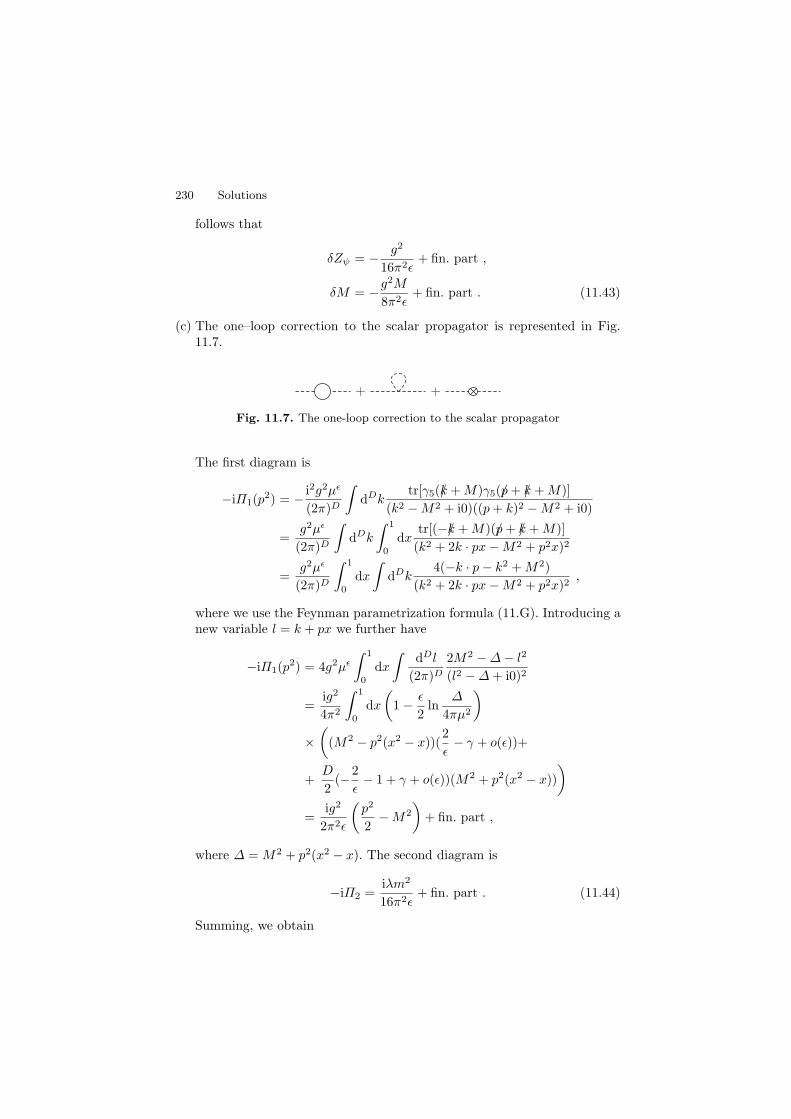
230 Solutions

follows that

δZψ = − g2

16π2ε+ fin. part ,

δM = −g2M

8π2ε+ fin. part . (11.43)

(c) The one–loop correction to the scalar propagator is represented in Fig.11.7.

Fig. 11.7. The one-loop correction to the scalar propagator

The first diagram is

−iΠ1(p2) = − i2g2µε

(2π)D

∫dDk

tr[γ5(/k + M)γ5(/p + /k + M)](k2 − M2 + i0)((p + k)2 − M2 + i0)

=g2µε

(2π)D

∫dDk

∫ 1

0

dxtr[(−/k + M)(/p + /k + M)]

(k2 + 2k · px − M2 + p2x)2

=g2µε

(2π)D

∫ 1

0

dx

∫dDk

4(−k · p − k2 + M2)(k2 + 2k · px − M2 + p2x)2

,

where we use the Feynman parametrization formula (11.G). Introducing anew variable l = k + px we further have

−iΠ1(p2) = 4g2µε

∫ 1

0

dx

∫dDl

(2π)D

2M2 − ∆ − l2

(l2 − ∆ + i0)2

=ig2

4π2

∫ 1

0

dx

(1 − ε

2ln

∆

4πµ2

)

×(

(M2 − p2(x2 − x))(2ε− γ + o(ε))+

+D

2(−2

ε− 1 + γ + o(ε))(M2 + p2(x2 − x))

)

=ig2

2π2ε

(p2

2− M2

)+ fin. part ,

where ∆ = M2 + p2(x2 − x). The second diagram is

−iΠ2 =iλm2

16π2ε+ fin. part . (11.44)

Summing, we obtain

Chapter 11. Renormalization and regularization 231

−iΠ(p2) =ig2

2π2ε

(p2

2− M2

)+

iλm2

16π2ε+iδZφp2−iδm2+fin.part . (11.45)

Using the renormalization conditions:

Π(p2 = m2) = 0dΠ

dp2

∣∣∣p2=m2

= 0 , (11.46)

we get

δZφ = − g2

4π2ε+ fin. part

δm2 =λm2

16π2ε− g2M2

2π2ε+ fin. part . (11.47)

(d) The amplitude of the diagram

is

iM3 = (ig)3µ3ε/2

∫dDk

(2π)D

γ5(/k + /q + M)γ5(/k + M)γ5

((k + q)2 − M2)(k2 − M2)((k − p)2 − m2)

= −2ig3µ3ε/2

(2π)Dγ5

∫ 1

0

dx

∫ 1−x

0

dz

∫dDk

M2 − /q/k + M/q − k2

((k + qx − pz)2 − ∆)3

= −2ig3µ3ε/2

(2π)Dγ5

∫ 1

0

dx

∫ 1−x

0

dz

∫dDl

N

(l2 − ∆)3,

where

∆ = x2q2 + z2p2 + (1 − z)M2 − xq2 + zm2 − p2z − 2xzq · p

andN = M2 − (l − xq + zp)2 + M/q − /q(/l − x/q + z/p) .

In the previous formulae we introduced a variable l = k + xq − zp. As weare interested to find only the divergent part of iM3, it is useful to notethat only l2–term in the numerator of the integrand is divergent. So, byusing (11.C) we get:

232 Solutions

iM3 = 2ig3µ3ε/2γ5

∫dDl

(2π)D

∫ 1

0

dx

∫ 1−x

0

dzl2

(l2 − ∆)3+ . . .

= −g3µε/2(4 − ε)32π2

γ5

(2ε− γ + . . .

)∫ 1

0

dx

×∫ 1−x

0

dz

(1 − ε

2ln

∆

4πµ2

).

Finally

iM3 = −g3µε/2

8π2εγ5 + fin. part . (11.48)

The vertex correction is

so, from

iV3 =(

gγ5µε/2 + δgγ5µ

ε/2 − g3µε/2

8π2ε+ fin.part

) ∣∣∣q2=0

= gγ5

follows

δg =g3

8π2ε+ fin. part .

(e) Let us first calculate the following diagram

Since we have to find the divergent part of this diagram we can put thatthe external momenta are equal to zero. Then,

iM4(k1 = k2 = k3 = k4 = 0) = −g4µ2ε

∫dDp

(2π)D

tr[γ5(/p + M)]4

(p2 − M2)4.

(11.49)Since

γ5(/p + M)γ5(/p + M) = (−/p + M)(/p + M) = M2 − p2

we have

Chapter 11. Renormalization and regularization 233

iM4(k1 = k2 = k3 = k4 = 0) = −4g4µ2ε

∫dDp

(2π)D

1(p2 − M2)2

= − ig4µε

4π2

(2ε− γ

)(1 − ε

2ln

M2

4πµ2

)

= − ig4µε

2π2ε+ fin. part . (11.50)

The previous result should be multiplied by a factor 6 as there are sixdiagrams of this type.The complete four vertex is

iV4 =(−iλµε − iδλµε − 6ig4µε

2π2ε+

3iλ2µε

16π2ε+ fin. part

) ∣∣∣s=4m2,t=u=0

= −iλ , (11.51)

and finally

δλ = −3g4

π2ε+

3λ2

16π2ε+ fin. part . (11.52)

11.13 In this problem dimension of spacetime is D = 2 − ε.

(a) The polarization of vacuum is given by:

−iΠµν(p) = (ie)2(−i2)∫

dDq

(2π)D

tr[(/q − /p)γν/qγµ]q2(q − p)2

. (11.53)

In D-dimensional space trace identities necessary to calculate the previousexpression read:

tr(γµγν) = f(D)gµν ,

tr(γµγνγργσ) = f(D)(gµνgρσ − gµρgνσ + gµσgρν) ,

where f(D) is any analytical function which satisfies the condition f(2) =2. Instead of f(D) we will write 2 as we did in the previous problems (ofcourse, there f(D) = 4). The Feynman parametrization gives

−iΠµν(p) =2e2

(2π)D

∫ 1

0

dx

∫dDq

× 2qµqν − q2gµν − pµqν − pνqµ + (p · q)gµν

(q2 − 2p · qx + p2x)2. (11.54)

By using (11.A–C) in (11.54) we obtain

−iΠµν = −2ie2πD/2

(2π)D

∫ 1

0

dx

[2(

x2pµpν

(−p2x + p2x2)1+ε/2Γ (1 +

ε

2)

− 12

gµν

(−p2x + p2x2)ε/2Γ (

ε

2))

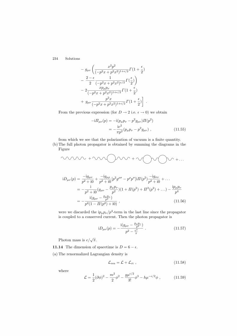
234 Solutions

− gµν

(x2p2

(−p2x + p2x2)1+ε/2Γ (1 +

ε

2)

− 2 − ε

21

(−p2x + p2x2)ε/2Γ (

ε

2))

− 2xpµpν

(−p2x + p2x2)1+ε/2Γ (1 +

ε

2)

+ gµνp2x

(−p2x + p2x2)1+ε/2Γ (1 +

ε

2)]

.

From the previous expression (for D → 2 i.e. ε → 0) we obtain

−iΠµν(p) = −i(pµpν − p2gµν)Π(p2)

= − ie2

πp2(pµpν − p2gµν) , (11.55)

from which we see that the polarization of vacuum is a finite quantity.(b) The full photon propagator is obtained by summing the diagrams in the

Figure

iDµν(p) =−igµν

p2 + i0+

−igµρ

p2 + i0[p2gρσ − pρpσ]iΠ(p2)

−igσν

p2 + i0+ . . .

= − ip2 + i0

(gµν − pµpν

p2)(1 + Π(p2) + Π2(p2) + . . .) − ipµpν

p4

= −i(gµν − pµpν

p2 )

p2(1 − Π(p2) + i0), (11.56)

were we discarded the ipµpν/p4-term in the last line since the propagatoris coupled to a conserved current. Then the photon propagator is

iDµν(p) = −i(gµν − pµpν

p2 )

p2 − e2

π

. (11.57)

Photon mass is e/√

π.

11.14 The dimension of spacetime is D = 6 − ε.

(a) The renormalized Lagrangian density is

Lren = L + Lct , (11.58)

where

L =12(∂φ)2 − m2

2φ2 − gµε/2

3!φ3 − hµ−ε/2φ , (11.59)

Chapter 11. Renormalization and regularization 235

Lct =12δZ(∂φ)2 − δm2

2φ2 − µε/2δg

3!φ3 − µ−ε/2δhφ . (11.60)

By introducing new quantities

Z = 1 + δZ , (11.61)m2

0Z = m2 + δm2 , (11.62)g0Z

3/2 = (g + δg)µε/2 , (11.63)h0Z

1/2 = (h + δh)µ−ε/2 , (11.64)

and rescaling the field, φ0 =√

Zφ, the renormalized Lagrangian densitybecomes

Lren =12(∂φ0)2 −

m20

2φ2

0 −g0

3!φ3

0 − h0φ0 .

The quantities with index 0 are called bare. The Feynman rules are givenin Figure 11.8.

Fig. 11.8. Feynman rules in φ3 theory

Superficially divergent amplitudes are:

Fig. 11.9. Divergent amplitudes in φ3 theory

(b) The tadpole diagram in one–loop order is shown in the following fihure .

236 Solutions

The second term is

− igµε/2

∫dDk

(2π)D

ik2 − m2 + i0

= −igµε/2

(2π)D

πD/2

(m2)−2+ε/2Γ(−2 +

ε

2

)

= − igm4µ−ε/2

128π3

(2ε

+ ln(

4πµ2

m2

)+

32− γ

)

= − igm4µ−ε/2

64π3ε+ fin. part ,

and it does not depend on momentum. Summing all diagrams we get

iH = −ihµ−ε/2 − igm4µ−ε/2

64π3ε− iδhµ−ε/2 + fin. part . (11.65)

Hence,

δh = − gm4

64π3ε+ fin. part . (11.66)

Finite part in the previous expression can be chosen so that H = 0 andwe can ignore all diagrams which contain tadpoles.

(c) The full one–loop propagator is shown in Fig. 11.10.

Fig. 11.10. The one–loop propagator in φ3 theory

The second diagram is

−iΠ2 =(ig)2µε

2

∫dDk

(2π)D

i2

(k2 − m2 + i0)((k − p)2 − m2 + i0)

=g2µε

2

∫ 1

0

dx

∫dDk

(2π)D

1(k2 − 2k · px + p2x − m2 + i0)2

= − ig2

128π3

(2ε

+ 1 − γ + o(ε))

×∫ 1

0

dx(m2 + p2x(x − 1))(

1 − ε

2ln

m2 + p2x(x − 1)4πµ2

)

= − ig2

64π3ε

(m2 − p2

6

)+ fin. part . (11.67)

Chapter 11. Renormalization and regularization 237

Propagator correction is

−iΠ(p2) = − ig2

64π3ε

(m2 − p2

6

)+ ip2δZ − iδm2 + fin. part . (11.68)

From the condition −iΠ(p2) = finite we get

δZ = − g2

384π3ε+ fin. part , (11.69)

δm2 = −m2g2

64π3ε+ fin. part . (11.70)

In MS scheme the finite parts in (11.69) and (11.70) are zero.(d) The vertex correction is given in the Fig 11.11.

Fig. 11.11. Vertex correction in φ3 theory

The second diagram is

iΓ = (−ig)3µ3ε/2

∫dDk

(2π)D

i3

(k2 − m2)((k + p2)2 − m2)((k − p1)2 − m2).

(11.71)By applying (11.H) and integrating over the momentum k we get

iΓ = − (−ig)3µ3ε/2 πD/2

(2π)DΓ( ε

2

)∫ 1

0

dx

∫ 1−x

0

dz

× 1(m2 − p2

2x − p21z + p2

2x2 + p2

1z2)ε/2

= − ig3µε/2

26−επ3−ε/2

(2ε

+ . . .

)∫ 1

0

dx

∫ 1−x

0

dz

×(

1 − ε

2ln

m2 − p22x − p2

1z + p22x

2 + p21z

2

µ2

). (11.72)

From the last formula we find that the divergent part of iΓ is given by

− ig3µε/2

64π3ε. (11.73)

The full one–loop vertex in the renormalized theory is

238 Solutions

iV3 = −igµε/2 − iδgµε/2 + iΓ .

In minimal subtraction scheme δg is

δg = − g3

64π3ε. (11.74)

(e) From (11.61), (11.69) and (11.70) follows

Z = 1 − g2

384π3ε, (11.75)

m2 = m20

(1 − g2

384π3ε

)+

m2g2

64π3ε

= m20 +

5m20g

2

384π3ε, (11.76)

in the one–loop order. Similarly, from (11.69) and (11.74) we have

g0 =(g + δg)µε/2

Z3/2(11.77)

= gµε/2

(1 − g2

64π3ε+

g2

256π3ε

)(11.78)

= gµε/2

(1 − 3g2

256π3ε

). (11.79)

The last expression is important for calculation of the β function.

References

1. D. Bailin and A. Love, Introduction to Gauge Field Theory, Adam Hilger, Bris-tol, 1986

2. J. Bjorken and S. Drell, Relativistic Quantum Mechanics, McGraw-Hill, NewYork, 1964

3. J. Bjorken and S. Drell, Relativistic Quantum Fields, McGraw-Hill, New York,1965

4. N. N. Bogoljubov and D.V. Shirkov, Introduction to the Theory of QuantizedFields, Wiley-Interscience, New York, 1980

5. M. Blagojevic, Gravitation and Gauge Symmetries, IOP Publishing, Bristol,2002

6. T.P. Cheng and L.F. Li, Gauge Theory of Elementary Particle Physics, OxfordUniversity Press, New York, 1984

7. T.P. Cheng and L.F. Li, Gauge Theory of Elementary Particle Physics, Problemsand Solutions, Oxford University Press, New York, 2000

8. M. Damnjanovic, Hilbert spaces and group theory, Faculty of Physics, Beograd,2000 (in Serbian)

9. I.S. Gradshteyn and I.M. Ryzhnik, Table of Integrals, Series and Products,(trans. and ed. by Alan Jeffrey), Academic Press, Orlando, Florida, 1980

10. W. Greiner and J, Reinhardt, Quantum Electrodinamics, Springer, Berlin, Hei-delberg, New York, 1996

11. W. Greiner and J, Reinhardt, Field Quantization, Springer, Berlin, Heidelberg,New York, 1996

12. F. Gross, Relativistic Quantum Mechanics and Field Theory, Wiley, New York,1993

13. C. Itzykson and J.B. Zuber, Quantum Field Theory, McGraw-Hill, New York,1980

14. M. Kaku, Quantum Field Theory: A Modern Introduction, Oxford UniversityPress, New York, 1993

15. F. Mandl and G. Show, Quantum Field Theory, New York, 199916. M. E. Peskin and D. V. Schroeder, An Introduction to Quantum Field Theory,

Addison Wesley, 199517. P. Ramond, Field Theory: A Modern Primer (second edition), Addison-Wesley,

RedwoodCity, California, 1989

240 References

18. L. Rayder, Quantum Field Theory, Cambridge University Press, Cambridge,1985

19. J. J. Sakurai, Advanced Quantum Mechanics, Addison-Wesley, Reading, 196720. S. S. Schweber, An Introduction to Relativistic Quantum Field Theory, Harpen

and Row, New York, 196221. A. G. Sveshnikov and A. N. Tikhonov, The Theory of Functions of a Complex

Variable, Mir Publisher, Moscow, 197822. G. Sterman, Introduction to Quantum Field Theory, Cambridge University

Press, Cambridge, 199323. S. Weinberg, The Quantum Theory of Fields I and II, Cambridge University

Press, New York, 1996

Index

Action 25Einstein–Hilbert 27

Advanced Green functionDirac equation 138Klein–Gordon equation 132

Angular momentum tensorDirac field 44, 45, 164electromagnetic field 52, 183–185Klein–Gordon field 36, 37, 144

Anticommutation relationsDirac field 43

Baker–Hausdorff formula 91, 144Bianchi identity 49

Casimir effect 53, 187–190Casimir operator 7Charge

Dirac field 45, 162Klein–Gordon field 37, 142

Charge conjugationDirac equation 18

bilinears 23–24, 115–118Dirac field 45

bilinears 47, 175–177scalar field 41, 159

Chiral transformations 28Coherent states 40, 156–158Commutation relations

electromagnetic field 50scalar field 35

Conformal group 75Conformal transformations 7Continuity equation 10

Cross section 55Cutkosky rule 62, 225

Decay rate 218Differential cross section 192Dilatations

Dirac field 30, 46, 129, 168scalar field 29, 38, 129, 148–150

Dimensional regularization 63Dirac equation 17

helicity 99, 118helicity basic 20, 95plane wave solutions 17, 18, 93–95spinor basic 20

Dirac fieldquantization 43

Dirac particlein a hole 22, 110–111in a magnetic field 23, 113

Dyson Green functionKlein–Gordon equation 133

Electromagnetic fieldquantization 49

Energy–momentum tensor 26, 126symmetric or Belinfante tensor 29,

127Euler–Lagrange equations 25, 121

Feynman parametrization 62, 211Feynman propagator

Dirac equation 138, 139Dirac field 44

242 Index

Klein–Gordon equation 31, 33, 132,136

Klein–Gordon field 36, 153Foldy–Wouthuysen transformation 24,

118–119Functional derivative 25, 121Furry theorem 225

Galilean algebra 39, 156Gamma matrices 13

contraction identities 14, 86–87Dirac representation 13Majorana representation 13trace identities 15, 87–89Weyl representation 13

Gamma–function 62, 213γ5–matrix 13, 86, 102γ5/s–operator 98gauge transformations 49Gordon identity 21, 104Grassmann variable 173Green function

Dirac equation 31, 33Klein-Gordon equation 31massive vector field 33, 140massless vector field 34, 140Schrodinger equation 154

Gupta–Bleuler quantization 50

HamiltonianDirac field 44, 45, 162Klein–Gordon field 36, 37, 142

Helicity 94, 165, 181

Klein paradoxDirac particle 109scalar particle 82

Klein–Gordon equation 9plane wave solutions 77

Klein–Gordon particlein a hole 10, 79in a magnetic field 10, 81in the Coulomb potential 10, 83

Lagrangian densityDirac field 43massive vector field 27massless vector field 49Schrodinger field 39

sigma model 28Left/right spinors 102–103Levi-Civita tensor 4, 5, 68Little group 74Lorentz group 5, 67

generators in defining repr. 69Lorentz transformations

Dirac equation 17bilinears 23–24, 115–118

Dirac field 44, 170bilinears 47, 174–177

scalar field 158–159

Majorana spinor 47, 173Maxwell equations 49Metric tensor 3Minkowski space 3Momentum

Dirac field 44, 45Klein–Gordon field 36, 37, 142

MS scheme 237

Noether theorem 26Normal ordering

Dirac field 44, 47, 172Klein–Gordon field 36

Optic theorem 220

ParityDirac equation 18

bilinears 23–24, 115–118Dirac field 44

bilinears 47, 174–177scalar field 41, 159

Pauli matrices 5Pauli–Lubanski vector 7, 19, 72–74, 98Pauli–Villars regularization 62, 215Phase transformations 28, 125φ3 theory in 4D 58φ3 theory in 6D 64, 234–238Poincare algebra 6, 71, 72Poincare group 4, 6Poincare transformations 4

scalar field 40Projection operators

energy 19, 95–96spin 100

QED processes

Index 243

scattering in an external electromag-netic field 202

QED processesµ−µ+ → e−e+ 58, 196–198e−µ+ → e−µ+ 58e−µ+ → e−µ+ 198Compton scattering 58, 199scattering in an external electromag-

netic field 58, 200

Reflection and transmission coefficientsDirac equation 22Klein–Gordon equation 10

Reiman ζ–function 53Retarded Green function

Klein–Gordon equation 132, 137

S–matrix 55Scalar electrodynamics 64, 226Scalar field

quantization 35Scalar product 4Scattering of polarized particles 59,

203–205Schrodinger equation 153Schwinger model 64, 233Σ–vector 96σµν–matrices 14, 85, 87

SL(2, C) group 5Superficial degree of divergence 64,

227Symmetry factor in φ4 theory 57,

194–195

Tensor of rank (m, n) 4Time reversal

Dirac equation 18bilinears 23–24, 115–118

Dirac field 44bilinears 47, 175–178

scalar field 41, 159

Vacuum polarization 63, 225Vector 3

contravariant components 3covariant components 4dual vector or one–form 4

Vertex correction 231–232, 237Virasora algebra 38

Weyl fields 20Wick rotation 212Wick theorem 55, 57, 152, 172,

193–196

Yukawa theory 64, 206, 227–233