Probing new physics in the laboratory and in spaceOvchynnikov, M.

CitationOvchynnikov, M. (2021, December 14). Probing new physics in the laboratory and in space.Casimir PhD Series. Retrieved from https://hdl.handle.net/1887/3247187 Version: Publisher's Version

License: Licence agreement concerning inclusion of doctoral thesis in theInstitutional Repository of the University of Leiden

Downloaded from: https://hdl.handle.net/1887/3247187 Note: To cite this publication please use the final published version (if applicable).

Probing new physicsin the laboratory and in space

Proefschrift

ter verkrijging vande graad van doctor aan de Universiteit Leiden,

op gezag van rector magnificus prof. dr. ir. H. Bijlvolgens besluit van het college voor promoties

te verdedigen op 14 december 2021klokke 12:30 uur

door

Maksym Ovchynnikov

geboren te Kiev (Oekraıne)in 1994

Promotores: Prof. dr. Alexey BoyarskyProf. dr. Ana Achucarro

Promotiecommissie: Prof.dr. J. AartsDr. D.F.E. SamtlebenProf. fr. K.E. SchalmProf. dr. N. Serra (University of Zurich, Switzerland)Prof. dr. O. Ruchayskiy (University of Copenhagen, Denmark)

Casimir PhD series Delft-Leiden 2021-37ISBN 978-90-8593-502-5An electronic version of this thesis can be found at https://openaccess.leidenuniv.nl

The cover shows the Big Bang Nucleosynthesis reactions framework, which may be affectedby currently undiscovered particles, and the SHiP experiment, the proposed flagman tosearch for heavy new physics particles in laboratory.

Contents

1 Introduction 61.1 Portals 81.2 LHC and dedicated accelerator experiments 9

1.2.1 Qualitative comparison of different experiments 101.3 Astrophysical and cosmological probes: defining the parameter space of

interest for accelerator experiments 141.3.1 BBN 16

1.3.1.1 How short-lived FIPs affect BBN 181.3.2 CMB 19

1.3.2.1 Impact of short-lived FIPs on CMB 221.4 Summary 23

2 Accelerator and laboratory searches 242.1 Bounds on HNLs from CHARM experiment 24

2.1.1 CHARM experiment 262.1.2 Bounds of CHARM on HNLs as reported in literature 272.1.3 Phenomenology of HNLs at CHARM 28

2.1.3.1 Production 282.1.3.2 Decays and their detection 30

2.1.4 Results 332.1.5 Comparison with atmospheric beam dumps 35

2.1.5.1 Analytic estimates: comparison with CHARM 362.1.5.2 Accurate estimate 37

2.2 Searches with displaced vertices at the LHC 382.2.1 Displaced vertices with muon tracker at CMS 40

2.2.1.1 Description of the scheme 412.2.1.2 Estimation of the number of events 432.2.1.3 HNLs 452.2.1.4 Chern-Simons portal 482.2.1.5 Dark scalars with quartic coupling 492.2.1.6 Summary 51

– 3 –

2.3 Searches for light dark matter at SND@LHC 522.3.1 Scattering off nucleons: different signatures 53

2.3.1.1 Model example: leptophobic portal 552.3.2 SND@LHC 57

2.3.2.1 Description of experiment 572.3.2.2 Search for scatterings of LDM 592.3.2.3 Search for decays of mediators 60

2.3.3 Sensitivity of SND@LHC 622.3.3.1 Leptophobic portal 622.3.3.2 Decays 66

2.3.4 Comparison with FASER 682.3.4.1 Lower and upper bound of the sensitivity 692.3.4.2 Decays 702.3.4.3 Scattering 71

2.3.5 Conclusions 72

Appendices 732.A CHARM sensitivity based on number of decay events estimate 732.B Decay events at SND@LHC 742.C Leptophobic mediator: production, decays and scatterings 75

2.C.1 Production and decay 752.C.2 Elastic and inelastic scattering cross sections 77

2.C.2.1 Elastic scattering 772.C.2.2 Inelastic scattering 78

3 Probes from cosmology 793.1 BBN and hadronically decaying particles 79

3.1.1 Measurements of 4He abundance 793.1.2 Bound on hadronically decaying particles 803.1.3 Limits of applicability of the bound 84

3.2 CMB 863.2.1 Impact of short-lived FIPs on Neff 88

3.2.1.1 Analytic considerations 883.2.1.2 Effect of Residual Non-equilibrium Neutrino Distortions 93

3.2.2 Summary 973.3 Case study: HNLs 98

3.3.1 Thermal history of HNLs 983.3.1.1 HNLs with mixing angles below Umin 993.3.1.2 HNLs with mixing angles above Umin 1013.3.1.3 Evolution after decoupling 104

3.3.2 Hadronic decays of HNLs 105

4

3.3.3 Bounds from BBN and CMB 1063.3.3.1 BBN 1063.3.3.2 Results 107

3.3.4 Bound from CMB 1083.3.4.1 Behavior of Neff 110

3.3.5 Bounds from CMB 1133.3.6 Implications for the Hubble Parameter 114

Appendices 1173.A Thermal dependence of mixing angle of HNLs 117

3.A.1 Neutrino self-energy 1173.A.2 Derivation of U2

m 1193.B Changes in p↔ n rates due to the presence of mesons 121

3.B.1 Numeric study 1223.B.2 Numeric approach for long-lived HNLs 125

3.C Temperature Evolution Equations 1263.D Comment on “Massive sterile neutrinos in the early universe: From thermal

decoupling to cosmological constraints” by Mastrototaro et al. 127

Samenvatting 144

Summary 146

List of publications 147

Curriculum vitæ 150

Acknowledgements 151

5

Chapter 1

Introduction

In the twentieth century, attempts to explain subatomic physics phenomena combined withtwo scientific revolutions – special relativity and quantum mechanics – have resulted inthe development of the Standard Model of particle physics (SM). The SM successfullydescribes all the particle physics processes that we observe at accelerators with the help ofonly 17 particles and interaction between them, that is based on the SU(3)⊗SU(2)⊗U(1)

gauge group, see Fig. 1.1. The SM has passed a number of precision tests [1–3]. The laststage of the confirmation of SM was the discovery of the Higgs boson at Large HadronCollider (LHC) [4, 5] and subsequent tests of its properties, which confirmed that it isexactly the same particle as predicted by the SM [6].

The SM is a closed theory and may be used as an effective theory that makes extremelyaccurate predictions up to the Planck scale. However, it is not complete. There are afew observational phenomena establishing that SM has to be extended, probably byadding new particles. These phenomena constitute the beyond the SM problems (orBSM problems).

The BSM problems are:

• Neutrino oscillations: measurements of solar neutrino flux, as well as observationsof atmospheric and collider neutrino interactions, suggest that neutrinos may changetheir flavor – the phenomenon called neutrino oscillations. The oscillations may occurif neutrinos have different masses. This is not possible in SM, in which neutrinos aremassless, but may be resolved by adding interactions with new particles.

• Dark matter (DM): Astrophysical and cosmological observations suggest that mostof the mass of the Universe is dominated by a specific type of matter that does notinteract with light – the dark matter. The only natural candidate for the role of DM inSM is the SM active neutrino. However, experimental restrictions on neutrino massesmake this scenario impossible.

6

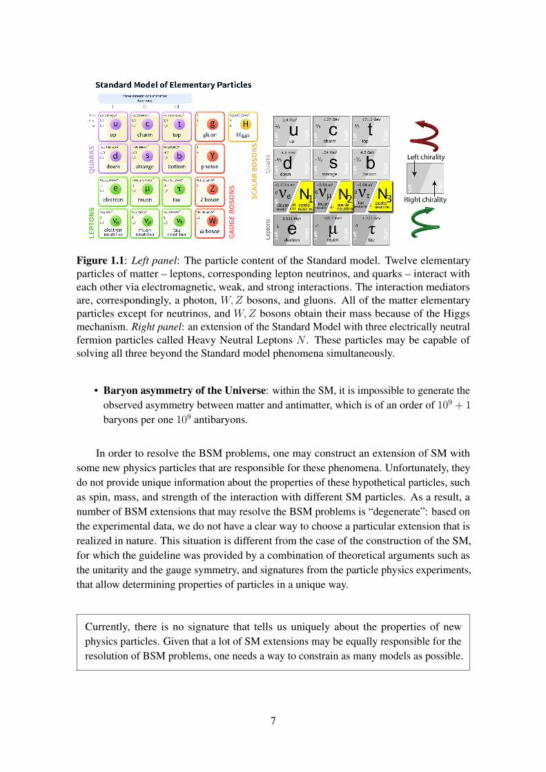
Figure 1.1: Left panel: The particle content of the Standard model. Twelve elementaryparticles of matter – leptons, corresponding lepton neutrinos, and quarks – interact witheach other via electromagnetic, weak, and strong interactions. The interaction mediatorsare, correspondingly, a photon, W,Z bosons, and gluons. All of the matter elementaryparticles except for neutrinos, and W,Z bosons obtain their mass because of the Higgsmechanism. Right panel: an extension of the Standard Model with three electrically neutralfermion particles called Heavy Neutral Leptons N . These particles may be capable ofsolving all three beyond the Standard model phenomena simultaneously.

• Baryon asymmetry of the Universe: within the SM, it is impossible to generate theobserved asymmetry between matter and antimatter, which is of an order of 109 + 1

baryons per one 109 antibaryons.

In order to resolve the BSM problems, one may construct an extension of SM withsome new physics particles that are responsible for these phenomena. Unfortunately, theydo not provide unique information about the properties of these hypothetical particles, suchas spin, mass, and strength of the interaction with different SM particles. As a result, anumber of BSM extensions that may resolve the BSM problems is “degenerate”: based onthe experimental data, we do not have a clear way to choose a particular extension that isrealized in nature. This situation is different from the case of the construction of the SM,for which the guideline was provided by a combination of theoretical arguments such asthe unitarity and the gauge symmetry, and signatures from the particle physics experiments,that allow determining properties of particles in a unique way.

Currently, there is no signature that tells us uniquely about the properties of newphysics particles. Given that a lot of SM extensions may be equally responsible for theresolution of BSM problems, one needs a way to constrain as many models as possible.

7

1.1 Portals

Non-observation of new physics particles at particle physics experiments may be explainedby two reasons: either they are too heavy to be produced at the currently reachable energies,or they are too feebly interacting, such that the intensity of events at the experiment isinsufficient to observe them. Further, we will consider the second class of the particles.They are called Feebly Interacting Particles, or FIPs.

The FIPs may be directly responsible for the BSM phenomena or serve as mediatorsbetween the dark sector and the SM. It is convenient to classify BSM extensions with FIPsby the properties of the particles-mediators:

1. Scalar portal:L = α1H

†HS + α2H†HS2, (1.1.1)

with H being the SM Higgs doublet, S being a new scalar particle, while α1,2 realcouplings. Phenomenologically, the scalar S interacts with SM particles in the sameway as a light Higgs boson, but the matrix element of any process is suppressed bythe mixing angle θ 1. S may play a role of a mediator for the dark sector [7], orbe responsible for the inflation by playing the role of an inflaton [8], if having massin GeV scale.

2. Neutrino portal:L = FαILαHNI + N mass term, (1.1.2)

where H = iσ2H∗ is the Higgs doublet in the conjugated representation, Lα =

(lανα

)

is the left SM lepton doublet, NI Heavy Neutral Leptons (or HNLs), and FαI complexcouplings. Phenomenologically, HNLs interact similarly to a SM neutrino να butsuppressed by the mixing angle Uα 1. HNLs may resolve all of the BSMproblems. In particular, to explain neutrino oscillations and the baryon asymmetry ofthe Universe, we need at least two HNLs with highly degenerate masses, while forDM one needs a long-lived HNL with mass in O(keV) range. A model with suchthree HNLs is called Neutrino Minimal Standard Model, or νMSM [9, 10].

3. Vector portal:L =

ε

2FµνV

µν , or L = εJµVµ (1.1.3)

where Fµν is the strength tensor of the gauge field associated with the UY (1) gaugegroup, V µν is the strength associated with the new vector field Vµ, and Jµ is theconserved SM current (for instance, B − 3L current).

8

1.2 LHC and dedicated accelerator experiments

During the last few years, particle physics experiments with large events intensity havebeen proposed to probe FIPs. They are called Intensity frontier experiments.

FIPs may interact with SM particles in different ways. In dependence on the type ofinteraction, different kinds of searching may be preferable. Based on the search type, theIntensity frontier experiments may be classified as follows:

1. Prompt or displaced visible decays of FIPs: a possible method to search for unsta-ble FIPs that decays into electrically charged particles is to produce them in collisionsof SM particles and then detect their decays into SM particles. Such kind eventsmust be distinguished from pure SM events. For instance, an event with the HNLdecay N → µ−π+ may be mimicked by a long-lived µ− and π+ produced outsidethe decay volume in some SM process, and whose trajectories closely intersect atone point inside the decay volume. The background reduction is typically reachedby preventing the outer particles from reaching the decay volume: either by plac-ing the decay volume far from the collision point (such that SM particles decaybefore reaching the decay volume), by placing SM particles absorbers/deflectorsbetween the collision point, or by imposing specific events selection criteria that min-imize the SM background. Examples include: prompt and displaced searches at theLHC, especially during its high-luminosity phase [11–16]; LHC-based experiments –FASER/FASER2 [17], MATHUSLA [18], Codex-b [19]; experiments at extractedbeams – SHiP [20], NA62 in the dump mode (SPS beam at CERN), DUNE neardetector [21], DarkQuest [22] (Fermilab).

2. Rare SM decays: if decays of FIPs cannot be distinguished from some rare SMprocesses, one may search for an excess of the corresponding events over the yieldpredicted by SM. Such rare decays are searched, e.g., at meson factories. Examplesinclude: rare decays of mesons – B → Kµµ at LHCb [23], BaBar [24], and BelleII [25], K → πνν at NA62 in the kaon mode [26].

3. Events with missing energy/momentum: Another class of events is common ifFIPs leave detectors invisibly, for instance decaying into uncharged particles. Suchtype of events may be characterized by a missing energy/momentum. Examplesare NA64 [27, 28], Belle, BaBar, which search for the process e + target → e +

missing energy, and events of the type p+ p→ jet + missing pT at the LHC [29–31].

4. Scatterings of new physics particles: If being stable, FIPs may still be detectedvia their scatterings off matter. In this case, the production of FIPs at the labora-tory is not necessary, as they could have been generated in the Early Universe and

9

SHADOWS

NA62

Excluded

SHiP

MATHUSLA

FASER2

BBN

0.05 0.10 0.50 1 510-13

10-11

10-9

10-7

mS [GeV]

θ2

CHARM

T2K

DELPHI

NA62

Belle

BBN

Seesaw

SHiPMATHUSLA

NA62

FASER2SHADOWS

DUNE

0.1 0.5 1 5 1010-12

10-10

10-8

10-6

10-4

mN [GeV]

Ue2

[GeV]A'm3−10 2−10 1−10 1 10 210 310

ε

9−10

8−10

7−10

6−10

5−10

4−10

3−10

2−10

NA62-dump

APEX

SHiP

pot (dotted)20 pot (solid), 1018DarkQuest: 10

HPS

FASER2

FASER

Belle II

(dotted)-1 (solid), 300 fb-1LHCb: 15 fb

HL-LHCe(g-2)

BaBar

CMSLHCb

A1NA48/2

mu3e (phase1)

mu3e (phase2)

E137

E141

NA64(e)

E774

SN1987A

nu-CalCHARM

Figure 1.2: Sensitivity reach of Intensity frontier experiment to decays of portal particles:dark scalars (1.1.1) that have zero quartic coupling HHSS (the left panel), Heavy NeutralLeptons (1.1.2) that mix purely with νe (the middle panel), and dark photons (1.1.3) (theright panel). The figure for the dark photon and sensitivity contours for HNLs and scalarsare given from [36]. The BBN bound for HNLs is reproduced from [37].

surround us today. This may be the case of dark matter particles. Examples ofexperiments that search for this signature include recently approved SND@LHC [32]and FASERν [33], DUNE near detector, and direct DM detection experiments suchas CRESST [34, 35].

The combined sensitivity reach of these experiments to different portal models is shown inFig. 1.2. We also show there the parameter space excluded by past experiments.

1.2.1 Qualitative comparison of different experiments

Using Fig. 1.2, we may formally compare the potential of different experiments to probenew physics particles. In addition, in order to study principal limitations and advantages ofthe given experimental setup to probe different new physics models, it would be useful tohave a qualitative understanding of the features of the sensitivity.

The sensitivity of the given experiment to FIPs may be estimated using Monte-Carlosimulations of the number of events. However, this method has several limitations whencomparing the sensitivity reach of different experiments.

Indeed, a simulation is typically a “black box” which does not allow us to understandthe characteristic features of the sensitivity curve. In addition, it typically costs a hugeamount of time and requires a lot of computational resources, which becomes crucial ifmany simulations are required. This is the case, for instance, during the optimizationstage of the experiment, when its design is changed. Another situation is when we changeparameters of the FIP model, which requires a new simulation each time.

A clear, fully controlled estimate of the sensitivity within a factor of few is provided bysemi-analytic calculations [9].

10

Let us consider for instance Intensity frontier experiments that search for visible decaysof FIPs X . The number of events at these experiments is given by

Nevents ≈∑

i

Ni · Br(i→ X) · ε(i)geom · P (i)decay · Br(X → vis) · εdecay · εrec (1.2.1)

Here, Ni is the total number of SM particle species i at the experiment (it may be forinstance a particle from the incoming beam, or a secondary particle produced in collisions),Br(i→ X) is the branching ratio of the process with i which leads to the production of X(it may be a decay or a scattering process), ε(i)geom is the geometric acceptance – the fractionof particles X that fly in the direction of the detector of the experiment. P (i)

decay is the decayprobability:

Pdecay ≈ exp[−lmin/cτXγ(i)X ]− exp

[−lmax/cτXγ

(i)X

]≈

≈

lfid/cτXγ

(i)X , cτXγ

(i)X lmax

exp[−lmax/cτXγ

(i)X

], cτXγ

(i)X . lmin

(1.2.2)

with lmin, lmax being the minimal and maximal distance defining the decay volume (lfid =

lmax− lmin), τX the proper lifetime and γ(i)X the mean γ factor. Br(X → vis) is the branching

ratio of decays of X into visible states (typically, a pair of charged particles). Finally, εdecay

is the decay acceptance – a fraction of decay products that travel in the direction of thedetector, and εrec is the reconstruction efficiency – the fraction of events that are successfullyreconstructed in detectors.

The sensitivity curve is defined by the condition Nevents > Nmin, where Nmin is thenumber of events required for the detection. The limiting cases in (1.2.2) define the lowerand upper bounds of the sensitivity of the experiments shown in Fig. 1.2. Using (1.2.2)together with (1.2.1), we may estimate these bounds analytically. We consider modelsin which the production and decays of X are controlled by the same coupling g of X toSM, such that Br(i → X), τ−1

X ∝ g2. Assuming for simplicity that the production of Xis dominated by one specific channel, the scaling of the lower and upper bounds of thesensitivity is given by the following formulas:

Nevents,lower bound ∝ g4 ⇒ g2lower bound ∼

√Nmin

Nevents,lower bound∣∣g=1

≡

≡ χlower ×√

cτXBr(i→ X)Br(X → vis)

∣∣∣∣g=1

(1.2.3)

Nevents,upper bound ∝ g2upper exp

[−lmin/cτXγ

(i)X

]⇒ g2

upper ∼γ

(i)X

lmincτX

∣∣∣∣g=1

≡ χupper ·1

cτX

∣∣∣∣g=1

,

(1.2.4)

11

Here, we have separated the experiment-independent parameters, which cancel out whencomparing different experiments, from the experiment-specific quantities:

χlower ≡

√√√√ Nmin · γ(i)X

Ni · ε(i)geom · lfid · εdecay · εrec

, χupper ≡γ

(i)X

lmin(1.2.5)

The lower and upper bounds of the sensitivity of the Intensity frontier experiments maybe estimated with the help of several geometric parameters.

We are now ready to compare the lower and upper bounds of different experiments. Weconsider the following experiments: MATHUSLA and FASER2 at the LHC, and SHiP andSHADOWS at SPS, and restrict the masses of FIPs by the GeV range. Their parametersare summarized in Table 1.1.

Experiment SHiP SHADOWS MATHUSLA FASER2√s, GeV 28 28 13000 13000NPoT 2 · 1020 ∼ 5 · 1019 2.2 · 1017 2.2 · 1017

lminm 50 10 40 480〈lfid〉

m 50 20 100 5θdetrad (0, 0.025) (0.03, 0.09) (0.48, 0.9) (0, 2.1 · 10−3)

Table 1.1: Parameters of different Intensity frontier experiments: the beam CM energy√s,

the total number of the proton-proton collisions expected during the working period NPoT,the distance to the beginning of the decay volume lmin, the average length of the decayvolume 〈lfid〉, polar angle coverage of detectors θdet.

We consider three different production channels: proton bremsstrahlung, that is impor-tant for dark photons and dark scalars, decays of D mesons, which are important for HNLs,and decays of B mesons, which are important for dark scalars and HNLs [38, 39], seeFig. 1.3. We adopt the description of the probabilities of these channels from [38, 39]. Forparticles from decays of mesons, we approximate the kinematic quantities such as γX andεgeom by the corresponding quantities of mesons. This is a meaningful approximation sincethe angular distribution differs only by the quantity ∆θ ' mB,D/EB,D, which is typicallymuch smaller than the angular coverage of the experiments of interest. We use the totalamount and spectra of D,B mesons at the LHC provided by the FONLL package [40–43]and at SPS by [44]. Finally, we estimate εdecay with the help of a simple Monte-Carlosimulation.1

Let us now highlight important points relevant for the comparison:

1We require decay products from two-body decays of particles with masses mB/D for decays from B/Dmesons and 1 GeV for the production by bremsstrahlung to point to detectors.

12

p

p

X

B/D

h

X

(a) (b)Figure 1.3: Typical production channels for a FIP X that has mass in O(GeV) range:proton bremsstrahlung (the diagram (a)), and decays of B,D mesons into a FIP and otherparticle h (the diagram (b)).

1. Particles produced by the proton bremsstrahlung have small transverse momentapT . ΛQCD and hence are very collimated with respect to the beam axis. Therefore,off-axis experiments like SHADOWS and MATHUSLA do not have the sensitivityto this channel.

2. For the production from mesons, the invariant mass of collisions√s must be much

larger than the doubled mass of meson; otherwise, the meson production probabilitygets suppressed. As a result, at the SPS beam energy, the fraction of produced Bmesons per one proton-proton collision is ' few · 10−7, since 2mB ≈ 10 GeV is nottoo far from

√sSPS ≈ 28 GeV. At the LHC,

√s = 13 TeV, and the probability is

much higher, reaching 10−2. For D mesons, there is no such significant difference,as their mass is significantly lower. However, the suppression at SPS is compensatedby a much larger beam intensity.

3. The distribution of B,D mesons is collimated, although not so strong as compared tothe bremsstrahlung. This leads to much lower (but non-zero) geometric acceptancefor the off-axis experiments. As a result of these factors, the amounts of B mesons atSHiP, FASER2, and MATHUSLA are comparable, while at SHADOWS it is evensuppressed.

4. Experiments located close to the beam collision point, such as SHADOWS, mayhave an advantage at the upper bound of the sensitivity even despite lower averagemomentum. On-axis experiments at the LHC such as FASER2, although beinglocated far away from the collision point, are still competitive at the upper bound dueto large average momenta of particles produced in energetic beams collisions in thefar-forward direction.

The resulting parameters (1.2.5) are summarized in Table 1.2.

13

Experiment SHiP SHADOWS MATHUSLA FASER2Nmin 3 3 3 3

NB · εBgeom 8 · 1013 5 · 1011 3 · 1013 1013

ND · εDgeom 8 · 1017 2 · 1016 5 · 1014 2 · 1014

NPoT · εbremgeom 1020 – – 2 · 1016

εdecay, B 0.4 < 0.4 O(1) O(1)εdecay, D 0.4 ' 0.3 O(1) O(1)εdecay, brem O(1) – – O(1)χlower, B 4 · 10−7 6 · 10−6 10−7 2 · 10−6

χlower, D 3 · 10−9 8 · 10−8 4 · 10−8 5 · 10−7

χlower, brem 10−10 – – 10−7

χupper, B 2 6 0.1 3χupper, D 1 2 0.03 2χupper, brem 3 – – 2

Table 1.2: Potential reach of different Intensity frontier experiments as predicted byEqns. (1.2.5). The relevant parameters NB,D, εgeom, εdecay. The minimal number of eventsrequired for the discovery, Nmin, corresponds to the assumption of absence of backgroundat 95% CL.

From the discussion, we conclude that SHiP is the most powerful “non-compromised”experiment proposed to search for FIPs with masses below 5 GeV.

1.3 Astrophysical and cosmological probes: defining the parameterspace of interest for accelerator experiments

Searches for FIPs at accelerator experiments are restricted by short-lived particles. Theupper bound on lifetimes that may be constrained is model-dependent. For instance, forHNLs it may be as large as τN ' 10−2 s at masses mN > 0.5 GeV, see Fig. 1.4. Itis therefore important to define the target parameter space of FIPs to be probed by theaccelerator experiments.

Signatures that may be sensitive to long-lived FIPs are cosmological and astrophysicalobservables.

In the Early universe or inside a dense medium of a supernova, the intensity of collisionswas much higher than at colliders. Therefore, despite tiny couplings to the SM particles,FIPs may be produced in amounts significant enough to potentially alter the cosmologicalobservables.

14

Lab experiments

Cosmology

SHiP

0.2 0.5 1 2 510-7

10-5

0.001

0.100

10

mN [GeV]

τ N,s

Figure 1.4: The complementarity of FIP signatures coming from past laboratory exper-iments and cosmological observations, demonstrated using a particular FIP example –HNLs with the pure e mixing. Laboratory experiments are able to probe the parameterspace of relatively short-lived particles, whereas cosmological observations such as BigBang Nucleosynthesis and Cosmic Microwave Background may rule out long-lived HNLs.Together, they define the target parameter space for future experiments such as SHiP.

Cosmological and astrophysical probes include: abundances of primordial light el-ements synthesized during Big Bang Nucleosynthesis (BBN); the spectrum of CosmicMicrowave Background (CMB); galactic X-ray lines; supernova explosion observation;primordial magnetic fields. The experimental status of these observations is different. Forinstance, while the CMB spectrum is measured very accurately, the supernova evolution isprobed poorly, as it is based on only one observation of the explosion of SN1987A.

Predictions for these observables based on the standard cosmological model (Λ ColdDark Matter, or ΛCDM) and only SM particles populating the plasma do not contradict themeasurements. By adding a new particle, we may break this agreement.

Cosmological probes that may constrain the shortest FIPs lifetimes are BBN and CMB.They may be affected by FIPs with lifetimes as small as τFIP ' 0.01 s.

The earliest probe from the Early Universe is BBN. BBN is sensitive to the evolution ofthe Universe at cosmological times as small as t ' O(1 s), when neutrons decouple fromthe primordial plasma (see subsection 1.3.1 below). As their decoupling is not instantaneous,the population of neutrons at decoupling is sensitive to the dynamics at even earlier times. Inparticular, it may constrain particles with lifetimes as small as τFIP & 0.01 s (see Sec. 1.3.1).Another probe is CMB: although it is associated to the epoch at which electrons and protonsget bounded into the Hydrogen atom, its characteristic features (i.e., the angular horizon orthe damping scale) depend on the primordial helium abundance and the effective number of

15

relativistic degrees of freedom, Neff, which, in their turn, are determined by the evolutionof the Universe at time scales as small as t ' 0.1 s. Below, we discuss them in more detail.

1.3.1 BBN

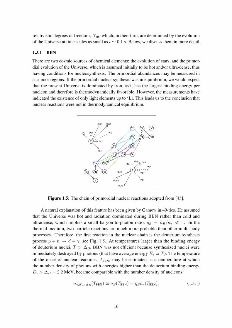
There are two cosmic sources of chemical elements: the evolution of stars, and the primor-dial evolution of the Universe, which is assumed initially to be hot and/or ultra-dense, thushaving conditions for nucleosynthesis. The primordial abundances may be measured instar-poor regions. If the primordial nuclear synthesis was in equilibrium, we would expectthat the present Universe is dominated by iron, as it has the largest binding energy pernucleon and therefore is thermodynamically favorable. However, the measurements haveindicated the existence of only light elements up to 7Li. This leads us to the conclusion thatnuclear reactions were not in thermodynamical equilibrium.

12C

13C

11C

12B

11B

10B

9Be

7Be

8Li

7Li

6Li

4He

3He

1H

2H

3H

n

X

(p,γ)

(α,γ)

(β+)

(β-)

(n,γ)

(t,γ)

(α,n)

X

(n,p)

(d,n)

(d,p)

(d,γ)

(p,α)

(n,α)

(t,p)

(t,n)

(d,nα)

Figure 1.5: The chain of primordial nuclear reactions adopted from [45].

A natural explanation of this feature has been given by Gamow in 40-ties. He assumedthat the Universe was hot and radiation dominated during BBN rather than cold andultradense, which implies a small baryon-to-photon ratio, ηB = nB/nγ 1. In thethermal medium, two-particle reactions are much more probable than other multi-bodyprocesses. Therefore, the first reaction in the nuclear chain is the deuterium synthesisprocess p + n → d + γ, see Fig. 1.5. At temperatures larger than the binding energyof deuterium nuclei, T > ∆D, BBN was not efficient because synthesized nuclei wereimmediately destroyed by photons (that have average energy Eγ ' T ). The temperatureof the onset of nuclear reactions, TBBN, may be estimated as a temperature at whichthe number density of photons with energies higher than the deuterium binding energy,Eγ > ∆D = 2.2 MeV, became comparable with the number density of nucleons:

nγ,Eγ>∆D(TBBN) ' nB(TBBN) = ηBnγ(TBBN), (1.3.1)

16

which implies TBBN ' ∆D/ ln(η−1B ) ∼ 0.1∆D ' 100 keV. At such low temperatures,

however, heavy elements cannot be formed because of the Coulomb barrier. Indeed, theprobability of the synthesis process X1 +X2 → X3, with Xi being some nucleus with massand charge mi and Zi, is suppressed by the Coulomb repulsion factor

σv ∝ e−η, η =Z1Z2αEM

v(T )=Z1Z2αEM√

T

√m1m2√

m1 +√m2

, (1.3.2)

The synthesis effectively does not occur if

η(TBBN) & 1⇒ TBBN . Tcoulomb =m1m2Z

21Z

22

(√m1 +

√m2)2

(1.3.3)

As a result, using TBBN ' 100 keV, we conclude that no nucleus heavier than 12C may besynthesized efficiently (12C is produced in the process 4He +8 Be→12 C + 2γ, for whichTcoulomb ' TBBN).

The only robust measurements of primordial abundances are those of d and 4He.

Indeed, the 3He isotope is measured only in regions with high metallicity, and it isnot possible to estimate the effect of the stellar evolution on its abundance [46]. Themeasurements of 7Li [47] set the lower bound on the primordial abundance since 7Li mightbe destroyed in low-metallicity stars.

The abundance of the primordial 4He, Yp, is measured by three ways: (i) the low-metallicity extragalactic method, according to which the helium abundance is measuredin low-metallicity regions and then extrapolated to zero metallicity; (ii) the intergalacticmethod – measurements of Yp in the low-metallicity extragalactic gas; and (iii) the CMBmethod, for which the helium abundance is extracted from the CMB damping tail. Thecurrent error in the determination of 4He at 1σ is around 4% (see Sec. 3.1.1).

In the Standard Model BBN (or SBBN), the only free parameter is ηB.

Using the value of ηB measured from CMB, we find that the predictions of SBBN agreewith measurements of d and 4He [48]. Therefore, to understand the impact of FIPs onBBN, we should first learn SBBN.

The SBBN proceeds as follows. Above TBBN, we have only p, n, e±, ν, ν, γ particles inthe plasma. During the whole BBN, ultrarelativistic particles dominate the energy densityof the Universe and determine the dynamics of the expansion of the Universe and hence theHubble rate H . e±, ν, ν, in addition, keep protons and neutrons in thermal equilibrium byweak reactions

p+ ν ↔ n+ e+, n+ νe ↔ p+ e (1.3.4)

17

at large temperatures T 1 MeV, such that nn/np = e−(mn−mp)/T . However, neutronsdecouple at some temperature of order Tdec ' 1 MeV, determined by the condition

Γp↔n(Tdec) ' H(Tdec), (1.3.5)

where Γp↔n is the p↔ n conversion rate. Afterwards, the population of neutrons evolvesdue to free decays only, n→ e+ p+ νe, with the neutron lifetime τn ≈ 880 s.

At temperatures around TBBN, the number density of photons with Eγ < ∆D dropsbelow nB, and the synthesis starts. Among all light elements which may be synthesized,remind Eq. (1.3.3), helium has the largest binding energy per nucleon. Therefore, itsabundance may be estimated from the assumption that all free neutrons got bound in 4He:

Yp =m4Henn

mB(nn + np)

∣∣∣∣T=TBBN

' nn/npnn/np + 1

∣∣∣∣T=Tdec

· e−t(TBBN)/τn (1.3.6)

The amounts of other elements is not possible to estimate analytically in accurate way, as theBBN dynamics is not equilibrium. In addition, the estimate of the helium abundance basedon Eq. (1.3.5) is very sensitive to Tdec, since it assumes the instant decoupling of neutronsand therefore Tdec enters the exponent in nn/np|T=Tdec = e−(mn−mp)/Tdec . Therefore, in orderto obtain precise values predicted by SBBN, one has to solve the system of Boltzmannequations for nuclear abundances (see, e.g. [48] and references therein).

1.3.1.1 How short-lived FIPs affect BBN

Let us now assume that in addition to SM particles we also have FIPs in the plasma. Weare interested in the lower bound on lifetimes for which BBN may be affected. Therefore,we consider “small” lifetimes τFIP 1 s, where the time scale is given by the rough timeof the neutron/neutrino decoupling. The most part of such short-lived FIPs decay at timest . τFIP (i.e. at temperatures when neutrinos and neutrons are in perfect equilibrium), andthus does not affect BBN. The BBN is changed by the residual population of FIPs thatsurvive at times t & τFIP, which is exponentially suppressed.2 FIPs may affect the dynamicsof BBN via the following mechanisms:

1. Change the dynamics of the expansion of the Universe. Before FIPs decay, the energydensity of heavy FIPs with mFIP T may contribute significantly to the total energydensity of the Universe, as the ratio of the energy density of non-relativistic relics tothe energy density of SM species scales as ρFIP/ρSM ∝ mFIP/T . The largeness of theratio mFIP/T may partially compensate the exponential suppression of the populationof FIPs at times t & τFIP, and effects of the energy density may not be neglected.Decays of remaining FIPs into neutrinos and EM particles reheat them, in general

2Further, we assume that the value of ηB after the disappearance of FIPs from the plasma is givenby the value predicted by CMB. This assumption is reasonable since we cannot extract ηB from earliermeasurements.

18

differently. This leads to a change of the number of the ultrarelativistic degrees offreedom, Neff:

Neff =4

7

(11

4

) 43 ρνργ

(1.3.7)

and thus the Hubble rate at times t > τFIP, which affects the dynamics of BBN.

2. Change the p ↔ n conversion reactions. This may happen for instance if FIPsdecay into neutrinos at temperatures O(1 MeV). Since neutrinos are not in perfectequilibrium at these temperatures [49], decays of FIPs change the shape of theirdistribution function, which affects the neutron-to-proton ratio via the conversionprocesses (1.3.4). Another example is long-lived mesons such as π±/K, which,being produced by FIPs, convert p↔ n via strong interactions:

π− + p→ n+ γ, π+ + n→ p+ γ, K− + p/n→ n/p+X (1.3.8)

If FIPs decay into mesons, the lower bound on lifetimes that may be constrained byBBN comes from the effect of the meson-driven p↔ n conversion.

Indeed, the cross sections the processes (1.3.8) are many orders of magnitude larger thanthe weak p↔ n conversion cross-section:

σstrongp↔n

σweakp↔n

∼ m−2p

G2FT

2∼ 10−16

(1 MeVT

)2

, (1.3.9)

Therefore, if FIPs decay into mesons, even their tiny amount comparable with the baryonnumber density (i.e., much smaller than the neutrino number density) may significantlyaffect the dynamics of the n/p ratio. The situation is different for the effects via neutrinospectral distortions and the expansion of the Universe. In the latter cases, the energy densityof FIPs has to contribute non-negligible to the energy density of the Universe, whichrequires a much larger number density of FIPs than in the case of mesons.

1.3.2 CMB

In the primordial Universe, protons, electrons and photons were connected to each othervia EM interactions, constituting the EM plasma. The hydrogen atom synthesis process,

p+ e→ H + γ, (1.3.10)

was much less efficient than the dissociation process

γ +H → p+ e (1.3.11)

19

driven by the plasma photons. However, as temperature dropped to values around T ' 1 eV(or redshifts z∗ ' 1100), the amount of photons with energies large enough to dissociatethe hydrogen dropped below the baryon number density nB. As a result, electrons andprotons got bounded into H , and the primordial plasma became transparent for photons.These primordial photons survive until our times in the form of CMB.

At large scales, the CMB spectrum is nearly homogeneous and isotropic and well-described by the Planck distribution with the temperature TCMB = 2.7255± 0.0006 K [50],which is one of the confirmations of the Big Bang theory. Interesting physics is hidden inits perturbations.

Let us introduce the variation of the temperature δT (n) = (T (n)− TCMB)/TCMB, andexpand it in terms of spherical harmonics Ylm:

δT (n) =∑

l,m

almYlm(θ, φ), (1.3.12)

where n(θ, φ) is the unit vector defining the direction on the sky. To characterize theinhomogeneities, we introduce the autocorrelation function

C(θ) = 〈|δT (n1)δT (n2)|〉, cos(θ) = n1 · n2 (1.3.13)

Using Eq. (1.3.12), we obtain

C(θ) =T 2

CMB

4π

∑

l

(2l + 1)ClPl(cos(θ)) (1.3.14)

Here, we have assumed that the coefficients alm satisfy the relation

〈a∗lmal′m′〉 = Clδmm′δll′ (1.3.15)

The monopole component of the CMB, C0, gives us the information about the CMBtemperature TCMB. The dipole component C2 comes from the relative motion of the Solarsystem with respect to the CMB radiation frame, which results in the Doppler shift (withβ = v/c being the β factor of the relative motion)

T (θ) ≈ Tγ(1 + β cos(θ) +O(β2)) (1.3.16)

Multi-poles Cl, l ≥ 2 provide us information about primordial perturbations of the powerspectrum. They are shown in Fig. 1.6.

The main characteristic features of the CMB anisotropy spectrum from Fig. 1.6 areinhomogeneities in the CMB temperature of order δT/TCMB ' 10−5, the presence ofoscillations for l & 100, their exponential suppression at scales l & 103.

20

0

1000

2000

3000

4000

5000

6000

DTT

`[µ

K2]

101

`

-200

-100

0

100

200

∆DTT

`

30 500 1000 1500 2000 2500

`

-10

0

10

∆DTT

`

-600

-300

0

300

600

2 10

Figure 1.6: The CMB power spectrum measured by PLANCK 2018 [51]. The light bluecurve corresponds to the best-fit spectrum in ΛCDM.

Qualitatively, the peaks at multipoles l & 100 result from acoustic oscillations of thematter density. They originate from the competition between the pressure of photons andthe gravitational pressure of matter which tries to form potential wells. There are threecharacteristics we can extract from the peaks:

1. Their relative height. Odd peaks correspond to compression of acoustic waves, evenpeaks to rarefaction. If we were to fix everything but increase the baryon density, thecompression peaks (first, third, fifth, etc.) would increase in height relative to therarefaction peaks (second, fourth, sixth, etc.). As a result, the ratio of the second tofirst peak amplitude tells us about the baryon density. The third peak is located atsmaller scales when the Universe was more radiation-dominated. The abundance ofDM alters when radiation domination stops and DM potential wells can grow. Thisthen determines how much the sound waves can compress. The height of the thirdpeak relative to the first or second peak thus tells us about the time of matter-radiationequality (and therefore matter density).

2. Their position as a function of angular scale. The most prominent one is the first peakand corresponds to the sound horizon rs – the distance sound waves have traveledbefore recombination:

rs =

∫csda

a2H, (1.3.17)

where cs =[3(

1 + 3ρb4ργ

)]−1/2

is the velocity of the sound waves. The corresponding

angular scale is θs = rs/DA, whereDA =0∫zeq

dz/H(z). Since TCMB (and thus ργ) has

been measured, the sound speed only depends on the baryon energy density. Basedon measurements of the location of this peak, one can deduce that Ωm + ΩΛ = 1, i.e.,the Universe is flat.

21

3. Their damping at smaller angular scales. Photons have a mean free path, diffuse andthus mix hot regions with cold regions. This leads to a dampening of small-scalefluctuations that goes as exp(−r2

d/λ2), where rd is the damping scale:

r2d =

∫da

a3σTneH

(R2 + 16

15(1 +R)

6(1 +R2)

), (1.3.18)

where R = 3ρb/4ργ . Note here that rd ∝ H−1/2.

1.3.2.1 Impact of short-lived FIPs on CMB

Short-lived FIPs with τFIP 1 s do not survive until the recombination and thus do notdirectly affect CMB. However, they may change populations of neutrinos and photons,and also affect the primordial helium abundance, which changes properties of CMB.

We may parametrize the first effect via a change in Neff, see Eq. (1.3.7). In general, itaffects many parameters important for CMB: examples are sound horizon and dampingscale rs, rd discussed in the previous subsection, and the redshift zeq of the radiation-matterequality. It is non-trivial to estimate the impact of the first effect on CMB, as it may bemimicked by variations of other cosmological parameters [52]. To characterize the lessdegenerate impact, it is possible to make a rescale of cosmological parameters which leavesθs = rs/dA, zeq invariant [53]. Under such a rescale, the remained impact of Neff is on thedamping scale, θd ∝ (1 + 0.22Neff)

14 (see also also [54]).

Even in these conditions, Neff is still, however, degenerate with the other parameterchanged by FIPs – the primordial helium abundance Yp. The degeneracy appears since rd

depends on the amount of free electrons, which at low temperature is given by the protonabundance, rd ∼ n−1

e ∼ 1/√

1− Yp. Therefore,

θd ∝(1 + 0.22Neff)

14√

1− Yp(1.3.19)

The effect caused by a change in Neff which is non-degenerate with ΛCDM parametersis the change of the CMB damping scale given by Eq. (1.3.18). There is, however, adegeneracy between Neff and the helium abundance Yp.

Marginalizing over the value of Yp, the current bounds imposed by CMB on Neff isNeff = 2.89± 0.62 at 2σ [55].

22

1.4 Summary

In the lack of explanations of several phenomena in particle physics, the Standard modelrequires to be extended, probably by adding new particles. However, from current obser-vations, we do not have a clear guideline on the choice of this extension. Therefore, it isreasonable to search for new particles in as much model-independent way as possible.

The work described in this thesis is devoted to a study of two different signatures ofnew physics particles: their search at future particle physics experiments, and their impacton different cosmological observables. They are complementary to each other, with the firstone allowing to probe the parameter space of short particle lifetimes, and the second oneconstraining large lifetimes. In Chapter 2, we study different signatures with new physicsparticles at laboratory experiments: their decays the past experiment CHARM (Sec. 2.1) andat displaced vertices at the LHC (Sec. 2.2), and their scatterings at SND@LHC (Sec. 2.3).In Chapter 3, we study the impact of short-lived particles on cosmological observations.Namely, we consider the bounds on particles decaying hadronically on BBN in Sec. 3.1,and the effect of short-lived particles on Neff in Sec. 3.2. We then apply these results toderive the constraints on HNLs in Sec. 3.3.1.

23

Chapter 2

Accelerator and laboratory searches1

In this chapter, we consider searches for FIPs at accelerator experiments. We first re-analyzethe bounds from the past experiment CHARM on HNLs, demonstrating for the first timethat the actual bounds are stronger by a factor of few (for the e/µ mixing) to a few ordersof magnitude (for the τ mixing), in dependence on the mixing pattern, see Sec. 2.1. Next,we consider the searches for FIPs using the displaced vertices scheme at the LHC, andin particular the search with muon trackers at CMS, see Sec. 2.2. Finally, we proceed toexperiments that search FIPs via their scattering, and estimate the potential of SND@LHCto search for scatterings of Light Dark Matter particles off nucleons, see Sec. 2.3.

2.1 Bounds on HNLs from CHARM experiment

In order to define the target parameter space for Intensity Frontier experiments for agiven model, we need to know constraints on it coming from past experiments.

Let us look closer at constraints on HNLs. The bounds on HNLs in the GeV mass range thatmix purely with electron and tau neutrino flavors as reported in [36] are shown in Fig. 2.1.

For the e mixing, below the kaon mass HNLs may be produced in decays K → N + e

of copiously produced kaons, and thus are severely constrained by kaon fabrics (T2K,NA62). Being combined with the parameter space excluded by BBN, they practically ruleout light HNLs. To search for heavier HNLs, we need D (mN < mDs ≈ 1.97 GeV), Bmesons (mN < mBc ≈ 6.3 GeV), or W/Z bosons (mN < mZ ≈ 91 GeV) in order toproduce them. The amounts of these particles at experiments are much lower than amountsof kaons, and constraints are much weaker. In particular, in the mass range mN < mDs thestrongest current bound comes from an old experiment CHARM, which was an SPS-based

1Results of this chapter are presented in papers [56–58]. The main contribution of Maksym Ovchynnikovto them are analytic estimates, simulations, and the main idea in [58].

24

beam dump experiment which searched for displaced decays into a di-lepton pair:

N → e+e−, N → µ+µ−, N → µ±e∓ (2.1.1)

Larger masses are constrained by DELPHI experiment, which was a e+e− collider atenergies equal to mZ .

CHARM

T2K

DELPHI

NA62

Belle

BBN

Seesaw

0.1 0.5 1 5 1010-12

10-10

10-8

10-6

10-4

mN [GeV]

Ue2

CHARMDELPHI

Belle

BBN

LHCbFASERNA62Belle II

DB@IceCubeAP@KM3NeTSND@LHCDarkQuest

0.1 0.5 1 5 1010-910-810-710-610-510-40.001

mN [GeV]U

τ2

Figure 2.1: The parameter space of HNLs with the pure e (the left panel) and τ (the rightpanel) mixing. Constraints from the previous experiments – NA62, T2K, Belle, CHARM,DELPHI – are shown as reported in [36]. We do not show sub-dominant bounds comingfrom past experiments, such as NOMAD [59] and ArgoNeuT [60] for the τ mixing. For thepure τ mixing, we do not show the constraints imposed by the T2K experiment [61], sincethey are reported for non-zero couplings Ue/µ which dominate the production Constraintsfrom the CHARM experiment are taken from the literature [62, 63], while our re-analysisfor them is shown in Fig. 2.6. The light gray domain corresponds to couplings that are eitherexcluded by BBN [37, 64] or too small to provide active neutrino masses. For the pure τmixing, we also show sensitivities of the next generation Intensity Frontier experiments (seetext for details). In cyan, we show HNL parameter space that may be probed by neutrinoobservatories: the solid line shows the sensitivity of IceCube to the “double bang” signaturefrom [65], while the dashed line corresponds to the sensitivity of KM3NeT to decays ofHNLs produced in the atmosphere, see text and Sec. 2.1.5 for details.

For the τ mixing, constraints at massmN < mDs are very different, being much weakerthan for the e mixing. Such HNLs cannot be constrained by kaon fabrics, as the productionchannel K → τ + N is kinematically impossible. Next, constraints from CHARM arerestricted by mass mN < 290 MeV, with no clear reason provided. This result lookssuspicious

As a result, the mass range 210 MeV < mN < mD is reported as a poorly constraineddomain, which is a reason of numerous experiments proposed to probe the unexploredparameter space: displaced decays at FASER [66, 67], Belle II [68], SND@LHC [57],DarkQuest [69], and NA62 in the dump mode [67]; prompt decays at LHCb [70, 71]; anddouble bang signature at IceCube, SuperKamiokande, DUNE and HyperKamiokande [65,72].

The planned neutrino observatory KM3NeT [73] working as an atmospheric beamdump may have sensitivity to such HNLs as well. Namely, HNLs may be produced innumerous collisions of cosmic protons with atmospheric particles, then reach the detector

25

volume located deeply underwater in the Mediterranean Sea, and further decay into adimuon pair inside. Such combination of decay products may be in principle distinguishedfrom the SM events due to neutrino scatterings and penetrating atmospheric muons. Wediscuss this signature in more detail and estimate the sensitivity of KM3NeT to HNLsproduced in the atmosphere in Sec. 2.1.5, and make the conclusions in Sec. 2.1.4.

Constraints from the CHARM experiment as reported in the literature for HNL thatmix purely with e/µ and τ neutrinos are very different, with no reason provided.

In this section, we re-analyze the bounds from the CHARM experiment. We study theHNL decay channel N → e+e−ν/µ+µ−ν and show for the first time that, in addition tothe constraints on the HNL’s mixings with νe or νµ, the same data also implies limits on theHNLs that mix only with ντ and have masses in the range 290 MeV < mN . 1.6 GeV.

The CHARM bounds re-analysis presented in this chapter may be similarly appliedfor the re-analysis of bounds coming from the NOMAD experiment [59]. However, due tothe smaller intensity of the proton beam at NOMAD and simultaneously similar geometricacceptance of the decay volume, the bounds imposed by NOMAD are sub-dominant, andwe therefore do not make the re-analysis in this work.

2.1.1 CHARM experiment

Figure 2.2: The layout of the CHARM facility, adopted from [62].

The CHARM experiment [62, 74] was a proton beam dump operating at the 400 GeVCERN SPS. The total number of exposed protons was split into 1.7 · 1018 protons ona solid copper target and 0.7 · 1018 on a laminated copper target with the 1/3 effectivedensity. Searches for decays of HNLs were performed in the lfid = 35 m long decay region(see Fig. 2.2) defined by the two scintillator planes SC1 and SC2, located at the distance

26

lmin = 480 m from the copper target. The decay detector covered the 3.9 · 10−5 sr solidangle and had the transverse dimensions 3× 3 m2, with the center displaced by 5 m fromthe axis. The fine-grain calorimeter at CHARM was aimed to detect inelastic scatteringof electrons and muons produced in hypothetical decays of HNLs [75]. The sets of tubeplanes P1-P5 [76] were installed to improve the reconstruction of the decay vertex and theangular resolution.

2.1.2 Bounds of CHARM on HNLs as reported in literature

As we have already discussed, in the GeV mass range, the constraints on the mixing angleU2τ

are orders of magnitude weaker as compared to the constraints on U2e/µ (constraints for the

µ mixing are similar to the ones for the e mixing), see Fig. 2.1. Namely, for the e/µ mixing,the large values of the couplings for HNLs with masses mK . mN . mD ' 2 GeV areexcluded by the CHARM experiment [62, 74], while for the τ mixing CHARM constraintson Uτ are reported in the literature only for masses mN < 290 MeV.

The reason is the following: the original analysis [62, 74] is based on negative resultsfor searches for decays of feebly interacting particles into one of the possible dilepton pair– µe, µµ, µe. For HNLs, they consider only decays mediated through the charged current(CC) interaction (see Fig. 2.3, diagram (a)) that give rise to leptonic decays

Nα → lαlβνβ, β = e, µ, τ (2.1.2)

If only CC interactions are taken into account, the search is suitable to constrain themixing of HNLs with νe and νµ. To search for CC mediated decays via the τ mixing (whichnecessarily include a τ lepton), the HNL mass should be mN > mτ ' mD in this model.Such HNLs are mainly produced in decays of heavy B mesons, the number of which atCHARM is insufficient to provide enough events for the couplings that are not excluded(see Fig. 2.1). Therefore, HNLs that mix only with ντ cannot be constrained by CHARMdata using only the decays via CC.

In order to constrain the τ mixing angles of the light HNLs mN < mτ , one shouldinclude the interactions via the neutral current (NC) into the analysis, see Fig. 2.3 (diagram(b)). In this case, the dileptonic decays are

Nα → ναlβ lβ, (2.1.3)

and do not require the creation of a τ lepton for the pure τ mixing.The works [63, 77, 78] have re-analyzed the CHARM constraints on HNLs by including

also the neutral current processes. However, their analysis was insufficient to put the boundson the pure τ mixing in GeV mass range. Namely, the work [63] (the results of which areused in [36]) has limited the study of the mass range by mN < 290 MeV, while [77, 78]considered the decays of HNLs via neutral currents but did not include the production of

27

HNLs from τ lepton (the diagrams (c) and (d) in Fig. 2.4). As a result, these works did notreport any CHARM limits on the pure τ mixing.

NαW

lα

lβ

νβ NαZ

να

lβ

lβ

(a) (b)

Figure 2.3: Diagrams of leptonic decays of an HNL that mixes purely with να via thecharged (the left diagram) and the neutral current (the right diagram).

2.1.3 Phenomenology of HNLs at CHARM

2.1.3.1 Production

τ N h

h

DlNW

WNlD

W

(a) (b) (c)

τW

νβ

lβ

N

(d)

Figure 2.4: Diagrams of HNL production in leptonic and semileptonic decays ofD mesons:Ds, D

0, D± (diagrams (a), (b)), and τ lepton, which is produced in decays of Ds mesononly (diagrams (c), (d)).

At the SPS energy of 400 GeV, HNLs with mass at the GeV scale may be produceddirectly either in the proton-target collisions, or in the decays of secondary particles:B,D mesons and τ leptons. The direct HNL production competes with strong interactionprocesses, while the production from secondary particles – with weak interactions. As aresult, the latter process is dominant even taking into account small production probabilityof mesons [39], and the former may be completely neglected. However, similarly to theother experiment operating at SPS – NA62 in the dump mode, the CHARM experimenthas no sensitivity to the HNLs produced from B mesons, implying the lower bound on theprobed mass mN . mDs ' 2 GeV.2

2To search for HNLs created in the decays of B mesons at SPS, an experiment like SHiP [20] withsignificantly larger beam intensity delivered to the experiment and much better geometrical acceptance wouldbe required.

28

Therefore, at CHARM, HNLs may be produced only in decays of D mesons and τleptons.

Let us define the HNL that mixes only with να by Nα. Neglecting the direct productionchannels, the total number of Nα produced at CHARM is given by:

N (α)prod = 2Ncc ·

[∑

Di

fc→DiBr(Di → NαX)+

+ fc→Ds · Br(Ds → τ ντ ) · Br(τ → NαX)], (2.1.4)

withNcc being the total number of quark-antiquark cc pairs produced at CHARM,Di = D±,D0, Ds, and fc→Di the corresponding quark fragmentation fractions at SPS. The first termin the brackets describes the production from decays of D mesons (diagrams (a), (b) inFig. 2.4) and the second – from τ leptons in the Ds → τ → N decay chain (diagrams (c),(d) in Fig. 2.4). Br(Di → NαX), Br(τ → NαX) are the branching ratios.

The amount of τ leptons is suppressed as compared to the number of D mesons, andtherefore the production channel from τ is subdominant.

Indeed, the second term in Eq. (2.1.4) includes a small factor fc→Ds ·Br(Ds → τ ντ ) '5 · 10−3; for the given HNL mass, it is suppressed as compared to the first term as soon asthe production from D is allowed.

The original analysis of the CHARM collaboration [62, 74] considered the mixingα = e, µ, for which decays from D mesons are possible for any mass in the range mN <

N(e)prod with Ds included

N(e)prod with Ds not included

0.1 0.2 0.5 11.×10-4

5.×10-40.001

0.0050.010

0.0500.100

mN [GeV]

N(τ) prod/N

(e) prod

Figure 2.5: The HNL mass dependence of the ratio of the numbers of produced HNLs withpure τ and e mixing N (τ)

prod/N(e)prod, see Eq. (2.1.5), assuming the same values of the mixing

angles U2e = U2

τ for the two models. The solid line corresponds to N (e)prod calculated keeping

the production from all D mesons D+, D0, Ds, while the dashed line corresponds to theestimate of N (e)

prod ≡ NCHARMprod calculated without the contribution of Ds, as has been done in

the analysis [62] by the CHARM collaboration (see text for details).

29

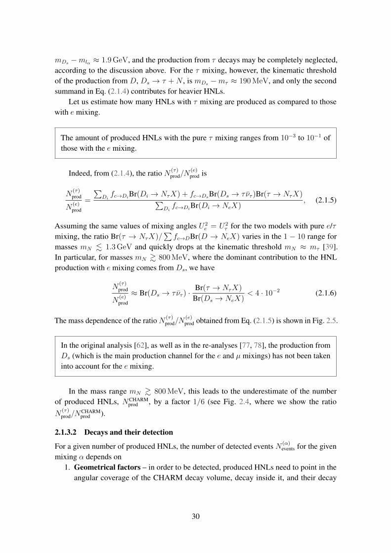
mDs −mlα ≈ 1.9 GeV, and the production from τ decays may be completely neglected,according to the discussion above. For the τ mixing, however, the kinematic thresholdof the production from D, Ds → τ + N , is mDs −mτ ≈ 190 MeV, and only the secondsummand in Eq. (2.1.4) contributes for heavier HNLs.

Let us estimate how many HNLs with τ mixing are produced as compared to thosewith e mixing.

The amount of produced HNLs with the pure τ mixing ranges from 10−3 to 10−1 ofthose with the e mixing.

Indeed, from (2.1.4), the ratio N (τ)prod/N

(e)prod is

N(τ)prod

N(e)prod

=

∑Difc→DiBr(Di → NτX) + fc→DsBr(Ds → τ ντ )Br(τ → NτX)∑

Difc→DiBr(Di → NeX)

, (2.1.5)

Assuming the same values of mixing angles U2e = U2

τ for the two models with pure e/τmixing, the ratio Br(τ → NτX)/

∑fc→DBr(D → NeX) varies in the 1 − 10 range for

masses mN . 1.3 GeV and quickly drops at the kinematic threshold mN ≈ mτ [39].In particular, for masses mN & 800 MeV, where the dominant contribution to the HNLproduction with e mixing comes from Ds, we have

N(τ)prod

N(e)prod

≈ Br(Ds → τ ντ ) ·Br(τ → NτX)

Br(Ds → NeX)< 4 · 10−2 (2.1.6)

The mass dependence of the ratio N (τ)prod/N

(e)prod obtained from Eq. (2.1.5) is shown in Fig. 2.5.

In the original analysis [62], as well as in the re-analyses [77, 78], the production fromDs (which is the main production channel for the e and µ mixings) has not been takeninto account for the e mixing.

In the mass range mN & 800 MeV, this leads to the underestimate of the numberof produced HNLs, NCHARM

prod , by a factor 1/6 (see Fig. 2.4, where we show the ratioN

(τ)prod/N

CHARMprod ).

2.1.3.2 Decays and their detection

For a given number of produced HNLs, the number of detected events N (α)events for the given

mixing α depends on1. Geometrical factors – in order to be detected, produced HNLs need to point in the

angular coverage of the CHARM decay volume, decay inside it, and their decay

30

products must then reach the detector and be successfully reconstructed. These factorsare: geometrical acceptance εgeom, i.e. the fraction of produced HNLs traveling inthe direction of the CHARM detector; the mean HNL gamma factor γN ; the decayacceptance εdecay, i.e. the fraction of HNL decay products that point to the CHARMdetector for HNLs that decay inside the fiducial volume.

2. The branching ratio Br(Nα → l+l′−ν) of the channels Nα → e+e−ν, Nα →µ+µ−ν, Nα → e−µ+ν (and their charge conjugated counterparts) used for detec-tion at CHARM [62].

The formula for N (α)events is:

N(α)events = N

(α)prod · ε(α)

geom ·∑

l,l′=e,µ

P(α)decay · Br(Nα → ll′ν) · εdet,ll′ · ε(α)

decay, (2.1.7)

where P (α)decay = e−lmin/cτ

(α)N γ

(α)N − e−(lmin+lfid)/cτ

(α)N γ

(α)N is the decay probability, and εdet,ll′ is the

reconstruction efficiency for the given channel.

Geometrical factors determining the sensitivity are the same for e, µ and τ mixing,while the branching ratio is smaller for the τ mixing channels, as in the former caseboth decays via the charged and neutral currents are relevant, while in the latter onlythe neutral current contribute.

Let us start by considering the lower bound of the sensitivity of the CHARM experiment,i.e. the minimal mixing angles that it may probe (the upper bound will be discussedin Sec. 2.1.4). In this regime, the decay length of the HNL cτ

(α)N γ

(α)N is much larger

than the geometric scale of the experiment, cτ (α)N γ

(α)N lmin + lfid ≈ 515 m. Then

P(α)decay ≈ lfid

cγ(α)N

· Γ(Nα), where Γ(Nα) is the total decay width, and it is convenient to rewrite

Eq. (2.1.7) in the form

N(α)events ≈ N

(α)prod × ε(α)

geom ·∑

l,l′=e,µ

lfid

cγ(α)N

· Γ(Nα → ll′ν)εdet,ll′ · ε(α)decay, (2.1.8)

where Γ(Nα → l+l′−ν) is the decay width into the dilepton pair ll′.We will first discuss the difference in Γ(Nα → l+l′−ν) between the cases of e and τ

mixings. Decays into dileptons occur via charged and neutral current, see Fig. 2.3. Forthe NC mediated processes, the kinematic threshold mN > 2me ≈ 1 MeV is mixing-independent. In contrast, for the CC mediated process for the τ mixing this threshold ismN > mτ + me ≈ 1.77 GeV, and HNLs lighter than τ lepton may decay into dileptonsonly via NC.

Decay widths for the processes Nα → l+l′−ν, assuming mN ml + ml′ , may be

31

given in the unified form

Γ(Nα → l+l′−ν) = c(α)ll′ν

G2Fm

5N

192π3, (2.1.9)

where the coefficients c(α)ll′ν are given in Table 2.1 [39]. For Ne, the largest decay width is

Γ(Ne → µ+e−νµ), where only CC contributes. The width Γ(Ne → e+e−νe) is smaller:

Γ(Ne → e−e+νe)/Γ(Ne → e−µ+νµ) ≈ 0.59, (2.1.10)

because both NC and CC contribute in this process and interfere destructively. The smallestwidth is Γ(Ne → µ+µ−νe), with the process occurring only via NC. For Nτ , there is noprocess Nτ → eµν, while in the process Nτ → e+e−ντ only NC contributes, and thus thewidth is smaller than for Ne:

Γ(Nτ → e+e−ντ )/Γ(Ne → e+e−νe) ≈ 0.22 (2.1.11)

For the decay into a dimuon pair, we have Γ(Nτ → µ+µ−ντ ) = Γ(Ne → µ+µ−νe).As a result, for mN mµ the ratio of the factors

∑l,l′ Γ(Nα → ll′ν)εdet,ll′ entering

Eq. (2.1.8) is given by ∑l Γ(Nτ → ll)εdet,ll∑

l,l′ Γ(Ne → ll′)εdet,ll′≈ 0.16 (2.1.12)

Here and below, we use the values of the efficiencies εdet,ll′ as reported in [62] for the HNLmass mN = 1 GeV: εdet,ee = 0.6, εdet,eµ = 0.65, εdet,µµ = 0.75.

In the original analysis of the sensitivity to the e mixing by the CHARM collabora-tion [62, 74], the Dirac nature of HNLs has been assumed (the decay widths are twicesmaller), and only the CC interactions have been considered. Instead of Eq. (2.1.12), theratio becomes

2∑

l Γ(Nτ → ll)εdet,ll∑l,l′ ΓCC(Ne → ll′)εdet,ll′

≈ 0.27 (2.1.13)

Process c(α)ll′ν

Ne/τ → µ+µ−νe/τ14(1− 4 sin2 θW + 8 sin4 θW ) ≈ 0.13

Nτ → e+e−ντ14(1− 4 sin2 θW + 8 sin4 θW ) ≈ 0.13

Ne → e−µ+νµ 1Ne → e+e−νe

14(1 + 4 sin2 θW + 8 sin4 θW ) ≈ 0.59

Ne → e+e−νe (CC) 1

Table 2.1: The values of c(α)ll′ν in Eq. (2.1.9) for different decay processes. For the process

Ne → e+e−νe, we also provide the value obtained if including the charged current (CC)contribution only – the assumption used in [62].

Let us now discuss geometric factors εgeom, γN , εdecay. It turns out that they depend

32

on the mixing pattern weakly, and as a result the geometry does not influence the relativeyield of events for e and τ mixing. Indeed, as was mentioned in Sec. 2.1.3.1, HNLs withτ mixing are produced in decays of τ leptons, that originate from decays of Ds. Sincemτ ' mDs , the angle-energy distribution of τ leptons is the same as of Ds (and hencealso other D mesons), whose decays produce HNLs with e mixing. The kinematics ofthe HNL production from D and τ is similar: two-body decays (a), (c) and three-bodydecays (b), (d) in Fig. 2.4 differ mainly be the replacement a neutrino or a lepton witha hadron h = π,K. However, since mh mτ,D, the replacement does not lead to thedifference in the distribution of produced HNLs. In addition, heavy HNLs with massesmN ' 1 GeV share the same distribution as their mother particles, and any differencedisappear. Therefore, the values εgeom, γN for different mixing are the same with goodprecision. Next, HNL decays contain the same final states independently of the mixing, andεdecay can also be considered the same.

To summarize, the ratio N (τ)events/N

(e)events is determined only by the difference in phe-

nomenological parameters – N (α)prod and Γ(Nα → ll′ν):

N(τ)events

N(e)events

'N

(τ)prod

N(e)prod

×∑

l Γ(Nτ → llν)εdet,ll∑l,l′ Γ(Ne → ll′ν)εdet,ll′

(2.1.14)

The total number of events for the τ mixing is 102 − 104 times smaller than for the emixing.

To compare with the estimate of the number of events for the e mixing made by theCHARM collaboration in [62], NCHARM

events , we need to take into account their assumptionson the description of HNL production and decays (see the discussion around Eqs. (2.1.5)and (2.1.13)). The resulting ratio is

N(τ)events

NCHARMevents

'N

(τ)prod

NCHARMprod

· 2∑

l Γ(Nτ → llν)εdet,ll∑l,l′ ΓCC(Ne → ll′ν)εdet,ll′

(2.1.15)

2.1.4 Results

Let us now derive the CHARM sensitivity to the τ mixing. In [62], it has been shown thatthe dilepton decay signature at CHARM is background free. Therefore, 90% CL sensitivityto each mixing is given by the condition

N(e,µ,τ)events > 2.3 (2.1.16)

Let us define U2lower,CHARM as the smallest mixing angle for which the condition (2.1.16)

is satisfied for the assumptions of the original analysis of [62] (see the discussion aboveEq. (2.1.15)). As the number of detected events at the lower bound N (α)

events scales with the

33

Excluded

BBN

LHCbFASERNA62Belle II

DB@IceCubeAP@KM3NeTSND@LHCSHiPDarkQuest

0.1 0.5 1 5 1010-11

10-9

10-7

10-5

0.001

mN [GeV]

Uτ2

CHARM

BBN

(this work)

LHCbFASERNA62Belle II

DB@IceCubeAP@KM3NeTSND@LHCDarkQuest

0.5 1 210-9

10-8

10-7

10-6

10-5

10-4

0.001

mN [GeV]

Uτ2

Figure 2.6: Parameter space of a single Majorana HNL that mixes with ντ . The excludedregion is a combined reach of the DELPHI [79], T2K [61] and CHARM experiments(our result). Bounds from BBN are reproduced from [37, 64]. The sensitivity of futureexperiments is also shown (see text around Fig. 2.1 for details). The top panel covers theHNL mass region mN = 0.1− 35 GeV, while the bottom panel is a zoom-in of the massdomain mN = O(1 GeV).

mixing angle as N (α)events ∝ U4

α (where U2α comes from the production and another U2

α fromdecay probability), we can use Eqs. (2.1.15) and (2.1.5) to obtain the lower bound of thesensitivity to the τ mixing, U2

τ,lower, by rescaling the results reported in [62]:

U4τ,lower

U4 CHARMlower

'NCHARM

prod

N(τ)prod

·∑

l,l′ ΓCC(Ne → ll′ν)εdet,ll′∑l Γ(Nτ → llν)εdet,ll

∣∣∣∣Ue=Uτ

. (2.1.17)

Using the ratio NCHARMprod /N

(τ)prod from Eq. (2.1.5) (see also Fig. 2.5), and the ratio of decay

widths from Eq. (2.1.13), we may compare the lower bounds of the excluded regions forHNLs with e and τ mixing.

We conclude that in the mass range mN > 200 MeV the lower bound for the τ mixingis a factor 10− 100 weaker than the lower bound for the e mixing reported in [62].

In the domain mDs −mτ < mN < 290 MeV, we validate the rescaled bound (2.1.17)by comparing it with the CHARM sensitivity to the τ mixing from [63], see Appendix 2.A.

Also, we compare our estimate for the e mixing with the CHARM sensitivity to the emixing from [62]. In our estimates, we include neutral current interactions, the productionfrom Ds mesons, and assume that HNLs are Majorana particles. In our estimates, weinclude neutral current interactions, the production from Ds mesons, and assume that HNLsare Majorana particles.

We find that for small mixing angles Ue and above mN & 1 GeV, the bound imposed byCHARM on the e mixing may be actually improved by up to a factor 3− 4 as comparedto [62].

34

At the upper bound of the sensitivity, the dependence of the number of events onU2α is complicated and the sensitivity cannot be obtained by rescaling the results of [62].

Therefore, we independently compute the number of decay events at CHARM for HNLswith e and τ mixing and then calculate the sensitivity numerically using Eq. (2.1.16), seeAppendix 2.A. In order to validate this estimate, we compare the resulting sensitivity for theτ mixing with the rescaled bound (2.1.17), and find that they are in very good agreement(Fig. 2.27).

Let us comment on errors of our estimates. We used the values of reconstructionefficiencies εrec,ll reported in [62] for the HNL mass mN = 1 GeV. Hence, the calculationmay be further refined by including HNL mass dependent reconstruction efficiencies.However, as the study [63] performed for the τ mixing and masses mN < 290 MeV hasshown similar efficiency, we do not expect any significant changes.

Our final results for the τ mixing are given in Fig. 2.6, where we show the domainexcluded by previous experiments together with updated CHARM bounds, and the sensitiv-ity of the future experiments mentioned in Sec. 2.1, together with SHiP [80]. Comparingwith Fig. 2.1, we find that in the mass range 380 MeV < mN < 1.6 GeV our resultsimprove previously reported bounds on the mixing angle U2

τ by two orders of magnitude.In particular, it excludes large part of the parameter space that was suggested to be probedby the future experiments. For instance, Belle II, FASER, DarkQuest and IceCube havesensitivity only in the narrow domain above the CHARM upper bound, while NA62 mayslightly push probed angles to lower values. Significant progress in testing the mixing ofHNLs with ντ can be achieved by LHCb, which probes the complementary mass rangemN > 2 GeV, and dedicated Intensity Frontier experiments, with SHiP being optimal forsearches of HNLs from decays of D mesons and τ leptons.

2.1.5 Comparison with atmospheric beam dumps

Apart from the production at accelerators, HNLs with masses in GeV range may benumerously produced in decays of τ leptons, originated from the collisions of high-energy cosmic protons with the well-known spectrum [81]

dΦ

dΩdtdSdEp≈

1.7 E−2.7p, GeV GeV−1sr−1cm−2s−1, Ep < 5 · 106 GeV

174 E−3p, GeV GeV−1sr−1cm−2s−1, Ep > 5 · 106 GeV

(2.1.18)

with atmospheric particles. If having significantly large lifetimes, produced HNLsmay enter the detector volume of neutrino telescopes, such as IceCube and KM3NeT,located deep in ice and the Mediterranean Sea correspondingly, and decay there.

In order to probe the parameter space of HNLs, it is necessary to distinguish their decaysfrom interactions of SM particles that are also produced in the atmosphere: neutrinos and

35

muons. IceCube and KM3NeT may only distinguish two event types: track-like, whichcorresponds to muons penetrating through the detector volume, and cascade-like, whichoriginates from other particles such as electrons and hadrons. Scatterings of neutrinosinside the detector volume produce cascade-like (if no high-energy muons are produced) orcombined cascade-like + track-like signature (if high-energy muons are produced), whilepenetrating atmospheric muons give rise to track-like signature.

A possible way to distinguish the SM particles events from HNLs is to look for theHNL decays into a di-muon pair, N → µµντ . They produce a signature of two tracksoriginated from one point inside the detector volume, which differs from the SM eventssignatures.

Detectors of KM3NeT have energy and angular resolution sufficient precise for resolv-ing the two tracks down to energies of a few tens of 10 GeV [73] (and much better thanthose at IceCube). On the other hand, characteristic energies of HNLs are EN ' 100 GeV.Therefore, we believe that the dimuon signature may be reconstructed in the backgroundfree regime with high efficiency.3

2.1.5.1 Analytic estimates: comparison with CHARM

Now, let us discuss the sensitivity of KM3NeT to HNLs. We will first compare the amountof HNL decay events at CHARM and KM3NeT for the given value of the mixing angle atthe lower bound of the sensitivity using simple analytic estimates. According to Eq. (2.1.8),for the ratio of decay events at these experiments we have

N(τ)events,CHARM

N(τ)events,KM3NeT

'NCHARMcc · εCHARM

geom · εCHARMdecay

NKM3NeTcc

× lCHARMfid

lKM3NeTfid

×

× γKM3NeTN

γCHARMN

×∑

l=e,µ Γ(Nτ → ll)εdet,ll

Γ(Nτ → µµ)(2.1.19)

Here, NCHARMcc ·εCHARM

geom ·εCHARMdecay ' 2 ·1013 (see Fig. 2.27 is the number of cc pairs detectable

fraction of HNL decay events at CHARM. NKM3NeTcc is the amount of cc pairs produced in

the upper hemisphere propagating to KM3NeT,

NKM3NeTcc ' 2π × 1 km2 × 5 years×

∫dΦ

dΩdtdSdEp· σpp→ccXσpp,total

dEp ' 1012, (2.1.20)

where σpp→ccX(Ep) is the energy-dependent charm production cross-section which we usefrom FONLL [43] and from [8], and σpp,total is the total pp-cross-section, which we use

3The possible background is combinatorial and originates from pairs of oppositely charged atmosphericmuons. However, it may be reduced to some extent by imposing veto on muons coming from the outer layerof the detector volume.

36

from [82]. The integrand in (2.1.20) is the product of two competing factors: dΦdΩdtdSdEp

,which decreases with the proton’s energy, and σpp→ccX(Ep), which increases, see Fig. 2.7.

100 1000 104 105 106 1070.1

10

1000

105

107

109

Ep

dNcc_/dEp

Figure 2.7: The integrand of Eq. (2.1.20).

We approximate the ratio of the mean HNL γ factors by the ratio of the mean γ factorsof D mesons:

γKM3NeTN /γCHARM

Ds ' γKM3NeTDs /γCHARM

Ds ' 3, (2.1.21)

where we calculate γKM3NeTDs

using the cc distribution dΦdΩdtdSdEp

· σpp→ccX , assuming thatED ≈ Ep/2.

Using the fiducial lengths lCHARMfid = 35 m and lKM3NeT

fid ' 1 km, and taking into accountthat the last factor in Eq. (2.1.19) is O(1) for mN 2mµ, we finally obtain

N(τ)events,CHARM

N(τ)events,KM3NeT

' 2 (2.1.22)

Using the analytic estimates, we conclude that even in the most optimistic case (assum-ing unit efficiency) the number of events at CHARM and KM3NeT are just comparable.We need more accurate estimate taking into account non-isotropic distribution of theproduced HNLs.

2.1.5.2 Accurate estimate

We compute the production of Ds mesons (and hence τ leptons) using the approachfrom [81]. The production was found to be maximal at O(10 km) height from the Earth’ssurface. The resulting spectrum dΦDs

dSdtdld cos(θ)dEDsof Ds mesons is in good agreement with

Fig. 2 from [83]. The total number of Ds mesons produced in the direction of KM3NeTduring the operating time 5 years was found to be NDs ' 5 · 1010.

Next, we use the approach from [83] in order to estimate the sensitivity of KM3NeT.

37

The number of decay events is

Nevents ≈ SKm3NeT × T ×∫

dΦDs

dSdtdld cos(θ)dEDs· Br(Ds → τ ντ )·

· Br(τ → NτX) · Pdecay(l, EN)d cos(θ)dldEN , (2.1.23)

where T = 5 years is the operating time, SKM3NeT = 1 km2 is the transverse area ofKM3NeT. The decay probability is

Pdecay ≈ e−(l+l1)/ldecay − e−(l+l2)/ldecay , (2.1.24)

where l is the distance from the HNL production point in atmosphere, l1 ≈ 3 km is thedistance from the surface of Earth to the KM3NeT detector, while l2 = l1 + 1 km is thedistance to the end of the KM3NeT. For simplicity, in ldecay we set EN ≈ EDs/2. In orderto show the maximal reach of KM3NeT, we optimistically assume unit efficiency of thedimuon event reconstruction, and require Nevents > 3 during the operating period.

The resulting sensitivity shown in Fig. 2.6 is worse than predicted by the simpleestimate by a factor of few. The reason is that at masses mN . 500 MeV there is anadditional suppression from Br(N → µµ), while at higher masses the scaling (2.1.8) is notvalid because the lower bound is close to the upper bound.

2.2 Searches with displaced vertices at the LHC

A peculiar feature of dedicated beam experiments such as SHiP, DUNE, and MATHUSLAis that they have macroscopic distance from the collision point lmin 1 m to the detectorvolume. On one hand, it allows to reduce background from SM particles down to control-lable and even negligible level. On the other hand, such experiments cannot search forshort-lived FIPs with decay lengths cτγ lmin.

Because of macroscopic distance from the FIP production point and the detector volumeat Intensity Frontier experiments, there is a domain of large couplings that is neitherexcluded by past experiments nor may be probed by dedicated beam experiments, seeFig. 2.8.

To probe such intermediate couplings, one needs experiments that have much shorterlmin, and simultaneously may handle the background coming from SM events, the amountof which increases if decreasing lmin. Such type of experiments exists at the LHC and iscalled displaced vertices scheme (DV).

An event at a given DV experiment has to meet some selection criteria which arespecific to the experiment, minimize the SM background yield and simultaneously shouldnot diminish the detected amount of events with FIPs. The physical process involving

38

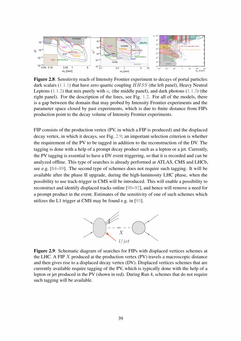
SHADOWS

NA62

Excluded

SHiP

MATHUSLA

FASER2

BBN

0.05 0.10 0.50 1 510-13

10-11

10-9

10-7

mS [GeV]

θ2

CHARM

T2K

DELPHI

NA62

Belle

BBN

Seesaw

SHiPMATHUSLA

NA62

FASER2SHADOWS

DUNE

0.1 0.5 1 5 1010-12

10-10

10-8

10-6

10-4

mN [GeV]

Ue2

[GeV]A'm3−10 2−10 1−10 1 10 210 310

ε

9−10

8−10

7−10

6−10

5−10

4−10

3−10

2−10

NA62-dump

APEX

SHiP

pot (dotted)20 pot (solid), 1018DarkQuest: 10

HPS

FASER2

FASER

Belle II

(dotted)-1 (solid), 300 fb-1LHCb: 15 fb

HL-LHCe(g-2)

BaBar

CMSLHCb

A1NA48/2

mu3e (phase1)

mu3e (phase2)

E137

E141

NA64(e)

E774

SN1987A

nu-CalCHARM

Figure 2.8: Sensitivity reach of Intensity Frontier experiment to decays of portal particles:dark scalars (1.1.1) that have zero quartic coupling HHSS (the left panel), Heavy NeutralLeptons (1.1.2) that mix purely with νe (the middle panel), and dark photons (1.1.3) (theright panel). For the description of the lines, see Fig. 1.2. For all of the models, thereis a gap between the domain that may probed by Intensity Frontier experiments and theparameter space closed by past experiments, which is due to finite distance from FIPsproduction point to the decay volume of Intensity Frontier experiments.

FIP consists of the production vertex (PV, in which a FIP is produced) and the displaceddecay vertex, in which it decays, see Fig. 2.9; an important selection criterion is whetherthe requirement of the PV to be tagged in addition to the reconstruction of the DV. Thetagging is done with a help of a prompt decay product such as a lepton or a jet. Currently,the PV tagging is essential to have a DV event triggering, so that it is recorded and can beanalyzed offline. This type of searches is already performed at ATLAS, CMS and LHCb,see e.g. [84–89]. The second type of schemes does not require such tagging. It will beavailable after the phase II upgrade, during the high-luminosity LHC phase, when thepossibility to use track-trigger in CMS will be introduced. This will enable a possibility toreconstruct and identify displaced tracks online [90–92], and hence will remove a need fora prompt product in the event. Estimates of the sensitivity of one of such schemes whichutilizes the L1 trigger at CMS may be found e.g. in [93].

X

l/jet

Figure 2.9: Schematic diagram of searches for FIPs with displaced vertices schemes atthe LHC. A FIP X produced at the production vertex (PV) travels a macroscopic distanceand then gives rise to a displaced decay vertex (DV). Displaced vertices schemes that arecurrently available require tagging of the PV, which is typically done with the help of alepton or jet produced in the PV (shown in red). During Run 4, schemes that do not requiresuch tagging will be available.

39

ATLAS, CMS and LHCb experiments complement each other in searches for FIPs:LHCb covers mass range mFIP . mB, while ATLAS/CMS allow for searching in therange mB . mFIP . mh.

Indeed, the flux of SM particles that may produce FIPs (such as W/Z bosons, theHiggs boson, and B,D mesons) is collimated with respect to the beam axis.4 Naively, onemay expect that the best placement of a DV experiment is in the forward region that coversrelatively small angles. However, decay products of these particles gain characteristictransverse momentum of order of pT ' mmother, where mmother is the mass of decayingparticle. For large enough mmother (for instance, for Higgs bosons), the characteristic angleθ ' arctan (pT/pL) becomes much larger than the angular width of the mother particledistribution. Then, instead of the forward region, the preferable setup is the one coveringlarge angular domain. ATLAS and CMS are located off-axis and have significant angularcoverage, thus allow us to search for FIPs produced in decays of heavy particles such asthe Higgs boson and W/Z bosons. LHCb, in its turn, covers much smaller angular domainbut in the forward region, and thus allow to search for FIPs originating from decays ofrelatively light B mesons, for which the broadening is insignificant.

In this section, we discuss the potential for the search scheme at CMS that utilizesmuon trackers. Advantages of this scheme is large length of the decay volume, which isessential to probe the parameter space of the LLPs with the decay lengths about 1 meter orlarger, and relatively small background as compared to the schemes that search for hadronicdecays. We use Heavy Neutral Leptons, Chern-Simons portal and dark scalars as threeexamples of long-lived particles for which the CMS muon tracker can provide essentialinformation about their properties.

2.2.1 Displaced vertices with muon tracker at CMS

Typically, DV search schemes use inner trackers to reconstruct events. Therefore, themaximal displacement that may be reconstructed is limited by O(0.5 m). Alternatively,one may use muon chambers, that cover much larger distance (up to 3 m in the transverseplane at CMS).

The use of the muon chambers to reconstruct di-muon DV signatures has been exploredin the past in [94–96] and recently in [97]. Ref. [98] that appeared when this work was atits final stage employed the event selection criteria that may be too optimistic with regardto the background estimates. Ref. [99] explored a potential of the CMS muon chambersalone to reconstruct dimuon DV. This search however, was constructed to be much more

4For instance, the angular distribution of B mesons and the Higgs bosons quickly drops at anglesθ > 0.01 rad.

40

Figure 2.10: Cross-section of the CMS experiment. Layers (muon stations) of the muondetector in the plane perpendicular to the beam direction. The figure is from [103].

general, and hence could not profit from the presence of a prompt lepton in the event. Thisnecessarily implied much more stringent cuts on pT of either of the two muons in the muontracker since these muons were used to record an event by a trigger, and therefore lowersensitivity.

2.2.1.1 Description of the scheme

CMS (compact muon solenoid) is a beam line azimuthally symmetric detector consisting ofa solenoid generating the 3.8 T magnetic field, the inner trackers that allow to reconstructthe momentum of particles produced in the pseudorapidity range |η| < 2.5 (where η =

− log[tan(θ/2)] and θ is the polar angle with respect to the anticlockwise-beam direction)and the muon trackers located outside the solenoid [100].

The muon system is located outside the solenoid and covers the range |η| < 2.4. Itis a set of gaseous detectors sandwiched among the layers of the steel flux-return yoke.This allows for a muon to be detected along the track path at multiple points [101]. Themagnetic field in the muon system is not uniform, and goes from 2 T in the innermost partdown to almost 0 T in the outer part [102]. Schematic drawing of the muon detector isshown in Fig. 2.10.

For the LHC Run 2, new reconstruction of muons has been introduced [104], theso-called displaced standalone muon reconstruction. This reconstruction is specificallydesigned to address cases when muons are produced in decays far away from the productionvertex. New algorithm achieves an almost 100% reconstruction efficiency for the muonproduction radius up to about 3 m. This is a significant gain in the efficiency comparedto the reconstruction which uses also inner tracker information, but at the same time, the

41

momentum resolution deteriorates by about a factor of 10 and is in the range 10–60%.The muon tracker can use two muon tracks to reconstruct a displaced vertex originating

from the decay X → µµ+ . . . . The reconstructed DV together with the production vertexthat can be tagged by prompt decays products, e.g. a prompt lepton, and an underlyingevent produced together with the X particle, is identified as a DV event. Due to the largedistance between a PV and a reconstructed DV, we will call this scheme the “the long DV”scheme.

It should be noticed, that after the phase II upgrade, during the high-luminosity LHCphase, the possibility to use track-trigger in CMS will be introduced. This will enablea possibility to reconstruct and identify displaced tracks online [90–92], and hence willremove a need for a prompt lepton in the event. However, for the models discussed in thispaper, current hardware configuration of the CMS allows to perform the searches with thealready recorded data, as well with the data to be obtained during the Run 3 of the LHC.

At the same time, final states with a prompt, well identified, object in the event, as e.g.a prompt muon or electron, have much lower background rate. In this case the instrumentalbackgrounds and non-muon backgrounds from cosmic rays are reduced to a negligiblelevel. The remaining cosmic-ray muon backgrounds can be suppressed by selections whichdo not impact signal efficiency, as described in Ref. [105]. The remaining sources of thebackground for the long DV scheme are processes with a presence of a prompt object (as e.g.W boson production) accompanied by decays of the SM particles into single muons, whichgive rise to combinatorial two-muon events, and two-muon decays of the SM particles(for example, J/ψ, ρ, ω mesons and the Z boson). The most significant displacement ofsuch DV appears in case of two muons originating for a heavy-flavor particle decay (b or chadrons). As we do not carry out an experimental analysis in this paper, we assume thatthis background is negligible if one requires the transverse position of the displaced vertexto be as far as lDV > 2 cm from the beam collision point, since most of the SM particlesdecay before reaching this displacement [106]. Under this assumption we lose a part ofthe efficiency for LLPs with shorter lifetimes, but at the same time we provide a morerobust estimate of the potential signal sensitivity. Because of the position of the muontrackers, the muon events can be reconstructed at the distances lDV < 3 m. The muons canbe reconstructed with high efficiency and low misidentification probability if each of themhas the transverse momentum pT > 5 GeV [107, 108].

To summarize, an event in the long DV search scheme should satisfy the followingselection criteria:– A prompt electron with |η| < 2.5, pT > 30 GeV or a prompt muon with |η| <

2.4, pT > 25 GeV, which are required for an event to be recorded by the singlelepton triggers;

– The minimal transverse displacement of the DV from the PV is lmin,⊥ = 2 cm; themaximal transverse and longitudinal displacements are lmax,⊥ = 3 m, lmax,l = 7 m;

42

– Two displaced muon tracks, each with |η| < 2.4, pT > 5 GeV.

The requirement of a large displacement of a DV from the PV helps to significantlyreduce the background from SM processes. Therefore, even in the region with the invariantmass of two muons below 5 GeV (mass of B-mesons) the SM background is considered tobe negligible. The scheme is presented in Fig. 2.11.

PV DVX

µ

µ

l,prompt

Figure 2.11: Schematic diagram of the search scheme of LLPs at CMS using the muondetectors. The production vertex (PV) is tagged by the prompt lepton l, while the displacedvertex (DV) is reconstructed by two muons produced in the decay X → µµ.

An event with prompt τ lepton can be tagged by its leptonic decays τ → lνlντ ,where the leptons l = e/µ satisfy the criteria for prompt leptons presented above. We donot consider the reconstruction of τ leptons by their hadronic decay products since thetrigger threshold for pT of hadronic decay products is too high for efficient reconstruction.5

However, in the future it is wise to invest into the development of a dedicated multi-object trigger which would allow to bring down the prompt tau pT by including additionaldisplaced leptons in the event.

In [98] a similar search scheme was discussed, albeit with less restrictive selectioncriteria lmin,⊥ = 0.5 cm, lmax,⊥ = 4 m, and |η| < 4 for leptons.6 A wider range ofmuon pseudorapidities leads to the enlargement of the selection efficiency, while a smallerdisplacement between a DV and the PV lifts up the upper bound of the sensitivity andhence increases the maximal mass reach. However, we caution that the background-freehypothesis for the region with smaller DV displacements adopted in [98] has not been tested.Nevertheless, to demonstrate potential improvement from considering lower displacementswe provide sensitivity for two scenarios: “realistic” for the selection criteria outlined above,and “optimistic”, defined according to [98].

2.2.1.2 Estimation of the number of events

The number of decay events of a new particle X that pass the selection criteria is

Nevents = Nparent · Brprod · Pdecay · ε, (2.2.1)

where5Current trigger threshold is pT > 180 GeV.6After the HL-LHC upgrade the CMS will extend its pseudorapidity range to |η| < 4.

43

– Nparent is the total number of parent particles that produce a particle X at the LHC;– Brprod is the branching fraction of the production of a particle X in decays of the parent

particle;– Pdecay is the decay probability,

Pdecay =

∫dθXdpXf(pX , θX) ×

(e−lmin/cτXγX − e−lmax/cτXγX

), (2.2.2)

with τX being the proper lifetime of the particle X , γX is its γ factor, and f(pX , γX) isthe distribution function of the X particle whose decay products satisfy the selectioncriteria;

– ε is the overall efficiency – the fraction of all decays of the X particle that occurred inthe decay volume between lmin and lmax, have passed the selection criteria, and weresuccessfully reconstructed.

The efficiency is a combination of several factors:

ε = εsel · εrec · BrX→µµ, (2.2.3)

where εsel, εrec are the efficiencies of the selection and subsequent reconstruction of an eventcorrespondingly, and BrX→µµ is the branching ratio of the decay of the X particle into twomuons. Clearly, εrec does not depend on the nature of LLP. The reconstruction efficiency forleptons is well above 95% for muons with pT > 5 GeV [101, 104, 107] and for electronswith pT > 30 GeV [109]. Therefore, for simplicity the reconstruction efficiency is taken tobe equal to 1 (εrec = 1) in what follows.

We define the sensitivity curves by the condition Nevents ' 3, corresponding to the 95%exclusion limit under the assumption of zero background. The lower boundary can be easilyrescaled to other Nevents.

The main advantage of the long DV scheme is the large length of the fiducial decayvolume lmax, which exceeds the lengths of the decay volumes of other DV search schemesat the LHC (see, e.g., [85, 110]) by ' 10 times. This has a benefit when searching for newparticle with large decay lengths,

ldecay ≡ cτXγX lmax (2.2.4)

Indeed, in this case the decay probability (2.2.2) is in the “linear regime”, Pdecay ≈lmax/ldecay, and as a result the number of events (2.2.1) is proportional to lmax. For de-cay lengths that do not satisfy the condition (2.2.4) the decay probability does not dependon lmax, and the improvement is lost (see Fig. 2.12).

In order to probe the domain (2.2.4) there must be sufficient production of the Xparticles, i.e.

Nprod · BrX→µµ > 3, (2.2.5)

44

0.001 0.010 0.100 1 10 100 100010-5

10-4

0.001

0.010

0.100

1

ldecay [m]

Pdecay

Figure 2.12: Dependence of the decay probability (2.2.2) on the decay length ldecay. Forsimplicity we assumed that all the particles travel with the same momentum and in thesame direction, and set lmax = 3 m. The dashed lines denote the values ldecay = lmin andldecay = lmax. In the domain ldecay lmax the decay probability scales as Pdecay ' lmax/ldecay,while in the domain lmin . ldecay . lmax it behaves approximately constantly and does notdepend on lmax.

where Nprod = Nparent ·Brprod. The parameter space defined by the conditions (2.2.4), (2.2.5)is optimal for being probed by the long DV scheme. A toy example of the parameter spaceis given in Fig. 2.13.

5 10 15 20 2510-9

10-7

10-5

10-3

mX [GeV]

θ2

Figure 2.13: The illustration of the parameter space which is optimal for being probedwith the long DV scheme, see text for details. We used a toy model with Nprod =

109 [1−m2X/(25 GeV)2]

2θ2X , BrX→µµ = 1 and ldecay = 0.1m−3

X θ−2X m.

2.2.1.3 HNLs

We start with HNLs. The main production channel of the HNLs with masses in the rangemN & 5 GeV is the decay of the W bosons. We use the value σW ≈ 190 nb for the totalproduction cross section of the W bosons at the LHC at energies

√s = 13 TeV [111].

To estimate the parameter space defined by (2.2.4) and (2.2.5), we calculated the energyspectrum and geometric acceptance εgeom of the HNLs in the pseudorapidity range |η| < 2.5

in LO using the model HeavyN [112]. We found εgeom ≈ 0.5 for the mass range mN .20 GeV and EN ≈ 80 GeV.

45

εsel e µ τRealistic 0.16 0.17 7 · 10−3

Optimistic 0.26 0.31 3.2 · 10−2

Table 2.2: The values of the selection efficiencies for HNLs of different flavors e, µ, τ inthe case of realistic and optimistic selection criteria

In Fig. 2.14, we show the parameter space for the HNLs mixing with νµ that can beoptimally probed by the long DV scheme. We see that the domain where the long DV

2 4 6 8 10 1210-10

10-9

10-8

10-7

10-6

10-5

HNL mass [GeV]

Uμ2

Figure 2.14: The parameters of HNLs mixing with νµ that satisfy criteria (2.2.4) –(2.2.5)for the LHC luminosity L = 3000 fb−1. Note, this is not an exclusion region, see textaround equations for details.

scheme has good potential corresponds to the masses mN < 10 GeV and the mixing anglesU2 & 10−9.

Simulations. To find the efficiency for the HNLs mixing with νe/µ, we used Mad-Graph5 [113] with the model HeavyN [112]. For simulating decays of τ lepton, weused taudecay UFO model [114]. For the mixing with νe/µ we simulated the processp+p→ W, W → l+N , where l = e for the mixing with νe and l = µ for the mixing withνµ, with subsequent decay N → µ+ +µ−+ν/νl. In the case of the mixing with ντ , we sim-ulated the process p+p→ W,W → τ+N with subsequent decays N → µ+ +µ−+ντ/ντand τ → l + νl + ντ , where l = e/µ.

Using the selection criteria for the long DV scheme, we computed the selectionefficiencies. They were found to be almost independent of the mass of the HNL in the massrange 1 GeV < mN < 20 GeV. We give their values in Table 2.2. The suppression of theefficiency for mixing with ντ is due mainly to the reconstruction of the prompt τ event.Indeed, the amount of the leptons produced in the decay τ → lνlντ and passing the pTselection criterion for the prompt leptons is ≈ 0.1.

For the average momentum we found pN ≈ 70 GeV and pN ≈ 180 GeV for therealistic and optimistic estimates correspondingly.

Comparison with other schemes. Let us compare the sensitivity of the long DVsearch scheme to the HNLs with a scheme from [110, 115] that uses inner trackers atATLAS to search for DVs events (c.f. [97]). Owing to its smaller transverse displacement

46

lmax = 0.3 m we call it the “short DV scheme”. For the estimation of the sensitivity of theshort DV scheme we use parameterized efficiencies ε(mN , U

2) provided by the authorsof [110]. The comparison of the sensitivities is given in Fig. 2.15. We show both optimisticand realistic estimate of the sensitivity of the long DV scheme. We also show the sensitivityof the SHiP experiment from [80] that serves for an illustration of the sensitivity reach ofIntensity Frontier experiments.

The long DV scheme allows to search for HNLs in the unexplored region of theparameter space that is not accessible to other Intensity Frontier experiments or other LHCsearches. Its difference in the sensitivity with the short DV scheme is due to three reasons.First, for masses mN . 10 GeV the decay probability for both the schemes is in the linearregime (see Sec. 2.2.1.2), and therefore the long DV scheme gets the benefit from the 10

times larger length of the decay volume lmax. Second, for the masses 5 GeV . mN .10 GeV there is a drop of the overall efficiency for the short DV scheme. This is causedby the selection criteria on the reconstructed invariant mass of the DV, mDV > 5 GeV, andthe charged tracks, Ntrk > 4, that are needed to remain in the background free region [87].Third, because of absence of the hadronic background the long DV scheme can probe theparameter space mN . 5 GeV, which is not reachable by the short DV scheme.

Nevertheless, both the schemes are complementary to each other and provide a cross-check in the mass region 5 GeV < mN < 15 GeV.

Previous searches

SHiP

DVS

DVL

1 2 5 10 2010-12

10-10

10-8

10-6

10-4

HNL mass [GeV]

Ue2

Previous searches

SHiP

DVS

DVL

1 2 5 10 2010-12

10-10

10-8

10-6

10-4

HNL mass [GeV]

Uμ2

Previous searches

SHiP DVS

DVL

1 2 5 10 2010-10

10-9

10-8

10-7

10-6

10-5

HNL mass [GeV]

Uτ2

Figure 2.15: The sensitivity of the long DV (DVL) and short DV (DVS) search schemes toHNLs mixing with νe (upper panel), νµ (middle panel) and ντ (lower panel). By the blueshort dashed line we denote the realistic sensitivity obtained using the selection criteriapresented in this paper, while the blue dashed line corresponds to the optimistic estimate ofthe sensitivity using relaxed selection criteria from [98], see Sec. 2.2.1.2 for details. Thesensitivity of the SHiP experiment is taken from [80]. Black long-dashed line indicatesHNL parameters that correspond to ldecay = 3 m. The estimates are for the high luminosityLHC phase, L = 3000 fb−1. For the DV search schemes sensitivity we require Nevents ≥ 3and assume zero background (see text for details).

47

2.2.1.4 Chern-Simons portal

Chern-Simons portal introduces a vector particle X interacting with pseudo-Chern-Simonscurrent of the SM gauge bosons [82, 116]:

LCS = cW εµνλρXµWν∂λWρ+

cγ cos θW εµνλρXµZν∂λγρ + cZ sin θW ε

µνλρXµZν∂λZρ (2.2.6)

We can add the interaction of the X boson with SM leptons in the form

LXµµ = cWgXllXν∑

l=e,µ,τ

lγ5γνl, (2.2.7)

where gXll is a dimensionless constant.7

Let us consider the case when cγ, cZ cW . Then the production of theX particle in ppcollisions goes through the XWW vertex, while the decay goes through the vertex (2.2.7)down to very small couplings g2

Xll ' 10−7 for the X bosons as heavy as mX ' 40 GeV,see Appendix 2.2.1.4. These vertices are parametrically independent, and for particularvalues of gXll it is possible to probe the parameter space in the optimal domain for the longDV scheme. The process of interest is

W → X + l + νl, X → µ+ + µ− (2.2.8)

The lepton l produced in the W decay can be triggered as a prompt lepton, while the muonpair from the decay of the X boson can be reconstructed as displaced muons, which meetsthe selection criteria of a DV event within the long DV scheme.

To find the selection efficiency and the energy spectrum of the W bosons, we im-plemented the model of the X boson (2.2.6), (2.2.7) into the MadGraph using Feyn-Rules [117, 118]. The model is publicly available [119]. We simulated the processesp+p→ e+/µ+ +νe/µ+X (plus the charge conjugated final states) with subsequent decaysX → µ+µ−. We have found that the overall efficiency is ε ≈ 2.3 · 10−2 for mX rangingfrom 1 GeV to 20 GeV. The average momentum of the X boson pX ≈ 40 GeV.

The sensitivity to the Chern-Simons portal is shown in Fig. 2.16. We conclude that thelong DV scheme can probe masses up to mX ' 30 GeV and couplings down to c2

W ' 10−9.We note that the probed parameter space is well below the current experimental bound oncW , which is c2

W . 10−3(mX/1 GeV)2 [82].

7The coupling gXll can be generated effectively by the interaction (2.2.6) or be an effect of new physics.

48

gXll2 = 10-5

gXll2 = 10-6

gXll2 = 10-7

1 2 5 10 20

10-11

10-8

10-5

mX [GeV]cW2

Figure 2.16: The sensitivity of the long DV scheme at the high luminosity phase to theChern-Simons portal for different values of the coupling to muons (2.2.7). For the DVsearch schemes sensitivity we require Nevents ≥ 3 and assume zero background (see text fordetails).

2.2.1.5 Dark scalars with quartic coupling

In the case of dark scalars with quartic coupling (remind Eq. (1.1.1)) and massesmS > mB, the production and decay channels are independent of each other [120],similarly to the case of Chern-Simons portal.

Namely, the production occurs via the quartic coupling – it is a decay of Higgs bosonsh → SS, while decays are mediated by the mixing angle [38]. The branching ratio of

10 20 30 40 50 6010-4

0.001

0.010

0.100

1

mS [GeV]

Br(S→

μμ)

Figure 2.17: The branching ratio of decays of scalars into two muons. It does not includemuons produced as secondary particles from decays of heavier decay products, whosecontribution may dominate at larger masses.

decays of scalars into two muons is shown in Fig. 2.17. The interaction of scalars withfermions is similar to the interaction of Higgs bosons. Therefore, above scalar massesmS ' 2mπ, it is strongly suppressed because of the Yukawa couplings. Nevertheless,despite the suppression of the signal yield by small Br(S → µµ) it is still possible to searchfor heavy scalars using the muon trackers. In addition, as in Fig. 2.17 we do not include pair

49

MadGraph (LO)[1801.06851] (LO)

0 50 100 150 200 250 3001.×10-4

5.×10-40.001

0.005

pT [GeV]

f pT[GeV

-1]

Excluded

Muon tracker

L1 trigger

0.5 1 5 10 5010-19

10-16

10-13

10-10

10-7

Scalar mass [GeV]

θ2

Br(h→SS) = 0.01

Figure 2.18: Left panel: The pT spectrum of Higgs bosons produced in the processp+ p→ h+W+, W+ → l+ + νl obtained in our simulations using MadGraph (blue) andin [121] for the selection criteria |ηl| < 2.5, pT,l > 15 GeV. Right panel: the sensitivityof the muon tracker DV scheme to scalars, assuming the production branching ratioBr(h→ SS) = 0.01. In green, we also show the sensitivity of the search scheme that usesL1 trigger from [122], assuming zero background.

of muons from decays of heavier decay products of scalars, our estimate of the sensitivityis conservative.

Unlike HNLs and Chern-Simons portal mediator, the main production channel ofscalars, h → SS, does not include a lepton, and naively it is impossible to tag theproduction vertex. However, one may use leptons produced together with Higgs bosonsin a process

p+ p→ h+W/Z, W/Z → l +X, h→ S + S (2.2.9)

Indeed, h,W,Z bosons have extremely small lifetimes, and all the processes (2.2.9)occur practically at one point. The process (2.2.9) is ' 50 times less frequent than the mainproduction channel of the Higgs boson – the gluon fusion.

Simulation. In order to simulate events of scalar decays, we have first implementedthe model of a scalar into MadGraph using FeynRules. Next, we have simulated thechain (2.2.9) at LO, together with further scalar decays. NLO corrections to the spectraare known to be negligibly small [121]. To validate our simulations for the production ofHiggs bosons and leptons in this process, we compare of the pT spectrum of Higgs bosonsproduced in the process p+ p→ h+W+, W+ → l+ + νl with the spectrum from [121],see Fig. 2.18.

Sensitivity. In Fig. 2.18, we show the sensitivity to the scalar portal assuming thebranching ratio Br(h→ SS) = 0.01, which is well below the reach of future searches forinvisible decays of Higgs bosons at LHC Run 3 and at the High-Luminosity (HL) LHC (HL-

50

LHC, Run 4), which are projected to have sensitivity at the level Brh→inv ∼ 0.05 — 0.15 at95% CL [123] maybe going all the way to a few percents [124].

We also include the sensitivity of the scheme with L1 tracker at CMS [122], which doesnot require a prompt lepton for triggering. Together with the fact that it requires 4 chargedtracks each with pT > 1 GeV, and may search for decay products other than muons,this leads to significantly better sensitivity at the lower bound. However, independentobservation (or non-observation) of events at this scheme and at the scheme with muontrackers would allow to measure independently branching ratios of different decay channelsof scalars, and in particular to distinguish it from other models that have similar decaymodes (such as an ALP with additional trilinear coupling to Higgs bosons).

2.2.1.6 Summary

In this section, we have proposed a new method of searching for long-lived particles atLHC (“the long DV scheme”) that utilizes the muon tracker at the CMS experiment. Ituses a prompt lepton and a displaced muon pair to reconstruct a displaced vertex event.The scheme is optimal for probing the parameter space of the LLPs with the decay lengthsldecay & 3 m. We demonstrated the potential of the scheme using three exemplary models:heavy neutral lepton (HNL), Chern-Simons portal, and scalars with quartic coupling. ForHNLs, we made a comparison between the long DV scheme and other planned searchingschemes at ATLAS/CMS, see e.g. [97, 110].

Our conclusions are the following:

– For the HNLs, the long DV scheme can probe the parameter space in the mass rangemN . 20 GeV and down to the mixing angles U2 ∼ 10−8 (when mixing with νµ).

– The long DV scheme has a unique opportunity to probe the LLPs that decay pre-dominantly into leptons, which is demonstrated by the example of the Chern-Simonsportal;

– The long DV search scheme has a sufficiently low SM background even for LLPswith the massesm . 5 GeV, which is unavailable for DV search schemes at the LHCthat look for hadronic decay products. In the case of HNLs, this gives a possibilityto probe the parts of the parameter space that have not been probed by previousexperiments and are outside the reach of the planned Intensity Frontier experiments.

– Although scalars have small branching ratio of decay into muons, the scheme stillhas potential to search for them, and may be complementary to other search schemes,e.g. those that do not require a prompt lepton for tagging.

51

2.3 Searches for light dark matter at SND@LHC

Historically, the first model of dark matter was WIMP (Weakly Interacting Massive Particle)– a massive electrically neutral fermion that interacts with SM particles via weak interactions.Similarly to neutrinos, WIMPs were at thermal equilibrium in the early Universe, whichhas maintained by processes WIMP + WIMP↔ SM + SM.

Because of tiny interaction strength, light WIMPs may leave thermal equilibrium at hightemperatures T ' mWIMP, when their number density is not Boltzmann-suppressed.Therefore, their energy density would overproduce the Universe. This happens ifmasses are mWIMP . 5 GeV. The corresponding bound is known as the Lee-Weinbergbound [125].

To evade the Lee-Weinberg bound, one may assume the existence of a mediator otherthan W,Z bosons that mediates the WIMP annihilation with larger strength. DM candidateparticles in such models may be made lighter than 5 GeV and are called light dark matter(or LDM).

In the minimal model with an LDM χ and mediator V , there are several parameters:LDM mass, mediator’s mass, mediator’s coupling to SM particles g, mediator’s couplingto LDM gχ. The information about these parameters may be obtained using combinedresults from searches by different experiments, see Sec. 1.2 and Fig. 2.19.

V

SM χ

(a) (b)

+χ

(d)

χ

(c)

χ

SM SMSM

SMSM

g gχ

Figure 2.19: Different search schemes for LDM and mediator: visible (a) and invisible (b)decays of mediator, scatterings of LDM χ from the local DM population in our galaxy (c),and scatterings of LDM produced at accelerator experiments (d).

52

For instance, direct dark matter detection experiments probe scatterings of non-relativistic DM particles off nuclei/electrons, and the number of events scales as Nevents ∝σscatt = g2

χg2/m2

V . Accelerator experiments that search for scatterings of LDM particlesrequire also its production, and therefore the number of events is Nevents ∝ Nprod · σscatt ∝g2 · Br(V → LDM) · g2

χg2f(mV ,mχ). Experiments that search for visible decays of V

constrain the combination Nprod · Pdecay ∝ g2 · g2Br(V → visible). Finally, at experimentsthat search for invisible decays of the mediator bounds, the number of events scales asg2 · Br(V → LDM).

Therefore, we see that in dependence on the scaling Nevents ∝ gα there are g2 experi-ments and g4 experiments. In the absence of limitations that are specific to the given searchscheme, g2 experiments are obviously more sensitive to small couplings than g4 experi-ments. This is indeed the case for electron fabric experiments such as NA64, Belle/Belle II,and BaBar, which search for events with missing energy/momentum. However, the situationis different for monojet searches at hadron colliders, which suffer from backgrounds andrequire severe cut on the transverse momentum/missing transverse energy, pT & 100 GeV,which is unrealistic for the case of light GeV-scale mediators [126].

LDM with mediators that interact with electrons/photons is strongly constrained by “g2

experiments”: Belle, BaBar, NA64. Such bounds may be diminished if consideringmodels in which mediators do not interact with leptons.

2.3.1 Scattering off nucleons: different signatures

Let us look closer at the LDM scattering off nucleons. This scattering may be mimickedby neutral current (NC) neutrino scattering events, and therefore, such a search is notbackground-free. Typically, to observe a signal over background, many LDM scatteringevents are required [127–131]. Under this condition, one can look for an excess of a signalover the numerous neutrino background, and in particular to distinguish events with LDMand neutrinos kinematically by comparing their reconstructed energy spectra. It would betherefore attractive to consider signatures that require less amount of events.

There are two types of LDM scattering off protons: elastic and inelastic, producingan isolated proton or hadronic showers, respectively. For light mediators with massesmV . 1 GeV, elastic events yield is dominant, while for heavier mediators inelasticscatterings become the main scattering channel. For neutrinos, the dominant channel isinelastic scatterings.

Indeed, both elastic and inelastic differential cross sections depend on the mediatormass mV as dσ/dΩ ∝ (Q2 + m2

V )−2 due to the propagator, where Q2 is the momentumtransfer. However, the elastic cross section also includes the proton form factor that limits

53

the possible momentum transfer to Q2 . r−2p ' 1 GeV2. For large masses mV , this leads to

an additional suppression as compared to the inelastic cross section, to which all Q2 . m2V

contribute without the suppression [131]. As a result, the ratio σel/σinel is a decreasingfunction of mV . We illustrate this feature in Fig. 2.20, considering a model of a scalarLDM that interacts with protons via a vector-like mediator. We see that in the case oflight mediator mV . 1 GeV, the elastic and inelastic scattering yields may be comparable,and therefore, the elastic signature is more sensitive due to the low background. However,with the increase of mV , σel/σinel quickly diminishes, and the inelastic signature starts todominate.

0.01 0.10 1 10 100

0.005

0.010

0.050

0.100

0.500

1

mV [GeV]

σel/σinel

mχ= 10 MeV, Eχ= 1 TeV, Ecut= 110 MeV

10 20 50 1000.01

0.05

0.10

0.50

1

5

Ep [MeV]

l att[cm]

Figure 2.20: Left panel: the ratio σel/σinel of elastic and inelastic scattering cross sections inthe model with a vector mediator V interacting with protons and a scalar dark sector particleχ of mass mχ = 10 MeV and energy Eχ = 1 TeV. The minimal proton kinetic energyEcut & 110 MeV is assumed, for which protons may travel 1 cm in tungsten before beingabsorbed (see text for details). For the description of the elastic and deep inelastic scattering(DIS) used in the estimates, see Appendix 2.C.2. Right panel: proton’s attenuation length(latt =

∫ Ep0

dEdE/dx

, where dE/dx is the energy loss per unit length) in tungsten as a functionof its kinetic energy. The value is calculated using the data from [132].

For masses mV & mp, LDM is more likely to scatter inelastically. In this case, we needto see these events over the numerous neutrino scattering background. A good signature inthis case is an increase of the ratio of neutral current and charged current events NNC/NCC

for neutrinos. On one hand, it is uniquely predicted within the SM. For the tungsten target,under the approximation of equal differential distributions of ν and ν, the ratio NNC/NCC

for deep inelastic scattering is equal to [32]

P =1

2

[1− 2 sin2 θW +

20

9sin4 θW − λ(1− 2 sin2 θW ) sin2 θW

]≈ 0.33 (2.3.1)

where λ = 0.040 for the tungsten target. Another advantage of the NC/CC signature isthat it is free from the total neutrino flux normalization. This is crucial as it is a subject oftheoretical uncertainties for some experiments, for instance, for those at the LHC that are

54

located in the far-forward direction [133]: currently approved FASER/FASERν [17, 33],and SND@LHC [32].8

For LDM particles that scatter of nucleons mostly inelastically, a good search signatureat any experiment is an increase of the NC/CC ratio as compared to SM predictions.

2.3.1.1 Model example: leptophobic portal

An example of a model with LDM in which the mediator does not interact with photonsand electrons is the leptophobic portal [127, 128, 131, 134, 135]:

Lleptophob = −gBV µJBµ + gχVµ(∂µχ

†χ− χ†∂µχ), JBµ =1

3

∑

q

qγµq (2.3.2)

Here, gχ, gB are coupling constants of the mediator to χ and SM sector, and the sum in Jµµis made over all quark flavors.

K→π+inv

η→γ+inv

π0→γ+inv

MiniBooNE

DM DD

Anomaly

CDF

αχ = αBαχ = 0.5

0.05 0.10 0.50 110-910-810-710-610-510-40.001

mV [GeV]

αB

Figure 2.21: Constraints on the leptophobic portal for the case mχ = mV /3 and two valuesof the coupling αχ = g2

χ/4π: αχ = αB (in gray) and αχ = 0.5 (in green). See text fordetails.

Constraints on the model (2.3.2) are summarized in Fig. 2.21. FormV & 0.1 GeV, theycome from searches for decays π,K, η → V γ at CB [136], E949 [137], and NA62 [138]experiments (for mV . 0.5 GeV), searches for scattering of χ particles off nucleonsat MiniBooNE [139] (for 0.5 GeV . mV . 1.5 GeV), a monojet signature analysis atCDF [140] (for mV & 1.5 GeV), and direct DM searches at CRESST III [34].

The weakness of the CDF monojet signature and the absence of direct constraintsfrom the LHC is caused by the requirement of a large missing transverse momentum

8One of goals of these experiments is to study the production of mesons in the far-forward direction.

55

pT ∼ 100 GeV for signal tagging and background suppression. Such large pT may beprovided only by large mass of a decaying particles, which is definitely not the case of lightO(1 GeV) mediators considered in this section. The bounds from MiniBooNE, being oneof the strongest in the region mV . 1 GeV, are much weaker at larger masses due to smallcenter-of-mass energy of the pp collisions,

√s ≈ 4 GeV.

Another constraint comes from DM direct detection experiments (DD) [127] that searchfor scattering of DM particles off nuclei. The sensitivity of these experiments dependson DM particle mass. Indeed, it determines the maximal kinetic energy of DM (whichis Tχ = mχv

2escape/2, where vescape = 544 km/s is the escape velocity), and, therefore, the

maximally possible nuclear recoil energy TN . The DD experiments have finite energythreshold, being TN > 30.1 eV for CRESST-III [34] that is currently the most sensitiveexperiment. As a result, current constraints from DD are limited by mχ & 160 MeV. Inaddition, the DD bounds may be significantly relaxed even for heavy χ particles if assumetheir axial-vector interaction with V instead of vector-like one (see [141]) that results in thevelocity-suppressed scattering cross section.

Finally, in [142–144], it was argued that the strongest constraint may come fromnegative results of searches for decays

K → π + inv, B → K + inv, Z → γ + inv (2.3.3)

at LHCb. In the model of the leptophobic portal (2.3.2), the decays (2.3.3) may resultfrom the anomalous violation of the baryon current conservation, which requires a UVcompletion in order to cancel the anomaly. Namely, in [142, 143], it was considered aUV completion with some heavy fermions such that the full theory is anomaly-free. Atenergies much lower than masses of these fermions, the effective theory contains, apartfrom the Lagrangian (2.3.2), pseudo-Chern-Simons (pCS) interaction operators between Vand electroweak bosons W,Z, γ that result from the contribution of massive fermions to theanomalous triangle diagrams. The latter include two summands: a mass-independent, and amass-dependent. The sum of the first terms over all fermions vanishes due to the anomalycancellation, while the net mass-dependent part is in general non-zero (for instance, if thereis a hierarchy in fermion masses). The corresponding interactions mediate the processZ → γ + X , and generate effective flavor changing neutral current couplings bsV , sdVbetween quarks and the leptophobic mediator (via penguin loop diagrams) that mediate thefirst two processes in Eq. (2.3.3).

pCS terms generically appear in effective theories with chiral fermions. However, theircontribution to the processes (2.3.3) depends on the UV completion of the model (2.3.2).For instance, one could consider a 3+n+1 dimensional model with SM physics localizedon a 3+1 dimensional sub-manifold (brane) and a large mass gap for the bulk modes (seee.g. [145, 146]). The higher-dimensional theory is anomaly free by construction withoutadding extra fermions. The anomaly of the low-dimensional 3+1 effective theory is doneby the “anomaly inflow” mechanism, non-local from 3+1 dimensional point of view. In

56

this case, the anomaly cancellation by massive modes does not contribute to decays.Due to the model dependence, the status of the anomaly constraint is different from

the status of the other bounds discussed above, as the latter require only the effectiveLagrangian (2.3.2). Therefore, in Fig. 2.21 we just indicate the parameter space potentiallyconstrained by processes (2.3.3) by showing its lower bound only, while for the otherconstraints discussed in this subsection the whole parameter space is shown in solid gray.

Choice of parameters. The parameters in the model are LDM particle and mediatormasses mχ,V , and the couplings αB = g2

B/4π, αχ = g2χ/4π.

The of the previous bounds with αχ is the following. While the scaling of the numberof events at MiniBooNE is Nevents ∝ αB · Br(V → χχ) · αB · αχ, the number of events atthe other experiments scales as Nevents ∝ αB · Br(V → χχ) for the collider experimentsand αB · αχ for DD experiments (remind the discussion in the beginning of Sec. 2.3).9

Further, we consider two values of αχ. The first one is αχ = αB, which is typicallyconsidered in the literature, and for which Nevents ∝ α3

B · Br(V → χχ) at the acceleratordirect detection experiments. The second one is αχ = 0.5, for which Nevents ∝ α2

B.Let us now comment on the choice of mχ. As we have discussed previously, masses

mχ > 160 MeV are significantly constrained by the DM direct detection experiments.Therefore, we consider two different choices: mχ = mV /3, which is commonly usedin literature and for which the DD constraint is important above mV = 480 MeV, andmχ = 20 MeV, for which there is no bound from DD at all.

2.3.2 SND@LHC

2.3.2.1 Description of experiment

Figure 2.22: Overview of the SND@LHC detector facility: the side view (on the left) andthe front view (on the right). The figure is taken from [32].

9For the calculation of the branching ratio Br(V → χχ), see Appendix 2.C.

57

SND@LHC facility is planned to be installed in the TI18 tunnel at the distance of480 m from the ATLAS interaction point along the beam collision axis. The SND@LHCdetector consists of the target region followed by the muon system, see Fig. 2.22. Thepseudorapidity range covered by the target will be 7.2 < η < 8.6, in which νe, ντ areproduced in decays of heavy mesons, with an additional component of muon neutrinosoriginated from decays of pions and kaons. The actual angular position of the target is(θx, θy) ∈ [0.17, 0.98]× [0.32, 1.14] mrad2.

The target has brick structure: bricks of emulsion cloud chambers (ECC) followedby Scintillating Fibre (SciFi) plates. Each of five emulsion bricks consists of 60 emulsionfilms interleaved with 59 tungsten plates of 1 mm thickness, which serve as target. Thetotal scattering length of the emulsion bricks is 29.5 cm, which corresponds to 84 radiationlengths (X0), and the total target length of about 40 cm. The ECC provide micrometricaccuracy that allows one to measure accurately tracks of charged particles, and reconstructvertices of neutrino interactions (for events without muons) and any other event that deposittheir energy within one emulsion brick.

SciFi predicts the neutrino interaction vertex location, connects the emulsion track withthe muon track identified by the muon detector, and provides timing information for theevents (with timing resolution of the order 100 ps). In this way, it serves for disentanglingthe piled up events occurring in one emulsion layer. In addition, the whole facility works asa hadronic calorimeter with 9-11 interaction lengths.

An important feature of SND@LHC is high neutrino type identification efficiency.The target construction allows track detection of charged particles produced in primaryinteractions and subsequent decays. Muons are identified as the most penetrating chargedparticles, while τ -leptons – via a displaced vertex with an electron or a muon track.

There are two phases of the event reconstruction at SND@LHC [32]. The first phaseuses electronic detectors: events are reconstructed based on veto, the target tracker and themuon system. The second phase adopts the emulsion target, and the event reconstructionwill be available six months after the exposure. It identifies EM showers, complements thetarget tracker for EM energy measurements, and allows for the neutrino vertex reconstruc-tion. The matching between these phases is required for events containing muons; it is thesubject of ongoing studies.

Although the main goal of SND@LHC is to probe high-energy neutrino scatterings, itmay also search for scatterings for LDM and probably even for decays of mediators.

Below, we illustrate the potential of SND@LHC to probe FIPs via decays and scatter-ings by estimating the sensitivity to several models. We consider two experimental setupsof the detector: one that will operate during Run 3, and a possible upgrade that will workduring Run 4 (see [32]). Their parameters are summarized in Table 2.3.

58

Setup L, fb−1 lscattdet , cm ldecay

det , cmSetup 1 150 30 50Setup 2 3000 75 125

Table 2.3: Experimental setups of the SND@LHC detector used in this work. The parame-ters are the integrated luminosity L, the detector’s length available for scatterings lscatt

det , thedetector’s length available for decays ldecay

det . See text for details.

2.3.2.2 Search for scatterings of LDM

Let us discuss signal efficiency and background at SND@LHC for the elastic signature.

Even a few of LDM elastic scattering events would lead to observable deviation fromSM predictions at SND@LHC.

According to [32], the selection criterion for the elastic scattering off protons is a singleisolated track with the momentum p > 170 MeV observed in the emulsion. Studies ofMC simulation containing produced particles prior to their interaction with the detectorhave shown that once this selection is applied to events with neutrinos, the only survivingbackground comes from neutrino NC resonant and deep inelastic scatterings, where onlyone charged track is visible, with the total number of events being 1.7. To overcome thisbackground with 2σ CL, we require 5 elastic events.10

At the same time, low-momentum protons with p ' 170 MeV that satisfy the selectioncriterion considered in [32] have small attenuation length11 in tungsten, latt . 1 mm, andget absorbed in the single tungsten plate before reaching the emulsion [147]. Therefore, thisrequirement is not appropriate for estimate of the number of elastic χ scatterings that canbe detected. Instead, for LDM signature, we require proton kinetic energy Ep > 110 MeV,for which protons have attenuation length latt = 1 cm, and therefore may pass through tenemulsion layers, see Fig. 2.20. We note that this criterion is conservative and may be furtherrelaxed.

Since the requirement on the proton energy is more tight than the one assumed in thesimulation in [32], the background would be lower and can go down to zero. However,precise background estimates require additional studies. Therefore, we conservativelyassume the same number of background events as for the looser requirement of p >

170 MeV as in [32].Still, even with the stronger cut, such protons may not reach SciFi plates, which may

lead to piled up events and potentially decrease the efficiency of the reconstruction of thesignal. Namely, there may be a coincidence between the neutrino and χ scattering events,

10We estimate it using the relation∑∞nev=0 P (nev|b + s)P (n ≥ nev|b) < 4.5%, where b = 1.7 is the

background, s is the signal, and P is the Poisson distribution.11Contrary to high-energy protons that produce hadronic cascades, protons with low energies lose this

energy electromagnetically and travel around O(1 cm) in tungsten before being absorbed [52].

59

accumulated during six months of the SND emulsion phase operation period. However, inpractice this feature does not affect the efficiency. The expected amount of neutrino eventsat SND@LHC during Run 3 is ' 2 · 103 [32]. Since the DIS event may be reconstructedby the single emulsion layer, for estimating of the pile up effect we are interested in thenumber of neutrino events per layer, instead of their total amount. During six months ofthe operation period and given that the SND target consists of 60 emulsion layers, only 6

neutrino events will occur per each layer. Taking into account the micrometric accuracy ofthe emulsion, this amount is vanishingly small to affect the signal.

Let us comment on effects that have not been included in the simulation discussedin [32]. The first effect is a possible background from neutrino DIS events, in which softparticles get absorbed in tungsten layer before reaching the emulsion. As a result, the DISevent may mimic an elastic scattering event. However, this effect can be neglected, ashigh-energy neutrinos typically deposit large amount of energy in their scattering leading tomany tracks in the event. Indeed, assuming the operating period corresponding to the LHCRun 3, the MC simulations in [32] have shown no events of neutrino DIS with only one trackhaving E > 110 MeV and all other tracks with energies E 100 MeV (such that theymay be absorbed in tungsten before reaching the emulsion layer) that would be recognizedas an elastic event. The second effect is a proton-to-neutron conversion, which may reducethe signal from the elastic scattering. However, the nuclear interaction length in tungsten,which is a characteristic scale of the conversion, is O(5 cm) corresponding to about 50emulsion layers in the target. Therefore, the proton would produce a visible track in largefraction of events, and this process will not affect the elastic event reconstruction. Finally,the third effect is possible background from radioactive isotopes that may be hypotheticallypresent in the target. However, the decay products are typically low-energy, as energyrelease for most isotopes does not exceed 10 MeV, and therefore, they get absorbed in thesingle tungsten layer without being detected.

For masses mV & mp, LDM is more likely to scatter inelastically, and we consider theNC/CC signature.

For the NC/CC signature, the required number of events at SND@LHC is O(100) at2σ confidence level.

Indeed, SND@LHC claims to measure the NC/CC ratio with the precision of 10%. As-suming NSND@LHC

CC = 1395 and NNC = 450 as predicted by simulations for the SND@LHCsetup [32], we require the yield of LDM inelastic scattering events to be 2

√450 + 45.02 ≈

100 in order to reach the 2σ confidence level.

2.3.2.3 Search for decays of mediators

Although SND@LHC is constructed to probe neutrino scatterings, it may also be capableof searching for decays of FIPs, for instance scattering mediators. It is attractive to probethe parameter space simultaneously by scatterings of LDM and decays of mediators.

60

However, for the given coupling g, the decay length of the mediator is typically muchshorter than the scattering length of LDM particles. Because of this, it is typically notpossible to probe decays of mediators and scatterings of LDM within the same domainof parameter space.

Indeed, consider scatterings and decays using as an example vector (dark photons) andscalar portals. The scattering probability is

Pscat = σscatnatomLdet, natom ∼ (1 keV)3 (2.3.4)

with the scattering cross section

σscat ∼αSχχy

2Nθ

2

mNEχ(scalar), σscat ∼

αDε2

m2V

(vector) (2.3.5)

In its turn, the decay probability is

Pdec =ΓLdet

γ, Γ ∼ θ2m

3S

v2(scalar), Γ ∼ ε2mV (vector) (2.3.6)

Comparing these two probabilities, one gets

Pscat

Pdec∼ γαSχχy

2N

(v

mS

)2natom

mSmNEχ(scalar),

Pscat

Pdec∼ γαD

natom

m3V

(vector) (2.3.7)

As a result, for large couplings, that are required to see scatterings, the decay length ismicroscopic, and mediators decay before reaching the detector. It may be still possiblethough to probe large couplings via scatterings of LDM and smaller couplings via decaysof the mediator.

There are potentially background-free signatures of mediators decays at SND@LHC.These are decays into a di-lepton pair, into a lepton and a meson, or into two mesons.

Indeed, a clear background-free signature may be decays of a FIP into a di-lepton pair,V → ll′/ll′ν, as scatterings of neutrinos produce at most one lepton.12 For the decays ofFIPs into a lepton and a meson, or into a pair of mesons there is a background that comesfrom the neutrino deep inelastic CC- and NC-scatterings correspondingly. However, decayproducts typically carry large energies E & 100 GeV and, therefore, can be distinguishedfrom (inelastic) neutrino scatterings with such large energy transfers as the latter typically

12The di-muon events may be produced by the scattering of photons in the detector. However, the photonsoccur in scattering of neutrinos, and apart from the di-muon pair there would be a lot of other tracks.

61

produce a lot of hadrons. Therefore, we believe that the mentioned background may berejected. This question requires an additional study.

To use these signatures, it is necessary to disentangle tracks from decays of FIPs. At theSND@LHC detector, this is possible if the transverse distance between the tracks exceedsthe spatial resolution, which is of the order of 1µm for the emulsion films. The transversedistance between two tracks is determined by the flight angle that can be estimated as∆θ ' mFIP

EFIP, and the distance l charged particles travel inside the target. For electrons, l is

the radiation length, which in tungsten is equal to 3.5 mm. Muons pass through the wholetarget without deflection, and therefore, we may conservatively restrict l to the thickness ofa single SND@LHC emulsion brick 7.8 cm. For FIPs flying in the far-forward direction,the typical energy is EFIP ' 1 TeV. Thus, the corresponding masses are

mFIP & min[EFIP

1µm

l, 2me or µ

]'

290 MeV, FIP→ ee

210 MeV, FIP→ µµ(2.3.8)

If the disentanglement is not possible, instead of tracks we observe a mono-cascade. Asimilar signature may come from FIPs decaying into neutral pions, such as from HNLsthat mix with tau flavor that decay into π0 and a neutrino. This type of events may stillbe distinguished from neutrino scatterings, as the latter typically contain many tracks, andhence may be a new physics signature.

Background evaluation and event reconstruction for both charged pair and monocascadesignatures are challenging tasks and require dedicated studies. Further, we will showthe fixed signal events contours, assuming that all events are detected.

2.3.3 Sensitivity of SND@LHC

2.3.3.1 Leptophobic portal

Let us now estimate the sensitivity of SND@LHC to LDM scattering in the model (2.3.2).The number of scattering events may be estimated using the formula

Nevents = 2·NSND@LHCχ ×ndetector×

Z · σel

scatt(〈Eχ〉) · lscattdet , elastic signature

A · σinelscatt(〈Eχ〉) · lscatt

det , inelastic signature(2.3.9)

Here, NSND@LHCχ is the number of χ particles produced in the direction of the SND@LHC

detector volume (a factor of 2 stays for χ), ndetector is the detector’s atomic number density(the tungsten material is considered), Z,A are atomic and mass numbers of the targetmaterial, and σel/inel

scatt is the elastic or inelastic scattering cross section of χ particles. Forsimplicity, in cross section calculation we assume that all χ particles have the same energyequal to their average energy 〈Eχ〉.

62

We adopt the description of the elastic scattering process from [134]. For the estimateof the cross-section for inelastic scattering, we use the calculation based on the partonmodel from [148], for which parton distribution functions are given by CT10nlo PDF setsfrom LHAPDF package [149] (see also Appendix 2.C.2).

Let us now consider the production of χ particles. The χχ pairs originate from decaysof V . Similarly to the dark photon case, the mediator may be produced:

1. in decays of unflavored mesons π, η,

π → V + γ, η → V + γ, (2.3.10)

2. by proton bremsstrahlung,p+ p→ V +X, (2.3.11)

3. in Drell-Yan process,q + q → V +X, (2.3.12)

see Fig. 2.23. For the description of these channels, we mainly follow [144, 150, 151].

p

p

V

π0, η

V

γ

V

q

qFppV

(a) (b) (c)

Figure 2.23: Diagrams of the production of the leptophobic mediator V : by protonbremsstrahlung (a), in decays of light unflavored mesons (b), and in Drell-Yan process (c).

For the production from mesons, we use the polar angle and energy distributions ofπ, η mesons generated by EPOS-LHC [152] as a part of the CRMC package [153]. Theresulting spectra of V and χ particles are obtained semi-analytically using an approachpresented in [120].

For obtaining the angle-energy distribution of the leptophobic mediator produced by theproton bremsstrahlung, we consider the kinematic range pT < 1 GeV and 0.1 < z < 0.9.The corresponding production probability is affected by the mixing of V with isoscalarω and φ mesons. To describe this effect, we follow the procedure described in [154] (seeAppendix 2.C for details). The distribution of subsequent χ particles produced by thebremsstrahlung is obtained in a similar way as for the case of the production from mesons.

For the production in the Drell-Yan process, we use our implementation of themodel (2.3.2) in MadGraph5 [113] with FeynRules [117, 118]. We then obtain the geo-

63

πη

BremDrell-Yan

0.05 0.10 0.50 1 5109

1011

1013

1015

1017

1019

mV [GeV]

Nχ,prod/αB

mχ = mV/3. Solid: αχ = αB. Dashed: αχ = 0.5

Figure 2.24: The number of χ particles produced in the direction of the SND@LHCexperiment, assuming the integrated luminosity L = 150 fb−1. mχ = mV /3 is assumed.Wiggles around V masses of 782 MeV, 1020 MeV and' 1.7 GeV are caused by the mixingof the mediator with isoscalar vector mesons ω, φ, and their excitations, which leads tothe resonant enhancement of 1) the ppV form-factor for the production by the protonbremsstrahlung, and 2) the decay width of the leptophobic mediator V into hadrons (andhence to a suppression of Br(V → χχ)). See text and Appendix 2.C for details.

metric acceptance and energy distribution of χ particles traveling into the direction of theSND@LHC detector by simulating the leading-order process p+ p→ V, V → χχ.

We find that the main production channel for masses mV . mη is decays of mesons,for masses mη . mV . 3 GeV is the proton bremsstrahlung, and, finally, for mV & 3 GeV

it is the Drell-Yan process, see Fig. 2.24.Most of the produced χ particles have γ factors∼ 103, independently of the production

channel. This means that the time-of-flight measurement is not efficient in separating signalχ particles and neutrinos.

Sensitivity. Let us now discuss the sensitivity. The parameters in the model are LDMparticle and mediator masses mχ,V , and the couplings αB = g2

B/4π, αχ = g2χ/4π.

The choice of αχ affects the parameter space probed by SND@LHC in the followingway. The number of scattering events at SND@LHC scales as

Nevents ∝ αB · Br(V → χχ)× αB · αχ (2.3.13)

Here, a factor αB · Br(V → χχ) comes from the production, while a factor αB · αχ– from the subsequent scattering of χ particles. The scaling of the previous bounds issomewhat different. While the scaling of events at MiniBooNE is similar, the numberof events at the other experiments scales as Nevents ∝ αB · Br(V → χχ) for the colliderexperiments and αB · αχ for DD experiments. Therefore, the dependence on αB and αχis weaker.13 Therefore, marginalizing over αχ, the optimal choice would be αχ ' 1, for

13For the calculation of the branching ratio Br(V → χχ), see Appendix 2.C.

64

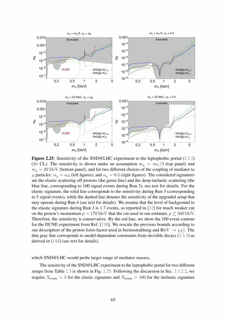
Excluded

DUNE SND@LHCinelSND@LHCel

0.2 0.5 1 2 510-7

10-6

10-5

10-4

0.001

0.010

mV [GeV]

αB

mχ = mV/3, αχ = αB

Excluded

SND@LHCinelSND@LHCel

0.2 0.5 1 2 510-9

10-8

10-7

10-6

10-5

10-4

0.001

mV [GeV]

αB

mχ = mV/3, αχ = 0.5

Excluded

DUNE SND@LHCinelSND@LHCel

0.2 0.5 1 2 510-7

10-6

10-5

10-4

0.001

0.010

mV [GeV]

αB

mχ = 20 MeV, αχ = αB

Excluded

SND@LHCinelSND@LHCel

0.2 0.5 1 2 510-9

10-8

10-7

10-6

10-5

10-4

0.001

mV [GeV]

αB

mχ = 20 MeV, αχ = 0.5

Figure 2.25: Sensitivity of the SND@LHC experiment to the leptophobic portal (2.3.2)(2σ CL). The sensitivity is shown under an assumption mχ = mV /3 (top panel) andmχ = 20 MeV (bottom panel), and for two different choices of the coupling of mediator toχ particles: αχ = αB (left figures), and αχ = 0.5 (right figures). The considered signaturesare the elastic scattering off protons (the green line) and the deep-inelastic scattering (theblue line, corresponding to 100 signal events during Run 3), see text for details. For theelastic signature, the solid line corresponds to the sensitivity during Run 3 (correspondingto 5 signal events), while the dashed line denotes the sensitivity of the upgraded setup thatmay operate during Run 4 (see text for details). We assume that the level of background tothe elastic signature during Run 3 is 1.7 events, as reported in [32] for much weaker cuton the proton’s momentum p > 170 MeV that the cut used in our estimate, p & 500 MeV.Therefore, the sensitivity is conservative. By the red line, we show the 100 event contourfor the DUNE experiment from Ref. [130]. We rescale the previous bounds according toour description of the proton form-factor used in bremsstrahlung and Br(V → χχ). Thethin gray line corresponds to model-dependent constraints from invisible decays (2.3.3) asderived in [144] (see text for details).

which SND@LHC would probe larger range of mediator masses.

The sensitivity of the SND@LHC experiment to the leptophobic portal for two differentsetups from Table 2.3 is shown in Fig. 2.25. Following the discussion in Sec. 2.3.2.2, werequire Nevents > 5 for the elastic signature and Nevents > 100 for the inelastic signature

65

during Run 3.The parameter space that may be probed by SND varies in dependence on the values

of parameters αχ,mχ. Namely, for the choice mχ = mV /3, SND@LHC only may probemasses 350 MeV < mV < 700 MeV. For the choice mχ = 20 MeV, it is possible inaddition to probe masses 700 MeV < mV . 7 GeV. Moreover, for the choice αχ = 0.5,the probed range of the coupling αB even competes with the model-dependent bound fromthe signature B → K + inv at the lower bound.

Unlike the case of the direct detection experiments, the sensitivity of SND@LHCdepends only weakly on the choice of mχ, as the production probability and thescattering cross section of χ particles is determined mainly by mV . In this way,SND@LHC and direct DM detection experiments may probe complementary massranges of χ.

In the figure, we also show the sensitivity of DUNE experiment from [130]. Thebackground estimate has not been made for this experiment. Therefore, we show thecontour corresponding to 100 events.

Finally, let us discuss the improvement of the sensitivity of SND@LHC for the up-graded setup. For the curve describing elastic scattering signature, the scaling of the lowerbound of the sensitivity with the integrated luminosity L and detector length lscatt

det is

αelB ∝

(NSND@LHCχ,prod · lscatt

det /√Nbg

)−1/n

∝ (L · lscattdet )−1/n, (2.3.14)

where the scaling of the number of neutrino background events is Nbg ∝ L · lscattdet , and

n = 2 or 3, depending on the choice for αχ. The improvement of the sensitivity for theupgraded setup reaches a factor of 2 to 3. We note, however, that due to tighter requirementon the proton energy used in our estimate, the elastic signature may be background-free, inwhich case the improvement increases by up to a factor 10. For the inelastic signature, thescaling depends on the improvement of the uncertainty in the NC/CC ratio measurementduring the time frame of the upgraded setup. In the optimistic scenario, the uncertainty willbe significantly smaller, and the lower bound will become better by the same factor as forthe elastic signature.

2.3.3.2 Decays

To illustrate the potential of SND@LHC to probe decays, we estimate the sensitivity toscalar, neutrino and vector portals, which introduce correspondingly a light Higgs-likescalar, a heavy neutral lepton (HNL) and a dark photon (see, e.g., [67] for the descriptionof the models). Decays with pairs of charged particles in the final state – muons, electronsand pions – are the main decay channels for all the portal particles, except for GeV scaleHNLs N that mix with ντ , for which the main decay channel is a decay N → π0ν.

66

In order to obtain the sensitivity of SND@LHC to various decaying FIPs, we use thefollowing estimate:

Nevents =∑

i

N iprod · εigeom · P i

decay · Brvis (2.3.15)

Here, N iprod is the total number of FIPs of species X produced via channel i, εigeom is the

geometric acceptance for particle X decay products, and P idecay is the decay probability

averaged over energies EX of particles X ,

P idecay =

∫(e−lmin/cτXγX − e−lmax/cτXγX )f iEXdEX , (2.3.16)

with fEX being the energy EX distribution of FIPs that fly in the decay volume, and τX andγX their lifetime and Lorentz boost factor, respectively. Finally, Brvis is the branching ratioof visible decays of particle X . Details of estimates are summarized in Appendix 2.B. Thesensitivities are shown in Fig. 2.26, where we show the estimate for the Run 3 setup, aswell as for the possible upgrade that may operate during Run 4. For the upgraded setup, thenumber of events at the lower bound is higher by a factor of ldec

det,upgr/ldecdet ·LRun 4/LRun 3 = 50.

Figure 2.26: Sensitivity of SND@LHC to (top left) dark scalars, (top right) dark photons,and HNLs that mix with (bottom left) νµ and (bottom right) ντ . Blue (green) contourscorrespond to 1 and 10 events in the (upgraded) SND@LHC target. Sensitivities of previousexperiments and of the FASER/FASER2 experiment are reproduced from [58, 67].

We conclude that for the Run 3 setup, SND@LHC may probe only a tiny parameterspace for dark scalars, dark photons and HNLs that mix with τ flavor. For the upgradedsetup, it may be possible to probe HNLs that mix exclusively with νµ in the mass range. 2.5 GeV, and in . 2.0 GeV for pure mixing with ντ . SND@LHC may also probe dark

67

photons at the upper bound of the sensitivity with masses mV . 0.1 GeV, and dark scalarswith masses mS . 0.8 GeV.

2.3.4 Comparison with FASER

There is a similarity between the facilities of SND@LHC and FASER/FASERν experiments.They are both placed in a large η region and at the same distance lmin = 480 m from theATLAS interaction point, but in the opposite tunnels. Parameters of the experiments aresummarized in Table 2.4. Below, we make a qualitative comparison of the sensitivitiesof the SND@LHC and FASER experiments, and then comment on the changes due toupgrades.

Detector lmin, m ldet, m θmin, mrad θmax, mrad Ω · 107, sr L, fb−1

SND@LHC

480

0.5 0.3 1.5 6.9150FASER 1.5 0. 0.2 1.4

FASERν 1. 0. 0.4 2.7SND@LHC upgr. 1.25 0.3 1.5 6.9

3000FASER2 5 0. 2.1 138

Table 2.4: Parameters of SND@LHC and FASER experiments: the distance to the decayvolume, the length of the decay volume, the polar coverage, covered solid angle, totalintegrated luminosity.

Let us summarize the main differences between SND@LHC and FASER/FASERνdetectors in the reconstruction of signal. For scattering, SND@LHC competes with theFASERν detector. FASERν consists of emulsion films interleaved with tungsten plates,only providing the information of spatial position of different tracks with 30% energyreconstruction accuracy for neutrino events (see also [155]). For muons, the situation ismuch better, as they, being produced in FASERν, may penetrate it and enter FASER, whichallows timing and momentum measurements. This option is unavailable, however, forother particles (hadrons, electrons), as they are effectively absorbed in the detector. On thecontrary, SND@LHC provides timing measurements by the use of the SciFi technologyand the energy reconstruction accuracy of 22% for electrons. For both experiments, timingis needed for rejecting the background induced by high-energy muons and secondaryparticles.14

In the case of decays, SND@LHC competes with FASER, and their detectors providecomparable FIP parameters reconstruction accuracy, thanks to good spatial resolution of theemulsion. Assuming that SND@LHC is a background free experiment when searching fordecays, the only relevant quantity for comparing the experiments is the number of correctlyidentified FIP decay events.

14In this work, we compare the signal of new physics to the number of neutrino interactions, which wasalready obtained under assumption of possible background. Therefore, these key features of the detectors’concept are omitted in our analysis.

68

2.3.4.1 Lower and upper bound of the sensitivity

Let us now consider the differences in the number of events at these experiments. Twofactors are important. First, SND@LHC is slightly off-axis, whereas FASER(ν) is placeddirectly on-axis. Second, SND@LHC covers ' 5 (1.25) times larger solid angle thanFASER(ν).

The different placements of SND@LHC and FASER/FASERν cause two effects thatdirectly affect the lower and upper bound of the sensitivity (we follow [9] here): (i)off-axis placement of SND@LHC causes smaller γ factor and thus worse potential toprobe the parameter space of short-lived FIPs; (ii) large angular coverage leads to largerfraction of particles from heavy mesons flying to the detector.

First, particles X flying off-axis have smaller energies than those flying on-axis. Thisis important for probing FIPs that have small decay lengths ldecay . lmin. Indeed, in thisregime, the decay probability is Pdecay ≈ exp[−lmin/cτXγX ]. The sensitivity to such largecouplings g determines the upper bound, which is very sensitive to the mean energy of X:

g2upper,SND@LHC

g2upper,FASER

∼ γSND@LHCX

γFASERX

(2.3.17)

The upper bound is important for particles that may be probed by the FASER and SND@LHCexperiments only in the regime of small decay lengths, including dark photons and axion-like particles (see Fig. 2.26). The ratio of the mean γ-factors of dark photons A′, flying inthe detector, is γSND@LHC

A′ /γFASERA′ ≈ 1/3. The resulting estimate (2.3.17) agrees with the

sensitivities in Fig. 2.26.Second, the off-axis placement may affect the geometric acceptance. Light portal

particles X are often produced in decays of mesons. The angular distribution of particlesX is similar to the distribution of parent mesons at angular scales larger than ∆θ '2pX,rest/〈Emeson〉, where pX,rest is the momentum of the daughter particle at rest frame ofthe decaying meson, being ' mmeson if masses of all decays products are mmeson. If∆θ > θSND@LHC ' O(1 mrad), the ratio of geometric acceptances εgeom for the SND@LHCand FASER experiments scales with their solid angle coverage. Using characteristicenergies 〈Emeson〉 ' 1 TeV for mesons produced in the far-forward region, we find that thisscaling is indeed the case of light particles produced in decays of D, B-mesons.

However, if the daughter particle is heavy mX ' mmeson, or if the decaying mesonis light (such as π, η, K), the geometric acceptance depends on the shape of the mesondistribution. Experimental measurements of the meson production cross section in theregion |η| < 5 [156–159] provide the following scaling:

dσdpT∼ pT

(p2T + Λ2

meson)2, (2.3.18)

69

independently of the pseudorapidity. The values of Λmeson are of order of ΛQCD ≈ 250 MeV

for light mesons π, η, K, and mD/B for D/B-mesons. Numeric approaches (see, forinstance, [43, 152, 160, 161]) predict the same behavior of dσ/dpT almost independently ofpseudorapidity, including the far-forward region.15 This means that the meson distributiondf/dΩ is flat for angles θ . θflat, where

θflat ∼〈pT〉〈Emeson〉

∼ Λmeson

1 GeVmrad '

O(1 mrad), B,D

O(0.1 mrad), π, η(2.3.19)

Using the spectra of mesons (see Appendix 2.B), we find

εSND@LHCgeom

εFASERgeom

'

1, π, η,ΩSND@LHC

ΩFASER≈ 5, D,B, τ

(2.3.20)

2.3.4.2 Decays

Based on these findings, we can make a simple comparison of minimal couplings that maybe probed by the FASER and SND@LHC experiments. Further, we will assume the mostoptimistic estimate for SND@LHC, according to which decays of FIPs may be clearlydistinguished from backgrounds, and therefore, only 3 events are required at 95% CL.

In the regime ldecay lmax, the number of decay events of particles that originate frommesons is

Ndecay ∝ εgeom · ldet · g4 · Brvis (2.3.21)

From this relation, we obtain

g2lower,SND@LHC

g2lower,FASER

∼√γSND@LHCX

γFASERX

·√

BrFASERvis

BrSND@LHCvis

·

1.7, particles from π, η

0.8, particles from D, B(2.3.22)

where we used lSND@LHCdet = 0.5 m.

Therefore, assuming that SND@LHC may reconstruct decay events in background-free regime, the reaches of SND@LHC and FASER to probe decays of particles arecomparable.

Comparing the lower bounds of the numerical sensitivities of SND@LHC and FASERfor dark photons and dark scalars in Fig. 2.26, we find that they agree with the esti-mates (2.3.22). However, for HNLs there is a disagreement as large as a factor of 3. A

15Some of these approaches suffer from theoretical uncertainties in far-forward direction [162]: small pTand large pseudorapidity require using parton distribution functions in the domain of small Bjorken scalingvariable x, which are poorly constrained. One of the goal SND@LHC and FASER may serve for checkingthe distributions (and in particular the property (2.3.19)) via studying the events with neutrinos produced inthe meson decays.

70

reason for this may be different distributions of D mesons used in our analysis and in [67](see also Appendix 2.B).

Let us now comment on the lower bounds ratio with the upgrade. With the help of theformulas (2.3.20), (2.3.22) and table 2.4, we conclude that the FASER2 experiment hasmuch better potential:

g2lower,SND@LHC upgr

g2lower,FASER2

' 20 ·√γSND@LHCX

γFASERX

·√

BrFASERvis

BrSND@LHCvis

(2.3.23)

A reason for this is mainly significantly larger angular coverage in the case of the FASER2.

2.3.4.3 Scattering

Consider now the scattering signature. For the leptophobic portal, from Eq. (2.3.9), theratio of minimal probed couplings is (for αχ = αB)

αB,FASERν

αB,SND@LHC∼(

εFASERνgeom

εSND@LHCgeom

lFASERνdet

lSND@LHCdet

σ(EFASERνthreshold)

σ(ESND@LHCthreshold )

√NFASERνν bg

NSND@LHCν bg

) 13

(2.3.24)

where Nν bg is the number of neutrino background events (different for the elastic andinelastic signatures), and we assume that the detection efficiency is equal to one. Theeffective cross section σ(Ethreshold) depends on momentum threshold for charged particlesto be visible. The dependence of σ on Ethreshold is very important for the elastic signature,as most of the elastic scattering events are characterized by low momenta. For the inelasticsignature, it is less relevant. For SND@LHC, the requirements are Ethreshold = 170 MeV forprotons and 100 MeV for other charged particles. For FASERν (Ref. [163]), we have notfound the information about Ethreshold. Instead, we assume Ethreshold = 1 GeV that was usedfor the pilot run in 2018 (see also [164], where 300 MeV cut is considered for FASERν2).

For small masses mV . 0.5, the mediator is mainly produced from π, η decays, asshown in Fig. 2.24. In this case, we have εSND@LHC

geom /εFASERνgeom ≈ 0.3. A similar increase

occurs for Nν bg, since neutrinos are abundantly produced in decays of pions, and therefore,we can use the same scaling for the total neutrino events, Nν bg ∝ εgeomldet. The estimatethen reads:

αB,SND@LHC

αB,FASERν∼ 9.61/6

(σ(ESND@LHC

cut )

σ(EFASERνcut )

)− 13

' 1.5

1, inelastic

0.2− 0.9, elastic(2.3.25)

We conclude that sensitivities of SND@LHC and FASER to scatterings are also compa-rable.

71

2.3.5 Conclusions

In this section, we have demonstrated the potential of the SND@LHC experiment to probefeebly interacting particles. We have considered scattering signatures and some decaysignatures as well.

Light dark matter particles coupled via mediators may be searched by looking at thescattering signature, see Sec. 2.3.2.2. These events need to be distinguished from neutrinoscatterings. Because of large mass of Z andW bosons that mediate the neutrino interactions,the neutrino scattering occurs inelastically most of the times. This may be not the casefor light dark matter particles interacting via a light O(1 GeV) mediator, for which theyields of elastic and inelastic scattering events are comparable (see Fig. 2.20). Therefore,looking for an excess in the yield of elastic scattering events is suitable for probing suchFIPs. For heavier mediators, FIPs scattering still may be searched via an increase in theratio of scattering events with a lepton and those without a lepton. On one hand, this ratiomay be accurately measured at SND@LHC. On the other hand, it is clearly predicted bythe SM. We have illustrated the power of these two signatures by estimating the sensitivityto the scattering of light dark sector particles via the leptophobic portal, see Fig. 2.25.

SND@LHC detector may also search for decays of mediators, see Sec. 2.3.4.2. Becauseof good spatial resolution of the emulsion in SND@LHC, decays into two charged particlesmay be distinguished from the neutrino scattering events. Such decays are main decaychannel in the case of heavy neutral leptons, dark scalars that mix with Higgs boson, anddark photons. It is possible to probe their parameter space at its upgraded version asdescribed in [32], see Fig. 2.26. However, further studies of possible backgrounds arerequired to clarify these results.

We have also compared the potential of SND@LHC and FASER/FASERν facilitiesto probe new physics, see Sec. 2.3.4. Placed at the same distance but at the opposite sidesof the ATLAS experiment interaction point, they are very similar. There are a few factors,however, leading to differences in the sensitivity of these facilities to new physics. First,FASER is on-axis, while SND@LHC is slightly off-axis. The off-axis placement decreasesthe mean momentum of particles produced in the direction of SND@LHC, which somewhatworsens its potential to probe short-lived particles with the decay lengths of the order ofthe distance to the detector. Second, SND@LHC covers ' 5 times larger solid anglethan FASER. Because of this, depending on the FIPs production channel, a fraction ofFIPs flying in the direction of FASER is smaller than that for SND@LHC. For scatterings,FASERν has higher event rate due to larger detector length and on-axis position, resultingin better sensitivity. This can be applied for the inelastic signature; for other possiblesignatures, e.g. elastic scattering off protons, SND@LHC might have better sensitivitythanks to its higher momentum resolution.

72

Appendix

2.A CHARM sensitivity based on number of decay events estimate

The number of decay events for the pure α mixing at CHARM is given by the formula

N(α)events =

∑

X=D,τ

NX · Br(X → Nα)×

×∫dEdθdz · fXNα(E, θ)

e−l(z)/cτNγ

cτ(α)N γ

∆φ(θ, z)

2π· εdecay(θ, z, E) · Br(Nα → ll′) · εdet,ll′

(2.A.1)

Here,NDi = NPoT × χcc × fc→Di , Nτ = NDs × Br(Ds → τ ντ ) (2.A.2)

are the total numbers ofD mesons (Di = Ds, D+, D0) and τ leptons, withNPoT = 2.4·1018

being the total number of proton-target collisions at CHARM and χcc ≈ 4 · 10−3 theproduction fraction of the cc at SPS energies for a thick target [44]. BrDs→τ ≈ 5.43% [52]and fc→Di are given from [80]. fXNα is the distribution of HNLs produced in decays ofX particles in polar angle and energy. z ∈ (480, 515) m is the longitudinal distance,θ ∈ (3.5/515, 6.5/515) is the polar angle coverage of the end of the CHARM’s decayvolume, while ∆φ(θ)/2π is the azimuthal acceptance for HNLs decaying inside the decayvolume. εdecay is the decay acceptance – a fraction of decay products of HNLs that bothpoint to the detector. Finally, εdet,ll′ are reconstruction efficiencies for leptonic decays:εee ≈ 60%, εµµ ≈ 75%, and εeµ ≈ 65%, which we use from [62].

Computing of fNα(E, θ) requires knowing the distribution of D mesons and τ leptonsfτ (E, θ) produced at the CHARM target. We approximate fτ by the distribution of Ds

mesons, while for the distribution of D mesons we use FairShip simulations [44] forcollisions of the SPS proton beam with a thick Tungsten target.16 The distribution of HNLsfXNα(E, θ) has been obtained from fX(E, θ) semi-analytically using the method from [120].

We have estimated εdecay by using a toy simulation for decays of HNLs inside the decayvolume into three massless particles, and requiring the momenta of the two charged leptonsto point towards the end of the decay volume. The acceptances are shown in Fig.2.27.

16Although at CHARM the target material is different, we believe that it is still a reasonable approximation.

– 73 –

In order to obtain the excluded domain, we assume the absence of background andrequire Nevents > 2.3, which corresponds to the 90% C.L.

The comparison of this estimate with the rescale from Sec. 2.1.4 and [63] is shown inFig. 2.27. We find that the estimates are in very good agreement. We also show our estimateof the CHARM bounds on the e mixing, which differs from the bounds obtained from [62]by including the production from Ds mesons, which dominates masses mN & 700 MeV

(see also Fig. 2.5). The resulting sensitivity at the lower bound improves by up to a factor3− 4 for this mass region.

0.2 0.4 0.6 0.8 1.0 1.2 1.4 1.60.002

0.003

0.004

0.005

0.006

0.007

0.008

mN [GeV]

<ϵ>,l decay>>l det

ϵgeom

ϵgeomϵdecay

Bergsma et al.Our result (number of events)Our result (rescale)

0.2 0.5 1 210-8

10-7

10-6

10-5

10-4

0.001

mN [GeV]

Ue2

Orloff et al.Our result (number of events)Our result (rescale)

0.1 0.2 0.5 110-7

10-6

10-5

10-4

0.001

mN [GeV]

Uτ2

Figure 2.27: The left panel: fraction of HNLs that point towards the detector (blue line)and fraction of HNLs whose decay products point towards the detector (red line). Themiddle and right panels: comparison of our estimates of the constraint from the CHARMexperiment on the pure e (the middle panel) and τ mixing (the right panel), with boundsreported in [62] and [63]. We show two estimates: the red line corresponds to the rescale ofthe bound on the e mixing from [62] (see Sec. 2.1.4 for details), while the blue line is ourindependent estimate based on Eq. (2.A.1).

2.B Decay events at SND@LHC

We estimate the number of decays using the following formula:

Nevents =∑

i

N iprod · εigeom · P i

decay · Brvis, (2.B.1)

Here,N iprod is the total number of particlesX produced via a channel i, εgeom is the geometric

acceptance, and Pdecay is the decay probability averaged over energies of X ,

P idecay =

∫(e−lmin/cτXγX − e−lmax/cτXγX )f iEXdEX , (2.B.2)

Here, lmin = 480 m is the distance to the SND@LHC detector, lmax − lmin = ldecaydet , fEX

is the energy distribution of particles X that fly in the decay volume. Finally, Brvis is thebranching ratio of visible decays.

HNLs that mix with νµ are produced in decays of Ds/D+/0 mesons. HNLs that mix

with ντ are produced mainly in decays of τ -leptons, which, in their turn, originate fromdecays Ds → τ ντ [39]. We have obtained the distribution of D mesons using SIBYLL

74

2.3c [161, 165] as a part of the CRMC package [153]. As a cross-check, for the charmproduction we have compared the predictions of SIBYLL with results of the FONLLprogram [40, 42, 43]. We have found that the results agree well for angles θ > 0.8 mrad.17

Having the D distribution, we have obtained the distribution of τ -leptons and, subsequently,HNLs angles and momenta using the approach described in [120]. For simplicity, weapproximate the angle-momentum distribution of HNLs by that of particles produced in atwo-body decay τ → πN (for the mixing with ντ ) and Ds → µN (for the mixing with νµ).

Dark photons V in sub-GeV mass range are produced in decays h = γV of π- andη-mesons, and by proton bremsstrahlung [134]. We use the angle-energy distributions ofthe mesons generated by EPOS-LHC [152] as a part of the CRMC package [153], andfollow [134] for the bremsstrahlung.

Dark scalars S are produced in decays B → XsS of B-mesons, where Xs is ahadron including an s-quark, and by the proton bremsstrahlung [38]. We use FONLL inorder to obtain the angle-energy distribution of B-mesons, and follow [38] for the protonbremsstrahlung.

Using the obtained distribution, we have reproduced the sensitivity of FASER to scalarsand dark photons from [67]. However, we have not reproduced the sensitivity to HNLs, seeFig. 2.28. A reason may be in different distributions of Ds-mesons used in the estimates.

Excluded

FASER

SND@LHC

0.1 0.2 0.5 1 21.×10-5

5.×10-51.×10-4

5.×10-410-3

mN [GeV]

Uτ2

Figure 2.28: The sensitivity of FASER to HNLs that mix with ντ . The solid line corre-sponds to the contour given in Ref. [67], while the dashed line – to our estimate. For thecomparison, we also show the sensitivity of SND@LHC (in blue).

2.C Leptophobic mediator: production, decays and scatterings

2.C.1 Production and decay

In order to describe interactions of V with hadrons, we follow [166] (see also [150]), inwhich vector mesons m play the role of gauge bosons of a “hidden” local SUf (3) symmetryin the space of pseudoscalar mesons nonet. The EM field is included as a background field

17For smaller angles, FONLL (both the online form and installed program) predicts zero or negative crosssections, which indicates some internal problem.

75

that is associated with the appropriate generator Q = diag(

23,−1

3,−1

3

), and mix with the

vector mesons. The coupling of the vector mesons to the pseudoscalar mesons is fixedby the anomalous decay π0 → γγ. This model is very successful in describing the EMscattering data e+e− → hadrons and decay widths of vector mesons. We assume that itmay be also used for describing the phenomenology of the leptophobic boson.

For the lephophobic mediator, the generator is TV = 13

, and its mixing coupling isgiven by

fV m = −2gBgmTr[TV Tm], (2.C.1)

where Tm is a generator associated with the given meson, and gm/m2m = 1/

√12π, as fixed

by the anomaly. The mixing occurs only with isosinglet ω- and φ-mesons, for which

Tω =1

2diag(1, 1, 0), Tφ =

1√2

diag(0, 0, 1) (2.C.2)

The decay width of V may be extracted from the experimental data on the EM ratiosσ(e+e− → hadrons)/σ(e+e− → µ+µ−), where the hadronic final states correspond toφ-like and ω-like decays. This has been made in [144], in which the data have been usedfor describing the decay widths up to masses mV ' 1.7 GeV, while for larger massesperturbative calculations were used. We use the results of this paper.

The resonant enhancement is also important when considering the production of themediator by the proton bremsstrahlung by affecting the form-factor FppV in the ppV vertex.The baryonic form factor FppV may be related to the proton and neutron EM dipole form-factors Fp/n, which are, in its turn, related to the isoscalar form factor Fω ≡ Fp+Fn

2, which

in the extended vector meson dominance model coincides with the ω contribution [154]:18

〈p|JB|p〉 = 〈p|JEM|p〉+ 〈n|JEM|p〉 −→ FppV = 2Fω (2.C.3)

Unfortunately, the experimental data on e+e− → p+p−, which may be used for extractingthe EM form-factors in the time-like region, is limited by the physical threshold q2 > 4m2

p.Following [154] (see also [151]), for extrapolating in the domain of lower invariant masseswe use

FppV (q2) =∑

ω

fωm2ω

m2ω − q2 − iΓωmω

, (2.C.4)

where the sum goes over ω(782), ω(1420), ω(1680), fω = 2fNNω/gω, with fNNω beingthe meson’s coupling to the nucleon, while gω is the meson’s coupling to photon. We usethe couplings fNNω(782) = 17.2 and gω(782) = 17.1 [154]. The couplings to the other tworesonances are unknown. However, the remaining two coefficients fω(1420) = −2.16+0.77i

and fω(1680) = 1.14− 0.57i in Eq. (2.C.4) may be fixed by two requirements: FppV (0) = 1,and FppV (−q2) ∼ 1/q4. The first requirement comes from the fact that the form-factor FppV

18We assume no contribution of the φ-meson to the form-factor, since the corresponding coupling fφNN isexpected to be suppressed [167, 168] (i.e., neglecting the s-quark contribution in the proton PDF).

76

is reduced to the baryon charge at low momenta transfer. The second requirement comesfrom the behavior of the proton’s dipole form-factor in the space-like region predicted bythe quark counting rules [169].

The behavior of the branching ratio into a χχ pair and the form-factor is shown inFig. 2.29. Note that for the choice αχ = αB, commonly considered in the literature, theenhancement of FppV near mV = mω(770) and suppression of Br(V → χχ) due to the ωresonances cancel each other.

|FppV2

Br(V→χχ)

|FppV2Br(V→χχ)

0.2 0.5 1 2

0.01

0.10

1

10

100

1000

104

mV [GeV]

Figure 2.29: The behavior of the ppV form-factor (2.C.4) and the branching ratio for theprocess V → χχ. The coupling αχ = αB is assumed, and mχ = mV /3.

2.C.2 Elastic and inelastic scattering cross sections

2.C.2.1 Elastic scattering

The cross section of the elastic scattering is

σelastic =

∫dEχfEχ

EN,max(Eχ)∫

EN,min

dENdσχN→χNdEN

, (2.C.5)

where EN,min is the minimal recoil energy that may be detected, the maximal recoil energyof the nucleon is

EN,max =mN(2E2

χ + 2EχmN +m2N −m2

χ)

2EχmN +m2N +m2

χ

, (2.C.6)

Q2 = 2mN(EN −mN) is the modulus of the squared momentum transfer, Q2 = −(pχ −p′χ)2. Finally, the differential cross section is

dσχN→χNdEN

= 4πα2DFN(Q2)

mN(2E2χ + 2EχmN +m2

χ)− EN(2EχmN +m2χ)

(E2χ −m2

χ)(2ENmN − 2m2N +m2

V )2, (2.C.7)

where FN(Q2) is the elastic form-factor, which we assume to be FN(Q2) = 1

(1+ Q2

0.71GeV2 ).

77

2.C.2.2 Inelastic scattering

In the case of the inelastic scattering, we follow [148], which uses the parton model. Let usintroduce the variables EV = Eχ − E ′χ, Q2. The differential cross section is

d2σ

dEV dQ2=πα2

D

9mN

1

E2χ −m2

χ

1

(m2V +Q2)2

(2p−q)µ(2p−q)νWµν

∑

q

xfq(x,Q2), (2.C.8)

where fq(x,Q2) is the parton distribution function (q = u/u/d/d/s/s), x = Q2

2mNEV, Wµν

is the hadronic tensor,

Wµν = −gµν +qµqνq2

+2x

pN · q + 2xm2N

(pNµ −

pN · qq2

qµ

)(pNν −

pN · qq2

qν

)(2.C.9)

Because of the property qµWµν = qνWµν = 0, we have

(2p− q)µ(2p− q)νWµν =4E2

χQ2 − 4EVEχQ

2 −Q4

E2V +Q2

− 4m2χ (2.C.10)

The kinematic limits are

Q2 < 2mNEV , 2µ2 < Q2 < 4(Eχ(Eχ − EV )−m2χ)− 2µ2, (2.C.11)

Emin < EV <2mN(E2

χ −m2χ)

2EχmN +m2N +m2

χ

, (2.C.12)

where Emin is the minimal recoil, and the function µ is

µ2 =m2χE

2V

Eχ(Eχ − EV )−m2χ −

√(Eχ(Eχ − EV )−m2

χ)2 −m2χE

2V

(2.C.13)

To get fq(x,Q2), we use LHAPDF with CT10nlo PDF sets. We assume that they are zeroif Q < 1 GeV.

78

Chapter 3

Probes from cosmology1

In this chapter, we consider two earliest messengers from cosmology: BBN and CMB, andstudy the impact of short-lived FIPs on corresponding observables. In the case of BBN,we concentrate on short-lived particles that decay hadronically, and derive analytically thebound on lifetimes that comes from the impact of mesons on the p↔ n conversion in theprimordial plasma, see Sec. 3.1. In the case of CMB, we study the impact of short-livedFIPs on the effective number of degrees of freedom, Neff, and in particular show thateven if decaying mostly into neutrinos they may decrease Neff, see Sec. 3.2. Finally, weapply the findings to the case of a particular model – HNLs, for which we first study theircosmological population (Sec. 3.3.4), and then derive constraints from BBN (Sec. 3.3.3.1)and CMB (Sec. 3.3.4).

3.1 BBN and hadronically decaying particles

In this section, we discuss bounds from BBN on hadronically decaying particles. We willfirst discuss the current measurements of the primordial abundance of helium, then derivethe bounds from BBN on hadronically decaying particles, and then comment until whichlifetimes the bound extends.

3.1.1 Measurements of 4He abundance

Over the last 6 years five works determined the primordial 4He abundance from stellarmeasurements [171–175]. The formal statistical errors of Yp are at the level of 1 − 3%,however, the scatter between different groups is larger, see Fig. 1.

All these works determine astrophysical Helium abundance through measurementsof recombination emission lines of 4He and H in the metal-poor extragalactic ionizedregions, then linearly extrapolating the measurements to zero metallicity. Given the highprecision of the results, it is important to take into account various smaller effects: including

1Results of this chapter are presented in papers [37, 170]. The main contribution of Maksym Ovchynnikovis analytic and numeric estimates of the BBN and CMB bounds.

– 79 –

Figure 1: Measurements of Yp of recent works [171–175]. The green shaded region isthe PDG recommended value [52] (with ±1σ). The gray dashed line denotes the SBBNprediction Yp = 0.247 from [45]. The red dashed-dotted line is the maximal admissiblevalue Yp,max on which we base our analysis.

4He fluorescent emission, different ion temperatures, spatial temperature fluctuations, andothers [176, 177]. Additionally, while it is true that the metallicity and Helium abundanceare positively correlated, the linear extrapolation to zero-metallicity may be prone tosystematic uncertainties.

The value of Yp predicted within the framework of SBBN is Yp = 0.24709± 0.00019

(see, e.g., [45]). The effect of mesons leads to an increase of Yp as compared to the SBBNvalue. Therefore, in order to get a conservative upper bound we assume that the maximallyallowed Yp is given by the 1σ deviation from the maximal value predicted by [171–175],which is Yp,max = 0.2573. Note that this upper value significantly deviates from thePDG-recommended value [52] Yp,max = 0.248 at 1σ. This translates to the bound

∆YpYp

< 4.35% (3.1.1)

3.1.2 Bound on hadronically decaying particles

Sufficiently heavy FIPs can decay into mesons h = π,K, etc. Charged pions drive thep↔ n conversion via processes [178]

π− + p→ n+ π0/γ, π+ + n→ p+ π0 (3.1.2)

The cross section of these reactions is much larger than the cross section of weak interactionsdriven conversion processes:

〈σπp↔nv〉〈σWeak

p↔nv〉' 1

G2Fm

2pT

2∼ 1016

(1 MeVT

)2

, (3.1.3)

Large cross section, absence of threshold and isotopic symmetry of these processes meanthat if pions are present in the plasma in the amounts at least comparable with that ofbaryons, they drive the number densities of protons and neutrons to equal values, nn/np '

80

〈σπp→nv〉/〈σπn→pv〉 ' 1.2 The effect of kaons is qualitatively similar, but leads to a slightlydifferent neutron-to-proton ratio (Appendix 3.B.1).

The impact of this effect on primordial 4He abundance depends on how long mesonsremain present in the plasma in significant amounts. Once mesons are created, theycan (i) scatter and lose energy; (ii) decay; (iii) participate in p ↔ n conversion. Thecorresponding rates are very different: at MeV temperatures and below, Γhscat Γhdecay Γhp↔n (see [179]).

The instantaneous number density of mesons is an interplay between their production(via decays of FIPs) and their decays:

ninsth = nFIP(T ) · BrN→h

ΓFIP,dec

Γh,dec= nN(T ) · BrN→h

τhτN. (3.1.4)

Here, BrFIP→h is the branching of FIPs into mesons. nFIP(T ) is the number density ofFIPs:

nFIP(T ) =

(adec

a(T )

)3

· ndecFIP · e

− t(T )τN , (3.1.5)

where ndecFIP is the FIP’s number density at decoupling (i.e. when their interaction with

plasma has been completely stopped), and a(T ) (adec) is the scale factor at temperature T(correspondingly, at FIP decoupling).

The number of p↔ n reactions per nucleon occurring after time t τFIP (or belowsome corresponding temperature T (t)) is thus

Nhp↔n(T ) =

∑

h

∞∫

t(T )

dt ninsth (T ) · 〈σhp↔nv〉 ≈

(adec

a

)3 ndecFIP

nB·e−

t(T )τFIP ·BrFIP→h ·Pconv, (3.1.6)

where nB is the baryon number density, the sum goes over meson species and Pconv is theprobability for a single meson to interact with nucleons before decaying:

Pconv 'nB · 〈σhp↔nv〉

Γhdecay. (3.1.7)

At O(1 MeV) temperatures, Pconv ∼ 10−2 − 10−1, see Appendix 3.B.

2For each of the processes (3.1.2), there are no inverse reactions. Indeed, π0 decays very fast, whereas γsquickly lose their energy. Therefore, the conversion (3.1.2) is highly non-equilibrium, and the correspondingvalue of nn/np is not given by the usual Boltzmann exponent.

81

The meson driven conversion keeps the value nn/np ' 1 roughly until a temperatureT0 when the number of reactions per nucleon drops below one,

Nhp↔n(T0) ' 1, (3.1.8)

and weak SBBN reactions start to relax the n/p ratio down to its SBBN value, seeFig. 2 (left panel).

However, if T0 is close enough to the freeze-out of weak p↔ n processes, occurringroughly at Tn ' 0.8 MeV, the relaxation is not complete (Fig. 2, right panel). This leadsto a positive correction ∆(nn/np) as compared to the SBBN case, which translates to anincrease of the 4He abundance ∆Yp.

SBBN+HNLsSBBN

0.1 0.5 1 5 10

0.2

0.3

0.4

0.5

0.6

T [MeV]

Xn

1.3 1.4 1.5 1.6 1.7

2

4

6

8

10

T0, MeV

ΔYp/Y

p,%

Figure 2: Left panel: temperature evolution of the neutron abundance Xn = nn/(nn + np)in the presence of pions from decays of an HNL with mass mN = 400 MeV and lifetimeτN = 0.03 s. Below T ' 100 MeV, pions drive the neutron abundance to Xn ≈ 0.5. Attemperatures T0 ' 1.3 MeV (the blue vertical dashed line) pions disappear, and Xn startsrelaxing towards its SBBN value but does not reach it. After the neutron decoupling (thegray vertical line) Xn evolves mainly due to the neutron decays. Right panel: a relationbetween the temperature T0 (defined by Eq. (3.1.8)) and corrections to the 4He abundance,as compared to the SBBN central value Yp ≈ 0.247. It corresponds to the case of when onlycharged pions are present in plasma. The gray horizontal line corresponds to maximallyallowed correction ∆Yp/Yp = 4.35% that we adopt in this work (see Appendix 3.1.1). Theintersection of gray and colored lines defines the temperature Tmin

0 .

In this way, the upper bound on the 4He abundance Yp,max is translated to the lowerbound T0 ≥ Tmin

0 . Together with the relations (3.1.6)–(3.1.8), this allow us to find an upperlimit on the FIP lifetime τFIP:

τFIP .t(Tmin

0 )

ln

[∑h

(adeca0

)3ndec

FIPPconvBrN→hnγ(Tmin

0 )ηB

] . (3.1.9)

82

Here, nγ is the number density of photons, ηB is the baryon-to-photon ratio, and t(T ) istime-temperature relation. t(T ) is given by the Standard Model relation: t(T ) = M∗

2T 2 , withM∗ = MPl

1.66√g∗

the reduced Planck mass, where g∗(T ) ' 10.6 for T ' 1− 2 MeV.3

Let us rewrite the logarithmic factor in (3.1.9) as

(adec

a0

)3nFIP,dec

nγ(Tmin0 )

=nFIP,dec

nγ(Tdec)· ζ, (3.1.10)

where ζ =(adecTdeca0Tmin

0

)3

is the “entropy dilution” factor. For example, if FIPs were inthermal equilibrium and decoupled while being ultrarelativistic, Tdec mFIP, we havenFIP,dec/nγ(Tdec) ≈ O(1). The dilution factor ζ is a product of the SBBN value times thevalue induced by FIPs during their evolution:

ζ =

(aSBBN

dec Tdec

aSBBN0 Tmin

0

)3

×(aSBBN

0 Tmin0

a0Tmin0

)3

≡ ζSBBN × ζFIP, (3.1.11)

where we used that adec ≈ aSBBNdec ; this approximation is valid since at temperatures Tdec

there are many SM particles, and FIPs only contribute a small fraction to the total energydensity of the Universe. In SBBN at temperatures T & 1 MeV, all particles are at localequilibrium, which defines the dynamics of the scale factor and hence the value of ζSBBN:

ζSBBN ≈g∗(T

min0 )

g∗(Tdec)' 1

8, (3.1.12)

where we used that aSBBN(T ) ∝ g−1/3∗ (T ) · T−1. Decays of heavy FIPs violate the thermal

equilibrium at O(1 MeV), and the scaling (3.1.12) changes. For GeV-scale particles withlifetimes τFIP ∼ 0.01 s − 0.1 s that were in thermal equilibrium, the factor ζFIP reachesO(0.1), see Appendix 3.3.1 using HNLs as an example.

The simple analytic estimate leads to the model-independent bound on FIPs that decayhadronically:

τFIP .0.023

(1.5 MeVTmin0

)2

s

1 + 0.07 ln

[Pconv0.1

BrFIP→h0.4

2nFIP,dec3nγ(Tdec)

· 24(adecTdeca0Tmin

0

)3] . (3.1.13)

The presence of mesons increases the 4He abundance. Therefore, in order to fixTmin

0 (mFIP), we need to adopt an upper bound on the primordial 4He abundance, Yp,max, thatis consistent with measurements [52]. The smallest error bars come from measuring Yp in

3This is indeed the case for short-lived FIPs with τFIP 0.1 s.

83

low-metallicity interstellar regions and extrapolating its value to zero metallicity (pioneeredin [180]). Several groups [171–175] have determined Yp using this method, albeit withdifferent data and assumptions. The resulting scatter between results is larger than thereported error bars. We treat this difference as an additional systematic uncertainty andadopt the maximal value Yp,max = 0.2573 (see Appendix 3.1.1). The maximally allowedrelative deviation is therefore

∆Yp/Yp,SBBN ≈ 4.35%. (3.1.14)

To relate ∆Yp and Tmin0 , we study how the nn/np ratio is relaxed below T0. The relaxation

occurs solely via the SBBN reaction,

dXn

dt= ΓSBBN

p→n(1−Xn)− ΓSBBNn→pXn, Xn =

nnnn + np

, (3.1.15)

albeit with the altered initial condition Xn(T0) = Xhn ' 1/2. (ΓSBBN

p↔n(t) are SBBN rates,see [45]). Non-SBBN value of Xn(T0) is the dominant effect of short-lived HNLs on Yp.At temperatures T . T0, for HNLs with lifetimes τN . 0.02 s, all other quantities that arerelevant for BBN dynamics – ηB, time-temperature relation, the nuclear reactions chain– remain the same as in SBBN, which is because most of HNLs are no longer left in theplasma at these temperatures (see also Appendix 3.B.1). As a result, a value of Xn(T0) istranslated into ∆Yp via

∆YpYp,SBBN

=∆Xn(TBBN)

Xn,SBBN(TBBN), (3.1.16)

where TBBN ≈ 84 keV is the temperature of the onset of nuclear reactions in SBBN [45].To obtain the bound (3.1.13), we considered exclusively meson-driven p↔ n processes

for T > Tmin0 and only weak SBBN processes for T < Tmin

0 . We also solved numericallythe equation (3.1.15) for the neutron abundance in the presence of both mesons-driven andSBBN p↔ n conversion rates in Appendix 3.B.1 using HNLs as an example model, andobtained results being in perfect agreement with the bound (3.3.24). We have also repeatedour analysis for the case of the GeV-mass scalar that mixes with the Higgs and found anexcellent agreement with [181, 182].

We conclude that BBN may constrain hadronically decaying FIPs with lifetimes assmall as τFIP ' 0.02 s.

3.1.3 Limits of applicability of the bound

Eq. (3.1.13) defines the lower bound on FIP lifetimes that may be constrained from themeson-driven 4He overproduction. Our simplified approach is limited by lifetimes forwhich FIPs or their decay products survive until the onset of nuclear reactions. In this case,the dynamics of nuclear reactions gets changed by

84

1. meson-driven p↔ n conversion and nuclear dissociation processes;

2. change of time-temperature relation by FIPs;

3. change of ηB during nuclear reaction;

4. photo-dissociation processes by high-energetic photons originating from EM decaysof FIPs.

Among these effects, the effect which firstly manifests with the increase of the lifetime isthe meson-driven nuclear dissociation. Indeed, a change of ηB and t(T ) requires a FIP tocontribute to the energy density significantly, while the effect of mesons only requires theamount of meson-driven reactions to be comparable with nB . As for the photo-dissociation,it becomes relevant only from lifetimes of order τFIP & 104 s, which is the time scaleat which photons with energies large enough to dissociate deuterium no longer instantlydisappear because of the annihilation γ + γSM plasma → e+ + e− (see, e.g., [182]). Let usnow estimate the upper bound on the FIP lifetimes at which the simple analysis presentedabove is valid. The 4He threshold-less dissociation processes with mesons are (see [178])

π− +4 He→ T + n, π− +4 He→ D + 2n, π− +4 He→ p+ 3n (3.1.17)

To estimate the lifetimes at which the processes (3.1.17) can be neglected, we compare thenumber density of mesons available for the dissociation with the number density of 4Henuclei:

nhHe diss(TBBN) nHe(TBBN), (3.1.18)

c.f. Eq. (3.1.8). Here, nπHe diss is defined via

nπHe diss(TBBN) = nFIP · BrFIP→π− · PHe diss, (3.1.19)

Here,

nFIP(T ) =

(aSBBN(tdec)

aSBBN(T )

)3

ndecFIP · ζFIP · e−t/τFIP (3.1.20)

is the FIP’s number density, and P4He diss is the probability for a single meson to dissociate4He nuclei before decaying:

PHe diss =〈σπHe dissv〉nHe

Γπdecay' 8.3 · 10−2 · 4 · nHe

nB

(T

1 MeV

)3

, (3.1.21)

where we used the total cross-section of the dissociation processes (3.1.17), 〈σπHe dissv〉 '6.5 · FHeπ− mb (a factor FHeπ− ' 3.5 accounts for the Coulomb attraction, Eq. (3.B.3)).

In our estimates, we use TBBN = 84 keV, assuming that all free nucleons becomebounded in 4He nuclei at this temperature. We also do not take into account that after thedissociation of Helium the abundance of lighter elements will be also increased significantly.

85

Further, to make a conservative upper bound estimate, we will assume that the FIPs werein thermal equilibrium and then decoupled while being UR, such that their abundanceis maximally possible. In this case, ζFIP ' 10−2 − 10−1 for FIPs with lifetimes τFIP ∼102 s, in dependence on the FIP mass.4 Requiring nHe ' nB/4 in (3.1.18), and usingEqs. (3.1.19), (3.1.21), we arrive at the upper bound on HNL lifetimes for which ouranalysis is applicable, τFIP . 50 s.

For FIPs that decay hadronically and have lifetimes τN . 104 s, the presence of mesonsfrom their decays may lead to an increase of primordial 4He abundance.

Indeed, nuclear reactions are efficient until temperatures T ' few keV. Therefore,once mesons disappear from the plasma (and nuclear dissociation processes stop), neutronsand protons get bounded into 4He. Since the meson-driven p↔ n conversion keeps n/pratio at the level of O(1), the resulting abundance may be still larger than the SBBN value.

In order to derive corrections to the nuclear abundances, we need to estimate the impactof effects of long-lived FIPs on BBN, which is complicated to perform analytically. Namely,the BBN reaction chain is non-equilibrium. In addition, the impact of FIPs on ηB andt(T ) cannot be estimated as a perturbation, since FIP may be abundant non-relativisticparticles which dominate the energy density of the Universe. Therefore, numeric solutionof equations for nuclear abundances and Friedmann equations in presence of decaying FIPsis required. We do this for long-lived HNLs in Sec. 3.3.3.1.

3.2 CMB

As we have discussed in the Introduction (remind Sec. 1.3.2), the main impact of FIPs withlifetimes τFIP trecombination on CMB comes from their change of Yp and Neff.

The value of Neff is given by

Neff ≡8

7

(11

4

)4/3(ρrad − ργ

ργ

), (3.2.1)

where ρrad and ργ are the total radiation and photon energy densities respectively. Wedefine the change in this quantity as ∆Neff = Neff − NSM

eff , where within the StandardModel NSM

eff ' 3.044 [183–187]. Any deviation from the SM value is regulated by weakinteractions between neutrinos and electromagnetic (EM) particles, which are efficientenough at temperatures T 1 MeV to keep these species in equilibrium with each other.At lower temperatures, the interactions gradually go out of equilibrium and the energyexchange between the two sectors will stop. Decaying FIPs can affect this delicate process

4As the bound is sensitive logarithmically to this product, its precise value is not so important.

86

in different ways, depending on whether they inject most of their energy into EM particlesor neutrinos.

The impact of FIPs predominantly decaying into EM particles has been extensivelystudied in the literature, see e.g. [64, 182, 188–191]. Such particles heat up the EM plasmaand consequently decrease Neff, independently of whether the decay happens during orafter neutrino decoupling.

For FIPs that mostly decay into neutrinos, we naively expect that Neff would increase.This is indeed true for lifetimes τFIP tdec

ν ∼ 0.1 − 1 s, where tdecν is the time of

neutrino decoupling, see e.g. [192]. However, there are controversial results for thelifetimes τFIP ∼ tdec

ν .

Neutrinos are still in partial equilibrium and try to equilibrate with the injected neutrinosat such time scale. This scenario has been considered before in [193–195] that arrivedat different conclusions about the impact on Neff. Namely, the work [193] studied areheating scenario in which all the SM particles are absent before FIPs start decaying.In such a framework, all neutrinos have high energies, which means that they mainlythermalize via neutrino-EM interactions andNeff naturally decreases. References [194, 195]considered HNLs with massesmN < mπ and lifetimes τN . 1 s. Such HNLs are in thermalequilibrium in the early Universe, but decouple as the Universe expands and eventuallydecay mainly into high-energy neutrinos at MeV temperatures. These two works drewdifferent conclusions aboutNeff: [194] reported ∆Neff > 0 for the whole studied mass range,whereas [195] presented in their Fig. 3 that ∆Neff < 0 for masses 60 MeV . mN < mπ

and lifetimes τN 1 s. The sign of ∆Neff is not emphasized in these two papers; [195] didnot comment on the contradiction with [194] on this issue and no physical discussion ofthis phenomenon was provided5.

In this section, we aim to clarify the behavior of Neff in the presence of FIPs that decaymainly into neutrinos and have lifetimes τFIP ∼ tdec

ν . Here we will assume that a thermalbath of SM particles is already present in the primordial Universe. We will first construct asimple model in Sec. 3.2.1 that provides us with a qualitative understanding of how suchparticles impact Neff, the findings of which we then confirm by using the Boltzmann codepyBBN [64].

5A more recent work [196] considered long-lived (i.e., decaying after e+e− annihilation) HNLs that coulddecay both into EM particles and neutrinos. In this case, Neff could both increase and decrease, as at such latetimes the injected energy densities from HNL decays can dominate over the SM densities of both the EMand neutrino sectors. Another recent paper [197], which appeared after our work was submitted, claims that∆Neff ≥ 0 for all cases in which FIPs decay mostly into neutrinos. We comment on it in Appendix 3.D.

87

Our analysis shows that short-lived FIPs that inject most of their energy into neutrinosmay decrease Neff. This is because during the equilibration process, the injectedhigh-energy neutrinos redistribute their energy among the neutrino and EM plasma.

If the energy of the injected neutrinos is sufficiently large, the energy transfer to the EMsector occurs faster than the equilibration with the neutrino sector. This means that the EMplasma heats up more than the neutrino plasma, which eventually leads to ∆Neff < 0. Wewill find that this mechanism is especially relevant for FIPs with masses larger than a fewtens of MeV. We will then apply these general considerations to the well-motivated case ofHNLs. Complementary details and simulation results are included in the appendix 3.2.1.2.

3.2.1 Impact of short-lived FIPs on Neff

We focus on FIPs with masses 1 MeV that decay when neutrinos are still in (partial)equilibrium. Such FIPs can decay into high-energy neutrinos with energies much higherthan those in the primordial plasma, that then participate in interactions with thermalneutrinos and electrons/positrons.

We will find that even if most of the FIP energy is injected into neutrinos, these interactionsmay still cause a decrease in Neff. This feature appears since the injected high-energyneutrinos get quickly converted into electrons/positrons and drag thermal neutrinos residingin the plasma along with them. During this process, neutrino-neutrino interactions lead tothe presence of residual non-thermal distortions in the distribution functions of neutrinos(neutrino spectral distortions) that keep the balance of ν ↔ EM interactions shifted to theright till long after the injection (i.e., more energy is transferred from the neutrino plasmato the electromagnetic plasma than vice versa). The energy transfer from neutrinos to EMparticles accumulated over time can then be sizeable enough, such that ∆Neff becomesnegative. This effect diminishes with larger FIP lifetime, as neutrino-EM interactions go outof equilibrium and neutrinos can no longer be converted into electrons/positrons. Therefore,FIPs that decay into neutrinos after neutrino decoupling will lead to ∆Neff > 0. In whatfollows, we will consider FIPs that can decay into both neutrinos and EM particles, andconstruct a simple model that provides a semi-analytic description of the aforementionedeffect. At the end of this section, we will also highlight and further elaborate on the centralrole of neutrino spectral distortions in the dynamics of Neff.

3.2.1.1 Analytic considerations

We assume that the amount of injected non-equilibrium neutrinos is only a small fraction ofthe thermal neutrinos in the plasma. The evolution of the injected neutrinos is then mainly

88

governed by the following reactions:

νnon-eq + νtherm → νnon-eq + νnon-eq (3.2.2)

νnon-eq + ν therm → e+ + e− (3.2.3)

νnon-eq + e± → νnon-eq + e± , (3.2.4)

where ‘non-eq’ and ‘therm’ refer to neutrinos with non-equilibrium and thermal energiesrespectively.

Through the thermalization reactions (3.2.2)-(3.2.4), non-equilibrium neutrinos ther-malize and quickly redistribute their energy among the neutrino and EM plasma.

The energy loss rate of these non-equilibrium neutrinos is higher than the interactionrates of thermal particles [49]:

Γnon-eq

Γtherm∼ G2

FT4Einj

ν

G2FT

5=Einjν

T 1 , (3.2.5)

where Einjν is the average energy of the injected non-equilibrium neutrinos. Note that

reactions between thermal particles also exchange energy between the neutrino and EMsectors, but this energy exchange is subdominant as far as Eq. (3.2.5) holds.

The amount of energy that ends up in the EM plasma has three contributions: 1) thedirect decay of FIPs into EM particles, 2) the energy transfer of non-equilibrium neutrinosto EM particles during thermalization and 3) the energy transfer from thermal neutrinos toEM particles as a consequence of them being dragged by non-equilibrium neutrinos duringthermalization (reactions (3.2.2) and (3.2.3)). The first process injects a fraction ξEM of thetotal FIP energy into the EM plasma, while the latter two increase this fraction to:

ξEM,eff(Einjν , T ) = ξEM + ξν × ε(Einj

ν , T ) , (3.2.6)

where ξν = 1− ξEM is the energy fraction that FIPs directly inject into the neutrino sectorand ε = εnon-eq + εthermal is the effective fraction of ξν that went to the EM plasma duringthe thermalization. The latter quantity can be split in a contribution from non-equilibriumneutrinos (εnon-eq = Enon-eq→EM

ν /E injν ) and an effective contribution from thermal neutrinos

(εthermal = E thermal→EMν /E inj

ν ).Now, based on Eq. (3.2.6), if ε > 0.5, then ξEM,eff > 0.5. This means that more than

half of the FIP energy eventually ends up in the EM plasma (i.e., EM plasma heats upmore than the neutrino plasma), which results in ∆Neff < 0 independently of the valueof ξEM

6. This simplified energy redistribution picture only holds if the non-equilibrium

6Note that it is not a requirement that ε must be larger than 0.5 in order for ∆Neff to be negative. It onlysignifies the independence from ξEM.

89

neutrino energy is much larger than the average energy of thermal neutrinos. Once thesetwo energies become similar in magnitude, backreactions cannot be neglected anymore andthe evolution can only be accurately described with a system of Boltzmann equations.

Because of much faster thermalization rate of EM plasma than of neutrinos and growthof the interaction rate with neutrino energy, neutrinos may store a huge amount of theirenergy ε in EM plasma during the thermalization. We may estimate it analytically.

We can make a simple estimate of ε as a function of the injected neutrino energy Einjν

and temperature T . We start with describing the thermalization process of a single injectedneutrino, which causes a cascade of non-equilibrium neutrinos. Such a cascade can resultafter the injected neutrino participates in the processes (3.2.2)−(3.2.4). We assume that inthe processes (3.2.2) and (3.2.4) each non-equilibrium neutrino in the final state carries halfof the energy of the non-equilibrium neutrino in the initial state. Thus, roughly speaking,the thermalization occurs during Ntherm ' log2(E inj

ν /3.15T ) interactions. In addition, theprocess (3.2.2) doubles the number of non-equilibrium neutrinos, while (3.2.3) makesneutrinos disappear and (3.2.4) leaves the number unchanged. Therefore, after the k-th stepin the cascade, the average number of non-equilibrium neutrinos is given by:

N (k)ν = N (k−1)

ν (2Pνν→νν + Pνe→νe) = N (0)ν (2Pνν→νν + Pνe→νe)

k , (3.2.7)

with N (0)ν = 1, and the total non-equilibrium energy is:

E(k)ν = E(k−1)

ν

(Pνν→νν +

1

2Pνe→νe

)= E inj

ν

(Pνν→νν +

1

2Pνe→νe

)k, (3.2.8)

where Pνν→νν , Pνν→ee, andPνe→νe are the average probabilities of the processes (3.2.2)-(3.2.4), respectively, and their sum equals unity. We define these probabilities as Pi =

Γi/Γtotν , where Γi is the interaction rate of each process and Γtot

ν is the total neutrino inter-action rate. The relevant reactions and their corresponding matrix elements are summarizedin appendix D of [64]. Assuming a Fermi-Dirac distribution for neutrinos and averagingover neutrino flavours, we find:

Pνν→νν ≈ 0.76, Pνν→ee ≈ 0.05, Pνe→νe ≈ 0.19 . (3.2.9)

Finally, the value of εnon-eq that accounts for the energy transfer from non-equilibriumneutrinos to the EM plasma is given by:

εnon-eq =1

E injν

Ntherm∑

k=0

(Pνe→νe

2+ Pνν→ee

)E(k)ν . (3.2.10)

90

In addition to the transferred non-equilibrium energy, the non-equilibrium neutrinos cat-alyze the energy transfer from thermal neutrinos to the EM plasma via the processes (3.2.2)and (3.2.3). In other words, during the thermalization process non-equilibrium neutrinosdrag thermal neutrinos along with them, which leads to part of the energy stored in thethermal neutrino sector to end up in the EM sector. We assume that each reaction (3.2.2)transfers an energy amount of 3.15T from the thermal neutrino sector to non-equilibriumneutrinos, which then via (3.2.3) ends up in the EM plasma. Moreover, each reaction (3.2.3)contributes to another energy transfer of 3.15T from thermal neutrinos to the EM plasma.The effective contribution coming from this transfer is therefore:

εthermal =3.15T

E injν

N therm→EMν =

3.15T

E injν

Pνν→ee

(Ntherm∑

k=0

N (k)ν +

[Pνν→νν +

Ntherm∑

k=1

(2Pνν→νν)(k)

]),

(3.2.11)where the first term in the round brackets is the contribution from the process (3.2.3) andthe terms in the square brackets are the contribution from the process (3.2.2). Note that thefactor of 2 in the second sum accounts for the doubling of non-equilibrium neutrinos in theprocess (3.2.2). We find that εthermal is at least 5 times smaller than εnon-eq, which makes thisa sub-dominant effect.

As the Universe expands and the temperature decreases, weak reaction rates start tocompete with the Hubble rate H . The energy transfer from neutrinos to the EM plasmatherefore becomes less and less efficient, and ε tends to zero. In order to incorporatethis effect, we multiply the probabilities in (3.2.9) with a factor min[Γi/H, 1], whereΓi = Γi(E

injν /2

k) is the interaction rate of any of the processes (3.2.2)−(3.2.4). Theresulting energy fraction of neutrinos that is transferred to the EM plasma ε = εnon-eq+εthermal

is shown in Fig. 3 for a number of injected neutrino energies E injν .

The analytic model tells us that ε can exceed 0.5 for Einjν & 60 MeV. This means

that when FIPs decay into neutrinos with such energies at temperatures of a few MeV,the majority of the injected neutrino energy will end up in the EM plasma during thethermalization. This then leads to a decrease ofNeff, independently of how much energythe FIPs inject into the EM sector.

Now that we are able to estimate ε, we can compute the correction to Neff for somebenchmark FIP scenario. It is worth noting here again that ε only depends on the energy ofthe injected neutrino and the temperature at which the injection happens. This means that εis an independent quantity of the FIP model considered, in contrast to ξEM and ξν , whichdo depend on the choice of the model. As an illustrative example, we assume that ξEM = 0,i.e., the FIP injects all of its energy into neutrinos (ξν = 1). Given that in our simple modelneutrinos thermalize very quickly, we assume that they have a thermal-like distribution witha temperature Tν and follow the approach in [184, 198] to obtain the time evolution of Tν

91

0.3 1 10Tinj [MeV]

0.1

0.2

0.3

0.4

0.5

0.6

0.7

0.8ε

E injν = 300 MeV

E injν = 70 MeV

E injν = 30 MeV

Figure 3: Estimate of the fraction of injected neutrino energy ε (both thermal and non-equilibrium) that gets transferred to the EM plasma during thermalization (see text fordetails). The three curves indicate the value of ε when a neutrino of energy Einj

ν is injectedat a temperature Tinj. At high temperatures of order of Tinj ' E inj

ν , the injected neutrinosare thermal-like, and hence ε is small. Once the temperature decreases, we enter theregime E inj

ν 3.15Tinj and neutrinos transfer a significant amount of their energy to theEM plasma while thermalising. With further decrease of Tinj, weak reactions go out ofequilibrium and the energy transfer becomes less and less efficient, which results in a quickdrop-off of ε.

and TEM in the presence of decaying FIPs (see Appendix 3.C, where we provide the relevantequations). In this benchmark example, we consider a generic FIP of mass 500 MeV thatcan decay only into three neutrinos and show ∆Neff as a function of its lifetime in Fig. 5.In order to compare the accuracy of our simple model, we also include in this figure theevolution of ∆Neff as obtained from the publicly available Boltzmann code pyBBN7 [64].The grey band in this figure indicates the current sensitivity of Neff by Planck, which at 2σ

7https://github.com/ckald/pyBBN

92

reads8 NCMBeff = 2.89 ± 0.62 [199, 200]. We see that Neff can significantly decrease as a

result of the thermalization of the injected neutrinos. This decrease of Neff would only befurther amplified if the FIPs were also to inject some of their energy into the EM plasma.

3.2.1.2 Effect of Residual Non-equilibrium Neutrino Distortions

The simple model described in Sec. 3.2.1 relies on the assumption that the remainingfraction 1− ε of the injected neutrino energy is perfectly thermal. In reality, this maynot be the case and the full thermalization would occur during a much larger number ofinteractions than Ntherm ' log2(E inj

ν /3.15T ).

Therefore, this simple model underestimates the energy fraction that goes into the EMplasma9. The remaining non-equilibrium neutrinos will manifest themselves as residualnon-thermal spectral distortions in the distribution function of neutrinos. These spectraldistortions keep the energy exchange balance of ν ↔ EM reactions shifted to the righttill long after FIP decay. As a result, more neutrino energy will be transferred to the EMplasma and Neff can further decrease. There is a subtlety here that the remaining 1 − εnon-equilibrium neutrinos are only slightly hotter than the thermal neutrinos, and we cannotdescribe their thermalization as an instant process: The corresponding rate is comparable tothe thermal energy exchange rate. As such, the energy transfer process is extended in time,and a proper study of this effect requires solving the Boltzmann equation for the neutrinodistribution function.

To study the impact of neutrino spectral distortions on the ν → EM energy balance shift,we consider a simple scenario where high-energy neutrinos are instantly injected into theprimordial plasma. We make use of the publicly available Boltzmann code pyBBN10 [64] tosimulate this process and to track the evolution of the neutrino distribution functions. Withinthis setup, neutrinos with energy Einj

ν = 70 MeV are instantly injected at T = 3 MeV. Theyamount for a fixed percentage of the total neutrino energy density and are equally distributedover the three neutrino flavours. All Standard Model interactions as specified in [64]are included, but with neutrino oscillations turned off (without any loss of generality).In order to highlight the importance of neutrino spectral distortions, we perform thisprocedure a second time, but with neutrino spectral distortions turned off. In that case,the neutrino distribution function is given by a Fermi-Dirac distribution with temperature

Tνα =(

240ρνα7π2gνα

)1/4

, where ρνα and gνα = 2 are the energy density (of both neutrinos andanti-neutrinos) and number of degrees of freedom of neutrino flavour α respectively.

8This value is obtained from the Planck 2018 baseline TTTEEE+lowE analysis, where Neff, YP and thesix base parameters in ΛCDM are varied.

9Once the energy of the non-equilibrium neutrinos is close to the average thermal energy of 3.15T , theylose roughly ∆Eν = (Eν − 3.15T )/2 of energy per scattering. Therefore, the number of scatterings requiredto diminish Eν down to 3.15T is larger.

10https://github.com/ckald/pyBBN

93

2.5 2.6 2.7 2.8 2.9 3.0T [MeV]

−2

−1

0

1

2

3

4

5

6(ρν e

ρE

M

)/(ρν e

ρE

M

) SM−

1[%

]

thermal

non− eq

ρinjνe/ρtot

ν = 5 %

ρinjνe/ρtot

ν = 1 %

ρinjνe/ρtot

ν = 0.2 %

2.5 2.6 2.7 2.8 2.9 3.0T [MeV]

0.99

1.00

1.01

1.02

1.03

1.04

1.05

Ti/T

TEM,eff (non− eq)

Tν (non− eq)

TEM,eff (thermal)

Tν (thermal)

Figure 4: Evolution of the neutrino and EM plasma after the instant injection of neutrinoswith energyE inj

ν = 70 MeV at T = 3 MeV. Left panel: The ratio of electron neutrino energydensity to electromagnetic energy density, relative to the SM prediction. Three fractions ofthe injected energy density are considered: ρinj

νe/ρtotν = 0.2%, 1%, 5%. The solid lines are

obtained by taking into account the full non-equilibrium spectrum of neutrinos, whereas thedashed lines correspond to the evolution assuming that neutrinos always have a thermal-likespectrum with temperature Tν ∝ ρ

1/4ν . Right panel: Evolution of the neutrino temperature

(dashed) and effective EM plasma temperature (solid) for which the energy transfer rate inEq. (3.2.13) vanishes. An injected fraction of ρinj

νe/ρtotν = 5% is considered here. The solid

and dashed lines indicate when non-equilibrium and thermal-like neutrino distributions areused respectively.

The evolution of the ratio ρνe/ρEM (relative to the one in the SM) is shown in theleft panel of Fig. 4 for different amounts of injected neutrino energy. In agreement withthe story in Sec. 3.2.1, we observe a fast drop-off in the ratio right after the injection,which signifies the quick transfer of energy from the neutrino plasma to the EM plasma.After reaching the SM value (which naively corresponds to an equilibrium state), the ratiocontinues decreasing. This is the effect of the extended thermalization due to neutrinospectral distortions, as caused by the remaining fraction 1− ε of non-equilibrium neutrinos.Eventually, the ratio will be smaller than the SM value and ∆Neff becomes negative. In thisplot, the dashed lines correspond to the same simulations but with a thermal-like distributionfor the neutrinos. It is clear that without spectral distortions, the energy transfer from theneutrino sector to the EM sector is much less efficient.

Another way to look at this shift in the energy transfer balance from the neutrinoplasma to the EM plasma is to ask the question: Which temperature TEM,eff is the EMplasma trying to reach after the injection? As we will see, depending on whether neutrinoshave a non-equilibrium or a thermal-like distribution, this temperature can be either largerthan or equal to the neutrino temperature11. In the former case, it means that the EM plasma

11In all cases, with ‘neutrino temperature’ we refer to the quantity Tν =(

240ρν7π2gν

)1/4, where gν = 2 and

ρν is the energy density of both neutrinos and anti-neutrinos.

94

temperature can exceed the neutrino temperature (and thus ∆Neff can be negative), while inthe latter case ∆Neff cannot be negative.

In more technical terms, the exchange of energy between neutrinos and EM particles isregulated by the Boltzmann collision integral Icoll, which encodes all interactions betweenthe species. For neutrinos that participate in reactions of the form ν + 2 ↔ 3 + 4, thecollision integral is given by [201]:

Iν =1

2gνEν

∑

reactions

∫ 4∏

i=2

(d3pi

(2π)32Ei

)|M|2×

× [(1− fν)(1− f2)f3f4 − fνf2(1− f3)(1− f4)]×× (2π)4δ4(Pν + P2 − P3 − P4) , (3.2.12)

where fi and Pi are the distribution function and four momentum of species i respec-tively, and |M|2 is the unaveraged squared matrix element summed over degrees of freedomof initial and final states. The energy transfer rate between the neutrino and EM plasma canbe written as:

Γ(TEM) =

∫d3pν(2π)3

Icoll(TEM)Eν , (3.2.13)

where we consider Icoll to be a function of the EM plasma temperature TEM. Thereexists a temperature TEM,eff for which this rate is equal to 0. This corresponds to thetemperature the EM plasma tends to during thermalization, since then the system wouldbe in equilibrium. In the case where neutrinos would have a thermal-like spectrum withtemperature Tν , the rate vanishes when TEM,eff = Tν . On the other hand, when a non-equilibrium neutrino spectrum is considered, we find that TEM,eff > Tν when Γ = 0. In theformer case Neff cannot decrease, while in the latter case the EM plasma temperature canexceed Tν and Neff can thus decrease. We show the evolution of TEM,eff and Tν as obtainedfrom the instant neutrino injection simulations in the right panel of Fig. 4.

The conclusion here is that neutrino spectral distortions play a central role in transfer-ring energy from the neutrino sector to the EM sector. When considering short-lived FIPsthat can decay into neutrinos, the impact of these distortions on the evolution of Neff shouldnot be neglected.

Comparing the analytic model with the numeric simulations, we find that when usingthe Boltzmann equation Neff decreases more than predicted by our semi-analytic model.

The remaining fraction 1− ε of the injected neutrinos is not perfectly thermal, manifest-ing themselves as residual spectral distortions in the distribution function of neutrinosthat further lead to a transfer of energy from the neutrino sector to the EM sector.

We see that in some cases the inclusion of this effect can make the difference between

95

being excluded by current data or not. We elaborate more on the effect of spectral distortionsin Appendix 3.2.1.2. In short, the semi-analytic model is useful in providing a qualitativeunderstanding of the behavior of Neff in the presence of decaying FIPs. On the otherhand, if the aim is to obtain accurate predictions for Neff (relevant for setting boundsand forecasting), it is crucial to use the Boltzmann equation to track the evolution of theneutrino distribution functions. As such, we will use pyBBN in the remainder of this paperto simulate the impact of FIPs on Neff.

10−2 10−1 100

τχ [s]

−1.0

−0.5

0.0

0.5

1.0

∆N

eff

mχ = 70 MeV (Analytic)

mχ = 70 MeV (pyBBN)

mχ = 500 MeV (Analytic)

mχ = 500 MeV (pyBBN)

Figure 5: ∆Neff as a function of the lifetime of a FIP χ that can only decay into neutrinosthrough χ → νe + νµ + νµ. The initial FIP abundance is assumed to be nχ/s = 0.01at T = 1 GeV, where s is the total entropy density of a universe consisting of photons,neutrinos and electrons/positrons. The solid lines are the result of our semi-analytic model,while the dotted lines are obtained with the Boltzmann code pyBBN. The grey band isthe current sensitivity by Planck (see text for details). The golden curves roughly indicatethe lowest FIP mass for which Neff can decrease due to the thermalization of the injectedneutrinos. The stronger decrease of the blue, dotted curve as compared to the solid curvehighlights the significance of residual neutrino spectral distortions in the evolution of Neff

(see Appendix 3.2.1.2 for more details).

96

As a final point, we can make a rough model-independent estimate for which neutrinoenergies the decrease of Neff happens. In the particular FIP scenario considered here, wefind that this effect occurs for masses higher than ∼70 MeV (see Fig. 5). Given that inthis case the neutrinos are created via 3-body decays, this would correspond to an averageinjected neutrino energy of roughly Einj

ν ∼ mFIP/3 ∼ 25 MeV.

As long as a FIP injects most of its energy into neutrinos around neutrino decoupling,Neff could decrease if neutrinos with energies of at least Einj

ν ∼ 25 MeV are produced.

3.2.2 Summary

In this work, we have studied how heavy, unstable FIMPs that can decay into neutrinosimpact the number of relativistic species Neff in the Early Universe. A particularly in-teresting effect that could occur with these particles, is when they inject most of theirenergy into neutrinos but still decrease Neff. This could happen if FIMPs decay whenneutrinos are still in (partial) equilibrium (τFIMP ∼ O(0.1) s) and is a direct consequenceof the thermalization process of the injected high-energy neutrinos (see Sec. 3.2.1 for asemi-analytical treatment of this effect). Here we identify neutrino spectral distortions asthe driving power behind this effect, since they lead to an efficient transfer of energy fromthe neutrino plasma to the electromagnetic plasma (see Figs. 5 and 4). Some of the injectedneutrino energy gets quickly transferred to the EM plasma, while the remaining will stay asresidual spectral distortions in the neutrino distribution functions. These spectral distortionskeep the energy transfer balance of ν ↔ EM reactions shifted to the right till long afterFIMP decay. In order to accurately account for this effect, it is therefore important to solvethe Boltzmann equation and track the evolution of the neutrino distribution functions. Usinga thermal-like distribution for neutrinos as an approximation can lead to incorrect results,e.g., that Neff can never decrease when FIMPs inject most of their energy into neutrinos.

From our simulations, done with the publicly available Boltzmann code pyBBN [64],we find that this mechanism is especially relevant for FIMPs that can decay into neutrinoswith average energies Einj

ν & 25 MeV. In case such neutrinos are created via 2- or 3-bodydecays, this roughly corresponds to FIMP massesm2-body

FIMP & 50 MeV andm3-bodyFIMP & 70 MeV

respectively. This is in agreement with the results presented in [193]. As such, this effectmay be relevant for many classes of FIMPs12, including Higgs-like dark scalars [38], darkphotons [202], neutralinos in supersymmetric models with broken R-parity [203], vectorportals coupled to anomaly-free currents [151] and short-lived neutrinophilic scalars [204].

12While pyBBN is mainly built to simulate the cosmological history in the presence of Heavy NeutralLeptons, it can in principle be modified to include many other classes of FIMPs.

97

3.3 Case study: HNLs

In this section, we consider applications of the findings of previous sections to the caseof HNLs. In what follows, we will consider two quasi-degenerate HNLs [205, 206], asmotivated by the Neutrino Minimal Standard Model (or νMSM) [see e.g. 207–209])

HNLs alter the cosmological history through their contribution to the total energydensity of the Universe and their decay into SM particles. HNLs that decay well before thedecoupling of active neutrinos, i.e. at temperatures T 1 MeV, will leave no traceableimpact. On the other hand, if HNLs live long enough, they could alter several physicalquantities, such asNeff and the primordial abundances of light elements [192, 194, 195, 210–212]. Indeed, strong limits have been set on their mass and lifetime by consideringtheir impact on Big Bang Nucleosynthesis and the Cosmic Microwave Background, seee.g. [37, 64, 196] for recent works on this subject.

The influence of HNLs on BBN and CMB depends on their abundance, and we willfirst discuss how HNLs are produced in the primordial plasma (Sec. 3.3.1). In Sec. 3.3.3.1,we derive the bounds from BBN, while in Sec. 3.3.4 we consider the impact of HNLs onCMB.

3.3.1 Thermal history of HNLs

At large temperatures, the interaction rate of HNLs with SM particles is temperature-suppressed, although the particle densities are high.

Indeed, in the plasma without lepton asymmetry at temperatures T & 1 GeV the effectivemixing angle is given by [213, 214]

U2m(T ) ≈ U2

[1 + 9.6 · 10−24

(T

1 MeV

)6 ( mN150 MeV

)−2]2 , (3.3.1)

see Appendix 3.A. As a result, the interaction rate of HNLs with SM particles ΓintN ∝

G2FT

5U2m is suppressed at both high and low temperatures and reaches its maximum at the

temperatureTmax ≈ 12(mN/1 GeV)1/3 GeV (3.3.2)

(see Fig. 6).

The HNLs were in thermal equilibrium if during some period T− < T < T+ theinteraction rate Γint

N (T ) exceeded the Hubble expansion rate. For heavy HNLs with

98

masses mN & 50 MeV, this happens for mixing angles larger than

U2 & U2min ≈ 3 · 10−12

(1 GeVmN

)(3.3.3)

Namely, using the condition ΓintN (Tmax) = 3H(Tmax), and approximating the interac-

tion rate as ΓintN ≈ 10U2

mG2FT

5, we find the minimal value on the mixing angle at whichHNLs may enter the equilibrium, Eq. (3.3.3).

Notice that if HNLs are responsible for the generation of neutrino masses, there existsanother lower bound on the mixing angle – the seesaw bound. At least one HNL with massmN should have mixing angle above this bound to be responsible for the generation ofthe atmospheric neutrino mass difference, c.f. [82]. The bound depends on details of thegiven HNL model – mixing pattern and neutrino mass hierarchy (see, e.g., [77, 208]). Forsimplicity, as the scale of the see-saw bound we will use the toy-model estimate

U2 & U2see−saw ' 5 · 10−11

(1 GeVmN

)(3.3.4)

The true see-saw bound may differ from the toy model estimate by within an order ofmagnitude.

The resulting parameter space of HNLs is shown in Fig. 6.It is convenient to parametrize the population of HNLs in terms of the abundance,

defined byYN =

(nNs

)T=T−

, (3.3.5)

where nN is the number density of HNLs and s = g∗2π2

45T 3 is the entropy density.

3.3.1.1 HNLs with mixing angles below Umin

Let us now calculate the abundance of HNLs that never enter thermal equilibrium, i.e. ofthose with U2 . U2

min. The temperature evolution of the HNL abundance, YN , may befound with the help of a simple equation

dYNdt

= −ΓN,int(YN − YN,eq), (3.3.6)

where YN,eq(T ) is the abundance of HNLs at equilibrium, YN is defined as the value ofYN(T Tmax), and ΓN,int is the total rate of processes A + N → X . At temperaturesT mN , we may approximate the rate ΓN,int by an expression

ΓN,int ≈ bG2FT

5 · U2m(T ), (3.3.7)

99

T- T+

U2 = 50 U2min

U2 = U2min

1 2 5 10 200.1

0.51

510

50

T [GeV]

Γint N/3H

τN (U 2

seesaw )

May explain oscillations

τN = 200 s

τN = 0.02 s

τN (U 2

m )

Freeze-in production

50 100 500 100010-4

0.01

1

100

104

mN [MeV]

τ N[s]

Figure 6: Left panel: The reaction rate of the HNL with SM particles, ΓintN , compared to

the Hubble rate, H(T ). T+ and T− are the temperatures at which HNLs enter and exitthe thermal equilibrium. For illustration, we used HNL mass mN = 1 GeV, and mixingangles U2 = U2

min and U2 = 50U2min, see Eq. (3.3.3). Right panel: the parameter space of

HNLs that mix purely with νe. The blue domain roughly denotes the parameter space ofHNLs that may explain neutrino oscillations, see Eq. (3.3.4). The red domain defines theparameter space for which HNLs never enter thermal equilibrium, see Eq. (3.3.3). Thedashed scale τN = 0.02 s denotes the shortest lifetime that may be constrained by BBN(the effect of the meson-driven p↔ n conversion as discussed in Sec. 3.1), while the scaleτN = 200 s defines the onset of nuclear reactions

where b(T ) is a factor depending on the number of SM species present in the primordialplasma. Also, if T ΛQCD, we may use g∗ ≈ 86.25 [215], and the equilibrium abundanceis YN,eq ≈ 0.01 for Dirac HNLs and 0.005 for Majorana HNLs.

Using matrix elements for processes N + A→ B + C from [64], we find b ≈ 10 forDirac HNLs (correspondingly, b ≈ 20 for Majorana HNLs) at T & 1 GeV. The value ofb for Majorana HNLs is a factor 5 larger than that is used in [196], b ≈ 3.6 (Majorananeutrinos are considered). A reason is that [196] uses rates from [216], where temperaturesbelow 20 MeV are considered (see Eq. (6.8) from [216]), and hence A,B,C may be e±, νonly, which is a huge underestimate.

Using (3.3.1), Eq. (3.3.12) may be integrated to obtain the final abundance of HNLsYN :

YN∫

0

dYNYN − YN,eq

= −∞∫

0

dTΓN,int(EN)

TH(T )≈ −2.8 · 107 b√

a

mN

1 GeVU2 ⇒ (3.3.8)

YN = YN,eq

(1− e−6·1011

mN1 GeVU

2)

(3.3.9)

100

Using U2 U2min, we find that the abundance of HNLs that never entered thermal

equilibrium is given by

YN ≈ 2.8 · 107 · YN,eq · 6 · 1011 mN

1 GeVU2 ≈ 5.7 · 1010 mN

1 GeVU2 (3.3.10)

3.3.1.2 HNLs with mixing angles above Umin

Let us now consider HNLs with mixing angles above Umin. It is important (i) whether HNLsfroze out while being ultra-relativistic (UR regime, mN T−, no exponential Boltzmannsuppression for the number density) or non-relativistic (NR regime, mN T−) and (ii)the value of g∗ at the moment of the decoupling (depending on decoupling temperatureit can change rapidly - see left Fig. 7). Using nN = 3

42 ζ(3)π2 T

2 for the UR regime or

nN ∼(mNT−

)3/2

e−mN/T− for the NR regime, we get the abundance in these two limits:

YN '

0.6

g∗(T−), UR regime

α(mN , τN)

(mN

T−

)3/2

e−mN/T− , NR regime(3.3.11)

The coefficient α(mN , τN) in Eq. (3.3.11) appears since the decoupling is not an instanta-neous process; in dependence on the mass and lifetime it can vary by a factor of O(10).

To improve these estimates, we find the abundance numerically. We assume theBoltzmann approximation for the distribution function of the plasma particles and theequilibrium shape of the energy distribution of HNLs (such that, in particular, 〈EN〉 is3.15T for T mN ). In this case, the equation for the evolution of the abundance of HNLshas the form (see, e.g., [217])

dYNdt

= −ΓN,int(YN − YN,eq), (3.3.12)

where ΓN,int is given by

ΓN,int =∑

A,B,C

gNgA8π4

∞∫

smin

p2AN

√sσN+A→B+CK1

(√s

T

)ds (3.3.13)

In ΓN,int, the threshold invariant mass is smin = min[(mN +mA)2, (mB +mC)2], and

p2AN =

s

4

(1− (mN −mA)2

s

)(1− (mN +mA)2

s

)(3.3.14)

101

The values of abundances YN for particular lifetimes are shown in Fig. 8 (right panel).

For masses 0.2 GeV . mN . 2 GeV and lifetimes above 0.001 s, HNLs decouple attemperatures T mN , i.e. being ultra-relativistic and above the QCD transition. Theirabundance YN is therefore universal and almost constant, owing to the temperaturedependence of g∗ (left panel) for T & 200 MeV. For masses O(100) MeV and forlarge lifetimes τN & 0.1 s, HNLs still decouple while being ultra-relativistic. With thedecrease of τN , YN first grows by a factor of few (due to rapid decrease of g∗), and withfurther decrease it becomes strongly suppressed.

Eq. (3.3.11) means that for UR regime later decoupling (i.e. larger mixing angles)leads to larger HNL abundance. In Fig. 6 (the right panel), we summarize the HNL

0.01 0.05 0.10 0.50 1

20

40

60

80

T [GeV]

g*

τN ∝ mN-5

τN ∝ mN-4

e mixingμ mixingτ mixing

50 100 500 1000

10-10

10-8

10-6

10-4

mN [MeV]

τ N[s]

Figure 7: Left panel: temperature dependence of g∗ in SM (reproduced from [215]). Thedrop around T = 200 MeV is caused by the entropy dilution at the QCD transition. Rightpanel: HNL lifetime as a function of mass for mixing with different flavors. The dashedgray lines show the scaling of the lifetime with mass. The lifetimes is shown for U2 = 1and scales as U−2.

parameter space explored by the current study. It shows the domain in which HNLs neverentered thermal equilibrium as well as the regime in which HNLs decouple while beingnon-relativistic. We see that these two regimes are separated by the broad parameter spacefor which HNLs enter thermal equilibrium and decouple while being UR. A dashed line inthe middle of this region is the seesaw bound (3.3.4).

The temperature of freeze-out (T−) is roughly defined via

ΓintN (T−) ' 3H(T−), (3.3.15)

see left panel in Fig. 6 (this equation has two solutions, the larger one defines T+). The

102

factor of two estimate for T− reads

T− ' Tν,dec ×

1

U2/3

1

n1/3int

(g∗(T−)

10.75

)1/6

, UR regime

1

U2

1

nint

(100 MeVmN

)2(g∗(T−)

10.75

)1/2

NR regime,

(3.3.16)

where Tν,dec ≈ 1.4 MeV is the decoupling temperature of active neutrinos, nint = ΓN,int/G2FT

5

is a factor that varies from ' 2 at T ' O(1 MeV) to ' 9 at O(1 GeV) temperatures. Thedifferent dependence on U2 and on mN in two regimes is due to the change of centre-of-mass energy (Ecm ∼ T for UR and Ecm ≈ mN in the NR regimes). The values of T− fordifferent masses are shown in Fig. 8 (left). Instead of the mixing angles we use the lifetimeτN ∝ U−2 (Fig. 7, left) that is more intuitive when studying the influence on BBN.

For masses around mN ' 200 MeV and lifetimes τN ∼ 0.1 s the HNL freeze-outoccurs around the hadronization epoch. During this epoch, g∗ drops by a factor ∼3 [215] while T− ' mN , and therefore the abundance of HNLs can be higher than forrelativistic decoupling.

For smaller masses, the decoupling temperature rapidly drops (see Fig. 8, left panel),which results in the Boltzmann suppression of the abundance. This effect is translated intoa factor of few “kink” below the mass mN ' 200 MeV in the final plots (Figs. 12).

τN = 0.1 sτN = 0.05 sτN = 0.02 s

0.05 0.10 0.50 10.01

0.05

0.10

0.50

1

mN [GeV]

T-[GeV

]

τN = 0.02 sτN = 0.05 sτN = 0.1 s

0.05 0.10 0.50 10.05

0.10

0.50

1

mN [GeV]

YN,10-2×

e mixing

Figure 8: Left panel: the behavior of the decoupling temperature T−, defined viaΓN,int(T−) = 3H(T−), versus the HNL mass for particular lifetimes. The black dashedline defines the parameter space T− = mN , which roughly indicates the transition fromrelativistic to non-relativistic regime of HNL decoupling. The gray horizontal band showsa temperature when the hadronization of quarks takes place, and therefore the effectivenumber of relativistic degrees of freedom, g∗, drops sharply (remind Fig. 7). Right panel:HNL abundances versus the HNL mass for particular values of the lifetime.

103

3.3.1.3 Evolution after decoupling

After the freeze-out, the comoving number density of HNLs changes only due to HNLdecays. The physical number density thus evolves as

nN(T ) = nN(Tdec) ·(a(Tdec)

a(T )

)3

· e−t/τN (3.3.17)

Decays of HNLs inject energy into the primordial plasma. This effect changes the time-temperature relation and the scale factor evolution as compared to SBBN. The HNL decaysprovide additional dilution of any decoupled relics (including themselves) in comparison tothe SBBN case:

ζ =

(aSBBN

aSBBN + N

)3

< 1, (3.3.18)

where a−1SBBN(T ) ∝ g

1/3∗ T is the scale factor in SBBN, and the scale factors are evaluated at

times t τN . To calculate ζ, we solve the Friedmann equation under an assumption thatneutrinos are in perfect equilibrium and neglecting the mass of electrons:

H2(t) =1

M2Pl

8π

3

[ρrad +mN · nN(T )

],

4ρrad

T

dT

dt=mNnN(t)

τN− 4H(t) · ρrad,

(3.3.19)

where the number density of HNLs is given by Eq. (3.3.17). This is a reasonable assumption,since most of the HNLs with lifetimes τN 0.1 s decay much earlier than neutrinosdecouple.

Effects of meson-driven conversion force us to trace the number density of HNLs evenat times t τN :

nN(t τN) = nN(T−) ·(aSBBN(T−)

aSBBN(T )

)3

· ζ · e−t(T )/τN ≈ 0.4YN · g∗,SBBN T3 · ζ · e−t(T )/τN ,

(3.3.20)where t(T ) is the same as in SBBN.13 Because of the suppression, the effect of thispopulation on the expansion of the Universe may be neglected. However, this exponentialtail still may produce mesons in amounts sufficient to change the dynamics of the n/p ratio.

The values of the HNL abundance and the dilution factor versus its mass and lifetimeare given in Fig. 9.

13At times t τN , the time-temperature relation differs from SBBN only by the value of Neff. However,the latter may change only if neutrinos are not in perfect equilibrium, and hence t(T ) is the same as in SBBNfor lifetimes τN 0.1 s.

104

mN = 1 GeVmN = 500 MeVmN = 140 MeV

0.01 0.02 0.03 0.04 0.050.2

0.4

0.6

0.8

1.0

τN [s]

ζ

τN = 0.01 sτN = 0.05 sτN = 0.1 s

0.2 0.4 0.6 0.8 1.00.1

0.2

0.5

1

mN [GeV]

YN×ζ,10-2×

Figure 9: Left panel: Dilution factor (3.3.18) for short-lived HNLs mixing with νe. Rightpanel: HNL abundance times dilution factor as a function of mass for particular values ofthe lifetime. Details of the calculation of the abundances and ζ are given in [218]. Dilutionfactor is calculated, when most of HNLs has decayed and do not contribute to entropydensity. Note, that we define abundance at the moment of decoupling, hence it does notchange with decays.

0.2 0.5 1 2

0.001

0.010

0.100

1

mN [GeV]

Br N

→h

N→π-X, e mixing

N→π-X, μ mixing

N→π-X, τ mixing

N→K-X, e mixing

N→K-X, μ mixing

N→K-X, τ mixing

N→K0LX, e mixing

N→K0LX, μ mixing

N→K0LX, τ mixing

Figure 10: Branching ratios of HNL decays into mesons h = π−, K−, K0L. Secondary

decays are also included (see text for details).

3.3.2 Hadronic decays of HNLs

In this work, we consider a pair of HNLs, degenerate in mass and having similar mixingangles. Two such HNLs form a single quasi-Dirac fermion [205, 219]. The abundanceof a meson h produced from such HNLs is proportional to the quantity YN · BrN→h. Themass dependence of BrN→h for different mesons h and mixing patterns is shown in Fig. 10.We are interested only in the abundances of light mesons (pions and kaons) and for HNLmasses well above pion/kaon thresholds we should account for “secondary mesons”. Thisis discussed below, mainly following [39]. Decays into pions. In the case of the pure e/µ

mixings, the charged pion production threshold corresponds to mN = mπ + ml, wherel = e/µ. For τ mixing, the similar charged current-mediated channel opens up only atmN = mτ +mπ ' 1.9 GeV. However, for all types of mixings charged pions may appear

105

as secondary particles in decays of neutral mesons,

N → h0 + να, h0 → π± +X, where h0 = ρ0, η0, η′, ω0, φ (3.3.21)

Therefore, for τ mixing charged pions may appear at masses mN ≥ mη0 . We use thebranching ratios Brη0→π±X ≈ 0.27, Brρ0,±→π±X ≈ 1 [52].

Above mN ' 1 GeV, decays of HNLs into pions cannot be approximated by singlemeson decays. Indeed, decays of GeV mass range HNLs are similar to decays of τ lep-ton [39], whereas for the latter hadronic decays are dominated by multi-pion channels [52].We estimate the width of multi-pion decays as the difference between the total width intoquarks and the width into single mesons:

ΓN→nπ = ΓN→quarks −∑

h=π,K,ρ,...

ΓN→hX (3.3.22)

For multiplicitiesN of decays of HNLs into charged pions N → π± (i.e., the amount of π±

per multi-hadronic decay of HNLs), we will use multiplicities for multihadronic decays ofτ leptons. Namely, NN→π+ = Nτ+→π+ ≈ 1.35, NN→π− = Nτ+→π− ≈ 0.34. The effectivebranching into π− from multi-pion decays is

Brmulti-pionN→π− = NN→π− ·

ΓN→nπΓN

, Brmulti-pionN→π− = NN→π− ·

ΓN→nπΓN

(3.3.23)

Since the bound on the meson driven p↔ n conversion is only logarithmically sensitive tothe value of BrN→π± , our results depend on these assumptions weakly.

Decays into kaons. Below mN = mφ, charged kaons may appear only through the mixingwith e/µ in the process N → K−l. This decay is Cabibbo suppressed [39] and almost twoorders of magnitude smaller than into pions. Neutral kaons appear only in the final stateswith three or more particles (such as N → K0 + K0 + να and N → K+ + K0 + `−, etc).

HNLs heavier than φ meson may produce both charged and neutral kaons via decaysN → φν, φ → KK. We assume that K0 contains equal admixtures of K0

L and K0S , i.e.

BrN→K0L

= BrN→K0/2. We use the branching ratios Brφ→K− ≈ 0.5, Brφ→K0L≈ 0.34 [52].

3.3.3 Bounds from BBN and CMB

3.3.3.1 BBN

Let us first consider the bound from BBN. From the previous section we conclude that independence on the mixing patter, decays into charged pions become possible for HNLswith masses from mN = mπ +me (for the pure e mixing) to mN = mη ≈ 547 MeV (forthe pure τ mixing), see [39, 220] or Sec. 3.3.2.

HNLs with minimal lifetimes that may be constrained by BBN, τN ' O(0.02 s), areproduced thermally, remind Fig. 6. For such HNLs, in Eq. (3.1.13) nN,dec/nγ(Tdec) ≈ 3/2.

106

The dilution factor (adecTdec/a0T0)3 is of 0.1− 0.6 for HNL masses mπ . mN . 3 GeV(we will use 1

3for normalization below), see Appendix 3.3.1.

Using values of BrN→h, Pconv and the scale factors ratio (which may be found inAppendix 3.B and sections 3.3.2 3.3.1), we conclude that the logarithm term in (3.1.13)is O(1) for HNLs in the mass range mN = O(1 GeV) and affects the overall bound veryweakly. Therefore, the bound depends only on Tmin

0 .The maximal admissible correction (3.1.14) is reached for Tmin

0 = 1.50 MeV, almostindependently on HNL mass (see Fig. 2 and Appendix 3.B.1).

Plugging Tmin0 = 1.50 MeV into (3.1.13), we obtain our final limit from the analytic

estimatesτN . 0.023 s. (3.3.24)

Numeric calculations from Appendix 3.B.1 confirm this result, predicting constraints atthe level of 0.019− 0.021 s.

Let us now comment on the maximal lifetimes for which our bounds are applicable.In Sec. 3.1.3, we restricted the applicability of our bounds by lifetimes τFIP ' O(50 s) –which is an estimate derived under the assumption of absence of effects of FIPs duringthe nuclear reaction chain. To push the bound to larger lifetimes, we solve numericallythe system of equations for abundances of d, t,3 He,4 He,7 Li,7 Be in presence of mesonsfrom decaying HNLs. We incorporate the change of the time-temperature relation and thedynamics of ηB via the Friedmann equations with HNLs. We use the nuclear rates andreactions chain from [48]. Further description of our numeric approach may be found inAppendix 3.B.2. The example of the temperature behavior of the nuclear abundances inpresence of HNLs is shown in Fig. 11.

Using the numeric approach, we conclude that long-lived HNLs with lifetimes τN .104 s increase nuclear abundances of all elements. The behavior of abundances withHNL lifetime for a particular mass mN = 200 MeV is shown in Fig. 11.

For larger lifetimes, we need to include the effect of photo-dissociation. Therefore,using numeric approach, we have extended the domain of applicability of BBN bounds onHNLs to lifetimes τN = 104 s.

3.3.3.2 Results

We demonstrated that HNLs with semi-leptonic decay channels significantly affect theprimordial 4He abundance, as mesons from their decays drive the p↔ n conversion ratesaway from their SBBN values (c.f. [178, 181, 182]). In order to avoid 4He overproduction,mesons should disappear from the primordial plasma by T = Tmin

0 ' 1.50 MeV. The

107

Xn

Xd

Xt

XHe-4

0.005 0.010 0.050 0.10010-11

10-9

10-7

10-5

0.001

0.100

T [MeV]

Xi

mN = 0.2 GeV, τN = 1000 s, e mixing

dHe-3He-4Li-7

0.1 1 10 100 1000 104

1

10

100

1000

104105106

τN [s]

δXi,%

mN = 0.2 GeV, e mixing

Figure 11: Left panel: the temperature behavior of the nuclear abundances in presence ofHNLs (the solid lines), as well as their behavior in SBBN (the dashed lines). Right panel:the behavior of the change of nuclear abundances δXi ≡ (Xi − X(SBBN)

i )/X(SBBN)i with

HNL lifetime. In both figures, an HNL with mass mN = 200 MeV and pure e mixing isconsidered.

neutron abundance will then have enough time to relax down to its SBBN value before theonset of deuteron formation. These requirements severely constrain the parameter space ofthe HNLs with 0.023 s ≤ τN ≤ 104 s for masses mN > 140 MeV.

The final bounds for different mixing patterns are shown in Figs. 13 and 12. Ourconstraints can be generalized to other HNL models, see e.g. [221].

Confronted with the bounds from accelerator searches, we ruled out HNLs with massbelow 500 MeV (for electron mixing) and 350 MeV (for muon mixing). Moreover, tighterbound means that future searches at Intensity Frontier (specifically, SHiP experiment [80])can reach the BBN bottom line and completely rule out HNLs with the masses up to750 MeV, which was not the case before [see e.g. 67, 222].

The comparison with the previous results [64, 194, 195] is shown in Fig. 13 (rightpanel). Our bound (3.3.24) is a factor of ∼ 5 stronger than the previous result [194]. Therecent reanalysis [64] did not take into account the effects of mesons, therefore their resultsare a factor 2− 3 less conservative.

The clear qualitative effect discussed in this paper not only leads to a tighter bound onHNL lifetime and provides an reachable goal for experimental searches, but also allows foran analytic description, unusual in the realm of BBN predictions driven by sophisticatednumerical codes.

3.3.4 Bound from CMB

Let us now discuss the influence of HNLs on the physics at the CMB epoch. We do notconsider masses higher than mN ' 1 GeV, since there is no adequate description of HNLdecay widths due to theoretical uncertainties [39], while it is crucial to know them for thecalculation of Neff. Indeed, this makes it complicated to compute ξν (and thus ∆Neff), as itdepends on the branching ratios of the different multi-meson decay channels. For instance,

108

Previous searches

Seesaw line

SHiP

Excluded by BBN

DUNE

Produced out of equilibrium

0.1 0.2 0.5 1 210-12

10-10

10-8

10-6

mN [GeV]

U2

Ue2:Uμ

2:Uτ2 = 1:0:0

Previous searches

Seesaw line

SHiP

Excluded by BBN

DUNE

Produced out of equilibrium

0.1 0.2 0.5 1 210-12

10-10

10-8

10-6

mN [GeV]

U2

Ue2:Uμ

2:Uτ2 = 0:1:0

Previous searches

Seesaw line

SHiP

Excluded by BBN

DUNE

Produced out of equilibrium

0.1 0.2 0.5 1 210-12

10-10

10-8

10-6

mN [GeV]

U2

Ue2:Uμ

2:Uτ2 = 0:0:1

Figure 12: Bounds for HNLs mixed with a particular flavor. The blue area is excludedby our present analysis combined with [218] (for HNL masses below the charged pionproduction threshold). The dark gray area denotes the excluded HNL parameter space fromprevious searches [82], including the latest NA62 search [223]. The red and greed dashedlines show the sensitivity of several future intensity frontier experiments with the highestsensitivity in the regions of interest – SHiP [80, 224] and DUNE [225–227] (see [67]).Finally, the black dashed line denotes the seesaw bound applicable if two degenerate inmass HNLs are responsible for neutrino oscillations (as in the νMSM) [77, 82]. Our boundsare applicable up to lifetimes τN = 104 s, from which EM decay products of HNLs maylead to nuclear photodissociation, see text for details.

Excluded region

Produced out of equilibrium

Ue2:Uμ

2:Uτ2=1:0:0

Ue2:Uμ

2:Uτ2=0:1:0

Ue2:Uμ

2:Uτ2=0:0:1

0.05 0.10 0.50 1

0.01

0.10

1

10

100

1000

mN [GeV]

τ N[s]

Excluded regionThis workRuchayskiy et al.Dolgov et al.Sabti et al.

0.05 0.10 0.50 10.01

0.02

0.05

0.10

0.20

mN [GeV]

τ N[s]

e mixing

Figure 13: Left panel: BBN bounds on HNL lifetime for different mixing patterns. Thegray region is excluded as a result of this work (for masses below pion threshold we use theresults of [218]). The magenta shaded region corresponds to the domain excluded in [196].Right panel: comparison of the results of this work (thick blue line) with the results of theprevious works [64, 194, 195] (purple lines) assuming mixing with electron flavor only.Notice that other works have adopted different values for the maximally admissible 4Heabundance when deriving their bounds: Yp,max = 0.2696 in [194, 195] and Yp,max = 0.253in [64] as compared to Yp,max = 0.2573 in this work (see text for details).

the decay N → 3π0 + ν injects more energy into the EM plasma and diminishes ξν , whileN → 3π± + `∓ may inject more energy into neutrinos and compensate for this decrease.Therefore, both such channels should be accounted for.

We make use of pyBBN [64] to simulate their impact on the cosmological history, in

109

particular on Neff. We examine the region of parameter space in which HNLs inject most oftheir energy into neutrinos, but where ∆Neff is negative, illustrating the effect describedin the previous section. Finally, we derive bounds from the CMB and comment on thepossible role of HNLs in alleviating the Hubble tension.

3.3.4.1 Behavior of Neff

HNLs inject (eventually) all of their energy either into the neutrino or electromagneticplasma. The fraction of the HNL energy that is injected into each of these two sectors ismass-dependent and shows a significant shift to the EM plasma once HNLs can decayinto neutral pions (∼135 MeV), see Fig. 16.

10−2 10−1 100

τN [s]

−1.0

−0.5

0.0

0.5

1.0

∆N

eff

mN = 30 MeV

mN = 110 MeV

mN = 200 MeV

Figure 14: ∆Neff as a function of HNL lifetime for a number of benchmark masses. Mixingwith electron neutrinos only is considered here. The curves illustrate three cases of howHNLs can affect Neff: 1) they can decay mostly into neutrinos and simply increase Neff

(30 MeV curve), 2) they can decay mostly into neutrinos and either decrease or increaseNeff depending on their lifetime (110 MeV curve), and 3) they can decay mostly into EMparticles and simply decrease Neff (200 MeV curve). HNLs with masses mN & 70 MeVthat decay mainly into neutrinos around neutrino decoupling, show an initial decrease of∆Neff as a result of the thermalization of the injected high-energy neutrinos. The grey bandis the current sensitivity by Planck.

This plot shows that HNLs below the pion mass decay mainly into neutrinos and,therefore,

One would naively expect that in the mass range mN < mπ Neff increases. However,we find that HNLs are able to decrease Neff for masses already above ∼70 MeV, whilefor smaller masses an increase of Neff is observed.

110

The origin of this sign change in ∆Neff at mN & 70 MeV (rather than mN > mπ

as one would guess from Fig. 16) lies in the energy transfer from the neutrino plasma tothe electromagnetic plasma that is induced by the injected non-equilibrium neutrinos, asdiscussed earlier in Sec. 3.2.1. We run pyBBN simulations to examine in which regionof parameter space this sign change happens14. We show ∆Neff as a function of the HNLlifetime in Fig. 14 for a number of benchmark masses. The grey band in this figure indicatesthe current sensitivity by Planck. Included in this figure is an HNL of mass 110 MeV, whichdecreases Neff for lifetimes below τN . 0.6 s and increases Neff for longer lifetimes. Sucha lifetime (τN ∼ 0.6 s) roughly corresponds to the time of neutrino decoupling, beyondwhich thermalization between the neutrino and EM plasma is not efficient anymore and theinjected neutrinos remain in the neutrino sector. This exemplifies the ability of HNLs belowthe pion mass to diminish Neff, even when neutrinos are on the verge of being completelydecoupled. With the current sensitivity of Planck, however, this initial decrease of ∆Neff

for this mass falls within the error range and is thus not observable. Nevertheless, a numberof upcoming and proposed CMB missions, such as the Simons Observatory [228] andCMB-S4 [229], could provide a determination of Neff around the percent-level and probethis effect.

We depict the region of HNL parameter space where ∆Neff changes sign in the toppanel of Fig. 15. This is shown for the case of pure mixing with tau neutrinos only,as the parameter space where HNLs mix purely with electron and muon neutrinos isexcluded in the lower mass range (where ∆Neff can be positive) by BBN, the CMB andexperimental searches [37, 64, 221]. In these latter two cases, ∆Neff can only be negativein the unconstrained parameter space. This top panel shows that there is a large region ofHNL parameter space, where these particles inject most of their energy into neutrinos andstill decrease Neff. The behavior of negative ∆Neff continues for short-lived HNLs withmasses mN > 1 GeV, since the neutrino energy increases with the HNL mass. On theother hand, for HNLs with lifetimes τN 1 s, it depends on how much energy they injectinto the neutrino plasma. Indeed, such HNLs decay long after neutrino decoupling, whennon-equilibrium effects are not important anymore and the injected neutrinos remain in theneutrino sector. This means that the sign of ∆Neff is simply determined by the value ofξν . As a result, for masses where ξν > 0.5 (see Fig. 16) this would mean that eventually∆Neff > 0 and vice versa (see Fig. 17 for an illustration).

We summarize pyBBN predictions for Neff in the form of fitting functions for the threepure HNL mixing cases. This may provide a quick way to predict the impact of HNLs onseveral cosmological probes through the change in Neff . They read:

14We note that pyBBN predicts a SM value for Neff of 3.026, rather than 3.044. This is because the codedoes not include higher-order QED corrections that account for a ∆Neff = 0.01 increase [183–187], whilethe remaining is due to numerical inaccuracy. This, however, is only a minor difference and does not changeany of the results presented in this work.

111

101 102 103

mN [MeV]

10−2

10−1

100

101

τ N[s

]

∆Neff > 0

∆Neff < 0

ξν > 0.5 ξν < 0.5 ξν > 0.5

101 102 103

mN [MeV]

BB

NCM

B

∆Neff = 0

+0.4

+0.40

−0.4

−0.4

Figure 15: How HNLs change ∆Neff as a function of their mass and lifetime. Mixingwith tau neutrinos only is considered here. Left panel: Regions of the HNL parameterspace that predict an increase (blue) or decrease (red) of Neff with respect to the SM value.The horizontal lines at the bottom of the plot indicate the mass ranges where HNLs injectmost of their energy into neutrinos (ξν > 0.5) or the EM plasma (ξν < 0.5). In theformer case, HNLs can still decrease Neff as a result of the efficient transfer of energyfrom neutrinos to EM particles. Right panel: Regions of the HNL parameter space that areexcluded by BBN abundance measurements (green) and CMB observations (yellow). The∆Neff = 0,±0.4 contours give an indication of by how much HNLs can change Neff atthe most in the unconstrained region. The BBN bound is from [64] and uses a central valuefor the primordial helium abundance of YP = 0.245 [230] with an error of 4.35% (see [37]for a discussion on how this error is obtained). For masses higher than the eta-meson mass(∼550 MeV), the meson effect from [37] is included in the analysis. The CMB constraint isobtained using the approach as detailed in [64] (see Sec. 3.3.5 for more details on the CMBbound). This panel also shows that there is only a relatively small unconstrained region ofparameter space left that can increase Neff and where HNLs could play a role in alleviatingthe Hubble tension.

∆NFiteff

∣∣∣e−mixing

= −9.78τNe5.72τN

1 + 1.28·105

m2.42N

(3.3.25)

∆NFiteff

∣∣∣µ−mixing

= −7.49τNe12.1τN

1 + 2.41·106

m2.87N

(3.3.26)

∆NFiteff

∣∣∣τ−mixing

= −8.72τNe13.9τN

1 + 3.49·103

m1.51N

, (3.3.27)

where mN is the HNL mass in MeV and τN is the HNL lifetime in seconds. The

112

change in Neff is with respect to the SM value of NSMeff = 3.026. The fitting functions are

tested for masses 100 MeV ≤ mN ≤ 1 GeV and lifetimes 0.02 s ≤ τN ≤ 0.05 s, and havea maximum deviation from the simulated data of roughly ∼3%.

0.2 0.4 0.6 0.8 1.0mN [GeV]

0.2

0.3

0.4

0.5

0.6

0.7

0.8

0.9

1.0

ξ ν

e−mixing

µ−mixing

τ −mixing

Figure 16: The fraction of HNL mass that is injected into the neutrino plasma. Contribu-tions to this fraction from unstable HNL decay products (mesons and muons) are includedand we assume that the kinetic energy of all created charged particles goes into the EMplasma. For mN & 135 MeV, HNLs can decay into neutral pions, which in their turndecay into two photons. This causes the sudden decrease of ξν around that mass. At highermasses, ξν keeps increasing in the case of τ -mixing, which is due to the absence of HNLdecays into charged mesons (such decays are possible in the other two mixing cases).

3.3.5 Bounds from CMB

The CMB anisotropies are mainly sensitive to Neff through its impact on the dampingtail [54, 230–232]. For example, a larger number of relativistic degrees of freedom causes astronger suppression of the power spectrum at high multipoles, as temperature anisotropiesbelow the scale of the photon diffusion length are more damped by the increased expansionrate. This effect is, however, degenerate if the primordial helium abundance YP is alsoconsidered as a free parameter [54]. YP is related to the number density of free electrons15,ne ∝ (1− YP), which in its turn enters in the CMB damping scale. A larger YP leads to alower electron density, a larger electron-photon interaction rate, a larger photon diffusionlength and thus a stronger damping.

We extend the CMB constraint on HNLs for masses up to 1 GeV using the sameapproach as detailed in [64, 233] and show the result in the bottom panel of Fig. 15. Alsoincluded in this panel are the contours where ∆Neff = ±0.4, which give an indication ofby how much HNLs can change Neff at the most, given the current constraints imposed

15This relation between ne and YP is obtained by imposing charge neutrality on the primordial plasma.Therefore, YP is allowed to change even if the total baryon density is fixed.

113

by BBN and the CMB. The CMB bound is only stronger than the BBN bound in thelower mass range, as this is where Neff strongly increases. HNLs with short lifetimesand masses around O(10) MeV decouple while being non-relativistic and thus have asuppressed number density. They can therefore survive beyond the decoupling of SM weakreactions, without significantly affecting the primordial abundances. However, since theHNL energy density here falls off as (scale factor)−3, the HNLs could eventually dominatethe total energy density of the Universe. As can be seen in Fig. 16, HNLs in this lowermass range inject most of their energy into neutrinos, which remains in the neutrino sectorafter neutrino decoupling. The result is then a significant increase in Neff, which can beconstrained with the CMB. On the other hand, for masses higher than ∼70 MeV, Neff

starts decreasing. This decrease is relatively small in magnitude, especially in the regionthat is not constrained by BBN, where Neff − NCMB

eff . 0.4. In addition, the error in thedetermination of YP by the CMB is larger than the one by BBN [199, 233]. These twoproperties make the CMB a weaker probe of HNLs in the higher mass range.

Currently, CMB is a weaker probe of HNLs than BBN in the mass rangemN & 40 MeV.However, as mentioned before, future CMB experiments could improve upon this result.

3.3.6 Implications for the Hubble Parameter

An increase or decrease of Neff subsequently also changes the Hubble parameter. As such,HNLs could play a role in alleviating the longstanding tension between local determinationsof the current day Hubble rate H0 and the one as inferred from the CMB16 [235, 236].The usual approach involves increasing Neff, while keeping the angular scale of the soundhorizon θs = rs/DA fixed, see e.g. [237–239]. Here, rs is the comoving sound horizon andDA is the comoving angular diameter distance to the surface of last scattering. Both ofthese quantities depend on the Hubble parameter:

rs(z∗) =

∫ ∞

z∗

cs(z)dz

H(z)(3.3.28)

DA(z∗) =

∫ z∗

0

dz

H(z), (3.3.29)

where z∗ is the redshift of the last-scattering surface and cs(z) is the speed of sound ofthe baryon-photon fluid in the early Universe. The Hubble rate in Eq. (3.3.28) dependsmainly on the radiation (photons and neutrinos) and matter energy densities, while the onein Eq. (3.3.29) is the late-time Hubble rate and depends mostly on the dark energy and

16This question has been considered before in [234]. Importantly, this study used the results of [194],where the assumption was made that any change in the primordial helium abundance is due to ∆Neff. Incontrast, here we find that neutrino spectral distortions are the driving power behind ∆Neff for short-livedHNLs. As a consequence, the results presented in our work and in [234] are rather different.

114

0.1 1.0mN [GeV]

10−2

100

102

104

106

108

1010

τ N[s

]

−2−1 0 1 5 30 60

∆Neff

Figure 17: Semi-analytic estimate of ∆Neff as a function of HNL mass and lifetime in thecase of pure tau mixing. This plot is obtained using the method described in Sec. 3.2.1 (andis therefore only accurate up to a factor 3− 4 for short lifetimes, when neutrinos are still inpartial equilibrium). Nevertheless, it allows for a qualitative understanding of the behaviorof ∆Neff at lifetimes larger than considered in the main analysis (Fig. 15). Importantly, forlifetimes well beyond the time of neutrino decoupling (O(1) s), non-equilibrium effects areabsent and the sign of ∆Neff is thus completely determined by the fraction of HNL energyξν that is injected into the neutrino plasma, see Fig. 16. We see that HNLs with low massesand long lifetimes can still considerably affect Neff, while in the higher mass range ∆Neff

tends to 0. This is because low-mass HNLs are more abundantly produced in this region ofparameter space [196], where their mixing angles are relatively large.

matter energy densities. This means that increasing Neff only results in a larger early-timeHubble rate and a smaller rs. In order to keep θs fixed, the comoving angular diameterdistance must satisfy DA = rs/θs, which then also decreases if rs decreases. Looking atEq. (3.3.29), such a decrease can be accomplished by increasing the dark energy densityωΛ, or equivalently, H0 (as ΩΛ = 1− Ωm). Since local measurements find a larger value ofH0 than the one inferred from the CMB within the Standard Model, this approach providesa way to reduce the Hubble tension.

This method, however, does not take into account the increased Silk damping inducedby a larger Neff [54, 230–232]. Therefore, a price must be paid when alleviating the Hubbletension in this way: An increase of Neff leads to a larger disagreement with the CMBitself. Given our CMB constraint in Fig. 15, we see that HNLs can increase Neff by atmost ∆Neff ≈ 0.4. This gives us an indication of the extent to which unconstrained HNLscould increase H0 and ameliorate the Hubble tension. We estimate the corresponding H0

by running Monte Python [240, 241] with the Planck 2018 baseline TTTEEE+lowEanalysis. Fixing the primordial helium abundance to17 YP = 0.25, we obtain18 H0 =

17This is approximately the value of YP along the ∆Neff = +0.4 curve on the left in the bottom panel ofFig. 15.

18All errors in H0 reported here are at 68% CL.

115

70.5± 0.7 km s−1Mpc−1. This value can be compared to the one as obtained from, e.g., adistance ladder approach, which gives H local

0 = 73.0± 1.4 km s−1Mpc−1 [242]. Given theHubble rate obtained within ΛCDM (H0 = 67.3 ± 0.6 km s−1Mpc−1 [199]), we see thatHNLs which are not excluded by BBN, the CMB and terrestrial experiments can moderatelyalleviate the Hubble tension.

116

Appendix

3.A Thermal dependence of mixing angle of HNLs

3.A.1 Neutrino self-energy

Consider hot dense plasma with 4-velocity uµ, u2 = 1, temperature T me and zerolepton asymmetry. Neutrinos in this plasma may interact elastically with electron-positronpairs:

ν + e± → ν + e± (3.A.1)

If the 4-momentum of the neutrino does not change in these processes, they contribute tothe self-energy of neutrinos Σ, see Fig. 18. In explicit form, the self-energy is

e+ e+

ν νW ν

e−e−

νW

+

Figure 18: Diagrams of the contribution of the processes (3.A.1) to the self-energy ofneutrinos.

Σ ∼ 2

∫d3k

(2π)3fFD(k)Σk, (3.A.2)

wherefFD(k) =

1

exp (k · u) + 1(3.A.3)

is the distribution function of electrons and positrons (with u being the 4-velocity of theplasma), while Σk is (σ denotes the equality up to sign)

Σk ∼1

2k

√2GF

2

[γµ(1− γ5)u(k)Dµν(p− k)u(k)γν(1− γ5)−

− γµ(1− γ5)v(k)Dµν(p+ k)v(k)γν(1− γ5)

], (3.A.4)

– 117 –

with Dµν being the W boson propagator

Dµν(p± k) = −gµν − (p±k)µ(p±k)ν

m2W

(p± k)2 −m2W

(3.A.5)

The minus sign in (3.A.4) appears because of the Pauli principle – the processes (3.A.1)differ only by exchanged in- and out- charged fermions lines.

Let us simplify estimates:

1. The self-energy (3.A.4) vanishes in the leading order on GFE2 (i.e., approximating

the propagator by −gµν/m−2W ). We need to keep the next order corrections:

Dµν(p± k) =gµνm2W

− 1

m4W

[gµν(p± k)2 + (p± k)µ(p± k)ν

]+ . . . (3.A.6)

The (p± k)µ(p± k)ν/m2W terms in the numerator either areO(me/mW ) suppressed

(this can be shown by acting them on electron-positron spinors u(k)/v(k)), or cancelwhen plugging in Eq. (3.A.4), so only the term gµν(p± k)2/m4

W matters. Averagingover incoming electron/positron polarizations, vv, uu→ /k/2, we get

Σk ∼√

2GF

8km2W

[(p+ k)2 − (p− k)2]γµ(1− γ5)/kγµ(1− γ5) =

=

√2GF (p · k)

2km2W

γµ(1− γ5)/kγµ(1− γ5) ∼ 2√

2GF (p · k)

km2W

/k(1− γ5), (3.A.7)

where in the last step we used the identity γµ(1− γ5)/kγµ(1− γ5) = −4/k(1− γ5).

2. Let us integrate Σk over the momenta of e±. We have

1

ne

∫d3k

(2π)3(p · k)

/k

kfFD(k) =

pαγβ

ne

∫d3k

(2π)3

kαkβk

fFD(k) = pαγβ(Agαβ +Buαuβ),

(3.A.8)where ne = 3ζ(3)T 3/4π2 is the number density of electrons and positrons, thecoefficients A,B can be obtained considering the integral at rest frame of the plasma(uα = δα0 ):

B = −4A =4〈Ee〉

3(3.A.9)

Therefore, we get

Σ =16√

2〈Ee〉neGF

3m2W

((p · u)/u− 1

4/p

)(1− γ5) (3.A.10)

Restoring the overall sign and making a completely similar calculation that involves the

118

contribution of neutrinos themselves to the self-energy, we get

Σ(p) = −16√

2〈Ee〉neGF

3m2W

[1 +

m2W

2m2Z

]((p · u)/u− 1

4/p

)(1− γ5) (3.A.11)

This expression agrees with [243] (Eq. (12)) at the rest frame of the plasma, uµ = (1, 0, 0, 0)

(see also Eq. (20) in [213]).19

At rest frame of the plasma, neglecting the neutrino mass, using the relation 〈Ee〉 =

7π4T/180ζ(3), for the correction to the neutrino energy we have

∆Eν(p) =1

2pTr[Σu(p)u(p)] = −14

√2π2GFT

4p

45m2W

(1 +

m2W

2m2Z

)(3.A.12)

This expression agrees with [213, 243].The self-energy modifies the neutrino propagator: after the resummation we get

Dν(p) =1

/p

∞∑

n=0

(−Σ

1

/p

)n=

1

/p+ A/c(1− γ5)(3.A.13)

3.A.2 Derivation of U2m

Now, consider the general matrix elementM of the interaction of an HNL N with SMparticles. It couples to the neutrino via the term Lmixing = mNθNν, where mN is the massof the HNL and θ 1 is the mixing angle. Therefore,M takes the form

M = θmNN(p)Dν(p)γµ(1− γ5) . . . , (3.A.14)

where . . . is the interaction dependent part and γµ(1− γ5) comes from the neutrino vertex.Let us use the series representation of the neutrino propagator (3.A.13). With the help ofthe identity [

/c(1− γ5)/p

p2

]nγµ(1− γ5) =

[2/c

/p

p2

]nγµ(1− γ5) (3.A.15)

we get

M = θmNN(p)1

/p+ 2A/cγµ(1−γ5) · · · = θmNN(p)

/p+ 2A/c

p2 + 4A(p · c) + 4A2c2γµ(1−γ5) . . . ,

(3.A.16)where in the last equality we multiplied the numerator and denominator of the propagatorby /p+ 2A/c. Finally, using the dispersion relation for HNLs (p2 = m2

N ), the Dirac equationN/p = mNN and neglecting the 4A2 term in comparison to 4A (valid everywhere for

19The expression (3.A.11) is larger from Eq. (12) in [243] by a factor of two, but this is most likely due toa misprint, as Eqs. (21) from [213] and (13) from [243] require twice larger value.

119

T mW ), we obtain

M = θMN(p)

[1 + 2A

((p · u)

mN/u− 1

4

)]γµ(1− γ5) . . . , (3.A.17)

where we introduced the effective mixing angle θM :

θM =θ

1 + 4A(

(p·u)2

m2N− 1

4

) ≈ θ

1 + 2.2 · 10−8(

T1 GeV

)4 (γ2N − 1

4

) , (3.A.18)

with γN = EN/mN . For practical purposes, the second term in the numerator,

X = 1 + 2A

((p · u)

mN/u− 1

4

), (3.A.19)

may be neglected, see a discussion below.

In the UR limit γN ≈ pN/mN ≈ 3.15T/mN 1, and we get

θM(T ) ≈ θ

1 + a(

T1 GeV

)6(

1 GeVmN

)2 , a = 2.2 · 10−7 (3.A.20)

The value of a fully coincides with that from the literature (see, e.g., [196]).

Role of the numerator. Let us now consider the operator in the square brackets fromEq. (3.A.17):

X = 1 + 2A

((p · u)

mN/u− 1

4

)(3.A.21)

Using (p · u)/u ' EN in the plasma rest frame and approximating EN ≈ 3.15T , we findthat the second term of the operator cannot be neglected (& 1) for temperatures

T & 31( mN

1 GeV

)1/5

(3.A.22)

In contrast, the second term in the denominator of (3.A.20) becomes non-negligible at

T & 12.9( mN

1 GeV

)1/3

(3.A.23)

So there is a temperature domain in which the θM is affected by the plasma effects, whereasthe numerator can be neglected. However, the numerator prevents the matrix element fromhuge suppression at large temperatures: the asymptotics of the suppression of the productX · θM is mN/EN .

120

3.B Changes in p↔ n rates due to the presence of mesons

In this section, we provide details on our estimate of the effect of mesons on BBN.

Pions. The threshold-less processes with charged pions are

π− + p→ n+ π0/γ, π+ + n→ p+ π0. (3.B.1)

The cross-sections at threshold are [179]

〈σπ−p→nv〉 ≈ 4.3 · 10−23F πc (T ) m3/s,

〈σπ−p→nv〉〈σπ+

n→pv〉≈ 0.9 F π

c (T ), (3.B.2)

where F hc is the Sommerfeld enhancement of the cross-section due to presence of two

oppositely charged particles in the in-state:

F hc =

x

1 + e−x, where x =

2παEM

ve, (3.B.3)

where ve ≈√

Tmh

+√

Tmp

is the relative velocity between a nucleon and a meson. Fc is oforder of one at T ' 1 MeV.

Kaons. The threshold-less n↔ p conversions driven by kaons are

K− + p→ Σ±/0/Λ + π∓/0/π0 → n+ 2π,

K− + n→ Σ−/0/Λ + π0/−/π− → n+ 2π,

K0L + p→ Σ0/+/Λ + π+/0/π+ → n+ 2π,

K0L + n→ Σ±/0/Λ + π∓/0/π0 → p+ 2π,

(3.B.4)

where Λ,Σ are the lightest strange hadronic resonances [178].Their effect is similar to the one of pions, but with small differences: (i) cross-sections

of above reactions are higher than the cross-sections of (3.1.2)20, (ii) there is no isotopicsymmetry - K+ mesons do not contribute to p↔ n conversion, since there are no threshold-less processes n+K+ → p+X . Indeed, the process n+K+ → p+K0 has the thresholdQ ≈ 2.8 MeV, while the threshold-less processes going through s-quark resonances, similarto (3.B.4), would require resonances with negative strangeness and positive baryon number,that do not exist, (iii) neutral kaons do not lose the energy before decaying (however, wefollow [178] and approximate the cross-sections by threshold values).

The threshold cross-sections are

〈σK−p→nv〉 ≈ 9.6 · 10−22FKc (T ) m3/s,

〈σK−p→nv〉〈σK−n→pv〉

≈ 2.46 FKc (T ), (3.B.5)

20The reason is that these reactions have higher available phase space and go through hadronic resonances.

121

〈σK0

p→nv〉 ≈ 1.95 · 10−22 m3/s,〈σK

0L

p→nv〉〈σK

0L

n→pv〉≈ 0.41. (3.B.6)

Conversion probabilities. A probability for a meson h to convert p↔ n before decayingis given by

P hconv ≈

〈σhp↔nv〉nBΓhdecay

, (3.B.7)

where Γhdecay is the decay width and nB is the baryon number density. The decay widths ofmesons are [52]

Γπ±

decay ≈ 3.8 · 107 s−1, ΓK−

decay ≈ 8.3 · 107 s−1, ΓK0L

decay ≈ 2 · 107 s−1 (3.B.8)

Using (3.B.2), (3.B.5), (3.B.8), for the p→ n conversion probabilities we obtain

P π−

conv(T ) ≈ 2.5 · 10−2

(T

1 MeV

)3

, PK−

conv(T ) ≈ 2.8 · 10−1

(T

1 MeV

)3

,

PK0L

conv(T ) ≈ 1.6 · 10−1

(T

1 MeV

)3

(3.B.9)

The largeness of the probabilities is caused by the fact that the decay of mesons proceedsthrough weak interactions, while the p↔ n conversion is mediated by strong interactions.In particular, at T & 2 MeV kaons participate in the conversion faster than they decay.

3.B.1 Numeric study

To verify the analytic estimate (3.3.24), we numerically solve equation for the neutronabundance Xn, where we include both weak conversion p↔ n processes and the mesondriven processes (3.B.1)-(3.B.4). The system of equations has the form

Xndt

=(dXndt

)SM +

(dXndt

)π

+(dXndt

)K−

+(dXndt

)K0L,

dnπ−dt

= nNBrN→π−

τN− Γπ

−decaynπ− − 〈σπ

−p→nv〉(1−Xn)nBnπ− ,

dnπ+dt

= nNBrN→π+

τN− Γπ

+

decaynπ+ − 〈σπ+

n→pv〉XnnBnπ+ ,dnK−dt

= nNBrN→K−

τN− ΓK

−decaynK− − 〈σK

−p→nv〉(1−Xn)nBnK− − 〈σK−n→pv〉XnnBnK− ,

dnK0L

dt= nN

BrN→K0

L

τN− Γ

K0L

decaynK0L− 〈σK

0L

p→nv〉(1−Xn)nBnK0L− 〈σK

0L

n→pv〉XnnBnK0L

(3.B.10)

122

Here the quantities(dXn

dt

)

π

= (1−Xn)nπ−〈σπ−

p→nv〉 −Xnnπ+〈σπ+

n→pv〉,

and(dXn

dt

)

K

= (1−Xn)nK〈σKp→nv〉 −XnnK〈σKn→pv〉

(3.B.11)

are the rates of change of Xn due to different mesons (K = K−/K0L); nB is the baryon

number density nB = ηBnγ . In equations for the number density of mesons nh, the firstterm comes from HNLs, the second due to decays of mesons and the last term is dueto p ↔ n conversion. The time-temperature relation and the scale factor dynamics areprovided by the solution of Eq. (3.3.19), and the HNL number density may be obtainedusing Eq. (3.3.17).

During times teq ' (Γhdecay)−1 ∼ 10−8 s, which are small in comparison to any other

time scale in the system, the solution for nh reaches the dynamical equilibrium:

nπ− =nN · BrN→π−

τN(Γπ−

decay + 〈σπ−p→nv〉(1−Xn)nB), nπ+ =

nN · BrN→π+

τN(Γπ+

decay + 〈σπ+

n→pv〉(1−Xn)nB),

(3.B.12)

nK =nN · BrN→K

τN(ΓKdecay + 〈σKp→nv〉(1−Xn)nB + 〈σKn→pv〉XnnB), (3.B.13)

where K = K−/K0L.

Therefore, we solve a single equation

Xn

dt=

(dXn

dt

)

SM+

(dXn

dt

)

π

+

(dXn

dt

)

K−+

(dXn

dt

)

K0L

. (3.B.14)

where we use meson number densities given by Eqs. (3.B.12) and (3.B.13) in the meson-driven conversion rates (3.B.11). The results are shown in Fig. 19. Our main result is theright panel of Fig. 19 – it shows that the value Tmin

0 ' 1.50 MeV and that its variation as afunction of the HNL mass is within ±1%.

With the help of Eqs. (3.B.2), (3.B.5), we obtain the value of the neutron abundancedriven solely by a given meson h. As long as T & T0 (see Eq. (3.1.9) and left panel ofFig. 19), the weak interaction processes may be completely neglected, and the resulting Xn

are given by

Xπ±

n =〈σπ−p→nv〉 · nπ−

〈σπ−p→nv〉 · nπ− + 〈σπ+

n→pv〉 · nπ+

≈ 0.9F πc (T )

1 + 0.9F πc (T )

,

XK−

n ≈ 2.46FKc

2.46FKc + 1

, XK0L

n ≈ 0.32 (3.B.15)

123

Γpnπ

ΓpnK

Γpn,SM

1.0 1.2 1.4 1.6 1.8 2.010-10

10-7

10-4

0.1

100

105

T [MeV]

Γ[s

-1]

mN = 1 GeV, τN = 0.02 s

mN = 1.5 GeVmN = 0.7 GeVmN = 0.2 GeV

0.6 0.8 1.0 1.2 1.4 1.6 1.8 2.00.1

0.2

0.3

0.4

0.5

0.6

T [MeV]

Xnh

0.5 1.0 1.5 2.0 2.5 3.01.500

1.505

1.510

1.515

mN [GeV]

T0min[MeV

]

Figure 19: Left panel: the behavior of the p → n (solid lines) and n → p (dashed lines)conversion rates in the case of pion and kaon driven conversions and SBBN. We considerHNLs mixing with e flavor, mass mN = 1 GeV and lifetime τN = 0.02 s as an example.Middle panel: the temperature dependence of the neutron abundance Xn assuming that itsevolution is completely dominated by the meson driven p↔ n conversions. We considerHNLs mixing with e flavor and different masses: mN = 200 MeV (only pions are present),mN = 700 MeV (pions and charged kaons are present),mN = 1.5 GeV (pions, charged andneutral kaons are present). The dashed gray line denotes the value of the neutron abundanceat equilibrium in SBBN. Right panel: the HNL mass dependence of the temperature Tmin

0 .

The values of Xπ−/K−n grow with the decrease of the temperature due to the growth of the

Coulomb factor Fc, which enhances the rate of the p→ n process.The quantities (3.B.15) provide us the qualitative estimate of the value of Xn in

presence of different mesons, Fig. 19. Below the kaon production threshold, Xhn = Xπ±

n .At larger masses, in order to findXh

n we need to set the whole right hand-side of Eq. (3.B.10)to zero. Below the K0

L production threshold (which occurs at mN = mφ), the value of Xhn

grows, since charged kaons tend Xn to higher values than Xπ−n . Above the neutral kaon

production threshold, the ratio BrN→K−/BrN→π− increases (Fig. 10) and Xhn grows further.

However, kaons K0L, that are present in small amounts, somewhat diminish this growth.

The value of Xhn(mN) provide us the mass dependence of Tmin

0 (mN), which is thesmallest temperature allowed by observations (c.f. Fig. 2). We show it in Fig. 19 (rightpanel).

Let us now comment on the approximations of this approach. If HNLs disappearfrom the plasma before neutrinos froze out, the evolution of the neutron abundance andsubsequent nuclear reactions proceed exactly as in SBBN case (albeit with modified initialvalue of Xn at T = Tmin

0 ).Indeed, the onset of nuclear reactions is determined by the dynamical balance between

reactions of deuterium synthesis and dissociation. This balance depends on the value of ηB .The latter gets diluted by the factor ζ due to decays of HNLs, see Section 3.3.1. However,we fix ηB at the beginning of nuclear reactions to be the same as measured by CMB. This ofcourse means that ηB has been ζ−1 times higher before decays of HNLs, but no observablescan probe the value of ηB in this epoch.

Another ingredient that affects dynamics of nuclear reactions is the time-temperaturerelation, traditionally encoded in the value of Neff. If HNLs have τN ' 0.02 s, neutrinos

124

are in equilibrium during the decay of the most of HNLs, and therefore they do not changeneither Neff nor weak p ↔ n conversion, see detailed analysis in [170]. As a result, theevolution of primordial plasma below Tmin

0 is governed by the SBBN equations, and ourprediction of the upper bound on the allowed HNL lifetimes is conservative. HNLs withlarger lifetimes do change Neff and rates. However, the net effect of this impact is anincrease of the 4He abundance [64, 170], and therefore the predictions of our approach inthe increase of the 4He abundance, which does not include changes in these quantities, areconservative.

3.B.2 Numeric approach for long-lived HNLs

The total system of equations for HNLs, mesons, SM plasma and nuclei reads

nN =(aN,dec

a

)3nN,dec · e−t/τN ,

a(t) = a(t) ·H(t),dTEM

dt+HTEM = ΓEM↔ν

ρEM

dρEM/dTEM+ ρN εEM

τN,

dTνdt

+HTν = −ΓEM↔νρν

dρν/dTν+ ρN εν

τN,

Xi =∑

j,kNi

(Γj→ki

∏j

YNjj

Nj !− Γki→j

∏k

YNkk

Nk!

)(3.B.16)

Here, Xi ≡ ni/nB, Ni denotes the stoichiometric coefficient, j → kl is the shortlandnotation for

j1 + · · ·+ jp → i+ k1 + · · ·+ kq, (3.B.17)

and∏

k

YNkk

Nk!is the shortland notation for

∏

k

Y Nkk

Nk!≡YNk1k1

. . . YNkqkq

Nk1 ! . . . Nkq !(3.B.18)

Γj→ik are the reaction rates of SBBN reactions governed the evolution of d, t,3 He,4 He,7 Be,7 Li,as well as weak p↔ n rates from from [48], and meson-driven dissociation rates, whichwe use from [182].21 The number density of mesons evolve due to Eqs. (3.B.10), wherein addition to p ↔ n rates there are now also nuclear dissociation rates. Our results fornuclear abundances in SBBN are in perfect agreement with predictions from [48].

We neglect the change of weak SM rates, since in presence of long-lived HNLs withτN 1 s they do not change at temperatures T ' O(1 MeV) at which weak interactionprocesses are important.

21We of course do not include the inverse reactions in which mesons occur, since these reactions areendotermic and practically impossible.

125

3.C Temperature Evolution Equations

Here we provide the relevant equations for the time evolution of the neutrino and photontemperatures in the presence of decaying FIPs. Assuming a Fermi-Dirac distribution forneutrinos, the equations read [184, 198]:

126

dTνdt

+ 4HTν =(1− ξEM,eff)

ρFIPτFIP

+ Γν↔EM(Tν , TEM)

dρν/dTν(3.C.1)

dTEM

dt+

(4Hργ + 3H(ρe + pe))

dρe/dT + dργ/dT

=ξEM,eff

ρFIPτFIP− Γν↔EM(Tν , TEM)

dρe/dT + dργ/dT(3.C.2)

dρFIP

dt+ 3HρFIP = −ρFIP

τFIP, (3.C.3)

where ξEM,eff is given in Eq. (3.2.6), ρi is the energy density of particle i, τFIP is the FIPlifetime and Γν↔EM(Tν , TEM) =

(Γνe↔EM + 2Γνµ↔EM

)/3 is the energy density exchange

rate averaged over neutrino flavours, given by Eqs. (2.12a) and (2.12b) in [198].

3.D Comment on “Massive sterile neutrinos in the early universe:From thermal decoupling to cosmological constraints” by Mas-trototaro et al.

After our work was submitted, the paper [197] appeared that studies the impact of HNLswith masses mN < mπ on Neff. The authors of this work used numerical simulations inorder to obtain Neff and disagree with our conclusion that Neff can decrease even if most ofthe HNL energy is injected into neutrinos. They have presented an analytic argument intheir Appendix C which aims to demonstrate that our conclusion on Neff is wrong. Theystart with a toy model in Eq. (C.1) that describes the evolution of the distribution functionof neutrinos fν :

x∂xfν(Eν , x) =1

H

[S(x,Eν) + ς2G2

FT4Eν(feq − fν)

], (3.D.1)

where x = ma (with a the scale factor and m = 1 MeV), H is the Hubble rate, ς is a con-stant and S(x) > 0 is the source term from decays of HNLs. The second term in the bracketsdescribes the interactions between neutrinos and EM particles, where feq is the equilibriumdistribution function resulting from the interaction dynamics of neutrinos and EM particlesin the presence of HNLs.

127

Their argument as to why Neff cannot decrease goes as follows: as far as the sourceinjecting rate S(x,Eν) and the collision rate G2

FT4Eν are much higher than the Hubble

rate, the solution of Eq. (3.D.1) may be given in terms of the quasi-static solution:

fν ≈ feq +S

G2FT

4Eν. (3.D.2)

In the limiting case S G2FT

4Eν , the solution is just fν = feq, while in the oppositecase fν feq. The authors conclude that in any case fν ≥ feq and thus ∆Neff ≥ 0.However, while this argument may be applicable at very early times when neutrinos are inperfect equilibrium, it is no longer valid at temperatures T = O(1 MeV), when they startto decouple. During the decoupling process, the dynamics of the equilibration betweenneutrinos and EM particles, i.e., the energy transfer between the two sectors, becomes veryimportant and is not captured by Eq. (3.D.1).

We reiterate our argument as to why Neff can decrease when FIPs inject most of theirenergy into neutrinos, but now from the point of view of the neutrino distribution function(see also the right panel of Fig. 4 and the surrounding text for a similar discussion). Beforethe decay of the FIP, the neutrino distribution function is the same as the equilibriumdistribution, fν = feq. Right after the decay of the FIP, the neutrino distribution athigh energies becomes fν > feq, while at low energies it is still fν = feq. During thethermalisation, high-energy neutrinos interact with both low-energy neutrinos and EMparticles. In this process, the temperature of the equilibrium distribution function feq

increases. Now, neutrinos in the high-energy tail of fν interact efficiently, see Eq. (3.2.5),and fν −→ feq for such neutrinos. But at low energies, neutrinos do not interact efficientlyanymore to catch up with the increase of feq, which eventually leads to fν < feq in thisenergy range. Given that these low-energy neutrinos contribute the most to Neff, it meansthat ∆Neff can become negative.

128

Bibliography

[1] ALEPH, DELPHI, L3, OPAL, SLD, LEP ELECTROWEAK WORKING GROUP, SLDELECTROWEAK GROUP, SLD HEAVY FLAVOUR GROUP collaboration, Precisionelectroweak measurements on the Z resonance, Phys. Rept. 427 (2006) 257[hep-ex/0509008].

[2] S. Bifani, S. Descotes-Genon, A. Romero Vidal and M.-H. Schune, Review of LeptonUniversality tests in B decays, J. Phys. G 46 (2019) 023001 [1809.06229].

[3] ATLAS collaboration, Precision measurement and interpretation of inclusive W+ , W−

and Z/γ∗ production cross sections with the ATLAS detector, Eur. Phys. J. C 77 (2017) 367[1612.03016].

[4] ATLAS collaboration, Observation of a new particle in the search for the Standard ModelHiggs boson with the ATLAS detector at the LHC, Phys. Lett. B 716 (2012) 1[1207.7214].

[5] CMS collaboration, Observation of a New Boson at a Mass of 125 GeV with the CMSExperiment at the LHC, Phys. Lett. B 716 (2012) 30 [1207.7235].

[6] ATLAS collaboration, Combined measurements of Higgs boson production and decay usingup to 80 fb−1 of proton–proton collision data at

√s = 13 TeV collected with the ATLAS

experiment, .

[7] G. Krnjaic, Probing Light Thermal Dark-Matter With a Higgs Portal Mediator, Phys. Rev. D94 (2016) 073009 [1512.04119].

[8] F. Bezrukov and D. Gorbunov, Light inflaton Hunter’s Guide, JHEP 05 (2010) 010[0912.0390].

[9] T. Asaka, S. Blanchet and M. Shaposhnikov, The nuMSM, dark matter and neutrino masses,Phys. Lett. B 631 (2005) 151 [hep-ph/0503065].

[10] T. Asaka and M. Shaposhnikov, The νMSM, dark matter and baryon asymmetry of theuniverse, Phys. Lett. B 620 (2005) 17 [hep-ph/0505013].

[11] ATLAS collaboration, Search for displaced vertices of oppositely charged leptons fromdecays of long-lived particles in pp collisions at

√s =13 TeV with the ATLAS detector, Phys.

Lett. B 801 (2020) 135114 [1907.10037].

[12] CMS collaboration, Search for long-lived particles decaying to jets with displaced verticesin proton-proton collisions at

√s = 13 TeV, [2104.13474].

– 129 –

[13] ATLAS collaboration, Search for long-lived, massive particles in events with a displacedvertex and a muon with large impact parameter in pp collisions at

√s = 13 TeV with the

ATLAS detector, Phys. Rev. D 102 (2020) 032006 [2003.11956].

[14] CMS collaboration, Search for heavy neutral leptons in events with three charged leptons inproton-proton collisions at

√s = 13 TeV, Phys. Rev. Lett. 120 (2018) 221801

[1802.02965].

[15] CMS collaboration, Search for heavy Majorana neutrinos in same-sign dilepton channels inproton-proton collisions at

√s = 13 TeV, JHEP 01 (2019) 122 [1806.10905].

[16] LHCB collaboration, Search for A′ → µ+µ− Decays, Phys. Rev. Lett. 124 (2020) 041801[1910.06926].

[17] FASER collaboration, Technical Proposal for FASER: ForwArd Search ExpeRiment at theLHC, [1812.09139].

[18] MATHUSLA collaboration, Explore the lifetime frontier with MATHUSLA, JINST 15(2020) C06026 [1901.04040].

[19] G. Aielli et al., Expression of interest for the CODEX-b detector, Eur. Phys. J. C 80 (2020)1177 [1911.00481].

[20] SHIP collaboration, A facility to Search for Hidden Particles (SHiP) at the CERN SPS,[1504.04956].

[21] DUNE collaboration, Long-baseline neutrino oscillation physics potential of the DUNEexperiment, Eur. Phys. J. C 80 (2020) 978 [2006.16043].

[22] A. Berlin, S. Gori, P. Schuster and N. Toro, Dark Sectors at the Fermilab SeaQuestExperiment, Phys. Rev. D 98 (2018) 035011 [1804.00661].

[23] LHCB collaboration, Test of lepton universality in beauty-quark decays, [2103.11769].

[24] BABAR collaboration, The BaBar detector, Nucl. Instrum. Meth. A 479 (2002) 1[hep-ex/0105044].

[25] BELLE-II collaboration, Belle II Technical Design Report, [1011.0352].

[26] NA62 collaboration, The Beam and detector of the NA62 experiment at CERN, JINST 12(2017) P05025 [1703.08501].

[27] S. Andreas et al., Proposal for an Experiment to Search for Light Dark Matter at the SPS,[1312.3309].

[28] S. N. Gninenko, Search for MeV dark photons in a light-shining-through-walls experimentat CERN, Phys. Rev. D 89 (2014) 075008 [1308.6521].

[29] ATLAS collaboration, Search for new phenomena in events with an energetic jet andmissing transverse momentum in pp collisions at

√s =13 TeV with the ATLAS detector,

Phys. Rev. D 103 (2021) 112006 [2102.10874].

[30] ATLAS collaboration, Search for dark matter and other new phenomena in events with anenergetic jet and large missing transverse momentum using the ATLAS detector, JHEP 01(2018) 126 [1711.03301].

130

[31] CMS collaboration, Searches for invisible decays of the Higgs boson in pp collisions at√s

= 7, 8, and 13 TeV, JHEP 02 (2017) 135 [1610.09218].

[32] SND@LHC collaboration, SND@LHC - Scattering and Neutrino Detector at the LHC,Scientific Committee Paper CERN-LHCC-2021-003; LHCC-P-016,https://cds.cern.ch/record/2750060, Jan, 2021.

[33] FASER collaboration, Technical Proposal: FASERnu, [2001.03073].

[34] CRESST collaboration, First results from the CRESST-III low-mass dark matter program,Phys. Rev. D 100 (2019) 102002 [1904.00498].

[35] DARKSIDE collaboration, Low-Mass Dark Matter Search with the DarkSide-50 Experiment,Phys. Rev. Lett. 121 (2018) 081307 [1802.06994].

[36] P. Agrawal et al., Feebly-Interacting Particles:FIPs 2020 Workshop Report,[2102.12143].

[37] A. Boyarsky, M. Ovchynnikov, O. Ruchayskiy and V. Syvolap, Improved BBN constraintson Heavy Neutral Leptons, [2008.00749].

[38] I. Boiarska, K. Bondarenko, A. Boyarsky, V. Gorkavenko, M. Ovchynnikov andA. Sokolenko, Phenomenology of GeV-scale scalar portal, JHEP 11 (2019) 162[1904.10447].

[39] K. Bondarenko, A. Boyarsky, D. Gorbunov and O. Ruchayskiy, Phenomenology ofGeV-scale Heavy Neutral Leptons, JHEP 11 (2018) 032 [1805.08567].

[40] M. Cacciari, M. Greco and P. Nason, The P(T) spectrum in heavy flavor hadroproduction,JHEP 05 (1998) 007 [hep-ph/9803400].

[41] M. Cacciari, S. Frixione and P. Nason, The p(T) spectrum in heavy flavor photoproduction,JHEP 03 (2001) 006 [hep-ph/0102134].

[42] M. Cacciari, S. Frixione, N. Houdeau, M. L. Mangano, P. Nason and G. Ridolfi, Theoreticalpredictions for charm and bottom production at the LHC, JHEP 10 (2012) 137[1205.6344].

[43] M. Cacciari, M. L. Mangano and P. Nason, Gluon PDF constraints from the ratio of forwardheavy-quark production at the LHC at

√S = 7 and 13 TeV, Eur. Phys. J. C 75 (2015) 610

[1507.06197].

[44] SHIP collaboration, H. Dijkstra and T. Ruf, Heavy Flavour Cascade Production in a BeamDump, Dec, 2015.

[45] C. Pitrou, A. Coc, J.-P. Uzan and E. Vangioni, Precision big bang nucleosynthesis withimproved Helium-4 predictions, Phys. Rept. 754 (2018) 1 [1801.08023].

[46] T. M. Bania, R. T. Rood and D. S. Balser, The cosmological density of baryons fromobservations of 3He+ in the Milky Way, Nature 415 (2002) 54.

[47] L. Sbordone et al., The metal-poor end of the Spite plateau. 1: Stellar parameters,metallicities and lithium abundances, Astron. Astrophys. 522 (2010) A26 [1003.4510].

131

[48] C. Pitrou, A. Coc, J.-P. Uzan and E. Vangioni, A new tension in the cosmological model fromprimordial deuterium?, Mon. Not. Roy. Astron. Soc. 502 (2021) 2474 [2011.11320].

[49] A. D. Dolgov, Neutrinos in cosmology, Phys. Rept. 370 (2002) 333 [hep-ph/0202122].

[50] D. J. Fixsen, The Temperature of the Cosmic Microwave Background, Astrophys. J. 707(2009) 916 [0911.1955].

[51] PLANCK collaboration, Planck 2018 results. V. CMB power spectra and likelihoods, Astron.Astrophys. 641 (2020) A5 [1907.12875].

[52] PARTICLE DATA GROUP collaboration, Review of Particle Physics, Phys. Rev. D 98 (2018)030001.

[53] J. Lesgourgues, G. Mangano, G. Miele and S. Pastor, Neutrino Cosmology. CambridgeUniversity Press, 2, 2013.

[54] Z. Hou, R. Keisler, L. Knox, M. Millea and C. Reichardt, How Massless Neutrinos Affect theCosmic Microwave Background Damping Tail, Phys. Rev. D 87 (2013) 083008[1104.2333].

[55] PLANCK collaboration, Planck 2018 results. VI. Cosmological parameters, Astron.Astrophys. 641 (2020) A6 [1807.06209].

[56] K. Bondarenko, A. Boyarsky, M. Ovchynnikov, O. Ruchayskiy and L. Shchutska, Probingnew physics with displaced vertices: muon tracker at CMS, Phys. Rev. D 100 (2019) 075015[1903.11918].

[57] A. Boyarsky, O. Mikulenko, M. Ovchynnikov and L. Shchutska, Searches for new physics atSND@LHC, [2104.09688].

[58] I. Boiarska, A. Boyarsky, O. Mikulenko and M. Ovchynnikov, Blast from the past:constraints from the CHARM experiment on Heavy Neutral Leptons with tau mixing,[2107.14685].

[59] NOMAD collaboration, Search for heavy neutrinos mixing with tau neutrinos, Phys. Lett. B506 (2001) 27 [hep-ex/0101041].

[60] ARGONEUT collaboration, New Constraints on Tau-Coupled Heavy Neutral Leptons withMasses mN=280–970 MeV, Phys. Rev. Lett. 127 (2021) 121801 [2106.13684].

[61] T2K collaboration, Search for heavy neutrinos with the T2K near detector ND280, Phys.Rev. D 100 (2019) 052006 [1902.07598].

[62] CHARM collaboration, A Search for Decays of Heavy Neutrinos in the Mass Range0.5-GeV to 2.8-GeV, Phys. Lett. B 166 (1986) 473.

[63] J. Orloff, A. N. Rozanov and C. Santoni, Limits on the mixing of tau neutrino to heavyneutrinos, Phys. Lett. B 550 (2002) 8 [hep-ph/0208075].

[64] N. Sabti, A. Magalich and A. Filimonova, An Extended Analysis of Heavy Neutral Leptonsduring Big Bang Nucleosynthesis, JCAP 11 (2020) 056 [2006.07387].

[65] P. Coloma, P. A. N. Machado, I. Martinez-Soler and I. M. Shoemaker, Double-CascadeEvents from New Physics in Icecube, Phys. Rev. Lett. 119 (2017) 201804 [1707.08573].

132

[66] FASER collaboration, FASER’s physics reach for long-lived particles, Phys. Rev. D 99(2019) 095011 [1811.12522].

[67] J. Beacham et al., Physics Beyond Colliders at CERN: Beyond the Standard Model WorkingGroup Report, J. Phys. G 47 (2020) 010501 [1901.09966].

[68] C. O. Dib, J. C. Helo, M. Nayak, N. A. Neill, A. Soffer and J. Zamora-Saa, Searching for asterile neutrino that mixes predominantly with ντ at B factories, Phys. Rev. D 101 (2020)093003 [1908.09719].

[69] B. Batell, J. A. Evans, S. Gori and M. Rai, Dark Scalars and Heavy Neutral Leptons atDarkQuest, JHEP 05 (2021) 049 [2008.08108].

[70] G. Cvetic and C. S. Kim, Sensitivity bounds on heavy neutrino mixing |UµN |2 and |UτN |2from LHCb upgrade, Phys. Rev. D 100 (2019) 015014 [1904.12858].

[71] E. J. Chun, A. Das, S. Mandal, M. Mitra and N. Sinha, Sensitivity of Lepton NumberViolating Meson Decays in Different Experiments, Phys. Rev. D 100 (2019) 095022[1908.09562].

[72] M. Atkinson, P. Coloma, I. Martinez-Soler, N. Rocco and I. M. Shoemaker, Heavy Neutrinosearches through Double-Bang Events at Super-Kamiokande, DUNE, andHyper-Kamiokande, [2105.09357].

[73] KM3NET collaboration, Letter of intent for KM3NeT 2.0, J. Phys. G 43 (2016) 084001[1601.07459].

[74] CHARM collaboration, A Search for Decays of Heavy Neutrinos, Phys. Lett. B 128 (1983)361.

[75] CERN-HAMBURG-AMSTERDAM-ROME-MOSCOW collaboration, A Detector for NeutralCurrent Interactions of High-energy Neutrinos, Nucl. Instrum. Meth. 178 (1980) 27.

[76] A. Diddens, M. Jonker, J. Panman, F. Udo, J. Allaby, U. Amaldi et al., Performance of alarge system of proportional drift tubes for a fine-grain calorimeter, Nuclear Instrumentsand Methods 176 (1980) 189.

[77] O. Ruchayskiy and A. Ivashko, Experimental bounds on sterile neutrino mixing angles,JHEP 06 (2012) 100 [1112.3319].

[78] M. Chrzaszcz, M. Drewes, T. E. Gonzalo, J. Harz, S. Krishnamurthy and C. Weniger, Afrequentist analysis of three right-handed neutrinos with GAMBIT, Eur. Phys. J. C 80 (2020)569 [1908.02302].

[79] DELPHI collaboration, Search for neutral heavy leptons produced in Z decays, Z. Phys. C74 (1997) 57.

[80] SHIP collaboration, Sensitivity of the SHiP experiment to Heavy Neutral Leptons, JHEP 04(2019) 077 [1811.00930].

[81] P. Gondolo, G. Ingelman and M. Thunman, Charm production and high-energy atmosphericmuon and neutrino fluxes, Astropart. Phys. 5 (1996) 309 [hep-ph/9505417].

133

[82] S. Alekhin et al., A facility to Search for Hidden Particles at the CERN SPS: the SHiPphysics case, Rept. Prog. Phys. 79 (2016) 124201 [1504.04855].

[83] C. Arguelles, P. Coloma, P. Hernandez and V. Munoz, Searches for Atmospheric Long-LivedParticles, JHEP 02 (2020) 190 [1910.12839].

[84] ATLAS collaboration, Search for exotic decays of the Higgs boson into long-lived particlesin pp collisions at

√s = 13 TeV using displaced vertices in the ATLAS inner detector,

[2107.06092].

[85] LHCB collaboration, Search for Majorana neutrinos in B− → π+µ−µ− decays, Phys. Rev.Lett. 112 (2014) 131802 [1401.5361].

[86] ATLAS collaboration, Search for long-lived particles produced in pp collisions at√s = 13

TeV that decay into displaced hadronic jets in the ATLAS muon spectrometer, Phys. Rev. D99 (2019) 052005 [1811.07370].

[87] ATLAS collaboration, Search for long-lived, massive particles in events with displacedvertices and missing transverse momentum in

√s = 13 TeV pp collisions with the ATLAS

detector, Phys. Rev. D 97 (2018) 052012 [1710.04901].

[88] CMS collaboration, Search for long-lived particles with displaced vertices in multijet eventsin proton-proton collisions at

√s =13 TeV, Phys. Rev. D 98 (2018) 092011

[1808.03078].

[89] CMS collaboration, Search for new long-lived particles at√s = 13 TeV, Phys. Lett. B 780

(2018) 432 [1711.09120].

[90] CMS collaboration, Search sensitivity for dark photons decaying to displaced muons withCMS at the high-luminosity LHC, CMS Physics Analysis Summary CMS-PAS-FTR-18-002,2018.

[91] CMS collaboration, First Level Track Jet Trigger for Displaced Jets at High LuminosityLHC, CMS Physics Analysis Summary CMS-PAS-FTR-18-018, 2018.

[92] ATLAS, CMS collaboration, Report on the Physics at the HL-LHC and Perspectives for theHE-LHC, in HL/HE-LHC Physics Workshop: final jamboree Geneva, CERN, March 1, 2019,2019, [1902.10229].

[93] Y. Gershtein, CMS Hardware Track Trigger: New Opportunities for Long-Lived ParticleSearches at the HL-LHC, Phys. Rev. D 96 (2017) 035027 [1705.04321].

[94] S. Bobrovskyi, W. Buchmuller, J. Hajer and J. Schmidt, Quasi-stable neutralinos at theLHC, JHEP 09 (2011) 119 [1107.0926].

[95] S. Bobrovskyi, J. Hajer and S. Rydbeck, Long-lived higgsinos as probes of gravitino darkmatter at the LHC, JHEP 02 (2013) 133 [1211.5584].

[96] E. Izaguirre and B. Shuve, Multilepton and Lepton Jet Probes of Sub-Weak-ScaleRight-Handed Neutrinos, Phys. Rev. D91 (2015) 093010 [1504.02470].

[97] I. Boiarska, K. Bondarenko, A. Boyarsky, S. Eijima, M. Ovchynnikov, O. Ruchayskiy et al.,Probing baryon asymmetry of the Universe at LHC and SHiP, [1902.04535].

134

[98] M. Drewes and J. Hajer, Heavy Neutrinos in displaced vertex searches at the LHC andHL-LHC, JHEP 02 (2020) 070 [1903.06100].

[99] CMS COLLABORATION collaboration, Search for long-lived particles that decay into finalstates containing two muons, reconstructed using only the CMS muon chambers, Tech. Rep.CMS-PAS-EXO-14-012, CERN, Geneva, 2015.

[100] CMS collaboration, The CMS Experiment at the CERN LHC, JINST 3 (2008) S08004.

[101] CMS collaboration, Performance of the CMS muon detector and muon reconstruction withproton-proton collisions at

√s = 13 TeV, JINST 13 (2018) P06015 [1804.04528].

[102] CMS collaboration, The CMS muon project, Technical Design ReportCERN-LHCC-97-032, CMS-TDR-3, 1997.

[103] CMS collaboration, “Muon detectors.”http://cms.web.cern.ch/news/muon-detectors.

[104] CMS collaboration, Muon Reconstruction and Identification Improvements for Run-2 andFirst Results with 2015 Run Data, CMS Detector Performance SummaryCMS-DP-2015-015, 2015.

[105] ATLAS collaboration, Search for heavy neutral leptons in decays of W bosons produced in13 TeV pp collisions using prompt and displaced signatures with the ATLAS detector, JHEP10 (2019) 265 [1905.09787].

[106] CMS collaboration, Measurement of b hadron lifetimes in pp collisions at√s = 8 TeV, Eur.

Phys. J. C 78 (2018) 457 [1710.08949].

[107] CMS collaboration, Muon ID performance: low-pT muon efficiencies, CMS DetectorPerformance Summary CMS-DP-2014-020, 2014.

[108] CMS collaboration, Muon Identification performance: hadron mis-Id measurements andRPC Muon selections, CMS Detector Performance Summary CMS-DP-2014-018, 2014.

[109] CMS collaboration, Performance of Electron Reconstruction and Selection with the CMSDetector in Proton-Proton Collisions at√s = 8 TeV, JINST 10 (2015) P06005[1502.02701].

[110] G. Cottin, J. C. Helo and M. Hirsch, Displaced vertices as probes of sterile neutrino mixingat the LHC, Phys. Rev. D 98 (2018) 035012 [1806.05191].

[111] ATLAS collaboration, Measurement of W± and Z-boson production cross sections in ppcollisions at

√s = 13 TeV with the ATLAS detector, Phys. Lett. B 759 (2016) 601

[1603.09222].

[112] C. Degrande, O. Mattelaer, R. Ruiz and J. Turner, Fully-Automated Precision Predictions forHeavy Neutrino Production Mechanisms at Hadron Colliders, Phys. Rev. D94 (2016)053002 [1602.06957].

[113] J. Alwall, R. Frederix, S. Frixione, V. Hirschi, F. Maltoni, O. Mattelaer et al., The automatedcomputation of tree-level and next-to-leading order differential cross sections, and theirmatching to parton shower simulations, JHEP 07 (2014) 079 [1405.0301].

135

[114] K. Hagiwara, T. Li, K. Mawatari and J. Nakamura, TauDecay: a library to simulatepolarized tau decays via FeynRules and MadGraph5, Eur. Phys. J. C 73 (2013) 2489[1212.6247].

[115] G. Cottin, J. C. Helo and M. Hirsch, Searches for light sterile neutrinos with multitrackdisplaced vertices, Phys. Rev. D97 (2018) 055025 [1801.02734].

[116] I. Antoniadis, A. Boyarsky, S. Espahbodi, O. Ruchayskiy and J. D. Wells, Anomaly drivensignatures of new invisible physics at the Large Hadron Collider, Nucl. Phys. B 824 (2010)296 [0901.0639].

[117] A. Alloul, N. D. Christensen, C. Degrande, C. Duhr and B. Fuks, FeynRules 2.0 - A completetoolbox for tree-level phenomenology, Comput. Phys. Commun. 185 (2014) 2250[1310.1921].

[118] N. D. Christensen and C. Duhr, FeynRules - Feynman rules made easy, Comput. Phys.Commun. 180 (2009) 1614 [0806.4194].

[119] M. Ovchynnikov, “Chern-Simons portal.”

[120] I. Boiarska, K. Bondarenko, A. Boyarsky, M. Ovchynnikov, O. Ruchayskiy andA. Sokolenko, Light scalar production from Higgs bosons and FASER 2, JHEP 05 (2020)049 [1908.04635].

[121] P. Obul, S. Dulat, T.-J. Hou, A. Tursun and N. Yalkun, Next-to-leading order QCD andelectroweak corrections to Higgs-strahlung processes at the LHC, Chin. Phys. C 42 (2018)093105 [1801.06851].

[122] Y. Gershtein, S. Knapen and D. Redigolo, Probing naturally light singlets with a displacedvertex trigger, [2012.07864].

[123] P. Bechtle, S. Heinemeyer, O. Stal, T. Stefaniak and G. Weiglein, Probing the StandardModel with Higgs signal rates from the Tevatron, the LHC and a future ILC, JHEP 11 (2014)039 [1403.1582].

[124] J. de Blas et al., Higgs Boson Studies at Future Particle Colliders, JHEP 01 (2020) 139[1905.03764].

[125] B. W. Lee and S. Weinberg, Cosmological Lower Bound on Heavy Neutrino Masses, Phys.Rev. Lett. 39 (1977) 165.

[126] A. Berlin and F. Kling, Inelastic Dark Matter at the LHC Lifetime Frontier: ATLAS, CMS,LHCb, CODEX-b, FASER, and MATHUSLA, Phys. Rev. D 99 (2019) 015021[1810.01879].

[127] B. Batell, P. deNiverville, D. McKeen, M. Pospelov and A. Ritz, Leptophobic Dark Matterat Neutrino Factories, Phys. Rev. D 90 (2014) 115014 [1405.7049].

[128] P. Coloma, B. A. Dobrescu, C. Frugiuele and R. Harnik, Dark matter beams at LBNF, JHEP04 (2016) 047 [1512.03852].

[129] B. Batell, A. Freitas, A. Ismail and D. Mckeen, Probing Light Dark Matter with aHadrophilic Scalar Mediator, Phys. Rev. D 100 (2019) 095020 [1812.05103].

136

[130] S. Naaz, J. Singh and R. Singh, DUNE prospect for leptophobic dark matter,[2004.10996].

[131] B. A. Dobrescu and C. Frugiuele, GeV-Scale Dark Matter: Production at the Main Injector,JHEP 02 (2015) 019 [1410.1566].

[132] National institute of standards and technology, “Stopping power and range tables for protonsin various materials.”

[133] F. Kling, Forward Neutrino Fluxes at the LHC, [2105.08270].

[134] P. deNiverville, C.-Y. Chen, M. Pospelov and A. Ritz, Light dark matter in neutrino beams:production modelling and scattering signatures at MiniBooNE, T2K and SHiP, Phys. Rev. D95 (2017) 035006 [1609.01770].

[135] L. Buonocore, C. Frugiuele, F. Maltoni, O. Mattelaer and F. Tramontano, Event generationfor beam dump experiments, JHEP 05 (2019) 028 [1812.06771].

[136] CRYSTAL BARREL collaboration, Search for a new light gauge boson in decays of pi0 andeta, Phys. Lett. B 333 (1994) 271.

[137] BNL-E949 collaboration, Study of the decay K+ → π+νν in the momentum region140 < Pπ < 199 MeV/c, Phys. Rev. D 79 (2009) 092004 [0903.0030].

[138] NA62 collaboration, Search for production of an invisible dark photon in π0 decays, JHEP05 (2019) 182 [1903.08767].

[139] MINIBOONE DM collaboration, Dark Matter Search in Nucleon, Pion, and ElectronChannels from a Proton Beam Dump with MiniBooNE, Phys. Rev. D 98 (2018) 112004[1807.06137].

[140] CDF collaboration, A Search for dark matter in events with one jet and missing transverseenergy in pp collisions at

√s = 1.96 TeV, Phys. Rev. Lett. 108 (2012) 211804

[1203.0742].

[141] S. Caron, J. A. Casas, J. Quilis and R. Ruiz de Austri, Anomaly-free Dark Matter withHarmless Direct Detection Constraints, JHEP 12 (2018) 126 [1807.07921].

[142] J. A. Dror, R. Lasenby and M. Pospelov, Dark forces coupled to nonconserved currents,Phys. Rev. D 96 (2017) 075036 [1707.01503].

[143] J. A. Dror, R. Lasenby and M. Pospelov, New constraints on light vectors coupled toanomalous currents, Phys. Rev. Lett. 119 (2017) 141803 [1705.06726].

[144] P. Ilten, Y. Soreq, M. Williams and W. Xue, Serendipity in dark photon searches, JHEP 06(2018) 004 [1801.04847].

[145] A. Boyarsky, O. Ruchayskiy and M. Shaposhnikov, Observational manifestations ofanomaly inflow, Phys. Rev. D 72 (2005) 085011 [hep-th/0507098].

[146] A. Boyarsky, O. Ruchayskiy and M. Shaposhnikov, Anomalies as a signature of extradimensions, Phys. Lett. B 626 (2005) 184 [hep-ph/0507195].

[147] R. Rayaprolu, S. Moller, C. Linsmeier and S. Spellerberg, Simulation of neutron irradiationdamage in tungsten using higher energy protons, Nuclear Materials and Energy 9 (2016) 29.

137

[148] D. E. Soper, M. Spannowsky, C. J. Wallace and T. M. P. Tait, Scattering of Dark Particleswith Light Mediators, Phys. Rev. D 90 (2014) 115005 [1407.2623].

[149] A. Buckley, J. Ferrando, S. Lloyd, K. Nordstrom, B. Page, M. Rufenacht et al., LHAPDF6:parton density access in the LHC precision era, Eur. Phys. J. C 75 (2015) 132[1412.7420].

[150] S. Tulin, New weakly-coupled forces hidden in low-energy QCD, Phys. Rev. D 89 (2014)114008 [1404.4370].

[151] F. Kling, Probing light gauge bosons in tau neutrino experiments, Phys. Rev. D 102 (2020)015007 [2005.03594].

[152] T. Pierog, I. Karpenko, J. M. Katzy, E. Yatsenko and K. Werner, EPOS LHC: Test ofcollective hadronization with data measured at the CERN Large Hadron Collider, Phys. Rev.C 92 (2015) 034906 [1306.0121].

[153] C. Baus, T. Pierog, and R. Ulrich, “Cosmic Ray Monte Carlo (CRMC).”

[154] A. Faessler, M. I. Krivoruchenko and B. V. Martemyanov, Once more on electromagneticform factors of nucleons in extended vector meson dominance model, Phys. Rev. C 82 (2010)038201 [0910.5589].

[155] A. Ismail, R. Mammen Abraham and F. Kling, Neutral current neutrino interactions atFASERν, Phys. Rev. D 103 (2021) 056014 [2012.10500].

[156] CMS collaboration, Measurement of charged pion, kaon, and proton production inproton-proton collisions at

√s = 13 TeV, Phys. Rev. D 96 (2017) 112003 [1706.10194].

[157] ATLAS collaboration, Measurement of D∗±, D± and D±s meson production cross sectionsin pp collisions at

√s = 7 TeV with the ATLAS detector, Nucl. Phys. B 907 (2016) 717

[1512.02913].

[158] LHCB collaboration, Measurement of B meson production cross-sections in proton-protoncollisions at

√s = 7 TeV, JHEP 08 (2013) 117 [1306.3663].

[159] CMS collaboration, Measurement of the total and differential inclusive B+ hadron crosssections in pp collisions at

√s = 13 TeV, Phys. Lett. B 771 (2017) 435 [1609.00873].

[160] P. Nason, S. Dawson and R. K. Ellis, The One Particle Inclusive Differential Cross-Sectionfor Heavy Quark Production in Hadronic Collisions, Nucl. Phys. B 327 (1989) 49.

[161] F. Riehn, H. P. Dembinski, R. Engel, A. Fedynitch, T. K. Gaisser and T. Stanev, Thehadronic interaction model SIBYLL 2.3c and Feynman scaling, PoS ICRC2017 (2018) 301[1709.07227].

[162] W. Bai, M. Diwan, M. V. Garzelli, Y. S. Jeong and M. H. Reno, Far-forward neutrinos at theLarge Hadron Collider, JHEP 06 (2020) 032 [2002.03012].

[163] FASER collaboration, Detecting and Studying High-Energy Collider Neutrinos with FASERat the LHC, Eur. Phys. J. C 80 (2020) 61 [1908.02310].

[164] B. Batell, J. L. Feng and S. Trojanowski, Detecting Dark Matter with Far-Forward Emulsionand Liquid Argon Detectors at the LHC, Phys. Rev. D 103 (2021) 075023 [2101.10338].

138

[165] A. Fedynitch, F. Riehn, R. Engel, T. K. Gaisser and T. Stanev, Hadronic interaction modelsibyll 2.3c and inclusive lepton fluxes, Phys. Rev. D 100 (2019) 103018 [1806.04140].

[166] T. Fujiwara, T. Kugo, H. Terao, S. Uehara and K. Yamawaki, Nonabelian Anomaly andVector Mesons as Dynamical Gauge Bosons of Hidden Local Symmetries, Prog. Theor. Phys.73 (1985) 926.

[167] H. Kuwabara and T. Hatsuda, phi meson in nuclear matter, Prog. Theor. Phys. 94 (1995)1163 [nucl-th/9507017].

[168] K. Nakayama, J. W. Durso, J. Haidenbauer, C. Hanhart and J. Speth, phi meson productionin proton proton collisions, Phys. Rev. C 60 (1999) 055209 [nucl-th/9904040].

[169] A. I. Vainshtein and V. I. Zakharov, Remarks on Electromagnetic Form-Factors of Hadronsin the Quark Model, Phys. Lett. B 72 (1978) 368.

[170] A. Boyarsky, M. Ovchynnikov, N. Sabti and V. Syvolap, When feebly interacting massiveparticles decay into neutrinos: The Neff story, Phys. Rev. D 104 (2021) 035006[2103.09831].

[171] Y. I. Izotov, T. X. Thuan and N. G. Guseva, A new determination of the primordial Heabundance using the He i λ10830 A emission line: cosmological implications, Mon. Not.Roy. Astron. Soc. 445 (2014) 778 [1408.6953].

[172] E. Aver, K. A. Olive and E. D. Skillman, The effects of He I λ10830 on helium abundancedeterminations, JCAP 1507 (2015) 011 [1503.08146].

[173] A. Peimbert, M. Peimbert and V. Luridiana, The primordial helium abundance and thenumber of neutrino families, Rev. Mex. Astron. Astrofis. 52 (2016) 419 [1608.02062].

[174] V. Fernandez, E. Terlevich, A. I. Dıaz, R. Terlevich and F. F. Rosales-Ortega, Primordialhelium abundance determination using sulphur as metallicity tracer, Monthly Notices of theRoyal Astronomical Society 478 (2018) 5301–5319.

[175] M. Valerdi, A. Peimbert, M. Peimbert and A. Sixtos, Determination of the PrimordialHelium Abundance Based on NGC 346, an H ii Region of the Small Magellanic Cloud,Astrophys. J. 876 (2019) 98 [1904.01594].

[176] Y. I. Izotov, F. H. Chaffee, C. B. Foltz, R. F. Green, N. G. Guseva and T. X. Thuan, Heliumabundance in the most metal-deficient blue compact galaxies: I zw 18 and sbs 0335-052,Astrophys. J. 527 (1999) 757 [astro-ph/9907228].

[177] K. A. Olive and E. D. Skillman, A Realistic determination of the error on the primordialhelium abundance: Steps toward non-parametric nebular helium abundances, Astrophys. J.617 (2004) 29 [astro-ph/0405588].

[178] M. Pospelov and J. Pradler, Metastable GeV-scale particles as a solution to thecosmological lithium problem, Phys. Rev. D 82 (2010) 103514 [1006.4172].

[179] K. Kohri, Primordial nucleosynthesis and hadronic decay of a massive particle with arelatively short lifetime, Phys. Rev. D 64 (2001) 043515 [astro-ph/0103411].

139

[180] Y. I. Izotov, G. Stasinska and N. G. Guseva, Primordial 4He abundance: a determinationbased on the largest sample of HII regions with a methodology tested on model HII regions,Astron. Astrophys. 558 (2013) A57 [1308.2100].

[181] A. Fradette and M. Pospelov, BBN for the LHC: constraints on lifetimes of the Higgs portalscalars, Phys. Rev. D 96 (2017) 075033 [1706.01920].

[182] A. Fradette, M. Pospelov, J. Pradler and A. Ritz, Cosmological beam dump: constraints ondark scalars mixed with the Higgs boson, Phys. Rev. D 99 (2019) 075004 [1812.07585].

[183] J. J. Bennett, G. Buldgen, M. Drewes and Y. Y. Wong, Towards a precision calculation ofthe effective number of neutrinos Neff in the Standard Model I: The QED equation of state,JCAP 03 (2020) 003 [1911.04504].

[184] M. Escudero Abenza, Precision early universe thermodynamics made simple: Neff andneutrino decoupling in the Standard Model and beyond, JCAP 05 (2020) 048[2001.04466].

[185] J. J. Bennett, G. Buldgen, P. F. de Salas, M. Drewes, S. Gariazzo, S. Pastor et al., Towards aprecision calculation of Neff in the Standard Model II: Neutrino decoupling in the presenceof flavour oscillations and finite-temperature QED, [2012.02726].

[186] J. Froustey, C. Pitrou and M. C. Volpe, Neutrino decoupling including flavour oscillationsand primordial nucleosynthesis, JCAP 12 (2020) 015 [2008.01074].

[187] K. Akita and M. Yamaguchi, A precision calculation of relic neutrino decoupling, JCAP 08(2020) 012 [2005.07047].

[188] M. Kawasaki, K. Kohri and N. Sugiyama, Cosmological constraints on late time entropyproduction, Phys. Rev. Lett. 82 (1999) 4168 [astro-ph/9811437].

[189] M. Kawasaki, K. Kohri and N. Sugiyama, MeV scale reheating temperature andthermalization of neutrino background, Phys. Rev. D62 (2000) 023506[astro-ph/0002127].

[190] M. Kawasaki, K. Nakayama and M. Senami, Cosmological implications of supersymmetricaxion models, JCAP 03 (2008) 009 [0711.3083].

[191] T. Hasegawa, N. Hiroshima, K. Kohri, R. S. L. Hansen, T. Tram and S. Hannestad,MeV-scale reheating temperature and thermalization of oscillating neutrinos by radiativeand hadronic decays of massive particles, JCAP 12 (2019) 012 [1908.10189].

[192] G. M. Fuller, C. T. Kishimoto and A. Kusenko, Heavy sterile neutrinos, entropy andrelativistic energy production, and the relic neutrino background, [1110.6479].

[193] S. Hannestad, What is the lowest possible reheating temperature?, Phys. Rev. D70 (2004)043506 [astro-ph/0403291].

[194] A. D. Dolgov, S. H. Hansen, G. Raffelt and D. V. Semikoz, Heavy sterile neutrinos: Boundsfrom big bang nucleosynthesis and SN1987A, Nucl. Phys. B590 (2000) 562[hep-ph/0008138].

140

[195] O. Ruchayskiy and A. Ivashko, Restrictions on the lifetime of sterile neutrinos fromprimordial nucleosynthesis, JCAP 1210 (2012) 014 [1202.2841].

[196] G. B. Gelmini, M. Kawasaki, A. Kusenko, K. Murai and V. Takhistov, Big BangNucleosynthesis constraints on sterile neutrino and lepton asymmetry of the Universe, JCAP09 (2020) 051 [2005.06721].

[197] L. Mastrototaro, P. D. Serpico, A. Mirizzi and N. Saviano, Massive sterile neutrinos in theearly universe: From thermal decoupling to cosmological constraints, [2104.11752].

[198] M. Escudero, Neutrino decoupling beyond the Standard Model: CMB constraints on theDark Matter mass with a fast and precise Neff evaluation, JCAP 02 (2019) 007[1812.05605].

[199] PLANCK collaboration, Planck 2018 results. VI. Cosmological parameters, Astron.Astrophys. 641 (2020) A6 [1807.06209].

[200] PLANCK collaboration, Planck 2018 results. V. CMB power spectra and likelihoods, Astron.Astrophys. 641 (2020) A5 [1907.12875].

[201] E. W. Kolb and M. S. Turner, The Early Universe, vol. 69. Front.Phys. 69 (1990) 1-547,1990.

[202] M. Fabbrichesi, E. Gabrielli and G. Lanfranchi, The Dark Photon, [2005.01515].

[203] S. Dumitru, B. A. Ovrut and A. Purves, The R-parity Violating Decays of Charginos andNeutralinos in the B-L MSSM, JHEP 02 (2019) 124 [1810.11035].

[204] K. J. Kelly and Y. Zhang, Mononeutrino at DUNE: New Signals from NeutrinophilicThermal Dark Matter, Phys. Rev. D 99 (2019) 055034 [1901.01259].

[205] M. Shaposhnikov, A Possible symmetry of the nuMSM, Nucl. Phys. B763 (2007) 49[hep-ph/0605047].

[206] M. B. Gavela, T. Hambye, D. Hernandez and P. Hernandez, Minimal Flavour SeesawModels, JHEP 09 (2009) 038 [0906.1461].

[207] A. Boyarsky, O. Ruchayskiy and M. Shaposhnikov, The Role of sterile neutrinos incosmology and astrophysics, Ann. Rev. Nucl. Part. Sci. 59 (2009) 191 [0901.0011].

[208] S. Eijima, M. Shaposhnikov and I. Timiryasov, Parameter space of baryogenesis in theνMSM, JHEP 07 (2019) 077 [1808.10833].

[209] J. Klaric, M. Shaposhnikov and I. Timiryasov, Uniting Low-Scale Leptogenesis Mechanisms,Phys. Rev. Lett. 127 (2021) 111802 [2008.13771].

[210] A. D. Dolgov, S. H. Hansen, G. Raffelt and D. V. Semikoz, Cosmological and astrophysicalbounds on a heavy sterile neutrino and the KARMEN anomaly, Nucl. Phys. B580 (2000) 331[hep-ph/0002223].

[211] A. D. Dolgov and F. L. Villante, BBN bounds on active sterile neutrino mixing, Nucl. Phys.B679 (2004) 261 [hep-ph/0308083].

[212] A. C. Vincent, E. F. Martinez, P. Hernandez, M. Lattanzi and O. Mena, Revisitingcosmological bounds on sterile neutrinos, JCAP 04 (2015) 006 [1408.1956].

141

[213] D. Notzold and G. Raffelt, Neutrino Dispersion at Finite Temperature and Density, Nucl.Phys. B 307 (1988) 924.

[214] A. D. Dolgov and S. H. Hansen, Massive sterile neutrinos as warm dark matter, Astropart.Phys. 16 (2002) 339 [hep-ph/0009083].

[215] L. Husdal, On Effective Degrees of Freedom in the Early Universe, Galaxies 4 (2016) 78[1609.04979].

[216] K. Abazajian, G. M. Fuller and M. Patel, Sterile neutrino hot, warm, and cold dark matter,Phys. Rev. D 64 (2001) 023501 [astro-ph/0101524].

[217] J. Edsjo and P. Gondolo, Neutralino relic density including coannihilations, Phys. Rev. D 56(1997) 1879 [hep-ph/9704361].

[218] A. Boyarsky, M. Ovchynnikov, O. Ruchayskiy and V. Syvolap, Constraints on MeV-GeVscale feebly interacting particles from primordial nucleosynthesis, to appear (2020) .

[219] J. Kersten and A. Y. Smirnov, Right-Handed Neutrinos at CERN LHC and the Mechanism ofNeutrino Mass Generation, Phys. Rev. D76 (2007) 073005 [0705.3221].

[220] D. Gorbunov and M. Shaposhnikov, How to find neutral leptons of the νMSM?, JHEP 10(2007) 015 [0705.1729].

[221] K. Bondarenko, A. Boyarsky, J. Klaric, O. Mikulenko, O. Ruchayskiy, V. Syvolap et al., Anallowed window for heavy neutral leptons below the kaon mass, [2101.09255].

[222] R. K. Ellis et al., Physics Briefing Book: Input for the European Strategy for Particle PhysicsUpdate 2020, [1910.11775].

[223] NA62 collaboration, Search for heavy neutral lepton production in K+ decays to positrons,Phys. Lett. B 807 (2020) 135599 [2005.09575].

[224] D. Gorbunov, I. Krasnov, Y. Kudenko and S. Suvorov, Heavy Neutral Leptons from kaondecays in the SHiP experiment, Phys. Lett. B 810 (2020) 135817 [2004.07974].

[225] P. Ballett, T. Boschi and S. Pascoli, Heavy Neutral Leptons from low-scale seesaws at theDUNE Near Detector, JHEP 03 (2020) 111 [1905.00284].

[226] DUNE collaboration, Deep Underground Neutrino Experiment (DUNE), Far DetectorTechnical Design Report, Volume II: DUNE Physics, [2002.03005].

[227] P. Coloma, E. Fernandez-Martınez, M. Gonzalez-Lopez, J. Hernandez-Garcıa andZ. Pavlovic, GeV-scale neutrinos: interactions with mesons and DUNE sensitivity, Eur. Phys.J. C 81 (2021) 78 [2007.03701].

[228] SIMONS OBSERVATORY collaboration, The Simons Observatory: Science goals andforecasts, JCAP 1902 (2019) 056 [1808.07445].

[229] K. Abazajian et al., CMB-S4 Science Case, Reference Design, and Project Plan,[1907.04473].

[230] PARTICLE DATA GROUP collaboration, Review of Particle Physics, PTEP 2020 (2020)083C01.

142

[231] W. Hu and M. J. White, The Damping tail of CMB anisotropies, Astrophys. J. 479 (1997)568 [astro-ph/9609079].

[232] S. Bashinsky and U. Seljak, Neutrino perturbations in CMB anisotropy and matterclustering, Phys. Rev. D 69 (2004) 083002 [astro-ph/0310198].

[233] N. Sabti, J. Alvey, M. Escudero, M. Fairbairn and D. Blas, Refined Bounds on MeV-scaleThermal Dark Sectors from BBN and the CMB, JCAP 01 (2020) 004 [1910.01649].

[234] G. B. Gelmini, A. Kusenko and V. Takhistov, Possible Hints of Sterile Neutrinos in RecentMeasurements of the Hubble Parameter, [1906.10136].

[235] L. Verde, T. Treu and A. G. Riess, Tensions between the Early and the Late Universe, NatureAstron. 3 (2019) 891 [1907.10625].

[236] G. Efstathiou, A Lockdown Perspective on the Hubble Tension (with comments from theSH0ES team), [2007.10716].

[237] L. Knox and M. Millea, Hubble constant hunter’s guide, Phys. Rev. D 101 (2020) 043533[1908.03663].

[238] S. Vagnozzi, New physics in light of the H0 tension: An alternative view, Phys. Rev. D 102(2020) 023518 [1907.07569].

[239] E. Di Valentino, O. Mena, S. Pan, L. Visinelli, W. Yang, A. Melchiorri et al., In the Realm ofthe Hubble tension − a Review of Solutions, [2103.01183].

[240] B. Audren, J. Lesgourgues, K. Benabed and S. Prunet, Conservative Constraints on EarlyCosmology: an illustration of the Monte Python cosmological parameter inference code,JCAP 1302 (2013) 001 [1210.7183].

[241] T. Brinckmann and J. Lesgourgues, MontePython 3: boosted MCMC sampler and otherfeatures, [1804.07261].

[242] A. G. Riess, S. Casertano, W. Yuan, J. B. Bowers, L. Macri, J. C. Zinn et al., CosmicDistances Calibrated to 1% Precision with Gaia EDR3 Parallaxes and Hubble SpaceTelescope Photometry of 75 Milky Way Cepheids Confirm Tension with LambdaCDM,[2012.08534].

[243] P. Elmfors, D. Grasso and G. Raffelt, Neutrino dispersion in magnetized media and spinoscillations in the early universe, Nucl. Phys. B 479 (1996) 3 [hep-ph/9605250].

– 143 –

Samenvatting

In de 20e eeuw hebben pogingen om een aantal verschijnselen in de deeltjesfysica teverklaren, samen met twee wetenschappelijke revoluties (de speciale relativiteitstheorieen de kwantummechanica), geresulteerd in de ontwikkeling van het Standaardmodel vande deeltjesfysica (SM). De huidige status van het SM is dubbel. Aan de ene kant ishet SM extreem succesvol in het zeer nauwkeurig beschrijven van talloze deeltjesfysica-experimenten bij versnellers. Aan de andere kant slaagt het SM er niet in om verschillendebevestigde fenomenen te verklaren die bekend staan als Buiten het Standaardmodel (BSM)verschijnselen: donkere materie in het heelal, neutrino-oscillaties en de oorsprong van dematerie-antimaterie asymmetrie in het heelal. Al deze fenomenen suggereren dat het SMmoet worden uitgebreid.

Helaas zeggen deze BSM-fenomenen niets over de precieze manier waarop het SMmoet worden uitgebreid: veel verschillende extensies kunnen de BSM-fenomenen evengoedverklaren. Om aanwijzingen te vinden waar te gaan zoeken, moeten wij observationeletekens bestuderen die kunnen worden veroorzaakt door verschillende uitbreidingen vanhet SM. Dit proefschrift is toegewijd aan het bestuderen van twee zulke zoekopdrachten:in deeltjes experimenten en in kosmologische waarnemingen. De twee benaderingen zijncomplementair: deeltjes versnellers onderzoeken deeltjes met een korte levensduur enkosmologische waarnemingen kunnen ons iets vertellen over langlevende deeltjes.

Bij deeltjesversnellers kunnen de nieuwe deeltjes worden geproduceerd en vervol-gens worden onderzocht, met name door hun verval of verstrooiing. Om het bereik inde parameter-ruimte voor toekomstige experimenten te kunnen definieren, is het belan-grijk om resultaten te bestuderen die voortkwamen uit eerdere experimenten. Voor ditdoeleinde, hebben wij de resultaten van het oude experiment CHARM opnieuw geana-lyseerd, in de context van een model met zware neutrale leptonen (HNL’s). Dit is eenuitbreiding waar nieuwe zware fermionen worden toegevoegd aan het SM die mogelijkdirect verantwoordelijk zijn voor alle BSM-verschijnselen. Wij hebben geconstateerd dateerdere gepubliceerde resultaten voor HNL’s met CHARM met twee ordes van groottewerden onderschat (afhankelijk van de eigenschappen van HNL’s). Vervolgens hebben wijgekeken naar zogenaamde ‘displaced vertices’ in de Large Hadron Collider (LHC), waarwij hun potentieel hebben bestudeerd om verval van verschillende deeltjes met een zwakkeinteractie (FIP’s) te onderzoeken. Vanwege de korte afstand tussen het FIP-productiepunten het vervalvolume, van de orde lmin = O(mm), kan zo een zoekactie de kloof in deparameterruimte van FIP’s die zijn uitgesloten door eerdere experimenten dichten en het

144

domein dat kan worden onderzocht met toekomstige experimenten, die grotere lmin & 1 mhebben. In het bijzonder, hebben wij voor het eerst het potentieel van de muon-tracker bijde CMS bestudeerd om naar FIP’s te zoeken, met als voorbeelden HNL’s, Higgs-achtigescalars en Chern-Simons-portalen. Vervolgens hebben wij FIP-verstrooiing overwogenen onderzocht hoe verstrooiing van FIP’s met hadronen kan worden onderscheiden vanSM-neutrinoverstrooiing, afhankelijk van de massa van een deeltje dat de verstrooiingbemiddelt. Met deze signalen hebben wij het bereik geschat van SND@LHC (een recentgoedgekeurd experiment bij de LHC) voor het model van lichte donkere materie dat via hetleptofobe portaal een interactie ondergaat met SM-deeltjes.

Kosmologie bepaalt doorgaans de ondergrens voor de koppelingen van FIP’s. Debelangrijkste waarnemingen voor FIP’s met een korte levensduur zijn BBN en CMB, diemogelijk gevoelig zijn voor FIP’s met een levensduur van slechts aantal × 10−2 s. Wijhebben ontdekt dat lichte, langlevende mesonen zoals π± en K±/0 protonen efficientomzetten in neutronen. Dit kan leiden tot een significante toename van de hoeveelheid4He als dergelijke mesonen aanwezig zijn in het primordiaal plasma met temperaturenonder 1.5 MeV. Met behulp van analytische technieken hebben wij met dit effect eenmodelonafhankelijke limiet aan FIP-levensduren afgeleid. Een belangrijke parameter dieverandert door FIP’s met een korte levensduur en die de CMB kan beınvloeden, is heteffectieve aantal aan vrijheidsgraden Neff. Bij het bestuderen van de impact van zware FIP’smet mFIP T op Neff, hebben wij ontdekt dat FIP’s met een levensduur van τFIP . 0.1 seen afname van Neff kunnen veroorzaken, zelfs als ze grotendeels vervallen in neutrino’s.Dit is te wijten aan het feit dat neutrino’s, die gecreeerd zijn door het verval van FIP’s, hetgrootste deel van hun energie opslaan in de EM-plasma tijdens hun thermalisatie.

Ten slotte hebben wij deze modelonafhankelijke resultaten toegepast in het geval vanHNL’s. Wij hebben hun kosmologische productie bestudeerd en rekening gehouden met deparameterruimte van HNL’s die ofwel nooit in thermisch evenwicht zijn gekomen, of erinzijn gekomen en vervolgens zijn ontkoppeld. Vervolgens hebben wij limieten afgeleid vanBBN van ongeveer τN . 0.02 s. Dit is een factor vijf sterker dan wat eerder in de literatuuris vermeld en wat verkregen is met de CMB. Ten slotte, hebben wij geconcludeerd datHNL’s met massa’s mN & 70 MeV Neff kunnen verminderen.

– 145 –

Summary

In the 20th century, attempts to explain the variety of particle physics phenomena, togetherwith two scientific revolutions – special relativity and quantum mechanics, have resulted inthe development of the Standard Model of particle physics (SM). The current status of SMis dual. Being extremely successful in describing very precisely countless particle physicsexperiments at accelerators, the SM fails to explain several well-established phenomena thatare known as Beyond the Standard Model (BSM) phenomena: dark matter in the Universe,neutrino oscillations, and the origin of matter-antimatter asymmetry of the Universe. Thissuggests that the SM has to be extended.

Unfortunately, the BSM phenomena do not tell us about the precise way in whichSM has to be extended, and a lot of different extensions may equally explain the BSMphenomena. In order to find hints where to go we have to study observational signaturesthat may be caused by various extensions of the SM. This thesis is devoted to studying twokinds of such searches: accelerator experiments, and cosmological observations. The twoapproaches are complementary: accelerator experiments probe short-lived particles andcosmological signatures constrain long-lived particles.

At accelerator experiments, the new particles may be produced and then searched inparticular by their decays or scatterings. In order to define the target parameter space forupcoming experiments, it is important to know constraints coming from past experiments.For these purposes, I have re-analyzed bounds coming from the past experiment CHARMto a model of Heavy Neutral Leptons (HNLs), which is an extension that adds massivefermions that may be directly responsible for the resolution of all BSM phenomena. Ihave found that previously reported bounds on HNLs from CHARM are underestimated bytwo orders of magnitude, in dependence on properties of HNLs. Next, I have consideredsearches for displaced vertices at the Large Hadron Collider (LHC) and studied theirpotential to probe decays of different feebly interacting particles (FIPs). Due to theshort distance between the FIP production point and the decay volume, of the order oflmin = O(mm), such kind of search is able to close the gap between the parameter spaceof FIPs that are ruled out by past experiments and the domain which may be probed bydedicated experiments, which have larger lmin & 1 m. In particular, I have demonstratedfor the first time the potential of the muon tracker at CMS to search for FIPs, using asexamples HNLs, Higgs-like scalar and Chern-Simons portals. Next, I have consideredFIP scattering, and studied how scatterings of FIPs off hadrons may be distinguished from

146

SM neutrino scatterings, dependent on the mass of a particle that mediates the scattering.Considering these signatures, I have estimated the sensitivity of SND@LHC, a recentlyapproved experiment at the LHC, to the model of light dark matter interacting with SMparticles via the leptophobic portal.

Cosmological signatures typically provide the lower bound on the values of FIP’scouplings. The most important observations for short-lived FIPs are BBN and CMB, whichmay be sensitive to FIPs with lifetimes as small as few × 10−2 s. I have found that lightlong-lived mesons such as π± and K±/0 efficiently convert protons into neutrons, whichmay lead to a significant increase of the 4He abundance if such mesons are present inthe primordial plasma at temperatures below 1.5 MeV. Using analytic considerations, Ihave derived a model-independent bound on FIP lifetimes from BBN from this effect. Animportant parameter that is changed by short-lived FIPs and may affect CMB is the effectivenumber of degrees of freedom Neff. Studying the impact of heavy FIPs with mFIP T

on Neff, I have found that FIPs with lifetimes τFIP . 0.1 s decrease Neff even if decayingmostly into neutrinos, which is due to the fact that neutrinos from decays of FIPs store mostof their energy in EM plasma during their thermalization.

Finally, I have applied these model-independent results to the case of HNLs. I havestudied their cosmological production, considering the parameter space of HNLs that eithernever entered thermal equilibrium, or entered it and then decoupled. Then, I have derivedbounds from BBN at the level τN . 0.02 s, which are a factor of five stronger than thosereported previously in the literature, and from CMB, finding in particular that HNLs withmasses mN & 70 MeV may decrease Neff.

– 147 –

List of publications

[1] A. Boyarsky, M. Ovchynnikov, V. Syvolap, N. Sabti, “Upper bound on neutrino mass fromcosmological observations in presence of Heavy Neutral Leptons”, in preparation

[2] I. Boiarska, A. Boyarsky, O. Mikulenko, M. Ovchynnikov, “Constraints from the CHARMexperiment on Heavy Neutral Leptons with tau mixing”, submitted to Phys.Rev.D,arXiv:2107.14685

[3] A. Boyarsky, O. Mikulenko, M. Ovchynnikov, L. Shchutska, “Searches for new physics atSND@LHC”, submitted to JHEP, arXiv:2104.09688

[4] A. Boyarsky, M. Ovchynnikov, N. Sabti, V. Syvolap, “When feebly interacting massiveparticles decay into neutrinos: The Neff story”, Phys.Rev.D 104 (2021) 3, 035006,arXiv:2103.09831

[5] A. Boyarsky, M. Ovchynnikov, O. Ruchayskiy, V. Syvolap, “Improved BBN constraints onHeavy Neutral Leptons”, Phys.Rev.D 104 (2021) 2, 023517, arXiv:2008.00749

[6] I. Boiarska, K. Bondarenko, A. Boyarsky, M. Ovchynnikov, O. Ruchayskiy et al., “Lightscalar production from Higgs bosons and FASER 2”, JHEP 05 (2020) 049, arXiv:1908.04635

[7] I. Boiarska, K. Bondarenko, A. Boyarsky, V. Gorkavenko, M. Ovchynnikov et al.,“Phenomenology of GeV-scale scalar portal ”, JHEP 11 (2019) 162, arXiv:1904.10447

[8] K. Bondarenko, A. Boyarsky, M. Ovchynnikov, Oleg Ruchayskiy, L. Shchutska, “Probingnew physics with displaced vertices: muon tracker at CMS ”, Phys.Rev.D 100 (2019) 7,075015, arXiv:1903.11918

[9] K. Bondarenko, A. Boyarsky, M. Ovchynnikov, O. Ruchayskiy, “Sensitivity of the intensityfrontier experiments for neutrino and scalar portals: analytic estimates ”, JHEP 08 (2019) 061,JHEP 2019, arXiv:1902.06240

[10] I. Boiarska, K. Bondarenko, A. Boyarsky, S. Eijima, M. Ovchynnikov, O. Ruchayskiy, I.Timiryasov, “Probing baryon asymmetry of the Universe at LHC and SHiP”,arXiv:1902.04535

[11] SHiP Collaboration, C. Ahdida et al., “Sensitivity of the SHiP experiment to dark photonsdecaying to a pair of charged particles”, Eur.Phys.J.C 81 (2021) 5, 451, arXiv:2011.05115

[12] SHiP Collaboration, C. Ahdida et al., “Sensitivity of the SHiP experiment to light darkmatter”, JHEP 04 (2021) 199, arXiv:2010.11057

148

[13] SHiP collaboration, C. Ahdida et al., “SND@LHC”, rep. num. CERN-LHCC-2020-002,LHCC-I-035, arXiv:2002.08722

[14] SHiP collaboration, C. Ahdida et al., “The experimental facility for the Search for HiddenParticles at the CERN SPS”, JINST 14 (2019) 03, P03025, arXiv:1810.06880

[15] SHiP collaboration, C. Ahdida et al., “Sensitivity of the SHiP experiment to Heavy NeutralLeptons”, JHEP 04 (2019) 077, arXiv:1811.00930. Contributing author.

– 149 –

Curriculum vitæ

I was born in Kyiv, Ukraine, on the 16th of April 1994. I have received my primaryeducation at the school #304.

After finishing the school, I entered the Physics Department of the Taras ShevchenkoNational University of Kyiv in 2011, where I have got the bachelor’s degree in 2015 and themaster’s degree in 2017. My master thesis was titled “Generation of primordial magneticfields by axion-like particle dark matter”. After graduation, I started my PhD at the LeidenInstitute of Physics under the supervision of Dr. Alexey Boyarsky.

While being a PhD student, I was a teaching assistant for the courses “Effective fieldtheory”, “Origin and structure of the Standard model”, and “Particle Physics in the EarlyUniverse”. I have become a member of the SHiP and SND@LHC collaborations, andstudied the sensitivity of these experiments to different models of new physics. I havevisited a number of schools and conferences in the Netherlands, Germany, Switzerland.

150

Acknowledgements

I want to thank my supervisor Alexey Boyarsky for guidance during the years of mybachelor’s and master’s studies and graduate school.

I am thankful for my second promotor Ana Achucarro and my collaborators, OlegRuchayskiy, Lesya Shchutska, Kyrylo Bondarenko, Alex Mikulenko, Nashwan Sabti,Vsevolod Syvolap for kindness, gaining experience, and spending many hours in discussions.I would especially like to mention Kyrylo Bondarenko, who was very kind to help me startmy research in searching for new physics at accelerators.

The Lorentz Institute has been a hospitable environment all these years.I would also like to thank Nashwan Sabti for help with the Dutch translation. I am

grateful the secretary of our institute, Fran, for the help in all sorts of practical things, andall the colleagues at the Lorentz Institute for providing the great atmosphere.

Finally, I would like to thank my family: my wife Iryna, who supported me both in myscientific research and in the life behind the science, my newborn son Matvii, who gaveme an opportunity to keep working on my thesis. I am grateful to my parents, Oksana andYurii, for bringing me up.

– 151 –