
Physics Laboratory Manual PHYC 10180 Physics for Ag ...
64
Physics Laboratory Manual PHYC 10180 Physics for Ag. Science 2015-2016 Name................................................................................. Partner’s Name ................................................................ Demonstrator ................................................................... Group ............................................................................... Laboratory Time ...............................................................
-
Upload
khangminh22 -
Category
Documents
-
view
1 -
download
0
Transcript of Physics Laboratory Manual PHYC 10180 Physics for Ag ...

Physics Laboratory Manual
PHYC 10180 Physics for Ag. Science
2015-2016
Name.................................................................................
Partner’s Name ................................................................
Demonstrator ...................................................................
Group ...............................................................................
Laboratory Time ...............................................................

2
3
Contents
Introduction 4
Laboratory Schedule 5
Springs 7
Investigation into the Behaviour of Gases and a Determination of Absolute Zero
15
Newton’s Second Law 25
Heat Capactity 35
An Investigation of Fluid Flow using a Venturi Apparatus
41
Archimedes’ Principle and Experimental Measurements
47
Rotation 53
Graphing 63
4
Introduction
Physics is an experimental science. The theory that is presented in lectures has its origins in, and is validated by, experimental measurement.
The practical aspect of Physics is an integral part of the subject. The laboratory practicals take place throughout the semester in parallel to the lectures. They serve a number of purposes:
• an opportunity, as a scientist, to test theories; • a means to enrich and deepen understanding of physical concepts
presented in lectures; • an opportunity to develop experimental techniques, in particular skills
of data analysis, the understanding of experimental uncertainty, and the development of graphical visualisation of data.
Some of the experiments in the manual may appear similar to those at school, but the emphasis and expectations are likely to be different. Do not treat this manual as a ‘cooking recipe’ where you follow a prescription. Instead, understand what it is you are doing, why you are asked to plot certain quantities, and how experimental uncertainties affect your results. It is more important to understand and show your understanding in the write-ups than it is to rush through each experiment ticking the boxes. This manual includes blanks for entering most of your observations. Do not feel obliged to fill in all the blank space, they are designed to provide plenty of space Additional space is included at the end of each experiment for other relevant information. All data, observations and conclusions should be entered in this manual. Graphs may be produced by hand or electronically (details of a simple computer package are provided) and should be secured to this manual.
There will be six 2-hour practical laboratories in this module evaluated by continual assessment. Note that each laboratory is worth 5% so each laboratory session makes a significant contribution to your final mark for the module. Consequently, attendance and application during the laboratories are of the utmost importance. At the end of each laboratory session, your demonstrator will collect your work and mark it. Remember,
If you do not turn up, you will get zero for that laboratory.
You are encouraged to prepare for your lab in advance.
5
Laboratory Schedule
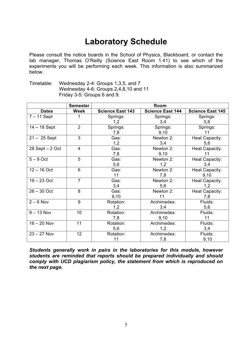
Please consult the notice boards in the School of Physics, Blackboard, or contact the lab manager, Thomas O’Reilly (Science East Room 1.41) to see which of the experiments you will be performing each week. This information is also summarized below. Timetable: Wednesday 2-4: Groups 1,3,5, and 7 Wednesday 4-6: Groups 2,4,8,10 and 11 Friday 3-5: Groups 6 and 9.
Semester Room Dates Week Science East 143 Science East 144 Science East 145
7 – 11 Sept 1 Springs: 1,2
Springs: 3,4
Springs: 5,6
14 – 18 Sept 2 Springs: 7,8
Springs: 9,10
Springs: 11
21 – 25 Sept 3 Gas: 1,2
Newton 2: 3,4
Heat Capacity: 5,6
28 Sept – 2 Oct 4 Gas: 7,8
Newton 2: 9,10
Heat Capacity: 11
5 – 9 Oct 5 Gas: 5,6
Newton 2: 1,2
Heat Capacity: 3,4
12 – 16 Oct 6 Gas: 11
Newton 2: 7,8
Heat Capacity: 9,10
19 – 23 Oct 7 Gas: 3,4
Newton 2: 5,6
Heat Capacity: 1,2
26 – 30 Oct 8 Gas: 9,10
Newton 2: 11
Heat Capacity: 7,8
2 – 6 Nov 9 Rotation: 1,2
Archimedes: 3,4
Fluids: 5,6
9 – 13 Nov 10 Rotation: 7,8
Archimedes: 9,10
Fluids: 11
16 – 20 Nov 11 Rotation: 5,6
Archimedes: 1,2
Fluids: 3,4
23 – 27 Nov 12 Rotation: 11
Archimedes: 7,8
Fluids: 9,10
Students generally work in pairs in the laboratories for this module, however students are reminded that reports should be prepared individually and should comply with UCD plagiarism policy, the statement from which is reproduced on the next page.

6
UCD Plagiarism Statement
(taken from http://www.ucd.ie/registry/academicsecretariat/docs/plagiarism_po.pdf)
The creation of knowledge and wider understanding in all academic disciplines depends on building from existing sources of knowledge. The University upholds the principle of academic integrity, whereby appropriate acknowledgement is given to the contributions of others in any work, through appropriate internal citations and references. Students should be aware that good referencing is integral to the study of any subject and part of good academic practice.
The University understands plagiarism to be the inclusion of another person’s writings or ideas or works, in any formally presented work (including essays, theses, projects, laboratory reports, examinations, oral, poster or slide presentations) which form part of the assessment requirements for a module or programme of study, without due acknowledgement either wholly or in part of the original source of the material through appropriate citation. Plagiarism is a form of academic dishonesty, where ideas are presented falsely, either implicitly or explicitly, as being the original thought of the author’s. The presentation of work, which contains the ideas, or work of others without appropriate attribution and citation, (other than information that can be generally accepted to be common knowledge which is generally known and does not require to be formally cited in a written piece of work) is an act of plagiarism. It can include the following:
1. Presenting work authored by a third party, including other students, friends, family, or work purchased through internet services;
2. Presenting work copied extensively with only minor textual changes from the internet, books, journals or any other source;
3. Improper paraphrasing, where a passage or idea is summarised without due acknowledgement of the original source;
4. Failing to include citation of all original sources; 5. Representing collaborative work as one’s own;
Plagiarism is a serious academic offence. While plagiarism may be easy to commit unintentionally, it is defined by the act not the intention. All students are responsible for being familiar with the University’s policy statement on plagiarism and are encouraged, if in doubt, to seek guidance from an academic member of staff. The University advocates a developmental approach to plagiarism and encourages students to adopt good academic practice by maintaining academic integrity in the presentation of all academic work.
7
Name:___________________________ Student No: ________________ Partner:____________________Date:___________Demonstrator:________________
Springs What should I expect in this experiment? You will investigate how springs stretch when different objects are attached to them and learn about graphing scientific data. Introduction: Plotting Scientific Data
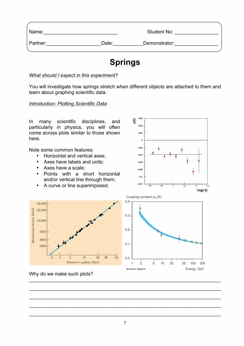
In many scientific disciplines, and particularly in physics, you will often come across plots similar to those shown here. Note some common features:
• Horizontal and vertical axes; • Axes have labels and units; • Axes have a scale; • Points with a short horizontal
and/or vertical line through them; • A curve or line superimposed.
Why do we make such plots? ______________________________________________________________________
______________________________________________________________________
______________________________________________________________________
______________________________________________________________________
______________________________________________________________________

8
______________________________________________________________________ ______________________________________________________________________
______________________________________________________________________
What features of the graphs do you think are important and why? ______________________________________________________________________
______________________________________________________________________
______________________________________________________________________
______________________________________________________________________
______________________________________________________________________
______________________________________________________________________
______________________________________________________________________
______________________________________________________________________
______________________________________________________________________
______________________________________________________________________
______________________________________________________________________
______________________________________________________________________
______________________________________________________________________
______________________________________________________________________
______________________________________________________________________
______________________________________________________________________
______________________________________________________________________
______________________________________________________________________
______________________________________________________________________
The equation of a straight line is often written as y = m x + c.
y tells you how far up the point is, whilst x is how far along the x-axis the point is. m is the slope (gradient) of the line, it tells you how steep the line is and is calculated by dividing the change in y by the change is x, for the same part of the line. A large value of m, indicates a steep line with a large change in y for a given change in x. c is the intercept of the line and is the point where the line crosses the y-axis, at x = 0.
9
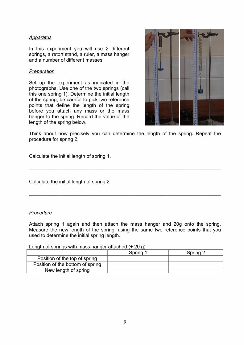
Apparatus In this experiment you will use 2 different springs, a retort stand, a ruler, a mass hanger and a number of different masses. Preparation Set up the experiment as indicated in the photographs. Use one of the two springs (call this one spring 1). Determine the initial length of the spring, be careful to pick two reference points that define the length of the spring before you attach any mass or the mass hanger to the spring. Record the value of the length of the spring below.
Think about how precisely you can determine the length of the spring. Repeat the procedure for spring 2. Calculate the initial length of spring 1. ______________________________________________________________________
Calculate the initial length of spring 2. ______________________________________________________________________
Procedure Attach spring 1 again and then attach the mass hanger and 20g onto the spring. Measure the new length of the spring, using the same two reference points that you used to determine the initial spring length. Length of springs with mass hanger attached (+ 20 g)
Spring 1 Spring 2 Position of the top of spring
Position of the bottom of spring New length of spring
10
Add another 10 gram disk to the mass hanger, determine the new length of the spring. Complete the table below. Measurements for spring 1
Object Added Total mass added to the mass hanger
(g)
New reference position (cm)
New spring length (cm)
Disk 1 30 Disk 2 40 Disk 3 Disk 4 Disk 5
Add more mass disks, one-by-one, to the mass hanger and record the new lengths in the table above. In the column labelled ‘total mass added to the mass hanger’, calculate the total mass added due to the disks. Carry out the same procedure for spring 2 and complete the table below. Use the same number of weights as for spring 1. Measurements for spring 2
Object Added Total mass added to the mass hanger
(g)
New reference position (cm)
New spring length (cm)
Disk 1 30 Disk 2
Graphical Analysis Add the data you have gathered for both springs to the graph below. You should plot the length of the spring in centimetres on the vertical y-axis and the total mass added to the hanger in grams on the horizontal axis. Start the y-axis at -10 cm and have the x-axis run from -40 to 100 g. Choose a scale that is simple to read and expands the data so it is spread across the page. Label your axes and include other features of the graph that you consider important.

11
Graph representing the length of the two springs for different masses added to the hanger.

12
In everyday language we may use the word ‘slope’ to describe a property of a hill. For example, we may say that a hill has a steep or gentle slope. Generally, the slope tells you how much the value on the vertical axis changes for a given change on the x-axis. Algebraically a straight line can be described by y = mx + c where x and y refer to any data on the x and y axes respectively, m is the slope of the line (change in y/ change in x), and c is the intercept (where the line crosses the y-axis at x=0). Suppose the data should be consistent with straight lines. Superimpose the two best straight lines, one for each spring, that you can draw on the data points. Examine the graphs you have drawn and describe the ‘steepness’ of the slopes for spring 1 and spring 2.
______________________________________________________________________
______________________________________________________________________
______________________________________________________________________
______________________________________________________________________
Work out the slopes of the two lines.
______________________________________________________________________
______________________________________________________________________
______________________________________________________________________
______________________________________________________________________
______________________________________________________________________
______________________________________________________________________
______________________________________________________________________ What are the two intercepts? ______________________________________________________________________
______________________________________________________________________
______________________________________________________________________
______________________________________________________________________
______________________________________________________________________ How can you use the slopes of the two lines to compare the stiffness of the springs? ______________________________________________________________________
______________________________________________________________________

13
______________________________________________________________________
______________________________________________________________________
______________________________________________________________________
______________________________________________________________________
In this experiment the points at which the straight lines cross the y-axis where x = 0 g (intercepts) correspond to physical quantities that you have determined in the experiment. How well do the graphical and measured values compare with each other? ______________________________________________________________________
______________________________________________________________________
______________________________________________________________________
______________________________________________________________________
______________________________________________________________________
______________________________________________________________________
____________________________________________________________________________________________________________________________________________ Look at the graphs on page 7, the horizontal and vertical lines through the data points represent the experimental uncertainty, or precision of measurement in many cases. In this experiment the uncertainty on the masses is insignificant, whilst those on the length measurements are related to how accurately the lengths of the springs can be determined. How large a vertical line would you consider reasonable for your length measurements? ______________________________________________________________________
What factors might explain any disagreement between the graphically determined intercepts and the measurements of the corresponding physical quantity? ______________________________________________________________________
______________________________________________________________________
______________________________________________________________________
______________________________________________________________________
______________________________________________________________________
The behaviour of the springs in this experiment is said to be “linear”. Looking at your
graphs does this make sense?
______________________________________________________________________

14
15
Name:___________________________ Student No: ________________ Partner:____________________Date:___________Demonstrator:________________
Investigation into the Behaviour of Gases and a Determination of Absolute Zero
What should I expect in this experiment? You will investigate gases behaviour, by varying their pressure, temperature and volume. You will also determine a value of absolute zero. Introduction: The gas laws are a macroscopic description of the behaviour of gases in terms of temperature, T, pressure, P, and volume, V. They are a reflection of the microscopic behaviour of the individual atoms and molecules that make up the gas which move randomly and collide many billions of times each second. Their speed is related to the temperature of the gas through the average value of the kinetic energy. An increase in temperature causes the atoms and molecules to move faster in the gas. The rate at which the atoms hit the walls of the container is related to the pressure of the gas. The volume of the gas is limited by the container it is in. Using the above description to explain the behaviour of gases, state whether each of P,V,T goes up (↑), down (↓) or stays the same (0) for the following cases.
P V T
A sealed pot containing water vapour is placed on a hot oven hob.
Blocking the air outlet, a bicycle pump is depressed.
A balloon full of air is squashed.
A balloon heats up in the sun.
From the arguments above you can see that at constant temperature, decreasing the volume in which you contain a gas should increase the pressure by a proportional amount. Thus VP 1∝ or introducing k, a constant of proportionality, V
kP = or
kPV = . This is Boyle’s Law.
16
Similarly you can see that at constant volume, increasing the temperature should increase the pressure by a proportional amount. So TP ∝ or introducing κ , a
constant of proportionality, TP κ= or κ=TP . This is Gay Lussac’s Law.
These laws can be combined into the Ideal Gas Law that relates all three quantities by
nRTPV = where n is the number of moles of gas and R is the ideal gas constant. Experiment 1: To test the validity of Boyle’s Law
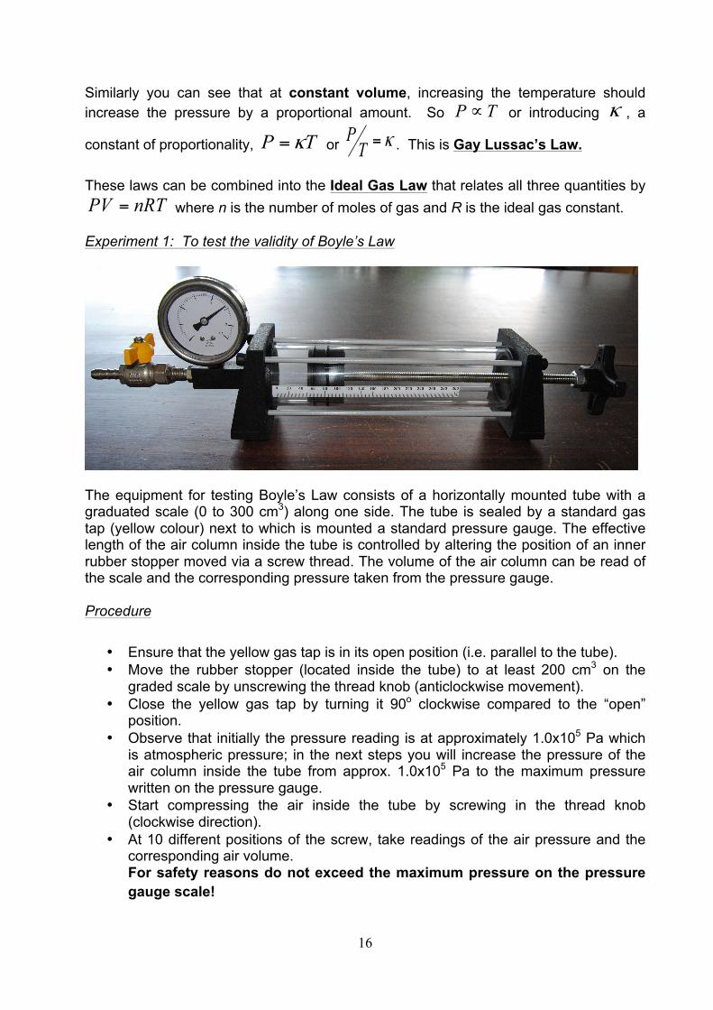
The equipment for testing Boyle’s Law consists of a horizontally mounted tube with a graduated scale (0 to 300 cm3) along one side. The tube is sealed by a standard gas tap (yellow colour) next to which is mounted a standard pressure gauge. The effective length of the air column inside the tube is controlled by altering the position of an inner rubber stopper moved via a screw thread. The volume of the air column can be read of the scale and the corresponding pressure taken from the pressure gauge. Procedure
• Ensure that the yellow gas tap is in its open position (i.e. parallel to the tube). • Move the rubber stopper (located inside the tube) to at least 200 cm3 on the
graded scale by unscrewing the thread knob (anticlockwise movement). • Close the yellow gas tap by turning it 90o clockwise compared to the “open”
position. • Observe that initially the pressure reading is at approximately 1.0x10⁵ Pa which
is atmospheric pressure; in the next steps you will increase the pressure of the air column inside the tube from approx. 1.0x10⁵ Pa to the maximum pressure written on the pressure gauge.
• Start compressing the air inside the tube by screwing in the thread knob (clockwise direction).
• At 10 different positions of the screw, take readings of the air pressure and the corresponding air volume. For safety reasons do not exceed the maximum pressure on the pressure gauge scale!

17
On the volume scale, each volume value is read by matching the position of the left extremity of the rubber stopper to the graded scale.
• Tabulate your results below. • Once you finished taking readings, depressurize the tube to atmospheric
pressure by turning the gas tap 90o anticlockwise.
Air Pressure (Pa) Volume of air (m3) Air Pressure (Pa) Volume of air
(m3)
Compare Boyle’s Law: V
kP = to the straight line formula y=mx+c.
What quantities should you plot on the x-axis and y–axis in order to get a linear relationship according to Boyle’s Law? Explain and tabulate these values below. ______________________________________________________________________
______________________________________________________________________
x-axis= y-axis=
What should the slope of your graph be equal to?
_______________________________
What should the intercept of the graph equal?_______________________________ Make a plot of those variables that ought to give a straight line, if Boyle’s Law is correct.

18
Use either the graph paper below or JagFit (see back of manual) and attach your printed graph below.

19
Comment on the linearity of your plot. Have you shown Boyle’s Law to be true? How precisely you can determine the pressures and volumes influence your answers? ______________________________________________________________________
______________________________________________________________________
______________________________________________________________________
______________________________________________________________________
______________________________________________________________________
______________________________________________________________________
______________________________________________________________________
______________________________________________________________________
What is the value for the slope? What is the value for the intercept? Use the Ideal Gas Law to figure out how many moles of air are trapped in the column. (The universal gas constant R=8.3145 J/mol K)
Number of moles of gas =

20
Experiment 2: To test the validity of Gay Lussac’s Law
The equipment for testing Gay Lussac’s Law consists of an enclosed can surrounded by a heating element. The volume of gas in the can is constant. A thermocouple measures the temperature of the gas and a pressure transducer measures the pressure.
Procedure Plug in the transformer to activate the temperature and pressure sensors. Set the multimeter for pressure to the 200mV scale and the one for temperature to the 2000mV scale. Connect the power supply to the apparatus and switch on. At the start your gas should be at room temperature and pressure, use approximate values for room temperature and pressure to work out by what factors of 10 you need to divide or multiply your voltages to convert to centigrade and Nm-2. Commence heating the gas, up to a final temperature of 100 C. Immediately switch off the power supply. While the gas is heating, take temperature and pressure readings at regular intervals (say every 5 C) and record them in the table below.
Temperature (C)
Pressure of gas (Nm-2)
Temperature (C)
Pressure of gas (Nm-2)

21
Gay Lussac’s Law states kTP = and by our earlier arguments heating the gas makes the atoms move faster which increases the pressure. We need to think a little about our scales and in particular what ‘zero’ means. Zero pressure would mean no atoms hitting the sides of the vessel and by the same token, zero temperature would mean the atoms have no thermal energy and don’t move. This is known as absolute zero. The zero on the centigrade scale is the point at which water changes to ice and is clearly nothing to do with absolute zero. So if you are measuring everything in centigrade you must change Gay Lussac’s Law to read )( zeroTTkP −= where Tzero is absolute zero on the centigrade scale. Compare )( zeroTTkP −= to the straight line formula y=mx+c. What should you plot on the x-axis and y–axis in order to get a linear relationship according to Gay Lussac’s Law? ______________________________________________________________________
______________________________________________________________________
______________________________________________________________________
______________________________________________________________________
______________________________________________________________________
______________________________________________________________________ What should the slope of your graph be equal to? What should the intercept of the graph equal? How can you work out Tzero? ______________________________________________________________________
______________________________________________________________________
______________________________________________________________________
______________________________________________________________________
______________________________________________________________________ ______________________________________________________________________
______________________________________________________________________
______________________________________________________________________

22
Make a plot of P versus T. Use either the graph paper below or JagFit (see back of manual) and attach your printed graph below.

23
Comment on the linearity of your plot. Have you shown Gay Lussac’s Law to be true? ______________________________________________________________________
______________________________________________________________________
______________________________________________________________________
______________________________________________________________________
______________________________________________________________________
______________________________________________________________________
______________________________________________________________________
______________________________________________________________________
What is the value for the slope? What is the value for the intercept? From these calculate a value for absolute zero temperature. Comment on the precision with which you have been able to find absolute zero
Absolute zero =

24
25
Name:___________________________ Student No: ________________ Partner:____________________Date:___________Demonstrator:________________
Newton’s Second Law. What should I expect in this experiment? This experiment has two parts. In the first part you will apply a fixed force, vary the mass and note how the acceleration changes. In the second part you will measure the acceleration due to the force of gravity. Pre-lab assignment Acting under constant acceleration, a cart starts from rest and travels 1m west in 5s. What are the acceleration and average velocity of the cart? Introduction
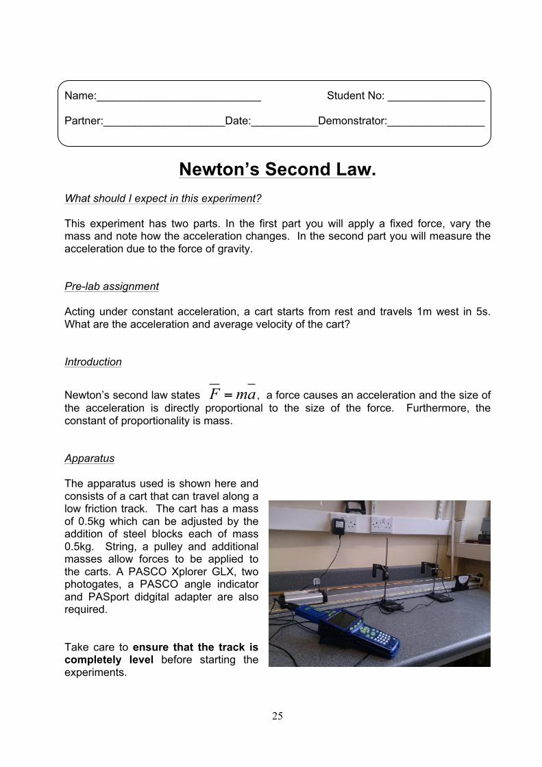
Newton’s second law states amF = , a force causes an acceleration and the size of the acceleration is directly proportional to the size of the force. Furthermore, the constant of proportionality is mass. Apparatus The apparatus used is shown here and consists of a cart that can travel along a low friction track. The cart has a mass of 0.5kg which can be adjusted by the addition of steel blocks each of mass 0.5kg. String, a pulley and additional masses allow forces to be applied to the carts. A PASCO Xplorer GLX, two photogates, a PASCO angle indicator and PASport didgital adapter are also required. Take care to ensure that the track is completely level before starting the experiments.
26
Configuring the Xplorer GLX In order to conduct the experiment in an accurate fashion, the PASCO Xplorer GLX must be configured to give you data about the velocity of the cart at two points along the track and how long it takes the cart to travel between the gates.
• Connect the AC adapter to the wall and plug it into the GLX. • Insert the connector for the first photogate into the port marked ‘1’ on the digital adapter
and insert the second into the port marked ‘2’. • Connect the digital adapter to the GLX. A menu should pop up. • Place the photogates at the 30 and 80 centimetre marks on the track. • Use the arrow keys to navigate to ‘Photogate Timing’ and press the button to select
it. • Using the navigation and select keys, set Photogate spacing to 0.5000m and ensure that
only ‘Velocity In Gate’ and ‘Time Between Gates’ are set to visible. • Press the Home key to navigate to the home screen. • Press F1 or navigate to the Graph section. Once on the Graph screen press F4 to open
the graph menu. Navigate to ‘Two Measurements’ and press select. • Press the select key and navigate to the ‘Y’ which should be visible on the right hand
side of the graph. Press select and choose ‘Time Between Gates’. Time between gates will now be displayed to the right of the graph.
• You can now record data by pressing to begin and stop recording data. • Velocity will be displayed as a line and the time between gates will be displayed as both
a single point on the graph and as a numerical value along the right Y axis of the graph. • To read the data from your completed run accurately, press F3 and select ‘Smart Tool’.
Use the navigation buttons to see the precise values for the points on the graph.
Plotting the GLX data: Use the arrow keys to highlight your data file in the RAM memory and press “F4 files”. Select the “copy file” option and then choose the external USB as the destination for the file, and press “F1 OK”.
Transfer the USB data stick to the lab computer and create a graph.

27
Investigation 1: To check that force is proportional to acceleration and show the constant of proportionality to be mass and calculate the acceleration due to gravity.
The apparatus should be set up as in the picture. Attach one end of the string to the cart, pass it over the pulley, and add a 0.012kg mass to the hook.
The weight of the hanging mass is a force, F, that acts on the cart. The whole system (both the hanging mass mh and the cart mcart) are accelerated. So long as you don’t change the hanging mass, F will remain constant. You can then change the mass of the system, M, by adding mass to the cart, noting the change in acceleration, and testing the relationship F=ma. If F=ma and you apply a constant force F, what do you expect will happen to the acceleration as you increase the mass? ______________________________________________________________________
______________________________________________________________________
______________________________________________________________________
______________________________________________________________________
______________________________________________________________________
______________________________________________________________________
______________________________________________________________________ In the configuration you are using, the GLX will give you data regarding the carts velocity at two points along the track and the times that it passed through each gate. Acceleration is rate of change of velocity. You can use the equation below, where the numbers refer to the times (t) and velocities (v) at the two gates, to calculate the average acceleration experienced by the cart between the gates.
𝑎 = !!!!!!!!!!
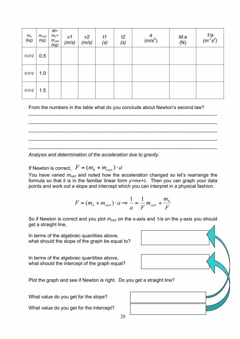
Place different masses on the cart. Using the GLX, fill in the table.
28
mh (kg)
mcart (kg)
M= mh+mcart (kg)
v1
(m/s)
v2
(m/s)
t1 (s)
t2 (s)
a (m/s2)
M.a (N)
1/a (m-1s2)
0.012 0.5
0.012 1.0
0.012 1.5
From the numbers in the table what do you conclude about Newton’s second law? ______________________________________________________________________
______________________________________________________________________
______________________________________________________________________
______________________________________________________________________
______________________________________________________________________
Analysis and determination of the acceleration due to gravity. If Newton is correct, ammF carth ⋅+= )( You have varied mcart and noted how the acceleration changed so let’s rearrange the formula so that it is in the familiar linear form y=mx+c. Then you can graph your data points and work out a slope and intercept which you can interpret in a physical fashion.
Fm
mFa
ammF hcartcarth +=⇒⋅+=
11)(
So if Newton is correct and you plot mcart on the x-axis and 1/a on the y-axis you should get a straight line. In terms of the algebraic quantities above, what should the slope of the graph be equal to? In terms of the algebraic quantities above, what should the intercept of the graph equal? Plot the graph and see if Newton is right. Do you get a straight line? What value do you get for the slope? What value do you get for the intercept?

29
Use JagFit to create your graph (see back of manual) and attach your printed graph below.

30
Now here comes the power of having plotted your results like this. Although we haven’t bothered working out the force we applied using the hanging weight, a comparison of the measured slope and intercept with the predicted values will let you work out F. From the measurement of the slope, the constant force applied can be calculated to be From the intercept of the graph you can calculate F in a different fashion. What value do you get? You’ve shown that F is proportional to a and the constant of proportionality is mass. If the force is the gravitational force, it will produce an acceleration due to gravity (usually written g instead of a) so once again a (gravitational) force F is proportional to acceleration, g. But what is the constant of proportionality? Are you surprised that it is the same mass m? (By the way, a good answer to this question gets you a Nobel prize.)
______________________________________________________________________
______________________________________________________________________
______________________________________________________________________
______________________________________________________________________
______________________________________________________________________
______________________________________________________________________
______________________________________________________________________
______________________________________________________________________ So since that force was just caused by the mass mh falling under gravity, F= mhg, you can calculate the acceleration due to gravity to be Comment on how this compares to the accepted value for gravity of about 9.8 m/s2. How does the accuracy of your measurements affect this comparison? ______________________________________________________________________
______________________________________________________________________
______________________________________________________________________
______________________________________________________________________
______________________________________________________________________
______________________________________________________________________

31
Investigation 2: Acceleration down an inclined plane.
The apparatus should be set up as in the picture. Raise one end of the track using the wooden block in place of the elevator. The carts can be released from rest at the top of the track.
A cart on a slope will experience the force of gravity which causes the cart to accelerate and roll down the incline. The acceleration due to gravity is as shown in the schematic. The component of this acceleration parallel to the inclined surface is, g.sinθ and this is the net acceleration of the cart (when friction is neglected). Note the acceleration depends on the angle of the incline.
Vary the angle of the incline (repeat for at least four different angles) and measure the acceleration of the cart. In the same way as was done in investigation 1. You will need to determine the angle of the incline. Summarise your results in this table.
Angle (radians)
Sin (Angle) v1 (m/s) v2 (m/s) t1 (s) t2 (s) Acceleration
(ms-2)

32
Since the acceleration θsinga = , there is a linear dependence on the sine of the angle. Make a graph with sin θ on the x-axis and a on the y-axis. What value do you expect (theoretically) for the slope? What value do you expect (theoretically) for the intercept? What value do you obtain (experimentally) for the slope? What value do you measure for the intercept? Comment on your results. How could you improve your measurements of g? ______________________________________________________________________
______________________________________________________________________
______________________________________________________________________
______________________________________________________________________
______________________________________________________________________
______________________________________________________________________
______________________________________________________________________
______________________________________________________________________
______________________________________________________________________
______________________________________________________________________ Use JagFit to create your graph (see back of manual) and attach your printed graph below.

33

34
35
Name:___________________________ Student No: ________________ Partner:____________________Date:___________Demonstrator:________________
To Determine the Specific Heat Capacity of Metals
Introduction The heat capacity of a material is a measure of the materials ability to absorb heat, or thermal energy, for a given rise in temperature. As a body becomes hotter, the atoms and molecules that comprise it begin to move more and more violently. In the case of solids, the atoms or molecules vibrate about the positions that they occupy in the solid. As the temperature of the material increases, the vibrations become more energetic, eventually breaking the bonds that hold the solid together as the solid begins to melt. The purpose of this experiment is to measure the heat capacity of two metals, copper and aluminium, by supplying a known quantity of heat and recording the resultant rise in temperature. The heat capacity of an object is defined as the energy required to raise the temperature of the object by 1 K. Clearly the greater the mass of the object the more heat is required, so a more useful quantity is the Specific Heat Capacity (SHC) of an object. This is defined as the energy required to raise the temperature of 1 kg of the material by 1 K. Expressing this mathematically,
)( if TTmcQ −= where Q is the amount of heat required, m is the mass of the object, Ti & Tf are the initial and final temperatures of the object and c is the SHC measured in units of Joules per kg per Kelvin (J kg-1 K-1). Apparatus:
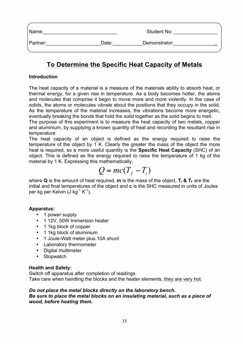
• 1 power supply • 1 12V, 50W Immersion heater • 1 1kg block of copper • 1 1kg block of aluminium • 1 Joule-Watt meter plus 10A shunt • Laboratory thermometer • Digital multimeter • Stopwatch
Health and Safety: Switch off apparatus after completion of readings. Take care when handling the blocks and the heater elements, they are very hot. Do not place the metal blocks directly on the laboratory bench. Be sure to place the metal blocks on an insulating material, such as a piece of wood, before heating them.

36
Set up:
• Set the power supply to 12V DC. • Connect cables from the power supply (DC output) to the Joule-Watt meter. • Connect the immersion heater to the Joule-Watt meter where it says ‘load’. • Insert the immersion heater into one of the metal blocks. • Insert a thermometer into the same block.
Figure 1. Specific heat experimental arrangement, be sure to connect the ac output (yellow) from the power supply to the Joule-Watt meter.
Procedure: Start with the aluminium block and repeat for the copper one.
• Measure the portion of the heater inserted into the block and express this as a fraction of the total length of the heater (f).
• Ensure that the multimeter is attached in series with the heater between the positive and negative load ports of the Joule-Watt meter as demonstrated in Figure 2. Set the multimeter to current (A) (to measure a current > 1A). The select button will also have to be pressed to swich the current measurement to DC.
• Attach a second multimeter in parallel to the DC ports of the power supply and set it to measure DC voltage (approximately 12V).
• From the current (measured through the heater) and the measured voltages you can work out the average electrical power, P, supplied to the block.
Figure 2. Set up for measuring the current flowing through the heater.
37
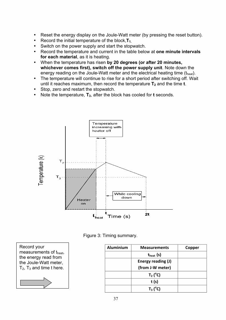
• Reset the energy display on the Joule-Watt meter (by pressing the reset button). • Record the initial temperature of the block,T1. • Switch on the power supply and start the stopwatch. • Record the temperature and current in the table below at one minute intervals
for each material, as it is heating. • When the temperature has risen by 20 degrees (or after 20 minutes,
whichever comes first), switch off the power supply unit. Note down the energy reading on the Joule-Watt meter and the electrical heating time (theat).
• The temperature will continue to rise for a short period after switching off. Wait until it reaches maximum, then record the temperature T2 and the time t.
• Stop, zero and restart the stopwatch. • Note the temperature, T3, after the block has cooled for t seconds.
Aluminium Measurements Copper theat (s)
Energy reading (J) (from J-‐W meter) T2 (oC) t (s) T3 (oC)
Figure 3: Timing summary.
Record your measurements of theat, the energy read from the Joule-Watt meter, T2, T3 and time t here.
38
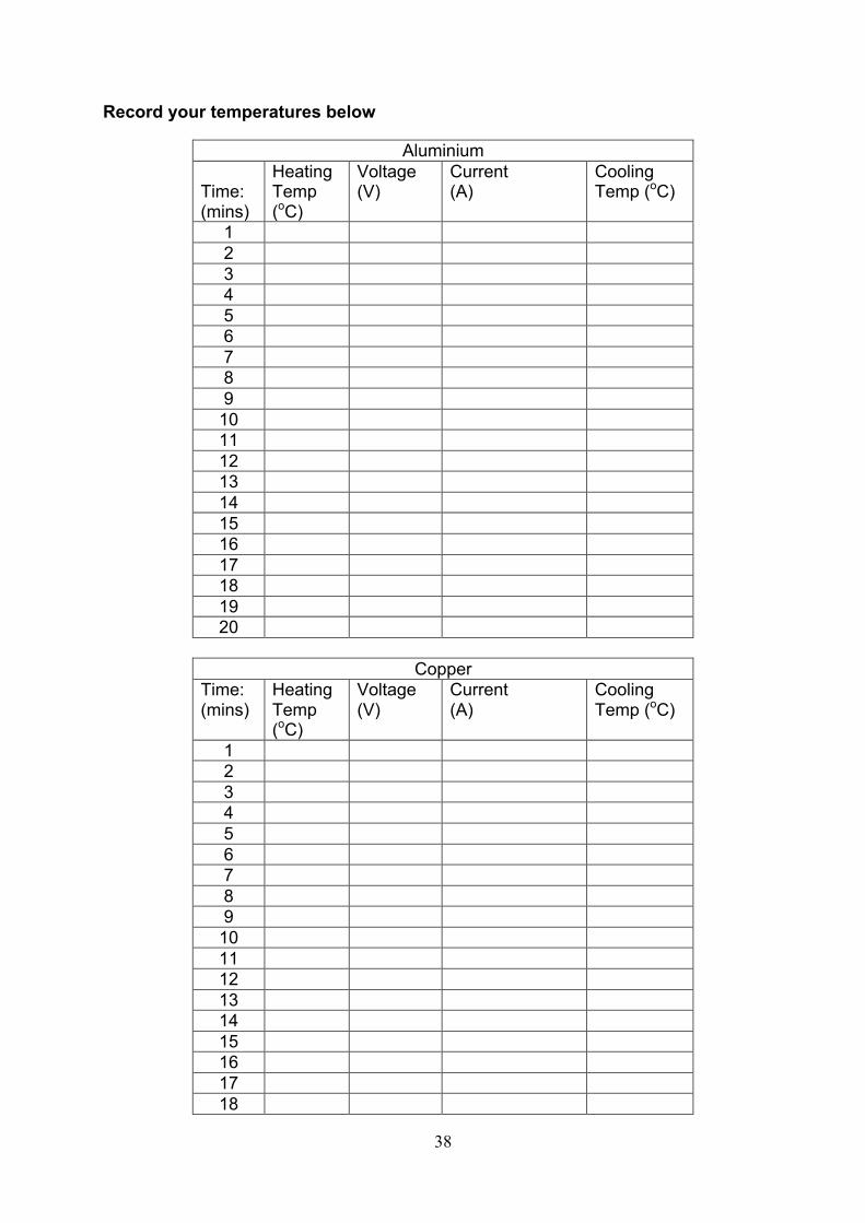
Record your temperatures below
Aluminium Time: (mins)
Heating Temp (oC)
Voltage (V)
Current (A)
Cooling Temp (oC)
1 2 3 4 5 6 7 8 9
10 11 12 13 14 15 16 17 18 19 20
Copper
Time: (mins)
Heating Temp (oC)
Voltage (V)
Current (A)
Cooling Temp (oC)
1 2 3 4 5 6 7 8 9
10 11 12 13 14 15 16 17 18

39
Plot the temperature of both blocks as a function of time on the same graph and comment on the graphs. ______________________________________________________________________ ______________________________________________________________________ ______________________________________________________________________ ______________________________________________________________________ ______________________________________________________________________ ______________________________________________________________________ Cooling Correction: The block loses heat during the heating cycle. In the absence of these losses it would have reached a higher final temperature. The uncorrected final temperature is T2. The corrected final temperature may be approximated as:
This formula assumes the dominant heat loss mechanism is due to convection by heated air, neglecting the cooling due to radiation and conduction. The readings should be recorded as follows:
Al Cu Units Fraction of the heater inserted in the block, f.
Mass of cylinder, m Kg Initial temperature, T1 K
Uncorrected final temperature, T2 K
Electrical Heating Time, theat Sec
Temperature after t sec cooling, T3 K Corrected final temperature, T4 K
Rise in temperature, (T4-T1) K Average Current through the Heater, I. A
Average Voltage, V. 12 12 V Average Power, 𝐏 = 𝐕 𝐱 𝐈 W
Energy supplied to heater, J = (P x theat)
J
432
2 2T
TTT =
−+
40
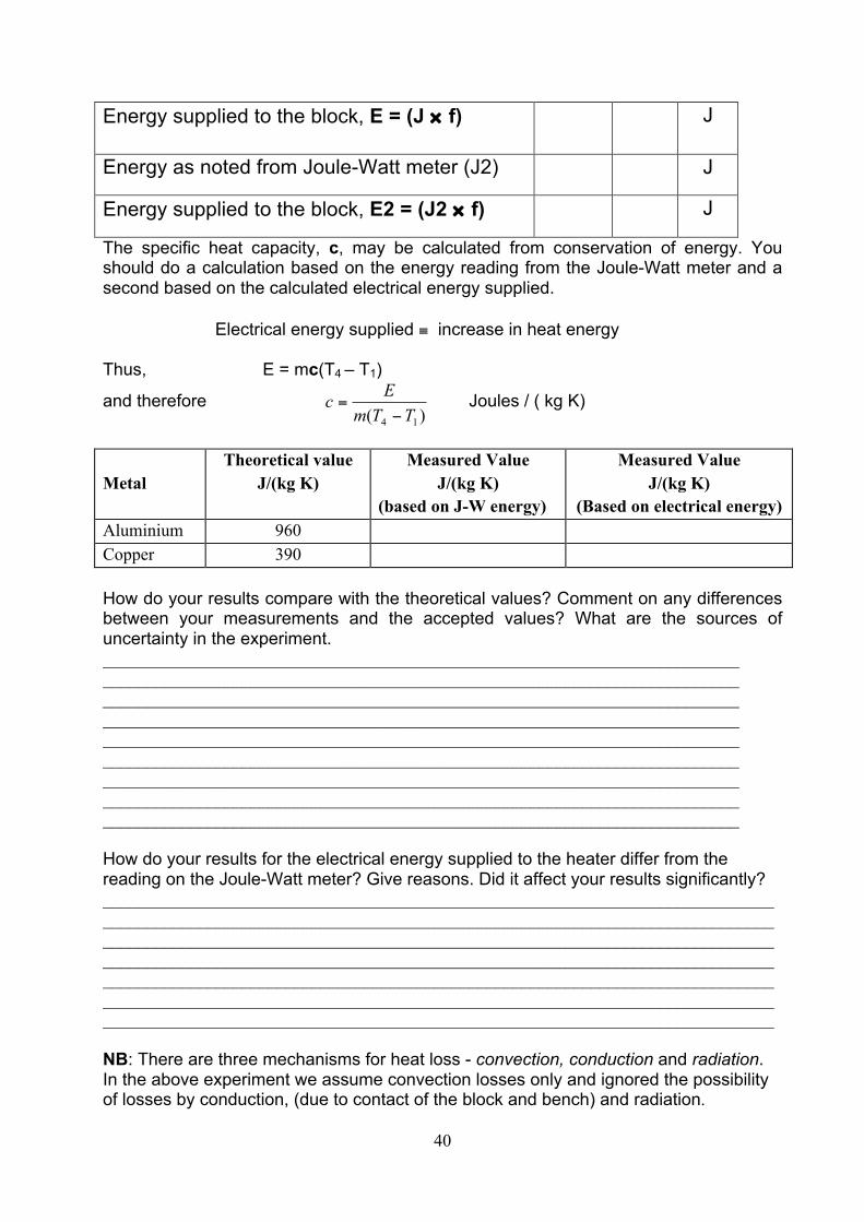
Energy supplied to the block, E = (J × f) J
Energy as noted from Joule-Watt meter (J2) J
Energy supplied to the block, E2 = (J2 × f) J
The specific heat capacity, c, may be calculated from conservation of energy. You should do a calculation based on the energy reading from the Joule-Watt meter and a second based on the calculated electrical energy supplied.
Electrical energy supplied ≡ increase in heat energy
Thus, E = mc(T4 – T1)
and therefore )( 14 TTm
Ec−
= Joules / ( kg K)
Metal
Theoretical value J/(kg K)
Measured Value J/(kg K)
(based on J-W energy)
Measured Value J/(kg K)
(Based on electrical energy) Aluminium 960 Copper 390 How do your results compare with the theoretical values? Comment on any differences between your measurements and the accepted values? What are the sources of uncertainty in the experiment. _________________________________________________________________________ _________________________________________________________________________ _________________________________________________________________________ _________________________________________________________________________ _________________________________________________________________________ _________________________________________________________________________ _________________________________________________________________________ _________________________________________________________________________ _________________________________________________________________________
How do your results for the electrical energy supplied to the heater differ from the reading on the Joule-Watt meter? Give reasons. Did it affect your results significantly? ___________________________________________________________________________________________________________________________________________________________________________________________________________________________________________________________________________________________________________________________________________________________________________________________________________________________________________________________________________________________________________________________________________________________ NB: There are three mechanisms for heat loss - convection, conduction and radiation. In the above experiment we assume convection losses only and ignored the possibility of losses by conduction, (due to contact of the block and bench) and radiation.

41
Name:___________________________ Student No: ________________ Partner:____________________Date:___________Demonstrator:________________
An Investigation of Fluid Flow using a Venturi Apparatus. Theory When a fluid moves through a channel of varying width, as in a Venturi apparatus, the volumetric flow rate (volume/time) remains constant but the velocity and pressure of the fluid vary. In the Venturi apparatus there are two different channel widths. The flow rate, Q, of the fluid through the tube is related to the speed of the fluid (v) and the cross-sectional area of the pipe (A). This relationship is known as the continuity equation, and can be expressed as
𝑄 = 𝐴!𝑣! = 𝐴𝑣 (Eq.1)
where A0 and v0 refer to the wide part of the tube and A and v to the narrow part. As the fluid flows from the narrow part of the pipe to the constriction, the speed increases from v0 to v and the pressure decreases from P0 to P.
The flow rate also depends on the pressure, P0, behind the fluid flowing into the apparatus. In this experiment the pump provides the pressure that makes the fluid flow through the apparatus. The higher the power to the pump the greater the pressure and the faster the fluid flows. In this experiment you will use the Venturi apparatus to investigate fluid flow and verify that equation 2 holds. You will also investigate how the volatge supplied to the pump affects the pressure and flow rate.
If the pressure change is due only to the velocity change, a simplified version of Bernoulli’s equation can be used: 𝑃 = 𝑃! −
!!{𝑣! − 𝑣!!} (Eq. 2)
Here ρ is the density of water: 1000 kg/m3.
42
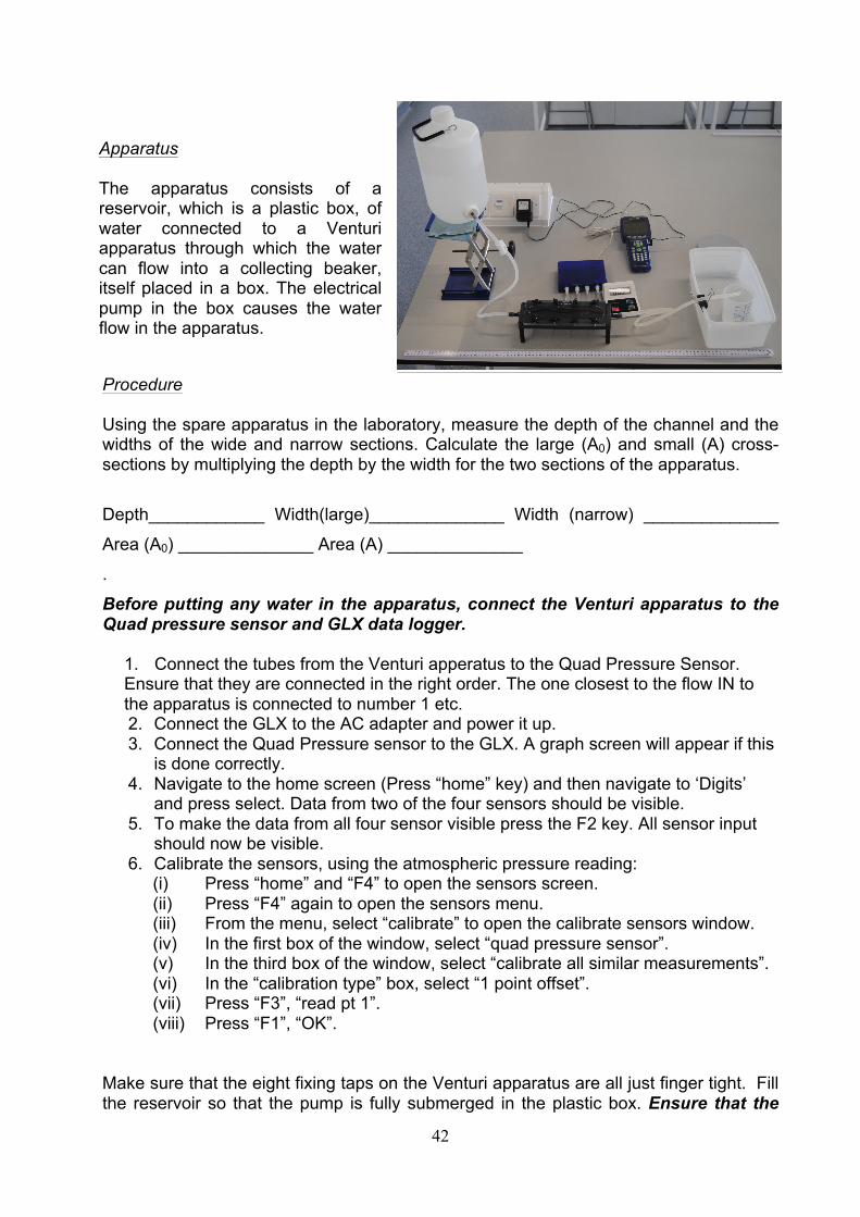
Apparatus The apparatus consists of a reservoir, which is a plastic box, of water connected to a Venturi apparatus through which the water can flow into a collecting beaker, itself placed in a box. The electrical pump in the box causes the water flow in the apparatus.
Procedure Using the spare apparatus in the laboratory, measure the depth of the channel and the widths of the wide and narrow sections. Calculate the large (A0) and small (A) cross-sections by multiplying the depth by the width for the two sections of the apparatus.
Depth____________ Width(large)______________ Width (narrow) ______________
Area (A0) ______________ Area (A) ______________
.
Before putting any water in the apparatus, connect the Venturi apparatus to the Quad pressure sensor and GLX data logger.
1. Connect the tubes from the Venturi apperatus to the Quad Pressure Sensor. Ensure that they are connected in the right order. The one closest to the flow IN to the apparatus is connected to number 1 etc. 2. Connect the GLX to the AC adapter and power it up. 3. Connect the Quad Pressure sensor to the GLX. A graph screen will appear if this
is done correctly. 4. Navigate to the home screen (Press “home” key) and then navigate to ‘Digits’
and press select. Data from two of the four sensors should be visible. 5. To make the data from all four sensor visible press the F2 key. All sensor input
should now be visible. 6. Calibrate the sensors, using the atmospheric pressure reading:
(i) Press “home” and “F4” to open the sensors screen. (ii) Press “F4” again to open the sensors menu. (iii) From the menu, select “calibrate” to open the calibrate sensors window. (iv) In the first box of the window, select “quad pressure sensor”. (v) In the third box of the window, select “calibrate all similar measurements”. (vi) In the “calibration type” box, select “1 point offset”. (vii) Press “F3”, “read pt 1”. (viii) Press “F1”, “OK”.
Make sure that the eight fixing taps on the Venturi apparatus are all just finger tight. Fill the reservoir so that the pump is fully submerged in the plastic box. Ensure that the

43
outlet of the apparatus is in the beaker which is in the box. Turn on the power suppl to the pump and set the voltage to 10V. Remove any air bubbles by gently tilting the outlet end of the Venturi apparatus upwards. Measure the time that it takes for 400 ml (0.4l = 4x10⁻⁴ m3) of water to flow through the Venturi apparatus. Be sure to read the water level by looking at the bottom of the meniscus. When the flow is steady note the pressures on the four sensors. Enter your data in the table. Repeat the measurements twice more. Be sure to return all the water to the reservoir (plastic box). Make sure that the apparatus stays free of air bubbles. Run P1
/kPa P2 /kPa
P3 /kPa
P4 /kPa
Time /s
1
2
3
Average
Calculate the flow rate, Q, volume/time, from the average value of the time taken for 400 ml to flow through the apparatus. 1ml = 1cm3 = 1x10⁻⁶ m3.
____________________________________________________________________
____________________________________________________________________
____________________________________________________________________
Use equation (1) and the cross-sectional areas that you calculcated to work out the velocity of the water in the wide (v0) and narrow (v) sections of the apparatus.
v0= ______________________________________________________________
v= ______________________________________________________________
Which is larger v or v0, is this what you expected?
____________________________________________________________________
____________________________________________________________________
If the apparatus was not constricted the pressure at point 2 (P0) is equal to the average value of P1 and P3. Use you average valies of P1 and P3 to calculate P0:
P0=1/2(P1+P3) _______________________________________________________
____________________________________________________________________
44
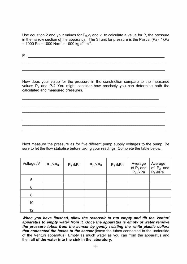
Use equation 2 and your values for P0,v0 and v to calculate a value for P, the pressure in the narrow section of the apparatus. The SI unit for pressure is the Pascal (Pa), 1kPa = 1000 Pa = 1000 N/m2 = 1000 kg s-2 m-1.
P= _________________________________________________________________
____________________________________________________________________
____________________________________________________________________
How does your value for the pressure in the constriction compare to the measured values P2 and P4? You might consider how precisely you can determine both the calculated and measured pressures.
_________________________________________________________________
____________________________________________________________________
____________________________________________________________________
____________________________________________________________________
____________________________________________________________________
____________________________________________________________________
Next measure the pressure as for five diferent pump supply voltages to the pump. Be sure to let the flow stabalise before taking your readings. Complete the table below.
Voltage /V
P1 /kPa
P2 /kPa
P3 /kPa
P4 /kPa Average of P1 and P3 /kPa
Average of P2 and P4 /kPa
5
6
8
10
12
When you have finished, allow the reservoir to run empty and tilt the Venturi apparatus to empty water from it. Once the apparatus is empty of water remove the pressure tubes from the sensor by gently twisting the white plastic collars that connected the hoses to the sensor (leave the tubes connected to the underside of the Venturi apparatus). Empty as much water as you can from the apparatus and then all of the water into the sink in the laboratory.

45
Plot a graph of the two average pressures as a function of pump voltage on the same graph. Create a graph either manually or using Jagfit (see back of manual) and attach your printed graph below.

46
Comment on your graph, is it consistent with what you expected to happen? __________________________________________________________________
____________________________________________________________________
____________________________________________________________________
____________________________________________________________________
____________________________________________________________________
What can you conclude from this part of the experiment?
____________________________________________________________________
____________________________________________________________________
____________________________________________________________________
____________________________________________________________________
____________________________________________________________________
____________________________________________________________________
____________________________________________________________________
____________________________________________________________________
____________________________________________________________________
____________________________________________________________________
47
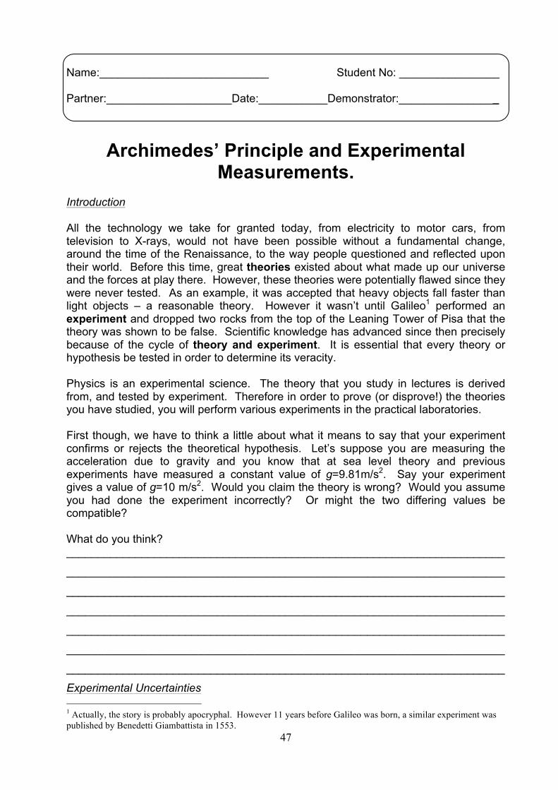
Name:___________________________ Student No: ________________ Partner:____________________Date:___________Demonstrator:________________
Archimedes’ Principle and Experimental
Measurements. Introduction All the technology we take for granted today, from electricity to motor cars, from television to X-rays, would not have been possible without a fundamental change, around the time of the Renaissance, to the way people questioned and reflected upon their world. Before this time, great theories existed about what made up our universe and the forces at play there. However, these theories were potentially flawed since they were never tested. As an example, it was accepted that heavy objects fall faster than light objects – a reasonable theory. However it wasn’t until Galileo1 performed an experiment and dropped two rocks from the top of the Leaning Tower of Pisa that the theory was shown to be false. Scientific knowledge has advanced since then precisely because of the cycle of theory and experiment. It is essential that every theory or hypothesis be tested in order to determine its veracity. Physics is an experimental science. The theory that you study in lectures is derived from, and tested by experiment. Therefore in order to prove (or disprove!) the theories you have studied, you will perform various experiments in the practical laboratories. First though, we have to think a little about what it means to say that your experiment confirms or rejects the theoretical hypothesis. Let’s suppose you are measuring the acceleration due to gravity and you know that at sea level theory and previous experiments have measured a constant value of g=9.81m/s2. Say your experiment gives a value of g=10 m/s2. Would you claim the theory is wrong? Would you assume you had done the experiment incorrectly? Or might the two differing values be compatible? What do you think? ______________________________________________________________________
______________________________________________________________________
______________________________________________________________________
______________________________________________________________________
______________________________________________________________________
______________________________________________________________________
______________________________________________________________________
Experimental Uncertainties 1 Actually, the story is probably apocryphal. However 11 years before Galileo was born, a similar experiment was published by Benedetti Giambattista in 1553.
48
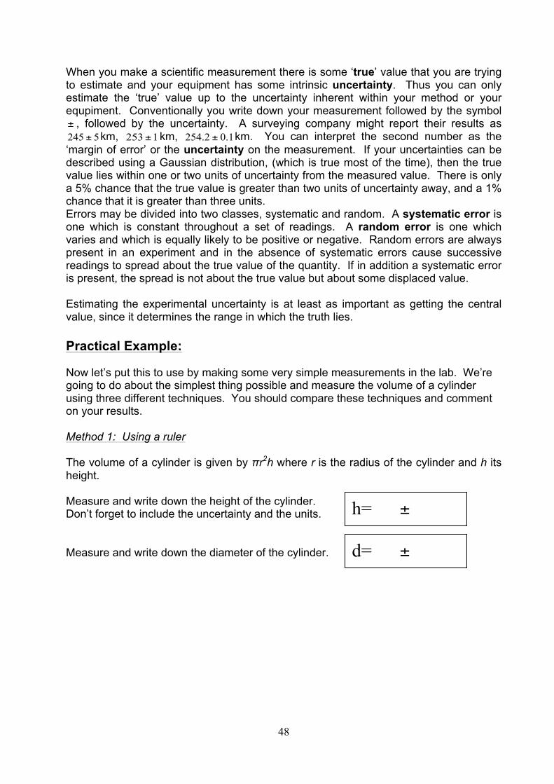
When you make a scientific measurement there is some ‘true’ value that you are trying to estimate and your equipment has some intrinsic uncertainty. Thus you can only estimate the ‘true’ value up to the uncertainty inherent within your method or your equpiment. Conventionally you write down your measurement followed by the symbol ± , followed by the uncertainty. A surveying company might report their results as
5245 ± km, 1253± km, 1.02.254 ± km. You can interpret the second number as the ‘margin of error’ or the uncertainty on the measurement. If your uncertainties can be described using a Gaussian distribution, (which is true most of the time), then the true value lies within one or two units of uncertainty from the measured value. There is only a 5% chance that the true value is greater than two units of uncertainty away, and a 1% chance that it is greater than three units. Errors may be divided into two classes, systematic and random. A systematic error is one which is constant throughout a set of readings. A random error is one which varies and which is equally likely to be positive or negative. Random errors are always present in an experiment and in the absence of systematic errors cause successive readings to spread about the true value of the quantity. If in addition a systematic error is present, the spread is not about the true value but about some displaced value. Estimating the experimental uncertainty is at least as important as getting the central value, since it determines the range in which the truth lies. Practical Example: Now let’s put this to use by making some very simple measurements in the lab. We’re going to do about the simplest thing possible and measure the volume of a cylinder using three different techniques. You should compare these techniques and comment on your results. Method 1: Using a ruler The volume of a cylinder is given by πr2h where r is the radius of the cylinder and h its height. Measure and write down the height of the cylinder. Don’t forget to include the uncertainty and the units. Measure and write down the diameter of the cylinder.
h= ±
d= ±
49
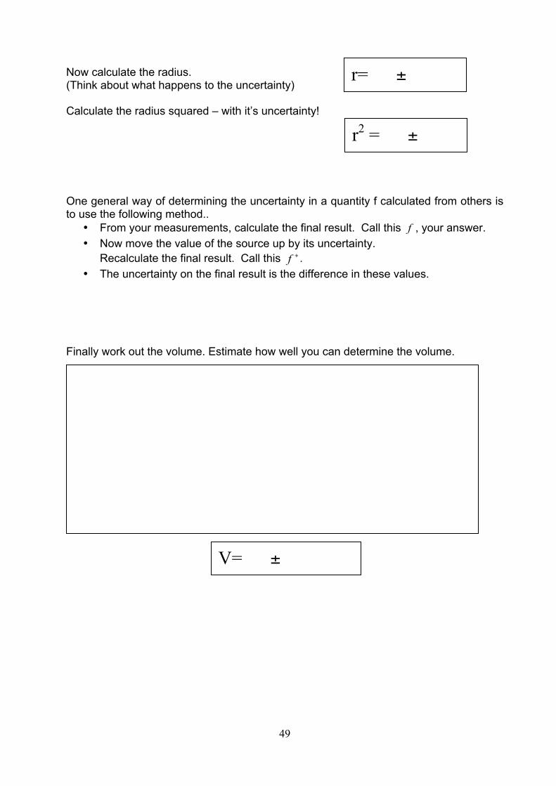
Now calculate the radius. (Think about what happens to the uncertainty) Calculate the radius squared – with it’s uncertainty! One general way of determining the uncertainty in a quantity f calculated from others is to use the following method..
• From your measurements, calculate the final result. Call this f , your answer. • Now move the value of the source up by its uncertainty. Recalculate the final result. Call this +f . • The uncertainty on the final result is the difference in these values.
Finally work out the volume. Estimate how well you can determine the volume.
V= ±
r2 = ±
r= ±

50
Method 2: Using a micrometer screw This uses the same prescription. However your precision should be a lot better. Measure and write down the height of the cylinder. Don’t forget to include the uncertainty and the units. Measure and write down the diameter of the cylinder. Now calculate the radius. Calculate the radius squared – with it’s uncertainty! Finally work out the volume.
h= ±
d= ±
r= ±
V= ±
(Show your workings)
r2 = ±

51
Method 3: Using Archimedes’ Principle You’ve heard the story about the ‘Eureka’ moment when Archimedes dashed naked through the streets having realised that an object submerged in water will displace an equivalent volume of water. You will repeat his experiment (the displacement part at least) by immersing the cylinder in water and working out the volume of water displaced. You can find this volume by measuring the mass of water and noting that a volume of 0.001m3 of water has a mass2 of 1kg. Write down the mass of water displaced. Calculate the volume of water displaced. What is the volume of the cylinder? Discussion and Conclusions. Summarise your results, writing down the volume of the cylinder as found from each method. Comment on how well they agree, taking account of the uncertainties. _____________________________________________________________________
______________________________________________________________________
______________________________________________________________________
______________________________________________________________________
______________________________________________________________________
______________________________________________________________________
______________________________________________________________________
______________________________________________________________________
______________________________________________________________________
______________________________________________________________________
2 In fact this is how the metric units are related. A litre of liquid is that quantity that fits into a cube of side 0.1m and a litre of water has a mass of 1kg.
±
±
±
± ± ±

52
Can you think of any systematic uncertainties that should be considered? Can you estimate their size? ______________________________________________________________________
______________________________________________________________________
______________________________________________________________________
______________________________________________________________________
______________________________________________________________________
______________________________________________________________________
______________________________________________________________________
______________________________________________________________________
______________________________________________________________________
______________________________________________________________________
Requote your results including the systematic uncertainties. What do you think the volume of the cylinder is? and why? My best estimate of the volume is because ______________________________________________________________ ______________________________________________________________________
______________________________________________________________________
______________________________________________________________________
______________________________________________________________________
______________________________________________________________________
______________________________________________________________________
______________________________________________________________________
______________________________________________________________________
______________________________________________________________________
± ± ± ±
± ±
± ±
53
Name:___________________________ Student No: ________________
Date:_________ Partner:_______________ Demonstrator:______________________
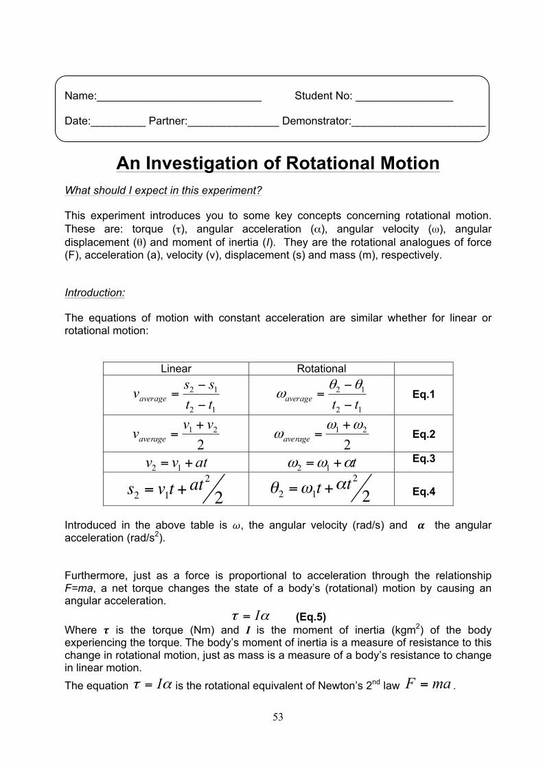
An Investigation of Rotational Motion What should I expect in this experiment? This experiment introduces you to some key concepts concerning rotational motion. These are: torque (τ), angular acceleration (α), angular velocity (ω), angular displacement (θ) and moment of inertia (I). They are the rotational analogues of force (F), acceleration (a), velocity (v), displacement (s) and mass (m), respectively. Introduction: The equations of motion with constant acceleration are similar whether for linear or rotational motion:
Linear Rotational
12
12
ttssvaverage −
−=
12
12
ttaverage −
−=
θθω
Eq.1
221 vvvaverage
+= 2
21 ωωω
+=average
Eq.2
atvv += 12 tαωω += 12 Eq.3
s2 = v1t + at2
2 θ2 =ω1t +αt2
2
Eq.4
Introduced in the above table is 𝜔, the angular velocity (rad/s) and 𝜶 the angular acceleration (rad/s2). Furthermore, just as a force is proportional to acceleration through the relationship F=ma, a net torque changes the state of a body’s (rotational) motion by causing an angular acceleration.
ατ I= (Eq.5) Where 𝝉 is the torque (Nm) and I is the moment of inertia (kgm2) of the body experiencing the torque. The body’s moment of inertia is a measure of resistance to this change in rotational motion, just as mass is a measure of a body’s resistance to change in linear motion. The equation ατ I= is the rotational equivalent of Newton’s 2nd law maF = .

54
You will use two pieces of apparatus to investigate these equations. The first lets you apply and calculate torque, measure angular acceleration and determine an unknown moment of inertia, I of a pair of cylindrical weights located at the ends of a bar. The second apparatus lets you investigate how I depends on the distribution of mass about the axis of rotation and lets you determine the value of I, already measured in the first part, by a second method. You can then compare the results you obtained from the two methods. Investigation 1: Measuring I from the torque and angular acceleration:
Place cylindrical masses on the bar at the r = 0.25m position with respect to the axis of rotation. The bar is attached to an axle which is free to rotate. The masses attached to the line wound around this axle are allowed to fall, causing a torque about the axle
The value of the torque caused by the falling masses is Fr=τ where F is the weight of the mass attached to the string and r is the radius of the axle to which it is attached (The rod to which the string is wrapped around). Calculate the value of τ.
Mass, m attached to string (kg)
Force, F = m . g (N)
Radius, r of axle (m)
Torque, τ = F × r (Nm)
Next you have to calculate the angular velocity, ω, and the angular acceleration, α. Describe the difference between these two underlined terms. ______________________________________________________________________
______________________________________________________________________
______________________________________________________________________
______________________________________________________________________

55
Wind the string attached to the mass around the axle until the mass is close to the pulley. Release it and measure the time for the bar to perform the first complete rotation, the second complete rotation, the third, fourth and fifth rotation. Estimate your experimental uncertainties.
Number of
Rotations θ (rad) Time (s)
0 0 0 1 2 3 4 5
Since you have the angular distance travelled in a given time you can use Eq. 4 to find the angular acceleration α. The total angular displacement after n rotations in Eq. 4 is denoted by 𝜃!. The initial angular velocity at time t=0 In Eq. 4 is denoted by 𝜔!. The total elapsed time since the releasing of the system is denoted in Eq. 4 by t. Explain how α can be obtained using Eq. 4. ______________________________________________________________________
______________________________________________________________________
______________________________________________________________________
______________________________________________________________________
______________________________________________________________________
______________________________________________________________________
______________________________________________________________________
______________________________________________________________________
______________________________________________________________________
______________________________________________________________________
______________________________________________________________________
______________________________________________________________________
______________________________________________________________________
______________________________________________________________________
α =

56
Using Eq.1, calculate the average velocity, averageω , during each rotation. If the acceleration is constant, this will be the instantaneous velocity at a time, tmid, exactly half-way between the start and the end of that rotation. Can you see this? Explain why it is so. ______________________________________________________________________
______________________________________________________________________
______________________________________________________________________
______________________________________________________________________
______________________________________________________________________
______________________________________________________________________
Enter the values in the table below and make a plot of averageω on the y-axis against tmid on the x-axis.
Number of
Rotation averageω (rad / s) tmid (s)
1
2
3
4
5
Since this graph gives the instantaneous velocity at a given time, Eq. 3 can be used to find the angular acceleration, α. What value do you get for α?
Now you know τ and α, so work out I from Eq. 5.

57
Use JagFit (see back of manual) to create your graph of averageω on the y-axis against tmid on the x-axis and attach your printed graph below.
58
Investigation 2: How I depends on the distribution of mass in a body Take the metal bar on the bench and roll it between your hands. Now hold it in the middle and rotate it about its centre so that the ends are moving most. Which is easier? Which way does the bar have a higher value of I? Why is it different?
______________________________________________________________________
______________________________________________________________________
______________________________________________________________________
______________________________________________________________________
______________________________________________________________________
______________________________________________________________________
______________________________________________________________________
______________________________________________________________________
______________________________________________________________________
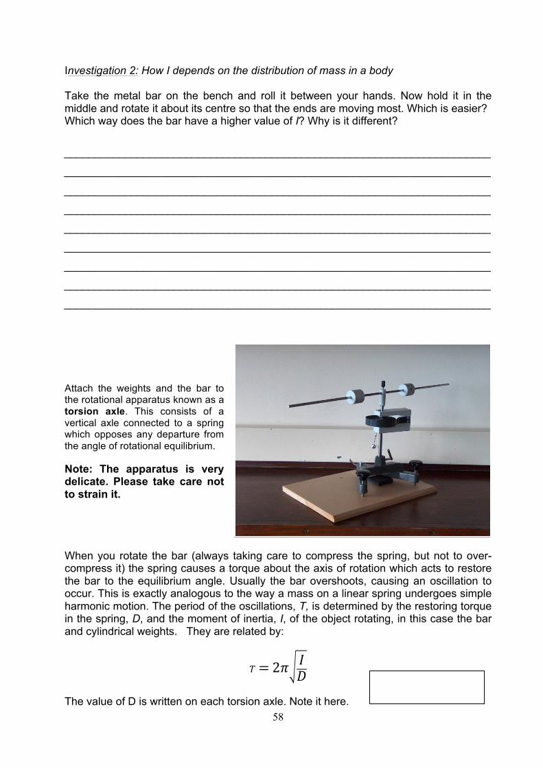
Attach the weights and the bar to the rotational apparatus known as a torsion axle. This consists of a vertical axle connected to a spring which opposes any departure from the angle of rotational equilibrium.
Note: The apparatus is very delicate. Please take care not to strain it.
When you rotate the bar (always taking care to compress the spring, but not to over-compress it) the spring causes a torque about the axis of rotation which acts to restore the bar to the equilibrium angle. Usually the bar overshoots, causing an oscillation to occur. This is exactly analogous to the way a mass on a linear spring undergoes simple harmonic motion. The period of the oscillations, T, is determined by the restoring torque in the spring, D, and the moment of inertia, I, of the object rotating, in this case the bar and cylindrical weights. They are related by:
𝑇= 2𝜋 𝐼𝐷
The value of D is written on each torsion axle. Note it here.
59
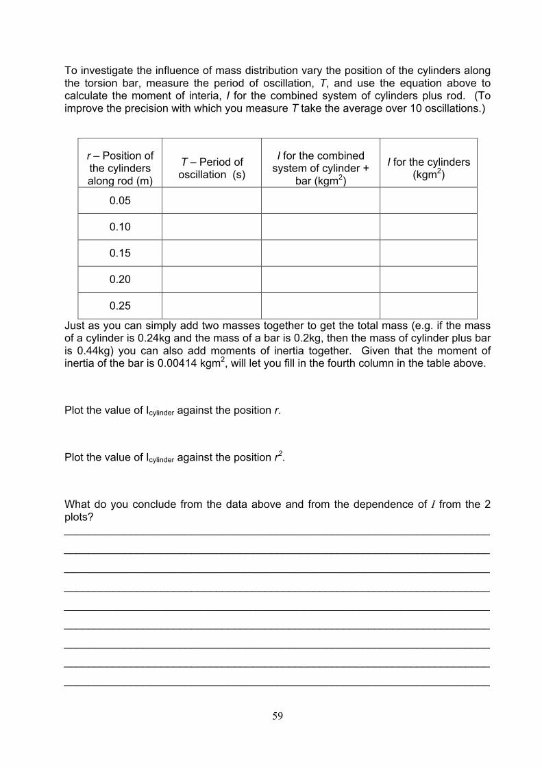
To investigate the influence of mass distribution vary the position of the cylinders along the torsion bar, measure the period of oscillation, T, and use the equation above to calculate the moment of interia, I for the combined system of cylinders plus rod. (To improve the precision with which you measure T take the average over 10 oscillations.)
r – Position of the cylinders along rod (m)
T – Period of oscillation (s)
I for the combined system of cylinder +
bar (kgm2)
I for the cylinders (kgm2)
0.05
0.10
0.15
0.20
0.25
Just as you can simply add two masses together to get the total mass (e.g. if the mass of a cylinder is 0.24kg and the mass of a bar is 0.2kg, then the mass of cylinder plus bar is 0.44kg) you can also add moments of inertia together. Given that the moment of inertia of the bar is 0.00414 kgm2, will let you fill in the fourth column in the table above.
Plot the value of Icylinder against the position r.
Plot the value of Icylinder against the position r2.
What do you conclude from the data above and from the dependence of I from the 2 plots? ______________________________________________________________________
______________________________________________________________________
______________________________________________________________________
______________________________________________________________________
______________________________________________________________________
______________________________________________________________________
______________________________________________________________________
______________________________________________________________________
______________________________________________________________________

60
Use JagFit to create a graph of Icylinder against the position r and attach your printed graph below.

61
Use JagFit to create a graph of Icylinder against the position r2.and attach your printed graph below.

62
The last measurement in the table above, with r= 0.25m, returns the bar + cylinders system to the orientation used in your first investigation. You have thus measured the moment of inertia of the bar + cylinder system in two independent ways. Write down the two answers that you got.
I from investigation 1:
I from investigation 2:
How do the two values compare? Which is more precise? Give reasons for your answers.
______________________________________________________________________
______________________________________________________________________
______________________________________________________________________
______________________________________________________________________
______________________________________________________________________
______________________________________________________________________
______________________________________________________________________
______________________________________________________________________
______________________________________________________________________
______________________________________________________________________
______________________________________________________________________
______________________________________________________________________
______________________________________________________________________
______________________________________________________________________
______________________________________________________________________
63
Graphing Many of the experiments in the 1st Year laboratory involve the plotting of a graph. Graphs are very important in Physics as they provide a simple display of the results obtained in an experiment and of the relationship between two variables. More accurate and reliable information can be obtained from a graph than from the analysis of any particular set of results. Plotting graphs by hand: (1) Scale: It is important to choose the scales so as to make full use of the squared
page. The scale divisions should be chosen for convenience; that is, one unit is either 1, 2 or 5 times a power of ten e.g. 0.5, 5, 100 etc., but never 3, 7, 9 etc.
(2) Marking the points: Readings should be indicated on the graph by a ringed dot ⊗
and drawn with pencil, so that it is possible to erase and correct any unsatisfactory data.
(3) Joining the points: In the case of a straight line which indicates a direct proportion
between the variables, the ruler is positioned so that the line drawn will pass through as many points as possible. Those points which do not lie on the line should be equally distributed on both sides of the line. A point which lies away from this line can be regarded as ‘doubtful’ and a recheck made on the readings. In the case of a curve, the individual experimental points are not joined with straight lines but a smooth curve is drawn through them so that as many as possible lie on the curve.
(4) Units: The graph is drawn on squared page. Each graph should carry title at the
top e.g. Time squared vs. Length. The axes should be labelled with the name and units of the quantities involved.
(5) In the case of a straight-line graph, the equation of the line representing the
relationship between the quantities x and y may be expressed in the form y = mx + c where m is the slope of the line and c the intercept on the y-axis. The slope may
be positive or negative. Many experiments require an accurate reading of the slope of a line.
64
Using JagFit
In the examples above we have somewhat causally referred to the ‘best fit’ through the data. What we mean by this, is the theoretical curve which comes closest to the data points having due regard for the experimental uncertainties. This is more or less what you tried to do by eye, but how could you tell that you indeed did have the best fit and what method did you use to work out statistical uncertainties on the slope and intercept? The theoretical curve which comes closest to the data points having due regard for the experimental uncertainties can be defined more rigorously3 and the mathematical definition in the footnote allows you to calculate explicitly what the best fit would be for a given data set and theoretical model. However, the mathematics is tricky and tedious, as is drawing plots by hand and for that reason.... We can use a computer to speed up the plotting of experimental data and to improve the precision of parameter estimation.
In the laboratories a plotting programme called Jagfit is installed on the computers. Jagfit is freely available for download from this address: http://www.southalabama.edu/physics/software/software.htm
Double-click on the JagFit icon to start the program. The working of JagFit is fairly intuitive. Enter your data in the columns on the left.
• Under Graph, select the columns to graph, and the name for the axes. • Under Error Method, you can include uncertainties on the points. • Under Tools, you can fit the data using a function as defined under
Fitting_Function. Normally you will just perform a linear fit. One of the experiments in this manual was developed by the Physics Education Group, CASTeL, Dublin City University.
3 If you want to know more about this equation, why it works, or how to solve it, ask your demonstrator or read about ‘least square fitting’ in a text book on data analysis or statistics.