Laboratory Exercises for Physics - Internet Archive

Laboratory

PHYSICS

HARVEY E. WHITE

0k liBBis

LABORATORY EXERCISES

for Physics

HARVEY E. WHITEProfessor of Physics, University of California

With the assistance of

EUGENE F. PECKMANSupervisor of Science, Pittsburgh, Pennsylvania

Public Schools

D. VAN NOSTRAND COMPANY, INC.PRINCETON, NEW JERSEY

TORONTO, CANADALONDON, ENGLAND

Van Nostrand Regional Offices: New York, Chicago, San Francisco

D. Van Nostrand Company, Ltd., London

D. Van Nostrand Company (Canada), Ltd., Toronto

Copyright ©1959, by D. VAN NOSTRAND COMPANY, INC.

Published simultaneously in Canada by

D. Van Nostrand Company (Canada), Ltd.

No reproduction in any form of this book, in whole or

in part (except for brief quotation in critical articles or

reviews), may be made without written authorization

from the publisher.

Library of Congress Catalog Card No. 59-12778

Designed by Lewis F. White

05677a40

PRINTED IN THE UNITED STATES OF AMERICA

Preface

Laboratory Exercises for Physics

is designed to be used as a laboratory guide

and manual for students enrolled in an in-

troductory course in fundamental physics.

Although this manual may be used in con-

junction with any well-written textbook, the

numbered order of the experiments follows

the numbering system used in the author’s

text, Physics—An Exact Science.

It is assumed here, as well as in the asso-

ciated text, that the student has had sometraining in the elementary principles of alge-

bra and plane geometry.

For a number of years a large majority of

laboratory manuals have been published in

an oversized format in which blank spaces

are provided for the student to use in record-

ing his own data and in giving answers to

specific questions. While this procedure has

definite advantages for teachers and stu-

dents alike, it has also had a number of dis-

advantages. Recent discussions among teach-

ers clearly indicate that some modifications

of procedure should be made.

With the hope of retaining the major ad-

vantages of such laboratory practice’s, arid

of replacing the objectionable features by

more desirable ones, the author is presenting

this somewhat new solution to the problem

of laboratory procedure.

The scientific method of today is one of

experimentation. It is a procedure in which

a problem or objective is first outlined and

clearly stated by the experimenter. This is

followed by a review of the theory and ex-

perimental observations of others, and the

resulting knowledge, having a direct bear-

ing upon the problem. Apparatus is then

constructed and assembled, observations of

events are made, and quantitative measure-

ments are recorded in tabular form. Results

are calculated according to the indicated

theory, and conclusions are usually pre-

sented in the form of a graph and one or

more statements.

While many schools have excellent labo-

ratory facilities and equipment, others have

little o*r none. As science progresses, new

and important experiments must be incor-

porated into the laboratory experience, and

this, of necfl^MB>^rn|»st be done at the ex-

pense of- less^jjjfefft^nt experiments previ-

ously listed.

Elaborate and expensive equipment for

iv

new and up-to-date experiments need not al-

ways be purchased. Through the “project”

method, apparatus can often be built by the

students and teacher in the home or school

workshop. Every school would do well to

provide time, space, and shop facilities where

talented students can carry out project work.

Where a project development is also aimed

at Science Fair display and competition, the

apparatus should by all means be simple in

construction, neat in appearance and opera-

tion, and capable of permitting the taking

of quantitative measurements.

When laboratory facilities and equipment

are available for any of the experiments de-

scribed in this book, the instructions given

should be followed by the student. The sam-

ple calculations near the end of each lesson

may be used as a student guide in making

the calculations necessary to the completion

of a “final report.”

When laboratory facilities and equipment

are not available for an experiment, it is still

possible for the student to derive some bene-

fit from the experiment by having him use

the data given in the exercises, record them

as though they were his own findings, and

write a final report based upon these data.

One of the principal criticisms made of

PREFACE

many students entering colleges and univer-

sities today is their inability to write a com-

position or report. It is not sufficient there-

fore that the science student perform each

experiment with his own hands; he must

also make out his own data sheet, and write

up his own final report.

It is recommended that each student’s

data be recorded in a notebook, and that a

clean page be started for each experiment.

In this way the original recorded measure-

ments will not be lost, and a periodic check

upon any or all of the laboratory work com-

pleted can be made at any time.

A sample “Data Sheet” is shown in the

appendix along with a brief form of a “Final

Report,” based on the laboratory experi-

ment in Mechanics on page 6. The sample

“Final Report” is not intended to be fol-

lowed exactly for all experiments, but to

serve as a minimum requirement guide for

student laboratory and homework. Lengthy

reports should not take the place of short,

concise, and clearly written ones, but some

kind of report written by the student is a very

necessary part of science training.

Berkeley, California Harvey E. WhiteJune, 1959

Contents

Lesson 4.

INTRODUCTION

Measurement of Distances and Angles

Lesson 2.

MECHANICSSpeed and Velocity 6

4. Accelerated Motion 8

8. Falling Bodies 10

11. Projectiles 13

13. The Force Equation 15

16. Concurrent Forces 18

18. Resolution of Forces 20

20. Parallel Forces 23

22. The Simple Crane 25

25. Coefficient of Friction 28

28. Center of Gravity 30

30. Horsepower 33

33. Energy and Momentum 35

35. Levers 38

38. Ballistics 41

40. Centripetal Force 43

43. Moment of Inertia 47

Lesson 2.

PROPERTIES OF MATTERHooke's Law 52

5. Pressure in Liquids 55

7. Density and Weight-Density 57

10. Density of Air 60

12. Fluid Friction 62

15. The Pendulum 64

Lesson 2.

HEATThermal Expansion 68

5. Specific Heat 70

7. Heat of Fusion 73

10 . Newton's Law of Cooling 75

Lesson

Lesson

Lesson

Lesson

Lesson

Lesson

CONTENTS

12 . Mechanical Equivalent of Heat 78

15. Boyle's Law 81

SOUND2 . Frequency of a Tuning Fork 86

5 . Vibrating Strings 88

7. Resonating Air Columns 90

10 . Speed of Sound 92

LIGHT

3. Photometry 96

5. Reflection from Plane Surfaces 98

8. Index of Refraction 101

10 . Lenses 103

13 . Magnifying Power 106

15 . Principles of the Microscope 108

ELECTRICITY AND MAGNETISM4. Electromotive Force of a Battery Cell 1 14

6. Series Circuits 116

9 . Parallel Resistances 119

11. The Potential Divider 122

14 . Wheatstone Bridge 125

16 . Electrical Equivalent of Heat 128

19 . A Study of Motors 131

21 . Coulomb's Law 134

24 . Transformers 137

ATOMIC PHYSICS

4 . Electronic Charge to Mass Ratio 142

6. Wave Lengths of Spectrum Lines 145

9 . Radioactivity Measurements 148

ELECTRONICS

3. Characteristics of Vacuum Tubes 154

6. Electromagnetic Waves 157

8. Geiger-Mueller and Scintillation Counters 160

NUCLEAR PHYSICS

4. Radiation Measurements 166

Appendices 171

Index 177

Instructions to Students

I n performing any of the various

laboratory experiments described in the fol-

lowing lessons, you as a physics student

should carry out the various steps and pro-

cedures outlined as follows. If you have

access to apparatus similar to that described

in the lesson, by all means do the experi-

ment yourself, record your own data, and

write a Final Report. If, on the other hand,

you do not have access to laboratory equip-

ment of the kind described, do the next

best thing: record the data given in that

particular lesson and write a Final Report

as if you had performed the experiment

yourself. (Oftentimes you may find it a

simple matter to procure or make the ap-

paratus yourself.)

If you do perform the experiment, you

should record your data on a Data Sheet,

following the sample form given on page 173.

For this purpose use a sheet of plain white

paper, 8^ x 11 in. in size, and record all

measurements, diagrams, formulas, and in-

formation you think will be needed in writ-

ing up your Report. Whether you do the

experiment yourself or use the data given

in the lesson, your Final Report should be

made on the same size paper and have the

following brief form (See Sample Final Re-

port on page 175.)

With your Name at the upper left corner

of the page and the Title of the experiment

at the upper right corner of the page, write

down the Object of the experiment.

Following this, and under the heading of

Theory, you should give the formulas

needed in the experiment. These will gen-

erally be copied directly from the book,

and they will be connected directly with pre-

ceding lessons in the text.

Next, under the heading of Apparatus and

Procedure, make a simple line diagram of the

apparatus used. Following this, under the

heading of Data and Measurements, list your

measurements in a well-drawn Table similar

to that given in each laboratory exercise.

Next, under the heading of Calculations or

Calculated Results, give the numerical calcu-

lations asked for. These will often be in

tabular form. Finally, under the headings of

Results and Conclusions, give the final nu-

merical results obtained, answers to all ques-

tions asked, and a graph wherever it is re-

quested.

Neatness is a prime requisite of a good

report. Use a ruler in making diagrams and

in ruling tables.

Digitized by the Internet Archive

in 2017 with funding from

University of Alberta Libraries

https://archive.org/details/physicsexactsciewhit

INTRODUCTION

Introduction|

Lesson 4

MEASUREMENT OF DISTANCES AND ANGLES

In performing the laboratory experiment

described in this lesson, you will learn howto measure the three angles of a triangle with

a protractor and the lengths of the three

sides with a centimeter rule. In learning to

use these simple measuring instruments, you

will learn how to interpolate.

Theory. Suppose that you are going to

determine accurately the length of a rectan-

gular block of steel with a centimeter rule.

With one end of the block at the zero end

of the rule, the other end is found to come

a little beyond the 8-cm mark as shown in

Fig. A.

In this illustration you could write downthe length as 8.7 cm or 8.8 cm; or you

could be more precise and note that the end

comes about % 0 of a millimeter beyond

the seventh millimeter mark. Hence you

could write more precisely 8.74 cm. This

process of making a reasonably good esti-

mate as to an intermediate value is called

interpolation. In laboratory practice of all

kinds, this process of interpolation arises

over and over again, and the more carefully

you make your estimates, the more pre-

cise you can expect your results to be and

the more reliable will be the conclusions

you decide to draw from them.

To measure the angle between two lines,

a protractor of the kind shown in Fig. B is

most commonly used. Protractors usually

Fig. A. Illustrating the process of interpolation when

used in measuring a length.

Fig. B. Diagram of a protractor as used in measuring

angles.

include angles up to half a circle; therefore,

they permit the measuring of angles up to

180°. In the illustration the scale starts

at the right and measures angles up and

around counterclockwise.

While some precision angle-measuring

devices divide each degree of angle into 60

minutes and each minute into 60 seconds, we

will always divide them decimally into

tenths and hundredths of a degree.

Suppose, for example, the angle 6 is to

be measured with your protractor. Close

examination of the scale in the region of 42°

might look like the detail in Fig. C. The

Fig. C. Illustrating the process of interpolation in meas-

uring angles.

0

_L_L

? (3

1 1 1 1 1 i

S

1 1 1 1 1 1

>

III

ii*'

2

MEASUREMENT OF DISTANCES AND ANGLES 3

Table 1. Measurements of the Sides and Angles of Two Right Triangles

AC AB CB Angle A Angle 8 Angle CTrial (cm) (cm) (cm) (degrees) (degrees) (degrees)

1 8.00 9.77 5.60 35.0 55.0 90.0

2 7.50 11.0 8.04 47.0 43.0 90.0

line comes beyond the 42° mark, but not

quite to the 43° mark. Interpolating, you

could write the angle as 42.6°.

Apparatus. Needed for this experiment

are a sharp pencil, a centimeter rule, a

protractor, and a sheet of white paper 8^ x

1 1 in.

Object. To measure the three sides

and three angles of a triangle.

Measurements and Data. Draw a hori-

zontal line on your paper and make two

marks on the line exactly 8 cm apart, labeling

them A and C. See Fig. D. With the center

mark of the protractor on A, make a mark at

the 35° angle and draw the line AP. With the

center mark of the protractor at C, make a

mark at the 90° angle and draw the line CB.

Now measure the lengths of the lines AB and

BC and record them in a table with column

headings like those in Table 1. Also measure

the angle at B and record its value. Note that

the sum of the angles at A and B should

be 90°.

As a second trial, repeat the experiment,

using a horizontal line 7.5 cm in length and

angles A and C of 47° and 90°, respec-

tively. When your measurements are com-

pleted and recorded, they will, if carefully

done, be close to the values given in Table 1.

If you have time, you may choose differ-

ent line and angle values for your triangles

and record the measurements in Table 1.

Calculations. You may well recall the

Pythagorean theorem from geometry in

which it is proved that for all right triangles

the square of the hypotenuse is equal to

the sum of the squares of the other two

sides. For the triangle in Fig. D, we can

therefore write

(AB)2 = (AC)2 + (CB)2( 1 )

Fig. D. Laboratory exercise in measuring lines and

angles.

We can use this equation as a check upon

the accuracy of the measured lengths of the

sides of the triangles.

Comparisons are most easily made by

tabulating as in Table 2. Note how well the

values in the last two columns agree.

Table 2. The Pythagorean Theorem Applied

to Two Measured Triangles

Trial (CB)2 (ACT (AB)2 (ACT + (CBT

1 31.4 64.0 95.5 95.4

2 64 6 56.2 121.0 120.8

4 INTRODUCTION-LESSON 2

Conclusions: Hence we conclude that

with a protractor we can measure angles with

precision, and with a centimeter rule and the

process of interpolation we can accurately

measure lengths of lines to three significant

figures.

We can apply the Pythagorean theorem to

our measured results and with confidence

feel that the fundamental principles upon

which they are based are valid.

In your report on this experiment, an-

swer the following questions:

1. What is the Pythagorean theorem?

2. What is meant by the term “interpola-

tion”?

3. How many degrees are there in (a)

a right angle and (b) a complete cir-

cle?

4. The lengths of the two sides of a right

triangle are 5 cm and 12 cm, respec-

tively. Find the length of the hypo-

tenuse by means of the Pythagorean

theorem.

MECHANICS

Mechanics|

Lesson 2

SPEED AND VELOCITY

Theory. This is to be a labo-

ratory lesson in which we will see how to

determine the speed of an electric train and

the velocity of a toy automobile. The prin-

ciples to be employed are those presented in

the preceding lesson, in which the scalar

quantity speed and the vector quantity ve-

locity are both given by the same algebraic

equation

where s is the distance travelled, t is the

elapsed time of travel, and v is the speed

or velocity.

Apparatus and Procedure. Part 1. For

an object to move with constant velocity,

it must not only travel equal distances in

equal intervals of times, but its direction

must also not change, i.e., it must movealong a straight line. For this part of the

experiment, a model car is pulled across the

table top by means of a string wrapped

around a drum, and a stop clock, C, is used

to measure the time. See Fig. A.

A small synchronous motor M, with a

geared down shaft making one revolution

per second, and a drum one inch in diameter

makes a suitable power unit.

Two markers, A and B, are located a

short distance apart and the distance s be-

tween them, is measured with a meter stick

Fig. A. Experimental arrangement for measuring the

velocity of a car.

t

A1

and recorded in centimeters. For recording

data make a table of three columns as shown

in Table 1. The car is started, and as it

passes marker A, the clock is started; and

as it passes marker B, the clock is stopped.

The time t in seconds, as read on the clock

dial, is then recorded. This procedure is

then repeated with the markers farther and

farther apart, and the data are recorded

in the table.

Part 2. For an object to move with constant

speed, it may move along any path, straight

or curved, but it must travel equal distances

along its path in equal intervals of time.

For this part of the experiment, a toy elec-

tric train is used, running at constant speed

around a circular track as shown in Fig. B.

Make a table of three columns, with head-

ing as shown in Table 2, for recording data.

As the train passes marker M, the clock

is started. The clock is stopped as the train

again passes marker M, but after it has

made three, four, or five complete trips

around the track. The time t is read from

the clock directly and the distance is deter-

mined by measuring the diameter d of the

center rail.

Fig. B. Experimental arrangement for measuring the

speed of a train locomotive.

6

SPEED AND VELOCITY 7

Since the circumference of a circle is

given by

circumference = -ird

the total distance s traveled by the train

will be

s = mrd (2)

where n is the number of trips around the

track, and ?r has the value

7T = 3.1

4

The distances traveled and their correspond-

ing times of travel should be recorded in

Table 2 and the speed calculated by use of

Eq. (1)

Object. To make a study of a bodymoving with constant speed and another

moving with constant velocity.

Measurements and Data. Suppose that

we have performed the experiments just

described, made the specified measurements,

and recorded the data as they are shown

in Table 1.

Table 1. Data for Car

Distance Time

s t

Trial (cm) (sec)

1 72.9 9.1

2 124.5 15.5

3 163.0 20.5

Table 2. Data for Train

Number Time

of t

Trial Turns (sec)

1 3 19.2

2 4 25.5

3 5 32.1

The center rail of the train’s circular

track is measured and found to have a

diameter

d = 74.6 cm

Calculations. To make your calcula-

tions of the speed and velocity, use a ruler

and construct two new tables having the

following headings.

Table 3. Results for the Car

Distance Time Velocity

s t V

Trial (cm) (sec) (cm/sec)

1 72.9 9.1 8.01

Table 4. Results for the Train

Number Time Distance Speed

of t s V

Trial Turns (sec) (cm) (cm/sec)

1 3 19.2 702 36.6

The first three columns of each table are

to be filled in for all trials by copying the

measured data from Table 1. The remaining

columns are then filled in by making the

proper calculations: For example, for trial

1 for the car, divide the first distance, s =72.9 cm, by the time, t = 9.1 sec, and you

will obtain 8.01 cm/sec. Therefore, as the

velocity for the first trial, record in the last

column of Table 3 the value 8.01. This has

already been done in the case of the first

trial and is to serve as your guide in calcu-

lating the other two. When similar calcula-

tions have been carried out for all three

trials, the velocities should be nearly alike.

To find the distances traveled by the train,

use Eq. (2). First multiply the measured

track diameter d = 74.6 cm by v = 3.14

to obtain the track circumference. Next

multiply this circumference by three, four,

and five, respectively, and record these in

column 4 of your last table. Finally, calcu-

late the train speed by dividing the distances

in the fourth column by the measured

times in the third column and record the

8 MECHANICS-LESSON 4

answers in the fifth column. Again all three

speeds should be nearly alike. Calculated

values for trial 1 are already given and

will serve as your guide for the other two.

Conclusions. For your conclusions, an-

swer each of the following questions:

1. What is the average value of v for

the car?

2. What is the average value of v for

the train?

3. Which of the two measurements in

this experiment, time or distance, has

the greater percentage error?

Mechanics|

Lesson 4

ACCELERATED MOTION

Theory. This is a laboratory lesson in

which we are going to make a study of a

steel ball undergoing uniformly accelerated

motion. In the preceding lesson, we have

seen the development of four fundamental

equations of the form

( 1 )

(2 )

(3)

(4)

Note that each of these four equations

involves only three of the four quantities,

v, a, t, and s. In other words, if in any ob-

servations of an object moving with uni-

formly accelerated motion we can measure

two of these four quantities, the other two

can be computed by using the appropriate

equations.

Apparatus and Measurements. There

are many methods for producing uniformly

accelerated motion and of observing and

measuring such motion. In this experiment,

we use an inclined plane in the form of a

U-shaped metal track down which we roll

a steel bearing ball 1 in. in diameter. The

apparatus is shown by a diagram in Fig. A.

Part J. The steel ball is held at the top

of the incline by a small electromagnet E.

When the electrical switch K is opened, the

magnet loses its force of attraction and

the ball is released. As it rolls down the

incline, constantly increasing its speed, we

propose to measure distances s and times

of travel t. To do this, a marker is set up

at any point and the distance s is measured

v = at

v2 = 2as

s = %at2

Fig. A. Inclined plane experiment for studying uniformly accelerated motion.

ACCELERATED MOTION 9

Fig. B. Inclined plane apparatus for measuring instantaneous velocity at any point.

with a meter stick and recorded. At the

instant the switch K is opened, and the ball

starts, the stop-watch stem is pressed, start-

ing the second hand from zero. As the ball

passes the marker position, the watch stem

is again pressed, stopping the watch. Hence

f, the time of travel, is determined and re-

corded. All data in this experiment is con-

veniently recorded in a table of five columns

with headings as shown in Table 1.

Part 2. Although measurements of s and

t in this experiment are sufficient to deter-

mine velocity v and acceleration a, we will

check the results by measuring the instan-

taneous velocity of the steel ball as it passes

various points along the inclined plane. Howthis is accomplished is shown in Fig. B.

Suppose, for example, that as the ball

rolls down the incline with ever increasing

speed, we wish to find its instantaneous

velocity as it passes the point C. A hori-

zontal track CG is mounted on the incline

so that the next time the ball rolls down and

reaches the point C with a given instanta-

neous velocity v, it will roll out along the

level track, maintaining a constant speed

v. If we then measure the time tfrequired to

move a distance s' along the level track, wecan calculate the velocity v by the formula

The procedure, therefore, is to place a

marker at C and one farther along at some

measured distance s' as shown in the figure.

Upon releasing the ball at A, the stop watch

is started as the ball passes the point C and

stopped as it passes the point H. Hence the

distance s' and corresponding time f' can be

recorded and v can be calculated.

Object. To study the laws of uniformly

accelerated motion.

Data. Suppose we have performed the

experiments just described, made the ap-

propriate measurements, and recorded the

data in a table as shown in Table 1.

Table 1. Data for Inclined Plane

Experiment

Trial

s

(cm)

t

(sec)

s'

(cm)

t'

(sec)

1 45.0 1.3 84.0 1.2

2 117 2.1 155 1.4

3 270 3.2 155 0.9

Calculations. To complete this experi-

ment, use a ruler and make two tables of

three columns each with headings as shown

in Tables 2 and 3.

Table 2. Velocity Results

s'/1'

2s/t

(cm/sec) (cm/sec) Average

70.0 69.2 69.6

To illustrate how the columns are to be

filled in, the calculations for the first trial


Table 3. Acceleration Results

v/t 2s/t2 v2/2s

(cm/sec2) (cm/sec2

) (cm/sec2)

53.5 53.2 53.8

are tabulated below each heading. To verify

the method, use the following procedure:

For the first column headed s'/f' in Table 2,

take s' = 84.0 cm and t' = 1.2 sec from the

last two data columns of Table 1, divide

one by the other according to Eq. (5), and

obtain v = 70.0 cm/sec. For the second col-

umn headed 2s/t, take s = 45.0 cm and t =1.3 sec from the second and third data col-

umns of Table 1, divide 2s by t according to

Eq. (2), and obtain v = 69.2 cm/sec. These

two values of v should be the same. Their

average value v = 69.6 cm/sec is obtained

by adding the two and dividing by 2.

For the first column headed v/t in Ta-

ble 3, take the average value of v = 69.6

cm/sec from Table 2 and f =1.3 sec from

data column 3, Table 1, divide one by the

other according to Eq. ( 1 ) ,and obtain a =

53.5 cm/sec2. For the second column, take

s = 45.0 cm and t = 1.3 sec from data col-

umns 2 and 3, Table 1, divide 2s/t2 accord-

ing to Eq. (4), and obtain a - 53.2 cm/sec.

Finally, for the last column, take the average

value of v = 69.6 cm/sec from Table 2 and

s = 45.0 cm from the data column 2, Table

1, divide v2/2s according to Eq. (3), and

obtain a = 53.8 cm/sec2. Note how nearly

all three of these values of a are alike.

Carry out the procedure just outlined for

the other two trial sets of data and tabulate

them in the proper columns of Tables 2

and 3. The average values of v for each of

the three trials will be different but all nine

values of a should be the same.

Results. For your final results, carry out

the following:

1. Calculate the average value of the ac-

celeration.

2. Plot a graph of t vs v. Plot t vertically.

3. Plot a graph of t vs s. Plot t vertically.

4. Plot a graph of t2 vs s. Plot t

2 vertically.

Mechanics|

Lesson 8

FALLING BODIES

Theory. In this laboratory expe-

riment, we are going to determine the ac-

celeration due to gravity by measuring the

acceleration of a freely falling body. Wehave seen in Mechanics, Lesson 7, that such

bodies, neglecting air friction, should fall

with uniformly accelerated motion and that

this motion may be described by four kine-

matic equations of the form

v = gt (1)

s = (2)

v2 = 2gs (3)

s = §gf2(4)

The constant g in these equations is the

acceleration due to gravity, and it is our

purpose to determine its value with pre-

cision. To do this, we will make use of one

equation only, Eq. (4). By measuring s,

the distance an object is allowed to fall, and

t, the time it takes to fall that distance, the

values can be substituted in Eq. (4) and g ,

the only unknown, can be computed. For

convenience, transpose Eq. (4) so that g

FALLING BODIES 11

only is on the left side of the equality sign.

Reversing the equation first, write

h9f

'

2 = s

gf _ s

2 “1

and then transposing, we obtain

Apparatus and Procedure. The appa-

ratus in this experiment consists of two es-

sential parts: ( 1 ) an electromagnet for hold-

ing and dropping a steel bearing ball and

(2) a turntable driven by a synchronous

electric motor for accurately measuring the

time of fall. See Fig. A.

The synchronous motor M keeps in step

with the 60-cycle electric current, as does

every household electric clock, and is geared

down so that the turntable T makes exactly

one revolution per second. The white face

of the turntable is divided angularly into one

hundred equal divisions as shown in Fig. B.

Each division therefore represents y100 of a

second.

Fig. A. Apparatus used in determining the acceleration

due to gravity.

When the switch K is closed, an electric

current from a battery V flows through the

contact switch C as well as the electromagnet

E, holding the steel ball B in the position

shown. As the turntable rotates, the front

end of the rider strip P strikes the tripping

switch prong at C, opening the electric cir-

cuit and dropping the ball. The rider strip

P and the switch C are so located as to open

the electric circuit when the zero mark

on the turntable lies directly beneath the

ball B. A plumb line is used to align these

two points. As the ball falls and the table

continues to turn, the ball strikes the table

surface at some point and makes a black

mark as indicated at A. The time of fall is

therefore determined by the divided circle.

Black soot can be deposited on the lower

side of the ball by holding it in a candle

flame.

Object. To study the laws of freely

falling bodies and to determine the ac-

celeration due to gravity.


we have performed this experiment, dropped

the ball from four different heights, and ob-

tained the four marks shown on the disk in

Fig. B. The heights s are measured with a

Fig. B. Timing table for laboratory experiment on falling

bodies.


meter stick and recorded in column 2 of

Table 1. The corresponding times t are

measured directly from the disk and re-

corded in column 3.

Table 1. Recorded Data

Trial

s

(cm)

t

(sec)

1 36.2 .272

2 85.7 .419

3 133.5 .522

4 196.4 .633

Calculations. For calculating the ac-

celeration due to gravity from these meas-

urements, make a table on your laboratory

report paper with the four headings as in

Table 2.

Table 2. Calculated Results

2s f2

9Trial (cm) (sec)

2 (cm/sec2)

1 72.4 .0740 978

Calculations for trial 1 are already madeand will serve as a guide and check upon

your calculations.

By referring to Eq. (5) we see that

column 2 of this table will contain a list

of figures representing the numerator and

column 3 will contain a list of figures repre-

senting the denominators for calculating g.

To fill in column 2 for all trials, multiply

the values of s in the second column of

Table 1 by 2. For column 3, square the

values of t recorded in column 3 of Table

1.

The last column is filled in with the cal-

culated values of g by dividing each value

of 2s by the corresponding value of t2

. (Donot use a slide rule in these calculations,

but express your results to three significant

figures only.)

Results and Conclusions. Your final re-

port should include answers to the follow-

ing:

1. What is the average value for the four

values of g obtained in this experi-

ment?

2. What is the percentage error between

the average value and the accepted

value g = 980 cm/sec2?

3. Make a graph for the data taken in

this experiment, by plotting 2s against

t2

. Cross-section paper may be used,

or you can make your own chart as

shown in Fig. C.

PROJECTILES 13

Mechanics|

Lesson 1

1

PROJECTILES

This is a descriptive kind of

laboratory experiment in which we are going

to study the paths of projectiles and particu-

larly how they change as we change the

elevation angle.

Theory. We have seen in the preceding

lesson, how, by knowing the initial velocity

of projection v and the elevation angle 0

of a body, we can calculate its range R,

maximum height H, and time of flight T.

The method by which the formulas given in

Table 1 of Mechanics, Lesson 10, are de-

rived is illustrated in Fig. A.

The initial velocity v is resolved into

two components vx and vy . We then visu-

alize the projectile as having two motions

at the same time: one is the motion of a

body moving horizontally with a velocity

vx ,and the other the motion of a body pro-

jected upward with the velocity vy . In other

words, if one projectile A is projected

straight upward with a velocity vy and

simultaneously another projectile S is pro-

jected with the velocity v at the elevation

angle d, the two will rise to the same maxi-

mum height in the same time and return to

strike the ground simultaneously.

Hence, by knowing v and 0 for any pro-

jectile, one can find the y-component of

the velocity vy and, using the formulas for

freely falling bodies, Eqs. (1), (2), (3),

and (4) in Mechanics, Lesson 10, determine

distances and times to any point of a trajec-

tory. These are the basic principles from

which the relations given in Table 1 of the

same lesson are derived.


ratus to be used in this experiment consists

of a large flat board as shown in Fig. B.

At the lower left corner, a small nozzle

producing a narrow stream of water is

mounted free to turn about a horizontal

axis. Waterdrops, therefore, become the

projectiles in our experiment. Not only does

the water stream permit one to see the

entire trajectory at a glance, but to observe

continuously how the shape changes with

the elevation angle.

The elevation angle 6 of the nozzle and

stream can be set to any desired angle by

means of a pointer and scale, while the

height and range can be measured with a

meter stick or the ruled lines of the back-

board. The scale of horizontal and vertical

Fig. A. The range R, maximum height H, and the time of flight of a projectile depends on the initial velocity v

and the elevation angle 6.

y


lines on the backboard are in centimeters

and the angles are in degrees.

To proceed with the experiment, the

stream of water is turned straight up to 90°

and the water valve adjusted until the stream

comes up to the 80 cm mark and no higher.

At this setting of the stream velocity, the

angles are set at 75°, 60°, 45°, 30°, 15°,

and 0° successively. For each position, the

range R and the maximum height H are

measured along and from the bottom line,

and the values recorded on your data sheet.

Object. To determine the range andmaximum height of a projectile for dif-

ferent elevation angles.


e

(deg)

H

(cm)

R

(cm)

90 80 0

75 75 80

60 60 140

45 40 160

30 20 140

15 5 80

0 0 0

Measurements and Data. As this ex-

periment is performed, the measurements

should be recorded in a table of three col-

umns. Suppose we have followed the specific

instructions given above, the recorded data

would be as given in Table 1

.

Calculations. Using the maximum range

R and the height H for elevation angle 6 =45°, calculate the initial velocity of the

water stream from the nozzle in this experi-

ment. Use the relations given for a 45° ele-

Fig. C. A polar graph for the range of a projectile.

THE FORCE EQUATION 15

vation angle in Table 1 of Mechanics, Lesson

10 .

Results and Conclusions. Draw two

graphs of the data taken in this experiment.

In the first graph, plot the elevation angles

0 horizontally from 0° to 90° and the maxi-

mum heights H vertically from 0 to 80 cm.

For the second graph, plot the elevation

angles 0 from 0° to 90° and the ranges R

vertically from 0 to 160 cm.

For your conclusions answer the follow-

ing questions:

1. At what elevation angle is the greatest

range attained?

2. At what elevation angle is the maxi-

mum height attained?

Where angles are involved in the plotting

of graphs, it is sometimes informative to

plot what is called a polar graph. Such a

graph is shown in Fig. C for the range

data taken in this experiment. The radial

lines from the origin O are drawn at the

proper elevation angles while the ranges R

are measured out along these radial lines.

Such a graph shows that there is a maximumrange and that there is symmetry about this

angle.

Mechanics|

Lesson 13

THE FORCE EQUATION

Theory. Our laboratory experi-

ment in this lesson is concerned with New-ton’s Second Law of motion as expressed

by the force equation.

F = ma (1

)

In its simplest terms, this law says that

if you apply a constant force F to a given

mass m, it will move with a uniform ac-

celeration a, given by the relation that F

equals the product of m times a. These

three measurable quantities are represented

schematically in Fig. A.

The three systems of units in which F, m,

and a are commonly measured are

F m a

newtons

dynes

lb

kg

gmslugs

m/sec2

cm/sec2

ft/sec2

We have seen in Mechanics, Lesson 12,

that the weight W of an object is simply a

measure of the force F with which the earth

pulls downward on any given mass m, and

if no other force acts on a body, it will fall

freely with an acceleration g. For this spe-

cial case, one usually writes

W = mg (2)

it being understood that this is Newton’s

second law and in reality is Eq. (1).

To find the weight of an object multiply

its mass by g, the acceleration due to grav-

ity. To find the mass of any object, divide

its weight by g.

g = 9.80

_ cmg = 980—

-

sec2

g = 32

We have seen in our laboratory experi-

ment in Mechanics, Lesson 4, that to de-

termine the acceleration of a body, we


Fig. A. illustration of the force equation F — ma. Fig. B. Laboratory experiment for measuring the ac-

celeration of a toy truck due to a known force.

measure the distance traveled and the time

of travel and make use of the kinematic

equation s = iat2 . Since a similar procedure

will be followed in this experiment, we will

use this same equation.

Upon transposing, we obtain the moreuseful form

Apparatus. The apparatus in this ex-

periment is easily secured and set up. It

consists of a toy truck with ball-bearing

wheels* and a strip of plate glass about 1 ft

wide and 6 ft long. See Fig. B. A strong

thread, fastened to the front of the car,

passes over two laboratory type ball-bear-

ing pulley wheels to a small mass at C.

Object. To study the dynamics of mo-

tion and Newton's Second Law of Motion.

Measurements. The truck is first put ona balance and its mass determined in kilo-

grams. It is then put on the glass plate, and

a number of small weights are added to

the car body to bring its total mass to ex-

actly 2.0 kg. This makes the total movingmass m = 2.000 kg.

Now with the thread attached at A, take a

small piece of wire or solder and fasten it

to the other end of the thread at C. Adjust

this mass until the car moves along the glass

track to the right with uniform speed. The

force due to the earth’s pull on this mass is

just sufficient to overcome friction, yet it

produces no acceleration.

The next step is to remove a 20-gm mass

m2 from the truck and add it to C. The car is

then allowed to accelerate, starting from rest

at the end of the track at A. With a stop

watch, measure the time t it takes to go

from A to B, and with a meter stick, meas-

ure the distance s. Record the data in a table

of five columns as shown in Table 1.

An additional 20-gm mass should be re-

moved from the truck and added at C. Again

the time to travel a given distance should

be determined and recorded. A third 20-gm

mass should be removed and the measure-

ments repeated again.

As a fourth trial, increase the total truck

mass by 500 gm and repeat the experiment

with m 2 — 60 gm. As a fifth and last trial,

increase the truck’s mass by another kilo-

gram and repeat the acceleration measure-

ments with m 2 = 60 gm.

It should be noted that although the ac-

celerating force F acting on the truck is

equal to W2 ,and W2 = m 2g, the total mass

that undergoes acceleration is the mass of

the truck plus the mass at C. Hence in

testing the force equation, F = ma, the total

moving mass must be used, and this is m,

or mi + m2 .

* A 2- to 3 -lb truck purchased at any toy store

is a satisfactory vehicle. Replace the customaryrubber wheels with the ball-bearing hubs of twofront bicycle wheels.

Data. Suppose that we have performed

the experiment as described above and have

recorded the data as shown in Table 1.

THE FORCE EQUATION 17


Trial

m i

(kg)

m2

(kg) (m)

t

(sec)

1 1.980 0.020 1.40 5.4

2 1.960 0.040 1.40 3.8

3 1.940 0.060 1.40 3.1

4 2.440 0.060 1.40 3.5

5 3.440 0.060 1.40 4.1

Calculations. To make your calcula-

tions and test Newton’s Second Law of Mo-

tion, make a table of six columns and give

them headings as follows:


mi + m2 m?g i/m 2 s/t2 m<ig/

m

Trial (kg) (newton) (1/kg) (m/sec2) (m/sec2

)

1 2.000 0.196 0.500 0.096 0.098

The row of numbers under the headings

are for the first trial only, and may be used

as a guide for your calculations for the other

four trials. If the force equation is valid, the

measured and theoretical values for the ac-

celeration a, as given in the last two col-

umns, should be the same for each trial.

Results. To complete your laboratory

report, two graphs should be drawn from

your results. One is already plotted in Fig.

C, and the other is left for you to do. In

Fig. C, the applied force F is plotted verti-

cally against the measured acceleration a

Fig. C. A graph of some experimental results showing

that force F is proportional to acceleration a, mass re-

maining constant.

for trials 1, 2, and 3, where the mass mremained constant.

For your second graph, plot the measured

a vertically against 1/m horizontally, for

the last three trials, where F remained con-

stant.

Conclusions. The fact that a very

straight line can be drawn through the

plotted points in Fig. C shows that F is

proportional to a. This means that

foe a

and that m is the proportionality constant.

F = ma

What similar conclusions can you draw

from your second graph?


Mechanics|

Lesson 1

6

CONCURRENT FORCES

Our laboratory experiment for

this lesson is concerned with forces acting

on a body in equilibrium. To be technical,

we are concerned with the special case of

three concurrent, coplanar forces. Concur-

rent forces are those forces whose lines of

action intersect at a common point, while

the term coplanar specifies that they all lie

in the same plane. Most common force

problems, but by no means all of them, are

of this type.

Theory. Let three concurrent, coplanar,

forces act on a single body as shown in

Fig. A. The directions of the forces Fu F2 ,

and F3 are all measured from the x-axis in

degrees and are designated 0 lf 02 ,and 03 re-

spectively. If we make vector diagrams for

these three forces, they should be drawn to

scale as shown in Fig. B. If the forces are in

equilibrium, their vector sum, as shown in

Fig. B, will form a closed triangle with a

zero resultant.

Fig. A. Diagram showing the direction angles of three

concurrent, coplanar forces.

Fig. B. Vector diagrams of three forces in equilibrium.

Start now with the left-hand diagram,

apply the parallelogram method of vector

addition to Fi and F2 alone, and find their

resultant. As shown in Fig. C, this vector

resultant R is equal in magnitude but op-

posite in direction to F3 . This must be true,

since R is equivalent to + F2 and can re-

place them. With R and F3 acting on a body

alone, these two forces could only produce

equilibrium if they are equal and opposite.

R is therefore called a resultant, and F3 can

be thought of as the equilibrant.

Fig. C. The resultant force R is equal and opposite to

the equilibrant force F3.

CONCURRENT FORCES 19

Fig. D. Experimental arrangements of spring scales and

weights on pegboard.

By making similar diagrams, it can be

shown that the resultant of F2 + Fa ,when

reversed in direction to become the equil-

ibrant of these two forces, is just the re-

maining force F x .


ratus in this experiment consists of a peg-

board with two spring scales, several cords

of different lengths with hooks at both ends,

two spring scales reading pounds weight,

and a small metal ring as shown in Fig. D.

A large protractor should be used for

measuring angles.

In performing the experiment, several

trials should be made. Different points of

suspension, different cord lengths, and dif-

ferent loads should be tried.

Object. To apply the principles of vec-

tor addition to find the resultant and equil-

ibrant of two forces acting at an angle to

each other.

Measurements and Data. As a first

trial, select two cords and mount themfrom two selected points A and B on the

pegboard. Be sure the scale casing of each

of the scales is at the upper end. Bring

the two scale plunger hooks together at the

ring and suspend a 3-lb load from the ring

for F3 . Read and record the spring scale

readings in Table 1, made up of seven

columns. Using the protractor, measure the

direction angles for each of the three forces,

and record.

Repeat this experiment by changing cords

and points A and B. Increase the load to 5

lb and make recordings as before. Change

initial conditions again and make a third

trial with a load of 8 lb.

Recording the data you have taken in this

experiment as shown in Table 1, you would

then have completed the experiment, and be

ready for your calculations and results.


Trial

F,

(lb)

Qx

(deg)

f2

(lb)

02

(deg)

h(lb)

03

(deg)

1 4.7 37.0 3.8 176.5 3.0 270

2 3.1 29.0 4.3 126.0 5.0 270

3 5.2 62.0 4.1 127.0 8.0 270

Calculations and Results. To complete

the laboratory report, you will need a table

of five columns with headings like those

shown in Table 2.

Table 2. Calculations and Results

Resultant Equilibrant

Trial R f3 Or 1 COoO

1 2.9 3.0 91.0 90

The results for the first trial are filled in

for comparison and check purposes. The

procedure carried out for these tabulated

results is shown in Fig. E, and should be

repeated for your report. Using a sharp

pencil, a centimeter ruler, and a protractor,

lay out x- and y-axes on a sheet of paper.

Draw both F x and F2 at their proper angles


R

Fig. E. Graphical construction for trial 1 in this ex-

periment.

0i and 02 respectively. Graphically, find their

resultant force and call it R. Measure the

length of R and the angle it makes with the

x-axis and tabulate in the second and fourth

columns respectively. Write in F3 directly

from your data in Table 1, and in the last

column record the direction 03 — 180°. The

magnitude of the resultant R should be the

same as the magnitude of F3 ,and the angle

0R should be the same as the value of 03 —180°, shown in the last column.

Repeat this graphical construction for

trials 2 and 3, and make similar measure-

ments of lengths and angles, and record in

Table 2. Because of the nature of the equip-

ment used in this experiment, errors of

about 5% are well to be expected between

the graphical data and the recorded data.

Conclusions. Make a short statement

in your own words of what you have learned

from this experiment as regards the equi-

librium of a body acted upon by three

forces.

Mechanics|

Lesson 1

8

RESOLUTION OF FORCES

Many problems in mechanics are

quite easily solved by the resolution of a

force into components. The principles in-

volved in such procedures are demonstrated

by a number of illustrations and examples

in the preceding lesson. In our laboratory

experiment we are going to set up two dif-

ferent objects, apply different sets of forces,

Fig. A. A force F is resolved into two component forces

Fx and Fy .

y

and employ the principles of components to

verify the results.

Theory. Suppose that a single force F,

acting at an angle 0 with the x-axis, is re-

solved into two components Fx and Fy ,as

shown in Fig. A. We have seen that the

magnitudes of these two components are

given by Eq. (2) of Mechanics, Lesson 17,

as

Fx = F cos 0

Fy = F sin 01

Now, if the magnitudes of these forces are

kept the same but their directions are re-

versed, as shown in Fig. B, we obtain the

two forces H and V as indicated. If we ap-

ply these three forces F, H, and V to a body

equilibrium is automatically established. The

resultant of Fx and Fy is F, and the resultant

RESOLUTION OF FORCES 21

Fig. B. If the components of any force F are reversed in

direction, the components and the original force have a

vector sum of zero.Fig. C. Experimental arrangement for measuring force

components on a pegboard.

of H and V is equal and opposite to F. Weare therefore imposing the fundamental

principle that equal and opposite forces

acting on the same body are in equilibrium,

and conclude that if the components of any

given force are reversed in direction, the

components and the original force have a

vector sum of zero.

Since kilogram weights are to be used to

produce the applied forces in this experi-

ment, we will employ the force equation in

the form

W = mg (2 )

Whenever a mass is recorded in kilo-

grams we will multiply by 9.8 m/sec2,the

acceleration due to gravity, to obtain the

force in newtons.

Begin by placing a 2.5-kg mass on the

upper hook for F. Now add weights for Hand V, and adjust the top pulley position if

necessary until the ring is centered and free

of the pin. When this is accomplished the

angle 6 is measured with a large protractor

and recorded, along with the three weights.

For the recording of data you should

make a table of five columns on your data

sheet, and head the columns as shown in

Table 1. All masses should be recorded in

kilograms and multiplied by 9.8.

For a second trial change both F and

the pulley position, and then alter H and

V until the ring is again free of the cen-

tering pin. Record both the angle and the

three weights in the same table.

Fig. D. Experimental arrangement for measuring force

components on an inclined plane.

Apparatus and Measurements. This

experiment is performed in two parts.

Part I. Suspend three hooked weights

with cords from two pulleys and a ring, all

fastened to a pegboard as shown in Fig. C.

A fixed pin at the center of the board holds

the ring in place while the three sets of

weights are adjusted.

22 MECHANICS — LESSON 18

Part 2. In this experiment a toy auto-

mobile, whose mass has been determined

by weighing, is supported on an inclined

board by a single cord passing over a

pulley 8 to a weight as shown in Fig. D.

With the incline angle 6 set at some value

the right-hand weights are adjusted until the

car accelerates neither up nor down the in-

cline.

A second cord is now hooked to the top

of the car and over a pulley to another set

of hooked weights. These weights are

changed until the wheels just barely lift

from the incline, and the direction of Nis at right angles to the surface.

Under these conditions the inclined plane

can be removed if desired. In any case re-

cord the angle 0, the magnitudes of P and

N, and the weight of the car. A second

table of five columns should be made, with

headings as shown in Table 2.

For your second trial change the angle

6 and again secure balance by adjusting the

pulleys and weights. Record the values in

Table 2.

Object. To apply the principles of equi-

librium to find two components of a single

force.

Data. Suppose we have made two trials

for each of the two experiments just de-

scribed, and have recorded the data as

shown in Tables 1 and 2.

Table 1. Recorded Data for

Peg board Experiment

0 F V H

Trial (deg) (newtons) (newtons) (newtons)

1 38 2.5 X 9.8 1.52 X 9.8 1.95 X 9.8

2 54 3.5 X 9.8 2.84 X 9.8 2.05 X 9.8

It now remains for you to determine

whether H and V have magnitudes equal

Table 2. Recorded Data for Inclined

Plane Experiment

0 w P NTrial (deg) (newtons) (newtons) (newtons)

1 35° 1.2 X 9.8 0.69 X 9.8 0.98 X 9.8

2O

O 1.2 X 9.8 0.78 X 9.8 0.93 X 9.8

to the horizontal and vertical components

of F, and whether P and N have magnitudes

equal to the parallel and normal components

of W.

Calculations. Make two tables of five

columns each and with headings as shown

in Tables 3 and 4. Trial 1 for Part 1 has

been calculated and recorded as a check

upon your procedure. Carry out the calcula-

tions for the other three trials.

Table 3. Calculations for Pegboard

Experiment

F sin 0 V F cos 0 H

Trial (newtons) (newtons) (newtons) (newtons)

1 15.1 14.9 19.3 19.1

Table 4. Calculations for Inclined

Plane Experiment

W sin 0 P Wcos 0 NTrial (newtons) (newtons) (newtons) (newtons)

Reading across each row in the com-

pleted tables the values in columns 2 and

3 should agree with each other, and the

values in columns 4 and 5 should also agree.

Any differences between them are due to

experimental errors such as friction in the

pulleys, inaccuracy of the weights used,

protractors, etc.

Results and Conclusions. In your final

report make a brief statement of what you

have learned from this experiment.

PARALLEL FORCES 23

Mechanics|

Lesson 20

PARALLEL FORCES

The general principles of the

equilibrium of a rigid body are so useful in

the solving of so many mechanical problems

that we should become more familiar with

the concepts involved. There is no better

way to do this than to perform a laboratory

experiment with apparatus similar to that

used in this lesson.

Theory. If forces are to be applied to a

rigid body and translational equilibrium is

to be established, we can begin by applying

the first condition of equilibrium, namely,

( 1 )

( 2 )

where represents the sum of all the

x-components of all the forces, and ^Fy the

sum of all the y-components of the same

forces. See Mechanics, Lesson 19.

If rotational equilibrium is to be estab-

lished we would apply the second condition

of equilibrium, namely,

2Fx = 0

2Fy = 0

(3)

where %L represents the sum of all the ap-

plied torques. Each torque is given by the

force F times its lever arm d.

L = FXd (4)

Torques tending to rotate a body counter-

clockwise about a pivot point are positive,

while those tending to turn it clockwise are

negative.

Apparatus. The apparatus to be used in

this experiment is illustrated in Fig. A. It

consists of two platform balances of the

laboratory type, a meter stick, and several

sets of gram and kilogram weights. The

rigid body in this arrangement is the meter

stick, and the applied forces are F i, F2 ,and

W. The upward forces F t and F2 are meas-

ured by the platform balances, and the

downward force W is determined by the

known weight suspended from a hook lo-

cated anywhere along the meter stick. The

Fig. A. Arrangement of apparatus for the laboratory experiment on parallel forces in equilibrium.


F,

,

- i ^ ^ 1 *

<F2

h *2

lo 10 20 30 40 >0 60 70 80 90 1001

<w

Fig. B. Isolated diagram of forces acting on the meter

stick used in this experiment on equilibrium.

geometry of the arrangement is more sim-

ply represented in Fig. B.

Object. To study the relations betweenforces and torques that produce transla-

tional and rotational equilibrium.

Measurements. The meter stick is first

suspended from the scales by hooks and

cords located at the 10-cm and 90-cm

marks, respectively. Weights are then added

to each scale pan to restore the balance.

Since these weights take care of the weight

of the meter stick, they need not be re-

corded.

Place a hook or slider on the meter stick

at the 50-cm mark and suspend from it a

1-kg weight. Now add weights to the scale

platforms and restore balance to each of the

two scales.

Construct a table of seven columns as

shown in Table 1, and record all masses in

kilograms and all distances in meters. Asmass is recorded, insert x 9.8 after each one

to be sure that all forces are in the proper

units of newtons. Also, in recording W , be

sure to weigh the hook or slider and add its

mass to that of the suspended 1-kg weight.

Move the load W to the 40-cm mark onthe meter stick and repeat the balancing of

the scales and the recording of data under

trial 2. Make two additional trials by setting

W on the 30-cm mark, and finally on the

20-cm mark.

Data. Suppose we have performed the

experiment as it is described above and

recorded the data shown in Table 1.

Calculations and Results. We now wish

to apply the first and second conditions of

equilibrium, as given by Eqs. (1), (2), and

(3), to the recorded data. First of all we

notice that all three forces are parallel to

each other and vertical. Since the x-com-

ponents of all three forces are therefore


Trial

Weight

Position

/i

(m)

b

(m)

Fi

(newtons)

f2

(newtons)

W(newtons)

1 .50 .40 .40 .516 X 9.8 .518 X 9.8 1.035 X 9.8

2 .40 .30 .50 .645 X 9.8 .389 X 9.8 1.035 X 9.8

3 .30 .20 .60 .775 X 9.8 .259 X 9.8 1.035 X 9.8

4 .20 .10 .70 .905 X 9.8 .129 X 9.8 1.035 X 9.8

mass of slider hook = 0.035 kg

Table 2. Calculations and Results

Trial

Fi

(newtons)

f2

(newtons)

W(newtons)

Fi + F2

(newtons)

Fi X h

(newton m)

F2 X I2

(newton m)

1 5.06 5.08 10.14 10.14 2.02 2.03

THE SIMPLE CRANE 25

zero, Eq. (1) is satisfied. The remaining

two equations are best applied to the data by

tabulation of the separate factors. For this

purpose construct a table of seven columns

with headings as shown in Table 2. The

calculations for trial 1 are already recorded,

and will serve as a guide and check on your

calculations for the other three trials.

The second, third, and fourth columns are

applied to Eq. (2) and are a test for

translational equilibrium. To interpret these

results it can be seen from Fig. B that Fx

and Fo are both upward, and therefore posi-

tive, while W is downward and therefore

negative. For this experiment Eq. (2) be-

comes

Fi + F2 - W = 0

or

F1 + F2 = WThis equation tells us that reading across

each row, values in columns 4 and 5 should

be the same. The last two columns are de-

rived from Eq. (3) and are a test for rota-

tional equilibrium. For this experiment

Eq. (3) can be written

Li + L2 + L3 = 0

Since we are free to chose a pivot point,

we select for each trial the point at which

W is applied to the meter stick. This elimi-

nates L3 as a torque since W then has no

lever arm. Around this pivot, however, Fx

exerts a clockwise torque while F2 exerts

a counterclockwise torque. Consequently

we may write

—Fi X li + F2 X h = 0

or

F2 X h = Fi X h

Reading across each row, the torques in

column 6 should be the same as the torques

in column 7.

Conclusions. Make a brief statement in

your final report of what you have learned

from this experiment as regards equilibrium.

Mechanics|

Lesson 22

THE SIMPLE CRANE

The engineering design of manylarge and small structures depends upon the

mechanics of forces in equilibrium. Someof the most important problems are con-

cerned with the equilibrium of rigid bodies,

problems to be found in this experiment on

the simple crane.

Theory. A body at rest or moving with

constant velocity is in equilibrium. To be in

equilibrium the forces acting on a rigid

body must satisfy two conditions. To be in

translational equilibrium the sum of all the

forces must be equal to zero, and to be in

rotational equilibrium the sum of all the

torques must be equal to zero.

Apparatus. The simple crane takes the

form shown in Fig. A, and consists of a

vertical member K called the king post, a

movable member B called the boom, a cable

or rope T called the tie rope, and a heavy

object W to be lifted called the load. Several

sets of gram and kilogram weights are used

for the applied forces.

The movable boom of the crane is the

rigid body in this experiment, and when it

is in any position the problem becomes one


of finding the tension in the tie rope T, and

the compression force acting at the outer end

of the boom. To simplify the experiment

we eliminate the weight of the boom from

consideration by using a uniform wooden

timber about one meter long and balanc-

ing it in a horizontal position as shown in

Fig. B.

Object. To apply the principles of

components and the principles of equi-

librium to the simple crane.

Procedure and Measurements. The

boom is pivoted at its center of gravity C

as shown in the diagram. A 2.5-kg load Wis suspended from one end and a block A

Fig. B. Arrangement of apparatus in experiment on the

simple crane.

placed under it to keep the beam horizontal.

Two cords are then fastened to the end of

the boom, one passing over a pulley on the

king post to a hook and weight 7, and the

other horizontally over a table pulley to a

hook and weight P. The tie-rope pulley

should be high up on the king post so the

angle 9 is about 65°.

The pivot hole in the boom at C should

be about one-half in. larger than the pin,

and a cord fastened to a clamp on the king

post should be used to lift the boom free

of the pin. The weight P is increased until

the pivot hole is centered around and com-pletely free of the pin as shown. The weight

T is then increased until the load W is just

lifted free of the block A as shown. Con-

tinue readjusting T and P until the boom is

free at C.

When complete balance is acquired, the

data should be recorded in a table of four

columns with headings as shown in Table 1.

With a large protractor, the tie-rope angle 9

is measured and recorded in column 1.

The three weights are then recorded in the

other three columns, and since they are

specified in kilograms, each should be multi-

plied by 9.8, the acceleration due to gravity.

These products give each of the forces in

the proper mks units of newtons.

Remove the weights, lower the tie-rope

pulley, and change the load to 2.0 kg. Addweights T and P, and again obtain free sus-

pended equilibrium of the boom. Again

measure the angle 9 and record the three

forces as a second trial.

Make two more trial adjustments of the

apparatus, each time lowering the tie-rope

pulley, decreasing the load W by 0.5 kg,

and recording the data.

Data. Assume that the above experi-

ment has been performed and the data has

been recorded as shown in Table 1.

Calculations. Since the weight of the

boom has been eliminated from the calcula-

THE SIMPLE CRANE 27

Fig. C. Three forces act through a common point at the

end of the boom.


e

(deg)

W(newtons)

T

(newtons)

P

(newtons)

65°

58°

51°

42°

2.5 X 9.8

2.0 X 9.8

1.5 X 9.8

1 .0 X 9.8

2.75 X 9.8

2.37 X 9.8

1.94 X 9.8

1 .50 X 9.8

1.17 X 9.8

1.26 X 9.8

1.23 X 9.8

1.12 X 9.8

tions by counterbalancing, equilibrium con-

ditions involve only the three concurrent

forces acting at the end of the boom.

These forces are shown in Fig. C are T, P,

and W.

Here we apply the principles developed

in Mechanics, Lesson 18, of resolving the

force F into x- and y-components as shown

in Fig. D. These components X and Y, if

reversed in direction, should be equal to the

measured forces P and W, respectively.

From the right triangle having the base

angle 0, we can write

Y Ysin 0 = - tan 0 = -

I A

y

Fig. D. The components of T should be equal and oppo-

site to P and W.

Since equilibrium requires X to be equal

to P, and Y to be equal to W, we can sub-

stitute and obtain

W „ Wsin 0 = — tan 0 = —

Solving the first equation for T and the

second for P, we find

( 1 )

Now we can compare the measured values

of T and P with W by means of these equa-

tions. For this purpose make a table of six

columns as shown in Table 2, and fill in

the columns for all four trials. The calcu-


w(newtons)

0

(deg)

W/sin 0

(newtons)

T

(newtons)

W/tan 0

(newtons)

P

(newtons)

24.5 65.0 27.0 26.9 11.4 11.5


lated results for the first trial are already

filled in as a guide and check on your

methods of calculation.

Equilibrium requires the values in col-

umns 3 and 4 to be the same, and those in

columns 5 and 6 to be the same. Any differ-

ences between them should not be over 3%

,

and are due to experimental errors.


your report of what you have learned from

this experiment.

COEFFICIENT OF FRICTION

The coefficient of sliding friction

was defined in the last lesson as the ratio be-

tween two forces, the force of friction and

the force pushing two surfaces together. Asshown in Fig. A, the force of friction is the

force f required to pull the mass m along

the surface with constant velocity, and the

force pushing the surfaces together is the

normal force N. By definition, we write

The coefficient of rolling friction is de-

fined in the same way and is given by the

same formula, Eq. (1). For the illustra-

tion in Fig. B, f is the horizontal force pull-

ing the wheel along, and N is the normal

force pushing the wheel down against the

road.

Theory. The method we are going to use

to measure the coefficient of sliding friction

Fig. A. The coefficient of friction depends upon f and

N.

Mechanics|

Lesson 25

N

Fig. B. The coefficient of rolling friction depends upon f

and N.

is to place a block on an inclined plane and

then tilt the plane until the block slides downwith constant velocity. See Fig. C. Whenthis condition exists, Eq. (1) can be im-

posed directly upon the components of the

weight W. The component F is equal in

magnitude to f, the sliding friction, and the

component N is the normal force pushing

the two surfaces together. If 0 is the angle

of the incline, then

Fig. C. Illustrating the angle of uniform slip for a block

on an inclined plane.

COEFFICIENT OF FRICTION 29

or

( 2 )

From the right triangle in Fig. C, it is clear

that

~ = tan 9 (3)

Therefore, we can write

ix = tan 6 (4)

where 9 is the so-called angle of uniform

slip.

Apparatus and Procedure. Part 1.

The apparatus for measuring the angle of

uniform slip is composed simply of a num-ber of smooth, straight boards of different

kinds of wood, and several smooth woodenblocks. Various materials such as sheet rub-

ber and metal can be fastened or glued to

the flat surfaces of some of the blocks and

used in the experiment.

A board such as walnut is selected and

tilted up against a support as shown in

Fig. D. Any block is then placed on the

board and the angle 9 increased or decreased

until the block slides down with a slow but

uniform speed. Although the sliding sur-

faces are not perfectly uniform and the

block will slow down and speed up, care-

ful observation enables one to set the angle

with considerable precision. The angle 9 is

Fig. D. Apparatus for determinng the coefficient of slid-

ing friction.

then measured with a large protractor and

recorded in a table of two columns as shown

in Table 1

.

The experiment should be repeated a

number of times with different combinations

of boards and blocks. For each one, only a

note as to the surfaces in contact and the

angle 9 need be recorded as shown. A shoe

placed on any one board should give an

interesting result.

Part 2. The apparatus for measuring the

coefficient of rolling friction is shown in

Fig. E. It consists of a small toy truck with

ball-bearing wheels mounted free to roll

along a plate of glass. The car is first

weighed to find its total mass M, and hence

the normal force N. A thread passing over

two pulleys to a small mass m is used to

measure f, the force of friction. A spirit

level should be used to get the glass plate

level, and the mass m should be carefully

altered until the truck moves along with

constant speed. Record the data in a table

of three columns as shown in Table 2.

As a second trial, cover the glass plate

with a strip of felt or velvet fabric, and inj

crease m until uniform velocity is attained.

Record as before in Table 2.

Similar trials can be made with another

small toy car having rubber-tired wheels.

Object. To determine the coefficients of

sliding friction and the coefficients of roll-

ing friction for various objects and ma-

terials.

Measurements and Data. After both

parts of this experiment have been per-

Fig. E. Laboratory experiment for determining the co-

efficient of rolling friction.

M

N


formed, the recorded data should appear as

shown in Tables 1 and 2.

Table 1. Sliding Friction Data

Materials

Q

(degrees)

pine on pine 19.0

oak on oak 14.0

maple on maple 16.5

walnut on walnut 13.0

steel on oak 14.5

rubber on oak 17.5

Table 2. Rolling Friction Data

Objects

M(kg)

m(kg)

truck with ball-bearing

wheels on glass 1.54 .006

truck with ball-bearing

wheels on velvet 1.54 .090

car with rubber-tired

wheels on glass 0.85 .025

car with rubber-tired

wheels on velvet 0.85 .070

Calculations and Results. For your cal-

culations and your report make two tables

with headings as shown in Tables 3 and 4.

The results of the first trial for each of

Parts 1 and 2 are included, and will serve

Table 3. Coefficient of Sliding Friction

Materials

pine on pine .34

Table 4. Coefficient of Rolling Friction

Objects

ball-bearing truck on glass .0039

as a guide in completing the table. Note in

Fig. E that f = mg and N = Mg, and that

when these two quantities are substituted

in Eq. (1),

mgM Mg

we obtain simply

This equation should be used for Part 2.

Conclusions. Under this heading in your

final report, answer the following questions:

1. What surfaces in your experiment have

the smallest coefficient of sliding fric-

tion?

2. What effect do each of the following

have upon rolling friction:

(a) a soft road surface, (b) a hard road

surface, (c) hard wheels, (d) soft

wheels, and (e) ball-bearing wheels?

Mechanics|

Lesson 28

CENTER OF GRAVITY

In our previous lesson the con-

cepts of center of mass and center of gravity

were introduced as an important part of the

development of mechanics. It is the pur-

pose of this lesson to set up a number of

combinations of masses of different shapes

and to determine experimentally their cen-

ters of gravity.

CENTER OF GRAVITY 31

Fig. A. Object shapes used in this experiment on the

center of gravity.

Fig. C. Apparatus for finding the center of mass of a

system of bodies.

Theory. The center of mass of any body

or system of bodies is defined as a point

at which all of the mass of the body may be

considered as concentrated. Similarly the

center of gravity of a body or system of

bodies is a point at which all of the weight

of a body may be considered as concen-

trated. The center of gravity of all regular

shaped bodies, like those shown in Fig. A,

are located at their geometrical center.

If two such bodies are located some fixed

distance apart, as shown in Fig. B, the two

considered as a system will have a center of

gravity C lying somewhere along the straight

line joining their centers.

The center of gravity is given by the rela-

tion that

m ig X ri = m 2g X r2 (1)

In other words, C is a point at which the

body is in rotational equilibrium and will

produce balance. The clockwise torque

m2g X r2 is equal to the counterclockwise

torque X fj. If we cancel the gs on

both sides of the equation, we obtain

mi X fi = m2 X r2 ( 2 )

Fig. B. Illustrating the center of gravity, point C, for a

system of two bodies.

which is the relation for the identical point,

the center of mass.

Object. To find the center of gravity of

several systems of regularly and irregu-

larly shaped objects.


periment is readily constructed from pieces

of f-in. plywood. Five pairs of objects are

cut out having shapes like those shown in

Fig. A. With holes drilled through their

centers, two pairs of these bodies at a time

are bolted with machine screws and wing

nuts to a crossbar as shown in Fig. C. Theslotted crossbar, made of |-in. plywood, is

symmetrical in shape and, when pivoted by

itself, will balance. All five pairs of masses,

each with their center bolt and wing nut, are

put on a beam balance and weighed. Make a

sketch on your data sheet, like the one in

Fig. A, and label each one with its mass in

grams.

Procedure and Measurements. Select

the large and small disk pairs and mount

them as far out on the ends of the crossbar

as possible. Slide either or both pairs back

and forth until balance is acquired, and

then measure the distances rx and r2 as

shown in Fig. C. Record the masses and

their distances in a table of five columns as

shown in Table 1. Give the system a push

and note that it rotates smoothly about its

center of mass.

Now fasten a cord to screw eyes in the

ends of the crossbeam and suspend the

system from the same pivot peg P as shown


P

Fig. D. Demonstration that the center of gravity is at

the same point as the center of mass.

in Fig. D. Suspend a plumb from the peg P,

and the plumb line should cross the center

of gravity hole at C. This latter part is a

check upon the previous balance position

and shows that the center of mass and cen-

ter of gravity are at the same point. Slip

the cord along the peg P, orienting the

system at a different angle, and note that

the plumb line still crosses at C.

Repeat this entire procedure for two dif-

ferent mass pairs and record the data in

Table 1. Third, fourth, and fifth configura-

tions should be selected, and the procedure

repeated. As each set is recorded, make a

simple sketch as shown in Fig. E of the

bodies selected so that no mistakes will be

made in recording the proper masses in

Table 1.

Fig. E. Mass configurations for the six different experi-

mental trials.

® A ® ° A]—2—A B—£—

[

@-t-A S-*-®

Data. We will now assume that the ex-

periment has been completed and that the

data shown in Table 1 have been recorded.


Config-

uration

mi

(gm)

ri

(cm)

m 2

(gm)

T2

(cm)

A 426 12.1 210 24.3

B 352 22.1 395 19.6

C 426 18.0 395 19.6

D 454 16.2 395 18.4

E 454 18.4 352 23.5

F 454 11.1 210 24.1

Calculations. To carry out the calcula-

tions for this experiment, make a table of

three columns as shown by the headings in

Table 2. The final values for configuration

A only are given as a guide and for com-

parison purposes. Complete the table by

filling in the columns for the other five

configurations. Express your answers to

three significant figures only.


mi X ri m2 X r2

Configuration (gm cm) (gm cm)

A 5150 5100

By Eq. (2) the so-called mass moments in

the second column should agree with those

in the third column. Differences of less than

3% can be expected in this experiment.

Results and Conclusions. In your lab-

oratory report answer the following ques-

tions:

1. What is the largest percentage error be-

tween mass moments in the six trials of

this experiment?

2. Why can we neglect the mass of the

crossbar in this experiment?

3. What have you learned about the center

of gravity in this experiment?

HORSEPOWER 33

Mechanics|

Lesson 30

HORSEPOWER

Today we are living in the ma-

chine age, an era of automation. A great

many people who buy a new car are inter-

ested in the horsepower of the motor as well

as its efficiency, etc. Our laboratory lesson

is one involving horsepower, and in perform-

ing it we will see one of the many ways one

can go about measuring this all-important

factor, horsepower.

Theory. Work and potential energy, wehave seen in previous lessons, is given by

force times distance.

work = F X s (1)

Power is defined as the time rate of doing

work and is given by

In the mks system of units, force is

measured in newtons, distance in meters,

and power in newton meters per second.

Since 1 newton meter = 1 joule, power is

also measured in joules per second.

1

joule

sec= 1 watt (3)

In the English system of units, force is

measured in pounds, distance in feet, and

power in foot-pounds per second. Further-

more

1 hp = 550ft-lb

sec(4)

Fig. A. The work done to overcome friction goes into

heat energy.

Fig. B. Work done against friction between wheel and

block is converted into heat energy.

To introduce the basic principles in this

experiment, let us imagine that we slide a

block along the table as shown in Fig. A.

Because of friction we exert a force F for

a distance s and do an amount of work

F X s.

Now suppose we change the shape of

things and slide a block around a wheel or

disk as shown in Fig. B. Or what is equally

effective, hold the block still and turn the

wheel. For one turn of the wheel the force

F has effectively traveled a distance equal

to the circumference of the wheel, s = trd.

If the wheel is turned n revolutions, the total

distance s will be

s = mrd (5)

and the work done will be

work - Fmrd (6)

If t is the time it takes to make the n

revolutions, the power developed is


PFmrd

t

(7)

Object. To determine the horsepower

of an electric motor .

Apparatus. The apparatus to be used

in this experiment consists of an electric

motor with a V-groove pulley mounted on

the shaft. The two ends of a heavy cord or

leather belt are fastened to spring scales and

looped under the pulley as shown in Fig.

C. If the motor turns counterclockwise, fric-

tion between the belt will increase the belt

tension on the left and decrease it on the

right. Since these forces oppose each other,

Fi opposing the motion and F2 aiding the

motion, the effective force F, against which

the pulley is turning, is given by the dif-

ference between the two:

(8 )

Fig. C. Electric motor with pulley, friction belt, and

spring scales for measuring mechanical power.

To determine the power developed by

the motor as it rotates at constant speed, wemust measure the time in seconds required

to make a given number of turns. The time

can be measured with a stop watch, and the

number of turns by a small revolutions

counter of the type found in every machine

shop (see Fig. D).

When the chisel-pointed end P of the

counter spindle K is inserted in the conical

center hole on the end of the motor shaft,

the dial pointer will make 1 complete turn

for every 100 turns of the motor.

Procedure. Set the motor running and

tighten the pulley belt until spring Fx shows

a force of 1 to 2 lb more tension than F2 .

With the revolutions counter in contact with

the motor shaft and turning smoothly, start

the watch as the pointer passes the zero

mark on the dial, and stop it as it passes the

same mark four turns later. While the motor

is still turning, note the two spring balance

readings. Also measure the belt diameter d

where it goes around the pulley.

Make a table of five columns, as shown

in Table 1, and record the measurements

just made. Then tighten up the belt a little

by raising the spring support until the spring

balance difference is almost 3 lb, and repeat

all measurements. Repeat this operation for

about five trials, tightening the belt each

time and recording all the measurements.

Data. Assume that we have performed

this experiment five times and recorded the

data given in Table 1.

ENERGY AND MOMENTUM 35


Trial

F,

(lb)

F2

(lb)

n

(turns)

t

(sec)

1 2.3 .8 400 8.9

2 4.6 1.1 400 9.3

3 6.8 1.4 400 9.9

4 9.2 1.7 400 11.0

5 11.4 1.9 400 12.3

d = 1.7 in.

These data should now be used to calcu-

late the horsepower of the motor under

these five different loaded conditions.

Calculations. A table of seven columns

should be made for your calculations. Col-

umn headings are given in Table 2, along

with the calculated results for trial 1. Com-plete the calculations for the other four

trials.

Table 2 . Calculated Results

Trial

n/t

(rps)

F

(lb) Fmrd

Fmrd

t

P

(hp)

P

(watts)

1 45.0 1.5 267 30.0 .055 41

Results and Conclusions. Draw a graph

for the results of this experiment. Plot the

values of n/t of column 2 vertically, against

values of hp of column 7 horizontally. The

divisions on the vertical scale should be

marked 0, 10, 20, 30, 40, and 50 rps, while

the divisions on the horizontal scale should

be 0, 0.05, 0.10, 0.15, 0.20, and 0.25 hp.

What conclusions can you draw from the

graph?

Mechanics|

Lesson 33

ENERGY AND MOMENTUM

The Problem. Everyone knows

that to push a large nail into a block of

wood requires a force of hundreds of pounds,

and yet, by means of a 1- or 2-lb hammerit is a simple matter to drive it in by a suc-

cession of blows. Here is an experiment to

see how this comes about. A heavy weight

is dropped several times from a height of

about one meter so as to drive a large nail

into a block of wood. Measurements of

mass and distance are made and the princi-

ples of energy and momentum are applied

to determine the enormous forces involved

during impact.

Theory. As shown in Fig. A, a mass Mof several kilograms falls a distance h, strik-

ing the head of a nail at point B. In coming

to rest the mass M exerts a force F, driving

the nail head to the point C.

Raised to the point A the mass M has

potential energy Mgh, and when it falls

freely, this energy is transformed into

kinetic energy |Mv2. By conservation of

energy, Mechanics, Lesson 31, Eq. (6),

Mgh = %Mv2(1)

In bringing the mass to rest, this energy

is expended as work done, exerting a force

F and driving the nail a distance s into the

wood. We therefore apply the work equation

from Mechanics, Lesson 31, Eq. (5), and

write

Fs = Mgh (2 )

During impact we can also apply the prin-

36

Fig. A. A falling mass /W drives a nail into a block of

wood.

ciples of momentum as given by the im-

pulse equation

Ft = Mv ( 3 )

where F is the average force on the nail

and t is the time over which it acts.

Apparatus. A large mass M of several

kilograms, with grooves or brackets on two

sides, is mounted between two rods as

shown in Fig. B. A large nail, or spike, with

only its point driven into a block of woodis carefully located at the base of the guide

rods so that the falling mass strikes the nail

head a direct and centered blow. The mass

is raised to the highest point A and released

a number of times. With each succeeding

blow the nail is driven farther and farther

into the wood. Since the frictional resistance

between the wood and the nail increases

the deeper the nail becomes embedded, the

distance the nail is driven with each succeed-

ing blow decreases.

MECHANICS-LESSON 33

]A

Fig. B. Nail-driving apparatus for laboratory experiment.

Object. To determine the magnitudeof the force required to drive a nail into

a block of wood.

Procedure. In order to proceed with

the experiment make a drawing like the

one shown in Fig. C. This will serve as a

guide in recording the proper data as well

as in making the final calculations from

the measurements. The data should be re-

corded in a table of two columns as shown

in Table 1.

First start the nail in the wood block by

means of a hammer, being sure that the

nail is vertical when centered between the

guide rods. Weigh the mass M and record

it in kilograms. Measure the initial distance

d from the top of the nail head to the

top of the block, and record it in column 1

as the initial length of the nail. Raise M to

its highest point A and measure the dis-

tance in meters. Now drop the mass M to

strike the first blow and record the reduced

nail height d as the first reading in the

second column.

ENERGY AND MOMENTUM 37

Raise M to the highest point, again drop

it to strike the second blow, and record the

new nail height d in the second column. Re-

peat this process until the nail is driven all

the way into the block of wood and the top

of the head is flush with the surface.


the measurements in this experiment have

been properly made and that they have the

values recorded in Table 1. We may now

proceed to make all our calculations from

these data.


Initial

Measurements

d

(m)

M = 5.2 kg .082

.061

d = .120 m .048

/ = 1.03 m .032

.022

.013

.005

0

Calculations. Proceed by making a

table of six columns with headings like those

shown in Table 2. The first row of calcula-

tions has been completed to serve as your

guide for computing the others.


s h Mgh F F k

(m) (m) (joules) (newtons) (lb) (m)

.038 .948 48.3 1270 284 .038

The values in column 1 are obtained by tak-

ing the differences between successive values

of d (see Fig. C). The values of h are found

by subtracting each value of d in Table 1,

column 2, from the fixed height /. The val-

ues of F in column 4 are obtained by use

Fig. C. Dimension diagram showing all measurable quan-

tities needed in this experiment.

of Eq. (2), that is, by dividing the values

Mgh in column 3 by the values of s in col-

umn 1. Since

1 newton = 0.224 lb

the values of F in lb are obtained by multi-

plying column 4 by 0.224. Finally, the

values of k are obtained by subtracting

each value of d in column 2 of Table 1 from

the initial length of the nail.

Results. Note from your calculated re-

sults in columns 4 and 5 the large forces

exerted. Even though the mass M has a

weight of a little over 10 lb, it can exert

forces of hundreds and even thousands of

pounds on impact. This clearly explains

why it is that a 1- or 2-lb hammer is able to

exert the large forces needed to drive a nail

into wood.

Conclusions. Interesting conclusions can

be drawn from this experiment by plotting

a graph of the calculated results in columns

4 and 6 of Table 2. Plot such a graph for

your data and compare it with the one

shown in Fig. D. (The graph in Fig. D is


10,000

8,000

6,000

f 4,000

F

j

2,000

0

Fig. D. Graph of the force impulses exerted in driving a

certain nail into a block of pine wood.

drawn for a different nail and block of wood

than the one recorded in Tables 1 and 2.)

It shows, as your graph should, that as the

nail is driven farther and farther into the

wood, the force F increases.

Not only does the friction between the

wood and metal increase because of in-

creased contact area but also new woodmust be penetrated with each blow. When a

region of hard wood, like a knot, is en-

countered, the nail is not driven in so far,

the impact time is shorter, and the force

is increased. Such a region is indicated by

the bump at H in Fig. D. Soft regions pro-

duce the opposite effects. The sudden rise

near the end, P to Q, is due to the larger

force needed to sink the nail head into the

wood.

Briefly explain the meaning of any irregu-

larities in your graph. If time permits, make

use of your recorded data, calculations, and

Eqs. (1) and (3), and compute the im-

pulse time for each blow of the mass Min this experiment. For these calculations

make a third table of four columns having

the following headings: 2gh, v, Mv, and t

respectively.

Mechanics|

Lesson 35

LEVERS

This is a laboratory experiment

on the principles of levers. In it we find a

great similarity to an earlier experiment on

the equilibrium of rigid bodies.

Theory. The theory of levers is relatively

simple and is based upon what are called

force moments, or mass moments. In Fig.

A we see a line diagram of a lever of the

first class along with a force diagram below.

To lift the heavy load W at a distance

ri from the pivot P, a smaller force F is

applied at a distance r2 from the pivot. Nowwe apply the principles of the lever.

W X f! = F X r2 ( 1 )

These products W x r x and F X r2 are called

force moments, and are simply counter-

clockwise and clockwise torques, respec-

tively, acting on the rigid body, the lever.

Since in performing this experiment we are

going to use weights that are specified in

Fig. A. Diagrams of a first-class lever.

wOffl p

F—m-fl i

r2

w p F

1f> 1“

f2

1

LEVERS 39

gram mass, we can express W and F of

Eq. (1) as m xg and m 2g, respectively.

rriig X n = m2g X r2

If we now cancel the g’s, we obtain

miri = m 2r2 (2 )

These products, 171^! and m2r2 ,are called

mass moments, and we recognize the rela-

tion as one locating the center of mass.

The primary function of a lever is to

produce a large force W at the expense of

a smaller force F. A lever, then, is a kind

of mechanical magnifier that has what is

called a mechanical advantage. The me-

chanical advantage of any lever is given by

the relation

WM.A. = j (3)

If the load lifted is 100 lb and the applied

force is 20 lb, the mechanical advantage is

100/20, or 5, the latter signifying that one

can lift a load five times that of the applied

force.

In Mechanics, Lesson 34, we saw how all

levers may be classified as first-, second-, or

third-class levers, all depending upon the

relative positions of the pivot with respect to

the load and the applied force. The prin-

ciples are the same in all and are given by

Eqs. (1) and (2).

Apparatus. We are going to set up

first-, second-, and third-class lever systems

and determine the mass moments involved

with each. The apparatus to be used is

shown in Fig. B, and consists of a meter

Fig. B. Apparatus for first-class lever experiment.

P M B

1 ..I. lI . .ti . 1

.

1 . J .

,

1 1 . . . 1 . . .t »p?|

Fig. C. Apparatus for second-class lever experiment.

stick with a movable pivot support, and

several hooks that can be moved along the

stick. A clamp stand and pulley, as well

as a platform balance and a set of metric

weights are needed, as shown in Fig. C.

Object. To test the law of moments as

it applies to levers of all classes.

Procedure and Measurements. Removeall hooks from the meter stick and weigh it

on the platform balance. Weigh one of the

several identical hooks and record the mass

in grams. For example, meter-stick mass

= 200 gm, hook mass = 38.0 gm. Mount

the meter stick on the pivot stand with the

pivot P at the center point M, that is, the

50-cm mark. Suspend a 1000-gm mass from

a hook at the 35-cm mark, and a mass of

300 gm from a hook on the other end of

the meter stick. Slide this smaller mass along

until balance is attained, and record the

data by making a line drawing as shown in

Fig. E. Be sure to include the mass of each

hook in recording mi and m2 .

Repeat the experiment by moving the

1000-gm mass to the 25-cm mark and use a

500-gm mass for the applied force. Record

the data by making another line drawing

as shown in Fig. E.

Move the pivot P to the 15-cm mark, the

load W to the 3-cm mark, and with a mass

of 100 gm for the applied force, locate

the balance point as before. Record the

data as illustrated by the third diagram in

Fig. E.


For a first trial with a second-class lever

move the pivot to the 3-cm mark of the

meter stick, the load W to the 15-cm mark,

and apply the upward force F with a clamp

stand and pulley and a 300-gm mass as

shown in Fig. C.

Slide the F hook along until balance is

acquired and record the data as indicated

by the fourth diagram in Fig. E. Note that

the weight of the hook at F is down, while

the force due to the 300-gm mass is up.

The total upward force F is represented by

the mass difference 300 — 38, or 262 gm.

Move the load W to the 20-cm mark,

increase the other mass to 350 gm and find

balance. Record the data as before.

For one trial with a third-class lever the

meter stick should be pivoted at its center

point by drilling a hole through the center

at the 50-cm mark and slipping it over a

steel pin held in a clamp stand (see Fig. D).

A 300-gm load should then be placed at

the 95-cm mark, and an upward force F

applied with a 1000-gm mass and pulley as

shown. Record the data in a line diagram

as shown at the bottom of Fig. E.

Calculations and Results. Your calcu-

lations can best be made by recording in a

table of four columns. Use headings as

shown in Table 1, and be sure to include the

mass moment due to the mass of the meter

stick itself when the pivot P is not located

in the center at M. An indication of howcarefully the measurements were made will

96.2T338

98.3

3 15 50 54.5+M200

138

3 15 50 86.5

50 65.8 95

f962

Fig. E. Recorded data.

338


Counter-

Lever clockwise Clockwise

Class Moments Moments M.A.

1 15570 15620 3.07

Fig. D. Apparatus for third-class lever.be shown by how nearly the values in col-

umn 2 are like those in column 3.

Calculated values for trial 1 are already

recorded in Table 1 to serve as a guide in

computing the others. Carry mass-moment

calculations to four significant figures only.

Conclusions. Make a brief statement of

what you have learned from this experi-

ment.

BALLISTICS 41

Mechanics|

Lesson 38

BALLISTICS

The term ballistics is applied to

the science of hurling missile weapons from

a gun or launching device. One of the major

problems in this science is concerned with

the determination of the muzzle velocity

of shells as they leave the end of the gun

barrel. In the experiment described here weare going to fire various kinds of cartridges

from a 22-caliber rifle and measure the

muzzle velocity of the bullets.

Theory. In a previous lesson we saw

how the law of conservation of momentumis applied to problems of this kind. Simpli-

fied diagrams of the barrel of a gun and the

exploding charge as it exerts equal but op-

posite forces on the bullet and shell hous-

ing, respectively, are shown in Fig. A.

Since the action force F on the bullet is

at all times equal and opposite to the reac-

tion force — F on the shell and gun, we can

apply the impulse equation to both

Ft = mv (1)

In general, the bullet will leave the gun

barrel with a momentum mv, and the gun

will recoil with an equal but opposite mo-

mentum mV.

Apparatus. Of the many methods that

have been employed for determining the

muzzle velocity of shells from guns we will

Fig. A. Diagram of a rifle bullet being fired from a gun

barrel.

rF f

Fig. B. Rifle arrangement with attachments for ballistics

experiment.

use the one shown in Fig. B. A 22-caliber

rifle is clamped tightly with its barrel point-

ing straight upward and the stock resting

against the floor. A small tubular fitting

over the top end of the barrel is used to sup-

port a cylindrical block of wood.*

As the bullet leaves the gun barrel, it

becomes embedded in the wood block, and

the two are carried upward to a height h

as shown. Since this is an impact or colli-

sion problem, we can apply the law of con-

servation of momentum from a previous

* Hard wood about 2 in. in diameter and 4.5

in. high, with two tightly fitted metal bands to pre-

vent splitting, are quite suitable. The same block

can be used for several firings.


Fig. C. Shows measurable quantities in the ballistics ex-

periment.

lesson: the total momentum before impact

equals the total momentum after impact.

With the wood block initially at rest, the

total momentum before impact is just that

of the bullet, mv. See Fig. C. After impact

the bullet and block, with a total mass

M + m, recoil upward with a velocity V

and total momentum (M + m)V.

Therefore, we can write

mv = (M + m)V (2)

Since v is the unknown, transpose m and

obtain

M + mv = V

m(3)

flfl HfillfiS L HV

Fig. D. Bullets, shells, and assembled cartridges for a

22-rifle.

for our use. These, as shown in Fig. D, are

combinations of two shell and charge sizes,

and two lead bullet sizes.

Object. To determine the muzzle veloc-

ity of a rifle bullet.

Procedure. For safety reasons this part

of the experiment should be performed by

the instructor. First, remove the bullets from

one each of the three types of shell. Weigh

the bullets and record their mass m in kilo-

grams. See Table 1. Weigh the wood block

and record its mass M in kilograms.

Insert a 22-short cartridge in the gun and

place the block of wood in the support at

the end of the gun barrel. Stand back so you

can see the scale clearly, and as the instruc-

tor fires the gun, note the maximum height

to which the block rises. A black band

around the center of the block helps in mak-

ing this observation. Record the height h

in meters.

Repeat the experiment with the other two

cartridge types, being sure to note the proper

mass M of the wood block. If the same block

is used several times, its mass will increase

each time it is fired. If time permits, repeat

the experiment once for each shell type and

record.

To find the recoil velocity V, we measure

the height h to which the block rises, and

apply the law of freely falling bodies. See

Mechanics, Lesson 10.

V = V2gh (4)

Typical cartridges known as 22-short,

22-long, and 22-high-velocity are convenient

Measurements and Data. Let us as-

sume that you have performed the experi-

ment and recorded the data for six trials as

shown in Table 1.


this experiment, the muzzle velocities must

be calculated and a final report written.

CENTRIPETAL FORCE 43


Trial

Shell

Desig.

m(kg)

M(kg)

h

(m)

1 22-short .0018 .224 .58

2 22-long .0026 .226 1.30

3 22-HV .0018 .229 .82

4 22-short .0018 .231 .56

5 22-long .0026 .234 1.18

6 22-HV .0018 .236 .78

For this purpose make a table of six col-

umns with headings as shown in Table 2.

Using Eq. (4), calculate the recoil velocity

V of the block for each trial, and with Eq.

(3) find the corresponding muzzle velocities

v. Finally, calculate the bullet momentummv. The computed values for the first trial

are given as your guide in making the neces-

sary calculations.

Conclusions. Answer the following

questions in your final report:

1. Which of the three cartridges gives the

highest muzzle velocity?

2. Which of the three cartridges gives the

highest momentum?3. Why do we apply conservation of mo-

mentum at impact of the bullet with the

wood block and not conservation of

energy?


Shell

Desig.

M + m(kg)

M + mm

V

(m/sec)

V

(m/sec)

mv

(kg m/sec)

22-short .226 126 3.37 424 .76

Mechanics|

Lesson 40

CENTRIPETAL FORCE

Every object that moves in a

circular path about some center has exerted

upon it an unbalanced force called the cen-

tripetal force. It is the purpose of this ex-

periment to measure this force and to see

how it depends upon the speed of rotation.

Theory. In Mechanics, Lesson 39, wesaw how angles in rotational motion are

measured in radians. In these angular units

there are 2 ?r, or 6.28, radians in one complete

circle.

2k r::dians = 360°

If an object moves around a circle of

radius r, the angle turned through (see Fig.

A) is given by

e = - (i)r

where s is the distance measured along the

circle and 6 is the angle in radians. See Eq.

(3), Mechanics, Lesson 39.

Transposing Eq. (1), we obtain

s = rd (2)

If a body moves with uniform speed v,

as shown in Fig. B, we have

s(3)


Fig. A. In mechanics angles are measured in radians.

Now if we take Eq. (3) and substitute for

s the value rd given by Eq. (2), we obtain

Since Eq. (4) shows that 6/t is equal to

w, we can substitute w for 6/t in Eq. (6)

and obtain

v = rco (7)

Centripetal force, as presented in the pre-

ceding lesson, is given by

y2

F = m- (8)r

If we now square both sides of Eq. (7)

and substitute r2<o2 for v2 in Eq. (8), we

obtain

and, in terms of angular velocity w,

CO =6

t(4)

If an object makes n revolutions, the total

angle 6 turned through is 2?rn. Substituting

27rn for the angle 6 in Eq. (4), we obtain for

the angular velocity w the relation

_ rurF = m

r

or finally,

F — mrco2(9)

Equations (8) and (9) are the most useful

forms for calculating centripetal force F.

CO

2ttn

t

(5)

Fig. B. Speed and distance along the circle are related to

the radius and the angular velocity.

Apparatus. A special piece of equip-

ment is used in this experiment, and a cross-

section diagram of the principal parts is

shown in Fig. C. It consists of a rectangu-

lar metal frame within which is located a

cylindrical mass m attached to a coil spring

S. A shaft mounted with its axis AA

'

passing

through the center of mass of the entire as-

sembly is connected to an electrically driven

variable speed rotator (not shown).

When the entire frame is set rotating,

the mass m moves outward from T to Q,

extending the spring as shown. By increas-

ing or decreasing the speed of rotation the

spring extension changes and the mass mcan be adjusted to an exact position by

watching a pointer P and index I. This

pointer is a lever L loosely pivoted at O,

and so shaped that when the mass m presses

against it at N, its tip end P moves up a

distance of about 5 mm.

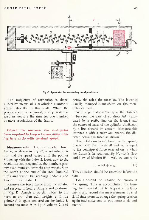
CENTRIPETAL FORCE 45

A

Fig. C. Apparatus for measuring centripetal force.

The frequency of revolution is deter-

mined by means of a revolution counter Cgeared directly to the shaft. When the

proper speed is acquired, a stop watch is

used to measure the time for one hundred

or more revolutions of the frame.

Object. To measure the centripetal

force required to keep a known mass mov-

ing in a circle with constant speed.

Measurements. The centripetal force

frame, as shown in Fig. C, is set into rota-

tion and the speed varied until the pointer

P lines up with the index Z. Look now to the

revolution counter, and as the numbers pass

any even hundred, start the stop watch. Stop

the watch at the end of the next hundred

turns and record the readings under n and

t as shown in Table 1.

Remove the force frame from the rotator

and suspend it from a clamp stand as shown

in Fig. D. Attach a weight holder to the

mass m and then add weights until the

pointer P is again centered on the index Z.

Record the mass Ad in kg in column 2, and

below the table the mass m. The latter is

usually stamped somewhere on the metal

cylinder itself.

With a pair of dividers span the distance

r between the axis of rotation AA' (indi-

cated by a scribe line on the frame) and

the center of mass of the cylinder (indicated

by a line around its center). Measure this

distance r with a ruler and record the dis-

tance below the table as shown.

The total downward force on the spring,

due to both the masses Ad and m, is equal

to the centripetal force exerted on m when

the frame is in rotation. By Newton’s Sec-

ond Law of Motion (F = ma), we can write

F = (M + m)g (10)

This equation should be recorded below the

table.

For a second trial change the tension in

the spring. This is accomplished by turn-

ing the threaded nut N. Repeat all adjust-

ments and record the measurements as trial

2. If time permits, change the spring tension

again and make one or two more trials and

record.


Fig. D. Centripetal force apparatus.

Data. If you have recorded the data,

the various readings you will have written

down will look like those given in Table 1.

Calculations. With the data recorded in

Table 1, the calculations to be made are

best carried out and tabulated under the

headings shown in Table 2.

The first row of calculations are already

completed, and may be used as a guide for


Trial

M(kg)

n

(turns)

t

(sec)

1 2.60 100 1 1.4

2 2.70 200 22.3

3 2.90 200 21.6

4 3.10 300 31.5

m = 0.1527 kg; r = 0.058 m

the other trials. Column 2 is calculated

from the data recorded in columns 3 and 4

in Table 1. The angular velocity <o is next

found by use of Eq. (5). Column 5 is cal-

culated by using Eq. (9), and column 6

by using Eq. (10).

Results. Column 5 of Table 2 gives the

centripetal force obtained by spinning the

apparatus, while column 6 gives the gravita-

tional force required to stretch the spring

the same amount. These two forces should

be equal in magnitude, and any differences

between the values in the last two columns

may be ascribed to experimental error.

Include a graph in your final report,

plotting (o2 vertically against F horizontally.

Make the vertical scale eight squares high

and label them 0, 500, 1000, . . . 4000

rad/sec. Make the horizontal scale seven

squares wide and label them 0, 5, 10, 15,

. . . 35 newtons.


your final report of what you have learned

from this experiment.


n/t CO CO2 mrco2 F

Trial (rps) (rad/sec) (rad/sec) 2 (newtons) (newtons)

1 8.77 55.0 3020 26.8 26.9

MOMENT OF INERTIA 47

Mechanics|

Lesson 43

MOMENT OF INERTIA

Our last experiment in mechanics

is concerned with the determination of the

moment of inertia of several regularly

shaped bodies. These bodies are readily

made from f-in. plywood and take the form

of a ring, a disk, and a rectangle.

or axle should be on the back face of the

disk, thereby leaving the front face clear for

mounting objects.) The rotational counter-

part of the force equation in linear motion

is the torque equation

L = la ( 1 )

Theory. We begin with a large disk of

|-in. plywood about 60 cm in diameter,

with a smaller disk of f-in. plywood glued

tightly to it as shown in Fig. A. As a wheel

and axle this basic turntable is mounted on

the front hub of a bicycle wheel and fastened

to the wall so it is free to turn about a

horizontal axis. A cord wrapped around the

axle several times has one end looped

over a small wire nail to keep it from slip-

ping and the other end fastened to a small

weight of mass m. {Note: The smaller disk

In this experiment we will determine by

measurement the values of the torque L

and the angular acceleration a, and calculate

the moment of inertia I. Transposing Eq.

(1), we have

a(2 )

The torque L acting on the turntable is

given by

L = FXrwhere in Fig. A it can be seen that

Fig. A. Turntable apparatus for experiment

of inertia.

Consequently we will use the relation

that

(3)mgr

To find the angular acceleration a we

use the angular formula for acceleration,

which is the counterpart of the linear equa-

tion.

9 = \at2(4)

Solving for a, we obtain

20

t2 (5)

1m

Now we are going to measure 9 and t to

find a, and measure m and r to find the

mg

torque L. These, substituted in Eq. (2), will

give us the moment of inertia I.


Fig. B. Diagrams of objects used in this experiment on

moment of inertia.

Object. The object of this experiment

is to determine the moment of inertia of

several regularly shaped bodies.

Apparatus. Besides the wheel and axle

shown in Fig. A we will use three objects

having the shapes shown in Fig. B. The

first is a uniform ring B, the second a disk

C, and the third a rectangle D. A set of

weights, a beam balance, and a stop watch,

or clock, are needed for weighing and meas-

uring time.

Procedure and Measurements. The first

step is to wrap the cord around the axle

several times, hang a 40-gm mass from the

end of the cord, and turn the disk so the

line drawn on it lines up with the starting

marker S. As the wheel is released and

starts from rest, start the watch. After three

complete turns of the wheel, stop the watch.

Repeat this timing process several times and

take the average time. Next measure the

radius r for the axle. Record your readings

in a table of eight columns with headings

like those shown in Table 1.

For the second trial weigh object B and

record its mass M. Measure the inside and

outside diameters and record under D in

Table 1. Mount the ring on the wheel and

axle with two small screws, being careful

to center it well so the entire system will

balance and rotate smoothly. Now wrap the

cord around the axle, attach a small mass of

60 gm to the cord, and again determine the

time for this system to make three complete

turns. Record the data as illustrated in row

two of Table 1.

Weigh the disk C and measure its di-

ameter. Remove the ring from the wheel and

axle, and attach the disk. Wrap the cord

around the axle, again attach a 60-gm mass,

and measure the time for three complete

turns.

Repeat this procedure for the rectangular

block and record the data.

Data. Let us assume that we have re-

corded the data as shown in Table 1, and

proceed to make calculations.

Calculations. Your calculations can be

conveniently recorded in a table of eight

columns as shown in Table 2.

The calculations for objects A and B are

already given and will serve as a guide and

check upon your method. Although the last

column is not filled in for A, computations


Object

D

(m)

R

(m)

M(kg)

m(kg) (m)

Q

(rev)

t

(sec)

A.420 .210

— .040 .068 3 7.3

B.510 .255

.925 .060 .068 3 9.1

C .384 .192 1.220 .060 .068 3 7.5

D .548 .274 1.180 .060 .068 3 8.0

MOMENT OF INERTIA 49


mg L 26 t2 a I /

Object (newtons) (newton m) (rad) (sec) 2 (rad/sec) (meas.) (theory)

A .392 .0267 37.7 53.3 .708 .0377 —B .588 .0400 37.7 82.8 .455 .0503 .0508

using the theoretical formulas should be

made and filled in for C and D. For this pur-

pose use the formulas shown in Fig. B. Cal-

culations for all other columns are made by

using Eqs. (3), (5), and (2) in that order.

Remember that when each of the objects

B, C, and D is mounted on the turntable,

the measurements of m, 6,and t are for the

entire rotating system. Therefore, when the

value of I is first calculated, the moment of

inertia I = 0.0377 kg m2 must be subtracted

from it to find the Z (meas.) and recorded

in column 7. A comparison of 1 (meas.)

with I (theory) for each of the bodies B, C,

and D will indicate the magnitude of any ex-

perimental errors.

Results and Conclusions. Make a brief

statement of what you have learned in this

experiment.

PROPERTIES

OF MATTER

Properties of Matter|

Lesson 2

HOOKE'S LAW

This is a laboratory experiment

on the elasticity of steel. In it we are going

to apply Hooke’s law to the stretching of a

steel wire and, from the measurements,

determine a constant called Young's modu-lus.

Theory. The principles involved in this

experiment and the formulas we will use

come directly from the preceding lesson on

elasticity. A long thin wire is suspended

from a rigid support, and a mass m is ap-

plied to the lower end to stretch it as shown

at the left in Fig. A.

We introduce again the two quantities,

called stress and strain, by the following

relations

:

stress = ~rA

F = mg ( 1 )

A is the cross-sectional area of the wire,

and is shown exaggerated at the right in

Fig. A. The original length of the wire is

given by /, and the elongation or amount of

stretch is given by e. The ratio of stress

divided by strain is called Young’s modulus

Y.

F

e

I

Inverting the denominator and multiply-

ing, we obtain

(2 )

strain =j

F is the force applied to stretch the wire

and is equal to mg.

Fig. A. Stress and strain factors in the stretching of a

wire.

By measuring the four quantities F, I, A,

and e, the elastic constant Y can be calcu-

lated.

Apparatus. A thin steel wire, called

piano wire, about one meter long is sus-

pended from a rigid support as shown in

Fig. B. The crossbar at the top must be

several inches thick to reduce bending to a

minimum. The wire is twisted tightly around

a metal rod P, with the rod resting on a metal

plate 5.

The lower end of the wire contains a

tightly twisted loop fitted around the hook

of a 1-kg weight holder. As 500-gm weights

are added to the load, one after the other,

the wire will stretch by very small amounts.

To measure this elongation accurately, a

mechanical lever system shown in Fig. C is

used. This latter is but one of many methods

that have been devised for such purposes.

A small collar C with a setscrew is

52

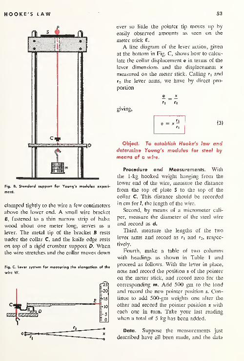
HOOKE'S LAW 53

merit.

clamped tightly to the wire a few centimeters

above the lower end. A small wire bracket

B, fastened to a thin narrow strip of balsa

wood about one meter long, serves as a

lever. The metal tip of the bracket B rests

under the collar C, and the knife edge rests

on top of a rigid crossbar support D. Whenthe wire stretches and the collar moves down

Fig. C. Lever system for measuring the elongation of the

wire W.

ever so little the pointer tip moves up by

easily observed amounts as seen on the

meter stick E.

A line diagram of the lever action, given

at the bottom in Fig. C, shows how to calcu-

late the collar displacement e in terms of the

lever dimensions and the displacement x

measured on the meter stick. Calling r x and

r2 the lever arms, we have by direct pro-

portion

£ _ X

ri r2

giving,

r\e = x

r2(3)

Object. To establish Hooke's law anddetermine Young's modulus for steel by

means of a wire.

Procedure and Measurements. With

the 1-kg hooked weight hanging from the

lower end of the wire, measure the distance

from the top of plate S to the top of the

collar C. This distance should be recorded

in cm for /, the length of the wire.

Second, by means of a micrometer cali-

per, measure the diameter of the steel wire

and record as d.

Third, measure the lengths of the two

lever arms and record as rx and r2 ,respec-

tively.

Fourth, make a table of two columns

with headings as shown in Table 1 and

proceed as follows. With the lever in place,

note and record the position s of the pointer

on the meter stick, and record zero for the

corresponding m. Add 500 gm to the load

and record the new pointer position s. Con-

tinue to add 500-gm weights one after the

other and record the pointer position s with

each one in turn. Take your last reading

when a total of 5 kg has been added.

Data. Suppose the measurements just

described have all been made, and the data

54 PROPERTIES OF MATTER-LESSON 2

in Table 1 have been recorded. All meas-

urements and calculations are in cgs units.

/ = 126.4 cm

d = 0.0320 cm

ri = 2.9 cm

r2 = 92.5 cm


m(gm) (cm)

0 10.0

500 11.25

1000 12.45

1500 13.70

2000 14.90

2500 16.15

3000 17.40

3500 18.60

4000 19.85

4500 21.10

5000 22.30

We will proceed to use these data for our

calculations.

Calculations. Make a table of three col-

umns as shown in Table 2 and determine

Table 2. Calculations

X e F

(cm) (cm) (dynes)

0 0 0

1.25 .0390 4.9 X 105

e and F for all readings. The first two rows

have been filled in to serve as your guide

in completing the calculations.

When you have completed the table,

plot a graph from the values in the last two

columns. Make your graph 8 cm high for

the e scale and 10 cm wide for the F scale.

Plot the points very carefully and draw

your graph line carefully through the points.

Determine from your graph the value of

e for a force F of 50 x 105 dynes. Substi-

tute this value of e and F in Eq. (2), along

with your calculated cross-sectional area Aand wire length I, and compute the value

of V. While there are other ways of using

these data to calculate Y, the method de-

scribed here is quite acceptable.

Results and Conclusions. The accepted

value of Young’s modulus for steel is 19.0 X

1011 dynes/cm2. Assuming this to be the

correct value for the steel wire used in this

experiment, calculate the percentage error

of your final calculated value. To do this,

use the following procedure: Take the dif-

ference between your experimental value

and the accepted value, divide by the ac-

cepted value, and multiply by one hundred.

Symbolically

acc. value — exp. value wx i uuacc. value

= percent error

Your final report should include an an-

swer to the following question: What con-

clusion can you draw from your graph?

PRESSURE IN LIQUIDS 55


Lesson 5

PRESSURE IN LIQUIDS

The purpose of this experiment

is to measure the pressure at different depths

within a vessel of water.

Theory. You will remember from our

previous lesson on liquid pressure that

( 1 )

and that the force on any given area is

given by

F = pA (2)

Furthermore, the total downward force

on any given area like that shown in Fig. Ais given by the weight of the column of fluid

above it. To find the weight of a column of

liquid it is convenient to know the liquid

density or weight density.

Fig. A. Pressure within a liquid increases with depth.

The density of any given substance or

body of matter is given by the mass per

unit volume. To find the density one deter-

mines the volume of a given mass of the

substance and divides one by the other.

density =mass

volume

In algebraic symbols

where the Greek letter P stands for density.

In the English system of units it is com-

mon to find the weight of a given substance,

rather than its mass, and to determine what

is called its weight density. Weight density

is defined as the weight per unit volume

and is given by

... . weightweight density = —;

volume

which in algebraic symbols can be written

(4)

The densities and weight densities of a

few common materials are given in Table 1.

The mass of any column of liquid is

given by Eq. (3). Transposing this equa-

tion, we obtain

M = pV (5)

To find the weight of any mass M we

multiply by g the acceleration due to gravity.

The weight, then, is the total downward

force F of a liquid column, and we can write

F = Mg (6)

and then

F = pVg

56

Table 1. Densities and Weight-Densities

of a Few Common Materials

PROPERTIES OF M A T T E R - L E S S O N 5

Material

P

(gm/cm 3)

Pw

(Ib/ft3 )

alcohol .79 49.3

benzine .70 43.7

blood 1.04 65.0

gasoline .69 41.2

mercury 13.6 849

olive oil .918 57.3

water 1.000 62.4

aluminum 2.7 169

copper 8.9 556

gold 19.3 1205

iron 7.9 493

lead 11.4 712

The volume V of a column of liquid (see

Fig. A) is given by

V = hA (7)

so that, upon substitution in Eq. (6), wehave

F = phAg (8)

By direct substitution of phAg for F in

Eq. ( 1 ) , we obtain our final equation.

Fig. B. Floating cylinder for measuring liquid pressure.

Object. To determine the pressure at

different depths within a liquid and to

establish the relation between pressure

and depth .

or

(9)

P = hpg ( 10 )

Apparatus. The apparatus to be used in

this experiment consists of a hollow glass

tube about 60 cm long and 4.0 cm outside

diameter and open at both ends. See Fig. B.

About 150 gm of lead shot are dropped into

the bottom of the tube, and some melted par-

affin is poured over the shot to hold it in

place.

The tube is placed with the weighted enddown in a tall cylinder containing water, andwe are ready to proceed with measurements.

Procedure and Measurements. With the

weighted tube in the water, slide a rubber

band over the tube and down to the water

level. Remove the tube and measure the

depth h. Weigh the tube and record its

mass M along with fi in a table of four col-

umns. Measure the outside diameter of

the tube and record as d below the table.

Add a 50-gm weight to the lead shot at

the bottom of the tube, insert the tube up-

right in the water, mark the water level

with a rubber band, and record the depth h

as trial 2. Repeat this procedure for a total

of five trials, adding 50 more grams with

each trial and recording the depth h in

Table 2.

Dissolve a quantity of salt in the water

DENSITY AND W E I G H T - D E N S I T Y 57

and repeat the above experiment. Use the

same weights in the tube as before and re-

cord the depth for the five trials.

Data. We will assume that the experi-

ment has been carried out and the data

recorded as shown in Table 2.


Mass Water Salt Water

M h h

Trial (gm) (cm) (cm)

1 375 30.0 26.6

2 425 33.6 30.0

3 475 37.8 33.9

4 525 41.7 37.0

5 575 45.8 40.8

d = 4.0 cm


this experiment you should make a table of

four columns with headings as shown in

Table 3. The results for the first trial have

been computed and will serve as a guide for

the remaining trials.

Table 3. Calculated Results for Water

F P hpg

Trial (dynes) (dynes/cm2) (dynes/cm2

)

1 368,000 29,300 29,400

To find the values of F for column 2,

follow Eq. (6) and multiply the M values in

Table 2 by 980 cm/sec2. With the measured

cylinder diameter d calculate the cylinder

area A. Having found the values of F in

column 2, use Eq. (1) to calculate the

values of p in column 3.

Values of hPg in column 4 are obtained

from the values of h in Table 2, the density

of water which is 1 gm/cm3,and the value

of g = 980 cm/sec2. See Eq. (10).

Conclusions. Find the salt water density

by using Eq. (3), the last value of M in

Table 2, and the corresponding value of h.

Use Eq. (7) to find V.

Plot a graph of h against p for the water.

The vertical scale for h should go from 0

to 50 cm, and the horizontal scale for pfrom 0 to 5 X 104 dynes/cm2

. Draw a

straight line from the origin through the

plotted points.


Lesson 7

DENSITY AND WEIGHT-DENSITY

In this experiment we are going

to make use of the principles of buoyancy to

determine the densities and weight-densities

of several common materials. The methodis undoubtedly similar to that used by Ar-

chimedes over 2000 years ago when he de-

termined the density of the metal in King

Hiero’s crown and found it was not made of

solid gold.

Theory. We have seen in previous les-

sons that the density P ,and the weight-

density Pw ,of any substance are given by

the relations

_ WPW — y

(2 )

58 PROPERTIES OF M A T T E R - L E S S O N 7

The density is usually given in gm/cm3,

and the weight-density in lb/ft3 .

The term specific gravity is often used

to designate the relative density of a ma-

terial, and it is defined as the weight of any

given body divided by the weight of an

equal volume of water.

= wt °f body(3 )

wt of equal vol water

Because of the fact that the gram is de-

fined as the mass of one cubic centimeter of

water, the specific gravity of any substance

is given by the same number as the density

in grams per cubic centimeter. For example,

the density of mercury is 13.6 gm/cm3,

while the specific gravity of mercury is 13.6.

The latter has no units: it is just the ratio

of two weights as given by Eq. (3).

Apparatus. To experimentally deter-

mine the density of materials, we are going

to weigh several objects, determine their

respective volumes by the principles of

buoyancy, substitute in Eq. ( 1 ) ,and calcu-

late p.

Fig. B. Weighings for materials denser than water.

By means of a platform balance the object

in question is suspended from one side and

its mass M determined by adding weights

to the other side. The body is then sub-

merged in water and again weighted to find

its apparent mass M A . See Fig. B.

The loss in mass M — A1 4 is equal to the

mass of the displaced water, and therefore

equal to the volume of the body. By direct

substitution in Eq. (1)

I Mp M- Ma

Part 1. If the object sinks in water, wewill employ the method shown in Fig. A.

Fig. A. Platform balance arrangement for weighing sub-

merged objects.

Part 2. If the object floats in water, wewill employ the same balance but use a

lead weight to sink the object while weigh-

ing. As shown in Fig. C, the body is first

weighed in air to find M, then with a sinker

attached and submerged in water it is

weighed again. Finally, with the sinker and

object submerged it is weighed again. M is

Fig. C. Shows the three steps of weighing as used in

Part 2.

DENSITY AND W E I G H T - D E N S i T Y 59

the mass of the object in air, MA its apparent

mass in water, and M s the apparent mass

of the sinker in water.

The loss of weight between the second

and third weighings is just due to the buoy-

ancy of the displaced water. Hence the

volume of the mass M is given by (M +M s ) - (M.i + Mg ). By direct substitution

in Eq. 1 we obtain

p (M -f- Ms) — (Ma + Msj

Object. To employ Archimedes' prin-

ciple of buoyancy to determine the density

and weight-density of several metals and

woods.

Procedure and Measurements. Suspend

an aluminum block, about 1 in. cube, from

the scales and determine its mass in grams.

Bring up a beaker of water and submerge

the block, being sure the block hangs free

of the glass walls. Make a table of five col-

umns as shown in Table 1 and record the

two weighings under M and MA ,respectively.

Repeat these two weighings for a similar

block of brass and again for a block of iron.

Record the measurements in Table 1.

Suspend a small block of maple wood,

about 2 in. by 2 in. by 3 in., from the

balance and determine its mass in grams.

Hang a small lead weight beneath the block,

bring up a beaker of water to submerge the

lead only, and determine the mass (M + Ms).

Finally, submerge the block as well as the

weight (see Fig. C) and again find the mass

(Ma + M s). Record these three weighings in

columns 2, 4, and 5, respectively.

Repeat these three weighings for two

other blocks of hardwood and record the

measured results in Table 1.

Data. Let us assume that the measure-

ments have been made and the data have

been recorded as shown in Table 1. We will

now proceed with the calculations and re-

sults.


Material

M(gm)

Ma(gm)

M T Ms(gm)

MA + Ms(gm)

aluminum 95.2 59.9 — —brass 284.0 250.3 — —iron 268.7 234.7 — —maple 172.5 — 328.7 74.7

walnut 186.4 — 342.6 64.6

oak i 65.5 — 321.7 26.7

Calculations and Results. Make a table

of six columns for your final calculations

and use the headings shown in Table 2.

The results for aluminum are already com-

puted and will serve as a guide for comput-

ing the other five.

The values in column 2 divided by the

values in column 3 give the densities of the

metals, while the values in column 2 di-

vided by the values in column 4 give the

densities of the woods. Multiplying the den-

sities in column 5 by the weight-density

of water, 62.4, will give the weight-densities

in column 6.

Conclusions. Conclude your laboratory

report by a brief statement of what you

have learned from this experiment.


M M- Ma (M + Ms ) P Pw

Material (gm) (grn) —(Ma + Ms) (gm/cm 3

) (lb/ft3)

aluminum 95.2 35.3 — 2.70 168

60 PROPERTIES OF MATTER-LESSON 10

DENSITY OF AIR

In our previous lesson on the

atmosphere we saw how, living on the sur-

face of the earth, we are at the bottom of

an ocean of air and therefore subject to large

and constant pressures. At sea level this

pressure amounts to about 15 lb/in. 2,

or,

as measured with a barometer, 76 cm of

mercury.

Theory. If the mercury column stands

at exactly 76 cm we say we have standard

atmospheric pressure, or a pressure of

one atmosphere. The pressure at any depth

below the surface of a liquid is given by

P = hpg (1)

where h is the height of the liquid column,

p is the liquid density, and g the accelera-

tion due to gravity. Since mercury has a

density of 13.6 gm/cm3,standard atmos-

pheric pressure is given by Eq. (1) as

1 atm = 76 cm X 13.6—, X 980—

2cm 3 sec2

from which

1 atm = 1,013,000^?cm"

(2 )

Since barometric pressure is used so much

by the Weather Bureau as an aid in pre-

dicting the weather, it has become commonpractice to define a new pressure unit called

the bar.

1 bar = 1,000,000 (3)cm2

With this as a definition, we have

1 atm = 1.013 bars (4)

A smaller unit of pressure, the millibar,

is one thousand times smaller, so that


Lesson 10

1 atm = 1013 millibars (5)

It is in millibars that the atmospheric

pressure is indicated on all U.S. weather

maps published daily in Washington, D.C.

In addition to the slight daily variations

in barometric pressure at sea level, the baro-

metric pressure decreases rapidly with alti-

tude. At a height of 3.5 mi the barometer

stands at 38 cm, or half an atmosphere.

This means that if we are 3.5 mi above the

surface of the earth, half the atmosphere lies

below us. At a level 19 mi above sea level

99% of the air lies beneath us.

That air has weight will be shown in this

experiment. Suppose we have a hollow glass

vessel, as shown in Fig. A, and we remove

all the air from inside of it by means of a vac-

uum pump. If we now open the flask to

let air rush in, the amount of air entering

will depend on where we are located. What-

ever amount of air would enter at sea level,

only 50% as much would enter if we were

3.5 mi high, and only 1% as much would

enter at 19 mi. In other words, the mass of

the gas entering the evacuated flask would

depend upon the pressure.

It is for this reason that the density of

Fig. A. Vacuum pump and glass flask used in finding

the density of air.

DENSITY OF AIR 61

Fig. B. Evacuated flask submerged in water fills up as

shown.

air, as well as the density of any gas, is gen-

erally specified as measured at standard at-

mospheric pressure, or one atmosphere. Thedensities of gases, like densities of solids and

liquids, are given by the equation

Apparatus. The apparatus used in this

experiment consists of a 3 -liter (3000 cm3),

round-bottomed flask and a vacuum pumpVP as shown in Fig. A. A small rectangular

glass-walled aquarium tank is conveniently

used as a reservoir for submerging the flask

as shown in Fig. B.

Object. To measure the density of air

at room temperature and pressure.

Procedure and Measurements. Because

of the hazards connected with the breaking

of an evacuated glass vessel this experiment

had best be done by the instructor while

you observe and record the data.

With a stopcock and rubber stopper fitted

to the flask, place the assembly on the plat-

form of a balance and determine its mass in

grams. Record as in Table 1.

Fit the vacuum pump hose over the stop-

cock opening and remove the air from the

vessel as shown in Fig. A. Close the stop-

cock S, shut off the vacuum pump, and dis-

connect the vacuum pump hose. Weigh the

evacuated flask assembly and again record

its mass in grams.

Finally submerge the flask in the water

tank as shown in Fig. B and very slowly

open the stopcock. Be sure to keep the flask

opening below the water surface to avoid

the entrance of any air. When no more water

appears to be entering the flask bring the

water level inside the flask even with

the water level outside. In this position only,

close the stopcock.

Remove the flask from the tank, wipe the

sides dry, and weigh the entire assembly.

Record the mass in Table 1.

Since no vacuum pump can remove quite

all of the air from a vessel, the flask will

never fill completely with water. By bringing

the two water levels together when closing

the stopcock the residual air in the flask will

be at the same pressure as the air outside,

and this is the same as the pressure of the

air filling the vessel in A.

Data. Let us assume that the experi-

ment has been performed and we have re-

corded the data as shown in Table 1.


A, mass of flask in air 5 12.2 gm

8, mass of evacuated flask 508.6 gm

C, mass of flask and water 3362.2 gm

Calculations. To determine the density

of air, your calculations can best be carried

out in four steps. These steps

their proper order in Table 2.

are listed in


mass of air (A — B) gm

mass of water (C — B) gm

volume of air cm3

density of air, p = gm/cm3

The first two steps are self-explanatory.

For the third step it should be noted that

1 cm3 of water has a mass of 1 gm. There-

fore the mass of water in grams is equal


numerically to the volume of the air re-

moved in cm3. For the fourth step use Eq.

( 6 ).

Results and Conclusions. Find the per-

centage error between the value of P ob-

tained from this experiment and the accepted

value of 0.00129 gm/cm3. In writing your

final report, answer the following questions:

1. Which of the three weighings requires

the utmost accuracy?

2. Which, if any, requires little accuracy?

Explain.


Lesson 12

FLUID FRICTION

When water flows through a pipe,

fluid friction tends to hold it back. Not only

does the viscosity set up retarding forces to

flow but the attractive forces between the

pipe walls and fluid molecules oppose the

motion.

Theory. In Properties of Matter, Lesson

1 1 ,a demonstration experiment there shown

in Fig. B was performed in which the con-

cepts of velocity head, friction head, and

pressure head were introduced. The water

pressure p at the pipe entrance J is given by

the height of the water column h.

Just inside the pipe at K the water is

flowing with a velocity v, and the pressure

is somewhat lower. The pressure difference

between points J and K, called the velocity

head hv ,is required to start the water from

rest at J and give it a velocity v as it enters

the pipe. This velocity head is given by

Torricelli’s theorem as

Although the velocity v along the uniform

pipe remains constant, fluid friction causes

the pressure all along the pipe to fall uni-

formly as indicated by the water levels in the

standpipes. The pressure differences between

the horizontal pipe ends, both measured

where the fluid has the velocity v, is called

the friction head.

Finally, the pressure drop between D, a

point just inside the pipe, and the point Z,

just outside, is called the final pressure head.

Hence the entrance pressure p is divided

into three parts, such that

p = hv 4- hf + hp (2)

In this experiment we propose to deter-

mine the flow velocity v by measuring the

quantity of water flowing through the pipe

per second. At flow velocities usually en-

countered, some turbulence also occurs. Onefinds by experiment that the friction head hfis proportional to the square of the flow ve-

locity, v2.

hf = Kv2

|

(3)

Let water flow through a uniform pipe

with a velocity v as shown in Fig. A. In 1

sec a column of water v cm long will flow

past any given point P, or out of the end.

The volume of this water flowing per second

Fig. A. Diagram showing the relation between the size

of a pipe and the rate of flow of a fluid.

FLUID FRICTION 63

is just the volume of the cylinder vA. If

we now collect in a measuring cup a volume

of water Q in a measured time interval f, wecan compute the volume of water flowing per

second. Therefore,

and, upon transposing, we find

Apparatus. The flow apparatus is

shown in Fig. B. In addition to this we will

use a graduated cylinder for measuring the

volume of water collected and a stop watch

or clock to measure the time of collection.

Object. To determine the velocity

head, the friction head, and the pressure

head of water flowing through a uniform

pipe.

Measurements. Open the valves V and

5 and adjust the water flow in and out until

a steady state of conditions approximately

like those shown in Fig. B exist. The over-

flow pipe at O helps maintain a constant

water level at a,and hence a constant pres-

sure p.

Insert the graduated cylinder in the outlet

stream and collect water for 15 sec. Measure

the quantity of water and record in Table 1.

With a meter stick locate the points A, B,

C, and D, and record them in Table 1 as

shown.

Readjust valves V and S for a more rapid

flow of water, and after steady conditions

have been achieved, repeat all measurements

and record them as trial 2. If time permits,

make third and fourth trial runs. {Note: Asmall cork in each of the standpipes will

float at the water surface as shown and mayhelp in setting the straight edge along the

tops of the water columns, thus serving as

an aid in locating points B and C.

)

64 PROPERTIES OF M A TT E R - L E S S O N 15

Measure the inside diameter of the flow

pipe. This is best done with an internal

caliper. Measure and record the pipe length /.

Data. We will assume that four trial

runs have been made and that the data has



Trial

Q(cm 3

)

t

(sec)

A

(cm)

B

(cm)

C(cm)

D

(cm)

1 340 15 40.9 38.1 29.7 0

2 460 15 40.9 35.7 20.4 0

3 570 15 40.8 32.8 9.0 0

4 640 15 40.8 30.6 0.5 0

pipe diameter = 0.620 cm

pipe length = 56.0 cm

Calculations and Results. The calcu-

lated results are best collected in a table of

seven columns with headings as shown in

Table 2. The results of the first trial are in-

cluded for comparison purposes and will

serve as your guide in completing the cal-

culations for the other three trials.


Trial

V

(cm/sec)

V2

(cm/sec) 2

h v

(cm)

calc.

f>„

(cm)

meas.

hf

(cm)

hp

(cm)

1 75.1 5640 2.88 2.8 8.4 29.7

First, from the measured pipe diameter

d m 0.620 cm, calculate the pipe’s cross-

sectional area A. Then substitute in Eq.

(4), along with the values of Q and t, to

obtain v recorded in column 2.

Column 4 is calculated by use of Eq. ( 1 ),

where g = 980 cm/sec2. Columns 5, 6, and

7 are just the differences A — B, B — C,

and C — D, respectively.

Plot a graph of your results from columns 3

and 6. The friction head hf plotted vertically

should have divisions marked 0, 5, 10, . . .

30 cm, while the v2 values plotted hori-

zontally should have divisions marked 0,

0.5, 1.0, 1.5, and 2.0 x 104 cm2/sec2 .

Conclusions. What can you conclude

from the graph drawn for this experiment?

Compare with Eq. (3).


Lesson 15

THE PENDULUM

In this laboratory experiment we

are going to study pendulums of two dif-

ferent kinds. One is called a simple pendu-

lum, and the other is called a spring pen-

dulum.

Theory. Diagrams of a simple pendulum

and a spring pendulum are shown in Fig. A.

The simple pendulum consists of a small

heavy weight, called a bob B, suspended by

a thin cord or wire from a pivot P. When

the bob is pulled to one side and released,

the pendulum will swing back and forth with

periodic motion.

The spring pendulum consists of a small

heavy weight W suspended by a coil spring

fastened to a support S. When the weight

of mass m is pulled down a short distance

and released, it will move up and down with

periodic motion called simple harmonic

motion.

In Properties of Matter, Lesson 14, on vi-

THE PENDULUM 65

, , , , ,, ,Fig. B. Pendulum support and pivot construction.

Fig. A. Diagrams of (a) a simple pendulum and (b) a

spring pendulum.

brations and waves, it was stated that the

periods of these two kinds of motion are

given by the relations

T = 2ir T-2*^ (1)

where T is the time in seconds required to

make one complete vibration. In these equa-

tions, / is the length of the pendulum meas-

ured from the pivot point to the center of

mass of the bob, g is the acceleration due

to gravity, m is the mass of the weight W,

and k is the spring constant. The constant ft

is determined by the stretching of the spring

with different weights and the application of

Hooke’s law, which in Properties of Matter,

Lesson 1, p. 162, we saw is given by

F = -kx (2)

In this experiment we are going to meas-

sure T and / for several different lengths of a

simple pendulum and with the use of Eq.

(1) compute g, the acceleration due to

gravity. We are also going to measure T

and m for several different weights on the

end of a spring and use Eq. ( 1 ) to compute

k the spring constant. Since g and k are the

unknowns, we should square both equations

in Eq. (1)

P = 4tt2 T2 = 4tt2

79 k

By transposing the measurable quantities

to one side, we obtain

(3)

Note the similarity in the forms of these

two equations.

Apparatus. The simple pendulum in

this experiment consists of a solid metal

sphere about 1.5 inches in diameter and

several lengths of fine steel wire with small

hooks at both ends of each piece. The pivot

mounting is readily made from pieces of

tin and arranged as shown in Fig. B. The

strip of tin A, with its lower edges sharpened

to a knife-edge, rests on the flat surfaces of

a flat tin sheet C. The pendulum lengths are

measured from the knife-edge to the center

of the bob 8, and need only be approxi-

mately 25, 50, 75, and 100 cm, respectively.

A small steel or bronze spring and a set

of metric weights are needed for the spring

pendulum. A stop watch or clock is used

for determining time intervals.

Object. To study the principles of a

simple pendulum as well as the principles

of a spring pendulum.

Procedure and Measurements. Part I.

Suspend the bob, with the shortest wire,

from the knife-edge pivot. Pull the bob

about 2 cm to one side and release it to

swing freely. Determine the time it takes

the pendulum to make 20 complete vibra-

47r2m~fr


tions. Repeat this timing process two more

times and record the average value. For

your data make a table of four columns as

shown in Table 1.

Measure the length of the pendulum and

record the result in the second column of

Table 1. Repeat these measurements for

each of the other three wire lengths and

record /, f, and N as before. When the long-

est wire is used, measure the time for 20

vibrations with starting amplitudes of 1 cm,

4 cm, 7 cm, and 10 cm. It will be difficult

to detect any real difference in the period

as long as the amplitude is this small.

Part 2. Suspend the spiral spring from a

rigid support and attach a metric weight to

the lower end. Select a 100-gm mass for

your first trial. Pull the weight down about

1 cm and release it to vibrate. Determine

the time it takes to make 20 complete vibra-

tions. Repeat this time measurement and

record the average value. For these data

make a table of four columns as shown in

Table 2. Record the mass m, the time t, and

the number of vibrations N. Repeat these

steps and measurements for masses of 200,

300, and 400 gms, and record them in Ta-

ble 2.

Data. Assume that the measurements

described above have been made and the

data have been recorded in Tables 1 and 2.

You should now proceed with the calcula-

tions.

Calculations and Results. To makeyour calculations for Part 1 ,

make a table of

Table 1. Data for Pendulum

Trial

/

(cm)

t

(sec)

N(no. of

vibrations)

1 26.4 20.6 20

2 55.8 30.2 20

3 77.3 35.4 20

4 104.2 40.8 20

Table 2. Data for Spring

Trial

m(gm)

t

(sec)

N(no. of

vib.)

1 100 7.7 20

2 200 10.9 20

3 300 13.4 20

4 400 15.5 20

four columns with headings as shown in

Table 3. The calculations for trial 1 are

Table 3. Results for Pendulum

T T2 4tt2I 9

(sec) (sec2) (cm) (cm/sec2

)

1.03 1.061 1040 980

already given and may be used as a guide

and check upon your calculations for the

others. The period T for one complete vibra-

tion is obtained by dividing the time t in

Table 1 by 20. Values of g in column 4

are obtained by use of Eq. (2) and columns

2 and 3.

Make another table of four columns for

Part 2 calculations, using headings as shown

in Table 4.

Table 4. Results for Spring

T T2 47

r

2m k

(sec) (sec2) (gm) (dynes/cm)

.385 .148 3950 26,700

Conclusions. The four values of g in

the last column of Table 3 should be the

same. Because of experimental errors they

will differ slightly. Find the average value of

g and then compute the percentage error

between the average value and the accepted

value of g = 980 cm/sec.

The four values of the spring constant k

in column 4 of Table 4 should be the same.

Calculate the average value.

THERMAL EXPANSION

Heat|

Lesson 2

There are many instances in en-

gineering where the expansion of solids is

an important factor in design and construc-

tion. Particularly is this true in the con-

struction of suspension bridges and rail-

roads. It was demonstrated in Heat, Les-

son 1, that not all substances expand by the

same amount when heated through the same

difference in temperature. This is illustrated

by the linear coefficients of thermal expan-

sion of a few common substances given in

Table 1.

Table 1. Linear Coefficients

of Thermal Expansion

Material

a

per °C

aluminum 25 X 10-6

brass 18 X 10-6

copper 17 X 10-6

gold 14 X 10-6

iron 1 1 x io-6

platinum 9 X 10~6

silver 18 X IO"6

steel 8 X 10~6

l

Fig. A. A metal rod expands upon heating.

which it is raised, and / its original length.*

To see how Eq. ( 1 ) may be derived, con-

sider a metal rod of length / and at a tem-

perature L as shown in Fig. A. If the

temperature is slowly raised, and the length

is carefully measured for every 10° rise,

the rod is found to become longer in equal

steps as shown in Fig. A.

If one plots a graph of the elongation e

as a function of the temperature t, starting

with 0°C, a graph like the one shown in

Fig. B is obtained. The straight line obtained

* It is customary in formulas to use the letter

/ for temperature on either the Centigrade or

Fahrenheit scale. When absolute temperature mustbe used, however, the capital letter T is used.

Fig. B. Expansion of an iron wire 2 meters long.

iron wire 2 meters long

Theory. The linear coefficient of thermal

expansion a may be defined as the change

in length per unit length of a substance per

1 ° rise in temperature. Once this constant is

known, the linear expansion for any sized

object made of that same material can be

calculated for any rise in temperature by the

following formula:

elongation = a X length X rise in temperature

( 1 )

In this equation L is the original tempera-

ture of the body, t2 the final temperature to

68

temperatur¥

THERMAL EXPANSION 69

is characteristic of the behavior of most

metals and shows that

e cc ( f2 — fj

Since a rod or wire twice as long would pro-

duce double the elongation, one can also

write

e oc /

Combining these two proportionalities,

one obtains

ecc l(t2 - h)

from which we obtain Eq. ( 1 ) . Upon trans-

posing Eq. (1) we obtain

(2 )

This is the relation we will use in calculating

the results of this experiment.


for measuring the expansion of metals is

shown in Fig. C. Any one of several rods

AB with cork stoppers on both ends is

mounted inside a metal jacket as indicated.

Steam from a small boiler H flows into the

jacket at C, around the rod, and out at D.

A thumbscrew R presses against one end of

the rod, and the tip of a lever L presses

Fig. C. Expansion apparatus showing boiler, steam

jacket, thermometer, mechanical pointer, and rod.

against the other. The temperature can be

measured at any time with the dial ther-

mometer T, and the expansion e is deter-

mined by the pointer readings Si and S2 on

the scale.

If r i and r2 represent the lengths of the

two lever arms as shown in the figure, the

elongation e is given by

e = ~(S-2 - SOf2

(3)

Object. To determine the linear coef-

ficient of thermal expansion for several

common metals .

Procedure and Measurements. Select

an aluminum rod, and after measuring its

length to the nearest millimeter with a meter

stick, insert it in the steam jacket as shown

in Fig. C. Turn up the thumbscrew R until

the thrust on the lever L at the other end

pushes the scale pointer to the 0.5-cm mark.

Note the temperature indicated on the ther-

mometer and record these initial measure-

ments in a table of six columns as shown in

Table 2.

Connect the steam hose from the water

boiler to the jacket and watch the thermom-

eter as the temperature rises. When the

thermometer stops rising, note the tempera-

ture t2 as well as the lever pointer reading S2 .

Record these in Table 2.

Disconnect the steam hose and cool the

jacket by immersing it in cold water. Select

a copper rod, measure its length, and insert

it in the jacket. Mount the jacket in its sup-

ports and repeat the steps described for the

aluminum rod. Record all readings in Table

2.

Repeat the above measurements with two

more rods, one of which is of an unknownmetal.

Data. Suppose that you have completed

the measurements on four metal rods and

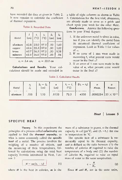
70 HEAT-LESSON 5

have recorded the data as given in Table 2.

It now remains to calculate the coefficient

of thermal expansion.


Metal

/

(cm)

h

(°C)

h

(°C)

Si

(cm)

s2

(cm)

aluminum 62.8 25.0 97.5 .50 1.60

copper 62.6 25.5 97.0 .50 1.22

brass 62.7 26.5 97.5 .50 1.28

unknown 62.5 26.0 97.0 .50 .96

ri — 3.4 cm; r2 = 32.5 cm

Calculations and Results. Your cal-

culations should be made and recorded in

a table of eight columns as shown in Table

3. Calculations for the first trial, aluminum,

are already made to serve as a guide andcheck upon your work for the other three.

Conclusions. Answer the following ques-

tions in your Final Report:

1 . If the unknown metal is silver in color,

see if you can identify the metal from

its measured thermal coefficient of

expansion. Look in Table 1 for values

of a.

2. If an error of 1 mm were made in

measuring /, what percent error would

occur in the final «?

3. If an error of 1 mm were made in the

value of e, what percent error would

occur in the final a?


ri S2 - Si e h ~ h l(t2—

fi) a a

Metal r2 (cm) (cm) (°C) Meas. Known

aluminum .105 1.10 .1 155 72.5 4550 .0000254 25 X IQ"6

Heat|

Lesson 5

SPECIFIC HEAT

Theory. In this experiment the

principles of a process called calorimetry are

applied to find the thermal capacity, or

what is more commonly called the specific

heat of a metal. The process involves the

weighing of a number of objects, and

the measuring of their temperatures, fol-

lowed by calculations using the total heat

capacity formula introduced in Heat, Les-

son 3

H = me ( to — ti) ( 1 )

where H is the heat in calories, m is the

mass of a substance in grams, c the thermal

capacity in cal/gm°C, and ( t2 —L) the rise

in temperature in °C.

The specific heat of a substance is nu-

merically equal to its thermal capacity,

and is defined as the ratio between (1) the

number of calories H required to raise the

temperature of a body and (2) the number

of calories Hw required to raise an equal

mass of water to the same temperature.

Since H and Hw are in the same units,

SPECIFIC HEAT 71

their units cancel out, and c has no dimen-

sions. While the c in Eq. ( 1 ) is actually the

thermal capacity, it is quite common to call

it the specific heat.


experiment consists of two principal parts.

The first part, shown in Fig. A, is a steam

boiler in which a quantity of metal m is

heated to the temperature of boiling water.

The second part, shown in Fig. B, is a

double-walled brass cup, called a calorime-

ter, containing a known amount of water,

a thermometer, and a brass stirrer. Mercury

or dial thermometers are used for measuring

temperatures, and a platform balance is used

for determining the masses of objects.

Object. To employ the principles of

calorimetry to find the specific heat of ametal.

Procedure and Measurements. Put the

small metal cup, the one that fits into the

boiler top, on the scales and determine its

mass. Pour into this cup about 500 gm of

Fig. B. Diagram of a calorimeter, with a thermometer,

stirrer, and water.

lead shot and weigh again. Record the dif-

ference in these two mass readings as m,

the mass of the metal whose specific heat

is to be determined, as in Table 1.

Insert this cup into the boiler as shown

in Fig. A, and while the metal is being

heated, remove the inner calorimeter cup

and find its mass. Record the cup’s mass as

m0 . See Table 1. Now pour into this cup

about 150 cm3 of cold water and again find

the mass. Record the difference between

these two masses as the mass of the water

mw . The best results will be obtained if the

temperature of this water is about 5 to 8°

below room temperature. Weigh the stirrer

and record its mass as ms .

When the temperature of the lead shot

has reached its highest point (about 99 °C),

note and record the temperature as t3 . Re-

cord the temperature 11 of the water in the

calorimeter cup, and then quickly lift the

lead-shot container from the boiler and pour

it into the water. Stir the shot and water, and

record the highest temperature reached by

the water-metal mixture as f2 . See Fig. C.

72 HEAT-LESSON 5

Fig. C. Calorimeter with lead shot, thermometer, stirrer,

and water.

Look in Table 1 of Heat, Lesson 3, for

the specific heat of the metal of which the

inner calorimeter cup is composed and re-

cord it as cc . Do the same for the stirrer and

record it as cs .

Data. Assume now that all the measure-

ments described above have been made, and

they are recorded as shown in Table 1.


tions to find the specific heat of the lead

metal we apply Eq. (1) to all parts of the

apparatus that gained or lost heat during

the mixing process. To keep things straight

we put under one heading all quantities of

Heat Lost and under another all quantities of


mass of metal m = 512 gmmass of water mw = 1 54 gmmass of cup mc = 62.2 gmmass of stirrer m s

= 3 1 .5 gminitial t of water h = 21.5°C

final t of water h = 28.3°C

hot metal t h = 99.0°C

sp ht of cup Cc = .092

sp ht of stirrer Cs = .092

Heat Gained . In the notation of the re-

corded data of Table 1, these are

Heat Lost

H = mc(t3 — h) (3)

Heat Gained

Hw= mwcw(t2 — h) (4)

Hc = m ccc(t2 — h) (5)

Hs = m scs(t2 — ti) (6)

By conservation of energy we can nowwrite

Heat Lost = Heat Gained (7)

Hence we obtain

H = Hw + Hc + Hs (8 )

Substitute the measured values from Ta-

ble 1 in Eqs. (3), (4), (5), and (6), and

calculate the only unknown, the specific heat

of lead c. Assume the specific heat of water,

cw — 1.0. As a guide for your calculations

the following substitutions are given for Hs :

Hs = 31.5 X .092 X (28.3 - 21.5)

Hs = 31.5 X .092 X 6.8

Hs = 19.7 calories

Conclusions. Compare your final cal-

culated value of c with the accepted value

and calculate the percentage error. The ac-

cepted value for lead is c = .0310.

HEAT OF FUSION 73

Heat|

Lesson 7

HEAT OF FUSION

When heat is continually added

to a solid body, its temperature will rise un-

til it reaches the melting point. At this tem-

perature added heat will no longer raise the

temperature but will be absorbed by the sub-

stance causing it to melt. Not until a suffi-

cient amount of heat has been added to melt

all the substance will the continued addition

of heat raise the temperature of the liquid

above its melting point.

Such a change of state from the solid to

liquid was briefly discussed in the case of

water in Heat, Lesson 3. There, in Fig. B,

the melting of ice into water and the boiling

of water into steam was shown graphically

to illustrate changes of state. Part of this

graph is reproduced in Fig. A to illustrate

the latent heat of fusion of ice as 80 cal/gm.

This is the constant we propose to determine

in this experiment.

Theory. The latent heat of fusion is

defined as the quantity of heat required to

change 7 gm of a solid into 1 gm of liquid

with no change in temperature. The re-

verse of fusion is solidification, a process in

Fig. A. Graph showing the change in temperature and

change of state as heat is added to 1 gm of ice.

which heat is liberated by the substance as it

changes from the liquid to the solid state.

The amount of heat liberated by matter

on solidification is equal to the amount of

heat taken in on fusion; pure water on freez-

ing gives up 80 cal/gm and on melting takes

in 80 cal/gm.

Let L represent the latent heat of fusion

and m the mass of a given substance to be

fused or solidified. The quantity of heat re-

quired or liberated, as the case may be, is

given by

H = mL ( 1 )

If m is the mass in grams, then L is in

cal/gm and H is in calories.

The latent heat of fusion for several com-

mon substances is given in Table 1.

Table 1. Heat of Fusion

Substance

L

(cal/gm)

aluminum 77

copper 42

gold 16

mercury 2.8

platinum 27

silver 21

tin 14

water 80


experiment on the latent heat of fusion of

ice is the following. Some clear cracked ice,

a calorimeter with thermometer and stirrer,

a platform balance, a set of weights, and a

towel are needed.

74 HEAT-LESSON 7

Fig. B. Calorimeter cup, stirrer, thermometer, and cracked

ice for experiment.

Object. To determine the latent heat

of fusion of ice.

Procedure and Measurements. Using

the platform balance, find the mass of the

stirrer. Place the inner calorimeter cup on

the platform balance and find its mass in

grams. Pour about 200 gm of fairly warmwater, at 50 to 60°C, into the cup and again

determine the mass. Record these as shown

in Table 2. Replace the inner cup in its con-

tainer.

Take about 40 to 50 gm of cracked ice

and roll the several pieces around in the

towel to remove any water from their sur-

faces. See Fig. B. When the ice is ready,

record the temperature t3 of water in the

calorimeter cup, then quickly but carefully

drop in the cracked ice, put on the cover,

stir, and watch the thermometer. Look in

occasionally and when all the ice has been

melted, record the temperature t2 . See Fig.

C. Remove the inner calorimeter cup and

find its mass in grams. Record this as the

mass of the cup, water, and ice.

Record the initial temperature of the ice

as 0°C.

Fig. C. Assembled calorimeter with cracked ice added to

water.

Data. Assume that the above measure-

ments have been made and recorded as

shown in Table 2.


mass of stirrer m s = 31.5 gmmass of cup m c = 62.2 gm

cup + water — 24 1 .4 gm

cup + water + ice — 284.7 gm

initial t of water h = 42.5°C

final t of mixture h = 19.8°C

initial f of ice h = 0°C


tions to find the latent heat of fusion of ice

we apply the principles of calorimetry em-

ployed in Heat, Lesson 5. For this purpose

we again use the equation

H = mc(f‘2 — fi) (2),

Find the heat changes H for each part of

the apparatus and substance involved, and

list them under one of two headings, Heat

Lost and Heat Gained.

The water, inner calorimeter cup, and

75NEWTON'S LAW OF COOLING

stirrer lose heat since the temperature of

all three drop from f3 to f2 . Their heat con-

tributions are

Heat Lost

Hw = m wcw(h ~ h) (3)

Hc = mccc(h ~ t2 ) (4)

Hs = m scs(h — t2 ) (5)

Only the ice gains heat, and the amountis given by Eq. (1) and Eq. (2) :

Heat Gained

Hi = m*L -f miCw(t2 — h) (6)

By conservation of energy

Heat Lost = Heat Gained (7)

and in terms of the preceding equations for

H

Hi = Hw + H c + Hs (8)

From the recorded data in Table 1, find

the mass of the water mw as the difference

between 241.4 gm and 62.2 gm. The mass

of ice melted m; is given by the difference

284.7 gm and 241.4 gm. Look up the spe-

cific heats of the metals of which the stirrer

and cup are composed. If these are both

brass, cc = .092 and cs = .092.

Substitute all known values in Eqs. (3),

(4), and (5) to find Hw ,Hc ,

and H s . Whenthese have been determined in calories, sub-

stitute their values in Eq. (8). On the

left side of Eq. (8), substitute the measured

values of m h cw , t2 and L. Calculate the only

unknown, L, the latent heat of fusion.

Conclusions. Compare your final calcu-

lated value of L with the generally accepted

value of

L = 80 cal/gm

Compute the percentage error for this ex-

periment.

Some ice will contain numerous bubbles

partially filled with water. Why should the

use of such ice be avoided in this experi-

ment?

Heat|

Lesson 1

0

NEWTON'S LAW OF COOLING

We have seen in Heat, Lesson 6,

that all objects radiate heat. The amount

of heat radiated depends upon the tempera-

ture of the body and the nature of the

surface area. The Stefan-Boltzmann law

shows that the higher the temperature the

greater is the amount of heat radiated.

E = kT4

Black surfaces are not only the best radi-

ators but also the best absorbers of heat.

White or shiny metal surfaces are poor radi-

ating and poor absorbing surfaces. What-

ever may be the nature of its surface, if a

hot body is put into a closed box or brought

into a room, Prevost’s law of heat exchanges

applies. The hot object gives up more heat

per second than it gains from the walls, and

it cools. See Fig. A.

The hotter the object, with respect to the

surrounding walls, the faster does it lose

heat and the faster does the temperature of

the body approach that of the walls.

Theory. The rate at which a hot body

cools to the temperature of its surroundings

is given by an empirical formula first de-

termined by Isaac Newton. The formula

76 HEAT-LESSON 10

Fig. A. A hot body cools to room temperature by the

process of heat exchange.

states that the rate at which heat is lost by

a body to its surroundings is proportional

to the difference in temperature between

them. Symbolically,

( 1 )

where H is the heat lost per second, t2 is the

temperature of the hot body, tx the tempera-

ture of the surroundings, and c a propor-

tionality constant. The law holds only ap-

proximately for temperature differences

that are small compared with the absolute

temperature, and includes losses due to both

convection and radiation.

A graph showing the cooling of a beaker

of hot water is shown in Fig. B. The data

Fig. B. Cooling curve for a beaker of hot water.

were taken by heating a beaker of water to

the boiling point and observing its tem-

perature with a thermometer at the end of

every minute.

In repeating this experiment we will try

to answer the following puzzle problem. Awaiter in a restaurant serves a patron a cup

of hot coffee before he is ready to drink it.

Wishing to drink the coffee 8 min later, the

patron wants the coffee to be as hot as

possible at that time. The problem is, should

he pour the cream into the coffee immedi-

ately and let it stand for 8 min, or should

he pour the cream in at the end of 8 minand then drink the coffee?


experiment consists of pyrex beakers, two

of 400-cm3 capacity and two of 50-cm3

capacity, two thermometers, a pyrex gradu-

ated cylinder, a pot of hot coffee, two Bun-

sen burners, and a clock or watch with a

one-minute sweep hand.

Object. To study Newton's law of cool-

ing as it applies to a cup of coffee under

different conditions.

Procedure and Measurements. Pour

out 40 cm3 of cream into each of the two

small beakers and set them one on either

side of a small cardboard screen as shown

in Fig. C. Measure out 300 cm3 of hot coffee

in a pyrex graduate, pour it into a beaker,

and place it on a ring stand to be kept at

the boiling temperature by a Bunsen burner.

Do the same with the second beaker.

Insert thermometers into both beakers

of coffee and when they both come to the

same boiling temperature, be prepared to

quickly carry out the following steps.

Remove one beaker A from the burner,

pour in the cream from one beaker, and set

it beside the screen as shown at the left in

Fig. C. Read the temperature and at the

same time start the clock. At the end of

about 25 sec remove the other beaker 8 from

NEWTON'S LAW OF COOLING 77

Fig. C. Two beakers of coffee, one containing cream, cool off at different rates.

the Bunsen burner, set it on the other side

of the screen as shown in Fig. C, and read

the temperature.

At the end of 1 min again read and

record the temperature of beaker A, and 30

sec later the temperature of beaker B. Re-

peat these readings every 30 sec, alternating

between the two, and record the tempera-

tures in a table of three columns. See Table

1 .

At the end of 8 min, when the tempera-

ture for beaker B has been recorded, pour

the remaining beaker of cream into beaker

8 and quickly stir with the thermometer.

Continue to record the temperatures of both

A and B for four more minutes. Finally

determine and record the room temperature.

Data. Assume that the measurements

have been made and recorded as shown in

Table 1.

Calculations. There are no calculations

to be made in this experiment. The results

and conclusions, however, are to be drawn

from the data plotted as a graph. For this

purpose set up co-ordinates as shown in

Fig. B. Carefully plot the points for both Aand B directly above the proper time marks

on the bottom scale. For example the first

readings of A and B, 91.5°C and 99.0°C,

respectively, should be plotted above the


Time

(min)

Temperature °C

A e

0 91.5 99.0

1 88.0 94.2

2 84.8 90.0

3 82.1 86.3

4 79.6 83.1

5 77.4 80.3

6 75.6 77.9

7 73.9 75.9

8 72.4 74.3

9 71.0 67.3

10 69.6 65.8

11 68.2 64.5

12 67.0 63.3

room temperature: 25.0°C

zero time position. The second two read-

ings, 88.0°C and 94.2°C, should be plotted

above the 1 min position, etc.

Conclusions. From the two cooling

curves plotted on your graph make a brief

statement of the answer to the puzzle prob-

lem stated near the beginning of this lesson.

Explain briefly why the one curve crosses

the other.

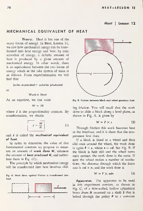
78 HEAT-LESSON 12

Heat|

Lesson 1

2

MECHANICAL EQUIVALENT OF HEAT

Theory. Heat is but one of the

many forms of energy. In Heat, Lesson 11,

we saw how mechanical energy can be trans-

formed into heat energy and how, by con-

servation of energy, a definite amount of

heat is produced by a given amount of

mechanical energy. In other words, there

is an equivalence between the two forms of

energy which in the mks system of units is

as follows. From experimentation we will

find that

joules expended oc calories produced

or

Work oc Heat

As an equation, we can write Fig. B. Friction between block and wheel produces heat.

W = JH

where J is the proportionality constant. Bytransformation, we obtain

ing friction. You will recall that the work

done to slide a block along a level plane, as

shown in Fig. A, is given by

and J is called the mechanical equivalent

of heat.

In order to determine the value of this

fundamental constant we propose to meas-

ure an amount of work done W, measure

the amount of heat produced H, and substi-

tute them in Eq. (1).

The principle by which mechanical energy

will be transformed into heat involves slid-

W = F X s (2)

Through friction this work becomes heat

at the interface, and it is there that the tem-

perature first rises.

If a block is fitted to a wheel and then

slid once around the wheel, the work done

is again F x s, where s = ttd. See Fig. B. If

the block is held still and the wheel turns

once around, the work done is the same. If

now the wheel makes a number of revolu-

tions, the distance through which the force

acts is ird x n, and the work done is

Fig. A. Work done against friction is transformed into

heat.

w = F X Trdn (3)


in this experiment consists, as shown in

Fig. C, of a thin-walled, hollow cylindrical

brass drum D mounted on a shaft S that is

belted through the pulley P to a constant

MECHANICAL EQUIVALENT OF HEAT 79

Fig. C. Principal elements in the mechanical equivalent

of heat experiment.

speed motor. Around the drum are three ny-

lon or cotton bands, wrapped around so that

weights can be suspended from the ends. Aknown mass of water is poured into the

drum, and a special bent thermometer T,

supported from the outside, dips into the

water to give the temperature. The number

of turns of the drum are counted automati-

cally by the counter C. The drum is set ro-

tating at a constant speed (about 120 rpm),

and the weights are adjusted to bring the

system into balance.

Two simplified diagrams of the essential

elements of experiment are shown in Figs.

D and E.

Object. To determine the joules of

mechanical energy required to produce 7

calorie of heat.

Fig. D. Diagram showing hooks and weights used to cre-

ate friction.

Fig. E. Thermometer position for recording temperature

rise of water and drum.

Procedure and Measurements. Make a

list of the quantities to be measured as

shown in Table 1 and proceed as follows.

Measure or weigh out about 200 gm of

water at about 10°C below room tempera-

ture and pour it into the cylinder. Insert the

bent thermometer, being careful to see that

it is everywhere free of the rotating drum.

Suspend masses from the ends of the belt

and adjust until they hang free. The purpose

of the spring scale m3 is to oppose the

cylinder’s motion and assist in retaining bal-

ance when the masses A1 l5 M 2 ,m lt and m2

are anywhere near balancing values.

Caution. Do not allow the bands or

cylinder surface to become wet.

As the drum turns and the temperature

rises, be prepared to take data in two col-

umns as shown in Table 2. Take your first

reading when the temperature is about 5°

below room temperature t and the counter

passes an even hundred number. Record

the turns as zero and the temperature t.

Every one hundred turns, indicated by the

counter, record the water temperature t.

Continue the run until a temperature sev-

eral degrees above room temperature is

reached, and then stop. Measure the diam-

eter of the drum d, the masses suspended

from the ribbon bands, etc., and record

their values in Table 1. The drum’s mass

and the hook’s mass are usually stamped

into the metal and should be recorded.

The last two values in Table 1 are found

80 HEAT-LESSON 12

from the data in Table 2. Locate the value

of t in Table 2 that is nearest the room tem-

perature t. Take the temperature 1 1 for the

reading 200 turns above this temperature and

t2 for the reading 200 turns below this tem-

perature. Then take the difference (t2 — h)

and divide by 4. This then is recorded in the

last row of Table 1 as the average tempera-

ture rise, to — h, for 100 turns.

Data. Assume that the experiment has

been performed and the data have been re-

corded as shown in Tables 1 and 2.


water mass mw = .205 kg

drum mass m b= .574 kg

hook mass Mi .446 kg

large mass m2= 1 .50 kg

drum diam. d = .155 mroom t t = 28°C

hook mass m 1= .056

small mass m2= .050

spring mass m 3= .035

sp. ht. drum cb = .092

number of turns n = 100

temperature rise t2 - h = 2


Number

of Turns

t

(°C)

0 23.2

100 24.4

200 25.5

300 26.5

400 27.4

500 28.2

600 29.0

700 29.8

800 30.5

900 31.2

Calculations. Using the data recorded

in Table 1, calculate the work done W for

100 turns by using the equation

W — (M — mjgirdn (4)

and the heat produced H by using the equa-

tion

H = (mwcw + m bc b)(t2 — h) (5)

It can be seen from Fig. D that M lt M 2 ,

and m:f oppose the rotation of the drum,

while mi and m2 act to assist. Consequently

we have, pulling down on the right-hand

side,

M = Mi + M2 (6 )

and pulling down on the left-hand side,

m — mi -|- m 2 — m 3 (7)

Since M and m oppose each other, the total

force F, to be used in Eq. (3), is given by

F = (M — m)g (8 )

The total heat gained H is made up of two

parts: the heat gained by the water

m wcw(t2 — h) (9)

plus that gained by the brass drum

m bc b(t2 — h) ( 10 )

Continue the calculations by substituting

measured masses in Eqs. (6) and (7), and

find M and m. Insert these in Eq. (4), along

with g = 9.80 m/sec2,n, and d, to find W.

Next, substitute directly into Eq. (5) to

find H. (Note: To find H in calories, put

masses in grams.) Finally insert W and Hin Eq. (1) to find J.

Conclusions. Compare your value of J

with the accepted value of

J = 4.18joules

calories

and calculate the percentage error.

BOYLE'S LAW 81

Heat|

Lesson 1

5

BOYLE'S LAW

In Heat, Lesson 1 1, we have seen

that Boyle’s law is one of the three special

cases of the general gas law and deals with

the compression and expansion of a gas at

constant temperature. The law is usually

written in either one of the two following

forms

:

( 1 )

( 2 )

Theory. The three diagrams in Fig. Aconstitute a schematic representation of

Boyle’s law, particularly as it is written in

the second form, Eq. (2).

A certain amount of gas at room tem-

perature T is trapped above the piston in

the left-hand diagram. The gas volume V x

is maintained at a pressure of as deter-

mined by the force F x on the piston rod.

With increased force F2 ,the piston moves

up, compressing the gas and raising its tem-

perature. In a reasonable amount of time

the cylinder and its confined gas will cool

down to room temperature T, and it will

have a new volume V2 and pressure p2 . If

pV — constant

PiVi — P2V2 = P3V3

Fig. A. Gas compressed at constant temperature obeys

Boyle's law.

the force is increased again to a value F3

and the gas is allowed to cool down, the

new volume will be V 3 and the new pressure

Pa-

Should the force on the piston be de-

creased, the piston will move down, the gas

will cool upon the expansion, and, by wait-

ing, the cylinder and gas will warm up to

room temperature T. Hence the process of

compression and liberation of heat is re-

versible by the expansion and absorption of

heat.

Apparatus. The laboratory apparatus to

be used in this experiment is shown in Fig.

B. A quantity of air is trapped by a column

of mercury in a straight uniform tube OD.

By raising the right-hand column the mer-

cury will, in seeking to equalize the columns,

compress the air into a smaller volume. Bylowering the right-hand column the volume

will increase and the gas pressure will de-

crease.

For each set position of the mercury col-

umn the volume V is read directly from the

scale and pointer, and the pressure is de-

termined by the measured difference in mer-

cury level h. If the level B lies above A, the

total gas pressure p is equal to the atmos-

pheric pressure p0 ,as read from a standard

barometer, plus the height #1 . If B lies below

A, the height h is subtracted from p0 .

Calling h plus for the arrangement in

Fig. B, we have

P = p 0 + h (3 )

or

P — p 0 + (A — B) (4 )

and

< II > 1 O (5 )

82 HEAT-LESSON 15

- o

Fig. B. Apparatus assembled for Boyle's law experiment.

Care must always be taken when chang-

ing the reservoir to each new position to al-

low several minutes for the gas to come to

room temperature. The necessity for doing

this is that upon compression the gas gets

warmer and on expansion it cools. Multi-

plying each of the measured gas pressures pby their corresponding volumes V will give

a series of products, which, within the limits

of experimental error, are constant.

Object. To measure the pressure andvolume changes of a gas at constant tem-

perature and thereby verify Boyle's law.

Procedure and Measurements. If your

apparatus is such that both mercury columns

are adjustable, open the stopcock at A and

raise the left-hand column so the top of the

air column is at the 20-cm mark of the

meter stick. Raise or lower the right-hand

column so their ends are about the same

height. Pour in enough mercury to bring

both columns up to about the 40-cm markand close the stopcock. Raise the left-hand

column and set O at the 10-cm mark.

Now lower the right-hand column as far

as you can, but do not go beyond the point

where the mercury level B is below the end

of the tube and into the flexible hose.

Wait 2 min for the air to reach room tem-

perature and record the positions O, A, and

6 in a table of three columns. See Table 1.

{Note: It is convenient to adjust the right-

hand mercury column so that the mercury

level A comes on an even centimeter mark.

)

Raise the right-hand mercury column and

by watching the left-hand mercury level

compress the gas by 2 cm. Wait 2 min and

record the levels O, A, and B in the table.

Repeat these steps, compressing the gas 2

cm at a time until the right-hand column

is as high as it will go.

Lower the left-hand column until Ocomes at the 20-cm mark. Adjust the right-

hand column until the mercury level A has

compressed the entrapped air 2 cm beyond

the preceding measurements. Record these

readings of O, A, and B as indicated in

Table 1.

Continue to compress the air column 2

cm at a time by lowering the left-hand

column and raising the right-hand column

whenever necessary. Finally, record the at-

mospheric pressure from a mercury or aner-

oid barometer.

Data. We will now assume that the

above measurements have been made and

the data have been recorded as shown in

Table 1.

BOYLE'S LAW 83


o(cm)

A

(cm)

B

(cm)

10 40.0 59.9

10 38.0 54.2

10 36.0 47.4

20 44.0 50.5

20 42.0 42.0

30 50.0 42.6

30 48.0 31.3

40 56.0 27.9

50 64.0 21.0

60 72.0 9.2

Atm pressure p 0 = 75.0 cm Hg

Calculations. For your calculations you

should make a table of four columns with

headings as shown in Table 2. The first row

of values have been calculated and will


CQ1<(cm Hg) P V pV

-19.9 55.1 30.0 1653

serve as a guide for the other nine trials.

Complete this table.

Results and Conclusions. Compare the

products pV in the last column to see if they

are constant. Calculate the average value of

PV.

Plot a graph of p against V. See Fig. F in

Heat, Lesson 11. For your vertical p scale

label the centimeter squares 40, 50, 60, etc.,

up to 140 cm Hg. For the horizontal V scale

label the centimeter squares 10, 12, 14, etc.,

up to 30. Draw a smooth curve through your

plotted points. What is the mathematical

term applied to this particular shape of

curve?

Sound|

Lesson 2

FREQUENCY OF A TUNING FORK

The difference between a musical

sound and a noise is sometimes difficult to

discern. Musical sounds involve periodic

motions of some vibrating source, whereas

a noise generally arises from some sudden

and violent disturbance like an explosion.

In Sound, Lesson 1, we considered

waves of two different kinds as well as sev-

eral kinds of sources that produce sounds of

different pitch and frequency. In particular

the sound waves generated by the vibrating

prongs of a tuning fork were introduced.

Although the transmission of sound from

one point to another involves longitudinal

waves, as shown in Figs. C and D, p. 258,

it is customary to represent them in dia-

grams as transverse waves. The reason for

this is simply that transverse waves are so

much easier to draw.

Theory. Two vibrating objects will be

used in this experiment: one is a weighted

leaf spring, or reed, as shown at the left in

Fig. A; and the other a tuning fork, as shown

Fig. A. A weighted leaf spring, or reed, and a tuning

fork.

at the right. Although each part of each vi-

brating prong moves in a slightly curved arc,

the motion along each path, if straightened

out, is simple harmonic motion.

The period T of any periodic motion (see

Properties of Matter, Lesson 14, p. 199) is

defined as the time in seconds required to

make one complete vibration. The frequency

n, on the other hand, is defined as the num-ber of vibrations made each second of time.

These two quantities, period and frequency,

are so related that either one is just the

reciprocal of the other.

T = 1 or n = i(1)

n T

If for example the prong of a tuning fork

makes 100 complete vibrations in 1 sec the

frequency n = 100 vib/sec, and the time

to make one vibration is 1/100 of a second.

T = tJ-t sec and n = 100— (2)1 00 sec

Apparatus. To find the frequency with

which the prongs of a tuning fork vibrate

we make use of the apparatus shown in Fig.

B. It consists of a base board about 2 ft long

Fig. B. Vibrograph apparatus showing the start and

finish positions of the slider plate D.

86

FREQUENCY OF A TUNING FORK 87

and 6 in. wide with two metal bars on top

to serve as guides for a sliding plate of sheet

metal D.

A weighted reed, or leaf spring S and a

tuning fork T are clamped at one end of the

board about an inch above the slider D, and

each carries an ink stylus at the vibrating

end as shown. Each stylus is bent down so

that each tip touches and draws a line on a

sheet of paper V. If the reed and fork are

vibrating, a wavy line trace is called a

vibrogram, while the apparatus itself is

called a vibrograph.

Object. To make a vibrograph trace

and from it determine the frequency of a

tuning fork.

Procedure. Place a sheet of paper onthe slider D and secure it at the corners

with masking tape. Move the slider to the po-

sition shown at the top in Fig. B. Spread the

tuning fork prongs so the block B slips be-

tween them and bend the leaf spring so the

end is held to one side by the pin P. Put

a drop of ink in each stylus and slip a small

piece of paper under each tip while you

check to see that the ink flows freely to the

paper. When this is accomplished, remove

the small piece of paper.

Now move the slider steadily toward the

position shown at the bottom in Fig. B, taking

about 1 to 2 sec as a transit time. If all

parts function properly, a vibrogram like

the one shown in Fig. C will be obtained.

Several trials may be necessary before a

satisfactory trace is obtained.

After two or three satisfactory records

have been made, use a stop watch, and de-

Fig. C. Vibrogram of the leaf spring and tuning fork

prongs.

termine the period and frequency of the

leaf-spring pendulum. Start the pendulum

vibrating and measure the time required to

make 100 complete vibrations. Repeat this

timing process several times and record

the average time for 100 vib.

Measurements. Make a table of three

columns on your data sheet in preparation

for recording measurements from your vi-

brogram. Use headings as shown in Table

1 . Select your best trace and label the inter-

sections A, B, C, and D as shown in Fig. C.

Count the number of fork vibrations be-

tween A and C and record them in column

2. Count the number between B and D and

record them in column 3.

Repeat this procedure for your second

and third vibrograms and record the data.

Data. Assuming the above procedure

has been carried out, and the measurements

have been recorded, the data should look

like that recorded in Table 1.


Trials A to C B to D

1 65.4 66.8

2 66.0 6653 65.5 67.0

average time for 100 vib

of leaf spring,

t = 49.2 sec

Calculations. From the average time

for 100 vib of the leaf spring, calculate the

period T. This is accomplished by dividing

the time t by the number of vibrations.

Find the average of the number of fork

vibrations as given in Table 1 and compute

the fork frequency from the relation

88 SOUND-LESSON 5

_ avg number of fork vib

period of leaf spring

Conclusions. Answer the following

questions in your final report:

1. Does the speed of the sliding plate affect

your final result?

2. Does the position of the weight on the

leaf spring affect your final result?

Sound|

Lesson 5

VIBRATING STRINGS

Vibrating strings are the basic

sources of musical sounds in many of

our present-day musical instruments. It is

the purpose of this experiment to vary the

conditions under which a string vibrates and

to make a quantitative study of its behavior

under greater and greater tension.

Theory. The diagram in Fig. A repre-

sents a string vibrating with standing trans-

verse waves. The heavy line represents the

position of the string at one instant and the

dotted line its position one-half a vibration

later.

The fundamental relation concerned with

vibrating strings is to be found in the wave

equation introduced in previous lessons:

or

V = n\

( 1 )

It will be noted that the total length L

Fig. A. Standing longitudinal waves on a vibrating

String.

N N N

of any one of the loops into which the string

divides is given by

(2 )

The velocity of transverse waves along a

string is given by

V = VF/m (3)

where, in the mks system of units, V is ve-

locity in meters per second, F is the string

tension in newtons, and m is the mass in

kilograms of one meter of string.

Apparatus. The equipment used in this

experiment is shown in Fig. B. It consists of

a tuning fork, a string about 2 meters long,

a pulley, and a set of metric weights. Al-

though it is not necessary, an electrically

driven tuning fork is the most satisfactory.

Instead of having to strike the fork a blow

every few seconds, an electric fork can be

turned on and run continuously for as long

as desired.

Fig. B. Tuning fork with vibrating string arrangement

for this experiment.

VIBRATING STRINGS 89

Object. To determine the effect of

length, mass, and tension on the vibration

of a string.

Procedure. Measure out several meters

of the string to be used in the experiment

and accurately determine its total mass.

Record the length in meters and the mass in

kilograms on your data sheet.

Fasten one end of the string to a tuning

fork prong and the other end to a hooked

weight over a pulley as shown in Fig. B.

The horizontal string section should be

about 1.5 meters long.

Set the fork vibrating and adjust the mass

load M and the pulley position so the string

vibrates with seven or eight loops. Note how

critically the vibration amplitude depends

upon string tension. Set up markers A and

B at nodes to include as many loops as you

can. Measure the distance between A and B,

and count the number of loops included be-

tween the markers. Record these data in a

table of five columns as shown in Table 1.

Gradually increase the load M until the

string again responds to standing longi-

tudinal waves. The equally spaced nodes

will now be found slightly farther apart.

Carefully set the markers A and B at nodes,

and again measure their distance apart.

Count the number of inoluded loops and re-

cord the data as trial 2 in Table 1.

Repeat this procedure, increasing the

load M each time to produce increasingly

longer loops, but adjusting the total string

length and mass to obtain maximum vibra-

tion amplitudes.


Trial

M(kg)

A(m)

8

(m)

N(loops)

1 .040 0 .795 5

2 .080 0 .896 4

3 .130 0 1.148 4

4 .190 0 1.038 3

5 .250 0 .796 2

6 .300 0 .868 2

7 .350 0 .936 2

/ = 10 m m — .0043 kg

Calculations. Calculations are most

easily obtained by making a table of six


F F/m L X V n

(newtons) (nt/kg) (m) (m) (m/sec) (vib/sec)

.392 912 .159 .318 30.2 95.0


Results of the first trial have already been

computed and are given as your guide for

completing the calculations. Column 1 repre-

sents string tension and is given by the

product Mg. For column 2 use the value of

m computed from Eq. (4). Column 3 gives

the average loop length L, and the values

are derived from the recorded data as

Data. If the above procedure has been

carefully followed, the recorded data will

have the general appearance of that shown

in Table 1.

From the recorded length and mass of

the string, calculate m, the mass per meter

of string.

string mass in kg ,

m = —.;—

(4)string length in meters

The wave lengths A are given by Eq. (2),

and the velocity V by Eq. (3) and column

2 in Table 2. The frequency n is computed

by use of Eq. ( 1 )

.

Results. When the calculations have

been completed for Table 2, compute the

average value of the frequency n as given in

the last column. This should agree with the

90 SOUND-LESSON 7

frequency number usually found stamped in

the metal of the tuning fork.

Plot a graph of the results. A chart ten

squares wide by ten squares high will be

adequate. Centimeter graph paper is quite

satisfactory for this. Plot the wave velocity

V vertically, labeling the division marks 0,

10, 20, 30 ... 100 m/sec. Plot the wavelength A horizontally, labeling the divisions

0, 0.1, 0.2, 0.3 . . . 1.0 m. The graph line

should pass through the origin.

Conclusions. What can you conclude

from the graph drawn in this experiment?

Sound|

Lesson 7

RESONATING AIR COLUMN

In this experiment we are going

to produce standing longitudinal waves in

a metal rod and use the resulting rod vibra-

tions to generate standing longitudinal waves

in a column of air.

An interesting demonstration of longitudi-

nal waves in a solid is shown in Fig. A. Ametal rod about 4 mm in diameter and 1 mlong is clamped tightly at the center in a

rigid support. With a little alcohol or rosin

on a cloth, the rod is stroked from the

center toward the free end. After a few

strokes the rod will sing out with a high-

pitched note indicating it is vibrating. That

the vibrations are longitudinal is shown by

the bouncing of a small ball suspended by

two cords at the far end.

Vibration modes giving rise to the first

three harmonics of such a rod are shown in

Fig. B. The top mode gives the lowest fre-

quency note the rod can produce and cor-

Fig. A. A long rod can be set to vibrate with standing

longitudinal waves.

1 n

N N2n

Fig. B. Longitudinal standing wave modes of vibra-

tion for a uniform rod.

responds to the first harmonic, or funda-

mental. The others correspond to the sec-

ond and third harmonics, respectively.


experiment employs a rod and glass tube

mounted coaxially as shown in Fig. C. Whenthe rod is set vibrating, the disk A at the

far end vibrates back and forth, sending

longitudinal waves through the air column.

These waves are reflected back from an ad-

justable plunger B at the other end. By ad-

justing this plunger, a position can be found

where the air column will resonate with

standing longitudinal waves.

A graphical pattern of these standing

waves is produced inside the tube by cork

dust, or lycopodium powder, distributed

along the bottom as shown.

Theory. There are two vibrating systems

involved in this experiment, and the wave

RESONATING AIR COLUMN 91

1 N.

N'2 B

Fig. C. Diagram of apparatus used in this experiment.

equation V = n\ can be applied to both.

These, when written,

for the for the

metal rod air column

Vm nm\m Va naXa

Vm velocity Va

nm frequency na

\m wave length \a

The subscripts simply indicate the me-

dium to which that quantity applies. Vm ,

the velocity of sound in metals, is muchgreater than Va ,

the velocity of sound in air.

The two factors that are the same in this

experiment, however, are the two fre-

quencies :

nm = na (1)

The plunger on the rod, with its fre-

quency nm ,sends waves of the same fre-

quency na through the air column. If wesolve each of the two wave equations for the

frequency,

we can, by Eq. ( 1 ) ,write

In this experiment the velocity of soundin metal becomes the unknown quantity.

Solving Eq. (3) for Vm ,we obtain

(4)

In this experiment Xm and \a will be

measured, while Va will be calculated fromthe formula given in Sound, Lesson 1:

Va = 331 — + .61 f

sec

where t is the temperature in °C.

(5)

Object. To study longitudinal standing

waves in a column of air and determine

the velocity of sound in a metal.

Procedure. Clamp a brass rod, about 1

meter long, at its middle point in the sup-

port provided. The disk on the end should

be centered within the end of the glass tube

so that it does not vibrate against the sides

of the glass tube.

Set the rod in vibration by stroking it

slowly. A small rotation of the glass tube

just prior to stroking the rod often results

in a better cork dust pattern upon resonance.

Adjust the plunger 6 by trial until a nicely

scalloped pattern appears. Examine the dust

near A and B, and note whether a node or

antinode forms at the ends.

Measure the distance d between two nodes

and N2 ,and count the number of in-

cluded loops N. Measure the length of the

brass rod / and record the readings in a

table of five columns. See Table 1.

Repeat this experiment by moving the

plunger B to a new position and record the

data. Make a third trial.

Replace the brass rod with an iron rod

and repeat all the steps outlined for the

brass. Record the data in Table 1.

Record the room temperature.

Data. Assume the above procedure has

been carried out and the data have been re~

corded as shown in Table 1.

92 SOUND-LESSON 10


Trial Metal

/

(m)

d

(m)

N(loops)

1 brass .860 .510 6

2 brass .860 .429 5

3 brass .860 .692 8

4 iron .796 .452 8

5 iron .796 .334 6

6 iron .796 .448 8

room temperature = 30°C

Calculations. Use Eq. (5) to calculate

the velocity of sound in air for the recorded

room temperature.

Make a table of five columns and label

them as shown in Table 2. Calculations for


K Aa Am vmMetal (m) (m) Aa (m/sec)

brass 1.72 .170 10.1 3520

trial 1 have already been made and will

serve as a guide in computing the others.

Since the vibration mode of the rod in

this experiment is that of the fundamental,

or first harmonic, as shown at the top in

Fig. B, the length of the metal rod / is just

half a wave length.

(6 )

From this relation and the recorded values

of /, the calculated Xa are obtained from

columns 4 and 5 of Table 1. (Note that each

cork dust loop is half a wave length.) The

final velocities Vm are computed from col-

umn 4 of Table 2, the velocity Va from Eq.

(5) and substitution in Eq. (4).

Results. Assume that the correct values

of the velocity of sound in metals are

for brass, Vm = 3500 m/sec

for iron, Vm = 5000 m/sec

Find the average value of the velocities

measured for each metal and calculate the

percentage error.

Sound|

Lesson 10

SPEED OF SOUND

There are many different ways of

measuring the speed of sound. It is the plan

of this experiment to fill a glass tube with

a known kind of gas, set the column vibrat-

ing with standing longitudinal waves, and,

from the known frequency of the wave

source, calculate the speed of sound in that

gas. This is to be done with several gases.

Theory. Suppose that a glass tube con-

taining a gas, like air, is arranged as shown

in Fig. A, with a tuning fork at the open end

of the tube and a plunger that can be

moved up or down from the other end.

Sound waves from the tuning fork travel

down the tube and reflect back from the

face of the plunger.

If the plunger is moved up or down, cer-

tain positions can be located where the two

oppositely directed wave trains set up stand-

ing waves and the gas column sings out in

resonance. Under these conditions a node Nis always to be found at the face of the

plunger and an antinode near the open end.

SPEED OF SOUND 93

Fig. A. Different lengths of gas column will resonate to

the same tuning fork.

Actually, the antinode at A is about four-

tenths the diameter of the tube beyond the

tube end.

The basic principles here involve the wave

equation

( 1 )

The wave length A is just twice the length

L of one loop.

(2 )

It will be noted that the first resonant

node Ni occurs when the resonating gas

column has a length of 1/2, or A/4.


experiment is shown in Fig. B. It consists

of a glass tube about 75 cm long, connected

at the bottom by a flexible hose H to a water

reservoir R, and a set of three tuning forks

of different frequency. By raising or lower-

ing the water reservoir, the water level in

the glass tube is raised or lowered. In this

way the plunger surface of Fig. A becomes

the water surface in Fig. B, and the air col-

umn above the water can be adjusted in

length to resonate to any one of the three

tuning forks.

In performing the experiment only the

top, or first, resonant node Ni of each gas

column will be located. While the other

nodes can be found and recorded if the

tube is long enough, the top one sings out

most loudly.

Object. To measure the speed of sound

in air and in other gases by means of

standing waves in a resonating gas col-

umn.

Procedure. Measure the inside diameter

d of the glass tube. Multiply this diameter

by 0.4 and set the zero end of the meter

stick at a distance s above the end of the

tube, as shown in Fig. B.

s = 0.4 X d

This automatically sets the end of the

meter stick at the topmost antinode A.

Read and record the room temperature.

Now select the tuning fork of highest fre-

quency, hold it over the top end of the glass

tube, and strike it a blow with a rubber

94 SOUND-LESSON 10

mallet. With the water level close to the

top of the tube, slowly lower the reservoir

and listen closely for the first resonance.

Raise and lower the water level around this

area until you feel the position marker is

well located at N 1 .

Make a table of four columns as shown

in Table 1 and record the resonant posi-

tion of the water level B in meters. Tuning

forks are universally marked with their vi-

bration frequency, and this should be re-

corded in Table 1 under n.

Select the second tuning fork and repeat

the above steps of carefully locating the

water level at which the tube sings out in

resonance. Record the position 8 and fre-

quency n.

Repeat these steps with the third fork as

trial 3.

If carbon dioxide gas is available, either

from a chemical generator or from a pres-

sure tank, lower the water level in the glass

tube until it is close to the bottom and in-

sert a rubber hose down into the air column

from the top. With the end of the hose

under water, bubble in carbon dioxide gas

until you think it has driven all the air from

the tube.

Remove the rubber hose and, with the

medium-frequency tuning fork held at the

top of the gas column, slowly raise the water

level and locate the resonance point 8.

Since raising the water level drives out C02

at the top, any lowering of the water level

will draw in air and give a spurious result.

Consequently, lower the water level, fill

again with C02 ,and again locate the reso-

nance position as the water level rises.

After several tries have been made, re-

cord the best position of 8 as well as the

fork frequency n.

Ether vapor can be used as a third gas in

this experiment. Lower the water level in

the glass tube and then pour in about 2 cm3

of the liquid ether. After running down the

tube and spreading over the water, the

ether will quickly evaporate, rise, and fill

the tube. Before it has all evaporated, raise

the water level and locate the point 8 where

resonance with the medium frequency tun-

ing fork occurs. Repeat this procedure un-

til you are reasonably satisfied you have

found the best position for B, and then re-

cord.

Data. Assume that the above steps have

been carried out and that the data have



Trial Gas (-)\sec/

B

A/4

(m)

1 air 528 .163

2 air 440 .196

3 air 264 .330

4 co2 440 .153

5 ether 440 .114

room temperature = 28°C

Calculations. Your calculations should

be carried out by first making a table of

four columns as shown in Table 2. Calcula-

tions for the first trial set of data are in-

cluded to serve as a guide for the others.

Complete these calculations for other trials.


Gas (i)A

(m)

V

(*)

air 528 .652 344

Results. Find the average value of your

experimental determinations of the speed

of sound in air. Compare this average value

with the speed computed from the formula

V = 331 m/sec + .61 t, and find your per-

centage error.

Light|

Lesson 3

PHOTOMETRY

Photometry, we have seen, is a

term applied to the experimental process by

which the relative intensities of two light

sources are compared and measured. Oneof these sources is usually of known candle

power, or luminance, and the other is one

of unknown candle power or luminance.

Apparatus. The fundamental principles

upon which photometry is based involve the

rectilinear propagation of light, the inverse

square law, and the ability of the observer to

adjust the distances of the two light sources

so that each one produces equal illumina-

tion on a screen.

While photometer screens of many kinds

and descriptions have been invented to

assist the observer in making precision dis-

tance settings, a very simple yet accurate

one will be used in this experiment. Asshown in Fig. A, it consists of two blocks

Fig. A. Paraffin blocks separated by tin foil make an

excellent photometer.

Fig. B. Photometer arrangement for measuring candle

power.

of paraffin, each about 3 in. square and \ in.

thick, with a sheet of tin foil between them.

This unit is mounted in a small cardboard

or wooden box, open at both ends and one

side as shown at the center in Fig. B.

The two hollow boxes on either side of

the photometer P contain the two light

sources, the known V and the unknown 1.

All three are mounted on two parallel bars

and are free to be moved. When such a

photometer is moved back and forth along

this optical bench, a position is easily located

where the edges of both paraffin blocks ap-

pear equally bright.

Light from each lamp entering the par-

affin block facing it is scattered throughout

that block only. Being side by side and prac-

tically touching each other, the blocks can

be easily matched, thereby indicating a posi-

tion of equal illumination from the two

sides.

Theory. Let I represent the unknown

candle power of any lamp, and I' the known

candle power of a lamp we will call the

standard. As these lamps are set up in Fig.

B, lamp I produces an illuminance E on one

paraffin block of the photometer and I' pro-

duces an illuminance Ef on the other.

By the inverse square law, Light, Lesson

2, we can write

96

PHOTOMETRY 97

and ( 1

)

E' =(̂f ')2

where r and r' are the distances to each of

the lamps as shown. If the photometer P is

set for matched paraffin blocks, the two

illuminations are equal and we can write

E = E' (2)

Equating the right-hand sides of Eq. (1),

we obtain

J-.JL(3)

(r')2

[JI

Solving this equation for the unknown I,

we obtain

In this experiment we are going to take

each one of several tungsten filament lamps,

set them up one at a time on an optical

bench with a lamp of known candle power

T, set the photometer P for equal illumi-

nance, and measure the lamp distances r

and r'. When these measured values are

substituted in Eq. (4), we can calculate 1.

The lamps to be used may be purchased at

various stores, and are rated at 15, 25, 40,

50, 60, 75, and 100 watts, respectively.

Object. To measure the candle power

of several light bulbs and to compute

their efficiency.

Procedure. Standard lamps of knowncandle power, burning under specified volt-

age and current, are available at laboratory

supply houses. If a standard lamp is not

available, select a new 60-watt, inside

frosted, lamp bulb and assume its candle

power is 66.0.

Place your standard lamp in one lamp

holder socket and a 15-watt lamp in the

other. Set the lamp centers exactly 80 cm

apart and leave the boxes in this position

throughout the experiment. Move the pho-

tometer P back and forth, and locate the

equal brightness position. A little practice at

this will enable you to repeat the setting each

time you try. Now measure the distance r

and record the interval in a table of four col-

umns as shown in Table 1. The distance r'

need not be measured, but recorded as the

difference between the total distance, 80 cmminus r.

Replace the 15-watt lamp by one speci-

fied as 25 watts. Repeat the setting of the

photometer P and record the measured dis-

tance r and the distance r'.

Repeat the procedure outlined above for

each of the other lamps in order of increas-

ing wattage and record the measurements in

Table 1.

Data. We may assume that the above

steps have been carried out and the data

recorded as shown in Table 1.


Lamp

Watts

/'

(c.p.)

r

(cm)

r'

(cm)

15 66.0 23.5 56.5

25 66.0 28.8 51.2

40 66.0 34.4 45.6

50 66.0 37.5 42.5

60 66.0 40.0 40.0

75 66.0 42.7 37.3

100 66.0 46.1 33.9

Calculations. Make a table of four col-


Calculations for the first lamp have already


Lamp

Watts

/

(c.p.)

I

(lumens)

c-P-

watt

15 11.4 143 .76

98 LIGHT-LESSON 5

been included and will serve as a guide in

completing the others.

The values of I in column 2 are computed

by means of Eq. (4) and the values of

r, r', and V recorded in Table 1. Since 1

c.p. = 12.57 lumens, values of 1 in column

3 are computed from those in column 2 by

multiplying by 12.57. Values in column 2

divided by those in column 1 will give values

of c.p./watt in column 4.

Results. Plot a graph of output candle

power against input watts. The vertical scale

for c.p. should be labeled 0, 10, 20, 30 . . .

130 c.p., while the horizontal scale should

be labeled 0, 10, 20 . . . 100 watts. Cen-

timeter graph paper is conveniently used

here.

Plot the graph points with great care.

Most higher wattage lamps are filled with

nitrogen and argon gas at atmospheric

pressure, while the smaller 15- and 25-watt

lamps are highly evacuated. Excluding these

two low wattage lamps, draw a straight

line, as best you can, through the plotted

points for the others. The intersection of

this line with the watt’s axis will show the

approximate energy loss in these lamps due

to (1) heat conduction to the lead and

support wires, (2) the absorption of some

light by the gas, and (3) bulb and base

absorption of light.

Starting at the graph origin, draw a

smooth curve through the plotted points for

the 15-, 25-, and 40-watt lamps.

Light|

Lesson 5

REFLECTION FROM PLANE SURFACES

The image of any object seen in

a plane mirror is just as far behind the mir-

ror as the object is in front of it. It is the

purpose of this laboratory lesson to try to

verify this statement by experimentally trac-

ing light rays incident on and reflected from

a mirror, graphically locating an image, and

then measuring the object and image dis-

tances from the reflecting surface.

Theory. The basic principles involved in

this experiment are concerned with ( 1 ) the

rectilinear propagation of light and (2)

the law of reflection. The law of reflection,

as demonstrated in various ways in Light,

Lesson 4, states that the angle of incidence is

always equal to the angle of reflection:

angle i = angle i'

It is to be understood that the incident

ray, the reflected ray, and the normal to the

surface all lie in the same plane and that

the two angles i and V are on opposite sides

of the normal.

To employ the established fact that light

travels in straight lines we make use of a

principle often used by surveyors. In mak-

ing a plan drawing to scale, they place their

paper on a plane table that has been care-

fully leveled and use a sighting device for

establishing line directions to distant points.

The principle is illustrated by three pins A,

B, and C in Fig. A.

Fig. A. A straight line path of a light ray can be estab-

lished by sighting along and lining up points.

E

( 1 )

C B A

REFLECTION FROM PLANE SURFACES 99

Fig. B. Sighting pin block and mirror mounting as used

in this experiment.

To establish the direction of a point Afrom a point C, the eye is located behind

C and the third pin is moved into a lined-up

position. Light traveling in a straight line

from A to E must pass directly over B and

C.

Apparatus. A suitable sighting device

can be made for this experiment by driving

two pins, or small wire brads, into a block

of wood, as shown in Fig. B. The block is

conveniently made from %-in. plywood about

3 in. long and f in. wide. After making a

V-shaped notch in the ends, a straight line

is drawn through their centers as shown.

Two pins or brads are then located exactly

on this line and accurately driven vertically

part way into the wood.

A pocket mirror about 2 by 3 in., or a

strip of glass cut from a larger mirror is

quite adequate. Two square blocks of wood,

each with a groove for the glass to fit into,

may be used to set the mirror upright on a

sheet of paper.

Several sheets of paper 8^ by 11 in., a

centimeter rule, a protractor, a sharp pencil,

and a flat board of soft wood 9 by 12 in.,

or larger, are needed.

Object. To make a study of the law of

reflection and the images seen in a plane

mirror .

M

A#

N

Fig. C. Showing preliminary steps in drawing.

Procedure. Use masking tape to fasten

a clean sheet of paper to the board. Use your

ruler and draw a straight line across the

center of the paper as shown in Fig. C.

Label this line MN. Locate a point A about

4 cm from this line and near the center as

shown.

Place the mirror upright on the paper so

that the back silvered surface is exactly on

the line as shown in Fig. D. Stick a pin into

the paper and wood at the point A, being sure

it is straight and vertical. This pin A becomes

the object, and A' as seen in the mirror is its

image.

Place the sighting-pin block on the paper

and, with one eye close to the table top and

looking into the mirror, line up the two

sighting pins with the image A'. Holding

this block down with one hand, use your

pencil and make two marks on the paper at

the tips of the two notches.

Move the sighting pins to the other side

of A, shown dotted in Fig. D, and again

Fig. D. Illustration showing two sighting positions.

/A

]

''sA#

* '

f

]

100 LIGHT-LESSON 5

line up with the image A'. Mark the notch

positions as before, and then remove all ob-

jects from the paper.

Using your ruler, draw straight lines

through each pair of notch marks and mark

their intersection point A' as shown in Fig.

E. Draw another line through A and A', and

two additional lines from A to points P and

Q. With your protractor, erect perpendicu-

lars from points P and Q as shown.

Before proceeding with measurements,

make a table of four columns with headings

as shown in Table 1. Measure the perpen-

dicular distances from A to AIN and A' to

MN, and record in columns 1 and 2. Meas-

ure the angles AQW and RQW with your

protractor, and record them as angles i and

T, respectively. Measure the angles APVand SPV, and record them as a second pair

of angles / and /'.

Replace this paper with a clean sheet

of paper, draw a line MN as before, and

locate a point, A, 7 cm in front of MN. Re-

peat all steps outlined above and record the

data as trial 2 in Table 1.

If time permits, repeat the experiment

with the point A located somewhat to one

side but 5 cm from the line MN. Take both

lines of sight from the same side of the

normal of A to M.

Data. Assume that the above experi-

ment has been performed and the data re-

corded as shown in Table 1. Note in your

experiment that the light rays travel fromA to the mirror and then off to the eye and

not the reverse.


A to MN B to MN Angle / Angle /'

(cm) (cm) (deg) (deg)

4.0 3.938.5

26.0

38.3

26.2

7.0 7.034.0

36.5

34.4

36.5

5.0 5.147.0 47.5

26.2 26.0

Results. There are no calculations re-

quired in this experiment, and your labo-

ratory report consists principally of the

sheets of paper on which you made your

drawings.

Conclusions. Compare the pairs of dis-

tance values given in columns 1 and 2.

Compare the pairs of angles in columns 3

and 4. What can you conclude from these

comparisons? Make a brief statement of

what you have learned from this experiment.

INDEX OF REFRACTION 101

Light|

Lesson 8

INDEX OF REFRACTION

When light crosses the boundary

separating two transparent media, like air

and water or air and glass, the light changes

its direction at the boundary. As we have

seen in Light, Lesson 7, this behavior is

called refraction, and a quantitative account

of the bending is given by a general rule

called Snell's law.

In this experiment we will allow a ray of

light to be refracted at the surface of glass,

measure the incident and refracted angles of

this light, and from these determinations

calculate the refractive index of glass.

Theory. The basic principles involved

in this experiment were presented in Light,

Lesson 7, and may be expressed by the rela-

tively simple relation known as Snell’s law:

As shown in Fig. A, / represents the angle

the incident light ray makes with the sur-

face normal NN', and r the angle the re-

fracted ray makes with the same normal.

When angles i and r are measured in

Fig. A. Refraction of light by glass.

N

degrees, we can look up the sine of these

angles in any table of the natural functions.

These numbers can be substituted in Eq. ( 1

)

and the refractive index jx calculated.

In effect, Snell’s law says that the sine

of the angle of incidence is directly propor-

tional to the sine of the angle of refraction

for all angles. If, therefore, the proportional-

ity constant /x turns out to have the same

value for all angles of incidence, the law can

be considered verified.

The glass to be used in this experiment

has the shape of one-half of a right circular

cylinder as shown in Fig. B. When a ray of

Fig. C. Refraction occurs at only one surface in this block

of glass.

102 LIGHT-LESSON 8

light enters the plane face at the center Cand at an angle / with the surface normal

NN', the refracted ray at an angle r will

emerge from the far side of the glass with-

out further refraction.

If the glass block is turned about C so as

to increase the angle i, the angle r will also

be increased and the ray will emerge from

the glass without further bending as shown

in Fig. C. If the initial light ray is always

incident at the center C, the refracted ray

will always arrive at the curved surface at

right angles to a tangent T drawn through

that point. Since its angle of incidence at

this curved surface is zero, the angle of

refraction is also zero and the light travels

through without bending.


experiment is called a Hard disk. As shown

in Fig. D, it consists of a metal disk, free

to turn about its center C and around its

periphery by an angular scale divided into

degrees.

A glass block, as described above, is

mounted at the disk center so that light

from a small carbon arc, confined to a nar-

row ribbonlike beam by a slit S, crosses

the disk face as shown. With the disk face

painted white and the room lights subdued,

the beam can easily be seen across the

disk. The angles at which it enters and leaves

the plane glass surface can be read directly

where they cross the scale.

By leaving the light and slit fixed, and

turning the disk, the angle of incidence can

be changed with ease.

Object. To determine the refractive

index of glass and thereby test Snell's law.

Procedure. Strike the arc and adjust

the slit to obtain a narrow beam across the

Hard disk. Mount the glass prism on

the disk, being careful to see that its face

is along the 90° line and centered exactly.

Turn the disk to 0° to see that the light

enters and leaves the glass along the line

NN'. Record this zero reading in a table of

three columns as shown in Table 1.

Turn the disk so the angle of incidence

is 10° and note the angle of refraction. Re-

cord these as trial 2 in Table 1.

Repeat this procedure, increasing the

angle of incidence 10° at a time, and for

each case record both angles in Table 1.

Data. We will assume that the above

procedure has been carried out and the

LENSES 103

measurements have been recorded as shown

in Table 1.


Trial

/

(deg)

r

(deg)

1 0 0

2 10 6.0

3 20 12.0

4 30 17.5

5 40 23.0

6 50 27.5

7 60 32.0

8 70 34.5

9 80 36.0

10 88 37.5

Calculations. It will be convenient to

record your calculated results in a table of

three columns with headings as shown in

Table 2. The results of the first two trials

are already completed and will serve as a

guide in completing the others. A value of

/m cannot be computed for trial 1 as both

angles are zero.


sin i sin r

0 0 —.174 .105 1.66

When all nine values of ^ have been

computed, find their average value.

Plot a graph, angle / plotted horizontally,

against angle r vertically.

Conclusions. Note from your graph as

well as from the table of recorded data

that angles i and r are nearly proportional

to each other for small angles, whereas for

large angles they are not.

Snell’s law requires that the sines of the

angles be proportional to each other for all

angles. Is this experimentally verified by this

experiment? Briefly explain.

Light|

Lesson 10

LENSES

In most of the hundreds of dif-

ferent kinds of optical instruments de-

veloped over the years, lenses in one form

or another certainly play the most important

role. Because they are the principal com-

ponents in such common instruments as

spectacles, cameras, picture projectors, bin-

oculars, telescopes, and microscopes, it is

worth while for us to make a quantitative

study of lenses.

Theory. The most common form of lens

is known as a positive, or converging,

lens, as shown in Fig. A. Its action is such

that a parallel beam of light entering one

side parallel to the axis emerges from the

other side converging to a focus at the focal

point F. The distance from the center of the

104 LIGHT-LESSON 10

Fig. B. Image formation with a converging lens.

lens to the focal point is called the focal

length f.

Such a converging lens also exhibits the

useful property that if it is located at an

appropriate distance from any object O, a

real image 1 of that object can be formed on

a screen. Rays leaving any one point of an

object like Q in Fig. B will, after traversing

the lens, come to a focus at the corresponding

image point P. Rays leaving M (not shown)

will come to a focus at N, etc.

The relation between the object distance

d0 and the image distance dt

is given by

the following simple equation:

1di

1

f( 1 )

where f, as shown in Light, Lesson 9, is the

focal length of the lens.

The relative sizes of object O and image

1 are given by the equation

/ = di

0~ d0

(2 )

This ratio is called the magnification M,

and we write

focal length of the lens. To solve Eq. (1)

for f we may carry out the following steps.

Multiply numerator and denominator of

the first term by d, and the second term

by d0 .

A_ _do_ = 1

did0 dido f

With a common denominator the two

terms on the left can be collected to give

dj + do = 1

did 0 f

Inverting this equation we obtain

dj X do

di + do(4)

Apparatus. The single converging lens

with a focal length of 15 to 20 cm is con-

veniently used in this experiment. A small

screen with an arrow-shaped hole cut in it,

as shown in Fig. C, and a common frosted

glass light bulb behind it, serves as a suitable

object. Another small screen about 4 in.

square makes a good image screen.

These three elements—object, lens, and

screen—can be mounted on separate stands

that can be moved around on a table, or

they may be mounted in holders on an

optical bench if available. A meter stick is

used for measuring object and image dis-

tances.

Object. To determine the focal length

of a convex lens and to study the laws of

image formation.

If the image is twice the size of the object,

the magnification is 2, and if I is ten times

the size of O, the magnification is 10, etc.

The plan in this experiment is to meas-

ure the size and position of an object and

the size and position of the image, and from

them to calculate the magnification and the

Fig. C. Apparatus for studying the properties of lenses.

LENSES 105

Procedure. Use masking tape and fasten

a sheet of white paper or cardboard to the

wall opposite a window of the room. Hold

the lens up in front of this screen and moveit back and forth until a sharp image of

some distant object outside the window can

be seen on the screen. Measure the distance

between the center of the lens and the

screen. Record this distance in centimeters

as the focal length of the lens.

Set up the object, lens, and screen as

close together on the table as possible and

adjust their centers to the same height. Nowmove the object (the cutout arrow) until it

is about one and a half times the focal length

from the lens. Move the screen back and

forth until a sharp image is formed on its sur-

face. Measure the object distance d0 and

image distance d( ,and record them in a table

of five columns. See Table 1. Measure the

height of the object O and the height of the

image I, and record.

Increase the object distance 5 cm and

then move the screen to obtain a sharp

image. Again measure the object and image

distances, and the object and image heights,

and record.

Repeat these steps for four or five moretrials, increasing the object distance 5 cmeach time and recording the measurements

in Table 1.


Trial

d0

(cm)

di

(cm)

O(cm)

/

(cm)

1 25.0 58.5 3.2 7.4

2 30.0 43.0 3.2 4.5

3 35.0 34.4 3.2 3.1

4 40.0 30.2 3.2 2.4

5 45.0 28.4 3.2 2.0

6 50.0 26.5 3.2 1.7

7 55.0 25.2 3.2 1.5

Data. Suppose the above measurements

have been made and the data recorded as

shown in Table 1. The directly measured

focal length is given just below the table.

Calculations. Your calculations are con-

veniently made by recording them in a

table of six columns. See Table 2. The col-

umn headings are self-explanatory as they

come directly from Eqs. (4), (2), and (3).

The first trial calculations are already com-

pleted and will serve as a guide for all the

others.


di X d0 I dj

di X d0 di + d0 di + d 0 O do

1460 83.5 17.5 2.31 2.34

Results. The calculated results in col-

umn 3 are values of the focal length and

should all be alike. Find their average value

and compare with directly measured value

under Table 1.

Plot a graph of object distance d0 against

image distance d{ . The vertical scale for d0

and the horizontal scale for d, should each be

labeled 0, 5, 10, 15, . . . 70 cm. Draw a

smooth curve through the plotted points.

Draw a horizontal line on the graph at a

height where d0 — f, and a vertical line

where d, = f. Extrapolate your curve to

d0 = 70 cm and d; = 70 cm.

Conclusions. How would your graph

look (a) if d0 became very large and (b)

if di became very large? Briefly explain.

What can you conclude about the last

two columns in Table 2? How does the

magnification change as the object comes

closer and closer to the focal point?measured f = 17.3 cm

106 LIGHT-LESSON 13

Light|

Lesson 13

MAGNIFYING POWER

A single converging lens is fre-

quently used to magnify small objects,

thereby enabling an observer to see detail

not possible with the unaided eye. As il-

lustrated in Light, Lesson 9, such usage of

a lens comes under the heading of virtual

images.

Theory. When a lens is to be used as

a magnifier, the object must be located in-

side the focal point as shown in Fig. A. This

diagram is drawn to scale and represents

an object located 3 in. from a lens of 4-in.

focal length. The object-image formula maybe applied to find the image distance.

Upon substitution, we find

i_ = i_i L - A _ A.

di~ 4 3 di~ 12 12

1 _ _JLdi " 12

Upon inversion, we obtain

di = -12 in.

The image is 12 in. from the lens, the

Fig. A. A converging lens used as a magnifier.

minus sign signifying the image is to the

left of the lens and virtual. The rays shownentering the eye only seem to be coming

from 1.

As presented in Light, Lesson 10, the

magnification is given by the image-to-ob-

ject ratio.

This ratio M is sometimes referred to as

the magnifying power.

In this example

The image appears to the eye to be 4

times (written 4x) the size of the object.

The normal unaided human eye is able

to focus upon objects as close as 25 cm or

10 in. This particular distance is called the

near point, or distance of most distinct

vision, and it is here that an image should

be located to see the greatest detail with a

magnifying lens. In the arrangement of Fig.

A the light rays entering the eye are brought

to focus on the eye retina. This is shown in

Fig. B, where the magnified image I appears

to be at the near point of 25 cm, the object

O is just inside the focal point F, and the

real image is formed on the retina. Although

the actual rays from the magnifier lens it-

Fig. B. The virtual image I seen by the eye is actually

a real image of /' formed on the retina.

MAGNIFYING POWER 107

self are diverging, the eye lens system con-

verges them.

The formula for the magnification, with

the image I at the near point of 25 cm, is

given by

(3)

where f is the focal length of the magnifier

in cm. It can be seen from this formula that

the shorter the focal length f, the greater

will be its magnification.

Apparatus. The lenses to be used in

this experiment are three in number, one

having a focal length of about 10 cm, a

second with a focal length of about 3 cm,

and a third with a focal length of about 1

cm. Any three lenses of approximately these

focal lengths are quite satisfactory.

Each lens L should be mounted in a holder

and placed in line with the center of a

screen S having a square opening about one-

fourth of the focal length on a side. A centi-

meter scale R is then located on the lens axis

and observed with one eye located as shown

in Fig. C.

Object. To determine the magnifying

power of a small converging lens.

cord this distance as the focal length of the

lens. Repeat this procedure for the other

lenses and record as indicated in the last

column of Table 1.

Set up the longer focal length lens 25 cmfrom the scale R as shown in Fig. C. With

one eye closed look through the lens with

the other, and move the screen S back and

forth until a sharp image of the square open-

ing falls on the scale.

To be sure the image is at R, move the

eye laterally with respect to the lens axis,

up and down or back and forth parallel to

R. If the edges of the square image stay fixed

in position on the scale, proper adjustment

has been achieved. If the image moves on

the scale as the eye moves at the lens, the

image is either in front of or behind the

scale. Move the screen until no motion (no

parallax) is observed.

Measure the object distance d0 , the height

of the open square O, and the image height I

as observed on the scale. Record these dis-

tances in a table of five columns, with head-

ings as shown in Table 1.

Set up the second lens with its appropriate

square hole screen S and locate the cmscale 25 cm away, as shown in Fig. C.

Repeat the procedure outlined above and

record the measurements in Table 1.

Repeat all procedures with your third

lens and record the measurements.

Procedure. With a small bright light as

an object 20 ft or more away from the lens,

find the image distance from the lens. Re-

Fig. C. Laboratory arrangement for the magnifier lens.

Data. Assuming the above measure-

ments have all been made and recorded, the

data will have the appearance of those

shown in Table 1.


I

cm

rule

Osquare

hole

di

near

point

do

lens to

square

f

(cm)

8.6 2.5 25 7.3 10.4

7.1 0.80 25 2.8 3.2

6.9 0.40 25 1.4 1.5

108 LIGHT-LESSON 15

Calculations. Your calculations are best

carried out by recording them in a table of

four columns, with headings as shown in

Table 2. These calculations are easily car-


IM = —

OM = —

do£ -IK + Average

M

ried out for all your lenses, using Eqs. (2)

and (3).

When the first three columns have been

completed, each of the three values of Mfor each one of the three lenses should be

the same. Any differences are due to experi-

mental errors.

Calculate the average value of M and re-

cord in column 4.

Conclusions. What have you learned

from this experiment?

Light|

Lesson 1

5

PRINCIPLES OF THE MICROSCOPE

The simplest of microscopes is

just a single converging lens used as a

magnifier. As we have seen in Light, Lesson

13, the shorter the focal length of a lens the

higher the magnification. It is not surprising

to find, therefore, that small glass beads in

the form of perfect spheres were the first

really successful microscopes.

Lenses of this description were first used

by the famous Dutch microscopist, Van

Leeuwenhoek, when in 1674 he discovered

and gave an accurate account of the red

corpuscles in blood.

The compound microscope, which nowexceeds by far the magnifying power of a

single lens, was invented by Janssen in 1590.

Theory. The (compound) microscope

Fig. A consists of two very short focus lenses,

one called the objective and the other the

Fig. A. Lens and ray diagram of a compound microscope.

PRINCIPLES OF THE MICROSCOPE 109

Fig. B. Showing the function of the objective lens of a

microscope.

eyepiece. The objective lens is located close

to the object O to be magnified and, as shown

in Fig. B, forms a magnified image Y just in

front of the eyepiece. Being another short

focus lens, the eyepiece is used as a mag-

nifier to produce a magnified virtual image

at I. In other words, the real image Y of the

first lens becomes the object for the second

lens.

It is convenient to divide the principles of

the microscope into two parts. The first

part concerns the magnification produced by

the objective lens. A diagram showing a

short focus lens with its focal points F, as

well as object and image, is shown in Fig. B.

Note how the object O, lying just out-

side the focal point at a distance d0 from

the lens, forms a large image Y at a distance

di. As we have seen in Light, Lesson 13,

the magnification of such a lens is given by

the relation

( 1 )

The second part, as shown in Fig. C, is

Fig. C. Showing the function of the eyepiece of a micro-

scope.

the eyepiece, with its object Y at a distance

d0 from the lens and its image I as a virtual

but magnified image. The magnification of

such a lens is given by

(2 )

When the two are combined as shown

in Fig. A, the over-all magnification is just

the ratio of the final image size I to the

original object size:

(3)

and this is just the product of one magnifica-

tion by the other:

M = Mo X Me (4)

For example, if the first lens made a

1-mm object appear 3 mm long, and the

second lens made this 3-mm image look

12 mm long, M 0 = 3x, ME = 4x, and M =12 X. The X is read as times.

Apparatus. While very short focus

lenses, each composed of several lens ele-

ments, are actually used as objectives and

eyepieces in microscopes, the principles in-

volved are best studied in this experiment

by two thin lenses with focal lengths of from

8 to 12 cm. Both lenses may have the same

or different focal lengths.

As an object, use a thin piece of sheet

metal 3 to 4 in. square with a carefully

drilled circular hole in the center. Drill the

hole with a No. 32 gage drill followed with

a ^-in. reamer. Such a hole will be very

round and have a diameter of 0.318 cm. Anordinary frosted lamp bulb behind this

screen will give plenty of light. A white

cardboard screen about 4 in. square is con-

veniently used to observe the image formed

by the first lens, and a short centimeter rule

is used for the final image measurement.

110 LIGHT-LESSON 15

Fig. C. Optical arrangement for objective lens measure-

ments.

Object. To investigate the possibility

of producing high magnification with two

short focus lenses .

Procedure. Select either one of your two

lenses and set it up with the object and

image screens as shown in Fig. D. Adjust

the lens L 0 and screen position until the image

is roughly five times as far from the lens

as the object. Make the circular image as

sharp as possible and measure d0 and d,.

Make a table of six columns, with headings

as shown in Table 1, and record your read-

ings in the first three columns.

Lower the image screen so that about

two-thirds of the disk of light goes over the

top. Set up the second lens LE a little more

than its focal length behind this screen as

shown in Fig. E. With the centimeter scale

R about 25 cm in front of the lens, and

looking through the lens LE ,adjust its posi-

tion until the magnified image I of the light

disk 1' can be seen superimposed on the

centimeter scale.

This can best be done by looking into the

second lens with one eye, and with the other

eye focusing on the centimeter scale, adjust

the position of LE until the sharply defined

circular light image seen through the lens is

superimposed on the centimeter scale. A little

practice will enable you to see the image I

with one eye and the scale with the other.

Measure the object and image distances,

as well as the final image size as seen on the

centimeter scale, and record them in the last

three columns of Table 1.

As a second trial, increase the object dis-

tance of the first lens by 1 cm and repeat

Fig. E. Optical arrangement with eyepiece lens and scale

in position for measurements.

all of the above steps and measurements. If

time permits, increase the original object

distance another 1 cm and repeat all steps.

Data. Suppose the above steps have

been carried out for three separate trials

and the data recorded as shown in Table 1.


Objective Eyepiece

O do di do di I

(cm) (cm) (cm) (cm) (cm) (cm)

.318 12.0 68.5 6.4 25.3 7.2

.318 13.0 47.1 6.2 24.5 4.5

.318 14.0 37.8 6.3 25.0 3.4

Calculations. Make a table of four


Values for each of the columns are obtained

by substituting the recorded data values into

Eqs. (1), (2), (4), and (3), respectively.


Mo(X)

Me

(X)

M(X)

I

O

From your last trial measurements of d0

and di for the eyepiece, calculate the focal

length of the eyepiece lens. Use this fo-

cal length to calculate the magnifying power

PRINCIPLES OF THE MICROSCOPE 111

of the eyepiece by means of the formula

M = y + 1 (5)

and compare with the values in column 2.

Results. When the calculations are com-

pleted, each pair of over-all magnification

values, as given in the last two columns,

should be alike. Furthermore, since the im-

age distance for the eyepiece was set at ap-

proximately 25 cm for all trials, ME should

be practically the same for all.

ELECTRICITY

AND MAGNETISM

Electricity and Magnetism|

Lesson 4

ELECTROMOTIVE FORCE OF A BATTERY CELL

To send an electric current

through any electrical appliance, circuit, or

conductor, one may use a generator or a

battery.

In Electricity and Magnetism, Lesson 5,

we will see that a battery is composed of two

or more identical battery cells.

In Electricity and Magnetism, Lesson 3,

we have seen that an individual cell of a

battery is composed of three principal parts

—a pair of electrodes, an electrolyte, and a

cell container—and that a continuous supply

of electrical charge to the cell terminals is at-

tributed to a chemical action.

The Voltaic Cell. A voltaic cell as shownin Fig. F of Electricity and Magnetism, Les-

son 3, contains all the essential elements of a

battery cell. The voltmeter shown there is for

measuring the potential difference between

the cell terminals, and this we call S, the

electromotive force.

The questions we wish to answer by the

performance of this experiment are the fol-

lowing:

How does the emf depend upon the

1. Electrolyte?

2. Electrodes?

3. Distance between electrodes?

4. Area of electrodes?

How does the current depend upon the

5. Distance between electrodes?

6. Area of electrodes?


in this experiment consists of two clamps

for suspending a pair of metal plates from

the rim of a rectangular-shaped glass cell as

shown in Fig. A. About 400 cm3 of dilute

Fig. A. Cell assembly for the voltaic cell experiment.

sulfuric acid and 400 cm3 of dilute hydro-

chloric acid are needed as electrolytes. AD.C. voltmeter with a 2-volt or 3-volt full-

scale reading should be used for measuring

terminal emf, and a milliammeter is needed

to measure current. A set of eight strips,

composed of zinc, aluminum, iron, tin,

nickel, lead, copper, and carbon, are suit-

able metals from which pairs of electrodes

can be selected.

Because acids are corrosive, set all bottles

and electrodes on paper toweling. Should

you spill any acid on your clothing or on

your person, notify the instructor at once.

Each tiny drop of acid will make a hole in

your clothing.

Object. To study the factors upon

which the electromotive force of a cell, and

the current supplied by a cell, depends.

Procedure. Make a table of nine col-

umns with headings as shown in Table 1

and leave space for three sets of trials as

shown.

Pour dilute sulfuric acid into the glass

cell until it is about two-thirds full. Insert

a carbon electrode into one holder and a

114

ELECTROMOTIVE FORCE OF A BATTERY CELL 115

zinc electrode into the other. Connect them

to the voltmeter and insert them into the

solution. Note the reading of the voltmeter

and record the emf under zinc as shown in

Table 1.

Note that the carbon electrode is the

anode and should be connected to the plus

terminal of the voltmeter.

Replace the zinc electrode with the alu-

minum electrode and record the emf as the

first trial in column 4. Replace the aluminum

by the iron, the tin, the nickel, and finally,

the copper electrode, and record each cor-

responding voltmeter reading.

Replace the carbon anode by the copper

and repeat the series of cathode metals

starting with zinc. Record the emf of each

pair of metals as shown in the second row

of Table 1.

Pour out the sulfuric acid, thoroughly

wash the cell and all electrodes with pure

clean water, and fill the cell with dilute

hydrochloric acid, HC1. With this new elec-

trolyte, insert the carbon electrode as an

anode and the zinc electrode as a cathode

and measure the emf as before. Keeping the

carbon anode, insert the other metals one

after the other in their proper order and re-

cord the corresponding emf.

Remove the cell holders. Take a commonnail and a copper penny, hold them in con-

tact with the wire leads from the voltmeter,

and dip their lower edges only into the

electrolyte. Read and record the voltage.

Replace the copper coin with a silver coin

and again record the emf produced. Wash

the coins thoroughly with water and dry

before returning them to your pocket.

To find the answer to question 3, insert

the zinc and carbon electrodes into the elec-

trolyte and note the voltmeter reading as

the plates are moved apart and then closely

together.

To find the answer to question 4, note

the voltmeter reading as the plates are

raised slowly out of the liquid. Slowly lower

the plates and note the voltmeter reading

from the instant they simultaneously touch

the liquid surface.

With the top of one electrode just touch-

ing the electrolyte, bring the other electrode

up slowly and note the voltmeter reading

as contact is made and broken intermit-

tently. Record your findings.

To find the answer to questions 5 and 6

connect the milliammeter to the cell, using

zinc and copper electrodes. Move the plates

close together and then far apart, noting any

possible change in current. Now lift the

plates slowly out of the solution and note

any change in current. Slowly insert the

plates again, lowering them slowly while

noting any current changes. {Note: As a

rule an ammeter should not be connected

directly across the terminals of a battery or

cell. It is permissible in this experiment

since the small plate areas will not permit

large currents to be drawn.)

Data. If the above procedure has been

carried out, the recorded data should have

the appearance of that shown in Table 1.

Table 1. Recorded Data (volts)

Electrolyte Anode Zinc Al Fe Sn Ni Pb Cu

h 2so4 C 1.27 .61 .70 .76 .29 .70 .29

H 0SO 4 Cu .92 .31 .40 .43 0 .38 —HCI C 1.21 1.10 .65 .77 .45 .73 .47

A nail and penny give .15 volts; a nail and dime give .35 volts.

116 ELECTRICITY AND M A G N E T I S M - L E S S O N 6

As the plates are moved apart or close

together, there is little or no change in the

emf produced by the cell.

No change in emf is observed as the plates

are raised or lowered. When the plates leave

the electrolyte, the emf drops to zero; whenthey first make contact with the liquid sur-

face, the emf immediately jumps to full

voltage.

With the milliammeter connected and

the plates moved apart, a small drop in cur-

rent is noted. As they come closer together,

the current rises slightly.

As the electrodes are raised, the current

falls. When the submerged plate area is re-

duced to one-half, the current drops to

one-half; when the submerged area is only

one-quarter, the current is reduced to one-

quarter. As the plates are lowered, the cur-

rent rises steadily, reaching a maximumwhen the largest areas are submerged.

Conclusions. Answer the following ques-

tions:

1. Which combination of electrodes and

electrolyte produce the largest emf?

2. Give brief answers to the six questions

proposed at the beginning of this experi-

ment.


Lesson 6

SERIES CIRCUITS

The fundamental relation con-

cerned with electrical circuits is Ohm’s law:R = Ri + R2 + R3 + R4 . •

.

(4)

( 1 )

where R is the resistance of the circuit in

ohms, V is the potential difference applied

in volts, and I is the current in amperes.

Transforming this equation one obtains

two other forms of Ohm’s law:

A circuit diagram containing three resis-

tors connected to a single battery is shown

in Fig. A. Let us assume that R x = 30,

Ro = 60, and R3 = 150, and that the bat-

tery maintains a potential difference V =60 volts.

To calculate the current supplied by the

battery, we first find the equivalent resis-

tance of the entire series circuit. By Eq. (4)

(2 )

(3)

Theory. Part of the theory of series cir-

cuits was presented in Electricity and Mag-netism, Lesson 5, where it was shown that

the circuit resistance R is just the sum of the

resistances of all the series elements:

R = 3 + 6 + 15 = 240

Fig. A. Circuit diagram of three resistors in series.

SERIES CIRCUITS 117

In other words, if the three resistors R lf

Ro, and R3 , are replaced by a single resistor

R of 2412, the electron current supplied by

the battery will be the same. To find this

current we use Ohm’s law, Eq. (2).

t 60 volts1 = 24lT

= 2 '5 °mpS

This same electron current of 2.5 amps

flows through Ru R2 ,and R3 ,

and can be

measured as such with an ammeter con-

nected as shown in Fig. A.

If the two leads of a voltmeter are

connected to the two points J and K, the

potential difference across R x is measured.

Knowing the resistance of Ri and the cur-

rent 7 through it, one can calculate this po-

tential difference by using Eq. (3).

Fig. B. A connector board for studying resistors in se-

ries.

The apparatus consists of a set of three

resistors—Ri, R2 ,and R3—of approximately

212, 512, and 1012; a connector board as

shown in Fig. B; an appropriate voltmeter

and ammeter; and a battery (preferably a

storage battery of 12 volts).

Vi = hRi

V\ — 2.5 amps X 312 = 7.5 volts

Because the potential falls by 7.5 volts,

from one side of the resistor to the other,

this potential difference is commonly called

the IR drop. In a similar way the 7R drop

across R2 or R3 can be measured by con-

necting the voltmeter to K and L, or L and

M, or computed by means of Eq. (3) :

Vo = 2.5 amps X 612 = 15 volts

Vs = 2.5 amps X 1512 — 37.5 volts

If we find the sum of all the IR drops

around the circuit, we obtain

7.5 + 15 + 37.5 = 60 volts

This is known as Kirchhoff’s law and is

usually written

V = Vi + V2 + Vs + . . . (5)

Object. To study the laws of electrical

resistors connected in series.

Procedure. Part 1. Assign numbers to

each of your resistors in the order of in-

creasing resistance. Connect R x into the

circuit as shown in Fig. B. Connect the bat-

tery to the lower binding posts marked +and —

,and the ammeter A in series as

shown. Read the ammeter current I in am-

peres and record in a table of three columns

with headings as shown in Table 1.

Touch the two voltmeter leads to the two

ends of R x as shown and record the volt-

meter reading as V in Table 1.

Replace R t by the second resistor R2 and

repeat voltmeter and ammeter measurements

as before. Record as indicated in Table 1.

Repeat these measurements for R3 and re-

cord.

Apparatus. It is the purpose of this

experiment to determine the resistance of

three separate resistors by measuring the

voltage applied to them and the current

passing through them in turn, and then to

connect these resistors in series and find the

IR drops across them.

Part 2. Remove jumper G between J and K,

and connect R x and R2 as shown in Fig. C.

When the battery is connected, read the

ammeter and record the current as 7. See

Table 2. Touch the voltmeter leads to P

and Q, and record the voltage as V. Next

touch the same leads to J and K, and record


as Vi. Finally, touch the voltmeter leads to

K and L, and record as V2 . These two read-

ings represent the measured IR drop across

each resistor, and their sum should be equal

to V.

Part 3. Remove jumper G between L and

M, and connect R3 as shown in Fig. D.

When the battery has been connected, read

the ammeter and record the current as I.

See Table 3. Touch the voltmeter leads to

P and Q, and record the voltage as V. Next

touch the same leads to J and K, then K and

L, and finally L and M, and record the read-

ings as Vi, V2 ,and V3 ,

respectively.

Data. Assume the above steps have been

properly carried out and the meter readings

recorded as follows. For Part 1, we have

Table 1.


R V I

(number) (volts) (amps)

Ri 12.2 5.80

r2 12.4 2.90

Rs 12.5 0.85

R1

R2

Fig. C. A connector board with two resistors in series.

find IR 1 and 1R2 . Compare these two IR

drops with the measured Vt and V2 from

Part 2. Add and V2 ,and compare with

V. This is a test of KirchhofFs law, Eq. (4).

Part 3. Using R i, R2 ,and R3 found in Part

1, and I from Part 3, calculate IRU IR2 ,and

IR3 . Compare these with the measured V 1}

V2 ,and V3 ,

respectively.

Add Vu V2 ,and V3 ,

and compare with

the measured V. This is a test of KirchhofFs

law, Eq. (4).

Results. List all your calculated data for

Parts 2 and 3 in one column and the com-

parison measurements directly behind them

in a second column.

Recorded data for Part 2 and Part 3,

respectively.

Table 2

1 = 2 amps

V =12.6 volts

Vi = 4.1 volts

V2 = 8.6 volts

Table 3

I = 0.6 amps

V =12.6 volts

Vi = 1.3 volts

V2 = 2.6 volts

V3 = 8.8 volts

Calculations. Part 7. Using the data

recorded in Part 1, and Ohm’s law, calcu-

late the resistance of R lf R2 ,and R3 .

Part 2. Using R i and R2 found in Part 1,

and the total current 1 measured in Part 2,

Conclusions. What conclusions can you

draw from this experiment?

Fig. D. A connector board with three resistors in series.

PARALLEL RESISTANCES 119


Lesson 9

PARALLEL RESISTANCES

Because of the numerous uses of

electrical devices involving resistors in paral-

lel it is important to every physicist that he

thoroughly understand their electrical char-

acteristics. It is for this reason that we pro-

pose to select several resistors, determine

their respective resistances, connect them in

parallel combinations, and measure the cur-

rents and voltages through and across each

one.

*,

Fig. A. Circuit with three resistors in parallel.

Theory. The fundamental principles con-

cerning all electric circuits are given in five

basic equations. They are Ohm’s law,

through the separate resistors, apply Ohm’slaw to each resistor separately.

the law of series resistances,

R = Ri + R2 + R3 + •

the law of parallel resistances,

R RiR2 R3

and Kirchhoff’s two laws.

(2 )

(3)

V = Vi + V2 + Vs + .

/ = I, + h + h +

(4)

(5)

For a circuit involving parallel resistors

only, see Fig. A. We may employ Eq. (2)

to find the equivalent resistance R of the

circuit, and upon substitution in Eq. (1),

find the total current I flowing through the

circuit. See Electricity and Magnetism, Les-

son 7.

To find how the current divides and flows

Kirchhoff’s law, which says that the sumof the currents flowing into any junction is

equal to the sum of the currents flowing

out, Eq. (5), can then be applied as a check

upon the results.

A circuit involving a combination of

series and parallel resistors will also be

studied in this experiment. As shown in

Fig. B, this particular circuit is composed of

two resistors R 1 and R2 in parallel, and this

Fig. B. A series-parallel combination.

*1


combination in series with a third resis-

tor R 3 .

If we apply Eq. (3) to Ri and R2 alone,

we find

where R ' is the equivalent resistance of the

parallel combination only. Since this part

of the circuit is in series with R3 ,the law of

series resistances, Eq. (2), is applied and

we find

R = R' + Rs (8)

where R is the equivalent resistance of the

entire circuit. Ohm’s law can then be ap-

plied to this R and to the applied potential

difference V to obtain the total current 1.

To find how the current divides at the

center junction, the potential difference

across the parallel circuit is calculated from

Ohm’s law.

V' = IR' (9)

Then with this value of V

'

as the potential

difference between the ends of Ri as well

as R2 ,Ohm’s law can be applied to each

resistance separately.

and

V'h = ~

( 10 )

Ko


periment consists of three separate con-

nector boards containing brass connector

Fig. C. A connector board for a laboratory experiment.

to battery

Fig. D. A connector board for parallel resistors.

strips with binding posts as shown in Figs.

C, D, and E. A 12-volt storage battery, a

d.-c. voltmeter, a d.-c. milliammeter, and

a set of three resistors with resistances—

R

l5

R2 ,and R3—of approximately 500, 300, and

150 ohms, respectively, are used.

Object. To study the principles of elec-

tric circuits involving resistors connected

in parallel.

Procedure. Part 7. Assemble the parts

for the first connector board and make all

connections as shown in Fig. C. With R x

connected between the two binding posts at

the top of the board, read the voltage across

PQ or JK and the current through LM. Re-

cord these in a table of three columns with

headings as shown in Table 1.

Replace R x by R2 and repeat these meas-

urements. Record the current and voltage

as trial 2.

Replace R2 by R3 and again record V and

I in Table 1.

Fig. E. Connector board for series-parallel combination

of resistors.

to battery

PARALLEL RESISTANCES 121

Part 2. Assemble the parts for the second

connector board and make all connections

as shown in Fig. D. With all three resistors

in place, read the battery voltage V and the

total current Z, and record them as shown

in Table 2.

Disconnect the milliammeter and put a

jumper connector across LM. Remove the

jumper from K to Ri and connect the milliam-

meter to these points. Read and record the

current as 1 1 .

Replace the jumper to R i and remove

the jumper from K to R2 and connect the

milliammeter there. Read and record the cur-

rent as Z2 .

Repeat this procedure to find Z3 .

Part 3. Assemble all parts for the third

connector board and make all connections

as shown in Fig. E. With all three resistors

in the positions shown, read and record the

battery voltage V and total current Z. See

Table 3.

With a jumper across GH and the jumper

from K to R i removed, connect the milliam-

meter and measure the current through Ri.

Record this current as Ii. Repeat this pro-

cedure and find the current Z2 flowing

through Ro.

With all connections as shown in Fig. E,

move the voltmeter connections from PQto LM and record the voltage as V3 . Movethe voltmeter connections to JK and record

the voltage as Vi as well as V2 .

Data. We will assume that all meas-

urements have been made and the data re-


V Z

R (volts) (amps)

1 12.6 .032

2 12.6 .044

3 12.6 .081

corded for Parts 1, 2, and 3 in Tables 1,

2, and 3, respectively.


V Z Zi h z3

12.6 .155 .033 .044 .081


V Vi V2 v3

12.6 6.5 6.5 6.1

I Zi h

.039 .016 .023

Calculations. Part I. Use Ohm’s law

and calculate values for R x ,R2 ,

and R3 . List

the results in your final report as Part 1.

Part 2. Using the measured V and I in Table

2, use Ohm’s law to find the circuit resis-

tance R. Compare this R with the combina-

tion resistance R calculated from Eq. (3)

and the values of R i, R2 ,and R3 from

Table 1.

Compute values of V/I i, V/Z2 ,and V/Z3

from Table 2, and compare them with Ri,

R2 ,and R3 ,

respectively, from Part 1. For

easy comparison, list these values as pairs

in your final report.

Part 3. Using the values of 11 ,I2 ,

and 1

from Part 3, and Ri, R2 ,and R3 from Part

1, calculate hRi, Z2R2 ,and ZR3 . List these

results on your final report and give the

values of Vu V2 ,and V3 as measured in Part

3 beside them.

From Part 3 data only, compute V^h,

V2/Z2 ,and V3/Z.

Compare these with Ru R2 ,and R3 from

Part 1

.

Finally, compute R' from the values of

122 ELECTRICITY AND M A G N E T I $ M - L E $ $ O N 11

R t and R2 in Part 1, using Eq. (7). Use Eq.

(8) to find R. Compare this resultant R

with V/I as found from the data in Table 3.

Conclusions. See if you can write down,

from memory, the five basic equations for

electrical circuits. If you can follow and

understand the principles of this experiment,

you have accomplished a great deal, and you

will be able to solve many of the most com-

plicated as well as the simplest problems of

electric circuits.


Lesson 1

1

THE POTENTIAL DIVIDER

The potential divider is an elec-

trical circuit constructed around a variable

resistor, or rheostat, with a sliding contact.

When such a device is connected to a bat-

tery as shown in Fig. A, the sliding contact

makes it possible to obtain any desired po-

tential difference from zero up to the full

voltage V of the battery.

Suppose, as shown in Fig. A, that a bat-

tery supplies 20 volts to the extreme ends of

a resistance wire AC, and a voltmeter V is

connected to one end A and to a sliding con-

tact B. When the slider B is at A, the volt-

meter will read zero, but as it moves downtoward C, the reading will steadily rise. One-

Fig. A. Potentiometer circuit for obtaining variable volt-

age.

20 v

quarter of the way to C the voltmeter will

read 5 volts; half-way, 10 volts; three-

quarters of the way, 15 volts; and finally at

C it will read 20 volts. As a general rule

the potential difference is directly propor-

tional to the length of the resistance wire

between A and B.

As a sample calculation let the total re-

sistance A to C in Fig. A be 100 ohms. ByOhm’s law the current through AC will be

20 volts

1 0012= 0.2 amp

Let B be located three-quarters of the way

to C so that the resistance A to B is 100 X f,

or 75 ohms. The IR drop across this portion

is, therefore,

IR = 0.2 X 75 = 15 volts

as also shown by the voltmeter.

Apparatus. A slide-wire rheostat of a

conventional type is shown in Fig. B. This is

a porcelain tube about 2 in. in diameter

Fig. B. Diagram of a slide-wire rheostat.

AHI*

B ClifeTT

1 1 II 1 1 1 1 1 l .it,

<•>1

1 sJL

THE POTENTIAL DIVIDER 123

Fig. C. Voltmeter with pointed probes for voltage-divider

experiment.

and 12 in. long, with a long, uniform re-

sistance wire wrapped around it in the form

of a coil of only one layer.

The slider at the top is mounted on a con-

ducting rod and by sliding it along, it makes

contact with the resistance wire at any de-

sired position. If desired, a short section of a

meter stick can be mounted close to the

slider, thus making it a simple matter to

determine the distance from either end of

the rheostat to any contact point.

Because most sliding contacts are usually

quite broad, thereby making their exact con-

tact point difficult to determine with pre-

cision, the slider will not be used.

In its place two pointed probes with in-

sulated handles, connected to a voltmeter

as shown in Fig. C, are used to “pinpoint”

the voltmeter contacts.

If a 110-volt to 120-volt, direct-current

line, or battery, is available for use, the

rheostat should have a resistance of 1000

O to 3000 n. If a 12-volt storage battery is

used, a 100-n to 300-O rheostat is con-

veniently employed. In either case a suitable

voltmeter capable of measuring the maxi-

mum available voltage is required.

The current I flowing through both resist-

ances (neglecting the voltmeter) is given by

Ohm’s law:

V = IR (1)

where

R = Ri + R2 (2)

The potential difference between points

A and 8 is just the IR drop across R,.

Vi = IR, (3)

If we divide Eq. (3) by Eq. (1), weobtain

Vi _ IR,

V ~ IR

Canceling I, we find

Vi = j Ri (4)

Since V and R do not change in value,

V/R is constant. This means that Vi is di-

rectly proportional to R,. Furthermore, since

the resistance of a uniform wire is propor-

tional to its length L, we can write

(5)

Theory. In effect, the sliding contact of

a rheostat divides the total resistance R

into two parts R , and R2 . The circuit maytherefore be drawn as shown in Fig. D.

Object. To study the principles of anelectrical circuit called a potential divider.

Procedure. Connect the full line or bat-

tery voltage V to the rheostat ends A and

124 ELECTRICITY AND M A G N E T I SM - L ES S O N 11

C. With one of the voltmeter probes in one

hand touch the point to position A at the

end of the resistance wire, and with the other

probe touch a point 5 cm to the right. Re-

cord the probe positions A and B as well

as the voltmeter reading ^ in a table of


Table 1.

With probe A still at the end, move probe

B 5 cm more to the right and record the

voltmeter reading. Repeat this process, mov-

ing probe B 5 cm at a time and recording

the position and voltage with each change.

When the end C has been reached, moveprobe A 5 cm from the end of the resistance

wire and probe B to a position 5 cm to its

right. Record these positions as well as the

voltage. Move probe A to a point 10 cm to

the right of the end and probe B 5 cm far-

ther along, and record.

Finally, move probe A to any position

along the rheostat and probe B to a position

just 5 cm away, and record the voltage.

If time and equipment are available, use

another source of voltage and another suit-

able rheostat and voltmeter, and repeat the

experiment.

Data. We will assume that the above

procedure has been carried out and the

data recorded as shown in Table 1.

Calculations. The calculations required

in this experiment consist first of taking the

difference between each pair of A and B

distances recorded in Table 1 and listing them

along with V x . For this purpose, make a

table of three columns with headings as


A(cm)

B

(cm)

Vi

(volts)

j

1.0 6.0 21.5

1.0 1 1.0 43.0

1.0 16.0 65.0

1.0 21.0 86.5

1.0 26.0 108

6.0 11.0 22.0

11.0 16.0 21.5

18.0 23.0 21.5

shown in Table 2. The first trial results are

included for comparison purposes.

Divide each value of V x by its correspond-

ing length L to obtain the values in column

3.


Vi L Vi/L

(volts) (cm) (volts/cm)

21.5 5.0 4.30

Results. Plot a graph to show the rela-

tion between the resistance wire length L

and the potential difference V x . Plot Vi ver-

tically and label the scale 0, 10, 20, 30, . . .

120 volts. Plot L horizontally and label the

scale 0, 5, 10, 15, 20, and 25 cm.

Calculate the average of the V x/L values

in column 3.

Using this average value, calculate the

potential difference between two points 12.5

cm apart on the rheostat.

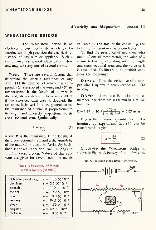
WHEATSTONE BRIDGE 125


Lesson 14

WHEATSTONE BRIDGE

The Wheatstone bridge is an

electrical circuit used quite widely to de-

termine with high precision the electrical re-

sistance of any wire or appliance. Such a

circuit involves several electrical resistors

and may take any one of several forms.

Theory. There are several factors that

determine the electric resistance of any

wire: (1) the material of which it is com-

posed, (2) the size of the wire, and (3) its

temperature. If the length of a wire is

doubled, its resistance is likewise doubled;

if the cross-sectional area is doubled, the

resistance is halved. In more general terms,

the resistance of a wire is proportional to

its length and inversely proportional to its

cross-sectional area. Symbolically,

« = 4 in

where R is the resistance, L the length, Athe cross-sectional area, and P the resistivity

of the material in question. Resistivity is de-

fined as the resistance of a wire 1 m long and

1 m2 in cross section. Values of this con-

stant are given for several common metals

Table 1. Resistivity of Metals

in Ohm Meters (at 20°C)

nichrome (resistance) p = 1.00 X 10~8

aluminum P = 3.2 X 10“8

bismuth P = 1 1 9 X 1

0~8

copper p = 1 .69 X 10~8

iron p = 1 0.0 x i o-8

mercury P = 94.1 X 10-8

silver p = 1.59 X 1

0-8

tungsten p = 5.5 X 10-8

platinum P = 1

0

x i o-8

in Table 1. The smaller the constant P ,the

better is the substance as a conductor.

To find the resistance of any sized wire

made of one of these metals, the value of P

is inserted in Eq. ( 1 ) along with the length

and cross-sectional area, and the value of R

is calculated. To illustrate the method, con-

sider the following:

Example. Find the resistance of a cop-

per wire 1 sq mm in cross section and 300

m long.

Solution. If we use Eq. (1) and re-

member that there are 1000 mm in 1 m, wefind that

R = 1.69 X 10~8 = 5.07 ohms

If p is the unknown quantity to be de-

termined by experiment, Eq. (1) can be

transformed to give

Circuitwise the Wheatstone bridge is

shown in Fig. A. A battery of but a few volts

Fig. A. The circuit of the Wheatstone bridge.


Fig. B. Galvanometer with two insulated probes.

is connected in parallel with a circuit in-

volving a resistance wire with a sliding

contact and two other resistors R and R x .

A switch S is connected into the battery cir-

cuit for applying the potential wherever de-

sired, and a galvanometer is connected to

the sliding contactor and the junction be-

tween R and Ri.

A galvanometer is a sensitive current-

reading instrument, with the zero point at

the center of its scale as shown in Fig. B.

If the current flows one way through the

instrument, the needle deflects to the right.

If the current flows in the other direction,

the needle deflects to the left. If the probes

make contact at two points in a circuit and

the needle shows no current one way or the

other, those two points are at the same po-

tential. If there were a difference of poten-

tial, a current would flow.

Of the different resistors shown in Fig.

A, R represents the unknown resistance to be

determined, R r a precision known resistance,

and R2 and R3

the sections of a uniform

slide wire.

When the switch is closed, a current I2

flows through the slide wire and a current

Zi through R and R t . If the sliding contact

is moved along until a point B is reached

where the galvanometer shows no current,

the points B and D will be at exactly the

same potential.

Under these balanced conditions the po-

tential difference between A and B will be

the same as between A and D, and the po-

tential difference between C and B will be

the same as between C and D. Since these

differences in potential are given by the re-

spective IR drops, we can write

and

11R1 — Z0R2

iiR = r2Rz

Since equals divided by equals give equals,

we find

IiR J2R3

I1R1 I2R2

Canceling, we obtain

R_

Ri

Rs

R2

Solving for the unknown resistance R,

we have

(3)

Since the resistance of a uniform wire is

proportional to its length, we can use the

measured lengths of the slide wire between

A and B and between B and C, and substi-

tute these for R2 and Rsin Eq. (3).

Apparatus. A convenient Wheatstone

bridge circuit board is shown in Fig. C. Ri

is a dial type of standard resistance box. By

Fig. C. A Wheatstone bridge circuit board and all con-

nections to auxiliary equipment.

WHEATSTONE BRIDGE 127

turning the dials the value of R t in ohms

can be set at any value in 1-0 steps up to

10,000 O.

A convenient set of unknown resistors is

obtained by stretching several strands of

standard gage copper, iron, or any com-

mercial make of resistance wire, between

insulated pegs or binding posts on a board.

Several such strands, each one meter long,

are shown in Fig. C.

Object. To use a Wheatstone bridge

circuit to find the resistance of several re-

sistors.

Procedure. If the diameters or cross-

sectional areas of the resistance wires of R

are not already known, measure their di-

ameters with a micrometer, compute their

areas in m2,and record them in a table of

six columns. See Table 2. If the gage num-

bers are known, their areas can be looked

up in standard tables.

When the bridge connections have been

made as shown in Fig. C, the connecting

wires for the first trial should include only

the first 1-m strand of resistance wire. Turn

the dials of R r to include about 100 Q. Mo-mentarily close the switch S and touch the

slide wire at the 50-cm mark with the probe

tip B.

If the galavanometer shows a deflection

(and it probably will), move the probe to

the left. If the deflection decreases, move it

farther to the left; if the deflection increases,

move it to the right. If when you find the

zero current position, the probe is outside

the 25-cm to 75-cm range, alter the box re-

sistance Ri and balance again. Try to make

the null position come as close to the cen-

ter as possible.

When the null position has been located,

record the wire length L, the box resistance

R t ,and the slide wire resistances R2 and R3

as shown in Table 2.

Connect two 1-m lengths of the same

resistance wire in series and connect them

into the bridge circuit as R. Balance the

bridge again, trying to make the balance

position of the probe B somewhere near the

middle of the slide wire, and record your

readings in Table 2.

Repeat all the above steps for each of

your unknown resistance wires. If several

strands of the same wire are available, use

3-, 4-, and 5-m lengths in series as your

third, fourth, and fifth trials.

Data. Let us suppose that the above

procedure has been carried out for eight

trials and the data have been recorded as

shown in Table 2. The wire used for this

particular data was standard gage, and its


Metal

A

(m2)

L

(m)

Ri

(O)

R>

(cm)

Rs

(cm)

nichrome 8.10 X 10“8 1.0 10.0 45.2 54.8

nichrome 8.10 X 10~8 2.0 20.0 44.4 55.6

nichrome 8.10 X 10“8 3.0 40.0 51.8 48.2

nichrome 8.10 X 10~8 4.0 50.0 50.3 49.7

iron 8.10 X 10-8 1.0 2.0 61.9 38.1

iron 32.6 X 10-8 1.0 1.0 76.3 23.7

copper 1.27 X 10-8 1.0 1.0 42.6 57.4

copper 8.10 X IQ-8

1.0 1.0 82.5 17.5

cross-sectional area is assumed to be as

listed in standard gage tables. (See Handbook

of Chemistry and Physics, Chemical Rubber

Publishing Co.)

Calculations. Make a table of four

columns for your calculations and use head-

ings shown in Table 3. The first trial com-

putations have been included for compari-

son purposes.


R RA P P

(fi) (S2 X m2) (O x m) (accepted)

12,1 98,0 X IQ-8

98,0 X IQ-8

100 X IQ-8

128 ELECTRICITY AND MAGNETISM — LESSON 16

The values of R in the first column are

found from Eq. (3). Column 3 is obtained

by use of Eq. (2). The accepted values of

p are obtained from Table 1.

Results. Calculate an average value of

p for each metal and compare the results

with accepted values.


Lesson 16

ELECTRICAL EQUIVALENT OF HEAT

It is the purpose of this experi-

ment to convert a measured amount of elec-

trical energy into heat and then, by measur-

ing the amount of heat produced, to attempt

to check the validity of Joule's law. Joule’s

law is just one of the many forms of the

more general law of the conservation of

energy, and involves the electrical equiva-

lent of heat .

terminal to the other and thereby doing

work, we connect the two terminals with a

conductor, a current l will flow and the bat-

tery will be doing work for us in creating

heat. By definition,ff,e curren t j ;s defined

as the amount of charge Q flowing per

second of time.

Theory. Consider the two terminals of

a battery as shown in Fig. A and the me-

chanical work that would be required to

move a negative charge from the ( + ) termi-

nal to the ( — ) terminal. The amount of

work done per unit charge in carrying any

charge Q from one terminal to the other is

called the difference of potential. Sym-

bolically,

where V is in volts, E is in joules, and Qis in coulombs.

If, instead of carrying a charge from one

Fig. A. The work done per unit charge in carrying any

charge Q from one terminal to the other is called the

difference of potential V.

r x

Q

If we solve this equation for Q

Q = It

and substitute It for Q in Eq. (1), we ob-

tain

Upon transposing, we find

E = Vlt

joules = volts X amperes X seconds

(4)

Since the electrical energy expended is

transformed into heat, the joules of energy

E should be expressed in calories of energy

H. As shown in Electricity and Magnetism,

Lesson 15, E and H are proportional to each

other and their ratio is given by a constant J,

called the electrical equivalent of heat.

J- | = 4.18^ (5)H cal

and is exactly the same as the mechanical

equivalent of heat.

ELECTRICAL EQUIVALENT OF HEAT 129

By inverting this equation, we obtain

1 = ”

J E0.239

calorie

joule(6 )

To measure the electrical energy con-

sumed by any circuit we can measure the

current I with an ammeter, the voltage V

with a voltmeter, and the time t with a

clock.

To measure the heat produced we make

use of the methods of calorimetry as pre-

sented in previous lessons. The heat gained

by any object is given by

H = mc(To - TJ (7)

where m is the mass of a body, c is its spe-

cific heat, and T2 — Ti is its rise in tempera-

ture.

Apparatus. A regular 60-watt tungsten

filament light bulb, mounted in a screw-base

porcelain socket, is used to convert electrical

energy into heat energy. The electrical en-

ergy input is measured by means of a volt-

meter and ammeter as shown in the circuit

diagram of Fig. B.

The heat developed is measured with a

calorimeter as shown in Fig. C. Any wind-up

clock or electric clock with a sweep second

hand will serve for determining the rate of

rise of the temperature of the water.

As the experiment is being performed,

Fig. B. Voltmeter and ammeter connections for lamp

bulb.

the heat developed by the light bulb goes to

heat up the water, the calorimeter cup, and

the bulb. To find H we must, therefore,

account for the heat that goes into these

three objects.

Object. To measure the heat produced

in a current-carrying resistor and deter-

mine the electrical equivalent of heat.

Procedure. Weigh the inner calorimeter

cup and then the light bulb, and record their

masses in grams as m c and m b . See Table 1.

Look up the specific heats of glass and alumi-

num, and record these in Table 1 as the

specific heats for the bulb and calorimeter

cup, respectively.

Fill the cup about half-full of cold water

and insert the light bulb to see how high

the water level rises. Sufficient water should

be added to bring the level close to but not

touching any metal parts of the socket. Re-

move and dry the bulb, and weigh the cup

and water. Record as mc + mw in Table 1.

Fig. C. Mounting of light bulb in a calorimeter.

130 ELECTRICITY AND MAGNETISM-LESSON 16

Read the thermometer and record the

room temperature T.

Assemble the calorimeter and insert the

bulb, stirrer, and thermometer as shown in

Fig. C. Make a table of two columns on

your data sheet and label them with head-

ings as ^hown in Table 2.

Turn on the light bulb and gently stir the

water. As the sweep hand of the clock passes

the vertical position, read and record the

water temperature. Watch the clock, and at

each succeeding 30 seconds read and record

the water temperature as shown in Table 2.

Continue to stir and take readings. Whenthe water temperature reaches 3°C above

the room temperature, make your last read-

ing on the minute. Read and record the am-

meter and voltmeter readings.

Data. Let us assume that the above

steps have been carried out and you have

recorded the data as shown in Tables 1 and

2 .


applied voltage V = 1 1 6 volts

applied current / = 0.52 ampmass of cup m, = 195 gmcup of water m, + mw = 806 gmmass of bulb mb = 50.8 gmsp ht of bulb c6 = 0.16

sp ht of cup cc = 0.22

room temp T = 25.0°C

mass of water mw = ?

rise in T r2 — h = ?

time interval t = ?

Calculations. To find the last two values

in Table 1, plot a graph of the data recorded

in Table 2. The vertical scale for T should


t

(min)

T

(°C)

0j

21.2i

0.5:

21.8 ;

1.0! 22.5

1 .5 23.2j

2.0 1 23.8 !

2.5 24.4

3.0 25.0

3.5 25.7

4.0 26.3

4.5 26.9

i

5.0 27.5

5.5 28.0

6.0 28.6

be labeled 20, 22, 24, . . . 30°C, and the

horizontal scale for t should be labeled 0, 1,

2, 3, 4, 5, and 6 min.

Draw a smooth curve through your

plotted points and then draw a tangent to

this curve at the point of room temperature.

Since this tangent represents the true rate

of temperature rise, use it to find the true

rise for a period of 5 min. Record these as

T2 — Ti and t in Table 1

.

Find the electrical energy input for a

period of 5 minutes by substitution in Eq.

(4)

.

Find the heat energy that went into (a)

the water, (b) the calorimeter cup, and (c)

the lamp bulb by using Eq. (7).

Take the ratio of E to H and find J.

Take the ratio of H to E and find 1/J.

Compare these last two ratios with the

accepted values of J and 1/J given in Eqs.

(5) and (6).

Find your percentage error.

A STUDY OF MOTORS 131


Lesson 19

A STUDY OF MOTORS

This lesson is a laboratory ex-

periment on the principles of the electric

motor. In essence it is a descriptive type of

experiment that requires careful observa-

tions but no quantitative measurements.

Theory. To introduce the principles of

the motor we will find it convenient to begin

with a U-shaped magnet and a short bar of

soft iron mounted free to turn between its

poles as shown in Fig. A (a). If one spins

the iron bar, it will slow down, oscillate, and

finally come to rest in the position shown,

with either end to the right or left.

If, on the other hand, a small permanent

magnet is mounted free to spin in the sameway, it will always come to rest in one posi-

tion only, with opposite poles adjacent, as

shown in diagram (b).

Let us now consider the magnetic fields

involved in the first demonstration. The field

between the poles of the magnet is shownin Fig. B. When the soft iron bar is inter-

posed, as in Fig. C, the lines of force not

only change their shape but they induce

N and S polar regions in the iron. Just as a

Fig. A. A soft iron bar, or a magnet, lines up with the

magnetic field.

Fig. B. The magnetic field between the two poles of a

U-shaped magnet.

copper wire is a good conductor of electron

currents, so soft iron acts as though it were

a good conductor of magnetic lines of force.

This property of a medium to conduct

Fig. C. A soft iron bar in the field of a permanent

magnet.

132 ELECTRICITY AND M A G N E T I S M - L ES S O N 19

lines of force is called reluctance, and it is

analogous to electrical resistance for cur-

rents. Air has a high reluctance, while soft

iron has a low reluctance. It is not to be

assumed by this analogy that magnetic lines

of force constitute a flow of any kind. The

arrows simply indicate the direction a com-

pass needle would point if located there.

In the case of the permanent bar magnet,

the bar again bridges the air gap by a “good

conductor,” i.e., one of low reluctance. Be-

cause of the strong interacting fields, the

permanent bar magnet experiences a stronger

force tending to line it up with the magnetic

field of the U-shaped magnet as shown in

Fig. D.

The Armature. We have seen in Elec-

tricity and Magnetism, Lesson 18, how the

magnetic induction B0 at the center of a sole-

noid is given by

Fig. F. Principal parts of a simple electric motor.

See Fig. E.

It is common practice to simplify this

equation and write it as

B„ = HoH (2)

in which H is called the magnetic intensity

and is given by

When an iron core is inserted into this

magnetic field, as shown in Fig. E, the mag-

netic induction B increases many fold, and

we write

B = mH (4)

where ^ is a constant hundreds and even

thousands of times larger than fi0 ,and is

Fig. E. An iron core greatly strengthens the magnetic in-

duction in a solenoid.

Fig. G. A field winding makes a more powerful motor.

A STUDY OF MOTORS 133

Fig. H. Principal elements of a laboratory type of electric motor.

called the permeability. The magnetic induc-

tion B beyond but near the coil ends is

not greatly different from that at the coil

center.

Suppose we now insert such an electro-

magnet between the poles of a magnet as

shown in Fig. F, and arrange sliding con-

tacts that will conduct the required current

to the winding and still permit the system

to turn. This rotating unit, called the arma-

ture, will experience a very strong resultant

torque tending to align it with the magnet’s

field.

As the armature swings around, to line up

the two fields, the current to the armature

winding reverses because of the split ring

of the commutator. The rotational inertia

of the armature then carries it part wayaround and strong torques again turn it

toward alignment.

To further increase the armature torque,

the field between the magnet poles is

strengthened by sending a current through

a coil called the field winding. See Fig. G.

Although electric motors usually have a

number of pairs of poles and windings in

the armature, and there are many varia-

tions in size, shape, and electrical circuits

used in their construction, most of the above

principles are involved in all of them.

Apparatus. A convenient form of ap-

paratus for this experiment is shown in Fig.

H and is called a St. Louis motor. It con-

sists of two straight bar magnets, an electro-

magnet attachment, and an armature with

sliding contacts and brushes. Additional

equipment needed will include three dry

cells, a switch, and a rheostat (not shown).

Object. To study the principles of elec-

tric motors.

Procedure. Part 1 . Connect the arma-

ture brushes to the switch and battery, and

with the permanent magnets in place as

shown, close the switch. If the armature fails

to turn, give it a spin. It should now turn

by itself and soon come up to full speed.

Gradually swing the magnet poles away

from the armature and record what you ob-

serve.

Part 2. Connect the rheostat in series with

the armature circuit, and with the field poles

close in, close the switch. Note the effect

on the speed of the armature as the current

is reduced. Record your observations.

Part 3. Reverse the battery connections

and note whether the armature rotates in

the same direction as before.


Turn the bar magnets end for end,

thereby reversing the field direction, and ob-

serve whether the armature rotation is re-

versed or not. Reverse both the armature

current and the field magnets and observe

the rotational direction.

Part 4. Replace the bar magnets with the

electromagnet field assembly. Connect the

armature and field winding in series and

then to the battery switch. Close the switch

and note the direction of rotation.

Part 5. Reverse the battery leads and note

the direction of rotation. Reverse the con-

nections to the armature only and note the

direction of rotation. Finally reverse the field

connections only and note the rotation. Re-

cord these observations.

Part 6. Connect the armature and field wind-

ings in parallel to the switch. This is called

a shunt motor. Close the switch and observe

the rotation. Reverse the battery connec-

tions and note the direction. Record your

observations.

Data. Your data consists of notes on

your data sheet made under the headings of

Part 1, Part 2, etc. If apparatus is not avail-

able for the performance of this experiment,

study the principles given in the theory

above and see if you can determine the an-

swers to the various steps taken in this ex-

periment.

Results. Answer the following questions

in your report.

Part 1. (a) Looking down from above,

which way does the armature rotate? (b)

What happens as the poles are moved apart?

Part 2. What happens as the armature cur-

rent increases?

Part 3. (a) What happens when the current

is reversed? (b) When the poles are re-

versed? (c) When both are reversed?

Part 4. In what direction does the armature

turn?

Part 5. (a) What is the effect of reversing

the battery connections? (b) The armature

connections? (c) The field connections?

Part 6. (a) In what direction does the ar-

mature rotate? (b) What is the effect of

reversing the battery connections?


Lesson 21

COULOMB'S LAW

It has been pointed out in Elec-

tricity and Magnetism, Lesson 12, that the

poles of any magnet are not located at specific

points but are distributed about certain areas

over the metal surface.

In spite of the uncertainty in the exact

location of a magnetic pole, a type of per-

manent bar magnet has been developed for

experimentally determining the laws of force

between poles. These special magnets, as

shown in Fig. A, consist of thin steel rods,

about 20 to 30 cm long, with steel balls at

the very ends. When magnetized, the N and

S poles become concentrated on these steel

balls.

Note how nearly radially outward the

COULOMB'S LAW 135

Fig. A. Map of the magnetic field around a special type

of permanent magnet.

magnetic lines of force are at the N pole and

how nearly radially inward they are at the

S pole. The result, in effect, is such as to

isolate one pole from the other and at the

same time to centralize the field of each pole

so that to nearby objects they act as though

they were concentrated at the spherical

centers.

Theory. A qualitative description of the

action between magnetic poles has already

been stated in Electricity and Magnetism,

Lesson 12, namely, like poles repel and un-

like poles attract.

Experimental measurements of a quanti-

tative nature show that the force acting be-

tween two poles is proportional to the

product of the pole strengths and inversely

proportional to the square of the distance

between them. In symbols

F = k (1)d“

where F is the force, m and m' are the pole

strengths, and d is the distance between

them. This relation is known as Coulomb’s

law. See Fig. B. In the rationalized mks sys-

tem of units, F is in newtons, m and m' are

Fig. B. Factors concerned with Coulomb's law for mag-

netic poles.

m m f

F

Fig. C. Geometry of the forces and torques involved in

the Hibbert balance.

in ampere meters, d is in meters, and k is

the proportionality constant given by

ampere meter

The magnets to be used in this experiment

are of the bar type shown in Fig. A. When

two such magnets are arranged in the con-

figuration shown in Fig. C, the two poles

nearest each other will exert by far the

strongest forces on each other. These forces,

represented by F in the diagram, are an

action and reaction pair.

To measure the force F exerted on the

lower S pole, the lower magnet is initially

balanced carefully on a pivot P at its center

of mass. Under these conditions the two at-

tractive forces f due to the poles of the upper

magnet will cancel out since they exert equal

and opposite torques.

If the magnets are long and the distance

d relatively small, the force of repulsion be-

tween the extreme end poles will be exceed-

ingly small. To a first approximation, this

force and the torque it exerts can be neg-

lected.


in this experiment is shown in Fig. D and is

known as a Hibbert balance. Two bar mag-

nets, just 20 cm between pole centers, are

used, along with a small 10-mg mass in the

form of a wire rider R as shown at the lower

left.

The upper magnet M 2 is free to be moved

up or down, and the rider can be moved


along on either side of the lower magnet

Mi to establish balance. By the principle of

levers, the force F is determined by the

10-mg rider and its distance from the pivot P.

A small removable gage block B should

be provided, and of such a height that whenthe magnet pole is held down against it, the

balance pointer is on zero.

Object. To study the inverse square

law as it applies to magnetic poles.

Procedure. To set up the Hibbert bal-

ance, select a table free from all iron. Avoid

tables containing large steel bolts, gas and

water pipes, as well as electrical conduits.

Be sure the table surface is level.

With magnet Mj removed from its pivot,

lower magnet M 2 so that its S pole rests on

the gage block B in exactly the position to be

later occupied by the S pole of magnet Miwhen in balance. Read the height position

on the vertical scale, and record as x0 below

Table 1.

Remove magnet M 2 to a distance of at

least 10 ft from the balance. Insert Mi and

balance it by adjusting the two thumb screws

T. Balance is secured when in the absence

of the gage block the magnet is horizontal

and the pointer is on zero.

Now place the 10-mg rider R on the mag-

net bar 1 cm to the left of the pivot P.

Bring up M 2 and place it in the vertical sup-

port with the two S poles lined up vertically

as shown.

Slowly lower or raise M 2 until M t is ex-

actly in balance again. Read and record the

magnet height x. For your data use a table

of three columns with headings as shown in

Table 1. {Note: Since the mass of the rider

is 10 mg and the S pole of M x is 10 cm from

the pivot, the rider position, 1 cm to the left

of P, is equivalent to the force F of a 1 mgweight at S.)

Move the 10-mg rider 2 cm to the left


Trial

F

(mg-wt)

X

(cm)

1 1 28.7

2 2 21.4

3 3 18.2

4 4 16.4

5 5 15.1

6 6 14.2

7 7 13.5

8 8 12.9

9 9 12.4

x 0 = 5.8 cm

TRANSFORMERS 137

of P and lower M 2 until Mi is exactly bal-

anced. Read and record the magnet height

x as trial 2.

Repeat this process, moving the rider 1

cm more to the left for each succeeding

trial, and record the height x for each posi-

tion of M 2 .

Data. Assume the above experiment has

been performed and the data have been re-


Calculations. It is most convenient to

record all calculations by tabulation. For


d d2 d3

(cm) (cm 2) (cm 3

)

22.9 524 12000


1 1_ 1_

d d 2 d3

(cm-1

) (cm-2

) (cm-3

)

.0437 .00191 .000083

this purpose make two tables of three col-

umns each, with headings as shown in Tables

2 and 3.

Calculations for the first trial have al-

ready been made and will serve as a guide

in making the others.

Results. Plot three separate graphs of

your calculations

:

( 1 ) Plot F vertically against 1 /d horizon-

tally.

(2) Plot F vertically against 1/d2 horizon-

tally.

(3) Plot F vertically against I/d3 horizon-

tally.

Conclusions. Which of the graphs gives

the straightest line? What can you conclude

from the results as determined from these

three graphs? To what is the slight curva-

ture due in graph number (2)? {Note: The

plotting of F in mg-wt is justified since each

force in dynes is obtained by multiplying

the mass in grams by g = 980 cm/sec.

Hence the values of F listed in Table 1 are

very nearly equal to the forces in dynes.)


Lesson 24

TRANSFORMERS

The widespread use of transform-

ers, large and small, is ample justification

for performing an experiment on this funda-

mental unit of electrical equipment. The

basic principles of the transformer are pre-

sented in Electricity and Magnetism, Lesson

22, and involve rapidly changing magnetic

fields.

Theory. The transformer, as shown in

Fig. A, consists essentially of three im-

portant parts: (1) a coil of wire called the

primary, (2) another coil of wire called the

secondary, and (3) a conductor of mag-

netic lines of force called the core linking

both coils.

When a source of alternating current is

applied to the two terminals of the primary

winding, an alternating emf is produced at

the secondary terminals. The increasing and

decreasing field B set up in the iron core

by the primary a.c. also links through the

138 ELECTRICITY AND M A G N E T I S M - L ES S O N 24

Fig. A. Typical closed-core transformer.

secondary and induces the same difference

of potential V0 in every turn of wire. Since

the secondary turns are all in series, the

over-all voltage delivered is the sum of those

for the separate turns. In other words, the

secondary voltage Vs should be directly pro-

portional to the number of turns N.

Vs = VoNs ( 1 )

The relation between primary and sec-

ondary voltage and the number of turns in

the coils is given by

where Np and Ns are the number of turns

in the primary and secondary, respectively,

and Vp and Vs are the corresponding termi-

nal voltages.

If Ns is greater than Np , we have a so-

called step-up transformer, while if Ns is

smaller than Np ,we have a step-down

transformer. The step-up transformer raises

the voltage above that applied to the pri-

mary, while the step-down transformer re-

duces it.

A second type of transformer in commonuse has a tapped secondary. A tapped sec-

ondary is one in which different secondary

voltages can be obtained by making con-

nections to different numbers of secondary

turns as shown in Fig. B. If secondary con-

nections are made to S0 and Si, a relatively

low voltage is obtained. If the upper con-

nection is shifted to S2 ,S3 ,

etc., more and

more secondary turns are included, and the

secondary voltage is proportionally larger.

The effect is similar in many ways to the po-

tential divider.

A third type of transformer of widespread

use has two or more independent secondary

windings. See Fig. C. Electrically insulated

from each other these secondaries produce

their own voltage as given by Eqs. 1 and 2.

Apparatus. The principal part of the

apparatus used in this experiment consists

of a closed core transformer with removable

coils, like those shown in Fig. D. A set of

Fig. B. Transformer with a tapped secondary.Fig. D. Experimental transformer with changeable coils.

crossbar

TRANSFORMERS 139

Fig. E. Electrical circuit diagram showing connections for

transformer experiment.

several coils wound on the same size tubing

but having different numbers of turns are

used in pairs for the windings.

Although coils with any desired number

of turns may be used, the ones described

here have 350, 250, 250, 200, 150, 100, and

50 turns, respectively. In addition to these, a

special coil of 100 turns with taps at every

twentieth turn, and a tube with two separate

windings of 200 turns and 20 turns, respec-

tively, will be used.

The auxiliary equipment needed is shown

in Fig. E, and consists of an a.-c. voltmeter

reading up to 150 volts, a potential divider

of several hundred ohms, a double-pole-sin-

gle-throw switch, and a double-pole-double-

throw switch.

Object. To study the principles of the

step-up and step-down transformer.

Procedure. Part 7. Remove the trans-

former crossbar. Place the 250-turn coil on

the primary leg of the core and the 350-

turn coil on the secondary leg. Replace the

crossbar and, if a clamp is available, clamp

it down tightly.

When all connections are made as shownin Fig. E, close switch K and P, and adjust

the potential divider P to give the maximuminput voltage to the primary. Read and re-

cord this voltage as Vp in a table of four

columns as shown in Table 1.

Throw switch D to the S position and re-

cord the secondary voltage reading as Vs .

Record the numbers of turns Np and Ns .

For your second trial replace the sec-

ondary coil by one of 250 turns. Be sure

the crossbar is secure, and with maximumvoltage on the primary, record the secondary

voltage V.s . Record N sand Np .

For your third and succeeding trials use

the other coils in their turn as secondary

coils, recording each time V s ,Vp , Ns, and

Np . (Note: Do not use a primary winding of

less than 100 turns, as an excessive current

will be drawn from the 120-volt lighting

circuit.

)

Part 2. With a 250-turn primary and a 150

turn secondary, carry out the following

trials. With the switch D to the left, adjust

the potential divider to give the primary 100

volts. Throw the switch D to the right and

find the secondary voltage. Record these

readings in Table 1.

With the switch to the left for trial two,

adjust the slider to give 80 volts. Throw the

switch to the right and read the secondary

voltage.

Repeat this procedure, reducing the pri-

mary voltage by 20-volt steps, each time

recording both voltages Vp and Vs as shown

in Table 1.

Part 3. Place the 200-turn coil on the pri-

mary leg and the tapped coil on the sec-

ondary leg. Set the primary voltage at 100

volts and make the secondary winding con-

nections to tap points S0 and S5 . See Fig. B.

Read and record your data as shown in

Table 1.

Move the upper tap connection from S5 to

S4 and repeat the voltage measurements. Re-

cord these as trial 2.

Repeat these steps for each tap on the

secondary winding and record.

Part 4. Replace the tapped secondary by the

tube containing two separate coils. Connect


the voltmeter leads to each coil in turn, and

with the primary at 110 volts, determine

the secondary voltage for each secondary

coil. Record these readings as shown in

Table 1.

Data. We will assume the above steps


NP Ns vP vs

(turns) (turns) (volts) (volts)

Part 1

250 350 118 150

250 250 118 107

250 200 118 86

250 150 118 64

250 100 118 43

250 50 118 22

Part 2

250 150 100 55

250 150 80 43

250 150 60 32

250 150 40 22

250 150 20 1

1

Part 3

200 100 100 46

200 80 100 37

200 60 100 28

200 40 100 18

200 20 100 9

Part 4

200 200 no 101

200 20 no 10

have been carried out and the data recorded

as shown in Table 1.

Calculations. Make a table of two col-


The two ratios shown should be computed

for all trials recorded in Table 1. The first

two trials are already calculated and will

serve as a guide for all the others.

By Eq. (2) we should expect each pair

of values to be the same. Transformers,

however, are not 100% efficient. A small

amount of energy is dissipated as heat both

in the coils and in the soft iron of the core.

The core of most transformers is laminated,

i.e., made up of thin layers, for the purpose

of reducing losses due to eddy curents in-

duced in the core by the changing field. As a

rule, transformers are over 90% efficient.


Ns

Np

Vs

yP

Pari\ i

1.40 1.27

1.00 .91

Results. Plot a graph of your recorded

data in Part 1. Plot Vs vertically with the

scale labeled 0, 25, 50, 75, 100, 125, and

150 volts, and Ns horizontally with the scale

labeled 0, 100, 200, 300, and 400 turns.

Use a ruler and draw as straight a line as

you can through the plotted points. Using

this graph, read off the value of Vs if a sec-

ondary of 300 turns had been used in Part 1.

From this V,, and N s ,and Eq. (1), calculate

the voltage per turn VQ .

ATOMIC PHYSICS

Atomic Physics|

Lesson 4

ELECTRONIC CHARGE TO MASS RATIO

The purpose of this experiment

is to determine by measurement and calcula-

tion the ratio of the electronic charge e to

the electronic mass m. This is known as the

"e over m experiment," and you should

find it most interesting.

Theory. When any substance is heated

to incandescence in a vacuum, it not only

gives off visible light radiation but it also

emits electrons as well. Such action is il-

lustrated in Fig. A, and is called thermionic

emission.

The thermal emission of electrons by a

hot tungsten filament F, heated to incandes-

cence by the current from a battery, is

analogous to the steam boiling off from a

tea kettle. The higher the current, the higher

is the surface temperature of the metal and

the greater are the number of electrons

emitted.

The surface temperature required for the

copious emission of electrons is greater for

some materials than for others. Low tem-

perature emitters are often used in electronic

devices, heated to their proper temperature

by an indirect heating element as shown in

Fig. B.

This particular device, called an electron

gun, is for the purpose of producing a strong

Fig. A. Thermionic emission.

Fig. B. Diagram of an electron gun.

but narrow beam of electrons. A battery of

a few volts, applied to a tungsten wire fila-

ment F, indirectly heats the electron-emitting

surface K called the cathode.

With a battery of several hundred volts V,

these electrons are accelerated toward the

positively charged, cone-shaped anode. Bygrounding the plus side of the battery the

anode is brought to the potential of the sur-

roundings, and the electrons, emerging as a

beam, travel with constant speed.

We have seen in Electricity and Magnet-

ism, Lesson 16, that if the difference of po-

tential between two terminals is V, the work

done on each charge e in going from one to

the other is given by Ve. Since this work is

converted into kinetic energy by giving elec-

trons a velocity v, we can write

( 1 )

This is one of the basic equations in

atomic physics.

Solving for v, we obtain

v = (2 )

If V is in volts, e is in coulombs, and mis in kilograms, v is in meters per second.

For electrons

e = 1.6019 X 10-19 coulomb (3)

m = 9.1072 X lO"31 kg (4)

142

ELECTRONIC CHARGE TO MASS RATIO 143

Fig. C. Circuit diagram for e/m experiment.


experiment consists, as shown in Fig. C, of

a highly evacuated glass bulb containing an

electron gun as just described. With the

entire tube located in the uniform magnetic

field of two current-carrying coils, the emer-

gent beam is bent into a circular path as

shown.

The battery circuit is for the purpose of

supplying current to heat the cathode of the

electron gun, as well as the voltage needed

to accelerate the liberated electrons.

Since the electrons travel through a mag-

netic field, their circular path is determined

by Eq. (2) of Atomic Physics, Lesson 3.

This equation gives

Beriz\v = — (5)

m

Since the left-hand sides of Eqs. (2) and

(5) are equal to each other, we can set

the right-hand sides equal:

m X m

Squaring both sides of this equation, weobtain

BW = 2Ve

m2 m

Canceling out like quantities, we can solve

for e/m, and obtain,

e _ 2Vm~

B 2r2 (6 )

All the quantities on the right are to be

measured. The accelerating voltage V ap-

plied to the electrons is measured with a

voltmeter, the radius r of the circular path

is measured with a meter stick, and the

magnetic induction B is determined from

the known dimensions of, and the current

flowing through, Helmholtz coils. As shown

in Fig. D, Helmholtz coils consist of two

identical coils placed side by side at a dis-

tance apart equal to their radius R.

Such an arrangement produces a relatively

uniform field over a considerable volume of

space, and the magnetic induction is given

by

B = 9.0 X lO"7NIweber

R meter2

where N is the number of turns per coil, R

is the coil radius in meters, and I is the cur-

rent in amperes. The number of turns of

wire can be counted, the radius can be meas-

ured with a meter stick, and the current can

be read from an ammeter as shown in Fig.

D.

Object. To determine the electronic

charge to electronic mass ratio.

Procedure. Since this kind of equipment

is delicate and easy to damage, follow the

144 ATOMIC PHYSICS-LESSON 4

instructions usually found attached to the

apparatus by the manufacturer.

Turn on the heater current and bring the

current up to the specified value. After about

60 sec, turn on the accelerating potential Vand bring it up to 155 volts.

Turn out the room lights, and the electron

beam should appear coming straight up out

of the opening of the electron gun. Thefluorescence of the small amount of hydro-

gen gas, or mercury vapor, in the evacuated

bulb should make the beam visible. Make a

table of three columns and record this volt-

age in the first column as shown in Table 1.

Now apply the field current to the Helm-holz coils. The electron beam will now bend

in the arc of a circle. Adjust the coil cur-

rent until the beam just misses the glass

walls of the tube opposite the gun as shown

in Fig. C. Read and record the current 7.

As a second trial, increase the accelerat-

ing voltage to 175 volts. Increase the field

current until the beam just misses the op-

posite glass wall. Read and record the volt-

age V and current 7 as shown in Table 1.

Increase the accelerating voltage another

20 volts and repeat the procedure as before.

Measure the number of coil turns and the

coil radius, and record them below your

table as shown in the example (Table 1).

To measure the diameter of the circular

beam of electrons, the beam can be turned

off and the room lights left on. Set up a

meter stick in a clamp stand and sight into

the tube using a right triangle of the type

used in drafting. Record the radius r.

Data. Assume that the above steps havebeen properly carried out and the data re-



V I

Trial (volts) (amps)

1 155 .94

2 175 1.01

3 195 1.06

radius of coils R = .18 mwire turns per coil N = 123

radius of electron beam r — .072 m

Calculations. Make a table of five col-


Make the necessary calculations to find the

ratio e/m for all three trials.

Compute your average e/m and compare

it with the most probable value known to

date:

- = 1.759 X 10 11

mcoulomb

kg


Nl

/ amp\

\turns/

B

(webers \

BV/webersA

2V

(volts)

e/m

(coulomb^

V meter2 / \ meters2 / V kg /

WAVE LENGTHS OF SPECTRUM LINES 145

Atomic Physics|

Lesson 6

WAVE LENGTHS OF SPECTRUM LINES

The wave lengths of visible light

emitted by different light sources are so ex-

tremely short that approximately one thou-

sand waves are no longer than the thickness

of a sheet of paper. As short as they are,

light of various wave lengths from any given

source can be measured with very high

precision.

Theory. The most common methods

used in the research laboratory for meas-

uring the wave length of light employ a dif-

fraction grating. If the instrument is de-

signed to photograph the spectrum, it is

called a spectrograph; if it is designed to

look at the spectrum, it is called a spectro-

scope.

We have seen in Light, Lesson 16, that

a diffraction grating is composed of thou-

sands of fine parallel and equally spaced

lines ruled on a smooth surface. If the sur-

Fig. A. Diagrams showing the wave fronts forming the

various spectrum orders observed with a diffraction

grating.

face is that of a mirrorlike reflector it is a

reflection grating, and if the surface is that

of a transparent medium like glass or plastic

it is a transmission grating.

While a grating may contain several thou-

sand lines per centimeter, the theory of its

action on light can be derived from the con-

sideration of but a few of the lines. Fig. Arepresents a cross-section diagram of a small

section of a transmission grating, the lines

being seen end on.

Parallel light waves coming from the left

are partly absorbed, partly reflected by the

rulings, and partly transmitted. Emerging

from the openings as identical wavelets, a

number of wave fronts of light are built up

as shown by the parallel lines. One set of

light waves travel straight on, while others

travel off at angles.

The new wave fronts in diagram (b) or

(c) constitute what is called the first-order

spectrum, while those in diagram (d) form

what is called the second-order spectrum.

To find a relation between measurable

quantities and the wave length of light con-

sider the wavelets emerging from two ad-

jacent slits to form the first-order spectrum

as shown in Fig. B. Note the right triangle

Fig. B. Diagram from which the grating formula is de-

rived.


G

Fig. C. Diagram for the diffraction grating measurements.

formed by the grating spacing d as the hy-

potenuse, and the wave length A as the side

opposite the angle <9. From this triangle wecan write

^= sin 6 (1)

Transpose d to the other side and we ob-

tain the basic equation for diffraction grat-

ings

A = d sin 6 (2)

Because the wave lengths of light are so

very small, the physicist has adopted a

smaller unit of length than the centimeter

or millimeter. This unit is called the ang-

strom after the Swedish scientist by that

name. In 1868, Angstrom published a mapof the visible spectrum of the sun, and on

this map he labeled the wave lengths in ten-

millionths of a millimeter. Since that time,

light waves have been specified in these

units.

In one centimeter there are 100,000,000

angstroms.

1 cm = 108 A (8)

In light the velocity c in a vacuum is

given by

The wave front normal AL and grating

normal AN also form the angle 6 and, at a

screen some distance away, form a similar

right triangle AOP. See Fig. C. For this tri-

angle

^= sin d (3)

Combining Eqs. (1) and (3), or from

the corresponding sides of similar triangles,

we can write

c = v\ (9)

where v is the vibration frequency and A

is the wave length. From this we see that

the longer the wave length, the lower is the

frequency; and the shorter the wave length,

the higher is the frequency. It is commonpractice among physicists to designate the

wave length of light waves by the Greek

letter A (lambda) and the frequency by the

Greek letter v (nu).

A _ x

d ~R

from which we obtain

(4 )

Apparatus. The source of light used in

this experiment is a mercury vapor discharge

tube of the form shown in Fig. D. A small

A diagram similar to Fig. B, drawn for

the second-order spectrum as shown in Fig.

A(d), shows that the side opposite the angle

6 has a length of 2A. From similar right tri-

angles in this case,

Fig. D. Mercury vapor discharge tube.

from which we obtain

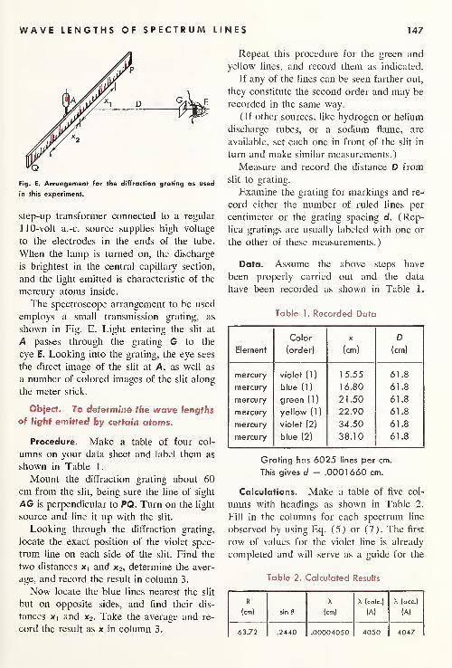
WAVE LENGTHS OF SPECTRUM LINES 147

Fig. E. Arrangement for the diffraction grating as used

in this experiment.

step-up transformer connected to a regular

110-volt a.-c. source supplies high voltage

to the electrodes in the ends of the tube.

When the lamp is turned on, the discharge

is brightest in the central capillary section,

and the light emitted is characteristic of the

mercury atoms inside.

The spectroscope arrangement to be used

employs a small transmission grating, as

shown in Fig. E. Light entering the slit at

A passes through the grating G to the

eye E. Looking into the grating, the eye sees

the direct image of the slit at A, as well as

a number of colored images of the slit along

the meter stick.

Object. To determine the wave lengths

of light emitted by certain atoms.

Procedure. Make a table of four col-

umns on your data sheet and label them as

shown in Table 1.

Mount the diffraction grating about 60

cm from the slit, being sure the line of sight

AG is perpendicular to PQ. Turn on the light

source and line it up with the slit.

Looking through the diffraction grating,

locate the exact position of the violet spec-

trum line on each side of the slit. Find the

two distances and x2 ,determine the aver-

age, and record the result in column 3.

Now locate the blue lines nearest the slit

but on opposite sides, and find their dis-

tances x 1 and x2 . Take the average and re-

cord the result as x in column 3.

Repeat this procedure for the green and

yellow lines, and record them as indicated.

If any of the lines can be seen farther out,

they constitute the second order and may be

recorded in the same way.

(If other sources, like hydrogen or helium

discharge tubes, or a sodium flame, are

available, set each one in front of the slit in

turn and make similar measurements.)

Measure and record the distance D from

slit to grating.

Examine the grating for markings and re-

cord either the number of ruled lines per

centimeter or the grating spacing d. (Rep-

lica gratings are usually labeled with one or

the other of these measurements.)

Data. Assume the above steps have

been properly carried out and the data

have been recorded as shown in Table 1.


Element

Color

(order) (cm)

D

(cm)

mercury violet (1

)

15.55 61.8

mercury blue (1) 16.80 61.8

mercury green (1) 21.50 61.8

mercury yellow (1

)

22.90 61.8

mercury violet (2) 34.50 61.8

mercury blue (2) 38.10 61.8

Grating has 6025 lines per cm.

This gives d = .0001660 cm.

Calculations. Make a table of five col-


Fill in the columns for each spectrum line

observed by using Eq. (5) or (7). The first

row of values for the violet line is already

completed and will serve as a guide for the


R X X (calc.) X (acc.)

(cm) sin 9 (cm) (A) (A)

63.72 .2440 .00004050 4050 4047


others. Carry out all calculations to four

significant figures. Use Eq. (3) for com-

puting column 2.

The accepted wave lengths for the mer-

cury lines are 4047 A, 4359 A, 5461 A,

and 5770 A, respectively.

Plot a graph of sin 0 against calculated A

for the first-order lines only. Use ten squares

vertically for sin 6,and label them .160,

.180, .200, . . . ,.360. Use ten squares

horizontally for A, and label alternate lines

4000, 4400, 4800, . . . ,6000 A.


draw from the graph? Would the graph line

pass through the origin if drawn? Do you

think a diffraction grating instrument is ca-

pable of high precision?

Atomic Physics|

Lesson 9

RADIOACTIVITY MEASUREMENTS

Radioactivity may be defined as

the spontaneous disintegration of atomic

nuclei. We have seen in Atomic Physics, Les-

son 8, that three kinds of rays are ejected

from radioactive elements and that these

rays, called alpha, beta, and gamma rays,

have different ionizing and penetrating pow-

ers.

When a strong radioactive source, like

radium, is brought close to a charged elec-

troscope, or an electrometer, rays passing

through the housing ionize the air mole-

cules inside. Some of these ions are attracted

to the electroscope and neutralize its charge.

Theory. A most effective detector of

radioactivity, known as a Geiger counter,

is to be used in this laboratory experiment.

The principal element of this device, known

as a Geiger-Mueller tube, is one of the

simplest devices ever designed. It consists,

as shown in Fig. A, of an open-ended cylin-

drical conductor, from 1 cm to 100 cmlong, fitted inside of a sealed thin-walled glass

tube, and with a fine tungsten wire stretched

along the axis.

After the tube has been evacuated, and

then partially filled with some gas, like air,

a potential of several hundred volts is ap-

plied, the positive to the center wire and the

negative to the cylinder.

When a single high-speed particle from a

radioactive source goes through the Geiger-

Mueller tube, ions are created along its path

by the freeing of electrons from the gas

molecules.

These freed electrons are attracted to the

positively charged wire and move toward it,

acquiring within a short distance of the wire

a high velocity of their own. Because of this

velocity they too can ionize molecules, thus

freeing more electrons. This multiplication

of electrons repeats itself in rapid succession,

Fig. A. Diagram of a Geiger-Mueller tube.

RADIOACTIVITY MEASUREMENTS 149

Fig. B. Electron avalanches developed in a Geiger-Mueller

tube.

producing within a very short interval of

time an avalanche of electrons surging to-

ward the central wire. See Fig. B.

The sudden arrival of charge at the wire

gives rise to the flow of a small current im-

pulse to an electrical circuit. When this cur-

rent has been intensified by an amplifier,

it may be made to activate an electric switch,

a radio loud-speaker, or any kind of elec-

trical device.

Quite frequently the impulses from a

Geiger-Mueller tube are made to operate

a small counting device, or a meter that

indicates the number of particles passing

through it per minute. The latter type of

attachment makes the instrument a Geiger

counter with a counting-rate meter.

Fig. C. Characteristic curve for a Geiger-Mueller tube.

Fig. D. Illustration of the inverse-square law for radio-

activity.

When a radioactive source is brought

close to a Geiger counter and the counting

rate determined for different applied volt-

ages, one obtains a curve like that shown

in Fig. C. As the voltage is slowly increased,

no counts are observed until a certain start-

ing voltage is reached.

Once the starting voltage is reached, the

counting rate increases rapidly and then

levels off to form a flattened part of the

curve called the plateau. When operating

with a voltage near the center of this region,

any increase or decrease of 50 volts or so

will not appreciably alter the instrument’s

counting rate.

If the applied voltage goes too high, as

shown by the dotted part of the graph, the

tube becomes unstable and a glow discharge

will develop, causing damage to the tube.

As a radioactive source is brought closer

and closer to a Geiger counter, the counting

rate increases because more rays pass

through it. Because of the straight line path

of the rays, the inverse-square law, found

to hold for sound waves and for light, should

hold for a, J3, and y rays. See Fig. D. Ioniza-

tion by, and absorption of, rays along their

paths through the air will cause departures

from this law. The a particles travel but a

few centimeters before all are stopped, while

most of the /3 and y rays will traverse 100

cm or more.


in this experiment is a common form of

Geiger counter as shown in Fig. E. It con-

sists of a G-M counter tube about 10 cmlong connected to a box containing vacuum


Fig. E. Geiger counter instrument complete with G-M

tube and counting-rate meter.

tube circuits, a small loud-speaker, and a

counting-rate meter M.

Dial (1) operates the speaker and per-

mits the individual ray pulses to be heard.

Dial (2) turns on the vacuum tubes as in

any radio or TV receiver, and turning it

clockwise increases the voltage supplied to

the G-M tube. Dial (3) has three position

points to which it can be turned. The posi-

tion marked “VOLTS” connects the meter

M so it shows the voltage on the G-M tube.

When in the X 1 position, under C/M, the

meter M directly reads counts per minute,

and in the X 10 position the meter reading

should be multiplied by 10.

A small capsule containing a source of

radium, or a watch with a radium painted

dial, may be used as a source of /3 and y

rays.

Object. To measure the radioactivity of

a radioactive element by means of a Gei-

ger counter.

Procedure. Be sure dial 2 is in the

“OFF” position before plugging the instru-

ment cord into the wall socket. Turn dial 3

to the “VOLTS” position and dial 1 clock-

wise as far as possible (maximum volume).

Dial 2 should now be turned clockwise just

enough to turn the instrument on. As the

tubes warm up, the meter will rise to some

steady value.

Part 1. Place the radioactive source near the

counter and slowly turn dial 2 clockwise.

Note the minimum voltage at which counts

are first heard. Increase the voltage 50 volts

above this threshold.

Turn dial 3 to the X 10 position and

move the source until the meter reads about

600. This gives a count rate of about 6,000

counts per minute. Do not move the G-Mtube or the source as the following steps

are carried out.

Turn dial 3 to the “VOLTS” position,

and with dial 2 locate the starting voltage

reading. Record this voltage in a table of

three columns as shown in Table 1.

Raise the voltage 25 volts, and turning

dial 3 to the X 10 position, record the

counting rate.

Continue to raise the voltage by 25 -volt

steps and record the corresponding counts

per minute ( abbr . C/M). The voltage

should not be raised over 150 volts beyond

the threshold.

Plot a graph with C/M on the vertical

scale and volts on the horizontal scale. If

the plateau region slopes upward by more

than a 5% increase in C/M for a 100-volt

increase in voltage, the G-M tube should be

replaced by a new one and the measure-

ments repeated.

Part 2. Adjust the counter voltage to the

center of the plateau. With the radioactive

source ten feet from the G-M counter, turn

dial 3 to the X 1 position. Slowly bring up

the source until the counting rate meter

shows about 100 C/M.With the zero end of the meter stick at

the G-M counter, move the source to the

nearest 10-cm mark and record the C/Mas trial 1. See Table 2.

Move the source 10 cm closer to the

G-M counter and record the C/M for trial 2.

Repeat these measurements, moving the

source 10 cm closer for each trial. Whenthe C/M are too high for the X 1 position,

turn dial 3 to the X 10 position and con-

RADIOACTIVITY MEASUREMENTS 151

tinue until you obtain readings of the order

of 10,000 C/M. At closest range, 5 cmchanges in distance are advisable.

When turning off the instrument, dial 3

should be turned to the “VOLTS” position

and dial 1 fully clockwise. This will greatly

reduce the possibility of damage when the

instrument is turned on again.

Table 1. Recorded Data, Part 1

Trial

V(volts)

Activity

(C/M)

1 675 —2 700 4800

3 725 5300

4 750 5350

5 775 5400

6 800 5450

7 825 5500

Table 2. Recorded Data, Part 2

Trial

Distance

(cm)

Activity

(C/M)

1 80 150

2 70 200

3 60 280

4 50 400

5 40 600

6 30 1100

7 20 2500

8 15 4300

9 10 8800

Data. Assuming that the above steps

have been carried out, your recorded data

will have the appearance of that shown in

Tables 1 and 2.

Calculations. Make a table of three


Fill in the columns, using the data recorded

in Part 2. The results for the first trial are

already completed and will serve as a guide

for the others.


Activity 1/d2

Trial (C/M) (cm-2

)

1 150 .000156

Results. Plot a “PLATEAU” curve from

your data in Table 1. The activity in C/Mshould be plotted vertically, and the applied

voltage V horizontally.

Plot a second graph from your data re-

corded in Table 2. The activity in C/Mshould be plotted vertically against distance

d in centimeters plotted horizontally.

Plot a third graph from your tabulated

results in Table 3. The activity in C/Mshould be plotted vertically against 1/d2

horizontally. This curve will give a visual

test of the inverse square law.

Conclusions. Briefly explain why your

third graph is slightly curved. Remember the

/3 and y rays must travel through the air.

ELECTRONICS

Electronics|

Lesson 3

CHARACTERISTICS OF VACUUM TUBES

Every radio enthusiast today

knows there are hundreds of different kinds

of radio tubes. Some contain two filaments

and two plates, while others contain as manyas three or four separate grids. Although a

treatment of such complex tubes is out of

place here, the fundamental principles of all

of them are little different from DeForest’s

audion. One important difference, however,

is illustrated in Fig. A, and that is the em-

ployment in some tubes of a cathode in place

of a filament as a source of thermal elec-

trons.

A fine tungsten-wire filament is threaded

through two small holes running lengthwise

through a porcelainlike insulating rod. Fitting

Fig. A. Modern radio tube with a cesium-coated cathode

as a source of thermal electrons. The filament serves

only to heat the cathode.

mica

plate

grid

cathode

tungsten

filament

glass stem

vacuum

tube base

Fig. B. Schematic diagram of a cathode type of radio

tube.

snugly around this rod is the cathode, a

metal cylinder coated on the outside with

a thin layer of thorium, strontium, or

cesium oxide. These particular oxides are

copious emitters of electrons when heated

to a dull red heat. Insulated from the cath-

ode, the filament as a source of heat can be,

and generally is, connected directly to an

appropriate transformer winding.

A schematic diagram of the cathode type

of tube containing one plate and one grid is

given in Fig. B.

Theory. A circuit diagram showing

the electrical connections and instruments

Fig. C. Circuit diagram for determining the character-

istics of a triode vacuum tube.

154

CHARACTERISTICS OF VACUUM TUBES 155

Fig. D. Characteristic curves for a triode vacuum tube.

needed to measure the grid-voltage vs

plate-current curve for vacuum tubes in gen-

eral is given in Fig. C. A variable voltage

is applied to the plate P by a potential divider

and a B battery, and a variable voltage is

applied to the grid G by another potential

divider and a C battery. The various applied

voltages are read from voltmeters VP and VG ,

respectively, and the corresponding plate

current is read from a milliammeter MA.Three characteristic curves taken with the

above circuit connections are reproduced in

Fig. D, one for each of three plate voltages,

80, 90, and 100 volts respectively.

The foot of each curve, near —6 to —9volts, indicates that with these negative po-

tentials on the grid very few electrons are

able to reach the plate. As the grid is madeless and less negative, more and more elec-

trons get through, thereby increasing the

current to the plate. The higher the positive

potential on the plate, the higher is the plate

current, and the more negative must be the

grid to stop the electrons.

The dotted lines near the center of the

curves illustrate the meaning of what is

called the voltage amplification factor [x of

the tube. The change in plate voltage giv-

ing rise to a change in plate current di-

vided by the change in grid voltage that

will give rise to the same change in plate

current is called the voltage amplification

factor /x.

To illustrate the meaning of /x,consider

the point A on the 90-volt center curve

where the grid voltage is —3 volts. Wherethe vertical line through A intersects the

upper and lower curves at B and C, hori-

zontal dotted lines are drawn as shown.

Where these lines intersect the 90-volt curve

at D and E, vertical dotted lines are drawn

downward, intersecting the baseline at F

and G.

It can now be seen from the graph that

if we maintain the plate voltage at +90volts and then change the grid voltage from

F to G—a change of about 2.4 volts—the

plate current will rise from J to H. Tochange the plate current this same amount

by keeping the grid voltage at —3 volts,

the plate voltage must be increased from

80 volts at C to 100 volts at B, or 20 volts.

Hence the voltage amplification factor is

M = 20 volts

2.4= 8.3

Apparatus. The circuit connections for

this experiment are shown in Fig. C, and

consist of two voltmeters, a milliammeter,

two rheostats, three batteries, and a triode

vacuum tube. Any one of a large number of

three-element vacuum tubes may be used,

and the batteries should be so chosen as to

enable the proper voltages to be applied

to the filament, grid, and plate.

Object. To determine the grid-voltage

and plate-current characteristics of a three-

element vacuum tube.

Procedure. Make a table of three col-


156

After making all connections as shown in

Fig. C, turn on the tube filament. After a

warm-up period of about three minutes, set

the plate voltage at +95 volts and the grid

voltage at zero. Read the three meters and

record the plate voltage VP, the grid voltage

VG ,and the plate current IP ,

as shown in the

first row.

Keep the plate voltage at +95 volts and

set the grid voltage at — 1 volt. Read the three

meters again and record.

Repeat this procedure, changing the grid

voltage by 1 volt at a time and keeping the

plate voltage constant at +95 volts, until

the plate current IP drops below 1 ma.

To obtain a second set of readings, lower

the plate voltage VP to +85 volts and the

grid voltage VG to zero. Read and record

the three meter readings.

Repeat the above procedure, changing the

grid voltage by 1-volt steps and keeping

the plate voltage constant at +85 volts, until

the plate current IP drops below 1 ma.

For a third set of readings, lower the plate

voltage VP to +75 volts and the grid voltage

VG to zero, and repeat the above meter read-

ings with 1-volt changes in VG . (Note:

Changing the grid voltage may effect the

plate voltage slightly, making it necessary to

readjust the plate potentiometer when the

grid potentiometer is moved.)

Data. Assuming the above steps have

been properly carried out, the recorded

meter readings will appear as shown in Table

1 .

ELECTRONICS-LESSON 3


Vp

(volts)

Vg

(volts)

Ip

(volts)

+ 95 0 9.7

-1 8.0

-2 6.5

-3 5.3

-4 4.2

-5 3.2

-6 2.4

-7 1.7

-8 1.2

-9 0.8

+ 85 0 6.6

-1 7.1

-2 5.3

-3 4.1

-4 3.1

-5 2.2

-6 1.5

-7 1.0

-8 0.5

+75 0 6.7

-1 5.3

-2 4.1

-3 3.0

-4 2.2

-5 1.5

-6 0.9

Calculations. Plot the characteristic

curves from your data recorded in Table 1.

Draw horizontal and vertical dotted lines

on the graph and determine the voltage

amplification factor at VG = — 2 volts.

ELECTROMAGNETIC WAVES 157

Electronics|

Lesson 6

ELECTROMAGNETIC WAVES

This laboratory lesson is con-

cerned with high-frequency radio waves. The

basic relation involved is the well-known

wave equation

c = v\ (1)

where v is the frequency, A the wave length,

and c the speed of the waves. In a vacuum,

c is the same for all electromagnetic waves

and is equal to the speed of light

c = 3 X 10»— (2)sec

A chart of the electromagnetic spectrum

extending from the shortest known waves,

the y rays, to the longest known waves of

radio is given in Fig. A. The long wave-

length end of this chart is seen to be divided

into equally spaced bands with the designa-

tions shown in Table 1.

The SHF and EHF bands are frequently

referred to as microwaves.

Theory. Most generators of radio waves

involve the use of vacuum tubes and oscil-

lating circuits. We will not be concerned in

this lesson with the tubes and circuits, but

rather with the source antennas; the wave

lengths; frequencies, behavior, and nature

of the waves emitted; and the receiving an-

tennas.

Fig. B shows an Hertzian dipole T emitting

electromagnetic waves, which, after traveling

some distance, are received by a similar di-

pole. These waves, vibrating with the elec-

tric intensity E in a plane of the dipole, are

polarized. As they pass the receiver, the

electrons in the metal rods of the dipole

experience periodic forces which by the prin-

ciple of resonance give rise to an alternating

emf of the same frequency as the source.

When such a dipole is oscillating, a voltage

node exists at the center and voltage anti-

nodes at the extreme ends, so that the natural

resonant frequency is such that each arm of

the dipole is ^A. Hence a dipole made up of

two 1-m arms will respond to 4-m waves,

which by Eqs. (1) and (2) correspond to a

frequency of

v = — .

-

Q8= 75 Mc/sec

4

If a straight conductor is stretched be-

tween transmitter and receiver, microwaves

Table 1. Radio Wave Bands

Band Designation V A

VLF very low frequency

LF low frequency

MF medium frequency

HF high frequency

VHF very high frequency

UHF ultra high frequency

SHF super high frequency

EHF extremely high frequency

( 3 Kc

](30 Kc

J(300 Kc

\ (3,000 Kc

\ f 30 Me( (300 Me

1(3,000 Me

](30,000 Me

(300,000 Me

100 Km

10 Km

1 Km

100 m10 m

1 m1 0 cm

1 cm

.1 cm

158

heat

infrared

ELECTRONICS-LESSON 6

Ifrays rX rays ultra-

^ violet ^9,

IJ L_ I L I I

radio

u. u. u. u. u.3: a: 3: a: 3:uj oo ^

111! I 1 1 I I J L

10 10 10 10 10 10 10 1

meters

u?2

id4

Fig. A. Electromagnetic spectrum showing wave lengths of radio bands.

tend to follow the conductor and at the

same time maintain very nearly their speed

in a vacuum. If, however, the wire is woundinto a long helical coil as shown in Fig. C,

the conductor still acts as a guide but the

speed of the waves is considerably attenu-

ated. Furthermore, on reaching the end they

behave like transverse waves on a rope and

reflect back and set up standing waves.

Nodes and antinodes on such a wave guide

are readily detected by means of a small

tungsten filament lamp. The alternating emf

developed in the lamp filament when located

at a voltage antinode causes it to light up

Object. To study the properties of elec-

tromagnetic waves in the VHF and micro-

wave region of the spectrum.

Apparatus and Procedure. Two trans-

mitters of high-frequency electromagnetic

waves will be used in this experiment. Both

are commercial products found in manyphysics laboratories, and each will be de-

scribed as measurements are made

Fig. B. Electromagnetic waves from an Hertzian dipole

are plane polarized.

Fig. C. Standing waves on a wave guide.

Part 1. The first transmitter and receiver

employs Hertzian dipole arms, each about

1 m long as shown in Fig. D. Rods, sliding

in close-fitting metal tubes, enable the re-

ceiver dipole length to be adjusted to reso-

nance.

The transmitter T is turned on and the

oscillator tubes are given several minutes to

warm up. With the receiver held parallel

to the transmitter and about 3 m away,

adjust the dipole arm lengths until the small

lamp L glows its brightest. {Note: Do not

bring the receiver too close to the transmit-

ter as the light will glow too brightly and

burn out.)

Fig. D. Arrangement for laboratory experiment on elec-

tromagnetic waves.

ELECTROMAGNETIC WAVES 159

Now turn the receiver arms to position B

and record the behavior of the light.

Turn the receiver arms to position C and

again record the behavior of the light. These

tests are concerned with the polarization of

electromagnetic waves from the transmitter.

If the frequency of this transmitter is

known, record this as part of your data.

{Note: With standing electromagnetic

waves along conductors, current nodes coin-

cide with voltage antinodes, and current

antinodes coincide with voltage nodes.)

With the lamp filament ends connected

directly to the adjacent dipole ends, the lamp

burns brightest at a current antinode.

Part 2 . Set up the helical coil wave guide

with the transmitter at one end and a meter

stick clamped alongside, as shown in Fig. E.

Place the light-bulb detector D on the

guide and move it along to detect the stand-

ing waves. The bulb in this case will light

up brightly at the voltage antinodes and go

out entirely at the nodes. Make a table of

two columns as shown in Table 2 and record

the antinode positions as read on the meter

stick.

Part 3. The second transmitter consists of a

small Hertzian dipole about 6 cm to 7 cmlong, mounted at the focal plane of a para-

bolic metal reflector about 20 cm in diame-

ter. See Fig. F. The receiver has a similar

dipole mounted in a receiver circuit box

containing a milliammeter as a signal indi-

cator.

Fig. E. Arrangement for laboratory experiment on stand-

ing waves.

Fig. F. Microwave transmitter and receiver for labora-

tory experiments. (Courtesy of the Central Scientific Co.)

The transmitter is turned on and the oscil-

lator tube permitted several minutes to warmup. Set the receiver about 6 ft away and

direct it toward the transmitter. Turn up the

input power of the transmitter until a rea-

sonably good signal is indicated by the re-

ceiver milliammeter.

A plane sheet of metal about 40 cm by

40 cm should now be set up about 1 m in

front of the transmitter as shown in Fig. G.

Lay a meter stick on the table, with the zero

end touching the reflector surface.

Move the receiver back and forth in the

Fig. G. Experimental arrangement for microwaves.

reflector.

160 ELECTRONICS — LESSON 8

beam and locate the points of maximumresponse. Tabulate these positions as shown

in Table 3.

Data. Assume the above procedures

have been carried out and the data have

been recorded as follows:

Part 7. Receiver in position A gives strong

signal.

No signal in position B.

No signal in position C.

Part 2. Transmitter frequency 78 Me per

second.


Voltage

Antinode

Distance

(cm)

1 4.2

2 12.0

3 19.8

4 27.9

5 36.1

6 43.9

7 52.0

8 59.8

Part 3.


Voltage

Antinode

Distance

(cm)

1 1 0.2

2 16.8

3 23.5

4 30.1

5 36.8

6 43.3

7 50.1

Calculations. Find the average distance

between antinodes from your data in Part 2.

Calculate the wave length and the velocity

of the waves along the helical wave guide.

Find the average distance between anti-

nodes from the data in Part 3. Calculate the

wave length, and the frequency. Assume the

velocity of light as given by Eq. (2).


draw from the observations in Part 1?

Briefly explain.

Does a voltage node or antinode form at

the reflector in Part 3?

Electronics|

Lesson 8

GEIGER-MUELLER AND SCINTILLATION COUNTERS

This laboratory experiment is

concerned with some of the characteristics

of two widely used detectors of atomic ra-

diation, Geiger counters and scintillation

counters.

In order to make accurate counting rates

with any radiation counter it is essential

that one know the instrument’s resolution

time, or dead time . As the term implies,

there is a certain time in the operation of

any counter in which it is inactive or dead.

When a single charged particle goes through

a counter and is recorded, there follows a

short period of time in which the device is

GEIGER-MUELLER AND SCINTILLATION COUNTERS 161

Fig. A. End on cross section of Geiger-Mueller tube show-

ing electron and positive ion migration.

inactive. Should another particle traverse

the tube during this period, it would not be

detected.

Theory. The dead time for any counter

depends upon a number of factors: the

counter design, the gas used, the voltage ap-

plied, etc. The Geiger-Mueller tubes—as in

Fig. A, Atomic Physics, Lesson 9—used in

most Geiger counters have a dead time of

a few milliseconds. When a charged particle

passes through such a tube, several atoms

become ionized by collision. In removing

electrons from neutral atoms or molecules,

positively charged atoms are left behind as

shown in Fig. A (a).

As the electrons speed toward the central

wire, as in diagram (b), they collide with

other atoms, liberating more electrons as in

diagram (c). The positive ions, being thou-

sands of times heavier, move slowly toward

the cylinder.

When the entire electron avalanche ar-

rives at the wire and registers a voltage

pulse, the many positive ions around the

wire, as shown in (d), neutralize the strong

electric field near the wire. Only when these

ions reach the outer cylinder, to which they

are attracted, does the tube become opera-

tive.

Fig. B. Radioactive sources in place for counting by a

Geiger-Mueller tube.

If we denote the dead time of a counting

device by T and the observed counting rate

in counts per minute by N, the counter is in-

sensitive for a time t given by

where T is in minutes and t is the total dead

time per second. The number of counts

missed per minute will therefore be N times

f.

(counts missed per minute) = N2(1)

Suppose we now place a radiation source

A at some fixed distance from a counter

tube as shown in Fig. B and determine the

counts per minute NA . Source A is then re-

moved, and a similar source B is located in

the position shown, the counts per minute

Nb being determined. With source B in

place, source A is brought back and placed

exactly in its previous position, and the

counts per minute NA+B determined.

Na+b will be somewhat less than NA +Nb because of the increased dead time. To

obtain a value for T, the following formula

can be used:

7 _ (Na 4~ Nfl — Na+b) 60 /«\

“(Na+b)2 ~ (NJ 2 - (Ng)

2 1

Having determined the value of T for any

given counting device, one can then proceed

162 ELECTRONICS-LESSON 8

to measure the C/M of any source as Nand make a correction for the dead time T.

The correct C/M will then be given by

N c N + N>- (3)

The principal advantages of scintillation

counters over other detectors of nuclear ra-

diation are first, they operate in air or in a

vacuum; second, they deliver an electrical

impulse which is roughly proportional to

the energy lost by the traversing particle;

and third, they can count at amazingly high

speeds because of their extremely short dead

time of 10~ 5 to 10-9 sec. When charged

atomic particles pass through certain crystals,

light characteristic of the substance is

emitted. Such light is called fluorescent radi-

ation.

For many crystals this fluorescent light

is blue or violet in color and therefore in a

region of the spectrum to which phototubes

are more sensitive. A scintillation counter

is made by placing a block of fluorescent

material—such as (a) zinc sulfide for a

particles, (b) anthracene for (3 particles, or

(c) thallium activated sodium iodide for

7 rays—close to the photocathode of a pho-

tomultiplier tube.

If atomic particles enter a crystal with

almost the speed of light, 3 X 108 m/sec,

their speed in the crystal will be greater than

the speed of light in the crystal.

The light waves produced by such high-

Fig. C. Cerenkov radiation from a high-speed atomic

particle.

speed particles are shown in Fig. C and are

called Cerenkov radiation. Such a coni-

cally shaped wave is analogous to the shock

wave from the nose of an airplane traveling

with a speed greater than sound or to the

V-shaped wave from the bow of a ship sail-

ing faster than the speed of surface water

waves.

A typical scintillation counter tube is

shown in Fig. D. The fluorescent block is

mounted on the flat end of a special photo-

multiplier tube and then encased in a thin-

walled, light-tight aluminum shield. When a

particle traverses the fluor, the light ejects

electrons from the photocathode, and the

charge multiplication built up by the eight or

ten dynodes make a sizeable voltage pulse

that can be made to activate a counting-rate

meter.

Apparatus. The Geiger counter to be

used in this experiment is the same as the

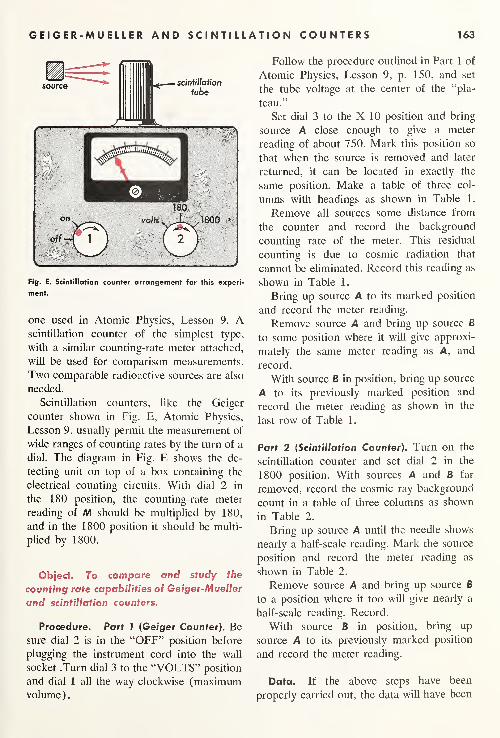
GEIGER-M U ELLER AND SCINTILLATION COUNTERS 163

source scintillation

tube

Fig. E. Scintillation counter arrangement for this experi-

ment.

one used in Atomic Physics, Lesson 9. Ascintillation counter of the simplest type,

with a similar counting-rate meter attached,

will be used for comparison measurements.

Two comparable radioactive sources are also

needed.

Scintillation counters, like the Geiger

counter shown in Fig. E, Atomic Physics,

Lesson 9, usually permit the measurement of

wide ranges of counting rates by the turn of a

dial. The diagram in Fig. E shows the de-

tecting unit on top of a box containing the

electrical counting circuits. With dial 2 in

the 180 position, the counting-rate meter

reading of M should be multiplied by 180,

and in the 1800 position it should be multi-

plied by 1800.

Object. To compare and study the

counting rate capabilities of Geiger-Mueller

and scintillation counters.

Procedure. Part 1 (Geiger Counter). Besure dial 2 is in the “OFF” position before

plugging the instrument cord into the wall

socket .Turn dial 3 to the “VOLTS” position

and dial 1 all the way clockwise (maximumvolume).

Follow the procedure outlined in Part 1 of

Atomic Physics, Lesson 9, p. 150, and set

the tube voltage at the center of the “pla-

teau.”

Set dial 3 to the X 10 position and bring

source A close enough to give a meter

reading of about 750. Mark this position so

that when the source is removed and later

returned, it can be located in exactly the

same position. Make a table of three col-


Remove all sources some distance from

the counter and record the background

counting rate of the meter. This residual

counting is due to cosmic radiation that

cannot be eliminated. Record this reading as

shown in Table 1.

Bring up source A to its marked position

and record the meter reading.

Remove source A and bring up source B

to some position where it will give approxi-

mately the same meter reading as A, and

record.

With source B in position, bring up source

A to its previously marked position and

record the meter reading as shown in the

last row of Table 1.

Part 2 (Scintillation Counter). Turn on the

scintillation counter and set dial 2 in the

1800 position. With sources A and B far

removed, record the cosmic ray background

count in a table of three columns as shown

in Table 2.

Bring up source A until the needle shows

nearly a half-scale reading. Mark the source

position and record the meter reading as

shown in Table 2.

Remove source A and bring up source B

to a position where it too will give nearly a

half-scale reading. Record.

With source B in position, bring up

source A to its previously marked position

and record the meter reading.

Data. If the above steps have been

properly carried out, the data will have been

164 ELECTRONICS — LESSON 8

recorded like that shown in Tables 1 and 2.

Table 1. Data for the Geiger Counter

Source

Meter

Reading

Mult.

Factor

zero 20 10

A 750 10

B 780 10

A + B 1240 10

Table 2. Data for the Scintillation Counter

Source

Meter

Reading

Mult.

Factor

zero 2.4 1800

A 9.2 1800

B 9.6 1800

A + B 16.2 1800

Calculations. Part 7. Make a table of


Table 3.

Table 3. Calculated Results for the Geiger

Counter

CC— — ZeroM

Corrected —M

M (N) (Nc )

200 0 0

7500 7300 11,100

The first and second rows of values have

been computed and will serve as a guide for

the others.

The dead time T is calculated by Eq. (2)

from the data in column 2. The corrected

C/M values in column 3 are then found

from this value of T and Eq. (3).

Part 2. Make another table of three columns

with headings like those in Table 3 and fill

in with your computations from the data on

the scintillation counter in Table 2.

Conclusions. What can you say about

the relative merits of the scintillation counter

as against the Geiger counter? Briefly ex-

plain.

NUCLEAR PHYSICS

Nuclear Physics|

Lesson 4

RADIATION MEASUREMENTS

Many aspects are involved in the

measurement of nuclear radiation. There are

not only a large number of different kinds

of detecting and measuring instruments but

also a considerable number of different kinds

of charged and uncharged atomic particles

involved in nuclear interactions.

A schematic diagram illustrating the pas-

sage of a few of the most common elemen-

tary particles through solid matter is shown

in Fig. A. The atoms of the solid, repre-

sented by the regular array of black dots, are

each composed of a nucleus surrounded by

electrons. In passing through millions of

such atoms each fast-moving particle,

whether it is charged or not, will make nu-

merous collisions with outer electrons and

gradually come to a stop. Only on rare oc-

casions is a single nucleus hit.

Theory. Suppose we have a beam of

charged particles, like electrons, entering

a solid body as shown in Fig. B. Because

of the random collisions with electrons,

particles are stopped within different dis-

tances of the front surface. At some depth

d i the intensity Z of the radiation will be

reduced to |Z0 .

Fig. A. In passing through solid matter high-energy ra-

diation encounters millions of electrons and is gradually

absorbed.

A —*. Y* *•> \ «i « V

’

' * ‘a * a " **O 'A * Af • V « MIX

n* •. J .• •. ; *. ^ . .• f . ,•

r

e+P /. 0 •" 0 \ 0; 0 ‘

* • • a**li " n ! • a a

*j •. V‘.«f=* H V * ».’/ .* • '• *•

y A A /> x • . *, •*'**•*

•

s \J \J ; •. ^ t •• .• • •. • .•

0 • *• *•*

fi •• • yf*•

f\V#

• .• > : .*•’ *• * .•* • t \

•*

r.'rV"--•••••••

solid matter

I—i

1 1 1—

r

' '/2 % % ’/6 '/u

Fig. B. Schematic diagram of radiation absorption.

Imagine now that we divide this solid

absorbing medium into layers, each of thick-

ness di. The beam intensity \l 0 entering the

second layer will be reduced to one-half of its

initial value and emerge to enter the third

layer with an intensity \l0 . Upon traversing

the third layer, the entering beam \

I

0 will be

reduced one-half, or to |Z0 ,etc.

If we now plot a graph of the beam in-

tensity I against the number of absorbing

layers, or the depth x, we obtain a curve as

shown in Fig. C. This is known as an ab-

sorption curve .

While the absorption curves for different

kinds of rays and different absorbers are not

alike, they are similar in that they all follow

the same law. This law is in the form of an

equation that represents the curve in Fig. C,

log f= —M* (1)

* o

Fig. C. Typical absorption curve.

166

RADIATION MEASUREMENTS 167

Fig. D. Semilog graph of radiation absorption.

where [x is a proportionality constant that

depends on the nature of the rays and the

absorbing medium, I0 is the initial intensity,

and I is the intensity after traversing any

thickness x.

To find the logarithm of any value of any

number, like I/I0 ,one can either look up the

number in a table of logarithms or use the

scale of a slide rule. The law is best illus-

trated by a graph as shown in Fig. D. The

vertical scale is ruled by removing the slip

stick from a slide rule and marking off the

main lines and numbers. Note that the same

points plotted in Fig. C now lie on a straight

line. (Graph paper printed like this, with one

scale a logarithmic scale, is called semilog

graph paper.)

The proportionality constant fx, is often

called the absorption coefficient and repre-

sents the fraction of the beam absorbed

from the beam per centimeter path. Al-

though ^ varies from substance to substance,

one finds experimentally that x, taken where

1 drops to any given fractional value of I0

and multiplied by the density of the ab-

sorber, is a constant for all materials.

k = xip (2 )

Now suppose we have two kinds of rays

present in a radiation beam, like (3 rays and

y rays from radium, and we detect them at

Fig. E. Schematic diagram shows absorption differences

between (3 rays and y rays.

various depths within an absorber. See Fig.

E. The y rays that have the greater pene-

trating power show less attenuation as they

traverse the medium.

If the rays are mixed and we plot a

semilog graph of the total detected intensity

1 as it varies with depth, we obtain a curve

as show in Fig. F. The upper left-hand

straight section is due largely to the (3 rays.

Note that with 9 to 15 mm of absorber the

direction of the curve changes. From ap-

proximately 15 on, the radiation is practi-

cally all composed of y rays. The dotted

lines indicate separate lines for the (3 rays

and y rays, and their sum is the solid line.

To find the value of the absorption con-

stant k we find the value of x 1 where I drops

to 1/10 the value of Z0 ,and multiply by the

absorber density. To find the value of xi

in Fig. F, the upper part of the curve is

extended downward to where it crosses a

value of I = 3000. This is 1/10 of 10 . The

intersection at x= 12.6 mm, giving xi =1.26 cm.

Since the density of the absorber used

p = .84 gm/cm3,the absorption constant is

k = 1.26 X .84 = 1.06


experiment consists of a small radium

source, two sets of absorbers, and a Geiger

counter. A radium source gives out «, (3, and

y rays, but the a rays are usually absorbed

by the walls of any container. Consequently

the radiation to be detected is a mixture of

(3 rays and y rays.

One set of 15 sheets of aluminum, about

30,000

20,000

c_M

10,0009.0008.0007.000

6.000

5.000

4.000

|

3,000

I

I 2,000

1,000

;\

7

\\

\

\\

A r< lys

f7-

N- \-

\-

\

-

YT"

\\ \

-

7 ra

f

ys ''v\

A''

.

Y*

I\\\\

'C

—

\

\\

Jy

* ^-

0 2 4 6 8 10 12 14 16 18 20 22 24 mm

Fig. F. Semilog graph of radiation from a source containing j3 rays and y rays.

10 cm square and 1 mm thick, and another

set of 20 sheets of common cardboard 10

cm square and 1 mm thick, are to be used.

The Geiger counter is the same as the one

used in Atomic Physics, Lesson 9, and Elec-

tronics, Lesson 8.

Object. To measure /3 ray and y ray

absorption by different substances.

Procedure. Turn on the Geiger counter,

following the instructions given in the pre-

vious lessons, and determine the plateau

region. Set the counter voltage at the cen-

ter of the plateau and keep it set at this value

for the entire experiment.

Set dial 3 to the X 10 position and bring

up the Ra source to a point where the

counting rate meter shows nearly a full-

scale reading. Leave the source and Geiger-

Mueller tube fixed in this position for the

remainder of the experiment.

Make a table of four columns with head-

ings as shown in Table 1. Record the initial

meter reading after multiplying by 10.

Insert the first cardboard sheet between

the Ra source and the Geiger-Mueller tube,

and record the C/M.Insert a second cardboard sheet between

the two and again record the C/M.Repeat this procedure, adding one ab-

sorber at a time until a total of 20 have been

inserted, recording the C/M with each one.

Allow time after the insertion of each ab-

sorber for the meter to reach its steady con-

dition.

Remove all cardboard absorbers and

carry out the same procedure with the

aluminum absorbers. Record the C/M val-

ues in the two right-hand columns of Table

1 .

Data. Assuming the above procedure

has been properly carried out, the recorded

RADIATION MEASUREMENTS 169

data will have the appearance of that shown

in Table 1.


Cardboard Aluminum

N C/M N C/M

0 12,900 0 12,900

1 10,800 1 6,900

2 9,300 2 3,800

3 8,000 3 2,400

4 7,000 4 2,000

5 6,000 5 1,800

6 5,200 6 1,700

7 4,500 7 1,650

8 3,750 8 1,600

9 3,300 9 1,550

10 2,850 10 1,500

1

1

2,500 11 1,450

12 2,250 12 1,400

13 2,100 13 1,350

14 2,000 14 1,300

15 1,900

16 1,800

17 1,700

18 1,600

19 1,500

20 1,450

cardboard size: 10 X 10 X 0.1 cm

aluminum size: 10 X 10 X 0.1 cm

mass of 10 cardboard abs = 702 gmmass of 10 aluminum abs = 270.1

Results. Prepare a graph on semilog

paper. Plot curves for both the cardboard

and aluminum absorbers on the same graph.

If commercially ruled paper is not avail-

able, remove the slip stick from an 8- or 10-

inch slide rule and use the B scale to lay off

your vertical I scale. Starting with 1 at

the bottom, mark all whole numbers up to

3 in the second scale. Label these marks

1000, 2000, 3000, . . . 30,000 C/M, as

shown in Fig. F.

With a uniform centimeter ruling as a

horizontal scale, label the centimeter marks

0, 2, 4, 6, . . . 20 to represent the num-

ber of absorbers or the thickness of total

absorber in millimeters.

Weigh a set of 10 cardboard absorbers

and a set of 10 aluminum absorbers, and

record their mass in grams. Measure the

size and thickness of one absorber and

record in cm.

Calculations. Extend the upper straight-

section of each curve downward and find the

thickness xi that will reduce the beam in-

tensity to 1/10 I0 .

From the weighings of absorber material,

find the densities of cardboard and alumi-

num. These will be approximately 0.70

gm/cm3 and 2.7 gm/cm3,respectively.

Using these values of P and the values of

x1? calculate the absorption constant k.

Repeat these calculations for a beam in-

tensity I = 4000 C/M.

Conclusions. Why is heavy shielding

used around powerful sources of radiation?

Does this shielding absorb all the radiation?

:

.

.

'

Appendix I

trigonometric functions (Natural

)

Angle Sine Cosine Tangent Angle Sine Cosine Tangent

o°jO

0.000.018

1 .0001 .000

0.000.018 46

:.719 .695 1.036

2° •°35 0.999 •035 47 •731 .682 1 .072

3

:

.052 •999 .052 48° •743 .669 1 . in4 .070 .998 .070 49

:•755 .656 1.150

5°

.087 .996 .088 50°

.766 •643 i .192

6° .105 •995 .105 5 i° •777 .629 1-235

7°

.122 •993 .123 52 .788 .616 1 .2808° .139 .990 .141 53

°•799 .602 1-327

9°

.156 .988 • J 58 54 809 .588 1-376io° •174 .985 .176 55

°.819 •574 1.428

n° .191 .982 .194 56:

.829 •559 1-48312

°.208 978 .213 57 •839 •545 1.540

I3o

.225 •974 .231 58I

.848 •530 1.600

14 .242 .970 .249 59 •857 • 5 i 5 1 .664

15°

•259 .966 .268 6o° .866 .500 1.732

i6° .276 .961 .287 6i° .875 .485 1.80417

°.292 .956 .306 62° .883 .470 1.881

i8° •309 •951 •325 63°

.891 •454 1.96319

l.326 .946 •344 64

°.899 •438 2.050

20°

•342 .940 •364 65°

.906 •423 2.145

21°

•358 •934 •384 66° .914 .407 2.24622

°•375 •927 .404 67

°.921 •391 2.356

*3°

•391 .921 .425 68° •927 •375 2-47524

°.407 .914 •445 69

I•934 .358 2.605

25°

.423 .906 .466 70° .940 •342 2-747

26° •438 •899 .488 7*: .946 .326 2.90427

°•454 .891 .510 72

o•951 • 3°9 3-078

28° •470 .883 •532 73!

-956 .292 3-27129

°.485 •875 •554 7< .961 .276 3-487

3°° .500 .866 •577 75

°.966 •259 3-732

3 «; .515 .857 .601 76I

.970 .242 4.on•530 .848 .625 77 •974 .225 4-331

33I

•545 • 839 • 649 78: .978 .208 4-70534 • 559 .829 .675 79 .982 .191 5-14535

°•574 .819 .700 80 •985 .174 5.671

36: .588 .809 .727 8i° .988 .156 6.31437

°.602 •799 •754 82° .990 •139 7.115

3K .616 .788 .781 83»

•993 .122 8.14439

°.629 •777 .810 8< •995 .105 9 - 5H

40 .643 .766 -839 85 .996 .087 U -43

< .656 •755 .869 86° .998 .070 14 - 3°42

I.669 •743 .900 87° •999 .052 19.08

43I

.682 •731 •933 88° •999 •035 28.6444

o.695 • 7 i 9 .966 89

:1.000 .018 57-29

45 .707 .707 1 .000 90 1.000 .000 00

171

Appendix II

VALUES OF THE GENERAL PHYSICAL CONSTANTS (AFTER DU MOND)

Planck’s constant of action

Electronic charge

Electronic charge

Specific electronic charge

Specific proton charge

Electronic mass

Mass of atom of unit atomic weight

Mass of proton

Ratio mass proton to mass electron.

Wien’s displacement-law constant.

.

Velocity of light. .... .........

h = 6.6238 X 10~34 joule sec

e = 1.6019 X 10~19 coulombs

e = 4.8022 X lO”10 e.s.u.

e/m = 1.7589 X 1011 coulombs/kg

e/Mp = 9.5795 X 107 coulombs/kg

m = 9.1072 X IQ"31 kg

M = 1.6600 X 10~27 kg

Mp = 1.6722 X lO"27 kg

Mp/m = 1836.1

C = 0.28976 cm deg.

c = 299,790 km/sec

c2 = 8.9874 X 1010 km2/sec2

Appendix III

THE GREEK ALPHABET

A a Alpha H V Eta N V Nu T r TauB P Beta © 0 Theta S { Xi T V Upsilon

r 7 Gamma I i Iota O o Omicron Phi

A 8 Delta K K Kappa n TT Pi X X Chi

E € Epsilon A X Lambda P P Rho Psi

Z c Zeta M Mu $ <T Sigma a (O Omega

172

SAMPLE DATA SHEETFOR

LABORATORY EXPERIMENTS

John E. Doe Speed and Velocity

Lesson 2

Object. To make a study of a body moving with constant speed and another


Equations Needed.

circumference of a circle = ttd

TT = 3.14

distance traveled by train = nwd

Apparatus. Toy automobile of sturdy metal construction, a geared-down

motor with an attached drum, toy electric train, three-rail circular track, small

train transformer for adjusting train speed, stop watch, meter stick.

Data.

Data for Car

Distance Time

s t

Trial (cm) (sec)

1 65.7 8.2

2 119.0 14.8

3 157.0 19.6

Data for Train

Number Time

of t

Trial Turns (sec)

1 4 21.4

2 5 26.7

3 6 32.1

track diameter d = 74.6 cm

173

174 SAMPLE DATA SHEET

Column Headings for Calculations and Results.

Results for Car

Distance Time Velocity

Trial s t V

(cm) (sec) (cm/sec)

Results for Train

Number Time Speed

Trial of t V

Turns (sec) (cm/sec)

Questions To Be Answered.

1. What is the average value of v for the car?

2. What is the average value of v for the train?

3. Which of the two measurements in this experiment, time or distance, has the

greater probable error?

SAMPLE FINAL REPORT ONLABORATORY EXPERIMENTS

John E. Doe Speed and Velocity

Lesson 2

Object. To make a study of a body moving with constant speed and another


Theory.

Equations Used.

sV =

t

v = speed or velocity

s = distance traveled

f = time of travel

circumference of circle = td

7r = 3.14 d = 74.6 cm

distance traveled s = mrd

Apparatus and Procedure. In Part I a toy automobile is pulled across the

table at constant velocity. This is accomplished by a string wrapped around a

drum driven by a geared down electric motor. Two markers are set up as start

and finish points, a meter stick is used to find the distance between them, and a

stop watch is used to measure the time of travel.

In Part II a toy electric train is made to run around a circular track at constant

speed. A single marker at the side of the track marks the start and finish points,

and the stop watch is used to measure the time for any given number of turns

around.

Data and Measurements.

Table 1. Data for Car

Distance Time

s t

Trial (cm) (sec)

1 65.7 8.2

2 119.0 14.8

3 157.0 19.6

175

176 SAMPLE FINAL REPORT

Table 2. Data for Train

Number Time

of t '

Trial Turns (sec)

1 4 21.4

2 5 26.7

3 6 32.1

track diameter d = 74.6 cmCalculated Results.

Table 3. Results for Car

Trial

Distance

(cm)

Time

t

(sec)

Velocity

V

(cm/sec)

1 65.7 8.2 8.01

2 119.0 14.8 8.04

3 157.0 19.6 8.01

Table 4. Results for Train

Trial

Number

of

Turns

Time

t

(sec)

Distance

(cm)

Speed

V

(cm/sec)

1 4 21.4 936 43.7

2 5 26.7 1170 43.8

3 6 32.1 1404 43.7

track circumference = 234 cm

Conclusions.

1. The average velocity of the car is 8.02 cm/sec.

2. The average speed of the train is 43.7 cm/sec.

3. The distance between markers in Part I can be measured to within an ac-

curacy of 1 mm. For trial 2, for example, this is 1 mm in 119.0 cm, or one part in

1190. This indicates a probable error of 0.1%.

The track diameter can be measured in several places and the average found to

within an accuracy of 1 mm. For the track this is 1 mm in 74.6 cm, or one part

in 746. This indicates a probable error of 0.13%.

Using a stop watch with tenth scale divisions, each time measurement, with a

little practice, can be repeated to within one-tenth of a second. For the second time

interval in Part I, this is 0.68% probable error.

The measurement of time therefore has the greater probable error in this

experiment.

Index

Page references in Roman type indicate pages in the textbook, while those in italic type followed by

the letter L indicate pages in the Laboratory Exercises.

Abbreviated system of numbers, 26Absolute, temperature scale, 208, 244; zero, 208,

244Absorption, coefficient, beta rays, 166L; curve,

166L; of beta rays, 166LAccelerated motion, 8LAcceleration, 40; angular, 145; constant, 41; due to

gravity, 55, 11L; negative, 40; uniform, 40Accelerators, atomic, 545Accommodation, eye, 338Action force, 7

1

Additive primaries, color, 334Adhesion, 180

Adiabatic, compression, 249; expansion, 249; proc-

ess, 240Air, column, 90L; density of, 60LAirplane, angle of attack, 103; attitude, 103; lift of,

197; mechanics, 102; thrust of, 102Algebra review, 25Alpha rays, discovery of, 469Alternating, current, 424; current, theory, 433; emf,

423Ammeter, principle, 413Ampere, Andre M., 371Ampere, 371

Amplification of vacuum tube, 155LAmplifier, vacuum tube, 491Amplitude, 198; of waves, 201Anatomical mechanics, 127

Anderson, C. D., positron discovery, 541Aneroid barometer, 185

Angle, of attack, airplane, 103; of uniform slip,

29LAngstrom, unit of, 512, 146LAngular, acceleration, 145; momentum, conserva-

tion of, 149; speed, 138; velocity, 139Apparent solar day, 13

Arc light, 298

Archimedes, 124; principle of, 176, 59LAristotle, 53

Arm, mechanics of, 130Armature, of motor, 132LAston's mass spectrograph, 456Atmosphere, 184

Atmospheric pressure, Standard, 60LAtomic, accelerators, 545; mass, unit of, 457; num-

ber, 457; physics, 5; structure, 154; weight, 457Attitude, of airplane, 103

Audiogram, sound, 280Audion, De Forest, 488Average velocity, 38; mechanics, 42

Back emf, 433Balanced forces, 73Ballistics, 41LBalmer series, 515Barometer, aneroid, 185; mercury, 185

Batteries, principles of, 372Battery cell, 114LBeat, frequency, sound, 263; notes, sound, 263Becquerel, Antoine H., 469Bel, sound, 279Bending, elastic, 166

Bernoulli's, principle, 194; theorem, 195

Beta-ray absorption, 166LBeta rays, discovery of, 469; origin of, 560Betatron, 549Biceps, arm mechanics, 130Bimetallic strip, 211

Binding forces, nuclear, 556Binoculars, 340Black-body radiation, 226Block and tackle, pulleys, 135Blue sky, 355, 357Bohr atom, 509

177

178 INDEX

Bohr, Niels, 511; nuclear model, 558Bohr-Stoner scheme, 516Boiling, at 0°C, 236; evaporation, 233; point, alti-

tude effect, 236; point, curve of, 234; point, table

of, 216

Boltzmann-Stefan law, 225Bouncing, elasticity, 166; marbles, 168

Bowen, I. S., 539Boyle, Robert, 241; gas law of, 241, 81

L

Brachistochrone, 116

Brasses, musical instruments, 269Breaking point, stretching, 162

Breathing, lung action, 187

Brewster's law, light, 349Brightness, 306British thermal unit, 214Brownian motion, 156

Calcite crystal, 157

Calorie, 214Calorimetry, 71LCamera, photographic, 337Canal rays, 453Candle power, 96L; light standard, 304Capacitance, 391-392

Capacitive reactance, 435Capacitors, 391; in parallel, 393; in series, 393Capillarity, 181

Carbon, arc, light, 298; cycle, sun, 567Carnot cycle, 249Cathode-ray oscilloscope, 526Cathode rays, 445Cell, battery, 114LCenter, of gravity, 87, 30L; of mass, 87; of mass,

rotation about, 89Centigrade temperature scale, 208Centimeter, unit of length, 1

1

Centrifugal force, 139

Centripetal force, 139, 43LCerenkov radiation, 162LChadwick, neutron discovery, 535Chain reaction, 564Change of state, 213, 215; fusion, 228Characteristics of vacuum tubes, 154LCharge, by induction, 368; coulomb, 367

Charles' law, gas, 242Chladni sand figures, 275Chord, musical, 286Chromatic scale, music, 286Circular motion, 45LClassical physics, 4Closed-core transformer, 138LCoaxial cable, 502Cockcroft-Walton experiment, 545Coefficient, of expansion, 68L; of friction, 28L; of

restitution, 169; of rolling friction, 98, 28L; of

sliding friction, 97; of thermal expansion, 210Cohesion, 180Coincidence counters, 540Color, 333; mixing, 333, 335; triangle, 334; TV,

335

Commutator, electric motor, 412Complementary images, color illusions, 8

Components of forces, 78Compression, gas, 244Compton effect, 520; electrons, 471, 521Concave, lenses, 323; mirror, 313Concentric line, 502Concordant, overtones, music, 290; sounds, 284Conduction, heat, 218; of electricity, 364Conservation, of angular momentum, 149; of

energy, mechanical, 114; of momentum, 119,

41LConsonances, music, 285Constant acceleration, 41; velocity, 38Continuous emission spectra, 459Convection, of heat, 220Convex lenses, 323

Cooling, by evaporation, 229; curve, 76L; Newton’slaw of, 75L

Core, of transformer, 137LCosine, trigonometry function, 30

Cosmic ray, 538; detectors, 540; showers, 541, 543Coulomb, 367Coulomb's law, electric charges, 366, 134LCrane, 25L; problem in mechanics, 96Critical angle, in light, 328Crookes, Sir William, 443Crookes' dark space, 444Crown glass, prisms, 330; refractive index, 331

Crystal, fluorescent, 162L; models, 157

Curie, Pierre and Marie, 469Current, 371; electric, 368Curvilinear motion, 38

Cyclotron, 546

Damped vibrations, 480Davisson, C. J., 522Dead time, Geiger counter, 160L; scintillation coun-

ter, 160LDe Broglie waves, 521

Decibel, sound, 279Declination, magnetic, 403De Forest, Lee, 488Density, 55L, 57L; of air, 60L; table of, 178

Dental orthopedics, 167

Derived, equations, mechanics, 42; units, 10

Detectors, of cosmic rays, 540Dew point, 23 1

Dewar flask, 225

Diamond, refractive index, 331

Dielectric constant, 393

Differential expansion, 211

Diffraction grating, 346, 145L; light, 343Dip, magnetic, 403-404

Discordant sounds, 284Disintegration, natural, 472Dispersion, of light, 328Dissociation, electrolytic, 372Dissonant interval, music, 285Distance of most distinct vision, 106LDominant mode in microwaves, 502

INDEX 179

Doppler effect, sound, 264Double refraction, 350Double-slit experiment, 344Dry-bulb thermometer, 231

Dry-cell batteries, 374Dyad, musical, 286Dynamics, 35; of rotation, 144

Dyne, centimeter, 106; unit of force, 65

Ear, human, 280Earth, its atmosphere, 184; magnetic field of, 402;

satellites, 141

Eddies in fluids, 101

Edge tones, 274Edgerton photographs, 168

Efficiency of machines, 133

Einstein, mass-energy relation, 536; photoelectric

equation, 496Elastic limit, stretching, 162

Elasticity, 161; bending, 166; bouncing, 166; twist-

ing, 166; Young’s modulus, 163

Electric, field, 387; field, uniform, 391; motor,

principle of, 411

Electrical, equivalent of heat, 128L; resistance, ther-

mometer, 209Electricity and magnetism, 5

Electrification, 363

Electrode, 114LElectrolyte, 114L; battery, 372Electrolytic dissociation, 372Electromagnet, 408Electromagnetic waves, 482, 157LElectromotive force, 114L; induced, 422Electron, charge on, 449; discovery, 443; e/m ex-

periment, 142L; e/m ratio, 448; gun, 522, 526;

lenses, 525; mass of, 451; microscope, 528;

optics, 524; refraction, 524; shells, 514; velocity

of cathode rays, 449Electronic charge, 367; to mass ratio, 142LElectronics, 5

Electroscope, gold-leaf, 363Electrostatics, 361

Elevation angle, for projectiles, 62e/m experiment, 142LEmission spectra, 459Energy, conservation of mechanical, 114; experi-

ment on, 35L; kinetic, 110; mechanics, 110;

potential, 107; relations, nuclear, 536; solar, 566Engine, Carnot, 249; gasoline, 248; rocket, 252;

turbo-jet, 251

Equal-tempered scale, music, 286Equator, magnetic, 402Equilibrium, conditions for, 83; conditions in me-

chanics, 75; experiment on, 19L, 24-25L; of

rigid bodies, 85; rotational, 83; translational, 83

Equivocal figures, 7

Erg, 106

Escape velocity, satellites, 142

Evaporation, cooling by, 229Expansion, differential, 211; gas, 244; thermal, 210Extraordinary ray, polarized light, 350

Eye, human, 337Eyepiece, of microscope, 108L

Fahrenheit, temperature scale, 208Falling bodies, 52Farad, 392Faraday, dark space, 444; ice pail, 368Faraday, Michael, 421Farsighted, vision, 339Ferromagnetism, 399

Field, electric, 386; magnetic, 401; sequential scan-

ning, 503Fifth, a musical interval, 285Filter circuit, radio, 487Final velocity, mechanics, 41

Fireplace, radiant heat, 224First-order spectrum, 145LFission, discovery of, 563Fizeau, velocity of light by, 300Flashlight, 377Flats, music, 286Fleming valve, 485Flettner rotor ship, 196

Flint-glass, prisms, 330; refractive index, 331Fluid friction, 95, 191, 62LFluids, in motion, 189

Fluorescence, in crystals, 162LFluorescent, crystals, 162L; light source, 298

Flux density, 418Focal, length, defined for mirror, 314; length, ex-

periment on, 104L; length, of lens, 324; plane,

of a lens, 324Foot, mechanics of, 128

Foot-candle, 305Foot-pound, 106

Force, action and reaction, 71; centrifugal, 139;

centripetal, 139; equation, 17L; moments, 38L;pound, 66; units of, 65

Forces, balanced, 73; components of, 78; in equi-

librium, 75, 19L; molecular, 156; parallel, 87,

23L; resolution of, 78, 20L; unbalanced, 73;

vector addition, 74Fourth, a musical interval, 285Fraunhofer lines, spectrum, 463Free fall, 54Frequency, measurement of tuning fork, 86L; nat-

ural, 273; sound waves, 266Friction, charging by, 362; experiment, 28L; fluid,

95, 191, 62L; head, 63L; head, in liquids, 191;

kinetic, 95; rolling, 95, 98; sliding, 95; static,

95; work against, 106

Fringes, diffraction, 344Full-wave rectilinear, 487Fundamental units, 10

Fusion, change of state, 228; experiment, 73L;nuclei, 567

g, acceleration due to gravity, 11LGalileo, 53; experiment on light, 300; thermometer,

207Galvanometer, principles of, 413; use of, 126L

180 INDEX

Gamma-ray absorption, 166LGamma rays, discovery of, 469; origin, 560Gas laws, 81L; heat, 238Geiger counter, 148L, 160LGeiger-Mueller, tube, 148LGeneral gas law, 240Generator, electric, 423Germer, L. H., 522Geysers, 234Gilbert, Sir William, 402Gram, unit of mass, 11; weight, 161

Gravitation, 53; Newton’s law of, 69

Gravitational constant, Newtonian, 70

Gravity, acceleration due to, 55; center of, 87, 30L;measurement of, 11L

Gun, ballistics, 41

L

Gyroscopes, 151

Half life, 472Half tone, music, 286Halos, light, 354Hard X rays, 465Harmonic triads, music, 286Harmonics, sound, 267, 273Harmony, 284Hearing, human ear, 280Heat, 207; adiabatic process, 240; Boyle’s law, 241;

by electric currents, 405; capacity, 213; conduc-tion, 218; convection, 220; described, 4; elec-

trical equivalent of, 128L, emission and absorp-

tion, 224; energy, 238; engine, efficiency, 250;

engines, 248; exchange, Prevost’s law, 226; ex-

change law, 76L; gas laws, 238; of fusion, 73L;radiation, 223; reflection of, 224; transfer, 218;

transfer, Prevost’s law, 226Height, of projectiles, 62, 14LHelmholtz, Hermann, 278; coils, 143LHenry, Joseph, 433; unit of inductance, 433Hertz, Heinrich Rudolph, 481Hertzian dipole, 482, 157L; waves, 481Hibbert balance, 135LHooke, Robert, 162

Hooke's law, 161, 52L, bending, 166; twisting, 167

Horsepower, 112; 33LHourglass, early time pieces, 12

Humidity, absolute, 230; dew point, 231; relative,

231

Huygens, Christian, 343; wave theory, 343Hydraulic press, 174

Hydrogen, atom, Bohr theory of, 511; bomb, 567Hydrometer, principle of, 177

Hypermetropia, vision, 339Hypotenuse, 4L

Ice, refractive index, 331Illuminance, in light, 304Illumination, 304Image, in concave mirror, 314; in plane mirror,

310; lens formation of, 324; magnified, 326;

perverted, 311; real, 325; virtual, 325

Impact, of elastic bodies, 167

Imperfect consonance, music, 287Impulse equation, 36LInclined plane, 21LIndex of refraction, 303, 318, 101L; table of, 331

Induced, currents, 421; radioactivity, discovered,

553Inductance, 433; calculation of, 434Induction, charging by, 368; magnetic, 415Inductive reactance, 435Inertia, 58; moment of, 147, 47LInfrared, radiation, 460Initial velocity, mechanics, 41

Instantaneous velocity, 38

Insulators, electrical, 364Intensity, of light, 96L; of sound, 278Interference, light, 343International candle, light Standard, 304Interpolate (Interpolation), 2LIntonation, music, 286Inverse square law, light, 303; magnetism, 136L;

radioactivity, 149L; sound, 280Ionization, process of, 454Ionizing power, radioactive rays, 470; X rays, 466Irradiation, optical illusions, 8

Isobars, 458Isoclinic, magnetic lines, 404Isothermal, compression, 249; expansion, 249Isotopes, discovery of, 455

Jaw, mechanics of, 129

Joule, James Prescott, 239; defined, 106; heat

energy, 79L; law of, 406, 128L

Karman trails, 101

Kelvin temperature scale, 208, 244Keynote, musical scale, 285Kilogram, standard of mass, 10; weight, 161

Kilowatt, electrical unit, 430; mechanical unit, 112

Kinematics, meaning of, 35; of rotation, 145

Kinescope, in TV, 503Kinetic, energy, 110; energy, of rotation, 147; fric-

tion, 95; theory of gases, 240Kirchhoff's laws, 117L, 119L; law of currents, 383;

law of radiation, 225Knot, unit of speed, 38

Laminar flow, 101

Latent heat of fusion, 73LLaw, of conservation of energy, 114; of conserva-

tion of momentum, 119; of reflection, 98LLawrence, E. O., 547; cyclotron, 547Left-hand rule, 407Leg, mechanics of, 128

Lenses, experiment, 103L; light, 322; magnetic, 527Lenz's law, 424Levers, experiment on, 38L; mechanical advantage,

132; simple, 124; use of, 53LLevitation, 437

N D EX 181

Leyden jar, 479Light, 4; color mixing of, 335; quantum, 496;

rectilinear propagation, 299; sources, 298Line, absorption spectra, 462; emission spectra, 461Linear coefficient of thermal expansion, 69LLiquid air, experiments, 246; machine, 245; prop-

erties of, 244Liquid pressure, 55LLongitudinal standing waves, 91LLongitudinal waves, 201, 258Loudness, sound, 278Loud-speaker, radio, 492low temperatures, 235Lumen, light standard, 305

Luminance (or Brightness), 306, 96LLuminous intensity, 304Lungs, action of, 187

Mach number, 104

Machine, efficiency, 133; mechanics of, 132

McMillan, E. M., 564Magdeburg hemispheres, 187

Magnetic, declination, 403; dip, 403; equator, 402;

fields, 401; flux, 418; induction, 415; lenses, 527;

poles, law of force between, 135LMagnetism, 396; theory of, 399Magnetization, 398Magnets, 396Magnification, 108L; Optics, 104LMagnifying power, 340, 106L; of microscope, 110LMajor, seventh, a musical interval, 285; sixth, 285;

third, 285; tones, in music, 285Marconi, Guglielmo, 485Marimba, 275Mass, 59; center of, 87

Mass, moments, 88, 32L, 38L; number, 457; num-ber, radioactive change of, 473; spectrograph,

454; vs. weight, 66; units of, 66Mass-energy, relations, 536Mean solar day, 13

Mechanical, advantage, 132, 39L; equivalent of heat,

239, 78LMechanics, of arm, 130; of foot, 128; of jaw, 129

Melody, 286Melting point, 216Mercury, barometer, 185; vapor lamp, 146LMesous, discovered, 543Meter, standard of length, 10

Method, of components, 49Metric, system, 10; units, 13

Michelson, Albert A., 301; velocity of light experi-

ment, 301

Microammeter, principles of, 413Microfarad, 392Micromicrofarad, 392Microscope, electron, 528; magnification, 108L; prin-

ciples of, 108LMicrowaves, 157LMiddle octave, musical scale, 285Miller, Dayton C., 259Milliammeter, principles of, 413

Millibar, unit of pressure, 60LMillihenry, unit of inductance, 434Millikan, R. A., 449, 496, 539; oil-drop experiment,

449Millimeter, unit of length, 1

1

Minor tones, in music, 285

Mirrors, reflection in, 310, 98LModern physics, 4Molecular forces, 156

Molecules, diatomic, 155

Moment, of a force, 124; of inertia, 147, 47LMoments, mass, 32LMomentum, 35L; conservation, 41

L

Motors, electric, 410; experiment on, 131L; parts

of, 132LMoving charge, force On, 417Multiple disintegrations, 552; reflections, in mirrors,

310Musical scale, diatomic, 284; octave, 285

Myopia, vision, 339

Nail, experiment on impulse, 36LNatural frequency, 273Near point, in vision, 106LNearsighted, vision, 339Negative, acceleration, 40; glow, discharge tube,

444; potential, 386Neon, light source, 298Neptunium, discovery of, 564Neutron, discovery of, 535; disintegrations, 553

Newton, Sir Isaac, 58-59; first law of motion, 58;

law of cooling, 75L; law of gravitation, 69;

meter, 106; second law of motion, 65, 16L,

third law of motion, 70; unit of force, 66Newtonian constant of gravitation, 70Nodes, standing waves, 267Nonconductors, electrical, 364Normal state, of atom, 515Nuclear, disintegration, 534; disintegration, dis-

covery, 533; energy, 563; forces, 556; model,

Bohr, 558; physics, 5; potential barrier, 557

Nucleons, 561

Objective, lens, microscope, 108L; methods of meas-urement, 6

Octave, musical scale, 285Oersted, Hans Christian, 406; experiment, 406Ohm, John Simon, 377; law of, 376Oil-drop experiment, 449Optical illusions, 5

Orbiting velocity, satellites, 142

Ordinary ray, polarized light, 350Organ pipes, 273

Orthodontia, dental, 167

Oscillator, vacuum tube, 489Oscillatory circuit, 479Oscilloscope, cathode-ray, 526Overtones, music, 290

Paint, color mixing, 335

Pairs, magnetic poles, 398

182 N D EX

Parallel, capacitors, 393; circuits, 382, 119L; forces,

23L; resistors, 381

Parallelogram method, vector addition, 75

Pascal, Blaise, 173; principle of, 173

Pauli exclusion principle, 518Peak voltage, a.C., 424Pendulum, 64L

;

simple, 116, 199; spring, 199

Percent error, calculation of, 54LPercussion instruments, music, 274Perfect consonance, music, 285Periodic motion, 198

Permeability, of magnetic material, 133LPermittivity, 393

Persistance of vision, 9

Perverted image, 311

Pharynx, human voice box, 292Photoelectric, cell, 494; effect, 494, effect, X rays,

520; equation, 496Photoelectrons, velocity of, 496Photometry, 96L; in light, 304Photomultiplier, tube, 497, 162LPhoton, 496, 513; momentum of, 521

Piano, scale range, 291

Pigment, color mixing, 335Pile, atomic, 565Pinhole camera, 300Pipe, standing waves in, 90LPitch, sound, 278Planck's constant h, 496, 512Plane mirror, reflection in, 309Plane-polarized light, 348Plateau, Geiger-counter curve, 149LPlutonium, discovery of, 564Polar graph, 14LPolarization, by reflection; 348; by scattering, 357;

by selective absorption, 350; by tourmaline, 351

Polarized light, 347Polarizing angle, 349Polaroid, 35 1

Poles, magnetic, 397Positive, column, 444; potential, meaning of, 386;

rays, 453Positron, discovery, 541

Potential, barrier, nuclear, 557; divider, 122L; elec-

trical, 386-387; energy, 107; energy, negative,

108

Potentiometer, 122LPound, standard of weight, 12; unit of force, 66Power, 111; a.c., 430; factor 436; horsepower, 112;

reactors, 566; transmission, 431; watt, 112

Powers of ten, designation of, 26

Presbyopia, vision, 339Pressure, 171, 55L, 61L; cooker, 234; head, 63L;

head, in liquids, 191; liquid, 171; surface, 173

Prevost's law, heat exchange, 226Primary, colors, 334; rainbow, 353; transformer,

428, 137LPrincipal, axis, of mirror, 313; foci, of a lens, 324Prism, refraction by, 320Projectiles, 13L; height, range, flight time, 61; me-

chanics, 60Properties of matter, 4, 161

Proton, gun, 545; -proton cycle, sun, 567Pulleys, 134; block and tackle, 135

Pulsed system, in radar, 500Pythagorean theorem, 4L

Quality, of musical sounds, 291; of sounds, 289Quanta, meaning of, 496Quantum, number, principal, 512; optics, 5

Quartz, crystals, 157; refractive index, 331

Radar, principles of, 500Radian, 138; unit angle, 44LRadiation, black-body, 225; heat, 223; Kirchhoff’s

law of, 225; measurements, 166LRadio, and TV bands, 157L; transmitter, 490Radioactivity, 148L; natural, 469Radiometer, Crooke’s, 223Radium, discovery, 469Rainbow, 353

Range, of alpha rays, 472; of human voice, 291; of

musical instruments, 291; of projectiles, 13L; of

projectiles, mechanics, 62

Rankine, temperature scale, 208, 244Reactance, capacitive, 435; inductive, 435Reaction, force, 7

1

Reactors, power, 566

Recoil electrons, 521

Rectifier, full-wave, 487; vacuum tube, 485Rectilinear, propagation of light, 299Reflection, curved mirrors, 313; grating, 145L; law

of, 309; of light, 309, 98L; total, 329Refraction, by a prism, 320; electron, 524; experi-

ment, 1 OIL; of light, 317Refractive index, 303, 318, 101L; table of, 331

Refrigeration, 233Regelation, ice, 228Relative velocity, 5

1

Resilience, 169

Resistance, 379Resistivity, 125LResistors, in parallel, 120L; in series, 116LResolution, of forces, 78, 20L; time, Geiger counter,

160L; time, scintillation counter, 160LResonance, electrical, 481; sound, 262Resonating air column, 90LRestitution, coefficient, 169

Reversibility of light rays, 319Rheostat, 122LRifle, ballistics experiment, 41L; bullet, velocity of,

42LRocket engine, 252Rods, vibrating, 274, 91LRolling friction, 95, 98, 29L; coefficients of, 98

Rontgen, Wilhelm, 464Root mean square voltage, 424Rotation, about center of mass, 88; dynamics of,

144; kinematics of, 145; kinetic energy of, 147

Rotational equilibrium, 83, 24LRutherford, Sir Ernest, 469, 533, 539; scattering,

509

INDEX 183

Sailboat, mechanics of tacking, 80St. Louis motor, 133LSatellites, earth, 141; escape velocity, 142; orbiting

velocity, 142

Scalar, 37

Scanning, in TV, 503

Scattering, of light, 355; Rutherford, 509

Scintillation, by alpha particles, 509; counter, 160LSeaborg, Glenn T., 564

Secondary, electrons, 497; emission, 497; rainbow,

353; transformer, 428, 137LSecond-order spectrum, 145LSelf-induction, 433

Semilog graph, absorption curve, 168LSemitones, in music, 285

Series, battery connections, 377; capacitors, 393;

circuits, 116L; resistors, 379

Shadows, light, 343

sharps, music, 286Shell structure, of atom, 514

Shock waves, 103

Showers, cosmic ray, 543

Sidereal time, 13

Significant, digits, 16; figures, 16

Simple crane, 25L; harmonic motion, 198, 257;

pendulum, 116, 199

Simultaneous velocities, 45

Sine, trigonometry function, 30Siren, air, 260Slide rule, principles of, 16

Slide-wire resistance, 122LSliding friction, 95, 28L; coefficient of, 97; table of

coefficient, 97

Sling psychrometer, humidity, 231

Slug, unit of mass, 66

Snell, Willebrord, 318; law of, 318, 101LSoft X rays, 465Solar, energy, 566; spectrum, 462Solenoid, 408Sound, 4; intensity, 279; loudness, 278; over light

beam, 495; pitch, 278; speed of, 259, 92L;transmission of, 258

Source, of light, 297Specific, gravity, 58L; heat, 215, 70LSpectacle lenses, 339Spectra, absorption, 459; line emission, 461; optical,

459Spectrograph, experiment with, 145L; mass, 454Spectroscope, 145LSpectrum, lines, 145L; microwave, 158L; solar, 462Speed, 37; angular, 138; of light, experiments on,

300; of light, in matter, 303; of sound, 259, 92LSpherical aberration, in mirrors, 316Spinning electron, 518; proton, 518; top, 152

Spring pendulum, 199, 64LStability, gyroscopic, 151

Standard, candle, light, 304; pressure, 60LStanding waves, 88L, 90L; in rods, 91L; sound, 267Static, electricity, theory of, 363; friction, 95

Statics, 35

Stefan-Boltzmann law, 225Step-down transformer, 137L

Step-up transformer, 137LStokes, Sir George, 102; law of, in fluids, 102Stoner, Bohr-Stoner scheme, 516Storage battery, principles of, 373Strain, 163

Streamlining, 100, 102

Stress, 163

Stretching, of a wire, 162Strings, vibrating, 267, 88LStroboscopic effect, 8

Subjective methods of measurement, 5

Subtractive primaries, color, 334Sundial, principle of, 12

Sun's energy, 566Sunset, experiment, specifications, 357; red color,

356Supersonic velocities, 103

Surface, pressure, 173; tension, 180; tension, table

of coefficients, 182

Tacking, sailboat mechanics, 80Tangent, trigonometry, 30Tapped transformer, 138LTelescope, 340Television, and radio bands, 157L; color, 335; prin-

ciples of, 500Temperature, 207; scales, 208; scales, absolute, 244Terminal velocity, 101

Tetrad, musical, 286Thermal, capacity, 214, 70L; coefficient of expan-

sion, 210; conductivity, 218; conductivity, table

of, 220; expansion, 210, 68LThermocouple, 209Thermodynamics, first law of, 238Thermo-electric effect, 209Thermometer, electrical resistance, 209; mercury,

208; thermocouple, 209Thermopile, 224Thermos bottle, 225Thermostat, 211

Thompson, Benjamin, 214Thomson, Sir Joseph John, 447, atom, 516; mass

spectrograph, 454Threshold, of Geiger counter, 149LTimbre of musical sounds, 291

Time, of flight, 14L; of flight, projectiles, 63; pieces,

early historical, 12

Tone, quality, music, 289; quality, sound, 267;

ratios, music, 285Top, spinning, 152

Torque, 84, 24L; equation, 47LTorricelli, Evangelista, 191; theorem of, 191

Torsion, elasticity, 167

Total reflection, of light, 329; prisms, 330Tourmaline, crystals, 351

Train-and-track, experiment, 71

Transformers, 427, 137L; step-down, 429; set-up,

429Translational equilibrium, 83, 24LTransmission grating, 145LTransmutation, 551; natural, 472

184 INDEX

Transverse waves, 200, 257Triangle, color, 334

Trigonometry, 29; review of, 29

Triode, vacuum tube experiment, 154LTungsten, lamp, 297Tuning fork, frequency of, 86LTurbo-jet engine, 251

Turbulent flow, 101

Twisting, elasticity, 166 _

Ultraviolet radiation, 460Unbalanced forces, 73

Uniform, acceleration, 40; electric field, 391

Uniformly accelerated motion, 10LUnit atomic mass, 457Units, of measurement, 10

Universal law of gravitation, 69Uranium pile, 565

Vacuum tube, 485; amplifier, 491; experiment, 154L;rectifier, 485

Van de Graff generator, 547Variable, capacitor, 392; velocity, 38

Vector, 37

Velocities, composition of, 45; resolution of, 48;

simultaneous, 45Velocity, 35; and speed compared, 37; angular, 139;

average, 38; average, mechanics, 42; compo-nents of, 49; constant, 38; final, 41; head, 63L;initial, 41; instantaneous, 38; mach number, 104;

of efflux, 191; of light, experiments on, 300; of

light, in matter, 303; of sound, 91-92L; relative,

51; supersonic, 103; terminal, 101; variable, 38;

vector quantity, 45Vibrating, air columns, 272; plates, sound, 275;

rod£, 2^4; strings, 267, 88LVibrations, and waves, 198

Vibrograph, 87LVideo signal, in TV, 503Viscosity, 191

Vocal cords, human, 292Voice, pitch of, 291; range of, 291

Volta, Alessandro, 372

Voltage amplification, vacuum tube, 155LVoltaic cell, 372, 114LVoltmeter, principles of, 413

Water clock, principle of, 12

Waterdrop model, 558

Watt, power in mechanics, 112

Wave, equation, 202, 266; De Broglie, 522; guides,

501

Wave length, light measurement of, 345; of light,

145L; sound waves, 266Waves, electromagnetic, 157L; frequency, 266;

from musical instruments, 289; in air columns,

269; longitudinal, 201, 258; on strings, 267;

shock, 103; standing, 267; transverse, 200, 257

Weight, vs. mass, 66Weight-density, 55L, 57L; table of, 178

Wet-bulb thermometer, 231

Wheatstone bridge, 125LWheel and axle, mechanics of, 133

Wilson cloud chamber, 471Wind instruments, 269Whole-tone, music, 286Woodwinds, music, 269Work, 105; against friction, 106; foot-pound, 106

X-ray, photoelectric effect, 520; photographs, 466;

tubes, 465X rays, 464; ionizing power, 466; properties of, 467Xylophone, 275

Yard, standard of length, 10

Young, Thomas, 163

Young's double-slit, 344; modulus, 163, 52L; modu-lus, table of, 164

f'

APH 1 RETURN

1 8 Kt JO WjTDRICAt

if)

Ua —U)— >I

"Hem 4i t xj ( zj i,

hH*

o—

m

JJiy

"UMVEBSpy LIBRXky

onon

HiSTpRICm;

rr)?1 FCTIOM

hf^776791

IQc White, H. E.

Physics, an exact^57 ^ science.Labi. Exer

.

C.|f

CVflCUWMeducation

library-

Laboratory Exercises for Physics - Internet Archive

Documents

Transcript of Laboratory Exercises for Physics - Internet Archive